economic returns to education for farm households - … · · 2013-05-282 economic returns to...
TRANSCRIPT

1
Economic Returns to Education for Farm Households
Michael T Wallace
School of Agriculture, Food Science and Veterinary Medicine University College Dublin
Belfield Dublin 4
Email: [email protected]
Claire G Jack Agricultural and Food Economics Division
Agri-Food and Biosciences Institute Newforge Lane
Belfast BT9 5PX
Email: [email protected]
Paper presented at the annual conference of the Agricultural Economics Society, Irish Management Institute, Dublin, 31 March – 1 April, 2009
Acknowledgement: The authors wish to acknowledge the Economic and Social Data Service, University of Essex for providing data from the British Panel Household Survey used in this paper. Note: This is a working paper and readers are requested not to quote without first contacting the authors.

2
Economic Returns to Education for Farm Households
Michael T Wallace and Claire G Jack
Abstract This paper explores the causal effect of education on off-farm wages of farm
operators and their spouses in Northern Ireland. In addition, it seeks to ascertain if
there are differences in returns to education between rural and urban based
individuals. A Mincerian human capital earnings equation is estimated to identify the
marginal return to additional time spent in education by individuals according to
location. In an extension of the initial model, instrumental variables are used to
control for the potential endogeneity of education in the econometric estimation of
the earnings equation. The analysis shows significant returns to education which
are somewhat higher for females than males. However, returns are significantly
lower for rural-based females than their urban counterparts. The paper also
examines the returns to specific qualifications. We find that returns to higher
qualifications (degree level) in the case of farm operators and especially their
spouses are somewhat lower than comparable estimates for the Northern Ireland
labour force as whole. This may indicate that rewards for high-level qualifications
are probably constrained by the “thinness” of the labour markets in some rural areas.
Introduction Historically education has been viewed as central to the formation of human capital
(Schultz, 1960). Previous research evidence shows that better educated individuals
earn higher wages and experience less unemployment than their less educated
counterparts; providing evidence of strong financial returns to investing in education
(Card, 1999). Within the UK, since the early 1970s, there has been a significant
increase in the number of people obtaining educational qualifications. In more
recent times, government policies, including the White Paper issued in early 2003,
have pushed for expansion of the further and higher education sectors in order to
meet rising skill needs; this drive being reiterated in the UK government’s goal of fifty
per cent participation in higher education among the 18-30 age cohort by 2010
(Department of Education and Skills, 2003).

3
Economists view the decision to invest in human capital through increasing
education as a private decision and have typically explored the ‘internal’ rate of
return from this investment decision in terms of the wage gain from investing in more
education. While there have been a number of studies of returns to schooling and
education in the mainstream economics literature (see review in Card, 1999) there
are few empirical studies that have estimated labour market returns to education for
farm households (Goetz & Rupasingha, 2004 provide a rare example). Previous
evidence shows that farm operators within the UK have tended to acquire few formal
qualifications. Generally males from farming backgrounds have fewer secondary
and tertiary qualifications compared to the wider male population (Gasson, 1998).
However, spouses generally have higher levels of educational attainment compared
to their farming partners (Moss et al., 2004).
However, the changing nature of global agriculture, from a market and policy
perspective, increasingly requires farm families to have a strong basic education in
order to adopt new technologies and integrate them into the farm business (Huffman,
2004). In addition, as it becomes increasingly difficult for farm businesses to
generate an adequate level of household income, there is an increased trend
towards off-farm employment in western agriculture, with the agricultural labour force
supplying labour to other sectors of the economy. In this environment, the available
returns to education will be an important factor in determining the educational
attainment and labour market participation of individuals. As labour markets demand
more skilled workers, education levels in rural areas, particularly for farm males, are
likely to constrain employment opportunities and this is of increasing concern to
policymakers (EU Commission, 2006). To achieve both occupational and sectoral
labour mobility in the off-farm labour market, skill levels and educational attainment
have a critical role in determining participation by farm household members in the
off-farm labour market and ultimately determining wages and farm household
incomes.
The general human capital investment model (Mincer, 1974) predicts a positive
correlation between levels of education and its return. However, level of investment
in education is also likely to vary with individual characteristics such as family
background and ability. Card (1999), extended the human capital investment model

4
of returns to education by incorporating the idea that returns will vary not only by
individual ability but also because individuals may have different rates of substitution
between current and future earnings. In other words, two individual with equal
abilities may exhibit different preferences for educational attainment depending on
future expectations. In addition, such variation in discount rates may come, for
example, from variation in access to funds or taste for schooling (Lang, 1993). More
recent research has explored the extent of heterogeneity in returns to education (e.g.
Harmon et al. 2003a). If average returns to education are lower for certain groups
within the population then the equilibrium may be one where, on average, individuals
within these groups obtain less education. For farm based individuals, it is
anticipated that they will select an optimal level of schooling by equating their
marginal cost of an extra unit of time spent in education to their expected marginal
return from that extra unit of time spent in education. So individuals will select that
level of schooling which they judge will give them the best return in the local labour
market. However, there may be spatial variation in returns to education in particular
between rural and urban residents. This variation is expected to be the result of the
thinness of rural labour markets and mobility constraints affecting some rural
residents. This effect is likely to contribute to the rural/urban pay gap identified in
several studies (e.g. Vera-Toscano et al. 2004; LeClere, 1991).
Within rural labour markets the range and diversity of employment opportunities may
be more restrictive reducing the options available to individuals in these areas. When
there are few high quality jobs, better educated workers may be forced to seek
employment for which they are overqualified (McLaughlin and Perman, 1991).
Consequently, such workers will be rewarded less for their education and training in
more restricted labour markets. Restricted opportunities also limit options for career
progression, reducing the value of experience or tenure with an employer. For these
reasons, it can be expected that returns to education may be less for workers in rural
labour markets.
The willingness to relocate in response to job opportunities is a source of spatial
differences in incomes (Ofek and Merrill, 1997). Farm operators and spouses are
likely to have reduced mobility because of ties associated with running a farm
business. A reluctance to forego the non-pecuniary benefits of a farming/rural way
of life, imposes geographic constraints on the range of employment opportunities

5
available to some farm families. In addition, the mobility of rural residents may also
be constrained by family ties in terms of caring responsibilities for children and
elderly relatives. These ties become more acute for rural residents because access
to higher quality jobs may necessitate lengthy commutes and longer working days
reducing the flexibility needed to balance work and caring commitments. Moreover,
facing spatially dispersed job opportunities, family members may impose mobility
constraints on each other. Ofek and Merrill (1997) suggest that such constraints are
likely to be more acute in local/rural labour markets than in urban ones and tend to
affect secondary family earners (typically the wife) more than the primary earners
(typically the husband). Given these constraints rural women in particular may be
more inclined to ‘trade down’ and accept a local job for which they are overqualified.
The economic return to education for such individuals is reduced compared to what
might occur in a larger urban labour market where individual may more readily find
jobs that match their level of training and skills.
This paper aims to estimate returns to education and qualifications for males and
females within farm households in Northern Ireland. Specifically, we explore the
extent of possible differences in average returns to education according to gender
and between farm-based (rural) and non-farm based (predominantly urban)
individuals. The paper contributes to existing literature by exploring how differences
in returns to education may contribute to urban/rural pay gaps.
The structure of the remainder of the paper is as follows. Section 2 summarises the
theoretical framework underpinning the analysis. Section 3 describes the data
sources and the empirical specifications employed. The main results of the analysis
are presented in Section 4. Finally, a summary of the main findings as well as a
critique of the analysis are provided in Section 5.
Section 2: Theoretical context
In his human capital theory, Becker (1964) assumes that individuals chose their
levels of educations within the context of a standard optimisation framework. The
return to an incremental year of education comprises the expected additional
earnings (consumption) attributable to that extra schooling. On the other hand, extra
6
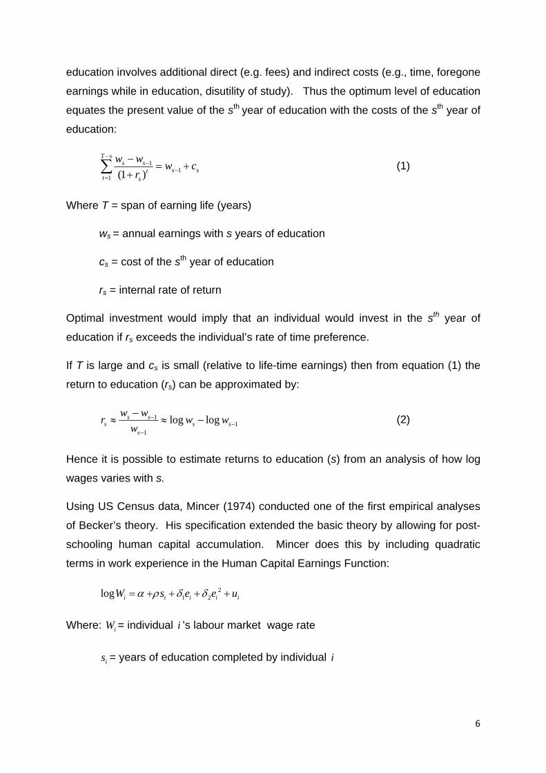
education involves additional direct (e.g. fees) and indirect costs (e.g., time, foregone
earnings while in education, disutility of study). Thus the optimum level of education
equates the present value of the sth year of education with the costs of the sth year of
education:
11
1 (1 )
T ss s
s stt s
w w w cr
−−
−=
−= +
+∑ (1)
Where T = span of earning life (years)
ws = annual earnings with s years of education
cs = cost of the sth year of education
rs = internal rate of return
Optimal investment would imply that an individual would invest in the sth year of
education if rs exceeds the individual’s rate of time preference.
If T is large and cs is small (relative to life-time earnings) then from equation (1) the
return to education (rs) can be approximated by:
11
1
log logs ss s s
s
w wr w ww
−−
−
−≈ ≈ − (2)
Hence it is possible to estimate returns to education (s) from an analysis of how log
wages varies with s.
Using US Census data, Mincer (1974) conducted one of the first empirical analyses
of Becker’s theory. His specification extended the basic theory by allowing for post-
schooling human capital accumulation. Mincer does this by including quadratic
terms in work experience in the Human Capital Earnings Function:
21 2log i i i i iW s e e uα ρ δ δ= + + + +
Where: iW = individual i ’s labour market wage rate
is = years of education completed by individual i
7
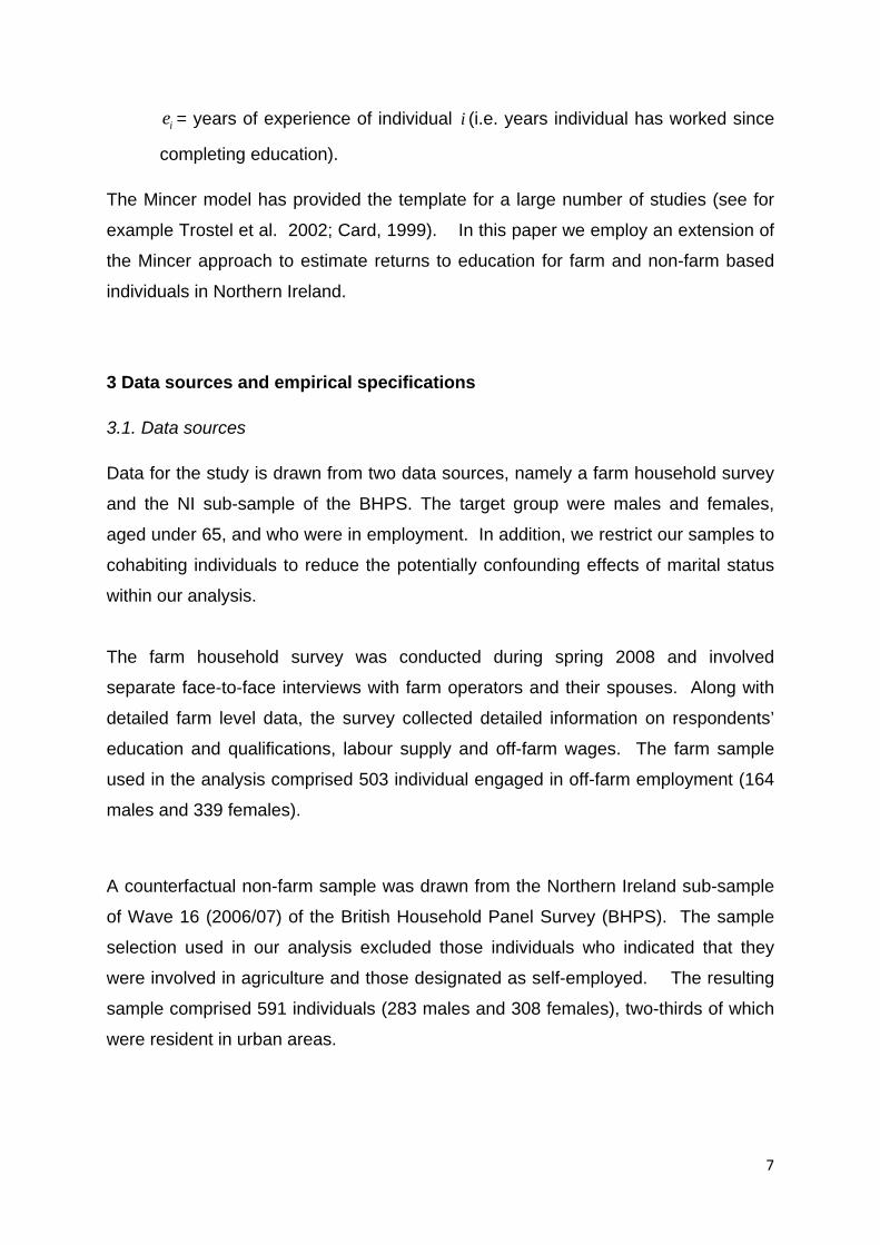
ie = years of experience of individual i (i.e. years individual has worked since
completing education).
The Mincer model has provided the template for a large number of studies (see for
example Trostel et al. 2002; Card, 1999). In this paper we employ an extension of
the Mincer approach to estimate returns to education for farm and non-farm based
individuals in Northern Ireland.
3 Data sources and empirical specifications
3.1. Data sources
Data for the study is drawn from two data sources, namely a farm household survey
and the NI sub-sample of the BHPS. The target group were males and females,
aged under 65, and who were in employment. In addition, we restrict our samples to
cohabiting individuals to reduce the potentially confounding effects of marital status
within our analysis.
The farm household survey was conducted during spring 2008 and involved
separate face-to-face interviews with farm operators and their spouses. Along with
detailed farm level data, the survey collected detailed information on respondents’
education and qualifications, labour supply and off-farm wages. The farm sample
used in the analysis comprised 503 individual engaged in off-farm employment (164
males and 339 females).
A counterfactual non-farm sample was drawn from the Northern Ireland sub-sample
of Wave 16 (2006/07) of the British Household Panel Survey (BHPS). The sample
selection used in our analysis excluded those individuals who indicated that they
were involved in agriculture and those designated as self-employed. The resulting
sample comprised 591 individuals (283 males and 308 females), two-thirds of which
were resident in urban areas.
8
The validity of using the separate datasets for comparative analysis was reinforced
by the fact that the survey questions on education, and incomes/wages were
identical for both survey questionnaires. In addition, the fieldwork for the survey
was also conducted by the same ‘interview team’ which undertakes the BHPS,
further enhancing comparability of the data.
For the purposes of the analysis and in line with previous studies we computed an
hourly wage rate, for the sample groups (see Gosling et al., 2000; and Harmon et al.
2003b). The hourly wage is calculated by average weekly net pay by normal working
hours per week. Hourly pay is preferable to weekly pay as it controls for any changes
in earnings due to hours at work e.g. part-time versus full-time work.
Within our analysis, years in education is calculated based on the age at which the
respondents finished their formal education less school starting age (5). For the
small number of individuals within the sample group who indicated that their
schooling went beyond the age of twenty three (perhaps where there has been a
break in education and the individual has returned) we follow Harmon and Walker
(1995) by recoding their school finishing age to a maximum of twenty three years of
age.
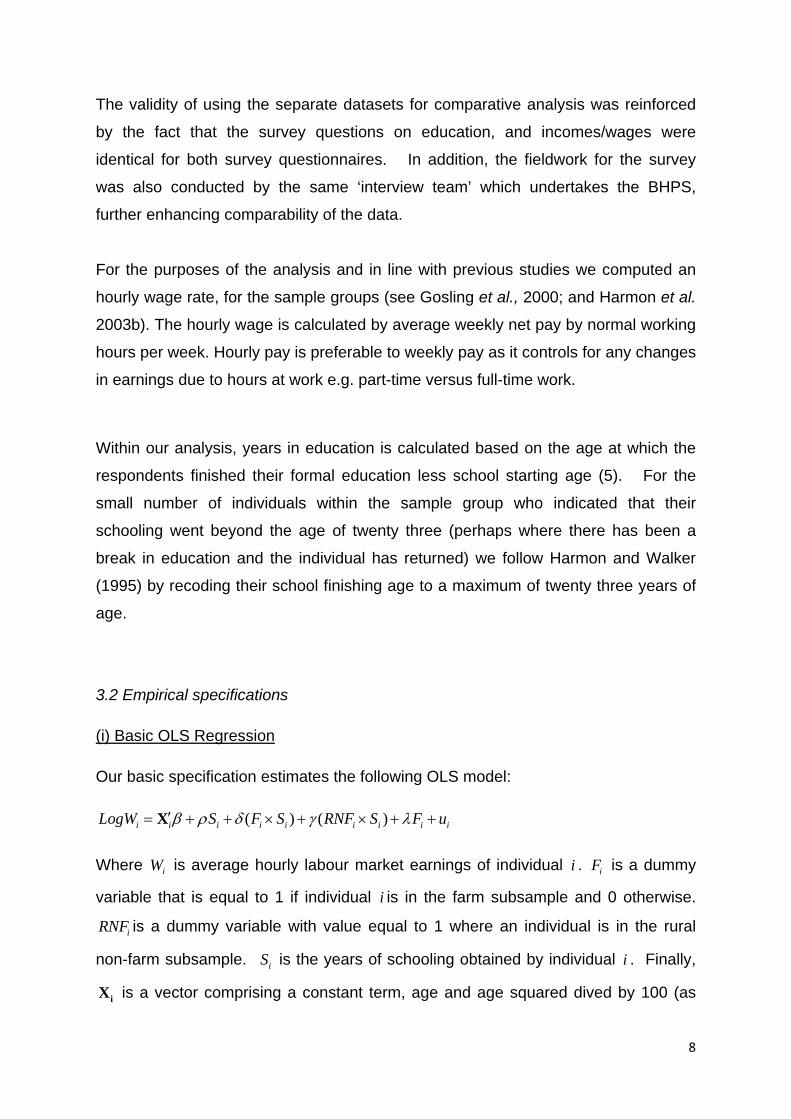
3.2 Empirical specifications
(i) Basic OLS Regression
Our basic specification estimates the following OLS model:
( ) ( )i i i i i i i i iLogW S F S RNF S F uβ ρ δ γ λ′= + + × + × + +X
Where iW is average hourly labour market earnings of individual i . iF is a dummy
variable that is equal to 1 if individual i is in the farm subsample and 0 otherwise.
iRNF is a dummy variable with value equal to 1 where an individual is in the rural
non-farm subsample. iS is the years of schooling obtained by individual i . Finally,
iX is a vector comprising a constant term, age and age squared dived by 100 (as

9
proxies for levels of experience) and a set of spatial dummies (rural west, urban east
urban west, Belfast with the omitted category being rural east). The parameter λ
captures the average difference in wage rates between the farm and non-farm
groups. Note that the coefficients on the spatial dummies in iX capture and
difference in average wages between rural and urban residents. The parameter ρ
measures the average return to education for members of the urban subsample.
Finally, the parameters δ and γ capture any difference in the average returns to
education between urban residents and farm and rural non-farm residents,
respectively. Thus a test that there is no difference in returns to education for each
group is simply a test of the null hypothesis that parameters δ and γ are not
significantly different from zero.
(ii) Instrumental Variables (IV) Estimation
There are a number of sources of bias associated with OLS estimates of the return
to schooling. Firstly, in terms of the individual’s optimisation problem we expect a
positive correlation between levels of education and its return which is likely to lead
to upward bias in the OLS estimate of the rate of return to education. Secondly,
there is the issue of ‘ability bias.’ Levels of academic ability are usually
unobservable (to the researcher) but are expected to be correlated with levels of
education and wages resulting in upward bias of OLS estimates. Thirdly, potential
bias arises from measurement error in schooling resulting in downward bias in OLS
estimates (Harmon and Walker, 1995)
The usual route to tackling the endogeneity and measurement error problems is
through the application of Instrumental Variables (IV). To explore the effects of
endogeneity on our estimates of the returns to education we estimate the following
two system for each sample subgroup:
i i i iLogW S uβ ρ′= + +X
i i iS vα′= +Z
With: ,( ) ( , ) 0i i i iE u E v= =X Z

10
Here iZ comprises a vector of instrumental variables. Valid instruments need to be
strongly correlated with the endogenous regressor but uncorrelated with the error
term of the schooling equation.
The instruments contained in Z comprise:
Siblings: Number of siblings of the respondent. For a given level of parental income,
family size is likely to reduce the per capita resources that can be spent on
educational investments.
Border: An index for birth order, i.e. the respondent’s place in the family. If
respondent is the first born then border = 1, if second born then border = 2 and so on
up to border = 10 (for tenth or more child ion the family). The reason for including
this variable is that the shares of family resources that each child receives are likely
to differ across birth order. In particular, given that parents have a fixed time
endowment, the first born will receive a greater time endowment than subsequent
children who have to compete for parental attention.
FewBooks, LotsBooks: Two dummy variables concerning the presence of books in
the parental home when the respondent was a child are used as a proxy for family-
specific attitudes to education1.
SLA16: Individual faced minimum School leaving age of 16 instead of 15. We follow
Harmon and Walker (1995) by using likely changes in the educational distribution of
individuals caused by the raising off the minimum school-leaving age. In 1973, the
minimum school leaving age in the United Kingdom was raised from 15 to 16. We
create a dummy variable (SLA16) equal to 1 for individuals who entering their 16th
year after 1973.
FatherProf: A dummy variable with value equal to 1 if the respondent’s father was
employed in a professional or associate professional occupation.
1 Respondents were asked: “Thinking about the time from when you were a baby until the age of ten, which of the following statements best describes your family home: There were a lot of books in the house; There were quite a few books in the house; There were not very many books in the house; Don’t know.” We constructed dummy variables for “a lot of books in the house” and “quite a few books in the house”. The base in the regressions is “not many books in the house”.

11
MotherProf: A dummy variable with value equal to 1 if the respondent’s mother was
employed in a professional or associate professional occupation.
DadFarm: A dummy variable with value equal to 1 if the respondent’s father was a
farmer and zero otherwise.
(iii) Sheepskin Effects
The basic Human Capital Earnings Function (HCEF) assumes linearity in S and that
ρ is a constant. However, it is likely that “credentials” matter more than years of
schooling implying the existence of non-linearities in the HCEF associated with
specific stages of the S distribution (e.g. completion of A levels, university
graduation). This hypothesis is referred to as the “sheepskin effect” and estimates
the wage premiums associated with fulfilling the final years of school or college and
securing a qualification (Card, 1999). In the final part of our analysis we test for
Sheepskin effects by estimating the wage premium associated with qualification
levels.
In this case we estimate the following regression equation with qualification dummies
for each sample sub-group:
1 2 3 4 51 2 3 4 5i i i i i i i iLogW Qual Qual Qual Qual Qual uβ ρ ρ ρ ρ ρ′= + + + + + +X
The vector X comprises a constant, age and age squared and a set of spatial
dummies. Qual1, Qual2, Qual3, Qual4 and Qual5 are dummy variables taking value
1 where a respondent’s highest qualification is at level 1, 2, 3, 4 or 5, respectively.
The omitted category is “no qualifications.” Actual qualifications within each level are
defined according to Office for National Statistics “Harmonised Concepts and
Questions for Government Social Surveys: Secondary Standards.” Level 1
comprises entry level qualifications including GCSE below grade C and GNVQ
foundation level. Level 2 includes trade apprenticeships, GCSE grades A*-C, GNVQ
intermediate, City and Guilds Craft/Part II. Level 3 includes A Levels, and higher
vocational qualifications such as NVQ level 3, OND, ONC and City and Guilds Craft

12
Part III. Level 4 comprises higher education qualifications below degree level, e.g.
HNC, HND, Nursing qualifications. Level 5 comprises degree level qualifications. A
full listing of qualifications within each level is provided in Appendix A.
Section 4: Results
4.1. Summary Statistics
Summary descriptive statistics by gender for the farm and non-farm sub-samples are
provided in Table 1. Amongst farm males, on average, there is a lower level of
education compared to the non-farm males as measured by years in full-time
education 14.12 years for the non-farm males, 12.85 for the farm based males. In
addition, there is a large percentage of the farm males (47%) who have no or
minimum qualifications (i.e. up to NVQ level 1 and Equivalent). In addition they also
have a low level of attainment at the higher level i.e. further and higher education
(18%) compared to 51% in the non-farm population.
Farm females obtain a similar level of educational attainment compared to non-farm
females but the wage rate for farm females (return) is much lower compared to the
non-farm cohort. The indication is that the intercept shifts down on this earnings
equation. This may suggest that the choices which farm females make in terms of
living on a farm and work is impacting on their returns to education and this is
demonstrated by what may be, in essence, from a female perspective a farm/non-
farm pay gap.

13
Table 1 Summary Statistics
Male diff sig
Female diff sig Farm Non-Farm Farm Non-Farm
Education (Years) 12.85 14.12 *** 14.05 13.92 ns (2.53) (2.63) (2.50) (2.58) Wage rate (£/hour) 10.27 14.54 *** 8.99 11.12 *** (6.06) (6.70) (4.45) (5.18) Labour market hours/week 33.92 38.39 *** 26.97 29.82 *** (1.06) (0.38) (0.66) (0.54) Age (Years) 47.95 41.79 *** 47.10 41.15 *** (8.23) (9.97) (8.53) (10.31) Highest qualification:
No qualifications 0.40 0.11 *** 0.10 0.10 ns Basic, e.g. GCSE, NVQ level1 0.07 0.03 ** 0.09 0.08 ns Trade apprenticeships/ NVQ Level 2 0.19 0.19 ns 0.21 0.22 ns A Level, OND, NVQ level3 0.16 0.16 ns 0.19 0.11 *** Higher, below degree, e.g. HND 0.07 0.25 *** 0.24 0.27 ns Degree level 0.11 0.26 *** 0.17 0.22 *
Observations 164 283 339 308 Note: Standard deviations in parentheses. Significance levels: *** p<0.01, ** p<0.05, * p<0.1, ns = not significant.
One other result that is worth noting is the large difference in wage rates between
those from non-farm and farm based households. This is demonstrated by the wage
rate returns at each qualification level as presented in Table 2.
Table 2 Mean Wage Rate by Level of Highest Qualification
Male Female
Farm Non-Farm Farm Non-FarmHighest Qualification: No qualifications 7.93 [66] 9.11 [31] 6.43 [34] 6.94 [31] (2.63) (2.23) (2.18) (1.99) Basic, e.g. GCSE, NVQ level1 10.64 [11] 14.40 [8] 6.20 [32] 8.83 [24]
(6.46) (6.18) (1.95) (2.86) Trade apprenticeships 10.84 [31] 10.96 [53] 7.76 [71] 8.88 [67]
(5.60) (3.32) (3.07) (3.62) A Level, OND, NVQ level 3 10.26 [27] 12.70 [47] 7.93 [64] 9.38 [35] (5.36) (5.52) (2.40) (2.57) Higher, below degree, e.g. HND 13.79 [11] 15.39 [71] 10.68 [81] 11.73 [83] (12.35) (6.25) (4.46) (4.93) Degree level 15.53 [18] 19.83 [73] 12.39 [57] 16.18 [68] (7.27) (7.14) (6.35) (5.39) Note: Standard deviations in parentheses; Sample size shown in square brackets
Table 2 provides evidence on the relative value of different levels of qualifications
ranging from no formal qualifications to academic/professional qualifications for
those males and females. The results clearly indicate that time spent participating in
education and attaining qualifications has a positive effect on earnings. An outcome

14
of interest is the significant difference in the wage level at degree level for both farm
males and farm females compared to the non-farm group.
4.2 Econometric results
OLS estimates of return to education
Results for the OLS individual subsamples regressions by farm and non-farm and
rural urban sub-samples are presented in Appendix B. Table 3 presents the OLS
estimates, for the entire sample group for males and females, incorporating farm,
rural non-farm interaction terms to test for differences in returns to education by sub-
group.
Table 3 OLS Model Estimates by Gender
Males Females (1) (2) Education (years) 0.065(0.010)*** 0.098 (0.010)*** Farm x Education 0.001(0.016) ‐0.022 (0.013)* Rural x Non‐Farm x Education 0.001(0.013) ‐0.023 (0.012)* Age 0.063(0.015)*** 0.018 (0.012) Age squared/100 ‐0.067(0.017)*** ‐0.016 (0.014) Belfast (D) ‐0.073(0.191) ‐0.298 (0.182) Urban East (D) 0.052(0.076) ‐0.024 (0.075) Urban West (D) ‐0.045(0.092) ‐0.099 (0.090) Rural West (D) ‐0.043(0.189) 0.287 (0.180) Farm (D) ‐0.293(0.233) ‐0.254 (0.198) Constant 0.261(0.361) 0.529 (0.293)* Observations 447 646 R‐squared 0.319 0.284 Note: Robust standard errors in parentheses; Significance: *** p<0.01, ** p<0.05, * p<0.1
(D) indicates regressor is a dummy variable; Omitted spatial category is Rural East
The rate of return to education for males (column 1) is 6.5 per cent and for females
(column 2) 9.8 per cent, both of which are significant. The interaction terms are used
to identify possible differences in returns to education for farm and rural non-farm
individuals compared to urban-based individuals. The results indicate that for males,
whether they are farm, rural or urban based there is no significant difference in
returns to education. However, for the rural females (farm and non-farm), returns to

15
education are 2 per cent lower compared to the urban female group, indicating that
for the females in the sample there are urban/rural differences in relation to the
returns to education.
For those in the male sample (see Table 3, column 1) age and aged squared are
significant. This result is expected and consistent with previous studies; as age
increases people gain further experience in employment, and their earnings
continues to rise eventually peaking around middle age, and declines thereafter. For
females however, the age effect is poorly determined, i.e. age does not prove to be
significant in determining returns to education.
Instrumental Variables estimates of returns to education
The IV estimates of the human capital earnings functions for each of the sample
groups are presented in Table 4. The IV estimates of the return to education are
considerably higher than the OLS estimates presented earlier. The highest returns
to education of over 15 per cent are associated with non-farm females with a
somewhat lower rate of about 13 percent for farm-based females. The IV estimates
suggest average marginal returns to education of almost 11 per cent for non-farm
males compared to about 8 per cent for farm-based males. Our diagnostic tests
indicate that the basic identification tests are satisfied for all but the farm male group.
In addition, our instruments are generally quite weak especially for the farm-based
male group. Consequently, our IV estimates especially for farm males group should
be treated with caution. Finally, it is interesting to note that Durbin-Wu-Hausman
tests suggest that education is endogenous in the human capital earnings equations
for the non-farm groups but surprising not so for the farm-based groups. This would
suggest that unobserved ability bias is less prominent in the estimates for the farm-
based individuals perhaps because they are less heterogenous than the non-farm
group. However, it may equally be a reflection of the weakness of the instruments
used to identify the models for these groups.

16
Table 4 IV Estimates by Sample Sub-group
Farm Males NonFarm Males Farm Females NonFarm Females
(3) (4) (5) (6)
Education (years) 0.078 (0.046)* 0.109 (0.027)*** 0.131 (0.039)*** 0.153 (0.032)***
Age 0.037 (0.038) 0.064 (0.021)*** 0.037 (0.024) ‐0.007 (0.019)
Age squared/100 ‐0.041 (0.040) ‐0.068 (0.023)*** ‐0.034 (0.026) 0.015 (0.023)
Belfast (D) ‐ ‐0.094 (0.099) ‐ 0.016 (0.093)
Urban East (D) ‐ ‐0.055 (0.072) ‐ 0.017 (0.071)
Urban West (D) ‐ ‐0.165 (0.091)* ‐ ‐0.054 (0.090)
Rural West (D) ‐0.111 (0.065)* ‐0.139 (0.090) 0.010 (0.047) 0.022 (0.084)
Constant 0.475 (1.182) ‐0.279 (0.532) ‐0.713 (0.871) 0.180 (0.464)
Observations 164 250 338 293
Regression F‐Statistic 2.01 [0.095] 5.49 [0.000] 3.20 [0.013] 4.21 [0.000]
Centred R‐squared 0.166 0.154 0.106 0.105
Diagnostics:
Under‐identification (Anderson), Chi‐sq (8) 11.82 [0.160] 33.57 [0.000] 17.48 [0.015] 27.95 [0.000]
Overidentificaion (Sargan) Chi‐sq (7) 3.47 [0.838] 6.66 [0.465] 2.51 [0.867] 3.43 [0.842]
Weak identification F‐statistic (8, 152) 1.48 [0.171] 4.56 [0.000] 2.55 [0.015] 3.66 [0.000]
Endogeneity of EducationDurbin‐Wu‐Hausman Chi‐sq (1)
0.088
[0.767] 3.49
[0.062] 2.27
[0.132]
6.05
[0.014]
Note: Standard errors in parentheses; Significance *** p<0.01, ** p<0.05, * p<0.1 P‐Values for diagnostics shown in square brackets (D) indicates regressor is a dummy variable; Omitted spatial category is Rural East Excluded instruments as described in Section 3.2: dadfarm(D), dadprof(D), mumprof(D), border, siblings, fewbooks(D), lotsbooks(D), sla16(D)
4.4 Sheepskin Effects
Finally Table 5 presents the OLS estimates from estimating the human capital
earnings function using qualification levels rather than years of education for the
relative value of highest levels of academic /vocational qualifications against having
no qualifications. For both males and females, the returns to each higher level of
education are consistently higher, with the highest level for degree around 74 per
cent for males and 87 per cent for females. So for instance, men choosing to do a
degree will earn on average, a 74 per cent higher wage compared to men without

17
qualifications. The Farm x Qual Level interaction terms capture the difference in
returns to qualification levels for farm-based individuals relative to non-farm based
individuals. In the case of farm-based males and females, it is noted that average
returns to higher qualifications such as degree level are significantly lower than those
achieved by non-farm based individuals. In particular, farm-based males with
degree level qualifications earn on average 28 per cent less than non-farm males
with an equivalent level of qualification. The return to level 5 qualifications in the
case of farm females is one third less than that achieved by non-farm females.
Table 5 OLS estimates of returns to qualification levels
Males Females (7) (8) Age 0.059 (0.015)*** 0.017 (0.012) Age squared/100 ‐0.061 (0.016)*** ‐0.014 (0.013) Qual Level 1 (D) 0.484 (0.147)*** 0.241 (0.099)** Qual Level 2 (D) 0.206 (0.083)** 0.249 (0.080)*** Qual Level 3 (D) 0.327 (0.086)*** 0.370 (0.091)*** Qual Level 4 (D) 0.481 (0.079)*** 0.512 (0.077)*** Qual Level 5 (D) 0.749 (0.079)*** 0.873 (0.080)*** Farm x Qual Level 0 (D) ‐0.153 (0.087)* ‐0.118 (0.093) Farm x Qual Level 1 (D) ‐0.453 (0.174)*** ‐0.390 (0.101)*** Farm x Qual Level 2 (D) ‐0.099 (0.089) ‐0.156 (0.067)** Farm x Qual Level 3 (D) ‐0.297 (0.093)*** ‐0.231 (0.080)*** Farm x Qual Level 4 (D) ‐0.245 (0.123)** ‐0.124 (0.064)* Farm x Qual Level 5 (D) ‐0.279 (0.102)*** ‐0.326 (0.071)*** Belfast (D) ‐0.105 (0.076) ‐0.023 (0.074) Urban East (D) ‐0.023 (0.054) ‐0.032 (0.050) Urban West (D) ‐0.107 (0.071) ‐0.128 (0.070)* Rural West (D) ‐0.107 (0.047)** ‐0.055 (0.036) Constant 0.865 (0.334)*** 1.451 (0.264)*** Observations 447 646
R‐squared 0.418 0.364 Note: Robust standard errors in parentheses; Significance: *** p<0.01, ** p<0.05, * p<0.1
(D) indicates regressor is a dummy variable; Omitted qualification level is Qual level 0 (no qualifications) Omitted spatial category is Rural East
Section 5 Summary and Conclusions
This paper estimated returns to education and qualifications for males and females
within farm households in Northern Ireland. In addition, it examined differences in
average returns to education according to gender and between farm-based (rural)
and non-farm based (predominantly urban) individuals.
18
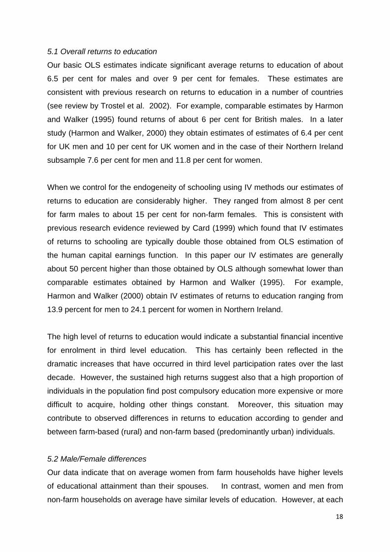
5.1 Overall returns to education
Our basic OLS estimates indicate significant average returns to education of about
6.5 per cent for males and over 9 per cent for females. These estimates are
consistent with previous research on returns to education in a number of countries
(see review by Trostel et al. 2002). For example, comparable estimates by Harmon
and Walker (1995) found returns of about 6 per cent for British males. In a later
study (Harmon and Walker, 2000) they obtain estimates of estimates of 6.4 per cent
for UK men and 10 per cent for UK women and in the case of their Northern Ireland
subsample 7.6 per cent for men and 11.8 per cent for women.
When we control for the endogeneity of schooling using IV methods our estimates of
returns to education are considerably higher. They ranged from almost 8 per cent
for farm males to about 15 per cent for non-farm females. This is consistent with
previous research evidence reviewed by Card (1999) which found that IV estimates
of returns to schooling are typically double those obtained from OLS estimation of
the human capital earnings function. In this paper our IV estimates are generally
about 50 percent higher than those obtained by OLS although somewhat lower than
comparable estimates obtained by Harmon and Walker (1995). For example,
Harmon and Walker (2000) obtain IV estimates of returns to education ranging from
13.9 percent for men to 24.1 percent for women in Northern Ireland.
The high level of returns to education would indicate a substantial financial incentive
for enrolment in third level education. This has certainly been reflected in the
dramatic increases that have occurred in third level participation rates over the last
decade. However, the sustained high returns suggest also that a high proportion of
individuals in the population find post compulsory education more expensive or more
difficult to acquire, holding other things constant. Moreover, this situation may
contribute to observed differences in returns to education according to gender and
between farm-based (rural) and non-farm based (predominantly urban) individuals.
5.2 Male/Female differences
Our data indicate that on average women from farm households have higher levels
of educational attainment than their spouses. In contrast, women and men from
non-farm households on average have similar levels of education. However, at each

19
qualification level, women earn on average less than men, identifying the presence
of a gender wage gap. However, the econometric estimates highlight that there are
significant gender differences in terms of the returns to education with on average
higher returns for women than men. But it must be noted that the higher percentage
returns for females may in part be a reflection of their lower average earnings. This
variation reflects different occupational characteristics between men and women and
coupled with the need to balance work and child care commitments. In some cases
women may be prepared to sacrifice higher levels of pay in order to secure jobs
which offer non-pecuniary benefits, such employment conditions which allow for
flexible working around childcare and other family commitments. This is consistent
with the higher levels of part-time employment among women in our dataset.
Females worked on average 28 hours per week compared to 36 hours per week for
males. Despite this factor there remains tentative evidence of the continued
existence of a regional gender pay gap, and given the age range of the sample
group may support previous research suggesting that this pay gap becomes
increasingly evident as women progress in the labour market (Manning, 2003).
A further feature of the male/female comparison is that the age-earnings profile is
relatively well determined for non-farm males but not for females. This was reflected
by the significance of the age and aged squared terms in the regression equations
for non-farm males (Table 4). Consistent with previous studies (Mincer, 1974) there
is a convex relationship between earnings and age and at least for males age related
experience has a strong positive effect on earnings in the early stage of the life cycle
which diminishes as individuals approach retirement. For females and also farm-
based males however, the age effect is less defined, i.e. age does not prove to be
significant in determining returns to education. There maybe a number of
explanations of this, perhaps for the females it may be higher job turnover or breaks
in employment due to time out from the labour market in order to have children or
undertake family caring responsibilities. In the case of farm males, the non-
significance of age related experience may reflect their participation in lower-skilled
manual jobs and also the relatively recent engagement of many of these individuals
in the off-farm labour market.

20
5.3 Farm/Non-Farm Differences
Our estimates suggest that average marginal returns to schooling are similar for farm
and non-farm males but that differences do exist in the case of farm and non-farm
females. For males the estimated returns to education across model specifications
ranged from 6.5 to 10.9 per cent. While there was no statistically significant
difference in average marginal returns for farm and non-farm males further results
suggested that returns to some qualifications (esp. degree level) are somewhat
lower for farm operators compared to the wider male population. It should be noted
that our measure of returns is based only on the labour market earnings for those
farm operators who have off-farm jobs. A future development of our research is
investigating the extent to which education enhances productivity of farm operators
in the running of their farm businesses as well as in the off-farm labour market.
Average wage rates for farm males were about 30 per cent below those of non-farm
males. This reflects the lower average levels of educational attainment among farm
males compared to their non-farm counterparts. In particular, distribution of
schooling attainment is much more heavily concentrated at the minimum school
leaving age. The low levels of educational attainment by farm males is not new, but
it presents a concern for policy makers in the context of farm adjustment. Previous
research has identified the importance of parental aspirations on young people’s
educational choices and that it is mothers in particular who influence the educational
pathway within households (Feinstein 2003; Brooks, 2004). This perhaps raises
further research questions regarding attitudinal differences within farm families
towards the educational attainment of males particularly towards those who have
been identified as potential successors on the farm. There is a clear need to
increase and improve the overall basic level of educational attainment amongst farm
based males.
It also must be noted that the results are affected by the conditions within the labour
market at the time of the survey. The returns to different qualifications will reflect the
supply and demand for those individual characteristics at a particular point in time.
Many of the farm based males were employed in unskilled/semi-skilled construction
and transport related occupations. Strong industry effects on earnings cannot be
ruled out as the survey was undertaken in early 2008 when the construction industry
21
was buoyant. Farm males may also be off-setting lower wages by travelling to jobs
beyond their local labour market in the wider regional labour market.
In the case of farm females, OLS estimates of returns to schooling were 7.6 per cent
compared to 9.8 per cent for their urban counterparts. However, the difference in
returns was significant only at the P < 0.1 level. The IV estimates of returns to
education were 13.1 per cent in the case of farm females compared to 15.3 per cent
for non-farm females. Moreover, estimated returns to degree level qualifications are
almost one third lower than the return achieved by urban females with the same
qualification level (P<0.01). The estimated difference in returns to schooling
between the farm and non-farm females would suggest that farm females face
additional constraints that reduce their returns to higher level skills. These may
reflect a combination of factors such as the need to balance longer commutes to
higher paid urban-based employment opportunities against farm and caring
responsibilities. In this context the utility maximizing choice for some farm-based
females may be to select lower paid local employment where it provides the flexibility
to accommodate other commitments.
5.4 Urban/Rural differences
Rural areas may have disadvantages relative to urban areas in terms of offering
employees competitive returns to education, or returns that are commensurate with
the costs incurred by individuals as they pursue education (Goetz and Rupasingha,
2004). Employment in rural areas is often focused on traditional industries which
are characterized by lower skills requirements and low wage levels. Mirroring the
effects for farm-based females the returns to education for non-farm rural women,
are less, compared to their urban counterparts. The OLS estimates of returns to
education are equal for farm and rural non-farm women at about 7.5 per cent
compared to 9.8 per cent for urban females. This may reflect the thinness of rural
labour markets. In the case of rural-based females our data indicates a
predominance of employment within the public sector at local level (esp. health and
education sectors). Rural labour markets sustain a less diverse range of
employment opportunities making it more difficult for individuals to find jobs that
closely match their skills and education. Where individuals have a preference (or
need) to find local employment better educated workers may be forced to seek

22
employment for which they are overqualified. The effect of this mismatch is likely to
lower average rewards for educational attainment.
5.5 Returns to qualifications (Sheepskin Effects)
Our analysis suggests that the human capital earnings function is non-linear in
schooling due to sheepskin effect. In particular, there are much higher return
associated with critical points of the education distribution especially with the
completion of A levels and especially degree level qualifications. It is clear that
higher level qualifications (i.e. degree and professional qualifications) provide a
substantial earnings premium within the Northern Ireland Labour market. In general,
returns to academic qualifications are higher than those to vocational qualifications.
Finally, there is evidence of significant differences in returns to qualifications
between farm-based and non-farm based individuals. Most notably the earnings
premium (over wage with no qualifications) for degree level qualifications is about 30
per cent lower for farm-based individuals compared to non-farm based individuals.
This again appears to be a reflection of the thinner nature of rural labour markets
typically focused on traditional sectors. In such areas there is likely to be fewer
opportunities for highly qualified individuals.
5.6 Critique of the analysis
There are a number of limitations of our analysis that deserve comment. First, there
are significant differences in key characteristics of our farm and non-farm samples
which may limit the effectiveness of the BHPS sample as a valid control. Although
we control for life-cycle stage in our analysis by including age and age squared in the
regression equations the average age of individuals in the BHPS sample was
significantly lower than in our farm sample. However, if there are differences
between the age-earnings profiles of the separate subsamples this would generate
bias as variation in returns to tenure would be attributed to differences in between-
group returns to education. However, our supplementary estimations of the human
capital earnings function for individual sample subgroups suggest that this effect is
likely to be quite small.

23
A more acute problem was the very small proportion of farm males with higher level
qualifications. Forty per cent of the farm males had no qualifications meaning that
estimates of returns to education for this group were impeded by the relatively small
numbers of observations in the upper range of the schooling distribution. In addition,
this meant that it was difficult to properly identify differences in returns to education
between farm and non-farm males since the educational characteristics of the
groups are quite dissimilar.
OLS estimates are likely to be biased due to the endogeneity of education variable in
the human capital equation. The conventional approach for controlling for this bias is
through the use of instrumental variables methods. However, it has been recognized
that these estimators often perform poorly in small samples and where the
instrumental variables are weak (Bound et al. 1995; Flores-Lagunes, 2007). Our IV
analysis experiences both of these problems. In particular, the F-statistic for the joint
significance of our excluded instruments was below 5 for each sample subgroup
indicating that our instruments are quite weak. Moreover, for the farm male
subgroup we our identification diagnostic tests are unsatisfactory suggesting that the
IV estimates for this group need to be interpreted with caution. Again, the probable
cause appears to be the very narrow range of education levels within that group of
the sample.
Finally, it should be noted that the relatively small geographic scale of Northern
Ireland weakens the power of our test for differences in returns to schooling between
rural and urban based individuals in our sample. Most rural-based individuals in the
province are within an hour and a half commute to the main urban centre of Belfast,
however there is a weak public transport infrastructure so commuting is very much
car dependent . A more powerful test might compare returns between individuals in
the Belfast metropolitan area with those in more remote rural locations (e.g. rural
west). We also tested this specification and found that the negative rural effect
becomes much larger. However, this approach means that we would exclude from
our analysis a large proportion of our dataset and our statistical inferences become
impeded through the reduction in degrees of freedom.
24
5.7 Concluding remarks
The preliminary results presented in this paper would appear to demonstrate a farm
versus non-farm pay gap and that labour market returns to education may be
somewhat lower for rural based individuals and especially for females compared to
their urban counterparts. Lower educational attainment and lower rewards to higher
education in rural areas have previously been identified as key factors in explaining a
rural earnings gap (Goetz and Rupasingha, 2004). If higher educational attainment
in a rural area typically earns less than in an urban area, there is a strong incentive
for more mobile individuals to seek employment in urban areas. However, some
rural dwellers face particular constraints affecting their employment mobility. For
example, farm operators and their spouses may be restricted in terms of where and
how they can work off-farm due to farming and family commitments. Faced with
such constraints these individuals may be forced to seek employment locally despite
lower rates of pay due to the thinness of many rural labour markets. In this situation
it may be optimal for some rural-based individuals to select low levels of education if
obtaining that education is costly and/or they perceive that there are weak returns on
such investment from within their local labour market. However, the results of our
analysis discount this latter point by indicating that there are in fact strong positive
returns to education in general. An issue for policy makers concerns how to
encourage more positive attitudes to educational attainment particularly among farm-
based males.

25
References
Becker, G. (1964). Human Capital: A Theoretical and Empirical Analysis, with Special Reference to Education. New York: Columbia University Press.
Bound, J., Jaeger, D.A. and Baker, R.M. (1995). Problems With Instrumental Variables Estimation When the Correlation Between the Instruments and the Endogenous Explanatory Variable Is Weak. Journal of the American Statistical Society, 90 (430, June), 443-450.
Brooks, R. (2004) “My mum would be pleased as punch if I actually went, but my dad seems more particular about it”: Paternal involvement in young peoples higher education choices. British Educational Research Journal, 30, 495-514.
Card, D. (1999). The causal effect of education on earnings. In O. Ashenfelter and D. Card (eds), Handbook of Labor Economics, vol. 3, Amsterdam: Elsevier-North Holland.
Card, D. (2001). Estimating the returns to schooling: progress on some persistent econometric problems. Econometrica, 69, 1127–60.
Commission of the European Communities (2006). Employment in rural areas: closing the jobs gap, SEC (2006) 1772.
Department of Education and Skills (2003). The future of higher education. London: HMSO.
Feinstein, L. (2003). Inequality in the Early Cognitive Development of British Children in the 1970 Cohort. Economica, 70, pp. 73-97.
Flores-Lagunes, A. (2007). Finite Sample Evidence of IV Estimators Under Weak Instruments. Journal of Applied Econometrics, 22, 677-694.
Gasson, R. (1998). Educational Qualifications of UK Farmers: A Review. Journal of Rural Studies, 14 (4) 487-498.
Goetz, S.J. and A. Rupasingha. (2004) “The Returns to Education in Rural Areas.” Review of Regional Studies 34 No. 3.
Gosling, A., Machin, S. and Meghir, C. (2000). The changing distribution of male wages,1966–93. Review of Economic Studies, 67, 635-666.
Harmon C and Walker I (1995). Estimating the economic return to schooling for the United Kingdom. American Economic Review, 85 (5), 1278-1286.
Harmon, C. and Walker, I. (2000). Education and Earnings in Northern Ireland, A Research Report to Analyse the Economic Returns to Education in Northern Ireland. Belfast: Department of Higher and Further Education, Training and Employment.
Harmon, C. Oosterbeek, H. and Walker, I. (2003a). The Returns to Education’: Microeconomics. Journal of Economic Surveys, 17, 115-156.
Harmon, C., Hogan, V. and Walker, I. (2003b). Dispersion in the Economic Return to Schooling. Labour Economics, 10, 205-214.
Huffman W and Orazam P (2004). The Role of Agriculture and Human Capital in Economic Growth: Farmers, Schooling, and Health. Working Paper Series
26
Lang, K. (1993), Ability Bias, Discount Rate Bias and the Return to Education, Mimeo,Boston University.
LeClere, F.B. (1991). The Effects of Metropolitan Residence on the Off-Farm Earnings of Farm Families in the United States. Rural Sociology, 53 (3, Fall), 366-390.
Manning, A. (2003). Life’s ups and downs: understanding the earnings profile. Paper presented at the Royal Economic Society annual conference, University of Warwick, April 2003.
McLaughlin, D.K. and Perman, L. (1991). Returns vs. Endowments in the Earnings Attainment Process for Metropolitan and Nonmetropolitan Men and Women. Rural Sociology, 56 (3), 339-365.
Mincer, J. (1974), Schooling, Experience and Earnings, Columbia University Press: New York.
Moss, J.E., Jack, C.G and Wallace, M.T. (2004). Employment location and associated commuting patterns for individuals in disadvantaged rural areas in Northern Ireland. Regional Studies, 38 (2).
Ofek, H. and Merrill, Y. (1997). Labor Mobility and the Formation of Gender Wage Gaps in Local Markets. Economic Inquiry, 35 (January), 28-47.
Schultz T.W. (1960). Capital Formation by Education. Journal of political economy, 68, 571-83.
Trostel, P., Walker, I. and Woolley, P. (2002). Estimates of the Economic Return to Schooling for 28 Countries. Labour Economics, 9, 1-16.
Vera-Toscano, E., Phimister, E. and Weersink, A. (2004). Panel Estimates of the Canadian Rural/Urban Women's Wage Gap. American Journal of Agricultural Economics, 86 (4, November), 1138-1151.

27
Appendix A
Classification of Qualifications
Level 0 - No qualifications
Level 1 - NVQ or SVQ level 1 - GNVQ Foundation level, GSVQ level 1 - GCSE or O level below grade C, SCE Standard or Ordinary below grade 3 - CSE below grade 1 - BTEC, SCOTVEC first or general certificate - SCOTVEC modules - RSA Stage I, II, or III - City and Guilds part 1 - Junior certificate Level 2 - Trade Apprenticeships , GCSE/O Level grade A*-C, vocational level 2 and equivalents - NVQ or SVQ level 2 - GNVQ intermediate or GSVQ level 2 - RSA Diploma - City & Guilds Craft or Part II (& other names) - BTEC, SCOTVEC first or general diploma et - O level or GCSE grade A-C, SCE Standard or Ordinary grades 1-3 Level 3 - Vocational level 3 and equivalents - A level or equivalent - AS level - SCE Higher, Scottish Certificate Sixth Year Studies or equivalent - NVQ or SVQ level 3 - GNVQ Advanced or GSVQ level 3 - OND, ONC, BTEC National, SCOTVEC National Certificate - City & Guilds advanced craft, Part III (& other names) - RSA advanced diploma Level 4 - Other Higher Education below degree level - Diplomas in higher education & other higher education qualifications - HNC, HND, Higher level BTEC - Teaching qualifications for schools or further education (below Degree level standard) - Nursing, or other medical qualifications not covered above (below Degree level standard) - RSA higher diploma Level 5 - Degree or Degree equivalent, and above - Higher degree and postgraduate qualifications - First degree (including B.Ed.) - Postgraduate Diplomas and Certificates (including PGCE) - Professional qualifications at degree level e.g. graduate member of professional institute, chartered accountant or surveyor - NVQ or SVQ level 4 or 5 Source: http://www.ons.gov.uk/about-statistics/harmonisation/secondary-concepts-and-questions/S1.pdf

28
Appendix B
OLS Estimates for Farm and Non-Farm Subsamples Males Females Farm Non-Farm Farm Non-Farm (1) (2) (3) (4) Education (years) 0.065 (0.012)*** 0.065 (0.009)*** 0.077 (0.008)*** 0.091 (0.009)*** Age 0.035 (0.038) 0.068 (0.017)*** 0.033 (0.023) 0.011 (0.015) Age squared/100 -0.040 (0.040) -0.073 (0.019)*** -0.033 (0.025) -0.008 (0.018) Belfast (D) - -0.095 (0.085) - 0.034 (0.085) Urban East (D) - -0.040 (0.064) - 0.001 (0.063) Urban West (D) - -0.143 (0.083)* - -0.032 (0.082) Rural West (D) -0.112 (0.066)* -0.129 (0.081) 0.005 (0.044) -0.006 (0.072) Constant 0.699 (0.918) 0.231 (0.381) 0.223 (0.542) 0.741 (0.332)** Observations 164 283 338 308 R-squared 0.171 0.233 0.204 0.274 Note: Robust standard errors in parentheses; Significance: *** p<0.01, ** p<0.05, * p<0.1
(D) indicates regressor is a dummy variable; Omitted spatial category is Rural East
OLS Estimates for Rural and Urban Subsamples Males Females Rural Urban Rural Urban (5) (6) (7) (8) Education (years) 0.073 (0.010)*** 0.068 (0.011)*** 0.073 (0.007)*** 0.100 (0.011)*** Age 0.027 (0.025) 0.065 (0.020)*** 0.014 (0.017) -0.001 (0.019) Age squared/100 -0.036 (0.027) -0.068 (0.023)*** -0.015 (0.019) 0.004 (0.022) Belfast (D) 0.000 (0.000) 0.000 (0.000) 0.000 (0.000) 0.000 (0.000) Urban East (D) 0.000 (0.000) 0.052 (0.078) 0.000 (0.000) -0.032 (0.077) Urban West (D) 0.000 (0.000) -0.055 (0.094) 0.000 (0.000) -0.110 (0.093) Rural West (D) -0.173 (0.051)*** 0.000 (0.000) -0.040 (0.038) 0.000 (0.000) Constant 1.043 (0.566)* 0.110 (0.460) 0.838 (0.381)** 0.915 (0.413)** Observations 256 191 452 194 R-squared 0.242 0.231 0.182 0.313 Note: Robust standard errors in parentheses; Significance: *** p<0.01, ** p<0.05, * p<0.1
(D) indicates regressor is a dummy variable; Omitted spatial category is Rural East