economic review - nbb.be
TRANSCRIPT

Economic ReviewDecember 2016

© National Bank of Belgium
All rights reserved.Reproduction of all or part of this publication for educational and non‑commercial purposes is permitted provided that the source is acknowledged.
ISSN 1780 ‑ 664X
5December 2016 ❙ CoNteNtS ❙
Contents
ECONOMIC PROJECTIONS FOR BELGIUM – AUTUMN 2016 7
HELICOPTER MONEY AND DEBT-FINANCED FISCAL STIMULUS : ONE AND THE SAME THING ? 31
SOCIO-ECONOMIC TRANSITIONS ON THE LABOUR MARKETS : A EUROPEAN BENCHMARKING EXERCISE 41
THREE REGIONS, THREE ECONOMIES ? 59
FINDINGS FROM THE EUROPEAN SURVEY ON WAGE-SETTING 75
THE SUSTAINABILITY OF PUBLIC FINANCES IN THE CONTEXT OF POPULATION AGEING 87
THE TRANSMISSION MECHANISM OF NEW AND TRADITIONAL INSTRUMENTS OF MONETARY AND MACROPRUDENTIAL POLICY 105
RESULTS AND FINANCIAL SITUATION OF FIRMS IN 2015 119
SUMMARIES OF ARTICLES 159
ABSTRACTS FROM THE WORKING PAPERS SERIES 163
CONVENTIONAL SIGNS 167
LIST OF ABBREVIATIONS 169

7December 2016 ❙ Economic pRojEctions foR BElgium – Autumn 2016 ❙
Economic projections for Belgium – Autumn 2016
Introduction
According to the latest estimates, the growth of the world economy weakened a little further in 2016, fol‑lowing the already modest rate recorded a year earlier. in addition, 2016 was characterised by a number of shocks, triggering periods of high volatility on the fi‑nancial markets. one of the most significant ones was the unexpected outcome of the Brexit referendum in the united Kingdom on 23 june, immediately after the publication of the Bank’s latest spring projections. the prospect of one of its largest economies leaving the eU prompted many national and international institutions to fear a sharp downgrading of the growth forecast for the united Kingdom, and – via trade and the heightened macroeconomic uncertainty – for other countries in the Eu and across the world. given the share in Belgian value added related to British final demand, Belgium is the euro area country most vulnerable, after ireland, to a slowdown in growth in the united Kingdom.
nonetheless, the global economy has proved surprisingly robust : world growth did not weaken further in the sec‑ond half of the year, and actually seems to have picked up slightly since the summer. that is due primarily to the improving situation in the emerging economies and the easing concerns about them. thus, some countries such as Russia and Brazil appear to be gradually emerging from the deep recession in which they were languishing. moreover, according to the official statistics, the difficult process of rebalancing the chinese economy is still ac‑companied by continuing vigorous and relatively stable growth, and the risk of a hard landing seems to have faded, even though that situation is due partly to credit expansion which may ultimately prove unsustainable. in addition, the signals from some advanced economies are
still favourable. in the united states, the economy and the labour market continue to pick up, now also clearly raising average wages, while the japanese economy continues to record moderate positive growth, following the contrac‑tion at the end of 2015. in the euro area, the economy has maintained slow but steady growth of 0.3 % per quarter, broadly in line with the Eurosystem’s spring projections. it is also note worthy that the growth dispersion between countries appears to be declining sharply. for example, in the third quarter of 2016, all the euro area countries were already recording positive growth rates.
finally, even the Brexit referendum has had little impact on British growth so far, as is evident from the first sta‑tistics for the third quarter, showing that growth was hardly any lower after the referendum compared to the previous quarter, and is still outpacing that in the euro area. However, this must be viewed in the context of the monetary policy adjustment and the ensuing depreciation of the pound sterling, as well as the fairly rapid dissipation of the political uncertainty. similarly, the current projec‑tions concerning the immediate future are now consider‑ably less gloomy than they were just after the referendum. the uncertainty about the eventual new relationship between the united Kingdom and the Eu is of course still justified, and there is little doubt that – all other things being equal – an effective exit from the Eu accompanied by greater restrictions on trade and the free movement of persons will depress both actual and potential growth. that applies more generally to any shift towards increased protectionism and isolationism.
A positive factor that has widened and strengthened the basis of global growth in 2016 is the trade revival, albeit still modest. At the beginning of 2016, trade had fallen to a historically low level, with growth lagging far behind that

8 ❙ Economic pRojEctions foR BElgium – Autumn 2016 ❙ nBB Economic Review
of global activity. that was attributable partly to cyclical factors, although the lower growth-elasticity of trade is also due to more structural developments, such as the increasing stake in the global economy of the emerging economies, which have a lower trade intensity, and the waning momentum generated by the lengthening of the global value chains and further trade liberalisation. Although the ratio between the growth of demand for imports and global gDp excluding the euro area is still well short of unitary elasticity, it nevertheless increased slightly in 2016, one factor being the relatively stronger demand for imports from a number of advanced economies. According to the current common assumptions for the Eurosystem estimates – the main ones concerning Belgium being presented in box 1 of this article – the trade intensity of growth is set to increase continuously, reverting to a more normal level of around 1 by 2018. that corresponds to the level prevailing from 2013 to 2014, but owing to the aforementioned structural factors, it is still well below the average level recorded in the preceding decades.
the latest Eurosystem estimates which incorporate the autumn projections covered by this article were finalised on 24 november, i.e. in the middle of a renewed period of volatility following the American elections at the be‑ginning of november. there was mounting uncertainty surrounding future policy in the united states, parti-cularly regarding the fiscal and trade policies. During november, interest rates rose sharply, not only in the United States but also in europe, for example. Although this may, in principle, have an adverse impact on invest‑ment – and hence on growth – the rise here seems to originate primarily from market expectations that an expansionary fiscal policy in the united states will drive up inflation and growth, and that is likewise reflected in rising American stock markets. However, in accord‑ance with the guidelines for the Eurosystem projection exercises, the baseline scenario cannot prejudge possible or probable future policy choices which, in this instance, might imply potential upside risks to world growth in the short term. At the same time, the political shocks and heightened uncertainty over the conduct of economic policy obviously increase any margin of error surrounding these estimates. moreover, for the first time, the current Eurosystem estimates run until 2019. that corresponds to the time horizon used for the stress tests conducted for the purpose of the prudential supervision of financial insti‑tutions. However, it goes without saying that the further the macroeconomic projections look into the future, the greater their margin of uncertainty.
According to the new Eurosystem projections, activity in the euro area will continue to expand at a fairly moder‑ate but steady pace of around 1.6 % to 1.7 % over the
projection period. taking account of the ultimately quite minor adjustments to the common assumptions, the growth outlook therefore remains practically unchanged compared to the EcB’s september 2016 forecasts. for the immediate future, the short‑term indicators also continue to suggest that growth will pick up from the fourth quar‑ter of 2016. inflation in the euro area will also increase, driven by higher oil prices and growing domestic cost pressures, but will still remain below 2 % in 2019.
for Belgium, the 2016 growth estimate has been revised down to 1.2 %, a minor adjustment due solely to the nAi’s downward adjustment of quarterly growth at the begin‑ning of the year. As in previous years, growth in 2016 will lag behind that in neighbouring countries and the euro area in general. According to the current quarterly accounts, the main explanatory factor is the lower consumption pattern by government and households. the recent wage modera‑tion policy forms part of a set of measures necessary to restore cost competitiveness and strengthen growth in the longer term, but it may depress spending in the short term. However, activity should regain momentum from 2017, as a result of a stronger rise in household consumption under‑pinned by solid income growth, and will thus move more in line with growth in the euro area. for the years 2017 and 2018, the growth estimates have undergone a very slight adjustment of less than 0.1 percentage point on average, compared to the latest spring projections. the negative effect of the less favourable common assumptions was in fact largely offset by a higher forecast for growth of private investment and a slightly bigger impact of increased competitiveness on exports in the course of 2017, in line with the latest available statistics.
the labour market is recovering further vigorously, and the employment growth in the first half of the year was actually slightly higher than predicted by the Bank’s spring projec‑tions. this growth is undoubtedly propelled by the recent policy measures, in particular the wage moderation which is reducing the relative cost of labour, plus a number of structural labour market reforms. these measures are also reflected in a marked rise in the labour intensity of growth. However, the present projections assume that, despite the new labour market reforms announced in october, this additional stimulus will fade away and the ratio between employment growth and activity growth will gradually revert to a level closer to its historical average. As a result, productivity growth – which actually appears to be negative in 2016 – should also begin rising again. in general, during the three years from 2017 to 2019, more than 120 000 new jobs should be created. Despite the further expansion of the labour force, that will reduce the unemployment rate to 7.6 %, though that is still slightly higher than the level prevailing just before the great recession.

9December 2016 ❙ Economic pRojEctions foR BElgium – Autumn 2016 ❙
inflation has continued to rise in recent months, approach‑ing 2 % year-on-year, mainly as a result of the increase in energy prices. Although the monthly figures exhibit wider fluctuations, the current projections suggest that price in‑creases will continue at an annual pace of 2 % in the com‑ing years. the expansion of corporate profit margins, which was particularly marked in 2015 and 2016, thus largely offsetting the downward impact of wage moderation on inflation, is likely to wane, but on the other hand labour costs are set to edge upwards. the index jump came to an end in the spring of 2016. In addition, in the absence of a central wage norm for the period 2017-2019, these projections – like those in the spring – adopt the technical assumption of collectively agreed wage growth of 1 % in 2018 in the context of an increasingly tight labour mar‑ket and rising productivity, an assumption which has now also been extended to 2019. in general, the inflation gap in relation to the rest of the euro area is expected to narrow but remain positive in 2019.
finally, turning to public finances, the budget deficit is forecast at exactly 3 % of gDp in 2016. it is expected to decline in 2017, but remain virtually unchanged there‑after. the additional interest charges gains, estimated at 0.4 % of gDp from 2017 to 2019, are likely to be offset by a new structural easing of fiscal policy, the main reason being that the additional reductions in charges planned for 2018 and 2019 under the tax shift have not yet been fully financed. At the end of the projection period, the deficit is forecast at 2.3 %, which is still a long way from the target of a structurally balanced budget. Even in 2019, the public debt will hardly dip below 2015’s level. However, in that connection it should be remembered that, in accordance with the rules on the Eurosystem projection exercises, account is only taken of measures which have been formally adopted by the government or which are very likely to be approved, and for which the details are sufficiently clear at the time of completion of the exercise. furthermore, the estimates of the budgetary impact of certain measures, such as those intended to combat fraud, may deviate from the amounts entered in the budget.
1. International environment and assumptions
1.1 World economy
During 2016, the growth of the world economy was moderate, overall, in an environment afflicted by many uncertainties. After a hesitant start, activity began to show some signs of picking up in the second half of
the year, notably due to vigorous private consumption. supported by accommodative monetary policies and low energy prices, advanced economies displayed some resil‑ience despite the fears triggered by Brexit. in emerging economies and commodity-exporting countries, activity gradually began to expand modestly again, after having bottomed out at the end of 2015. nonetheless, wide vari‑ations between countries persist.
As expected, following the adoption of a new growth model considered to be more sustainable, the expansion of the chinese economy slowed again slightly. However, it remained robust, stabilising at around 6.7 %, well within the official target range of 6.5 to 7 %. stimulus measures and sustained credit expansion continued to bolster the growth of output. As is evident from the dynamism of consumption and the gradual shift in activity from indus‑try to services, the rebalancing of the economy in favour of a domestic demand-led growth continued, without any major difficulties. Economic activity in the commodity-exporting countries in general was still adversely affected by the on-going transition of the chinese economy and the low level of commodity prices. Brazil slid into a deep recession, further aggravated by a political crisis which seriously dented confidence. However, there seems to be an end in sight to the slowdown in activity, given the re‑cent rise in commodity prices and a new boost to exports, thanks to the past depreciation of the real. the Russian economy, weakened by the international sanctions im‑posed in response to the conflict in ukraine and by the fall in oil prices, displayed some signs of stabilisation fol‑lowing the recovery in crude oil prices. finally, economic growth remained solid in india, backed by the improve‑ment in the terms of trade, lower inflation and various reforms favourable to the business climate. the country still records the highest growth rate among the world’s major economies.
After a slowdown at the beginning of the year, the American economy recovered in the third quarter. the growth revival largely reflected the surge in exports and, to a lesser extent, the increased stock‑building and the rise in federal public expenditure. Although the growth of consumption expenditure slowed down, it remained signifi‑cant and is still the principal engine of activity. it was sup‑ported mainly by wage rises and the continuing expansion of employment. the unemployment rate in fact dropped below 5 %, while towards the end of the year hourly wages recorded their strongest rise since 2009.
in japan, activity grew strongly in the first quarter of 2016, but then decelerated. the economy nevertheless maintained moderate growth, underpinned by resilient consumption in the context of a gradual improvement

10 ❙ Economic pRojEctions foR BElgium – Autumn 2016 ❙ nBB Economic Review
in employment and incomes. japanese economic growth also benefited from very favourable financial conditions and government support measures. However, it was tempered by the reduced demand from emerging econo‑mies and the appreciation of the yen, two factors which inhibited exports.
In the United Kingdom, the unexpected outcome of the Brexit referendum on 23 june has so far had no signifi‑cant impact on growth, which barely dipped in the third quarter. similarly, the outlook for the immediate future is now already much less gloomy than indicated by the initial analyses presented by various institutions. that is evident, for instance, from the marked upward revision of the Bank of England’s growth estimates for 2016 and 2017, unveiled in its november 2016 inflation Report, compared to the August edition. undoubtedly, that is partly due to the ad‑justment of monetary policy and the fairly rapid fading of the political uncertainty. this being said, the question of the longer-term macroeconomic effects remains. the uncertainty surrounding future relations between the Eu and the united Kingdom could depress investment and job creation. the strong appreciation of the pound against the euro in the sec‑ond half of the year also threatens to apply the brakes to the euro area’s foreign demand, as the United Kingdom is one of its main trading partners. finally, all other things being equal, the actual exit from the Eu and the greater restrictions that will apply to trade and the free movement of people will inevitably depress both actual and potential growth of the United Kingdom and its trading partners.
in the euro area itself, activity surged at the beginning of the year, mainly thanks to some temporary effects, before contracting slightly as anticipated in the previ‑ous Eurosystem projections. thus, quarterly gDp growth dipped from 0.5 % in the first quarter to 0.3 % in the two ensuing quarters. private consumption, bolstered by a gradual improvement in the labour market situation, remained the primary engine of growth. supported by favourable financing conditions, investment also made a significant contribution while exports were held back by the inertia of world trade.
With the possible exception of greece, which saw a sub‑stantial fall in its net exports in the context of the continu‑ing capital controls, all the euro area countries contributed to the area’s economic growth in 2016. moreover, the di‑vergences between member states generally diminished. Among the large countries, germany still benefited from robust domestic demand and job creation, although growth slowed significantly during the year. in italy and france, the economy stagnated after a strong start to the year. However, growth returned to positive territory in the third quarter. By contrast, spain maintained a vigorous
recovery throughout the year, underpinned by domestic consumption and exports.
After reaching a low point in April, inflation in the euro area edged upwards. Although running at 0.5 % in october, it remained well below the target of close to 2 % defined by the EcB. the rise in inflation largely reflected the less negative energy price inflation, in line with the recovery of oil prices. core inflation, i.e. excluding prices of food and energy, dipped slightly during the year, as a result of the still subdued growth of prices and wages. it stood at 0.8 % in october, compared to 1.0 % in january. in the coming months, headline inflation should continue to climb owing to positive base effects of energy prices.
World trade flows, also when expressed as a percentage of activity growth, declined to an absolute low point at the beginning of 2016. Apart from the increasing share of global gDp represented by emerging economies, which still exhibit a lower trade intensity, and other structural factors such as a the waning momentum of trade liberalisation and of the extension of global value chains, that decline was also due to a number of specific cyclical factors. for instance, weak investment is regarded as a major factor behind this slump. China’s transition to a more consump‑tion and service-driven model – and hence less dependent on imports of commodities and machinery – and the fall in capital expenditure by countries exporting basic goods are likely to have played a significant role here. this being said, there were some signs of a trade revival in the second part of 2016, thanks in particular to the strengthening demand for imports in some advanced economies.
the financial markets were confronted with an initial wave of turbulence at the beginning of the year, caused by new fears over growth in emerging countries and the profitability of the banking sector. nonetheless, in parallel with the improvement of the outlook for world growth, investors soon found a renewed appetite for risk. that reduced volatility, bolstered asset prices and lowered risk premiums. Sentiment regarding emerging economies also improved as a result of expectations of a long period of low interest rates in the advanced economies, easing of concerns about chinese growth and a favourable move‑ment in commodity prices. the return of capital flows to those countries was accompanied by a sharp stock market rise and an appreciation of their currencies. At the end of june, markets responded vigorously to the vote in favour of the united Kingdom’s withdrawal from the European union. While a wave of optimism had driven up asset prices in the preceding days, the unexpected referendum outcome sent stock markets tumbling and reduced risk‑free yields. At the same time, the pound fell sharply while the us dollar and the japanese yen appreciated.

11December 2016 ❙ Economic pRojEctions foR BElgium – Autumn 2016 ❙
Chart 1 WORLD ECONOMY AND DEVELOPMENTS ON FINANCIAL AND COMMODITY MARKETS
2007 2008 2009 2010 2011 2012 2013 2014 2015 2016–24–20–16–12–8–4048
12162024
–24–20–16–12–8–404812162024
–1
0
1
2
3
4
5
6
0
1
2
3
4
5
6
2007 2008 2009 2010 2011 2012 2013 2014 2015 2016–10
–8–6–4–202468
10121416
–10–8–6–4–20246810121416
1
80
100
120
140
160
180
30
50
70
90
110
130
150
30
50
70
90
110
130
150
2007 2008 2009 2010 2011 2012 2013 2015
2007 2008 2009 2010 2011 2012 2013 2015 2007 2008 2009 2010 2011 2012 2013 2015
2014
2014 201425
45
65
85
105
125
145
165
185
25
45
65
85
105
125
145
165
2007 2008 2009 2010 2011 2012 2013 20152014 2016
2016 2016
2016
Food commodities
Brent (per barrel)
CoMMoDIty PRICeS(daily data, in USD)
INteRNAtIoNAL tRADe(seasonally adjusted three‑month moving average of export and import volumes, percentage changes compared to the previous year)
US
emerging countries
World euro area
teN‑yeAR GoVeRNMeNt BoND yIeLDS(in %)
Germany US Japan
REAL GDP(quarterly data, percentage changes compared to the previous year)
euro area ChinaUnited States
Japan
Industrial commodities(indices 2007 = 100)
0.6
0.8
1.2
1.4
1.6
1.8
USD / eUR (left‑hand scale)
JPy / eUR (right‑hand scale)
eURo eXCHANGe RAteS(daily data)
Nominal effective exchange rate(right‑hand scale, indices 1st quarter of 1999 = 100)
EURO STOXX (EA) S&P 500 (US)
StoCK MARKet PRICeS(daily data, indices 2007 = 100)
NIKKEI 225 (JP)
Russia
Emerging countries
GBP / eUR (right‑hand scale)
185
India
Sources : CPB World trade Monitor, oeCD, thomson Reuters Datastream.

12 ❙ Economic pRojEctions foR BElgium – Autumn 2016 ❙ nBB Economic Review
Table 1 PROJECTIONS FOR THE MAIN ECONOMIC REGIONS
(percentage changes compared to the previous year, unless otherwise stated)
2015
2016 e
2017 e
2018 e
Real GDP
World . . . . . . . . . . . . . . . . . . . . . . . . . . . . . . . . . . . . . . . . . . . . . . . . . . 3.1 2.9 3.3 3.6
of which :
Advanced countries . . . . . . . . . . . . . . . . . . . . . . . . . . . . . . . . . . 2.1 1.7 2.0 2.3
United States . . . . . . . . . . . . . . . . . . . . . . . . . . . . . . . . . . . . . 2.6 1.5 2.3 3.0
United Kingdom . . . . . . . . . . . . . . . . . . . . . . . . . . . . . . . . . . . 2.2 2.0 1.2 1.0
Japan . . . . . . . . . . . . . . . . . . . . . . . . . . . . . . . . . . . . . . . . . . . . 0.6 0.8 1.0 0.8
Euro area . . . . . . . . . . . . . . . . . . . . . . . . . . . . . . . . . . . . . . . . . 1.5 1.7 1.6 1.7
Emerging countries . . . . . . . . . . . . . . . . . . . . . . . . . . . . . . . . . . 3.8 4.0 4.5 4.6
China . . . . . . . . . . . . . . . . . . . . . . . . . . . . . . . . . . . . . . . . . . . . 6.9 6.7 6.4 6.1
India . . . . . . . . . . . . . . . . . . . . . . . . . . . . . . . . . . . . . . . . . . . . . 7.6 7.4 7.6 7.7
Russia . . . . . . . . . . . . . . . . . . . . . . . . . . . . . . . . . . . . . . . . . . . . −3.7 −0.8 0.8 1.0
Brazil . . . . . . . . . . . . . . . . . . . . . . . . . . . . . . . . . . . . . . . . . . . . −3.9 −3.4 0.0 1.2
p.m. World imports . . . . . . . . . . . . . . . . . . . . . . . . . . . . . . . . . . . . . . 2.6 1.9 2.9 3.2
Inflation (1)
United States . . . . . . . . . . . . . . . . . . . . . . . . . . . . . . . . . . . . . . . . . . . 0.1 1.2 1.9 2.2
Japan . . . . . . . . . . . . . . . . . . . . . . . . . . . . . . . . . . . . . . . . . . . . . . . . . . 0.8 −0.3 0.3 1.0
Euro area . . . . . . . . . . . . . . . . . . . . . . . . . . . . . . . . . . . . . . . . . . . . . . . 0.0 0.2 1.2 1.4
China . . . . . . . . . . . . . . . . . . . . . . . . . . . . . . . . . . . . . . . . . . . . . . . . . . 1.5 2.1 2.2 2.9
Unemployment (2)
United States . . . . . . . . . . . . . . . . . . . . . . . . . . . . . . . . . . . . . . . . . . . 5.3 4.9 4.7 4.5
Japan . . . . . . . . . . . . . . . . . . . . . . . . . . . . . . . . . . . . . . . . . . . . . . . . . . 3.4 3.1 3.0 2.9
Euro area . . . . . . . . . . . . . . . . . . . . . . . . . . . . . . . . . . . . . . . . . . . . . . . 10.9 10.0 9.5 9.1
Source : OECD.(1) Consumer price index.(2) In % of the labour force.
Although the initial reaction was very marked, the tumult subsided when the central banks declared their willing‑ness to provide sufficient liquidity and, if necessary, to adopt new monetary easing measures. the tensions then continued to ebb away against the backdrop of a cau‑tious recovery in the outlook for the global economy. nonetheless, the pound remained low and, following reappraisal of the future path of monetary policies, yields on sovereign securities stayed close to their historical floor.
on the foreign exchange markets, the euro was fairly stable, overall, in relation to the US dollar. After raising its key interest rates in December 2015, the federal Reserve decided to keep rates on hold, and that kept the dollar from strengthening. conversely, the euro edged upwards in effective terms, notably on account of its marked
appreciation against the pound, which more than offset the fall against other currencies.
Although oil prices had dropped below $ 30 in mid-january, they climbed rapidly throughout the first half of the year, passing the $ 50 mark during the summer. in the second half of the year, oil prices were more vola‑tile. After peaking in early october, they dropped below $ 50. supplies remained abundant as a result of record production by the opEc countries and an increase in Russian output, while demand contracted in both ad‑vanced and emerging economies. However, after the oPeC countries had agreed to cut production, prices began rising sharply again at the end of november. in general, commodity prices excluding energy dis‑played a modest rise in the first half of the year, before

13December 2016 ❙ Economic pRojEctions foR BElgium – Autumn 2016 ❙
stabilising. the price increase recorded is directly linked to the higher prices of energy, which is a major input in both industrial and agricultural production.
towards the end of the year, the unexpected outcome of the American presidential elections on 8 november triggered various shocks, both on the financial markets and on the foreign exchange and commodity markets. the prospect of a major programme of investment in infrastructure and tax cuts favoured by the winning can‑didate was beneficial to the equity markets. American stock markets soared to new record levels. conversely, investors turned away from the bond markets owing to the inflationary risk of such a fiscal stimulus plan in a situation of virtually full employment for the American economy, and hence the possibility that the federal Reserve would raise its policy interest rates more quickly. Yields on us treasuries staged a marked recovery during
the week following the election, with the 10-year rate gaining more than 40 basis points. that increase spread to other regions of the world, including the euro area and emerging economies. taking account of the height‑ened risk of a capital flight, interest rates in those coun‑tries actually rose more steeply overall. on the foreign exchange markets, the dollar appreciated, particularly against certain emerging currencies such as the Mexican peso and the Brazilian real.
the unexpected outcome of the American elections there‑fore undoubtedly shocked the markets. more generally, there was mounting uncertainty, particularly concerning the future fiscal and trade policies in the united states. Any radical change of course in that respect could have a major impact on American and global growth, and there‑fore increase the margins of uncertainty concerning these autumn projections.
Box 1 – Assumptions for the projections
the macroeconomic projections for Belgium described in this article form part of the joint Eurosystem projections for the euro area. that projection exercise is based on a set of technical assumptions and forecasts for the international environment drawn up jointly by the participating institutions, namely the EcB and the national central banks of the euro area.
in the projections, it is assumed that future exchange rates will remain constant throughout the projection period at the average levels recorded in the last ten working days before the cut-off date of the assumptions, i.e. 18 november 2016. the euro-dollar exchange rate then stood at $ 1.09 to the euro. it should be noted that the dollar has continued to appreciate since then in the wake of the American elections.
As usual, the assumptions concerning oil prices are based on market expectations reflected in forward contracts on international markets. following the significant decline which had begun in the autumn of 2014, the Brent price per barrel embarked on a clear upward trend from the beginning of 2016. in mid-november 2016, the markets expected that oil prices would rise gradually during the projection period, from an average of $ 43 in 2016 to around $ 55 in 2019. for the period 2017-2018, that is close to the assumptions in the spring projections.
the interest rate assumptions are likewise based on market expectations in mid-november 2016. in the second half of 2016, the three-month interbank deposit rate stood at around –30 basis points ; it would only return to positive territory at the end of the projection period. the level of long-term interest rates on Belgian government bonds is projected to rise more sharply, from 0.2 % in the third quarter of 2016 to an average of 1.3 % in 2019.
the predicted movement in retail banks’ interest rates on corporate loans and household mortgage loans may however diverge somewhat from the movement in market rates. for instance, the average mortgage interest rate is historically low, on account of the particularly accommodative monetary policy of the EcB and the resulting abundant liquidity; alignment with the upward movement in long-term market rates will probably be only gradual. that rate is predicted to rise from around 2 % in mid-2016 to 2.5 % by the end of the projection period. the average interest rate on business loans, which is closer to the short-term segment, is also expected to rise more
4

14 ❙ Economic pRojEctions foR BElgium – Autumn 2016 ❙ nBB Economic Review
slowly over the projection period : an average rate of 1.9 % is expected in 2019, which is hardly any higher than the 2016 rate.
Although the outlook for global economic growth excluding the euro area has not worsened greatly since the spring projections published in june 2016, the recent sluggishness of international trade mentioned above has led to a new downward revision of the trade intensity of world growth for 2016 and 2017. that has a particularly adverse effect on the growth of export markets outside the euro area, which is therefore predicted to remain very weak in 2016 and 2017, following the record low level in 2015. overall, the growth of the foreign markets relevant for Belgian exports should continue to strengthen steadily over the projection period, to reach an average of 4 % in 2019.
the trend in Belgian exports is determined not only by the growth of those foreign markets but also by the movement in market shares, and consequently by Belgium’s competitiveness. As regards the cost aspects of competitiveness, fluctuations in the prices that competitors charge on the export markets are a key factor. Assuming that the exchange rate remains constant, rising inflation in the euro area – but also elsewhere – will gradually lead to renewed upward pressure on the prices of Belgian exporters’ competitors in the years ahead.
overall, the adjustment of the assumptions compared to the latest spring projections for the period up to 2018 has a rather negative impact on the forecast for Belgium’s growth, as the adverse effect of the less favourable export market situation is only partly offset by the cheaper euro.
INTEREST RATES AND VOLUME GROWTH OF EXPORT MARKETS
(in %)
2013 2014 2015 2016 2017 2018 2019 2013 2014 2015 2016 2017 2018 20190
1
2
3
4
5
6
7
0
1
2
3
4
5
6
7
1.5
2.0
2.5
3.0
3.5
4.0
1.5
2.0
2.5
3.0
3.5
4.0
BELGIUM’S RELEVANT EXPORT MARKETS(percentage change)INTEREST RATES
Interest rate on business loans
Interest rate on household mortgage loans
Export markets outside the euro area
Export markets in the euro area
source : Eurosystem.
4

15December 2016 ❙ Economic pRojEctions foR BElgium – Autumn 2016 ❙
EUROSYSTEM PROJECTION ASSUMPTIONS
(in %, unless otherwise stated)
2016
2017
2018
2019
(annual averages)
EUR / USD exchange rate . . . . . . . . . . . . . . . . . . . . . . . . . . . . . . . . . . 1.11 1.09 1.09 1.09
Oil price (US dollars per barrel) . . . . . . . . . . . . . . . . . . . . . . . . . . . . 43.1 49.3 52.6 54.6
Interest rate on three‑month interbank deposits in euro . . . . . . . −0.26 −0.27 −0.18 −0.01
Yield on ten‑year Belgian government bonds . . . . . . . . . . . . . . . . 0.5 0.8 1.1 1.3
Business loan interest rate . . . . . . . . . . . . . . . . . . . . . . . . . . . . . . . . 1.8 1.8 1.8 1.9
Household mortgage interest rate . . . . . . . . . . . . . . . . . . . . . . . . . . 2.1 2.1 2.2 2.4
(percentage changes)
Belgium’s relevant export markets . . . . . . . . . . . . . . . . . . . . . . . . . . 2.4 3.4 4.0 4.0
Export competitors’ prices . . . . . . . . . . . . . . . . . . . . . . . . . . . . . . . . . −3.3 2.1 2.1 1.9
Source : Eurosystem.
1.2 estimates for the euro area
the growth estimates in the Eurosystem’s autumn pro‑jections are very similar to the previous projections of both the EcB (september 2016) and the Eurosystem (june 2016). over the projection period as a whole, the euro area’s economy is expected to grow at a fairly steady rate of between 1.6 and 1.7 %. the slight fall anticipated for the final two years is attributable in particular to a slowdown in the german economy, where a tight sup‑ply situation on the labour market is likely to gradually inhibit growth. compared to the latest EcB estimates, these autumn projections incorporate a minimal upward revision of the growth estimate for the euro area for 2016 and 2017, despite the admittedly minor adjustment to the common technical and international assumptions which could, in principle, imply lower growth owing to the rise in long-term market interest rates and a slight weakening of foreign demand. In fact, the short‑term outlook, based partly on confidence indicators, continues to suggest a marked revival of economic growth at the end of 2016 and in early 2017.
growth is still supported by favourable initial conditions, such as a relatively cheap euro and low interest rates, fos‑tered partly by monetary policy. sluggish foreign demand is still depressing the growth contribution of net exports, but is offset by a surge in domestic demand driven not
only by private consumption but also by investment. As growth and trade pick up at a global level over the pro‑jection period, the euro area’s exports also begin rising again, largely offsetting the slackening of household and government consumption.
During the projection period, inflation is set to increase sharply, although it should still remain slightly below 2 % at the end of 2019. Although that rise is determined partly by the turnaround in the energy component, which – as a result of the recent and expected move‑ment in oil prices – will cease to restrain price growth from 2017, core inflation – i.e. inflation excluding its vola‑tile components – is also expected to increase : compared to its current level of less than 1 %, core inflation is expex‑ted to virtually double by 2019. this mainly reflects wage acceleration in the context of improving labour markets.
During the recent period, employment has expanded strongly : compared to the growth of activity, the recent recovery on the labour market even exceeded expecta‑tions based on historical elasticities. Although trend shifts towards more labour-intensive sectors of activity have played a part in that recovery, the improvement is due primarily to the reduction in labour costs and structural reforms in certain countries. According to the estimates, the job intensity of growth is likely to diminish gradually as the impact of those recent measures on job

16 ❙ Economic pRojEctions foR BElgium – Autumn 2016 ❙ nBB Economic Review
creation fades away. nonetheless, those measures will have a lasting effect on the level of employment, which is set to grow by an average of almost 0.9 % per an‑num, even after 2016. that also implies a steep decline in unemployment, although in 2019 it will still be slightly higher than before the great recession.
the average budget deficit in the euro area is set to fall sharply to 1.2 % of gDp in 2019. that improvement is attributable solely to the upturn in economic activity and, especially, to the further reduction in interest charges resulting from the exceptionally low interest rates. the fiscal policy stance is expected to remain relatively neu‑tral, following the easing in 2016, which was largely due to increased expenditure for hosting refugees in some countries. the public debt ratio will continue to fall, albeit slowly : by the end of 2019, it should be more than 6 per‑centage points below its 2014 peak.
2. Activity and demand
According to the current quarterly statistics, the pattern of economic activity was rather erratic in 2016. compared to an earlier NAI estimate taken as the basis for the spring projections, quarterly growth in the first three months of the year was revised downwards recently, to barely 0.1 %. in the second quarter, however, growth gathered pace to 0.5 %, which was higher than estimated in the spring pro‑jections. growth then slowed again in the third quarter to
0.2 %, a sharper fall than predicted in the spring projec‑tions. over the three quarters considered, growth was essentially driven by a strong expansion of business and housing investment, while household consumption was less buoyant. from the production side, all the main branches of activity contributed to growth, although the key driving sector was market services.
turning to the short-term growth estimate, the situation outlined by the confidence indicators is not so evident at first sight. While the confidence of Belgian producers weak‑ened somewhat during the summer – though it remained above its long‑term average and has recovered since september – consumer confidence initially fell much more sharply this autumn, dropping to its lowest level for about two years. that decline was due mainly to the consumer survey component that asks about the respondents’ expec‑tations concerning unemployment, and must therefore be considered in the context of the numerous announcements of corporate restructuring and closures, implying multiple job losses in September and october, and the associated media attention. However, the pessimism of households is at odds with the actual labour market situation, because job creation outstrips the job losses announced. Moreover, there is nothing to suggest any sharp deterioration in the labour market since the summer, as demonstrated by the employment growth that remained vigorous in the third quarter of 2016. furthermore, as expected, the latest figures show that consumer confidence revived strongly in november. the “nowcasting“ models used by the Bank
Table 2 EUROSYSTEM PROJECTIONS FOR THE EURO AREA
(percentage changes compared to the previous year, unless otherwise stated)
2016 e
2017 e
2018 e
2019 e
Real GDP . . . . . . . . . . . . . . . . . . . . . . . . . . . . . . . . . . . . . . . . . . . . . . . 1.7 1.7 1.6 1.6
Household and NPI final consumption expenditure . . . . . . . . . . 1.7 1.5 1.5 1.4
General government final consumption expenditure . . . . . . . . 2.0 1.3 1.1 1.1
Gross fixed capital formation . . . . . . . . . . . . . . . . . . . . . . . . . . . . 3.0 3.1 3.1 2.7
Exports of goods and services . . . . . . . . . . . . . . . . . . . . . . . . . . . 2.7 3.7 3.9 4.0
Imports of goods and services . . . . . . . . . . . . . . . . . . . . . . . . . . . 3.3 4.1 4.3 4.1
Inflation (HICP) . . . . . . . . . . . . . . . . . . . . . . . . . . . . . . . . . . . . . . . . . . 0.2 1.3 1.5 1.7
Core inflation (1) . . . . . . . . . . . . . . . . . . . . . . . . . . . . . . . . . . . . . . . . . . 0.9 1.1 1.4 1.7
Domestic employment . . . . . . . . . . . . . . . . . . . . . . . . . . . . . . . . . . . . 1.4 1.1 0.8 0.8
Unemployment rate (2) . . . . . . . . . . . . . . . . . . . . . . . . . . . . . . . . . . . . 10.0 9.5 9.1 8.7
General government financing requirement (−) or capacity (3) . . . −1.8 –1.6 –1.5 –1.2
Source : ECB.(1) Measured by the HICP excluding food and energy.(2) In % of the labour force.(3) In % of GDP.

17December 2016 ❙ Economic pRojEctions foR BElgium – Autumn 2016 ❙
therefore show a growth surge in the final quarter of 2016. in that context, the short-term estimate for that quarter consequently remains close to 0.4 %, in line with the spring projections, so annual growth for 2016 should ultimately reach 1.2 %. compared to the spring projections, the downward revision of annual growth is due entirely to the aforementioned statistical revision for the first quarter.
Economic growth should then rise to 1.4 % in 2017 and 1.6 % in 2018 on an annual basis. compared to the spring projections, that is a small downward adjustment for 2017, attributable partly to the common assumptions which are less favourable to growth, as explained in box 1. more specifically, the assumptions concerning the international environment, and hence Belgium’s export markets, are less favourable than expected in june. moreover, certain fiscal measures an‑nounced recently weigh on the growth forecasts for 2017, essentially on account of lower government consumption. However, the impact of these factors is partly negated by the short-term outlook which is still relatively favourable, particu‑larly thanks to the strong growth of private investment. in addition, the estimate of gains of export market shares has been slightly upgraded on the basis of the latest statistics. for the first time, the current autumn projections also include an estimate for 2019, which must of course be interpreted with due caution owing to the great uncertainty inherent in longer-term macroeconomic estimates. in 2019, growth should not rise further but weaken marginally to 1.5 %, owing to the relatively flat profile of Belgium’s export markets growth and the waning impact of the recent improvements in cost com‑petitiveness, as wages start to rise more strongly. in that year, the post-election fall in local investment will also curb growth to some extent. furthermore, economic growth is likewise expected to slow somewhat at the end of the projection pe‑riod on account of supply side constraints, notably on certain labour market segments.
Domestic demand will be the main engine of growth in the coming years, as it has been in the recent past. the growth contribution of domestic demand (excluding changes in inventories) will be virtually stable for the next three years, at 1.5 percentage points. the contribution of net exports to growth is rather small over the projec‑tion period, although this year is an (apparent) exception. in 2016, net exports should contribute 0.9 percentage point to growth, but this is essentially derived from the data already available for the first three quarters. the current quarterly accounts in fact indicate that exports in that period were bolstered by substantial market share gains on foreign markets, mostly outside the euro area. However, these large gains will gradually diminish over the projection horizon, even disappearing completely in 2018, since unit wage costs are expected to rise again more noticeably from next year, therefore reducing cost
Chart 2 GDP AND CONFIDENCE INDICATORS
2012 2013 2014 2015 2016
J
J
JJJ
–16
–14
–12
–10
–8
–6
–4
–2
0
2
2012 2013 2014 2015 2016–30
–25
–20
–15
–10
–5
0
5
–30
–25
–20
–15
–10
–5
0
5
2012 2013 2014 2015 20160
10
20
30
40
50
60
70
0
10
20
30
40
50
60
70
–1.0
–0.5
0.0
0.5
1.0
1.5
2.0
Real GDP (1)
(year-on-year percentage changes)
Gross series
Smoothed series
Overall synthetic business survey curve (right-hand scale)
Real GDP (1)
(quarter-on-quarter changes)
(left-handscale)
GDP AND BUSINESS CONFIDENCE
CONSUMER CONFIDENCE
EXPECTATIONS REGARDING UNEMPLOYMENT (2)
Long-term average
Balance of replies
2017 r 2018 r 2019 r
Sources : NAI, NBB.(1) Data adjusted for seasonal and calendar effects.(2) A rise indicates a less favourable movement while a fall indicates a more
favourable movement.

18 ❙ Economic pRojEctions foR BElgium – Autumn 2016 ❙ nBB Economic Review
Chart 3 EXPORTS AND EXPORT MARKETS
(volume data adjusted for seasonal and calendar effects, percentage changes compared to the previous year)
2012 2013 2014 20150
1
2
3
4
5
6
0
1
2
3
4
5
6
2016 e 2017 e 2018 e 2019 e
Exports Export markets
Sources : NAI, NBB.
Chart 4 HOUSEHOLD CONSUMPTION AND DISPOSABLE INCOME (1)
(volume data, percentage changes compared to the previous year, unless otherwise stated)
2012 2013 2014 201511
12
13
14
15
2012 2013 2014 20152016 e 2017 e 2018 e 2019 e–1.5
–1.0
–0.5
0.0
0.5
1.0
1.5
2.0
2.5
COMPOSITION OF DISPOSABLE INCOME(growth contributions)
Savings ratio (in % of disposable income, right-hand scale)
Consumption (left-hand scale)
Disposable income (left-hand scale)
CONSUMPTION, DISPOSABLE INCOME AND SAVINGS RATIO
Wages and salaries (2)
Other (4)
Property income (net)
Secondary income distribution (3)
Disposable income, of which :
2016 e 2017 e 2018 e 2019 e–1.5
–1.0
–0.5
0.0
0.5
1.0
1.5
2.0
2.5
–1.5
–1.0
–0.5
0.0
0.5
1.0
1.5
2.0
2.5
Sources : NAI, NBB.(1) Data deflated by the household consumption expenditure deflator.(2) Excluding social contributions payable by employers.(3) including social contributions payable by employers.(4) “other“ comprises the gross operating surplus and gross mixed income (of self-employed persons).
competitiveness. According to the projections, export growth should nevertheless increase until 2018 in parallel with the expansion of global demand, while imports are likely to rise at more or less the same pace, thus maintain‑ing the growth contribution of net exports close to zero.
the substantial contribution of net exports to growth in 2016 is largely offset by the negative growth contribu‑tion of inventories, suggesting that firms have recently curbed their stock-building or, on the contrary, increased the rate of their stock reduction. that will still generate a spillover effect in 2017, although for all quarters of the projection period the usual technical assumption holds that changes in inventories have a neutral impact on growth, in view of the great statistical uncertainty sur‑rounding that concept.
As already stated, domestic demand will therefore be the main engine of economic growth, being largely supported by private investment at the start of the projection period (as it was in the preceding quarters). on the basis of the available quarterly figures, private consumption recorded rather weak growth in 2016, despite the large wage increase amounting to almost 2 % in real terms. that increase resulted from the rise in labour incomes and the fall in personal income tax in the context of the tax shift. Dividends received by households also listed strong growth, so property incomes made a positive contribution to households’ income growth again, for the first time in a long while. However, a large proportion of those property incomes

19December 2016 ❙ Economic pRojEctions foR BElgium – Autumn 2016 ❙
is saved, and that explains – albeit only partly – the sharp rise in the savings ratio in 2016.
the growth of household consumption is expected to re‑main relatively moderate in 2017, averaging around 0.3 % per quarter ; income growth is likely to subside again since no new tax cuts are planned for that year. However, taking account of the usual inertia of consumption habits, house‑holds will make hardly any adjustment to their consump‑tion pattern so that the slowdown in disposable income mainly influences the savings ratio, which is expected to dip slightly. over the final two years of the projection period, income growth is set to rise again, driven mainly by the steady increase in labour incomes, in particular as a result of the strengthening wage growth, and the additional tax cuts planned as part of the tax shift, which will create extra scope in household budgets. Households should thus smoothly adapt their consumption to this higher income growth, but the time lag inherent in that process will again lead to a small rise in the savings ratio.
As regards business investment, the annual growth for 2016 is somewhat biased by specific factors relating to substantial purchases of investment goods abroad, which raised the level of investment (and imports) in the past two years. if we exclude these specific factors (in 2015), the volume of business investment is estimat‑ed to rise by more than 5 % in 2016, largely as a result of exceptionally strong figures in the first half of the year.
moreover, the statistics currently available show that both business investment and housing investment have surprised on the upside in the first two quarters of 2016, but they are both likely to revert to a “more normal” growth rate during the projection period. in the case of business investment, that corresponds to an annual growth averaging 3 % over the last three years of the projection period. the continuing business investment revival is linked to positive underlying determinants : firms have large liquidity reserves, the operating surplus is increasing and interest rates remain low. in addition, capacity utilisation in manufacturing industry has been above its long‑term average for some time, so that the rise in demand will generate ever-increasing expansion investment. the low interest rate environment is also stimulating investment in housing, in the form of both new building and renovation projects. in that regard, there are clear signs that property is increasingly becom‑ing an alternative form of investment for individuals in their search for yield. However, the projections indicate here, too, a gradual return to a normal growth rate in view of the expected rise in mortgage interest rates. nonetheless, it should be noted that while business in‑vestment surpassed its pre‑crisis level some time ago, in‑vestment in housing is still well below that level, and that gap is barely closed by the end of the projection period.
Regarding public expenditure, investment is estimated to have risen significantly in 2016, driven by substantial
Chart 5 BUSINESS AND HOUSING INVESTMENT
(volume data, percentage changes compared to the previous year, unless otherwise stated)
2012 2013 2014 2015–2
0
2
4
6
8
72
73
74
75
76
77
78
79
80
81
2012 2013 2014 2015–6
–4
–2
0
2
4
6
8
–15
–10
–5
0
5
10
15
20
2016 e 2017 e 2018 e 2019 e
BUSINESS INVESTMENT AND DETERMINANTS
(left-hand scale)
2016 e 2017 e 2018 e 2019 e
HOUSING INVESTMENT
Business investment
Gross operating surplus (1)
Capacity utilisation in manufacturing industry (in %, right-hand scale)
Housing investment (left-hand scale)
Percentage below the pre-crisis level (right-hand scale)
Sources : NAI, NBB.(1) In nominal terms.

20 ❙ Economic pRojEctions foR BElgium – Autumn 2016 ❙ nBB Economic Review
amounts related to the building of schools in the Flemish community. the decline in these specific investment projects explains why the increase in the volume of government investment will be only very small in 2017. furthermore, in accordance with the pattern of the elec‑toral cycle, public investment is set to decline in 2019 fol‑lowing strong growth in the run-up to the 2018 elections. the growth of public consumption in 2016 appears weak‑er than expected, despite some exceptional expenditure incurred in addressing the heightened terrorist threat. the adoption of some consolidation measures which have just been announced for the 2017 budgets will likewise slow the growth of public consumption somewhat in 2017, compared to the June projections.
3. Labour market
since the start of the economic recovery in 2013, activity growth in Belgium has become increasingly job-intensive. that is due partly to structural factors, such as the grow‑ing importance of labour‑intensive services branches, but also reflects the normal pattern typical of the start of an economic recovery. in that case, productivity, and to a lesser extent average working time, are the first variables to increase ; employment expansion comes only later. However, there is little doubt that the strong job creation seen lately is also attributable to the favourable impact of the wage moderation policy, which reduces the relative cost of the production factor labour, and more especially
that of new recruits, and to a series of structural reforms aimed at boosting the effective labour supply. the down‑side to this rising employment growth is that it inhibits productivity growth – which actually became negative in 2016 – because activity is expanding at a rather mod‑erate pace.
since the effect of the wage moderation and structural reforms will gradually ebb away, the ratio between em‑ployment growth and activity growth is expected to revert to a level closer to the long‑term average, according to the current autumn projections, even though labour costs will begin rising again from 2017. A number of new la‑bour market reforms were announced in october 2016, including more flexible working times, but they are likely to have less of a positive impact on the job intensity of growth compared to the previous measures, according to the initial estimates.
Against that backdrop, the expansion of domestic em‑ployment is estimated at around 55 000 jobs in 2016, a figure which is ultimately a little higher than expected in the spring projections. Although job creation has been even more vigorous at certain times in the past, for example in the years preceding the great recession, the situation is rather exceptional as this job creation is cur‑rently accompanied by overall moderate activity growth. one point worth mentioning here is that average work‑ing time is displaying a slight downward trend. that is taking place in an increasingly flexible labour market,
Table 3 GDP AND MAIN EXPENDITURE CATEGORIES
(volume data adjusted for seasonal effects ; percentage changes compared to the previous year, unless otherwise stated)
2015
2016 e
2017 e
2018 e
2019 e
Household and NPI final consumption expenditure . . . . . . . . . . . . 1.1 0.7 1.3 1.4 1.9
General government final consumption expenditure . . . . . . . . . . 0.5 0.2 0.5 0.3 0.5
Gross fixed capital formation . . . . . . . . . . . . . . . . . . . . . . . . . . . . . . 2.4 2.6 3.2 3.2 1.7
general government . . . . . . . . . . . . . . . . . . . . . . . . . . . . . . . . . . . 1.9 3.6 1.8 6.6 −2.6
housing . . . . . . . . . . . . . . . . . . . . . . . . . . . . . . . . . . . . . . . . . . . . . . 0.8 5.4 3.0 1.8 2.0
business . . . . . . . . . . . . . . . . . . . . . . . . . . . . . . . . . . . . . . . . . . . . . . 3.1 1.5 3.5 3.1 2.3
p.m. Domestic expenditure excluding change in inventories (1) . . 1.2 1.0 1.5 1.5 1.5
Change in inventories (1) . . . . . . . . . . . . . . . . . . . . . . . . . . . . . . . . . . . 0.3 −0.7 −0.2 0.0 0.0
Net exports of goods and services (1) . . . . . . . . . . . . . . . . . . . . . . . . 0.0 0.9 0.2 0.1 0.0
Exports of goods and services . . . . . . . . . . . . . . . . . . . . . . . . . . . 4.3 4.0 4.1 4.3 4.1
Imports of goods and services . . . . . . . . . . . . . . . . . . . . . . . . . . . 4.3 3.0 4.1 4.4 4.3
Gross domestic product . . . . . . . . . . . . . . . . . . . . . . . . . . . . . . . . . . 1.5 1.2 1.4 1.6 1.5
Sources : NAI, NBB.(1) Contribution to the change in GDP compared to the previous year, in percentage points.

21December 2016 ❙ Economic pRojEctions foR BElgium – Autumn 2016 ❙
last two years of the projection period. During the period from 2017 to 2019, net job creation totalling around 120 000 units is supported mainly by market activities. in the branches sensitive to the business cycle, however, the pattern is variable, with the main job creation taking place in market services, and particularly in business services. following the fiscal consolidation measures, jobs in gener‑al government are expected to fall slightly between 2017 and 2019, by 6 000 persons, for the first time in almost 20 years. conversely, the number of self-employed people is set to continue rising, increasing by 40 000 workers during that same period.
population ageing is reflected in the ever-diminishing growth of the population of working age, which is al‑ready set to decline by 5 000 units by 2019, while the total population will continue to expand rapidly. However, in 2016 and 2017, ageing is partly offset by the arrival of numerous refugees in the second half of 2015 ; the im‑pact on the labour force takes time to become apparent as their integration into the labour market is very gradual. Moreover, these projections are based on continuation of the structural rise in the participation rate, which reflects both longer‑term tendencies and recent reforms to the schemes for early retirement from the labour market. consequently, the labour force continues to expand throughout the projection period.
since demand for labour is growing faster than the labour force over the whole of the projection period, the number of unemployed job-seekers should continue to fall. At the end of 2019, it is estimated at 56 000 fewer unemployed than in 2015. the harmonised unemployment rate will reflect those developments, dropping from 8.6 % of the labour force in 2015 to 7.6 % in 2019.
4. Prices and costs
in recent years, there have been a number of measures such as the restrictions on collectively agreed wage increases, reductions in employers’ social security con‑tributions, and the index jump, in order to eliminate the wage handicap in relation to the three main neighbour‑ing countries and to boost the cost competitiveness of Belgian firms. in consequence, unit labour costs declined in both 2014 and 2015.
in 2016, the growth of hourly labour costs will remain slightly negative. first, the wage moderation was still in force, and although the government authorised col‑lectively agreed wage increases in 2016 – in contrast to 2015 – , a limit of 0.67 % was imposed. furthermore, collectively agreed wage growth seems to have remained
Chart 6 JOB INTENSITY OF GROWTH
2012 2013 2014 2015
0.0
0.2
0.4
0.6
0.8
1.0
1.2
Job intensity of growth
Long-term average, 2000-2012
RATIO BETWEEN EMPLOYMENT GROWTH AND ACTIVITY GROWTH(growth compared to the corresponding quarter of the previous year)
–1.0 %
–0.5 %
0.0 %
0.5 %
1,0 %
1.5 %
2.0 %
2.5 %
Domestic employment
Productivity
Average working time
p.m. Real GDP
DOMESTIC EMPLOYMENT, WORKING TIME AND PRODUCTIVITY(contributions to annual GDP growth, in percentage points ; data adjusted for seasonal and calendar effects)
2018 e 2019 e2016 e 2017 e
2014 2015 2016 e 2017 e 2018 e 2019 e
Sources : NAI, NBB.
where part-time work and short-term contracts are more common. the expansion of the economy’s tertiary sector is another contributory factor, as the services branches employ a higher proportion of part-time workers than the industrial branches, and that is driving down the general trend in average hours. the increased participation of workers aged 50 years and over, who are more commonly employed part-time, is also a factor reducing the average working time.
mainly as a result of the estimated decline in labour in‑tensity, employment is expected to slow down somewhat in the future. that also implies the recovery of labour productivity, forecast to grow by around 1 % over the

22 ❙ Economic pRojEctions foR BElgium – Autumn 2016 ❙ nBB Economic Review
under that limit for now, according to indications for the first three quarters of 2016 : in fact, it seems that few negotiated pay rises were decided at sectoral level. the index jump ended in April 2016, but taking account of the delays inherent in the way in which indexation operates in some of the joint committees, the effect of the index jump will still be felt in 2016 as the effect of indexation on wage growth is significantly below infla‑tion. in general, nominal gross wages should therefore increase only slightly, on average, in 2016. However, that modest rise is more than offset by the new sub‑stantial cuts in employers’ social contributions applied in 2016. With effect from 1 january 2016, the first employee recruited by smEs or self-employed workers was granted exemption from employers’ social contri‑butions, and the system of reduced charges applicable from the first to the fifth recruit in 2015 now applies from the second to the sixth. on 1 April, the so-called facial rate of social contributions was cut to 30 % (from 32.4 % previously). the flat-rate reduction in social con‑tributions was cut (from € 462.6 to € 438), while at the same time the threshold for the structural reduction in contributions for low wages was raised and the calcula‑tion parameter was adjusted so that a larger proportion of wages would qualify for a structural reduction in contributions for low wages.
Despite the reduction in hourly labour costs and contrary to what the june projections predicted, unit labour costs are estimated to have more or less stabilised in 2016 ; that is due entirely to the fall in labour productivity mentioned above.
According to the present projections, hourly labour costs will rise sharply again from 2017, with the increase actual‑ly reaching 3 % in 2019. that is due to the steady increase in indexation linked to the health index, but also – and above all – to an acceleration in collectively agreed wages. for 2017 and 2018, the agreed norm for real negotiated adjustments will only become known on conclusion of the collective agreement negotiations that will start at the end of 2016. the norm applicable for 2019 will not be known until after the negotiations at the end of 2018. Also, a draft law revising the 1996 law on the promotion of Employment and the preventive safeguarding of competitiveness is currently under consideration and aims to modify the method of calculating the maximum margin available for negotiation. in accordance with the Eurosystem rules, however, the projections can only take account of laws which have already been passed or which have been specified in sufficient detail. in view of the continuing labour market recovery and the expected movement in wages in the neighbouring countries, the technical assumption adopted here is broadly the same
Table 4 LABOUR SUPPLY AND DEMAND
(seasonally adjusted data; change in thousands of persons, unless otherwise stated)
2014
2015
2016 e
2017 e
2018 e
2019 e
Total population . . . . . . . . . . . . . . . . . . . . . . . . . . . . 55 59 61 71 61 44
Working age population . . . . . . . . . . . . . . . . . . . . 9 16 18 21 9 −5
Labour force . . . . . . . . . . . . . . . . . . . . . . . . . . . . . . . 32 22 29 36 30 24
Domestic employment . . . . . . . . . . . . . . . . . . . . . . . 19 42 55 46 38 37
Employees . . . . . . . . . . . . . . . . . . . . . . . . . . . . . . . 12 31 41 31 25 25
Branches sensitive to the business cycle (1) . . −1 16 24 19 15 16
Public administration and education . . . . . . . 6 1 0 −1 −2 −2
Other services (2) . . . . . . . . . . . . . . . . . . . . . . . . 7 14 17 14 12 11
Self‑employed . . . . . . . . . . . . . . . . . . . . . . . . . . . . 7 11 14 15 13 12
Unemployed job‑seekers . . . . . . . . . . . . . . . . . . . . . 14 −19 −26 −10 −8 −12
p.m. Harmonised unemployment rate (3) (4) . . . . . . 8.6 8.6 8.2 8.0 7.8 7.6
Harmonised employment rate (3) (5) . . . . . . . . . 67.3 67.2 67.4 67.9 68.3 68.9
Sources : DGS, FPB, NAI, NEO, NBB.(1) Agriculture, industry, energy and water, construction, trade, hotels and restaurants, transport and communication, financial activities, property services and business services.(2) Health, welfare, community, public social services, personal services and domestic services.(3) On the basis of data from the labour force survey.(4) Job‑seekers in % of the labour force aged 15‑64 years.(5) Persons in work in % of the total population of working age (20‑64 years).

23December 2016 ❙ Economic pRojEctions foR BElgium – Autumn 2016 ❙
as that in the spring projections, namely real negotiated wages increasing by 0.7 % in 2017 and 1 % in 2018. this last assumption was extended to 2019. Depending on the specific projections relating to the three main neighbour‑ing countries and in view of the aforementioned impend‑ing revision of the legal framework, it is still possible that wage growth may deviate from these forecasts.
for 2018 and 2019, account is also taken of additional measures under the Competitiveness Pact and the tax shift, which curb the growth of labour costs. for instance, the nominal rate of employers’ social security contribu‑tions will be further reduced to 25 % in 2018, the flat-rate reduction will be abolished in that same year and the method of calculating the structural reduction in employers’ contributions will be adjusted again in 2018 and 2019. from 2018 onwards, there will be no further cuts in employers’ contributions on high wages, but in 2018 and in 2019 a bigger proportion of lower wages will be granted a structural reduction in employers’ social security contributions.
In all, the reductions in the burden of charges on labour should reduce labour costs per hour worked by around
1.4 % between 2016 and 2019, the effects of that be‑ing felt mainly in 2016 and to a lesser extent in 2018. that assessment is unchanged compared to the spring projections except – obviously – for the incorporation of the effect of the measures planned for 2019, since that year was not included in the projection period at that time. Although the increased productivity will somewhat restrain the rise in unit labour costs, those costs will rise faster during the projection period to reach annual growth in the order of 2 % by 2019.
Despite the significant wage moderation efforts, core inflation in Belgium remained relatively high in 2016, at 1.8 %. that is due partly to certain government measures which drove up core inflation, the main one being the october 2015 increase in higher education fees in the flemish community. furthermore, it seems that selling prices barely reflect the moderate movement in labour costs. At macroeconomic level, that is clear from the movement in corporate profit margins which rose sharply in 2016, as in the previous year. Yet, core inflation has eased a little recently, but the main reason is that the said effect of the increased higher education fees in the flemish community is no longer reflected in the monthly
Table 5 PRICE AND COST INDICATORS
(percentage changes compared to the previous year, unless otherwise stated)
2014
2015
2016 e
2017 e
2018 e
2019 e
Labour costs in the private sector (1)
Labour costs per hour worked . . . . . . . . . . . . . . . . . . . . . . . . . . . 1.0 −0.1 −0.2 2.0 2.5 3.0
of which : indexation . . . . . . . . . . . . . . . . . . . . . . . . . . . . . . . . . 0.8 0.1 0.6 1.3 1.6 1.8
Labour productivity (2) . . . . . . . . . . . . . . . . . . . . . . . . . . . . . . . . . . . 1.3 1.1 −0.3 0.4 0.9 0.8
Unit labour costs . . . . . . . . . . . . . . . . . . . . . . . . . . . . . . . . . . . . . . −0.3 −1.1 0.1 1.6 1.6 2.1
p.m. Labour costs per hour worked according to the national accounts (3) . . . . . . . . . . . . . . . . . . . . . . . . . . . . . . . . . . . . . . . . . 1.1 0.0 −0.4 1.9 2.5 2.9
Core inflation (4) . . . . . . . . . . . . . . . . . . . . . . . . . . . . . . . . . . . . . . . . . . 1.5 1.6 1.8 1.6 2.0 2.0
Energy . . . . . . . . . . . . . . . . . . . . . . . . . . . . . . . . . . . . . . . . . . . . . . . . . −6.0 −8.0 −1.0 5.5 2.1 1.8
Food . . . . . . . . . . . . . . . . . . . . . . . . . . . . . . . . . . . . . . . . . . . . . . . . . . . 0.8 1.8 3.2 1.8 2.1 2.0
Total inflcation (HICP) . . . . . . . . . . . . . . . . . . . . . . . . . . . . . . . . . . . . 0.5 0.6 1.8 2.0 2.0 2.0
p.m. Inflation according to the national consumer price index (NCPI) . . . . . . . . . . . . . . . . . . . . . . . . . . . . . . . . . . . . . . . . . . . . . 0.3 0.6 2.0 1.9 1.9 1.9
Health index (5) . . . . . . . . . . . . . . . . . . . . . . . . . . . . . . . . . . . . . . . . . . . 0.4 1.0 2.1 1.5 1.8 1.8
Sources : EC, DGS, FPS Employment, Labour and Social Dialogue, NAI, NBB.(1) Labour costs per hour worked are not shown here according to the national accounts concept but according to a broader concept that also includes reductions
in contributions for target groups and wage subsidies. That concept gives a better idea of the true labour cost for firms.(2) Value added in volume per hour worked by employees and self‑employed persons.(3) Excluding wage subsidies and targeted reductions in social security contributions.(4) Measured by the HICP excluding food and energy.(5) Measured by the national consumer price index excluding tobacco, alcohol and motor fuel.

24 ❙ Economic pRojEctions foR BElgium – Autumn 2016 ❙ nBB Economic Review
inflation statistics from october onwards. According to the current projections, core inflation should fall in the first half of 2017 – as a result of other base effects too, such as the disappearance from the statistics of the marked rise in the tariffs charged by telecommunications operators at the beginning of 2016 – before gathering pace to reach around 2 % in mid-2018.
this picture is defined by the steady rise in labour costs described above, which will increase the price of labour-intensive services, in particular. similarly, during the pro‑jection period, the rise in prices of non-energy industrial goods – forming the other (less important) component of core inflation – will accelerate, even though their prices are also determined by competitors’ prices on the inter‑national markets where growth is expected to slow down slightly at the end of the projection period, according to the common assumptions. the impact of the higher wage costs is also greatly tempered by a weakening in profit margins, the annual growth of which is expected to fall to less than 1 % from 2018. that decline should be viewed partly as a return to a more normal growth rate. past developments in which steep wage cost increases were often offset by a narrowing of margins suggest that in Belgium there is also a degree of upward rigidity in pricing.
in addition to core inflation, energy and food prices also influence headline inflation over the projection period. the sharp fall in oil prices, leading to an improvement in the terms of trade up to 2016, is part of the reason why headline inflation remained below core inflation up to then. However, oil prices, like the prices of other com‑modities, began rising again during 2016. more generally, as a result of various factors, the negative contribution of the energy component to observed inflation turned into a positive contribution from the third quarter of 2016. the slower pace of the rise in electricity prices is due essen‑tially to the disappearance of various effects connected with the september 2015 increase in the VAt rate, the introduction of a “prosumer” distribution tariff in flanders in july 2015 and the imposition of a rate of “corporation tax” on intermunicipal associations in the three Regions between march and August 2015. However, electric‑ity inflation remains high owing to the increase in other charges (essentially the larger contribution to the Energy fund introduced in the flemish Region in march 2016) and the abolition of the free kWh in Flanders. Prices of road fuel and heating oil should rise from the final quarter of 2016 throughout the projection period, mainly as a result of the expected movement in oil prices. Gas prices should stabilise from 2017. the widely oscillating energy inflation figure, varying from –1.0 % in 2016 to 5.5 % in 2017, then subsiding to an average of 2.1 % in 2018,
Chart 7 INFLATION AND DETERMINANTS
(percentage change compared to the previous year, unless otherwise stated)
2010
2011
2012
2013
2014
2015
2010
2011
2012
2013
2014
2015
2010
2011
2012
2013
2014
2015
–4
–2
0
2
4
6
8
–2.0–1.5–1.0–0.50.00.51.01.52.0
–1.0
0.0
1.0
2.0
3.0
4.0
TERMS OF TRADE
INFLATION
Services
Non‑energy industrial goods
Core inflationof which (in percentage points) :
Total inflation
Unit labour costs (1)
Gross operating margin per unit of sales
PROFIT MARGINS AND UNIT LABOUR COSTS
2016
e
2017
e
2018
e
2019
e
2016
e
2017
e
2018
e
2019
e
2016
e
2017
e
2018
e
2019
e
Sources : eC, NBB.(1) including wage subsidies and reductions for target groups.
clearly influences the overall inflation rate. that is largely why real inflation will exceed core inflation in 2017, con‑trary to what has been the case in previous years, and will only revert to a level close to core inflation from 2018. the movement in the terms of trade is also projected to flatten out from 2017, as a result of the expected modest rise in oil prices and slightly slower price increases on the international markets.

25December 2016 ❙ Economic pRojEctions foR BElgium – Autumn 2016 ❙
food prices were driven up in 2016 by a number of gov‑ernment measures, such as the increase in excise duty on alcohol (november 2015) and tobacco (january 2016), and the introduction of a “health tax” on sugary drinks as part of the tax shift. the rate of food inflation is thus expected to increase to 3.2 % in 2016 before dropping thereafter. All the measures already known – such as the increase in excise duty – have been taken into account.
Altogether, inflation is estimated at 1.8 % in 2016. As already mentioned, numerous measures have contrib‑uted to this general price increase : 0.4 percentage point is attributable to the tax shift and 0.4 percentage point is due to the measures concerning electricity, with the exception of the VAt increase (which forms part of the tax shift). the increase in prices significantly exceeds that in the euro area (0.2 %), the main reason for that difference being the services category, where prices are rising much faster in Belgium than elsewhere. inflation is then set to accelerate somewhat to reach 2 % during 2017-2019, and the gap with the euro area average would become considerably smaller.
the above analysis concerns the harmonised index of consumer prices (Hicp), which permits comparison of
inflation across all European countries. inflation measured according to the Belgian national consumer price index (ncpi) may deviate from that figure owing to meth‑odological differences. the NCPI is used to calculate the health index, i.e. the national index which excludes tobac‑co, alcoholic beverages and road fuel. that health index, which forms the basis of wage indexation, is forecast to rise more slowly and remain below 2 % from 2017.
5. public finances
5.1 Budget balance and debt
According to the latest estimates, the public finances should end the year 2016 with a deficit of 3 % of gDp, a 0.5 percentage point deterioration compared to 2015. in the macroeconomic context described above, the general government budget deficit is expected to fall to 2.3 % of gDp in 2017 and remain at that level for the ensuing two years.
the deficits will be concentrated mainly at federal govern‑ment level, but the sub‑sector comprising the Communities
Table 6 GENERAL GOVERNMENT ACCOUNTS
(in % of GDP)
2015
2016 e
2017 e
2018 e
2019 e
General government
Revenue . . . . . . . . . . . . . . . . . . . . . . . . . . . . . . . . . . . . . . . . . . . . . . . . 51.3 50.7 50.6 50.2 49.8
Primary expenditure . . . . . . . . . . . . . . . . . . . . . . . . . . . . . . . . . . . . . . 50.9 51.0 50.6 50.4 50.1
Primary balance . . . . . . . . . . . . . . . . . . . . . . . . . . . . . . . . . . . . . . . . . 0.5 −0.3 0.1 −0.2 −0.3
Interest charges . . . . . . . . . . . . . . . . . . . . . . . . . . . . . . . . . . . . . . . . . 3.0 2.7 2.4 2.1 2.0
Financing requirement (−) or capacity . . . . . . . . . . . . . . . . . . . −2.5 −3.0 −2.3 −2.3 −2.3
p.m. Structural budget balance . . . . . . . . . . . . . . . . . . . . . . . . . . . . −2.5 −2.7 −2.1 −2.2 −2.1
Overall balance per sub-sector
Federal government (1) . . . . . . . . . . . . . . . . . . . . . . . . . . . . . . . . . . . . −2.4 −2.9 −2.1 −2.0 −2.0
Social security . . . . . . . . . . . . . . . . . . . . . . . . . . . . . . . . . . . . . . . . . . . 0.1 0.0 0.0 0.0 0.0
Communities and Regions (1) . . . . . . . . . . . . . . . . . . . . . . . . . . . . . . . −0.3 −0.2 −0.3 −0.3 −0.4
Local authorities . . . . . . . . . . . . . . . . . . . . . . . . . . . . . . . . . . . . . . . . . 0.1 0.1 0.0 −0.1 0.1
Consolidated gross debt . . . . . . . . . . . . . . . . . . . . . . . . . . . . . . . . 105.8 106.5 106.3 106.0 105.6
Sources : NAI, NBB.(1) These figures were drawn up in accordance with a budgetary approach. They include the advances on the regional additional percentages on personal income tax although,
according to the methodology of the ESA 2010, those advances are regarded as purely financial transactions and the regional additional percentages are only taken into account at the time of collection. The adjustment for these advances was handled in accordance with the provisions of the Special Finance Act.

26 ❙ Economic pRojEctions foR BElgium – Autumn 2016 ❙ nBB Economic Review
and Regions will also record a deficit – albeit smaller – during the projection period. conversely, the local authority and social security accounts will be more or less in balance.
the increase in the budget deficit in 2016 is due to a sharp fall in revenue and a small rise in primary expendi‑ture as a ratio of gDp, causing the primary balance to become negative again. interest charges will be down by 0.3 percentage point of gDp, as maturing government loans can be refinanced at interest rates favourable for public authorities.
the expected improvement in the budget balance in 2017 is due to a reduction in both primary expenditure and interest charges as a ratio of gDp, while revenues should remain practically unchanged.
in 2018 and 2019, primary expenditure and interest charges are set to continue falling, but the decline in interest charges will weaken at the end of the projec‑tion period. the favourable impact of these two fac‑tors on the budget balance is likely to be offset by a fall in revenues owing to the measures taken via the tax shift.
the public debt is forecast to rise in proportion to GDP in 2016, but the debt ratio should fall slightly from 2017 until the end of the projection period. However, that re‑duction is smaller than the decline for the euro area as a whole, so the gap between Belgium’s debt ratio and that of the euro area will widen.
these projections take account of all the budget measures which have been announced and specified in sufficient detail. measures which have been insufficiently specified in‑clude the measures to combat fraud and those concerning tax regularisation, while the under-utilisation of spending appropriations and certain economy measures concerning social security are also expected to generate a lower yield. the potential impact of the planned reforms or the harmo‑nisation of corporation tax in the european Union Member States has not been taken into account. the projections show that additional consolidation measures will be neces‑sary to achieve a structurally balanced budget.
5.2 Revenue
government revenues are forecast to fall by 0.6 percent‑age point of gDp in 2016 and should remain at much the same level in 2017. in 2018 and 2019, the revenue ratio will fall again by 0.5 and 0.4 percentage point of gDp respectively.
this marked decline in the revenue ratio is due to the tax shift which considerably reduces the levies on la‑bour incomes, in order to boost firms’ competitiveness, stimulate employment and increase household purchas‑ing power.
in 2016, the revenues originating from personal income tax and social contributions are set to fall by 0.4 and 0.5 percentage point of gDp respectively. in the case of
Table 7 PUBLIC REVENUES
(in % of GDP)
2015
2016 e
2017 e
2018 e
2019 e
Fiscal and parafiscal revenues . . . . . . . . . . . . . . . . . . . . . . . . . . . . . . 44.5 43.8 43.8 43.4 43.0
Levies applicable mainly to labour income . . . . . . . . . . . . . . . . . 26.0 25.1 24.9 24.5 24.1
Personal income tax . . . . . . . . . . . . . . . . . . . . . . . . . . . . . . . . . . 11.5 11.1 11.0 10.7 10.4
Social contributions . . . . . . . . . . . . . . . . . . . . . . . . . . . . . . . . . . 14.5 14.0 13.9 13.8 13.7
Taxes on corporate profits . . . . . . . . . . . . . . . . . . . . . . . . . . . . . . . 3.4 3.2 3.2 3.2 3.3
Levies on other incomes and on assets . . . . . . . . . . . . . . . . . . . . 4.2 4.2 4.3 4.3 4.2
Taxes on goods and services . . . . . . . . . . . . . . . . . . . . . . . . . . . . . 10.9 11.3 11.3 11.4 11.4
of which :
VAT . . . . . . . . . . . . . . . . . . . . . . . . . . . . . . . . . . . . . . . . . . . . . . 6.7 6.9 6.9 7.0 7.1
Excise duty . . . . . . . . . . . . . . . . . . . . . . . . . . . . . . . . . . . . . . . 2.1 2.2 2.2 2.2 2.1
Non‑fiscal and non‑parafiscal revenues . . . . . . . . . . . . . . . . . . . . . . 6.8 6.9 6.9 6.8 6.7
Total revenues . . . . . . . . . . . . . . . . . . . . . . . . . . . . . . . . . . . . . . . . . . . 51.3 50.7 50.6 50.2 49.8
Sources : NAI. NBB.

27December 2016 ❙ Economic pRojEctions foR BElgium – Autumn 2016 ❙
personal income tax, the fall is due to the adjustment of the tax scales aimed at boosting purchasing power, par‑ticularly for low and middle incomes, and the increase in deductible business expenses. Social contributions should fall owing to the reduction in the rate of employers’ con‑tributions from 1 April 2016.
this decline in revenues should be partly offset by an in‑crease in taxes on goods and services. in 2016, VAt reve‑nues are set to rise by 0.2 percentage point of gDp, mainly owing to the entry into force on 1 september 2015 of the increase in VAt on electricity consumption, which will take full effect in 2016. in addition, successive increases in the excise duty on diesel, tobacco and alcohol have gener‑ated a rise of around 0.1 percentage point of gDp in the revenues derived from excise duties.
corporation tax revenues should fall by 0.2 percentage point of gDp owing to a reduction in advance payments. the shift away from advance payments towards collection via the assessments, apparent since the financial crisis, therefore seems to be continuing.
Revenues generated by the withholding tax on income from movable property are likely to remain more or less stable, despite the increase in the standard rate from 25 % to 27 %, applicable since 1 january 2016. the rea‑son lies in a smaller yield from lower interest rates and the use of existing liquidation reserves, so that the withhold‑ing tax is no longer due on dividends.
in 2017, most revenue categories are expected to remain relatively stable in relation to their 2016 level. social con‑tributions are set to contract slightly as the reduction in employers’ contributions exerts its full impact.
in 2018 and 2019, revenues are forecast to fall further as a result of the measures adopted in relation to the tax shift. thus, in both of these two years, personal income tax revenues are expected to fall by 0.3 percentage point of gDp. moreover, a further cut in the employers’ rates should reduce social contributions by 0.2 percentage point of gDp in 2018.
5.3 primary expenditure
the fall in primary expenditure as a ratio of gDp will be suspended in 2016 before resuming its downward trend in the ensuing two years. in nominal terms, the increase in that expenditure will therefore be outpaced, during the projection period, by the expansion of economic activity. that picture largely reflects the economy measures adopted by the governments formed after the may 2014 elections.
Chart 8 PRIMARY EXPENDITURE OF GENERAL GOVERNMENT AND GDP
(percentage changes compared to the previous year)
2007
2008
2009
2010
2011
2012
2013
2014
2015
–3
–2
–1
0
1
2
3
4
5
–3
–2
–1
0
1
2
3
4
5
Adjusted primary expenditure (1)
2016
e
2017
e
2018
e
2019
e
Real GDP (2)
Sources : NAI, NBB.(1) primary expenditure deflated by the gDp deflator and adjusted for cyclical,
one-off and fiscally neutral factors, and for the effect of indexation. the latter is due to the difference between the actual indexation (or the theoretical figure for 2015 and 2016, as a result of the approved index jump) of civil service pay and social benefits and the increase in the gDp deflator.
(2) Calendar adjusted data.
the federal government is endeavouring to reduce its operating expenses considerably, e.g. by cutting the size of the public workforce and reducing purchases of goods and services. the growth of social security expenditure will be moderated by a range of measures designed to curb the rise in health care costs, among other things. the communities and Regions have likewise decided to cut back their expenditure. finally, the local authorities also had to implement restrictions to maintain sound finances, but these budget cuts will probably be offset by the revival of public investment in the run-up to the 2018 municipal and provincial elections.
in 2016, however, a number of unforeseen factors thwarted the moves to control expenditure. they included the exceptional efforts made to combat terrorism and to manage the influx of asylum-seekers, while various one-off factors also entailed additional expense.
following adjustment for these temporary factors, the impact of the business cycle and the time lag between inflation and indexation, real primary expenditure will rise by 1 % in 2016, which is somewhat less than the forecast real gDp growth. in 2017, 2018 and 2019, adjusted ex‑penditure growth will be more clearly below the increase in real economic activity.

28 ❙ Economic pRojEctions foR BElgium – Autumn 2016 ❙ nBB Economic Review
Conclusion and risk factor assessment
the present autumn projections produced by the Eurosystem – both for the euro area and for Belgium – are still very close to the june 2016 spring projections and the EcB’s september 2016 estimates. in the case of Belgium, the growth estimates have remained virtually unchanged compared to the spring projections. However, in that regard, the recent rise in employment, which has been significant and has exceeded expectations, strengthens the foundations of economic growth. the short-term outlook therefore continues to point to growth picking up in late 2016 and early 2017. conversely, the estimates for inflation have been revised upwards slightly, though that increase is due mainly to the sharper rise in energy prices, as the core inflation profile has remained more or less unchanged.
these growth estimates are quite similar to the latest projections by other institutions, despite possible diver‑gences in the dataset owing to the different periods in which they were produced. the growth projections issued before November, such as the FPB’s economic Budget (september) and the latest imf forecasts (october), did not take account of the revisions of the quarterly ac‑counts published by the nAi at the end of october (which included the downward revision of growth for the first quarter of 2016), so that the estimated growth in 2016 is too high. the fact that the Bank’s projections for the years ahead are at the top of the range is probably also due in part to the more recent cut‑off date so that, on the basis of the short-term models, they take more account of the slightly more favourable outlook for the immediate future. for inflation, too, these projections are in the upper part
of the range of other available estimates, although that may equally be due to different assumptions for the ex‑change rate and the oil price.
the convergence of macroeconomic projections should not mask the fact that such forecasts are always subject to great uncertainty. for instance, although the concerns over the emerging countries have waned somewhat, the height‑ened political uncertainty in the developed economies im‑plies a considerable increase in the overall risks surrounding these specific projections. the extent to which American policy will change course is indeed particularly hard to determine at the current juncture, although the financial markets now seem to anticipate higher nominal and real growth, on account of substantial infrastructure projects. A significant rise in public spending at the beginning of 2017 should in all probability revitalise growth, but it may also encourage a new rise in inflation expectations and long-term interest rates, not only in the united states but also on other markets, which could depress private investment. A new appreciation of the us dollar could similarly boost the cost competitiveness of european exporters, but major downside risks also exist in the medium term, due to possi‑ble protectionist measures which would limit trade and the free circulation of persons. this would imply a reduction in the labour supply, a deterioration in international competi‑tion, and a decline in household purchasing power.
However, the political uncertainty also concerns the euro area. Although the recent turmoil in italy following the referendum rejecting constitutional change has so far caused only moderate turbulence on the financial markets, national elections are scheduled in other large countries in 2017. fundamental changes of course in the economic
Table 8 COMPARISON WITH FORECASTS FROM OTHER INSTITUTIONS
(in %)
Institution
Publication date
Real GDP growth
Inflation (HICP, unless otherwise stated)
2016
2017
2018
2019
2016
2017
2018
2019
Federal Planning Bureau (1) . . . . . . September 2016 1.4 1.2 2.0 1.6
IMF . . . . . . . . . . . . . . . . . . . . . . . . . October 2016 1.4 1.4 1.4 2.0 1.6 1.7
EC . . . . . . . . . . . . . . . . . . . . . . . . . . November 2016 1.2 1.3 1.5 1.7 1.7 1.8
OECD . . . . . . . . . . . . . . . . . . . . . . . November 2016 1.2 1.3 1.5 1.7 1.7 1.7
Consensus Economics ........... . . . December 2016 1.3 1.4 1.8 1.7
NBB . . . . . . . . . . . . . . . . . . . . . . . . December 2016 1.2 1.4 1.6 1.5 1.8 2.0 2.0 2.0
(1) Economic Budget. The inflation rates correspond to the NCPI.

29December 2016 ❙ Economic pRojEctions foR BElgium – Autumn 2016 ❙
policy of those countries would naturally have a direct impact on the growth outlook for all euro area countries.
As regards the purely domestic risks, the forecast trend in the job intensity of growth might be mentioned : regardless of any prolonged beneficial impact of labour cost moderation and structural reforms, employment growth may also be largely underpinned by more persistent factors such as a new upward trend in the importance of the labour‑intensive services branches. moreover, taking account of the divergence between the budget estimates and the official targets for the
budget deficit, additional consolidation measures may be needed when budget reviews or the preparation of new budgets for 2018 and 2019 are drawn ; this would obviously have an impact on the macroeconomic outlook. finally, the assumptions concerning real wage growth and profit margins, based on past observations, are somewhat uncertain : if the future wage norm indi‑cated a different path for wages, or if the impact of the wage increase on selling prices were to diverge from that foreseen in these estimates, the picture concerning activ‑ity, employment, the budget balance or inflation could differ from the current autumn projections.

30 ❙ Economic pRojEctions foR BElgium – Autumn 2016 ❙ nBB Economic Review
Annex
PROJECTIONS FOR THE BELGIAN ECONOMY : SUMMARY OF THE MAIN RESULTS
(percentage changes compared to the previous year, unless otherwise stated)
2015
2016 e
2017 e
2018 e
2019 e
Growth (calendar adjusted data)
Real GDP . . . . . . . . . . . . . . . . . . . . . . . . . . . . . . . . . . . . . . . . . . . . . . . 1.5 1.2 1.4 1.6 1.5
Contributions to growth :
Domestic expenditure, excluding change in inventories . . . . . . 1.2 1.0 1.5 1.5 1.5
Net exports of goods and services . . . . . . . . . . . . . . . . . . . . . . . . 0.0 0.9 0.2 0.1 0.0
Change in inventories . . . . . . . . . . . . . . . . . . . . . . . . . . . . . . . . . . 0.3 −0.7 −0.2 0.0 0.0
Prices and costs
Harmonised index of consumer prices . . . . . . . . . . . . . . . . . . . . . . 0.6 1.8 2.0 2.0 2.0
Health index . . . . . . . . . . . . . . . . . . . . . . . . . . . . . . . . . . . . . . . . . . . . 1.0 2.1 1.5 1.8 1.8
GDP deflator . . . . . . . . . . . . . . . . . . . . . . . . . . . . . . . . . . . . . . . . . . . . 0.9 1.6 1.7 1.7 1.9
Terms of trade . . . . . . . . . . . . . . . . . . . . . . . . . . . . . . . . . . . . . . . . . . 1.0 0.9 −0.1 −0.2 0.2
Unit labour costs in the private sector (1) . . . . . . . . . . . . . . . . . . . . . −1.1 0.1 1.6 1.6 2.1
Hourly labour costs in the private sector (1) . . . . . . . . . . . . . . . . . . . −0.1 −0.2 2.0 2.5 3.0
Hourly productivity in the private sector . . . . . . . . . . . . . . . . . . . . . 1.1 −0.3 0.4 0.9 0.8
Labour market
Domestic employment (annual average change in thousands of persons) . . . . . . . . . . . . 42.1 55.0 45.8 38.0 36.6
Total volume of labour (2) . . . . . . . . . . . . . . . . . . . . . . . . . . . . . . . . . . 0.6 1.4 0.9 0.7 0.7
Harmonised unemployment rate (in % of the labour force aged 15 years and over) . . . . . . . . . . . . 8.6 8.2 8.0 7.8 7.6
Incomes
Real disposable income of individuals . . . . . . . . . . . . . . . . . . . . . . . 0.7 1.8 1.1 1.7 1.9
Savings ratio of individuals (in % of disposable income) . . . . . . . 11.7 12.6 12.5 12.7 12.7
Public finances
Primary balance (in % of GDP) . . . . . . . . . . . . . . . . . . . . . . . . . . . . 0.5 −0.3 0.1 −0.2 −0.3
Budget balance (in % of GDP) . . . . . . . . . . . . . . . . . . . . . . . . . . . . . −2.5 −3.0 −2.3 −2.3 −2.3
Public debt (in % of GDP) . . . . . . . . . . . . . . . . . . . . . . . . . . . . . . . . 105.8 106.5 106.3 106.0 105.6
Current account (according to the balance of payments, in % of GDP) . . . . . . . . . 0.4 1.4 1.6 1.8 2.2
Sources : EC, DGS, NAI, NBB.(1) Including wage subsidies (mainly reductions in payroll tax) and targeted reductions in social contributions.(2) Total number of hours worked in the economy.

31December 2016 ❙ HeLICoPteR MoNey AND DeBt‑FINANCeD FISCAL StIMULUS : oNe AND tHe SAMe tHING ? ❙
Helicopter money and debt-financed fiscal stimulus : one and the same thing ?
M. Kasongo Kashama (*)
Introduction
first floated almost 50 years ago, the idea of helicopter money has recently been subject to renewed interest. some observers actually reckon that, in certain economies strug‑gling to pick up again, this kind of instrument deserves to be considered as an integral part of the policy-makers’ toolkit. in this context, this article strives to throw some light on the effectiveness of helicopter money in stimulat‑ing economic activity and bringing inflation back towards its target, notably by comparing it with the likely effects of a conventional (i.e. debt-financed) fiscal stimulus.
it should be noted that the economic analysis carried out here is purely conceptual. in other words, it does not in any way seek to derive any particular implications for implementing fiscal or monetary policy in the euro area countries. nor does it have any specific implications for the national Bank of Belgium functioning within the European system of central Banks (EscB). moreover, this analysis does not investigate any legal aspects either. in particular, this article does not intend to take a stance on the legal feasibility of helicopter money in regard to the rules governing the EscB, and more specifically from the perspective of Article 123 of the treaty on the functioning of the European union (tfEu), which pro‑hibits the monetary financing of European governments by the European central Bank (EcB) and by the member States’ national central banks.
the article begins with an overview of what mechanisms proponents of helicopter money traditionally propose to
explain its effectiveness and then goes on to provide an integrated analysis of stylised balance sheets of a central bank and a State to examine these claims in more detail and facilitate a comparison between helicopter money and debt-financed fiscal stimulus.
from this analysis, it appears that helicopter money looks very much like financing public expenditure via the issu‑ance of short‑term government debt. even if helicopter money does not increase gross government debt, the decline in central bank equity lowers the government’s net worth position or, equivalently, increases its net debt position because the central bank is issuing a debt instru‑ment (base money). furthermore, in modern monetary systems, this base money is not interest free so that, after implementation, the dynamics for the consolidated government sector’s finances look remarkably similar in the helicopter money and debt-financed fiscal expansion scenarios. Both policies will lead to higher interest charges for the public sector, through payments of interest, either by the central bank on its reserves or by the state on its outstanding debt.
the article then puts forward a series of elements explain‑ing why helicopter money might nevertheless prove to be more effective than conventional debt-financed fiscal expansions. the last part, on the other hand, raises a pos‑sible complication of this policy option : the risk, even if it is remote, of creating an inflationary spiral in the event of any lack of coordination between monetary and fiscal policies. the main conclusion to be drawn seems – as Reis (2013) had earlier observed in his article on the mystique surrounding the central bank’s balance sheet – that allow‑ing inflation to rise is the major, if not the only, power that central banks have to generate resources.
(*) the author would like to thank jef Boeckx and luc Aucremanne for their valuable remarks and suggestions.

32 ❙ HeLICoPteR MoNey AND DeBt‑FINANCeD FISCAL StIMULUS : oNe AND tHe SAMe tHING ? ❙ nBB Economic Review
1. Definition
the notion of “helicopter money” refers to policies where a permanent / irreversible increase in the monetary base, i.e. the sum of currency in circulation and commercial bank reserves held at the central bank (also referred to as central bank reserves), is used to finance a stimulus to aggregate demand. the concept was originally introduced by friedman (1969), establishing a parallel between a “helicopter drop” and the idea of a central bank printing and distributing new banknotes to households as a one-off transfer payment to boost spending. given the fiscal attributes of such a policy, the intervention of the govern‑ment has been added to the picture, which broadened the definition of helicopter money to a “money-financed fiscal stimulus” (Bernanke, 2016 ; Buiter, 2014 ; gali, 2014) or “overt monetary financing” (turner, 2015). from this perspective, helicopter money requires explicit coordina‑tion between the government and the central bank as it consists of an expansionary fiscal policy (implemented by the government) funded by a permanent increase in the monetary base (thanks to the central bank) rather than by new public debt securities issuance.
2. General relevance in the current context
Against a backdrop of persistent production capacity under-utilisation issues, many of the major advanced economies are still faced with relatively low inflation rates. to create the necessary conditions for a sound recovery and to avoid a deflationary scenario, central banks across the globe have also loosened their mon‑etary policy stance significantly in recent years. Among the policy measures they have used, central banks have reduced nominal interest rates towards their lower bound (in some cases, most notably by resorting to negative interest rates), made massive asset purchases (under so-called quantitative easing programmes) and adopted forward guidance ensuring that accommoda‑tive monetary conditions will be maintained for an extended period of time (1). With the deployment of this wide range of monetary policy instruments, fears of
seeing undesirable spillovers set in – especially as regards financial stability – have started to emerge.
In this context, it is no accident that the idea of resort‑ing to measures of a fiscal nature – including helicopter money – has come under the spotlight. these measures are regarded as supplementary instruments which, work‑ing together with monetary easing, can contribute to the process of stimulating aggregate demand. for any such contribution to work, it is of course vital to have sound public finances, which partly determine the efficiency of both monetary and fiscal impetus (2).
fiscal policies may seem all the more advisable given that, in the current economic environment, they are associated with a particularly high multiplier (i.e. greater efficiency) (3). the main rationale behind this is as follows : since central banks are expected to keep their policy rates low – close to their lower bound – into the foreseeable future, there will indeed be no offsetting increase in nominal interest rates in reaction to the fiscal stimulus. in other words, there will be no crowding out effect “at least until the economy exits from the (zero) lower bound or cyclical un‑employment drops substantially” (Delong and summers, 2012). from an alternative point of view, if it is assumed that some of the limits of monetary policy could to be related to a liquidity trap issue in the low-growth and low-rate environment (4), (theoretical) evidence suggests that fiscal policies – operating via the “income flow”, i.e. targeting more directly expenditure than (conventional) monetary policy which relies on the “interest rate flow” – will help to boost spending more appropriately.
3. Helicopter money vs debt-financed fiscal stimulus
in today’s context, some argue the case for deploying pol‑icy options of a fiscal nature – along with other economic policies like monetary policy and structural policies – to fuel the global recovery. so, helicopter money has come to be hotly debated, not least because it is often seen as the best option among policies of a fiscal nature in terms of effectiveness. this point of view is examined below.
According to its proponents, helicopter money would have an amplified impact on the economy in comparison to conventional debt-financed fiscal stimulus because, unlike the latter, it does not add to the future tax burden…
if appropriately designed (e.g. by targeting those with a high marginal propensity to consume out of wealth), both types of fiscal stimulus policies directly boost spending
(1) see, for example, the nBB’s Annual Reports since 2007 for details on the various monetary policy measures taken by the Eurosystem in recent years. see also cordemans and ide (2014) for a brief review of monetary policy stances in the advanced economies since the economic and financial crisis. in addition, Cordemans et al. (2016) throws more light on the asset purchase programme launched by the Eurosystem in 2015.
(2) see Boeckx and Deroose (2016) for an extensive discussion of the role given to fiscal policy alongside monetary policy in the current economic debate.
(3) See in particular Christiano et al. (2009), Woodford (2012), Delong and summers (2012) or melyn et al. (2016).
(4) A liquidity trap is a situation where money demand has become perfectly interest elastic as nominal interest rates are close to their lower bound. this causes conventional monetary policy to lose all traction while, at the same time, a more negative real interest rate may be desirable to appropriately boost the (very weak) economy. see e.g. Krugman (1998) and Dotsey (2010).

33December 2016 ❙ HeLICoPteR MoNey AND DeBt‑FINANCeD FISCAL StIMULUS : oNe AND tHe SAMe tHING ? ❙
and consequently nominal aggregate demand, too. As already mentioned, this kind of boost should be stronger in a very low interest rate environment than in normal circumstances because of the absence of crowding out ef‑fects. generally speaking, how and how quickly the nomi‑nal expansion will eventually be split between increases in the price level and real output will depend on the more structural features of the economy. that said, because we initially assume here excess capacity, it is highly likely that suppliers will meet – at least in part – the higher de‑mand by producing new goods and services using the idle resources or by selling from inventories. in this respect, Delong and summers (2012) show that, if the slack in the economy is sufficiently large, a large part of the fis‑cal stimulus can translate into a real output effect (rather than a pure price effect), and this not only in the short term but also in the long term because of avoided hyster‑esis (hysteresis arising when persistent weak growth ends up reducing the level of long-term production capacity).
since debt-financed fiscal stimulus implies, in principle, an increase in privately-held gross public debt, and thus also higher debt‑servicing costs for the State in future, private agents risk associating them with future tax burdens and will consequently spend less. this behaviour, referred to as “Ricardian”, is likely to offset all or part of the initial expansionary effect of the stimulus policy (1). As a general rule, it is hard to assess to what extent Ricardian effects may arise. in the most extreme case, one could argue that the initial multiplier effect of fiscal stimuli in a low-growth and low-rate environment is so large that it will eventually lead to a decline in the ratio of gross government debt to gDp, making Ricardian effects less likely (Delong and summers, 2012). conversely, because concerns about the sustainability of gross government debt in many countries are widely discussed in political debates and economic commentary, Ricardian effects could also be very much at play today (turner, 2015).
since helicopter money is perceived by its proponents as a fiscal expansion that does not inflate government debt, they argue that it does not require higher taxes in the future and is not expected to in any case. so, they explain that there is no room for Ricardian offsetting ef‑fects to deploy. Basically, the “free lunch” character of helicopter money stems from the (more or less explicit)
assumption that the “money” used to finance the stimu‑lus is not in any way comparable to the public debt resulting from new debt securities issued by the govern‑ment, whether by its very nature (money that never has to be repaid against gross debt maturing one day) or whether one considers the related debt-servicing costs (non-interest-bearing money versus bonds with interest payments) (2).
…yet, an integrated analysis shows that helicopter money is akin to financing public expenditure via the issuance of short-term government debt.
to see more formally to what extent helicopter money can be compared to conventional debt-financed fiscal stimulus, it may be useful to disentangle the impact and implications of both policies on the net position of the overall public sector.
to this end, it is worth starting with an explanation of the effect of the different possible forms of helicopter money on the central bank’s balance sheet. Although there are generally assumed to be four options for im‑plementing helicopter money, only three of them are illustrated in chart 1 (3). the figure essentially shows that the common denominator of these helicopter money options is that central bank equity falls in order to fund the increase in liquidity ultimately available to the gen‑eral public.
(a) Helicopter drop : the central bank “creates” money and transfers it to private individuals directly (and ir‑reversibly). in this case, the central bank’s monetary liabilities rise as the public’s money holdings against the central bank go up. this increase is offset by a corresponding loss on central bank equity. in principle, the intervention of the government is not required. in practice, however, the possibility of seeing the central bank coordinating action with the government and getting its support in order to provide funds to indi‑viduals on a conditional basis should not be ruled out. for instance, money could be retrieved from individu‑als if it is not spent after a certain period of time. An alternative option would be to only target individuals with the highest propensity to consume.
(b) Direct transfer to the government’s account : the account the government has with the central bank is directly credited by the latter. losses on central bank equity cover the increase in the credit available in the government’s account. As soon as the fiscal expansion is launched, it creates money transfers to the private sector and the government balance transforms into additional base money (see dotted arrow). in a way,
(1) When assuming that private agents might reduce their consumption in the face of an expected increase in the future tax burden, the theory of Ricardian equivalence assumes that they are indifferent between increases in taxes today or in the future. this also implies that the government debt securities that they hold do not constitute net wealth for them as they are counterbalanced by the discounted value of future taxes.
(2) for instance, see Buiter (2014) who strongly argues that irredeemable non-interest-bearing money is “by nature” net wealth to private agents in order to explain the superiority of helicopter money.
(3) the reason for the “omission” of the option where the central bank purchases zero coupon sovereign perpetuities directly from the government is given later on.

34 ❙ HeLICoPteR MoNey AND DeBt‑FINANCeD FISCAL StIMULUS : oNe AND tHe SAMe tHING ? ❙ nBB Economic Review
helicopter money here is transforming the govern‑ment’s stake in the central bank’s capital into a more liquid asset that the state can use to finance a fiscal expansion.
(c) Government debt cancelling : the central bank unilaterally restructures and / or forgives (a share of) its government debt holdings. the central bank’s assets contract by an amount corresponding to the haircut, and this is registered as a loss on central bank equity. Because the government now no longer has to raise its primary balance to pay the central bank (in interest and / or principal), it has some fiscal space which enables it to go ahead with the fiscal expan‑sion. superficially, this operation does not look like a permanent increase in the monetary base. However, when judged against the counterfactual scenario, one can see that this transaction does indeed entail such an increase in the monetary base. Effectively, if the government had to repay the bonds held by the central bank, it would cause the monetary authority’s portfolio of bond holdings to shrink, on the assets side, as well as the central bank reserves, on the liabili‑ties side, because the government extracts resources from the private sector to repay the central bank. the debt cancellation makes it possible to avoid the drop in central bank reserves – they are kept constant – since the offsetting movement consists of a reduction in the monetary authority’s equity.
Although it is an option which is sometimes envisaged, this article does not consider here helicopter money implemented via the central bank directly purchasing zero coupon sovereign perpetuities. In fact, this form of helicopter money does not have the same immediate impact on the central bank balance sheet as the other options. indeed, it does not imply any immediate fall in equity to compensate for the additional liquidity. that said, the impact on the central bank balance sheet across the four different forms of helicopter money is roughly equivalent assuming a more dynamic perspective : at some stage, they all imply a decline in equity compared to the counterfactual scenario if the interest rate on cen‑tral bank reserves rises above zero. this issue is discussed in greater detail below.
Based on the above discussion, chart 2 presents a global analysis of the impact of helicopter money and convention‑al debt-financed fiscal stimulus using the simplified balance sheets of the central bank, on the one hand, and the gov‑ernment, on the other, as well as their consolidation into the overall public sector (the “consolidated public sector”).
An analysis of the impact on the central bank balance sheet essentially points to the difference in the nature of funding the two policies. on the one hand, because the funding of debt-financed fiscal stimulus is in principle not associated with any increase in the monetary base or other central bank involvement, this type of stimulus does
Chart 1 THE VARIOUS FORMS OF HELICOPTER MONEY AND THE CENTRAL BANK BALANCE SHEET (1)
Assets
Government bonds Banknotes in circulation
Non-monetaryliabilities
Central bank reserves
Government’s account
(Net) equity
Monetary baseOther assets
(a) HELICOPTER DROP
Liabilities
(c) GOVERNMENT DEBT CANCELLING
Monetary base
Assets
Government bonds Banknotes in circulation
Central bank reserves
Government’s account
Other assets
(b) DIRECT TRANSFER TO THE GOVERNMENT’S ACCOUNT
Liabilities
Assets
Government bonds Banknotes in circulation
Central bank reserves
Government’s account
Monetary baseOthers assets
repayment
cancelling
Liabilities
Non-monetaryliabilities(Net) equity
Non-monetaryliabilities(Net) equity
(1) the arrows indicate movements on impact in the balance sheet items. movements are judged against the counterfactual situation (no policy), all other things being equal. in all cases, the net additional liquidity (compared to the counterfactual scenario) fans out between banknotes in circulation and central bank reserves depending on people’s relative preference for these assets.

35December 2016 ❙ HeLICoPteR MoNey AND DeBt‑FINANCeD FISCAL StIMULUS : oNe AND tHe SAMe tHING ? ❙
not change the central bank balance sheet. on the other hand, in the case of helicopter money, the composition of the liabilities side of the central bank balance sheet changes : as already demonstrated in chart 1, a fall in its equity does actually finance the increase in base money available to the private sector economy.
When looking at the balance sheets of the government and the consolidated public sector, the effects are more similar, whether from a static or a more dynamic perspec‑tive. more precisely,
(i) on impact, both types of stimulus imply a decline in the net worth of government and the overall public sector. this is the case in the helicopter money scenario, de‑spite the fact that the gross government debt remains unchanged as the fall in the central bank’s equity used to finance the fiscal expansion means a decrease in the
government’s assets – and this is because the central bank is, after all, owned by the government (1). likewise, the decline in central bank equity ultimately triggers an increase in the net debt position of the overall public sector because at the consolidated level the liability position worsens following the creation of additional base money. these subsequent effects are very similar to a debt-financed fiscal stimulus where the increase in gross debt is counterbalanced by a contraction in the government and consolidated public sector’s net worth ;
(ii) subsequently, both stimuli lead to a rise in the interest payments of the overall public sector since an interest-bearing debt instrument is in fact issued to pay for current expenditure. in other words, given that today’s monetary frameworks provide for central bank re‑serves to be remunerated, helicopter money effectively also shows up as an increase in a form of interest-paying government debt, namely the short-term rate. Although part of the additional base money will be made up of banknotes, i.e. a non-remunerated liability
Chart 2 IMPACT OF HELICOPTER MONEY AND DEBT-FINANCED FISCAL STIMULUS ON THE SIMPLIFIED BALANCE SHEETS OF THE CENTRAL BANK, THE GOVERNMENT AND THE CONSOLIDATED PUBLIC SECTOR (1)
Assets
Government bonds Monetary base
Government’s accountOther assets
Other assets
(a) HELICOPTER MONEY
Liabilities
Central bank (CB)
Assets
Account at the CB Government bonds held bythe public
Government bonds held bythe CB
Net worth
CB equity
Liabilities
Government
+
Other assets
Assets
Government bonds held bythe public
Net worth
Liabilities
Consolidated public sector
=
Assets
Governments bonds Monetary base
Government’s account
(Net) equity
Other assets
Other assets
(b) DEBT-FINANCED FISCAL STIMULUS
Liabilities
(Net) equity
Central bank (CB)
Assets
Account at the CB Government bonds held by the public
Government bonds held bythe CB
Net worth
CB equity
Liabilities
Government
+
Other assets
Assets
Government bonds held by the public
Net worth
Liabilities
Consolidated public sector
=
Monetary base Monetary base
(1) the arrows indicate movements due to the impact of each policy on the balance sheet items. movements are judged against the counterfactual situation (no policy), all other things being equal. We consider here in both cases a fiscal stimulus which has the immediate effect of a deterioration in the government balance sheet, such as an increase in expenditure on public sector wages or social transfers (this excludes public investment programmes which serve to accumulate assets and which could lead to – as long as the return on those assets exceeds the cost of funding them – a strengthening of the government balance sheet).
(1) Here, we exclude the case of central banks like the national Bank of Belgium that also have private shareholders.

36 ❙ HeLICoPteR MoNey AND DeBt‑FINANCeD FISCAL StIMULUS : oNe AND tHe SAMe tHING ? ❙ nBB Economic Review
for the central bank, it can reasonably be assumed that this share will not radically change things. if helicopter money is not forcing private agents to hold more banknotes than usual, there is indeed no reason to believe that demand for the latter will be driven by anything other than its “typical” structural determi‑nants (1) after the helicopter money is launched. to put it in another way, there is basically no reason to expect a substantial rise in demand for banknotes in the wake of the helicopter money experiment. thus, if interest rates on central bank reserves and government debt securities are initially in negative territory, both poli‑cies will originally result in a source of revenue for the government – because non-remunerated liabilities (net worth) are exchanged for “interest-receiving” li‑abilities (2) – and hence lead to (temporarily) rising net worth compared to the counterfactual scenario. in the longer term, however, it will imply declining net worth once again if interest rates return to positive figures as the recovery gains ground.
in both scenarios, wealth initially held in a collective form (i.e. the public net worth) is thus transformed into a more liquid asset made available to private hands (i.e. govern‑ment debt securities or money). to the extent that this asset is a net debt to the public entity and entails interest pay‑ments in both cases, there is a priori no reason to assume that rational private agents will form different expectations about the possible future tax burden that it might imply (or not). consequently, it is unlikely that helicopter money would make a difference in terms of effectiveness com‑pared to conventional debt-financed fiscal policy.
that said, a situation could be envisaged whereby the central bank decides not to remunerate the additional reserves injected on a permanent basis in the helicopter
money scenario with a view to ensuring the latter’s supe‑riority in terms of effectiveness over a conventional fis‑cal stimulus. As a lot of excess liquidity would not be remunerated, overnight market rates would still be stuck at 0 % for probably a very long period (i.e. the time needed for this excess liquidity to be fully absorbed by the “growth-driven” net liquidity-absorbing autonomous factors and required reserves (3)). overall, this would be equivalent to the central bank abandoning an active monetary policy and its primary objective of reaching price stability probably for some time (4), while also leaving room for the undesirable consequences of maintaining low rates for too long. At the end of the day, a scenario of this kind may push the economy into a spiral of explosive inflation (5). Although this is highly undesirable, the mere possibility of allowing inflation to rise is a very powerful mechanism, which is discussed in the following section.
4. When can helicopter money nevertheless be more effective ?
notwithstanding the above conclusions, there are two conditions that spring to mind that would make Ricardian equivalence effects less likely in the helicopter money case than in the conventional debt-financed fiscal stimulus case, thereby ensuring the superiority of the former policy over the latter in terms of a boost to the economy in a zero lower bound / low-growth environment.
4.1 the shallow argument : when no public sector balance sheet consolidation is deemed necessary
Helicopter money is likely to be more effective than debt-financed stimulus if private agents consider that the consolidation between the central bank and government balance sheets is not necessary. Consequently, lower central bank equity need not lead agents to anticipate higher future taxes or lower government expenditure.
As a general rule, such absence of a need to consolidate bal‑ance sheets could reflect “the real world” to the extent that financial markets, international institutions and also national and supranational governance frameworks often focus largely on gross government debt, while the net position of the consolidated public sector (including short‑term mon‑etary debt) tends to be neglected. in the euro area’s context, it could also be argued that the absence of balance sheet consolidation applies to some extent because monetary policy operations (in principle) lie under a risk-sharing regime while there is no fiscal union (6). in any case and even if a link
(1) those determinants are demand for transaction balances, agents’ propensity to hoard cash (which depends in part on the level of interest rate, i.e. the opportunity cost of holding banknotes), the availability of alternative means of payment, the size of the shadow economy and demand by non-residents.
(2) As regards the option where the central bank purchases zero coupon sovereign perpetuities, non-remunerated assets would be initially matched by “interest-receiving” liabilities.
(3) see, for example, Boeckx and ide (2012) for more details about a central bank’s balance sheet items and its liquidity management.
(4) Borio et al. (2016) go even further by arguing that, in view of the fact that the liquidity absorption process related to growth in the economy would take too long, the decision not to remunerate the excess reserves created as part of the helicopter money exercise would entail giving up on monetary policy “forever”.
(5) the possibilities for the central bank to impose a non-interest-bearing compulsory reserve requirement equivalent to the amount of the monetary expansion (so that the level of excess reserves remains unchanged) or to remunerate the additional reserves but recoup the costs through a separate levy on banks (Bernanke, 2016) are also commonly brought up to promote the superiority of the helicopter money argument. However, these suggestions amount to the same thing : tax-financed deficit spending as in both cases banks – that belong to the private sector – bear the ultimate costs (see also Borio et al., 2016).
(6) consequently, in a (very) hypothetical example where jurisdictions deemed to have the highest estimated marginal propensity to consume would enjoy helicopter money, more limited Ricardian effects would be expected at euro area level. there, the liquidity would effectively fall into the hands of residents with a high estimated marginal propensity to consume from it, while the ultimate costs would be shared across the euro area, including among people with a lower propensity to consume less in the face of a negative shock to the net domestic public wealth. in fact, the increase in interest expenses resulting from helicopter money would be pooled in the Eurosystem’s monetary (net) income and ultimately shared across euro area countries according to the EcB capital key.
37December 2016 ❙ HeLICoPteR MoNey AND DeBt‑FINANCeD FISCAL StIMULUS : oNe AND tHe SAMe tHING ? ❙
between government and central banks is factored in, the central bank – which typically has positive equity – could be more easily viewed as able to cope with the decline in its net worth. therefore, an increase in interest payments on its li‑abilities in the future could be financed without levying new taxes, so that Ricardian equivalence effects would not be of the same order of magnitude.
4.2 A more convincing argument : when a temporary acceleration in inflation is tolerated by the central bank
What is crucial here is that the central bank has the interest rate policy under control. this means that, un‑like the government, it can decide on its debt‑servicing costs. indeed, not raising interest rates when helicopter money kick-starts the economy is still an option for the central bank so as to limit the costs of this stimulus and hence make Ricardian effects less likely (1). of course, the ultimate “price to pay” in this strategy is higher inflation in the meantime.
one question that may arise here is whether such accel‑eration in inflation is welfare-enhancing. there are strong reasons for answering positively in the current context – where some economies tend to be faced with liquid‑ity trap issues. Why ? Because in a situation where the nominal rate cannot go further down, the fisher equation indeed implies that the desirability of a more negative real interest rate also means that a (more) positive expected inflation is to be welcomed. to put it simply : if after the nominal rate has reached its lower bound, the real rate is still above its (negative) natural level, boosting (further) inflation expectations constitutes the key channel through which the real interest rate can continue to adjust further downwards to its desirable level, thus encouraging the recovery in an appropriate manner. it is important to note here that the inflation “overshoot“ – in relation to the counterfactual situation of raising interest rates as soon as the economy recovers – does not necessarily imply seeing inflation overshoot the target set by the central bank, as the counterfactual situation can a fortiori imply an expec‑tation of inflation below the target.
it goes without saying that such a strategy of keeping interest rates low for long while the recovery acceler‑ates – and hence letting inflation go – could also be
implemented independently of helicopter money, that is also after a debt-financed fiscal expansion. that said, one can reasonably assume that such a commitment is easier to communicate and to be understood in the helicopter money scenario. indeed, the central bank’s concern with its equity position has a signalling function in this case, leading private agents to attach more weight to the prom‑ise that interest rates will not be raised too quickly (be‑cause, otherwise, it could hurt the central bank’s financ‑es). After all, this is also one of the assumed transmission channels of quantitative easing : buying long-term bonds sends out a signal about the path of future central bank policy rates as the latter have an impact on central bank finances (2). like quantitative easing, helicopter money can thus also be a powerful commitment device if the central bank believes in and is willing to use odyssian forward guidance ; in other words, forward guidance in a context where nominal short-term interest rates are close to their lower bound and where the central bank is trying to con‑vince private agents that the recovery of the economy will not be accompanied by a rise in interest rates as has been the case in the past, but that it will instead wait longer before reacting to rising inflation and growth, and this to exert further downward pressure on long-term rates (Campbell et al., 2012). in contrast, it is certainly not pos‑sible for governments in countries belonging to a mon‑etary union, and also less straightforward for countries with an independent central bank to commit to keeping the service cost of its gross debt at low levels.
5. A limit to helicopter money : central bank capital losses and hyperinflation
Helicopter money as defined in this article implies an im‑mediate decrease in central bank capital as well as further reductions in equity in the future if interest rates rise. if, for some reason, the path of central bank equity is seen as unsustainable, this could seriously undermine trust in money in the long run which could lead to a hyperinfla‑tion spiral where people cease to attach any value to the newly created money. obviously, such a spiral would not only render any further monetary stimulus ineffective, but also any other expansionary policy denominated in domestic currency. this common argument against heli‑copter money opens the door to various considerations related to the central bank balance sheets which fall outside the scope of this article. that said, we set out be‑low a few specific considerations that seem of particular relevance here :
(i) the extent to which the government will ultimately support the central bank’s mandate to preserve price
(1) to put it differently : because the price level is allowed to increase via the acceleration in inflation, losses on real net worth can be (at least to some extent) avoided at the public sector level. letting inflation go thus means that the real liabilities remain unchanged while the nominal public debt rises. As the Ricardian equivalence is a real concept, there is thus less room to see related effects deployed in such case.
(2) See Cordemans et al. (2016) for an overview of the quantitative easing transmission channels.

38 ❙ HeLICoPteR MoNey AND DeBt‑FINANCeD FISCAL StIMULUS : oNe AND tHe SAMe tHING ? ❙ nBB Economic Review
stability (for example, by allowing the central bank not to remit positive dividends for some periods or by committing to recapitalising it when needed (i.e. in the more extreme cases)) is crucial to determine to what extent / how quickly the central bank might be forced to allow more inflation than it would otherwise like (1). in other words, coordination between the central bank and the government when implementing a (substan‑tial) increase in the monetary base is fundamental to avoid falling into a scheme where an insolvent central bank becomes trapped in a “hyperinflationary ponzi scheme” – i.e. a situation where the central bank cre‑ates new liabilities (that is, new base money) in order to pay interest on existing liabilities because seignior‑age income only covers in part the obligations related to these already existing liabilities (2).
(ii) the initial composition of the balance sheet of the central bank may also be important when judging the (perceived) capacity of a central bank to cope with a permanent increase in the monetary base without neglecting its inflation objective. in particular, jurisdic‑tions with a central bank that is initially well capitalised are likely to be better candidates for a helicopter-money-type stimulus.
(iii) Because hyperinflation (or expectations thereof which might ultimately become self-fulfilling, see also Del negro and sims (2015)) might also arise more specifically because people become convinced that moderate mon‑etary financing today will be followed by excessive mon‑etary financing in the future (e.g. because the central bank’s independence is called into question), the need for appropriate communication and good coordination around the deployment of a helicopter money policy is also essential. overall, helicopter money policies do in‑deed pose “the challenge of achieving the necessary co‑ordination between fiscal and monetary policy-makers, without compromising central bank independence or long-run fiscal discipline” (Bernanke, 2016).
Conclusion
Although helicopter money is often seen as a way of imple‑menting a fiscal expansion at no cost, a thorough analysis based on the balance sheet of the consolidated public sec‑tor suggests that this policy at the end of the day is similar to issuing short‑term public debt to fund current expendi‑ture. consequently, and as notably stressed by Borio et al. (2016), helicopter money is by no means a free lunch. it nevertheless seems that helicopter money could be more effective than conventional debt-financed fiscal stimulus if the central bank allows inflation to rise when the positive effects of the economic recovery fully emerge. this is also the essence of Reis’ analysis of the mystique surrounding the central bank balance sheet (Reis, 2013). While such a rise in inflation could also be considered in the conven‑tional fiscal stimulus scenario, it might be somewhat easier to implement and be understood by the general public in the helicopter money scenario where the central bank is a genuine stakeholder of the fiscal impulse and where the helicopter money is therefore a commitment device. overall, to be fully effective, there is no doubt that helicop‑ter money would require strong coordination between the central bank and the government, as well as appropriate communication. likewise, strong coordination and good communication would be key conditions if helicopter mon‑ey were to be deployed to protect the economy from the possible danger of falling into a spiral of (expected) high inflation. in this respect, it also seems fundamental that the central bank is initially well capitalised. Although such an analysis is beyond the scope of this article, it is nevertheless worth pointing out that, within the euro area, it is possible that helicopter money might raise questions of compatibil‑ity with the legal framework of the EscB, and in particular with the monetary financing prohibition.
(1) Besides the existence of fiscal / government support, the ability of the central bank to generate sufficient seigniorage revenues when inflation is high also plays a key role in the determination of central bank solvency (Del negro and sims, 2015).
(2) see, in particular, Del negro and sims (2015) and Reis (2015) for deeper analyses of a central bank’s economic net worth (as opposed to accounting net worth) and the concept of solvency.

39December 2016 ❙ HeLICoPteR MoNey AND DeBt‑FINANCeD FISCAL StIMULUS : oNe AND tHe SAMe tHING ? ❙
Bibliography
Bernanke B. (2002), Deflation : Making Sure ‘It’ Doesn’t Happen Here, speech before National economists Club, 21 november.
Bernanke B. (2003), Some Thoughts on Monetary Policy in Japan, speech before japan society of monetary Economics, 31 may.
Bernanke B. (2016), What Tools Does the Fed Have Left ? Part 3 : Helicopter Money, Brookings Institution, Ben Bernanke’s blog, 11 April, http : / / www.brookings.edu / blogs / ben-bernanke / posts / 2016 / 04 / 11-helicopter-money.
Boeckx j. and m. Deroose (2016), “monetary policy in the euro area : independent but nevertheless connected”, nBB, Economic Review, September, 7‑25.
Boeckx j. and s. ide (2012), “What can we and can’t we infer from the recourse to the deposit facility”, nBB, Economic Review, June, 31‑37.
Borio c., p. Disyatat and A. Zabai (2016), Helicopter money : The illusion of a free lunch, 24 may, http : / / voxeu.org / article / helicopter-money-illusion-free-lunch.
Brehon D., g. saravelos and R. Winkler (2016), Helicopters 101 : Your Guide to Monetary Financing, Deutsche Bank Research, 14 April.
Buiter W. (2014), "the simple Analytics of Helicopter money : Why it works – Always”, Economics : The Open-Access, Open-Assessment E-Journal, 8, 1‑51.
campbell j.R., c.l. Evans, D. fisher and A. justiniano (2012), “macroeconomic Effects of a federal Reserve forward guidance”, Brookings Papers on Economic Activity, Spring, 1‑54.
cecchetti s. and K. schoenholtz (2016), A primer on helicopter money, 19 August, http : / / voxeu.org / article / primer-helicopter-money.
christiano l., m. Eichenbaum and s. Rebelo (2009), When is the government spending multiplier large ?, NBeR, Working paper 15394.
cohen-setton j. (2015), Permanent QE and helicopter money, january, http : / / bruegel.org / 2015 / 01 / permanent-qe-and-helicopter-money.
cordemans n, and s. ide (2014), “normalisation of monetary policy : prospects and divergences”, nBB, Economic Review, December, 29-52.
cordemans n, m. Deroose, m. Kasongo Kashama and A. stevens (2016), “the ABc of quantitative easing – or the basics of asset purchases by central banks”, nBB, Economic Review, june, 29-41.
Delong B.j. and l.H. summers (2012), “fiscal policy in a Deprssed Economy”, Brookings Papers on Economic Activity, Economic studies program, the Brookings institution, vol. 44(1), 233-297.
Del negro m. and c. sims (2015), "When does a central bank's balance sheet require fiscal support ?", Journal of Monetary Economics, vol. 73(c), 1-19.
Dotsey m. (2010), "monetary policy in a liquidity trap", Federal Reserve Bank of Philadelphia, Business Review, 9-15.
friedman m. (2006) [1969], The Optimum Quantity of Money : And Other Essays, new jersey : transaction publishers.

40 ❙ HeLICoPteR MoNey AND DeBt‑FINANCeD FISCAL StIMULUS : oNe AND tHe SAMe tHING ? ❙ nBB Economic Review
galí j. (2014), The Effects of a Money-Financed Fiscal Stimulus, CePR Discussion Paper, 10165.
Krugman p. (1998), “it’s Baaack : japan’s slump and the Return of the liquidity trap”, Brookings Papers on Economic Activity 2, 137‑205.
melyn W., R. schoonakers, p ; stinglhamber and l. Van meensel (2016), “should government investment be promoted”, nBB, Economic Review, september, 99-113.
Reis R. (2013), "the mystique surrounding the central Bank’s Balance sheet, Applied to the European crisis", American Economic Review, vol. 103(3), 135-40, may.
Reis R. (2015), Different Types of Central Bank Insolvency and the Central Role of Seignorage, NBeR, Working paper 21226.
stella p. (2016), Helicopter Money without Helicopter and without Central Banks, August, http : / / stellarconsultllc.com / blog / wp-content / uploads / 2016 / 08 / Helicopter-money-without-Helicopters-and-without-Central‑Banks_August‑2016.pdf
svensson l. (2003), Escaping from a Liquidity Trap and Deflation : The Foolproof Way and Others, NBeR, Working papers 10195.
turner A. (2015), The Case for Monetary Finance – An Essentially Political Issue, November.
Woodford m. (2012), "methods of policy accommodation at the interest-rate lower bound" ? Proceedings – Economic Policy Symposium – Jackson Hole, Federal Reserve Bank of Kansas City, 185‑288.

41December 2016 ❙ SoCIo‑eCoNoMIC tRANSItIoNS oN tHe LABoUR MARKetS : A eURoPeAN BeNCHMARKING eXeRCISe ❙
Socio‑economic transitions on the labour markets : a european benchmarking exercise
Y. Saks (*)
Introduction
one of the characteristics of the great economic and financial crisis was its widely varying impact on levels of unemployment in the Eu countries. Why does the un‑employment rate rise ? is it because of an increase in job losses, and hence a rise in the number of people becom‑ing unemployed, or is it a deterioration in the prospects for people already seeking employment, who therefore remain unemployed for longer ?
in this article, we consider worker flows in order to improve our understanding of the dynamics of the un‑employment rate and the variations in those dynamics between countries.
We quantify labour market transitions on the basis of in‑dividual data from harmonised labour force surveys. this source has the advantage of not being influenced either by national employment legislation or by the administra‑tive management of unemployment and employment, which may vary from one country to another.
We examine these flows over the period from 1998 to 2014 for seven countries (Belgium, Denmark, france, germany, spain, sweden and united Kingdom), chosen as typical of the European social models.
the article is structured as follows. section 1 looks at the dynamics of employment for people aged between 25 and 49 years, the age group with the highest labour
market participation. section 2 discusses the rates of transition from employment to unemployment and back into employment on the basis of multivariate models es‑timated for each country. finally, the conclusion sets out the main findings.
1. unemployment rates and labour market dynamics
How can fluctuations in a country’s unemployment rate be explained ? the number of unemployed people in an economy is never zero because, while firms are constantly developing new projects enabling them to offer jobs, the unemployed need time to find a job appropriate to their skills. on both sides of the market, information on oppor‑tunities is not available immediately or in full, and that is reflected in frictional unemployment.
When activity contracts, there is an ensuing deteriora‑tion in the labour market situation. for example, if firms encounter a demand shock, they have to adjust their production schedule and their costs. At the level of their workforce, that may take the form of a cut in the hours worked, non-renewal of temporary and fixed-term con‑tracts, or even redundancies. the adjustment takes place almost exclusively in terms of quantity, not price, because individual wages are notoriously rigid (1). In the event of major shocks, wage adjustment may occur at macroeco‑nomic level but that is due mainly to the pay conditions under new contracts (orsini, 2014).
We illustrate the dynamics of the unemployment rate for various European countries, chosen as typical of the European social models. the Esping-Andersen typology
(*) the author is grateful to eurostat for providing microdata from the labour force surveys, and to Anja termote of the Directorate general statistics (Belgium).
(1) For an empirical account, see Dickens et al. (2007) and the updates of that research in the Wage Dynamics network of the European system of central Banks.

42 ❙ SoCIo‑eCoNoMIC tRANSItIoNS oN tHe LABoUR MARKetS : A eURoPeAN BeNCHMARKING eXeRCISe ❙ nBB Economic Review
(1999) is the one most frequently used ; it identifies four ways of organising social protection. the continental model (germany, Belgium, france, etc.) is based on insur‑ance benefits for employees, financed mainly by social contributions. the social partners play a large role in the management of social security, notably because the nego‑tiated collective agreements are general in scope. In the Nordic model, the level of social expenditure is substantial and – in principle – the cover is universal. the role of the social partners is essential in view of the importance of contractual sources in employment law and the man‑agement of unemployment insurance. nordic society is fairly egalitarian, and wage dispersion is rather low. Active labour market policies are highly developed there. the Anglo-saxon model (united Kingdom, ireland) puts the emphasis on protecting the most vulnerable. Wage dis‑persion is relatively high. finally, the mediterranean model (spain, italy, portugal, etc.) concentrates social expendi‑ture on the pension system. permanent contracts enjoy strong protection and the various branches of activity are likewise covered by collective agreements. conversely, the informal economy is also fairly extensive.
this is merely a typology ; specific national characteristics are apparent within each group. finally, since the 1990s in the case of the Nordic countries and the 2000s for the others, major changes have had to be made to the social protection systems, notably because economies are more open than in the past, family structures are changing, and population ageing is placing a burden on the social accounts. While some nowadays refer to a hybridisation of the European social systems (palier, 2011), the original typology still has its uses.
the contraction of activity is reflected in two ways in the level of unemployment. on the one hand, job losses mean a larger inflow into unemployment. Also, firms cre‑ate fewer jobs, while occupational mobility also declines : resignations and changes of employer are less frequent in a worsening economic climate. that means fewer job opportunities for those seeking work, and hence longer periods of unemployment. the rise in the unemployment rate is the outcome of these two processes : the numbers becoming unemployed (the ins) increase while the num‑bers leaving unemployment (the outs) decline (1).
there are numerous empirical studies on the rates of unemployment inflows and outflows, most based on American data. We shall concentrate on two dimensions
of cyclical behaviour. first, how are the inflow rate into unemployment and the outflow rate to employment cor‑related with the business cycle ? second, what are the respective contributions of the movements in these two rates to the overall variability of unemployment ? if we know the contributions and timing, that permits a better understanding of the phenomenon.
the American studies are far from unanimous. However, according to the review of the literature by Yashiv (2007), certain facts have been established. the rate of access to employment is procyclical, while the job loss rate (transition from employment to unemployment) seems to be countercyclical. As regards their respective contribu‑tions to the rise in unemployment, the traditional view was that variations in job losses were the driving force, so that the main point was to understand the peaks in those losses and their volatility. However, Hall (2005) and shimer (2012) obtain a different result : job losses in the united states appear to be relatively acyclical, so that the main reason for higher unemployment in an economic downturn is the greater difficulty that the unemployed experience in finding a job.
the importance of the data used and the assumptions made in order to state stylised facts is clear from the debate in the American studies. Here we use survey data collected by the statistical institutes of the member states, surveys which are harmonised at European level, namely the Eu labour force surveys. that source provides the longest and most internationally comparable time series for studying the labour market.
the link between the unemployment rate and rates of access to employment (f, for job-finding rate) and job losses (s, for job separation rate) is easy to establish if we assume a given active population L and if we work under the steady-state assumption, in other words if the stock of unemployed people U is constant over time. At equilibrium, the number becoming unemployed equals the number finding a job. since the active population is given, we have just two states here : employment and unemployment.
therefore, according to these assumptions :
f U = s(L–U) and consequently the equilibrium unemploy‑ment rate U / L is equal to s / (s+f). in other words, there is a one-to-one relationship between the steady-state value of the unemployment rate and the job separation rate, on the one hand, and the job-finding rate on the other. this dynamic relationship forms the basis of the models in terms of labour market flows. macroeconomic mod‑els usually have homogenous job separation rates s and
(1) in addition, when the economic climate deteriorates, the activity rate sometimes increases : in this more uncertain context, the non-working partner in a couple may decide to participate in the labour market in order to make up for any loss of income for the household. the general rise in the participation of women in the labour market has made this “additional worker effect” less significant than previously.

43December 2016 ❙ SoCIo‑eCoNoMIC tRANSItIoNS oN tHe LABoUR MARKetS : A eURoPeAN BeNCHMARKING eXeRCISe ❙
job-finding rates f, which correspond to the average of those rates in the economy over the period considered.
of course, we know that labour is actually a heterogene‑ous factor and that both the unemployment rate and the transition rates vary greatly according to the respective characteristics of the workers (such as their level of edu‑cation, age or gender) and the employers (such as the branch of activity or firm size). microdata make it possible to measure these variables in greater detail.
We would point out that the equation f U=s (L–U) ex‑cludes the state of inactivity. Here, we are dealing with a given active population and are not interested in those entering or returning to the labour market, such as young people who have completed their education and present themselves to an employer for the first time, nor are we interested in those leaving the active population, mainly when switching from employment to retirement. there are at least two good reasons for dealing with these transitions separately. first, the cyclical properties of rates of transition between employment and inactivity could be rather different from those considered here, namely transitions between employment and unemployment. second, much use has been made of retirement and early
retirement systems as a discretionary labour market man‑agement policy, so that the profile of these transitions is very closely linked to these policy choices, which have varied not only over time but also from one country to another. Demographic structures, the budgetary context, the generosity of the retirement and early retirement sys‑tems, and the degree of labour market flexibility are all parameters which account for the very widely varying use of these measures.
in this section, in order to analyse the data while staying close to the theoretical model of labour market flows, we compare the unemployment and transition rates of the 25-49 age group. in this prime-age group, the participa‑tion rate is highest and varies little, so that the assumption of a constant active population is a good approximation of reality.
the labour market reacts to fluctuations in economic activity. Among the six European countries presented, chart 1 reveals significant variations, even though the economies are relatively close geographically and similar in terms of structure and development. During the obser‑vation period, we identify two episodes : the slowdown in activity from 2001 to 2003 and, in particular, the
Chart 1 UNEMPLOYMENT AND ACTIVITY IN VARIOUS EUROPEAN COUNTRIES
(in %)
1998
2000
2002
2004
2006
2008
2010
2012
2014
–6–4–20
2468
2
4
6
8
10
12
1998
2000
2002
2004
2006
2008
2010
2012
2014
–6–4–20
2468
2
4
6
8
10
12
1998
2000
2002
2004
2006
2008
2010
2012
2014
–6–4–20
2468
5
10
15
20
25
1998
2000
2002
2004
2006
2008
2010
2012
2014
–6–4–2
0246
8
2
4
6
8
10
12
1998
2000
2002
2004
2006
2008
2010
2012
2014
–6–4–2
0246
8
2
4
6
8
10
12
1998
2000
2002
2004
2006
2008
2010
2012
2014
–6–4–2
0246
8
2
4
6
8
10
12
DK
GDP growth (left-hand scale)
Unemployment rate (1) (right-hand scale)
UK ES
SE FR DE
Source : eC.(1) unemployment rate of persons aged from 25 to 49 years.

44 ❙ SoCIo‑eCoNoMIC tRANSItIoNS oN tHe LABoUR MARKetS : A eURoPeAN BeNCHMARKING eXeRCISe ❙ nBB Economic Review
economic and financial crisis of 2008. We cannot ignore the historical context ; we also need to draw attention to the situation of these countries right at the beginning of that period.
During the 2008 economic and financial crisis, germany recorded only a small rise in the unemployment rate, whereas activity declined sharply in view of the impor‑tance of exports. thereafter, unemployment continued to fall steadily. this good performance on the labour market during the recent period prompted some to refer to a “german model” (1). However, if we consider the period as a whole, the situation is less clear-cut, with mediocre per‑formance and a deteriorating labour market during the ten-year period from 1995 to 2005. german reunification took place in 1990, and that had to be financed in order to create conditions favouring economic convergence for the former East germany, with its antiquated production facilities. that also sparked a series of disturbances on the labour market, as the level of wages (and productivity) was much lower in the East. the effect of reunification was dissipated over time and there was also an impact on trading partners, as germany focused more on its domes‑tic market. the reunification (and subsequent anaemic growth) also led to a period of strict wage moderation which persisted until 2013.
the nordic countries likewise underwent substantial ad‑justments. in the 1970s and 1980s, sweden and Denmark experienced inflationary pressure, causing them to de‑value their currencies in order to remain competitive. In the mid-1990s, the economic and banking crisis (when the property bubble burst) was all the deeper because of the accumulated macroeconomic imbalances. finally, the dynamism of employment in sweden during the 1980s originated largely from the growth of the public sector. this serious crisis, particularly in sweden, triggered a rise in unemployment. the “scandinavian model” notable for its universality (few conditions for gaining access to unem‑ployment insurance and social security in general) and its generous replacement incomes also implies the citizens’ willingness to adapt to structural changes. Both sweden and Denmark had already developed active back-to-work policies in the 1970s. At first, the emphasis was on offer‑ing training, redeployment and support. With the crisis of the mid-1990s, the costs of this system greatly increased. it was necessary to initiate reforms, and in particular to reduce the universal coverage and generosity of unem‑ployment insurance. in sweden, unemployment protec‑tion now comprises basic insurance, corresponding to a fixed-rate replacement income, and voluntary standard
insurance providing benefits proportionate to income. the basic insurance is intended for people who are not mem‑bers of an insurance fund or who do not qualify for the standard benefits. this is a guaranteed minimum so that the system remains universal but offers reduced benefits.
Much the same happened in Denmark. the Danish “flexicurity” system is similar to that of the other nordic countries, but is notable for the low employment pro‑tection. As a result of the high level of replacement in‑comes and the limited duration of unemployment spells (thanks in particular to active policies), it is career paths that are protected rather than specific employment con‑tracts or situations.
in short, in both germany and the nordic countries, the severe shocks of the years from 1980 to 1990 created a window of opportunity for carrying out substantial re‑forms in the functioning of the labour market.
in spain, the situation is totally different. from 1980 to 1990, it enjoyed a catch-up effect, but the job inten‑sity of growth remained mediocre. During the 1990s, a large-scale reform was introduced, freeing up the use of fixed-term contracts while leaving the legislation ap‑plicable to permanent contracts largely unchanged. the asymmetrical character of the law made it more accept‑able. With economic expansion, and particularly the very strong growth in construction and services, hundreds of thousands of jobs were created, primarily in the form of temporary contracts. the spanish unemployment rate declined almost continuously up to 2007. that was totally reversed at the time of the economic and financial crisis, which thus highlighted the need to reduce this dualism on the spanish labour market. the employment protection legislation was revised in depth in 2012, in particular with the redefinition of the grounds for economic redundancy. firms forced to make permanent staff redundant were now able to do so with greater certainty than before in regard to times and costs. in addition, a new type of permanent contract was created, available only to firms with fewer than 50 employees. this contract comprises a one-year trial period. more generally, the 2012 reform aimed to make the collective bargaining system more flexible, notably via stricter limits on the automatic exten‑sion of sectoral wage agreements (oEcD, 2013). these legislative changes have hardly any impact on the findings presented, as our observation window ends in 2014.
chart 2 shows the rates of unemployment, job-finding and job separation. the aim is to determine which component played the biggest role in the movement in unemployment. As already mentioned, there are consid‑erable differences between countries in the variability of (1) See Dustmann et al. (2014).

45December 2016 ❙ SoCIo‑eCoNoMIC tRANSItIoNS oN tHe LABoUR MARKetS : A eURoPeAN BeNCHMARKING eXeRCISe ❙
the unemployment rate. over the observation period as a whole (1998-2014), by far the greatest variability was seen in spain, and to a lesser extent in germany and Denmark.
the series mentioned here were established indepen‑dently of one another. in the literature, it is common to take as the basis the (observed) unemployment rate series,
Chart 2 LABOUR MARKET DYNAMICS (1) IN VARIOUS EUROPEAN COUNTRIES
(in %)
1998
2000
2002
2004
2006
2008
2010
2012
2014
0123
4567
0
10
20
30
40
50
60
1998
2000
2002
2004
2006
2008
2010
2012
2014
01
2345
67
0
10
20
30
40
50
60
1998
2000
2002
2004
2006
2008
2010
2012
2014
0
5
10
15
20
25
0
10
20
30
40
50
60
1998
2000
2002
2004
2006
2008
2010
2012
2014
0123456789
0
10
20
30
40
50
6019
98
2000
2002
2004
2006
2008
2010
2012
2014
0
2
4
6
8
10
12
0
10
20
30
40
50
60
1998
2000
2002
2004
2006
2008
2010
2012
2014
0
2
4
6
8
10
12
0
10
20
30
40
50
60
DK UK ES (2)
SE (2) FR
(2)
Unemployment rate
Job separation rate(left-hand scale)
Job-finding rate (right-hand scale)
DE
Source : eC.(1) for persons aged from 25 to 49 years.(2) for these three countries, labour market status one year earlier is lacking for certain years so that the transition rates cannot be calculated.
Table 1 CONTRIBUTIONS OF JOB‑FINDING AND JOB SEPARATION RATES TO THE UNEMPLOYMENT RATE (1)
(1998‑2014)
Coefficient of correlation with the unemployment rate
Unemployment rate (in %)
Job separation rate
Job‑finding rate
Average
Standard deviation
Denmark . . . . . . . . . . . . . . . . . . . . . . . . . . . . . . . . . . 0.884 −0.505 4.8 1.4
Sweden . . . . . . . . . . . . . . . . . . . . . . . . . . . . . . . . . . . 0.298 −0.188 5.8 1.2
United Kingdom . . . . . . . . . . . . . . . . . . . . . . . . . . . . 0.825 −0.762 4.8 1.0
France . . . . . . . . . . . . . . . . . . . . . . . . . . . . . . . . . . . . 0.785 −0.829 8.5 1.2
Spain . . . . . . . . . . . . . . . . . . . . . . . . . . . . . . . . . . . . . 0.801 −0.981 14.5 6.0
Germany . . . . . . . . . . . . . . . . . . . . . . . . . . . . . . . . . . 0.937 −0.247 7.4 1.7
Belgium . . . . . . . . . . . . . . . . . . . . . . . . . . . . . . . . . . . 0.514 −0.143 7.1 0.8
Sources : DGS, EC.(1) For people aged from 25 to 49 years.

46 ❙ SoCIo‑eCoNoMIC tRANSItIoNS oN tHe LABoUR MARKetS : A eURoPeAN BeNCHMARKING eXeRCISe ❙ nBB Economic Review
to construct the series for the flow into unemployment and, finally, to derive from that the third series (the job-finding rate) by using the steady-state unemployment rate formula. Here, we do not impose a structure linking the three series.
For all countries considered, the job separation rate (the “inflow”) is essential to explain the movements in the unemployment rate. the job-finding or return-to-employ‑ment rate (the “outflow”) also plays a major role in all the countries, but it is only in france and spain that it is the driving force behind the unemployment rate cycle (see table 1 for the descriptive statistics). in those two countries, the rise in unemployment appears to be driven mainly by a reduction in the numbers returning to employment, and not just by the increase in the rate of job losses.
for Belgium, we have chosen to present those rates by Region. in this small, open economy where labour laws, unemployment insurance, collective wage bargaining and the institutional framework are common to the three Regions, we find that – among people in the prime-age group – the level of unemployment varies very widely be‑tween Regions. While the unemployment rate in flanders hovers around 4 %, with marked fluctuations depending on the economic situation, in Wallonia the rate is 10 % for these adults in their prime. In the Brussels‑Capital Region, it is higher still – averaging 16 % over the observation period – and appears to be following an upward trend.
to calculate the rates of inflow into unemployment, we base our figures on the number of people who have been looking for work for less than three months and who had a job before becoming unemployed. We thus exclude returnees – predominantly women – and, in general, any‑one who was previously inactive, e.g. on health grounds. these annual averages are compared to the correspond‑ing employment in the previous year. We thus obtain a measure of the probability that a person in work will lose the job and revert to being unemployed.
unemployment inflow rates, in other words the job sepa‑ration rates, are more volatile than the unemployment rate itself. During the most recent economic episode, namely the 2008 economic and financial crisis, extended by the sovereign debt crisis, there was a marked rise in the job separation rate in Wallonia from 2008, whereas that trend was only apparent from 2009 in flanders and Brussels. on the Belgian labour market, the double‑dip recession took the form of a new rise in the unemploy‑ment inflow rate from 2012 in Wallonia, and 2013 in flanders and Brussels. this measure of job loss probability is at a relatively similar level in flanders and Wallonia, even if the figures are systematically lower in flanders (0.7 %
Chart 3 LABOUR MARKET DYNAMICS (1) IN BELGIUM, BY REGION
2000
2002
2004
2006
2008
2010
2012
2014
0
5
10
15
20
1
2
3
4
5
2000
2002
2004
2006
2008
2010
2012
2014
2000
2002
2004
2006
2008
2010
2012
2014
0
10
20
30
40
50
0
10
20
30
40
50
Brussels
Flanders
Wallonia
UNEMPLOYMENT RATE (in % of the labour force)
UNEMPLOYMENT INFLOW RATE(in % of employment in the previous year)
RATE OF OUTFLOW FROM UNEMPLOYMENT INTO EMPLOYMENT(in % of persons who were unemployed a year previously)
Brussels
Flanders (right‑hand scale)
Wallonia(left‑hand scale)
0.0
0.5
1.0
1.5
2.0
2.5
0.0
0.5
1.0
1.5
2.0
2.5
Source : DGS.(1) for persons aged from 25 to 49 years.
on average over the period 2000‑2014, compared to just under 1 % in Wallonia). conversely, the unemployment inflow rate is much higher in the Brussels-capital Region,

47December 2016 ❙ SoCIo‑eCoNoMIC tRANSItIoNS oN tHe LABoUR MARKetS : A eURoPeAN BeNCHMARKING eXeRCISe ❙
at 1.8 %. in other words, the characteristics of residents of the Brussels Region and / or the branches or firms where they work or the types of contract used are such that their job security is lower than in the other Regions. moreover, there is a fairly clear, growing trend over the observa‑tion period, indicating rising employment instability for Brussels residents over the past 15 years.
the rate of transition between unemployment and em‑ployment, measured here by the proportion of unem‑ployed people who have found another job a year later, likewise exhibits very marked differences. the procyclical‑ity of the job-finding rate is confirmed, but in the three Regions the cyclical fluctuations in that rate were greater at the beginning of the 2000s (when Belgium – like other advanced economies – recorded very modest growth which subsequently had an impact on the labour market from 2002) than they were during the 2008 economic and financial crisis, though the fall in activity then was more abrupt and more severe. As regards this transition, rates for Brussels and Wallonia were relatively similar during the observation period, whereas flanders clearly differed with a 50 to 75 % higher job-finding rate. out of ten persons in the 25-49 age group who were unem‑ployed in Brussels or Wallonia, barely 20 % found a job in the following year, whereas that figure averaged around 35 % during the same period in flanders. While the tran‑sition is procyclical in the three Regions, sensitivity to the cycle is more marked in flanders.
given that, in the survey, people becoming unemployed have to supply certain information about their previous job, we can calculate a job separation rate per branch. the definition is similar to that used previously, namely the numbers becoming unemployed compared to the cor‑responding employment. As expected, the job separation rate varies widely from one branch to another. it is much higher in the hotel and catering branch, at 2.8 %, while the average for all branches together is 0.8 %, still in the 25-49 age group. the remaining branches can be divided into three main groups : the first comprises the arts and entertainment, and in particular administrative and sup‑port services, which include temporary employment agen‑cies. the second group includes construction, manufac‑turing industry, it, trade, specialist activities and transport. In this group, the highest job separation rate is found in construction and the lowest in transport. finally, the last group covers education, human health and social work, financial services and the “utilities” branch, namely com‑munity services (energy, water, waste management, etc.). Activities here are similar to those in the public sector and generally feature very stable employment, according to the picture presented by the results for this particular year. the banking and insurance sector had undergone massive
restructuring in the recent past, which partly explains the low job separation rate in 2014.
in the same way, we can calculate the job separation rates by status and occupation. from 2012 onwards, the rules on dismissing blue-collar workers were gradually aligned with those for white-collar workers, and since 1 january 2014, the status has been the same for every‑one. Briefly, and in simple terms, the cost of dismissing blue-collar workers has risen for employers, whereas the cost of dismissing white-collar workers has fallen. According to the 2014 data, however, the job separation rate for blue-collar workers in the private sector is still twice that for white-collar workers in the private sector, as the new status only applies pro rata temporis to old contracts. the job separation rate for contract agents in the public sector is also considerably higher than for white-collar workers in the private sector.
the breakdown of job losses by occupation also reveals significant disparities. the lowest-skilled occupations have substantial job separation rates. Skilled blue‑collar workers, administrative staff, and traders and sales staff also suffer above-average job losses, while employment is
Chart 4 JOB SEPARATION RATE BY BRANCH OF ACTIVITY (1)
(in % of the corresponding employment, 25-49 years, Belgium, 2014)
Hot
els
and
cate
ring
Art
s, e
nter
tain
men
t
Adm
inis
trat
ive
and
supp
ort
serv
ices
Con
stru
ctio
n
Man
ufac
turin
g in
dust
ry
Info
rmat
ion
and
com
mun
icat
ion
Who
lesa
le a
nd r
etai
l tra
de
Spec
ialis
t, s
cien
tific
and
tech
nica
l act
iviti
es
Tran
spor
t
Educ
atio
n
Hum
an h
ealth
and
soc
ial w
ork
Wat
er, g
as, e
lect
ricity
, was
te m
anag
emen
t
Fina
nce
and
insu
ranc
e
0.0
0.5
1.0
1.5
2.0
2.5
3.0
0.0
0.5
1.0
1.5
2.0
2.5
3.0(3.1)
(1.5)
(5.9) (7.5)(13.4)
(3.6)(13.6)
(5.3)(5.1)
(8.9)(13.6)
(1.5)(3.6)
Source : DGS.(1) the figures in brackets show the share of the branch in total employment
(employees and self-employed).

48 ❙ SoCIo‑eCoNoMIC tRANSItIoNS oN tHe LABoUR MARKetS : A eURoPeAN BeNCHMARKING eXeRCISe ❙ nBB Economic Review
stable for the intermediate occupations (1), managers and intellectual, scientific and artistic occupations.
2. Determinants of job-finding rates and job separation rates
Various authors have used the survey data to conduct stud‑ies on socio‑economic transitions in europe. For instance, Erhel and guergoat-larivière (2013) use the statistics on incomes and living conditions in the european Union (eU‑silc) to estimate movements between the three states (employment, unemployment, inactivity) on the labour market between 2006 and 2007. they use a logit model to estimate the transition probability, first for all countries together (except germany) and then per country, ag‑gregating the states of unemployment and inactivity in a single non-employment category. the most favourable transitions, in other words those leading to employment, are correlated with the people’s characteristics, such as their level of education, gender, age, and health and mari‑tal status. in particular, those with a low level of education, the older age groups and those reporting ill health are
over‑represented in the unfavourable transitions. the au‑thors also highlight the wide variations between European countries. the Nordic countries do better than others in encouraging positive mobility. moreover, the disparities in terms of mobility between socio-economic groups are much more marked in certain countries.
Ward-Warmedinger and macchiarelli (2014) estimate the annual transition rates for two sub-periods : 1998-2003 and 2004-2008. they base their work on the data from the labour force surveys (lfs) conducted in 23 European Union countries, excluding the United Kingdom, Ireland and germany. compared to rates in the nordic countries, rates of transition from unemployment and inactivity to employment are low in the former East European coun‑tries, the Mediterranean countries and the continental countries. for example, the probability of remaining unemployed is over 70 % in Belgium and greece, and only slightly lower in italy. that probability is almost twice the figure for Denmark, sweden, the netherlands and Spain (2), and almost three quarters of the figure for france, Austria and portugal. the Dutch, Danish, swedish and spanish labour markets are the most dynamic. these findings are due mainly to the better performance in those countries by persons aged under 30 years, those with higher education qualifications, and women. finally, the authors try to link mobility with the labour market
Chart 5 JOB SEPARATION RATE BY STATUS AND OCCUPATION
(in % of the corresponding employment, 25-49 years, Belgium, 2014)
Private – blue‑collar worker
Private – white‑collar worker
Public – contract agent
0.0
0.2
0.4
0.6
0.8
1.0
1.2
1.4
1.6
0.0
0.2
0.4
0.6
0.8
1.0
1.2
1.4
1.6
Basi
c oc
cupa
tions
Plan
t op
erat
ors,
ass
embl
y w
orke
rs
Skill
ed b
lue‑
colla
r w
orke
rs
Adm
inis
trat
ive
staf
f
Trad
ers
and
sale
s st
aff
Inte
rmed
iate
occ
upat
ions
Man
ager
s
Inte
llect
ual a
nd s
cien
tific
occu
patio
ns
0.0
0.2
0.4
0.6
0.8
1.0
1.2
1.4
1.6
0.0
0.2
0.4
0.6
0.8
1.0
1.2
1.4
1.6
Source : DGS.
(1) particularly technicians and intermediate jobs in the field of science, technology, health, finance, legal services, social services and the like, or certain information and communication occupations.
(2) their observation period ends before the great economic and financial crisis of 2008.

49December 2016 ❙ SoCIo‑eCoNoMIC tRANSItIoNS oN tHe LABoUR MARKetS : A eURoPeAN BeNCHMARKING eXeRCISe ❙
institutions (employment protection legislation, income replacement rates for low wage earners, spending on ac‑tive labour market policies, etc.). they fail to establish any stable empirical relationship between the institutions and performance, which suggests that the disparity between countries cannot be reduced to differences between mar‑ket institutions as measured by the usual indicators.
Bachmann et al. (2015) estimate a multinomial logit model across all eU countries using eU‑SILC data for 2008-2010. the great economic and financial crisis had a more severe impact on certain groups of workers, particu‑larly men and young people. that specific impact is due to a sectoral effect : branches such as construction, which mainly employ young male workers, were more seriously affected. in the first phase of that crisis, job losses were the main reason for the rise in unemployment, rather than lengthening periods of unemployment.
Here, we make use of the labour force surveys. to exam‑ine the transitions between states, a retrospective element was introduced into the lfs in the form of a question about the socio-economic situation of the person a year before the survey. consequently, our data enable us to record a maximum of one transition per year and per person, whereas a number of movements may have taken place during that period. In particular, if the person has reverted to the same activity situation as a year previ‑ously, no transition is recorded. these statistics therefore underestimate the actual mobility. the socio-economic situation a year before the survey is the situation reported by the person. that potentially leaves scope for differing interpretations depending on the individuals, an inherent feature of all survey data. Apart from the situation one year before the survey and the current status, we also know the person’s gender, level of education, age and country of residence.
the quality of the retrospective information is very good. In fact, for some countries, apart from the cross‑sectional version, there is also an LFS panel version. It is therefore possible to compare the transition rates estimated on the basis of the retrospective question (as here) with those obtained on the basis of the panel in which the same individuals are followed up and questioned at different moments. Casado et al. (2015) conduct this exercise for the spanish lfs data over the period from 2006 to 2012. the annual transition rates estimated by the two sources are virtually the same. the longitudinal version can also be used to calculate quarterly transitions. As expected, the number of transitions recorded is higher if we can observe movements within the year. ultimately, the estimates based on an annual frequency represent a lower bound of the real dynamics of the labour market.
the socio-economic status at the time of the survey is based on the international labour office criteria. it does not depend on the type of benefits that the person re‑ceives. thus, in Belgium, a person receiving a minimum subsistence allowance under the assistance scheme but remaining available for the labour market and actively seeking employment will be recorded as a job-seeker. the transitions from work to unemployment and from unem‑ployment into work are analysed separately.
the estimates are produced for data grouped according to the socio-economic status in year t of people who were in a given socio‑economic situation in t–1. We use a logit model, estimated via the minimum chi-square method, which makes it possible to use such data (Amemiya, 1981). By means of a multivariate analysis, the effect of a variable is measured by controlling all other available vari‑ables. For example, the effect of gender is not linked to the difference in the average level of education of women compared to men, nor to the potentially different male-female breakdown between countries in the sample, because the model also takes account of these specific ef‑fects. As our model’s explanatory variables are exclusively dichotomous, the results are calculated for a reference individual. the estimates presented here were produced for each country to avoid imposing any common structure at the level of the economic cycle.
2.1 Determinants of job separation
We examine the empirical determinants of the job separation rate by comparing the estimates for the seven countries. the lfs tells us that a person had a job a year earlier (though we don’t know how long the person had been in the job) and is now unemployed. the estimate takes account of the following factors : level of education, gender, marital status and age. Dummy variables for each year are used to control the time profile, namely both the effects of the business cycle and trend phenomena over the period. since we are looking at transitions into unem‑ployment, the job separation rate figure does not include resignations in this case. the cyclical profile of resignations is very different from the profile of job terminations, be‑cause it is easier to move from one employer to another when economic activity is buoyant, whereas in contrast the job separation rate seems to be countercyclical. in ad‑dition, job‑to‑job transitions are harder to count (Hobijn and Şahin, 2009) than transitions between different states, in this case from employment into unemployment.
the differences between countries are very considerable. in 2014, for our reference group – unmarried male work‑ers aged between 35 and 39 years with an average level

50 ❙ SoCIo‑eCoNoMIC tRANSItIoNS oN tHe LABoUR MARKetS : A eURoPeAN BeNCHMARKING eXeRCISe ❙ nBB Economic Review
of education – the job loss rate was 3 % in germany, 3.3 % in sweden and the united Kingdom, and 3.5 % in Belgium, whereas it reached 4.2 % in Denmark, 5.2 % in france and 8.7 % in spain. that ranking was not always the same over the observation period. At the time of the 2003 cyclical trough, Denmark topped the rankings for the inflow into unemployment, at 6.3 %, followed by spain and germany at 5.4 % each. the lowest rates of job losses were recorded by the united Kingdom and Belgium. over the period as a whole, Belgium recorded the lowest and most stable separation rate, on average, indicating that workers here enjoy very stable employment.
A breakdown of the time profile into cyclical and trend components via a conventional Hodrick-prescott filter method is not feasible in view of the short period from 1998 to 2014 and the annual frequency of the data. However, we can calculate some linear trends. Various studies have focused on the change in the stability of employment over time. According to some studies (based mainly on north American or french data), job stability has declined since the 1980s, notably as a result of changes in the labour market institutions (less restrictive employ‑ment protection legislation, increase in the proportion of flexible contracts (temporary agency work, fixed-term, etc.), development of new forms of working other than as salaried employees) combined with a greater number of transitions. the rise of the services sector also seems to im‑ply a decline in job stability within the economy. similarly, technological progress means that ever more routine tasks can be automated, which also implies more redeployment of labour, possibly to branches with lower job stability.
According to the estimated annual rates, there has been no increase in job instability in germany, Denmark and sweden. conversely, that increase was very marked in spain following the crisis. in the united Kingdom, france and Belgium, we find a moderate upward trend over those 16 years. Variability according to the business cycle is very high in spain, but also in sweden, Denmark, and the united Kingdom, possibly owing to such factors as weak employment protection (Denmark, united Kingdom) and / or the high proportion of various forms of temporary contracts, which are, by nature, short-term contracts (par‑ticularly spain, but to a lesser extent sweden and france, too). to smooth out fluctuations in economic activity, in the initial phase of the 2008 economic and financial crisis, some countries, such as germany and Belgium, favoured adjustments via the intensive margin, i.e. they allowed firms to adjust the number of hours worked rather than the number of people employed. However, transitions between
Chart 6 RATES OF TRANSITION (1) FROM EMPLOYMENT TO UNEMPLOYMENT
1998
2000
2002
2004
2006
2008
2010
2012
2014
1
2
3
4
5
6
7
1
2
3
4
5
6
7
1998
2000
2002
2004
2006
2008
2010
2012
2014
1
2
3
4
5
6
7
1
2
3
4
5
6
7
1998
2000
2002
2004
2006
2008
2010
2012
2014
1
3
5
7
9
11
13
1
3
5
7
9
11
13
FR DEBE
DK SEBE UK
ESBE
Source : eC.(1) transition rates estimated according to a multivariate model per country for the
reference individual, namely an unmarried male aged between 35 and 39 years with an average level of education.
states take no account of these other mechanisms for ad‑justment in line with the economic cycle.
the multivariate model of the job separation rate esti‑mated per country shows the crucial importance of the level of education and age. Compared to our reference group of semi‑skilled persons (1), the job loss probability is higher for people with few qualifications and much lower for the most educated, whichever the country consid‑ered. this protective role of qualifications for job stability is most pronounced in sweden, Denmark, Belgium and
(1) persons with no more than a lower secondary education diploma have a low level of education, while those with a secondary education diploma are averagely educated, and those with a tertiary education diploma are highly educated.

51December 2016 ❙ SoCIo‑eCoNoMIC tRANSItIoNS oN tHe LABoUR MARKetS : A eURoPeAN BeNCHMARKING eXeRCISe ❙
germany, where the rates recorded for those with an average level of education are only half as high as for the low-skilled. in germany and Belgium, the difference is also very marked for the most highly-skilled : for that group, the job separation rate is barely a third as high as for the least‑educated people.
Age is the other essential factor accounting for the level of the job separation rate. for all countries, the probability of employment being terminated declines with age. that is due to the strong correlation between the age of the workers and the number of years’ experience that they have built up on the labour market, or their length of service with the same employer. given the information asymmetries between workers and employers, especially at the time of recruitment, some new employment relationships are soon dissolved ; the probability of that declines subsequently as the information asymmetries are reduced. furthermore, a higher proportion of young workers are employed under temporary contracts. the estimated profile is therefore in line with the theory’s predictions. However, that profile according to age is less clear in germany, Denmark, sweden and the united Kingdom. for those countries, there are instead two age groups, namely those under 30, for whom the job separation rate is very high, and those aged 30 and over, for whom the probability is low. in contrast, in france,
spain and Belgium, the estimated profile shows a virtually monotonic declining relationship. that differentiation, which continues beyond the age of 40 years, could indicate the existence of a selection process : the characteristics of people with very long careers may be better, on average, than those of workers who have had to change their employer or retire early from the labour market. the effect of seniority on remuneration combined with the impact of employment protection legislation also makes it more expensive to dismiss those workers.
the model also controls for the effects of gender and marital status. gender has very little impact compared to the other variables. in Denmark and spain, the effect is virtually zero. in the united Kingdom, germany and sweden, the job loss rate is lower for women than for men. conversely, in france and Belgium, it is slightly higher. this variable in fact captures largely sectoral effects. in the countries where women are over-represented in the civil service (such as sweden) and / or less active in branches with low job stability (hotels and catering, temporary agency work, etc.), the probability of redundancy or termination of employment is lower for women. conversely, in Belgium and france, women are over-represented in local services and personal care in the broad sense, and sometimes have greater job instability owing to their contract or status.
Table 2 ECONOMETRIC RESULTS FOR THE JOB SEPARATION RATE, 1998‑2014
(in %)
Probability (1) (unemployment | employment one year earlier)
BE
DE
FR
DK
SE
UK
ES
Reference (2) . . . . . . . . . . . . . . . . . . . . . . . . . 3.5 3.0 5.2 4.2 3.3 3.3 8.7
Low level of education . . . . . . . . . . . . . . . 7.0 6.0 8.9 8.7 7.0 5.7 10.6
Highly‑educated . . . . . . . . . . . . . . . . . . . . . 2.6 2.1 3.7 4.1 3.1 3.0 5.6
Female . . . . . . . . . . . . . . . . . . . . . . . . . . . . . 4.0 2.5 5.9 4.3 2.8 2.5 9.2
Married . . . . . . . . . . . . . . . . . . . . . . . . . . . . 2.5 2.0 3.7 2.6 2.7 2.0 6.6
20‑24 years . . . . . . . . . . . . . . . . . . . . . . . . . 7.4 3.6 12.0 4.7 6.7 6.2 14.9
25‑29 years . . . . . . . . . . . . . . . . . . . . . . . . . 5.7 3.5 8.3 4.4 4.5 4.2 12.0
30‑34 years . . . . . . . . . . . . . . . . . . . . . . . . . 4.2 3.2 6.4 4.7 3.9 3.7 10.2
40‑44 years . . . . . . . . . . . . . . . . . . . . . . . . . 2.9 2.5 4.4 4.9 3.0 2.8 8.4
45‑49 years . . . . . . . . . . . . . . . . . . . . . . . . . 2.8 2.5 3.6 4.7 3.0 2.9 7.1
50‑54 years . . . . . . . . . . . . . . . . . . . . . . . . . 2.5 2.4 3.1 4.7 2.3 3.0 6.7
55‑64 years . . . . . . . . . . . . . . . . . . . . . . . . . 1.9 2.8 2.7 3.2 2.6 2.8 4.8
Source : EC.(1) The probabilities shown in the table are not additive. The presentation used is of the ceteris paribus type : only one characteristic at a time is changed compared to the reference
individual. For instance, the female whose probability of transition is shown in the table differs from the reference individual only in her gender ; her other characteristics (such as level of education, marital status, age, year of transition, etc.) are the same as those of the reference individual.
(2) Male, unmarried, aged between 35 and 39 years, with an average level of education, 2014.

52 ❙ SoCIo‑eCoNoMIC tRANSItIoNS oN tHe LABoUR MARKetS : A eURoPeAN BeNCHMARKING eXeRCISe ❙ nBB Economic Review
Marital status has a much more marked impact than gender. this variable, which is very often available in data banks concerning individuals, generally has a very sig‑nificant effect in empirical questions on labour economics, notably those concerning remuneration (see Becker (1973) and Dougherty (2006)). for our estimates of the rate of transition from employment to unemployment, the effect is significant and on a similar scale in the seven countries examined : unmarried people always have a higher job sep‑aration rate than those who are married. there are various possible explanations. According to some researchers (fol‑lowing the seminal work of Becker), there is a causal differ‑ence in terms of productivity between couples and singles. In the case of couples, the partners can be more specialised in their work and domestic tasks, so that married people are actually more productive and more attached to the labour market ; that is reflected in higher remuneration and – as shown by the results here – greater job stability. other authors tend instead to favour a selection or signalling phenomenon. on average, married people present more favourable characteristics than singles, and that has a posi‑tive impact both on their productivity at work and on their probability of being married. for the employer, if a worker is married that could therefore indirectly indicate that the person has these favourable characteristics (not observed in questionnaires), although we cannot say that there is any causal connection between the fact of being married and the level of productivity.
2.2 Determinants of the job-finding rate
the rate of transition from unemployment to employment is largely determined by the business cycle. in an expan‑sion period, more jobs are created and they represent new opportunities for people seeking work. given the great diversity of candidates and jobs and the information asymmetries between the two parties, the matching pro‑cess takes some time. government employment services act as intermediaries here in the same way as private em‑ployment agencies. moreover, the technology matching workers to jobs may have become more efficient in recent years : the it revolution, modernisation of the infrastruc‑ture of employment agencies and firms in general, and households’ better access to the internet help to boost the efficiency of interaction.
Apart from the business cycle and structural factors, a key factor in the return to employment concerns the way in which unemployment insurance is designed and how it works in practice. All the countries studied have a system for insuring employees against the risk of unemployment. the advantage of such a system is that it allows income to be smoothed over time and it acts as an automatic
stabiliser at macroeconomic level. its cost is due primarily to moral hazard, i.e. the phenomenon whereby insured peo‑ple may change their behaviour because they are insured. unemployment insurance means that individuals can make less effort to find or keep a job. periods of unemployment are therefore longer (or, conversely, the rate of transition to employment is lower) than in the hypothetical situation where that insurance does not exist. the incidence of un‑employment could also be higher, as employers find it eas‑ier to impose redundancies since their workers are assured of an income funded by social security. there are various techniques for minimising the costs of moral hazard, and they are used in unemployment insurance. first, full insur‑ance is never provided : the replacement income is always lower than the wage previously received ; second, there is generally a time limit on the payment of benefits ; third, eli‑gibility conditions are strictly defined according to the past employment record ; fourth and finally, the system often includes arrangements for monitoring efforts to find work.
the transition rate is constructed here on the basis of the situation of all people unemployed a year previously compared to their current situation. Some of them have found a new job ; that proportion is an estimate of the annual rate of transition from unemployment to employ‑ment for a given population (i.e. depending on the coun‑try, year, level of education, gender, etc.). one drawback of these data is that we do not know the length of time that these people were unemployed. the population of unemployed people comprises both those recently made redundant or having reached the end of a temporary contract and the longer-term unemployed. job-finding levels vary greatly between countries. moreover, for this particular transition, the ranking of the countries changed little during the observation period, with the exception of spain. for a male job-seeker, aged between 35 and 39 years, and averagely educated, the rate of outflow from unemployment over one year is 55 % in Denmark, 51 % in sweden and 46 % in the united Kingdom. in spain, the job-finding rate averages 45 % during that period, but was higher in the first part of the period before falling sharply from 2008, i.e. the time of the economic and financial crisis. the rate of transition from unemployment to employment is 42 % in france and only 35 % in germany ; in the latter country, it was in fact very low between 1998 and 2005. Belgium is notable for an even lower rate averaging barely 34 % during that period. the dispersion of the estimated rates over time is modest for Denmark, France and the United Kingdom, and – as expected – is highest for spain.
the multivariate model, estimated per country, shows the crucial role of the level of education in the transi‑tion to employment. the gap between the job-finding

53December 2016 ❙ SoCIo‑eCoNoMIC tRANSItIoNS oN tHe LABoUR MARKetS : A eURoPeAN BeNCHMARKING eXeRCISe ❙
in Denmark and 8 points in sweden, while it is below 5 points in spain.
on average, the estimated duration of unemployment is slightly longer for women than for men, but that is primarily true in spain and Belgium, while the differences are very small or non-existent in sweden, germany and Denmark. in the united Kingdom, the job-finding rate actually appears to be slightly higher for women than for men. the estimates also illustrate the minimal effect of marital status on the job-finding rate. the effect is no more marked than in france and germany. in contrast, the effect is substantial in the united Kingdom, where single people remain unemployed for a significantly longer period.
once again, age has a noticeable effect on the transition. For the seven countries considered, a certain gradient is apparent, with higher job-finding rates among the young which then decline steadily for the older age groups. in Belgium, germany, spain and – to a lesser extent – france, this gradient is steep, whereas in the united Kingdom, Denmark and sweden, the profile is different : variations between age groups are not so marked except in the case of the 55-64 group for whom the likelihood of finding work falls rapidly compared to all the younger age groups.
the age gradient is due partly to the correlation between age and the duration of unemployment : there are more long-term unemployed (12 months or more) among the older age groups than among the young, and the job-finding rate declines the longer the duration of unemploy‑ment. this negative duration dependence is due either to the gradual depreciation of the human capital of the unemployed or to a “discouragement effect” leading to a less active search ; finally, it may also be the outcome of a selection process over time : the characteristics of people remaining unemployed for longer could be less favour‑able, on average, in terms of employability than those of people who quickly find another job. these explanations are not mutually exclusive.
However, age does not capture the whole of the depend‑ence in relation to the duration of unemployment. As already mentioned, the lfs data do not reveal how long people were unemployed before finding another job. that has a considerable influence on the international com‑parison since the transition rates are lower for countries where, on average, the unemployed have already been out of work for a considerable time. the Belgian unem‑ployment insurance system is unusual in that there is no time limit unless the job‑seeker is subject to sanctions. Compared to the other countries in the sample, Belgium has a hybrid system combining unemployment insurance with an unemployment assistance scheme (1). In other
Chart 7 RATES OF TRANSITION (1) FROM UNEMPLOYMENT TO EMPLOYMENT
1998
2000
2002
2004
2006
2008
2010
2012
2014
20
25
30
35
40
45
50
20
25
30
35
40
45
50
1998
2000
2002
2004
2006
2008
2010
2012
2014
20
30
40
50
60
70
20
30
40
50
60
70
1998
2000
2002
2004
2006
2008
2010
2012
2014
20
30
40
50
60
70
20
30
40
50
60
70
FR DEBE
DK SEBE UK
ESBE
Source : eC.(1) transition rates estimated according to a multivariate model per country for the
reference individual, namely an unmarried male aged between 35 and 39 years with an average level of education.
rate for those with an average level of education and those with a low level of education exceeds 10 points in the united Kingdom, whereas it is around 8 points in germany, sweden and Belgium. it is smaller in Denmark (6 points) and spain (5 points). the highly educated have the highest job-finding rate, particularly in Belgium and germany (around 14 points higher than for the averagely educated group) and in the united Kingdom (12 points). that gap is 10 points in france, 9 points
(1) Without the “means-tested” aspect which is generally a feature of assistance schemes.

54 ❙ SoCIo‑eCoNoMIC tRANSItIoNS oN tHe LABoUR MARKetS : A eURoPeAN BeNCHMARKING eXeRCISe ❙ nBB Economic Review
words, the proportion of long-term unemployed is insti‑tutionally higher in Belgium than in the other countries examined because the latter have a separate system for the very long-term unemployed. this implies that, since it is not possible to control for the elapsed unemployment duration, the international comparison of rates of transi‑tion from unemployment to employment is always very unfavourable to Belgium.
since wages increase with experience in all countries, older job-seekers often received higher pay than young ones before losing their job. that drives up their res‑ervation wage, so that they consider fewer offers and remain unemployed for longer. under all unemployment systems, the replacement income depends on the previ‑ous wage. in the initial phase, older people are therefore entitled to higher benefits. in addition, some countries have adopted rules reinforcing that generosity, e.g. via a flat-rate supplement for the 50+ age group (1) or exten‑sion of the benefit period. According to the job search theory and numerous empirical studies (for a recent ac‑count, see schmieder and von Wachter (2016)), these more favourable conditions are reflected, on average, in a lower job-finding rate (2).
Alongside the unemployment insurance parameters, other institutional characteristics also influence the job-finding rate of older people. thus, in the past, at a time when there was sustained growth of the population of working age combined with a sluggish economy, it was common to encourage early retirement, either by introducing a specific scheme (such as the “pre-pen‑sion” scheme in Belgium) or by adapting the existing schemes (unemployment or sickness insurance), e.g. by abolishing the job search condition while granting these people the same benefits as the unemployed. such measures existed in seven countries, but were
gradually tightened up (increase in the qualifying ages, etc.) before being abolished altogether in most cases by the end of the observation period. for older workers who had lost their job, the prospect of qualifying for an early retirement scheme in the relatively near future meant that most of them did not look for work, even though they stated in the survey that they were unem‑ployed (and not inactive).
other factors relating to the labour supply, institutions and policies encouraging retirement, and demand for experienced workers likewise play a role. it can be ex‑pensive for firms to recruit older workers, particularly in countries such as Belgium, Austria (which was not included in the sample) and spain, where seniority is a key factor in wage progression, even taking account of productivity (lallemand and Rycx, 2009). some of the experience built up during the career is specific and will not necessarily be of value to a new employer. the retirement horizon may also be an inhibiting factor for the new employer because the period for gaining a re‑turn on his investment is (potentially) shorter than in the case of a young worker. the fixed costs associated with recruitment (3) militate in favour of taking on workers for whom retirement from the labour market is a more distant prospect.
finally, we cannot rule out the possibility that recruit‑ers may discriminate on age grounds. A recent Belgian experiment (Baert et al., 2015) based on cVs in which the only difference was the age of the candidates (4) showed a higher response rate for younger applicants ; that result is similar to findings in other countries. other controlled experiments have shown that the age differ‑ence between recruiter and applicant also seems to exert an influence.
the effects of the generally higher recruitment and wage costs for older workers may be reinforced by employment protection legislation. for instance, france introduced a levy in 1987 on the dismissal of workers over the age of 55 years, payable by the employer and proportionate to the wage of the per‑son dismissed. the aim of this measure was to make the employer bear the social cost of such dismissals, since these older people remained unemployed for longer. the rules have been adjusted on several occa‑sions (age limit reduced to 50 years, etc.). According to econometric research (see Behaghel et al., 2008), the main effect of this additional protection for older workers has been to inhibit their recruitment. conversely, its effect on dismissals – in principle, more direct – has been small. this levy was abolished alto‑gether in 2008.
(1) in Belgium, in particular, such a system existed in the form of “seniority supplements”. from 2012, the qualifying age was raised from 50 to 55 years. the supplements were abolished on 1 january 2015.
(2) the longer period of unemployment observed when compensation conditions are more favourable is not only due to moral hazard (job search less active or postponed). some people who lose their job have little if any savings and cannot readily obtain credit. Without benefits, they would be forced to find paid work as quickly as possible. the extension of the period of unemployment is therefore also explained by the removal of these liquidity constraints (chetty, 2008). that study and the subsequent research analysed the differences in the effect of benefits according to whether the household was financially constrained or not, and the specific cases in which the total amount of the benefits was paid at one go, on termination of the contract. in this last configuration, moral hazard is not a factor because there is no financial incentive to remain unemployed. nonetheless, an increase in the duration of unemployment is still observed.
(3) A higher fixed recruitment cost makes employers more sensitive to the time remaining before the applicant reaches retirement (see Challe et al., 2016).for example, in the case of call centre workers, the generic skill of managing calls may have been acquired elsewhere but specific training in the use of the call centre platform and a minimum initiation into the products / services sold by the firm is still essential before they can start work. According to empirical studies, sectors of this type exhibit greater sensitivity to the time remaining before retirement than sectors where recruits do not require training.
(4) the authors used identical cVs for two age pairs : 38-44 years and 44-50 years. the cVs differed only in the way in which the additional years at work had been spent (job comparable to the advertised post, job unrelated to that post, or inactivity). the response rate for “old” was only similar to that for “young” if the previous job had been comparable to the one offered by the employer.

55December 2016 ❙ SoCIo‑eCoNoMIC tRANSItIoNS oN tHe LABoUR MARKetS : A eURoPeAN BeNCHMARKING eXeRCISe ❙
Conclusion
this article describes the rates of job separation and job‑finding during the period 1998-2014 for seven countries (Belgium, Denmark, france, germany, spain, sweden and united Kingdom). these rates are estimated on the basis of the harmonised labour force surveys (lfs) using the same procedure and assumptions in order to ensure the best possible comparability.
the transitions measure changes in socio‑economic sta‑tus (employed, unemployed, inactive), in other words, changes in the extensive margin. other mechanisms for adjustment to the business cycle, such as variations in hours worked, do not give rise to transitions.
that partly explains the substantial differences between countries. For example, in the initial phase of the great crisis of 2008, the job separation rate hardly increased in Belgium and germany compared to the other countries studied. By contrast, in the second phase of the crisis or at the time of the cyclical trough in the early 2000s, there was an increase in the job separation rate in each country.
the dynamics of the unemployment rate can be seen as the outcome of the rate of inflow into unemployment
(i.e. the job separation rate) and the rate of outflow from unemployment (i.e. the job-finding rate). in order to ex‑clude flows relating to inactivity, these rates are calculated for persons aged between 25 and 49 years, the age group whose labour market participation rate is at its maximum and varies little. Differences in national policies concern‑ing the transition of young people from education to the labour market or the management of the end of working life therefore did not distort the comparison. In all these countries, the job separation rate largely explains the vari‑ability in the unemployment rate. the job-finding rate also contributes to that variability but is not the driving force except in France and Spain.
for Belgium, these aggregate measures are presented by Region. Rates of inflow into unemployment are similar in Flanders and Wallonia, but much higher in the Brussels‑capital Region. in other words, the characteristics of residents of the Brussels Region and / or the branches or firms where they work or the types of contract used are such that their job security is lower than in the other Regions. the rate of transition from unemployment to employment also features very marked differences. it has been systematically higher in flanders than in the other two Regions. the transition to employment is procyclical everywhere, but that sensitivity to the cycle seems to be more pronounced in Flanders.
Table 3 ECONOMETRIC RESULTS FOR THE JOB‑FINDING RATE, 1998‑2014
(in %)
Probability (1) (employment | unemployment one year earlier)
BE
DE
FR
DK
SE
UK
ES
Reference (2) . . . . . . . . . . . . . . . . . . . . . . . . . 31.5 33.8 38.1 53.5 51.9 47.3 30.5
Low level of education . . . . . . . . . . . . . . . 24.0 25.5 27.9 47.6 44.3 36.4 25.3
Highly educated . . . . . . . . . . . . . . . . . . . . . 45.2 47.4 48.4 62.4 59.8 59.5 35.0
Female . . . . . . . . . . . . . . . . . . . . . . . . . . . . . 26.4 33.0 34.6 49.9 52.0 52.7 22.9
Married . . . . . . . . . . . . . . . . . . . . . . . . . . . . 30.3 37.4 41.8 53.5 50.9 58.3 31.6
20‑24 years . . . . . . . . . . . . . . . . . . . . . . . . . 43.2 44.6 45.3 57.7 51.3 52.5 38.5
25‑29 years . . . . . . . . . . . . . . . . . . . . . . . . . 36.8 39.4 42.5 57.7 55.9 51.2 36.2
30‑34 years . . . . . . . . . . . . . . . . . . . . . . . . . 33.0 35.4 39.6 54.4 51.6 48.8 32.4
40‑44 years . . . . . . . . . . . . . . . . . . . . . . . . . 30.7 30.5 36.4 53.2 51.2 46.8 28.5
45‑49 years . . . . . . . . . . . . . . . . . . . . . . . . . 27.5 27.8 33.6 52.4 50.0 44.7 26.7
50‑54 years . . . . . . . . . . . . . . . . . . . . . . . . . 18.6 23.5 30.0 48.8 46.8 43.4 21.9
55‑64 years . . . . . . . . . . . . . . . . . . . . . . . . . 8.9 13.4 13.4 34.0 36.3 32.1 13.8
Source : EC.(1) The probabilities shown in the table are not additive. The presentation used is of the ceteris paribus type : only one characteristic at a time is changed compared to the reference
individual. For instance, the female whose probability of transition is shown in the table differs from the reference individual only in her gender ; her other characteristics (such as level of education, marital status, age, year of transition, etc.) are the same as those of the reference individual.
(2) Male, unmarried, aged between 35 and 39 years, average level of education, 2014.

56 ❙ SoCIo‑eCoNoMIC tRANSItIoNS oN tHe LABoUR MARKetS : A eURoPeAN BeNCHMARKING eXeRCISe ❙ nBB Economic Review
job separation and job-finding rates are then analysed using a multivariate model to estimate the relative importance of the observed characteristics. these estimates were produced per country for the whole population of working age (20 to 64 years).
As had already been established on the basis of the ag‑gregate measures, differences between countries are substantial. in 2014, for workers aged between 35 and 39 years, the estimated job separation rate was 3 % in germany, 3.3 % in sweden and the united Kingdom, and 3.5 % in Belgium, whereas in Denmark the rate reached 4.2 %, in france 5.2 % and in spain 8.7 %. that ranking has not always been the same over the years. on average over the period, the job separation rate is lower and more stable in Belgium. In the case of the United Kingdom, france and Belgium, there is a moderate upward trend in the instability of employment over the period, and that is much more marked for Spain.
the multivariate model highlights the importance of education for job stability. Age (or seniority) is also a key variable, with high job separation rates for young people and very low rates for older workers. in france, spain and Belgium, there is a virtually monotonic declining relation‑ship, with a differentiation that continues beyond the age of 40 years, while for the other countries the distinction tends to be between people under 30 and other workers. marital status likewise plays a role : singles have signifi‑cantly higher job separation rates than married people.
the job-finding rate also displays wide variations between countries, not explained by the observed characteris‑tics. in 2014, for the reference individual, that rate is over 50 % in Denmark and sweden, but barely 30 % in Belgium and spain. the job-finding rate is procyclical because the business cycle is a decisive factor. the model also shows the importance of education for a rapid return to employment, true for all seven countries. it is easy for the young to find work again, but that becomes increas‑ingly difficult for the older age groups. in the united Kingdom, Denmark and sweden the differences between age groups are less marked, except in the case of the 55 to 64 age group where the probability of finding work declines sharply. Various factors account for these difficul‑ties in finding work among older people, including some institutional and political factors which have gradually been corrected in recent years. conversely, gender and
marital status have less influence on the differences in the level of job-finding rates.
in theory, apart from the business cycle and structural fac‑tors, a fundamental determinant of the job-finding rate is the way unemployment insurance is designed and how it works in practice. All the empirical studies show a nega‑tive dependence between the job-finding rate and the duration of unemployment, possibly due to depreciation of the human capital or a process of selection over time, as the individuals with more favourable characteristics find work more quickly.
in the case of people finding another job, the retrospec‑tive elements in the LFS data do not contain information on the length of time that those people were previously unemployed. that has important implications for the international comparison, because in countries where the unemployed have already been without work for a long time, on average, the transition rates are lower. the Belgian unemployment insurance system is unusual in that there is no time limit unless the job‑seeker is subject to sanctions. Compared to the other countries in the sample, Belgium has a hybrid system combining unem‑ployment insurance with an unemployment assistance scheme. in other words, the proportion of long-term unemployed is institutionally higher in Belgium than in the other countries examined because the latter have a separate system for the very long-term unemployed. since it is not possible to control for the elapsed unemployment duration, the international comparison of rates of transi‑tion from unemployment to employment is therefore bound to be unfavourable for Belgium.
to sum up, the European benchmarking shows that job stability is high in Belgium. it also reveals the low job-finding rate in Belgium, although that is due partly to a statistical phenomenon. in an increasingly fast-changing world, it is vital to boost that rate. Apart from establishing the conditions for sustainable economic growth, we need to take action on the possible levers, such as education or the (age-correlated) weight of seniority, notably in decisions on recruitment and dismissal (and in remuneration). it is also crucial to improve the readability of the incentive aspects of the Belgian unemployment insurance system (time profile of benefits, etc.) so that the rights and responsibilities are clear for benefit recipients, in order to get them back into work faster.

57December 2016 ❙ SoCIo‑eCoNoMIC tRANSItIoNS oN tHe LABoUR MARKetS : A eURoPeAN BeNCHMARKING eXeRCISe ❙
Bibliography
Amemiya t. (1981), “Qualitative Response models : a survey”, Journal of Economic Literature, 19(4), 1483-1536.
Bachmann R., p. Bechara, A. Kramer and s. Rzepka (2015), “labour market dynamics and worker heterogeneity during the great Recession – Evidence from Europe”, IZA Journal of European Labor Studies, 4(19).
Baert s., j. norga, Y. thuy and m. Van Hecke (2015), Getting Grey Hairs in the Labour Market : An Alternative Experiment on Age Discrimination, iZA, Discussion paper 9289.
Barnichon R. and ch. nekarda (2012), “the ins and outs of forecasting unemployment : using labor force flows to forecast the labor market”, Brookings Papers on Economic Activity, 45(2), 83-131.
Becker g. (1973), “A theory of marriage : part one”, Journal of Political Economy, 81(4), 813-846.
Behaghel l., B. crépon and B. sédillot (2008), “the perverse Effects of partial Employment protection Reform : the case of french older Workers”, Journal of Public Economics, 92(3-4), 696-721.
casado j. m., c. fernandez and j. f. jimeno (2015), Worker flows in the European Union during the Great Recession, eCB, Working Paper 1862.
challe l., f. fremigacci, f. langot, Y. l’Horty and l. Du parquet, (2016), Access to employment with age and gender : results of a controlled experiment, 28th eALe Conference, Ghent.
chetty R. (2008), “moral Hazard versus liquidity and optimal unemployment insurance”, Journal of Political Economy, 116(2), 173-234.
Dickens W. t., l. goette, E. groshen, s. Holden, j. messina, m. schweitzer, j. turunen and m. Ward (2007), “How Wages change : micro Evidence from the international Wage flexibility project”, Journal of Economic Perspectives, 21(2), 195-214.
Dougherty c. (2006), “the marriage Earnings premium as a Distributed fixed Effect”, Journal of Human Resources, 41(2), 433-443.
Dustmann c., B. fitzenberger, u. schönberg and A. spitz-oener (2014), “from sick man of Europe to Economic superstar : germany’s Resurgent Economy”, Journal of Economic Perspectives, 28(1), 167-188.
Elsby m., B. Hobijn and A. Şahin (2013), “unemployment Dynamics in the oEcD”, Review of Economics and Statistics, 95(2), 530-548.
Erhel c. and m. guergoat-larivière (2013), “la mobilité de la main-d’œuvre en Europe : le rôle des caractéristiques individuelles et de l’hétérogénéité entre pays”, Revue économique de Science Po, 64(2), 309-343.
fujita s. and g. Ramey (2009), “the cyclicality of separation and job finding rates”, International Economic Review, 50(2), 415-430.
givord p. and E. maurin (2004), “changes in job security and their causes : an empirical analysis for france, 1982-2002”, European Economic Review, 48, 595-615.
Hairault j.-o., t. le Barbanchon and t. sopraseuth (2015), “the cyclicality of the separation and job finding Rates in france”, European Economic Review, 76, 60‑84.
Hobijn B. and A. Şahin (2009), “job-finding and separation Rates in the oEcD”, Economics Letters, 104(3), 107-111.

58 ❙ SoCIo‑eCoNoMIC tRANSItIoNS oN tHe LABoUR MARKetS : A eURoPeAN BeNCHMARKING eXeRCISe ❙ nBB Economic Review
lallemand t. and f. Rycx (2009), “Are older Workers Harmful for firm productivity ?”, De Economist, 157(3), 273-292.
orsini K. (2014), “Wage adjustment in spain : slow, inefficient and unfair ?”, Ecfin Country Focus, 10.
palier B. (2011), “la dualisation progressive des systèmes de protection sociale bismarckiens”, Revue belge de sécurité sociale, (53)3, 323-342.
petrongolo B. and ch. pissarides (2008), “the ins and outs of European unemployment”, American Economic Review, 98(2), 256-262.
shimer R. (2012), “Reassessing the ins and outs of unemployment”, Review of Economic Dynamics, 15(2), 127-148.
schmieder j. and t. von Wachter (2016), “the Effects of unemployment insurance : new Evidence and interpretation”, Annual Review of Economics, 8, 547‑581.
Ward-Warmedinger m. and c. macchiarelli (2014), “transitions in labour market status in Eu labour markets”, IZA Journal of European Labor Studies, 3(17).
Yashiv E. (2007), “u.s. labor market Dynamics Revisited”, Scandinavian Journal of Economics, 109(4), 779-806.

59December 2016 ❙ tHRee ReGIoNS, tHRee eCoNoMIeS ? ❙
three regions, three economies ?
E. DhyneC. Duprez (*)
Introduction
Are the production structures in the Flemish, Walloon and Brussels Regions interconnected, or conversely, do they tend to function independently of one another ? is there significant trade between the three regions ? up to now, very few studies have examined these questions in depth (1), yet they are relevant in various respects.
As a result of the successive transfers of powers in which the sixth state Reform marked an important step, regional powers have been extended. substantial areas of economic policy, particularly in regard to regu‑lation and the labour market, are now delegated to the regions. Moreover, the organisation of the production chains is a central focus of the economic literature. Analysis of that subject permits a better understanding of globalisation, which has major economic implica‑tions. However, it obliges economists to develop new analysis tools and explore new databases. this article uses detailed data on Belgian firms and the interre‑gional input‑output table, and refers to recent research conducted at the Bank on the organisation of value creation chains (2). While the often complex techniques used do have their limitations, and the results are sub‑ject to a margin of error, this approach nevertheless helps to describe, compare and assess the complemen‑tarity of each region’s production structures.
the first part of the article examines trade relations be‑tween Belgian firms. it describes the organisation of the domestic production network, concentrating on trade in intermediate goods and services between firms. that yields various findings which appear to be new. for in‑stance, the probability of a trading relationship between two firms is in inverse proportion to the geographical distance between them. in that regard, it is notable that, even in a small country like Belgium, geographical distance is a key determinant of trade. taking account of that aspect and a series of economic factors, we as‑sess the relative importance of interregional barriers (3). Expressed in kilometres, they provide a simple and easily interpreted way of measuring any difficulty in establishing a trading relationship with a firm located in a different re‑gion. finally, we identify sub-networks of closely intercon‑nected firms, with emphasis on their geographical extent and their influence on interregional trade.
the second part of the article quantifies trade between the regions. It presents the contribution of each region to domestic demand and to the exports of the other two regions. It also establishes the scale of the interregional market as an outlet for each region’s value creation, and highlights the striking contrast between the destinations of exports from flanders and those from Wallonia. finally, it describes the position of each region and the length of the production chains to which they belong. A final discussion concludes the article.
1. Interregional trade
in order to gain an understanding of any regional barriers to trade, we analyse the data on trade between Belgian firms. those data originate from the individual customer
(*) We thank l. Aucremanne, j. De mulder and l. Dresse (nBB), D. jinkins (cBs), f. mayneris (ucl), p. schott (Yale u.) and j. tybout (penn state u.) for their valuable comments on earlier versions of this article.
(1) See Avonds et al. (2016) and iWEps (2016) for a presentation of the macroeconomic results based on the interregional input‑output table for 2010.
(2) see Dhyne et al. (2015), Dhyne and Duprez (2015), and Duprez (2014).(3) Although there are obviously no tariff barriers to trade between the regions,
cultural or regulatory factors can nevertheless hamper trade between firms located in two different regions. that is the type of factor that we mean by the term interregional barriers.

60 ❙ tHRee ReGIoNS, tHRee eCoNoMIeS ? ❙ nBB Economic Review
base declarations submitted to the tax authorities (1). For each firm (defined by its VAt number) those data comprise the annual total of all transactions with any other Belgian firm during a given year. these data are available for the period 2002-2014. they provide very interesting informa‑tion and can be used to produce a microeconomic picture of the organisation of the Belgian production network by describing trade relations between customers and their suppliers. However, they only offer information on relations between Belgian firms, and not relations with firms located abroad. nor do they tell us anything about goods or ser‑vices supplied by firms to households or the government. the analysis of interregional trade in this first part therefore concentrates on trade in intermediate goods and services between firms, disregarding goods and services that firms supply to meet final demand. Also, the analysis is based solely on observation of the existence of a trading relation‑ship between two firms, regardless of the amounts of the transactions. in this article, we opt for the macrosectoral approach developed in the second part for analysing the amounts, the goods and services destined to meet final demand, and links with other countries.
1.1 geography of trade
nowadays, production processes are highly fragmented, and firms specialise in particular production segments. for the earlier production stages in which they are less profi‑cient – the production of commodities or components, and support services – they make intermediate purchases from suppliers. Economic theory tells us that the costs incurred in finding a supplier depend on geographical factors (the dis‑tance between the two firms), economic factors (the size and sector of activity of the two firms), cultural factors (whether the firms have a common language), and regulatory factors (differences in legislation that may limit market access) (2).
in order to determine the influence of geographical fac‑tors on trade, we considered the economic relationships within a very large group of firms (3). in 2014, that group comprised 321 824 companies, of which 63 % were lo‑cated in flanders, 24 % in Wallonia and 13 % in Brussels (see left-hand panel of chart 1 for a depiction of the geo‑graphical location of the firms) (4).
in 2014, 8.9 million bilateral trading relationships were observed (see table 1). of those, 24 % involved firms lo‑cated in different regions. Brussels had the largest propor‑tion of relationships with another region. However, rela‑tionships between flanders and Wallonia are certainly not insignificant. overall, while the bulk of trade takes place within one region, 49 % of Belgian firms are involved in at least one interregional sale.
Although the number of trading relationships appears high, it nevertheless represents only 0.01 % of the po‑tential number of trading relationships that firms could theoretically establish. if every company traded with all other companies, there would be almost 103.6 billion relationships. obviously, a company normally has only a small number of business customers (and suppliers), as its production capacity is finite. moreover, a firm forms part of a network involving only a specific group of companies. A firm specialising in heavy metallurgy is hardly likely to have an advertising agency among its customers. more specifically, only 10 % of firms have more than 100 business customers. At the other end of the spectrum, more than 10 % of firms have only one business customer. the median firm has a portfolio of five business customers (5).
Analysis of the geography of trade is also highly informa‑tive (see right-hand panel in chart 1). Even in a small coun‑try like Belgium, we find that economic relationships are heavily concentrated. for instance, 15 % of the observed relationships concern firms located less than 5 km apart, or even based in the same municipality in almost half of cases. more generally, the median and average distances observed are 25 km and 38 km respectively. only 10 % of relationships involve a distance of more than 92 km. By comparison, in Belgium the theoretical average distance between two firms selected at random would be 72 km,
(1) see Dhyne et al. (2015) for a description of this database.(2) this approach based on gravity equations has hitherto been used mainly in the
analysis of international trade flows. Here we apply it to domestic relationships.(3) this group consists of firms registered both with the central Balance sheet office
and the Bank’s central Balance sheet office. firms which do not have an address in Belgium and firms subject to VAt which do not file annual accounts were excluded.
(4) the geographical location of firms is based solely on the post code of their registered office. However, that criterion is imperfect since it introduces a bias, increasing the relative importance of the Brussels region to the detriment of the other two regions.
(5) only firms in our sample are considered as customers. trading relationships with foreign firms or households are therefore disregarded.
Table 1 NUMBER OF INTRA‑ AND INTER‑REGIONAL RELATIONSHIPS
(in thousands, 2014)
Customer’s region
Flanders
Wallonia
Brussels
Supplier’s region
Flanders . . . . . . . . . . . . . 5 043.4 569.5 386.8
Wallonia . . . . . . . . . . . . 264.0 1 165.7 163.3
Brussels . . . . . . . . . . . . . 557.0 312.5 389.4
Source : Own calculations.

61December 2016 ❙ tHRee ReGIoNS, tHRee eCoNoMIeS ? ❙
while the longest distance found in our sample – namely between ostend and Aubange – is 277 km.
In order to assess the impact of the geographical dimen‑sion on relationships between firms, we used a probit equation to model the probability of a relationship between two firms. this type of modelling allows us to quantify the relative importance of regional barriers to trade between firms, while taking account of the firms’ location. this control is in fact crucial. the average dis‑tance between suppliers and customers is 32 km if the relationship involves two companies based in the same region, whereas it is 82 km if one of them is located in Flanders and the other in Wallonia. that additional dis‑tance may be part of the reason for the lower incidence of interregional relationships.
on the lines of the gravity equations used in international economics, we first modelled the probability that two firms will trade with one another according to a set of
geographical characteristics, namely the distance be‑tween them, a variable indicating whether the two firms are located in the same municipality, and a number of variables indicating the regions involved (1) (see table 2).
However, the geographical dimension is not the only factor in the organisation of the domestic production network. moreover, if distance alone were taken into account, that would not explain any asymmetry of relations between two regions. Economic factors are also in play. in a second specification, we added economic aspects of the supplier firms and the customers, such as their respective size, their respective sectors of activity, a variable indicating whether they are active in the same sector and a variable defining whether there is any financial involvement between them (2).
specifications (1) and (2) were estimated on the basis of a sample of 132 981 firms each employing at least one paid worker in 2014. the results confirm that geographi‑cal distance has a significant effect on the probability of a trading relationship between two companies. the farther apart they are, the lower the probability of trade between them. similarly, firms located in different municipalities, active in different sectors or having no financial links are significantly less likely to trade with one another.
(1) the intraregional relationship of the supplier’s region is taken as the reference.(2) We would point out that we do not control for whether the firm has an
establishment in another region, nor do we consider the productive efficiency of the supplier or customer. However, the firm’s size does permit an indirect – albeit imperfect – control for these two characteristics, as large firms more often have multiple establishments, and are generally more productive.
Chart 1 GEOGRAPHICAL LOCATION OF BELGIAN FIRMS (1) AND DISTRIBUTION OF TRADING DISTANCES (2)
(2014)
0
2
4
6
8
10
12
14
16
Den
sity
(in
%)
from
0 t
o 5
km
from
50
to 5
5 km
from
100
to
105
km
from
150
to
155
km
from
200
to
205
km
DISTRIBUTION OF THE DISTANCES BETWEEN CUSTOMERS AND SUPPLIERS
(3)THE PRODUCTION NETWORK
source : own calculations.(1) the analysis only considers firms registered with the central Balance sheet office for which we have the post code of the registered office and the sector of activity at
the 2-digit nAcE Rev2 level. the location of the firms is based solely on the post code of their registered office. that criterion introduces a bias, increasing the relative importance of the Brussels Region to the detriment of the other two regions.
(2) the distance between customers and their suppliers is measured as the crow flies. for two firms located in the same municipality, that distance is set arbitrarily at 0, because the firms’ location is based on the post code of the companies and not on their full address. Each bar represents a 5 km interval (the 0-5 km interval therefore covers relations between firms in the same municipality and between firms located in municipalities less than 5 km apart).
(3) the green bar indicates the median observed distance (25 km), the red bar indicates the average observed distance (38 km), and the brown bar indicates the theoretical average distance for trade organised at random (72 km).

62 ❙ tHRee ReGIoNS, tHRee eCoNoMIeS ? ❙ nBB Economic Review
these different variables reflect search costs which in‑crease with the geographical or economic distance be‑tween suppliers and potential customers. However, those costs are lower for larger firms.
the different interregional binary variables estimate the scale of the barriers to interregional trade. For ease of interpretation, their impact on the probability of the for‑mation of trading links can be converted into additional kilometres implicit in the crossing of a regional border (1). Except in the case of firms based in the Brussels Region, which seem able to trade more easily with firms out‑side their own region than within it (2), our calculations indicate that it is relatively harder for a company to find a customer in another region. let us consider the case of a flemish supplier and two identical potential customers, one flemish and the other Walloon, which
are therefore located at the same distance from the supplier and have the same economic characteristics. According to our estimates, if a Flemish supplier forms a relationship with the Walloon customer rather than the customer in its own region, that entails an implicit additional distance of around 20 km. this naturally re‑duces the probability of selling goods and services to the Walloon firm rather than to the flemish firm. for a Walloon supplier, the interregional barrier is greater. According to our calculations, it comes to almost 70 km for a Walloon company wishing to sell to a flemish firm rather than to an otherwise identical Walloon company. finally, in the case of sales to a firm in Brussels, the interregional barriers for a flemish firm and a Walloon company are 40 and 60 km respectively.
1.2 geography of the production systems
While the regional barriers estimated in the previous section may reflect cultural or regulatory impediments, they may equally be due to incompatibilities in the
Table 2 ESTIMATED PROBABILITY OF A TRADING RELATIONSHIP
(between supplier i and customer j, average marginal effects × 1000 (1), 2014)
(1)
(2)
(3)
(4) i and j in industry
(5) i in
support services
Distance between i and j (km) . . . . . . . . . . . . . . . . −0.007*** −0.007*** −0.005*** −0.014*** −0.005***
i and j not in the same municipality . . . . . . . . . . . −2.033*** −1.992*** −1.960*** −5.053*** −1.278***
i in Flanders, j in Wallonia (2) . . . . . . . . . . . . . . . . . . −0.144*** −0.145*** −0.055** −0.096 −0.139***
i in Flanders, j in Brussels (2) . . . . . . . . . . . . . . . . . . . −0.245*** −0.238*** −0.150*** −0.266 −0.159***
i in Wallonia, j in Flanders (2) . . . . . . . . . . . . . . . . . . −0.427*** −0.485*** −0.150*** −0.617 −0.244***
i in Wallonia, j in Brussels (2) . . . . . . . . . . . . . . . . . . −0.359*** −0.392*** −0.072** −0.351 −0.110
i in Brussels, j in Flanders (2) . . . . . . . . . . . . . . . . . . . 0.046** −0.002 0.028 −0.433 0.020
i in Brussels, j in Wallonia (2) . . . . . . . . . . . . . . . . . . 0.190*** 0.148*** 0.154*** −0.015 0.176**
Size of i . . . . . . . . . . . . . . . . . . . . . . . . . . . . . . . . . . . − 0.220*** 0.225*** 0.557*** 0.198***
Size of j . . . . . . . . . . . . . . . . . . . . . . . . . . . . . . . . . . . − 0.156*** 0.159*** 0.652*** 0.148***
i and j not in the same sector of activity . . . . . . . − −0.300*** −0.239*** −2.734*** −0.663***
No financial link between i and j . . . . . . . . . . . . . . − −301.8*** −278.3*** − −
i and j not in the same sub‑network in 2014 . . . − − −0.377*** −0.725*** −0.314***
i and j not in the same sub‑network in 2013 and in 2014 . . . . . . . . . . . . . . . . . . . . . . . . . . . . . . . − − −0.232*** −0.911*** −0.198***
Sectoral binary variables of i and j . . . . . . . . . . . . No Yes Yes Yes Yes
Pseudo R² . . . . . . . . . . . . . . . . . . . . . . . . . . . . . . . . . 0.059 0.200 0.225 0.202 0.216
Source : Own calculations(1) Supplier and customer sizes are measured as the log of employment in full‑time equivalents. The sector of activity is defined according to the 2‑digit NACE Rev2
nomenclature. The existence of a financial link means that one of the two firms (supplier or customer) has a stake in the other. The sectoral binary variables concern the sectors of activity of the supplier and the customer considered separately. To estimate the Probit regression, we made a random selection of pairs of firms that do not trade with one another and added them to our sample of observed relationships. We used the adapted econometric techniques to correct the sampling bias introduced by that methodology (see Manski and Lerman, 1977). The symbols ***, ** and * indicate that the average marginal effect is significant at 1, 5 and 10 % respectively.
(2) Taking as the reference the intraregional relationship of i (the supplier). This barrier is an estimate of the effect that a firm in a given region experiences when selling to a firm in one of the other two regions.
(1) in order to express the impact of the interregional binary variables in kilometres, it is necessary to divide the marginal effect of each interregional binary variable by the marginal effect of the distance.
(2) this result is probably influenced by the presence in Brussels of the registered offices of many firms which have establishments in the other two region.

63December 2016 ❙ tHRee ReGIoNS, tHRee eCoNoMIeS ? ❙
production systems. Why would a firm in the Kortrijk district trade with a firm in the Virton district if the former is active in electronic components and the latter in timber production (1) ? Any network effects have also been ignored up to now. the relationship between two customers of the same supplier could well be easier than a relationship between two firms with no com‑mon link.
network theory proposes a methodological approach which can take account of these two aspects by iden‑tifying groups of individuals or firms which are poten‑tially more closely connected with one another. use of the ‘community detection’ method (2) makes it possible to identify groups of firms for which the probability of mutual trade is above average. these groups, referred to here as economic sub-networks, imply that as well as belonging to mutual production systems the companies have indirect links, in particular, which may connect them. By definition, the methodological approach disregards the geographical dimension of trade in that it takes no ac‑count of the geographical distance between the firms (3).
Before describing the results, it is worth specifying that the economic sub-networks are obtained on the basis of the links observed for a given year. for 2014, the application of this method identifies a total of 18 sub-networks. However, that number may vary from year to year. in order to isolate the structural component, we defined the sub-networks for 2013-2014 as sub-sets
(1) such effects are only imperfectly captured by the sectoral binary variables included in our second specification, as the sectors of activity of suppliers and customers are introduced separately and not together. these sectoral binary variables therefore reflect sectoral differences in terms of the average number of customers or suppliers, but not the fact that a relationship involving, for example, firms in branches 02 (forestry and logging) and 26 (manufacture of computer, electronic and optical products) is less probable than a transaction between firms in branches 01 (crop and animal production, hunting and related service activities) and 10 (manufacture of food products).
(2) ‘community detection’ is the usual term. However, in order to avoid the ambiguity of the word “community” in the Belgian context, we prefer the term sub-network detection. the community detection method applied to a graph or network is similar to a data clustering technique and involves determining the best division of the network into interconnected sub-networks. By using detection algorithms, such as the louvain algorithm, the aim is to identify sub-sets of individuals (in our case firms) which potentially have mutual connections. it should be stressed that two firms in the same sub-network do not necessarily trade with one another but are indirectly linked via mutual customers or suppliers, customers of customers, etc. the detailed presentation of this method is beyond the scope of this article. For full details, see Blondel et al. (2008).
(3) However, network effects may be connected with a degree of geographical proximity.
Chart 2 THE SIX MAIN ECONOMIC SUB-NETWORKS (1)
(2013-2014)
(2) (3)(1)
(4) (5) (6)
source : own calculations.(1) on the basis of the louvain community detection algorithm applied to relationships observed in 2013 and in 2014.

64 ❙ tHRee ReGIoNS, tHRee eCoNoMIeS ? ❙ nBB Economic Review
of firms belonging to the same sub-network in both 2013 and 2014. We also repeated the exercise for the whole period 2002-2014. it emerges that the main sub-networks for 2013-2014 are found fairly systematically throughout the observation period.
By way of illustration, chart 2 shows the six main sub-networks for 2013-2014. Altogether, they represent 64 % of employment and 60 % of value added in our sample of firms, and half of exports. sub-networks (1), (2) and (5) consist mainly of flemish firms. sub-network (1), the largest, comprises 40 507 firms of which 97 % are located in flanders (mainly in West flanders and East flanders). sub-network (2) contains 39 504 firms of which 99 % are flemish (more specifically, from the provinces of Antwerp and limburg). sub-network (5), which contains 28 247 firms, consists of 75 % flemish firms, 20 % Brussels companies and 5 % Walloon firms (it mainly covers the province of Flemish Brabant, part of the provinces of Antwerp and East flanders, and the Brussels Region).
sub-networks (4) and (6) are predominantly Walloon. sub-network (4) comprises 32 402 firms of which 80 % are located in Wallonia (more specifically in the provinces of Hainaut, Walloon Brabant and namur), 15 % in Brussels and 5 % in flanders. sub-network (6) contains 22 961 firms of which 98 % are Walloon (mainly in the provinces of liège and luxembourg). sub-network (3) is dominated by Brussels. it comprises 33 608 firms of which 60 % are located in Brussels, 15 % in flanders and 25 % in Wallonia. However, we would point out that each sub-network includes large Brussels firms which play a key role in establishing links between the different regions. We would also mention that while all the sub-networks have their own particular geographical territory, they dif‑fer relatively little in terms of economic structure. By way of information, only sub-network (1) features a relative dominance of industrial firms (particularly in textiles and the manufacture of machinery and equipment).
the geographical dimension of the economic sub‑net‑works is particularly marked. the barriers to interregional trade estimated in section 1.1 therefore partly reflect that segmentation of the production structure. on the basis of the economic sub-networks identified, links between a firm located in West flanders and another firm in limburg seem just as unusual as links between a firm in West flanders and another firm in Walloon Brabant. We there‑fore effected a third estimation using two additional vari‑ables to take account of the influence of membership of an economic sub-network (see table 2). the first variable indicates whether the customer and the supplier belong to the same sub-network in both 2013 and 2014, while the second specifies whether that applies only in 2014.
this latter variable therefore takes account of new links formed in 2014.
the results of the third specification confirm the impor‑tance of economic sub-networks, as we find that the dis‑tance increases by around 120 km if the supplier and the customer do not belong to the same sub-network either in 2013 or in 2014. membership of the same sub-network in 2014 but not in 2013 already implicitly increases the distance by 75 km. membership of the same economic sub-network apparently does much to facilitate trade.
the fact that economic sub-networks are taken into account affects the estimation of regional barriers (see chart 3). the flanders-Wallonia and Wallonia-flanders barriers are now estimated respectively at 10 and 30 km. these barriers are only half as great as those calculated in section 1.1. However, the relative handicap suffered by Walloon suppliers is still considerable in view of the country’s size.
so far we have analysed the interregional barriers in general. However, the question is whether they affect all sectors of activity to the same degree or whether,
Chart 3 ESTIMATION OF BARRIERS TO INTERREGIONAL TRADE
(expressed in additional kilometres, 2014)
–60
–40
–20
0
20
40
60
80
impl
icit
km
Margin of error
Barriers (specification 3)
p.m. Barriers without taking account of economic sub-networks (specification 2)
Flanders to Wallonia Brussels
Wallonia toFlanders Brussels
Brussels toFlanders Wallonia
source : own calculations.

65December 2016 ❙ tHRee ReGIoNS, tHRee eCoNoMIeS ? ❙
conversely, there are characteristics specific to certain types of traded goods or services. to answer that ques‑tion we made two additional estimations (see table 2). specification (4) was estimated solely on the basis of rela‑tions between industrial firms, whereas (5) only considers relations in which the supplier is active in the support service branches (1). the first sub-sample covers trade involving mainly transfers of goods between firms, while the second covers intangible trade for which the cultural barriers are likely to be more important, as such trade involves a greater degree of interpersonal relationships.
the results of specifications (4) and (5) display marked contrasts. in the case of purely industrial relationships there is no longer any significant interregional barrier. While some coefficients have a high value, that value never differs significantly from 0. conversely, in the case of suppliers of support services, the barriers are still considerable.
We conducted an additional test to check whether a regional bias affects the consumption of certain specific products. for that purpose, we used sectoral data from the interregional input‑output table for 2010. For each branch of activity, we compared the actual regional breakdown of sales with a theoretical breakdown that neutralised any regional bias. We conducted the same exercise for purchases. ultimately, each branch of activity has a dual indicator of regional bias : one for (intermediate and final) sales, and one for (intermediate) purchases. the higher these indicators, the greater the regional bias.
in general, the results of this exercise are in line with the econometric results obtained for specifications (4) and (5) in table 2. the regional bias is greater in the service branches than in the industrial branches (see chart 4) (2). Differences in legislation, culture and language are prob‑ably more of an impediment for service providers than for manufacturers, whose products are more universal. For example, car manufacturing, textiles and the food industry are highly integrated, whereas the regional bias is relatively considerable in the case of accommodation, information services, legal and accounting activities, and other specialist and technical activities. However, there are some evident exceptions. the wholesale trade, employ‑ment‑related activities, and maritime or road transport are
relatively well integrated. conversely, as regards industry, the extraction, treatment and distribution of water and the production, transport and distribution of electricity are highly regional in character, but so are glass manufactur‑ing and the pharmaceuticals industry.
2. the three regions in the value chains
so far, we have not examined a number of elements such as goods and services supplied to final demand (households or the government) in the various regions, the value of trade between the regions, and the regions’ economic relations with foreign countries. the purpose of this section is to address these points, primarily on the basis of the interregional input‑output table for 2010 (3). In order to position the domestic production segment in global value chains we have also used the WioD’s world input‑output matrix for 2010. this global macroeconomic framework enables us to define the position of the re‑gions in global value chains.
Chart 4 REGIONAL BIAS BY BRANCH OF ACTIVITY (1)
0
0.1
0.2
0.3
0.4
0.5
0.6
0.7
0.8
0.9
1
0 0.1 0.2 0.3 0.4 0.5 0.6 0.7 0.8 0.9 1
Industry Market services
Regi
onal
bia
s af
fect
ing
purc
hase
s
Regional bias affecting sales
source : own calculations based on tables produced in the context of the agreement between the fpB, the BisA, the sVR and the iWEps on “Regional monetary input-output tables for Belgium for the year 2010”.
(1) the regional bias is constructed by the following method. for each pair i–j (i is the supplier branch of activity, j the customer branch of activity or final demand), the interregional input-output table provides a regional breakdown in the form of a matrix [3X3]. the regional bias of each pair (i,j) is the ratio between (1) the square of the sum of the differences between the observed regional breakdown and a theoretical regional breakdown and (2) the variance of the nine components of the regional breakdown matrix. the theoretical breakdown is constructed by modelling the regional breakdown of purchases (sales) of branch j concerning branch i on the regional breakdown of production i (sales by j). for a branch of activity i, the regional bias in the case of sales is the weighted sum of the biases (i,j) weighted by the importance of branch j as a customer. For a branch of activity j, the regional bias in the case of purchases is the weighted sum of the biases (i,j) weighted by the importance of branch i as a supplier.
(1) in specification (4), we consider industrial customers only, so as to ensure that the inclusion of transport or trade firms does not influence the results. in specification (5), we take account of all potential customers.
(2) it is worth noting that, in general, the branches of activity where sales are affected by a substantial regional bias also display a strong regional bias in their purchases (see chart 4), as we find that most of the points are concentrated around a 45° line. We therefore refer to a regional bias with no distinction between purchases and sales.
(3) this table was produced in the context of the agreement between the fpB, the BisA, the sVR and the iWEps on “Regional monetary input-output tables for Belgium for the year 2010”.
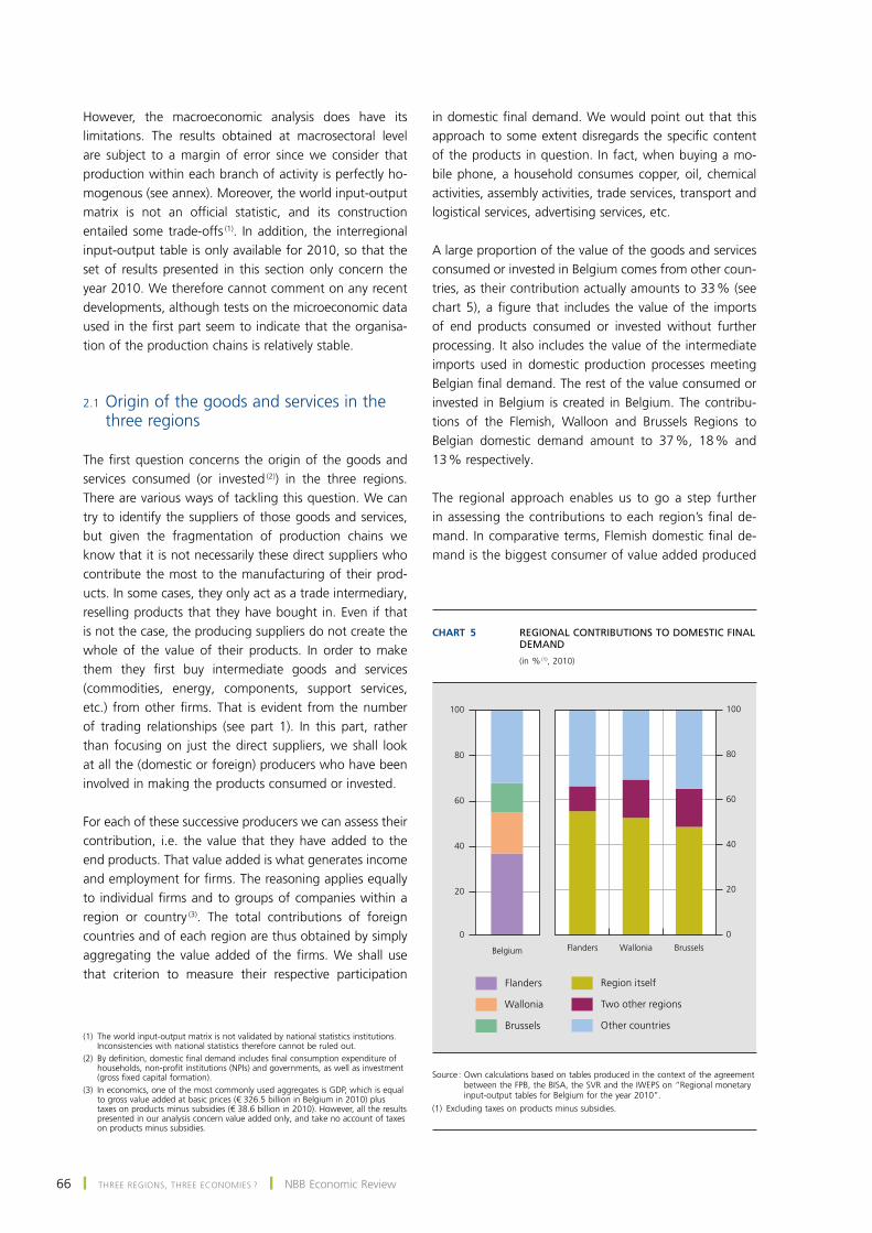
66 ❙ tHRee ReGIoNS, tHRee eCoNoMIeS ? ❙ nBB Economic Review
However, the macroeconomic analysis does have its limitations. the results obtained at macrosectoral level are subject to a margin of error since we consider that production within each branch of activity is perfectly ho‑mogenous (see annex). moreover, the world input-output matrix is not an official statistic, and its construction entailed some trade‑offs (1). In addition, the interregional input-output table is only available for 2010, so that the set of results presented in this section only concern the year 2010. We therefore cannot comment on any recent developments, although tests on the microeconomic data used in the first part seem to indicate that the organisa‑tion of the production chains is relatively stable.
2.1 origin of the goods and services in the three regions
the first question concerns the origin of the goods and services consumed (or invested (2)) in the three regions. there are various ways of tackling this question. We can try to identify the suppliers of those goods and services, but given the fragmentation of production chains we know that it is not necessarily these direct suppliers who contribute the most to the manufacturing of their prod‑ucts. in some cases, they only act as a trade intermediary, reselling products that they have bought in. Even if that is not the case, the producing suppliers do not create the whole of the value of their products. in order to make them they first buy intermediate goods and services (commodities, energy, components, support services, etc.) from other firms. that is evident from the number of trading relationships (see part 1). in this part, rather than focusing on just the direct suppliers, we shall look at all the (domestic or foreign) producers who have been involved in making the products consumed or invested.
for each of these successive producers we can assess their contribution, i.e. the value that they have added to the end products. that value added is what generates income and employment for firms. the reasoning applies equally to individual firms and to groups of companies within a region or country (3). the total contributions of foreign countries and of each region are thus obtained by simply aggregating the value added of the firms. We shall use that criterion to measure their respective participation
in domestic final demand. We would point out that this approach to some extent disregards the specific content of the products in question. in fact, when buying a mo‑bile phone, a household consumes copper, oil, chemical activities, assembly activities, trade services, transport and logistical services, advertising services, etc.
A large proportion of the value of the goods and services consumed or invested in Belgium comes from other coun‑tries, as their contribution actually amounts to 33 % (see chart 5), a figure that includes the value of the imports of end products consumed or invested without further processing. It also includes the value of the intermediate imports used in domestic production processes meeting Belgian final demand. the rest of the value consumed or invested in Belgium is created in Belgium. the contribu‑tions of the Flemish, Walloon and Brussels Regions to Belgian domestic demand amount to 37 %, 18 % and 13 % respectively.
the regional approach enables us to go a step further in assessing the contributions to each region’s final de‑mand. in comparative terms, flemish domestic final de‑mand is the biggest consumer of value added produced
(1) the world input-output matrix is not validated by national statistics institutions. inconsistencies with national statistics therefore cannot be ruled out.
(2) By definition, domestic final demand includes final consumption expenditure of households, non-profit institutions (npis) and governments, as well as investment (gross fixed capital formation).
(3) in economics, one of the most commonly used aggregates is gDp, which is equal to gross value added at basic prices (€ 326.5 billion in Belgium in 2010) plus taxes on products minus subsidies (€ 38.6 billion in 2010). However, all the results presented in our analysis concern value added only, and take no account of taxes on products minus subsidies.
Chart 5 REGIONAL CONTRIBUTIONS TO DOMESTIC FINAL DEMAND
(in % (1), 2010)
0
20
40
60
80
100
0
20
40
60
80
100
Belgium Flanders Wallonia Brussels
Flanders
Wallonia
Brussels
Region itself
Two other regions
Other countries
source : own calculations based on tables produced in the context of the agreement between the fpB, the BisA, the sVR and the iWEps on “Regional monetary input-output tables for Belgium for the year 2010”.
(1) excluding taxes on products minus subsidies.

67December 2016 ❙ tHRee ReGIoNS, tHRee eCoNoMIeS ? ❙
in its own region (55 %), against 52 % for Wallonia and 48 % for Brussels. nonetheless, the final demand of each region is based to a significant extent on value from the other two regions. the contributions of the Walloon and Brussels Regions amount to 11 % of final demand in flanders, compared to 34 % for other countries. the other two regions therefore represent almost a quarter of the external value consumed or invested by flanders, the remaining three-quarters coming from foreign countries. For Wallonia and Brussels, one‑third comes from the other two regions compared to two-thirds originating from abroad.
Not all Belgian production is consumed in Belgium. Part of it is exported to other countries. to assess the participation of the various regions in exports, we shall here analyse their contributions in terms of value added. Admittedly, there are alternative indicators for assessing the role of the various regions in exports. traditionally, exports are allocated according to the regions that dis‑patch the products abroad. However, owing to the frag‑mentation of the production chains, that indicator must be interpreted with caution, because a region may serve as the transit point for a product leaving Belgian territory. that has a particular influence on exports by flanders, because the two main gateways to foreign markets – the port of Antwerp and Zaventem airport – are located in the flemish Region. Another option which avoids these gate‑way effects entails considering the region in which the exported goods are produced. once again, the criterion is imperfect because it identifies the region that effects the final domestic stage in production, yet to make products destined for the rest of the world, a region’s firms use inputs originating from other regions or countries. to take account of indirect participation in exports, we use the concept of each region’s value added contained in Belgian exports, regardless of the exporting region (1) and the nature of the exported products.
flanders contributes 24 % to Belgium’s exports, compared to 7 % for both Wallonia and Brussels (see chart 6). With a contribution of 62 %, other countries therefore have a predominant weight in Belgian exports, even exceeding their weight in domestic demand. there are two reasons for that. first, the exports consist mainly of industrial goods, production of which involves large quantities of
commodities or components from abroad. conversely, do‑mestic consumption is based more on services, including public services. the production of services requires fewer foreign inputs. Also, the importance of foreign countries in Belgium’s exports is due to Belgium’s central position at the heart of the Eu and to its excellent, highly developed logistics and transport infrastructures. Belgium acts as a trade hub and, in particular, forms the gateway to the north european market via the activities of its sea ports. in practice, a significant proportion of Belgium’s imports is immediately re-exported. those re-exports simultaneously inflate Belgium’s imports and (the foreign value content of its) exports (2).
Re‑exports are also recorded in the regional export sta‑tistics and inflate them by a factor of around 40 % (3). However, to obtain a more accurate picture of the exports of the three regions, we exclude re-exports, focusing sole‑ly on domestic export production. in comparative terms, Walloon export production contains the most value added originating from its own region (48 %), against 45 % for flanders and 40 % for Brussels. the regions also rely on value created outside their territory. the contribution of
Chart 6 REGIONAL CONTRIBUTIONS TO EXPORTED PRODUCTION
(in % (1), 2010)
0
20
40
60
80
100
0
20
40
60
80
100
Belgium Flanders (2) Wallonia
(2) Brussels (2)
Flanders
Wallonia
Brussels
Region itself
Two other regions
Foreign countries (excluding re‑exports)
Re‑exports
source : own calculations based on tables produced in the context of the agreement between the fpB, the BisA, the sVR and the iWEps on “Regional monetary input-output tables for Belgium for the year 2010”.
(1) excluding taxes on products minus subsidies.(2) Region of production of the goods and services exported to other countries.
(1) A discussion of the role of the various stages leading up to the actual export of the product is beyond the scope of this article. for more information on producing and exporting regions, see Avonds et al. (2016).
(2) in the case of re-exports, the value added is due to any transport and logistical costs invoiced to resident firms.
(3) According to the regional input-output table, re-exports totalled € 50.4 billion for flanders, € 12.5 billion for Wallonia and € 11.5 billion for Brussels. As pointed out in the iWEps report (2016), in the input-output system imports of goods destined for re-export are imputed to the region where the flows originate, and not to the trade intermediary for whom only the trade margin received is recorded.

68 ❙ tHRee ReGIoNS, tHRee eCoNoMIeS ? ❙ nBB Economic Review
the other two regions comes to almost a fifth of that external value that Wallonia and Brussels include in their respective exports (the remaining four-fifths coming from abroad), compared to almost a tenth of that used by Flanders (the other nine‑tenths originating from foreign countries). Although these interregional contributions are smaller than those recorded for domestic final demand, notably because more foreign components are used in the processes of producing exported industrial goods, they are still significant.
2.2 Destinations of the value added of the three regions
the preceding section aimed to define the origin of the goods and services consumed or invested. In that section, we assessed interregional trade from the point of view of the final consumers. nonetheless, we can also ana‑lyse trade from the producers’ point of view. Analysing trade from that angle amounts to identifying the final destinations of the value added created in each region.
We expressly refer to final destinations, and not direct destinations. For producers of intermediate goods and services, that means that we determine the place of consumption of the finished product incorporating these intermediate components.
obviously, a region’s own market is its preferred final destination. thus, 64 % of Walloon value added, 57 % of flemish value added and 28 % of Brussels value added is ultimately consumed or invested in the respective regions (see table 3) (1). Each region also responds to the final de‑mand from the other two regions and from foreign coun‑tries. In that regard, the interregional market represents around a sixth of the value added sold by flanders outside its region, compared to a quarter for Wallonia and over half for Brussels (2). these shares are considerable. In the case of flanders, the other two regions together are more important than any neighbouring country considered indi‑vidually. moreover, the importance of the Walloon market alone is comparable to that of the German or French market, and greater than that of the Dutch market. For Wallonia and Brussels, the interregional market is more important than the German and French markets together.
one peculiarity of the Brussels Region is that it exports a very large proportion of its value added to the other two regions. it also imports value added from flanders and Wallonia, but to a much lesser degree. It therefore records a positive value added balance in regard to the other two regions (see chart 7) (3). that is due partly to the very numerous services (financial, government, education services, etc.) that Brussels provides for the other two
Table 3 DESTINATIONS OF THE VALUE ADDED OF THE THREE REGIONS
(in %, 2010)
Region creating the value added
Brussels
Flanders
Wallonia
Total Belgium
Destination of the value added (1)
Belgium . . . . . . . . . . . . . . . . . . . . . . . . . . . . . . . . . . . 67.9 63.3 73.0 66.5
Brussels . . . . . . . . . . . . . . . . . . . . . . . . . . . . . . . . . 28.2 2.4 2.3 7.3
Flanders . . . . . . . . . . . . . . . . . . . . . . . . . . . . . . . . . 27.0 56.6 6.5 39.0
Wallonia . . . . . . . . . . . . . . . . . . . . . . . . . . . . . . . . 12.7 4.4 64.2 20.2
Foreign countries . . . . . . . . . . . . . . . . . . . . . . . . . . . 32.1 36.7 27.0 33.5
Total . . . . . . . . . . . . . . . . . . . . . . . . . . . . . . . . . . . . . 100.0 100.0 100.0 100.0
Source : Own calculations based on tables produced in the context of the agreement between the FPB, the BISA, the SVR and the IWEPS on “Regional monetary input‑output tables for Belgium for the year 2010”.
(1) The results include an estimate of any repatriation effect, namely the amount of each region’s value added which is initially exported but then re‑imported for consumption or investment purposes.
(1) this table is similar to table 7 in Avonds et al. (2016). the differences are due to estimation of the repatriation effect in our analysis, i.e. the Belgian value added initially exported but later reimported for consumption or investment purposes.
(2) in accordance with the residence principle, household consumption expenditure is apportioned according to the household’s region of residence, regardless of the place of purchase. For more information, see Avonds et al. (2016).
(3) for a region or country, the total balance of value added corresponds exactly to the total trade balance established on the basis of imports and exports of goods and services. However, bilateral balances may diverge depending on the approach (for more information, see Benedetto (2012), among others). thus, in contrast to the traditional concept, the balance of value added between two countries (or regions) can neutralise the effect of re-exports or imported inputs which could inflate the exports of a country (or region).
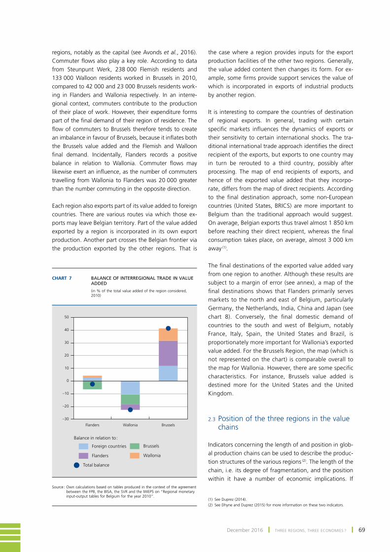
69December 2016 ❙ tHRee ReGIoNS, tHRee eCoNoMIeS ? ❙
regions, notably as the capital (see Avonds et al., 2016). commuter flows also play a key role. According to data from steunpunt Werk, 238 000 flemish residents and 133 000 Walloon residents worked in Brussels in 2010, compared to 42 000 and 23 000 Brussels residents work‑ing in flanders and Wallonia respectively. in an interre‑gional context, commuters contribute to the production of their place of work. However, their expenditure forms part of the final demand of their region of residence. the flow of commuters to Brussels therefore tends to create an imbalance in favour of Brussels, because it inflates both the Brussels value added and the Flemish and Walloon final demand. incidentally, flanders records a positive balance in relation to Wallonia. commuter flows may likewise exert an influence, as the number of commuters travelling from Wallonia to flanders was 20 000 greater than the number commuting in the opposite direction.
each region also exports part of its value added to foreign countries. there are various routes via which those ex‑ports may leave Belgian territory. part of the value added exported by a region is incorporated in its own export production. Another part crosses the Belgian frontier via the production exported by the other regions. that is
the case where a region provides inputs for the export production facilities of the other two regions. generally, the value added content then changes its form. For ex‑ample, some firms provide support services the value of which is incorporated in exports of industrial products by another region.
It is interesting to compare the countries of destination of regional exports. in general, trading with certain specific markets influences the dynamics of exports or their sensitivity to certain international shocks. the tra‑ditional international trade approach identifies the direct recipient of the exports, but exports to one country may in turn be rerouted to a third country, possibly after processing. the map of end recipients of exports, and hence of the exported value added that they incorpo‑rate, differs from the map of direct recipients. According to the final destination approach, some non-European countries (united states, BRics) are more important to Belgium than the traditional approach would suggest. on average, Belgian exports thus travel almost 1 850 km before reaching their direct recipient, whereas the final consumption takes place, on average, almost 3 000 km away (1).
the final destinations of the exported value added vary from one region to another. Although these results are subject to a margin of error (see annex), a map of the final destinations shows that flanders primarily serves markets to the north and east of Belgium, particularly germany, the netherlands, india, china and japan (see chart 8). conversely, the final domestic demand of countries to the south and west of Belgium, notably france, italy, spain, the united states and Brazil, is proportionately more important for Wallonia’s exported value added. for the Brussels Region, the map (which is not represented on the chart) is comparable overall to the map for Wallonia. However, there are some specific characteristics. For instance, Brussels value added is destined more for the United States and the United Kingdom.
2.3 Position of the three regions in the value chains
Indicators concerning the length of and position in glob‑al production chains can be used to describe the produc‑tion structures of the various regions (2). the length of the chain, i.e. its degree of fragmentation, and the position within it have a number of economic implications. if
Chart 7 BALANCE OF INTERREGIONAL TRADE IN VALUE ADDED
(in % of the total value added of the region considered, 2010)
–30
–20
–10
0
10
20
30
40
50
Flanders Wallonia Brussels
Foreign countries Brussels
Flanders Wallonia
Total balance
Balance in relation to :
source : own calculations based on tables produced in the context of the agreement between the fpB, the BisA, the sVR and the iWEps on “Regional monetary input-output tables for Belgium for the year 2010”.
(1) see Duprez (2014).(2) see Dhyne and Duprez (2015) for more information on these two indicators.

70 ❙ tHRee ReGIoNS, tHRee eCoNoMIeS ? ❙ nBB Economic Review
a region forms part of fragmented chains, that means that its firms are generally more specialised in a par‑ticular production segment. that specialisation is often accompanied by greater productivity. Also, if a region is positioned towards the end of production chains, its companies are fairly close to the final consumer. in some sectors that is a considerable advantage, as competition with foreign firms, particularly those from emerging countries, is less fierce and the margins are bigger.
on average, flemish and Brussels firms form part of relatively fragmented chains with more than three pro‑duction links. conversely, Wallonia is more active in fairly short production chains. In terms of position, Brussels comes at quite an early stage in the production chains. Wallonia and flanders are closer to the final consumer (see table 4).
Chart 8 GEOGRAPHICAL DISTRIBUTION OF EXPORTED VALUE ADDED (1)
10% 1%
USA
CHN
IND
JAP
CAN
BRA
KOR
AUS
MEX
Large difference
Small difference
Market more important for Wallonia
Market more important for Flanders
Importance of the market for Belgium
source : own calculations based on tables produced in the context of the agreement between the fpB, the BisA, the sVR and the iWEps on “Regional monetary input-output tables for Belgium for the year 2010”.
(1) the size of the disc represents the importance of the market for exported Belgian value added. the colour of the disc depends on the difference between the share of a given market in the total Wallonian exported value added and the corresponding share for flanders. the difference is called small (large) if it is below (above) 10 %.
Table 4 POSITION IN AND LENGTH OF REGIONAL PRODUCTION CHAINS (1)
(2010)
Average length of the production chains
Average position in the production chains
Flanders . . . . . . . . . . . 3.22 0.48
Wallonia . . . . . . . . . . 2.74 0.49
Brussels . . . . . . . . . . . 3.12 0.45
Source : Own calculations based on tables produced in the context of the agreement between the FPB, the BISA, the SVR and the IWEPS on “Regional monetary input‑output tables for Belgium for the year 2010”.
(1) The average length of the production chains of which the regions form part expresses the average number of successive processing stages in making the end products. The position is an indicator ranging between 0 and 1. A value close to 0 means an initial production stage, while a value close to 1 indicates a final production stage, close to the final consumer. See Dhyne and Duprez (2015) for more information on these indicators.

71December 2016 ❙ tHRee ReGIoNS, tHRee eCoNoMIeS ? ❙
Conclusion
the production structures of the various regions have their own specific characteristics. Wallonia forms part of less fragmented chains than Flanders and Brussels. Also, Brussels holds a position closer to the start of the chains, while flanders and Wallonia are closer to the final consumer. the final destinations of the exported value added likewise vary from one region to another. the value created in Flanders is destined more for the markets to the north and east of Belgium (particu‑larly germany, the netherlands, india and china), while Walloon value added is more specifically destined for countries to the south and west of Belgium (such as france, italy, the united states and Brazil). the Brussels Region’s destinations are comparable overall to those of Wallonia, although the United States and the United Kingdom represent a larger share.
Various authors have studied the tariff and non-tariff bar‑riers confronting export firms (see Araujo et al. (2012) for Belgium). As far as we know, this article is the first to study potential interregional barriers within Belgium. for that purpose, we examined trading relationships between firms. According to our estimates, a flemish firm faces an implicit barrier equivalent to 10 km when wishing to sell to a Walloon firm, whereas a Walloon supplier is confronted by an implicit barrier of 30 km if it wants to find a business customer in flanders. that is also reflected at overall level. for its final consumption or its export production, Flanders is less dependent on value originat‑ing from the other two regions than are Wallonia and Brussels. the Brussels Region is a special case, to some degree. firms there often form a link between the various economic sub-networks. they do not appear to encounter any barriers when establishing connections with firms in the other two regions. the role of Brussels as the capital providing services for the whole country, and the pres‑ence there of registered offices of numerous firms which also have establishments in the other two regions, prob‑ably make it easier to trade.
of course, the scale of the barriers must be viewed in per‑spective. Economic relations between supplier firms and customer firms are determined primarily by the distance between them, regardless of their respective regions. Economic factors, such as the firms’ size, their sector of activity, any financial links or their membership of the same economic sub-network, also play a crucial role. in that regard, a map of the sub-networks indicates the existence of a number of areas in which trading is more intense. in addition, interregional barriers mainly have an impact on trade in services. Legislation, language and culture are more important factors for services than for industrial goods.
the presence of interregional barriers does not prevent trade between the various regions. in Belgium, one in two firms sells to a business customer in another region. overall, each of the three regions is involved in the exports of the other two. in addition, 6.8 % of flemish value added is invested or consumed by households or government services in the other two regions. for Flanders, the importance of the Walloon market alone is comparable to that of the German or French market, and exceeds that of the Dutch market. For Wallonia and Brussels, the interregional market absorbs 8.8 % and 39.7 % respectively of the value added created. it is more important than the German and French markets taken together.
finally, Belgium can take advantage of the specific char‑acteristics of each region by limiting the interregional barriers to trade. those barriers often have an adverse effect for suppliers and customers, as well as weakening the interregional market which represents a significant outlet. in that connection, we would stress the impor‑tance of regional policies designed to facilitate inter‑regional trade, in particular via coordinated legislation. Worker training policies, particularly those concerning acquisition of another language, and policies that en‑courage mobility, are likewise important catalysts of that trade.

72 ❙ tHRee ReGIoNS, tHRee eCoNoMIeS ? ❙ nBB Economic Review
Annex
this annex presents the matrix calculation formulas used for the analysis in the second part of the article.
for any vector f (366X1) which gives the quantity of demand for each product / region (122 products in each of the three regions), the content in terms of value added originating from a branch / region i is the component i of the matrix E (366X1), in which :
E=(VT#B*f),
VT (1X366) being the transposed vector of the coefficients of value added vi / pi for each product / region i (vi is the value added and pi is the production of the branch / region i). B (366X366) is the leontief inverse matrix (i–A)–1, in which i (366X366) is the identity matrix and each coefficient aij =cij / pj of matrix A (366X366) gives the quantity of products of branch / region i necessary to produce one unit of product of branch / region j (cij is the intermediate consumption by branch / region j of products of branch / region i and pj is the total production of branch / region j). # is the symbol of the multiplication component by component.
to ascertain the destinations of the exported regional value added, the international exports of each branch of activity / region were divided into four categories : intermediate goods, end products, intermediate services and final services. the distinction between goods exports and services exports is derived from the interregional input-output table. conversely, the breakdown between intermediate products and end products is not directly available. it is estimated by modelling it on the breakdown between intermediate products and end products in the case of products destined for the domestic market. for each category y (y = intermediate goods, end products, intermediate services, final services), the direct destination d (among c countries) of the exported value added originating from a branch / region i is the component (i,d) of matrix Ey (366Xc), in which :
ey=(VT#B*Fy)*gy,
VT (1X366) being the transposed vector of the coefficients of value added vi / pi for each product / region i (vi is the value added and pi is the production of the branch / region i). B (366X366) = (i–A)–1 the leontief inverse matrix, fy (366X366) divides each product / producer region i into products / exporting region j (for a given product, the exporting region exports the production originating from the three regions). gy (366Xc) gives the breakdown by country of final destination (the c destinations are the countries in the WioD world input-output matrix, shown in the columns) of an exported unit of product / exporting region.
for end products and final services, the final destination is assumed to be the direct destination, derived from the foreign trade data for goods and the balance of payments data for services (1) . For intermediate goods and services, the direct destination is obtained from the foreign trade data for goods and the balance of payments data for services. However, the direct destination is not the final destination.
to ascertain the final destinations of exports of intermediate goods and services, we analysed the WioD data using the method proposed by Wang et al. (2013). that method makes it possible to find the final destinations by means of the following breakdown of intermediate exports of each Belgian product i (among the n products included in the WioD) to a destination r (among the c destinations included in the WioD) :
(ArBrryrr)+∑t≠r(ArBrtytt)+∑t≠r(A
rBrryrt)+∑t≠r,u∑u≠r,t(ArBruyut)
Ak (nXn) is the sub-matrix that gives the intermediate use in country k of intermediate products exported by Belgium. Bkl (nXn) is the leontief inverse matrix. Ykl (nX1) is the domestic final consumption by country l of end products sold by country k.
(1) this breakdown is imperfect because the foreign trade data differ from those in the regional accounts (see Avonds et al. (2016) and iWEps (2016)).the same applies to the balance of payments data.

73December 2016 ❙ tHRee ReGIoNS, tHRee eCoNoMIeS ? ❙
Bibliography
Araujo l., g. mion and E. ornelas (2012), Institutions and export dynamics, NBB, Working Paper 220.
Avonds l., c. Hambÿe, B. Hertveldt, B. michel, B. Van den cruyce (2016), Analysis of the interregional input-output table for 2010, FBP, Working Paper 5.
Benedetto j. (2012), “implications and interpretations of Value-Added trade Balances”, Journal of International commerce and economics, 4(2), 39–53.
Blondel, V., j-l. guillaume, R. lambiotte and E. lefevre (2008), Fast unfolding of communities in large networks, journal of statistical mechanics – theory and Experiments, 10.
Dhyne E. and c. Duprez (2015), “Has the crisis altered the Belgian economy’s DnA ?”, nBB, Economic Review, september, 31–43.
Dhyne E., g. magerman and s. Rubínová (2015), The Belgian production network 2002-2012, NBB, Working paper 288.
Duprez c. (2014), “Value creation in exports : a diagnosis for Belgium”, nBB, Economic Review, september, 27–42.
iWEps (2016), Rapport sur l’économie wallonne.
manski c. f. and s. R. lerman (1977), “the Estimation of choice probabilities from choice Based samples”, Econometrica, 45(8), 1977-1988.
Wang Z., s-j Wei and K. Zhu (2013), Quantifying international production sharing at the bilateral and sector levels, nBER, Working paper series, 19677.

75December 2016 ❙ finDings fRom tHE EuRopEAn suRVEY on WAgE-sEtting ❙
findings from the European survey on wage-setting (*)
D. Cornille
Introduction
the harmonised survey of European firms’ wage-setting practices was conducted in twenty-five countries of the European union in 2014 and in 2015. focusing in particular on the period 2010-2013, it featured questions on firms’ perception of the nature of the changes in the economic environment after the sovereign debt crisis, on their reac‑tions to these changes and on the role of financial con‑straints. this update of the two previous surveys, carried out respectively in 2007 and in 2009, was largely inspired by the need to gain a better understanding of the nature of the shocks that have hit companies and how they have reacted to them in a context marked by reforms affecting the functioning of the labour market in many countries.
the survey (1) as well as initial analyses of the findings have been compiled and coordinated under the auspices of the Wage Dynamics network (WDn), a European system of central Banks (EscB) research network that studies the characteristics of wage dynamics. the country-by-country results have been analysed in detail in a series of na‑tional reports published on the EcB’s website in 2015 and in 2016 (2). in Belgium’s case, the findings were also covered in an article which appeared in the December 2015 edi‑tion of the Bank’s Economic Review (3). the Bank has also
published detailed results per branch of activity for Belgium on its website (4). this article draws on one of the survey’s plus points, namely the harmonisation of the question‑naire compiled jointly through consultations between the 25 participant countries, thus adding to previous analyses with a comparative study of the data gathered in the dif‑ferent countries. for this reason, it is largely based on a pre‑liminary version of the research network report compiled by seven of its members (mario izquierdo, juan f. jimeno, theodora Kosma, Ana Lamo, Stephen Millard, tairi Rõõm and Eliana Viviano) and entitled "labour market adjust‑ment in europe during crisis : Microeconomic evidence from the Wage Dynamics network survey". this report will be published shortly as an EcB occasional paper.
the article only covers part of the aspects addressed by the survey. the wealth of information gathered calls for more specific research projects, some of which are underway in different national central banks. they will be covered by separate publications, for example in the Bank’s or the eCB’s Working Paper series. Another of the article’s objectives is to encourage further studies outside the network : arrange‑ments are in fact being made for interested research workers to have access to the database during the course of 2017.
in this article, as in the network report mentioned above, the results given are weighted by employment (5), to make them representative of the entire company popula‑tion. Moreover, even though certain countries, including Belgium, have also collected information for very small businesses, the analysis here focuses on firms employing five or more workers.
the article contains four parts. After a short recapitula‑tion on the economic context and a description of the
(*) the article is largely based on a preliminary version of the report from the WDn research network compiled by seven of its members, mario izquierdo, Juan F. Jimeno, theodora Kosma, Ana Lamo, Stephen Millard, tairi Rõõm and Eliana Viviano, and entitled “labour market adjustment in Europe during the crisis : microeconomic evidence from the Wage Dynamics network survey”. this report will shortly be available in the form of an EcB occasional paper.
(1) the questionnaire for Belgium can be consulted on the Bank’s website (www.nbb.be / en / wage-dynamics-network-wdn-3).
(2) see http : / / www.ecb.europa.eu / pub / economic-research / research-networks / html / researcher_wdn.en.html.
(3) see cornille (2015).(4) see www.nbb.be / fr / wage-dynamics-network-wdn-3.(5) See Druant et al. (2008).

76 ❙ finDings fRom tHE EuRopEAn suRVEY on WAgE-sEtting ❙ nBB Economic Review
selections made to facilitate the analysis (for example as regards country groupings), it describes how companies have perceived changes in the economic environment. It then goes on to study the adjustment channels open to firms, before broaching public authorities’ reactions and the challenges in the field of economic policy.
1. A mixed economic context in the european Union
the survey covers the years 2010 to 2013, which, in the majority of European nations, were marked by changes in the economic environment following the sovereign debt crisis. However, they were not all affected in the same way nor with the same intensity ; and episodes of strong economic tensions did not always coincide. one of the difficulties encountered when the survey was being compiled was choosing a common reference period for all countries, even though it was decided not to establish any explicit link in the questionnaire between the period selected and the term “crisis“.
several macroeconomic indicators reflect these mixed reactions of the european economies, and on the la‑bour market in particular. the period is thus marked not just by a rise in the unemployment rate, but also by a widening of the differentials between the various countries’ unemployment rates. increasing labour mar‑ket participation rates can also be observed, including in countries where the unemployment rate is on the rise, something which is quite atypical in crisis times, as well as a decline in hours worked per person, always with major divergences between countries. As far as Belgium is concerned, a relatively weak rise in the un‑employment rate, a virtually unchanged labour market participation rate and a slight upturn in hours worked per person can be noted.
in analysing the 25 countries taking part in the survey from the perspective of the link between unemployment and gDp growth, a relationship also known as okun’s law, it also appears that the 2010-2013 period was marked by a certain degree of heterogeneity. After the great reces‑sion, most countries returned to positive growth, but two groups among them can be distinguished, depending on whether unemployment fell back there or not. this way of classifying countries, according to changes in their unem‑ployment and their gDp rates between 2010 and 2013, has been chosen by the network to facilitate presentation and analysis of the survey results. this analytical grouping enables three groups to be defined :– group 1 : countries that saw their unemployment
rate go down and their gDp increase (germany,
Estonia, Hungary, ireland, latvia, lithuania, malta, czech Republic, united Kingdom and slovakia)
– group 2 : countries whose unemployment rate has gone up while gDp was rising (Austria, Belgium, Bulgaria, France, Luxembourg, the Netherlands, Poland and Romania)
– group 3 : countries hit by a rise in unemployment and a fall in gDp (cyprus, croatia, spain, greece, italy, portugal and slovenia).
the picture in Belgium is one of relative stability. for instance, although the unemployment rate did not drop back, the crisis did not have a very great impact on em‑ployment, with the exception of the manufacturing sec‑tor. nor has Belgium featured any radical labour market reforms, although various measures have been taken, for example in the area of wage moderation or job protection in the form of mechanisms intended to boost flexibility (temporary lay-offs). nevertheless, as in the other coun‑tries, firms have been affected to varying degrees.
2. Firms’ perception of the changing economic environment
the survey contains a wealth of information about firms’ perception of the changes in their economic environment
Chart 1 ANALYTICAL GROUPING OF COUNTRIES COVERED BY THE SURVEY
(in %)
–10
–5
0
5
10
15
20
–10 –5 0 5 10
CZDE
EE
IEHU
LT
LV
MTSKUK
ROPL
ATBE
BGLUFR
NL
CY
ES
EL
HR
ITPT
SI
Cha
nge
in t
he u
nem
ploy
men
t ra
te b
etw
een
2013
and
201
0,in
per
cent
age
poin
ts
Annual average GDP growth rate over the 2010-2013 period
Group 1 Group 2 Group 3
sources : Ec ; m. izquierdo, j. f. jimeno, t. Kosma, A. lamo, s. millard, t. Rõõm and E. Viviano (2017, to be published).

77December 2016 ❙ finDings fRom tHE EuRopEAn suRVEY on WAgE-sEtting ❙
over the 2010-2013 period. for instance, it covers the impact on firms’ activity of not only demand for their products, but also of uncertainty about fluctuations in this demand. the role of access to external financing can also be studied quite carefully, by means of details by type of objective (new investment, working capital, refinancing) and constraints (rationing or excessively onerous condi‑tions). the survey also makes it possible to assess such things as the extent to which firms have been affected by customers’ ability to pay and the availability of goods and services procured from their suppliers.
chart 2 sums up the way in which firms have perceived the impact of the economic situation on their own activ‑ity, for a selection of five factors (namely, level of demand, volatility of demand, access to external financing, custom‑ers’ ability to pay and availability of supplies). for this pur‑pose, values have been attributed to firms’ replies to the questions : –2 for “strong decrease“ (in activity), –1 for “moderate decrease“, 0 for “unchanged“, 1 for "moder‑ate increase" and 2 for “strong increase“. A weighted average of these indicators has then been calculated per
country and for the three groups of countries previously described. the chart also includes the results for countries positioned at the extremes (minimum and maximum) for each group, as well as those for Belgium. As a reminder, negative values indicate that the impact of the factor on firms’ activity has been negative on average.
it is interesting to note that, for each of the five factors studied, the three analytical groups as defined above obtain an identical ranking. It appears that, on average, the com‑panies in group 1 (countries characterised by a rise in gDp and a drop in unemployment over the period 2010-2013) suffered almost no impact on their activity from changes in economic environment, except – and only marginally – in the case of customers’ ability to pay. the findings from group 2 (countries where both gDp and unemployment have risen) are less favourable, suggesting that firms have seen their activity affected by each of the selected factors, albeit to a lesser extent than those from group 3 (countries that have registered a fall in gDp and a rise in unemployment), which posted the worst results. the analysis by m. izquierdo, j.f. jimeno, t. Kosma, A. lamo, s. millard, t. Rõõm and
Chart 2 ECONOMIC SITUATION AND ITS EFFECTS ON FIRMS’ ACTIVITY OVER THE PERIOD 2010 2013
(firms’ replies standardised to 0, positive (negative) values indicate positive (negative) effects, averages per group of countries)
0
Gro
up 1
Gro
up 2
Gro
up 3
–1.4
–1.2
–1
–0.8
–0.6
–0.4
–0.2
0.2
0.4
0.6
0.8
Gro
up 1
Gro
up 2
Gro
up 3
Gro
up 1
Gro
up 2
Gro
up 3
Gro
up 1
Gro
up 2
Gro
up 3
Gro
up 1
Gro
up 2
Gro
up 3
Belgium
Average for the countries in the group
LEVEL OF DEMAND
VOLATILITY /UNCERTAINTYOF DEMAND
ACCESS TOEXTERNAL FINANCE
AVAILABILITYOF SUPPLIES
CUSTOMERS’ABILITY TO PAY
Minimum / Maximum for the countries in the group
1.56
sources : WDn, m. izquierdo, j.f. jimeno, t. Kosma, A. lamo, s. millard, t. Rõõm and E. Viviano (2017, to be published).Weighted and re-scaled results disregarding missing answers.

78 ❙ finDings fRom tHE EuRopEAn suRVEY on WAgE-sEtting ❙ nBB Economic Review
E. Viviano (2017, to be published) confirms through robust econometric methods that there is in fact a strong correla‑tion between the way in which shocks are felt by firms and changes in gDp or unemployment.
Calculation of the averages masks different situations from one country to another, and even more so within countries themselves. As regards divergences between countries, even between those in group 1, it can be seen that some countries have suffered negative repercussions from the shocks more than others, even though, on aver‑age, the group as a whole has not. the opposite applies to group 2, where several countries post positive results while, on average, the group is in negative territory. By contrast, the impact is negative for all the countries in group 3. Belgium is almost always at the average for group 2, which it belongs to alongside france and the netherlands. However, these two countries’ scores in nearly all cases are more negative than those for Belgium, not least as regards the effect of the level of demand and, for the netherlands, regarding access to financing too. on the other hand, the results for germany, a heavyweight in group 1, are always above the group average.
the WDn survey also enables an assessment of the impact of shocks according to firms’ individual characteristics, such as their size, their sector of activity, whether they are subsidiaries or stand‑alone companies, foreign or domestic, whether they are active or not on international markets, etc. Although a systematic analysis of these char‑acteristics is outside the scope of this article, a few salient features are nevertheless worth mentioning. it actually turns out that, whatever group they belong to, small firms are more sensitive to shocks, in particular concerning demand and access to financing. As far as branch of ac‑tivity is concerned, services firms generally tend to be the most sensitive to negative shocks, although that seems to be less the case in Belgium, where industry is hit harder, especially by demand-related shocks. these aspects are examined in more detail in m. izquierdo, j.f. jimeno, t. Kosma, A. lamo, s. millard, t. Rõõm and E. Viviano (2017, to be published).
3. Firms are using varied adjustment channels
the survey helps identify the channels that companies are using to meet the challenges facing them. As far as production costs are concerned, the survey shows that a majority of firms have been subject to rising costs, and in particular wage costs (a trend apparent in all countries apart from greece and cyprus). now, wage costs can in theory be adjusted by adapting either the volume of
labour, i.e. employment, or the cost of labour, i.e. wages. from a macroeconomic point of view, one observation is that the dynamics of hours worked have actually been very diverse from one country to another, while those for nominal hourly wages have been a lot less varied. thanks to the survey, it can be checked whether that is linked to the shocks firms have suffered and, to some extent, the specific role of labour market institutions can also be singled out.
If the appraisal is limited to just demand shocks and comparing the reactions of firms that mentioned such a negative shock with those of firms which said it had a neutral or positive effect, it appears that companies which have suffered a shock of this kind have tended more to adjust the various determinants of wage costs downwards. the difference is the most evident for the volume of labour used as an input, and particularly for the number of permanent employees. the effect is not quite so pronounced for the number of temporary workers, and it is even less so when it comes to hours worked per person. on average, the variable com‑ponent of wages has also played an adjustment role, while that has been much less the case for base wages. However, the survey does not enable us to measure the exact magnitude of these adjustments, as it is not, for example, possible to determine a priori whether a sharp reduction in the variable wage components has a bigger or smaller impact on costs than a small decline in base wages.
there does not seem to have been any profound impact per group of countries, except as regards adjustment of the number of permanent employees, which seems more evident for countries in group 2 (countries registering a rise in both gDp and unemployment), a characteristic that can be compared with more frequent recourse to a freeze or slowdown in new hirings by firms in this group (see below).
A close analysis of these results using multivariate econometric methods corroborates these conclusions, while highlighting other significant effects. By fol‑lowing this approach (controlling for sectoral and firm-size effects), m. izquierdo, j.f. jimeno, t. Kosma, A. lamo, s. millard, t. Rõõm and E. Viviano (2017, to be published) show that demand shocks are effectively correlated to larger adjustments in wage costs. these findings indicate that, apart from adapting permanent employment more frequently, countries in group 2 are also distinctive in terms of a smaller revision of hours worked. furthermore, these countries, and even more so those from group 3, are less likely to change base wages than those in group 1 in the event of a demand

79December 2016 ❙ finDings fRom tHE EuRopEAn suRVEY on WAgE-sEtting ❙
shock (a similar but insignificant result is obtained for the flexible part of wages). finally, this analysis confirms the important role of shocks involving access to external financing, even though the effect of this type of shock on the probability of limiting the different wage costs components is a lot smaller than in the case of demand shocks and there does not seem to be any specific and significant effect per group of countries.
the impact of a demand shock on the adjustment of wage costs is quite noteworthy in Belgium. Even more so than for group 2, to which Belgium belongs, firms’ reac‑tions focus on permanent job numbers (the most clear‑cut result for this group), hours worked and temporary workers. on the other hand, pay reviews, whether for base or variable wages, are the most limited among all the countries that took part in the survey. this suggests that national features of labour market institutions play a key role in firms’ reactions. this is notably the case for
wage formation in the private sector in Belgium, which is largely based on pay scales and collectively bargained job classifications, as well as on a wage norm (indicative or maximum) set at national level and supplemented by automatic wage indexation. this framework effectively makes wage cuts very exceptional (see below) and forces firms to turn to other strategies if they need to adjust their labour force.
Labour force adjustments
the survey points up these strategies through a specific question about measures companies have resorted to for reducing their workforces or changing their composition. this question was only intended for those firms that had actually had to cut back their staff numbers over the period 2010-2013, that is 22 % of the respondents in group 1, 33 % in group 2 (39 % in Belgium) and 44 % in group 3.
Chart 3 EFFECT OF A DEMAND SHOCK ON WAGE COST ADJUSTMENT
(negative (positive) values indicate that firms suffering a demand shock adjusted the factor downwards (upwards), averages par group of countries)
Gro
up 1
Gro
up 2
Gro
up 3
–1.2
–1
–0.8
–0.6
–0.4
–0.2
0
0.2
Gro
up 1
Gro
up 2
Gro
up 3
Gro
up 1
Gro
up 2
Gro
up 3
Gro
up 1
Gro
up 2
Gro
up 3
Gro
up 1
Gro
up 2
Gro
up 3
BASE WAGESFLEXIBLE WAGE COMPONENTS
NUMBER OF PERMANENT EMPLOYEES
NUMBER OF HOURS WORKED PER PERSON
NUMBER OF TEMPORARY WORKERS
Belgium
Average for the countries in the group
Minimum / maximum for the countries in the group
WAGES EMPLOYMENT
Source : WDN.Weighted and re-scaled results disregarding missing answers.Difference between firms saying they had suffered a negative effect and those mentioning a positive or neutral effect.

80 ❙ finDings fRom tHE EuRopEAn suRVEY on WAgE-sEtting ❙ nBB Economic Review
more often than not, firms combine several strategies for adjusting employment. the number of instruments used (among those listed in the survey) is higher than two in all countries ; in Belgium, it is among the highest with more than three instruments brought into play (see chart 4). of course, the type of instrument that can be used is closely as‑sociated with the national labour market institutions, which explains the relative heterogeneity of the replies, although some broad lines do emerge for the different groups.
the most frequently used instrument is a freeze or re‑duction of new hires. this applies to Belgium as to all three groups of countries, although it was less the case in group 1 (featuring a rise in gDp and a drop in un‑employment). the non-renewal of temporary contracts, just as the reduction in the number of agency work‑ers, have been popular options, and even more so the more the macroeconomic environment was unfavour‑able. individual lay-offs have been found more often
in countries from group 1, but this is no doubt largely offset in the other countries by wider recourse to collec‑tive lay-offs, which have been more common in group 3. there is a more contrasting situation for reductions (subsidised or not) in working hours : Belgium is way behind the average for the other groups, just as that for the group 2 it is part of. it is worth noting that tempo‑rary lay-offs, which are very common in Belgium, are not covered by this category for instance and that subsidised reduction of working hours is not an option open to all countries. this instrument was mainly used in germany and italy (respectively 36 and 66 %).
Early retirement schemes have generally tended to be used less, except in Belgium, where this instrument re‑mained quite popular. moreover, the situation is similar with recourse to temporary lay-offs, an option which clearly emerges as the instrument that on average is the least frequently used, regardless of the country group,
Chart 4 EMPLOYMENT ADJUSTMENT CHANNELS IN FIRMS DECLARING A SIGNIFICANT CUT IN THEIR WORKFORCE OR A CHANGE IN ITS COMPOSITION PROPORTION OF FIRMS HAVING USED EACH INSTRUMENT
(percentages, unless otherwise mentioned)
0 10 20 30 40 50 60 70 80
0 1 2 3 4
Temporary lay-offs
Early retirement schemes
Collective redundancies
Non-subsidised reduction of the number of hours
Subsidised reduction of the number of hours
Cuts in the number of agency workers
Individual lay-offs
Non-renewal of temporary contracts
Freeze or reduction of new hires
Number of instruments used on average
Group 1
Of which : Belgium
Group 2 Group 3
Source : WDN.

81December 2016 ❙ finDings fRom tHE EuRopEAn suRVEY on WAgE-sEtting ❙
while in Belgium it is precisely one of the most widely used schemes.
overall, companies seem to have been more inclined to squeeze their extensive margin than their intensive margin, preferring to reduce or keep under control the number of workers rather than the quantity of hours they work. this choice is nevertheless largely influenced by the specific features of national labour market legislation.
Wage adjustments
Another channel that firms can use for adjusting to shocks is that of wages. on the basis of information gathered by means of the survey, two dimensions can be addressed : the frequency of wage changes and the proportion of wages frozen or cut.
As far as the frequency of base wage changes is concerned, although it is found to be lower than the results from the first WDn survey conducted in 2007, it is hard to draw any firm conclusions. these findings have further shown that institutional factors are the main determinants of these changes and that there are still some marked differences from one country to another. A lower level of inflation may also have played a role. However, base wages are adjusted less often when firms are confronted with a restricted access to finance or a demand shock and they are reluctant to cut back nominal wages (m. izquierdo, j.f. jimeno, t. Kosma, A. lamo, s. millard, t. Rõõm and E. Viviano, 2017, to be published). moreover, a low wage change frequency may also be a sign that companies wanting to cut them are obliged to stick to the status quo, which indicates the pres‑ence of downward wage rigidity.
companies surveyed also replied to questions seeking to as‑sess the extent of wage cuts and possible wage freezes, as had been the case in previous waves of the survey. Although the length of the reference periods is not directly comparable between the different surveys, the proportion of firms saying they had cut wages at least once has gone up (see table 1). some degree of heterogeneity can be observed between the three analytical groups. not only does group 3 (countries featuring a drop in gDp and a rise in unemployment) have the highest proportion of all firms surveyed, but this remains the case if the analysis focuses in more detail on firms that have been affected the most by shocks (they mention that they have had to cut wages more frequently). group 1 has a similar profile, but with a smaller proportion. By contrast, countries from group 2 are well below those in the other two groups. Belgium is one of the countries where wage cuts have been implemented the least often.
the wage freeze indicators give similar information and flag up the prevalence of downward wage rigidities, which is also confirmed by other measures (see m. izquierdo, j.f. jimeno, t. Kosma, A. lamo, s. millard, t. Rõõm and E. Viviano, 2017, to be published). this downward nominal wage rigidity may be a factor preventing firms from making an optimal adjustment and forcing them to adapt employment more, as the above-mentioned analysis suggests. one important explanatory factor, particularly pertinent for Belgium, is the role played by labour regulations and collective wage-bargaining agreements, which limit recourse to this option. firms nonetheless generally tend to avoid cutting wages, fearing that this would sink morale or efforts among staff, just as it would trigger a risk of seeing the most productive workers leave the company. so they only tend to use this channel as a last resort, or in extreme situations.
Table 1 SHARE OF FIRMS THAT HAVE CUT WAGES AT LEAST ONCE IN THE PERIOD
(in %)
Period
Group 1
Group 2
Belgium
Group 3
Total
Share of firms that have cut wages at least once . . . . . . . . . . . . . 2002‑2007 – – 3,1 – 2,3
2008‑2009 – – 1,0 – 3,1
2010‑2013 4,8 2,3 1,5 7,9 4,6 (1)
Share of firms reporting being hit by a fall in demand and which have cut wages . . . . . . . . . . . . . . . . . . . . . . . . . . . . . . . . 2010‑2013 5,7 3,1 0,9 10,2 6,0
Share of firms reporting being hit by a fall in demand and credit restrictions and which have cut wages . . . . . . . . . . . . . . . . 2010‑2013 10,0 4,1 2,0 13,4 9,4
Share of firms reporting being hit by a sharp fall in demand and credit restrictions and which have cut wages . . . 2010‑2013 18,7 3,3 0,0 21,7 13,9
Sources : WDN, M. Izquierdo, J.F. Jimeno, T. Kosma, A. Lamo, S. Millard, T. Rõõm and E. Viviano (2017, to be published).Weighted and re‑scaled results disregarding missing answers.(1) The total for countries that also took part in the first WDN survey conducted in 2007 is 4.1 %.

82 ❙ finDings fRom tHE EuRopEAn suRVEY on WAgE-sEtting ❙ nBB Economic Review
in fact, in countries which have had to endure par‑ticuliarly serious economic difficulties, like greece and cyprus, substantial wage cuts have been observed. Respondents for greek and cypriot firms said respective‑ly 55 and 38 % of them had resorted to cutting wages. the survey does not easily capture the impact of these extreme shocks ; it does nor provide sufficient granularity in terms of information about the intensity of the shocks (a major shock in a country very badly affected by the crisis cannot be directly distinguished from a major shock experienced in a country hit less heavily). it is therefore necessary to combine various replies to the question or use external indicators.
Relative importance of wage and employment adjustments
A combination of replies to the question whether firms had reduced or frozen wages as well as those asking about their need to shed staff or modify the composition of their workforce helps to identify the policy mix used the most often to bring down wage costs (see chart 5). it is clear that this mix has been very varied in Europe. However, the analytical grouping shows that adjust‑ments were not only more frequent in countries from group 3, but also that a high proportion of companies there actually combined the two channels (wages and employment). the greek and cypriot cases are striking :
more than 80 % of firms that had to change the compo‑sition of their workforce resorted to using both channels, usually by also cutting or freezing wages too. Within group 2, Belgium features among those countries which opted for changes the most (51 % of firms did so when a labour force adjustment had proved necessary), just behind the netherlands (64 %) and well ahead of france (37 %). for groups 2 and 3, the most widely used op‑tion has been to reduce staff numbers, while in group 1 more firms resorted to a wage cut or freeze at least once between 2010 and 2013. this option has been implemented a lot less in Belgium than on average in the other countries.
Price adjustments
Wage costs are not the only adjustment channel that firms have as they can in principle also act on prices. the survey does provide information on this subject, but this part of the questionnaire has not been included in all countries (only the following 14 countries included these questions in their survey : Belgium, spain, Estonia, greece, Hungary, ireland, italy, latvia, lithuania, luxembourg, malta, poland, portugal and the czech Republic). some general findings are set out here but interested readers should refer to the various country reports that have al‑ready been released and to the research work that will be published later by the WDn network.
Chart 5 REDUCTION IN WAGE COSTS: RELATIVE SIGNIFICANCE OF WAGES AND LABOUR INPUT
(in %)
HU EE DE SK LT CZ LV UK IE AT FR RO BG LU PL BE NL SI IT PT HR ES EL CY0 %
20 %
40 %
60 %
80 %
100 %
0 %
20 %
40 %
60 %
80 %
100 %
No reduction in workforce, nor wage freeze or cuts
Reduction in workforce, but no wage freeze or cuts
No reduction in workforce, but wage freeze or cuts
Reduction in workforce, and wage freeze or cuts
Group 1 Group 2 Group 3
Average
Gro
up 1
Gro
up 2
Gro
up 3
Source : WDN.Weighted and re-scaled results disregarding missing answers.

83December 2016 ❙ finDings fRom tHE EuRopEAn suRVEY on WAgE-sEtting ❙
overall, the results available tend to confirm those gleaned from previous waves of the survey. they indicate that, in most countries, firms adapt their prices once a year. A minority of firms declared that they had to change the frequency of their price adjustments over the period 2010‑2013. the proportion of these companies is highest in group 3, and it is also higher for firms mentioning that they had been hit by a negative demand shock. more often than not, the change was upwards, in other words the frequency with which they adjusted prices speeded up. the explanatory factors are mainly related to increased competition and also to more volatile demand.
4. Reforms
Alongside the strategies that firms have put in place to deal with the crisis, the public authorities have reacted too, by taking measures ranging from slight adapta‑tions to labour market institutions to more fundamental
reforms. one section of the survey examines the way in which firms have perceived these reforms. the questions sought to assess to what extent they have helped them to better face up to the difficulties and also to identify aspects where there is still room for improvement.
Although this article does not seek to describe in any detail the measures or reforms that have been taken in the different countries, some broad lines can be set out. During the initial phase of the crisis, between 2007 and 2010, they mainly sought to preserve em‑ployment and limit the negative consequences for the most vulnerable. As the crisis got worse, wider-ranging reforms were adopted with a view to boosting labour market efficiency and competitiveness. the scale of the measures has often been proportional to under‑performance of the labour market (see m. izquierdo, J.F. Jimeno, t. Kosma, A. Lamo, S. Millard, t. Rõõm and E. Viviano, 2017, to be published). in countries from group 1, marked by a falling unemployment rate, these
Chart 6 HAVE SPECIFIC HR POLICIES BECOME MORE OR LESS DIFFICULT TO IMPLEMENT THAN IN 2010 ?
(firms’ replies standardised to 0, positive (negative) values indicate that firms reckon it has become harder (easier) to follow the policy in question, averages per group of countries)
0
Adj
ustin
g w
ages
of
incu
mbe
nt e
mpl
oyee
s
Dis
mis
sal f
or d
isci
pilin
ary
reas
ons
(for
ser
ious
mis
cond
uct)
Low
er w
ages
for
new
lyhi
red
empl
oyee
s
Lay‑
off
for
econ
omic
reas
ons
(col
lect
ivel
y)
Adj
ustin
g w
orki
ng h
ours
Mov
ing
empl
oyee
s to
posi
tions
in o
ther
loca
tions
Lay
‑off
for
eco
nom
icre
ason
s (in
divi
dual
ly)
Tem
pora
ry la
y‑of
f fo
rec
onom
ic r
easo
ns
Mov
ing
empl
oyee
s ac
ross
diff
eren
t jo
b po
sitio
ns
–1.2
–1
–0.8
–0.6
–0.4
–0.2
0.2
0.4
0.6
0.8
–1.2
–1
–0.8
–0.6
–0.4
–0.2
0
0.2
0.4
0.6
0.8
Group 1
Of which : Belgium
Group 2 Group 3
Minimum / maximum (for all countries)
Hiri
ng e
mpl
oyee
s (c
ost
of r
ecru
itmen
t, in
clud
ing
adm
inis
trat
ive
cost
s)
Source : WDN.Weighted and re-scaled results disregarding missing answers.

84 ❙ finDings fRom tHE EuRopEAn suRVEY on WAgE-sEtting ❙ nBB Economic Review
measures have for instance taken the form of training schemes for the unemployed and workers on short-term contracts, so as to boost their employability (germany). measures designed to reduce working hours have been taken in several countries from group 2, as in Belgium. Reforms of a more structural nature have also been put in place in these countries, such as increasingly degressive unemployment benefits and a scaling down of options for early retirement with supplementary pension payments from companies in Belgium. However, the most radical measures have been introduced in countries from group 3, in particular those from southern Europe, where they were largely framed by imf and Eu assistance programmes.
the companies surveyed were given a selection of ten human resources policy options and asked to say whether certain actions had become more or less difficult to apply than in 2010. chart 6 sets out the results for the three country groupings as well as for Belgium, a positive figure indicating that firms reckon that it had become harder to follow this policy. it is striking to note that group 3 countries, which are also the ones to have introduced substantial reforms the most often, give replies confirming that they have indeed facilitated human resources man‑agement. In the case of the other groups of countries, the tendency is leaning more in the opposite direction, but the variety of the results is once again a striking element. Belgium is rather atypical. firms there feel that the various aspects of human resources management mentioned have become more complicated to put in place, and in propor‑tions that are among the least favourable. For four of the ten options (adjusting wages of incumbent employees, dismissing an employee for serious misconduct, laying off employees for economic reasons and collective lay-offs), Belgium is even at the far end of the range of answers. However, there is at first sight no direct explanatory factor, whether from the institutional or labour market reforms that were undertaken in Belgium at the time. one of the reasons put forward, which is also discussed in cornille (2015), is that the wage moderation policy left little room for flexibility at firm level, notably in terms of wage dif‑ferentiation. this goes some way towards explaining why adjusting wages of incumbent employees was the meas‑ure that most firms considered as being harder to apply than before. other factors may be related to the reform of early retirement regimes or the harmonisation of the status of manual worker and employee which, although implemented in 2014, seems to have been perceived by firms as having an indirect influence on their flexibility.
Apart from the appraisal of the reforms over the period 2010-2013, firms were also consulted on what, in their view, were the principal obstacles to hiring workers that would remain pertinent for the future (see chart 7).
in group 1 countries, where growth and unemployment developments are favorable, companies seem mainly concerned about the availability of suitably skilled labour. on the other hand, they do not seem to worry about other potential obstacles. Firms in group 2, and those in Belgium in particular, also see the non-availability of a suitably trained labour force as a relevant obstacle. By contrast, those in group 3 do not mention this criterion. However, these two groups share the most relevant ob‑stacles : namely, uncertainty about the economic situation and high payroll taxes. in Belgium’s case, the high level of wages comes on top of these two factors, while it is judged to be less pertinent by other countries. Belgium is in fact at the top of the ranking for these two aspects – level of wages and taxes. the cost of laying off staff is qualified as relevant in Belgium, as well as in countries from group 3, even though firms from this group of coun‑tries acknowledge that it has recently become easier to lay
Chart 7 OBSTACLES TO HIRING WORKERS WITH AN OPEN-ENDED CONTRACT IN THE PERIOD 2010-2013
(firms’ replies standardised to 0, positive (negative) values indicate that firms reckon the factor is relevant (of little relevance or not relevant))
Unc
erta
inty
abo
ut e
cono
mic
con
ditio
ns
Hig
h pa
yrol
l tax
es
Insu
ffici
ent a
vaila
bilit
y of
labo
ur w
ith th
e re
quire
d sk
ills
Hig
h w
ages
Firin
g co
sts
Risk
s th
at la
bour
law
s ar
e ch
ange
d
Cos
ts o
f oth
er in
puts
com
plem
enta
ry to
labo
ur
Acc
ess
to fi
nanc
e
Hiri
ng c
osts
–1
–0.8
–0.6
–0.4
–0.2
0
0.2
0.4
0.6
0.8
1
Group 1
Of which : Belgium
Group 2 Group 3
Minimum / maximum (for all countries)
Source : WDN.Weighted and re-scaled results disregarding missing answers.

85December 2016 ❙ finDings fRom tHE EuRopEAn suRVEY on WAgE-sEtting ❙
off staff. this suggests that, despite all the reforms that have been implemented, there is still a certain degree of rigidity. other costs and access to financing are generally judged to be of little relevance on average, even though a sizeable share of firms surveyed continue to point to these factors as being a relevant or very relevant obstacle, especially in countries from groups 2 and 3 (respectively around 30 and 40 %, compared with 16 % in group 1), while this is an aspect that may appear to be less directly linked to recruitment of staff.
Conclusion
the survey on wage-setting and price adjustments con‑ducted under the Wage Dynamics network constitutes a very wide-ranging database enabling more light to be shed on the way in which firms perceive the labour mar‑ket and on their reactions to the economic and financial crisis over the period 2010‑2013. the objective of this article, as well as the network report on which it is largely based, is to set out the main findings of the survey, while acknowledging that many aspects can be studied in more detail. for this reason, the database will be opened to interested researchers in the course of 2017.
generally speaking, the findings drawn from analysis cor‑roborate the characteristics of the labour market flagged up by the macroeconomic indicators, while shedding fresh light on companies’ perceptions. of course, not all coun‑tries went through the period of economic turmoil in the same way, which is why grouping them together accord‑ing to their performance in terms of economic growth and trend in unemployment offers a useful template.
Various channels enable companies to adjust. When they resort to the wage cost channel, notably when confronted with demand shocks or problems gaining access to finance, it is more often than not the number of permanent em‑ployees, rather than the wages, that are adjusted. in this respect, labour market institutions play a significant role, by largely determining the options open. for instance, in Belgium, the policy of wage moderation has forced com‑panies to look for other margins for adjustment, something which has not been so evident in other countries.
just as labour market features differ from one country to another, the measures put in place or reforms implemented over the period surveyed have been quite varied. However, the scale of these reforms seems to be affected by a thresh‑old effect : in the event of a major shock – the most striking examples of which being situations where imf or Eu assis‑tance programmes have been needed –, countries have had to implement wide-reaching reforms, while in most other cases, governments have adopted more gradual measures. All the same, firms are still pointing up some rigidity.
Among the barriers to hiring that still give cause for con‑cern among firms, the accent generally tends to be on the uncertainty with regard to the economic situation, as well as high taxation, and in Belgium high wage levels, too. strategies aiming to reduce the uncertainty should there‑fore be encouraged, along with measures seeking to ease the burden on labour. in Belgium, the measures taken by the federal government as part of the tax shift should help to meet some of these concerns. Furthermore, extra investment in training should make it possible to tackle the issues firms have flagged up regarding the availibility of skilled manpower.

86 ❙ finDings fRom tHE EuRopEAn suRVEY on WAgE-sEtting ❙ nBB Economic Review
Bibliography
cornille D. (2015), “Results of the third wave of the survey on wage-setting in Belgium”, nBB, Economic Review, December, 117‑133.
de Walque g., m. Druant, ph. Du caju and c. fuss (2010), “lessons of the Wage Dynamics network ?”, nBB, Economic Review, June, 55‑75.
Druant m., ph. Du caju and ph. Delhez (2008), “Results of the Bank’s survey on wage-setting in Belgian firms”, nBB, Economic Review, september, 49-74.
izquierdo m., j.f. jimeno, t. Kosma, A. lamo, s. millard, t. Rõõm and E. Viviano (2017, to be published), “labour market adjustment in Europe during the crisis : microeconomic evidence from the Wage Dynamics network survey”, mimeo.

87December 2016 ❙ tHe SUStAINABILIty oF PUBLIC FINANCeS IN tHe CoNteXt oF PoPULAtIoN AGeING ❙
the sustainability of public finances in the context of population ageing
W. MelynL. Van MeenselS. Van Parys
Introduction
in almost every country in the world, populations are growing considerably older, a development known as ageing. that process is farthest advanced in the industri‑alised countries. Belgium, too, is experiencing population ageing, and that will continue in the coming decades owing to expansion of the older population and a tempo‑rary decline in the population of working age.
these demographic developments have a huge impact on society. for instance, economic growth slows down owing to the temporary reduction in the population of working age. in addition, there is a strong upward pres‑sure on public expenditure relating to pensions, health care and care of the elderly as a result of the steep rise in the number of pensioners. this demographic change therefore brings serious social and economic challenges, including in the sphere of public finances.
this article will endeavour to explain these challenges and investigate how the government can respond, including via an appropriate fiscal policy, an economic policy that encourages growth, and reforms in the sphere of pen‑sions and health care, in order to maintain sound public finances.
the article begins with an overview of the main demo‑graphic developments. section 2 deals with the economic and budgetary impact of ageing. section 3 explains what is meant by sustainable public finances and how that con‑cept can be put into practice. finally, section 4 addresses the way in which the Belgian government can respond to
the challenges of ageing. the article ends with a summary of the main conclusions.
1. Demographic developments
At global level, there are two dominant demographic trends. While the population continues to expand in most regions of the world, the population is ageing at a rapid pace, although there are variations between regions and countries. these trends are expected to persist in the com‑ing decades.
the demographic developments in Belgium will be analysed below. the data used for that purpose come from the latest population forecasts for Belgium for the period 2015-2060, as published in march 2016 by the Federal Planning Bureau and the Directorate General for statistics of fps Economy. Reliable population fore‑casts are important to obtain an idea of the challenges that lie ahead. Here, specific attention focuses on the changing age pyramid, as that determines the budgetary, economic and social challenges confronting the policy-makers.
1.1 Determinants of population patterns and structure
three factors determine population patterns and struc‑ture : life expectancy, the average number of children per woman, and net migration. We shall examine them in succession.

88 ❙ tHe SUStAINABILIty oF PUBLIC FINANCeS IN tHe CoNteXt oF PoPULAtIoN AGeING ❙ nBB Economic Review
1.1.1 life expectancy
in the past few decades, there has been a significant rise in life expectancy at birth in Belgium : between 1960 and 2015 it increased from 67.6 to 78.6 years for men, and from 73.6 to 83.5 years for women. that in‑creased life expectancy is due primarily to the fact that, particularly since the first half of the 20th century, ad‑vances in medical science have meant that more children survive infancy and reach adulthood. At the same time, as a result of improvements in diet and medical progress, more and more people are living to a greater age.
in the coming decades, life expectancy at birth is likely to increase further. According to most forecasts, that in‑crease will be slightly smaller in the future than it has been in past decades. on the basis of the latest predictions, life expectancy at birth in Belgium will rise to 86.5 years for men and 88.7 years for women in 2060. the gender gap will therefore diminish.
1.1.2 Average number of children per woman
since the end of the post-war baby boom that lasted until the second half of the 1960s, when women in Belgium had an average of 2.7 children each, the average num‑ber of children per woman has declined sharply overall. nowadays, the number is around 1.7.
Apart from the end of the temporary surge that followed World War II, that trend is due to a number of factors : birth control options increased, the average age at which couples get married or set up home together has risen, and women are having children later. these factors partly reflect socio-economic trends, such as the rising level of education for women and their increased participation in the labour market.
According to the latest population forecasts, the average number of children per woman is set to rise gradually in the coming years to 1.9 in 2035, and is expected to become almost stable thereafter. this means that fertility will remain at a relatively low level in historical terms, and below the natural replacement rate of 2.1.
1.1.3 Net migration
the third and final factor determining the change in the total population and its age structure is net migration, which is equal to the difference between the number of immigrants and the number of emigrants.
In Belgium, annual net migration increased from around 15 000 persons at the beginning of the 2000s to more than 65 000 during the period 2008-2011. it then subsided for a time, before recently reverting to the level prevailing before the financial and economic crisis. According to the latest population forecasts, net migration is expected to fall to between 20 000 and 25 000 persons per annum. that represents roughly 0.2 % of the Belgian population.
1.2 Population forecasts reveal the impact of ageing
the change in the population can be expressed as the sum of the natural balance (the number of births minus
Chart 1 DETERMINANTS OF POPULATION PATTERNS AND STRUCTURE IN BELGIUM
1960
1970
1980
1990
2000
2010
2020
2030
2040
2050
2060
60
65
70
75
80
85
90
95
60
65
70
75
80
85
90
95
1960
1970
1980
1990
2000
2010
2020
2030
2040
2050
2060
0.0
0.5
1.0
1.5
2.0
2.5
3.0
0.0
0.5
1.0
1.5
2.0
2.5
3.0
1960
1970
1980
1990
2000
2010
2020
2030
2040
2050
2060
–20
0
20
40
60
80
100
–20
0
20
40
60
80
100
2015
2015
2015
Women
Men
LIFE EXPECTANCY AT BIRTH(in years)
AVERAGE NUMBER OF CHILDREN PER WOMAN
NET MIGRATION(in thousands of persons)
sources : federal planning Bureau, fps Economy – Dgs, nBB.

89December 2016 ❙ tHe SUStAINABILIty oF PUBLIC FINANCeS IN tHe CoNteXt oF PoPULAtIoN AGeING ❙
the number of deaths), net migration and a practically negligible statistical adjustment. the figures for Belgium over the period 1995-2005 illustrate that. over those ten years, the population grew by an average of 53 800 per‑sons per year. that is attributable to a natural increase of 15 000 persons per year and net migration of 37 200 per‑sons. on average, the statistical adjustment concerns 1 600 persons per year. the projections indicate that, up to 2060, the population will expand by an annual average of 40 000 persons : 16 000 as a result of natural increase and 24 000 via net migration. these figures show that during those periods net migration is the principal factor behind the overall population growth in Belgium.
A breakdown of the overall population figures by age group reveals the changes in the age structure of the popu‑lation. in the future, that structure will change significantly, with major economic and budgetary implications.
When analysing the age structure, it is usual to distinguish between the population of working age and other popu‑lation groups, namely the younger and older categories. for the purposes of this article, the population of working age was taken as equivalent to the age group ranging from 18 to 66 years. the age of 67 years was chosen as the criterion because that will be the statutory retirement age in Belgium from 2030. the study committee on Ageing uses the same approach in its 2016 report.
According to the latest population forecasts, the expan‑sion of the population of working age will slow down
sharply between 2010 and 2036, actually becoming negative from 2020. it will become positive again from 2037 until the end of the projection period in 2060. over the period 2015-2060 as a whole, the population of working age is set to grow by around 300 000 persons. expressed as a ratio of the total population, that age group will decline almost continuously from around 64 % in 2015 to 57.2 % in 2060.
in contrast, during the period 2015-2060, the group aged 67 years or older will expand steadily by a total of almost 1.2 million persons. Expressed as a ratio of the total popu‑lation, the share of this age group will increase almost continuously from 15.9 % in 2015 to 22.6 % in 2060 (1).
these two developments form the basis of population ageing. that is generally summarised in the form of the dependency ratio of older persons, which will be de‑fined here as the ratio between the number of persons aged 67 years or more and the number of persons in the 18-66 age group. for Belgium, that ratio increased from 21.1 % to 24.9 % between 1995 and 2015, and – according to the population forecasts – will continue rising to almost 40 % in 2060. in other words, this means that in 1995 there were roughly 5 actives per pensioner, and that is expected to fall to just 2.5 by 2060.
Chart 2 SHARP RISE IN THE DEPENDENCY RATIO, DUE MAINLY TO AN INCREASE IN THE ELDERLY POPULATION
1995
2000
2005
2010
2015
2020
2025
2030
2035
2040
2045
2050
2055
2060
–20
–10
0
10
20
30
40
50
60
70
80
–20
–10
0
10
20
30
40
50
60
70
80
1995
2005
2000
2010
2015
2020
2025
2030
2035
2040
2045
2050
2055
2060
0
5
10
15
20
25
30
35
40
45
0
5
10
15
20
25
30
35
40
45
67 years or older
18‑66 years
CHANGE IN THE SIZE OF THE POPULATION(year‑on‑year change in the population per age group, thousands of persons)
DEPENDENCY RATIO(in %, ratio of persons aged 67 years or older to persons aged 18‑66 years)
sources : federal planning Bureau, fps Economy – Dgs, nBB.
(1) the share of the young age group (0-17 years) is expected to stay fairly constant over the whole projection period at around 20 % of the total population.

90 ❙ tHe SUStAINABILIty oF PUBLIC FINANCeS IN tHe CoNteXt oF PoPULAtIoN AGeING ❙ nBB Economic Review
in Belgium, there are wide regional variations in the de‑mographic picture. Regional data show that population ageing is primarily evident in the flemish Region and to a lesser extent in the Walloon Region. In contrast, in the Brussels capital Region, the population of working age continues to expand faster than the population of pen‑sionable age throughout the period. that is due to the younger age structure of the Brussels population (more children and persons of working age, particularly in the 20-40 years age group) and to the stronger growth of the population of working age in Brussels.
2. Economic and budgetary implications of ageing
Population ageing can be described as a demographic success story. However, it presents the government with a number of challenges concerning care of the ageing population and the associated sustainability of the Belgian social model.
2.1 economic implications
the movement in the population of working age de‑scribed above has significant implications for the econ‑omy’s growth potential. According to the reference
scenario in the 2016 report of the study committee on Ageing, employment growth will diminish compared to the period preceding the financial and economic crisis, and from 2032 will average only around 0.2 % per year. the annual rise in labour productivity is expected to pick up gradually from 0.4 % in 2015 to 1.5 % from 2035, and will thus become the main – and almost the only – engine of economic growth. consequently, potential economic growth will average 1.6 % in the period 2016-2060, compared to an average of 2.3 % in the period prior to the financial and economic crisis (2000-2007).
the pattern is likely to be similar in most other European countries. there, too, increased labour productivity will become the main factor driving economic growth.
2.2 Budgetary implications
population ageing will bring increased costs for the government in the decades ahead. the main reason is that more people will be entitled to a pension and the costs of health care will increase, partly because of the larger proportion of older people. Moreover, that is a
Chart 3 ECONOMIC ACTIVITY
(percentage changes compared to the previous year)
2000
2005
2015
2025
2035
2045
2055
2010
2020
2030
2040
2050
2060
–3
–2
–1
0
1
2
3
4
–3
–2
–1
0
1
2
3
4
Employment
Labour productivity
Average GDP growth
source : study committee on Ageing (scA).
Chart 4 BUDGETARY COSTS OF AGEING
(change in social benefits in percentage points of gDp compared to 2015)
2015
2020
2025
2030
2035
2040
2045
2050
2055
2060
–1.5
–1.0
–0.5
0.0
0.5
1.0
1.5
2.0
2.5
3.0
3.5
–1.5
–1.0
–0.5
0.0
0.5
1.0
1.5
2.0
2.5
3.0
3.5
Health care
Disability
Pensions (1)
Unemployment
Family allowances
Other social expenditure
Total
Source : SCA.(1) the increase in expenditure on pensions by 2060 (2.3 percentage points of gDp)
can be broken down as follows: 1.5 percentage points for the employee scheme, 0.2 percentage point for the self-employed scheme, and 0.5 percentage point for public sector pensions.

91December 2016 ❙ tHe SUStAINABILIty oF PUBLIC FINANCeS IN tHe CoNteXt oF PoPULAtIoN AGeING ❙
problem confronting all european countries, albeit to varying degrees. the differences are due in part to diver‑gences between pension systems.
in Belgium, it is the study committee on Ageing (scA) that estimates the budgetary costs of ageing, defined as the change in social benefits as a percentage of gDp.
the impact of population ageing on public finances is estimated on the basis of projections of social benefits, as demographic changes have a significant effect on that expenditure. Various demographic, socio-economic, macroeconomic and social policy assumptions are ap‑plied here. the modelling is based on an unchanged regulatory framework, after inclusion of the reforms al‑ready approved, particularly those concerning pensions. measures not yet clearly defined at the time of publica‑tion of the report by the study committee on Ageing are disregarded.
According to the latest estimates by the study committee on Ageing dating from july 2016, demographic changes will cause social benefits to increase further in the long term, compared to 2015. for instance, according to the reference scenario, total social benefits will increase from 25.3 % of gDp in 2015 to 27.6 % in 2060, after having reached a maximum of 28.2 % during the period 2039-2047.
the budgetary cost of ageing will therefore peak at 2.9 percentage points during that period, then gradually decline to 2.3 percentage points in 2060. Expenditure on pensions and health care will rise during 2015-2060 by 2.3 and 1.9 percentage points of gDp respectively. All other expenditure together will fall by 1.9 percentage points of gDp. that mainly concerns expenditure on un‑employment benefits (–1.1 percentage point of gDp) and family allowances (–0.4 percentage point of gDp). that fall occurs because fixed benefits are only partly adjusted in line with prosperity, but also because there are fewer claimants entitled to unemployment benefits.
It must be remembered that, if these forecasts are to become reality, it is necessary to pursue an active policy of supporting productivity growth and increasing labour market participation. moreover, these estimates are purely indicative, since they are very susceptible to changes in the assumptions adopted. estimates based on a different assumption concerning the annual rise in productivity are discussed in section 4.2.
Estimates of the budgetary impact of ageing are also pro‑duced at european level. For that purpose, the european commission and the member states together draw up long-term projections in the Economic policy committee’s Working group on Ageing populations. the first projections
Chart 5 INTERNATIONAL COMPARISON OF THE EXPECTED CHANGE IN AGE-RELATED PUBLIC EXPENDITURE
(changes in percentage points of gDp over the period 2013-2060)
LU BE DE NL AT BE FI IE PT ES IT FR EL–3
–2
–1
0
1
2
3
4
5
6
7
8
–3
–2
–1
0
1
2
3
4
5
6
7
8
–1 0 1 2 3 4 5 6
Total
Unemploymentbenefits
Education
Health care
Pensions
Belgium
Belgium after the recent pension reform
Euro area
Euro area average 1.5 (1)
Recent pension reform
TOTAL AGE‑RELATED PUBLIC EXPENDITUREMAIN CATEGORIES OF AGE‑RELATED PUBLIC EXPENDITURE
Sources : eC, NBB.(1) the average is 1.4 if the recent Belgian pension reform is taken into account.

92 ❙ tHe SUStAINABILIty oF PUBLIC FINANCeS IN tHe CoNteXt oF PoPULAtIoN AGeING ❙ nBB Economic Review
of this technical working group, founded in 1999, date from 2001 and covered only expenditure on pensions and health care. in 2003, those data were supplemented with projections for expenditure on education and unem‑ployment benefits. these projections show that almost all Eu member states will face a substantial rise in age-related public expenditure. the methodology used by the European commission here is not entirely comparable to that of the study committee on Ageing.
A comparison of the first twelve member countries of the euro area on the basis of the figures in the 2015 edi‑tion of the European commission’s Ageing Report shows that age-related expenditure in the euro area as a whole will rise by 1.5 percentage points of gDp over the period 2013-2060. However, that euro area average conceals wide variations between the member states. At one end of the spectrum, there is a group of countries comprising luxembourg, Belgium (before the pension reform) and germany where the expected increase in ageing costs comes to 5 percentage points of gDp or more (1). At the other extreme is a group of countries comprising Spain, italy, france and greece where age-related government expenditure is set to decline during 2013‑2060. the main reason for the fall expected in those countries is that reforms which are already in place reduce public expenditure relating to pensions during the projection period.
Belgium is among the countries where the budgetary costs of ageing are above average, even taking account of the downward impact of the 2015 pension reform. that is mainly because the expected increase in pension expenditure in Belgium is considerably higher than the euro area average.
3. What are sustainable public finances ?
3.1 theoretical concept of sustainable public finances
the sustainability of public finances is not a clear-cut con‑cept. nonetheless, it is intuitively obvious that sustainable public finances must imply that the government can avoid defaulting on the public debt and is therefore solvent.
A generally accepted definition of sustainable public debt in the long term is the situation in which a govern‑ment can meet its current debt obligations on the basis of future primary surpluses (i.e. budget surpluses exclud‑ing interest charges). in formal terms, it means that the intertemporal budget constraint must be met, i.e. the value of the current debt must equal the discounted value of future primary surpluses. Here it is assumed that the current contractual obligations relating to the debt are fulfilled, so that there is no default or delayed pay‑ment, and that the debt is not monetised by the mon‑etary authorities in the form of inflation. if the current debt exceeds the discounted value of the future primary surpluses expected in a constant policy scenario, then additional consolidation measures are essential to ensure the sustainability of public finances. since there is a limit on the future primary surpluses that can be achieved – e.g. because there is a limit on the tax burden that an economy can bear, or austerity fatigue may ultimately set in – the intertemporal budget constraint implies an upper limit to the debt ratio ; beyond that limit the gov‑ernment becomes insolvent.
the intertemporal budget constraint does not mean that a country with public debts must always maintain a primary budget surplus in order to remain solvent. Deficits and an increase in the debt may even be desirable at certain times. However, in the long term, they must be offset by surpluses.
Although government solvency needs to be considered from a long‑term perspective, short‑term developments may have an impact, especially as regards the liquidity of the public debt. A large proportion of that debt is renewed each year, so the financial markets must always comprise counterparties willing to (re)finance the debt, otherwise the government may face liquidity problems. in certain periods, as during the recent sovereign debt crisis that affected cer‑tain euro area countries in particular, the financial markets may lose confidence in the government of a country, mak‑ing it very expensive, or even impossible, to raise finance. Although financial market sentiment does not always ac‑curately reflect the fundamentals of the public finances in question, a lack of access to finance in the short term may threaten solvency. the broad analysis of the sustainability of public finances must therefore also take account of fac‑tors that influence the sustainability of the debt in the short term, such as liquidity.
(1) in the original Ageing Report 2015, the European commission did not take account of the impact of the 2015 pension reform. However, at the end of 2015, it published an adjusted estimate of the ageing costs for Belgium, which does take account of that pension reform. in this estimate, the costs for Belgium were adjusted from 5.2 to 2.8 percentage points of gDp. As a result of this adjustment for Belgium, ageing costs for the euro area will fall from 1.5 to 1.4 percentage points of GDP.

93December 2016 ❙ tHe SUStAINABILIty oF PUBLIC FINANCeS IN tHe CoNteXt oF PoPULAtIoN AGeING ❙
3.2 indicators of the sustainability of public finances
to calculate the current value of future budget bal‑ances in order to see whether or not a country needs to take consolidation measures in order to meet the intertemporal budget constraint, it is necessary to con‑sider numerous assumptions, e.g. concerning the future macroeconomic environment, the movement in public revenue and expenditure with no change of policy, interest rates, etc. on the basis of such assumptions, the European commission calculates two sustainability indicators – known as s1 and s2 – which determine the degree to which the primary balance needs to improve in the future in order to maintain the debt at a certain level. Account is also taken of the expected budgetary costs of ageing. for Belgium, the downward impact of the 2015 pension reform was taken into account.
3.2.1 the s2 sustainability indicator
the European commission’s s2 sustainability indica‑tor closely fits the intertemporal budget constraint. it indicates for each country the change in the structural
primary balance (1) necessary to stabilise the debt ratio in the long term, taking account of the costs of ageing. If a country achieves that structural adjustment immediately, it satisfies the intertemporal budget constraint.
With the s2 indicator, the European commission there‑fore gives an indication of the budget adjustment that a country must achieve in order to ensure the long-term sustainability of its public finances. A positive s2 indica‑tor means that – with no change of policy and taking account of ageing-related costs – the future primary surpluses are insufficient to repay the current public debt. An s2 indicator of 2.5 % of gDp, as in Belgium’s case, indicates that the structural primary balance would always have to be 2.5 % of gDp higher than the current structural primary balance in order to stabilise the debt ratio in the long term.
A positive s2 indicator does not necessarily mean that the public finances are unsustainable, but that consolida‑tion efforts must be made to ensure their sustainability.
Chart 6 S2 INDICATOR: ADJUSTMENT OF THE STRUCTURAL PRIMARY BALANCE REQUIRED TO MEET THE INTERTEMPORAL BUDGET CONSTRAINT
(in % of gDp)
NL LU FI AT BE DE IE PT FR ES IT
–4
–2
0
2
4
6
8
10
NL LU FI AT BE DE IE PT FR ES IT
–6
–5
–4
–3
–2
–1
0
1
2
3
J
LEVEL OF THE S2 INDICATOR CHANGE IN THE S2 INDICATOR (2015‑2012)
Initial budget position
Ageing costs
Initial budget position
Ageing costs
S2 indicator in 2015
S2 indicator in 2012
Source : eC.
(1) in other words, the balance adjusted for one-off factors and the influence of the business cycle.

94 ❙ tHe SUStAINABILIty oF PUBLIC FINANCeS IN tHe CoNteXt oF PoPULAtIoN AGeING ❙ nBB Economic Review
the value of the s2 indicator should be seen as a refer‑ence point and not necessarily as a policy recommenda‑tion. for instance, a consolidation effort equivalent to the s2 may be undesirable in the short term. it should also be noted that the s2 indicator does not concern the required level of the debt ratio, but is aimed merely at stabilising that ratio. consequently, the s2 indicator should be in‑terpreted with due caution, especially in countries with a high debt ratio.
the s2 indicator can be divided into two components, namely the budget adjustment necessary in view of the initial budget position, and the budget adjustment nec‑essary as a result of the expected ageing-related costs. the first component indicates the difference between the structural primary balance needed to stabilise the current debt ratio and the current structural primary balance, assuming that the current balance always remains the same. the second component shows the additional budget adjustment needed in view of the ex‑pected future costs relating to ageing, which will cause the current structural primary balance to deteriorate rather than remain constant if there is no change of policy. that component therefore corresponds to the current (discounted) value of future ageing-related costs.
for Belgium, the first component comes to 0.5 % of gDp, and the second to 2.1 % of gDp. that means that, leaving aside the ageing‑related costs, the structural balance has to improve by 0.5 % of gDp in order to stabilise the debt ratio in the long term. An additional improvement in the structural balance of 2.1 % of gDp is needed to cover the costs of ageing.
Belgium is in the middle of the ranking when compared with the other original euro area members. in most coun‑tries, including Belgium, ageing costs are the main threat to the sustainability of public finances. italy has a surprisingly low or even negative score, despite having the highest debt ratio of all the countries considered. the reason is that italy’s initial budget balance contributes to a small reduction in the debt. Furthermore, the costs relating to population ageing are not expected to increase there.
comparison of the s2 indicators for 2012 and those for 2015 reveals that the long-term sustainability of public finances has improved in almost all countries ex‑cept for italy (1). Belgium is among the countries with the biggest reduction. compared to 2012, the required struc‑tural primary effort has declined by 4.8 % of gDp. that is attributable mainly to more favourable expectations con‑cerning ageing-related costs, which are in turn due partly to the structural reforms undertaken by the governments
since 2012 – particularly in regard to labour market policy and pensions, in order to curb the expected expenditure and support growth – and partly to a revision of the population assumptions. the improvement in the struc‑tural primary budget balance between 2012 and 2015 is also a factor.
3.2.2 the s1 sustainability indicator
the European commission’s s1 sustainability indicator shows the required level of the cumulative change in the structural primary balance over 5 years to arrive at a debt ratio of 60 % of gDp by 2030, that being the maximum debt ratio stipulated by the treaty on the functioning of the european Union.
unlike the s2 indicator, the s1 indicator therefore does not require stabilisation of the debt ratio, but conver‑gence towards 60 % of gDp. A higher initial debt position therefore means that a greater effort is required. As in the s2 indicator, the s1 indicator takes account of the expected costs of ageing, but the period to which the s1 indicator relates ends in 2030 (2).
the s1 indicator can also be divided into various com‑ponents. the first component – the “initial budget po‑sition” – indicates the amount by which the structural primary balance must change in order to stabilise the debt ratio, assuming that this balance is maintained until 2030. the second component – “ageing costs” – measures the additional change that must be made to the structural primary balance in order to stabilise the debt ratio, taking account of the ageing costs. the third component – the “debt criterion” – measures the further adjustment of the structural primary balance needed to reduce the public debt to 60 % of gDp in 2030.
to cut the debt ratio to 60 % of gDp by 2030, Belgium needs to improve its structural primary balance by 3.8 % of gDp over five years. By far the largest part of that, namely 3.6 percentage points, is due to Belgium’s high level of debt, amounting to 106.7 % of gDp when the indicators were calculated. in view of the shorter time horizon of this indicator, the impact of the ageing costs is considerably less than in the case of the s2 indicator.
(1) the European commission only publishes the s2 indicator every 3 years, namely in the fiscal sustainability Report. the latest report dates from the beginning of 2016 (Fiscal Sustainability Report 2015), and the previous one from the end of 2012.
(2) finally, in the calculation of the adjustment to be made, the s1 indicator takes account of a 5-year adjustment period, whereas the s2 assumes immediate adjustment of the structural balance.

95December 2016 ❙ tHe SUStAINABILIty oF PUBLIC FINANCeS IN tHe CoNteXt oF PoPULAtIoN AGeING ❙
in comparison with the other original euro area mem‑bers, Belgium has a less favourable s1 score owing to its high level of debt. italy, with debt amounting to more than 130 % of gDp, would have to make a ma‑jor effort to bring its debt down to the required level. conversely, luxembourg – which has one of the worst s2 scores – gets a favourable medium-term score on account of its low debt ratio in the region of 20 % of gDp. it therefore makes sense to consider the two sus‑tainability indicators together and take account of their various components.
4. How can the government respond to the challenge of ageing ?
it is clear from the above analysis that the challenge of population ageing should be a priority on the political agenda. to ensure the sustainability of public finances in the long term in the context of ageing, a three‑pronged strategy was devised at European level, and forms the common theme of this section. the strategy involves consolidation of public finances, an active policy to boost
potential GDP, and a limit on ageing‑related expenditure. this section presents these three aspects in more detail, with particular attention to the situation in Belgium.
4.1 fiscal strategy
the government has to bring about and maintain sound budgetary positions as well as reducing the public debt. that is necessary, among other things, to create the scope needed to cover the costs of ageing. to do that it has to adopt additional consolidation measures in order to achieve a structural balance in the medium term. this consolidation must be based primarily on selective expenditure cuts. In addition, an effort must be made to ensure that taxes are properly collected, while use can be made of the scope in some revenues.
Although the government has managed, by dint of struc‑tural measures, to achieve a substantial reduction in the expected costs of ageing, those costs nevertheless remain considerable. combined with the high public debt, far exceeding the maastricht treaty criterion of 60 % of gDp,
Chart 7 S1 INDICATOR: REQUIRED CHANGE IN THE STRUCTURAL PRIMARY BALANCE IN ORDER TO ACHIEVE A DEBT RATIO OF 60% OF GDP BY 2030
(in % of gDp)
PT FR IT BE IE FI ES AT NL DE LU–8
–6
–4
–2
0
2
4
6
8
PT FR IT BE IE FI ES AT NL DE LU
–8
–6
–4
–2
0
2
4
6
8
J
Initial budget position
Debt criterion
Ageing costs
Initial budget position
Debt criterion
Ageing costs
S1 indicator in 2015
S1 indicator in 2012
LEVEL OF THE S1 INDICATOR CHANGE IN THE S1 INDICATOR (2015‑2012)
Source : eC.

96 ❙ tHe SUStAINABILIty oF PUBLIC FINANCeS IN tHe CoNteXt oF PoPULAtIoN AGeING ❙ nBB Economic Review
and the budget deficit which still stood at 2.5 % of gDp in 2015, that continues to raise concern over the sustain‑ability of Belgian public finances.
By adhering to the European fiscal framework, Belgium would be able to ensure the sustainability of its public finances. if that condition were met, there would be scope in the budget to cover the costs of ageing, because the accelerated debt reduction would bring down the interest charges, and use could be made of the budget balance.
that prospect is borne out by the results of a simulation exercise concerning the long-term trend in public finances. the exercise assumes that a structurally balanced budget will be achieved in 2018, in line with the April 2016 stability programme target, and will be maintained until 2025. the general government budget balance would tend towards a deficit of 0.5 % of gDp after 2025. once the debt ratio falls below 60 % of gDp, the deficit rises to 1 % of gDp. this picture is totally consistent with the European fiscal framework, which specifies that the budget deficit must not exceed 0.5 % of gDp in the medium term but may rise to 1 % of gDp in countries where the debt ratio is below 60 % of gDp and where the risks to the long-term sustain‑ability of public finances are low. this exercise also uses the growth assumptions adopted by the study committee on
Ageing. According to that scenario, labour productivity will increase by an average of 1.3 % per annum over the period 2016-2060, while employment will expand by 0.3 %, so that the growth of economic activity averages 1.6 % per annum.
According to this simulation exercise, the primary balance comes to 2.4 % of gDp in 2020, after which it gradu‑ally subsides to 1 % in 2040, and then 0.5 % of gDp in 2060. the permitted deterioration in the primary surplus amounting to 1.4 % of gDp between 2020 and 2040 cor‑responds to just under half of the expected impact of the ageing costs during that period. By 2060, the reduction in the primary surplus would release scope corresponding broadly to the expected costs of ageing. the debt would fall below 60 % of gDp by about 2035.
to continue being able to fund social benefits and other expenditure in the future without an excessive increase in the tax burden, it is therefore advisable, in accordance with the rules of the European fiscal framework, to improve the budget position in order to achieve a structural balance.
4.2 strategy for sustainable growth
it is also necessary to pursue an active policy designed to boost potential GDP. the main scope here exists in regard to the promotion of employment, since Belgium has a relatively low employment rate compared with other countries. moreover, labour productivity needs to be sup‑ported. Although private initiatives are the main source of increased productivity, the government can make a significant contribution by creating favourable framework conditions via targeted public investment and expenditure on research and development, by encouraging more effi‑cient market functioning, entrepreneurship and creativity, and by making institutions more efficient, etc. the de‑gree of funding future public expenditure including the costs of ageing in fact depends very largely on economic growth in the years ahead.
Economic growth is derived from two components, namely expansion of employment and increased labour productivity. it is therefore vital to support both compo‑nents as far as possible via an active government policy.
4.2.1 Employment
Belgium still has very substantial scope for increasing employment. in 2015, the employment rate of persons aged between 20 and 64 years in Belgium was 67.2 %, whereas the target according to the Europe 2020 strategy for growth and employment is 73.2 %. for persons aged between 55 and 64 years, the Belgian
Chart 8 THE STABILITY PROGRAMME BUDGET PATH PERMITS PARTIAL PRE-FINANCING OF THE AGEING COSTS
(1)
(in % of gDp)
2015
2020
2025
2030
2035
2040
2045
2050
2055
2060
0
20
40
60
80
100
120
–3
–2
–1
0
1
2
3
1.91.4
Primary balance
Budget balance(right-hand scale)
Public debt (left-hand scale)
Sources : SCA, NAI, NBB.(1) on the basis of the macroeconomic assumptions of the SCA reference scenario
and the assumption that the implicit interest rate on the public debt will rise to 3.75 % in 2035 and then remain stable at that level.

97December 2016 ❙ tHe SUStAINABILIty oF PUBLIC FINANCeS IN tHe CoNteXt oF PoPULAtIoN AGeING ❙
employment rate was 44.7 % in 2015, compared to a target of 50 % by 2020.
in its reference scenario, the study committee on Ageing assumes a steady expansion of employment from 2015 to 2035. During the period 2015-2060, the employment rate is projected to rise by 7.9 percentage points, from 65.3 to 73.2 % (for the 18-66 age group). first, the activity rate is
forecast to rise by 4.6 percentage points, i.e. a larger pro‑portion of the population of working age will be available for the labour market, either in work or as job-seekers. the increase applies mainly to persons aged from 55 to 66 years, as a result of the pension reform and the rising participation of women in the labour market. second, a larger proportion of the labour force is expected to be in work, as the unemployment rate is projected to decline in the long term from 11.8 % to 7 % (1).
the above assumptions take account of the measures approved up to mid‑2016 concerning pension and labour market reforms, such as the adjustment of the system of insertion allowances, tightening of the conditions for ac‑cess to the system of unemployment with employer top-up (2), more stringent requirements concerning availability for the labour market, stricter controls over access to time credit and career breaks, etc. Employment policy must continue to aim at maximum job creation in the future, too. particular attention should focus on rectifying the ex‑tremely low employment rate of certain risk groups which have difficulty in entering the labour market.
Despite an improvement compared to the figure for 2000, the employment rate of persons aged over 55 years in Belgium is 9.1 percentage points below the euro area average, and much lower than in germany and the netherlands. However, the successive reforms since 2011, which included tightening of the conditions of access to early retirement, have not yet been fully effective. the sta‑tus of an older unemployed person not seeking work was also changed : with effect from 2015, new unemployed
Chart 9 A FAVOURABLE TREND IN EMPLOYMENT REQUIRES AN ACTIVE LABOUR MARKET POLICY
(in % of the corresponding population)
2000
2005
2010
2015
2020
2025
2030
2035
2040
2045
2050
2055
2060
20
30
40
50
60
70
80
3
5
7
9
11
13
15
J
H
Employment 55‑66 years
Total employment (18‑66)
Unemployment (1) (right‑hand scale)
Total employment (20‑64)target 2020
Employment 55‑64 yearstarget 2020
(left‑hand scale)
Actual figures SCA estimate
Source : SCA.(1) this concerns the administrative definition of the unemployment rate.
Table 1 EMPLOYMENT RATE OF RISK GROUPS
(in % of the corresponding population aged from 20 to 64 years, unless otherwise stated ; 2015)
Belgium
p.m. Belgium,change
since 2000 (1)
Germany
France
Netherlands
Euro area
Total . . . . . . . . . . . . . . . . . . . . . . . . . . . . . . 67.2 +1.8 78.3 69.5 76.6 69.3
20-29 years . . . . . . . . . . . . . . . . . . . . . . . . . 57.1 −7.6 71.8 60.8 75.7 59.1
55-64 years . . . . . . . . . . . . . . . . . . . . . . . . . 44.7 +17.9 67.0 48.8 62.2 53.8
Non-EU nationals . . . . . . . . . . . . . . . . . . . . 44.3 n. 57.1 45.6 50.5 56.0
Low-skilled . . . . . . . . . . . . . . . . . . . . . . . . . 45.8 −4.2 59.3 50.6 60.0 52.7
Source : EC.(1) Percentage points.
(1) the unemployment rate is calculated on the basis of the administrative concept and not the survey concept normally used for international comparisons.
(2) these used to be "pre-pensions".

98 ❙ tHe SUStAINABILIty oF PUBLIC FINANCeS IN tHe CoNteXt oF PoPULAtIoN AGeING ❙ nBB Economic Review
persons are obliged to look for work until they reach the age of 65 years.
in addition, the labour market participation of young persons and the low-skilled has fallen in Belgium over the past 15 years. However, the decline in the employment of young people is due partly to a larger percentage of stu‑dents and the extension of the period of study. Belgium is the European country with the lowest employment rate for non-European nationals, and the gap between that group’s employment rate and that of Belgian nationals is much wider than the European average. Each of these groups therefore merits special attention, particularly in the form of training and measures to combat discrimina‑tion. it is also important to ensure that asylum-seekers are integrated into the labour market. that population has a number of strengths : in particular, it could offset popula‑tion ageing to some extent. While 21 % of the Belgian population is aged between 18 and 34 years, around half of the asylum-seekers are in that age group.
4.2.2 productivity
the second component of economic growth, the increase in labour productivity, is also essential for creating the economic basis to finance the costs of ageing.
According to the reference scenario of the study committee on Ageing, productivity growth will rise steadily year by year, from 0.5 % in 2021 to 1.5 % in
2035, and then remain constant. over the period as a whole, productivity growth averages 1.2 % per annum, a rate that roughly corresponds to the average increase in productivity from 2000 to 2007, but is relatively high con‑sidering recent observations. the Ageing Working Group assumes year-on-year growth of 1.5 % in the long term.
two alternative scenarios with lower productivity growth in the long term, namely annual growth of 1.25 % and 1 % respectively, demonstrate that increased productivity is crucial to contain the costs of ageing. the average year-on-year growth of activity between 2015 and 2060 would be 0.15 % lower in the 1.25 % productivity scenario, and 0.32 % lower in the 1 % scenario. the budgetary costs of ageing would be respectively 1.1 and 2.3 percentage points of GDP higher than in the reference scenario.
it is therefore extremely important to support the growth of labour productivity, hence the need for the government to invest sufficiently in infrastructure, research and develop‑ment, and education, and to create an attractive environ‑ment for private initiatives and entrepreneurship.
4.3 Limiting ageing‑related expenditure
finally, the three-pronged strategy requires maintaining control over the rise in expenditure on pensions and health care in order to safeguard the affordability of social protec‑tion in the long term.
Chart 10 INCREASED LABOUR PRODUCTIVITY IS VITAL TO CONTAIN THE COSTS OF AGEING
2015
2020
2025
2030
2035
2040
2045
2050
2055
2060
0.0
0.5
1.0
1.5
2.0
0.0
0.5
1.0
1.5
2.0
1.25 % scenario
Reference scenario
1 % scenario
p.m. average 2000-2007
PRODUCTIVITY PER PERSON IN WORK(percentage changes compared to the previous year)
AGEING COSTS 2015-2060(in percentage points of GDP)
Reference scenario 1.25 % scenario 1 % scenario0.0
0.5
1.0
1.5
2.0
2.5
3.0
3.5
4.0
4.5
5.0
0.0
0.5
1.0
1.5
2.0
2.5
3.0
3.5
4.0
4.5
5.0
2.3
3.4
4.6
Source : SCA.

99December 2016 ❙ tHe SUStAINABILIty oF PUBLIC FINANCeS IN tHe CoNteXt oF PoPULAtIoN AGeING ❙
4.3.1 Pension expenditure
When it took office in october 2014, the federal govern‑ment announced measures to extend the reform of the pen‑sion system. those measures aimed essentially to keep em‑ployees in work for longer. that would reduce the spending on pensions, increase employment and support economic activity, bringing down the budgetary costs of ageing.
the most notable measures concerned increasing the statutory retirement age, further tightening the conditions for early retirement, and abolishing the pension bonus, which was a financial incentive intended to encourage employees reaching the end of their career to continue working for longer. in addition, the government expressed its intention to bring the pension system for civil service staff more into line with private sector schemes. Apart from these reforms, when the government took office it also announced the creation of a National Pension committee. this advisory committee prepares a number of structural reforms and systematically monitors the financial and social sustainability of the pension schemes. it is supported by the pensions Knowledge centre and by an Academic council. those institutions were established in the spring of 2015.
some important pension reform measures were already taken in 2015. for instance, the statutory retirement age is being increased from 65 to 66 years in 2025 and to 67 years in 2030. on reaching that age, people are allowed to take their pension without having to fulfil any career conditions. the conditions for access to early retire‑ment were also tightened further. At the end of 2011, the previous federal government had decided to raise the stipulated minimum age for that from 60 to 62 years, and to increase the length of service from 35 to 40 years. the current federal government decided to raise the minimum age to 62.5 years in 2017 and 63 years in 2018. the career condition will be further increased to 41 years in 2017 and 42 years from 2019. However, there are exceptions in regard to very long careers. furthermore, the number of persons entitled to a survivor’s pension is being limited by gradually raising the minimum age applicable, namely from 45 years to 50 years in 2025 and 55 years in 2030. finally, the pension bonus system was abolished with effect from 1 january 2015 ; from then on, the only bonus rights will be those built up before the announcement that the system was being abolished. these reforms apply to the three principal pension systems, namely the public sector scheme, the scheme for employees and the scheme for the self-employed.
In addition, a number of adjustments to public sec‑tor pensions were approved. A key change in this
system concerned the so-called ”diploma bonus” where‑by years spent studying are taken into account in calcu‑lating the length of the career ; this is being phased out between 2016 and 2030.
following on from the measures adopted by the previous government, the conditions for granting unemployment benefits with an employer top-up, i.e. what used to be “pre-pensions”, were also tightened up. two important changes were made here. first, the minimum age for eligibility for this scheme was increased, and next, these unemployed persons must in the future be registered as job-seekers who are available for the labour market. Nevertheless, there are exceptions, e.g. in the case of arduous occupations, long careers and serious medical problems. in regard to the supplementary occupational pension, the federal government decided that in future it will be impossible to draw that pension before the person concerned actually takes (early) retirement. moreover, with effect from 1 january 2016, new pension plans may no longer expire before the age of 65 years.
in its 2015 report, the study committee on Ageing examined how the principal measures in the recent pen‑sion reform affected the labour market, economic activity and ageing costs. In the process, the reference scenario used at that time was compared with a scenario excluding those measures.
the results show that, in the long term (by 2060), the reforms will reduce by 395 000 units altogether the num‑ber entitled to a retirement pension and the number of non-job-seeking unemployed with an employer top-up. As a corollary to that, the non-retired population – i.e. the labour force and inactives – will increase to the same extent. the expansion of the labour force will bring a 5.6 % increase in employment. As a result of the reforms, the total employment rate will be 3.9 percentage points higher and the employment rate for persons aged between 55 and 66 years will actually rise by 16.4 percentage points. gDp will also increase by 5.6 % since it is assumed that productivity growth remains unchanged.
the reforms should bring ageing costs down by 2.1 per‑centage points of gDp, of which 1.5 percentage points can be attributed to lower pension expenditure and 0.6 per‑centage point concerns other social benefits. the fall in social expenditure is due to three factors : the decline in the number of pensioners and non-job-seeking unemployed with an employer top-up, abolition of the pension bonus, and the upward revision of economic growth.
Despite this favourable effect of the pension reform on ageing costs, social benefits will continue to rise steeply

100 ❙ tHe SUStAINABILIty oF PUBLIC FINANCeS IN tHe CoNteXt oF PoPULAtIoN AGeING ❙ nBB Economic Review
in the future, namely by 2.3 percentage points of gDp in the period 2015-2060, as stated in section 2.2.
in 2016, the government took a number of steps to make further adjustments to the pension system. they included the harmonisation of the diploma bonus for calculating pensions under the three pension systems, the phasing out of the preferential ‘tantièmes’ and the revaluation coefficients in the civil service pension scheme, introduc‑tion of a mixed pension in the public sector (contract agent / civil servant), abolition of a number of special pen‑sion schemes, and reform of disability pensions for civil servants. However, the details of the implementation of these proposals have not yet been defined and are still under discussion between the various parties concerned.
in the coming years, further radical reforms to the various pension schemes are to be expected. the National Pension committee was instructed to prepare a range of reforms. it has to examine how the strenuousness of the job can be taken into account in pension entitlements, and investigate the possibility of including a part-time pension and intro‑ducing a points system for pensions. in regard to this last aspect, the federal government has expressed the intention to reach agreement on such a system by the end of its term in office so that it can be introduced by no later than 2030. other reforms which have been announced concern reform of the pension institutions and strengthening of the link between the work done and the amount of the pension. Measures have also been announced concerning reinforcement of the second pension pillar.
in view of the longer working life resulting from the pension reform, the average amount of the pension will be higher than in a scenario without the reform. that together with the greater participation of women in the labour market will reduce the risk of poverty among pensioners. similarly, inequality among pensioners will diminish. the pension reform measures which have al‑ready been introduced would therefore not only lower the budgetary costs of ageing, they would also improve the social sustain ability of pensions.
4.3.2 Health care expenditure
In the coming decades, public health care expenditure will be influenced by the needs inherent in the growing number of elderly persons, as that will lead to increased demand for health care. in addition, specific facilities will be required for the diagnosis and treatment of certain disorders and diseases associated with that age group. However, ageing is only one factor driving up expenditure on health care, because that spending is also being pro‑pelled by increased prosperity and the rising cost of treat‑ment, attributable partly to rapid technological progress.
public spending on health care increased from 5.9 % of gDp in 2000 to 8 % in 2015. According to the forecasts of the study committee on Ageing, that expenditure will continue climbing to reach 9.9 % of gDp in 2060, so that this spending category will contribute 1.9 percentage points to the costs of ageing.
the average annual real increase in health care expendi‑ture is expected to gradually accelerate from around 1.8 % in 2015 to around 2.5 % in 2025. in subsequent years, that growth rate will continue edging upwards to 3.1 % in 2031 and 2032. During that period, the number of persons aged between 75 and 84 years will increase steeply, and the proportion of the population aged between 65 and 74 years will reach a peak. After that the growth rate will diminish to around 1.4 % by the end of the projection period.
in the period 2016-2060, the average real growth rate of health care expenditure will come to 2 %, while activity growth is expected to average 1.6 % during that period. However, if health care expenditure were to increase faster than expected, there is a risk that ageing costs would be substantially higher. this can be clearly demonstrated using two simulation exercises. those exercises presuppose that annual expenditure growth is respectively 0.5 and 1 percentage point higher. that would mean average real expenditure growth during the projection period of 2.5 % and 3 % respectively. in the first exercise, health care expenditure would contribute
Chart 11 SOCIAL BENEFITS BEFORE AND AFTER THE RECENT PENSION REFORM
(in % of gDp)
2012
2015
2020
2025
2030
2035
2040
2045
2050
2055
2060
23
25
27
29
31
33
23
25
27
29
31
33
+2.9 +2.3
SCA Report 2014
SCA Report 2016
Source : SCA.

101December 2016 ❙ tHe SUStAINABILIty oF PUBLIC FINANCeS IN tHe CoNteXt oF PoPULAtIoN AGeING ❙
4.1 percentage points of gDp to the cost of ageing, whereas in the second exercise that figure would increase to no less than 7 percentage points of gDp. this simula‑tion clearly shows that it is essential to maintain strict control over the growth of health care expenditure.
Conclusion
in the coming decades, Belgium’s public finances like those of most European countries, will be confronted by the ef‑fects of population ageing. for instance, between 2015 and 2060, the social benefits paid by the government in Belgium will rise by 2.3 percentage points of gDp.
the recent pension reform has curbed the expected in‑crease in pension expenditure, but the costs of ageing are still high by European standards. there is also a risk that the costs have been underestimated, for example if the rise in labour productivity is weaker than the assumed figure forming the basis of the reference scenario of the study committee on Ageing.
population ageing therefore remains a vital policy chal‑lenge for Belgium. to meet that challenge, further work is needed on a coherent strategy comprising a three-pronged policy covering targeted budgetary, economic and social aspects.
first, the budgetary policy must include a consolidation programme aimed at achieving a structurally balanced budget in the medium term. it should consist mainly of a selective reduction in expenditure. efforts must also be made to ensure that taxes are properly collected, and use can be made of margins in some revenues.
in addition, the economic policy should aim to stimulate growth by boosting potential gDp. to that end, every effort must be made to drive up the employment rate, particularly that of a number of risk groups, via an ac‑tive employment policy. there is also a need to increase productivity, e.g. by stimulating investment, research and development, and more efficient market functioning.
finally, the increase in expenditure on pensions and health care must be kept under control. that is important to ensure the sustainability of public finances and the afford‑ability of social protection in the long term.
Chart 12 PUBLIC EXPENDITURE ON HEALTH CARE
20
15
2020
2025
2030
2035
2040
2045
2050
2055
2060
7
8
9
10
11
12
13
14
15
16
7
8
9
10
11
12
13
14
15
16
2015
2020
2025
2030
2035
2040
2045
2050
2055
2060
+7.0 %
+4.1 %
+1.9 %
0.5 % additional real growth
SCA projection
HEALTH CARE EXPENDITURE : ALTERNATIVE SCENARIOS(in % of GDP)
0.0
0.5
1.0
1.5
2.0
2.5
3.0
3.5
0.0
0.5
1.0
1.5
2.0
2.5
3.0
3.5
REAL GROWTH OF HEALTH CARE EXPENDITURE ACCORDING TO THE SCA PROJECTION(in %)
1 % additional real growth
Average 2016-2050 : 2.0 %
Sources : SCA, NBB.

102 ❙ tHe SUStAINABILIty oF PUBLIC FINANCeS IN tHe CoNteXt oF PoPULAtIoN AGeING ❙ nBB Economic Review
Bibliography
Balassone f., j. cunha, g. langenus, B. manzke, j. pavot, D. prammer and p. tommasino (2009), Fiscal sustainability and policy implications for the euro area, NBB Working Paper 155.
Bisciari p., D. Dury, B. Eugène and l. Van meensel (2009), “pension system reforms in the Eu15 countries”, nBB, Economic Review, December, 21‑45.
Burggraeve K. and c. piton (2016), “the economic consequences of the flow of refugees into Belgium”, nBB, Economic Review, June, 43‑61.
clements B., K. Dybczak, V. gaspar, s. gupta and m. soto (2015), The Fiscal Consequences of Shrinking Populations, IMF Staff Discussion Note 15 / 21.
Dury D. and l. Van meensel (2007), “the sustainability of public finances in the context of population ageing”, nBB, Economic Review, september, 81-95.
Ec (2012), Fiscal Sustainability Report 2012, European Economy 8.
Ec (2014), The 2015 Ageing Report : Underlying Assumptions and Projection Methodologies, European Economy 8.
Ec (2014), Assessing Public Debt Sustainability in EU Member States : A Guide, occasional Papers 200, September.
Ec (2015), The 2015 Ageing Report : Economic and budgetary projections for the 28 EU Member States (2013-2060), European Economy 3, may.
Ec (2015), 2015 Pension Reform in Belgium.
Ec (2016), Fiscal Sustainability Report 2015, institutional paper 018, january.
Ec (2016), Joint Report on Health Care and Long-Term Care Systems & Fiscal Sustainability, Institutional Paper 037, october.
EcB (2012), “Analysing government debt sustainability in the euro area”, Monthly Bulletin, April, 55‑70.
Escolano j. (2010), A pratical guide to public debt dynamics, fiscal sustainability, and cyclical adjustment of budgetary aggregates, technical notes and manuals, IMF, Fiscal Affairs Departement.
fasquelle n., s. Weemaes and p. Willemé (2010), “De gezondheidszorguitgaven : determinanten en projecties”, Documentatieblad van de federale overheidsdienst financiën, 1st quarter.
federal planning Bureau, fps Economy – Directorate general of statistics (2016), Perspectives démographiques 2015-2060 – Population, ménages et quotients de mortalité prospectifs, March.
High Council of Finance, Opinions.
langenus g. (2006), Fiscal sustainability indicators and policy design in the face of ageing, NBB, Working Paper 102, october.
melyn W., l. Van meensel and s. Van parys (2015), “European governance framework for public finances : presentation and evaluation”, nBB, Economic Review, september, 73-99.
oEcD (2015), Ageing : debate the issues, oeCD Insights.

103December 2016 ❙ tHe SUStAINABILIty oF PUBLIC FINANCeS IN tHe CoNteXt oF PoPULAtIoN AGeING ❙
Reinhard n. and j.-E. sturm (2008), Sustainability of public debt, CeSifo seminar series, the MIt Press.
study committee on Ageing, Report 2016 and preceding years.
united nations (2015), World Population Ageing Report.
united nations (2015), World Population Prospects, Key Findings and Advance Tables.
Van Ewijk c., n. Draper, H. ter Rele and E. Westerhout in cooperation with j. Donders (2006), Ageing and the Sustainability of Dutch Public Finances, cpB netherlands Bureau for Economic policy Analysis.
Willemé p. (2014), Structurele determinanten van de publieke gezondheidszorguitgaven, Working Paper 06‑14, September.

105December 2016 ❙ tHe tRANSMISSIoN MeCHANISM oF NeW AND tRADItIoNAL INStRUMeNtS oF MoNetARy AND MACRoPRUDeNtIAL PoLICy ❙
the transmission mechanism of new and traditional instruments of monetary and macroprudential policy
R. Wouters
Introduction
on 13 and 14 october 2016, the national Bank of Belgium (nBB) held its ninth academic conference on the theme “the transmission mechanism of new and traditional in‑struments of monetary and macroprudential policy”.
the financial crisis and the resulting economic recession created new challenges for monetary policy and proved the need for a macroprudential policy to guarantee fi‑nancial stability. the current economic environment of low inflation and zero interest rates also illustrates the limitations of traditional monetary policy instruments. this situation implies that new instruments need to be imple‑mented to achieve both monetary and macroprudential policy objectives.
from the monetary policy perspective, these new instru‑ments are related to the composition and size of the central bank balance sheet – policies of credit and quan‑titative easing – and to forward guidance about future policy intentions. How do these measures encourage financial institutions to relax their credit supply policies and how do lower future borrowing costs convince firms and households to expand their investment plans ? From the macroprudential perspective, the new countercyclical capital buffers, liquidity and leverage ratios, and specific target instruments – such as loan-to-value and debt-to-income restrictions – offer new ways to control the credit and financial cycle. clearly, monetary policy and macro‑prudential policy interact directly : the monetary policy stance – which is a key determinant of nominal incomes – has an impact on the credit quality of borrowers. At the
same time, macroprudential policy has a first-order impact on banks’ balance sheets. therefore, the instruments and decisions in these two policy domains affect and poten‑tially complement each other, and this explains why the conference topic was so broadly defined.
Recent policy discussions have revealed a lot of unan‑swered questions about the transmission channels of these new instruments.
there is ample evidence that unconventional policy meas‑ures have helped to stabilise tensions in the financial mar‑kets, led to lower risk-free rates and supported the valu‑ation of riskier asset classes. Yet many questions remain unanswered. What is the exact impact of monetary policy actions on real rates and inflation expectations ? What does that imply for the reaction of the nominal long-term rate ? In fact, could it not be that the preferred outcome of announcing QE or forward guidance would be a rise – rather than a decline – in long-term nominal rates, as such polices should provoke higher inflation expecta‑tions ? other key questions of pressing concern to central bankers these days are the role of risk premiums – includ‑ing inflation risk premiums – in explaining the dynamics of bond yields, and whether more QE has any further impact on long rates and inflation.
While the financial market impact of monetary policy an‑nouncements is relatively easy to observe and evaluate, the impact on the rest of the economy is much harder to identify and quantify. indeed, why inflation remains subdued despite all the measures taken by central banks is a frequently recurring question. the answer involves

106 ❙ tHe tRANSMISSIoN MeCHANISM oF NeW AND tRADItIoNAL INStRUMeNtS oF MoNetARy AND MACRoPRUDeNtIAL PoLICy ❙ nBB Economic Review
a counterfactual economic impact assessment – in other words, it entails estimating how inflation would have looked if the central bank had not taken any action. to do that, we need models of the transmission mechanism.
An important element in such an assessment is why bank lending has grown by less than 2 %, despite the EcB balance sheet growing from about € 2.2 tril‑lion prior to the asset purchase programme (App) to some € 3.4 trillion today. this is especially important in the euro area, where households and firms typically borrow through banks. Weak demand may be at the root of this moderate credit growth, though for some countries there are also credit supply factors. in fact, even though the Eurosystem’s various credit support measures have alleviated funding constraints for banks, and the APP frees up space on their balance sheets and pushes up asset prices, the financial sector remains exposed to various challenges. Some institutions in the euro area are still struggling with the legacies of the financial and economic crisis, such as the large pools of non-performing loans or, in some cases, insufficient (re)capitalisation. moreover, several new developments such as a persistently low – and even negative – interest rate environment could in the longer term weigh on the banks’ profitability, and eventually on the financial sec‑tor’s intermediation capacity. in this context, it is crucial that monetary policy should deliver on its mandate to support the health of banks : it is only when inflation is back on target in a durable way that nominal interest rates will revert to a sustainably higher level. However, policy-makers must also consider the policies’ potential side effects on banks, for instance when the banks ob‑tain most of their funding from retail deposits. other ex‑amples are the efforts to reduce leverage in the banking system or, more generally, the more stringent regulatory requirements that banks must comply with. the crisis taught us the importance of a resilient banking system. But at the same time, policy should avoid any undue harm to the credit supply.
monetary policy today must perform a difficult balanc‑ing act between its various objectives. the measures that central banks have taken over the past years have aimed at reviving the credit creation process. At the same time, we should be aware that ‘too much’ or the ‘wrong type’ of credit growth may also be harmful. fortunately, the new macroprudential instruments developed since the crisis make that balancing act less difficult. in Belgium too, the national Bank of Belgium (nBB) has experience with these types of macroprudential measures. for mortgage lending, it has already introduced an add-on for the risk weights used by banks with internal risk models, and it was recently decided, subject to approval by the EcB and
the European commission, to supplement this with an additional targeted capital add-on for riskier loans with a relatively high loan-to-value ratio. these measures should help to safeguard banks’ resilience in the face of dynamic mortgage credit growth.
Empirical research on how prudential policy works – both at the bank level and at the macroeconomic level – is essential to inform policy-makers. At the same time, it is also essential to make progress in theoretical models that can inform macroprudential policy, including its interaction with monetary policy. these models can help us in assessing the potential impact and reach of the vari‑ous macroprudential instruments such as countercyclical buffers on banks’ resilience as well as the economy at large, and may help us in optimally assigning these instru‑ments to the final objectives of the central bank as the macroprudential authority. Examining the effectiveness of macroprudential instruments seems especially relevant for the euro area, in which monetary policy is centralised while macroprudential responsibilities are shared between the national and supranational levels.
At the conference, these topics were discussed from a range of perspectives. in this article, we summarise some of the findings around three themes. the first of these is the increased importance of financial stability for monetary policy. to what extent may this cause potential conflicts between the various objectives and does the new macroprudential framework offer solutions to such conflicts ? section 2 focuses on the transmission and the efficiency of prudential and macroprudential instruments. section 3 goes into the findings on the transmission of unconventional monetary policy instruments.
1. financial stability and the interaction between monetary and macroprudential policies
giovanni Dell’Ariccia, the conference’s first keynote speaker, described how the financial crisis had thrust the issue of financial stability right back to centre stage, in both academic research and policy discussions.
pre-crisis macroeconomic analyses devoted little time to the role of financial intermediation, with the financial sector pretty much seen as a neutral go-between in the transmission of monetary policies. Any changes in asset prices and net worth would either intensify or weaken the transmission of shocks, but financial institutions and active risk-taking in themselves were never considered as key sources of financial instability. the literature on the bank‑ing industry, by contrast, did touch on potentially excessive

107December 2016 ❙ tHe tRANSMISSIoN MeCHANISM oF NeW AND tRADItIoNAL INStRUMeNtS oF MoNetARy AND MACRoPRUDeNtIAL PoLICy ❙
risk-taking on the part of financial institutions operating with limited liability and on asymmetrical information – behaviour that may trigger bank runs and bankruptcies in imperfect markets. However, these insights were not tested against a broader macroeconomic framework and neither were monetary policy implications identified.
these theoretical insights were likewise reflected in actual monetary policy-making. the monetary policy focus was to combat inflation first and foremost and a stabilisation of inflation was typically assumed to imply that output would closely align with its potential levels, thus ensuring the efficient operation of the economic order. financial developments were factored in as much as these could be expected to impact expected inflation or output, greatly downplaying the monetary policy importance of any imbalances in the financial markets. there was no need for central bank pronouncements on over‑priced or under-priced financial markets, while ex-post policy accommodation was believed to curtail the costs of any financial crisis in the event of unexpectedly major cor‑rections. Prudential policies providing supervision on individual institutions and arriving at correct estimates of individual risk positions were considered adequate guar‑antees of financial stability.
the financial crisis challenged this consensus. corrections in the property markets and us sub-prime lending set off a systemic crisis in the international financial order. standard monetary instruments soon proved inadequate and the crisis triggered a major downturn in output and employment, as well as significant budget deficits. many countries faced a banking crisis, particularly where lend‑ing to the government or the private sector had taken off substantially in the run-up to the crisis and / or where residential property prices had boomed. A systematic re‑lationship between the extent of the crisis and pre-crisis imbalances supported the view that relatively low interest rates in the previous period had contributed to excessive risk‑taking.
At that point, the risk-taking mechanism and its role were pre‑eminent in both theoretical thinking and empirical research. interest rates that were too low were argued to encourage financial institutions to take on greater risks (Borio and Zhu, 2008). Rajan (2005) identified an increased ‘search for yield’ among portfolio managers in an environment of low interest rates and deregulated markets. Asymmetrical information and adverse selection problems may also prompt more relaxed lending stand‑ards and excessive lending in an environment of monetary stimulus (Dell’Ariccia and marquez, 2006), while low leverage costs encourage banks to further expand their balance sheets (Adrian and shin, 2008). constraints on
risk-taking behaviour may weaken further because of ex‑pected bail‑outs of institutions considered too big to fail and of the broader financial industry in the case of acute risk externalities.
empirical information corroborates the importance of risk-taking in the monetary transmission mechanism. Ioannidou et al. (2015) showed how exogenous interest rate falls in Bolivia encouraged financial institutions to grant higher-risk loans to debtors with poorer credit re‑cords – a trend most marked for banks with bigger agency problems. Jiminez et al. (2014) found that, after a fall in overnight rates, spanish banks with relatively low capital ratios lent more to ex-ante risky firms providing less in the way of security and running higher ex-post default risks. similar outcomes were found for other countries, showing a clear negative correlation between financial in‑stitutions’ risk‑taking behaviour and short‑term rates (see maddaloni and peydro (2011) for details about the united states and the euro area). most studies find that this risk-taking channel comes into play most markedly at fragile banks that are most subject to moral hazard. However, Dell’Ariccia, laeven and suarez (2016) established that ex-ante risk‑taking on short‑term interest rate falls picks up particularly at banks that are sitting on relatively large amounts of capital. they argue that banks with high leverage ratios will prefer to focus on shifting risk due to moral hazard, and will in fact take fewer risks when inter‑est rates are lower and profitability higher.
Despite strong evidence, then, that risk-taking is a key channel in the transmission of monetary policy, it remains unclear which banks are most prone to this mechanism. Yet that is important to know if we are to evaluate the implications of the risk‑taking mechanism for the interac‑tion between monetary and macroprudential policy. if it turns out to be mainly weaker banks that take greater risks when monetary policy is expansive, concerns about financial stability should emerge sooner and any conflicts between monetary and macroprudential objectives will be much clearer than if it is chiefly stronger banks that take on additional risks at times of monetary expansion.
in this new post-crisis environment, the question arises wheth‑er monetary policy should continue to focus solely on inflation targets and the concomitant balance in the real economy and the labour market. if the spillover effects of monetary policy are also having major repercussions for financial stability, broadening the objectives would appear to be advisable. it may be desirable for monetary policy to respond to a rapid expansion of financial variables by adopting a ‘leaning against the wind’ policy. that said, there should be less concern about spillover effects when central banks have in place strong macroprudential policies to ensure financial stability.

108 ❙ tHe tRANSMISSIoN MeCHANISM oF NeW AND tRADItIoNAL INStRUMeNtS oF MoNetARy AND MACRoPRUDeNtIAL PoLICy ❙ nBB Economic Review
Both academics and policy-makers hold widely different views about the optimum coordination of the two policy domains. Dell’Ariccia suggested conducting a cost-benefit analysis to evaluate the policy response to financial varia‑bles, with the benefits inversely reflecting the real costs of a financial crisis multiplied by the chances of such a crisis if there is no timely monetary policy response to financial expansion. the costs would be real short-term output losses arising from early rate hikes. this analysis shows the benefits outstripping the costs only in exceptional cases, as there is usually only a slim chance that a financial crisis will be sparked by less-than-timely monetary policy action.
Dell’Ariccia identified alternative ways to boost efficiency in both policy domains. When assessing inflation and output expectations, for instance, monetary policy could devote more attention to financial data, while forward-looking information from financial variables can help improve real‑time assessment of the potential output gap. it goes without saying that the development of a robust macroprudential framework should also help to secure financial stability, but with Western economies having built this new framework only since the financial crisis, there is simply not enough evidence yet to evaluate its outcomes. to date, such policies have primarily focused on bolstering acyclical instruments such as improved bank regulation and rules on bank governance. It remains to be seen to what extent these policies prove useful as cyclical risk controls. As such policies translate into more far-reaching measures that directly affect specific groups, a debate may well ensue about the independence of such decision-making powers relative to political bodies.
the subsequent panel debate delved deeper into the interaction between monetary and macroprudential poli‑cies. landau noted a clear trade-off between recent experiences of both policy perspectives : monetary policy attempting to rekindle lending, while the goal of financial stability is predicated on deleveraging. it is a trade-off that is even more marked in a zero‑interest environment in which short-term interest rates are kept at nil over a lengthy period – a policy that is supposed to work precisely by way of the risk-taking channel. What is more, landau argued that unconventional measures may be showing diminishing returns, causing unwanted spillover effects on financial stability to take on a relatively greater role in the trade-off. A protracted period of low and even nega‑tive interest rates, combined with more rigorous rules and caution on the part of banks when it comes to changing their business models, has put pressure on banks’ profit‑ability, preventing them from translating the benefits of monetary policy into their lending conditions. Having fac‑tored in all these considerations, he conceded that today’s conditions do not offer any solution other than to focus
monetary policy on inflation targets first and foremost. uncertainty over policy efficacy should not be made even worse by questioning central banks’ willingness to pursue their primary goal of price stability. Keeping separate the implementation of both policy objectives is still the best so‑lution, landau felt. He also noted that ample and flexible liquidity policies are allowing monetary policy to support both objectives by combating one of the causes of today’s low rates, i.e. the shortage of risk-free assets. By actively managing the central bank balance sheet, monetary policy can offer a flexible response to the high demand for safe assets and gain a better handle on liquidity creation by the financial sector. Within such a framework, reserve require‑ments may prove a useful instrument to control liquidity creation and maturity transformation in the private sec‑tor. He reckoned this to be a more flexible instrument to control financial sector debt than countercyclical capital requirements or other instruments that directly or indirectly influence the financial cycle.
tucker pointed out that the trade‑off problem depends on how macroprudential policy objectives are defined. there is more of a trade-off if policy objectives include active supervision of bank lending and financial risk premiums during the business cycle. macroprudential policies that primarily focus on ensuring the resilience of the financial system, especially at times of exuberant markets, are probably less likely to face these issues.
2. the transmission of prudential and macroprudential policies and their instruments
the first debate clearly showed the absence as yet of a consensus on the objectives of and the analytical frame‑work for modelling and evaluating macroprudential policies. there is no doubt that traditional macroeconomic models must be expanded to include a financial sector whose lending and asset prices may deviate from their optimum equilibrium levels. such financial sector imper‑fections are necessary to motivate a policy response that either focuses on stabilising the short-term fluctuations of these variables around the desired equilibrium or on limit‑ing the costs of such fluctuations by making the financial system fundamentally more resilient.
professor javier suarez’s keynote speech presented such a model‑based approach aimed at setting the optimum level of required bank capital. it arrives at an optimum calibration of the required capital policy rule that is rel‑evant in the current Basel framework. His analysis drew on work done on the so-called three layers of default (3D) model (clerc et al., 2015), which was developed

109December 2016 ❙ tHe tRANSMISSIoN MeCHANISM oF NeW AND tRADItIoNAL INStRUMeNtS oF MoNetARy AND MACRoPRUDeNtIAL PoLICy ❙
by the Eurosystem’s macro-prudential Research network and which the EcB considers a key analytical instrument in thinking about optimum macroprudential policies and required capital ratios.
An original feature when compared with standard DsgE macro models is that this model explicitly captures the costs of excessive bank lending and financial fragility. these costs are determined by losses incurred in defaults and bankruptcies for the three types of agents in the model : households taking on mortgage loans to pay for their homes, businesses financing their company spend‑ing and banks allocating savings deposits across the vari‑ous types of borrower. such defaults do not only imply transfers between the various agents but also reflect real costs for the broader economy. And this is on top of the welfare costs of the general economic cycle and its related under- or over-utilisation of production capacity.
in the absence of any prudential policy, costs such as these are likely to be inadequately priced into the cost of lending, given banks’ limited liability and deposit insur‑ance when finance turns sour. this leads to excessive lending and consequently also higher default levels in all three sectors of the economy, and necessitates regulation of capital requirements for banks to adjust for distor‑tion in lending costs. if capital requirements are low, any increase in the minimum ratio should benefit all sectors of the economy and the costs saved by curbing defaults should outstrip any other effects. A further increase in banks’ capital ratio should protect savers from the costs of financial fragility, but debtors stand to pay the price in the shape of higher borrowing costs. A realistic calibration of the model puts the optimum capital ratio for mortgage loans at a minimum 4.5 % – i.e. the optimum from a bor‑rower’s perspective – and a maximum 7.5-8 % to optimise benefits to savers. these ratios move between a minimum 9 % and a maximum 10-13 % for business loans, depend‑ing on the default risk. obviously, even these minimum levels are typically higher than those currently imposed by Basel ii. the modelling exercise suggests that only limited welfare gains can be obtained from dynamically adjusting capital ratios across the cycle. the model puts the optimum adjustment for cyclical default risk below that prescribed by the point-in-time application of the iRB approach under Basel II and III.
At this point, the model does not contain a detailed nominal and monetary dimension and does not therefore allow for a precise assessment of the interaction between prudential and monetary policies. from a general perspec‑tive, the model suggests an important complementarity between the two sets of policies, as the imposition of higher capital requirements reduces the financial risks in
the various sectors. Default costs so saved are in addition to the benefits of greater cyclical stability. meanwhile, scope for monetary support during recessions is enhanced as any spillover effects in risk-taking behaviour are less likely to lead to excesses, or to do so less quickly.
in addition to this keynote presentation, the session also included a discussion of two empirical studies attempting to estimate the impact of concrete prudential measures. these studies analyse the impact of prudential measures recently taken by nBB within the framework of its pru‑dential responsibilities and reflect on how these (macro)prudential measures have influenced the lending behav‑iour of Belgium’s financial institutions.
ferrari, pirovano and Rovira Kaltwasser investigated the impact of a 5 percentage point increase in the risk weights of Belgian mortgage loans for banks calculating their regulatory minimum capital requirements in accordance with an iRB model. the nBB introduced this measure in December 2013 as part of its macroprudential policy framework. it aims to enhance the capacity of lending institutions with the highest exposures to mortgage loans to accommodate potentially steeper-than-expected losses on Belgian mortgage loans. this add‑on pushed average risk weights at these iRB banks from around 10 % at the end of 2012 to nearly 15 % by the end of 2013. the change involved a macroprudential measure intended to raise sector-specific capital requirements for mortgage loans for institutions using IRB models to calculate their risk weights. professor suarez argued that such a specific increase of risk weights is in perfect alignment with the recommendations arising from his model.
the paper by ferrari, pirovano and Rovira Kaltwasser con‑centrates on the measure’s impact on the interest margin that credit institutions charge on new mortgage loans. Depending on the review period for which the interest margin is being estimated, the measure has pushed up the average spread by 4 to 11 basis points. this average effect on institutions’ credit supply remains very subdued indeed, even more so if high spread volatility is factored in for the 2003-15 review period, with negative spreads between 2006 and 2007, and spreads exceeding 150 ba‑sis points in the 2012-13 period. more important than the measure’s average impact, however, are the significant differences between the credit institutions surveyed. the interest margin showed a much more robust reaction for institutions with lower capital buffers and at those with larger mortgage loan exposures. credit institutions whose balance sheets display only a limited proportion of mortgage loans and large capital buffers have hardly changed their credit conditions in response to the meas‑ure. institutions with major mortgage loan portfolios and

110 ❙ tHe tRANSMISSIoN MeCHANISM oF NeW AND tRADItIoNAL INStRUMeNtS oF MoNetARy AND MACRoPRUDeNtIAL PoLICy ❙ nBB Economic Review
relatively small capital buffers, by contrast, ratcheted up their interest rate spreads : depending on the period and specifications, the impact for the most affected among them ranged between 10 and 35 basis points.
on average, then, the measure has had but a minor effect on credit policies pursued by the institutions surveyed, but has sparked adjustments in the policies of those institu‑tions that are most at risk and that have relatively limited buffers to cushion any unforeseen loan loss shocks.
A second study, by De jonghe, Dewachter and ongena, focuses on bank-specific pillar 2 capital requirements imposed by the nBB on individual credit institutions as part of its microprudential oversight. more precisely, their study reviews the effect of bank-specific capital require‑ments that the nBB imposed between April 2011 and november 2014 as part of its annual sREp test of financial institutions active in Belgium. the study investigates what impact, if any, changes to these capital requirements had on the total assets and the composition of the balance sheets of the institutions so reviewed. it also estimates the effect on their lending as reflected in the central corporate credit Register, that is to say at the level of in‑dividual loans issued by their banking businesses. in addi‑tion to the impact of the changes in regulatory minimum capital requirements, the study also reviews the effect of the actual capital position on lending behaviour.
As for financial institutions’ overall balance sheets, the study finds that an increase in actual and required capital ratios prompted a reduction in total assets and a shift in the composition of these assets : the institutions got rid of assets with relatively higher risk weights when calculating their minimum capital. lending to individual firms allowed for more detailed analysis, as the central corporate credit Register keeps monthly records of all loan operations be‑tween Belgian lenders and firms. more specifically, the study reviews the effect on authorised credits. Key information is that the analysis can control for loan demand by restricting the sample to firms with credit lines from multiple financial institutions or by using firm-time fixed effects. the study then reviewed the impact on different types of credit.
on average, any increase in regulatory capital require‑ments reduces credit supply in terms of both the inten‑sive and extensive margins. When both required and actual capital ratios increase at the same time, this effect is stronger still. Raising both ratios by one standard devia‑tion – i.e. 1.5 percentage point – reduces loan growth by 0.39 percentage point every quarter and causes a 1.11 percentage point fall in the chances of new bank-customer relationships. these effects are significant and long-lasting, but still relatively modest on average.
Much more interesting, once again, is that this impact var‑ies greatly between financial institutions. small institutions (the 5 % with the smallest total assets) will cut their lend‑ing three times as hard when facing steeper capital re‑quirements than will larger institutions (the 95 % largest). the differences are greater still when we factor in the heterogeneity in loan loss provisions : institutions that have taken steep provisions in previous quarters will re‑duce their loan growth by 0.53 of a percentage point for each 1.5 percentage point of additional capital require‑ments, while those with relatively low loan loss provisions are unlikely to restrict such growth. institutions that have increased their equity in the recent past or that have curbed their asset growth are liable to display a much more muted response to higher capital requirements. controlled for individual characteristics, larger firms, vola‑tile or high-risk firms and firms with low implicit loan rates are more affected.
to summarise, capital requirement measures chiefly af‑fect loans offered by small banks, institutions with higher risk profiles, less profitable institutions and those with fewer capital reserves. these measures also have a greater impact on institutions facing high costs of new capital. lending is mostly curbed in areas with the biggest influ‑ence on risk-weighted assets, i.e. where this contributes most to compliance with weighted capital requirements.
microprudential measures have probably had a negligible macroeconomic impact on credit supply, and their effects have remained highly bank-specific. it is unclear whether these conclusions pertaining to the effects of individual capital requirements in the microprudential policy frame‑work may be extrapolated to general or sector-specific capital requirements imposed as part of macroprudential policy. Whatever the case may be, the findings of both studies discussed in this session point to similar outcomes with a limited macroeconomic impact but targeted conse‑quences for institutions running the greatest risks and fac‑ing the highest costs to meet their capital requirements.
3. empirical evidence on the impact of unconventional monetary policies
unconventional monetary policies percolate through to the real economy and the inflation process via a range of channels. the first group of instruments operates via the expected future short rates. examples include the explicit forward guidance on policy intentions for future short-term rates, implicit signals on future rates via quantitative easing, and targeted longer-term financing operations in which central banks actually charge low policy rates for longer‑term funding or investment. other instruments

111December 2016 ❙ tHe tRANSMISSIoN MeCHANISM oF NeW AND tRADItIoNAL INStRUMeNtS oF MoNetARy AND MACRoPRUDeNtIAL PoLICy ❙
attempt to influence the risk premiums in the long-term yields and other lending rates. Examples are quantitative easing operations through the purchase of government paper or more or less risky private securities, relaxing lend‑ing criteria or cutting credit costs for longer-term refinanc‑ing operations, etc. these instruments mainly attempt to encourage risk-taking by investors and offer opportunities to take advantage of a variety of risk components : dura‑tion risk, credit risk, liquidity and funding risk. these risk premiums can be influenced on the one hand via the portfolio channel, which operates using substitution and arbitrage between a range of assets in the financial mar‑kets, and on the other hand via a bank lending channel that attempts to address all kinds of restrictions imposed by financial institutions to ease their interest rate margins and lending criteria and so expand the credit supply. in this context, the traditional bank lending channel focuses on the availability of sufficient liquid funding as a key credit supply obstacle. the risk-taking channel rather em‑phasises the ability or willingness of financial institutions to take on additional risk. the impact of the various policy instruments is typically down to one or more of these channels. Note that in the european context the bank credit channel typically takes centre stage because of the comparatively important role the region’s credit institu‑tions play in lending to firms and households.
Empirically, it remains difficult to estimate exactly the quantitative impact of the various channels in supporting lending and thus also economic activity and inflation – as became clear from the conference’s various contributions on the subject.
in his keynote presentation on the transmission of quanti‑tative easing, professor Reis focused on the consequences of QE for the reserves that financial institutions keep with central banks. Whenever a central bank buys government securities and thus expands the asset side of its balance sheet, reserves will be the natural counterpart on the liability side. A greater supply of reserves will depress prices of such reserves. this price may be defined as the expected real return on alternative investments less the expected return on the reserves – a spread that will nar‑row as the supply of reserves increases. However, Reis identifies a saturation point at which spreads become negligible and financial institutions no longer make any distinction between the different ways in which they hold their cash. By this point, further easing will no longer have any effect via the reserve supply channel.
to support this view, Reis analysed the impact of the various QE programmes in the united states on infla‑tion expectations, which can be considered a proxy for the ultimate monetary policy objective. the probability
distribution of inflation expectations may be derived from option prices for inflation contracts. the first QE programme had a clear impact on the distribution : five-year inflation expectations moved to the right as a much lower probability was put on very low future inflation. later QE programmes failed to show similar effects – in Reis’s view because the saturation point has been reached and further quantitative easing no longer had an effect via the reserve supply.
Reis’s analysis primarily focused on the reserve supply ef‑fect, i.e. the expansion on the liabilities side of the central bank balance sheet. it barely mentioned the consequences for the asset side and, more particularly, the breakdown of the assets purchased in the easing operations. the sta‑ble distribution of inflation expectations he observed for later QE operations – in which a range of asset categories were purchased, including mortgage-backed securities, and which were accompanied with forward guidance messages – also implies that the breakdown on the assets side and the additional unconventional measures failed to have any major effects. the other transmission chan‑nels that operate via signs about future short‑term rates, or via the portfolio balance channel and the bank credit channel appear to have been insufficiently robust to have had a meaningful impact on inflation expectations. this is not to say that these channels had no real effects on the economy : an absence of an effect on inflation expecta‑tions might also be explained by the inflation process’s lack of sensitivity to real economic activity. After all, a flat phillips curve is more probable at times of financial crisis and major slack in production capacity.
Reis saw no reason for concern over the easing opera‑tions and their concomitant increase in the size of central bank balance sheets. the present value of the seigniorage income is more than sufficient to guarantee the value of the reserves and there are no pressing signs that sizeable central bank balance sheets constitute a risk to financial stability. central banks have other options at their dispos‑al to achieve their inflation targets, Reis noted. the most obvious instrument is the reserve deposit with longer maturities and at fixed rates. such measures guarantee low rates at longer durations and may actually be more ef‑fective than forward guidance on future short-term rates, which invariably create commitment problems. in fact, these measures are comparable with the EcB’s longer-term refinancing operations, albeit that those directly af‑fect bank funding and not the reserve holdings.
Impact via expectations and portfolio balance channel
De Graeve’s paper presented a more positive take on the efficiency of quantitative easing in the united states and,

112 ❙ tHe tRANSMISSIoN MeCHANISM oF NeW AND tRADItIoNAL INStRUMeNtS oF MoNetARy AND MACRoPRUDeNtIAL PoLICy ❙ nBB Economic Review
more specifically, on operation twist as part of QE2. De graeve posits a structural macro model with an explicit portfolio balance channel, which assumes that investors prefer a specific portfolio breakdown. Whenever the sup‑ply of long-dated government paper available to private investors dips below this preferred portfolio demand, long-dated paper will command higher prices and returns will fall. to some extent, lower-term premiums will be passed on to firms’ and households’ costs of credit and thus boost investment in the economy. operation twist saw the us federal Reserve buy long-dated paper and fund its purchases through the sale of short-term treasury bills, specifically playing to preferred-habitat investors to help bring down long-term yields. on De graeve’s esti‑mates, it succeeded : long-term yields fell. By encouraging more investment, this specific operation added 0.6 % to gDp, while its effect on inflation was limited to 0.3 %, as the estimated phillips curve is fairly flat.
this reaction is more marked than Reis’s findings sug‑gested and significantly outpaces the original estimates for this portfolio model by chen, curdia and ferrero (2012). possible explanations include De graeve’s flexible modelling of the portfolio structure and more precise esti‑mates of interest rate expectations. As optimum portfolio structures can vary over time in De graeve’s model, this allows for distinctions between short-term and long-term effects of changes in the supply of government paper. Any adjustment in the portfolio structure will require big‑ger yield differentials in the short run than in the long run. this makes it possible to estimate sizeable dynamic effects of operation twist on long yields while still remaining consistent with a stable yield curve over the long run. identification of the portfolio balance effect on long-term yields also presupposes an appropriate modelling of inter‑est rate expectations. long-term yields being the outcome of the expected development of short‑term rates and term premiums – including portfolio balance premiums – all these components need to be modelled correctly for their specific contribution to be determined. this necessi‑tates a joint estimation of the effects of forward guidance and the portfolio balance effects of QE operations. Key to this identification is that any structural modelling also makes it possible to evaluate the announcement effects of these instruments. the study identified a key role for the coordination of monetary policy and fiscal policies, particularly in terms of the composition of government debt at times when short-term yields are constrained by the effective lower bound.
other contributions to this session on unconventional monetary instruments discussed experiences in the euro area. Dewachter, iania and Wijnandts analysed the trans‑mission of the EcB’s range of policy instruments using
a term structure model to decompose yields. this approach also attempts to identify the size of the various channels for unconventional policies, by breaking down long-term yields into their expected and term premium components. the analysis is done in two steps : the authors first posit a term structure model for risk-free yields based on ois rates and then put forward a similar model for country spreads, more specifically for government paper in italy, spain, France and Belgium. their risk‑free rate model also includes a variant explicitly factoring in lower-bound constraints. these models allow for a breakdown of risk-free rates and country spreads into expected rates and term premiums for future interest rate risk. next, the authors review how the observed yield curves and their estimated sub-components reacted to announcements of unconventional monetary policy measures. this event study makes it possible to break down the interest rate response by its underlying transmis‑sion channels : which part of the response reflects changes in expected future yields and which part relates to risk premiums for future interest rate risks or compensation for expected or unexpected country risks.
the EcB’s first three unconventional measures – its smp, (t)ltRo and omt programmes – sparked significant falls in expected future yields according to the model for risk-free ois interest rates, but these were largely offset by higher term premiums. more recent measures – in particu‑lar its forward guidance and asset purchase programmes as repeatedly announced from August 2014 – had only limited effect on the ois rates. controlling for the lower-bound constraint turned out to be an important model feature to avoid an overestimation of the expectations channel. Both the expectations effect and the portfolio balance effect for risk-free interest rates – and by exten‑sion the yield curves of the euro area’s core countries – remained very limited in scale in this analysis.
By contrast, the effects on the country premiums were significantly greater, with the larger part of the fall in the country premiums – i.e. over two-thirds for all pro‑grammes – related to lower risk premiums for the uncer‑tainty over future country spreads. this is not surprising, as the euro area was hit by a crisis of confidence over sovereign debt in the period, which closely tied in with the banking crisis. this is why the EcB’s unconventional measures primarily focused on repairing the transmission mechanism of the low rates in the fragmented euro area. it may in part also explain why the impact on risk-free rates and yield curves in the core countries hardly budged : reviv‑ing confidence in the monetary union reversed the flight to safety that pushed down risk-free rates exceptionally as the financial crisis unfolded. A normalising risk-free term structure post-measures was the counterpart of the fall in the country premiums for the peripheral countries.

113December 2016 ❙ tHe tRANSMISSIoN MeCHANISM oF NeW AND tRADItIoNAL INStRUMeNtS oF MoNetARy AND MACRoPRUDeNtIAL PoLICy ❙
Impact via the bank credit channel
In their contributions, Boeckx et al. as well as lamers et al. discussed in greater detail how the banking sec‑tor responded to monetary stimuli during and after the financial crisis.
Boeckx, de Sola Perea and Peersman focused on the bank credit channel in the transmission of monetary impulses driven by the EcB’s balance sheet expansion. they build on from the 2014 research presented by Boeckx, Dossche and peersman, which put forward a macroeconomic sVAR model to gauge the impact of such shocks in the euro area, and whose outcomes demonstrated that these shocks had a positive effect on bank lending and the financial markets, and were therefore also supportive of economic activity and inflation. their new paper discusses in some greater detail the mechanisms by which lending was stimulated, and in particular which financial institu‑tions the credit increase was concentrated with.
the authors proposed a panel regression model relat‑ing monetary easing-driven lending growth at individual banks to a series of bank characteristics. their findings strongly support the bank credit channel, as the biggest effects in this channel occur at banks that find it hard to tap into external resources to fund their lending in nor‑mal circumstances. monetary easing has provided access to much-needed funds for precisely these banks and, in keeping with the bank credit channel, the authors discov‑ered the credit growth response to monetary easing to be most marked for smaller banks, banks with relatively fewer retail deposits, and for banks with lower liquidity levels and lower capital ratios. put differently : the effects are greater for banks that rely more on external funding but have problems getting access to such resources be‑cause of asymmetric information or moral hazard. loan volumes and rates responded more strongly to monetary shocks at these banks. meanwhile, the non-linear role of capital requirements should also be factored in : banks that are close to their minimum capital requirements and that have no access to additional funding will continue to face obstacles to their lending. Empirical specifications must allow for the interaction with capital requirements or else the bank credit channel will be underestimated. small banks that have little cash and are highly depend‑ent on market funding will benefit most from central-bank-provided liquidity but only if their capital position effectively allows them to take on extra risk.
panel data analysis revealed that, on average, lending rose six basis points while credit rates fell by four basis points in the event of a monetary shock in accordance with an EcB total asset expansion of 1.5 %. this average response
is relatively minor and coincides with past outcomes in the macroeconomic arena. that said, there are major differ‑ences between financial institutions and credit growth in particular may well be a multiple of that figure at precisely those institutions most severely restricted in their funding.
these outcomes match the conclusions of similar papers drawing on the same dataset of banks’ balance sheet data and interest rates. Altavilla, Canova and Ciccarelli (2016), for their part, focused rather more on shocks in short rates and how they are transmitted to lending rates. they find that the sharp widening of lending rates between banks at the time of the euro area sovereign debt crisis in 2012 and 2013 was mainly caused by low market rates being insufficiently passed on by banks with little capital and high exposures to government pa‑per. it would appear that the bank credit channel for the transmission of traditional interest rate shocks is also ob‑structed in times of crisis, when multiple institutions face binding restrictions in terms of capital requirements, for instance, or other economic or regulatory constraints. the authors also demonstrated that the unconventional measures taken since 2014 – and particularly the tltRo and App programmes – have done much to repair lend‑ing capacity for these banks : banks weighed down by many non-performing loans and little capital benefited most from fresh monetary support. At the same time, they note that these effects came at the expense of interest rate margins, which may cause problems in the rather longer term as this might erode the profitability of the relevant institutions.
In their contribution, Lamers, Mergaerts, Meuleman and Vander Vennet explicitly investigated the extent to which monetary policy shocks have influenced financial stability since the start of the financial crisis. more specifically, their study reviews the effect of monetary stimulus on the share prices of financial institutions as well as share price sensitivity to systemic risks. monetary innovations are identified by an original technique exploiting the hetero‑scedasticity in a set of financial variables among days with and without monetary policy announcements. the impact of systemic risk on the financial sector is measured by the long-term marginal expected shortfall (mEs), a measure of potential price adjustment in a banking share over six months should the financial sector market index come down by 40 % over that same period.
the paper is underpinned by an analysis of a database of listed banks in the united states (438 institutions) and the euro area (63 institutions) containing information on their market values and a set of other bank charac‑teristics. In the United States, both market prices and systemic risks of these financial institutions responded

114 ❙ tHe tRANSMISSIoN MeCHANISM oF NeW AND tRADItIoNAL INStRUMeNtS oF MoNetARy AND MACRoPRUDeNtIAL PoLICy ❙ nBB Economic Review
positively to expansionary monetary shocks on aver‑age. such shocks proved particularly supportive for the market values of financial institutions with relatively more risk-weighted assets, less deposit funding and a larger proportion of their income from interest margins. systemic risks, by contrast, mostly increased for institu‑tions with fewer risk-weighted assets, more deposit funding and more equity. in other words, market prices moved up at riskier institutions, while higher systemic risks were concentrated at robust institutions.
similarly, monetary support boosted the market prices of riskier and more interest‑rate‑margin‑dependent banks in the euro area, while this was also the case for banks with low equity in the periphery. unlike the united states, the euro area recorded a fall in systemic risk, particularly at the riskier peripheral banks.
these findings show that post-financial crisis monetary stimulus has benefited both the financial sector and financial stability. that said, there are indications that these measures have allowed some institutions to post‑pone a much-needed review of their balance sheet struc‑tures. At the same time, the situation might get worse if long-term low interest rates continue to undermine finan‑cial institutions’ interest income and thus encourage them to take on riskier activities. this would be a major problem if such risk-taking was primarily concentrated at weaker banks. As already noted, however, the empirical evidence for this type of reaction is not clear-cut and this trend may well depend on the response to banking supervision as well. monetary easing having mostly benefited riskier institutions that rely heavily on market funding and have relatively little equity, the question arises as to whether stricter monetary policies in the future might cause trou‑ble for this group of more risk‑sensitive institutions.
Conclusions
Several contributors to the conference attempted to quantify the transmission channels for monetary and prudential instruments. Changes in prudential capital requirements are found to have steeply diverging effects, depending on the characteristics of individual banks. the institutions at greatest risk are effectively also the most restrained by these measures, while any undesirable costs arising from lending restrictions were found to be limited. this shows that such measures can be efficiently used to enhance the financial stability and resilience of financial institutions, without sparking major macroeconomic spill-over effects. these same observations also apply to the effects of unconventional monetary policy incentives. Here too, the relevant instruments manage to reach the
financial institutions that most need the additional fund‑ing. there are few signs that such capital injections are encouraging excessive risk behaviour, even at less robust institutions. A more rigorous regulatory framework may have helped to ensure this stability.
many contributions at the conference took a critical view of any active cyclical fine-tuning of macroprudential policy. the focus was rather on a stable and rigorous prudential framework with steep capital requirements for the financial sector, based on correct assessments of credit risks. this way, policy could contribute most efficiently to keeping in check any excess risk-taking behaviour by the most vulnerable institutions. After a period of crisis and financial stress, it is essential that financial institutions quickly review their balance sheet structure and bolster their capital positions. only by doing this will they be able to allocate new lending to healthy and productive investment. the current environment of low returns also demands that financial institutions adjust their business models flexibly and so safeguard their long-term profit‑ability. it is up to the (macro)prudential framework to monitor this.
in the tough conditions over the past few years, monetary policy has succeeded in getting the transmission mecha‑nism back on track and scaling back the main credit con‑straints on the supply side. unconventional instruments have restored calm to the financial markets and have created scope for financial institutions to live up to their roles as financial intermediaries. Active and ample liquidity provision by central banks may remain in place for a good while yet, but it is still unclear whether these policies have had much impact on their ultimate target : the inflation process. it is not evident to stabilise inflation permanently during a protracted period of subdued growth and low nominal interest rates ; it is therefore imperative that no doubts emerge about the preparedness of the monetary authorities to persist in their monetary policies by all pos‑sible means until they achieve their ultimate goal.
the contributions at the conference clearly demonstrated the usefulness of microeconomic research into the trans‑mission mechanism of the various instruments at the financial institutions. moreover, it is important to use data for individual credit institutions that can be related to information on individual borrowers, and to follow these relationships over time – this is the only way to clearly identify the role of credit supply, a necessary prerequisite for any evaluation of the transmission mechanism. this type of analysis is crucial if we are to fully understand the interaction between monetary and (macro)prudential policies. Such studies should also devote more attention to the effective use of additional financial resources and

115December 2016 ❙ tHe tRANSMISSIoN MeCHANISM oF NeW AND tRADItIoNAL INStRUMeNtS oF MoNetARy AND MACRoPRUDeNtIAL PoLICy ❙
to how such resources eventually influence output and price‑setting. Macroeconomic models offer an advantage in that they can explicitly control for expectations in the analysis and so facilitate interpretation of leading financial variables. such models need further work to enable the integration of monetary and macroprudential instruments into a consistent framework, and further research is also needed into the optimum coordination of these policy domains. contributions at the conference by Dennis and ilbas and by lewis and Villa proved that these interactions
are complex and that further investigation is imperative. Any macro model should also take account of the hetero‑geneous nature of the financial sector, as the transmis‑sion mechanism has very diverse effects depending on the specific characteristics of the financial institutions. the interaction between the financial institutions is also relevant, as Gnabo and Scholtes demonstrated in their contribution about the role of the network structure in the transmission mechanism.

116 ❙ tHe tRANSMISSIoN MeCHANISM oF NeW AND tRADItIoNAL INStRUMeNtS oF MoNetARy AND MACRoPRUDeNtIAL PoLICy ❙ nBB Economic Review
Bibliography
Adrian t. and H.s. shin (2008), Financial Intermediaries, Financial Stability, and Monetary Policy, Federal Reserve Bank of new York staff Reports 346, september.
Altavilla c., f. canova and m. ciccarelli (2016), Mending the broken link : heterogeneous bank lending and monetary policy pass-through, EcB, Working paper 1978.
Boeckx j., m. de sola perea and g. peersman (2016), The transmission mechanism of credit support policies in the euro area, NBB, Working Paper 302.
Boeckx j., m. Dossche and g. peersman (2014), Effectiveness and transmission of the ECB’s balance sheet policies, NBB, Working Paper Research 275.
Borio c. and H. Zhu (2008), Capital regulation, risk-taking and monetary policy : a missing link in the transmission mechanism ?, BIS Working Paper 268.
Brunnermeier m.K., H. james and j.-p. landau (2016), The Euro and the Battle of Ideas, princeton university press.
chen H., V. curdia and A. ferrero (2012), “the macroeconomic Effects of large-scale Asset purchase programmes”, The Economic Journal, 122(564), pp. 289-315.
clerc l., s. moyen, A. Derviz, c. mendicino, K. nikolov, l. stracca, j. suarez and A. Vardoulakis (2015), “Assessing capital regulation in a macroeconomic model with three layers of default”, International Journal of Central Banking, 11(3), 9-63, june.
De graeve f. and K. theodoridis (2016), Forward guidance, quantitative easing, or both ?, NBB, Working Paper 305.
De jonghe o., H. Dewachter and s. ongena (2016), Bank capital (requirements) and credit supply : evidence from Pillar 2 decisions, NBB, Working Paper 303.
Dell’Ariccia g. (2016), The relationship between monetary policy and financial stability, keynote presentation.
Dell’Ariccia g. and R. marquez (2006), “lending Booms and lending standards”, Journal of Finance, American Finance Association, 61(5), pp. 2511-2546, october.
Dell’Ariccia g., l. laeven and g. A. suarez (2016), Bank leverage and monetary policy’s risk-taking channel : evidence from the United States, EcB, Working paper series 1903.
Dennis R. and p. ilbas (2016), Monetary and macroprudential policy games in a Monetary Union, nBB Working paper 304.
Dewachter H., l. iania and j.-c. Wijnandts (2016), The response of euro area sovereign spreads to the ECB unconventional monetary policies, nBB, Working paper 309.
ferrari s., m. pirovano and p. Rovira Kaltwasser (2016), The impact of sectoral macroprudential capital requirements on mortgage loan pricing : evidence from the Belgian risk weight add-on, NBB Working Paper 306.
gnabo j.Y. and n.K. scholtes (2016), Assessing the role of interbank network structure in business and financial cycle analysis, NBB Working Paper 307.
ioannidou V., s. ongena and j.-l. peydró (2015). “monetary policy, Risk-taking, and pricing : Evidence from a Quasi-natural Experiment”, Review of Finance, 19(1), pp. 95-144.

117December 2016 ❙ tHe tRANSMISSIoN MeCHANISM oF NeW AND tRADItIoNAL INStRUMeNtS oF MoNetARy AND MACRoPRUDeNtIAL PoLICy ❙
jimenez g., s. ongena, j.l. peydró and j. saurina (2014), “Hazardous times for monetary policy : What Do twenty-three million Bank loans say About the Effects of monetary policy on credit Risk-taking ?”, Econometrica, 82(2), pp. 463-505.
lewis V. and s. Villa (2016), The interdependence of monetary and macroprudential policy under the zero lower bound, NBB, Working Paper 310.
lamers m., f. mergaerts, E. meuleman and R. Vander Vennet (2016), The trade-off between monetary policy and bank stability, NBB, Working Paper 308.
maddaloni A. and j. l. peydró (2011), “Bank Risk-taking, securitization, supervision, and low interest Rates : Evidence from the Euro Area and u.s. lending standards”, Review of Financial Studies, 24(6), pp. 2121-2165.
Rajan R.g. (2005), “Has financial Development made the World Riskier ?, proceedings – Economic policy symposium – jackson Hole”, Federal Reserve Bank of Kansas City, August, pp. 313-369.
Reis R. (2016), Funding quantitative easing to target inflation, keynote presentation.
suarez j. (2016), Optimal dynamic capital requirements, keynote presentation.
tucker p. (2016), The Design and Governance of Financial Stability Regimes : A Common-resource Problem That Challenges Technical Know-How, Democratic Accountability and International Coordination, Essays on international Finance, CIGI, 3, September.

119December 2016 ❙ REsults AnD finAnciAl situAtion of fiRms in 2015 ❙
Results and financial situation of firms in 2015
I. Rubbrecht (*)
D. Vivet
Introduction
Each year, in the December issue of the Economic Review, the national Bank describes the develop‑ments reflected in the annual accounts of non-financial corporations. By the autumn, the central Balance sheet office already has a representative sample of annual ac‑counts for the previous year. the conclusions based on that sample can therefore be fairly reliably extrapolated to the population as a whole.
this article is divided into three parts. the first one briefly describes the method used and the population studied. the second part presents an extrapolation of the main items in the operating account for the 2015 financial year, focusing mainly on value added, staff costs, depreciation and the operating result. the ex‑trapolations are presented by company size and ac‑cording to the main branches of activity, this year with a special analysis of the construction sector. A regional perspective is also put forward, through an analysis of sectoral contributions to growth in value added in each of the country’s three Regions.
the third and final part assesses the financial position of companies in terms of profitability and financial structure. this analysis provides both a macroeconomic view (with globalised figures) and a microeconomic pic‑ture (medians and other distribution measures). it uses a range of tools for measuring profitability (including the financial leverage effect) and solvency. Among the aspects examined in this part are corporate dividend
policy, companies’ net financial indebtedness ratio and credit risk (calculated on the basis of the Bank’s in‑house credit assessment system (icAs)).
1. Method and description of the population studied
1.1 Method
since the end of the 1970s, the central Balance sheet office has collected the accounts of non-financial corporations. to that end, firms are required to file their annual accounts in a standardised form no later than seven months after the end of the financial year. the data are then checked and corrected if neces‑sary in order to meet the required quality standards, following which an initial analysis is possible from september onwards.
However, every year, there are always some annual accounts for the latest year considered – in this case 2015 – that are not yet available by then. that is be‑cause a significant number of accounts are filed late or fail the arithmetical and logical checks conducted by the central Balance sheet office. that is why the data for 2015 are estimated on the basis of a constant sample. the sample comprises firms which have filed annual accounts covering a 12-month financial year for both the 2014 and 2015 financial years. the method involves extrapolating the 2015 results according to developments observed in the sample, which are presumed to be representative of changes affecting (*) the authors would like to thank jean-marc troch for his technical support.

120 ❙ REsults AnD finAnciAl situAtion of fiRms in 2015 ❙ nBB Economic Review
the population as a whole. As verified in previous edi‑tions of this yearly article, that assumption has broadly proved to be correct : in the majority of cases, the ex‑trapolations give a good indication of the direction and scale of the real movements.
this year’s sample was drawn on 9 september 2016. it comprises 262 526 sets of annual accounts, or 75.2 % of the total number filed for the 2014 financial year. In terms of value added, its representativeness is much higher, at 86.7 %. As pointed out on previous occasions, the sample has become significantly more representative over the years, due to technical progress that has been made at the central Balance sheet office, and to the introduction of surcharges in the event of late filing. for the record, in 2005, representativeness of the sample was 52.6 % of the number of companies, and 82.4 % of value added.
1.2 Description of the population studied
the population studied corresponds to all non-financial corporations as defined by the central Balance sheet office. However, the “head office activities” branch (nAcE-BEl 70 100) is excluded from this population because it comprises companies which generally pro‑vide internal banking or cash management services for corporate groups, and are therefore comparable to financial corporations.
Annex 1 itemises the nAcE-BEl codes for the branches of activity covered. the sectoral groupings are based on the nAcE-BEl 2008 nomenclature. for presenta‑tion and interpretation purposes, the structure used here differs slightly from the official structure of the nomenclature.
the article also distinguishes between companies ac‑cording to their size, on the basis of criteria set out by the company code. these criteria were amended by the law of 18 December 2015 transposing into Belgian law Directive 2013 / 34 / eU of the european Parliament and of the council of 26 june 2013 on the annual financial statements, consolidated financial statements and related reports of certain types of undertakings. the new criteria apply to annual accounts relating to financial years begin‑ning on or after 1 january 2016.
As this article only covers financial years prior to 2016, it is the old criteria that will be used here, and for the last time, to distinguish between companies according to their size. As a reminder, these criteria make a distinction between just two categories of firms : large and small.
A company is deemed to be small if it has not exceeded more than one of the following limits in the last two financial years :– annual average number of employees : 50 ;– turnover (excluding VAt) : € 7 300 000 ;– balance sheet total : € 3 650 000 ;unless the number of employees is above an average of 100 units per annum (1).
in all other cases the company is regarded as large.
under this principle, the company code authorises small unlisted firms to file their annual accounts using an abridged format, while companies listed on the stock exchange, both large and small, are required to file full-format accounts. It is for this reason that companies dis‑closing full-format accounts are defined as large firms for the purposes of this study, as in previous editions, while other companies filing abbreviated accounts are deemed to be SMes.
the new size criteria will be used in the next edition of this article and their statistical impact discussed. noteworthy among the main changes that have been made is that a sub-category for “microfirms“ has been created in the small firms category. the thresholds themselves, as well as how they should be interpreted, have also been adapted. for instance, the criteria will no longer be calculated on a consolidated basis, except for parent companies.
table 1 presents a brief summary of changes in the popu‑lation under study over the last few years. Data relating to 2015 are given as a token entry because, as mentioned above, they were not complete when this article went to press. smEs are still largely in the majority (348 769 com‑panies in 2014, or 94 % of the total). in terms of value added and employment, on the other hand, large firms are predominant (€ 135 billion worth of value added and 1.3 million jobs in 2014, which is respectively 74 and 70 % of the total).
it should be stressed that the type of format used for the annual accounts is just one criterion among others enabling a distinction between companies according to their size. in the statistical analyses, other criteria are frequently used, and in particular turnover and employment. However, the turnover criterion cannot be applied to annual accounts, because the item is optional in the abbreviated formats. in 2014, out of
(1) if the financial year covers either more or less than 12 months, the turnover criterion is calculated on a pro rata basis. if the enterprise is affiliated to one or more companies, the criterion for the annual average workforce is calculated by adding up the average annual number of workers employed by all the enterprises concerned, and the turnover and balance sheet total criteria are calculated on a consolidated basis. for more details, see the advisory opinion cnc 2010-5 of the Belgian Accounting standards commission (www.cnc-cbn.be).

121December 2016 ❙ REsults AnD finAnciAl situAtion of fiRms in 2015 ❙
the 327 357 abbreviated format accounts filed, only 10 % mentioned turnover. moreover, this proportion has shrunk continuously over time : at the beginning of the 2000s, it was still as high as 37 %.
unlike turnover, there is some indication of employ‑ment in all the annual accounts filed. By way of exam‑ple, table 2 gives a breakdown of companies on the basis of item 9087 in the annual accounts, which is the average number of workers listed in the staff register, in full-time equivalents. note that 27 % of large firms and 63 % of smEs do not declare any staff members in their annual accounts. While these kinds of firms can be found in virtually all fields of activity, they are particularly common in services, notably in manage‑ment consultancy, real estate, it activities and business services. this plethora of very small business units is inextricably linked to Belgian legal provisions, which require almost all businesses operating as a company to file annual accounts. conversely, firms reporting more than 250 workers are very much in the minority, as they only account for 0.2 % of the total, or 827 entities.
nevertheless, these firms still have a major macroeco‑nomic impact : they alone make up more than 40 % of value added and employment among non-financial corporations. lastly, it can be seen that 57 firms men‑tion more than 2 000 employees, while 23 firms declare more than 5 000 employees.
it should be stressed that employment as reported in the annual accounts is not always representative of the actual size of a company. in fact, it only concerns people linked to a company by an employment or traineeship contract : temp agency workers, seconded workers, peo‑ple working for the company under self-employed status and those employed in foreign establishments are not included as staff members. Moreover, the relevance of the criteria is prone to being blurred by a whole host of economic phenomena, including sub‑contracting, intensive automation and the proliferation of companies within the same group.
the population studied can also be characterised on the basis of age. For a given set of annual accounts, the
Table 1 POPULATION STUDIED, BY ACCOUNTING YEAR
(situation as at 10 September 2016)
2010
2011
2012
2013
2014
p.m. 2015
Total number of firms . . . . . . . . . . . . . . . . . . . . . 318 008 336 684 342 428 346 574 348 769 271 768
of which :
Large firms . . . . . . . . . . . . . . . . . . . . . . . . . . . . 19 268 20 091 20 539 20 887 21 412 17 466
SMEs . . . . . . . . . . . . . . . . . . . . . . . . . . . . . . . . . 298 740 316 593 321 889 325 687 327 357 254 302
Manufacturing industry . . . . . . . . . . . . . . . . . . 22 001 21 848 22 000 21 642 22 308 22 198
Non‑manufacturing branches . . . . . . . . . . . . . 270 998 279 178 291 457 296 366 314 376 320 230
Value added (in € million) . . . . . . . . . . . . . . . . . . . 167 797 173 907 176 361 179 014 181 537 164 768
of which :
Large firms . . . . . . . . . . . . . . . . . . . . . . . . . . . . 126 412 128 874 130 850 133 355 135 233 128 947
SMEs . . . . . . . . . . . . . . . . . . . . . . . . . . . . . . . . . 41 385 45 033 45 511 45 659 46 304 35 821
Manufacturing industry . . . . . . . . . . . . . . . . . . 46 820 46 602 46 809 47 442 48 647 46 358
Non‑manufacturing branches . . . . . . . . . . . . . 120 978 127 305 129 552 131 572 132 890 118 409
Employment (1) . . . . . . . . . . . . . . . . . . . . . . . . . . . . . 1 816 637 1 880 090 1 878 294 1 870 700 1 877 138 1 592 606
of which :
Large firms . . . . . . . . . . . . . . . . . . . . . . . . . . . . 1 268 985 1 302 404 1 304 675 1 303 497 1 314 258 1 192 406
SMEs . . . . . . . . . . . . . . . . . . . . . . . . . . . . . . . . . 547 652 577 687 573 619 567 203 562 880 400 200
Manufacturing industry . . . . . . . . . . . . . . . . . . 457 515 460 096 454 466 445 541 436 168 382 634
Non‑manufacturing branches . . . . . . . . . . . . . 1 359 122 1 419 994 1 423 827 1 425 159 1 440 971 1 209 972
Source : NBB.(1) Average staff numbers, in full‑time equivalents.

122 ❙ REsults AnD finAnciAl situAtion of fiRms in 2015 ❙ nBB Economic Review
company’s age is defined as the difference between the date of creation of the company and the closing date of the accounts. this difference expressed in number of years is rounded up to the nearest unit. under this defi‑nition, one can see that 42 % of the companies studied are less than ten years old, while 69 % of them are less than 20 years old. the full distribution of the population is presented in chart 1. it should also be noted that the large firms surveyed are structurally older, with an average age of 24 years and a median age of 22, compared with respectively 15 and 13 years for smEs. moreover, just as in the case of company size, the distribution by age is spread
widely across the spectrum : there are in fact 3 800 com‑panies that were founded more than 50 years ago, and even 154 companies established over 100 years ago.
on this subject, for information, table 3 lists the ten compa‑nies whose establishment dates back the furthest. the old‑est of all the firms studied is immobel (founded in 1863 un‑der the name compagnie immobilière de Belgique), ahead of solvay (1863) and scR-sibelco (1872). it goes without saying that most of the firms featuring on the list have metamorphosed since their establishment, in terms of business activities as well as structure and shareholdership.
Table 2 BREAKDOWN OF FIRMS BY EMPLOYMENT (1)
(2014 accounting year, number of annual accounts)
Large firms
SMEs
Total
Employment = 0 . . . . . . . . . . . . . . . . . . . . . . . . . . . . . . . . . . . . . . . . . 5 753 205 095 210 848
0 < Employment < 10 . . . . . . . . . . . . . . . . . . . . . . . . . . . . . . . . . . . . 4 914 108 218 113 132
10 ≤ Employment < 50 . . . . . . . . . . . . . . . . . . . . . . . . . . . . . . . . . . . 6 566 13 724 20 290
50 ≤ Employment < 250 . . . . . . . . . . . . . . . . . . . . . . . . . . . . . . . . . . 3 352 320 3 672
250 ≤ Employment < 500 . . . . . . . . . . . . . . . . . . . . . . . . . . . . . . . . 459 459
Employment ≥ 500 . . . . . . . . . . . . . . . . . . . . . . . . . . . . . . . . . . . . . . 368 368
Total . . . . . . . . . . . . . . . . . . . . . . . . . . . . . . . . . . . . . . . . . . . . . . . . . . 21 412 327 357 348 769
Source : NBB.(1) Average number of workers recorded in the staff register, in full‑time equivalents.
Chart 1 DISTRIBUTION OF COMPANIES ACCORDING TO THEIR AGE
(number of annual accounts, financial year 2014)
1 3 5 7 9 11 13 15 17 19 21 23 25 27 29 31 33 35 37 39 41 43 45 47 49
0
2 000
4 000
6 000
8 000
10 000
12 000
14 000
16 000
18 000
20 000
0
2 000
4 000
6 000
8 000
10 000
12 000
14 000
16 000
18 000
20 000
51 a
nd +
Company age (in years)
Source : NBB.

123December 2016 ❙ REsults AnD finAnciAl situAtion of fiRms in 2015 ❙
For some of them, that has also led to changes of name. for instance, compagnie d’entreprises cfE was founded as the Compagnie Générale de Chemins de Fer Secondaires, while saint-gobain innovative materials has been called glaceries saint-Roch for more than 100 years.
2. trend in components of the operating account
2.1 Economic climate in 2015
In Belgium, just as in the rest of the euro area, the mode‑rate pace of economic expansion, observed since the second quarter of 2013, continued in 2015, although it slowed down a little towards the end of the year. As an annual average, Belgium’s gDp was up by 1.5 % in 2015, reflecting a similar rate of growth to that recorded in 2014 (+1.7 %), and well above the sluggish growth rates seen in 2013 (0.1 %) and 2012 (+0.2 %).
overall, the Belgian economy enjoyed the same relatively favourable context as its euro area partners. First of all, owing to the accommodating monetary policy, borrowing conditions have once again been conducive to investment by businesses and households. secondly, the depreciation of the euro against the dollar, and particularly between mid-2014 and the beginning of 2015, strengthened firms’ position vis‑à‑vis their competitors from outside the euro area. lastly, commodity prices, and especially oil prices,
have continued to fall, which has eased producers’ costs and boosted private individuals’ purchasing power.
Among the main categories of expenditure, it was pri‑vate consumption that was the main driver of economic
Table 3 OVERVIEW OF THE OLDEST NON‑FINANCIAL CORPORATIONS FILING ANNUAL ACCOUNTS WITH THE CENTRAL BALANCE SHEET OFFICE
Current name
Date of incorporation
Location of head office
Activity
Immobel . . . . . . . . . . . . . . . . . . . . . . . . . . . . . . . . . . 9 July 1863 Brussels Real estate promotion
Solvay . . . . . . . . . . . . . . . . . . . . . . . . . . . . . . . . . . . . . 26 December 1863 Brussels Chemicals
SCR – Sibelco . . . . . . . . . . . . . . . . . . . . . . . . . . . . . . 4 April 1872 Antwerp Extractive industries
Compagnie internationale des wagons‑lits et du tourisme . . . . . . . . . . . . . . . . . . . . . . . . . . . . . . . . . . 4 December 1876 Brussels Travel and catering
Compagnie d’entreprises CFE . . . . . . . . . . . . . . . . . 27 June 1880 Auderghem General construction
Vooruit Nr 1 . . . . . . . . . . . . . . . . . . . . . . . . . . . . . . . 21 September 1886 Ghent Retail pharmacies
Molenbergnatie . . . . . . . . . . . . . . . . . . . . . . . . . . . . 24 February 1888 Antwerp Logistics
Carrières du Hainaut . . . . . . . . . . . . . . . . . . . . . . . . 28 May 1888 Soignies Extractive industries
Saint‑Gobain Innovative Materials . . . . . . . . . . . . . 16 September 1889 Wavre Glass industry
Group Sopex . . . . . . . . . . . . . . . . . . . . . . . . . . . . . . . 23 April 1894 Antwerp Wholesale trade
Source : Crossroads Bank for Enterprises.
Chart 2 NUMBER OF BUSINESS BANKRUPTCIES IN BELGIUM
(percentage change in the number of bankruptcies compared to the corresponding month of the previous year)
JJJJJ
JJ
2003
2005
2007
2009
2011
2013
2015
–16
–12
–8
–4
0
4
8
12
16
20
–16
–12
–8
–4
0
4
8
12
16
20
Smoothed data (1)
Non‑smoothed data
sources : fps Economy, smEs, self-employed and Energy, own calculations.(1) Data smoothed by a twelve-month centred moving average.

124 ❙ REsults AnD finAnciAl situAtion of fiRms in 2015 ❙ nBB Economic Review
growth in 2015 : it was up by 1.1 %, the highest rate of growth since 2010. Household consumption has benefited from boosts like gains in purchasing power from the sharp drop in oil prices and the renewed confidence generated by a brighter assessment of the labour market.
the relative benign economic environment of the last few years has had positive repercussions on busi‑ness vulnerability, as can be seen from figures on bankruptcies declared by the commercial courts to the crossroads Bank for Enterprises (see chart 2 and table 4) : while it had recorded an unprecedented rise from the year 2007 and the onset of the financial cri‑sis, the number of bankruptcies actually contracted in both 2014 and 2015, by respectively 8.6 and 9.1 %. over 2015 as a whole, Belgium registered 9 762 bank‑ruptcies, compared with 10 736 in 2014 and 11 740 in 2013. it is worth pointing out that this reverse tide was widespread : all branches of activity, legal types and Regions without exception posted declines in bank‑ruptcy numbers of similar proportions in both 2014
and 2015. the downward trend continued during the first half of 2016, with a contraction of 14 % compared with the first half of 2015.
this decline in the number of bankruptcies for more than two years now stands in contrast to the often very big increases recorded in previous years. However, it should not hide the fact that bankruptcy figures remain high, and well above the levels observed before the financial crisis : in the first half of 2016, the number of bankruptcies actually reached 4 798 units, compared with 4 020 in the first half of 2007. furthermore, the demise of many risky businesses in the post-recession years undoubtedly contributed to an automatic drop in the figures over the recent period.
the issue of companies facing difficulties can also be broached through debt moratoriums (payment de‑ferrals) granted by the commercial courts under the law on continuity of Enterprises (lcE). to recap, this piece of legislation, which came into force on 1 April 2009, replaced the pre-bankruptcy regime (concordat
Table 4 BREAKDOWN OF NUMBER OF BANKRUPTCIES BY BRANCH OF ACTIVITY, BY LEGAL STRUCTURE AND BY REGION
2007
2008
2009
2010
2011
2012
2013
2014
2015
By branch of activity
Manufacturing industry . . . . . . . . . . . . . 410 449 544 541 563 611 619 585 482
Construction . . . . . . . . . . . . . . . . . . . . . . 1 102 1 249 1 442 1 560 1 693 1 802 2 065 1 977 1 777
Trade . . . . . . . . . . . . . . . . . . . . . . . . . . . . 2 239 2 456 2 603 2 649 2 691 2 744 2 993 2 766 2 499
Hotels, restaurants and catering . . . . . 1 453 1 592 1 798 1 788 1 987 2 062 2 261 2 011 1 843
Transport and communications . . . . . . 663 760 851 858 907 942 948 859 751
Business and real estate services . . . . . 954 1 034 1 147 1 396 1 573 1 507 1 786 1 658 1 648
Other . . . . . . . . . . . . . . . . . . . . . . . . . . . . 859 936 1 035 778 810 919 1 068 880 762
By legal structure
Self‑employed . . . . . . . . . . . . . . . . . . . . . 1 677 1 677 1 915 1 833 1 771 1 918 2 003 1 990 1 767
Public limited companies . . . . . . . . . . . . 1 129 1 154 1 194 1 388 1 368 1 589 1 733 1 605 1 475
Private limited liability companies . . . . 4 468 5 228 5 850 5 915 6 481 6 636 7 525 6 723 6 151
Cooperatives . . . . . . . . . . . . . . . . . . . . . . 370 379 422 327 385 358 392 355 324
Other . . . . . . . . . . . . . . . . . . . . . . . . . . . . 36 38 39 107 219 86 87 63 45
By Region
Brussels . . . . . . . . . . . . . . . . . . . . . . . . . . 1 485 1 813 1 788 1 915 2 348 2 263 2 652 2 203 2 142
Flanders . . . . . . . . . . . . . . . . . . . . . . . . . . 3 994 4 273 4 983 4 918 4 908 5 356 5 742 5 285 4 769
Wallonia . . . . . . . . . . . . . . . . . . . . . . . . . 2 201 2 390 2 649 2 737 2 968 2 968 3 346 3 248 2 851
Total . . . . . . . . . . . . . . . . . . . . . . . . . . . . . . 7 680 8 476 9 420 9 570 10 224 10 587 11 740 10 736 9 762
p.m. Debt moratoriums granted under the LCE . . . . . . . . . . . . . . . . . . – – 633 1 253 1 389 1 538 1 460 1 117 877
Sources : FPS Economy, SMEs, Self‑employed and Energy, own calculations, Graydon.

125December 2016 ❙ REsults AnD finAnciAl situAtion of fiRms in 2015 ❙
(1) for more information on the amendments to the law on continuity of Enterprises, see for example graydon (2016), La LCE après 7 ans : la situation sur le plan statistique (www.graydon.be), and Zenner A. (2013), Difficultés d’application de la loi sur la continuité des entreprises et projet de loi d’ajustement (www.oeccbb.be).
judiciaire) with new judicial reorganisation procedures putting the emphases more on prevention. As soon as it was launched, it was used by a large number of en‑terprises. for instance, while scarcely 78 firms had ben‑efited from a debt restructuring moratorium in 2008, no fewer than 1 886 requests for payment deferrals under the terms of the new law were lodged between April 2009 and December 2010 (see last line of table 4). the success of the new law in numbers was confirmed up until August 2013, when conditions for access and application were tightened up, notably to clamp down on misuse of the scheme (1). A fee of € 1 000 for proce‑dural costs was also intoduced from 1 january 2015, to be paid up by companies at the start of the procedure. After these restrictions were imposed, the number of payment deferrals granted plummeted by 43 %. According to graydon, the underlying financial situa‑tion of the applicant companies has not improved, nor has their survival rate on completion of the procedure.
2.2 Global trends in the operating account
over 2015 as a whole, the total value added generated by non-financial corporations, i.e. the difference between sales revenues and the cost of goods and services sup‑plied by third parties, increased by 3.9 % at current prices
(see table 5), a significantly stronger increase than that observed in the three previous years. According to the an‑nual accounts of large firms, which enable a breakdown of value added, this third consecutive year of growth is mainly attributable to the decline in purchases, while sales figures have shrunk further.
the value added generated by a company enables it to cover its operating expenses and to record any excess as its net operating profit. staff costs usually make up the major part of the operating expenses. in 2015, they once again rose at a moderate pace (+1.9 %) and, for the first time since 2011, their growth rate was well below that for value added. the increase in staff costs was mainly a reflection of the 1.5 % rise in the number of workers in 2015 (to reach 1.9 million jobs in full-time equivalents) : there was actually no increase in hourly wage costs in 2015 (see table 6). this stagnation in la‑bour costs, well below the average of the ten previous years (+2.5 %), is largely a reflection of the freeze on conventional wage adjustments, the low level of infla‑tion and the suspension of the indexation mechanism by the government from 1 April 2015.
After staff costs, the biggest operating expenses comprise item 630 in the annual accounts, namely depreciation and write-downs on tangible fixed assets, intangible fixed assets and start-up costs. in 2015, their growth rate remained relatively low, at 2.4 %, which is well below the average for the past ten years (+4.1 %), reflecting an investment policy that has become a lot more cautious over the last few years.
Table 5 TRENDS IN THE MAIN COMPONENTS OF THE OPERATING ACCOUNT
(current prices)
Percentage changes compared to the previous year
In € million
In % of value added
2011
2012
2013
2014
2015 e
2015 e
2015 e
Value added . . . . . . . . . . . . . . . . . . . . . . . . . . . . . . 3.6 1.4 1.5 1.4 3.9 188 597 100.0
Staff costs . . . . . . . . . . . . . . . . . . . . . . . . . . . . . . (−) 5.3 3.0 1.7 1.5 1.9 107 066 56.8
Depreciation and write‑downs (1) . . . . . . . . . . . (−) 4.1 3.4 2.6 3.1 2.4 35 731 18.9
Other operating expenses . . . . . . . . . . . . . . . . . (−) 4.7 2.6 −0.4 −3.8 1.4 10 723 5.7
Total operating expenses . . . . . . . . . . . . . . . . . . . . . 5.0 3.1 1.7 1.5 2.0 153 520 81.4
Net operating result . . . . . . . . . . . . . . . . . . . . . . . −1.7 −5.8 0.7 1.0 13.2 35 077 18.6
Source : NBB.(1) On tangible and intangible fixed assets and start‑up costs (item 630).

126 ❙ REsults AnD finAnciAl situAtion of fiRms in 2015 ❙ nBB Economic Review
in the annual accounts, this trend is especially clear from the ratio of new tangible fixed assets, which divides acquisitions of tangible fixed assets during the year by the stock of tangible fixed assets at the end of the previous year. Whatever the yardstick used, the ratio contracted very sharply in the wake of the 2008-2009 recession, and has since remained at levels well below those prevailing before the financial crisis (see chart 3). this downward trend has affected almost all branches of the Belgian economy. for the last two years under review, while the globalised ratios have continued to drop, a slight recovery in the median ra‑tios has been observed, which suggests that a majority of firms are once again making an effort to invest. this could have been induced by several factors, such as the low interest rates, the size of cash reserves or the high
production capacity utilisation rate in the manufactur‑ing industry. in this respect, it should be pointed out that the globalised ratio has been picking up slightly in industry for two years now and the continued recov‑ery is thus exclusively due to the non-manufacturing branches. Sectoral trends in the globalised ratio are given in Annex 2.
total operating expenses, determined largely by staff costs and depreciation, grew by 2.0 % in 2015. combined with the stronger rise in value added, this modest in‑crease in costs led to a net expansion of the operating result (up 13 % to € 35 billion), after four years of virtu‑ally no change. At current prices, the operating result of non-financial corporations was almost back to the peak seen before the onset of the financial crisis (€ 35 billion in 2007).
the analysis by size shows that it was mainly large firms that contributed to the expansion of the opera-ting account in 2015 : during the course of the year, they recorded a 4.4 % increase in value added and a 17.8 % rise in the operating result, compared to 2.5 % and 4.4 % respectively in the case of smEs. this more favourable situation for large firms is largely due to them being more closely geared towards activities that make intensive use of raw materials and oil products, such as basic chemicals, petrochemicals and metallurgy, branches that have again benefited form the drop in commodity prices (see below).
2.3 Developments per branch of activity
table 7 describes the movements in the operating ac‑count for each branch of activity over the past two years under review. over the last two years, and contrary to the long-term trend, the manufacturing industry has re‑corded the most rapid rise in profits, especially as regards the operating result. over the years 2014 and 2015 as a whole, these branches actually posted increases of 6.1 % in value added and 44.7 % in operating result,
Chart 3 RATIO OF NEW TANGIBLE FIXED ASSETS
(in %)
1997
1999
2001
2003
2005
2007
2009
2011
2013
14
16
18
20
22
24
26
28
30
14
16
18
20
22
24
26
28
30
Large firms (globalised)
SMEs (globalised)
Large firms (median)
SMEs (median)
2015
e
Source : NBB.
Table 6 LABOUR COSTS IN THE PRIVATE SECTOR
(calendar adjusted data ; percentage change on the previous year)
2007
2008
2009
2010
2011
2012
2013
2014
2015
Hourly labour costs . . . . . . . . . . . . . . . . . . 3.6 3.9 2.7 1.2 2.1 3.1 2.5 1.1 0.0
Sources : NAI, FPS Employment, Labour and Social Dialogue, NBB.

127December 2016 ❙ REsults AnD finAnciAl situAtion of fiRms in 2015 ❙
compared with respectively 5.0 and 4.5 % in the non-manufacturing branches.
2.3.1 manufacturing industry
As annex 3 shows, in its detailed breakdown of the operating account for a selection of branches of activity, industrial concerns have managed to recover despite the decline in sales figures (–2.8 % over the whole of 2014 and 2015), as purchases have contracted more sharply (–7.9 %). the fall in supplies to industry was largely in‑duced by the widespread drop in prices of raw materials (see chart 4), in a context of economic activity running out of steam again in the emerging nations and especially in China. For example, the price of Brent crude oil expressed in euros slumped 36 % in 2015, after it had already dropped back by 10 % in 2014. the fall in costs was partially re‑flected in manufacturing firms’ sales prices : while, on the one hand, sales figures were down, on the other hand, the industrial output index, as calculated by fps Economy, rose over the whole of 2014 and 2015 : it effectively increased from 106.2 in December 2013 to 107.6 in December 2014, and then moved up to 108.3 in December 2015. logically speaking, the manufacturing branches posting the most significant increases in profits for the last two years are the most intensive in raw materials, namely chemicals, metal‑lurgy, petrochemicals and refining.
By contrast, the agri-food industry posted weaker performance in 2015, mainly because of difficulties
faced by sugar producers, who have been hit by the global slump in sugar prices and by the anticipations surrounding the end of the Eu sugar quota regime, scheduled for 2017. lastly, figures in the pharmaceu‑ticals industry were once again distorted by one-off operations in a number of firms, such as intra-group rebilling of research costs or changes made to a li‑cence write-down plan. But it should be borne in mind that, however mixed the results may have been recently, both pharmaceuticals and agri-food have fared a lot better than most industrial branches since the 2008-2009 recession : overall, the pharmaceuticals industry has capitalised on its innovative character, as reflected inter alia by a much higher rate of value added and investment in R&D than in the other industrial branches. for its part, the agri-food industry has been largely spared from international fluctuations thanks to its clear orientation towards the domestic market.
2.3.2 Non‑manufacturing branches
While the effect of falling commodity prices has also been felt in the main non‑manufacturing branches, the impact there has been a lot weaker owing to their much smaller share in these sectors’ purchases, which mainly consist of consumables, goods and services Moreover, non-manufacturing dynamics have been more varied and dependent on specific sectoral features.
For instance, trends in the operating result in the wholesale trade have turned out to be quite similar to those observed in industry, namely a reduction in sales figures at the same time as a more substantial drop in purchases. these similar trends may be explained by the close links between the two branches, and because some wholesalers are partly involved in industrial or ancillary activities, particularly in petrochemicals and pharmaceuticals.
trade in motor vehicles and related equipment has also benefited from the fall in commodity prices (notably in the tyre-making sector), as well as from a more favour‑able economic environment, with households being more inclined to buy consumer durables. the number of new vehicle registrations in Belgium thus soared to 632 358 in 2015, compared with 600 102 in 2014 and 592 055 in 2013 (1).
in the retail trade sector, while sales have continued to expand along with the pick-up in private consumption, value added has only risen very slightly : margins have remained squeezed in an environment that is still highly
Chart 4 COMMODITY PRICES
(daily data in us dollars)
25
45
65
85
105
125
145
165
185
25
45
65
85
105
125
145
165
185
2016
2014
2012
2010
2008
Brent crude oil (per barrel)
Food commodities (indices 2007 = 100)
Industrial commodities (indices 2007 = 100)
Source : HWWI.
(1) Source : Febiac.

128 ❙ REsults AnD finAnciAl situAtion of fiRms in 2015 ❙ nBB Economic Review
competitive. the last two years have also been marked by major restructuring efforts at one of the main distribution chains, which has been reflected in a contraction in the operating result because of the provisions set aside for this restructuring.
2.3.3 Construction
the overall results in construction have again been large‑ly influenced by civil engineering, and more particularly by dredging and maritime construction projects, which mainly tend to be carried out by (very) large enterprises. chart 5 gives a breakdown by company size of value added in construction between its main sub-sectors. it points up the structural differences that exist between large firms and smEs in the construction industry. 28 %
of the value added of large firms comes from civil en‑gineering (with more than half of them operating in the field of dredging and maritime construction), com‑pared with just 6 % in the case of smEs. Big companies are more involved in general construction work too, with a share of 29 %, compared with 19 % for smEs. conversely, smEs are a lot more active in installation (such as electricity, plumbing, heating, ventilation and insulation) and finishing work (like carpentry, floor and wall coverings, painting and glazing), which take up a 49 % share of value added generated, against 24 % for large enterprises.
these differences between the two categories of compa‑ny have heavy repercussions on movements in their profit and loss accounts, as market conditions vary considerably
Table 7 VALUE ADDED AND OPERATING RESULT PER BRANCH OF ACTIVITY
(percentage changes compared to the previous year)
Value added
Net operating result
p.m. Branch’s share
in % of total value added in 2015 e
2014
2015 e
2014
2015 e
Manufacturing industry . . . . . . . . . . . . . . . . . . . . 2.5 3.5 17.0 23.7 26.7
of which :
Agri‑food industries . . . . . . . . . . . . . . . . . . . . . 5.3 −0.3 5.9 −9.1 4.2
Textiles, clothing and footwear . . . . . . . . . . . 8.4 6.4 54.9 13.3 0.9
Wood, paper and printing . . . . . . . . . . . . . . . 0.3 0.4 31.9 4.0 1.6
Chemicals industry . . . . . . . . . . . . . . . . . . . . . . 8.5 8.8 41.9 55.9 4.3
Pharmaceuticals industry . . . . . . . . . . . . . . . . . 1.9 −0.6 −27.5 43.7 3.1
Metallurgy and metalworking . . . . . . . . . . . . 1.2 3.6 133.9 26.3 3.6
Metal manufactures . . . . . . . . . . . . . . . . . . . . . 0.6 1.0 6.4 7.3 4.9
Non‑manufacturing branches . . . . . . . . . . . . . . 1.0 4.0 −4.2 9.1 73.3
of which :
Trade in motor vehicles . . . . . . . . . . . . . . . . . . 7.0 6.9 26.1 26.2 2.6
Wholesale trade (1) . . . . . . . . . . . . . . . . . . . . . . 0.4 5.8 17.8 21.5 12.6
Retail trade (1) . . . . . . . . . . . . . . . . . . . . . . . . . . . 1.1 1.5 −3.6 −6.9 6.4
Accommodation and food service activities . . 5.5 5.1 36.1 11.4 2.1
Information and communication . . . . . . . . . . 0.7 2.8 1.3 7.5 6.7
Real estate activities . . . . . . . . . . . . . . . . . . . . . 5.2 4.6 4.0 1.8 3.2
Business services . . . . . . . . . . . . . . . . . . . . . . . . 6.1 2.9 −9.4 0.0 15.6
Energy, water and waste . . . . . . . . . . . . . . . . . −5.5 5.7 8.7 −7.2 4.7
Construction . . . . . . . . . . . . . . . . . . . . . . . . . . . −0.5 2.4 −3.1 7.8 7.6
Total . . . . . . . . . . . . . . . . . . . . . . . . . . . . . . . . . . . . . 1.4 3.9 1.0 13.2 100.0
Source : NBB.(1) Excluding trade in motor vehicles.

129December 2016 ❙ REsults AnD finAnciAl situAtion of fiRms in 2015 ❙
from one sub-sector to another : civil engineering firms are partly reliant on the international environment and on obtaining specific public procurement contracts ; moreover, as in general construction, they generally tend to outsource a large part of their contracts. By contrast, smEs carrying out installation and finishing work rely much more heavily on domestic demand, and regularly operate as subcontractors.
total value added generated by the construction indus‑try rose from € 13.3 billion in 2011 to € 14.3 billion in 2015, a growth rate of 7 %. As can be seen from table 8, it is principally big civil engineering concerns behind this increase, with total value added up from € 1.6 to 2.2 billion over the same period, and most of the difference being due to above‑mentioned dredging and maritime construction activities. Large enterprises also posted significant increases in other sub-branches, such as real estate promotion, plumbing and ancil‑lary activities, electricity and general construction. conversely, total value added of smEs has been eroded somewhat over the same period, coming down from
€ 7.4 to 7.2 billion. this decline is largely attributable to civil engineering and general construction, while the other sub-branches either stagnated or recorded only modest increases.
the trends set out in table 8 should be interpreted with caution, not least because of transfers of value added relating to subcontracting and secondment of foreign workers. on this latter point, it should be noted that the number of foreign workers seconded to Belgium rose from 90 000 in 2007 to 216 000 in 2014, accord‑ing to nsso figures compiled from limosa declara‑tions (1), with almost 60 % of them employed by con‑struction firms (2). Both subcontracting and secondment of foreign workers imply an increase in intermediate consumption for the companies using these options and thus an automatic drop in value added. Moreover,
Chart 5 BREAKDOWN OF VALUE ADDED IN THE CONSTRUCTION SUB-SECTORS, BY COMPANY SIZE (2015)
7 %
29 %
28 %
3 %
8 %
11 %
3 %2 %
1 %8 % 5 %
19 %
6 %
5 %
11 %
14 %
13 %
10 %
7 %
9 %
Real estate promotion
General construction
Civil engineering
Demolition and site clearance
Electricity
LARGE FIRMS(€ 6.8 billion)
Plumbing, heating, ventilation and insulation
Carpentry
Finishings (1)
SMEs(€ 7.2 billion)
Other (2)
Coverings (roofing, etc.)
Source : NBB.(1) mainly including plastering, wall and floor covering work, painting and glazing.(2) mainly including damp-proofing, repointing, facade renovation, restoration and sub-flooring work.
(1) prior and compulsory declaration on employment of seconded workers in Belgium.
(2) on the subject of workers posted from abroad in the construction industry, see for example box 4 of the Bank’s Annual Report 2015 (seconded workers in construction).

130 ❙ REsults AnD finAnciAl situAtion of fiRms in 2015 ❙ nBB Economic Review
secondment of foreign workers weighs heavily on the volume of domestic firms’ activity, especially when working conditions for the former are less restrictive and their pay lower.
2.4 Regional perspective
this section puts the findings into a regional perspective. this analysis is compiled from a breakdown of annual accounts by the Region in which the companies are lo‑cated, on the basis of data from the National Accounts Institute. the main focus is on sectoral contributions to growth in value added in each of Belgium’s Regions since the 2008-2009 recession.
2.4.1 Regional breakdown
single-region firms, i.e. firms whose headquarters and operating establishment(s) are located in one and the same Region, are assigned immediately to a Region. in 2014, there were 346 915 single-region firms, that is, 99.5 % of the firms studied. they are mainly (very) small entities : 60 % of them do not declare workers to the staff register, and their average value added figure is just below € 400 000.
in 2014, there were 1 854 multi-region firms, i.e. firms located in more than one Region, and 445 of them opera ted in all three Belgian Regions. Most of them are very large : their average value added is over € 26 million.
Table 8 TRENDS IN VALUE ADDED IN THE CONSTRUCTION SUB‑SECTORS
(in € million)
2011
2012
2013
2014
2015 e
Difference 2015‑2011
Large firms
Real estate promotion . . . . . . . . . . . . . . . . . . . . . 376 465 571 470 488 +112
General construction . . . . . . . . . . . . . . . . . . . . . . 1 890 2 008 1 937 2 002 2 011 +120
Civil engineering . . . . . . . . . . . . . . . . . . . . . . . . . . 1 598 1 889 2 106 1 936 2 156 +558
Demolition and site clearance . . . . . . . . . . . . . . 177 178 187 177 178 +1
Electricity . . . . . . . . . . . . . . . . . . . . . . . . . . . . . . . . 435 474 505 525 529 +94
Plumbing, heating, ventilation and insulation . . 598 651 694 737 742 +143
Carpentry . . . . . . . . . . . . . . . . . . . . . . . . . . . . . . . 179 198 196 197 202 +23
Finishings (1) . . . . . . . . . . . . . . . . . . . . . . . . . . . . . . 153 125 131 149 149 −4
Roofing works . . . . . . . . . . . . . . . . . . . . . . . . . . . 78 77 71 78 72 −6
Other (2) . . . . . . . . . . . . . . . . . . . . . . . . . . . . . . . . . 427 487 499 525 609 +182
Total . . . . . . . . . . . . . . . . . . . . . . . . . . . . . . . . . . . 5 911 6 552 6 897 6 796 7 136 +1 223
SMEs
Real estate promotion . . . . . . . . . . . . . . . . . . . . . 395 428 405 389 385 −10
General construction . . . . . . . . . . . . . . . . . . . . . . 1 397 1 355 1 294 1 326 1 308 −89
Civil engineering . . . . . . . . . . . . . . . . . . . . . . . . . . 524 483 451 430 421 −103
Demolition and site clearance . . . . . . . . . . . . . . 397 401 401 389 397 +1
Electricity . . . . . . . . . . . . . . . . . . . . . . . . . . . . . . . . 852 896 817 796 820 −32
Plumbing, heating, ventilation and insulation . . 1 003 1 012 1 023 1 015 1 037 +34
Carpentry . . . . . . . . . . . . . . . . . . . . . . . . . . . . . . . 952 943 942 961 972 +21
Finishings (1) . . . . . . . . . . . . . . . . . . . . . . . . . . . . . . 795 765 747 749 764 −31
Roofing works . . . . . . . . . . . . . . . . . . . . . . . . . . . 477 474 461 487 478 +2
Other (2) . . . . . . . . . . . . . . . . . . . . . . . . . . . . . . . . . 607 596 574 609 626 +19
Total . . . . . . . . . . . . . . . . . . . . . . . . . . . . . . . . . . . 7 397 7 353 7 116 7 150 7 208 −189
Grand total . . . . . . . . . . . . . . . . . . . . . . . . . . . . . . . 13 308 13 905 14 013 13 946 14 344 +1 036
Source : NBB.(1) Mainly including plastering, wall and floor covering work, painting and glazing.(2) Mainly including damp‑proofing, repointing, facade renovation, restoration and sub‑flooring work.

131December 2016 ❙ REsults AnD finAnciAl situAtion of fiRms in 2015 ❙
for these firms, the items completed in the annual ac‑counts are broken down in proportion to the number of jobs in each Region, which is tantamount to assuming that employment is proportionate to the accounting items. since multi-region firms account for just over one-quarter of the total value added and employment, the bulk of the regional breakdown is not affected by this assumption. It should be noted that the National Accounts Institute also uses a proportional method for compiling the regional accounts.
chart 6 shows the regional breakdown of value added and employment obtained on the basis of these pro‑cedures. in 2015, Brussels-based companies made up 16.4 % of total value added, 10.9 % of which came from single-region firms and 5.6 % from multi-region firms. flanders could claim 63.8 % of the total (48.5 % + 15.3 %), and Wallonia 19.7 % (14.4 % + 5.3 %). owing to their numbers, and despite their relatively small size, single-region firms thus account for about two-thirds or more of total value added in each of the Regions. While the regional breakdown by employment gives similar re‑sults to those obtained from value added, there are still a few differences that emerge : among them, it can be seen that Wallonia’s share is growing, mainly to the detriment of the Brussels-capital Region’s share, specially because
of the bigger contribution of employment-intensive branches to the economy in the south of the country like retail trade and construction. last but not least, it is worth noting that these regional shares have remained highly stable over the last ten years.
the sectoral breakdown of value added reveal some specific regional characteristics (see table 9). owing to its metropolitan region status, Brussels is character‑ised by strong specialisation in the non-manufacturing branches (91 % of the regional value added), particu‑larly in business services (including consulting, legal and accounting, it and research services), telecom‑munications, real estate, and food and accommodation activities. it is also worth noting that, since many head offices are established in the capital city, part of the value added attributed to the Brussels Region is related to support activities, which may not be directly opera‑tional but are no less a contributor to the formation of companies’ value added.
on the whole, flanders’ and Wallonia’s sectoral structures are more similar, being marked by a much stronger manu‑facturing share, of around 30 %. the two Regions are nev‑ertheless quite different in many ways. flanders, for instance, is relatively more highly specialised in basic chemicals, (port)
Chart 6 REGIONAL BREAKDOWN OF VALUE ADDED AND EMPLOYMENT IN 2015
(in %)
10,9 %
5,6 %
48,5 %
15,3 %
14,4 %
5,3 % 9,5 %
5,1 %
45,4 %
16,8 %
16,5 %
6,6 %
Brussels (single-region firms)
Brussels (multi-region firms)
Flanders (single-region firms)
VALUE ADDED
Flanders (multi-region firms)
Wallonia (single-region firms)
Wallonia (multi-region firms)
EMPLOYMENT
Source : NBB.

132 ❙ REsults AnD finAnciAl situAtion of fiRms in 2015 ❙ nBB Economic Review
logistics, industrial and raw materials wholesale trade, the automobile industry, leasing services, dredging and maritime construction. for its part, Wallonia is geared more towards pharmaceuticals and aeronautics, the glass and cement in‑dustries, as well as financial data transmission.
2.4.2 Sectoral contributions since 2007
2.4.2.1 manufacturing industry
It is in Brussels that manufacturing value added has posted by far the highest growth since 2007 (+14.6 %). this increase is mainly related to the presence of the head office of a large chemicals concern in the capital city and, to a lesser extent, to the strong performance of a major motor vehicle manufacturer (classified under
metal manufactures). the impact on the Brussels Region’s economy as a whole has nevertheless remained fairly small as it is not closely geared towards industrial activity.
In Flanders and Wallonia, manufacturing value added has expanded in much more modest proportions, by respectively 5.0 and 2.7 %. in the north of the country, the most significant contribution has been made by the agri-food industry, where numerous sub-branches have posted positive results since 2007, such as fruit and vegetable processing and preserving, industrial bakeries and patisseries, breweries, the dairy industry and manu‑facturing of sugar and confectionery products. flemish manufacturing activity has also been buoyed up by the chemicals (and especially basic chemicals) and pharma‑ceuticals industries. By contrast, the other manufacturing
Table 9 REGIONAL STRUCTURE OF VALUE ADDED IN 2015
(in % of the total, unless otherwise stated)
Brussels
Flanders
Wallonia
Belgium
Manufacturing industry . . . . . . . . . . . . . . . . . . . . . . . . . . . . . . . . . 8.9 30.1 30.6 26.7
of which :
Agri‑food industries . . . . . . . . . . . . . . . . . . . . . . . . . . . . . . . . . . 1.6 4.9 4.3 4.2
Textiles, clothing and footwear . . . . . . . . . . . . . . . . . . . . . . . . 0.1 1.2 0.3 0.9
Wood, paper and printing . . . . . . . . . . . . . . . . . . . . . . . . . . . . 0.3 1.8 1.8 1.6
Chemicals industry . . . . . . . . . . . . . . . . . . . . . . . . . . . . . . . . . . . 2.2 5.1 3.1 4.3
Pharmaceuticals industry . . . . . . . . . . . . . . . . . . . . . . . . . . . . . . 0.7 2.7 6.3 3.1
Metallurgy and metalworking . . . . . . . . . . . . . . . . . . . . . . . . . 0.7 4.0 4.6 3.6
Metal manufactures . . . . . . . . . . . . . . . . . . . . . . . . . . . . . . . . . . 2.6 5.3 5.7 4.9
Non‑manufacturing branches . . . . . . . . . . . . . . . . . . . . . . . . . . . 91.1 69.9 69.4 73.3
of which :
Trade in motor vehicles . . . . . . . . . . . . . . . . . . . . . . . . . . . . . . . 1.5 2.8 3.1 2.6
Wholesale trade . . . . . . . . . . . . . . . . . . . . . . . . . . . . . . . . . . . . . 14.4 13.2 9.2 12.6
Retail trade . . . . . . . . . . . . . . . . . . . . . . . . . . . . . . . . . . . . . . . . . 4.9 6.0 9.3 6.4
Transport and storage . . . . . . . . . . . . . . . . . . . . . . . . . . . . . . . . 10.0 8.2 5.0 7.9
Accommodation and food service activities . . . . . . . . . . . . . . 3.6 1.7 2.0 2.1
Information and communication . . . . . . . . . . . . . . . . . . . . . . . 14.2 5.3 5.0 6.7
Real estate activities . . . . . . . . . . . . . . . . . . . . . . . . . . . . . . . . . . 5.7 2.8 2.5 3.2
Other business services . . . . . . . . . . . . . . . . . . . . . . . . . . . . . . . 21.8 15.0 12.4 15.6
Energy. water and waste . . . . . . . . . . . . . . . . . . . . . . . . . . . . . . 5.9 3.9 6.2 4.7
Construction . . . . . . . . . . . . . . . . . . . . . . . . . . . . . . . . . . . . . . . . 4.2 8.2 8.3 7.6
Total . . . . . . . . . . . . . . . . . . . . . . . . . . . . . . . . . . . . . . . . . . . . . . . . . . 100.0 100.0 100.0 100.0
p.m. Value added total in 2015 e . . . . . . . . . . . . . . . . . . . . . . . . . . 31 011 120 368 37 219 188 597
Source : NBB.

133December 2016 ❙ REsults AnD finAnciAl situAtion of fiRms in 2015 ❙
branches have made a negative contribution to growth, under the impact of factory closures or production cuts, notably in the steel sector and automobile assembly (classified under metal manufactures).
in line with the long-term trend, the pharmaceuticals industry is still by far the biggest driving force behind manufacturing sector growth in Wallonia, following a new increase in economic activity and despite a slight erosion of profit margins. the other main positive contribution in Wallonia has been provided by certain high-tech indus‑tries specialised notably in aerospace activities, but also in the production of medical devices (metal manufactures branch). conversely, the metallurgy sector in the south of the country has been hit badly by the fallout from the 2008-2009 recession, which has in part resulted in major restructuring efforts in the steel industry.
2.4.2.2 Non‑manufacturing branches
to start with, it is worth recalling that, over the long run and in all three Regions, growth in the services branches has been boosted by a tendancy among firms to out‑source tasks that they regard as secondary. While the business services category has been the most affected by this phenomen, it has also become quite evident in other services too, such as logistics and distribution.
In Brussels, the expansion of non‑manufacturing activities has thus been largely driven by business services, includ‑ing consulting, legal, engineering, R&D, cleaning services, etc. With the exception of real estate, most of the other non-manufacturing branches have made only very minor, or even negative, contributions to the Brussels‑Capital Region’s growth in value added.
In Flanders and in Wallonia, business services have also been the leading contributors to non-manufacturing growth, un‑der the impetus of the principal activities making up this branch. in comparison to Brussels, the two other Regions have nevertheless shown rather more diversified profiles, with almost all the non-manufacturing branches making a positive contribution. Moreover, Flanders and Wallonia have some of their own specific features. flanders, for instance, still stands out for its much bigger contribution from wholesale trade, in particular in industrial and food products, as well as in machinery. the transport branch has made a more ambiguous contribution to Flemish growth, mainly because of less favourable results in maritime freight transport (within an international con‑text of lower growth for several years now), which has been partly offset by good performance in the fields of storage and warehousing (notably liquids). Wallonia’s key feature is the relatively high contribution from ‘other non-manufacturing branches’, which can be mainly explained
Table 10 SECTORAL CONTRIBUTIONS TO GROWTH IN VALUE ADDED IN THE MANUFACTURING INDUSTRY, BETWEEN 2007 AND 2015
(contributions in percentage points to the total change, unless otherwise stated)
Brussels
Flanders
Wallonia
Contribution
Rank
Contribution
Rank
Contribution
Rank
Agri-food industries . . . . . . . . . . . . . . . . . . . . . . . . . +2.1 3 +4.1 1 +1.9 3
Textiles, clothing and footwear . . . . . . . . . . . . . . . −3.5 8 −0.4 4 −0.1 6
Wood, paper and printing . . . . . . . . . . . . . . . . . . . −2.7 7 −0.8 6 −1.4 7
Chemicals industry . . . . . . . . . . . . . . . . . . . . . . . . . . +11.1 1 +2.8 3 +0.4 4
Pharmaceuticals industry . . . . . . . . . . . . . . . . . . . . . +1.4 4 +3.3 2 +7.0 1
Metallurgy and metalworking . . . . . . . . . . . . . . . . +0.8 6 −1.9 8 −7.8 8
Metal manufactures . . . . . . . . . . . . . . . . . . . . . . . . . +4.5 2 −1.4 7 +2.9 2
Other manufacturing branches . . . . . . . . . . . . . . . +0.9 5 −0.6 5 0.0 5
Total (1) . . . . . . . . . . . . . . . . . . . . . . . . . . . . . . . . . . . . +14.6 +5.0 +2.7
p.m. Manufacturing industry’s share of regional value added in 2015 e, percentages . . . . . . 8.9 30.1 30.6
Source : NBB.(1) Percentage changes between 2007 and 2015, at current prices.

134 ❙ REsults AnD finAnciAl situAtion of fiRms in 2015 ❙ nBB Economic Review
by the growth of companies offering auxilliary financial services, such as international payments systems and the transmission of financial data.
3. trends in the financial situation of firms
the financial analysis which follows is based on the theory of interpretation of the annual accounts, from which several ratios have been borrowed. they are defined in detail in Annex 4. the financial ratios are presented in the form of global figures and medians. the globalised ratios are obtained by taking the sum of the numerators of all companies and dividing it by the sum of their denominators. the globalised ratio is therefore the weighted average of each ratio at the level of each firm, whose weight represents each firm’s share in the total value of the ratio’s denominator. thus, the globalised average represents the situation of the firms having the largest value in the denominator. the median is the central value in an ordered distribution where
50 % of firms have a ratio above the median and 50 % have a ratio below the median. these two measures are used in order to permit a complementary analysis. Since the averages, and hence the globalised ratio, are influenced by extreme values (outliers), the median value is important to neutralise those extremes. Also, the glo‑balised average presents the situation from the macro‑ and meso-economic angle, while the median reflects the microeconomic situation.
3.1 profitability
this section analyses a company’s profitability in relation to sales, equity capital and the balance sheet total, as well as operating assets. It then goes on to examine the impact of the dividend policy.
3.1.1 Net margin on sales
the profitability of sales can be measured by the net margin on sales, which is equal to the ratio between
Tabel 11 SECTORAL CONTRIBUTIONS TO GROWTH IN VALUE ADDED IN THE NON-MANUFACTURING BRANCHES, BETWEEN 2007 AND 2015 (1)
(contributions in percentage points to the total change, unless otherwise stated)
Brussels
Flanders
Wallonia
Contribution
Rank
Contribution
Rank
Contribution
Rank
Trade in motor vehicles . . . . . . . . . . . . . . . . . . . . . . −0.3 7 +1.0 10 +1.0 7
Wholesale trade . . . . . . . . . . . . . . . . . . . . . . . . . . . −0.4 8 +2.6 3 +0.3 10
Retail trade . . . . . . . . . . . . . . . . . . . . . . . . . . . . . . . +1.2 3 +2.4 4 +3.0 3
Transport and storage . . . . . . . . . . . . . . . . . . . . . . . +0.1 6 +1.1 9 −1.0 11
Hotels, restaurants and catering . . . . . . . . . . . . . . +0.6 5 +1.0 11 +1.2 6
Information and communication . . . . . . . . . . . . . . −1.8 11 +2.3 5 +0.7 9
Real estate activities . . . . . . . . . . . . . . . . . . . . . . . . +2.0 2 +1.9 6 +1.3 5
Business services . . . . . . . . . . . . . . . . . . . . . . . . . . . +10.2 1 +8.5 1 +6.8 1
Energy, water and waste . . . . . . . . . . . . . . . . . . . . −1.1 10 +1.5 8 +0.9 8
Construction . . . . . . . . . . . . . . . . . . . . . . . . . . . . . . . +0.7 4 +3.3 2 +2.1 4
Other non-manufacturing branches (1) . . . . . . . . . . −0.8 9 +1.9 7 +5.2 2
Total (2) . . . . . . . . . . . . . . . . . . . . . . . . . . . . . . . . . . . . +10.4 +27.4 +21.5
p.m. Non-manufacturing branches’ share of regional value added in 2015 e, percentages . . . . . . . . . . . . . . . . . . . . . . . . . . . 91.1 69.9 69.4
Source : NBB.(1) With respect to value added, the “Other non-manufacturing branches” category’s principal component is auxiliary financial and insurance services (40 % of the total). The
rest of the category is made up notably of cultural and artistic activities, sports and recreational activities, gambling and betting activities, and personal services such as hairdressing, beauty care and funeral services.
(2) Percentage changes between 2007 and 2015, at current prices.

135December 2016 ❙ REsults AnD finAnciAl situAtion of fiRms in 2015 ❙
the net operating result and sales. the net margin on sales gives an idea of the firm’s relative efficiency after deduction of all operating expenses including deprecia‑tion, write-downs and provisions. it gives an indication of the firm’s ability to achieve a positive operating result from the proceeds of sales after deduction of all oper‑ating costs (excluding financial and exceptional items and taxes).
the net margin on sales achieved by smEs exceeded that of large firms for almost the whole of the period, which means that smEs get a bigger operating profit per € 100 of sales. However, the analysis only takes ac‑count of smEs for which a net margin on sales can be calculated, that is, small and medium-sized firms whose turnover is disclosed in their annual accounts. As this item is optional in the abridged formats, fewer and fewer small firms now declare their sales revenue, which can skew the results of the analysis.
the difference between the globalised net margin on sales of smEs and that of large firms has neverthe‑less narrowed over the last two years under review (2014-2015e). there are various possible reasons for this trend. the biggest industrial concerns have seen a drop in their production costs thanks to the fall in
commodity prices and the depreciation of the euro against the us dollar, which marked the period running from mid-2014 to the beginning of 2015 and enabled them to improve their sales margins. By contrast, the effect of this drop in the price of raw materials has been much smaller on smEs, which are more likely to be active in the services market. Moreover, large firms generally tend to provide more jobs, implying a relatively larger weight of the staff costs, an expense item which has risen more slowly than value added (see table 5) over the last two years (2014-2015 e). As men‑tioned above, the rate of growth in hourly labour costs in the total economy slowed down considerably to just 1.1 % in 2014 and 0.0 % in 2015, a result of the freeze on real conventional wage adjustments in the private sector for the third consecutive year and the suspension of index‑linking (1) introduced by the government from 1 April 2015. for large firms, this relatively lower wage cost burden in 2014 and 2015 is reflected in a slight improvement in their net sales margins.
Between 2002 and 2014, non-manufacturing smEs recorded a higher globalised net margin on sales than
Chart 7 NET MARGIN ON SALES
(in %)
2001
2003
2005
2007
2009
2011
2013
2001
2003
2005
2007
2009
2011
2013
Large firms (globalised)
SMEs (globalised)
Large firms (median)
SMEs (median)
LARGE FIRMS AND SMEs(globalised and median figures)
MANUFACTURING AND NON-MANUFACTURING INDUSTRY (globalised figures)
Large firms – Non-manufacturing industry
SMEs – Non-manufacturing industry
Large firms – Manufacturing industry
SMEs – Manufacturing industry
2015
e2.0
2.5
3.0
3.5
4.0
4.5
5.0
5.5
2.0
2.5
3.0
3.5
4.0
4.5
5.0
5.5
2015
e
2.0
2.5
3.0
3.5
4.0
4.5
5.0
5.5
2.0
2.5
3.0
3.5
4.0
4.5
5.0
5.5
Source : NBB.
(1) the index suspension or ‘jump’ was introduced by the government with effect from 1 April 2015. this measure consists of a freeze in the index-linking of wages in both the private sector and the public sector.

136 ❙ REsults AnD finAnciAl situAtion of fiRms in 2015 ❙ nBB Economic Review
those active in the manufacturing industry. the better returns posted by non-manufacturing firms can be large‑ly explained by much wider margins in the business ser‑vices branch, where 20 % of all small and medium-sized enterprises operate. Business services encompass legal and accounting activities, management consultancy, of‑fice cleaning and security services, office administration services, architecture and engineering, travel agency activities, advertising and market research, research and development and other specialised, scientific and tech‑nological activities. the high degree of specialisation has clearly enabled this branch to obtain a higher level of profitability.
up until the end of 2007, large firms in the manufactur‑ing industry had posted a higher net margin on sales than those in other branches, under the impetus of chemicals, pharmaceuticals, wood, paper, metallurgy and metalwork‑ing. But as it turns out, these big industrial enterprises’ net margin on sales have suffered more acutely from the downturn in the wake of the financial crisis since 2008. Sharper reductions have been registered in the branches of activity that had driven the upturn before, in view of the fact that they are particularly sensitive to cyclical fluctua‑tions and the international environment.
According to estimates for 2015, a pick-up in the glo‑balised net margin on sales in the manufacturing indus‑try can be observed in large enterprises (5 %) as well as among smEs (4.9 %). this recovery is mainly evident in refining, chemicals, pharmaceuticals, owing to the fall in commodity prices and labour cost moderation. in 2015, smEs active in the non-manufacturing branches saw a limited decline in their globalised net margin on sales (4.3 %) under the impact of shrinking margins in business services and construction branches, even though the median firm had earned a net margin on sales in 2015 that was almost identical (3.4 %) to that recorded in 2014 (3.2 %).
3.1.2 Economic and financial profitability
in the analysis of profitability in relation to the equity capital and the balance sheet total, it is possible to distinguish be‑tween a company’s economic profitability and its financial profitability. Economic profitability is measured by the ratio between the net result before tax and interest charges and total assets. in that connection, exceptional results were deliberately excluded because they are non-recurring and the analysis only concerns the net result of normal business activities. the ratio is an indicator of the firm’s economic health, regardless of how it finances its business. in con‑trast, financial profitability takes account of the funding method and is estimated in this study by the net return on
equity, which is the pre-tax profit divided by the total equity capital. this ratio therefore gives an indication of the return that shareholders receive on the firm’s current activities, once again excluding exceptional results and taxes. these two profitability ratios are calculated before deduction of taxes in order to permit comparison.
the differences between a company’s economic and finan‑cial profitability can be explained by the financial leverage effect. if a firm can borrow funds at a rate lower than its economic profitability, it can boost its financial profitability. so, its financial leverage ratio is higher than 1. in other words, the company’s financial profitability is therefore determined by its economic profitability multiplied by its financial leverage effect, which is influenced by the degree to which the firm is funded by borrowings, and by the as‑sociated interest rates. this concerns not only the interest charges on bank loans and bonds, but also costs associated with debts contracted from other companies in the same group and any discount charges borne by the firm from debt origination in the event of factoring.
the globalised economic profitability among large firms and smEs alike has been on a downward trend since 2007. Although the biggest fall in globalised economic profitability among small firms was at the height of the financial crisis, in the years 2008-2009, it still managed to hold up well in the following years (5.7 % in 2015e). smEs are more closely geared towards services activities, and more particularly business services, which tends to make them less sensitive to downturns in the economic cycle.
Large non-manufacturing firms have followed a similar trend, i.e. a net decline in globalised economic profitability over the 2008-2009 period, followed by a small dip over the next few years, principally in the energy and business services branches. this decline in energy companies’ globalised economic profitability is very probably due to further liberalisation of the energy market and the introduction of energy price monitoring. the greater transparency gives residential and industrial customers alike the chance to carefully compare prices charged by different suppliers. Energy users are also turning to the many intermediaries and group-buying schemes now available. moreover, the year 2014 was marked by a sharp drop in sales of gas owing to record high average temperatures. the deterioration of the globalised economic profitability in the field of business services is mainly evident in 2014 and 2015. in the case of 2014, the decline is largely due to one big firm that stopped lending to intra‑group companies, triggering a drop in related interest income. the decline for the year 2015 is mainly due to one large firm falling under the biotechnology research and development branch

137December 2016 ❙ REsults AnD finAnciAl situAtion of fiRms in 2015 ❙
that recorded a sharp increase in its R&D expenses and write-downs on licences.
under the influence of the adverse economic climate, globalised economic profitability of large industrial enterprises has been on a very clear downard path post-2007. All the manufacturing industry branches lost ground between 2007 and 2013, with the biggest declines recorded in metallurgy. the impact of the lesss favourable international context has brought temporary
shut-downs and even closures of production units. the agricultural and chemicals industries also posted a major drop in their economic profitability. the contraction in the chemicals industry was mainly due to volatile com‑modity prices and profit margins being squeezed. the return to economic growth in 2014 has led to a slight recovery of economic profitability among almost all industrial branches. However, according to estimates for 2015, globalised economic profitability is falling again for the majority of industrial branches, while the
Chart 8 GLOBALISED ECONOMIC AND FINANCIAL PROFITABILITY, AND FINANCIAL LEVERAGE BY FIRM SIZE AND ACTIVITY
(in %)
2001
2003
2005
2007
2009
2011
2013
2
4
6
8
10
12
14
16
2
4
6
8
10
12
14
16
2001
2003
2005
2007
2009
2011
2013
2001
2003
2005
2007
2009
2011
2013
2
4
6
8
10
12
14
16
2
4
6
8
10
12
14
16
2001
2003
2005
2007
2009
2011
2013
Financial profitability (manufacturing)
Economic profitability (manufacturing)
Financial profitability (non-manufacturing)
Economic profitability (non-manufacturing)
SMALL AND MEDIUM-SIZED ENTERPRISESECONOMIC AND FINANCIAL PROFITABILITY
SMALL AND MEDIUM-SIZED ENTERPRISESBREAKDOWN OF THE FINANCIAL LEVERAGE EFFECT
Financial leverage (manufacturing)
Total capital / Equity capital(manufacturing)
Financial leverage(non-manufacturing)
Total capital / Equity capital(non-manufacturing)
Profit/Net result (manufacturing) (right-handscale)
(left-hand scale)
LARGE FIRMSECONOMIC AND FINANCIAL PROFITABILITY
LARGE FIRMSBREAKDOWN OF THE FINANCIAL LEVERAGE EFFECT
1.0
1.5
2.0
2.5
3.0
3.5
0.0
0.1
0.2
0.3
0.4
0.5
0.6
0.7
0.8
0.9
1.0
1.5
2.0
2.5
3.0
3.5
0.0
0.1
0.2
0.3
0.4
0.5
0.6
0.7
0.8
0.9
2015
e
2015
e
2015
e
2015
e
Profit/Net result (non-manufacturing)
Source : NBB.

138 ❙ REsults AnD finAnciAl situAtion of fiRms in 2015 ❙ nBB Economic Review
median value is rising, the reason being that several large industries saw a big drop in their financial income from participating interests.
chart 8 shows that globalised financial profitability exceeded globalised economic profitability over the whole period considered, indicating that firms – regardless of size – are able to contract debts at a rate below their eco‑nomic profitability. the globalised financial profitability of smEs recovered after 2008 thanks to a relatively constant economic profitability rate and greater financial leverage, in the manufacturing industry as in non-manufacturing. the rise in the leverage effect (up from 1.57 % in 2009 to 1.85 % in 2015 for industrial smEs and from 1.58 % in 2009 to 1.72 % in 2015 for non-manufacturing industry smEs) can be explained by the fact that, over the period 2009-2015e, small and medium-sized enterprises have had a very great advantage with the cost of new borrow‑ings coming down dramatically after 2008 (right-hand part of chart 14).
the globalised financial profitability rate among large firms has continued to fall year-on-year in the aftermath of the financial crisis. large industrial concerns hit their lowest point for 16 years (6.3 %) in 2013, while those in non-manufacturing reached a trough (5.7 %) in 2014. this falling profitability is attributable, on the one hand,
to economic profitability running out of steam and, on the other hand, to a drop in the financial leverage effect just after the financial crisis. from 2009, the financial leverage effect has continued to fluctuate between 1.6 and 1.7 %.
the lower level of the leverage multiplier among large industrial enterprises compared with those in non-manufacturing branches – especially from 2010 to 2014 – stems mainly from a difference in method of funding their respective activities. While large industrial concerns have tended to use their own equity, funding for non-industrial activities has come more from borrowed capital.
3.1.3 Net return on operating assets
While the estimates for net margins on sales of large industrial firms point to a further increase in globalised terms in 2015 (see chart 7), the same could not be said for globalised economic profitability (see chart 8). the fact that these two profitability indicators followed divergent trends in 2015 is mainly due to the decline in financial income earned from ‘shares in associate companies’. Besides their core activities, large industrial concerns also manage stake‑holdings in companies of the same group, from which they earn ‘financial income from participating interests’. in 2015, this revenue fell back for large industrial firms, pushing down their estimated globalised economic profitability.
Chart 9 NET RETURN ON OPERATING ASSETS
(in %)
2001
2003
2005
2007
2009
2011
2013
3
4
5
6
7
8
9
10
3
4
5
6
7
8
9
10
2001
2003
2005
2007
2009
2011
2013
3
4
5
6
7
8
9
10
3
4
5
6
7
8
9
10
Large firms (globalised)
SMEs (globalised)
Large firms (median)
SMEs (median)
LARGE FIRMS AND SMEs (globalised and median figures)
MANUFACTURING AND NON-MANUFACTURING INDUSTRY(globalised figures)
Large firms – Non-manufacturing industry
SMEs – Non-manufacturing industry
Large firms – Manufacturing industry
SMEs – Manufacturing industry
2015
e
2015
e
Source : NBB.

139December 2016 ❙ REsults AnD finAnciAl situAtion of fiRms in 2015 ❙
in order to exclude the financial impact of stakeholdings of entities in the same group and the resultant income, it is worth looking at the trend in an additional profit‑ability ratio, namely the net return on operating assets. this is the ratio of net operating result to operating assets – defined as the sum of non-financial fixed assets, inven‑tories, receivables at less than one year and adjustment accounts. the items on the assets side of the balance sheet that have not yet been mentioned (financial fixed assets, amounts receivable after one year, cash and cash equivalents) are not recorded in the ratio’s denominator as they are regarded as a type of financial asset. this profit‑ability ratio therefore expresses the company’s commercial performance relative to the balance sheet items that are directly influenced by its day-to-day operations.
the globalised net return on operating assets of large firms recovered in 2015e, especially among large indus‑trial firms operating in the chemicals sector, in metal‑lurgy and metalworking, as well as in refining. the main explanation is the falling cost of raw materials purchases (natural gas and oil, naptha, iron ore, coking coal, pellets, etc.), which helped cut production costs considerably and boost operating results.
globalised economic profitability and globalised net re‑turns on operating assets follow almost identical trends, regardless of the size and activity of the firms. there are still some divergences to point up, especially as regards
large enterprises operating in the manufacturing industry. the fact that these two profitability ratios are on diver‑gent trajectories is notably because of trends in financial income from “stakeholdings in subsidiaries or in associate companies“.
3.1.4 Dividend policy
Estimates suggest that the profitability of Belgian com‑panies improved marginally in 2015, but the globalised investment rate (see chart 3) does not seem to have kept pace. yet, investment is an important factor for potential growth of companies and for the Belgian economy to get back on track to a sustainable recovery in the long term. the combination of weak investment and strong balance sheets can help firms to free up the necessary margin to be able to continue paying out substantial dividends, when it is precisely extra investment that is needed to secure the future. this argument is examined below.
out of the population analysed before, only large enterprises that filed annual accounts for a twelve-month accounting period over the period running from 2007 to 2015 and paid out a dividend during the course of the financial year in question are taken into considera‑tion. in this section, figures for the 2015 financial year are not estimated on the basis of a constant sample, as is the case in the rest of the study. for 2015, only annual accounts covering a twelve-month accounting period that
Chart 10 GLOBALISED AND MEDIAN RATIOS FOR ALL LARGE FIRMS AND FOR ALL LARGE DIVIDEND-PAYING FIRMS
(in %)
2007
2009
2011
2013
2015
0
2
4
6
8
10
12
14
2007
2009
2011
2013
2015
0
5
10
15
20
25
30
35
2007
2009
2011
2013
2015
10
12
14
16
18
20
22
24
26
28
Globalised ratio (all) Median (all)
Globalised ratio (dividend) Median (dividend)
ECONOMIC PROFITABILITY FINANCIAL PROFITABILITYRATIO FOR NEW TANGIBLEFIXED ASSETS
Source : NBB.

140 ❙ REsults AnD finAnciAl situAtion of fiRms in 2015 ❙ nBB Economic Review
were available from the central Balance sheet office as at 10 september 2016 are taken into account. this meth‑odology can skew the figures a bit since it is largely the best-performing firms that file annual accounts on time. in other words, it is possible that profitable firms are over-represented in the research sample for the year 2015.
on average, 22 % of all large firms pay out a dividend. it seems to be the big energy companies that offer profit shares the most frequently. in addition, big enterprises operating in the motor vehicle trade, the food industry and metal manufactures distribute a dividend on a regular basis. the share of the big dividend-paying companies only dropped back very marginally during the financial crisis (see chart 11). this proportion has meanwhile re‑covered and increased. it seems that large firms that issue profit shares tend to show a relatively better economic and financial profitability rate, in both globalised and median rates (see chart 10). this means that it is above all firms that are in an economically sound position that pay out dividends. moreover, the big dividend-paying enterprises generally tend to have a weaker globalised investment rate, under the influence of the big energy companies. in fact, not only do these energy companies pay out a dividend more frequently, but they also account for a larger share in the globalised investment rate owing to the important size of their tangible fixed assets, while these companies renew their tangible fixed assets less rapidly (see Annex 2). When the energy companies are left out of the calculation of the globalised investment rate, this ratio appears to be higher for the ‘dividend-paying enterprises’ group. the investment rates of median firms confirm that many of the dividend-paying enterprises have a higher investment rate.
more than one-fifth of all large firms offer profit shares, but it remains to be seen to what extent their financial situation can afford to do so. the amount of available free cash flow is of importance here. this refers to the financial resources remaining once the company has paid all operational costs and its investments, or in other words, the margin that a company may have to pay interest due on its debts, to repay loans, to release extra cash or to make dividend payments, for example. When a company pays out more in dividends than its available cash flow, this means it is having to dip into its liquid assets or borrow to be able to do so. this kind of situation is nevertheless not sustainable in the long term. Between 2007 and 2015, on average 45 % of dividend-paying firms granted each year a profit share of more than their available free cash flow (see chart 11). can it be inferred from this that these companies prefer to honour their commitments towards their shareholders rather than following a stable forward investment policy ?
medians are calculated because outliers tend to skew the globalised averages and it is not easy to interpret aggregate cash flow figures (1). Referring to the population of large dividend-paying firms (2), chart 12 gives the medians for dif‑ferent categories of cash flow in annual figures over the pe‑riod from 2007-2015. these medians make up a fictitious median company, known as firm 1. the same calculations have been made for the sub-population of “firms paying out dividends higher than available free cash flow“, giving median firm 2 that can be seen in the right-hand part of chart 12. it should be pointed out that the medians for the cash-flow variables within the fictitious median entities cannot be inferred from one another. in other words, un‑like the situation at firm level, the median for available cash flow does not tally perfectly with the difference between the median for operating cash flow and that for investment cash flow. the figures for both median firms are shown in Annex 5. judging by their balance sheet total, they are both comparable in size.
A company’s operating cash flow represents incomings and outgoing relating to its normal business activity. it cor‑responds to the net profit adjusted for non-cash expenses and changes in working capital. for example, working
Chart 11 BREAKDOWN OF THE SHARE OF DIVIDEND-PAYING FIRMS
(in %)
20
07
2008
2009
2010
2011
2012
2013
2014
2015
0
5
10
15
20
25
0
5
10
15
20
2522.7
21.5 20.8 21.5 22.120.8
22.1 22.3
24.9
Share where dividend > free cash flow
Share where dividend < free cash flow
Share with dividend payment
Source : NBB.
(1) companies’ working capital fluctuates greatly from one accounting year to another because of changes in their inventories, trade receivables, trade payables and provisions. it is therefore not advisable to add up all these cash flows owing to the risk of seeing the positive values qualified by negative values and vice versa, which complicates interpretation of the data.
(2) this refers to all large firms that pay out dividends, regardless of the amount.

141December 2016 ❙ REsults AnD finAnciAl situAtion of fiRms in 2015 ❙
capital changes when the total amount of trade receivables increases at the end of the accounting year, which means that the company’s customers are its debtors. the company has not actually received these funds but they are included in the net profits via the turnover figures and therefore have to be deducted from the operating cash flow.
chart 12 shows that median firm 2 – which distributes dividends worth more than its available free cash flow – has a lower operating cash flow, even though it made a net profit similar to that earned by median firm 1. this can be explained by sharp changes in its working capital. the investment cash flow – essentially outgoing cash flows together with investment made during the accounting year – is similar in the two median firms, or even slightly higher in the case of median firm 2. this suggests that the two firms spend similar sums on buying new machinery or on other investment for the company.
the free cash flow is equal to the difference between the operating and investment cash flow. it represents the fi‑nancial resources that are left after the firm has incurred all operating expenses and investment. since median firm 2’s operating cash flow is less than median firm 1’s for identi‑cal investment expenditure, median firm 2 had a smaller available free cash flow. However, this firm decides to pay out exactly the same amount in dividends because its profit is the same. the figures (see Annex 5) make it possible to
deduce that, in order to do so, median firm 2 will have to dip into part of its cash assets. A problem could of course arise if that were to happen year after year.
Among the population of large firms that paid out dividends in 2014 (4 778 entities), 44.6 % (2 131 enti‑ties) distributed a profit share exceeding the available free cash flow. 562 of them did so in 2013, too. 191 firms allocated a profit share exceeding the available free cash flow for three consecutive years (from 2012 to 2014). 87 enterprises pursued such a dividend policy for four years in a row, 34 of them for five consecutive years, 16 for 6 years running and 10 did so for seven years. in the cases of all these sub‑populations, median values have been calculated for certain categories of cash flow, eco‑nomic profitability, the investment rate and the balance sheet total (see table 12). companies that pay out more in dividends than their available free cash flow for up to four consecutive years tend to be those that enjoy good economic profitability (i.e. exceeding the median value of 4 % of all large enterprises active in 2014) and have a suf‑ficiently high investment rate (exceeding the median value of 18 % of all large firms active in 2014). Yet, it may still prove necessary to assume financial debts to cover part of their dividends. Companies that pursue such a dividend distribution policy for more than four years in a row tend to be less economically viable, less likely to replace their tangible fixed assets and are more likely to resort to taking
Chart 12 CHANGES IN CASH FLOW, DIVIDENDS AND NET PROFIT OF THE MEDIAN DIVIDEND-PAYING FIRM AND THE MEDIAN FIRM WHOSE DIVIDENDS EXCEED THE FREE CASH FLOW
(in € thousand)
2007
2008
2009
2010
2011
2012
2013
2014
2015
–200
0
200
400
600
800
1 000
–200
0
200
400
600
800
1 000
2007
2008
2009
2010
2011
2012
2013
2014
2015
–200
0
200
400
600
800
1 000
–200
0
200
400
600
800
1 000MEDIAN FIRM 1 PAYS OUT DIVIDEND
MEDIAN FIRM 2 PAYS OUT LARGER DIVIDENDTHAN FREE CASH FLOW
Operating cash flow
Investment cash flow
Free cash flow
Dividend
Net profit
Source : NBB.

142 ❙ REsults AnD finAnciAl situAtion of fiRms in 2015 ❙ nBB Economic Review
on financial debts to be able to pay out their dividends.the number of firms in such a situation is very small.
Companies seem to be able to remunerate their share‑holders without hurting their economc profitability or their investment rate unless they pay out dividends ex‑ceeding their available free cash flow and this for more than four years in a row.
3.2 solvency
the main aim of the solvency ratios is to see the extent to which the firm can meet its financial liabilities, i.e. its inter‑est charges and debt repayments. these ratios play a crucial role in the in-house credit Assessment system (icAs) (1), which the nBB has officially applied since 2013 to firms reporting under the international financial reporting stand‑ards (ifRs), and since 2015 to BE gAAp entities. the ratios play also an important role in the financial health model included in the central Balance sheet office company file.
3.2.1 Degree of financial independence
the main measurement of solvency is the firm’s degree of financial independence, which is the ratio between the
equity and the total assets. the greater the financial inde‑pendence, the lower the firm’s debt ratio and the larger the buffer – comprising equity capital – for repaying the creditors. the degree of financial independence measures the robustness of the firm’s capital structure.
companies with a high degree of financial independence will generally pay lower interest charges on their debts (be‑cause the risk is lower), which will leave them with a larger buffer for investment or for the distribution of dividends. When they need to raise extra funds, firms with greater financial independence will also find it easier to obtain a bank loan or to raise finance on the capital market.
large firms tend to have a higher degree of financial inde‑pendence than smEs, especially in globalised terms. this means that large companies finance a bigger proportion of their balance sheet total from their equity capital. since the introduction in 2005 of the tax allowance for risk capi‑tal – also referred to as the notional interest deduction –, the gap between the degree of financial independence of large firms and that of smEs is widening with each passing year. this scheme has attracted vast amounts of foreign capital to Belgium, which has largely favoured big firms and has considerably boosted their degree of finan‑cial independence. the biggest inflow of foreign capital has been observed in the “head office activities” branch, which is not included in the population under review. By way of example, the development of the globalised
Table 12 MEDIAN VALUES FOR SUB-POPULATIONS DISTRIBUTING DIVIDENDS EXCEEDING THE FREE CASH FLOW FOR ONE OR MORE CONSECUTIVE YEARS
1 year
2 year
3 year
4 year
5 year
6 year
7 year
Number of firms concerned . . . . . . . . . . . 2 131 562 191 87 34 16 10
Median values (in %)
Economic profitability . . . . . . . . . . . . . . 8.56 8.14 6.31 4.78 4.06 2.30 2.30
Investment rate for new tangible fixed assets . . . . . . . . . . . . . . . . . . . . . . . 26.34 31.02 22.69 21.28 12.61 12.81 12.13
Median values in euros
Balance sheet total . . . . . . . . . . . . . . . . . 8 189 067 10 023 145 17 015 715 36 104 333 118 025 481 202 710 706 346 756 865
Net profit . . . . . . . . . . . . . . . . . . . . . . . . . 453 635 558 650 713 972 986 406 1 378 260 3 197 467 5 125 449
Operating cash flow . . . . . . . . . . . . . . . 285 629 448 614 809 289 1 828 997 3 564 816 6 506 576 16 112 182
Investment cash flow . . . . . . . . . . . . . . . −151 876 −248 461 −782 263 −1.824 367 −5 639 411 −12 566 390 −19 480 799
Free cash flow . . . . . . . . . . . . . . . . . . . . 9 660 25 380 −24 155 −335 829 −1 763 005 −6 059 291 −6 059 291
Dividends . . . . . . . . . . . . . . . . . . . . . . . . . 550 000 530 418 753 137 1 000 500 1 025 250 998 544 490 532
Change in cash equivalents . . . . . . . . . −50 681 −34 144 −5 258 −89 −11 380 −11 375 −858 504
Change in financial debts . . . . . . . . . . . 0 0 76 666 606 199 2 785 388 9 736 018 9 736 018
Source : NBB.
(1) the icAs system is an instrument for analysing the credit quality of Belgian non-financial corporations in the context of the Eurosystem’s monetary policy.

143December 2016 ❙ REsults AnD finAnciAl situAtion of fiRms in 2015 ❙
degree of financial independence of large firms including this branch of activity is presented in the left-hand part of chart 13. large industrial concerns have registered a stronger increase in their globalised degree of financial in‑dependence than large enterprises operating in the non‑manufacturing industry, probably because several of the biggest industries have meanwhile started to take on ad‑ditional coordinating tasks, on top of their main industrial production activity, assuming the role of financial centre for the group, another consequence of the introduction of the tax allowance scheme for risk capital. As a result of this trend, a lot more of the group’s foreign capital has been transferred to Belgium. from 2012, however,
the trend has stagnated among large firms owing to the drop in the notional interest deduction rate over time (1). Among the big industries, the globalised ratio has even been in decline since 2014, having been influenced by a few big industrial firms that have increased their partici‑pating interests thanks to intra‑group loans. on the SMes’ side, the degree of financial independence continues to
Chart 13 DEGREE OF FINANCIAL INDEPENDENCE
(in %)
2001
2003
2005
2007
2009
2011
2013
20
25
30
35
40
45
50
55
20
25
30
35
40
45
50
55
2001
2003
2005
2007
2009
2011
2013
20
25
30
35
40
45
50
20
25
30
35
40
45
50
2015
e
Large firms (globalised)
SMEs (globalised)
Large firms (median)
SMEs (median)
LARGE FIRMS AND SMEs
2015
e
LARGE FIRMS : MANUFACTURING ANDNON-MANUFACTURING INDUSTRY
Manufacturing industry (globalised)
Non-manufacturing industry (globalised)
Manufacturing industry (median)
Non-manufacturing industry (median)
Large firms (globalised) (1)
Source : NBB.(1) including the “head office activities” branch.
Table 13 NOTIONAL INTEREST DEDUCTION RATES
(in %)
Tax year
2008
2009
2010
2011
2012
2013
2014
2015
2016
2017
Basic rate . . . . . . . . . . . . . . . . . . . . . . . . . . . 3.781 4.307 4.473 3.800 3.425 3.000 2.742 2.630 1.630 1.131
Higher rate for SMEs . . . . . . . . . . . . . . . . . 4.281 4.807 4.973 4.300 3.925 3.500 3.242 3.130 2.130 1.631
Source : FPS Economy.
(1) the notional interest deduction rate has fallen in the last few years, on the one hand, because the basic allowance deduction has come down every year since the 2011 tax year (more precisely, to 1.131 % for the 2017 tax year compared with 4.473 % in 2010) and, on the other hand, because since the 2013 tax year, it has no longer been possible for companies to carry over to a later year interest payments exceeding the tax base. the basic rate of notional interest deduction is fixed on the basis of the yield on ten-year linear bonds (olo) issued by the Belgian State.

144 ❙ REsults AnD finAnciAl situAtion of fiRms in 2015 ❙ nBB Economic Review
progress slowly but surely : here too, the attraction of the tax allowance for risk capital, which gives small firms a better rate, comes into play (see table 9). in 2015, the estimated globalised average degree of financial inde‑pendence of large firms remained more or less stable, at 44.1 %, while the globalised ratio for smEs has continued to rise, reaching 39.8 %.
3.2.2 interest charges and net financial indebtedness ratio
A company’s solvency position can be estimated by com‑bining the dependence of the company on financial debts to fund its assets – gauged by the net financial indebted‑ness ratio – and interest charges.
interest charges measure the weight of the costs borne by a company in terms of interest due on its financial debts in proportion to the sum of its financial debts contracted in both the short and long term. As SMes do not mention separately the interest charges due on financial debts, the numerator is higher in their case and incorporates all financial costs. Apart from interest charges, exchange rate costs and any reductions granted for cash payments from clients are also counted here, for example. A low ratio means that the firm can take on financial debts at
favourable conditions. falling interest charges year on year can be partly attributable to loan refinancing to obtain bet‑ter interest rates. A ratio that goes up over the years under the impact of a rise in interest charges can also imply that the firm has to pay a higher risk premium in order to take on extra financial debts. this latter case may be a sign of potential credit problems.
in 2008, average interest charges peaked for large firms and smEs alike, before dropping back and hitting a floor in 2015 (according to estimates, the globalised averages came to respectively 2.8 and 5.9 % for large firms and smEs). the almost constant decline in interest charges for all firms regardless of their size shows a similar trend to that for weighted average costs that Belgian banks charge on new loans they grant to businesses, or that for corporate bond yields (right-hand side of chart 14). in 2015, the cost of bank credit (especially long-term loans) continued to decline gradually thanks to the particularly accommodating stance that the Eurosystem has given to its monetary policy once again through a raft of measures such as forward guidance (1)
Chart 14 FINANCING COSTS
(in %)
2001
2003
2005
2007
2009
2011
2013
0
1
2
3
4
5
6
7
8
9
10
0
1
2
3
4
5
6
7
8
9
10
2006
2008
2010
2012
2014
2016
0
1
2
3
4
5
6
7
8
9
10
0
1
2
3
4
5
6
7
8
9
10
2015
e
Large firms (globalised)
SMEs (globalised)
Large firms (median)
SMEs (median)
AVERAGE INTEREST CHARGES ON FINANCIAL DEBTS OVERALL WEIGHTED COST OF FUNDS
Bank credit (1)
Corporate bonds (2)
Sources : thomson Reuters Datastream, NBB.(1) Weighted average rate charged by Belgian banks on new loans to businesses. the weighting is based on amounts outstanding for the various types of credit.(2) Yield of an index of euro-denominated bonds issued by Belgian non-financial corporations, with maturities of longer then one year and a rating higher than Baa. index
weighted by outstanding amounts.
(1) forward guidance is a policy instrument that central banks use to give an indication of future movements in their key interest rates. it is assumed that a set policy line (i.e. keeping key interest rates at their current low levels) will be pursued as long as certain conditions are met. the objective is to encourage financial institutions to grant loans to borrowers on better conditions.

145December 2016 ❙ REsults AnD finAnciAl situAtion of fiRms in 2015 ❙
and the expanded asset purchase programme. Considering globalised figures as well as the median, average interest charges are higher for SMes than for large enterprises. this can be largely explained by the method of calculation, since the numerator of the ratio for smEs covers a wider concept than that for large firms (see above). But there are other explanations, too : smEs’ higher credit risk (see chart 17) for which they incur a higher risk premium, as well as the fact that smEs are assumed to have less frequent access to group financing with lower interest charges, unlike large firms, that often use this option.
the net financial indebtedness ratio calculates the relationship between a company’s net financial debt and balance sheet total. the numerator is obtained by adding up all the short- and long-term financial debts the firm has contracted and working out cash
equivalents from (1) it. Financial debts include not just all bank loans, but also bond issues, leasing debts, sub‑ordinated loans (2), intra‑group loans or loans through factoring (3). A low ratio is an indication of a cautious external financing policy that will help the company to attract external funds more easily in the future. the higher the ratio, the harder it will be for a company to contract additional loans, without having to pay higher borrowing costs. if the ratio rises constantly over time, this shows that the company is permanently financing its day-to-day business by contracting new loans from lenders instead of self-financing.
Chart 15 BREAKDOWN OF THE NET FINANCIAL INDEBTEDNESS RATIO
(in %)
2001
2003
2005
2007
2009
2011
2013
–20
–10
0
10
20
30
40
–20
–10
0
10
20
30
40
2001
2003
2005
2007
2009
2011
2013
–20
–10
0
10
20
30
40
–20
–10
0
10
20
30
40
2001
2003
2005
2007
2009
2011
2013
–20
–10
0
10
20
30
40
50
–20
–10
0
10
20
30
40
50
2001
2003
2005
2007
2009
2011
2013
–20
–10
0
10
20
30
40
–20
–10
0
10
20
30
40
2015
e
Financial debt in relation to balance sheet total
Cash equivalents in relation to balance sheet total
Net financial indebtedness (globalised)
LARGE FIRMS
Net financial indebtedness (median)
2015
e
SMEs
2015
e
LARGE FIRMS IN MANUFACTURING INDUSTRY
2015
e
LARGE FIRMS IN NON-MANUFACTURING INDUSTRY
Source : NBB.
(1) cash equivalents refer to disposable assets and short-term financial investments.(2) subordinated loans are unsecured credits and can ony be repaid after
other debts.(3) factoring enables a company to obtain a loan based on outstanding customer
liabilities.

146 ❙ REsults AnD finAnciAl situAtion of fiRms in 2015 ❙ nBB Economic Review
While the globalised net financial debt ratio for large firms has been relatively stable over the period under review (2000-2015), the ratio for smaller firms has come down. Between 2000 and 2007, the globalised ratio for smEs dropped, as they have boosted the proportion of their cash equivalents in the balance sheet total over time (from 12 % in 2000 to 16 % in 2007). there may, however, be another explanation for the post- financial-crisis period, in that smEs have reduced the share of their financial debt in the bal‑ance sheet total (from 30 % in 2007 to 27 % in 2015) and financed more of their operational activities from their own funds (see chart 13). the median value of the net financial debt ratio even dipped into negative territory between 2014 and 2015, indicating that a lot of small and medium-sized enterprises can pay off their financial debts from their cash equivalents. the globalised net financial indebted‑ness ratio for large enterprises (24 % on average between 2000 and 2015) is higher than that for smEs (15 % on average between 2000 and 2015), even though both types of company finance roughly 30 % of their balance sheet total from financial debts. the difference lies in the ratio of cash resources to the size of the balance sheet. SMes have relatively more disposable assets and short-term financial investments. constituting such reserves may be a sign of less easy access to new borrowings to meet their growing (and unplanned) needs in terms of working capital, to cover current expenses like paying wages and purchasing raw ma‑terials, or even to finance future investment.
large industrial concerns tend to have a higher net fi‑nancial indebtedness ratio than large firms in non-manu‑facturing branches, given that they have relatively fewer cash equivalents (see chart 15) and they finance a larger part of their balance sheet total through financial debts. these are mainly “other loans” (see chart 16), essentially intra-group loans. from 2005 onwards, their net financial indebtedness ratio has been falling, as they have less and less recourse to bank loans, having been able to attract more foreign capital to Belgium via the tax allowance for risk capital scheme. the estimate for the year 2015 nevertheless points to a rise in the globalised net financial indebtedness ratio for large industrial firms while the median value continues to drop back (see chart 15). this can be largely explained by one very big pharmaceuticals company setting up a subsidiary financed, on the one hand, by mobilising available cash equivalents and, on the other hand, by contracting additional bank debts, thanks to the drop in borrowing costs in 2015 (see right-hand side of chart 14).
chart 16 shows that large enterprises do not just use bank loans for their external funding, but are increasingly resort‑ing to “other loans” (in other words, getting loans from companies within the same group). After the financial crisis, they have also been seeking alternative routes by issuing corporate bonds, the main issuers being compa‑nies from the non‑manufacturing branches. Some of the
Chart 16 BREAKDOWN OF LARGE FIRMS’ FINANCIAL DEBT BURDEN IN RELATION TO THEIR TOTAL BALANCE SHEET
(in %)
2001
2003
2005
2007
2009
2011
2013
0
5
10
15
20
25
30
35
40
45
0
5
10
15
20
25
30
35
40
45
2001
2003
2005
2007
2009
2011
2013
0
5
10
15
20
25
30
35
40
45
0
5
10
15
20
25
30
35
40
45
Share of bank debts Share of subordinated loans
Total financial debts in relationto balance sheet total
2015
e
MANUFACTURING INDUSTRY NON-MANUFACTURING INDUSTRY
Share of non-subordinated bonds
Share of leasing debts Share of other loans
2015
e
Source : NBB.

147December 2016 ❙ REsults AnD finAnciAl situAtion of fiRms in 2015 ❙
electricity sector heavyweights, as well as large telecom‑munications companies, retail chains and pharmaceuticals companies are making wide use of corporate bonds.
table 14 reveals that the pharmaceuticals industry has the lowest globalised net financial indebtedness ratio, even posting a negative figure for the years 2012 and 2014. this negative ratio is a good indication that pharmaceu‑ticals companies are in a position to repay their financial debts immediately from their cash flow, which is hardly surprising when they generate such huge funds and con‑sidering that this sector is renowned for its moderate debt ratio. the increase in the estimated ratio for 2015 comes from cash equivalents disbursed and – as mentioned above – additional financial debts contracted by a big pharmaceuticals company to establish a subsidiary. this
movement largely determines the rise in the ratio for the sector as a whole. metal manufacturers, wholesale trad‑ers and vehicle traders (respectively 10.2 %, 11.7 % and 11.6 % in 2015) also tend to have a modest net financial indebtedness ratio, given that they take on relatively less financial debt and have more cash assets.
the globalised net financial indebtedness ratio remains high in the real estate activities branch, as companies operating in this sector are characterised by a relatively high financial debt ratio of 48.5 % on average over the period 2012–2015, while it came to 32 % on average for a large firm over the same period.
Among the industrial branches, the chemicals and agri‑food industries have the heaviest debt ratio in relation to
Table 14 GLOBALISED NET FINANCIAL INDEBTEDNESS RATIO OF LARGE FIRMS BY BRANCH OF ACTIVITY
(in %)
Net financial indebtedness ratio
Share in the balance sheet
total in 2015e
2012
2013
2014
2015 r
Manufacturing industry . . . . . . . . . . . . . . . . . . . . 25.5 26.1 26.0 29.1 32
of which :
Agri-food industries . . . . . . . . . . . . . . . . . . . . . 36.7 35.2 33.9 32.6 5
Textiles, clothing and footwear . . . . . . . . . . . 20.5 15.4 12.5 12.0 0
Wood, paper and printing . . . . . . . . . . . . . . . 23.6 37.5 35.4 27.2 1
Chemicals industry . . . . . . . . . . . . . . . . . . . . . . 29.2 28.5 31.7 27.3 8
Pharmaceuticals industry . . . . . . . . . . . . . . . . . −4.3 0.0 −8.4 5.0 4
Metallurgy and metalworking . . . . . . . . . . . . 24.4 23.6 21.8 19.7 2
Metal manufactures . . . . . . . . . . . . . . . . . . . . . 10.1 8.6 9.8 10.2 4
Non-manufacturing branches . . . . . . . . . . . . . . 23.9 25.2 24.5 24.5 68
of which :
Trade in motor vehicles . . . . . . . . . . . . . . . . . . 14.5 11.9 12.9 11.6 2
Wholesale trade . . . . . . . . . . . . . . . . . . . . . . . 15.3 13.2 12.2 11.7 11
Retail trade . . . . . . . . . . . . . . . . . . . . . . . . . . . 20.8 20.0 19.0 17.9 3
Transport and storage . . . . . . . . . . . . . . . . . . . 16.7 17.0 18.8 18.6 7
Hotels, restaurants and catering 22.2 21.9 23.2 26.3 1
Information and communication . . . . . . . . . . 31.1 33.1 32.3 32.1 4
Real estate activities . . . . . . . . . . . . . . . . . . . . . . 38.6 40.4 40.9 41.5 6
Business services . . . . . . . . . . . . . . . . . . . . . . . 18.4 15.1 13.3 13.7 11
Energy, water and waste . . . . . . . . . . . . . . . . . 30.1 30.4 30.4 33.8 13
Construction . . . . . . . . . . . . . . . . . . . . . . . . . . . 16.7 18.5 17.6 22.1 4
Total . . . . . . . . . . . . . . . . . . . . . . . . . . . . . . . . . . . . . 24.4 25.5 25.0 26.0 100
Source : NBB.

148 ❙ REsults AnD finAnciAl situAtion of fiRms in 2015 ❙ nBB Economic Review
their balance sheet total. in the chemicals industry, the weakening of the estimated globalised net financial in‑debtedness ratio in 2015 is above all due to the increasing proportion of cash equivalents in the size of the balance sheet. the rise in these reserves may reflect implementa‑tion of future investment or potentially growing require‑ments for working capital in the chemicals industry. As for the agri-food industry, the drop in the globalised ratio stems from a reduction in the weight of financial debts in the balance sheet total. taken as a whole, the manufac‑turing industry nevertheless shows some increase in the estimated globalised ratio for 2015, mainly attributable to the rising movement in the pharmaceuticals industry (see above).
In terms of balance sheet total, the main non‑manufactur‑ing branches recorded varying trends in 2015, so that the globalised ratio for the whole sector has remained con‑stant. the globalised net financial indebtedness ratio for the “energy, water and waste“ branch was up, as a major gas and electricity supplier had to dip into its cash assets to pay out a very high dividend. in the wholesale trade, a slight drop in the ratio was observed owing to some relative strengthening of cash assets within the branch. the globalised net financial indebtedness ratio estimated for the construction sector increased in 2015, because a big underwater pipeline construction firm had acquired a majority stake that was largely financed through intra-group loans.
3.3 Credit risk
in 2015, the EcB approved the Bank’s in-house credit Assessment system (icAs) (1), which is now used to as‑sess the credit quality of Belgian non-financial corpora‑tions in the context of the Eurosystem’s monetary policy. this credit quality is a measure of the default risk. A risk indicator can be calculated for each branch of activity. chart 17 illustrates changes in the quartiles (first quar‑tile, median and last quartile) of the sectoral credit risk for smEs and large firms. the quarterly data show the changes from mid-2012 up to the third quarter of 2016. the higher the upper (third quartile) and lower (first quar‑tile) lines, the higher the estimated credit risk.
the chart leads to the conclusion that the default risk is more widely dispersed, and therefore bigger, among smEs than for large firms. it is also possible to deduce that large firms operating in the pharmaceuticals industry had the lowest credit risk over the period 2012-2016,
and that the third quartile has risen in 2016 despite the median remaining very low. As there are only a few very big companies in the pharmaceuticals industry popula‑tion (2), the higher figure for the third quartile for 2016 is not a cause for concern. the probability of default over the next twelve months is still minute in this branch of activity. similarly, in chemicals, the food industry and the ’energy, water and waste‘ branch, the credit risk of large firms is relatively low. firms in the hotels, restaurants and catering sector have a fairly high default risk. for smEs, the probability of default came down in 2015. According to the latest data, the credit risk has remained moderate during the first three quarters of 2016.
the above findings drawn on the basis of the trend in the credit risk broadly confirm the results of the ratio analysis discussed in the preceding sections. thus, the higher rate of self-financing in large firms suggests that their credit risk is lower, and chart 17 confirms that. the observation that large firms in the pharmaceuticals and metalwork‑ing industries make less use of financial debts to fund their activities also implies that those firms have a lower credit risk. Another point worth noting is that, in order to calculate the credit risk indicator, several ratios are combined and in some cases they are even supplemented by expert analysis. unlike the ratios, which are calculated solely from the annual accounts, the risk indicator is also available for more recent periods, implying a significant advantage for this indicator and making it possible to enhance traditional analysis.
Conclusion
in 2015, the Belgian economy, just like its euro area counterparts, enjoyed a relatively favourable context, reflected by a 3.9 % rate of growth in total value added for non-financial corporations, a significantly stronger in‑crease than that observed in the previous years. According to the annual accounts of large firms, which enable a breakdown of value added, this third consecutive year of growth is mainly attributable to the decline in purchases, while sales figures have shrunk further.
meanwhile, the rise in staff costs has remained mode-rate, partly as a result of the freeze on conventional wage adjustments, low inflation and the suspension of index-linking decreed by the government from 1 April 2015. Even the increase in depreciation is still well below its long-term average, which tends to confirm that compa‑nies have been treading carefully with their investment for several years now. this is notably because the rate of investment in tangible fixed assets is still at all-time low, whatever measurement or branch of activity considered.
(1) see https : / / www.ecb.europa.eu / paym / coll / risk / ecaf / html / index.en.html.(2) thirty large enterprises are said to be in financial debt in 2016.

149December 2016 ❙ REsults AnD finAnciAl situAtion of fiRms in 2015 ❙
Chart 17 CREDIT RISK BY BRANCH OF ACTIVITY AND FIRM SIZE
(in %, showing quartile1, the median and quartile 3)
0
1
2
3
4
5
2012 2013 2014 2016
0
1
2
3
4
5
0
1
2
3
4
5
0
1
2
3
4
5
0
1
2
3
4
5
0
1
2
3
4
5
2012 2013 2014 2016
0
1
2
3
4
5
0
1
2
3
4
5
0
1
2
3
4
5
0
1
2
3
4
5
0
1
2
3
4
5
2012 2013 2014 2016
0
1
2
3
4
5
0
1
2
3
4
5
0
1
2
3
4
5
0
1
2
3
4
5
2015 2015 2015
2012 2013 2014 2016 2012 2013 2014 2016 2012 2013 2014 20162015 2015 2015
2012 2013 2014 2016 2012 2013 2014 2016 2012 2013 2014 20162015 2015 2015
2012 2013 2014 2016 2012 2013 2014 2016 2012 2013 2014 20162015 2015 2015
2012 2013 2014 2016 2012 2013 2014 2016 2012 2013 2014 20162015 2015 2015
AGRI-FOOD INDUSTRY
CHEMICALS
METAL MANUFACTURES
TRANSPORT AND STORAGE
REAL ESTATE ACTIVITIES
TEXTILES, CLOTHING AND FOOTWEAR
PHARMACEUTICALS INDUSTRY
WHOLESALE TRADE
HOTELS, RESTAURANTS AND CATERING
ENERGY, WATER AND WASTE
WOOD, PAPER AND PRINTING
METALLURGY AND METALWORKING
RETAIL TRADE
INFORMATION AND COMMUNICATION
CONSTRUCTION
Large firms SMEs
Source : ICAS.

150 ❙ REsults AnD finAnciAl situAtion of fiRms in 2015 ❙ nBB Economic Review
nevertheless, for the last two years under review, a defi‑nite recovery in the median ratio has been observed, for smEs as well as large corporations ; this suggests that a majority of firms are once again making an effort to invest. this slight revival may be due to several factors, including low interest rates, the size of cash reserves or the high production capacity utilisation rate in the manu‑facturing industry.
combined with the more pronounced upward trend in value added, the moderate rise in costs led to a marked improvement in operating profit in 2015 (up 13 % to € 35 billion), after four years of stability. At current prices, the operating result of non-financial corporations was almost back to the peak seen before the onset of the financial crisis (€ 35 billion in 2007).
over the last two years under review, and contrary to the long-term trend, it has been the manufacturing industry where profits have risen the most rapidly, especially as regards the operating result. Industrial concerns have managed to recover despite the decline in sales figures, as purchases have contracted more sharply under the impact of the widespread drop in prices of raw materials and energy products, itself largely a consequence of economic activity running out of steam again in the emerging na‑tions. logically, the manufacturing branches posting the most significant increases in profits for the last two years are the most intensive in raw materials, namely chemicals, metallurgy, petrochemicals and refining.
While the effect of falling commodity prices has also been felt in the main non‑manufacturing branches, the impact there has been a lot weaker owing to their much smaller share in these sectors’ purchases which mainly consist of consumables, goods and supplies. Moreover, non‑manufacturing dynamics have been more varied and de‑pendent on specific sectoral features. in the trade sector, for instance, wholesale activities have followed the same kind of trends as seen in industry, owing to the close links between the two branches, and because some wholesal‑ers are partly involved in industrial or ancillary activities. conversely, while sales in the retail trade sector have continued to expand along with the pick-up in private consumption, value added has only risen very slightly, so margins have remained squeezed in an environment that is still highly competitive. the retail trade sector has also been hit by major restructuring efforts at one of the main distribution chains, which has been reflected in a contrac‑tion in the operating result because of related provisions.
furthermore, this article pays particular attention to the specific features of the construction industry. the overall results for this branch of activity appear to be largely
influenced by civil engineering, and more particularly by dredging and maritime construction projects, which mainly tend to be carried out by (very) large enterprises. A breakdown of value added by company size confirms the structural differences there are between large firms and SMes in this branch. For instance, the big construc‑tion firms are much more closely geared towards civil engineering (with more than half of them operating in the field of dredging and maritime construction) and general construction work. By contrast, smEs are much more in‑volved in installation work (such as electricity, plumbing, heating, ventilation and insulation) and finishing work (like carpentry, floor and wall coverings, painting and glazing). these differences between the two categories of company have significant repercussions on movements in their profit and loss accounts, as market conditions vary considerably from one sub-sector to another : civil engi‑neering firms are partly reliant on the international en‑vironment and on obtaining specific public procurement contracts ; moreover, as in general construction, they generally tend to outsource a large part of their contracts. conversely, smEs carrying out installation and finishing work rely much more heavily on domestic demand, and regularly operate as subcontractors.
profitability ratios that disregard financial income from participating interests – that is, the net sales margin and net return on operating assets – saw a small increase among large firms in 2015, especially in the manufac-turing industry. profitability is relatively high among smEs, thanks to wider margins in the business services sector, where 20 % of all small and medium-sized enterprises operate, and has remained quite steady over the last two years. small firms are in fact less sensitive to the business cycle because they are not so frequently geared towards industrial activities and international trade.
profitability among large firms picked up cautiously in 2015, but the globalised investment rate does not seem to have followed suit, despite being absolutely crucial for companies’ growth potential. the tried and tested argu‑ment that a low level of investment is the consequence of high dividend payments was not confirmed. on aver‑age, 22 % of all large firms pay out a dividend, and 45 % of them hand out profit shares exceeding their available free cash flow. compared with the overall population of large firms, companies that pay out more in dividends than their available free cash flow for up to four consecu‑tive years, tend to be those that enjoy a positive level of profitability and have a sufficiently high investment rate. But, besides cash outflow, some of these firms are still having to assume debts to cover part of their profit shares. companies that pursue such a dividend policy for more than four years in a row tend to be less economically

151December 2016 ❙ REsults AnD finAnciAl situAtion of fiRms in 2015 ❙
viable, less likely to replace their tangible fixed assets and have to take on more financial debts to be able to pay out their dividends. the number of firms in such a situation is very small.
from 2005 onwards, large industrial concerns have seen their globalised degree of financial independence increase more strongly than for large firms in the non-manufac-turing branches, probably because several big industries have meanwhile assumed additional coordinating tasks, on top of their main industrial production activity, by taking on the role of financial centre for the group. large firms have seen stagnation from 2012 because the notional interest deduction under the tax allowance scheme for risk capital has shrunk every year since then. smEs have also seen slow growth in their degree of financial independence through the attraction of the notional interest deduction, not least because it gives them a better rate.
Average interest expenses have been coming down almost continuously since 2008 for all companies, regardless of their size, a downward trend that coincides with the move‑ment in the average weightings applied by Belgian banks to new loans as well as yields on corporate bonds.
the globalised net financial indebtedness ratio for smEs declined over the period from 2000 to 2015, partly be‑cause they have stepped up the proportion of their cash equivalents and partly because they have gradually scaled
down their financial debt burden in the wake of the finan‑cial crisis. smEs tend to have relatively more liquid assets and short‑term cash investments than large enterprises. the establishment of these reserves may suggest that they are not securing new loans so easily. large industrial concerns have seen their net financial indebtedness ratio fall since 2005 ; they are resorting less and less to bank lending, because they have been able to attract more foreign capital from their group to Belgium as a result of the tax allowance for risk capital. Big companies do not just get their external funding from bank loans, but also from issuing corporate bonds and via intra‑group loans. this latter type of external financing is very important for industrial enterprises.
one notable feature of the pharmaceuticals industry is its very low net financial indebtedness ratio, given that this branch of activity generates a great deal of cash and is re‑nowned for its low debts. the real estate sector has a perma‑nently high ratio because of the scale of its financial debts.
the in-house credit Assessment system (icAs) makes it possible to estimate the risk of default among Belgian non-financial corporations over the coming years. the findings on this subject broadly corroborate the results obtained from the ratio analysis, namely that the risk of default among SMes got smaller in 2015. According to the latest data, this credit risk remained low in the first three quarters of 2016.

152 ❙ REsults AnD finAnciAl situAtion of fiRms in 2015 ❙ nBB Economic Review
ANNeXeS
Annex 1
SECTORAL GROUPINGS
NACE‑BEL 2008 divisions
Manufacturing industry . . . . . . . . . . . . . . . . . . . . . . . . . . . . . . . . . . . . . . . . . . . . . . . . . . . . . . . . . . . . . . . 10‑33
of which :
Agri‑food industries . . . . . . . . . . . . . . . . . . . . . . . . . . . . . . . . . . . . . . . . . . . . . . . . . . . . . . . . . . . . . . . . 10‑12
Textiles, clothing and footwear . . . . . . . . . . . . . . . . . . . . . . . . . . . . . . . . . . . . . . . . . . . . . . . . . . . . . . 13‑15
Wood, paper products and printing . . . . . . . . . . . . . . . . . . . . . . . . . . . . . . . . . . . . . . . . . . . . . . . . . . 16‑18
Chemicals industry . . . . . . . . . . . . . . . . . . . . . . . . . . . . . . . . . . . . . . . . . . . . . . . . . . . . . . . . . . . . . . . . . 20
Pharmaceuticals industry . . . . . . . . . . . . . . . . . . . . . . . . . . . . . . . . . . . . . . . . . . . . . . . . . . . . . . . . . . . . 21
Metallurgy and metalworking . . . . . . . . . . . . . . . . . . . . . . . . . . . . . . . . . . . . . . . . . . . . . . . . . . . . . . . 24‑25
Metal manufactures . . . . . . . . . . . . . . . . . . . . . . . . . . . . . . . . . . . . . . . . . . . . . . . . . . . . . . . . . . . . . . . . 26‑30
Non‑manufacturing branches . . . . . . . . . . . . . . . . . . . . . . . . . . . . . . . . . . . . . . . . . . . . . . . . . . . . . . . . . 01‑09, 35‑82, 85.5 and 9 (1)
of which :
Trade in motor vehicles . . . . . . . . . . . . . . . . . . . . . . . . . . . . . . . . . . . . . . . . . . . . . . . . . . . . . . . . . . . . . 45
Wholesale trade (2) . . . . . . . . . . . . . . . . . . . . . . . . . . . . . . . . . . . . . . . . . . . . . . . . . . . . . . . . . . . . . . . . . 46
Retail trade (2) . . . . . . . . . . . . . . . . . . . . . . . . . . . . . . . . . . . . . . . . . . . . . . . . . . . . . . . . . . . . . . . . . . . . . . 47
Transportation and storage . . . . . . . . . . . . . . . . . . . . . . . . . . . . . . . . . . . . . . . . . . . . . . . . . . . . . . . . . . 49‑53
Accommodation and food service activities . . . . . . . . . . . . . . . . . . . . . . . . . . . . . . . . . . . . . . . . . . . . 55‑56
Information and communication . . . . . . . . . . . . . . . . . . . . . . . . . . . . . . . . . . . . . . . . . . . . . . . . . . . . . 58‑63
Real estate activities . . . . . . . . . . . . . . . . . . . . . . . . . . . . . . . . . . . . . . . . . . . . . . . . . . . . . . . . . . . . . . . . 68
Business services (3) . . . . . . . . . . . . . . . . . . . . . . . . . . . . . . . . . . . . . . . . . . . . . . . . . . . . . . . . . . . . . . . . . 69‑82
Energy, water supply and waste . . . . . . . . . . . . . . . . . . . . . . . . . . . . . . . . . . . . . . . . . . . . . . . . . . . . . 35‑39
Construction . . . . . . . . . . . . . . . . . . . . . . . . . . . . . . . . . . . . . . . . . . . . . . . . . . . . . . . . . . . . . . . . . . . . . . 41‑43
(1) Except 64, 65, 70100, 75, 94, 98 and 99.(2) Excluding motor vehicles and motor cycles.(3) Excluding head office activities (70100).

153December 2016 ❙ REsults AnD finAnciAl situAtion of fiRms in 2015 ❙
Annex 2
RATIO OF NEW TANGIBLE FIXED ASSETS, BY BRANCH OF ACTIVITY
(globalised figures, in %)
2009
2010
2011
2012
2013
2014
2015 e
Manufacturing industry . . . . . . . . . . . . . . . . . . . . 22.2 20.2 22.2 24.1 21.6 23.0 23.3
of which :
Agri‑food industries . . . . . . . . . . . . . . . . . . . . . 28.4 21.7 21.8 22.5 24.1 23.1 25.2
Textiles, clothing and footwear . . . . . . . . . . . 17.8 18.5 22.8 21.3 22.4 26.7 23.4
Wood, paper and printing . . . . . . . . . . . . . . . 19.4 18.5 16.9 18.6 17.7 20.1 18.8
Chemical industry . . . . . . . . . . . . . . . . . . . . . . . 14.9 18.8 23.2 31.2 22.6 26.1 22.8
Pharmaceuticals industry . . . . . . . . . . . . . . . . . 37.9 22.9 25.8 25.1 22.7 18.8 18.2
Metallurgy and metalworking . . . . . . . . . . . . 19.9 18.6 21.4 19.8 17.0 22.2 22.6
Metal manufactures . . . . . . . . . . . . . . . . . . . . . 22.8 21.2 21.4 20.6 17.4 22.0 21.1
Non‑manufacturing branches . . . . . . . . . . . . . . 18.7 16.5 18.3 16.0 17.6 15.9 13.8
of which :
Trade in motor vehicles . . . . . . . . . . . . . . . . . . 20.6 23.9 23.1 21.6 18.9 20.8 20.5
Wholesale trade (1) . . . . . . . . . . . . . . . . . . . . . . 21.9 21.9 23.9 22.5 22.3 20.8 20.1
Retail trade (1) . . . . . . . . . . . . . . . . . . . . . . . . . . . 22.3 22.1 23.1 22.9 20.8 21.1 21.2
Accommodation and food service activities . . 15.4 15.9 16.1 15.6 13.7 13.6 12.6
Information and communication . . . . . . . . . . 21.1 18.7 24.0 24.6 27.6 29.2 24.1
Real estate activities . . . . . . . . . . . . . . . . . . . . . 10.6 9.8 13.1 10.0 10.3 10.9 9.3
Business services . . . . . . . . . . . . . . . . . . . . . . . 27.3 26.8 31.4 28.5 24.2 27.0 25.3
Energy, water and waste . . . . . . . . . . . . . . . . . 17.4 13.0 11.8 10.9 17.3 9.9 7.7
Construction . . . . . . . . . . . . . . . . . . . . . . . . . . . 27.0 22.9 25.8 20.9 18.4 19.8 18.3
Total . . . . . . . . . . . . . . . . . . . . . . . . . . . . . . . . . . . . . 19.3 17.0 18.9 17.1 18.2 16.8 15.0
Source : NBB.(1) Excluding trade in motor vehicles.

154 ❙ REsults AnD finAnciAl situAtion of fiRms in 2015 ❙ nBB Economic Review
Annex 3
COMPONENTS OF THE OPERATING ACCOUNT FOR SELECTED BRANCHES OF ACTIVITY, LARGE FIRMS
(in € million)
2013
2014
2015 e
Difference 2015‑2013
Manufacturing industry
Operating income . . . . . . . . . . . . . . . . . . . . . . . . . . . . . . . . . . (+) 222 683 221 488 216 512 −6 171
Purchases . . . . . . . . . . . . . . . . . . . . . . . . . . . . . . . . . . . . . . . . . . (−) 145 389 142 649 133 867 −11 522
Services and other goods . . . . . . . . . . . . . . . . . . . . . . . . . . . . (−) 34 898 35 232 37 451 +2 553
Value added . . . . . . . . . . . . . . . . . . . . . . . . . . . . . . . . . . . . . . . . . 42 396 43 607 45 194 +2 798
Staff costs . . . . . . . . . . . . . . . . . . . . . . . . . . . . . . . . . . . . . . . . . (−) 25 887 25 816 25 803 −84
Depreciation and write‑downs (1) . . . . . . . . . . . . . . . . . . . . . . (−) 8 011 8 298 7 882 −129
Other operating expenses . . . . . . . . . . . . . . . . . . . . . . . . . . . . (−) 1 602 1 381 1 384 −218
Net operating result . . . . . . . . . . . . . . . . . . . . . . . . . . . . . . . . . . 6 896 8 113 10 125 +3 229
Wholesale trade
Operating income . . . . . . . . . . . . . . . . . . . . . . . . . . . . . . . . . . (+) 202 236 199 653 192 583 −9 652
Purchases . . . . . . . . . . . . . . . . . . . . . . . . . . . . . . . . . . . . . . . . . . (−) 167 675 164 926 155 377 −12 297
Services and other goods . . . . . . . . . . . . . . . . . . . . . . . . . . . . (−) 16 556 16 659 17 983 +1 427
Value added . . . . . . . . . . . . . . . . . . . . . . . . . . . . . . . . . . . . . . . . . 18 006 18 067 19 223 +1 218
Staff costs . . . . . . . . . . . . . . . . . . . . . . . . . . . . . . . . . . . . . . . . . (−) 9 674 9 627 9 651 −23
Depreciation and write‑downs (1) . . . . . . . . . . . . . . . . . . . . . . (−) 2 319 1 752 1 733 −586
Other operating expenses . . . . . . . . . . . . . . . . . . . . . . . . . . . . (−) 3 073 3 135 3 359 +286
Net operating result . . . . . . . . . . . . . . . . . . . . . . . . . . . . . . . . . . 2 940 3 554 4 481 +1 541
Major other market services (2)
Operating income . . . . . . . . . . . . . . . . . . . . . . . . . . . . . . . . . . (+) 151 096 157 492 166 016 +14 920
Purchases . . . . . . . . . . . . . . . . . . . . . . . . . . . . . . . . . . . . . . . . . . (−) 81 732 84 122 88 116 +6 384
Services and other goods . . . . . . . . . . . . . . . . . . . . . . . . . . . . (−) 28 819 30 644 32 893 +4 073
Value added . . . . . . . . . . . . . . . . . . . . . . . . . . . . . . . . . . . . . . . . . 40 545 42 726 45 007 +4 462
Staff costs . . . . . . . . . . . . . . . . . . . . . . . . . . . . . . . . . . . . . . . . . (−) 25 614 26 832 28 038 +2 424
Depreciation and write‑downs (1) . . . . . . . . . . . . . . . . . . . . . . (−) 7 491 8 656 9 574 +2 083
Other operating expenses . . . . . . . . . . . . . . . . . . . . . . . . . . . . (−) 1 420 1 533 1 534 +115
Net operating result . . . . . . . . . . . . . . . . . . . . . . . . . . . . . . . . . . 6 021 5 705 5 860 −160
Construction
Operating income . . . . . . . . . . . . . . . . . . . . . . . . . . . . . . . . . . (+) 27 185 27 953 28 810 1 625
Purchases . . . . . . . . . . . . . . . . . . . . . . . . . . . . . . . . . . . . . . . . . . (−) 16 185 16 777 17 136 951
Services and other goods . . . . . . . . . . . . . . . . . . . . . . . . . . . . (−) 4 103 4 381 4 538 435
Value added . . . . . . . . . . . . . . . . . . . . . . . . . . . . . . . . . . . . . . . . . 6 897 6 796 7 136 239
Staff costs . . . . . . . . . . . . . . . . . . . . . . . . . . . . . . . . . . . . . . . . . (−) 4 500 4 624 4 700 200
Depreciation and write‑downs (1) . . . . . . . . . . . . . . . . . . . . . . (−) 757 756 788 31
Other operating expenses . . . . . . . . . . . . . . . . . . . . . . . . . . . . (−) 337 224 272 −65
Net operating result . . . . . . . . . . . . . . . . . . . . . . . . . . . . . . . . . . 1 303 1 192 1 376 73
Source : NBB.(1) On tangible fixed assets, intangible fixed assets and start‑up costs (item 630).(2) Namely, the sum of retail trade, business services, information and communication, trade in motor vehicles, real estate, hotels and catering activities.

155December 2016 ❙ REsults AnD finAnciAl situAtion of fiRms in 2015 ❙
Annex 4
DEFINITION OF THE RATIOS
Item numbers allocated
in the full format
in the abbreviated format
1. Ratio of new tangible fixed assets
Numerator (N) . . . . . . . . . . . . . . . . . . . . . . . . . . . . . . . . . 8169 + 8229 − 8299 8169 + 8229 − 8299
Denominator (D) . . . . . . . . . . . . . . . . . . . . . . . . . . . . . . . 8199 P + 8259 P − 8329 P 8199 P + 8259 P − 8329 P
Ratio = N / D × 100
Conditions for calculation of the ratio :
12‑month financial year
8169 + 8229 − 8299 > 0 (1)
2. Net margin on sales
Numerator (N) . . . . . . . . . . . . . . . . . . . . . . . . . . . . . . . . . 9901 + 9125 9901 + 9125
Denominator (D) . . . . . . . . . . . . . . . . . . . . . . . . . . . . . . . 70 + 74 − 740 70
Ratio = N / D × 100
Condition for calculation of the ratio :
Simplified format : 70 > 0
3. Net return on total assets before tax and debt servicing, excluding exceptional result
Numerator (N) . . . . . . . . . . . . . . . . . . . . . . . . . . . . . . . . . 9904 + 650 + 653 − 9126 + 9134 − 76 + 66
9904 + 65 − 9126 + 67 / 77 − 76 + 66
Denominator (D) . . . . . . . . . . . . . . . . . . . . . . . . . . . . . . . 20 / 58 20 / 58
Ratio = N / D × 100
Condition for calculation of the ratio :
12‑month financial year
4. Return on equity, before tax, excluding the exceptional result
Numerator (N) . . . . . . . . . . . . . . . . . . . . . . . . . . . . . . . . . 9904 − 76 + 66 + 9134 9904 − 76 + 66 + 9134
Denominator (D) . . . . . . . . . . . . . . . . . . . . . . . . . . . . . . . 10 / 15 10 / 15
Ratio = N / D × 100
Conditions for calculation of the ratio :
12‑month financial year
10 / 15 > 0 (1)
5. Return on operating assets
Numerator (N) . . . . . . . . . . . . . . . . . . . . . . . . . . . . . . . . . 9901 9901
Denominator (D) . . . . . . . . . . . . . . . . . . . . . . . . . . . . . . . 20 + 21 + 22 / 27 + 3 + 40 / 41 + 490 / 1
20 + 21 + 22 / 27 + 3 + 40 / 41 + 490 / 1
Ratio = N / D × 100
Conditions for calculation of the ratio :
12‑month financial year
10 / 15 > 0 (1)
(1) Condition valid for the calculation of the median but not for the globalised ratio.

156 ❙ REsults AnD finAnciAl situAtion of fiRms in 2015 ❙ nBB Economic Review
DEFINITION OF THE RATIOS (continued)
Item numbers allocated
in the full format
in the abbreviated format
6. Degree of financial independence
Numerator (N) . . . . . . . . . . . . . . . . . . . . . . . . . . . . . . . . . 10 / 15 10 / 15
Denominator (D) . . . . . . . . . . . . . . . . . . . . . . . . . . . . . . . 10 / 49 10 / 49
Ratio = N / D × 100
7. Average interest expense on financial debts
Numerator (N) . . . . . . . . . . . . . . . . . . . . . . . . . . . . . . . . . 650 65 – 9125 – 9126
Denominator (D) . . . . . . . . . . . . . . . . . . . . . . . . . . . . . . . 170 / 4 + 42 + 43 170 / 4 + 42 + 43
Ratio = N / D × 100
Condition for calculation of the ratio :
12‑month financial year
8. Net financial indebtedness ratio
Numerator (N) . . . . . . . . . . . . . . . . . . . . . . . . . . . . . . . . . 170 / 4 + 43 + 8801 − 54 / 58 − 50 / 53
170 / 4 + 43 + 42 − 54 / 58 − 50 / 53
Denominator (D) . . . . . . . . . . . . . . . . . . . . . . . . . . . . . . . 20 / 58 20 / 58
Ratio = N / D × 100

157December 2016 ❙ REsults AnD finAnciAl situAtion of fiRms in 2015 ❙
Annex 5
MEDIAN CASH FLOW VALUES FOR DIVIDEND‑PAYING FIRMS
(in € thousand)
2007
2008
2009
2010
2011
2012
2013
2014
2015 (1)
(median firm 1)
Operating cash flow . . . . . . . . . . . . . . . . . 835 845 968 891 750 782 782 747 776
Investment cash flow . . . . . . . . . . . . . . . . . −140 −140 −105 −103 −119 −120 −100 −98 −105
Free cash flow . . . . . . . . . . . . . . . . . . . . . . 428 404 560 483 363 429 420 416 419
Dividends . . . . . . . . . . . . . . . . . . . . . . . . . . . 427 450 450 450 415 400 466 400 405
Net profit for the year . . . . . . . . . . . . . . . . 631 586 535 566 531 524 453 467 504
Change in cash equivalents . . . . . . . . . . . 9 2 9 8 0 1 1 4 9
Balance sheet total . . . . . . . . . . . . . . . . . . . 8 183 8 143 7 965 7 928 7 626 7 942 7 689 7 559 7 874
(median firm 2)
Operating cash flow . . . . . . . . . . . . . . . . . 303 303 302 327 289 255 312 286 273
Investment cash flow . . . . . . . . . . . . . . . . . −207 −200 −148 −143 −169 −188 −141 −152 −161
Free cash flow . . . . . . . . . . . . . . . . . . . . . . −22 −18 3 30 −4 −5 29 10 −5
Dividends . . . . . . . . . . . . . . . . . . . . . . . . . . . 500 500 500 500 476 435 598 502 480
Net profit for the year . . . . . . . . . . . . . . . . 630 565 529 557 511 505 433 454 486
Change in cash equivalents . . . . . . . . . . . −59 −91 −75 −94 −91 −93 −66 −46 −70
Balance sheet total . . . . . . . . . . . . . . . . . . . 8 794 8 671 8 401 8 602 8 455 8 040 7 905 8 189 7 986
Source : NBB.(1) Figures for 2015 are based on the population available as at 10 September 2016.

December 2016 ❙ SUMMARIeS oF ARtICLeS ❙ 159
Summaries of articles
Economic projections for Belgium – Autumn 2016
the article presents the new macroeconomic projections for Belgium, produced by the Bank as part of the Eurosystem forecasting exercises.
Despite an environment affected by manifold – primarily political – uncertainties, the global economy has appeared to recover somewhat in recent months and is set to gain momentum from 2017. the medium-term growth prospects for the euro area are favourable and stable : according to the Eurosystem projections, the volume of gDp will expand by around 1.6 -1.7 % over the period 2017-2019.
in Belgium, growth was down slightly in 2016 at 1.2 % and is expected to strengthen somewhat in 2017 to 1.4 % before reaching 1.6 % in 2018 and 1.5 % in 2019. investment and private consumption are likely to be the main factors supporting growth in the medium term. Households should benefit both from renewed wage growth and from the measures to cut taxes, that should bolster their disposable income. firms should continue to invest steadily thanks to the improving outlook for demand and continuing extremely favourable financing conditions.
the very positive dynamic on the labour market – that has been evident for more than two years – is set to continue, albeit at a more moderate pace. some 120 000 new jobs are likely to be created over the next three years, implying a decrease in the unemployment rate from 8.2 % this year to 7.6 % by 2019. Hicp inflation will have averaged 1.8 % in 2016, mainly backed by the increase in indirect taxes and factors affecting inflation in services. over the period 2017-2019, Belgian inflation is projected to average 2 %. the public deficit should fall to 2.3 % of gDp in 2017 (from 3.0 % in 2016), notably as a result of the consolidation measures announced, but will hardly improve at all thereafter.
JeL codes : e17, e25, e37, e66
Key words : Belgium, macroeconomic projections, Eurosystem
Helicopter money and debt-financed fiscal stimulus : one and the same thing ?
the article sheds light on helicopter money’s effectiveness in stimulating activity and bringing inflation back to target, in particular compared to the expected effect of a conventional debt-financed fiscal stimulus, while also drawing attention to the risks and limitations of such a policy option. it does not seek to either examine in detail the possible modalities for implementing such a policy or to broach the related legal aspects, and starts by providing an overview of what mechanisms proponents of this policy typically put forward to explain its effectiveness after which it resorts to an integrated analysis of the central bank and government balance sheet to investigate these claims in more detail. from that analysis, it appears that helicopter money very much looks like financing public expenditure via the issuance of short-term government debt. the article then goes on to explain how helicopter money might nevertheless be more effective

160 ❙ SUMMARIeS oF ARtICLeS ❙ nBB Economic Review
than conventional debt-financed fiscal expansions in a low-rate and low-growth environment. A key conclusion seems to be that allowing inflation to rise is the main, if not only, power that central banks have to generate resources. A final section also briefly discusses a major possible complication of this policy option, which is the danger, even if it is remote, of creating a spiral of hyperinflation. in this context, the article also emphasises the need for sufficient initial central bank equity, strong coordination between the central bank and the government, as well as appropriate communication for helicopter money to be effective.
JeL codes : e52, e58, e62
Key words : helicopter money, debt-financed fiscal policy, base money, central bank reserves, government debt, central bank capital, hyperinflation
Socio‑economic transitions on the labour market : a european benchmarking exercise
the dynamics of the unemployment rate can be seen as the outcome of movements in the inflow into unemployment (i.e. the job separation rate) and movements of the outflow from unemployment (i.e. the job-finding rate).
the article describes those rates during the period 1998-2014 for seven countries (Belgium, Denmark, france, germany, spain, sweden and united Kingdom), estimated on the basis of the harmonised labour force surveys. in all those countries, the job separation rate largely explains the variability of the unemployment rate. the job-finding rate also contributes to that variability, but is not the driving force except in france and spain.
the multivariate analysis reveals that education and age are important determinants, apart from the business cycle. the job-finding rate appears to be very low in Belgium compared to the other examined countries, although that is due in part to a statistical phenomenon.
JeL codes : J21, J60, J82, e24
Key words : labour markets dynamics, job separation rate, outflow rate to employment, harmonised European microdata
three Regions, three economies ?
Are the production structures in the flemish, Walloon and Brussels Regions interconnected, or conversely, do they tend to function independently of one another ? the article shines a light on trade between the three Regions and assesses the size of the regional barriers that exist in Belgium. Establishing a trade relationship with a firm located in a different Region does in fact entail an additional cost. the estimates indicate that a flemish firm faces an implicit barrier equivalent to 10 km when wishing to make a sale to a Walloon firm. A Walloon supplier seeking a flemish trade customer is confronted by an implicit barrier of 30 km.
the presence of interregional barriers does not prevent trade between the Regions. Half of all firms in Belgium sell to trade customers in another Region. overall, each Region is involved in the export trade of the other two Regions. moreover, 7 % of flemish value added is invested or consumed by households or public authorities in the other two Regions. for flanders, the Walloon market alone is comparable in size to the German or French market, and larger than the Dutch market. For Wallonia and Brussels, the interregional market absorbs 9 % and 40 % respectively of the value added created. it accounts for a bigger share than the german and french markets taken together. in that connection, the authors draw attention to the striking contrast between the foreign markets served by flanders and those of Wallonia.
JeL codes : F15, L14, L16, R12, R15
Key words : interregional trade, non-tariff trade barriers, input-output, firm networks

December 2016 ❙ SUMMARIeS oF ARtICLeS ❙ 161
findings from the European survey on wage-setting
the article presents the main results of the 2014 survey on European firms’ wage-setting practices over the period 2010-2013, within the framework of the Wage Dynamics network (WDn), an EscB research project network. the survey, which covers 25 countries, constitutes a very wide-ranging database that can shed some light on firms’ perception of the labour market, and on their reactions during the economic and financial crisis. it enables an analysis of the various channels for adjustment (wages, staff numbers, prices, etc.) open to firms when confronted with demand shocks or problems gaining access to finance. the article also identifies different domains where a number of rigidities are still being pointed up, despite the various labour market reforms that have been implemented over the period under review.
JeL codes : D21, e31, J31
Key words : survey, wages, employment
the sustainability of public finances in the context of population ageing
in virtually every country in the world, populations are growing considerably older, a development known as ageing. that process is farthest advanced in the industrialised countries. in Belgium, too, the population is ageing and that will continue in the coming decades owing to expansion of the older population and a temporary decline in the population of working age.
these demographic developments have a huge impact on society. for instance, economic growth slows down owing to the temporary decline in the population of working age. in addition, there is a strong upward pressure on public expenditure relating to pensions, health care and care of the elderly as a result of the steep rise in the number of pensioners. this demographic change therefore brings serious social and economic challenges, including in the sphere of public finances.
the article describes these challenges and investigates how the government can respond, including via an appropriate fiscal policy, an economic policy that encourages growth, and reforms in the sphere of pensions and health care, in order to maintain sound public finances in the long term.
JeL codes : H0, H3, H5, H6, J1
Key words : sustainability, demographics, ageing, health expenditure, public finances, budgetary surveillance
the transmission mechanism of new and traditional instruments of monetary and macroprudential policy
on 13 and 14 october 2016, the national Bank of Belgium held its ninth academic conference on the theme “the transmission mechanism of new and traditional instruments of monetary and macroprudential policy”. the article discusses a range of conference outcomes, grouped into three themes. the first section focuses on the impact of monetary policy measures on financial stability. these spillover effects of monetary and macroprudential policies are important for deciding on an efficient allocation of objectives and instruments in the two policy domains. section 2 covers the transmission and efficiency of (macro)prudential instruments. changes in prudential capital requirements are found to have steeply diverging effects depending on the characteristics of individual banks. the institutions at greatest risk are effectively also the most restrained by these measures, while any undesirable costs arising from lending restrictions were found to be limited. the third section summarises the findings on the transmission of unconventional monetary policy measures. Here too, the relevant instruments have managed to reach the financial institutions that most needed the additional funding. there are few signs that such capital injections are encouraging excessive risk behaviour, even at less robust institutions. A more rigorous regulatory framework may have helped to ensure this stability.
JeL codes : e44, e52, e58, G21
Key words : monetary policy, macroprudential policy, monetary transmission mechanism

162 ❙ SUMMARIeS oF ARtICLeS ❙ nBB Economic Review
Results and financial situation of firms in 2015
the article looks at the financial situation of non-financial corporations in Belgium over the period from 1 january to 31 December 2015. After briefly describing the methodology and the population studied, it presents an extrapolation of the main operating result items for 2015, with a sectoral, regional and size breakdown. the article then assesses the financial situation of companies as regards profitability, solvency, dividend payout policy as well as credit risk.
JeL codes : G30, G33, G35, L60, L80
Key words : firms’ results, financial structure, financial leverage, credit risk, sectoral analysis, regional analysis, dividend policy

December 2016 ❙ ABStRACtS FRoM tHe WoRKING PAPeRS SeRIeS ❙ 163
301. the European payments union and the origins of triffin’s regional approach towards international monetary integration, by i. maes, i. pasotti, september 2016
Robert triffin (1911-1993) played an important role in the international monetary debates in the postwar period. He was known as one of the main advocates of a multipolar international monetary system. in the paper, the authors analyse the origins of triffin’s “regional” approach towards international monetary integration. they argue that triffin’s experience with the European payments union (Epu) played a crucial role here. triffin was not only an “architect” of the Epu, but the Epu also led to an important shift in triffin’s view of the geography of the international monetary system. Before his work on the Epu, triffin thought of the international economy as being composed of two geographical entities : national economies and the world economy. With his work on the Epu, he introduced a third geographical entity : the region. the Epu thus came to be at the heart of triffin’s advocacy of a regional approach towards international monetary integration. moreover, while triffin was initially quite positive on the imf, he became, through his Epu experience, more critical of the imf and its worldwide approach.
302. the transmission mechanism of credit support policies in the Euro Area, by j. Boeckx, m. de sola perea, g. peersman, october 2016
the authors use an original monthly dataset of 131 individual euro area banks to examine the effectiveness and transmission mechanism of the Eurosystem’s credit support policies since the start of the crisis. first, they show that these policies have indeed been successful in stimulating the flow of credit from banks to the private sector. second, the authors find support for the « bank lending view » of monetary transmission. specifically, the policies have had a greater impact on the supply of loans from banks that are more constrained to obtain unsecured external funding, i.e. small banks (size effect), banks with less liquid balance sheets (liquidity effect), banks that depend more on wholesale funding (retail effect) and low-capitalised banks (capital effect). the role of bank capital is, however, ambiguous. Besides the above favourable direct effect on loan supply, lower levels of bank capitalisation at the same time mitigate the size, retail and liquidity effects of the policies. the drag on the other channels has even been dominant during the sample period, i.e. better capitalised banks have on average responded more to the credit support policies of the Eurosystem as a result of more favourable size, retail and liquidity effects.
303. Bank capital (requirements) and credit supply : Evidence from pillar 2 decisions, by o. De jonghe, H. Dewachter, s. ongena, october 2016
the authors analyse how time-varying bank-specific capital requirements a ect banks’ balance sheet adjustments as well as bank lending to the non-financial corporate sector. to do so, they relate pillar 2 capital requirements to bank
Abstracts from the Working Papers series

164 ❙ ABStRACtS FRoM tHe WoRKING PAPeRS SeRIeS ❙ nBB Economic Review
balance sheet data, a fully documented corporate credit register and firm balance sheet data. their analysis consists of three components. first, the authors examine how time-varying bank-specific capital requirements affect banks’ balance sheet composition. subsequently, they investigate how capital requirements affect the supply of bank credit to the corporate sector, both on the intensive and extensive margin, as well as for different types of credit. finally, they document how bank characteristics, firm characteristics and the monetary policy stance impact the relationship between bank capital requirements and credit supply.
304. monetary and macroprudential policygames in a monetary union, by R. Dennis, p. ilbas october 2016
the authors use the two-country model of the euro area developed by Quint and Rabanal (2014) to study policy-making in the European monetary union (Emu). in particular, they focus on strategic interactions : 1) between monetary policy and a common macroprudential authority, and 2) between an Emu-level monetary authority and regional macroprudential authorities. in the first case, price stability and financial stability are pursued at the Emu level, while in the second case, each macroprudential authority adopts region-specific objectives. the authors compare cooperative equilibria in the simultaneous-move and leadership solutions, each obtained assuming policy discretion. further, the authors assess the effects on policy performance of assigning shared objectives across policy-makers and of altering the level of importance attached to various policy objectives.
305. forward guidance, quantitative easing, or both ?, by f. De graeve, K. theodoridis, october 2016
During the great recession, numerous central banks implemented various unconventional monetary policy measures. the paper aims to empirically evaluate two particular types of unconventional policy (forward guidance and quantitative easing) in a structural manner. the primary aim is to evaluate the policies jointly, to mitigate concerns that empirical evaluation of either policy in isolation is prone to at least partially absorb the effects of the other – typically simultaneously implemented – policy. the approach is structural to overcome inherent empirical difficulties in evaluating policies, e.g. in the wake of anticipation. the model is estimated for the us (1975-2015) and sheds light on the historical real effects of the government debt maturity structure as well as the contribution of fed policy through its maturity policy during the crisis.
306. the impact of sectoral macroprudential capital requirements on mortgage loan pricing : Evidence from the Belgian risk weight add-on, by s. ferrari, m. pirovano, p. Rovira Kaltwasser, october 2016
in December 2013, the national Bank of Belgium introduced a sectoral capital requirement aimed at strengthening the resilience of Belgian banks against adverse developments in the real estate market. the paper assesses the impact of this macroprudential measure on mortgage lending spreads. their results indicate that affected banks reacted heterogeneously to the introduction of the measure. specifically, mortgage-specialised and capital-constrained banks increase mortgage lending spreads by a greater amount. As expected, the impact of the measure on mortgage loan pricing has been rather modest in economic terms.
307. Assessing the role of interbank network structure in business and financial cycle analysis, by j.Y. gnabo, n.K. scholtes, october 2016
the authors develop a DsgE model incorporating a banking sector comprising four banks connected in a stylised network representing their interbank exposures. the micro-founded framework allows inter alia for endogenous bank defaults and bank capital requirements. in addition, they introduce a central bank which intervenes directly in the interbank market through liquidity injections. model dynamics are driven by standard productivity as well as banking sector shocks. in their simulations, the authors incorporate four different interbank network structures : complete, cyclical and two variations of the core-periphery topology. comparison of interbank market dynamics under the different topologies reveals a strong stabilising role played by the complete network while the remaining structures show a non-negligible shock propagation mechanism. finally, the authors show that central bank interventions can counteract negative banking shocks with the effect depending again on the network structure.

December 2016 ❙ ABStRACtS FRoM tHe WoRKING PAPeRS SeRIeS ❙ 165
308. the trade-off between monetary policy and bank stability, by m. lamers, f. mergaerts, E. meuleman, R. Vander Vennet, october 2016
the paper investigates how monetary policy interventions by the European central Bank and the federal Reserve affect the stock market perception of bank systemic risk. in a first step, the authors identify monetary policy shocks using a structural VAR approach by exploiting the changes of the volatility of these shocks on days on which there are monetary policy announcements. the second step consists of a panel regression analysis, in which the authors relate monetary policy shocks to market-based measures of bank systemic risk. their sample includes information on both Euro Area and u.s. listed banks, covering a sample period from october 2008 to December 2015. the authors condition the impact of the monetary policy shocks on a set of bank-specific variables, thereby allowing for a heterogeneous transmission of monetary policy. they furthermore use the differences between Euro Area core and periphery countries and the additional granularity of u.s. accounting data to assess which channels determine the transmission of monetary policy. their results indicate that by supporting weaker banks and allowing banks to delay recognising bad loans, accommodative monetary policy may contribute to the build-up of vulnerabilities in the banking sector and may make eventual policy tightening more difficult. on the other hand, a continuation of expansionary monetary policy may increase risk-taking incentives by further compressing banks’ net interest margins.
309. the response of euro area sovereign spreads to the EcB unconventional monetary policies, by H. Dewachter, l. iania, j. ch. Wijnandts, october 2016
the authors analyse variations in sovereign bond yields and spreads following unconventional monetary policy announcements by the European central Bank. using a two-country, arbitrage-free, shadow-rate dynamic term structure model (sR-Dtsm), they decompose countries’ yields into expectation and risk premium components. By means of an event study analysis, the authors show that the EcB’s announcements reduced both the average expected instantaneous spread and risk repricing components of Italian and Spanish spreads. For countries such as Belgium and France, the eCB announcements impacted primarily the risk repricing component of the spread.
310. the interdependence of monetary and macroprudential policy under the zero lower bound, by V. lewis, s. Villa, october 2016
the paper considers the interdependence of monetary and macroprudential policy in a new Keynesian business cycle model under the zero lower bound constraint. Entrepreneurs borrow in nominal terms from banks and are subject to idiosyncratic default risk. the realised loan return to the bank varies with aggregate risk, such that bank balance sheets are affected by higher-than-expected firm defaults. monetary and macroprudential policies are defined by an interest rate rule and a capital requirement rule, respectively. the authors first characterise the model’s stability properties under different steady-state policies. they then analyse the transmission of a risk shock under the zero lower bound and different macroprudential policies. finally, they investigate whether these policies are in fact optimal.
311. the impact of exporting on smE capital structure and debt maturity choices, by E. maes, n. Dewaelheyns, c. fuss, c. Van nulle, october 2016
using a longitudinal dataset comprising of detailed financial and exporting data from Belgian small and medium-sized enterprises (smE) between 1998 and 2013, the article examines the way in which firms manage to finance their export activities and the resulting impact on corporate capital structure. the authors find that exporters have to finance relatively more working capital than their non-exporting peers and that they meet this financing need by carrying more short-term debt. in addition, the authors find evidence that the relationship between pledgeable short-term assets, such as working capital, and short-term debt financing is more pronounced for exporters. in particular, they show that the ties between pledgeable short-term assets and short-term debt financing are stronger for export-intensive firms and firms that serve distant and risky export destinations. overall, what their empirical findings seem to suggest is that developing tools which facilitate the pledging of assets is likely to boost smE export activities by widening access to bank financing and reducing financial constraints.

166 ❙ ABStRACtS FRoM tHe WoRKING PAPeRS SeRIeS ❙ nBB Economic Review
312. Heterogeneous firms and the micro origins of aggregate fluctuations, by g. magerman, K. De Bruyne, E. Dhyne, j. Van Hove, october 2016
the paper evaluates the impact of idiosyncratic productivity shocks to individual firms on aggregate output. two sources of firm-level heterogeneity contribute to aggregate fluctuations : (i) asymmetries in supplier-buyer relationships and (ii) the skewed distribution of sales to final demand. the authors first develop a model with monopolistic competitive firms and derive a generalised centrality measure that takes these two sources of heterogeneity into account. the model is subsequently estimated using unique data on firm-to-firm transactions across all economic activities in Belgium. the model generates aggregate volatility from micro origins in the same order of magnitude as observed volatility in gDp. the top 100 firms contribute to 90 % of the volatility generated by the model, underlining a strong granularity of the economy. counterfactual analysis further shows that both sources of micro heterogeneity contribute substantially to aggregate fluctuations, while the relative contribution of each channel crucially depends on the labour share in the economy.
313. A dynamic factor model for forecasting house prices in Belgium, by m. Emiris, october 2016
the paper forecasts the residential property price index in Belgium with a dynamic factor model (Dfm) estimated with a dataset of macroeconomic variables describing the Belgian and euro area economy. the model is validated with out-of-sample forecasts which are obtained recursively over an expanding window over the period 2000q1-2012q4. the author illustrates how the model reads information from mortgage loans, interest rates, gDp and inflation to revise the residential property price forecast as a result of a change in assumptions for the future paths of these variables.
314. Belgium and Europe in the monetary turmoil of the seventies, by i. maes, s. péters : conversations with jacques van Ypersele, December 2016
jacques van Ypersele de strihou is a discreet person but well-known in Belgian and international political and economic circles. After an outstanding academic career at the Universities of Namur, Leuven and Louvain and then at yale in the united states where he gained a phD, he started out his professional life as an official at the international monetary fund. He then returned to Belgium where he held important posts in various finance ministers’ cabinets. He played a major role in European and international monetary negotiations, notably in his capacity as president of the European monetary committee when the European monetary system was being set up. later, as head of prime minister Wilfried martens’ cabinet, he was one of the architects of the 1982 devaluation of the Belgian franc. Discretion and modesty prevented jacques van Ypersele from talking about himself much. He took some convincing before agreeing to be interviewed. the end result was these three interviews which took place at his home between june and october 2015 which he re-read the following summer.

167December 2016 ❙ conVEntionAl signs ❙
Conventional signs
% percente estimatee.g. exempli gratia (for example)etc. et ceterai.e. id est (that is)n. not availablep.m. pro memoria

169December 2016 ❙ list of ABBREViAtions ❙
List of abbreviations
Countries or regions
Be BelgiumDE germanyee estoniaIe IrelandeL GreeceeS SpainFR Franceit italycY cyprusLt LithuaniaLU LuxembourglV latviaMt MaltaNL NetherlandsAt AustriaPt PortugalSI SloveniaSK SlovakiaFI Finland
eA euro area
BG BulgariacZ czech RepublicDK DenmarkHR CroatiaHu HungaryPL PolandRo RomaniasE sweden
eU european UnioneU15 european Union of 15 countries, before the 2004 enlargement
UK United Kingdom

170 ❙ list of ABBREViAtions ❙ nBB Economic Review
CN ChinaJP JapanUS United States
other
AQR Asset Quality Review
BE gAAp Belgian generally Accepted Accounting principlesBls Bank lending survey
CA Comprehensive assessmentCICR Central Individual Credit RegistercmE comprehensive monetary easingcpB central planning Bureau (the netherlands)CPI Consumer price index
DGS Directorate General StatisticsDpo Days payable outstandingDso Days sales outstandingDStI Debt‑service‑to‑income
eAD exposure at defaultEBA European Banking AuthorityeC european CommissioneCB european Central BankeL expected lossEmu Economic and monetary unionEsA European system of AccountsEscB European system of central BanksEu KlEms European database on Kapital, labour, Energy, material and services
fisim financial intermediation services indirectly measuredFoMC Federal open Market CommitteeFPB Federal Planning BureauFPS Federal Public Service
GDP Gross domestic product
Hfcs Househould finance and consumption surveyHICP Harmonised index of consumer prices
icAs in-house credit assessment systemicio inter-country input-outputICt Information and communication technologiesIFRS International Financial Reporting Standardsilo international labour officeIMD International Institute for Management Developmentimf international monetary fundIRB Internal ratings‑basediscED international standard classification of Educationisco international standard classification of occupationsit information technology

171December 2016 ❙ list of ABBREViAtions ❙
ItU International telecommunication Union
lAtD liquid-assets-to-debtlfs labour force surveyLGD Loss given defaultltV loan-to-value
miR monetary financial institutions interest rates
nAcE nomenclature of economic activities in the European communitynAcE-Bel nomenclature of economic activities in the European community, Belgian versionNAI National Accounts InstituteNBB National Bank of BelgiumNCPI National consumer price indexnEo national Employment officenfc non-financial corporationNPe Non‑performing exposuresnpi non-profit institutionNPL Non‑performing loannsso national social security office
oeCD organisation for economic Cooperation and DevelopmentoLo Linear bondsomt outright monetary transactions
PCe Personal consumption expenditurepD probability of defaultPHL Mortgage loanspRoDcom pRoDucts of the European community
QE Quantitative easingQQE Quantitative and qualitative easing
R&D Research and development
sAfE survey on the access to finance of enterprisesSMe Small and medium‑sized enterprises&p standard and poor'ssuRE seemingly unrelated Regression Equation
tfp total factor productivitytltRo targeted longer-term refinancing operations
UNCtAD United Nations Conference on trade and DevelopmentunEsco united nations Education, scientific and cultural organization
VAR Vector autoregressionVAt Value added tax
WDn Wage Dynamics networkWIoD World Input‑output DatabaseWto World trade organisation
XBRL extensible business reporting language

E N T R E P R I S E
ECOONDERNEMING
DYNAMIQUEDYNAMISCHE
BRUXELLESENVIRONNEMENT
LEEFMILIEUBRUSSEL
label n. 2008/132/3
National Bank of Belgiumlimited liability companyRlp Brussels – company number : 0203.201.340Registered office : boulevard de Berlaimont 14 – BE - 1000 Brusselswww.nbb.be
Publisher
Jan SmetsGovernor
National Bank of BelgiumBoulevard de Berlaimont 14 – BE - 1000 Brussels
Contact for the publication
Pierre CrevitsChief of the Secretariat General
tel. +32 2 221 30 [email protected]
© Illustrations : National Bank of Belgium
cover and layout : nBB Ag – prepress & image
published in february 2017