economic review novembre 2020 special edition ... - | nbb.be
TRANSCRIPT

ECONOMIC REVIEWNovember 2020
Special edition
The economic impact of immigration in Belgium
ECONOMIC REVIEW Novembre 2020 Special edition

© National Bank of Belgium
All rights reserved.Reproduction of all or part of this publication for educational and non‑commercial purposes is permitted provided that the source is acknowledged.

Contents
Foreword and acknowledgments 4
Executive summary 5
General Introduction 19
Part I Immigration and public finances 24
Part II The labour market integration of first- and second-generation immigrants 58
Part III A general equilibrium analysis of immigration in Belgium 130
Annexes 153
Bibliography 222
Conventional signs 239
List of abbreviations 240
3NBB Economic Review ¡ November 2020 ¡ Contents

4NBB Economic Review ¡ November 2020 ¡ Foreword and acknowledgments
Foreword and acknowledgments
Following a request in 2018 from Johan Van Overtveldt, the then Minister of Finance, the National Bank of Belgium agreed to launch a study of the economic impact of immigration in Belgium to substantiate the debate on this issue.
This report presents the results of this all‑encompassing study.
The analyses set out in the report rely on a database obtained from the Crossroads Bank for Social Security (CBSS). Three distinct parts are devoted to the analysis. The first one provides an overview of net transfers to the government depending on people’s origin. The second part studies the labour market integration of immigrants and tries to explain Belgium’s performance in that respect. The third and final part defines a general equilibrium model built to evaluate the aggregate economic impact of recent immigration inflows in Belgium.
To ensure the scientific validity of the methods and analyses included in the report, the Bank wanted its economists to be supported by an Accompanying Committee made up of independent experts, namely Stijn Baert (UGent), Frédéric Docquier (UCL), Alain Jousten (ULiège), Ilse Ruyssen (UGent) and Hanne Vandermeerschen (KULeuven‑HIVA). It should be stressed that the conclusions of the report do not in any way engage their responsibility.
The authors would like to thank the members of this Accompanying Committee for their very relevant and useful comments. They are also grateful to Chris Brijs, Data Manager at the Crossroads Bank for Social Security, for providing the necessary data for this report. The authors also thank Koen Burggraeve, Barbara Coppens, Gregory De Walque, Wouter Gelade and Thomas Lejeune, economists at the National Bank of Belgium’s Economics and Research Department.

5NBB Economic Review ¡ November 2020 ¡ Executive summary
Executive summary
In April 2018, the National Bank of Belgium (NBB) was asked by the then Minister of Finance Johan Van Overtveldt to analyse the economic impact of immigration in Belgium to substantiate debate on this issue. In order to provide a robust and complete analysis of the impact on public finances and the integration of immigrants in the labour market, the NBB relies on data from the Crossroads Bank for Social Security (CBSS) which includes all individuals present in the National Register over the period 2009‑2016 1 and provides information on their characteristics by category (country of birth, country of birth of the parents, age, gender, level of education, Region of residence and type of household) as well as their activity status (in employment, etc), the transfers they receive from the government and their revenues from work. We know factors specific to immigrants, such as their channel of migration, their nationality and the number of years of residence.
The aim of this report is to provide an overview of the economic impact of immigration in Belgium, distinguishing between first- and second-generation immigrants as well as between immigrants of EU 2 or non-EU origin. Three distinct parts will be devoted to the analysis. The first one provides an overview of net transfers to the government depending on people’s origin. The second part studies the labour market integration of immigrants and tries to explain Belgium’s performance in that respect. The third and final part defines a general equilibrium model built to evaluate the aggregate economic impact of recent immigration inflows in Belgium.
Although the focus of this study is economic, any broad assessment of migration should also take into account other considerations such as human rights and international law, in particular with regard to protection for and reception of refugees.
People's origin is defined on the basis of country of birth rather than on nationality, as long‑residing immigrants (as well as their parents) may have adopted Belgian nationality.
All individuals born outside Belgium are defined as “first‑generation immigrants”. A further distinction can be made between individuals born in another EU country and those born outside the EU.
For individuals born in Belgium a further distinction is made based on the country of birth of their parents. When both parents are born in Belgium, the individual is defined as “native”. If one or both parents are born outside Belgium, the individual is assigned to the “second generation” category. The second generation can further be distinguished between EU and non‑EU origins. Following the literature, the country of birth of the father is the first to be investigated to define the origin of an individual. If the origin of the father is unknown or if the father was born in Belgium, the origin of the mother is considered.
According to the variable described above, 69.8 % of the whole Belgian population in 2016 are identified as natives, 16.5 % as first-generation immigrants, and 13.7 % as the second generation. The distinction between EU and non‑EU immigrants is more or less evenly dispersed both among first and second generation,
1 Given the access procedures and time needed by the CBSS to collect data, the last available year that we could obtain was 2016. This database includes all individuals present in the National Register, so immigrants without residence permits, asylum seekers, posted workers, temporary or seasonal immigrants are excluded from the analysis.
2 What we consider as EU throughout the report is EU28, before Brexit.

6NBB Economic Review ¡ November 2020 ¡ Executive summary
with a slightly higher share of non‑EU immigrants (53.1 % for first generation and 52.3 % for second generation). Breaking down first‑generation immigrants into more detailed groups of origin, the most represented immigrants are those born in an EU14 country (i.e. EU15 excluding Belgium) (36 %), followed by individuals born in the Maghreb (14 %), in Sub‑Saharan Africa (12 %), in EU13 (new Member States) (11 %), Other European countries, EU candidate countries (including Turkey) and the Near and Middle East (6 % each), Latin America, Other Asian countries and Oceania and the Far East (3 % each). Finally, the least represented are people born in North America (1 %).
There is considerable heterogeneity across the Belgian Regions. Individuals with a migration background make up a much larger share of the population in Brussels (71.8 % of whom 6 out of 10 are first‑generation immigrants) than in Wallonia (31.1 %, of whom a bit more than 5 out of 10 are first‑generation immigrants) and Flanders (22.1 %, with 55 % from the first generation). Moreover, people living in Brussels have more often a non‑EU origin and this is particularly true for the second generation (72 % of non‑EU among the second generation). The reverse is true in Wallonia with a majority of EU immigrants : 55 % of the first generation and 63 % of the second generation. Flanders has an in‑between position with 44 % immigrants originating from the EU and 56 % with a non‑EU origin.
Comparing the age distributions of origin groups, 75 % of first‑generation immigrants are of working age (20 to 64 years old), while this proportion is 57 % for natives and 50 % for the second‑generation. The native population is more often at retirement age (22 %, against 13 % for first‑generation immigrants and only 4 % for the second‑generation), where second‑generation immigrants are mainly younger than 20 years old (46 %, against 21 % for natives and 12 % for first‑generation immigrants). This breakdown, together with differences in employment rates presented in Part II, will have a significant influence in the public finance analysis.
Chart 1
Breakdown of the population by origin and by Region of residence(in % of the total population, 2016)
0 10 20 30 40 50 60 70 80 90 100
70 8 9 7 7
28 19 26 8 19
78 5 7 4 6
69 78 10 6Wallonia
Flanders
Brussels
Belgium
Natives First-generation EU immigrants
First-generation non-EU immigrants
Second-generation EU immigrants
Second-generation non-EU immigrants
Source : CBSS Datawarehouse.

7NBB Economic Review ¡ November 2020 ¡ Executive summary
Part I : Immigration and public finances
How to accurately measure the impact of migration on public finances has been the subject of several research projects in recent years. There is no simple answer to this, as many different factors are interconnected at macroeconomic level in a highly complex way. The main approach followed in this part of the report adopts a partial viewpoint by analysing the extent to which immigrants contribute to government revenue and to what extent they are beneficiaries of public spending, the combination of which gives the net contribution to public finances. This static approach is a snapshot at one moment in time and does not incorporate any indirect effects nor any dynamic effect. The model developed in the last part of the report supplements it by simulating the main macroeconomic interactions at play. But the two approaches are not directly comparable, the latter being more theoretical.
The extract from the CBSS database that has been used for this analysis proved to be very rich and made it possible to obtain rather unique results for Belgium (for which there are very few other analyses). Transfers received by individuals are estimated based on pension benefits, unemployment benefits, family allowances, health care costs, social assistance benefits, sickness benefits. Transfers paid by individuals are estimated based on social security contributions and taxes.
Net transfers are obtained by subtracting transfers received by individuals from the transfers paid by individuals to the government. However, whether these net transfers are in positive or negative territory is very much related to the different transfer components that were taken on board in this exercise (not all expenditure and revenue items are covered 1), as well as by the fiscal situation in the chosen year. Therefore, the results from this exercise are presented as differences compared to the country average. A positive figure thus indicates a group for which net transfers are higher than the average. A negative figure points to a lower‑than‑average net contribution to public finances. An added advantage of this approach is that it yields exactly the same results as when all other public expenditure and revenue – those that are not explicitly covered in the proposed approach – are distributed equally over all residents on a per capita basis.
The different types of transfers, received and paid by individuals, are very closely related to age. At the aggregate level, transfers received by individuals gradually rise with age until around the age of 60, where they show a significant rise corresponding to pension benefits. Transfers paid by individuals also increase with age up to around 50 after which they start falling, reflecting to a large extent the career path of most workers. The employment rate together with wages are thus also key elements in explaining differences in transfers paid.
1 It is a deliberate choice to limit the analysis to transfers paid and received by government. Transfers are by definition payments without a direct counterpart. Hence, these are purely distributive transactions. Other individualisable expenditure, such as education, is not taken into account in the analysis. From a theoretical point of view, it is impossible to define the ultimate beneficiaries of this expenditure : these are clearly students themselves, but also employers and society as a whole. Moreover, the choice to include this type of expenditure in the analysis would be problematic because of a lack of detailed information.

8NBB Economic Review ¡ November 2020 ¡ Executive summary
The analysis conducted here indicates that the net contribution from first-generation immigrants to public finances is lower than the average, whereas the net contribution of the second generation is higher than the average and higher than the net contribution of natives.
Regarding first-generation immigrants, differences in contributions are to a large extent attributable to differences in transfers paid by individuals : comparably less taxes and social security contributions
Chart 2
Transfers received by individuals and transfers paid by individuals 1 : total, and total by activity status(€ per year per person in the age group)
Natives (incl. second generation) First-generation immigrants
All individuals
0-14
15-1
920
-24
25-2
930
-34
35-3
940
-44
45-4
950
-54
55-5
960
-64
65−69
70-7
475
+
0
5 000
10 000
15 000
20 000
25 000
30 000
35 000
Age groups
Individuals in employment
0-14
15-1
920
-24
25-2
930
-34
35-3
940
-44
45-4
950
-54
55-5
960
-64
65-6
970
-74
75+
0
5 000
10 000
15 000
20 000
25 000
30 000
35 000
Age groups
0-14
15-1
920
-24
25-2
930
-34
35-3
940
-44
45-4
950
-54
55-5
960
-64
65-6
970
-74
75+
0
5 000
10 000
15 000
20 000
25 000
30 000
35 000
Individuals not in employment
Age groups
All individuals
0-14
15-1
920
-24
25-2
930
-34
35-3
940
-44
45-4
950
-54
55-5
960
-64
65-6
970
-74
75+
0
5 000
10 000
15 000
20 000
25 000
30 000
35 000
Individuals in employment
0-14
15-1
920
-24
25-2
930
-34
35-3
940
-44
45-4
950
-54
55-5
960
-64
65-6
970
-74
75+
0
5 000
10 000
15 000
20 000
25 000
30 000
35 0000-
1415
-19
20-2
425
-29
30-3
435
-39
40-4
445
-49
50-5
455
-59
60-6
465
-69
70-7
475
+
0
5 000
10 000
15 000
20 000
25 000
30 000
35 000
Individuals not in employment
Total transfers received by individuals
Total transfers paid by individuals
Age groups Age groups Age groups
Source : NBB calculations.1 The results obtained for the different types of transfers have been scaled by corresponding items from the general government statistics in
the national accounts. They are presented in detail in the report.

9NBB Economic Review ¡ November 2020 ¡ Executive summary
are paid. This is a direct result of differences in employment rates between the groups. But lower average wages for people born outside Belgium also play a role. Differences from transfers received are smaller and can be traced back to the average social situation of various groups of the population. Again, access to the labour market plays an important role in these differences as employed people show similar levels of transfers received irrespective of their (broad) origin. The analysis of net transfers also provides some interesting insight into divergences between different groups of first‑generation migrants. It is shown that people born outside the EU make lower net contributions than those born in the EU, a situation that can again be associated with a lower employment rate and lower average wages.
A focus on the group of recent first‑generation immigrants, defined as immigrants who arrived in Belgium in the last five years or less (which is also the focus of the general equilibrium analysis, see part III) indicates that, as an aggregate, their net contribution is higher than the average for Belgium, but not as high as for natives. By broad groups of country of origin, it appears that individuals born in EU countries and recently settled in Belgium make net transfers largely above the national average. The group of non-EU origin immigrants shows relatively lower contributions than the average for Belgium and the other groups, as well as a much lower employment rate.
Contrary to first-generation immigrants, the net contribution of the second generation is higher than the average and higher than the net contribution of natives. This finding clearly reflects differences in age structures between the groups. The second generation is on average younger than the native population. Assessed over the active lifetime of workers, the contribution of the second generation remains higher than the first generation, but lower than natives.
As these results are (partly) related to differences in employment rates, raising the employment rate among immigrants (and their children) is key to enhancing their contribution to public finances.
Table 1
Differences in net transfers by country of origin, compared to the average for Belgium (all residents and all ages)(in € per capita per year, 2016, unless otherwise stated)
Aged 20‑64 Total (all ages)
p.m.
In employees
Out of employees
All Employment rate
(in %)
Average age
First generation 11 530 −8 361 1 303 −1 905 49 42
EU 14 330 −6 506 4 368 −1 224 52 44
Non‑EU 9 208 −9 560 −935 −2 506 46 41
of which:
Recent first‑generation immigrants (0‑5 years) 9 815 −4 661 1 189 159 40 29
EU 11 630 −3 268 4 231 2 419 50 29
Non‑EU 7 049 −5 605 −1 674 −2 013 31 29
Second generation 14 943 −9 482 5 739 784 62 28
Natives 1 18 967 −10 764 10 571 296 72 44
Belgium (all residents) 17 375 −9 843 8 069 0 66 42
Source : NBB calculations.1 Excluding the second generation.

10NBB Economic Review ¡ November 2020 ¡ Executive summary
Part II : The labour market integration of first- and second-generation immigrants
The findings presented in the public finance part depend heavily on the degree of labour market integration of immigrants. Throughout Europe, their integration tends to be lower than for natives ; in 2019, for instance, the average gap in the employment rate between natives and first‑generation immigrants amounted to 5 pp for the population aged between 20 and 64. However, within the immigrant population, there are two distinct groups : those born in the EU, on the one hand, whose employment rate is very close or even higher to that of natives in all countries. For immigrants born abroad (with a non‑EU origin), on the other hand, getting into employment is much more problematic : there, the gap in the employment rate is about 9 pp on average in the EU.
Belgium is no exception and figures among the worst performers. It has one of the lowest employment rates for first‑generation immigrants in the EU, just behind Greece and France. In 2019, 61 % of them were employed, which is almost 12 pp lower than for a person born in Belgium. While the gap is not as large for immigrants coming from another EU country (2 pp compared to natives and an employment rate of 71 %), the employment rate of non‑EU immigrants was 54 %, almost 19 pp lower than for natives. Reducing the employment gap between Belgians and non‑EU foreigners was part of the EU2020 strategy. However, over the last 10 years, there has been no significant improvement in that respect.
The level of education is the most often cited argument to explain the lower employment rate of immigrants. The dataset provided by the CBSS gives an overview on how the employment and participation rates of first‑ and second‑generation immigrants vary with their personal characteristics (age, gender, level of education, Region of residence and type of household). It offers the possibility of analysing whether those characteristics can explain the gaps with respect to natives.
While the average labour market integration gap between first‑generation immigrants and natives is wide by international comparison, our analysis shows that it remains large and significant even after controlling for personal characteristics, and this is especially true for non‑EU immigrants. As a result, we state that they are not sufficient to explain the worse labour market outcomes of first‑generation immigrants with respect to natives. Oaxaca‑Blinder decompositions, enabling gaps between explained and unexplained parts to be distinguished, show that only 18 % of the employment gap between first-generation immigrants and natives is explained by the identified characteristics (30 % for EU immigrants, 15 % for non-EU immigrants) while tested personal characteristics do not explain the participation gap for both EU and non-EU immigrants.
The analysis for the second generation shows an improvement in labour market integration compared to first-generation immigrants. Nevertheless, the gaps remain wide, with a penalty of 10 pp in employment and of 5 pp in labour market participation probability compared to natives. Differences in immigration history among EU countries make the international comparison difficult. Nonetheless, Sweden is similar to Belgium both in terms of proportions of its population being first‑ and second‑generation immigrants and regarding the employment gap between first‑generation immigrants and natives. Belgium’s performance falls far short of Swedish outcomes for the second generation, meaning that there is still a margin of improvement in Belgium regarding labour market integration of second‑generation immigrants.
A much larger part of the gap is explained by personal characteristics of second‑generation immigrants than what we found for first‑generation immigrants. Almost half of the employment and participation gaps between second-generation immigrants and natives is explained by their differences in personal characteristics. While almost three quarters of both gaps can be explained for second-generation EU immigrants, the proportion is only one third for non-EU immigrants.

11NBB Economic Review ¡ November 2020 ¡ Executive summary
Although our analysis shows an increase in the explained part for second‑generation immigrants, it does not mean that the gap with respect to natives is justified. In fact, while lower level of education among second‑generation immigrants explains a larger part of their differences in labour market integration compared to natives, they do not to have the same opportunities in educational attainment. This was made explicit by Danhier and Jacobs (2017), who find that Belgium has the lowest level of equity in terms of origin in its schooling system among OECD countries and also a high level of segregation based on school performance.
Besides personal characteristics, other factors specific to immigrants can provide an insight into why they have more difficulties than natives in entering the labour market and finding a job. First, the channel of migration used by immigrants affects their labour market outcomes. In Belgium, the main channel of migration recorded in administrative data is family reunification (41 %), followed by work (27 %) and international protection or regularisation (21 %). Almost half of non‑EU immigrants, came through family reunification procedures, while this is only the second channel of migration for EU immigrants, for which work is, with 49 %, the main registered channel of migration. Our estimates show that individuals migrating through family reunification or international protection channels are 30 pp less likely to have a job then labour migrants and 34 pp less likely to get into the labour market.
A second explanatory factor for better labour market integration is the nationality of individuals. Our findings show that, other things being equal, a first-generation immigrant with Belgian nationality is 9 pp more likely to be employed than a first-generation immigrant with foreign nationality. The difference is 10 pp regarding the probability of being active. This finding could be partially explained by the fact that individuals applying for Belgian citizenship are also those better integrated or wanting to stay for a longer period. However,
Chart 3
Penalty in employment and participation probabilities compared to natives for first- and second-generation immigrants(in percentage points (margins of the Probit model), people aged between 20 and 64 years, annual data from 2009 to 2016, based on a Probit model with time fixed effects controlling for gender, Region of residence, age, level of education, type of household)
Employment gap Participation gap
First−generation
imm
igra
nts
EU
non−EU
Second−generation
imm
igra
nts
EU
non−EU
−25
−20
−15
−10
−5
0
Source : CBSS Datawarehouse, NBB calculations.

12NBB Economic Review ¡ November 2020 ¡ Executive summary
when comparing differences in employment probabilities among EU versus non‑EU immigrants, results show that nationality acquisition is a significant advantage for non‑EU immigrants. EU immigrants, on the contrary, already benefit from advantages linked with EU membership and are thus less likely to apply for Belgian nationality.
Thirdly, recognition of diplomas and skills gained abroad by first-generation immigrants is essential to their chances of getting a job, as it tackles the problem of information asymmetry between potential employers, who do not know if the diploma is equivalent to host requirements, and immigrants. This issue is particularly true for non‑EU immigrants for whom recognition is not as easy as what the Bologna system allows for immigrants who studied in an EU country.
The fourth explanatory factor refers to human capital acquisition (increasing with the number of years of residence) : a growing literature suggests that immigrants’ proficiency in the host country language is key to their social and economic integration. A social network also plays a crucial role in facilitating entry to the labour market. However, the quality of this network is essential to avoiding getting only limited, lower‑paid job opportunities. Mentoring projects could help to connect newcomers with natives.
Fifth and finally, although discrimination is prohibited, it remains a reality for people of foreign origin when applying for a job. Based on experiments involving sending fictive CVs to employers with identical characteristics but different names, economic literature provides evidence of such hiring discrimination based on ethnic origin. Discrimination has different sources. On the one hand, it can be due to preferences (“taste‑based discrimination”) : members of the mainstream majority want to avoid interacting with workers from the minority. On the other hand, the reason can lie in “statistical discrimination” : owing to asymmetric information on the candidate’s productivity, the employer examines the statistics on the average performance of the group to which the candidate belongs in order to estimate his / her productivity. The literature is not unanimous on which effect dominates, so both reasons may play a role.
So far, the analysis has not come up with enough evidence to completely understand the worse labour market outcomes for immigrants compared to natives and why Belgium’s performance is so bad in this respect. Based on a new dataset including EU countries over the period 2006‑2019 and merging information from different sources, an econometric analysis tests 25 explanatory variables 1, including personal characteristics, for employment and labour market participation gaps between first-generation (non-EU) immigrants and natives.
Results show that education is a key factor in explaining employment and labour market participation gaps between first-generation immigrants and natives but not the only one. When focusing on non‑EU immigrants results are less robust. On the one hand, a high level of education (based on self‑reporting) is less beneficial for a non‑EU immigrant, probably because of the diploma recognition issue. On the other hand, a low level of education is less detrimental for them. One explanation could be that they are more active in low‑skilled sectors and are more inclined to accept lower wages than natives. This boosts their chances of getting a job compared to natives.
The over‑representation of immigrants, especially non‑EU immigrants, in low‑paid jobs is also reflected in the results obtained for net replacement income rate. A high replacement rate in the event of unemployment increases the effect of the unemployment trap and the effect is more pronounced for (non-EU) immigrants who are entitled to unemployment benefits.
Regarding employment protection in regular contracts, our findings support the view expressed in the literature that a higher level of protection reduces the gap in labour market integration between immigrants
1 Those variables are : personal characteristics of immigrants (age, gender, high or low level of education), history of migration (share among the population), economic environment (unemployment rate), labour market features (employment protection legislation (EPL), public employment, self‑employment, job tenure, union density, net replacement rate, labour market policy measures) and integration policy indicators (12 MIPEX sub‑indicators).

13NBB Economic Review ¡ November 2020 ¡ Executive summary
and natives. Immigrants, who are usually less aware of employment protection regulations, are also less likely to claim their rights, and this makes it cheaper for employers to hire immigrants than natives.
Labour market rigidities, such as a high level of job tenure, make it more difficult for not yet active individuals to enter the labour market, because of lower turnover among firms. A higher level of union density also widens the gap with natives in terms of both employment and labour market participation. A higher level of union density tends to favour established workers (insiders) rather than unemployed people or new entrants (outsiders) and immigrants are over‑represented among outsiders.
Because of their low time variability, results on migrant integration policies should be considered with caution. Nevertheless, some interesting findings show up from the analysis. Activation policies to get people into work and general support for better access to the labour market tend to accentuate the employment and participation gaps between immigrants and natives. Those types of policies rarely reach immigrants unless they specifically target them, whereas they are efficient for natives, who therefore benefit from them. In order to significantly improve labour market outcomes of immigrants, targeted policies tend to be more efficient.
Access to education is significantly and positively associated with the labour market integration of immigrants compared to natives, and this result is true for all types of immigrants. Design of educational policies specifically targeted to immigrants is also beneficial. But the positive impact disappears when looking at employment of non‑EU immigrants. Non‑EU immigrants are temporarily kept away from the labour market to upgrade their skills, so that the insignificant effect on the employment rate could be counterbalanced by a positive impact on the quality of their jobs.
Policies designed to encourage immigrants to stay in the country for a longer period tend to reduce the employment and labour market participation gaps with respect to natives. In that respect, the most powerful tool is easier access to permanent residence, while the other indicators, family reunion and access to nationality, do not always provide significant results.
Finally, anti-discrimination policies are efficient in reducing the labour market integration gap between immigrants and natives when we consider total first‑generation immigrants. However, the positive impact is less clear for non-EU immigrants. As for activation policies or education policies, anti‑discrimination policies might not target immigrants enough, as those policies are often designed in common with other potential characteristics leading to discrimination such as gender, age, handicap, etc.
Those results provide a consistent explanation of Belgium’s relatively poor performance in integrating immigrants into the labour market. Compared to the average of the countries analysed, Belgium is slightly less likely to have high-educated immigrants and more likely to attract low-educated foreigners. Its labour market rigidities could also be an explanatory factor. In addition, few policies are specifically designed to help immigrants find a job. However, some policies, in which Belgium performs much better, should favour the labour market integration of immigrants, namely, easier access to permanent residence, wider access to education, targeting needs in that respect and strong anti‑discrimination policies ; for the latter two, some improvements are nevertheless still possible compared to best performer, in particular regarding education policies.

14NBB Economic Review ¡ November 2020 ¡ Executive summary
Part III : A general equilibrium analysis of immigration in Belgium
The two first parts of the report sketch a portrait of immigration in Belgium, the position of immigrants on the labour market and their contribution to public finances. The third and last part shifts the focus to estimating the aggregate impact of recent immigration on the economy with specific attention paid to the effect on natives 1 and previously established immigrants and taking into account direct and indirect effects. The estimated impacts include demographic effects of immigration as well as aggregate effects on employment, unemployment and participation rates, on wages, on net income, on welfare and on GDP and GDP per capita.
To achieve this goal, a general equilibrium model has specifically been developed. To assess the impact of immigration, a baseline scenario is constructed by calibrating the model to the Belgian economic situation and by excluding immigrants who arrived in Belgium in the last five years (defined hereafter as recent immigrants). Next, the economic impact of immigration is computed by comparing this baseline scenario (without recent immigration) with a situation where recent immigrants are included again (distinguishing between EU and non‑EU origins).2
First, immigration affects the economy through the composition of the population. Demographically speaking, recent immigration has led to a population growth of 2.7 %, spread equally between EU and non-EU immigrants. The inflow has consisted chiefly of young individuals. The stock of retired immigrants almost fully consists of immigrants who arrived more than five years earlier. The recent wave of immigrants therefore reduces the share of retired people in the population. Recent immigrants are slightly more likely to be high educated3 than the native population in Belgium, (this is true for the recent inflow of EU immigrants and to a lesser extent for non‑EU immigrants) and previously established immigrants.
The aggregate wage effect of immigration appears to be close to zero, but the impact is not equally spread among individuals. While wages of natives rise slightly (0.4 %), the impact is clearly negative for incumbent immigrants (–2 %). Following the principles of complementarity and substitution over skill, age and origin in the production function, a larger labour supply of young, high‑skilled immigrants leads to higher labour demand and wages for complementary labour (i.e. low‑skilled, older people and natives), while depressing the wages of more substitutable labour, especially previously established young and high‑educated immigrants.
The modelling of a simplified public sector reveals that the public finance impact of immigration constitutes an important addition to the wage effect of immigration. The computed rise in government expenditure (+2.2 %) is lower than the population growth (+2.7 %). This implies that the recent wave of immigrants imposes a below-average burden on government expenditure, mainly thanks to the young age of immigrants. Therefore, the tax base increases by 3.4 %. Since the tax base rises more sharply than government expenditure as a result of recent immigration, and the government is assumed to be keeping a balanced budget, the income tax rate comes down, by 0.6 pp. Although using different methodologies and not being directly comparable, the positive net government contributions observed in the general equilibrium model are in line with the positive net transfers found in the first part of the report for recent waves of immigration.
The cut in the income tax rate leads to a positive net income effect for all working people, reducing or reverting the net wage cut for individuals substitutable to recent immigrants and pushing up the net wage of complementary workers. On average, net income per person increases by 0.7 %.
1 Those we consider here as natives include second‑generation immigrants because of data availability.2 Note that for this type of analysis, we need to define different scenarios in order to compute the gap between the baseline scenario
(without inflows of immigrants over the last five years) and the estimated scenario (including inflows of immigrants over the last five years). We cannot assess the total economic impact of the entire history of immigration in Belgium.
3 More recent immigrants are generally more likely to be highly‑educated, mainly because of temporary migration for high‑skilled workers. Moreover, merging low‑educated with medium‑educated (which is needed to avoid even more complexity in the model and because elasticities of substitution to calibrate the model are available only for the chosen definition of the two groups) hides the higher proportion of low‑educated immigrants in Belgium.

15NBB Economic Review ¡ November 2020 ¡ Executive summary
The decision to join the labour market or not is driven by the net income of individuals once employed. People losing net income (i.e. low‑skilled immigrants aged 20‑34 years and high‑skilled immigrants aged 20‑49 years) reduce their labour market participation, while people seeing their net income grow step up participation. Even though most of the population raise their participation on the labour market, the aggregate participation change remains small. This is driven by the higher share of immigrants in the population because, although their participation rate increases, it is still significantly lower than that of natives.
Once employed, immigrants have a higher separation rate : either being dismissed, because of information asymmetry between employers and immigrants on their skills at the time of hiring and revealed productivity once hired or because immigrants decide to resign due to their return to their home country. This means that despite a larger potential labour supply, firms evaluate the cost of posting a new vacancy as higher than before and thus tend to create less jobs. Conversely, with wages reduced for incumbent immigrants, hiring them is less costly, so that the job creation incentive increases. Overall, it appears that both effects cancel each other out so that the average impact on established immigrants is very close to zero. For natives, wage growth is not sufficient to overcome the lower risk of separation compared to immigrants, so they have a lower unemployment rate.
Combining unemployment effects both for incumbent immigrants and natives with the inflow of newcomers (having greater difficulty on average in finding a job), the aggregate unemployment rate is pushed up by 0.2 pp.
Individuals positively evaluate consumption of a larger amount of goods (if their income rises) but also from consuming a larger variety of goods. The model assumes that each firm produces one variety of good. Because of the increase in net income in the economy and the higher number of employed people, more retailers can enter the market so that a larger variety of goods are produced. This means that the welfare of individuals increases by more than the rise in net income (+1.2 % compared to 0.7 %).
Chart 4
Aggregate impacts of recent immigration(in percent or percentage points)
−1
0
1
2
3
4
GDP (%) GDP/cap (%) Unemployment (pp)
Impact of recent non‑EU immigration
Impact of recent EU immigration
Impact of all recent immigration
Source : NBB calculations.

16NBB Economic Review ¡ November 2020 ¡ Executive summary
Summing up results from the different impact channels, recent immigration has a positive impact on GDP, pushing it up by 3.5 %. The effect is positive for both origins with a 2 % increase from EU immigration and a 1.5 % rise from non‑EU immigration. Evidently, immigration also induces an increase in the population. Nevertheless, it still leads to a 0.7 % rise in GDP per capita.
It is important to stress that these findings are robust for changes in the value of exogenous parameters (elasticity of labour supply, elasticity of substitution between age and origin groups ; elasticity of substitution between goods). Although the precise value of the wage, income or welfare changes differs, the interpretation of outcomes is similar.
Finally, alternative impact channels such as productivity gains, innovation or barriers to international trade and investment are also likely to provide a positive estimated economic impact of immigration. Relaxing assumptions (i.e. allowing natives to optimise their skill set to complement immigrants after an inflow of new immigrants or imposing a progressive tax rate) should also increase the positive economic effects of immigration obtained by the model. The results presented here should be viewed as lower bound estimates of the economic impact of immigration in Belgium.
Main messages
The aim of this report is to provide an overview of the economic impact of immigration in Belgium, distinguishing between first‑ and second‑generation immigrants as well as between immigrants with an EU or a non‑EU origin. Although the focus of this study is economic, any broad assessment of migration should also take into account other considerations such as human rights and international law, in particular with regard to protection for and reception of refugees.
According to CBSS data, in 2016, 69.8 % of the whole Belgian population was native (born in Belgium with both parents born in Belgium), 16.5 % first generation immigrants, and 13.7 % second generation.
The analysis of the impact of immigration on public finances indicates that the net contribution of a working‑age individual to public finances at a certain moment in time primarily depends on his / her labour market position : it is positive for people in employment and negative for people not in employment. The age structure of different groups also play a significant role. The net contribution from first‑generation immigrants to public finances is on average lower than that from natives. Differences in contributions are to a large extent attributable to differences in transfers paid by individuals : comparably less taxes and social security contributions are paid by immigrants. This is a direct result of differences in employment rates between the groups. But lower average wages for people born outside Belgium also play a role. Based on 2016 data, the net contribution of the children of first‑generation immigrants (the second generation) to public finances is on average higher than that of natives, mainly because of their younger age structure. Raising the employment rate among immigrants (and their children) is key to enhance their contribution to public finances.
Nevertheless, Belgium is among the worst performers in the EU in integrating immigrants into the labour market. In 2019, 61 % of them were employed, which is almost 12 pp lower than for a person born in Belgium. Personal characteristics only explain 18 % of this gap. The second‑generation improves its labour market integration and a larger part of the gap with natives can be explained (46 %), education opportunities appear to be their main disadvantage. The migration channel is not neutral for labour market outcomes. People migrating through family reunification or international protection are 30 pp less likely to have a job than labour migrants. Citizenship acquisition, recognition of diplomas and skills, proficiency in host country language(s) and discrimination clearly influence migrants’ integration. The poor performance of Belgium in this area is found to be due to the level of education of immigrants but also to rigidities of the Belgian labour market and the fact that few policies are specifically designed to help immigrants find a job.

17NBB Economic Review ¡ November 2020 ¡ Executive summary
A theoretical model, calibrated to Belgium, shows that immigration inflows over the last five years had a positive impact on GDP, pushing it up by 3.5 %. The effect is positive for both EU and non‑EU origins with a 2 % increase from EU immigration and a 1.5 % rise from non‑EU immigrants. Moreover, no detrimental effects of immigration are found for natives in terms of wages, unemployment, participation, net income or welfare. Previously established immigrants, more substitutable by newcomers, are more likely to be negatively affected, something which is confirmed by the academic literature on the subject. The positive aggregate impact of immigration depends on the labour market integration of immigrants. A higher employment rate will be associated with a larger increase in GDP and GDP per capita.

18NBB Economic Review ¡ November 2020 ¡ The economic impact of immigration in Belgium
The economic impact of immigration in Belgium
Arnout Baeyens
David Cornille
Philippe Delhez
Céline Piton
Luc Van Meensel
19NBB Economic Review ¡ November 2020 ¡ General Introduction
Table 1
Public opinion over immigration in Belgium(in % of the respondents, 2018, in parenthesis variation with respect to 2014)
Negative Neutral Positive
Place to live 1 17.2 (−9.2) 56.5 (+3.7) 26.3 (+5.5)
Cultural live 1 14.5 (−3.4) 36.3 (−4.1) 49.2 (+7.5)
Impact on the economy 1 20.6 (−12.8) 47.8 (+1.5) 31.6 (+11.3)
Immigration from different ethnicity 2 8.1 (−4.7) 75.6 (−2.3) 16.3 (+7.0)
Immigration from same ethnicity 2 2.9 (−4.7) 73.0 (−2.6) 24.1 (+7.3)
Immigration from poorer countries 2 8.0 (−10.4) 75.7 (+3.1) 16.3 (+7.3)
Source : ESS.1 The survey provides a ranking from 0 to 10. Negative opinion is the sum from 0 to 3, neutral opinion is the sum from 4 to 6 and
positive opinion is the sum from 7 to 10.2 The survey distinguishes four outcomes : allow none, allow a few, allow some, allow many. Negative opinion is allowing none,
neutral opinion is the sum of allow a few and allow some, and positive opinion is allowing many immigrants to come.
General Introduction
Since the civil war in Syria and the refugee crisis it caused, many countries have placed immigration high on their political agenda. Refugees have become increasingly prevalent in the world. While there were an estimated 11 million refugees in 2010, this number more than doubled to around 24 million in 2019 (UNHCR, 2020). A large part of the increase can be attributed to Syrians (6.6 million), but the violence in South Sudan, the DRC, the Central African Republic, Somalia and Burundi also pushed up the number of subSaharan African refugees from 2.2 to 6.3 million over the last decade. Finally, 3.6 million Venezuelans have also been forced to flee their country because of its current economic collapse.
Although the initial reason for political attention regarding immigration may have been the refugee crisis, a broader picture is needed to better understand the economic impact of immigration and the integration of refugees in host countries. Several surveys in recent years have shown that a considerable share of the population has concerns regarding immigration in general. Since 2015, the Eurobarometer surveys showed that most of the EU population sees immigration as the second biggest issue faced by their country after unemployment. In Belgium, it has been the first cited issue over the last five years.
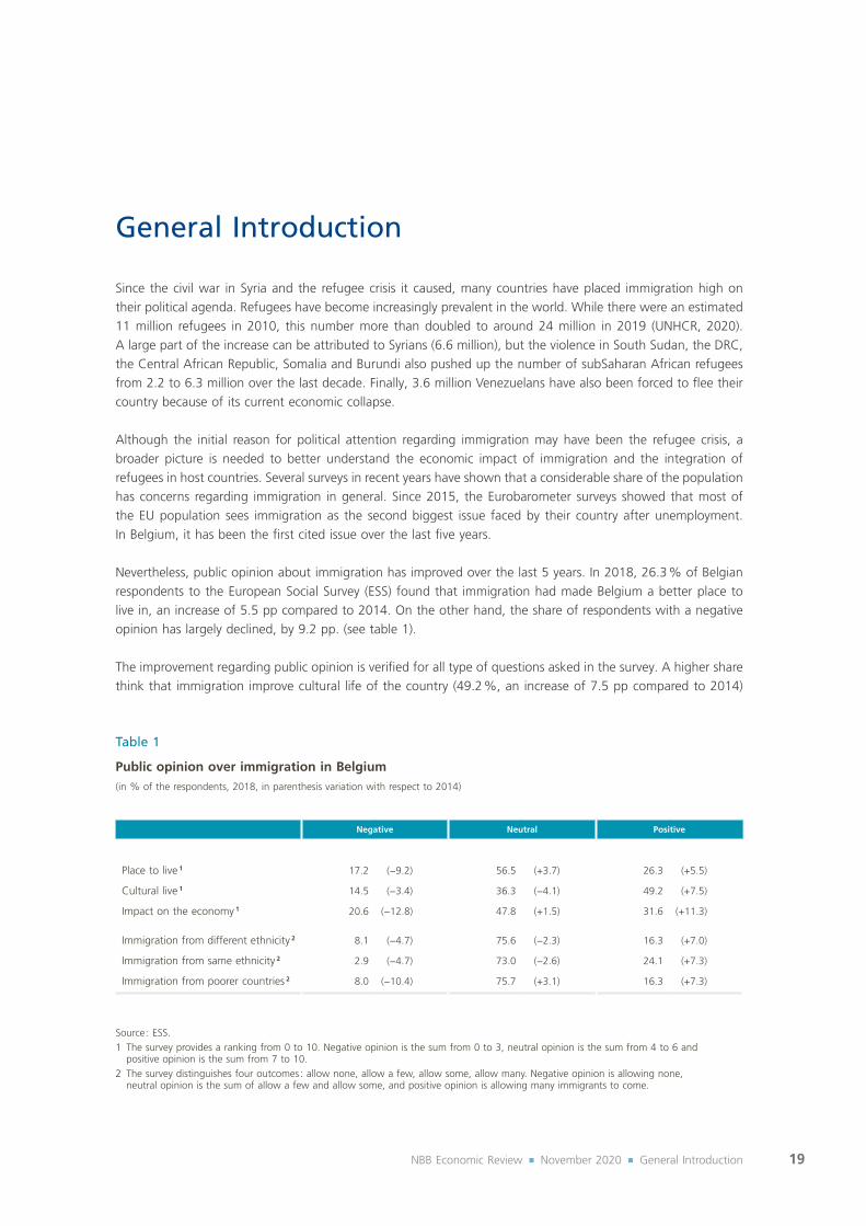
Nevertheless, public opinion about immigration has improved over the last 5 years. In 2018, 26.3 % of Belgian respondents to the European Social Survey (ESS) found that immigration had made Belgium a better place to live in, an increase of 5.5 pp compared to 2014. On the other hand, the share of respondents with a negative opinion has largely declined, by 9.2 pp. (see table 1).
The improvement regarding public opinion is verified for all type of questions asked in the survey. A higher share think that immigration improve cultural life of the country (49.2 %, an increase of 7.5 pp compared to 2014)

20NBB Economic Review ¡ November 2020 ¡ General Introduction
and has a good impact on the economy (31.6 % or a raise of 11.3 pp over the last 5 years). Note however, that one‑fifth of the respondents still think that immigration is bad for the economy, despite the wide‑ranging economic literature (institutional reports as well as academic research) showing an overall neutral or positive effect of immigration.
While reluctance to immigration is more pronounced against people with different ethnic origin or from poorer countries than against people of the same ethnicity, negative opinion for the three categories has shifted towards a more positive opinion.
The aim of this report is to provide an overview of the economic impact of immigration in Belgium distinguishing between first‑ and second‑generation immigrants but also between immigrants with an EU 1 or a non‑EU origin. To do so, we rely on data from the Crossroads Bank for Social Security (CBSS). This database includes all individuals present in the National Register, so that illegal immigrants, asylum seekers, posted workers 2, temporary or seasonal immigrants are excluded from the analysis.
Given different definitions which co‑exist when talking about immigration, it is important to state precisely what we consider here as natives, first‑generation immigrants and second‑generation immigrants. The report opts to distinguish between these groups on the basis of country of birth, rather than on nationality, as long‑residing immigrants are likely to have adopted Belgian nationality 3. Unless otherwise stated, the definitions used through the report are those described below.
First, all individuals who not born in Belgium are defined as ”first‑generation immigrants”. A further distinction can be made between individuals born in an EU country and those born outside the EU. Thanks to different origin groups defined by the Socio‑economic Monitoring 4, the CBSS also gives twelve groups 5 of origin, namely Belgium, EU14, EU13, EU candidates, Other European countries, Maghreb, Sub‑Saharan Africa, Near and Middle East, Oceania and Far East, Other Asian countries, North America and Latin America. Wherever possible, distinctions between those groups will be provided.
To separate people born in Belgium into “natives” and ”second‑generation immigrants”, the country of birth of parents comes into play. When both parents are born in Belgium, the individual is defined as “native”. If one or both parents are born outside Belgium, the individual is assigned to the ”second generation”. Note that there is a relatively large number of individuals born in Belgium for which the country of birth is not known for both parents, or one parent was born in Belgium and the country of birth is not known for the other parent (18.5 %). There are strong indications that the vast majority of these missing values are natives. The main argument for this assumption is the fact that observations with missing countries of birth of parents are primarily part of the retired population (70.3 %). Given the relatively young age structure of the first generation of immigrants, it is unlikely that these observations would be second‑generation immigrants 6. Therefore, parents whose country of birth is unknown will be assumed to have been born in Belgium. While this can incorrectly identify a small share of second‑generation immigrants as natives, it avoids the bias of underestimating natives of older ages, especially for the public finance aspects. As for the labour market analysis, the incidence of making this assumption is limited since we only use the working‑age population (20‑64 years), for which the proportion of missing data is relatively limited.
1 What we consider as EU throughout the report is EU28, before Brexit.2 See annex 1 for more information on recent evolution regarding posted workers.3 The incidence of nationality acquisition will also be analysed.4 See reports 2013, 2015, 2017, 2019.5 The list of the countries included in each group is provided in annex 2.6 If observations with missing countries of birth of parents were part of the second generation, a large fraction of the second generation
would be retired (39.5 % compared to 4.3 % without missing observations). This is an unrealistic assumption, given the fact that the presence of immigrants in Belgium has steadily increased, and the retired fraction of the first generation of immigrants is only 13.4 %.

21NBB Economic Review ¡ November 2020 ¡ General Introduction
Second‑generation immigrants can further be distinguished between EU and non‑EU origins. Following the literature, the country of birth of the father is the first to be investigated to define the more precise origin of an individual. If the origin of the father is unknown or if the father was born in Belgium, the origin of the mother is taken into account to define whether the individual is a second‑generation EU or non‑EU immigrant. The database does not provide origin by more precise groups of country of birth for the second‑generation.
Employing the variable as described above, 69.8 % of the whole Belgian population in 2016 are identified as natives, 16.5 % is defined as immigrants of the first generation, and 13.7 % is immigrants of the second generation (see chart 1). The distinction between EU and non‑EU immigrants is almost evenly dispersed both among first and second generation with a slightly higher share of non‑EU immigrants (53.1 % for first‑generation and 52.3 % for second‑generation immigrants). Spreading first‑generation into more detailed groups of origin, the most represented immigrants are those born in an EU14 country (36 %), followed by individuals born in Maghreb (14 %), in Sub‑Saharan Africa (12 %), in EU13 (11 %), Other European countries, EU candidate countries and the Near and Middle East (6 % each), Latin America, Other Asian countries and Oceania and the Far East (3 % each) and finally the least represented are people born in North America (1 %).
There is considerable heterogeneity across the Regions. Immigrants make up a much larger share of the population in Brussels (71.8 %) than in Wallonia (31.1 %) and Flanders (22.1 %). Moreover, immigrants living in Brussels have more often a non‑EU origin and this is particularly true for the second generation (72 % of non‑EU among second‑generation immigrants). The reverse is true in Wallonia, with a majority of EU immigrants : 55 % of first‑generation and 63 % of second‑generation immigrants. Flanders has an intermediary position with on average 44 % immigrants originating from the EU and 56 % with a non‑EU origin.
This regional distribution depends on the history of migration. After the Second World War, labour migrants, mainly coming from Italy and later from Spain and Greece, were recruited for the coal industry, in Wallonia, to hold down commodity prices and further support the industrial revival. Regarding the Brussels situation, it is often stated that foreign populations tend to concentrate around big cities and in particular in the capital.
Chart 1
Share of population by origin and by Region of residence(in % of the total population, 2016)
0 10 20 30 40 50 60 70 80 90 100
Wallonia
Flanders
Brussels
Belgium
Natives First-generation EU immigrants
First-generation non-EU immigrants
Second-generation EU immigrants
Second-generation non-EU immigrants
Source : CBSS Datawarehouse.

22NBB Economic Review ¡ November 2020 ¡ General Introduction
Ch
art
2
Ag
e d
istr
ibu
tio
n b
y o
rig
in a
nd
by
gen
der
(in t
hous
ands
of
peop
le,
2016
)
05101520253035404550556065707580859095100
105
110
656055504540353025201510505
101520253035404550556065
21
18
15
12
9
6
3
0
3
6
9
12
15
18
21
24
20
16
12
8
4
0
4
8
12
16
20
24
Men
Wom
enEU
men
Non
-EU
men
EU w
omen
Non
-EU
wom
en
EU m
en
Non
-EU
men
EU w
omen
Non
-EU
wom
en
Nat
ives
Seco
nd
-gen
erat
ion
Firs
t-g
ener
atio
n
Sour
ce :
CBS
S D
ataw
areh
ouse
.

23NBB Economic Review ¡ November 2020 ¡ General Introduction
The presence of international institutions as well as important administrations for foreigners such as the Immigration Office or the Commission for Refugees and Stateless Persons make Brussels particularly attractive for immigrants.
Comparing the age distributions of origin groups, three‑quarters of first‑generation immigrants are among the working‑age population while this proportion is 57 % for natives and 50 % for second‑generation immigrants (see chart 2). The native population is more often at retirement age (22 %, against 13 % for first‑generation immigrants and only 4 % for the second‑generation) and on the contrary second‑generation immigrants are largely less than 20 years old (46 %, against 21 % for natives and 12 % for first‑generation immigrants). This breakdown will have a significant influence regarding the public finance analysis.
The report is divided into three distinct parts. The first part assesses the impact of immigration on public finances, primarily focusing on a static approach based on administrative data from the CBSS. The computation of approximated net transfers of individuals to the public sector highlights the huge variety of contributions of individuals throughout their life cycle, as well as the key role of labour market integration.
As a result, the second part is devoted to an analysis of the labour market integration of immigrants in Belgium. The study attempts to provide the relevant factors that can explain the poorer labour market outcomes for immigrants (first‑ and second‑generation, with EU or non‑EU origin) compared to natives. Personal characteristics available in the CBSS database will be analysed in depth (age, gender, level of education, Region of residence, type of household, detailed origin 1) as well as specific characteristics of first‑generation immigrants (nationality acquisition, number of years of residence, channel of migration). The incidence of policies is also determined looking at both instruments targeting immigrants and more general employment activation tools. Finally, institutional factors and the functioning of the labour market is assessed as an important factor explaining the labour market performance of immigrants.
Finally, a general equilibrium model is constructed to assess the economic impact of recent immigration on the Belgian economy. First, aggregate effects are presented regarding wages, participation, welfare and GDP. In a second step, this Part III assesses the interaction between endogenous variables in the model and between model actors to understand the mechanisms driving the aggregate effects of immigration in Belgium. An evaluation of parameters used, the required assumptions and the potential alternative impact channels rounds off Part III by checking the findings for sensitivity to the model characteristics.
1 More detailed groups of origin are analysed for first‑generation immigrants while for the second generation the incidence of the origin of the father and the mother is determined.

24NBB Economic Review ¡ November 2020 ¡ Immigration and public finances
PART I Immigration and public finances

25NBB Economic Review ¡ November 2020 ¡ Immigration and public finances
Contents
Introduction 26
1. Methodological issues and literature review 271.1 The static approach 271.2 The intertemporal approach 291.3 The approach with macroeconomic models 301.4 Main findings 31
2. Approach followed in this Part of the report 32
3. Analysis 363.1 Transfers received by individuals from the government sector 373.2 Transfers from individuals to the government sector 423.3 Net transfers 453.4 Impact on net transfers of a simulated increase of the
employment rate 55
4. Conclusion 57

26NBB Economic Review ¡ November 2020 ¡ Immigration and public finances
Introduction
Any macroeconomic impact assessment study of immigration inevitably involves a public finance dimension. Indeed, all changes in the demographic structure of a country’s population have an impact on a wide range of public expenditure and affect government revenue. One additional migrant worker and his or her family for instance would lead to an increase in social benefits like family allowances or health care expenditure, but he / she would also generate income tax and social security contributions as well as consumption taxes. The impact on other expenditure (infrastructure or defence for example) is less straightforward.
How to accurately measure this impact on public finances has been the subject of several research projects in recent years. There is no simple answer to this, as many different factors are interconnected at macroeconomic level. The analysis set out below adopts a partial viewpoint by seeking to work out the extent to which immigrants contribute to government revenue and to what extent they are beneficiaries of public spending in a given year. Using a very rich database supplemented by estimates, it provides a rather new and unique overview of the issue in Belgium. But there are also limits to this assessment of the net contribution to public finances, because it does not incorporate any indirect effects nor any dynamic effect. In order to take all pertinent factors into account, a general equilibrium type of approach would be needed. The model developed in the last part of the report provides a very good exploration of the main macroeconomic interactions at play, even if its public finance component is simplified and not directly comparable to the static approach presented here (see Part III).
The first section below presents a brief review of the economic literature on this theme, with a focus on the results for the European countries. The article then examines in more detail expenditure and revenue by population origin for Belgium. On this basis, an analysis of the net contribution to Belgium’s public finances is then given in the following sections.

27NBB Economic Review ¡ November 2020 ¡ Immigration and public finances
1. Methodological issues and literature review
In the economic literature, several approaches have been followed in order to assess the contribution from immigrants to public finances. On the one hand, there are accounting‑type static approaches, referring to one particular year or a series of years. They are sometimes limited to an analysis of the differences in terms of expenditure between immigrants and natives, or extended to all expenditure and revenue generated by the population of foreign origin in order to obtain an estimate of its net contribution to public finances. On the other hand, some authors add an intertemporal dimension to their analyses, in order to assess the impact over a long period, in a hypothetical future. However, few of them also incorporate the indirect effects (i.e. effects of migration on other economic variables such as wages, prices, productivity, decisions to invest in education, labour and capital markets, which in turn affect public finances), that call for more complex models. While some authors stick to one single approach, others explore several different approaches.
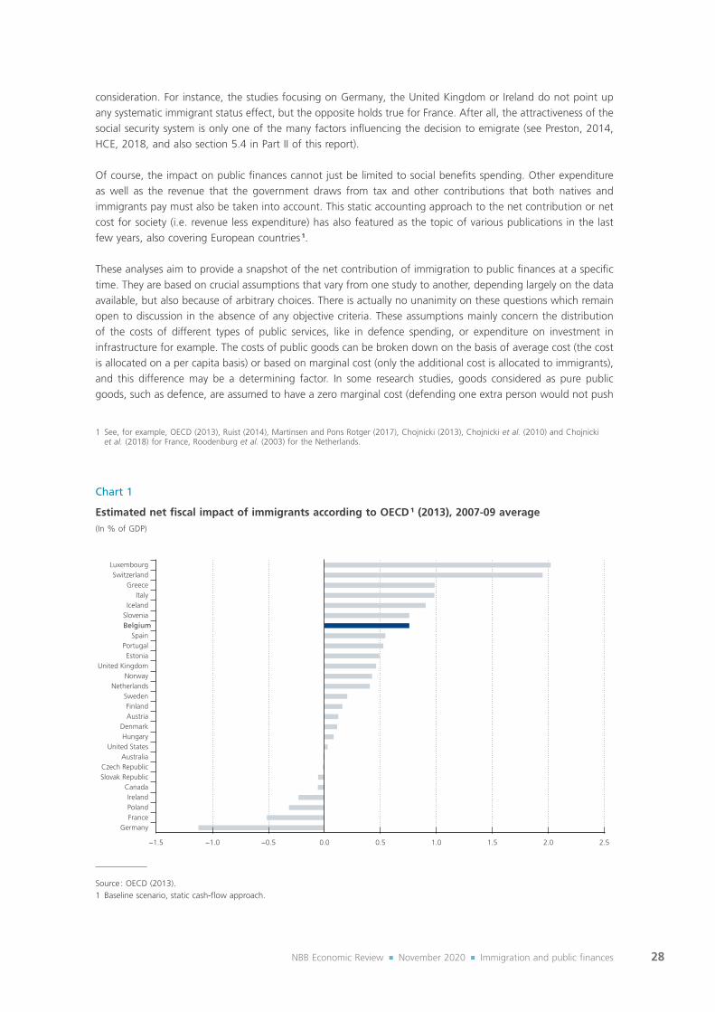
Various recent publications review this literature 1. In brief, they generally tend to conclude that the impact in terms of net contribution to public finances is small (Rowthorn, 2008 ; OECD, 2013 ; Preston, 2014 ; Edo et al., 2018 ; Vargas‑Silva and Sumption, 2019). Most results from studies following the static approach or the intertemporal approach fluctuate between –1 % and +1 % of GDP, depending on the period, the country surveyed and the assumptions made.
However, there are no studies focusing specifically on Belgium 2, even though, in a few rare cases, Belgium features among the countries studied, such as in OECD (2013) for example. The latter shows that the estimated impact is positive and slightly above the average of the countries considered.
The rest of this section describes in more depth the different approaches and their main results for European countries. Excluding some special cases (such as Luxembourg, with very few natives of native background), these countries actually bear more similarities to Belgium in terms of socio‑economic situation and immigration characteristics than what can be observed on other continents (for example, in the United States, Canada or Australia or the situation of temporary immigrant workers in Middle East oil‑exporting countries).
1.1 The static approach
Apart from expenditure related specifically to immigrant reception, such as asylum procedure costs, the provision of aid to refugees (housing, material assistance), and integration policies (including language courses) – which mainly concern the arrival of new immigrants – the literature has been more widely concerned with evaluating the degree of use of the social security system according to beneficiary status. In line with the theory whereby the relative generosity of the social assistance system should determine the degree of attractiveness of a country for various types of applicants for immigration, a series of authors 3 have studied the breakdown of social security expenditure by origin of beneficiary.
The most recent studies from this strand of literature often focus on one specific country. They generally tend to show that wherever an overrepresentation with regard to the use of certain social benefits is detected, it is exclusively due to the socio‑demographic characteristics of the populations studied, rather than to immigrant status (Edo et al., 2018). However, these findings vary depending on the country or the years taken into
1 See, for example, Edo et al. (2018), Preston (2014) Chojnicki et al. (2018), OECD (2013), Vargas‑Silva and Sumption (2019) and to a lesser extent Rowthorn(2008).
2 An estimate of the fiscal impact of the arrival of refugees in 2015 and 2016 can be found in Burggraeve and Piton (2016).3 For example, Borjas (1999), Borjas and Hilton (1996) for the United States : Barrett and Maître (2013) for different European countries,
Barrett and McCarthy (2008) for the United Kingdom and Ireland, Dustmann and Frattini (2014) for the United Kingdom ; Riphahn et al. (2013), Riphahn (2004), Castronova et al. (2001) for Germany ; Chojnicki et al. (2010) for France in 2005, Brücker et al. (2002), for European countries, Boeri (2010), Huber and Oberdabernig,(2016) for 16 for European countries or Cohen and Razin (2008) from a more theoretical point of view.
28NBB Economic Review ¡ November 2020 ¡ Immigration and public finances
consideration. For instance, the studies focusing on Germany, the United Kingdom or Ireland do not point up any systematic immigrant status effect, but the opposite holds true for France. After all, the attractiveness of the social security system is only one of the many factors influencing the decision to emigrate (see Preston, 2014, HCE, 2018, and also section 5.4 in Part II of this report).
Of course, the impact on public finances cannot just be limited to social benefits spending. Other expenditure as well as the revenue that the government draws from tax and other contributions that both natives and immigrants pay must also be taken into account. This static accounting approach to the net contribution or net cost for society (i.e. revenue less expenditure) has also featured as the topic of various publications in the last few years, also covering European countries 1.
These analyses aim to provide a snapshot of the net contribution of immigration to public finances at a specific time. They are based on crucial assumptions that vary from one study to another, depending largely on the data available, but also because of arbitrary choices. There is actually no unanimity on these questions which remain open to discussion in the absence of any objective criteria. These assumptions mainly concern the distribution of the costs of different types of public services, like in defence spending, or expenditure on investment in infrastructure for example. The costs of public goods can be broken down on the basis of average cost (the cost is allocated on a per capita basis) or based on marginal cost (only the additional cost is allocated to immigrants), and this difference may be a determining factor. In some research studies, goods considered as pure public goods, such as defence, are assumed to have a zero marginal cost (defending one extra person would not push
1 See, for example, OECD (2013), Ruist (2014), Martinsen and Pons Rotger (2017), Chojnicki (2013), Chojnicki et al. (2010) and Chojnicki et al. (2018) for France, Roodenburg et al. (2003) for the Netherlands.
Chart 1
Estimated net fiscal impact of immigrants according to OECD 1 (2013), 2007-09 average(In % of GDP)
e
GermanyFrancePolandIreland
CanadaSlovak RepublicCzech Republic
AustraliaUnited States
HungaryDenmark
AustriaFinland
SwedenNetherlands
NorwayUnited Kingdom
EstoniaPortugal
SpainBelgiumSloveniaIceland
ItalyGreece
SwitzerlandLuxembourg
−1.5 −1.0 −0.5 0.0 0.5 1.0 1.5 2.0 2.5
Source : OECD (2013).1 Baseline scenario, static cash‑flow approach.

29NBB Economic Review ¡ November 2020 ¡ Immigration and public finances
up the cost), which would broadly lower the average cost per inhabitant if the population grows. Yet, to assume that this type of cost does absolutely not depend on the size of the population may seem excessive. The case of rival public goods, those whose consumption by some also affects consumption by others from a certain level of congestion, is particularly difficult to estimate. The way in which the net contribution of descendants of immigrants, and especially those born in the host country, is taken into account also plays a role for instance 1.
In this literature, the effects calculated in terms of net contributions tend to be relatively low in proportion to GDP, whether positive or negative (Edo et al., 2018, Rowthorn, 2008). They are slightly positive or negative in the countries surveyed in the work of the OECD (2013), with an average net fiscal impact of immigrants of +0.3 % of GDP.
The estimated baseline impact for Belgium is slightly higher at +0.8 % of GDP according to this static cash flow approach. In this assessment, the OECD (2013) has taken into account direct monetary transfers from and to households (taxes and social security contributions paid by households and social benefits in cash), as well as indirect taxes on the revenue side and other budget components that generally also vary on a person‑by‑person basis, such as expenditure on education, health and active labour market policy on the expenditure side. On average, immigrants tend to have a more favourable age structure which results in a brighter picture for public health expenditure, but also higher estimated expenditure on education, due to the fact that they have more school‑age children. If the other revenue and expenditure items (except defence and debt services) are also attributed on a per capita basis, the net fiscal impact of immigrants for Belgium is estimated at +0.1 % of GDP.
This type of study shows, for example, that the net contribution by non‑natives generally tends to be lower, but that this is actually due to a smaller contribution and not to wider recourse to social benefits. Above all, employment appears to be the principal determinant of differences in net contribution. The socio‑demographic characteristics of non‑natives are less favourable and even when these are taken into account, their position on the labour market is also more disadvantageous (all other things being equal). Moreover, the composition of the immigrant population by migration channel category (work, family reunification, or humanitarian protection) goes a long way to explaining the international differences. The other important factors are age and skill level. Social benefit spending per person is actually lower for working‑age people, and even more so if they are highly skilled. Also, as non‑natives are usually more badly hit by recessions in terms of employment, the year selected as a reference might not be neutral either. The choice of reference year also determines the level of net contributions in euros, depending on whether the budget is in balance, in surplus or deficit for example. In order to neutralise the impact of the reference year, one option is to present the results in terms of deviations from the average, as proposed in section 3.3 of this part of the report.
1.2 The intertemporal approach
In order to assess the impact of immigration on public finances over a longer period, and in particular in the future, an intertemporal approach is necessary. This type of study usually makes a link with the challenge of population ageing and considers different demographic scenarios of which immigration is an important component.
The intertemporal approach consists of estimating the costs and benefits throughout the (theoretical) life of natives and non‑natives by extrapolating them based on current characteristics of immigrants – obtained from the static perspective. This is the net present value approach 2. Its results depend heavily on assumptions for a range of variables shrouded in uncertainty (the annual discount rate used to convert future costs into current
1 This is sometimes the case indirectly, depending on whether the analysis covers individuals or households, whether as e result of a methodological choice, or because of data availability.
2 See, for example, Monso (2008) and Chojnicki et al. (2010) for France, Storesletten (2003) for Sweden, or Roodenburg et al. (2003) for the Netherlands.

30NBB Economic Review ¡ November 2020 ¡ Immigration and public finances
prices, evolution of future income, costs and benefits over a lifetime, length of presence in the country, number of children expected, etc.) 1. So, it is generally necessary to appraise the findings on the basis of different scenarios that also include alternatives for demographic change and immigration flows.
Another approach is based on the previously mentioned one, i.e. the net present value approach (and its highly uncertain assumptions), added to which is the intertemporal budgetary constraint, whereby a budget deficit has to be borne by resident taxpayers in the end. This is the generational accounting methodology. The idea is to calculate the impact of a change in migration policy on the tax burden borne by different generations 2.
Research work that has sought to calculate the net present value has often produced a negative figure, although highly sensitive to the assumptions, especially when it comes to integration into the labour market. A younger and better‑ educated immigrant population generally obtains more positive results. Nevertheless, the generational accounting approach suggests that immigration has a positive and significant effect on the intertemporal budgetary constraint in the case of the European countries (Edo et al., 2018), and this is probably related to the constant arrival of people of working age, combined with the positive contributions from their descendants in a context of an ageing population. But the positive effects are by far not enough to completely offset the effects of population ageing.
1.3 The approach with macroeconomic models
One fundamental weakness of the approaches described so far is that they completely ignore any indirect effects ; they only look at direct effects. As mentioned in Part II and Part III, the labour market is also affected by the arrival of immigrants, which potentially exerts an effect on wages, on the level of taxation, labour supply decisions, investment in human capital, etc., so that migration has an impact on the supply of and demand for factors of production. Besides, the consumption channel plays a not insignificant role, as does the productivity channel. The presence of foreign workers may have a downward influence on production costs of certain public services themselves, as is the case in health care and care for the elderly in the United Kingdom, for example (Citi, 2018).
Only general equilibrium models are capable of taking into consideration these direct and indirect effects at the same time, even though they obviously cannot reflect the whole range of complex interactions between the numerous pertinent factors. In Part III of this report, a theoretical model accounting for the labour market participation effect, fiscal effect and price effect for the Belgian economy is used to estimate and illustrate these interactions.
The research studies that develop macro‑economic models to try to estimate the impact of immigration on public finances while taking account of the overall effects on the economy 3 – which are still few in number – reach the conclusion that the effect is positive but small and mainly reflects the structure of net migratory flows by age. A policy that is more selective in terms of skills would have a more positive effect in the short term, but in the long term, this positive effect would be more than offset by the wider longevity and lower fertility of highly‑skilled immigrants (Edo et al., 2018).
1 “(…) the approach is unavoidably and arguably dangerously ambitious in the assumptions it needs to rely upon”. Preston (2014).2 See, for example, Bonin et al. (2000) for Germany, Collado et al. (2004) for Spain, Mayr (2005) for Austria, Chojnicki (2013) for France. 3 See, for example, Hansen et al. (2017), Schou (2006), Storesletten (2000), Fehr et al. (2004), Chojnicki and Ragot (2015) and Chojnicki
et al. (2010)

31NBB Economic Review ¡ November 2020 ¡ Immigration and public finances
1.4 Main findings
The review of the economic literature on the impact of immigration on public finances suggests a certain consensus about the different possible approaches and the limitations related to the strong assumptions that they imply. Despite their simplified nature, the static approaches constitute a significant input, even though often constrained by available data. Similar to what emerges from the literature focusing on the labour market, the positive or negative impact depending on the study and on the approach always remains at a moderate level, at least at the national or international level. Even though it seems intuitively obvious that at local level the costs, notably those associated with certain public services, and the benefits can diverge strongly from one place to another, to our knowledge, this aspect is not dealt with very much in the literature.
Generally speaking, migrants are found to have a less favourable net contribution. The position of highly‑skilled people seems to be more positive, but the low‑skilled can also have a positive impact in certain cases. The differences between countries obviously depend on the tax and social benefits system, but also on the structure of the immigrant population and especially on age and migration channel. Where the migration channel is employment, the contribution is generally more positive.
In the OECD study (OECD, 2013), Belgium is singled out as the country where raising the employment rate of immigrants has the biggest impact on public finances (this rate being particularly low there). Employment explains roughly three‑quarters of the difference in contribution between immigrants and natives. And this is even more so for women, owing to the importance of the family reunification channel which mainly concerns them.
This study seeks to examine in more detail the situation in Belgium, based on more recent and previously unused information. The following chapter sets out the method followed, and then moves onto an analysis of the findings obtained. They largely mirror the main findings presented above, albeit with some nuances related to country‑specific characteristics.

32NBB Economic Review ¡ November 2020 ¡ Immigration and public finances
2. Approach followed in this Part of the report
One of the objectives of this study is to make up for the lack of any specific analysis for Belgium in the field of the impact of immigration on public finances, and to gauge more accurately the impact on revenue and on individually identifiable public expenditure. In this part of the report, the results of a static approach are presented.
As is often the case in practice, it is partly the available data that determine the type of analysis that can be carried out. The gradual development of an administrative database within the Crossroads Bank for Social Security (CBSS) is a major advance on this front, which has already helped produce publications, mainly in the field of labour market analysis 1. But this is the first time that data covering a large part of the individually identifiable public revenue and expenditure have been used to analyse the public finance impact of immigration in Belgium. The database extract provided by the CBSS is particularly rich in information here. In line with the recent literature, these data make it possible to put forward a static analysis of the net contribution to public finances by people of foreign origin living in Belgium (especially following a similar approach to Chojnicki, et al., 2018 for France or Oxford Economics, 2018 for the United Kingdom).
The idea is therefore to analyse the transfers paid and received by government – these are the different types of expenditure (social benefits) and the various sources of revenue (tax and social security contributions) – corresponding to different population groups so as to determine their net contributions to public finances. The rest of this section briefly describes the variables taken into account and the methodology followed to obtain these net transfers. Annex I.1 looks at the different methodological aspects of the selected approach in more detail.
The reference year is 2016. This is the most recent year for which CBSS data could be obtained. It is also a year that has the advantage of not corresponding to any extreme economic cyclicality (even if it is a year with many asylum‑seekers being granted the status of refugee). If it had been a year marked by a severe economic crisis, like the year 2009 or the year 2020 for example, the results would probably have been strongly biased (some authors do actually point out that the impact of a recession may differ significantly from one population group to another). The current situation is therefore potentially very different from that analysed below, which can be considered relevant for an average, neutral year.
The analysis is based in the first place on the general government accounts from the national accounts for Belgium. The official data from the national accounts on government transfers paid and received are allocated to various population groups using distribution keys relying on alternative databases. The main source is the extract from the Crossroads Bank for Social Security (CBSS) database, which includes all individuals recorded in the national register of the resident population.
The basic unit is individuals (as opposed to households). However, it is not a micro database : data is aggregated by groups defined by 11 common variables, such as the place of birth (also of parents), age, nationality, education, (in)activity status, etc. The most detailed sub‑groups are defined by the privacy constraints imposed within the CBSS. Of course, these detailed sub‑groups can be aggregated. The data is quite detailed as far as individualisable social transfers are concerned. The following transfers received in cash by individuals are covered : family allowances, pensions, unemployment benefits, social assistance and sickness benefits. Other ad-hoc data sources are also used to complement the main database, more especially data on age‑related health expenditure (from INAMI).
1 See for example HCE (2018), various Socio‑economic Monitoring (FPS Employment and Unia, 2017, 2018, 2019), Vandermeerschen et al. (2017) or View.Brussels (2019).

33NBB Economic Review ¡ November 2020 ¡ Immigration and public finances
The CBSS database also includes data for income from work (employees and self‑employed). This information is used to estimate taxes and social security contributions, that are transfers from individuals to the government. Social security contributions by employees are directly inferred from the database, whereas the social security contributions of the self‑employed are estimated using a (macro) average rate of contribution. Personal income taxes paid by individuals are estimated based on data linking average revenues and average taxation rates. These rates are derived from a fiscal and parafiscal simulation model, adapted to approximate the impact of the deduction for children, and to correct the aggregation bias that results from using average incomes by population groups in the database (see annex I.1). Employers’ social security contributions are estimated using the same approach (but with no impact of children).
Finally, an estimate for value added tax (VAT) and excise duties is derived from alternative sources, combining indirect tax rates by products, detailed data on consumption by age from the household budget survey (HBS) provided by Statbel, experimental data from Eurostat for saving rates by age, and income data from the CBSS database. On this basis, the share of indirect taxes in consumption has been estimated by age categories. It has not been possible to obtain a distinction by country of origin, nor to use any distinct propension to consume according to income levels for example. It is interesting to note that, all in all, there is little variation between age groups.
It is a deliberate choice to limit the analysis to transfers paid (social benefits) and received (taxes and social contributions) by government. Transfers are by definition payments without a direct counterpart. Hence, these are purely distributive transactions. Other individualisable expenditure, such as education, is not taken into account in the analysis. From a theoretical point of view, it is impossible to define the ultimate beneficiaries of this expenditure : these are clearly the students themselves, but also employers and society as a whole. Moreover, a choice to include this type of expenditure in the analysis would be problematic because of a lack of detailed information. The lack of detailed information on the distribution of the remaining taxes is also the reason why these are not taken into account. However, this may only marginally affect the results on the net contribution to public finances expressed in relative terms given the minor importance of these taxes.
Although very detailed and informative data has been gathered, some elements are not covered. The contribution of European civil servants is not taken into account, although they are often included in the group of people born abroad. Of course, these international civil servants do not pay income taxes or social security contributions to the Belgian authorities. Although, in practice, they contribute to indirect taxes through their consumption for instance, this effect cannot be captured in the absence of income data for that group. Moreover, it is often argued that international organisations (such as the European institutions or the NATO) and their staff attract many other activities and therefore in the end contribute positively to the economy and the public finances of the country were they are active. This is just another example of indirect or dynamic effects that cannot be captured by the static approach adapted in this part of the study.
Another group that is not covered are the posted workers from other countries (unless they are present in the national register). Undocumented migrants and undeclared workers are also de facto excluded from the analysis. As the database only covers people residing in Belgium, people who are not (or no longer) living in Belgium but who receive transfers from this country are not included in the analysis. These are, for instance, Belgian retirees in countries like Spain or immigrants who returned to their home country, or children living abroad with one parent working in Belgium. As long as they are not considered as refugees (or granted the subsidiary protection status) asylum‑seekers form another group that is not considered in the database (see box 1). Nevertheless, these shortcomings do not seem to skew the static results significantly.
As mentioned above, a large share of public expenditures is not considered, as is a large share of government revenues (capital taxes, housing taxes, etc.). Moreover, the education level of individuals, which is an important variable (see section 1.1.1 of Part II of the report where the link between employment and education is highlighted), is unfortunately not complete nor unbiased, which should be kept in mind when interpreting the results.

34NBB Economic Review ¡ November 2020 ¡ Immigration and public finances
Costs related to refugee reception
The reception of refugees is a humanitarian and moral obligation framed by international law since the First World War. It is also linked with the 1948 Universal Declaration of Human Rights. A refugee claimant is any person who, "owing to a well‑founded fear of being persecuted for reasons of race, religion, nationality, membership of a particular social group or political opinion, is outside the country of his nationality and is unable or, owing to such fear, is unwilling to avail himself of the protection of that country”. Once a positive response to their application has been obtained, they are either considered as a refugee or a beneficiary of subsidiary protection 1. Otherwise the application is rejected.
The organisation of refugee reception involves different types of expenditure which are not included separately in the main analysis. Applicants for protection are not registered as residents until they have received a positive reply. Moreover, these expenses are largely aid in kind. Although there is no complete information on the total cost of reception (Court of Auditors, 2017), it is possible to identify parts of the expenditure incurred by the different institutions involved in this mission.
The Federal Agency for the Reception of Asylum‑Seekers, Fedasil, is responsible for the support and material reception of asylum‑seekers in the broadest sense. This includes housing (collective or individual), food, medical care (in part), legal aid etc. Fedasil’s expenditure amounted to € 370 million in 2018 2. This expenditure is not a financial transfer to the refugees but corresponds in practice to the salaries of some 700 employees, building rent, payments for supplies of goods and services to Belgian suppliers. More than 50 % of Fedasil’s budget covers the costs of refugees’ reception organised on behalf of Fedasil by partner organisations such as the Red Cross or local councils. However, part of the costs are not taken into account, such as the provision of buildings free of charge, e.g. by the building authority (Régie des bâtiments) or other public authorities, and certain expenditure borne by other institutions (part of the medical costs being borne by FPS Integration).
The administrative management of applications is handled by the CGRS (General Commission for Refugees and Stateless Persons), the Council for Alien Law Litigation (Conseil du contentieux des étrangers, CCE) and the Immigration Office (Office des Etrangers, OE), which all depend on the FPS Interior. The budget of the GCRS, which analyses individual files and takes decisions, amounted to € 33.4 million in 2018 (Annual Report 2018). More than 500 people work there. The CCE, which manages the appeals, employs approximately 250 people. Its expenditure amounted to about € 20 million in 2019. As for the Immigration Office, which registers initial applications, grants visas, manages non‑voluntary returns and closed centres, it has about 2 000 staff (2017), and its expenditure was slightly below € 130 million in 2019. Allocating sufficient and flexible means for a rapid administrative management of applications enables substantial savings in reception costs 3 (accommodation, etc.) to be made during the waiting period. It also benefits the applicant, who, if the application is accepted, will be able to start social and labour market integration more quickly (which is only possible as an asylum‑seeker after a four‑month waiting period).
Once recognised, refugees are registered as residents of the country, and are therefore included in the main analysis of the study. They are generally entitled to the social integration income (RIS, revenu d’intégration sociale) and, where applicable, to family allowances, often with increased amounts. These individualisable transfers are taken into account in the database. They also benefit from health
BOX 1
u

35NBB Economic Review ¡ November 2020 ¡ Immigration and public finances
The amounts included in the resulting database represent around 80 % to 90 % of the corresponding national accounts statistics corresponding to transfers paid and received. They are subsequently used to allocate these officials statistics on both types of transfers to the different population groups covered.
To answer the core question of this part of the study, one common approach is to look at how the different types of transfers paid and received evolve according to age for different groups of the population defined by their origin, approximated by the country of birth variable. The following broad groups are considered : people born in Belgium (natives), people born in core EU countries (EU14), people born in new Member States of the EU (EU13), and people born outside the EU (non‑EU). In this decomposition, natives include second‑generations individuals, i.e. individuals born in Belgium with one or two parents that are born outside Belgium. Section 3.3.5 is dedicated to a separate analysis of natives of native origin (individuals born in Belgium with two parents born in Belgium) and natives with a migration background, referred to as “the second generation”.
More information on the methodology and the data used is presented in annex I.1.
care. On the other hand, specific integration policies, such as language courses or integration pathways are not identified separately. The same applies to other policies that provide for adaptations for this particular target group even though there are not many targeted policies (employment, etc.) apart from the integration policies in Belgium, as shown in section 3.4 of Part II of this report.
As integration policies are a competence of the Communities, with a role for the Regions, different policies co‑exist in Belgium, and the stakeholders involved are many and varied, which makes it difficult to easily identify the related costs. Moreover, these policies not only apply to refugees but also to many different categories of foreign‑born people (integration policies are described and analysed more in depth in section 3.1 of part II). The Flemish Agency for Integration and Civic Integration (Agentschap Integratie en Inburgering) has more than 500 employees and a budget of 53 million in 2018 (Court of Auditors, 2020). The Agency is active in the Flemish Region, where there has been an obligation to follow an integration pathway for a long time, but it also has activities in Brussels, where there is no such obligation yet. In the Walloon Region, a budget of € 23 million (2019) is planned for the integration process, while for the French‑speaking population of Brussels, € 6 million was allocated by the COCOF in 2019. The coordination of integration policies in Brussels is complex. The content of integration policies can be freely defined by the two Communities, and therefore differs substantially, but the compulsory character of the policies must be imposed by the Common Community Commission (COCOM). It was initially expected for 2020 but has been delayed.
1 In the case of persons at risk of death or risk of inhuman and degrading treatment as a result, for example, of armed conflict, an applicant who has not been granted refugee status may be granted another form of protection called subsidiary protection.
2 The various budget lines intended for Fedasil in the Budget of the federal Government in 2018 amount to about 280 million euros. As a result, Fedasil used his own reserve funds to compensate for the difference. In 2019 these budget lines have been increased to above 410 million.
3 The average monthly Fedasil costs per asylum‑seeker are higher than the monthly social integration income.

36NBB Economic Review ¡ November 2020 ¡ Immigration and public finances
3. Analysis
Considering the identified transfers and following on the methodology highlighted above, this section starts by presenting a number of stylised facts for the different types of transfers received and paid by individuals. In a following step, net transfers are presented, and the results are further analysed along various relevant aspects.
The various components of transfers presented hereafter reflect amounts or averages for sub‑groups of the population. They are expressed as an average amount per person in the group.
Table 1
Coverage and scaling of the data (2016)
National accounts statistics 1 Coverage : CBSS
(in € million)
(in % of GDP)
(in % of national accounts statistics)
Pensions 43 850 10.2 97
Unemployment 8 257 1.9 97
Family allowances 6 373 1.5 94
Health care 28 640 6.7 96
Social assistance 3 716 0.9 85
Sickness 8 693 2.0 93
Other social transfers 6 642 1.5 0
Total received by households 2 106 171 24.7 90
Income tax 45 851 10.7 84
Social contributions Employers 35 194 8.2 86
Social contributions Employees 3 22 999 5.3 94
Consumption taxes 4 20 421 4.7 74
Total paid by households 124 465 28.9 85
p.m. Balance 18 294 4.3 –
p.m. Total income / Revenue 50.7
Total primary spending / Expenditure 50.4
Interest 2.7
Balance −2.4
Sources : CBSS Datawarehouse, NAI, NBB calculations.1 Data as of January 2020. Own calculation based on detailed government accounts.2 For the scaling of the data, the category “other” social transfers is spread proportionally over the other social transfers.3 Including self‑employed in the CBSS column.4 Own estimates (VAT and excise duties).

37NBB Economic Review ¡ November 2020 ¡ Immigration and public finances
3.1 Transfers received by individuals from the government sector
3.1.1 Pensions
The age pattern of pension transfers is no surprise, with higher payments per capita at older ages (note that early retirement schemes are included in unemployment benefits, see below). The average pension transfer per person is higher for natives than for people born abroad, and people born in the core EU countries receive on average higher pensions than people born outside the EU. These differences can be explained by a combination of factors : natives more often have a job during their active life, they have higher‑paid jobs and they contribute for longer than migrants arriving at older ages on the labour market in Belgium. Besides, natives tend to account for a higher share of public sector jobs known for their comfortable pension schemes (see HCR, 2018). The fact that pensions from European civil servants are not covered in the database explains part of the gap with natives (they are implicitly considered as having no pension at all). But this is not a bias, since these pensions are not (directly) paid by the Belgium authorities. The pattern for people born in new EU Member States is less clear‑cut, probably because the number of older people in that group is still relatively low.
As mentioned earlier, the numbers in the charts are averages of all the amounts received by groups, spread over all members of the group, even those who do not receive anything. Moreover, differences between groups, say between two age groups, do not say anything about the effective contribution of the group , or about the share of the group in the total amount, which also depends on its relative size, i.e. the number of people in that group. Finally, there is also a group of beneficiaries from pension transfers that is not covered in the database. This is the case of people who have been contributing to public finances during their active life, who are now retired and drawing their pensions, but not living in Belgium anymore. This group includes people born abroad as well as natives.
3.1.2 Family allowances
The pattern for family allowances by age groups follows a bell curve, with a peak at around 40 years old for the parent receiving the benefit, often the mother (in the CBSS database, family allowances are allocated to the person receiving the payment, not the beneficiary child). This seems to reflect the biological constraints of family‑building : the older the mother / parents, the more likely that the number of children in the household increases, up to the age when children start to leave the initial household to start their own. The differences by origin, with higher average allowances per capita for the group of people born outside the EU, followed by people born in Belgium, and lower still, people born in other EU countries (EU13), largely reflect the fact that people born outside the EU have more children on average, and therefore have larger families (in 2016, the family allowance per child was still rising with the number of children per family up to the third child). Moreover, these families also benefit more often from family allowance supplements when their income is below a defined level or because they are single‑parent families (see also the discussion in section 1.1.5 of Part II)

38NBB Economic Review ¡ November 2020 ¡ Immigration and public finances
3.1.3 Unemployment benefits and social assistance
As a group, foreign born people tend to receive higher average benefits, because a larger share of the group does not have a job. However, among the jobless, foreign‑born people tend to benefit less from unemployment benefits than natives because they do not meet all the requirements (such as previous job tenure). In that group more people receive no benefits at all and those who are beneficiaries receive lower amounts, so the average benefit per unemployed person is lower than for natives. The peak around the age of 60 is largely due to early retirement benefits being recorded in this category, in line with national accounts methodology. As shown in section 1.1.3 of Part II, non‑natives have shorter careers in Belgium and therefore have less incentive to switch to early retirement schemes.
Unemployment benefits tend to be lower for the group of people born in the new EU Member States than in all other groups (considering per capita averages for the groups, taking employed and unemployed people together). This could be linked to a more recent immigration wave, mainly through the work channel, with a larger share of these sub‑groups in employment (or self‑employment).
For social assistance, the picture is similar to unemployment benefits. Here too, people born outside Europe tend to receive higher average benefits as a group because a larger share of the group has no job or a very low income. EU‑born people present lower averages, similar or even lower than natives, except for people older than 50 who were born in the new EU Member States (but this is a very small group in relative terms).
Chart 2
Transfers received by individuals : Pensions and Family allowances(€ per year per person in the age group)
0‑14
15‑1
9
Age groups Age groups
20‑2
4
25‑2
9
30‑3
4
35‑3
9
40‑4
4
45‑4
9
50‑5
4
55‑5
9
60‑6
4
65‑6
9
70‑7
4
75+
0
500
1000
1500
2000
2500
3000
3500
Pensions Family allowances
0‑14
15‑1
9
20‑2
4
25‑2
9
30‑3
4
35‑3
9
40‑4
4
45‑4
9
50‑5
4
55‑5
9
60‑6
4
65‑6
9
70‑7
4
75+
0
5 000
10 000
15 000
20 000
25 000
Natives EU14EU13 (Other EU28)Non‑EU
Non‑natives, of which :
Sources : CBSS Datawarehouse, NBB calculations.Note : unless otherwise specified natives include second generations individuals, throughout this Part of the report (Part I).

39NBB Economic Review ¡ November 2020 ¡ Immigration and public finances
3.1.4 Health transfers
Health transfers include sickness benefits identified in the CBSS database (such as sick pay, inability to work, occupational injury, occupational illnesses) as well as health care costs estimated on the basis of expenditure by age group (source INAMI).
Sickness benefits tend be higher on average for natives, especially between the ages of 25 and 55. They are lower for people born in the new Member States, a feature also seen for unemployment benefits 1.
Health care costs account for a large share of public expenditure, but are not considered as individualisable cash transfers because they are to large extent provided in kind (such as hospital infrastructure, reimbursement through public mutual insurance institutions, etc.) and are therefore not available in the CBSS database. However, data for health expenditure by age group received from INAMI (2017) have made it possible to include this type of transfer in the analysis. As distribution of health care costs by origin is not available, only the age dimension is considered hereafter. Age is of course the major driver of health costs. So, in this exercise, different outcomes
1 Note that undeclared work does not give access to sickness benefits. The introduction of the service voucher scheme in Belgium changed the situation in this respect. According to Leduc and Tojerow (2020), it resulted in increased employment within the subsidised domestic services sector, especially for women of foreign nationality. They also find that programme participation adversely affects physical health, thus increasing the worker’s probability of claiming disability insurance benefits.
Chart 3
Transfers received by individuals : Unemployment benefits and social assistance(€ per year per person in the age group)
0‑14
15‑1
9
20‑2
4
25‑2
9
30‑3
4
35‑3
9
40‑4
4
45‑4
9
50‑5
4
55‑5
9
60‑6
4
65‑6
9
70‑7
4
75+
0
500
1 000
1 500
2 000
2 500
3 000
3 500
Unemployment benefits Social assistance
0‑14
15‑1
9
20‑2
4
25‑2
9
30‑3
4
35‑3
9
40‑4
4
45‑4
9
50‑5
4
55‑5
9
60‑6
4
65‑6
9
70‑7
4
75+
0
500
1 000
1 500
2 000
2 500
3 000
3 500
Age groups Age groups
Natives EU14EU13 (Other EU28)Non‑EU
Non‑natives, of which :
Sources : CBSS Datawarehouse, NBB calculations

40NBB Economic Review ¡ November 2020 ¡ Immigration and public finances
in terms of health care cost transfers received by different groups will reflect their respective age structure only 1 (a group with more older people, such as natives, will exhibit higher health care costs, compared to foreign‑born citizens who are on average younger).
3.1.5 Total transfers received by individuals
Our aggregate for total transfers received is computed by adding these various transfers together (family allowances, pensions, unemployment benefits, social assistance and sickness benefits as well as health care costs).
For the age category below 20 years old, the transfers considered here are mainly only health care costs. These are the same for each age category by definition, so there are virtually no differences between groups. However, the relative weight effect plays a role when considering all age groups together.
Under the age of 60, the average amount of transfers received by people born outside the EU is slightly higher than the average received by natives. The numbers for people born in EU countries are below those for natives. In other words, during most of their active lifetime, people born outside the EU receive more than other
1 In practice, it cannot be ruled out that different groups of immigrants face higher or lower health costs. Refugees often require specific care and psychological support. The composition of the work channel migrant population may be biased toward adults in very good health. Besides, a lack of supplementary health insurance for people without work contracts or with precarious employment contracts can also lead to lower use of health services because of the additional cost.
Chart 4
Transfers received by individuals : Sickness benefits and health care in kind(€ per year per person in the age group)
0‑14
15‑1
9
20‑2
4
25‑2
9
30‑3
4
35‑3
9
40‑4
4
45‑4
9
50‑5
4
55‑5
9
60‑6
4
65‑6
9
70‑7
4
75+
0
2000
4000
6000
8000
10000
12000
Sickness benefits Health care in kind
0‑14
15‑1
9
20‑2
4
25‑2
9
30‑3
4
35‑3
9
40‑4
4
45‑4
9
50‑5
4
55‑5
9
60‑6
4
65‑6
9
70‑7
4
75+
0
500
1000
1500
2000
2500
3000
3500
Age groups Age groups
Natives AllEU14EU13 (Other EU28)Non‑EU
Non‑natives, of which :
Sources : CBSS Datawarehouse, INAMI, NBB calculations.

41NBB Economic Review ¡ November 2020 ¡ Immigration and public finances
groups on average (mainly through family allowance, unemployment benefits and social assistance). However, differences are not so big, especially when considering the average for all foreign‑born people. When looking only at people not currently working, however, those born in Belgium receive on average more transfers than all other groups from the age of 25. Among people in employment, the differences are very small. Clearly, work opportunities largely define the extent of transfers received by individuals.
After the age of 60, another pattern emerges. Natives tend to receive more transfers on average, mainly through higher pension benefits per person in those age groups. This is also the case for people born in core EU countries. The fact that people born outside the EU receive less in older age can also be linked to labour market considerations, with fewer jobs during (previous) active life and lower‑paid jobs on top of lower length of contributions for people who arrived later in their career.
Globally, over all age groups, it appears that non‑natives receive on average 13 % less transfers than the average for Belgium, while natives receive 2 % more. Among non‑natives, the group born in EU14 countries receives about the same amount as the country average, the group born outside the EU receives 14 % less transfers than the average, and the group originating from new Member States only 50 %. These results are of course largely impacted by the relative importance of different groups of the population. Pensioners are the best example. When excluding this subpopulation by considering only the working‑age population (20 to 64), natives receive 1 % more than the average for Belgium (20‑64), and non‑natives 4 % less, but with a large disparity between non‑EU‑born immigrants, who receive 11 % more on average, and EU‑born immigrants (15 % less for EU14 and 38 % less for EU13).
Chart 5
Transfers received by individuals : total, and total by activity status(€ per year per person in the age group)
Total
0‑14
15‑1
920
‑24
25‑2
930
‑34
35‑3
940
‑44
45‑4
950
‑54
55‑5
960
‑64
65‑6
970
‑74
75+
0
5 000
10 000
15 000
20 000
25 000
30 000
35 000
Age groups
Individualsin employment
0‑14
15‑1
920
‑24
25‑2
930
‑34
35‑3
940
‑44
45‑4
950
‑54
55‑5
960
‑64
65‑6
970
‑74
75+
0
5 000
10 000
15 000
20 000
25 000
30 000
35 000
Age groups
0‑14
15‑1
920
‑24
25‑2
930
‑34
35‑3
940
‑44
45‑4
950
‑54
55‑5
960
‑64
65‑6
970
‑74
75+
0
5 000
10 000
15 000
20 000
25 000
30 000
35 000
Individualsnot in employment
Age groups
Natives EU14EU13 (Other EU28)Non‑EU
Non‑natives, of which :
Sources : CBSS Datawarehouse, NBB calculations.

42NBB Economic Review ¡ November 2020 ¡ Immigration and public finances
3.2 Transfers from individuals to the government sector
Transfers from individuals to the government come from the payment of taxes and social contributions. In practice, the analysis focuses on social contributions, personal income tax, and indirect taxes (VAT and excise duties). Other taxes paid by households, such as real estate taxes, withholding tax, local taxes, etc. are not considered because these are of minor importance and information on the distribution of these taxes is lacking. As explained above (see section 2 and annex I.1), only social contribution for employees is (in)‑directly available from the CBSS (2016) database. All the other transfers need to be estimated based on the income data provided by the CBSS, combined with other sources.
3.2.1 Social contributions and personal income tax
The common pattern observed for social contributions of employees and self‑employed and employers as well as for personal income tax, is a bell shape, culminating near the age of 50, with a tail at older ages. This is mainly the result of a combination of two factors linked to revenue from work : average wages and the employment rate, i.e. the number of people who are wage earners or self‑employed. Average wages increase with age : the increase in human capital through experience is better rewarded, up to a certain point at least. Besides, seniority pay also plays a role, especially in a country like Belgium where the practice is widespread and entrenched in social legislation. Regarding the second factor, employment rates go up at the beginning of the active lifetime, and later decline at older ages. As a result, the contribution from wages on average also decreases at older ages, albeit remaining above levels seen at the beginning of active lifetime.
The same two factors, average wage and employment rate, play a role in explaining the differences observed between groups by origin. Natives, characterised by a higher employment rate and better‑paid jobs, contribute proportionally more on average, whereas people born abroad and especially outside the core EU14 countries contribute less. They have lower‑paid jobs or are more often without jobs (see also HCE, 2018 and section 1.1 of Part II of this report). The large share of posted workers originating from these countries could also play a role : they are counted as resident if they stay more than three months, but their income is not declared in Belgium, which could possibly distort the result for this group (see also annex 1). However, this is not confirmed by evidence from the database, probably because posted workers are themselves not often recorded in the national register.
Wage is clearly a fundamental determinant of the contribution to public finances : social security contributions are to a large extent fixed as a percentage of income, while for personal income taxes, the tax rate rises with the income level. But, in this exercise, it is not possible to distinguish between wages from the private sector and wages from government jobs. Contributions from government sector jobs are partly artificial (remember that taxes and social contributions are mainly estimated, see also section 2 and annex I.1) and could bias the results towards the natives, who have a more than proportional share of public jobs.

43NBB Economic Review ¡ November 2020 ¡ Immigration and public finances
3.2.2 Taxes on consumption : VAT and excise duties
For taxes on consumption, such as VAT and excise duties, the pattern is by construction largely driven by the income of the different groups (section 2 and annex I.1 give more information on the assumption needed to estimate consumption taxes). Wages play an important role again, but income from transfers are also considered here. That type of contribution is rather stable from the age of 30 onwards, and is larger for people born in Belgium, who can afford to consume more, because of their higher income. For people born outside Belgium, there is no major difference between the groups, though again those born in new member countries seem to contribute the least (worse than non‑EU).
Chart 6
Transfers paid by individuals : income taxes and social contributions(€ per year per person in the age group)
Income taxes Social contributions employeesand self-employed
0‑14
15‑1
920
‑24
25‑2
930
‑34
35‑3
940
‑44
45‑4
950
‑54
55‑5
960
‑64
65‑6
970
‑74
75+
0
1000
2000
3000
4000
5000
6000
7000
8000
9000
10000
0‑14
15‑1
920
‑24
25‑2
930
‑34
35‑3
940
‑44
45‑4
950
‑54
55‑5
960
‑64
65‑6
970
‑74
75+
0
1000
2000
3000
4000
5000
6000
7000
8000
9000
10000
0‑14
15‑1
920
‑24
25‑2
930
‑34
35‑3
940
‑44
45‑4
950
‑54
55‑5
960
‑64
65‑6
970
‑74
75+
0
1000
2000
3000
4000
5000
6000
7000
8000
9000
10000
Social contribution employers
Age groups Age groups Age groups
Natives EU14EU13 (Other EU28)Non‑EU
Non‑natives, of which :
Sources : CBSS Datawarehouse, NBB calculations.

44NBB Economic Review ¡ November 2020 ¡ Immigration and public finances
3.2.3 Total transfers paid by individuals
When considering all transfers paid together, our aggregate measure is largely driven by work‑related transfers (social contributions and personal income taxes). The observation made above for this type of transfer remains valid in this case : a bell shape culminating around 50 and higher contributions from natives followed by people born in core EU countries. People born outside EU and in the new member contribute less on average. The differences between groups are quite bigger than for transfers received and are even more closely driven by economic activity status, as can been seen from the considerable differences between contributions from people in employment and those not in employment.
Among people in employment, it is interesting to note that that natives and people from EU14 countries show a very similar pattern. The group of individuals from other EU countries (EU13) is the one with the lower contributions, despite a high employment rate, indicating low average wages. The non‑EU group is in a middle‑of‑the‑road position.
Chart 7
Transfers paid by individuals : taxes on consumption(euros per year per person in the age group)
0
1000
2000
3000
4000
5000
6000
7000
8000
9000
10000
Consumption taxes
Age groups
Natives
EU14EU13(Other EU28)Non‑EU
Non‑natives, of which :
0‑14
15‑1
9
20‑2
4
25‑2
9
30‑3
4
35‑3
9
40‑4
4
45‑4
9
50‑5
4
55‑5
9
60‑6
4
65‑6
9
70‑7
4
75+
Sources : CBSS Datawarehouse, NBB calculations.

45NBB Economic Review ¡ November 2020 ¡ Immigration and public finances
3.3 Net transfers
When transfers received by individuals from the government are compared with transfers paid by individuals to the government, the result is the net contribution of residents to the public finances of the country. Combining the aggregates constructed in the two previous sections, it is possible to compute an indicator for these net transfers.
Again, the net transfers of different groups of the population can be examined using the detailed information available in the database. For instance, by country of birth, or by occupational status, or by education obtained. However, it is necessary to remember the limitations of this approach, which is still based on several simplifying assumptions and is not covering all expenditures and revenues aspects of public finances. Moreover, it remains a static approach, not taking all the dynamic and indirect effects into account (see section 3.2 of Part III on the general equilibrium model for more intuitions on the mechanism that are at play and annex III.1 for model specification regarding government).
Because the database has been scaled on the basis of the government accounts statistics from the national accounts, by construction, the global net transfer is equal to €+18.294 million, or €+1.615 per inhabitant (there were 11 327 794 inhabitants in Belgium in 2016).
The level of the net transfers is not the most relevant indicator. What is more important is the difference between the various groups. Whether the results are in positive or negative territory is also very much related to the different transfer components we take on board in this exercise, as well as by the assumptions needed
Chart 8
Total transfers paid by individuals(euros per year per person in the age group)
0‑14
15‑1
920
‑24
25‑2
930
‑34
35‑3
940
‑44
45‑4
950
‑54
55‑5
960
‑64
65‑6
970
‑74
75+
0
5 000
10 000
15 000
20 000
25 000
30 000
35 000
Age groups
0‑14
15‑1
920
‑24
25‑2
930
‑34
35‑3
940
‑44
45‑4
950
‑54
55‑5
960
‑64
65‑6
970
‑74
75+
0
5 000
10 000
15 000
20 000
25 000
30 000
35 000
Age groups
0‑14
15‑1
920
‑24
25‑2
930
‑34
35‑3
940
‑44
45‑4
950
‑54
55‑5
960
‑64
65‑6
970
‑74
75+
0
5 000
10 000
15 000
20 000
25 000
30 000
35 000
Age groups
Natives EU14EU13 (Other EU28)Non‑EU
Non‑natives, of which :
Total Individualsin employment
Individuals notin employment
Sources : CBSS Datawarehouse, NBB calculations.

46NBB Economic Review ¡ November 2020 ¡ Immigration and public finances
to estimate them. Therefore, the results from this exercise are presented as differences compared to the average aggregate per capita for the country as whole (all ages considered together). A positive figure thus indicates a group for which net transfers are higher than the average. A negative figure points to a lower‑than‑average net contribution for the group. The focus is on the relative positioning of the different groups. An added advantage of this approach is that it yields exactly the same results as when all other public expenses and public revenues – those that are not explicitly covered in the proposed approach – are distributed equally over all residents on a per capita basis, as would be the case if the average cost method were used to assign these expenses to all individuals within a country. Moreover, an additional advantage of this approach is that results are hardly affected by the fiscal position of the chosen year.
Analysed by age, net transfers are below the global average for Belgium in the first stages of life. It follows logically from the characteristic of the transfers presented in the previous sections that, for individuals below 20 years old, transfers received are higher than the average and transfers paid by individuals are lower than the average. In the 20s, the gap becomes positive, with transfers paid to the government sector increasing progressively above the average as individuals start to contribute to active life through work. The gap peaks in the 50s, when it starts to decline when some people start leaving the labour market. In the 60s, it is clearly becoming negative, with transfers received by individuals overtaking the transfers paid to the government, especially driven by pensions and health costs.
Chart 9
Net transfers by age and by country of birth, differences compared to the global average for Belgium(differences in € per year))
−30000
−25000
−20000
−15000
−10000
−5000
0
5000
10000
15000
20000
Net transfers by age and by countries of birth,differences compared to the average forBelgium for all ages(differences in euros)
Age groups
Natives
Non‑natives, of which :
0-14
15-1
9
20-2
4
25-2
9
30-3
4
35-3
9
40-4
4
45-4
9
50-5
4
55-5
9
60-6
4
65-6
9
70-7
4
75+
EU14EU13(Other EU28)Non‑EU
Sources : CBSS Datawarehouse, NBB calculations.

47NBB Economic Review ¡ November 2020 ¡ Immigration and public finances
This general pattern can be observed for the different groups according to broad origin. It is however more pronounced for natives. They present a higher net positive contribution during active life, but also a higher net negative contribution after retirement. The negative net contribution after retirement is lower for the other groups, i.e. the people born outside Belgium, but within a closer range, indicating lower differences between these groups. During active life, between 20 and 60 years old, the differences between groups and compared to natives are much larger. After natives, the second highest net contribution is registered by the group of people born in core EU countries (EU14), followed by a wide margin by the other EU countries (EU13). The net contribution of the group of people born outside the EU remains lower than the average for Belgium until around 30 years old, it then remains close to the average but lower than that of the other groups. From pension age onwards, all groups present lower net contribution than the average, but this is less so for the non‑EU group. It is even lower for the new EU Member States origin, because the share of people with a full career in Belgium is quite limited.
A more summarised indicator of net transfers can be obtained by combining the results by age class with the corresponding age structure of the different population groups, that is their weights structure according to their respective population. Given the large differences observed between the characteristics of individuals of working age compared to the young or the retired, it is useful to make a distinction between the total for all ages and the total for the age classes between 20 and 64, computed for the main broad origin groups. These indicators display a much lower variation than what the age profile could suggest. Here again, the focus is on differences compared to the average for Belgium.
3.3.1 Net transfers by origin
Considering all age groups together the net contribution of natives is the highest and, given their large weight in the total population, quite close to the global average 1. It is followed by the average for people born in the new EU members states. Indeed, despite much lower net contributions there are not many retired people in that group, which limits the negative impact of retirees on net contributions. This is less the case for people born in the core EU countries, for which the average net contribution is lower than the country average. For people born outside the EU the average net contribution is the lowest according to this exercise.
It is also interesting to look more closely at the group of recent non‑natives, defined as migrants who arrived in Belgium in the last five years or less, which is also the focus in Part III of the report. As an aggregate, their net contribution is higher than the average, but not as high as natives. By broad groups of country of origin, it appears that individuals born in EU countries (old and new Member States) and recently settled in Belgium present net transfers largely above the national average. Only the group of non‑EU origin present relatively lower contributions. Of course, the main reason behind these globally positive results is that recent migrants receive fewer social transfers, even if their employment rate is lower than other groups. They are seldom entitled to pensions rights, because they are mostly young or have very short careers, and they benefit less automatically from other sorts of social transfers.
When the analysis focuses on individuals in the working‑age population (defined here as aged 20‑64), net transfers are much higher, and almost always higher than the global average (even if only natives have higher net transfers than the national average for that age group). Non‑EU is the only group that presents lower net transfers than the global average. Compared to all residents born abroad, the outcome for recent migrants is better for the EU group but worse for third‑country individuals. The difference between natives and non‑natives (and within the non‑natives between EU and non‑EU nationals) is partly due to a lower employment rate for the latter, but it is not the only factor.
1 Note that when one group is characterised by a very large weight in the total, its deviation from the average tends towards zero, but the gap between groups remains meaningful.

48NBB Economic Review ¡ November 2020 ¡ Immigration and public finances
There is clearly a link between the employment rate of a group and its relative position in terms of net contributions compared to the average for Belgium. The higher the employment rate, the higher share of individuals receiving an income from work from which a contribution is paid into the public coffers. This link is present between origin groups but also within origin groups.
Note that the apparently low employment rate of people born in EU14 countries compared to other sources is due to the fact that civil servants working for international organisations such as the EU are not recorded as employed in the administrative data underlying the CBSS database. If inactive people without benefits who arrived in Belgium via the work channel are considered as civil servants of international organisations, then the employment rate for that category reaches 57 %, which is already closer to the 67 % employment rate derived from the LFS 1, 2. However, for the analysis of contribution to Belgium’s public finances, this is only marginally relevant since European civil servants only contribute to indirect taxes through their consumption, as they do not pay Belgian income tax.
It is interesting to note that, within the non‑natives, even groups with relatively a high employment rate, such as the new EU Member States, make a much smaller relative contribution than groups with a lower rate. The other two factors that can affect the relative rankings are thus related to the average wage – if it is low, then contributions will be low for that group – and to the average net cost of inactivity (the level of transfers received).
1 Alternatively adding 80 % of the 48 000 European civil servants (from other sources), taking into account that 20 % of them are of Belgian nationality, an employment rate of 58 % is found.
2 The presence of posted workers could explain part of the remaining difference because they are counted as resident if they stay more than 3 months in Belgium but do not appear in the administrative databases and are not considered as in employment.
Table 2
Differences in net transfers by country of origin compared to the average for Belgium (all residents)(in € per capita per year, 2016, unless otherwise stated)
Total Aged 20‑64 p.m.
of which :
Shares of the total
population
Shares in 20‑64
Employment rate
In employment
Out of employment
(in %)
Belgium (all residents) 0 8 069 17 375 −9 843 100 100 66
Natives 1 376 9 861 18 444 −10 524 84 79 70
Non‑natives −1 905 1 303 11 530 −8 361 16 21 49
EU14 −1 675 5 496 18 599 −6 763 6 6 48
EU13 (other EU28) 201 1 662 6 273 −5 681 2 3 61
Non‑EU −2 506 −935 9 208 −9 560 9 12 46
of which :
Recent non‑natives (0‑5 years) 159 1 189 9 815 −4 661 4 6 40
EU14 3 385 6 142 18 762 −3 031 1 2 42
EU13 (other EU28) 1 012 1 875 5 511 −3 696 1 1 61
Non‑EU −2 013 −1 674 7 049 −5 605 2 3 31
Sources : CBSS Datawarehouse, NBB calculations.1 Including the second generation.

49NBB Economic Review ¡ November 2020 ¡ Immigration and public finances
Migrants tend to earn lower average wages, because of unfavourable sector specialisation, lower educational attainment or lack of international recognition of diplomas, and other forms of potential unidentified discrimination (see also chapter 2 of Part II of the report). As a result, they contribute less in taxes and social contributions. Job tenure is another factor. In a system where wages rise with seniority, as is the case in Belgium, longer job tenure implies higher wages, and this benefits individuals that started their career early in Belgium. That is of course the case for natives, but also foreign‑born people that settled long ago, as can been observed if a distinction is made for recent migrants (within the group of individuals aged 20‑65 in employment) compared to all individuals born abroad. These factors are also linked to the quality or sustainability of jobs, in terms of type of contract, in terms of intrinsic job value (having a motivating job), or in terms of support given by firms to employees (health, maintaining employees’ employability) for instance. It is easier to find a new job when new skills have been learned. It is easier to remain in work and lengthen job tenure with a motivating job and supporting employer. It is also easier to keep one’s job when working as civil servant. Based on the dataset available for this part of the study, it is not possible to assess the precise impact of these elements on the employment rate or the average wage, but it is probably because immigrants are less well‑off in terms of job sustainability 1.
1 For instance, the 2020 report of the Belgian HCE (High Council for Employment) analyses occupational pathways from 2008 to 2014 and shows that immigrants have more frequent periods of unemployment and inactivity.
Chart 10
Average wage (of employed individuals) and net transfers 1 by age and education
(€ per capita per year)
Low education
Ave
rage
wag
e
Differences in net transfers
Age groups (9 groups between 20 and 64), by education :
Natives
0
10 000
20 000
30 000
40 000
50 000
60 000
−20
000
−10
000 0
10 0
00
20 0
00
30 0
00
EU origin
−20
000
−10
000 0
10 0
00
20 0
00
30 0
00
0
10 000
20 000
30 000
40 000
50 000
60 000
−20
000
−10
000 0
10 0
00
20 0
00
30 0
00
Non−EU
Medium education
High education
No information on education
Sources : CBSS Datawarehouse, NBB calculations.1 Differences in net transfers (employed and unemployed together) compared to the global average for Belgium.

50NBB Economic Review ¡ November 2020 ¡ Immigration and public finances
The second potential factor is related to the level of negative net transfers for individuals aged 20‑65 and not in employment. Although this factor certainly contributes to the results, it does not seem to be the most decisive. The key takeaway here is that natives present higher costs than the average individual in the same socio‑economic position. For this age group, the negative contributions recorded for recent migrants are smaller. This is because a foreign‑born individual tends to benefit less from social protection than a native in the same social situation, and this is even more the case for recent migrants.
These findings confirm the major role of employment and average wage : they are the main drivers of higher net transfers to public finances. In this respect, natives present a relative advantage (see also the annex I.2 on the decomposition of the differences in net transfers between native and non‑natives).
3.3.2 Net transfers by migration channels
One of the advantages of the main database used for the study is that it enables quite detailed information to be identified on additional aspects of the immigrants and resident populations that can be useful to decompose the contribution according to different characteristics.
One aspect of interest is the immigration channels. As previous studies have shown, differences in immigration channels partly explain outcomes on the labour market (see also section 2.1 of Part II), and therefore also play a role in terms of net transfers. The type of information available here is of an administrative nature. Therefore, it does not necessarily perfectly match the underlying reasons for migration 1. It should also be noted that the coverage and quality of the information for the channels for migration declines for migrations from a more distant past. In fact, the information is not available for about 40 % of the non‑natives, although for recent migrants (less than 5 years), that proportion is around 10 %. If there is a bias in missing information towards a certain category, that is if the missing data are not equally balanced across migration channels, this would significantly affect the findings. Keeping this caveat in mind, a number of interesting stylised facts can still be learned.
Foreign born people that migrated through the work channel are contributing more to the government sector than any other channels, they also contribute more if they arrived recently (in the last five years). All groups show higher contributions than the average for Belgium when employed (even if they came through other channels than work). However, considering all individuals per channel other than work, migrants all contribute less than the average (the same is true for the sub‑category aged 20‑64). Although the group that arrived via the international protection channel or people with subsidiary protection status, in other words refugees, shows the biggest difference from the average, it is also the only one registering an improvement after five years in this presentation. Indeed, the data confirm that after a sufficiently long adaptation period, the employment rate of that group starts to catch up.
Considering only people born outside the EU according to length of residence, channels of migration and activity status (not illustrated), it appears that length of stay tends to slightly raise the positive net contribution of employed people, especially if their channel of immigration is international protection (see section 2.1 of Part II). However, it also increases the net negative contribution of people not in in employment, probably because of retirees (but even correcting for people over 60, the contributions of the non‑working groups remain similar).
1 It refers to the official motives for residence permits. In reality, different motives can coexist (for instance, family reunification can be the official administrative channel for individuals aspiring to find a job, etc.). Moreover, the channel of immigration recorded for children is associated with the parents’ channel.

51NBB Economic Review ¡ November 2020 ¡ Immigration and public finances
3.3.3 Net transfers by education levels
Breaking down net transfers by education and activity status, it once again appears clearly that employment is associated with higher net contributions. The available data also seems to confirm that a better education increases the contribution. This probably happens through higher wages, but also through the employment rate which is higher for better educated groups. However, the magnitude of the share of missing data on the level of education – almost 50 % for natives and more than 61 % for non‑natives – is such that no robust conclusions can be made on this basis. It is certainly an aspect where an improvement of the CBSS information would be particularly welcome.
Table 3
Differences in net transfers by migration channels compared to the average for Belgium (all residents)(in € per capita per year, 2016, unless otherwise stated)
Aged 20‑64 Total p.m.
of which :
Employment rate
Population share in
20‑64
In employment
Out of employment
(in %)
Belgium (all residents) 8 069 17 375 −9 843 0 66 100
Natives 1 9 861 18 444 −10 524 376 70 79
Non‑natives 1 303 11 530 −8 361 −1 905 49 21
Work 9 526 17 279 −5 789 6 629 66 4
Family −1 978 5 876 −7 781 −3 542 42 5
Protection 2 −4 963 3 595 −11 504 −5 042 43 2
Studies 545 10 578 −2685 401 24 1
Others 3 −1 659 9 130 −5 866 −6 290 28 1
Unknown 636 12 011 −9 976 −3 489 48 8
of which :
Recent non‑natives (0‑5 years) 1 189 9 815 −4 661 159 40 6
Work 9 377 14 543 −2 642 9 344 70 2
Family −2 372 3 557 −5 440 −2 535 34 2
Protection 2 −7 406 220 −10 355 −6 614 28 1
Studies −429 8 649 −2 574 −550 19 0.5
Others 3 −1 122 7 138 −4 054 −1 858 26 0.5
Unknown −2 634 1 469 −3 224 −2 681 13 1
Sources : CBSS Datawarehouse, NBB calculations.1 Including the second generation.2 Including regularisation channel.3 Including the following channels : long‑term resident, foreigner with special status, other.

52NBB Economic Review ¡ November 2020 ¡ Immigration and public finances
3.3.4 Net transfers, distinction between first and second generations
Using the variable from the database that reflects the country of birth of parents, it is possible to identify second‑ generation migrants, i.e. people born in Belgium, but with at least one parent who was also a (first‑generation) migrant. First‑generation migrants are defined as people born abroad, irrespective of where their parents were born. In the previous sections, second‑generation migrants were included in the native category, which is now split into two groups. The second group includes natives of native origin. These are individuals born in Belgium from parents born in Belgium. Unfortunately, this variable (birthplace of parents) is also characterised by a large share of missing observations, about 7 % for the 20‑64‑year‑old population, but more than 25 % of observations in the population as a whole. Many of these missing observations are in fact identified for older people. As they are suspected to indicate that parents were in fact born in Belgium, these are considered as natives.
At the aggregate level, it appears that the net transfers of the second generation are on average higher than the net transfers of the first generation. It is also higher than that of natives of native origin, but this clearly reflects differences in age structures between the sub‑groups. The second generation is on average younger than the native population of native background. Assessed over the active lifetime (20 to 64 years old), the contribution of the second generation remains higher than that of the first generation, but lower than natives. These results are (partly) related to differences in employment rates. For the group over 60 years old, there is almost no difference between second‑generation migrants and other natives, whereas the first generation still exhibits less negative net transfers, partly reflecting shorter careers for people who arrived in Belgium at a later stage of their active life. For the youngest groups, under 25 years old, there are no large differences between the first and second generation, because it is at subsequent stages in life that the gap widens.
Table 4
Differences in net transfers by education level compared to the average for Belgium (all residents)(in € per capita per year, 2016, unless otherwise stated)
Aged 20‑64 Total p.m.
of which :
Employment rate
Population share in
20‑64
In employees
Out of employees
(in %)
Belgium (all residents) 8 069 17 375 −9 843 0 66 100
Natives 1 9 861 18 444 −10 524 376 70 79
Education low and medium −392 7 112 −10 936 −1 165 58 25
Education high 17 372 22 341 −4 724 17 040 82 15
Missing information 13 665 22 675 −11 716 −1 834 74 38
Non‑natives 1 303 11 530 −8 361 −1 905 49 21
Education low and medium −4 738 3 528 −11 841 −4 887 46 6
Education high 6 929 16 321 −6 918 6 610 60 2
Missing information 2 918 13 847 −6 985 −2 036 48 13
Sources : CBSS Datawarehouse, NBB calculations.1 Including the second generation.
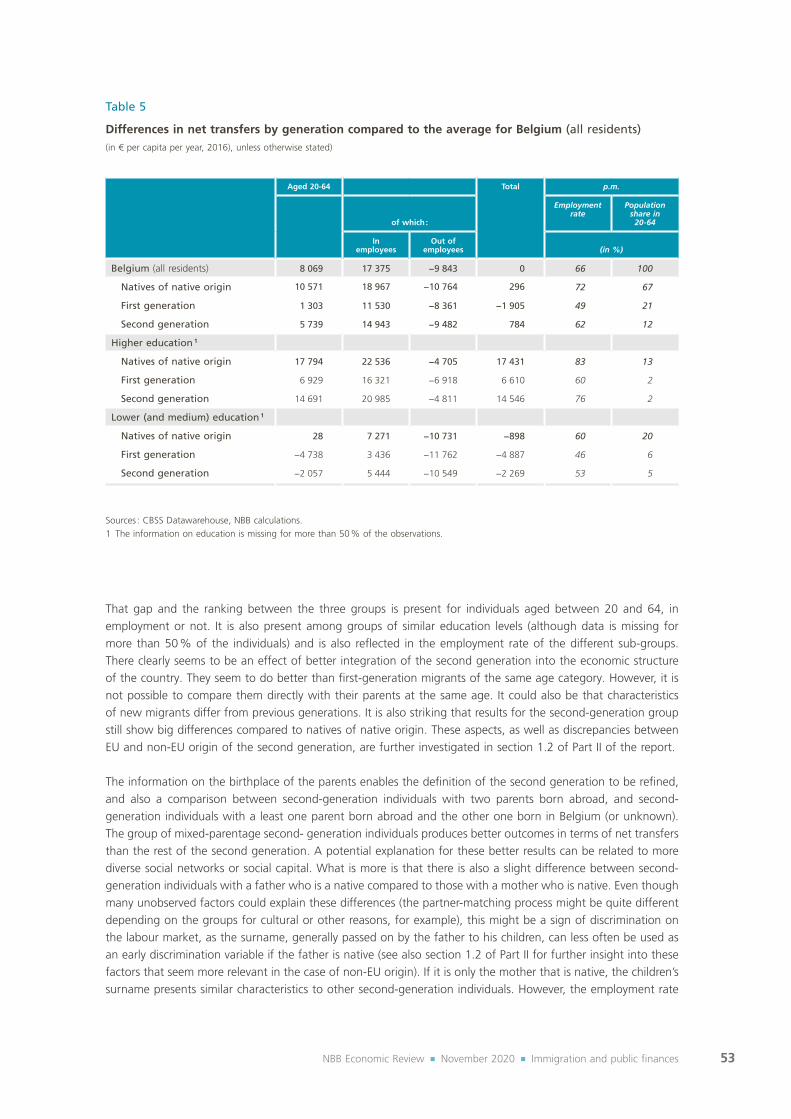
53NBB Economic Review ¡ November 2020 ¡ Immigration and public finances
That gap and the ranking between the three groups is present for individuals aged between 20 and 64, in employment or not. It is also present among groups of similar education levels (although data is missing for more than 50 % of the individuals) and is also reflected in the employment rate of the different sub‑groups. There clearly seems to be an effect of better integration of the second generation into the economic structure of the country. They seem to do better than first‑generation migrants of the same age category. However, it is not possible to compare them directly with their parents at the same age. It could also be that characteristics of new migrants differ from previous generations. It is also striking that results for the second‑generation group still show big differences compared to natives of native origin. These aspects, as well as discrepancies between EU and non‑EU origin of the second generation, are further investigated in section 1.2 of Part II of the report.
The information on the birthplace of the parents enables the definition of the second generation to be refined, and also a comparison between second‑generation individuals with two parents born abroad, and second‑generation individuals with a least one parent born abroad and the other one born in Belgium (or unknown). The group of mixed‑parentage second‑ generation individuals produces better outcomes in terms of net transfers than the rest of the second generation. A potential explanation for these better results can be related to more diverse social networks or social capital. What is more is that there is also a slight difference between second‑generation individuals with a father who is a native compared to those with a mother who is native. Even though many unobserved factors could explain these differences (the partner‑matching process might be quite different depending on the groups for cultural or other reasons, for example), this might be a sign of discrimination on the labour market, as the surname, generally passed on by the father to his children, can less often be used as an early discrimination variable if the father is native (see also section 1.2 of Part II for further insight into these factors that seem more relevant in the case of non‑EU origin). If it is only the mother that is native, the children’s surname presents similar characteristics to other second‑generation individuals. However, the employment rate
Table 5
Differences in net transfers by generation compared to the average for Belgium (all residents)(in € per capita per year, 2016), unless otherwise stated)
Aged 20‑64 Total p.m.
of which :
Employment rate
Population share in
20‑64
In employees
Out of employees
(in %)
Belgium (all residents) 8 069 17 375 −9 843 0 66 100
Natives of native origin 10 571 18 967 −10 764 296 72 67
First generation 1 303 11 530 −8 361 −1 905 49 21
Second generation 5 739 14 943 −9 482 784 62 12
Higher education 1
Natives of native origin 17 794 22 536 −4 705 17 431 83 13
First generation 6 929 16 321 −6 918 6 610 60 2
Second generation 14 691 20 985 −4 811 14 546 76 2
Lower (and medium) education 1
Natives of native origin 28 7 271 −10 731 −898 60 20
First generation −4 738 3 436 −11 762 −4 887 46 6
Second generation −2 057 5 444 −10 549 −2 269 53 5
Sources : CBSS Datawarehouse, NBB calculations.1 The information on education is missing for more than 50 % of the observations.

54NBB Economic Review ¡ November 2020 ¡ Immigration and public finances
of these two groups is remarkably identical (and higher than the second‑generation group as a whole) and the share of higher‑educated people in the working population is also identical (and higher than natives and first‑generation immigrants). One explanatory factor for these differences is the average wage, which seems to be higher for the group with a native father. Of course, these are only partial results that deserve further research (see also section 1.2 of Part II).
3.3.5 Net transfers by more detailed origin
The database includes more detailed information on the country of birth than the broad categories used so far, at least for non‑EU origins. The additional available groups are the following : “other European countries”, “EU candidate countries”, “North America”, “South and Central America”, “Near and Middle East”, “Maghreb”, “Sub‑Saharan Africa”, “Oceania / Far East”, and “other Asia” (see annex 2 for a more detailed description).
Among the non‑EU group, there is a large degree of heterogeneity between origins, and some groups tend to present much higher or lower net contribution than others. Education and activity status are again important determinants here. Considering only people with high education, or people active on the labour market, largely shifts net contributions to public coffers upwards. Nevertheless, within the groups that contribute less on average, the share of people employed or with higher education level is not large enough to compensate for the lower contributions of the other sub‑groups. Compared to other advanced countries in the world, Belgium attracts much less high‑skilled labour.
Chart 11
Differences in net transfers by generation compared to the average for Belgium (all residents)(differences in € per capita per year in the age group, 2016)
Natives of native origin
Age categories Age categories
First generation
Second generation
p.m. Total Belgium
0-14
15-1
9
20-2
4
25-2
9
30-3
4
35-3
9
40-4
4
45-4
9
50-5
4
55-5
9
60-6
4
65-6
9
7-74
0
75+
0-14
15-1
9
20-2
4
25-2
9
30-3
4
35-3
9
40-4
4
45-4
9
50-5
4
55-5
9
60-6
4
65-6
9
7-74
0
75+
−30 000
−25 000
−20 000
−15 000
−10 000
−5 000
0
5 000
10 000
15 000
20 000
−30 000
−25 000
−20 000
−15 000
−10 000
−5 000
0
5 000
10 000
15 000
20 000
Second generation
Second generation (both parents born abroad)
Second generation, mixed parents
Father is native
Mother is native
Sources : CBSS Datawarehouse, NBB calculations.

55NBB Economic Review ¡ November 2020 ¡ Immigration and public finances
Only migrants from North America present a significantly higher share of highly‑educated migrants (excluding 75 % of missing observations) than natives, but it is a very small group, and their per capita net contributions might be somewhat exaggerated because the simplified computation of transfers via taxes and contributions fails to capture the specific tax provisions for high‑level expatriates. Results for this group are therefore not representative. At the other end of the spectrum, there are two groups with a large population weight that have lower transfers than the average population between 20 and 64 in Belgium. These are the Maghreb group and the EU candidate countries group (mainly Turkey). In those groups, the share of highly‑educated people is also lower than for other groups, as is their employment rate. Education is clearly associated with employment rates : the higher the education level, the higher the employment rate seems to be. And as a result, it also affects net transfers. However, there are still big differences between groups of countries, even for a similar education level as well as in terms of employment rates and average wages.
3.4 Impact on net transfers of a simulated increase of the employment rate
It clearly emerges from the preceding analysis that employment is an important factor for the net contribution of individuals to public finances. In order to explore this relationship further, it is possible to compare the main results with a hypothetical situation where the employment rate is higher. The idea is to run a simple accounting simulation where aggregate net transfers per capita are computed for the population between 20 and 64 if the share of people in employment is changed (as well as the corresponding share of people not in employment) in a purely static context. A per capita total for all ages together can then also be computed. The simulation
Chart 12
Differences in net transfers by detailed country groups, for individuals between 20 and 65 years old(differences compared to the global average for Belgium, in € per year per person, unless otherwise stated)
By detailed country groups By employment rate and by detailedcountry groups and education levels
Differences in net transfers for 20-64 comparedto Belgium as whole (bottom scale)
Share of high educated in the 20-64 population,excluding missings (top scale)
EU candidate countries
Maghreb
Near and Middle East
Other European countries
Other Africa
Other Asia
EU13 (Other EU28)
South and Central America
Oceania / Far East
EU14
North America
Natives
–6000 –2000 2000 6000 10000 14000
0 % 10 % 20 % 30 % 40 % 50 % 60 % 70 % 80 %
20 %
30 %
40 %
50 %
60 %
70 %
80 %
90 %
–10000 –5000 0 5000 10000 15000 20000
Low education
Empl
oym
ent
rate
Differences in net transfers compared to Belgium
Medium educationHigh educationWithout information on education
Sources : CBSS Datawarehouse, NBB calculations.1 Each dot is representing country group, combined with a level of education.

56NBB Economic Review ¡ November 2020 ¡ Immigration and public finances
corresponds to an increase in the employment rate for non‑natives by 50 % of the employment gap between natives and non‑natives, estimated at 21 % in our database (that is, the differences between the employment rate of 70 % for natives and 49 % for non‑natives). This would be an increase of +11 percentage points for non‑natives on average (the simulation is made for the three main groups of non‑natives, EU14, EU13 and non‑EU, and then aggregated). If an alternative simulation were to be run where the full gap between natives and non‑natives is closed, the resulting impact on net transfers would simply be twice that recorded hereafter.
If non‑natives between 20 and 64 years old had an employment rate closer to natives, the (per capita) net transfers from individuals to the government would be significantly higher for Belgium as a whole. The biggest increase would be recorded for people born in EU14 countries. The contribution of the non‑EU group would also be higher, but not as high. With an increase in employment rate of the same intensity in the two groups, the impact is higher for the group of EU14 origin because the contribution of individuals in employment is highest in that group (and also because the difference between the contribution of people in employment and out of employment is greatest). For the group of new Member States (EU13), the increase would be smaller because their employment rate is already the highest among non‑natives.
The results for all age groups taken together suggest that natives would then on average contribute only marginally more than the average for Belgium. This is because average net transfers for Belgium as a whole would increase while the per capita contribution of natives would remain unchanged. Although very simplified, this illustration shows how policies aiming for a higher employment rate can positively affect the public finance position of the economy. The relationships between public policies and socio‑professional participation are further explored in chapter 5 of Part II of the report, with a focus on the foreign‑born population. And the interactions between employment, public finances, economic activity, welfare, etc. are investigated using a general equilibrium model in Part III.
Table 6
Increases in net transfers compared to the baseline for 2016 with a scenario of static increase of the employment rate(in euro per capita per year, 2016, unless otherwise stated)
p.m. Employment rate
p.m. Population shares in
20‑64
(in %)
Observed
(in %)
Required increase to close 50 % of
the gap compared to natives
(pp)
Simulated impact on net transfers if the employment rate
for non‑natives is increased by 50% of the gap compared to natives
Aged 20‑64 Total
Belgium (all residents) 66 +2 +621 +366 100
Natives 1 70 − − − 79
Non‑natives 49 +11 +2 167 +1 622 21
EU14 48 +11 +2 794 +1 751 6
EU13 (other EU28) 61 +4 + 535 + 441 3
Non‑EU 46 +12 +2 291 +1 866 12
Sources : CBSS Datawarehouse, NBB calculations.1 Including the second generation.

57NBB Economic Review ¡ November 2020 ¡ Immigration and public finances
4. Conclusion
In line with the literature, the static analysis conducted for 2016 in this part of the report indicates that the estimated per capita net contribution from first‑generation migrants to public finances is lower than the average, whereas the net contribution of the second generation is higher than the average and higher than the net contribution of natives. Differences in per capita contributions are to a large extent attributable to differences in transfers paid by individuals : comparably less taxes and social security contributions are paid by non‑natives. This is a direct result of differences in employment rates between the groups. But lower average wages for people born outside Belgium also play a role. Differences from transfers received are smaller and can be traced back to the average social situation of different groups of the population. Again, access to the labour market plays an important role in these differences as employed people show similar level of transfers received irrespective of their (broad) origin.
The analysis of net transfers also provides some interesting insight into differences between different groups of first‑generation migrants. It is shown that people born outside the EU present lower per capita net contributions than those born in the EU, a situation that can be related to their lower employment rate, even though other factors such as the average wage also plays a role.
A focus on the group of recently arrived non‑natives, defined as migrants who arrived in Belgium in the last five years or less indicates that, as an aggregate, their per capita net contribution is higher than the average for Belgium, but not as high as natives. By broad groups of country of origin, it appears that individuals born in EU countries and recently settled in Belgium present net transfers largely above the national average. The group of non‑EU origin migrants presents relatively lower contributions than the average for Belgium and the other groups, as well as a much lower employment rate.
Considering more specifically the children of first‑generation migrants (the second generation), it appears that their net average contribution to public finances is higher than that of the first generation. It is also higher than that of natives of native origin, but this finding clearly reflects differences in age structures between the sub‑groups. The second generation is on average younger than the native population of native background. Assessed over the active lifetime (20 to 64 years old), the per capita contribution of second‑generation migrants remains higher than the first generation’s, but lower than that for natives. As these results are (partly) related to differences in employment rates, raising the employment rate for immigrants (and their children) is key to enhancing their contribution to public finances. The next part of the report (Part II) investigates further these specific labour market issues
Although this analysis is a rather unique addition to the understanding of the contributions of different population groups to Belgium’s public finances, it is also important to acknowledge that the static approach presented in this part of the report faces some crucial limitations. Not only is it is based on a number of simplifying assumptions for the construction of the transfers, mainly for the transfers paid to government, but more importantly, the static nature of the exercise conceals several channels through which immigration contributes indirectly and dynamically to the global welfare of the economy, and as a result to public finances as well. The Part III of the report seeks to illustrate these other indirect channels.

58NBB Economic Review ¡ November 2020 ¡ The labour market integration of first‑ and second‑generation immigrants
PART II The labour market integration of first‑ and second‑generation immigrants

59NBB Economic Review ¡ November 2020 ¡ The labour market integration of first‑ and second‑generation immigrants
Contents
Introduction 60
1. Personal characteristics 621.1 First‑generation immigrants 631.2 Second‑generation immigrants 751.3 Conclusion 85
2. Factors specific to immigrants 852.1 Channel of migration 862.2 Citizenship acquisition 912.3 Recognition of diploma’s and skills gained abroad 932.4 Human capital 952.5 Discrimination and diversity 982.6 Conclusion 100
3. Policies 1013.1 Integration programmes 1013.2 Access to the labour market including self‑employment
and the public sector 1043.3 General activation policies 1053.4 International comparison of targeted and general
policies using MIPEX 107
4. Institutional factors and economic environment 109
5. A macro analysis to explain Belgium’s bad performance 1115.1 Database description 1125.2 Methodology 1135.3 Main results 1145.4 How those results help to explain Belgium’s bad
performance 125
6. Conclusion 128

60NBB Economic Review ¡ November 2020 ¡ The labour market integration of first‑ and second‑generation immigrants
Introduction
The findings presented in the previous part of the report depend heavily on the labour market integration of immigrants. Throughout Europe, the integration of immigrants into the labour market tends to be lower than for natives ; in 2019, for instance, the average gap in the employment rate came to 5 pp for the population aged between 20 and 64. However, within the immigrant population itself, there are two distinct groups : those originating from another EU country, on the one hand, whose employment rate is very close to or even higher than that for the natives, and immigrants with a non‑EU origin, on the other hand, for whom getting into employment is much more problematic ; the gap in the employment rate is about 9 pp on average in the EU.
Belgium is no exception to this observation and is even among the worst performers in the EU. It has one of the lowest employment rates for first‑generation immigrants in the European Union, just behind Greece and France (see chart 1). In 2019, 61 % of those immigrants were employed, which is almost 12 pp lower than for a person born in Belgium 1. While the gap is not so large for immigrants coming from an EU country (2 pp compared to
1 Note that because of data unavailability for international comparison, what we consider here as natives are those born in the home country without distinction for second generation immigrants. The Labour Force Surveys only provided information about second‑generation immigrants in 2008 and 2014 (see section 1.2).
Chart 1
Employment rate of first-generation immigrants and gap compared to natives : an international comparison(in % of the corresponding population aged between 20 and 64 years, 2019)
Rate
SE NL DK FR BE FI DE AT SI EL LV BG HR EE LT RO ES CY UK IE IT CZ PT HU LU PL SK MT
−40
−20
0
20
40
60
80
100
Gap
Source : Eurostat (LFS).

61NBB Economic Review ¡ November 2020 ¡ The labour market integration of first‑ and second‑generation immigrants
natives and an employment rate of 71 %), the employment rate of non‑EU immigrants came to 54 %, almost 19 pp lower than for natives. Reducing the employment rate gap between Belgians and non‑EU foreigners was part of the EU2020 strategy. However, over the last 10 years, no improvement has been made in that respect.
Moreover, immigrants are not only less often in employment, they are also more often in low‑skilled jobs with less favourable working conditions than the native people. Focusing on non‑EU first‑generation immigrants in Belgium, the HCE (2018) report finds a wage penalty of 22 % compared to natives after controlling for gender, age, education, region of employer, branch of activity and analysing only full‑time salaried workers in the private sector. They are also found to be more often under temporary employment contracts and are more likely to be overqualified for their jobs. Immigrants also tend to have less stable careers with more frequent periods of unemployment and inactivity. HCE (2018) computations show that while 58 % of natives were in work between 2008 and 2014, the figure was only 30 % for non‑EU immigrants.
While employment characteristics, job quality and career paths are relevant in terms of labour market outcomes and regarding the public finance impact, the aim of this Part II is to provide an in‑depth understanding of the participation and employment rate of immigrants in Belgium. The analysis considers both first‑ and second‑generation immigrants (as defined in the introduction) and separates the findings depending on EU or non‑EU origin. The often‑cited factor explaining the lower employment rate of immigrants is the level of education. Along with other personal characteristics available in the CBSS database (gender, age, Region of residence, type of household), the first chapter aims to analyse how educational attainment can influence labour market participation and employment probabilities of immigrants. An Oaxaca‑Blinder decomposition is then provided to quantify which part of the gap with respect to natives can be explained by those analysed personal characteristics.
Apart from the common factors between immigrants and natives, other factors specific to the population with an immigrant background have to be taken into account, such as acquisition of Belgian nationality, the number of years of residence in Belgium, and the reason for immigration. Furthermore, there are quite a few obstacles holding up their integration into the labour market, such as recognition of their diploma, lack of knowledge of national languages, the absence of networks, or even discrimination. All those potential explanations will be analysed in the second chapter of this Part II.
A third chapter is devoted to policies both specific to immigrants (integration programs and access to the labour market) and in general (employment activation policies). This chapter also provides a summary of the integration policies in Belgium compared to what can be found abroad using the MIPEX.
The integration of immigrants into the labour market also depends on institutional factors unconnected with immigration, which influence the labour market participation of natives too. This concerns the rigidities that affect all potential workers, and doubtless have more impact on the most vulnerable, including immigrants. A literature review on the impact of labour market rigidities, employment protection, minimum wage, union, tax wedge and replacement rates is provided in chapter four.
A macro‑analysis comparing all EU countries over the period 2006‑2019 in terms of labour market integration of first‑generation immigrants is presented in the fifth chapter. In order to analyse disparities between countries in labour market integration of immigrants, we test 25 explanatory variables chosen based on previous analysis and on the availabilities of the data. Those variables can be sorted in five dimensions : personal characteristics of immigrants (age, gender, level of education (high or low)), history of migration (share among the population), economic environment (unemployment rate), labour market features (EPL, public employment, self‑employment, job tenure, union density, net replacement rate, labour market policy measures) and MIPEX (12 sub‑indicators).
The last chapter aims to provide a clear overview of our findings by concluding with the main messages that can be drawn from the analysis of the labour market integration of immigrants in Belgium.

62NBB Economic Review ¡ November 2020 ¡ The labour market integration of first‑ and second‑generation immigrants
1. Personal characteristics
In order to analyse how the employment and participation rates of first‑ and second‑generation immigrants vary with their personal characteristics, we use the database provided by the Crossroads Bank for Social Security (CBSS). The data covers the entire population over the years 2009 to 2016. For each year, we know the number of people corresponding to all possible cross values of the variables. For example, the data tells us how many men living in Brussels are born in an EU country with both parents born in an EU country, have a high level of education and are married with children. The available variables used here are the following : country of birth (by detailed groups), country of birth of the parents (EU, non‑EU, Belgium), level of education 1 (high, medium, low), age (in 5‑year tranches), gender, Region of residence (Brussels, Flanders, Wallonia) and the type of household (married, cohabiting or single, with or without children). Our analysis will focus only on the individuals aged between 20 and 64 years 2.
The methodology consists of running a Probit regression in which the dependent variable is binary and takes the value of one if people are employed 3 and zero if they are not employed (either unemployed or inactive). We also test for participation probability, the dependent variable being one if the person is active (employed or unemployed) and zero if he / she does not participate in the labour market (inactive). Unemployed workers are defined as people registered in the National Employment Office (NEO) regardless as to whether or not they receive unemployment benefits. Inactive people include all persons who are not employed (neither salaried or self‑employed) and not registered in the NEO.
A first estimation is done considering the entire population and including gender, age, level of education, Region of residence and type of household as independent variables, to see whether employment and labour market participation probabilities vary with the origin groups considered. We compute the employment and labour market participation penalty of being an immigrant with a specific origin compared to natives, controlling for other personal characteristics.
Separate Probit regressions are then run to evaluate how those probabilities vary with personal characteristics, depending if people are natives, first‑generation immigrants or second‑generation immigrants. As an illustration, we see that being a woman does not induce the same employment penalty for natives than for immigrants.
In each estimation, we include a time fixed effect to capture the impact of unobserved time‑varying shocks that are common to all, such as the financial crisis and the sovereign debt crisis which occurred during the studied period.
Finally, for both first‑ and second‑generation immigrants we compute a Oaxaca‑Blinder decomposition allowing to split employment and labour market participation gaps with respect to natives into an explained and an unexplained part. More details on the methodology are provided in the corresponding sections.
Results are as much as possible compared to the existing findings in the literature, either for Belgium or for other countries. All detailed econometric results for this chapter can be found in annex II.1.
1 Note that the level of education is that registered in administrative data. As explained earlier in the report, some of the information is missing. However, we compared our results from the Probit regression analysis with those provided in the HCE (2018) or in Piton and Rycx (2020), in which they use the self‑reported level of education through labour force survey data and the results are similar including for the education variable. The advantage of using the CBSS database here is that we analyse the entire population over 8 years and we can control for the type of household which may play an important role, especially for participation rates.
2 This age range will be used for the employment rate and for the participation rate in order to provide homogenous results between the two rates but also with the definition used in part III for the general equilibrium model.
3 Note that people who are considered as employed are those registered in the administrative database. For some categories of workers, we thus lack the information because they work in international institutions (they do not pay taxes and are thus not registered in administrative data). This is particularly true for people from the EU14 and North America. The coefficients for those origins should then be treated with caution. We partially correct for this by assuming that immigrants who came for work‑related reasons and who are considered as inactive in our database should count as employed. A second possible bias is illegal work which is not recorded in administrative data. Unfortunately, we cannot correct for this.
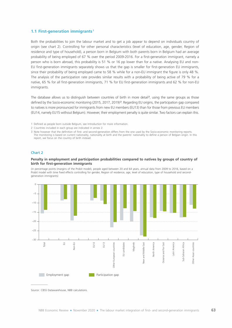
63NBB Economic Review ¡ November 2020 ¡ The labour market integration of first‑ and second‑generation immigrants
1.1 First-generation immigrants 1
Both the probabilities to join the labour market and to get a job appear to depend on individuals country of origin (see chart 2). Controlling for other personal characteristics (level of education, age, gender, Region of residence and type of household), a person born in Belgium with both parents born in Belgium had an average probability of being employed of 67 % over the period 2009‑2016. For a first‑generation immigrant, namely a person who is born abroad, this probability is 51 % or 16 pp lower than for a native. Analysing EU and non‑EU first‑generation immigrants separately shows us that the gap is smaller for first‑generation EU immigrants, since their probability of being employed came to 58 % while for a non‑EU immigrant the figure is only 48 %. The analysis of the participation rate provides similar results with a probability of being active of 79 % for a native, 65 % for all first‑generation immigrants, 71 % for EU first‑generation immigrants and 62 % for non‑EU immigrants.
The database allows us to distinguish between countries of birth in more detail 2, using the same groups as those defined by the Socio‑economic monitoring (2015, 2017, 2019) 3. Regarding EU origins, the participation gap compared to natives is more pronounced for immigrants from new EU members (EU13) than for those from previous EU members (EU14, namely EU15 without Belgium). However, their employment penalty is quite similar. Two factors can explain this.
1 Defined as people born outside Belgium, see Introduction for more information.2 Countries included in each group are indicated in annex 2.3 Note however that the definition of first‑ and second‑generation differs from the one used by the Socio‑economic monitoring reports.
The monitoring is based on current nationality, nationality at birth and the parents’ nationality to define a person of Belgian origin. In this report, we focus on the country of birth instead.
Chart 2
Penalty in employment and participation probabilities compared to natives by groups of country of birth for first-generation immigrants(in percentage points (margins of the Probit model), people aged between 20 and 64 years, annual data from 2009 to 2016, based on a Probit model with time fixed effects controlling for gender, Region of residence, age, level of education, type of household and second‑generation immigrants)
Employment gap
Tota
l
EU
Non
‑EU
EU14
EU13
Oth
er E
urop
ean
coun
trie
s
EU c
andi
date
s
Mag
hreb
Nea
r an
d M
iddl
e Ea
st
Nor
th A
mer
ica
Oce
ania
and
Far
Eas
t
Latin
Am
eric
a
Sub‑
Saha
ran
Afr
ica
Oth
er A
sian
cou
ntrie
s
−30
−25
−20
−15
−10
−5
0
Participation gap
Source : CBSS Datawarehouse, NBB calculations.

64NBB Economic Review ¡ November 2020 ¡ The labour market integration of first‑ and second‑generation immigrants
The first is related to the database itself, with a lack of information for workers in international institutions who mainly originate from EU14 countries. While we partially correct for this, the true employment gap is probably higher than the one we computed here. Secondly, the large number of individuals originating from EU13 countries and coming for work, especially in the construction sector, could explain why they can more easily find a job 1.
Among non‑EU origins, the largest gaps, for employment as well as for participation, occurred for immigrants originating from the Near and Middle East and from other European countries (mainly Russia, Serbia, Ukraine 2). The situation of immigrants from EU candidate countries (mainly Turkey) and Maghreb should also be highlighted. While for other origins the difference between employment and participation gaps is marginal, in the case of immigrants from EU candidate countries or from Maghreb the penalty is greated for their employment probability than for their participation probability. Their willingness to enter the labour market is therefore more similar to that of other immigrants and natives than their probability of getting a job.
In addition to origin itself, personal characteristics have an influence on the labour market outcomes of immigrants. Next sections are devoted to the analysis of those characteristics, namely level of education, Region of residence, age, gender and type of household. In order to observe the effect of those characteristics on the employment and participation rates of first‑generation immigrants, we run two separate regressions, one for natives and one for first‑generation immigrants (including their country of birth group as a control variable). For each regression we will analyse the coefficient of the different variables. The graphs presented in each section are thus derived from the same analysis. The section concludes with an Oaxaca‑Blinder decomposition providing an estimation of the share of the gap that can be explained by those characteristics.
1.1.1 Level of education
The probability of being employed increases greatly for natives if they get a higher degree (see chart 3). Progressing from low‑ to medium‑educated, they gain 17 pp and a further 11 pp if they are highly educated (so 28 pp in total more than a for a low‑educated native). The impact associated with a higher level of education for first‑generation immigrants are significantly lower. While a low‑educated first‑generation immigrant has a 42 % probability of being employed, that figure reaches 54 % for a medium‑educated immigrant (+12 pp) and only 55 % for a high‑educated immigrant (+14 pp). While participation in the labour market (either employed or unemployed) increases with the level of education for natives, first‑generation immigrants with a high level of education tend to have a lower probability of being active than medium‑educated immigrants. This could probably be explained by the large penalty incurred by tertiary‑educated immigrants compared to natives and also by the fact that they are more often over‑educated or their diplomas and skills have not been recognized (see sections 2.3 and 2.4). Those factors may affect their willingness to enter the labour market, with the effect of worker discouragement lowering the participation rate.
1.1.2 Region of residence
Controlling for other personal characteristics, employment rates are similar in Brussels and in Wallonia, for both natives and first‑generation immigrants, while they are systematically higher in Flanders (see chart 4). The gap compared to natives is, however, a bit larger in Flanders than in the other two Regions. In terms of participation rates, Wallonia has the lowest rates for both natives and immigrants, and also the largest gap between those two populations. The reason for those small differences in gaps between Regions but a more pronounced difference in rates, probably relate to Flanders’ better economic performance in terms of GDP (e.g. GDP growth of 3.3 % in 2018, compared to 3.0 % in Wallonia and 2.1 % in Brussels according to the Eurostat regional accounts) and the overall employment rate (based on LFS data, 76 % in 2019 compared to 65 % in Wallonia and 62 % in Brussels).
1 Note that posted workers are not included in the analysis because they are not present in administrative data and remain registered in their country of origin. This is also the case of seasonal or any temporary immigrants who came in Belgium for less than 3 months. See also annex 1.
2 See HCE (2018) about the main nationalities of international immigrants entering Belgium in 2010 and 2017.

65NBB Economic Review ¡ November 2020 ¡ The labour market integration of first‑ and second‑generation immigrants
The study by Englert (2013), shows that the higher unemployment rate in Brussels is not only due to low education levels of the population but also to specific labour demand characteristics implying a higher risk of unemployment for all Brussels residents, and in particular for non‑EU immigrants as they constitute a large share of the Region population. Owing to the high percentage of commuters, the labour supply is larger than the resident population of Brussels, making it easier for employers to recruit overqualified workers and potentially to discriminate. Employers are also imposing tougher requirements, in particular regarding language knowledge.
Encouraging geographical mobility could help to boost employment rates for both natives and immigrants. As highlighted in the HCE report of 2018, worker mobility is more common among immigrants than among natives, even though the great majority work in the same Region as their Region of residence. The choice of where to live when arriving in Belgium could also be a determinant of immigrants’ employment rate. For example, a recent report for the Brussels Capital Region (View.Brussels 2019), focusing on the nationality of job‑seekers, showed that most of the immigrant population, and in particular non‑EU immigrants, live in the most deprived area (“croissant pauvre”) of Brussels. The authors conclude that there is both ethnic and socio‑geographical segregation. It is not only socio‑economically disadvantaged people who predominated in this deprived area, origin also seems to play a role. Looking at people in a comparable socio‑economic position (unemployed jobseekers), the report shows that people of foreign origin are more likely to be stuck in the ‘croissant pauvre’ than native Belgians. 79 % of unemployed jobseekers in this area are of non‑EU foreign origin. Moreover, people tend to leave the “croissant pauvre” area once they find jobs, meaning that the causal link could also be inverse.
Chart 3
Predicted employment and participation probabilities for natives and first-generation immigrants by level of education 1
(in % and difference in percentage points compared to low‑educated, people aged between 20 and 64 years, annual data from 2009 to 2016, based on the computed margins of a Probit model with time fixed effects considering gender, Region of residence, age and type of household at their mean values)
Natives
High educated Middle educated Low educated High educated Middle educated Low educated
0
10
20
30
40
50
60
70
80
90
First‑generation immigrants
Employment probability Participation probability
+28
+14
+17
+12
+15
+6
+11
+12
Source : CBSS Datawarehouse, NBB calculations.Note : Results are computed from separate regressions for natives and first‑generation immigrants. The regressions for first‑generation
immigrants also control for the detailed country of birth groups.1 Low‑educated individuals have at most their lower secondary education diploma, medium‑educated have a certificate of higher secondary
education and high‑educated hold a degree in tertiary education.

66NBB Economic Review ¡ November 2020 ¡ The labour market integration of first‑ and second‑generation immigrants
In general, the labour market impact of immigration will depend on the distribution of existing skill levels in the region where the immigrants settle, as well as their own level of education. A fair distribution of immigrants across the country therefore does not necessarily imply a fair distribution of the impact on the labour market (Glitz, 2012). As immigrants tend to react more quickly to changes in labour demand (Roed and Schone, 2012), there will be market equilibrium only if a certain degree of worker mobility exists (Cadena and Kovak, 2013). So, in the long run, immigration can actually improve flexibility on the labour market and the skills match, and reduce the variation in overall employment rates over the business cycle (Basso et al., 2018).
Moreover, the initial choice of Region of residence for newly arriving immigrants may depend on network effects as well as location‑specific characteristics such as local labour or housing market conditions and the presence of public amenities. Using administrative data on Belgian municipalities between 1994 and 2007, Jayet et al. (2016) tried to disentangle the network effect from the other local factors. They found that housing and labour market variables drive the geographical distribution of immigrants in Belgium, so that the attractiveness of particular municipalities predominates over the positive influence of social networks, even if the magnitude of the effects varies from one nationality to another.
1.1.3 Age
Both immigrants and natives have the same profile over the age categories, with increasing employment and participation rates in the younger age groups and a stronger decrease towards retirement age (see chart 5). However, while natives are most likely to be in work at 25‑29 years (80 %), the highest level of employment for first‑generation immigrants, still significantly below that for natives, is reached at 40‑44 years old (55 %). In terms of participation, the difference is even larger with the highest rate reaching 88 % at 25‑29 years for
Chart 4
Predicted employment and participation probabilities for natives and first-generation immigrants by Region of residence(in % and difference in percentage points compared to natives, people aged between 20 and 64 years, annual data from 2009 to 2016, based on the computed margins of a Probit model with time fixed effects considering level of education, gender, age and type of household at their mean values)
Brussels Flanders Wallonia Brussels Flanders Wallonia
0
10
20
30
40
50
60
70
80
90
−17
−19
−13−13
−17
−15
Natives First‑generation immigrants
Employment probability Participation probability
Source : CBSS Datawarehouse, NBB calculations.Note : Results are computed from separate regressions for natives and first‑generation immigrants. The regressions for first‑generation
immigrants also control for the detailed country of birth groups.

67NBB Economic Review ¡ November 2020 ¡ The labour market integration of first‑ and second‑generation immigrants
natives, while the peak is not achieved until age 50‑54 for immigrants, when there is a participation probability of 71 %. This can be explained by the fact that, even if immigrants are young when they arrive, they often have to follow additional training or integration programmes which delay their integration into the labour market (see also section 2.3 about diploma recognition and sections 3.1 and 3.2 on integration programmes and access to the labour market).
Moreover, immigrants seem to leave the labour market at an older age. Their employment and participation probabilities decrease less than for natives at age 50 or more, so that the gaps compared to natives diminish with the age groups. Those results suggest that, because of their shorter career or their delayed entrance into
Chart 5
Predicted employment and participation probabilities for natives and first-generation immigrants by age(in %, people aged between 20 and 64 years, annual data from 2009 to 2016, based on the computed margins of a Probit model with time fixed effects considering gender, Region of residence, level of education and type of household at their mean values)
Natives
20‑24 years 25‑29 years 30‑34 years 35‑39 years 40‑44 years 45‑49 years 50‑54 years 55‑59 years 60‑64 years
0
10
20
30
40
50
60
70
80
90
First‑generation immigrants
Employment probability
20‑24 years 25‑29 years 30‑34 years 35‑39 years 40‑44 years 45‑49 years 50‑54 years 55‑59 years 60‑64 years
0
10
20
30
40
50
60
70
80
90
100
Participation probability
Source : CBSS Datawarehouse, NBB calculations.Note : Results are computed from separate regressions for natives and first‑generation immigrants. The regressions for first‑generation
immigrants also control for the detailed country of birth groups.

68NBB Economic Review ¡ November 2020 ¡ The labour market integration of first‑ and second‑generation immigrants
the labour market, they need to continue working at an older age either to accumulate more savings through wages or to increase their pension benefit entitlements by extending their career.
1.1.4 Gender
A foreign‑born woman is 10 pp less likely to be employed than a foreign‑born man (see chart 6). Immigrant women hence face what is called a “double disadvantage”. This penalty is halved if the woman is a native person.
Moreover, distinguishing between EU and non‑EU immigrants, Piton and Rycx (2020) show that immigrant women of EU origin face a double penalty, which means that the penalty for immigrant women of EU origin corresponds to the sum of the penalties faced respectively by women and immigrants of EU origin. For those of non‑EU origin (excluding Sub‑Saharan origin for whom the penalty is similar to that faced by EU‑born women), the penalty is even greater since it outweighs the sum of both penalties of being a woman and being an immigrant.
In addition, Bentouhami and Khadhraoui (2018), studying gender discrimination, showed that the impact of being a woman varies across origins. More precisely, Belgian women do not immediately face any gender inequality when entering the labour market. The gender gap occurs gradually. Conversely, (non‑EU) foreign women face the gender gap immediately through downgrading or over‑qualification (in the health sector, for example) or through factors which prevent them from joining the labour market (such as family responsibilities, especially for single mothers, or specific rules regarding the wearing of headscarves).
The difference between natives and first‑generation immigrant women is even greater if we look at participation probabilities. While a foreign‑born woman is 13 pp less likely to be active on the labour market than an immigrant man, this penalty is only 4 pp for a native woman compared to a native man (see chart 6).
Chart 6
Predicted employment and participation probabilities for natives and first-generation immigrants by gender(in % and difference in percentage points compared to men, people aged between 20 and 64 years, annual data from 2009 to 2016, based on the computed margins of a Probit model with time fixed effects considering level of education, Region of residence, age and type of household at their mean values)
Men Women Men Women
0
10
20
30
40
50
60
70
80
90
−5
−10
−4
−13
Natives First‑generation immigrants
Employment probability Participation probability
Source : CBSS Datawarehouse, NBB calculations.Note : Results are computed from separate regressions for natives and first‑generation immigrants. The regressions for first‑generation
immigrants also control for the detailed country of birth groups.

69NBB Economic Review ¡ November 2020 ¡ The labour market integration of first‑ and second‑generation immigrants
In a study concerning the United States, Blau et al. (2011) showed that female immigrants from countries where women have a high rate of participation in the labour market also had much higher employment rates in the United States than women from countries where their participation is low. In addition, while working less than comparable natives on arrival, women from countries with a higher participation rate tend to almost entirely close the gap with natives. Conversely, in the case of women from low female participation countries, the participation rate in the US seems to remain below that of natives even after some years of residence. The same type of analysis was done for men, but the findings were not similar so that we can assume that this situation reflects the position of women in the household in their country of origin.
This finding also seems to be confirmed by the analysis of detailed country of birth (see chart 7). The gender gap is much more pronounced for individuals from the Near and Middle East, Maghreb and Turkey (EU candidate countries) than for other countries of origin. Those countries are in fact also among the ones where women tend to participate less in the labour market (see chart 8).
Based on the three main nationalities of international immigrants entering Belgium 1 by country of origin groups, we can see that the lowest participation rates of women are reflected in the two groups Maghreb and the Near and Middle East, and to a lesser extent in EU candidate countries.
1 Data from Statbel for 2017.
Chart 7
Gender gap in employment and participation probabilities at constant characteristics for first-generation immigrants by detailed country of birth(difference in percentage points between predicted probability for women and men1, people aged between 20 and 64 years, annual data from 2009 to 2016, based on the computed margins of a Probit model with time fixed effects considering level of education, Region of residence, age and type of household at their mean values, separate regressions for men and women)
p.m
. Nat
ives
Tota
l firs
t-ge
nera
tion
EU14
EU13
Oth
er E
urop
ean
coun
trie
s
EU c
andi
date
s
Mag
hreb
Nea
r an
d M
iddl
e Ea
st
Nor
th A
mer
ica
Oce
ania
and
Far
Eas
t
Latin
Am
eric
a
Sub-
saha
ran
Afr
ica
Oth
er A
sian
cou
ntrie
s
–20
–15
–10
–5
0
5
Gender employment gap Gender participation gap
Source : CBSS Datawarehouse, NBB calculations.1 Note that the methodology being different, the gender gap for natives and total first‑generation immigrants are not equal to those defined
in chart 6. The objective here is to see to what extent gender gaps are higher for some groups of country of origin.
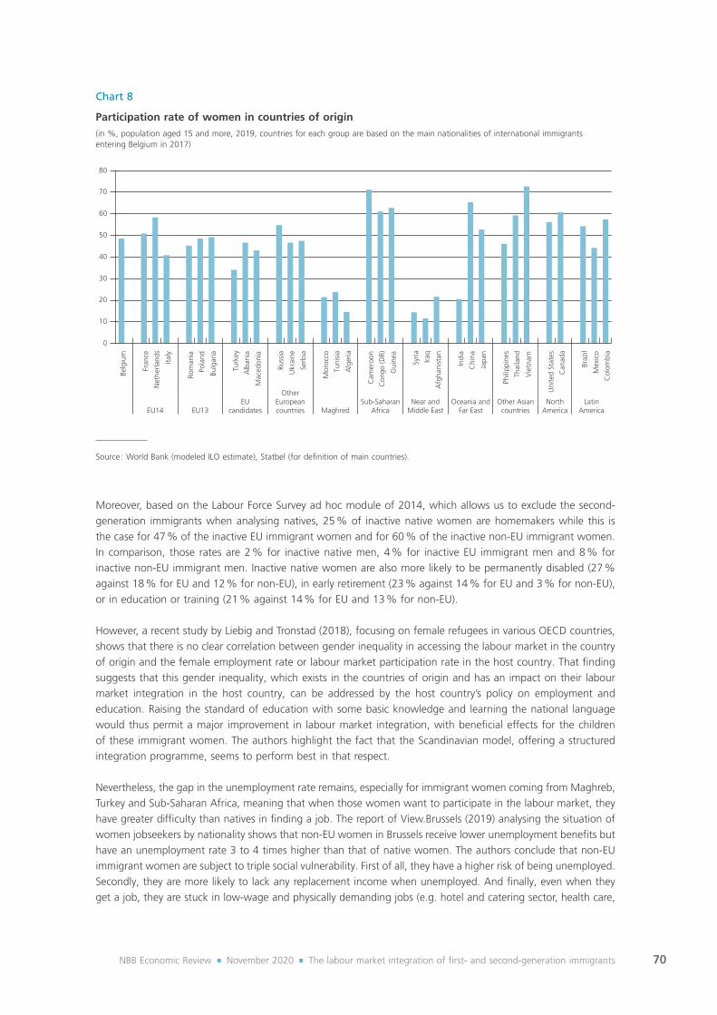
70NBB Economic Review ¡ November 2020 ¡ The labour market integration of first‑ and second‑generation immigrants
Moreover, based on the Labour Force Survey ad hoc module of 2014, which allows us to exclude the second‑generation immigrants when analysing natives, 25 % of inactive native women are homemakers while this is the case for 47 % of the inactive EU immigrant women and for 60 % of the inactive non‑EU immigrant women. In comparison, those rates are 2 % for inactive native men, 4 % for inactive EU immigrant men and 8 % for inactive non‑EU immigrant men. Inactive native women are also more likely to be permanently disabled (27 % against 18 % for EU and 12 % for non‑EU), in early retirement (23 % against 14 % for EU and 3 % for non‑EU), or in education or training (21 % against 14 % for EU and 13 % for non‑EU).
However, a recent study by Liebig and Tronstad (2018), focusing on female refugees in various OECD countries, shows that there is no clear correlation between gender inequality in accessing the labour market in the country of origin and the female employment rate or labour market participation rate in the host country. That finding suggests that this gender inequality, which exists in the countries of origin and has an impact on their labour market integration in the host country, can be addressed by the host country’s policy on employment and education. Raising the standard of education with some basic knowledge and learning the national language would thus permit a major improvement in labour market integration, with beneficial effects for the children of these immigrant women. The authors highlight the fact that the Scandinavian model, offering a structured integration programme, seems to perform best in that respect.
Nevertheless, the gap in the unemployment rate remains, especially for immigrant women coming from Maghreb, Turkey and Sub‑Saharan Africa, meaning that when those women want to participate in the labour market, they have greater difficulty than natives in finding a job. The report of View.Brussels (2019) analysing the situation of women jobseekers by nationality shows that non‑EU women in Brussels receive lower unemployment benefits but have an unemployment rate 3 to 4 times higher than that of native women. The authors conclude that non‑EU immigrant women are subject to triple social vulnerability. First of all, they have a higher risk of being unemployed. Secondly, they are more likely to lack any replacement income when unemployed. And finally, even when they get a job, they are stuck in low‑wage and physically demanding jobs (e.g. hotel and catering sector, health care,
Chart 8
Participation rate of women in countries of origin(in %, population aged 15 and more, 2019, countries for each group are based on the main nationalities of international immigrants entering Belgium in 2017)
Belg
ium
Fran
ce
Net
herla
nds
Italy
Rom
ania
Pola
nd
Bulg
aria
Turk
ey
Alb
ania
Mac
edon
ia
Russ
ia
Ukr
aine
Serb
ia
Mor
occo
Tuni
sia
Alg
eria
Cam
eroo
n
Con
go (D
R)
Gui
nea
Syria
Iraq
Afg
hani
stan
Indi
a
Chi
na
Japa
n
Phili
ppin
es
Thai
land
Vie
tnam
Uni
ted
Stat
es
Can
ada
Braz
il
Mex
ico
Col
ombi
a
0
10
20
30
40
50
60
70
80
EU14 EU13EU
candidates
OtherEuropeancountries Maghred
Sub‑SaharanAfrica
Near andMiddle East
Oceania andFar East
Other Asiancountries
NorthAmerica
LatinAmerica
Source : World Bank (modeled ILO estimate), Statbel (for definition of main countries).

71NBB Economic Review ¡ November 2020 ¡ The labour market integration of first‑ and second‑generation immigrants
cleaning). Note that this last point on job quality is also true for immigrant women from EU13 countries, many of whom are employed under the service voucher system, for example. Female non‑EU immigrants are also more likely to be single parents in Brussels, which increases their risk of becoming unemployed.
1.1.5 Type of household
Unmarried couples without children are the most likely than other types of household to be employed or to participate in the labour market, and this is true for both natives (89 % participation probability, 81 % employment probability) and first‑generation immigrants (73 % participation probability, 58 % employment probability). In contrast, single people without children have the lowest probabilities, again both for natives (80.5 % participation probability, 64 % employment probability) and for first‑generation immigrants (63 % participation probability, 43 % employment probability).
For all types of household, the employment gap compared to natives is systematically larger than the participation gap (see chart 9). This shows that immigrants and natives are quite similar in their willingness to be active on the labour market, but it is harder for immigrants to find a job.
There is a more pronounced difference between natives and first‑generation immigrants in the case of married couples, and in particular for married women with children. A first‑generation immigrant woman who is married and has children is 24 pp less likely to enter the labour market and 29 pp less likely to be employed than a married native mother.
Previous literature shows that the type of household and the presence of (young) children in the household have a negative impact on the participation rate of women 1. The increased burden of domestic tasks during a child’s first years, escalating with each additional child, reduces mothers’ participation in the labour market. Being a single mother also has a significant effect : single mothers are less likely to have an active career than single women without children or partnered women, with or without children, regardless of their nationality (Rea and Wets 2015). However, our results show that the largest differences with respect to native women do not occur when immigrant women become mothers but when they marry, even though among firstgeneration immigrant women it is single mothers who are least likely to be employed (41 %) 2.
Focusing on the Brussels‑Capital Region, View.Brussels (2019) shows an increasing percentage of single mothers among unemployed jobseekers in case of Sub‑Saharan immigrants (more than one out of three) compared to natives (one out of eight). For the other origin groups, the percentages are similar to those for unemployed native women. Nevertheless, the proportion of cohabiting unemployed women (married or not) with children is much larger for all foreign origins (between 23 % and 38 %) than for natives (16 %).
1.1.6 Oaxaca-Blinder decomposition
Computing a Oaxaca‑Blinder decomposition to compare native employment and participation probabilities with those of first‑generation immigrants, we can estimate the part of the gaps that can be explained by personal characteristics, namely level of education, Region of residence, age, gender and type of household. The analysis will also distinguish between EU and non‑EU immigrants 3. Drawing on the theory developed by Blinder and Oaxaca (Blinder, 1973 ; Oaxaca, 1973), we can decompose the employment probability between two population groups – immigrants vs natives in our case – into two components. First, the part that is explained by differences in individual characteristics. This is the endowment effect, which means that employment differences are partly explained by the fact that the average factors are different depending on whether one is dealing with natives or
1 Correll et al. (2007), Paull (2008), Bertrand et al. (2010), Fitzenberger et al. (2013), Goldin (2014), Adda et al. (2017), Goldin and Katz (2016), Kleven et al. (2018).
2 See also Kil et al. (2018)3 Full results and tables are available in annex II.4.
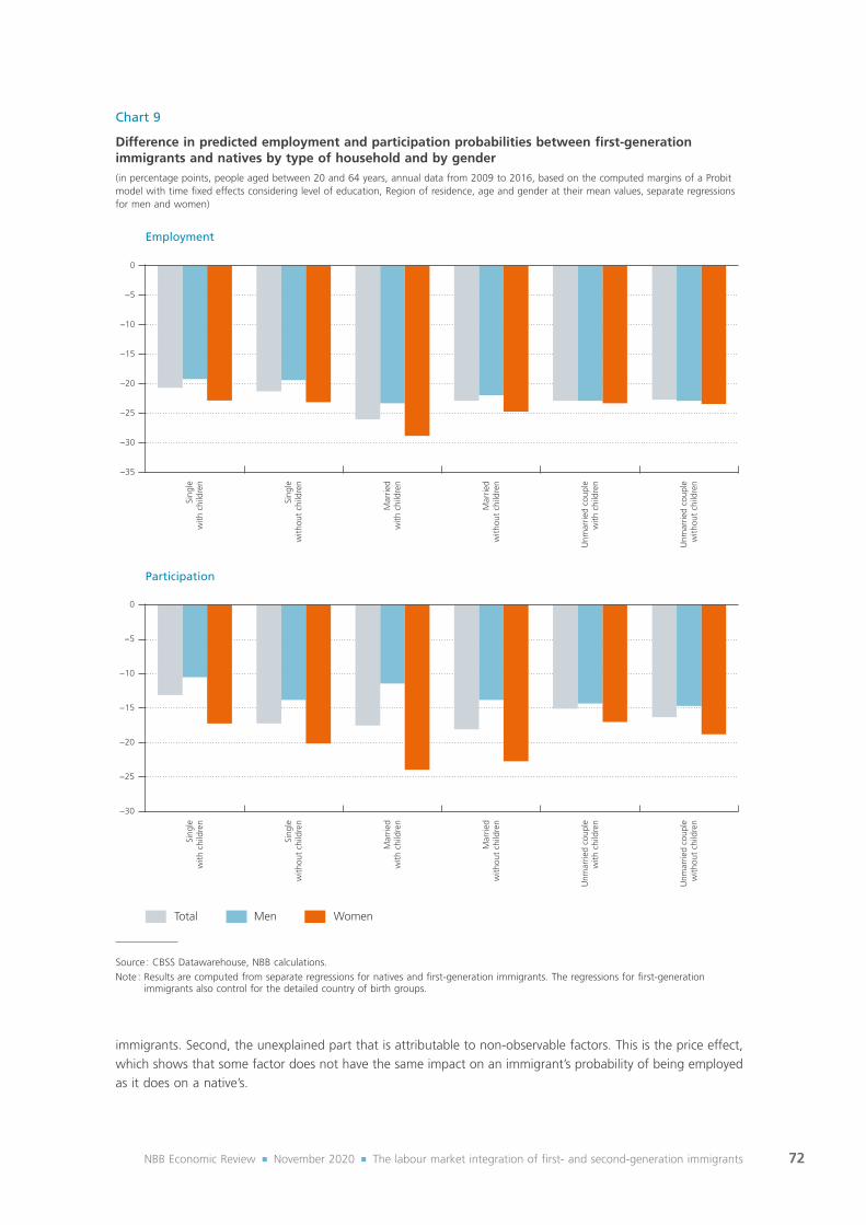
72NBB Economic Review ¡ November 2020 ¡ The labour market integration of first‑ and second‑generation immigrants
immigrants. Second, the unexplained part that is attributable to non‑observable factors. This is the price effect, which shows that some factor does not have the same impact on an immigrant’s probability of being employed as it does on a native’s.
Chart 9
Difference in predicted employment and participation probabilities between first-generation immigrants and natives by type of household and by gender(in percentage points, people aged between 20 and 64 years, annual data from 2009 to 2016, based on the computed margins of a Probit model with time fixed effects considering level of education, Region of residence, age and gender at their mean values, separate regressions for men and women)
−30
−25
−20
−15
−10
−5
0
Sing
lew
ith c
hild
ren
Sing
lew
ithou
t ch
ildre
n
Mar
ried
with
chi
ldre
n
Mar
ried
with
out
child
ren
Unm
arrie
d co
uple
with
chi
ldre
n
Unm
arrie
d co
uple
with
out
child
ren
Sing
lew
ith c
hild
ren
Sing
lew
ithou
t ch
ildre
n
Mar
ried
with
chi
ldre
n
Mar
ried
with
out
child
ren
Unm
arrie
d co
uple
with
chi
ldre
n
Unm
arrie
d co
uple
with
out
child
ren
−35
−30
−25
−20
−15
−10
−5
0
Employment
Total Men Women
Participation
Source : CBSS Datawarehouse, NBB calculations.Note : Results are computed from separate regressions for natives and first‑generation immigrants. The regressions for first‑generation
immigrants also control for the detailed country of birth groups.

73NBB Economic Review ¡ November 2020 ¡ The labour market integration of first‑ and second‑generation immigrants
When this type of decomposition is used, the results must be interpreted with caution, as the unexplained part partly covers discrimination but also the reality of all non‑observable factors and all factors which could not be included in the regression, for example language knowledge (for which we do not have any data). Those non‑observable factors include certain individual preferences, such as the field of study, or cultural differences and network effects. Conversely, the explained part does not contain any justification for the gap. Some forms of discrimination may also appear in the explanatory variables. Take the level of education, for example : natives and immigrants may not have the same opportunities to attain higher education levels (Baert et al., 2016 ; Baert and Cockx, 2013).
Before looking at the results of the Oaxaca‑Blinder decomposition, we first analyse what would be the expected impact of each personal characteristic. To do so, we run a Probit regression with year fixed effect and look at the coefficient of our variables of interest for the entire population. Then, for each group of the population, namely natives, first‑generation immigrants, first‑generation EU immigrants and first‑generation non‑EU immigrants, we consider the share of each of those characteristics to see if they are over‑represented in some categories which are beneficial or detrimental for labour market integration. The complete descriptive statistics can be found in annex II.3.
The descriptive statistics indicate that the proportions by Region of residence differ greatly between natives and first‑generation immigrants since the latter are over‑represented in Brussels and under‑represented in the other two Regions. The Brussels‑Capital Region displays the largest negative effect in terms of employment and participation probabilities (together with Wallonia for which coefficients are fairly similar to those of Brussels). The over‑representation of Brussels as the Region of residence is more pronounced for non‑EU first‑generation immigrants (28 % of them live in Brussels, compared to 5 % of natives) than for EU immigrants (22 %) who are also slightly overrepresented in Wallonia (34 % living in Wallonia against 33 % of natives and 24 % of non‑EU immigrants). Both first‑generation groups are underrepresented in Flanders. The Region of residence is thus a potential explanatory factor for the employment and participation gap between natives and first‑generation immigrants.
Half as many first‑generation immigrants (both EU and non‑EU) are in the younger age group (20‑24 years) compared to natives ; in contrast, they are more heavily represented in the middle‑aged categories. The second lowest employment and participation rates are recorded for younger people, just behind those for the older age group (60‑64 years), while the highest rates occur for middle‑aged categories. Note however that EU immigrants are over‑represented in the 55‑59 years age group (8 % against 6 % for non‑EU immigrants and natives) and the 60‑64 years age group (5 % compared to 3 % for natives and 3 % for non‑EU immigrants). The age composition of first‑generation immigrants could, on average, be considered beneficial for their labour market integration.
There is a more pronounced difference in the composition of natives versus immigrants regarding the level of education. As expected, first‑generation immigrants comprise a smaller proportion of high‑educated (7 pp) and medium‑educated individuals (–18 pp) and a larger share of low‑educated (+25 pp). This remains true for both EU and non‑EU immigrants ; however, the disparities are more pronounced for non‑EU immigrants, 53 % of whom have a low level of education (against 23 % for natives and 39 % for EU immigrants). Moreover, the proportion of high‑ educated individuals is close to the figure for native Belgians in the case of EU immigrants (36 % against 37 %), but again much lower for non‑EU immigrants (28 %). Those stylised facts suggest that the level of education could explain a significant part of the labour market integration gap.
Regarding the type of households, many immigrants are married with children (33 %), and that applies in particular to non‑EU immigrants (37 %), while this is less the case for natives (19 %). To a lesser extent, they are also more likely to be single but less likely to be cohabiting. There is also a large difference for ‘children living with their parents’ 1, the category with the lowest labour market integration. 25 % of natives are in this category,
1 This category includes individuals who are still living with their parents regardless of the status of their parents ((un)married, in couple or not). Each defined category is mutually exclusive so that those children do not enter in the shares defined for their parents.

74NBB Economic Review ¡ November 2020 ¡ The labour market integration of first‑ and second‑generation immigrants
compared to only about 10 % of first‑generation immigrants. This finding could be connected with the fact that natives are more likely to study for a tertiary education degree, staying at home with their parents and not working. Types of households are therefore not similarly spread over different categories between natives and first‑generation immigrants. The repartition of immigrants among household types are favouring employment and participation (smaller share of children living with their parents and greater share of married couples with children).
In terms of gender, women have on average both lower labour market participation (–6 pp) and employment (–6 pp) probabilities than men. However, there are slightly less women among first‑generation immigrants (51 %) than among natives (52 %). The same holds for non‑EU immigrants with women representing 49 %, but the reverse is true for EU immigrants, 55 % of whom are women. In sum, non‑EU immigrants should on average be more likely to be employed or to participate to the labour market given their relative larger share of men, while the opposite is true for EU immigrants.
Men and women also differ in terms of other personal characteristics, and particularly education and type of household. Women tend to be more educated than men with a significantly larger share of tertiary‑educated and a smaller share of low‑educated. This finding is confirmed for all origins but is more pronounced for EU immigrant women. The type of household variable highlights a larger proportion of single mothers (rising from 10 % for natives to 18 % for non‑EU immigrants) than single fathers (approximately 2 % for all origins). Conversely, men are more likely to be single and without children. Moreover, women are less likely to stay at home with their parents.
The Oaxaca‑Blinder decomposition results show that personal characteristics can only explain 18 % of the employment gap between first‑generation immigrants and natives, which comes to 17 pp (see chart 10). For immigrants from an EU country, almost one third of the gap can be explained and the gap itself is smaller
Chart 10
Explained and unexplained part of the employment and participation gaps between natives and first-generation immigrants(in percentage points, people aged between 20 and 64 years, annual data from 2009 to 2016, based on a Oaxaca‑Blinder decomposition using estimations from a Probit model with time fixed effects controlling for gender, level of education, Region of residence, age and type of household)
First‑generationimmigrants
First‑generationEU immigrants
First‑generationnon‑EU immigrants
First‑generationimmigrants
First‑generationEU immigrants
First‑generationnon‑EU immigrants
–5
0
5
10
15
20
25
Explained part Unexplained part
Employment probability Participation probability
Source : CBSS Datawarehouse, NBB calculations.

75NBB Economic Review ¡ November 2020 ¡ The labour market integration of first‑ and second‑generation immigrants
(10 pp). However, the employment gap reaches 21 pp for non‑EU immigrants and only 15 % can be explained by personal characteristics. Making the same kind of analysis for Belgium, Corluy and Verbist (2014), have already shown that the explained part of the employment gap between immigrants and people born in Belgium is halved in the case of non‑EU immigrants. Looking at more detailed country of birth for non‑EU immigrants, the HCE report of 2018 shows that personal characteristics (gender, age, level of education and Region of residence) can explain a larger share of the gap for people from Maghreb even though the gap itself was much larger than for the other countries of origin. In contrast, only a very small part of the employment gap could be explained for people from the Near and Middle East and Asia.
As expected, some of the personal characteristics tested are supposed to increase employment and participation rate of immigrants. This is the case for the type of household and for gender and age (except for EU immigrants), which should make them more likely to be in work than natives. On the other hand, other variables have a negative impact on the employment probability of immigrants. This is true for the level of education, notably for non‑EU immigrants, and the Region of residence, with most of the immigrant population living in Brussels.
A separate analysis for men and women shows that we can explain a bit more of the employment gap between male immigrants and male natives (19 %) than for women (17 %). However, EU and non‑EU analyses provide very different results. The total explained part in the case of EU immigrants conceals a large difference between men and women. While 45 % of the gap between EU immigrant men and native men can be explained, that figure is only 17 % for women ; moreover, for women the gap is larger than for men. For non‑EU immigrants, a larger – though still small – part can be explained for women than for men (17 % against 13 %). This difference is mainly due to their type of household. In fact, non‑EU immigrant women are more likely to be single mothers, and that has a negative effect on their employment rate.
Concerning participation rates, none of the gap compared to natives can be explained by personal characteristics included in our analysis.
Distinguishing between men and women, 9 % of the participation gap between EU‑immigrant men and natives can be explained, the main factors being level of education, Region of residence and age profile. Interestingly, for female EU immigrants, the explained part is negative, the main reason being that their level of education should make them more likely to participate in the labour market than native women. For all other specifications, none of the gap can be explained by personal characteristics either for total or non‑EU immigrants, and for both men and women.
Overall, the share of the participation and employment rate gaps that can be explained through personal characteristics is fairly small. Hence, to better understand the employment and participation penalty of first‑generation immigrants, it is necessary to go beyond the impact of gender, age, level of education, Region of residence and type of households.
1.2 Second-generation immigrants 1
Given that children of immigrants are born, educated and socialized in the country of residence, their relative success or failure is often seen as the ultimate benchmark of integration (Card, 2005). The standard assumption is that second‑generation immigrants should fare better than their parents and ultimately ‘catch up’ with the children of native‑born parents, thanks to their improved language proficiency, their greater opportunity in getting a higher level of skills and qualifications and their higher social and cultural capital specific to the host country compared to their parents. Results for advanced economies suggest, however, that this view is somewhat too optimistic (Brinbaum, 2018). The majority of the literature supports the segmented assimilation
1 Defined as people born in Belgium with at least one parent born abroad. See Introduction for more information.
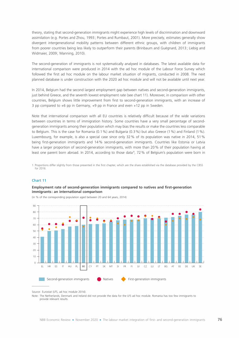
76NBB Economic Review ¡ November 2020 ¡ The labour market integration of first‑ and second‑generation immigrants
theory, stating that second‑generation immigrants might experience high levels of discrimination and downward assimilation (e.g. Portes and Zhou, 1993 ; Portes and Rumbaut, 2001). More precisely, estimates generally show divergent intergenerational mobility patterns between different ethnic groups, with children of immigrants from poorer countries being less likely to outperform their parents (Brinbaum and Guégnard, 2013 ; Liebig and Widmaier, 2009 ; Manning, 2010).
The second‑generation of immigrants is not systematically analysed in databases. The latest available data for international comparison were produced in 2014 with the ad hoc module of the Labour Force Survey which followed the first ad hoc module on the labour market situation of migrants, conducted in 2008. The next planned database is under construction with the 2020 ad hoc module and will not be available until next year.
In 2014, Belgium had the second largest employment gap between natives and second‑generation immigrants, just behind Greece, and the seventh lowest employment rate (see chart 11). Moreover, in comparison with other countries, Belgium shows little improvement from first to second‑generation immigrants, with an increase of 3 pp compared to +6 pp in Germany, +9 pp in France and even +12 pp in Sweden.
Note that international comparison with all EU countries is relatively difficult because of the wide variations between countries in terms of immigration history. Some countries have a very small percentage of second‑generation immigrants among their population which may bias the results or make the countries less comparable to Belgium. This is the case for Romania (0.1 %) and Bulgaria (0.3 %) but also Greece (1 %) and Finland (1 %). Luxembourg, for example, is also a special case since only 32 % of its population was native in 2014, 51 % being first‑generation immigrants and 14 % second‑generation immigrants. Countries like Estonia or Latvia have a larger proportion of second‑generation immigrants, with more than 20 % of their population having at least one parent born abroad. In 2014, according to those data 1, 72 % of Belgium’s population were born in
1 Proportions differ slightly from those presented in the first chapter, which are the share established via the database provided by the CBSS for 2016.
Chart 11
Employment rate of second-generation immigrants compared to natives and first-generation immigrants : an international comparison(in % of the corresponding population aged between 20 and 64 years, 2014)
Second‑generation immigrants First‑generation immigrants
EL HR ES IT HU PL BE CY PT SK MT SI FR FI LV CZ LU LT BG AT EE DE UK SE0
10
20
30
40
50
60
70
80
90
Natives
Source : Eurostat (LFS, ad hoc module 2014).Note : The Netherlands, Denmark and Ireland did not provide the data for the LFS ad hoc module. Romania has too few immigrants to
provide relevant results.

77NBB Economic Review ¡ November 2020 ¡ The labour market integration of first‑ and second‑generation immigrants
Belgium with both parents having also been born in Belgium, 17 % were born abroad and 10 % had at least one parent born abroad. Even considering heterogeneities across countries, if we compare Belgium’s performance with that of Sweden, the country with the most similar proportion of immigrants compared to Belgium (69 % natives, 20 % first‑generation and 10 % second‑generation) and also with the most similar gap regarding first‑generation immigrants, Belgium’s performance falls far short of Swedish outcomes for the second‑generation. The employment rate of second‑generation immigrants stood at 59 %, 12 pp below the figure for natives, compared to 80 % in Sweden or 4 pp below the figure for natives.
Just as we did for the first‑generation, we will conduct an analysis that aims to provide explanations for this large gap. Considering all individuals aged between 20 and 64 years, we run a Probit regression for both the probability of being employed and the probability of participating in the labour market, controlling for all available personal characteristics, namely gender, age, level of education, Region of residence and type of household and including a time fixed‑effect.
Our first regression includes the entire population and looks at the effect of being a second‑generation immigrant when maintaining other characteristics constant at their mean value. In line with previous findings for Belgium 1, the results show that, compared to a native person, a second‑generation immigrant is 6 pp less likely to find a job than a native. While the penalty is 10 pp lower than for first‑generation immigrants, the difference with respect to natives is still significant (see chart 12). There is a stark difference between EU and non‑EU origins in terms of the employment penalty. A second‑generation immigrant from the EU is 3 pp less likely to be employed. For a non‑EU second‑generation immigrant, the penalty is almost four times larger at –10 pp. Studying more detailed groups of origin 2, Piton and Rycx (2020) show that the improvement between the
1 Corluy et al. (2015), Socio‑economic monitoring (2015, 2017, 2019), Liebig and Widmaier (2009), Piton and Rycx (2020).2 This paper is based on a sample of the population (respondents of the LFS ad hoc modules of 2008 and 2014) which allow the authors to
get more detailed groups of origin. Given the protection on individual data, such details are not feasible for the entire population without losing information on other variables.
Chart 12
Penalty in employment and participation probabilities compared to natives by groups of country of birth for second-generation immigrants(in percentage points (margins of the Probit model), people aged between 20 and 64 years, annual data from 2009 to 2016, based on a Probit model with time fixed effects controlling for gender, Region of residence, age, level of education, type of household and first‑generation immigrants)
Employment gap Participation gap
Total EU non‑EU p.m. first generation−18
−16
−14
−12
−10
−8
−6
−4
−2
0
−5,9
−2,8 −2,6−1,3
−10,3
−4,8
−15,6
−13,7
Source : CBSS Datawarehouse, NBB calculations.

78NBB Economic Review ¡ November 2020 ¡ The labour market integration of first‑ and second‑generation immigrants
first and second generations is much smaller for immigrants from EU candidate countries, and almost zero for second‑generation immigrants from the Maghreb.
Regarding participation rates, differences are less pronounced compared to natives and between the two groups studied. A second‑generation immigrant is 3 pp less likely to be active on the labour market compared to a native (1 pp for an EU second‑generation immigrant and 5 pp for a non‑EU second‑generation immigrant). Those lower penalties denote a willingness to participate in the labour market, but there is still a large handicap for persons trying to get a job.
By running separate Probit regressions for second‑generation immigrants, natives and first‑generation immigrants, we can estimate the impact of various characteristics on employment and participation probabilities.
Being highly educated significantly increases the employment and participation probabilities of second‑generation immigrants i.e. individuals born in Belgium with a migration background have on average 28 pp higher probability of being employed if they hold a tertiary education diploma, compared to those who are low educated (see chart 13). This figure is equivalent to that of natives and higher than that found for first‑generation immigrants. Studying in the country therefore has a significant impact on the probability of being employed, even if gap with respect to natives is recorder for both first‑ and second‑generation immigrants. Note also that the penalty facing second‑generation immigrants with a low level of education, compared to natives, is exactly the same as for first‑generation immigrants. The biggest improvement occurs for high‑educated individuals. However, while the proportion of the low‑educated declines significantly between first‑ and second‑generation immigrants (from 48 % to 30 %) for both EU and non‑EU, the proportion of second‑generation immigrants with a tertiary
Chart 13
Predicted employment and participation probabilities for natives, first- and second-generation immigrants by level of education1(in % and difference in percentage points compared to low‑educated, people aged between 20 and 64 years, annual data from 2009 to 2016, based on the computed margins of a Probit model with time fixed effects considering Region of residence, age, gender and type of household at their mean values)
High educated Middle educated Low educated High educated Middle educated Low educated
0
10
20
30
40
50
60
70
80
90
+28
+17
+15+11
+9
Second‑generation immigrants
+14
+28
+12+15
+6
+13+12
Natives First‑generation immigrants
Employment probability Participation probability
Source : CBSS Datawarehouse, NBB calculations.Note : Results are computed from separate regressions for natives, first‑ and second‑generation immigrants. The regressions for first‑ and
second‑generation immigrants also control for the more detailed group of origin available.1 Low‑educated individuals have at most their lower secondary education diploma, medium‑educated have a certificate of higher secondary
education and high‑educated hold a degree in tertiary education.

79NBB Economic Review ¡ November 2020 ¡ The labour market integration of first‑ and second‑generation immigrants
education is 10 pp lower than the corresponding figure for natives, but also 3 pp lower than the proportion of first‑generation immigrants. This result is true for both EU and non‑EU second‑generation immigrants. This could be linked to their younger age structure with a high proportion of 20‑24 years old second‑generation immigrants compared to other origin groups but also to unequal opportunities in obtaining tertiary degree (see below).
Regarding age categories, labour market integration increases for all age groups between the first and second generations except for older workers (60‑64 years). For this age group, the predicted probabilities are lowest for second‑generation immigrants compared to first‑generation and natives. Delayed retirement is thus only a factor for the first generation but not for the second. In any case, employment and participation probabilities are always lower for both first‑ and second‑generation immigrants than for natives. None of the age groups reports some sort of catch‑up.
The penalty for being a woman remains significant for second‑generation immigrants, with a gender employment gap of –7 pp and a gender participation gap of –6 pp, and exceeds the figures computed for natives (see chart 14). Nevertheless, the estimated impact is much less pronounced than for first‑generation immigrants regarding both employment and participation. A second‑generation immigrant woman is 10 pp (respectively 12 pp) more likely to be in work (respectively active) than a first‑generation woman. For a second‑generation immigrant man, the rise is 7 pp for employment probability and 5 pp for participation with respect to first‑generation immigrant men.
Large disparities are found between EU and non‑EU origins. While the gender penalty becomes equal to that observed for natives in the case of second‑generation EU immigrants, it is still considerable for non‑EU second‑generation immigrants. Among non‑EU second‑generation immigrants, being a woman decreases the probability
Chart 14
Penalty in employment and participation probabilities compared to men for natives, first- and second-generation immigrants(in percentage points (margins of the Probit model), people aged between 20 and 64 years, annual data from 2009 to 2016, based on a Probit model with time fixed effects controlling for level of education, Region of residence, age and type of household)
Employment gap Participation gap
p.m
. Nat
ives
Seco
nd‑g
ener
atio
n
Seco
nd‑g
ener
atio
n EU
Seco
nd‑g
ener
atio
n no
n‑EU
Firs
t‑ge
nera
tion
Firs
t‑ge
nera
tion
EU
Firs
t‑ge
nera
tion
non‑
EU
−16
−14
−12
−10
−8
−6
−4
−2
0
Source : CBSS Datawarehouse, NBB calculations.Note : Results are computed from separate regressions for natives, first‑ and second‑generation immigrants. The regressions for first‑ and
second‑generation immigrants also control for the more detailed group of origin available.

80NBB Economic Review ¡ November 2020 ¡ The labour market integration of first‑ and second‑generation immigrants
of being employed by 10 pp and reduces the probability of participating in the labour market by 8 pp. For first‑generation non‑EU immigrants, attention has been drawn to cultural aspects and female participation in the labour market in the country of origin. For second‑generation immigrants, however, the penalty seems to be lower in terms of participation than in terms of employment. Therefore, second‑generation non‑EU women are not less willing to be active, but they have greater difficulties in finding a job.
Regarding the Region of residence, the impact estimated by means of Probit regressions does not differ significantly between first‑ and second‑generation immigrants. However, the geographical distribution does change (see char 15). The percentage of second‑generation immigrants living in Brussels decreases compared to the first generation, but is still four times higher than for natives. This shift masks large differences between EU and non‑EU immigrants. While EU second‑generation immigrants tend to leave Brussels and live in Wallonia, the proportion of non‑EU immigrants living in the Capital Region remains similar, and is even a bit larger for second‑generation (33 %) than for the first‑generation immigrants (28 %). For both origin groups, the proportion resident in Flanders is reduced despite the fact that the probability of finding a job is higher than in the other two Regions.
Regarding the type of households, participation probabilities improve greatly, especially for married couples without children, with a smaller but still significant reduction in the gap compared to natives regarding employment probabilities (see chart 16). Comparing the proportion of each type of households with respect to natives, the over‑representation of married couples with children is no longer verified for second‑generation immigrants, and this is also true for non‑EU second‑generation immigrants.
Computing a Oaxaca‑Blinder decomposition to compare native employment and participation probabilities with those of second‑generation immigrants, we can estimate what part of the gaps can be explained by personal characteristics, namely level of education, Region of residence, age, gender and type of household. This analysis distinguishes again between EU and non‑EU immigrants and compares the results with those obtained for the first‑generation in section 1.1.6 1.
1 Full results and tables are available in annexe II.4.
Chart 15
Breakdown of natives, first- and second-generation immigrants by Region of residence(in %, people aged between 20 and 64 years, average over the period 2009 to 2016)
Natives First‑generation First‑generationEU
First‑generationnon‑EU
Second‑generation Second‑generationEU
Second‑generationnon‑EU
0
10
20
30
40
50
60
70
80
90
100
Brussels Flanders Wallonia
Source : CBSS Datawarehouse, NBB calculations.

81NBB Economic Review ¡ November 2020 ¡ The labour market integration of first‑ and second‑generation immigrants
As previously stated, the employment gap with respect to natives diminishes between first‑ and second‑generation immigrants. Moreover, a larger part of this gap can be explained by the immigrants’ personal characteristics. Age, gender, level of education, Region of residence and type of household explain 47 % of the employment gap between second‑generation immigrants and natives (the explained part was 18 % for the first
Chart 16
Difference in predicated employment and participation probabilities between second-generation immigrants and natives by type of household(in percentage points, people aged between 20 and 64 years, annual data from 2009 to 2016, based on the computed margins of a Probit model with time fixed effects considering Region of residence, age, gender and level of education at their mean values)
−20
−18
−16
−14
−12
−10
−8
−6
−4
−2
0
−30
−25
−20
−15
−10
−5
0
p.m. First-generation immigrants Second‑generation immigrants
Sing
lew
ith c
hild
ren
Sing
lew
ithou
t ch
ildre
n
Mar
ried
with
chi
ldre
n
Mar
ried
with
out
child
ren
Unm
arrie
d co
uple
with
chi
ldre
n
Unm
arrie
d co
uple
with
out
child
ren
Sing
lew
ith c
hild
ren
Sing
lew
ithou
t ch
ildre
n
Mar
ried
with
chi
ldre
n
Mar
ried
with
out
child
ren
Unm
arrie
d co
uple
with
chi
ldre
n
Unm
arrie
d co
uple
with
out
child
ren
Employment
Participation
Source : CBSS Datawarehouse, NBB calculations.Note : Results are computed from separate regressions for natives first‑ and second‑generation immigrants. The regressions for first‑ and
second‑generation immigrants also control for the more detailed group of origin available.

82NBB Economic Review ¡ November 2020 ¡ The labour market integration of first‑ and second‑generation immigrants
generation). However, this aggregate result again masks very different results for EU and non‑EU immigrants. Regarding second‑generation EU immigrants, the explained part amounts to 76 % while it is still only 26 % for non‑EU second‑generation immigrants (see chart 17).
Analysis of the participation gaps yields similar results. The gaps are significantly smaller than for first‑generation immigrants. The explained part is now 46 % on average for second‑generation immigrants, 72 % for EU and 37 % for non‑EU.
The remaining gap with respect to natives, even after controlling for the personal characteristics of second‑generation immigrants, is in line with previous research on that issue for Belgium. To our knowledge, the only in‑depth econometric investigation comparing access to employment for natives, first‑ and second‑generation immigrants in the whole Belgian economy has been undertaken by Corluy et al. (2015). The authors rely on data from the 2008 ad hoc module of the Labour Force Survey, merged with administrative records. Their results show that employment rates for children of immigrants are not much better than for their parents, and that employment outcomes vary considerably by country of origin. In a more recent exercise, De Cuyper et al. (2018) have merged data on job seekers from the VDAB (Flanders’ Public Employment Service) and the CBSS (Crossroads Bank for Social Security) over the period 2008‑2012. Their findings for the Flemish region show that exit rates to employment of second‑generation non‑EU immigrant job seekers are lower than for natives, even after controlling for differences in socio‑economic characteristics, such as the educational level.
Chart 17
Explained and unexplained part of the employment and participation gaps between natives and second-generation immigrants(in percentage points, people aged between 20 and 64 years, annual data from 2009 to 2016, based on a Oaxaca‑Blinder decomposition using estimations from a Probit model with time fixed effects controlling for gender, level of education, Region of residence, age and type of household)
Seco
nd‑g
ener
atio
nim
mig
rant
s
Seco
nd‑g
ener
atio
nEU
imm
igra
nts
Seco
nd‑g
ener
atio
nno
n‑EU
imm
igra
nts
p.m
. Firs
t‑ge
nera
tion
imm
igra
nts
p.m
. Firs
t‑ge
nera
tion
EU im
mig
rant
s
p.m
. Firs
t‑ge
nera
tion
non‑
EU im
mig
rant
s
Seco
nd‑g
ener
atio
nim
mig
rant
s
Seco
nd‑g
ener
atio
nEU
imm
igra
nts
Seco
nd‑g
ener
atio
n n
on‑E
U im
mig
rant
s
p.m
. Firs
t‑ge
nera
tion
imm
igra
nts
p.m
. Firs
t‑ge
nera
tion
EU im
mig
rant
s
p.m
. Firs
t‑ge
nera
tion
non‑
EU im
mig
rant
s
−5
0
5
10
15
20
25
Explained part Unexplained part
Employment Participation
Source : CBSS Datawarehouse, NBB calculations.

83NBB Economic Review ¡ November 2020 ¡ The labour market integration of first‑ and second‑generation immigrants
Although our analysis shows that the explained part increases for second‑generation immigrants, it does not mean that the gap with respect to natives can be justified. Level of education is an important factor explaining the gap. Previous literature has already shown that the employment gap is due, in particular, to much larger differences in educational outcomes in Belgium between second‑generation immigrants and the children of native‑born parents, in comparison with most OECD countries (Pina et al., 2015 ; Timmerman et al., 2003). Nevertheless, it appears that also the opportunities to get a higher degree are lower for second‑generation immigrants. Analysing the 2015 PISA results for Belgium, Danhier and Jacobs (2017) emphasise the low level of equity in terms of origin in the Belgian schooling system, one of the lowest among industrialised and democratic countries.
Furthermore, reviewing the literature 1 on immigrants’ education outcomes, Bilgili et al. (2015) state that the parents’ social and educational background is the most significant determinant of children’s educational attainment, and this is true for both immigrants and non‑immigrants. In fact, the parents’ socio‑economic status is the strongest predictor of school success for both non‑immigrants and immigrants. Children are much more likely to excel at school if their parents have a higher level of educational attainment, higher socioeconomic status and more cultural capital.
For Belgium, the 2014 ad hoc module indicates the highest level of education achieved by either the father or the mother, so that we can compare it with the level of education of individuals according to their migration background. For the population aged between 20 and 64 years, among individuals with at least one parent having a tertiary education level, 67 % are also highly educated. This proportion is 68 % for natives and 70 % for first‑generation immigrants, but only 53 % for second‑generation immigrants.
Taking into account the percentage of immigrants at school and average parental education in the student body of the schools, Cebolla‑Boado and Finotelli (2014) illustrate that, among European countries, in schools where there is a higher percentage of immigrants and parents with lower educational attainment, children in general have significantly lower levels of numeracy and literacy. In 2006, also studying European countries, Dronkers and Levels, had already concluded that socio‑economic school segregation has a significant negative effect on the school achievement of children. However, Belgium has a high level of segregation based on school performances (Danhier and Jacobs, 2017)
Another determinant of immigrants’ performance at school is the parents’ language skills. Immigrant pupils do better at school if their parents are fluent enough to speak the country’s language at home (Bilgili et al., 2015).
However, while achievements at school of pupils with a migration background can be partly explained by the socio‑economic situation of their parents or the language spoken at home, those factors do not account for the entire gap compared to natives (Danhier and Jacobs, 2017). On top of these factors, the quality of the general education system also matters. Immigrant pupils are especially dependent on the quality of teaching, since their parents often possess fewer social and economic resources and weaker proficiency in the language of instruction. The average immigrant pupil does much better in school systems where the average nonimmigrant pupil excels (Levels et al., 2008). Moreover, educational attainment is higher in countries with a lower student‑teacher ratio in primary education, higher government expenditure on education and more years of compulsory education (De Heus and Dronkers, 2010). A shortage of qualified teachers and staff significantly diminishes immigrant pupils’ opportunities to use the education system as a means of social mobility (Dronkers and de Heus, 2012).
The still large unexplained part of the employment and participation gap of second‑generation immigrants in Belgium compared to natives confirms that other explanatory factors, such as network effects, cultural differences and discriminatory practices, are also likely to be in play, just as in the case of first‑generation immigrants (see section 2.5).
1 Not specifically focusing on Belgium, but considering all research on this issue.

84NBB Economic Review ¡ November 2020 ¡ The labour market integration of first‑ and second‑generation immigrants
Having one parent born in Belgium can be an advantage for second‑generation immigrants. To evaluate the effect of the parents’ origin, we run a Probit regression for the entire population, controlling for personal characteristics and adding a variable defining the precise origin of individuals. The reference group comprises natives and we compute penalties according to the origin of both father and mother 1. The eight possible combinations are evaluated.
Having one parent born in Belgium helps to reduce the penalty with respect to natives compared to second‑generation immigrants whose parents were both born abroad, except for those who have both parents born in an EU country, which is the combination with the lowest penalty. Moreover, having a native mother seems to help in reducing the participation gap but not necessarily the employment gap. The largest penalty is found for second‑generation immigrants with both parents born in a non‑EU country (see chart 18).
1 Note that for this analysis, we do not include parents for whom we have no information about their country of birth.
Chart 18
Penalty in employment and participation probabilities compared to natives for second-generation immigrants by country of birth of their parents(in percentage points (margins of the Probit model), people aged between 20 and 64 years, annual data from 2009 to 2016, based on a Probit model with time fixed effects controlling for gender, Region of residence, age, level of education and type of household)
Employment gap Participation gap
Second−generation
imm
igra
nts
EU im
mig
rant
fat
her,
EU im
mig
rant
mot
her
EU im
mig
rant
fat
her,
nativ
e m
othe
r
Nat
ive
fath
er,
EU im
mig
rant
mot
her
Nat
ive
fath
er,
non‑
EU im
mig
rant
mot
her
Non
‑EU
imm
igra
nt f
athe
r,na
tive
mot
her
EU im
mig
rant
fat
her,
non‑
EU im
mig
rant
mot
her
Non
‑EU
imm
igra
nt f
athe
r,EU
imm
igra
nt m
othe
r
Non
‑EU
imm
igra
nt f
athe
r,no
n‑EU
imm
igra
nt m
othe
r
−14
−12
−10
−8
−6
−4
−2
0
Source : CBSS Datawarehouse, NBB calculations.

85NBB Economic Review ¡ November 2020 ¡ The labour market integration of first‑ and second‑generation immigrants
1.3 Conclusion
Using a rich dataset from the CBSS covering the entire population over the period 2009‑2016, this chapter aims to provide an overview on how the employment and participation rates of first‑ and second‑generation immigrants vary with their personal characteristics and to what extent those characteristics can explain the gaps with respect to natives. The tested characteristics include age, gender, level of education, Region of residence and type of household.
While the average labour market integration gap between first‑generation immigrants and natives is wide in international comparison, our analysis shows that employment and labour market participation gaps remain large and significant even after controlling for personal characteristics, and this is especially true for non‑EU immigrants. As a result, we state that age, gender, level of education, Region of residence and type of household are not sufficient to explain the worse labour market outcomes of first‑generation immigrants with respect to natives. Oaxaca‑Blinder decompositions, enabling gaps between explained and unexplained parts to be distinguished, show that only 18 % of the employment gap between first‑generation immigrants and natives is explained (30 % for EU immigrants, 15 % for non‑EU immigrants) while tested personal characteristics offer no explanation at all for the participation gap for both EU and non‑EU immigrants.
The analysis for the second‑generation immigrants shows an improvement in labour market outcomes compared to first‑generation immigrants. Nevertheless, the gaps remain important with a penalty of 10 pp in employment probability and 5 pp in labour market participation probability compared to natives. Differences in immigration history among EU countries make any international comparison difficult. Nonetheless, Sweden is similar to Belgium both in terms of proportions of its population being first‑ and second‑generation immigrants and regarding the employment gap between first‑generation immigrants and natives. Belgium’s performance falls far short of Swedish outcomes for the second‑generation, meaning that there is still room for improvement in Belgium regarding labour market integration of second‑generation immigrants.
An Oaxaca‑Blinder decomposition provides a much larger explained part for second‑generation immigrants than for first‑generation immigrants. Almost half of the employment and participation gaps between second‑generation immigrants and natives is explained by their differences in personal characteristics. While almost three quarter of both gaps is explained for second‑generation EU immigrants, it is only one‑third for non‑EU immigrants.
Although our analysis shows an increase in the explained part for second‑generation immigrants, it does not mean that the gap with respect to natives is justified. In fact, second‑generation immigrants could have unequal opportunities in educational attainment. This was made explicit through Danhier and Jacobs (2017) analysis of the 2015 PISA results, in which they find that Belgium has the lowest level of equity in terms of origin in its schooling system among OECD countries and also a high level of segregation based on school performance.
2. Factors specific to immigrants
Apart from the common factors between immigrants and natives, other factors specific to population with an immigrant background have to be taken into account. Immigrants can enter the territory through different channels and those channels will affect their future potential employment rate. Economic migrants, for example, tend to participate more in the labour market than refugees or immigrants who came for family reunification. The first section presents findings for Belgium with a specific focus on refugees. Regardless of other characteristics, immigrants with a Belgian nationality show better labour market outcomes. It can be the case that immigrants applying for nationality acquisition are those who are already the most integrated (especially since a minimum number of working days must be fulfilled to obtain Belgian nationality). However, we cannot exclude the fact that citizenship acquisition can also help immigrants via easier access to the labour
86NBB Economic Review ¡ November 2020 ¡ The labour market integration of first‑ and second‑generation immigrants
market, in particular for the public sector. Those findings are discussed in section 2.2. Recognition of diploma and skill acquired abroad and human capital acquisition are two other main factors explaining larger difficulties for immigrants to entre the labour market and find an appropriate job. They are presented in section 2.3 and 2.4 respectively. Finally, a large literature provides evidence of discrimination based on individuals’ origin in the labour market. The main findings are highlighted in section 2.5. The last section concludes.
2.1 Channel of migration
Over the period 2009‑2016, by far the commonest channel of migration recorded in administrative data is family reunification (41 %), followed by work (27 %) and international protection or regularisation (21 %). However, as in the case of other variables studied so far, there are large disparities between EU and non‑EU immigrants. Among non‑EU immigrants, 48 % obtained a residence permit through the family reunification procedure and 34 % by applying for international protection or for a regularisation permit. Only 12 % of non‑EU immigrants entered Belgium via acquisition of a work permit. In contrast, almost half of the EU immigrants came through the work channel (49 %), with family reunification being the second most important channel (32 %), while 6 % came to study.
In 2017, the Socio‑economic monitoring report analysed for the first time the channel of migration recorded in administrative data from the CBSS and updated the analysis in 2019. This involved selecting all newly arrived immigrants in 2010, 2011 and 2012, registered in the administrative data at that time and still registered five years later, which corresponds to nearly 145 600 individuals. If the channel of migration is correlated with the immigrants’ socio‑economic status, the report shows that labour migrants maintain a constant rate of employment from the first year to the fifth year (last available data). For all other forms of migration, the employment rate increases but always remains below the level for labour migrants. Immigrants coming for international protection show the largest increase in their employment rate, especially during the first two years following arrival, and they catch up with the rate for immigrants arriving via family reunification procedures.
Using the same database and controlling for personal characteristics as well as for nationality acquisition and the number of years of residence, our estimations show that individuals migrating through family reunification or international protection channel are 30 pp less likely to have a job then labour migrants and 34 pp less likely to participate in the labour market. This also means that, controlling for personal characteristics, nationality acquisition and number of years of residence, refugees and family reunification immigrants have, on average, similar predicted probabilities of participating in the labour market and being employed. Evaluating the situation across several EU countries, including Belgium, Fasani et al. (2018) found a systematically worse labour market outcome for refugees than for other migrants with comparable individual characteristics, area of origin, entry cohort and destination country. They found a penalty of –12 pp in terms of employment probability and of +22 pp for unemployment probability. Interestingly, they also found a positive link between the asylum application recognition rate and labour market integration.
Recent literature for Belgium, using self‑reported reasons for migration from the Labour Force Survey instead of administrative channels, also suggests that refugees and “family‑reunification” migrants have significantly lower employment probabilities than migrants came for work reasons and the native‑born (HCE, 2018 ; Lens et al., 2018a ; Piton and Rycx 2020). According to the HCE (2018), the employment penalty is greatest in the case of family reunification (–7 pp) and somewhat smaller for immigrants seeking international protection (–3 pp). In a complementary study using labour market outcomes of people who arrived in Belgium between 2003 and 2009, Lens et al. (2018b) show that refugees take significantly longer than other groups of migrants before entering their first job (partly owing to mental and physical health problems, see box 3). In addition, they find that refugees are more likely to leave their first job and become unemployed or depend on social assistance.
Piton and Rycx (2020) computed the penalties associated with the reason for migration according to the number of years of residence. Results show that, among non‑EU‑born immigrants who have been living in Belgium for at most 5 years, the employment penalty compared to natives is largest for refugees (–41 pp), somewhat smaller in

87NBB Economic Review ¡ November 2020 ¡ The labour market integration of first‑ and second‑generation immigrants
the case of family reunification (–36 pp) and smallest for economic migrants (–26 pp). This penalty decreases for all categories of immigrants the longer they are resident, though the pace of that decline varies. After 10 years in Belgium, the ranking is thus substantially modified : the penalty becomes equivalent for refugees and for economic migrants (–17 pp) and is somewhat higher for family‑reunification migrants (–20 pp). Findings indicate that it takes around a decade for the employment gap between refugees and other foreign‑born workers to be (largely) eliminated. This outcome validates the thesis, notably put forward by Bevelander (2016) studying Sweden, that refugees start at a lower employment level upon arrival in the host country but subsequently ‘catch up’. An extensive literature confirms this finding for many countries, although the time taken to catch up may vary between 10 and 20 years following arrival (Bevelander and Pendakur, 2014 ; Brell et al., 2020 ; Connor, 2010 ; Cortes, 2004 ; EC and OECD, 2016 ; Evans and Fitzgerald, 2017 ; Lens et al., 2018b ; OECD, 2019).
This finding indicating that refugees catch up may be linked to the fact that they are less likely to return home, especially since they often retain fewer social ties with their country of origin ; that encourages them to invest more in the host country’s own human capital (by learning one of the national languages, for instance), which ultimately facilitates their integration (Cortes, 2004). We see, for example, in the CBSS database that immigrants seeking international protection form the largest proportion of those obtaining Belgian nationality (22 %), followed by family reunification immigrants (16 %), while the proportion is quite low for labour migrants, at 5 %. Rea and Wets (2015) also show that, over time, refugees acquire better qualifications such as better language proficiency, better knowledge of institutional settings and are more able to mobilise their social network.
In the short run however, since many refugees have experienced trauma which is reflected in poorer physical health (Burnett and Peel 2001) and mental health (Ben Farhat et al., 2018 ; Lindert et al., 2009 ; Phillimore, 2011 ; Steel et al., 2009) relative to other migrants, their labour market integration could be compromised. Moreover, their initial level of host country knowledge is lower because of the unplanned nature of their migration (Fasani et al., 2018). As an illustration, before the war in Syria, barely 5 % of that country’s population lived abroad and only 6 % of Syrian residents wanted to emigrate if they were given the opportunity to do so, despite a per capita income of just 11 % of the Belgian average (Esipova et al. 2011). Thus, they have weak attachment or links to the host country. Moreover, they have more difficulties in providing official documents that would certify their level of education or skills (OECD, 2016). Conversely, despite their lower investment and their greater likelihood of returning home, migrants who initially came for work reason are initially more aligned with the requirements of the labour market.
Focus on the 2015 inflow of refugees
In Belgium, three major waves of asylum seekers’ inflows have already been observed in the past : in 1993 (the fall of the Berlin Wall and the crisis in Bosnia), when 27 000 applications were registered ; in 2000 (crisis in Kosovo and regularisation campaign), when 43 000 applications were recorded ; and, to a lesser extent, in 2011 (regularisation process), when 25 000 asylum‑seekers came to Belgium. Together with the 44 800 applications received in 2015, the inflow was much bigger than those seen in 1993 and 2011, but it matched that of the year 2000, even though the 2015 inflow occurred over a much shorter period. The refugee status recognition rate was nevertheless higher than in the past, due to differences in the composition effects of the asylum‑seekers population with respect to country of citizenship, age and sex (Leerkes, 2015).
BOX 3
u

88NBB Economic Review ¡ November 2020 ¡ The labour market integration of first‑ and second‑generation immigrants
The 2015 wave of refugees spanned the whole of Europe. Against a backdrop of heightened geopolitical tension, deteriorating living conditions and security fears in the countries of origin, the number of asylum applications rose significantly in the EU in 2015 and 2016, to reach 1.3 million per year. Over the past three years the figures have fallen to an average of about 700 000 application per year, though that is
still higher than the figure for ten years ago. In Belgium, however, the number of applicants per year had already reverted to the previous average by 2016.
Asylum applications lodged in Belgium accounted for 2 % of the total number of asylum requests registered in the EU in 2015 and 2016. With almost 6 applicants per 1 000 inhabitants, Belgium is eleventh on the list of host countries taking in the most asylum‑seekers. In absolute figures, the leading host is Germany (47 % of all applicants), while Hungary, Sweden and Austria lead the ranking in terms of applicants per capita (respectively 21, 19 and 15 applicants per 1 000 inhabitants). It should nevertheless be noted that Hungary is regarded as a transit country, unlike the other three countries, which constitute the final destination for potential refugees. By December 2020, in Europe, the inflow of refugees will have increased the working‑age population by less than 0.3 % according to OECD projections (OECD, 2019)
The data collected by the CGRS give some information about the characteristics of these asylum‑seekers in Belgium. In 2015, arrivals came mainly from Syria (10 415 applicants), Iraq (9 470), Afghanistan (8 310) and Somalia (2 090). Those four origins represented 68 % of the applications. Recognition rates are particularly high for those origins : 98 % for Syrians, 82 % for Somalians, 77 % for Afghans, and 72 % for Iraqis. For comparison, in 2019, the top four nationalities of asylum seekers were Afghan, Syrian, Palestinian and Iraqi, and they represented 37 % of the applications.
Key figures of the 2015 refugee crisis
1991
1992
1993
1994
1995
1996
1997
1998
1999
2000
2001
2002
2003
2004
2005
2006
2007
2008
2009
2010
2011
2012
2013
2014
2015
2016
2017
2018
2019
2020
0
1 000
2 000
3 000
4 000
5 000
6 000
7 000
8 000
Asylum‑seekers in Belgium(in persons, monthly data)
Recognition rate(in percent)
2012 2013 2014 2015 2016 2017 2018 20190
10
20
30
40
50
60
70
Source : CGRS.
u

89NBB Economic Review ¡ November 2020 ¡ The labour market integration of first‑ and second‑generation immigrants
In June 2016, an assessment of the impact of the migration crisis on Belgian economic growth, public finances and the labour market was conducted for the period 2015‑2020 by Burggraeve and Piton. The macroeconomic impact shows a very small but positive cumulative effect on GDP, of around +0.17 %. This finding is in line with estimates made by international institutions at that time for Belgium (EC, IMF, OECD) and consistent with the literature for other countries (Barslund et al., 2018 ; d’Albis et al., 2018 ; OECD, 2017b). While, to start with, the extra growth is principally due to increased public expenditure, this government spending is gradually replaced by private consumption which rises thanks to additional disposable income. On the public finance front, the primary balance returns to equilibrium at the end of the period, mainly because of the increasingly large number of refugees in employment and thus the levying of additional revenue via direct and indirect taxation as well as social security contributions. Hence, their successful integration into the labour market is crucial to ensuring that they make a positive contribution to long‑term growth.
Based on Labour Force Survey data about non‑EU immigrants by year of residence, Burggraeve and Piton (2016) estimated the employment rate of individuals who were granted refugee or subsidiary protection status at 5 % on average in 2015 and 15 % on average in 2016. The latest available data from the CBSS allow us to specify precisely how refugees were integrated into the labour market one year after their arrival.
Given the delay 1 in obtaining refugee or subsidiary protection and the recognition rate of 53 %, the national register records about 13 000 individuals in 2016. Only 6 % of them participate in the labour market, a significantly lower rate than in previous years. Note, however, that in 2010 newcomers obtained refugee status via a legalisation procedure, so that we can assume that they were already in Belgium for more than 1 year and was more likely to already had a job before. Still, that should not be the case for the other years, yet the employment and participation rates are still higher than in 2016, at approximately 17 % to 20 %.
Note that for refugees, participation rate and employment rate are quasi‑equivalent. In fact, very few of them are registered as unemployed during this first year of residence since they do not have the right to receive any unemployment benefits. We talk about 3 persons in 2016 according to the CBSS data. Nevertheless, the role of the Public Employment Services is crucial for their labour market integration. A recent study by Vansteenkiste and De Graeve (2018) over asylum seekers registered in the VDAB (PES in Flanders) show that one in four found a job 12 months after their registration.
The CBSS database also allows us to define the personal characteristics of refugees in 2016. The refugees are mainly men, at 71 %, and men are also more often employed since they represent 83 % of the employed refugees. A large majority were born in the Near and Middle East (76 %) and to a lesser extent in Sub‑Saharan Africa (16 %). In 2009, inflows were more equally spread over various origins (those two origins accounted for 45 % of total refugees against 91 % in 2016). Other country of origin groups also became more prevalent, such as Maghreb (20 %), Other European countries (14 %) and Latin America (8 %). As previously shown, the labour market penalty for persons from those other origins is smaller
1 Note that the average time taken to process asylum applications is particularly short in Belgium compared to other European countries. Adecco (2017) assessed it as equal to 2 and a half months, the shortest processing time (ranked equally with Denmark) while France takes the longest, namely 7 months.
u

90NBB Economic Review ¡ November 2020 ¡ The labour market integration of first‑ and second‑generation immigrants
than for immigrants born in the Near and Middle East, and this is also verified for earlier periods so that it is not linked to the refugee crisis itself.
For a large majority of new refugees, the level of education is unknown (81 %). However, when it is provided by administrative data, refugees are more likely to be low‑educated (18 %) while medium‑ and high‑educated groups are very small (0.1 % and 0.7 % respectively). In terms of employment, the medium‑educated achieves the highest rate at 40 %, followed by the high educated (24 %). Low‑educated refugees have an employment rate of 6 %.
Finally, refugees from the 2015 wave are mostly young : 50 % of them are aged between 20 and 29, 43 % between 30 and 49, and only 8 % are over 50 years old. They are also more likely to live in Flanders, since 60 % of refugees have chosen that Region of residence, against 22 % for Wallonia and 17 % for Brussels. Nevertheless, Brussels records the highest employment rate, though it is very low (8 %). In Flanders, their employment rate is 6 % and in Wallonia 3 %.
Employment and participation rate of new cohorts of refugees(in % (left‑scale) and in person (right‑scale), first generation immigrants aged between 20 and 64 years, granted refugee status during the year or in the preceding year)
2009 2010 2011 2012 2013 2014 2015 20160
5
10
15
20
25
30
35
0
2 000
4 000
6 000
8 000
10 000
12 000
14 000
Employment rate (left‑scale) Participation rate (left‑scale) Number of new refugees (right‑scale)
Source : CBSS datawarehouse.

91NBB Economic Review ¡ November 2020 ¡ The labour market integration of first‑ and second‑generation immigrants
2.2 Citizenship acquisition
According to Statbel, around 40 600 people obtained Belgian nationality in 2019 (see chart 19). This is the highest figure since 2002. However, looking at historical numbers, we cannot distinguish a clear upward trend in the number of people acquiring Belgian nationality. Nevertheless, the figures are influenced by various reforms in the Belgian Nationality Code, two in 1991 and 2000 which made it easier to acquire nationality, and one in 2013 which tightened up the criteria.
Comparing the situation in Belgium with that in other EU countries, Belgium is slightly more likely to grant citizenship than the EU average : 3 % of foreign citizens obtained Belgian nationality in 2018 against an EU average of 2 % on average, ranging from 0.4 % in Estonia to 7 % in Sweden (see also section 3.4 about MIPEX and chapter 5 for the macro analysis).
A recent paper by Sredanovic (2019) studied the application of nationality law in Belgium. Based on officers’ interviews, he shows how there are significant variations, mainly between territorial offices, in the application of the law. The author argues that such variations arise mainly from the decentralised organisation of the procedure and the lack of measures to ensure consistent interpretations of the law at the national level. This is not the only drawback of the decentralised system for immigrants. Complex administrative procedures form one of the main obstacles to immigrants’ integration into the labour market cited by representatives of unions and employers, together with diploma recognition and language knowledge (HCE, 2018).
Considering our CBSS database from 2009 to 2016 and estimating a time fixed effects Probit regression 1 for first‑generation immigrants with a control for gender, Region of residence, age, level of education, type of household, country of birth, years of residence and channel of migration, a first‑generation immigrant with Belgian nationality is 9 pp more likely to be employed (with an employment probability of 58 %) than a first‑generation immigrant with foreign nationality. In terms of participation, the gain secured by having Belgian nationality is 10 pp, a Belgian first‑generation immigrant has a 75 % chance of being active (see chart 20).
1 Complete table presenting econometric results for specific characteristics of immigrants (years of residence, nationality acquisition and channel for migration) can be found in annex II.2.
Chart 19
Number of foreigners acquiring the Belgian nationality(in persons)
1991
1992
1993
1994
1995
1996
1997
1998
1999
2000
2001
2002
2003
2004
2005
2006
2007
2008
2009
2010
2011
2012
2013
2014
2015
2016
2017
2018
2019
0
10 000
20 000
30 000
40 000
50 000
60 000
70 000
Source : Statbel.

92NBB Economic Review ¡ November 2020 ¡ The labour market integration of first‑ and second‑generation immigrants
Having Belgian nationality is more beneficial for non‑EU immigrants than for EU immigrants. The reason probably lies in the greater difficulty that third country nationals encounter if they do not have Belgian nationality, in contrast to people with European nationality eligible for the advantages of EU membership. Moreover, government jobs are not open to people who are not nationals of an EU member country, and the public sector constitutes a large part of employment in Belgium (see also section 3.2 on access to public employment and chapter 5 for macro‑analysis). This distinguished impact between EU and non‑EU diverges from what is found by Corluy et al. (2011) who only find a significant impact for non‑Western immigrants. For Western countries (EU and North America), their estimates suggest that citizenship acquisition does not play a significant role. This is also reflected in the percentage of first‑generation immigrants with or without Belgian nationality : only 3 % of the EU immigrants in our database have acquired Belgian nationality. The figure is 20 % for non‑EU immigrants.
The positive effect of nationality acquisition could also apply in the other direction, i.e. it is generally the best integrated people, or at least those wishing to remain in the country for the long term, who are more likely to apply for Belgian nationality. The percentage of immigrants who have acquired Belgian nationality increases with the number of years of residence. From almost zero during the first years, the proportion of first‑generation immigrants with Belgian nationality rises to 6 % after 5 years and reaches 26 % 10 years after arrival. This phenomenon may have become more prevalent in recent years since, following the 2013 revision of the Belgian Nationality Code, the law requires people wishing to acquire Belgian nationality after 5 years of lawful residence in Belgium to prove that they have been employed (full‑time) continuously for 22 months or have paid social contributions for self‑employed people for 6 quarters over the past five years. So far, the nexus between citizenship take‑up and immigrants’ labour market status has primarily been studied in countries with relatively strict acquisition rules (Fougère and Safi 2009 for France, Gathmann and Keller 2018 for Germany). Using data covering the period just before the reform and taking into account the number of years of residence, Piton and Rycx (2020) evaluate the impact of nationality acquisition in an almost unrestricted context. Their estimates support the evidence of a significant citizenship premium in employment probability. Among EU‑born
Chart 20
Gain in employment and participation probabilities for first-generation immigrants with Belgian nationality compared to those with a foreign nationality(in percentage points (margins of the Probit model), people aged between 20 and 64 years, annual data from 2009 to 2016, based on a Probit model with time fixed effects controlling for gender, level of education, Region of residence, age, type of household, group of country of birth, channel of migration and number of years of residence)
First−generation immigrants First−generation EU immigrants First−generation non−EU immigrants0
2
4
6
8
10
12
Employment probability Participation probability
Source : CBSS Datawarehouse, NBB calculations.

93NBB Economic Review ¡ November 2020 ¡ The labour market integration of first‑ and second‑generation immigrants
immigrants, this premium stands at 9 pp and is found to be quite stable with additional years of residence. Among non‑EU immigrants, it is estimated at 6 pp for those who have been living in Belgium for at most 15 years and at around 13 pp for those who have been resident for longer.
It is not only the nationality law itself which matters but also the nationality procedures. Using data from the European Social Survey to conduct a multi‑level analysis of nationality acquisition in 17 European countries ; controlling for individual, origin and destination country characteristics, Huddleston and Falcke (2019) found that nationality procedures are as important as nationality laws for nationality acquisition, especially for immigrants who are most likely to benefit and apply.
2.3 Recognition of diploma’s and skills gained abroad
Recognition of diploma’s and skills gained abroad by first‑generation immigrants is essential to their chances of getting a job. Recognition is used to tackle the problem of information asymmetry : employers may have doubts about the content of a diploma obtained abroad because they do not know if it is equivalent to the skills required in the home country, or if that expertise is relevant to the society (e.g. law, customs, etc.). Equivalence is also essential for the pursuit of regulated occupations such as doctor, dentist, pharmacist, lawyer, architect, nurse, psychologist, etc. This is not only about tertiary education : secondary education diplomas already need to be recognized if immigrants wish to pursue higher education, to work, to qualify for the statutory wage scales fixed according to their education level, to set themselves up as self‑employed, or to pursue vocational training.
In Belgium (Flanders and the Brussels‑Capital Region) employers often require concrete evidence of skills when taking on new staff. (Vandermeerschen et al., 2017 ; Chakkar and De Cuyper, 2019 ; View.Brussels, 2019). Jobseekers with certificates of vocational training find it easier to find jobs than those who have proved their ability to do the same work in a traineeship but cannot produce a diploma or certificate. Thus, this ‘diploma culture’ disadvantages immigrant jobseekers, who frequently do not hold any recognised diplomas. Moreover, the issue of diploma equivalence is not the same for all origins. A jobseeker who gained his / her diploma in Europe (and even in the EU15) will have a better chance of getting a job than someone with a diploma obtained outside the European Union, thanks to the Bologna system 1. Tibajev and Hellgren (2019) estimated the effects of formal recognition of foreign higher education on employment probabilities for newly arrived immigrants in Sweden (using treated and control groups) and found that official recognition raises the employment probability by 4 pp.
The complexity of the Belgian system does not help in that respect. The three language Communities all have their own procedures for recognising foreign qualifications. They check whether the diploma corresponds to a diploma in the Belgian education system.
The LFS ad‑hoc module of 2008 2 concerning the labour market situation of immigrants contained a question about diploma recognition. Among immigrant respondents, only 11 % had established what their highest qualification equates to in the Belgian education system. This rate is constant whether we look at EU or non‑EU immigrants. 5 % of them had applied for equivalence but had not yet received an answer. There are some disparities here depending on the country of origin : while the figure is 3 % for immigrants from the EU15, it rises to 7 % and 8 % for non‑EU and EU13 immigrants, respectively. Over one third of respondents did not need equivalence because they obtained their diploma in Belgium (except for EU13 immigrants for whom the rate drops to 10 %). The remaining share spreads between immigrants who think they do not need equivalence (28 % for the total, 34 % of EU immigrants, 23 % of non‑EU immigrants) and those who do not apply for it for other reasons (27 % for the total, 22 % of EU immigrants, 31 % of non‑EU immigrants). Looking at their position in the labour market, the survey shows that obtaining diploma equivalence raises the employment rate
1 For more information: https://ec.europa.eu/education/policies/higher‑education/bologna‑process‑and‑european‑higher‑education‑area_en2 We do not have more recent data on that issue. The 2014 ad‑hoc module did not ask that question.

94NBB Economic Review ¡ November 2020 ¡ The labour market integration of first‑ and second‑generation immigrants
by 14 pp and lowers the unemployment rate by 11 pp compared to immigrants who have not yet been granted equivalence or those who have not asked for equivalence for other reasons. Among the potential other reasons for not seeking diploma recognition, Caritas international (2014) cites the cost of the application (including translation costs), the length of time to wait before receiving an answer, or the fact that immigrants do not have the original diploma and could not ask for a copy from the country of origin owing to geopolitical instability (which is particularly relevant for refugees).
Immigrants who lack the official diploma required to pursue certain types of occupation but have the necessary skills can apply for a validating skills certificate. The service responsible for validating skills is meant to grant official recognition of professional skills and expertise acquired outside conventional training schemes. To obtain a certificate of competence, the candidate has to pass a test demonstrating those skills in an approved test centre. The French‑speaking governments have set up a system for the validation of occupational skills. It involves the social partners, the public employment services, and bodies providing education and vocational training. A similar system exists in Flanders : specific certificates (“ervaringsbewijzen”) are issued based on tests in recognised test centers.
Despite the recognition of diploma and skills, there is plenty of evidence that the labour market attributes a lower value to education and experience acquired by immigrants outside the host country (OECD 2007 and 2014, Nordin 2007, Arbeit and Warren 2013). This leads to mismatches in the labour market and to a higher proportion of immigrants being over‑qualified compared to natives (i.e. to have a higher level of education than that required for the job). In 2006, Fernandez and Ortega highlighted this jobs mismatches in Spain by studying the boom in immigration over the last decade. While the economy and the labour market were able to absorb the large inflow of immigrants (five years after their arrival, participation rates converge to native rates and their unemployment rate was actually lower than that of natives), no reduction in the gap with respect to natives was observed in terms of temporary contracts and overeducation.
Using a matched employer‑employee database for the Belgian private sector over the period 1999‑2010, Jacobs et al. (2020) confirm that immigrant workers are more likely to be over‑educated than their native counterparts, especially when they originate from Maghreb or Asia. Over‑education is particularly marked among highly educated immigrants. Workers’ years of tenure and citizenship acquisition moderate the effect. The decreasing level of overeducation with the number of years spent with the same employer is compatible with a statistical discrimination story : asymmetrical information on the true productivity of immigrants diminishes as years of tenure increase.
In terms of gender, immigrant women are on average more educated than men and are thus more likely to be overeducated (View.Brussels 2019). Nevertheless, controlling for firms and personal characteristics, Jacobs et al. (2020) found that this holds only for immigrant women from the Near and Middle East and Maghreb.
The 2014 labour force survey ad‑hoc module sheds interesting light on this, since it questions people about how they perceive themselves regarding over‑education. A quarter of respondents attribute their over‑education to the lack of recognition of qualifications obtained abroad, and 19 % to inadequate knowledge of the host country’s languages, while 6 % cite obstacles relating to employment law and 6 % mention origin (country, religion or social standing). The largest proportion of over‑educated people (28 %) indicate other obstacles. These responses tally with the economic literature, in particular Piracha and Vadean (2012), who mention the quality of education, cultural proximity, and the language spoken among the factors determining over‑education.
The same authors also mention previous professional experience or the history of over‑education in the countries of origin as decisive factors for the likelihood of a mismatch in the host country. For instance, workers who have performed a job below their education level give the new employer a negative signal about their capabilities or motivation. Over‑education for a job may lead to a loss of skills because the person’s potential is not fully used.

95NBB Economic Review ¡ November 2020 ¡ The labour market integration of first‑ and second‑generation immigrants
2.4 Human capital
According to the human capital theory, originally developed by Becker (1964) and Mincer (1958), selection on the labour market is based on the skills that the individual has acquired. By investing in training and education, or acquiring professional experience, individuals gain additional skills and hence greater human capital, which increases their productivity. The more productive the person, the more the employer will wish to recruit him / her or pay him / her higher wages. Moreover, knowledge of how the labour market operates is also crucial. For example, the job application process varies considerably between countries. Generally, the greater the structural and cultural differences, the harder it is for immigrants to adapt to their new society and secure a good position on the labour market (Vandermeerschen et al. 2017)
Apart from the education level (discussed in section 1.1.1) and the issue of diploma recognition (discussed in section 2.3), language learning is an integral part of that human capital and is therefore necessary in order to improve the chances of entering the labour market. A growing literature suggests that immigrants’ proficiency in the host country language is key to their social and economic integration (Bleackley and Chin 2004, 2010, Chiswick 1991, Chiswick and Miller 2014). The HCE, in its 2018 report, highlighted that language is one of the main obstacles to employment mentioned by immigrants. Moreover, the fact that three national languages co‑exist in Belgium does not help, knowledge of both French and Dutch often being a prerequisite for a job.
The OECD, in partnership with the German association of chambers of commerce and industry (DIHK – Deutscher Industrie‑ und Handelskammertag) and the Ministry of Social Affairs and Labour, conducted a survey among German employers in 2017 to ascertain the obstacles to the recruitment of people of foreign origin, and more particularly asylum‑seekers and refugees. The survey results show that a good to very good command of German is a prerequisite for recruitment, even for low‑skilled jobs, since 50 % of firms require at least a good knowledge of the language. That rises to 90 % for medium‑skilled jobs. Moreover, among the difficulties encountered in taking on refugees, knowledge of the language is the primary problem, followed by the lack of skills, different working practices, and finally uncertainty about the length of stay in Germany. As regards the factors which may facilitate the integration of asylum‑seekers on the labour market, more than three‑quarters of employers consider language training to be very important.
Using a linked database from the CBSS and the LFS for Belgium, Piton and Rycx (2020) analyse the role of language knowledge. Their statistics show that around 40 % of immigrants born outside the EU have no more than intermediate skills in one of Belgium’s three official languages and around 20 % have at most beginner skills. This low level of knowledge of the country’s language is particularly true for immigrants originating from the Near and Middle East, EU candidate countries, other European countries, and Asian countries. This is less a concern among immigrants born in the EU, since fewer than 10 % have no more than beginner skills, two‑third have intermediate skills, and for more than 20 % the host country language corresponds to their mother tongue. The paper also show that immigrants’ host language proficiency improves with years of residence, even though the results vary considerably among groups of country of birth. Controlling for other personal characteristics, the authors show that immigrants who are more literate in the host country language are significantly more likely to have a job. For EU‑born immigrants, the employment penalty (compared to natives) decreases slightly from –23 pp for beginners to –21 pp for those with at least intermediate skills. The gains are much larger for non‑EU immigrants since the penalty drops from –39 pp to –20 pp.
Given the significant impact of language knowledge, it is interesting to see to what extent Belgian programmes of language classes are efficient. De Cuyper and Vandermeerschen (2017) evaluate the impact of language courses provided for newcomers in Flanders between 2007 and 2009 in terms of their employment rate 2 years after completion. Their findings do not confirm that language training always has a positive impact on labour market integration. The relationship does not seem to be linear, and other factors enter the equation. While some positive results show up, it is not always the case that a higher level of language knowledge is associated with a higher employment rate.
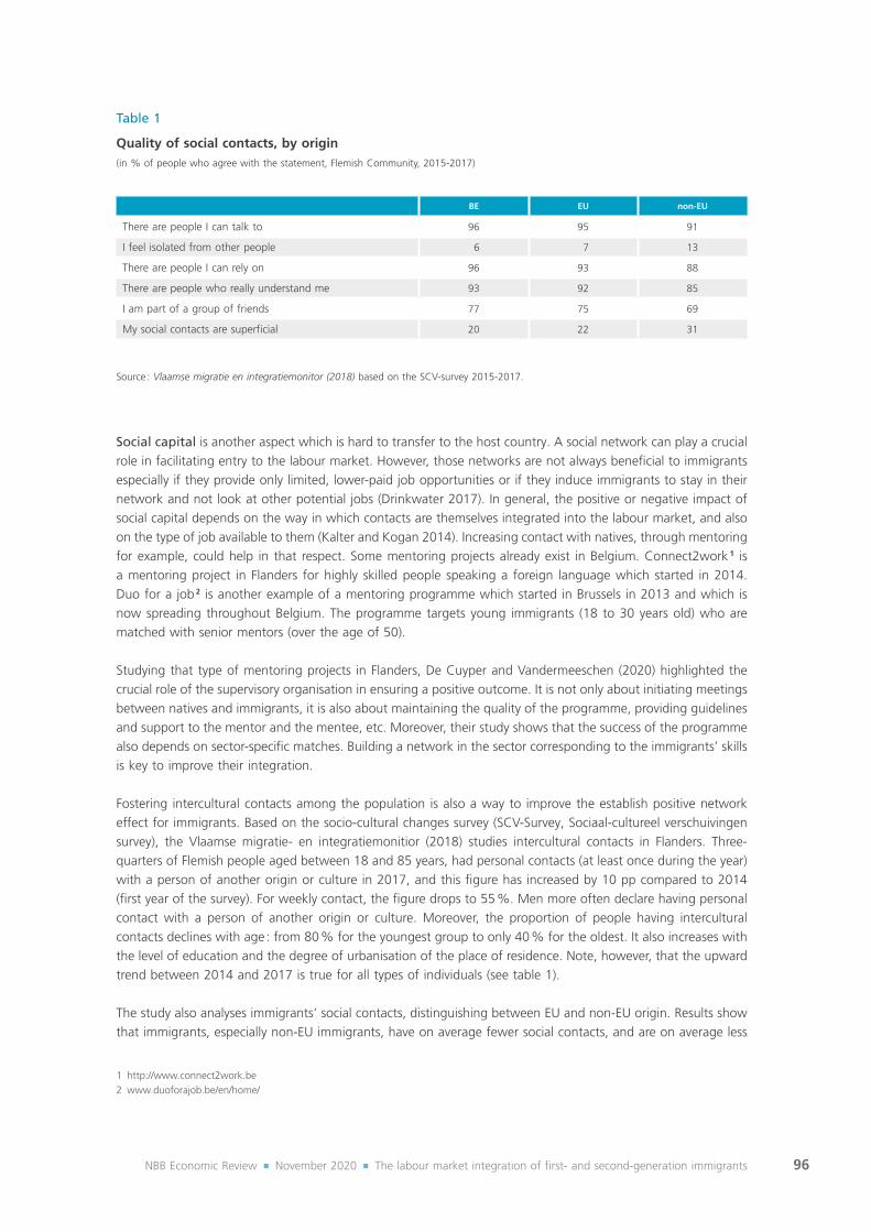
96NBB Economic Review ¡ November 2020 ¡ The labour market integration of first‑ and second‑generation immigrants
Social capital is another aspect which is hard to transfer to the host country. A social network can play a crucial role in facilitating entry to the labour market. However, those networks are not always beneficial to immigrants especially if they provide only limited, lower‑paid job opportunities or if they induce immigrants to stay in their network and not look at other potential jobs (Drinkwater 2017). In general, the positive or negative impact of social capital depends on the way in which contacts are themselves integrated into the labour market, and also on the type of job available to them (Kalter and Kogan 2014). Increasing contact with natives, through mentoring for example, could help in that respect. Some mentoring projects already exist in Belgium. Connect2work 1 is a mentoring project in Flanders for highly skilled people speaking a foreign language which started in 2014. Duo for a job 2 is another example of a mentoring programme which started in Brussels in 2013 and which is now spreading throughout Belgium. The programme targets young immigrants (18 to 30 years old) who are matched with senior mentors (over the age of 50).
Studying that type of mentoring projects in Flanders, De Cuyper and Vandermeeschen (2020) highlighted the crucial role of the supervisory organisation in ensuring a positive outcome. It is not only about initiating meetings between natives and immigrants, it is also about maintaining the quality of the programme, providing guidelines and support to the mentor and the mentee, etc. Moreover, their study shows that the success of the programme also depends on sector‑specific matches. Building a network in the sector corresponding to the immigrants’ skills is key to improve their integration.
Fostering intercultural contacts among the population is also a way to improve the establish positive network effect for immigrants. Based on the socio‑cultural changes survey (SCV‑Survey, Sociaal‑cultureel verschuivingen survey), the Vlaamse migratie‑ en integratiemonitior (2018) studies intercultural contacts in Flanders. Three‑quarters of Flemish people aged between 18 and 85 years, had personal contacts (at least once during the year) with a person of another origin or culture in 2017, and this figure has increased by 10 pp compared to 2014 (first year of the survey). For weekly contact, the figure drops to 55 %. Men more often declare having personal contact with a person of another origin or culture. Moreover, the proportion of people having intercultural contacts declines with age : from 80 % for the youngest group to only 40 % for the oldest. It also increases with the level of education and the degree of urbanisation of the place of residence. Note, however, that the upward trend between 2014 and 2017 is true for all types of individuals (see table 1).
The study also analyses immigrants’ social contacts, distinguishing between EU and non‑EU origin. Results show that immigrants, especially non‑EU immigrants, have on average fewer social contacts, and are on average less
1 http://www.connect2work.be2 www.duoforajob.be/en/home/
Table 1
Quality of social contacts, by origin(in % of people who agree with the statement, Flemish Community, 2015‑2017)
BE EU non‑EU
There are people I can talk to 96 95 91
I feel isolated from other people 6 7 13
There are people I can rely on 96 93 88
There are people who really understand me 93 92 85
I am part of a group of friends 77 75 69
My social contacts are superficial 20 22 31
Source : Vlaamse migratie en integratiemonitor (2018) based on the SCV‑survey 2015‑2017.

97NBB Economic Review ¡ November 2020 ¡ The labour market integration of first‑ and second‑generation immigrants
satisfied by those contacts. Compared to the previous edition, for 2012‑2014, the situation has improved slightly for EU immigrants, but has worsened for people of non‑EU origin.
Immigrants’ lack of human and cultural capital specific to Belgium may gradually improve with the number of years of residence, for example if they learn the language(s) and how the labour market operates, follow training or gain local work experience. Altogether, this could help them to increase their chance of integration on the labour market. This is also apparent from our regression analysis (see results in annex II.2). The employment and participation probabilities increase with the number of years of residence but at a decreasing rate (see chart 21).
Analysing more precisely the number of years of residence for immigrants in Belgium, Piton and Rycx (2020) found similar results : the employment penalty is, ceteris paribus, largest for those who have been living in Belgium for at most one year. For people born in the EU, this penalty reaches –36 pp compared to –44 pp for those born outside the EU. The situation is less detrimental for people who have been resident for longer, but the effect remains significant after ten years of residence (–20 pp) and even after 35 years (–8 pp to –10 pp). So, improvement remains low on average. Moreover, results vary among different origin groups. After 10 years of residence, the penalty drops from –26 pp to –3 pp for people born in other Asian countries and is more than halved for those from Sub‑Saharan Africa (from –24 pp to –10 pp). In contrast, the penalty remains quite persistent for people born in the Maghreb and in EU candidate countries, amounting to 21 pp after 10 years and 17 pp to 20 pp after 35 years. The employment gap for people born in other European countries and in the Near and Middle East also remains substantial after more than a decade of residence in Belgium (–19 pp and –28 pp respectively).
Chart 21
Variation on employment and participation probabilities by years of residence for first-generation immigrants(in %, people aged between 20 and 64 years, annual data from 2009 to 2016, based on a Probit model with time fixed effects controlling for education, Region of residence, age, type of household, group of country of birth, channel of migration and nationality acquisition)
0 1 2 3 4 5 6 7 8 9 100
5
10
15
20
25
30
35
Employment Participation
Source : CBSS Datawarehouse, NBB calculations.

98NBB Economic Review ¡ November 2020 ¡ The labour market integration of first‑ and second‑generation immigrants
2.5 Discrimination and diversity
In legal terms, there is discrimination if a person is adversely affected on the basis of one or more of the following criteria : apparent race, nationality, skin colour, ethnic origin, national origin, gender, age, sexual orientation, civil status, birth, wealth, political views, philosophical views, religious beliefs, language, state of health, disability, physical characteristics, genetic characteristics or social origin. Discrimination may be direct – i.e. based on one of the protected criteria, the person suffering discrimination is unjustifiably treated less favourably than another person in a comparable situation – or indirect – i.e. the person is put at a disadvantage by ostensibly neutral measures, such as rules or a particular corporate culture, but without any justification.
In Belgium, the Law of 10 May 2007 was designed to combat discrimination based on certain criteria such as place of birth and religious or philosophical persuasion. More recently, the Law of 15 January 2018, which laid down several provisions relating to work, was added as Section 9 in the Belgian Criminal Code, giving labour inspectors the ability to utilise “mystery calls” to combat discrimination in recruitment and to carry out situation checks (using fake CVs) to establish whether employers are in breach of anti‑discrimination legislation. The text came into force on 1 April 2018.
Although discrimination is prohibited and punishable by law, it remains a reality for people of foreign origin. Their integration on the labour market is sometimes not limited by their skills but rather by their origin. The economic literature considers this issue by trying to quantify the differences of treatment – ceteris paribus – occurring on the labour market according to the person’s origin. For that purpose, economists have set up an experiment which involves sending curricula vitae (CVs) with the same individual characteristics (age, gender, Region of residence, education level, professional experience, etc.) but with different names that sound either native or foreign. In Germany, Kaas and Manger (2011) considered that having a German name increased the probability of being invited to an interview by 14 %. Also for Germany, Andriessen et al. (2012) also noted that there was no distinction between the various ethnic minorities, but there was between foreigners and Germans. Moreover, discrimination was even more marked if the job involved contact with customers. The same conclusions were drawn by Oreopoulos (2011) for Canada and by Carlsson and Rooth (2008) for Sweden, who found a significantly lower response rate if the candidate had a foreign name. The scale of the discrimination seemed to depend on the difficulty of filling the post, but also on the origin of the business manager. If there are few applicants for a job, it becomes expensive for the employer to exclude part of the population, reducing the inclination to discriminate against candidates. Conversely, if it is easy to fill the post, foreigners need to send in twice as many CVs as natives (Baert et al., 2015). Furthermore, managers tend to take on workers of the same origin as themselves (Aslund et al., 2014). As few immigrants are in managerial posts, there is an increased risk of discrimination. Another finding was that discrimination in inviting job applicants to an interview disappears if the native and immigrant candidates mention (i) voluntary work or (ii) a high number of work experience in their CV (Baert and Vujic, 2016 ; Baert et al., 2017).
Based on data for 53 countries, Cooray et al. (2018) showed that discrimination against immigrants in the recruitment process is greatest among older people, the low‑educated, and those from low‑income households. Conversely, immigrants themselves and women are less inclined to discriminate on the labour market.
Evidence of discrimination by origin in Belgium was already provided in 1997 by Arrijn et al. The results show that a person of Moroccan origin has, on average, 33 % less chance of reaching the end of the selection procedure than a Belgian candidate. The worst discrimination was seen in Flanders (39 %) and Brussels (34 %). This finding has persisted over the years, since in 2005, Martens et al. demonstrated that, in the Brussels‑Capital Region, jobseekers of foreign origin face discrimination in the process of looking for work in 45 % of cases. Moreover, this applies equally to women and to men, whatever their education level, and even if they have Belgian nationality. In 2012, the Equal Opportunities Centre (renamed Unia) produced the same finding with its diversity barometer. When invited to an interview, a candidate of foreign origin has 7 pp greater chance of suffering discrimination compared to a 35‑year‑old male of Belgian origin.

99NBB Economic Review ¡ November 2020 ¡ The labour market integration of first‑ and second‑generation immigrants
According to the theoretical models, there are two reasons that may account for discrimination. The first is a question of preference (“taste‑based discrimination”) : members of the majority want to avoid interacting with workers from the minority. This type of discrimination may come from employers, colleagues or customers (Becker 1957). The second reason lies in “statistical discrimination” : owing to asymmetric information on the candidate’s productivity, the employer examines the statistics on the average performance of the group to which the candidate belongs in order to estimate his productivity (Phelps, 1972 ; Arrow, 1973).
If the discrimination depends on individuals’ preferences, it is not possible to judge whether it is economically efficient or inefficient. In such cases it is a question of ethics rather than efficiency. Conversely, statistical discrimination may affect the optimum allocation of resources. That is what Schwab (1986) tries to explain in his article on the efficiency of that type of discrimination. Although it is partly justified by the use of available information, discrimination does not always help to achieve the optimum allocation of resources. That is the case, in particular, if the group suffering discrimination is largely low‑skilled. In that case, even if the potential worker is highly‑skilled, the employer will regard him as low‑skilled (or less skilled) according to what is apparent for the group to which the worker belongs. The employer thus loses significant potential for his business.
In a study on Belgium in 2014, Baert and De Pauw tested these two theoretical models. Their method is based on an experiment involving 268 Microeconomics students at Ghent University, in which participants have to answer a number of questions based on a role play situation. The participant acts as someone recruiting for a salesman’s job in a firm selling building materials, and assesses the fictional application from an individual. The various participants receive the same CV but with different names for the applicant : Jonas Vermeulen (Flemish name) or Emre Sahin (Turkish name). They then have to answer a series of questions and state whether they would take on that applicant. The results show that discrimination cases are due more to a question of preference, since the participants consider that colleagues and customers would prefer to deal with a Belgian rather than a foreigner. This finding is further supported by Lippens et al. (2020) who reviewed the recent literature and provide evidence that taste‑based mechanism might better explain ethnic discrimination in hiring.
In 2017, Baert and his co‑authors conducted a new study in which they tested the influence of the number of years’ experience on discrimination in recruitment. The results suggest that discrimination declines with the number of years’ experience (–5 % for each year’s experience). That finding therefore points towards statistical discrimination, since employers who can see a particular level of productivity based on past experience are less inclined to discriminate. It therefore seems that the two theories coexist in society.
Filippin (2009) analyses the persistence of discrimination in connection with people’s productivity. His theoretical model takes account of the fact that, when the person belongs to a group which regularly suffers discrimination, the person is aware of that and adjusts his / her behaviour accordingly. Thus, a worker who expects to face discrimination will make less effort to raise his / her productivity, and will therefore ultimately be promoted less often by employers who had not, in principle, discriminated against him / her. This theory implies that, even if the percentage of employers practising discrimination is reduced, the minority group may continue failing to secure better jobs or failing to enter the labour market at all.
Discrimination based on origin has thus been proved to be present in Belgium. A recent study by Quillian et al. (2019) analysing discrimination in hiring in nine European countries and in North America allows us to rank Belgium’s performance in that respect. Through a meta‑analysis of 97 field experiments on discrimination incorporating more than 200,000 job applications in those countries, the authors find significant discrimination against nonwhite natives is all countries, while discrimination against white immigrants is present but low. The authors also find small differences between Belgium and the other countries (United Kingdom, Canada, the Netherlands, Norway, the United States and Germany) : white natives receive about 25 % more callbacks than nonwhites. France has the highest discrimination rates, followed by Sweden, with a probability of callbacks reduced by two is the person if nonwhite.

100NBB Economic Review ¡ November 2020 ¡ The labour market integration of first‑ and second‑generation immigrants
2.6 Conclusion
Besides personal characteristics analysed in the previous chapter, other factors, specific to immigrants, can provide some insight into why they have more difficulties than natives in entering the labour market and finding a job. This chapter highlights five other potential explanatory factors. First of all, the channel of migration used by immigrants affects their labour market outcomes. In Belgium, the most common channel of migration recorded in administrative data is family reunification (41 %), followed by work (27 %) and international protection or regularisation (21 %). Among non‑EU immigrants, almost half of them came through family reunification procedures while this is only the second channel of migration for EU immigrants, behind work which represents 49 % of the recorded channel of migration for EU immigrants. Those differences in migration’s channel could probably partly explain disparities between EU and non‑EU immigrants in terms of labour market integration. In fact, our estimates show that individuals migrating through family reunification or international protection channel are 30 pp less likely to have a job then labour migrants and 34 pp less likely to participate in the labour market.
A second explanatory factor for better labour market integration is the nationality of individuals. Our findings show that, other things being equal, a first‑generation immigrant with Belgian nationality is 9 pp more likely to be employed than a first‑generation immigrant with foreign nationality. The difference is 10 pp regarding the probability of being active. This finding could be partially explained by the fact that people applying for citizenship acquisition are also those who are better integrated or who want to stay for a longer time. However, when comparing differences in employment probabilities among EU versus non‑EU immigrants, results show that nationality acquisition is a significant advantage for non‑EU immigrants helping them to access the labour market. EU immigrants, on the contrary, already benefit from advantages linked to EU membership and are thus less likely to apply for Belgian nationality.
Recognition of diplomas and skills gained abroad by first‑generation immigrants is essential to their chances of getting a job, as it tackles the problem of information asymmetry between potential employers, who do not know if the diploma is equivalent to host requirements, and immigrants. This issue is particularly true for non‑EU immigrants for whom recognition is less easy than what the Bologna system allows for immigrants who studied in an EU country.
Regarding human capital acquisition (increasing with the number of years of residence), a growing literature suggests that immigrants’ proficiency in the host country’s language is key to social and economic integration of immigrants. A social network also plays a crucial role in facilitating entry to the labour market. However, those networks are not always beneficial to immigrants especially if they provide only limited, lower‑paid job opportunities or if they induce immigrants to stay in their network and not look at other potential jobs. With the purpose of connecting newcomers with natives, mentoring projects developed in Belgium could help in that respect.
Finally, although discrimination is prohibited and punishable by law, it remains a reality for people of foreign origin, when they apply for a job. Based on experiments in which fictive CVs were sent to employers with identical characteristics but different names, economic literature provides evidence of such hiring discrimination based on ethnic origin. Discrimination has different sources. First of all, it can be due to preferences (“taste‑based discrimination”) : members of the majority want to avoid interacting with workers from the minority. The second reason lies in “statistical discrimination” : owing to asymmetric information on the candidate’s productivity, the employer examines the statistics on the average performance of the group to which the candidate belongs in order to estimate his productivity. Literature is not unanimous on which effect dominates, both reasons may play a role.

101NBB Economic Review ¡ November 2020 ¡ The labour market integration of first‑ and second‑generation immigrants
3. Policies
The federated entities, which are mainly responsible for the different aspects related to integration, consider socio‑professional participation as one of the main challenges of integration in Belgium and makes it part of their programmes (along with knowledge of one of the national languages, civic participation and enhancing mutual respect, promoting diversity and fighting against discrimination). For example, one of the objectives of the regional action regarding the integration of foreigners in Wallonia is social and economic participation (Walloon Code for Social Action and Health). The same holds in Flanders where the Flemish Horizontal Integration Policy Plan and the Integration Decree includes the socio‑economic participation of people of foreign origin as one of its objectives.
Note that, although the federated entities are responsible for integration, the federal law of 18 December 2016 1 inserted new residence conditions into the Immigration Act, which focuses on integration. Certain third‑country nationals 2 who have been granted permission to reside in Belgium for longer than three months need to provide evidence of their willingness and efforts to integrate into society, such as attending an integration course, being economically active, providing a degree, a certificate, or proof of registration ; attending vocational training ; having knowledge of the language of the municipality where the foreigner is officially registered, actively participating in civil society organisations and / or having no criminal record. Moreover, labour market integration and more generally social integration are among the criteria for acquiring Belgian nationality.
Immigrants thus have further incentives to improve their integration. To help them attain this objective, they need efficient policies to be implemented and to have access to integration programmes defined by each of the federated entities. The next section presents those integration programmes. Limited access to the labour market in general or to specific sectors such as the public sector, for example, as well as the difficulty in obtaining self‑employment status, are other obstacles to immigrants’ integration. The Belgium’s situation in this regard is described in section 3.2. Some policies designed to improve the labour market integration of individuals in general and not specifically targeting immigrants may also have an influence on the participation and employment of first‑generation immigrants. Impact of general activation policies is evaluated in section 3.3. Finally, the last section provides an international comparison of integration policies through the analysis of the MIPEX index.
3.1 Integration programmes 3
All regions of Belgium and the German‑speaking Community have integration programmes. While the programme has been compulsory in Flanders since 2003, the integration process was only made compulsory in 2016 in Wallonia and in 2017 in the German‑speaking Community. Obligation is also planned in Brussels but has yet to come into force. The set‑up of the process is similar across the Regions and essentially comprises a “welcome” module with a review of the rights and duties of people living in Belgium, an individual assessment identifying the person’s needs in terms of housing, education, social and economic integration, and citizenship training ; and language lessons where necessary (French, Dutch or German depending on the Region or Community).
1 Law of 18 December 2016 inserting a general residence condition into the law of 15 December 1980 on the access to the territory, residence, settlement and the removal of foreign nationals
(www.ejustice.just.fgov.be/cgi_loi/change_lg.pl?language=fr&la=F&table_name=loi&cn=2016121816)2 Outside the Schengen area.3 For more information see EMN (2018).

102NBB Economic Review ¡ November 2020 ¡ The labour market integration of first‑ and second‑generation immigrants
3.1.1 Brussels
In the Brussels‑Capital Region, integration programmes are divided into French‑speaking and Dutch‑speaking components. The Dutch‑speaking integration programme falls within the responsibility of the Flemish Community and is designed as described below, except that it is not yet mandatory. The organisation in charge is BON.
The French‑speaking integration programme was defined by the COCOF (the French Community Commission) via the Decree of 18 July 2013. The programme is only accessible to foreign nationals over the age of 18 who have been legally resident in Belgium for less than three years and who actually live in Brussels with a residence permit of more than three months. It is not yet mandatory (but planned to become so) and it is free of charge. The Reception Offices for Newcomers (BAPA‑BXL and VIA) are responsible for organising the integration programme. Foreigners are offered a welcome module which consists of an individual interview, an information module on rights and obligations, and a linguistic assessment. Based on the results of the welcome module, a support module is defined and provides support for administrative procedures, socio‑occupational guidance, French courses (from 120 to 1150 hours depending on the needs), and a civic integration course with information on the history of Belgium, its political system, its institutions, its economy, culture, etc. Participants receive a certificate of attendance (solely on condition that they attend the programme).
Until recently, there were no specific measures for migrants in Brussels to help them join the labour market. However, the 2017‑2022 management contract of Actiris, the Regional Public Employment Service, takes the integration of newcomers as one main objective. As a first step, the situation was therefore monitored in 2019 to see what are the main obstacles that immigrant jobseekers face in finding a job, and how the current policies can help, such as the Youth Guarantee, for example, or the activation policy in general. The report finds that people of non‑EU origin are over‑represented among jobseekers (60 %) compared to their share in the population (42 %). Regarding the integration policy for younger jobseekers, while 68 % of natives are employed 3 years after registration, that is the case for only 55 % of Turkish jobseekers, 46 % of those from Maghreb, 38 % of people from Congo, Burundi or Rwanda and 34 % of persons from elsewhere in Africa. Moreover, they do not get long‑term jobs (75 % for natives against 42 % to 57 % for people of foreign origin).
3.1.2 Flanders
The Flemish Government established an updated integration plan in 2018 focusing on reducing the gap in social integration between foreigners and Belgians. This plan has five main objectives : (1) improving participation in social life ; (2) improving knowledge of the Dutch language among non‑native speakers ; (3) promoting mutual respect ; (4) providing a tailored, soundly based and supported policy ; (5) specific policies for the travelling community. 1
Flanders introduced an integration programme for newcomers in 2003 through the Decree of 28 February 2003. This Decree was amended in 2013 and 2015 in order to achieve a better coordinated approach, and resulted in the creation of a new autonomous Agency for Civic Integration as well as two local agencies for the cities of Ghent (IN‑Gent) and Antwerp (Atlas). Conditions for access to this integration programme are the following : being registered in the National Register in a municipality in Flanders or Brussels, and either (1) being a foreign national aged at least 18 years intending to reside in Flanders or Brussels for a long period of time (more than one year) or (2) being a Belgian born abroad or with at least one parent born abroad. The civic integration programme is mandatory for certain categories including nationals from a non‑EU country, over the age of 18 years, who have come to Belgium for the first time. This programme is free of charge and consists of a course in Dutch as a second language, a social orientation course and individual assistance. At the end of the programme, the foreigner receives a certificate of civic integration for which, since February 2016, they have
1 For more information see https://integratiebeleid.vlaanderen.be/beleid.

103NBB Economic Review ¡ November 2020 ¡ The labour market integration of first‑ and second‑generation immigrants
to provide proof of their Dutch language skills and the learning outcomes of the citizenship course (attendance only is no longer sufficient).
Besides the integration programme, since 2016 Flanders has also had a programme called ‘Integratie door Werk’ (Integration through work) developed by the VDAB, the Regional Public Employment Service. The main objective is to help unemployed jobseekers with a migration background to find a job by providing the necessary support with respect to language knowledge, training and required skills. This approach will be preferably consisting of on‑the‑job training, which the Public Employment Service considers to be quicker and more efficient.
According to the 2018 Flemish Migration and Integration Monitor, just over 118 000 persons signed an integration contract over the period 2012‑2017. Among them, 44 % came through family reunification, 27 % through asylum and 13 % for work. While the report discusses the labour market integration of people of foreign origin in Flanders, it does not consider whether the integration programme is effective or not.
3.1.3 Wallonia
Policies regarding the integration of foreigners are part of the Walloon Code for Social Action and Health (Code wallon de l’action sociale et de la santé CWASS) 1. The objectives of the regional action regarding integration of people of foreign origin are the following : equal opportunities, citizenship, social cohesion for a multicultural society, access to public and private services, and social and economic participation. The Walloon Government is to receive an evaluation of those policies every five years.
The eight Regional Integration Centres are responsible for developing a local integration plan for their respective territories. They are responsible for the integration programme, but they should also support local initiatives, coordinate integration activities, encourage foreigners’ social, economic and political participation and intercultural exchanges, and collect local statistical data.
The integration programme, which is accessible to all foreign nationals in Wallonia, is defined by the Decree of 27 March 2014. The Decree of 28 April 2016 made the programme mandatory for certain categories of foreigners, namely foreign nationals who have been living in Belgium for less than 3 years and who have a residence permit valid for longer than 3 months ; there are some exceptions such as EU, EEA and Swiss citizens and their family members, foreign nationals younger than 18 and older than 65 years, etc. The programme is free of charge and is composed of two modules. The welcome module consists of information on the rights and duties of people residing in Belgium, a social assessment to identify the needs of the person, and assistance with administrative procedures. The second module is defined according to the needs identified during the social assessment. It includes a civic participation course, a French language course and guidance on the appropriate socio‑economic integration scheme based on an individual socio‑occupational assessment. This last assessment is organised in collaboration with the Walloon Public Employment Service (Forem).
In 2019, the IWEPS 2 produced an evaluation of the integration programme, including socio‑economic integration. The study shows that the aspects defined, namely citizenship, language courses and socio‑economic integration, meet newcomers’ needs. However, the action taken does not necessarily lead to an improvement for the immigrant, and some other issues such as housing or mental health remain unaddressed. Moreover, variations between regional integration centres in the method of implementing the integration programme hamper collaboration between them and are confusing for immigrants. While it may be useful to make the programme mandatory, the authors of the evaluation consider it inefficient to stipulate that the programme must be completed in 18 months. Finally, they point out that the integration programme takes place in a broader context of immigrants’ difficulties in achieving social and occupational integration. Thus, they conclude that this scheme only partially solves the problems faced by migrants.
1 For more information see https://wallex.wallonie.be/files/medias/10/CWASS_EV16‑07‑2020.pdf.2 Walloon Institute for evaluation, perspectives and statistics ‑ Institut wallon de l’évaluation, de la prospective et de la statistique.

104NBB Economic Review ¡ November 2020 ¡ The labour market integration of first‑ and second‑generation immigrants
3.1.4 German-speaking Community
The integration of third‑country nationals has been identified as one of the priorities of the “Regional Development Concept” defined by the German‑speaking Community. Part of the report describes how the integration programme was devised in this Region. Starting in 2015, the German‑speaking Community created a working group which took 18 months to analyse existing integration programmes abroad and to define the features which are already present in the Community and those which are missing. After that, they started to draw up the integration programme in the second half of 2016. The Decree of 11 December 2017, which came into force on 1 January 2018, made the integration programme mandatory for foreigners over 18 years of age who live in the German‑speaking Community and who have a residence permit for at least three months. As in the other regions, there are exceptions such as EU, EEA and Swiss citizens, students, immigrants over the age of 65, long‑term migrants (living in Belgium for more than 3 years), etc. Nevertheless, any immigrant who wants to do so can register, and the programme is free of charge.
The programme consists of four modules. The first comprises an interview and a social assessment to define the needs of the participant. Next, language classes are offered to the immigrant based on his / her level of German. Integration classes are also provided in order to present Belgian social values, rights and duties of citizens, etc. Finally, social and occupational guidance is given, including information on training, work and leisure activities, or the recognition of foreign diploma’s, organisations to contact to find a job, the role of the Public Employment Service, etc. The participant receives a certificate at the end of the programme if he / she has attended at least 80 % of the language and integration courses.
3.2 Access to the labour market including self-employment and the public sector
Recent developments in Belgium related to labour market access have mainly concerned asylum‑seekers, just as in most other European countries after the 2015 refugee crisis. Since December 2015, asylum‑seekers have been allowed to take a job, four months after lodging their application (as opposed to six months previously). Following this reform, Belgium is now among the European countries with the shortest delay for obtaining a work permit 1. Only Greece and Sweden have shorter waiting periods, as they allow immediate entry, and Austria and Germany, where workers have to wait three months. The maximum waiting period is a year, as in Bulgaria, Croatia, France, Malta and the United Kingdom. Unlike Belgium, some countries make work permits conditional on taking a test beforehand. The purpose of this test is not necessarily to assess the asylum‑seeker’s skills, but rather to make sure that a national or European resident is not interested in the vacancy. Other quite common restrictions include limits on the duration of employment contracts and on the sectors of activity where asylum‑seekers are allowed to work. Added to all this are restrictions on access to self‑employment, notably in Germany and the United Kingdom.
In Belgium, residence permit rules also changed in 2015, in the sense that refugees are no longer granted immediate permanent residence but rather a permit for five years, after which their situation is reassessed. If there has been no change, refugees will receive their permanent residence permit, but if the conditions for refugee status are no longer met, they must return to their country of origin. Importantly, however, Bertrand (2017), studying how refugees get on Switzerland, show that the access to stable permits significantly increases the chances of entering the labour market.
Access to the labour market has also been made easier for long‑term residents who, since 2015, no longer need to apply for a work permit if they have been working for at least 12 months in a job classed as shortage profession (‘bottleneck jobs’, ‘fonctions critiques’ in French, ‘knelpuntberoepen’ in Dutch).
1 Source : AIDA.

105NBB Economic Review ¡ November 2020 ¡ The labour market integration of first‑ and second‑generation immigrants
Moreover, immigrants holding a type‑B work permit – i.e. those who arrived in Belgium specifically to work – are obliged to continue working for the same employer. A procedure is in place to determine whether their position ranks among the critical jobs, but their work permits will not be valid for the same position with another employer or outside a specific sector. Economic migration is controlled to establish whether there are no natives that could fill the vacancy, but also to check whether immigrants are recruited under much worse conditions than those prevailing in the labour market.
Note that even though a rapid access to the labour market is helpful in integrating immigrants, this does not necessarily imply sustainable integration. If entry is achieved at the cost of over‑qualification, a better long‑term outcome for the migrant would be to study first and then find a job in line with his / her skills (Dullien, 2016).
An important restriction on labour market access, especially for non‑EU foreigners, is the requirement to hold Belgian or European nationality to obtain an established post in public administration. This restricted access implies the under‑representation of non‑EU immigrants in the public sector, whereas this is the leading sector of employment for natives (HCE, 2018). Pina et al. (2015) also highlight the potential role of the public sector in supporting further economic and social integration of immigrants in Belgium. It can act as a role model for private firms (potentially helping to reduce discrimination practices), increases the visibility of immigrants and better addresses their needs as users of public services.
Finally, the literature often puts forward that setting up an own business may act as a faster route into the labour market for immigrant workers. However, it seems that this is only true for EU immigrants in Belgium. Workers born in a third country are on average not more likely to be self‑employed than workers born in Belgium 1. The proportion of self‑employed workers only exceeds the figure for natives in the case of people from the Near and Middle East, Oceania and the Far East, and to a lesser degree the EU candidate countries. This can probably be explained by the current rules. In Belgium, non‑EU citizens are required to hold a “professional card” to be allowed to run their own business. Besides EEA citizens, some other categories of foreigners are exempt from the professional card requirement because of the nature of their activities, the nature of their stay, or pursuant to international treaties. Preconditions for applying for the card include the right of residence, compliance with regulatory requirements and, more particularly, requirements related to the project and its importance to the region. The application must be filed with a Belgian diplomatic mission or consulate in the country of residence if a foreign self‑employed person resides abroad, or with a recognised enterprise office of their choice if the foreign self‑employed person has a valid residence document for Belgium (type A certificate of residence or certificate of inscription on the aliens’ register). The application is tested for the three criteria as described above. The professional card is issued for a maximum of five years, and its validity is related to its holder’s right of residence. Once this right of residence expires, the card is no longer valid and has to be returned to the administration.
A joint report by the OECD and the European Commission in 2016 on inclusive entrepreneurship policies in Belgium concludes that many policies and programmes have been introduced and that overall the inclusive entrepreneurship support system is quite strong. However, there is a lack of more tailored entrepreneurship support for migrant entrepreneurs.
3.3 General activation policies
Some policies designed to improve the labour market integration of individuals in general may also have an influence on the participation and employment of first‑generation immigrants. Reviewing an extensive literature on this subject, Bilgili (2015) analyses three types of policies : job search assistance (mainly provided by Public
1 Note that Belgium is characterized by a large share of high‑educated self‑employed workers, mainly because of liberal professions being exert as self‑employed.

106NBB Economic Review ¡ November 2020 ¡ The labour market integration of first‑ and second‑generation immigrants
Employment Services), vocational training, and acquiring work experience through subsidised employment. On the basis of his work plus more recent research, we assess the potential impact of those policies in Belgium.
Regarding job search assistance, Public Employment Services (Actiris, ADG, Forem, VDAB) have a key role to play. They are the primary actor connecting jobseekers and employers and matching labour supply and demand. In Belgium, a package of activation measures (vocational transition programme, SINE, Activa, return‑to‑work supplement, Activa Start, transition traineeships) aims to help the unemployed get back into work. Among the beneficiaries, the proportion of Belgians exceeds their share in the number of fully unemployed people (89 % compared to 86 % in 2014). For foreign nationals the opposite is true, with a more pronounced effect for European nationals. They represent 6.4 % of the total beneficiaries and 8.3 % of the wholly unemployed. For non‑EU immigrants, the figures are 4.6 % and 5.5 % respectively. Foreign jobseekers therefore benefit proportionately less from an activation programme than Belgians (HCE, 2018). View.Brussels (2019) has studied the Youth Guarantee in the Brussels Capital Region and found that a higher proportion of natives are employed three years after their registration compared to people of foreign origin (especially non‑EU). Moreover, they more often get a permanent contract and it takes less time for them to find a job. Nevertheless, the study also shows that immigrants registered in the programme have a higher employability index than other unemployed immigrant workers. Note however that self‑selection may bias the results : immigrants who are more active in looking for a job might be more likely to register for this type of programmes. A systematic assessment of the impact of activation policies would be needed to define which one is (the most) efficient.
Literature on integration policies often assumes that training is the solution to helping immigrants find a job. Nevertheless, impact assessments have demonstrated that it is not always the case, as employers require skills that cannot be easily provided by publicly available programmes (Bilgili, 2015). Huber et al. (2009), for example, studying welfare‑to‑work programmes in Germany, show that only training schemes providing minor skills improvement (specific to some types of jobs) and combined with job search assistance have a significant positive effect on employment. However, the effect for immigrants is weak and the programme is of greater benefit to natives who already have a sufficient (or recognized) level of qualifications. Given the employers’ specific requirements, in‑company training could provide a better outcome than classroom courses. This seems to be verified by the literature. Nevertheless, Wolff and Jozwiak (2007) stress that increased employment after the training is linked to a selection bias rather than genuinely more effective in‑company training.
Vandermeerschen et al. (2018) analyse the effectiveness of labour market programmes provided by the VDAB in Flanders distinguishing between newcomers and ‘former arrivals’. Following jobseekers who entered the VDAB between 2008 and 2012 and tracking them until 2016, they find that the programmes are more efficient for newcomers than for other immigrants (and the least so for second‑generation immigrants). Moreover, ‘individual vocational‑training’ appears to be the program providing the best outcomes for beneficiaries. More generally, vocational training seems more effective in terms of exiting unemployment than a competence‑enhancing traineeship.
However, the literature still questions the impact of job search assistance and training. Linking labour training and counselling to immigrants’ employability in 15 European countries, Kogan (2016) does not find any evidence of the efficiency of this type of policies. Immigrants’ employability or job status did not improve in three out of four of the countries analysed. The author concludes that, instead of really improving productivity and skills, those programmes work more by creating signals on willingness to find a job and are biased by self‑selection.
Another popular way to activate unemployed or inactive (potential) workers or to deter illegal work, is through subsidized jobs, as in the case of service voucher systems for example. Although this type of policy does not directly target immigrants, it could have an impact on their labour market integration. In theory, this work experience gives first‑generation immigrants an opportunity to demonstrate their professional skills and qualifications to employers and thus to offset employers’ uncertainty about recruiting them. The positive impact of this type of policies on employment rates has been verified in Scandinavian countries, Germany and Switzerland (Bernhard et al., Brussig et al 2008 ; Brussig et al., 2008 ; Gerfin and Lechner, 2002 ; Hardoy and

107NBB Economic Review ¡ November 2020 ¡ The labour market integration of first‑ and second‑generation immigrants
Zhang, 2010 ; Hohmeyer and Wolff, 2007 ; Jahn and Rosholm, 2013 ; Stephan, 2010). Nevertheless, this type of employment scheme cannot be considered as a steppingstone towards regular employment. A recent study by Leduc and Tojerow (2020) illustrates this point in the context of the service voucher system in Belgium. Largely used by women of foreign origin (42 % from EU13 and 29 % from Latin America according to the socio‑economic monitoring report 2019), the system is shown to be effective in reducing unemployment and inactivity, but only by increasing employment within the subsidised domestic service sector. There is little if any transition to other sectors and to other type of contracts. There are three potential explanations for this : (1) jobs with regular employers may require additional skills ; (2) subsidised works stigmatises its participants who are seen as hard‑to‑employ workers and thus low productivity workers (Walter, 2013) ; and (3) employers may choose to rely on subsidized contracts instead of regular contracts.
Another type of subsidized employment in Belgium is the “employment by the Public Centres for Social Welfare (CPAS / OCMW) generally under Article 60”, in short Article 60 workers. The recent socio‑economic monitoring report (2019) provides descriptive statistics on the use of the scheme and the potential effect on employment. Less than one third of the beneficiaries are of Belgian origin. 16 % are from Sub‑Saharan Africa, 12.5 % from the Maghreb, 11 % from EU13 countries and 6 % from the Near and Middle East. More than half of workers employed under Article 60 are low‑educated and this is true for all origins. The case of people originating from the Near and Middle East should be highlighted since almost a quarter of them are highly educated, a larger share than for any other origin. The report followed individuals for three years after the end of their Article 60 contract. Results show that in the short term (three months), a large majority of beneficiaries are unemployed (between 45 % for Belgian and 63 % for people from Sub‑Saharan Africa countries). After three years, unemployment decreases for all origins. However, while Belgians becomes inactive (the proportion in work remaining constant at 28 %), employment increases for immigrants and especially for people from the Near and Middle East (shift from 26 % after three months to almost 50 % after three years). Nevertheless, this type of statistics does not allow to assess the impact of the policy itself. It may be that those individuals would have been employed even without Article 60 scheme.
Butschek and Walter (2014), making a meta‑analysis condensing 93 estimates from 33 empirical studies, find that wage subsidies remain the most efficient way of boosting the immigrant employment rate, compared to other types of labour market activation policies (training, job search assistance and subsidised public sector employment), even though good quality of the obtained jobs is not guaranteed.
3.4 International comparison of targeted and general policies using MIPEX
The Migrant Integration Policy Index provides an aggregate indicator per country of the policies that are decided and implemented in order to promote the integration of migrants. This tool, updated for the last time in 2014 1, considers a broader definition of integration than the one that we have considered so far, and includes social integration and individuals’ well‑being, which are, nonetheless, also linked to labour market integration. Some of the policies studied are therefore not directly linked to employment objectives but may have an indirect (positive or negative) impact on the integration of immigrant into the labour market.
The MIPEX indicators include policies specific to immigrants, but also some general tools that they can use in order to improve their integration. It is computed on the basis of almost 300 questions and is aggregated in eight different policy areas :
¡ Labour market mobility : do legally resident foreign citizens have comparable workers’ rights and opportunities like nationals to access jobs and improve their skills ?
1 A new index is planned to be published at the end of 2020 for the period 2014‑2020.

108NBB Economic Review ¡ November 2020 ¡ The labour market integration of first‑ and second‑generation immigrants
� Access to the labour market : can legal migrant workers and their family access and change jobs in all sectors like nationals ?
� Access to general support : can legal migrant workers and their families improve their skills and qualifications like nationals ?
� Targeted support : can legal migrants have their specific needs addressed as workers born and trained abroad ?
� Workers’ rights : Do legal migrants have the same work and social security rights like EU nationals / nationals ?
¡ Family reunion for foreign citizens : Do legally resident foreign citizens have a facilitated right to reunite in their families (e.g. like nationals or EU citizens who move from one Member State to another) ?
¡ Education : are all children of immigrants encouraged to achieve and develop in school like the children of nationals ?� Education access : Do all children, with or without a legal status, have equal access to all levels of
education ?� Education targeting needs : Are migrant children, parents, and their teachers entitled to have their
specific needs addressed in school ?� New educational opportunities : Do all pupils benefit from the new opportunities that immigration
brings to schools like immigrant languages, cultures, diverse classrooms, and parental outreach ?� Intercultural education for all : are all pupils and teachers supported to learn and work together in a
diverse society ?
¡ Political participation : Do legally resident foreign citizens have comparable opportunities as nationals to participate in political life (e.g. like EU nationals) ?
¡ Permanent residence : Do temporary legal residents have facilitated access to a long‑term residence permit (e.g. like EU nationals) ?
¡ Access to nationality : Are legal immigrants encouraged to naturalise and are their children born in the country entitled to become full citizens ?
¡ Anti-discrimination : Do all residents have effective legal protection from racial, ethnic, religious, and nationality discrimination in all areas of life ?
¡ Health : Is the health system responsive to immigrants’ needs ?
In the European Union, Belgium ranks 4th on the global MIPEX score at 70 / 100, behind Portugal (80 / 100), Sweden (80 / 100) and Finland (71 / 100). For all types of policies, the Belgian MIPEX score is higher than the average for EU countries.
As shown in chart 22, Belgium scores high in terms of family reunion and access to nationality, even though the 2013 reform imply stricter access than before. Belgium is also ranked first in terms of the presence of policies facilitating permanent residence. Also anti‑discrimination policies are at a high level compared to other countries (78 / 100, 6th over Europe) thanks to strong anti‑discrimination laws and an equality body. Nevertheless, MIPEX analysts highlight the fact that “government could take a greater lead to promote equality through public sector jobs and contracts” 1.
1 Source: https://www.mipex.eu/
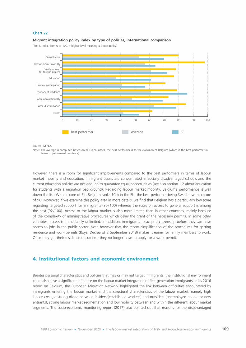
109NBB Economic Review ¡ November 2020 ¡ The labour market integration of first‑ and second‑generation immigrants
However, there is a room for significant improvements compared to the best performers in terms of labour market mobility and education. Immigrant pupils are concentrated in socially disadvantaged schools and the current education policies are not enough to guarantee equal opportunities (see also section 1.2 about education for students with a migration background). Regarding labour market mobility, Belgium’s performance is well down the list. With a score of 64, Belgium ranks 10th in the EU, the best performer being Sweden with a score of 98. Moreover, if we examine this policy area in more details, we find that Belgium has a particularly low score regarding targeted support for immigrants (30 / 100) whereas the score on access to general support is among the best (92 / 100). Access to the labour market is also more limited than in other countries, mainly because of the complexity of administrative procedures which delay the grant of the necessary permits. In some other countries, access is immediately unlimited. In addition, immigrants to acquire citizenship before they can have access to jobs in the public sector. Note however that the recent simplification of the procedures for getting residence and work permits (Royal Decree of 2 September 2018) makes it easier for family members to work. Once they get their residence document, they no longer have to apply for a work permit.
4. Institutional factors and economic environment
Besides personal characteristics and policies that may or may not target immigrants, the institutional environment could also have a significant influence on the labour market integration of first‑generation immigrants. In its 2016 report on Belgium, the European Migration Network highlighted the link between difficulties encountered by immigrants entering the labour market and the structural characteristics of the labour market, namely high labour costs, a strong divide between insiders (established workers) and outsiders (unemployed people or new entrants), strong labour market segmentation and low mobility between and within the different labour market segments. The socio‑economic monitoring report (2017) also pointed out that reasons for the disadvantaged
Chart 22
Migrant integration policy index by type of policies, international comparison(2014, index from 0 to 100, a higher level meaning a better policy)
Best performer Average
Health
Anti−discrimination
Access to nationality
Permanent residence
Political participation
Education
Family reunionfor foreign citizens
Labour market mobility
Overall score
0 10 20 30 40 50 60 70 80 90 100
BE
Source : MIPEX.Note : The average is computed based on all EU countries, the best performer is to the exclusion of Belgium (which is the best performer in
terms of permanent residence).

110NBB Economic Review ¡ November 2020 ¡ The labour market integration of first‑ and second‑generation immigrants
position of people of foreign origin on the labour market includes the structural characteristics of the Belgian labour market, which means that all groups ‘at risk’ experience difficulties in joining the labour market. Pina et al. (2015) emphasise the over‑representation of foreign‑born persons among low‑wage and vulnerable workers, the group for which the Belgian labour market characteristics are particularly unfavourable (high labour costs deterring demand for low‑productivity workers, small income gains when moving from unemployment or inactivity to a job, discouraging labour supply).
A more flexible labour market can improve access to the labour market and to employment for immigrants as it does for any other outsiders (Bilgili et al. 2015). Studies comparing countries’ performance show that immigrants’ employment rates tend to be higher in countries with a more flexible labour market compared to countries with a more rigid labour market (Angrist and Kugler, 2003 ; Aleksynska and Tritah, 2013 ; Bisin et al., 2011 ; Corrigan, 2013 ; Kahn, 2007 ; Kogan, 2006).
Trying to capture the role of labour market institutions in explaining immigrant‑native gaps in European labour markets, Guzi et al. (2015) highlights that the better performance of more liberal countries is due to the fact that they seem to attract and keep immigrants who are better equipped to succeed in the labour market. Mixed market economies provide favourable conditions in terms of immigrants’ labour force participation and permanent employment but their results are mixed regarding unemployment and low‑skilled employment.
Moreover, Angrist and Kugler (2003) test the argument which states that native workers can be more protected from immigrant competition as employment protection increases. Their results show that the effect of a stricter employment protection legislation is also negative for natives as they tend to lose their jobs more often in countries with restrictive labour market institutions.
In addition, a flexible labour market is not associated with a higher level of over‑qualification, meaning that they are not only helpful in finding a job but also in finding a job corresponding to the workers’ skills. The intuition is that when employment protection is strict and the firing costs are high, employers tend to increase the education requirements when hiring (making it more likely that the employee will in fact match the job). This strategy is detrimental to immigrants who will be hired for less prestigious jobs below their skill level as an insurance against the risk of poorer performance and difficulty of firing (Aleksynska and Tritah, 2013). Comparing regulations of regular and temporary contracts in 19 European countries, Markaki (2014) provides evidence that stricter regulation of regular contracts increases the immigrants’ chances of holding a temporary contract. Conversely, stricter regulation of temporary contracts increases immigrants’ risk of unemployment and underemployment. The findings of Guzi et al. (2015) point in the same direction, with a negative effect of stricter regulations on regular and temporary contracts being detrimental to immigrants in finding a (skilled) job and getting a permanent contract. The increase in labour market dualism because of employment protection reforms tends to disproportionally harm immigrants. In that respect, the 2014 reform in Belgium unifying the rules for blue and white‑collar regular workers by increasing employment protection for the blue‑collar segment, could have been detrimental to immigrants. As they are over‑represented among blue‑collar workers, this reform may increase the dualism between regular and temporary contract with immigrants and other vulnerable groups increasingly hired under temporary contracts (Pina et al., 2015).
While the employment rate of immigrants could increase with less strict employment protection legislation, more stringent protection could reduce the gap compared to natives (Sa, 2011). Immigrants are usually less aware of employment protection regulations and are thus also less likely to claim their rights ; this creates a gap between the costs for employers of hiring a native relative to hiring an immigrant. Moreover, employment protection can also protect immigrants’ workers from discrimination. Bisin et al. (2011) find that employment protection legislation tends to lower the penalty that immigrants face in regard to hiring.
Furthermore, analysing 12 OECD countries’ performance in the integration of immigrants into the labour market, Causa and Jean (2007) find that differences between countries could largely be explained by differences in labour market policies, especially the level of unemployment benefits, the level of the tax wedge and the existence

111NBB Economic Review ¡ November 2020 ¡ The labour market integration of first‑ and second‑generation immigrants
of a minimum wage. The introduction of a minimum wage helps to prevent in‑work poverty but may also create a barrier to the employment of low‑skilled immigrants, especially for young people (Pina et al., 2015).
Bergh (2014) confirms the negative impact of more generous replacement income rates, the increase in unemployment being greater for immigrants than for natives. In Belgium, work incentives are reduced by the combination of relatively generous unemployment benefits and a substantial tax wedge. This creates unemployment and inactivity traps for low‑wage workers, in which immigrants are overrepresented (Pina et al., 2015). Note however, that immigrants are less likely to receive unemployment benefits than natives. The 2018 HCE report using NEO statistics shows that, although their unemployment rate exceeds that of natives, only 44.2 % of jobseekers of non‑EU origin receive unemployment benefits, compared to 69.9 % of EU immigrants and 79.1 % of Belgians. Many empirical studies reveal that immigrants do not necessarily receive more social assistance than natives (Barrett and Maitre, 2013) or actually receive less than natives (Dustmann and Frattini, 2014).
Bergh (2014) also highlights the role of collective bargaining agreements. If they cover a larger share of the labour market, the unemployment rate of immigrants increases more significantly than that of natives. Huber (2015) confirms this result by showing that countries with more centralized wage bargaining and higher union density have worse labour market outcomes for immigrants compared to natives even after controlling for compositional effects. Regarding the role of unions, Harcourt et al. (2008) examine to what extent they are exclusive or inclusive with respect to immigrants. Analysing the case of New Zealand, they show that while unions are helpful in promoting diversity, they are not efficient in combating discrimination against immigrants in hiring.
Economic conditions in host countries also influence the probability that immigrants will be active on the labour market and find a job. In fact, immigrants are found to be more often unemployed in countries with an overall higher unemployment rate (Pichler, 2011) or a higher unemployment rate among natives (Fleischmann and Dronkers, 2010). Furthermore, immigrants adapt more quickly to economic growth, which implies that their unemployment rate decreases faster than that of natives during prosperous periods (Cebolla and Finotelli, 2011). Finally, immigrants are less disadvantaged at employment entry when the host country has strong demand for low‑skilled jobs (Kogan, 2006) or a large segment of low‑status jobs (Fleischmann and Dronkers, 2010).
The type of government could also influence immigrants’ labour market outcomes. Given the multidimensionality of integration policies, it is harder for coalition and minority governments to implement effective labour market integration policies. Conversely, single‑party majority government are better able to foster efficient policies (Aaskoven, 2019).
5. A macro analysis to explain Belgium’s bad performance
As emphasised above, it is only recently that the economic literature has tried to assess which factors can explain disparities between countries in integrating immigrants into the labour market. Analysing 21‑28 countries (depending on data availability), Bergh (2014) compares nine potential explanations for these gaps : collective bargaining, net replacement rate, xenophobia, employment protection laws, social expenditure, asylum applications, the share of immigrants in the population, the education of immigrants and migrant integration policies. All factors had explanatory power except education and migrant integration policies.
Conducting a similar analysis, we will complement this study by considering longitudinal dynamics – which is possible given our dataset – through the inclusion of time fixed effect to control for common shocks among countries and country fixed effects to control for unobserved time‑invariant differences between countries.

112NBB Economic Review ¡ November 2020 ¡ The labour market integration of first‑ and second‑generation immigrants
The dataset was created by merging information from different sources for all EU countries 1 over the period 2006‑2019. Our variables of interest – employment and participation gaps – are derived from the Labour Force Survey which provides data, since 2006, on the country of birth of individuals (native, EU, non‑EU). For all years and all countries in the sample, we compute the gap between the employment (participation) rate of first‑generation immigrants and that of natives 2 for people aged between 20 and 64 years. We do this for the total foreign‑born immigrants as well as for non‑EU born immigrants 3. For both categories, we compute the gap for the total population and the gap for men (supposedly less influenced by cultural aspects such as their role in the household, for example).
In order to analyse disparities between countries in the labour market integration of immigrants, we test 25 explanatory variables chosen on the basis of previous analysis and given data availability. Those variables can be categorized into five dimensions : personal characteristics of immigrants (age, gender, level of education (high or low)), history of migration (share among the population), economic environment (unemployment rate), labour market features (EPL, public employment, self‑employment, job tenure, union density, net replacement rate, labour market policy measures) and integration policy indicators (12 MIPEX sub‑indicators).
5.1 Database description
Using data from the Eurostat Labour Force Survey, the history of migration in the country is captured by the percentage of immigrants among the population aged 15 and over. Personal characteristics of immigrants are computed by comparing them to natives using the same database 4. The age structure of immigrants is proxied by the percentage of working age immigrants among the total population of immigrants divided by the percentage of working age natives among the total population of natives. Similarly, gender is captured by the ratio of the corresponding percentages of men, high level of education by the ratio of the corresponding percentages of high‑educated individuals, and low level of education by the ratio of the corresponding percentages of low‑educated individuals, in all cases considering the population aged between 20 and 64. In other words, the variables capture to what extent first‑generation immigrants are more likely to be of working‑age, male, high‑educated or low‑educated than natives.
The economic environment 5 is assessed via the aggregate unemployment rate one year earlier, available in the LFS data. Its definition is the usual one : the percentage of unemployed individuals among active people aged between 15 and 74 years.
Employment protection legislation is defined using the OECD index on regular contracts for both individual and collective dismissals, which was recently updated so that we have the information for all the years studied. The index is computed every year and is compiled on the basis of statutory laws, collective bargaining agreements and case‑law, with contributions from country experts. It is scaled from zero to six and rises with the level of strictness. Although the complexity of employment protection legislation is difficult to summarise in an index, the EPL indicator provides a quantitative and comprehensive measure which is comparable across countries and over time. This index is not available for four of the European Union countries, Cyprus, Malta, Bulgaria and Romania. For the final analysis, we therefore estimate results for the 24 remaining countries.
1 EU countries are defined as at the time of the dataset, so that the United Kingdom is still considered as an EU country.2 Note that in this chapter, natives include second‑generation immigrants. Data do not allow us to make a separate analysis for second‑
generation immigrants since this information is only available for 2008 and 2014 with the ad hoc modules. Making this distinction would thus imply a significant drop in the sample size which may hinder a robust analysis.
3 The distinction between EU and non‑EU immigrants in terms of labour market performance is not available for Germany before 2017.4 Data on the level of education by country of birth is only available via microdata for which there is a one‑year delay. This is the reason why
we cannot include 2019 in our dataset even if data is available for other variables.5 We also tested for the output gap, but the results were not conclusive.

113NBB Economic Review ¡ November 2020 ¡ The labour market integration of first‑ and second‑generation immigrants
The share of public employment is computed among workers in the 20‑64 age group using the NACE codes OP which include public administration and education 1. Similarly, the share of self‑employment is the number of self‑employed workers aged between 20 and 64 years divided by the total number of employed workers in the same age range. Job tenure, capturing the level of mobility in the labour market, is defined as the proportion of employed workers aged 25 or over who are employed by the same employer for 10 years or more. Those three variables are available in the LFS dataset.
The generosity of the social welfare is determined by the net replacement income rate given to individuals when they become unemployed. This rate is obtained from the OECD database for long‑term unemployed workers averaging two types of earnings (67 % and 100 % of average earnings) and three types of family (single, couple with one out of work, couple with two earners, all without children).
Available via the European Commission database, active labour market policy measures are computed as a percentage of GDP and include training, employment incentives, supported employment and rehabilitation, direct job creation and start‑up incentives.
Finally, migrant integration policies are provided by MIPEX and are divided into 12 types of policies 2 : access to the labour market, access to general support for labour market mobility, targeted support for labour market mobility, workers’ rights, access to education, targeting needs in terms of education, new opportunities in education, intercultural education, permanent residence, access to nationality and anti‑discrimination (see section 3.4 for more details). Those indicators are available from 2007 until 2014. To avoid excluding a large proportion of our observations for other variables, and because this type of indicator is almost time‑invariant, we maintain MIPEX sub‑indicators constant for year 2006 and equal to the level of 2007, and constant for the years 2015‑2019 equal to 2014 level.
5.2 Methodology
A multivariate analysis 3 is conducted under the following specification :
L MIito = α + λ Hito + βj Xitoj + ρUit−1 + γk L Mitk + δhMIPE Xith + μt + ηi + εito
where L MIito is the labour market integration of immigrants (measured by employment or participation gap) for country i at time t for the group o (o ∈ {FG, FG n on EU, FG_ m en , FG n on EU_ m en}) ; Hito is the share of immigrants of type o present in country i at time t ; Xitoj is the matrix of personal characteristics of immigrants of type o in country i at time t and βj the vector of coefficients for those j characteristics ; Uit−1 is the unemployment rate in country i at time t − 1 ; L Mitk is the matrix of labour market characteristics in country i at time t and γk the vector of coefficients for those k labour market features ; MIPE Xith is the matrix for sub‑indicators of migration integration policies provided by MIPEX for country i at time t and δh the corresponding coefficients of the h estimated MIPEX sub‑indicators ; α is a constant ; μt is the year fixed effect ; ηi is the country fixed effect and εito are the residuals.
1 In view of the NACE coding reform in 2008, we computed the shares for the years 2004 to 2007 manually by applying the changes in the share using the previous NACE definition to the latest data (2008 for computing 2007, the computed 2007 data for computing 2006, etc.).
2 Computing the correlation matrix between all sub‑indicators of MIPEX, we find that indicator of immigrants’ political participation is closely correlated with the index of nationality acquisition, as immigrants can usually vote once they acquire nationality. We thus exclude it from the regression analysis. Regarding the Health index, not enough observations were provided since it is only available in 2014. This does not allow us to provide consistent results.
3 A bivariate analysis has been estimated, testing the link between immigrants’ integration into the labour and all 25 variables separately. Regressions are estimated using Ordinary Least Square (OLS), year fixed‑effects (YFE), country fixed‑effects (CFE) and both country and year fixed‑effects simultaneously (CYFE). Results can be found in annex II.5.

114NBB Economic Review ¡ November 2020 ¡ The labour market integration of first‑ and second‑generation immigrants
All regressions are estimated using Ordinary Least Square (OLS), year fixed effect (YFE), country fixed effect (CFE) and both year and country fixed effects (CYFE) 1 and presented in tables 2 to 5.
The year fixed effect is included in order to control for any shock common to all countries that could influence the employment and / or labour market participation gap between first‑generation immigrants and natives. In addition, our explanatory variables, mainly structural variables such as EPL or MIPEX sub‑indicators, being relatively invariant over time could capture not only changes in policies but also other time‑invariant country characteristics which are not included in the regression. To avoid this, we also consider results including a country fixed effect.
Following the recommendation made by researchers concerning the MIPEX score (Bilgili et al. 2015), whereby the immigrant population should not be considered as a homogenous group, we provide a separate analysis for non‑EU first‑generation immigrants and for men.
Finally, because of potential reverse causality issue, it is challenging to provide a robust assessment of whether different policies are effective. For example, a policy which show detrimental impact on the employment gap between immigrants and natives could, in fact, have been implemented because of the large gap, so that the relationship goes in the other direction. The same holds for the proportion of high‑skilled immigrants for instance. Results providing a significant positive effect of a higher share of tertiary educated immigrants could be due to a higher attractiveness of the country for high‑skilled because of the high employment rate.
We will partially control for that, using the lagged values of some potential endogenous variables as an instrument, and defining educational variables in such a way that the reverse causality is reduced (not considering the proportion of high / low‑skilled but how their proportion differ from that of natives). Nevertheless, we do not claim to find a causal relationship between explanatory variables and gaps in labour market integration. Our analysis aims to provide a clear understanding of which factors could have an impact on the employment or participation gaps between first‑generation immigrants and natives without being categorical on the direction of the link.
5.3 Main results
The percentage of immigrants among the population is an indicator of the country’s history of migration but also its openness and the potential network effect for newcomers. Results for both labour market participation and employment (and also for men) show that while it seems statistically significant and positive for the total first‑generation immigrants, in line with the theory of the network effects, previous immigrants in the host country help newcomers to find a job or to be better integrated in general, when we focus on non‑EU immigrants the statement is no longer true. The coefficient remains statistically significant but becomes negative. The more non‑EU immigrants present in the country, the higher the negative gap between them and natives in terms of labour market integration. Results, however, are not robust to the inclusion of a country fixed effect as all specifications provide non‑significant coefficients.
The personal characteristics of immigrants provide the expected signs, even though coefficients are not always statistically significant to the inclusion of country fixed effect, especially regarding non‑EU first‑generation immigrants. If immigrants are more likely to be of working age than natives, they tend to integrate better into the labour market with a larger statistically significant positive impact for non‑EU immigrants (but not for men). The gender effect seems
1 As a robustness test, we also tested for country random effects which could be a better estimator for the inclusion of time‑invariant variables. We also test for the endogeneity of some variables, namely the percentage of immigrants in the population, EPL, public employment and MIPEX, by using lag values as instruments. The percentage of immigrants is obtained using the lag 5 and lag 10 values of the variable. When controlling for personal characteristics, the variable is found to be endogenous (better labour market integration of immigrants induces more inflows) and the instruments pass various tests. However, once we include the unemployment rate in the regression the variable is no longer endogenous, the phenomenon being captured by the unemployment variable (a more prosperous economic environment brings more immigrants). EPL and public employment are obtained using lag 1 and 2, which are always found to be endogenous and the instruments pass the tests. MIPEX indicators are also obtained using lag 1 and 2 but the results show that those variables are not endogenous. All estimated regressions can be found in annex II.5.

115NBB Economic Review ¡ November 2020 ¡ The labour market integration of first‑ and second‑generation immigrants
very limited with almost always non‑significant impact for non‑EU immigrants (both total and men) and a statistically significant positive impact of being more likely to be men for total immigrants in OLS and YFE specifications.
The educational level of immigrants also plays a significant role. If the percentage of high-educated immigrants exceeds that of natives, the gaps between them tend to decrease in terms of both employment and participation. However, focusing on non‑EU immigrants only, the positive effect is more limited and shows insignificant results when considering country fixed effects. Since our dataset is based on self‑reported level of education, the diploma recognition can partly explain this less robust finding for non‑EU immigrants. Conversely, if first‑generation immigrants are more likely to be low educated than natives then the effect is negative, meaning that the negative gaps widen. Nevertheless, this detrimental effect is smaller for men, and particularly for non‑EU immigrant men where it becomes insignificant. The potential explanation could be that they are more active in low‑skilled sectors and are more inclined to accept lower wages than natives. This increases their chance of getting a job compared to natives.
The economic environment does not seem to play a significant role to explain the integration of immigrants into the labour market compared to natives. The lag of the unemployment rate is insignificant in all specifications, except for total immigrants where the coefficient is slightly significant (at 90 %) and negative (YFE, CFE and CYFE specifications). The hypothesis of higher sensitivity to the economic environment is thus not verified here.
Given the restricted access to the public sector and the predominance of natives in this sector, countries with a higher share of public employment could also show greater discrepancies between immigrants and natives. While this is not the case for the regression on total first‑generation immigrants, the results are negative and significant for non‑EU immigrants, even after controlling for country fixed effects. However, the findings are less robust for men, which could imply that the effect is more detrimental to women. Restricted access to the public sector could have a negative influence on the integration of immigrant women, whereas it is a major sector of employment for native women (usually seen as a sector allowing for an easier combination between work and family life). Unrestricted access to the public sector could thus be potentially more beneficial for immigrant women.
As previously mentioned, self-employment can be viewed as a way to avoid the difficulties of finding a salaried job. However, results highlight detrimental impact instead. While coefficients are statistically significant and positive for labour market participation of men, the effect becomes insignificant for them in terms of employment. Furthermore, having a higher share of self‑employed within the country is even detrimental to immigrant employment (including non‑EU immigrants). Since we control for specific policies in terms of access to self‑employment (MIPEX and ALMP measures), the analysis shows that it is not really the country’s more pronounced entrepreneurship culture that matters, but more the easing of access to this type of jobs. Moreover, if there are already many self‑employed workers in the country, that could become an obstacle as the sector is more crowded.
Regarding employment protection on regular contracts, our findings support the view expressed by Sa (2011) and Bisin et al. (2011) that a higher level of protection reduces the gap in labour market integration between immigrants and natives. Immigrants, usually less aware of employment protection regulations, are thus also less likely to claim their rights, and this makes it cheaper for employers to hire immigrants than to hire natives. In our estimations, this is particularly true for non‑EU immigrants who are more positively impacted when employment protection on regular contracts increases. They are probably more likely to accept temporary contracts, which become more spread over the labour market as the regulation becomes too strict for regular contract, than natives.
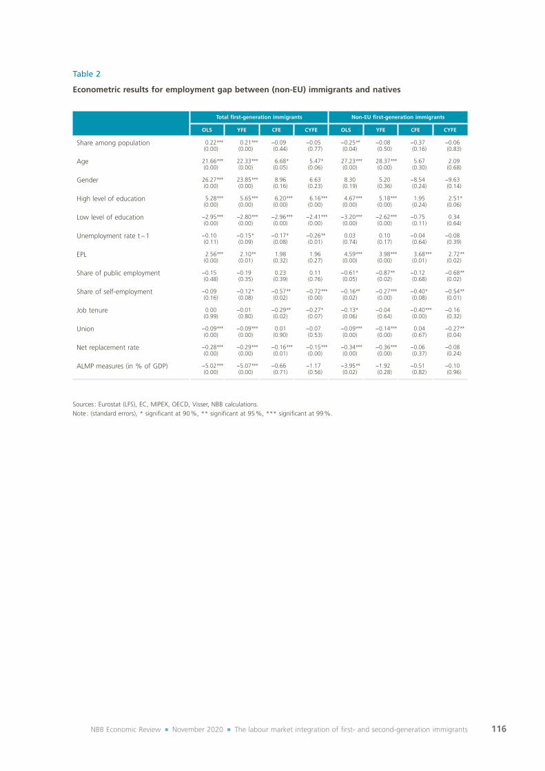
116NBB Economic Review ¡ November 2020 ¡ The labour market integration of first‑ and second‑generation immigrants
Table 2
Econometric results for employment gap between (non‑EU) immigrants and natives
Total first‑generation immigrants Non‑EU first‑generation immigrants
OLS YFE CFE CYFE OLS YFE CFE CYFE
Share among population 0.22***(0.00)
0.21***(0.00)
−0.09(0.44)
−0.05(0.77)
−0.25**(0.04)
−0.08(0.50)
−0.37(0.16)
−0.06(0.83)
Age 21.66***(0.00)
22.33***(0.00)
6.68*(0.05)
5.47*(0.06)
27.23***(0.00)
28.37***(0.00)
5.67(0.30)
2.09(0.68)
Gender 26.27***(0.00)
23.85***(0.00)
8.96(0.16)
6.63(0.23)
8.30(0.19)
5.20(0.36)
−8.54(0.24)
−9.63(0.14)
High level of education 5.28***(0.00)
5.65***(0.00)
6.20***(0.00)
6.16***(0.00)
4.67***(0.00)
5.18***(0.00)
1.95(0.24)
2.51*(0.06)
Low level of education −2.95***(0.00)
−2.80***(0.00)
−2.96***(0.00)
−2.41***(0.00)
−3.20***(0.00)
−2.62***(0.00)
−0.75(0.11)
0.34(0.64)
Unemployment rate t − 1 −0.10(0.11)
−0.15*(0.09)
−0.17*(0.08)
−0.26**(0.01)
0.03(0.74)
0.10(0.17)
−0.04(0.64)
−0.08(0.39)
EPL 2.56***(0.00)
2.10**(0.01)
1.98(0.32)
1.96(0.27)
4.59***(0.00)
3.98***(0.00)
3.68***(0.01)
2.72**(0.02)
Share of public employment −0.15(0.48)
−0.19(0.35)
0.23(0.39)
0.11(0.76)
−0.61*(0.05)
−0.87**(0.02)
−0.12(0.68)
−0.68**(0.02)
Share of self‑employment −0.09(0.16)
−0.12*(0.08)
−0.57**(0.02)
−0.72***(0.00)
−0.16**(0.02)
−0.27***(0.00)
−0.40*(0.08)
−0.54**(0.01)
Job tenure 0.00(0.99)
−0.01(0.80)
−0.29**(0.02)
−0.27*(0.07)
−0.13*(0.06)
−0.04(0.64)
−0.40***(0.00)
−0.16(0.32)
Union −0.09***(0.00)
−0.09***(0.00)
0.01(0.90)
−0.07(0.53)
−0.09***(0.00)
−0.14***(0.00)
0.04(0.67)
−0.27**(0.04)
Net replacement rate −0.28***(0.00)
−0.29***(0.00)
−0.16***(0.01)
−0.15***(0.00)
−0.34***(0.00)
−0.36***(0.00)
−0.06(0.37)
−0.08(0.24)
ALMP measures (in % of GDP) −5.02***(0.00)
−5.07***(0.00)
−0.66(0.71)
−1.17(0.56)
−3.95**(0.02)
−1.92(0.28)
−0.51(0.82)
−0.10(0.96)
Sources : Eurostat (LFS), EC, MIPEX, OECD, Visser, NBB calculations.Note : (standard errors), * significant at 90 %, ** significant at 95 %, *** significant at 99 %.

117NBB Economic Review ¡ November 2020 ¡ The labour market integration of first‑ and second‑generation immigrants
Table 2 (continued)
Econometric results for employment gap between (non‑EU) immigrants and natives
Total first‑generation immigrants Non‑EU first‑generation immigrants
OLS YFE CFE CYFE OLS YFE CFE CYFE
MIPEX
Labour market mobility
Access to labour market 0.00(0.74)
0.01(0.46)
0.05(0.32)
0.07*(0.09)
−0.05**(0.02)
−0.05**(0.01)
−0.14***(0.00)
−0.08**(0.04)
Access to general support −0.07***(0.00)
−0.07**(0.02)
−0.04*(0.09)
−0.05(0.14)
−0.03(0.18)
−0.01(0.65)
−0.06(0.14)
−0.03(0.31)
Targeted support 0.01(0.50)
0.00(0.76)
−0.00(0.94)
−0.01(0.64)
0.04***(0.00)
0.04***(0.00)
−0.01(0.53)
−0.00(0.96)
Workers rights −0.09***(0.00)
−0.08***(0.00)
−0.12***(0.00)
−0.12***(0.00)
−0.10***(0.00)
−0.13***(0.00)
−0.13**(0.01)
−0.09***(0.00)
Family reunion 0.08***(0.00)
0.08***(0.00)
−0.14**(0.03)
−0.10*(0.07)
0.16***(0.00)
0.15***(0.00)
−0.02(0.73)
−0.02(0.69)
Education
Access to education 0.06***(0.01)
0.06**(0.02)
0.07(0.15)
0.07(0.22)
0.08***(0.00)
0.05***(0.01)
0.17(0.12)
0.17*(0.08)
Targeting needs 0.02(0.43)
0.00(0.90)
0.07**(0.02)
0.08***(0.00)
−0.02(0.44)
−0.00(0.95)
0.01(0.90)
0.05(0.26)
New opportunities −0.06***(0.01)
−0.07***(0.00)
0.01(0.94)
−0.00(0.95)
−0.07***(0.01)
−0.09***(0.01)
0.17(0.19)
0.09(0.32)
Intercultural education for all −0.07***(0.00)
−0.07***(0.00)
−0.10(0.15)
−0.12**(0.04)
0.00(0.89)
−0.00(0.76)
0.02(0.69)
−0.03(0.63)
Permanent residence 0.19***(0.00)
0.21***(0.00)
0.09(0.21)
0.13*(0.08)
0.17***(0.01)
0.21***(0.00)
0.14(0.18)
0.20*(0.06)
Access to nationality −0.01(0.64)
−0.00(0.88)
0.07(0.17)
0.06(0.21)
−0.11***(0.00)
−0.09***(0.00)
−0.02(0.46)
−0.01(0.58)
Anti‑discrimination 0.01(0.61)
0.01(0.70)
0.21**(0.02)
0.22***(0.01)
−0.04(0.16)
−0.02(0.50)
0.08(0.16)
0.11(0.11)
Constant −50.45***(0.00)
−46.84***(0.00)
−9.79(0.24)
−6.57(0.33)
−25.07***(0.01)
−24.12***(0.00)
9.47(0.40)
12.55(0.35)
Observations 276 276 276 276 248 248 248 248
R‑squared 0.89 0.89 0.61 0.65 0.92 0.92 0.54 0.61
Number of countries 24 24 24 24 23 23 23 23
Number of years 13 13 13 13 13 13 13 13
Sources : Eurostat (LFS), EC, MIPEX, OECD, Visser, NBB calculations.Note : (standard errors), * significant at 90 %, ** significant at 95 %, *** significant at 99 %.

118NBB Economic Review ¡ November 2020 ¡ The labour market integration of first‑ and second‑generation immigrants
Table 3
Econometric results for participation gap between (non‑EU) immigrants and natives
Total first‑generation immigrants Non‑EU first‑generation immigrants
OLS YFE CFE CYFE OLS YFE CFE CYFE
Share among population 0.24***(0.00)
0.22***(0.00)
0.03(0.78)
−0.17(0.37)
−0.19*(0.09)
−0.08(0.46)
−0.14(0.49)
0.04(0.88)
Age 24.28***(0.00)
24.92***(0.00)
7.13(0.13)
6.18(0.14)
32.74***(0.00)
33.28***(0.00)
9.06**(0.03)
4.32(0.22)
Gender 27.36***(0.00)
27.12***(0.00)
7.48(0.17)
5.39(0.26)
9.62*(0.06)
7.41*(0.05)
−3.48(0.54)
−4.74(0.32)
High level of education 4.33***(0.00)
4.19***(0.00)
5.50***(0.00)
4.88***(0.01)
6.32***(0.00)
6.61***(0.00)
2.38(0.26)
2.84(0.11)
Low level of education −2.29***(0.00)
−2.34***(0.00)
−3.44***(0.00)
−3.54***(0.01)
−2.53***(0.00)
−2.22***(0.00)
−0.85*(0.09)
0.10(0.89)
EPL 1.72***(0.00)
1.99***(0.01)
2.04(0.20)
2.93**(0.05)
2.10***(0.00)
1.51***(0.00)
2.15(0.12)
1.94(0.11)
Share of public employment 0.42*(0.07)
0.33(0.23)
0.76***(0.00)
0.51(0.12)
0.42*(0.08)
0.25(0.45)
0.68**(0.01)
0.11(0.68)
Share of self‑employment 0.11(0.17)
0.06(0.48)
−0.34(0.13)
−0.56**(0.02)
0.09(0.13)
0.01(0.93)
−0.02(0.91)
−0.27(0.18)
Job tenure −0.07(0.25)
−0.12(0.12)
−0.40***(0.01)
−0.52**(0.01)
−0.19***(0.00)
−0.14*(0.08)
−0.33***(0.01)
−0.16(0.28)
Union −0.04**(0.04)
−0.04**(0.02)
0.06(0.44)
0.02(0.76)
0.00(0.91)
−0.02(0.26)
0.11(0.17)
−0.19*(0.05)
Net replacement rate −0.25***(0.00)
−0.26***(0.00)
−0.19***(0.00)
−0.18***(0.00)
−0.31***(0.00)
−0.32***(0.00)
−0.11*(0.08)
−0.12**(0.03)
ALMP measures (in % of GDP) −4.02***(0.01)
−4.24***(0.01)
−0.50(0.79)
−0.99(0.57)
−2.68*(0.06)
−1.54(0.42)
0.48(0.82)
0.97(0.64)
Sources : Eurostat (LFS), EC, MIPEX, OECD, Visser, NBB calculations.Note : (standard errors), * significant at 90 %, ** significant at 95 %, *** significant at 99 %.

119NBB Economic Review ¡ November 2020 ¡ The labour market integration of first‑ and second‑generation immigrants
Table 3 (continued)
Econometric results for participation gap between (non‑EU) immigrants and natives
Total first‑generation immigrants Non‑EU first‑generation immigrants
OLS YFE CFE CYFE OLS YFE CFE CYFE
MIPEX
Labour market mobility
Access to labour market 0.03*(0.06)
0.03***(0.00)
0.16**(0.04)
0.16**(0.01)
−0.02*(0.09)
−0.02**(0.04)
−0.01(0.66)
0.04(0.29)
Access to general support −0.09***(0.00)
−0.10**(0.01)
−0.07***(0.01)
−0.09***(0.00)
−0.01(0.57)
−0.00(0.94)
−0.06***(0.00)
−0.05**(0.02)
Targeted support −0.02(0.11)
−0.03***(0.00)
−0.03*(0.07)
−0.04**(0.04)
0.01(0.41)
0.00(0.58)
−0.04***(0.00)
−0.04***(0.00)
Workers rights −0.04*(0.07)
−0.04**(0.03)
−0.10**(0.04)
−0.10***(0.01)
−0.03(0.13)
−0.05(0.13)
−0.10***(0.01)
−0.07***(0.00)
Family reunion 0.12***(0.00)
0.12***(0.00)
−0.17**(0.01)
−0.14**(0.03)
0.25***(0.00)
0.25***(0.00)
0.01(0.84)
−0.00(0.93)
Education
Access to education 0.10***(0.00)
0.12***(0.00)
0.13**(0.02)
0.16***(0.01)
0.17***(0.00)
0.16***(0.00)
0.21**(0.01)
0.21**(0.01)
Targeting needs 0.01(0.75)
−0.00(0.81)
0.10**(0.01)
0.10***(0.01)
−0.06***(0.00)
−0.06***(0.00)
0.05(0.23)
0.08**(0.03)
New opportunities −0.03(0.17)
−0.03(0.36)
−0.08(0.41)
−0.05(0.47)
−0.07***(0.00)
−0.08***(0.01)
0.00(0.96)
−0.05(0.47)
Intercultural education for all −0.07***(0.00)
−0.06***(0.00)
−0.08(0.4)
−0.08(0.29)
0.00(0.86)
−0.00(0.90)
0.09*(0.08)
0.04(0.28)
Permanent residence 0.12**(0.02)
0.14***(0.00)
0.03(0.68)
0.03(0.58)
0.05(0.27)
0.08*(0.08)
0.04(0.55)
0.07(0.30)
Access to nationality −0.02(0.43)
−0.00(0.88)
0.12**(0.05)
0.12**(0.02)
−0.13***(0.00)
−0.12***(0.00)
−0.00(0.98)
0.02(0.27)
Anti‑discrimination −0.01(0.67)
−0.03(0.42)
0.22**(0.04)
0.19**(0.03)
−0.08***(0.00)
−0.08**(0.02)
−0.01(0.73)
0.01(0.87)
Constant −62.13***(0.00)
−59.35***(0.00)
−19.51**(0.04)
−3.69(0.74)
−48.63***(0.00)
−46.33***(0.00)
−15.68(0.12)
−5.12(0.69)
Observations 276 276 276 276 248 248 248 248
R‑squared 0.84 0.85 0.61 0.66 0.92 0.92 0.49 0.61
Number of countries 24 24 24 24 23 23 23 23
Number of years 13 13 13 13 13 13 13 13
Sources : Eurostat (LFS), EC, MIPEX, OECD, Visser, NBB calculations.Note : (standard errors), * significant at 90 %, ** significant at 95 %, *** significant at 99 %.

120NBB Economic Review ¡ November 2020 ¡ The labour market integration of first‑ and second‑generation immigrants
Table 4
Econometric results for employment gap between (non‑EU) immigrants and natives – specific analysis for men
Total first‑generation immigrants men Non‑EU first‑generation immigrants men
OLS YFE CFE CYFE OLS YFE CFE CYFE
Share among population 0.26***(0.00)
0.29***(0.00)
−0.18(0.29)
−0.18(0.43)
−0.51***(0.00)
−0.46**(0.02)
−0.42(0.21)
−0.47(0.18)
Age 26.32***(0.00)
27.31***(0.00)
−1.86(0.82)
−2.27(0.79)
16.50***(0.00)
17.10**(0.02)
−2.93(0.72)
−3.57(0.64)
High level of education 1.90*(0.06)
2.26**(0.05)
5.05***(0.01)
4.67**(0.02)
3.08**(0.01)
3.30**(0.04)
3.74**(0.04)
3.84**(0.03)
Low level of education −1.19***(0.00)
−0.91*(0.09)
−2.57***(0.01)
−2.38***(0.00)
−0.93**(0.02)
−0.55(0.17)
−0.25(0.74)
0.11(0.90)
Unemployment rate t − 1 −0.12(0.12)
−0.14(0.14)
−0.08(0.45)
−0.14(0.20)
−0.13(0.17)
−0.03(0.63)
−0.04(0.78)
−0.00(0.99)
EPL 3.35***(0.00)
2.61***(0.01)
3.11**(0.02)
3.01**(0.02)
3.70***(0.00)
3.75***(0.00)
3.37**(0.02)
2.79**(0.05)
Share of public employment −0.53**(0.03)
−0.59***(0.01)
−0.14(0.74)
−0.30(0.50)
−0.19(0.65)
−0.22(0.58)
−0.31(0.49)
−0.80*(0.09)
Share of self‑employment −0.07(0.33)
−0.10*(0.08)
−0.45(0.13)
−0.54*(0.08)
0.09(0.20)
0.08(0.18)
−0.52(0.15)
−0.55(0.10)
Job tenure −0.00(0.95)
0.01(0.82)
−0.18*(0.10)
−0.19(0.16)
0.04(0.71)
0.05(0.7)
−0.30**(0.04)
−0.24(0.29)
Union −0.10***(0.00)
−0.12***(0.00)
−0.28***(0.00)
−0.34**(0.01)
−0.06**(0.02)
−0.08***(0.00)
−0.28**(0.02)
−0.45***(0.01)
Net replacement rate −0.28***(0.00)
−0.27***(0.00)
−0.06(0.35)
−0.05(0.40)
−0.39***(0.00)
−0.39***(0.00)
0.08(0.45)
0.06(0.51)
ALMP measures (in % of GDP) −5.42***(0.00)
−5.52***(0.00)
−1.95(0.24)
−2.74(0.12)
−2.96*(0.09)
−3.03**(0.03)
−2.45(0.51)
−4.55(0.28)
Sources : Eurostat (LFS), EC, MIPEX, OECD, Visser, NBB calculations.Note : (standard errors), * significant at 90 %, ** significant at 95 %, *** significant at 99 %.

121NBB Economic Review ¡ November 2020 ¡ The labour market integration of first‑ and second‑generation immigrants
Table 4 (continued)
Econometric results for employment gap between (non‑EU) immigrants and natives – specific analysis for men
Total first‑generation immigrants men Non‑EU first‑generation immigrants men
OLS YFE CFE CYFE OLS YFE CFE CYFE
MIPEX
Labour market mobility
Access to labour market −0.04*(0.09)
−0.03**(0.03)
−0.09**(0.01)
−0.07*(0.09)
−0.07***(0.00)
−0.08**(0.01)
−0.20**(0.01)
−0.19**(0.01)
Access to general support −0.06**(0.01)
−0.03(0.22)
−0.03(0.20)
−0.04(0.14)
−0.05(0.27)
−0.04(0.49)
−0.02(0.68)
−0.04(0.41)
Targeted support 0.00(0.79)
0.01(0.66)
0.04*(0.05)
0.03(0.11)
0.03**(0.02)
0.04***(0.00)
0.02(0.32)
0.03(0.27)
Workers rights −0.12***(0.00)
−0.12***(0.00)
−0.06**(0.02)
−0.07**(0.01)
−0.13***(0.00)
−0.14***(0.00)
−0.07*(0.10)
−0.08**(0.04)
Family reunion 0.02(0.52)
0.02(0.38)
−0.03(0.66)
−0.01(0.93)
0.05*(0.08)
0.04(0.21)
0.01(0.93)
0.02(0.72)
Education
Access to education 0.04(0.13)
0.03**(0.05)
0.11(0.13)
0.13(0.12)
0.10***(0.00)
0.08***(0.00)
0.12(0.30)
0.20*(0.08)
Targeting needs 0.07***(0.00)
0.06**(0.02)
0.05(0.21)
0.07(0.10)
0.01(0.66)
0.03(0.19)
0.02(0.70)
0.08(0.15)
New opportunities −0.06**(0.03)
−0.08**(0.02)
0.13(0.11)
0.12*(0.09)
−0.11***(0.00)
−0.14***(0.00)
0.23*(0.08)
0.18(0.11)
Intercultural education for all −0.09***(0.00)
−0.10***(0.00)
−0.09(0.32)
−0.11(0.25)
0.04(0.13)
0.03(0.20)
−0.04(0.74)
−0.05(0.69)
Permanent residence 0.21***(0.00)
0.22***(0.00)
0.15(0.13)
0.20*(0.07)
0.18***(0.00)
0.21***(0.00)
0.13(0.25)
0.26**(0.04)
Access to nationality −0.00(0.78)
−0.01(0.53)
−0.04(0.15)
−0.05*(0.10)
−0.06(0.14)
−0.06(0.32)
−0.08***(0.01)
−0.08**(0.03)
Anti‑discrimination 0.10***(0.00)
0.12***(0.00)
0.08(0.12)
0.10*(0.09)
−0.03(0.56)
−0.01(0.86)
0.07(0.28)
0.07(0.35)
Constant −21.58***(0.00)
−23.06***(0.00)
13.12(0.34)
13.95(0.34)
−8.26*(0.09)
−11.80(0.120)
19.18(0.20)
20.39(0.10)
Observations 257 257 257 257 231 231 231 231
R‑squared 0.85 0.86 0.47 0.50 0.87 0.88 0.43 0.48
Number of countries 22 22 22 22 21 21 21 21
Number of years 13 13 13 13 13 13 13 13
Sources : Eurostat (LFS), EC, MIPEX, OECD, Visser, NBB calculations.Note : (standard errors), * significant at 90 %, ** significant at 95 %, *** significant at 99 %.

122NBB Economic Review ¡ November 2020 ¡ The labour market integration of first‑ and second‑generation immigrants
Table 5
Econometric results for participation gap between (non‑EU) immigrants and natives – specific analysis for men
Total first‑generation immigrants men Non‑EU first‑generation immigrants men
OLS YFE CFE CYFE OLS YFE CFE CYFE
Share among population 0.25***(0.00)
0.27***(0.00)
0.06(0.61)
−0.04(0.80)
−0.52***(0.00)
−0.49***(0.00)
−0.10(0.64)
−0.26(0.41)
Age 32.16***(0.00)
33.03***(0.00)
1.81(0.78)
0.76(0.90)
15.78***(0.00)
16.12***(0.00)
2.68(0.57)
0.65(0.89)
High level of education 0.77(0.41)
1.04(0.11)
3.71**(0.04)
3.69**(0.03)
2.85***(0.00)
3.13***(0.00)
0.72(0.61)
0.95(0.46)
Low level of education −0.21(0.57)
−0.02(0.97)
−1.57**(0.03)
−1.56**(0.02)
0.07(0.79)
0.15(0.59)
−0.50(0.42)
−0.25(0.69)
EPL 1.98***(0.00)
1.58***(0.00)
0.79(0.40)
1.30*(0.10)
1.77***(0.00)
1.51**(0.03)
1.12(0.31)
1.16(0.23)
Share of public employment 0.15(0.48)
−0.02(0.92)
0.65**(0.01)
0.30(0.31)
1.05***(0.00)
1.04***(0.00)
0.70***(0.00)
0.21(0.29)
Share of self‑employment 0.20***(0.00)
0.14**(0.02)
0.12(0.44)
−0.11(0.53)
0.50***(0.00)
0.49***(0.00)
0.19(0.31)
0.00(0.99)
Job tenure −0.07(0.28)
−0.07(0.37)
−0.13(0.11)
−0.19*(0.05)
0.06(0.31)
0.08(0.15)
−0.22*(0.06)
−0.22(0.22)
Union −0.06**(0.02)
−0.07***(0.00)
−0.03(0.65)
−0.15**(0.03)
0.05***(0.00)
0.05*(0.07)
−0.03(0.73)
−0.19**(0.05)
Net replacement rate −0.23***(0.00)
−0.23***(0.00)
−0.15**(0.02)
−0.13**(0.02)
−0.35***(0.00)
−0.35***(0.00)
−0.01(0.88)
−0.02(0.80)
ALMP measures (in % of GDP) −4.11***(0.01)
−3.74**(0.01)
−0.99(0.39)
−1.24(0.27)
−1.76(0.16)
−1.51(0.19)
−2.02(0.29)
−3.11(0.11)
Sources : Eurostat (LFS), EC, MIPEX, OECD, Visser, NBB calculations.Note : (standard errors), * significant at 90 %, ** significant at 95 %, *** significant at 99 %.

123NBB Economic Review ¡ November 2020 ¡ The labour market integration of first‑ and second‑generation immigrants
Table 5 (continued)
Econometric results for participation gap between (non‑EU) immigrants and natives – specific analysis for men
Total first‑generation immigrants men Non‑EU first‑generation immigrants men
OLS YFE CFE CYFE OLS YFE CFE CYFE
MIPEX
Labour market mobility
Access to labour market −0.02(0.21)
−0.02**(0.04)
0.00(0.94)
0.02(0.43)
−0.06***(0.00)
−0.06***(0.00)
−0.04(0.28)
−0.01(0.77)
Access to general support −0.06**(0.01)
−0.04*(0.08)
−0.04***(0.01)
−0.05***(0.00)
−0.07**(0.02)
−0.06(0.14)
−0.04(0.18)
−0.07**(0.01)
Targeted support −0.03*(0.08)
−0.03**(0.02)
−0.00(0.75)
−0.01(0.49)
0.00(0.92)
0.00(0.75)
−0.01(0.32)
−0.02(0.24)
Workers rights −0.05***(0.00)
−0.06***(0.01)
−0.08***(0.00)
−0.08***(0.00)
−0.06***(0.00)
−0.06***(0.01)
−0.07**(0.02)
−0.08***(0.01)
Family reunion 0.06**(0.03)
0.06**(0.02)
−0.03(0.55)
−0.02(0.73)
0.09***(0.00)
0.09***(0.00)
0.03(0.60)
0.04(0.40)
Education
Access to education 0.08***(0.00)
0.08***(0.00)
0.16**(0.01)
0.18**(0.01)
0.20***(0.00)
0.20***(0.00)
0.18**(0.02)
0.25***(0.01)
Targeting needs 0.04**(0.02)
0.04***(0.00)
0.11***(0.00)
0.13***(0.00)
−0.04**(0.02)
−0.04**(0.01)
0.07(0.26)
0.11**(0.04)
New opportunities −0.00(0.94)
−0.01(0.73)
−0.01(0.93)
−0.01(0.89)
−0.07***(0.00)
−0.08***(0.00)
0.04(0.75)
−0.00(0.99)
Intercultural education for all −0.08***(0.00)
−0.09***(0.00)
0.02(0.59)
−0.00(0.91)
0.07***(0.00)
0.07***(0.00)
0.06(0.19)
0.03(0.50)
Permanent residence 0.10**(0.04)
0.13***(0.00)
0.09(0.12)
0.11**(0.03)
0.11**(0.01)
0.11***(0.01)
0.03(0.60)
0.12**(0.04)
Access to nationality −0.02(0.19)
−0.02(0.18)
0.01(0.81)
0.01(0.81)
−0.03(0.25)
−0.03(0.40)
−0.02(0.55)
−0.02(0.59)
Anti‑discrimination 0.06**(0.05)
0.08**(0.03)
0.02(0.62)
0.01(0.76)
−0.15***(0.00)
−0.15***(0.00)
−0.07*(0.09)
−0.08(0.11)
Constant −37.46***(0.00)
−36.37***(0.00)
−13.74*(0.06)
−2.93(0.72)
−30.26***(0.00)
−31.63***(0.00)
−9.25(0.35)
0.87(0.93)
Observations 257 257 257 257 231 231 231 231
R‑squared 0.84 0.85 0.35 0.46 0.91 0.91 0.32 0.43
Number of countries 22 22 22 22 21 21 21 21
Number of years 13 13 13 13 13 13 13 13
Sources : Eurostat (LFS), EC, MIPEX, OECD, Visser, NBB calculations.Note : (standard errors), * significant at 90 %, ** significant at 95 %, *** significant at 99 %.

124NBB Economic Review ¡ November 2020 ¡ The labour market integration of first‑ and second‑generation immigrants
Labour market rigidities 1 are also captured by the proportion of people working for the same employer for more than 10 years (‘job tenure’ in the regressions). In our analysis, we find that job tenure has a negative impact on employment and participation gaps (though it is not always significant). This is in line in the theory that, for a given segment of the economy, if the labour market is more rigid it decreases turnover and thus disadvantages outsiders 2 (where immigrants are over‑represented).
The negative impact of union density and the net replacement income rate in the event of unemployment, previously stated in the literature (see chapter 4), is verified in our own analysis. A higher level of union density favours insiders (employed workers who obtained a sustainable position at the labour market) as unions tend to protect established workers. It is thus detrimental to immigrants who are more often out of the labour market. Moreover, a high replacement income in the event of unemployment increases the effect of the unemployment trap among immigrants (for those eligible for unemployment benefits), who are more often in low‑skilled and low‑paid jobs. Note also that the effect of the net income replacement rate is more pronounced for non‑EU immigrants, who are particularly over‑represented in low‑paid jobs (HCE, 2018).
The active labour market policy (ALMP) measures provide interesting results since a higher percentage of GDP devoted to those activation policies seems to be detrimental to immigrants, and the effect is larger for non‑EU born individuals. The reasoning is that those types of policies rarely reach immigrants unless they specifically target them, whereas they are efficient for natives, who therefore benefit for them. Specifications including country fixed effects, however, provide insignificant results.
As highlighted by Bilgili et al. (2015), migrant integration policies may have a varying impact on different types of migrants ; this may make the analysis of the global impact irrelevant, so that controlling for immigrants’ personal characteristics may provide more robust results. MIPEX sub‑indicators, having not been updated since 2014, are almost time‑invariant. This makes the analysis including country fixed effects more complicated as cross‑country variation is entirely absorbed by the country fixed effect. As a result, few indicators keep a significant impact when controlling for other time‑invariant factors. The index update, planned at the end of this year, could help in that respect.
The labour market mobility results confirm our finding on ALMPs : regressions show a negative coefficient for all indicators except for targeted support, which is beneficial for the employment of non‑EU immigrants (in the OLS and YFE specifications, insignificant for the rest). While this type of policies can help migrants to increase their employment rate (see section 3.3), the effect is less pronounced than for natives so that the impact on the gap remains negative. This statement supposes that countries with more policies on labour market mobility for immigrants are also those with the same type of policies for natives. Finding similar results, Bredtmann and Otten (2013) emphasise that targeted employment policies must be suited to the country’s specific immigration populations and labour markets. Moreover, across all specifications and for all studied groups, the impact of workers’ rights is always statistically significant and negative. This finding highlights the somehow perverse effect of verifying if both natives and immigrants have the same rights in terms of work and social security access. The effect of being less informed about their rights disappear and with it the advantage of immigrant population with respect to natives.
Access to education is significantly positively associated with the labour market integration of immigrants compared to natives, and this result is true for all types of immigrants. Targeting needs is also beneficial even after controlling for country and year fixed effects. The positive impact disappears however when looking at
1 We also tested for minimum wage (using Visser database) as an explanatory factor in a bivariate estimation. Results (provided in annex II.5) show that the introduction of a minimum wage in the country reduces the gap between immigrants and natives, especially in terms of employment, and the effect is larger for non‑EU immigrants. When a minimum wage is implemented, natives are more likely to end up in the unemployment trap. Immigrants, however, who often do not have direct access to unemployment benefits, are more likely to accept low‑paid jobs. Nevertheless, for the multivariate analysis, we decided to drop the minimum wage variable from the regression. First of all, the presence of a minimum wage in a country is closely correlated with the degree of unionisation (66 %), and secondly, there are very few variations in the database within countries; it is therefore difficult to present conclusive results.
2 Unemployed workers with higher difficulties to get a new job.

125NBB Economic Review ¡ November 2020 ¡ The labour market integration of first‑ and second‑generation immigrants
employment of non‑EU immigrants. Non‑EU immigrants showing larger gaps compared to natives in terms of education and skills, perhaps because they cannot get recognition for their qualifications in the host country are more likely to be enrolled in education – and for longer periods – if access is made easier. In the short‑term this can keep them away from the labour market to upgrade their skills. Results on education are more robust in terms of labour market participation than regarding employment. While a larger access to education increases their willingness to be active, this does not necessarily translate in an easier access to jobs.
Analysis of permanent residence MIPEX scores confirms the argument that immigrants who enter the country to stay for a long period are more inclined to invest in human and cultural capital specific to the host country, and then to have higher employment and participation rates. Countries which facilitate access to permanent residence seem to have smaller gaps between immigrants and natives in terms of integration into the labour market. This is in line with the literature (see for example Bisin et al., 2011).
While family reunion provides similar results, the impact become insignificant when we include a country fixed effect and even significantly negative for total first‑generation immigrants. The argument on human capital could hold but allowing family reunion also induces a higher share of immigrants who potentially do not have adequate characteristics to enter the labour market (in comparison to immigrants coming for work who directly get their contract).
Access to nationality gives more ambiguous results, almost always not significant. This implies that it is not the access to nationality in itself which matters, but more the prospect of long‑term residence in the country. Moreover, if restricted access to nationality implies a certain level of economic integration (as in Belgium with the 2013 reform), then immigrants could have a higher incentive to work in stricter countries
Anti-discrimination policies seem to be efficient in reducing labour market integration gaps between immigrants and natives on average. Coefficients when controlling for country and year fixed effects are statistically significant and positive for both employment and participation gaps. However, our analysis show that those policies do not significantly influence labour market outcomes of non‑EU immigrants. As for other policy indexes, they are potentially not enough targeted to specificities of immigrants. In fact, anti‑discrimination policies are often broader than discrimination against origin. Note also that some reverse causality could appear here. Anti‑discrimination policies might be started especially in countries and regions where discrimination is perceived to be high. Then this index might be correlated with the a priori importance of discrimination.
5.4 How those results help to explain Belgium’s bad performance
In brief, the personal characteristics of a country’s immigrants, mainly their level of education, explain part of the discrepancies between countries in terms of labour market integration of immigrants and the gap with respect to natives. Labour market features nevertheless constitute powerful explanatory factors, in particular employment protection (positive impact), union density and replacement income rates in the event of unemployment. Regarding integration policies, the most efficient appear those that are particularly designed for immigrants. Once again, integration policies regarding education are key in that respect. Moreover, also incentives to stay for a long period could be beneficial since they induce immigrants to invest in human capital specific to the host country. Anti‑discrimination policies could also help even if they seem less efficient to tackle difficulties encountered by non‑EU immigrants.
Those results provide a consistent explanation of Belgium’s relatively poor performance in integrating immigrants into the labour market, especially for non‑EU born individuals. In fact, compared to the average of the countries analysed, Belgium is less likely to have immigrants who are high‑educated and more likely to attract low‑educated foreigners. Its labour market rigidities could also be an explanatory factor. In addition, few policies are specifically designed to help immigrants find a job (see table 6).
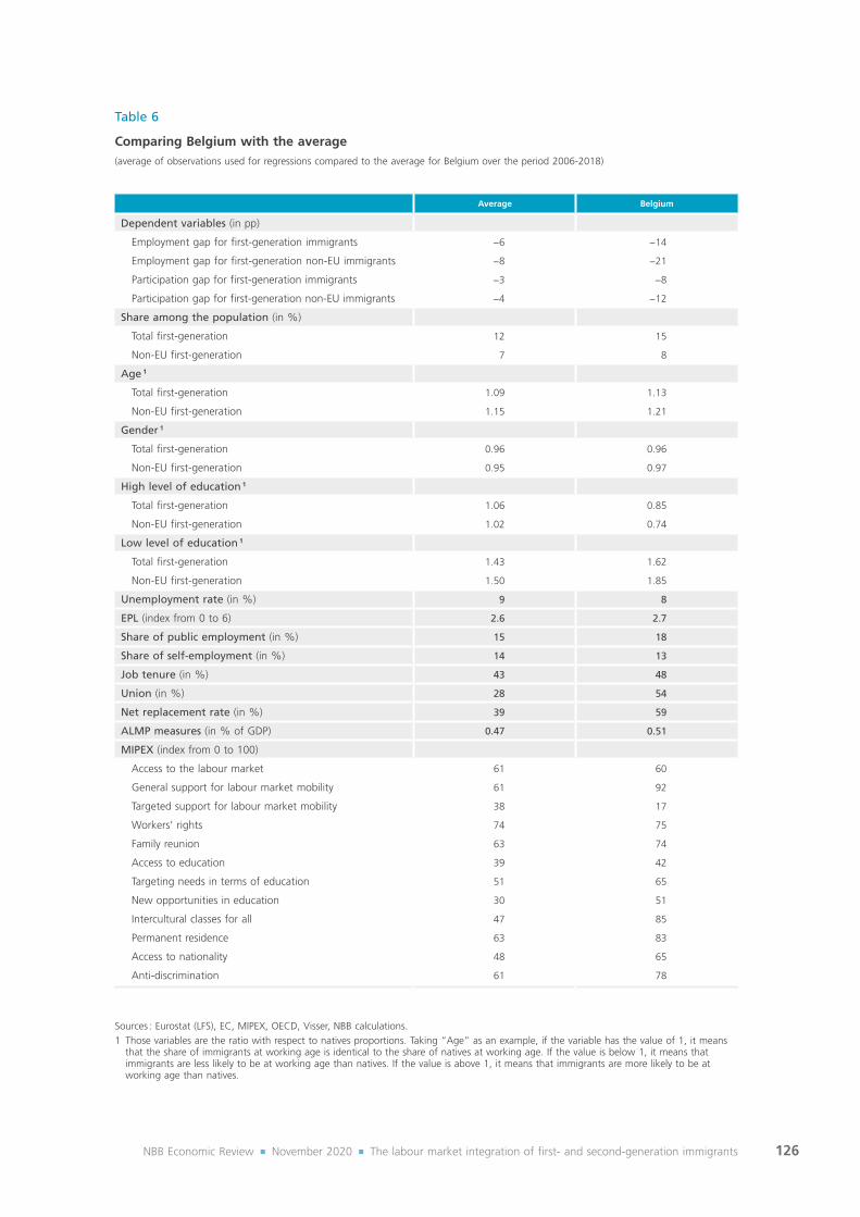
126NBB Economic Review ¡ November 2020 ¡ The labour market integration of first‑ and second‑generation immigrants
Table 6
Comparing Belgium with the average(average of observations used for regressions compared to the average for Belgium over the period 2006‑2018)
Average Belgium
Dependent variables (in pp)
Employment gap for first‑generation immigrants −6 −14
Employment gap for first‑generation non‑EU immigrants −8 −21
Participation gap for first‑generation immigrants −3 −8
Participation gap for first‑generation non‑EU immigrants −4 −12
Share among the population (in %)
Total first‑generation 12 15
Non‑EU first‑generation 7 8
Age 1
Total first‑generation 1.09 1.13
Non‑EU first‑generation 1.15 1.21
Gender 1
Total first‑generation 0.96 0.96
Non‑EU first‑generation 0.95 0.97
High level of education 1
Total first‑generation 1.06 0.85
Non‑EU first‑generation 1.02 0.74
Low level of education 1
Total first‑generation 1.43 1.62
Non‑EU first‑generation 1.50 1.85
Unemployment rate (in %) 9 8
EPL (index from 0 to 6) 2.6 2.7
Share of public employment (in %) 15 18
Share of self‑employment (in %) 14 13
Job tenure (in %) 43 48
Union (in %) 28 54
Net replacement rate (in %) 39 59
ALMP measures (in % of GDP) 0.47 0.51
MIPEX (index from 0 to 100)
Access to the labour market 61 60
General support for labour market mobility 61 92
Targeted support for labour market mobility 38 17
Workers’ rights 74 75
Family reunion 63 74
Access to education 39 42
Targeting needs in terms of education 51 65
New opportunities in education 30 51
Intercultural classes for all 47 85
Permanent residence 63 83
Access to nationality 48 65
Anti‑discrimination 61 78
Sources : Eurostat (LFS), EC, MIPEX, OECD, Visser, NBB calculations.1 Those variables are the ratio with respect to natives proportions. Taking “Age” as an example, if the variable has the value of 1, it means
that the share of immigrants at working age is identical to the share of natives at working age. If the value is below 1, it means that immigrants are less likely to be at working age than natives. If the value is above 1, it means that immigrants are more likely to be at working age than natives.

127NBB Economic Review ¡ November 2020 ¡ The labour market integration of first‑ and second‑generation immigrants
The two ‘negative’ factors, namely labour market institutions and level of education, complement one another : features of the Belgian labour market explain why our country attracts proportionately fewer high‑skilled migrants and / or low‑skilled migrants. While immigrants (including from non‑EU countries) in the countries studied are more likely to be high‑educated than natives, this is not the case in Belgium, where immigrants are 15 % less likely to be high‑educated (25 % for non‑EU immigrants). Cohen and Razin (2008) developed a theoretical model to find out the effect of a more generous social security system on immigrant education levels, and conducted an analysis across OECD countries. Assuming free access to the country, the effect would be negative : more generous social systems would tend to attract low‑skilled immigrants. Boeri et al. (2012) state that attracting talents depends mainly on the labour market, and wage premiums on education. While R&D spending induces greater inflows of highly skilled migrants, generous welfare benefits and strict employment protection attract more unskilled workers. This finding was corroborated by Eichhorst et al. (2017), who found that a more generous unemployment benefit system was negatively correlated with the presence of high‑skilled immigrants. These people are often in work and so contribute to the social security system, and a more generous system could in fact reduce their reasons for moving to a particular country. The same is found to be true for union representation, which could help improve labour conditions for the lower skilled and so mainly attract lower‑skilled immigrants.
Nevertheless, the literature is not unanimous in saying that individual decisions to move to a specific country are induced by its social system (Edo et al., 2018). Theoretically, that could be the case, but the most frequently quoted criteria are unemployment and wage differences compared to the country of origin, the existence of social networks, and regional proximity (Giulietti 2014). In 2018, Docquier et al. produced similar results showing that the size of the network of previous migrants and the average income per capita in the country are crucial determinants of the size of migration inflows.
Moreover, while migrants selectivity increases over time throughout the world (Rayp et al., forthcoming), recent literature shows that migration policies based on skill selectivity are not efficient, and that push and pull factors, such as geographical proximity or cultural similarities, are more relevant explaining the magnitude and the structure of migration flows (Antecol et al., 2003 ; Bélot and Hatton, 2012). Rayp et al. (forthcoming) recently confirm previous findings. Computing a unique indicator of migration policies in 42 OECD and non‑OECD countries from 1990 to 2014, they find that skill selectivity has a weak effect on the scale and structure of migration flows.
According to our analysis, some factors in Belgium should favour better integration outcomes compared to other countries. First, Belgium provides easier access to permanent residence. Combining data on bilateral migration desires from 140 origin countries and data on policies in 38 destination countries over the period 2007‑2014, Beine et al. (2019) find that, in addition to labour market features, access to nationality and permanent residence may also influence migrant inflows. More precisely, those factors increase the perceived attractiveness of a destination country. Belgium also scores higher than the average regarding anti‑discrimination policies and access to education including targeting needs.

128NBB Economic Review ¡ November 2020 ¡ The labour market integration of first‑ and second‑generation immigrants
6. Conclusion
The aim of this second part of the report is first to provide a clear understanding of which factors could have an impact on the employment or participation gaps between first‑generation immigrants and natives and, secondly, to find an explanation for Belgium’s poor performance compared to other EU countries. To do so, we created a new dataset including EU countries over the period 2006‑2019 and merging information from different sources allowing us to test 25 explanatory variables for employment and participation gaps between first‑generation (non‑EU) immigrants and natives. Those variables are : personal characteristics of immigrants (age, gender, level of education (high or low)), history of migration (share among the population), economic environment (unemployment rate), labour market features (EPL, public employment, self‑employment, job tenure, union density, net replacement rate, labour market policy measures) and integration policy indicators (12 MIPEX sub‑indicators).
The findings once again show that education is a key factor in explaining employment and labour market participation gaps between first‑generation immigrants and natives. When focusing on non‑EU immigrants, the results are however less robust. On the one hand, a high level of education (based on self‑reporting from Labour Force Survey) is less beneficial for a non‑EU immigrant, probably because of the diploma recognition issue. On the other hand, being low‑educated is less detrimental for them too. The potential explanation could be that they are more active in low‑skilled sectors and are more inclined to accept lower wages than natives. This increases their chance of getting a job compared to natives.
The over‑representation of immigrants, and in particular non‑EU immigrants, in low‑paid jobs is also reflected in the results obtained for net replacement income rate. A high replacement income in the event of unemployment increases the effect of the unemployment trap among immigrants and the effect is more pronounced for non‑EU immigrants.
Regarding employment protection on regular contracts, our findings support the view expressed in the literature that a higher level of protection reduces the gap in labour market integration between immigrants and natives. Immigrants, usually less aware of employment protection regulations, are also less likely to claim their rights, and this makes it cheaper for employers to hire immigrants than to hire natives.
Labour market rigidities, such as a high level of job tenure, make it more difficult for individuals who are not yet active to enter the labour market, because of lower turnover among firms. The degree of union density also tends to favour established workers rather than unemployed or new entrants. As immigrants are over‑represented among both categories, a higher level of union density widens the gap with natives in terms of both employment and labour market participation.
Because of their low time variability, results on migrant integration policies should be considered with caution. Nevertheless, some interesting results show up from the analysis. Activation policies and general support for a better access to the labour market tend to widen the labour market integration gap between immigrants and natives. In order to significantly improve labour market outcomes of immigrants, targeted policies tend to be more efficient.
Access to education is significantly and positively associated with the labour market integration of immigrants compared to natives, and this result is true for all types of immigrants. Design of educational policies specifically targeted to immigrants is also beneficial even after controlling for country and year fixed effects. The positive impact disappears however when looking at employment of non‑EU immigrants. Non‑EU immigrants are temporarily kept away from the labour market to upgrade their skills, so that the insignificant effect on the employment rate could be counterbalanced by a positive impact on the quality of their jobs.

129NBB Economic Review ¡ November 2020 ¡ The labour market integration of first‑ and second‑generation immigrants
Policies designed to induce immigrants to stay in the country for a longer period tend to reduce the employment and labour market participation gaps with respect to natives. In that respect, the most powerful policy is providing easier access to permanent residence, while the other indicators, family reunion and access to nationality, do not always give significant results.
Finally, anti‑discrimination policies are efficient in reducing the labour market integration gap between immigrants and natives when we consider total first‑generation immigrants. However, the positive impact is less clear for non‑EU immigrants. As for employment activation policies or education policies, discrimination policies are maybe not targeting immigrants enough, as they are often designed in common with other potential characteristics leading to discrimination such as gender, age, handicap, etc.
Those results provide a consistent explanation of Belgium’s relatively poor performance in integrating immigrants into the labour market. Compared to the average of the countries analysed, Belgium is less likely to have immigrants who are high‑educated and more likely to attract low‑educated foreigners. Its labour market rigidities could also be an explanatory factor. In addition, few policies are specifically designed to help immigrants find a job. While Belgium scores high on the aggregate MIPEX (4th among all EU countries), it performs badly regarding targeted support for immigrants. However, some policies should be in favour of labour market integration of immigrants, namely, easier access to permanent residence, the high level of access to education and targeting needs in that respect and strong anti‑discrimination policies, even though some improvements are still possible for the two latter compared to best performer, in particular regarding education policies.

130NBB Economic Review ¡ November 2020 ¡ A general equilibrium analysis of immigration in Belgium
PART III A general equilibrium analysis of immigration in Belgium
131NBB Economic Review ¡ November 2020 ¡ A general equilibrium analysis of immigration in Belgium
Contents
Introduction 132
1. Literature review 1321.1 Spatial correlation 1331.2 Skill cells and structure 1341.3 Interacting economic impact channels 134
2. Model characteristics 135
3. Analysis 1373.1 Demographic effects of immigration 1383.2 Aggregate effects of immigration 1393.3 Wages 1413.4 Unemployment 1433.5 Labour market participation 1443.6 Net income and welfare 1453.7 Conclusion 147
4. The influence of parameters, assumptions and the theoretical framework 1474.1 Robustness checks 1474.2 Assumptions 1504.3 Alternative impact channels 150
5. Conclusion 151
132NBB Economic Review ¡ November 2020 ¡ A general equilibrium analysis of immigration in Belgium
Introduction
Previous parts have sketched an extensive image of immigration in Belgium, the position of immigrants on the labour market and their contribution to public finance. This third part shifts the focus to estimating the aggregate impact of recent immigration on the economy with specific attention given to the effect on natives 1 and previously established immigrants and taking into account direct and indirect effects. The estimated impacts include demographic effects of immigration as well as aggregate effects on employment, unemployment and participation rates, on wages, on net income, on welfare and on GDP and GDP per capita.
In the first chapter, an overview of the relevant literature is provided.
The second chapter constructs a general equilibrium model for the economy. Several assumptions are imposed to determine the relationships between the actors in the model, enabling the interaction between immigrants and natives to be approximated. Finally, the model is tailored to the Belgian economy by using parameter estimates based on data and by calibrating other parameters to reflect reality.
The third chapter makes use of the model to assess the economic impact of recent immigration. It takes the Belgian population in 2017 2 as the baseline scenario, excluding immigrants who arrived in Belgium in the last five years (defined hereafter as recent immigrants). Next, the economic impact of immigration is computed by comparing this baseline scenario (without recent immigration) with a situation where recent immigrants are included again (distinguishing between EU and non‑EU origins).
In the final chapter of this Part III, the limitations of the methodology are discussed. First, the model is run with alternative sets of exogenous parameter values to check the robustness of the results obtained. Second, the findings will be framed in a broader set of results from the literature, as it has identified several mechanisms influencing the impact of immigration on natives, which could not be captured by this model.
1. Literature review
Understanding the economic impact of immigration has long been an important goal for many economists. Over the years, several methodologies have been developed, each focusing on a particular aspect of the economy. Two main strands in this literature can be identified, namely a strand focusing on the public finance impact of immigration and one focusing on the labour market (and especially the wage) impact of immigration. An elaborate overview of the impact of immigration on public finance can be found in Part I of the present report. Therefore, this review focuses primarily on the wage impact of immigration.
From a labour market perspective, immigration can be interpreted as a positive labour supply shock. The canonical labour market model then dictates that in the short run – when capital stock has not yet adapted to the new stock of labour supply – this should lead to a fall in the average wage of workers. When capital is adapted to the new stock of labour supply, the average wage level should be restored to its previous equilibrium level. This is conditional on the assumption that immigrants and natives are perfectly substitutable. If the labour
1 Those we consider here as natives include second‑generation immigrants because of data availability.2 Data that are used to calibrate the model are from other sources than the CBSS data since we need macroeconomic variables. This allows
us to take the most recent data at the time of the analysis, which was 2017.
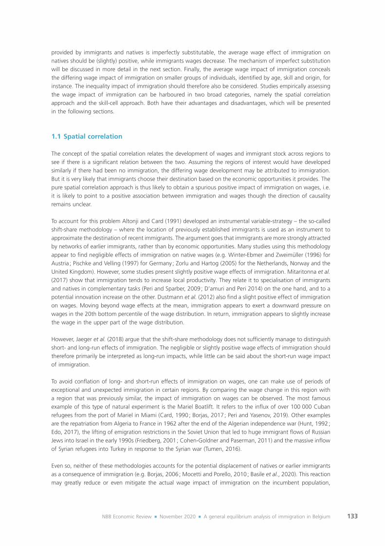
133NBB Economic Review ¡ November 2020 ¡ A general equilibrium analysis of immigration in Belgium
provided by immigrants and natives is imperfectly substitutable, the average wage effect of immigration on natives should be (slightly) positive, while immigrants wages decrease. The mechanism of imperfect substitution will be discussed in more detail in the next section. Finally, the average wage impact of immigration conceals the differing wage impact of immigration on smaller groups of individuals, identified by age, skill and origin, for instance. The inequality impact of immigration should therefore also be considered. Studies empirically assessing the wage impact of immigration can be harboured in two broad categories, namely the spatial correlation approach and the skill‑cell approach. Both have their advantages and disadvantages, which will be presented in the following sections.
1.1 Spatial correlation
The concept of the spatial correlation relates the development of wages and immigrant stock across regions to see if there is a significant relation between the two. Assuming the regions of interest would have developed similarly if there had been no immigration, the differing wage development may be attributed to immigration. But it is very likely that immigrants choose their destination based on the economic opportunities it provides. The pure spatial correlation approach is thus likely to obtain a spurious positive impact of immigration on wages, i.e. it is likely to point to a positive association between immigration and wages though the direction of causality remains unclear.
To account for this problem Altonji and Card (1991) developed an instrumental variable‑strategy – the so‑called shift‑share methodology – where the location of previously established immigrants is used as an instrument to approximate the destination of recent immigrants. The argument goes that immigrants are more strongly attracted by networks of earlier immigrants, rather than by economic opportunities. Many studies using this methodology appear to find negligible effects of immigration on native wages (e.g. Winter‑Ebmer and Zweimüller (1996) for Austria ; Pischke and Velling (1997) for Germany ; Zorlu and Hartog (2005) for the Netherlands, Norway and the United Kingdom). However, some studies present slightly positive wage effects of immigration. Mitaritonna et al. (2017) show that immigration tends to increase local productivity. They relate it to specialisation of immigrants and natives in complementary tasks (Peri and Sparber, 2009 ; D’amuri and Peri 2014) on the one hand, and to a potential innovation increase on the other. Dustmann et al. (2012) also find a slight positive effect of immigration on wages. Moving beyond wage effects at the mean, immigration appears to exert a downward pressure on wages in the 20th bottom percentile of the wage distribution. In return, immigration appears to slightly increase the wage in the upper part of the wage distribution.
However, Jaeger et al. (2018) argue that the shift‑share methodology does not sufficiently manage to distinguish short‑ and long‑run effects of immigration. The negligible or slightly positive wage effects of immigration should therefore primarily be interpreted as long‑run impacts, while little can be said about the short‑run wage impact of immigration.
To avoid conflation of long‑ and short‑run effects of immigration on wages, one can make use of periods of exceptional and unexpected immigration in certain regions. By comparing the wage change in this region with a region that was previously similar, the impact of immigration on wages can be observed. The most famous example of this type of natural experiment is the Mariel Boatlift. It refers to the influx of over 100 000 Cuban refugees from the port of Mariel in Miami (Card, 1990 ; Borjas, 2017 ; Peri and Yasenov, 2019). Other examples are the repatriation from Algeria to France in 1962 after the end of the Algerian independence war (Hunt, 1992 ; Edo, 2017), the lifting of emigration restrictions in the Soviet Union that led to huge immigrant flows of Russian Jews into Israel in the early 1990s (Friedberg, 2001 ; Cohen‑Goldner and Paserman, 2011) and the massive inflow of Syrian refugees into Turkey in response to the Syrian war (Tumen, 2016).
Even so, neither of these methodologies accounts for the potential displacement of natives or earlier immigrants as a consequence of immigration (e.g. Borjas, 2006 ; Mocetti and Porello, 2010 ; Basile et al., 2020). This reaction may greatly reduce or even mitigate the actual wage impact of immigration on the incumbent population,

134NBB Economic Review ¡ November 2020 ¡ A general equilibrium analysis of immigration in Belgium
although Peri and Sparber (2011) argue that “the cross‑region analyses of immigration’s effect on wages are still informative”.
1.2 Skill cells and structure
To address the two main problems of the spatial correlation approach, the skill‑cell approach was developed by Borjas (2003). Instead of sub‑dividing a country into regions, the approach creates cells of individuals by education, experience and origin, the main indicators of productivity. It assumes that immigrants and natives in each cell compete for similar jobs, so heterogeneity in the inflow of immigrants across skill cells can be assessed.
In its initial iteration, the approach filtered out the cross‑cell impact of immigration on wages, leaving only the average in‑cell impact. Since immigrants and natives are assumed to compete for similar jobs within these cells, immigration of individuals with similar characteristics is found to reduce the wage of natives. A 10 % increase in labour supply is estimated to reduce native wages by 3 % to 4 % in the short run (Borjas, 2003).
Although in‑cell wage effects of immigration are interesting in their own right, it is crucial to understand the relation of wages to immigration in other groups as well to get a complete image. As it is not feasible to estimate the relation of each cell to all other cells at the same time, a structure needs to be imposed on the production function. In this way, the number of elasticities to be estimated is reduced to a manageable quantity. Two key findings emerge from these studies.
First, immigration appears to have a slight positive effect on the average native wage in the long run (when capital has adapted to the labour supply), if imperfect substitution between natives and immigrants is observed (Gerfin and Kaiser, 2010 for Switzerland ; D’amuri et al., 2010 for Germany ; Manacorda et al., 2012 for the United Kingdom ; Ottaviano and Peri, 2012 for the United States ; Brücker et al., 2014 for Denmark). In contrast, the average wage of previously established immigrants decreased because of immigration. When immigrants and natives of similar skill are found to be perfectly substitutable, there appears to be no long‑run effect of immigration on the average wage (Borjas, 2014 for the United States ; Edo and Toubal, 2015 for France).
Second, the skill composition of the immigrant wave has a significant impact on the relative distribution of native wages. By increasing the labour supply in some skill cells, immigration will decrease the wage of natives with similar skill, while raising the wages of natives with complementary skills. This implies that immigration may reduce inequality among natives, conditional on the fact that the share of high skilled among recent immigrants is larger than in the population. On the other hand, if the share of low skilled dominates, inequality is found to increase (e.g. Docquier et al., 2014).
The skill cell approach has some downsides of its own, though. Imposing a structure on the production function requires assumptions on behaviour of firms and individuals. The assumption that immigrants and natives of the same skill (education – experience) compete for the same job is one such example. Per cell, it appears as if immigrants earn a lower wage than natives, which is often related to a lower productivity in the same type of jobs. However, several studies have argued that immigrants experience skill downgrading when entering the host economy (e.g. Dustmann et al., 2012 ; Peri and Sparber, 2009). They therefore do not compete with natives of similar skill, which may have significant implications for the obtained outcomes of the model.
1.3 Interacting economic impact channels
Studies estimating the impact of immigration on wages or public finance offer a valuable contribution to understanding the overall economic impact of immigration. However, these studies only present a partial image of the economic impact of immigration. Other channels, such as employment, labour market frictions, market size or trade have not been taken into consideration.

135NBB Economic Review ¡ November 2020 ¡ A general equilibrium analysis of immigration in Belgium
To account for (some of) the additional impact channels, several authors have constructed models describing a wider image of the economy. Aubry et al. (2016), for instance, include employment, market size and trade effects into a model of 34 OECD countries. They find that immigration has improved the welfare for 69 % of the non‑migrant OECD population, and for 83 % of non‑migrant citizens of the 22 richest OECD countries. Although the wage and fiscal effects are significant in some countries, it appears that the market size effect – the number of varieties available to individuals – is the strongest contributor to the welfare increase. In the case of Belgium, they find that average welfare gains are combined with close to zero welfare losses for the low‑skilled.
Using a similar model structure, barring the trade effect of immigration, Burzynski et al. (2018) compare the welfare effect of two pre‑crisis immigration waves (1991–2000 and 2001–2010) and of the post‑crisis wave (2011–2015) for native citizens in 20 OECD countries. They confirm that immigration has a positive impact on the real income of natives but note that this effect is strongly heterogenous across countries and skill groups. The post‑crisis wave of immigrants appears to bring smaller welfare gains compared to previous waves. This is driven by the change in origin mix of immigrants, leading to lower levels of human capital. Although the welfare increase of immigration in Belgium is also weaker post‑crisis than pre‑crisis, this is not driven by lower levels of human capital. The 2011‑2015 immigrant wave has reduced human capital less severely than immigration from 2001‑2010 (respectively –1.03 % and –1.66 %). Still, the overall welfare effect is lower post‑crisis (+2.01 % compared to 2.29 %) because the immigrant wave is smaller, leading to a smaller positive market size effect.
Finally, Battisti et al. (2018) include search frictions and wage bargaining in their model economy. It appears that immigration attenuates the effect of search frictions, by increasing the size of the labour market. Especially in countries with high native unemployment and large immigrant wage gaps, the job creation effect is found to be strong. Although the gains from immigration tend to outweigh the welfare costs of redistribution for most countries, this is not the case in Belgium. A one percentage point increase in immigration is found to slightly reduce native welfare by 0.02 %. In contrast, it appears to increase welfare of previously established immigrants by 0.12 %, because they are significantly more likely to be unemployed than natives.
Overall, it appears that additional impact channels may play an important role in understanding the wage and welfare effects of immigration on the native population.
2. Model characteristics
As the literature study shows, immigration may influence the economy in multiple ways. In an attempt to provide a comprehensive image of their impact, a model featuring five impact channels is used. This chapter provides a more general overview of the actors in the model and the way they interact, while a detailed discussion of the model characteristics can be found in annex III.1. The potential effect of alternative impact channels which we were unable to incorporate will be discussed in chapter 4.
The model assumes there are four types of actors in the economy, namely individuals (potential workers / retirees / consumers), intermediate firms, retailers and a government. Each individual is part of a skill age and origin group. Someone is high‑skilled if he or she obtained a tertiary education degree. Everyone who has a degree up to secondary education is assumed to be low‑to‑medium‑skilled 1. There are four age groups, namely people aged 20‑34, 35‑49, 50‑64 and 65+. This final age group is assumed to be retired from the labour market. Regarding origin, one is assumed to be native if his or her country of birth is Belgium. Otherwise, independent of nationality, one is assumed to be immigrant. Note that the second generation of immigrants are part of the native population in this analysis, because research on the substitutability of the second generation to natives is
1 This definition differs from what we used so far in the report but is the classical way to define low‑skilled in theoretical models.

136NBB Economic Review ¡ November 2020 ¡ A general equilibrium analysis of immigration in Belgium
insufficiently developed. All working‑age individuals are assumed to maximise welfare by choosing the share of the time they spend on the labour market.
Suppose a certain share of working‑age individuals chooses to be active on the labour market 1. This decision is based on the trade‑off between the negative effect on welfare of spending time on the labour market and the positive welfare effect of the expected income and the derived consumption from becoming active. At the end, the section will return to this expected consumption and the factors by which it is determined.
Intermediate firms maximise their profit by posting vacancies directed towards workers with certain skills and experience – assumed to be proxied by age – and selling intermediate goods to the retail market. This implies that not all individuals who decided to become active on the labour market will be able to find a job. Because of labour market frictions, some of them will not be able to match with a vacancy posted by a firm and will therefore become unemployed. Instead of a wage, unemployed individuals will earn unemployment benefits.
The group of employed individuals will be set to work by the intermediate firms in a job requiring their skill, age and origin. Each of these employees produce an intermediate good in exchange for a wage, which depends on the marginal productivity of the intermediate good in the production of the final goods in the retail market.
Retail firms determine the composition of the intermediate goods they buy by minimising the cost of producing one retail good. Following the complementarity and substitution‑effects in the production function, an intermediate good input that is relatively scarce will be more productive than a relatively abundant intermediate good 2.
Although every retailer buys exactly the same number of intermediate goods from the intermediate sector, they spend a portion of the intermediate goods composite they bought to differentiate their product from the other retailers. The monopoly on producing its variety of consumption goods allows the retailer to charge a mark‑up to maximise profits. However, since entry into the retail market is free, the equilibrium profit of a retailer will still be equal to zero. Nonetheless, a larger market size leads to a higher number of varieties and given the consumers’ love of variety, the better‑off a consumer will be with the same quantity of goods consumed.
Lastly, the government taxes the gross wage and consumption of individuals at a flat rate to fund unemployment benefits and group‑specific transfers (e.g. roads, education, healthcare, child and retirement benefits, etc.).
In the end, individual expected income of a certain skill‑, age‑ and origin‑group will depend on the groups’ participation rate, unemployment rate, gross wage or unemployment benefit, income tax rate and group‑specific transfers. The expected welfare from consumption is then determined by the expected income, the consumption tax rate, and the number of consumption good varieties.
The exact theoretical relations between all actors – see annex III.1 – determine the framework of the model and the potential interactions between actors discussed above. This framework is then tailored to the Belgian economy by choosing Belgium‑specific exogenous parameters and the calibration of a wide set of parameters to match empirically observed moments from the Belgian economy in the latest year available, which is 2017. The methodology of this calibration can be found in annex III.2.
1 In a general equilibrium model, each variable is dependent on other endogenous variables, it is one needs to enter this cycle at some point.2 See box 4 for an intuitive explanation of substitutability and complementarity.

137NBB Economic Review ¡ November 2020 ¡ A general equilibrium analysis of immigration in Belgium
3. Analysis
Having constructed a general equilibrium model for the Belgian economy, the impact of immigration can be computed. A baseline equilibrium is determined based on information from 2017 excluding all immigrants who arrived in the five years beforehand (hereafter referred to as recent immigrants). Comparing the equilibrium in the model without recent immigrants to the model with (a subset of) recent immigrants, their impact on the economy can be observed. Thanks to this construction, this approach enables the impact of EU and non‑EU immigrants to be approximated separately by including (non‑)EU immigrants only. Note that this approach removes interaction effects between EU and non‑EU immigrants, so that the sum of both effects will not match the total impact of recent immigration. Note that the estimation of the economic impact of immigrant subgroups is hypothetical. This will be discussed in more detail in section 3.1.
To understand the impact of immigration on the economy, this chapter looks specifically into wages, employment, public finance and welfare. However, because all these variables are connected in the general
Productivity and complementarity between immigrants and natives
Employees usually have a wide range of tasks to perform. Fortunately, they do not need to do this on their own, but they can rely on their colleagues to share the workload. For example, you may get stuck working in Excel, but your colleague appears to be an IT genius helping you out. Conversely, your genius colleague is not good at writing a report for your boss and is happy to accept your tips to write a convincing text.
The previous paragraph is a simple example of complementarity. People can do more, or better work if they work together with people who have different skills than their own. This example can easily be interpreted as an example of complementarity over age / experience groups.
In the same vein, economists have argued that similar complementarity exists between natives and immigrants. Although the task distribution is not necessarily equally clear as in the case of skill or experience, empirical evidence on the aggregate level shows that natives are more productive if they work together with immigrants than when they work with other natives (e.g. Ottaviano and Peri, 2012 ; Manacorda et al., 2012). Note that the estimated complementarity by origin is significantly weaker than complementarity over skill or experience. As there is evidence of native occupational mobility towards more complex jobs (D’Amuri and Peri, 2010), the complementarity across origin likely occurs through the manual‑routine‑jobs versus the abstract‑complex‑jobs axis.
This implies that, while immigrants may on average be less productive than natives of a similar skill and age level 1, they do raise the productivity of these natives, attenuating their negative direct effect on income and employment.
BOX 4
1 Refer to the skill downgrading observed by Dustmann et al. (2012) and Peri and Sparber (2009), for instance.

138NBB Economic Review ¡ November 2020 ¡ A general equilibrium analysis of immigration in Belgium
equilibrium model, a comprehensive view of them in relation to each other is required. Immigration changes labour market competition and the relative productivity of individuals with certain characteristics, which has a direct impact on their wage level and unemployment probability. Through government redistribution, the net income of individuals is obtained, and the market size determines the welfare corresponding to this income. Finally, it will be the expected welfare of joining the labour market that determines labour market participation – and thus in large part employment – of individuals. So, when wages rise for a certain type of individual thanks to immigration, their labour market participation and employment is also expected to increase. This attenuates the wage impact in turn. On the other hand, groups expected to see their wages cut by immigration are less likely to be active on the labour market. The following section presents the demographic impact of recent immigration, while the second section assesses the aggregate economic impact. Sections 3.3, 3.4 and 3.5 then assess the heterogenous impact of immigration on respectively the wages (production function), income (government) and welfare (market size) of individuals. Section 3.6 winds up by assessing the impact of the welfare change on labour market participation and employment.
Note that this approach remains an approximation of the economic impact of immigration. Several mechanisms such as discrimination (see also part II) or endogenous productivity 1 are not included in the model, and several simplifying assumptions were imposed for tractability of the results. The next section is therefore devoted to framing the model outcomes with alternative impact channels of immigration.
3.1 Demographic effects of immigration
The channel through which immigration affects the economy is the composition of the Belgian population. The number of people in Belgium determines overall production, while the size of the workforce will affect the ratio of productive individuals to retired individuals. Finally, the share of each group of individuals will determine the marginal productivity of each of the groups, which will play a crucial role regarding wage and labour market participation effects.
The share of recent immigrants is small compared to the overall size of the population (2.7 %). Nonetheless, this implies that the share of immigrants in the population has risen by 2.18 pp, which equals 12.67 % of the previous immigrant population. This inflow consists for 50.1 % of EU immigrants and for 49.9 % of non‑EU immigrants.
Looking into the age of the recent immigrant inflow, it turns out that they are primarily part of the young‑ and middle‑aged workforce. The stock of retired immigrants in 2017 almost fully consists of immigrants who arrived more than five years earlier. The recent wave of immigrants therefore reduces the share of retired in the population by 0.56 pp.
Recent immigrants are slightly more likely to be high educated than the native population in Belgium, (this is true for the recent inflow of EU immigrants and to a lesser extent for non‑EU immigrants) and previously established immigrants (see chart 1). The inflow of all recent immigrants thus raises the share of high‑skilled in the population by 0.35 pp. We find that 0.31 pp of the increase is driven by EU immigration and just 0.04 pp comes from non‑EU immigration. The share of high‑skilled individuals among recent immigrants is thus clearly higher than in the total of previously established immigrants 2 (respectively 35.7 % versus 26.5 % of high‑skilled immigrants). Note that the information on education is self‑reported and may therefore not correspond to recognised degrees on the Belgian labour market.
1 Increasing diversity of the workforce may lead to a positive impact on the degree of innovation in an economy, and consequently on the general level of productivity in this economy.
2 See also part II on the level of education of all immigrants in Belgium.

139NBB Economic Review ¡ November 2020 ¡ A general equilibrium analysis of immigration in Belgium
Note that each of the scenario’s (including all recent immigrants, including only recent EU immigrants or including only non‑EU recent immigrants), is compared with the baseline situation of no recent immigration at all. This is an imperfect way of distinguishing the effects depending on the origin, given that there are a multitude of channels through which these subgroups (EU vs non‑EU) of recent immigrants interact with each other. If non‑EU immigration were actually to be stopped, a large part of this inflow is likely to be substituted by EU immigration. Moreover, changes in return migration behaviour may lead to counterproductive effects of limiting immigration in the short run. Allowing only for high skilled immigration would not simply mean removing low‑to‑medium skilled recent immigrants, because low and high skilled immigration are likely to be related to each other by means of family ties. Finally, Belgium signed the Geneva Convention, effectively committing itself to take care of refugees meeting a certain set of requirements. Even so, the assessment of each scenario provides valuable insight into the economic contributions of different groups of individuals.
3.2 Aggregate effects of immigration
When comparing the scenarios described above with the baseline scenario, it appears that recent immigration has a profound impact on the aggregate indicators of the economy, pushing GDP up by 3.47 % (see chart 2). This effect appears to be primarily driven by high‑skilled immigration, as the scenario with only EU immigration leads to an increase in GDP of 1.96 %, while this is only 1.56 % for non‑EU immigration (who tends to be more low‑to‑medium educated). Taking the accompanying population increase into account, recent immigration still leads to a 0.75 % increase in the GDP per capita. Although the impact of both EU and non‑EU recent immigration are positive, EU immigration had a more positive effect than non‑EU immigration.
The aggregate wage effect of immigration appears to be small, but this is a feature of the general equilibrium model with the assumption of perfectly elastic labour supply. Since labour supply changes are matched by
Chart 1
(Recent) immigrants by skill and age(in person, 2017, recent immigrants defined as immigration over the last five years)
20‑34 35‑49 50‑64 +64 20‑34 35‑49 50‑64 +64
0
50 000
100 000
150 000
200 000
250 000
300 000
350 000
400 000
Low‑to‑medium‑skilled High‑skilled
Recent non‑EU immigrants
Recent EU immigrants
Previously established immigrants
Source : Eurostat (LFS).

140NBB Economic Review ¡ November 2020 ¡ A general equilibrium analysis of immigration in Belgium
capital supply, the average productivity in the economy does not change, nor will the average wage either. However, relative productivity between individuals with different characteristics changes considerably as a result of complementarity and substitution. The corresponding wage changes on the group level will therefore be discussed in section 3.3.
Similar to the wage effect, employment effects appear to be remarkably small, at a percentage point change of just 0.02 for the scenario including all recent immigration. However, the aggregate effect shrouds the fact that EU immigration leads to a rise in employment (+0.10 pp), while non‑EU immigration reduces overall employment (–0.07 pp).
When the population size expands as a result of immigration, government revenue and expenditure grow with it. The important question though, is whether revenue or expenditure rise more sharply as a result of immigration. The recent wave of immigration is found to have inflated government expenditure by 2.17 %. EU immigrants account for 1.07 % of the increase, while non‑EU immigrants account for 1.1 %. The fact that the government expenditure increase is lower than the population growth (+2.7 %) implies that the recent wave of immigrants imposes a below‑average burden on government expenditure. This is driven by the fact that the large majority of recent immigrants are of working age. Looking at government revenue, it turns out that the tax base has increased by 3.4 %. In the general equilibrium model, the fact government revenue have risen more sharply than expenditure translates into a cut in the income tax rate by 0.6 pp. This corresponds with the positive net government contributions observed in previous studies (Bonin, 2006 for Germany ; Rowthorn, 2008 for the UK ; Chojnicki, 2013 for France). Although using different methodologies and not being directly comparable, the positive net government contributions observed are in line with the positive net transfers found in the first part of the report for recent waves of immigration.
Although wage effects are close to zero on average, the average net income per individual increases by 0.69 % thanks to the reduction of the tax rate. Since welfare from consumption also depends on the market size
Chart 2
Aggregate impact of recent immigration(in % or percentage points)
−1
0
1
2
3
4
GDP (%) GDP/cap (%) Unemployment (pp)
Impact of recent non‑EU immigration
Impact of recent EU immigration
Impact of all recent immigration
Source : NBB calculations.

141NBB Economic Review ¡ November 2020 ¡ A general equilibrium analysis of immigration in Belgium
and number of consumption good varieties, a sharper rise in the average welfare of individuals, of 1.15 %, is observed.
Finally, recent immigration also has an impact on the distribution of this income. In line with the observation made by Docquier et al. (2014), an inflow of immigrants with an above‑average share of skilled workers affects the wages of unskilled individuals more positively than those of skilled people. Therefore, the skill‑to‑wage ratio 1 is found to decline from 1.746 to 1.738 as a result of all recent immigrant inflows. Because previously established immigrants face more fierce competition from the recently arrived immigrants, the change among natives (from 1.689 to 1.681) is smaller than the change among immigrants (from 2.095 to 2.026).
In the same vein, an increase in the relative supply of immigrant labour compared to native labour leads to an increase in the origin‑to‑wage ratio 2 (from 1.016 to 1.042). Note that the origin‑to‑wage ratio also goes up more sharply among high‑skilled workers (from 0.881 to 0.933) than among low‑to‑medium‑skilled individuals (from 1.092 to 1.125), because the relative increase of immigrants compared to natives is stronger in the group of high‑skilled individuals (see table 1).
3.3 Wages
To understand the impact of immigration on the wages of specific types of individuals, it is crucial to look at the structure of the production function. As presented in the model description, individuals with differing characteristics will complement each other in production. Individuals with a set of characteristics which are scarce will be relatively more productive, because they can work together with a large number of complementary individuals. Since immigration is essentially a labour supply shock, altering the relative supply of immigrants and natives, age groups and high‑ and low‑to‑medium‑skilled individuals, marginal productivity of individuals will change. Groups becoming relatively more abundant will experience a decrease of marginal productivity, while groups becoming relatively more scarce become relatively more productive. Consequently, the remuneration for their effort, their wages, changes accordingly.
Following the reasoning above, chart 3 shows that an inflow of recent immigrants leads to more labour supply competition and an average wage decrease of 2.0 % among immigrants. Since recent immigration to Belgium consists of a slightly larger share of high skilled than in the population, this effect is relatively stronger for high skilled immigrants (–5.4 %) compared to low‑to‑medium skilled immigrants (–2.2 %). Note that the aggregate wage decrease across immigrant skill groups is lower than the per‑skill wage change. This is driven by the
1 The ratio between the average wage of high‑skilled workers and the average wage of the low‑to‑medium skilled.2 The ratio between the average wage of natives and the average wage of immigrants.
Table 1
Skill and origin wage ratios
Skill Wage Ratio (H / L) Origin Wage Ratio (N / M)
Total population
Natives Immigrants Total population
Low‑skilled High‑skilled
Baseline 1.746 1.689 2.095 1.016 1.092 0.881
All recent immigration 1.738 1.681 2.026 1.042 1.125 0.933
EU immigration 1.737 1.682 2.033 1.025 1.106 0.915
Non‑EU immigration 1.747 1.688 2.081 1.033 1.112 0.902
Source : NBB calculations.

142NBB Economic Review ¡ November 2020 ¡ A general equilibrium analysis of immigration in Belgium
increased share of high skilled immigrants, also called the composition effect. The fact that recent immigration is primarily aged 20‑34 is reflected by the observation that older immigrants experience weaker wage decreases. Nonetheless, high skilled immigrants see their wage decrease in all age groups. In contrast, the inflow of recent immigrants appears to increase the wage of low‑to‑medium skilled immigrants aged 5064.
Thanks to imperfect substitution between immigrants and natives, the inflow of immigrants leads to a wage increase of 0.41 % for all natives. Once again, the primarily young and high skilled inflow of immigrants leads to differing wage effects across skill and age groups. Low‑to‑medium skilled natives appear to have larger wage increases than high‑skilled natives (respectively 0.72 % and 0.22 %) and gains are higher for the older age groups. In the case of young and high‑skilled natives, the tougher labour market competition with immigrants even dominates the imperfect substitution effect, leading to a wage cut.
Assessing the impact of EU and non‑EU immigration separately, it appears that the general direction of the findings is fairly similar. However, non‑EU immigrants are slightly less likely to be high‑skilled than EU immigrants (see also Part II). This implies that the negative wage impact of non‑EU immigration on high‑skilled immigrants is weaker and low‑to‑medium skilled immigrants experience a stronger negative impact of non‑EU immigration. Consequently, high‑ / low‑to‑medium‑skilled natives will benefit relatively more / less from non‑EU immigration than from EU immigration.
Chart 3
Wage impact of recent immigration on natives and previsouly established immigrants(in %)
–8
20‑3
4
35‑4
9
50‑6
4
All
ages
20‑3
4
35‑4
9
50‑6
4
All
ages
20‑3
4
35‑4
9
50‑6
4
All
ages
20‑3
4
35‑4
9
50‑6
4
All
ages
Nat
ives
Imm
igra
nts
Impact of recent non‑EU immigration
Impact of recent EU immigration
Impact of all recent immigration
Low‑to‑medium‑skilled
Natives Immigrants
High‑skilled
Natives Immigrants
Total
−7
−6
−5
−4
−3
−2
−1
0
1
Source : NBB calculations.

143NBB Economic Review ¡ November 2020 ¡ A general equilibrium analysis of immigration in Belgium
3.4 Unemployment
Of course, there is more to the economic impact of immigration than wage effect. The inflow of immigrants onto the labour markets affect the unemployment rate of natives and immigrants in the model by altering the value of posting a vacancy for intermediate firms. If the value of a vacancy goes up, more vacancies will be posted, and unemployment will come down.
Following Battisti et al. (2018), immigration changes the value of a vacancy in two ways. On the one hand, it alters the ratio of wage cost to marginal productivity of an individual. Since wages appear to fall slightly relative to marginal productivity as a result of recent immigration (–0.068 %), the job creation incentive increases. On the other hand, the probability of a job‑worker match breaking at the end of each period also has a significant impact on the value of posting a vacancy. Namely, the separation rate governs the number of periods the firm can expect the worker to produce before it has to post a new vacancy. Since immigrants are calibrated to have a significantly higher separation rate than natives 1, the inflow of recent immigrants will increase the average separation rate in the labour markets. This mechanism thus reduces the expected value of posting a vacancy and will therefore lead to higher unemployment.
1 Once employed, immigrants have a higher separation rate: either being dismissed, because of information asymmetry between employers and immigrants on their skills at the time of hiring and revealed productivity once hired or because immigrants decide to resign due to their return to their home country. This means that despite a larger potential labour supply, firms evaluate the cost of posting a new vacancy as higher than before and thus tend to create less jobs.
Chart 4
Unemployment impact of recent immigration on natives and previously established immigrants(in percentage point)
−0.2
−0.2
−0.1
−0.1
0.0
0.0
0.1
20-3
4
35-4
9
50-6
4
All
ages
20-3
4
35-4
9
50-6
4
All
ages
20-3
4
35-4
9
50-6
4
All
ages
20-3
4
35-4
9
50-6
4
All
ages
Nat
ives
Imm
igra
nts
Impact of recent non-EU immigration
Impact of recent EU immigration
Impact of all recent immigration
Low-to-medium-skilled
Natives Immigrants
High-skilled
Natives Immigrants
Total
Source : NBB calculations.

144NBB Economic Review ¡ November 2020 ¡ A general equilibrium analysis of immigration in Belgium
Overall, it appears that the effect of the reduced wage / productivity ratio dominates the higher separation rate effect of immigration. Only in the groups with the sharpest inflow of labour market competition (i.e. young immigrants) does unemployment increase (see chart 4). Although wages have fallen significantly in these groups, this does not sufficiently offset the drop in marginal productivity.
3.5 Labour market participation
Thanks to the integration of labour market participation into the welfare function, the model also makes it possible to assess the impact of immigration on the participation rate (see chart 5). Through welfare maximization, individuals choose their level of labour market participation based on the expected welfare of being active. This is determined by the wage level, but also by the income tax rate (fixing the net wage), the unemployment rate (fixing the probability of earning wages as opposed to unemployment benefit) and the value of consumption goods (fixing the welfare value of the expected wage).
The previous section already went over the impact of immigration on wages, public finance (see section 3.2) and unemployment. In short, wages tend to increase for natives, especially when low‑to‑medium‑skilled and older, because they are complementary to recent immigrants. In contrast, immigrants, especially when they are young and high‑skilled, will experience a reduction in wages. Thanks to the reduced income tax rate, the wage effect of immigration will be more positive for natives while the negative wage impact for immigrants is attenuated. Although unemployment effects of recent immigration are small to the point of being negligible, young immigrants appear to push up unemployment slightly, while all other groups reduce it slightly.
Chart 5
Labour market participation impact of recent immigration on natives and previously established immigrants(in percentage point)
−1.2
−0.9
−0.6
−0.3
0.0
0.3
0.6
20-3
4
35-4
9
50-6
4
All
ages
20-3
4
35-4
9
50-6
4
All
ages
20-3
4
35-4
9
50-6
4
All
ages
20-3
4
35-4
9
50-6
4
All
ages
Nat
ives
Imm
igra
nts
Impact of recent non-EU immigration
Impact of recent EU immigration
Impact of all recent immigration
Low-to-medium-skilled
Natives Immigrants
High-skilled
Natives Immigrants
Total
Source : NBB calculations.

145NBB Economic Review ¡ November 2020 ¡ A general equilibrium analysis of immigration in Belgium
Since all previously discussed effects of immigration have a clear positive impact on the expected wage from being active, the labour market participation rate of natives should increase. For immigrants, the negative wage effect and the positive tax rate effect give no clear indication of the direction in which the participation rate will go.
Looking at its overall effect, recent immigration is found to boost labour market participation of individuals. This is not surprising in the case of natives, given their higher incentives to join the labour market (i.e. higher wages, lower tax rate, lower unemployment and larger market size). The image is less clear‑cut in the case of immigrants. The negative wage effect appears to dominate the positive tax rate and market size effect for high skilled immigrants (except those aged 50‑64), leading to lower labour market participation. Low‑to‑medium‑skilled immigrants (except those aged 20‑34) experience weaker wage cuts. Consequently, they also boost their labour market participation, although less strongly than low‑to‑medium‑skilled natives.
3.6 Net income and welfare
To make an overall assessment of the effects of immigration, this section looks into the welfare effect of immigration. The welfare of individuals is determined by their expected net income and the value of consumption. On the one hand, net income takes into consideration the wage, the probability of being active on the labour market and of being unemployed. On the other hand, it also takes into account the government redistribution through taxation, transfers and the provision of public goods. The expected net income of an individual is similar over all individuals with the same set of skill, age and origin characteristics.
Chart 6
Net income impact of recent immigration on natives and previously established immigrants(in %)
−7
−6
−5
−4
−3
−2
−1
0
1
2
20-3
4
35-4
9
50-6
4
All
ages
20-3
4
35-4
9
50-6
4
All
ages
20-3
4
35-4
9
50-6
4
All
ages
20-3
4
35-4
9
50-6
4
All
ages
Nat
ives
Imm
igra
nts
Impact of recent non-EU immigration
Impact of recent EU immigration
Impact of all recent immigration
Low-to-medium-skilled
Natives Immigrants
High-skilled
Natives Immigrants
Total
Source : NBB calculations.
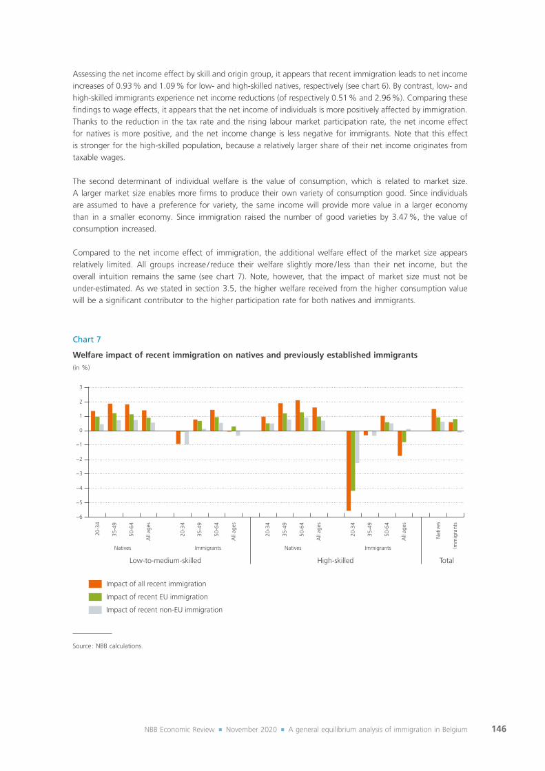
146NBB Economic Review ¡ November 2020 ¡ A general equilibrium analysis of immigration in Belgium
Assessing the net income effect by skill and origin group, it appears that recent immigration leads to net income increases of 0.93 % and 1.09 % for low‑ and high‑skilled natives, respectively (see chart 6). By contrast, low‑ and high‑skilled immigrants experience net income reductions (of respectively 0.51 % and 2.96 %). Comparing these findings to wage effects, it appears that the net income of individuals is more positively affected by immigration. Thanks to the reduction in the tax rate and the rising labour market participation rate, the net income effect for natives is more positive, and the net income change is less negative for immigrants. Note that this effect is stronger for the high‑skilled population, because a relatively larger share of their net income originates from taxable wages.
The second determinant of individual welfare is the value of consumption, which is related to market size. A larger market size enables more firms to produce their own variety of consumption good. Since individuals are assumed to have a preference for variety, the same income will provide more value in a larger economy than in a smaller economy. Since immigration raised the number of good varieties by 3.47 %, the value of consumption increased.
Compared to the net income effect of immigration, the additional welfare effect of the market size appears relatively limited. All groups increase / reduce their welfare slightly more / less than their net income, but the overall intuition remains the same (see chart 7). Note, however, that the impact of market size must not be under‑estimated. As we stated in section 3.5, the higher welfare received from the higher consumption value will be a significant contributor to the higher participation rate for both natives and immigrants.
Chart 7
Welfare impact of recent immigration on natives and previously established immigrants(in %)
−6
−5
−4
−3
−2
−1
0
1
2
3
20-3
4
35-4
9
50-6
4
All
ages
20-3
4
35-4
9
50-6
4
All
ages
20-3
4
35-4
9
50-6
4
All
ages
20-3
4
35-4
9
50-6
4
All
ages
Nat
ives
Imm
igra
nts
Impact of recent non-EU immigration
Impact of recent EU immigration
Impact of all recent immigration
Low-to-medium-skilled
Natives Immigrants
High-skilled
Natives Immigrants
Total
Source : NBB calculations.

147NBB Economic Review ¡ November 2020 ¡ A general equilibrium analysis of immigration in Belgium
3.7 Conclusion
Overall, recent immigration appears to have had a positive economic impact in Belgium. In line with the literature on the wage effects of immigration, some groups of individuals end up with a lower wage – mainly high‑skilled workers, those aged 20‑34 and immigrants. However, the public finance effect of immigration ensures that most individuals end up with a higher net wage thanks to immigration. Following the findings of Aubry et al. (2016), this effect is reinforced by the market size effect of immigration, which leads to more positive welfare effects for natives and immigrants. The impact of immigration of unemployment appears to be small, as a result of the counteracting effects of a declining wage‑to‑productivity ratio and an increasing average separation rate, highlighted in Battisti et al. (2018). All natives end up being better off as a result of immigration, and among low‑to‑medium‑skilled immigrants only the group aged 20‑34 is worse off. High‑skilled immigrants aged 20‑34 bear the brunt of the welfare loss, primarily driven by large wage cuts.
Finally, when assessing the inflow of EU and non‑EU immigrants separately, it appears that both inflows end up positively affects the welfare of all natives. However, because the share of high‑skilled individuals among recent non‑EU immigrants is lower than among EU immigrants, the welfare effect of recent non‑EU immigration will be less positive for low‑to‑medium‑skilled natives than the effect of recent EU immigration. In return, the negative effect on high‑skilled immigrants will also be weaker.
4. The influence of parameters, assumptions and the theoretical framework
The general equilibrium model shows that recent immigration has had an overall positive economic impact in Belgium. To improve the reliability of the findings, the first section performs robustness checks regarding the parameter values used in the reference model. Section 4.2 then discusses the impact of assumptions on the model outcomes and section 4.3 assesses the potential effect of impact channels which are absent in the model economy (e.g. discrimination or productivity).
4.1 Robustness checks
Although the general equilibrium model is built to reflect the Belgian economy, it remains an imperfect representation of reality. For example, the parameter values used in the above‑mentioned model are only estimates of the true behaviour of actors in the model. To avoid excessive reliance on these parameter values, this section compares the economic impact of recent immigration using several sets of exogenous parameters.
More specifically, three alternative sets of parameters will be compared to the baseline (see table 2). The first set strengthens the elasticity of labour supply to the expected income from labour (see table 3). This implies that wage or tax changes have a stronger impact on the labour market participation of individuals. The second set strengthens the elasticity of substitution between age and origin groups, thereby limiting the relative productivity and wage impact of immigration (see table 4). The third set strengthens the elasticity of substitution between goods, essentially removing the market size impact on welfare of individuals (see table 5). Finally, a fourth set of exogenous parameters, standardising the parameters governing the frictional labour market, has been assessed. However, because recent immigration only showed a negligible impact on unemployment in the baseline model and this is not different using this set of parameters, it will not be discussed separately.
Following recent literature on the estimation of the elasticity of labour supply to labour income, the consensus value of the elasticity is higher than the estimate for Belgium used in the model. More precisely,

148NBB Economic Review ¡ November 2020 ¡ A general equilibrium analysis of immigration in Belgium
the consensus elasticity has been found to be around 0.5 to 1 (e.g. Chetty et al., 2011 ; Rogerson and Wallenius, 2013). Using an elasticity of labour supply equal to 0.5, the impact of recent immigration on wages and unemployment appears to be similar to the baseline parametrisation. By contrast, the stronger elasticity of labour supply to labour income implies that the participation effect of recent immigration will be higher for both natives and immigrants. Consequently, the tax base increases relatively strongly and the tax rate comes down more sharply than in the baseline scenario. When using the consensus elasticities of labour supply to labour income, the income and welfare effects of immigration will thus be more positive than in the baseline scenario.
Alternatively, inserting stronger elasticities of substitution between age and origin groups, the overall welfare effect of recent immigration declines. However, unlike the first set of alternative parameters where both immigrants and natives experience lower welfare standards, the welfare of immigrants appears to increase more strongly than in the baseline model. A different mechanism thus appears behind the lower welfare in this iteration of the model. Looking at the wage change because of immigration, the stronger elasticities of substitution appear to significantly reduce the positive wage impact on natives. In return, the wages of immigrants fall less sharply. Thanks to the reduction of the tax rate, which remains close to the baseline reduction, participation of natives is only slightly lower than in the baseline parametrisation, while it increases more strongly for immigrants. So, using stronger elasticities between age and origin groups, the welfare gains of natives (and older individuals)
Table 2
Impact of recent immigration in baseline parametrisation
Natives Previously established immigrants
Total 1
Wage (in %) 0.406 −2.022 −0.069
Participation (pp) 0.292 −0.053 0.158
Unemployment (pp) −0.025 −0.073 0.199
Income (in %) 1.003 0.243 0.686
Welfare (in %) 1.498 0.587 1.154
Tax rate (pp) −0.599
Source : NBB calculations.1 Including recent immigrants
Table 3
Impact of recent immigration with a stronger elasticity of labour supply
Natives Previously established immigrants
Total 1
Wage (in %) 0.375 −2.004 −0.092
Participation (pp) 1.098 0.227 0.868
Unemployment (pp) −0.073 −0.178 0.141
Income (in %) 0.800 0.158 0.502
Welfare (in %) 2.467 1.079 2.043
Tax rate (pp) −1.113
Source : NBB calculations.1 Including recent immigrants
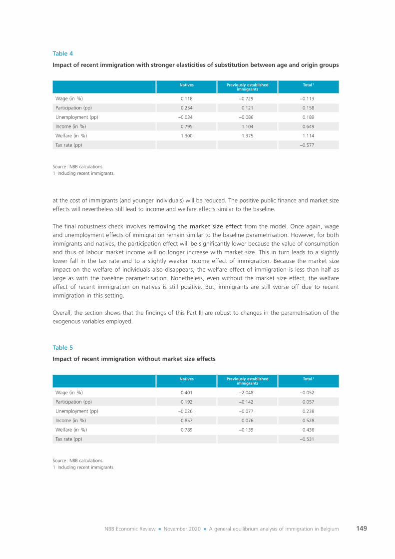
149NBB Economic Review ¡ November 2020 ¡ A general equilibrium analysis of immigration in Belgium
at the cost of immigrants (and younger individuals) will be reduced. The positive public finance and market size effects will nevertheless still lead to income and welfare effects similar to the baseline.
The final robustness check involves removing the market size effect from the model. Once again, wage and unemployment effects of immigration remain similar to the baseline parametrisation. However, for both immigrants and natives, the participation effect will be significantly lower because the value of consumption and thus of labour market income will no longer increase with market size. This in turn leads to a slightly lower fall in the tax rate and to a slightly weaker income effect of immigration. Because the market size impact on the welfare of individuals also disappears, the welfare effect of immigration is less than half as large as with the baseline parametrisation. Nonetheless, even without the market size effect, the welfare effect of recent immigration on natives is still positive. But, immigrants are still worse off due to recent immigration in this setting.
Overall, the section shows that the findings of this Part III are robust to changes in the parametrisation of the exogenous variables employed.
Table 4
Impact of recent immigration with stronger elasticities of substitution between age and origin groups
Natives Previously established immigrants
Total 1
Wage (in %) 0.118 −0.729 −0.113
Participation (pp) 0.254 0.121 0.158
Unemployment (pp) −0.034 −0.086 0.189
Income (in %) 0.795 1.104 0.649
Welfare (in %) 1.300 1.375 1.114
Tax rate (pp) −0.577
Source : NBB calculations.1 Including recent immigrants.
Table 5
Impact of recent immigration without market size effects
Natives Previously established immigrants
Total 1
Wage (in %) 0.401 −2.048 −0.052
Participation (pp) 0.192 −0.142 0.057
Unemployment (pp) −0.026 −0.077 0.238
Income (in %) 0.857 0.076 0.528
Welfare (in %) 0.789 −0.139 0.436
Tax rate (pp) −0.531
Source : NBB calculations.1 Including recent immigrants

150NBB Economic Review ¡ November 2020 ¡ A general equilibrium analysis of immigration in Belgium
4.2 Assumptions
In the presented model of the Belgian economy, we disregard other countries. The way immigration alters trade and investment flows between countries and its impact on the economy could therefore not be modelled. Trade and investment links between countries is more thoroughly discussed in section 4.3 as an element of the productivity impact of immigration.
A second assumption of the model is perfectly mobile capital. This implies that capital will immediately flow to places where the highest return can be achieved, immediately depressing it. This essentially leads to constant returns to capital, because the capital stock immediately adapts to any changes in the stock of other production factors such as labour. This is found to the be most likely assumption according to e.g. Ottaviano and Peri (2012) in the US. In Belgium, being a small open economy, this assumption is even more likely to hold. If capital is imperfectly mobile, the distinction between a short‑ and long‑run effect could be made. Because of a shortage of capital in the short run, labour will not be optimally productive, leading to a negative effect in the short run. As capital stocks adapt to the labour supply in the long run, this negative effect disappears.
Third, the labour market is assumed to be perfectly competitive, which implies that wage differences in the model are perfectly attributable to productivity differences. However, there is ample evidence of labour market discrimination against immigrants (see section 2.5 of Part II). This is the case in the selection process for potential employees (Baert et al., 2015) as well as in the wage earned of employed workers with the same productivity level (Solé and Parella, 2003 ; Harris et al., 2006). Since our model is calibrated on the observed wage differences between immigrants and natives, the actual productivity gap is over‑estimated, as is immigrants’ disutility of entering the labour market and their separation rate. Nonetheless, assuming discrimination remains stable over time, the outcomes should remain representative for the Belgian economy. However, it is important to bear in mind that the model under‑estimates the productivity of immigrants, and that reducing discrimination in the selection process is also a factor with potential to improve the economic performance of immigrants.
Fourth, our model imposes a flat income tax rate. Should taxation be progressive instead, government revenues would depend relatively more on high‑skilled incomes. As the recent wave of immigrants is more often high‑skilled than the native average, recent immigration would even further increase government incomes under progressive taxation. Through redistribution, higher government revenue would also imply higher native incomes.
Another assumption that could have a big impact on the findings of the model is its static nature. As the complementarity between groups of individuals is fixed by exogenous parameters, individuals are assumed to never change their skill set. However, empirical evidence shows that an immigrant inflow in European economies leads to native occupational shifts from manual jobs to more complex jobs (D’Amuri and Peri, 2010 ; Cattaneo et al., 2015). Consequently, immigration has positive effects on native low skilled wages, employment and occupational mobility (Foged and Peri, 2016). Low‑skilled natives are thus clearly found to adapt their skill set to become more complementary to the inflow of immigrants. In the same vein, it is quite likely that immigrants will adapt their skill set to better resemble the skills of natives over time (e.g. language classes). Note that the report makes use of a five‑year immigration shock, which is deemed sufficiently short to accept the assumption.
4.3 Alternative impact channels
On top of alternative impact channels of immigration mentioned above, there are a couple of additional mechanisms that are not directly related to assumptions made in the model. For example, there is ample evidence that immigration leads to increases in productivity measured as GDP (Sparber, 2008 ; Sparber, 2010), patents (Hunt and Gauthier‑Loiselle, 2010 ; Parrota et al., 2012 ; Koppel et al., 2018) or product innovation (Khanna and Lee, 2019). Several channels have been suggested through which immigration boosts productivity.

151NBB Economic Review ¡ November 2020 ¡ A general equilibrium analysis of immigration in Belgium
On the one hand, diasporic networks lead to an enhanced dispersion of knowledge, so researchers encounter more ideas, challenging and improving their own views. On the other hand, diverse teams are better at problem‑solving than homogenous teams. Cognitive diversity – a variety of ways of thinking, knowledge, skills, experiences and values – can play an important role in knowledge intensive environments (Van der Vegt and Janssen, 2003 ; Fujita and Weber, 2004). Note that immigrants are not per se more innovative than the native population. Their knowledge simply leads to positive externalities, improving native research as well (Ganguli, 2015 ; Freeman and Huang, 2015). Although sectors employing low skilled labour benefit less from a diversity of employees, the positive productivity effect is not exclusively attributable to high skill sectors only (Suedekum et al., 2014).
Immigration can also make significant contributions to productivity through the enhancement of international trade and investment. Knowing the context of far‑away investment opportunities may take away uncertainties regarding foreign direct investment, leading to a more efficient use of available capital. The empirical literature confirms that investment is positively correlated to immigration. Immigration leads to a significant increase in venture capital investment (Leblang, 2011 ; Pandya and Leblang, 2011). The fact that skilled diasporic groups appear to be an important indicator predicting future investment flows (Kugler and Rapoport, 2007) further supports this hypothesis.
Several studies show that a larger share of immigrants in professional jobs significantly increases trade (e.g. Piperakis et al., 2003 ; Sgrignoli et al., 2015). However, the origin of the immigrants in questions appears to have an important impact in this regard. Only immigrants originating from a region which is sufficiently different with respect to culture contribute to the trade creation (Girma and Yu, 2002 ; Peri and Requena‑Silvente, 2010). Immigrants importing goods from their home country – home bias – and reductions in the information and communication costs of trade appear to contribute equally to the trade creation (Felbermayr and Toubal, 2012).
Finally, immigration has a non‑negligible impact on the size of the population. While our model does not take into account space constraints on production, the number of housing units or transport (especially at peak hours), these are effectively constrained by the available space in a country. Empirical estimates do find that immigration leads to rising housing prices (Saiz, 2007) and congestion (Tsang and Rohr, 2011), which have an overall negative effect on the welfare of inhabitants.
Overall, alternative impact channels such as international trade and investment or productivity effects of immigration should have a positive effect on the economic impact of immigration. Moreover, relaxing assumptions (i.e. allowing natives to optimise their skill set to complement immigrants after an inflow of new immigrants or imposing a progressive tax rate) should also increase the positive economic effects of immigration obtained by the model. As long as immigration does not push the population size to the limit of its space constraints, the model outcomes should therefore be viewed as lower‑bound estimates of the economic impact of immigration.
5. Conclusion
This third part of the report has developed a general equilibrium model to measure the impact of immigration on the Belgian economy. The model was tailored to the Belgian economy by means of calibration and a baseline equilibrium was determined based on the economic situation in 2017. To assess the impact of immigration, the baseline scenario is constructed by taking the situation in the same year after removing immigrants who arrived in Belgium in the last five years. Next, the economic impact of several hypothetic recent immigration inflows is computed by comparing the baseline with the scenario where all immigrants arrived or only (non‑)EU immigrants entered Belgium.
Demographically, recent immigration has led to a population growth of 2.7 %. The inflow has consisted primarily of young individuals, and recent immigrants are also slightly more likely to be high skilled than the

152NBB Economic Review ¡ November 2020 ¡ A general equilibrium analysis of immigration in Belgium
population in Belgium. The latter is true for the recent inflow of EU immigrants, but to a lesser extent for non‑EU immigrants as well.
Following the principles of complementarity and substitution over skill, age and origin in the production function, the more ample labour supply of young, high‑skilled immigrants leads to higher labour demand and wages for complementary labour (i.e. low‑to‑medium‑skilled, older and native individuals), while depressing the wages of more substitutable labour.
However, the inclusion of the public finance impact of immigration reveals an important addition to the wage effect of immigration. Since the tax base increases more sharply than government expenditure as a result of recent immigration, and the government is assumed to be keeping a balanced budget, the income tax rate comes down. This leads to a positive net income effect for all working individuals, reducing or reverting the net wage cut for individuals substitutable to recent immigrants and pushing up the net wage of complementary individuals.
Moreover, immigration leads to a bigger economy. Thanks to the related wider variety of consumption goods, the welfare derived from the net income increases. Minor net income reductions are mitigated in terms of welfare effects, while the welfare increase of individuals gaining net income from recent immigration is reinforced.
Because the expected welfare of participating in the labour market changes, the participation rates change accordingly, attenuating the wage effect. People losing net income (i.e. low‑to‑medium‑skilled immigrants aged 20‑34 years and high‑skilled immigrants aged 20‑49 years) reduce participation, while people seeing their net income grow step up participation. Even though the vast majority of the population increases their participation on the labour market, the aggregate participation change remains close to zero. This is driven by the higher share of immigrants in the population who, although their participation increases on average, still have a significantly lower participation rate than that of natives.
In contrast, unemployment among workers appears to change only marginally as a result of recent immigration, because of the counteracting effect of the higher separation rate and the lower wage cost of immigrants.
Overall, the wage effect of immigration is the main driver of heterogeneous effects of immigration between individuals. Public finance and market size effects then drive the positive income and welfare effects of immigration, while labour market participation primarily serves as an attenuating factor. The unemployment effect of immigration appears limited in this model. Importantly, these findings are robust for changes in the value of exogenous parameters. Although the precise value of the wage, income or welfare changes differs, the interpretation of the outcomes is similar.
Finally, alternative impact channels such as productivity, innovation or barriers to international trade and investment are likely to also likely to provide a positive estimated economic impact of immigration. Relaxing assumptions (i.e. allowing natives to optimise their skill set to complement immigrants after an inflow of new immigrants or imposing a progressive tax rate) should also increase the positive economic effects of immigration obtained by the model. As long as immigration does not push the population size to the limit of its space constraints, the results presented here should therefore be viewed as a lower bound for the economic impact of immigration in Belgium.

153NBB Economic Review ¡ November 2020 ¡ Annexes
Annexes

154NBB Economic Review ¡ November 2020 ¡ Common annexes
Common annexes
Annex 1 International labour mobility : posted workers
Migration is not the only way an economy has to use foreign labour on its soil. Employees can work under regular fixed‑term or temporary contracts in a country but are recognised as residing in another neighbouring EU Member State. These are the cross‑border workers : 52 000 people from France, Germany, the Grand‑Duchy of Luxembourg and the Netherlands were working in Belgium in 2019 and 94 000 Belgian residents were working in these countries. Other foreign workers are present in the territory on a temporary basis, to meet specific labour needs. This temporary migration notably includes seasonal workers (22,000) and posted workers (260 000). They are registered as residents in Belgium, only if the employment and stay in Belgium exceeds 90 days, which is rarely the case. Most of them are therefore not recorded in the National Register nor in the CBSS database.
Regarding posted workers, they are not even recorded in Belgian employment statistics. Indeed, salaried or self‑employed, they are only supposed to provide a service on a temporary basis in Belgium. They are still recorded in the labour force of their home country. Rules to hire posted workers are defined at EU level. In order to avoid unfair competition in the host country, posted workers are entitled to the same working conditions and remuneration as local workers, unless conditions in their home country are more favourable.
The use of posted workers has grown strongly over time. According to NSSO figures based on Limosa forms, they were 88 863 in 2007, but no less than 257 728 1 in 2019 2, which is equivalent to 5 % of domestic employment. One‑third of them were working for the no further specified “Other branch”, 30 % in construction, 10 % in transport and distribution, another 10 % in metalworking, 5 % in electrical installation works and 3 % in petrochemicals. The jobs of posted workers in Belgium are by their nature temporary and could not necessarily have been carried out by resident workers.
From year to year the countries of origin of employers of posted employees or posted self‑employed are broadly the same. We find (figures in brackets correspond to 2019 data) : the Netherlands (24 %), Poland (17 %), Germany (9 %), Portugal (7 %), France, (7 %) and Romania (6 %). It should be pointed out that the country of origin of the employer does not necessarily correspond to the nationality of the posted worker.
On the basis of European A1 statistics 3, Belgium emerges as the third most important destination country for posted workers after Germany and France, but ahead of the Netherlands and Austria. The same statistical source shows that Belgium also sends its workers abroad under posting contracts. In 2018, this concerned 38 000 people.
1 224,638 employees and 36,747 self‑employed persons.2 During the first 6 months of 2020, no less than 177,518 were recorded.3 De Wispelaere et al. (2019)

155NBB Economic Review ¡ November 2020 ¡ Common annexes
Annex 2 List of countries for each country of birth category
EU14 : Austria, Denmark, Finland, France, Germany, Greece, Ireland, Italy, Luxembourg, the Netherlands, Portugal, Sweden Spain, United Kingdom.
EU13 : Bulgaria, Cyprus, Croatia, Czech Republic, Estonia, Hungary, Latvia, Lithuania, Malta, Poland, Romania, Slovakia, Slovenia.
EU candidates : Albania, Former Yugoslav Republic of Macedonia, Montenegro, Turkey.
Other European countries : Andorra, Belarus, Bosnia‑Herzegovina, Holy See, Iceland, Liechtenstein, Moldova, Monaco, Norway, Russia, San Marino, Serbia, Switzerland, Ukraine, etc.
Maghreb : Algeria, Libya, Mauritania, Morocco, Tunisia.
Sub-Saharan Africa : Burundi, Cameroon, Congo, Rwanda, Senegal, South Africa etc.
Near and Middle East : Afghanistan, Bahrain, Egypt, Iran, Iraq, Israel, Jordan, Kuwait, Lebanon, Oman, Pakistan, Palestinian Territories, Qatar, Saudi Arabia, Syria, United Arab Emirates, Yemen.
Oceania, Far East : Australia, China, India, Japan, New Zealand, South Korea, Taiwan.
Other Asian countries : Cambodia, Indonesia, Malaysia, Nepal, Philippines, Sri Lanka, Thailand, Vietnam, etc.
North America : Canada, United States
Latin America : Argentina, Bolivia, Brazil, Chile, Colombia, Cuba, Ecuador, Guatemala, Mexico, Nicaragua, Peru, Venezuela, etc.

156NBB Economic Review ¡ November 2020 ¡ Annexes Part I
Annexes Part I Immigration and public finances
Annex I.1 Methodological aspects of the analysis of net transfers
The main specific database used for the study consists of extracts from CBSS (Crossroads Bank for Social Security) database(s). A number of extracts, reflecting social transfers and income from work for different population groups, have been obtained specifically for the public finance part of the study. Other extracts, have been obtained for other parts of the study. In each of these extracts, variables of interest, such as family allowances for instance, are computed as averages for different groups of the population. They are expressed as an average amount per person in the group, in euro per year. Although the source database covers all residents for Belgium, for privacy reasons the extracts do not present data at the individual level – it is not a pure “micro” database. It is only possible to combine the extracts using common variables defining the sub‑groups of the population, such as age and country of birth for instance. Extracts also include demographics data, i.e. number of individuals in each group.
At the most detailed level, population groups are defined by the following 11 variables : Gender, Region, Age group, Nationality, Country of Birth, Country of Birth of the Mother, Country of Birth of the Father, Migration channel, Length of stay, Socio‑economic position (in employment or not), Education.
The extracts from the CBSS database include the following variables for the social transfers : family allowances, unemployment benefits, pensions, social assistance (allocation de remplacement de revenus, allocation d’intégration, aide aux personnes âgées, revenu d’intégration sociale), and sickness benefits (incapacity for work, work‑related accident and occupational diseases). Data for health care costs by age categories from INAMI have also been used.
There is no information on taxes, and only partial information on social contributions in the CBSS extracts. These items have been estimated based on information on income from work (see next section). The database includes the following incomes : income from self‑employment, income of employees and income of public sector employees.
The next sections provide more detailed information on the methodology used to estimate transfers paid by individuals to the government, i.e. personal income tax, social contributions, and consumption tax.
For the analysis, the different items (transfers paid and received) have been scaled using corresponding statistics from the general governments statistics that are part of the national accounts. In other words, the estimated items, as well as the items directly obtained from the CBSS Database, are used as distribution keys to allocate the statistics to the different groups of the population (see chapter 2 of Part I).
A. Estimation of personal income taxes
Personal income taxes are not available from the BCSS database. They have been estimated using adapted tax functions. Firstly, a fiscal and parafiscal simulation module for 2016 has been used to define average taxes rates for each income level and in the case of 0, 1, 2, 3, 4, or 5 dependent children. Secondly, the tax functions have been adapted to correct for an aggregation bias. As the available information on incomes are averages, it conceals the real distribution of incomes around the average and this is not neutral because the tax functions are not linear (see below for additional information). Thirdly, the average number of dependent children in each group has been estimated based on the amount of family allowance received by the group compared to the theoretical average amount per child. And finally, combining average income, the estimated number of children,

157NBB Economic Review ¡ November 2020 ¡ Annexes Part I
and the corresponding adapted tax functions, it has been possible to estimate the income tax paid per person per year by each sub‑group (5 children was assumed in case there was more than 5 children).
The fiscal and parafiscal simulation module used to construct the tax functions is simplified because it does not account for the many special cases. For example, personal income tax expenditure regimes (deductions related to mortgages for owner occupied dwellings, deductions for second and third pillar pension savings, waiver for research, etc.) are not taken into account. The same applies to the specific expatriate personal income tax scheme for example. Moreover, the database does not include information on company cars and group insurances.
The need for a correction of the initial tax functions to account for the potential aggregation bias can be illustrated by an example. At an average income of 800 euros / month the tax functions imply a zero tax rate. If all individuals in the group have that same income, then the zero rate is correct for the group. However most often the income level of the different individuals in the group will differ to some degree. If a uniform distribution of income around 800 euros / month is assumed for a group, a share of the group will have a higher income and hence a tax rate higher than zero. After averaging all the individual tax rates, a higher average (corrected) tax rate is obtained in this specific case. The opposite can be true at other income levels, depending on the form of the initial tax functions. The adapted tax functions have been constructed assuming a uniform distribution of income around the average plus / minus approximately one standard deviation. The result is a more realistic “adapted” tax function.
B. Estimation of employer’s social contributions
The employer’s social contributions are not available from the CBSS database. To estimate these a similar approach was used as for the personal income tax estimates. Firstly, a fiscal and parafiscal simulation module for 2016 has been used to define average contribution rates for each income level. Secondly, the tax functions have been adapted to correct for an aggregation bias. And finally, combining average income and the corresponding adapted contribution rate function, it has been possible to estimate the employer’s social contributions paid per person per year by each sub‑group.
The fiscal and parafiscal simulation module used to construct the function is simplified because it does not account for the many special cases. Targeted and general social insurance contribution relief measures are not taken into account for instance.
C. Employee’s social contributions
Employee’s social contributions are directly computed on the basis of the information provided in the BCSS database. It as obtained as the difference between gross taxable income and gross income.
D. Estimation of social contributions of self-employed
For self‑employed there is no information on social contributions in the database. In order to estimate social contributions of self‑employed, a simplified uniform contribution rate is assumed. It is based on macroeconomic data, dividing the total revenue from social contributions by total income of self‑employed.
E. Estimation of consumption taxes
To estimate consumption taxes, i.e. VAT and excise duties, various data sources has to be combined. Three steps are needed. Firstly, the share of indirect taxes in total consumption of a group has to be computed. In order to

158NBB Economic Review ¡ November 2020 ¡ Annexes Part I
do so, Statbel used information from the Households budget survey to provide consumption profiles by group, by VAT rate and for the different categories of excise duties. Next, VAT rates are used to compute the share of indirect taxes in consumption. The same is done for excise duties, using information on the share of excise duties in average prices of the selected items derived from CPI statistics.
Secondly, consumption by group has to be computed based on income data in a broad sense (including transfers received) from the CBSS database. To obtain an average propensity to consume, information on saving rates are needed. Saving rates by age groups have been taken form experimental data from Eurostat. These have been extrapolated from 4 age groups to the age groups categories in the database.
In a last step, the two previous results – i.e. average consumption spending by person and by group, and group specific shares of taxes – are combined to obtain average consumption tax paid by person for the different groups. This has been done by age groups – the same for the different origins. This is clearly a second‑best solution. In fact, consumption and savings are to a much larger extent linked to income levels. However, in this exercise the available data has not made it possible to combine CBSS data and other sources based on income levels, using income deciles for example.

159NBB Economic Review ¡ November 2020 ¡ Annexes Part I
Annex I.2 Decomposition of the differences in net transfers between natives and non-natives
Following Chojnick et al. 2018 (Appendix F.2. Pages 76‑78), it is possible to make a breakdown (along the lines of Benet, 1920) of the difference between the per capita contributions of natives and non‑natives.
The table below shows the results of this breakdown. The largest part of the difference between the average per capita contribution of natives and immigrants, which amounts to € 2.281, is due to differences between natives and immigrants in the population aged 20‑65 (€ 4.222). It is the tax component that weighs most heavily in this difference (€ 5.592), while the demographic component is negative (€ –1.370). The rest of the difference (€ –1.941) stems from dissimilarities between the other individuals (the young and the elderly), which stem almost entirely from their different shares in their population of origin (€ –1.889), while their individual contributions play only a very secondary role (€ –52).
This decomposition therefore confirms the predominant role of differences in net transfers between the working population. If this factor is broken down further, it appears that it is essentially the differences in transfers from individuals to the government, i.e. contributions through taxes and social contributions, that explain the observed difference.
Decomposition of the gap between the per capita contribution of natives and immigrants
Total Difference attributable to
Individuals between 20 and 64 years old
Other individuals
Decomposition of the gap between the per capita contribution 2 281 4 222 −1 941
Demographic component −3 259 −1 370 −1 889
Fiscal component 5 540 5 592 −52
Decomposition of the fiscal component
Tax component 5 912 5 784 128
Transfer component −372 −192 −181
Sources : NBB calculations.

160NBB Economic Review ¡ November 2020 ¡ Annexes Part II
Annex II.1
The labour market integration of immigrants : Incidence of personal characteristics by origin
Table 1.1
Probit regression of the employment probability by origin(marginal effect 1 coefficients multiplied by 100 (can be interpreted as a percentage point variation in the probability) and predicted probabilities in percent, people aged between 20 and 64 years, annual data from 2009 to 2016, year fixed‑effect estimation)
Natives First‑generation immigrants
Second‑generation immigrants
Coefficient Predicted probability
Coefficient Predicted probability
Coefficient Predicted probability
GenderMen Ref 71.2 Ref 53.3 Ref 60.3Women −4.9 66.3 −9.7 43.6 −6.9 53.3
Region of residenceBrussels Ref 59.7 Ref 42.9 Ref 51.4Flanders 13.8 73.5 11.6 54.5 11.7 63.1Wallonia 0.3 60.0 0.0 43.0 2.4 53.8
Age20‑24 Ref 58.7 Ref 36.9 Ref 45.525‑29 21.6 80.3 14.8 51.7 19.2 64.630‑34 19.2 77.9 16.6 53.5 17.8 63.335‑39 14.9 73.6 17.4 54.3 15.5 61.040‑44 12.8 71.5 18.0 54.9 15.2 60.645‑49 11.3 70.0 16.3 53.2 14.0 59.550‑54 5.2 63.9 9.9 46.8 8.1 53.655‑59 −13.2 45.5 −3.1 33.8 −9.4 36.160‑64 −37.0 21.7 −17.5 19.4 −28.6 16.8
Level of educationHigh educated Ref 78.8 Ref 55.3 Ref 70.6Middle educated −10.9 67.9 −1.4 53.9 −13.1 57.5Low educated −28.1 50.7 −13.7 41.6 −28.3 42.3
Type of householdSingle without children Ref 64.1 Ref 42.8 Ref 51.0Married with children 14.3 78.4 9.6 52.4 12.4 63.4Married without children 10.0 74.1 8.4 51.2 15.6 66.6Unmarried couple with children 13.0 77.1 11.3 54.2 18.5 69.4Unmarried couple without children 17 81.1 15.6 58.4 22.3 73.3Single with children 1.9 66.0 2.5 45.3 0.5 51.5Children living with their parents −12.7 51.4 −4.5 38.3 −4.9 46.1Other 0.9 65.0 1.6 44.5 5.0 55.9
Detailed originEU14 Ref 55.7EU13 1.4 57.2Other European countries −13.2 42.5EU candidates −13.2 42.5Maghreb −13.6 42.1Near and Middle East −18.7 37.0North America −4.0 51.7Oceania and Far East −2.8 53.0Latin America −4.7 51.0Sub‑saharan Africa −9.3 46.4Other Asian countries −1.8 53.9
EU Ref 59.9Non‑EU −7.1 52.8
Sources : CBSS Datawarehouse, NBB calculations.Note : given the almost exhaustivity of the database, all coefficients are significant at 99 % so that to simplify the table,
we do not put the usual *** and standard errors.1 The marginal effects have been calculated holding all other variables constant at their average level.
Annexes Part II The labour market integration of first- and second-generation immigrants

161NBB Economic Review ¡ November 2020 ¡ Annexes Part II
Table 1.2
Probit regression of the participation probability by origin(marginal effect 1 coefficients multiplied by 100 (can be interpreted as a percentage point variation in the probability) and predicted probabilities in percent, people aged between 20 and 64 years, annual data from 2009 to 2016, year fixed‑effect estimations)
Natives First‑generation immigrants
Second‑generation immigrants
Coefficient Predicted probability
Coefficient Predicted probability
Coefficient Predicted probability
GenderMen Ref 81.8 Ref 71.4 Ref 76.5Women −4.4 77.3 −12.6 58.7 −6.3 70.3
Region of residenceBrussels Ref 76.6 Ref 63.7 Ref 73.4Flanders 4.8 81.4 4.4 68.1 1.0 74.5Wallonia −0.4 76.1 −2.7 61.1 −0.8 72.6
Age20‑24 Ref 66.0 Ref 46.3 Ref 58.725‑29 21.7 87.7 18.0 64.4 21.4 80.030‑34 20.5 86.5 21.2 67.6 21.1 79.735‑39 17.6 83.6 23.0 69.3 18.7 77.440‑44 15.9 81.9 24.6 70.9 17.7 76.445‑49 15.1 81.1 25.0 71.3 16.6 75.350‑54 14.9 81.0 25.1 71.4 16.8 75.455‑59 6.8 72.9 21.2 67.5 9.8 68.560‑64 −35.9 30.1 −15.2 31.1 −32.1 26.6
Level of educationHigh educated Ref 84.5 Ref 66.8 Ref 78.4Middle educated −4.7 79.8 5.6 72.4 −3.3 75.1Low educated −15.4 69.1 −6.2 60.6 −12.6 65.8
Type of householdSingle without children Ref 80.5 Ref 63.3 Ref 74.6Married with children 4.4 84.9 4.1 67.4 2.3 77.0Married without children 2.5 83.0 1.6 64.9 6.5 81.1Unmarried couple with children 4.8 85.3 6.9 70.2 7.1 81.7Unmarried couple without children 8.5 89.0 9.4 72.7 10.4 85.1Single with children 0.5 81.0 4.6 67.9 0.2 74.9Children living with their parents −17.6 62.9 −9.3 54.0 −13.4 61.2Other −4.1 76.4 −5.6 57.7 −3.5 71.1
Detailed originEU14 Ref 71.6EU13 −1.6 70.1Other European countries −12.2 59.4EU candidates −7.8 63.8Maghreb −9.1 62.5Near and Middle East −21.1 50.6North America −6.5 65.1Oceania and Far East −4.3 67.3Latin America −5.9 65.7Sub‑saharan Africa −9.9 61.8Other Asian countries −5.2 66.4
EU Ref 75.1Non‑EU −3.8 71.3
Sources : CBSS Datawarehouse, NBB calculations.Note : given the almost exhaustivity of the database, all coefficients are significant at 99 % so that to simplify the table,
we do not put the usual *** and standard errors.1 The marginal effects have been calculated holding all other variables constant at their average level.

162NBB Economic Review ¡ November 2020 ¡ Annexes Part II
Table 1.3
Probit regression of the employment probability by origin and gender(marginal effect 1 coefficients multiplied by 100 (can be interpreted as a percentage point variation in the probability), people aged between 20 and 64 years, annual data from 2009 to 2016, year fixed‑effect estimations)
Natives First‑generation immigrants
Second‑generation immigrants
Men Women Men Women Men Women
Region of residenceBrussels Ref Ref Ref Ref Ref RefFlanders 13.3 14.3 11.5 11.8 10.7 12.8Wallonia −0.2 0.8 −0.6 0.9 1.6 3.3
Age20‑24 Ref Ref Ref Ref Ref Ref25‑29 20.8 22.7 14.3 15.5 18.6 20.430‑34 17.8 21.0 15.4 18.0 16.2 20.335‑39 12.6 17.7 14.7 20.0 11.8 19.740‑44 9.8 16.2 13.0 22.3 9.4 20.745‑49 7.6 15.0 8.9 22.5 7.6 19.750‑54 1.3 8.4 2.0 16.3 2.0 12.655‑59 −18.2 −9.8 −10.8 2.7 −15.6 −5.460‑64 −41.2 −34.0 −24.4 −12.1 −33.4 −25.3
Level of educationHigh educated Ref Ref Ref Ref Ref RefMiddle educated −6.8 −14.3 −0.6 −1.6 −7.8 −16.5Low educated −24.8 −30.6 −12.3 −14.6 −23.5 −31.5
Type of householdSingle without children Ref Ref Ref Ref Ref RefMarried with children 22.0 5.8 18.2 −0.1 25.4 −0.5Married without children 15.9 3.3 13.3 1.7 20.8 8.2Unmarried couple with children 17.9 6.6 14.4 6.3 23.7 10.2Unmarried couple without children 18.4 13.5 14.9 13.2 23.5 17.9Single with children 6.6 −4.2 6.8 −3.9 7.1 −7.8Children living with their parents −9.0 −19.0 −4.4 −6.7 −3.1 −10.0Other 1.1 0.1 3.1 −2.0 5.6 2.3
Detailed originEU14 Ref RefEU13 3.9 −0.5Other European countries −13.6 −13.1EU candidates −9.2 −17.5Maghreb −10.1 −17.7Near and Middle East −14.2 −25.8North America −7.1 −1.4Oceania and Far East −1.2 −4.3Latin America −5.6 −4.4Sub‑saharan Africa −9.8 −8.2Other Asian countries −0.7 −2.4
EU Ref RefNon‑EU −5.5 −8.6
Sources : CBSS Datawarehouse, NBB calculations.Note : given the almost exhaustivity of the database, all coefficients are significant at 99 % so that to simplify the table,
we do not put the usual *** and standard errors.1 The marginal effects have been calculated holding all other variables constant at their average level.

163NBB Economic Review ¡ November 2020 ¡ Annexes Part II
Table 1.4
Probit regression of the participation probability by origin and gender(marginal effect 1 coefficients multiplied by 100 (can be interpreted as a percentage point variation in the probability), people aged between 20 and 64 years, annual data from 2009 to 2016, year fixed‑effect estimations)
Natives First‑generation immigrants
Second‑generation immigrants
Men Women Men Women Men Women
Region of residenceBrussels Ref Ref Ref Ref Ref RefFlanders 4.5 5.0 3.8 5.0 0.6 1.4Wallonia −0.3 −0.6 −2.9 −2.3 −0.9 −0.8
Age20‑24 Ref Ref Ref Ref Ref Ref25‑29 21.1 22.2 17.2 18.9 20.4 22.630‑34 20.1 20.9 20.1 22.6 20.3 22.135‑39 17.0 18.2 21.1 24.7 17.1 20.440‑44 15.1 16.8 21.3 27.2 15.1 20.145‑49 14.3 16.0 20.4 28.3 13.7 18.950‑54 13.9 15.7 20.2 28.3 13.9 18.655‑59 2.7 9.9 14.9 25.7 3.6 14.360‑64 −40.3 −32.3 −23.7 −7.2 −37.6 −27.8
Level of educationHigh educated Ref Ref Ref Ref Ref RefMiddle educated −0.9 −7.9 6.3 5.7 1.5 −6.4Low educated −11 −19.4 −2.4 −9.3 −6.9 −17.2
Type of householdSingle without children Ref Ref Ref Ref Ref RefMarried with children 9.2 −0.2 11.4 −4 11.5 −6.1Married without children 4.2 0.3 4.2 −2.3 8.5 3.0Unmarried couple with children 8.0 1.3 7.4 4.5 10.3 2.3Unmarried couple without children 8.9 7.0 7.8 8.4 10.9 7.9Single with children 3.3 −2.1 6.6 0.9 4.0 −4.2Children living with their parents −13.8 −23.2 −8.5 −11 −10.9 −18.2Other −4.5 −3.4 −4.5 −8.0 −3.5 −4.2
Detailed originEU14 Ref RefEU13 0.9 −3.8Other European countries −10.9 −13.7EU candidates −3.3 −12.5Maghreb −4.1 −15.0Near and Middle East −15.9 −28.2North America −8.7 −4.3Oceania and Far East −3.2 −5.8Latin America −5.8 −6.4Sub‑saharan Africa −9.1 −9.8Other Asian countries −3.8 −6.1
EU Ref RefNon‑EU −2.7 −4.7
Sources : CBSS Datawarehouse, NBB calculations.Note : given the almost exhaustivity of the database, all coefficients are significant at 99 % so that to simplify the table,
we do not put the usual *** and standard errors.1 The marginal effects have been calculated holding all other variables constant at their average level.

164NBB Economic Review ¡ November 2020 ¡ Annexes Part II
Annex II.2
The labour market integration of immigrants : Incidence of specific characteristics for first‑ and second‑generation immigrants
Table 2.1
Probit regression of the employment probability for first‑generation immigrants(marginal effect 1 coefficients multiplied by 100 (can be interpreted as a percentage point variation in the probability), people aged between 20 and 64 years, annual data from 2009 to 2016, year fixed‑effect estimation)
First‑generation immigrants
Total EU non‑EU
GenderMen Ref Ref RefWomen −9.3 −2.0 −13.9
Region of residenceBrussels Ref Ref RefFlanders 9.5 7.7 10.6Wallonia −2.2 0.2 −3.0
Age20‑24 Ref Ref Ref25‑29 10.3 11.2 9.430‑34 9.8 8.9 10.135‑39 9.0 6.6 10.140‑44 8.0 6.5 8.945‑49 5.1 5.7 4.950‑54 −2.2 −0.9 −2.355‑59 −17.2 −18.4 −13.460‑64 −31.3 −36.4 −23.6
Level of educationHigh educated Ref Ref RefMiddle educated −3.0 −4.6 −0.6Low educated −10.1 −12.3 −8.2
Type of householdSingle without children Ref Ref RefMarried with children 4.2 7.4 3.6Married without children 7.2 6.9 9.9Unmarried couple with children 5.1 7.2 4.8Unmarried couple without children 13.1 13.6 12.1Single with children −3.0 −1.8 −1.9Children living with their parents −9.7 −6.9 −9.2Other 3.8 6.5 2.9
Detailed originEU14 Ref RefEU13 1.7 2.1Other European countries −9.4 RefEU candidates −10.3 −1.9Maghreb −11.4 −2.7Near and Middle East −15.1 −6.6North America −4.0 6.3Oceania and Far East −1.1 8.6Latin America −1.2 9.0Sub‑saharan Africa −6.8 2.6Other Asian countries 1.2 10.9
Nationality acquisitionForeign nationality Ref Ref RefBelgian nationality 8.7 5.7 8.4
Stay durationNumber of years of residence 4.3 0.3 6.8Number of years of residence^2 −0.3 0.0 −0.5
Channel of migrationLabour Ref Ref RefFamily reunion −30.2 −30.8 −28.7Studies −46.0 −48.4 −43.5Asylum −30.0 −43.7 −29.0Other −39.0 −42.4 −30.7
Sources : CBSS Datawarehouse, NBB calculations.Note : given the almost exhaustivity of the database, all coefficients are significant at 99 % so that to simplify the table,
we do not put the usual *** and standard errors.1 The marginal effects have been calculated holding all other variables constant at their average level.

165NBB Economic Review ¡ November 2020 ¡ Annexes Part II
Table 2.2
Probit regression of the participation probability for first‑generation immigrants(marginal effect 1 coefficients multiplied by 100 (can be interpreted as a percentage point variation in the probability), people aged between 20 and 64 years, annual data from 2009 to 2016, year fixed‑effect estimation)
First‑generation immigrants
Total EU non‑EU
GenderMen Ref Ref RefWomen −13.0 −3.4 −19.4
Region of residenceBrussels Ref Ref RefFlanders 6.1 2.1 8.8Wallonia −3.4 0.0 −5.2
Age20‑24 Ref Ref Ref25‑29 11.6 11.7 11.330‑34 12.0 11.9 11.935‑39 11.2 10.0 11.640‑44 10.2 9.1 10.545‑49 8.5 8.8 8.250‑54 5.3 8.0 3.455‑59 −3.5 1.1 −5.560‑64 −40.8 −41.9 −32.9
Level of educationHigh educated Ref Ref RefMiddle educated −0.4 −1.0 1.0Low educated −5.8 −6.1 −5.2
Type of householdSingle without children Ref Ref RefMarried with children −0.9 0.5 −0.6Married without children 2.2 1.4 5.3Unmarried couple with children 1.2 2.1 1.4Unmarried couple without children 8.3 7.7 7.8Single with children −2.6 −3 −0.6Children living with their parents −17.4 −12.5 −17.8Other −1.4 1.8 −2.7
Detailed originEU14 Ref RefEU13 −1.9 −1.8Other European countries −10.5 RefEU candidates −8.1 1.8Maghreb −9.0 1.5Near and Middle East −17.5 −8.1North America −6.4 5.0Oceania and Far East −4.9 6.3Latin America −3.2 8.7Sub‑saharan Africa −7.7 3.5Other Asian countries −3.6 7.7
Nationality acquisitionForeign nationality Ref Ref RefBelgian nationality 9.6 4.8 10.4
Stay durationNumber of years of residence 6.4 2.7 9.0Number of years of residence^2 −0.3 −0.1 −0.5
Channel of migrationLabour Ref Ref RefFamily reunion −33.5 −30.4 −35.5Studies −55.8 −55.3 −57.8Asylum −34.1 −41.8 −36.4Other −38.0 −39.6 −31.2
Sources : CBSS Datawarehouse, NBB calculations.Note : given the almost exhaustivity of the database, all coefficients are significant at 99 % so that to simplify the table,
we do not put the usual *** and standard errors.1 The marginal effects have been calculated holding all other variables constant at their average level.

166NBB Economic Review ¡ November 2020 ¡ Annexes Part II
Table 2.3
Probit regression of the employment and participation probability for second‑generation immigrants focusing on parents’ origin(marginal effect 1 coefficients multiplied by 100 (can be interpreted as a percentage point variation in the probability), people aged between 20 and 64 years, annual data from 2009 to 2016, year fixed‑effect estimation)
Employment Participation
GenderMen Ref Ref
Women −6.0 −6.0
Region of residenceBrussels Ref Ref
Flanders 13.7 4.3
Wallonia 0.8 −0.7
Age20‑24 Ref Ref
25‑29 21.2 22.0
30‑34 19.3 21.2
35‑39 16.0 19.1
40‑44 14.8 18.3
45‑49 13.4 17.9
50‑54 7.2 17.9
55‑59 −10.2 10.8
60‑64 −31.9 −30.9
Level of educationHigh educated Ref Ref
Middle educated −10.2 −3.4
Low educated −26.0 −13.8
Type of householdSingle without children Ref Ref
Married with children 13.2 4.2
Married without children 10.2 2.5
Unmarried couple with children 14.4 6.3
Unmarried couple without children 18.7 9.9
Single with children 1.8 1.3
Children living with their parents −10.1 −15.6
Other 1.8 −4.4
Country of birth of parentsNatives Ref Ref
First‑generation immigrants −15.9 −13.8
Second‑generation immigrantsFather native Mother EU −2.9 −1.8
Father native Mother non‑EU −5.8 −4.7
Father EU Mother native −2.3 −0.9
Father EU Mother EU −1.9 −0.5
Father EU Mother non‑EU −8.2 −6.3
Father non‑EU Mother native −6.0 −4.2
Father non‑EU Mother EU −9.4 −6.1
Father non‑EU Mother non‑EU −13.3 −5.0
Sources : CBSS Datawarehouse, NBB calculations.Note : given the almost exhaustivity of the database, all coefficients are significant at 99 % so that to simplify the table,
we do not put the usual *** and standard errors.1 The marginal effects have been calculated holding all other variables constant at their average level.

167NBB Economic Review ¡ November 2020 ¡ Annexes Part II
Annex II.3
The labour market integration of immigrants : Descriptive statistics
Table 3.1
Proportion of individuals by variables and by origin(in %, people aged between 20 and 64 years, average from annual covering the period 2009 to 2016)
Natives First‑generation immigrants Second‑ generation immigrants
Total EU non‑EU Total EU non‑EU
Gender
Men 47.8 48.8 44.7 50.9 49.0 48.6 49.6
Women 52.2 51.2 55.3 49.1 51.0 51.4 50.4
Region of residence
Brussels 4.8 26.3 22.3 28.4 19.6 10.9 33.2
Flanders 62.5 46.5 44.0 47.7 36.0 30.1 41.5
Wallonia 32.6 27.2 33.7 23.9 44.5 59.0 25.3
Age
20‑24 21.2 11.6 12.9 11.0 22.3 16.8 28.4
25‑29 20.2 15.5 16.4 15.0 22.2 17.5 27.6
30‑34 15.3 15.4 14.1 16.1 17.4 15.0 21.0
35‑39 10.3 14.3 11.9 15.5 12.3 13.1 12.5
40‑44 8.5 13.0 11.1 14.0 9.2 12.1 6.4
45‑49 8.2 11.1 10.7 11.4 6.8 10.2 2.7
50‑54 7.3 9.0 9.9 8.6 4.8 7.7 0.7
55‑59 5.8 6.6 8.4 5.8 3.4 5.4 0.3
60‑64 3.1 3.3 4.7 2.6 1.5 2.2 0.1
Level of education
High educated 37.4 30.4 35.6 27.8 27.8 26.5 24.0
Middle educated 39.5 21.1 25.4 18.9 41.6 39.6 46.1
Low educated 23.1 48.5 39.0 53.3 30.5 33.8 29.9
Type of household
Single without children 6.1 9.1 7.4 10.0 7.3 8.9 5.7
Married with children 16.1 19.9 20.7 19.5 16.9 18.4 14.3
Married without children 19.3 32.9 24.9 36.9 20.7 20.1 24.0
Unmarried couple with children 7.7 8.1 9.5 7.4 5.8 5.9 5.6
Unmarried couple without children 11.6 8.0 10.4 6.8 9.1 11.5 4.9
Single with children 10.6 5.8 10.1 3.6 7.1 8.0 4.2
Children living with their parents 25.0 10.0 10.7 9.6 29.2 23.4 37.1
Other 3.6 6.2 6.3 6.2 4.0 3.7 4.2
Sources : CBSS Datawarehouse, NBB calculations.

168NBB Economic Review ¡ November 2020 ¡ Annexes Part II
Table 3.2
Proportion of individuals men by variables and by origin(in %, people aged between 20 and 64 years, average from annual covering the period 2009 to 2016)
Natives First‑generation immigrants Second‑ generation immigrants
Total EU non‑EU Total EU non‑EU
Region of residence
Brussels 5.1 26.5 20.8 29.0 22.6 11.4 33.4
Flanders 62.5 46.4 44.0 47.4 35.2 29.6 41.1
Wallonia 32.4 27.2 35.2 23.6 42.2 59.0 25.5
Age
20‑24 22.6 11.6 13.1 11.0 23.3 17.7 29.3
25‑29 21.0 14.3 15.2 14.0 23.0 18.0 28.0
30‑34 15.1 14.6 13.1 15.2 17.9 14.8 20.6
35‑39 9.9 13.9 11.2 15.1 12.4 12.7 12.0
40‑44 8.0 13.0 10.6 14.1 8.9 11.5 6.2
45‑49 7.7 11.6 10.9 12.0 6.2 9.7 2.7
50‑54 7.0 9.7 10.7 9.3 4.2 7.7 0.7
55‑59 5.6 7.3 9.6 6.3 2.9 5.5 0.3
60‑64 3.1 3.8 5.6 3.0 1.2 2.3 0.1
Level of education
High educated 33.1 27.1 29.8 25.9 21.1 22.5 19.6
Middle educated 41.7 20.5 26.6 17.8 42.0 38.9 44.8
Low educated 25.2 52.3 43.5 56.2 36.9 38.6 35.5
Type of household
Single without children 1.6 2.0 1.9 2.0 1.4 2.1 0.7
Married with children 19.8 25.7 24.5 26.3 21.3 23.4 19.0
Married without children 16.5 32.8 23.6 36.9 17.9 17.4 18.1
Unmarried couple with children 6.8 7.5 9.3 6.7 5.2 5.3 5.0
Unmarried couple without children 10.3 7.5 9.8 6.5 7.6 10.8 4.6
Single with children 10.3 5.2 9.4 3.3 6.0 7.9 4.1
Children living with their parents 30.3 11.8 13.8 11.0 36.0 28.3 43.7
Other 4.5 7.5 7.7 7.3 4.7 4.6 4.8
Sources : CBSS Datawarehouse, NBB calculations.

169NBB Economic Review ¡ November 2020 ¡ Annexes Part II
Table 3.3
Proportion of individuals women by variables and by origin(in %, people aged between 20 and 64 years, average from annual covering the period 2009 to 2016)
Natives First‑generation immigrants Second‑ generation immigrants
Total EU non‑EU Total EU non‑EU
Region of residence
Brussels 4.6 26.2 23.4 27.8 19.0 10.5 33.0
Flanders 62.6 46.6 44.0 48.1 36.4 30.5 42.0
Wallonia 32.8 27.2 32.6 24.1 44.6 59.0 25.0
Age
20‑24 20.0 11.6 12.7 11.0 21.4 16.0 27.6
25‑29 19.5 16.5 17.4 16.0 21.7 17.0 27.3
30‑34 15.5 16.3 15.0 17.0 17.6 15.1 21.4
35‑39 10.7 14.7 12.4 15.9 12.7 13.5 13.0
40‑44 9.0 13.0 11.4 13.9 9.6 12.6 6.7
45‑49 8.6 10.7 10.5 10.8 7.2 10.5 2.7
50‑54 7.5 8.4 9.2 7.9 4.9 7.7 0.7
55‑59 6.0 6.0 7.4 5.2 3.3 5.3 0.3
60‑64 3.2 2.9 4.0 2.2 1.5 2.1 0.1
Level of education
High educated 41.3 33.5 40.2 29.7 32.0 30.4 28.3
Middle educated 37.5 21.5 24.4 19.9 42.0 40.3 47.3
Low educated 21.2 44.9 35.4 50.3 26.0 29.3 24.4
Type of household
Single without children 10.2 15.9 11.9 18.2 12.9 15.3 10.6
Married with children 12.7 14.3 17.6 12.4 12.4 13.6 9.8
Married without children 21.9 32.9 26.0 36.9 24.3 22.7 29.7
Unmarried couple with children 8.5 8.7 9.6 8.1 6.4 6.5 6.2
Unmarried couple without children 12.9 8.4 10.8 7.1 9.8 12.2 5.1
Single with children 10.9 6.4 10.7 4.0 7.2 8.2 4.4
Children living with their parents 20.1 8.2 8.3 8.2 23.8 18.7 30.5
Other 2.8 5.1 5.1 5.0 3.2 2.8 3.5
Sources : CBSS Datawarehouse, NBB calculations.
170NBB Economic Review ¡ November 2020 ¡ Annexes Part II
Table 3.4
Proportion of first‑generation immigrants by specific characteristics(in %, people aged between 20 and 64 years, average from annual covering the period 2009 to 2016)
First‑generation immigrants
Total EU immigrants non‑EU immigrants
Nationality acquisition
Foreign nationality 86.8 96.8 80.2
Belgian nationality 13.2 3.2 19.8
Stay duration
0 to 1 year 4.2 4.6 4.0
1 to 2 years 6.6 6.4 6.7
2 to 3 years 7.1 6.7 7.4
3 to 4 years 7.3 6.6 7.8
4 to 5 years 7.3 6.2 8.0
5 to 6 years 7.0 5.7 7.9
6 to 7 years 6.5 5.2 7.3
7 to 8 years 5.8 4.6 6.7
8 to 9 years 5.2 4.1 5.9
9 to 10 years 4.7 3.5 5.5
10 years or more 38.3 46.5 32.8
Channel of migration
Labour 27.0 49.4 12.1
Family reunion 41.4 31.7 47.8
Studies 4.5 5.8 3.6
Asylum 21.0 1.4 34.1
Other 6.1 11.7 2.3
Sources : CBSS Datawarehouse, NBB calculations.

171NBB Economic Review ¡ November 2020 ¡ Annexes Part II
Table 3.5
Proportion of first‑generation immigrants nationality acquisition by specific characteristics(in %, people aged between 20 and 64 years, average from annual covering the period 2009 to 2016)
First‑generation immigrants
Total EU non‑EU
Foreign nationality
Belgian nationality
Foreign nationality
Belgian nationality
Foreign nationality
Belgian nationality
Stay duration
0 to 1 year 99.8 0.2 100.0 0.0 99.7 0.3
1 to 2 years 99.5 0.5 100.0 0.0 99.2 0.8
2 to 3 years 99.3 0.7 99.9 0.1 98.9 1.1
3 to 4 years 97.5 2.4 99.8 0.2 96.3 3.7
4 to 5 years 94.3 5.7 99.5 0.5 91.6 8.4
5 to 6 years 91.2 8.8 99.0 1.0 87.5 12.5
6 to 7 years 85.5 14.5 97.3 2.7 79.9 20.1
7 to 8 years 80.2 19.7 95.6 4.4 73.1 26.9
8 to 9 years 75.5 24.5 93.4 6.6 67.3 32.7
9 to 10 years 73.9 26.1 92.0 8.0 66.4 33.6
10 years or more 81.0 19.0 95.2 4.8 67.6 32.4
Channel of migration
Labour 95.1 4.9 97.7 2.3 88.0 12.0
Family reunion 83.5 16.5 95.1 4.9 78.3 21.7
Studies 97.1 2.9 98.9 1.1 95.2 4.8
Asylum 78.1 21.9 84.6 15.4 77.9 22.1
Other 95.7 4.3 97.7 2.3 88.8 11.2
Sources : CBSS Datawarehouse, NBB calculations.

172NBB Economic Review ¡ November 2020 ¡ Annexes Part II
Table 3.6
Proportion of second‑generation immigrants by country of birth of their parents(in %, people aged between 20 and 64 years, average from annual covering the period 2009 to 2016)
Second‑generation immigrants
Father native Mother EU 19.3
Father native Mother non‑EU 7.6
Father EU Mother native 20.8
Father EU Mother EU 14.3
Father EU Mother non‑EU 0.6
Father non‑EU Mother native 9.9
Father non‑EU Mother EU 1.0
Father non‑EU Mother non‑EU 26.5
Sources : CBSS Datawarehouse, NBB calculations.

173NBB Economic Review ¡ November 2020 ¡ Annexes Part II
Annex II.4
The labour market integration of immigrants : Oaxaca‑Blinder decomposition
Table 4.1
Decomposition of the participation gap between natives and first‑generation immigrants and between natives and second‑generation immigrants(Oaxaca‑Blinder decomposition, people aged between 20 and 64 years, annual data from 2009 to 2016)
First‑generation immigrants Second‑generation immigrants
Total EU Non‑EU Total EU Non‑EU
Aggregate decomposition
Estimated employment rate of natives 65.9 65.9 65.9 65.9 65.9 65.9
Estimated employment rate of corresponding immigrants 48.6 55.4 45.1 56.0 58.6 52.9
Gap 17.3 10.5 20.7 9.9 7.3 13.0
Explained part 3.2 3.1 3.2 4.6 5.6 3.4
Unexplained part 14.1 7.4 17.6 5.3 1.7 9.6
Sources : CBSS Datawarehouse, NBB calculations.Note : given the almost exhaustivity of the database, all coefficients are significant at 99 % so that to simplify the table,
we do not put the usual *** and standard errors.

174NBB Economic Review ¡ November 2020 ¡ Annexes Part II
Table 4.2
Decomposition of the participation gap between natives and first‑generation immigrants and between natives and second‑generation immigrants(Oaxaca‑Blinder decomposition, people aged between 20 and 64 years, annual data from 2009 to 2016)
First‑generation immigrants Second‑generation immigrants
Total EU Non‑EU Total EU Non‑EU
Aggregate decomposition
Estimated employment rate of natives 76.2 76.2 76.2 76.2 76.2 76.2
Estimated employment rate of corresponding immigrants 64.3 69.6 61.7 71.7 74.0 68.8
Gap 11.9 6.7 14.6 4.6 2.2 7.5
Explained part −0.6 −0.2 −0.8 2.1 1.6 2.7
Unexplained part 12.5 6.8 15.3 2.5 0.6 4.7
Sources : CBSS Datawarehouse, NBB calculations.Note : given the almost exhaustivity of the database, all coefficients are significant at 99 % so that to simplify the table,
we do not put the usual *** and standard errors.

175NBB Economic Review ¡ November 2020 ¡ Annexes Part II
Table 4.3
Decomposition of the men participation gap between natives and first‑generation immigrants and between natives and second‑generation immigrants(Oaxaca‑Blinder decomposition, people aged between 20 and 64 years, annual data from 2009 to 2016)
First‑generation immigrants men Second‑generation immigrants men
Total EU Non‑EU Total EU Non‑EU
Aggregate decomposition
Estimated employment rate of natives 66.0 66.0 66.0 66.0 66.0 66.0
Estimated employment rate of corresponding immigrants 51.3 56.7 48.9 56.8 58.4 54.9
Gap 14.8 9.3 17.2 9.2 7.6 11.1
Explained part 2.8 4.2 2.2 4.8 5.9 3.5
Unexplained part 11.9 5.1 14.9 4.4 1.7 7.6
Sources : CBSS Datawarehouse, NBB calculations.Note : given the almost exhaustivity of the database, all coefficients are significant at 99 % so that to simplify the table,
we do not put the usual *** and standard errors.

176NBB Economic Review ¡ November 2020 ¡ Annexes Part II
Table 4.4
Decomposition of the men participation gap between natives and first‑generation immigrants and between natives and second‑generation immigrants(Oaxaca‑Blinder decomposition, people aged between 20 and 64 years, annual data from 2009 to 2016)
First‑generation immigrants men Second‑generation immigrants men
Total EU Non‑EU Total EU Non‑EU
Aggregate decomposition
Estimated employment rate of natives 76.7 76.7 76.7 76.7 76.7 76.7
Estimated employment rate of corresponding immigrants 69.0 72.2 67.5 72.9 74.7 70.8
Gap 7.7 4.5 9.2 3.8 2.0 5.9
Explained part −1.1 0.4 −1.8 1.8 1.4 2.4
Unexplained part 8.9 4.1 10.9 1.9 0.7 3.5
Sources : CBSS Datawarehouse, NBB calculations.Note : given the almost exhaustivity of the database, all coefficients are significant at 99 % so that to simplify the table,
we do not put the usual *** and standard errors.
177NBB Economic Review ¡ November 2020 ¡ Annexes Part II
Table 4.5
Decomposition of the women participation gap between natives and first‑generation immigrants and between natives and second‑generation immigrants(Oaxaca‑Blinder decomposition, people aged between 20 and 64 years, annual data from 2009 to 2016)
First‑generation immigrants women Second‑generation immigrants women
Total EU Non‑EU Total EU Non‑EU
Aggregate decomposition
Estimated employment rate of natives 65.7 65.7 65.7 65.7 65.7 65.7
Estimated employment rate of corresponding immigrants 46.0 54.3 41.3 55.2 58.7 50.9
Gap 19.7 11.4 24.5 10.5 7.1 14.9
Explained part 3.3 2.0 4.0 4.5 5.4 3.5
Unexplained part 16.5 9.5 20.4 6.0 1.7 11.4
Sources : CBSS Datawarehouse, NBB calculations.Note : given the almost exhaustivity of the database, all coefficients are significant at 99 % so that to simplify the table,
we do not put the usual *** and standard errors.

178NBB Economic Review ¡ November 2020 ¡ Annexes Part II
Table 4.6
Decomposition of the women participation gap between natives and first‑generation immigrants and between natives and second‑generation immigrants(Oaxaca‑Blinder decomposition, people aged between 20 and 64 years, annual data from 2009 to 2016)
First‑generation immigrants women Second‑generation immigrants women
Total EU Non‑EU Total EU Non‑EU
Aggregate decomposition
Estimated employment rate of natives 75.8 75.8 75.8 75.8 75.8 75.8
Estimated employment rate of corresponding immigrants 59.9 67.5 55.5 70.4 73.4 66.8
Gap 15.9 8.3 20.3 5.4 2.4 9.0
Explained part −0.1 −0.8 0.4 2.5 1.9 3.2
Unexplained part 16.0 9.2 19.9 2.9 0.6 5.9
Sources : CBSS Datawarehouse, NBB calculations.Note : given the almost exhaustivity of the database, all coefficients are significant at 99 % so that to simplify the table,
we do not put the usual *** and standard errors.

179NBB Economic Review ¡ November 2020 ¡ Annexes Part II
Annex II.5
The labour market integration of immigrants : Macro analysis
Table 5.1
Bivariate analysis of the employment gap between natives and first‑generation immigrants(separate regressions for each variable)
Total immigrants Non‑EU immigrants
OLS CFE YFE CYFE OLS CFE YFE CYFE
Share among population 0.0101(0.830)
0.0555(0.643)
0.0116(0.448)
0.0936(0.684)
−0.6918***(0.000)
−0.2683(0.236)
−0.6828***(0.000)
−0.0176(0.961)
Age 5.4433***(0.007)
17.1376**(0.032)
5.4897**(0.027)
20.6280***(0.001)
0.6942(0.719)
12.1978(0.216)
0.9754(0.551)
18.3225**(0.025)
Gender 18.3005***(0.002)
26.1884*(0.077)
18.0209***(0.000)
25.9864*(0.089)
1.6760(0.774)
7.7319(0.546)
1.6490(0.767)
7.3733(0.571)
High level of education 6.2102***(0.000)
7.5895**(0.025)
6.2145***(0.000)
7.7366*(0.064)
6.3273***(0.000)
6.6088(0.102)
6.2416***(0.000)
5.5168(0.287)
Low level of education −4.9239***(0.000)
−3.9686**(0.048)
−4.9705***(0.000)
−3.9611(0.124)
−4.4353***(0.000)
−1.5672(0.139)
−4.3409***(0.000)
1.5865(0.101)
Unemployment rate t − 1 0.0721(0.240)
−0.3553***(0.005)
0.1030(0.145)
−0.4729**(0.014)
0.2183***(0.002)
−0.3736**(0.010)
0.3041***(0.000)
−0.4413**(0.045)
EPL 1.4739*(0.059)
4.2894*(0.053)
1.4484*(0.070)
4.7718*(0.084)
4.8643***(0.000)
6.4433***(0.006)
4.7110***(0.000)
5.3384**(0.048)
Share of public employment −0.0069(0.972)
−0.1423(0.649)
0.0145(0.906)
−0.0691(0.829)
−0.4467**(0.043)
−0.2158(0.586)
−0.4227***(0.005)
−0.0139(0.969)
Minimum wage 6.1698***(0.000)
6.1918***(0.000)
8.5072***(0.000)
8.5054***(0.000)
Share of self‑employment 0.3277***(0.000)
−0.3092(0.195)
0.3287***(0.000)
−0.3415(0.126)
0.4846***(0.000)
−0.2320(0.429)
0.4792***(0.000)
−0.3753(0.129)
Job tenure 0.1021**(0.024)
−0.2859**(0.013)
0.1065***(0.000)
−0.2970**(0.027)
0.1355**(0.014)
−0.3420**(0.026)
0.1475***(0.000)
−0.2953**(0.033)
Union −0.0872***(0.000)
−0.0342(0.751)
−0.0881***(0.000)
−0.1149(0.497)
−0.1711***(0.000)
0.0854(0.360)
−0.1769***(0.000)
−0.1900(0.194)
Net replacement rate −0.2076***(0.000)
−0.3072**(0.042)
−0.2086***(0.000)
−0.3321***(0.009)
−0.3761***(0.000)
−0.1654(0.265)
−0.3826***(0.000)
−0.2405*(0.054)
ALMP measures (in % of GDP) −11.5923***(0.000)
−2.3504(0.114)
−11.6467***(0.000)
−2.0419(0.285)
−17.7980***(0.000)
−3.7319(0.155)
−17.8551***(0.000)
−1.9680(0.453)
Sources : Eurostat (LFS), EC, MIPEX, OECD, Visser, NBB calculations.Note : (standard errors), * significant at 90 %, ** significant at 95 %, *** significant at 99 %.

180NBB Economic Review ¡ November 2020 ¡ Annexes Part II
Table 5.1 (continued)
Bivariate analysis of the employment gap between natives and first‑generation immigrants(separate regressions for each variable)
Total immigrants Non‑EU immigrants
OLS CFE YFE CYFE OLS CFE YFE CYFE
MIPEX
Labour market mobility
Access to labour market −0.0481***(0.000)
0.0407(0.816)
−0.0479***(0.000)
0.0518(0.763)
−0.0597***(0.000)
−0.0178(0.918)
−0.0587***(0.000)
0.0170(0.920)
Access to general support −0.0989***(0.000)
−0.0494(0.215)
−0.0998***(0.000)
−0.0545(0.269)
−0.1209***(0.000)
−0.1130**(0.015)
−0.1192***(0.000)
−0.0885*(0.076)
Targeted support −0.1007***(0.000)
0.0024(0.894)
−0.1015***(0.000)
0.0059(0.789)
−0.1495***(0.000)
−0.0229(0.435)
−0.1489***(0.000)
−0.0035(0.888)
Workers rights −0.1209***(0.000)
−0.0544*(0.066)
−0.1213***(0.000)
−0.0511(0.247)
−0.1553***(0.000)
−0.1132**(0.044)
−0.1543***(0.000)
−0.0768(0.164)
Family reunion 0.0066(0.793)
−0.1162(0.248)
0.0064(0.452)
−0.1152(0.249)
0.0211(0.478)
−0.1015(0.397)
0.0212**(0.045)
−0.0907(0.428)
Education
Access to education −0.1263***(0.000)
0.0231(0.833)
−0.1257***(0.000)
0.0355(0.754)
−0.1926***(0.000)
0.0806(0.289)
−0.1915***(0.000)
0.1441**(0.037)
Targeting needs −0.0626***(0.000)
−0.0436(0.376)
−0.0628***(0.000)
−0.0418(0.431)
−0.1171***(0.000)
−0.0686*(0.068)
−0.1171***(0.000)
−0.0480(0.148)
New opportunities −0.1542***(0.000)
−0.0501(0.154)
−0.1539***(0.000)
−0.0536(0.229)
−0.2239***(0.000)
−0.0260(0.445)
−0.2241***(0.000)
−0.0564(0.219)
Intercultural education for all −0.0560***(0.000)
0.1076**(0.020)
−0.0556***(0.000)
0.1069**(0.018)
−0.1086***(0.000)
0.1045(0.282)
−0.1084***(0.000)
0.0947(0.168)
Permanent residence −0.1874***(0.000)
−0.1663(0.124)
−0.1874***(0.000)
−0.1720(0.117)
−0.2852***(0.000)
−0.0750(0.436)
−0.2857***(0.000)
−0.0832(0.398)
Access to nationality −0.0605***(0.003)
0.1276(0.411)
−0.0605***(0.000)
0.1589(0.311)
−0.1482***(0.000)
0.0708(0.627)
−0.1459***(0.000)
0.1354(0.354)
Anti‑discrimination −0.0373*(0.090)
0.3264*(0.081)
−0.0378***(0.001)
0.4558**(0.020)
−0.0936***(0.000)
0.2057(0.281)
−0.0915***(0.000)
0.3765*(0.055)
Sources : Eurostat (LFS), EC, MIPEX, OECD, Visser, NBB calculations.Note : (standard errors), * significant at 90 %, ** significant at 95 %, *** significant at 99 %.

181NBB Economic Review ¡ November 2020 ¡ Annexes Part II
Table 5.1 (continued)
Bivariate analysis of the employment gap between natives and first‑generation immigrants(separate regressions for each variable)
Total immigrants Non‑EU immigrantsOLS CFE YFE CYFE OLS CFE YFE CYFEMIPEXLabour market mobilityAccess to labour market −0.0481***(0.000) 0.0407(0.816) −0.0479***(0.000) 0.0518(0.763) −0.0597***(0.000) −0.0178(0.918) −0.0587***(0.000) 0.0170(0.920)Access to general support −0.0989***(0.000) −0.0494(0.215) −0.0998***(0.000) −0.0545(0.269) −0.1209***(0.000) −0.1130**(0.015) −0.1192***(0.000) −0.0885*(0.076)Targeted support −0.1007***(0.000) 0.0024(0.894) −0.1015***(0.000) 0.0059(0.789) −0.1495***(0.000) −0.0229(0.435) −0.1489***(0.000) −0.0035(0.888)Workers rights −0.1209***(0.000) −0.0544*(0.066) −0.1213***(0.000) −0.0511(0.247) −0.1553***(0.000) −0.1132**(0.044) −0.1543***(0.000) −0.0768(0.164)Family reunion 0.0066(0.793) −0.1162(0.248) 0.0064(0.452) −0.1152(0.249) 0.0211(0.478) −0.1015(0.397) 0.0212**(0.045) −0.0907(0.428)EducationAccess to education −0.1263***(0.000) 0.0231(0.833) −0.1257***(0.000) 0.0355(0.754) −0.1926***(0.000) 0.0806(0.289) −0.1915***(0.000) 0.1441**(0.037)Targeting needs −0.0626***(0.000) −0.0436(0.376) −0.0628***(0.000) −0.0418(0.431) −0.1171***(0.000) −0.0686*(0.068) −0.1171***(0.000) −0.0480(0.148)New opportunities −0.1542***(0.000) −0.0501(0.154) −0.1539***(0.000) −0.0536(0.229) −0.2239***(0.000) −0.0260(0.445) −0.2241***(0.000) −0.0564(0.219)Intercultural education for all −0.0560***(0.000) 0.1076**(0.020) −0.0556***(0.000) 0.1069**(0.018) −0.1086***(0.000) 0.1045(0.282) −0.1084***(0.000) 0.0947(0.168)Permanent residence −0.1874***(0.000) −0.1663(0.124) −0.1874***(0.000) −0.1720(0.117) −0.2852***(0.000) −0.0750(0.436) −0.2857***(0.000) −0.0832(0.398)Access to nationality −0.0605***(0.003) 0.1276(0.411) −0.0605***(0.000) 0.1589(0.311) −0.1482***(0.000) 0.0708(0.627) −0.1459***(0.000) 0.1354(0.354)Anti‑discrimination −0.0373*(0.090) 0.3264*(0.081) −0.0378***(0.001) 0.4558**(0.020) −0.0936***(0.000) 0.2057(0.281) −0.0915***(0.000) 0.3765*(0.055)
Sources : Eurostat (LFS), EC, MIPEX, OECD, Visser, NBB calculations.Note : (standard errors), * significant at 90 %, ** significant at 95 %, *** significant at 99 %.
Table 5.2
Bivariate analysis of the participation gap between natives and first-generation immigrants(separate regressions for each variable)
Total immigrants Non-EU immigrants
OLS CFE YFE CYFE OLS CFE YFE CYFE
Share among population 0.0914**(0.020)
0.0781(0.468)
0.0928***(0.000)
0.0955(0.707)
−0.4624***(0.000)
−0.1756(0.489)
−0.4512***(0.000)
0.0538(0.896)
Age 11.9453***(0.000)
21.9088**(0.013)
12.0408***(0.000)
25.8708***(0.001)
7.3124***(0.000)
17.9813*(0.056)
7.6526***(0.000)
24.0348***(0.003)
Gender 20.4053***(0.000)
24.3171(0.105)
21.0026***(0.000)
26.0273*(0.094)
11.1319**(0.034)
11.8364(0.342)
11.5534**(0.012)
12.6001(0.331)
High level of education 3.8549***(0.000)
7.6734**(0.042)
3.8401***(0.000)
8.1769*(0.097)
3.5161***(0.000)
6.7974(0.135)
3.4537***(0.000)
6.3227(0.285)
Low level of education −3.9282***(0.000)
−3.5859(0.181)
−3.9965***(0.000)
−3.9059(0.255)
−3.0288***(0.000)
−1.0008(0.440)
−2.9176***(0.000)
1.8219(0.198)
EPL 0.9869(0.184)
2.6830*(0.070)
1.0208(0.167)
3.5433(0.155)
4.4462***(0.000)
4.3492***(0.002)
4.3544***(0.000)
3.5658(0.132)
Share of public employment 0.1841(0.296)
0.2147(0.341)
0.1862(0.167)
0.1494(0.558)
−0.0792(0.680)
0.1604(0.523)
−0.0702(0.596)
0.2341(0.337)
Minimum wage 3.4646***(0.000)
3.4872***(0.000)
5.2704***(0.000)
5.2715***(0.000)
Share of self‑employment 0.4300***(0.000)
−0.1837(0.469)
0.4301***(0.000)
−0.2336(0.283)
0.5639***(0.000)
−0.1127(0.712)
0.5565***(0.000)
−0.2619(0.285)
Job tenure 0.2190***(0.000)
−0.2576***(0.005)
0.2196***(0.000)
−0.3129**(0.018)
0.2778***(0.000)
−0.2985**(0.015)
0.2864***(0.000)
−0.2960**(0.029)
Union −0.0282(0.105)
−0.0192(0.862)
−0.0278***(0.000)
−0.0285(0.839)
−0.0915***(0.000)
0.1077(0.289)
−0.0960***(0.000)
−0.0576(0.645)
Net replacement rate −0.1490***(0.000)
−0.2778(0.110)
−0.1492***(0.000)
−0.2895**(0.036)
−0.2800***(0.000)
−0.1461(0.359)
−0.2853***(0.000)
−0.2057(0.104)
ALMP measures (in % of GDP) −6.6996***(0.000)
0.2029(0.893)
−6.7618***(0.000)
0.0876(0.965)
−12.0133***(0.000)
−1.5631(0.487)
−12.0628***(0.000)
−0.5795(0.814)
Sources : Eurostat (LFS), EC, MIPEX, OECD, Visser, NBB calculations.Note : (standard errors), * significant at 90 %, ** significant at 95 %, *** significant at 99 %.

182NBB Economic Review ¡ November 2020 ¡ Annexes Part II
Table 5.2 (continued)
Bivariate analysis of the participation gap between natives and first-generation immigrants(separate regressions for each variable)
Total immigrants Non-EU immigrants
OLS CFE YFE CYFE OLS CFE YFE CYFE
MIPEX
Labour market mobility
Access to labour market −0.0102(0.362)
0.1650(0.368)
−0.0103**(0.010)
0.1756(0.326)
−0.0267**(0.031)
0.1172(0.504)
−0.0258***(0.000)
0.1538(0.370)
Access to general support −0.0429***(0.001)
−0.0426(0.145)
−0.0441***(0.000)
−0.0612(0.192)
−0.0518***(0.000)
−0.0906***(0.000)
−0.0502***(0.000)
−0.0795**(0.045)
Targeted support −0.0610***(0.000)
0.0018(0.921)
−0.0621***(0.000)
−0.0022(0.935)
−0.0991***(0.000)
−0.0260(0.369)
−0.0984***(0.000)
−0.0146(0.621)
Workers rights −0.0547***(0.002)
−0.0208(0.413)
−0.0553***(0.004)
−0.0270(0.529)
−0.0773***(0.000)
−0.0741**(0.035)
−0.0760***(0.001)
−0.0474(0.242)
Family reunion 0.0637***(0.006)
−0.0418(0.542)
0.0632***(0.000)
−0.0482(0.494)
0.1027***(0.000)
−0.0130(0.866)
0.1025***(0.000)
−0.0102(0.891)
Education
Access to education −0.0351**(0.045)
0.1064(0.280)
−0.0346***(0.001)
0.1138(0.290)
−0.0814***(0.000)
0.1326(0.101)
−0.0802***(0.000)
0.1885**(0.026)
Targeting needs −0.0179(0.149)
−0.0282(0.422)
−0.0180**(0.023)
−0.0191(0.649)
−0.0623***(0.000)
−0.0543(0.108)
−0.0622***(0.000)
−0.0261(0.295)
New opportunities −0.0737***(0.000)
−0.0293(0.414)
−0.0733***(0.000)
−0.0250(0.549)
−0.1191***(0.000)
−0.0083(0.793)
−0.1189***(0.000)
−0.0310(0.407)
Intercultural education for all −0.0117(0.433)
0.1203***(0.005)
−0.0114*(0.073)
0.1188**(0.011)
−0.0433***(0.005)
0.1057(0.237)
−0.0433***(0.000)
0.0951(0.153)
Permanent residence −0.0818***(0.005)
−0.1276(0.115)
−0.0808***(0.000)
−0.1174(0.148)
−0.1406***(0.000)
−0.0708(0.253)
−0.1399***(0.000)
−0.0625(0.351)
Access to nationality 0.0109(0.554)
0.1775(0.289)
0.0107(0.172)
0.2025(0.235)
−0.0534**(0.012)
0.1268(0.406)
−0.0506***(0.000)
0.1843(0.231)
Anti‑discrimination −0.0219(0.325)
0.3695(0.105)
−0.0238*(0.058)
0.4685*(0.056)
−0.0632***(0.007)
0.2302(0.308)
−0.0621***(0.000)
0.3655(0.126)
Sources : Eurostat (LFS), EC, MIPEX, OECD, Visser, NBB calculations.Note : (standard errors), * significant at 90 %, ** significant at 95 %, *** significant at 99 %.

183NBB Economic Review ¡ November 2020 ¡ Annexes Part II
Table 5.3
Bivariate analysis of the men employment gap between natives and first-generation immigrants(separate regressions for each variable)
Total immigrants Non-EU immigrants
OLS CFE YFE CYFE OLS CFE YFE CYFE
Share among population 0.0024(0.958)
0.1185(0.196)
−0.0016(0.902)
0.0255(0.896)
−0.9016***(0.000)
−0.1395(0.484)
−0.9099***(0.000)
−0.0843(0.819)
Age 7.4677***(0.002)
14.0128*(0.055)
7.2632**(0.025)
13.0543**(0.026)
0.7402(0.743)
6.5853(0.465)
0.8421(0.684)
8.7607(0.249)
High level of education 3.3599***(0.000)
8.1729**(0.034)
3.4198***(0.001)
8.9117**(0.044)
5.0633***(0.000)
8.4969***(0.004)
4.9637***(0.000)
7.4066**(0.014)
Low level of education −2.8347***(0.000)
−2.5084*(0.100)
−2.8681***(0.000)
−2.4881*(0.090)
−1.8557***(0.000)
−0.4101(0.754)
−1.8149***(0.000)
0.7599(0.459)
Unemployment rate t − 1 0.0309(0.598)
−0.2783*(0.092)
0.0364(0.449)
−0.4174*(0.058)
0.1399*(0.052)
−0.2470(0.219)
0.1813***(0.001)
−0.3114(0.268)
EPL 1.0570(0.154)
3.8837*(0.099)
1.1177(0.128)
5.3654*(0.071)
3.7213***(0.000)
5.6156**(0.045)
3.6513***(0.001)
5.3166*(0.081)
Share of public employment 0.0015(0.993)
−0.1562(0.648)
0.0104(0.909)
−0.1764(0.620)
−0.2977(0.140)
−0.3364(0.511)
−0.2907**(0.021)
−0.2587(0.619)
Minimum wage 3.8897***(0.000)
3.8660***(0.000)
5.8426***(0.000)
5.8416***(0.000)
Share of self‑employment 0.1888**(0.015)
−0.4272(0.127)
0.1962***(0.000)
−0.3591(0.195)
0.2907***(0.001)
−0.3033(0.357)
0.2913***(0.000)
−0.3763(0.214)
Job tenure 0.1392***(0.001)
−0.1243(0.406)
0.1402***(0.000)
−0.1578(0.299)
0.1855***(0.000)
−0.2067(0.185)
0.1908***(0.000)
−0.1864(0.235)
Union −0.0910***(0.000)
−0.2572**(0.033)
−0.0890***(0.000)
−0.3297*(0.070)
−0.1760***(0.000)
−0.1205(0.365)
−0.1791***(0.000)
−0.4239**(0.011)
Net replacement rate −0.2090***(0.000)
−0.2556*(0.097)
−0.2080***(0.000)
−0.2361*(0.070)
−0.3365***(0.000)
0.0357(0.825)
−0.3413***(0.000)
0.0012(0.993)
ALMP measures (in % of GDP) −9.0769***(0.000)
−4.0283**(0.010)
−9.2700***(0.000)
−4.9332**(0.035)
−14.2500***(0.000)
−8.0176**(0.035)
−14.4525***(0.000)
−8.6264*(0.051)
Sources : Eurostat (LFS), EC, MIPEX, OECD, Visser, NBB calculations.Note : (standard errors), * significant at 90 %, ** significant at 95 %, *** significant at 99 %.

184NBB Economic Review ¡ November 2020 ¡ Annexes Part II
Table 5.3 (continued)
Bivariate analysis of the men employment gap between natives and first-generation immigrants(separate regressions for each variable)
Total immigrants Non-EU immigrants
OLS CFE YFE CYFE OLS CFE YFE CYFE
MIPEX
Labour market mobility
Access to labour market −0.0300***(0.005)
0.0075(0.966)
−0.0305***(0.000)
−0.0058(0.973)
−0.0284*(0.060)
−0.0514(0.771)
−0.0281**(0.026)
−0.0405(0.813)
Access to general support −0.0942***(0.000)
−0.0239(0.627)
−0.0971***(0.000)
−0.0516(0.339)
−0.1329***(0.000)
−0.1097(0.126)
−0.1333***(0.000)
−0.1109(0.119)
Targeted support −0.0808***(0.000)
0.0141(0.346)
−0.0827***(0.000)
0.0052(0.829)
−0.1282***(0.000)
−0.0084(0.719)
−0.1292***(0.000)
−0.0006(0.982)
Workers rights −0.0949***(0.000)
−0.0608(0.176)
−0.0962***(0.001)
−0.0896(0.162)
−0.1365***(0.000)
−0.1600(0.141)
−0.1364***(0.000)
−0.1548(0.169)
Family reunion 0.0109(0.629)
−0.0411(0.760)
0.0107(0.250)
−0.0412(0.750)
0.0370(0.170)
−0.0887(0.471)
0.0372***(0.001)
−0.0821(0.491)
Education
Access to education −0.0975***(0.000)
0.0900(0.403)
−0.0976***(0.000)
0.0570(0.624)
−0.1676***(0.000)
0.1220*(0.087)
−0.1674***(0.000)
0.1421*(0.063)
Targeting needs −0.0546***(0.000)
−0.0093(0.885)
−0.0547***(0.000)
−0.0261(0.641)
−0.1159***(0.000)
−0.0428*(0.067)
−0.1159***(0.000)
−0.0395(0.398)
New opportunities −0.1118***(0.000)
−0.0714**(0.040)
−0.1112***(0.000)
−0.0524(0.218)
−0.1678***(0.000)
−0.0636**(0.048)
−0.1681***(0.000)
−0.0784*(0.081)
Intercultural education for all −0.0357**(0.024)
0.0535***(0.000)
−0.0353***(0.001)
0.0612**(0.014)
−0.0701***(0.000)
0.0525(0.304)
−0.0702***(0.000)
0.0499(0.220)
Permanent residence −0.1300***(0.000)
−0.0954(0.441)
−0.1305***(0.000)
−0.1039(0.369)
−0.1689***(0.000)
−0.0495(0.645)
−0.1693***(0.000)
−0.0560(0.601)
Access to nationality −0.0324*(0.072)
0.1359(0.425)
−0.0346***(0.001)
0.1339(0.431)
−0.1054***(0.000)
0.0585(0.710)
−0.1054***(0.000)
0.0908(0.565)
Anti‑discrimination 0.0090(0.656)
0.3435*(0.058)
0.0071(0.403)
0.4247**(0.028)
−0.0361(0.128)
0.2059(0.319)
−0.0358***(0.000)
0.3173(0.148)
Sources : Eurostat (LFS), EC, MIPEX, OECD, Visser, NBB calculations.Note : (standard errors), * significant at 90 %, ** significant at 95 %, *** significant at 99 %.

185NBB Economic Review ¡ November 2020 ¡ Annexes Part II
Table 5.4
Bivariate analysis of the men participation gap between natives and first-generation immigrants(separate regressions for each variable)
Total immigrants Non-EU immigrants
OLS CFE YFE CYFE OLS CFE YFE CYFE
Share among population 0.1084***(0.001)
0.1411(0.120)
0.1057***(0.000)
0.0969(0.628)
−0.4235***(0.000)
−0.1145(0.623)
−0.4204***(0.000)
−0.0268(0.942)
Age 16.8878***(0.000)
18.0531**(0.018)
16.9926***(0.000)
19.3657***(0.004)
10.3712***(0.000)
9.7078(0.234)
10.7483***(0.000)
12.1971*(0.097)
High level of education −0.7946(0.381)
6.2960*(0.079)
−0.7240(0.248)
7.3922*(0.075)
1.1170(0.156)
5.4964**(0.011)
1.0366**(0.021)
4.6693**(0.039)
Low level of education −1.5174***(0.000)
−0.9644(0.525)
−1.5469***(0.000)
−0.8588(0.585)
−0.5855*(0.082)
0.4667(0.693)
−0.5010**(0.015)
1.5318(0.221)
EPL 0.7048(0.294)
1.6582(0.109)
0.7986(0.189)
3.0060(0.160)
3.5047***(0.000)
2.7517**(0.014)
3.4708***(0.000)
2.3135(0.206)
Share of public employment 0.1712(0.249)
0.1937(0.284)
0.1442(0.128)
−0.0252(0.898)
0.2475(0.120)
0.1241(0.672)
0.2311**(0.012)
0.0297(0.922)
Minimum wage 0.9274(0.215)
0.9386***(0.002)
2.4358***(0.010)
2.4466***(0.000)
Share of self‑employment 0.3494***(0.000)
−0.1030(0.735)
0.3523***(0.000)
−0.0981(0.719)
0.4247***(0.000)
−0.0880(0.753)
0.4204***(0.000)
−0.1880(0.449)
Job tenure 0.3141***(0.000)
−0.0576(0.558)
0.3103***(0.000)
−0.1342(0.289)
0.3862***(0.000)
−0.1007(0.322)
0.3877***(0.000)
−0.1312(0.302)
Union −0.0170(0.257)
−0.1630(0.205)
−0.0146***(0.004)
−0.1538(0.364)
−0.0709***(0.000)
−0.0862(0.496)
−0.0726***(0.000)
−0.2677**(0.039)
Net replacement rate −0.1431***(0.000)
−0.2386(0.148)
−0.1425***(0.000)
−0.2145*(0.090)
−0.2101***(0.000)
−0.0279(0.854)
−0.2142***(0.000)
−0.0440(0.721)
ALMP measures (in % of GDP) −3.7863***(0.000)
−0.4545(0.743)
−3.9917***(0.000)
−1.7292(0.423)
−7.7200***(0.000)
−4.1893(0.156)
−7.9596***(0.000)
−5.8172*(0.083)
Sources : Eurostat (LFS), EC, MIPEX, OECD, Visser, NBB calculations.Note : (standard errors), * significant at 90 %, ** significant at 95 %, *** significant at 99 %.

186NBB Economic Review ¡ November 2020 ¡ Annexes Part II
Table 5.4 (continued)
Bivariate analysis of the men participation gap between natives and first-generation immigrants(separate regressions for each variable)
Total immigrants Non-EU immigrants
OLS CFE YFE CYFE OLS CFE YFE CYFE
MIPEX
Labour market mobility
Access to labour market 0.0081(0.417)
0.1443(0.398)
0.0076*(0.062)
0.1362(0.410)
−0.0014(0.909)
0.0894(0.566)
−0.0008(0.925)
0.1022(0.499)
Access to general support −0.0188(0.104)
−0.0055(0.878)
−0.0215***(0.001)
−0.0393(0.400)
−0.0322**(0.012)
−0.0539(0.158)
−0.0323***(0.000)
−0.0636(0.149)
Targeted support −0.0354***(0.000)
0.0094(0.510)
−0.0373***(0.000)
−0.0052(0.838)
−0.0735***(0.000)
−0.0177(0.417)
−0.0740***(0.000)
−0.0195(0.528)
Workers rights −0.0092(0.556)
−0.0395(0.249)
−0.0104(0.564)
−0.0708(0.164)
−0.0438**(0.021)
−0.1207*(0.090)
−0.0434**(0.031)
−0.1283*(0.085)
Family reunion 0.0745***(0.000)
0.0359(0.677)
0.0742***(0.000)
0.0279(0.736)
0.1176***(0.000)
0.0307(0.698)
0.1178***(0.000)
0.0336(0.676)
Education
Access to education 0.0149(0.348)
0.1249(0.298)
0.0144**(0.023)
0.1043(0.371)
−0.0142(0.399)
0.1821***(0.000)
−0.0142**(0.043)
0.1954***(0.000)
Targeting needs −0.0010(0.935)
0.0234(0.671)
−0.0012(0.882)
0.0204(0.627)
−0.0454***(0.000)
−0.0060(0.713)
−0.0454***(0.000)
0.0051(0.813)
New opportunities −0.0180(0.136)
−0.0401(0.198)
−0.0179***(0.003)
−0.0201(0.567)
−0.0429***(0.003)
−0.0300(0.245)
−0.0429***(0.000)
−0.0334(0.293)
Intercultural education for all 0.0120(0.390)
0.0648***(0.000)
0.0119*(0.060)
0.0692**(0.016)
0.0088(0.564)
0.0431(0.408)
0.0082(0.168)
0.0402(0.427)
Permanent residence −0.0286(0.241)
−0.1113(0.193)
−0.0275*(0.054)
−0.0966(0.175)
−0.0332(0.295)
−0.0579(0.383)
−0.0320(0.196)
−0.0466(0.517)
Access to nationality 0.0476***(0.002)
0.1815(0.234)
0.0455***(0.000)
0.1794(0.247)
0.0054(0.759)
0.0975(0.439)
0.0060(0.456)
0.1180(0.348)
Anti‑discrimination 0.0252(0.211)
0.3534*(0.086)
0.0227**(0.047)
0.3991*(0.074)
−0.0112(0.583)
0.1833(0.385)
−0.0110(0.228)
0.2466(0.278)
Sources : Eurostat (LFS), EC, MIPEX, OECD, Visser, NBB calculations.Note : (standard errors), * significant at 90 %, ** significant at 95 %, *** significant at 99 %.
187NBB Economic Review ¡ November 2020 ¡ Annexes Part II
Table 5.5
Multivariate analysis of the employment gap between natives and first-generation immigrants(regressions including all variables simultaneously)
OLS CFE CRE YFE CYFE IV-FE IV-FE IV-FE
Share among pop 0.2175***(0.000)
−0.0897(0.443)
0.2175***(0.000)
0.2116***(0.000)
−0.0467(0.769)
0.0409(0.795)
−0.0154(0.919)
0.0583(0.722)
Age 21.6579***(0.000)
6.6827*(0.051)
21.6579***(0.000)
22.3306***(0.000)
5.4691*(0.059)
5.0700(0.395)
8.3102(0.160)
9.7819(0.100)
Gender 26.2706***(0.000)
8.9639(0.164)
26.2706***(0.001)
23.8460***(0.004)
6.6329(0.235)
7.2513(0.240)
8.0833(0.164)
9.1925(0.109)
High level of education 5.2842***(0.000)
6.1968***(0.001)
5.2842***(0.000)
5.6528***(0.000)
6.1639***(0.002)
6.7744***(0.001)
5.9506***(0.004)
6.7134***(0.002)
Low level of education −2.9503***(0.000)
−2.9594***(0.000)
−2.9503***(0.000)
−2.8030***(0.000)
−2.4153***(0.002)
−2.5788***(0.001)
−2.4431***(0.005)
−2.5859***(0.003)
Unemployment rate t − 1 −0.0995(0.111)
−0.1738*(0.085)
−0.0995(0.283)
−0.1460*(0.086)
−0.2580**(0.013)
−0.2840***(0.000)
−0.3013***(0.000)
−0.3265***(0.000)
EPL 2.5608***(0.000)
1.9811(0.318)
2.5608***(0.002)
2.1049**(0.013)
1.9581(0.272)
1.4175(0.292)
1.4901(0.155)
1.1023(0.448)
Share of public employment −0.1519(0.477)
0.2337(0.391)
−0.1519(0.679)
−0.1946(0.351)
0.1067(0.756)
0.5330(0.205)
0.1895(0.510)
0.8758**(0.019)
Share of self‑employment −0.0894(0.159)
−0.5669**(0.016)
−0.0894(0.346)
−0.1223*(0.081)
−0.7242***(0.002)
−0.6243***(0.001)
−0.8019***(0.000)
−0.6794***(0.000)
Job tenure 0.0005(0.993)
−0.2882**(0.024)
0.0005(0.994)
−0.0143(0.797)
−0.2657*(0.073)
−0.2715**(0.023)
−0.1722(0.164)
−0.2031(0.117)
Union −0.0890***(0.000)
0.0076(0.902)
−0.0890***(0.000)
−0.0905***(0.000)
−0.0719(0.530)
−0.0319(0.664)
−0.0519(0.510)
0.0468(0.590)
Net replacement rate −0.2788***(0.000)
−0.1605***(0.006)
−0.2788***(0.000)
−0.2886***(0.000)
−0.1517***(0.005)
−0.1372***(0.008)
−0.1709***(0.002)
−0.1471***(0.009)
ALMP measures (in % of GDP) −5.0198***(0.000)
−0.6642(0.712)
−5.0198***(0.008)
−5.0721***(0.000)
−1.1691(0.558)
−1.3865(0.305)
−0.2490(0.878)
−0.5525(0.734)
Observations 276 276 276 276 276 276 276 276
R‑squared 0.890 0.609 0.894 0.646 0.949 0.941 0.939
Number of countries 24 24 24 24 24 24 24 24
Number of years 13 13 13 13 13 13 13 13
Endogenous variables EPLPub empl
MIPEX
EPLPub emplMIPEX
Hausman tests FE better
Sources : Eurostat (LFS), EC, MIPEX, OECD, Visser, NBB calculations.Note : (standard errors), * significant at 90 %, ** significant at 95 %, *** significant at 99 %.

188NBB Economic Review ¡ November 2020 ¡ Annexes Part II
Table 5.5 (continued)
Multivariate analysis of the employment gap between natives and first-generation immigrants(regressions including all variables simultaneously)
OLS CFE CRE YFE CYFE IV-FE IV-FE IV-FE
MIPEX
Labour market mobility
Access to labour market 0.0049(0.745)
0.0480(0.320)
0.0049(0.781)
0.0070(0.456)
0.0719*(0.086)
0.0683***(0.005)
0.0704**(0.028)
0.0468(0.150)
Access to general support −0.0732***(0.001)
−0.0437*(0.086)
−0.0732**(0.019)
−0.0681**(0.024)
−0.0469(0.140)
−0.0504**(0.030)
−0.0709**(0.012)
−0.0698**(0.019)
Targeted support 0.0072(0.501)
−0.0010(0.945)
0.0072(0.697)
0.0024(0.760)
−0.0087(0.635)
−0.0067(0.639)
−0.0082(0.665)
−0.0011(0.953)
Workers rights −0.0859***(0.000)
−0.1219***(0.005)
−0.0859***(0.003)
−0.0834***(0.000)
−0.1227***(0.003)
−0.1266***(0.000)
−0.2750***(0.000)
−0.2871***(0.000)
Family reunion 0.0807***(0.002)
−0.1387**(0.028)
0.0807**(0.045)
0.0838***(0.000)
−0.1036*(0.075)
−0.1313**(0.015)
−0.0872(0.354)
−0.0976(0.302)
Education
Access to education 0.0563***(0.010)
0.0691(0.154)
0.0563*(0.060)
0.0636**(0.016)
0.0693(0.217)
0.0436(0.458)
0.1309*(0.080)
0.0737(0.330)
Targeting needs 0.0170(0.427)
0.0682**(0.016)
0.0170(0.557)
0.0027(0.904)
0.0834***(0.002)
0.0956**(0.014)
0.2343***(0.001)
0.2467***(0.001)
New opportunities −0.0634***(0.006)
0.0057(0.939)
−0.0634*(0.064)
−0.0714***(0.003)
−0.0033(0.951)
−0.0180(0.839)
−0.2334**(0.013)
−0.2891***(0.007)
Intercultural education for all −0.0668***(0.000)
−0.1032(0.153)
−0.0668***(0.007)
−0.0661***(0.001)
−0.1245**(0.044)
−0.1248***(0.002)
−0.1727***(0.001)
−0.1710***(0.001)
Permanent residence 0.1925***(0.000)
0.0931(0.213)
0.1925**(0.019)
0.2115***(0.000)
0.1265*(0.082)
0.1285*(0.080)
0.5410***(0.000)
0.5679***(0.000)
Access to nationality −0.0094(0.636)
0.0722(0.166)
−0.0094(0.740)
−0.0034(0.880)
0.0614(0.206)
0.0688**(0.014)
0.0633(0.166)
0.0712(0.125)
Anti‑discrimination 0.0134(0.614)
0.2121**(0.020)
0.0134(0.777)
0.0094(0.696)
0.2243***(0.006)
0.2149***(0.000)
0.2683***(0.001)
0.2577***(0.001)
Constant −50.4528***(0.000)
−9.7879(0.241)
−50.4528***(0.000)
−46.8449***(0.000)
−6.5724(0.333)
−12.0911(0.394)
−28.7829*(0.095)
−39.6711**(0.030)
Observations 276 276 276 276 276 276 276 276
R‑squared 0.890 0.609 0.894 0.646 0.949 0.941 0.939
Number of countries 24 24 24 24 24 24 24 24
Number of years 13 13 13 13 13 13 13 13
Endogenous variables EPLPub empl
MIPEX
EPLPub emplMIPEX
Hausman tests FE better
Sources : Eurostat (LFS), EC, MIPEX, OECD, Visser, NBB calculations.Note : (standard errors), * significant at 90 %, ** significant at 95 %, *** significant at 99 %.

189NBB Economic Review ¡ November 2020 ¡ Annexes Part II
Table 5.6
Multivariate analysis of the employment gap between natives and first‑generation non‑EU immigrants(regressions including all variables simultaneously)
OLS CFE CRE YFE CYFE IV‑FE IV‑FE IV‑FE
Share among pop −0.2476**(0.038)
−0.3735(0.163)
−0.2476(0.143)
−0.0822(0.499)
−0.0572(0.827)
−0.0325(0.904)
−0.0786(0.805)
0.0149(0.962)
Age 27.2289***(0.000)
5.6694(0.303)
27.2289***(0.000)
28.3741***(0.000)
2.0897(0.678)
2.9793(0.470)
2.7322(0.569)
3.1088(0.507)
Gender 8.3001(0.187)
−8.5442(0.243)
8.3001(0.450)
5.2051(0.360)
−9.6274(0.137)
−9.4952*(0.074)
−7.9740(0.161)
−8.5948(0.111)
High level of education 4.6722***(0.000)
1.9484(0.236)
4.6722***(0.000)
5.1847***(0.000)
2.5113*(0.062)
3.4235***(0.005)
3.5878**(0.036)
3.9498**(0.014)
Low level of education −3.2043***(0.000)
−0.7458(0.113)
−3.2043***(0.000)
−2.6188***(0.000)
0.3400(0.642)
0.1253(0.862)
−0.0818(0.909)
−0.3173(0.647)
Unemployment rate t − 1 0.0267(0.744)
−0.0439(0.638)
0.0267(0.803)
0.0984(0.175)
−0.0819(0.393)
−0.1260(0.109)
−0.1093(0.134)
−0.1553*(0.071)
EPL 4.5911***(0.000)
3.6827***(0.007)
4.5911***(0.000)
3.9836***(0.000)
2.7222**(0.025)
2.8488**(0.032)
2.7134***(0.008)
3.4717***(0.010)
Share of public employment −0.6092*(0.052)
−0.1202(0.678)
−0.6092(0.118)
−0.8678**(0.020)
−0.6794**(0.024)
−0.1977(0.634)
−0.4370(0.197)
0.1239(0.747)
Share of self‑employment −0.1612**(0.017)
−0.4017*(0.085)
−0.1612*(0.089)
−0.2734***(0.002)
−0.5452**(0.014)
−0.5151**(0.030)
−0.7463***(0.000)
−0.7400***(0.000)
Job tenure −0.1342*(0.058)
−0.3957***(0.002)
−0.1342(0.149)
−0.0427(0.645)
−0.1595(0.320)
−0.1582(0.336)
−0.0586(0.683)
−0.1273(0.402)
Union −0.0942***(0.000)
0.0385(0.668)
−0.0942***(0.000)
−0.1400***(0.000)
−0.2710**(0.044)
−0.2108**(0.043)
−0.2508***(0.005)
−0.1422(0.190)
Net replacement rate −0.3451***(0.000)
−0.0648(0.375)
−0.3451***(0.000)
−0.3630***(0.000)
−0.0845(0.239)
−0.0883(0.146)
−0.1329**(0.014)
−0.1112**(0.046)
ALMP measures (in % of GDP) −3.9482**(0.018)
−0.5150(0.819)
−3.9482**(0.035)
−1.9239(0.278)
−0.1020(0.964)
−0.1939(0.912)
1.7644(0.378)
1.1631(0.566)
Observations 248 248 248 248 248 248 248 248
R‑squared 0.916 0.542 0.922 0.612 0.965 0.955 0.953
Number of countries 23 23 23 23 23 23 23 23
Number of years 13 13 13 13 13 13 13 13
Endogenous variables EPLPub empl
MIPEX
EPLPub emplMIPEX
Hausman tests FE better
Sources : Eurostat (LFS), EC, MIPEX, OECD, Visser, NBB calculations.Note : (standard errors), * significant at 90 %, ** significant at 95 %, *** significant at 99 %.
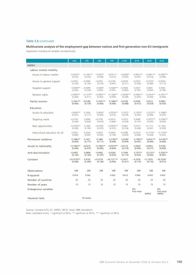
190NBB Economic Review ¡ November 2020 ¡ Annexes Part II
Table 5.6 (continued)
Multivariate analysis of the employment gap between natives and first‑generation non‑EU immigrants(regressions including all variables simultaneously)
OLS CFE CRE YFE CYFE IV‑FE IV‑FE IV‑FE
MIPEX
Labour market mobility
Access to labour market −0.0475**(0.023)
−0.1361***(0.003)
−0.0475*(0.096)
−0.0511**(0.015)
−0.0838**(0.045)
−0.0812***(0.007)
−0.0901***(0.010)
−0.0997***(0.006)
Access to general support −0.0352(0.183)
−0.0582(0.143)
−0.0352(0.219)
−0.0106(0.647)
−0.0334(0.311)
−0.0323(0.306)
−0.0720*(0.060)
−0.0630(0.113)
Targeted support 0.0449***(0.002)
−0.0090(0.530)
0.0449*(0.061)
0.0444***(0.001)
−0.0006(0.965)
0.0037(0.781)
0.0081(0.663)
0.0052(0.784)
Workers rights −0.0993***(0.000)
−0.1279**(0.011)
−0.0993***(0.002)
−0.1286***(0.000)
−0.0944***(0.008)
−0.0983***(0.002)
−0.2916***(0.000)
−0.3051***(0.000)
Family reunion 0.1641***(0.000)
−0.0189(0.729)
0.1641***(0.000)
0.1486***(0.000)
−0.0194(0.688)
−0.0396(0.412)
0.0512(0.629)
0.0893(0.420)
Education
Access to education 0.0830***(0.001)
0.1656(0.117)
0.0830*(0.050)
0.0554***(0.010)
0.1673*(0.078)
0.1503**(0.032)
0.2225***(0.006)
0.1848**(0.024)
Targeting needs −0.0195(0.436)
0.0060(0.904)
−0.0195(0.618)
−0.0014(0.946)
0.0510(0.258)
0.0668(0.107)
0.2472***(0.000)
0.2546***(0.000)
New opportunities −0.0706***(0.009)
0.1663(0.193)
−0.0706*(0.079)
−0.0936***(0.010)
0.0941(0.318)
0.0710(0.436)
−0.1115(0.261)
−0.1234(0.259)
Intercultural education for all 0.0025(0.890)
0.0226(0.691)
0.0025(0.932)
−0.0043(0.759)
−0.0288(0.629)
−0.0374(0.406)
−0.1274**(0.038)
−0.1336**(0.032)
Permanent residence 0.1680***(0.005)
0.1421(0.177)
0.1680(0.111)
0.2140***(0.000)
0.2038*(0.059)
0.1995***(0.007)
0.6541***(0.000)
0.6190***(0.000)
Access to nationality −0.1066***(0.000)
−0.0216(0.457)
−0.1066***(0.000)
−0.0919***(0.004)
−0.0114(0.579)
0.0020(0.945)
−0.0052(0.917)
0.0106(0.830)
Anti‑discrimination −0.0402(0.156)
0.0808(0.164)
−0.0402(0.187)
−0.0244(0.503)
0.1099(0.113)
0.1072**(0.033)
0.2132**(0.042)
0.2542***(0.007)
Constant −25.0739***(0.009)
9.4702(0.399)
−25.0739(0.109)
−24.1211***(0.005)
12.5477(0.351)
−4.3330(0.714)
−21.3935(0.216)
−30.7039*(0.073)
Observations 248 248 248 248 248 248 248 248
R‑squared 0.916 0.542 0.922 0.612 0.965 0.955 0.953
Number of countries 23 23 23 23 23 23 23 23
Number of years 13 13 13 13 13 13 13 13
Endogenous variables EPLPub empl
MIPEX
EPLPub emplMIPEX
Hausman tests FE better
Sources : Eurostat (LFS), EC, MIPEX, OECD, Visser, NBB calculations.Note : (standard errors), * significant at 90 %, ** significant at 95 %, *** significant at 99 %.

191NBB Economic Review ¡ November 2020 ¡ Annexes Part II
Table 5.7
Multivariate analysis of the participation gap between natives and first‑generation immigrants(regressions including all variables simultaneously)
OLS CFE CRE YFE CYFE IV‑FE IV‑FE IV‑FE
Share among pop 0.2362***(0.000)
0.0299(0.785)
0.2362***(0.000)
0.2191***(0.000)
−0.1665(0.373)
−0.1167(0.469)
−0.0894(0.557)
0.0047(0.976)
Age 24.2846***(0.000)
7.1290(0.131)
24.2846***(0.000)
24.9190***(0.000)
6.1784(0.140)
4.7361(0.487)
6.3133(0.319)
7.0863(0.255)
Gender 27.3583***(0.001)
7.4795(0.173)
27.3583***(0.008)
27.1238***(0.004)
5.3925(0.265)
6.5149(0.339)
8.5355(0.191)
10.0406(0.123)
High level of education 4.3292***(0.000)
5.4971***(0.003)
4.3292***(0.002)
4.1866***(0.000)
4.8778***(0.007)
4.7861**(0.021)
4.8215**(0.023)
5.0370**(0.020)
Low level of education −2.2918***(0.000)
−3.4428***(0.002)
−2.2918***(0.000)
−2.3428***(0.000)
−3.5377***(0.006)
−3.6367***(0.000)
−3.2307***(0.001)
−3.6210***(0.000)
EPL 1.7250***(0.005)
2.0377(0.205)
1.7250(0.108)
1.9901***(0.007)
2.9293**(0.050)
3.0167**(0.011)
2.5640***(0.005)
2.7351**(0.023)
Share of public employment 0.4158*(0.070)
0.7595***(0.004)
0.4158(0.170)
0.3290(0.228)
0.5068(0.119)
0.7167*(0.061)
0.7262**(0.014)
1.4239***(0.000)
Share of self‑employment 0.1078(0.168)
−0.3377(0.132)
0.1078(0.315)
0.0619(0.476)
−0.5619**(0.016)
−0.5311***(0.003)
−0.6650***(0.000)
−0.5283***(0.002)
Job tenure −0.0749(0.252)
−0.3980***(0.006)
−0.0749(0.379)
−0.1251(0.125)
−0.5246**(0.012)
−0.5151***(0.000)
−0.4235***(0.001)
−0.4525***(0.001)
Union −0.0453**(0.037)
0.0596(0.438)
−0.0453(0.110)
−0.0430**(0.024)
0.0248(0.758)
0.0346(0.620)
0.0163(0.826)
0.0829(0.287)
Net replacement rate −0.2526***(0.000)
−0.1943***(0.000)
−0.2526***(0.000)
−0.2566***(0.000)
−0.1757***(0.001)
−0.1663***(0.002)
−0.1914***(0.001)
−0.1609***(0.006)
ALMP measures (in % of GDP) −4.0233***(0.007)
−0.4981(0.795)
−4.0233*(0.070)
−4.2429***(0.007)
−0.9954(0.571)
−1.1803(0.385)
0.2276(0.883)
0.0614(0.968)
Observations 276 276 276 276 276 276 276 276
R‑squared 0.843 0.610 0.852 0.664 0.945 0.935 0.931
Number of countries 24 24 24 24 24 24 24 24
Number of years 13 13 13 13 13 13 13 13
Endogenous variables EPLPub empl
MIPEX
EPLPub emplMIPEX
Hausman tests FE better
Sources : Eurostat (LFS), EC, MIPEX, OECD, Visser, NBB calculations.Note : (standard errors), * significant at 90 %, ** significant at 95 %, *** significant at 99 %.

192NBB Economic Review ¡ November 2020 ¡ Annexes Part II
Table 5.7 (continued)
Multivariate analysis of the participation gap between natives and first‑generation immigrants(regressions including all variables simultaneously)
OLS CFE CRE YFE CYFE IV‑FE IV‑FE IV‑FE
MIPEX
Labour market mobility
Access to labour market 0.0300*(0.064)
0.1562**(0.041)
0.0300(0.202)
0.0298***(0.005)
0.1590**(0.011)
0.1538***(0.000)
0.1666***(0.000)
0.1436***(0.000)
Access to general support −0.0877***(0.000)
−0.0688***(0.006)
−0.0877**(0.010)
−0.0986**(0.012)
−0.0939***(0.005)
−0.0955***(0.000)
−0.1090***(0.000)
−0.1077***(0.000)
Targeted support −0.0181(0.107)
−0.0305*(0.072)
−0.0181(0.408)
−0.0263***(0.004)
−0.0437**(0.036)
−0.0426***(0.001)
−0.0406**(0.023)
−0.0312*(0.083)
Workers rights −0.0365*(0.072)
−0.0962**(0.039)
−0.0365(0.337)
−0.0367**(0.027)
−0.1051***(0.008)
−0.1026***(0.001)
−0.2384***(0.000)
−0.2527***(0.000)
Family reunion 0.1187***(0.000)
−0.1704**(0.012)
0.1187**(0.015)
0.1220***(0.000)
−0.1387**(0.026)
−0.1535***(0.004)
−0.2197**(0.017)
−0.2597***(0.005)
Education
Access to education 0.1036***(0.000)
0.1344**(0.019)
0.1036***(0.002)
0.1175***(0.001)
0.1591***(0.007)
0.1478**(0.013)
0.1877**(0.020)
0.1309*(0.095)
Targeting needs 0.0062(0.753)
0.1041**(0.013)
0.0062(0.832)
−0.0035(0.809)
0.0956***(0.007)
0.0963**(0.010)
0.2539***(0.000)
0.2753***(0.000)
New opportunities −0.0335(0.169)
−0.0799(0.410)
−0.0335(0.427)
−0.0259(0.363)
−0.0552(0.468)
−0.0610(0.512)
−0.3770***(0.000)
−0.3837***(0.000)
Intercultural education for all −0.0664***(0.000)
−0.0785(0.400)
−0.0664**(0.030)
−0.0620***(0.004)
−0.0783(0.293)
−0.0753**(0.049)
−0.1152**(0.023)
−0.1255**(0.011)
Permanent residence 0.1183**(0.019)
0.0277(0.683)
0.1183(0.178)
0.1384***(0.002)
0.0304(0.584)
0.0256(0.697)
0.4063***(0.003)
0.4219***(0.002)
Access to nationality −0.0169(0.430)
0.1229**(0.046)
−0.0169(0.554)
−0.0035(0.881)
0.1170**(0.025)
0.1198***(0.000)
0.1480***(0.005)
0.1643***(0.001)
Anti‑discrimination −0.0137(0.673)
0.2157**(0.037)
−0.0137(0.817)
−0.0268(0.419)
0.1917**(0.031)
0.1853***(0.000)
0.2296***(0.002)
0.2149***(0.004)
Constant −62.1298***(0.000)
−19.5117**(0.036)
−62.1298***(0.000)
−59.3492***(0.000)
−3.6891(0.740)
−2.1318(0.888)
−14.9343(0.399)
−25.6675(0.158)
Observations 276 276 276 276 276 276 276 276
R‑squared 0.843 0.610 0.852 0.664 0.945 0.935 0.931
Number of countries 24 24 24 24 24 24 24 24
Number of years 13 13 13 13 13 13 13 13
Endogenous variables EPLPub empl
MIPEX
EPLPub emplMIPEX
Hausman tests FE better
Sources : Eurostat (LFS), EC, MIPEX, OECD, Visser, NBB calculations.Note : (standard errors), * significant at 90 %, ** significant at 95 %, *** significant at 99 %.

193NBB Economic Review ¡ November 2020 ¡ Annexes Part II
Table 5.8
Multivariate analysis of the participation gap between natives and first‑generation non‑EU immigrants(regressions including all variables simultaneously)
OLS CFE CRE YFE CYFE IV‑FE IV‑FE IV‑FE
Share among pop −0.1871*(0.094)
−0.1423(0.495)
−0.1871(0.236)
−0.0848(0.462)
0.0401(0.881)
0.0171(0.932)
0.0303(0.895)
0.0697(0.767)
Age 32.7372***(0.000)
9.0636**(0.027)
32.7372***(0.000)
33.2802***(0.000)
4.3157(0.224)
4.2520(0.165)
4.9451(0.188)
4.5817(0.211)
Gender 9.6255*(0.062)
−3.4792(0.541)
9.6255(0.273)
7.4127*(0.051)
−4.7356(0.317)
−4.1837(0.265)
−2.5522(0.511)
−2.6974(0.474)
High level of education 6.3218***(0.000)
2.3789(0.263)
6.3218***(0.000)
6.6111***(0.000)
2.8387(0.108)
3.1083**(0.014)
3.6946**(0.011)
4.0442***(0.005)
Low level of education −2.5265***(0.000)
−0.8484*(0.091)
−2.5265***(0.000)
−2.2246***(0.001)
0.0989(0.889)
0.0525(0.928)
−0.1252(0.838)
−0.3133(0.601)
EPL 2.0999***(0.000)
2.1533(0.124)
2.0999**(0.017)
1.5123***(0.003)
1.9386(0.109)
2.1584**(0.026)
2.1603***(0.005)
2.6429***(0.004)
Share of public employment 0.4158*(0.082)
0.6766**(0.010)
0.4158(0.201)
0.2485(0.449)
0.1102(0.683)
0.2399(0.401)
0.3467(0.223)
0.7748**(0.010)
Share of self‑employment 0.0901(0.135)
−0.0255(0.905)
0.0901(0.296)
0.0076(0.934)
−0.2676(0.183)
−0.2866*(0.082)
−0.3762***(0.010)
−0.3609**(0.019)
Job tenure −0.1918***(0.001)
−0.3266***(0.008)
−0.1918**(0.034)
−0.1370*(0.080)
−0.1605(0.279)
−0.1641(0.199)
−0.1176(0.308)
−0.1768(0.147)
Union 0.0023(0.907)
0.1132(0.166)
0.0023(0.904)
−0.0244(0.264)
−0.1942*(0.054)
−0.1818**(0.018)
−0.1951***(0.004)
−0.1150(0.128)
Net replacement rate −0.3065***(0.000)
−0.1072*(0.081)
−0.3065***(0.000)
−0.3186***(0.000)
−0.1207**(0.029)
−0.1290***(0.003)
−0.1412***(0.001)
−0.1350***(0.002)
ALMP measures (in % of GDP) −2.6786*(0.057)
0.4806(0.823)
−2.6786(0.123)
−1.5439(0.424)
0.9690(0.645)
1.0192(0.491)
1.7098(0.284)
1.4199(0.375)
Observations 248 248 248 248 248 248 248 248
R‑squared 0.919 0.488 0.923 0.605 0.972 0.966 0.964
Number of countries 23 23 23 23 23 23 23 23
Number of years 13 13 13 13 13 13 13 13
Endogenous variables EPLPub empl
MIPEX
EPLPub emplMIPEX
Hausman tests FE better
Sources : Eurostat (LFS), EC, MIPEX, OECD, Visser, NBB calculations.Note : (standard errors), * significant at 90 %, ** significant at 95 %, *** significant at 99 %.

194NBB Economic Review ¡ November 2020 ¡ Annexes Part II
Table 5.8 (continued)
Multivariate analysis of the participation gap between natives and first‑generation non‑EU immigrants(regressions including all variables simultaneously)
OLS CFE CRE YFE CYFE IV‑FE IV‑FE IV‑FE
MIPEX
Labour market mobility
Access to labour market −0.0242*(0.095)
−0.0154(0.661)
−0.0242(0.311)
−0.0209**(0.039)
0.0362(0.294)
0.0383(0.118)
0.0415(0.110)
0.0277(0.327)
Access to general support −0.0155(0.571)
−0.0631***(0.003)
−0.0155(0.596)
−0.0019(0.944)
−0.0497**(0.018)
−0.0545**(0.036)
−0.0521(0.115)
−0.0559(0.124)
Targeted support 0.0100(0.409)
−0.0403***(0.002)
0.0100(0.605)
0.0055(0.576)
−0.0372***(0.002)
−0.0364***(0.000)
−0.0308**(0.029)
−0.0295**(0.035)
Workers rights −0.0321(0.135)
−0.1014***(0.007)
−0.0321(0.270)
−0.0456(0.126)
−0.0668***(0.005)
−0.0711***(0.004)
−0.1899***(0.000)
−0.2079***(0.000)
Family reunion 0.2555***(0.000)
0.0100(0.839)
0.2555***(0.000)
0.2487***(0.000)
−0.0037(0.926)
−0.0066(0.852)
−0.0193(0.809)
−0.0148(0.851)
Education
Access to education 0.1693***(0.000)
0.2088**(0.013)
0.1693***(0.000)
0.1565***(0.000)
0.2138**(0.012)
0.2021***(0.000)
0.2515***(0.001)
0.2176***(0.003)
Targeting needs −0.0651***(0.001)
0.0498(0.232)
−0.0651**(0.038)
−0.0639***(0.001)
0.0848**(0.030)
0.0888***(0.004)
0.2390***(0.000)
0.2491***(0.000)
New opportunities −0.0713***(0.003)
0.0051(0.962)
−0.0713**(0.014)
−0.0800***(0.010)
−0.0505(0.468)
−0.0555(0.407)
−0.1320(0.150)
−0.1780*(0.064)
Intercultural education for all 0.0031(0.860)
0.0862*(0.080)
0.0031(0.912)
−0.0022(0.897)
0.0387(0.284)
0.0409(0.181)
−0.0256(0.563)
−0.0256(0.568)
Permanent residence 0.0551(0.275)
0.0417(0.552)
0.0551(0.557)
0.0840*(0.082)
0.0709(0.305)
0.0659(0.235)
0.3287***(0.001)
0.3178***(0.002)
Access to nationality −0.1350***(0.000)
−0.0010(0.977)
−0.1350***(0.000)
−0.1192***(0.000)
0.0170(0.272)
0.0211(0.354)
0.0474(0.251)
0.0759*(0.063)
Anti‑discrimination −0.0798***(0.003)
−0.0146(0.728)
−0.0798**(0.021)
−0.0778**(0.023)
0.0077(0.872)
−0.0048(0.912)
0.0794(0.255)
0.0904(0.186)
Constant −48.6260***(0.000)
−15.6800(0.121)
−48.6260***(0.000)
−46.3317***(0.000)
−5.1157(0.693)
−10.2699(0.305)
−29.4831**(0.018)
−31.7320**(0.011)
Observations 248 248 248 248 248 248 248 248
R‑squared 0.919 0.488 0.923 0.605 0.972 0.966 0.964
Number of countries 23 23 23 23 23 23 23 23
Number of years 13 13 13 13 13 13 13 13
Endogenous variables EPLPub empl
MIPEX
EPLPub emplMIPEX
Hausman tests FE better
Sources : Eurostat (LFS), EC, MIPEX, OECD, Visser, NBB calculations.Note : (standard errors), * significant at 90 %, ** significant at 95 %, *** significant at 99 %.

195NBB Economic Review ¡ November 2020 ¡ Annexes Part II
Table 5.9
Multivariate analysis of the men employment gap between natives and first-generation immigrants(regressions including all variables simultaneously)
OLS CFE CRE YFE CYFE IV-FE IV-FE IV-FE
Share among pop 0.2632***(0.000)
−0.1778(0.293)
0.2632***(0.005)
0.2922***(0.000)
−0.1764(0.435)
−0.0872(0.601)
−0.2332(0.177)
−0.1705(0.336)
Age 26.3177***(0.000)
−1.8572(0.818)
26.3177***(0.000)
27.3129***(0.000)
−2.2720(0.791)
−6.4186(0.155)
4.6003(0.406)
0.1666(0.974)
High level of education 1.8966*(0.056)
5.0460***(0.009)
1.8966(0.220)
2.2614**(0.046)
4.6755**(0.020)
5.3903***(0.000)
4.4386**(0.015)
4.3684**(0.015)
Low level of education −1.1862***(0.003)
−2.5733***(0.009)
−1.1862*(0.071)
−0.9057*(0.089)
−2.3820***(0.004)
−2.4564***(0.000)
−1.7332**(0.016)
−2.0255***(0.005)
Unemployment rate t − 1 −0.1226(0.118)
−0.0854(0.448)
−0.1226(0.260)
−0.1382(0.141)
−0.1369(0.196)
−0.1200(0.154)
−0.2385***(0.003)
−0.2719***(0.003)
EPL 3.3499***(0.000)
3.1153**(0.018)
3.3499***(0.000)
2.6136***(0.006)
3.0109**(0.023)
3.0558**(0.041)
2.3876**(0.037)
2.5483*(0.085)
Share of public employment −0.5340**(0.029)
−0.1419(0.741)
−0.5340(0.239)
−0.5911***(0.006)
−0.3031(0.504)
0.1484(0.781)
−0.5247(0.110)
0.2332(0.592)
Share of self‑employment −0.0681(0.327)
−0.4519(0.131)
−0.0681(0.499)
−0.1048*(0.081)
−0.5419*(0.082)
−0.5148**(0.027)
−0.7109***(0.001)
−0.6413***(0.003)
Job tenure −0.0042(0.946)
−0.1789*(0.096)
−0.0042(0.964)
0.0153(0.820)
−0.1879(0.162)
−0.1978*(0.061)
−0.2008(0.103)
−0.2467**(0.048)
Union −0.1048***(0.000)
−0.2777***(0.004)
−0.1048***(0.001)
−0.1178***(0.000)
−0.3452**(0.014)
−0.3244***(0.000)
−0.2640***(0.002)
−0.1704*(0.063)
Net replacement rate −0.2768***(0.000)
−0.0596(0.353)
−0.2768***(0.000)
−0.2743***(0.000)
−0.0503(0.405)
−0.0304(0.600)
−0.0660(0.196)
−0.0418(0.415)
ALMP measures (in % of GDP) −5.4219***(0.001)
−1.9479(0.239)
−5.4219***(0.001)
−5.5210***(0.001)
−2.7420(0.116)
−3.5131**(0.045)
−2.1183(0.258)
−2.8545(0.113)
Observations 257 257 257 257 257 257 257 257
R‑squared 0.854 0.474 0.863 0.502 0.937 0.922 0.92
Number of countries 22 22 22 22 22 22 22 22
Number of years 13 13 13 13 13 13 13 13
Endogenous variables EPLPub empl
MIPEX
EPLPub emplMIPEX
Hausman tests FE better
Sources : Eurostat (LFS), EC, MIPEX, OECD, Visser, NBB calculations.Note : (standard errors), * significant at 90 %, ** significant at 95 %, *** significant at 99 %.

196NBB Economic Review ¡ November 2020 ¡ Annexes Part II
Table 5.9 (continued)
Multivariate analysis of the men employment gap between natives and first-generation immigrants(regressions including all variables simultaneously)
OLS CFE CRE YFE CYFE IV-FE IV-FE IV-FE
MIPEX
Labour market mobility
Access to labour market −0.0374*(0.089)
−0.0911**(0.011)
−0.0374(0.290)
−0.0322**(0.029)
−0.0733*(0.086)
−0.0855***(0.008)
−0.0991**(0.011)
−0.1128***(0.002)
Access to general support −0.0594**(0.014)
−0.0286(0.200)
−0.0594(0.162)
−0.0333(0.216)
−0.0356(0.143)
−0.0449*(0.076)
−0.0556(0.100)
−0.0801**(0.015)
Targeted support 0.0040(0.795)
0.0374*(0.051)
0.0040(0.890)
0.0059(0.660)
0.0325(0.112)
0.0302**(0.039)
0.0133(0.518)
0.0095(0.632)
Workers rights −0.1220***(0.000)
−0.0642**(0.023)
−0.1220***(0.000)
−0.1199***(0.000)
−0.0706**(0.011)
−0.0646*(0.078)
−0.2630***(0.001)
−0.2728***(0.001)
Family reunion 0.0178(0.522)
−0.0340(0.664)
0.0178(0.693)
0.0176(0.376)
−0.0070(0.933)
−0.0500(0.391)
0.1951*(0.061)
0.1766*(0.081)
Education
Access to education 0.0396(0.130)
0.1116(0.133)
0.0396(0.363)
0.0297**(0.047)
0.1260(0.120)
0.0913(0.149)
0.1743**(0.020)
0.1355*(0.075)
Targeting needs 0.0667***(0.005)
0.0483(0.213)
0.0667**(0.023)
0.0651**(0.016)
0.0724(0.100)
0.0695*(0.080)
0.2389***(0.000)
0.2387***(0.000)
New opportunities −0.0623**(0.029)
0.1294(0.115)
−0.0623*(0.082)
−0.0833**(0.024)
0.1239*(0.087)
0.1345**(0.046)
0.1047(0.380)
0.0215(0.839)
Intercultural education for all −0.0877***(0.000)
−0.0867(0.323)
−0.0877***(0.010)
−0.1027***(0.000)
−0.1108(0.255)
−0.0901(0.101)
−0.1877***(0.005)
−0.1740***(0.009)
Permanent residence 0.2075***(0.000)
0.1494(0.126)
0.2075***(0.006)
0.2205***(0.000)
0.2032*(0.067)
0.1743**(0.033)
0.6741***(0.000)
0.6835***(0.000)
Access to nationality −0.0051(0.777)
−0.0390(0.146)
−0.0051(0.850)
−0.0129(0.528)
−0.0493*(0.100)
−0.0398*(0.082)
−0.1185**(0.027)
−0.0967*(0.059)
Anti‑discrimination 0.1001***(0.000)
0.0790(0.117)
0.1001**(0.042)
0.1219***(0.000)
0.0977*(0.088)
0.0890*(0.088)
0.2773***(0.007)
0.2743***(0.005)
Constant −21.5776***(0.000)
13.1254(0.340)
−21.5776***(0.003)
−23.0605***(0.001)
13.9514(0.337)
11.7780(0.309)
−24.3612(0.146)
−25.1279(0.131)
Observations 257 257 257 257 257 257 257 257
R‑squared 0.854 0.474 0.863 0.502 0.937 0.922 0.92
Number of countries 22 22 22 22 22 22 22 22
Number of years 13 13 13 13 13 13 13 13
Endogenous variables EPLPub empl
MIPEX
EPLPub emplMIPEX
Hausman tests FE better
Sources : Eurostat (LFS), EC, MIPEX, OECD, Visser, NBB calculations.Note : (standard errors), * significant at 90 %, ** significant at 95 %, *** significant at 99 %.

197NBB Economic Review ¡ November 2020 ¡ Annexes Part II
Table 5.10
Multivariate analysis of the men employment gap between natives and first‑generation non‑EU immigrants(regressions including all variables simultaneously)
OLS CFE CRE YFE CYFE
Share among pop −0.5078***(0.003)
−0.4221(0.212)
−0.5078***(0.004)
−0.4580**(0.016)
−0.4668(0.182)
Age 16.5043***(0.001)
−2.9262(0.720)
16.5043***(0.005)
17.1019**(0.018)
−3.5706(0.642)
High level of education 3.0807**(0.011)
3.7439**(0.043)
3.0807***(0.009)
3.3047**(0.036)
3.8428**(0.028)
Low level of education −0.9288**(0.023)
−0.2537(0.738)
−0.9288*(0.090)
−0.5541(0.166)
0.1091(0.900)
Unemployment rate t − 1 −0.1273(0.173)
−0.0388(0.779)
−0.1273(0.361)
−0.0337(0.626)
−0.0012(0.994)
EPL 3.7032***(0.000)
3.3721**(0.016)
3.7032***(0.000)
3.7505***(0.001)
2.7947**(0.048)
Share of public employment −0.1878(0.648)
−0.3154(0.490)
−0.1878(0.644)
−0.2184(0.577)
−0.8045*(0.090)
Share of self‑employment 0.0954(0.204)
−0.5184(0.153)
0.0954(0.352)
0.0781(0.185)
−0.5528(0.100)
Job tenure 0.0358(0.709)
−0.2962**(0.042)
0.0358(0.719)
0.0471(0.712)
−0.2439(0.294)
Union −0.0646**(0.023)
−0.2839**(0.018)
−0.0646**(0.023)
−0.0759***(0.001)
−0.4470***(0.009)
Net replacement rate −0.3891***(0.000)
0.0774(0.446)
−0.3891***(0.000)
−0.3904***(0.000)
0.0650(0.511)
ALMP measures (in % of GDP) −2.9588*(0.088)
−2.4495(0.509)
−2.9588(0.143)
−3.0346**(0.026)
−4.5499(0.282)
Observations 231 231 231 231 231
R‑squared 0.869 0.433 0.876 0.483
Number of countries 21 21 21 21 21
Number of years 13 13 13 13 13
Hausman tests FE better
Sources : Eurostat (LFS), EC, MIPEX, OECD, Visser, NBB calculations.Note : (standard errors), * significant at 90 %, ** significant at 95 %, *** significant at 99 %.

198NBB Economic Review ¡ November 2020 ¡ Annexes Part II
Table 5.10 (continued)
Multivariate analysis of the men employment gap between natives and first‑generation non‑EU immigrants(regressions including all variables simultaneously)
OLS CFE CRE YFE CYFE
MIPEX
Labour market mobility
Access to labour market −0.0741***(0.002)
−0.2017**(0.010)
−0.0741***(0.004)
−0.0822**(0.011)
−0.1892**(0.012)
Access to general support −0.0555(0.267)
−0.0219(0.677)
−0.0555(0.338)
−0.0445(0.487)
−0.0404(0.407)
Targeted support 0.0352**(0.016)
0.0246(0.320)
0.0352(0.126)
0.0431***(0.000)
0.0290(0.272)
Workers rights −0.1270***(0.000)
−0.0751*(0.096)
−0.1270***(0.000)
−0.1391***(0.000)
−0.0822**(0.039)
Family reunion 0.0532*(0.083)
0.0060(0.926)
0.0532(0.255)
0.0423(0.214)
0.0234(0.725)
Education
Access to education 0.0961***(0.000)
0.1226(0.304)
0.0961***(0.000)
0.0855***(0.000)
0.1960*(0.081)
Targeting needs 0.0123(0.659)
0.0217(0.704)
0.0123(0.746)
0.0307(0.186)
0.0770(0.149)
New opportunities −0.1121***(0.001)
0.2323*(0.077)
−0.1121***(0.005)
−0.1402***(0.002)
0.1855(0.110)
Intercultural education for all 0.0361(0.133)
−0.0356(0.740)
0.0361(0.216)
0.0285(0.199)
−0.0487(0.690)
Permanent residence 0.1852***(0.003)
0.1336(0.252)
0.1852*(0.056)
0.2152***(0.000)
0.2644**(0.038)
Access to nationality −0.0591(0.137)
−0.0803***(0.006)
−0.0591*(0.060)
−0.0586(0.324)
−0.0801**(0.026)
Anti‑discrimination −0.0333(0.559)
0.0722(0.282)
−0.0333(0.486)
−0.0132(0.859)
0.0722(0.346)
Constant −8.2646*(0.088)
19.1769(0.205)
−8.2646*(0.069)
−11.8028(0.120)
20.3884(0.101)
Observations 231 231 231 231 231
R‑squared 0.869 0.433 0.876 0.483
Number of countries 21 21 21 21 21
Number of years 13 13 13 13 13
Hausman tests FE better
Sources : Eurostat (LFS), EC, MIPEX, OECD, Visser, NBB calculations.Note : (standard errors), * significant at 90 %, ** significant at 95 %, *** significant at 99 %.
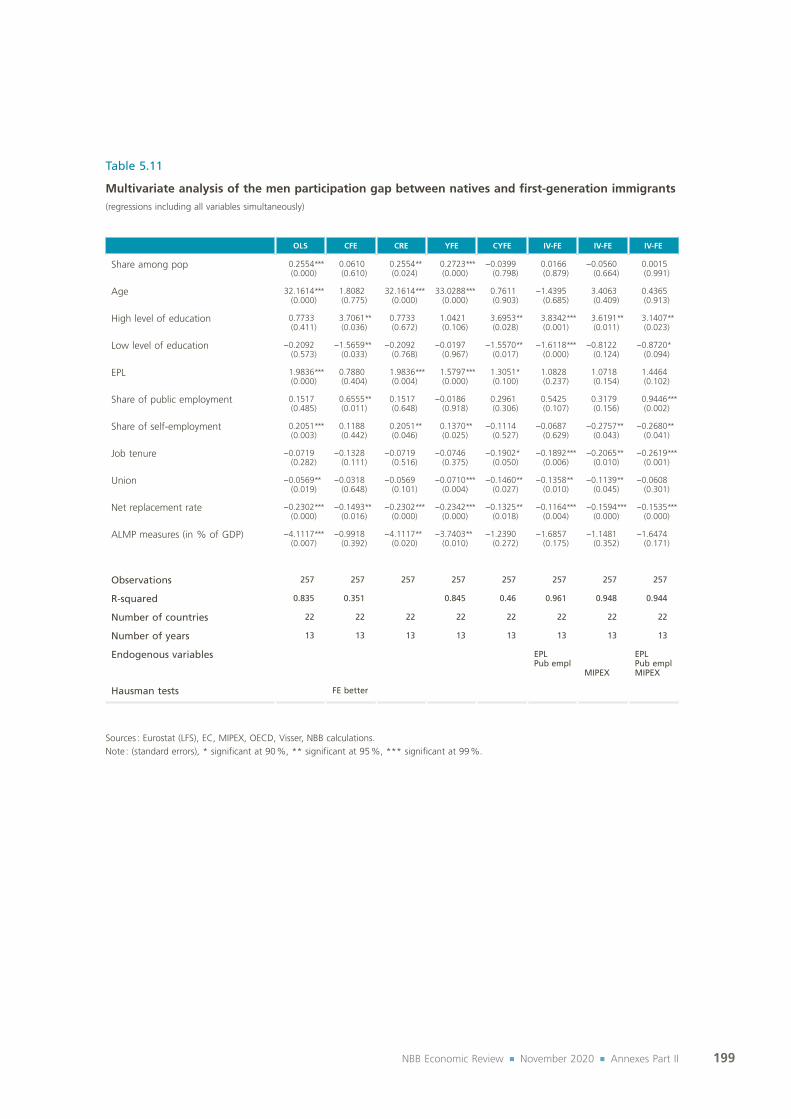
199NBB Economic Review ¡ November 2020 ¡ Annexes Part II
Table 5.11
Multivariate analysis of the men participation gap between natives and first‑generation immigrants(regressions including all variables simultaneously)
OLS CFE CRE YFE CYFE IV‑FE IV‑FE IV‑FE
Share among pop 0.2554***(0.000)
0.0610(0.610)
0.2554**(0.024)
0.2723***(0.000)
−0.0399(0.798)
0.0166(0.879)
−0.0560(0.664)
0.0015(0.991)
Age 32.1614***(0.000)
1.8082(0.775)
32.1614***(0.000)
33.0288***(0.000)
0.7611(0.903)
−1.4395(0.685)
3.4063(0.409)
0.4365(0.913)
High level of education 0.7733(0.411)
3.7061**(0.036)
0.7733(0.672)
1.0421(0.106)
3.6953**(0.028)
3.8342***(0.001)
3.6191**(0.011)
3.1407**(0.023)
Low level of education −0.2092(0.573)
−1.5659**(0.033)
−0.2092(0.768)
−0.0197(0.967)
−1.5570**(0.017)
−1.6118***(0.000)
−0.8122(0.124)
−0.8720*(0.094)
EPL 1.9836***(0.000)
0.7880(0.404)
1.9836***(0.004)
1.5797***(0.000)
1.3051*(0.100)
1.0828(0.237)
1.0718(0.154)
1.4464(0.102)
Share of public employment 0.1517(0.485)
0.6555**(0.011)
0.1517(0.648)
−0.0186(0.918)
0.2961(0.306)
0.5425(0.107)
0.3179(0.156)
0.9446***(0.002)
Share of self‑employment 0.2051***(0.003)
0.1188(0.442)
0.2051**(0.046)
0.1370**(0.025)
−0.1114(0.527)
−0.0687(0.629)
−0.2757**(0.043)
−0.2680**(0.041)
Job tenure −0.0719(0.282)
−0.1328(0.111)
−0.0719(0.516)
−0.0746(0.375)
−0.1902*(0.050)
−0.1892***(0.006)
−0.2065**(0.010)
−0.2619***(0.001)
Union −0.0569**(0.019)
−0.0318(0.648)
−0.0569(0.101)
−0.0710***(0.004)
−0.1460**(0.027)
−0.1358**(0.010)
−0.1139**(0.045)
−0.0608(0.301)
Net replacement rate −0.2302***(0.000)
−0.1493**(0.016)
−0.2302***(0.000)
−0.2342***(0.000)
−0.1325**(0.018)
−0.1164***(0.004)
−0.1594***(0.000)
−0.1535***(0.000)
ALMP measures (in % of GDP) −4.1117***(0.007)
−0.9918(0.392)
−4.1117**(0.020)
−3.7403**(0.010)
−1.2390(0.272)
−1.6857(0.175)
−1.1481(0.352)
−1.6474(0.171)
Observations 257 257 257 257 257 257 257 257
R‑squared 0.835 0.351 0.845 0.46 0.961 0.948 0.944
Number of countries 22 22 22 22 22 22 22 22
Number of years 13 13 13 13 13 13 13 13
Endogenous variables EPLPub empl
MIPEX
EPLPub emplMIPEX
Hausman tests FE better
Sources : Eurostat (LFS), EC, MIPEX, OECD, Visser, NBB calculations.Note : (standard errors), * significant at 90 %, ** significant at 95 %, *** significant at 99 %.

200NBB Economic Review ¡ November 2020 ¡ Annexes Part II
Table 5.11 (continued)
Multivariate analysis of the men participation gap between natives and first‑generation immigrants(regressions including all variables simultaneously)
OLS CFE CRE YFE CYFE IV‑FE IV‑FE IV‑FE
MIPEX
Labour market mobility
Access to labour market −0.0232(0.210)
0.0018(0.936)
−0.0232(0.529)
−0.0215**(0.037)
0.0230(0.427)
0.0171(0.386)
0.0180(0.526)
0.0049(0.859)
Access to general support −0.0621**(0.014)
−0.0405***(0.006)
−0.0621(0.169)
−0.0440*(0.079)
−0.0519***(0.001)
−0.0557***(0.001)
−0.0738***(0.003)
−0.0862***(0.000)
Targeted support −0.0256*(0.084)
−0.0041(0.751)
−0.0256(0.425)
−0.0301**(0.024)
−0.0107(0.492)
−0.0111(0.261)
−0.0264**(0.049)
−0.0273**(0.035)
Workers rights −0.0526***(0.005)
−0.0811***(0.003)
−0.0526(0.163)
−0.0561***(0.007)
−0.0821***(0.001)
−0.0818***(0.002)
−0.2265***(0.000)
−0.2364***(0.000)
Family reunion 0.0653**(0.026)
−0.0313(0.555)
0.0653(0.231)
0.0636**(0.025)
−0.0214(0.730)
−0.0404(0.321)
0.0166(0.799)
0.0069(0.911)
Education
Access to education 0.0782***(0.005)
0.1599**(0.010)
0.0782(0.110)
0.0767***(0.000)
0.1847**(0.010)
0.1734***(0.000)
0.2031***(0.001)
0.1422**(0.019)
Targeting needs 0.0436**(0.024)
0.1101***(0.004)
0.0436(0.184)
0.0377***(0.002)
0.1290***(0.001)
0.1292***(0.000)
0.2814***(0.000)
0.3008***(0.000)
New opportunities −0.0018(0.936)
−0.0060(0.931)
−0.0018(0.950)
−0.0121(0.727)
−0.0096(0.887)
−0.0082(0.885)
0.0116(0.909)
−0.0681(0.470)
Intercultural education for all −0.0826***(0.000)
0.0210(0.586)
−0.0826**(0.042)
−0.0895***(0.000)
−0.0047(0.909)
−0.0011(0.970)
−0.0577(0.159)
−0.0609(0.129)
Permanent residence 0.1020**(0.037)
0.0861(0.116)
0.1020(0.201)
0.1295***(0.000)
0.1112**(0.032)
0.1231**(0.037)
0.4479***(0.001)
0.4639***(0.000)
Access to nationality −0.0243(0.188)
0.0057(0.814)
−0.0243(0.410)
−0.0229(0.180)
0.0069(0.815)
0.0083(0.646)
0.0100(0.781)
0.0312(0.361)
Anti‑discrimination 0.0642**(0.048)
0.0160(0.616)
0.0642(0.268)
0.0763**(0.026)
0.0123(0.763)
0.0128(0.719)
0.1597**(0.024)
0.1863***(0.006)
Constant −37.4573***(0.000)
−13.7440*(0.062)
−37.4573***(0.000)
−36.3695***(0.000)
−2.9351(0.720)
−3.0560(0.702)
−24.8348**(0.022)
−25.0969**(0.014)
Observations 257 257 257 257 257 257 257 257
R‑squared 0.835 0.351 0.845 0.46 0.961 0.948 0.944
Number of countries 22 22 22 22 22 22 22 22
Number of years 13 13 13 13 13 13 13 13
Endogenous variables EPLPub empl
MIPEX
EPLPub emplMIPEX
Hausman tests FE better
Sources : Eurostat (LFS), EC, MIPEX, OECD, Visser, NBB calculations.Note : (standard errors), * significant at 90 %, ** significant at 95 %, *** significant at 99 %.

201NBB Economic Review ¡ November 2020 ¡ Annexes Part II
Table 5.12
Multivariate analysis of the men participation gap between natives and first‑generation non‑EU immigrants(regressions including all variables simultaneously)
OLS CFE CRE YFE CYFE
Share among pop −0.5235***(0.000)
−0.1010(0.644)
−0.5235***(0.001)
−0.4859***(0.000)
−0.2639(0.407)
Age 15.7845***(0.000)
2.6764(0.572)
15.7845***(0.004)
16.1162***(0.001)
0.6469(0.892)
High level of education 2.8461***(0.000)
0.7202(0.612)
2.8461***(0.010)
3.1332***(0.003)
0.9527(0.457)
Low level of education 0.0738(0.795)
−0.4980(0.418)
0.0738(0.796)
0.1538(0.589)
−0.2553(0.688)
EPL 1.7744***(0.000)
1.1184(0.312)
1.7744***(0.004)
1.5091**(0.026)
1.1604(0.230)
Share of public employment 1.0548***(0.000)
0.7026***(0.001)
1.0548***(0.001)
1.0357***(0.000)
0.2123(0.293)
Share of self‑employment 0.4993***(0.000)
0.1866(0.311)
0.4993***(0.000)
0.4894***(0.000)
0.0021(0.991)
Job tenure 0.0562(0.307)
−0.2185*(0.057)
0.0562(0.410)
0.0828(0.155)
−0.2251(0.219)
Union 0.0524***(0.003)
−0.0259(0.732)
0.0524**(0.010)
0.0494*(0.067)
−0.1939**(0.048)
Net replacement rate −0.3502***(0.000)
−0.0114(0.878)
−0.3502***(0.000)
−0.3525***(0.000)
−0.0181(0.805)
ALMP measures (in % of GDP) −1.7567(0.160)
−2.0178(0.286)
−1.7567(0.237)
−1.5104(0.186)
−3.1064(0.115)
Observations 231 231 231 231 231
R‑squared 0.907 0.323 0.908 0.431
Number of countries 21 21 21 21 21
Number of years 13 13 13 13 13
Hausman tests FE better
Sources : Eurostat (LFS), EC, MIPEX, OECD, Visser, NBB calculations.Note : (standard errors), * significant at 90 %, ** significant at 95 %, *** significant at 99 %.

202NBB Economic Review ¡ November 2020 ¡ Annexes Part II
Table 5.12 (continued)
Multivariate analysis of the men participation gap between natives and first‑generation non‑EU immigrants(regressions including all variables simultaneously)
OLS CFE CRE YFE CYFE
MIPEX
Labour market mobility
Access to labour market −0.0604***(0.000)
−0.0402(0.282)
−0.0604***(0.003)
−0.0600***(0.005)
−0.0107(0.772)
Access to general support −0.0728**(0.018)
−0.0393(0.184)
−0.0728(0.123)
−0.0635(0.143)
−0.0662**(0.012)
Targeted support 0.0011(0.922)
−0.0145(0.319)
0.0011(0.947)
0.0023(0.746)
−0.0200(0.240)
Workers rights −0.0558***(0.004)
−0.0686**(0.022)
−0.0558*(0.051)
−0.0595***(0.007)
−0.0786***(0.006)
Family reunion 0.0871***(0.000)
0.0296(0.598)
0.0871***(0.008)
0.0856***(0.001)
0.0428(0.403)
Education
Access to education 0.2039***(0.000)
0.1795**(0.024)
0.2039***(0.000)
0.2011***(0.000)
0.2458***(0.008)
Targeting needs −0.0397**(0.017)
0.0684(0.262)
−0.0397(0.136)
−0.0384**(0.015)
0.1126**(0.044)
New opportunities −0.0748***(0.001)
0.0388(0.753)
−0.0748***(0.002)
−0.0848***(0.001)
−0.0007(0.994)
Intercultural education for all 0.0725***(0.000)
0.0563(0.188)
0.0725***(0.001)
0.0698***(0.000)
0.0333(0.499)
Permanent residence 0.1056**(0.012)
0.0267(0.597)
0.1056(0.165)
0.1114***(0.006)
0.1206**(0.044)
Access to nationality −0.0287(0.253)
−0.0207(0.554)
−0.0287(0.234)
−0.0304(0.400)
−0.0205(0.586)
Anti‑discrimination −0.1544***(0.000)
−0.0707*(0.090)
−0.1544***(0.000)
−0.1507***(0.005)
−0.0785(0.106)
Constant −30.2571***(0.000)
−9.2552(0.346)
−30.2571***(0.000)
−31.6322***(0.000)
0.8726(0.932)
Observations 231 231 231 231 231
R‑squared 0.907 0.323 0.908 0.431
Number of countries 21 21 21 21 21
Number of years 13 13 13 13 13
Hausman tests FE better
Sources : Eurostat (LFS), EC, MIPEX, OECD, Visser, NBB calculations.Note : (standard errors), * significant at 90 %, ** significant at 95 %, *** significant at 99 %.

203NBB Economic Review ¡ November 2020 ¡ Annexes Part III
Annexes Part III A general equilibrium analysis of immigration in Belgium
Annex III.1 Description of the general equilibrium model
In order to analyse the economic impact of immigration on macroeconomic variables and on the welfare of native citizens in Belgium, a static model of general equilibrium is defined. Note that Belgium is modelled here as an entity unrelated to other countries. Disregarding trade and capital links removes some potential interactions between immigration and the economy, which is discussed in the limitations of the model.
There are four different types of actors : individuals, intermediate firms, retail firms and the government.
The functioning of the modelled economy is the following. Intermediate firms open vacancies in a frictional labour market in order to hire workers and produce intermediate goods. At the same time, retail firms buy these goods in order to produce and sell final goods in a monopolistically competitive market. The government taxes income and consumption to finance redistributive transfers, public consumption and unemployment benefits. Individuals decide to enter or not the labour market and receive a revenue equal to their wage (depending on their bargaining power) and transfers from the government. They optimise their consumption under the constraint of their revenue and decide what quantity of final goods to buy with a preference for varieties.
1. Preferences and consumers decisions
The population is exogenously set and divided between working‑age individuals,
ANNEXES PART III – A GENERAL EQUILIBRIUM ANALYSIS OF IMMIGRATION IN BELGIUM
ANNEX III.1 - DESCRIPTION OF THE GENERAL EQUILIBRIUM MODEL
In order to analyse the economic impact of immigration on macroeconomic variables and on the welfare of native citizens in Belgium, a static model of general equilibrium is defined. Note that Belgium is modelled here as an entity unrelated to other countries. Disregarding trade and capital links removes some potential interactions between immigration and the economy, which is discussed in the limitations of the model.
There are four different types of actors: individuals, intermediate firms, retail firms and the government.
The functioning of the modelled economy is the following. Intermediate firms open vacancies in a frictional labour market in order to hire workers and produce intermediate goods. At the same time, retail firms buy these goods in order to produce and sell final goods in a monopolistically competitive market. The government taxes income and consumption to finance redistributive transfers, public consumption and unemployment benefits. Individuals decide to enter or not the labour market and receive a revenue equal to their wage (depending on their bargaining power) and transfers from the government. They optimise their consumption under the constraint of their revenue and decide what quantity of final goods to buy with a preference for varieties.
A. PREFERENCES AND CONSUMERS DECISIONS
The population is exogenously set and divided between working-age individuals, 𝑁𝑁���� and retirees
1, 𝑁𝑁��
� .
The working-age population is then divided into 16 types of individuals depending on their skills, age and origin, with 𝑆𝑆 ∈ {𝐿𝐿, 𝐻𝐻} being the level of education which can be low
2 (lower or equal to secondary education)
or high (tertiary education); 𝐴𝐴 ∈ {𝐴𝐴�, 𝐴𝐴�, 𝐴𝐴�} are the age categories, 20 to 34 years, 35 to 49 years and 50 to 64 years,
3 which will be used as a proxy for labour market experience; and 𝑂𝑂 ∈ {𝑁𝑁, 𝑀𝑀} is the origin of the
individual, Belgian-born individuals, named as natives or foreign-born individuals, named as immigrants.
The retirees in this model could be of four types depending on their skills and origin, defined in the same way as for the working-age population. They are assumed to be out of the labour market (full leisure time) and to get revenue only from government transfers.
Individuals are assumed to be homogenous within each group so that we disregard heterogeneity based on unobserved characteristics. As an illustration, we assume that all immigrant workers in a given skill and age cell are perfect substitutes on the labour market.
There are no savings in the model, so the revenue is entirely consumed.
Individuals decide the amount of time spent in the labour market and the level of consumption given their budget constraint.
1 Retirees are included in the model because they will receive transfers from the government for their pension. Children, on the contrary,
are excluded because their transfers (e.g. family allowances) are supposed to be received by their parents and thus included in the parents’ consumption decision.
2 Note that what we consider here as low education differs from what is presented in the rest of the paper. Here, we consider low-and
middle-educated as low-skilled workers. 3 We start at the age of 20 because of data availability in terms of participation and unemployment rates.
and retirees 1,
ANNEXES PART III – A GENERAL EQUILIBRIUM ANALYSIS OF IMMIGRATION IN BELGIUM
ANNEX III.1 - DESCRIPTION OF THE GENERAL EQUILIBRIUM MODEL
In order to analyse the economic impact of immigration on macroeconomic variables and on the welfare of native citizens in Belgium, a static model of general equilibrium is defined. Note that Belgium is modelled here as an entity unrelated to other countries. Disregarding trade and capital links removes some potential interactions between immigration and the economy, which is discussed in the limitations of the model.
There are four different types of actors: individuals, intermediate firms, retail firms and the government.
The functioning of the modelled economy is the following. Intermediate firms open vacancies in a frictional labour market in order to hire workers and produce intermediate goods. At the same time, retail firms buy these goods in order to produce and sell final goods in a monopolistically competitive market. The government taxes income and consumption to finance redistributive transfers, public consumption and unemployment benefits. Individuals decide to enter or not the labour market and receive a revenue equal to their wage (depending on their bargaining power) and transfers from the government. They optimise their consumption under the constraint of their revenue and decide what quantity of final goods to buy with a preference for varieties.
A. PREFERENCES AND CONSUMERS DECISIONS
The population is exogenously set and divided between working-age individuals, 𝑁𝑁���� and retirees
1, 𝑁𝑁��
� .
The working-age population is then divided into 16 types of individuals depending on their skills, age and origin, with 𝑆𝑆 ∈ {𝐿𝐿, 𝐻𝐻} being the level of education which can be low
2 (lower or equal to secondary education)
or high (tertiary education); 𝐴𝐴 ∈ {𝐴𝐴�, 𝐴𝐴�, 𝐴𝐴�} are the age categories, 20 to 34 years, 35 to 49 years and 50 to 64 years,
3 which will be used as a proxy for labour market experience; and 𝑂𝑂 ∈ {𝑁𝑁, 𝑀𝑀} is the origin of the
individual, Belgian-born individuals, named as natives or foreign-born individuals, named as immigrants.
The retirees in this model could be of four types depending on their skills and origin, defined in the same way as for the working-age population. They are assumed to be out of the labour market (full leisure time) and to get revenue only from government transfers.
Individuals are assumed to be homogenous within each group so that we disregard heterogeneity based on unobserved characteristics. As an illustration, we assume that all immigrant workers in a given skill and age cell are perfect substitutes on the labour market.
There are no savings in the model, so the revenue is entirely consumed.
Individuals decide the amount of time spent in the labour market and the level of consumption given their budget constraint.
1 Retirees are included in the model because they will receive transfers from the government for their pension. Children, on the contrary,
are excluded because their transfers (e.g. family allowances) are supposed to be received by their parents and thus included in the parents’ consumption decision.
2 Note that what we consider here as low education differs from what is presented in the rest of the paper. Here, we consider low-and
middle-educated as low-skilled workers. 3 We start at the age of 20 because of data availability in terms of participation and unemployment rates.
.
The working‑age population is then divided into 16 types of individuals depending on their skills, age and origin, with
ANNEXES PART III – A GENERAL EQUILIBRIUM ANALYSIS OF IMMIGRATION IN BELGIUM
ANNEX III.1 - DESCRIPTION OF THE GENERAL EQUILIBRIUM MODEL
In order to analyse the economic impact of immigration on macroeconomic variables and on the welfare of native citizens in Belgium, a static model of general equilibrium is defined. Note that Belgium is modelled here as an entity unrelated to other countries. Disregarding trade and capital links removes some potential interactions between immigration and the economy, which is discussed in the limitations of the model.
There are four different types of actors: individuals, intermediate firms, retail firms and the government.
The functioning of the modelled economy is the following. Intermediate firms open vacancies in a frictional labour market in order to hire workers and produce intermediate goods. At the same time, retail firms buy these goods in order to produce and sell final goods in a monopolistically competitive market. The government taxes income and consumption to finance redistributive transfers, public consumption and unemployment benefits. Individuals decide to enter or not the labour market and receive a revenue equal to their wage (depending on their bargaining power) and transfers from the government. They optimise their consumption under the constraint of their revenue and decide what quantity of final goods to buy with a preference for varieties.
A. PREFERENCES AND CONSUMERS DECISIONS
The population is exogenously set and divided between working-age individuals, 𝑁𝑁���� and retirees
1, 𝑁𝑁��
� .
The working-age population is then divided into 16 types of individuals depending on their skills, age and origin, with 𝑆𝑆 ∈ {𝐿𝐿, 𝐻𝐻} being the level of education which can be low
2 (lower or equal to secondary education)
or high (tertiary education); 𝐴𝐴 ∈ {𝐴𝐴�, 𝐴𝐴�, 𝐴𝐴�} are the age categories, 20 to 34 years, 35 to 49 years and 50 to 64 years,
3 which will be used as a proxy for labour market experience; and 𝑂𝑂 ∈ {𝑁𝑁, 𝑀𝑀} is the origin of the
individual, Belgian-born individuals, named as natives or foreign-born individuals, named as immigrants.
The retirees in this model could be of four types depending on their skills and origin, defined in the same way as for the working-age population. They are assumed to be out of the labour market (full leisure time) and to get revenue only from government transfers.
Individuals are assumed to be homogenous within each group so that we disregard heterogeneity based on unobserved characteristics. As an illustration, we assume that all immigrant workers in a given skill and age cell are perfect substitutes on the labour market.
There are no savings in the model, so the revenue is entirely consumed.
Individuals decide the amount of time spent in the labour market and the level of consumption given their budget constraint.
1 Retirees are included in the model because they will receive transfers from the government for their pension. Children, on the contrary,
are excluded because their transfers (e.g. family allowances) are supposed to be received by their parents and thus included in the parents’ consumption decision.
2 Note that what we consider here as low education differs from what is presented in the rest of the paper. Here, we consider low-and
middle-educated as low-skilled workers. 3 We start at the age of 20 because of data availability in terms of participation and unemployment rates.
being the level of education which can be low 2 (lower or equal to secondary education) or high (tertiary education) ;
ANNEXES PART III – A GENERAL EQUILIBRIUM ANALYSIS OF IMMIGRATION IN BELGIUM
ANNEX III.1 - DESCRIPTION OF THE GENERAL EQUILIBRIUM MODEL
In order to analyse the economic impact of immigration on macroeconomic variables and on the welfare of native citizens in Belgium, a static model of general equilibrium is defined. Note that Belgium is modelled here as an entity unrelated to other countries. Disregarding trade and capital links removes some potential interactions between immigration and the economy, which is discussed in the limitations of the model.
There are four different types of actors: individuals, intermediate firms, retail firms and the government.
The functioning of the modelled economy is the following. Intermediate firms open vacancies in a frictional labour market in order to hire workers and produce intermediate goods. At the same time, retail firms buy these goods in order to produce and sell final goods in a monopolistically competitive market. The government taxes income and consumption to finance redistributive transfers, public consumption and unemployment benefits. Individuals decide to enter or not the labour market and receive a revenue equal to their wage (depending on their bargaining power) and transfers from the government. They optimise their consumption under the constraint of their revenue and decide what quantity of final goods to buy with a preference for varieties.
A. PREFERENCES AND CONSUMERS DECISIONS
The population is exogenously set and divided between working-age individuals, 𝑁𝑁���� and retirees
1, 𝑁𝑁��
� .
The working-age population is then divided into 16 types of individuals depending on their skills, age and origin, with 𝑆𝑆 ∈ {𝐿𝐿, 𝐻𝐻} being the level of education which can be low
2 (lower or equal to secondary education)
or high (tertiary education); 𝐴𝐴 ∈ {𝐴𝐴�, 𝐴𝐴�, 𝐴𝐴�} are the age categories, 20 to 34 years, 35 to 49 years and 50 to 64 years,
3 which will be used as a proxy for labour market experience; and 𝑂𝑂 ∈ {𝑁𝑁, 𝑀𝑀} is the origin of the
individual, Belgian-born individuals, named as natives or foreign-born individuals, named as immigrants.
The retirees in this model could be of four types depending on their skills and origin, defined in the same way as for the working-age population. They are assumed to be out of the labour market (full leisure time) and to get revenue only from government transfers.
Individuals are assumed to be homogenous within each group so that we disregard heterogeneity based on unobserved characteristics. As an illustration, we assume that all immigrant workers in a given skill and age cell are perfect substitutes on the labour market.
There are no savings in the model, so the revenue is entirely consumed.
Individuals decide the amount of time spent in the labour market and the level of consumption given their budget constraint.
1 Retirees are included in the model because they will receive transfers from the government for their pension. Children, on the contrary,
are excluded because their transfers (e.g. family allowances) are supposed to be received by their parents and thus included in the parents’ consumption decision.
2 Note that what we consider here as low education differs from what is presented in the rest of the paper. Here, we consider low-and
middle-educated as low-skilled workers. 3 We start at the age of 20 because of data availability in terms of participation and unemployment rates.
are the age categories, 20 to 34 years, 35 to 49 years and 50 to 64 years,3 which will be used as a proxy for labour market experience ; and
ANNEXES PART III – A GENERAL EQUILIBRIUM ANALYSIS OF IMMIGRATION IN BELGIUM
ANNEX III.1 - DESCRIPTION OF THE GENERAL EQUILIBRIUM MODEL
In order to analyse the economic impact of immigration on macroeconomic variables and on the welfare of native citizens in Belgium, a static model of general equilibrium is defined. Note that Belgium is modelled here as an entity unrelated to other countries. Disregarding trade and capital links removes some potential interactions between immigration and the economy, which is discussed in the limitations of the model.
There are four different types of actors: individuals, intermediate firms, retail firms and the government.
The functioning of the modelled economy is the following. Intermediate firms open vacancies in a frictional labour market in order to hire workers and produce intermediate goods. At the same time, retail firms buy these goods in order to produce and sell final goods in a monopolistically competitive market. The government taxes income and consumption to finance redistributive transfers, public consumption and unemployment benefits. Individuals decide to enter or not the labour market and receive a revenue equal to their wage (depending on their bargaining power) and transfers from the government. They optimise their consumption under the constraint of their revenue and decide what quantity of final goods to buy with a preference for varieties.
A. PREFERENCES AND CONSUMERS DECISIONS
The population is exogenously set and divided between working-age individuals, 𝑁𝑁���� and retirees
1, 𝑁𝑁��
� .
The working-age population is then divided into 16 types of individuals depending on their skills, age and origin, with 𝑆𝑆 ∈ {𝐿𝐿, 𝐻𝐻} being the level of education which can be low
2 (lower or equal to secondary education)
or high (tertiary education); 𝐴𝐴 ∈ {𝐴𝐴�, 𝐴𝐴�, 𝐴𝐴�} are the age categories, 20 to 34 years, 35 to 49 years and 50 to 64 years,
3 which will be used as a proxy for labour market experience; and 𝑂𝑂 ∈ {𝑁𝑁, 𝑀𝑀} is the origin of the
individual, Belgian-born individuals, named as natives or foreign-born individuals, named as immigrants.
The retirees in this model could be of four types depending on their skills and origin, defined in the same way as for the working-age population. They are assumed to be out of the labour market (full leisure time) and to get revenue only from government transfers.
Individuals are assumed to be homogenous within each group so that we disregard heterogeneity based on unobserved characteristics. As an illustration, we assume that all immigrant workers in a given skill and age cell are perfect substitutes on the labour market.
There are no savings in the model, so the revenue is entirely consumed.
Individuals decide the amount of time spent in the labour market and the level of consumption given their budget constraint.
1 Retirees are included in the model because they will receive transfers from the government for their pension. Children, on the contrary,
are excluded because their transfers (e.g. family allowances) are supposed to be received by their parents and thus included in the parents’ consumption decision.
2 Note that what we consider here as low education differs from what is presented in the rest of the paper. Here, we consider low-and
middle-educated as low-skilled workers. 3 We start at the age of 20 because of data availability in terms of participation and unemployment rates.
is the origin of the individual, Belgian‑born individuals, named as natives or foreign‑born individuals, named as immigrants.
The retirees in this model could be of four types depending on their skills and origin, defined in the same way as for the working‑age population. They are assumed to be out of the labour market (full leisure time) and to get revenue only from government transfers.
Individuals are assumed to be homogenous within each group so that we disregard heterogeneity based on unobserved characteristics. As an illustration, we assume that all immigrant workers in a given skill and age cell are perfect substitutes on the labour market.
There are no savings in the model, so the revenue is entirely consumed.
Individuals decide the amount of time spent in the labour market and the level of consumption given their budget constraint.
1 Retirees are included in the model because they will receive transfers from the government for their pension. Children, on the contrary, are excluded because their transfers (e.g. family allowances) are supposed to be received by their parents and thus included in the parents’ consumption decision.
2 Note that what we consider here as low education differs from what is presented in the rest of the paper. Here, we consider low‑and middle‑educated as low‑skilled workers.
3 We start at the age of 20 because of data availability in terms of participation and unemployment rates.

204NBB Economic Review ¡ November 2020 ¡ Annexes Part III
The preferences of a representative individual are described by the following utility function :The preferences of a representative individual are described by the following utility function:
��𝑈���� = 𝑈𝑈𝑈𝑈���
� − �Φ���(1 − 𝑙𝑙���
� )���
1 + 𝜂𝜂 �
with 𝑎𝑎 ∈ {𝑤𝑤, 𝑟𝑟}, 𝑆𝑆 ∈ {𝐿𝐿, 𝐻𝐻}, 𝐴𝐴 ∈ {𝐴𝐴�, 𝐴𝐴�, 𝐴𝐴�}, 𝑂𝑂 ∈ {𝑁𝑁, 𝑀𝑀}
and where 𝑈𝑈𝑈𝑈���� is the utility derived from consumption (defined just below); 𝑙𝑙���
� is leisure, the amount of time spent outside the labour market (or the proportion of the time devoted to leisure) with 𝑙𝑙��
� = 1 ∀𝑆𝑆, 𝑂𝑂 and 0 < 𝑙𝑙���
� < 1; 𝜂𝜂 is the inverse of the elasticity of labour supply; Φ��� captures the disutility of participating in the labour market. It is allowed to vary by age group, education level and country of origin, so to match differences in participation rates deriving for example from cultural traits or social norms between countries. It can also take into account the fact that some discouraged potential workers remain inactive because they know they will not get a job.
Following Krugman (1980), the utility of consumption is described by a CES function over the continuum of varieties offered by retail firms.
𝑈𝑈𝑈𝑈���� = �� 𝑞𝑞���
� (𝑖𝑖)���
� 𝑑𝑑𝑖𝑖�
��
����
where B is the amount of varieties available for consumption (and the number of retail firms); 𝜀𝜀 > 1 is the constant elasticity of substitution between varieties; 𝑞𝑞���
� (𝑖𝑖) is the quantitiy of variety 𝑖𝑖(∈ 𝐵𝐵) produced by retail firm 𝑖𝑖 and consumed by a retired or working-age individual of type (S, A, O).
Consumers prefer variety so that their utility from consumption increases with the number of varieties as well as the quantity consumed.
Working-age individuals either participate in the labour market or enjoy their leisure time. Employed individuals earn different wage rates 𝑤𝑤��� according to their education, age and origin. Individuals who are looking for a job (i.e. unemployed) receive unemployment benefits 𝑏𝑏��� which are assumed to be proportional to their potential wage rate:
𝑏𝑏��� = 𝜇𝜇𝑤𝑤���
with 𝜇𝜇 being the replacement rate.
The government taxes wages at a flat rate 𝜏𝜏 and consumption at a flat rate 𝜈𝜈.
For an individual, the consumption basket must be equal to the expected net income so that the individual budget constraint writes:
� 𝑞𝑞���� (𝑖𝑖)(1 + 𝜈𝜈)𝑝𝑝(𝑖𝑖)𝑑𝑑𝑖𝑖
�
�= (1 − 𝑙𝑙���
� )[(1 − 𝑢𝑢���)𝑤𝑤���(1 − 𝜏𝜏) + 𝑢𝑢���𝑏𝑏���] + 𝑇𝑇����
⇔ � 𝑞𝑞���� (𝑖𝑖)(1 + 𝜈𝜈)𝑝𝑝(𝑖𝑖)𝑑𝑑𝑖𝑖
�
�= (1 − 𝑙𝑙���
� )𝑤𝑤���� + 𝑇𝑇����
where 𝑝𝑝(𝑖𝑖) is the price of good i; 𝑢𝑢��� is the group-specific unemployment rate (endogenously determined on the labour market); 𝑇𝑇���
� stand for redistributive transfers (that vary across age, origin and education) and public consumption (assumed to be identical across all individuals) provided by the government, so 𝑇𝑇���
� =𝑡𝑡���
� + 𝑔𝑔.
with
The preferences of a representative individual are described by the following utility function:
��𝑈���� = 𝑈𝑈𝑈𝑈���
� − �Φ���(1 − 𝑙𝑙���
� )���
1 + 𝜂𝜂 �
with 𝑎𝑎 ∈ {𝑤𝑤, 𝑟𝑟}, 𝑆𝑆 ∈ {𝐿𝐿, 𝐻𝐻}, 𝐴𝐴 ∈ {𝐴𝐴�, 𝐴𝐴�, 𝐴𝐴�}, 𝑂𝑂 ∈ {𝑁𝑁, 𝑀𝑀}
and where 𝑈𝑈𝑈𝑈���� is the utility derived from consumption (defined just below); 𝑙𝑙���
� is leisure, the amount of time spent outside the labour market (or the proportion of the time devoted to leisure) with 𝑙𝑙��
� = 1 ∀𝑆𝑆, 𝑂𝑂 and 0 < 𝑙𝑙���
� < 1; 𝜂𝜂 is the inverse of the elasticity of labour supply; Φ��� captures the disutility of participating in the labour market. It is allowed to vary by age group, education level and country of origin, so to match differences in participation rates deriving for example from cultural traits or social norms between countries. It can also take into account the fact that some discouraged potential workers remain inactive because they know they will not get a job.
Following Krugman (1980), the utility of consumption is described by a CES function over the continuum of varieties offered by retail firms.
𝑈𝑈𝑈𝑈���� = �� 𝑞𝑞���
� (𝑖𝑖)���
� 𝑑𝑑𝑖𝑖�
��
����
where B is the amount of varieties available for consumption (and the number of retail firms); 𝜀𝜀 > 1 is the constant elasticity of substitution between varieties; 𝑞𝑞���
� (𝑖𝑖) is the quantitiy of variety 𝑖𝑖(∈ 𝐵𝐵) produced by retail firm 𝑖𝑖 and consumed by a retired or working-age individual of type (S, A, O).
Consumers prefer variety so that their utility from consumption increases with the number of varieties as well as the quantity consumed.
Working-age individuals either participate in the labour market or enjoy their leisure time. Employed individuals earn different wage rates 𝑤𝑤��� according to their education, age and origin. Individuals who are looking for a job (i.e. unemployed) receive unemployment benefits 𝑏𝑏��� which are assumed to be proportional to their potential wage rate:
𝑏𝑏��� = 𝜇𝜇𝑤𝑤���
with 𝜇𝜇 being the replacement rate.
The government taxes wages at a flat rate 𝜏𝜏 and consumption at a flat rate 𝜈𝜈.
For an individual, the consumption basket must be equal to the expected net income so that the individual budget constraint writes:
� 𝑞𝑞���� (𝑖𝑖)(1 + 𝜈𝜈)𝑝𝑝(𝑖𝑖)𝑑𝑑𝑖𝑖
�
�= (1 − 𝑙𝑙���
� )[(1 − 𝑢𝑢���)𝑤𝑤���(1 − 𝜏𝜏) + 𝑢𝑢���𝑏𝑏���] + 𝑇𝑇����
⇔ � 𝑞𝑞���� (𝑖𝑖)(1 + 𝜈𝜈)𝑝𝑝(𝑖𝑖)𝑑𝑑𝑖𝑖
�
�= (1 − 𝑙𝑙���
� )𝑤𝑤���� + 𝑇𝑇����
where 𝑝𝑝(𝑖𝑖) is the price of good i; 𝑢𝑢��� is the group-specific unemployment rate (endogenously determined on the labour market); 𝑇𝑇���
� stand for redistributive transfers (that vary across age, origin and education) and public consumption (assumed to be identical across all individuals) provided by the government, so 𝑇𝑇���
� =𝑡𝑡���
� + 𝑔𝑔.
and where
The preferences of a representative individual are described by the following utility function:
��𝑈���� = 𝑈𝑈𝑈𝑈���
� − �Φ���(1 − 𝑙𝑙���
� )���
1 + 𝜂𝜂 �
with 𝑎𝑎 ∈ {𝑤𝑤, 𝑟𝑟}, 𝑆𝑆 ∈ {𝐿𝐿, 𝐻𝐻}, 𝐴𝐴 ∈ {𝐴𝐴�, 𝐴𝐴�, 𝐴𝐴�}, 𝑂𝑂 ∈ {𝑁𝑁, 𝑀𝑀}
and where 𝑈𝑈𝑈𝑈���� is the utility derived from consumption (defined just below); 𝑙𝑙���
� is leisure, the amount of time spent outside the labour market (or the proportion of the time devoted to leisure) with 𝑙𝑙��
� = 1 ∀𝑆𝑆, 𝑂𝑂 and 0 < 𝑙𝑙���
� < 1; 𝜂𝜂 is the inverse of the elasticity of labour supply; Φ��� captures the disutility of participating in the labour market. It is allowed to vary by age group, education level and country of origin, so to match differences in participation rates deriving for example from cultural traits or social norms between countries. It can also take into account the fact that some discouraged potential workers remain inactive because they know they will not get a job.
Following Krugman (1980), the utility of consumption is described by a CES function over the continuum of varieties offered by retail firms.
𝑈𝑈𝑈𝑈���� = �� 𝑞𝑞���
� (𝑖𝑖)���
� 𝑑𝑑𝑖𝑖�
��
����
where B is the amount of varieties available for consumption (and the number of retail firms); 𝜀𝜀 > 1 is the constant elasticity of substitution between varieties; 𝑞𝑞���
� (𝑖𝑖) is the quantitiy of variety 𝑖𝑖(∈ 𝐵𝐵) produced by retail firm 𝑖𝑖 and consumed by a retired or working-age individual of type (S, A, O).
Consumers prefer variety so that their utility from consumption increases with the number of varieties as well as the quantity consumed.
Working-age individuals either participate in the labour market or enjoy their leisure time. Employed individuals earn different wage rates 𝑤𝑤��� according to their education, age and origin. Individuals who are looking for a job (i.e. unemployed) receive unemployment benefits 𝑏𝑏��� which are assumed to be proportional to their potential wage rate:
𝑏𝑏��� = 𝜇𝜇𝑤𝑤���
with 𝜇𝜇 being the replacement rate.
The government taxes wages at a flat rate 𝜏𝜏 and consumption at a flat rate 𝜈𝜈.
For an individual, the consumption basket must be equal to the expected net income so that the individual budget constraint writes:
� 𝑞𝑞���� (𝑖𝑖)(1 + 𝜈𝜈)𝑝𝑝(𝑖𝑖)𝑑𝑑𝑖𝑖
�
�= (1 − 𝑙𝑙���
� )[(1 − 𝑢𝑢���)𝑤𝑤���(1 − 𝜏𝜏) + 𝑢𝑢���𝑏𝑏���] + 𝑇𝑇����
⇔ � 𝑞𝑞���� (𝑖𝑖)(1 + 𝜈𝜈)𝑝𝑝(𝑖𝑖)𝑑𝑑𝑖𝑖
�
�= (1 − 𝑙𝑙���
� )𝑤𝑤���� + 𝑇𝑇����
where 𝑝𝑝(𝑖𝑖) is the price of good i; 𝑢𝑢��� is the group-specific unemployment rate (endogenously determined on the labour market); 𝑇𝑇���
� stand for redistributive transfers (that vary across age, origin and education) and public consumption (assumed to be identical across all individuals) provided by the government, so 𝑇𝑇���
� =𝑡𝑡���
� + 𝑔𝑔.
is the utility derived from consumption (defined just below) ;
The preferences of a representative individual are described by the following utility function:
��𝑈���� = 𝑈𝑈𝑈𝑈���
� − �Φ���(1 − 𝑙𝑙���
� )���
1 + 𝜂𝜂 �
with 𝑎𝑎 ∈ {𝑤𝑤, 𝑟𝑟}, 𝑆𝑆 ∈ {𝐿𝐿, 𝐻𝐻}, 𝐴𝐴 ∈ {𝐴𝐴�, 𝐴𝐴�, 𝐴𝐴�}, 𝑂𝑂 ∈ {𝑁𝑁, 𝑀𝑀}
and where 𝑈𝑈𝑈𝑈���� is the utility derived from consumption (defined just below); 𝑙𝑙���
� is leisure, the amount of time spent outside the labour market (or the proportion of the time devoted to leisure) with 𝑙𝑙��
� = 1 ∀𝑆𝑆, 𝑂𝑂 and 0 < 𝑙𝑙���
� < 1; 𝜂𝜂 is the inverse of the elasticity of labour supply; Φ��� captures the disutility of participating in the labour market. It is allowed to vary by age group, education level and country of origin, so to match differences in participation rates deriving for example from cultural traits or social norms between countries. It can also take into account the fact that some discouraged potential workers remain inactive because they know they will not get a job.
Following Krugman (1980), the utility of consumption is described by a CES function over the continuum of varieties offered by retail firms.
𝑈𝑈𝑈𝑈���� = �� 𝑞𝑞���
� (𝑖𝑖)���
� 𝑑𝑑𝑖𝑖�
��
����
where B is the amount of varieties available for consumption (and the number of retail firms); 𝜀𝜀 > 1 is the constant elasticity of substitution between varieties; 𝑞𝑞���
� (𝑖𝑖) is the quantitiy of variety 𝑖𝑖(∈ 𝐵𝐵) produced by retail firm 𝑖𝑖 and consumed by a retired or working-age individual of type (S, A, O).
Consumers prefer variety so that their utility from consumption increases with the number of varieties as well as the quantity consumed.
Working-age individuals either participate in the labour market or enjoy their leisure time. Employed individuals earn different wage rates 𝑤𝑤��� according to their education, age and origin. Individuals who are looking for a job (i.e. unemployed) receive unemployment benefits 𝑏𝑏��� which are assumed to be proportional to their potential wage rate:
𝑏𝑏��� = 𝜇𝜇𝑤𝑤���
with 𝜇𝜇 being the replacement rate.
The government taxes wages at a flat rate 𝜏𝜏 and consumption at a flat rate 𝜈𝜈.
For an individual, the consumption basket must be equal to the expected net income so that the individual budget constraint writes:
� 𝑞𝑞���� (𝑖𝑖)(1 + 𝜈𝜈)𝑝𝑝(𝑖𝑖)𝑑𝑑𝑖𝑖
�
�= (1 − 𝑙𝑙���
� )[(1 − 𝑢𝑢���)𝑤𝑤���(1 − 𝜏𝜏) + 𝑢𝑢���𝑏𝑏���] + 𝑇𝑇����
⇔ � 𝑞𝑞���� (𝑖𝑖)(1 + 𝜈𝜈)𝑝𝑝(𝑖𝑖)𝑑𝑑𝑖𝑖
�
�= (1 − 𝑙𝑙���
� )𝑤𝑤���� + 𝑇𝑇����
where 𝑝𝑝(𝑖𝑖) is the price of good i; 𝑢𝑢��� is the group-specific unemployment rate (endogenously determined on the labour market); 𝑇𝑇���
� stand for redistributive transfers (that vary across age, origin and education) and public consumption (assumed to be identical across all individuals) provided by the government, so 𝑇𝑇���
� =𝑡𝑡���
� + 𝑔𝑔.
is leisure, the amount of time spent outside the labour market (or the proportion of the time devoted to leisure) with
The preferences of a representative individual are described by the following utility function:
��𝑈���� = 𝑈𝑈𝑈𝑈���
� − �Φ���(1 − 𝑙𝑙���
� )���
1 + 𝜂𝜂 �
with 𝑎𝑎 ∈ {𝑤𝑤, 𝑟𝑟}, 𝑆𝑆 ∈ {𝐿𝐿, 𝐻𝐻}, 𝐴𝐴 ∈ {𝐴𝐴�, 𝐴𝐴�, 𝐴𝐴�}, 𝑂𝑂 ∈ {𝑁𝑁, 𝑀𝑀}
and where 𝑈𝑈𝑈𝑈���� is the utility derived from consumption (defined just below); 𝑙𝑙���
� is leisure, the amount of time spent outside the labour market (or the proportion of the time devoted to leisure) with 𝑙𝑙��
� = 1 ∀𝑆𝑆, 𝑂𝑂 and 0 < 𝑙𝑙���
� < 1; 𝜂𝜂 is the inverse of the elasticity of labour supply; Φ��� captures the disutility of participating in the labour market. It is allowed to vary by age group, education level and country of origin, so to match differences in participation rates deriving for example from cultural traits or social norms between countries. It can also take into account the fact that some discouraged potential workers remain inactive because they know they will not get a job.
Following Krugman (1980), the utility of consumption is described by a CES function over the continuum of varieties offered by retail firms.
𝑈𝑈𝑈𝑈���� = �� 𝑞𝑞���
� (𝑖𝑖)���
� 𝑑𝑑𝑖𝑖�
��
����
where B is the amount of varieties available for consumption (and the number of retail firms); 𝜀𝜀 > 1 is the constant elasticity of substitution between varieties; 𝑞𝑞���
� (𝑖𝑖) is the quantitiy of variety 𝑖𝑖(∈ 𝐵𝐵) produced by retail firm 𝑖𝑖 and consumed by a retired or working-age individual of type (S, A, O).
Consumers prefer variety so that their utility from consumption increases with the number of varieties as well as the quantity consumed.
Working-age individuals either participate in the labour market or enjoy their leisure time. Employed individuals earn different wage rates 𝑤𝑤��� according to their education, age and origin. Individuals who are looking for a job (i.e. unemployed) receive unemployment benefits 𝑏𝑏��� which are assumed to be proportional to their potential wage rate:
𝑏𝑏��� = 𝜇𝜇𝑤𝑤���
with 𝜇𝜇 being the replacement rate.
The government taxes wages at a flat rate 𝜏𝜏 and consumption at a flat rate 𝜈𝜈.
For an individual, the consumption basket must be equal to the expected net income so that the individual budget constraint writes:
� 𝑞𝑞���� (𝑖𝑖)(1 + 𝜈𝜈)𝑝𝑝(𝑖𝑖)𝑑𝑑𝑖𝑖
�
�= (1 − 𝑙𝑙���
� )[(1 − 𝑢𝑢���)𝑤𝑤���(1 − 𝜏𝜏) + 𝑢𝑢���𝑏𝑏���] + 𝑇𝑇����
⇔ � 𝑞𝑞���� (𝑖𝑖)(1 + 𝜈𝜈)𝑝𝑝(𝑖𝑖)𝑑𝑑𝑖𝑖
�
�= (1 − 𝑙𝑙���
� )𝑤𝑤���� + 𝑇𝑇����
where 𝑝𝑝(𝑖𝑖) is the price of good i; 𝑢𝑢��� is the group-specific unemployment rate (endogenously determined on the labour market); 𝑇𝑇���
� stand for redistributive transfers (that vary across age, origin and education) and public consumption (assumed to be identical across all individuals) provided by the government, so 𝑇𝑇���
� =𝑡𝑡���
� + 𝑔𝑔.
and
The preferences of a representative individual are described by the following utility function:
��𝑈���� = 𝑈𝑈𝑈𝑈���
� − �Φ���(1 − 𝑙𝑙���
� )���
1 + 𝜂𝜂 �
with 𝑎𝑎 ∈ {𝑤𝑤, 𝑟𝑟}, 𝑆𝑆 ∈ {𝐿𝐿, 𝐻𝐻}, 𝐴𝐴 ∈ {𝐴𝐴�, 𝐴𝐴�, 𝐴𝐴�}, 𝑂𝑂 ∈ {𝑁𝑁, 𝑀𝑀}
and where 𝑈𝑈𝑈𝑈���� is the utility derived from consumption (defined just below); 𝑙𝑙���
� is leisure, the amount of time spent outside the labour market (or the proportion of the time devoted to leisure) with 𝑙𝑙��
� = 1 ∀𝑆𝑆, 𝑂𝑂 and 0 < 𝑙𝑙���
� < 1; 𝜂𝜂 is the inverse of the elasticity of labour supply; Φ��� captures the disutility of participating in the labour market. It is allowed to vary by age group, education level and country of origin, so to match differences in participation rates deriving for example from cultural traits or social norms between countries. It can also take into account the fact that some discouraged potential workers remain inactive because they know they will not get a job.
Following Krugman (1980), the utility of consumption is described by a CES function over the continuum of varieties offered by retail firms.
𝑈𝑈𝑈𝑈���� = �� 𝑞𝑞���
� (𝑖𝑖)���
� 𝑑𝑑𝑖𝑖�
��
����
where B is the amount of varieties available for consumption (and the number of retail firms); 𝜀𝜀 > 1 is the constant elasticity of substitution between varieties; 𝑞𝑞���
� (𝑖𝑖) is the quantitiy of variety 𝑖𝑖(∈ 𝐵𝐵) produced by retail firm 𝑖𝑖 and consumed by a retired or working-age individual of type (S, A, O).
Consumers prefer variety so that their utility from consumption increases with the number of varieties as well as the quantity consumed.
Working-age individuals either participate in the labour market or enjoy their leisure time. Employed individuals earn different wage rates 𝑤𝑤��� according to their education, age and origin. Individuals who are looking for a job (i.e. unemployed) receive unemployment benefits 𝑏𝑏��� which are assumed to be proportional to their potential wage rate:
𝑏𝑏��� = 𝜇𝜇𝑤𝑤���
with 𝜇𝜇 being the replacement rate.
The government taxes wages at a flat rate 𝜏𝜏 and consumption at a flat rate 𝜈𝜈.
For an individual, the consumption basket must be equal to the expected net income so that the individual budget constraint writes:
� 𝑞𝑞���� (𝑖𝑖)(1 + 𝜈𝜈)𝑝𝑝(𝑖𝑖)𝑑𝑑𝑖𝑖
�
�= (1 − 𝑙𝑙���
� )[(1 − 𝑢𝑢���)𝑤𝑤���(1 − 𝜏𝜏) + 𝑢𝑢���𝑏𝑏���] + 𝑇𝑇����
⇔ � 𝑞𝑞���� (𝑖𝑖)(1 + 𝜈𝜈)𝑝𝑝(𝑖𝑖)𝑑𝑑𝑖𝑖
�
�= (1 − 𝑙𝑙���
� )𝑤𝑤���� + 𝑇𝑇����
where 𝑝𝑝(𝑖𝑖) is the price of good i; 𝑢𝑢��� is the group-specific unemployment rate (endogenously determined on the labour market); 𝑇𝑇���
� stand for redistributive transfers (that vary across age, origin and education) and public consumption (assumed to be identical across all individuals) provided by the government, so 𝑇𝑇���
� =𝑡𝑡���
� + 𝑔𝑔.
is the inverse of the elasticity of labour supply ;
The preferences of a representative individual are described by the following utility function:
��𝑈���� = 𝑈𝑈𝑈𝑈���
� − �Φ���(1 − 𝑙𝑙���
� )���
1 + 𝜂𝜂 �
with 𝑎𝑎 ∈ {𝑤𝑤, 𝑟𝑟}, 𝑆𝑆 ∈ {𝐿𝐿, 𝐻𝐻}, 𝐴𝐴 ∈ {𝐴𝐴�, 𝐴𝐴�, 𝐴𝐴�}, 𝑂𝑂 ∈ {𝑁𝑁, 𝑀𝑀}
and where 𝑈𝑈𝑈𝑈���� is the utility derived from consumption (defined just below); 𝑙𝑙���
� is leisure, the amount of time spent outside the labour market (or the proportion of the time devoted to leisure) with 𝑙𝑙��
� = 1 ∀𝑆𝑆, 𝑂𝑂 and 0 < 𝑙𝑙���
� < 1; 𝜂𝜂 is the inverse of the elasticity of labour supply; Φ��� captures the disutility of participating in the labour market. It is allowed to vary by age group, education level and country of origin, so to match differences in participation rates deriving for example from cultural traits or social norms between countries. It can also take into account the fact that some discouraged potential workers remain inactive because they know they will not get a job.
Following Krugman (1980), the utility of consumption is described by a CES function over the continuum of varieties offered by retail firms.
𝑈𝑈𝑈𝑈���� = �� 𝑞𝑞���
� (𝑖𝑖)���
� 𝑑𝑑𝑖𝑖�
��
����
where B is the amount of varieties available for consumption (and the number of retail firms); 𝜀𝜀 > 1 is the constant elasticity of substitution between varieties; 𝑞𝑞���
� (𝑖𝑖) is the quantitiy of variety 𝑖𝑖(∈ 𝐵𝐵) produced by retail firm 𝑖𝑖 and consumed by a retired or working-age individual of type (S, A, O).
Consumers prefer variety so that their utility from consumption increases with the number of varieties as well as the quantity consumed.
Working-age individuals either participate in the labour market or enjoy their leisure time. Employed individuals earn different wage rates 𝑤𝑤��� according to their education, age and origin. Individuals who are looking for a job (i.e. unemployed) receive unemployment benefits 𝑏𝑏��� which are assumed to be proportional to their potential wage rate:
𝑏𝑏��� = 𝜇𝜇𝑤𝑤���
with 𝜇𝜇 being the replacement rate.
The government taxes wages at a flat rate 𝜏𝜏 and consumption at a flat rate 𝜈𝜈.
For an individual, the consumption basket must be equal to the expected net income so that the individual budget constraint writes:
� 𝑞𝑞���� (𝑖𝑖)(1 + 𝜈𝜈)𝑝𝑝(𝑖𝑖)𝑑𝑑𝑖𝑖
�
�= (1 − 𝑙𝑙���
� )[(1 − 𝑢𝑢���)𝑤𝑤���(1 − 𝜏𝜏) + 𝑢𝑢���𝑏𝑏���] + 𝑇𝑇����
⇔ � 𝑞𝑞���� (𝑖𝑖)(1 + 𝜈𝜈)𝑝𝑝(𝑖𝑖)𝑑𝑑𝑖𝑖
�
�= (1 − 𝑙𝑙���
� )𝑤𝑤���� + 𝑇𝑇����
where 𝑝𝑝(𝑖𝑖) is the price of good i; 𝑢𝑢��� is the group-specific unemployment rate (endogenously determined on the labour market); 𝑇𝑇���
� stand for redistributive transfers (that vary across age, origin and education) and public consumption (assumed to be identical across all individuals) provided by the government, so 𝑇𝑇���
� =𝑡𝑡���
� + 𝑔𝑔.
captures the disutility of participating in the labour market. It is allowed to vary by age group, education level and country of origin, so to match differences in participation rates deriving for example from cultural traits or social norms between countries. It can also take into account the fact that some discouraged potential workers remain inactive because they know they will not get a job.
Following Krugman (1980), the utility of consumption is described by a CES function over the continuum of varieties offered by retail firms.
The preferences of a representative individual are described by the following utility function:
��𝑈���� = 𝑈𝑈𝑈𝑈���
� − �Φ���(1 − 𝑙𝑙���
� )���
1 + 𝜂𝜂 �
with 𝑎𝑎 ∈ {𝑤𝑤, 𝑟𝑟}, 𝑆𝑆 ∈ {𝐿𝐿, 𝐻𝐻}, 𝐴𝐴 ∈ {𝐴𝐴�, 𝐴𝐴�, 𝐴𝐴�}, 𝑂𝑂 ∈ {𝑁𝑁, 𝑀𝑀}
and where 𝑈𝑈𝑈𝑈���� is the utility derived from consumption (defined just below); 𝑙𝑙���
� is leisure, the amount of time spent outside the labour market (or the proportion of the time devoted to leisure) with 𝑙𝑙��
� = 1 ∀𝑆𝑆, 𝑂𝑂 and 0 < 𝑙𝑙���
� < 1; 𝜂𝜂 is the inverse of the elasticity of labour supply; Φ��� captures the disutility of participating in the labour market. It is allowed to vary by age group, education level and country of origin, so to match differences in participation rates deriving for example from cultural traits or social norms between countries. It can also take into account the fact that some discouraged potential workers remain inactive because they know they will not get a job.
Following Krugman (1980), the utility of consumption is described by a CES function over the continuum of varieties offered by retail firms.
𝑈𝑈𝑈𝑈���� = �� 𝑞𝑞���
� (𝑖𝑖)���
� 𝑑𝑑𝑖𝑖�
��
����
where B is the amount of varieties available for consumption (and the number of retail firms); 𝜀𝜀 > 1 is the constant elasticity of substitution between varieties; 𝑞𝑞���
� (𝑖𝑖) is the quantitiy of variety 𝑖𝑖(∈ 𝐵𝐵) produced by retail firm 𝑖𝑖 and consumed by a retired or working-age individual of type (S, A, O).
Consumers prefer variety so that their utility from consumption increases with the number of varieties as well as the quantity consumed.
Working-age individuals either participate in the labour market or enjoy their leisure time. Employed individuals earn different wage rates 𝑤𝑤��� according to their education, age and origin. Individuals who are looking for a job (i.e. unemployed) receive unemployment benefits 𝑏𝑏��� which are assumed to be proportional to their potential wage rate:
𝑏𝑏��� = 𝜇𝜇𝑤𝑤���
with 𝜇𝜇 being the replacement rate.
The government taxes wages at a flat rate 𝜏𝜏 and consumption at a flat rate 𝜈𝜈.
For an individual, the consumption basket must be equal to the expected net income so that the individual budget constraint writes:
� 𝑞𝑞���� (𝑖𝑖)(1 + 𝜈𝜈)𝑝𝑝(𝑖𝑖)𝑑𝑑𝑖𝑖
�
�= (1 − 𝑙𝑙���
� )[(1 − 𝑢𝑢���)𝑤𝑤���(1 − 𝜏𝜏) + 𝑢𝑢���𝑏𝑏���] + 𝑇𝑇����
⇔ � 𝑞𝑞���� (𝑖𝑖)(1 + 𝜈𝜈)𝑝𝑝(𝑖𝑖)𝑑𝑑𝑖𝑖
�
�= (1 − 𝑙𝑙���
� )𝑤𝑤���� + 𝑇𝑇����
where 𝑝𝑝(𝑖𝑖) is the price of good i; 𝑢𝑢��� is the group-specific unemployment rate (endogenously determined on the labour market); 𝑇𝑇���
� stand for redistributive transfers (that vary across age, origin and education) and public consumption (assumed to be identical across all individuals) provided by the government, so 𝑇𝑇���
� =𝑡𝑡���
� + 𝑔𝑔.
where B is the amount of varieties available for consumption (and the number of retail firms) ;
The preferences of a representative individual are described by the following utility function:
��𝑈���� = 𝑈𝑈𝑈𝑈���
� − �Φ���(1 − 𝑙𝑙���
� )���
1 + 𝜂𝜂 �
with 𝑎𝑎 ∈ {𝑤𝑤, 𝑟𝑟}, 𝑆𝑆 ∈ {𝐿𝐿, 𝐻𝐻}, 𝐴𝐴 ∈ {𝐴𝐴�, 𝐴𝐴�, 𝐴𝐴�}, 𝑂𝑂 ∈ {𝑁𝑁, 𝑀𝑀}
and where 𝑈𝑈𝑈𝑈���� is the utility derived from consumption (defined just below); 𝑙𝑙���
� is leisure, the amount of time spent outside the labour market (or the proportion of the time devoted to leisure) with 𝑙𝑙��
� = 1 ∀𝑆𝑆, 𝑂𝑂 and 0 < 𝑙𝑙���
� < 1; 𝜂𝜂 is the inverse of the elasticity of labour supply; Φ��� captures the disutility of participating in the labour market. It is allowed to vary by age group, education level and country of origin, so to match differences in participation rates deriving for example from cultural traits or social norms between countries. It can also take into account the fact that some discouraged potential workers remain inactive because they know they will not get a job.
Following Krugman (1980), the utility of consumption is described by a CES function over the continuum of varieties offered by retail firms.
𝑈𝑈𝑈𝑈���� = �� 𝑞𝑞���
� (𝑖𝑖)���
� 𝑑𝑑𝑖𝑖�
��
����
where B is the amount of varieties available for consumption (and the number of retail firms); 𝜀𝜀 > 1 is the constant elasticity of substitution between varieties; 𝑞𝑞���
� (𝑖𝑖) is the quantitiy of variety 𝑖𝑖(∈ 𝐵𝐵) produced by retail firm 𝑖𝑖 and consumed by a retired or working-age individual of type (S, A, O).
Consumers prefer variety so that their utility from consumption increases with the number of varieties as well as the quantity consumed.
Working-age individuals either participate in the labour market or enjoy their leisure time. Employed individuals earn different wage rates 𝑤𝑤��� according to their education, age and origin. Individuals who are looking for a job (i.e. unemployed) receive unemployment benefits 𝑏𝑏��� which are assumed to be proportional to their potential wage rate:
𝑏𝑏��� = 𝜇𝜇𝑤𝑤���
with 𝜇𝜇 being the replacement rate.
The government taxes wages at a flat rate 𝜏𝜏 and consumption at a flat rate 𝜈𝜈.
For an individual, the consumption basket must be equal to the expected net income so that the individual budget constraint writes:
� 𝑞𝑞���� (𝑖𝑖)(1 + 𝜈𝜈)𝑝𝑝(𝑖𝑖)𝑑𝑑𝑖𝑖
�
�= (1 − 𝑙𝑙���
� )[(1 − 𝑢𝑢���)𝑤𝑤���(1 − 𝜏𝜏) + 𝑢𝑢���𝑏𝑏���] + 𝑇𝑇����
⇔ � 𝑞𝑞���� (𝑖𝑖)(1 + 𝜈𝜈)𝑝𝑝(𝑖𝑖)𝑑𝑑𝑖𝑖
�
�= (1 − 𝑙𝑙���
� )𝑤𝑤���� + 𝑇𝑇����
where 𝑝𝑝(𝑖𝑖) is the price of good i; 𝑢𝑢��� is the group-specific unemployment rate (endogenously determined on the labour market); 𝑇𝑇���
� stand for redistributive transfers (that vary across age, origin and education) and public consumption (assumed to be identical across all individuals) provided by the government, so 𝑇𝑇���
� =𝑡𝑡���
� + 𝑔𝑔.
is the constant elasticity of substitution between varieties ;
The preferences of a representative individual are described by the following utility function:
��𝑈���� = 𝑈𝑈𝑈𝑈���
� − �Φ���(1 − 𝑙𝑙���
� )���
1 + 𝜂𝜂 �
with 𝑎𝑎 ∈ {𝑤𝑤, 𝑟𝑟}, 𝑆𝑆 ∈ {𝐿𝐿, 𝐻𝐻}, 𝐴𝐴 ∈ {𝐴𝐴�, 𝐴𝐴�, 𝐴𝐴�}, 𝑂𝑂 ∈ {𝑁𝑁, 𝑀𝑀}
and where 𝑈𝑈𝑈𝑈���� is the utility derived from consumption (defined just below); 𝑙𝑙���
� is leisure, the amount of time spent outside the labour market (or the proportion of the time devoted to leisure) with 𝑙𝑙��
� = 1 ∀𝑆𝑆, 𝑂𝑂 and 0 < 𝑙𝑙���
� < 1; 𝜂𝜂 is the inverse of the elasticity of labour supply; Φ��� captures the disutility of participating in the labour market. It is allowed to vary by age group, education level and country of origin, so to match differences in participation rates deriving for example from cultural traits or social norms between countries. It can also take into account the fact that some discouraged potential workers remain inactive because they know they will not get a job.
Following Krugman (1980), the utility of consumption is described by a CES function over the continuum of varieties offered by retail firms.
𝑈𝑈𝑈𝑈���� = �� 𝑞𝑞���
� (𝑖𝑖)���
� 𝑑𝑑𝑖𝑖�
��
����
where B is the amount of varieties available for consumption (and the number of retail firms); 𝜀𝜀 > 1 is the constant elasticity of substitution between varieties; 𝑞𝑞���
� (𝑖𝑖) is the quantitiy of variety 𝑖𝑖(∈ 𝐵𝐵) produced by retail firm 𝑖𝑖 and consumed by a retired or working-age individual of type (S, A, O).
Consumers prefer variety so that their utility from consumption increases with the number of varieties as well as the quantity consumed.
Working-age individuals either participate in the labour market or enjoy their leisure time. Employed individuals earn different wage rates 𝑤𝑤��� according to their education, age and origin. Individuals who are looking for a job (i.e. unemployed) receive unemployment benefits 𝑏𝑏��� which are assumed to be proportional to their potential wage rate:
𝑏𝑏��� = 𝜇𝜇𝑤𝑤���
with 𝜇𝜇 being the replacement rate.
The government taxes wages at a flat rate 𝜏𝜏 and consumption at a flat rate 𝜈𝜈.
For an individual, the consumption basket must be equal to the expected net income so that the individual budget constraint writes:
� 𝑞𝑞���� (𝑖𝑖)(1 + 𝜈𝜈)𝑝𝑝(𝑖𝑖)𝑑𝑑𝑖𝑖
�
�= (1 − 𝑙𝑙���
� )[(1 − 𝑢𝑢���)𝑤𝑤���(1 − 𝜏𝜏) + 𝑢𝑢���𝑏𝑏���] + 𝑇𝑇����
⇔ � 𝑞𝑞���� (𝑖𝑖)(1 + 𝜈𝜈)𝑝𝑝(𝑖𝑖)𝑑𝑑𝑖𝑖
�
�= (1 − 𝑙𝑙���
� )𝑤𝑤���� + 𝑇𝑇����
where 𝑝𝑝(𝑖𝑖) is the price of good i; 𝑢𝑢��� is the group-specific unemployment rate (endogenously determined on the labour market); 𝑇𝑇���
� stand for redistributive transfers (that vary across age, origin and education) and public consumption (assumed to be identical across all individuals) provided by the government, so 𝑇𝑇���
� =𝑡𝑡���
� + 𝑔𝑔.
is the quantitiy of variety
The preferences of a representative individual are described by the following utility function:
��𝑈���� = 𝑈𝑈𝑈𝑈���
� − �Φ���(1 − 𝑙𝑙���
� )���
1 + 𝜂𝜂 �
with 𝑎𝑎 ∈ {𝑤𝑤, 𝑟𝑟}, 𝑆𝑆 ∈ {𝐿𝐿, 𝐻𝐻}, 𝐴𝐴 ∈ {𝐴𝐴�, 𝐴𝐴�, 𝐴𝐴�}, 𝑂𝑂 ∈ {𝑁𝑁, 𝑀𝑀}
and where 𝑈𝑈𝑈𝑈���� is the utility derived from consumption (defined just below); 𝑙𝑙���
� is leisure, the amount of time spent outside the labour market (or the proportion of the time devoted to leisure) with 𝑙𝑙��
� = 1 ∀𝑆𝑆, 𝑂𝑂 and 0 < 𝑙𝑙���
� < 1; 𝜂𝜂 is the inverse of the elasticity of labour supply; Φ��� captures the disutility of participating in the labour market. It is allowed to vary by age group, education level and country of origin, so to match differences in participation rates deriving for example from cultural traits or social norms between countries. It can also take into account the fact that some discouraged potential workers remain inactive because they know they will not get a job.
Following Krugman (1980), the utility of consumption is described by a CES function over the continuum of varieties offered by retail firms.
𝑈𝑈𝑈𝑈���� = �� 𝑞𝑞���
� (𝑖𝑖)���
� 𝑑𝑑𝑖𝑖�
��
����
where B is the amount of varieties available for consumption (and the number of retail firms); 𝜀𝜀 > 1 is the constant elasticity of substitution between varieties; 𝑞𝑞���
� (𝑖𝑖) is the quantitiy of variety 𝑖𝑖(∈ 𝐵𝐵) produced by retail firm 𝑖𝑖 and consumed by a retired or working-age individual of type (S, A, O).
Consumers prefer variety so that their utility from consumption increases with the number of varieties as well as the quantity consumed.
Working-age individuals either participate in the labour market or enjoy their leisure time. Employed individuals earn different wage rates 𝑤𝑤��� according to their education, age and origin. Individuals who are looking for a job (i.e. unemployed) receive unemployment benefits 𝑏𝑏��� which are assumed to be proportional to their potential wage rate:
𝑏𝑏��� = 𝜇𝜇𝑤𝑤���
with 𝜇𝜇 being the replacement rate.
The government taxes wages at a flat rate 𝜏𝜏 and consumption at a flat rate 𝜈𝜈.
For an individual, the consumption basket must be equal to the expected net income so that the individual budget constraint writes:
� 𝑞𝑞���� (𝑖𝑖)(1 + 𝜈𝜈)𝑝𝑝(𝑖𝑖)𝑑𝑑𝑖𝑖
�
�= (1 − 𝑙𝑙���
� )[(1 − 𝑢𝑢���)𝑤𝑤���(1 − 𝜏𝜏) + 𝑢𝑢���𝑏𝑏���] + 𝑇𝑇����
⇔ � 𝑞𝑞���� (𝑖𝑖)(1 + 𝜈𝜈)𝑝𝑝(𝑖𝑖)𝑑𝑑𝑖𝑖
�
�= (1 − 𝑙𝑙���
� )𝑤𝑤���� + 𝑇𝑇����
where 𝑝𝑝(𝑖𝑖) is the price of good i; 𝑢𝑢��� is the group-specific unemployment rate (endogenously determined on the labour market); 𝑇𝑇���
� stand for redistributive transfers (that vary across age, origin and education) and public consumption (assumed to be identical across all individuals) provided by the government, so 𝑇𝑇���
� =𝑡𝑡���
� + 𝑔𝑔.
produced by retail firm
The preferences of a representative individual are described by the following utility function:
��𝑈���� = 𝑈𝑈𝑈𝑈���
� − �Φ���(1 − 𝑙𝑙���
� )���
1 + 𝜂𝜂 �
with 𝑎𝑎 ∈ {𝑤𝑤, 𝑟𝑟}, 𝑆𝑆 ∈ {𝐿𝐿, 𝐻𝐻}, 𝐴𝐴 ∈ {𝐴𝐴�, 𝐴𝐴�, 𝐴𝐴�}, 𝑂𝑂 ∈ {𝑁𝑁, 𝑀𝑀}
and where 𝑈𝑈𝑈𝑈���� is the utility derived from consumption (defined just below); 𝑙𝑙���
� is leisure, the amount of time spent outside the labour market (or the proportion of the time devoted to leisure) with 𝑙𝑙��
� = 1 ∀𝑆𝑆, 𝑂𝑂 and 0 < 𝑙𝑙���
� < 1; 𝜂𝜂 is the inverse of the elasticity of labour supply; Φ��� captures the disutility of participating in the labour market. It is allowed to vary by age group, education level and country of origin, so to match differences in participation rates deriving for example from cultural traits or social norms between countries. It can also take into account the fact that some discouraged potential workers remain inactive because they know they will not get a job.
Following Krugman (1980), the utility of consumption is described by a CES function over the continuum of varieties offered by retail firms.
𝑈𝑈𝑈𝑈���� = �� 𝑞𝑞���
� (𝑖𝑖)���
� 𝑑𝑑𝑖𝑖�
��
����
where B is the amount of varieties available for consumption (and the number of retail firms); 𝜀𝜀 > 1 is the constant elasticity of substitution between varieties; 𝑞𝑞���
� (𝑖𝑖) is the quantitiy of variety 𝑖𝑖(∈ 𝐵𝐵) produced by retail firm 𝑖𝑖 and consumed by a retired or working-age individual of type (S, A, O).
Consumers prefer variety so that their utility from consumption increases with the number of varieties as well as the quantity consumed.
Working-age individuals either participate in the labour market or enjoy their leisure time. Employed individuals earn different wage rates 𝑤𝑤��� according to their education, age and origin. Individuals who are looking for a job (i.e. unemployed) receive unemployment benefits 𝑏𝑏��� which are assumed to be proportional to their potential wage rate:
𝑏𝑏��� = 𝜇𝜇𝑤𝑤���
with 𝜇𝜇 being the replacement rate.
The government taxes wages at a flat rate 𝜏𝜏 and consumption at a flat rate 𝜈𝜈.
For an individual, the consumption basket must be equal to the expected net income so that the individual budget constraint writes:
� 𝑞𝑞���� (𝑖𝑖)(1 + 𝜈𝜈)𝑝𝑝(𝑖𝑖)𝑑𝑑𝑖𝑖
�
�= (1 − 𝑙𝑙���
� )[(1 − 𝑢𝑢���)𝑤𝑤���(1 − 𝜏𝜏) + 𝑢𝑢���𝑏𝑏���] + 𝑇𝑇����
⇔ � 𝑞𝑞���� (𝑖𝑖)(1 + 𝜈𝜈)𝑝𝑝(𝑖𝑖)𝑑𝑑𝑖𝑖
�
�= (1 − 𝑙𝑙���
� )𝑤𝑤���� + 𝑇𝑇����
where 𝑝𝑝(𝑖𝑖) is the price of good i; 𝑢𝑢��� is the group-specific unemployment rate (endogenously determined on the labour market); 𝑇𝑇���
� stand for redistributive transfers (that vary across age, origin and education) and public consumption (assumed to be identical across all individuals) provided by the government, so 𝑇𝑇���
� =𝑡𝑡���
� + 𝑔𝑔.
and consumed by a retired or working‑age individual of type (S, A, O).
Consumers prefer variety so that their utility from consumption increases with the number of varieties as well as the quantity consumed.
Working‑age individuals either participate in the labour market or enjoy their leisure time. Employed individuals earn different wage rates
The preferences of a representative individual are described by the following utility function:
��𝑈���� = 𝑈𝑈𝑈𝑈���
� − �Φ���(1 − 𝑙𝑙���
� )���
1 + 𝜂𝜂 �
with 𝑎𝑎 ∈ {𝑤𝑤, 𝑟𝑟}, 𝑆𝑆 ∈ {𝐿𝐿, 𝐻𝐻}, 𝐴𝐴 ∈ {𝐴𝐴�, 𝐴𝐴�, 𝐴𝐴�}, 𝑂𝑂 ∈ {𝑁𝑁, 𝑀𝑀}
and where 𝑈𝑈𝑈𝑈���� is the utility derived from consumption (defined just below); 𝑙𝑙���
� is leisure, the amount of time spent outside the labour market (or the proportion of the time devoted to leisure) with 𝑙𝑙��
� = 1 ∀𝑆𝑆, 𝑂𝑂 and 0 < 𝑙𝑙���
� < 1; 𝜂𝜂 is the inverse of the elasticity of labour supply; Φ��� captures the disutility of participating in the labour market. It is allowed to vary by age group, education level and country of origin, so to match differences in participation rates deriving for example from cultural traits or social norms between countries. It can also take into account the fact that some discouraged potential workers remain inactive because they know they will not get a job.
Following Krugman (1980), the utility of consumption is described by a CES function over the continuum of varieties offered by retail firms.
𝑈𝑈𝑈𝑈���� = �� 𝑞𝑞���
� (𝑖𝑖)���
� 𝑑𝑑𝑖𝑖�
��
����
where B is the amount of varieties available for consumption (and the number of retail firms); 𝜀𝜀 > 1 is the constant elasticity of substitution between varieties; 𝑞𝑞���
� (𝑖𝑖) is the quantitiy of variety 𝑖𝑖(∈ 𝐵𝐵) produced by retail firm 𝑖𝑖 and consumed by a retired or working-age individual of type (S, A, O).
Consumers prefer variety so that their utility from consumption increases with the number of varieties as well as the quantity consumed.
Working-age individuals either participate in the labour market or enjoy their leisure time. Employed individuals earn different wage rates 𝑤𝑤��� according to their education, age and origin. Individuals who are looking for a job (i.e. unemployed) receive unemployment benefits 𝑏𝑏��� which are assumed to be proportional to their potential wage rate:
𝑏𝑏��� = 𝜇𝜇𝑤𝑤���
with 𝜇𝜇 being the replacement rate.
The government taxes wages at a flat rate 𝜏𝜏 and consumption at a flat rate 𝜈𝜈.
For an individual, the consumption basket must be equal to the expected net income so that the individual budget constraint writes:
� 𝑞𝑞���� (𝑖𝑖)(1 + 𝜈𝜈)𝑝𝑝(𝑖𝑖)𝑑𝑑𝑖𝑖
�
�= (1 − 𝑙𝑙���
� )[(1 − 𝑢𝑢���)𝑤𝑤���(1 − 𝜏𝜏) + 𝑢𝑢���𝑏𝑏���] + 𝑇𝑇����
⇔ � 𝑞𝑞���� (𝑖𝑖)(1 + 𝜈𝜈)𝑝𝑝(𝑖𝑖)𝑑𝑑𝑖𝑖
�
�= (1 − 𝑙𝑙���
� )𝑤𝑤���� + 𝑇𝑇����
where 𝑝𝑝(𝑖𝑖) is the price of good i; 𝑢𝑢��� is the group-specific unemployment rate (endogenously determined on the labour market); 𝑇𝑇���
� stand for redistributive transfers (that vary across age, origin and education) and public consumption (assumed to be identical across all individuals) provided by the government, so 𝑇𝑇���
� =𝑡𝑡���
� + 𝑔𝑔.
according to their education, age and origin. Individuals who are looking for a job (i.e. unemployed) receive unemployment benefits
The preferences of a representative individual are described by the following utility function:
��𝑈���� = 𝑈𝑈𝑈𝑈���
� − �Φ���(1 − 𝑙𝑙���
� )���
1 + 𝜂𝜂 �
with 𝑎𝑎 ∈ {𝑤𝑤, 𝑟𝑟}, 𝑆𝑆 ∈ {𝐿𝐿, 𝐻𝐻}, 𝐴𝐴 ∈ {𝐴𝐴�, 𝐴𝐴�, 𝐴𝐴�}, 𝑂𝑂 ∈ {𝑁𝑁, 𝑀𝑀}
and where 𝑈𝑈𝑈𝑈���� is the utility derived from consumption (defined just below); 𝑙𝑙���
� is leisure, the amount of time spent outside the labour market (or the proportion of the time devoted to leisure) with 𝑙𝑙��
� = 1 ∀𝑆𝑆, 𝑂𝑂 and 0 < 𝑙𝑙���
� < 1; 𝜂𝜂 is the inverse of the elasticity of labour supply; Φ��� captures the disutility of participating in the labour market. It is allowed to vary by age group, education level and country of origin, so to match differences in participation rates deriving for example from cultural traits or social norms between countries. It can also take into account the fact that some discouraged potential workers remain inactive because they know they will not get a job.
Following Krugman (1980), the utility of consumption is described by a CES function over the continuum of varieties offered by retail firms.
𝑈𝑈𝑈𝑈���� = �� 𝑞𝑞���
� (𝑖𝑖)���
� 𝑑𝑑𝑖𝑖�
��
����
where B is the amount of varieties available for consumption (and the number of retail firms); 𝜀𝜀 > 1 is the constant elasticity of substitution between varieties; 𝑞𝑞���
� (𝑖𝑖) is the quantitiy of variety 𝑖𝑖(∈ 𝐵𝐵) produced by retail firm 𝑖𝑖 and consumed by a retired or working-age individual of type (S, A, O).
Consumers prefer variety so that their utility from consumption increases with the number of varieties as well as the quantity consumed.
Working-age individuals either participate in the labour market or enjoy their leisure time. Employed individuals earn different wage rates 𝑤𝑤��� according to their education, age and origin. Individuals who are looking for a job (i.e. unemployed) receive unemployment benefits 𝑏𝑏��� which are assumed to be proportional to their potential wage rate:
𝑏𝑏��� = 𝜇𝜇𝑤𝑤���
with 𝜇𝜇 being the replacement rate.
The government taxes wages at a flat rate 𝜏𝜏 and consumption at a flat rate 𝜈𝜈.
For an individual, the consumption basket must be equal to the expected net income so that the individual budget constraint writes:
� 𝑞𝑞���� (𝑖𝑖)(1 + 𝜈𝜈)𝑝𝑝(𝑖𝑖)𝑑𝑑𝑖𝑖
�
�= (1 − 𝑙𝑙���
� )[(1 − 𝑢𝑢���)𝑤𝑤���(1 − 𝜏𝜏) + 𝑢𝑢���𝑏𝑏���] + 𝑇𝑇����
⇔ � 𝑞𝑞���� (𝑖𝑖)(1 + 𝜈𝜈)𝑝𝑝(𝑖𝑖)𝑑𝑑𝑖𝑖
�
�= (1 − 𝑙𝑙���
� )𝑤𝑤���� + 𝑇𝑇����
where 𝑝𝑝(𝑖𝑖) is the price of good i; 𝑢𝑢��� is the group-specific unemployment rate (endogenously determined on the labour market); 𝑇𝑇���
� stand for redistributive transfers (that vary across age, origin and education) and public consumption (assumed to be identical across all individuals) provided by the government, so 𝑇𝑇���
� =𝑡𝑡���
� + 𝑔𝑔.
which are assumed to be proportional to their potential wage rate :
The preferences of a representative individual are described by the following utility function:
��𝑈���� = 𝑈𝑈𝑈𝑈���
� − �Φ���(1 − 𝑙𝑙���
� )���
1 + 𝜂𝜂 �
with 𝑎𝑎 ∈ {𝑤𝑤, 𝑟𝑟}, 𝑆𝑆 ∈ {𝐿𝐿, 𝐻𝐻}, 𝐴𝐴 ∈ {𝐴𝐴�, 𝐴𝐴�, 𝐴𝐴�}, 𝑂𝑂 ∈ {𝑁𝑁, 𝑀𝑀}
and where 𝑈𝑈𝑈𝑈���� is the utility derived from consumption (defined just below); 𝑙𝑙���
� is leisure, the amount of time spent outside the labour market (or the proportion of the time devoted to leisure) with 𝑙𝑙��
� = 1 ∀𝑆𝑆, 𝑂𝑂 and 0 < 𝑙𝑙���
� < 1; 𝜂𝜂 is the inverse of the elasticity of labour supply; Φ��� captures the disutility of participating in the labour market. It is allowed to vary by age group, education level and country of origin, so to match differences in participation rates deriving for example from cultural traits or social norms between countries. It can also take into account the fact that some discouraged potential workers remain inactive because they know they will not get a job.
Following Krugman (1980), the utility of consumption is described by a CES function over the continuum of varieties offered by retail firms.
𝑈𝑈𝑈𝑈���� = �� 𝑞𝑞���
� (𝑖𝑖)���
� 𝑑𝑑𝑖𝑖�
��
����
where B is the amount of varieties available for consumption (and the number of retail firms); 𝜀𝜀 > 1 is the constant elasticity of substitution between varieties; 𝑞𝑞���
� (𝑖𝑖) is the quantitiy of variety 𝑖𝑖(∈ 𝐵𝐵) produced by retail firm 𝑖𝑖 and consumed by a retired or working-age individual of type (S, A, O).
Consumers prefer variety so that their utility from consumption increases with the number of varieties as well as the quantity consumed.
Working-age individuals either participate in the labour market or enjoy their leisure time. Employed individuals earn different wage rates 𝑤𝑤��� according to their education, age and origin. Individuals who are looking for a job (i.e. unemployed) receive unemployment benefits 𝑏𝑏��� which are assumed to be proportional to their potential wage rate:
𝑏𝑏��� = 𝜇𝜇𝑤𝑤���
with 𝜇𝜇 being the replacement rate.
The government taxes wages at a flat rate 𝜏𝜏 and consumption at a flat rate 𝜈𝜈.
For an individual, the consumption basket must be equal to the expected net income so that the individual budget constraint writes:
� 𝑞𝑞���� (𝑖𝑖)(1 + 𝜈𝜈)𝑝𝑝(𝑖𝑖)𝑑𝑑𝑖𝑖
�
�= (1 − 𝑙𝑙���
� )[(1 − 𝑢𝑢���)𝑤𝑤���(1 − 𝜏𝜏) + 𝑢𝑢���𝑏𝑏���] + 𝑇𝑇����
⇔ � 𝑞𝑞���� (𝑖𝑖)(1 + 𝜈𝜈)𝑝𝑝(𝑖𝑖)𝑑𝑑𝑖𝑖
�
�= (1 − 𝑙𝑙���
� )𝑤𝑤���� + 𝑇𝑇����
where 𝑝𝑝(𝑖𝑖) is the price of good i; 𝑢𝑢��� is the group-specific unemployment rate (endogenously determined on the labour market); 𝑇𝑇���
� stand for redistributive transfers (that vary across age, origin and education) and public consumption (assumed to be identical across all individuals) provided by the government, so 𝑇𝑇���
� =𝑡𝑡���
� + 𝑔𝑔.
with
The preferences of a representative individual are described by the following utility function:
��𝑈���� = 𝑈𝑈𝑈𝑈���
� − �Φ���(1 − 𝑙𝑙���
� )���
1 + 𝜂𝜂 �
with 𝑎𝑎 ∈ {𝑤𝑤, 𝑟𝑟}, 𝑆𝑆 ∈ {𝐿𝐿, 𝐻𝐻}, 𝐴𝐴 ∈ {𝐴𝐴�, 𝐴𝐴�, 𝐴𝐴�}, 𝑂𝑂 ∈ {𝑁𝑁, 𝑀𝑀}
and where 𝑈𝑈𝑈𝑈���� is the utility derived from consumption (defined just below); 𝑙𝑙���
� is leisure, the amount of time spent outside the labour market (or the proportion of the time devoted to leisure) with 𝑙𝑙��
� = 1 ∀𝑆𝑆, 𝑂𝑂 and 0 < 𝑙𝑙���
� < 1; 𝜂𝜂 is the inverse of the elasticity of labour supply; Φ��� captures the disutility of participating in the labour market. It is allowed to vary by age group, education level and country of origin, so to match differences in participation rates deriving for example from cultural traits or social norms between countries. It can also take into account the fact that some discouraged potential workers remain inactive because they know they will not get a job.
Following Krugman (1980), the utility of consumption is described by a CES function over the continuum of varieties offered by retail firms.
𝑈𝑈𝑈𝑈���� = �� 𝑞𝑞���
� (𝑖𝑖)���
� 𝑑𝑑𝑖𝑖�
��
����
where B is the amount of varieties available for consumption (and the number of retail firms); 𝜀𝜀 > 1 is the constant elasticity of substitution between varieties; 𝑞𝑞���
� (𝑖𝑖) is the quantitiy of variety 𝑖𝑖(∈ 𝐵𝐵) produced by retail firm 𝑖𝑖 and consumed by a retired or working-age individual of type (S, A, O).
Consumers prefer variety so that their utility from consumption increases with the number of varieties as well as the quantity consumed.
Working-age individuals either participate in the labour market or enjoy their leisure time. Employed individuals earn different wage rates 𝑤𝑤��� according to their education, age and origin. Individuals who are looking for a job (i.e. unemployed) receive unemployment benefits 𝑏𝑏��� which are assumed to be proportional to their potential wage rate:
𝑏𝑏��� = 𝜇𝜇𝑤𝑤���
with 𝜇𝜇 being the replacement rate.
The government taxes wages at a flat rate 𝜏𝜏 and consumption at a flat rate 𝜈𝜈.
For an individual, the consumption basket must be equal to the expected net income so that the individual budget constraint writes:
� 𝑞𝑞���� (𝑖𝑖)(1 + 𝜈𝜈)𝑝𝑝(𝑖𝑖)𝑑𝑑𝑖𝑖
�
�= (1 − 𝑙𝑙���
� )[(1 − 𝑢𝑢���)𝑤𝑤���(1 − 𝜏𝜏) + 𝑢𝑢���𝑏𝑏���] + 𝑇𝑇����
⇔ � 𝑞𝑞���� (𝑖𝑖)(1 + 𝜈𝜈)𝑝𝑝(𝑖𝑖)𝑑𝑑𝑖𝑖
�
�= (1 − 𝑙𝑙���
� )𝑤𝑤���� + 𝑇𝑇����
where 𝑝𝑝(𝑖𝑖) is the price of good i; 𝑢𝑢��� is the group-specific unemployment rate (endogenously determined on the labour market); 𝑇𝑇���
� stand for redistributive transfers (that vary across age, origin and education) and public consumption (assumed to be identical across all individuals) provided by the government, so 𝑇𝑇���
� =𝑡𝑡���
� + 𝑔𝑔.
being the replacement rate.
The government taxes wages at a flat rate
The preferences of a representative individual are described by the following utility function:
��𝑈���� = 𝑈𝑈𝑈𝑈���
� − �Φ���(1 − 𝑙𝑙���
� )���
1 + 𝜂𝜂 �
with 𝑎𝑎 ∈ {𝑤𝑤, 𝑟𝑟}, 𝑆𝑆 ∈ {𝐿𝐿, 𝐻𝐻}, 𝐴𝐴 ∈ {𝐴𝐴�, 𝐴𝐴�, 𝐴𝐴�}, 𝑂𝑂 ∈ {𝑁𝑁, 𝑀𝑀}
and where 𝑈𝑈𝑈𝑈���� is the utility derived from consumption (defined just below); 𝑙𝑙���
� is leisure, the amount of time spent outside the labour market (or the proportion of the time devoted to leisure) with 𝑙𝑙��
� = 1 ∀𝑆𝑆, 𝑂𝑂 and 0 < 𝑙𝑙���
� < 1; 𝜂𝜂 is the inverse of the elasticity of labour supply; Φ��� captures the disutility of participating in the labour market. It is allowed to vary by age group, education level and country of origin, so to match differences in participation rates deriving for example from cultural traits or social norms between countries. It can also take into account the fact that some discouraged potential workers remain inactive because they know they will not get a job.
Following Krugman (1980), the utility of consumption is described by a CES function over the continuum of varieties offered by retail firms.
𝑈𝑈𝑈𝑈���� = �� 𝑞𝑞���
� (𝑖𝑖)���
� 𝑑𝑑𝑖𝑖�
��
����
where B is the amount of varieties available for consumption (and the number of retail firms); 𝜀𝜀 > 1 is the constant elasticity of substitution between varieties; 𝑞𝑞���
� (𝑖𝑖) is the quantitiy of variety 𝑖𝑖(∈ 𝐵𝐵) produced by retail firm 𝑖𝑖 and consumed by a retired or working-age individual of type (S, A, O).
Consumers prefer variety so that their utility from consumption increases with the number of varieties as well as the quantity consumed.
Working-age individuals either participate in the labour market or enjoy their leisure time. Employed individuals earn different wage rates 𝑤𝑤��� according to their education, age and origin. Individuals who are looking for a job (i.e. unemployed) receive unemployment benefits 𝑏𝑏��� which are assumed to be proportional to their potential wage rate:
𝑏𝑏��� = 𝜇𝜇𝑤𝑤���
with 𝜇𝜇 being the replacement rate.
The government taxes wages at a flat rate 𝜏𝜏 and consumption at a flat rate 𝜈𝜈.
For an individual, the consumption basket must be equal to the expected net income so that the individual budget constraint writes:
� 𝑞𝑞���� (𝑖𝑖)(1 + 𝜈𝜈)𝑝𝑝(𝑖𝑖)𝑑𝑑𝑖𝑖
�
�= (1 − 𝑙𝑙���
� )[(1 − 𝑢𝑢���)𝑤𝑤���(1 − 𝜏𝜏) + 𝑢𝑢���𝑏𝑏���] + 𝑇𝑇����
⇔ � 𝑞𝑞���� (𝑖𝑖)(1 + 𝜈𝜈)𝑝𝑝(𝑖𝑖)𝑑𝑑𝑖𝑖
�
�= (1 − 𝑙𝑙���
� )𝑤𝑤���� + 𝑇𝑇����
where 𝑝𝑝(𝑖𝑖) is the price of good i; 𝑢𝑢��� is the group-specific unemployment rate (endogenously determined on the labour market); 𝑇𝑇���
� stand for redistributive transfers (that vary across age, origin and education) and public consumption (assumed to be identical across all individuals) provided by the government, so 𝑇𝑇���
� =𝑡𝑡���
� + 𝑔𝑔.
and consumption at a flat rate
The preferences of a representative individual are described by the following utility function:
��𝑈���� = 𝑈𝑈𝑈𝑈���
� − �Φ���(1 − 𝑙𝑙���
� )���
1 + 𝜂𝜂 �
with 𝑎𝑎 ∈ {𝑤𝑤, 𝑟𝑟}, 𝑆𝑆 ∈ {𝐿𝐿, 𝐻𝐻}, 𝐴𝐴 ∈ {𝐴𝐴�, 𝐴𝐴�, 𝐴𝐴�}, 𝑂𝑂 ∈ {𝑁𝑁, 𝑀𝑀}
and where 𝑈𝑈𝑈𝑈���� is the utility derived from consumption (defined just below); 𝑙𝑙���
� is leisure, the amount of time spent outside the labour market (or the proportion of the time devoted to leisure) with 𝑙𝑙��
� = 1 ∀𝑆𝑆, 𝑂𝑂 and 0 < 𝑙𝑙���
� < 1; 𝜂𝜂 is the inverse of the elasticity of labour supply; Φ��� captures the disutility of participating in the labour market. It is allowed to vary by age group, education level and country of origin, so to match differences in participation rates deriving for example from cultural traits or social norms between countries. It can also take into account the fact that some discouraged potential workers remain inactive because they know they will not get a job.
Following Krugman (1980), the utility of consumption is described by a CES function over the continuum of varieties offered by retail firms.
𝑈𝑈𝑈𝑈���� = �� 𝑞𝑞���
� (𝑖𝑖)���
� 𝑑𝑑𝑖𝑖�
��
����
where B is the amount of varieties available for consumption (and the number of retail firms); 𝜀𝜀 > 1 is the constant elasticity of substitution between varieties; 𝑞𝑞���
� (𝑖𝑖) is the quantitiy of variety 𝑖𝑖(∈ 𝐵𝐵) produced by retail firm 𝑖𝑖 and consumed by a retired or working-age individual of type (S, A, O).
Consumers prefer variety so that their utility from consumption increases with the number of varieties as well as the quantity consumed.
Working-age individuals either participate in the labour market or enjoy their leisure time. Employed individuals earn different wage rates 𝑤𝑤��� according to their education, age and origin. Individuals who are looking for a job (i.e. unemployed) receive unemployment benefits 𝑏𝑏��� which are assumed to be proportional to their potential wage rate:
𝑏𝑏��� = 𝜇𝜇𝑤𝑤���
with 𝜇𝜇 being the replacement rate.
The government taxes wages at a flat rate 𝜏𝜏 and consumption at a flat rate 𝜈𝜈.
For an individual, the consumption basket must be equal to the expected net income so that the individual budget constraint writes:
� 𝑞𝑞���� (𝑖𝑖)(1 + 𝜈𝜈)𝑝𝑝(𝑖𝑖)𝑑𝑑𝑖𝑖
�
�= (1 − 𝑙𝑙���
� )[(1 − 𝑢𝑢���)𝑤𝑤���(1 − 𝜏𝜏) + 𝑢𝑢���𝑏𝑏���] + 𝑇𝑇����
⇔ � 𝑞𝑞���� (𝑖𝑖)(1 + 𝜈𝜈)𝑝𝑝(𝑖𝑖)𝑑𝑑𝑖𝑖
�
�= (1 − 𝑙𝑙���
� )𝑤𝑤���� + 𝑇𝑇����
where 𝑝𝑝(𝑖𝑖) is the price of good i; 𝑢𝑢��� is the group-specific unemployment rate (endogenously determined on the labour market); 𝑇𝑇���
� stand for redistributive transfers (that vary across age, origin and education) and public consumption (assumed to be identical across all individuals) provided by the government, so 𝑇𝑇���
� =𝑡𝑡���
� + 𝑔𝑔.
.
For an individual, the consumption basket must be equal to the expected net income so that the individual budget constraint writes :
The preferences of a representative individual are described by the following utility function:
��𝑈���� = 𝑈𝑈𝑈𝑈���
� − �Φ���(1 − 𝑙𝑙���
� )���
1 + 𝜂𝜂 �
with 𝑎𝑎 ∈ {𝑤𝑤, 𝑟𝑟}, 𝑆𝑆 ∈ {𝐿𝐿, 𝐻𝐻}, 𝐴𝐴 ∈ {𝐴𝐴�, 𝐴𝐴�, 𝐴𝐴�}, 𝑂𝑂 ∈ {𝑁𝑁, 𝑀𝑀}
and where 𝑈𝑈𝑈𝑈���� is the utility derived from consumption (defined just below); 𝑙𝑙���
� is leisure, the amount of time spent outside the labour market (or the proportion of the time devoted to leisure) with 𝑙𝑙��
� = 1 ∀𝑆𝑆, 𝑂𝑂 and 0 < 𝑙𝑙���
� < 1; 𝜂𝜂 is the inverse of the elasticity of labour supply; Φ��� captures the disutility of participating in the labour market. It is allowed to vary by age group, education level and country of origin, so to match differences in participation rates deriving for example from cultural traits or social norms between countries. It can also take into account the fact that some discouraged potential workers remain inactive because they know they will not get a job.
Following Krugman (1980), the utility of consumption is described by a CES function over the continuum of varieties offered by retail firms.
𝑈𝑈𝑈𝑈���� = �� 𝑞𝑞���
� (𝑖𝑖)���
� 𝑑𝑑𝑖𝑖�
��
����
where B is the amount of varieties available for consumption (and the number of retail firms); 𝜀𝜀 > 1 is the constant elasticity of substitution between varieties; 𝑞𝑞���
� (𝑖𝑖) is the quantitiy of variety 𝑖𝑖(∈ 𝐵𝐵) produced by retail firm 𝑖𝑖 and consumed by a retired or working-age individual of type (S, A, O).
Consumers prefer variety so that their utility from consumption increases with the number of varieties as well as the quantity consumed.
Working-age individuals either participate in the labour market or enjoy their leisure time. Employed individuals earn different wage rates 𝑤𝑤��� according to their education, age and origin. Individuals who are looking for a job (i.e. unemployed) receive unemployment benefits 𝑏𝑏��� which are assumed to be proportional to their potential wage rate:
𝑏𝑏��� = 𝜇𝜇𝑤𝑤���
with 𝜇𝜇 being the replacement rate.
The government taxes wages at a flat rate 𝜏𝜏 and consumption at a flat rate 𝜈𝜈.
For an individual, the consumption basket must be equal to the expected net income so that the individual budget constraint writes:
� 𝑞𝑞���� (𝑖𝑖)(1 + 𝜈𝜈)𝑝𝑝(𝑖𝑖)𝑑𝑑𝑖𝑖
�
�= (1 − 𝑙𝑙���
� )[(1 − 𝑢𝑢���)𝑤𝑤���(1 − 𝜏𝜏) + 𝑢𝑢���𝑏𝑏���] + 𝑇𝑇����
⇔ � 𝑞𝑞���� (𝑖𝑖)(1 + 𝜈𝜈)𝑝𝑝(𝑖𝑖)𝑑𝑑𝑖𝑖
�
�= (1 − 𝑙𝑙���
� )𝑤𝑤���� + 𝑇𝑇����
where 𝑝𝑝(𝑖𝑖) is the price of good i; 𝑢𝑢��� is the group-specific unemployment rate (endogenously determined on the labour market); 𝑇𝑇���
� stand for redistributive transfers (that vary across age, origin and education) and public consumption (assumed to be identical across all individuals) provided by the government, so 𝑇𝑇���
� =𝑡𝑡���
� + 𝑔𝑔.
where
The preferences of a representative individual are described by the following utility function:
��𝑈���� = 𝑈𝑈𝑈𝑈���
� − �Φ���(1 − 𝑙𝑙���
� )���
1 + 𝜂𝜂 �
with 𝑎𝑎 ∈ {𝑤𝑤, 𝑟𝑟}, 𝑆𝑆 ∈ {𝐿𝐿, 𝐻𝐻}, 𝐴𝐴 ∈ {𝐴𝐴�, 𝐴𝐴�, 𝐴𝐴�}, 𝑂𝑂 ∈ {𝑁𝑁, 𝑀𝑀}
and where 𝑈𝑈𝑈𝑈���� is the utility derived from consumption (defined just below); 𝑙𝑙���
� is leisure, the amount of time spent outside the labour market (or the proportion of the time devoted to leisure) with 𝑙𝑙��
� = 1 ∀𝑆𝑆, 𝑂𝑂 and 0 < 𝑙𝑙���
� < 1; 𝜂𝜂 is the inverse of the elasticity of labour supply; Φ��� captures the disutility of participating in the labour market. It is allowed to vary by age group, education level and country of origin, so to match differences in participation rates deriving for example from cultural traits or social norms between countries. It can also take into account the fact that some discouraged potential workers remain inactive because they know they will not get a job.
Following Krugman (1980), the utility of consumption is described by a CES function over the continuum of varieties offered by retail firms.
𝑈𝑈𝑈𝑈���� = �� 𝑞𝑞���
� (𝑖𝑖)���
� 𝑑𝑑𝑖𝑖�
��
����
where B is the amount of varieties available for consumption (and the number of retail firms); 𝜀𝜀 > 1 is the constant elasticity of substitution between varieties; 𝑞𝑞���
� (𝑖𝑖) is the quantitiy of variety 𝑖𝑖(∈ 𝐵𝐵) produced by retail firm 𝑖𝑖 and consumed by a retired or working-age individual of type (S, A, O).
Consumers prefer variety so that their utility from consumption increases with the number of varieties as well as the quantity consumed.
Working-age individuals either participate in the labour market or enjoy their leisure time. Employed individuals earn different wage rates 𝑤𝑤��� according to their education, age and origin. Individuals who are looking for a job (i.e. unemployed) receive unemployment benefits 𝑏𝑏��� which are assumed to be proportional to their potential wage rate:
𝑏𝑏��� = 𝜇𝜇𝑤𝑤���
with 𝜇𝜇 being the replacement rate.
The government taxes wages at a flat rate 𝜏𝜏 and consumption at a flat rate 𝜈𝜈.
For an individual, the consumption basket must be equal to the expected net income so that the individual budget constraint writes:
� 𝑞𝑞���� (𝑖𝑖)(1 + 𝜈𝜈)𝑝𝑝(𝑖𝑖)𝑑𝑑𝑖𝑖
�
�= (1 − 𝑙𝑙���
� )[(1 − 𝑢𝑢���)𝑤𝑤���(1 − 𝜏𝜏) + 𝑢𝑢���𝑏𝑏���] + 𝑇𝑇����
⇔ � 𝑞𝑞���� (𝑖𝑖)(1 + 𝜈𝜈)𝑝𝑝(𝑖𝑖)𝑑𝑑𝑖𝑖
�
�= (1 − 𝑙𝑙���
� )𝑤𝑤���� + 𝑇𝑇����
where 𝑝𝑝(𝑖𝑖) is the price of good i; 𝑢𝑢��� is the group-specific unemployment rate (endogenously determined on the labour market); 𝑇𝑇���
� stand for redistributive transfers (that vary across age, origin and education) and public consumption (assumed to be identical across all individuals) provided by the government, so 𝑇𝑇���
� =𝑡𝑡���
� + 𝑔𝑔.
is the price of good i ;
The preferences of a representative individual are described by the following utility function:
��𝑈���� = 𝑈𝑈𝑈𝑈���
� − �Φ���(1 − 𝑙𝑙���
� )���
1 + 𝜂𝜂 �
with 𝑎𝑎 ∈ {𝑤𝑤, 𝑟𝑟}, 𝑆𝑆 ∈ {𝐿𝐿, 𝐻𝐻}, 𝐴𝐴 ∈ {𝐴𝐴�, 𝐴𝐴�, 𝐴𝐴�}, 𝑂𝑂 ∈ {𝑁𝑁, 𝑀𝑀}
and where 𝑈𝑈𝑈𝑈���� is the utility derived from consumption (defined just below); 𝑙𝑙���
� is leisure, the amount of time spent outside the labour market (or the proportion of the time devoted to leisure) with 𝑙𝑙��
� = 1 ∀𝑆𝑆, 𝑂𝑂 and 0 < 𝑙𝑙���
� < 1; 𝜂𝜂 is the inverse of the elasticity of labour supply; Φ��� captures the disutility of participating in the labour market. It is allowed to vary by age group, education level and country of origin, so to match differences in participation rates deriving for example from cultural traits or social norms between countries. It can also take into account the fact that some discouraged potential workers remain inactive because they know they will not get a job.
Following Krugman (1980), the utility of consumption is described by a CES function over the continuum of varieties offered by retail firms.
𝑈𝑈𝑈𝑈���� = �� 𝑞𝑞���
� (𝑖𝑖)���
� 𝑑𝑑𝑖𝑖�
��
����
where B is the amount of varieties available for consumption (and the number of retail firms); 𝜀𝜀 > 1 is the constant elasticity of substitution between varieties; 𝑞𝑞���
� (𝑖𝑖) is the quantitiy of variety 𝑖𝑖(∈ 𝐵𝐵) produced by retail firm 𝑖𝑖 and consumed by a retired or working-age individual of type (S, A, O).
Consumers prefer variety so that their utility from consumption increases with the number of varieties as well as the quantity consumed.
Working-age individuals either participate in the labour market or enjoy their leisure time. Employed individuals earn different wage rates 𝑤𝑤��� according to their education, age and origin. Individuals who are looking for a job (i.e. unemployed) receive unemployment benefits 𝑏𝑏��� which are assumed to be proportional to their potential wage rate:
𝑏𝑏��� = 𝜇𝜇𝑤𝑤���
with 𝜇𝜇 being the replacement rate.
The government taxes wages at a flat rate 𝜏𝜏 and consumption at a flat rate 𝜈𝜈.
For an individual, the consumption basket must be equal to the expected net income so that the individual budget constraint writes:
� 𝑞𝑞���� (𝑖𝑖)(1 + 𝜈𝜈)𝑝𝑝(𝑖𝑖)𝑑𝑑𝑖𝑖
�
�= (1 − 𝑙𝑙���
� )[(1 − 𝑢𝑢���)𝑤𝑤���(1 − 𝜏𝜏) + 𝑢𝑢���𝑏𝑏���] + 𝑇𝑇����
⇔ � 𝑞𝑞���� (𝑖𝑖)(1 + 𝜈𝜈)𝑝𝑝(𝑖𝑖)𝑑𝑑𝑖𝑖
�
�= (1 − 𝑙𝑙���
� )𝑤𝑤���� + 𝑇𝑇����
where 𝑝𝑝(𝑖𝑖) is the price of good i; 𝑢𝑢��� is the group-specific unemployment rate (endogenously determined on the labour market); 𝑇𝑇���
� stand for redistributive transfers (that vary across age, origin and education) and public consumption (assumed to be identical across all individuals) provided by the government, so 𝑇𝑇���
� =𝑡𝑡���
� + 𝑔𝑔.
is the group‑specific unemployment rate (endogenously determined on the labour market) ;
The preferences of a representative individual are described by the following utility function:
��𝑈���� = 𝑈𝑈𝑈𝑈���
� − �Φ���(1 − 𝑙𝑙���
� )���
1 + 𝜂𝜂 �
with 𝑎𝑎 ∈ {𝑤𝑤, 𝑟𝑟}, 𝑆𝑆 ∈ {𝐿𝐿, 𝐻𝐻}, 𝐴𝐴 ∈ {𝐴𝐴�, 𝐴𝐴�, 𝐴𝐴�}, 𝑂𝑂 ∈ {𝑁𝑁, 𝑀𝑀}
and where 𝑈𝑈𝑈𝑈���� is the utility derived from consumption (defined just below); 𝑙𝑙���
� is leisure, the amount of time spent outside the labour market (or the proportion of the time devoted to leisure) with 𝑙𝑙��
� = 1 ∀𝑆𝑆, 𝑂𝑂 and 0 < 𝑙𝑙���
� < 1; 𝜂𝜂 is the inverse of the elasticity of labour supply; Φ��� captures the disutility of participating in the labour market. It is allowed to vary by age group, education level and country of origin, so to match differences in participation rates deriving for example from cultural traits or social norms between countries. It can also take into account the fact that some discouraged potential workers remain inactive because they know they will not get a job.
Following Krugman (1980), the utility of consumption is described by a CES function over the continuum of varieties offered by retail firms.
𝑈𝑈𝑈𝑈���� = �� 𝑞𝑞���
� (𝑖𝑖)���
� 𝑑𝑑𝑖𝑖�
��
����
where B is the amount of varieties available for consumption (and the number of retail firms); 𝜀𝜀 > 1 is the constant elasticity of substitution between varieties; 𝑞𝑞���
� (𝑖𝑖) is the quantitiy of variety 𝑖𝑖(∈ 𝐵𝐵) produced by retail firm 𝑖𝑖 and consumed by a retired or working-age individual of type (S, A, O).
Consumers prefer variety so that their utility from consumption increases with the number of varieties as well as the quantity consumed.
Working-age individuals either participate in the labour market or enjoy their leisure time. Employed individuals earn different wage rates 𝑤𝑤��� according to their education, age and origin. Individuals who are looking for a job (i.e. unemployed) receive unemployment benefits 𝑏𝑏��� which are assumed to be proportional to their potential wage rate:
𝑏𝑏��� = 𝜇𝜇𝑤𝑤���
with 𝜇𝜇 being the replacement rate.
The government taxes wages at a flat rate 𝜏𝜏 and consumption at a flat rate 𝜈𝜈.
For an individual, the consumption basket must be equal to the expected net income so that the individual budget constraint writes:
� 𝑞𝑞���� (𝑖𝑖)(1 + 𝜈𝜈)𝑝𝑝(𝑖𝑖)𝑑𝑑𝑖𝑖
�
�= (1 − 𝑙𝑙���
� )[(1 − 𝑢𝑢���)𝑤𝑤���(1 − 𝜏𝜏) + 𝑢𝑢���𝑏𝑏���] + 𝑇𝑇����
⇔ � 𝑞𝑞���� (𝑖𝑖)(1 + 𝜈𝜈)𝑝𝑝(𝑖𝑖)𝑑𝑑𝑖𝑖
�
�= (1 − 𝑙𝑙���
� )𝑤𝑤���� + 𝑇𝑇����
where 𝑝𝑝(𝑖𝑖) is the price of good i; 𝑢𝑢��� is the group-specific unemployment rate (endogenously determined on the labour market); 𝑇𝑇���
� stand for redistributive transfers (that vary across age, origin and education) and public consumption (assumed to be identical across all individuals) provided by the government, so 𝑇𝑇���
� =𝑡𝑡���
� + 𝑔𝑔.
stand for redistributive transfers (that vary across age, origin and education) and public consumption (assumed to be identical across all individuals) provided by the government, so
The preferences of a representative individual are described by the following utility function:
��𝑈���� = 𝑈𝑈𝑈𝑈���
� − �Φ���(1 − 𝑙𝑙���
� )���
1 + 𝜂𝜂 �
with 𝑎𝑎 ∈ {𝑤𝑤, 𝑟𝑟}, 𝑆𝑆 ∈ {𝐿𝐿, 𝐻𝐻}, 𝐴𝐴 ∈ {𝐴𝐴�, 𝐴𝐴�, 𝐴𝐴�}, 𝑂𝑂 ∈ {𝑁𝑁, 𝑀𝑀}
and where 𝑈𝑈𝑈𝑈���� is the utility derived from consumption (defined just below); 𝑙𝑙���
� is leisure, the amount of time spent outside the labour market (or the proportion of the time devoted to leisure) with 𝑙𝑙��
� = 1 ∀𝑆𝑆, 𝑂𝑂 and 0 < 𝑙𝑙���
� < 1; 𝜂𝜂 is the inverse of the elasticity of labour supply; Φ��� captures the disutility of participating in the labour market. It is allowed to vary by age group, education level and country of origin, so to match differences in participation rates deriving for example from cultural traits or social norms between countries. It can also take into account the fact that some discouraged potential workers remain inactive because they know they will not get a job.
Following Krugman (1980), the utility of consumption is described by a CES function over the continuum of varieties offered by retail firms.
𝑈𝑈𝑈𝑈���� = �� 𝑞𝑞���
� (𝑖𝑖)���
� 𝑑𝑑𝑖𝑖�
��
����
where B is the amount of varieties available for consumption (and the number of retail firms); 𝜀𝜀 > 1 is the constant elasticity of substitution between varieties; 𝑞𝑞���
� (𝑖𝑖) is the quantitiy of variety 𝑖𝑖(∈ 𝐵𝐵) produced by retail firm 𝑖𝑖 and consumed by a retired or working-age individual of type (S, A, O).
Consumers prefer variety so that their utility from consumption increases with the number of varieties as well as the quantity consumed.
Working-age individuals either participate in the labour market or enjoy their leisure time. Employed individuals earn different wage rates 𝑤𝑤��� according to their education, age and origin. Individuals who are looking for a job (i.e. unemployed) receive unemployment benefits 𝑏𝑏��� which are assumed to be proportional to their potential wage rate:
𝑏𝑏��� = 𝜇𝜇𝑤𝑤���
with 𝜇𝜇 being the replacement rate.
The government taxes wages at a flat rate 𝜏𝜏 and consumption at a flat rate 𝜈𝜈.
For an individual, the consumption basket must be equal to the expected net income so that the individual budget constraint writes:
� 𝑞𝑞���� (𝑖𝑖)(1 + 𝜈𝜈)𝑝𝑝(𝑖𝑖)𝑑𝑑𝑖𝑖
�
�= (1 − 𝑙𝑙���
� )[(1 − 𝑢𝑢���)𝑤𝑤���(1 − 𝜏𝜏) + 𝑢𝑢���𝑏𝑏���] + 𝑇𝑇����
⇔ � 𝑞𝑞���� (𝑖𝑖)(1 + 𝜈𝜈)𝑝𝑝(𝑖𝑖)𝑑𝑑𝑖𝑖
�
�= (1 − 𝑙𝑙���
� )𝑤𝑤���� + 𝑇𝑇����
where 𝑝𝑝(𝑖𝑖) is the price of good i; 𝑢𝑢��� is the group-specific unemployment rate (endogenously determined on the labour market); 𝑇𝑇���
� stand for redistributive transfers (that vary across age, origin and education) and public consumption (assumed to be identical across all individuals) provided by the government, so 𝑇𝑇���
� =𝑡𝑡���
� + 𝑔𝑔.
.

205NBB Economic Review ¡ November 2020 ¡ Annexes Part III
This means that, for a working‑age individual, the budget constraint is :This means that, for a working-age individual, the budget constraint is:
� 𝑞𝑞���� (𝑖𝑖)(1 + 𝜈𝜈)𝑝𝑝(𝑖𝑖)𝑑𝑑𝑖𝑖�
�= (1 − 𝑙𝑙���� )𝑤𝑤���� + 𝑇𝑇����
while, for a retiree, it is:
� 𝑞𝑞��� (𝑖𝑖)(1 + 𝜈𝜈)𝑝𝑝(𝑖𝑖)𝑑𝑑𝑖𝑖�
�= 𝑇𝑇���
Since individuals have symmetric preferences over varieties of goods, they will choose the same amount of goods to consume for all varieties and retail firms will have to set the same prices so that 𝑞𝑞(𝑖𝑖) = 𝑞𝑞(𝑗𝑗) = 𝑞𝑞 and 𝑝𝑝(𝑖𝑖) = 𝑝𝑝(𝑗𝑗) = 𝑝𝑝.
So since 𝑈𝑈𝑈𝑈���� = �∫ 𝑞𝑞���� (𝑖𝑖)���� 𝑑𝑑𝑖𝑖�
� ��
���and if we state4 that P is the price index which is defined as
𝑃𝑃 = 𝑃 �∫ 𝑝𝑝(𝑖𝑖)���𝑑𝑑𝑖𝑖�� �
����, then we can say that:
� 𝑞𝑞���� (𝑖𝑖)(1 + 𝜈𝜈)𝑝𝑝(𝑖𝑖)𝑑𝑑𝑖𝑖�
�= 𝑈𝑈𝑈𝑈���� (1 + 𝜈𝜈)𝑃𝑃
The representative working-age individual chooses the optimal number of hours to spend in the labour market by maximising his/her utility under the budget constraint.
𝑀𝑀𝑀𝑀𝑀𝑀𝑃��𝑈���� = 𝑈𝑈𝑈𝑈���� − �Φ���(1 − 𝑙𝑙���� )���
1 + 𝜂𝜂 �
Under constraints
𝑈𝑈𝑈𝑈���� (1 + 𝜈𝜈)𝑃𝑃 = (1 − 𝑙𝑙���� )𝑤𝑤���� +𝑃𝑇𝑇����
From the first-order condition, we get:
⇔ (1 − 𝑙𝑙���� ) = �𝑤𝑤����
(1 + 𝜈𝜈)𝑃𝑃Φ�������
So, the labour force participation rate is increasing in the real income per active hour (𝑤𝑤����) and decreasing in disutility of labor (Φ���). Moreover, as long as 𝜇𝜇 𝜇 1 − 𝜇𝜇, the labour force is also decreasing in the expected unemployment rate.
Given the optimal number of hours to spend in the labour market, we can compute the optimal utility level of consumption and the optimal level of global utility.
The utility of consumption under optimum is:
𝑈𝑈𝑈𝑈���� (1 + 𝜈𝜈)𝑃𝑃 = (1 − 𝑙𝑙���� )𝑤𝑤���� + 𝑇𝑇����
4See section about retail firms for details about the definition of the prices.
while, for a retiree, it is :
This means that, for a working-age individual, the budget constraint is:
� 𝑞𝑞���� (𝑖𝑖)(1 + 𝜈𝜈)𝑝𝑝(𝑖𝑖)𝑑𝑑𝑖𝑖�
�= (1 − 𝑙𝑙���� )𝑤𝑤���� + 𝑇𝑇����
while, for a retiree, it is:
� 𝑞𝑞��� (𝑖𝑖)(1 + 𝜈𝜈)𝑝𝑝(𝑖𝑖)𝑑𝑑𝑖𝑖�
�= 𝑇𝑇���
Since individuals have symmetric preferences over varieties of goods, they will choose the same amount of goods to consume for all varieties and retail firms will have to set the same prices so that 𝑞𝑞(𝑖𝑖) = 𝑞𝑞(𝑗𝑗) = 𝑞𝑞 and 𝑝𝑝(𝑖𝑖) = 𝑝𝑝(𝑗𝑗) = 𝑝𝑝.
So since 𝑈𝑈𝑈𝑈���� = �∫ 𝑞𝑞���� (𝑖𝑖)���� 𝑑𝑑𝑖𝑖�
� ��
���and if we state4 that P is the price index which is defined as
𝑃𝑃 = 𝑃 �∫ 𝑝𝑝(𝑖𝑖)���𝑑𝑑𝑖𝑖�� �
����, then we can say that:
� 𝑞𝑞���� (𝑖𝑖)(1 + 𝜈𝜈)𝑝𝑝(𝑖𝑖)𝑑𝑑𝑖𝑖�
�= 𝑈𝑈𝑈𝑈���� (1 + 𝜈𝜈)𝑃𝑃
The representative working-age individual chooses the optimal number of hours to spend in the labour market by maximising his/her utility under the budget constraint.
𝑀𝑀𝑀𝑀𝑀𝑀𝑃��𝑈���� = 𝑈𝑈𝑈𝑈���� − �Φ���(1 − 𝑙𝑙���� )���
1 + 𝜂𝜂 �
Under constraints
𝑈𝑈𝑈𝑈���� (1 + 𝜈𝜈)𝑃𝑃 = (1 − 𝑙𝑙���� )𝑤𝑤���� +𝑃𝑇𝑇����
From the first-order condition, we get:
⇔ (1 − 𝑙𝑙���� ) = �𝑤𝑤����
(1 + 𝜈𝜈)𝑃𝑃Φ�������
So, the labour force participation rate is increasing in the real income per active hour (𝑤𝑤����) and decreasing in disutility of labor (Φ���). Moreover, as long as 𝜇𝜇 𝜇 1 − 𝜇𝜇, the labour force is also decreasing in the expected unemployment rate.
Given the optimal number of hours to spend in the labour market, we can compute the optimal utility level of consumption and the optimal level of global utility.
The utility of consumption under optimum is:
𝑈𝑈𝑈𝑈���� (1 + 𝜈𝜈)𝑃𝑃 = (1 − 𝑙𝑙���� )𝑤𝑤���� + 𝑇𝑇����
4See section about retail firms for details about the definition of the prices.
Since individuals have symmetric preferences over varieties of goods, they will choose the same amount of goods to consume for all varieties and retail firms will have to set the same prices so that
This means that, for a working-age individual, the budget constraint is:
� 𝑞𝑞���� (𝑖𝑖)(1 + 𝜈𝜈)𝑝𝑝(𝑖𝑖)𝑑𝑑𝑖𝑖�
�= (1 − 𝑙𝑙���� )𝑤𝑤���� + 𝑇𝑇����
while, for a retiree, it is:
� 𝑞𝑞��� (𝑖𝑖)(1 + 𝜈𝜈)𝑝𝑝(𝑖𝑖)𝑑𝑑𝑖𝑖�
�= 𝑇𝑇���
Since individuals have symmetric preferences over varieties of goods, they will choose the same amount of goods to consume for all varieties and retail firms will have to set the same prices so that 𝑞𝑞(𝑖𝑖) = 𝑞𝑞(𝑗𝑗) = 𝑞𝑞 and 𝑝𝑝(𝑖𝑖) = 𝑝𝑝(𝑗𝑗) = 𝑝𝑝.
So since 𝑈𝑈𝑈𝑈���� = �∫ 𝑞𝑞���� (𝑖𝑖)���� 𝑑𝑑𝑖𝑖�
� ��
���and if we state4 that P is the price index which is defined as
𝑃𝑃 = 𝑃 �∫ 𝑝𝑝(𝑖𝑖)���𝑑𝑑𝑖𝑖�� �
����, then we can say that:
� 𝑞𝑞���� (𝑖𝑖)(1 + 𝜈𝜈)𝑝𝑝(𝑖𝑖)𝑑𝑑𝑖𝑖�
�= 𝑈𝑈𝑈𝑈���� (1 + 𝜈𝜈)𝑃𝑃
The representative working-age individual chooses the optimal number of hours to spend in the labour market by maximising his/her utility under the budget constraint.
𝑀𝑀𝑀𝑀𝑀𝑀𝑃��𝑈���� = 𝑈𝑈𝑈𝑈���� − �Φ���(1 − 𝑙𝑙���� )���
1 + 𝜂𝜂 �
Under constraints
𝑈𝑈𝑈𝑈���� (1 + 𝜈𝜈)𝑃𝑃 = (1 − 𝑙𝑙���� )𝑤𝑤���� +𝑃𝑇𝑇����
From the first-order condition, we get:
⇔ (1 − 𝑙𝑙���� ) = �𝑤𝑤����
(1 + 𝜈𝜈)𝑃𝑃Φ�������
So, the labour force participation rate is increasing in the real income per active hour (𝑤𝑤����) and decreasing in disutility of labor (Φ���). Moreover, as long as 𝜇𝜇 𝜇 1 − 𝜇𝜇, the labour force is also decreasing in the expected unemployment rate.
Given the optimal number of hours to spend in the labour market, we can compute the optimal utility level of consumption and the optimal level of global utility.
The utility of consumption under optimum is:
𝑈𝑈𝑈𝑈���� (1 + 𝜈𝜈)𝑃𝑃 = (1 − 𝑙𝑙���� )𝑤𝑤���� + 𝑇𝑇����
4See section about retail firms for details about the definition of the prices.
and
This means that, for a working-age individual, the budget constraint is:
� 𝑞𝑞���� (𝑖𝑖)(1 + 𝜈𝜈)𝑝𝑝(𝑖𝑖)𝑑𝑑𝑖𝑖�
�= (1 − 𝑙𝑙���� )𝑤𝑤���� + 𝑇𝑇����
while, for a retiree, it is:
� 𝑞𝑞��� (𝑖𝑖)(1 + 𝜈𝜈)𝑝𝑝(𝑖𝑖)𝑑𝑑𝑖𝑖�
�= 𝑇𝑇���
Since individuals have symmetric preferences over varieties of goods, they will choose the same amount of goods to consume for all varieties and retail firms will have to set the same prices so that 𝑞𝑞(𝑖𝑖) = 𝑞𝑞(𝑗𝑗) = 𝑞𝑞 and 𝑝𝑝(𝑖𝑖) = 𝑝𝑝(𝑗𝑗) = 𝑝𝑝.
So since 𝑈𝑈𝑈𝑈���� = �∫ 𝑞𝑞���� (𝑖𝑖)���� 𝑑𝑑𝑖𝑖�
� ��
���and if we state4 that P is the price index which is defined as
𝑃𝑃 = 𝑃 �∫ 𝑝𝑝(𝑖𝑖)���𝑑𝑑𝑖𝑖�� �
����, then we can say that:
� 𝑞𝑞���� (𝑖𝑖)(1 + 𝜈𝜈)𝑝𝑝(𝑖𝑖)𝑑𝑑𝑖𝑖�
�= 𝑈𝑈𝑈𝑈���� (1 + 𝜈𝜈)𝑃𝑃
The representative working-age individual chooses the optimal number of hours to spend in the labour market by maximising his/her utility under the budget constraint.
𝑀𝑀𝑀𝑀𝑀𝑀𝑃��𝑈���� = 𝑈𝑈𝑈𝑈���� − �Φ���(1 − 𝑙𝑙���� )���
1 + 𝜂𝜂 �
Under constraints
𝑈𝑈𝑈𝑈���� (1 + 𝜈𝜈)𝑃𝑃 = (1 − 𝑙𝑙���� )𝑤𝑤���� +𝑃𝑇𝑇����
From the first-order condition, we get:
⇔ (1 − 𝑙𝑙���� ) = �𝑤𝑤����
(1 + 𝜈𝜈)𝑃𝑃Φ�������
So, the labour force participation rate is increasing in the real income per active hour (𝑤𝑤����) and decreasing in disutility of labor (Φ���). Moreover, as long as 𝜇𝜇 𝜇 1 − 𝜇𝜇, the labour force is also decreasing in the expected unemployment rate.
Given the optimal number of hours to spend in the labour market, we can compute the optimal utility level of consumption and the optimal level of global utility.
The utility of consumption under optimum is:
𝑈𝑈𝑈𝑈���� (1 + 𝜈𝜈)𝑃𝑃 = (1 − 𝑙𝑙���� )𝑤𝑤���� + 𝑇𝑇����
4See section about retail firms for details about the definition of the prices.
.
So since
This means that, for a working-age individual, the budget constraint is:
� 𝑞𝑞���� (𝑖𝑖)(1 + 𝜈𝜈)𝑝𝑝(𝑖𝑖)𝑑𝑑𝑖𝑖�
�= (1 − 𝑙𝑙���� )𝑤𝑤���� + 𝑇𝑇����
while, for a retiree, it is:
� 𝑞𝑞��� (𝑖𝑖)(1 + 𝜈𝜈)𝑝𝑝(𝑖𝑖)𝑑𝑑𝑖𝑖�
�= 𝑇𝑇���
Since individuals have symmetric preferences over varieties of goods, they will choose the same amount of goods to consume for all varieties and retail firms will have to set the same prices so that 𝑞𝑞(𝑖𝑖) = 𝑞𝑞(𝑗𝑗) = 𝑞𝑞 and 𝑝𝑝(𝑖𝑖) = 𝑝𝑝(𝑗𝑗) = 𝑝𝑝.
So since 𝑈𝑈𝑈𝑈���� = �∫ 𝑞𝑞���� (𝑖𝑖)���� 𝑑𝑑𝑖𝑖�
� ��
���and if we state4 that P is the price index which is defined as
𝑃𝑃 = 𝑃 �∫ 𝑝𝑝(𝑖𝑖)���𝑑𝑑𝑖𝑖�� �
����, then we can say that:
� 𝑞𝑞���� (𝑖𝑖)(1 + 𝜈𝜈)𝑝𝑝(𝑖𝑖)𝑑𝑑𝑖𝑖�
�= 𝑈𝑈𝑈𝑈���� (1 + 𝜈𝜈)𝑃𝑃
The representative working-age individual chooses the optimal number of hours to spend in the labour market by maximising his/her utility under the budget constraint.
𝑀𝑀𝑀𝑀𝑀𝑀𝑃��𝑈���� = 𝑈𝑈𝑈𝑈���� − �Φ���(1 − 𝑙𝑙���� )���
1 + 𝜂𝜂 �
Under constraints
𝑈𝑈𝑈𝑈���� (1 + 𝜈𝜈)𝑃𝑃 = (1 − 𝑙𝑙���� )𝑤𝑤���� +𝑃𝑇𝑇����
From the first-order condition, we get:
⇔ (1 − 𝑙𝑙���� ) = �𝑤𝑤����
(1 + 𝜈𝜈)𝑃𝑃Φ�������
So, the labour force participation rate is increasing in the real income per active hour (𝑤𝑤����) and decreasing in disutility of labor (Φ���). Moreover, as long as 𝜇𝜇 𝜇 1 − 𝜇𝜇, the labour force is also decreasing in the expected unemployment rate.
Given the optimal number of hours to spend in the labour market, we can compute the optimal utility level of consumption and the optimal level of global utility.
The utility of consumption under optimum is:
𝑈𝑈𝑈𝑈���� (1 + 𝜈𝜈)𝑃𝑃 = (1 − 𝑙𝑙���� )𝑤𝑤���� + 𝑇𝑇����
4See section about retail firms for details about the definition of the prices.
and if we state 1 that P is the price index which is defined as
This means that, for a working-age individual, the budget constraint is:
� 𝑞𝑞���� (𝑖𝑖)(1 + 𝜈𝜈)𝑝𝑝(𝑖𝑖)𝑑𝑑𝑖𝑖�
�= (1 − 𝑙𝑙���� )𝑤𝑤���� + 𝑇𝑇����
while, for a retiree, it is:
� 𝑞𝑞��� (𝑖𝑖)(1 + 𝜈𝜈)𝑝𝑝(𝑖𝑖)𝑑𝑑𝑖𝑖�
�= 𝑇𝑇���
Since individuals have symmetric preferences over varieties of goods, they will choose the same amount of goods to consume for all varieties and retail firms will have to set the same prices so that 𝑞𝑞(𝑖𝑖) = 𝑞𝑞(𝑗𝑗) = 𝑞𝑞 and 𝑝𝑝(𝑖𝑖) = 𝑝𝑝(𝑗𝑗) = 𝑝𝑝.
So since 𝑈𝑈𝑈𝑈���� = �∫ 𝑞𝑞���� (𝑖𝑖)���� 𝑑𝑑𝑖𝑖�
� ��
���and if we state4 that P is the price index which is defined as
𝑃𝑃 = 𝑃 �∫ 𝑝𝑝(𝑖𝑖)���𝑑𝑑𝑖𝑖�� �
����, then we can say that:
� 𝑞𝑞���� (𝑖𝑖)(1 + 𝜈𝜈)𝑝𝑝(𝑖𝑖)𝑑𝑑𝑖𝑖�
�= 𝑈𝑈𝑈𝑈���� (1 + 𝜈𝜈)𝑃𝑃
The representative working-age individual chooses the optimal number of hours to spend in the labour market by maximising his/her utility under the budget constraint.
𝑀𝑀𝑀𝑀𝑀𝑀𝑃��𝑈���� = 𝑈𝑈𝑈𝑈���� − �Φ���(1 − 𝑙𝑙���� )���
1 + 𝜂𝜂 �
Under constraints
𝑈𝑈𝑈𝑈���� (1 + 𝜈𝜈)𝑃𝑃 = (1 − 𝑙𝑙���� )𝑤𝑤���� +𝑃𝑇𝑇����
From the first-order condition, we get:
⇔ (1 − 𝑙𝑙���� ) = �𝑤𝑤����
(1 + 𝜈𝜈)𝑃𝑃Φ�������
So, the labour force participation rate is increasing in the real income per active hour (𝑤𝑤����) and decreasing in disutility of labor (Φ���). Moreover, as long as 𝜇𝜇 𝜇 1 − 𝜇𝜇, the labour force is also decreasing in the expected unemployment rate.
Given the optimal number of hours to spend in the labour market, we can compute the optimal utility level of consumption and the optimal level of global utility.
The utility of consumption under optimum is:
𝑈𝑈𝑈𝑈���� (1 + 𝜈𝜈)𝑃𝑃 = (1 − 𝑙𝑙���� )𝑤𝑤���� + 𝑇𝑇����
4See section about retail firms for details about the definition of the prices.
, then we can say that :
This means that, for a working-age individual, the budget constraint is:
� 𝑞𝑞���� (𝑖𝑖)(1 + 𝜈𝜈)𝑝𝑝(𝑖𝑖)𝑑𝑑𝑖𝑖�
�= (1 − 𝑙𝑙���� )𝑤𝑤���� + 𝑇𝑇����
while, for a retiree, it is:
� 𝑞𝑞��� (𝑖𝑖)(1 + 𝜈𝜈)𝑝𝑝(𝑖𝑖)𝑑𝑑𝑖𝑖�
�= 𝑇𝑇���
Since individuals have symmetric preferences over varieties of goods, they will choose the same amount of goods to consume for all varieties and retail firms will have to set the same prices so that 𝑞𝑞(𝑖𝑖) = 𝑞𝑞(𝑗𝑗) = 𝑞𝑞 and 𝑝𝑝(𝑖𝑖) = 𝑝𝑝(𝑗𝑗) = 𝑝𝑝.
So since 𝑈𝑈𝑈𝑈���� = �∫ 𝑞𝑞���� (𝑖𝑖)���� 𝑑𝑑𝑖𝑖�
� ��
���and if we state4 that P is the price index which is defined as
𝑃𝑃 = 𝑃 �∫ 𝑝𝑝(𝑖𝑖)���𝑑𝑑𝑖𝑖�� �
����, then we can say that:
� 𝑞𝑞���� (𝑖𝑖)(1 + 𝜈𝜈)𝑝𝑝(𝑖𝑖)𝑑𝑑𝑖𝑖�
�= 𝑈𝑈𝑈𝑈���� (1 + 𝜈𝜈)𝑃𝑃
The representative working-age individual chooses the optimal number of hours to spend in the labour market by maximising his/her utility under the budget constraint.
𝑀𝑀𝑀𝑀𝑀𝑀𝑃��𝑈���� = 𝑈𝑈𝑈𝑈���� − �Φ���(1 − 𝑙𝑙���� )���
1 + 𝜂𝜂 �
Under constraints
𝑈𝑈𝑈𝑈���� (1 + 𝜈𝜈)𝑃𝑃 = (1 − 𝑙𝑙���� )𝑤𝑤���� +𝑃𝑇𝑇����
From the first-order condition, we get:
⇔ (1 − 𝑙𝑙���� ) = �𝑤𝑤����
(1 + 𝜈𝜈)𝑃𝑃Φ�������
So, the labour force participation rate is increasing in the real income per active hour (𝑤𝑤����) and decreasing in disutility of labor (Φ���). Moreover, as long as 𝜇𝜇 𝜇 1 − 𝜇𝜇, the labour force is also decreasing in the expected unemployment rate.
Given the optimal number of hours to spend in the labour market, we can compute the optimal utility level of consumption and the optimal level of global utility.
The utility of consumption under optimum is:
𝑈𝑈𝑈𝑈���� (1 + 𝜈𝜈)𝑃𝑃 = (1 − 𝑙𝑙���� )𝑤𝑤���� + 𝑇𝑇����
4See section about retail firms for details about the definition of the prices.
The representative working‑age individual chooses the optimal number of hours to spend in the labour market by maximising his / her utility under the budget constraint.
This means that, for a working-age individual, the budget constraint is:
� 𝑞𝑞���� (𝑖𝑖)(1 + 𝜈𝜈)𝑝𝑝(𝑖𝑖)𝑑𝑑𝑖𝑖�
�= (1 − 𝑙𝑙���� )𝑤𝑤���� + 𝑇𝑇����
while, for a retiree, it is:
� 𝑞𝑞��� (𝑖𝑖)(1 + 𝜈𝜈)𝑝𝑝(𝑖𝑖)𝑑𝑑𝑖𝑖�
�= 𝑇𝑇���
Since individuals have symmetric preferences over varieties of goods, they will choose the same amount of goods to consume for all varieties and retail firms will have to set the same prices so that 𝑞𝑞(𝑖𝑖) = 𝑞𝑞(𝑗𝑗) = 𝑞𝑞 and 𝑝𝑝(𝑖𝑖) = 𝑝𝑝(𝑗𝑗) = 𝑝𝑝.
So since 𝑈𝑈𝑈𝑈���� = �∫ 𝑞𝑞���� (𝑖𝑖)���� 𝑑𝑑𝑖𝑖�
� ��
���and if we state4 that P is the price index which is defined as
𝑃𝑃 = 𝑃 �∫ 𝑝𝑝(𝑖𝑖)���𝑑𝑑𝑖𝑖�� �
����, then we can say that:
� 𝑞𝑞���� (𝑖𝑖)(1 + 𝜈𝜈)𝑝𝑝(𝑖𝑖)𝑑𝑑𝑖𝑖�
�= 𝑈𝑈𝑈𝑈���� (1 + 𝜈𝜈)𝑃𝑃
The representative working-age individual chooses the optimal number of hours to spend in the labour market by maximising his/her utility under the budget constraint.
𝑀𝑀𝑀𝑀𝑀𝑀𝑃��𝑈���� = 𝑈𝑈𝑈𝑈���� − �Φ���(1 − 𝑙𝑙���� )���
1 + 𝜂𝜂 �
Under constraints
𝑈𝑈𝑈𝑈���� (1 + 𝜈𝜈)𝑃𝑃 = (1 − 𝑙𝑙���� )𝑤𝑤���� +𝑃𝑇𝑇����
From the first-order condition, we get:
⇔ (1 − 𝑙𝑙���� ) = �𝑤𝑤����
(1 + 𝜈𝜈)𝑃𝑃Φ�������
So, the labour force participation rate is increasing in the real income per active hour (𝑤𝑤����) and decreasing in disutility of labor (Φ���). Moreover, as long as 𝜇𝜇 𝜇 1 − 𝜇𝜇, the labour force is also decreasing in the expected unemployment rate.
Given the optimal number of hours to spend in the labour market, we can compute the optimal utility level of consumption and the optimal level of global utility.
The utility of consumption under optimum is:
𝑈𝑈𝑈𝑈���� (1 + 𝜈𝜈)𝑃𝑃 = (1 − 𝑙𝑙���� )𝑤𝑤���� + 𝑇𝑇����
4See section about retail firms for details about the definition of the prices.
Under constraints
This means that, for a working-age individual, the budget constraint is:
� 𝑞𝑞���� (𝑖𝑖)(1 + 𝜈𝜈)𝑝𝑝(𝑖𝑖)𝑑𝑑𝑖𝑖�
�= (1 − 𝑙𝑙���� )𝑤𝑤���� + 𝑇𝑇����
while, for a retiree, it is:
� 𝑞𝑞��� (𝑖𝑖)(1 + 𝜈𝜈)𝑝𝑝(𝑖𝑖)𝑑𝑑𝑖𝑖�
�= 𝑇𝑇���
Since individuals have symmetric preferences over varieties of goods, they will choose the same amount of goods to consume for all varieties and retail firms will have to set the same prices so that 𝑞𝑞(𝑖𝑖) = 𝑞𝑞(𝑗𝑗) = 𝑞𝑞 and 𝑝𝑝(𝑖𝑖) = 𝑝𝑝(𝑗𝑗) = 𝑝𝑝.
So since 𝑈𝑈𝑈𝑈���� = �∫ 𝑞𝑞���� (𝑖𝑖)���� 𝑑𝑑𝑖𝑖�
� ��
���and if we state4 that P is the price index which is defined as
𝑃𝑃 = 𝑃 �∫ 𝑝𝑝(𝑖𝑖)���𝑑𝑑𝑖𝑖�� �
����, then we can say that:
� 𝑞𝑞���� (𝑖𝑖)(1 + 𝜈𝜈)𝑝𝑝(𝑖𝑖)𝑑𝑑𝑖𝑖�
�= 𝑈𝑈𝑈𝑈���� (1 + 𝜈𝜈)𝑃𝑃
The representative working-age individual chooses the optimal number of hours to spend in the labour market by maximising his/her utility under the budget constraint.
𝑀𝑀𝑀𝑀𝑀𝑀𝑃��𝑈���� = 𝑈𝑈𝑈𝑈���� − �Φ���(1 − 𝑙𝑙���� )���
1 + 𝜂𝜂 �
Under constraints
𝑈𝑈𝑈𝑈���� (1 + 𝜈𝜈)𝑃𝑃 = (1 − 𝑙𝑙���� )𝑤𝑤���� +𝑃𝑇𝑇����
From the first-order condition, we get:
⇔ (1 − 𝑙𝑙���� ) = �𝑤𝑤����
(1 + 𝜈𝜈)𝑃𝑃Φ�������
So, the labour force participation rate is increasing in the real income per active hour (𝑤𝑤����) and decreasing in disutility of labor (Φ���). Moreover, as long as 𝜇𝜇 𝜇 1 − 𝜇𝜇, the labour force is also decreasing in the expected unemployment rate.
Given the optimal number of hours to spend in the labour market, we can compute the optimal utility level of consumption and the optimal level of global utility.
The utility of consumption under optimum is:
𝑈𝑈𝑈𝑈���� (1 + 𝜈𝜈)𝑃𝑃 = (1 − 𝑙𝑙���� )𝑤𝑤���� + 𝑇𝑇����
4See section about retail firms for details about the definition of the prices.
From the first‑order condition, we get :
This means that, for a working-age individual, the budget constraint is:
� 𝑞𝑞���� (𝑖𝑖)(1 + 𝜈𝜈)𝑝𝑝(𝑖𝑖)𝑑𝑑𝑖𝑖�
�= (1 − 𝑙𝑙���� )𝑤𝑤���� + 𝑇𝑇����
while, for a retiree, it is:
� 𝑞𝑞��� (𝑖𝑖)(1 + 𝜈𝜈)𝑝𝑝(𝑖𝑖)𝑑𝑑𝑖𝑖�
�= 𝑇𝑇���
Since individuals have symmetric preferences over varieties of goods, they will choose the same amount of goods to consume for all varieties and retail firms will have to set the same prices so that 𝑞𝑞(𝑖𝑖) = 𝑞𝑞(𝑗𝑗) = 𝑞𝑞 and 𝑝𝑝(𝑖𝑖) = 𝑝𝑝(𝑗𝑗) = 𝑝𝑝.
So since 𝑈𝑈𝑈𝑈���� = �∫ 𝑞𝑞���� (𝑖𝑖)���� 𝑑𝑑𝑖𝑖�
� ��
���and if we state4 that P is the price index which is defined as
𝑃𝑃 = 𝑃 �∫ 𝑝𝑝(𝑖𝑖)���𝑑𝑑𝑖𝑖�� �
����, then we can say that:
� 𝑞𝑞���� (𝑖𝑖)(1 + 𝜈𝜈)𝑝𝑝(𝑖𝑖)𝑑𝑑𝑖𝑖�
�= 𝑈𝑈𝑈𝑈���� (1 + 𝜈𝜈)𝑃𝑃
The representative working-age individual chooses the optimal number of hours to spend in the labour market by maximising his/her utility under the budget constraint.
𝑀𝑀𝑀𝑀𝑀𝑀𝑃��𝑈���� = 𝑈𝑈𝑈𝑈���� − �Φ���(1 − 𝑙𝑙���� )���
1 + 𝜂𝜂 �
Under constraints
𝑈𝑈𝑈𝑈���� (1 + 𝜈𝜈)𝑃𝑃 = (1 − 𝑙𝑙���� )𝑤𝑤���� +𝑃𝑇𝑇����
From the first-order condition, we get:
⇔ (1 − 𝑙𝑙���� ) = �𝑤𝑤����
(1 + 𝜈𝜈)𝑃𝑃Φ�������
So, the labour force participation rate is increasing in the real income per active hour (𝑤𝑤����) and decreasing in disutility of labor (Φ���). Moreover, as long as 𝜇𝜇 𝜇 1 − 𝜇𝜇, the labour force is also decreasing in the expected unemployment rate.
Given the optimal number of hours to spend in the labour market, we can compute the optimal utility level of consumption and the optimal level of global utility.
The utility of consumption under optimum is:
𝑈𝑈𝑈𝑈���� (1 + 𝜈𝜈)𝑃𝑃 = (1 − 𝑙𝑙���� )𝑤𝑤���� + 𝑇𝑇����
4See section about retail firms for details about the definition of the prices.
So, the labour force participation rate is increasing in the real income per active hour
This means that, for a working-age individual, the budget constraint is:
� 𝑞𝑞���� (𝑖𝑖)(1 + 𝜈𝜈)𝑝𝑝(𝑖𝑖)𝑑𝑑𝑖𝑖�
�= (1 − 𝑙𝑙���� )𝑤𝑤���� + 𝑇𝑇����
while, for a retiree, it is:
� 𝑞𝑞��� (𝑖𝑖)(1 + 𝜈𝜈)𝑝𝑝(𝑖𝑖)𝑑𝑑𝑖𝑖�
�= 𝑇𝑇���
Since individuals have symmetric preferences over varieties of goods, they will choose the same amount of goods to consume for all varieties and retail firms will have to set the same prices so that 𝑞𝑞(𝑖𝑖) = 𝑞𝑞(𝑗𝑗) = 𝑞𝑞 and 𝑝𝑝(𝑖𝑖) = 𝑝𝑝(𝑗𝑗) = 𝑝𝑝.
So since 𝑈𝑈𝑈𝑈���� = �∫ 𝑞𝑞���� (𝑖𝑖)���� 𝑑𝑑𝑖𝑖�
� ��
���and if we state4 that P is the price index which is defined as
𝑃𝑃 = 𝑃 �∫ 𝑝𝑝(𝑖𝑖)���𝑑𝑑𝑖𝑖�� �
����, then we can say that:
� 𝑞𝑞���� (𝑖𝑖)(1 + 𝜈𝜈)𝑝𝑝(𝑖𝑖)𝑑𝑑𝑖𝑖�
�= 𝑈𝑈𝑈𝑈���� (1 + 𝜈𝜈)𝑃𝑃
The representative working-age individual chooses the optimal number of hours to spend in the labour market by maximising his/her utility under the budget constraint.
𝑀𝑀𝑀𝑀𝑀𝑀𝑃��𝑈���� = 𝑈𝑈𝑈𝑈���� − �Φ���(1 − 𝑙𝑙���� )���
1 + 𝜂𝜂 �
Under constraints
𝑈𝑈𝑈𝑈���� (1 + 𝜈𝜈)𝑃𝑃 = (1 − 𝑙𝑙���� )𝑤𝑤���� +𝑃𝑇𝑇����
From the first-order condition, we get:
⇔ (1 − 𝑙𝑙���� ) = �𝑤𝑤����
(1 + 𝜈𝜈)𝑃𝑃Φ�������
So, the labour force participation rate is increasing in the real income per active hour (𝑤𝑤����) and decreasing in disutility of labor (Φ���). Moreover, as long as 𝜇𝜇 𝜇 1 − 𝜇𝜇, the labour force is also decreasing in the expected unemployment rate.
Given the optimal number of hours to spend in the labour market, we can compute the optimal utility level of consumption and the optimal level of global utility.
The utility of consumption under optimum is:
𝑈𝑈𝑈𝑈���� (1 + 𝜈𝜈)𝑃𝑃 = (1 − 𝑙𝑙���� )𝑤𝑤���� + 𝑇𝑇����
4See section about retail firms for details about the definition of the prices.
and decreasing in disutility of labor
This means that, for a working-age individual, the budget constraint is:
� 𝑞𝑞���� (𝑖𝑖)(1 + 𝜈𝜈)𝑝𝑝(𝑖𝑖)𝑑𝑑𝑖𝑖�
�= (1 − 𝑙𝑙���� )𝑤𝑤���� + 𝑇𝑇����
while, for a retiree, it is:
� 𝑞𝑞��� (𝑖𝑖)(1 + 𝜈𝜈)𝑝𝑝(𝑖𝑖)𝑑𝑑𝑖𝑖�
�= 𝑇𝑇���
Since individuals have symmetric preferences over varieties of goods, they will choose the same amount of goods to consume for all varieties and retail firms will have to set the same prices so that 𝑞𝑞(𝑖𝑖) = 𝑞𝑞(𝑗𝑗) = 𝑞𝑞 and 𝑝𝑝(𝑖𝑖) = 𝑝𝑝(𝑗𝑗) = 𝑝𝑝.
So since 𝑈𝑈𝑈𝑈���� = �∫ 𝑞𝑞���� (𝑖𝑖)���� 𝑑𝑑𝑖𝑖�
� ��
���and if we state4 that P is the price index which is defined as
𝑃𝑃 = 𝑃 �∫ 𝑝𝑝(𝑖𝑖)���𝑑𝑑𝑖𝑖�� �
����, then we can say that:
� 𝑞𝑞���� (𝑖𝑖)(1 + 𝜈𝜈)𝑝𝑝(𝑖𝑖)𝑑𝑑𝑖𝑖�
�= 𝑈𝑈𝑈𝑈���� (1 + 𝜈𝜈)𝑃𝑃
The representative working-age individual chooses the optimal number of hours to spend in the labour market by maximising his/her utility under the budget constraint.
𝑀𝑀𝑀𝑀𝑀𝑀𝑃��𝑈���� = 𝑈𝑈𝑈𝑈���� − �Φ���(1 − 𝑙𝑙���� )���
1 + 𝜂𝜂 �
Under constraints
𝑈𝑈𝑈𝑈���� (1 + 𝜈𝜈)𝑃𝑃 = (1 − 𝑙𝑙���� )𝑤𝑤���� +𝑃𝑇𝑇����
From the first-order condition, we get:
⇔ (1 − 𝑙𝑙���� ) = �𝑤𝑤����
(1 + 𝜈𝜈)𝑃𝑃Φ�������
So, the labour force participation rate is increasing in the real income per active hour (𝑤𝑤����) and decreasing in disutility of labor (Φ���). Moreover, as long as 𝜇𝜇 𝜇 1 − 𝜇𝜇, the labour force is also decreasing in the expected unemployment rate.
Given the optimal number of hours to spend in the labour market, we can compute the optimal utility level of consumption and the optimal level of global utility.
The utility of consumption under optimum is:
𝑈𝑈𝑈𝑈���� (1 + 𝜈𝜈)𝑃𝑃 = (1 − 𝑙𝑙���� )𝑤𝑤���� + 𝑇𝑇����
4See section about retail firms for details about the definition of the prices.
. Moreover, as long as
This means that, for a working-age individual, the budget constraint is:
� 𝑞𝑞���� (𝑖𝑖)(1 + 𝜈𝜈)𝑝𝑝(𝑖𝑖)𝑑𝑑𝑖𝑖�
�= (1 − 𝑙𝑙���� )𝑤𝑤���� + 𝑇𝑇����
while, for a retiree, it is:
� 𝑞𝑞��� (𝑖𝑖)(1 + 𝜈𝜈)𝑝𝑝(𝑖𝑖)𝑑𝑑𝑖𝑖�
�= 𝑇𝑇���
Since individuals have symmetric preferences over varieties of goods, they will choose the same amount of goods to consume for all varieties and retail firms will have to set the same prices so that 𝑞𝑞(𝑖𝑖) = 𝑞𝑞(𝑗𝑗) = 𝑞𝑞 and 𝑝𝑝(𝑖𝑖) = 𝑝𝑝(𝑗𝑗) = 𝑝𝑝.
So since 𝑈𝑈𝑈𝑈���� = �∫ 𝑞𝑞���� (𝑖𝑖)���� 𝑑𝑑𝑖𝑖�
� ��
���and if we state4 that P is the price index which is defined as
𝑃𝑃 = 𝑃 �∫ 𝑝𝑝(𝑖𝑖)���𝑑𝑑𝑖𝑖�� �
����, then we can say that:
� 𝑞𝑞���� (𝑖𝑖)(1 + 𝜈𝜈)𝑝𝑝(𝑖𝑖)𝑑𝑑𝑖𝑖�
�= 𝑈𝑈𝑈𝑈���� (1 + 𝜈𝜈)𝑃𝑃
The representative working-age individual chooses the optimal number of hours to spend in the labour market by maximising his/her utility under the budget constraint.
𝑀𝑀𝑀𝑀𝑀𝑀𝑃��𝑈���� = 𝑈𝑈𝑈𝑈���� − �Φ���(1 − 𝑙𝑙���� )���
1 + 𝜂𝜂 �
Under constraints
𝑈𝑈𝑈𝑈���� (1 + 𝜈𝜈)𝑃𝑃 = (1 − 𝑙𝑙���� )𝑤𝑤���� +𝑃𝑇𝑇����
From the first-order condition, we get:
⇔ (1 − 𝑙𝑙���� ) = �𝑤𝑤����
(1 + 𝜈𝜈)𝑃𝑃Φ�������
So, the labour force participation rate is increasing in the real income per active hour (𝑤𝑤����) and decreasing in disutility of labor (Φ���). Moreover, as long as 𝜇𝜇 𝜇 1 − 𝜇𝜇, the labour force is also decreasing in the expected unemployment rate.
Given the optimal number of hours to spend in the labour market, we can compute the optimal utility level of consumption and the optimal level of global utility.
The utility of consumption under optimum is:
𝑈𝑈𝑈𝑈���� (1 + 𝜈𝜈)𝑃𝑃 = (1 − 𝑙𝑙���� )𝑤𝑤���� + 𝑇𝑇����
4See section about retail firms for details about the definition of the prices.
, the labour force is also decreasing in the expected unemployment rate.
Given the optimal number of hours to spend in the labour market, we can compute the optimal utility level of consumption and the optimal level of global utility.
The utility of consumption under optimum is :
This means that, for a working-age individual, the budget constraint is:
� 𝑞𝑞���� (𝑖𝑖)(1 + 𝜈𝜈)𝑝𝑝(𝑖𝑖)𝑑𝑑𝑖𝑖�
�= (1 − 𝑙𝑙���� )𝑤𝑤���� + 𝑇𝑇����
while, for a retiree, it is:
� 𝑞𝑞��� (𝑖𝑖)(1 + 𝜈𝜈)𝑝𝑝(𝑖𝑖)𝑑𝑑𝑖𝑖�
�= 𝑇𝑇���
Since individuals have symmetric preferences over varieties of goods, they will choose the same amount of goods to consume for all varieties and retail firms will have to set the same prices so that 𝑞𝑞(𝑖𝑖) = 𝑞𝑞(𝑗𝑗) = 𝑞𝑞 and 𝑝𝑝(𝑖𝑖) = 𝑝𝑝(𝑗𝑗) = 𝑝𝑝.
So since 𝑈𝑈𝑈𝑈���� = �∫ 𝑞𝑞���� (𝑖𝑖)���� 𝑑𝑑𝑖𝑖�
� ��
���and if we state4 that P is the price index which is defined as
𝑃𝑃 = 𝑃 �∫ 𝑝𝑝(𝑖𝑖)���𝑑𝑑𝑖𝑖�� �
����, then we can say that:
� 𝑞𝑞���� (𝑖𝑖)(1 + 𝜈𝜈)𝑝𝑝(𝑖𝑖)𝑑𝑑𝑖𝑖�
�= 𝑈𝑈𝑈𝑈���� (1 + 𝜈𝜈)𝑃𝑃
The representative working-age individual chooses the optimal number of hours to spend in the labour market by maximising his/her utility under the budget constraint.
𝑀𝑀𝑀𝑀𝑀𝑀𝑃��𝑈���� = 𝑈𝑈𝑈𝑈���� − �Φ���(1 − 𝑙𝑙���� )���
1 + 𝜂𝜂 �
Under constraints
𝑈𝑈𝑈𝑈���� (1 + 𝜈𝜈)𝑃𝑃 = (1 − 𝑙𝑙���� )𝑤𝑤���� +𝑃𝑇𝑇����
From the first-order condition, we get:
⇔ (1 − 𝑙𝑙���� ) = �𝑤𝑤����
(1 + 𝜈𝜈)𝑃𝑃Φ�������
So, the labour force participation rate is increasing in the real income per active hour (𝑤𝑤����) and decreasing in disutility of labor (Φ���). Moreover, as long as 𝜇𝜇 𝜇 1 − 𝜇𝜇, the labour force is also decreasing in the expected unemployment rate.
Given the optimal number of hours to spend in the labour market, we can compute the optimal utility level of consumption and the optimal level of global utility.
The utility of consumption under optimum is:
𝑈𝑈𝑈𝑈���� (1 + 𝜈𝜈)𝑃𝑃 = (1 − 𝑙𝑙���� )𝑤𝑤���� + 𝑇𝑇����
4See section about retail firms for details about the definition of the prices.
1 See section about retail firms for details about the definition of the prices.

206NBB Economic Review ¡ November 2020 ¡ Annexes Part III
So, the value for retirees is :So, the value for retirees is:
⇔ 𝑈𝑈𝑈𝑈��� =𝑇𝑇���
(1 + 𝜈𝜈)𝑃𝑃
and the value for working-age individuals is:
⇔ 𝑈𝑈𝑈𝑈���� = Φ��� ������
(1 + 𝜈𝜈)𝑃𝑃Φ��������+
𝑇𝑇����
(1 + 𝜈𝜈)𝑃𝑃
The global utility under optimum (including consumption and decision to enter the labour market) is:
��𝑈���� = 𝑈𝑈𝑈𝑈���� − �Φ���(1 − 𝑙𝑙���� )���
1 + 𝜂𝜂 �
which equals the following for retirees:
��𝑈���� = 𝑈𝑈𝑈𝑈���� =𝑇𝑇���
(1 + 𝜈𝜈)𝑃𝑃
and the following for working-age individuals:
⇔ ��𝑈���� =𝜂𝜂
1 + 𝜂𝜂𝑈𝑈𝑈𝑈���� +
𝑇𝑇����
(1 + 𝜈𝜈)𝑃𝑃(1 + 𝜂𝜂)
B. LABOUR MARKET
Once the fraction of individuals willing to work is established, they offer their labour on the labour market and get hired by intermediate firms to produce intermediate goods which are then bought by retailers to produce the final good. The model integrates a search and matching process based on Battisti et al. (2018).
Intermediate firms post a vacancy to attract new workers and will do so until the expected profit of posting a new vacancy is equal to zero. They do it for a specific level of experience (proxied by age) or level of education (high or low). There are separate labour markets for each skill-age type, so that natives and immigrants of the same skill and age compete for the same jobs. At the time in which the firm pays the cost to open a vacancy, it cannot target immigrants or natives. So, firms are not able to discriminate between immigrant and native workers at the vacancy posting stage. Once a match has been formed, the firm and the worker (or the union that represents them) bargain the wage, immigrants and natives are then distinguishable and may be offered different wages.
1. THE MATCHING PROCESS
At each instant of time, a mass 𝑉𝑉�� of open vacancies and a mass 𝑈𝑈�� = ∑ 𝑈𝑈����𝜈��,�� of unemployed workers exist in each labour market SA. The matching process is governed by the following Cobb-Douglas matching function:
𝑀𝑀(𝑈𝑈��, 𝑉𝑉��) = 𝜉𝜉𝑈𝑈��� 𝑉𝑉�����
Where 𝑀𝑀 is the flow contact rate and is defined as a function of 𝑈𝑈 and 𝑉𝑉, 𝑈𝑈�� is the total amount of unemployed workers of skill 𝑠𝑠 and age 𝑎𝑎, 𝑉𝑉�� is the total amount of vacancies of skill 𝑠𝑠 and age 𝑎𝑎, 𝜉𝜉 is a constant matching efficiency parameter (scale parameter) and 𝜈𝜈 𝜈 (𝜈,1) is the matching elasticity.
and the value for working‑age individuals is :
So, the value for retirees is:
⇔ 𝑈𝑈𝑈𝑈��� =𝑇𝑇���
(1 + 𝜈𝜈)𝑃𝑃
and the value for working-age individuals is:
⇔ 𝑈𝑈𝑈𝑈���� = Φ��� ������
(1 + 𝜈𝜈)𝑃𝑃Φ��������+
𝑇𝑇����
(1 + 𝜈𝜈)𝑃𝑃
The global utility under optimum (including consumption and decision to enter the labour market) is:
��𝑈���� = 𝑈𝑈𝑈𝑈���� − �Φ���(1 − 𝑙𝑙���� )���
1 + 𝜂𝜂 �
which equals the following for retirees:
��𝑈���� = 𝑈𝑈𝑈𝑈���� =𝑇𝑇���
(1 + 𝜈𝜈)𝑃𝑃
and the following for working-age individuals:
⇔ ��𝑈���� =𝜂𝜂
1 + 𝜂𝜂𝑈𝑈𝑈𝑈���� +
𝑇𝑇����
(1 + 𝜈𝜈)𝑃𝑃(1 + 𝜂𝜂)
B. LABOUR MARKET
Once the fraction of individuals willing to work is established, they offer their labour on the labour market and get hired by intermediate firms to produce intermediate goods which are then bought by retailers to produce the final good. The model integrates a search and matching process based on Battisti et al. (2018).
Intermediate firms post a vacancy to attract new workers and will do so until the expected profit of posting a new vacancy is equal to zero. They do it for a specific level of experience (proxied by age) or level of education (high or low). There are separate labour markets for each skill-age type, so that natives and immigrants of the same skill and age compete for the same jobs. At the time in which the firm pays the cost to open a vacancy, it cannot target immigrants or natives. So, firms are not able to discriminate between immigrant and native workers at the vacancy posting stage. Once a match has been formed, the firm and the worker (or the union that represents them) bargain the wage, immigrants and natives are then distinguishable and may be offered different wages.
1. THE MATCHING PROCESS
At each instant of time, a mass 𝑉𝑉�� of open vacancies and a mass 𝑈𝑈�� = ∑ 𝑈𝑈����𝜈��,�� of unemployed workers exist in each labour market SA. The matching process is governed by the following Cobb-Douglas matching function:
𝑀𝑀(𝑈𝑈��, 𝑉𝑉��) = 𝜉𝜉𝑈𝑈��� 𝑉𝑉�����
Where 𝑀𝑀 is the flow contact rate and is defined as a function of 𝑈𝑈 and 𝑉𝑉, 𝑈𝑈�� is the total amount of unemployed workers of skill 𝑠𝑠 and age 𝑎𝑎, 𝑉𝑉�� is the total amount of vacancies of skill 𝑠𝑠 and age 𝑎𝑎, 𝜉𝜉 is a constant matching efficiency parameter (scale parameter) and 𝜈𝜈 𝜈 (𝜈,1) is the matching elasticity.
The global utility under optimum (including consumption and decision to enter the labour market) is :
So, the value for retirees is:
⇔ 𝑈𝑈𝑈𝑈��� =𝑇𝑇���
(1 + 𝜈𝜈)𝑃𝑃
and the value for working-age individuals is:
⇔ 𝑈𝑈𝑈𝑈���� = Φ��� ������
(1 + 𝜈𝜈)𝑃𝑃Φ��������+
𝑇𝑇����
(1 + 𝜈𝜈)𝑃𝑃
The global utility under optimum (including consumption and decision to enter the labour market) is:
��𝑈���� = 𝑈𝑈𝑈𝑈���� − �Φ���(1 − 𝑙𝑙���� )���
1 + 𝜂𝜂 �
which equals the following for retirees:
��𝑈���� = 𝑈𝑈𝑈𝑈���� =𝑇𝑇���
(1 + 𝜈𝜈)𝑃𝑃
and the following for working-age individuals:
⇔ ��𝑈���� =𝜂𝜂
1 + 𝜂𝜂𝑈𝑈𝑈𝑈���� +
𝑇𝑇����
(1 + 𝜈𝜈)𝑃𝑃(1 + 𝜂𝜂)
B. LABOUR MARKET
Once the fraction of individuals willing to work is established, they offer their labour on the labour market and get hired by intermediate firms to produce intermediate goods which are then bought by retailers to produce the final good. The model integrates a search and matching process based on Battisti et al. (2018).
Intermediate firms post a vacancy to attract new workers and will do so until the expected profit of posting a new vacancy is equal to zero. They do it for a specific level of experience (proxied by age) or level of education (high or low). There are separate labour markets for each skill-age type, so that natives and immigrants of the same skill and age compete for the same jobs. At the time in which the firm pays the cost to open a vacancy, it cannot target immigrants or natives. So, firms are not able to discriminate between immigrant and native workers at the vacancy posting stage. Once a match has been formed, the firm and the worker (or the union that represents them) bargain the wage, immigrants and natives are then distinguishable and may be offered different wages.
1. THE MATCHING PROCESS
At each instant of time, a mass 𝑉𝑉�� of open vacancies and a mass 𝑈𝑈�� = ∑ 𝑈𝑈����𝜈��,�� of unemployed workers exist in each labour market SA. The matching process is governed by the following Cobb-Douglas matching function:
𝑀𝑀(𝑈𝑈��, 𝑉𝑉��) = 𝜉𝜉𝑈𝑈��� 𝑉𝑉�����
Where 𝑀𝑀 is the flow contact rate and is defined as a function of 𝑈𝑈 and 𝑉𝑉, 𝑈𝑈�� is the total amount of unemployed workers of skill 𝑠𝑠 and age 𝑎𝑎, 𝑉𝑉�� is the total amount of vacancies of skill 𝑠𝑠 and age 𝑎𝑎, 𝜉𝜉 is a constant matching efficiency parameter (scale parameter) and 𝜈𝜈 𝜈 (𝜈,1) is the matching elasticity.
which equals the following for retirees :
So, the value for retirees is:
⇔ 𝑈𝑈𝑈𝑈��� =𝑇𝑇���
(1 + 𝜈𝜈)𝑃𝑃
and the value for working-age individuals is:
⇔ 𝑈𝑈𝑈𝑈���� = Φ��� ������
(1 + 𝜈𝜈)𝑃𝑃Φ��������+
𝑇𝑇����
(1 + 𝜈𝜈)𝑃𝑃
The global utility under optimum (including consumption and decision to enter the labour market) is:
��𝑈���� = 𝑈𝑈𝑈𝑈���� − �Φ���(1 − 𝑙𝑙���� )���
1 + 𝜂𝜂 �
which equals the following for retirees:
��𝑈���� = 𝑈𝑈𝑈𝑈���� =𝑇𝑇���
(1 + 𝜈𝜈)𝑃𝑃
and the following for working-age individuals:
⇔ ��𝑈���� =𝜂𝜂
1 + 𝜂𝜂𝑈𝑈𝑈𝑈���� +
𝑇𝑇����
(1 + 𝜈𝜈)𝑃𝑃(1 + 𝜂𝜂)
B. LABOUR MARKET
Once the fraction of individuals willing to work is established, they offer their labour on the labour market and get hired by intermediate firms to produce intermediate goods which are then bought by retailers to produce the final good. The model integrates a search and matching process based on Battisti et al. (2018).
Intermediate firms post a vacancy to attract new workers and will do so until the expected profit of posting a new vacancy is equal to zero. They do it for a specific level of experience (proxied by age) or level of education (high or low). There are separate labour markets for each skill-age type, so that natives and immigrants of the same skill and age compete for the same jobs. At the time in which the firm pays the cost to open a vacancy, it cannot target immigrants or natives. So, firms are not able to discriminate between immigrant and native workers at the vacancy posting stage. Once a match has been formed, the firm and the worker (or the union that represents them) bargain the wage, immigrants and natives are then distinguishable and may be offered different wages.
1. THE MATCHING PROCESS
At each instant of time, a mass 𝑉𝑉�� of open vacancies and a mass 𝑈𝑈�� = ∑ 𝑈𝑈����𝜈��,�� of unemployed workers exist in each labour market SA. The matching process is governed by the following Cobb-Douglas matching function:
𝑀𝑀(𝑈𝑈��, 𝑉𝑉��) = 𝜉𝜉𝑈𝑈��� 𝑉𝑉�����
Where 𝑀𝑀 is the flow contact rate and is defined as a function of 𝑈𝑈 and 𝑉𝑉, 𝑈𝑈�� is the total amount of unemployed workers of skill 𝑠𝑠 and age 𝑎𝑎, 𝑉𝑉�� is the total amount of vacancies of skill 𝑠𝑠 and age 𝑎𝑎, 𝜉𝜉 is a constant matching efficiency parameter (scale parameter) and 𝜈𝜈 𝜈 (𝜈,1) is the matching elasticity.
and the following for working‑age individuals :
So, the value for retirees is:
⇔ 𝑈𝑈𝑈𝑈��� =𝑇𝑇���
(1 + 𝜈𝜈)𝑃𝑃
and the value for working-age individuals is:
⇔ 𝑈𝑈𝑈𝑈���� = Φ��� ������
(1 + 𝜈𝜈)𝑃𝑃Φ��������+
𝑇𝑇����
(1 + 𝜈𝜈)𝑃𝑃
The global utility under optimum (including consumption and decision to enter the labour market) is:
��𝑈���� = 𝑈𝑈𝑈𝑈���� − �Φ���(1 − 𝑙𝑙���� )���
1 + 𝜂𝜂 �
which equals the following for retirees:
��𝑈���� = 𝑈𝑈𝑈𝑈���� =𝑇𝑇���
(1 + 𝜈𝜈)𝑃𝑃
and the following for working-age individuals:
⇔ ��𝑈���� =𝜂𝜂
1 + 𝜂𝜂𝑈𝑈𝑈𝑈���� +
𝑇𝑇����
(1 + 𝜈𝜈)𝑃𝑃(1 + 𝜂𝜂)
B. LABOUR MARKET
Once the fraction of individuals willing to work is established, they offer their labour on the labour market and get hired by intermediate firms to produce intermediate goods which are then bought by retailers to produce the final good. The model integrates a search and matching process based on Battisti et al. (2018).
Intermediate firms post a vacancy to attract new workers and will do so until the expected profit of posting a new vacancy is equal to zero. They do it for a specific level of experience (proxied by age) or level of education (high or low). There are separate labour markets for each skill-age type, so that natives and immigrants of the same skill and age compete for the same jobs. At the time in which the firm pays the cost to open a vacancy, it cannot target immigrants or natives. So, firms are not able to discriminate between immigrant and native workers at the vacancy posting stage. Once a match has been formed, the firm and the worker (or the union that represents them) bargain the wage, immigrants and natives are then distinguishable and may be offered different wages.
1. THE MATCHING PROCESS
At each instant of time, a mass 𝑉𝑉�� of open vacancies and a mass 𝑈𝑈�� = ∑ 𝑈𝑈����𝜈��,�� of unemployed workers exist in each labour market SA. The matching process is governed by the following Cobb-Douglas matching function:
𝑀𝑀(𝑈𝑈��, 𝑉𝑉��) = 𝜉𝜉𝑈𝑈��� 𝑉𝑉�����
Where 𝑀𝑀 is the flow contact rate and is defined as a function of 𝑈𝑈 and 𝑉𝑉, 𝑈𝑈�� is the total amount of unemployed workers of skill 𝑠𝑠 and age 𝑎𝑎, 𝑉𝑉�� is the total amount of vacancies of skill 𝑠𝑠 and age 𝑎𝑎, 𝜉𝜉 is a constant matching efficiency parameter (scale parameter) and 𝜈𝜈 𝜈 (𝜈,1) is the matching elasticity.
2. Labour market
Once the fraction of individuals willing to work is established, they offer their labour on the labour market and get hired by intermediate firms to produce intermediate goods which are then bought by retailers to produce the final good. The model integrates a search and matching process based on Battisti et al. (2018).
Intermediate firms post a vacancy to attract new workers and will do so until the expected profit of posting a new vacancy is equal to zero. They do it for a specific level of experience (proxied by age) or level of education (high or low). There are separate labour markets for each skill‑age type, so that natives and immigrants of the same skill and age compete for the same jobs. At the time in which the firm pays the cost to open a vacancy, it cannot target immigrants or natives. So, firms are not able to discriminate between immigrant and native workers at the vacancy posting stage. Once a match has been formed, the firm and the worker (or the union that represents them) bargain the wage, immigrants and natives are then distinguishable and may be offered different wages.
2.1. The matching process
At each instant of time, a mass
So, the value for retirees is:
⇔ 𝑈𝑈𝑈𝑈��� =𝑇𝑇���
(1 + 𝜈𝜈)𝑃𝑃
and the value for working-age individuals is:
⇔ 𝑈𝑈𝑈𝑈���� = Φ��� ������
(1 + 𝜈𝜈)𝑃𝑃Φ��������+
𝑇𝑇����
(1 + 𝜈𝜈)𝑃𝑃
The global utility under optimum (including consumption and decision to enter the labour market) is:
��𝑈���� = 𝑈𝑈𝑈𝑈���� − �Φ���(1 − 𝑙𝑙���� )���
1 + 𝜂𝜂 �
which equals the following for retirees:
��𝑈���� = 𝑈𝑈𝑈𝑈���� =𝑇𝑇���
(1 + 𝜈𝜈)𝑃𝑃
and the following for working-age individuals:
⇔ ��𝑈���� =𝜂𝜂
1 + 𝜂𝜂𝑈𝑈𝑈𝑈���� +
𝑇𝑇����
(1 + 𝜈𝜈)𝑃𝑃(1 + 𝜂𝜂)
B. LABOUR MARKET
Once the fraction of individuals willing to work is established, they offer their labour on the labour market and get hired by intermediate firms to produce intermediate goods which are then bought by retailers to produce the final good. The model integrates a search and matching process based on Battisti et al. (2018).
Intermediate firms post a vacancy to attract new workers and will do so until the expected profit of posting a new vacancy is equal to zero. They do it for a specific level of experience (proxied by age) or level of education (high or low). There are separate labour markets for each skill-age type, so that natives and immigrants of the same skill and age compete for the same jobs. At the time in which the firm pays the cost to open a vacancy, it cannot target immigrants or natives. So, firms are not able to discriminate between immigrant and native workers at the vacancy posting stage. Once a match has been formed, the firm and the worker (or the union that represents them) bargain the wage, immigrants and natives are then distinguishable and may be offered different wages.
1. THE MATCHING PROCESS
At each instant of time, a mass 𝑉𝑉�� of open vacancies and a mass 𝑈𝑈�� = ∑ 𝑈𝑈����𝜈��,�� of unemployed workers exist in each labour market SA. The matching process is governed by the following Cobb-Douglas matching function:
𝑀𝑀(𝑈𝑈��, 𝑉𝑉��) = 𝜉𝜉𝑈𝑈��� 𝑉𝑉�����
Where 𝑀𝑀 is the flow contact rate and is defined as a function of 𝑈𝑈 and 𝑉𝑉, 𝑈𝑈�� is the total amount of unemployed workers of skill 𝑠𝑠 and age 𝑎𝑎, 𝑉𝑉�� is the total amount of vacancies of skill 𝑠𝑠 and age 𝑎𝑎, 𝜉𝜉 is a constant matching efficiency parameter (scale parameter) and 𝜈𝜈 𝜈 (𝜈,1) is the matching elasticity.
of open vacancies and a mass
So, the value for retirees is:
⇔ 𝑈𝑈𝑈𝑈��� =𝑇𝑇���
(1 + 𝜈𝜈)𝑃𝑃
and the value for working-age individuals is:
⇔ 𝑈𝑈𝑈𝑈���� = Φ��� ������
(1 + 𝜈𝜈)𝑃𝑃Φ��������+
𝑇𝑇����
(1 + 𝜈𝜈)𝑃𝑃
The global utility under optimum (including consumption and decision to enter the labour market) is:
��𝑈���� = 𝑈𝑈𝑈𝑈���� − �Φ���(1 − 𝑙𝑙���� )���
1 + 𝜂𝜂 �
which equals the following for retirees:
��𝑈���� = 𝑈𝑈𝑈𝑈���� =𝑇𝑇���
(1 + 𝜈𝜈)𝑃𝑃
and the following for working-age individuals:
⇔ ��𝑈���� =𝜂𝜂
1 + 𝜂𝜂𝑈𝑈𝑈𝑈���� +
𝑇𝑇����
(1 + 𝜈𝜈)𝑃𝑃(1 + 𝜂𝜂)
B. LABOUR MARKET
Once the fraction of individuals willing to work is established, they offer their labour on the labour market and get hired by intermediate firms to produce intermediate goods which are then bought by retailers to produce the final good. The model integrates a search and matching process based on Battisti et al. (2018).
Intermediate firms post a vacancy to attract new workers and will do so until the expected profit of posting a new vacancy is equal to zero. They do it for a specific level of experience (proxied by age) or level of education (high or low). There are separate labour markets for each skill-age type, so that natives and immigrants of the same skill and age compete for the same jobs. At the time in which the firm pays the cost to open a vacancy, it cannot target immigrants or natives. So, firms are not able to discriminate between immigrant and native workers at the vacancy posting stage. Once a match has been formed, the firm and the worker (or the union that represents them) bargain the wage, immigrants and natives are then distinguishable and may be offered different wages.
1. THE MATCHING PROCESS
At each instant of time, a mass 𝑉𝑉�� of open vacancies and a mass 𝑈𝑈�� = ∑ 𝑈𝑈����𝜈��,�� of unemployed workers exist in each labour market SA. The matching process is governed by the following Cobb-Douglas matching function:
𝑀𝑀(𝑈𝑈��, 𝑉𝑉��) = 𝜉𝜉𝑈𝑈��� 𝑉𝑉�����
Where 𝑀𝑀 is the flow contact rate and is defined as a function of 𝑈𝑈 and 𝑉𝑉, 𝑈𝑈�� is the total amount of unemployed workers of skill 𝑠𝑠 and age 𝑎𝑎, 𝑉𝑉�� is the total amount of vacancies of skill 𝑠𝑠 and age 𝑎𝑎, 𝜉𝜉 is a constant matching efficiency parameter (scale parameter) and 𝜈𝜈 𝜈 (𝜈,1) is the matching elasticity.
of unemployed workers exist in each labour market SA. The matching process is governed by the following Cobb‑Douglas matching function :
So, the value for retirees is:
⇔ 𝑈𝑈𝑈𝑈��� =𝑇𝑇���
(1 + 𝜈𝜈)𝑃𝑃
and the value for working-age individuals is:
⇔ 𝑈𝑈𝑈𝑈���� = Φ��� ������
(1 + 𝜈𝜈)𝑃𝑃Φ��������+
𝑇𝑇����
(1 + 𝜈𝜈)𝑃𝑃
The global utility under optimum (including consumption and decision to enter the labour market) is:
��𝑈���� = 𝑈𝑈𝑈𝑈���� − �Φ���(1 − 𝑙𝑙���� )���
1 + 𝜂𝜂 �
which equals the following for retirees:
��𝑈���� = 𝑈𝑈𝑈𝑈���� =𝑇𝑇���
(1 + 𝜈𝜈)𝑃𝑃
and the following for working-age individuals:
⇔ ��𝑈���� =𝜂𝜂
1 + 𝜂𝜂𝑈𝑈𝑈𝑈���� +
𝑇𝑇����
(1 + 𝜈𝜈)𝑃𝑃(1 + 𝜂𝜂)
B. LABOUR MARKET
Once the fraction of individuals willing to work is established, they offer their labour on the labour market and get hired by intermediate firms to produce intermediate goods which are then bought by retailers to produce the final good. The model integrates a search and matching process based on Battisti et al. (2018).
Intermediate firms post a vacancy to attract new workers and will do so until the expected profit of posting a new vacancy is equal to zero. They do it for a specific level of experience (proxied by age) or level of education (high or low). There are separate labour markets for each skill-age type, so that natives and immigrants of the same skill and age compete for the same jobs. At the time in which the firm pays the cost to open a vacancy, it cannot target immigrants or natives. So, firms are not able to discriminate between immigrant and native workers at the vacancy posting stage. Once a match has been formed, the firm and the worker (or the union that represents them) bargain the wage, immigrants and natives are then distinguishable and may be offered different wages.
1. THE MATCHING PROCESS
At each instant of time, a mass 𝑉𝑉�� of open vacancies and a mass 𝑈𝑈�� = ∑ 𝑈𝑈����𝜈��,�� of unemployed workers exist in each labour market SA. The matching process is governed by the following Cobb-Douglas matching function:
𝑀𝑀(𝑈𝑈��, 𝑉𝑉��) = 𝜉𝜉𝑈𝑈��� 𝑉𝑉�����
Where 𝑀𝑀 is the flow contact rate and is defined as a function of 𝑈𝑈 and 𝑉𝑉, 𝑈𝑈�� is the total amount of unemployed workers of skill 𝑠𝑠 and age 𝑎𝑎, 𝑉𝑉�� is the total amount of vacancies of skill 𝑠𝑠 and age 𝑎𝑎, 𝜉𝜉 is a constant matching efficiency parameter (scale parameter) and 𝜈𝜈 𝜈 (𝜈,1) is the matching elasticity.
Where
So, the value for retirees is:
⇔ 𝑈𝑈𝑈𝑈��� =𝑇𝑇���
(1 + 𝜈𝜈)𝑃𝑃
and the value for working-age individuals is:
⇔ 𝑈𝑈𝑈𝑈���� = Φ��� ������
(1 + 𝜈𝜈)𝑃𝑃Φ��������+
𝑇𝑇����
(1 + 𝜈𝜈)𝑃𝑃
The global utility under optimum (including consumption and decision to enter the labour market) is:
��𝑈���� = 𝑈𝑈𝑈𝑈���� − �Φ���(1 − 𝑙𝑙���� )���
1 + 𝜂𝜂 �
which equals the following for retirees:
��𝑈���� = 𝑈𝑈𝑈𝑈���� =𝑇𝑇���
(1 + 𝜈𝜈)𝑃𝑃
and the following for working-age individuals:
⇔ ��𝑈���� =𝜂𝜂
1 + 𝜂𝜂𝑈𝑈𝑈𝑈���� +
𝑇𝑇����
(1 + 𝜈𝜈)𝑃𝑃(1 + 𝜂𝜂)
B. LABOUR MARKET
Once the fraction of individuals willing to work is established, they offer their labour on the labour market and get hired by intermediate firms to produce intermediate goods which are then bought by retailers to produce the final good. The model integrates a search and matching process based on Battisti et al. (2018).
Intermediate firms post a vacancy to attract new workers and will do so until the expected profit of posting a new vacancy is equal to zero. They do it for a specific level of experience (proxied by age) or level of education (high or low). There are separate labour markets for each skill-age type, so that natives and immigrants of the same skill and age compete for the same jobs. At the time in which the firm pays the cost to open a vacancy, it cannot target immigrants or natives. So, firms are not able to discriminate between immigrant and native workers at the vacancy posting stage. Once a match has been formed, the firm and the worker (or the union that represents them) bargain the wage, immigrants and natives are then distinguishable and may be offered different wages.
1. THE MATCHING PROCESS
At each instant of time, a mass 𝑉𝑉�� of open vacancies and a mass 𝑈𝑈�� = ∑ 𝑈𝑈����𝜈��,�� of unemployed workers exist in each labour market SA. The matching process is governed by the following Cobb-Douglas matching function:
𝑀𝑀(𝑈𝑈��, 𝑉𝑉��) = 𝜉𝜉𝑈𝑈��� 𝑉𝑉�����
Where 𝑀𝑀 is the flow contact rate and is defined as a function of 𝑈𝑈 and 𝑉𝑉, 𝑈𝑈�� is the total amount of unemployed workers of skill 𝑠𝑠 and age 𝑎𝑎, 𝑉𝑉�� is the total amount of vacancies of skill 𝑠𝑠 and age 𝑎𝑎, 𝜉𝜉 is a constant matching efficiency parameter (scale parameter) and 𝜈𝜈 𝜈 (𝜈,1) is the matching elasticity.
is the flow contact rate and is defined as a function of
So, the value for retirees is:
⇔ 𝑈𝑈𝑈𝑈��� =𝑇𝑇���
(1 + 𝜈𝜈)𝑃𝑃
and the value for working-age individuals is:
⇔ 𝑈𝑈𝑈𝑈���� = Φ��� ������
(1 + 𝜈𝜈)𝑃𝑃Φ��������+
𝑇𝑇����
(1 + 𝜈𝜈)𝑃𝑃
The global utility under optimum (including consumption and decision to enter the labour market) is:
��𝑈���� = 𝑈𝑈𝑈𝑈���� − �Φ���(1 − 𝑙𝑙���� )���
1 + 𝜂𝜂 �
which equals the following for retirees:
��𝑈���� = 𝑈𝑈𝑈𝑈���� =𝑇𝑇���
(1 + 𝜈𝜈)𝑃𝑃
and the following for working-age individuals:
⇔ ��𝑈���� =𝜂𝜂
1 + 𝜂𝜂𝑈𝑈𝑈𝑈���� +
𝑇𝑇����
(1 + 𝜈𝜈)𝑃𝑃(1 + 𝜂𝜂)
B. LABOUR MARKET
Once the fraction of individuals willing to work is established, they offer their labour on the labour market and get hired by intermediate firms to produce intermediate goods which are then bought by retailers to produce the final good. The model integrates a search and matching process based on Battisti et al. (2018).
Intermediate firms post a vacancy to attract new workers and will do so until the expected profit of posting a new vacancy is equal to zero. They do it for a specific level of experience (proxied by age) or level of education (high or low). There are separate labour markets for each skill-age type, so that natives and immigrants of the same skill and age compete for the same jobs. At the time in which the firm pays the cost to open a vacancy, it cannot target immigrants or natives. So, firms are not able to discriminate between immigrant and native workers at the vacancy posting stage. Once a match has been formed, the firm and the worker (or the union that represents them) bargain the wage, immigrants and natives are then distinguishable and may be offered different wages.
1. THE MATCHING PROCESS
At each instant of time, a mass 𝑉𝑉�� of open vacancies and a mass 𝑈𝑈�� = ∑ 𝑈𝑈����𝜈��,�� of unemployed workers exist in each labour market SA. The matching process is governed by the following Cobb-Douglas matching function:
𝑀𝑀(𝑈𝑈��, 𝑉𝑉��) = 𝜉𝜉𝑈𝑈��� 𝑉𝑉�����
Where 𝑀𝑀 is the flow contact rate and is defined as a function of 𝑈𝑈 and 𝑉𝑉, 𝑈𝑈�� is the total amount of unemployed workers of skill 𝑠𝑠 and age 𝑎𝑎, 𝑉𝑉�� is the total amount of vacancies of skill 𝑠𝑠 and age 𝑎𝑎, 𝜉𝜉 is a constant matching efficiency parameter (scale parameter) and 𝜈𝜈 𝜈 (𝜈,1) is the matching elasticity.
and
So, the value for retirees is:
⇔ 𝑈𝑈𝑈𝑈��� =𝑇𝑇���
(1 + 𝜈𝜈)𝑃𝑃
and the value for working-age individuals is:
⇔ 𝑈𝑈𝑈𝑈���� = Φ��� ������
(1 + 𝜈𝜈)𝑃𝑃Φ��������+
𝑇𝑇����
(1 + 𝜈𝜈)𝑃𝑃
The global utility under optimum (including consumption and decision to enter the labour market) is:
��𝑈���� = 𝑈𝑈𝑈𝑈���� − �Φ���(1 − 𝑙𝑙���� )���
1 + 𝜂𝜂 �
which equals the following for retirees:
��𝑈���� = 𝑈𝑈𝑈𝑈���� =𝑇𝑇���
(1 + 𝜈𝜈)𝑃𝑃
and the following for working-age individuals:
⇔ ��𝑈���� =𝜂𝜂
1 + 𝜂𝜂𝑈𝑈𝑈𝑈���� +
𝑇𝑇����
(1 + 𝜈𝜈)𝑃𝑃(1 + 𝜂𝜂)
B. LABOUR MARKET
Once the fraction of individuals willing to work is established, they offer their labour on the labour market and get hired by intermediate firms to produce intermediate goods which are then bought by retailers to produce the final good. The model integrates a search and matching process based on Battisti et al. (2018).
Intermediate firms post a vacancy to attract new workers and will do so until the expected profit of posting a new vacancy is equal to zero. They do it for a specific level of experience (proxied by age) or level of education (high or low). There are separate labour markets for each skill-age type, so that natives and immigrants of the same skill and age compete for the same jobs. At the time in which the firm pays the cost to open a vacancy, it cannot target immigrants or natives. So, firms are not able to discriminate between immigrant and native workers at the vacancy posting stage. Once a match has been formed, the firm and the worker (or the union that represents them) bargain the wage, immigrants and natives are then distinguishable and may be offered different wages.
1. THE MATCHING PROCESS
At each instant of time, a mass 𝑉𝑉�� of open vacancies and a mass 𝑈𝑈�� = ∑ 𝑈𝑈����𝜈��,�� of unemployed workers exist in each labour market SA. The matching process is governed by the following Cobb-Douglas matching function:
𝑀𝑀(𝑈𝑈��, 𝑉𝑉��) = 𝜉𝜉𝑈𝑈��� 𝑉𝑉�����
Where 𝑀𝑀 is the flow contact rate and is defined as a function of 𝑈𝑈 and 𝑉𝑉, 𝑈𝑈�� is the total amount of unemployed workers of skill 𝑠𝑠 and age 𝑎𝑎, 𝑉𝑉�� is the total amount of vacancies of skill 𝑠𝑠 and age 𝑎𝑎, 𝜉𝜉 is a constant matching efficiency parameter (scale parameter) and 𝜈𝜈 𝜈 (𝜈,1) is the matching elasticity.
is the total amount of unemployed workers of skill
So, the value for retirees is:
⇔ 𝑈𝑈𝑈𝑈��� =𝑇𝑇���
(1 + 𝜈𝜈)𝑃𝑃
and the value for working-age individuals is:
⇔ 𝑈𝑈𝑈𝑈���� = Φ��� ������
(1 + 𝜈𝜈)𝑃𝑃Φ��������+
𝑇𝑇����
(1 + 𝜈𝜈)𝑃𝑃
The global utility under optimum (including consumption and decision to enter the labour market) is:
��𝑈���� = 𝑈𝑈𝑈𝑈���� − �Φ���(1 − 𝑙𝑙���� )���
1 + 𝜂𝜂 �
which equals the following for retirees:
��𝑈���� = 𝑈𝑈𝑈𝑈���� =𝑇𝑇���
(1 + 𝜈𝜈)𝑃𝑃
and the following for working-age individuals:
⇔ ��𝑈���� =𝜂𝜂
1 + 𝜂𝜂𝑈𝑈𝑈𝑈���� +
𝑇𝑇����
(1 + 𝜈𝜈)𝑃𝑃(1 + 𝜂𝜂)
B. LABOUR MARKET
Once the fraction of individuals willing to work is established, they offer their labour on the labour market and get hired by intermediate firms to produce intermediate goods which are then bought by retailers to produce the final good. The model integrates a search and matching process based on Battisti et al. (2018).
Intermediate firms post a vacancy to attract new workers and will do so until the expected profit of posting a new vacancy is equal to zero. They do it for a specific level of experience (proxied by age) or level of education (high or low). There are separate labour markets for each skill-age type, so that natives and immigrants of the same skill and age compete for the same jobs. At the time in which the firm pays the cost to open a vacancy, it cannot target immigrants or natives. So, firms are not able to discriminate between immigrant and native workers at the vacancy posting stage. Once a match has been formed, the firm and the worker (or the union that represents them) bargain the wage, immigrants and natives are then distinguishable and may be offered different wages.
1. THE MATCHING PROCESS
At each instant of time, a mass 𝑉𝑉�� of open vacancies and a mass 𝑈𝑈�� = ∑ 𝑈𝑈����𝜈��,�� of unemployed workers exist in each labour market SA. The matching process is governed by the following Cobb-Douglas matching function:
𝑀𝑀(𝑈𝑈��, 𝑉𝑉��) = 𝜉𝜉𝑈𝑈��� 𝑉𝑉�����
Where 𝑀𝑀 is the flow contact rate and is defined as a function of 𝑈𝑈 and 𝑉𝑉, 𝑈𝑈�� is the total amount of unemployed workers of skill 𝑠𝑠 and age 𝑎𝑎, 𝑉𝑉�� is the total amount of vacancies of skill 𝑠𝑠 and age 𝑎𝑎, 𝜉𝜉 is a constant matching efficiency parameter (scale parameter) and 𝜈𝜈 𝜈 (𝜈,1) is the matching elasticity.
and age
So, the value for retirees is:
⇔ 𝑈𝑈𝑈𝑈��� =𝑇𝑇���
(1 + 𝜈𝜈)𝑃𝑃
and the value for working-age individuals is:
⇔ 𝑈𝑈𝑈𝑈���� = Φ��� ������
(1 + 𝜈𝜈)𝑃𝑃Φ��������+
𝑇𝑇����
(1 + 𝜈𝜈)𝑃𝑃
The global utility under optimum (including consumption and decision to enter the labour market) is:
��𝑈���� = 𝑈𝑈𝑈𝑈���� − �Φ���(1 − 𝑙𝑙���� )���
1 + 𝜂𝜂 �
which equals the following for retirees:
��𝑈���� = 𝑈𝑈𝑈𝑈���� =𝑇𝑇���
(1 + 𝜈𝜈)𝑃𝑃
and the following for working-age individuals:
⇔ ��𝑈���� =𝜂𝜂
1 + 𝜂𝜂𝑈𝑈𝑈𝑈���� +
𝑇𝑇����
(1 + 𝜈𝜈)𝑃𝑃(1 + 𝜂𝜂)
B. LABOUR MARKET
Once the fraction of individuals willing to work is established, they offer their labour on the labour market and get hired by intermediate firms to produce intermediate goods which are then bought by retailers to produce the final good. The model integrates a search and matching process based on Battisti et al. (2018).
Intermediate firms post a vacancy to attract new workers and will do so until the expected profit of posting a new vacancy is equal to zero. They do it for a specific level of experience (proxied by age) or level of education (high or low). There are separate labour markets for each skill-age type, so that natives and immigrants of the same skill and age compete for the same jobs. At the time in which the firm pays the cost to open a vacancy, it cannot target immigrants or natives. So, firms are not able to discriminate between immigrant and native workers at the vacancy posting stage. Once a match has been formed, the firm and the worker (or the union that represents them) bargain the wage, immigrants and natives are then distinguishable and may be offered different wages.
1. THE MATCHING PROCESS
At each instant of time, a mass 𝑉𝑉�� of open vacancies and a mass 𝑈𝑈�� = ∑ 𝑈𝑈����𝜈��,�� of unemployed workers exist in each labour market SA. The matching process is governed by the following Cobb-Douglas matching function:
𝑀𝑀(𝑈𝑈��, 𝑉𝑉��) = 𝜉𝜉𝑈𝑈��� 𝑉𝑉�����
Where 𝑀𝑀 is the flow contact rate and is defined as a function of 𝑈𝑈 and 𝑉𝑉, 𝑈𝑈�� is the total amount of unemployed workers of skill 𝑠𝑠 and age 𝑎𝑎, 𝑉𝑉�� is the total amount of vacancies of skill 𝑠𝑠 and age 𝑎𝑎, 𝜉𝜉 is a constant matching efficiency parameter (scale parameter) and 𝜈𝜈 𝜈 (𝜈,1) is the matching elasticity.
is the total amount of vacancies of skill
So, the value for retirees is:
⇔ 𝑈𝑈𝑈𝑈��� =𝑇𝑇���
(1 + 𝜈𝜈)𝑃𝑃
and the value for working-age individuals is:
⇔ 𝑈𝑈𝑈𝑈���� = Φ��� ������
(1 + 𝜈𝜈)𝑃𝑃Φ��������+
𝑇𝑇����
(1 + 𝜈𝜈)𝑃𝑃
The global utility under optimum (including consumption and decision to enter the labour market) is:
��𝑈���� = 𝑈𝑈𝑈𝑈���� − �Φ���(1 − 𝑙𝑙���� )���
1 + 𝜂𝜂 �
which equals the following for retirees:
��𝑈���� = 𝑈𝑈𝑈𝑈���� =𝑇𝑇���
(1 + 𝜈𝜈)𝑃𝑃
and the following for working-age individuals:
⇔ ��𝑈���� =𝜂𝜂
1 + 𝜂𝜂𝑈𝑈𝑈𝑈���� +
𝑇𝑇����
(1 + 𝜈𝜈)𝑃𝑃(1 + 𝜂𝜂)
B. LABOUR MARKET
Once the fraction of individuals willing to work is established, they offer their labour on the labour market and get hired by intermediate firms to produce intermediate goods which are then bought by retailers to produce the final good. The model integrates a search and matching process based on Battisti et al. (2018).
Intermediate firms post a vacancy to attract new workers and will do so until the expected profit of posting a new vacancy is equal to zero. They do it for a specific level of experience (proxied by age) or level of education (high or low). There are separate labour markets for each skill-age type, so that natives and immigrants of the same skill and age compete for the same jobs. At the time in which the firm pays the cost to open a vacancy, it cannot target immigrants or natives. So, firms are not able to discriminate between immigrant and native workers at the vacancy posting stage. Once a match has been formed, the firm and the worker (or the union that represents them) bargain the wage, immigrants and natives are then distinguishable and may be offered different wages.
1. THE MATCHING PROCESS
At each instant of time, a mass 𝑉𝑉�� of open vacancies and a mass 𝑈𝑈�� = ∑ 𝑈𝑈����𝜈��,�� of unemployed workers exist in each labour market SA. The matching process is governed by the following Cobb-Douglas matching function:
𝑀𝑀(𝑈𝑈��, 𝑉𝑉��) = 𝜉𝜉𝑈𝑈��� 𝑉𝑉�����
Where 𝑀𝑀 is the flow contact rate and is defined as a function of 𝑈𝑈 and 𝑉𝑉, 𝑈𝑈�� is the total amount of unemployed workers of skill 𝑠𝑠 and age 𝑎𝑎, 𝑉𝑉�� is the total amount of vacancies of skill 𝑠𝑠 and age 𝑎𝑎, 𝜉𝜉 is a constant matching efficiency parameter (scale parameter) and 𝜈𝜈 𝜈 (𝜈,1) is the matching elasticity.
and age
So, the value for retirees is:
⇔ 𝑈𝑈𝑈𝑈��� =𝑇𝑇���
(1 + 𝜈𝜈)𝑃𝑃
and the value for working-age individuals is:
⇔ 𝑈𝑈𝑈𝑈���� = Φ��� ������
(1 + 𝜈𝜈)𝑃𝑃Φ��������+
𝑇𝑇����
(1 + 𝜈𝜈)𝑃𝑃
The global utility under optimum (including consumption and decision to enter the labour market) is:
��𝑈���� = 𝑈𝑈𝑈𝑈���� − �Φ���(1 − 𝑙𝑙���� )���
1 + 𝜂𝜂 �
which equals the following for retirees:
��𝑈���� = 𝑈𝑈𝑈𝑈���� =𝑇𝑇���
(1 + 𝜈𝜈)𝑃𝑃
and the following for working-age individuals:
⇔ ��𝑈���� =𝜂𝜂
1 + 𝜂𝜂𝑈𝑈𝑈𝑈���� +
𝑇𝑇����
(1 + 𝜈𝜈)𝑃𝑃(1 + 𝜂𝜂)
B. LABOUR MARKET
Once the fraction of individuals willing to work is established, they offer their labour on the labour market and get hired by intermediate firms to produce intermediate goods which are then bought by retailers to produce the final good. The model integrates a search and matching process based on Battisti et al. (2018).
Intermediate firms post a vacancy to attract new workers and will do so until the expected profit of posting a new vacancy is equal to zero. They do it for a specific level of experience (proxied by age) or level of education (high or low). There are separate labour markets for each skill-age type, so that natives and immigrants of the same skill and age compete for the same jobs. At the time in which the firm pays the cost to open a vacancy, it cannot target immigrants or natives. So, firms are not able to discriminate between immigrant and native workers at the vacancy posting stage. Once a match has been formed, the firm and the worker (or the union that represents them) bargain the wage, immigrants and natives are then distinguishable and may be offered different wages.
1. THE MATCHING PROCESS
At each instant of time, a mass 𝑉𝑉�� of open vacancies and a mass 𝑈𝑈�� = ∑ 𝑈𝑈����𝜈��,�� of unemployed workers exist in each labour market SA. The matching process is governed by the following Cobb-Douglas matching function:
𝑀𝑀(𝑈𝑈��, 𝑉𝑉��) = 𝜉𝜉𝑈𝑈��� 𝑉𝑉�����
Where 𝑀𝑀 is the flow contact rate and is defined as a function of 𝑈𝑈 and 𝑉𝑉, 𝑈𝑈�� is the total amount of unemployed workers of skill 𝑠𝑠 and age 𝑎𝑎, 𝑉𝑉�� is the total amount of vacancies of skill 𝑠𝑠 and age 𝑎𝑎, 𝜉𝜉 is a constant matching efficiency parameter (scale parameter) and 𝜈𝜈 𝜈 (𝜈,1) is the matching elasticity.
is a constant matching efficiency parameter (scale parameter) and
So, the value for retirees is:
⇔ 𝑈𝑈𝑈𝑈��� =𝑇𝑇���
(1 + 𝜈𝜈)𝑃𝑃
and the value for working-age individuals is:
⇔ 𝑈𝑈𝑈𝑈���� = Φ��� ������
(1 + 𝜈𝜈)𝑃𝑃Φ��������+
𝑇𝑇����
(1 + 𝜈𝜈)𝑃𝑃
The global utility under optimum (including consumption and decision to enter the labour market) is:
��𝑈���� = 𝑈𝑈𝑈𝑈���� − �Φ���(1 − 𝑙𝑙���� )���
1 + 𝜂𝜂 �
which equals the following for retirees:
��𝑈���� = 𝑈𝑈𝑈𝑈���� =𝑇𝑇���
(1 + 𝜈𝜈)𝑃𝑃
and the following for working-age individuals:
⇔ ��𝑈���� =𝜂𝜂
1 + 𝜂𝜂𝑈𝑈𝑈𝑈���� +
𝑇𝑇����
(1 + 𝜈𝜈)𝑃𝑃(1 + 𝜂𝜂)
B. LABOUR MARKET
Once the fraction of individuals willing to work is established, they offer their labour on the labour market and get hired by intermediate firms to produce intermediate goods which are then bought by retailers to produce the final good. The model integrates a search and matching process based on Battisti et al. (2018).
Intermediate firms post a vacancy to attract new workers and will do so until the expected profit of posting a new vacancy is equal to zero. They do it for a specific level of experience (proxied by age) or level of education (high or low). There are separate labour markets for each skill-age type, so that natives and immigrants of the same skill and age compete for the same jobs. At the time in which the firm pays the cost to open a vacancy, it cannot target immigrants or natives. So, firms are not able to discriminate between immigrant and native workers at the vacancy posting stage. Once a match has been formed, the firm and the worker (or the union that represents them) bargain the wage, immigrants and natives are then distinguishable and may be offered different wages.
1. THE MATCHING PROCESS
At each instant of time, a mass 𝑉𝑉�� of open vacancies and a mass 𝑈𝑈�� = ∑ 𝑈𝑈����𝜈��,�� of unemployed workers exist in each labour market SA. The matching process is governed by the following Cobb-Douglas matching function:
𝑀𝑀(𝑈𝑈��, 𝑉𝑉��) = 𝜉𝜉𝑈𝑈��� 𝑉𝑉�����
Where 𝑀𝑀 is the flow contact rate and is defined as a function of 𝑈𝑈 and 𝑉𝑉, 𝑈𝑈�� is the total amount of unemployed workers of skill 𝑠𝑠 and age 𝑎𝑎, 𝑉𝑉�� is the total amount of vacancies of skill 𝑠𝑠 and age 𝑎𝑎, 𝜉𝜉 is a constant matching efficiency parameter (scale parameter) and 𝜈𝜈 𝜈 (𝜈,1) is the matching elasticity. (0,1) is the matching elasticity.

207NBB Economic Review ¡ November 2020 ¡ Annexes Part III
For each labour market, it is a standard constant return to scale matching function increasing in both its arguments, concave and homogenous of degree 1.
The probabilities of finding a job and filling a vacancy depend on the labour market tightness, i.e. the number of vacancies per unemployed person :
For each labour market, it is a standard constant return to scale matching function increasing in both its arguments, concave and homogenous of degree 1.
The probabilities of finding a job and filling a vacancy depend on the labour market tightness, i.e. the number of vacancies per unemployed person:
𝜃𝜃�� ≡𝑉𝑉��
𝑈𝑈��
The rate at which firms fill vacancies (vacancy filling rate) is:
𝑀𝑀��
𝑉𝑉��=
𝜉𝜉𝑈𝑈��� 𝑉𝑉��
���
𝑉𝑉��= 𝜉𝜉 �
𝑈𝑈��
𝑉𝑉���
�
= 𝜉𝜉(𝜃𝜃��)�� ≡ ℎ(𝜃𝜃��)
The rate at which unemployed workers find a job (job finding rate) is:
𝑀𝑀��
𝑈𝑈��=
𝜉𝜉𝑈𝑈��� 𝑉𝑉��
���
𝑈𝑈��= 𝜉𝜉 �
𝑉𝑉��
𝑈𝑈���
���
= 𝜉𝜉(𝜃𝜃��)��� ≡ 𝑚𝑚(𝜃𝜃��)
Higher market tightness makes it more difficult for firms to fill vacancies, but easier for searchers to find a job. Existing matches are broken down at the exogenous rate 𝛿𝛿��� which may differ between natives and immigrants, and across skill-age types.
The search and matching process is a dynamic problem for which we need a static value in order to implement it in the model. To do so, we will use Bellman equations.
2. ASSET VALUE FUNCTIONS – BELLMAN EQUATIONS
The Bellman equation determining the value of an open vacancy 𝐽𝐽��� can be written as follows:
𝑟𝑟𝐽𝐽��� = −𝑘𝑘�� + ℎ(𝜃𝜃��)[(1 − 𝜙𝜙���)𝐽𝐽���
� + 𝜙𝜙���𝐽𝐽���� − 𝐽𝐽��
� ]
where 𝑟𝑟 is the risk-free interest rate (exogenous); 𝑘𝑘�� is the fixed cost of an open vacancy for a type SA worker; 𝜙𝜙��� ≡ 𝑈𝑈��� ∑ 𝑈𝑈����∈{�,�}⁄ is the share of unemployed immigrants among all searching individuals of skill-age type SA; and 𝐽𝐽���
� is the value of a filled vacancy (defined below).
The flow value of an open vacancy, 𝑟𝑟𝐽𝐽��� has no index O because firms cannot direct their search ex ante to
natives or immigrants. Whether the vacancy is filled by an immigrant or a native worker is not known to the firm and depends on the share of immigrants among the unemployed of a particular skill-age group.
The value of a vacancy depends on the fixed cost of opening a vacancy 𝑘𝑘�� and on the expected capital gains, which equal the probability, ℎ(𝜃𝜃��), that the vacancy will turn into a filled job, multiplied by the value of such an event (value of the filled job), minus the value of the vacancy remaining open.
The flow value of a filled vacancy 𝐽𝐽���� can be written as follows:
𝑟𝑟𝐽𝐽���� = 𝑝𝑝���� − 𝑤𝑤��� − 𝛿𝛿���(𝐽𝐽���
� − 𝐽𝐽��� )
where 𝑝𝑝���� captures the labour productivity for group SAO (how much of good SA a worker can produce depending on his/her origin) which is defined in the next section when computing the equilibrium in production.
The flow value of a filled vacancy is equal to its rate of return, net of the wage paid to the worker 𝑝𝑝���� −𝑤𝑤��� minus the expected capital loss occurring if the match between worker and firm is broken (expected value of firing the worker). The exogenous separation occurs at rate 𝛿𝛿��� and entails a loss equal to the
The rate at which firms fill vacancies (vacancy filling rate) is :
For each labour market, it is a standard constant return to scale matching function increasing in both its arguments, concave and homogenous of degree 1.
The probabilities of finding a job and filling a vacancy depend on the labour market tightness, i.e. the number of vacancies per unemployed person:
𝜃𝜃�� ≡𝑉𝑉��
𝑈𝑈��
The rate at which firms fill vacancies (vacancy filling rate) is:
𝑀𝑀��
𝑉𝑉��=
𝜉𝜉𝑈𝑈��� 𝑉𝑉��
���
𝑉𝑉��= 𝜉𝜉 �
𝑈𝑈��
𝑉𝑉���
�
= 𝜉𝜉(𝜃𝜃��)�� ≡ ℎ(𝜃𝜃��)
The rate at which unemployed workers find a job (job finding rate) is:
𝑀𝑀��
𝑈𝑈��=
𝜉𝜉𝑈𝑈��� 𝑉𝑉��
���
𝑈𝑈��= 𝜉𝜉 �
𝑉𝑉��
𝑈𝑈���
���
= 𝜉𝜉(𝜃𝜃��)��� ≡ 𝑚𝑚(𝜃𝜃��)
Higher market tightness makes it more difficult for firms to fill vacancies, but easier for searchers to find a job. Existing matches are broken down at the exogenous rate 𝛿𝛿��� which may differ between natives and immigrants, and across skill-age types.
The search and matching process is a dynamic problem for which we need a static value in order to implement it in the model. To do so, we will use Bellman equations.
2. ASSET VALUE FUNCTIONS – BELLMAN EQUATIONS
The Bellman equation determining the value of an open vacancy 𝐽𝐽��� can be written as follows:
𝑟𝑟𝐽𝐽��� = −𝑘𝑘�� + ℎ(𝜃𝜃��)[(1 − 𝜙𝜙���)𝐽𝐽���
� + 𝜙𝜙���𝐽𝐽���� − 𝐽𝐽��
� ]
where 𝑟𝑟 is the risk-free interest rate (exogenous); 𝑘𝑘�� is the fixed cost of an open vacancy for a type SA worker; 𝜙𝜙��� ≡ 𝑈𝑈��� ∑ 𝑈𝑈����∈{�,�}⁄ is the share of unemployed immigrants among all searching individuals of skill-age type SA; and 𝐽𝐽���
� is the value of a filled vacancy (defined below).
The flow value of an open vacancy, 𝑟𝑟𝐽𝐽��� has no index O because firms cannot direct their search ex ante to
natives or immigrants. Whether the vacancy is filled by an immigrant or a native worker is not known to the firm and depends on the share of immigrants among the unemployed of a particular skill-age group.
The value of a vacancy depends on the fixed cost of opening a vacancy 𝑘𝑘�� and on the expected capital gains, which equal the probability, ℎ(𝜃𝜃��), that the vacancy will turn into a filled job, multiplied by the value of such an event (value of the filled job), minus the value of the vacancy remaining open.
The flow value of a filled vacancy 𝐽𝐽���� can be written as follows:
𝑟𝑟𝐽𝐽���� = 𝑝𝑝���� − 𝑤𝑤��� − 𝛿𝛿���(𝐽𝐽���
� − 𝐽𝐽��� )
where 𝑝𝑝���� captures the labour productivity for group SAO (how much of good SA a worker can produce depending on his/her origin) which is defined in the next section when computing the equilibrium in production.
The flow value of a filled vacancy is equal to its rate of return, net of the wage paid to the worker 𝑝𝑝���� −𝑤𝑤��� minus the expected capital loss occurring if the match between worker and firm is broken (expected value of firing the worker). The exogenous separation occurs at rate 𝛿𝛿��� and entails a loss equal to the
The rate at which unemployed workers find a job (job finding rate) is :
For each labour market, it is a standard constant return to scale matching function increasing in both its arguments, concave and homogenous of degree 1.
The probabilities of finding a job and filling a vacancy depend on the labour market tightness, i.e. the number of vacancies per unemployed person:
𝜃𝜃�� ≡𝑉𝑉��
𝑈𝑈��
The rate at which firms fill vacancies (vacancy filling rate) is:
𝑀𝑀��
𝑉𝑉��=
𝜉𝜉𝑈𝑈��� 𝑉𝑉��
���
𝑉𝑉��= 𝜉𝜉 �
𝑈𝑈��
𝑉𝑉���
�
= 𝜉𝜉(𝜃𝜃��)�� ≡ ℎ(𝜃𝜃��)
The rate at which unemployed workers find a job (job finding rate) is:
𝑀𝑀��
𝑈𝑈��=
𝜉𝜉𝑈𝑈��� 𝑉𝑉��
���
𝑈𝑈��= 𝜉𝜉 �
𝑉𝑉��
𝑈𝑈���
���
= 𝜉𝜉(𝜃𝜃��)��� ≡ 𝑚𝑚(𝜃𝜃��)
Higher market tightness makes it more difficult for firms to fill vacancies, but easier for searchers to find a job. Existing matches are broken down at the exogenous rate 𝛿𝛿��� which may differ between natives and immigrants, and across skill-age types.
The search and matching process is a dynamic problem for which we need a static value in order to implement it in the model. To do so, we will use Bellman equations.
2. ASSET VALUE FUNCTIONS – BELLMAN EQUATIONS
The Bellman equation determining the value of an open vacancy 𝐽𝐽��� can be written as follows:
𝑟𝑟𝐽𝐽��� = −𝑘𝑘�� + ℎ(𝜃𝜃��)[(1 − 𝜙𝜙���)𝐽𝐽���
� + 𝜙𝜙���𝐽𝐽���� − 𝐽𝐽��
� ]
where 𝑟𝑟 is the risk-free interest rate (exogenous); 𝑘𝑘�� is the fixed cost of an open vacancy for a type SA worker; 𝜙𝜙��� ≡ 𝑈𝑈��� ∑ 𝑈𝑈����∈{�,�}⁄ is the share of unemployed immigrants among all searching individuals of skill-age type SA; and 𝐽𝐽���
� is the value of a filled vacancy (defined below).
The flow value of an open vacancy, 𝑟𝑟𝐽𝐽��� has no index O because firms cannot direct their search ex ante to
natives or immigrants. Whether the vacancy is filled by an immigrant or a native worker is not known to the firm and depends on the share of immigrants among the unemployed of a particular skill-age group.
The value of a vacancy depends on the fixed cost of opening a vacancy 𝑘𝑘�� and on the expected capital gains, which equal the probability, ℎ(𝜃𝜃��), that the vacancy will turn into a filled job, multiplied by the value of such an event (value of the filled job), minus the value of the vacancy remaining open.
The flow value of a filled vacancy 𝐽𝐽���� can be written as follows:
𝑟𝑟𝐽𝐽���� = 𝑝𝑝���� − 𝑤𝑤��� − 𝛿𝛿���(𝐽𝐽���
� − 𝐽𝐽��� )
where 𝑝𝑝���� captures the labour productivity for group SAO (how much of good SA a worker can produce depending on his/her origin) which is defined in the next section when computing the equilibrium in production.
The flow value of a filled vacancy is equal to its rate of return, net of the wage paid to the worker 𝑝𝑝���� −𝑤𝑤��� minus the expected capital loss occurring if the match between worker and firm is broken (expected value of firing the worker). The exogenous separation occurs at rate 𝛿𝛿��� and entails a loss equal to the
Higher market tightness makes it more difficult for firms to fill vacancies, but easier for searchers to find a job. Existing matches are broken down at the exogenous rate
For each labour market, it is a standard constant return to scale matching function increasing in both its arguments, concave and homogenous of degree 1.
The probabilities of finding a job and filling a vacancy depend on the labour market tightness, i.e. the number of vacancies per unemployed person:
𝜃𝜃�� ≡𝑉𝑉��
𝑈𝑈��
The rate at which firms fill vacancies (vacancy filling rate) is:
𝑀𝑀��
𝑉𝑉��=
𝜉𝜉𝑈𝑈��� 𝑉𝑉��
���
𝑉𝑉��= 𝜉𝜉 �
𝑈𝑈��
𝑉𝑉���
�
= 𝜉𝜉(𝜃𝜃��)�� ≡ ℎ(𝜃𝜃��)
The rate at which unemployed workers find a job (job finding rate) is:
𝑀𝑀��
𝑈𝑈��=
𝜉𝜉𝑈𝑈��� 𝑉𝑉��
���
𝑈𝑈��= 𝜉𝜉 �
𝑉𝑉��
𝑈𝑈���
���
= 𝜉𝜉(𝜃𝜃��)��� ≡ 𝑚𝑚(𝜃𝜃��)
Higher market tightness makes it more difficult for firms to fill vacancies, but easier for searchers to find a job. Existing matches are broken down at the exogenous rate 𝛿𝛿��� which may differ between natives and immigrants, and across skill-age types.
The search and matching process is a dynamic problem for which we need a static value in order to implement it in the model. To do so, we will use Bellman equations.
2. ASSET VALUE FUNCTIONS – BELLMAN EQUATIONS
The Bellman equation determining the value of an open vacancy 𝐽𝐽��� can be written as follows:
𝑟𝑟𝐽𝐽��� = −𝑘𝑘�� + ℎ(𝜃𝜃��)[(1 − 𝜙𝜙���)𝐽𝐽���
� + 𝜙𝜙���𝐽𝐽���� − 𝐽𝐽��
� ]
where 𝑟𝑟 is the risk-free interest rate (exogenous); 𝑘𝑘�� is the fixed cost of an open vacancy for a type SA worker; 𝜙𝜙��� ≡ 𝑈𝑈��� ∑ 𝑈𝑈����∈{�,�}⁄ is the share of unemployed immigrants among all searching individuals of skill-age type SA; and 𝐽𝐽���
� is the value of a filled vacancy (defined below).
The flow value of an open vacancy, 𝑟𝑟𝐽𝐽��� has no index O because firms cannot direct their search ex ante to
natives or immigrants. Whether the vacancy is filled by an immigrant or a native worker is not known to the firm and depends on the share of immigrants among the unemployed of a particular skill-age group.
The value of a vacancy depends on the fixed cost of opening a vacancy 𝑘𝑘�� and on the expected capital gains, which equal the probability, ℎ(𝜃𝜃��), that the vacancy will turn into a filled job, multiplied by the value of such an event (value of the filled job), minus the value of the vacancy remaining open.
The flow value of a filled vacancy 𝐽𝐽���� can be written as follows:
𝑟𝑟𝐽𝐽���� = 𝑝𝑝���� − 𝑤𝑤��� − 𝛿𝛿���(𝐽𝐽���
� − 𝐽𝐽��� )
where 𝑝𝑝���� captures the labour productivity for group SAO (how much of good SA a worker can produce depending on his/her origin) which is defined in the next section when computing the equilibrium in production.
The flow value of a filled vacancy is equal to its rate of return, net of the wage paid to the worker 𝑝𝑝���� −𝑤𝑤��� minus the expected capital loss occurring if the match between worker and firm is broken (expected value of firing the worker). The exogenous separation occurs at rate 𝛿𝛿��� and entails a loss equal to the
which may differ between natives and immigrants, and across skill‑age types.
The search and matching process is a dynamic problem for which we need a static value in order to implement it in the model. To do so, we will use Bellman equations.
2.2. Asset value functions – bellman equations
The Bellman equation determining the value of an open vacancy
For each labour market, it is a standard constant return to scale matching function increasing in both its arguments, concave and homogenous of degree 1.
The probabilities of finding a job and filling a vacancy depend on the labour market tightness, i.e. the number of vacancies per unemployed person:
𝜃𝜃�� ≡𝑉𝑉��
𝑈𝑈��
The rate at which firms fill vacancies (vacancy filling rate) is:
𝑀𝑀��
𝑉𝑉��=
𝜉𝜉𝑈𝑈��� 𝑉𝑉��
���
𝑉𝑉��= 𝜉𝜉 �
𝑈𝑈��
𝑉𝑉���
�
= 𝜉𝜉(𝜃𝜃��)�� ≡ ℎ(𝜃𝜃��)
The rate at which unemployed workers find a job (job finding rate) is:
𝑀𝑀��
𝑈𝑈��=
𝜉𝜉𝑈𝑈��� 𝑉𝑉��
���
𝑈𝑈��= 𝜉𝜉 �
𝑉𝑉��
𝑈𝑈���
���
= 𝜉𝜉(𝜃𝜃��)��� ≡ 𝑚𝑚(𝜃𝜃��)
Higher market tightness makes it more difficult for firms to fill vacancies, but easier for searchers to find a job. Existing matches are broken down at the exogenous rate 𝛿𝛿��� which may differ between natives and immigrants, and across skill-age types.
The search and matching process is a dynamic problem for which we need a static value in order to implement it in the model. To do so, we will use Bellman equations.
2. ASSET VALUE FUNCTIONS – BELLMAN EQUATIONS
The Bellman equation determining the value of an open vacancy 𝐽𝐽��� can be written as follows:
𝑟𝑟𝐽𝐽��� = −𝑘𝑘�� + ℎ(𝜃𝜃��)[(1 − 𝜙𝜙���)𝐽𝐽���
� + 𝜙𝜙���𝐽𝐽���� − 𝐽𝐽��
� ]
where 𝑟𝑟 is the risk-free interest rate (exogenous); 𝑘𝑘�� is the fixed cost of an open vacancy for a type SA worker; 𝜙𝜙��� ≡ 𝑈𝑈��� ∑ 𝑈𝑈����∈{�,�}⁄ is the share of unemployed immigrants among all searching individuals of skill-age type SA; and 𝐽𝐽���
� is the value of a filled vacancy (defined below).
The flow value of an open vacancy, 𝑟𝑟𝐽𝐽��� has no index O because firms cannot direct their search ex ante to
natives or immigrants. Whether the vacancy is filled by an immigrant or a native worker is not known to the firm and depends on the share of immigrants among the unemployed of a particular skill-age group.
The value of a vacancy depends on the fixed cost of opening a vacancy 𝑘𝑘�� and on the expected capital gains, which equal the probability, ℎ(𝜃𝜃��), that the vacancy will turn into a filled job, multiplied by the value of such an event (value of the filled job), minus the value of the vacancy remaining open.
The flow value of a filled vacancy 𝐽𝐽���� can be written as follows:
𝑟𝑟𝐽𝐽���� = 𝑝𝑝���� − 𝑤𝑤��� − 𝛿𝛿���(𝐽𝐽���
� − 𝐽𝐽��� )
where 𝑝𝑝���� captures the labour productivity for group SAO (how much of good SA a worker can produce depending on his/her origin) which is defined in the next section when computing the equilibrium in production.
The flow value of a filled vacancy is equal to its rate of return, net of the wage paid to the worker 𝑝𝑝���� −𝑤𝑤��� minus the expected capital loss occurring if the match between worker and firm is broken (expected value of firing the worker). The exogenous separation occurs at rate 𝛿𝛿��� and entails a loss equal to the
can be written as follows :
For each labour market, it is a standard constant return to scale matching function increasing in both its arguments, concave and homogenous of degree 1.
The probabilities of finding a job and filling a vacancy depend on the labour market tightness, i.e. the number of vacancies per unemployed person:
𝜃𝜃�� ≡𝑉𝑉��
𝑈𝑈��
The rate at which firms fill vacancies (vacancy filling rate) is:
𝑀𝑀��
𝑉𝑉��=
𝜉𝜉𝑈𝑈��� 𝑉𝑉��
���
𝑉𝑉��= 𝜉𝜉 �
𝑈𝑈��
𝑉𝑉���
�
= 𝜉𝜉(𝜃𝜃��)�� ≡ ℎ(𝜃𝜃��)
The rate at which unemployed workers find a job (job finding rate) is:
𝑀𝑀��
𝑈𝑈��=
𝜉𝜉𝑈𝑈��� 𝑉𝑉��
���
𝑈𝑈��= 𝜉𝜉 �
𝑉𝑉��
𝑈𝑈���
���
= 𝜉𝜉(𝜃𝜃��)��� ≡ 𝑚𝑚(𝜃𝜃��)
Higher market tightness makes it more difficult for firms to fill vacancies, but easier for searchers to find a job. Existing matches are broken down at the exogenous rate 𝛿𝛿��� which may differ between natives and immigrants, and across skill-age types.
The search and matching process is a dynamic problem for which we need a static value in order to implement it in the model. To do so, we will use Bellman equations.
2. ASSET VALUE FUNCTIONS – BELLMAN EQUATIONS
The Bellman equation determining the value of an open vacancy 𝐽𝐽��� can be written as follows:
𝑟𝑟𝐽𝐽��� = −𝑘𝑘�� + ℎ(𝜃𝜃��)[(1 − 𝜙𝜙���)𝐽𝐽���
� + 𝜙𝜙���𝐽𝐽���� − 𝐽𝐽��
� ]
where 𝑟𝑟 is the risk-free interest rate (exogenous); 𝑘𝑘�� is the fixed cost of an open vacancy for a type SA worker; 𝜙𝜙��� ≡ 𝑈𝑈��� ∑ 𝑈𝑈����∈{�,�}⁄ is the share of unemployed immigrants among all searching individuals of skill-age type SA; and 𝐽𝐽���
� is the value of a filled vacancy (defined below).
The flow value of an open vacancy, 𝑟𝑟𝐽𝐽��� has no index O because firms cannot direct their search ex ante to
natives or immigrants. Whether the vacancy is filled by an immigrant or a native worker is not known to the firm and depends on the share of immigrants among the unemployed of a particular skill-age group.
The value of a vacancy depends on the fixed cost of opening a vacancy 𝑘𝑘�� and on the expected capital gains, which equal the probability, ℎ(𝜃𝜃��), that the vacancy will turn into a filled job, multiplied by the value of such an event (value of the filled job), minus the value of the vacancy remaining open.
The flow value of a filled vacancy 𝐽𝐽���� can be written as follows:
𝑟𝑟𝐽𝐽���� = 𝑝𝑝���� − 𝑤𝑤��� − 𝛿𝛿���(𝐽𝐽���
� − 𝐽𝐽��� )
where 𝑝𝑝���� captures the labour productivity for group SAO (how much of good SA a worker can produce depending on his/her origin) which is defined in the next section when computing the equilibrium in production.
The flow value of a filled vacancy is equal to its rate of return, net of the wage paid to the worker 𝑝𝑝���� −𝑤𝑤��� minus the expected capital loss occurring if the match between worker and firm is broken (expected value of firing the worker). The exogenous separation occurs at rate 𝛿𝛿��� and entails a loss equal to the
where
For each labour market, it is a standard constant return to scale matching function increasing in both its arguments, concave and homogenous of degree 1.
The probabilities of finding a job and filling a vacancy depend on the labour market tightness, i.e. the number of vacancies per unemployed person:
𝜃𝜃�� ≡𝑉𝑉��
𝑈𝑈��
The rate at which firms fill vacancies (vacancy filling rate) is:
𝑀𝑀��
𝑉𝑉��=
𝜉𝜉𝑈𝑈��� 𝑉𝑉��
���
𝑉𝑉��= 𝜉𝜉 �
𝑈𝑈��
𝑉𝑉���
�
= 𝜉𝜉(𝜃𝜃��)�� ≡ ℎ(𝜃𝜃��)
The rate at which unemployed workers find a job (job finding rate) is:
𝑀𝑀��
𝑈𝑈��=
𝜉𝜉𝑈𝑈��� 𝑉𝑉��
���
𝑈𝑈��= 𝜉𝜉 �
𝑉𝑉��
𝑈𝑈���
���
= 𝜉𝜉(𝜃𝜃��)��� ≡ 𝑚𝑚(𝜃𝜃��)
Higher market tightness makes it more difficult for firms to fill vacancies, but easier for searchers to find a job. Existing matches are broken down at the exogenous rate 𝛿𝛿��� which may differ between natives and immigrants, and across skill-age types.
The search and matching process is a dynamic problem for which we need a static value in order to implement it in the model. To do so, we will use Bellman equations.
2. ASSET VALUE FUNCTIONS – BELLMAN EQUATIONS
The Bellman equation determining the value of an open vacancy 𝐽𝐽��� can be written as follows:
𝑟𝑟𝐽𝐽��� = −𝑘𝑘�� + ℎ(𝜃𝜃��)[(1 − 𝜙𝜙���)𝐽𝐽���
� + 𝜙𝜙���𝐽𝐽���� − 𝐽𝐽��
� ]
where 𝑟𝑟 is the risk-free interest rate (exogenous); 𝑘𝑘�� is the fixed cost of an open vacancy for a type SA worker; 𝜙𝜙��� ≡ 𝑈𝑈��� ∑ 𝑈𝑈����∈{�,�}⁄ is the share of unemployed immigrants among all searching individuals of skill-age type SA; and 𝐽𝐽���
� is the value of a filled vacancy (defined below).
The flow value of an open vacancy, 𝑟𝑟𝐽𝐽��� has no index O because firms cannot direct their search ex ante to
natives or immigrants. Whether the vacancy is filled by an immigrant or a native worker is not known to the firm and depends on the share of immigrants among the unemployed of a particular skill-age group.
The value of a vacancy depends on the fixed cost of opening a vacancy 𝑘𝑘�� and on the expected capital gains, which equal the probability, ℎ(𝜃𝜃��), that the vacancy will turn into a filled job, multiplied by the value of such an event (value of the filled job), minus the value of the vacancy remaining open.
The flow value of a filled vacancy 𝐽𝐽���� can be written as follows:
𝑟𝑟𝐽𝐽���� = 𝑝𝑝���� − 𝑤𝑤��� − 𝛿𝛿���(𝐽𝐽���
� − 𝐽𝐽��� )
where 𝑝𝑝���� captures the labour productivity for group SAO (how much of good SA a worker can produce depending on his/her origin) which is defined in the next section when computing the equilibrium in production.
The flow value of a filled vacancy is equal to its rate of return, net of the wage paid to the worker 𝑝𝑝���� −𝑤𝑤��� minus the expected capital loss occurring if the match between worker and firm is broken (expected value of firing the worker). The exogenous separation occurs at rate 𝛿𝛿��� and entails a loss equal to the
is the risk‑free interest rate (exogenous) ;
For each labour market, it is a standard constant return to scale matching function increasing in both its arguments, concave and homogenous of degree 1.
The probabilities of finding a job and filling a vacancy depend on the labour market tightness, i.e. the number of vacancies per unemployed person:
𝜃𝜃�� ≡𝑉𝑉��
𝑈𝑈��
The rate at which firms fill vacancies (vacancy filling rate) is:
𝑀𝑀��
𝑉𝑉��=
𝜉𝜉𝑈𝑈��� 𝑉𝑉��
���
𝑉𝑉��= 𝜉𝜉 �
𝑈𝑈��
𝑉𝑉���
�
= 𝜉𝜉(𝜃𝜃��)�� ≡ ℎ(𝜃𝜃��)
The rate at which unemployed workers find a job (job finding rate) is:
𝑀𝑀��
𝑈𝑈��=
𝜉𝜉𝑈𝑈��� 𝑉𝑉��
���
𝑈𝑈��= 𝜉𝜉 �
𝑉𝑉��
𝑈𝑈���
���
= 𝜉𝜉(𝜃𝜃��)��� ≡ 𝑚𝑚(𝜃𝜃��)
Higher market tightness makes it more difficult for firms to fill vacancies, but easier for searchers to find a job. Existing matches are broken down at the exogenous rate 𝛿𝛿��� which may differ between natives and immigrants, and across skill-age types.
The search and matching process is a dynamic problem for which we need a static value in order to implement it in the model. To do so, we will use Bellman equations.
2. ASSET VALUE FUNCTIONS – BELLMAN EQUATIONS
The Bellman equation determining the value of an open vacancy 𝐽𝐽��� can be written as follows:
𝑟𝑟𝐽𝐽��� = −𝑘𝑘�� + ℎ(𝜃𝜃��)[(1 − 𝜙𝜙���)𝐽𝐽���
� + 𝜙𝜙���𝐽𝐽���� − 𝐽𝐽��
� ]
where 𝑟𝑟 is the risk-free interest rate (exogenous); 𝑘𝑘�� is the fixed cost of an open vacancy for a type SA worker; 𝜙𝜙��� ≡ 𝑈𝑈��� ∑ 𝑈𝑈����∈{�,�}⁄ is the share of unemployed immigrants among all searching individuals of skill-age type SA; and 𝐽𝐽���
� is the value of a filled vacancy (defined below).
The flow value of an open vacancy, 𝑟𝑟𝐽𝐽��� has no index O because firms cannot direct their search ex ante to
natives or immigrants. Whether the vacancy is filled by an immigrant or a native worker is not known to the firm and depends on the share of immigrants among the unemployed of a particular skill-age group.
The value of a vacancy depends on the fixed cost of opening a vacancy 𝑘𝑘�� and on the expected capital gains, which equal the probability, ℎ(𝜃𝜃��), that the vacancy will turn into a filled job, multiplied by the value of such an event (value of the filled job), minus the value of the vacancy remaining open.
The flow value of a filled vacancy 𝐽𝐽���� can be written as follows:
𝑟𝑟𝐽𝐽���� = 𝑝𝑝���� − 𝑤𝑤��� − 𝛿𝛿���(𝐽𝐽���
� − 𝐽𝐽��� )
where 𝑝𝑝���� captures the labour productivity for group SAO (how much of good SA a worker can produce depending on his/her origin) which is defined in the next section when computing the equilibrium in production.
The flow value of a filled vacancy is equal to its rate of return, net of the wage paid to the worker 𝑝𝑝���� −𝑤𝑤��� minus the expected capital loss occurring if the match between worker and firm is broken (expected value of firing the worker). The exogenous separation occurs at rate 𝛿𝛿��� and entails a loss equal to the
is the fixed cost of an open vacancy for a type SA worker ;
For each labour market, it is a standard constant return to scale matching function increasing in both its arguments, concave and homogenous of degree 1.
The probabilities of finding a job and filling a vacancy depend on the labour market tightness, i.e. the number of vacancies per unemployed person:
𝜃𝜃�� ≡𝑉𝑉��
𝑈𝑈��
The rate at which firms fill vacancies (vacancy filling rate) is:
𝑀𝑀��
𝑉𝑉��=
𝜉𝜉𝑈𝑈��� 𝑉𝑉��
���
𝑉𝑉��= 𝜉𝜉 �
𝑈𝑈��
𝑉𝑉���
�
= 𝜉𝜉(𝜃𝜃��)�� ≡ ℎ(𝜃𝜃��)
The rate at which unemployed workers find a job (job finding rate) is:
𝑀𝑀��
𝑈𝑈��=
𝜉𝜉𝑈𝑈��� 𝑉𝑉��
���
𝑈𝑈��= 𝜉𝜉 �
𝑉𝑉��
𝑈𝑈���
���
= 𝜉𝜉(𝜃𝜃��)��� ≡ 𝑚𝑚(𝜃𝜃��)
Higher market tightness makes it more difficult for firms to fill vacancies, but easier for searchers to find a job. Existing matches are broken down at the exogenous rate 𝛿𝛿��� which may differ between natives and immigrants, and across skill-age types.
The search and matching process is a dynamic problem for which we need a static value in order to implement it in the model. To do so, we will use Bellman equations.
2. ASSET VALUE FUNCTIONS – BELLMAN EQUATIONS
The Bellman equation determining the value of an open vacancy 𝐽𝐽��� can be written as follows:
𝑟𝑟𝐽𝐽��� = −𝑘𝑘�� + ℎ(𝜃𝜃��)[(1 − 𝜙𝜙���)𝐽𝐽���
� + 𝜙𝜙���𝐽𝐽���� − 𝐽𝐽��
� ]
where 𝑟𝑟 is the risk-free interest rate (exogenous); 𝑘𝑘�� is the fixed cost of an open vacancy for a type SA worker; 𝜙𝜙��� ≡ 𝑈𝑈��� ∑ 𝑈𝑈����∈{�,�}⁄ is the share of unemployed immigrants among all searching individuals of skill-age type SA; and 𝐽𝐽���
� is the value of a filled vacancy (defined below).
The flow value of an open vacancy, 𝑟𝑟𝐽𝐽��� has no index O because firms cannot direct their search ex ante to
natives or immigrants. Whether the vacancy is filled by an immigrant or a native worker is not known to the firm and depends on the share of immigrants among the unemployed of a particular skill-age group.
The value of a vacancy depends on the fixed cost of opening a vacancy 𝑘𝑘�� and on the expected capital gains, which equal the probability, ℎ(𝜃𝜃��), that the vacancy will turn into a filled job, multiplied by the value of such an event (value of the filled job), minus the value of the vacancy remaining open.
The flow value of a filled vacancy 𝐽𝐽���� can be written as follows:
𝑟𝑟𝐽𝐽���� = 𝑝𝑝���� − 𝑤𝑤��� − 𝛿𝛿���(𝐽𝐽���
� − 𝐽𝐽��� )
where 𝑝𝑝���� captures the labour productivity for group SAO (how much of good SA a worker can produce depending on his/her origin) which is defined in the next section when computing the equilibrium in production.
The flow value of a filled vacancy is equal to its rate of return, net of the wage paid to the worker 𝑝𝑝���� −𝑤𝑤��� minus the expected capital loss occurring if the match between worker and firm is broken (expected value of firing the worker). The exogenous separation occurs at rate 𝛿𝛿��� and entails a loss equal to the
is the share of unemployed immigrants among all searching individuals of skill‑age type SA ; and
For each labour market, it is a standard constant return to scale matching function increasing in both its arguments, concave and homogenous of degree 1.
The probabilities of finding a job and filling a vacancy depend on the labour market tightness, i.e. the number of vacancies per unemployed person:
𝜃𝜃�� ≡𝑉𝑉��
𝑈𝑈��
The rate at which firms fill vacancies (vacancy filling rate) is:
𝑀𝑀��
𝑉𝑉��=
𝜉𝜉𝑈𝑈��� 𝑉𝑉��
���
𝑉𝑉��= 𝜉𝜉 �
𝑈𝑈��
𝑉𝑉���
�
= 𝜉𝜉(𝜃𝜃��)�� ≡ ℎ(𝜃𝜃��)
The rate at which unemployed workers find a job (job finding rate) is:
𝑀𝑀��
𝑈𝑈��=
𝜉𝜉𝑈𝑈��� 𝑉𝑉��
���
𝑈𝑈��= 𝜉𝜉 �
𝑉𝑉��
𝑈𝑈���
���
= 𝜉𝜉(𝜃𝜃��)��� ≡ 𝑚𝑚(𝜃𝜃��)
Higher market tightness makes it more difficult for firms to fill vacancies, but easier for searchers to find a job. Existing matches are broken down at the exogenous rate 𝛿𝛿��� which may differ between natives and immigrants, and across skill-age types.
The search and matching process is a dynamic problem for which we need a static value in order to implement it in the model. To do so, we will use Bellman equations.
2. ASSET VALUE FUNCTIONS – BELLMAN EQUATIONS
The Bellman equation determining the value of an open vacancy 𝐽𝐽��� can be written as follows:
𝑟𝑟𝐽𝐽��� = −𝑘𝑘�� + ℎ(𝜃𝜃��)[(1 − 𝜙𝜙���)𝐽𝐽���
� + 𝜙𝜙���𝐽𝐽���� − 𝐽𝐽��
� ]
where 𝑟𝑟 is the risk-free interest rate (exogenous); 𝑘𝑘�� is the fixed cost of an open vacancy for a type SA worker; 𝜙𝜙��� ≡ 𝑈𝑈��� ∑ 𝑈𝑈����∈{�,�}⁄ is the share of unemployed immigrants among all searching individuals of skill-age type SA; and 𝐽𝐽���
� is the value of a filled vacancy (defined below).
The flow value of an open vacancy, 𝑟𝑟𝐽𝐽��� has no index O because firms cannot direct their search ex ante to
natives or immigrants. Whether the vacancy is filled by an immigrant or a native worker is not known to the firm and depends on the share of immigrants among the unemployed of a particular skill-age group.
The value of a vacancy depends on the fixed cost of opening a vacancy 𝑘𝑘�� and on the expected capital gains, which equal the probability, ℎ(𝜃𝜃��), that the vacancy will turn into a filled job, multiplied by the value of such an event (value of the filled job), minus the value of the vacancy remaining open.
The flow value of a filled vacancy 𝐽𝐽���� can be written as follows:
𝑟𝑟𝐽𝐽���� = 𝑝𝑝���� − 𝑤𝑤��� − 𝛿𝛿���(𝐽𝐽���
� − 𝐽𝐽��� )
where 𝑝𝑝���� captures the labour productivity for group SAO (how much of good SA a worker can produce depending on his/her origin) which is defined in the next section when computing the equilibrium in production.
The flow value of a filled vacancy is equal to its rate of return, net of the wage paid to the worker 𝑝𝑝���� −𝑤𝑤��� minus the expected capital loss occurring if the match between worker and firm is broken (expected value of firing the worker). The exogenous separation occurs at rate 𝛿𝛿��� and entails a loss equal to the
is the value of a filled vacancy (defined below).
The flow value of an open vacancy,
For each labour market, it is a standard constant return to scale matching function increasing in both its arguments, concave and homogenous of degree 1.
The probabilities of finding a job and filling a vacancy depend on the labour market tightness, i.e. the number of vacancies per unemployed person:
𝜃𝜃�� ≡𝑉𝑉��
𝑈𝑈��
The rate at which firms fill vacancies (vacancy filling rate) is:
𝑀𝑀��
𝑉𝑉��=
𝜉𝜉𝑈𝑈��� 𝑉𝑉��
���
𝑉𝑉��= 𝜉𝜉 �
𝑈𝑈��
𝑉𝑉���
�
= 𝜉𝜉(𝜃𝜃��)�� ≡ ℎ(𝜃𝜃��)
The rate at which unemployed workers find a job (job finding rate) is:
𝑀𝑀��
𝑈𝑈��=
𝜉𝜉𝑈𝑈��� 𝑉𝑉��
���
𝑈𝑈��= 𝜉𝜉 �
𝑉𝑉��
𝑈𝑈���
���
= 𝜉𝜉(𝜃𝜃��)��� ≡ 𝑚𝑚(𝜃𝜃��)
Higher market tightness makes it more difficult for firms to fill vacancies, but easier for searchers to find a job. Existing matches are broken down at the exogenous rate 𝛿𝛿��� which may differ between natives and immigrants, and across skill-age types.
The search and matching process is a dynamic problem for which we need a static value in order to implement it in the model. To do so, we will use Bellman equations.
2. ASSET VALUE FUNCTIONS – BELLMAN EQUATIONS
The Bellman equation determining the value of an open vacancy 𝐽𝐽��� can be written as follows:
𝑟𝑟𝐽𝐽��� = −𝑘𝑘�� + ℎ(𝜃𝜃��)[(1 − 𝜙𝜙���)𝐽𝐽���
� + 𝜙𝜙���𝐽𝐽���� − 𝐽𝐽��
� ]
where 𝑟𝑟 is the risk-free interest rate (exogenous); 𝑘𝑘�� is the fixed cost of an open vacancy for a type SA worker; 𝜙𝜙��� ≡ 𝑈𝑈��� ∑ 𝑈𝑈����∈{�,�}⁄ is the share of unemployed immigrants among all searching individuals of skill-age type SA; and 𝐽𝐽���
� is the value of a filled vacancy (defined below).
The flow value of an open vacancy, 𝑟𝑟𝐽𝐽��� has no index O because firms cannot direct their search ex ante to
natives or immigrants. Whether the vacancy is filled by an immigrant or a native worker is not known to the firm and depends on the share of immigrants among the unemployed of a particular skill-age group.
The value of a vacancy depends on the fixed cost of opening a vacancy 𝑘𝑘�� and on the expected capital gains, which equal the probability, ℎ(𝜃𝜃��), that the vacancy will turn into a filled job, multiplied by the value of such an event (value of the filled job), minus the value of the vacancy remaining open.
The flow value of a filled vacancy 𝐽𝐽���� can be written as follows:
𝑟𝑟𝐽𝐽���� = 𝑝𝑝���� − 𝑤𝑤��� − 𝛿𝛿���(𝐽𝐽���
� − 𝐽𝐽��� )
where 𝑝𝑝���� captures the labour productivity for group SAO (how much of good SA a worker can produce depending on his/her origin) which is defined in the next section when computing the equilibrium in production.
The flow value of a filled vacancy is equal to its rate of return, net of the wage paid to the worker 𝑝𝑝���� −𝑤𝑤��� minus the expected capital loss occurring if the match between worker and firm is broken (expected value of firing the worker). The exogenous separation occurs at rate 𝛿𝛿��� and entails a loss equal to the
has no index O because firms cannot direct their search ex ante to natives or immigrants. Whether the vacancy is filled by an immigrant or a native worker is not known to the firm and depends on the share of immigrants among the unemployed of a particular skill‑age group.
The value of a vacancy depends on the fixed cost of opening a vacancy
For each labour market, it is a standard constant return to scale matching function increasing in both its arguments, concave and homogenous of degree 1.
The probabilities of finding a job and filling a vacancy depend on the labour market tightness, i.e. the number of vacancies per unemployed person:
𝜃𝜃�� ≡𝑉𝑉��
𝑈𝑈��
The rate at which firms fill vacancies (vacancy filling rate) is:
𝑀𝑀��
𝑉𝑉��=
𝜉𝜉𝑈𝑈��� 𝑉𝑉��
���
𝑉𝑉��= 𝜉𝜉 �
𝑈𝑈��
𝑉𝑉���
�
= 𝜉𝜉(𝜃𝜃��)�� ≡ ℎ(𝜃𝜃��)
The rate at which unemployed workers find a job (job finding rate) is:
𝑀𝑀��
𝑈𝑈��=
𝜉𝜉𝑈𝑈��� 𝑉𝑉��
���
𝑈𝑈��= 𝜉𝜉 �
𝑉𝑉��
𝑈𝑈���
���
= 𝜉𝜉(𝜃𝜃��)��� ≡ 𝑚𝑚(𝜃𝜃��)
Higher market tightness makes it more difficult for firms to fill vacancies, but easier for searchers to find a job. Existing matches are broken down at the exogenous rate 𝛿𝛿��� which may differ between natives and immigrants, and across skill-age types.
The search and matching process is a dynamic problem for which we need a static value in order to implement it in the model. To do so, we will use Bellman equations.
2. ASSET VALUE FUNCTIONS – BELLMAN EQUATIONS
The Bellman equation determining the value of an open vacancy 𝐽𝐽��� can be written as follows:
𝑟𝑟𝐽𝐽��� = −𝑘𝑘�� + ℎ(𝜃𝜃��)[(1 − 𝜙𝜙���)𝐽𝐽���
� + 𝜙𝜙���𝐽𝐽���� − 𝐽𝐽��
� ]
where 𝑟𝑟 is the risk-free interest rate (exogenous); 𝑘𝑘�� is the fixed cost of an open vacancy for a type SA worker; 𝜙𝜙��� ≡ 𝑈𝑈��� ∑ 𝑈𝑈����∈{�,�}⁄ is the share of unemployed immigrants among all searching individuals of skill-age type SA; and 𝐽𝐽���
� is the value of a filled vacancy (defined below).
The flow value of an open vacancy, 𝑟𝑟𝐽𝐽��� has no index O because firms cannot direct their search ex ante to
natives or immigrants. Whether the vacancy is filled by an immigrant or a native worker is not known to the firm and depends on the share of immigrants among the unemployed of a particular skill-age group.
The value of a vacancy depends on the fixed cost of opening a vacancy 𝑘𝑘�� and on the expected capital gains, which equal the probability, ℎ(𝜃𝜃��), that the vacancy will turn into a filled job, multiplied by the value of such an event (value of the filled job), minus the value of the vacancy remaining open.
The flow value of a filled vacancy 𝐽𝐽���� can be written as follows:
𝑟𝑟𝐽𝐽���� = 𝑝𝑝���� − 𝑤𝑤��� − 𝛿𝛿���(𝐽𝐽���
� − 𝐽𝐽��� )
where 𝑝𝑝���� captures the labour productivity for group SAO (how much of good SA a worker can produce depending on his/her origin) which is defined in the next section when computing the equilibrium in production.
The flow value of a filled vacancy is equal to its rate of return, net of the wage paid to the worker 𝑝𝑝���� −𝑤𝑤��� minus the expected capital loss occurring if the match between worker and firm is broken (expected value of firing the worker). The exogenous separation occurs at rate 𝛿𝛿��� and entails a loss equal to the
and on the expected capital gains, which equal the probability,
For each labour market, it is a standard constant return to scale matching function increasing in both its arguments, concave and homogenous of degree 1.
The probabilities of finding a job and filling a vacancy depend on the labour market tightness, i.e. the number of vacancies per unemployed person:
𝜃𝜃�� ≡𝑉𝑉��
𝑈𝑈��
The rate at which firms fill vacancies (vacancy filling rate) is:
𝑀𝑀��
𝑉𝑉��=
𝜉𝜉𝑈𝑈��� 𝑉𝑉��
���
𝑉𝑉��= 𝜉𝜉 �
𝑈𝑈��
𝑉𝑉���
�
= 𝜉𝜉(𝜃𝜃��)�� ≡ ℎ(𝜃𝜃��)
The rate at which unemployed workers find a job (job finding rate) is:
𝑀𝑀��
𝑈𝑈��=
𝜉𝜉𝑈𝑈��� 𝑉𝑉��
���
𝑈𝑈��= 𝜉𝜉 �
𝑉𝑉��
𝑈𝑈���
���
= 𝜉𝜉(𝜃𝜃��)��� ≡ 𝑚𝑚(𝜃𝜃��)
Higher market tightness makes it more difficult for firms to fill vacancies, but easier for searchers to find a job. Existing matches are broken down at the exogenous rate 𝛿𝛿��� which may differ between natives and immigrants, and across skill-age types.
The search and matching process is a dynamic problem for which we need a static value in order to implement it in the model. To do so, we will use Bellman equations.
2. ASSET VALUE FUNCTIONS – BELLMAN EQUATIONS
The Bellman equation determining the value of an open vacancy 𝐽𝐽��� can be written as follows:
𝑟𝑟𝐽𝐽��� = −𝑘𝑘�� + ℎ(𝜃𝜃��)[(1 − 𝜙𝜙���)𝐽𝐽���
� + 𝜙𝜙���𝐽𝐽���� − 𝐽𝐽��
� ]
where 𝑟𝑟 is the risk-free interest rate (exogenous); 𝑘𝑘�� is the fixed cost of an open vacancy for a type SA worker; 𝜙𝜙��� ≡ 𝑈𝑈��� ∑ 𝑈𝑈����∈{�,�}⁄ is the share of unemployed immigrants among all searching individuals of skill-age type SA; and 𝐽𝐽���
� is the value of a filled vacancy (defined below).
The flow value of an open vacancy, 𝑟𝑟𝐽𝐽��� has no index O because firms cannot direct their search ex ante to
natives or immigrants. Whether the vacancy is filled by an immigrant or a native worker is not known to the firm and depends on the share of immigrants among the unemployed of a particular skill-age group.
The value of a vacancy depends on the fixed cost of opening a vacancy 𝑘𝑘�� and on the expected capital gains, which equal the probability, ℎ(𝜃𝜃��), that the vacancy will turn into a filled job, multiplied by the value of such an event (value of the filled job), minus the value of the vacancy remaining open.
The flow value of a filled vacancy 𝐽𝐽���� can be written as follows:
𝑟𝑟𝐽𝐽���� = 𝑝𝑝���� − 𝑤𝑤��� − 𝛿𝛿���(𝐽𝐽���
� − 𝐽𝐽��� )
where 𝑝𝑝���� captures the labour productivity for group SAO (how much of good SA a worker can produce depending on his/her origin) which is defined in the next section when computing the equilibrium in production.
The flow value of a filled vacancy is equal to its rate of return, net of the wage paid to the worker 𝑝𝑝���� −𝑤𝑤��� minus the expected capital loss occurring if the match between worker and firm is broken (expected value of firing the worker). The exogenous separation occurs at rate 𝛿𝛿��� and entails a loss equal to the
, that the vacancy will turn into a filled job, multiplied by the value of such an event (value of the filled job), minus the value of the vacancy remaining open.
The flow value of a filled vacancy
For each labour market, it is a standard constant return to scale matching function increasing in both its arguments, concave and homogenous of degree 1.
The probabilities of finding a job and filling a vacancy depend on the labour market tightness, i.e. the number of vacancies per unemployed person:
𝜃𝜃�� ≡𝑉𝑉��
𝑈𝑈��
The rate at which firms fill vacancies (vacancy filling rate) is:
𝑀𝑀��
𝑉𝑉��=
𝜉𝜉𝑈𝑈��� 𝑉𝑉��
���
𝑉𝑉��= 𝜉𝜉 �
𝑈𝑈��
𝑉𝑉���
�
= 𝜉𝜉(𝜃𝜃��)�� ≡ ℎ(𝜃𝜃��)
The rate at which unemployed workers find a job (job finding rate) is:
𝑀𝑀��
𝑈𝑈��=
𝜉𝜉𝑈𝑈��� 𝑉𝑉��
���
𝑈𝑈��= 𝜉𝜉 �
𝑉𝑉��
𝑈𝑈���
���
= 𝜉𝜉(𝜃𝜃��)��� ≡ 𝑚𝑚(𝜃𝜃��)
Higher market tightness makes it more difficult for firms to fill vacancies, but easier for searchers to find a job. Existing matches are broken down at the exogenous rate 𝛿𝛿��� which may differ between natives and immigrants, and across skill-age types.
The search and matching process is a dynamic problem for which we need a static value in order to implement it in the model. To do so, we will use Bellman equations.
2. ASSET VALUE FUNCTIONS – BELLMAN EQUATIONS
The Bellman equation determining the value of an open vacancy 𝐽𝐽��� can be written as follows:
𝑟𝑟𝐽𝐽��� = −𝑘𝑘�� + ℎ(𝜃𝜃��)[(1 − 𝜙𝜙���)𝐽𝐽���
� + 𝜙𝜙���𝐽𝐽���� − 𝐽𝐽��
� ]
where 𝑟𝑟 is the risk-free interest rate (exogenous); 𝑘𝑘�� is the fixed cost of an open vacancy for a type SA worker; 𝜙𝜙��� ≡ 𝑈𝑈��� ∑ 𝑈𝑈����∈{�,�}⁄ is the share of unemployed immigrants among all searching individuals of skill-age type SA; and 𝐽𝐽���
� is the value of a filled vacancy (defined below).
The flow value of an open vacancy, 𝑟𝑟𝐽𝐽��� has no index O because firms cannot direct their search ex ante to
natives or immigrants. Whether the vacancy is filled by an immigrant or a native worker is not known to the firm and depends on the share of immigrants among the unemployed of a particular skill-age group.
The value of a vacancy depends on the fixed cost of opening a vacancy 𝑘𝑘�� and on the expected capital gains, which equal the probability, ℎ(𝜃𝜃��), that the vacancy will turn into a filled job, multiplied by the value of such an event (value of the filled job), minus the value of the vacancy remaining open.
The flow value of a filled vacancy 𝐽𝐽���� can be written as follows:
𝑟𝑟𝐽𝐽���� = 𝑝𝑝���� − 𝑤𝑤��� − 𝛿𝛿���(𝐽𝐽���
� − 𝐽𝐽��� )
where 𝑝𝑝���� captures the labour productivity for group SAO (how much of good SA a worker can produce depending on his/her origin) which is defined in the next section when computing the equilibrium in production.
The flow value of a filled vacancy is equal to its rate of return, net of the wage paid to the worker 𝑝𝑝���� −𝑤𝑤��� minus the expected capital loss occurring if the match between worker and firm is broken (expected value of firing the worker). The exogenous separation occurs at rate 𝛿𝛿��� and entails a loss equal to the
can be written as follows :
For each labour market, it is a standard constant return to scale matching function increasing in both its arguments, concave and homogenous of degree 1.
The probabilities of finding a job and filling a vacancy depend on the labour market tightness, i.e. the number of vacancies per unemployed person:
𝜃𝜃�� ≡𝑉𝑉��
𝑈𝑈��
The rate at which firms fill vacancies (vacancy filling rate) is:
𝑀𝑀��
𝑉𝑉��=
𝜉𝜉𝑈𝑈��� 𝑉𝑉��
���
𝑉𝑉��= 𝜉𝜉 �
𝑈𝑈��
𝑉𝑉���
�
= 𝜉𝜉(𝜃𝜃��)�� ≡ ℎ(𝜃𝜃��)
The rate at which unemployed workers find a job (job finding rate) is:
𝑀𝑀��
𝑈𝑈��=
𝜉𝜉𝑈𝑈��� 𝑉𝑉��
���
𝑈𝑈��= 𝜉𝜉 �
𝑉𝑉��
𝑈𝑈���
���
= 𝜉𝜉(𝜃𝜃��)��� ≡ 𝑚𝑚(𝜃𝜃��)
Higher market tightness makes it more difficult for firms to fill vacancies, but easier for searchers to find a job. Existing matches are broken down at the exogenous rate 𝛿𝛿��� which may differ between natives and immigrants, and across skill-age types.
The search and matching process is a dynamic problem for which we need a static value in order to implement it in the model. To do so, we will use Bellman equations.
2. ASSET VALUE FUNCTIONS – BELLMAN EQUATIONS
The Bellman equation determining the value of an open vacancy 𝐽𝐽��� can be written as follows:
𝑟𝑟𝐽𝐽��� = −𝑘𝑘�� + ℎ(𝜃𝜃��)[(1 − 𝜙𝜙���)𝐽𝐽���
� + 𝜙𝜙���𝐽𝐽���� − 𝐽𝐽��
� ]
where 𝑟𝑟 is the risk-free interest rate (exogenous); 𝑘𝑘�� is the fixed cost of an open vacancy for a type SA worker; 𝜙𝜙��� ≡ 𝑈𝑈��� ∑ 𝑈𝑈����∈{�,�}⁄ is the share of unemployed immigrants among all searching individuals of skill-age type SA; and 𝐽𝐽���
� is the value of a filled vacancy (defined below).
The flow value of an open vacancy, 𝑟𝑟𝐽𝐽��� has no index O because firms cannot direct their search ex ante to
natives or immigrants. Whether the vacancy is filled by an immigrant or a native worker is not known to the firm and depends on the share of immigrants among the unemployed of a particular skill-age group.
The value of a vacancy depends on the fixed cost of opening a vacancy 𝑘𝑘�� and on the expected capital gains, which equal the probability, ℎ(𝜃𝜃��), that the vacancy will turn into a filled job, multiplied by the value of such an event (value of the filled job), minus the value of the vacancy remaining open.
The flow value of a filled vacancy 𝐽𝐽���� can be written as follows:
𝑟𝑟𝐽𝐽���� = 𝑝𝑝���� − 𝑤𝑤��� − 𝛿𝛿���(𝐽𝐽���
� − 𝐽𝐽��� )
where 𝑝𝑝���� captures the labour productivity for group SAO (how much of good SA a worker can produce depending on his/her origin) which is defined in the next section when computing the equilibrium in production.
The flow value of a filled vacancy is equal to its rate of return, net of the wage paid to the worker 𝑝𝑝���� −𝑤𝑤��� minus the expected capital loss occurring if the match between worker and firm is broken (expected value of firing the worker). The exogenous separation occurs at rate 𝛿𝛿��� and entails a loss equal to the
where
For each labour market, it is a standard constant return to scale matching function increasing in both its arguments, concave and homogenous of degree 1.
The probabilities of finding a job and filling a vacancy depend on the labour market tightness, i.e. the number of vacancies per unemployed person:
𝜃𝜃�� ≡𝑉𝑉��
𝑈𝑈��
The rate at which firms fill vacancies (vacancy filling rate) is:
𝑀𝑀��
𝑉𝑉��=
𝜉𝜉𝑈𝑈��� 𝑉𝑉��
���
𝑉𝑉��= 𝜉𝜉 �
𝑈𝑈��
𝑉𝑉���
�
= 𝜉𝜉(𝜃𝜃��)�� ≡ ℎ(𝜃𝜃��)
The rate at which unemployed workers find a job (job finding rate) is:
𝑀𝑀��
𝑈𝑈��=
𝜉𝜉𝑈𝑈��� 𝑉𝑉��
���
𝑈𝑈��= 𝜉𝜉 �
𝑉𝑉��
𝑈𝑈���
���
= 𝜉𝜉(𝜃𝜃��)��� ≡ 𝑚𝑚(𝜃𝜃��)
Higher market tightness makes it more difficult for firms to fill vacancies, but easier for searchers to find a job. Existing matches are broken down at the exogenous rate 𝛿𝛿��� which may differ between natives and immigrants, and across skill-age types.
The search and matching process is a dynamic problem for which we need a static value in order to implement it in the model. To do so, we will use Bellman equations.
2. ASSET VALUE FUNCTIONS – BELLMAN EQUATIONS
The Bellman equation determining the value of an open vacancy 𝐽𝐽��� can be written as follows:
𝑟𝑟𝐽𝐽��� = −𝑘𝑘�� + ℎ(𝜃𝜃��)[(1 − 𝜙𝜙���)𝐽𝐽���
� + 𝜙𝜙���𝐽𝐽���� − 𝐽𝐽��
� ]
where 𝑟𝑟 is the risk-free interest rate (exogenous); 𝑘𝑘�� is the fixed cost of an open vacancy for a type SA worker; 𝜙𝜙��� ≡ 𝑈𝑈��� ∑ 𝑈𝑈����∈{�,�}⁄ is the share of unemployed immigrants among all searching individuals of skill-age type SA; and 𝐽𝐽���
� is the value of a filled vacancy (defined below).
The flow value of an open vacancy, 𝑟𝑟𝐽𝐽��� has no index O because firms cannot direct their search ex ante to
natives or immigrants. Whether the vacancy is filled by an immigrant or a native worker is not known to the firm and depends on the share of immigrants among the unemployed of a particular skill-age group.
The value of a vacancy depends on the fixed cost of opening a vacancy 𝑘𝑘�� and on the expected capital gains, which equal the probability, ℎ(𝜃𝜃��), that the vacancy will turn into a filled job, multiplied by the value of such an event (value of the filled job), minus the value of the vacancy remaining open.
The flow value of a filled vacancy 𝐽𝐽���� can be written as follows:
𝑟𝑟𝐽𝐽���� = 𝑝𝑝���� − 𝑤𝑤��� − 𝛿𝛿���(𝐽𝐽���
� − 𝐽𝐽��� )
where 𝑝𝑝���� captures the labour productivity for group SAO (how much of good SA a worker can produce depending on his/her origin) which is defined in the next section when computing the equilibrium in production.
The flow value of a filled vacancy is equal to its rate of return, net of the wage paid to the worker 𝑝𝑝���� −𝑤𝑤��� minus the expected capital loss occurring if the match between worker and firm is broken (expected value of firing the worker). The exogenous separation occurs at rate 𝛿𝛿��� and entails a loss equal to the
captures the labour productivity for group SAO (how much of good SA a worker can produce depending on his / her origin) which is defined in the next section when computing the equilibrium in production.

208NBB Economic Review ¡ November 2020 ¡ Annexes Part III
The flow value of a filled vacancy is equal to its rate of return, net of the wage paid to the worker
For each labour market, it is a standard constant return to scale matching function increasing in both its arguments, concave and homogenous of degree 1.
The probabilities of finding a job and filling a vacancy depend on the labour market tightness, i.e. the number of vacancies per unemployed person:
𝜃𝜃�� ≡𝑉𝑉��
𝑈𝑈��
The rate at which firms fill vacancies (vacancy filling rate) is:
𝑀𝑀��
𝑉𝑉��=
𝜉𝜉𝑈𝑈��� 𝑉𝑉��
���
𝑉𝑉��= 𝜉𝜉 �
𝑈𝑈��
𝑉𝑉���
�
= 𝜉𝜉(𝜃𝜃��)�� ≡ ℎ(𝜃𝜃��)
The rate at which unemployed workers find a job (job finding rate) is:
𝑀𝑀��
𝑈𝑈��=
𝜉𝜉𝑈𝑈��� 𝑉𝑉��
���
𝑈𝑈��= 𝜉𝜉 �
𝑉𝑉��
𝑈𝑈���
���
= 𝜉𝜉(𝜃𝜃��)��� ≡ 𝑚𝑚(𝜃𝜃��)
Higher market tightness makes it more difficult for firms to fill vacancies, but easier for searchers to find a job. Existing matches are broken down at the exogenous rate 𝛿𝛿��� which may differ between natives and immigrants, and across skill-age types.
The search and matching process is a dynamic problem for which we need a static value in order to implement it in the model. To do so, we will use Bellman equations.
2. ASSET VALUE FUNCTIONS – BELLMAN EQUATIONS
The Bellman equation determining the value of an open vacancy 𝐽𝐽��� can be written as follows:
𝑟𝑟𝐽𝐽��� = −𝑘𝑘�� + ℎ(𝜃𝜃��)[(1 − 𝜙𝜙���)𝐽𝐽���
� + 𝜙𝜙���𝐽𝐽���� − 𝐽𝐽��
� ]
where 𝑟𝑟 is the risk-free interest rate (exogenous); 𝑘𝑘�� is the fixed cost of an open vacancy for a type SA worker; 𝜙𝜙��� ≡ 𝑈𝑈��� ∑ 𝑈𝑈����∈{�,�}⁄ is the share of unemployed immigrants among all searching individuals of skill-age type SA; and 𝐽𝐽���
� is the value of a filled vacancy (defined below).
The flow value of an open vacancy, 𝑟𝑟𝐽𝐽��� has no index O because firms cannot direct their search ex ante to
natives or immigrants. Whether the vacancy is filled by an immigrant or a native worker is not known to the firm and depends on the share of immigrants among the unemployed of a particular skill-age group.
The value of a vacancy depends on the fixed cost of opening a vacancy 𝑘𝑘�� and on the expected capital gains, which equal the probability, ℎ(𝜃𝜃��), that the vacancy will turn into a filled job, multiplied by the value of such an event (value of the filled job), minus the value of the vacancy remaining open.
The flow value of a filled vacancy 𝐽𝐽���� can be written as follows:
𝑟𝑟𝐽𝐽���� = 𝑝𝑝���� − 𝑤𝑤��� − 𝛿𝛿���(𝐽𝐽���
� − 𝐽𝐽��� )
where 𝑝𝑝���� captures the labour productivity for group SAO (how much of good SA a worker can produce depending on his/her origin) which is defined in the next section when computing the equilibrium in production.
The flow value of a filled vacancy is equal to its rate of return, net of the wage paid to the worker 𝑝𝑝���� −𝑤𝑤��� minus the expected capital loss occurring if the match between worker and firm is broken (expected value of firing the worker). The exogenous separation occurs at rate 𝛿𝛿��� and entails a loss equal to the
minus the expected capital loss occurring if the match between worker and firm is broken (expected value of firing the worker). The exogenous separation occurs at rate
For each labour market, it is a standard constant return to scale matching function increasing in both its arguments, concave and homogenous of degree 1.
The probabilities of finding a job and filling a vacancy depend on the labour market tightness, i.e. the number of vacancies per unemployed person:
𝜃𝜃�� ≡𝑉𝑉��
𝑈𝑈��
The rate at which firms fill vacancies (vacancy filling rate) is:
𝑀𝑀��
𝑉𝑉��=
𝜉𝜉𝑈𝑈��� 𝑉𝑉��
���
𝑉𝑉��= 𝜉𝜉 �
𝑈𝑈��
𝑉𝑉���
�
= 𝜉𝜉(𝜃𝜃��)�� ≡ ℎ(𝜃𝜃��)
The rate at which unemployed workers find a job (job finding rate) is:
𝑀𝑀��
𝑈𝑈��=
𝜉𝜉𝑈𝑈��� 𝑉𝑉��
���
𝑈𝑈��= 𝜉𝜉 �
𝑉𝑉��
𝑈𝑈���
���
= 𝜉𝜉(𝜃𝜃��)��� ≡ 𝑚𝑚(𝜃𝜃��)
Higher market tightness makes it more difficult for firms to fill vacancies, but easier for searchers to find a job. Existing matches are broken down at the exogenous rate 𝛿𝛿��� which may differ between natives and immigrants, and across skill-age types.
The search and matching process is a dynamic problem for which we need a static value in order to implement it in the model. To do so, we will use Bellman equations.
2. ASSET VALUE FUNCTIONS – BELLMAN EQUATIONS
The Bellman equation determining the value of an open vacancy 𝐽𝐽��� can be written as follows:
𝑟𝑟𝐽𝐽��� = −𝑘𝑘�� + ℎ(𝜃𝜃��)[(1 − 𝜙𝜙���)𝐽𝐽���
� + 𝜙𝜙���𝐽𝐽���� − 𝐽𝐽��
� ]
where 𝑟𝑟 is the risk-free interest rate (exogenous); 𝑘𝑘�� is the fixed cost of an open vacancy for a type SA worker; 𝜙𝜙��� ≡ 𝑈𝑈��� ∑ 𝑈𝑈����∈{�,�}⁄ is the share of unemployed immigrants among all searching individuals of skill-age type SA; and 𝐽𝐽���
� is the value of a filled vacancy (defined below).
The flow value of an open vacancy, 𝑟𝑟𝐽𝐽��� has no index O because firms cannot direct their search ex ante to
natives or immigrants. Whether the vacancy is filled by an immigrant or a native worker is not known to the firm and depends on the share of immigrants among the unemployed of a particular skill-age group.
The value of a vacancy depends on the fixed cost of opening a vacancy 𝑘𝑘�� and on the expected capital gains, which equal the probability, ℎ(𝜃𝜃��), that the vacancy will turn into a filled job, multiplied by the value of such an event (value of the filled job), minus the value of the vacancy remaining open.
The flow value of a filled vacancy 𝐽𝐽���� can be written as follows:
𝑟𝑟𝐽𝐽���� = 𝑝𝑝���� − 𝑤𝑤��� − 𝛿𝛿���(𝐽𝐽���
� − 𝐽𝐽��� )
where 𝑝𝑝���� captures the labour productivity for group SAO (how much of good SA a worker can produce depending on his/her origin) which is defined in the next section when computing the equilibrium in production.
The flow value of a filled vacancy is equal to its rate of return, net of the wage paid to the worker 𝑝𝑝���� −𝑤𝑤��� minus the expected capital loss occurring if the match between worker and firm is broken (expected value of firing the worker). The exogenous separation occurs at rate 𝛿𝛿��� and entails a loss equal to the
and entails a loss equal to the difference between the value of a filled vacancy and that of an open one. The value of a filled vacancy depends both on the skill‑age group and on the origin of the worker.
Bellman equation determining the flow value of employment can be written as :
difference between the value of a filled vacancy and that of an open one. The value of a filled vacancy depends both on the skill-age group and on the origin of the worker.
Bellman equation determining the flow value of employment can be written as:
𝑟𝑟𝑟𝑟���� = 𝑇𝑇���
� + (1 − 𝜏𝜏)𝑤𝑤��� − 𝛿𝛿���(𝑟𝑟���� − 𝑟𝑟���
� )
The flow value of getting employed is equal to the transfer from the government (𝑇𝑇���� ) plus the after-tax
wage ((1 − 𝜏𝜏)𝑤𝑤���), plus the expected capital loss arising from job destruction (𝛿𝛿���(𝑟𝑟���� − 𝑟𝑟���
� )).
The flow value of unemployment can be written as:
𝑟𝑟𝑟𝑟���� = 𝑇𝑇���
� + 𝑏𝑏��� + 𝑚𝑚(𝜃𝜃��)(𝑟𝑟���� − 𝑟𝑟���
� )
The flow value of being unemployed is equal to the transfer from the government (𝑇𝑇���� ) plus the
unemployment benefit (𝑏𝑏���), plus the expected capital gain arising from a successful match, i.e. of finding a job (𝑚𝑚(𝜃𝜃���)(𝑟𝑟���
� − 𝑟𝑟���� ) ∶ the difference between the value of employment and that of unemployment
which comes at probability 𝑚𝑚(𝜃𝜃��))
3. EQUILIBRIUM AND WAGE BARGAINING
Assume that firms post vacancies until the value of posting a vacancy drops to zero. So until then, it is no longer profitable to post a new vacancy.
The free entry condition holds for every skill-age group:
𝑟𝑟��� = 0
Combining Bellman equations for firms along with the free entry condition, we derive, for each labor market SA, a relationship between labour market tightness 𝜃𝜃�� and the expected present discounted value of the job surplus to the firm
From the flow value of a filled vacancy:
𝑟𝑟𝑟𝑟���� = 𝑝𝑝���� − 𝑤𝑤��� − 𝛿𝛿���(𝑟𝑟���
� − 0)
⇔ 𝑟𝑟���� =
𝑝𝑝���� − 𝑤𝑤���
𝑟𝑟 + 𝛿𝛿���
From the flow value of an open vacancy:
𝑟𝑟 ∗ 0 = −𝑘𝑘�� + ℎ(𝜃𝜃��)[(1 − 𝜙𝜙���)𝑟𝑟���� + 𝜙𝜙���𝑟𝑟���
� ]
⇔ 𝑘𝑘�� = ℎ(𝜃𝜃��)[(1 − 𝜙𝜙���)𝑟𝑟���� + 𝜙𝜙���𝑟𝑟���
� ]
⇔ 𝑘𝑘�� = ℎ(𝜃𝜃��) �(1 − 𝜙𝜙���)𝑝𝑝���� − 𝑤𝑤���
𝑟𝑟 + 𝛿𝛿���+ 𝜑𝜑���
𝑝𝑝���� − 𝑤𝑤���
𝑟𝑟 + 𝛿𝛿����
The expected cost of an open vacancy 𝑘𝑘�� must be equal to the expected profit from a job filled by either a native or an immigrant, 𝑝𝑝���� − 𝑤𝑤��� , weighted by the probability of the candidate being either a native or an immigrant 𝜙𝜙���, discounted at the specific effective discount rate 𝑟𝑟 + 𝛿𝛿��� and multiplied by the probability of the vacancy being filled ℎ(𝜃𝜃��)
A higher market tightness would translate to higher costs of creating a vacancy, since the vacancy filling rate (h) would fall and firms will expect to spend more time with an unfilled vacancy.
The flow value of getting employed is equal to the transfer from the government
difference between the value of a filled vacancy and that of an open one. The value of a filled vacancy depends both on the skill-age group and on the origin of the worker.
Bellman equation determining the flow value of employment can be written as:
𝑟𝑟𝑟𝑟���� = 𝑇𝑇���
� + (1 − 𝜏𝜏)𝑤𝑤��� − 𝛿𝛿���(𝑟𝑟���� − 𝑟𝑟���
� )
The flow value of getting employed is equal to the transfer from the government (𝑇𝑇���� ) plus the after-tax
wage ((1 − 𝜏𝜏)𝑤𝑤���), plus the expected capital loss arising from job destruction (𝛿𝛿���(𝑟𝑟���� − 𝑟𝑟���
� )).
The flow value of unemployment can be written as:
𝑟𝑟𝑟𝑟���� = 𝑇𝑇���
� + 𝑏𝑏��� + 𝑚𝑚(𝜃𝜃��)(𝑟𝑟���� − 𝑟𝑟���
� )
The flow value of being unemployed is equal to the transfer from the government (𝑇𝑇���� ) plus the
unemployment benefit (𝑏𝑏���), plus the expected capital gain arising from a successful match, i.e. of finding a job (𝑚𝑚(𝜃𝜃���)(𝑟𝑟���
� − 𝑟𝑟���� ) ∶ the difference between the value of employment and that of unemployment
which comes at probability 𝑚𝑚(𝜃𝜃��))
3. EQUILIBRIUM AND WAGE BARGAINING
Assume that firms post vacancies until the value of posting a vacancy drops to zero. So until then, it is no longer profitable to post a new vacancy.
The free entry condition holds for every skill-age group:
𝑟𝑟��� = 0
Combining Bellman equations for firms along with the free entry condition, we derive, for each labor market SA, a relationship between labour market tightness 𝜃𝜃�� and the expected present discounted value of the job surplus to the firm
From the flow value of a filled vacancy:
𝑟𝑟𝑟𝑟���� = 𝑝𝑝���� − 𝑤𝑤��� − 𝛿𝛿���(𝑟𝑟���
� − 0)
⇔ 𝑟𝑟���� =
𝑝𝑝���� − 𝑤𝑤���
𝑟𝑟 + 𝛿𝛿���
From the flow value of an open vacancy:
𝑟𝑟 ∗ 0 = −𝑘𝑘�� + ℎ(𝜃𝜃��)[(1 − 𝜙𝜙���)𝑟𝑟���� + 𝜙𝜙���𝑟𝑟���
� ]
⇔ 𝑘𝑘�� = ℎ(𝜃𝜃��)[(1 − 𝜙𝜙���)𝑟𝑟���� + 𝜙𝜙���𝑟𝑟���
� ]
⇔ 𝑘𝑘�� = ℎ(𝜃𝜃��) �(1 − 𝜙𝜙���)𝑝𝑝���� − 𝑤𝑤���
𝑟𝑟 + 𝛿𝛿���+ 𝜑𝜑���
𝑝𝑝���� − 𝑤𝑤���
𝑟𝑟 + 𝛿𝛿����
The expected cost of an open vacancy 𝑘𝑘�� must be equal to the expected profit from a job filled by either a native or an immigrant, 𝑝𝑝���� − 𝑤𝑤��� , weighted by the probability of the candidate being either a native or an immigrant 𝜙𝜙���, discounted at the specific effective discount rate 𝑟𝑟 + 𝛿𝛿��� and multiplied by the probability of the vacancy being filled ℎ(𝜃𝜃��)
A higher market tightness would translate to higher costs of creating a vacancy, since the vacancy filling rate (h) would fall and firms will expect to spend more time with an unfilled vacancy.
plus the after‑tax wage
difference between the value of a filled vacancy and that of an open one. The value of a filled vacancy depends both on the skill-age group and on the origin of the worker.
Bellman equation determining the flow value of employment can be written as:
𝑟𝑟𝑟𝑟���� = 𝑇𝑇���
� + (1 − 𝜏𝜏)𝑤𝑤��� − 𝛿𝛿���(𝑟𝑟���� − 𝑟𝑟���
� )
The flow value of getting employed is equal to the transfer from the government (𝑇𝑇���� ) plus the after-tax
wage ((1 − 𝜏𝜏)𝑤𝑤���), plus the expected capital loss arising from job destruction (𝛿𝛿���(𝑟𝑟���� − 𝑟𝑟���
� )).
The flow value of unemployment can be written as:
𝑟𝑟𝑟𝑟���� = 𝑇𝑇���
� + 𝑏𝑏��� + 𝑚𝑚(𝜃𝜃��)(𝑟𝑟���� − 𝑟𝑟���
� )
The flow value of being unemployed is equal to the transfer from the government (𝑇𝑇���� ) plus the
unemployment benefit (𝑏𝑏���), plus the expected capital gain arising from a successful match, i.e. of finding a job (𝑚𝑚(𝜃𝜃���)(𝑟𝑟���
� − 𝑟𝑟���� ) ∶ the difference between the value of employment and that of unemployment
which comes at probability 𝑚𝑚(𝜃𝜃��))
3. EQUILIBRIUM AND WAGE BARGAINING
Assume that firms post vacancies until the value of posting a vacancy drops to zero. So until then, it is no longer profitable to post a new vacancy.
The free entry condition holds for every skill-age group:
𝑟𝑟��� = 0
Combining Bellman equations for firms along with the free entry condition, we derive, for each labor market SA, a relationship between labour market tightness 𝜃𝜃�� and the expected present discounted value of the job surplus to the firm
From the flow value of a filled vacancy:
𝑟𝑟𝑟𝑟���� = 𝑝𝑝���� − 𝑤𝑤��� − 𝛿𝛿���(𝑟𝑟���
� − 0)
⇔ 𝑟𝑟���� =
𝑝𝑝���� − 𝑤𝑤���
𝑟𝑟 + 𝛿𝛿���
From the flow value of an open vacancy:
𝑟𝑟 ∗ 0 = −𝑘𝑘�� + ℎ(𝜃𝜃��)[(1 − 𝜙𝜙���)𝑟𝑟���� + 𝜙𝜙���𝑟𝑟���
� ]
⇔ 𝑘𝑘�� = ℎ(𝜃𝜃��)[(1 − 𝜙𝜙���)𝑟𝑟���� + 𝜙𝜙���𝑟𝑟���
� ]
⇔ 𝑘𝑘�� = ℎ(𝜃𝜃��) �(1 − 𝜙𝜙���)𝑝𝑝���� − 𝑤𝑤���
𝑟𝑟 + 𝛿𝛿���+ 𝜑𝜑���
𝑝𝑝���� − 𝑤𝑤���
𝑟𝑟 + 𝛿𝛿����
The expected cost of an open vacancy 𝑘𝑘�� must be equal to the expected profit from a job filled by either a native or an immigrant, 𝑝𝑝���� − 𝑤𝑤��� , weighted by the probability of the candidate being either a native or an immigrant 𝜙𝜙���, discounted at the specific effective discount rate 𝑟𝑟 + 𝛿𝛿��� and multiplied by the probability of the vacancy being filled ℎ(𝜃𝜃��)
A higher market tightness would translate to higher costs of creating a vacancy, since the vacancy filling rate (h) would fall and firms will expect to spend more time with an unfilled vacancy.
, plus the expected capital loss arising from job destruction
difference between the value of a filled vacancy and that of an open one. The value of a filled vacancy depends both on the skill-age group and on the origin of the worker.
Bellman equation determining the flow value of employment can be written as:
𝑟𝑟𝑟𝑟���� = 𝑇𝑇���
� + (1 − 𝜏𝜏)𝑤𝑤��� − 𝛿𝛿���(𝑟𝑟���� − 𝑟𝑟���
� )
The flow value of getting employed is equal to the transfer from the government (𝑇𝑇���� ) plus the after-tax
wage ((1 − 𝜏𝜏)𝑤𝑤���), plus the expected capital loss arising from job destruction (𝛿𝛿���(𝑟𝑟���� − 𝑟𝑟���
� )).
The flow value of unemployment can be written as:
𝑟𝑟𝑟𝑟���� = 𝑇𝑇���
� + 𝑏𝑏��� + 𝑚𝑚(𝜃𝜃��)(𝑟𝑟���� − 𝑟𝑟���
� )
The flow value of being unemployed is equal to the transfer from the government (𝑇𝑇���� ) plus the
unemployment benefit (𝑏𝑏���), plus the expected capital gain arising from a successful match, i.e. of finding a job (𝑚𝑚(𝜃𝜃���)(𝑟𝑟���
� − 𝑟𝑟���� ) ∶ the difference between the value of employment and that of unemployment
which comes at probability 𝑚𝑚(𝜃𝜃��))
3. EQUILIBRIUM AND WAGE BARGAINING
Assume that firms post vacancies until the value of posting a vacancy drops to zero. So until then, it is no longer profitable to post a new vacancy.
The free entry condition holds for every skill-age group:
𝑟𝑟��� = 0
Combining Bellman equations for firms along with the free entry condition, we derive, for each labor market SA, a relationship between labour market tightness 𝜃𝜃�� and the expected present discounted value of the job surplus to the firm
From the flow value of a filled vacancy:
𝑟𝑟𝑟𝑟���� = 𝑝𝑝���� − 𝑤𝑤��� − 𝛿𝛿���(𝑟𝑟���
� − 0)
⇔ 𝑟𝑟���� =
𝑝𝑝���� − 𝑤𝑤���
𝑟𝑟 + 𝛿𝛿���
From the flow value of an open vacancy:
𝑟𝑟 ∗ 0 = −𝑘𝑘�� + ℎ(𝜃𝜃��)[(1 − 𝜙𝜙���)𝑟𝑟���� + 𝜙𝜙���𝑟𝑟���
� ]
⇔ 𝑘𝑘�� = ℎ(𝜃𝜃��)[(1 − 𝜙𝜙���)𝑟𝑟���� + 𝜙𝜙���𝑟𝑟���
� ]
⇔ 𝑘𝑘�� = ℎ(𝜃𝜃��) �(1 − 𝜙𝜙���)𝑝𝑝���� − 𝑤𝑤���
𝑟𝑟 + 𝛿𝛿���+ 𝜑𝜑���
𝑝𝑝���� − 𝑤𝑤���
𝑟𝑟 + 𝛿𝛿����
The expected cost of an open vacancy 𝑘𝑘�� must be equal to the expected profit from a job filled by either a native or an immigrant, 𝑝𝑝���� − 𝑤𝑤��� , weighted by the probability of the candidate being either a native or an immigrant 𝜙𝜙���, discounted at the specific effective discount rate 𝑟𝑟 + 𝛿𝛿��� and multiplied by the probability of the vacancy being filled ℎ(𝜃𝜃��)
A higher market tightness would translate to higher costs of creating a vacancy, since the vacancy filling rate (h) would fall and firms will expect to spend more time with an unfilled vacancy.
.
The flow value of unemployment can be written as :
difference between the value of a filled vacancy and that of an open one. The value of a filled vacancy depends both on the skill-age group and on the origin of the worker.
Bellman equation determining the flow value of employment can be written as:
𝑟𝑟𝑟𝑟���� = 𝑇𝑇���
� + (1 − 𝜏𝜏)𝑤𝑤��� − 𝛿𝛿���(𝑟𝑟���� − 𝑟𝑟���
� )
The flow value of getting employed is equal to the transfer from the government (𝑇𝑇���� ) plus the after-tax
wage ((1 − 𝜏𝜏)𝑤𝑤���), plus the expected capital loss arising from job destruction (𝛿𝛿���(𝑟𝑟���� − 𝑟𝑟���
� )).
The flow value of unemployment can be written as:
𝑟𝑟𝑟𝑟���� = 𝑇𝑇���
� + 𝑏𝑏��� + 𝑚𝑚(𝜃𝜃��)(𝑟𝑟���� − 𝑟𝑟���
� )
The flow value of being unemployed is equal to the transfer from the government (𝑇𝑇���� ) plus the
unemployment benefit (𝑏𝑏���), plus the expected capital gain arising from a successful match, i.e. of finding a job (𝑚𝑚(𝜃𝜃���)(𝑟𝑟���
� − 𝑟𝑟���� ) ∶ the difference between the value of employment and that of unemployment
which comes at probability 𝑚𝑚(𝜃𝜃��))
3. EQUILIBRIUM AND WAGE BARGAINING
Assume that firms post vacancies until the value of posting a vacancy drops to zero. So until then, it is no longer profitable to post a new vacancy.
The free entry condition holds for every skill-age group:
𝑟𝑟��� = 0
Combining Bellman equations for firms along with the free entry condition, we derive, for each labor market SA, a relationship between labour market tightness 𝜃𝜃�� and the expected present discounted value of the job surplus to the firm
From the flow value of a filled vacancy:
𝑟𝑟𝑟𝑟���� = 𝑝𝑝���� − 𝑤𝑤��� − 𝛿𝛿���(𝑟𝑟���
� − 0)
⇔ 𝑟𝑟���� =
𝑝𝑝���� − 𝑤𝑤���
𝑟𝑟 + 𝛿𝛿���
From the flow value of an open vacancy:
𝑟𝑟 ∗ 0 = −𝑘𝑘�� + ℎ(𝜃𝜃��)[(1 − 𝜙𝜙���)𝑟𝑟���� + 𝜙𝜙���𝑟𝑟���
� ]
⇔ 𝑘𝑘�� = ℎ(𝜃𝜃��)[(1 − 𝜙𝜙���)𝑟𝑟���� + 𝜙𝜙���𝑟𝑟���
� ]
⇔ 𝑘𝑘�� = ℎ(𝜃𝜃��) �(1 − 𝜙𝜙���)𝑝𝑝���� − 𝑤𝑤���
𝑟𝑟 + 𝛿𝛿���+ 𝜑𝜑���
𝑝𝑝���� − 𝑤𝑤���
𝑟𝑟 + 𝛿𝛿����
The expected cost of an open vacancy 𝑘𝑘�� must be equal to the expected profit from a job filled by either a native or an immigrant, 𝑝𝑝���� − 𝑤𝑤��� , weighted by the probability of the candidate being either a native or an immigrant 𝜙𝜙���, discounted at the specific effective discount rate 𝑟𝑟 + 𝛿𝛿��� and multiplied by the probability of the vacancy being filled ℎ(𝜃𝜃��)
A higher market tightness would translate to higher costs of creating a vacancy, since the vacancy filling rate (h) would fall and firms will expect to spend more time with an unfilled vacancy.
The flow value of being unemployed is equal to the transfer from the government
difference between the value of a filled vacancy and that of an open one. The value of a filled vacancy depends both on the skill-age group and on the origin of the worker.
Bellman equation determining the flow value of employment can be written as:
𝑟𝑟𝑟𝑟���� = 𝑇𝑇���
� + (1 − 𝜏𝜏)𝑤𝑤��� − 𝛿𝛿���(𝑟𝑟���� − 𝑟𝑟���
� )
The flow value of getting employed is equal to the transfer from the government (𝑇𝑇���� ) plus the after-tax
wage ((1 − 𝜏𝜏)𝑤𝑤���), plus the expected capital loss arising from job destruction (𝛿𝛿���(𝑟𝑟���� − 𝑟𝑟���
� )).
The flow value of unemployment can be written as:
𝑟𝑟𝑟𝑟���� = 𝑇𝑇���
� + 𝑏𝑏��� + 𝑚𝑚(𝜃𝜃��)(𝑟𝑟���� − 𝑟𝑟���
� )
The flow value of being unemployed is equal to the transfer from the government (𝑇𝑇���� ) plus the
unemployment benefit (𝑏𝑏���), plus the expected capital gain arising from a successful match, i.e. of finding a job (𝑚𝑚(𝜃𝜃���)(𝑟𝑟���
� − 𝑟𝑟���� ) ∶ the difference between the value of employment and that of unemployment
which comes at probability 𝑚𝑚(𝜃𝜃��))
3. EQUILIBRIUM AND WAGE BARGAINING
Assume that firms post vacancies until the value of posting a vacancy drops to zero. So until then, it is no longer profitable to post a new vacancy.
The free entry condition holds for every skill-age group:
𝑟𝑟��� = 0
Combining Bellman equations for firms along with the free entry condition, we derive, for each labor market SA, a relationship between labour market tightness 𝜃𝜃�� and the expected present discounted value of the job surplus to the firm
From the flow value of a filled vacancy:
𝑟𝑟𝑟𝑟���� = 𝑝𝑝���� − 𝑤𝑤��� − 𝛿𝛿���(𝑟𝑟���
� − 0)
⇔ 𝑟𝑟���� =
𝑝𝑝���� − 𝑤𝑤���
𝑟𝑟 + 𝛿𝛿���
From the flow value of an open vacancy:
𝑟𝑟 ∗ 0 = −𝑘𝑘�� + ℎ(𝜃𝜃��)[(1 − 𝜙𝜙���)𝑟𝑟���� + 𝜙𝜙���𝑟𝑟���
� ]
⇔ 𝑘𝑘�� = ℎ(𝜃𝜃��)[(1 − 𝜙𝜙���)𝑟𝑟���� + 𝜙𝜙���𝑟𝑟���
� ]
⇔ 𝑘𝑘�� = ℎ(𝜃𝜃��) �(1 − 𝜙𝜙���)𝑝𝑝���� − 𝑤𝑤���
𝑟𝑟 + 𝛿𝛿���+ 𝜑𝜑���
𝑝𝑝���� − 𝑤𝑤���
𝑟𝑟 + 𝛿𝛿����
The expected cost of an open vacancy 𝑘𝑘�� must be equal to the expected profit from a job filled by either a native or an immigrant, 𝑝𝑝���� − 𝑤𝑤��� , weighted by the probability of the candidate being either a native or an immigrant 𝜙𝜙���, discounted at the specific effective discount rate 𝑟𝑟 + 𝛿𝛿��� and multiplied by the probability of the vacancy being filled ℎ(𝜃𝜃��)
A higher market tightness would translate to higher costs of creating a vacancy, since the vacancy filling rate (h) would fall and firms will expect to spend more time with an unfilled vacancy.
plus the unemployment benefit
difference between the value of a filled vacancy and that of an open one. The value of a filled vacancy depends both on the skill-age group and on the origin of the worker.
Bellman equation determining the flow value of employment can be written as:
𝑟𝑟𝑟𝑟���� = 𝑇𝑇���
� + (1 − 𝜏𝜏)𝑤𝑤��� − 𝛿𝛿���(𝑟𝑟���� − 𝑟𝑟���
� )
The flow value of getting employed is equal to the transfer from the government (𝑇𝑇���� ) plus the after-tax
wage ((1 − 𝜏𝜏)𝑤𝑤���), plus the expected capital loss arising from job destruction (𝛿𝛿���(𝑟𝑟���� − 𝑟𝑟���
� )).
The flow value of unemployment can be written as:
𝑟𝑟𝑟𝑟���� = 𝑇𝑇���
� + 𝑏𝑏��� + 𝑚𝑚(𝜃𝜃��)(𝑟𝑟���� − 𝑟𝑟���
� )
The flow value of being unemployed is equal to the transfer from the government (𝑇𝑇���� ) plus the
unemployment benefit (𝑏𝑏���), plus the expected capital gain arising from a successful match, i.e. of finding a job (𝑚𝑚(𝜃𝜃���)(𝑟𝑟���
� − 𝑟𝑟���� ) ∶ the difference between the value of employment and that of unemployment
which comes at probability 𝑚𝑚(𝜃𝜃��))
3. EQUILIBRIUM AND WAGE BARGAINING
Assume that firms post vacancies until the value of posting a vacancy drops to zero. So until then, it is no longer profitable to post a new vacancy.
The free entry condition holds for every skill-age group:
𝑟𝑟��� = 0
Combining Bellman equations for firms along with the free entry condition, we derive, for each labor market SA, a relationship between labour market tightness 𝜃𝜃�� and the expected present discounted value of the job surplus to the firm
From the flow value of a filled vacancy:
𝑟𝑟𝑟𝑟���� = 𝑝𝑝���� − 𝑤𝑤��� − 𝛿𝛿���(𝑟𝑟���
� − 0)
⇔ 𝑟𝑟���� =
𝑝𝑝���� − 𝑤𝑤���
𝑟𝑟 + 𝛿𝛿���
From the flow value of an open vacancy:
𝑟𝑟 ∗ 0 = −𝑘𝑘�� + ℎ(𝜃𝜃��)[(1 − 𝜙𝜙���)𝑟𝑟���� + 𝜙𝜙���𝑟𝑟���
� ]
⇔ 𝑘𝑘�� = ℎ(𝜃𝜃��)[(1 − 𝜙𝜙���)𝑟𝑟���� + 𝜙𝜙���𝑟𝑟���
� ]
⇔ 𝑘𝑘�� = ℎ(𝜃𝜃��) �(1 − 𝜙𝜙���)𝑝𝑝���� − 𝑤𝑤���
𝑟𝑟 + 𝛿𝛿���+ 𝜑𝜑���
𝑝𝑝���� − 𝑤𝑤���
𝑟𝑟 + 𝛿𝛿����
The expected cost of an open vacancy 𝑘𝑘�� must be equal to the expected profit from a job filled by either a native or an immigrant, 𝑝𝑝���� − 𝑤𝑤��� , weighted by the probability of the candidate being either a native or an immigrant 𝜙𝜙���, discounted at the specific effective discount rate 𝑟𝑟 + 𝛿𝛿��� and multiplied by the probability of the vacancy being filled ℎ(𝜃𝜃��)
A higher market tightness would translate to higher costs of creating a vacancy, since the vacancy filling rate (h) would fall and firms will expect to spend more time with an unfilled vacancy.
, plus the expected capital gain arising from a successful match, i.e. of finding a job
difference between the value of a filled vacancy and that of an open one. The value of a filled vacancy depends both on the skill-age group and on the origin of the worker.
Bellman equation determining the flow value of employment can be written as:
𝑟𝑟𝑟𝑟���� = 𝑇𝑇���
� + (1 − 𝜏𝜏)𝑤𝑤��� − 𝛿𝛿���(𝑟𝑟���� − 𝑟𝑟���
� )
The flow value of getting employed is equal to the transfer from the government (𝑇𝑇���� ) plus the after-tax
wage ((1 − 𝜏𝜏)𝑤𝑤���), plus the expected capital loss arising from job destruction (𝛿𝛿���(𝑟𝑟���� − 𝑟𝑟���
� )).
The flow value of unemployment can be written as:
𝑟𝑟𝑟𝑟���� = 𝑇𝑇���
� + 𝑏𝑏��� + 𝑚𝑚(𝜃𝜃��)(𝑟𝑟���� − 𝑟𝑟���
� )
The flow value of being unemployed is equal to the transfer from the government (𝑇𝑇���� ) plus the
unemployment benefit (𝑏𝑏���), plus the expected capital gain arising from a successful match, i.e. of finding a job (𝑚𝑚(𝜃𝜃���)(𝑟𝑟���
� − 𝑟𝑟���� ) ∶ the difference between the value of employment and that of unemployment
which comes at probability 𝑚𝑚(𝜃𝜃��))
3. EQUILIBRIUM AND WAGE BARGAINING
Assume that firms post vacancies until the value of posting a vacancy drops to zero. So until then, it is no longer profitable to post a new vacancy.
The free entry condition holds for every skill-age group:
𝑟𝑟��� = 0
Combining Bellman equations for firms along with the free entry condition, we derive, for each labor market SA, a relationship between labour market tightness 𝜃𝜃�� and the expected present discounted value of the job surplus to the firm
From the flow value of a filled vacancy:
𝑟𝑟𝑟𝑟���� = 𝑝𝑝���� − 𝑤𝑤��� − 𝛿𝛿���(𝑟𝑟���
� − 0)
⇔ 𝑟𝑟���� =
𝑝𝑝���� − 𝑤𝑤���
𝑟𝑟 + 𝛿𝛿���
From the flow value of an open vacancy:
𝑟𝑟 ∗ 0 = −𝑘𝑘�� + ℎ(𝜃𝜃��)[(1 − 𝜙𝜙���)𝑟𝑟���� + 𝜙𝜙���𝑟𝑟���
� ]
⇔ 𝑘𝑘�� = ℎ(𝜃𝜃��)[(1 − 𝜙𝜙���)𝑟𝑟���� + 𝜙𝜙���𝑟𝑟���
� ]
⇔ 𝑘𝑘�� = ℎ(𝜃𝜃��) �(1 − 𝜙𝜙���)𝑝𝑝���� − 𝑤𝑤���
𝑟𝑟 + 𝛿𝛿���+ 𝜑𝜑���
𝑝𝑝���� − 𝑤𝑤���
𝑟𝑟 + 𝛿𝛿����
The expected cost of an open vacancy 𝑘𝑘�� must be equal to the expected profit from a job filled by either a native or an immigrant, 𝑝𝑝���� − 𝑤𝑤��� , weighted by the probability of the candidate being either a native or an immigrant 𝜙𝜙���, discounted at the specific effective discount rate 𝑟𝑟 + 𝛿𝛿��� and multiplied by the probability of the vacancy being filled ℎ(𝜃𝜃��)
A higher market tightness would translate to higher costs of creating a vacancy, since the vacancy filling rate (h) would fall and firms will expect to spend more time with an unfilled vacancy.
: the difference between the value of employment and that of unemployment which comes at probability
difference between the value of a filled vacancy and that of an open one. The value of a filled vacancy depends both on the skill-age group and on the origin of the worker.
Bellman equation determining the flow value of employment can be written as:
𝑟𝑟𝑟𝑟���� = 𝑇𝑇���
� + (1 − 𝜏𝜏)𝑤𝑤��� − 𝛿𝛿���(𝑟𝑟���� − 𝑟𝑟���
� )
The flow value of getting employed is equal to the transfer from the government (𝑇𝑇���� ) plus the after-tax
wage ((1 − 𝜏𝜏)𝑤𝑤���), plus the expected capital loss arising from job destruction (𝛿𝛿���(𝑟𝑟���� − 𝑟𝑟���
� )).
The flow value of unemployment can be written as:
𝑟𝑟𝑟𝑟���� = 𝑇𝑇���
� + 𝑏𝑏��� + 𝑚𝑚(𝜃𝜃��)(𝑟𝑟���� − 𝑟𝑟���
� )
The flow value of being unemployed is equal to the transfer from the government (𝑇𝑇���� ) plus the
unemployment benefit (𝑏𝑏���), plus the expected capital gain arising from a successful match, i.e. of finding a job (𝑚𝑚(𝜃𝜃���)(𝑟𝑟���
� − 𝑟𝑟���� ) ∶ the difference between the value of employment and that of unemployment
which comes at probability 𝑚𝑚(𝜃𝜃��))
3. EQUILIBRIUM AND WAGE BARGAINING
Assume that firms post vacancies until the value of posting a vacancy drops to zero. So until then, it is no longer profitable to post a new vacancy.
The free entry condition holds for every skill-age group:
𝑟𝑟��� = 0
Combining Bellman equations for firms along with the free entry condition, we derive, for each labor market SA, a relationship between labour market tightness 𝜃𝜃�� and the expected present discounted value of the job surplus to the firm
From the flow value of a filled vacancy:
𝑟𝑟𝑟𝑟���� = 𝑝𝑝���� − 𝑤𝑤��� − 𝛿𝛿���(𝑟𝑟���
� − 0)
⇔ 𝑟𝑟���� =
𝑝𝑝���� − 𝑤𝑤���
𝑟𝑟 + 𝛿𝛿���
From the flow value of an open vacancy:
𝑟𝑟 ∗ 0 = −𝑘𝑘�� + ℎ(𝜃𝜃��)[(1 − 𝜙𝜙���)𝑟𝑟���� + 𝜙𝜙���𝑟𝑟���
� ]
⇔ 𝑘𝑘�� = ℎ(𝜃𝜃��)[(1 − 𝜙𝜙���)𝑟𝑟���� + 𝜙𝜙���𝑟𝑟���
� ]
⇔ 𝑘𝑘�� = ℎ(𝜃𝜃��) �(1 − 𝜙𝜙���)𝑝𝑝���� − 𝑤𝑤���
𝑟𝑟 + 𝛿𝛿���+ 𝜑𝜑���
𝑝𝑝���� − 𝑤𝑤���
𝑟𝑟 + 𝛿𝛿����
The expected cost of an open vacancy 𝑘𝑘�� must be equal to the expected profit from a job filled by either a native or an immigrant, 𝑝𝑝���� − 𝑤𝑤��� , weighted by the probability of the candidate being either a native or an immigrant 𝜙𝜙���, discounted at the specific effective discount rate 𝑟𝑟 + 𝛿𝛿��� and multiplied by the probability of the vacancy being filled ℎ(𝜃𝜃��)
A higher market tightness would translate to higher costs of creating a vacancy, since the vacancy filling rate (h) would fall and firms will expect to spend more time with an unfilled vacancy.
.
2.3. Equilibrium and wage bargaining
Assume that firms post vacancies until the value of posting a vacancy drops to zero. So until then, it is no longer profitable to post a new vacancy.
The free entry condition holds for every skill‑age group :
difference between the value of a filled vacancy and that of an open one. The value of a filled vacancy depends both on the skill-age group and on the origin of the worker.
Bellman equation determining the flow value of employment can be written as:
𝑟𝑟𝑟𝑟���� = 𝑇𝑇���
� + (1 − 𝜏𝜏)𝑤𝑤��� − 𝛿𝛿���(𝑟𝑟���� − 𝑟𝑟���
� )
The flow value of getting employed is equal to the transfer from the government (𝑇𝑇���� ) plus the after-tax
wage ((1 − 𝜏𝜏)𝑤𝑤���), plus the expected capital loss arising from job destruction (𝛿𝛿���(𝑟𝑟���� − 𝑟𝑟���
� )).
The flow value of unemployment can be written as:
𝑟𝑟𝑟𝑟���� = 𝑇𝑇���
� + 𝑏𝑏��� + 𝑚𝑚(𝜃𝜃��)(𝑟𝑟���� − 𝑟𝑟���
� )
The flow value of being unemployed is equal to the transfer from the government (𝑇𝑇���� ) plus the
unemployment benefit (𝑏𝑏���), plus the expected capital gain arising from a successful match, i.e. of finding a job (𝑚𝑚(𝜃𝜃���)(𝑟𝑟���
� − 𝑟𝑟���� ) ∶ the difference between the value of employment and that of unemployment
which comes at probability 𝑚𝑚(𝜃𝜃��))
3. EQUILIBRIUM AND WAGE BARGAINING
Assume that firms post vacancies until the value of posting a vacancy drops to zero. So until then, it is no longer profitable to post a new vacancy.
The free entry condition holds for every skill-age group:
𝑟𝑟��� = 0
Combining Bellman equations for firms along with the free entry condition, we derive, for each labor market SA, a relationship between labour market tightness 𝜃𝜃�� and the expected present discounted value of the job surplus to the firm
From the flow value of a filled vacancy:
𝑟𝑟𝑟𝑟���� = 𝑝𝑝���� − 𝑤𝑤��� − 𝛿𝛿���(𝑟𝑟���
� − 0)
⇔ 𝑟𝑟���� =
𝑝𝑝���� − 𝑤𝑤���
𝑟𝑟 + 𝛿𝛿���
From the flow value of an open vacancy:
𝑟𝑟 ∗ 0 = −𝑘𝑘�� + ℎ(𝜃𝜃��)[(1 − 𝜙𝜙���)𝑟𝑟���� + 𝜙𝜙���𝑟𝑟���
� ]
⇔ 𝑘𝑘�� = ℎ(𝜃𝜃��)[(1 − 𝜙𝜙���)𝑟𝑟���� + 𝜙𝜙���𝑟𝑟���
� ]
⇔ 𝑘𝑘�� = ℎ(𝜃𝜃��) �(1 − 𝜙𝜙���)𝑝𝑝���� − 𝑤𝑤���
𝑟𝑟 + 𝛿𝛿���+ 𝜑𝜑���
𝑝𝑝���� − 𝑤𝑤���
𝑟𝑟 + 𝛿𝛿����
The expected cost of an open vacancy 𝑘𝑘�� must be equal to the expected profit from a job filled by either a native or an immigrant, 𝑝𝑝���� − 𝑤𝑤��� , weighted by the probability of the candidate being either a native or an immigrant 𝜙𝜙���, discounted at the specific effective discount rate 𝑟𝑟 + 𝛿𝛿��� and multiplied by the probability of the vacancy being filled ℎ(𝜃𝜃��)
A higher market tightness would translate to higher costs of creating a vacancy, since the vacancy filling rate (h) would fall and firms will expect to spend more time with an unfilled vacancy.
Combining Bellman equations for firms along with the free entry condition, we derive, for each labor market SA, a relationship between labour market tightness
difference between the value of a filled vacancy and that of an open one. The value of a filled vacancy depends both on the skill-age group and on the origin of the worker.
Bellman equation determining the flow value of employment can be written as:
𝑟𝑟𝑟𝑟���� = 𝑇𝑇���
� + (1 − 𝜏𝜏)𝑤𝑤��� − 𝛿𝛿���(𝑟𝑟���� − 𝑟𝑟���
� )
The flow value of getting employed is equal to the transfer from the government (𝑇𝑇���� ) plus the after-tax
wage ((1 − 𝜏𝜏)𝑤𝑤���), plus the expected capital loss arising from job destruction (𝛿𝛿���(𝑟𝑟���� − 𝑟𝑟���
� )).
The flow value of unemployment can be written as:
𝑟𝑟𝑟𝑟���� = 𝑇𝑇���
� + 𝑏𝑏��� + 𝑚𝑚(𝜃𝜃��)(𝑟𝑟���� − 𝑟𝑟���
� )
The flow value of being unemployed is equal to the transfer from the government (𝑇𝑇���� ) plus the
unemployment benefit (𝑏𝑏���), plus the expected capital gain arising from a successful match, i.e. of finding a job (𝑚𝑚(𝜃𝜃���)(𝑟𝑟���
� − 𝑟𝑟���� ) ∶ the difference between the value of employment and that of unemployment
which comes at probability 𝑚𝑚(𝜃𝜃��))
3. EQUILIBRIUM AND WAGE BARGAINING
Assume that firms post vacancies until the value of posting a vacancy drops to zero. So until then, it is no longer profitable to post a new vacancy.
The free entry condition holds for every skill-age group:
𝑟𝑟��� = 0
Combining Bellman equations for firms along with the free entry condition, we derive, for each labor market SA, a relationship between labour market tightness 𝜃𝜃�� and the expected present discounted value of the job surplus to the firm
From the flow value of a filled vacancy:
𝑟𝑟𝑟𝑟���� = 𝑝𝑝���� − 𝑤𝑤��� − 𝛿𝛿���(𝑟𝑟���
� − 0)
⇔ 𝑟𝑟���� =
𝑝𝑝���� − 𝑤𝑤���
𝑟𝑟 + 𝛿𝛿���
From the flow value of an open vacancy:
𝑟𝑟 ∗ 0 = −𝑘𝑘�� + ℎ(𝜃𝜃��)[(1 − 𝜙𝜙���)𝑟𝑟���� + 𝜙𝜙���𝑟𝑟���
� ]
⇔ 𝑘𝑘�� = ℎ(𝜃𝜃��)[(1 − 𝜙𝜙���)𝑟𝑟���� + 𝜙𝜙���𝑟𝑟���
� ]
⇔ 𝑘𝑘�� = ℎ(𝜃𝜃��) �(1 − 𝜙𝜙���)𝑝𝑝���� − 𝑤𝑤���
𝑟𝑟 + 𝛿𝛿���+ 𝜑𝜑���
𝑝𝑝���� − 𝑤𝑤���
𝑟𝑟 + 𝛿𝛿����
The expected cost of an open vacancy 𝑘𝑘�� must be equal to the expected profit from a job filled by either a native or an immigrant, 𝑝𝑝���� − 𝑤𝑤��� , weighted by the probability of the candidate being either a native or an immigrant 𝜙𝜙���, discounted at the specific effective discount rate 𝑟𝑟 + 𝛿𝛿��� and multiplied by the probability of the vacancy being filled ℎ(𝜃𝜃��)
A higher market tightness would translate to higher costs of creating a vacancy, since the vacancy filling rate (h) would fall and firms will expect to spend more time with an unfilled vacancy.
and the expected present discounted value of the job surplus to the firm.
From the flow value of a filled vacancy :
difference between the value of a filled vacancy and that of an open one. The value of a filled vacancy depends both on the skill-age group and on the origin of the worker.
Bellman equation determining the flow value of employment can be written as:
𝑟𝑟𝑟𝑟���� = 𝑇𝑇���
� + (1 − 𝜏𝜏)𝑤𝑤��� − 𝛿𝛿���(𝑟𝑟���� − 𝑟𝑟���
� )
The flow value of getting employed is equal to the transfer from the government (𝑇𝑇���� ) plus the after-tax
wage ((1 − 𝜏𝜏)𝑤𝑤���), plus the expected capital loss arising from job destruction (𝛿𝛿���(𝑟𝑟���� − 𝑟𝑟���
� )).
The flow value of unemployment can be written as:
𝑟𝑟𝑟𝑟���� = 𝑇𝑇���
� + 𝑏𝑏��� + 𝑚𝑚(𝜃𝜃��)(𝑟𝑟���� − 𝑟𝑟���
� )
The flow value of being unemployed is equal to the transfer from the government (𝑇𝑇���� ) plus the
unemployment benefit (𝑏𝑏���), plus the expected capital gain arising from a successful match, i.e. of finding a job (𝑚𝑚(𝜃𝜃���)(𝑟𝑟���
� − 𝑟𝑟���� ) ∶ the difference between the value of employment and that of unemployment
which comes at probability 𝑚𝑚(𝜃𝜃��))
3. EQUILIBRIUM AND WAGE BARGAINING
Assume that firms post vacancies until the value of posting a vacancy drops to zero. So until then, it is no longer profitable to post a new vacancy.
The free entry condition holds for every skill-age group:
𝑟𝑟��� = 0
Combining Bellman equations for firms along with the free entry condition, we derive, for each labor market SA, a relationship between labour market tightness 𝜃𝜃�� and the expected present discounted value of the job surplus to the firm
From the flow value of a filled vacancy:
𝑟𝑟𝑟𝑟���� = 𝑝𝑝���� − 𝑤𝑤��� − 𝛿𝛿���(𝑟𝑟���
� − 0)
⇔ 𝑟𝑟���� =
𝑝𝑝���� − 𝑤𝑤���
𝑟𝑟 + 𝛿𝛿���
From the flow value of an open vacancy:
𝑟𝑟 ∗ 0 = −𝑘𝑘�� + ℎ(𝜃𝜃��)[(1 − 𝜙𝜙���)𝑟𝑟���� + 𝜙𝜙���𝑟𝑟���
� ]
⇔ 𝑘𝑘�� = ℎ(𝜃𝜃��)[(1 − 𝜙𝜙���)𝑟𝑟���� + 𝜙𝜙���𝑟𝑟���
� ]
⇔ 𝑘𝑘�� = ℎ(𝜃𝜃��) �(1 − 𝜙𝜙���)𝑝𝑝���� − 𝑤𝑤���
𝑟𝑟 + 𝛿𝛿���+ 𝜑𝜑���
𝑝𝑝���� − 𝑤𝑤���
𝑟𝑟 + 𝛿𝛿����
The expected cost of an open vacancy 𝑘𝑘�� must be equal to the expected profit from a job filled by either a native or an immigrant, 𝑝𝑝���� − 𝑤𝑤��� , weighted by the probability of the candidate being either a native or an immigrant 𝜙𝜙���, discounted at the specific effective discount rate 𝑟𝑟 + 𝛿𝛿��� and multiplied by the probability of the vacancy being filled ℎ(𝜃𝜃��)
A higher market tightness would translate to higher costs of creating a vacancy, since the vacancy filling rate (h) would fall and firms will expect to spend more time with an unfilled vacancy.
From the flow value of an open vacancy :
difference between the value of a filled vacancy and that of an open one. The value of a filled vacancy depends both on the skill-age group and on the origin of the worker.
Bellman equation determining the flow value of employment can be written as:
𝑟𝑟𝑟𝑟���� = 𝑇𝑇���
� + (1 − 𝜏𝜏)𝑤𝑤��� − 𝛿𝛿���(𝑟𝑟���� − 𝑟𝑟���
� )
The flow value of getting employed is equal to the transfer from the government (𝑇𝑇���� ) plus the after-tax
wage ((1 − 𝜏𝜏)𝑤𝑤���), plus the expected capital loss arising from job destruction (𝛿𝛿���(𝑟𝑟���� − 𝑟𝑟���
� )).
The flow value of unemployment can be written as:
𝑟𝑟𝑟𝑟���� = 𝑇𝑇���
� + 𝑏𝑏��� + 𝑚𝑚(𝜃𝜃��)(𝑟𝑟���� − 𝑟𝑟���
� )
The flow value of being unemployed is equal to the transfer from the government (𝑇𝑇���� ) plus the
unemployment benefit (𝑏𝑏���), plus the expected capital gain arising from a successful match, i.e. of finding a job (𝑚𝑚(𝜃𝜃���)(𝑟𝑟���
� − 𝑟𝑟���� ) ∶ the difference between the value of employment and that of unemployment
which comes at probability 𝑚𝑚(𝜃𝜃��))
3. EQUILIBRIUM AND WAGE BARGAINING
Assume that firms post vacancies until the value of posting a vacancy drops to zero. So until then, it is no longer profitable to post a new vacancy.
The free entry condition holds for every skill-age group:
𝑟𝑟��� = 0
Combining Bellman equations for firms along with the free entry condition, we derive, for each labor market SA, a relationship between labour market tightness 𝜃𝜃�� and the expected present discounted value of the job surplus to the firm
From the flow value of a filled vacancy:
𝑟𝑟𝑟𝑟���� = 𝑝𝑝���� − 𝑤𝑤��� − 𝛿𝛿���(𝑟𝑟���
� − 0)
⇔ 𝑟𝑟���� =
𝑝𝑝���� − 𝑤𝑤���
𝑟𝑟 + 𝛿𝛿���
From the flow value of an open vacancy:
𝑟𝑟 ∗ 0 = −𝑘𝑘�� + ℎ(𝜃𝜃��)[(1 − 𝜙𝜙���)𝑟𝑟���� + 𝜙𝜙���𝑟𝑟���
� ]
⇔ 𝑘𝑘�� = ℎ(𝜃𝜃��)[(1 − 𝜙𝜙���)𝑟𝑟���� + 𝜙𝜙���𝑟𝑟���
� ]
⇔ 𝑘𝑘�� = ℎ(𝜃𝜃��) �(1 − 𝜙𝜙���)𝑝𝑝���� − 𝑤𝑤���
𝑟𝑟 + 𝛿𝛿���+ 𝜑𝜑���
𝑝𝑝���� − 𝑤𝑤���
𝑟𝑟 + 𝛿𝛿����
The expected cost of an open vacancy 𝑘𝑘�� must be equal to the expected profit from a job filled by either a native or an immigrant, 𝑝𝑝���� − 𝑤𝑤��� , weighted by the probability of the candidate being either a native or an immigrant 𝜙𝜙���, discounted at the specific effective discount rate 𝑟𝑟 + 𝛿𝛿��� and multiplied by the probability of the vacancy being filled ℎ(𝜃𝜃��)
A higher market tightness would translate to higher costs of creating a vacancy, since the vacancy filling rate (h) would fall and firms will expect to spend more time with an unfilled vacancy.

209NBB Economic Review ¡ November 2020 ¡ Annexes Part III
The expected cost of an open vacancy
difference between the value of a filled vacancy and that of an open one. The value of a filled vacancy depends both on the skill-age group and on the origin of the worker.
Bellman equation determining the flow value of employment can be written as:
𝑟𝑟𝑟𝑟���� = 𝑇𝑇���
� + (1 − 𝜏𝜏)𝑤𝑤��� − 𝛿𝛿���(𝑟𝑟���� − 𝑟𝑟���
� )
The flow value of getting employed is equal to the transfer from the government (𝑇𝑇���� ) plus the after-tax
wage ((1 − 𝜏𝜏)𝑤𝑤���), plus the expected capital loss arising from job destruction (𝛿𝛿���(𝑟𝑟���� − 𝑟𝑟���
� )).
The flow value of unemployment can be written as:
𝑟𝑟𝑟𝑟���� = 𝑇𝑇���
� + 𝑏𝑏��� + 𝑚𝑚(𝜃𝜃��)(𝑟𝑟���� − 𝑟𝑟���
� )
The flow value of being unemployed is equal to the transfer from the government (𝑇𝑇���� ) plus the
unemployment benefit (𝑏𝑏���), plus the expected capital gain arising from a successful match, i.e. of finding a job (𝑚𝑚(𝜃𝜃���)(𝑟𝑟���
� − 𝑟𝑟���� ) ∶ the difference between the value of employment and that of unemployment
which comes at probability 𝑚𝑚(𝜃𝜃��))
3. EQUILIBRIUM AND WAGE BARGAINING
Assume that firms post vacancies until the value of posting a vacancy drops to zero. So until then, it is no longer profitable to post a new vacancy.
The free entry condition holds for every skill-age group:
𝑟𝑟��� = 0
Combining Bellman equations for firms along with the free entry condition, we derive, for each labor market SA, a relationship between labour market tightness 𝜃𝜃�� and the expected present discounted value of the job surplus to the firm
From the flow value of a filled vacancy:
𝑟𝑟𝑟𝑟���� = 𝑝𝑝���� − 𝑤𝑤��� − 𝛿𝛿���(𝑟𝑟���
� − 0)
⇔ 𝑟𝑟���� =
𝑝𝑝���� − 𝑤𝑤���
𝑟𝑟 + 𝛿𝛿���
From the flow value of an open vacancy:
𝑟𝑟 ∗ 0 = −𝑘𝑘�� + ℎ(𝜃𝜃��)[(1 − 𝜙𝜙���)𝑟𝑟���� + 𝜙𝜙���𝑟𝑟���
� ]
⇔ 𝑘𝑘�� = ℎ(𝜃𝜃��)[(1 − 𝜙𝜙���)𝑟𝑟���� + 𝜙𝜙���𝑟𝑟���
� ]
⇔ 𝑘𝑘�� = ℎ(𝜃𝜃��) �(1 − 𝜙𝜙���)𝑝𝑝���� − 𝑤𝑤���
𝑟𝑟 + 𝛿𝛿���+ 𝜑𝜑���
𝑝𝑝���� − 𝑤𝑤���
𝑟𝑟 + 𝛿𝛿����
The expected cost of an open vacancy 𝑘𝑘�� must be equal to the expected profit from a job filled by either a native or an immigrant, 𝑝𝑝���� − 𝑤𝑤��� , weighted by the probability of the candidate being either a native or an immigrant 𝜙𝜙���, discounted at the specific effective discount rate 𝑟𝑟 + 𝛿𝛿��� and multiplied by the probability of the vacancy being filled ℎ(𝜃𝜃��)
A higher market tightness would translate to higher costs of creating a vacancy, since the vacancy filling rate (h) would fall and firms will expect to spend more time with an unfilled vacancy.
must be equal to the expected profit from a job filled by either a native or an immigrant,
difference between the value of a filled vacancy and that of an open one. The value of a filled vacancy depends both on the skill-age group and on the origin of the worker.
Bellman equation determining the flow value of employment can be written as:
𝑟𝑟𝑟𝑟���� = 𝑇𝑇���
� + (1 − 𝜏𝜏)𝑤𝑤��� − 𝛿𝛿���(𝑟𝑟���� − 𝑟𝑟���
� )
The flow value of getting employed is equal to the transfer from the government (𝑇𝑇���� ) plus the after-tax
wage ((1 − 𝜏𝜏)𝑤𝑤���), plus the expected capital loss arising from job destruction (𝛿𝛿���(𝑟𝑟���� − 𝑟𝑟���
� )).
The flow value of unemployment can be written as:
𝑟𝑟𝑟𝑟���� = 𝑇𝑇���
� + 𝑏𝑏��� + 𝑚𝑚(𝜃𝜃��)(𝑟𝑟���� − 𝑟𝑟���
� )
The flow value of being unemployed is equal to the transfer from the government (𝑇𝑇���� ) plus the
unemployment benefit (𝑏𝑏���), plus the expected capital gain arising from a successful match, i.e. of finding a job (𝑚𝑚(𝜃𝜃���)(𝑟𝑟���
� − 𝑟𝑟���� ) ∶ the difference between the value of employment and that of unemployment
which comes at probability 𝑚𝑚(𝜃𝜃��))
3. EQUILIBRIUM AND WAGE BARGAINING
Assume that firms post vacancies until the value of posting a vacancy drops to zero. So until then, it is no longer profitable to post a new vacancy.
The free entry condition holds for every skill-age group:
𝑟𝑟��� = 0
Combining Bellman equations for firms along with the free entry condition, we derive, for each labor market SA, a relationship between labour market tightness 𝜃𝜃�� and the expected present discounted value of the job surplus to the firm
From the flow value of a filled vacancy:
𝑟𝑟𝑟𝑟���� = 𝑝𝑝���� − 𝑤𝑤��� − 𝛿𝛿���(𝑟𝑟���
� − 0)
⇔ 𝑟𝑟���� =
𝑝𝑝���� − 𝑤𝑤���
𝑟𝑟 + 𝛿𝛿���
From the flow value of an open vacancy:
𝑟𝑟 ∗ 0 = −𝑘𝑘�� + ℎ(𝜃𝜃��)[(1 − 𝜙𝜙���)𝑟𝑟���� + 𝜙𝜙���𝑟𝑟���
� ]
⇔ 𝑘𝑘�� = ℎ(𝜃𝜃��)[(1 − 𝜙𝜙���)𝑟𝑟���� + 𝜙𝜙���𝑟𝑟���
� ]
⇔ 𝑘𝑘�� = ℎ(𝜃𝜃��) �(1 − 𝜙𝜙���)𝑝𝑝���� − 𝑤𝑤���
𝑟𝑟 + 𝛿𝛿���+ 𝜑𝜑���
𝑝𝑝���� − 𝑤𝑤���
𝑟𝑟 + 𝛿𝛿����
The expected cost of an open vacancy 𝑘𝑘�� must be equal to the expected profit from a job filled by either a native or an immigrant, 𝑝𝑝���� − 𝑤𝑤��� , weighted by the probability of the candidate being either a native or an immigrant 𝜙𝜙���, discounted at the specific effective discount rate 𝑟𝑟 + 𝛿𝛿��� and multiplied by the probability of the vacancy being filled ℎ(𝜃𝜃��)
A higher market tightness would translate to higher costs of creating a vacancy, since the vacancy filling rate (h) would fall and firms will expect to spend more time with an unfilled vacancy.
, weighted by the probability of the candidate being either a native or an immigrant
difference between the value of a filled vacancy and that of an open one. The value of a filled vacancy depends both on the skill-age group and on the origin of the worker.
Bellman equation determining the flow value of employment can be written as:
𝑟𝑟𝑟𝑟���� = 𝑇𝑇���
� + (1 − 𝜏𝜏)𝑤𝑤��� − 𝛿𝛿���(𝑟𝑟���� − 𝑟𝑟���
� )
The flow value of getting employed is equal to the transfer from the government (𝑇𝑇���� ) plus the after-tax
wage ((1 − 𝜏𝜏)𝑤𝑤���), plus the expected capital loss arising from job destruction (𝛿𝛿���(𝑟𝑟���� − 𝑟𝑟���
� )).
The flow value of unemployment can be written as:
𝑟𝑟𝑟𝑟���� = 𝑇𝑇���
� + 𝑏𝑏��� + 𝑚𝑚(𝜃𝜃��)(𝑟𝑟���� − 𝑟𝑟���
� )
The flow value of being unemployed is equal to the transfer from the government (𝑇𝑇���� ) plus the
unemployment benefit (𝑏𝑏���), plus the expected capital gain arising from a successful match, i.e. of finding a job (𝑚𝑚(𝜃𝜃���)(𝑟𝑟���
� − 𝑟𝑟���� ) ∶ the difference between the value of employment and that of unemployment
which comes at probability 𝑚𝑚(𝜃𝜃��))
3. EQUILIBRIUM AND WAGE BARGAINING
Assume that firms post vacancies until the value of posting a vacancy drops to zero. So until then, it is no longer profitable to post a new vacancy.
The free entry condition holds for every skill-age group:
𝑟𝑟��� = 0
Combining Bellman equations for firms along with the free entry condition, we derive, for each labor market SA, a relationship between labour market tightness 𝜃𝜃�� and the expected present discounted value of the job surplus to the firm
From the flow value of a filled vacancy:
𝑟𝑟𝑟𝑟���� = 𝑝𝑝���� − 𝑤𝑤��� − 𝛿𝛿���(𝑟𝑟���
� − 0)
⇔ 𝑟𝑟���� =
𝑝𝑝���� − 𝑤𝑤���
𝑟𝑟 + 𝛿𝛿���
From the flow value of an open vacancy:
𝑟𝑟 ∗ 0 = −𝑘𝑘�� + ℎ(𝜃𝜃��)[(1 − 𝜙𝜙���)𝑟𝑟���� + 𝜙𝜙���𝑟𝑟���
� ]
⇔ 𝑘𝑘�� = ℎ(𝜃𝜃��)[(1 − 𝜙𝜙���)𝑟𝑟���� + 𝜙𝜙���𝑟𝑟���
� ]
⇔ 𝑘𝑘�� = ℎ(𝜃𝜃��) �(1 − 𝜙𝜙���)𝑝𝑝���� − 𝑤𝑤���
𝑟𝑟 + 𝛿𝛿���+ 𝜑𝜑���
𝑝𝑝���� − 𝑤𝑤���
𝑟𝑟 + 𝛿𝛿����
The expected cost of an open vacancy 𝑘𝑘�� must be equal to the expected profit from a job filled by either a native or an immigrant, 𝑝𝑝���� − 𝑤𝑤��� , weighted by the probability of the candidate being either a native or an immigrant 𝜙𝜙���, discounted at the specific effective discount rate 𝑟𝑟 + 𝛿𝛿��� and multiplied by the probability of the vacancy being filled ℎ(𝜃𝜃��)
A higher market tightness would translate to higher costs of creating a vacancy, since the vacancy filling rate (h) would fall and firms will expect to spend more time with an unfilled vacancy.
, discounted at the specific effective discount rate
difference between the value of a filled vacancy and that of an open one. The value of a filled vacancy depends both on the skill-age group and on the origin of the worker.
Bellman equation determining the flow value of employment can be written as:
𝑟𝑟𝑟𝑟���� = 𝑇𝑇���
� + (1 − 𝜏𝜏)𝑤𝑤��� − 𝛿𝛿���(𝑟𝑟���� − 𝑟𝑟���
� )
The flow value of getting employed is equal to the transfer from the government (𝑇𝑇���� ) plus the after-tax
wage ((1 − 𝜏𝜏)𝑤𝑤���), plus the expected capital loss arising from job destruction (𝛿𝛿���(𝑟𝑟���� − 𝑟𝑟���
� )).
The flow value of unemployment can be written as:
𝑟𝑟𝑟𝑟���� = 𝑇𝑇���
� + 𝑏𝑏��� + 𝑚𝑚(𝜃𝜃��)(𝑟𝑟���� − 𝑟𝑟���
� )
The flow value of being unemployed is equal to the transfer from the government (𝑇𝑇���� ) plus the
unemployment benefit (𝑏𝑏���), plus the expected capital gain arising from a successful match, i.e. of finding a job (𝑚𝑚(𝜃𝜃���)(𝑟𝑟���
� − 𝑟𝑟���� ) ∶ the difference between the value of employment and that of unemployment
which comes at probability 𝑚𝑚(𝜃𝜃��))
3. EQUILIBRIUM AND WAGE BARGAINING
Assume that firms post vacancies until the value of posting a vacancy drops to zero. So until then, it is no longer profitable to post a new vacancy.
The free entry condition holds for every skill-age group:
𝑟𝑟��� = 0
Combining Bellman equations for firms along with the free entry condition, we derive, for each labor market SA, a relationship between labour market tightness 𝜃𝜃�� and the expected present discounted value of the job surplus to the firm
From the flow value of a filled vacancy:
𝑟𝑟𝑟𝑟���� = 𝑝𝑝���� − 𝑤𝑤��� − 𝛿𝛿���(𝑟𝑟���
� − 0)
⇔ 𝑟𝑟���� =
𝑝𝑝���� − 𝑤𝑤���
𝑟𝑟 + 𝛿𝛿���
From the flow value of an open vacancy:
𝑟𝑟 ∗ 0 = −𝑘𝑘�� + ℎ(𝜃𝜃��)[(1 − 𝜙𝜙���)𝑟𝑟���� + 𝜙𝜙���𝑟𝑟���
� ]
⇔ 𝑘𝑘�� = ℎ(𝜃𝜃��)[(1 − 𝜙𝜙���)𝑟𝑟���� + 𝜙𝜙���𝑟𝑟���
� ]
⇔ 𝑘𝑘�� = ℎ(𝜃𝜃��) �(1 − 𝜙𝜙���)𝑝𝑝���� − 𝑤𝑤���
𝑟𝑟 + 𝛿𝛿���+ 𝜑𝜑���
𝑝𝑝���� − 𝑤𝑤���
𝑟𝑟 + 𝛿𝛿����
The expected cost of an open vacancy 𝑘𝑘�� must be equal to the expected profit from a job filled by either a native or an immigrant, 𝑝𝑝���� − 𝑤𝑤��� , weighted by the probability of the candidate being either a native or an immigrant 𝜙𝜙���, discounted at the specific effective discount rate 𝑟𝑟 + 𝛿𝛿��� and multiplied by the probability of the vacancy being filled ℎ(𝜃𝜃��)
A higher market tightness would translate to higher costs of creating a vacancy, since the vacancy filling rate (h) would fall and firms will expect to spend more time with an unfilled vacancy.
and multiplied by the probability of the vacancy being filled
difference between the value of a filled vacancy and that of an open one. The value of a filled vacancy depends both on the skill-age group and on the origin of the worker.
Bellman equation determining the flow value of employment can be written as:
𝑟𝑟𝑟𝑟���� = 𝑇𝑇���
� + (1 − 𝜏𝜏)𝑤𝑤��� − 𝛿𝛿���(𝑟𝑟���� − 𝑟𝑟���
� )
The flow value of getting employed is equal to the transfer from the government (𝑇𝑇���� ) plus the after-tax
wage ((1 − 𝜏𝜏)𝑤𝑤���), plus the expected capital loss arising from job destruction (𝛿𝛿���(𝑟𝑟���� − 𝑟𝑟���
� )).
The flow value of unemployment can be written as:
𝑟𝑟𝑟𝑟���� = 𝑇𝑇���
� + 𝑏𝑏��� + 𝑚𝑚(𝜃𝜃��)(𝑟𝑟���� − 𝑟𝑟���
� )
The flow value of being unemployed is equal to the transfer from the government (𝑇𝑇���� ) plus the
unemployment benefit (𝑏𝑏���), plus the expected capital gain arising from a successful match, i.e. of finding a job (𝑚𝑚(𝜃𝜃���)(𝑟𝑟���
� − 𝑟𝑟���� ) ∶ the difference between the value of employment and that of unemployment
which comes at probability 𝑚𝑚(𝜃𝜃��))
3. EQUILIBRIUM AND WAGE BARGAINING
Assume that firms post vacancies until the value of posting a vacancy drops to zero. So until then, it is no longer profitable to post a new vacancy.
The free entry condition holds for every skill-age group:
𝑟𝑟��� = 0
Combining Bellman equations for firms along with the free entry condition, we derive, for each labor market SA, a relationship between labour market tightness 𝜃𝜃�� and the expected present discounted value of the job surplus to the firm
From the flow value of a filled vacancy:
𝑟𝑟𝑟𝑟���� = 𝑝𝑝���� − 𝑤𝑤��� − 𝛿𝛿���(𝑟𝑟���
� − 0)
⇔ 𝑟𝑟���� =
𝑝𝑝���� − 𝑤𝑤���
𝑟𝑟 + 𝛿𝛿���
From the flow value of an open vacancy:
𝑟𝑟 ∗ 0 = −𝑘𝑘�� + ℎ(𝜃𝜃��)[(1 − 𝜙𝜙���)𝑟𝑟���� + 𝜙𝜙���𝑟𝑟���
� ]
⇔ 𝑘𝑘�� = ℎ(𝜃𝜃��)[(1 − 𝜙𝜙���)𝑟𝑟���� + 𝜙𝜙���𝑟𝑟���
� ]
⇔ 𝑘𝑘�� = ℎ(𝜃𝜃��) �(1 − 𝜙𝜙���)𝑝𝑝���� − 𝑤𝑤���
𝑟𝑟 + 𝛿𝛿���+ 𝜑𝜑���
𝑝𝑝���� − 𝑤𝑤���
𝑟𝑟 + 𝛿𝛿����
The expected cost of an open vacancy 𝑘𝑘�� must be equal to the expected profit from a job filled by either a native or an immigrant, 𝑝𝑝���� − 𝑤𝑤��� , weighted by the probability of the candidate being either a native or an immigrant 𝜙𝜙���, discounted at the specific effective discount rate 𝑟𝑟 + 𝛿𝛿��� and multiplied by the probability of the vacancy being filled ℎ(𝜃𝜃��)
A higher market tightness would translate to higher costs of creating a vacancy, since the vacancy filling rate (h) would fall and firms will expect to spend more time with an unfilled vacancy.
.
A higher market tightness would translate to higher costs of creating a vacancy, since the vacancy filling rate (h) would fall and firms will expect to spend more time with an unfilled vacancy.
The expected surplus to the firm from opening a vacancy can be high because market tightness is low, because the worker has high productivity
The expected surplus to the firm from opening a vacancy can be high because market tightness is low, because the worker has high productivity (𝜆𝜆�), because he/she is paid a low wage (𝑤𝑤���) or because he/she has a low separation rate 𝛿𝛿���.
If immigrants are paid a lower wage than natives with the same productivity, an increase in theirshare 𝜙𝜙��� raises the firm’s surplus and, in equilibrium, it must boost job creation and labour markettightness 𝜃𝜃��
If immigrants have a higher separation rate 𝛿𝛿���, an increase in their share 𝜙𝜙��� reduces the firm’ssurplus and leads to less job creation
As hiring activity generates positive surplus for both firms and workers, we follow the mainstream search and matching literature and assume that wage rates are determined through Nash bargaining. Note that the model features an implicit minimum wage which is equal to the outside option:
𝑏𝑏���
1 − 𝜏𝜏< 𝑤𝑤���
Wages are bargained efficiently once a match has been formed and the identity of the matched worker, native or immigrant, has been revealed.
Let the bargaining power of the worker be 𝛽𝛽� ∈ (0,1), then the worker receives the share 𝛽𝛽� of the total surplus of the match: 𝐽𝐽���
� + 𝐽𝐽���� − 𝐽𝐽���
� − 𝐽𝐽��� .
Incorporating the free entry condition, Nash bargaining implies:
(1 − 𝛽𝛽�)(𝐽𝐽���� − 𝐽𝐽���
� ) = 𝛽𝛽�𝐽𝐽����
If the worker has all bargaining power, then 𝛽𝛽� = 1 and the expected value for the firm is zero. If the firm has all the bargaining power, then 𝛽𝛽� = 0 and the expected value for the worker is zero.
We will find the equilibrium wage so that this condition is fulfilled. Using Bellman equations, we have:
𝑤𝑤��� = 𝛽𝛽� �𝑝𝑝����(𝛿𝛿��� + 𝑚𝑚(𝜃𝜃��) + 𝑟𝑟)
(𝑟𝑟 + 𝛿𝛿���)�1 − 𝜏𝜏(1 − 𝛽𝛽�)� + 𝛽𝛽� 𝑚𝑚(𝜃𝜃��)�
+ (1 − 𝛽𝛽�)[𝑏𝑏���(𝑟𝑟 + 𝛿𝛿���)
(𝑟𝑟 + 𝛿𝛿���)�1 − 𝜏𝜏(1 − 𝛽𝛽�)� + 𝛽𝛽�𝑚𝑚(𝜃𝜃��)
Which can be seen as a weighted average between the productivity (𝑝𝑝����) and the outside option (𝑏𝑏���). The lower the worker’s bargaining power, the closer the wage is to the outside option. If 𝛽𝛽� = 0, then 𝑤𝑤��� =����(���)
As 𝛽𝛽� approaches unity, the worker’s income approaches the product of his/her labour 𝑝𝑝���� and the outside option becomes irrelevant.
Moreover, the tighter the market, the larger the weight on 𝑝𝑝���� (given that 𝑚𝑚(𝜃𝜃��) > 0), because workers have a stronger effective bargaining position.
For a given equilibrium value of labour market tightness, higher separation rates are associated with lower wages. If we adjust the separation rates of two groups in such a way that market tightness is unaffected, the group with a higher separation rate is going to have lower equilibrium wages.
In this model, the unemployment benefit is endogenous and proportional to the wage rate
𝑏𝑏��� = 𝜇𝜇𝑤𝑤���
, because he / she is paid a low wage The expected surplus to the firm from opening a vacancy can be high because market tightness is low, because the worker has high productivity (𝜆𝜆�), because he/she is paid a low wage (𝑤𝑤���) or because he/she has a low separation rate 𝛿𝛿���.
If immigrants are paid a lower wage than natives with the same productivity, an increase in theirshare 𝜙𝜙��� raises the firm’s surplus and, in equilibrium, it must boost job creation and labour markettightness 𝜃𝜃��
If immigrants have a higher separation rate 𝛿𝛿���, an increase in their share 𝜙𝜙��� reduces the firm’ssurplus and leads to less job creation
As hiring activity generates positive surplus for both firms and workers, we follow the mainstream search and matching literature and assume that wage rates are determined through Nash bargaining. Note that the model features an implicit minimum wage which is equal to the outside option:
𝑏𝑏���
1 − 𝜏𝜏< 𝑤𝑤���
Wages are bargained efficiently once a match has been formed and the identity of the matched worker, native or immigrant, has been revealed.
Let the bargaining power of the worker be 𝛽𝛽� ∈ (0,1), then the worker receives the share 𝛽𝛽� of the total surplus of the match: 𝐽𝐽���
� + 𝐽𝐽���� − 𝐽𝐽���
� − 𝐽𝐽��� .
Incorporating the free entry condition, Nash bargaining implies:
(1 − 𝛽𝛽�)(𝐽𝐽���� − 𝐽𝐽���
� ) = 𝛽𝛽�𝐽𝐽����
If the worker has all bargaining power, then 𝛽𝛽� = 1 and the expected value for the firm is zero. If the firm has all the bargaining power, then 𝛽𝛽� = 0 and the expected value for the worker is zero.
We will find the equilibrium wage so that this condition is fulfilled. Using Bellman equations, we have:
𝑤𝑤��� = 𝛽𝛽� �𝑝𝑝����(𝛿𝛿��� + 𝑚𝑚(𝜃𝜃��) + 𝑟𝑟)
(𝑟𝑟 + 𝛿𝛿���)�1 − 𝜏𝜏(1 − 𝛽𝛽�)� + 𝛽𝛽� 𝑚𝑚(𝜃𝜃��)�
+ (1 − 𝛽𝛽�)[𝑏𝑏���(𝑟𝑟 + 𝛿𝛿���)
(𝑟𝑟 + 𝛿𝛿���)�1 − 𝜏𝜏(1 − 𝛽𝛽�)� + 𝛽𝛽�𝑚𝑚(𝜃𝜃��)
Which can be seen as a weighted average between the productivity (𝑝𝑝����) and the outside option (𝑏𝑏���). The lower the worker’s bargaining power, the closer the wage is to the outside option. If 𝛽𝛽� = 0, then 𝑤𝑤��� =����(���)
As 𝛽𝛽� approaches unity, the worker’s income approaches the product of his/her labour 𝑝𝑝���� and the outside option becomes irrelevant.
Moreover, the tighter the market, the larger the weight on 𝑝𝑝���� (given that 𝑚𝑚(𝜃𝜃��) > 0), because workers have a stronger effective bargaining position.
For a given equilibrium value of labour market tightness, higher separation rates are associated with lower wages. If we adjust the separation rates of two groups in such a way that market tightness is unaffected, the group with a higher separation rate is going to have lower equilibrium wages.
In this model, the unemployment benefit is endogenous and proportional to the wage rate
𝑏𝑏��� = 𝜇𝜇𝑤𝑤���
or because he / she has a low separation rate
The expected surplus to the firm from opening a vacancy can be high because market tightness is low, because the worker has high productivity (𝜆𝜆�), because he/she is paid a low wage (𝑤𝑤���) or because he/she has a low separation rate 𝛿𝛿���.
If immigrants are paid a lower wage than natives with the same productivity, an increase in theirshare 𝜙𝜙��� raises the firm’s surplus and, in equilibrium, it must boost job creation and labour markettightness 𝜃𝜃��
If immigrants have a higher separation rate 𝛿𝛿���, an increase in their share 𝜙𝜙��� reduces the firm’ssurplus and leads to less job creation
As hiring activity generates positive surplus for both firms and workers, we follow the mainstream search and matching literature and assume that wage rates are determined through Nash bargaining. Note that the model features an implicit minimum wage which is equal to the outside option:
𝑏𝑏���
1 − 𝜏𝜏< 𝑤𝑤���
Wages are bargained efficiently once a match has been formed and the identity of the matched worker, native or immigrant, has been revealed.
Let the bargaining power of the worker be 𝛽𝛽� ∈ (0,1), then the worker receives the share 𝛽𝛽� of the total surplus of the match: 𝐽𝐽���
� + 𝐽𝐽���� − 𝐽𝐽���
� − 𝐽𝐽��� .
Incorporating the free entry condition, Nash bargaining implies:
(1 − 𝛽𝛽�)(𝐽𝐽���� − 𝐽𝐽���
� ) = 𝛽𝛽�𝐽𝐽����
If the worker has all bargaining power, then 𝛽𝛽� = 1 and the expected value for the firm is zero. If the firm has all the bargaining power, then 𝛽𝛽� = 0 and the expected value for the worker is zero.
We will find the equilibrium wage so that this condition is fulfilled. Using Bellman equations, we have:
𝑤𝑤��� = 𝛽𝛽� �𝑝𝑝����(𝛿𝛿��� + 𝑚𝑚(𝜃𝜃��) + 𝑟𝑟)
(𝑟𝑟 + 𝛿𝛿���)�1 − 𝜏𝜏(1 − 𝛽𝛽�)� + 𝛽𝛽� 𝑚𝑚(𝜃𝜃��)�
+ (1 − 𝛽𝛽�)[𝑏𝑏���(𝑟𝑟 + 𝛿𝛿���)
(𝑟𝑟 + 𝛿𝛿���)�1 − 𝜏𝜏(1 − 𝛽𝛽�)� + 𝛽𝛽�𝑚𝑚(𝜃𝜃��)
Which can be seen as a weighted average between the productivity (𝑝𝑝����) and the outside option (𝑏𝑏���). The lower the worker’s bargaining power, the closer the wage is to the outside option. If 𝛽𝛽� = 0, then 𝑤𝑤��� =����(���)
As 𝛽𝛽� approaches unity, the worker’s income approaches the product of his/her labour 𝑝𝑝���� and the outside option becomes irrelevant.
Moreover, the tighter the market, the larger the weight on 𝑝𝑝���� (given that 𝑚𝑚(𝜃𝜃��) > 0), because workers have a stronger effective bargaining position.
For a given equilibrium value of labour market tightness, higher separation rates are associated with lower wages. If we adjust the separation rates of two groups in such a way that market tightness is unaffected, the group with a higher separation rate is going to have lower equilibrium wages.
In this model, the unemployment benefit is endogenous and proportional to the wage rate
𝑏𝑏��� = 𝜇𝜇𝑤𝑤���
.
¡ If immigrants are paid a lower wage than natives with the same productivity, an increase in their share
The expected surplus to the firm from opening a vacancy can be high because market tightness is low, because the worker has high productivity (𝜆𝜆�), because he/she is paid a low wage (𝑤𝑤���) or because he/she has a low separation rate 𝛿𝛿���.
If immigrants are paid a lower wage than natives with the same productivity, an increase in theirshare 𝜙𝜙��� raises the firm’s surplus and, in equilibrium, it must boost job creation and labour markettightness 𝜃𝜃��
If immigrants have a higher separation rate 𝛿𝛿���, an increase in their share 𝜙𝜙��� reduces the firm’ssurplus and leads to less job creation
As hiring activity generates positive surplus for both firms and workers, we follow the mainstream search and matching literature and assume that wage rates are determined through Nash bargaining. Note that the model features an implicit minimum wage which is equal to the outside option:
𝑏𝑏���
1 − 𝜏𝜏< 𝑤𝑤���
Wages are bargained efficiently once a match has been formed and the identity of the matched worker, native or immigrant, has been revealed.
Let the bargaining power of the worker be 𝛽𝛽� ∈ (0,1), then the worker receives the share 𝛽𝛽� of the total surplus of the match: 𝐽𝐽���
� + 𝐽𝐽���� − 𝐽𝐽���
� − 𝐽𝐽��� .
Incorporating the free entry condition, Nash bargaining implies:
(1 − 𝛽𝛽�)(𝐽𝐽���� − 𝐽𝐽���
� ) = 𝛽𝛽�𝐽𝐽����
If the worker has all bargaining power, then 𝛽𝛽� = 1 and the expected value for the firm is zero. If the firm has all the bargaining power, then 𝛽𝛽� = 0 and the expected value for the worker is zero.
We will find the equilibrium wage so that this condition is fulfilled. Using Bellman equations, we have:
𝑤𝑤��� = 𝛽𝛽� �𝑝𝑝����(𝛿𝛿��� + 𝑚𝑚(𝜃𝜃��) + 𝑟𝑟)
(𝑟𝑟 + 𝛿𝛿���)�1 − 𝜏𝜏(1 − 𝛽𝛽�)� + 𝛽𝛽� 𝑚𝑚(𝜃𝜃��)�
+ (1 − 𝛽𝛽�)[𝑏𝑏���(𝑟𝑟 + 𝛿𝛿���)
(𝑟𝑟 + 𝛿𝛿���)�1 − 𝜏𝜏(1 − 𝛽𝛽�)� + 𝛽𝛽�𝑚𝑚(𝜃𝜃��)
Which can be seen as a weighted average between the productivity (𝑝𝑝����) and the outside option (𝑏𝑏���). The lower the worker’s bargaining power, the closer the wage is to the outside option. If 𝛽𝛽� = 0, then 𝑤𝑤��� =����(���)
As 𝛽𝛽� approaches unity, the worker’s income approaches the product of his/her labour 𝑝𝑝���� and the outside option becomes irrelevant.
Moreover, the tighter the market, the larger the weight on 𝑝𝑝���� (given that 𝑚𝑚(𝜃𝜃��) > 0), because workers have a stronger effective bargaining position.
For a given equilibrium value of labour market tightness, higher separation rates are associated with lower wages. If we adjust the separation rates of two groups in such a way that market tightness is unaffected, the group with a higher separation rate is going to have lower equilibrium wages.
In this model, the unemployment benefit is endogenous and proportional to the wage rate
𝑏𝑏��� = 𝜇𝜇𝑤𝑤���
raises the firm’s surplus and, in equilibrium, it must boost job creation and labour market tightness
The expected surplus to the firm from opening a vacancy can be high because market tightness is low, because the worker has high productivity (𝜆𝜆�), because he/she is paid a low wage (𝑤𝑤���) or because he/she has a low separation rate 𝛿𝛿���.
If immigrants are paid a lower wage than natives with the same productivity, an increase in theirshare 𝜙𝜙��� raises the firm’s surplus and, in equilibrium, it must boost job creation and labour markettightness 𝜃𝜃��
If immigrants have a higher separation rate 𝛿𝛿���, an increase in their share 𝜙𝜙��� reduces the firm’ssurplus and leads to less job creation
As hiring activity generates positive surplus for both firms and workers, we follow the mainstream search and matching literature and assume that wage rates are determined through Nash bargaining. Note that the model features an implicit minimum wage which is equal to the outside option:
𝑏𝑏���
1 − 𝜏𝜏< 𝑤𝑤���
Wages are bargained efficiently once a match has been formed and the identity of the matched worker, native or immigrant, has been revealed.
Let the bargaining power of the worker be 𝛽𝛽� ∈ (0,1), then the worker receives the share 𝛽𝛽� of the total surplus of the match: 𝐽𝐽���
� + 𝐽𝐽���� − 𝐽𝐽���
� − 𝐽𝐽��� .
Incorporating the free entry condition, Nash bargaining implies:
(1 − 𝛽𝛽�)(𝐽𝐽���� − 𝐽𝐽���
� ) = 𝛽𝛽�𝐽𝐽����
If the worker has all bargaining power, then 𝛽𝛽� = 1 and the expected value for the firm is zero. If the firm has all the bargaining power, then 𝛽𝛽� = 0 and the expected value for the worker is zero.
We will find the equilibrium wage so that this condition is fulfilled. Using Bellman equations, we have:
𝑤𝑤��� = 𝛽𝛽� �𝑝𝑝����(𝛿𝛿��� + 𝑚𝑚(𝜃𝜃��) + 𝑟𝑟)
(𝑟𝑟 + 𝛿𝛿���)�1 − 𝜏𝜏(1 − 𝛽𝛽�)� + 𝛽𝛽� 𝑚𝑚(𝜃𝜃��)�
+ (1 − 𝛽𝛽�)[𝑏𝑏���(𝑟𝑟 + 𝛿𝛿���)
(𝑟𝑟 + 𝛿𝛿���)�1 − 𝜏𝜏(1 − 𝛽𝛽�)� + 𝛽𝛽�𝑚𝑚(𝜃𝜃��)
Which can be seen as a weighted average between the productivity (𝑝𝑝����) and the outside option (𝑏𝑏���). The lower the worker’s bargaining power, the closer the wage is to the outside option. If 𝛽𝛽� = 0, then 𝑤𝑤��� =����(���)
As 𝛽𝛽� approaches unity, the worker’s income approaches the product of his/her labour 𝑝𝑝���� and the outside option becomes irrelevant.
Moreover, the tighter the market, the larger the weight on 𝑝𝑝���� (given that 𝑚𝑚(𝜃𝜃��) > 0), because workers have a stronger effective bargaining position.
For a given equilibrium value of labour market tightness, higher separation rates are associated with lower wages. If we adjust the separation rates of two groups in such a way that market tightness is unaffected, the group with a higher separation rate is going to have lower equilibrium wages.
In this model, the unemployment benefit is endogenous and proportional to the wage rate
𝑏𝑏��� = 𝜇𝜇𝑤𝑤���
¡ If immigrants have a higher separation rate
The expected surplus to the firm from opening a vacancy can be high because market tightness is low, because the worker has high productivity (𝜆𝜆�), because he/she is paid a low wage (𝑤𝑤���) or because he/she has a low separation rate 𝛿𝛿���.
If immigrants are paid a lower wage than natives with the same productivity, an increase in theirshare 𝜙𝜙��� raises the firm’s surplus and, in equilibrium, it must boost job creation and labour markettightness 𝜃𝜃��
If immigrants have a higher separation rate 𝛿𝛿���, an increase in their share 𝜙𝜙��� reduces the firm’ssurplus and leads to less job creation
As hiring activity generates positive surplus for both firms and workers, we follow the mainstream search and matching literature and assume that wage rates are determined through Nash bargaining. Note that the model features an implicit minimum wage which is equal to the outside option:
𝑏𝑏���
1 − 𝜏𝜏< 𝑤𝑤���
Wages are bargained efficiently once a match has been formed and the identity of the matched worker, native or immigrant, has been revealed.
Let the bargaining power of the worker be 𝛽𝛽� ∈ (0,1), then the worker receives the share 𝛽𝛽� of the total surplus of the match: 𝐽𝐽���
� + 𝐽𝐽���� − 𝐽𝐽���
� − 𝐽𝐽��� .
Incorporating the free entry condition, Nash bargaining implies:
(1 − 𝛽𝛽�)(𝐽𝐽���� − 𝐽𝐽���
� ) = 𝛽𝛽�𝐽𝐽����
If the worker has all bargaining power, then 𝛽𝛽� = 1 and the expected value for the firm is zero. If the firm has all the bargaining power, then 𝛽𝛽� = 0 and the expected value for the worker is zero.
We will find the equilibrium wage so that this condition is fulfilled. Using Bellman equations, we have:
𝑤𝑤��� = 𝛽𝛽� �𝑝𝑝����(𝛿𝛿��� + 𝑚𝑚(𝜃𝜃��) + 𝑟𝑟)
(𝑟𝑟 + 𝛿𝛿���)�1 − 𝜏𝜏(1 − 𝛽𝛽�)� + 𝛽𝛽� 𝑚𝑚(𝜃𝜃��)�
+ (1 − 𝛽𝛽�)[𝑏𝑏���(𝑟𝑟 + 𝛿𝛿���)
(𝑟𝑟 + 𝛿𝛿���)�1 − 𝜏𝜏(1 − 𝛽𝛽�)� + 𝛽𝛽�𝑚𝑚(𝜃𝜃��)
Which can be seen as a weighted average between the productivity (𝑝𝑝����) and the outside option (𝑏𝑏���). The lower the worker’s bargaining power, the closer the wage is to the outside option. If 𝛽𝛽� = 0, then 𝑤𝑤��� =����(���)
As 𝛽𝛽� approaches unity, the worker’s income approaches the product of his/her labour 𝑝𝑝���� and the outside option becomes irrelevant.
Moreover, the tighter the market, the larger the weight on 𝑝𝑝���� (given that 𝑚𝑚(𝜃𝜃��) > 0), because workers have a stronger effective bargaining position.
For a given equilibrium value of labour market tightness, higher separation rates are associated with lower wages. If we adjust the separation rates of two groups in such a way that market tightness is unaffected, the group with a higher separation rate is going to have lower equilibrium wages.
In this model, the unemployment benefit is endogenous and proportional to the wage rate
𝑏𝑏��� = 𝜇𝜇𝑤𝑤���
, an increase in their share
The expected surplus to the firm from opening a vacancy can be high because market tightness is low, because the worker has high productivity (𝜆𝜆�), because he/she is paid a low wage (𝑤𝑤���) or because he/she has a low separation rate 𝛿𝛿���.
If immigrants are paid a lower wage than natives with the same productivity, an increase in theirshare 𝜙𝜙��� raises the firm’s surplus and, in equilibrium, it must boost job creation and labour markettightness 𝜃𝜃��
If immigrants have a higher separation rate 𝛿𝛿���, an increase in their share 𝜙𝜙��� reduces the firm’ssurplus and leads to less job creation
As hiring activity generates positive surplus for both firms and workers, we follow the mainstream search and matching literature and assume that wage rates are determined through Nash bargaining. Note that the model features an implicit minimum wage which is equal to the outside option:
𝑏𝑏���
1 − 𝜏𝜏< 𝑤𝑤���
Wages are bargained efficiently once a match has been formed and the identity of the matched worker, native or immigrant, has been revealed.
Let the bargaining power of the worker be 𝛽𝛽� ∈ (0,1), then the worker receives the share 𝛽𝛽� of the total surplus of the match: 𝐽𝐽���
� + 𝐽𝐽���� − 𝐽𝐽���
� − 𝐽𝐽��� .
Incorporating the free entry condition, Nash bargaining implies:
(1 − 𝛽𝛽�)(𝐽𝐽���� − 𝐽𝐽���
� ) = 𝛽𝛽�𝐽𝐽����
If the worker has all bargaining power, then 𝛽𝛽� = 1 and the expected value for the firm is zero. If the firm has all the bargaining power, then 𝛽𝛽� = 0 and the expected value for the worker is zero.
We will find the equilibrium wage so that this condition is fulfilled. Using Bellman equations, we have:
𝑤𝑤��� = 𝛽𝛽� �𝑝𝑝����(𝛿𝛿��� + 𝑚𝑚(𝜃𝜃��) + 𝑟𝑟)
(𝑟𝑟 + 𝛿𝛿���)�1 − 𝜏𝜏(1 − 𝛽𝛽�)� + 𝛽𝛽� 𝑚𝑚(𝜃𝜃��)�
+ (1 − 𝛽𝛽�)[𝑏𝑏���(𝑟𝑟 + 𝛿𝛿���)
(𝑟𝑟 + 𝛿𝛿���)�1 − 𝜏𝜏(1 − 𝛽𝛽�)� + 𝛽𝛽�𝑚𝑚(𝜃𝜃��)
Which can be seen as a weighted average between the productivity (𝑝𝑝����) and the outside option (𝑏𝑏���). The lower the worker’s bargaining power, the closer the wage is to the outside option. If 𝛽𝛽� = 0, then 𝑤𝑤��� =����(���)
As 𝛽𝛽� approaches unity, the worker’s income approaches the product of his/her labour 𝑝𝑝���� and the outside option becomes irrelevant.
Moreover, the tighter the market, the larger the weight on 𝑝𝑝���� (given that 𝑚𝑚(𝜃𝜃��) > 0), because workers have a stronger effective bargaining position.
For a given equilibrium value of labour market tightness, higher separation rates are associated with lower wages. If we adjust the separation rates of two groups in such a way that market tightness is unaffected, the group with a higher separation rate is going to have lower equilibrium wages.
In this model, the unemployment benefit is endogenous and proportional to the wage rate
𝑏𝑏��� = 𝜇𝜇𝑤𝑤���
reduces the firm’s surplus and leads to less job creation
As hiring activity generates positive surplus for both firms and workers, we follow the mainstream search and matching literature and assume that wage rates are determined through Nash bargaining. Note that the model features an implicit minimum wage which is equal to the outside option :
The expected surplus to the firm from opening a vacancy can be high because market tightness is low, because the worker has high productivity (𝜆𝜆�), because he/she is paid a low wage (𝑤𝑤���) or because he/she has a low separation rate 𝛿𝛿���.
If immigrants are paid a lower wage than natives with the same productivity, an increase in theirshare 𝜙𝜙��� raises the firm’s surplus and, in equilibrium, it must boost job creation and labour markettightness 𝜃𝜃��
If immigrants have a higher separation rate 𝛿𝛿���, an increase in their share 𝜙𝜙��� reduces the firm’ssurplus and leads to less job creation
As hiring activity generates positive surplus for both firms and workers, we follow the mainstream search and matching literature and assume that wage rates are determined through Nash bargaining. Note that the model features an implicit minimum wage which is equal to the outside option:
𝑏𝑏���
1 − 𝜏𝜏< 𝑤𝑤���
Wages are bargained efficiently once a match has been formed and the identity of the matched worker, native or immigrant, has been revealed.
Let the bargaining power of the worker be 𝛽𝛽� ∈ (0,1), then the worker receives the share 𝛽𝛽� of the total surplus of the match: 𝐽𝐽���
� + 𝐽𝐽���� − 𝐽𝐽���
� − 𝐽𝐽��� .
Incorporating the free entry condition, Nash bargaining implies:
(1 − 𝛽𝛽�)(𝐽𝐽���� − 𝐽𝐽���
� ) = 𝛽𝛽�𝐽𝐽����
If the worker has all bargaining power, then 𝛽𝛽� = 1 and the expected value for the firm is zero. If the firm has all the bargaining power, then 𝛽𝛽� = 0 and the expected value for the worker is zero.
We will find the equilibrium wage so that this condition is fulfilled. Using Bellman equations, we have:
𝑤𝑤��� = 𝛽𝛽� �𝑝𝑝����(𝛿𝛿��� + 𝑚𝑚(𝜃𝜃��) + 𝑟𝑟)
(𝑟𝑟 + 𝛿𝛿���)�1 − 𝜏𝜏(1 − 𝛽𝛽�)� + 𝛽𝛽� 𝑚𝑚(𝜃𝜃��)�
+ (1 − 𝛽𝛽�)[𝑏𝑏���(𝑟𝑟 + 𝛿𝛿���)
(𝑟𝑟 + 𝛿𝛿���)�1 − 𝜏𝜏(1 − 𝛽𝛽�)� + 𝛽𝛽�𝑚𝑚(𝜃𝜃��)
Which can be seen as a weighted average between the productivity (𝑝𝑝����) and the outside option (𝑏𝑏���). The lower the worker’s bargaining power, the closer the wage is to the outside option. If 𝛽𝛽� = 0, then 𝑤𝑤��� =����(���)
As 𝛽𝛽� approaches unity, the worker’s income approaches the product of his/her labour 𝑝𝑝���� and the outside option becomes irrelevant.
Moreover, the tighter the market, the larger the weight on 𝑝𝑝���� (given that 𝑚𝑚(𝜃𝜃��) > 0), because workers have a stronger effective bargaining position.
For a given equilibrium value of labour market tightness, higher separation rates are associated with lower wages. If we adjust the separation rates of two groups in such a way that market tightness is unaffected, the group with a higher separation rate is going to have lower equilibrium wages.
In this model, the unemployment benefit is endogenous and proportional to the wage rate
𝑏𝑏��� = 𝜇𝜇𝑤𝑤���
Wages are bargained efficiently once a match has been formed and the identity of the matched worker, native or immigrant, has been revealed.
Let the bargaining power of the worker be
The expected surplus to the firm from opening a vacancy can be high because market tightness is low, because the worker has high productivity (𝜆𝜆�), because he/she is paid a low wage (𝑤𝑤���) or because he/she has a low separation rate 𝛿𝛿���.
If immigrants are paid a lower wage than natives with the same productivity, an increase in theirshare 𝜙𝜙��� raises the firm’s surplus and, in equilibrium, it must boost job creation and labour markettightness 𝜃𝜃��
If immigrants have a higher separation rate 𝛿𝛿���, an increase in their share 𝜙𝜙��� reduces the firm’ssurplus and leads to less job creation
As hiring activity generates positive surplus for both firms and workers, we follow the mainstream search and matching literature and assume that wage rates are determined through Nash bargaining. Note that the model features an implicit minimum wage which is equal to the outside option:
𝑏𝑏���
1 − 𝜏𝜏< 𝑤𝑤���
Wages are bargained efficiently once a match has been formed and the identity of the matched worker, native or immigrant, has been revealed.
Let the bargaining power of the worker be 𝛽𝛽� ∈ (0,1), then the worker receives the share 𝛽𝛽� of the total surplus of the match: 𝐽𝐽���
� + 𝐽𝐽���� − 𝐽𝐽���
� − 𝐽𝐽��� .
Incorporating the free entry condition, Nash bargaining implies:
(1 − 𝛽𝛽�)(𝐽𝐽���� − 𝐽𝐽���
� ) = 𝛽𝛽�𝐽𝐽����
If the worker has all bargaining power, then 𝛽𝛽� = 1 and the expected value for the firm is zero. If the firm has all the bargaining power, then 𝛽𝛽� = 0 and the expected value for the worker is zero.
We will find the equilibrium wage so that this condition is fulfilled. Using Bellman equations, we have:
𝑤𝑤��� = 𝛽𝛽� �𝑝𝑝����(𝛿𝛿��� + 𝑚𝑚(𝜃𝜃��) + 𝑟𝑟)
(𝑟𝑟 + 𝛿𝛿���)�1 − 𝜏𝜏(1 − 𝛽𝛽�)� + 𝛽𝛽� 𝑚𝑚(𝜃𝜃��)�
+ (1 − 𝛽𝛽�)[𝑏𝑏���(𝑟𝑟 + 𝛿𝛿���)
(𝑟𝑟 + 𝛿𝛿���)�1 − 𝜏𝜏(1 − 𝛽𝛽�)� + 𝛽𝛽�𝑚𝑚(𝜃𝜃��)
Which can be seen as a weighted average between the productivity (𝑝𝑝����) and the outside option (𝑏𝑏���). The lower the worker’s bargaining power, the closer the wage is to the outside option. If 𝛽𝛽� = 0, then 𝑤𝑤��� =����(���)
As 𝛽𝛽� approaches unity, the worker’s income approaches the product of his/her labour 𝑝𝑝���� and the outside option becomes irrelevant.
Moreover, the tighter the market, the larger the weight on 𝑝𝑝���� (given that 𝑚𝑚(𝜃𝜃��) > 0), because workers have a stronger effective bargaining position.
For a given equilibrium value of labour market tightness, higher separation rates are associated with lower wages. If we adjust the separation rates of two groups in such a way that market tightness is unaffected, the group with a higher separation rate is going to have lower equilibrium wages.
In this model, the unemployment benefit is endogenous and proportional to the wage rate
𝑏𝑏��� = 𝜇𝜇𝑤𝑤���
, then the worker receives the share
The expected surplus to the firm from opening a vacancy can be high because market tightness is low, because the worker has high productivity (𝜆𝜆�), because he/she is paid a low wage (𝑤𝑤���) or because he/she has a low separation rate 𝛿𝛿���.
If immigrants are paid a lower wage than natives with the same productivity, an increase in theirshare 𝜙𝜙��� raises the firm’s surplus and, in equilibrium, it must boost job creation and labour markettightness 𝜃𝜃��
If immigrants have a higher separation rate 𝛿𝛿���, an increase in their share 𝜙𝜙��� reduces the firm’ssurplus and leads to less job creation
As hiring activity generates positive surplus for both firms and workers, we follow the mainstream search and matching literature and assume that wage rates are determined through Nash bargaining. Note that the model features an implicit minimum wage which is equal to the outside option:
𝑏𝑏���
1 − 𝜏𝜏< 𝑤𝑤���
Wages are bargained efficiently once a match has been formed and the identity of the matched worker, native or immigrant, has been revealed.
Let the bargaining power of the worker be 𝛽𝛽� ∈ (0,1), then the worker receives the share 𝛽𝛽� of the total surplus of the match: 𝐽𝐽���
� + 𝐽𝐽���� − 𝐽𝐽���
� − 𝐽𝐽��� .
Incorporating the free entry condition, Nash bargaining implies:
(1 − 𝛽𝛽�)(𝐽𝐽���� − 𝐽𝐽���
� ) = 𝛽𝛽�𝐽𝐽����
If the worker has all bargaining power, then 𝛽𝛽� = 1 and the expected value for the firm is zero. If the firm has all the bargaining power, then 𝛽𝛽� = 0 and the expected value for the worker is zero.
We will find the equilibrium wage so that this condition is fulfilled. Using Bellman equations, we have:
𝑤𝑤��� = 𝛽𝛽� �𝑝𝑝����(𝛿𝛿��� + 𝑚𝑚(𝜃𝜃��) + 𝑟𝑟)
(𝑟𝑟 + 𝛿𝛿���)�1 − 𝜏𝜏(1 − 𝛽𝛽�)� + 𝛽𝛽� 𝑚𝑚(𝜃𝜃��)�
+ (1 − 𝛽𝛽�)[𝑏𝑏���(𝑟𝑟 + 𝛿𝛿���)
(𝑟𝑟 + 𝛿𝛿���)�1 − 𝜏𝜏(1 − 𝛽𝛽�)� + 𝛽𝛽�𝑚𝑚(𝜃𝜃��)
Which can be seen as a weighted average between the productivity (𝑝𝑝����) and the outside option (𝑏𝑏���). The lower the worker’s bargaining power, the closer the wage is to the outside option. If 𝛽𝛽� = 0, then 𝑤𝑤��� =����(���)
As 𝛽𝛽� approaches unity, the worker’s income approaches the product of his/her labour 𝑝𝑝���� and the outside option becomes irrelevant.
Moreover, the tighter the market, the larger the weight on 𝑝𝑝���� (given that 𝑚𝑚(𝜃𝜃��) > 0), because workers have a stronger effective bargaining position.
For a given equilibrium value of labour market tightness, higher separation rates are associated with lower wages. If we adjust the separation rates of two groups in such a way that market tightness is unaffected, the group with a higher separation rate is going to have lower equilibrium wages.
In this model, the unemployment benefit is endogenous and proportional to the wage rate
𝑏𝑏��� = 𝜇𝜇𝑤𝑤���
of the total surplus of the match :
The expected surplus to the firm from opening a vacancy can be high because market tightness is low, because the worker has high productivity (𝜆𝜆�), because he/she is paid a low wage (𝑤𝑤���) or because he/she has a low separation rate 𝛿𝛿���.
If immigrants are paid a lower wage than natives with the same productivity, an increase in theirshare 𝜙𝜙��� raises the firm’s surplus and, in equilibrium, it must boost job creation and labour markettightness 𝜃𝜃��
If immigrants have a higher separation rate 𝛿𝛿���, an increase in their share 𝜙𝜙��� reduces the firm’ssurplus and leads to less job creation
As hiring activity generates positive surplus for both firms and workers, we follow the mainstream search and matching literature and assume that wage rates are determined through Nash bargaining. Note that the model features an implicit minimum wage which is equal to the outside option:
𝑏𝑏���
1 − 𝜏𝜏< 𝑤𝑤���
Wages are bargained efficiently once a match has been formed and the identity of the matched worker, native or immigrant, has been revealed.
Let the bargaining power of the worker be 𝛽𝛽� ∈ (0,1), then the worker receives the share 𝛽𝛽� of the total surplus of the match: 𝐽𝐽���
� + 𝐽𝐽���� − 𝐽𝐽���
� − 𝐽𝐽��� .
Incorporating the free entry condition, Nash bargaining implies:
(1 − 𝛽𝛽�)(𝐽𝐽���� − 𝐽𝐽���
� ) = 𝛽𝛽�𝐽𝐽����
If the worker has all bargaining power, then 𝛽𝛽� = 1 and the expected value for the firm is zero. If the firm has all the bargaining power, then 𝛽𝛽� = 0 and the expected value for the worker is zero.
We will find the equilibrium wage so that this condition is fulfilled. Using Bellman equations, we have:
𝑤𝑤��� = 𝛽𝛽� �𝑝𝑝����(𝛿𝛿��� + 𝑚𝑚(𝜃𝜃��) + 𝑟𝑟)
(𝑟𝑟 + 𝛿𝛿���)�1 − 𝜏𝜏(1 − 𝛽𝛽�)� + 𝛽𝛽� 𝑚𝑚(𝜃𝜃��)�
+ (1 − 𝛽𝛽�)[𝑏𝑏���(𝑟𝑟 + 𝛿𝛿���)
(𝑟𝑟 + 𝛿𝛿���)�1 − 𝜏𝜏(1 − 𝛽𝛽�)� + 𝛽𝛽�𝑚𝑚(𝜃𝜃��)
Which can be seen as a weighted average between the productivity (𝑝𝑝����) and the outside option (𝑏𝑏���). The lower the worker’s bargaining power, the closer the wage is to the outside option. If 𝛽𝛽� = 0, then 𝑤𝑤��� =����(���)
As 𝛽𝛽� approaches unity, the worker’s income approaches the product of his/her labour 𝑝𝑝���� and the outside option becomes irrelevant.
Moreover, the tighter the market, the larger the weight on 𝑝𝑝���� (given that 𝑚𝑚(𝜃𝜃��) > 0), because workers have a stronger effective bargaining position.
For a given equilibrium value of labour market tightness, higher separation rates are associated with lower wages. If we adjust the separation rates of two groups in such a way that market tightness is unaffected, the group with a higher separation rate is going to have lower equilibrium wages.
In this model, the unemployment benefit is endogenous and proportional to the wage rate
𝑏𝑏��� = 𝜇𝜇𝑤𝑤���
.
Incorporating the free entry condition, Nash bargaining implies :
The expected surplus to the firm from opening a vacancy can be high because market tightness is low, because the worker has high productivity (𝜆𝜆�), because he/she is paid a low wage (𝑤𝑤���) or because he/she has a low separation rate 𝛿𝛿���.
If immigrants are paid a lower wage than natives with the same productivity, an increase in theirshare 𝜙𝜙��� raises the firm’s surplus and, in equilibrium, it must boost job creation and labour markettightness 𝜃𝜃��
If immigrants have a higher separation rate 𝛿𝛿���, an increase in their share 𝜙𝜙��� reduces the firm’ssurplus and leads to less job creation
As hiring activity generates positive surplus for both firms and workers, we follow the mainstream search and matching literature and assume that wage rates are determined through Nash bargaining. Note that the model features an implicit minimum wage which is equal to the outside option:
𝑏𝑏���
1 − 𝜏𝜏< 𝑤𝑤���
Wages are bargained efficiently once a match has been formed and the identity of the matched worker, native or immigrant, has been revealed.
Let the bargaining power of the worker be 𝛽𝛽� ∈ (0,1), then the worker receives the share 𝛽𝛽� of the total surplus of the match: 𝐽𝐽���
� + 𝐽𝐽���� − 𝐽𝐽���
� − 𝐽𝐽��� .
Incorporating the free entry condition, Nash bargaining implies:
(1 − 𝛽𝛽�)(𝐽𝐽���� − 𝐽𝐽���
� ) = 𝛽𝛽�𝐽𝐽����
If the worker has all bargaining power, then 𝛽𝛽� = 1 and the expected value for the firm is zero. If the firm has all the bargaining power, then 𝛽𝛽� = 0 and the expected value for the worker is zero.
We will find the equilibrium wage so that this condition is fulfilled. Using Bellman equations, we have:
𝑤𝑤��� = 𝛽𝛽� �𝑝𝑝����(𝛿𝛿��� + 𝑚𝑚(𝜃𝜃��) + 𝑟𝑟)
(𝑟𝑟 + 𝛿𝛿���)�1 − 𝜏𝜏(1 − 𝛽𝛽�)� + 𝛽𝛽� 𝑚𝑚(𝜃𝜃��)�
+ (1 − 𝛽𝛽�)[𝑏𝑏���(𝑟𝑟 + 𝛿𝛿���)
(𝑟𝑟 + 𝛿𝛿���)�1 − 𝜏𝜏(1 − 𝛽𝛽�)� + 𝛽𝛽�𝑚𝑚(𝜃𝜃��)
Which can be seen as a weighted average between the productivity (𝑝𝑝����) and the outside option (𝑏𝑏���). The lower the worker’s bargaining power, the closer the wage is to the outside option. If 𝛽𝛽� = 0, then 𝑤𝑤��� =����(���)
As 𝛽𝛽� approaches unity, the worker’s income approaches the product of his/her labour 𝑝𝑝���� and the outside option becomes irrelevant.
Moreover, the tighter the market, the larger the weight on 𝑝𝑝���� (given that 𝑚𝑚(𝜃𝜃��) > 0), because workers have a stronger effective bargaining position.
For a given equilibrium value of labour market tightness, higher separation rates are associated with lower wages. If we adjust the separation rates of two groups in such a way that market tightness is unaffected, the group with a higher separation rate is going to have lower equilibrium wages.
In this model, the unemployment benefit is endogenous and proportional to the wage rate
𝑏𝑏��� = 𝜇𝜇𝑤𝑤���
If the worker has all bargaining power, then
The expected surplus to the firm from opening a vacancy can be high because market tightness is low, because the worker has high productivity (𝜆𝜆�), because he/she is paid a low wage (𝑤𝑤���) or because he/she has a low separation rate 𝛿𝛿���.
If immigrants are paid a lower wage than natives with the same productivity, an increase in theirshare 𝜙𝜙��� raises the firm’s surplus and, in equilibrium, it must boost job creation and labour markettightness 𝜃𝜃��
If immigrants have a higher separation rate 𝛿𝛿���, an increase in their share 𝜙𝜙��� reduces the firm’ssurplus and leads to less job creation
As hiring activity generates positive surplus for both firms and workers, we follow the mainstream search and matching literature and assume that wage rates are determined through Nash bargaining. Note that the model features an implicit minimum wage which is equal to the outside option:
𝑏𝑏���
1 − 𝜏𝜏< 𝑤𝑤���
Wages are bargained efficiently once a match has been formed and the identity of the matched worker, native or immigrant, has been revealed.
Let the bargaining power of the worker be 𝛽𝛽� ∈ (0,1), then the worker receives the share 𝛽𝛽� of the total surplus of the match: 𝐽𝐽���
� + 𝐽𝐽���� − 𝐽𝐽���
� − 𝐽𝐽��� .
Incorporating the free entry condition, Nash bargaining implies:
(1 − 𝛽𝛽�)(𝐽𝐽���� − 𝐽𝐽���
� ) = 𝛽𝛽�𝐽𝐽����
If the worker has all bargaining power, then 𝛽𝛽� = 1 and the expected value for the firm is zero. If the firm has all the bargaining power, then 𝛽𝛽� = 0 and the expected value for the worker is zero.
We will find the equilibrium wage so that this condition is fulfilled. Using Bellman equations, we have:
𝑤𝑤��� = 𝛽𝛽� �𝑝𝑝����(𝛿𝛿��� + 𝑚𝑚(𝜃𝜃��) + 𝑟𝑟)
(𝑟𝑟 + 𝛿𝛿���)�1 − 𝜏𝜏(1 − 𝛽𝛽�)� + 𝛽𝛽� 𝑚𝑚(𝜃𝜃��)�
+ (1 − 𝛽𝛽�)[𝑏𝑏���(𝑟𝑟 + 𝛿𝛿���)
(𝑟𝑟 + 𝛿𝛿���)�1 − 𝜏𝜏(1 − 𝛽𝛽�)� + 𝛽𝛽�𝑚𝑚(𝜃𝜃��)
Which can be seen as a weighted average between the productivity (𝑝𝑝����) and the outside option (𝑏𝑏���). The lower the worker’s bargaining power, the closer the wage is to the outside option. If 𝛽𝛽� = 0, then 𝑤𝑤��� =����(���)
As 𝛽𝛽� approaches unity, the worker’s income approaches the product of his/her labour 𝑝𝑝���� and the outside option becomes irrelevant.
Moreover, the tighter the market, the larger the weight on 𝑝𝑝���� (given that 𝑚𝑚(𝜃𝜃��) > 0), because workers have a stronger effective bargaining position.
For a given equilibrium value of labour market tightness, higher separation rates are associated with lower wages. If we adjust the separation rates of two groups in such a way that market tightness is unaffected, the group with a higher separation rate is going to have lower equilibrium wages.
In this model, the unemployment benefit is endogenous and proportional to the wage rate
𝑏𝑏��� = 𝜇𝜇𝑤𝑤���
and the expected value for the firm is zero. If the firm has all the bargaining power, then
The expected surplus to the firm from opening a vacancy can be high because market tightness is low, because the worker has high productivity (𝜆𝜆�), because he/she is paid a low wage (𝑤𝑤���) or because he/she has a low separation rate 𝛿𝛿���.
If immigrants are paid a lower wage than natives with the same productivity, an increase in theirshare 𝜙𝜙��� raises the firm’s surplus and, in equilibrium, it must boost job creation and labour markettightness 𝜃𝜃��
If immigrants have a higher separation rate 𝛿𝛿���, an increase in their share 𝜙𝜙��� reduces the firm’ssurplus and leads to less job creation
As hiring activity generates positive surplus for both firms and workers, we follow the mainstream search and matching literature and assume that wage rates are determined through Nash bargaining. Note that the model features an implicit minimum wage which is equal to the outside option:
𝑏𝑏���
1 − 𝜏𝜏< 𝑤𝑤���
Wages are bargained efficiently once a match has been formed and the identity of the matched worker, native or immigrant, has been revealed.
Let the bargaining power of the worker be 𝛽𝛽� ∈ (0,1), then the worker receives the share 𝛽𝛽� of the total surplus of the match: 𝐽𝐽���
� + 𝐽𝐽���� − 𝐽𝐽���
� − 𝐽𝐽��� .
Incorporating the free entry condition, Nash bargaining implies:
(1 − 𝛽𝛽�)(𝐽𝐽���� − 𝐽𝐽���
� ) = 𝛽𝛽�𝐽𝐽����
If the worker has all bargaining power, then 𝛽𝛽� = 1 and the expected value for the firm is zero. If the firm has all the bargaining power, then 𝛽𝛽� = 0 and the expected value for the worker is zero.
We will find the equilibrium wage so that this condition is fulfilled. Using Bellman equations, we have:
𝑤𝑤��� = 𝛽𝛽� �𝑝𝑝����(𝛿𝛿��� + 𝑚𝑚(𝜃𝜃��) + 𝑟𝑟)
(𝑟𝑟 + 𝛿𝛿���)�1 − 𝜏𝜏(1 − 𝛽𝛽�)� + 𝛽𝛽� 𝑚𝑚(𝜃𝜃��)�
+ (1 − 𝛽𝛽�)[𝑏𝑏���(𝑟𝑟 + 𝛿𝛿���)
(𝑟𝑟 + 𝛿𝛿���)�1 − 𝜏𝜏(1 − 𝛽𝛽�)� + 𝛽𝛽�𝑚𝑚(𝜃𝜃��)
Which can be seen as a weighted average between the productivity (𝑝𝑝����) and the outside option (𝑏𝑏���). The lower the worker’s bargaining power, the closer the wage is to the outside option. If 𝛽𝛽� = 0, then 𝑤𝑤��� =����(���)
As 𝛽𝛽� approaches unity, the worker’s income approaches the product of his/her labour 𝑝𝑝���� and the outside option becomes irrelevant.
Moreover, the tighter the market, the larger the weight on 𝑝𝑝���� (given that 𝑚𝑚(𝜃𝜃��) > 0), because workers have a stronger effective bargaining position.
For a given equilibrium value of labour market tightness, higher separation rates are associated with lower wages. If we adjust the separation rates of two groups in such a way that market tightness is unaffected, the group with a higher separation rate is going to have lower equilibrium wages.
In this model, the unemployment benefit is endogenous and proportional to the wage rate
𝑏𝑏��� = 𝜇𝜇𝑤𝑤���
and the expected value for the worker is zero.
We will find the equilibrium wage so that this condition is fulfilled. Using Bellman equations, we have :
The expected surplus to the firm from opening a vacancy can be high because market tightness is low, because the worker has high productivity (𝜆𝜆�), because he/she is paid a low wage (𝑤𝑤���) or because he/she has a low separation rate 𝛿𝛿���.
If immigrants are paid a lower wage than natives with the same productivity, an increase in theirshare 𝜙𝜙��� raises the firm’s surplus and, in equilibrium, it must boost job creation and labour markettightness 𝜃𝜃��
If immigrants have a higher separation rate 𝛿𝛿���, an increase in their share 𝜙𝜙��� reduces the firm’ssurplus and leads to less job creation
As hiring activity generates positive surplus for both firms and workers, we follow the mainstream search and matching literature and assume that wage rates are determined through Nash bargaining. Note that the model features an implicit minimum wage which is equal to the outside option:
𝑏𝑏���
1 − 𝜏𝜏< 𝑤𝑤���
Wages are bargained efficiently once a match has been formed and the identity of the matched worker, native or immigrant, has been revealed.
Let the bargaining power of the worker be 𝛽𝛽� ∈ (0,1), then the worker receives the share 𝛽𝛽� of the total surplus of the match: 𝐽𝐽���
� + 𝐽𝐽���� − 𝐽𝐽���
� − 𝐽𝐽��� .
Incorporating the free entry condition, Nash bargaining implies:
(1 − 𝛽𝛽�)(𝐽𝐽���� − 𝐽𝐽���
� ) = 𝛽𝛽�𝐽𝐽����
If the worker has all bargaining power, then 𝛽𝛽� = 1 and the expected value for the firm is zero. If the firm has all the bargaining power, then 𝛽𝛽� = 0 and the expected value for the worker is zero.
We will find the equilibrium wage so that this condition is fulfilled. Using Bellman equations, we have:
𝑤𝑤��� = 𝛽𝛽� �𝑝𝑝����(𝛿𝛿��� + 𝑚𝑚(𝜃𝜃��) + 𝑟𝑟)
(𝑟𝑟 + 𝛿𝛿���)�1 − 𝜏𝜏(1 − 𝛽𝛽�)� + 𝛽𝛽� 𝑚𝑚(𝜃𝜃��)�
+ (1 − 𝛽𝛽�)[𝑏𝑏���(𝑟𝑟 + 𝛿𝛿���)
(𝑟𝑟 + 𝛿𝛿���)�1 − 𝜏𝜏(1 − 𝛽𝛽�)� + 𝛽𝛽�𝑚𝑚(𝜃𝜃��)
Which can be seen as a weighted average between the productivity (𝑝𝑝����) and the outside option (𝑏𝑏���). The lower the worker’s bargaining power, the closer the wage is to the outside option. If 𝛽𝛽� = 0, then 𝑤𝑤��� =����(���)
As 𝛽𝛽� approaches unity, the worker’s income approaches the product of his/her labour 𝑝𝑝���� and the outside option becomes irrelevant.
Moreover, the tighter the market, the larger the weight on 𝑝𝑝���� (given that 𝑚𝑚(𝜃𝜃��) > 0), because workers have a stronger effective bargaining position.
For a given equilibrium value of labour market tightness, higher separation rates are associated with lower wages. If we adjust the separation rates of two groups in such a way that market tightness is unaffected, the group with a higher separation rate is going to have lower equilibrium wages.
In this model, the unemployment benefit is endogenous and proportional to the wage rate
𝑏𝑏��� = 𝜇𝜇𝑤𝑤���
Which can be seen as a weighted average between the productivity
The expected surplus to the firm from opening a vacancy can be high because market tightness is low, because the worker has high productivity (𝜆𝜆�), because he/she is paid a low wage (𝑤𝑤���) or because he/she has a low separation rate 𝛿𝛿���.
If immigrants are paid a lower wage than natives with the same productivity, an increase in theirshare 𝜙𝜙��� raises the firm’s surplus and, in equilibrium, it must boost job creation and labour markettightness 𝜃𝜃��
If immigrants have a higher separation rate 𝛿𝛿���, an increase in their share 𝜙𝜙��� reduces the firm’ssurplus and leads to less job creation
As hiring activity generates positive surplus for both firms and workers, we follow the mainstream search and matching literature and assume that wage rates are determined through Nash bargaining. Note that the model features an implicit minimum wage which is equal to the outside option:
𝑏𝑏���
1 − 𝜏𝜏< 𝑤𝑤���
Wages are bargained efficiently once a match has been formed and the identity of the matched worker, native or immigrant, has been revealed.
Let the bargaining power of the worker be 𝛽𝛽� ∈ (0,1), then the worker receives the share 𝛽𝛽� of the total surplus of the match: 𝐽𝐽���
� + 𝐽𝐽���� − 𝐽𝐽���
� − 𝐽𝐽��� .
Incorporating the free entry condition, Nash bargaining implies:
(1 − 𝛽𝛽�)(𝐽𝐽���� − 𝐽𝐽���
� ) = 𝛽𝛽�𝐽𝐽����
If the worker has all bargaining power, then 𝛽𝛽� = 1 and the expected value for the firm is zero. If the firm has all the bargaining power, then 𝛽𝛽� = 0 and the expected value for the worker is zero.
We will find the equilibrium wage so that this condition is fulfilled. Using Bellman equations, we have:
𝑤𝑤��� = 𝛽𝛽� �𝑝𝑝����(𝛿𝛿��� + 𝑚𝑚(𝜃𝜃��) + 𝑟𝑟)
(𝑟𝑟 + 𝛿𝛿���)�1 − 𝜏𝜏(1 − 𝛽𝛽�)� + 𝛽𝛽� 𝑚𝑚(𝜃𝜃��)�
+ (1 − 𝛽𝛽�)[𝑏𝑏���(𝑟𝑟 + 𝛿𝛿���)
(𝑟𝑟 + 𝛿𝛿���)�1 − 𝜏𝜏(1 − 𝛽𝛽�)� + 𝛽𝛽�𝑚𝑚(𝜃𝜃��)
Which can be seen as a weighted average between the productivity (𝑝𝑝����) and the outside option (𝑏𝑏���). The lower the worker’s bargaining power, the closer the wage is to the outside option. If 𝛽𝛽� = 0, then 𝑤𝑤��� =����(���)
As 𝛽𝛽� approaches unity, the worker’s income approaches the product of his/her labour 𝑝𝑝���� and the outside option becomes irrelevant.
Moreover, the tighter the market, the larger the weight on 𝑝𝑝���� (given that 𝑚𝑚(𝜃𝜃��) > 0), because workers have a stronger effective bargaining position.
For a given equilibrium value of labour market tightness, higher separation rates are associated with lower wages. If we adjust the separation rates of two groups in such a way that market tightness is unaffected, the group with a higher separation rate is going to have lower equilibrium wages.
In this model, the unemployment benefit is endogenous and proportional to the wage rate
𝑏𝑏��� = 𝜇𝜇𝑤𝑤���
and the outside option
The expected surplus to the firm from opening a vacancy can be high because market tightness is low, because the worker has high productivity (𝜆𝜆�), because he/she is paid a low wage (𝑤𝑤���) or because he/she has a low separation rate 𝛿𝛿���.
If immigrants are paid a lower wage than natives with the same productivity, an increase in theirshare 𝜙𝜙��� raises the firm’s surplus and, in equilibrium, it must boost job creation and labour markettightness 𝜃𝜃��
If immigrants have a higher separation rate 𝛿𝛿���, an increase in their share 𝜙𝜙��� reduces the firm’ssurplus and leads to less job creation
As hiring activity generates positive surplus for both firms and workers, we follow the mainstream search and matching literature and assume that wage rates are determined through Nash bargaining. Note that the model features an implicit minimum wage which is equal to the outside option:
𝑏𝑏���
1 − 𝜏𝜏< 𝑤𝑤���
Wages are bargained efficiently once a match has been formed and the identity of the matched worker, native or immigrant, has been revealed.
Let the bargaining power of the worker be 𝛽𝛽� ∈ (0,1), then the worker receives the share 𝛽𝛽� of the total surplus of the match: 𝐽𝐽���
� + 𝐽𝐽���� − 𝐽𝐽���
� − 𝐽𝐽��� .
Incorporating the free entry condition, Nash bargaining implies:
(1 − 𝛽𝛽�)(𝐽𝐽���� − 𝐽𝐽���
� ) = 𝛽𝛽�𝐽𝐽����
If the worker has all bargaining power, then 𝛽𝛽� = 1 and the expected value for the firm is zero. If the firm has all the bargaining power, then 𝛽𝛽� = 0 and the expected value for the worker is zero.
We will find the equilibrium wage so that this condition is fulfilled. Using Bellman equations, we have:
𝑤𝑤��� = 𝛽𝛽� �𝑝𝑝����(𝛿𝛿��� + 𝑚𝑚(𝜃𝜃��) + 𝑟𝑟)
(𝑟𝑟 + 𝛿𝛿���)�1 − 𝜏𝜏(1 − 𝛽𝛽�)� + 𝛽𝛽� 𝑚𝑚(𝜃𝜃��)�
+ (1 − 𝛽𝛽�)[𝑏𝑏���(𝑟𝑟 + 𝛿𝛿���)
(𝑟𝑟 + 𝛿𝛿���)�1 − 𝜏𝜏(1 − 𝛽𝛽�)� + 𝛽𝛽�𝑚𝑚(𝜃𝜃��)
Which can be seen as a weighted average between the productivity (𝑝𝑝����) and the outside option (𝑏𝑏���). The lower the worker’s bargaining power, the closer the wage is to the outside option. If 𝛽𝛽� = 0, then 𝑤𝑤��� =����(���)
As 𝛽𝛽� approaches unity, the worker’s income approaches the product of his/her labour 𝑝𝑝���� and the outside option becomes irrelevant.
Moreover, the tighter the market, the larger the weight on 𝑝𝑝���� (given that 𝑚𝑚(𝜃𝜃��) > 0), because workers have a stronger effective bargaining position.
For a given equilibrium value of labour market tightness, higher separation rates are associated with lower wages. If we adjust the separation rates of two groups in such a way that market tightness is unaffected, the group with a higher separation rate is going to have lower equilibrium wages.
In this model, the unemployment benefit is endogenous and proportional to the wage rate
𝑏𝑏��� = 𝜇𝜇𝑤𝑤���
. The lower the worker’s bargaining power, the closer the wage is to the outside option. If
The expected surplus to the firm from opening a vacancy can be high because market tightness is low, because the worker has high productivity (𝜆𝜆�), because he/she is paid a low wage (𝑤𝑤���) or because he/she has a low separation rate 𝛿𝛿���.
If immigrants are paid a lower wage than natives with the same productivity, an increase in theirshare 𝜙𝜙��� raises the firm’s surplus and, in equilibrium, it must boost job creation and labour markettightness 𝜃𝜃��
If immigrants have a higher separation rate 𝛿𝛿���, an increase in their share 𝜙𝜙��� reduces the firm’ssurplus and leads to less job creation
As hiring activity generates positive surplus for both firms and workers, we follow the mainstream search and matching literature and assume that wage rates are determined through Nash bargaining. Note that the model features an implicit minimum wage which is equal to the outside option:
𝑏𝑏���
1 − 𝜏𝜏< 𝑤𝑤���
Wages are bargained efficiently once a match has been formed and the identity of the matched worker, native or immigrant, has been revealed.
Let the bargaining power of the worker be 𝛽𝛽� ∈ (0,1), then the worker receives the share 𝛽𝛽� of the total surplus of the match: 𝐽𝐽���
� + 𝐽𝐽���� − 𝐽𝐽���
� − 𝐽𝐽��� .
Incorporating the free entry condition, Nash bargaining implies:
(1 − 𝛽𝛽�)(𝐽𝐽���� − 𝐽𝐽���
� ) = 𝛽𝛽�𝐽𝐽����
If the worker has all bargaining power, then 𝛽𝛽� = 1 and the expected value for the firm is zero. If the firm has all the bargaining power, then 𝛽𝛽� = 0 and the expected value for the worker is zero.
We will find the equilibrium wage so that this condition is fulfilled. Using Bellman equations, we have:
𝑤𝑤��� = 𝛽𝛽� �𝑝𝑝����(𝛿𝛿��� + 𝑚𝑚(𝜃𝜃��) + 𝑟𝑟)
(𝑟𝑟 + 𝛿𝛿���)�1 − 𝜏𝜏(1 − 𝛽𝛽�)� + 𝛽𝛽� 𝑚𝑚(𝜃𝜃��)�
+ (1 − 𝛽𝛽�)[𝑏𝑏���(𝑟𝑟 + 𝛿𝛿���)
(𝑟𝑟 + 𝛿𝛿���)�1 − 𝜏𝜏(1 − 𝛽𝛽�)� + 𝛽𝛽�𝑚𝑚(𝜃𝜃��)
Which can be seen as a weighted average between the productivity (𝑝𝑝����) and the outside option (𝑏𝑏���). The lower the worker’s bargaining power, the closer the wage is to the outside option. If 𝛽𝛽� = 0, then 𝑤𝑤��� =����(���)
As 𝛽𝛽� approaches unity, the worker’s income approaches the product of his/her labour 𝑝𝑝���� and the outside option becomes irrelevant.
Moreover, the tighter the market, the larger the weight on 𝑝𝑝���� (given that 𝑚𝑚(𝜃𝜃��) > 0), because workers have a stronger effective bargaining position.
For a given equilibrium value of labour market tightness, higher separation rates are associated with lower wages. If we adjust the separation rates of two groups in such a way that market tightness is unaffected, the group with a higher separation rate is going to have lower equilibrium wages.
In this model, the unemployment benefit is endogenous and proportional to the wage rate
𝑏𝑏��� = 𝜇𝜇𝑤𝑤���
, then
The expected surplus to the firm from opening a vacancy can be high because market tightness is low, because the worker has high productivity (𝜆𝜆�), because he/she is paid a low wage (𝑤𝑤���) or because he/she has a low separation rate 𝛿𝛿���.
If immigrants are paid a lower wage than natives with the same productivity, an increase in theirshare 𝜙𝜙��� raises the firm’s surplus and, in equilibrium, it must boost job creation and labour markettightness 𝜃𝜃��
If immigrants have a higher separation rate 𝛿𝛿���, an increase in their share 𝜙𝜙��� reduces the firm’ssurplus and leads to less job creation
As hiring activity generates positive surplus for both firms and workers, we follow the mainstream search and matching literature and assume that wage rates are determined through Nash bargaining. Note that the model features an implicit minimum wage which is equal to the outside option:
𝑏𝑏���
1 − 𝜏𝜏< 𝑤𝑤���
Wages are bargained efficiently once a match has been formed and the identity of the matched worker, native or immigrant, has been revealed.
Let the bargaining power of the worker be 𝛽𝛽� ∈ (0,1), then the worker receives the share 𝛽𝛽� of the total surplus of the match: 𝐽𝐽���
� + 𝐽𝐽���� − 𝐽𝐽���
� − 𝐽𝐽��� .
Incorporating the free entry condition, Nash bargaining implies:
(1 − 𝛽𝛽�)(𝐽𝐽���� − 𝐽𝐽���
� ) = 𝛽𝛽�𝐽𝐽����
If the worker has all bargaining power, then 𝛽𝛽� = 1 and the expected value for the firm is zero. If the firm has all the bargaining power, then 𝛽𝛽� = 0 and the expected value for the worker is zero.
We will find the equilibrium wage so that this condition is fulfilled. Using Bellman equations, we have:
𝑤𝑤��� = 𝛽𝛽� �𝑝𝑝����(𝛿𝛿��� + 𝑚𝑚(𝜃𝜃��) + 𝑟𝑟)
(𝑟𝑟 + 𝛿𝛿���)�1 − 𝜏𝜏(1 − 𝛽𝛽�)� + 𝛽𝛽� 𝑚𝑚(𝜃𝜃��)�
+ (1 − 𝛽𝛽�)[𝑏𝑏���(𝑟𝑟 + 𝛿𝛿���)
(𝑟𝑟 + 𝛿𝛿���)�1 − 𝜏𝜏(1 − 𝛽𝛽�)� + 𝛽𝛽�𝑚𝑚(𝜃𝜃��)
Which can be seen as a weighted average between the productivity (𝑝𝑝����) and the outside option (𝑏𝑏���). The lower the worker’s bargaining power, the closer the wage is to the outside option. If 𝛽𝛽� = 0, then 𝑤𝑤��� =����(���)
As 𝛽𝛽� approaches unity, the worker’s income approaches the product of his/her labour 𝑝𝑝���� and the outside option becomes irrelevant.
Moreover, the tighter the market, the larger the weight on 𝑝𝑝���� (given that 𝑚𝑚(𝜃𝜃��) > 0), because workers have a stronger effective bargaining position.
For a given equilibrium value of labour market tightness, higher separation rates are associated with lower wages. If we adjust the separation rates of two groups in such a way that market tightness is unaffected, the group with a higher separation rate is going to have lower equilibrium wages.
In this model, the unemployment benefit is endogenous and proportional to the wage rate
𝑏𝑏��� = 𝜇𝜇𝑤𝑤���
As
The expected surplus to the firm from opening a vacancy can be high because market tightness is low, because the worker has high productivity (𝜆𝜆�), because he/she is paid a low wage (𝑤𝑤���) or because he/she has a low separation rate 𝛿𝛿���.
If immigrants are paid a lower wage than natives with the same productivity, an increase in theirshare 𝜙𝜙��� raises the firm’s surplus and, in equilibrium, it must boost job creation and labour markettightness 𝜃𝜃��
If immigrants have a higher separation rate 𝛿𝛿���, an increase in their share 𝜙𝜙��� reduces the firm’ssurplus and leads to less job creation
As hiring activity generates positive surplus for both firms and workers, we follow the mainstream search and matching literature and assume that wage rates are determined through Nash bargaining. Note that the model features an implicit minimum wage which is equal to the outside option:
𝑏𝑏���
1 − 𝜏𝜏< 𝑤𝑤���
Wages are bargained efficiently once a match has been formed and the identity of the matched worker, native or immigrant, has been revealed.
Let the bargaining power of the worker be 𝛽𝛽� ∈ (0,1), then the worker receives the share 𝛽𝛽� of the total surplus of the match: 𝐽𝐽���
� + 𝐽𝐽���� − 𝐽𝐽���
� − 𝐽𝐽��� .
Incorporating the free entry condition, Nash bargaining implies:
(1 − 𝛽𝛽�)(𝐽𝐽���� − 𝐽𝐽���
� ) = 𝛽𝛽�𝐽𝐽����
If the worker has all bargaining power, then 𝛽𝛽� = 1 and the expected value for the firm is zero. If the firm has all the bargaining power, then 𝛽𝛽� = 0 and the expected value for the worker is zero.
We will find the equilibrium wage so that this condition is fulfilled. Using Bellman equations, we have:
𝑤𝑤��� = 𝛽𝛽� �𝑝𝑝����(𝛿𝛿��� + 𝑚𝑚(𝜃𝜃��) + 𝑟𝑟)
(𝑟𝑟 + 𝛿𝛿���)�1 − 𝜏𝜏(1 − 𝛽𝛽�)� + 𝛽𝛽� 𝑚𝑚(𝜃𝜃��)�
+ (1 − 𝛽𝛽�)[𝑏𝑏���(𝑟𝑟 + 𝛿𝛿���)
(𝑟𝑟 + 𝛿𝛿���)�1 − 𝜏𝜏(1 − 𝛽𝛽�)� + 𝛽𝛽�𝑚𝑚(𝜃𝜃��)
Which can be seen as a weighted average between the productivity (𝑝𝑝����) and the outside option (𝑏𝑏���). The lower the worker’s bargaining power, the closer the wage is to the outside option. If 𝛽𝛽� = 0, then 𝑤𝑤��� =����(���)
As 𝛽𝛽� approaches unity, the worker’s income approaches the product of his/her labour 𝑝𝑝���� and the outside option becomes irrelevant.
Moreover, the tighter the market, the larger the weight on 𝑝𝑝���� (given that 𝑚𝑚(𝜃𝜃��) > 0), because workers have a stronger effective bargaining position.
For a given equilibrium value of labour market tightness, higher separation rates are associated with lower wages. If we adjust the separation rates of two groups in such a way that market tightness is unaffected, the group with a higher separation rate is going to have lower equilibrium wages.
In this model, the unemployment benefit is endogenous and proportional to the wage rate
𝑏𝑏��� = 𝜇𝜇𝑤𝑤���
approaches unity, the worker’s income approaches the product of his / her labour
The expected surplus to the firm from opening a vacancy can be high because market tightness is low, because the worker has high productivity (𝜆𝜆�), because he/she is paid a low wage (𝑤𝑤���) or because he/she has a low separation rate 𝛿𝛿���.
If immigrants are paid a lower wage than natives with the same productivity, an increase in theirshare 𝜙𝜙��� raises the firm’s surplus and, in equilibrium, it must boost job creation and labour markettightness 𝜃𝜃��
If immigrants have a higher separation rate 𝛿𝛿���, an increase in their share 𝜙𝜙��� reduces the firm’ssurplus and leads to less job creation
As hiring activity generates positive surplus for both firms and workers, we follow the mainstream search and matching literature and assume that wage rates are determined through Nash bargaining. Note that the model features an implicit minimum wage which is equal to the outside option:
𝑏𝑏���
1 − 𝜏𝜏< 𝑤𝑤���
Wages are bargained efficiently once a match has been formed and the identity of the matched worker, native or immigrant, has been revealed.
Let the bargaining power of the worker be 𝛽𝛽� ∈ (0,1), then the worker receives the share 𝛽𝛽� of the total surplus of the match: 𝐽𝐽���
� + 𝐽𝐽���� − 𝐽𝐽���
� − 𝐽𝐽��� .
Incorporating the free entry condition, Nash bargaining implies:
(1 − 𝛽𝛽�)(𝐽𝐽���� − 𝐽𝐽���
� ) = 𝛽𝛽�𝐽𝐽����
If the worker has all bargaining power, then 𝛽𝛽� = 1 and the expected value for the firm is zero. If the firm has all the bargaining power, then 𝛽𝛽� = 0 and the expected value for the worker is zero.
We will find the equilibrium wage so that this condition is fulfilled. Using Bellman equations, we have:
𝑤𝑤��� = 𝛽𝛽� �𝑝𝑝����(𝛿𝛿��� + 𝑚𝑚(𝜃𝜃��) + 𝑟𝑟)
(𝑟𝑟 + 𝛿𝛿���)�1 − 𝜏𝜏(1 − 𝛽𝛽�)� + 𝛽𝛽� 𝑚𝑚(𝜃𝜃��)�
+ (1 − 𝛽𝛽�)[𝑏𝑏���(𝑟𝑟 + 𝛿𝛿���)
(𝑟𝑟 + 𝛿𝛿���)�1 − 𝜏𝜏(1 − 𝛽𝛽�)� + 𝛽𝛽�𝑚𝑚(𝜃𝜃��)
Which can be seen as a weighted average between the productivity (𝑝𝑝����) and the outside option (𝑏𝑏���). The lower the worker’s bargaining power, the closer the wage is to the outside option. If 𝛽𝛽� = 0, then 𝑤𝑤��� =����(���)
As 𝛽𝛽� approaches unity, the worker’s income approaches the product of his/her labour 𝑝𝑝���� and the outside option becomes irrelevant.
Moreover, the tighter the market, the larger the weight on 𝑝𝑝���� (given that 𝑚𝑚(𝜃𝜃��) > 0), because workers have a stronger effective bargaining position.
For a given equilibrium value of labour market tightness, higher separation rates are associated with lower wages. If we adjust the separation rates of two groups in such a way that market tightness is unaffected, the group with a higher separation rate is going to have lower equilibrium wages.
In this model, the unemployment benefit is endogenous and proportional to the wage rate
𝑏𝑏��� = 𝜇𝜇𝑤𝑤���
and the outside option becomes irrelevant.
Moreover, the tighter the market, the larger the weight on
The expected surplus to the firm from opening a vacancy can be high because market tightness is low, because the worker has high productivity (𝜆𝜆�), because he/she is paid a low wage (𝑤𝑤���) or because he/she has a low separation rate 𝛿𝛿���.
If immigrants are paid a lower wage than natives with the same productivity, an increase in theirshare 𝜙𝜙��� raises the firm’s surplus and, in equilibrium, it must boost job creation and labour markettightness 𝜃𝜃��
If immigrants have a higher separation rate 𝛿𝛿���, an increase in their share 𝜙𝜙��� reduces the firm’ssurplus and leads to less job creation
As hiring activity generates positive surplus for both firms and workers, we follow the mainstream search and matching literature and assume that wage rates are determined through Nash bargaining. Note that the model features an implicit minimum wage which is equal to the outside option:
𝑏𝑏���
1 − 𝜏𝜏< 𝑤𝑤���
Wages are bargained efficiently once a match has been formed and the identity of the matched worker, native or immigrant, has been revealed.
Let the bargaining power of the worker be 𝛽𝛽� ∈ (0,1), then the worker receives the share 𝛽𝛽� of the total surplus of the match: 𝐽𝐽���
� + 𝐽𝐽���� − 𝐽𝐽���
� − 𝐽𝐽��� .
Incorporating the free entry condition, Nash bargaining implies:
(1 − 𝛽𝛽�)(𝐽𝐽���� − 𝐽𝐽���
� ) = 𝛽𝛽�𝐽𝐽����
If the worker has all bargaining power, then 𝛽𝛽� = 1 and the expected value for the firm is zero. If the firm has all the bargaining power, then 𝛽𝛽� = 0 and the expected value for the worker is zero.
We will find the equilibrium wage so that this condition is fulfilled. Using Bellman equations, we have:
𝑤𝑤��� = 𝛽𝛽� �𝑝𝑝����(𝛿𝛿��� + 𝑚𝑚(𝜃𝜃��) + 𝑟𝑟)
(𝑟𝑟 + 𝛿𝛿���)�1 − 𝜏𝜏(1 − 𝛽𝛽�)� + 𝛽𝛽� 𝑚𝑚(𝜃𝜃��)�
+ (1 − 𝛽𝛽�)[𝑏𝑏���(𝑟𝑟 + 𝛿𝛿���)
(𝑟𝑟 + 𝛿𝛿���)�1 − 𝜏𝜏(1 − 𝛽𝛽�)� + 𝛽𝛽�𝑚𝑚(𝜃𝜃��)
Which can be seen as a weighted average between the productivity (𝑝𝑝����) and the outside option (𝑏𝑏���). The lower the worker’s bargaining power, the closer the wage is to the outside option. If 𝛽𝛽� = 0, then 𝑤𝑤��� =����(���)
As 𝛽𝛽� approaches unity, the worker’s income approaches the product of his/her labour 𝑝𝑝���� and the outside option becomes irrelevant.
Moreover, the tighter the market, the larger the weight on 𝑝𝑝���� (given that 𝑚𝑚(𝜃𝜃��) > 0), because workers have a stronger effective bargaining position.
For a given equilibrium value of labour market tightness, higher separation rates are associated with lower wages. If we adjust the separation rates of two groups in such a way that market tightness is unaffected, the group with a higher separation rate is going to have lower equilibrium wages.
In this model, the unemployment benefit is endogenous and proportional to the wage rate
𝑏𝑏��� = 𝜇𝜇𝑤𝑤���
(given that
The expected surplus to the firm from opening a vacancy can be high because market tightness is low, because the worker has high productivity (𝜆𝜆�), because he/she is paid a low wage (𝑤𝑤���) or because he/she has a low separation rate 𝛿𝛿���.
If immigrants are paid a lower wage than natives with the same productivity, an increase in theirshare 𝜙𝜙��� raises the firm’s surplus and, in equilibrium, it must boost job creation and labour markettightness 𝜃𝜃��
If immigrants have a higher separation rate 𝛿𝛿���, an increase in their share 𝜙𝜙��� reduces the firm’ssurplus and leads to less job creation
As hiring activity generates positive surplus for both firms and workers, we follow the mainstream search and matching literature and assume that wage rates are determined through Nash bargaining. Note that the model features an implicit minimum wage which is equal to the outside option:
𝑏𝑏���
1 − 𝜏𝜏< 𝑤𝑤���
Wages are bargained efficiently once a match has been formed and the identity of the matched worker, native or immigrant, has been revealed.
Let the bargaining power of the worker be 𝛽𝛽� ∈ (0,1), then the worker receives the share 𝛽𝛽� of the total surplus of the match: 𝐽𝐽���
� + 𝐽𝐽���� − 𝐽𝐽���
� − 𝐽𝐽��� .
Incorporating the free entry condition, Nash bargaining implies:
(1 − 𝛽𝛽�)(𝐽𝐽���� − 𝐽𝐽���
� ) = 𝛽𝛽�𝐽𝐽����
If the worker has all bargaining power, then 𝛽𝛽� = 1 and the expected value for the firm is zero. If the firm has all the bargaining power, then 𝛽𝛽� = 0 and the expected value for the worker is zero.
We will find the equilibrium wage so that this condition is fulfilled. Using Bellman equations, we have:
𝑤𝑤��� = 𝛽𝛽� �𝑝𝑝����(𝛿𝛿��� + 𝑚𝑚(𝜃𝜃��) + 𝑟𝑟)
(𝑟𝑟 + 𝛿𝛿���)�1 − 𝜏𝜏(1 − 𝛽𝛽�)� + 𝛽𝛽� 𝑚𝑚(𝜃𝜃��)�
+ (1 − 𝛽𝛽�)[𝑏𝑏���(𝑟𝑟 + 𝛿𝛿���)
(𝑟𝑟 + 𝛿𝛿���)�1 − 𝜏𝜏(1 − 𝛽𝛽�)� + 𝛽𝛽�𝑚𝑚(𝜃𝜃��)
Which can be seen as a weighted average between the productivity (𝑝𝑝����) and the outside option (𝑏𝑏���). The lower the worker’s bargaining power, the closer the wage is to the outside option. If 𝛽𝛽� = 0, then 𝑤𝑤��� =����(���)
As 𝛽𝛽� approaches unity, the worker’s income approaches the product of his/her labour 𝑝𝑝���� and the outside option becomes irrelevant.
Moreover, the tighter the market, the larger the weight on 𝑝𝑝���� (given that 𝑚𝑚(𝜃𝜃��) > 0), because workers have a stronger effective bargaining position.
For a given equilibrium value of labour market tightness, higher separation rates are associated with lower wages. If we adjust the separation rates of two groups in such a way that market tightness is unaffected, the group with a higher separation rate is going to have lower equilibrium wages.
In this model, the unemployment benefit is endogenous and proportional to the wage rate
𝑏𝑏��� = 𝜇𝜇𝑤𝑤���
> 0), because workers have a stronger effective bargaining position.
The expected surplus to the firm from opening a vacancy can be high because market tightness is low, because the worker has high productivity (𝜆𝜆�), because he/she is paid a low wage (𝑤𝑤���) or because he/she has a low separation rate 𝛿𝛿���.
If immigrants are paid a lower wage than natives with the same productivity, an increase in theirshare 𝜙𝜙��� raises the firm’s surplus and, in equilibrium, it must boost job creation and labour markettightness 𝜃𝜃��
If immigrants have a higher separation rate 𝛿𝛿���, an increase in their share 𝜙𝜙��� reduces the firm’ssurplus and leads to less job creation
As hiring activity generates positive surplus for both firms and workers, we follow the mainstream search and matching literature and assume that wage rates are determined through Nash bargaining. Note that the model features an implicit minimum wage which is equal to the outside option:
𝑏𝑏���
1 − 𝜏𝜏< 𝑤𝑤���
Wages are bargained efficiently once a match has been formed and the identity of the matched worker, native or immigrant, has been revealed.
Let the bargaining power of the worker be 𝛽𝛽� ∈ (0,1), then the worker receives the share 𝛽𝛽� of the total surplus of the match: 𝐽𝐽���
� + 𝐽𝐽���� − 𝐽𝐽���
� − 𝐽𝐽��� .
Incorporating the free entry condition, Nash bargaining implies:
(1 − 𝛽𝛽�)(𝐽𝐽���� − 𝐽𝐽���
� ) = 𝛽𝛽�𝐽𝐽����
If the worker has all bargaining power, then 𝛽𝛽� = 1 and the expected value for the firm is zero. If the firm has all the bargaining power, then 𝛽𝛽� = 0 and the expected value for the worker is zero.
We will find the equilibrium wage so that this condition is fulfilled. Using Bellman equations, we have:
𝑤𝑤��� = 𝛽𝛽� �𝑝𝑝����(𝛿𝛿��� + 𝑚𝑚(𝜃𝜃��) + 𝑟𝑟)
(𝑟𝑟 + 𝛿𝛿���)�1 − 𝜏𝜏(1 − 𝛽𝛽�)� + 𝛽𝛽� 𝑚𝑚(𝜃𝜃��)�
+ (1 − 𝛽𝛽�)[𝑏𝑏���(𝑟𝑟 + 𝛿𝛿���)
(𝑟𝑟 + 𝛿𝛿���)�1 − 𝜏𝜏(1 − 𝛽𝛽�)� + 𝛽𝛽�𝑚𝑚(𝜃𝜃��)
Which can be seen as a weighted average between the productivity (𝑝𝑝����) and the outside option (𝑏𝑏���). The lower the worker’s bargaining power, the closer the wage is to the outside option. If 𝛽𝛽� = 0, then 𝑤𝑤��� =����(���)
As 𝛽𝛽� approaches unity, the worker’s income approaches the product of his/her labour 𝑝𝑝���� and the outside option becomes irrelevant.
Moreover, the tighter the market, the larger the weight on 𝑝𝑝���� (given that 𝑚𝑚(𝜃𝜃��) > 0), because workers have a stronger effective bargaining position.
For a given equilibrium value of labour market tightness, higher separation rates are associated with lower wages. If we adjust the separation rates of two groups in such a way that market tightness is unaffected, the group with a higher separation rate is going to have lower equilibrium wages.
In this model, the unemployment benefit is endogenous and proportional to the wage rate
𝑏𝑏��� = 𝜇𝜇𝑤𝑤���
The expected surplus to the firm from opening a vacancy can be high because market tightness is low, because the worker has high productivity (𝜆𝜆�), because he/she is paid a low wage (𝑤𝑤���) or because he/she has a low separation rate 𝛿𝛿���.
If immigrants are paid a lower wage than natives with the same productivity, an increase in theirshare 𝜙𝜙��� raises the firm’s surplus and, in equilibrium, it must boost job creation and labour markettightness 𝜃𝜃��
If immigrants have a higher separation rate 𝛿𝛿���, an increase in their share 𝜙𝜙��� reduces the firm’ssurplus and leads to less job creation
As hiring activity generates positive surplus for both firms and workers, we follow the mainstream search and matching literature and assume that wage rates are determined through Nash bargaining. Note that the model features an implicit minimum wage which is equal to the outside option:
𝑏𝑏���
1−𝜏𝜏<𝑤𝑤���
Wages are bargained efficiently once a match has been formed and the identity of the matched worker, native or immigrant, has been revealed.
Let the bargaining power of the worker be 𝛽𝛽�∈(0,1), then the worker receives the share 𝛽𝛽� of the total surplus of the match: 𝐽𝐽���
�+𝐽𝐽����−𝐽𝐽���
�−𝐽𝐽���.
Incorporating the free entry condition, Nash bargaining implies:
(1−𝛽𝛽�)(𝐽𝐽����−𝐽𝐽���
�)=𝛽𝛽�𝐽𝐽����
If the worker has all bargaining power, then 𝛽𝛽�=1 and the expected value for the firm is zero. If the firm has all the bargaining power, then 𝛽𝛽�=0 and the expected value for the worker is zero.
We will find the equilibrium wage so that this condition is fulfilled. Using Bellman equations, we have:
𝑤𝑤���=𝛽𝛽��𝑝𝑝����(𝛿𝛿���+𝑚𝑚(𝜃𝜃��)+𝑟𝑟)
(𝑟𝑟+𝛿𝛿���)�1−𝜏𝜏(1−𝛽𝛽�)�+ 𝛽𝛽� 𝑚𝑚(𝜃𝜃��)�
+(1−𝛽𝛽�)[𝑏𝑏���(𝑟𝑟+𝛿𝛿���)
(𝑟𝑟+𝛿𝛿���)�1−𝜏𝜏(1−𝛽𝛽�)�+ 𝛽𝛽�𝑚𝑚(𝜃𝜃��)
Which can be seen as a weighted average between the productivity (𝑝𝑝����) and the outside option (𝑏𝑏���). The lower the worker’s bargaining power, the closer the wage is to the outside option. If 𝛽𝛽�=0, then 𝑤𝑤���=����(���)
As 𝛽𝛽� approaches unity, the worker’s income approaches the product of his/her labour 𝑝𝑝���� and the outside option becomes irrelevant.
Moreover, the tighter the market, the larger the weight on 𝑝𝑝���� (given that 𝑚𝑚(𝜃𝜃��)>0), because workers have a stronger effective bargaining position.
For a given equilibrium value of labour market tightness, higher separation rates are associated with lower wages. If we adjust the separation rates of two groups in such a way that market tightness is unaffected, the group with a higher separation rate is going to have lower equilibrium wages.
In this model, the unemployment benefit is endogenous and proportional to the wage rate
𝑏𝑏���=𝜇𝜇𝑤𝑤���

210NBB Economic Review ¡ November 2020 ¡ Annexes Part III
For a given equilibrium value of labour market tightness, higher separation rates are associated with lower wages. If we adjust the separation rates of two groups in such a way that market tightness is unaffected, the group with a higher separation rate is going to have lower equilibrium wages.
In this model, the unemployment benefit is endogenous and proportional to the wage rate
The expected surplus to the firm from opening a vacancy can be high because market tightness is low, because the worker has high productivity (𝜆𝜆�), because he/she is paid a low wage (𝑤𝑤���) or because he/she has a low separation rate 𝛿𝛿���.
If immigrants are paid a lower wage than natives with the same productivity, an increase in theirshare 𝜙𝜙��� raises the firm’s surplus and, in equilibrium, it must boost job creation and labour markettightness 𝜃𝜃��
If immigrants have a higher separation rate 𝛿𝛿���, an increase in their share 𝜙𝜙��� reduces the firm’ssurplus and leads to less job creation
As hiring activity generates positive surplus for both firms and workers, we follow the mainstream search and matching literature and assume that wage rates are determined through Nash bargaining. Note that the model features an implicit minimum wage which is equal to the outside option:
𝑏𝑏���
1 − 𝜏𝜏< 𝑤𝑤���
Wages are bargained efficiently once a match has been formed and the identity of the matched worker, native or immigrant, has been revealed.
Let the bargaining power of the worker be 𝛽𝛽� ∈ (0,1), then the worker receives the share 𝛽𝛽� of the total surplus of the match: 𝐽𝐽���
� + 𝐽𝐽���� − 𝐽𝐽���
� − 𝐽𝐽��� .
Incorporating the free entry condition, Nash bargaining implies:
(1 − 𝛽𝛽�)(𝐽𝐽���� − 𝐽𝐽���
� ) = 𝛽𝛽�𝐽𝐽����
If the worker has all bargaining power, then 𝛽𝛽� = 1 and the expected value for the firm is zero. If the firm has all the bargaining power, then 𝛽𝛽� = 0 and the expected value for the worker is zero.
We will find the equilibrium wage so that this condition is fulfilled. Using Bellman equations, we have:
𝑤𝑤��� = 𝛽𝛽� �𝑝𝑝����(𝛿𝛿��� + 𝑚𝑚(𝜃𝜃��) + 𝑟𝑟)
(𝑟𝑟 + 𝛿𝛿���)�1 − 𝜏𝜏(1 − 𝛽𝛽�)� + 𝛽𝛽� 𝑚𝑚(𝜃𝜃��)�
+ (1 − 𝛽𝛽�)[𝑏𝑏���(𝑟𝑟 + 𝛿𝛿���)
(𝑟𝑟 + 𝛿𝛿���)�1 − 𝜏𝜏(1 − 𝛽𝛽�)� + 𝛽𝛽�𝑚𝑚(𝜃𝜃��)
Which can be seen as a weighted average between the productivity (𝑝𝑝����) and the outside option (𝑏𝑏���). The lower the worker’s bargaining power, the closer the wage is to the outside option. If 𝛽𝛽� = 0, then 𝑤𝑤��� =����(���)
As 𝛽𝛽� approaches unity, the worker’s income approaches the product of his/her labour 𝑝𝑝���� and the outside option becomes irrelevant.
Moreover, the tighter the market, the larger the weight on 𝑝𝑝���� (given that 𝑚𝑚(𝜃𝜃��) > 0), because workers have a stronger effective bargaining position.
For a given equilibrium value of labour market tightness, higher separation rates are associated with lower wages. If we adjust the separation rates of two groups in such a way that market tightness is unaffected, the group with a higher separation rate is going to have lower equilibrium wages.
In this model, the unemployment benefit is endogenous and proportional to the wage rate
𝑏𝑏��� = 𝜇𝜇𝑤𝑤���
So, the equilibrium wage becomes :So, the equilibrium wage becomes:
𝑤𝑤��� =𝛽𝛽�𝑝𝑝����(𝛿𝛿��� + 𝑚𝑚(𝜃𝜃��) + 𝑟𝑟)
(𝑟𝑟 + 𝛿𝛿���)�1 − (𝜏𝜏 + 𝜇𝜇)(1 − 𝛽𝛽�)� + 𝛽𝛽�𝑚𝑚(𝜃𝜃��)
A higher bargaining power of worker leads to higher wage rates. The higher the replacement rate, the higher the wage rates since it raises the worker’s outside option.
4. UNEMPLOYMENT RATES
Define 𝐸𝐸𝐸𝐸��� as the number of active individuals 𝐸𝐸𝐸𝐸��� ≡ (1 − 𝑙𝑙���� )𝑁𝑁���
� (or = 𝐸𝐸��� + 𝐸𝐸��� , where 𝐸𝐸��� is total employment in labour market cell SAO)
Focus on the steady state: the situation where the flows into and out of unemployment are equal to each other for each type of worker.
𝛿𝛿���(𝐸𝐸𝐸𝐸��� − 𝐸𝐸���) = 𝑚𝑚(𝜃𝜃��)𝐸𝐸���
⇒ 𝐸𝐸��� =𝛿𝛿���
𝑚𝑚(𝜃𝜃��) + 𝛿𝛿���𝐸𝐸𝐸𝐸���
𝛿𝛿���𝐸𝐸��� = 𝑚𝑚(𝜃𝜃��)(𝐸𝐸𝐸𝐸��� − 𝐸𝐸���)
⇒ 𝐸𝐸��� =𝑚𝑚(𝜃𝜃��)
𝑚𝑚(𝜃𝜃��) + 𝛿𝛿���𝐸𝐸𝐸𝐸���
Higher labour market tightness and lower separation rates lead to lower equilibrium unemployment.
The unemployment rate is:
𝑢𝑢��� =𝛿𝛿���
𝑚𝑚(𝜃𝜃��) + 𝛿𝛿���
C. PRODUCTION FUNCTION – INTERACTIONS BETWEEN INTERMEDIATE AND RETAIL FIRMS
There is a continuum of monopolistically competitive retailers with a measure 𝐵𝐵. Each monopolistic firm 𝑖𝑖 buys a bundle of intermediate goods 𝑞𝑞� and differentiates them with a technology 𝐴𝐴 that transform intermediate goods into retail goods 𝑞𝑞(𝑖𝑖) (note that we assume no capital in the production function). Hence, the total production of the final good in the economy can be expressed as 𝑄𝑄 = 𝐵𝐵𝑞𝑞(𝑖𝑖).
1. PRODUCTION FUNCTION AND MARGINAL PRODUCTIVITY
The intermediate goods are produced by intermediate firms who employs individuals of heterogenous skill, age and origin (see previous section). Following recent studies (such as Manacorda et al., 2012 and Ottaviano and Peri, 2012), intermediate goods are taken as imperfect substitutes. The production function of firm 𝑖𝑖 is defined as a nested CES combination of intermediate goods:
𝑞𝑞(𝑖𝑖) = 𝐴𝐴𝑞𝑞�(𝑖𝑖) = 𝐴𝐴 �𝜆𝜆��𝑞𝑞��(𝑖𝑖)�����
�� + 𝜆𝜆��𝑞𝑞��(𝑖𝑖)�����
�� �
������
with 𝜆𝜆� ∈ (0,1) ∀𝑆𝑆 𝑎𝑎𝑎𝑎𝑎𝑎 𝜆𝜆� + 𝜆𝜆� = 1
𝑞𝑞��(𝑖𝑖) = �� 𝜆𝜆��𝑞𝑞���(𝑖𝑖)�����
��
�
�
������
A higher bargaining power of worker leads to higher wage rates. The higher the replacement rate, the higher the wage rates since it raises the worker’s outside option.
2.4. Unemployment Rates
Define
So, the equilibrium wage becomes:
𝑤𝑤��� =𝛽𝛽�𝑝𝑝����(𝛿𝛿��� + 𝑚𝑚(𝜃𝜃��) + 𝑟𝑟)
(𝑟𝑟 + 𝛿𝛿���)�1 − (𝜏𝜏 + 𝜇𝜇)(1 − 𝛽𝛽�)� + 𝛽𝛽�𝑚𝑚(𝜃𝜃��)
A higher bargaining power of worker leads to higher wage rates. The higher the replacement rate, the higher the wage rates since it raises the worker’s outside option.
4. UNEMPLOYMENT RATES
Define 𝐸𝐸𝐸𝐸��� as the number of active individuals 𝐸𝐸𝐸𝐸��� ≡ (1 − 𝑙𝑙���� )𝑁𝑁���
� (or = 𝐸𝐸��� + 𝐸𝐸��� , where 𝐸𝐸��� is total employment in labour market cell SAO)
Focus on the steady state: the situation where the flows into and out of unemployment are equal to each other for each type of worker.
𝛿𝛿���(𝐸𝐸𝐸𝐸��� − 𝐸𝐸���) = 𝑚𝑚(𝜃𝜃��)𝐸𝐸���
⇒ 𝐸𝐸��� =𝛿𝛿���
𝑚𝑚(𝜃𝜃��) + 𝛿𝛿���𝐸𝐸𝐸𝐸���
𝛿𝛿���𝐸𝐸��� = 𝑚𝑚(𝜃𝜃��)(𝐸𝐸𝐸𝐸��� − 𝐸𝐸���)
⇒ 𝐸𝐸��� =𝑚𝑚(𝜃𝜃��)
𝑚𝑚(𝜃𝜃��) + 𝛿𝛿���𝐸𝐸𝐸𝐸���
Higher labour market tightness and lower separation rates lead to lower equilibrium unemployment.
The unemployment rate is:
𝑢𝑢��� =𝛿𝛿���
𝑚𝑚(𝜃𝜃��) + 𝛿𝛿���
C. PRODUCTION FUNCTION – INTERACTIONS BETWEEN INTERMEDIATE AND RETAIL FIRMS
There is a continuum of monopolistically competitive retailers with a measure 𝐵𝐵. Each monopolistic firm 𝑖𝑖 buys a bundle of intermediate goods 𝑞𝑞� and differentiates them with a technology 𝐴𝐴 that transform intermediate goods into retail goods 𝑞𝑞(𝑖𝑖) (note that we assume no capital in the production function). Hence, the total production of the final good in the economy can be expressed as 𝑄𝑄 = 𝐵𝐵𝑞𝑞(𝑖𝑖).
1. PRODUCTION FUNCTION AND MARGINAL PRODUCTIVITY
The intermediate goods are produced by intermediate firms who employs individuals of heterogenous skill, age and origin (see previous section). Following recent studies (such as Manacorda et al., 2012 and Ottaviano and Peri, 2012), intermediate goods are taken as imperfect substitutes. The production function of firm 𝑖𝑖 is defined as a nested CES combination of intermediate goods:
𝑞𝑞(𝑖𝑖) = 𝐴𝐴𝑞𝑞�(𝑖𝑖) = 𝐴𝐴 �𝜆𝜆��𝑞𝑞��(𝑖𝑖)�����
�� + 𝜆𝜆��𝑞𝑞��(𝑖𝑖)�����
�� �
������
with 𝜆𝜆� ∈ (0,1) ∀𝑆𝑆 𝑎𝑎𝑎𝑎𝑎𝑎 𝜆𝜆� + 𝜆𝜆� = 1
𝑞𝑞��(𝑖𝑖) = �� 𝜆𝜆��𝑞𝑞���(𝑖𝑖)�����
��
�
�
������
as the number of active individuals
So, the equilibrium wage becomes:
𝑤𝑤��� =𝛽𝛽�𝑝𝑝����(𝛿𝛿��� + 𝑚𝑚(𝜃𝜃��) + 𝑟𝑟)
(𝑟𝑟 + 𝛿𝛿���)�1 − (𝜏𝜏 + 𝜇𝜇)(1 − 𝛽𝛽�)� + 𝛽𝛽�𝑚𝑚(𝜃𝜃��)
A higher bargaining power of worker leads to higher wage rates. The higher the replacement rate, the higher the wage rates since it raises the worker’s outside option.
4. UNEMPLOYMENT RATES
Define 𝐸𝐸𝐸𝐸��� as the number of active individuals 𝐸𝐸𝐸𝐸��� ≡ (1 − 𝑙𝑙���� )𝑁𝑁���
� (or = 𝐸𝐸��� + 𝐸𝐸��� , where 𝐸𝐸��� is total employment in labour market cell SAO)
Focus on the steady state: the situation where the flows into and out of unemployment are equal to each other for each type of worker.
𝛿𝛿���(𝐸𝐸𝐸𝐸��� − 𝐸𝐸���) = 𝑚𝑚(𝜃𝜃��)𝐸𝐸���
⇒ 𝐸𝐸��� =𝛿𝛿���
𝑚𝑚(𝜃𝜃��) + 𝛿𝛿���𝐸𝐸𝐸𝐸���
𝛿𝛿���𝐸𝐸��� = 𝑚𝑚(𝜃𝜃��)(𝐸𝐸𝐸𝐸��� − 𝐸𝐸���)
⇒ 𝐸𝐸��� =𝑚𝑚(𝜃𝜃��)
𝑚𝑚(𝜃𝜃��) + 𝛿𝛿���𝐸𝐸𝐸𝐸���
Higher labour market tightness and lower separation rates lead to lower equilibrium unemployment.
The unemployment rate is:
𝑢𝑢��� =𝛿𝛿���
𝑚𝑚(𝜃𝜃��) + 𝛿𝛿���
C. PRODUCTION FUNCTION – INTERACTIONS BETWEEN INTERMEDIATE AND RETAIL FIRMS
There is a continuum of monopolistically competitive retailers with a measure 𝐵𝐵. Each monopolistic firm 𝑖𝑖 buys a bundle of intermediate goods 𝑞𝑞� and differentiates them with a technology 𝐴𝐴 that transform intermediate goods into retail goods 𝑞𝑞(𝑖𝑖) (note that we assume no capital in the production function). Hence, the total production of the final good in the economy can be expressed as 𝑄𝑄 = 𝐵𝐵𝑞𝑞(𝑖𝑖).
1. PRODUCTION FUNCTION AND MARGINAL PRODUCTIVITY
The intermediate goods are produced by intermediate firms who employs individuals of heterogenous skill, age and origin (see previous section). Following recent studies (such as Manacorda et al., 2012 and Ottaviano and Peri, 2012), intermediate goods are taken as imperfect substitutes. The production function of firm 𝑖𝑖 is defined as a nested CES combination of intermediate goods:
𝑞𝑞(𝑖𝑖) = 𝐴𝐴𝑞𝑞�(𝑖𝑖) = 𝐴𝐴 �𝜆𝜆��𝑞𝑞��(𝑖𝑖)�����
�� + 𝜆𝜆��𝑞𝑞��(𝑖𝑖)�����
�� �
������
with 𝜆𝜆� ∈ (0,1) ∀𝑆𝑆 𝑎𝑎𝑎𝑎𝑎𝑎 𝜆𝜆� + 𝜆𝜆� = 1
𝑞𝑞��(𝑖𝑖) = �� 𝜆𝜆��𝑞𝑞���(𝑖𝑖)�����
��
�
�
������
(or =
So, the equilibrium wage becomes:
𝑤𝑤��� =𝛽𝛽�𝑝𝑝����(𝛿𝛿��� + 𝑚𝑚(𝜃𝜃��) + 𝑟𝑟)
(𝑟𝑟 + 𝛿𝛿���)�1 − (𝜏𝜏 + 𝜇𝜇)(1 − 𝛽𝛽�)� + 𝛽𝛽�𝑚𝑚(𝜃𝜃��)
A higher bargaining power of worker leads to higher wage rates. The higher the replacement rate, the higher the wage rates since it raises the worker’s outside option.
4. UNEMPLOYMENT RATES
Define 𝐸𝐸𝐸𝐸��� as the number of active individuals 𝐸𝐸𝐸𝐸��� ≡ (1 − 𝑙𝑙���� )𝑁𝑁���
� (or = 𝐸𝐸��� + 𝐸𝐸��� , where 𝐸𝐸��� is total employment in labour market cell SAO)
Focus on the steady state: the situation where the flows into and out of unemployment are equal to each other for each type of worker.
𝛿𝛿���(𝐸𝐸𝐸𝐸��� − 𝐸𝐸���) = 𝑚𝑚(𝜃𝜃��)𝐸𝐸���
⇒ 𝐸𝐸��� =𝛿𝛿���
𝑚𝑚(𝜃𝜃��) + 𝛿𝛿���𝐸𝐸𝐸𝐸���
𝛿𝛿���𝐸𝐸��� = 𝑚𝑚(𝜃𝜃��)(𝐸𝐸𝐸𝐸��� − 𝐸𝐸���)
⇒ 𝐸𝐸��� =𝑚𝑚(𝜃𝜃��)
𝑚𝑚(𝜃𝜃��) + 𝛿𝛿���𝐸𝐸𝐸𝐸���
Higher labour market tightness and lower separation rates lead to lower equilibrium unemployment.
The unemployment rate is:
𝑢𝑢��� =𝛿𝛿���
𝑚𝑚(𝜃𝜃��) + 𝛿𝛿���
C. PRODUCTION FUNCTION – INTERACTIONS BETWEEN INTERMEDIATE AND RETAIL FIRMS
There is a continuum of monopolistically competitive retailers with a measure 𝐵𝐵. Each monopolistic firm 𝑖𝑖 buys a bundle of intermediate goods 𝑞𝑞� and differentiates them with a technology 𝐴𝐴 that transform intermediate goods into retail goods 𝑞𝑞(𝑖𝑖) (note that we assume no capital in the production function). Hence, the total production of the final good in the economy can be expressed as 𝑄𝑄 = 𝐵𝐵𝑞𝑞(𝑖𝑖).
1. PRODUCTION FUNCTION AND MARGINAL PRODUCTIVITY
The intermediate goods are produced by intermediate firms who employs individuals of heterogenous skill, age and origin (see previous section). Following recent studies (such as Manacorda et al., 2012 and Ottaviano and Peri, 2012), intermediate goods are taken as imperfect substitutes. The production function of firm 𝑖𝑖 is defined as a nested CES combination of intermediate goods:
𝑞𝑞(𝑖𝑖) = 𝐴𝐴𝑞𝑞�(𝑖𝑖) = 𝐴𝐴 �𝜆𝜆��𝑞𝑞��(𝑖𝑖)�����
�� + 𝜆𝜆��𝑞𝑞��(𝑖𝑖)�����
�� �
������
with 𝜆𝜆� ∈ (0,1) ∀𝑆𝑆 𝑎𝑎𝑎𝑎𝑎𝑎 𝜆𝜆� + 𝜆𝜆� = 1
𝑞𝑞��(𝑖𝑖) = �� 𝜆𝜆��𝑞𝑞���(𝑖𝑖)�����
��
�
�
������
, where
So, the equilibrium wage becomes:
𝑤𝑤��� =𝛽𝛽�𝑝𝑝����(𝛿𝛿��� + 𝑚𝑚(𝜃𝜃��) + 𝑟𝑟)
(𝑟𝑟 + 𝛿𝛿���)�1 − (𝜏𝜏 + 𝜇𝜇)(1 − 𝛽𝛽�)� + 𝛽𝛽�𝑚𝑚(𝜃𝜃��)
A higher bargaining power of worker leads to higher wage rates. The higher the replacement rate, the higher the wage rates since it raises the worker’s outside option.
4. UNEMPLOYMENT RATES
Define 𝐸𝐸𝐸𝐸��� as the number of active individuals 𝐸𝐸𝐸𝐸��� ≡ (1 − 𝑙𝑙���� )𝑁𝑁���
� (or = 𝐸𝐸��� + 𝐸𝐸��� , where 𝐸𝐸��� is total employment in labour market cell SAO)
Focus on the steady state: the situation where the flows into and out of unemployment are equal to each other for each type of worker.
𝛿𝛿���(𝐸𝐸𝐸𝐸��� − 𝐸𝐸���) = 𝑚𝑚(𝜃𝜃��)𝐸𝐸���
⇒ 𝐸𝐸��� =𝛿𝛿���
𝑚𝑚(𝜃𝜃��) + 𝛿𝛿���𝐸𝐸𝐸𝐸���
𝛿𝛿���𝐸𝐸��� = 𝑚𝑚(𝜃𝜃��)(𝐸𝐸𝐸𝐸��� − 𝐸𝐸���)
⇒ 𝐸𝐸��� =𝑚𝑚(𝜃𝜃��)
𝑚𝑚(𝜃𝜃��) + 𝛿𝛿���𝐸𝐸𝐸𝐸���
Higher labour market tightness and lower separation rates lead to lower equilibrium unemployment.
The unemployment rate is:
𝑢𝑢��� =𝛿𝛿���
𝑚𝑚(𝜃𝜃��) + 𝛿𝛿���
C. PRODUCTION FUNCTION – INTERACTIONS BETWEEN INTERMEDIATE AND RETAIL FIRMS
There is a continuum of monopolistically competitive retailers with a measure 𝐵𝐵. Each monopolistic firm 𝑖𝑖 buys a bundle of intermediate goods 𝑞𝑞� and differentiates them with a technology 𝐴𝐴 that transform intermediate goods into retail goods 𝑞𝑞(𝑖𝑖) (note that we assume no capital in the production function). Hence, the total production of the final good in the economy can be expressed as 𝑄𝑄 = 𝐵𝐵𝑞𝑞(𝑖𝑖).
1. PRODUCTION FUNCTION AND MARGINAL PRODUCTIVITY
The intermediate goods are produced by intermediate firms who employs individuals of heterogenous skill, age and origin (see previous section). Following recent studies (such as Manacorda et al., 2012 and Ottaviano and Peri, 2012), intermediate goods are taken as imperfect substitutes. The production function of firm 𝑖𝑖 is defined as a nested CES combination of intermediate goods:
𝑞𝑞(𝑖𝑖) = 𝐴𝐴𝑞𝑞�(𝑖𝑖) = 𝐴𝐴 �𝜆𝜆��𝑞𝑞��(𝑖𝑖)�����
�� + 𝜆𝜆��𝑞𝑞��(𝑖𝑖)�����
�� �
������
with 𝜆𝜆� ∈ (0,1) ∀𝑆𝑆 𝑎𝑎𝑎𝑎𝑎𝑎 𝜆𝜆� + 𝜆𝜆� = 1
𝑞𝑞��(𝑖𝑖) = �� 𝜆𝜆��𝑞𝑞���(𝑖𝑖)�����
��
�
�
������
is total employment in labour market cell SAO).
Focus on the steady state : the situation where the flows into and out of unemployment are equal to each other for each type of worker.
So, the equilibrium wage becomes:
𝑤𝑤��� =𝛽𝛽�𝑝𝑝����(𝛿𝛿��� + 𝑚𝑚(𝜃𝜃��) + 𝑟𝑟)
(𝑟𝑟 + 𝛿𝛿���)�1 − (𝜏𝜏 + 𝜇𝜇)(1 − 𝛽𝛽�)� + 𝛽𝛽�𝑚𝑚(𝜃𝜃��)
A higher bargaining power of worker leads to higher wage rates. The higher the replacement rate, the higher the wage rates since it raises the worker’s outside option.
4. UNEMPLOYMENT RATES
Define 𝐸𝐸𝐸𝐸��� as the number of active individuals 𝐸𝐸𝐸𝐸��� ≡ (1 − 𝑙𝑙���� )𝑁𝑁���
� (or = 𝐸𝐸��� + 𝐸𝐸��� , where 𝐸𝐸��� is total employment in labour market cell SAO)
Focus on the steady state: the situation where the flows into and out of unemployment are equal to each other for each type of worker.
𝛿𝛿���(𝐸𝐸𝐸𝐸��� − 𝐸𝐸���) = 𝑚𝑚(𝜃𝜃��)𝐸𝐸���
⇒ 𝐸𝐸��� =𝛿𝛿���
𝑚𝑚(𝜃𝜃��) + 𝛿𝛿���𝐸𝐸𝐸𝐸���
𝛿𝛿���𝐸𝐸��� = 𝑚𝑚(𝜃𝜃��)(𝐸𝐸𝐸𝐸��� − 𝐸𝐸���)
⇒ 𝐸𝐸��� =𝑚𝑚(𝜃𝜃��)
𝑚𝑚(𝜃𝜃��) + 𝛿𝛿���𝐸𝐸𝐸𝐸���
Higher labour market tightness and lower separation rates lead to lower equilibrium unemployment.
The unemployment rate is:
𝑢𝑢��� =𝛿𝛿���
𝑚𝑚(𝜃𝜃��) + 𝛿𝛿���
C. PRODUCTION FUNCTION – INTERACTIONS BETWEEN INTERMEDIATE AND RETAIL FIRMS
There is a continuum of monopolistically competitive retailers with a measure 𝐵𝐵. Each monopolistic firm 𝑖𝑖 buys a bundle of intermediate goods 𝑞𝑞� and differentiates them with a technology 𝐴𝐴 that transform intermediate goods into retail goods 𝑞𝑞(𝑖𝑖) (note that we assume no capital in the production function). Hence, the total production of the final good in the economy can be expressed as 𝑄𝑄 = 𝐵𝐵𝑞𝑞(𝑖𝑖).
1. PRODUCTION FUNCTION AND MARGINAL PRODUCTIVITY
The intermediate goods are produced by intermediate firms who employs individuals of heterogenous skill, age and origin (see previous section). Following recent studies (such as Manacorda et al., 2012 and Ottaviano and Peri, 2012), intermediate goods are taken as imperfect substitutes. The production function of firm 𝑖𝑖 is defined as a nested CES combination of intermediate goods:
𝑞𝑞(𝑖𝑖) = 𝐴𝐴𝑞𝑞�(𝑖𝑖) = 𝐴𝐴 �𝜆𝜆��𝑞𝑞��(𝑖𝑖)�����
�� + 𝜆𝜆��𝑞𝑞��(𝑖𝑖)�����
�� �
������
with 𝜆𝜆� ∈ (0,1) ∀𝑆𝑆 𝑎𝑎𝑎𝑎𝑎𝑎 𝜆𝜆� + 𝜆𝜆� = 1
𝑞𝑞��(𝑖𝑖) = �� 𝜆𝜆��𝑞𝑞���(𝑖𝑖)�����
��
�
�
������
Higher labour market tightness and lower separation rates lead to lower equilibrium unemployment.
The unemployment rate is :
So, the equilibrium wage becomes:
𝑤𝑤��� =𝛽𝛽�𝑝𝑝����(𝛿𝛿��� + 𝑚𝑚(𝜃𝜃��) + 𝑟𝑟)
(𝑟𝑟 + 𝛿𝛿���)�1 − (𝜏𝜏 + 𝜇𝜇)(1 − 𝛽𝛽�)� + 𝛽𝛽�𝑚𝑚(𝜃𝜃��)
A higher bargaining power of worker leads to higher wage rates. The higher the replacement rate, the higher the wage rates since it raises the worker’s outside option.
4. UNEMPLOYMENT RATES
Define 𝐸𝐸𝐸𝐸��� as the number of active individuals 𝐸𝐸𝐸𝐸��� ≡ (1 − 𝑙𝑙���� )𝑁𝑁���
� (or = 𝐸𝐸��� + 𝐸𝐸��� , where 𝐸𝐸��� is total employment in labour market cell SAO)
Focus on the steady state: the situation where the flows into and out of unemployment are equal to each other for each type of worker.
𝛿𝛿���(𝐸𝐸𝐸𝐸��� − 𝐸𝐸���) = 𝑚𝑚(𝜃𝜃��)𝐸𝐸���
⇒ 𝐸𝐸��� =𝛿𝛿���
𝑚𝑚(𝜃𝜃��) + 𝛿𝛿���𝐸𝐸𝐸𝐸���
𝛿𝛿���𝐸𝐸��� = 𝑚𝑚(𝜃𝜃��)(𝐸𝐸𝐸𝐸��� − 𝐸𝐸���)
⇒ 𝐸𝐸��� =𝑚𝑚(𝜃𝜃��)
𝑚𝑚(𝜃𝜃��) + 𝛿𝛿���𝐸𝐸𝐸𝐸���
Higher labour market tightness and lower separation rates lead to lower equilibrium unemployment.
The unemployment rate is:
𝑢𝑢��� =𝛿𝛿���
𝑚𝑚(𝜃𝜃��) + 𝛿𝛿���
C. PRODUCTION FUNCTION – INTERACTIONS BETWEEN INTERMEDIATE AND RETAIL FIRMS
There is a continuum of monopolistically competitive retailers with a measure 𝐵𝐵. Each monopolistic firm 𝑖𝑖 buys a bundle of intermediate goods 𝑞𝑞� and differentiates them with a technology 𝐴𝐴 that transform intermediate goods into retail goods 𝑞𝑞(𝑖𝑖) (note that we assume no capital in the production function). Hence, the total production of the final good in the economy can be expressed as 𝑄𝑄 = 𝐵𝐵𝑞𝑞(𝑖𝑖).
1. PRODUCTION FUNCTION AND MARGINAL PRODUCTIVITY
The intermediate goods are produced by intermediate firms who employs individuals of heterogenous skill, age and origin (see previous section). Following recent studies (such as Manacorda et al., 2012 and Ottaviano and Peri, 2012), intermediate goods are taken as imperfect substitutes. The production function of firm 𝑖𝑖 is defined as a nested CES combination of intermediate goods:
𝑞𝑞(𝑖𝑖) = 𝐴𝐴𝑞𝑞�(𝑖𝑖) = 𝐴𝐴 �𝜆𝜆��𝑞𝑞��(𝑖𝑖)�����
�� + 𝜆𝜆��𝑞𝑞��(𝑖𝑖)�����
�� �
������
with 𝜆𝜆� ∈ (0,1) ∀𝑆𝑆 𝑎𝑎𝑎𝑎𝑎𝑎 𝜆𝜆� + 𝜆𝜆� = 1
𝑞𝑞��(𝑖𝑖) = �� 𝜆𝜆��𝑞𝑞���(𝑖𝑖)�����
��
�
�
������
3. Production function – interactions between intermediate and retail firms
There is a continuum of monopolistically competitive retailers with a measure
So, the equilibrium wage becomes:
𝑤𝑤��� =𝛽𝛽�𝑝𝑝����(𝛿𝛿��� + 𝑚𝑚(𝜃𝜃��) + 𝑟𝑟)
(𝑟𝑟 + 𝛿𝛿���)�1 − (𝜏𝜏 + 𝜇𝜇)(1 − 𝛽𝛽�)� + 𝛽𝛽�𝑚𝑚(𝜃𝜃��)
A higher bargaining power of worker leads to higher wage rates. The higher the replacement rate, the higher the wage rates since it raises the worker’s outside option.
4. UNEMPLOYMENT RATES
Define 𝐸𝐸𝐸𝐸��� as the number of active individuals 𝐸𝐸𝐸𝐸��� ≡ (1 − 𝑙𝑙���� )𝑁𝑁���
� (or = 𝐸𝐸��� + 𝐸𝐸��� , where 𝐸𝐸��� is total employment in labour market cell SAO)
Focus on the steady state: the situation where the flows into and out of unemployment are equal to each other for each type of worker.
𝛿𝛿���(𝐸𝐸𝐸𝐸��� − 𝐸𝐸���) = 𝑚𝑚(𝜃𝜃��)𝐸𝐸���
⇒ 𝐸𝐸��� =𝛿𝛿���
𝑚𝑚(𝜃𝜃��) + 𝛿𝛿���𝐸𝐸𝐸𝐸���
𝛿𝛿���𝐸𝐸��� = 𝑚𝑚(𝜃𝜃��)(𝐸𝐸𝐸𝐸��� − 𝐸𝐸���)
⇒ 𝐸𝐸��� =𝑚𝑚(𝜃𝜃��)
𝑚𝑚(𝜃𝜃��) + 𝛿𝛿���𝐸𝐸𝐸𝐸���
Higher labour market tightness and lower separation rates lead to lower equilibrium unemployment.
The unemployment rate is:
𝑢𝑢��� =𝛿𝛿���
𝑚𝑚(𝜃𝜃��) + 𝛿𝛿���
C. PRODUCTION FUNCTION – INTERACTIONS BETWEEN INTERMEDIATE AND RETAIL FIRMS
There is a continuum of monopolistically competitive retailers with a measure 𝐵𝐵. Each monopolistic firm 𝑖𝑖 buys a bundle of intermediate goods 𝑞𝑞� and differentiates them with a technology 𝐴𝐴 that transform intermediate goods into retail goods 𝑞𝑞(𝑖𝑖) (note that we assume no capital in the production function). Hence, the total production of the final good in the economy can be expressed as 𝑄𝑄 = 𝐵𝐵𝑞𝑞(𝑖𝑖).
1. PRODUCTION FUNCTION AND MARGINAL PRODUCTIVITY
The intermediate goods are produced by intermediate firms who employs individuals of heterogenous skill, age and origin (see previous section). Following recent studies (such as Manacorda et al., 2012 and Ottaviano and Peri, 2012), intermediate goods are taken as imperfect substitutes. The production function of firm 𝑖𝑖 is defined as a nested CES combination of intermediate goods:
𝑞𝑞(𝑖𝑖) = 𝐴𝐴𝑞𝑞�(𝑖𝑖) = 𝐴𝐴 �𝜆𝜆��𝑞𝑞��(𝑖𝑖)�����
�� + 𝜆𝜆��𝑞𝑞��(𝑖𝑖)�����
�� �
������
with 𝜆𝜆� ∈ (0,1) ∀𝑆𝑆 𝑎𝑎𝑎𝑎𝑎𝑎 𝜆𝜆� + 𝜆𝜆� = 1
𝑞𝑞��(𝑖𝑖) = �� 𝜆𝜆��𝑞𝑞���(𝑖𝑖)�����
��
�
�
������
. Each monopolistic firm
So, the equilibrium wage becomes:
𝑤𝑤��� =𝛽𝛽�𝑝𝑝����(𝛿𝛿��� + 𝑚𝑚(𝜃𝜃��) + 𝑟𝑟)
(𝑟𝑟 + 𝛿𝛿���)�1 − (𝜏𝜏 + 𝜇𝜇)(1 − 𝛽𝛽�)� + 𝛽𝛽�𝑚𝑚(𝜃𝜃��)
A higher bargaining power of worker leads to higher wage rates. The higher the replacement rate, the higher the wage rates since it raises the worker’s outside option.
4. UNEMPLOYMENT RATES
Define 𝐸𝐸𝐸𝐸��� as the number of active individuals 𝐸𝐸𝐸𝐸��� ≡ (1 − 𝑙𝑙���� )𝑁𝑁���
� (or = 𝐸𝐸��� + 𝐸𝐸��� , where 𝐸𝐸��� is total employment in labour market cell SAO)
Focus on the steady state: the situation where the flows into and out of unemployment are equal to each other for each type of worker.
𝛿𝛿���(𝐸𝐸𝐸𝐸��� − 𝐸𝐸���) = 𝑚𝑚(𝜃𝜃��)𝐸𝐸���
⇒ 𝐸𝐸��� =𝛿𝛿���
𝑚𝑚(𝜃𝜃��) + 𝛿𝛿���𝐸𝐸𝐸𝐸���
𝛿𝛿���𝐸𝐸��� = 𝑚𝑚(𝜃𝜃��)(𝐸𝐸𝐸𝐸��� − 𝐸𝐸���)
⇒ 𝐸𝐸��� =𝑚𝑚(𝜃𝜃��)
𝑚𝑚(𝜃𝜃��) + 𝛿𝛿���𝐸𝐸𝐸𝐸���
Higher labour market tightness and lower separation rates lead to lower equilibrium unemployment.
The unemployment rate is:
𝑢𝑢��� =𝛿𝛿���
𝑚𝑚(𝜃𝜃��) + 𝛿𝛿���
C. PRODUCTION FUNCTION – INTERACTIONS BETWEEN INTERMEDIATE AND RETAIL FIRMS
There is a continuum of monopolistically competitive retailers with a measure 𝐵𝐵. Each monopolistic firm 𝑖𝑖 buys a bundle of intermediate goods 𝑞𝑞� and differentiates them with a technology 𝐴𝐴 that transform intermediate goods into retail goods 𝑞𝑞(𝑖𝑖) (note that we assume no capital in the production function). Hence, the total production of the final good in the economy can be expressed as 𝑄𝑄 = 𝐵𝐵𝑞𝑞(𝑖𝑖).
1. PRODUCTION FUNCTION AND MARGINAL PRODUCTIVITY
The intermediate goods are produced by intermediate firms who employs individuals of heterogenous skill, age and origin (see previous section). Following recent studies (such as Manacorda et al., 2012 and Ottaviano and Peri, 2012), intermediate goods are taken as imperfect substitutes. The production function of firm 𝑖𝑖 is defined as a nested CES combination of intermediate goods:
𝑞𝑞(𝑖𝑖) = 𝐴𝐴𝑞𝑞�(𝑖𝑖) = 𝐴𝐴 �𝜆𝜆��𝑞𝑞��(𝑖𝑖)�����
�� + 𝜆𝜆��𝑞𝑞��(𝑖𝑖)�����
�� �
������
with 𝜆𝜆� ∈ (0,1) ∀𝑆𝑆 𝑎𝑎𝑎𝑎𝑎𝑎 𝜆𝜆� + 𝜆𝜆� = 1
𝑞𝑞��(𝑖𝑖) = �� 𝜆𝜆��𝑞𝑞���(𝑖𝑖)�����
��
�
�
������
buys a bundle of intermediate goods
So, the equilibrium wage becomes:
𝑤𝑤��� =𝛽𝛽�𝑝𝑝����(𝛿𝛿��� + 𝑚𝑚(𝜃𝜃��) + 𝑟𝑟)
(𝑟𝑟 + 𝛿𝛿���)�1 − (𝜏𝜏 + 𝜇𝜇)(1 − 𝛽𝛽�)� + 𝛽𝛽�𝑚𝑚(𝜃𝜃��)
A higher bargaining power of worker leads to higher wage rates. The higher the replacement rate, the higher the wage rates since it raises the worker’s outside option.
4. UNEMPLOYMENT RATES
Define 𝐸𝐸𝐸𝐸��� as the number of active individuals 𝐸𝐸𝐸𝐸��� ≡ (1 − 𝑙𝑙���� )𝑁𝑁���
� (or = 𝐸𝐸��� + 𝐸𝐸��� , where 𝐸𝐸��� is total employment in labour market cell SAO)
Focus on the steady state: the situation where the flows into and out of unemployment are equal to each other for each type of worker.
𝛿𝛿���(𝐸𝐸𝐸𝐸��� − 𝐸𝐸���) = 𝑚𝑚(𝜃𝜃��)𝐸𝐸���
⇒ 𝐸𝐸��� =𝛿𝛿���
𝑚𝑚(𝜃𝜃��) + 𝛿𝛿���𝐸𝐸𝐸𝐸���
𝛿𝛿���𝐸𝐸��� = 𝑚𝑚(𝜃𝜃��)(𝐸𝐸𝐸𝐸��� − 𝐸𝐸���)
⇒ 𝐸𝐸��� =𝑚𝑚(𝜃𝜃��)
𝑚𝑚(𝜃𝜃��) + 𝛿𝛿���𝐸𝐸𝐸𝐸���
Higher labour market tightness and lower separation rates lead to lower equilibrium unemployment.
The unemployment rate is:
𝑢𝑢��� =𝛿𝛿���
𝑚𝑚(𝜃𝜃��) + 𝛿𝛿���
C. PRODUCTION FUNCTION – INTERACTIONS BETWEEN INTERMEDIATE AND RETAIL FIRMS
There is a continuum of monopolistically competitive retailers with a measure 𝐵𝐵. Each monopolistic firm 𝑖𝑖 buys a bundle of intermediate goods 𝑞𝑞� and differentiates them with a technology 𝐴𝐴 that transform intermediate goods into retail goods 𝑞𝑞(𝑖𝑖) (note that we assume no capital in the production function). Hence, the total production of the final good in the economy can be expressed as 𝑄𝑄 = 𝐵𝐵𝑞𝑞(𝑖𝑖).
1. PRODUCTION FUNCTION AND MARGINAL PRODUCTIVITY
The intermediate goods are produced by intermediate firms who employs individuals of heterogenous skill, age and origin (see previous section). Following recent studies (such as Manacorda et al., 2012 and Ottaviano and Peri, 2012), intermediate goods are taken as imperfect substitutes. The production function of firm 𝑖𝑖 is defined as a nested CES combination of intermediate goods:
𝑞𝑞(𝑖𝑖) = 𝐴𝐴𝑞𝑞�(𝑖𝑖) = 𝐴𝐴 �𝜆𝜆��𝑞𝑞��(𝑖𝑖)�����
�� + 𝜆𝜆��𝑞𝑞��(𝑖𝑖)�����
�� �
������
with 𝜆𝜆� ∈ (0,1) ∀𝑆𝑆 𝑎𝑎𝑎𝑎𝑎𝑎 𝜆𝜆� + 𝜆𝜆� = 1
𝑞𝑞��(𝑖𝑖) = �� 𝜆𝜆��𝑞𝑞���(𝑖𝑖)�����
��
�
�
������
and differentiates them with a technology
So, the equilibrium wage becomes:
𝑤𝑤��� =𝛽𝛽�𝑝𝑝����(𝛿𝛿��� + 𝑚𝑚(𝜃𝜃��) + 𝑟𝑟)
(𝑟𝑟 + 𝛿𝛿���)�1 − (𝜏𝜏 + 𝜇𝜇)(1 − 𝛽𝛽�)� + 𝛽𝛽�𝑚𝑚(𝜃𝜃��)
A higher bargaining power of worker leads to higher wage rates. The higher the replacement rate, the higher the wage rates since it raises the worker’s outside option.
4. UNEMPLOYMENT RATES
Define 𝐸𝐸𝐸𝐸��� as the number of active individuals 𝐸𝐸𝐸𝐸��� ≡ (1 − 𝑙𝑙���� )𝑁𝑁���
� (or = 𝐸𝐸��� + 𝐸𝐸��� , where 𝐸𝐸��� is total employment in labour market cell SAO)
Focus on the steady state: the situation where the flows into and out of unemployment are equal to each other for each type of worker.
𝛿𝛿���(𝐸𝐸𝐸𝐸��� − 𝐸𝐸���) = 𝑚𝑚(𝜃𝜃��)𝐸𝐸���
⇒ 𝐸𝐸��� =𝛿𝛿���
𝑚𝑚(𝜃𝜃��) + 𝛿𝛿���𝐸𝐸𝐸𝐸���
𝛿𝛿���𝐸𝐸��� = 𝑚𝑚(𝜃𝜃��)(𝐸𝐸𝐸𝐸��� − 𝐸𝐸���)
⇒ 𝐸𝐸��� =𝑚𝑚(𝜃𝜃��)
𝑚𝑚(𝜃𝜃��) + 𝛿𝛿���𝐸𝐸𝐸𝐸���
Higher labour market tightness and lower separation rates lead to lower equilibrium unemployment.
The unemployment rate is:
𝑢𝑢��� =𝛿𝛿���
𝑚𝑚(𝜃𝜃��) + 𝛿𝛿���
C. PRODUCTION FUNCTION – INTERACTIONS BETWEEN INTERMEDIATE AND RETAIL FIRMS
There is a continuum of monopolistically competitive retailers with a measure 𝐵𝐵. Each monopolistic firm 𝑖𝑖 buys a bundle of intermediate goods 𝑞𝑞� and differentiates them with a technology 𝐴𝐴 that transform intermediate goods into retail goods 𝑞𝑞(𝑖𝑖) (note that we assume no capital in the production function). Hence, the total production of the final good in the economy can be expressed as 𝑄𝑄 = 𝐵𝐵𝑞𝑞(𝑖𝑖).
1. PRODUCTION FUNCTION AND MARGINAL PRODUCTIVITY
The intermediate goods are produced by intermediate firms who employs individuals of heterogenous skill, age and origin (see previous section). Following recent studies (such as Manacorda et al., 2012 and Ottaviano and Peri, 2012), intermediate goods are taken as imperfect substitutes. The production function of firm 𝑖𝑖 is defined as a nested CES combination of intermediate goods:
𝑞𝑞(𝑖𝑖) = 𝐴𝐴𝑞𝑞�(𝑖𝑖) = 𝐴𝐴 �𝜆𝜆��𝑞𝑞��(𝑖𝑖)�����
�� + 𝜆𝜆��𝑞𝑞��(𝑖𝑖)�����
�� �
������
with 𝜆𝜆� ∈ (0,1) ∀𝑆𝑆 𝑎𝑎𝑎𝑎𝑎𝑎 𝜆𝜆� + 𝜆𝜆� = 1
𝑞𝑞��(𝑖𝑖) = �� 𝜆𝜆��𝑞𝑞���(𝑖𝑖)�����
��
�
�
������
that transform intermediate goods into retail goods
So, the equilibrium wage becomes:
𝑤𝑤��� =𝛽𝛽�𝑝𝑝����(𝛿𝛿��� + 𝑚𝑚(𝜃𝜃��) + 𝑟𝑟)
(𝑟𝑟 + 𝛿𝛿���)�1 − (𝜏𝜏 + 𝜇𝜇)(1 − 𝛽𝛽�)� + 𝛽𝛽�𝑚𝑚(𝜃𝜃��)
A higher bargaining power of worker leads to higher wage rates. The higher the replacement rate, the higher the wage rates since it raises the worker’s outside option.
4. UNEMPLOYMENT RATES
Define 𝐸𝐸𝐸𝐸��� as the number of active individuals 𝐸𝐸𝐸𝐸��� ≡ (1 − 𝑙𝑙���� )𝑁𝑁���
� (or = 𝐸𝐸��� + 𝐸𝐸��� , where 𝐸𝐸��� is total employment in labour market cell SAO)
Focus on the steady state: the situation where the flows into and out of unemployment are equal to each other for each type of worker.
𝛿𝛿���(𝐸𝐸𝐸𝐸��� − 𝐸𝐸���) = 𝑚𝑚(𝜃𝜃��)𝐸𝐸���
⇒ 𝐸𝐸��� =𝛿𝛿���
𝑚𝑚(𝜃𝜃��) + 𝛿𝛿���𝐸𝐸𝐸𝐸���
𝛿𝛿���𝐸𝐸��� = 𝑚𝑚(𝜃𝜃��)(𝐸𝐸𝐸𝐸��� − 𝐸𝐸���)
⇒ 𝐸𝐸��� =𝑚𝑚(𝜃𝜃��)
𝑚𝑚(𝜃𝜃��) + 𝛿𝛿���𝐸𝐸𝐸𝐸���
Higher labour market tightness and lower separation rates lead to lower equilibrium unemployment.
The unemployment rate is:
𝑢𝑢��� =𝛿𝛿���
𝑚𝑚(𝜃𝜃��) + 𝛿𝛿���
C. PRODUCTION FUNCTION – INTERACTIONS BETWEEN INTERMEDIATE AND RETAIL FIRMS
There is a continuum of monopolistically competitive retailers with a measure 𝐵𝐵. Each monopolistic firm 𝑖𝑖 buys a bundle of intermediate goods 𝑞𝑞� and differentiates them with a technology 𝐴𝐴 that transform intermediate goods into retail goods 𝑞𝑞(𝑖𝑖) (note that we assume no capital in the production function). Hence, the total production of the final good in the economy can be expressed as 𝑄𝑄 = 𝐵𝐵𝑞𝑞(𝑖𝑖).
1. PRODUCTION FUNCTION AND MARGINAL PRODUCTIVITY
The intermediate goods are produced by intermediate firms who employs individuals of heterogenous skill, age and origin (see previous section). Following recent studies (such as Manacorda et al., 2012 and Ottaviano and Peri, 2012), intermediate goods are taken as imperfect substitutes. The production function of firm 𝑖𝑖 is defined as a nested CES combination of intermediate goods:
𝑞𝑞(𝑖𝑖) = 𝐴𝐴𝑞𝑞�(𝑖𝑖) = 𝐴𝐴 �𝜆𝜆��𝑞𝑞��(𝑖𝑖)�����
�� + 𝜆𝜆��𝑞𝑞��(𝑖𝑖)�����
�� �
������
with 𝜆𝜆� ∈ (0,1) ∀𝑆𝑆 𝑎𝑎𝑎𝑎𝑎𝑎 𝜆𝜆� + 𝜆𝜆� = 1
𝑞𝑞��(𝑖𝑖) = �� 𝜆𝜆��𝑞𝑞���(𝑖𝑖)�����
��
�
�
������
(note that we assume no capital in the production function). Hence, the total production of the final good in the economy can be expressed as
So, the equilibrium wage becomes:
𝑤𝑤��� =𝛽𝛽�𝑝𝑝����(𝛿𝛿��� + 𝑚𝑚(𝜃𝜃��) + 𝑟𝑟)
(𝑟𝑟 + 𝛿𝛿���)�1 − (𝜏𝜏 + 𝜇𝜇)(1 − 𝛽𝛽�)� + 𝛽𝛽�𝑚𝑚(𝜃𝜃��)
A higher bargaining power of worker leads to higher wage rates. The higher the replacement rate, the higher the wage rates since it raises the worker’s outside option.
4. UNEMPLOYMENT RATES
Define 𝐸𝐸𝐸𝐸��� as the number of active individuals 𝐸𝐸𝐸𝐸��� ≡ (1 − 𝑙𝑙���� )𝑁𝑁���
� (or = 𝐸𝐸��� + 𝐸𝐸��� , where 𝐸𝐸��� is total employment in labour market cell SAO)
Focus on the steady state: the situation where the flows into and out of unemployment are equal to each other for each type of worker.
𝛿𝛿���(𝐸𝐸𝐸𝐸��� − 𝐸𝐸���) = 𝑚𝑚(𝜃𝜃��)𝐸𝐸���
⇒ 𝐸𝐸��� =𝛿𝛿���
𝑚𝑚(𝜃𝜃��) + 𝛿𝛿���𝐸𝐸𝐸𝐸���
𝛿𝛿���𝐸𝐸��� = 𝑚𝑚(𝜃𝜃��)(𝐸𝐸𝐸𝐸��� − 𝐸𝐸���)
⇒ 𝐸𝐸��� =𝑚𝑚(𝜃𝜃��)
𝑚𝑚(𝜃𝜃��) + 𝛿𝛿���𝐸𝐸𝐸𝐸���
Higher labour market tightness and lower separation rates lead to lower equilibrium unemployment.
The unemployment rate is:
𝑢𝑢��� =𝛿𝛿���
𝑚𝑚(𝜃𝜃��) + 𝛿𝛿���
C. PRODUCTION FUNCTION – INTERACTIONS BETWEEN INTERMEDIATE AND RETAIL FIRMS
There is a continuum of monopolistically competitive retailers with a measure 𝐵𝐵. Each monopolistic firm 𝑖𝑖 buys a bundle of intermediate goods 𝑞𝑞� and differentiates them with a technology 𝐴𝐴 that transform intermediate goods into retail goods 𝑞𝑞(𝑖𝑖) (note that we assume no capital in the production function). Hence, the total production of the final good in the economy can be expressed as 𝑄𝑄 = 𝐵𝐵𝑞𝑞(𝑖𝑖).
1. PRODUCTION FUNCTION AND MARGINAL PRODUCTIVITY
The intermediate goods are produced by intermediate firms who employs individuals of heterogenous skill, age and origin (see previous section). Following recent studies (such as Manacorda et al., 2012 and Ottaviano and Peri, 2012), intermediate goods are taken as imperfect substitutes. The production function of firm 𝑖𝑖 is defined as a nested CES combination of intermediate goods:
𝑞𝑞(𝑖𝑖) = 𝐴𝐴𝑞𝑞�(𝑖𝑖) = 𝐴𝐴 �𝜆𝜆��𝑞𝑞��(𝑖𝑖)�����
�� + 𝜆𝜆��𝑞𝑞��(𝑖𝑖)�����
�� �
������
with 𝜆𝜆� ∈ (0,1) ∀𝑆𝑆 𝑎𝑎𝑎𝑎𝑎𝑎 𝜆𝜆� + 𝜆𝜆� = 1
𝑞𝑞��(𝑖𝑖) = �� 𝜆𝜆��𝑞𝑞���(𝑖𝑖)�����
��
�
�
������
.

211NBB Economic Review ¡ November 2020 ¡ Annexes Part III
3.1. Production function and marginal productivity
The intermediate goods are produced by intermediate firms who employs individuals of heterogenous skill, age and origin (see previous section). Following recent studies (such as Manacorda et al., 2012 and Ottaviano and Peri, 2012), intermediate goods are taken as imperfect substitutes. The production function of firm
So, the equilibrium wage becomes:
𝑤𝑤��� =𝛽𝛽�𝑝𝑝����(𝛿𝛿��� + 𝑚𝑚(𝜃𝜃��) + 𝑟𝑟)
(𝑟𝑟 + 𝛿𝛿���)�1 − (𝜏𝜏 + 𝜇𝜇)(1 − 𝛽𝛽�)� + 𝛽𝛽�𝑚𝑚(𝜃𝜃��)
A higher bargaining power of worker leads to higher wage rates. The higher the replacement rate, the higher the wage rates since it raises the worker’s outside option.
4. UNEMPLOYMENT RATES
Define 𝐸𝐸𝐸𝐸��� as the number of active individuals 𝐸𝐸𝐸𝐸��� ≡ (1 − 𝑙𝑙���� )𝑁𝑁���
� (or = 𝐸𝐸��� + 𝐸𝐸��� , where 𝐸𝐸��� is total employment in labour market cell SAO)
Focus on the steady state: the situation where the flows into and out of unemployment are equal to each other for each type of worker.
𝛿𝛿���(𝐸𝐸𝐸𝐸��� − 𝐸𝐸���) = 𝑚𝑚(𝜃𝜃��)𝐸𝐸���
⇒ 𝐸𝐸��� =𝛿𝛿���
𝑚𝑚(𝜃𝜃��) + 𝛿𝛿���𝐸𝐸𝐸𝐸���
𝛿𝛿���𝐸𝐸��� = 𝑚𝑚(𝜃𝜃��)(𝐸𝐸𝐸𝐸��� − 𝐸𝐸���)
⇒ 𝐸𝐸��� =𝑚𝑚(𝜃𝜃��)
𝑚𝑚(𝜃𝜃��) + 𝛿𝛿���𝐸𝐸𝐸𝐸���
Higher labour market tightness and lower separation rates lead to lower equilibrium unemployment.
The unemployment rate is:
𝑢𝑢��� =𝛿𝛿���
𝑚𝑚(𝜃𝜃��) + 𝛿𝛿���
C. PRODUCTION FUNCTION – INTERACTIONS BETWEEN INTERMEDIATE AND RETAIL FIRMS
There is a continuum of monopolistically competitive retailers with a measure 𝐵𝐵. Each monopolistic firm 𝑖𝑖 buys a bundle of intermediate goods 𝑞𝑞� and differentiates them with a technology 𝐴𝐴 that transform intermediate goods into retail goods 𝑞𝑞(𝑖𝑖) (note that we assume no capital in the production function). Hence, the total production of the final good in the economy can be expressed as 𝑄𝑄 = 𝐵𝐵𝑞𝑞(𝑖𝑖).
1. PRODUCTION FUNCTION AND MARGINAL PRODUCTIVITY
The intermediate goods are produced by intermediate firms who employs individuals of heterogenous skill, age and origin (see previous section). Following recent studies (such as Manacorda et al., 2012 and Ottaviano and Peri, 2012), intermediate goods are taken as imperfect substitutes. The production function of firm 𝑖𝑖 is defined as a nested CES combination of intermediate goods:
𝑞𝑞(𝑖𝑖) = 𝐴𝐴𝑞𝑞�(𝑖𝑖) = 𝐴𝐴 �𝜆𝜆��𝑞𝑞��(𝑖𝑖)�����
�� + 𝜆𝜆��𝑞𝑞��(𝑖𝑖)�����
�� �
������
with 𝜆𝜆� ∈ (0,1) ∀𝑆𝑆 𝑎𝑎𝑎𝑎𝑎𝑎 𝜆𝜆� + 𝜆𝜆� = 1
𝑞𝑞��(𝑖𝑖) = �� 𝜆𝜆��𝑞𝑞���(𝑖𝑖)�����
��
�
�
������
is defined as a nested CES combination of intermediate goods :
So, the equilibrium wage becomes:
𝑤𝑤��� =𝛽𝛽�𝑝𝑝����(𝛿𝛿��� + 𝑚𝑚(𝜃𝜃��) + 𝑟𝑟)
(𝑟𝑟 + 𝛿𝛿���)�1 − (𝜏𝜏 + 𝜇𝜇)(1 − 𝛽𝛽�)� + 𝛽𝛽�𝑚𝑚(𝜃𝜃��)
A higher bargaining power of worker leads to higher wage rates. The higher the replacement rate, the higher the wage rates since it raises the worker’s outside option.
4. UNEMPLOYMENT RATES
Define 𝐸𝐸𝐸𝐸��� as the number of active individuals 𝐸𝐸𝐸𝐸��� ≡ (1 − 𝑙𝑙���� )𝑁𝑁���
� (or = 𝐸𝐸��� + 𝐸𝐸��� , where 𝐸𝐸��� is total employment in labour market cell SAO)
Focus on the steady state: the situation where the flows into and out of unemployment are equal to each other for each type of worker.
𝛿𝛿���(𝐸𝐸𝐸𝐸��� − 𝐸𝐸���) = 𝑚𝑚(𝜃𝜃��)𝐸𝐸���
⇒ 𝐸𝐸��� =𝛿𝛿���
𝑚𝑚(𝜃𝜃��) + 𝛿𝛿���𝐸𝐸𝐸𝐸���
𝛿𝛿���𝐸𝐸��� = 𝑚𝑚(𝜃𝜃��)(𝐸𝐸𝐸𝐸��� − 𝐸𝐸���)
⇒ 𝐸𝐸��� =𝑚𝑚(𝜃𝜃��)
𝑚𝑚(𝜃𝜃��) + 𝛿𝛿���𝐸𝐸𝐸𝐸���
Higher labour market tightness and lower separation rates lead to lower equilibrium unemployment.
The unemployment rate is:
𝑢𝑢��� =𝛿𝛿���
𝑚𝑚(𝜃𝜃��) + 𝛿𝛿���
C. PRODUCTION FUNCTION – INTERACTIONS BETWEEN INTERMEDIATE AND RETAIL FIRMS
There is a continuum of monopolistically competitive retailers with a measure 𝐵𝐵. Each monopolistic firm 𝑖𝑖 buys a bundle of intermediate goods 𝑞𝑞� and differentiates them with a technology 𝐴𝐴 that transform intermediate goods into retail goods 𝑞𝑞(𝑖𝑖) (note that we assume no capital in the production function). Hence, the total production of the final good in the economy can be expressed as 𝑄𝑄 = 𝐵𝐵𝑞𝑞(𝑖𝑖).
1. PRODUCTION FUNCTION AND MARGINAL PRODUCTIVITY
The intermediate goods are produced by intermediate firms who employs individuals of heterogenous skill, age and origin (see previous section). Following recent studies (such as Manacorda et al., 2012 and Ottaviano and Peri, 2012), intermediate goods are taken as imperfect substitutes. The production function of firm 𝑖𝑖 is defined as a nested CES combination of intermediate goods:
𝑞𝑞(𝑖𝑖) = 𝐴𝐴𝑞𝑞�(𝑖𝑖) = 𝐴𝐴 �𝜆𝜆��𝑞𝑞��(𝑖𝑖)�����
�� + 𝜆𝜆��𝑞𝑞��(𝑖𝑖)�����
�� �
������
with 𝜆𝜆� ∈ (0,1) ∀𝑆𝑆 𝑎𝑎𝑎𝑎𝑎𝑎 𝜆𝜆� + 𝜆𝜆� = 1
𝑞𝑞��(𝑖𝑖) = �� 𝜆𝜆��𝑞𝑞���(𝑖𝑖)�����
��
�
�
������
with 𝜆𝜆� ∈ (0,1)∀𝐴𝐴 𝑎𝑎𝑎𝑎𝑎𝑎 ∑ 𝜆𝜆�� = 1
𝑞𝑞���(𝑖𝑖) = �𝜆𝜆��𝑞𝑞����(𝑖𝑖)�����
�� + 𝜆𝜆��𝑞𝑞����(𝑖𝑖)�����
�� �
������
with 𝜆𝜆� ∈ (0,1) ∀𝑂𝑂 𝑎𝑎𝑎𝑎𝑎𝑎 𝜆𝜆� + 𝜆𝜆� = 1
For 𝑆𝑆 ∈ {𝐿𝐿, 𝐻𝐻}, 𝐴𝐴 ∈ {𝐴𝐴�, 𝐴𝐴�, 𝐴𝐴�}, 𝑂𝑂 ∈ {𝑁𝑁, 𝑀𝑀}
Where 𝐴𝐴 is the total factor productivity of the country (level of technology); 𝜎𝜎�, 𝜎𝜎�, 𝜎𝜎� are the elasticity of substitution between skill, age and origin groups; 𝜆𝜆� denotes the relative productivity of different skill-groups; 𝜆𝜆� denotes the relative productivity of different age-groups (for a given skill level) and 𝜆𝜆� denotes the relative productivity of different origin-groups (for a given skill and experience level).
Since all retail firms behave symmetrically, we have that 𝑞𝑞����(𝑖𝑖) = 𝑞𝑞����
Intermediate goods are produced under perfect competition, so their prices5 are equal to their marginal
contributions to the production of all final goods 𝑄𝑄.
𝑝𝑝���� =𝜕𝜕𝑄𝑄
𝜕𝜕𝑞𝑞����
𝑝𝑝���� =𝜕𝜕𝑄𝑄𝜕𝜕𝑞𝑞
𝜕𝜕𝑞𝑞𝜕𝜕𝑞𝑞��
𝜕𝜕𝑞𝑞��
𝜕𝜕𝑞𝑞��
𝜕𝜕𝑞𝑞��
𝜕𝜕𝑞𝑞���
𝜕𝜕𝑞𝑞���
𝜕𝜕𝑞𝑞���
𝜕𝜕𝑞𝑞���
𝜕𝜕𝑞𝑞����
𝜕𝜕𝑞𝑞����
𝜕𝜕𝑞𝑞����
𝑝𝑝���� = 𝐴𝐴𝜆𝜆�𝜆𝜆�𝜆𝜆� �𝑞𝑞𝑞𝑞��
��/��
�𝑞𝑞��
𝑞𝑞����
�/��
�𝑞𝑞���
𝑞𝑞�����
�/��
For 𝑆𝑆 ∈ {𝐿𝐿, 𝐻𝐻}, 𝐴𝐴 ∈ {𝐴𝐴�, 𝐴𝐴�, 𝐴𝐴�}, 𝑂𝑂 ∈ {𝑁𝑁, 𝑀𝑀}
2. DEMAND FOR INTERMEDIATE GOODS
As described by Aubry et al. (2016), the ideal composite price indices 𝑝𝑝�, 𝑝𝑝�� 𝑎𝑎𝑎𝑎𝑎𝑎 𝑝𝑝���result from the cost minimisation of retail firms. Since high-skilled workers are on average more productive, we have 𝑝𝑝�� > 𝑝𝑝��. Within each skill category, age is valuable as a proxy for experience. A more experienced worker will be more productive than a less experienced one, so that 𝑝𝑝���� > 𝑝𝑝���� > 𝑝𝑝���� ∀𝑆𝑆 ∈ {𝐻𝐻, 𝐿𝐿}. Finally, in a given skill and age group, natives are usually more productive than immigrants because of imperfect transferability of skills and experience acquired abroad, so that 𝑝𝑝���� > 𝑝𝑝���� ∀𝑆𝑆 ∈ {𝐻𝐻, 𝐿𝐿}, ∀𝐴𝐴 ∈ {𝐴𝐴�, 𝐴𝐴�, 𝐴𝐴�}.
Note that the labour market, however, is not competitive, so wages are different from the prices of the intermediate goods and depend on the bargaining power of firms and workers (see previous section).
The optimal demand for intermediate goods allocated to the production process is determined by a three-stage cost minimisation.
For a given production level 𝑞𝑞(𝑖𝑖), each firm 𝑖𝑖 chooses the optimal combination of intermediary goods produced by high-skilled and low-skilled workers that minimise the total cost. The cost minimisation problem faced by firm 𝑖𝑖 is the following:
min���(�),���(�)
𝑝𝑝��𝑞𝑞��(𝑖𝑖) + 𝑝𝑝��𝑞𝑞��(𝑖𝑖)
5 Note that prices of the intermediate goods are not taxed since they are considered as inputs, only the final goods are. It is the same as assuming that the firm (as it is the case in Belgium) can get back from the government the amount of taxes paid on inputs.
Where
with 𝜆𝜆� ∈ (0,1)∀𝐴𝐴 𝑎𝑎𝑎𝑎𝑎𝑎 ∑ 𝜆𝜆�� = 1
𝑞𝑞���(𝑖𝑖) = �𝜆𝜆��𝑞𝑞����(𝑖𝑖)�����
�� + 𝜆𝜆��𝑞𝑞����(𝑖𝑖)�����
�� �
������
with 𝜆𝜆� ∈ (0,1) ∀𝑂𝑂 𝑎𝑎𝑎𝑎𝑎𝑎 𝜆𝜆� + 𝜆𝜆� = 1
For 𝑆𝑆 ∈ {𝐿𝐿, 𝐻𝐻}, 𝐴𝐴 ∈ {𝐴𝐴�, 𝐴𝐴�, 𝐴𝐴�}, 𝑂𝑂 ∈ {𝑁𝑁, 𝑀𝑀}
Where 𝐴𝐴 is the total factor productivity of the country (level of technology); 𝜎𝜎�, 𝜎𝜎�, 𝜎𝜎� are the elasticity of substitution between skill, age and origin groups; 𝜆𝜆� denotes the relative productivity of different skill-groups; 𝜆𝜆� denotes the relative productivity of different age-groups (for a given skill level) and 𝜆𝜆� denotes the relative productivity of different origin-groups (for a given skill and experience level).
Since all retail firms behave symmetrically, we have that 𝑞𝑞����(𝑖𝑖) = 𝑞𝑞����
Intermediate goods are produced under perfect competition, so their prices5 are equal to their marginal
contributions to the production of all final goods 𝑄𝑄.
𝑝𝑝���� =𝜕𝜕𝑄𝑄
𝜕𝜕𝑞𝑞����
𝑝𝑝���� =𝜕𝜕𝑄𝑄𝜕𝜕𝑞𝑞
𝜕𝜕𝑞𝑞𝜕𝜕𝑞𝑞��
𝜕𝜕𝑞𝑞��
𝜕𝜕𝑞𝑞��
𝜕𝜕𝑞𝑞��
𝜕𝜕𝑞𝑞���
𝜕𝜕𝑞𝑞���
𝜕𝜕𝑞𝑞���
𝜕𝜕𝑞𝑞���
𝜕𝜕𝑞𝑞����
𝜕𝜕𝑞𝑞����
𝜕𝜕𝑞𝑞����
𝑝𝑝���� = 𝐴𝐴𝜆𝜆�𝜆𝜆�𝜆𝜆� �𝑞𝑞𝑞𝑞��
��/��
�𝑞𝑞��
𝑞𝑞����
�/��
�𝑞𝑞���
𝑞𝑞�����
�/��
For 𝑆𝑆 ∈ {𝐿𝐿, 𝐻𝐻}, 𝐴𝐴 ∈ {𝐴𝐴�, 𝐴𝐴�, 𝐴𝐴�}, 𝑂𝑂 ∈ {𝑁𝑁, 𝑀𝑀}
2. DEMAND FOR INTERMEDIATE GOODS
As described by Aubry et al. (2016), the ideal composite price indices 𝑝𝑝�, 𝑝𝑝�� 𝑎𝑎𝑎𝑎𝑎𝑎 𝑝𝑝���result from the cost minimisation of retail firms. Since high-skilled workers are on average more productive, we have 𝑝𝑝�� > 𝑝𝑝��. Within each skill category, age is valuable as a proxy for experience. A more experienced worker will be more productive than a less experienced one, so that 𝑝𝑝���� > 𝑝𝑝���� > 𝑝𝑝���� ∀𝑆𝑆 ∈ {𝐻𝐻, 𝐿𝐿}. Finally, in a given skill and age group, natives are usually more productive than immigrants because of imperfect transferability of skills and experience acquired abroad, so that 𝑝𝑝���� > 𝑝𝑝���� ∀𝑆𝑆 ∈ {𝐻𝐻, 𝐿𝐿}, ∀𝐴𝐴 ∈ {𝐴𝐴�, 𝐴𝐴�, 𝐴𝐴�}.
Note that the labour market, however, is not competitive, so wages are different from the prices of the intermediate goods and depend on the bargaining power of firms and workers (see previous section).
The optimal demand for intermediate goods allocated to the production process is determined by a three-stage cost minimisation.
For a given production level 𝑞𝑞(𝑖𝑖), each firm 𝑖𝑖 chooses the optimal combination of intermediary goods produced by high-skilled and low-skilled workers that minimise the total cost. The cost minimisation problem faced by firm 𝑖𝑖 is the following:
min���(�),���(�)
𝑝𝑝��𝑞𝑞��(𝑖𝑖) + 𝑝𝑝��𝑞𝑞��(𝑖𝑖)
5 Note that prices of the intermediate goods are not taxed since they are considered as inputs, only the final goods are. It is the same as assuming that the firm (as it is the case in Belgium) can get back from the government the amount of taxes paid on inputs.
is the total factor productivity of the country (level of technology) ;
with 𝜆𝜆� ∈ (0,1)∀𝐴𝐴 𝑎𝑎𝑎𝑎𝑎𝑎 ∑ 𝜆𝜆�� = 1
𝑞𝑞���(𝑖𝑖) = �𝜆𝜆��𝑞𝑞����(𝑖𝑖)�����
�� + 𝜆𝜆��𝑞𝑞����(𝑖𝑖)�����
�� �
������
with 𝜆𝜆� ∈ (0,1) ∀𝑂𝑂 𝑎𝑎𝑎𝑎𝑎𝑎 𝜆𝜆� + 𝜆𝜆� = 1
For 𝑆𝑆 ∈ {𝐿𝐿, 𝐻𝐻}, 𝐴𝐴 ∈ {𝐴𝐴�, 𝐴𝐴�, 𝐴𝐴�}, 𝑂𝑂 ∈ {𝑁𝑁, 𝑀𝑀}
Where 𝐴𝐴 is the total factor productivity of the country (level of technology); 𝜎𝜎�, 𝜎𝜎�, 𝜎𝜎� are the elasticity of substitution between skill, age and origin groups; 𝜆𝜆� denotes the relative productivity of different skill-groups; 𝜆𝜆� denotes the relative productivity of different age-groups (for a given skill level) and 𝜆𝜆� denotes the relative productivity of different origin-groups (for a given skill and experience level).
Since all retail firms behave symmetrically, we have that 𝑞𝑞����(𝑖𝑖) = 𝑞𝑞����
Intermediate goods are produced under perfect competition, so their prices5 are equal to their marginal
contributions to the production of all final goods 𝑄𝑄.
𝑝𝑝���� =𝜕𝜕𝑄𝑄
𝜕𝜕𝑞𝑞����
𝑝𝑝���� =𝜕𝜕𝑄𝑄𝜕𝜕𝑞𝑞
𝜕𝜕𝑞𝑞𝜕𝜕𝑞𝑞��
𝜕𝜕𝑞𝑞��
𝜕𝜕𝑞𝑞��
𝜕𝜕𝑞𝑞��
𝜕𝜕𝑞𝑞���
𝜕𝜕𝑞𝑞���
𝜕𝜕𝑞𝑞���
𝜕𝜕𝑞𝑞���
𝜕𝜕𝑞𝑞����
𝜕𝜕𝑞𝑞����
𝜕𝜕𝑞𝑞����
𝑝𝑝���� = 𝐴𝐴𝜆𝜆�𝜆𝜆�𝜆𝜆� �𝑞𝑞𝑞𝑞��
��/��
�𝑞𝑞��
𝑞𝑞����
�/��
�𝑞𝑞���
𝑞𝑞�����
�/��
For 𝑆𝑆 ∈ {𝐿𝐿, 𝐻𝐻}, 𝐴𝐴 ∈ {𝐴𝐴�, 𝐴𝐴�, 𝐴𝐴�}, 𝑂𝑂 ∈ {𝑁𝑁, 𝑀𝑀}
2. DEMAND FOR INTERMEDIATE GOODS
As described by Aubry et al. (2016), the ideal composite price indices 𝑝𝑝�, 𝑝𝑝�� 𝑎𝑎𝑎𝑎𝑎𝑎 𝑝𝑝���result from the cost minimisation of retail firms. Since high-skilled workers are on average more productive, we have 𝑝𝑝�� > 𝑝𝑝��. Within each skill category, age is valuable as a proxy for experience. A more experienced worker will be more productive than a less experienced one, so that 𝑝𝑝���� > 𝑝𝑝���� > 𝑝𝑝���� ∀𝑆𝑆 ∈ {𝐻𝐻, 𝐿𝐿}. Finally, in a given skill and age group, natives are usually more productive than immigrants because of imperfect transferability of skills and experience acquired abroad, so that 𝑝𝑝���� > 𝑝𝑝���� ∀𝑆𝑆 ∈ {𝐻𝐻, 𝐿𝐿}, ∀𝐴𝐴 ∈ {𝐴𝐴�, 𝐴𝐴�, 𝐴𝐴�}.
Note that the labour market, however, is not competitive, so wages are different from the prices of the intermediate goods and depend on the bargaining power of firms and workers (see previous section).
The optimal demand for intermediate goods allocated to the production process is determined by a three-stage cost minimisation.
For a given production level 𝑞𝑞(𝑖𝑖), each firm 𝑖𝑖 chooses the optimal combination of intermediary goods produced by high-skilled and low-skilled workers that minimise the total cost. The cost minimisation problem faced by firm 𝑖𝑖 is the following:
min���(�),���(�)
𝑝𝑝��𝑞𝑞��(𝑖𝑖) + 𝑝𝑝��𝑞𝑞��(𝑖𝑖)
5 Note that prices of the intermediate goods are not taxed since they are considered as inputs, only the final goods are. It is the same as assuming that the firm (as it is the case in Belgium) can get back from the government the amount of taxes paid on inputs.
are the elasticity of substitution between skill, age and origin groups ;
with 𝜆𝜆� ∈ (0,1)∀𝐴𝐴 𝑎𝑎𝑎𝑎𝑎𝑎 ∑ 𝜆𝜆�� = 1
𝑞𝑞���(𝑖𝑖) = �𝜆𝜆��𝑞𝑞����(𝑖𝑖)�����
�� + 𝜆𝜆��𝑞𝑞����(𝑖𝑖)�����
�� �
������
with 𝜆𝜆� ∈ (0,1) ∀𝑂𝑂 𝑎𝑎𝑎𝑎𝑎𝑎 𝜆𝜆� + 𝜆𝜆� = 1
For 𝑆𝑆 ∈ {𝐿𝐿, 𝐻𝐻}, 𝐴𝐴 ∈ {𝐴𝐴�, 𝐴𝐴�, 𝐴𝐴�}, 𝑂𝑂 ∈ {𝑁𝑁, 𝑀𝑀}
Where 𝐴𝐴 is the total factor productivity of the country (level of technology); 𝜎𝜎�, 𝜎𝜎�, 𝜎𝜎� are the elasticity of substitution between skill, age and origin groups; 𝜆𝜆� denotes the relative productivity of different skill-groups; 𝜆𝜆� denotes the relative productivity of different age-groups (for a given skill level) and 𝜆𝜆� denotes the relative productivity of different origin-groups (for a given skill and experience level).
Since all retail firms behave symmetrically, we have that 𝑞𝑞����(𝑖𝑖) = 𝑞𝑞����
Intermediate goods are produced under perfect competition, so their prices5 are equal to their marginal
contributions to the production of all final goods 𝑄𝑄.
𝑝𝑝���� =𝜕𝜕𝑄𝑄
𝜕𝜕𝑞𝑞����
𝑝𝑝���� =𝜕𝜕𝑄𝑄𝜕𝜕𝑞𝑞
𝜕𝜕𝑞𝑞𝜕𝜕𝑞𝑞��
𝜕𝜕𝑞𝑞��
𝜕𝜕𝑞𝑞��
𝜕𝜕𝑞𝑞��
𝜕𝜕𝑞𝑞���
𝜕𝜕𝑞𝑞���
𝜕𝜕𝑞𝑞���
𝜕𝜕𝑞𝑞���
𝜕𝜕𝑞𝑞����
𝜕𝜕𝑞𝑞����
𝜕𝜕𝑞𝑞����
𝑝𝑝���� = 𝐴𝐴𝜆𝜆�𝜆𝜆�𝜆𝜆� �𝑞𝑞𝑞𝑞��
��/��
�𝑞𝑞��
𝑞𝑞����
�/��
�𝑞𝑞���
𝑞𝑞�����
�/��
For 𝑆𝑆 ∈ {𝐿𝐿, 𝐻𝐻}, 𝐴𝐴 ∈ {𝐴𝐴�, 𝐴𝐴�, 𝐴𝐴�}, 𝑂𝑂 ∈ {𝑁𝑁, 𝑀𝑀}
2. DEMAND FOR INTERMEDIATE GOODS
As described by Aubry et al. (2016), the ideal composite price indices 𝑝𝑝�, 𝑝𝑝�� 𝑎𝑎𝑎𝑎𝑎𝑎 𝑝𝑝���result from the cost minimisation of retail firms. Since high-skilled workers are on average more productive, we have 𝑝𝑝�� > 𝑝𝑝��. Within each skill category, age is valuable as a proxy for experience. A more experienced worker will be more productive than a less experienced one, so that 𝑝𝑝���� > 𝑝𝑝���� > 𝑝𝑝���� ∀𝑆𝑆 ∈ {𝐻𝐻, 𝐿𝐿}. Finally, in a given skill and age group, natives are usually more productive than immigrants because of imperfect transferability of skills and experience acquired abroad, so that 𝑝𝑝���� > 𝑝𝑝���� ∀𝑆𝑆 ∈ {𝐻𝐻, 𝐿𝐿}, ∀𝐴𝐴 ∈ {𝐴𝐴�, 𝐴𝐴�, 𝐴𝐴�}.
Note that the labour market, however, is not competitive, so wages are different from the prices of the intermediate goods and depend on the bargaining power of firms and workers (see previous section).
The optimal demand for intermediate goods allocated to the production process is determined by a three-stage cost minimisation.
For a given production level 𝑞𝑞(𝑖𝑖), each firm 𝑖𝑖 chooses the optimal combination of intermediary goods produced by high-skilled and low-skilled workers that minimise the total cost. The cost minimisation problem faced by firm 𝑖𝑖 is the following:
min���(�),���(�)
𝑝𝑝��𝑞𝑞��(𝑖𝑖) + 𝑝𝑝��𝑞𝑞��(𝑖𝑖)
5 Note that prices of the intermediate goods are not taxed since they are considered as inputs, only the final goods are. It is the same as assuming that the firm (as it is the case in Belgium) can get back from the government the amount of taxes paid on inputs.
denotes the relative productivity of different skill‑groups ;
with 𝜆𝜆� ∈ (0,1)∀𝐴𝐴 𝑎𝑎𝑎𝑎𝑎𝑎 ∑ 𝜆𝜆�� = 1
𝑞𝑞���(𝑖𝑖) = �𝜆𝜆��𝑞𝑞����(𝑖𝑖)�����
�� + 𝜆𝜆��𝑞𝑞����(𝑖𝑖)�����
�� �
������
with 𝜆𝜆� ∈ (0,1) ∀𝑂𝑂 𝑎𝑎𝑎𝑎𝑎𝑎 𝜆𝜆� + 𝜆𝜆� = 1
For 𝑆𝑆 ∈ {𝐿𝐿, 𝐻𝐻}, 𝐴𝐴 ∈ {𝐴𝐴�, 𝐴𝐴�, 𝐴𝐴�}, 𝑂𝑂 ∈ {𝑁𝑁, 𝑀𝑀}
Where 𝐴𝐴 is the total factor productivity of the country (level of technology); 𝜎𝜎�, 𝜎𝜎�, 𝜎𝜎� are the elasticity of substitution between skill, age and origin groups; 𝜆𝜆� denotes the relative productivity of different skill-groups; 𝜆𝜆� denotes the relative productivity of different age-groups (for a given skill level) and 𝜆𝜆� denotes the relative productivity of different origin-groups (for a given skill and experience level).
Since all retail firms behave symmetrically, we have that 𝑞𝑞����(𝑖𝑖) = 𝑞𝑞����
Intermediate goods are produced under perfect competition, so their prices5 are equal to their marginal
contributions to the production of all final goods 𝑄𝑄.
𝑝𝑝���� =𝜕𝜕𝑄𝑄
𝜕𝜕𝑞𝑞����
𝑝𝑝���� =𝜕𝜕𝑄𝑄𝜕𝜕𝑞𝑞
𝜕𝜕𝑞𝑞𝜕𝜕𝑞𝑞��
𝜕𝜕𝑞𝑞��
𝜕𝜕𝑞𝑞��
𝜕𝜕𝑞𝑞��
𝜕𝜕𝑞𝑞���
𝜕𝜕𝑞𝑞���
𝜕𝜕𝑞𝑞���
𝜕𝜕𝑞𝑞���
𝜕𝜕𝑞𝑞����
𝜕𝜕𝑞𝑞����
𝜕𝜕𝑞𝑞����
𝑝𝑝���� = 𝐴𝐴𝜆𝜆�𝜆𝜆�𝜆𝜆� �𝑞𝑞𝑞𝑞��
��/��
�𝑞𝑞��
𝑞𝑞����
�/��
�𝑞𝑞���
𝑞𝑞�����
�/��
For 𝑆𝑆 ∈ {𝐿𝐿, 𝐻𝐻}, 𝐴𝐴 ∈ {𝐴𝐴�, 𝐴𝐴�, 𝐴𝐴�}, 𝑂𝑂 ∈ {𝑁𝑁, 𝑀𝑀}
2. DEMAND FOR INTERMEDIATE GOODS
As described by Aubry et al. (2016), the ideal composite price indices 𝑝𝑝�, 𝑝𝑝�� 𝑎𝑎𝑎𝑎𝑎𝑎 𝑝𝑝���result from the cost minimisation of retail firms. Since high-skilled workers are on average more productive, we have 𝑝𝑝�� > 𝑝𝑝��. Within each skill category, age is valuable as a proxy for experience. A more experienced worker will be more productive than a less experienced one, so that 𝑝𝑝���� > 𝑝𝑝���� > 𝑝𝑝���� ∀𝑆𝑆 ∈ {𝐻𝐻, 𝐿𝐿}. Finally, in a given skill and age group, natives are usually more productive than immigrants because of imperfect transferability of skills and experience acquired abroad, so that 𝑝𝑝���� > 𝑝𝑝���� ∀𝑆𝑆 ∈ {𝐻𝐻, 𝐿𝐿}, ∀𝐴𝐴 ∈ {𝐴𝐴�, 𝐴𝐴�, 𝐴𝐴�}.
Note that the labour market, however, is not competitive, so wages are different from the prices of the intermediate goods and depend on the bargaining power of firms and workers (see previous section).
The optimal demand for intermediate goods allocated to the production process is determined by a three-stage cost minimisation.
For a given production level 𝑞𝑞(𝑖𝑖), each firm 𝑖𝑖 chooses the optimal combination of intermediary goods produced by high-skilled and low-skilled workers that minimise the total cost. The cost minimisation problem faced by firm 𝑖𝑖 is the following:
min���(�),���(�)
𝑝𝑝��𝑞𝑞��(𝑖𝑖) + 𝑝𝑝��𝑞𝑞��(𝑖𝑖)
5 Note that prices of the intermediate goods are not taxed since they are considered as inputs, only the final goods are. It is the same as assuming that the firm (as it is the case in Belgium) can get back from the government the amount of taxes paid on inputs.
denotes the relative productivity of different age‑groups (for a given skill level) and
with 𝜆𝜆� ∈ (0,1)∀𝐴𝐴 𝑎𝑎𝑎𝑎𝑎𝑎 ∑ 𝜆𝜆�� = 1
𝑞𝑞���(𝑖𝑖) = �𝜆𝜆��𝑞𝑞����(𝑖𝑖)�����
�� + 𝜆𝜆��𝑞𝑞����(𝑖𝑖)�����
�� �
������
with 𝜆𝜆� ∈ (0,1) ∀𝑂𝑂 𝑎𝑎𝑎𝑎𝑎𝑎 𝜆𝜆� + 𝜆𝜆� = 1
For 𝑆𝑆 ∈ {𝐿𝐿, 𝐻𝐻}, 𝐴𝐴 ∈ {𝐴𝐴�, 𝐴𝐴�, 𝐴𝐴�}, 𝑂𝑂 ∈ {𝑁𝑁, 𝑀𝑀}
Where 𝐴𝐴 is the total factor productivity of the country (level of technology); 𝜎𝜎�, 𝜎𝜎�, 𝜎𝜎� are the elasticity of substitution between skill, age and origin groups; 𝜆𝜆� denotes the relative productivity of different skill-groups; 𝜆𝜆� denotes the relative productivity of different age-groups (for a given skill level) and 𝜆𝜆� denotes the relative productivity of different origin-groups (for a given skill and experience level).
Since all retail firms behave symmetrically, we have that 𝑞𝑞����(𝑖𝑖) = 𝑞𝑞����
Intermediate goods are produced under perfect competition, so their prices5 are equal to their marginal
contributions to the production of all final goods 𝑄𝑄.
𝑝𝑝���� =𝜕𝜕𝑄𝑄
𝜕𝜕𝑞𝑞����
𝑝𝑝���� =𝜕𝜕𝑄𝑄𝜕𝜕𝑞𝑞
𝜕𝜕𝑞𝑞𝜕𝜕𝑞𝑞��
𝜕𝜕𝑞𝑞��
𝜕𝜕𝑞𝑞��
𝜕𝜕𝑞𝑞��
𝜕𝜕𝑞𝑞���
𝜕𝜕𝑞𝑞���
𝜕𝜕𝑞𝑞���
𝜕𝜕𝑞𝑞���
𝜕𝜕𝑞𝑞����
𝜕𝜕𝑞𝑞����
𝜕𝜕𝑞𝑞����
𝑝𝑝���� = 𝐴𝐴𝜆𝜆�𝜆𝜆�𝜆𝜆� �𝑞𝑞𝑞𝑞��
��/��
�𝑞𝑞��
𝑞𝑞����
�/��
�𝑞𝑞���
𝑞𝑞�����
�/��
For 𝑆𝑆 ∈ {𝐿𝐿, 𝐻𝐻}, 𝐴𝐴 ∈ {𝐴𝐴�, 𝐴𝐴�, 𝐴𝐴�}, 𝑂𝑂 ∈ {𝑁𝑁, 𝑀𝑀}
2. DEMAND FOR INTERMEDIATE GOODS
As described by Aubry et al. (2016), the ideal composite price indices 𝑝𝑝�, 𝑝𝑝�� 𝑎𝑎𝑎𝑎𝑎𝑎 𝑝𝑝���result from the cost minimisation of retail firms. Since high-skilled workers are on average more productive, we have 𝑝𝑝�� > 𝑝𝑝��. Within each skill category, age is valuable as a proxy for experience. A more experienced worker will be more productive than a less experienced one, so that 𝑝𝑝���� > 𝑝𝑝���� > 𝑝𝑝���� ∀𝑆𝑆 ∈ {𝐻𝐻, 𝐿𝐿}. Finally, in a given skill and age group, natives are usually more productive than immigrants because of imperfect transferability of skills and experience acquired abroad, so that 𝑝𝑝���� > 𝑝𝑝���� ∀𝑆𝑆 ∈ {𝐻𝐻, 𝐿𝐿}, ∀𝐴𝐴 ∈ {𝐴𝐴�, 𝐴𝐴�, 𝐴𝐴�}.
Note that the labour market, however, is not competitive, so wages are different from the prices of the intermediate goods and depend on the bargaining power of firms and workers (see previous section).
The optimal demand for intermediate goods allocated to the production process is determined by a three-stage cost minimisation.
For a given production level 𝑞𝑞(𝑖𝑖), each firm 𝑖𝑖 chooses the optimal combination of intermediary goods produced by high-skilled and low-skilled workers that minimise the total cost. The cost minimisation problem faced by firm 𝑖𝑖 is the following:
min���(�),���(�)
𝑝𝑝��𝑞𝑞��(𝑖𝑖) + 𝑝𝑝��𝑞𝑞��(𝑖𝑖)
5 Note that prices of the intermediate goods are not taxed since they are considered as inputs, only the final goods are. It is the same as assuming that the firm (as it is the case in Belgium) can get back from the government the amount of taxes paid on inputs.
denotes the relative productivity of different origin‑groups (for a given skill and experience level).
Since all retail firms behave symmetrically, we have that
with 𝜆𝜆� ∈ (0,1)∀𝐴𝐴 𝑎𝑎𝑎𝑎𝑎𝑎 ∑ 𝜆𝜆�� = 1
𝑞𝑞���(𝑖𝑖) = �𝜆𝜆��𝑞𝑞����(𝑖𝑖)�����
�� + 𝜆𝜆��𝑞𝑞����(𝑖𝑖)�����
�� �
������
with 𝜆𝜆� ∈ (0,1) ∀𝑂𝑂 𝑎𝑎𝑎𝑎𝑎𝑎 𝜆𝜆� + 𝜆𝜆� = 1
For 𝑆𝑆 ∈ {𝐿𝐿, 𝐻𝐻}, 𝐴𝐴 ∈ {𝐴𝐴�, 𝐴𝐴�, 𝐴𝐴�}, 𝑂𝑂 ∈ {𝑁𝑁, 𝑀𝑀}
Where 𝐴𝐴 is the total factor productivity of the country (level of technology); 𝜎𝜎�, 𝜎𝜎�, 𝜎𝜎� are the elasticity of substitution between skill, age and origin groups; 𝜆𝜆� denotes the relative productivity of different skill-groups; 𝜆𝜆� denotes the relative productivity of different age-groups (for a given skill level) and 𝜆𝜆� denotes the relative productivity of different origin-groups (for a given skill and experience level).
Since all retail firms behave symmetrically, we have that 𝑞𝑞����(𝑖𝑖) = 𝑞𝑞����
Intermediate goods are produced under perfect competition, so their prices5 are equal to their marginal
contributions to the production of all final goods 𝑄𝑄.
𝑝𝑝���� =𝜕𝜕𝑄𝑄
𝜕𝜕𝑞𝑞����
𝑝𝑝���� =𝜕𝜕𝑄𝑄𝜕𝜕𝑞𝑞
𝜕𝜕𝑞𝑞𝜕𝜕𝑞𝑞��
𝜕𝜕𝑞𝑞��
𝜕𝜕𝑞𝑞��
𝜕𝜕𝑞𝑞��
𝜕𝜕𝑞𝑞���
𝜕𝜕𝑞𝑞���
𝜕𝜕𝑞𝑞���
𝜕𝜕𝑞𝑞���
𝜕𝜕𝑞𝑞����
𝜕𝜕𝑞𝑞����
𝜕𝜕𝑞𝑞����
𝑝𝑝���� = 𝐴𝐴𝜆𝜆�𝜆𝜆�𝜆𝜆� �𝑞𝑞𝑞𝑞��
��/��
�𝑞𝑞��
𝑞𝑞����
�/��
�𝑞𝑞���
𝑞𝑞�����
�/��
For 𝑆𝑆 ∈ {𝐿𝐿, 𝐻𝐻}, 𝐴𝐴 ∈ {𝐴𝐴�, 𝐴𝐴�, 𝐴𝐴�}, 𝑂𝑂 ∈ {𝑁𝑁, 𝑀𝑀}
2. DEMAND FOR INTERMEDIATE GOODS
As described by Aubry et al. (2016), the ideal composite price indices 𝑝𝑝�, 𝑝𝑝�� 𝑎𝑎𝑎𝑎𝑎𝑎 𝑝𝑝���result from the cost minimisation of retail firms. Since high-skilled workers are on average more productive, we have 𝑝𝑝�� > 𝑝𝑝��. Within each skill category, age is valuable as a proxy for experience. A more experienced worker will be more productive than a less experienced one, so that 𝑝𝑝���� > 𝑝𝑝���� > 𝑝𝑝���� ∀𝑆𝑆 ∈ {𝐻𝐻, 𝐿𝐿}. Finally, in a given skill and age group, natives are usually more productive than immigrants because of imperfect transferability of skills and experience acquired abroad, so that 𝑝𝑝���� > 𝑝𝑝���� ∀𝑆𝑆 ∈ {𝐻𝐻, 𝐿𝐿}, ∀𝐴𝐴 ∈ {𝐴𝐴�, 𝐴𝐴�, 𝐴𝐴�}.
Note that the labour market, however, is not competitive, so wages are different from the prices of the intermediate goods and depend on the bargaining power of firms and workers (see previous section).
The optimal demand for intermediate goods allocated to the production process is determined by a three-stage cost minimisation.
For a given production level 𝑞𝑞(𝑖𝑖), each firm 𝑖𝑖 chooses the optimal combination of intermediary goods produced by high-skilled and low-skilled workers that minimise the total cost. The cost minimisation problem faced by firm 𝑖𝑖 is the following:
min���(�),���(�)
𝑝𝑝��𝑞𝑞��(𝑖𝑖) + 𝑝𝑝��𝑞𝑞��(𝑖𝑖)
5 Note that prices of the intermediate goods are not taxed since they are considered as inputs, only the final goods are. It is the same as assuming that the firm (as it is the case in Belgium) can get back from the government the amount of taxes paid on inputs.
Intermediate goods are produced under perfect competition, so their prices 1 are equal to their marginal contributions to the production of all final goods
with 𝜆𝜆� ∈ (0,1)∀𝐴𝐴 𝑎𝑎𝑎𝑎𝑎𝑎 ∑ 𝜆𝜆�� = 1
𝑞𝑞���(𝑖𝑖) = �𝜆𝜆��𝑞𝑞����(𝑖𝑖)�����
�� + 𝜆𝜆��𝑞𝑞����(𝑖𝑖)�����
�� �
������
with 𝜆𝜆� ∈ (0,1) ∀𝑂𝑂 𝑎𝑎𝑎𝑎𝑎𝑎 𝜆𝜆� + 𝜆𝜆� = 1
For 𝑆𝑆 ∈ {𝐿𝐿, 𝐻𝐻}, 𝐴𝐴 ∈ {𝐴𝐴�, 𝐴𝐴�, 𝐴𝐴�}, 𝑂𝑂 ∈ {𝑁𝑁, 𝑀𝑀}
Where 𝐴𝐴 is the total factor productivity of the country (level of technology); 𝜎𝜎�, 𝜎𝜎�, 𝜎𝜎� are the elasticity of substitution between skill, age and origin groups; 𝜆𝜆� denotes the relative productivity of different skill-groups; 𝜆𝜆� denotes the relative productivity of different age-groups (for a given skill level) and 𝜆𝜆� denotes the relative productivity of different origin-groups (for a given skill and experience level).
Since all retail firms behave symmetrically, we have that 𝑞𝑞����(𝑖𝑖) = 𝑞𝑞����
Intermediate goods are produced under perfect competition, so their prices5 are equal to their marginal
contributions to the production of all final goods 𝑄𝑄.
𝑝𝑝���� =𝜕𝜕𝑄𝑄
𝜕𝜕𝑞𝑞����
𝑝𝑝���� =𝜕𝜕𝑄𝑄𝜕𝜕𝑞𝑞
𝜕𝜕𝑞𝑞𝜕𝜕𝑞𝑞��
𝜕𝜕𝑞𝑞��
𝜕𝜕𝑞𝑞��
𝜕𝜕𝑞𝑞��
𝜕𝜕𝑞𝑞���
𝜕𝜕𝑞𝑞���
𝜕𝜕𝑞𝑞���
𝜕𝜕𝑞𝑞���
𝜕𝜕𝑞𝑞����
𝜕𝜕𝑞𝑞����
𝜕𝜕𝑞𝑞����
𝑝𝑝���� = 𝐴𝐴𝜆𝜆�𝜆𝜆�𝜆𝜆� �𝑞𝑞𝑞𝑞��
��/��
�𝑞𝑞��
𝑞𝑞����
�/��
�𝑞𝑞���
𝑞𝑞�����
�/��
For 𝑆𝑆 ∈ {𝐿𝐿, 𝐻𝐻}, 𝐴𝐴 ∈ {𝐴𝐴�, 𝐴𝐴�, 𝐴𝐴�}, 𝑂𝑂 ∈ {𝑁𝑁, 𝑀𝑀}
2. DEMAND FOR INTERMEDIATE GOODS
As described by Aubry et al. (2016), the ideal composite price indices 𝑝𝑝�, 𝑝𝑝�� 𝑎𝑎𝑎𝑎𝑎𝑎 𝑝𝑝���result from the cost minimisation of retail firms. Since high-skilled workers are on average more productive, we have 𝑝𝑝�� > 𝑝𝑝��. Within each skill category, age is valuable as a proxy for experience. A more experienced worker will be more productive than a less experienced one, so that 𝑝𝑝���� > 𝑝𝑝���� > 𝑝𝑝���� ∀𝑆𝑆 ∈ {𝐻𝐻, 𝐿𝐿}. Finally, in a given skill and age group, natives are usually more productive than immigrants because of imperfect transferability of skills and experience acquired abroad, so that 𝑝𝑝���� > 𝑝𝑝���� ∀𝑆𝑆 ∈ {𝐻𝐻, 𝐿𝐿}, ∀𝐴𝐴 ∈ {𝐴𝐴�, 𝐴𝐴�, 𝐴𝐴�}.
Note that the labour market, however, is not competitive, so wages are different from the prices of the intermediate goods and depend on the bargaining power of firms and workers (see previous section).
The optimal demand for intermediate goods allocated to the production process is determined by a three-stage cost minimisation.
For a given production level 𝑞𝑞(𝑖𝑖), each firm 𝑖𝑖 chooses the optimal combination of intermediary goods produced by high-skilled and low-skilled workers that minimise the total cost. The cost minimisation problem faced by firm 𝑖𝑖 is the following:
min���(�),���(�)
𝑝𝑝��𝑞𝑞��(𝑖𝑖) + 𝑝𝑝��𝑞𝑞��(𝑖𝑖)
5 Note that prices of the intermediate goods are not taxed since they are considered as inputs, only the final goods are. It is the same as assuming that the firm (as it is the case in Belgium) can get back from the government the amount of taxes paid on inputs.
.
3.2. Demand for intermediate goods
As described by Aubry et al. (2016), the ideal composite price indices
with 𝜆𝜆� ∈ (0,1)∀𝐴𝐴 𝑎𝑎𝑎𝑎𝑎𝑎 ∑ 𝜆𝜆�� = 1
𝑞𝑞���(𝑖𝑖) = �𝜆𝜆��𝑞𝑞����(𝑖𝑖)�����
�� + 𝜆𝜆��𝑞𝑞����(𝑖𝑖)�����
�� �
������
with 𝜆𝜆� ∈ (0,1) ∀𝑂𝑂 𝑎𝑎𝑎𝑎𝑎𝑎 𝜆𝜆� + 𝜆𝜆� = 1
For 𝑆𝑆 ∈ {𝐿𝐿, 𝐻𝐻}, 𝐴𝐴 ∈ {𝐴𝐴�, 𝐴𝐴�, 𝐴𝐴�}, 𝑂𝑂 ∈ {𝑁𝑁, 𝑀𝑀}
Where 𝐴𝐴 is the total factor productivity of the country (level of technology); 𝜎𝜎�, 𝜎𝜎�, 𝜎𝜎� are the elasticity of substitution between skill, age and origin groups; 𝜆𝜆� denotes the relative productivity of different skill-groups; 𝜆𝜆� denotes the relative productivity of different age-groups (for a given skill level) and 𝜆𝜆� denotes the relative productivity of different origin-groups (for a given skill and experience level).
Since all retail firms behave symmetrically, we have that 𝑞𝑞����(𝑖𝑖) = 𝑞𝑞����
Intermediate goods are produced under perfect competition, so their prices5 are equal to their marginal
contributions to the production of all final goods 𝑄𝑄.
𝑝𝑝���� =𝜕𝜕𝑄𝑄
𝜕𝜕𝑞𝑞����
𝑝𝑝���� =𝜕𝜕𝑄𝑄𝜕𝜕𝑞𝑞
𝜕𝜕𝑞𝑞𝜕𝜕𝑞𝑞��
𝜕𝜕𝑞𝑞��
𝜕𝜕𝑞𝑞��
𝜕𝜕𝑞𝑞��
𝜕𝜕𝑞𝑞���
𝜕𝜕𝑞𝑞���
𝜕𝜕𝑞𝑞���
𝜕𝜕𝑞𝑞���
𝜕𝜕𝑞𝑞����
𝜕𝜕𝑞𝑞����
𝜕𝜕𝑞𝑞����
𝑝𝑝���� = 𝐴𝐴𝜆𝜆�𝜆𝜆�𝜆𝜆� �𝑞𝑞𝑞𝑞��
��/��
�𝑞𝑞��
𝑞𝑞����
�/��
�𝑞𝑞���
𝑞𝑞�����
�/��
For 𝑆𝑆 ∈ {𝐿𝐿, 𝐻𝐻}, 𝐴𝐴 ∈ {𝐴𝐴�, 𝐴𝐴�, 𝐴𝐴�}, 𝑂𝑂 ∈ {𝑁𝑁, 𝑀𝑀}
2. DEMAND FOR INTERMEDIATE GOODS
As described by Aubry et al. (2016), the ideal composite price indices 𝑝𝑝�, 𝑝𝑝�� 𝑎𝑎𝑎𝑎𝑎𝑎 𝑝𝑝���result from the cost minimisation of retail firms. Since high-skilled workers are on average more productive, we have 𝑝𝑝�� > 𝑝𝑝��. Within each skill category, age is valuable as a proxy for experience. A more experienced worker will be more productive than a less experienced one, so that 𝑝𝑝���� > 𝑝𝑝���� > 𝑝𝑝���� ∀𝑆𝑆 ∈ {𝐻𝐻, 𝐿𝐿}. Finally, in a given skill and age group, natives are usually more productive than immigrants because of imperfect transferability of skills and experience acquired abroad, so that 𝑝𝑝���� > 𝑝𝑝���� ∀𝑆𝑆 ∈ {𝐻𝐻, 𝐿𝐿}, ∀𝐴𝐴 ∈ {𝐴𝐴�, 𝐴𝐴�, 𝐴𝐴�}.
Note that the labour market, however, is not competitive, so wages are different from the prices of the intermediate goods and depend on the bargaining power of firms and workers (see previous section).
The optimal demand for intermediate goods allocated to the production process is determined by a three-stage cost minimisation.
For a given production level 𝑞𝑞(𝑖𝑖), each firm 𝑖𝑖 chooses the optimal combination of intermediary goods produced by high-skilled and low-skilled workers that minimise the total cost. The cost minimisation problem faced by firm 𝑖𝑖 is the following:
min���(�),���(�)
𝑝𝑝��𝑞𝑞��(𝑖𝑖) + 𝑝𝑝��𝑞𝑞��(𝑖𝑖)
5 Note that prices of the intermediate goods are not taxed since they are considered as inputs, only the final goods are. It is the same as assuming that the firm (as it is the case in Belgium) can get back from the government the amount of taxes paid on inputs.
result from the cost minimisation of retail firms. Since high‑skilled workers are on average more productive, we have
with 𝜆𝜆� ∈ (0,1)∀𝐴𝐴 𝑎𝑎𝑎𝑎𝑎𝑎 ∑ 𝜆𝜆�� = 1
𝑞𝑞���(𝑖𝑖) = �𝜆𝜆��𝑞𝑞����(𝑖𝑖)�����
�� + 𝜆𝜆��𝑞𝑞����(𝑖𝑖)�����
�� �
������
with 𝜆𝜆� ∈ (0,1) ∀𝑂𝑂 𝑎𝑎𝑎𝑎𝑎𝑎 𝜆𝜆� + 𝜆𝜆� = 1
For 𝑆𝑆 ∈ {𝐿𝐿, 𝐻𝐻}, 𝐴𝐴 ∈ {𝐴𝐴�, 𝐴𝐴�, 𝐴𝐴�}, 𝑂𝑂 ∈ {𝑁𝑁, 𝑀𝑀}
Where 𝐴𝐴 is the total factor productivity of the country (level of technology); 𝜎𝜎�, 𝜎𝜎�, 𝜎𝜎� are the elasticity of substitution between skill, age and origin groups; 𝜆𝜆� denotes the relative productivity of different skill-groups; 𝜆𝜆� denotes the relative productivity of different age-groups (for a given skill level) and 𝜆𝜆� denotes the relative productivity of different origin-groups (for a given skill and experience level).
Since all retail firms behave symmetrically, we have that 𝑞𝑞����(𝑖𝑖) = 𝑞𝑞����
Intermediate goods are produced under perfect competition, so their prices5 are equal to their marginal
contributions to the production of all final goods 𝑄𝑄.
𝑝𝑝���� =𝜕𝜕𝑄𝑄
𝜕𝜕𝑞𝑞����
𝑝𝑝���� =𝜕𝜕𝑄𝑄𝜕𝜕𝑞𝑞
𝜕𝜕𝑞𝑞𝜕𝜕𝑞𝑞��
𝜕𝜕𝑞𝑞��
𝜕𝜕𝑞𝑞��
𝜕𝜕𝑞𝑞��
𝜕𝜕𝑞𝑞���
𝜕𝜕𝑞𝑞���
𝜕𝜕𝑞𝑞���
𝜕𝜕𝑞𝑞���
𝜕𝜕𝑞𝑞����
𝜕𝜕𝑞𝑞����
𝜕𝜕𝑞𝑞����
𝑝𝑝���� = 𝐴𝐴𝜆𝜆�𝜆𝜆�𝜆𝜆� �𝑞𝑞𝑞𝑞��
��/��
�𝑞𝑞��
𝑞𝑞����
�/��
�𝑞𝑞���
𝑞𝑞�����
�/��
For 𝑆𝑆 ∈ {𝐿𝐿, 𝐻𝐻}, 𝐴𝐴 ∈ {𝐴𝐴�, 𝐴𝐴�, 𝐴𝐴�}, 𝑂𝑂 ∈ {𝑁𝑁, 𝑀𝑀}
2. DEMAND FOR INTERMEDIATE GOODS
As described by Aubry et al. (2016), the ideal composite price indices 𝑝𝑝�, 𝑝𝑝�� 𝑎𝑎𝑎𝑎𝑎𝑎 𝑝𝑝���result from the cost minimisation of retail firms. Since high-skilled workers are on average more productive, we have 𝑝𝑝�� > 𝑝𝑝��. Within each skill category, age is valuable as a proxy for experience. A more experienced worker will be more productive than a less experienced one, so that 𝑝𝑝���� > 𝑝𝑝���� > 𝑝𝑝���� ∀𝑆𝑆 ∈ {𝐻𝐻, 𝐿𝐿}. Finally, in a given skill and age group, natives are usually more productive than immigrants because of imperfect transferability of skills and experience acquired abroad, so that 𝑝𝑝���� > 𝑝𝑝���� ∀𝑆𝑆 ∈ {𝐻𝐻, 𝐿𝐿}, ∀𝐴𝐴 ∈ {𝐴𝐴�, 𝐴𝐴�, 𝐴𝐴�}.
Note that the labour market, however, is not competitive, so wages are different from the prices of the intermediate goods and depend on the bargaining power of firms and workers (see previous section).
The optimal demand for intermediate goods allocated to the production process is determined by a three-stage cost minimisation.
For a given production level 𝑞𝑞(𝑖𝑖), each firm 𝑖𝑖 chooses the optimal combination of intermediary goods produced by high-skilled and low-skilled workers that minimise the total cost. The cost minimisation problem faced by firm 𝑖𝑖 is the following:
min���(�),���(�)
𝑝𝑝��𝑞𝑞��(𝑖𝑖) + 𝑝𝑝��𝑞𝑞��(𝑖𝑖)
5 Note that prices of the intermediate goods are not taxed since they are considered as inputs, only the final goods are. It is the same as assuming that the firm (as it is the case in Belgium) can get back from the government the amount of taxes paid on inputs.
.
1 Note that prices of the intermediate goods are not taxed since they are considered as inputs, only the final goods are. It is the same as assuming that the firm (as it is the case in Belgium) can get back from the government the amount of taxes paid on inputs.
with 𝜆𝜆� ∈ (0,1)∀𝐴𝐴 𝑎𝑎𝑎𝑎𝑎𝑎 ∑ 𝜆𝜆�� = 1
𝑞𝑞���(𝑖𝑖) = �𝜆𝜆��𝑞𝑞����(𝑖𝑖)�����
�� + 𝜆𝜆��𝑞𝑞����(𝑖𝑖)�����
�� �
������
with 𝜆𝜆� ∈ (0,1) ∀𝑂𝑂 𝑎𝑎𝑎𝑎𝑎𝑎 𝜆𝜆� + 𝜆𝜆� = 1
For 𝑆𝑆 ∈ {𝐿𝐿, 𝐻𝐻}, 𝐴𝐴 ∈ {𝐴𝐴�, 𝐴𝐴�, 𝐴𝐴�}, 𝑂𝑂 ∈ {𝑁𝑁, 𝑀𝑀}
Where 𝐴𝐴 is the total factor productivity of the country (level of technology); 𝜎𝜎�, 𝜎𝜎�, 𝜎𝜎� are the elasticity of substitution between skill, age and origin groups; 𝜆𝜆� denotes the relative productivity of different skill-groups; 𝜆𝜆� denotes the relative productivity of different age-groups (for a given skill level) and 𝜆𝜆� denotes the relative productivity of different origin-groups (for a given skill and experience level).
Since all retail firms behave symmetrically, we have that 𝑞𝑞����(𝑖𝑖) = 𝑞𝑞����
Intermediate goods are produced under perfect competition, so their prices5 are equal to their marginal
contributions to the production of all final goods 𝑄𝑄.
𝑝𝑝���� =𝜕𝜕𝑄𝑄
𝜕𝜕𝑞𝑞����
𝑝𝑝���� =𝜕𝜕𝑄𝑄𝜕𝜕𝑞𝑞
𝜕𝜕𝑞𝑞𝜕𝜕𝑞𝑞��
𝜕𝜕𝑞𝑞��
𝜕𝜕𝑞𝑞��
𝜕𝜕𝑞𝑞��
𝜕𝜕𝑞𝑞���
𝜕𝜕𝑞𝑞���
𝜕𝜕𝑞𝑞���
𝜕𝜕𝑞𝑞���
𝜕𝜕𝑞𝑞����
𝜕𝜕𝑞𝑞����
𝜕𝜕𝑞𝑞����
𝑝𝑝���� = 𝐴𝐴𝜆𝜆�𝜆𝜆�𝜆𝜆� �𝑞𝑞𝑞𝑞��
��/��
�𝑞𝑞��
𝑞𝑞����
�/��
�𝑞𝑞���
𝑞𝑞�����
�/��
For 𝑆𝑆 ∈ {𝐿𝐿, 𝐻𝐻}, 𝐴𝐴 ∈ {𝐴𝐴�, 𝐴𝐴�, 𝐴𝐴�}, 𝑂𝑂 ∈ {𝑁𝑁, 𝑀𝑀}
2. DEMAND FOR INTERMEDIATE GOODS
As described by Aubry et al. (2016), the ideal composite price indices 𝑝𝑝�, 𝑝𝑝�� 𝑎𝑎𝑎𝑎𝑎𝑎 𝑝𝑝���result from the cost minimisation of retail firms. Since high-skilled workers are on average more productive, we have 𝑝𝑝�� > 𝑝𝑝��. Within each skill category, age is valuable as a proxy for experience. A more experienced worker will be more productive than a less experienced one, so that 𝑝𝑝���� > 𝑝𝑝���� > 𝑝𝑝���� ∀𝑆𝑆 ∈ {𝐻𝐻, 𝐿𝐿}. Finally, in a given skill and age group, natives are usually more productive than immigrants because of imperfect transferability of skills and experience acquired abroad, so that 𝑝𝑝���� > 𝑝𝑝���� ∀𝑆𝑆 ∈ {𝐻𝐻, 𝐿𝐿}, ∀𝐴𝐴 ∈ {𝐴𝐴�, 𝐴𝐴�, 𝐴𝐴�}.
Note that the labour market, however, is not competitive, so wages are different from the prices of the intermediate goods and depend on the bargaining power of firms and workers (see previous section).
The optimal demand for intermediate goods allocated to the production process is determined by a three-stage cost minimisation.
For a given production level 𝑞𝑞(𝑖𝑖), each firm 𝑖𝑖 chooses the optimal combination of intermediary goods produced by high-skilled and low-skilled workers that minimise the total cost. The cost minimisation problem faced by firm 𝑖𝑖 is the following:
min���(�),���(�)
𝑝𝑝��𝑞𝑞��(𝑖𝑖) + 𝑝𝑝��𝑞𝑞��(𝑖𝑖)
5 Note that prices of the intermediate goods are not taxed since they are considered as inputs, only the final goods are. It is the same as assuming that the firm (as it is the case in Belgium) can get back from the government the amount of taxes paid on inputs.

212NBB Economic Review ¡ November 2020 ¡ Annexes Part III
Within each skill category, age is valuable as a proxy for experience. A more experienced worker will be more productive than a less experienced one, so that
with 𝜆𝜆� ∈ (0,1)∀𝐴𝐴 𝑎𝑎𝑎𝑎𝑎𝑎 ∑ 𝜆𝜆�� = 1
𝑞𝑞���(𝑖𝑖) = �𝜆𝜆��𝑞𝑞����(𝑖𝑖)�����
�� + 𝜆𝜆��𝑞𝑞����(𝑖𝑖)�����
�� �
������
with 𝜆𝜆� ∈ (0,1) ∀𝑂𝑂 𝑎𝑎𝑎𝑎𝑎𝑎 𝜆𝜆� + 𝜆𝜆� = 1
For 𝑆𝑆 ∈ {𝐿𝐿, 𝐻𝐻}, 𝐴𝐴 ∈ {𝐴𝐴�, 𝐴𝐴�, 𝐴𝐴�}, 𝑂𝑂 ∈ {𝑁𝑁, 𝑀𝑀}
Where 𝐴𝐴 is the total factor productivity of the country (level of technology); 𝜎𝜎�, 𝜎𝜎�, 𝜎𝜎� are the elasticity of substitution between skill, age and origin groups; 𝜆𝜆� denotes the relative productivity of different skill-groups; 𝜆𝜆� denotes the relative productivity of different age-groups (for a given skill level) and 𝜆𝜆� denotes the relative productivity of different origin-groups (for a given skill and experience level).
Since all retail firms behave symmetrically, we have that 𝑞𝑞����(𝑖𝑖) = 𝑞𝑞����
Intermediate goods are produced under perfect competition, so their prices5 are equal to their marginal
contributions to the production of all final goods 𝑄𝑄.
𝑝𝑝���� =𝜕𝜕𝑄𝑄
𝜕𝜕𝑞𝑞����
𝑝𝑝���� =𝜕𝜕𝑄𝑄𝜕𝜕𝑞𝑞
𝜕𝜕𝑞𝑞𝜕𝜕𝑞𝑞��
𝜕𝜕𝑞𝑞��
𝜕𝜕𝑞𝑞��
𝜕𝜕𝑞𝑞��
𝜕𝜕𝑞𝑞���
𝜕𝜕𝑞𝑞���
𝜕𝜕𝑞𝑞���
𝜕𝜕𝑞𝑞���
𝜕𝜕𝑞𝑞����
𝜕𝜕𝑞𝑞����
𝜕𝜕𝑞𝑞����
𝑝𝑝���� = 𝐴𝐴𝜆𝜆�𝜆𝜆�𝜆𝜆� �𝑞𝑞𝑞𝑞��
��/��
�𝑞𝑞��
𝑞𝑞����
�/��
�𝑞𝑞���
𝑞𝑞�����
�/��
For 𝑆𝑆 ∈ {𝐿𝐿, 𝐻𝐻}, 𝐴𝐴 ∈ {𝐴𝐴�, 𝐴𝐴�, 𝐴𝐴�}, 𝑂𝑂 ∈ {𝑁𝑁, 𝑀𝑀}
2. DEMAND FOR INTERMEDIATE GOODS
As described by Aubry et al. (2016), the ideal composite price indices 𝑝𝑝�, 𝑝𝑝�� 𝑎𝑎𝑎𝑎𝑎𝑎 𝑝𝑝���result from the cost minimisation of retail firms. Since high-skilled workers are on average more productive, we have 𝑝𝑝�� > 𝑝𝑝��. Within each skill category, age is valuable as a proxy for experience. A more experienced worker will be more productive than a less experienced one, so that 𝑝𝑝���� > 𝑝𝑝���� > 𝑝𝑝���� ∀𝑆𝑆 ∈ {𝐻𝐻, 𝐿𝐿}. Finally, in a given skill and age group, natives are usually more productive than immigrants because of imperfect transferability of skills and experience acquired abroad, so that 𝑝𝑝���� > 𝑝𝑝���� ∀𝑆𝑆 ∈ {𝐻𝐻, 𝐿𝐿}, ∀𝐴𝐴 ∈ {𝐴𝐴�, 𝐴𝐴�, 𝐴𝐴�}.
Note that the labour market, however, is not competitive, so wages are different from the prices of the intermediate goods and depend on the bargaining power of firms and workers (see previous section).
The optimal demand for intermediate goods allocated to the production process is determined by a three-stage cost minimisation.
For a given production level 𝑞𝑞(𝑖𝑖), each firm 𝑖𝑖 chooses the optimal combination of intermediary goods produced by high-skilled and low-skilled workers that minimise the total cost. The cost minimisation problem faced by firm 𝑖𝑖 is the following:
min���(�),���(�)
𝑝𝑝��𝑞𝑞��(𝑖𝑖) + 𝑝𝑝��𝑞𝑞��(𝑖𝑖)
5 Note that prices of the intermediate goods are not taxed since they are considered as inputs, only the final goods are. It is the same as assuming that the firm (as it is the case in Belgium) can get back from the government the amount of taxes paid on inputs.
. Finally, in a given skill and age group, natives are usually more productive than immigrants because of imperfect transferability of skills and experience acquired abroad, so that
with 𝜆𝜆� ∈ (0,1)∀𝐴𝐴 𝑎𝑎𝑎𝑎𝑎𝑎 ∑ 𝜆𝜆�� = 1
𝑞𝑞���(𝑖𝑖) = �𝜆𝜆��𝑞𝑞����(𝑖𝑖)�����
�� + 𝜆𝜆��𝑞𝑞����(𝑖𝑖)�����
�� �
������
with 𝜆𝜆� ∈ (0,1) ∀𝑂𝑂 𝑎𝑎𝑎𝑎𝑎𝑎 𝜆𝜆� + 𝜆𝜆� = 1
For 𝑆𝑆 ∈ {𝐿𝐿, 𝐻𝐻}, 𝐴𝐴 ∈ {𝐴𝐴�, 𝐴𝐴�, 𝐴𝐴�}, 𝑂𝑂 ∈ {𝑁𝑁, 𝑀𝑀}
Where 𝐴𝐴 is the total factor productivity of the country (level of technology); 𝜎𝜎�, 𝜎𝜎�, 𝜎𝜎� are the elasticity of substitution between skill, age and origin groups; 𝜆𝜆� denotes the relative productivity of different skill-groups; 𝜆𝜆� denotes the relative productivity of different age-groups (for a given skill level) and 𝜆𝜆� denotes the relative productivity of different origin-groups (for a given skill and experience level).
Since all retail firms behave symmetrically, we have that 𝑞𝑞����(𝑖𝑖) = 𝑞𝑞����
Intermediate goods are produced under perfect competition, so their prices5 are equal to their marginal
contributions to the production of all final goods 𝑄𝑄.
𝑝𝑝���� =𝜕𝜕𝑄𝑄
𝜕𝜕𝑞𝑞����
𝑝𝑝���� =𝜕𝜕𝑄𝑄𝜕𝜕𝑞𝑞
𝜕𝜕𝑞𝑞𝜕𝜕𝑞𝑞��
𝜕𝜕𝑞𝑞��
𝜕𝜕𝑞𝑞��
𝜕𝜕𝑞𝑞��
𝜕𝜕𝑞𝑞���
𝜕𝜕𝑞𝑞���
𝜕𝜕𝑞𝑞���
𝜕𝜕𝑞𝑞���
𝜕𝜕𝑞𝑞����
𝜕𝜕𝑞𝑞����
𝜕𝜕𝑞𝑞����
𝑝𝑝���� = 𝐴𝐴𝜆𝜆�𝜆𝜆�𝜆𝜆� �𝑞𝑞𝑞𝑞��
��/��
�𝑞𝑞��
𝑞𝑞����
�/��
�𝑞𝑞���
𝑞𝑞�����
�/��
For 𝑆𝑆 ∈ {𝐿𝐿, 𝐻𝐻}, 𝐴𝐴 ∈ {𝐴𝐴�, 𝐴𝐴�, 𝐴𝐴�}, 𝑂𝑂 ∈ {𝑁𝑁, 𝑀𝑀}
2. DEMAND FOR INTERMEDIATE GOODS
As described by Aubry et al. (2016), the ideal composite price indices 𝑝𝑝�, 𝑝𝑝�� 𝑎𝑎𝑎𝑎𝑎𝑎 𝑝𝑝���result from the cost minimisation of retail firms. Since high-skilled workers are on average more productive, we have 𝑝𝑝�� > 𝑝𝑝��. Within each skill category, age is valuable as a proxy for experience. A more experienced worker will be more productive than a less experienced one, so that 𝑝𝑝���� > 𝑝𝑝���� > 𝑝𝑝���� ∀𝑆𝑆 ∈ {𝐻𝐻, 𝐿𝐿}. Finally, in a given skill and age group, natives are usually more productive than immigrants because of imperfect transferability of skills and experience acquired abroad, so that 𝑝𝑝���� > 𝑝𝑝���� ∀𝑆𝑆 ∈ {𝐻𝐻, 𝐿𝐿}, ∀𝐴𝐴 ∈ {𝐴𝐴�, 𝐴𝐴�, 𝐴𝐴�}.
Note that the labour market, however, is not competitive, so wages are different from the prices of the intermediate goods and depend on the bargaining power of firms and workers (see previous section).
The optimal demand for intermediate goods allocated to the production process is determined by a three-stage cost minimisation.
For a given production level 𝑞𝑞(𝑖𝑖), each firm 𝑖𝑖 chooses the optimal combination of intermediary goods produced by high-skilled and low-skilled workers that minimise the total cost. The cost minimisation problem faced by firm 𝑖𝑖 is the following:
min���(�),���(�)
𝑝𝑝��𝑞𝑞��(𝑖𝑖) + 𝑝𝑝��𝑞𝑞��(𝑖𝑖)
5 Note that prices of the intermediate goods are not taxed since they are considered as inputs, only the final goods are. It is the same as assuming that the firm (as it is the case in Belgium) can get back from the government the amount of taxes paid on inputs.
.
Note that the labour market, however, is not competitive, so wages are different from the prices of the intermediate goods and depend on the bargaining power of firms and workers (see previous section).
The optimal demand for intermediate goods allocated to the production process is determined by a three‑stage cost minimisation.
For a given production level
with 𝜆𝜆� ∈ (0,1)∀𝐴𝐴 𝑎𝑎𝑎𝑎𝑎𝑎 ∑ 𝜆𝜆�� = 1
𝑞𝑞���(𝑖𝑖) = �𝜆𝜆��𝑞𝑞����(𝑖𝑖)�����
�� + 𝜆𝜆��𝑞𝑞����(𝑖𝑖)�����
�� �
������
with 𝜆𝜆� ∈ (0,1) ∀𝑂𝑂 𝑎𝑎𝑎𝑎𝑎𝑎 𝜆𝜆� + 𝜆𝜆� = 1
For 𝑆𝑆 ∈ {𝐿𝐿, 𝐻𝐻}, 𝐴𝐴 ∈ {𝐴𝐴�, 𝐴𝐴�, 𝐴𝐴�}, 𝑂𝑂 ∈ {𝑁𝑁, 𝑀𝑀}
Where 𝐴𝐴 is the total factor productivity of the country (level of technology); 𝜎𝜎�, 𝜎𝜎�, 𝜎𝜎� are the elasticity of substitution between skill, age and origin groups; 𝜆𝜆� denotes the relative productivity of different skill-groups; 𝜆𝜆� denotes the relative productivity of different age-groups (for a given skill level) and 𝜆𝜆� denotes the relative productivity of different origin-groups (for a given skill and experience level).
Since all retail firms behave symmetrically, we have that 𝑞𝑞����(𝑖𝑖) = 𝑞𝑞����
Intermediate goods are produced under perfect competition, so their prices5 are equal to their marginal
contributions to the production of all final goods 𝑄𝑄.
𝑝𝑝���� =𝜕𝜕𝑄𝑄
𝜕𝜕𝑞𝑞����
𝑝𝑝���� =𝜕𝜕𝑄𝑄𝜕𝜕𝑞𝑞
𝜕𝜕𝑞𝑞𝜕𝜕𝑞𝑞��
𝜕𝜕𝑞𝑞��
𝜕𝜕𝑞𝑞��
𝜕𝜕𝑞𝑞��
𝜕𝜕𝑞𝑞���
𝜕𝜕𝑞𝑞���
𝜕𝜕𝑞𝑞���
𝜕𝜕𝑞𝑞���
𝜕𝜕𝑞𝑞����
𝜕𝜕𝑞𝑞����
𝜕𝜕𝑞𝑞����
𝑝𝑝���� = 𝐴𝐴𝜆𝜆�𝜆𝜆�𝜆𝜆� �𝑞𝑞𝑞𝑞��
��/��
�𝑞𝑞��
𝑞𝑞����
�/��
�𝑞𝑞���
𝑞𝑞�����
�/��
For 𝑆𝑆 ∈ {𝐿𝐿, 𝐻𝐻}, 𝐴𝐴 ∈ {𝐴𝐴�, 𝐴𝐴�, 𝐴𝐴�}, 𝑂𝑂 ∈ {𝑁𝑁, 𝑀𝑀}
2. DEMAND FOR INTERMEDIATE GOODS
As described by Aubry et al. (2016), the ideal composite price indices 𝑝𝑝�, 𝑝𝑝�� 𝑎𝑎𝑎𝑎𝑎𝑎 𝑝𝑝���result from the cost minimisation of retail firms. Since high-skilled workers are on average more productive, we have 𝑝𝑝�� > 𝑝𝑝��. Within each skill category, age is valuable as a proxy for experience. A more experienced worker will be more productive than a less experienced one, so that 𝑝𝑝���� > 𝑝𝑝���� > 𝑝𝑝���� ∀𝑆𝑆 ∈ {𝐻𝐻, 𝐿𝐿}. Finally, in a given skill and age group, natives are usually more productive than immigrants because of imperfect transferability of skills and experience acquired abroad, so that 𝑝𝑝���� > 𝑝𝑝���� ∀𝑆𝑆 ∈ {𝐻𝐻, 𝐿𝐿}, ∀𝐴𝐴 ∈ {𝐴𝐴�, 𝐴𝐴�, 𝐴𝐴�}.
Note that the labour market, however, is not competitive, so wages are different from the prices of the intermediate goods and depend on the bargaining power of firms and workers (see previous section).
The optimal demand for intermediate goods allocated to the production process is determined by a three-stage cost minimisation.
For a given production level 𝑞𝑞(𝑖𝑖), each firm 𝑖𝑖 chooses the optimal combination of intermediary goods produced by high-skilled and low-skilled workers that minimise the total cost. The cost minimisation problem faced by firm 𝑖𝑖 is the following:
min���(�),���(�)
𝑝𝑝��𝑞𝑞��(𝑖𝑖) + 𝑝𝑝��𝑞𝑞��(𝑖𝑖)
5 Note that prices of the intermediate goods are not taxed since they are considered as inputs, only the final goods are. It is the same as assuming that the firm (as it is the case in Belgium) can get back from the government the amount of taxes paid on inputs.
, each firm
with 𝜆𝜆� ∈ (0,1)∀𝐴𝐴 𝑎𝑎𝑎𝑎𝑎𝑎 ∑ 𝜆𝜆�� = 1
𝑞𝑞���(𝑖𝑖) = �𝜆𝜆��𝑞𝑞����(𝑖𝑖)�����
�� + 𝜆𝜆��𝑞𝑞����(𝑖𝑖)�����
�� �
������
with 𝜆𝜆� ∈ (0,1) ∀𝑂𝑂 𝑎𝑎𝑎𝑎𝑎𝑎 𝜆𝜆� + 𝜆𝜆� = 1
For 𝑆𝑆 ∈ {𝐿𝐿, 𝐻𝐻}, 𝐴𝐴 ∈ {𝐴𝐴�, 𝐴𝐴�, 𝐴𝐴�}, 𝑂𝑂 ∈ {𝑁𝑁, 𝑀𝑀}
Where 𝐴𝐴 is the total factor productivity of the country (level of technology); 𝜎𝜎�, 𝜎𝜎�, 𝜎𝜎� are the elasticity of substitution between skill, age and origin groups; 𝜆𝜆� denotes the relative productivity of different skill-groups; 𝜆𝜆� denotes the relative productivity of different age-groups (for a given skill level) and 𝜆𝜆� denotes the relative productivity of different origin-groups (for a given skill and experience level).
Since all retail firms behave symmetrically, we have that 𝑞𝑞����(𝑖𝑖) = 𝑞𝑞����
Intermediate goods are produced under perfect competition, so their prices5 are equal to their marginal
contributions to the production of all final goods 𝑄𝑄.
𝑝𝑝���� =𝜕𝜕𝑄𝑄
𝜕𝜕𝑞𝑞����
𝑝𝑝���� =𝜕𝜕𝑄𝑄𝜕𝜕𝑞𝑞
𝜕𝜕𝑞𝑞𝜕𝜕𝑞𝑞��
𝜕𝜕𝑞𝑞��
𝜕𝜕𝑞𝑞��
𝜕𝜕𝑞𝑞��
𝜕𝜕𝑞𝑞���
𝜕𝜕𝑞𝑞���
𝜕𝜕𝑞𝑞���
𝜕𝜕𝑞𝑞���
𝜕𝜕𝑞𝑞����
𝜕𝜕𝑞𝑞����
𝜕𝜕𝑞𝑞����
𝑝𝑝���� = 𝐴𝐴𝜆𝜆�𝜆𝜆�𝜆𝜆� �𝑞𝑞𝑞𝑞��
��/��
�𝑞𝑞��
𝑞𝑞����
�/��
�𝑞𝑞���
𝑞𝑞�����
�/��
For 𝑆𝑆 ∈ {𝐿𝐿, 𝐻𝐻}, 𝐴𝐴 ∈ {𝐴𝐴�, 𝐴𝐴�, 𝐴𝐴�}, 𝑂𝑂 ∈ {𝑁𝑁, 𝑀𝑀}
2. DEMAND FOR INTERMEDIATE GOODS
As described by Aubry et al. (2016), the ideal composite price indices 𝑝𝑝�, 𝑝𝑝�� 𝑎𝑎𝑎𝑎𝑎𝑎 𝑝𝑝���result from the cost minimisation of retail firms. Since high-skilled workers are on average more productive, we have 𝑝𝑝�� > 𝑝𝑝��. Within each skill category, age is valuable as a proxy for experience. A more experienced worker will be more productive than a less experienced one, so that 𝑝𝑝���� > 𝑝𝑝���� > 𝑝𝑝���� ∀𝑆𝑆 ∈ {𝐻𝐻, 𝐿𝐿}. Finally, in a given skill and age group, natives are usually more productive than immigrants because of imperfect transferability of skills and experience acquired abroad, so that 𝑝𝑝���� > 𝑝𝑝���� ∀𝑆𝑆 ∈ {𝐻𝐻, 𝐿𝐿}, ∀𝐴𝐴 ∈ {𝐴𝐴�, 𝐴𝐴�, 𝐴𝐴�}.
Note that the labour market, however, is not competitive, so wages are different from the prices of the intermediate goods and depend on the bargaining power of firms and workers (see previous section).
The optimal demand for intermediate goods allocated to the production process is determined by a three-stage cost minimisation.
For a given production level 𝑞𝑞(𝑖𝑖), each firm 𝑖𝑖 chooses the optimal combination of intermediary goods produced by high-skilled and low-skilled workers that minimise the total cost. The cost minimisation problem faced by firm 𝑖𝑖 is the following:
min���(�),���(�)
𝑝𝑝��𝑞𝑞��(𝑖𝑖) + 𝑝𝑝��𝑞𝑞��(𝑖𝑖)
5 Note that prices of the intermediate goods are not taxed since they are considered as inputs, only the final goods are. It is the same as assuming that the firm (as it is the case in Belgium) can get back from the government the amount of taxes paid on inputs.
chooses the optimal combination of intermediary goods produced by high‑skilled and low‑skilled workers that minimise the total cost. The cost minimisation problem faced by firm
with 𝜆𝜆� ∈ (0,1)∀𝐴𝐴 𝑎𝑎𝑎𝑎𝑎𝑎 ∑ 𝜆𝜆�� = 1
𝑞𝑞���(𝑖𝑖) = �𝜆𝜆��𝑞𝑞����(𝑖𝑖)�����
�� + 𝜆𝜆��𝑞𝑞����(𝑖𝑖)�����
�� �
������
with 𝜆𝜆� ∈ (0,1) ∀𝑂𝑂 𝑎𝑎𝑎𝑎𝑎𝑎 𝜆𝜆� + 𝜆𝜆� = 1
For 𝑆𝑆 ∈ {𝐿𝐿, 𝐻𝐻}, 𝐴𝐴 ∈ {𝐴𝐴�, 𝐴𝐴�, 𝐴𝐴�}, 𝑂𝑂 ∈ {𝑁𝑁, 𝑀𝑀}
Where 𝐴𝐴 is the total factor productivity of the country (level of technology); 𝜎𝜎�, 𝜎𝜎�, 𝜎𝜎� are the elasticity of substitution between skill, age and origin groups; 𝜆𝜆� denotes the relative productivity of different skill-groups; 𝜆𝜆� denotes the relative productivity of different age-groups (for a given skill level) and 𝜆𝜆� denotes the relative productivity of different origin-groups (for a given skill and experience level).
Since all retail firms behave symmetrically, we have that 𝑞𝑞����(𝑖𝑖) = 𝑞𝑞����
Intermediate goods are produced under perfect competition, so their prices5 are equal to their marginal
contributions to the production of all final goods 𝑄𝑄.
𝑝𝑝���� =𝜕𝜕𝑄𝑄
𝜕𝜕𝑞𝑞����
𝑝𝑝���� =𝜕𝜕𝑄𝑄𝜕𝜕𝑞𝑞
𝜕𝜕𝑞𝑞𝜕𝜕𝑞𝑞��
𝜕𝜕𝑞𝑞��
𝜕𝜕𝑞𝑞��
𝜕𝜕𝑞𝑞��
𝜕𝜕𝑞𝑞���
𝜕𝜕𝑞𝑞���
𝜕𝜕𝑞𝑞���
𝜕𝜕𝑞𝑞���
𝜕𝜕𝑞𝑞����
𝜕𝜕𝑞𝑞����
𝜕𝜕𝑞𝑞����
𝑝𝑝���� = 𝐴𝐴𝜆𝜆�𝜆𝜆�𝜆𝜆� �𝑞𝑞𝑞𝑞��
��/��
�𝑞𝑞��
𝑞𝑞����
�/��
�𝑞𝑞���
𝑞𝑞�����
�/��
For 𝑆𝑆 ∈ {𝐿𝐿, 𝐻𝐻}, 𝐴𝐴 ∈ {𝐴𝐴�, 𝐴𝐴�, 𝐴𝐴�}, 𝑂𝑂 ∈ {𝑁𝑁, 𝑀𝑀}
2. DEMAND FOR INTERMEDIATE GOODS
As described by Aubry et al. (2016), the ideal composite price indices 𝑝𝑝�, 𝑝𝑝�� 𝑎𝑎𝑎𝑎𝑎𝑎 𝑝𝑝���result from the cost minimisation of retail firms. Since high-skilled workers are on average more productive, we have 𝑝𝑝�� > 𝑝𝑝��. Within each skill category, age is valuable as a proxy for experience. A more experienced worker will be more productive than a less experienced one, so that 𝑝𝑝���� > 𝑝𝑝���� > 𝑝𝑝���� ∀𝑆𝑆 ∈ {𝐻𝐻, 𝐿𝐿}. Finally, in a given skill and age group, natives are usually more productive than immigrants because of imperfect transferability of skills and experience acquired abroad, so that 𝑝𝑝���� > 𝑝𝑝���� ∀𝑆𝑆 ∈ {𝐻𝐻, 𝐿𝐿}, ∀𝐴𝐴 ∈ {𝐴𝐴�, 𝐴𝐴�, 𝐴𝐴�}.
Note that the labour market, however, is not competitive, so wages are different from the prices of the intermediate goods and depend on the bargaining power of firms and workers (see previous section).
The optimal demand for intermediate goods allocated to the production process is determined by a three-stage cost minimisation.
For a given production level 𝑞𝑞(𝑖𝑖), each firm 𝑖𝑖 chooses the optimal combination of intermediary goods produced by high-skilled and low-skilled workers that minimise the total cost. The cost minimisation problem faced by firm 𝑖𝑖 is the following:
min���(�),���(�)
𝑝𝑝��𝑞𝑞��(𝑖𝑖) + 𝑝𝑝��𝑞𝑞��(𝑖𝑖)
5 Note that prices of the intermediate goods are not taxed since they are considered as inputs, only the final goods are. It is the same as assuming that the firm (as it is the case in Belgium) can get back from the government the amount of taxes paid on inputs.
is the following :
with 𝜆𝜆� ∈ (0,1)∀𝐴𝐴 𝑎𝑎𝑎𝑎𝑎𝑎 ∑ 𝜆𝜆�� = 1
𝑞𝑞���(𝑖𝑖) = �𝜆𝜆��𝑞𝑞����(𝑖𝑖)�����
�� + 𝜆𝜆��𝑞𝑞����(𝑖𝑖)�����
�� �
������
with 𝜆𝜆� ∈ (0,1) ∀𝑂𝑂 𝑎𝑎𝑎𝑎𝑎𝑎 𝜆𝜆� + 𝜆𝜆� = 1
For 𝑆𝑆 ∈ {𝐿𝐿, 𝐻𝐻}, 𝐴𝐴 ∈ {𝐴𝐴�, 𝐴𝐴�, 𝐴𝐴�}, 𝑂𝑂 ∈ {𝑁𝑁, 𝑀𝑀}
Where 𝐴𝐴 is the total factor productivity of the country (level of technology); 𝜎𝜎�, 𝜎𝜎�, 𝜎𝜎� are the elasticity of substitution between skill, age and origin groups; 𝜆𝜆� denotes the relative productivity of different skill-groups; 𝜆𝜆� denotes the relative productivity of different age-groups (for a given skill level) and 𝜆𝜆� denotes the relative productivity of different origin-groups (for a given skill and experience level).
Since all retail firms behave symmetrically, we have that 𝑞𝑞����(𝑖𝑖) = 𝑞𝑞����
Intermediate goods are produced under perfect competition, so their prices5 are equal to their marginal
contributions to the production of all final goods 𝑄𝑄.
𝑝𝑝���� =𝜕𝜕𝑄𝑄
𝜕𝜕𝑞𝑞����
𝑝𝑝���� =𝜕𝜕𝑄𝑄𝜕𝜕𝑞𝑞
𝜕𝜕𝑞𝑞𝜕𝜕𝑞𝑞��
𝜕𝜕𝑞𝑞��
𝜕𝜕𝑞𝑞��
𝜕𝜕𝑞𝑞��
𝜕𝜕𝑞𝑞���
𝜕𝜕𝑞𝑞���
𝜕𝜕𝑞𝑞���
𝜕𝜕𝑞𝑞���
𝜕𝜕𝑞𝑞����
𝜕𝜕𝑞𝑞����
𝜕𝜕𝑞𝑞����
𝑝𝑝���� = 𝐴𝐴𝜆𝜆�𝜆𝜆�𝜆𝜆� �𝑞𝑞𝑞𝑞��
��/��
�𝑞𝑞��
𝑞𝑞����
�/��
�𝑞𝑞���
𝑞𝑞�����
�/��
For 𝑆𝑆 ∈ {𝐿𝐿, 𝐻𝐻}, 𝐴𝐴 ∈ {𝐴𝐴�, 𝐴𝐴�, 𝐴𝐴�}, 𝑂𝑂 ∈ {𝑁𝑁, 𝑀𝑀}
2. DEMAND FOR INTERMEDIATE GOODS
As described by Aubry et al. (2016), the ideal composite price indices 𝑝𝑝�, 𝑝𝑝�� 𝑎𝑎𝑎𝑎𝑎𝑎 𝑝𝑝���result from the cost minimisation of retail firms. Since high-skilled workers are on average more productive, we have 𝑝𝑝�� > 𝑝𝑝��. Within each skill category, age is valuable as a proxy for experience. A more experienced worker will be more productive than a less experienced one, so that 𝑝𝑝���� > 𝑝𝑝���� > 𝑝𝑝���� ∀𝑆𝑆 ∈ {𝐻𝐻, 𝐿𝐿}. Finally, in a given skill and age group, natives are usually more productive than immigrants because of imperfect transferability of skills and experience acquired abroad, so that 𝑝𝑝���� > 𝑝𝑝���� ∀𝑆𝑆 ∈ {𝐻𝐻, 𝐿𝐿}, ∀𝐴𝐴 ∈ {𝐴𝐴�, 𝐴𝐴�, 𝐴𝐴�}.
Note that the labour market, however, is not competitive, so wages are different from the prices of the intermediate goods and depend on the bargaining power of firms and workers (see previous section).
The optimal demand for intermediate goods allocated to the production process is determined by a three-stage cost minimisation.
For a given production level 𝑞𝑞(𝑖𝑖), each firm 𝑖𝑖 chooses the optimal combination of intermediary goods produced by high-skilled and low-skilled workers that minimise the total cost. The cost minimisation problem faced by firm 𝑖𝑖 is the following:
min���(�),���(�)
𝑝𝑝��𝑞𝑞��(𝑖𝑖) + 𝑝𝑝��𝑞𝑞��(𝑖𝑖)
5 Note that prices of the intermediate goods are not taxed since they are considered as inputs, only the final goods are. It is the same as assuming that the firm (as it is the case in Belgium) can get back from the government the amount of taxes paid on inputs.
Subject toSubject to
𝐴𝐴�𝜆𝜆��𝑞𝑞��(𝑖𝑖)������� + 𝜆𝜆��𝑞𝑞��(𝑖𝑖)�
������ �
������
≥ 𝑞𝑞(𝑖𝑖)
From the first-order conditions, we get:
𝑞𝑞��(𝑖𝑖) =𝑞𝑞(𝑖𝑖)𝐴𝐴 �
𝜆𝜆�𝑝𝑝�𝑝𝑝��
���
For 𝑆𝑆 ∈ {𝐻𝐻, 𝐿𝐿} and where 𝑝𝑝� = (𝜆𝜆���(𝑝𝑝��)���� + 𝜆𝜆�
��(𝑝𝑝��)����)�
����
Within each education category, each firm chooses the optimal combination of intermediate goods produced by young, middle-aged and old-aged workers taking the total supply of efficient intermediate goods produced by high-skilled and low-skilled workers as given.
For 𝑆𝑆 ∈ {𝐻𝐻, 𝐿𝐿}, the cost minimisation problem faced by firm i is the following:
min�����(�),�����(�),�����(�)
𝑝𝑝����𝑞𝑞����(𝑖𝑖) + 𝑝𝑝����𝑞𝑞����(𝑖𝑖) + 𝑝𝑝����𝑞𝑞����(𝑖𝑖)
Subject to
�𝜆𝜆�� �𝑞𝑞����(𝑖𝑖)������� + 𝜆𝜆�� �𝑞𝑞����(𝑖𝑖)�
������ + 𝜆𝜆�� �𝑞𝑞����(𝑖𝑖)�
������ �
������
≥ 𝑞𝑞��(𝑖𝑖)
From the first-order conditions, we get:
𝑞𝑞���(𝑖𝑖) =𝑞𝑞(𝑖𝑖)𝐴𝐴 �
𝜆𝜆�𝑝𝑝�𝑝𝑝��
����𝜆𝜆�𝑝𝑝��𝑝𝑝���
���
For 𝑆𝑆 ∈ {𝐻𝐻, 𝐿𝐿}, 𝐴𝐴 ∈ {𝐴𝐴�, 𝐴𝐴�, 𝐴𝐴�}
and where 𝑝𝑝�� = �𝜆𝜆�����𝑝𝑝�����
���� + 𝜆𝜆�����𝑝𝑝�����
���� + 𝜆𝜆�����𝑝𝑝�����
������
����
Within each age and education category, each firm chooses the optimal combination of intermediate goods produced by natives and immigrants taking the total supply of efficient intermediate goods produced by each age and skill category as given.
For 𝑆𝑆 ∈ {𝐻𝐻, 𝐿𝐿}, 𝐴𝐴 ∈ {𝐴𝐴�, 𝐴𝐴�, 𝐴𝐴�}, the cost minimization problem faced by firm i is the following:
min�����(�),�����(�)
𝑝𝑝����𝑞𝑞����(𝑖𝑖) + 𝑝𝑝����𝑞𝑞����(𝑖𝑖)
From the first‑order conditions, we get :
Subject to
𝐴𝐴�𝜆𝜆��𝑞𝑞��(𝑖𝑖)������� + 𝜆𝜆��𝑞𝑞��(𝑖𝑖)�
������ �
������
≥ 𝑞𝑞(𝑖𝑖)
From the first-order conditions, we get:
𝑞𝑞��(𝑖𝑖) =𝑞𝑞(𝑖𝑖)𝐴𝐴 �
𝜆𝜆�𝑝𝑝�𝑝𝑝��
���
For 𝑆𝑆 ∈ {𝐻𝐻, 𝐿𝐿} and where 𝑝𝑝� = (𝜆𝜆���(𝑝𝑝��)���� + 𝜆𝜆�
��(𝑝𝑝��)����)�
����
Within each education category, each firm chooses the optimal combination of intermediate goods produced by young, middle-aged and old-aged workers taking the total supply of efficient intermediate goods produced by high-skilled and low-skilled workers as given.
For 𝑆𝑆 ∈ {𝐻𝐻, 𝐿𝐿}, the cost minimisation problem faced by firm i is the following:
min�����(�),�����(�),�����(�)
𝑝𝑝����𝑞𝑞����(𝑖𝑖) + 𝑝𝑝����𝑞𝑞����(𝑖𝑖) + 𝑝𝑝����𝑞𝑞����(𝑖𝑖)
Subject to
�𝜆𝜆�� �𝑞𝑞����(𝑖𝑖)������� + 𝜆𝜆�� �𝑞𝑞����(𝑖𝑖)�
������ + 𝜆𝜆�� �𝑞𝑞����(𝑖𝑖)�
������ �
������
≥ 𝑞𝑞��(𝑖𝑖)
From the first-order conditions, we get:
𝑞𝑞���(𝑖𝑖) =𝑞𝑞(𝑖𝑖)𝐴𝐴 �
𝜆𝜆�𝑝𝑝�𝑝𝑝��
����𝜆𝜆�𝑝𝑝��𝑝𝑝���
���
For 𝑆𝑆 ∈ {𝐻𝐻, 𝐿𝐿}, 𝐴𝐴 ∈ {𝐴𝐴�, 𝐴𝐴�, 𝐴𝐴�}
and where 𝑝𝑝�� = �𝜆𝜆�����𝑝𝑝�����
���� + 𝜆𝜆�����𝑝𝑝�����
���� + 𝜆𝜆�����𝑝𝑝�����
������
����
Within each age and education category, each firm chooses the optimal combination of intermediate goods produced by natives and immigrants taking the total supply of efficient intermediate goods produced by each age and skill category as given.
For 𝑆𝑆 ∈ {𝐻𝐻, 𝐿𝐿}, 𝐴𝐴 ∈ {𝐴𝐴�, 𝐴𝐴�, 𝐴𝐴�}, the cost minimization problem faced by firm i is the following:
min�����(�),�����(�)
𝑝𝑝����𝑞𝑞����(𝑖𝑖) + 𝑝𝑝����𝑞𝑞����(𝑖𝑖)
For
Subject to
𝐴𝐴�𝜆𝜆��𝑞𝑞��(𝑖𝑖)������� + 𝜆𝜆��𝑞𝑞��(𝑖𝑖)�
������ �
������
≥ 𝑞𝑞(𝑖𝑖)
From the first-order conditions, we get:
𝑞𝑞��(𝑖𝑖) =𝑞𝑞(𝑖𝑖)𝐴𝐴 �
𝜆𝜆�𝑝𝑝�𝑝𝑝��
���
For 𝑆𝑆 ∈ {𝐻𝐻, 𝐿𝐿} and where 𝑝𝑝� = (𝜆𝜆���(𝑝𝑝��)���� + 𝜆𝜆�
��(𝑝𝑝��)����)�
����
Within each education category, each firm chooses the optimal combination of intermediate goods produced by young, middle-aged and old-aged workers taking the total supply of efficient intermediate goods produced by high-skilled and low-skilled workers as given.
For 𝑆𝑆 ∈ {𝐻𝐻, 𝐿𝐿}, the cost minimisation problem faced by firm i is the following:
min�����(�),�����(�),�����(�)
𝑝𝑝����𝑞𝑞����(𝑖𝑖) + 𝑝𝑝����𝑞𝑞����(𝑖𝑖) + 𝑝𝑝����𝑞𝑞����(𝑖𝑖)
Subject to
�𝜆𝜆�� �𝑞𝑞����(𝑖𝑖)������� + 𝜆𝜆�� �𝑞𝑞����(𝑖𝑖)�
������ + 𝜆𝜆�� �𝑞𝑞����(𝑖𝑖)�
������ �
������
≥ 𝑞𝑞��(𝑖𝑖)
From the first-order conditions, we get:
𝑞𝑞���(𝑖𝑖) =𝑞𝑞(𝑖𝑖)𝐴𝐴 �
𝜆𝜆�𝑝𝑝�𝑝𝑝��
����𝜆𝜆�𝑝𝑝��𝑝𝑝���
���
For 𝑆𝑆 ∈ {𝐻𝐻, 𝐿𝐿}, 𝐴𝐴 ∈ {𝐴𝐴�, 𝐴𝐴�, 𝐴𝐴�}
and where 𝑝𝑝�� = �𝜆𝜆�����𝑝𝑝�����
���� + 𝜆𝜆�����𝑝𝑝�����
���� + 𝜆𝜆�����𝑝𝑝�����
������
����
Within each age and education category, each firm chooses the optimal combination of intermediate goods produced by natives and immigrants taking the total supply of efficient intermediate goods produced by each age and skill category as given.
For 𝑆𝑆 ∈ {𝐻𝐻, 𝐿𝐿}, 𝐴𝐴 ∈ {𝐴𝐴�, 𝐴𝐴�, 𝐴𝐴�}, the cost minimization problem faced by firm i is the following:
min�����(�),�����(�)
𝑝𝑝����𝑞𝑞����(𝑖𝑖) + 𝑝𝑝����𝑞𝑞����(𝑖𝑖)
and where
Subject to
𝐴𝐴�𝜆𝜆��𝑞𝑞��(𝑖𝑖)������� + 𝜆𝜆��𝑞𝑞��(𝑖𝑖)�
������ �
������
≥ 𝑞𝑞(𝑖𝑖)
From the first-order conditions, we get:
𝑞𝑞��(𝑖𝑖) =𝑞𝑞(𝑖𝑖)𝐴𝐴 �
𝜆𝜆�𝑝𝑝�𝑝𝑝��
���
For 𝑆𝑆 ∈ {𝐻𝐻, 𝐿𝐿} and where 𝑝𝑝� = (𝜆𝜆���(𝑝𝑝��)���� + 𝜆𝜆�
��(𝑝𝑝��)����)�
����
Within each education category, each firm chooses the optimal combination of intermediate goods produced by young, middle-aged and old-aged workers taking the total supply of efficient intermediate goods produced by high-skilled and low-skilled workers as given.
For 𝑆𝑆 ∈ {𝐻𝐻, 𝐿𝐿}, the cost minimisation problem faced by firm i is the following:
min�����(�),�����(�),�����(�)
𝑝𝑝����𝑞𝑞����(𝑖𝑖) + 𝑝𝑝����𝑞𝑞����(𝑖𝑖) + 𝑝𝑝����𝑞𝑞����(𝑖𝑖)
Subject to
�𝜆𝜆�� �𝑞𝑞����(𝑖𝑖)������� + 𝜆𝜆�� �𝑞𝑞����(𝑖𝑖)�
������ + 𝜆𝜆�� �𝑞𝑞����(𝑖𝑖)�
������ �
������
≥ 𝑞𝑞��(𝑖𝑖)
From the first-order conditions, we get:
𝑞𝑞���(𝑖𝑖) =𝑞𝑞(𝑖𝑖)𝐴𝐴 �
𝜆𝜆�𝑝𝑝�𝑝𝑝��
����𝜆𝜆�𝑝𝑝��𝑝𝑝���
���
For 𝑆𝑆 ∈ {𝐻𝐻, 𝐿𝐿}, 𝐴𝐴 ∈ {𝐴𝐴�, 𝐴𝐴�, 𝐴𝐴�}
and where 𝑝𝑝�� = �𝜆𝜆�����𝑝𝑝�����
���� + 𝜆𝜆�����𝑝𝑝�����
���� + 𝜆𝜆�����𝑝𝑝�����
������
����
Within each age and education category, each firm chooses the optimal combination of intermediate goods produced by natives and immigrants taking the total supply of efficient intermediate goods produced by each age and skill category as given.
For 𝑆𝑆 ∈ {𝐻𝐻, 𝐿𝐿}, 𝐴𝐴 ∈ {𝐴𝐴�, 𝐴𝐴�, 𝐴𝐴�}, the cost minimization problem faced by firm i is the following:
min�����(�),�����(�)
𝑝𝑝����𝑞𝑞����(𝑖𝑖) + 𝑝𝑝����𝑞𝑞����(𝑖𝑖)
Within each education category, each firm chooses the optimal combination of intermediate goods produced by young, middle‑aged and old‑aged workers taking the total supply of efficient intermediate goods produced by high‑skilled and low‑skilled workers as given.
For
Subject to
𝐴𝐴�𝜆𝜆��𝑞𝑞��(𝑖𝑖)������� + 𝜆𝜆��𝑞𝑞��(𝑖𝑖)�
������ �
������
≥ 𝑞𝑞(𝑖𝑖)
From the first-order conditions, we get:
𝑞𝑞��(𝑖𝑖) =𝑞𝑞(𝑖𝑖)𝐴𝐴 �
𝜆𝜆�𝑝𝑝�𝑝𝑝��
���
For 𝑆𝑆 ∈ {𝐻𝐻, 𝐿𝐿} and where 𝑝𝑝� = (𝜆𝜆���(𝑝𝑝��)���� + 𝜆𝜆�
��(𝑝𝑝��)����)�
����
Within each education category, each firm chooses the optimal combination of intermediate goods produced by young, middle-aged and old-aged workers taking the total supply of efficient intermediate goods produced by high-skilled and low-skilled workers as given.
For 𝑆𝑆 ∈ {𝐻𝐻, 𝐿𝐿}, the cost minimisation problem faced by firm i is the following:
min�����(�),�����(�),�����(�)
𝑝𝑝����𝑞𝑞����(𝑖𝑖) + 𝑝𝑝����𝑞𝑞����(𝑖𝑖) + 𝑝𝑝����𝑞𝑞����(𝑖𝑖)
Subject to
�𝜆𝜆�� �𝑞𝑞����(𝑖𝑖)������� + 𝜆𝜆�� �𝑞𝑞����(𝑖𝑖)�
������ + 𝜆𝜆�� �𝑞𝑞����(𝑖𝑖)�
������ �
������
≥ 𝑞𝑞��(𝑖𝑖)
From the first-order conditions, we get:
𝑞𝑞���(𝑖𝑖) =𝑞𝑞(𝑖𝑖)𝐴𝐴 �
𝜆𝜆�𝑝𝑝�𝑝𝑝��
����𝜆𝜆�𝑝𝑝��𝑝𝑝���
���
For 𝑆𝑆 ∈ {𝐻𝐻, 𝐿𝐿}, 𝐴𝐴 ∈ {𝐴𝐴�, 𝐴𝐴�, 𝐴𝐴�}
and where 𝑝𝑝�� = �𝜆𝜆�����𝑝𝑝�����
���� + 𝜆𝜆�����𝑝𝑝�����
���� + 𝜆𝜆�����𝑝𝑝�����
������
����
Within each age and education category, each firm chooses the optimal combination of intermediate goods produced by natives and immigrants taking the total supply of efficient intermediate goods produced by each age and skill category as given.
For 𝑆𝑆 ∈ {𝐻𝐻, 𝐿𝐿}, 𝐴𝐴 ∈ {𝐴𝐴�, 𝐴𝐴�, 𝐴𝐴�}, the cost minimization problem faced by firm i is the following:
min�����(�),�����(�)
𝑝𝑝����𝑞𝑞����(𝑖𝑖) + 𝑝𝑝����𝑞𝑞����(𝑖𝑖)
, the cost minimisation problem faced by firm i is the following :
Subject to
𝐴𝐴�𝜆𝜆��𝑞𝑞��(𝑖𝑖)������� + 𝜆𝜆��𝑞𝑞��(𝑖𝑖)�
������ �
������
≥ 𝑞𝑞(𝑖𝑖)
From the first-order conditions, we get:
𝑞𝑞��(𝑖𝑖) =𝑞𝑞(𝑖𝑖)𝐴𝐴 �
𝜆𝜆�𝑝𝑝�𝑝𝑝��
���
For 𝑆𝑆 ∈ {𝐻𝐻, 𝐿𝐿} and where 𝑝𝑝� = (𝜆𝜆���(𝑝𝑝��)���� + 𝜆𝜆�
��(𝑝𝑝��)����)�
����
Within each education category, each firm chooses the optimal combination of intermediate goods produced by young, middle-aged and old-aged workers taking the total supply of efficient intermediate goods produced by high-skilled and low-skilled workers as given.
For 𝑆𝑆 ∈ {𝐻𝐻, 𝐿𝐿}, the cost minimisation problem faced by firm i is the following:
min�����(�),�����(�),�����(�)
𝑝𝑝����𝑞𝑞����(𝑖𝑖) + 𝑝𝑝����𝑞𝑞����(𝑖𝑖) + 𝑝𝑝����𝑞𝑞����(𝑖𝑖)
Subject to
�𝜆𝜆�� �𝑞𝑞����(𝑖𝑖)������� + 𝜆𝜆�� �𝑞𝑞����(𝑖𝑖)�
������ + 𝜆𝜆�� �𝑞𝑞����(𝑖𝑖)�
������ �
������
≥ 𝑞𝑞��(𝑖𝑖)
From the first-order conditions, we get:
𝑞𝑞���(𝑖𝑖) =𝑞𝑞(𝑖𝑖)𝐴𝐴 �
𝜆𝜆�𝑝𝑝�𝑝𝑝��
����𝜆𝜆�𝑝𝑝��𝑝𝑝���
���
For 𝑆𝑆 ∈ {𝐻𝐻, 𝐿𝐿}, 𝐴𝐴 ∈ {𝐴𝐴�, 𝐴𝐴�, 𝐴𝐴�}
and where 𝑝𝑝�� = �𝜆𝜆�����𝑝𝑝�����
���� + 𝜆𝜆�����𝑝𝑝�����
���� + 𝜆𝜆�����𝑝𝑝�����
������
����
Within each age and education category, each firm chooses the optimal combination of intermediate goods produced by natives and immigrants taking the total supply of efficient intermediate goods produced by each age and skill category as given.
For 𝑆𝑆 ∈ {𝐻𝐻, 𝐿𝐿}, 𝐴𝐴 ∈ {𝐴𝐴�, 𝐴𝐴�, 𝐴𝐴�}, the cost minimization problem faced by firm i is the following:
min�����(�),�����(�)
𝑝𝑝����𝑞𝑞����(𝑖𝑖) + 𝑝𝑝����𝑞𝑞����(𝑖𝑖)
Subject to
Subject to
𝐴𝐴�𝜆𝜆��𝑞𝑞��(𝑖𝑖)������� + 𝜆𝜆��𝑞𝑞��(𝑖𝑖)�
������ �
������
≥ 𝑞𝑞(𝑖𝑖)
From the first-order conditions, we get:
𝑞𝑞��(𝑖𝑖) =𝑞𝑞(𝑖𝑖)𝐴𝐴 �
𝜆𝜆�𝑝𝑝�𝑝𝑝��
���
For 𝑆𝑆 ∈ {𝐻𝐻, 𝐿𝐿} and where 𝑝𝑝� = (𝜆𝜆���(𝑝𝑝��)���� + 𝜆𝜆�
��(𝑝𝑝��)����)�
����
Within each education category, each firm chooses the optimal combination of intermediate goods produced by young, middle-aged and old-aged workers taking the total supply of efficient intermediate goods produced by high-skilled and low-skilled workers as given.
For 𝑆𝑆 ∈ {𝐻𝐻, 𝐿𝐿}, the cost minimisation problem faced by firm i is the following:
min�����(�),�����(�),�����(�)
𝑝𝑝����𝑞𝑞����(𝑖𝑖) + 𝑝𝑝����𝑞𝑞����(𝑖𝑖) + 𝑝𝑝����𝑞𝑞����(𝑖𝑖)
Subject to
�𝜆𝜆�� �𝑞𝑞����(𝑖𝑖)������� + 𝜆𝜆�� �𝑞𝑞����(𝑖𝑖)�
������ + 𝜆𝜆�� �𝑞𝑞����(𝑖𝑖)�
������ �
������
≥ 𝑞𝑞��(𝑖𝑖)
From the first-order conditions, we get:
𝑞𝑞���(𝑖𝑖) =𝑞𝑞(𝑖𝑖)𝐴𝐴 �
𝜆𝜆�𝑝𝑝�𝑝𝑝��
����𝜆𝜆�𝑝𝑝��𝑝𝑝���
���
For 𝑆𝑆 ∈ {𝐻𝐻, 𝐿𝐿}, 𝐴𝐴 ∈ {𝐴𝐴�, 𝐴𝐴�, 𝐴𝐴�}
and where 𝑝𝑝�� = �𝜆𝜆�����𝑝𝑝�����
���� + 𝜆𝜆�����𝑝𝑝�����
���� + 𝜆𝜆�����𝑝𝑝�����
������
����
Within each age and education category, each firm chooses the optimal combination of intermediate goods produced by natives and immigrants taking the total supply of efficient intermediate goods produced by each age and skill category as given.
For 𝑆𝑆 ∈ {𝐻𝐻, 𝐿𝐿}, 𝐴𝐴 ∈ {𝐴𝐴�, 𝐴𝐴�, 𝐴𝐴�}, the cost minimization problem faced by firm i is the following:
min�����(�),�����(�)
𝑝𝑝����𝑞𝑞����(𝑖𝑖) + 𝑝𝑝����𝑞𝑞����(𝑖𝑖)
From the first‑order conditions, we get :
Subject to
𝐴𝐴�𝜆𝜆��𝑞𝑞��(𝑖𝑖)������� + 𝜆𝜆��𝑞𝑞��(𝑖𝑖)�
������ �
������
≥ 𝑞𝑞(𝑖𝑖)
From the first-order conditions, we get:
𝑞𝑞��(𝑖𝑖) =𝑞𝑞(𝑖𝑖)𝐴𝐴 �
𝜆𝜆�𝑝𝑝�𝑝𝑝��
���
For 𝑆𝑆 ∈ {𝐻𝐻, 𝐿𝐿} and where 𝑝𝑝� = (𝜆𝜆���(𝑝𝑝��)���� + 𝜆𝜆�
��(𝑝𝑝��)����)�
����
Within each education category, each firm chooses the optimal combination of intermediate goods produced by young, middle-aged and old-aged workers taking the total supply of efficient intermediate goods produced by high-skilled and low-skilled workers as given.
For 𝑆𝑆 ∈ {𝐻𝐻, 𝐿𝐿}, the cost minimisation problem faced by firm i is the following:
min�����(�),�����(�),�����(�)
𝑝𝑝����𝑞𝑞����(𝑖𝑖) + 𝑝𝑝����𝑞𝑞����(𝑖𝑖) + 𝑝𝑝����𝑞𝑞����(𝑖𝑖)
Subject to
�𝜆𝜆�� �𝑞𝑞����(𝑖𝑖)������� + 𝜆𝜆�� �𝑞𝑞����(𝑖𝑖)�
������ + 𝜆𝜆�� �𝑞𝑞����(𝑖𝑖)�
������ �
������
≥ 𝑞𝑞��(𝑖𝑖)
From the first-order conditions, we get:
𝑞𝑞���(𝑖𝑖) =𝑞𝑞(𝑖𝑖)𝐴𝐴 �
𝜆𝜆�𝑝𝑝�𝑝𝑝��
����𝜆𝜆�𝑝𝑝��𝑝𝑝���
���
For 𝑆𝑆 ∈ {𝐻𝐻, 𝐿𝐿}, 𝐴𝐴 ∈ {𝐴𝐴�, 𝐴𝐴�, 𝐴𝐴�}
and where 𝑝𝑝�� = �𝜆𝜆�����𝑝𝑝�����
���� + 𝜆𝜆�����𝑝𝑝�����
���� + 𝜆𝜆�����𝑝𝑝�����
������
����
Within each age and education category, each firm chooses the optimal combination of intermediate goods produced by natives and immigrants taking the total supply of efficient intermediate goods produced by each age and skill category as given.
For 𝑆𝑆 ∈ {𝐻𝐻, 𝐿𝐿}, 𝐴𝐴 ∈ {𝐴𝐴�, 𝐴𝐴�, 𝐴𝐴�}, the cost minimization problem faced by firm i is the following:
min�����(�),�����(�)
𝑝𝑝����𝑞𝑞����(𝑖𝑖) + 𝑝𝑝����𝑞𝑞����(𝑖𝑖)
For
Subject to
𝐴𝐴�𝜆𝜆��𝑞𝑞��(𝑖𝑖)������� + 𝜆𝜆��𝑞𝑞��(𝑖𝑖)�
������ �
������
≥ 𝑞𝑞(𝑖𝑖)
From the first-order conditions, we get:
𝑞𝑞��(𝑖𝑖) =𝑞𝑞(𝑖𝑖)𝐴𝐴 �
𝜆𝜆�𝑝𝑝�𝑝𝑝��
���
For 𝑆𝑆 ∈ {𝐻𝐻, 𝐿𝐿} and where 𝑝𝑝� = (𝜆𝜆���(𝑝𝑝��)���� + 𝜆𝜆�
��(𝑝𝑝��)����)�
����
Within each education category, each firm chooses the optimal combination of intermediate goods produced by young, middle-aged and old-aged workers taking the total supply of efficient intermediate goods produced by high-skilled and low-skilled workers as given.
For 𝑆𝑆 ∈ {𝐻𝐻, 𝐿𝐿}, the cost minimisation problem faced by firm i is the following:
min�����(�),�����(�),�����(�)
𝑝𝑝����𝑞𝑞����(𝑖𝑖) + 𝑝𝑝����𝑞𝑞����(𝑖𝑖) + 𝑝𝑝����𝑞𝑞����(𝑖𝑖)
Subject to
�𝜆𝜆�� �𝑞𝑞����(𝑖𝑖)������� + 𝜆𝜆�� �𝑞𝑞����(𝑖𝑖)�
������ + 𝜆𝜆�� �𝑞𝑞����(𝑖𝑖)�
������ �
������
≥ 𝑞𝑞��(𝑖𝑖)
From the first-order conditions, we get:
𝑞𝑞���(𝑖𝑖) =𝑞𝑞(𝑖𝑖)𝐴𝐴 �
𝜆𝜆�𝑝𝑝�𝑝𝑝��
����𝜆𝜆�𝑝𝑝��𝑝𝑝���
���
For 𝑆𝑆 ∈ {𝐻𝐻, 𝐿𝐿}, 𝐴𝐴 ∈ {𝐴𝐴�, 𝐴𝐴�, 𝐴𝐴�}
and where 𝑝𝑝�� = �𝜆𝜆�����𝑝𝑝�����
���� + 𝜆𝜆�����𝑝𝑝�����
���� + 𝜆𝜆�����𝑝𝑝�����
������
����
Within each age and education category, each firm chooses the optimal combination of intermediate goods produced by natives and immigrants taking the total supply of efficient intermediate goods produced by each age and skill category as given.
For 𝑆𝑆 ∈ {𝐻𝐻, 𝐿𝐿}, 𝐴𝐴 ∈ {𝐴𝐴�, 𝐴𝐴�, 𝐴𝐴�}, the cost minimization problem faced by firm i is the following:
min�����(�),�����(�)
𝑝𝑝����𝑞𝑞����(𝑖𝑖) + 𝑝𝑝����𝑞𝑞����(𝑖𝑖)
and where
Subject to
𝐴𝐴�𝜆𝜆��𝑞𝑞��(𝑖𝑖)������� + 𝜆𝜆��𝑞𝑞��(𝑖𝑖)�
������ �
������
≥ 𝑞𝑞(𝑖𝑖)
From the first-order conditions, we get:
𝑞𝑞��(𝑖𝑖) =𝑞𝑞(𝑖𝑖)𝐴𝐴 �
𝜆𝜆�𝑝𝑝�𝑝𝑝��
���
For 𝑆𝑆 ∈ {𝐻𝐻, 𝐿𝐿} and where 𝑝𝑝� = (𝜆𝜆���(𝑝𝑝��)���� + 𝜆𝜆�
��(𝑝𝑝��)����)�
����
Within each education category, each firm chooses the optimal combination of intermediate goods produced by young, middle-aged and old-aged workers taking the total supply of efficient intermediate goods produced by high-skilled and low-skilled workers as given.
For 𝑆𝑆 ∈ {𝐻𝐻, 𝐿𝐿}, the cost minimisation problem faced by firm i is the following:
min�����(�),�����(�),�����(�)
𝑝𝑝����𝑞𝑞����(𝑖𝑖) + 𝑝𝑝����𝑞𝑞����(𝑖𝑖) + 𝑝𝑝����𝑞𝑞����(𝑖𝑖)
Subject to
�𝜆𝜆�� �𝑞𝑞����(𝑖𝑖)������� + 𝜆𝜆�� �𝑞𝑞����(𝑖𝑖)�
������ + 𝜆𝜆�� �𝑞𝑞����(𝑖𝑖)�
������ �
������
≥ 𝑞𝑞��(𝑖𝑖)
From the first-order conditions, we get:
𝑞𝑞���(𝑖𝑖) =𝑞𝑞(𝑖𝑖)𝐴𝐴 �
𝜆𝜆�𝑝𝑝�𝑝𝑝��
����𝜆𝜆�𝑝𝑝��𝑝𝑝���
���
For 𝑆𝑆 ∈ {𝐻𝐻, 𝐿𝐿}, 𝐴𝐴 ∈ {𝐴𝐴�, 𝐴𝐴�, 𝐴𝐴�}
and where 𝑝𝑝�� = �𝜆𝜆�����𝑝𝑝�����
���� + 𝜆𝜆�����𝑝𝑝�����
���� + 𝜆𝜆�����𝑝𝑝�����
������
����
Within each age and education category, each firm chooses the optimal combination of intermediate goods produced by natives and immigrants taking the total supply of efficient intermediate goods produced by each age and skill category as given.
For 𝑆𝑆 ∈ {𝐻𝐻, 𝐿𝐿}, 𝐴𝐴 ∈ {𝐴𝐴�, 𝐴𝐴�, 𝐴𝐴�}, the cost minimization problem faced by firm i is the following:
min�����(�),�����(�)
𝑝𝑝����𝑞𝑞����(𝑖𝑖) + 𝑝𝑝����𝑞𝑞����(𝑖𝑖)

213NBB Economic Review ¡ November 2020 ¡ Annexes Part III
Within each age and education category, each firm chooses the optimal combination of intermediate goods produced by natives and immigrants taking the total supply of efficient intermediate goods produced by each age and skill category as given.
For
Subject to
𝐴𝐴�𝜆𝜆��𝑞𝑞��(𝑖𝑖)������� + 𝜆𝜆��𝑞𝑞��(𝑖𝑖)�
������ �
������
≥ 𝑞𝑞(𝑖𝑖)
From the first-order conditions, we get:
𝑞𝑞��(𝑖𝑖) =𝑞𝑞(𝑖𝑖)𝐴𝐴 �
𝜆𝜆�𝑝𝑝�𝑝𝑝��
���
For 𝑆𝑆 ∈ {𝐻𝐻, 𝐿𝐿} and where 𝑝𝑝� = (𝜆𝜆���(𝑝𝑝��)���� + 𝜆𝜆�
��(𝑝𝑝��)����)�
����
Within each education category, each firm chooses the optimal combination of intermediate goods produced by young, middle-aged and old-aged workers taking the total supply of efficient intermediate goods produced by high-skilled and low-skilled workers as given.
For 𝑆𝑆 ∈ {𝐻𝐻, 𝐿𝐿}, the cost minimisation problem faced by firm i is the following:
min�����(�),�����(�),�����(�)
𝑝𝑝����𝑞𝑞����(𝑖𝑖) + 𝑝𝑝����𝑞𝑞����(𝑖𝑖) + 𝑝𝑝����𝑞𝑞����(𝑖𝑖)
Subject to
�𝜆𝜆�� �𝑞𝑞����(𝑖𝑖)������� + 𝜆𝜆�� �𝑞𝑞����(𝑖𝑖)�
������ + 𝜆𝜆�� �𝑞𝑞����(𝑖𝑖)�
������ �
������
≥ 𝑞𝑞��(𝑖𝑖)
From the first-order conditions, we get:
𝑞𝑞���(𝑖𝑖) =𝑞𝑞(𝑖𝑖)𝐴𝐴 �
𝜆𝜆�𝑝𝑝�𝑝𝑝��
����𝜆𝜆�𝑝𝑝��𝑝𝑝���
���
For 𝑆𝑆 ∈ {𝐻𝐻, 𝐿𝐿}, 𝐴𝐴 ∈ {𝐴𝐴�, 𝐴𝐴�, 𝐴𝐴�}
and where 𝑝𝑝�� = �𝜆𝜆�����𝑝𝑝�����
���� + 𝜆𝜆�����𝑝𝑝�����
���� + 𝜆𝜆�����𝑝𝑝�����
������
����
Within each age and education category, each firm chooses the optimal combination of intermediate goods produced by natives and immigrants taking the total supply of efficient intermediate goods produced by each age and skill category as given.
For 𝑆𝑆 ∈ {𝐻𝐻, 𝐿𝐿}, 𝐴𝐴 ∈ {𝐴𝐴�, 𝐴𝐴�, 𝐴𝐴�}, the cost minimization problem faced by firm i is the following:
min�����(�),�����(�)
𝑝𝑝����𝑞𝑞����(𝑖𝑖) + 𝑝𝑝����𝑞𝑞����(𝑖𝑖)
, the cost minimization problem faced by firm i is the following :
Subject to
𝐴𝐴�𝜆𝜆��𝑞𝑞��(𝑖𝑖)������� + 𝜆𝜆��𝑞𝑞��(𝑖𝑖)�
������ �
������
≥ 𝑞𝑞(𝑖𝑖)
From the first-order conditions, we get:
𝑞𝑞��(𝑖𝑖) =𝑞𝑞(𝑖𝑖)𝐴𝐴 �
𝜆𝜆�𝑝𝑝�𝑝𝑝��
���
For 𝑆𝑆 ∈ {𝐻𝐻, 𝐿𝐿} and where 𝑝𝑝� = (𝜆𝜆���(𝑝𝑝��)���� + 𝜆𝜆�
��(𝑝𝑝��)����)�
����
Within each education category, each firm chooses the optimal combination of intermediate goods produced by young, middle-aged and old-aged workers taking the total supply of efficient intermediate goods produced by high-skilled and low-skilled workers as given.
For 𝑆𝑆 ∈ {𝐻𝐻, 𝐿𝐿}, the cost minimisation problem faced by firm i is the following:
min�����(�),�����(�),�����(�)
𝑝𝑝����𝑞𝑞����(𝑖𝑖) + 𝑝𝑝����𝑞𝑞����(𝑖𝑖) + 𝑝𝑝����𝑞𝑞����(𝑖𝑖)
Subject to
�𝜆𝜆�� �𝑞𝑞����(𝑖𝑖)������� + 𝜆𝜆�� �𝑞𝑞����(𝑖𝑖)�
������ + 𝜆𝜆�� �𝑞𝑞����(𝑖𝑖)�
������ �
������
≥ 𝑞𝑞��(𝑖𝑖)
From the first-order conditions, we get:
𝑞𝑞���(𝑖𝑖) =𝑞𝑞(𝑖𝑖)𝐴𝐴 �
𝜆𝜆�𝑝𝑝�𝑝𝑝��
����𝜆𝜆�𝑝𝑝��𝑝𝑝���
���
For 𝑆𝑆 ∈ {𝐻𝐻, 𝐿𝐿}, 𝐴𝐴 ∈ {𝐴𝐴�, 𝐴𝐴�, 𝐴𝐴�}
and where 𝑝𝑝�� = �𝜆𝜆�����𝑝𝑝�����
���� + 𝜆𝜆�����𝑝𝑝�����
���� + 𝜆𝜆�����𝑝𝑝�����
������
����
Within each age and education category, each firm chooses the optimal combination of intermediate goods produced by natives and immigrants taking the total supply of efficient intermediate goods produced by each age and skill category as given.
For 𝑆𝑆 ∈ {𝐻𝐻, 𝐿𝐿}, 𝐴𝐴 ∈ {𝐴𝐴�, 𝐴𝐴�, 𝐴𝐴�}, the cost minimization problem faced by firm i is the following:
min�����(�),�����(�)
𝑝𝑝����𝑞𝑞����(𝑖𝑖) + 𝑝𝑝����𝑞𝑞����(𝑖𝑖)
Subject to
Subject to
�𝜆𝜆��𝑞𝑞����(𝑖𝑖)�����
�� + 𝜆𝜆��𝑞𝑞����(𝑖𝑖)�����
�� �
������
≥ 𝑞𝑞���(𝑖𝑖)
From the first-order conditions, we get:
𝑞𝑞����(𝑖𝑖) =𝑞𝑞(𝑖𝑖)
𝐴𝐴 �𝜆𝜆�𝑝𝑝�𝑝𝑝��
���
�𝜆𝜆�𝑝𝑝��
𝑝𝑝����
��
�𝜆𝜆�𝑝𝑝���
𝑝𝑝�����
��
For 𝑆𝑆 ∈ {𝐻𝐻, 𝐿𝐿}, 𝐴𝐴 ∈ {𝐴𝐴�, 𝐴𝐴�, 𝐴𝐴�}, 𝑂𝑂 ∈ {𝑁𝑁, 𝑀𝑀} and where 𝑝𝑝��� = (𝜆𝜆���(𝑝𝑝����)���� + 𝜆𝜆�
��(𝑝𝑝����)����)�
����
Summing those quantity values across all retail firms (B), and taking into account the fact that every retail firm decides to buy the same quantity of each intermediate good (since they face symmetric problem), gives the aggregate demand of intermediate goods produced by each type of worker: 𝑄𝑄���� = 𝐵𝐵𝑞𝑞���� . Similarly summing the quantity of intermediate good composites used in production over all retail firms gives 𝑄𝑄� =𝐵𝐵𝑞𝑞�(𝑖𝑖).
It should nevertheless be noted that the total demand of retailers for intermediate goods is larger than the demand for intermediate goods used in production. Before retailers can convert intermediate goods in the consumption good, they need to invest to enter the retail market and diversify their production from competitors. This investment is formalised as a fixed cost for each retail firm, in the form of the intermediate good composite.
Following the new trade literature, the model formalises this investment in terms of units of the intermediate good composite. The aggregate demand for intermediate goods will therefore consist of demand for intermediate goods used in production, as well as demand for intermediate goods used for investment purposes.
3. PRICE OF RETAIL GOODS
To compute the quantity of retail goods production per firm, the total demand for the intermediate good composite and the number of retailers, the optimal price level first needs to be computed. This requires a return to the consumer problem, to determine the residual demand function for each of the retail firms.
Considering the utility function from consumption of a representative individual of type 𝑎𝑎, 𝑆𝑆, 𝐴𝐴, 𝑂𝑂:
𝑈𝑈𝑈𝑈���� = �� 𝑞𝑞���
� (𝑖𝑖)���
� 𝑑𝑑𝑖𝑖�
��
����
Facing the following budget constraint:
� 𝑞𝑞���� (𝑖𝑖)(1 + 𝜈𝜈)𝑝𝑝(𝑖𝑖)𝑑𝑑𝑖𝑖
�
�≤ 𝑅𝑅���
�
With 𝑅𝑅���� being the revenue of consumer of type a, S, A, O (previously defined in the model depending on
the number of hours spend in the labour market, the level of wage (or unemployment benefits) and the transfer from the government). Since there are no savings in the model, consumers will use up their entire revenue and the budget constraint becomes: ∫ 𝑞𝑞���
� (𝑖𝑖)(1 + 𝜈𝜈)𝑝𝑝(𝑖𝑖)𝑑𝑑𝑖𝑖�� = 𝑅𝑅���
� .
Because all products enter symmetrically into demand, two firms will never want to produce the same product and each good will be produced by only one firm.
From the first‑order conditions, we get :
Subject to
�𝜆𝜆��𝑞𝑞����(𝑖𝑖)�����
�� + 𝜆𝜆��𝑞𝑞����(𝑖𝑖)�����
�� �
������
≥ 𝑞𝑞���(𝑖𝑖)
From the first-order conditions, we get:
𝑞𝑞����(𝑖𝑖) =𝑞𝑞(𝑖𝑖)
𝐴𝐴 �𝜆𝜆�𝑝𝑝�𝑝𝑝��
���
�𝜆𝜆�𝑝𝑝��
𝑝𝑝����
��
�𝜆𝜆�𝑝𝑝���
𝑝𝑝�����
��
For 𝑆𝑆 ∈ {𝐻𝐻, 𝐿𝐿}, 𝐴𝐴 ∈ {𝐴𝐴�, 𝐴𝐴�, 𝐴𝐴�}, 𝑂𝑂 ∈ {𝑁𝑁, 𝑀𝑀} and where 𝑝𝑝��� = (𝜆𝜆���(𝑝𝑝����)���� + 𝜆𝜆�
��(𝑝𝑝����)����)�
����
Summing those quantity values across all retail firms (B), and taking into account the fact that every retail firm decides to buy the same quantity of each intermediate good (since they face symmetric problem), gives the aggregate demand of intermediate goods produced by each type of worker: 𝑄𝑄���� = 𝐵𝐵𝑞𝑞���� . Similarly summing the quantity of intermediate good composites used in production over all retail firms gives 𝑄𝑄� =𝐵𝐵𝑞𝑞�(𝑖𝑖).
It should nevertheless be noted that the total demand of retailers for intermediate goods is larger than the demand for intermediate goods used in production. Before retailers can convert intermediate goods in the consumption good, they need to invest to enter the retail market and diversify their production from competitors. This investment is formalised as a fixed cost for each retail firm, in the form of the intermediate good composite.
Following the new trade literature, the model formalises this investment in terms of units of the intermediate good composite. The aggregate demand for intermediate goods will therefore consist of demand for intermediate goods used in production, as well as demand for intermediate goods used for investment purposes.
3. PRICE OF RETAIL GOODS
To compute the quantity of retail goods production per firm, the total demand for the intermediate good composite and the number of retailers, the optimal price level first needs to be computed. This requires a return to the consumer problem, to determine the residual demand function for each of the retail firms.
Considering the utility function from consumption of a representative individual of type 𝑎𝑎, 𝑆𝑆, 𝐴𝐴, 𝑂𝑂:
𝑈𝑈𝑈𝑈���� = �� 𝑞𝑞���
� (𝑖𝑖)���
� 𝑑𝑑𝑖𝑖�
��
����
Facing the following budget constraint:
� 𝑞𝑞���� (𝑖𝑖)(1 + 𝜈𝜈)𝑝𝑝(𝑖𝑖)𝑑𝑑𝑖𝑖
�
�≤ 𝑅𝑅���
�
With 𝑅𝑅���� being the revenue of consumer of type a, S, A, O (previously defined in the model depending on
the number of hours spend in the labour market, the level of wage (or unemployment benefits) and the transfer from the government). Since there are no savings in the model, consumers will use up their entire revenue and the budget constraint becomes: ∫ 𝑞𝑞���
� (𝑖𝑖)(1 + 𝜈𝜈)𝑝𝑝(𝑖𝑖)𝑑𝑑𝑖𝑖�� = 𝑅𝑅���
� .
Because all products enter symmetrically into demand, two firms will never want to produce the same product and each good will be produced by only one firm.
For
Subject to
�𝜆𝜆��𝑞𝑞����(𝑖𝑖)�����
�� + 𝜆𝜆��𝑞𝑞����(𝑖𝑖)�����
�� �
������
≥ 𝑞𝑞���(𝑖𝑖)
From the first-order conditions, we get:
𝑞𝑞����(𝑖𝑖) =𝑞𝑞(𝑖𝑖)
𝐴𝐴 �𝜆𝜆�𝑝𝑝�𝑝𝑝��
���
�𝜆𝜆�𝑝𝑝��
𝑝𝑝����
��
�𝜆𝜆�𝑝𝑝���
𝑝𝑝�����
��
For 𝑆𝑆 ∈ {𝐻𝐻, 𝐿𝐿}, 𝐴𝐴 ∈ {𝐴𝐴�, 𝐴𝐴�, 𝐴𝐴�}, 𝑂𝑂 ∈ {𝑁𝑁, 𝑀𝑀} and where 𝑝𝑝��� = (𝜆𝜆���(𝑝𝑝����)���� + 𝜆𝜆�
��(𝑝𝑝����)����)�
����
Summing those quantity values across all retail firms (B), and taking into account the fact that every retail firm decides to buy the same quantity of each intermediate good (since they face symmetric problem), gives the aggregate demand of intermediate goods produced by each type of worker: 𝑄𝑄���� = 𝐵𝐵𝑞𝑞���� . Similarly summing the quantity of intermediate good composites used in production over all retail firms gives 𝑄𝑄� =𝐵𝐵𝑞𝑞�(𝑖𝑖).
It should nevertheless be noted that the total demand of retailers for intermediate goods is larger than the demand for intermediate goods used in production. Before retailers can convert intermediate goods in the consumption good, they need to invest to enter the retail market and diversify their production from competitors. This investment is formalised as a fixed cost for each retail firm, in the form of the intermediate good composite.
Following the new trade literature, the model formalises this investment in terms of units of the intermediate good composite. The aggregate demand for intermediate goods will therefore consist of demand for intermediate goods used in production, as well as demand for intermediate goods used for investment purposes.
3. PRICE OF RETAIL GOODS
To compute the quantity of retail goods production per firm, the total demand for the intermediate good composite and the number of retailers, the optimal price level first needs to be computed. This requires a return to the consumer problem, to determine the residual demand function for each of the retail firms.
Considering the utility function from consumption of a representative individual of type 𝑎𝑎, 𝑆𝑆, 𝐴𝐴, 𝑂𝑂:
𝑈𝑈𝑈𝑈���� = �� 𝑞𝑞���
� (𝑖𝑖)���
� 𝑑𝑑𝑖𝑖�
��
����
Facing the following budget constraint:
� 𝑞𝑞���� (𝑖𝑖)(1 + 𝜈𝜈)𝑝𝑝(𝑖𝑖)𝑑𝑑𝑖𝑖
�
�≤ 𝑅𝑅���
�
With 𝑅𝑅���� being the revenue of consumer of type a, S, A, O (previously defined in the model depending on
the number of hours spend in the labour market, the level of wage (or unemployment benefits) and the transfer from the government). Since there are no savings in the model, consumers will use up their entire revenue and the budget constraint becomes: ∫ 𝑞𝑞���
� (𝑖𝑖)(1 + 𝜈𝜈)𝑝𝑝(𝑖𝑖)𝑑𝑑𝑖𝑖�� = 𝑅𝑅���
� .
Because all products enter symmetrically into demand, two firms will never want to produce the same product and each good will be produced by only one firm.
and where
Subject to
�𝜆𝜆��𝑞𝑞����(𝑖𝑖)�����
�� + 𝜆𝜆��𝑞𝑞����(𝑖𝑖)�����
�� �
������
≥ 𝑞𝑞���(𝑖𝑖)
From the first-order conditions, we get:
𝑞𝑞����(𝑖𝑖) =𝑞𝑞(𝑖𝑖)
𝐴𝐴 �𝜆𝜆�𝑝𝑝�𝑝𝑝��
���
�𝜆𝜆�𝑝𝑝��
𝑝𝑝����
��
�𝜆𝜆�𝑝𝑝���
𝑝𝑝�����
��
For 𝑆𝑆 ∈ {𝐻𝐻, 𝐿𝐿}, 𝐴𝐴 ∈ {𝐴𝐴�, 𝐴𝐴�, 𝐴𝐴�}, 𝑂𝑂 ∈ {𝑁𝑁, 𝑀𝑀} and where 𝑝𝑝��� = (𝜆𝜆���(𝑝𝑝����)���� + 𝜆𝜆�
��(𝑝𝑝����)����)�
����
Summing those quantity values across all retail firms (B), and taking into account the fact that every retail firm decides to buy the same quantity of each intermediate good (since they face symmetric problem), gives the aggregate demand of intermediate goods produced by each type of worker: 𝑄𝑄���� = 𝐵𝐵𝑞𝑞���� . Similarly summing the quantity of intermediate good composites used in production over all retail firms gives 𝑄𝑄� =𝐵𝐵𝑞𝑞�(𝑖𝑖).
It should nevertheless be noted that the total demand of retailers for intermediate goods is larger than the demand for intermediate goods used in production. Before retailers can convert intermediate goods in the consumption good, they need to invest to enter the retail market and diversify their production from competitors. This investment is formalised as a fixed cost for each retail firm, in the form of the intermediate good composite.
Following the new trade literature, the model formalises this investment in terms of units of the intermediate good composite. The aggregate demand for intermediate goods will therefore consist of demand for intermediate goods used in production, as well as demand for intermediate goods used for investment purposes.
3. PRICE OF RETAIL GOODS
To compute the quantity of retail goods production per firm, the total demand for the intermediate good composite and the number of retailers, the optimal price level first needs to be computed. This requires a return to the consumer problem, to determine the residual demand function for each of the retail firms.
Considering the utility function from consumption of a representative individual of type 𝑎𝑎, 𝑆𝑆, 𝐴𝐴, 𝑂𝑂:
𝑈𝑈𝑈𝑈���� = �� 𝑞𝑞���
� (𝑖𝑖)���
� 𝑑𝑑𝑖𝑖�
��
����
Facing the following budget constraint:
� 𝑞𝑞���� (𝑖𝑖)(1 + 𝜈𝜈)𝑝𝑝(𝑖𝑖)𝑑𝑑𝑖𝑖
�
�≤ 𝑅𝑅���
�
With 𝑅𝑅���� being the revenue of consumer of type a, S, A, O (previously defined in the model depending on
the number of hours spend in the labour market, the level of wage (or unemployment benefits) and the transfer from the government). Since there are no savings in the model, consumers will use up their entire revenue and the budget constraint becomes: ∫ 𝑞𝑞���
� (𝑖𝑖)(1 + 𝜈𝜈)𝑝𝑝(𝑖𝑖)𝑑𝑑𝑖𝑖�� = 𝑅𝑅���
� .
Because all products enter symmetrically into demand, two firms will never want to produce the same product and each good will be produced by only one firm.
Summing those quantity values across all retail firms (B), and taking into account the fact that every retail firm decides to buy the same quantity of each intermediate good (since they face symmetric problem), gives the aggregate demand of intermediate goods produced by each type of worker :
Subject to
�𝜆𝜆��𝑞𝑞����(𝑖𝑖)�����
�� + 𝜆𝜆��𝑞𝑞����(𝑖𝑖)�����
�� �
������
≥ 𝑞𝑞���(𝑖𝑖)
From the first-order conditions, we get:
𝑞𝑞����(𝑖𝑖) =𝑞𝑞(𝑖𝑖)
𝐴𝐴 �𝜆𝜆�𝑝𝑝�𝑝𝑝��
���
�𝜆𝜆�𝑝𝑝��
𝑝𝑝����
��
�𝜆𝜆�𝑝𝑝���
𝑝𝑝�����
��
For 𝑆𝑆 ∈ {𝐻𝐻, 𝐿𝐿}, 𝐴𝐴 ∈ {𝐴𝐴�, 𝐴𝐴�, 𝐴𝐴�}, 𝑂𝑂 ∈ {𝑁𝑁, 𝑀𝑀} and where 𝑝𝑝��� = (𝜆𝜆���(𝑝𝑝����)���� + 𝜆𝜆�
��(𝑝𝑝����)����)�
����
Summing those quantity values across all retail firms (B), and taking into account the fact that every retail firm decides to buy the same quantity of each intermediate good (since they face symmetric problem), gives the aggregate demand of intermediate goods produced by each type of worker: 𝑄𝑄���� = 𝐵𝐵𝑞𝑞���� . Similarly summing the quantity of intermediate good composites used in production over all retail firms gives 𝑄𝑄� =𝐵𝐵𝑞𝑞�(𝑖𝑖).
It should nevertheless be noted that the total demand of retailers for intermediate goods is larger than the demand for intermediate goods used in production. Before retailers can convert intermediate goods in the consumption good, they need to invest to enter the retail market and diversify their production from competitors. This investment is formalised as a fixed cost for each retail firm, in the form of the intermediate good composite.
Following the new trade literature, the model formalises this investment in terms of units of the intermediate good composite. The aggregate demand for intermediate goods will therefore consist of demand for intermediate goods used in production, as well as demand for intermediate goods used for investment purposes.
3. PRICE OF RETAIL GOODS
To compute the quantity of retail goods production per firm, the total demand for the intermediate good composite and the number of retailers, the optimal price level first needs to be computed. This requires a return to the consumer problem, to determine the residual demand function for each of the retail firms.
Considering the utility function from consumption of a representative individual of type 𝑎𝑎, 𝑆𝑆, 𝐴𝐴, 𝑂𝑂:
𝑈𝑈𝑈𝑈���� = �� 𝑞𝑞���
� (𝑖𝑖)���
� 𝑑𝑑𝑖𝑖�
��
����
Facing the following budget constraint:
� 𝑞𝑞���� (𝑖𝑖)(1 + 𝜈𝜈)𝑝𝑝(𝑖𝑖)𝑑𝑑𝑖𝑖
�
�≤ 𝑅𝑅���
�
With 𝑅𝑅���� being the revenue of consumer of type a, S, A, O (previously defined in the model depending on
the number of hours spend in the labour market, the level of wage (or unemployment benefits) and the transfer from the government). Since there are no savings in the model, consumers will use up their entire revenue and the budget constraint becomes: ∫ 𝑞𝑞���
� (𝑖𝑖)(1 + 𝜈𝜈)𝑝𝑝(𝑖𝑖)𝑑𝑑𝑖𝑖�� = 𝑅𝑅���
� .
Because all products enter symmetrically into demand, two firms will never want to produce the same product and each good will be produced by only one firm.
. Similarly summing the quantity of intermediate good composites used in production over all retail firms gives
Subject to
�𝜆𝜆��𝑞𝑞����(𝑖𝑖)�����
�� + 𝜆𝜆��𝑞𝑞����(𝑖𝑖)�����
�� �
������
≥ 𝑞𝑞���(𝑖𝑖)
From the first-order conditions, we get:
𝑞𝑞����(𝑖𝑖) =𝑞𝑞(𝑖𝑖)
𝐴𝐴 �𝜆𝜆�𝑝𝑝�𝑝𝑝��
���
�𝜆𝜆�𝑝𝑝��
𝑝𝑝����
��
�𝜆𝜆�𝑝𝑝���
𝑝𝑝�����
��
For 𝑆𝑆 ∈ {𝐻𝐻, 𝐿𝐿}, 𝐴𝐴 ∈ {𝐴𝐴�, 𝐴𝐴�, 𝐴𝐴�}, 𝑂𝑂 ∈ {𝑁𝑁, 𝑀𝑀} and where 𝑝𝑝��� = (𝜆𝜆���(𝑝𝑝����)���� + 𝜆𝜆�
��(𝑝𝑝����)����)�
����
Summing those quantity values across all retail firms (B), and taking into account the fact that every retail firm decides to buy the same quantity of each intermediate good (since they face symmetric problem), gives the aggregate demand of intermediate goods produced by each type of worker: 𝑄𝑄���� = 𝐵𝐵𝑞𝑞���� . Similarly summing the quantity of intermediate good composites used in production over all retail firms gives 𝑄𝑄� =𝐵𝐵𝑞𝑞�(𝑖𝑖).
It should nevertheless be noted that the total demand of retailers for intermediate goods is larger than the demand for intermediate goods used in production. Before retailers can convert intermediate goods in the consumption good, they need to invest to enter the retail market and diversify their production from competitors. This investment is formalised as a fixed cost for each retail firm, in the form of the intermediate good composite.
Following the new trade literature, the model formalises this investment in terms of units of the intermediate good composite. The aggregate demand for intermediate goods will therefore consist of demand for intermediate goods used in production, as well as demand for intermediate goods used for investment purposes.
3. PRICE OF RETAIL GOODS
To compute the quantity of retail goods production per firm, the total demand for the intermediate good composite and the number of retailers, the optimal price level first needs to be computed. This requires a return to the consumer problem, to determine the residual demand function for each of the retail firms.
Considering the utility function from consumption of a representative individual of type 𝑎𝑎, 𝑆𝑆, 𝐴𝐴, 𝑂𝑂:
𝑈𝑈𝑈𝑈���� = �� 𝑞𝑞���
� (𝑖𝑖)���
� 𝑑𝑑𝑖𝑖�
��
����
Facing the following budget constraint:
� 𝑞𝑞���� (𝑖𝑖)(1 + 𝜈𝜈)𝑝𝑝(𝑖𝑖)𝑑𝑑𝑖𝑖
�
�≤ 𝑅𝑅���
�
With 𝑅𝑅���� being the revenue of consumer of type a, S, A, O (previously defined in the model depending on
the number of hours spend in the labour market, the level of wage (or unemployment benefits) and the transfer from the government). Since there are no savings in the model, consumers will use up their entire revenue and the budget constraint becomes: ∫ 𝑞𝑞���
� (𝑖𝑖)(1 + 𝜈𝜈)𝑝𝑝(𝑖𝑖)𝑑𝑑𝑖𝑖�� = 𝑅𝑅���
� .
Because all products enter symmetrically into demand, two firms will never want to produce the same product and each good will be produced by only one firm.
.
It should nevertheless be noted that the total demand of retailers for intermediate goods is larger than the demand for intermediate goods used in production. Before retailers can convert intermediate goods in the consumption good, they need to invest to enter the retail market and diversify their production from competitors. This investment is formalised as a fixed cost for each retail firm, in the form of the intermediate good composite.
Following the new trade literature, the model formalises this investment in terms of units of the intermediate good composite. The aggregate demand for intermediate goods will therefore consist of demand for intermediate goods used in production, as well as demand for intermediate goods used for investment purposes.
3.3. Price of retail goods
To compute the quantity of retail goods production per firm, the total demand for the intermediate good composite and the number of retailers, the optimal price level first needs to be computed. This requires a return to the consumer problem, to determine the residual demand function for each of the retail firms.
Considering the utility function from consumption of a representative individual of type
Subject to
�𝜆𝜆��𝑞𝑞����(𝑖𝑖)�����
�� + 𝜆𝜆��𝑞𝑞����(𝑖𝑖)�����
�� �
������
≥ 𝑞𝑞���(𝑖𝑖)
From the first-order conditions, we get:
𝑞𝑞����(𝑖𝑖) =𝑞𝑞(𝑖𝑖)
𝐴𝐴 �𝜆𝜆�𝑝𝑝�𝑝𝑝��
���
�𝜆𝜆�𝑝𝑝��
𝑝𝑝����
��
�𝜆𝜆�𝑝𝑝���
𝑝𝑝�����
��
For 𝑆𝑆 ∈ {𝐻𝐻, 𝐿𝐿}, 𝐴𝐴 ∈ {𝐴𝐴�, 𝐴𝐴�, 𝐴𝐴�}, 𝑂𝑂 ∈ {𝑁𝑁, 𝑀𝑀} and where 𝑝𝑝��� = (𝜆𝜆���(𝑝𝑝����)���� + 𝜆𝜆�
��(𝑝𝑝����)����)�
����
Summing those quantity values across all retail firms (B), and taking into account the fact that every retail firm decides to buy the same quantity of each intermediate good (since they face symmetric problem), gives the aggregate demand of intermediate goods produced by each type of worker: 𝑄𝑄���� = 𝐵𝐵𝑞𝑞���� . Similarly summing the quantity of intermediate good composites used in production over all retail firms gives 𝑄𝑄� =𝐵𝐵𝑞𝑞�(𝑖𝑖).
It should nevertheless be noted that the total demand of retailers for intermediate goods is larger than the demand for intermediate goods used in production. Before retailers can convert intermediate goods in the consumption good, they need to invest to enter the retail market and diversify their production from competitors. This investment is formalised as a fixed cost for each retail firm, in the form of the intermediate good composite.
Following the new trade literature, the model formalises this investment in terms of units of the intermediate good composite. The aggregate demand for intermediate goods will therefore consist of demand for intermediate goods used in production, as well as demand for intermediate goods used for investment purposes.
3. PRICE OF RETAIL GOODS
To compute the quantity of retail goods production per firm, the total demand for the intermediate good composite and the number of retailers, the optimal price level first needs to be computed. This requires a return to the consumer problem, to determine the residual demand function for each of the retail firms.
Considering the utility function from consumption of a representative individual of type 𝑎𝑎, 𝑆𝑆, 𝐴𝐴, 𝑂𝑂:
𝑈𝑈𝑈𝑈���� = �� 𝑞𝑞���
� (𝑖𝑖)���
� 𝑑𝑑𝑖𝑖�
��
����
Facing the following budget constraint:
� 𝑞𝑞���� (𝑖𝑖)(1 + 𝜈𝜈)𝑝𝑝(𝑖𝑖)𝑑𝑑𝑖𝑖
�
�≤ 𝑅𝑅���
�
With 𝑅𝑅���� being the revenue of consumer of type a, S, A, O (previously defined in the model depending on
the number of hours spend in the labour market, the level of wage (or unemployment benefits) and the transfer from the government). Since there are no savings in the model, consumers will use up their entire revenue and the budget constraint becomes: ∫ 𝑞𝑞���
� (𝑖𝑖)(1 + 𝜈𝜈)𝑝𝑝(𝑖𝑖)𝑑𝑑𝑖𝑖�� = 𝑅𝑅���
� .
Because all products enter symmetrically into demand, two firms will never want to produce the same product and each good will be produced by only one firm.
:
Subject to
�𝜆𝜆��𝑞𝑞����(𝑖𝑖)�����
�� + 𝜆𝜆��𝑞𝑞����(𝑖𝑖)�����
�� �
������
≥ 𝑞𝑞���(𝑖𝑖)
From the first-order conditions, we get:
𝑞𝑞����(𝑖𝑖) =𝑞𝑞(𝑖𝑖)
𝐴𝐴 �𝜆𝜆�𝑝𝑝�𝑝𝑝��
���
�𝜆𝜆�𝑝𝑝��
𝑝𝑝����
��
�𝜆𝜆�𝑝𝑝���
𝑝𝑝�����
��
For 𝑆𝑆 ∈ {𝐻𝐻, 𝐿𝐿}, 𝐴𝐴 ∈ {𝐴𝐴�, 𝐴𝐴�, 𝐴𝐴�}, 𝑂𝑂 ∈ {𝑁𝑁, 𝑀𝑀} and where 𝑝𝑝��� = (𝜆𝜆���(𝑝𝑝����)���� + 𝜆𝜆�
��(𝑝𝑝����)����)�
����
Summing those quantity values across all retail firms (B), and taking into account the fact that every retail firm decides to buy the same quantity of each intermediate good (since they face symmetric problem), gives the aggregate demand of intermediate goods produced by each type of worker: 𝑄𝑄���� = 𝐵𝐵𝑞𝑞���� . Similarly summing the quantity of intermediate good composites used in production over all retail firms gives 𝑄𝑄� =𝐵𝐵𝑞𝑞�(𝑖𝑖).
It should nevertheless be noted that the total demand of retailers for intermediate goods is larger than the demand for intermediate goods used in production. Before retailers can convert intermediate goods in the consumption good, they need to invest to enter the retail market and diversify their production from competitors. This investment is formalised as a fixed cost for each retail firm, in the form of the intermediate good composite.
Following the new trade literature, the model formalises this investment in terms of units of the intermediate good composite. The aggregate demand for intermediate goods will therefore consist of demand for intermediate goods used in production, as well as demand for intermediate goods used for investment purposes.
3. PRICE OF RETAIL GOODS
To compute the quantity of retail goods production per firm, the total demand for the intermediate good composite and the number of retailers, the optimal price level first needs to be computed. This requires a return to the consumer problem, to determine the residual demand function for each of the retail firms.
Considering the utility function from consumption of a representative individual of type 𝑎𝑎, 𝑆𝑆, 𝐴𝐴, 𝑂𝑂:
𝑈𝑈𝑈𝑈���� = �� 𝑞𝑞���
� (𝑖𝑖)���
� 𝑑𝑑𝑖𝑖�
��
����
Facing the following budget constraint:
� 𝑞𝑞���� (𝑖𝑖)(1 + 𝜈𝜈)𝑝𝑝(𝑖𝑖)𝑑𝑑𝑖𝑖
�
�≤ 𝑅𝑅���
�
With 𝑅𝑅���� being the revenue of consumer of type a, S, A, O (previously defined in the model depending on
the number of hours spend in the labour market, the level of wage (or unemployment benefits) and the transfer from the government). Since there are no savings in the model, consumers will use up their entire revenue and the budget constraint becomes: ∫ 𝑞𝑞���
� (𝑖𝑖)(1 + 𝜈𝜈)𝑝𝑝(𝑖𝑖)𝑑𝑑𝑖𝑖�� = 𝑅𝑅���
� .
Because all products enter symmetrically into demand, two firms will never want to produce the same product and each good will be produced by only one firm.
Facing the following budget constraint :
Subject to
�𝜆𝜆��𝑞𝑞����(𝑖𝑖)�����
�� + 𝜆𝜆��𝑞𝑞����(𝑖𝑖)�����
�� �
������
≥ 𝑞𝑞���(𝑖𝑖)
From the first-order conditions, we get:
𝑞𝑞����(𝑖𝑖) =𝑞𝑞(𝑖𝑖)
𝐴𝐴 �𝜆𝜆�𝑝𝑝�𝑝𝑝��
���
�𝜆𝜆�𝑝𝑝��
𝑝𝑝����
��
�𝜆𝜆�𝑝𝑝���
𝑝𝑝�����
��
For 𝑆𝑆 ∈ {𝐻𝐻, 𝐿𝐿}, 𝐴𝐴 ∈ {𝐴𝐴�, 𝐴𝐴�, 𝐴𝐴�}, 𝑂𝑂 ∈ {𝑁𝑁, 𝑀𝑀} and where 𝑝𝑝��� = (𝜆𝜆���(𝑝𝑝����)���� + 𝜆𝜆�
��(𝑝𝑝����)����)�
����
Summing those quantity values across all retail firms (B), and taking into account the fact that every retail firm decides to buy the same quantity of each intermediate good (since they face symmetric problem), gives the aggregate demand of intermediate goods produced by each type of worker: 𝑄𝑄���� = 𝐵𝐵𝑞𝑞���� . Similarly summing the quantity of intermediate good composites used in production over all retail firms gives 𝑄𝑄� =𝐵𝐵𝑞𝑞�(𝑖𝑖).
It should nevertheless be noted that the total demand of retailers for intermediate goods is larger than the demand for intermediate goods used in production. Before retailers can convert intermediate goods in the consumption good, they need to invest to enter the retail market and diversify their production from competitors. This investment is formalised as a fixed cost for each retail firm, in the form of the intermediate good composite.
Following the new trade literature, the model formalises this investment in terms of units of the intermediate good composite. The aggregate demand for intermediate goods will therefore consist of demand for intermediate goods used in production, as well as demand for intermediate goods used for investment purposes.
3. PRICE OF RETAIL GOODS
To compute the quantity of retail goods production per firm, the total demand for the intermediate good composite and the number of retailers, the optimal price level first needs to be computed. This requires a return to the consumer problem, to determine the residual demand function for each of the retail firms.
Considering the utility function from consumption of a representative individual of type 𝑎𝑎, 𝑆𝑆, 𝐴𝐴, 𝑂𝑂:
𝑈𝑈𝑈𝑈���� = �� 𝑞𝑞���
� (𝑖𝑖)���
� 𝑑𝑑𝑖𝑖�
��
����
Facing the following budget constraint:
� 𝑞𝑞���� (𝑖𝑖)(1 + 𝜈𝜈)𝑝𝑝(𝑖𝑖)𝑑𝑑𝑖𝑖
�
�≤ 𝑅𝑅���
�
With 𝑅𝑅���� being the revenue of consumer of type a, S, A, O (previously defined in the model depending on
the number of hours spend in the labour market, the level of wage (or unemployment benefits) and the transfer from the government). Since there are no savings in the model, consumers will use up their entire revenue and the budget constraint becomes: ∫ 𝑞𝑞���
� (𝑖𝑖)(1 + 𝜈𝜈)𝑝𝑝(𝑖𝑖)𝑑𝑑𝑖𝑖�� = 𝑅𝑅���
� .
Because all products enter symmetrically into demand, two firms will never want to produce the same product and each good will be produced by only one firm.

214NBB Economic Review ¡ November 2020 ¡ Annexes Part III
With
Subject to
�𝜆𝜆��𝑞𝑞����(𝑖𝑖)�����
�� + 𝜆𝜆��𝑞𝑞����(𝑖𝑖)�����
�� �
������
≥ 𝑞𝑞���(𝑖𝑖)
From the first-order conditions, we get:
𝑞𝑞����(𝑖𝑖) =𝑞𝑞(𝑖𝑖)
𝐴𝐴 �𝜆𝜆�𝑝𝑝�𝑝𝑝��
���
�𝜆𝜆�𝑝𝑝��
𝑝𝑝����
��
�𝜆𝜆�𝑝𝑝���
𝑝𝑝�����
��
For 𝑆𝑆 ∈ {𝐻𝐻, 𝐿𝐿}, 𝐴𝐴 ∈ {𝐴𝐴�, 𝐴𝐴�, 𝐴𝐴�}, 𝑂𝑂 ∈ {𝑁𝑁, 𝑀𝑀} and where 𝑝𝑝��� = (𝜆𝜆���(𝑝𝑝����)���� + 𝜆𝜆�
��(𝑝𝑝����)����)�
����
Summing those quantity values across all retail firms (B), and taking into account the fact that every retail firm decides to buy the same quantity of each intermediate good (since they face symmetric problem), gives the aggregate demand of intermediate goods produced by each type of worker: 𝑄𝑄���� = 𝐵𝐵𝑞𝑞���� . Similarly summing the quantity of intermediate good composites used in production over all retail firms gives 𝑄𝑄� =𝐵𝐵𝑞𝑞�(𝑖𝑖).
It should nevertheless be noted that the total demand of retailers for intermediate goods is larger than the demand for intermediate goods used in production. Before retailers can convert intermediate goods in the consumption good, they need to invest to enter the retail market and diversify their production from competitors. This investment is formalised as a fixed cost for each retail firm, in the form of the intermediate good composite.
Following the new trade literature, the model formalises this investment in terms of units of the intermediate good composite. The aggregate demand for intermediate goods will therefore consist of demand for intermediate goods used in production, as well as demand for intermediate goods used for investment purposes.
3. PRICE OF RETAIL GOODS
To compute the quantity of retail goods production per firm, the total demand for the intermediate good composite and the number of retailers, the optimal price level first needs to be computed. This requires a return to the consumer problem, to determine the residual demand function for each of the retail firms.
Considering the utility function from consumption of a representative individual of type 𝑎𝑎, 𝑆𝑆, 𝐴𝐴, 𝑂𝑂:
𝑈𝑈𝑈𝑈���� = �� 𝑞𝑞���
� (𝑖𝑖)���
� 𝑑𝑑𝑖𝑖�
��
����
Facing the following budget constraint:
� 𝑞𝑞���� (𝑖𝑖)(1 + 𝜈𝜈)𝑝𝑝(𝑖𝑖)𝑑𝑑𝑖𝑖
�
�≤ 𝑅𝑅���
�
With 𝑅𝑅���� being the revenue of consumer of type a, S, A, O (previously defined in the model depending on
the number of hours spend in the labour market, the level of wage (or unemployment benefits) and the transfer from the government). Since there are no savings in the model, consumers will use up their entire revenue and the budget constraint becomes: ∫ 𝑞𝑞���
� (𝑖𝑖)(1 + 𝜈𝜈)𝑝𝑝(𝑖𝑖)𝑑𝑑𝑖𝑖�� = 𝑅𝑅���
� .
Because all products enter symmetrically into demand, two firms will never want to produce the same product and each good will be produced by only one firm.
being the revenue of consumer of type a, S, A, O (previously defined in the model depending on the number of hours spend in the labour market, the level of wage (or unemployment benefits) and the transfer from the government). Since there are no savings in the model, consumers will use up their entire revenue and the budget constraint becomes :
Subject to
�𝜆𝜆��𝑞𝑞����(𝑖𝑖)�����
�� + 𝜆𝜆��𝑞𝑞����(𝑖𝑖)�����
�� �
������
≥ 𝑞𝑞���(𝑖𝑖)
From the first-order conditions, we get:
𝑞𝑞����(𝑖𝑖) =𝑞𝑞(𝑖𝑖)
𝐴𝐴 �𝜆𝜆�𝑝𝑝�𝑝𝑝��
���
�𝜆𝜆�𝑝𝑝��
𝑝𝑝����
��
�𝜆𝜆�𝑝𝑝���
𝑝𝑝�����
��
For 𝑆𝑆 ∈ {𝐻𝐻, 𝐿𝐿}, 𝐴𝐴 ∈ {𝐴𝐴�, 𝐴𝐴�, 𝐴𝐴�}, 𝑂𝑂 ∈ {𝑁𝑁, 𝑀𝑀} and where 𝑝𝑝��� = (𝜆𝜆���(𝑝𝑝����)���� + 𝜆𝜆�
��(𝑝𝑝����)����)�
����
Summing those quantity values across all retail firms (B), and taking into account the fact that every retail firm decides to buy the same quantity of each intermediate good (since they face symmetric problem), gives the aggregate demand of intermediate goods produced by each type of worker: 𝑄𝑄���� = 𝐵𝐵𝑞𝑞���� . Similarly summing the quantity of intermediate good composites used in production over all retail firms gives 𝑄𝑄� =𝐵𝐵𝑞𝑞�(𝑖𝑖).
It should nevertheless be noted that the total demand of retailers for intermediate goods is larger than the demand for intermediate goods used in production. Before retailers can convert intermediate goods in the consumption good, they need to invest to enter the retail market and diversify their production from competitors. This investment is formalised as a fixed cost for each retail firm, in the form of the intermediate good composite.
Following the new trade literature, the model formalises this investment in terms of units of the intermediate good composite. The aggregate demand for intermediate goods will therefore consist of demand for intermediate goods used in production, as well as demand for intermediate goods used for investment purposes.
3. PRICE OF RETAIL GOODS
To compute the quantity of retail goods production per firm, the total demand for the intermediate good composite and the number of retailers, the optimal price level first needs to be computed. This requires a return to the consumer problem, to determine the residual demand function for each of the retail firms.
Considering the utility function from consumption of a representative individual of type 𝑎𝑎, 𝑆𝑆, 𝐴𝐴, 𝑂𝑂:
𝑈𝑈𝑈𝑈���� = �� 𝑞𝑞���
� (𝑖𝑖)���
� 𝑑𝑑𝑖𝑖�
��
����
Facing the following budget constraint:
� 𝑞𝑞���� (𝑖𝑖)(1 + 𝜈𝜈)𝑝𝑝(𝑖𝑖)𝑑𝑑𝑖𝑖
�
�≤ 𝑅𝑅���
�
With 𝑅𝑅���� being the revenue of consumer of type a, S, A, O (previously defined in the model depending on
the number of hours spend in the labour market, the level of wage (or unemployment benefits) and the transfer from the government). Since there are no savings in the model, consumers will use up their entire revenue and the budget constraint becomes: ∫ 𝑞𝑞���
� (𝑖𝑖)(1 + 𝜈𝜈)𝑝𝑝(𝑖𝑖)𝑑𝑑𝑖𝑖�� = 𝑅𝑅���
� .
Because all products enter symmetrically into demand, two firms will never want to produce the same product and each good will be produced by only one firm.
.
Because all products enter symmetrically into demand, two firms will never want to produce the same product and each good will be produced by only one firm.
If the number of goods produced is large, the effect of the price of any one good on the demand for any other will be negligible. So, each firm can ignore the effect of its actions on other firms’ behaviour.
As firms use the same technology and preferences over varieties are symmetric, the same pricing rule holds for all
If the number of goods produced is large, the effect of the price of any one good on the demand for any other will be negligible. So, each firm can ignore the effect of its actions on other firms’ behaviour.
As firms use the same technology and preferences over varieties are symmetric, the same pricing rule holds for all 𝑖𝑖 monopolistic firms so that 𝑝𝑝(𝑖𝑖) = 𝑝𝑝(𝑗𝑗) = 𝑝𝑝
To compute the equilibrium number of firms, we need to look at the demand faced by firm j which is defined using the consumer problem. A consumer wants to maximise his/her utility subject to the budget constraint:
𝑀𝑀𝑀𝑀𝑀𝑀 �� 𝑞𝑞���� (𝑖𝑖)
���� 𝑑𝑑𝑖𝑖
�
��
����
+ 𝜆𝜆 �𝑅𝑅���� − � 𝑞𝑞���
� (𝑖𝑖)(1 + 𝜈𝜈)𝑝𝑝(𝑖𝑖)𝑑𝑑𝑖𝑖�
��
The first-order condition for good i gives:
�� 𝑞𝑞���� (𝑖𝑖)
���� 𝑑𝑑𝑖𝑖
�
��
����
𝑞𝑞���� (𝑖𝑖)
��� − 𝜆𝜆(1 + 𝜈𝜈)𝑝𝑝(𝑖𝑖) = 0
The first-order condition for good j gives:
�� 𝑞𝑞���� (𝑖𝑖)
���� 𝑑𝑑𝑖𝑖
�
��
����
𝑞𝑞���� (𝑗𝑗)
��� − 𝜆𝜆(1 + 𝜈𝜈)𝑝𝑝(𝑗𝑗) = 0
Equalising both first-order conditions, we find:
𝑞𝑞���� (𝑖𝑖)
𝑞𝑞���� (𝑗𝑗) = �
𝑝𝑝(𝑗𝑗)𝑝𝑝(𝑖𝑖)
��
⇔ 𝑞𝑞���� (𝑖𝑖) = 𝑞𝑞���
� (𝑗𝑗)𝑝𝑝(𝑗𝑗)�𝑝𝑝(𝑖𝑖)��
If goods are equally priced, they will be equally demanded
𝑝𝑝(𝑗𝑗) = 𝑝𝑝(𝑖𝑖) = 𝑝𝑝 ⇒ 𝑞𝑞���� (𝑖𝑖) = 𝑞𝑞���
� (𝑗𝑗)
Putting the demand into the budget constraint, we find:
𝑅𝑅���� = � 𝑞𝑞���
� (𝑖𝑖)(1 + 𝜈𝜈)𝑝𝑝(𝑖𝑖)𝑑𝑑𝑖𝑖�
�
⟺ 𝑅𝑅���� = � 𝑞𝑞���
� (𝑗𝑗)𝑝𝑝(𝑗𝑗)�𝑝𝑝(𝑖𝑖)��(1 + 𝜈𝜈)𝑝𝑝(𝑖𝑖)𝑑𝑑𝑖𝑖�
�
⇔ 𝑞𝑞���� (𝑗𝑗) =
𝑅𝑅����
∫ (1 + 𝜈𝜈)𝑝𝑝(𝑖𝑖)���𝑑𝑑𝑖𝑖��
𝑝𝑝(𝑗𝑗)��
Defining the ideal price index:
𝑃𝑃 ≡ �� 𝑝𝑝(𝑖𝑖)(���)𝑑𝑑𝑖𝑖�
��
����
Note that given the fact that the same pricing rule holds for all i monopolistic firm, this ideal price index reads:
𝑃𝑃 = �∫ 𝑝𝑝(���)𝑑𝑑𝑖𝑖�� �
���� = �𝑝𝑝(���) ∫ 1 𝑑𝑑𝑖𝑖�
� ��
��� = 𝑝𝑝𝑝𝑝�
���. Given that 𝜀𝜀 > 1, this implies that an increase in the number of varieties available to consumers reduces the ideal price index, due to stronger competition between monopolistic firms.
monopolistic firms so that
If the number of goods produced is large, the effect of the price of any one good on the demand for any other will be negligible. So, each firm can ignore the effect of its actions on other firms’ behaviour.
As firms use the same technology and preferences over varieties are symmetric, the same pricing rule holds for all 𝑖𝑖 monopolistic firms so that 𝑝𝑝(𝑖𝑖) = 𝑝𝑝(𝑗𝑗) = 𝑝𝑝
To compute the equilibrium number of firms, we need to look at the demand faced by firm j which is defined using the consumer problem. A consumer wants to maximise his/her utility subject to the budget constraint:
𝑀𝑀𝑀𝑀𝑀𝑀 �� 𝑞𝑞���� (𝑖𝑖)
���� 𝑑𝑑𝑖𝑖
�
��
����
+ 𝜆𝜆 �𝑅𝑅���� − � 𝑞𝑞���
� (𝑖𝑖)(1 + 𝜈𝜈)𝑝𝑝(𝑖𝑖)𝑑𝑑𝑖𝑖�
��
The first-order condition for good i gives:
�� 𝑞𝑞���� (𝑖𝑖)
���� 𝑑𝑑𝑖𝑖
�
��
����
𝑞𝑞���� (𝑖𝑖)
��� − 𝜆𝜆(1 + 𝜈𝜈)𝑝𝑝(𝑖𝑖) = 0
The first-order condition for good j gives:
�� 𝑞𝑞���� (𝑖𝑖)
���� 𝑑𝑑𝑖𝑖
�
��
����
𝑞𝑞���� (𝑗𝑗)
��� − 𝜆𝜆(1 + 𝜈𝜈)𝑝𝑝(𝑗𝑗) = 0
Equalising both first-order conditions, we find:
𝑞𝑞���� (𝑖𝑖)
𝑞𝑞���� (𝑗𝑗) = �
𝑝𝑝(𝑗𝑗)𝑝𝑝(𝑖𝑖)
��
⇔ 𝑞𝑞���� (𝑖𝑖) = 𝑞𝑞���
� (𝑗𝑗)𝑝𝑝(𝑗𝑗)�𝑝𝑝(𝑖𝑖)��
If goods are equally priced, they will be equally demanded
𝑝𝑝(𝑗𝑗) = 𝑝𝑝(𝑖𝑖) = 𝑝𝑝 ⇒ 𝑞𝑞���� (𝑖𝑖) = 𝑞𝑞���
� (𝑗𝑗)
Putting the demand into the budget constraint, we find:
𝑅𝑅���� = � 𝑞𝑞���
� (𝑖𝑖)(1 + 𝜈𝜈)𝑝𝑝(𝑖𝑖)𝑑𝑑𝑖𝑖�
�
⟺ 𝑅𝑅���� = � 𝑞𝑞���
� (𝑗𝑗)𝑝𝑝(𝑗𝑗)�𝑝𝑝(𝑖𝑖)��(1 + 𝜈𝜈)𝑝𝑝(𝑖𝑖)𝑑𝑑𝑖𝑖�
�
⇔ 𝑞𝑞���� (𝑗𝑗) =
𝑅𝑅����
∫ (1 + 𝜈𝜈)𝑝𝑝(𝑖𝑖)���𝑑𝑑𝑖𝑖��
𝑝𝑝(𝑗𝑗)��
Defining the ideal price index:
𝑃𝑃 ≡ �� 𝑝𝑝(𝑖𝑖)(���)𝑑𝑑𝑖𝑖�
��
����
Note that given the fact that the same pricing rule holds for all i monopolistic firm, this ideal price index reads:
𝑃𝑃 = �∫ 𝑝𝑝(���)𝑑𝑑𝑖𝑖�� �
���� = �𝑝𝑝(���) ∫ 1 𝑑𝑑𝑖𝑖�
� ��
��� = 𝑝𝑝𝑝𝑝�
���. Given that 𝜀𝜀 > 1, this implies that an increase in the number of varieties available to consumers reduces the ideal price index, due to stronger competition between monopolistic firms.
.
To compute the equilibrium number of firms, we need to look at the demand faced by firm j which is defined using the consumer problem. A consumer wants to maximise his / her utility subject to the budget constraint :
If the number of goods produced is large, the effect of the price of any one good on the demand for any other will be negligible. So, each firm can ignore the effect of its actions on other firms’ behaviour.
As firms use the same technology and preferences over varieties are symmetric, the same pricing rule holds for all 𝑖𝑖 monopolistic firms so that 𝑝𝑝(𝑖𝑖) = 𝑝𝑝(𝑗𝑗) = 𝑝𝑝
To compute the equilibrium number of firms, we need to look at the demand faced by firm j which is defined using the consumer problem. A consumer wants to maximise his/her utility subject to the budget constraint:
𝑀𝑀𝑀𝑀𝑀𝑀 �� 𝑞𝑞���� (𝑖𝑖)
���� 𝑑𝑑𝑖𝑖
�
��
����
+ 𝜆𝜆 �𝑅𝑅���� − � 𝑞𝑞���
� (𝑖𝑖)(1 + 𝜈𝜈)𝑝𝑝(𝑖𝑖)𝑑𝑑𝑖𝑖�
��
The first-order condition for good i gives:
�� 𝑞𝑞���� (𝑖𝑖)
���� 𝑑𝑑𝑖𝑖
�
��
����
𝑞𝑞���� (𝑖𝑖)
��� − 𝜆𝜆(1 + 𝜈𝜈)𝑝𝑝(𝑖𝑖) = 0
The first-order condition for good j gives:
�� 𝑞𝑞���� (𝑖𝑖)
���� 𝑑𝑑𝑖𝑖
�
��
����
𝑞𝑞���� (𝑗𝑗)
��� − 𝜆𝜆(1 + 𝜈𝜈)𝑝𝑝(𝑗𝑗) = 0
Equalising both first-order conditions, we find:
𝑞𝑞���� (𝑖𝑖)
𝑞𝑞���� (𝑗𝑗) = �
𝑝𝑝(𝑗𝑗)𝑝𝑝(𝑖𝑖)
��
⇔ 𝑞𝑞���� (𝑖𝑖) = 𝑞𝑞���
� (𝑗𝑗)𝑝𝑝(𝑗𝑗)�𝑝𝑝(𝑖𝑖)��
If goods are equally priced, they will be equally demanded
𝑝𝑝(𝑗𝑗) = 𝑝𝑝(𝑖𝑖) = 𝑝𝑝 ⇒ 𝑞𝑞���� (𝑖𝑖) = 𝑞𝑞���
� (𝑗𝑗)
Putting the demand into the budget constraint, we find:
𝑅𝑅���� = � 𝑞𝑞���
� (𝑖𝑖)(1 + 𝜈𝜈)𝑝𝑝(𝑖𝑖)𝑑𝑑𝑖𝑖�
�
⟺ 𝑅𝑅���� = � 𝑞𝑞���
� (𝑗𝑗)𝑝𝑝(𝑗𝑗)�𝑝𝑝(𝑖𝑖)��(1 + 𝜈𝜈)𝑝𝑝(𝑖𝑖)𝑑𝑑𝑖𝑖�
�
⇔ 𝑞𝑞���� (𝑗𝑗) =
𝑅𝑅����
∫ (1 + 𝜈𝜈)𝑝𝑝(𝑖𝑖)���𝑑𝑑𝑖𝑖��
𝑝𝑝(𝑗𝑗)��
Defining the ideal price index:
𝑃𝑃 ≡ �� 𝑝𝑝(𝑖𝑖)(���)𝑑𝑑𝑖𝑖�
��
����
Note that given the fact that the same pricing rule holds for all i monopolistic firm, this ideal price index reads:
𝑃𝑃 = �∫ 𝑝𝑝(���)𝑑𝑑𝑖𝑖�� �
���� = �𝑝𝑝(���) ∫ 1 𝑑𝑑𝑖𝑖�
� ��
��� = 𝑝𝑝𝑝𝑝�
���. Given that 𝜀𝜀 > 1, this implies that an increase in the number of varieties available to consumers reduces the ideal price index, due to stronger competition between monopolistic firms.
The first‑order condition for good i gives :
If the number of goods produced is large, the effect of the price of any one good on the demand for any other will be negligible. So, each firm can ignore the effect of its actions on other firms’ behaviour.
As firms use the same technology and preferences over varieties are symmetric, the same pricing rule holds for all 𝑖𝑖 monopolistic firms so that 𝑝𝑝(𝑖𝑖) = 𝑝𝑝(𝑗𝑗) = 𝑝𝑝
To compute the equilibrium number of firms, we need to look at the demand faced by firm j which is defined using the consumer problem. A consumer wants to maximise his/her utility subject to the budget constraint:
𝑀𝑀𝑀𝑀𝑀𝑀 �� 𝑞𝑞���� (𝑖𝑖)
���� 𝑑𝑑𝑖𝑖
�
��
����
+ 𝜆𝜆 �𝑅𝑅���� − � 𝑞𝑞���
� (𝑖𝑖)(1 + 𝜈𝜈)𝑝𝑝(𝑖𝑖)𝑑𝑑𝑖𝑖�
��
The first-order condition for good i gives:
�� 𝑞𝑞���� (𝑖𝑖)
���� 𝑑𝑑𝑖𝑖
�
��
����
𝑞𝑞���� (𝑖𝑖)
��� − 𝜆𝜆(1 + 𝜈𝜈)𝑝𝑝(𝑖𝑖) = 0
The first-order condition for good j gives:
�� 𝑞𝑞���� (𝑖𝑖)
���� 𝑑𝑑𝑖𝑖
�
��
����
𝑞𝑞���� (𝑗𝑗)
��� − 𝜆𝜆(1 + 𝜈𝜈)𝑝𝑝(𝑗𝑗) = 0
Equalising both first-order conditions, we find:
𝑞𝑞���� (𝑖𝑖)
𝑞𝑞���� (𝑗𝑗) = �
𝑝𝑝(𝑗𝑗)𝑝𝑝(𝑖𝑖)
��
⇔ 𝑞𝑞���� (𝑖𝑖) = 𝑞𝑞���
� (𝑗𝑗)𝑝𝑝(𝑗𝑗)�𝑝𝑝(𝑖𝑖)��
If goods are equally priced, they will be equally demanded
𝑝𝑝(𝑗𝑗) = 𝑝𝑝(𝑖𝑖) = 𝑝𝑝 ⇒ 𝑞𝑞���� (𝑖𝑖) = 𝑞𝑞���
� (𝑗𝑗)
Putting the demand into the budget constraint, we find:
𝑅𝑅���� = � 𝑞𝑞���
� (𝑖𝑖)(1 + 𝜈𝜈)𝑝𝑝(𝑖𝑖)𝑑𝑑𝑖𝑖�
�
⟺ 𝑅𝑅���� = � 𝑞𝑞���
� (𝑗𝑗)𝑝𝑝(𝑗𝑗)�𝑝𝑝(𝑖𝑖)��(1 + 𝜈𝜈)𝑝𝑝(𝑖𝑖)𝑑𝑑𝑖𝑖�
�
⇔ 𝑞𝑞���� (𝑗𝑗) =
𝑅𝑅����
∫ (1 + 𝜈𝜈)𝑝𝑝(𝑖𝑖)���𝑑𝑑𝑖𝑖��
𝑝𝑝(𝑗𝑗)��
Defining the ideal price index:
𝑃𝑃 ≡ �� 𝑝𝑝(𝑖𝑖)(���)𝑑𝑑𝑖𝑖�
��
����
Note that given the fact that the same pricing rule holds for all i monopolistic firm, this ideal price index reads:
𝑃𝑃 = �∫ 𝑝𝑝(���)𝑑𝑑𝑖𝑖�� �
���� = �𝑝𝑝(���) ∫ 1 𝑑𝑑𝑖𝑖�
� ��
��� = 𝑝𝑝𝑝𝑝�
���. Given that 𝜀𝜀 > 1, this implies that an increase in the number of varieties available to consumers reduces the ideal price index, due to stronger competition between monopolistic firms.
The first‑order condition for good j gives :
If the number of goods produced is large, the effect of the price of any one good on the demand for any other will be negligible. So, each firm can ignore the effect of its actions on other firms’ behaviour.
As firms use the same technology and preferences over varieties are symmetric, the same pricing rule holds for all 𝑖𝑖 monopolistic firms so that 𝑝𝑝(𝑖𝑖) = 𝑝𝑝(𝑗𝑗) = 𝑝𝑝
To compute the equilibrium number of firms, we need to look at the demand faced by firm j which is defined using the consumer problem. A consumer wants to maximise his/her utility subject to the budget constraint:
𝑀𝑀𝑀𝑀𝑀𝑀 �� 𝑞𝑞���� (𝑖𝑖)
���� 𝑑𝑑𝑖𝑖
�
��
����
+ 𝜆𝜆 �𝑅𝑅���� − � 𝑞𝑞���
� (𝑖𝑖)(1 + 𝜈𝜈)𝑝𝑝(𝑖𝑖)𝑑𝑑𝑖𝑖�
��
The first-order condition for good i gives:
�� 𝑞𝑞���� (𝑖𝑖)
���� 𝑑𝑑𝑖𝑖
�
��
����
𝑞𝑞���� (𝑖𝑖)
��� − 𝜆𝜆(1 + 𝜈𝜈)𝑝𝑝(𝑖𝑖) = 0
The first-order condition for good j gives:
�� 𝑞𝑞���� (𝑖𝑖)
���� 𝑑𝑑𝑖𝑖
�
��
����
𝑞𝑞���� (𝑗𝑗)
��� − 𝜆𝜆(1 + 𝜈𝜈)𝑝𝑝(𝑗𝑗) = 0
Equalising both first-order conditions, we find:
𝑞𝑞���� (𝑖𝑖)
𝑞𝑞���� (𝑗𝑗) = �
𝑝𝑝(𝑗𝑗)𝑝𝑝(𝑖𝑖)
��
⇔ 𝑞𝑞���� (𝑖𝑖) = 𝑞𝑞���
� (𝑗𝑗)𝑝𝑝(𝑗𝑗)�𝑝𝑝(𝑖𝑖)��
If goods are equally priced, they will be equally demanded
𝑝𝑝(𝑗𝑗) = 𝑝𝑝(𝑖𝑖) = 𝑝𝑝 ⇒ 𝑞𝑞���� (𝑖𝑖) = 𝑞𝑞���
� (𝑗𝑗)
Putting the demand into the budget constraint, we find:
𝑅𝑅���� = � 𝑞𝑞���
� (𝑖𝑖)(1 + 𝜈𝜈)𝑝𝑝(𝑖𝑖)𝑑𝑑𝑖𝑖�
�
⟺ 𝑅𝑅���� = � 𝑞𝑞���
� (𝑗𝑗)𝑝𝑝(𝑗𝑗)�𝑝𝑝(𝑖𝑖)��(1 + 𝜈𝜈)𝑝𝑝(𝑖𝑖)𝑑𝑑𝑖𝑖�
�
⇔ 𝑞𝑞���� (𝑗𝑗) =
𝑅𝑅����
∫ (1 + 𝜈𝜈)𝑝𝑝(𝑖𝑖)���𝑑𝑑𝑖𝑖��
𝑝𝑝(𝑗𝑗)��
Defining the ideal price index:
𝑃𝑃 ≡ �� 𝑝𝑝(𝑖𝑖)(���)𝑑𝑑𝑖𝑖�
��
����
Note that given the fact that the same pricing rule holds for all i monopolistic firm, this ideal price index reads:
𝑃𝑃 = �∫ 𝑝𝑝(���)𝑑𝑑𝑖𝑖�� �
���� = �𝑝𝑝(���) ∫ 1 𝑑𝑑𝑖𝑖�
� ��
��� = 𝑝𝑝𝑝𝑝�
���. Given that 𝜀𝜀 > 1, this implies that an increase in the number of varieties available to consumers reduces the ideal price index, due to stronger competition between monopolistic firms.
Equalising both first‑order conditions, we find :
If the number of goods produced is large, the effect of the price of any one good on the demand for any other will be negligible. So, each firm can ignore the effect of its actions on other firms’ behaviour.
As firms use the same technology and preferences over varieties are symmetric, the same pricing rule holds for all 𝑖𝑖 monopolistic firms so that 𝑝𝑝(𝑖𝑖) = 𝑝𝑝(𝑗𝑗) = 𝑝𝑝
To compute the equilibrium number of firms, we need to look at the demand faced by firm j which is defined using the consumer problem. A consumer wants to maximise his/her utility subject to the budget constraint:
𝑀𝑀𝑀𝑀𝑀𝑀 �� 𝑞𝑞���� (𝑖𝑖)
���� 𝑑𝑑𝑖𝑖
�
��
����
+ 𝜆𝜆 �𝑅𝑅���� − � 𝑞𝑞���
� (𝑖𝑖)(1 + 𝜈𝜈)𝑝𝑝(𝑖𝑖)𝑑𝑑𝑖𝑖�
��
The first-order condition for good i gives:
�� 𝑞𝑞���� (𝑖𝑖)
���� 𝑑𝑑𝑖𝑖
�
��
����
𝑞𝑞���� (𝑖𝑖)
��� − 𝜆𝜆(1 + 𝜈𝜈)𝑝𝑝(𝑖𝑖) = 0
The first-order condition for good j gives:
�� 𝑞𝑞���� (𝑖𝑖)
���� 𝑑𝑑𝑖𝑖
�
��
����
𝑞𝑞���� (𝑗𝑗)
��� − 𝜆𝜆(1 + 𝜈𝜈)𝑝𝑝(𝑗𝑗) = 0
Equalising both first-order conditions, we find:
𝑞𝑞���� (𝑖𝑖)
𝑞𝑞���� (𝑗𝑗) = �
𝑝𝑝(𝑗𝑗)𝑝𝑝(𝑖𝑖)
��
⇔ 𝑞𝑞���� (𝑖𝑖) = 𝑞𝑞���
� (𝑗𝑗)𝑝𝑝(𝑗𝑗)�𝑝𝑝(𝑖𝑖)��
If goods are equally priced, they will be equally demanded
𝑝𝑝(𝑗𝑗) = 𝑝𝑝(𝑖𝑖) = 𝑝𝑝 ⇒ 𝑞𝑞���� (𝑖𝑖) = 𝑞𝑞���
� (𝑗𝑗)
Putting the demand into the budget constraint, we find:
𝑅𝑅���� = � 𝑞𝑞���
� (𝑖𝑖)(1 + 𝜈𝜈)𝑝𝑝(𝑖𝑖)𝑑𝑑𝑖𝑖�
�
⟺ 𝑅𝑅���� = � 𝑞𝑞���
� (𝑗𝑗)𝑝𝑝(𝑗𝑗)�𝑝𝑝(𝑖𝑖)��(1 + 𝜈𝜈)𝑝𝑝(𝑖𝑖)𝑑𝑑𝑖𝑖�
�
⇔ 𝑞𝑞���� (𝑗𝑗) =
𝑅𝑅����
∫ (1 + 𝜈𝜈)𝑝𝑝(𝑖𝑖)���𝑑𝑑𝑖𝑖��
𝑝𝑝(𝑗𝑗)��
Defining the ideal price index:
𝑃𝑃 ≡ �� 𝑝𝑝(𝑖𝑖)(���)𝑑𝑑𝑖𝑖�
��
����
Note that given the fact that the same pricing rule holds for all i monopolistic firm, this ideal price index reads:
𝑃𝑃 = �∫ 𝑝𝑝(���)𝑑𝑑𝑖𝑖�� �
���� = �𝑝𝑝(���) ∫ 1 𝑑𝑑𝑖𝑖�
� ��
��� = 𝑝𝑝𝑝𝑝�
���. Given that 𝜀𝜀 > 1, this implies that an increase in the number of varieties available to consumers reduces the ideal price index, due to stronger competition between monopolistic firms.
If goods are equally priced, they will be equally demanded
If the number of goods produced is large, the effect of the price of any one good on the demand for any other will be negligible. So, each firm can ignore the effect of its actions on other firms’ behaviour.
As firms use the same technology and preferences over varieties are symmetric, the same pricing rule holds for all 𝑖𝑖 monopolistic firms so that 𝑝𝑝(𝑖𝑖) = 𝑝𝑝(𝑗𝑗) = 𝑝𝑝
To compute the equilibrium number of firms, we need to look at the demand faced by firm j which is defined using the consumer problem. A consumer wants to maximise his/her utility subject to the budget constraint:
𝑀𝑀𝑀𝑀𝑀𝑀 �� 𝑞𝑞���� (𝑖𝑖)
���� 𝑑𝑑𝑖𝑖
�
��
����
+ 𝜆𝜆 �𝑅𝑅���� − � 𝑞𝑞���
� (𝑖𝑖)(1 + 𝜈𝜈)𝑝𝑝(𝑖𝑖)𝑑𝑑𝑖𝑖�
��
The first-order condition for good i gives:
�� 𝑞𝑞���� (𝑖𝑖)
���� 𝑑𝑑𝑖𝑖
�
��
����
𝑞𝑞���� (𝑖𝑖)
��� − 𝜆𝜆(1 + 𝜈𝜈)𝑝𝑝(𝑖𝑖) = 0
The first-order condition for good j gives:
�� 𝑞𝑞���� (𝑖𝑖)
���� 𝑑𝑑𝑖𝑖
�
��
����
𝑞𝑞���� (𝑗𝑗)
��� − 𝜆𝜆(1 + 𝜈𝜈)𝑝𝑝(𝑗𝑗) = 0
Equalising both first-order conditions, we find:
𝑞𝑞���� (𝑖𝑖)
𝑞𝑞���� (𝑗𝑗) = �
𝑝𝑝(𝑗𝑗)𝑝𝑝(𝑖𝑖)
��
⇔ 𝑞𝑞���� (𝑖𝑖) = 𝑞𝑞���
� (𝑗𝑗)𝑝𝑝(𝑗𝑗)�𝑝𝑝(𝑖𝑖)��
If goods are equally priced, they will be equally demanded
𝑝𝑝(𝑗𝑗) = 𝑝𝑝(𝑖𝑖) = 𝑝𝑝 ⇒ 𝑞𝑞���� (𝑖𝑖) = 𝑞𝑞���
� (𝑗𝑗)
Putting the demand into the budget constraint, we find:
𝑅𝑅���� = � 𝑞𝑞���
� (𝑖𝑖)(1 + 𝜈𝜈)𝑝𝑝(𝑖𝑖)𝑑𝑑𝑖𝑖�
�
⟺ 𝑅𝑅���� = � 𝑞𝑞���
� (𝑗𝑗)𝑝𝑝(𝑗𝑗)�𝑝𝑝(𝑖𝑖)��(1 + 𝜈𝜈)𝑝𝑝(𝑖𝑖)𝑑𝑑𝑖𝑖�
�
⇔ 𝑞𝑞���� (𝑗𝑗) =
𝑅𝑅����
∫ (1 + 𝜈𝜈)𝑝𝑝(𝑖𝑖)���𝑑𝑑𝑖𝑖��
𝑝𝑝(𝑗𝑗)��
Defining the ideal price index:
𝑃𝑃 ≡ �� 𝑝𝑝(𝑖𝑖)(���)𝑑𝑑𝑖𝑖�
��
����
Note that given the fact that the same pricing rule holds for all i monopolistic firm, this ideal price index reads:
𝑃𝑃 = �∫ 𝑝𝑝(���)𝑑𝑑𝑖𝑖�� �
���� = �𝑝𝑝(���) ∫ 1 𝑑𝑑𝑖𝑖�
� ��
��� = 𝑝𝑝𝑝𝑝�
���. Given that 𝜀𝜀 > 1, this implies that an increase in the number of varieties available to consumers reduces the ideal price index, due to stronger competition between monopolistic firms.
Putting the demand into the budget constraint, we find :
If the number of goods produced is large, the effect of the price of any one good on the demand for any other will be negligible. So, each firm can ignore the effect of its actions on other firms’ behaviour.
As firms use the same technology and preferences over varieties are symmetric, the same pricing rule holds for all 𝑖𝑖 monopolistic firms so that 𝑝𝑝(𝑖𝑖) = 𝑝𝑝(𝑗𝑗) = 𝑝𝑝
To compute the equilibrium number of firms, we need to look at the demand faced by firm j which is defined using the consumer problem. A consumer wants to maximise his/her utility subject to the budget constraint:
𝑀𝑀𝑀𝑀𝑀𝑀 �� 𝑞𝑞���� (𝑖𝑖)
���� 𝑑𝑑𝑖𝑖
�
��
����
+ 𝜆𝜆 �𝑅𝑅���� − � 𝑞𝑞���
� (𝑖𝑖)(1 + 𝜈𝜈)𝑝𝑝(𝑖𝑖)𝑑𝑑𝑖𝑖�
��
The first-order condition for good i gives:
�� 𝑞𝑞���� (𝑖𝑖)
���� 𝑑𝑑𝑖𝑖
�
��
����
𝑞𝑞���� (𝑖𝑖)
��� − 𝜆𝜆(1 + 𝜈𝜈)𝑝𝑝(𝑖𝑖) = 0
The first-order condition for good j gives:
�� 𝑞𝑞���� (𝑖𝑖)
���� 𝑑𝑑𝑖𝑖
�
��
����
𝑞𝑞���� (𝑗𝑗)
��� − 𝜆𝜆(1 + 𝜈𝜈)𝑝𝑝(𝑗𝑗) = 0
Equalising both first-order conditions, we find:
𝑞𝑞���� (𝑖𝑖)
𝑞𝑞���� (𝑗𝑗) = �
𝑝𝑝(𝑗𝑗)𝑝𝑝(𝑖𝑖)
��
⇔ 𝑞𝑞���� (𝑖𝑖) = 𝑞𝑞���
� (𝑗𝑗)𝑝𝑝(𝑗𝑗)�𝑝𝑝(𝑖𝑖)��
If goods are equally priced, they will be equally demanded
𝑝𝑝(𝑗𝑗) = 𝑝𝑝(𝑖𝑖) = 𝑝𝑝 ⇒ 𝑞𝑞���� (𝑖𝑖) = 𝑞𝑞���
� (𝑗𝑗)
Putting the demand into the budget constraint, we find:
𝑅𝑅���� = � 𝑞𝑞���
� (𝑖𝑖)(1 + 𝜈𝜈)𝑝𝑝(𝑖𝑖)𝑑𝑑𝑖𝑖�
�
⟺ 𝑅𝑅���� = � 𝑞𝑞���
� (𝑗𝑗)𝑝𝑝(𝑗𝑗)�𝑝𝑝(𝑖𝑖)��(1 + 𝜈𝜈)𝑝𝑝(𝑖𝑖)𝑑𝑑𝑖𝑖�
�
⇔ 𝑞𝑞���� (𝑗𝑗) =
𝑅𝑅����
∫ (1 + 𝜈𝜈)𝑝𝑝(𝑖𝑖)���𝑑𝑑𝑖𝑖��
𝑝𝑝(𝑗𝑗)��
Defining the ideal price index:
𝑃𝑃 ≡ �� 𝑝𝑝(𝑖𝑖)(���)𝑑𝑑𝑖𝑖�
��
����
Note that given the fact that the same pricing rule holds for all i monopolistic firm, this ideal price index reads:
𝑃𝑃 = �∫ 𝑝𝑝(���)𝑑𝑑𝑖𝑖�� �
���� = �𝑝𝑝(���) ∫ 1 𝑑𝑑𝑖𝑖�
� ��
��� = 𝑝𝑝𝑝𝑝�
���. Given that 𝜀𝜀 > 1, this implies that an increase in the number of varieties available to consumers reduces the ideal price index, due to stronger competition between monopolistic firms.
Defining the ideal price index :
If the number of goods produced is large, the effect of the price of any one good on the demand for any other will be negligible. So, each firm can ignore the effect of its actions on other firms’ behaviour.
As firms use the same technology and preferences over varieties are symmetric, the same pricing rule holds for all 𝑖𝑖 monopolistic firms so that 𝑝𝑝(𝑖𝑖) = 𝑝𝑝(𝑗𝑗) = 𝑝𝑝
To compute the equilibrium number of firms, we need to look at the demand faced by firm j which is defined using the consumer problem. A consumer wants to maximise his/her utility subject to the budget constraint:
𝑀𝑀𝑀𝑀𝑀𝑀 �� 𝑞𝑞���� (𝑖𝑖)
���� 𝑑𝑑𝑖𝑖
�
��
����
+ 𝜆𝜆 �𝑅𝑅���� − � 𝑞𝑞���
� (𝑖𝑖)(1 + 𝜈𝜈)𝑝𝑝(𝑖𝑖)𝑑𝑑𝑖𝑖�
��
The first-order condition for good i gives:
�� 𝑞𝑞���� (𝑖𝑖)
���� 𝑑𝑑𝑖𝑖
�
��
����
𝑞𝑞���� (𝑖𝑖)
��� − 𝜆𝜆(1 + 𝜈𝜈)𝑝𝑝(𝑖𝑖) = 0
The first-order condition for good j gives:
�� 𝑞𝑞���� (𝑖𝑖)
���� 𝑑𝑑𝑖𝑖
�
��
����
𝑞𝑞���� (𝑗𝑗)
��� − 𝜆𝜆(1 + 𝜈𝜈)𝑝𝑝(𝑗𝑗) = 0
Equalising both first-order conditions, we find:
𝑞𝑞���� (𝑖𝑖)
𝑞𝑞���� (𝑗𝑗) = �
𝑝𝑝(𝑗𝑗)𝑝𝑝(𝑖𝑖)
��
⇔ 𝑞𝑞���� (𝑖𝑖) = 𝑞𝑞���
� (𝑗𝑗)𝑝𝑝(𝑗𝑗)�𝑝𝑝(𝑖𝑖)��
If goods are equally priced, they will be equally demanded
𝑝𝑝(𝑗𝑗) = 𝑝𝑝(𝑖𝑖) = 𝑝𝑝 ⇒ 𝑞𝑞���� (𝑖𝑖) = 𝑞𝑞���
� (𝑗𝑗)
Putting the demand into the budget constraint, we find:
𝑅𝑅���� = � 𝑞𝑞���
� (𝑖𝑖)(1 + 𝜈𝜈)𝑝𝑝(𝑖𝑖)𝑑𝑑𝑖𝑖�
�
⟺ 𝑅𝑅���� = � 𝑞𝑞���
� (𝑗𝑗)𝑝𝑝(𝑗𝑗)�𝑝𝑝(𝑖𝑖)��(1 + 𝜈𝜈)𝑝𝑝(𝑖𝑖)𝑑𝑑𝑖𝑖�
�
⇔ 𝑞𝑞���� (𝑗𝑗) =
𝑅𝑅����
∫ (1 + 𝜈𝜈)𝑝𝑝(𝑖𝑖)���𝑑𝑑𝑖𝑖��
𝑝𝑝(𝑗𝑗)��
Defining the ideal price index:
𝑃𝑃 ≡ �� 𝑝𝑝(𝑖𝑖)(���)𝑑𝑑𝑖𝑖�
��
����
Note that given the fact that the same pricing rule holds for all i monopolistic firm, this ideal price index reads:
𝑃𝑃 = �∫ 𝑝𝑝(���)𝑑𝑑𝑖𝑖�� �
���� = �𝑝𝑝(���) ∫ 1 𝑑𝑑𝑖𝑖�
� ��
��� = 𝑝𝑝𝑝𝑝�
���. Given that 𝜀𝜀 > 1, this implies that an increase in the number of varieties available to consumers reduces the ideal price index, due to stronger competition between monopolistic firms.

215NBB Economic Review ¡ November 2020 ¡ Annexes Part III
Note that given the fact that the same pricing rule holds for all i monopolistic firm, this ideal price index reads :
If the number of goods produced is large, the effect of the price of any one good on the demand for any other will be negligible. So, each firm can ignore the effect of its actions on other firms’ behaviour.
As firms use the same technology and preferences over varieties are symmetric, the same pricing rule holds for all 𝑖𝑖 monopolistic firms so that 𝑝𝑝(𝑖𝑖) = 𝑝𝑝(𝑗𝑗) = 𝑝𝑝
To compute the equilibrium number of firms, we need to look at the demand faced by firm j which is defined using the consumer problem. A consumer wants to maximise his/her utility subject to the budget constraint:
𝑀𝑀𝑀𝑀𝑀𝑀 �� 𝑞𝑞���� (𝑖𝑖)
���� 𝑑𝑑𝑖𝑖
�
��
����
+ 𝜆𝜆 �𝑅𝑅���� − � 𝑞𝑞���
� (𝑖𝑖)(1 + 𝜈𝜈)𝑝𝑝(𝑖𝑖)𝑑𝑑𝑖𝑖�
��
The first-order condition for good i gives:
�� 𝑞𝑞���� (𝑖𝑖)
���� 𝑑𝑑𝑖𝑖
�
��
����
𝑞𝑞���� (𝑖𝑖)
��� − 𝜆𝜆(1 + 𝜈𝜈)𝑝𝑝(𝑖𝑖) = 0
The first-order condition for good j gives:
�� 𝑞𝑞���� (𝑖𝑖)
���� 𝑑𝑑𝑖𝑖
�
��
����
𝑞𝑞���� (𝑗𝑗)
��� − 𝜆𝜆(1 + 𝜈𝜈)𝑝𝑝(𝑗𝑗) = 0
Equalising both first-order conditions, we find:
𝑞𝑞���� (𝑖𝑖)
𝑞𝑞���� (𝑗𝑗) = �
𝑝𝑝(𝑗𝑗)𝑝𝑝(𝑖𝑖)
��
⇔ 𝑞𝑞���� (𝑖𝑖) = 𝑞𝑞���
� (𝑗𝑗)𝑝𝑝(𝑗𝑗)�𝑝𝑝(𝑖𝑖)��
If goods are equally priced, they will be equally demanded
𝑝𝑝(𝑗𝑗) = 𝑝𝑝(𝑖𝑖) = 𝑝𝑝 ⇒ 𝑞𝑞���� (𝑖𝑖) = 𝑞𝑞���
� (𝑗𝑗)
Putting the demand into the budget constraint, we find:
𝑅𝑅���� = � 𝑞𝑞���
� (𝑖𝑖)(1 + 𝜈𝜈)𝑝𝑝(𝑖𝑖)𝑑𝑑𝑖𝑖�
�
⟺ 𝑅𝑅���� = � 𝑞𝑞���
� (𝑗𝑗)𝑝𝑝(𝑗𝑗)�𝑝𝑝(𝑖𝑖)��(1 + 𝜈𝜈)𝑝𝑝(𝑖𝑖)𝑑𝑑𝑖𝑖�
�
⇔ 𝑞𝑞���� (𝑗𝑗) =
𝑅𝑅����
∫ (1 + 𝜈𝜈)𝑝𝑝(𝑖𝑖)���𝑑𝑑𝑖𝑖��
𝑝𝑝(𝑗𝑗)��
Defining the ideal price index:
𝑃𝑃 ≡ �� 𝑝𝑝(𝑖𝑖)(���)𝑑𝑑𝑖𝑖�
��
����
Note that given the fact that the same pricing rule holds for all i monopolistic firm, this ideal price index reads:
𝑃𝑃 = �∫ 𝑝𝑝(���)𝑑𝑑𝑖𝑖�� �
���� = �𝑝𝑝(���) ∫ 1 𝑑𝑑𝑖𝑖�
� ��
��� = 𝑝𝑝𝑝𝑝�
���. Given that 𝜀𝜀 > 1, this implies that an increase in the number of varieties available to consumers reduces the ideal price index, due to stronger competition between monopolistic firms. Given that
If the number of goods produced is large, the effect of the price of any one good on the demand for any other will be negligible. So, each firm can ignore the effect of its actions on other firms’ behaviour.
As firms use the same technology and preferences over varieties are symmetric, the same pricing rule holds for all 𝑖𝑖 monopolistic firms so that 𝑝𝑝(𝑖𝑖) = 𝑝𝑝(𝑗𝑗) = 𝑝𝑝
To compute the equilibrium number of firms, we need to look at the demand faced by firm j which is defined using the consumer problem. A consumer wants to maximise his/her utility subject to the budget constraint:
𝑀𝑀𝑀𝑀𝑀𝑀 �� 𝑞𝑞���� (𝑖𝑖)
���� 𝑑𝑑𝑖𝑖
�
��
����
+ 𝜆𝜆 �𝑅𝑅���� − � 𝑞𝑞���
� (𝑖𝑖)(1 + 𝜈𝜈)𝑝𝑝(𝑖𝑖)𝑑𝑑𝑖𝑖�
��
The first-order condition for good i gives:
�� 𝑞𝑞���� (𝑖𝑖)
���� 𝑑𝑑𝑖𝑖
�
��
����
𝑞𝑞���� (𝑖𝑖)
��� − 𝜆𝜆(1 + 𝜈𝜈)𝑝𝑝(𝑖𝑖) = 0
The first-order condition for good j gives:
�� 𝑞𝑞���� (𝑖𝑖)
���� 𝑑𝑑𝑖𝑖
�
��
����
𝑞𝑞���� (𝑗𝑗)
��� − 𝜆𝜆(1 + 𝜈𝜈)𝑝𝑝(𝑗𝑗) = 0
Equalising both first-order conditions, we find:
𝑞𝑞���� (𝑖𝑖)
𝑞𝑞���� (𝑗𝑗) = �
𝑝𝑝(𝑗𝑗)𝑝𝑝(𝑖𝑖)
��
⇔ 𝑞𝑞���� (𝑖𝑖) = 𝑞𝑞���
� (𝑗𝑗)𝑝𝑝(𝑗𝑗)�𝑝𝑝(𝑖𝑖)��
If goods are equally priced, they will be equally demanded
𝑝𝑝(𝑗𝑗) = 𝑝𝑝(𝑖𝑖) = 𝑝𝑝 ⇒ 𝑞𝑞���� (𝑖𝑖) = 𝑞𝑞���
� (𝑗𝑗)
Putting the demand into the budget constraint, we find:
𝑅𝑅���� = � 𝑞𝑞���
� (𝑖𝑖)(1 + 𝜈𝜈)𝑝𝑝(𝑖𝑖)𝑑𝑑𝑖𝑖�
�
⟺ 𝑅𝑅���� = � 𝑞𝑞���
� (𝑗𝑗)𝑝𝑝(𝑗𝑗)�𝑝𝑝(𝑖𝑖)��(1 + 𝜈𝜈)𝑝𝑝(𝑖𝑖)𝑑𝑑𝑖𝑖�
�
⇔ 𝑞𝑞���� (𝑗𝑗) =
𝑅𝑅����
∫ (1 + 𝜈𝜈)𝑝𝑝(𝑖𝑖)���𝑑𝑑𝑖𝑖��
𝑝𝑝(𝑗𝑗)��
Defining the ideal price index:
𝑃𝑃 ≡ �� 𝑝𝑝(𝑖𝑖)(���)𝑑𝑑𝑖𝑖�
��
����
Note that given the fact that the same pricing rule holds for all i monopolistic firm, this ideal price index reads:
𝑃𝑃 = �∫ 𝑝𝑝(���)𝑑𝑑𝑖𝑖�� �
���� = �𝑝𝑝(���) ∫ 1 𝑑𝑑𝑖𝑖�
� ��
��� = 𝑝𝑝𝑝𝑝�
���. Given that 𝜀𝜀 > 1, this implies that an increase in the number of varieties available to consumers reduces the ideal price index, due to stronger competition between monopolistic firms.
>1, this implies that an increase in the number of varieties available to consumers reduces the ideal price index, due to stronger competition between monopolistic firms.
We have, We have, ∫ 𝑝𝑝(𝑖𝑖)���𝑑𝑑𝑖𝑖�� = 𝑃𝑃��� , which is viewed by firm 𝑗𝑗 as fixed. In other words, each firm will choose the
price of its variety to maximise its profits taking as given the price charged by other firms. An individual firm j thus faces a constant elasticity demand curve from one consumer of type 𝑎𝑎, 𝑆𝑆, 𝐴𝐴, 𝑂𝑂 defined as:
𝑞𝑞���� (𝑗𝑗) =
𝑅𝑅���� 𝑝𝑝(𝑗𝑗)��
(1 + 𝜈𝜈)𝑃𝑃���
As all individuals act in a similar way, the total demand function faced by firm 𝑗𝑗 is the following:
𝑞𝑞(𝑗𝑗) = � 𝑁𝑁���� 𝑞𝑞���
� (𝑗𝑗)�,�,�,�
⇔ 𝑞𝑞(𝑗𝑗) =𝑝𝑝(𝑗𝑗)��
(1 + 𝜈𝜈)𝑃𝑃��� � 𝑅𝑅���� 𝑁𝑁���
�
�,�,�,�
We know that every variety is produced with the same production function (𝑞𝑞(𝑖𝑖) = 𝐴𝐴𝑞𝑞�).
Focus on a representative firm 𝑖𝑖 (producing a unique variety), whose problem is to pick its price to maximise its profit:
𝜋𝜋(𝑖𝑖) = 𝑝𝑝(𝑖𝑖)𝑞𝑞(𝑖𝑖) − 𝑘𝑘(𝑖𝑖)𝑞𝑞(𝑖𝑖) − 𝑝𝑝�𝜑𝜑
Where 𝑘𝑘(𝑖𝑖) is the marginal cost for producing a good 𝑞𝑞(𝑖𝑖) which means that 𝑘𝑘(𝑖𝑖) is the cost per unit produced, so that 𝑘𝑘(𝑖𝑖) = ����
�(�), the price at which the firm buy the intermediate goods times the quantity of
intermediate goods divided by the quantity produced by firm 𝑖𝑖, given the production function, we have that 𝑞𝑞(𝑖𝑖) = 𝐴𝐴𝑞𝑞�, so 𝑘𝑘(𝑖𝑖) = ��
�); 𝜑𝜑 is a fixed cost expressed in terms of intermediate good composite.
Subject to the demand function
𝑞𝑞(𝑗𝑗) =𝑝𝑝(𝑗𝑗)��
(1 + 𝜈𝜈)𝑃𝑃��� � 𝑅𝑅���� 𝑁𝑁���
�
�,�,�,�
For simplification, define 𝐷𝐷 ≡ �(���)���� ∑ 𝑅𝑅���
� 𝑁𝑁���
�,�,�,�
So, the maximisation problem becomes:
𝑀𝑀𝑎𝑎𝑀𝑀 𝜋𝜋(𝑖𝑖) = �𝑝𝑝(𝑖𝑖) − 𝑘𝑘(𝑖𝑖)�(𝐷𝐷𝑝𝑝(𝑖𝑖)��) − 𝑝𝑝�𝜑𝜑
From the first-order condition, we get:
𝑝𝑝(𝑖𝑖) = 𝑝𝑝 =𝜀𝜀
𝜀𝜀 − 1𝑝𝑝�𝐴𝐴
All varieties are priced equally and in the limit as elasticity becomes infinite, price equals cost ( lim�→�
𝑝𝑝 = 𝑘𝑘).
4. PRODUCTION QUANTITY AND NUMBER OF FIRMS
Taking the price as given, the zero-profit condition of retail firms leads to the optimal quantity of goods produced for each retailer. Because the fixed cost of entry onto the retail market is expressed in units of intermediate good composite, the fixed cost will be expressed in terms of the price paid for the intermediate goods, which equals their marginal productivity.
𝜋𝜋(𝑖𝑖) = 𝑝𝑝(𝑖𝑖)𝑞𝑞(𝑖𝑖) − 𝑘𝑘(𝑖𝑖)𝑞𝑞(𝑖𝑖) − 𝑝𝑝�𝜑𝜑
, which is viewed by firm We have, ∫ 𝑝𝑝(𝑖𝑖)���𝑑𝑑𝑖𝑖�� = 𝑃𝑃��� , which is viewed by firm 𝑗𝑗 as fixed. In other words, each firm will choose the
price of its variety to maximise its profits taking as given the price charged by other firms. An individual firm j thus faces a constant elasticity demand curve from one consumer of type 𝑎𝑎, 𝑆𝑆, 𝐴𝐴, 𝑂𝑂 defined as:
𝑞𝑞���� (𝑗𝑗) =
𝑅𝑅���� 𝑝𝑝(𝑗𝑗)��
(1 + 𝜈𝜈)𝑃𝑃���
As all individuals act in a similar way, the total demand function faced by firm 𝑗𝑗 is the following:
𝑞𝑞(𝑗𝑗) = � 𝑁𝑁���� 𝑞𝑞���
� (𝑗𝑗)�,�,�,�
⇔ 𝑞𝑞(𝑗𝑗) =𝑝𝑝(𝑗𝑗)��
(1 + 𝜈𝜈)𝑃𝑃��� � 𝑅𝑅���� 𝑁𝑁���
�
�,�,�,�
We know that every variety is produced with the same production function (𝑞𝑞(𝑖𝑖) = 𝐴𝐴𝑞𝑞�).
Focus on a representative firm 𝑖𝑖 (producing a unique variety), whose problem is to pick its price to maximise its profit:
𝜋𝜋(𝑖𝑖) = 𝑝𝑝(𝑖𝑖)𝑞𝑞(𝑖𝑖) − 𝑘𝑘(𝑖𝑖)𝑞𝑞(𝑖𝑖) − 𝑝𝑝�𝜑𝜑
Where 𝑘𝑘(𝑖𝑖) is the marginal cost for producing a good 𝑞𝑞(𝑖𝑖) which means that 𝑘𝑘(𝑖𝑖) is the cost per unit produced, so that 𝑘𝑘(𝑖𝑖) = ����
�(�), the price at which the firm buy the intermediate goods times the quantity of
intermediate goods divided by the quantity produced by firm 𝑖𝑖, given the production function, we have that 𝑞𝑞(𝑖𝑖) = 𝐴𝐴𝑞𝑞�, so 𝑘𝑘(𝑖𝑖) = ��
�); 𝜑𝜑 is a fixed cost expressed in terms of intermediate good composite.
Subject to the demand function
𝑞𝑞(𝑗𝑗) =𝑝𝑝(𝑗𝑗)��
(1 + 𝜈𝜈)𝑃𝑃��� � 𝑅𝑅���� 𝑁𝑁���
�
�,�,�,�
For simplification, define 𝐷𝐷 ≡ �(���)���� ∑ 𝑅𝑅���
� 𝑁𝑁���
�,�,�,�
So, the maximisation problem becomes:
𝑀𝑀𝑎𝑎𝑀𝑀 𝜋𝜋(𝑖𝑖) = �𝑝𝑝(𝑖𝑖) − 𝑘𝑘(𝑖𝑖)�(𝐷𝐷𝑝𝑝(𝑖𝑖)��) − 𝑝𝑝�𝜑𝜑
From the first-order condition, we get:
𝑝𝑝(𝑖𝑖) = 𝑝𝑝 =𝜀𝜀
𝜀𝜀 − 1𝑝𝑝�𝐴𝐴
All varieties are priced equally and in the limit as elasticity becomes infinite, price equals cost ( lim�→�
𝑝𝑝 = 𝑘𝑘).
4. PRODUCTION QUANTITY AND NUMBER OF FIRMS
Taking the price as given, the zero-profit condition of retail firms leads to the optimal quantity of goods produced for each retailer. Because the fixed cost of entry onto the retail market is expressed in units of intermediate good composite, the fixed cost will be expressed in terms of the price paid for the intermediate goods, which equals their marginal productivity.
𝜋𝜋(𝑖𝑖) = 𝑝𝑝(𝑖𝑖)𝑞𝑞(𝑖𝑖) − 𝑘𝑘(𝑖𝑖)𝑞𝑞(𝑖𝑖) − 𝑝𝑝�𝜑𝜑
as fixed. In other words, each firm will choose the price of its variety to maximise its profits taking as given the price charged by other firms. An individual firm We have, ∫ 𝑝𝑝(𝑖𝑖)���𝑑𝑑𝑖𝑖�
� = 𝑃𝑃��� , which is viewed by firm 𝑗𝑗 as fixed. In other words, each firm will choose the price of its variety to maximise its profits taking as given the price charged by other firms. An individual firm j thus faces a constant elasticity demand curve from one consumer of type 𝑎𝑎, 𝑆𝑆, 𝐴𝐴, 𝑂𝑂 defined as:
𝑞𝑞���� (𝑗𝑗) =
𝑅𝑅���� 𝑝𝑝(𝑗𝑗)��
(1 + 𝜈𝜈)𝑃𝑃���
As all individuals act in a similar way, the total demand function faced by firm 𝑗𝑗 is the following:
𝑞𝑞(𝑗𝑗) = � 𝑁𝑁���� 𝑞𝑞���
� (𝑗𝑗)�,�,�,�
⇔ 𝑞𝑞(𝑗𝑗) =𝑝𝑝(𝑗𝑗)��
(1 + 𝜈𝜈)𝑃𝑃��� � 𝑅𝑅���� 𝑁𝑁���
�
�,�,�,�
We know that every variety is produced with the same production function (𝑞𝑞(𝑖𝑖) = 𝐴𝐴𝑞𝑞�).
Focus on a representative firm 𝑖𝑖 (producing a unique variety), whose problem is to pick its price to maximise its profit:
𝜋𝜋(𝑖𝑖) = 𝑝𝑝(𝑖𝑖)𝑞𝑞(𝑖𝑖) − 𝑘𝑘(𝑖𝑖)𝑞𝑞(𝑖𝑖) − 𝑝𝑝�𝜑𝜑
Where 𝑘𝑘(𝑖𝑖) is the marginal cost for producing a good 𝑞𝑞(𝑖𝑖) which means that 𝑘𝑘(𝑖𝑖) is the cost per unit produced, so that 𝑘𝑘(𝑖𝑖) = ����
�(�), the price at which the firm buy the intermediate goods times the quantity of
intermediate goods divided by the quantity produced by firm 𝑖𝑖, given the production function, we have that 𝑞𝑞(𝑖𝑖) = 𝐴𝐴𝑞𝑞�, so 𝑘𝑘(𝑖𝑖) = ��
�); 𝜑𝜑 is a fixed cost expressed in terms of intermediate good composite.
Subject to the demand function
𝑞𝑞(𝑗𝑗) =𝑝𝑝(𝑗𝑗)��
(1 + 𝜈𝜈)𝑃𝑃��� � 𝑅𝑅���� 𝑁𝑁���
�
�,�,�,�
For simplification, define 𝐷𝐷 ≡ �(���)���� ∑ 𝑅𝑅���
� 𝑁𝑁���
�,�,�,�
So, the maximisation problem becomes:
𝑀𝑀𝑎𝑎𝑀𝑀 𝜋𝜋(𝑖𝑖) = �𝑝𝑝(𝑖𝑖) − 𝑘𝑘(𝑖𝑖)�(𝐷𝐷𝑝𝑝(𝑖𝑖)��) − 𝑝𝑝�𝜑𝜑
From the first-order condition, we get:
𝑝𝑝(𝑖𝑖) = 𝑝𝑝 =𝜀𝜀
𝜀𝜀 − 1𝑝𝑝�𝐴𝐴
All varieties are priced equally and in the limit as elasticity becomes infinite, price equals cost ( lim�→�
𝑝𝑝 = 𝑘𝑘).
4. PRODUCTION QUANTITY AND NUMBER OF FIRMS
Taking the price as given, the zero-profit condition of retail firms leads to the optimal quantity of goods produced for each retailer. Because the fixed cost of entry onto the retail market is expressed in units of intermediate good composite, the fixed cost will be expressed in terms of the price paid for the intermediate goods, which equals their marginal productivity.
𝜋𝜋(𝑖𝑖) = 𝑝𝑝(𝑖𝑖)𝑞𝑞(𝑖𝑖) − 𝑘𝑘(𝑖𝑖)𝑞𝑞(𝑖𝑖) − 𝑝𝑝�𝜑𝜑
thus faces a constant elasticity demand curve from one consumer of type
We have, ∫ 𝑝𝑝(𝑖𝑖)���𝑑𝑑𝑖𝑖�� = 𝑃𝑃��� , which is viewed by firm 𝑗𝑗 as fixed. In other words, each firm will choose the
price of its variety to maximise its profits taking as given the price charged by other firms. An individual firm j thus faces a constant elasticity demand curve from one consumer of type 𝑎𝑎, 𝑆𝑆, 𝐴𝐴, 𝑂𝑂 defined as:
𝑞𝑞���� (𝑗𝑗) =
𝑅𝑅���� 𝑝𝑝(𝑗𝑗)��
(1 + 𝜈𝜈)𝑃𝑃���
As all individuals act in a similar way, the total demand function faced by firm 𝑗𝑗 is the following:
𝑞𝑞(𝑗𝑗) = � 𝑁𝑁���� 𝑞𝑞���
� (𝑗𝑗)�,�,�,�
⇔ 𝑞𝑞(𝑗𝑗) =𝑝𝑝(𝑗𝑗)��
(1 + 𝜈𝜈)𝑃𝑃��� � 𝑅𝑅���� 𝑁𝑁���
�
�,�,�,�
We know that every variety is produced with the same production function (𝑞𝑞(𝑖𝑖) = 𝐴𝐴𝑞𝑞�).
Focus on a representative firm 𝑖𝑖 (producing a unique variety), whose problem is to pick its price to maximise its profit:
𝜋𝜋(𝑖𝑖) = 𝑝𝑝(𝑖𝑖)𝑞𝑞(𝑖𝑖) − 𝑘𝑘(𝑖𝑖)𝑞𝑞(𝑖𝑖) − 𝑝𝑝�𝜑𝜑
Where 𝑘𝑘(𝑖𝑖) is the marginal cost for producing a good 𝑞𝑞(𝑖𝑖) which means that 𝑘𝑘(𝑖𝑖) is the cost per unit produced, so that 𝑘𝑘(𝑖𝑖) = ����
�(�), the price at which the firm buy the intermediate goods times the quantity of
intermediate goods divided by the quantity produced by firm 𝑖𝑖, given the production function, we have that 𝑞𝑞(𝑖𝑖) = 𝐴𝐴𝑞𝑞�, so 𝑘𝑘(𝑖𝑖) = ��
�); 𝜑𝜑 is a fixed cost expressed in terms of intermediate good composite.
Subject to the demand function
𝑞𝑞(𝑗𝑗) =𝑝𝑝(𝑗𝑗)��
(1 + 𝜈𝜈)𝑃𝑃��� � 𝑅𝑅���� 𝑁𝑁���
�
�,�,�,�
For simplification, define 𝐷𝐷 ≡ �(���)���� ∑ 𝑅𝑅���
� 𝑁𝑁���
�,�,�,�
So, the maximisation problem becomes:
𝑀𝑀𝑎𝑎𝑀𝑀 𝜋𝜋(𝑖𝑖) = �𝑝𝑝(𝑖𝑖) − 𝑘𝑘(𝑖𝑖)�(𝐷𝐷𝑝𝑝(𝑖𝑖)��) − 𝑝𝑝�𝜑𝜑
From the first-order condition, we get:
𝑝𝑝(𝑖𝑖) = 𝑝𝑝 =𝜀𝜀
𝜀𝜀 − 1𝑝𝑝�𝐴𝐴
All varieties are priced equally and in the limit as elasticity becomes infinite, price equals cost ( lim�→�
𝑝𝑝 = 𝑘𝑘).
4. PRODUCTION QUANTITY AND NUMBER OF FIRMS
Taking the price as given, the zero-profit condition of retail firms leads to the optimal quantity of goods produced for each retailer. Because the fixed cost of entry onto the retail market is expressed in units of intermediate good composite, the fixed cost will be expressed in terms of the price paid for the intermediate goods, which equals their marginal productivity.
𝜋𝜋(𝑖𝑖) = 𝑝𝑝(𝑖𝑖)𝑞𝑞(𝑖𝑖) − 𝑘𝑘(𝑖𝑖)𝑞𝑞(𝑖𝑖) − 𝑝𝑝�𝜑𝜑
defined as :
We have, ∫ 𝑝𝑝(𝑖𝑖)���𝑑𝑑𝑖𝑖�� = 𝑃𝑃��� , which is viewed by firm 𝑗𝑗 as fixed. In other words, each firm will choose the
price of its variety to maximise its profits taking as given the price charged by other firms. An individual firm j thus faces a constant elasticity demand curve from one consumer of type 𝑎𝑎, 𝑆𝑆, 𝐴𝐴, 𝑂𝑂 defined as:
𝑞𝑞���� (𝑗𝑗) =
𝑅𝑅���� 𝑝𝑝(𝑗𝑗)��
(1 + 𝜈𝜈)𝑃𝑃���
As all individuals act in a similar way, the total demand function faced by firm 𝑗𝑗 is the following:
𝑞𝑞(𝑗𝑗) = � 𝑁𝑁���� 𝑞𝑞���
� (𝑗𝑗)�,�,�,�
⇔ 𝑞𝑞(𝑗𝑗) =𝑝𝑝(𝑗𝑗)��
(1 + 𝜈𝜈)𝑃𝑃��� � 𝑅𝑅���� 𝑁𝑁���
�
�,�,�,�
We know that every variety is produced with the same production function (𝑞𝑞(𝑖𝑖) = 𝐴𝐴𝑞𝑞�).
Focus on a representative firm 𝑖𝑖 (producing a unique variety), whose problem is to pick its price to maximise its profit:
𝜋𝜋(𝑖𝑖) = 𝑝𝑝(𝑖𝑖)𝑞𝑞(𝑖𝑖) − 𝑘𝑘(𝑖𝑖)𝑞𝑞(𝑖𝑖) − 𝑝𝑝�𝜑𝜑
Where 𝑘𝑘(𝑖𝑖) is the marginal cost for producing a good 𝑞𝑞(𝑖𝑖) which means that 𝑘𝑘(𝑖𝑖) is the cost per unit produced, so that 𝑘𝑘(𝑖𝑖) = ����
�(�), the price at which the firm buy the intermediate goods times the quantity of
intermediate goods divided by the quantity produced by firm 𝑖𝑖, given the production function, we have that 𝑞𝑞(𝑖𝑖) = 𝐴𝐴𝑞𝑞�, so 𝑘𝑘(𝑖𝑖) = ��
�); 𝜑𝜑 is a fixed cost expressed in terms of intermediate good composite.
Subject to the demand function
𝑞𝑞(𝑗𝑗) =𝑝𝑝(𝑗𝑗)��
(1 + 𝜈𝜈)𝑃𝑃��� � 𝑅𝑅���� 𝑁𝑁���
�
�,�,�,�
For simplification, define 𝐷𝐷 ≡ �(���)���� ∑ 𝑅𝑅���
� 𝑁𝑁���
�,�,�,�
So, the maximisation problem becomes:
𝑀𝑀𝑎𝑎𝑀𝑀 𝜋𝜋(𝑖𝑖) = �𝑝𝑝(𝑖𝑖) − 𝑘𝑘(𝑖𝑖)�(𝐷𝐷𝑝𝑝(𝑖𝑖)��) − 𝑝𝑝�𝜑𝜑
From the first-order condition, we get:
𝑝𝑝(𝑖𝑖) = 𝑝𝑝 =𝜀𝜀
𝜀𝜀 − 1𝑝𝑝�𝐴𝐴
All varieties are priced equally and in the limit as elasticity becomes infinite, price equals cost ( lim�→�
𝑝𝑝 = 𝑘𝑘).
4. PRODUCTION QUANTITY AND NUMBER OF FIRMS
Taking the price as given, the zero-profit condition of retail firms leads to the optimal quantity of goods produced for each retailer. Because the fixed cost of entry onto the retail market is expressed in units of intermediate good composite, the fixed cost will be expressed in terms of the price paid for the intermediate goods, which equals their marginal productivity.
𝜋𝜋(𝑖𝑖) = 𝑝𝑝(𝑖𝑖)𝑞𝑞(𝑖𝑖) − 𝑘𝑘(𝑖𝑖)𝑞𝑞(𝑖𝑖) − 𝑝𝑝�𝜑𝜑
As all individuals act in a similar way, the total demand function faced by firm We have, ∫ 𝑝𝑝(𝑖𝑖)���𝑑𝑑𝑖𝑖�� = 𝑃𝑃��� , which is viewed by firm 𝑗𝑗 as fixed. In other words, each firm will choose the
price of its variety to maximise its profits taking as given the price charged by other firms. An individual firm j thus faces a constant elasticity demand curve from one consumer of type 𝑎𝑎, 𝑆𝑆, 𝐴𝐴, 𝑂𝑂 defined as:
𝑞𝑞���� (𝑗𝑗) =
𝑅𝑅���� 𝑝𝑝(𝑗𝑗)��
(1 + 𝜈𝜈)𝑃𝑃���
As all individuals act in a similar way, the total demand function faced by firm 𝑗𝑗 is the following:
𝑞𝑞(𝑗𝑗) = � 𝑁𝑁���� 𝑞𝑞���
� (𝑗𝑗)�,�,�,�
⇔ 𝑞𝑞(𝑗𝑗) =𝑝𝑝(𝑗𝑗)��
(1 + 𝜈𝜈)𝑃𝑃��� � 𝑅𝑅���� 𝑁𝑁���
�
�,�,�,�
We know that every variety is produced with the same production function (𝑞𝑞(𝑖𝑖) = 𝐴𝐴𝑞𝑞�).
Focus on a representative firm 𝑖𝑖 (producing a unique variety), whose problem is to pick its price to maximise its profit:
𝜋𝜋(𝑖𝑖) = 𝑝𝑝(𝑖𝑖)𝑞𝑞(𝑖𝑖) − 𝑘𝑘(𝑖𝑖)𝑞𝑞(𝑖𝑖) − 𝑝𝑝�𝜑𝜑
Where 𝑘𝑘(𝑖𝑖) is the marginal cost for producing a good 𝑞𝑞(𝑖𝑖) which means that 𝑘𝑘(𝑖𝑖) is the cost per unit produced, so that 𝑘𝑘(𝑖𝑖) = ����
�(�), the price at which the firm buy the intermediate goods times the quantity of
intermediate goods divided by the quantity produced by firm 𝑖𝑖, given the production function, we have that 𝑞𝑞(𝑖𝑖) = 𝐴𝐴𝑞𝑞�, so 𝑘𝑘(𝑖𝑖) = ��
�); 𝜑𝜑 is a fixed cost expressed in terms of intermediate good composite.
Subject to the demand function
𝑞𝑞(𝑗𝑗) =𝑝𝑝(𝑗𝑗)��
(1 + 𝜈𝜈)𝑃𝑃��� � 𝑅𝑅���� 𝑁𝑁���
�
�,�,�,�
For simplification, define 𝐷𝐷 ≡ �(���)���� ∑ 𝑅𝑅���
� 𝑁𝑁���
�,�,�,�
So, the maximisation problem becomes:
𝑀𝑀𝑎𝑎𝑀𝑀 𝜋𝜋(𝑖𝑖) = �𝑝𝑝(𝑖𝑖) − 𝑘𝑘(𝑖𝑖)�(𝐷𝐷𝑝𝑝(𝑖𝑖)��) − 𝑝𝑝�𝜑𝜑
From the first-order condition, we get:
𝑝𝑝(𝑖𝑖) = 𝑝𝑝 =𝜀𝜀
𝜀𝜀 − 1𝑝𝑝�𝐴𝐴
All varieties are priced equally and in the limit as elasticity becomes infinite, price equals cost ( lim�→�
𝑝𝑝 = 𝑘𝑘).
4. PRODUCTION QUANTITY AND NUMBER OF FIRMS
Taking the price as given, the zero-profit condition of retail firms leads to the optimal quantity of goods produced for each retailer. Because the fixed cost of entry onto the retail market is expressed in units of intermediate good composite, the fixed cost will be expressed in terms of the price paid for the intermediate goods, which equals their marginal productivity.
𝜋𝜋(𝑖𝑖) = 𝑝𝑝(𝑖𝑖)𝑞𝑞(𝑖𝑖) − 𝑘𝑘(𝑖𝑖)𝑞𝑞(𝑖𝑖) − 𝑝𝑝�𝜑𝜑
is the following :
We have, ∫ 𝑝𝑝(𝑖𝑖)���𝑑𝑑𝑖𝑖�� = 𝑃𝑃��� , which is viewed by firm 𝑗𝑗 as fixed. In other words, each firm will choose the
price of its variety to maximise its profits taking as given the price charged by other firms. An individual firm j thus faces a constant elasticity demand curve from one consumer of type 𝑎𝑎, 𝑆𝑆, 𝐴𝐴, 𝑂𝑂 defined as:
𝑞𝑞���� (𝑗𝑗) =
𝑅𝑅���� 𝑝𝑝(𝑗𝑗)��
(1 + 𝜈𝜈)𝑃𝑃���
As all individuals act in a similar way, the total demand function faced by firm 𝑗𝑗 is the following:
𝑞𝑞(𝑗𝑗) = � 𝑁𝑁���� 𝑞𝑞���
� (𝑗𝑗)�,�,�,�
⇔ 𝑞𝑞(𝑗𝑗) =𝑝𝑝(𝑗𝑗)��
(1 + 𝜈𝜈)𝑃𝑃��� � 𝑅𝑅���� 𝑁𝑁���
�
�,�,�,�
We know that every variety is produced with the same production function (𝑞𝑞(𝑖𝑖) = 𝐴𝐴𝑞𝑞�).
Focus on a representative firm 𝑖𝑖 (producing a unique variety), whose problem is to pick its price to maximise its profit:
𝜋𝜋(𝑖𝑖) = 𝑝𝑝(𝑖𝑖)𝑞𝑞(𝑖𝑖) − 𝑘𝑘(𝑖𝑖)𝑞𝑞(𝑖𝑖) − 𝑝𝑝�𝜑𝜑
Where 𝑘𝑘(𝑖𝑖) is the marginal cost for producing a good 𝑞𝑞(𝑖𝑖) which means that 𝑘𝑘(𝑖𝑖) is the cost per unit produced, so that 𝑘𝑘(𝑖𝑖) = ����
�(�), the price at which the firm buy the intermediate goods times the quantity of
intermediate goods divided by the quantity produced by firm 𝑖𝑖, given the production function, we have that 𝑞𝑞(𝑖𝑖) = 𝐴𝐴𝑞𝑞�, so 𝑘𝑘(𝑖𝑖) = ��
�); 𝜑𝜑 is a fixed cost expressed in terms of intermediate good composite.
Subject to the demand function
𝑞𝑞(𝑗𝑗) =𝑝𝑝(𝑗𝑗)��
(1 + 𝜈𝜈)𝑃𝑃��� � 𝑅𝑅���� 𝑁𝑁���
�
�,�,�,�
For simplification, define 𝐷𝐷 ≡ �(���)���� ∑ 𝑅𝑅���
� 𝑁𝑁���
�,�,�,�
So, the maximisation problem becomes:
𝑀𝑀𝑎𝑎𝑀𝑀 𝜋𝜋(𝑖𝑖) = �𝑝𝑝(𝑖𝑖) − 𝑘𝑘(𝑖𝑖)�(𝐷𝐷𝑝𝑝(𝑖𝑖)��) − 𝑝𝑝�𝜑𝜑
From the first-order condition, we get:
𝑝𝑝(𝑖𝑖) = 𝑝𝑝 =𝜀𝜀
𝜀𝜀 − 1𝑝𝑝�𝐴𝐴
All varieties are priced equally and in the limit as elasticity becomes infinite, price equals cost ( lim�→�
𝑝𝑝 = 𝑘𝑘).
4. PRODUCTION QUANTITY AND NUMBER OF FIRMS
Taking the price as given, the zero-profit condition of retail firms leads to the optimal quantity of goods produced for each retailer. Because the fixed cost of entry onto the retail market is expressed in units of intermediate good composite, the fixed cost will be expressed in terms of the price paid for the intermediate goods, which equals their marginal productivity.
𝜋𝜋(𝑖𝑖) = 𝑝𝑝(𝑖𝑖)𝑞𝑞(𝑖𝑖) − 𝑘𝑘(𝑖𝑖)𝑞𝑞(𝑖𝑖) − 𝑝𝑝�𝜑𝜑
We know that every variety is produced with the same production function
We have, ∫ 𝑝𝑝(𝑖𝑖)���𝑑𝑑𝑖𝑖�� = 𝑃𝑃��� , which is viewed by firm 𝑗𝑗 as fixed. In other words, each firm will choose the
price of its variety to maximise its profits taking as given the price charged by other firms. An individual firm j thus faces a constant elasticity demand curve from one consumer of type 𝑎𝑎, 𝑆𝑆, 𝐴𝐴, 𝑂𝑂 defined as:
𝑞𝑞���� (𝑗𝑗) =
𝑅𝑅���� 𝑝𝑝(𝑗𝑗)��
(1 + 𝜈𝜈)𝑃𝑃���
As all individuals act in a similar way, the total demand function faced by firm 𝑗𝑗 is the following:
𝑞𝑞(𝑗𝑗) = � 𝑁𝑁���� 𝑞𝑞���
� (𝑗𝑗)�,�,�,�
⇔ 𝑞𝑞(𝑗𝑗) =𝑝𝑝(𝑗𝑗)��
(1 + 𝜈𝜈)𝑃𝑃��� � 𝑅𝑅���� 𝑁𝑁���
�
�,�,�,�
We know that every variety is produced with the same production function (𝑞𝑞(𝑖𝑖) = 𝐴𝐴𝑞𝑞�).
Focus on a representative firm 𝑖𝑖 (producing a unique variety), whose problem is to pick its price to maximise its profit:
𝜋𝜋(𝑖𝑖) = 𝑝𝑝(𝑖𝑖)𝑞𝑞(𝑖𝑖) − 𝑘𝑘(𝑖𝑖)𝑞𝑞(𝑖𝑖) − 𝑝𝑝�𝜑𝜑
Where 𝑘𝑘(𝑖𝑖) is the marginal cost for producing a good 𝑞𝑞(𝑖𝑖) which means that 𝑘𝑘(𝑖𝑖) is the cost per unit produced, so that 𝑘𝑘(𝑖𝑖) = ����
�(�), the price at which the firm buy the intermediate goods times the quantity of
intermediate goods divided by the quantity produced by firm 𝑖𝑖, given the production function, we have that 𝑞𝑞(𝑖𝑖) = 𝐴𝐴𝑞𝑞�, so 𝑘𝑘(𝑖𝑖) = ��
�); 𝜑𝜑 is a fixed cost expressed in terms of intermediate good composite.
Subject to the demand function
𝑞𝑞(𝑗𝑗) =𝑝𝑝(𝑗𝑗)��
(1 + 𝜈𝜈)𝑃𝑃��� � 𝑅𝑅���� 𝑁𝑁���
�
�,�,�,�
For simplification, define 𝐷𝐷 ≡ �(���)���� ∑ 𝑅𝑅���
� 𝑁𝑁���
�,�,�,�
So, the maximisation problem becomes:
𝑀𝑀𝑎𝑎𝑀𝑀 𝜋𝜋(𝑖𝑖) = �𝑝𝑝(𝑖𝑖) − 𝑘𝑘(𝑖𝑖)�(𝐷𝐷𝑝𝑝(𝑖𝑖)��) − 𝑝𝑝�𝜑𝜑
From the first-order condition, we get:
𝑝𝑝(𝑖𝑖) = 𝑝𝑝 =𝜀𝜀
𝜀𝜀 − 1𝑝𝑝�𝐴𝐴
All varieties are priced equally and in the limit as elasticity becomes infinite, price equals cost ( lim�→�
𝑝𝑝 = 𝑘𝑘).
4. PRODUCTION QUANTITY AND NUMBER OF FIRMS
Taking the price as given, the zero-profit condition of retail firms leads to the optimal quantity of goods produced for each retailer. Because the fixed cost of entry onto the retail market is expressed in units of intermediate good composite, the fixed cost will be expressed in terms of the price paid for the intermediate goods, which equals their marginal productivity.
𝜋𝜋(𝑖𝑖) = 𝑝𝑝(𝑖𝑖)𝑞𝑞(𝑖𝑖) − 𝑘𝑘(𝑖𝑖)𝑞𝑞(𝑖𝑖) − 𝑝𝑝�𝜑𝜑
.
Focus on a representative firm
If the number of goods produced is large, the effect of the price of any one good on the demand for any other will be negligible. So, each firm can ignore the effect of its actions on other firms’ behaviour.
As firms use the same technology and preferences over varieties are symmetric, the same pricing rule holds for all 𝑖𝑖 monopolistic firms so that 𝑝𝑝(𝑖𝑖) = 𝑝𝑝(𝑗𝑗) = 𝑝𝑝
To compute the equilibrium number of firms, we need to look at the demand faced by firm j which is defined using the consumer problem. A consumer wants to maximise his/her utility subject to the budget constraint:
𝑀𝑀𝑀𝑀𝑀𝑀 �� 𝑞𝑞���� (𝑖𝑖)
���� 𝑑𝑑𝑖𝑖
�
��
����
+ 𝜆𝜆 �𝑅𝑅���� − � 𝑞𝑞���
� (𝑖𝑖)(1 + 𝜈𝜈)𝑝𝑝(𝑖𝑖)𝑑𝑑𝑖𝑖�
��
The first-order condition for good i gives:
�� 𝑞𝑞���� (𝑖𝑖)
���� 𝑑𝑑𝑖𝑖
�
��
����
𝑞𝑞���� (𝑖𝑖)
��� − 𝜆𝜆(1 + 𝜈𝜈)𝑝𝑝(𝑖𝑖) = 0
The first-order condition for good j gives:
�� 𝑞𝑞���� (𝑖𝑖)
���� 𝑑𝑑𝑖𝑖
�
��
����
𝑞𝑞���� (𝑗𝑗)
��� − 𝜆𝜆(1 + 𝜈𝜈)𝑝𝑝(𝑗𝑗) = 0
Equalising both first-order conditions, we find:
𝑞𝑞���� (𝑖𝑖)
𝑞𝑞���� (𝑗𝑗) = �
𝑝𝑝(𝑗𝑗)𝑝𝑝(𝑖𝑖)
��
⇔ 𝑞𝑞���� (𝑖𝑖) = 𝑞𝑞���
� (𝑗𝑗)𝑝𝑝(𝑗𝑗)�𝑝𝑝(𝑖𝑖)��
If goods are equally priced, they will be equally demanded
𝑝𝑝(𝑗𝑗) = 𝑝𝑝(𝑖𝑖) = 𝑝𝑝 ⇒ 𝑞𝑞���� (𝑖𝑖) = 𝑞𝑞���
� (𝑗𝑗)
Putting the demand into the budget constraint, we find:
𝑅𝑅���� = � 𝑞𝑞���
� (𝑖𝑖)(1 + 𝜈𝜈)𝑝𝑝(𝑖𝑖)𝑑𝑑𝑖𝑖�
�
⟺ 𝑅𝑅���� = � 𝑞𝑞���
� (𝑗𝑗)𝑝𝑝(𝑗𝑗)�𝑝𝑝(𝑖𝑖)��(1 + 𝜈𝜈)𝑝𝑝(𝑖𝑖)𝑑𝑑𝑖𝑖�
�
⇔ 𝑞𝑞���� (𝑗𝑗) =
𝑅𝑅����
∫ (1 + 𝜈𝜈)𝑝𝑝(𝑖𝑖)���𝑑𝑑𝑖𝑖��
𝑝𝑝(𝑗𝑗)��
Defining the ideal price index:
𝑃𝑃 ≡ �� 𝑝𝑝(𝑖𝑖)(���)𝑑𝑑𝑖𝑖�
��
����
Note that given the fact that the same pricing rule holds for all i monopolistic firm, this ideal price index reads:
𝑃𝑃 = �∫ 𝑝𝑝(���)𝑑𝑑𝑖𝑖�� �
���� = �𝑝𝑝(���) ∫ 1 𝑑𝑑𝑖𝑖�
� ��
��� = 𝑝𝑝𝑝𝑝�
���. Given that 𝜀𝜀 > 1, this implies that an increase in the number of varieties available to consumers reduces the ideal price index, due to stronger competition between monopolistic firms.
(producing a unique variety), whose problem is to pick its price to maximise its profit :
We have, ∫ 𝑝𝑝(𝑖𝑖)���𝑑𝑑𝑖𝑖�� = 𝑃𝑃��� , which is viewed by firm 𝑗𝑗 as fixed. In other words, each firm will choose the
price of its variety to maximise its profits taking as given the price charged by other firms. An individual firm j thus faces a constant elasticity demand curve from one consumer of type 𝑎𝑎, 𝑆𝑆, 𝐴𝐴, 𝑂𝑂 defined as:
𝑞𝑞���� (𝑗𝑗) =
𝑅𝑅���� 𝑝𝑝(𝑗𝑗)��
(1 + 𝜈𝜈)𝑃𝑃���
As all individuals act in a similar way, the total demand function faced by firm 𝑗𝑗 is the following:
𝑞𝑞(𝑗𝑗) = � 𝑁𝑁���� 𝑞𝑞���
� (𝑗𝑗)�,�,�,�
⇔ 𝑞𝑞(𝑗𝑗) =𝑝𝑝(𝑗𝑗)��
(1 + 𝜈𝜈)𝑃𝑃��� � 𝑅𝑅���� 𝑁𝑁���
�
�,�,�,�
We know that every variety is produced with the same production function (𝑞𝑞(𝑖𝑖) = 𝐴𝐴𝑞𝑞�).
Focus on a representative firm 𝑖𝑖 (producing a unique variety), whose problem is to pick its price to maximise its profit:
𝜋𝜋(𝑖𝑖) = 𝑝𝑝(𝑖𝑖)𝑞𝑞(𝑖𝑖) − 𝑘𝑘(𝑖𝑖)𝑞𝑞(𝑖𝑖) − 𝑝𝑝�𝜑𝜑
Where 𝑘𝑘(𝑖𝑖) is the marginal cost for producing a good 𝑞𝑞(𝑖𝑖) which means that 𝑘𝑘(𝑖𝑖) is the cost per unit produced, so that 𝑘𝑘(𝑖𝑖) = ����
�(�), the price at which the firm buy the intermediate goods times the quantity of
intermediate goods divided by the quantity produced by firm 𝑖𝑖, given the production function, we have that 𝑞𝑞(𝑖𝑖) = 𝐴𝐴𝑞𝑞�, so 𝑘𝑘(𝑖𝑖) = ��
�); 𝜑𝜑 is a fixed cost expressed in terms of intermediate good composite.
Subject to the demand function
𝑞𝑞(𝑗𝑗) =𝑝𝑝(𝑗𝑗)��
(1 + 𝜈𝜈)𝑃𝑃��� � 𝑅𝑅���� 𝑁𝑁���
�
�,�,�,�
For simplification, define 𝐷𝐷 ≡ �(���)���� ∑ 𝑅𝑅���
� 𝑁𝑁���
�,�,�,�
So, the maximisation problem becomes:
𝑀𝑀𝑎𝑎𝑀𝑀 𝜋𝜋(𝑖𝑖) = �𝑝𝑝(𝑖𝑖) − 𝑘𝑘(𝑖𝑖)�(𝐷𝐷𝑝𝑝(𝑖𝑖)��) − 𝑝𝑝�𝜑𝜑
From the first-order condition, we get:
𝑝𝑝(𝑖𝑖) = 𝑝𝑝 =𝜀𝜀
𝜀𝜀 − 1𝑝𝑝�𝐴𝐴
All varieties are priced equally and in the limit as elasticity becomes infinite, price equals cost ( lim�→�
𝑝𝑝 = 𝑘𝑘).
4. PRODUCTION QUANTITY AND NUMBER OF FIRMS
Taking the price as given, the zero-profit condition of retail firms leads to the optimal quantity of goods produced for each retailer. Because the fixed cost of entry onto the retail market is expressed in units of intermediate good composite, the fixed cost will be expressed in terms of the price paid for the intermediate goods, which equals their marginal productivity.
𝜋𝜋(𝑖𝑖) = 𝑝𝑝(𝑖𝑖)𝑞𝑞(𝑖𝑖) − 𝑘𝑘(𝑖𝑖)𝑞𝑞(𝑖𝑖) − 𝑝𝑝�𝜑𝜑
Where
We have, ∫ 𝑝𝑝(𝑖𝑖)���𝑑𝑑𝑖𝑖�� = 𝑃𝑃��� , which is viewed by firm 𝑗𝑗 as fixed. In other words, each firm will choose the
price of its variety to maximise its profits taking as given the price charged by other firms. An individual firm j thus faces a constant elasticity demand curve from one consumer of type 𝑎𝑎, 𝑆𝑆, 𝐴𝐴, 𝑂𝑂 defined as:
𝑞𝑞���� (𝑗𝑗) =
𝑅𝑅���� 𝑝𝑝(𝑗𝑗)��
(1 + 𝜈𝜈)𝑃𝑃���
As all individuals act in a similar way, the total demand function faced by firm 𝑗𝑗 is the following:
𝑞𝑞(𝑗𝑗) = � 𝑁𝑁���� 𝑞𝑞���
� (𝑗𝑗)�,�,�,�
⇔ 𝑞𝑞(𝑗𝑗) =𝑝𝑝(𝑗𝑗)��
(1 + 𝜈𝜈)𝑃𝑃��� � 𝑅𝑅���� 𝑁𝑁���
�
�,�,�,�
We know that every variety is produced with the same production function (𝑞𝑞(𝑖𝑖) = 𝐴𝐴𝑞𝑞�).
Focus on a representative firm 𝑖𝑖 (producing a unique variety), whose problem is to pick its price to maximise its profit:
𝜋𝜋(𝑖𝑖) = 𝑝𝑝(𝑖𝑖)𝑞𝑞(𝑖𝑖) − 𝑘𝑘(𝑖𝑖)𝑞𝑞(𝑖𝑖) − 𝑝𝑝�𝜑𝜑
Where 𝑘𝑘(𝑖𝑖) is the marginal cost for producing a good 𝑞𝑞(𝑖𝑖) which means that 𝑘𝑘(𝑖𝑖) is the cost per unit produced, so that 𝑘𝑘(𝑖𝑖) = ����
�(�), the price at which the firm buy the intermediate goods times the quantity of
intermediate goods divided by the quantity produced by firm 𝑖𝑖, given the production function, we have that 𝑞𝑞(𝑖𝑖) = 𝐴𝐴𝑞𝑞�, so 𝑘𝑘(𝑖𝑖) = ��
�); 𝜑𝜑 is a fixed cost expressed in terms of intermediate good composite.
Subject to the demand function
𝑞𝑞(𝑗𝑗) =𝑝𝑝(𝑗𝑗)��
(1 + 𝜈𝜈)𝑃𝑃��� � 𝑅𝑅���� 𝑁𝑁���
�
�,�,�,�
For simplification, define 𝐷𝐷 ≡ �(���)���� ∑ 𝑅𝑅���
� 𝑁𝑁���
�,�,�,�
So, the maximisation problem becomes:
𝑀𝑀𝑎𝑎𝑀𝑀 𝜋𝜋(𝑖𝑖) = �𝑝𝑝(𝑖𝑖) − 𝑘𝑘(𝑖𝑖)�(𝐷𝐷𝑝𝑝(𝑖𝑖)��) − 𝑝𝑝�𝜑𝜑
From the first-order condition, we get:
𝑝𝑝(𝑖𝑖) = 𝑝𝑝 =𝜀𝜀
𝜀𝜀 − 1𝑝𝑝�𝐴𝐴
All varieties are priced equally and in the limit as elasticity becomes infinite, price equals cost ( lim�→�
𝑝𝑝 = 𝑘𝑘).
4. PRODUCTION QUANTITY AND NUMBER OF FIRMS
Taking the price as given, the zero-profit condition of retail firms leads to the optimal quantity of goods produced for each retailer. Because the fixed cost of entry onto the retail market is expressed in units of intermediate good composite, the fixed cost will be expressed in terms of the price paid for the intermediate goods, which equals their marginal productivity.
𝜋𝜋(𝑖𝑖) = 𝑝𝑝(𝑖𝑖)𝑞𝑞(𝑖𝑖) − 𝑘𝑘(𝑖𝑖)𝑞𝑞(𝑖𝑖) − 𝑝𝑝�𝜑𝜑
is the marginal cost for producing a good
We have, ∫ 𝑝𝑝(𝑖𝑖)���𝑑𝑑𝑖𝑖�� = 𝑃𝑃��� , which is viewed by firm 𝑗𝑗 as fixed. In other words, each firm will choose the
price of its variety to maximise its profits taking as given the price charged by other firms. An individual firm j thus faces a constant elasticity demand curve from one consumer of type 𝑎𝑎, 𝑆𝑆, 𝐴𝐴, 𝑂𝑂 defined as:
𝑞𝑞���� (𝑗𝑗) =
𝑅𝑅���� 𝑝𝑝(𝑗𝑗)��
(1 + 𝜈𝜈)𝑃𝑃���
As all individuals act in a similar way, the total demand function faced by firm 𝑗𝑗 is the following:
𝑞𝑞(𝑗𝑗) = � 𝑁𝑁���� 𝑞𝑞���
� (𝑗𝑗)�,�,�,�
⇔ 𝑞𝑞(𝑗𝑗) =𝑝𝑝(𝑗𝑗)��
(1 + 𝜈𝜈)𝑃𝑃��� � 𝑅𝑅���� 𝑁𝑁���
�
�,�,�,�
We know that every variety is produced with the same production function (𝑞𝑞(𝑖𝑖) = 𝐴𝐴𝑞𝑞�).
Focus on a representative firm 𝑖𝑖 (producing a unique variety), whose problem is to pick its price to maximise its profit:
𝜋𝜋(𝑖𝑖) = 𝑝𝑝(𝑖𝑖)𝑞𝑞(𝑖𝑖) − 𝑘𝑘(𝑖𝑖)𝑞𝑞(𝑖𝑖) − 𝑝𝑝�𝜑𝜑
Where 𝑘𝑘(𝑖𝑖) is the marginal cost for producing a good 𝑞𝑞(𝑖𝑖) which means that 𝑘𝑘(𝑖𝑖) is the cost per unit produced, so that 𝑘𝑘(𝑖𝑖) = ����
�(�), the price at which the firm buy the intermediate goods times the quantity of
intermediate goods divided by the quantity produced by firm 𝑖𝑖, given the production function, we have that 𝑞𝑞(𝑖𝑖) = 𝐴𝐴𝑞𝑞�, so 𝑘𝑘(𝑖𝑖) = ��
�); 𝜑𝜑 is a fixed cost expressed in terms of intermediate good composite.
Subject to the demand function
𝑞𝑞(𝑗𝑗) =𝑝𝑝(𝑗𝑗)��
(1 + 𝜈𝜈)𝑃𝑃��� � 𝑅𝑅���� 𝑁𝑁���
�
�,�,�,�
For simplification, define 𝐷𝐷 ≡ �(���)���� ∑ 𝑅𝑅���
� 𝑁𝑁���
�,�,�,�
So, the maximisation problem becomes:
𝑀𝑀𝑎𝑎𝑀𝑀 𝜋𝜋(𝑖𝑖) = �𝑝𝑝(𝑖𝑖) − 𝑘𝑘(𝑖𝑖)�(𝐷𝐷𝑝𝑝(𝑖𝑖)��) − 𝑝𝑝�𝜑𝜑
From the first-order condition, we get:
𝑝𝑝(𝑖𝑖) = 𝑝𝑝 =𝜀𝜀
𝜀𝜀 − 1𝑝𝑝�𝐴𝐴
All varieties are priced equally and in the limit as elasticity becomes infinite, price equals cost ( lim�→�
𝑝𝑝 = 𝑘𝑘).
4. PRODUCTION QUANTITY AND NUMBER OF FIRMS
Taking the price as given, the zero-profit condition of retail firms leads to the optimal quantity of goods produced for each retailer. Because the fixed cost of entry onto the retail market is expressed in units of intermediate good composite, the fixed cost will be expressed in terms of the price paid for the intermediate goods, which equals their marginal productivity.
𝜋𝜋(𝑖𝑖) = 𝑝𝑝(𝑖𝑖)𝑞𝑞(𝑖𝑖) − 𝑘𝑘(𝑖𝑖)𝑞𝑞(𝑖𝑖) − 𝑝𝑝�𝜑𝜑
which means that
We have, ∫ 𝑝𝑝(𝑖𝑖)���𝑑𝑑𝑖𝑖�� = 𝑃𝑃��� , which is viewed by firm 𝑗𝑗 as fixed. In other words, each firm will choose the
price of its variety to maximise its profits taking as given the price charged by other firms. An individual firm j thus faces a constant elasticity demand curve from one consumer of type 𝑎𝑎, 𝑆𝑆, 𝐴𝐴, 𝑂𝑂 defined as:
𝑞𝑞���� (𝑗𝑗) =
𝑅𝑅���� 𝑝𝑝(𝑗𝑗)��
(1 + 𝜈𝜈)𝑃𝑃���
As all individuals act in a similar way, the total demand function faced by firm 𝑗𝑗 is the following:
𝑞𝑞(𝑗𝑗) = � 𝑁𝑁���� 𝑞𝑞���
� (𝑗𝑗)�,�,�,�
⇔ 𝑞𝑞(𝑗𝑗) =𝑝𝑝(𝑗𝑗)��
(1 + 𝜈𝜈)𝑃𝑃��� � 𝑅𝑅���� 𝑁𝑁���
�
�,�,�,�
We know that every variety is produced with the same production function (𝑞𝑞(𝑖𝑖) = 𝐴𝐴𝑞𝑞�).
Focus on a representative firm 𝑖𝑖 (producing a unique variety), whose problem is to pick its price to maximise its profit:
𝜋𝜋(𝑖𝑖) = 𝑝𝑝(𝑖𝑖)𝑞𝑞(𝑖𝑖) − 𝑘𝑘(𝑖𝑖)𝑞𝑞(𝑖𝑖) − 𝑝𝑝�𝜑𝜑
Where 𝑘𝑘(𝑖𝑖) is the marginal cost for producing a good 𝑞𝑞(𝑖𝑖) which means that 𝑘𝑘(𝑖𝑖) is the cost per unit produced, so that 𝑘𝑘(𝑖𝑖) = ����
�(�), the price at which the firm buy the intermediate goods times the quantity of
intermediate goods divided by the quantity produced by firm 𝑖𝑖, given the production function, we have that 𝑞𝑞(𝑖𝑖) = 𝐴𝐴𝑞𝑞�, so 𝑘𝑘(𝑖𝑖) = ��
�); 𝜑𝜑 is a fixed cost expressed in terms of intermediate good composite.
Subject to the demand function
𝑞𝑞(𝑗𝑗) =𝑝𝑝(𝑗𝑗)��
(1 + 𝜈𝜈)𝑃𝑃��� � 𝑅𝑅���� 𝑁𝑁���
�
�,�,�,�
For simplification, define 𝐷𝐷 ≡ �(���)���� ∑ 𝑅𝑅���
� 𝑁𝑁���
�,�,�,�
So, the maximisation problem becomes:
𝑀𝑀𝑎𝑎𝑀𝑀 𝜋𝜋(𝑖𝑖) = �𝑝𝑝(𝑖𝑖) − 𝑘𝑘(𝑖𝑖)�(𝐷𝐷𝑝𝑝(𝑖𝑖)��) − 𝑝𝑝�𝜑𝜑
From the first-order condition, we get:
𝑝𝑝(𝑖𝑖) = 𝑝𝑝 =𝜀𝜀
𝜀𝜀 − 1𝑝𝑝�𝐴𝐴
All varieties are priced equally and in the limit as elasticity becomes infinite, price equals cost ( lim�→�
𝑝𝑝 = 𝑘𝑘).
4. PRODUCTION QUANTITY AND NUMBER OF FIRMS
Taking the price as given, the zero-profit condition of retail firms leads to the optimal quantity of goods produced for each retailer. Because the fixed cost of entry onto the retail market is expressed in units of intermediate good composite, the fixed cost will be expressed in terms of the price paid for the intermediate goods, which equals their marginal productivity.
𝜋𝜋(𝑖𝑖) = 𝑝𝑝(𝑖𝑖)𝑞𝑞(𝑖𝑖) − 𝑘𝑘(𝑖𝑖)𝑞𝑞(𝑖𝑖) − 𝑝𝑝�𝜑𝜑
is the cost per unit produced, so that
We have, ∫ 𝑝𝑝(𝑖𝑖)���𝑑𝑑𝑖𝑖�� = 𝑃𝑃��� , which is viewed by firm 𝑗𝑗 as fixed. In other words, each firm will choose the
price of its variety to maximise its profits taking as given the price charged by other firms. An individual firm j thus faces a constant elasticity demand curve from one consumer of type 𝑎𝑎, 𝑆𝑆, 𝐴𝐴, 𝑂𝑂 defined as:
𝑞𝑞���� (𝑗𝑗) =
𝑅𝑅���� 𝑝𝑝(𝑗𝑗)��
(1 + 𝜈𝜈)𝑃𝑃���
As all individuals act in a similar way, the total demand function faced by firm 𝑗𝑗 is the following:
𝑞𝑞(𝑗𝑗) = � 𝑁𝑁���� 𝑞𝑞���
� (𝑗𝑗)�,�,�,�
⇔ 𝑞𝑞(𝑗𝑗) =𝑝𝑝(𝑗𝑗)��
(1 + 𝜈𝜈)𝑃𝑃��� � 𝑅𝑅���� 𝑁𝑁���
�
�,�,�,�
We know that every variety is produced with the same production function (𝑞𝑞(𝑖𝑖) = 𝐴𝐴𝑞𝑞�).
Focus on a representative firm 𝑖𝑖 (producing a unique variety), whose problem is to pick its price to maximise its profit:
𝜋𝜋(𝑖𝑖) = 𝑝𝑝(𝑖𝑖)𝑞𝑞(𝑖𝑖) − 𝑘𝑘(𝑖𝑖)𝑞𝑞(𝑖𝑖) − 𝑝𝑝�𝜑𝜑
Where 𝑘𝑘(𝑖𝑖) is the marginal cost for producing a good 𝑞𝑞(𝑖𝑖) which means that 𝑘𝑘(𝑖𝑖) is the cost per unit produced, so that 𝑘𝑘(𝑖𝑖) = ����
�(�), the price at which the firm buy the intermediate goods times the quantity of
intermediate goods divided by the quantity produced by firm 𝑖𝑖, given the production function, we have that 𝑞𝑞(𝑖𝑖) = 𝐴𝐴𝑞𝑞�, so 𝑘𝑘(𝑖𝑖) = ��
�); 𝜑𝜑 is a fixed cost expressed in terms of intermediate good composite.
Subject to the demand function
𝑞𝑞(𝑗𝑗) =𝑝𝑝(𝑗𝑗)��
(1 + 𝜈𝜈)𝑃𝑃��� � 𝑅𝑅���� 𝑁𝑁���
�
�,�,�,�
For simplification, define 𝐷𝐷 ≡ �(���)���� ∑ 𝑅𝑅���
� 𝑁𝑁���
�,�,�,�
So, the maximisation problem becomes:
𝑀𝑀𝑎𝑎𝑀𝑀 𝜋𝜋(𝑖𝑖) = �𝑝𝑝(𝑖𝑖) − 𝑘𝑘(𝑖𝑖)�(𝐷𝐷𝑝𝑝(𝑖𝑖)��) − 𝑝𝑝�𝜑𝜑
From the first-order condition, we get:
𝑝𝑝(𝑖𝑖) = 𝑝𝑝 =𝜀𝜀
𝜀𝜀 − 1𝑝𝑝�𝐴𝐴
All varieties are priced equally and in the limit as elasticity becomes infinite, price equals cost ( lim�→�
𝑝𝑝 = 𝑘𝑘).
4. PRODUCTION QUANTITY AND NUMBER OF FIRMS
Taking the price as given, the zero-profit condition of retail firms leads to the optimal quantity of goods produced for each retailer. Because the fixed cost of entry onto the retail market is expressed in units of intermediate good composite, the fixed cost will be expressed in terms of the price paid for the intermediate goods, which equals their marginal productivity.
𝜋𝜋(𝑖𝑖) = 𝑝𝑝(𝑖𝑖)𝑞𝑞(𝑖𝑖) − 𝑘𝑘(𝑖𝑖)𝑞𝑞(𝑖𝑖) − 𝑝𝑝�𝜑𝜑
, the price at which the firm buy the intermediate goods times the quantity of intermediate goods divided by the quantity produced by firm
If the number of goods produced is large, the effect of the price of any one good on the demand for any other will be negligible. So, each firm can ignore the effect of its actions on other firms’ behaviour.
As firms use the same technology and preferences over varieties are symmetric, the same pricing rule holds for all 𝑖𝑖 monopolistic firms so that 𝑝𝑝(𝑖𝑖) = 𝑝𝑝(𝑗𝑗) = 𝑝𝑝
To compute the equilibrium number of firms, we need to look at the demand faced by firm j which is defined using the consumer problem. A consumer wants to maximise his/her utility subject to the budget constraint:
𝑀𝑀𝑀𝑀𝑀𝑀 �� 𝑞𝑞���� (𝑖𝑖)
���� 𝑑𝑑𝑖𝑖
�
��
����
+ 𝜆𝜆 �𝑅𝑅���� − � 𝑞𝑞���
� (𝑖𝑖)(1 + 𝜈𝜈)𝑝𝑝(𝑖𝑖)𝑑𝑑𝑖𝑖�
��
The first-order condition for good i gives:
�� 𝑞𝑞���� (𝑖𝑖)
���� 𝑑𝑑𝑖𝑖
�
��
����
𝑞𝑞���� (𝑖𝑖)
��� − 𝜆𝜆(1 + 𝜈𝜈)𝑝𝑝(𝑖𝑖) = 0
The first-order condition for good j gives:
�� 𝑞𝑞���� (𝑖𝑖)
���� 𝑑𝑑𝑖𝑖
�
��
����
𝑞𝑞���� (𝑗𝑗)
��� − 𝜆𝜆(1 + 𝜈𝜈)𝑝𝑝(𝑗𝑗) = 0
Equalising both first-order conditions, we find:
𝑞𝑞���� (𝑖𝑖)
𝑞𝑞���� (𝑗𝑗) = �
𝑝𝑝(𝑗𝑗)𝑝𝑝(𝑖𝑖)
��
⇔ 𝑞𝑞���� (𝑖𝑖) = 𝑞𝑞���
� (𝑗𝑗)𝑝𝑝(𝑗𝑗)�𝑝𝑝(𝑖𝑖)��
If goods are equally priced, they will be equally demanded
𝑝𝑝(𝑗𝑗) = 𝑝𝑝(𝑖𝑖) = 𝑝𝑝 ⇒ 𝑞𝑞���� (𝑖𝑖) = 𝑞𝑞���
� (𝑗𝑗)
Putting the demand into the budget constraint, we find:
𝑅𝑅���� = � 𝑞𝑞���
� (𝑖𝑖)(1 + 𝜈𝜈)𝑝𝑝(𝑖𝑖)𝑑𝑑𝑖𝑖�
�
⟺ 𝑅𝑅���� = � 𝑞𝑞���
� (𝑗𝑗)𝑝𝑝(𝑗𝑗)�𝑝𝑝(𝑖𝑖)��(1 + 𝜈𝜈)𝑝𝑝(𝑖𝑖)𝑑𝑑𝑖𝑖�
�
⇔ 𝑞𝑞���� (𝑗𝑗) =
𝑅𝑅����
∫ (1 + 𝜈𝜈)𝑝𝑝(𝑖𝑖)���𝑑𝑑𝑖𝑖��
𝑝𝑝(𝑗𝑗)��
Defining the ideal price index:
𝑃𝑃 ≡ �� 𝑝𝑝(𝑖𝑖)(���)𝑑𝑑𝑖𝑖�
��
����
Note that given the fact that the same pricing rule holds for all i monopolistic firm, this ideal price index reads:
𝑃𝑃 = �∫ 𝑝𝑝(���)𝑑𝑑𝑖𝑖�� �
���� = �𝑝𝑝(���) ∫ 1 𝑑𝑑𝑖𝑖�
� ��
��� = 𝑝𝑝𝑝𝑝�
���. Given that 𝜀𝜀 > 1, this implies that an increase in the number of varieties available to consumers reduces the ideal price index, due to stronger competition between monopolistic firms.
, given the production function, we have that
We have, ∫ 𝑝𝑝(𝑖𝑖)���𝑑𝑑𝑖𝑖�� = 𝑃𝑃��� , which is viewed by firm 𝑗𝑗 as fixed. In other words, each firm will choose the
price of its variety to maximise its profits taking as given the price charged by other firms. An individual firm j thus faces a constant elasticity demand curve from one consumer of type 𝑎𝑎, 𝑆𝑆, 𝐴𝐴, 𝑂𝑂 defined as:
𝑞𝑞���� (𝑗𝑗) =
𝑅𝑅���� 𝑝𝑝(𝑗𝑗)��
(1 + 𝜈𝜈)𝑃𝑃���
As all individuals act in a similar way, the total demand function faced by firm 𝑗𝑗 is the following:
𝑞𝑞(𝑗𝑗) = � 𝑁𝑁���� 𝑞𝑞���
� (𝑗𝑗)�,�,�,�
⇔ 𝑞𝑞(𝑗𝑗) =𝑝𝑝(𝑗𝑗)��
(1 + 𝜈𝜈)𝑃𝑃��� � 𝑅𝑅���� 𝑁𝑁���
�
�,�,�,�
We know that every variety is produced with the same production function (𝑞𝑞(𝑖𝑖) = 𝐴𝐴𝑞𝑞�).
Focus on a representative firm 𝑖𝑖 (producing a unique variety), whose problem is to pick its price to maximise its profit:
𝜋𝜋(𝑖𝑖) = 𝑝𝑝(𝑖𝑖)𝑞𝑞(𝑖𝑖) − 𝑘𝑘(𝑖𝑖)𝑞𝑞(𝑖𝑖) − 𝑝𝑝�𝜑𝜑
Where 𝑘𝑘(𝑖𝑖) is the marginal cost for producing a good 𝑞𝑞(𝑖𝑖) which means that 𝑘𝑘(𝑖𝑖) is the cost per unit produced, so that 𝑘𝑘(𝑖𝑖) = ����
�(�), the price at which the firm buy the intermediate goods times the quantity of
intermediate goods divided by the quantity produced by firm 𝑖𝑖, given the production function, we have that 𝑞𝑞(𝑖𝑖) = 𝐴𝐴𝑞𝑞�, so 𝑘𝑘(𝑖𝑖) = ��
�); 𝜑𝜑 is a fixed cost expressed in terms of intermediate good composite.
Subject to the demand function
𝑞𝑞(𝑗𝑗) =𝑝𝑝(𝑗𝑗)��
(1 + 𝜈𝜈)𝑃𝑃��� � 𝑅𝑅���� 𝑁𝑁���
�
�,�,�,�
For simplification, define 𝐷𝐷 ≡ �(���)���� ∑ 𝑅𝑅���
� 𝑁𝑁���
�,�,�,�
So, the maximisation problem becomes:
𝑀𝑀𝑎𝑎𝑀𝑀 𝜋𝜋(𝑖𝑖) = �𝑝𝑝(𝑖𝑖) − 𝑘𝑘(𝑖𝑖)�(𝐷𝐷𝑝𝑝(𝑖𝑖)��) − 𝑝𝑝�𝜑𝜑
From the first-order condition, we get:
𝑝𝑝(𝑖𝑖) = 𝑝𝑝 =𝜀𝜀
𝜀𝜀 − 1𝑝𝑝�𝐴𝐴
All varieties are priced equally and in the limit as elasticity becomes infinite, price equals cost ( lim�→�
𝑝𝑝 = 𝑘𝑘).
4. PRODUCTION QUANTITY AND NUMBER OF FIRMS
Taking the price as given, the zero-profit condition of retail firms leads to the optimal quantity of goods produced for each retailer. Because the fixed cost of entry onto the retail market is expressed in units of intermediate good composite, the fixed cost will be expressed in terms of the price paid for the intermediate goods, which equals their marginal productivity.
𝜋𝜋(𝑖𝑖) = 𝑝𝑝(𝑖𝑖)𝑞𝑞(𝑖𝑖) − 𝑘𝑘(𝑖𝑖)𝑞𝑞(𝑖𝑖) − 𝑝𝑝�𝜑𝜑
, so
We have, ∫ 𝑝𝑝(𝑖𝑖)���𝑑𝑑𝑖𝑖�� = 𝑃𝑃��� , which is viewed by firm 𝑗𝑗 as fixed. In other words, each firm will choose the
price of its variety to maximise its profits taking as given the price charged by other firms. An individual firm j thus faces a constant elasticity demand curve from one consumer of type 𝑎𝑎, 𝑆𝑆, 𝐴𝐴, 𝑂𝑂 defined as:
𝑞𝑞���� (𝑗𝑗) =
𝑅𝑅���� 𝑝𝑝(𝑗𝑗)��
(1 + 𝜈𝜈)𝑃𝑃���
As all individuals act in a similar way, the total demand function faced by firm 𝑗𝑗 is the following:
𝑞𝑞(𝑗𝑗) = � 𝑁𝑁���� 𝑞𝑞���
� (𝑗𝑗)�,�,�,�
⇔ 𝑞𝑞(𝑗𝑗) =𝑝𝑝(𝑗𝑗)��
(1 + 𝜈𝜈)𝑃𝑃��� � 𝑅𝑅���� 𝑁𝑁���
�
�,�,�,�
We know that every variety is produced with the same production function (𝑞𝑞(𝑖𝑖) = 𝐴𝐴𝑞𝑞�).
Focus on a representative firm 𝑖𝑖 (producing a unique variety), whose problem is to pick its price to maximise its profit:
𝜋𝜋(𝑖𝑖) = 𝑝𝑝(𝑖𝑖)𝑞𝑞(𝑖𝑖) − 𝑘𝑘(𝑖𝑖)𝑞𝑞(𝑖𝑖) − 𝑝𝑝�𝜑𝜑
Where 𝑘𝑘(𝑖𝑖) is the marginal cost for producing a good 𝑞𝑞(𝑖𝑖) which means that 𝑘𝑘(𝑖𝑖) is the cost per unit produced, so that 𝑘𝑘(𝑖𝑖) = ����
�(�), the price at which the firm buy the intermediate goods times the quantity of
intermediate goods divided by the quantity produced by firm 𝑖𝑖, given the production function, we have that 𝑞𝑞(𝑖𝑖) = 𝐴𝐴𝑞𝑞�, so 𝑘𝑘(𝑖𝑖) = ��
�); 𝜑𝜑 is a fixed cost expressed in terms of intermediate good composite.
Subject to the demand function
𝑞𝑞(𝑗𝑗) =𝑝𝑝(𝑗𝑗)��
(1 + 𝜈𝜈)𝑃𝑃��� � 𝑅𝑅���� 𝑁𝑁���
�
�,�,�,�
For simplification, define 𝐷𝐷 ≡ �(���)���� ∑ 𝑅𝑅���
� 𝑁𝑁���
�,�,�,�
So, the maximisation problem becomes:
𝑀𝑀𝑎𝑎𝑀𝑀 𝜋𝜋(𝑖𝑖) = �𝑝𝑝(𝑖𝑖) − 𝑘𝑘(𝑖𝑖)�(𝐷𝐷𝑝𝑝(𝑖𝑖)��) − 𝑝𝑝�𝜑𝜑
From the first-order condition, we get:
𝑝𝑝(𝑖𝑖) = 𝑝𝑝 =𝜀𝜀
𝜀𝜀 − 1𝑝𝑝�𝐴𝐴
All varieties are priced equally and in the limit as elasticity becomes infinite, price equals cost ( lim�→�
𝑝𝑝 = 𝑘𝑘).
4. PRODUCTION QUANTITY AND NUMBER OF FIRMS
Taking the price as given, the zero-profit condition of retail firms leads to the optimal quantity of goods produced for each retailer. Because the fixed cost of entry onto the retail market is expressed in units of intermediate good composite, the fixed cost will be expressed in terms of the price paid for the intermediate goods, which equals their marginal productivity.
𝜋𝜋(𝑖𝑖) = 𝑝𝑝(𝑖𝑖)𝑞𝑞(𝑖𝑖) − 𝑘𝑘(𝑖𝑖)𝑞𝑞(𝑖𝑖) − 𝑝𝑝�𝜑𝜑
is a fixed cost expressed in terms of intermediate good composite.
Subject to the demand function
We have, ∫ 𝑝𝑝(𝑖𝑖)���𝑑𝑑𝑖𝑖�� = 𝑃𝑃��� , which is viewed by firm 𝑗𝑗 as fixed. In other words, each firm will choose the
price of its variety to maximise its profits taking as given the price charged by other firms. An individual firm j thus faces a constant elasticity demand curve from one consumer of type 𝑎𝑎, 𝑆𝑆, 𝐴𝐴, 𝑂𝑂 defined as:
𝑞𝑞���� (𝑗𝑗) =
𝑅𝑅���� 𝑝𝑝(𝑗𝑗)��
(1 + 𝜈𝜈)𝑃𝑃���
As all individuals act in a similar way, the total demand function faced by firm 𝑗𝑗 is the following:
𝑞𝑞(𝑗𝑗) = � 𝑁𝑁���� 𝑞𝑞���
� (𝑗𝑗)�,�,�,�
⇔ 𝑞𝑞(𝑗𝑗) =𝑝𝑝(𝑗𝑗)��
(1 + 𝜈𝜈)𝑃𝑃��� � 𝑅𝑅���� 𝑁𝑁���
�
�,�,�,�
We know that every variety is produced with the same production function (𝑞𝑞(𝑖𝑖) = 𝐴𝐴𝑞𝑞�).
Focus on a representative firm 𝑖𝑖 (producing a unique variety), whose problem is to pick its price to maximise its profit:
𝜋𝜋(𝑖𝑖) = 𝑝𝑝(𝑖𝑖)𝑞𝑞(𝑖𝑖) − 𝑘𝑘(𝑖𝑖)𝑞𝑞(𝑖𝑖) − 𝑝𝑝�𝜑𝜑
Where 𝑘𝑘(𝑖𝑖) is the marginal cost for producing a good 𝑞𝑞(𝑖𝑖) which means that 𝑘𝑘(𝑖𝑖) is the cost per unit produced, so that 𝑘𝑘(𝑖𝑖) = ����
�(�), the price at which the firm buy the intermediate goods times the quantity of
intermediate goods divided by the quantity produced by firm 𝑖𝑖, given the production function, we have that 𝑞𝑞(𝑖𝑖) = 𝐴𝐴𝑞𝑞�, so 𝑘𝑘(𝑖𝑖) = ��
�); 𝜑𝜑 is a fixed cost expressed in terms of intermediate good composite.
Subject to the demand function
𝑞𝑞(𝑗𝑗) =𝑝𝑝(𝑗𝑗)��
(1 + 𝜈𝜈)𝑃𝑃��� � 𝑅𝑅���� 𝑁𝑁���
�
�,�,�,�
For simplification, define 𝐷𝐷 ≡ �(���)���� ∑ 𝑅𝑅���
� 𝑁𝑁���
�,�,�,�
So, the maximisation problem becomes:
𝑀𝑀𝑎𝑎𝑀𝑀 𝜋𝜋(𝑖𝑖) = �𝑝𝑝(𝑖𝑖) − 𝑘𝑘(𝑖𝑖)�(𝐷𝐷𝑝𝑝(𝑖𝑖)��) − 𝑝𝑝�𝜑𝜑
From the first-order condition, we get:
𝑝𝑝(𝑖𝑖) = 𝑝𝑝 =𝜀𝜀
𝜀𝜀 − 1𝑝𝑝�𝐴𝐴
All varieties are priced equally and in the limit as elasticity becomes infinite, price equals cost ( lim�→�
𝑝𝑝 = 𝑘𝑘).
4. PRODUCTION QUANTITY AND NUMBER OF FIRMS
Taking the price as given, the zero-profit condition of retail firms leads to the optimal quantity of goods produced for each retailer. Because the fixed cost of entry onto the retail market is expressed in units of intermediate good composite, the fixed cost will be expressed in terms of the price paid for the intermediate goods, which equals their marginal productivity.
𝜋𝜋(𝑖𝑖) = 𝑝𝑝(𝑖𝑖)𝑞𝑞(𝑖𝑖) − 𝑘𝑘(𝑖𝑖)𝑞𝑞(𝑖𝑖) − 𝑝𝑝�𝜑𝜑
For simplification, define
We have, ∫ 𝑝𝑝(𝑖𝑖)���𝑑𝑑𝑖𝑖�� = 𝑃𝑃��� , which is viewed by firm 𝑗𝑗 as fixed. In other words, each firm will choose the
price of its variety to maximise its profits taking as given the price charged by other firms. An individual firm j thus faces a constant elasticity demand curve from one consumer of type 𝑎𝑎, 𝑆𝑆, 𝐴𝐴, 𝑂𝑂 defined as:
𝑞𝑞���� (𝑗𝑗) =
𝑅𝑅���� 𝑝𝑝(𝑗𝑗)��
(1 + 𝜈𝜈)𝑃𝑃���
As all individuals act in a similar way, the total demand function faced by firm 𝑗𝑗 is the following:
𝑞𝑞(𝑗𝑗) = � 𝑁𝑁���� 𝑞𝑞���
� (𝑗𝑗)�,�,�,�
⇔ 𝑞𝑞(𝑗𝑗) =𝑝𝑝(𝑗𝑗)��
(1 + 𝜈𝜈)𝑃𝑃��� � 𝑅𝑅���� 𝑁𝑁���
�
�,�,�,�
We know that every variety is produced with the same production function (𝑞𝑞(𝑖𝑖) = 𝐴𝐴𝑞𝑞�).
Focus on a representative firm 𝑖𝑖 (producing a unique variety), whose problem is to pick its price to maximise its profit:
𝜋𝜋(𝑖𝑖) = 𝑝𝑝(𝑖𝑖)𝑞𝑞(𝑖𝑖) − 𝑘𝑘(𝑖𝑖)𝑞𝑞(𝑖𝑖) − 𝑝𝑝�𝜑𝜑
Where 𝑘𝑘(𝑖𝑖) is the marginal cost for producing a good 𝑞𝑞(𝑖𝑖) which means that 𝑘𝑘(𝑖𝑖) is the cost per unit produced, so that 𝑘𝑘(𝑖𝑖) = ����
�(�), the price at which the firm buy the intermediate goods times the quantity of
intermediate goods divided by the quantity produced by firm 𝑖𝑖, given the production function, we have that 𝑞𝑞(𝑖𝑖) = 𝐴𝐴𝑞𝑞�, so 𝑘𝑘(𝑖𝑖) = ��
�); 𝜑𝜑 is a fixed cost expressed in terms of intermediate good composite.
Subject to the demand function
𝑞𝑞(𝑗𝑗) =𝑝𝑝(𝑗𝑗)��
(1 + 𝜈𝜈)𝑃𝑃��� � 𝑅𝑅���� 𝑁𝑁���
�
�,�,�,�
For simplification, define 𝐷𝐷 ≡ �(���)���� ∑ 𝑅𝑅���
� 𝑁𝑁���
�,�,�,�
So, the maximisation problem becomes:
𝑀𝑀𝑎𝑎𝑀𝑀 𝜋𝜋(𝑖𝑖) = �𝑝𝑝(𝑖𝑖) − 𝑘𝑘(𝑖𝑖)�(𝐷𝐷𝑝𝑝(𝑖𝑖)��) − 𝑝𝑝�𝜑𝜑
From the first-order condition, we get:
𝑝𝑝(𝑖𝑖) = 𝑝𝑝 =𝜀𝜀
𝜀𝜀 − 1𝑝𝑝�𝐴𝐴
All varieties are priced equally and in the limit as elasticity becomes infinite, price equals cost ( lim�→�
𝑝𝑝 = 𝑘𝑘).
4. PRODUCTION QUANTITY AND NUMBER OF FIRMS
Taking the price as given, the zero-profit condition of retail firms leads to the optimal quantity of goods produced for each retailer. Because the fixed cost of entry onto the retail market is expressed in units of intermediate good composite, the fixed cost will be expressed in terms of the price paid for the intermediate goods, which equals their marginal productivity.
𝜋𝜋(𝑖𝑖) = 𝑝𝑝(𝑖𝑖)𝑞𝑞(𝑖𝑖) − 𝑘𝑘(𝑖𝑖)𝑞𝑞(𝑖𝑖) − 𝑝𝑝�𝜑𝜑
So, the maximisation problem becomes :
We have, ∫ 𝑝𝑝(𝑖𝑖)���𝑑𝑑𝑖𝑖�� = 𝑃𝑃��� , which is viewed by firm 𝑗𝑗 as fixed. In other words, each firm will choose the
price of its variety to maximise its profits taking as given the price charged by other firms. An individual firm j thus faces a constant elasticity demand curve from one consumer of type 𝑎𝑎, 𝑆𝑆, 𝐴𝐴, 𝑂𝑂 defined as:
𝑞𝑞���� (𝑗𝑗) =
𝑅𝑅���� 𝑝𝑝(𝑗𝑗)��
(1 + 𝜈𝜈)𝑃𝑃���
As all individuals act in a similar way, the total demand function faced by firm 𝑗𝑗 is the following:
𝑞𝑞(𝑗𝑗) = � 𝑁𝑁���� 𝑞𝑞���
� (𝑗𝑗)�,�,�,�
⇔ 𝑞𝑞(𝑗𝑗) =𝑝𝑝(𝑗𝑗)��
(1 + 𝜈𝜈)𝑃𝑃��� � 𝑅𝑅���� 𝑁𝑁���
�
�,�,�,�
We know that every variety is produced with the same production function (𝑞𝑞(𝑖𝑖) = 𝐴𝐴𝑞𝑞�).
Focus on a representative firm 𝑖𝑖 (producing a unique variety), whose problem is to pick its price to maximise its profit:
𝜋𝜋(𝑖𝑖) = 𝑝𝑝(𝑖𝑖)𝑞𝑞(𝑖𝑖) − 𝑘𝑘(𝑖𝑖)𝑞𝑞(𝑖𝑖) − 𝑝𝑝�𝜑𝜑
Where 𝑘𝑘(𝑖𝑖) is the marginal cost for producing a good 𝑞𝑞(𝑖𝑖) which means that 𝑘𝑘(𝑖𝑖) is the cost per unit produced, so that 𝑘𝑘(𝑖𝑖) = ����
�(�), the price at which the firm buy the intermediate goods times the quantity of
intermediate goods divided by the quantity produced by firm 𝑖𝑖, given the production function, we have that 𝑞𝑞(𝑖𝑖) = 𝐴𝐴𝑞𝑞�, so 𝑘𝑘(𝑖𝑖) = ��
�); 𝜑𝜑 is a fixed cost expressed in terms of intermediate good composite.
Subject to the demand function
𝑞𝑞(𝑗𝑗) =𝑝𝑝(𝑗𝑗)��
(1 + 𝜈𝜈)𝑃𝑃��� � 𝑅𝑅���� 𝑁𝑁���
�
�,�,�,�
For simplification, define 𝐷𝐷 ≡ �(���)���� ∑ 𝑅𝑅���
� 𝑁𝑁���
�,�,�,�
So, the maximisation problem becomes:
𝑀𝑀𝑎𝑎𝑀𝑀 𝜋𝜋(𝑖𝑖) = �𝑝𝑝(𝑖𝑖) − 𝑘𝑘(𝑖𝑖)�(𝐷𝐷𝑝𝑝(𝑖𝑖)��) − 𝑝𝑝�𝜑𝜑
From the first-order condition, we get:
𝑝𝑝(𝑖𝑖) = 𝑝𝑝 =𝜀𝜀
𝜀𝜀 − 1𝑝𝑝�𝐴𝐴
All varieties are priced equally and in the limit as elasticity becomes infinite, price equals cost ( lim�→�
𝑝𝑝 = 𝑘𝑘).
4. PRODUCTION QUANTITY AND NUMBER OF FIRMS
Taking the price as given, the zero-profit condition of retail firms leads to the optimal quantity of goods produced for each retailer. Because the fixed cost of entry onto the retail market is expressed in units of intermediate good composite, the fixed cost will be expressed in terms of the price paid for the intermediate goods, which equals their marginal productivity.
𝜋𝜋(𝑖𝑖) = 𝑝𝑝(𝑖𝑖)𝑞𝑞(𝑖𝑖) − 𝑘𝑘(𝑖𝑖)𝑞𝑞(𝑖𝑖) − 𝑝𝑝�𝜑𝜑
From the first‑order condition, we get :
We have, ∫ 𝑝𝑝(𝑖𝑖)���𝑑𝑑𝑖𝑖�� = 𝑃𝑃��� , which is viewed by firm 𝑗𝑗 as fixed. In other words, each firm will choose the
price of its variety to maximise its profits taking as given the price charged by other firms. An individual firm j thus faces a constant elasticity demand curve from one consumer of type 𝑎𝑎, 𝑆𝑆, 𝐴𝐴, 𝑂𝑂 defined as:
𝑞𝑞���� (𝑗𝑗) =
𝑅𝑅���� 𝑝𝑝(𝑗𝑗)��
(1 + 𝜈𝜈)𝑃𝑃���
As all individuals act in a similar way, the total demand function faced by firm 𝑗𝑗 is the following:
𝑞𝑞(𝑗𝑗) = � 𝑁𝑁���� 𝑞𝑞���
� (𝑗𝑗)�,�,�,�
⇔ 𝑞𝑞(𝑗𝑗) =𝑝𝑝(𝑗𝑗)��
(1 + 𝜈𝜈)𝑃𝑃��� � 𝑅𝑅���� 𝑁𝑁���
�
�,�,�,�
We know that every variety is produced with the same production function (𝑞𝑞(𝑖𝑖) = 𝐴𝐴𝑞𝑞�).
Focus on a representative firm 𝑖𝑖 (producing a unique variety), whose problem is to pick its price to maximise its profit:
𝜋𝜋(𝑖𝑖) = 𝑝𝑝(𝑖𝑖)𝑞𝑞(𝑖𝑖) − 𝑘𝑘(𝑖𝑖)𝑞𝑞(𝑖𝑖) − 𝑝𝑝�𝜑𝜑
Where 𝑘𝑘(𝑖𝑖) is the marginal cost for producing a good 𝑞𝑞(𝑖𝑖) which means that 𝑘𝑘(𝑖𝑖) is the cost per unit produced, so that 𝑘𝑘(𝑖𝑖) = ����
�(�), the price at which the firm buy the intermediate goods times the quantity of
intermediate goods divided by the quantity produced by firm 𝑖𝑖, given the production function, we have that 𝑞𝑞(𝑖𝑖) = 𝐴𝐴𝑞𝑞�, so 𝑘𝑘(𝑖𝑖) = ��
�); 𝜑𝜑 is a fixed cost expressed in terms of intermediate good composite.
Subject to the demand function
𝑞𝑞(𝑗𝑗) =𝑝𝑝(𝑗𝑗)��
(1 + 𝜈𝜈)𝑃𝑃��� � 𝑅𝑅���� 𝑁𝑁���
�
�,�,�,�
For simplification, define 𝐷𝐷 ≡ �(���)���� ∑ 𝑅𝑅���
� 𝑁𝑁���
�,�,�,�
So, the maximisation problem becomes:
𝑀𝑀𝑎𝑎𝑀𝑀 𝜋𝜋(𝑖𝑖) = �𝑝𝑝(𝑖𝑖) − 𝑘𝑘(𝑖𝑖)�(𝐷𝐷𝑝𝑝(𝑖𝑖)��) − 𝑝𝑝�𝜑𝜑
From the first-order condition, we get:
𝑝𝑝(𝑖𝑖) = 𝑝𝑝 =𝜀𝜀
𝜀𝜀 − 1𝑝𝑝�𝐴𝐴
All varieties are priced equally and in the limit as elasticity becomes infinite, price equals cost ( lim�→�
𝑝𝑝 = 𝑘𝑘).
4. PRODUCTION QUANTITY AND NUMBER OF FIRMS
Taking the price as given, the zero-profit condition of retail firms leads to the optimal quantity of goods produced for each retailer. Because the fixed cost of entry onto the retail market is expressed in units of intermediate good composite, the fixed cost will be expressed in terms of the price paid for the intermediate goods, which equals their marginal productivity.
𝜋𝜋(𝑖𝑖) = 𝑝𝑝(𝑖𝑖)𝑞𝑞(𝑖𝑖) − 𝑘𝑘(𝑖𝑖)𝑞𝑞(𝑖𝑖) − 𝑝𝑝�𝜑𝜑
All varieties are priced equally and in the limit as elasticity becomes infinite, price equals cost
We have, ∫ 𝑝𝑝(𝑖𝑖)���𝑑𝑑𝑖𝑖�� = 𝑃𝑃��� , which is viewed by firm 𝑗𝑗 as fixed. In other words, each firm will choose the
price of its variety to maximise its profits taking as given the price charged by other firms. An individual firm j thus faces a constant elasticity demand curve from one consumer of type 𝑎𝑎, 𝑆𝑆, 𝐴𝐴, 𝑂𝑂 defined as:
𝑞𝑞���� (𝑗𝑗) =
𝑅𝑅���� 𝑝𝑝(𝑗𝑗)��
(1 + 𝜈𝜈)𝑃𝑃���
As all individuals act in a similar way, the total demand function faced by firm 𝑗𝑗 is the following:
𝑞𝑞(𝑗𝑗) = � 𝑁𝑁���� 𝑞𝑞���
� (𝑗𝑗)�,�,�,�
⇔ 𝑞𝑞(𝑗𝑗) =𝑝𝑝(𝑗𝑗)��
(1 + 𝜈𝜈)𝑃𝑃��� � 𝑅𝑅���� 𝑁𝑁���
�
�,�,�,�
We know that every variety is produced with the same production function (𝑞𝑞(𝑖𝑖) = 𝐴𝐴𝑞𝑞�).
Focus on a representative firm 𝑖𝑖 (producing a unique variety), whose problem is to pick its price to maximise its profit:
𝜋𝜋(𝑖𝑖) = 𝑝𝑝(𝑖𝑖)𝑞𝑞(𝑖𝑖) − 𝑘𝑘(𝑖𝑖)𝑞𝑞(𝑖𝑖) − 𝑝𝑝�𝜑𝜑
Where 𝑘𝑘(𝑖𝑖) is the marginal cost for producing a good 𝑞𝑞(𝑖𝑖) which means that 𝑘𝑘(𝑖𝑖) is the cost per unit produced, so that 𝑘𝑘(𝑖𝑖) = ����
�(�), the price at which the firm buy the intermediate goods times the quantity of
intermediate goods divided by the quantity produced by firm 𝑖𝑖, given the production function, we have that 𝑞𝑞(𝑖𝑖) = 𝐴𝐴𝑞𝑞�, so 𝑘𝑘(𝑖𝑖) = ��
�); 𝜑𝜑 is a fixed cost expressed in terms of intermediate good composite.
Subject to the demand function
𝑞𝑞(𝑗𝑗) =𝑝𝑝(𝑗𝑗)��
(1 + 𝜈𝜈)𝑃𝑃��� � 𝑅𝑅���� 𝑁𝑁���
�
�,�,�,�
For simplification, define 𝐷𝐷 ≡ �(���)���� ∑ 𝑅𝑅���
� 𝑁𝑁���
�,�,�,�
So, the maximisation problem becomes:
𝑀𝑀𝑎𝑎𝑀𝑀 𝜋𝜋(𝑖𝑖) = �𝑝𝑝(𝑖𝑖) − 𝑘𝑘(𝑖𝑖)�(𝐷𝐷𝑝𝑝(𝑖𝑖)��) − 𝑝𝑝�𝜑𝜑
From the first-order condition, we get:
𝑝𝑝(𝑖𝑖) = 𝑝𝑝 =𝜀𝜀
𝜀𝜀 − 1𝑝𝑝�𝐴𝐴
All varieties are priced equally and in the limit as elasticity becomes infinite, price equals cost ( lim�→�
𝑝𝑝 = 𝑘𝑘).
4. PRODUCTION QUANTITY AND NUMBER OF FIRMS
Taking the price as given, the zero-profit condition of retail firms leads to the optimal quantity of goods produced for each retailer. Because the fixed cost of entry onto the retail market is expressed in units of intermediate good composite, the fixed cost will be expressed in terms of the price paid for the intermediate goods, which equals their marginal productivity.
𝜋𝜋(𝑖𝑖) = 𝑝𝑝(𝑖𝑖)𝑞𝑞(𝑖𝑖) − 𝑘𝑘(𝑖𝑖)𝑞𝑞(𝑖𝑖) − 𝑝𝑝�𝜑𝜑
.

216NBB Economic Review ¡ November 2020 ¡ Annexes Part III
3.4. Production quantity and number of firms
Taking the price as given, the zero‑profit condition of retail firms leads to the optimal quantity of goods produced for each retailer. Because the fixed cost of entry onto the retail market is expressed in units of intermediate good composite, the fixed cost will be expressed in terms of the price paid for the intermediate goods, which equals their marginal productivity.
We have, ∫ 𝑝𝑝(𝑖𝑖)���𝑑𝑑𝑖𝑖�� = 𝑃𝑃��� , which is viewed by firm 𝑗𝑗 as fixed. In other words, each firm will choose the
price of its variety to maximise its profits taking as given the price charged by other firms. An individual firm j thus faces a constant elasticity demand curve from one consumer of type 𝑎𝑎, 𝑆𝑆, 𝐴𝐴, 𝑂𝑂 defined as:
𝑞𝑞���� (𝑗𝑗) =
𝑅𝑅���� 𝑝𝑝(𝑗𝑗)��
(1 + 𝜈𝜈)𝑃𝑃���
As all individuals act in a similar way, the total demand function faced by firm 𝑗𝑗 is the following:
𝑞𝑞(𝑗𝑗) = � 𝑁𝑁���� 𝑞𝑞���
� (𝑗𝑗)�,�,�,�
⇔ 𝑞𝑞(𝑗𝑗) =𝑝𝑝(𝑗𝑗)��
(1 + 𝜈𝜈)𝑃𝑃��� � 𝑅𝑅���� 𝑁𝑁���
�
�,�,�,�
We know that every variety is produced with the same production function (𝑞𝑞(𝑖𝑖) = 𝐴𝐴𝑞𝑞�).
Focus on a representative firm 𝑖𝑖 (producing a unique variety), whose problem is to pick its price to maximise its profit:
𝜋𝜋(𝑖𝑖) = 𝑝𝑝(𝑖𝑖)𝑞𝑞(𝑖𝑖) − 𝑘𝑘(𝑖𝑖)𝑞𝑞(𝑖𝑖) − 𝑝𝑝�𝜑𝜑
Where 𝑘𝑘(𝑖𝑖) is the marginal cost for producing a good 𝑞𝑞(𝑖𝑖) which means that 𝑘𝑘(𝑖𝑖) is the cost per unit produced, so that 𝑘𝑘(𝑖𝑖) = ����
�(�), the price at which the firm buy the intermediate goods times the quantity of
intermediate goods divided by the quantity produced by firm 𝑖𝑖, given the production function, we have that 𝑞𝑞(𝑖𝑖) = 𝐴𝐴𝑞𝑞�, so 𝑘𝑘(𝑖𝑖) = ��
�); 𝜑𝜑 is a fixed cost expressed in terms of intermediate good composite.
Subject to the demand function
𝑞𝑞(𝑗𝑗) =𝑝𝑝(𝑗𝑗)��
(1 + 𝜈𝜈)𝑃𝑃��� � 𝑅𝑅���� 𝑁𝑁���
�
�,�,�,�
For simplification, define 𝐷𝐷 ≡ �(���)���� ∑ 𝑅𝑅���
� 𝑁𝑁���
�,�,�,�
So, the maximisation problem becomes:
𝑀𝑀𝑎𝑎𝑀𝑀 𝜋𝜋(𝑖𝑖) = �𝑝𝑝(𝑖𝑖) − 𝑘𝑘(𝑖𝑖)�(𝐷𝐷𝑝𝑝(𝑖𝑖)��) − 𝑝𝑝�𝜑𝜑
From the first-order condition, we get:
𝑝𝑝(𝑖𝑖) = 𝑝𝑝 =𝜀𝜀
𝜀𝜀 − 1𝑝𝑝�𝐴𝐴
All varieties are priced equally and in the limit as elasticity becomes infinite, price equals cost ( lim�→�
𝑝𝑝 = 𝑘𝑘).
4. PRODUCTION QUANTITY AND NUMBER OF FIRMS
Taking the price as given, the zero-profit condition of retail firms leads to the optimal quantity of goods produced for each retailer. Because the fixed cost of entry onto the retail market is expressed in units of intermediate good composite, the fixed cost will be expressed in terms of the price paid for the intermediate goods, which equals their marginal productivity.
𝜋𝜋(𝑖𝑖) = 𝑝𝑝(𝑖𝑖)𝑞𝑞(𝑖𝑖) − 𝑘𝑘(𝑖𝑖)𝑞𝑞(𝑖𝑖) − 𝑝𝑝�𝜑𝜑
0 =𝜀𝜀
𝜀𝜀 − 1𝑝𝑝�𝐴𝐴
𝑞𝑞(𝑖𝑖) −𝑝𝑝�𝐴𝐴
𝑞𝑞(𝑖𝑖) − 𝑝𝑝�𝜑𝜑
�1
𝜀𝜀 − 1�𝑝𝑝�𝐴𝐴
𝑞𝑞(𝑖𝑖) = 𝑝𝑝�𝜑𝜑
𝑞𝑞(𝑖𝑖) = 𝐴𝐴𝜑𝜑(𝜀𝜀 − 1)
The total production of consumption goods in the economy then writes
𝑄𝑄 = 𝐵𝐵𝑞𝑞(𝑖𝑖)
Writing this equation as a function of 𝜑𝜑 gives:
𝜑𝜑 =𝑞𝑞(𝑖𝑖)
𝐴𝐴(𝜀𝜀 − 1)
The total sum of intermediate good composites required for investment then equals:
𝐵𝐵𝜑𝜑 = 𝐵𝐵𝑞𝑞(𝑖𝑖)
𝐴𝐴(𝜀𝜀 − 1) = 𝑄𝑄
𝐴𝐴(𝜀𝜀 − 1) = 𝑄𝑄�
(𝜀𝜀 − 1)
And the total demand for intermediate good composites becomes:
𝑄𝑄� = 𝑄𝑄� + 𝐵𝐵𝜑𝜑 = 𝑄𝑄� +𝑄𝑄�
(𝜀𝜀 − 1) = 𝜀𝜀
(𝜀𝜀 − 1) 𝑄𝑄�
Consequently, the share of investment in the total demand for intermediate good composites is fixed, and equal to:
𝐵𝐵𝜑𝜑𝑄𝑄�
=
1(𝜀𝜀 − 1) 𝑄𝑄�
𝜀𝜀(𝜀𝜀 − 1) 𝑄𝑄�
= 1𝜀𝜀
Rewriting gives us an expression for the optimal number of retail firms in the economy depending on the quantity of intermediate good composites produced:
𝐵𝐵 =𝑄𝑄�
𝜀𝜀𝜑𝜑
Note that, thanks to constant returns to scale, the relation between the total demand of intermediate good composites and the intermediate good composites used in production is also true at firm level.
𝑞𝑞�(𝑖𝑖) = 𝜀𝜀
(𝜀𝜀 − 1) 𝑞𝑞�(𝑖𝑖)
Since all intermediate good composites are created following the structure of the retailer production function, the composition of the intermediate good composites destined for investment is the same as those destined for production of the final good. The total demand of one retail firm for intermediate goods will therefore be:
𝑞𝑞����(𝑖𝑖) = 𝜀𝜀
(𝜀𝜀 − 1) 𝑞𝑞����(𝑖𝑖) =𝜀𝜀
(𝜀𝜀 − 1)𝑞𝑞(𝑖𝑖)
𝐴𝐴 �𝜆𝜆�𝑝𝑝�𝑝𝑝��
���
�𝜆𝜆�𝑝𝑝��
𝑝𝑝����
��
�𝜆𝜆�𝑝𝑝���
𝑝𝑝�����
��
The total production of consumption goods in the economy then writes
0 =𝜀𝜀
𝜀𝜀 − 1𝑝𝑝�𝐴𝐴
𝑞𝑞(𝑖𝑖) −𝑝𝑝�𝐴𝐴
𝑞𝑞(𝑖𝑖) − 𝑝𝑝�𝜑𝜑
�1
𝜀𝜀 − 1�𝑝𝑝�𝐴𝐴
𝑞𝑞(𝑖𝑖) = 𝑝𝑝�𝜑𝜑
𝑞𝑞(𝑖𝑖) = 𝐴𝐴𝜑𝜑(𝜀𝜀 − 1)
The total production of consumption goods in the economy then writes
𝑄𝑄 = 𝐵𝐵𝑞𝑞(𝑖𝑖)
Writing this equation as a function of 𝜑𝜑 gives:
𝜑𝜑 =𝑞𝑞(𝑖𝑖)
𝐴𝐴(𝜀𝜀 − 1)
The total sum of intermediate good composites required for investment then equals:
𝐵𝐵𝜑𝜑 = 𝐵𝐵𝑞𝑞(𝑖𝑖)
𝐴𝐴(𝜀𝜀 − 1) = 𝑄𝑄
𝐴𝐴(𝜀𝜀 − 1) = 𝑄𝑄�
(𝜀𝜀 − 1)
And the total demand for intermediate good composites becomes:
𝑄𝑄� = 𝑄𝑄� + 𝐵𝐵𝜑𝜑 = 𝑄𝑄� +𝑄𝑄�
(𝜀𝜀 − 1) = 𝜀𝜀
(𝜀𝜀 − 1) 𝑄𝑄�
Consequently, the share of investment in the total demand for intermediate good composites is fixed, and equal to:
𝐵𝐵𝜑𝜑𝑄𝑄�
=
1(𝜀𝜀 − 1) 𝑄𝑄�
𝜀𝜀(𝜀𝜀 − 1) 𝑄𝑄�
= 1𝜀𝜀
Rewriting gives us an expression for the optimal number of retail firms in the economy depending on the quantity of intermediate good composites produced:
𝐵𝐵 =𝑄𝑄�
𝜀𝜀𝜑𝜑
Note that, thanks to constant returns to scale, the relation between the total demand of intermediate good composites and the intermediate good composites used in production is also true at firm level.
𝑞𝑞�(𝑖𝑖) = 𝜀𝜀
(𝜀𝜀 − 1) 𝑞𝑞�(𝑖𝑖)
Since all intermediate good composites are created following the structure of the retailer production function, the composition of the intermediate good composites destined for investment is the same as those destined for production of the final good. The total demand of one retail firm for intermediate goods will therefore be:
𝑞𝑞����(𝑖𝑖) = 𝜀𝜀
(𝜀𝜀 − 1) 𝑞𝑞����(𝑖𝑖) =𝜀𝜀
(𝜀𝜀 − 1)𝑞𝑞(𝑖𝑖)
𝐴𝐴 �𝜆𝜆�𝑝𝑝�𝑝𝑝��
���
�𝜆𝜆�𝑝𝑝��
𝑝𝑝����
��
�𝜆𝜆�𝑝𝑝���
𝑝𝑝�����
��
Writing this equation as a function of
0 =𝜀𝜀
𝜀𝜀 − 1𝑝𝑝�𝐴𝐴
𝑞𝑞(𝑖𝑖) −𝑝𝑝�𝐴𝐴
𝑞𝑞(𝑖𝑖) − 𝑝𝑝�𝜑𝜑
�1
𝜀𝜀 − 1�𝑝𝑝�𝐴𝐴
𝑞𝑞(𝑖𝑖) = 𝑝𝑝�𝜑𝜑
𝑞𝑞(𝑖𝑖) = 𝐴𝐴𝜑𝜑(𝜀𝜀 − 1)
The total production of consumption goods in the economy then writes
𝑄𝑄 = 𝐵𝐵𝑞𝑞(𝑖𝑖)
Writing this equation as a function of 𝜑𝜑 gives:
𝜑𝜑 =𝑞𝑞(𝑖𝑖)
𝐴𝐴(𝜀𝜀 − 1)
The total sum of intermediate good composites required for investment then equals:
𝐵𝐵𝜑𝜑 = 𝐵𝐵𝑞𝑞(𝑖𝑖)
𝐴𝐴(𝜀𝜀 − 1) = 𝑄𝑄
𝐴𝐴(𝜀𝜀 − 1) = 𝑄𝑄�
(𝜀𝜀 − 1)
And the total demand for intermediate good composites becomes:
𝑄𝑄� = 𝑄𝑄� + 𝐵𝐵𝜑𝜑 = 𝑄𝑄� +𝑄𝑄�
(𝜀𝜀 − 1) = 𝜀𝜀
(𝜀𝜀 − 1) 𝑄𝑄�
Consequently, the share of investment in the total demand for intermediate good composites is fixed, and equal to:
𝐵𝐵𝜑𝜑𝑄𝑄�
=
1(𝜀𝜀 − 1) 𝑄𝑄�
𝜀𝜀(𝜀𝜀 − 1) 𝑄𝑄�
= 1𝜀𝜀
Rewriting gives us an expression for the optimal number of retail firms in the economy depending on the quantity of intermediate good composites produced:
𝐵𝐵 =𝑄𝑄�
𝜀𝜀𝜑𝜑
Note that, thanks to constant returns to scale, the relation between the total demand of intermediate good composites and the intermediate good composites used in production is also true at firm level.
𝑞𝑞�(𝑖𝑖) = 𝜀𝜀
(𝜀𝜀 − 1) 𝑞𝑞�(𝑖𝑖)
Since all intermediate good composites are created following the structure of the retailer production function, the composition of the intermediate good composites destined for investment is the same as those destined for production of the final good. The total demand of one retail firm for intermediate goods will therefore be:
𝑞𝑞����(𝑖𝑖) = 𝜀𝜀
(𝜀𝜀 − 1) 𝑞𝑞����(𝑖𝑖) =𝜀𝜀
(𝜀𝜀 − 1)𝑞𝑞(𝑖𝑖)
𝐴𝐴 �𝜆𝜆�𝑝𝑝�𝑝𝑝��
���
�𝜆𝜆�𝑝𝑝��
𝑝𝑝����
��
�𝜆𝜆�𝑝𝑝���
𝑝𝑝�����
��
gives :
0 =𝜀𝜀
𝜀𝜀 − 1𝑝𝑝�𝐴𝐴
𝑞𝑞(𝑖𝑖) −𝑝𝑝�𝐴𝐴
𝑞𝑞(𝑖𝑖) − 𝑝𝑝�𝜑𝜑
�1
𝜀𝜀 − 1�𝑝𝑝�𝐴𝐴
𝑞𝑞(𝑖𝑖) = 𝑝𝑝�𝜑𝜑
𝑞𝑞(𝑖𝑖) = 𝐴𝐴𝜑𝜑(𝜀𝜀 − 1)
The total production of consumption goods in the economy then writes
𝑄𝑄 = 𝐵𝐵𝑞𝑞(𝑖𝑖)
Writing this equation as a function of 𝜑𝜑 gives:
𝜑𝜑 =𝑞𝑞(𝑖𝑖)
𝐴𝐴(𝜀𝜀 − 1)
The total sum of intermediate good composites required for investment then equals:
𝐵𝐵𝜑𝜑 = 𝐵𝐵𝑞𝑞(𝑖𝑖)
𝐴𝐴(𝜀𝜀 − 1) = 𝑄𝑄
𝐴𝐴(𝜀𝜀 − 1) = 𝑄𝑄�
(𝜀𝜀 − 1)
And the total demand for intermediate good composites becomes:
𝑄𝑄� = 𝑄𝑄� + 𝐵𝐵𝜑𝜑 = 𝑄𝑄� +𝑄𝑄�
(𝜀𝜀 − 1) = 𝜀𝜀
(𝜀𝜀 − 1) 𝑄𝑄�
Consequently, the share of investment in the total demand for intermediate good composites is fixed, and equal to:
𝐵𝐵𝜑𝜑𝑄𝑄�
=
1(𝜀𝜀 − 1) 𝑄𝑄�
𝜀𝜀(𝜀𝜀 − 1) 𝑄𝑄�
= 1𝜀𝜀
Rewriting gives us an expression for the optimal number of retail firms in the economy depending on the quantity of intermediate good composites produced:
𝐵𝐵 =𝑄𝑄�
𝜀𝜀𝜑𝜑
Note that, thanks to constant returns to scale, the relation between the total demand of intermediate good composites and the intermediate good composites used in production is also true at firm level.
𝑞𝑞�(𝑖𝑖) = 𝜀𝜀
(𝜀𝜀 − 1) 𝑞𝑞�(𝑖𝑖)
Since all intermediate good composites are created following the structure of the retailer production function, the composition of the intermediate good composites destined for investment is the same as those destined for production of the final good. The total demand of one retail firm for intermediate goods will therefore be:
𝑞𝑞����(𝑖𝑖) = 𝜀𝜀
(𝜀𝜀 − 1) 𝑞𝑞����(𝑖𝑖) =𝜀𝜀
(𝜀𝜀 − 1)𝑞𝑞(𝑖𝑖)
𝐴𝐴 �𝜆𝜆�𝑝𝑝�𝑝𝑝��
���
�𝜆𝜆�𝑝𝑝��
𝑝𝑝����
��
�𝜆𝜆�𝑝𝑝���
𝑝𝑝�����
��
The total sum of intermediate good composites required for investment then equals :
0 =𝜀𝜀
𝜀𝜀 − 1𝑝𝑝�𝐴𝐴
𝑞𝑞(𝑖𝑖) −𝑝𝑝�𝐴𝐴
𝑞𝑞(𝑖𝑖) − 𝑝𝑝�𝜑𝜑
�1
𝜀𝜀 − 1�𝑝𝑝�𝐴𝐴
𝑞𝑞(𝑖𝑖) = 𝑝𝑝�𝜑𝜑
𝑞𝑞(𝑖𝑖) = 𝐴𝐴𝜑𝜑(𝜀𝜀 − 1)
The total production of consumption goods in the economy then writes
𝑄𝑄 = 𝐵𝐵𝑞𝑞(𝑖𝑖)
Writing this equation as a function of 𝜑𝜑 gives:
𝜑𝜑 =𝑞𝑞(𝑖𝑖)
𝐴𝐴(𝜀𝜀 − 1)
The total sum of intermediate good composites required for investment then equals:
𝐵𝐵𝜑𝜑 = 𝐵𝐵𝑞𝑞(𝑖𝑖)
𝐴𝐴(𝜀𝜀 − 1) = 𝑄𝑄
𝐴𝐴(𝜀𝜀 − 1) = 𝑄𝑄�
(𝜀𝜀 − 1)
And the total demand for intermediate good composites becomes:
𝑄𝑄� = 𝑄𝑄� + 𝐵𝐵𝜑𝜑 = 𝑄𝑄� +𝑄𝑄�
(𝜀𝜀 − 1) = 𝜀𝜀
(𝜀𝜀 − 1) 𝑄𝑄�
Consequently, the share of investment in the total demand for intermediate good composites is fixed, and equal to:
𝐵𝐵𝜑𝜑𝑄𝑄�
=
1(𝜀𝜀 − 1) 𝑄𝑄�
𝜀𝜀(𝜀𝜀 − 1) 𝑄𝑄�
= 1𝜀𝜀
Rewriting gives us an expression for the optimal number of retail firms in the economy depending on the quantity of intermediate good composites produced:
𝐵𝐵 =𝑄𝑄�
𝜀𝜀𝜑𝜑
Note that, thanks to constant returns to scale, the relation between the total demand of intermediate good composites and the intermediate good composites used in production is also true at firm level.
𝑞𝑞�(𝑖𝑖) = 𝜀𝜀
(𝜀𝜀 − 1) 𝑞𝑞�(𝑖𝑖)
Since all intermediate good composites are created following the structure of the retailer production function, the composition of the intermediate good composites destined for investment is the same as those destined for production of the final good. The total demand of one retail firm for intermediate goods will therefore be:
𝑞𝑞����(𝑖𝑖) = 𝜀𝜀
(𝜀𝜀 − 1) 𝑞𝑞����(𝑖𝑖) =𝜀𝜀
(𝜀𝜀 − 1)𝑞𝑞(𝑖𝑖)
𝐴𝐴 �𝜆𝜆�𝑝𝑝�𝑝𝑝��
���
�𝜆𝜆�𝑝𝑝��
𝑝𝑝����
��
�𝜆𝜆�𝑝𝑝���
𝑝𝑝�����
��
And the total demand for intermediate good composites becomes :
0 =𝜀𝜀
𝜀𝜀 − 1𝑝𝑝�𝐴𝐴
𝑞𝑞(𝑖𝑖) −𝑝𝑝�𝐴𝐴
𝑞𝑞(𝑖𝑖) − 𝑝𝑝�𝜑𝜑
�1
𝜀𝜀 − 1�𝑝𝑝�𝐴𝐴
𝑞𝑞(𝑖𝑖) = 𝑝𝑝�𝜑𝜑
𝑞𝑞(𝑖𝑖) = 𝐴𝐴𝜑𝜑(𝜀𝜀 − 1)
The total production of consumption goods in the economy then writes
𝑄𝑄 = 𝐵𝐵𝑞𝑞(𝑖𝑖)
Writing this equation as a function of 𝜑𝜑 gives:
𝜑𝜑 =𝑞𝑞(𝑖𝑖)
𝐴𝐴(𝜀𝜀 − 1)
The total sum of intermediate good composites required for investment then equals:
𝐵𝐵𝜑𝜑 = 𝐵𝐵𝑞𝑞(𝑖𝑖)
𝐴𝐴(𝜀𝜀 − 1) = 𝑄𝑄
𝐴𝐴(𝜀𝜀 − 1) = 𝑄𝑄�
(𝜀𝜀 − 1)
And the total demand for intermediate good composites becomes:
𝑄𝑄� = 𝑄𝑄� + 𝐵𝐵𝜑𝜑 = 𝑄𝑄� +𝑄𝑄�
(𝜀𝜀 − 1) = 𝜀𝜀
(𝜀𝜀 − 1) 𝑄𝑄�
Consequently, the share of investment in the total demand for intermediate good composites is fixed, and equal to:
𝐵𝐵𝜑𝜑𝑄𝑄�
=
1(𝜀𝜀 − 1) 𝑄𝑄�
𝜀𝜀(𝜀𝜀 − 1) 𝑄𝑄�
= 1𝜀𝜀
Rewriting gives us an expression for the optimal number of retail firms in the economy depending on the quantity of intermediate good composites produced:
𝐵𝐵 =𝑄𝑄�
𝜀𝜀𝜑𝜑
Note that, thanks to constant returns to scale, the relation between the total demand of intermediate good composites and the intermediate good composites used in production is also true at firm level.
𝑞𝑞�(𝑖𝑖) = 𝜀𝜀
(𝜀𝜀 − 1) 𝑞𝑞�(𝑖𝑖)
Since all intermediate good composites are created following the structure of the retailer production function, the composition of the intermediate good composites destined for investment is the same as those destined for production of the final good. The total demand of one retail firm for intermediate goods will therefore be:
𝑞𝑞����(𝑖𝑖) = 𝜀𝜀
(𝜀𝜀 − 1) 𝑞𝑞����(𝑖𝑖) =𝜀𝜀
(𝜀𝜀 − 1)𝑞𝑞(𝑖𝑖)
𝐴𝐴 �𝜆𝜆�𝑝𝑝�𝑝𝑝��
���
�𝜆𝜆�𝑝𝑝��
𝑝𝑝����
��
�𝜆𝜆�𝑝𝑝���
𝑝𝑝�����
��
Consequently, the share of investment in the total demand for intermediate good composites is fixed, and equal to :
0 =𝜀𝜀
𝜀𝜀 − 1𝑝𝑝�𝐴𝐴
𝑞𝑞(𝑖𝑖) −𝑝𝑝�𝐴𝐴
𝑞𝑞(𝑖𝑖) − 𝑝𝑝�𝜑𝜑
�1
𝜀𝜀 − 1�𝑝𝑝�𝐴𝐴
𝑞𝑞(𝑖𝑖) = 𝑝𝑝�𝜑𝜑
𝑞𝑞(𝑖𝑖) = 𝐴𝐴𝜑𝜑(𝜀𝜀 − 1)
The total production of consumption goods in the economy then writes
𝑄𝑄 = 𝐵𝐵𝑞𝑞(𝑖𝑖)
Writing this equation as a function of 𝜑𝜑 gives:
𝜑𝜑 =𝑞𝑞(𝑖𝑖)
𝐴𝐴(𝜀𝜀 − 1)
The total sum of intermediate good composites required for investment then equals:
𝐵𝐵𝜑𝜑 = 𝐵𝐵𝑞𝑞(𝑖𝑖)
𝐴𝐴(𝜀𝜀 − 1) = 𝑄𝑄
𝐴𝐴(𝜀𝜀 − 1) = 𝑄𝑄�
(𝜀𝜀 − 1)
And the total demand for intermediate good composites becomes:
𝑄𝑄� = 𝑄𝑄� + 𝐵𝐵𝜑𝜑 = 𝑄𝑄� +𝑄𝑄�
(𝜀𝜀 − 1) = 𝜀𝜀
(𝜀𝜀 − 1) 𝑄𝑄�
Consequently, the share of investment in the total demand for intermediate good composites is fixed, and equal to:
𝐵𝐵𝜑𝜑𝑄𝑄�
=
1(𝜀𝜀 − 1) 𝑄𝑄�
𝜀𝜀(𝜀𝜀 − 1) 𝑄𝑄�
= 1𝜀𝜀
Rewriting gives us an expression for the optimal number of retail firms in the economy depending on the quantity of intermediate good composites produced:
𝐵𝐵 =𝑄𝑄�
𝜀𝜀𝜑𝜑
Note that, thanks to constant returns to scale, the relation between the total demand of intermediate good composites and the intermediate good composites used in production is also true at firm level.
𝑞𝑞�(𝑖𝑖) = 𝜀𝜀
(𝜀𝜀 − 1) 𝑞𝑞�(𝑖𝑖)
Since all intermediate good composites are created following the structure of the retailer production function, the composition of the intermediate good composites destined for investment is the same as those destined for production of the final good. The total demand of one retail firm for intermediate goods will therefore be:
𝑞𝑞����(𝑖𝑖) = 𝜀𝜀
(𝜀𝜀 − 1) 𝑞𝑞����(𝑖𝑖) =𝜀𝜀
(𝜀𝜀 − 1)𝑞𝑞(𝑖𝑖)
𝐴𝐴 �𝜆𝜆�𝑝𝑝�𝑝𝑝��
���
�𝜆𝜆�𝑝𝑝��
𝑝𝑝����
��
�𝜆𝜆�𝑝𝑝���
𝑝𝑝�����
��
Rewriting gives us an expression for the optimal number of retail firms in the economy depending on the quantity of intermediate good composites produced :
0 =𝜀𝜀
𝜀𝜀 − 1𝑝𝑝�𝐴𝐴
𝑞𝑞(𝑖𝑖) −𝑝𝑝�𝐴𝐴
𝑞𝑞(𝑖𝑖) − 𝑝𝑝�𝜑𝜑
�1
𝜀𝜀 − 1�𝑝𝑝�𝐴𝐴
𝑞𝑞(𝑖𝑖) = 𝑝𝑝�𝜑𝜑
𝑞𝑞(𝑖𝑖) = 𝐴𝐴𝜑𝜑(𝜀𝜀 − 1)
The total production of consumption goods in the economy then writes
𝑄𝑄 = 𝐵𝐵𝑞𝑞(𝑖𝑖)
Writing this equation as a function of 𝜑𝜑 gives:
𝜑𝜑 =𝑞𝑞(𝑖𝑖)
𝐴𝐴(𝜀𝜀 − 1)
The total sum of intermediate good composites required for investment then equals:
𝐵𝐵𝜑𝜑 = 𝐵𝐵𝑞𝑞(𝑖𝑖)
𝐴𝐴(𝜀𝜀 − 1) = 𝑄𝑄
𝐴𝐴(𝜀𝜀 − 1) = 𝑄𝑄�
(𝜀𝜀 − 1)
And the total demand for intermediate good composites becomes:
𝑄𝑄� = 𝑄𝑄� + 𝐵𝐵𝜑𝜑 = 𝑄𝑄� +𝑄𝑄�
(𝜀𝜀 − 1) = 𝜀𝜀
(𝜀𝜀 − 1) 𝑄𝑄�
Consequently, the share of investment in the total demand for intermediate good composites is fixed, and equal to:
𝐵𝐵𝜑𝜑𝑄𝑄�
=
1(𝜀𝜀 − 1) 𝑄𝑄�
𝜀𝜀(𝜀𝜀 − 1) 𝑄𝑄�
= 1𝜀𝜀
Rewriting gives us an expression for the optimal number of retail firms in the economy depending on the quantity of intermediate good composites produced:
𝐵𝐵 =𝑄𝑄�
𝜀𝜀𝜑𝜑
Note that, thanks to constant returns to scale, the relation between the total demand of intermediate good composites and the intermediate good composites used in production is also true at firm level.
𝑞𝑞�(𝑖𝑖) = 𝜀𝜀
(𝜀𝜀 − 1) 𝑞𝑞�(𝑖𝑖)
Since all intermediate good composites are created following the structure of the retailer production function, the composition of the intermediate good composites destined for investment is the same as those destined for production of the final good. The total demand of one retail firm for intermediate goods will therefore be:
𝑞𝑞����(𝑖𝑖) = 𝜀𝜀
(𝜀𝜀 − 1) 𝑞𝑞����(𝑖𝑖) =𝜀𝜀
(𝜀𝜀 − 1)𝑞𝑞(𝑖𝑖)
𝐴𝐴 �𝜆𝜆�𝑝𝑝�𝑝𝑝��
���
�𝜆𝜆�𝑝𝑝��
𝑝𝑝����
��
�𝜆𝜆�𝑝𝑝���
𝑝𝑝�����
��

217NBB Economic Review ¡ November 2020 ¡ Annexes Part III
Note that, thanks to constant returns to scale, the relation between the total demand of intermediate good composites and the intermediate good composites used in production is also true at firm level.
0 =𝜀𝜀
𝜀𝜀 − 1𝑝𝑝�𝐴𝐴
𝑞𝑞(𝑖𝑖) −𝑝𝑝�𝐴𝐴
𝑞𝑞(𝑖𝑖) − 𝑝𝑝�𝜑𝜑
�1
𝜀𝜀 − 1�𝑝𝑝�𝐴𝐴
𝑞𝑞(𝑖𝑖) = 𝑝𝑝�𝜑𝜑
𝑞𝑞(𝑖𝑖) = 𝐴𝐴𝜑𝜑(𝜀𝜀 − 1)
The total production of consumption goods in the economy then writes
𝑄𝑄 = 𝐵𝐵𝑞𝑞(𝑖𝑖)
Writing this equation as a function of 𝜑𝜑 gives:
𝜑𝜑 =𝑞𝑞(𝑖𝑖)
𝐴𝐴(𝜀𝜀 − 1)
The total sum of intermediate good composites required for investment then equals:
𝐵𝐵𝜑𝜑 = 𝐵𝐵𝑞𝑞(𝑖𝑖)
𝐴𝐴(𝜀𝜀 − 1) = 𝑄𝑄
𝐴𝐴(𝜀𝜀 − 1) = 𝑄𝑄�
(𝜀𝜀 − 1)
And the total demand for intermediate good composites becomes:
𝑄𝑄� = 𝑄𝑄� + 𝐵𝐵𝜑𝜑 = 𝑄𝑄� +𝑄𝑄�
(𝜀𝜀 − 1) = 𝜀𝜀
(𝜀𝜀 − 1) 𝑄𝑄�
Consequently, the share of investment in the total demand for intermediate good composites is fixed, and equal to:
𝐵𝐵𝜑𝜑𝑄𝑄�
=
1(𝜀𝜀 − 1) 𝑄𝑄�
𝜀𝜀(𝜀𝜀 − 1) 𝑄𝑄�
= 1𝜀𝜀
Rewriting gives us an expression for the optimal number of retail firms in the economy depending on the quantity of intermediate good composites produced:
𝐵𝐵 =𝑄𝑄�
𝜀𝜀𝜑𝜑
Note that, thanks to constant returns to scale, the relation between the total demand of intermediate good composites and the intermediate good composites used in production is also true at firm level.
𝑞𝑞�(𝑖𝑖) = 𝜀𝜀
(𝜀𝜀 − 1) 𝑞𝑞�(𝑖𝑖)
Since all intermediate good composites are created following the structure of the retailer production function, the composition of the intermediate good composites destined for investment is the same as those destined for production of the final good. The total demand of one retail firm for intermediate goods will therefore be:
𝑞𝑞����(𝑖𝑖) = 𝜀𝜀
(𝜀𝜀 − 1) 𝑞𝑞����(𝑖𝑖) =𝜀𝜀
(𝜀𝜀 − 1)𝑞𝑞(𝑖𝑖)
𝐴𝐴 �𝜆𝜆�𝑝𝑝�𝑝𝑝��
���
�𝜆𝜆�𝑝𝑝��
𝑝𝑝����
��
�𝜆𝜆�𝑝𝑝���
𝑝𝑝�����
��
Since all intermediate good composites are created following the structure of the retailer production function, the composition of the intermediate good composites destined for investment is the same as those destined for production of the final good. The total demand of one retail firm for intermediate goods will therefore be :
0 =𝜀𝜀
𝜀𝜀 − 1𝑝𝑝�𝐴𝐴
𝑞𝑞(𝑖𝑖) −𝑝𝑝�𝐴𝐴
𝑞𝑞(𝑖𝑖) − 𝑝𝑝�𝜑𝜑
�1
𝜀𝜀 − 1�𝑝𝑝�𝐴𝐴
𝑞𝑞(𝑖𝑖) = 𝑝𝑝�𝜑𝜑
𝑞𝑞(𝑖𝑖) = 𝐴𝐴𝜑𝜑(𝜀𝜀 − 1)
The total production of consumption goods in the economy then writes
𝑄𝑄 = 𝐵𝐵𝑞𝑞(𝑖𝑖)
Writing this equation as a function of 𝜑𝜑 gives:
𝜑𝜑 =𝑞𝑞(𝑖𝑖)
𝐴𝐴(𝜀𝜀 − 1)
The total sum of intermediate good composites required for investment then equals:
𝐵𝐵𝜑𝜑 = 𝐵𝐵𝑞𝑞(𝑖𝑖)
𝐴𝐴(𝜀𝜀 − 1) = 𝑄𝑄
𝐴𝐴(𝜀𝜀 − 1) = 𝑄𝑄�
(𝜀𝜀 − 1)
And the total demand for intermediate good composites becomes:
𝑄𝑄� = 𝑄𝑄� + 𝐵𝐵𝜑𝜑 = 𝑄𝑄� +𝑄𝑄�
(𝜀𝜀 − 1) = 𝜀𝜀
(𝜀𝜀 − 1) 𝑄𝑄�
Consequently, the share of investment in the total demand for intermediate good composites is fixed, and equal to:
𝐵𝐵𝜑𝜑𝑄𝑄�
=
1(𝜀𝜀 − 1) 𝑄𝑄�
𝜀𝜀(𝜀𝜀 − 1) 𝑄𝑄�
= 1𝜀𝜀
Rewriting gives us an expression for the optimal number of retail firms in the economy depending on the quantity of intermediate good composites produced:
𝐵𝐵 =𝑄𝑄�
𝜀𝜀𝜑𝜑
Note that, thanks to constant returns to scale, the relation between the total demand of intermediate good composites and the intermediate good composites used in production is also true at firm level.
𝑞𝑞�(𝑖𝑖) = 𝜀𝜀
(𝜀𝜀 − 1) 𝑞𝑞�(𝑖𝑖)
Since all intermediate good composites are created following the structure of the retailer production function, the composition of the intermediate good composites destined for investment is the same as those destined for production of the final good. The total demand of one retail firm for intermediate goods will therefore be:
𝑞𝑞����(𝑖𝑖) = 𝜀𝜀
(𝜀𝜀 − 1) 𝑞𝑞����(𝑖𝑖) =𝜀𝜀
(𝜀𝜀 − 1)𝑞𝑞(𝑖𝑖)
𝐴𝐴 �𝜆𝜆�𝑝𝑝�𝑝𝑝��
���
�𝜆𝜆�𝑝𝑝��
𝑝𝑝����
��
�𝜆𝜆�𝑝𝑝���
𝑝𝑝�����
��
In equilibrium, the demand for intermediate goods summed up over all retail firms should match the supply of intermediate goods. As in Acemoglu (2001), it is assumed that the number of intermediate goods and employed workers coincide for each specific skill, age and origin group, so that :
In equilibrium, the demand for intermediate goods summed up over all retail firms should match the supply of intermediate goods. As in Acemoglu (2001), it is assumed that the number of intermediate goods and employed workers coincide for each specific skill, age and origin group, so that:
𝐵𝐵𝐵𝐵����(𝑖𝑖) = 𝑄𝑄���� = 𝐸𝐸���
D. THE GOVERNMENT
The final actor in the model is a government, which is assumed to impose a flat-rate tax on actual consumption (𝜈𝜈) and labour income (𝜏𝜏) and uses this revenue to finance unemployment benefits (𝑈𝑈���𝜇𝜇𝜇𝜇���), group-specific transfers (𝑡𝑡���
� ) and public consumption per capita (𝑔𝑔).
In steady state, government revenue should be equal to government expenditure:
�νQp + τ � � � 𝐸𝐸���𝜇𝜇������,�����,��,�����,�
�
= �𝜇𝜇 � � � 𝑈𝑈���𝜇𝜇������,�����,��,�����,�
+ � � � 𝑇𝑇����
���,�����,��,�����,�
+ � � 𝑇𝑇���
���,����,�
�
Where 𝜏𝜏 endogenously adjusts to balance the budget.
4. The government
The final actor in the model is a government, which is assumed to impose a flat‑rate tax on actual consumption
In equilibrium, the demand for intermediate goods summed up over all retail firms should match the supply of intermediate goods. As in Acemoglu (2001), it is assumed that the number of intermediate goods and employed workers coincide for each specific skill, age and origin group, so that:
𝐵𝐵𝐵𝐵����(𝑖𝑖) = 𝑄𝑄���� = 𝐸𝐸���
D. THE GOVERNMENT
The final actor in the model is a government, which is assumed to impose a flat-rate tax on actual consumption (𝜈𝜈) and labour income (𝜏𝜏) and uses this revenue to finance unemployment benefits (𝑈𝑈���𝜇𝜇𝜇𝜇���), group-specific transfers (𝑡𝑡���
� ) and public consumption per capita (𝑔𝑔).
In steady state, government revenue should be equal to government expenditure:
�νQp + τ � � � 𝐸𝐸���𝜇𝜇������,�����,��,�����,�
�
= �𝜇𝜇 � � � 𝑈𝑈���𝜇𝜇������,�����,��,�����,�
+ � � � 𝑇𝑇����
���,�����,��,�����,�
+ � � 𝑇𝑇���
���,����,�
�
Where 𝜏𝜏 endogenously adjusts to balance the budget.
and labour income
In equilibrium, the demand for intermediate goods summed up over all retail firms should match the supply of intermediate goods. As in Acemoglu (2001), it is assumed that the number of intermediate goods and employed workers coincide for each specific skill, age and origin group, so that:
𝐵𝐵𝐵𝐵����(𝑖𝑖) = 𝑄𝑄���� = 𝐸𝐸���
D. THE GOVERNMENT
The final actor in the model is a government, which is assumed to impose a flat-rate tax on actual consumption (𝜈𝜈) and labour income (𝜏𝜏) and uses this revenue to finance unemployment benefits (𝑈𝑈���𝜇𝜇𝜇𝜇���), group-specific transfers (𝑡𝑡���
� ) and public consumption per capita (𝑔𝑔).
In steady state, government revenue should be equal to government expenditure:
�νQp + τ � � � 𝐸𝐸���𝜇𝜇������,�����,��,�����,�
�
= �𝜇𝜇 � � � 𝑈𝑈���𝜇𝜇������,�����,��,�����,�
+ � � � 𝑇𝑇����
���,�����,��,�����,�
+ � � 𝑇𝑇���
���,����,�
�
Where 𝜏𝜏 endogenously adjusts to balance the budget.
and uses this revenue to finance unemployment benefits
In equilibrium, the demand for intermediate goods summed up over all retail firms should match the supply of intermediate goods. As in Acemoglu (2001), it is assumed that the number of intermediate goods and employed workers coincide for each specific skill, age and origin group, so that:
𝐵𝐵𝐵𝐵����(𝑖𝑖) = 𝑄𝑄���� = 𝐸𝐸���
D. THE GOVERNMENT
The final actor in the model is a government, which is assumed to impose a flat-rate tax on actual consumption (𝜈𝜈) and labour income (𝜏𝜏) and uses this revenue to finance unemployment benefits (𝑈𝑈���𝜇𝜇𝜇𝜇���), group-specific transfers (𝑡𝑡���
� ) and public consumption per capita (𝑔𝑔).
In steady state, government revenue should be equal to government expenditure:
�νQp + τ � � � 𝐸𝐸���𝜇𝜇������,�����,��,�����,�
�
= �𝜇𝜇 � � � 𝑈𝑈���𝜇𝜇������,�����,��,�����,�
+ � � � 𝑇𝑇����
���,�����,��,�����,�
+ � � 𝑇𝑇���
���,����,�
�
Where 𝜏𝜏 endogenously adjusts to balance the budget.
, group‑specific transfers
In equilibrium, the demand for intermediate goods summed up over all retail firms should match the supply of intermediate goods. As in Acemoglu (2001), it is assumed that the number of intermediate goods and employed workers coincide for each specific skill, age and origin group, so that:
𝐵𝐵𝐵𝐵����(𝑖𝑖) = 𝑄𝑄���� = 𝐸𝐸���
D. THE GOVERNMENT
The final actor in the model is a government, which is assumed to impose a flat-rate tax on actual consumption (𝜈𝜈) and labour income (𝜏𝜏) and uses this revenue to finance unemployment benefits (𝑈𝑈���𝜇𝜇𝜇𝜇���), group-specific transfers (𝑡𝑡���
� ) and public consumption per capita (𝑔𝑔).
In steady state, government revenue should be equal to government expenditure:
�νQp + τ � � � 𝐸𝐸���𝜇𝜇������,�����,��,�����,�
�
= �𝜇𝜇 � � � 𝑈𝑈���𝜇𝜇������,�����,��,�����,�
+ � � � 𝑇𝑇����
���,�����,��,�����,�
+ � � 𝑇𝑇���
���,����,�
�
Where 𝜏𝜏 endogenously adjusts to balance the budget.
and public consumption per capita
In equilibrium, the demand for intermediate goods summed up over all retail firms should match the supply of intermediate goods. As in Acemoglu (2001), it is assumed that the number of intermediate goods and employed workers coincide for each specific skill, age and origin group, so that:
𝐵𝐵𝐵𝐵����(𝑖𝑖) = 𝑄𝑄���� = 𝐸𝐸���
D. THE GOVERNMENT
The final actor in the model is a government, which is assumed to impose a flat-rate tax on actual consumption (𝜈𝜈) and labour income (𝜏𝜏) and uses this revenue to finance unemployment benefits (𝑈𝑈���𝜇𝜇𝜇𝜇���), group-specific transfers (𝑡𝑡���
� ) and public consumption per capita (𝑔𝑔).
In steady state, government revenue should be equal to government expenditure:
�νQp + τ � � � 𝐸𝐸���𝜇𝜇������,�����,��,�����,�
�
= �𝜇𝜇 � � � 𝑈𝑈���𝜇𝜇������,�����,��,�����,�
+ � � � 𝑇𝑇����
���,�����,��,�����,�
+ � � 𝑇𝑇���
���,����,�
�
Where 𝜏𝜏 endogenously adjusts to balance the budget.
.
In steady state, government revenue should be equal to government expenditure :
In equilibrium, the demand for intermediate goods summed up over all retail firms should match the supply of intermediate goods. As in Acemoglu (2001), it is assumed that the number of intermediate goods and employed workers coincide for each specific skill, age and origin group, so that:
𝐵𝐵𝐵𝐵����(𝑖𝑖) = 𝑄𝑄���� = 𝐸𝐸���
D. THE GOVERNMENT
The final actor in the model is a government, which is assumed to impose a flat-rate tax on actual consumption (𝜈𝜈) and labour income (𝜏𝜏) and uses this revenue to finance unemployment benefits (𝑈𝑈���𝜇𝜇𝜇𝜇���), group-specific transfers (𝑡𝑡���
� ) and public consumption per capita (𝑔𝑔).
In steady state, government revenue should be equal to government expenditure:
�νQp + τ � � � 𝐸𝐸���𝜇𝜇������,�����,��,�����,�
�
= �𝜇𝜇 � � � 𝑈𝑈���𝜇𝜇������,�����,��,�����,�
+ � � � 𝑇𝑇����
���,�����,��,�����,�
+ � � 𝑇𝑇���
���,����,�
�
Where 𝜏𝜏 endogenously adjusts to balance the budget. Where
In equilibrium, the demand for intermediate goods summed up over all retail firms should match the supply of intermediate goods. As in Acemoglu (2001), it is assumed that the number of intermediate goods and employed workers coincide for each specific skill, age and origin group, so that:
𝐵𝐵𝐵𝐵����(𝑖𝑖) = 𝑄𝑄���� = 𝐸𝐸���
D. THE GOVERNMENT
The final actor in the model is a government, which is assumed to impose a flat-rate tax on actual consumption (𝜈𝜈) and labour income (𝜏𝜏) and uses this revenue to finance unemployment benefits (𝑈𝑈���𝜇𝜇𝜇𝜇���), group-specific transfers (𝑡𝑡���
� ) and public consumption per capita (𝑔𝑔).
In steady state, government revenue should be equal to government expenditure:
�νQp + τ � � � 𝐸𝐸���𝜇𝜇������,�����,��,�����,�
�
= �𝜇𝜇 � � � 𝑈𝑈���𝜇𝜇������,�����,��,�����,�
+ � � � 𝑇𝑇����
���,�����,��,�����,�
+ � � 𝑇𝑇���
���,����,�
�
Where 𝜏𝜏 endogenously adjusts to balance the budget.
endogenously adjusts to balance the budget.

218NBB Economic Review ¡ November 2020 ¡ Annexes Part III
Annex III.2 Exogenous parameters and calibration of the general equilibrium model
Given the theoretical framework of the analysis, the next step is to make the model reflect the Belgian reality. Two strategies are employed to make this happen. First, exogenous parameters estimated on Belgian data, or on data from countries like Belgium (when the former are missing) are plugged into the model. Second, the remaining set of parameters are calibrated. These parameters are set in such way that, when plugged in a certain set of observed exogenous variables, the model will produce a number of ‘moments’ (i.e. participation rates, unemployment rates, job‑finding rates, government revenue as % of GDP) which match their empirically observed counterparts. Given the calibrated parameter values, changes in the endogenous variables as a result of a shock to the exogenous variables will / should closely reflect the way the real Belgian economy would respond to such a shock, taking into consideration the assumptions of the model.
1. Exogenous parameters
The elasticity of labour supply (in terms of participation to the labour market) to labour income has been estimated for men, women, singles and couples by Bargain et al. (2011). They find that in Belgium, the elasticity of labour supply to labour income is equal to 0.23 for single men and 0,25 for single women. Coupled men and women appear to have a slightly lower elasticity of labour supply (respectively 0,10 and 0,22). Since our model does not accommodate any distinction of these groups, the overall elasticity of labour supply to labour income is set to 0,2, so the inverse elasticity of labour supply to labour income
ANNEX III.2 - EXOGENOUS PARAMETERS AND CALIBRATION OF THE GENERAL EQUILIBRIUM MODEL
Given the theoretical framework of the analysis, the next step is to make the model reflect the Belgian reality. Two strategies are employed to make this happen. First, exogenous parameters estimated on Belgian data, or on data from countries like Belgium (when the former are missing) are plugged into the model. Second, the remaining set of parameters are calibrated. These parameters are set in such way that, when plugged in a certain set of observed exogenous variables, the model will produce a number of ‘moments’ (i.e. participation rates, unemployment rates, job-finding rates, government revenue as % of GDP) which match their empirically observed counterparts. Given the calibrated parameter values, changes in the endogenous variables as a result of a shock to the exogenous variables will/should closely reflect the way the real Belgian economy would respond to such a shock, taking into consideration the assumptions of the model.
A. EXOGENOUS PARAMETERS
The elasticity of labour supply (in terms of participation to the labour market) to labour income has been estimated for men, women, singles and couples by Bargain et al. (2011). They find that in Belgium, the elasticity of labour supply to labour income is equal to 0.23 for single men and 0,25 for single women. Coupled men and women appear to have a slightly lower elasticity of labour supply (respectively 0,10 and 0,22). Since our model does not accommodate any distinction of these groups, the overall elasticity of labour supply to labour income is set to 0,2, so the inverse elasticity of labour supply to labour income (𝜂𝜂) is equal to 5.
The three elasticities of substitution in the production function are taken from the literature. The elasticity of substitution between high- and low-skilled (𝜎𝜎�) is commonly accepted to be in the range of 1 to 2 (e.g. Debuisson et al., 2004). In our model, we conservatively set this value equal to 2. Ariu and Vandenberge (2014) estimate that the elasticity of substitution between age groups (𝜎𝜎�) ranges from 2.2 to 4.8 in Belgium, so we use a value of 3 in our model. Finally, the elasticity of substitution between natives and immigrants (𝜎𝜎�) has been estimated to be close to 7 in the EU area (e.g. 6.7 by Brücker et al., 2014 and 7.0 by Brucker and Jahn, 2011), so this is the value the elasticity will take in our model.
An estimation of the Belgian labour market by Pierrard and Sneessens (2008) identifies differing constant matching elasticities for high- (𝜉𝜉�) and low-skilled workers (𝜉𝜉�) (respectively 0.4 and 0.3). In addition, the paper estimates the elasticity of the matching function (𝜈𝜈) in Belgium to be equal to 0.4 for both skill levels. The bargaining power of high- (𝐵𝐵�) and low-skilled (𝐵𝐵�) individuals is also found to differ slightly over skill groups in Belgium, respectively at 0.5 and 0.56 (Cardullo, Van der Linden, 2006). The authors link this observation to differences in union density, which is more important among blue-collar workers than among white-collar workers.
The elasticity of substitution between goods (𝜀𝜀) is set at equal to 7, to fall withing the estimated range of 3 to 8.4 reported in Feenstra (1994). The value is deliberately set on the upper side of the range, so as to not overstate the potential impact of consumption good variety on behaviour.
In line with Chassamboulli and Palivos (2014) and similar literature, the monthly interest rate (𝑟𝑟) is set at 0.4 %. For simplicity, total factor productivity (𝐴𝐴) and the fixed entry cost on the retail market (𝜑𝜑) are set at equal to one.
is equal to 5.
The three elasticities of substitution in the production function are taken from the literature. The elasticity of substitution between high‑ and low‑skilled
ANNEX III.2 - EXOGENOUS PARAMETERS AND CALIBRATION OF THE GENERAL EQUILIBRIUM MODEL
Given the theoretical framework of the analysis, the next step is to make the model reflect the Belgian reality. Two strategies are employed to make this happen. First, exogenous parameters estimated on Belgian data, or on data from countries like Belgium (when the former are missing) are plugged into the model. Second, the remaining set of parameters are calibrated. These parameters are set in such way that, when plugged in a certain set of observed exogenous variables, the model will produce a number of ‘moments’ (i.e. participation rates, unemployment rates, job-finding rates, government revenue as % of GDP) which match their empirically observed counterparts. Given the calibrated parameter values, changes in the endogenous variables as a result of a shock to the exogenous variables will/should closely reflect the way the real Belgian economy would respond to such a shock, taking into consideration the assumptions of the model.
A. EXOGENOUS PARAMETERS
The elasticity of labour supply (in terms of participation to the labour market) to labour income has been estimated for men, women, singles and couples by Bargain et al. (2011). They find that in Belgium, the elasticity of labour supply to labour income is equal to 0.23 for single men and 0,25 for single women. Coupled men and women appear to have a slightly lower elasticity of labour supply (respectively 0,10 and 0,22). Since our model does not accommodate any distinction of these groups, the overall elasticity of labour supply to labour income is set to 0,2, so the inverse elasticity of labour supply to labour income (𝜂𝜂) is equal to 5.
The three elasticities of substitution in the production function are taken from the literature. The elasticity of substitution between high- and low-skilled (𝜎𝜎�) is commonly accepted to be in the range of 1 to 2 (e.g. Debuisson et al., 2004). In our model, we conservatively set this value equal to 2. Ariu and Vandenberge (2014) estimate that the elasticity of substitution between age groups (𝜎𝜎�) ranges from 2.2 to 4.8 in Belgium, so we use a value of 3 in our model. Finally, the elasticity of substitution between natives and immigrants (𝜎𝜎�) has been estimated to be close to 7 in the EU area (e.g. 6.7 by Brücker et al., 2014 and 7.0 by Brucker and Jahn, 2011), so this is the value the elasticity will take in our model.
An estimation of the Belgian labour market by Pierrard and Sneessens (2008) identifies differing constant matching elasticities for high- (𝜉𝜉�) and low-skilled workers (𝜉𝜉�) (respectively 0.4 and 0.3). In addition, the paper estimates the elasticity of the matching function (𝜈𝜈) in Belgium to be equal to 0.4 for both skill levels. The bargaining power of high- (𝐵𝐵�) and low-skilled (𝐵𝐵�) individuals is also found to differ slightly over skill groups in Belgium, respectively at 0.5 and 0.56 (Cardullo, Van der Linden, 2006). The authors link this observation to differences in union density, which is more important among blue-collar workers than among white-collar workers.
The elasticity of substitution between goods (𝜀𝜀) is set at equal to 7, to fall withing the estimated range of 3 to 8.4 reported in Feenstra (1994). The value is deliberately set on the upper side of the range, so as to not overstate the potential impact of consumption good variety on behaviour.
In line with Chassamboulli and Palivos (2014) and similar literature, the monthly interest rate (𝑟𝑟) is set at 0.4 %. For simplicity, total factor productivity (𝐴𝐴) and the fixed entry cost on the retail market (𝜑𝜑) are set at equal to one.
is commonly accepted to be in the range of 1 to 2 (e.g. Debuisson et al., 2004). In our model, we conservatively set this value equal to 2. Ariu and Vandenberge (2014) estimate that the elasticity of substitution between age groups
ANNEX III.2 - EXOGENOUS PARAMETERS AND CALIBRATION OF THE GENERAL EQUILIBRIUM MODEL
Given the theoretical framework of the analysis, the next step is to make the model reflect the Belgian reality. Two strategies are employed to make this happen. First, exogenous parameters estimated on Belgian data, or on data from countries like Belgium (when the former are missing) are plugged into the model. Second, the remaining set of parameters are calibrated. These parameters are set in such way that, when plugged in a certain set of observed exogenous variables, the model will produce a number of ‘moments’ (i.e. participation rates, unemployment rates, job-finding rates, government revenue as % of GDP) which match their empirically observed counterparts. Given the calibrated parameter values, changes in the endogenous variables as a result of a shock to the exogenous variables will/should closely reflect the way the real Belgian economy would respond to such a shock, taking into consideration the assumptions of the model.
A. EXOGENOUS PARAMETERS
The elasticity of labour supply (in terms of participation to the labour market) to labour income has been estimated for men, women, singles and couples by Bargain et al. (2011). They find that in Belgium, the elasticity of labour supply to labour income is equal to 0.23 for single men and 0,25 for single women. Coupled men and women appear to have a slightly lower elasticity of labour supply (respectively 0,10 and 0,22). Since our model does not accommodate any distinction of these groups, the overall elasticity of labour supply to labour income is set to 0,2, so the inverse elasticity of labour supply to labour income (𝜂𝜂) is equal to 5.
The three elasticities of substitution in the production function are taken from the literature. The elasticity of substitution between high- and low-skilled (𝜎𝜎�) is commonly accepted to be in the range of 1 to 2 (e.g. Debuisson et al., 2004). In our model, we conservatively set this value equal to 2. Ariu and Vandenberge (2014) estimate that the elasticity of substitution between age groups (𝜎𝜎�) ranges from 2.2 to 4.8 in Belgium, so we use a value of 3 in our model. Finally, the elasticity of substitution between natives and immigrants (𝜎𝜎�) has been estimated to be close to 7 in the EU area (e.g. 6.7 by Brücker et al., 2014 and 7.0 by Brucker and Jahn, 2011), so this is the value the elasticity will take in our model.
An estimation of the Belgian labour market by Pierrard and Sneessens (2008) identifies differing constant matching elasticities for high- (𝜉𝜉�) and low-skilled workers (𝜉𝜉�) (respectively 0.4 and 0.3). In addition, the paper estimates the elasticity of the matching function (𝜈𝜈) in Belgium to be equal to 0.4 for both skill levels. The bargaining power of high- (𝐵𝐵�) and low-skilled (𝐵𝐵�) individuals is also found to differ slightly over skill groups in Belgium, respectively at 0.5 and 0.56 (Cardullo, Van der Linden, 2006). The authors link this observation to differences in union density, which is more important among blue-collar workers than among white-collar workers.
The elasticity of substitution between goods (𝜀𝜀) is set at equal to 7, to fall withing the estimated range of 3 to 8.4 reported in Feenstra (1994). The value is deliberately set on the upper side of the range, so as to not overstate the potential impact of consumption good variety on behaviour.
In line with Chassamboulli and Palivos (2014) and similar literature, the monthly interest rate (𝑟𝑟) is set at 0.4 %. For simplicity, total factor productivity (𝐴𝐴) and the fixed entry cost on the retail market (𝜑𝜑) are set at equal to one.
ranges from 2.2 to 4.8 in Belgium, so we use a value of 3 in our model. Finally, the elasticity of substitution between natives and immigrants
ANNEX III.2 - EXOGENOUS PARAMETERS AND CALIBRATION OF THE GENERAL EQUILIBRIUM MODEL
Given the theoretical framework of the analysis, the next step is to make the model reflect the Belgian reality. Two strategies are employed to make this happen. First, exogenous parameters estimated on Belgian data, or on data from countries like Belgium (when the former are missing) are plugged into the model. Second, the remaining set of parameters are calibrated. These parameters are set in such way that, when plugged in a certain set of observed exogenous variables, the model will produce a number of ‘moments’ (i.e. participation rates, unemployment rates, job-finding rates, government revenue as % of GDP) which match their empirically observed counterparts. Given the calibrated parameter values, changes in the endogenous variables as a result of a shock to the exogenous variables will/should closely reflect the way the real Belgian economy would respond to such a shock, taking into consideration the assumptions of the model.
A. EXOGENOUS PARAMETERS
The elasticity of labour supply (in terms of participation to the labour market) to labour income has been estimated for men, women, singles and couples by Bargain et al. (2011). They find that in Belgium, the elasticity of labour supply to labour income is equal to 0.23 for single men and 0,25 for single women. Coupled men and women appear to have a slightly lower elasticity of labour supply (respectively 0,10 and 0,22). Since our model does not accommodate any distinction of these groups, the overall elasticity of labour supply to labour income is set to 0,2, so the inverse elasticity of labour supply to labour income (𝜂𝜂) is equal to 5.
The three elasticities of substitution in the production function are taken from the literature. The elasticity of substitution between high- and low-skilled (𝜎𝜎�) is commonly accepted to be in the range of 1 to 2 (e.g. Debuisson et al., 2004). In our model, we conservatively set this value equal to 2. Ariu and Vandenberge (2014) estimate that the elasticity of substitution between age groups (𝜎𝜎�) ranges from 2.2 to 4.8 in Belgium, so we use a value of 3 in our model. Finally, the elasticity of substitution between natives and immigrants (𝜎𝜎�) has been estimated to be close to 7 in the EU area (e.g. 6.7 by Brücker et al., 2014 and 7.0 by Brucker and Jahn, 2011), so this is the value the elasticity will take in our model.
An estimation of the Belgian labour market by Pierrard and Sneessens (2008) identifies differing constant matching elasticities for high- (𝜉𝜉�) and low-skilled workers (𝜉𝜉�) (respectively 0.4 and 0.3). In addition, the paper estimates the elasticity of the matching function (𝜈𝜈) in Belgium to be equal to 0.4 for both skill levels. The bargaining power of high- (𝐵𝐵�) and low-skilled (𝐵𝐵�) individuals is also found to differ slightly over skill groups in Belgium, respectively at 0.5 and 0.56 (Cardullo, Van der Linden, 2006). The authors link this observation to differences in union density, which is more important among blue-collar workers than among white-collar workers.
The elasticity of substitution between goods (𝜀𝜀) is set at equal to 7, to fall withing the estimated range of 3 to 8.4 reported in Feenstra (1994). The value is deliberately set on the upper side of the range, so as to not overstate the potential impact of consumption good variety on behaviour.
In line with Chassamboulli and Palivos (2014) and similar literature, the monthly interest rate (𝑟𝑟) is set at 0.4 %. For simplicity, total factor productivity (𝐴𝐴) and the fixed entry cost on the retail market (𝜑𝜑) are set at equal to one.
has been estimated to be close to 7 in the EU area (e.g. 6.7 by Brücker et al., 2014 and 7.0 by Brucker and Jahn, 2011), so this is the value the elasticity will take in our model.
An estimation of the Belgian labour market by Pierrard and Sneessens (2008) identifies differing constant matching elasticities for high‑
ANNEX III.2 - EXOGENOUS PARAMETERS AND CALIBRATION OF THE GENERAL EQUILIBRIUM MODEL
Given the theoretical framework of the analysis, the next step is to make the model reflect the Belgian reality. Two strategies are employed to make this happen. First, exogenous parameters estimated on Belgian data, or on data from countries like Belgium (when the former are missing) are plugged into the model. Second, the remaining set of parameters are calibrated. These parameters are set in such way that, when plugged in a certain set of observed exogenous variables, the model will produce a number of ‘moments’ (i.e. participation rates, unemployment rates, job-finding rates, government revenue as % of GDP) which match their empirically observed counterparts. Given the calibrated parameter values, changes in the endogenous variables as a result of a shock to the exogenous variables will/should closely reflect the way the real Belgian economy would respond to such a shock, taking into consideration the assumptions of the model.
A. EXOGENOUS PARAMETERS
The elasticity of labour supply (in terms of participation to the labour market) to labour income has been estimated for men, women, singles and couples by Bargain et al. (2011). They find that in Belgium, the elasticity of labour supply to labour income is equal to 0.23 for single men and 0,25 for single women. Coupled men and women appear to have a slightly lower elasticity of labour supply (respectively 0,10 and 0,22). Since our model does not accommodate any distinction of these groups, the overall elasticity of labour supply to labour income is set to 0,2, so the inverse elasticity of labour supply to labour income (𝜂𝜂) is equal to 5.
The three elasticities of substitution in the production function are taken from the literature. The elasticity of substitution between high- and low-skilled (𝜎𝜎�) is commonly accepted to be in the range of 1 to 2 (e.g. Debuisson et al., 2004). In our model, we conservatively set this value equal to 2. Ariu and Vandenberge (2014) estimate that the elasticity of substitution between age groups (𝜎𝜎�) ranges from 2.2 to 4.8 in Belgium, so we use a value of 3 in our model. Finally, the elasticity of substitution between natives and immigrants (𝜎𝜎�) has been estimated to be close to 7 in the EU area (e.g. 6.7 by Brücker et al., 2014 and 7.0 by Brucker and Jahn, 2011), so this is the value the elasticity will take in our model.
An estimation of the Belgian labour market by Pierrard and Sneessens (2008) identifies differing constant matching elasticities for high- (𝜉𝜉�) and low-skilled workers (𝜉𝜉�) (respectively 0.4 and 0.3). In addition, the paper estimates the elasticity of the matching function (𝜈𝜈) in Belgium to be equal to 0.4 for both skill levels. The bargaining power of high- (𝐵𝐵�) and low-skilled (𝐵𝐵�) individuals is also found to differ slightly over skill groups in Belgium, respectively at 0.5 and 0.56 (Cardullo, Van der Linden, 2006). The authors link this observation to differences in union density, which is more important among blue-collar workers than among white-collar workers.
The elasticity of substitution between goods (𝜀𝜀) is set at equal to 7, to fall withing the estimated range of 3 to 8.4 reported in Feenstra (1994). The value is deliberately set on the upper side of the range, so as to not overstate the potential impact of consumption good variety on behaviour.
In line with Chassamboulli and Palivos (2014) and similar literature, the monthly interest rate (𝑟𝑟) is set at 0.4 %. For simplicity, total factor productivity (𝐴𝐴) and the fixed entry cost on the retail market (𝜑𝜑) are set at equal to one.
and low‑skilled workers
ANNEX III.2 - EXOGENOUS PARAMETERS AND CALIBRATION OF THE GENERAL EQUILIBRIUM MODEL
Given the theoretical framework of the analysis, the next step is to make the model reflect the Belgian reality. Two strategies are employed to make this happen. First, exogenous parameters estimated on Belgian data, or on data from countries like Belgium (when the former are missing) are plugged into the model. Second, the remaining set of parameters are calibrated. These parameters are set in such way that, when plugged in a certain set of observed exogenous variables, the model will produce a number of ‘moments’ (i.e. participation rates, unemployment rates, job-finding rates, government revenue as % of GDP) which match their empirically observed counterparts. Given the calibrated parameter values, changes in the endogenous variables as a result of a shock to the exogenous variables will/should closely reflect the way the real Belgian economy would respond to such a shock, taking into consideration the assumptions of the model.
A. EXOGENOUS PARAMETERS
The elasticity of labour supply (in terms of participation to the labour market) to labour income has been estimated for men, women, singles and couples by Bargain et al. (2011). They find that in Belgium, the elasticity of labour supply to labour income is equal to 0.23 for single men and 0,25 for single women. Coupled men and women appear to have a slightly lower elasticity of labour supply (respectively 0,10 and 0,22). Since our model does not accommodate any distinction of these groups, the overall elasticity of labour supply to labour income is set to 0,2, so the inverse elasticity of labour supply to labour income (𝜂𝜂) is equal to 5.
The three elasticities of substitution in the production function are taken from the literature. The elasticity of substitution between high- and low-skilled (𝜎𝜎�) is commonly accepted to be in the range of 1 to 2 (e.g. Debuisson et al., 2004). In our model, we conservatively set this value equal to 2. Ariu and Vandenberge (2014) estimate that the elasticity of substitution between age groups (𝜎𝜎�) ranges from 2.2 to 4.8 in Belgium, so we use a value of 3 in our model. Finally, the elasticity of substitution between natives and immigrants (𝜎𝜎�) has been estimated to be close to 7 in the EU area (e.g. 6.7 by Brücker et al., 2014 and 7.0 by Brucker and Jahn, 2011), so this is the value the elasticity will take in our model.
An estimation of the Belgian labour market by Pierrard and Sneessens (2008) identifies differing constant matching elasticities for high- (𝜉𝜉�) and low-skilled workers (𝜉𝜉�) (respectively 0.4 and 0.3). In addition, the paper estimates the elasticity of the matching function (𝜈𝜈) in Belgium to be equal to 0.4 for both skill levels. The bargaining power of high- (𝐵𝐵�) and low-skilled (𝐵𝐵�) individuals is also found to differ slightly over skill groups in Belgium, respectively at 0.5 and 0.56 (Cardullo, Van der Linden, 2006). The authors link this observation to differences in union density, which is more important among blue-collar workers than among white-collar workers.
The elasticity of substitution between goods (𝜀𝜀) is set at equal to 7, to fall withing the estimated range of 3 to 8.4 reported in Feenstra (1994). The value is deliberately set on the upper side of the range, so as to not overstate the potential impact of consumption good variety on behaviour.
In line with Chassamboulli and Palivos (2014) and similar literature, the monthly interest rate (𝑟𝑟) is set at 0.4 %. For simplicity, total factor productivity (𝐴𝐴) and the fixed entry cost on the retail market (𝜑𝜑) are set at equal to one.
(respectively 0.4 and 0.3). In addition, the paper estimates the elasticity of the matching function
ANNEX III.2 - EXOGENOUS PARAMETERS AND CALIBRATION OF THE GENERAL EQUILIBRIUM MODEL
Given the theoretical framework of the analysis, the next step is to make the model reflect the Belgian reality. Two strategies are employed to make this happen. First, exogenous parameters estimated on Belgian data, or on data from countries like Belgium (when the former are missing) are plugged into the model. Second, the remaining set of parameters are calibrated. These parameters are set in such way that, when plugged in a certain set of observed exogenous variables, the model will produce a number of ‘moments’ (i.e. participation rates, unemployment rates, job-finding rates, government revenue as % of GDP) which match their empirically observed counterparts. Given the calibrated parameter values, changes in the endogenous variables as a result of a shock to the exogenous variables will/should closely reflect the way the real Belgian economy would respond to such a shock, taking into consideration the assumptions of the model.
A. EXOGENOUS PARAMETERS
The elasticity of labour supply (in terms of participation to the labour market) to labour income has been estimated for men, women, singles and couples by Bargain et al. (2011). They find that in Belgium, the elasticity of labour supply to labour income is equal to 0.23 for single men and 0,25 for single women. Coupled men and women appear to have a slightly lower elasticity of labour supply (respectively 0,10 and 0,22). Since our model does not accommodate any distinction of these groups, the overall elasticity of labour supply to labour income is set to 0,2, so the inverse elasticity of labour supply to labour income (𝜂𝜂) is equal to 5.
The three elasticities of substitution in the production function are taken from the literature. The elasticity of substitution between high- and low-skilled (𝜎𝜎�) is commonly accepted to be in the range of 1 to 2 (e.g. Debuisson et al., 2004). In our model, we conservatively set this value equal to 2. Ariu and Vandenberge (2014) estimate that the elasticity of substitution between age groups (𝜎𝜎�) ranges from 2.2 to 4.8 in Belgium, so we use a value of 3 in our model. Finally, the elasticity of substitution between natives and immigrants (𝜎𝜎�) has been estimated to be close to 7 in the EU area (e.g. 6.7 by Brücker et al., 2014 and 7.0 by Brucker and Jahn, 2011), so this is the value the elasticity will take in our model.
An estimation of the Belgian labour market by Pierrard and Sneessens (2008) identifies differing constant matching elasticities for high- (𝜉𝜉�) and low-skilled workers (𝜉𝜉�) (respectively 0.4 and 0.3). In addition, the paper estimates the elasticity of the matching function (𝜈𝜈) in Belgium to be equal to 0.4 for both skill levels. The bargaining power of high- (𝐵𝐵�) and low-skilled (𝐵𝐵�) individuals is also found to differ slightly over skill groups in Belgium, respectively at 0.5 and 0.56 (Cardullo, Van der Linden, 2006). The authors link this observation to differences in union density, which is more important among blue-collar workers than among white-collar workers.
The elasticity of substitution between goods (𝜀𝜀) is set at equal to 7, to fall withing the estimated range of 3 to 8.4 reported in Feenstra (1994). The value is deliberately set on the upper side of the range, so as to not overstate the potential impact of consumption good variety on behaviour.
In line with Chassamboulli and Palivos (2014) and similar literature, the monthly interest rate (𝑟𝑟) is set at 0.4 %. For simplicity, total factor productivity (𝐴𝐴) and the fixed entry cost on the retail market (𝜑𝜑) are set at equal to one.
in Belgium to be equal to 0.4 for both skill levels. The bargaining power of high‑
ANNEX III.2 - EXOGENOUS PARAMETERS AND CALIBRATION OF THE GENERAL EQUILIBRIUM MODEL
Given the theoretical framework of the analysis, the next step is to make the model reflect the Belgian reality. Two strategies are employed to make this happen. First, exogenous parameters estimated on Belgian data, or on data from countries like Belgium (when the former are missing) are plugged into the model. Second, the remaining set of parameters are calibrated. These parameters are set in such way that, when plugged in a certain set of observed exogenous variables, the model will produce a number of ‘moments’ (i.e. participation rates, unemployment rates, job-finding rates, government revenue as % of GDP) which match their empirically observed counterparts. Given the calibrated parameter values, changes in the endogenous variables as a result of a shock to the exogenous variables will/should closely reflect the way the real Belgian economy would respond to such a shock, taking into consideration the assumptions of the model.
A. EXOGENOUS PARAMETERS
The elasticity of labour supply (in terms of participation to the labour market) to labour income has been estimated for men, women, singles and couples by Bargain et al. (2011). They find that in Belgium, the elasticity of labour supply to labour income is equal to 0.23 for single men and 0,25 for single women. Coupled men and women appear to have a slightly lower elasticity of labour supply (respectively 0,10 and 0,22). Since our model does not accommodate any distinction of these groups, the overall elasticity of labour supply to labour income is set to 0,2, so the inverse elasticity of labour supply to labour income (𝜂𝜂) is equal to 5.
The three elasticities of substitution in the production function are taken from the literature. The elasticity of substitution between high- and low-skilled (𝜎𝜎�) is commonly accepted to be in the range of 1 to 2 (e.g. Debuisson et al., 2004). In our model, we conservatively set this value equal to 2. Ariu and Vandenberge (2014) estimate that the elasticity of substitution between age groups (𝜎𝜎�) ranges from 2.2 to 4.8 in Belgium, so we use a value of 3 in our model. Finally, the elasticity of substitution between natives and immigrants (𝜎𝜎�) has been estimated to be close to 7 in the EU area (e.g. 6.7 by Brücker et al., 2014 and 7.0 by Brucker and Jahn, 2011), so this is the value the elasticity will take in our model.
An estimation of the Belgian labour market by Pierrard and Sneessens (2008) identifies differing constant matching elasticities for high- (𝜉𝜉�) and low-skilled workers (𝜉𝜉�) (respectively 0.4 and 0.3). In addition, the paper estimates the elasticity of the matching function (𝜈𝜈) in Belgium to be equal to 0.4 for both skill levels. The bargaining power of high- (𝐵𝐵�) and low-skilled (𝐵𝐵�) individuals is also found to differ slightly over skill groups in Belgium, respectively at 0.5 and 0.56 (Cardullo, Van der Linden, 2006). The authors link this observation to differences in union density, which is more important among blue-collar workers than among white-collar workers.
The elasticity of substitution between goods (𝜀𝜀) is set at equal to 7, to fall withing the estimated range of 3 to 8.4 reported in Feenstra (1994). The value is deliberately set on the upper side of the range, so as to not overstate the potential impact of consumption good variety on behaviour.
In line with Chassamboulli and Palivos (2014) and similar literature, the monthly interest rate (𝑟𝑟) is set at 0.4 %. For simplicity, total factor productivity (𝐴𝐴) and the fixed entry cost on the retail market (𝜑𝜑) are set at equal to one.
and low‑skilled
ANNEX III.2 - EXOGENOUS PARAMETERS AND CALIBRATION OF THE GENERAL EQUILIBRIUM MODEL
Given the theoretical framework of the analysis, the next step is to make the model reflect the Belgian reality. Two strategies are employed to make this happen. First, exogenous parameters estimated on Belgian data, or on data from countries like Belgium (when the former are missing) are plugged into the model. Second, the remaining set of parameters are calibrated. These parameters are set in such way that, when plugged in a certain set of observed exogenous variables, the model will produce a number of ‘moments’ (i.e. participation rates, unemployment rates, job-finding rates, government revenue as % of GDP) which match their empirically observed counterparts. Given the calibrated parameter values, changes in the endogenous variables as a result of a shock to the exogenous variables will/should closely reflect the way the real Belgian economy would respond to such a shock, taking into consideration the assumptions of the model.
A. EXOGENOUS PARAMETERS
The elasticity of labour supply (in terms of participation to the labour market) to labour income has been estimated for men, women, singles and couples by Bargain et al. (2011). They find that in Belgium, the elasticity of labour supply to labour income is equal to 0.23 for single men and 0,25 for single women. Coupled men and women appear to have a slightly lower elasticity of labour supply (respectively 0,10 and 0,22). Since our model does not accommodate any distinction of these groups, the overall elasticity of labour supply to labour income is set to 0,2, so the inverse elasticity of labour supply to labour income (𝜂𝜂) is equal to 5.
The three elasticities of substitution in the production function are taken from the literature. The elasticity of substitution between high- and low-skilled (𝜎𝜎�) is commonly accepted to be in the range of 1 to 2 (e.g. Debuisson et al., 2004). In our model, we conservatively set this value equal to 2. Ariu and Vandenberge (2014) estimate that the elasticity of substitution between age groups (𝜎𝜎�) ranges from 2.2 to 4.8 in Belgium, so we use a value of 3 in our model. Finally, the elasticity of substitution between natives and immigrants (𝜎𝜎�) has been estimated to be close to 7 in the EU area (e.g. 6.7 by Brücker et al., 2014 and 7.0 by Brucker and Jahn, 2011), so this is the value the elasticity will take in our model.
An estimation of the Belgian labour market by Pierrard and Sneessens (2008) identifies differing constant matching elasticities for high- (𝜉𝜉�) and low-skilled workers (𝜉𝜉�) (respectively 0.4 and 0.3). In addition, the paper estimates the elasticity of the matching function (𝜈𝜈) in Belgium to be equal to 0.4 for both skill levels. The bargaining power of high- (𝐵𝐵�) and low-skilled (𝐵𝐵�) individuals is also found to differ slightly over skill groups in Belgium, respectively at 0.5 and 0.56 (Cardullo, Van der Linden, 2006). The authors link this observation to differences in union density, which is more important among blue-collar workers than among white-collar workers.
The elasticity of substitution between goods (𝜀𝜀) is set at equal to 7, to fall withing the estimated range of 3 to 8.4 reported in Feenstra (1994). The value is deliberately set on the upper side of the range, so as to not overstate the potential impact of consumption good variety on behaviour.
In line with Chassamboulli and Palivos (2014) and similar literature, the monthly interest rate (𝑟𝑟) is set at 0.4 %. For simplicity, total factor productivity (𝐴𝐴) and the fixed entry cost on the retail market (𝜑𝜑) are set at equal to one.
individuals is also found to differ slightly over skill groups in Belgium, respectively at 0.5 and 0.56 (Cardullo and Van der Linden, 2006). The authors link this observation to differences in union density, which is more important among blue‑collar workers than among white‑collar workers.
The elasticity of substitution between goods
ANNEX III.2 - EXOGENOUS PARAMETERS AND CALIBRATION OF THE GENERAL EQUILIBRIUM MODEL
Given the theoretical framework of the analysis, the next step is to make the model reflect the Belgian reality. Two strategies are employed to make this happen. First, exogenous parameters estimated on Belgian data, or on data from countries like Belgium (when the former are missing) are plugged into the model. Second, the remaining set of parameters are calibrated. These parameters are set in such way that, when plugged in a certain set of observed exogenous variables, the model will produce a number of ‘moments’ (i.e. participation rates, unemployment rates, job-finding rates, government revenue as % of GDP) which match their empirically observed counterparts. Given the calibrated parameter values, changes in the endogenous variables as a result of a shock to the exogenous variables will/should closely reflect the way the real Belgian economy would respond to such a shock, taking into consideration the assumptions of the model.
A. EXOGENOUS PARAMETERS
The elasticity of labour supply (in terms of participation to the labour market) to labour income has been estimated for men, women, singles and couples by Bargain et al. (2011). They find that in Belgium, the elasticity of labour supply to labour income is equal to 0.23 for single men and 0,25 for single women. Coupled men and women appear to have a slightly lower elasticity of labour supply (respectively 0,10 and 0,22). Since our model does not accommodate any distinction of these groups, the overall elasticity of labour supply to labour income is set to 0,2, so the inverse elasticity of labour supply to labour income (𝜂𝜂) is equal to 5.
The three elasticities of substitution in the production function are taken from the literature. The elasticity of substitution between high- and low-skilled (𝜎𝜎�) is commonly accepted to be in the range of 1 to 2 (e.g. Debuisson et al., 2004). In our model, we conservatively set this value equal to 2. Ariu and Vandenberge (2014) estimate that the elasticity of substitution between age groups (𝜎𝜎�) ranges from 2.2 to 4.8 in Belgium, so we use a value of 3 in our model. Finally, the elasticity of substitution between natives and immigrants (𝜎𝜎�) has been estimated to be close to 7 in the EU area (e.g. 6.7 by Brücker et al., 2014 and 7.0 by Brucker and Jahn, 2011), so this is the value the elasticity will take in our model.
An estimation of the Belgian labour market by Pierrard and Sneessens (2008) identifies differing constant matching elasticities for high- (𝜉𝜉�) and low-skilled workers (𝜉𝜉�) (respectively 0.4 and 0.3). In addition, the paper estimates the elasticity of the matching function (𝜈𝜈) in Belgium to be equal to 0.4 for both skill levels. The bargaining power of high- (𝐵𝐵�) and low-skilled (𝐵𝐵�) individuals is also found to differ slightly over skill groups in Belgium, respectively at 0.5 and 0.56 (Cardullo, Van der Linden, 2006). The authors link this observation to differences in union density, which is more important among blue-collar workers than among white-collar workers.
The elasticity of substitution between goods (𝜀𝜀) is set at equal to 7, to fall withing the estimated range of 3 to 8.4 reported in Feenstra (1994). The value is deliberately set on the upper side of the range, so as to not overstate the potential impact of consumption good variety on behaviour.
In line with Chassamboulli and Palivos (2014) and similar literature, the monthly interest rate (𝑟𝑟) is set at 0.4 %. For simplicity, total factor productivity (𝐴𝐴) and the fixed entry cost on the retail market (𝜑𝜑) are set at equal to one.
is set at equal to 7, to fall withing the estimated range of 3 to 8.4 reported in Feenstra (1994). The value is deliberately set on the upper side of the range, so as to not overstate the potential impact of consumption good variety on behaviour.
In line with Chassamboulli and Palivos (2014) and similar literature, the monthly interest rate
ANNEX III.2 - EXOGENOUS PARAMETERS AND CALIBRATION OF THE GENERAL EQUILIBRIUM MODEL
Given the theoretical framework of the analysis, the next step is to make the model reflect the Belgian reality. Two strategies are employed to make this happen. First, exogenous parameters estimated on Belgian data, or on data from countries like Belgium (when the former are missing) are plugged into the model. Second, the remaining set of parameters are calibrated. These parameters are set in such way that, when plugged in a certain set of observed exogenous variables, the model will produce a number of ‘moments’ (i.e. participation rates, unemployment rates, job-finding rates, government revenue as % of GDP) which match their empirically observed counterparts. Given the calibrated parameter values, changes in the endogenous variables as a result of a shock to the exogenous variables will/should closely reflect the way the real Belgian economy would respond to such a shock, taking into consideration the assumptions of the model.
A. EXOGENOUS PARAMETERS
The elasticity of labour supply (in terms of participation to the labour market) to labour income has been estimated for men, women, singles and couples by Bargain et al. (2011). They find that in Belgium, the elasticity of labour supply to labour income is equal to 0.23 for single men and 0,25 for single women. Coupled men and women appear to have a slightly lower elasticity of labour supply (respectively 0,10 and 0,22). Since our model does not accommodate any distinction of these groups, the overall elasticity of labour supply to labour income is set to 0,2, so the inverse elasticity of labour supply to labour income (𝜂𝜂) is equal to 5.
The three elasticities of substitution in the production function are taken from the literature. The elasticity of substitution between high- and low-skilled (𝜎𝜎�) is commonly accepted to be in the range of 1 to 2 (e.g. Debuisson et al., 2004). In our model, we conservatively set this value equal to 2. Ariu and Vandenberge (2014) estimate that the elasticity of substitution between age groups (𝜎𝜎�) ranges from 2.2 to 4.8 in Belgium, so we use a value of 3 in our model. Finally, the elasticity of substitution between natives and immigrants (𝜎𝜎�) has been estimated to be close to 7 in the EU area (e.g. 6.7 by Brücker et al., 2014 and 7.0 by Brucker and Jahn, 2011), so this is the value the elasticity will take in our model.
An estimation of the Belgian labour market by Pierrard and Sneessens (2008) identifies differing constant matching elasticities for high- (𝜉𝜉�) and low-skilled workers (𝜉𝜉�) (respectively 0.4 and 0.3). In addition, the paper estimates the elasticity of the matching function (𝜈𝜈) in Belgium to be equal to 0.4 for both skill levels. The bargaining power of high- (𝐵𝐵�) and low-skilled (𝐵𝐵�) individuals is also found to differ slightly over skill groups in Belgium, respectively at 0.5 and 0.56 (Cardullo, Van der Linden, 2006). The authors link this observation to differences in union density, which is more important among blue-collar workers than among white-collar workers.
The elasticity of substitution between goods (𝜀𝜀) is set at equal to 7, to fall withing the estimated range of 3 to 8.4 reported in Feenstra (1994). The value is deliberately set on the upper side of the range, so as to not overstate the potential impact of consumption good variety on behaviour.
In line with Chassamboulli and Palivos (2014) and similar literature, the monthly interest rate (𝑟𝑟) is set at 0.4 %. For simplicity, total factor productivity (𝐴𝐴) and the fixed entry cost on the retail market (𝜑𝜑) are set at equal to one.
is set at 0.4 %. For simplicity, total factor productivity
ANNEX III.2 - EXOGENOUS PARAMETERS AND CALIBRATION OF THE GENERAL EQUILIBRIUM MODEL
Given the theoretical framework of the analysis, the next step is to make the model reflect the Belgian reality. Two strategies are employed to make this happen. First, exogenous parameters estimated on Belgian data, or on data from countries like Belgium (when the former are missing) are plugged into the model. Second, the remaining set of parameters are calibrated. These parameters are set in such way that, when plugged in a certain set of observed exogenous variables, the model will produce a number of ‘moments’ (i.e. participation rates, unemployment rates, job-finding rates, government revenue as % of GDP) which match their empirically observed counterparts. Given the calibrated parameter values, changes in the endogenous variables as a result of a shock to the exogenous variables will/should closely reflect the way the real Belgian economy would respond to such a shock, taking into consideration the assumptions of the model.
A. EXOGENOUS PARAMETERS
The elasticity of labour supply (in terms of participation to the labour market) to labour income has been estimated for men, women, singles and couples by Bargain et al. (2011). They find that in Belgium, the elasticity of labour supply to labour income is equal to 0.23 for single men and 0,25 for single women. Coupled men and women appear to have a slightly lower elasticity of labour supply (respectively 0,10 and 0,22). Since our model does not accommodate any distinction of these groups, the overall elasticity of labour supply to labour income is set to 0,2, so the inverse elasticity of labour supply to labour income (𝜂𝜂) is equal to 5.
The three elasticities of substitution in the production function are taken from the literature. The elasticity of substitution between high- and low-skilled (𝜎𝜎�) is commonly accepted to be in the range of 1 to 2 (e.g. Debuisson et al., 2004). In our model, we conservatively set this value equal to 2. Ariu and Vandenberge (2014) estimate that the elasticity of substitution between age groups (𝜎𝜎�) ranges from 2.2 to 4.8 in Belgium, so we use a value of 3 in our model. Finally, the elasticity of substitution between natives and immigrants (𝜎𝜎�) has been estimated to be close to 7 in the EU area (e.g. 6.7 by Brücker et al., 2014 and 7.0 by Brucker and Jahn, 2011), so this is the value the elasticity will take in our model.
An estimation of the Belgian labour market by Pierrard and Sneessens (2008) identifies differing constant matching elasticities for high- (𝜉𝜉�) and low-skilled workers (𝜉𝜉�) (respectively 0.4 and 0.3). In addition, the paper estimates the elasticity of the matching function (𝜈𝜈) in Belgium to be equal to 0.4 for both skill levels. The bargaining power of high- (𝐵𝐵�) and low-skilled (𝐵𝐵�) individuals is also found to differ slightly over skill groups in Belgium, respectively at 0.5 and 0.56 (Cardullo, Van der Linden, 2006). The authors link this observation to differences in union density, which is more important among blue-collar workers than among white-collar workers.
The elasticity of substitution between goods (𝜀𝜀) is set at equal to 7, to fall withing the estimated range of 3 to 8.4 reported in Feenstra (1994). The value is deliberately set on the upper side of the range, so as to not overstate the potential impact of consumption good variety on behaviour.
In line with Chassamboulli and Palivos (2014) and similar literature, the monthly interest rate (𝑟𝑟) is set at 0.4 %. For simplicity, total factor productivity (𝐴𝐴) and the fixed entry cost on the retail market (𝜑𝜑) are set at equal to one.
and the fixed entry cost on the retail market
ANNEX III.2 - EXOGENOUS PARAMETERS AND CALIBRATION OF THE GENERAL EQUILIBRIUM MODEL
Given the theoretical framework of the analysis, the next step is to make the model reflect the Belgian reality. Two strategies are employed to make this happen. First, exogenous parameters estimated on Belgian data, or on data from countries like Belgium (when the former are missing) are plugged into the model. Second, the remaining set of parameters are calibrated. These parameters are set in such way that, when plugged in a certain set of observed exogenous variables, the model will produce a number of ‘moments’ (i.e. participation rates, unemployment rates, job-finding rates, government revenue as % of GDP) which match their empirically observed counterparts. Given the calibrated parameter values, changes in the endogenous variables as a result of a shock to the exogenous variables will/should closely reflect the way the real Belgian economy would respond to such a shock, taking into consideration the assumptions of the model.
A. EXOGENOUS PARAMETERS
The elasticity of labour supply (in terms of participation to the labour market) to labour income has been estimated for men, women, singles and couples by Bargain et al. (2011). They find that in Belgium, the elasticity of labour supply to labour income is equal to 0.23 for single men and 0,25 for single women. Coupled men and women appear to have a slightly lower elasticity of labour supply (respectively 0,10 and 0,22). Since our model does not accommodate any distinction of these groups, the overall elasticity of labour supply to labour income is set to 0,2, so the inverse elasticity of labour supply to labour income (𝜂𝜂) is equal to 5.
The three elasticities of substitution in the production function are taken from the literature. The elasticity of substitution between high- and low-skilled (𝜎𝜎�) is commonly accepted to be in the range of 1 to 2 (e.g. Debuisson et al., 2004). In our model, we conservatively set this value equal to 2. Ariu and Vandenberge (2014) estimate that the elasticity of substitution between age groups (𝜎𝜎�) ranges from 2.2 to 4.8 in Belgium, so we use a value of 3 in our model. Finally, the elasticity of substitution between natives and immigrants (𝜎𝜎�) has been estimated to be close to 7 in the EU area (e.g. 6.7 by Brücker et al., 2014 and 7.0 by Brucker and Jahn, 2011), so this is the value the elasticity will take in our model.
An estimation of the Belgian labour market by Pierrard and Sneessens (2008) identifies differing constant matching elasticities for high- (𝜉𝜉�) and low-skilled workers (𝜉𝜉�) (respectively 0.4 and 0.3). In addition, the paper estimates the elasticity of the matching function (𝜈𝜈) in Belgium to be equal to 0.4 for both skill levels. The bargaining power of high- (𝐵𝐵�) and low-skilled (𝐵𝐵�) individuals is also found to differ slightly over skill groups in Belgium, respectively at 0.5 and 0.56 (Cardullo, Van der Linden, 2006). The authors link this observation to differences in union density, which is more important among blue-collar workers than among white-collar workers.
The elasticity of substitution between goods (𝜀𝜀) is set at equal to 7, to fall withing the estimated range of 3 to 8.4 reported in Feenstra (1994). The value is deliberately set on the upper side of the range, so as to not overstate the potential impact of consumption good variety on behaviour.
In line with Chassamboulli and Palivos (2014) and similar literature, the monthly interest rate (𝑟𝑟) is set at 0.4 %. For simplicity, total factor productivity (𝐴𝐴) and the fixed entry cost on the retail market (𝜑𝜑) are set at equal to one.
are set at equal to one.

219NBB Economic Review ¡ November 2020 ¡ Annexes Part III
2. Calibrated parameters
Next, a series of parameters are calibrated to match empirical observations for the year 2017. Firms’ preferences for workers
Table 1 - Sources of employed exogenous variables
Parameter Description Value Source
𝜂𝜂 Inverse elasticity of labour supply to labour income 5 Bargain et al. (2011)
𝜎𝜎� Elasticity of substitution between skills 2 Debuisson et al. (2004)
𝜎𝜎� Elasticity of substitution between age 3 Ariu, Vandenberge (2014)
𝜎𝜎� Elasticity of substitution between origin 7 Brücker and Jahn (2011)
𝜉𝜉� Constant matching efficiency parameter high skilled 0.4 Sneessens, Pierrard (2008)
𝜉𝜉� Constant matching efficiency parameter low skilled 0.3 Sneessens, Pierrard (2008)
𝜈𝜈 Elasticity of the matching function 0.4 Sneessens, Pierrard (2008)
𝛽𝛽� Bargaining power of high skilled 0.5 Cardullo, Van der Linden (2006)
𝛽𝛽� Bargaining power of low skilled 0.56 Cardullo, Van der Linden (2006)
𝜀𝜀 Elasticity of substitution between goods 7 Feenstra (1994)
B. CALIBRATED PARAMETERS
Next, a series of parameters are calibrated to match empirical observations for the year 2017. Firms’ preferences for workers {𝜆𝜆�, 𝜆𝜆�, 𝜆𝜆�� , 𝜆𝜆��, 𝜆𝜆��} are calibrated to match the wage ratios between workers. 𝜆𝜆� and 𝜆𝜆� are calibrated to match the ratio of average return to skill, while 𝜆𝜆�� and 𝜆𝜆�� match the average native wage premium of each skill group. 𝜆𝜆�� are set to match the wage ratios between age groups. The empirical wage ratios are derived from the EU-SILC database.
The separation rates 𝛿𝛿��� and the disutility of labour parameters Φ��� are set to match the unemployment rates and the labour force participation rates provided by the LFS data, respectively. A higher level of Φ��� implies a lower labour market participation rate of less-educated immigrants compared to other cohorts. Similarly, the cost of posting a vacancy 𝜅𝜅�� is set to match the job finding rates of individuals of a certain skill and age group (the percentage of unemployed individuals one year before who have now found a job), provided by LFS data.
As far as fiscal parameters are concerned, the replacement rate 𝜇𝜇 is set to match the level of public unemployment spending as percentage of GDP. The level of public goods expenditure per capita is set to match total government expenditures as a share of GDP. Empirical observations for these moments are found in the National Bank of Belgium’s Annual Report. Using the same source, we also calibrate the consumption tax rate 𝑣𝑣 to match the government revenues through taxes on goods and services as a share of GDP.
Finally, the relative height of received benefits for each group is calibrated to match this ratio observed in the CBSS data, while the height of the transfers is set to match government social expenditure as a percentage of GDP.
are calibrated to match the wage ratios between workers.
Table 1 - Sources of employed exogenous variables
Parameter Description Value Source
𝜂𝜂 Inverse elasticity of labour supply to labour income 5 Bargain et al. (2011)
𝜎𝜎� Elasticity of substitution between skills 2 Debuisson et al. (2004)
𝜎𝜎� Elasticity of substitution between age 3 Ariu, Vandenberge (2014)
𝜎𝜎� Elasticity of substitution between origin 7 Brücker and Jahn (2011)
𝜉𝜉� Constant matching efficiency parameter high skilled 0.4 Sneessens, Pierrard (2008)
𝜉𝜉� Constant matching efficiency parameter low skilled 0.3 Sneessens, Pierrard (2008)
𝜈𝜈 Elasticity of the matching function 0.4 Sneessens, Pierrard (2008)
𝛽𝛽� Bargaining power of high skilled 0.5 Cardullo, Van der Linden (2006)
𝛽𝛽� Bargaining power of low skilled 0.56 Cardullo, Van der Linden (2006)
𝜀𝜀 Elasticity of substitution between goods 7 Feenstra (1994)
B. CALIBRATED PARAMETERS
Next, a series of parameters are calibrated to match empirical observations for the year 2017. Firms’ preferences for workers {𝜆𝜆�, 𝜆𝜆�, 𝜆𝜆�� , 𝜆𝜆��, 𝜆𝜆��} are calibrated to match the wage ratios between workers. 𝜆𝜆� and 𝜆𝜆� are calibrated to match the ratio of average return to skill, while 𝜆𝜆�� and 𝜆𝜆�� match the average native wage premium of each skill group. 𝜆𝜆�� are set to match the wage ratios between age groups. The empirical wage ratios are derived from the EU-SILC database.
The separation rates 𝛿𝛿��� and the disutility of labour parameters Φ��� are set to match the unemployment rates and the labour force participation rates provided by the LFS data, respectively. A higher level of Φ��� implies a lower labour market participation rate of less-educated immigrants compared to other cohorts. Similarly, the cost of posting a vacancy 𝜅𝜅�� is set to match the job finding rates of individuals of a certain skill and age group (the percentage of unemployed individuals one year before who have now found a job), provided by LFS data.
As far as fiscal parameters are concerned, the replacement rate 𝜇𝜇 is set to match the level of public unemployment spending as percentage of GDP. The level of public goods expenditure per capita is set to match total government expenditures as a share of GDP. Empirical observations for these moments are found in the National Bank of Belgium’s Annual Report. Using the same source, we also calibrate the consumption tax rate 𝑣𝑣 to match the government revenues through taxes on goods and services as a share of GDP.
Finally, the relative height of received benefits for each group is calibrated to match this ratio observed in the CBSS data, while the height of the transfers is set to match government social expenditure as a percentage of GDP.
and
Table 1 - Sources of employed exogenous variables
Parameter Description Value Source
𝜂𝜂 Inverse elasticity of labour supply to labour income 5 Bargain et al. (2011)
𝜎𝜎� Elasticity of substitution between skills 2 Debuisson et al. (2004)
𝜎𝜎� Elasticity of substitution between age 3 Ariu, Vandenberge (2014)
𝜎𝜎� Elasticity of substitution between origin 7 Brücker and Jahn (2011)
𝜉𝜉� Constant matching efficiency parameter high skilled 0.4 Sneessens, Pierrard (2008)
𝜉𝜉� Constant matching efficiency parameter low skilled 0.3 Sneessens, Pierrard (2008)
𝜈𝜈 Elasticity of the matching function 0.4 Sneessens, Pierrard (2008)
𝛽𝛽� Bargaining power of high skilled 0.5 Cardullo, Van der Linden (2006)
𝛽𝛽� Bargaining power of low skilled 0.56 Cardullo, Van der Linden (2006)
𝜀𝜀 Elasticity of substitution between goods 7 Feenstra (1994)
B. CALIBRATED PARAMETERS
Next, a series of parameters are calibrated to match empirical observations for the year 2017. Firms’ preferences for workers {𝜆𝜆�, 𝜆𝜆�, 𝜆𝜆�� , 𝜆𝜆��, 𝜆𝜆��} are calibrated to match the wage ratios between workers. 𝜆𝜆� and 𝜆𝜆� are calibrated to match the ratio of average return to skill, while 𝜆𝜆�� and 𝜆𝜆�� match the average native wage premium of each skill group. 𝜆𝜆�� are set to match the wage ratios between age groups. The empirical wage ratios are derived from the EU-SILC database.
The separation rates 𝛿𝛿��� and the disutility of labour parameters Φ��� are set to match the unemployment rates and the labour force participation rates provided by the LFS data, respectively. A higher level of Φ��� implies a lower labour market participation rate of less-educated immigrants compared to other cohorts. Similarly, the cost of posting a vacancy 𝜅𝜅�� is set to match the job finding rates of individuals of a certain skill and age group (the percentage of unemployed individuals one year before who have now found a job), provided by LFS data.
As far as fiscal parameters are concerned, the replacement rate 𝜇𝜇 is set to match the level of public unemployment spending as percentage of GDP. The level of public goods expenditure per capita is set to match total government expenditures as a share of GDP. Empirical observations for these moments are found in the National Bank of Belgium’s Annual Report. Using the same source, we also calibrate the consumption tax rate 𝑣𝑣 to match the government revenues through taxes on goods and services as a share of GDP.
Finally, the relative height of received benefits for each group is calibrated to match this ratio observed in the CBSS data, while the height of the transfers is set to match government social expenditure as a percentage of GDP.
are calibrated to match the ratio of average return to skill, while
Table 1 - Sources of employed exogenous variables
Parameter Description Value Source
𝜂𝜂 Inverse elasticity of labour supply to labour income 5 Bargain et al. (2011)
𝜎𝜎� Elasticity of substitution between skills 2 Debuisson et al. (2004)
𝜎𝜎� Elasticity of substitution between age 3 Ariu, Vandenberge (2014)
𝜎𝜎� Elasticity of substitution between origin 7 Brücker and Jahn (2011)
𝜉𝜉� Constant matching efficiency parameter high skilled 0.4 Sneessens, Pierrard (2008)
𝜉𝜉� Constant matching efficiency parameter low skilled 0.3 Sneessens, Pierrard (2008)
𝜈𝜈 Elasticity of the matching function 0.4 Sneessens, Pierrard (2008)
𝛽𝛽� Bargaining power of high skilled 0.5 Cardullo, Van der Linden (2006)
𝛽𝛽� Bargaining power of low skilled 0.56 Cardullo, Van der Linden (2006)
𝜀𝜀 Elasticity of substitution between goods 7 Feenstra (1994)
B. CALIBRATED PARAMETERS
Next, a series of parameters are calibrated to match empirical observations for the year 2017. Firms’ preferences for workers {𝜆𝜆�, 𝜆𝜆�, 𝜆𝜆�� , 𝜆𝜆��, 𝜆𝜆��} are calibrated to match the wage ratios between workers. 𝜆𝜆� and 𝜆𝜆� are calibrated to match the ratio of average return to skill, while 𝜆𝜆�� and 𝜆𝜆�� match the average native wage premium of each skill group. 𝜆𝜆�� are set to match the wage ratios between age groups. The empirical wage ratios are derived from the EU-SILC database.
The separation rates 𝛿𝛿��� and the disutility of labour parameters Φ��� are set to match the unemployment rates and the labour force participation rates provided by the LFS data, respectively. A higher level of Φ��� implies a lower labour market participation rate of less-educated immigrants compared to other cohorts. Similarly, the cost of posting a vacancy 𝜅𝜅�� is set to match the job finding rates of individuals of a certain skill and age group (the percentage of unemployed individuals one year before who have now found a job), provided by LFS data.
As far as fiscal parameters are concerned, the replacement rate 𝜇𝜇 is set to match the level of public unemployment spending as percentage of GDP. The level of public goods expenditure per capita is set to match total government expenditures as a share of GDP. Empirical observations for these moments are found in the National Bank of Belgium’s Annual Report. Using the same source, we also calibrate the consumption tax rate 𝑣𝑣 to match the government revenues through taxes on goods and services as a share of GDP.
Finally, the relative height of received benefits for each group is calibrated to match this ratio observed in the CBSS data, while the height of the transfers is set to match government social expenditure as a percentage of GDP.
and
Table 1 - Sources of employed exogenous variables
Parameter Description Value Source
𝜂𝜂 Inverse elasticity of labour supply to labour income 5 Bargain et al. (2011)
𝜎𝜎� Elasticity of substitution between skills 2 Debuisson et al. (2004)
𝜎𝜎� Elasticity of substitution between age 3 Ariu, Vandenberge (2014)
𝜎𝜎� Elasticity of substitution between origin 7 Brücker and Jahn (2011)
𝜉𝜉� Constant matching efficiency parameter high skilled 0.4 Sneessens, Pierrard (2008)
𝜉𝜉� Constant matching efficiency parameter low skilled 0.3 Sneessens, Pierrard (2008)
𝜈𝜈 Elasticity of the matching function 0.4 Sneessens, Pierrard (2008)
𝛽𝛽� Bargaining power of high skilled 0.5 Cardullo, Van der Linden (2006)
𝛽𝛽� Bargaining power of low skilled 0.56 Cardullo, Van der Linden (2006)
𝜀𝜀 Elasticity of substitution between goods 7 Feenstra (1994)
B. CALIBRATED PARAMETERS
Next, a series of parameters are calibrated to match empirical observations for the year 2017. Firms’ preferences for workers {𝜆𝜆�, 𝜆𝜆�, 𝜆𝜆�� , 𝜆𝜆��, 𝜆𝜆��} are calibrated to match the wage ratios between workers. 𝜆𝜆� and 𝜆𝜆� are calibrated to match the ratio of average return to skill, while 𝜆𝜆�� and 𝜆𝜆�� match the average native wage premium of each skill group. 𝜆𝜆�� are set to match the wage ratios between age groups. The empirical wage ratios are derived from the EU-SILC database.
The separation rates 𝛿𝛿��� and the disutility of labour parameters Φ��� are set to match the unemployment rates and the labour force participation rates provided by the LFS data, respectively. A higher level of Φ��� implies a lower labour market participation rate of less-educated immigrants compared to other cohorts. Similarly, the cost of posting a vacancy 𝜅𝜅�� is set to match the job finding rates of individuals of a certain skill and age group (the percentage of unemployed individuals one year before who have now found a job), provided by LFS data.
As far as fiscal parameters are concerned, the replacement rate 𝜇𝜇 is set to match the level of public unemployment spending as percentage of GDP. The level of public goods expenditure per capita is set to match total government expenditures as a share of GDP. Empirical observations for these moments are found in the National Bank of Belgium’s Annual Report. Using the same source, we also calibrate the consumption tax rate 𝑣𝑣 to match the government revenues through taxes on goods and services as a share of GDP.
Finally, the relative height of received benefits for each group is calibrated to match this ratio observed in the CBSS data, while the height of the transfers is set to match government social expenditure as a percentage of GDP.
match the average native wage premium of each skill group.
Table 1 - Sources of employed exogenous variables
Parameter Description Value Source
𝜂𝜂 Inverse elasticity of labour supply to labour income 5 Bargain et al. (2011)
𝜎𝜎� Elasticity of substitution between skills 2 Debuisson et al. (2004)
𝜎𝜎� Elasticity of substitution between age 3 Ariu, Vandenberge (2014)
𝜎𝜎� Elasticity of substitution between origin 7 Brücker and Jahn (2011)
𝜉𝜉� Constant matching efficiency parameter high skilled 0.4 Sneessens, Pierrard (2008)
𝜉𝜉� Constant matching efficiency parameter low skilled 0.3 Sneessens, Pierrard (2008)
𝜈𝜈 Elasticity of the matching function 0.4 Sneessens, Pierrard (2008)
𝛽𝛽� Bargaining power of high skilled 0.5 Cardullo, Van der Linden (2006)
𝛽𝛽� Bargaining power of low skilled 0.56 Cardullo, Van der Linden (2006)
𝜀𝜀 Elasticity of substitution between goods 7 Feenstra (1994)
B. CALIBRATED PARAMETERS
Next, a series of parameters are calibrated to match empirical observations for the year 2017. Firms’ preferences for workers {𝜆𝜆�, 𝜆𝜆�, 𝜆𝜆�� , 𝜆𝜆��, 𝜆𝜆��} are calibrated to match the wage ratios between workers. 𝜆𝜆� and 𝜆𝜆� are calibrated to match the ratio of average return to skill, while 𝜆𝜆�� and 𝜆𝜆�� match the average native wage premium of each skill group. 𝜆𝜆�� are set to match the wage ratios between age groups. The empirical wage ratios are derived from the EU-SILC database.
The separation rates 𝛿𝛿��� and the disutility of labour parameters Φ��� are set to match the unemployment rates and the labour force participation rates provided by the LFS data, respectively. A higher level of Φ��� implies a lower labour market participation rate of less-educated immigrants compared to other cohorts. Similarly, the cost of posting a vacancy 𝜅𝜅�� is set to match the job finding rates of individuals of a certain skill and age group (the percentage of unemployed individuals one year before who have now found a job), provided by LFS data.
As far as fiscal parameters are concerned, the replacement rate 𝜇𝜇 is set to match the level of public unemployment spending as percentage of GDP. The level of public goods expenditure per capita is set to match total government expenditures as a share of GDP. Empirical observations for these moments are found in the National Bank of Belgium’s Annual Report. Using the same source, we also calibrate the consumption tax rate 𝑣𝑣 to match the government revenues through taxes on goods and services as a share of GDP.
Finally, the relative height of received benefits for each group is calibrated to match this ratio observed in the CBSS data, while the height of the transfers is set to match government social expenditure as a percentage of GDP.
are set to match the wage ratios between age groups. The empirical wage ratios are derived from the EU‑SILC database.
The separation rates
Table 1 - Sources of employed exogenous variables
Parameter Description Value Source
𝜂𝜂 Inverse elasticity of labour supply to labour income 5 Bargain et al. (2011)
𝜎𝜎� Elasticity of substitution between skills 2 Debuisson et al. (2004)
𝜎𝜎� Elasticity of substitution between age 3 Ariu, Vandenberge (2014)
𝜎𝜎� Elasticity of substitution between origin 7 Brücker and Jahn (2011)
𝜉𝜉� Constant matching efficiency parameter high skilled 0.4 Sneessens, Pierrard (2008)
𝜉𝜉� Constant matching efficiency parameter low skilled 0.3 Sneessens, Pierrard (2008)
𝜈𝜈 Elasticity of the matching function 0.4 Sneessens, Pierrard (2008)
𝛽𝛽� Bargaining power of high skilled 0.5 Cardullo, Van der Linden (2006)
𝛽𝛽� Bargaining power of low skilled 0.56 Cardullo, Van der Linden (2006)
𝜀𝜀 Elasticity of substitution between goods 7 Feenstra (1994)
B. CALIBRATED PARAMETERS
Next, a series of parameters are calibrated to match empirical observations for the year 2017. Firms’ preferences for workers {𝜆𝜆�, 𝜆𝜆�, 𝜆𝜆�� , 𝜆𝜆��, 𝜆𝜆��} are calibrated to match the wage ratios between workers. 𝜆𝜆� and 𝜆𝜆� are calibrated to match the ratio of average return to skill, while 𝜆𝜆�� and 𝜆𝜆�� match the average native wage premium of each skill group. 𝜆𝜆�� are set to match the wage ratios between age groups. The empirical wage ratios are derived from the EU-SILC database.
The separation rates 𝛿𝛿��� and the disutility of labour parameters Φ��� are set to match the unemployment rates and the labour force participation rates provided by the LFS data, respectively. A higher level of Φ��� implies a lower labour market participation rate of less-educated immigrants compared to other cohorts. Similarly, the cost of posting a vacancy 𝜅𝜅�� is set to match the job finding rates of individuals of a certain skill and age group (the percentage of unemployed individuals one year before who have now found a job), provided by LFS data.
As far as fiscal parameters are concerned, the replacement rate 𝜇𝜇 is set to match the level of public unemployment spending as percentage of GDP. The level of public goods expenditure per capita is set to match total government expenditures as a share of GDP. Empirical observations for these moments are found in the National Bank of Belgium’s Annual Report. Using the same source, we also calibrate the consumption tax rate 𝑣𝑣 to match the government revenues through taxes on goods and services as a share of GDP.
Finally, the relative height of received benefits for each group is calibrated to match this ratio observed in the CBSS data, while the height of the transfers is set to match government social expenditure as a percentage of GDP.
and the disutility of labour parameters
Table 1 - Sources of employed exogenous variables
Parameter Description Value Source
𝜂𝜂 Inverse elasticity of labour supply to labour income 5 Bargain et al. (2011)
𝜎𝜎� Elasticity of substitution between skills 2 Debuisson et al. (2004)
𝜎𝜎� Elasticity of substitution between age 3 Ariu, Vandenberge (2014)
𝜎𝜎� Elasticity of substitution between origin 7 Brücker and Jahn (2011)
𝜉𝜉� Constant matching efficiency parameter high skilled 0.4 Sneessens, Pierrard (2008)
𝜉𝜉� Constant matching efficiency parameter low skilled 0.3 Sneessens, Pierrard (2008)
𝜈𝜈 Elasticity of the matching function 0.4 Sneessens, Pierrard (2008)
𝛽𝛽� Bargaining power of high skilled 0.5 Cardullo, Van der Linden (2006)
𝛽𝛽� Bargaining power of low skilled 0.56 Cardullo, Van der Linden (2006)
𝜀𝜀 Elasticity of substitution between goods 7 Feenstra (1994)
B. CALIBRATED PARAMETERS
Next, a series of parameters are calibrated to match empirical observations for the year 2017. Firms’ preferences for workers {𝜆𝜆�, 𝜆𝜆�, 𝜆𝜆�� , 𝜆𝜆��, 𝜆𝜆��} are calibrated to match the wage ratios between workers. 𝜆𝜆� and 𝜆𝜆� are calibrated to match the ratio of average return to skill, while 𝜆𝜆�� and 𝜆𝜆�� match the average native wage premium of each skill group. 𝜆𝜆�� are set to match the wage ratios between age groups. The empirical wage ratios are derived from the EU-SILC database.
The separation rates 𝛿𝛿��� and the disutility of labour parameters Φ��� are set to match the unemployment rates and the labour force participation rates provided by the LFS data, respectively. A higher level of Φ��� implies a lower labour market participation rate of less-educated immigrants compared to other cohorts. Similarly, the cost of posting a vacancy 𝜅𝜅�� is set to match the job finding rates of individuals of a certain skill and age group (the percentage of unemployed individuals one year before who have now found a job), provided by LFS data.
As far as fiscal parameters are concerned, the replacement rate 𝜇𝜇 is set to match the level of public unemployment spending as percentage of GDP. The level of public goods expenditure per capita is set to match total government expenditures as a share of GDP. Empirical observations for these moments are found in the National Bank of Belgium’s Annual Report. Using the same source, we also calibrate the consumption tax rate 𝑣𝑣 to match the government revenues through taxes on goods and services as a share of GDP.
Finally, the relative height of received benefits for each group is calibrated to match this ratio observed in the CBSS data, while the height of the transfers is set to match government social expenditure as a percentage of GDP.
are set to match the unemployment rates and the labour force participation rates provided by the LFS data, respectively. A higher level of
Table 1 - Sources of employed exogenous variables
Parameter Description Value Source
𝜂𝜂 Inverse elasticity of labour supply to labour income 5 Bargain et al. (2011)
𝜎𝜎� Elasticity of substitution between skills 2 Debuisson et al. (2004)
𝜎𝜎� Elasticity of substitution between age 3 Ariu, Vandenberge (2014)
𝜎𝜎� Elasticity of substitution between origin 7 Brücker and Jahn (2011)
𝜉𝜉� Constant matching efficiency parameter high skilled 0.4 Sneessens, Pierrard (2008)
𝜉𝜉� Constant matching efficiency parameter low skilled 0.3 Sneessens, Pierrard (2008)
𝜈𝜈 Elasticity of the matching function 0.4 Sneessens, Pierrard (2008)
𝛽𝛽� Bargaining power of high skilled 0.5 Cardullo, Van der Linden (2006)
𝛽𝛽� Bargaining power of low skilled 0.56 Cardullo, Van der Linden (2006)
𝜀𝜀 Elasticity of substitution between goods 7 Feenstra (1994)
B. CALIBRATED PARAMETERS
Next, a series of parameters are calibrated to match empirical observations for the year 2017. Firms’ preferences for workers {𝜆𝜆�, 𝜆𝜆�, 𝜆𝜆�� , 𝜆𝜆��, 𝜆𝜆��} are calibrated to match the wage ratios between workers. 𝜆𝜆� and 𝜆𝜆� are calibrated to match the ratio of average return to skill, while 𝜆𝜆�� and 𝜆𝜆�� match the average native wage premium of each skill group. 𝜆𝜆�� are set to match the wage ratios between age groups. The empirical wage ratios are derived from the EU-SILC database.
The separation rates 𝛿𝛿��� and the disutility of labour parameters Φ��� are set to match the unemployment rates and the labour force participation rates provided by the LFS data, respectively. A higher level of Φ��� implies a lower labour market participation rate of less-educated immigrants compared to other cohorts. Similarly, the cost of posting a vacancy 𝜅𝜅�� is set to match the job finding rates of individuals of a certain skill and age group (the percentage of unemployed individuals one year before who have now found a job), provided by LFS data.
As far as fiscal parameters are concerned, the replacement rate 𝜇𝜇 is set to match the level of public unemployment spending as percentage of GDP. The level of public goods expenditure per capita is set to match total government expenditures as a share of GDP. Empirical observations for these moments are found in the National Bank of Belgium’s Annual Report. Using the same source, we also calibrate the consumption tax rate 𝑣𝑣 to match the government revenues through taxes on goods and services as a share of GDP.
Finally, the relative height of received benefits for each group is calibrated to match this ratio observed in the CBSS data, while the height of the transfers is set to match government social expenditure as a percentage of GDP.
implies a lower labour market participation rate of less‑educated immigrants compared to other cohorts. Similarly, the cost of posting a vacancy
Table 1 - Sources of employed exogenous variables
Parameter Description Value Source
𝜂𝜂 Inverse elasticity of labour supply to labour income 5 Bargain et al. (2011)
𝜎𝜎� Elasticity of substitution between skills 2 Debuisson et al. (2004)
𝜎𝜎� Elasticity of substitution between age 3 Ariu, Vandenberge (2014)
𝜎𝜎� Elasticity of substitution between origin 7 Brücker and Jahn (2011)
𝜉𝜉� Constant matching efficiency parameter high skilled 0.4 Sneessens, Pierrard (2008)
𝜉𝜉� Constant matching efficiency parameter low skilled 0.3 Sneessens, Pierrard (2008)
𝜈𝜈 Elasticity of the matching function 0.4 Sneessens, Pierrard (2008)
𝛽𝛽� Bargaining power of high skilled 0.5 Cardullo, Van der Linden (2006)
𝛽𝛽� Bargaining power of low skilled 0.56 Cardullo, Van der Linden (2006)
𝜀𝜀 Elasticity of substitution between goods 7 Feenstra (1994)
B. CALIBRATED PARAMETERS
Next, a series of parameters are calibrated to match empirical observations for the year 2017. Firms’ preferences for workers {𝜆𝜆�, 𝜆𝜆�, 𝜆𝜆�� , 𝜆𝜆��, 𝜆𝜆��} are calibrated to match the wage ratios between workers. 𝜆𝜆� and 𝜆𝜆� are calibrated to match the ratio of average return to skill, while 𝜆𝜆�� and 𝜆𝜆�� match the average native wage premium of each skill group. 𝜆𝜆�� are set to match the wage ratios between age groups. The empirical wage ratios are derived from the EU-SILC database.
The separation rates 𝛿𝛿��� and the disutility of labour parameters Φ��� are set to match the unemployment rates and the labour force participation rates provided by the LFS data, respectively. A higher level of Φ��� implies a lower labour market participation rate of less-educated immigrants compared to other cohorts. Similarly, the cost of posting a vacancy 𝜅𝜅�� is set to match the job finding rates of individuals of a certain skill and age group (the percentage of unemployed individuals one year before who have now found a job), provided by LFS data.
As far as fiscal parameters are concerned, the replacement rate 𝜇𝜇 is set to match the level of public unemployment spending as percentage of GDP. The level of public goods expenditure per capita is set to match total government expenditures as a share of GDP. Empirical observations for these moments are found in the National Bank of Belgium’s Annual Report. Using the same source, we also calibrate the consumption tax rate 𝑣𝑣 to match the government revenues through taxes on goods and services as a share of GDP.
Finally, the relative height of received benefits for each group is calibrated to match this ratio observed in the CBSS data, while the height of the transfers is set to match government social expenditure as a percentage of GDP.
is set to match the job finding rates of individuals of a certain skill and age group (the percentage of unemployed individuals one year before who have now found a job), provided by LFS data.
As far as fiscal parameters are concerned, the replacement rate
Table 1 - Sources of employed exogenous variables
Parameter Description Value Source
𝜂𝜂 Inverse elasticity of labour supply to labour income 5 Bargain et al. (2011)
𝜎𝜎� Elasticity of substitution between skills 2 Debuisson et al. (2004)
𝜎𝜎� Elasticity of substitution between age 3 Ariu, Vandenberge (2014)
𝜎𝜎� Elasticity of substitution between origin 7 Brücker and Jahn (2011)
𝜉𝜉� Constant matching efficiency parameter high skilled 0.4 Sneessens, Pierrard (2008)
𝜉𝜉� Constant matching efficiency parameter low skilled 0.3 Sneessens, Pierrard (2008)
𝜈𝜈 Elasticity of the matching function 0.4 Sneessens, Pierrard (2008)
𝛽𝛽� Bargaining power of high skilled 0.5 Cardullo, Van der Linden (2006)
𝛽𝛽� Bargaining power of low skilled 0.56 Cardullo, Van der Linden (2006)
𝜀𝜀 Elasticity of substitution between goods 7 Feenstra (1994)
B. CALIBRATED PARAMETERS
Next, a series of parameters are calibrated to match empirical observations for the year 2017. Firms’ preferences for workers {𝜆𝜆�, 𝜆𝜆�, 𝜆𝜆�� , 𝜆𝜆��, 𝜆𝜆��} are calibrated to match the wage ratios between workers. 𝜆𝜆� and 𝜆𝜆� are calibrated to match the ratio of average return to skill, while 𝜆𝜆�� and 𝜆𝜆�� match the average native wage premium of each skill group. 𝜆𝜆�� are set to match the wage ratios between age groups. The empirical wage ratios are derived from the EU-SILC database.
The separation rates 𝛿𝛿��� and the disutility of labour parameters Φ��� are set to match the unemployment rates and the labour force participation rates provided by the LFS data, respectively. A higher level of Φ��� implies a lower labour market participation rate of less-educated immigrants compared to other cohorts. Similarly, the cost of posting a vacancy 𝜅𝜅�� is set to match the job finding rates of individuals of a certain skill and age group (the percentage of unemployed individuals one year before who have now found a job), provided by LFS data.
As far as fiscal parameters are concerned, the replacement rate 𝜇𝜇 is set to match the level of public unemployment spending as percentage of GDP. The level of public goods expenditure per capita is set to match total government expenditures as a share of GDP. Empirical observations for these moments are found in the National Bank of Belgium’s Annual Report. Using the same source, we also calibrate the consumption tax rate 𝑣𝑣 to match the government revenues through taxes on goods and services as a share of GDP.
Finally, the relative height of received benefits for each group is calibrated to match this ratio observed in the CBSS data, while the height of the transfers is set to match government social expenditure as a percentage of GDP.
is set to match the level of public unemployment spending as percentage of GDP. The level of public goods expenditure per capita is set to match total government expenditures as a share of GDP. Empirical observations for these moments are found in the National Bank of Belgium’s Annual Report. Using the same source, we also calibrate the consumption tax rate
Table 1 - Sources of employed exogenous variables
Parameter Description Value Source
𝜂𝜂 Inverse elasticity of labour supply to labour income 5 Bargain et al. (2011)
𝜎𝜎� Elasticity of substitution between skills 2 Debuisson et al. (2004)
𝜎𝜎� Elasticity of substitution between age 3 Ariu, Vandenberge (2014)
𝜎𝜎� Elasticity of substitution between origin 7 Brücker and Jahn (2011)
𝜉𝜉� Constant matching efficiency parameter high skilled 0.4 Sneessens, Pierrard (2008)
𝜉𝜉� Constant matching efficiency parameter low skilled 0.3 Sneessens, Pierrard (2008)
𝜈𝜈 Elasticity of the matching function 0.4 Sneessens, Pierrard (2008)
𝛽𝛽� Bargaining power of high skilled 0.5 Cardullo, Van der Linden (2006)
𝛽𝛽� Bargaining power of low skilled 0.56 Cardullo, Van der Linden (2006)
𝜀𝜀 Elasticity of substitution between goods 7 Feenstra (1994)
B. CALIBRATED PARAMETERS
Next, a series of parameters are calibrated to match empirical observations for the year 2017. Firms’ preferences for workers {𝜆𝜆�, 𝜆𝜆�, 𝜆𝜆�� , 𝜆𝜆��, 𝜆𝜆��} are calibrated to match the wage ratios between workers. 𝜆𝜆� and 𝜆𝜆� are calibrated to match the ratio of average return to skill, while 𝜆𝜆�� and 𝜆𝜆�� match the average native wage premium of each skill group. 𝜆𝜆�� are set to match the wage ratios between age groups. The empirical wage ratios are derived from the EU-SILC database.
The separation rates 𝛿𝛿��� and the disutility of labour parameters Φ��� are set to match the unemployment rates and the labour force participation rates provided by the LFS data, respectively. A higher level of Φ��� implies a lower labour market participation rate of less-educated immigrants compared to other cohorts. Similarly, the cost of posting a vacancy 𝜅𝜅�� is set to match the job finding rates of individuals of a certain skill and age group (the percentage of unemployed individuals one year before who have now found a job), provided by LFS data.
As far as fiscal parameters are concerned, the replacement rate 𝜇𝜇 is set to match the level of public unemployment spending as percentage of GDP. The level of public goods expenditure per capita is set to match total government expenditures as a share of GDP. Empirical observations for these moments are found in the National Bank of Belgium’s Annual Report. Using the same source, we also calibrate the consumption tax rate 𝑣𝑣 to match the government revenues through taxes on goods and services as a share of GDP.
Finally, the relative height of received benefits for each group is calibrated to match this ratio observed in the CBSS data, while the height of the transfers is set to match government social expenditure as a percentage of GDP.
to match the government revenues through taxes on goods and services as a share of GDP.
Finally, the relative height of received benefits for each group is calibrated to match this ratio observed in the CBSS data, while the height of the transfers is set to match government social expenditure as a percentage of GDP.
Table 1
Sources of employed exogenous variables
Parameter Description Value Source
η Inverse elasticity of labour supply to labour income 5 Bargain et al. (2011)
σ1 Elasticity of substitution between skills 2 Debuisson et al. (2004)
σ2 Elasticity of substitution between age 3 Ariu and Vandenberge (2014)
σ3 Elasticity of substitution between origin 7 Brücker and Jahn (2011)
ξH Constant matching efficiency parameter high skilled 0.4 Pierrard and Sneessens (2008)
ξL Constant matching efficiency parameter low skilled 0.3 Pierrard and Sneessens (2008)
υ Elasticity of the matching function 0.4 Pierrard and Sneessens (2008)
βH Bargaining power of high skilled 0.5 Cardullo and Van der Linden (2006)
βL Bargaining power of low skilled 0.56 Cardullo and Van der Linden (2006)
ε Elasticity of substitution between goods 7 Feenstra (1994)

220NBB Economic Review ¡ November 2020 ¡ Annexes Part III
Table 2
Calibrated values of the disutility of labour
Parameter Description Matched moment
ϕSAO Disutility of labour Participation rate
Age Low-skilled High-skilled
Natives Immigrants Natives Immigrants
20-34 0.9046 1.3651 0.5448 0.7695
35-49 0.4763 0.7691 0.3691 0.6499
50-64 3.8567 5.0387 1.1977 1.5264
Source : NBB calculations.
Table 3
Calibrated values of the separation rates
Parameter Description Matched moment
ϕSAO Separation rate Unemployment rate
Age Low-skilled High-skilled
Natives Immigrants Natives Immigrants
20-34 0.0494 0.0965 0.0264 0.0522
35-49 0.0143 0.0416 0.0070 0.0347
50-64 0.0047 0.0135 0.0030 0.0108
Source : NBB calculations.
Table 4
Calibrated values of the cost of posting a vacancy
Parameter Description Matched moment
κSA Cost of posting a vacancy Job finding rate
Age Low-skilled High-skilled
20-34 0.0096 0.0173
35-49 0.0213 0.0385
50-64 0.1384 0.3282
Source : NBB calculations.

221NBB Economic Review ¡ November 2020 ¡ Annexes Part III
Table 5
Calibrated values of transfers by the government
Parameter Description Matched moment
tSAO Transfers by the government Government social expenditures / GDP
Age Low-skilled High-skilled
Natives Immigrants Natives Immigrants
20-34 0.0034 0.0048 0.0026 0.0030
35-49 0.0075 0.0077 0.0049 0.0050
50-64 0.0088 0.0085 0.0066 0.0060
Source : NBB calculations.
a
Table 6
Calibrated values of economywide parameters
Parameter Description Value Matched moment
λL Firms’ preference for low-skilled workers 0.3837 Skill wage ratio
λH Firms’ preference for high-skilled workers 0.6163 Skill wage ratio
λA 1 Firms’ preference for workers aged 20-34 years 0.2562 Age wage ratio
λA 2 Firms’ preference for workers aged 35-49 years 0.3685 Age wage ratio
λA 3 Firms’ preference for workers aged 50-64 years 0.3753 Age wage ratio
λLN Firms’ preference for low-skilled natives 0.5722 Low-skilled origin wage ratio
λLM Firms’ preference for low-skilled immigrants 0.4278 Low-skilled origin wage ratio
λHN Firms’ preference for high-skilled natives 0.5339 High-skilled origin wage ratio
λHM Firms’ preference for high-skilled immigrants 0.4661 High-skilled origin wage ratio
µ Replacement rate 0.2437 Government unemployment expenditure / GDP
g Public good per capita 0.0106 Government total expenditure / GDP
υ Consumption tax rate 0.1111 National accounts
Source : NBB calculations.

222NBB Economic Review ¡ November 2020 ¡ Bibliography
Bibliography
Aaskoven L. (2019), “Parties, governments and the integration of immigrants”, Journal of European Public Policy, 27(7), 995‑1014.
Acemoglu D. (2001), “Good jobs versus bad jobs”, Journal of Labor Economics, 19(1), 1‑21.
Adda J., C. Dustmann and K. Stevens (2017), “The career costs of children”, Journal of Political Economy, 125(2), 293‑337.
Adecco (2017), The labour market integration of refugees, A focus on Europe, White Paper 06 / 17.
Aleksynska M. and A. Tritah (2013), “Occupation‑education mismatch of migrant workers in Europe : Context and policies”, Economics of Education Review, 36, 229‑244.
Altonji J. G. and D. Card (1991), “The effects of immigration on the labor market outcomes of less‑skilled natives”, Immigration, trade and the labor market, University of Chicago Press, 201‑234.
Andriessen I., E. Nievers, J. Dagevos and L. Faulk (2012) “Ethnic discrimination in the Dutch labor market : Its relationship with job characteristics and multiple group membership”, Work and Occupations, 39(3), 237‑269.
Angrist J. D. and A.D. Kugler (2003), “Protective or counter‑productive ? Labour market institutions and the effect of immigration on EU natives”, The Economic Journal, 113(488), 302‑331.
Antecol H., D.A. Cobb‑Clark and S.J. Trejo (2003), “Immigration Policy and the Skills of Immigrants to Australia, Canada and the United States”, The Journal of Human Resources, 38(1), 192‑218.
Arbeit C.A. and J.R. Warren (2013), “Market penalties for foreign degrees among college educated immigrants”, Social Science Research, 42, 852‑871.
Ariu A. and V. Vandenberghe (2014), Assessing the role of ageing, feminising and better-educated workforces on TFP growth, NBB, Working Paper 265.
Arrijn P., S. Feld and A. Nayer (1997), Discrimination in access to employment on grounds of foreign origin : the case of Belgium, International Migration Papers, ILO, 23.
Arrow K.J. (1973), “The theory of discrimination” in Ashenfelter O. and Rees A. (Eds.), “Discrimination in labor markets”, Princeton University Press.
Aslund O., L. Hensvik and O.N. Skans (2014), “How immigrants and natives manage in the labor market”, Journal of Labor Economics, 32(3), 405‑441.
Aubry A., M. Burzynski and F. Docquier (2016), “The welfare impact of global migration in OECD countries”, Journal of International Economics, 101, 1‑21.
Baert S. and Cockx B. (2013), “Pure ethnic gaps in educational attainment and school to work transitions : when do they arise ?”, Economics of Education Review, 36, 276‑294.
Baert S., B. Cockx, N. Gheyle and C. Vandamme (2015), “Is there less discrimination in occupations where recruitment is difficult ?”, ILR Review, 68(3), 467‑500.

223NBB Economic Review ¡ November 2020 ¡ Bibliography
Baert S. and A.‑S. De Pauw (2014), “Is ethnic discrimination due to distaste or statistics”, Economics Letters, 125, 270‑273.
Baert S. and S. Vujic (2016), “Immigrant volunteering : A way out of labour market discrimination ?”, Economics Letters, 146, 95‑98.
Baert S., Heiland F.W. and Korenman S. (2016), “Native‑immigrant gaps in educational and school‑to‑work transitions in the 2nd generation : the role of gender and ethnicity”, De Economist, 164, 159‑186.
Baert S., A. Albanese, S. du Gardien and J. Ovaere (2017), “Does work experience mitigate discrimination ?”, Economics Letters, 155, 35‑38.
Bargain O., K. Orsini and A. Peichl (2011), Labor supply elasticities in Europe and the US, IZA, Discussion Paper 5820.
Barrett A. and B. Maître (2013), “Immigrant welfare receipt across Europe”, International Journal of Manpower, 34(1), 8‑23.
Barslund M., M. Di Salvo and N. Laurentsyeva (2018), The impact of refugees on the labour market : a big splash in a small pond ?, CEPS, Working Document 2018 / 07.
Basile R., L. D. Benedictis, M. Durban, A. Faggian and R. Mínguez (2020), “The impact of immigration on the internal mobility of natives and foreign‑born residents : evidence from Italy”, Spatial Economic Analysis, 1‑18.
Basso G., F. D’Amuri and G. Peri (2018), Immigrants, labor market dynamics and adjustment to shocks in the euro area, NBER, Working Paper Series, 25091.
Battisti M., G. Felbermayr, G. Peri and P. Poutvaara (2018), “Immigration, Search and Redistribution : A Quantitative Assessment of Native Welfare”, Journal of the European Economic Association, 16(4), 1137‑1188.
Becker G. (1957), The economics of discrimination, The University of Chicago Press.
Becker G. (1964), Human Capital : A theoretical and empirical analysis, with special reference to education, New York : Columbia University Press.
Beine M., J. Machado and I. Ruyssen (2019), Do potential migrants internalise migrant rights on OECD host societies, CREA, Discussion Paper Series 19‑07, University of Luxembourg.
Bélot M.V.K. and T.J. Hatton (2012), “Immigration Selection in the OECD”, The Scandinavian Journal of Economics, 114(4), 1105–1128.
Ben Farhat J., K. Blanchet, P. Juul Bjertrup, A. Veizis, C. Perrin, R. Coulborn and S. Cohuet (2018), “Syrian refugees in Greece : experience with violence, mental health status, and access to information during the journey and while in Greece”, BMC Medicine.
Bentouhami H. and R. Khadhraoui (2018), Analyse de la transposition du concept d’intersectionnalité dans le cadre de la réforme des instruments de promotion de la diversité et de lutte contre les discriminations, Center for intersectional justice, Actiris Brussels.
Bergh A. (2014), Explaining Cross-country Differences in Labor Market Gaps between Immigrants and Natives in the OECD, IFN, Working Paper 1036.

224NBB Economic Review ¡ November 2020 ¡ Bibliography
Bernhard S., H. Gartner and G. Stephan (2008), Wage subsidies for needy job-seekers and their effect on individual labour market outcomes after the German reforms, IAB, discussion paper 21.
Bertrand A‑L. (2017), Refugees’ trajectories in Switzerland : Legislation’s impact on labour market integration, Conference Paper for Quetelet Conference on the Demography of Refugees and Displaced Populations, Université catholique de Louvain, November 29‑30.
Bertrand M., C. Goldin and L. Katz (2010), “Dynamics of the gender gap for young professionals in the financial and corporate sectors”, American Economic Journal : Applied economics, 2, 228‑255.
Bevelander P. (2016), “Integrating refugees into labor markets”, IZA World of Labor, 269, 1‑8.
Bevelander P. and R. Pendakur (2014), “The labour market integration of refugee and family reunion immigrants : a comparison of outcomes in Canada and Sweden”, Journal of Ethnic and Migration Studies, 40(5), 689‑709.
Bilgili O. (2015), Evaluating impact : lessons learned from robust evaluations of labour market integration policies, MIPEX.
Bilgili O., T. Huddleston and A.‑L. Joki. (2015), The dynamic between integration policies and outcomes : a synthesis of the literature, MIPEX.
Bisin A., E. Patacchini, T. Verdier and Y. Zenou (2011), “Ethnic identity and labour market outcomes of immigrants in Europe”, Economic Policy, 26(65), 57‑92.
Blau F.D., L.M. Kahn and K.L. Papps (2011), “Gender, source country characteristics, and labor market assimilation among immigrants”, The Review of Economics and Statistics, 93(1), 43‑58.
Bleackley H. and A. Chin (2004), “Language skills and earnings : evidence from childhood immigrants”, Review of Economics and Statistics, 86, 481‑496.
Bleackley H. and A. Chin (2010), “Age at arrival, English proficiency and social assimilation among US immigrants”, American Economic Journal : Applied Economics, 2, 165‑192.
Blinder A. S. (1973), “Wage Discrimination : Reduced Form and Structural Estimates”, The Journal of Human Resources, 8, 436‑455.
Boeri T., H. Brücker, F. Docquier and H. Rapoport (2012), Brain drain and brain gain : the global competition to attract high-skilled migrants, Oxford Scholarship Online.
Bonin H., B. Raffelhüschen, and J. Walliser (2000), “Can Immigration Alleviate the Demographic Burden ?”, FinanzArchiv, 57(1), 1‑21.
Bonin H. (2006), Der Finanzierungsbeitrag der Auslaender ze den deutschen Staatsfinanzen : Eine Bilanz fuer 2004, IZA, Discussion Paper 2444.
Borjas G. J. (2003), “The Labour Demand Curve Is Downward Sloping : Reexamining the Impact of Immigration on the labour Market”, Quarterly Journal of Economics, 118(4), 1335‑1374.
Borjas G. J. (2006), “Native internal migration and the labor market impact of immigration”, Journal of Human resources, 41(2), 221‑258.

225NBB Economic Review ¡ November 2020 ¡ Bibliography
Borjas G. J. (2014), Immigration Economics, Harvard University Press.
Borjas G. J. (2017), “The wage impact of the Marielitos : A reappraisal”, ILR Review, 70(5), 1077‑1110.
Bredtmann J. and S. Otten (2013), The role of source- and host-country characteristics in female immigrant labor supply, MPRA Paper 44544.
Brell C., C. Dustmann and I. Preston (2020), “The labor market integration of refugee migrants in high‑income countries”, Journal of Economic Perspectives, 34(1), 94‑121.
Brinbaum Y. (2018), “Incorporation of immigrants and second generations into the French labour market : changes between generations and the role of human capital and origins”, Social Inclusion, 6(3), 104‑118.
Brinbaum Y. and C. Guégnard (2013), “Choices and enrolments in French secondary and higher education : repercussions for second‑generation immigrants”, Comparative Education Review, 57(3), 481‑502.
Brücker H., G. Epstein, B. McCormick et al. (2002), “Managing Migration in the European Welfare State”, In : Boeri T., G. Hanson, and B. McCormick, (eds), Immigration Policy and the Welfare System, Oxford University Press, 1‑167.
Brücker H. and E.J. Jahn (2011), “Migration and wage‑setting : reassessing the labor market effects of migration”, Scandinavian Journal of Economics, 113(2), 286‑317.
Brücker H., A. Hauptmann, E.J. Jahn and R. Upward (2014), “Migration and Imperfect Labour Markets : Theory and Cross‑Country Evidence from Denmark, Germany and the UK”, European Economic Review, 66, 205‑225.
Brussig M., S. Bernhard and U. Jaenichen (2008), Die Reform der Eingliederungszuschüsse durch Hartz III und ihre Auswirkungen für die Förderung von Arbeitslosen. Sozialer Fortschritt, 57(3).
Burggraeve K. and C. Piton (2016), “The economic consequences of the flow of refugees into Belgium”, NBB, Economic Review, June, 43‑62.
Burnett A. and M. Peel (2001), “Health needs of asylum seekers and refugees”, BMJ, 322(7285), 544‑547.
Burzynski M., F. Docquier and H. Rapoport (2018), “The Changing Structure of Immigration to the OECD : What Welfare Effects on Member Countries ?”, IMF, Economic Review, 66 (3), 564‑601.
Butschek S. and T. Walter (2014), What active labour market programmes work for immigrants in Europe ? A meta-analysis of the evaluation literature, IZA, Journal of Migration, 3(48).
Cadena B. C. and B.K. Kovak (2013), Immigrants equilibrate local labor markets : Evidence from the Great Recession, NBER, Working Paper 19272.
Card D. (1990), “The Impact of the Mariel Boatlift on the Miami Labour Market”, ILR Review, 43(2), 245‑257.
Card D. (2005), “Is the new immigration really so bad ?”, Economic Journal, 115(507), F300‑F323.
Cardullo G. and B. Van der Linden (2006), Employment subsidies and substitutable skills : An equilibrium matching approach, IZA, Discussion Paper 2073.

226NBB Economic Review ¡ November 2020 ¡ Bibliography
Carlsson M. and D.O. Rooth (2008), Is it your foreign name or foreign qualifications ? An experimental study of ethnic discrimination in hiring, IZA, Discussion Paper 3810.
Castronova E. J., H. Kayser, J. R. Frick, and G. G. Wagner (2001), “Immigrants, Natives and Social Assistance : Comparable Take‑Up under Comparable Circumstances”, International Migration Review, 35(3), 726‑748.
Cattaneo C., C.V. Fiorio and G. Peri (2015), “What Happens to the Careers of European Workers When Immigrants “Take Their Jobs’ ?”, Journal of Human Resources, 50(3), 655‑693.
Causa O. and S. Jean (2007), Integration of immigrants in OECD countries : do policies matter ?, OECD Economics Department, Working Paper 564, OECD Publishing.
Cebolla H. and C. Finotelli (2011), Integration beyond models : An empirical outlook to the impact of integration models, CEACS, Working Paper 264, December.
Cebolla‑Boado H. and C. Finotelli (2014), “Is There a North‑South Divide in Integration Outcomes ? A Comparison of the Integration Outcomes of Immigrants in Southern and Northern Europe”, European Journal of Population, 31(1), 77‑102.
Chakkar S. and P. De Cuyper (2019), “De gepercipieerde waarde van diploma‑erkenning op de arbeidsmarkt. Een analyse vanuit een werkgevers‑ en een aanvragersperspectief”, Leuven : HIVA‑KULeuven.
Chassamboulli A. and T. Palivos (2014), “A search‑equilibrium approach to the effects of immigration on labor market outcomes”, International Economic Review, 55(1), 111‑129.
Chetty R., A. Guren, D. Manoli and A. Weber (2011), “Are micro and macro labor supply elasticities consistent ? A review of evidence on the intensive and extensive margins”, American Economic Review, 101(3), 471‑75.
Chiswick B. (1991), “Speaking, reading and earnings among low‑skilled immigrants”, Journal of Labor Economics, 9(2), 149‑170.
Chiswick B. and P. Miller (2014), International migration and migration and the economics of language, IZA, Discussion Paper, 7880, Bonn.
Chojnicki X. (2013), “The Fiscal Impact of Immigration in France : A Generational Accounting Approach”, The World Economy, 36(8), 1065‑1090.
Chojnicki X., C. Defoort, C. Drapier and L. Ragot (2010), Migrations et protection sociale étude sur les liens et les impacts de court et long terme, Rapport, Drees‑Mire.
Chojnicki X. and L. Ragot (2015), “Impacts of Immigration on an Ageing Welfare State : An Applied General Equilibrium Model for France”, Fiscal Studies, 37(2), 258–284.
Chojnicki X., L. Ragot and N.‑P. Sokhna (2018), Impact budgétaire de 30 ans d'immigration en France – Une approche comptable, CEPII, Document de travail, 4.
Cigagna C. and G. Sulis (2015), “On the potential interaction between labour market institutions and immigration policies”, 36(4), 441‑468.
Citi (2018), Migration and the Economy, Economic Realities, Social Impacts and Political Choices, Citi Global Perspectives and Solutions.

227NBB Economic Review ¡ November 2020 ¡ Bibliography
Cocquyt P. (2019), Labour market integration of refugees in developed countries : A comparison between Belgium and Switzerland, Ghent University.
Cohen A. and A. Razin (2008), The skill composition of immigrants and the generosity of the welfare state : free vs. policy controlled migration, NBER, Working Paper 14459.
Cohen‑Goldner S. and M.D. Paserman (2011), “The Dynamic Impact of Immigration on Natives’ Labour Market Outcomes : Evidence from Israel”, European Economic Review, 55(8), 1027‑1045.
Collado M. D., I. Iturbe‑Ormaetxe and G. Valera (2004), “Quantifying the Impact of Immigration on the Spanish Welfare State”, International Tax and Public Finance, 11(3), 335‑353.
Connor P. (2010), “Explaining the refugee gap : economic outcomes of refugees versus other immigrants”, Journal of Refugee Studies, 23(3), 377‑397.
Cooray A., A. Marfouk A. and M. Nazir (2018), Public opinion and immigration : who favors employment discrimination against immigrants, GLO, Discussion Paper 175.
Corluy V. and G. Verbist (2014), Can education bridge the gap ? Education and the employment position of immigrants in Belgium, ImPRovE, Discussion paper 14 / 02.
Corluy V., J. Haemels, I. Marx and G. Verbist (2015), The labour market position of second-generation immigrants in Belgium, NBB, Working Paper, 285.
Corluy V., I. Marx and G. Verbist (2011), “Employment chances and changes of immigrants in Belgium : the impact of citizenship”, International Journal of Comparative Sociology, 52(4), 350‑368.
Correll S.J., S. Benard and I. Paik (2007), “Getting a job : is there a motherhood penalty”, American Journal of Sociology, 112, 1297‑1339.
Corrigan O. (2013), “Conditionality of legal status and immigrant occupational attainment in Western Europe”, Policy & Politics, 43(2), 181‑202.
Cortes K. (2004), “Are refugees different from economic immigrants ? Some empirical evidence on the heterogeneity of immigrant groups in the United States”, Review of Economics and Statistics, 86(2), 465‑480.
Cour des comptes (2017), Accueil des demandeurs d’asile.
D’Albis H., E. Boubtane and D. Coulibaly (2018), “Macroeconomic evidence suggests that asylum seekers are not a ‘burden’ for Western European countries”, Science Advances, 4(6), Research Article.
D’Amuri F. and G. Peri (2014), “Immigration, Jobs, and Employment Protection : Evidence from Europe before and During the Great Recession”, Journal of the European Economic Association, 12(2), 432‑464.
D’Amuri F., G.I.P. Ottaviano and G. Peri (2010), “The Labour Market Impact of Immigration in Western Germany in the 1990s”, European Economic Review, 54(4), 550‑570.
D’Amuri F. and G. Peri (2010), Immigration and occupations in Europe. Centre for Research and Analysis of Migration (CReAM), University College London, Discussion Paper 1026.
Danhier J. and D. Jacobs (2017), Aller au-delà de la ségrégation scolaire. Analyse des résultats à l’enquête PISA 2015 en Flandre et en Fédération Wallonie-Bruxelles, Fondation Roi Baudoin.

228NBB Economic Review ¡ November 2020 ¡ Bibliography
De Cuyper P. and H. Vandermeerschen (2017), Helpt bijkomende taalopleiding inburgeraars op de arbeidsmarkt ? Het rendement van opeenvolgende NT2-opleidingen voor inburgeraars in kaart gebracht, HIVA, KU Leuven, Steunpunt Inburgering en Integratie.
De Cuyper P. and H. Vandermeerschen (2020), Mentoring to work for highly skilled immigrants. An effective tool against brain waste ? An analysis of an innovative policy instrument, HIVA, KU Leven Working Paper.
De Cuyper P., N. Havermans and H. Vandermeerschen (2018), Labour market outcomes and activation of second-generation jobseekers in Belgium, HIVA‑KU Leuven, Leuven
De Heus M. and J. Dronkers (2010), “De schoolprestaties van migrantenkinderen in 16 OECD‑landen”, Tijdschrift voor Sociologie, 3(4), 260‑294.
Debuisson M., F. Docquier, A. Noury and M. Nantcho (2004), “Immigration and aging in the Belgian regions”, Brussels Economic Review, 47(1), 138‑58.
Desmet K., J.F. Gomes and I. Ortuño‑Ortín (2020), “The geography of linguistic diversity and the provision of public goods”, Journal of Development Economics, 143.
De Wispelaere, F., De Smedt, L. and Pacolet, J. (2019), “Posting of workers – Report on A1 Portable Documents issued in 2018”, HIVA‑KU Leuven, October 2019.
DG (2016), DG – Ostbelgien leben 2025, Concept de développement régional de la Communauté Germanophone, Tome 4.
Docquier F., I. Ruyssen and G. Peri (2018), “The cross‑country determinants of potential and actual migration”, International Migration Review, 48(1), 3‑39.
Drinkwater S. (2017), Why does unemployment differ for immigrants, IZA, World of Labor, 376.
Dronkers J. and M. de Heus (2012), The educational performance of children of immigrants in sixteen OECD countries, CReAM, Department of Economics, University College London, Discussion Paper Series, 10(12).
Dronkers J. and M. Levels (2006), Social-economic and ethnic school-segregation in Europe and Australia and educational achievement of migrant-pupils coming from various regions of origins, In Meeting of the ISA Research Committee on Social Stratification and Mobility ‘Intergenerational Transmissions : Cultural, Economic or Social Resources.
Dullien S. (2016), Paying the price : The cost of Europe’s refugee crisis, European Council on Foreign Relations, Policy brief.
Dustmann C., T. Frattini and I.P. Preston (2012), “The Effect of Immigration Along the Distribution of Wages”, The Review of Economic Studies, 80(1), 145‑173.
Dustmann C. and T. Frattini (2014), “The fiscal effects of immigration to the UK”, The Economic Journal, 124(580), 593‑643.
EC and OECD (2016), How are refugees faring on the labour market in Europe ? A first evaluation based on the 2014 EU Labour Force Survey ad hoc module, Working paper 1.
Edo A. (2017), The Impact of Immigration on Wage Dynamics : Evidence from the Algerian Independence War, CEPII, Working Paper 13.

229NBB Economic Review ¡ November 2020 ¡ Bibliography
Edo A. and F. Toubal (2015), “Selective immigration policies and wages inequality”, Review of International Economics, 23(1), 160‑187.
Edo A., L. Ragot, H. Rapoport, S. Sardoschau and A. Steinmayr (2018), The effect of immigration in developed countries : insights from recent economic research, EconPol Policy Report, 5(2).
Eichhorst W., T. Colussi, M. Guzi, M. Kahanec, A. Lichter, M. Nikolova and E. Sommer (2017), People to jobs, jobs to people. Global Mobility and Labor Migration, IZA, Research Report, 74.
EMN (2016), Integration of beneficiaries of international protection into the labour market in Belgium, Study of the Belgian Contact Point of the European Migration Network.
EMN (2018), Labour market integration of third-country nationals in Belgium, Study of the Belgian Contact Point of the European Migration Network, September.
Englert M. (2013), Analyse des déterminants du chômage urbain et politique de rééquilibrage entre l’offre et la demande de travail en Région de Bruxelles-Capitale, Working Paper 3.
Esipova N., J. Ray and R. Srinivasan (2011), The world’s potential migrants. Who they are, where they want to go, and why it matters, Gallup Inc, Washington DC.
Evans W. N. and D. Fitzgerald (2017), The economic and social outcomes of refugees in the United-States : evidence from the acs, NBER, Working Paper 23498.
Fasani F., T. Frattini and L. Minale (2018), (The struggle for) Refugee integration into the labour market : Evidence from Europe, CEPR, Discussion Paper 12718.
Feenstra R.C. (1994), “New product varieties and the measurement of international prices”, American Economic Review, 84 (1), 157‑177.
Fehr H., S. Jokisch, and L. J. Kotlikoff (2004), “The role of immigration in dealing with the developed world’s demographic transition”, FinanzArchiv, 60(3), 296‑324.
Felbermayr G.J. and F. Toubal (2012), “Revisiting the trade‑migration nexus : Evidence from new OECD data”, World Development, 40(5), 928‑937.
Fernandez C. and C. Ortega (2006), Labour market assimilation of immigrants in Spain : Employment at the expense of bad job-matches ?, IESE, Working Paper 644.
Filippin A. (2009), Can workers’ expectations account for the persistence of discrimination ?, IZA, Discussion Paper 4490.
Fitzenberg B., K. Sommerfeld and S. Steffes (2013), Causal effects on employment after first birth : a dynamic treatment approach, SOEP, Working Paper 576.
Fleischmann F. and J. Dronkers (2010), “Unemployment among immigrants in European labour markets : an analysis of origin and destination effects”, British Sociological Association, Work, Employment and Society, 24(2), 337‑354.
Foged M. and G. Peri (2016), “Immigrants’ effect on native workers : New analysis on longitudinal data”, American Economic Journal : Applied Economics, 8(2), 1‑34.

230NBB Economic Review ¡ November 2020 ¡ Bibliography
Fougère D. and M. Safi (2009), “Naturalization and employment of immigrants in France (1986‑1999)” International Journal of Manpower, 30(1‑2), 83‑96.
FPS Employment and Unia (2015), Socio-economic monitoring 2015 : Labour market and origin, Brussels.
FPS Employment and Unia (2017), Socio-economic monitoring 2017 : Labour market and origin, Brussels.
FPS Employment and Unia (2019), Socio-economic monitoring 2019 : Labour market and origin, Brussels.
Freeman R. B. and W. Huang (2015), “Collaborating with people like me : Ethnic coauthorship within the United States”, Journal of Labor Economics, 33(S1), 289‑318.
Friedberg R. M. (2001), “The impact of mass migration on the Israeli labor market”, The Quarterly Journal of Economics, 116(4), 1373‑1408.
Fujita M. and S. Weber (2004), Strategic immigration policies and welfare in heterogeneous countries, Nota di Lavoro 2.
Ganguli I. (2015), “Immigration and ideas : What did Russian scientists “bring” to the United States ?”, Journal of Labor Economics, 33(S1), 257‑288.
Gathman C. and N. Keller (2018), “Access to citizenship and the economic assimilation of immigrants”, Economic Journal, 128(616), 3141‑3181.
Gerfin M. and B. Kaiser (2010), “The Effects of Immigration on Wages : An Application of the Structural Skill‑Cell Approach”, SJES, 146(4), 709‑739.
Gerfin M. and M. Lechner (2002), “A Microeconometric Evaluation of the Active Labour Market Policy in Switzerland”, The Economic Journal, 112(482), 854‑893.
Girma S. and Z. Yu (2002), “The link between immigration and trade : Evidence from the United Kingdom”, Weltwirtschaftliches Archiv, 138(1), 115‑130.
Giulietti C. (2014), The welfare magnet hypothesis and the welfare take-up of migrants, IZA, World of Labor 37.
Glitz A. (2012), “The labor market impact of immigration : A quasi‑experiment exploiting immigrant location rules in Germany”, Journal of Labor Economics, 30(1), 175‑213.
Goldin C. (2014), “A grand gender convergence : its last chapter”, American Economic Review, 104, 1091‑1119.
Goldin C. and L. Katz (2016), “A most egalitarian profession : pharmacy and the evolution of a family‑friendly occupation”, Journal of Labor Economics, 34, 705‑746.
Guzi M., M. Kahanec and L. Kurelova (2015), What explains immigrant-native gaps in European Labor Markets : The role of institutions, IZA, Discussion Paper 8847.
Hainmueller J. and M.J. Hiscox (2007), “Educated Preferences : Explaining Attitudes toward Immigration in Europe”, International Organization, 61(2), 399‑442.

231NBB Economic Review ¡ November 2020 ¡ Bibliography
Hansen M.F., M.L. Schultz‑Nielsen and T. Tranæs (2017), “The fiscal impact of immigration to welfare states of the Scandinavian type”, Journal of Population Economics, 30(3), 925‑952.
Harcourt M., H. Lam, S. Harcourt and M. Flynn (2008), “Discrimination in hiring against immigrants and ethnic minorities : the effect of unionization”, The International Journal of Human Resource Management, 19(1), 98‑115.
Hardoy I. and T. Zhang (2010), “Innvandrere i arbeid : Virker arbeidsmarkedstiltak ? Søkelys pa arbeidslivet”, 4, 343‑363.
Harris R., Tobias M., Jeffreys M., Waldegrave K., Karlsen S. and Nazroo J. (2006), “Racism and health : The relationship between experience of racial discrimination and health in New Zealand”, Social Science & Medicine, 63(6), 1426‑1441.
High Council for Employment (HCE) (2018), Immigrants Born Outside the European Union on the Belgian Labour Market, Report 2018, Brussels.
Hjerm M. and A. Schnabel (2012), “How much Heterogeneity can the Welfare State Endure ? The Influence of Heterogeneity on Attitudes to the Welfare State”, Nations and Nationalism, 18(2), 346‑369.
Hohmeyer K. and J. Wolff (2007), A fistful of euros : Does One-Euro-Job participation lead means-tested benefit recipients into regular jobs and out of unemployment benefit II receipt ?, IAB, discussion paper 32.
Huber M., M. Lechner, C. Wunsch and T. Walter (2009), Do German welfare-to-work programmes reduce welfare and increase work ?, IZA, discussion papers 4090.
Huber P. (2015), What institutions help immigrants integrate ?, WWWforEurope, Working Papers 77.
Huber P. and D.A. Oberdabernig (2016), “Decomposing Welfare Wedges : An Analysis of Welfare Dependence of Immigrants and Natives in Europe”, KYKLOS, 69(1), 82‑107.
Huddleston T. and S. Falcke (2019), “Nationality policies in the books and in practice : comparing immigrant naturalization across Europe”, International Migration, 58(2), 255‑271.
Hunt J. (1992), “The impact of the 1962 repatriates from Algeria on the French labor market”, ILR Review, 45(3), 556‑572.
Hunt J. and M. Gauthier‑Loiselle (2010), “How much does immigration boost innovation ?”, American Economic Journal : Macroeconomics, 2(2), 31‑56.
IOM (2020), World Migration Report 2020, International Organization for Migration.
IPSOS (2017), Global views on immigration and the refugee crisis
IWEPS (2019), Évaluation du parcours d’intégration et du dispositif ISP dédiés aux primo-arrivants en Wallonie, Rapport de recherche 33.
Jacobs V., B. Mahy, F. Rycx and M. Voral (2020), “Over‑education among immigrants : the role of demographics, time, and firm characteristics”, Applied Economics, 1‑18.
Jaeger D.A., J. Ruist and J. Stuhler (2018), Shift-share instruments and the impact of immigration, NBER, Working Paper, 24285.

232NBB Economic Review ¡ November 2020 ¡ Bibliography
Jahn E. and M. Rosholm (2013), “Is temporary agency employment a stepping stone for immigrants ?”, Economics Letters, 118(1), 225‑228.
Jayet H., G. Rayp, I. Ruyssen and N. Ukrayinchuk (2016), “Immigrants’ location choice in Belgium”, The Annals of Regional Science, 57, 63‑89.
Kaas L. and C. Manger (2011), “Ethnic discrimination in Germany’s labour market : A field experiment”, German Economic Review, 13(1), 1‑20.
Kahn L. (2007), “The impact of employment protection mandates on demographic temporary employment patterns : International microeconomic evidence”, The Economic Journal, 117(521), 333‑356.
Kalter F. and I. Kogan (2014), “Migrant networks and labor market integration of immigrants from the Former Soviet Union in Germany”, Social Forces, 92(4), 1435‑1455.
Kesler C. and I. Bloemraad (2010), “Does immigration erode social capital ? The conditional effects of immigration‑generated diversity on trust, membership, and participation across 19 countries, 1981‑2000”, Canadian Journal of Political Science / Revue canadienne de science politique, 43(2), 319‑347.
Khanna G. and M. Lee (2019), “High‑skill immigration, innovation, and creative destruction”, The Roles of Immigrants and Foreign Students in US Science, Innovation, and Entrepreneurship, University of Chicago Press, 73‑98.
Kil, T., Neels, K., Wood, J., and de Valk, H.A.G. (2018), “Employment after parenthood : women of migrant origin and natives compared”, European Journal of Population, 34, 413‑440.
Kleven H., C. Landais and J.E. Sogaard (2018), “Children and gender inequality : evidence from Denmark”, NBER, Working paper 24219.
Kogan I. (2006), “Labor markets and economic incorporation among recent immigrants in Europe”, Social Forces, 85(2), 697‑721.
Kogan I. (2016), “Integration policies and immigrants’ labor market outcomes in Europe”, Sociological Science, 335‑358.
Koppel O., D. Lüke and E. Röben (2018), “Migration und die Innovationskraft Deutschlands : Eine neue Methode zur soziodemografischen Analyse von Patentanmeldungen”, IW-Trends-Vierteljahresschrift zur empirischen Wirtschaftsforschung, 45(4), 23‑40.
Krugman P. (1980), “Scale economies, product differentiation, and the pattern of trade”, The American Economic Review, 70(5), 950‑959.
Kugler M. and H. Rapoport (2007), International labor and capital flows : Complements or substitutes ?, Economics Letters, 94(2), 155‑162.
Lancee B. and J. Dronkers (2008), Ethnic diversity in neighborhoods and individual trust of immigrants and natives : A replication of Putnam (2007) in a West-European country, International Conference on Theoretical Perspectives on Social Cohesion and Social Capital, Royal Flemish Academy of Belgium for Science and the Arts, Brussels.
Leblang D. (2011), “Another link in the chain : Migrant networks and international investment”, DIASPORA, 79‑101.

233NBB Economic Review ¡ November 2020 ¡ Bibliography
Leduc E. and I. Tojerow (2020), Subsidizing domestic services as a tool to fight unemployment : effectiveness and hidden costs, IZA, Discussion Paper 13544.
Leerkes A. (2015), How (un)restrictive are we ? Adjusted and expected asylum recognition rates in Europe, WODC Publicaties, Cahier 2015‑10.
Lens D., I. Marx and S. Vujic (2018a), Does migration motive matter for migrants’ employment outcomes ? The case of Belgium, IZA, Discussion Paper 11906, Bonn.
Lens D., I. Marx and S. Vujic (2018b), Is quick access to the labour market enough ? Refugees’ labour market integration in Belgium, IZA Discussions Paper 11905, Bonn.
Levels M., J. Dronkers and G. Kraaykamp (2008), “Immigrant Children’s Educational Achievement in Western Countries : Origin, Destination, and Community Effects on Mathematical Performance”, American Sociological Review, 73, 835‑853.
Liebig T. and K. Tronstad (2018), Triple disadvantage ? : a first overview of the integration of refugee women, OECD Social, Employment and Migration Working Papers 216, OECD Publishing, Paris.
Liebig T. and S. Widmaier (2009), Children of immigrants in the labour markets of EU and OECD countries : an overview, OECD Social, Employment and Migration Working Papers 97, OECD Publishing, Paris.
Lindert J., O.S. von Ehrenstein, S. Priebe, A. Mielck, and E. Brahler (2009), “Depression and anxiety in labor migrants and refugees–a systematic review and meta‑analysis”, Social science & medicine, 69(2), 246‑257.
Lippens L., Baert S., Ghekiere A., Verhaeghe P‑P and Derous E. (2020), “Is labour market discrimination against ethnic minorities better explained by taste or statistics ? A systematic review of the empirical evidence”, IZA Discussion Papers, 13523.
Mäkelä E. (2017), “The Effect of Mass Influx on Labour Markets : Portuguese 1974 Evidence Revisited”, European Economic Review, 98, 240‑263.
Manacorda M., A. Manning and J. Wadsworth (2012), “The Impact of Immigration on the Structure of Wages : Theory and Evidence from Britain”, Journal of the European Economic Association, 10(1), 120‑151.
Manning A. (2010), “Feature : the integration of immigrants and their children in Europe : introduction”, The Economic Journal, 120(542), 1‑3
Markaki Y. (2014), Do labour market conditions shape immigrant-native gaps in employment outcomes ? A comparison of 19 European countries, Institute for Social and Economic Research, 41.
Martens A., N. Ouali, M. Van de maele, S. Vertommen, P. Dryon and H. Verheoven (2005), Discriminations des étrangers et des personnes d’origine étrangère sur le marché du travail de la Région de Bruxelles-Capitale, Recherche dans le cadre du Pacte social pour l’emploi.
Martinsen D. S. and G. Pons Rotger (2017), “The fiscal impact of EU immigration on the tax‑financed welfare state : Testing the a welfare burden’ thesis”, European Union Politics, 18(4), 620‑639.
Mau S. and C. Burkhardt (2009), “Migration and Welfare State Solidarity in Western Europe”, Journal of European Social Policy, 19(3), 213‑229.

234NBB Economic Review ¡ November 2020 ¡ Bibliography
Mayr K. (2005), “The Fiscal Impact of Immigrants in Austria – A Generational Accounting Analysis”, Empirica, 32(2), 181‑216.
MEDAM (2018), MEDAM Assessment Report on Asylum and Migration Policies in Europe, IfW.
Mincer J. (1958), “Investment in human capital and personal income distribution”, The Journal of Political Economy, 66(4), 281‑302.
Mocetti S. and C. Porello (2010), “How does immigration affect native internal mobility ? New evidence from Italy”, Regional Science and Urban Economics, 40(6), 427‑439.
Monso O. (2008), “L’immigration a‑t‑elle un effet sur les finances publiques ?”, Revue française d’économie, 23(2), 3‑56.
MYRIA (2017), La migration en chiffres et en droits.
National Academies of Sciences E. a.M. (2017), The Economic and Fiscal Consequences of Immigration, Washington, DC.
Noppe J., M. Vanweddingen, G. Doyen, K. Stuyck, Y. Feys and P. Buysschaert (2018), Vlaamse migratie- en integratiemonitor 2018, Statistiek Vlaanderen, Agentschap binnenlands bestuur.
Nordin M. (2007), Immigrants’ Returns to Schooling in Sweden, IFAU, Working Paper 12.
Oaxaca R. (1973), “Male‑Female Wage Differentials in Urban Labor Markets”, International Economic Review, 14(3), 693‑709.
OCDE (2013), “Chapter 3 – The Fiscal Impact of Immigration in OECD Countries”, in International Migration Outlook 2013, OECD Publishing, Paris
OECD (2007), International Migration Outlook, OECD Publishing, Paris.
OECD (2014), International Migration Outlook, OECD Publishing, Paris.
OECD (2016), Making integration work : refugees and others in need of protection, OECD Publishing, Paris.
OECD (2017a), Finding their way : Labour market integration of refugees in Germany, International Migration Division, OECD, Paris.
OECD (2017b), The contribution of recent refugee flows to the labour force in European countries, Working Party on Migration, WP2(2017)9.
OECD (2019), Ready to help ? Improving resilience of integration systems for refugees and other vulnerable migrants, OECD Publishing, Paris.
OECD, European Commission (2016), Inclusive Entrepreneurship Policies, Country Assessment Notes, Belgium, OECD Publishing, Paris.
Oreopoulos P. (2011), “Why do skilled immigrants struggle in the labor market ? A field experiment with thirteen thousand resumes”, American Economic Journal, Economic Policy, 3(4), 148‑171.

235NBB Economic Review ¡ November 2020 ¡ Bibliography
Ottaviano G. I. and G. Peri (2012), “Rethinking the effect of immigration on wages”, Journal of the European economic association, 10(1), 152‑197.
Oxford Economics (2018), The Fiscal Impact of Immigration on the UK, A report for the Migration Advisory Committee.
Pandya S. and D. Leblang (2011), Deal or No Deal : The Growth of International Venture Capital Investment, Working Paper (http://citese erx.ist.psu.edu/viewdoc/download).
Parrotta P., D. Pozzoli and M. Pytlikova (2014), “The nexus between labor diversity and firm’s innovation”, Journal of Population Economics, 27(2), 303‑364.
Paull G. (2008), “Children and women’s hours of work”, Economic Journal, 118, 8‑27.
Peri G. and F. Requena‑Silvente (2010), “The trade creation effect of immigrants : evidence from the remarkable case of Spain”, Canadian Journal of Economics, 43(4), 1433‑1459.
Peri G. and C. Sparber (2009), “Task Specialization, Immigration, and Wages”, American Economic Journal : Applied Economics, 1(3), 135‑169.
Peri G. and C. Sparber (2011), “Assessing inherent model bias : An application to native displacement in response to immigration”, Journal of Urban Economics, 69(1), 82‑91.
Peri G. and V. Yasenov (2019), “The labor market effects of a refugee wave synthetic control method meets the mariel boatlift”, Journal of Human Resources, 54(2), 267‑309.
Phelps E.S. (1972), “The statistical theory of racism and sexism”, American Economic Review, 62, 659‑661.
Phillimore J. (2011), “Refugees, acculturation strategies, stress and integration”, Journal of Social Policy, 40(3), 575‑593.
Pichler F. (2011), “Success on European Labor Markets : A Cross‑national Comparison of Attainment between Migrant and Majority Populations”, International Migration Review, 45(4), 938‑978.
Pierrard O. and H.R. Sneessens (2008), “Biased technological shocks, relative wage rigidities and low‑skilled unemployment”, Scottish Journal of Political Economy, 55(3), 330‑352.
Pina A., V. Corluy and G. Verbist (2015), Improving the labour market integration of immigrants in Belgium, OECD Economics Department Working Papers 1195, OECD Publishing, Paris.
Piperakis A. S., C. Milner and P.W. Wright (2003), “Immigration, trade costs, and trade : gravity evidence for Greece”, Journal of Economic Integration, 18(4), 750‑762.
Piracha M. and F. Vadean (2012), Migrant educational mismatch and the labour market, IZA, Discussion Paper 6414.
Pischke J. S. and J. Velling (1997), “Employment Effects of Immigration to Germany : An Analysis Based on Local Labour Markets”, The Review of Economics and Statistics, 79(4), 594‑604.
Piton C. and F. Rycx (2020), The heterogenous employment outcomes of first- and second-generation immigrants in Belgium, NBB, Working Paper Research 381, January.

236NBB Economic Review ¡ November 2020 ¡ Bibliography
Portes A. and R. Rumbaut (2001), Legacies : The Story of the Immigrant Second Generation, University of California Press, Berkeley.
Portes A. and M. Zhou (1993), “The new second generation : segmented assimilation and its variants”, Annals of the American Academy of Political Science, 530, 74‑96.
Preston I. (2014), “The Effect of Immigration on Public Finances”, The Economic Journal, 124(580), 569‑592.
Putnam R. D. (2007), “E Pluribus Unum : Diversity and community in the twenty‑first century. The 2006 Johan Skytte prize lecture”, Scandinavian Political Studies, 30(2), 137‑174
Quillian L., A. Heath, D. Pager, A.H. Midtboen, F. Fleischmann and O. Hexe (2019), “Do some countries discriminate more than others ? Evidence from 97 field experiments of racial discrimination in hiring”, Sociological Science, 6,467‑496.
Rayp G., I. Ruyssen and S. Standaert (forthcoming), Selecting only the best and brightest ? An assessment of migration policy selectivity and its effectiveness.
Rea A. and J. Wets (2015), La longue et sinueuse route menant à l’emploi, European Migration Network.
Rekenhof (2018), Impact van de vluchtelingencrisis op de Vlaamse begrotingsuitvoering 2016.
Riphahn R. (2004), “Immigrant Participation in Social Assistance Programs : Evidence from German Guestworkers”, Applied Economics Quarterly, 50(4), 329‑362.
Riphahn R. T., M. Sander and C. Wunder (2013), “The welfare use of immigrants and natives in Germany : the case of Turkish immigrants”, International Journal of Manpower, 34(1), 70‑82.
Roed M. and P. Schone (2012), “Does immigration increase labour market flexibility ?”, Labour Economics, 19, 527‑540.
Rogerson R. and J. Wallenius (2013), “Nonconvexities, retirement, and the elasticity of labor supply”, American Economic Review, 103(4), 1445‑62.
Roodenburg H., R. Euwals and H. ter Rele (2003), Immigration and the Dutch economy, CPB Special Publication 47, June.
Roodenburg H., R. Euwals, and H. ter Rele (2004), “Effects of immigration on labour markets and government budgets : the case of the Netherlands”, European Review, 12(3), 377‑398.
Rowthorn R. (2008), “The Fiscal Impact of Immigration on the Advanced Economies”, Oxford Review of Economic Policy, 24(3), 560‑580.
Ruist J. (2014), “Free Immigration and Welfare Access : The Swedish Experience”, Fiscal studies, 35(1), 19‑39.
Sa F. (2011), “Does employment protection help immigrants ? Evidence from European labor markets”, Labour Economics, 18(5), 624‑642.
Saiz A. (2007), “Immigration and housing rents in American cities”, Journal of urban Economics, 61(2), 345‑371.

237NBB Economic Review ¡ November 2020 ¡ Bibliography
Schou P. (2006), “Immigration, Integration and Fiscal Sustainability”, Journal of Population Economics, 19(4), 671‑689.
Schwab S. (1986), “Is statistical discrimination efficient ?”, The American Economic Review, 76(1), 228‑234.
Sgrignoli P., R. Metulini, S. Schiavo and M. Riccaboni (2015), “The relation between global migration and trade networks”, Physica A : Statistical Mechanics and its Applications, 417, 245‑260.
Solé C. and S. Parella (2003), “The labour market and racial discrimination in Spain”, Ethnic and Migration Studies, 29(1), 121‑140.
Sparber C. (2008), “A theory of racial diversity, segregation, and productivity”, Journal of Development Economics, 87(2), 210‑226.
Sparber C. (2010), “Racial diversity and macroeconomic productivity across US states and cities”, Regional Studies, 44(1), 71‑85.
Sredanovic D. (2019), “Barriers to equal treatment of (aspirant) citizens : the case of the application of nationality law in Belgium”, International Migration, 58(2), 15‑29.
Steel Z., T. Chey, D. Silove, C. Marnane, R.A. Bryant and M. van Ommeren (2009), “Association of Torture and Other Potentially Traumatic Events with Mental Health Outcomes Among Populations Exposed to Mass Conflict and Displacement : A Systematic Review and Meta‑analysis”, Journal of the American Medical Association, 302(5), 537‑549.
Stephan G. (2010), “Employer wage subsidies and wages in Germany : empirical evidence from individual data”, Zeitschrift für ArbeitsmarktForschung,43(1), 53‑71.
Storesletten K. (2000), “Sustaining Fiscal Policy Through Immigration”, Journal of Political Economy, 108(2), 300‑323.
Storesletten K. (2003), “Fiscal Implications of Immigration – a Net Present Value Calculation”, Scandinavian Journal of Economics, 105(3), 487‑506.
Suedekum J., K. Wolf and U. Blien (2014), “Cultural diversity and local labour markets”, Regional Studies, 48(1), 173‑191.
Tibajev A. and C. Hellgren (2019), “The effects of recognition of foreign education for newly arrived immigrants”, European Sociological review, 35(4), 506‑521.
Timmerman C., E. Vanderwaeren and M. Crul (2003), “The second generation in Belgium”, International Migration Review, 37(4), 1065‑1090.
Tsang F. and C. Rohr (2011), The impact of migration on transport and congestion, Rand Europe, Technical report.
Tumen S. (2016), “The Economic Impact of Syrian Refugees on Host Countries : Quasi‑Experimental Evidence from Turkey”, The American Economic Review, 106(5), 456‑460.
UNHCR (2020), Global Trends : Forced Displacement in 2019, Statistics and Demographics Section UNHCR Global Data Service.

238NBB Economic Review ¡ November 2020 ¡ Bibliography
Van der Vegt G. S. and O. Janssen (2003), “Joint impact of interdependence and group diversity on innovation”, Journal of management, 29(5), 729‑751.
Vandermeerschen H., De Cuyper P., R. De Blander and S. Groenez (2017), Kristische succesfactoren in het activeringsbeleid naar mensen met een buitenlandse herkomst, onderzoek in opdracht van de Vlaamse minister bevoegd voor Werk, in het kader van het VIONA‑onderzoeksprogramma, HIVA KU Leuven.
Vandermeerschen H., S. Groenez, R. De Blander and P. De Cuyper (2018), The labour market integration of people of foreign origin in Flanders (Belgium) : in search of effective interventions, HIVA KU Leuven.
Vansteenkiste S. and P‑J De Graeve (2018), De arbeidsmarktintegratie van asielzoekers in Vlaanderen, Werk. Rapport 2018(2), Steunpunt Werk, KU Leuven.
Vargas‑Silva C. and M. Sumption (2019), The fiscal impact of immigration in the UK, Briefing for The Migration Observatory at the University of Oxford, 6th Revision.
VDAB (2017), Programme : Integration through work, Action plan.
View.Brussels (2019), Profil et trajectoire des chercheuses et chercheurs d’emploi en Région de Bruxelles-Capitale, Monitoring selon l’origine nationale, juin, Observatoire Bruxellois de l’emploi et de la formation.
Vlaanderen (2017), Geactualiseerd horizontaal integratiebeleidsplan Vlaanderen 2018-2019.
Wallex (2020), Code Wallon de l’action sociale et de la santé.
Walter T. (2013), “Chapter 5 : The Effectiveness of Temporary Extra Jobs and Short‑Term Training Programmes. In : Germany’s 2005 Welfare Reform. Evaluating Key Characteristics with a Focus on Immigrants”, Series : ZEW Economic Studies, 46.
Winter‑Ebmer R. and J. Zweimüller (1996), “Immigration and the Earnings of Young Native Workers”, Oxford Economic Papers, 48(3), 473‑491.
Wolff J. and E. Jozwiak (2007), Does short-term training activate means-tested unemployment benefit recipients in Germany ?, IAB, Discussion paper 29.
Zorlu A. and J. Hartog (2005), “The Effect of Immigration on Wages in Three European Countries”, Journal of Population Economics, 18(1), 113‑151.

239NBB Economic Review ¡ November 2020 ¡ Conventional signs
Conventional signs
% per cente.g. exempli gratiaet al. et aliaetc. et ceterai.e. id estp.m. pro memoria (token entry)pp percentage point

240NBB Economic Review ¡ November 2020 ¡ List of abbreviations
List of abbreviations
Countries or regions
AT AustriaBE BelgiumBG BulgariaCY CyprusCZ Czech RepublicDE GermanyDK DenmarkEE EstoniaEL GreeceES SpainFI FinlandFR FranceHR CroatiaHU HungaryIE IrelandIT ItalyLT LithuaniaLU LuxembourgLV LatviaMT MaltaNL NetherlandsPL PolandPT PortugalRO RomaniaSE SwedenSI SloveniaSK Slovakia
EU European UnionEU13 new Member StatesEU14 EU15 excluding Belgium
UK United KingdomUS United States

241NBB Economic Review ¡ November 2020 ¡ List of abbreviations
Other abbreviations
Actiris Regional public service for employment in BrusselsADG Arbeitsamt der Deutschsprachigen Gemeinschaft Belgiens – Office for Labour in the German‑
speaking CommunityAIDA Asylum Information DatabaseALMP Active labour market policy
BAPA‑BXL Reception agency for newcomers in the Brussels Capital RegionBON Brussels reception agency for integration
CALL/CCE Council for Alien Law Litigation – Conseil du contentieux des étrangersCBSS Crossroads Bank for Social SecurityCEACS Centro de Estudios Avanzados en Ciencias Sociales – Center for Advanced Study in the Social
SciencesCEPII Centre d’Etudes Prospectives et d’Informations InternationalesCEPS Centre for European Policy StudiesCES Constant elasticity of substitutionCFE Country‑fixed effectCGRS Commissioner General for Refugees and Stateless PersonsCOCOF Commission communautaire française – French Community CommissionCOCOM Common Community Commission – Commission communautaire communeCPAS Centre Public d’Action Sociale – Public Centre for Social WelfareCPB Netherlands Bureau for Economic Policy AnalysisCRE Country random effectCREA Center for Research in Economic AnalysisCV Curriculum vitaeCWASS Code wallon de l’action sociale et de la santé – Walloon Code for Social Action and HealthCYFE Country‑ and year‑fixed effect
DIHK Deutscher Industrie- und Handelskammertag – German association of chambers of commerce and industry
DRC Democratic Republic of the Congo
EC European CommissionEEA European Economic AreaEMN European Migration NetworkEPL Employment protection legislationESS European social surveyEU‑SILC European Union Statistics on Income and Living Conditions
Fedasil Federal agency for the reception of asylum‑seekersForem Office wallon de la formation professionnelle et de l’emploi – Regional and Community public
service for employment and professional education in WalloniaFPS Federal Public Service
GDP Gross domestic productGLO Global Labor Organization
HCE High Council for EmploymentHIVA High Institute for Labour (KULeuven)

242NBB Economic Review ¡ November 2020 ¡ List of abbreviations
IAB Institut Für Arbeitsmarkt – Institute for Employment ResearchIFAU Institutet för arbetsmarknads‑ och utbildningspolitisk utvärdering – Institute for Evaluation of
Labour Market and Education PolicyIFN Institutet för Näringslivsforskning – Research Institute of Industrial EconomicsILO International Labour OrganisationIMF International Monetary FundINAMI/NIHDI Institut national d’assurance maladie-invalidité – National Institute for Health and Disability
InsuranceIV‑FE Instrumental variable and fixed effectIWEPS Institut wallon de l’évaluation, de la prospective et de la statistique – Walloon Institute for
evaluation, projections and statisticsIZA Institute of Labor Economics
LFS Labour force survey
MIPEX Migrant integration policy indexMPRA Munich Personal RePEc ArchiveMyria Belgian Federal Migration Centre
NACE Statistical Classification of Economic Activities in the European CommunityNAI National Accounts InstituteNATO North Atlantic Treaty OrganisationNBB National Bank of BelgiumNBER National Bureau of Economic ResearchNEO National Employment OfficeNon‑EU Outside the European UnionNSSO National Social Security Office
OCMW Openbaar centrum voor maatschappelijk welzijn – Public Centre for Social WelfareOE Immigration office – Office des étrangersOECD Organisation for Economic Co‑operation and DevelopmentOLS Ordinary least square
PES Public Employment ServicesPISA Programme for International Student Assessment
RIS Social integration income – Revenu d’intégration sociale
SCV‑survey Sociaal-culturele verschuivingen survey – Survey on sociocultural changeSOEP Research Infrastructure Socio‑Economic PanelStatbel Belgian Statistical Office
UNHCR United Nations High Commissioner for RefugeesUnia Belgian independent public institution combating discrimination and defending equal
opportunities
VAT Value added tax

243NBB Economic Review ¡ November 2020 ¡ List of abbreviations
VDAB Vlaamse Dienst voor Arbeidsbemiddeling en Beroepsopleiding – Flemish Public Service for Employment and Professional Training
VIA ESF‑funded project for foreign‑language speakersView.Brussels Observatoire bruxellois de l’emploi et de la formation – Brussels Observatory of Employment
and Training
YFE Year‑fixed effect

National Bank of BelgiumLimited liability companyRLP Brussels – Company number : 0203.201.340Registered office : boulevard de Berlaimont 14 – BE ‑ 1000 Brusselswww.nbb.be
Publisher
Pierre WunschGovernor
National Bank of BelgiumBoulevard de Berlaimont 14 – BE ‑ 1000 Brussels
Contact for the publication
Dominique ServaisHead of General Secretariat and Communication
Tel. +32 2 221 21 [email protected]
Cover : the dealing room of the National Bank
© Illustrations : National Bank of Belgium
Cover and layout : NBB CM – Prepress & Image
Published in November 2020