NBB WORKING PAPER No. 49 - MAY 2004

NATIONAL BANK OF BELGIUM

WORKING PAPERS - RESEARCH SERIES

How does liquidity react to stress periods in a limit order market?

___________________

Helena Beltran (*) Alain Durré (**) Pierre Giot (***)

We are very grateful to the National Bank of Belgium for providing financial support for this research. We thank Olivier Lefebvre and Patrick Hazart at Euronext for giving us access to the data. We also thank Rob Engle, Bruce Lehmann and Gunther Wuyts for helpful comments and suggestions. The views expressed in this paper are those of the authors and do not necessarily reflect the views of the National Bank of Belgium.

__________________________________

(*) Helena Beltran is a FRNS research fellow at CORE, Université catholique de Louvain, Voie du Roman Pays 34, BE-1348 Louvain-la-Neuve. e-mail: beltran@core.ucl.ac.be

(**) Alain Durré is from the Institut d'Économie Scientifique et de Gestion of the Catholic University of Lille (France), member of the LABORES (CNRS-U.R.A. 362) and member of the Research Department of the National Bank of Belgium. e-mail: alain.durré@nbb.be (***) Pierre Giot is Professor of finance at the Department of Business Administration & CEREFIM, University

of Namur, Rempart de la Vierge 8, BE-5000 Namur and CORE at Université catholique de Louvain. e-mail: pierre.giot@fundp.ac.be Send all correspondence to beltran@core.ucl.ac.be

NBB WORKING PAPER No. 49 - MAY 2004

Editorial Director

Jan Smets, Member of the Board of Directors of the National Bank of Belgium Statement of purpose:

The purpose of these working papers is to promote the circulation of research results (Research Series) and analytical studies (Documents Series) made within the National Bank of Belgium or presented by external economists in seminars, conferences and conventions organised by the Bank. The aim is therefore to provide a platform for discussion. The opinions expressed are strictly those of the authors and do not necessarily reflect the views of the National Bank of Belgium. The Working Papers are available on the website of the Bank: http://www.nbb.be Individual copies are also available on request to: NATIONAL BANK OF BELGIUM Documentation Service boulevard de Berlaimont 14 BE - 1000 Brussels Imprint: Responsibility according to the Belgian law: Jean Hilgers, Member of the Board of Directors, National Bank of Belgium. Copyright © fotostockdirect - goodshoot gettyimages - digitalvision gettyimages - photodisc National Bank of Belgium Reproduction for educational and non-commercial purposes is permitted provided that the source is acknowledged. ISSN: 1375-680X

NBB WORKING PAPER No. 49 - MAY 2004

Editorial

On May 17-18, 2004 the National Bank of Belgium hosted a Conference on "Efficiency and stability

in an evolving financial system". Papers presented at this conference are made available to a

broader audience in the NBB Working Paper Series (www.nbb.be).

Abstract

This paper looks at the interplay of volatility and liquidity on the Euronext trading platform during the

December 2, 2002 to April 30, 2003 time period. Using transaction and order book data for some

large- and mid-cap Brussels-traded stocks on Euronext, we study the ex-ante liquidity vs volatility

and ex-post liquidity vs volatility relationships to ascertain if the high volatility led to decreases in

liquidity and large trading costs. We show that the provision of liquidity remains adequate when

volatility increases, although we do find that it is more costly to trade and that the market dynamics

is somewhat affected when volatility is high.

JEL-code : G10, C32

Keywords: order book, volatility, liquidity

NBB WORKING PAPER No. 49 - MAY 2004

TABLE OF CONTENTS

I. Introduction...........................................................................................................................1

II. Review of the literature.........................................................................................................4

A. Automated auction markets, liquidity and volatility...................................................................4

B. The regulator's point of view ...................................................................................................7

III. The Euronext platform and the dataset ...............................................................................9

A. Trading on the Euronext platform ............................................................................................9

B. The dataset ..........................................................................................................................10

IV. Empirical analysis ..............................................................................................................11

A. The importance of intraday seasonality .................................................................................11

B. The impact of volatility on liquidity measures.........................................................................14

B.1. High and low volatility regimes............................................................................................16

B.2. Additional results................................................................................................................18

V. Trading dynamics ...............................................................................................................18

A. VAR models and impulse response functions........................................................................19

B. Impulse response functions and the dynamics of liquidity ......................................................21

VI. Conclusion..........................................................................................................................22

References ..................................................................................................................................25

Tables..........................................................................................................................................29

Figures.........................................................................................................................................36

I. Introduction

Modelling and appraising liquidity in financial markets has been of paramount importance for cen-

tral banks, regulators and practitioners for the last decade. The perceived liquidity decrease during

the financial crisis of 1998 has led many to question the functioning of stock markets during stress

periods. Moreover, the well-publicized problems of large hedge funds such as LTCM have also

pointed out that liquidity could dry out rapidly during crisis periods, hence normal market condi-

tions do not offer much information regarding what happens during volatile periods. As pointed

out in the empirical and theoretical literature, liquidity depends crucially on the market structure.

In price-driven markets (e.g. at the NASDAQ or in bond and FOREX markets), a market maker

ensures the continuity and viability of the trading process by quoting firm bid and ask prices what-

ever the market conditions. Thus, the inside spread (i.e. the difference between the best buy and

sell prices) and depth at the best quotes seem to be good measures of the available liquidity, that is

on an ex-ante basis. Ex-post, the liquidity of an exchange is often assessed by computing measures

such as the effective or realized spread, or VWAP (volume-weighted average price) measures. Note

that measures related to the liquidity displayed by the order book refer to pre-trade liquidity, and

will correspondingly be referred to as ex-ante liquidity measures. Examples of such measures are

the quoted spread and bid/ask depths. Measures computed with transaction data refer to realized

trading costs, thus called ex-post liquidity measures. Effective spread is a well-known example of

an ex-post liquidity measure.

In pure order-driven markets, no market maker stands ready to trade. Liquidity is thus provided

by limit orders entered throughout the day by ‘patient’ or liquidity supplier investors (often value

investors), and orders are executed only when prices match, i.e when liquidity is demanded by

‘impatient’ or liquidity demander investors. Examples of impatient traders include traders who

wish to transact near the close of the trading session (so that the price of their trade is not far from

the official closing price), see Cushing and Madhavan (2000), or momentum traders who are keen

on entering immediate long or short positions (Keim and Madhavan, 1997). Therefore, the inside

spread is not as relevant as in price-driven markets and depth outside the quotes (i.e. the complete

state of the order book) and times between order entry and execution (the immediacy component)

become crucial. As shown in Handa and Schwartz (1996), and discussed below, there exists a

dynamical equilibrium between limit order and market order trading which strongly determines the

available liquidity of the order book.

1

While in a price-driven market the market makers ensure the continuity of the price process (for

example specialists at the NYSE are required by the exchange to maintain an ‘orderly market’), in

order-driven markets no investors have to provide liquidity. Thus it is not inconceivable that order

book systems could break down in times of stress because the dynamical equilibrium of Handa and

Schwartz (1996) between limit orders and market orders is disrupted. Which trading platform best

performs in such time periods? Some argue that the main advantage of price-driven platforms is the

presence of market makers who always have to deal, even during highly disturbed periods. On the

contrary, as no market participant has to submit limit orders in order-book markets, it is likely that,

during periods of stress, fewer limit orders are entered into the book. This then decreases liquidity.1

On the other hand, it could be argued that the heterogeneity of liquidity providers in order-driven

markets is indeed a strong advantage as it leaves room for ‘contrarian’ traders to submit orders.

These traders, unlike market makers, are not constrained by inventory holding issues and they may

have a long-term vision that incites them to enter positions which go against the current market trend

(for an example of such behaviour in the FOREX market see the report “Structural aspects of market

liquidity from a financial stability perspective” by the Committee on the Global Financial System,

2001). Indeed, the presence of enough contrarian traders could lead to increased order-book market

liquidity than in a (pure) specialist market trading system during periods of stress.2

Finally, a key issue for central banks and regulators is how the market maker system and com-

puterized order book system behave in periods of stress.3 As argued in Mishkin and White (2002),

stock markets are influenced by monetary policy but are mainly driven by fundamentals or animal

spirits. Central banks have therefore few instruments at hand to influence the way markets behave.

For central banks and regulators the key issue is then to understand the liquidity dynamics in order

to develop prudential rules (for instance by imposing a market structure) that prevent and anticipate

the buildup of liquidity crises and price disruptions.

In this paper we analyze how liquidity is affected by increases in volatility for some stocks

traded on the Euronext trading platform during the time period that ranges from December 2, 2002

to April 30, 2003. A period with a high level of volatility will be referred to as a “stress period”,

1Another concern is the ability of order books to provide liquidity for large orders without big price discrepancies(hence the recurrent use of upstairs or block markets for large trades in order book markets). This is not the focus of thecurrent study.

2In case of extreme volatility events, such as on September 11th, 2001, few contrarians would be ready to act as acounterparts. Thus it is likely that liquidity dries out in the book whereas the specialist has to ensure the continuity ofthe trading process.

3See Borio (2000) and the report “The implications of electronic trading in financial markets” by the Committee onthe Global Financial System (2001).

2

while low-volatility periods are referred as “normal periods”. Note that, contrary to most papers

dealing with high volatility periods, we do not focus on one (or succession of) extreme event(s). For

some days during that time frame, volatility was unusually large as market participants anticipated

the start of the second Gulf war and markets were quite jittery till the end of the conflict. The last

month of 2002 and the first months of 2003 (i.e. just before the start of the war) were truly horrible

months for stock investors as most stock indexes (and especially European stock markets) were in a

free fall. The end of the conflict in Irak led to a complete turnaround for stock markets as investors

rushed to buy (then deemed oversold) equities. Using high-frequency trade and order book data,

we analyze the liquidity and volatility exhibited by some large- and mid-cap Brussels traded stocks

on the Euronext platform. We study more particularly the ex-ante liquidity vs volatility and ex-post

liquidity (effective spread for example) vs volatility relationships to ascertain if the high volatility

led to decreases in liquidity and large trading costs. From an econometric point of view, the low

and high-volatility regime states will be determined according to an endogenous classification rule

based on Markov switching models. Besides the ex-ante and ex-post assessment of liquidity, we

also estimate VAR models for some of the variables measured on an intraday basis. Thereafter, we

assess the impulse response functions derived from these estimated VAR models and analyze the

dynamics of liquidity. Because we choose large- and mid-cap stocks for which there are no market

makers, we thus shed light on the ex-ante and ex-post liquidity vs volatility relationships in a pure

automated auction market.

The results indicate that, while ex-ante or ex-post trading costs somewhat increased with volatil-

ity, liquidity remained high (trading costs were ‘reasonable’) and the trading process did not break

down. The dynamical analysis based on the VAR model presented in the second part of the paper

offers a balanced view according to which the volatility regime bears moderately on the dynamics

of the liquidity provision. As such and anticipating on the conclusion of the paper, our results seem

to indicate that there is no real important deterioration in the provision of liquidity when volatility

increases, although we do find that it is more costly to trade when volatility is high and that the

market dynamics is somewhat affected.

The rest of the paper is structured as follows. After this introduction, we present a review of

the literature in Section II. The Euronext trading system and the dataset are discussed in Section

III. The first part of the empirical analysis is presented in Section IV, while the trading dynamics is

given in Section V. Finally, Section VI concludes.

3

II. Review of the literature

A. Automated auction markets, liquidity and volatility

The literature on market microstructure has traditionally focused on dealership markets. Indeed,

most of the models surveyed in O’Hara (1995) focus on the behavior of market makers or deal with

fixed costs, inventory costs or asymmetric information costs models in the framework of market

maker based trading systems. Because of the growing popularity of automated auction systems in

European countries or in the electronic trading systems in the United States, there is now a rapidly

evolving literature on order book markets.4 Most of the empirical studies in that field focus on the

provision of liquidity in automated auction markets. Indeed, as no market makers stand ready to

buy and sell the traded assets in this setting, the viability of pure electronic order book markets and

the ability to trade at all times are far from ascertained. Crucially, the provision of liquidity in times

of crisis is of paramount importance. We thereafter survey some of the recent empirical work that

focuses on the provision of liquidity in order book markets, the relationship between volatility and

liquidity and the characteristics of automated auction markets in times of crisis.

In an important extension of pure dealership markets, automated auction markets allow a rela-

tively easy ex-ante characterization of liquidity beyond the inside bid-ask spread. Because the state

of the order book is usually fully or partially made available to market participants, price impact

curves (i.e. unit bid and ask prices for a given volume, also called costs of buy and sell trades

by Irvine, Benston, and Kandel, 2000) can be computed which allow the computation of extended

liquidity measures such as the cost of buy or sell trades. These measures, popularized in Irvine,

Benston, and Kandel (2000), Martinez, Tapia, and Rubio (2000), Coppejans, Domowitz, and Mad-

havan (2002) or Beltran, Giot, and Grammig (2003), aggregate the status of the order book at any

given time and offer a relatively accurate picture of the available ex-ante liquidity, i.e. before the

submission of a buy or sell trade.5

In a now seminal paper, Biais, Hillion, and Spatt (1995) provide one of the first empirical analysis

of a limit order book market (the Paris Bourse). They study the joint dynamics of the order flow

(placement of market or limit orders) and the order book: investors place limit (market) orders

4See the book by Harris (2002).5In dealership markets, the ex-ante available liquidity often reduces to the best bid and ask prices (or quoted spread),

and the available depth at these prices. Effective spreads or realized spreads are ex-post liquidity measures as they arecomputed after the submission of the buy or sell trade.

4

when the bid-ask spread is large (small) or the order book is thin (thick). Therefore, “investors

provide liquidity when it is valuable to the marketplace and consume liquidity when it is plentiful”.

They also show that there is a strong competition among traders (who monitor the state of the

order book) to provide liquidity as the flow of order placements is concentrated at or inside the

bid-ask quote and the corresponding limit orders are placed in quick succession. For stocks traded

on the pure electronic limit order platform of the Hong Kong stock exchange, Ahn, Bae, and Chan

(2001) investigate the ‘ecological’ nature of the pure order driven market such as put forward in

Handa and Schwartz (1996). They show that there exists a dynamical equilibrium between limit

order trading and transitory (or short-term) volatility: market depth rises subsequent to increases

in transitory volatility and transitory volatility declines subsequent to increases in market depth.

Indeed transitory volatility attracts the placement of limit orders (instead of market orders) which

therefore add liquidity to the order book. They also show the need to separate volatility at the ask

and bid sides of the order book: when transitory volatility arises from the ask (bid) side, investors

submit more limit sell (buy) orders than market sell (buy) orders. On a related topic and for NYSE

stocks, Bae, Jang, and Park (2003) show that it is important to distinguish between transitory and

informational volatility: “a rise in transitory volatility induces a new placement of limit orders.

A rise in informational volatility appear neither to increase nor decrease the placement of limit

orders relative to market orders”. Using a Probit model applied to Swiss stocks traded on the Swiss

Stock Exchange, Ranaldo (2004) presents quite similar results: orders are more aggressive (i.e.

traders submit more marketable limit orders than just plain limit orders) when the order queue on

the incoming trader’s side of the book is larger. For example, buyers then face a smaller execution

probability and have to raise their order aggressiveness. The opposite is true for sellers. Moreover,

temporary volatility and larger spreads imply weaker trading aggressiveness. Note however that

these studies do not focus on times of crises and it is thus not clear whether they would get similar

results when trading is hectic.

Danielsson and Payne (2001) study the dynamics of liquidity supply and demand in the Reuters

D2000-2 order book trading system.6 They focus on the interaction between market and limit or-

ders and show that the probability of a limit buy (sell) order is relatively low after a market sell

(buy). Therefore, there could be strong fluctuations in the provision of liquidity because of the com-

plex interplay between market and limit orders (what they call dynamic illiquidity). In agreement

with Foucault (1999), they show that the fraction of limit orders in total order arrivals increases

6The Reuters D2000-2 system is an electronic order book system designed for inter-dealer FOREX trades.

5

with volatility (which increases liquidity), although the bid-ask spread also increases with volatility

(which decreases liquidity). Hence, increases in volatility yield wider bid-ask spreads and lead to

the increased placement of limit order relatively far from the quote mid-point. They also show that

market participants react strongly to the unanticipated component of volume (predictable volume

increases liquidity, unpredictable decreases liquidity). This hints at the importance of asymmetric

information in automated auction markets and suggests the need for extensions of the models by

Glosten and Milgrom (1985) and Easley and O’Hara (1987).

Goldstein and Kavajecz (2000) focus on the liquidity provision at the New York Stock Exchange

during extreme market crises. Indeed, they deal with the very short time period that surrounds

October 27, 1997. On that day, the Dow Jones Industrial Average lost 554 points (which triggered

the circuit breakers) and on October 28, 1997 the index shot up by 337 points. They examine the

liquidity supplied by the limit orders (routed by the SuperDOT order book trading system) and by

the NYSE market participants (specialists and floor brokers). They show that a substantial liquidity

drain occurred on the day after the market crash (i.e. on October 28, 1997) as the order book

exhibited continuous large spreads and poor depth. However, the overall market liquidity did not

drop dramatically as the specialists and floor brokers fulfilled their functions of liquidity providers

and thus ensured good overall depth and low spreads at the NYSE. This hints at the adequacy of

hybrid7 market structures and shows that the viability of pure automated auction markets in times

of crisis can be threatened by the significant drop in liquidity (due to the substantial fall in the

number of limit orders entered in the trading system). Note that Venkatamaran (2001) also stresses

the merits of hybrid trading structures which lead to reduced trading costs. This literature is also

closely connected to the literature on block trading. For example, Bessembinder and Venkatamaran

(2001) show that the upstairs (block trading) market at the Paris Bourse provides a key role in

facilitating large trades. The dealership type block trading structure thus provides considerable

additional liquidity beyond the liquidity supplied by the pure limit orders entered in the order book.

The study by Chordia, Sarkar, and Subrahmanyam (2002) focuses on the commonality in liq-

uidity for stocks and bonds markets.8 Not surprisingly, they show that the correlation between stock

and bond market liquidity (proxied by OLS innovations in their linear regressions of daily liquidity

measures) sharply increases during periods of crises. This indicates greater simultaneous bond and

7A hybrid trading structure combines features of order book markets (the existence of a centralized order book runby a computer system) and of dealership markets (the existence of market makers or floor brokers). A good example ofsuch a structure is the NYSE, see for example Bauwens and Giot (2001) or Sofianos and Werner (2000).

8Chordia, Roll, and Subrahmanyam (2001a) and Chordia, Roll, and Subrahmanyam (2001b) focus on the common-ality in liquidity for a large set of stocks traded on the New York Stock Exchange.

6

stock investor uncertainty during periods of crises and shows that the loss of liquidity in times of

crisis is systemic in nature. Note that liquidity commonality (either across stocks traded at the same

venue, or across both stocks and bonds in a given country or in a set of countries) poses a problem

to diversification strategies as ‘standard’ mean-variance analysis does not take into account liquidity

commonality when efficient frontiers are computed. Domowitz and Wang (2002), as an extension of

Amihud and Mendelson (1986), focus on this issue and show that liquidity commonality is strongly

shaped by order (market vs limit orders) types. Finally, Chordia, Roll, and Subrahmanyam (2002)

focus on order imbalances (buy orders less sell orders) and show that, for aggregated intraday NYSE

data at the daily level, order imbalances decrease market liquidity.

Most empirical studies thus conclude that the ‘ecological’ nature of the pure order driven market

works quite well: traders enter limit orders when liquidity is needed and are more impatient when

liquidity is plentiful. Automated auction markets are also quite cheap to run, and bid-ask spreads

for small to medium trades are quite low (see also Degryse, 1999). It is however not clear whether

these results hold in all circumstances. Indeed, almost all studies on automated auction markets

focus on the provision of liquidity in normal periods, i.e. not in times of crisis. In that latter case,

liquidity could rapidly deteriorate if the sole provision of liquidity comes from limit orders (i.e. in

the absence of hybrid systems that allow some provision of liquidity by market makers). Note also

that the literature on the placement of limit orders and market volatility works with the hypothe-

sis of ‘normal’/transitory market volatility. In periods of crisis where market volatility increases

significantly and stays at high levels for many days or weeks, the ‘volatility attracts limit orders’

relationship should perhaps be qualified. These are however working hypotheses that deserve to be

investigated.

B. The regulator’s point of view

During the nineties, the growing concern in monetary economics has been the opportunity for mon-

etary authorities to react to stock market crashes and financial distress. The key question is whether

Central Banks should have a prudential role in targeting financial stability. This is clearly rele-

vant as history is plentiful of periods where financial instability involved macroeconomic instability.

According to this paradigm, a financial crisis, because it acts for instance on the solvability of finan-

cial intermediaries, could affect the activity of firms through credit rationing, also called the credit

7

crunch.9 See Bernanke and Gertler (1995) and Bernanke and Gertler (1999). A key underpinning of

this rationale is that price and financial stability are symbiotic in order to maintain a sustainable non

inflationary growth. Solow argued that Central Banks should aim for financial stability as a larger

risky asset volatility increases the probability of failure for financial institutions. If the Central Bank

does not include the financial stability criterium as a monetary policy target, an increasing number

of failures is to be expected which would be costly for the economy.10 In the same vein and because

the potential vulnerability of financial systems increases the probability of huge and costly crises

(Borio, 2003), Borio and Lowe (2002) call for the inclusion of a financial target along the usual

macroeconomic targets. Of course, this issue is controversial because it implies an ability to deter-

mine an equilibrium level for financial prices (Cecchetti, Genberg, Lipsky, and Wadhwani, 2000 and

Borio and Lowe, 2002) discuss this problem). Note also that theoretical models and discussions of

this problem (Bernanke and Gertler, 1999 and Borio and Lowe, 2002) yield ambiguous results and

raise the issue of the choice of the financial asset whose price must be monitored.

Recently, Mishkin and White (2002) analyze fifteen historical episodes of stock market crashes

in the US and examine the aftermath of these crises. Interestingly, their study suggests that stock

market crashes by themselves do not involve financial instability. They show that the state of the

financial system and the nature of stress in financial markets seem to be important. In particular,

rapidly falling stock prices in conjunction with decreasing liquidity may be particularly destabiliz-

ing.11 Therefore, as a first step towards a prudential role of monetary authorities, a comprehensive

understanding of the dynamics of liquidity during stress periods is warranted. Moreover, a closer

look at the relationship between liquidity and volatility in times of crisis sheds light on key issues

relevant to Central Banks and regulators in the future.

9An example is the constraint in the real activity in Japan from 1992 onwards.10See Bernanke and Gertler (1999), Cecchetti, Genberg, Lipsky, and Wadhwani (2000) or Durre (2003) for a discus-

sion.11Mishkin and White (2002) point out for instance that the responses of the Federal Reserve during the stock market

declines in 1929 and 1987 were more appropriate than during the recent decline which began in 2000.

8

III. The Euronext platform and the dataset

A. Trading on the Euronext platform

Euronext encompasses five exchanges, namely the Amsterdam, Brussels, Lisbon, Paris exchanges

and the LIFFE. Euronext aims to put forward a unique electronic trading platform for all financial

assets. This is already the case for equities trading, as the same trading platform is now used by

all exchanges. Trading on the Euronext platform takes place from 9 to 5.25 p.m CET. Limit or-

ders are matched according to the standard price and time priority rules. Market orders (also called

marketable limit orders) are executed against the best (in terms of price) prevailing order on the

opposite side of the book. If there is not enough volume to fully execute the incoming order, the

remaining part of the order is transformed into a limit order at the best price. Traders can also use

more sophisticated orders, e.g. fill-or-kill orders (the limit order is either fully executed or can-

celled), must-be-filled orders (the market order is completely executed, whatever the price), iceberg

orders (part of the volume is not displayed in the book),. . . Block trading is allowed for large volume

trades (the size of these trades is larger than the stock specific minimum block size, called “Taille

normale de bloc”). Although the block trade formally takes place outside the book (akin to the up-

stairs market at the NYSE), the transaction price is actually constrained by the available liquidity in

the book. Indeed, Euronext displays throughout the day the hypothetical prices for a sell and a buy

order with a volume equal to the minimum block volume. No blocks can be traded at a price outside

these limits. Besides block trades, Euronext also allows so-called iceberg (or hidden) orders. As the

name suggests, a hidden limit order is not (fully) visible in the order book. This implies that if a

market order is executed against a hidden order, the trader submitting the market order may receive

an unexpected price improvement. As on other automated auction exchanges (XETRA, Toronto

stock exchange,. . . ), iceberg orders have been allowed to heed the request of investors who were

reluctant to see their (potentially large) limit orders openly revealed in the order book.12

At the start of the trading day and before the regular continuous trading, a pre-opening auction

takes place: limit orders are submitted and a start-of-day auction sets the opening price; all orders

not executed at the end of the opening period remain in the order book.13 Throughout the trading

day, achievable trade prices are bounded by a static and a dynamic price limit. The static bounds

12See D’Hondt, De Winne, and Francois-Heude (2002) for a description of hidden orders on the Euronext tradingplatform.

13See also Biais, Hillion, and Spatt (1999).

9

are set immediately after the opening auction: they are equal to the auction price +- 10%. During

the day, if a trade takes place outside these static bounds, trading is stopped and a new auction

takes place (for a time period of 5 minutes). This auction final price defines new static bounds,

used thereafter. The second type of bounds are dynamic: a trade cannot take place at a price larger

(smaller) than the last trade price plus 2% (minus 2%). If orders can be matched at a transaction

price outside the dynamic bounds, the trade is not executed and trading is stopped. A new auction

takes place and defines new static and dynamic bounds. A final auction occurs between 5.25 and

5.30 p.m., followed by an additional 10-minute period where traders can trade at the price set by the

end-of-day auction.

Note that, depending on the stock, two different Euronext members are involved in the trading

process: brokers (called “Negociateurs”) and market makers (called “Animateurs de marche”). All

stocks do not feature a market maker. Indeed, stocks belonging to the Euronext 100 index (the first

100 Euronext stocks which have the largest market capitalizations) don’t feature any market maker.

Nevertheless, market makers are still allowed to enter orders for these stocks, but then they are

considered as simple brokers.

B. The dataset

We were granted access to two historical datasets (for Brussels-traded stocks over a period ranging

from December 2, 2002 to April 30, 2003) by Euronext. The first dataset contains the limit order

book (LOB) as available to market participants who are not formally Euronext members, i.e. the

historical real-time feed of the 5 best orders (price, total volume at that price and number of standing

limit orders at that price) on the bid and ask sides of the order book. Indeed, all order book events

(order entry, cancellation,. . . ) are time-stamped to the second and lead to a potential order book

modification, which is recorded in real-time by Euronext. We thus have snapshots of the 5 best

bid and ask limit orders in real-time over the historical period we work with. It should however be

stressed that the hidden portion of the iceberg orders is not included in the dataset. As discussed

below, this will impact some of our conclusions (regarding the available ex-ante liquidity in the

order book for example), while others should not be affected (the ex-post assessment of trading

costs for example). The second dataset contains all transactions, more specifically the prices and

volumes of the trades time-stamped to the second. Moreover, we also know if the orders matched in

the transaction were so-called client or proprietary orders (the two most frequent cases), or market

10

maker orders (a third possibility).14 Note that the LOB dataset sometimes contains errors as the

ordering of prices is not always enforced (e.g. the best ask price is sometimes larger than the ask

price ranked second). These errors amount to less than 2% percent of all LOB observations and

are removed from the dataset. Furthermore, the trades dataset did not give any information on the

side (buy or sell) from which the trade originated. By using the LOB data, we are however able to

determine rigourously the sign of the trade, as trades can only occur at the prices displayed in the

book. Thus we did not have to rely on the Lee and Ready (1991) algorithm as used by most authors

who work with NYSE data.

In this study we focus on three large-cap Belgian stocks (Dexia, Electrabel and Interbrew) and

three mid-cap Belgian Stocks (KBC, Solvay and UCB).15 The first three stocks are characterized

by a very large trading activity and are well-known blue-chip stocks widely held by individual

and institutional investors. The three mid-cap stocks are also quite actively traded stocks. All six

stocks are members of the BEL20 stock index (which features the most ‘representative’ stocks of

the Belgian economy) and no market maker (“animateurs de marche”) is involved in the trading of

any of these stocks. Descriptive characteristics for the six selected stocks are given in Table I. The

stock prices for each stock are plotted in Figure 1.

IV. Empirical analysis

A. The importance of intraday seasonality

Most empirical studies on high-frequency data (Engle and Russell, 1998; Bisiere and Kamionka,

2000; Bauwens and Giot, 2001; Bauwens and Giot, 2003) stress the need to correctly model the

intraday seasonality exhibited by this kind of data. Indeed, when modelling the volatility, the traded

volume, or the spread on an intraday basis, it is of paramount importance to proceed along a four-

step procedure: (1) define regularly time-spaced measures of interest (e.g. working at the 15-minute

frequency, the 15-minute return volatility, the 15-minute traded volume, the average effective spread

over the 15-minute interval,. . . ); (2) compute the time-of-day pattern for each measure; (3) desea-

14A so-called client order is an order routed to a Euronext member for execution by an outside investor. A proprietaryorder is executed by a Euronext member for his own trading account.

15This classification of large- and mid-cap stocks is relevant for average European investors. US investors (and moreparticularly large institutional investors) would consider all these stocks to be only mid-cap stocks, and some of theseeven almost small-cap stocks.

11

sonalize each measure by its respective time-of-day pattern; (4) model the deseasonalized variable

using an econometric model. Failure to recognize the importance of steps (2) and (3) often lead to

incorrect model estimations (see Andersen and Bollerslev, 1997, for an application to the modelling

of intraday volatility). Moreover there is also an economic justification in the modelling of the intra-

day seasonality. Because market participants are actively involved in the day-to-day market action,

they know and expect a given pattern of activity (or volatility, spread,. . . ) and are only affected by

deviations (or surprises) from what was expected. A well-known example is the reaction of eco-

nomic agents to news announcements: by itself, the news (e.g. the CPI number in the US) is not

really relevant; what matters is the difference between the actual number and the expected number

(see e.g. Bauwens, Ben Omrane, and Giot, 2003 or Andersen, Bollerslev, Diebold, and Vega, 2003).

As a illustration, we plot in Figures 2 to 5 the time-of-day pattern for the (annualized) volatility of

the 15-minute returns, the 15-minute average traded volume, the relative quoted spread, the current

and effective spread (on the same figure), the bid and ask quoted depth, the price impacts for the bid

and ask sides, and the trade aggressiveness. Quoted spreads, effective spreads and the quoted ask

and bid depths are defined as usual, see Harris (2002). Note that, because we deal with an automated

auction market, the effective spread can be larger than the quoted spread, as some transactions walk

up the book and thus transaction prices are larger than the quoted spread. The current spread is the

quoted spread as observed before the transaction takes place (thus a comparison with the quoted

spread allows to assess the extent of traders’ market timing). Price impacts capture the premium

paid by traders when the transaction is executed against standing limit orders beyond the best quotes.

Formally, the average price paid per share for a sell of av shares at timet is

bt(v) = ∑ki=1 pivi

∑ki=1vi

(1)

with ∑ki=1vi = v, andpi(vi) the ith bid price (volume) available in the book. The bid price impact is

then defined as

bpt(v) =bt(1)−bt(v)

bt(1)∗100. (2)

The same formula is used for the ask side (see Beltran, Giot, and Grammig (2003) for a discussion

of this measure of liquidity). By construction, the larger the transaction (i.e. the largerv), the larger

the price paid as the market order hits more and more limit orders and is likely to walk up further in

the book. We compute the price impacts for a volumev equal to 0.5, 1, 1.5 and 2 times a reference

volume (the corresponding price impacts are labelled price impact level 1 to 4). The reference

12

volume corresponds to a transaction for a nominal amount of 30,000 euros divided by the average

price over the sample; this provides an easy comparison across stocks. Price impacts measure

liquidity as offered by the book on an ex-ante basis, i.e before the transaction takes place. Trade

aggressiveness measures how much traders use the book. It is computed as the volume-weighted

average of the trades which are matched by standing limit orders strictly beyond the best quotes.16

When trading volume rises, trade aggressiveness can remain low if the book provides more liquidity

to the market (thus quoted depths rise).

As suggested by Figure 3, trading activity is highly concentrated in the afternoon trading session.

This is consistent with the well-known influence of the pre-opening and opening of the US stock

markets on the dynamics of the European markets. At the start of the trading session on Euronext, the

volatility is particularly high (Figure 2), while the traded volume (Figure 3) or the average volume

per trade (Figure 4) are not that large. On the other hand, traded volume increases at the end of the

day while the increases in volatility appear more subdued. As far as the order book is concerned,

it provides a reasonable amount of liquidity throughout the day. Although quoted spread and price

impacts (see Figures 6, 9) are larger at the opening, they remain small and stable throughout the

trading day, with a slight deterioration near the close of the trading session.17 Depths at the quotes

are up by roughly 50% in the afternoon compared with the morning (see Figure 8). Moreover

and although trading volumes are larger after 2 pm, transaction costs, as measured by the effective

spread (Figure 7), are quite low and constant, except at the start of the trading session where traders

have to pay twice the price they pay during the rest of the day. Indeed, while trade aggressiveness

appears to be large on average at the opening of the trading session and around the opening of the

US markets, the provision of liquidity by limit orders in the book seems to avoid a sharp increase

in transaction costs (except at the opening). These empirical facts are consistent with the previous

findings reported in the literature (see Biais, Hillion, and Spatt (1995) for the Paris Bourse, Beltran,

Giot, and Grammig (2003) for the Frankfurt XETRA platform, or Hamao and Hasbrouck (1995) for

the Tokyo Stock Exchange). Note that for the whole sample, the average depth offered on the bid

side is higher than on the ask side and, on average, the buy side of the order book seems to be more

aggressive in price than the sell side. Nevertheless, these results may be only relevant for the time

period considered in this study (as we ‘only’ deal with 5 months).

16For example, a buy trade must be matched with at least one standing limit order above the best ask price to becharacterized as being ‘aggressive’.

17Note that the figures for the ask side of the book are very similar to those presented for the bid side. Hence they arenot given here but are available on request.

13

B. The impact of volatility on liquidity measures

The main goal of the paper is to study how market conditions and liquidity are affected by volatility.

As discussed above, what matters for market participants are deviations from expected volatility,

hence the need to focus on the deseasonalized volatility and its impact on (deseasonalized) liq-

uidity measures. While the raw data are first pre-sampled at the 15-minute frequency (to define

the 15-minute returns and to compute the time-of-day patterns as given above for example), we

thereafter focus on 4 sub-intervals which span one trading day: [9h:11h], [11h:13h], [13h:15h] and

[15h:17h30]. The [9h:11h] interval is just after the market open, [11h:13h] ends with the traders’

lunchtime, [13h:15h] ranges from the start of the afternoon trading up to the New York pre-open and

[15h:17h30] should capture the increased activity due to the opening of the US markets and ends

with the close of trading on the Euronext platform. Besides, the switch from 15-minute intervals to

2-hours intervals is consistent with the notion of realized volatility (see below) as a volatility mea-

sure computed from the ‘aggregation’ of really high-frequency squared returns. As such, estimation

results (see the log-log regressions below) from models where the volatility is the independent vari-

able should be less noisy. With respect to these 4 intervals, we thus compute the realized volatility,

aggregated effective spread, aggregated quoted spread, aggregated traded volume, aggregated trade

aggressiveness, aggregated ask and bid depths and different measures of the aggregated ask and bid

price impacts (as defined above). We now proceed with the definition of these aggregated measures

computed from the data sampled at the 15-minute frequency.

First and following Andersen and Bollerslev (1998) or Giot and Laurent (2004), we define the

realized volatility as the sum of the intraday squared returns which pertain to the required intervals.

As shown in Andersen and Bollerslev (1998), the realized volatility measure provides a model-free

estimation of return volatility over a given time interval (provided that high-frequency returns are

available). For example, with 15-minute returns and for the [11h-13h] time interval, the realized

volatility on December 2, 2002 is computed as:

RV13h,2/12/02 = r211h15+ . . .+ r2

13h (3)

wherer11h15 is the 15-minute return for the [11h-11h15] time interval andr13h is the 15-minute

return for the [12h45-13h] time interval on December 2, 2002. The aggregated effective spread,

quoted spread, traded volume, trade aggressiveness, ask and bid depths and price impacts are re-

spectively the mean effective spread, mean quoted spread, traded volume, mean trade aggressive-

14

ness, mean depths and mean price impacts (computed from the 15-minute intervals) averaged over

the [9h:11h], [11h:13h], [13h:15h] and [15h:17h30] intervals.

In a second step and for each interval, the time-of-day pattern of each measure is computed (see

above for the discussion of seasonality and the computation of the deseasonalized measures). Next

we compute the deseasonalized variables by dividing each measure by its respective time-of-day.

We then estimate the following log-log regressions:

ln(Xi) = β0 +β1ln(RVi)+ εi , i = 1. . .N, (4)

whereXi is successivelySi , Qi , Vi , TAi , DBi , DAi , BPIi andAPIi (respectively the deseasonalized

aggregated effective spread, quoted spread, traded volume, trade aggressiveness, bid depth, ask

depth, bid price impact and ask price impact),RVi is the deseasonalized realized volatility andN is

the total number of observations. Because we use log-log regressions,β1 can be interpreted as an

elasticity that ‘links’ deseasonalized variables. The interpretation of these elasticities is as follows.

For theln(Si) = β0 + β1ln(RVi)+ εi regression for example, aβ1 of 0.3 would imply that a 100%

increase in the level of realized volatility (with respect to its expected level based on the time-of-day)

would yield a 30% increase in the effective spread (with respect to its expected level based on the

time-of-day).

Estimation results for the six stocks are given in the top panel of Table II. Note that we also

plot the relationship between the deseasonalized aggregated effective spread and the deseasonalized

realized volatility in Figure 10 and the relationship between the deseasonalized aggregated trade

aggressiveness and the deseasonalized realized volatility in Figure 11. The results indicate that the

elasticity for the effective spread - realized volatility relationship is around 8% for Dexia, and a

bit more than 20% for the other five stocks. For the trade aggressiveness - realized volatility rela-

tionship, the elasticities are around 15% for the three large-cap stocks, and range between 9% and

23% for the other three stocks. The figures also show that there is no sharp deterioration in market

liquidity when volatility increases sharply. Indeed a positive relationship between both effective

spread and trade aggressiveness vs realized volatility is at play (which is expected from the market

microstructure literature), but this positive dependence is somewhat muted (see below for additional

discussions). The analysis for the quoted spread and depths yields similar results. Table III shows

that the elasticity for the quoted spread-realized volatility relationship is around 12% for Dexia, and

between 22% and 28% for the other stocks. Furthermore, while there is a negative relationship be-

15

tween the depth (for both sides of the order book) and the realized volatility, it is not significant. We

also look at the relationship between the deseasonalized aggregated price impact (level 1 to 4) and

the deseasonalized realized volatility (this last analysis thus uses information provided by the full

limit order book dataset). The outputs of the log-log regressions are given in Table IV and Table V.

We can see that, for the elasticity between the bid price impact (for level 2, the reference volume of

30,000 euros) and the realized volatility, this relationship is slightly weaker for Dexia at 10% than

for the other stocks (at more than 14%). Moreover, the numerical values are quite similar for the

four price impact levels. For the sell side, results are roughly the same, as the elasticities remain

below 10% (except for UCB and KBC, around 20%). These results are displayed graphically in

Figures 12 and 13.

B.1. High and low volatility regimes

Up to now we analyzed the whole bunch of observations put together, i.e. we did not deal separately

with high-volatility and low-volatility time periods. Thereafter we split the deseasonalized measures

defined on the [9h:11h], [11h:13h], [13h:15h] and [15h:17h30] intervals into a low-volatility and

high-volatility subset. To construct the two sub-datasets, we apply a two-state Markov switching

model (such as introduced by Hamilton, 1989) to the series of deseasonalized realized volatility.

Using the smoothed transition probabilities, we can then immediately determine which observations

belong to the low-volatility regime and which ones can be put into the high-volatility sub-dataset.

More formally, we assume that the deseasonalized realized volatilityRVi switches regime ac-

cording to an unobserved variablesi : regime 1 (si = 1) is the low-volatility state, while regime 2

(si = 2) is the high-volatility state. At timei, the volatility state is thussi ∈ {1,2} and the dynamics

of si is governed by a Markov process:P(si = 1|si−1 = 1) = p11, P(si = 2|si−1 = 1) = 1− p11,

P(si = 2|si−1 = 2) = p22 andP(si = 1|si−1 = 2) = 1− p22, wherep11 (p22) is the probability of be-

ing in the low-volatility (high-volatility) state at timei given that the low-volatility (high-volatility)

state is observed at timei−1. In statem, the deseasonalized realized volatility is equal toµm, with

varianceσ2m. We estimate the parameters of the model using the MSVAR package (maximum likeli-

hood, EM algorithm) of H.-M. Krolzig in the OX 3.2 econometric framework, which also computes

the smoothed transition probabilities. Finally, these are used to separate the observations into the

two sub-datasets. We then re-run the log-log regressions.

16

Estimation results for these regressions are given in the middle and bottom panels of Tables II,

III, IV and V. Let us consider first the effective spread and trade aggressiveness. A comparison of

the elasticities in both regimes indicates that the numerical values are close to one another for the

effective spread, quite similar although sometimes different for the trade aggressiveness and very

dissimilar for the traded volume. In all cases, the effective spread - realized volatility and trade

aggressiveness - realized volatility elasticities do not significantly change when volatility switches

from the low- to the high-volatility state.18 In other words, these relationships (which focus mainly

on the ex-post liquidity or actual cost of trading) do not seem to significantly deteriorate in times

of high volatility. These results are corroborated by the estimates for the limit order book dataset

(quoted spread, bid and ask depths, bid and ask price impacts), see the results given in Tables III,

IV and V. As reported, most elasticities are not significant and only the quoted spread elasticity is

significant during stress periods. This suggests that the Euronext system provides adequate liquidity

in both low- and high-volatility regimes as the slopes of these key relationships do not change

in a meaningful way (a trading system with poor liquidity would be characterized by increasing

elasticities as volatility increases, indicating that liquidity dries up in high volatility regimes).

If high-volatility regimes do not significantly impact the elasticities of the effective spread -

realized volatility and trade aggressiveness - realized volatility relationships, they do affect themean

(or expected value) of the effective spread and trade aggressiveness. These results, computed from

a comparison of the figures given in the middle and bottom panels of Tables II, III, IV and V, are

reported in Table VI. For UCB (the “worst case” in terms of deterioration of liquidity during the

high-volatility regime), the effective spread goes up by 60% and trades are more aggressive (+9%)

despite the decrease of liquidity in the book. Indeed, price impacts (bid side, level 3) surged by 39%

on average, and quoted depths were 13% lower. This suggests that traders were somehow reluctant

to enter large orders given the low liquidity offered by the book. Note that DEXIA is the most liquid

stock as the effective spread only increases by 10%. Broadly speaking and looking at all reported

results for the six stocks, the decrease in liquidity seems very reasonable when compared with the

increase in average volatility between the low- and high-volatility regimes (nearly 500%). Moreover

and given that the amount (in share volume) of the hidden orders (not featured in our database) on

the Euronext trading platform is estimated at 30% of the total book (see D’Hondt, De Winne, and

Francois-Heude (2002)), the argument according to which there is a sufficient liquidity provision

seems to be valid.18This was tested using regression analysis and appropriately defined dummy variables.

17

B.2. Additional results

For the aggregated effective spread and aggregated trade aggressiveness, we also re-estimate some

of the log-log regressions allowing for a quadratic effect, i.e. we include the squared independent

variable as an additional explicative variable. We thus estimate:

ln(Si) = β0 +β1ln(RVi)+β2(ln(RVi))2 + εi , (5)

and

ln(TAi) = β0 +β1ln(RVi)+β2(ln(RVi))2 + εi (6)

where the variables are defined as before. For the 6 stocks and for both liquidity measures, theβ2

coefficient is however not significant (full numerical results are available on request).

Finally, in a previous version of the paper, we also considered an exogenous volatility crite-

ria: the low-volatility subset featured the measures for which the realized volatility was within one

standard deviation of its expected value (‘average volatility’ group) while the high-volatility sub-

set featured the intervals for which the realized volatility was beyond one standard deviation of its

expected value (‘above-average volatility’ group). The estimation results were quite close to those

shown above for the volatility criteria based on the Markov switching process and are therefore not

included in this version of the paper.

V. Trading dynamics

In this section we analyze how the volatility level affects the interplay between the main liquidity

components (spreads, price impacts, average volume per trade,. . . ) and the relationships between

liquidity and volatility. Because this analysis hinges on the investigation of the dynamics of liquidity,

we use VAR models applied to the original data sampled at the 15-minute frequency. The VAR

analysis will thus first be performed on the whole dataset, and then on the subsets defined by the

low- and high-volatility states identified by the Markov switching model.19

19The use of VAR models to analyze high-frequency equidistantly time spaced data has been advocated by JoelHasbrouck, see e.g. Hasbrouck (1999).

18

A. VAR models and impulse response functions

We model the dynamics between liquidity and volatility using a Vector Autoregression (VAR)

model. VAR models are to some extent a-theoretical, in the sense that we do not really specify

economic relationships. Hence, we need to impose some restrictions on the estimated coefficients

to reconstruct the underlying structural model. We consider a VAR(p) model of the following type:

Xt = Γ0 +p

∑i=1

ΓiXt−i + εt (7)

whereXt is the vector of endogenous variables andεt is the usual error term. With respect to the

application considered in this paper, we estimate a 4-lag VAR (the lag dynamics is thus roughly

equal to one hour as we work with 15-minute intervals), with 7 variables (6 of the 7 variables

are endogenous and the last one is exogenous, see below). These variables, which have all been

previously deseasonalized by their respective time-of-day as described in the preceding section, are:

- Liquidity ex-ante: quoted spread and the price impact for a trade of 45,000 euros (average of the

ask and bid sides);

- Liquidity ex-post: effective spread and trade aggressiveness;

- Activity variables: number of trades and average volume per trade;

- Volatility.

We first test for block exogeneity of each of the variables and ascertain that only trade aggressive-

ness is exogenous at the 5% level. Thereafter, we thus estimate a VAR with 6 endogenous variables:

quoted spread, average price impact for a transaction of 45,000 euros, number of trades, average

volume per trade, the effective spread, and volatility; trade aggressiveness is the only exogenous

variable. Using the BIC criteria, we further reduce the dimension of the system as it indicates that

a 2-lag structure is adequate. Finally we estimate the selected VAR(2) model twice: first with the

observations belonging to the low-volatility regime, and then with the observations which pertain to

the high-volatility regime. Using a Cholesky decomposition, we further decompose the residualsεt

to get a structural model:

Xt =∞

∑j=1

Cjet− j (8)

19

This decomposition ensures that the individual shocks are orthogonal, i.e. that the variance-covariance

matrixV(et) is diagonal. It also allows the system analysis of the impact of a one-period shock to

a given variable, also called impulse response functions. We compute the 20-lag (5 hours, about

half a trading day) impulse response functions for the VAR model estimated first with all the data,

and then with the data provided by the low- and high-volatility regime classification. For the first

VAR(2) model as for the low- and high-volatility regime VAR(2) models, we tried several endoge-

nous variable ordering to ascertain that the choice of ordering did not lead to different results. The

impulse responses exhibit remarkably similar shapes whatever the ordering. This is important as it

implies that the correlation between the individual shocksejt (where j denotes thej-th variable) is

small and thus does not appear as important as in many macroeconomic structural models. The main

argument as to why cross-correlations between shocks are large in macroeconomic models is that

the data is typically monthly/quarterly and thus lagged response to a single shock within the month

are aggregated and consequently treated as a contemporaneous impact when dealing with monthly

data. This suggests that the chosen 15-minute interval is small enough to avoid aggregation issues.

Figures 14 to 25 report the impulse response for the 6 variables and for the 6 stocks in both

regimes. We also compute 95% level confidence intervals, but do not report these in the paper. In

both regimes, most of the impulse responses are significantly different from zero (flat IR), but there

are no marked differences between the low- and high-volatility regimes (see below for additional

discussion). Moreover, the confidence intervals for the high-volatility regime are larger than for the

low-volatility regime; for many impulse responses, the confidence intervals for the low-volatility

regime lie within the ones for the high-volatility regime.20 In all cases the width of the confidence

intervals strongly decreases after 4 periods on average, i.e. roughly one hour. Furthermore, for

volatility shocks and the impulse responses of a variable to its own shock, impulse responses are

significantly different between regimes at the 95% confidence level. To improve on the impulse

response analysis, we compute two additional statistics: half-life times and cumulated impacts. The

cumulated impact of a shock is defined as the sum of the impulse responses over all 20 periods; it

is also the long-run impact of a permanent shock. The half-life is the time needed to achieve half of

the cumulated impact; thus it measures the speed of return to equilibrium.

20The number of observations in the low-volatility regime is roughly twice the number of observations in the high-volatility regime.

20

B. Impulse response functions and the dynamics of liquidity

The impulse responses are reported in Figures 14 to 25. We summarize all results in Tables VII and

VIII, which thus supplement/summarize the description given below.

A look at the impulse responses show that in both regimes, an increase in volatility decreases

ex-ante and ex-post liquidity. Indeed, as the winner’s curse rises with volatility, limit order traders

want to be better rewarded for their provision of liquidity and consequently market orders become

more expensive (see e.g. Foucault (1999)). This explains why, in both regimes, we find that liquidity

drops when volatility surges. However we also find that, when faced with higher volatility, traders

submit larger market orders despite higher potential trading costs. Traders also submit more frequent

orders. If volatility is a proxy for the arrival of information, this is consistent with the the presence

of informed traders keen on trading quickly.

For all variables, volatility shocks are significantly larger in the high-volatility regime. A one-

standard-deviation volatility shock immediately increases the quoted spread by less than 16% in the

low-volatility regime, and by 16% to 35% (depending on the stock) in the high-volatility regime. A

similar result holds in the long run. Looking at the dynamics of the book depth, the contemporaneous

effect of a volatility shock is positive in both regimes and larger during stress periods. Nevertheless,

the long-term impact is smaller in the high-volatility regime for half of the stocks. Thus, we cannot

conclude that book depth is significantly lower in the high-volatility regime. Regarding trading

costs, the long-run impact of a volatility shock is 6% to 20% higher when volatility is high than when

volatility is low. Finally, volatility shocks have a long-lasting impact on the liquidity measures. For

example, after one hour, only half of the effect of the shock has been incorporated into liquidity. On

the contrary, activity reacts within the first 15 minutes. Note also that the book reacts more rapidly

(within 15 minutes) in the high-volatility regime. This is consistent with larger adverse selection

risks and thus a more active monitoring of limit orders by traders. Overall, the impact of volatility

on liquidity and trading costs is indeed more pronounced during stress periods, but the provision of

liquidity does not really deteriorate either.

The analysis also shows that trading activity attracts the submission of aggressive limit orders

(the spread decreases), whereas large trades deter them (larger spread). Besides, during the first hour

after the shock, the surge in average volume attracts limit orders, but not at the best quotes: spreads

rise, but the price impact is smaller. If there are more trades, the spread decreases while the book

becomes thinner, which is the same result as in the long-run. Contrary to volatility shocks, liquidity

21

reacts to an increase in activity quite quickly (15 minutes); this is likely due to competition in the

provision of liquidity in non-informative periods.

When the quoted spread rises or the book becomes thinner, trading intensity and the average

size of the trade drops. Interestingly, the impulse response of the average volume per trade to quoted

spread shocks is (although negative) not significantly different from zero in both regimes. This may

imply that the spread is not a key variable for the average volume per trade; depth seems more rel-

evant for traders. Furthermore, the analysis highlights the fact that there is some kind of short-term

trade-off in the provision of liquidity: a positive shock on the price impacts (lower depth) decreases

contemporaneous spread, but increases it subsequently. Albeit not statistically significant, this ef-

fect is more pronounced when volatility is high.21 In the long run, negative liquidity shocks lead to

subsequent decreases in ex-ante and ex-post liquidity. This “vicious circle” seems to be more pro-

nounced in the high-volatility regime (although the difference may not be statistically significant).

For some stocks, the drop in liquidity (ex-ante and ex-post) is five times larger in the high-volatility

regime. This shows that, in periods of turmoil, even without new information, liquidity can shrink

when many traders withdraw from the exchange (liquidity shock). It is also worth stressing that a

spread positive shock has a positive and significant impact on volatility.

Finally, for all stocks, the impulse responses of a variable to its own shock are always signifi-

cantly lower in the low-volatility regime. Although shocks last for roughly the same time in both

regimes, the impact on market conditions is thus much larger during turmoil. For instance, a neg-

ative shock to ex-ante liquidity when markets are volatile leads to a long-term decrease (in ex-ante

liquidity) 20% to 80% larger than in normal periods. The good news (for the Euronext platform and

for central banks) is however that, although shocks have larger impacts on average in high-volatility

regimes, they are still absorbed quite rapidly as they last for about the same time in both regimes.

VI. Conclusion

Using limit order book and transaction data for three large-cap and three mid-cap Belgian stocks

traded on the Euronext system, we study the relationships between different liquidity measures and

market volatility. We consider ex-ante (e.g. quoted spread, bid and price price impacts, depths)

21We checked that this effect was not due to a particular ordering of the variables. Indeed, if we reorder the variablessuch that the spread causes the price impact (in the model presented, it is the opposite), we found exactly the sameeffect: a negative shock on the spread (smaller spread) increases contemporaneously price impacts (thinner book), butdecreases it subsequently (the book fills up).

22

and ex-post (e.g. effective spread, trade aggressiveness) liquidity measures which are fully available

once complete order book data is at hand. From an econometric point of view, we work with the

realized volatility as popularized recently in Andersen and Bollerslev (1998), which allows us to de-

fine a low- and high-volatility regime based on Markov switching techniques, and with VAR models

(a la Hasbrouck) that allow insight into the dynamical analysis of liquidity components. Thereafter,

we thus assess the different relationships (mostly modelled as log-log regressions on appropriately

defined liquidity measures) with all the data, and then separately in the low- and high-volatility

regimes. This analysis thus sheds light on the behaviour of automated auction markets in times of

low and high volatility, and allows us to quantify the impact of the switch in volatility regimes on

key ex-ante and ex-post liquidity measures relevant for traders and/or institutional investors. In the

last part of the paper, we model the trading dynamics using a VAR system (and impulse response

analysis) applied to some market variables.

Our results indicate that the provision of liquidity in the Euronext trading system seems to be

quite resilient to increases in volatility. Indeed, the slopes of these liquidity measures - volatility

relationships (e.g. effective spread - volatility or trade aggressiveness - volatility relationships for

example) do not significantly change when volatility switches from the low-volatility to the high-

volatility regime. In contrast, the mean (or expected value) of each liquidity measure is usually

significantly higher in the high-volatility state, but this was expected from the market microstructure

literature. The dynamical analysis based on the VAR model presented in the second part of the

paper does not allow us to be conclusive in either way (i.e. whether volatility seriously impacts

liquidity, or that there is no impact). On the contrary, it offers a more balanced view according to

which the volatility regime bears moderately on the dynamics of the liquidity provision. As such, the

main empirical result of this study is that there is no real important deterioration in the provision of

liquidity when volatility increases, although we do find that it is more costly to trade when volatility

is high and that the market dynamics is somewhat affected.

As indicated by many theoretical studies, adverse selection increases when volatility increases,

which results in a more costly provision of limit orders. As a consequence, market liquidity drops

when volatility increases. In periods of financial distress, this is the one of the main concerns of

central banks since this behavior may lead to the collapse or near-collapse of financial markets (e.g.

the 1987 krach and the LTCM failure in 1998, among others). As recently suggested by Mishkin

and White (2002), a financial crisis combined with a large drop in liquidity may be particularly

destabilizing, and thus potentially requires prompt and adequate action by monetary authorities.

23

The concern about a systemic drop in financial liquidity, shared by many studies (see e.g. Borio

and Lowe (2002) and Borio (2003)), leads many academics and practitioners to suggest that central

banks should perhaps play a regulatory role in financial markets. However and given the many ways

stock markets can be set up (pure order book market, price-driven market, hybrid market), the first

natural step is to understand the dynamics of liquidity in stress periods in each type of market. While

this kind of study had already been done for some price-driven markets or for some hybrid markets,

no empirical study had yet focused on that topic for Euronext. Regarding the behavior of liquidity in

high-volatility regimes, the results presented in this paper are particularly promising. Indeed, even

if trading costs are larger in stress periods, the trading system does not seem to break down.

Our results of course pave the way for additional research linked to that topic. An obvious

extension would be to assess our relationships on an extended dataset which would feature a much

larger number of stocks sub-divided into smaller groups based on the firms’ characteristics. In

this extended setting, we could thus quantify the possible deterioration in the provision of liquidity

according to the most salient characteristics of the stock (e.g. small-cap, mid-cap, large-cap; type

of industry;. . . ). It could also be argued that the Markov switching algorithm should be applied to

the overall market volatility (for example the volatility of the index). This would lead to the same

classification of low- and high-volatility regimes for all stocks. In the same vein, the classification

into low- and high-regimes could also be done with respect to the trading activity for example

(instead of volatility). This would yield insights into the provision of liquidity in different trading

environments.

24

References

Ahn, H., K. Bae, and K. Chan, 2001, Limit orders, depth and volatility: evidence from the stock

exchange of Hong Kong,Journal of Finance56, 767–788.

Amihud, A., and H. Mendelson, 1986, Asset pricing and the bid-ask spread,Journal of Financial

Economics17, 223–249.

Andersen, T.G., and T. Bollerslev, 1997, Intraday periodicity and volatility persistence in financial

markets,Journal of Empirical Finance4, 115–158.

Andersen, T.G., and T. Bollerslev, 1998, Answering the skeptics: yes, standard volatility models do

provide accurate forecasts,International Economic Review39, 885–905.

Andersen, T.G., T. Bollerslev, F.X. Diebold, and C. Vega, 2003, Micro effects of macro announce-

ments: real-time price discovery in foreign exchange,American Economic Review93, 38–62.

Bae, K., H. Jang, and S. Park, 2003, Traders’ choice between limit and market orders: evidence

from NYSE stocks,Journal of Financial Markets6, 517–538.

Bauwens, L., W. Ben Omrane, and P. Giot, 2003, News announcements, market activity and volatil-

ity in the euro/dollar foreign exchange market,Forthcoming in Journal of International Money

and Finance.

Bauwens, L., and P. Giot, 2001,Econometric modelling of stock market intraday activity. (Kluwer

Academic Publishers).

Bauwens, L., and P. Giot, 2003, Asymmetric ACD model: introducing price information in the ACD

model,Empirical Economics28, 1–23.

Beltran, H., P. Giot, and J. Grammig, 2003, Liquidity, volatility and trading activity in the XETRA

automated auction market, Mimeo, University of Namur.

Bernanke, B.S., and M. Gertler, 1995, Inside the black box : the credit channel of monetary trans-

mission,Journal of Economic Perspectives9, 27–48.

Bernanke, B.S., and M. Gertler, 1999, Monetary policy and asset price volatility, Federal Reserve

of Kansas City Conference on New Challenges for Monetary Policy.

Bessembinder, H., and K. Venkatamaran, 2001, Does an electronic stock exchange need an upstairs

market?, Mimeo.

Biais, B., P. Hillion, and C. Spatt, 1995, An empirical analysis of the limit order book and the order

flow in the Paris Bourse,Journal of Finance50, 1655–1689.

25

Biais, B., P. Hillion, and C. Spatt, 1999, Price discovery and learning during the preopening period

in the Paris Bourse,Journal of Political Economy107, 1218–1248.

Bisiere, C., and T. Kamionka, 2000, Timing of orders, orders aggressiveness and the order book at

the Paris Bourse,Annales d’Economie et de Statistique60, 43–72.

Borio, C., 2000, Market liquidity and stress: selected issues and policy implications, BIS Quarterly

Review.

Borio, C., 2003, Towards a macroprudential framework for financial supervision and regulation?,

BIS Working Papers 128.

Borio, C., and Ph. Lowe, 2002, Asset prices, financial and monetary stability: exploring the nexus,

BIS Working Papers 114.

Cecchetti, S.G., H. Genberg, J. Lipsky, and S. Wadhwani, 2000,Geneva reports on the World Econ-

omy 2. (Centre for Economic Policy Research).

Chordia, T., R. Roll, and A. Subrahmanyam, 2001a, Commonality in liquidity,Journal of Financial

Economics56, 3–28.

Chordia, T., R. Roll, and A. Subrahmanyam, 2001b, Market liquidity and trading activity,Journal

of Finance56, 501–530.

Chordia, T., R. Roll, and A. Subrahmanyam, 2002, Order imbalance, liquidity, and market returns,

Journal of Financial Economics65, 111–130.

Chordia, T., a. Sarkar, and A. Subrahmanyam, 2002, An empirical analysis of stock and bond market

liquidity, Anderson Graduate School of Management, University of California at Los Angeles.

Coppejans, M., I. Domowitz, and A. Madhavan, 2002, Liquidity in an automated auction, Mimeo.

Cushing, D., and A. Madhavan, 2000, Stock returns and trading at the close,Journal of Financial

Markets3, 45–67.

Danielsson, J., and R. Payne, 2001, Measuring and explaining liquidity on an electronic limit order

book: evidence from Reuters D2000-2, Financial Markets Group, London School of Economics.

Degryse, H., 1999, the total cost of trading belgian shares: Brussels versus London,Journal of

Banking and Finance23, 1331–1355.

D’Hondt, C., R. De Winne, and A. Francois-Heude, 2002, Market liquidity on Euronext Paris:

nothing is quite it seems, Working paper, FUCaM.

26

Domowitz, I., and X. Wang, 2002, Liquidity, liquidity commonality and its impact on portfolio

theory, Mimeo.

Durre, A., 2003,Essays on the interaction between monetary policy and financial markets. (Presses

Universitaires de Louvain).

Easley, D., and M. O’Hara, 1987, Price, trade size and information in securities markets,Journal of

Financial Economics19, 69–90.

Engle, R.F., and J. Russell, 1998, Autoregressive conditional duration; a new model for irregularly

spaced transaction data,Econometrica66, 1127–1162.

Foucault, T., 1999, Order flow composition and trading costs in a dynamic limit order marker,

Journal of Financial Markets2, 99–134.

Giot, P., and S. Laurent, 2004, Modelling daily Value-at-Risk using realized volatility and ARCH

type models,Journal of Empirical Finance11, 379–398.

Glosten, L., and P. Milgrom, 1985, Bid, ask and transaction prices in a specialist market with het-

erogeneously informed traders,Journal of Financial Economics14, 71–100.

Goldstein, M.A., and K.A. Kavajecz, 2000, Liquidity provision during circuit breakers and extreme

market movements, The Wharton School, University of Pennsylvania.

Hamao, Y., and J. Hasbrouck, 1995, Securities trading in the absence of dealers: trades, and quotes

on the Tokyo stock exchange,The Review of Financial Studies8, 849–878.

Hamilton, J.D., 1989, A new approach to the economic analysis of nonstationary time series and the

business cycle,Econometrica57, 357–384.

Handa, Puneet, and Robert Schwartz, 1996, Limit order trading,Journal of Finance51, 1835–1861.

Harris, L., 2002,Trading and exchanges. (Oxford University Press).

Hasbrouck, J., 1999, The dynamics of discrete bid and ask quotes,Journal of Finance54, 2109–

2142.

Irvine, P., G. Benston, and E. Kandel, 2000, Liquidity beyond the inside spread: measuring and

using information in the limit order book, Mimeo, Goizueta Business School, Emory University,

Atlanta.

Keim, D.B., and A. Madhavan, 1997, Transaction costs and investment style: an inter-exchange

analysis of institutional equity trades,Journal of Financial Economics46, 265–292.

Lee, C., and M. Ready, 1991, Inferring trade direction from intraday data,Journal of Finance.

27

Martinez, M.A., M. Tapia, and G. Rubio, 2000, Understanding liquidity: a closer look at the limit

order book, Working Paper 00-52, Universidad Carlos III de Madrid, Departamento de Economia

de la Empresa.

Mishkin, F.S., and E.N. White, 2002, U.S. stock market crashes and their aftermath: implications

for monetary policy, NBER working paper 8992.

O’Hara, M., 1995,Market microstructure theory. (Basil Blackwell Oxford).

Ranaldo, A., 2004, Order aggressiveness in limit order book markets,Journal of Financial Markets

7, 53–74.

Sofianos, G., and I.M. Werner, 2000, The trades of NYSE floor brokers,Journal of Financial Mar-

kets3, 139–176.

Venkatamaran, K., 2001, Automated versus floor trading: an analysis of execution costs on the Paris

and New York Stock Exchange,Journal of Finance56, 1445–1485.

28

Table IDescriptive statistics.

DE

XIA

ELE

CT

RA

BE

LIN

TE

RB

RE

WK

BC

SO

LVA

YU

CB

Mar

ketc

apita

lizat

ion

17.4

413

.54

9.27

12.7

65.

664.

53

Ave

rage

pric

e10

.01

228.

2918

.94

29.3

959

.56

24.7

2

Ave

rage

volu

me

per

trad

e16

95.1

815

9.67

1048

.36

502.

1030

2.63

524.

51

Ave

rage

num

ber

oftr

ansa

ctio

nspe

rda

y71

9.42

329.

2541

1.34

354.

3726

1.73

275.

61

%of

aggr

essi

vetr

ades

16.3

220

.10

22.2

724

.31

21.4

025

.46

%of

volu

me

trad

edfo

ra

clie

ntac

coun

t57

.74

70.3

077

.36

71.9

570

.66

74.1

%of

volu

me

trad

edfo

ra

prop

rieta

ryac

coun

t42

.17

29.6

522

.58

27.9

429

.25

25.8

6

%of

volu

me

trad

edon

am

arke

tmak

erac

coun

t0.

090.

040.

060.

120.

100.

04

%of

tran

sact

ions

with

unkn

own

sign

0.83

0.67

0.64

0.79

0.43

0.72

%of

inco

nsis

tenc

ies

(LO

Bvs

trad

esda

tase

ts)

1.79

1.14

1.32

1.44

0.91

1.21

Des

crip

tive

stat

istic

sfo

rth

e6

Bru

ssel

str

aded

stoc

ksse

lect

edin

the

empi

rical

anal

ysis

.A

nag

gres

sive

trad

eis

defin

edas

atr

ade

whi

chis

mat

ched

with

stan

ding

limit

orde

rsbe

yond

the

best

quot

e.M

arke

tca

psar

eex

pres

sed

inbi

llion

sof

euro

s.

29

Table IIDescriptive statistics and elasticities (I).

All observations

N Effective spread Traded volume Trade aggressiveness

Elasticity Mean Elasticity Mean Elasticity Mean

DEXIA 409 0.081 (0) 0.152 (0) 0.148 (0)

ELECTRABEL 409 0.248 (0) 0.159 (0) 0.167 (0)

INTERBREW 409 0.215 (0) 0.131 (0) 0.130 (0)

KBC 409 0.241 (0) 0.045 (0.16) 0.109 (0)

SOLVAY 409 0.235 (0) 0.117 (0) 0.227 (0)

UCB 409 0.255 (0) 0.055 (0.08) 0.089 (0)

Low-volatility regime

N Effective spread Traded volume Trade aggressiveness

Elasticity Mean Elasticity Mean Elasticity Mean

DEXIA 335 0.092 (0) 0.982 0.110 (0) 0.949 0.183 (0) 0.980

ELECTRABEL 358 0.246 (0) 0.933 0.111 (0) 0.926 0.174 (0) 0.973

INTERBREW 245 0.202 (0) 0.856 0.081 (0.09) 0.879 0.140 (0.03) 0.919

KBC 293 0.237 (0) 0.898 0.025 (0.59) 0.986 0.151 (0) 0.973

SOLVAY 267 0.224 (0) 0.844 0.161 (0) 0.961 0.206 (0) 0.902

UCB 324 0.270 (0) 0.889 0.043 (0.27) 0.957 0.116 (0.01) 0.981

High-volatility regime

N Effective spread Traded volume Trade aggressiveness

Elasticity Mean Elasticity Mean Elasticity Mean

DEXIA 74 0.073 (0.14) 1.083 (0) 0.418 (0) 1.230 (0) 0.251 (0.01) 1.089 (0.07)

ELECTRABEL 51 0.307 (0) 1.469 (0) 0.491 (0.01) 1.516 (0) 0.295 (0.29) 1.189 (0.01)

INTERBREW 164 0.198 (0) 1.215 (0) 0.229 (0.09) 1.181 (0) -0.015 (0.85) 1.121 (0)

KBC 116 0.274 (0) 1.259 (0) 0.382 (0.01) 1.035 (0.51) 0.121 (0.41) 1.068 (0.06)

SOLVAY 142 0.239 (0) 1.294 (0) 0.124 (0.22) 1.074 (0.09) 0.186 (0.04) 1.184 (0)

UCB 85 0.208 (0.01) 1.422 (0) 0.293 (0.10) 1.162 (0.05) 0.146 (0.27) 1.072 (0.12)

Descriptive statistics and outputs of the log-log regressions where the dependent variable is successively the ag-

gregated effective spread, the aggregated traded volume and the aggregated trade aggressiveness, the independent

variable is the realized volatility in all cases. All measures are computed over the [9h:11h], [11h:13h], [13h:15h]

and [15h:17h30] intervals and are deseasonalized (by their respective time-of-day) prior to running the regres-

sions. The panel ‘Low-volatility regime’ gives the outputs for the sub-datasets where the realized volatility is in

the low-volatility regime; the panel ‘High-volatility regime’ gives the outputs for the sub-datasets where the real-

ized volatility is in the high-volatility regime. ‘Mean’ is the mean of the dependent variable and ‘elasticity’ is the

regression coefficient. For the ‘elasticity’ column, heteroscedastic-consistent P-values for the null hypothesis that

the coefficient is significant are provided in parenthesis; for the ‘mean’ column, we provide the P-value for the

equality test across both panels. The time period is December 2, 2002 to April 30, 2003.

30

Table IIIDescriptive statistics and elasticities (II).

All observations

N Quoted spread Bid depth (euros) Ask depth (euros)

Elasticity Mean Elasticity Mean Elasticity Mean

DEXIA 409 0.118 (0) -0.065 (0.03) -0.063 (0.03)

ELECTRABEL 409 0.266 (0) -0.009 (0.81) -0.025 (0.51)

INTERBREW 409 0.218 (0) -0.002 (1) -0.014 (0.64)

KBC 409 0.246 (0) 0.018 (0.62) 0.004 (0.91)

SOLVAY 409 0.229 (0) 0.009(0.79) 0.007 (0.84)

UCB 409 0.287 (0) -0.024 (0.48) -0.043 (0.20)

Low-volatility regime

N Quoted spread Bid depth (euros) Ask depth (euros)

Elasticity Mean Elasticity Mean Elasticity Mean

DEXIA 335 0.130 (0) 0.970 -0.090 (0.04) 1.022 -0.084 (0.05) 1.021

ELECTRABEL 358 0.262 (0) 0.926 -0.016 (0.66) 0.984 -0.031 (0.40) 0.988

INTERBREW 245 0.207 (0) 0.857 0 (1) 0.992 -0.013 (0.80) 0.997

KBC 293 0.253 (0) 0.898 -0.084 (0.13) 0.977 -0.089 (0.11) 0.985

SOLVAY 267 0.218 (0) 0.845 0.020 (0.71) 1.005 0.008 (0.88) 1.015

UCB 324 0.295 (0) 0.869 -0.003 (0.95) 1.028 -0.016 (0.74) 1.039

High-volatility regime

N Quoted spread Bid depth (euros) Ask depth (euros)

Elasticity Mean Elasticity Mean Elasticity Mean

DEXIA 74 0.170 (0) 1.135 0.108 (0.42) 0.898 0.077 (0.56) 0.906

ELECTRABEL 51 0.353 (0) 1.525 -0.250 (0.47) 1.115 -0.254 (0.46) 1.082

INTERBREW 164 0.200 (0) 1.213 0.077 (0.55) 1.012 0.031 (0.81) 1.004

KBC 116 0.194 (0.02) 1.258 0.265 (0.10) 1.058 0.225 (0.16) 1.038

SOLVAY 142 0.189 (0.01) 1.291 -0.126 (0.31) 0.990 -0.154 (0.20) 0.972

UCB 85 0.189 (0.02) 1.498 -0.137 (0.41) 0.893 -0.149 (0.39) 0.852

Descriptive statistics and outputs of the log-log regressions where the dependent variable is successively

the aggregated quoted spread, the aggregated bid depth (in euros) and the aggregated ask depth (in

euros), the independent variable is the realized volatility in all cases (and a constant). All measures

are computed over the [9h:11h], [11h:13h], [13h:15h] and [15h:17h30] intervals and are deseasonalized

(by their respective time-of-day) prior to running the regressions. The panel ‘Low-volatility regime’

gives the outputs for the sub-datasets where the realized volatility is in the low-volatility regime; the

panel ‘High-volatility regime’ gives the outputs for the sub-datasets where the realized volatility is in

the high-volatility regime. ‘Mean’ is the mean of the dependent variable and ‘elasticity’ is the regression

coefficient. For the ‘elasticity’ column, heteroscedastic-consistent P-values for the null hypothesis that

the coefficient is significant are provided in parenthesis; for the ‘mean’ column, we provide the P-value

for the equality test across both panels. The time period is December 2, 2002 to April 30, 2003.

31

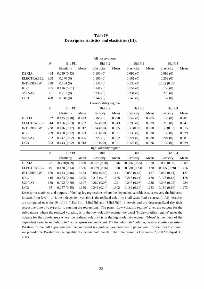
Table IVDescriptive statistics and elasticities (III).

All observations

N Bid PI1 Bid PI2 Bid PI3 Bid PI4

Elasticity Mean Elasticity Mean Elasticity Mean Elasticity Mean

DEXIA 404 0.059 (0.43) 0.100 (0) 0.096 (0) 0.096 (0)

ELECTRABEL 363 0.170 (0) 0.186 (0) 0.181 (0) 0.203 (0)

INTERBREW 398 0.134 (0) 0.146 (0) 0.136 (0) 0.132 (0.03)

KBC 405 0.126 (0.01) 0.141 (0) 0.154 (0) 0.153 (0)

SOLVAY 391 0.231 (0) 0.239 (0) 0.231 (0) 0.228 (0)

UCB 408 0.146 (0) 0.142 (0) 0.148 (0) 0.152 (0)

Low-volatility regime

N Bid PI1 Bid PI2 Bid PI3 Bid PI4

Elasticity Mean Elasticity Mean Elasticity Mean Elasticity Mean

DEXIA 332 0.115 (0.18) 0.993 0.166 (0) 0.990 0.149 (0) 0.985 0.135 (0) 0.981

ELECTRABEL 314 0.166 (0.03) 0.952 0.167 (0.01) 0.943 0.193 (0) 0.939 0.218 (0) 0.941

INTERBREW 238 0.116 (0.17) 0.917 0.154 (0.04) 0.905 0.139 (0.03) 0.908 0.136 (0.03) 0.915

KBC 289 0.100 (0.22) 0.923 0.135 (0.01) 0.931 0.139 (0) 0.930 0.130 (0) 0.929

SOLVAY 252 0.247 (0.02) 0.895 0.220 (0) 0.882 0.221 (0) 0.880 0.204 (0) 0.881

UCB 323 0.143 (0.02) 0.913 0.118 (0.01) 0.921 0.126 (0) 0.926 0.132 (0) 0.929

High-volatility regime

N Bid PI1 Bid PI2 Bid PI3 Bid PI4

Elasticity Mean Elasticity Mean Elasticity Mean Elasticity Mean

DEXIA 72 -0.778(0.29) 1.030 -0.077 (0.70) 1.046 -0.086 (0.65) 1.070 0.066 (0.69) 1.087

ELECTRABEL 49 0.478 (0.14) 1.336 -0.139 (0.76) 1.398 -0.580 (0.23) 1.430 -0.365 (0.28) 1.416

INTERBREW 160 0.113 (0.46) 1.123 0.084 (0.55) 1.141 0.050 (0.67) 1.137 0.052 (0.61) 1.127

KBC 116 0.183 (0.38) 1.195 0.216 (0.15) 1.175 0.218 (0.11) 1.178 0.176 (0.15) 1.178

SOLVAY 139 0.092 (0.60) 1.197 0.262 (0.05) 1.221 0.247 (0.03) 1.226 0.246 (0.02) 1.224

UCB 85 0.257 (0.25) 1.330 0.246 (0.14) 1.302 0.189 (0.14) 1.283 0.180 (0.10) 1.272

Descriptive statistics and outputs of the log-log regressions where the dependent variable is successively the bid price

impacts from level 1 to 4, the independent variable is the realized volatility in all cases (and a constant). All measures

are computed over the [9h:11h], [11h:13h], [13h:15h] and [15h:17h30] intervals and are deseasonalized (by their

respective time-of-day) prior to running the regressions. The panel ‘Low-volatility regime’ gives the outputs for the

sub-datasets where the realized volatility is in the low-volatility regime; the panel ‘High-volatility regime’ gives the

outputs for the sub-datasets where the realized volatility is in the high-volatility regime. ‘Mean’ is the mean of the

dependent variable and ‘elasticity’ is the regression coefficient. For the ‘elasticity’ column, heteroscedastic-consistent

P-values for the null hypothesis that the coefficient is significant are provided in parenthesis; for the ‘mean’ column,

we provide the P-value for the equality test across both panels. The time period is December 2, 2002 to April 30,

2003.

32

Table VDescriptive statistics and elasticities (IV).

All observations

N Ask PI1 Ask PI2 Ask PI3 Ask PI4

Elasticity Mean Elasticity Mean Elasticity Mean Elasticity Mean

DEXIA 403 0.094 (0.03) 0.089 (0.01) 0.087 (0) 0.088 (0)

ELECTRABEL 350 0.098 (0.13) 0.083 (0.08) 0.110 (0.01) 0.091 (0.03)

INTERBREW 397 0.107 (0.03) 0.098 (0.01) 0.090 (0.01) 0.083 (0.01)

KBC 407 0.218 (0) 0.213 (0) 0.211 (0) 0.211 (0)

SOLVAY 397 0.048 (0.36) 0.092 (0.03) 0.116 (0) 0.125 (0)

UCB 407 0.188 (0) 0.193 (0) 0.191 (0) 0.176 (0)

Low-volatility regime

N Ask PI1 Ask PI2 Ask PI3 Ask PI4

Elasticity Mean Elasticity Mean Elasticity Mean Elasticity Mean

DEXIA 329 0.083 (0.16) 0.976 0.085 (0.06) 0.975 0.092 (0.02) 0.974 0.096 (0.01) 0.975

ELECTRABEL 303 0.062 (0.42) 0.903 0.036 (0.53) 0.917 0.056 (0.27) 0.923 0.054 (0.25) 0.928

INTERBREW 239 0.081 (0.29) 0.910 0.062 (0.38) 0.918 0.040 (0.51) 0.918 0.048 (0.38) 0.923

KBC 293 0.236 (0) 0.914 0.231 (0) 0.912 0.217 (0) 0.916 0.217 (0) 0.917

SOLVAY 259 -0.046 (0.59) 0.941 -0.008 (0.91) 0.916 0.032 (0.57) 0.907 0.053 (0.31) 0.904

UCB 322 0.148 (0.01) 0.905 0.191 (0) 0.917 0.185 (0) 0.924 0.172 (0) 0.934

High-volatility regime

N Ask PI1 Ask PI2 Ask PI3 Ask PI4

Elasticity Mean Elasticity Mean Elasticity Mean Elasticity Mean

DEXIA 74 0.251 (0.17) 1.107 0.122 (0.37) 1.113 0.107 (0.34) 1.118 0.101 (0.29) 1.114

ELECTRABEL 47 -0.110 (0.84) 1.683 -0.119 (0.70) 1.582 -0.079 (0.74) 1.543 -0.052 (0.81) 1.502

INTERBREW 158 -0.084 (0.69) 1.134 0.054 (0.70) 1.122 0.068 (0.58) 1.122 0.034 (0.74) 1.115

KBC 114 0.082 (0.79) 1.218 0.140 (0.47) 1.222 0.078 (0.61) 1.211 0.080 (0.54) 1.210

SOLVAY 138 0.397 (0.02) 1.111 0.397 (0) 1.159 0.311 (0) 1.175 0.260 (0) 1.180

UCB 85 -0.114 (0.55) 1.361 -0.082 (0.60) 1.317 0.044 (0.72) 1.289 0.086 (0.44) 1.251

Descriptive statistics and outputs of the log-log regressions where the dependent variable is successively the ask price

impacts from level 1 to 4, the independent variable is the realized volatility in all cases (and a constant). All measures are

computed over the [9h:11h], [11h:13h], [13h:15h] and [15h:17h30] intervals and are deseasonalized (by their respective

time-of-day) prior to running the regressions. The panel ‘Low-volatility regime’ gives the outputs for the sub-datasets

where the realized volatility is in the low-volatility regime; the panel ‘High-volatility regime’ gives the outputs for the

sub-datasets where the realized volatility is in the high-volatility regime. ‘Mean’ is the mean of the dependent variable

and ‘elasticity’ is the regression coefficient. For the ‘elasticity’ column, heteroscedastic-consistent P-values for the null

hypothesis that the coefficient is significant are provided in parenthesis; for the ‘mean’ column, we provide the P-value

for the equality test across both panels. The time period is December 2, 2002 to April 30, 2003.

33

Table VI% change in the mean of each liquidity variable when switching from the low- to the

high-volatility regime.

%of

limit

Effe

ctiv

eT

rade

dT

rade

Quo

ted

BID

AS

K

orde

rssp

read

volu

me

aggr

essi

vene

sssp

read

Dep

thP

I1P

I3D

epth

PI1

PI3

DE

XIA

9%10

%30

%11

%17

%-1

2%4%

9%-1

1%13

%15

%

ELE

CT

RA

BE

L1%

57%

64%

22%

65%

13%

40%

52%

10%

86%

67%

INT

ER

BR

EW

4%42

%34

%22

%42

%2%

22%

25%

1%25

%22

%

KB

C6%

40%

5%10

%40

%8%

29%

27%

5%33

%32

%

SO

LVA

Y9%

53%

12%

31%

53%

-1%

34%

39%

-4%

18%

30%

UC

B9%

60%

21%

9%72

%-1

3%46

%39

%-1

8%50

%40

%

The

tabl

ere

port

sth

e%

chan

gein

the

mea

nof

each

liqui

dity

varia

ble

whe

nsw

itchi

ngfr

omth

elo

w-

toth

ehi

gh-v

olat

ility

regi

me.

Dep

thco

rres

pond

sto

the

dept

hat

the

best

pric

es.

PI1

and

PI3

corr

espo

ndto

the

pric

eim

pact

sco

mpu

ted

for

atr

ansa

ctio

nof

15,0

00an

d45

,000

euro

sre

spec

tivel

y.T

henu

llhy

poth

esis

ofth

eeq

ualit

yin

mea

nsis

reje

cted

atth

e5%

leve

lfor

allv

aria

bles

.

34

Table VIIThe dynamics of liquidity.

shock volatility av. volu nb tr pi3 qsp sp

L H L H L H L H L H L H

volatility + + + +

av. volu + + + + - -

nb tr + + + + - - -

pi3 + + - + + +

qsp + + + - - -+ -+ + + + +

sp + + + + - - + + + +

This table presents a summary of the VAR results (analysis of the dy-

namics of liquidity). A “+” (“-”) means that the shock on the given

variable (in the top row) has a positive (negative) and significant impact

on the variable (in the first column). In a few cases, we report a “-+”,

which indicates that the shock is first negative and then positive. “H”

refers to the high-volatility state, while “L” refers to the low-volatility

state. Note that av. volu relates to the average volume per trade, nb

tr, the number of trades, pi3, the level 3 price impact, qsp, the quoted

spread, sp, the effective spread.

Table VIIIHalf-life of the impulse responses.

shock volatility av. volu nb tr pi3 qsp sp

volatility 15 30 (15 mn)

av. volu 15 1H 15

nb tr 15 15 15 15

pi3 1H (15 mn) 15 30 (15 mn) 1H30

qsp 1H 15 15 1H 15 30

sp 1H 15 15 45 15

This table reports the half-life of the impulse responses. All results

are expressed in minutes except when there is an “H” (for hour). We

only report results for the significant impulse responses. All results are

for the low- and high-volatility states, except when there is a number

in parenthesis (high-volatility state). Note that av. volu relates to the

average volume per trade, nb tr, the number of trades, pi3, the level 3

price impact, qsp, the quoted spread, sp, the effective spread.

35

Figure 1. Stock prices. This figure shows the pattern of the stock prices (sampled at 15-minuteintervals) over our sample. The time period is December 2, 2002 to April 30, 2003 36.

Figure 2. Time-of-day for the volatility. This figure shows the time-of-day pattern for the 15-minute return volatility (smoothed using the Nadaraya-Watson estimator). The time period is De-cember 2, 2002 to April 30, 2003. 37

Figure 3. Time-of-day for the traded volume. This figure shows the time-of-day pattern for the15-minute traded volume (smoothed using the Nadaraya-Watson estimator). The time period isDecember 2, 2002 to April 30, 2003. 38

Figure 4. Time-of-day for the average volume per trade. This figure shows the time-of-daypattern for the average volume per trade (smoothed using the Nadaraya-Watson estimator). Thetime period is December 2, 2002 to April 30, 2003. 39

Figure 5. Time-of-day for the trade aggressiveness.This figure shows the time-of-day patternfor the trade aggressiveness (smoothed using the Nadaraya-Watson estimator). The time period isDecember 2, 2002 to April 30, 2003. 40

Figure 6. Time-of-day for the relative inside spread.This figure shows the time-of-day patternfor the relative inside spread (smoothed using the Nadaraya-Watson estimator). The time period isDecember 2, 2002 to April 30, 2003.

41

Figure 7. Time-of-day for the current and effective spread.This figure shows the time-of-daypattern for the current and effective spread (smoothed using the Nadaraya-Watson estimator). Thetime period is December 2, 2002 to April 30, 2003. 42

Figure 8. Time-of-day for the inside bid depth (in euros). This figure shows the time-of-daypattern for the inside bid depth (in euros) (smoothed using the Nadaraya-Watson estimator). Thetime period is December 2, 2002 to April 30, 2003. 43

Figure 9. Time-of-day for the bid price impacts.This figure shows the time-of-day pattern for thebid price impacts (smoothed using the Nadaraya-Watson estimator). Price impacts are computedfor volumes of 0.5, 1, 1.5 and 2 times the reference volume, which is computed as the volumecorresponding to a transaction of 30,000 euros at the average price for the stock over the sample.The time period is December 2, 2002 to April 30, 2003. 44

Figure 10. Aggregated effective spread vs realized volatility.Relationship between the aggre-gated effective spread and the realized volatility. The aggregated effective spread is the averageeffective spread over the [9h:11h], [11h:13h], [13h:15h] and [15h:17h30] intervals; the realizedvolatility is defined over the same intervals. Both measures are deseasonalized by their respectivetime-of-day. The time period is December 2, 2002 to April 30, 2003. 45

Figure 11. Aggregated trade aggressiveness vs realized volatility.Relationship between theaggregated trade aggressiveness and the realized volatility. The aggregated trade aggressiveness isthe average trade aggressiveness over the [9h:11h], [11h:13h], [13h:15h] and [15h:17h30] intervals;the realized volatility is defined over the same intervals. Both measures are deseasonalized by theirrespective time-of-day. The time period is December 2, 2002 to April 30, 2003. 46

Figure 12. Aggregated bid inside depth (in euros) vs realized volatility.Relationship betweenthe aggregated bid inside depth (in euros) and the realized volatility. The aggregated bid insidedepth (in euros) is the average bid inside depth (in euros) over the [9h:11h], [11h:13h], [13h:15h]and [15h:17h30] intervals; the realized volatility is defined over the same intervals. Both measuresare deseasonalized by their respective time-of-day. The time period is December 2, 2002 to April30, 2003.

47

Figure 13. Aggregated bid price impact (level 3) vs realized volatility.Relationship betweenthe aggregated bid price impact (level 3) and the realized volatility. The aggregated bid price im-pact (level 3) is the average bid price impact (level 3) over the [9h:11h], [11h:13h], [13h:15h] and[15h:17h30] intervals; the realized volatility is defined over the same intervals. Both measures aredeseasonalized by their respective time-of-day. The time period is December 2, 2002 to April 30,2003.

48

Fig

ure

14.

Impu

lse

resp

onse

func

tions

ofth

ein

side

spre

ad,l

ow-v

olat

ility

regi

me.T

hefig

ures

repo

rtth

eim

puls

ere

spon

sefu

nctio

nsof

the

insi

desp

read

(QS

P)

toa

one-

unit

shoc

kto

the

othe

r6

varia

bles

:vo

latil

ity(R

2),

pric

eim

pact

for

atr

ansa

ctio

nof

45,0

00eu

ros

(PI3

),nu

mbe

rof

trad

es(N

TR

),av

erag

evo

lum

epe

rtr

ade

(AV

VO

L),

effe

ctiv

esp

read

(SP

),an

dits

elf.

The

impu

lse

resp

onse

sar

ere

cons

truc

ted

bym

eans

ofa

Cho

lesk

yde

com

posi

tion

from

aVA

R(2

)m

odel

estim

ated

with

the

low

-vol

atili

tyre

gim

eob

serv

atio

nson

ly.

The

6st

ocks

are

DE

XIA

(DE

X),

ELE

CT

RA

BE

L(E

LE),

INT

ER

BR

EW

(IN

T),

KB

C(K

BC

),S

OLV

AY

(SO

L),a

ndU

CB

(UC

B).

49

Fig

ure

15.

Impu

lse

resp

onse

func

tions

ofth

ein

side

spre

ad,h

igh-

vola

tility

regi

me.T

hefig

ures

repo

rtth

eim

puls

ere

spon

sefu

nctio

nsof

the

insi

desp

read

(QS

P)

toa

one-

unit

shoc

kto

the

othe

r6

varia

bles

:vo

latil

ity(R

2),

pric

eim

pact

for

atr

ansa

ctio

nof

45,0

00eu

ros

(PI3

),nu

mbe

rof

trad

es(N

TR

),av

erag

evo

lum

epe

rtr

ade

(AV

VO

L),

effe

ctiv

esp

read

(SP

),an

dits

elf.

The

impu

lse

resp

onse

sar

ere

cons

truc

ted

bym

eans

ofa

Cho

lesk

yde

com

posi

tion

from

aVA

R(2

)m

odel

estim

ated

with

the

high

-vol

atili

tyre

gim

eob

serv

atio

nson

ly.

The

6st

ocks

are

DE

XIA

(DE

X),

ELE

CT

RA

BE

L(E

LE),

INT

ER

BR

EW

(IN

T),

KB

C(K

BC

),S

OLV

AY

(SO

L),a

ndU

CB

(UC

B).

50

Fig

ure

16.

Impu

lse

resp

onse

func

tions

ofth

epr

ice

impa

ct,

leve

l3,

low

-vol

atili

tyre

gim

e.The

figur

esre

port

the

impu

lse

resp

onse

func

tions

ofth

epr

ice

impa

ctfo

ra

trad

eof

45,0

00eu

ros

(PI3

)to

aon

e-un

itsh

ock

toth

eot

her

6va

riabl

es:

vola

tility

(R2)

,ins

ide

spre

ad(Q

SP

),nu

mbe

rof

trad

es(N

TR

),av

erag

evo

lum

epe

rtr

ade

(AV

VO

L),

effe

ctiv

esp

read

(SP

),an

dits

elf.

The

impu

lse

resp

onse

sar

ere

cons

truc

ted

bym

eans

ofa

Cho

lesk

yde

com

posi

tion

from

aVA

R(2

)m

odel

estim

ated

with

the

low

-vol

atili

tyre

gim

eob

serv

atio

nson

ly.

The

6st

ocks

are

DE

XIA

(DE

X),

ELE

CT

RA

BE

L(E

LE),

INT

ER

BR

EW

(IN

T),

KB

C(K

BC

),S

OLV

AY

(SO

L),a

ndU

CB

(UC

B).

51

Fig

ure

17.

Impu

lse

resp

onse

func

tions

ofth

epr

ice

impa

ct,l

evel

3,hi

gh-v

olat

ility

regi

me.T

hefig

ures

repo

rtth

eim

puls

ere

spon

sefu

nctio

nsof

the

pric

eim

pact

for

atr

ade

of45

,000

euro

s(P

I3)

toa

one-

unit

shoc

kto

the

othe

r6

varia

bles

:vo

latil

ity(R

2),i

nsid

esp

read

(QS

P),

num

ber

oftr

ades

(NT

R),

aver

age

volu

me

per

trad

e(A

VV

OL)

,ef

fect

ive

spre

ad(S

P),

and

itsel

f.T

heim

puls

ere

spon

ses

are

reco

nstr

ucte

dby

mea

nsof

aC

hole

sky

deco

mpo

sitio

nfr

oma

VAR

(2)

mod

eles

timat

edw

ithth

ehi

gh-v

olat

ility

regi

me

obse

rvat

ions

only

.T

he6

stoc

ksar

eD

EX

IA(D

EX

),E

LEC

TR

AB

EL

(ELE

),IN

TE

RB

RE

W(I

NT

),K

BC

(KB

C),

SO

LVA

Y(S

OL)

,and

UC

B(U

CB

).

52

Fig

ure

18.

Impu

lse

resp

onse

func

tions

ofth

evo

latil

ity,l

ow-v

olat

ility

regi

me.

The

figur

esre

port

the

impu

lse

resp

onse

func

tions

ofth

evo

latil

ity(R

2)to

aon

e-un

itsh

ock

toth

eot

her

6va

riabl

es:

insi

desp

read

(QS

P),

pric

eim

pact

for

atr

ansa

ctio

nof

45,0

00eu

ros

(PI3

),nu

mbe

rof

trad

es(N

TR

),av

erag

evo

lum

epe

rtr

ade

(AV

VO

L),

effe

ctiv

esp

read

(SP

),an

dits

elf.

The

impu

lse

resp

onse

sar

ere

cons

truc

ted

bym

eans

ofa

Cho

lesk

yde

com

posi

tion

from

aVA

R(2

)m

odel

estim

ated

with

the

low

-vol

atili

tyre

gim

eob

serv

atio

nson

ly.

The

6st

ocks

are

DE

XIA

(DE

X),

ELE

CT

RA

BE

L(E

LE),

INT

ER

BR

EW

(IN

T),

KB

C(K

BC

),S

OLV

AY

(SO

L),a

ndU

CB

(UC

B).

53

Fig

ure

19.

Impu

lse

resp

onse

func

tions

ofth

evo

latil

ity,h

igh-

vola

tility

regi

me.

The

figur

esre

port

the

impu

lse

resp

onse

func

tions

ofth

evo

latil

ity(R

2)to

aon

e-un

itsh

ock

toth

eot

her

6va

riabl

es:

insi

desp

read

(QS

P),

pric

eim

pact

for

atr

ansa

ctio

nof

45,0

00eu

ros

(PI3

),nu

mbe

rof

trad

es(N

TR

),av

erag

evo

lum

epe

rtr

ade

(AV

VO

L),

effe

ctiv

esp

read

(SP

),an

dits

elf.

The

impu

lse

resp

onse

sar

ere

cons

truc

ted

bym

eans

ofa

Cho

lesk

yde

com

posi

tion

from

aVA

R(2

)m

odel

estim

ated

with

the

high

-vol

atili

tyre

gim

eob

serv

atio

nson

ly.

The

6st

ocks

are

DE

XIA

(DE

X),

ELE

CT

RA

BE

L(E

LE),

INT

ER

BR

EW

(IN

T),

KB

C(K

BC

),S

OLV

AY

(SO

L),a

ndU

CB

(UC

B).

54

Fig

ure

20.

Impu

lse

resp

onse

func

tions

ofth

eav

erag

evo

lum

epe

rtra

de,l

ow-v

olat

ility

regi

me.T

hefig

ures

repo

rtth

eim

puls

ere

spon

sefu

nctio

nsof

the

aver

age

volu

me

per

trad

e(A

VV

OL)

toa

one-

unit

shoc

kto

the

othe

r6

varia

bles

:in

side

spre

ad(Q

SP

),vo

latil

ity(R

2),

pric

eim

pact

for

atr

ansa

ctio

nof

45,0

00eu

ros

(PI3

),nu

mbe

rof

trad

es(N

TR

),ef

fect

ive

spre

ad(S

P),

and

itsel

f.T

heim

puls

ere

spon

ses

are

reco

nstr

ucte

dby

mea

nsof

aC

hole

sky

deco

mpo

sitio

nfr

oma

VAR

(2)

mod

eles

timat

edw

ithth

elo

w-v

olat

ility

regi

me

obse

rvat

ions

only

.T

he6

stoc

ksar

eD

EX

IA(D

EX

),E

LEC

TR

AB

EL

(ELE

),IN

TE

RB

RE

W(I

NT

),K

BC

(KB

C),

SO

LVA

Y(S

OL)

,and

UC

B(U

CB

).

55

Fig

ure

21.

Impu

lse

resp

onse

func

tions

ofth

eav

erag

evo

lum

epe

rtra

de,h

igh-

vola

tility

regi

me.T

hefig

ures

repo

rtth

eim

puls

ere

spon

sefu

nctio

nsof

the

aver

age

volu

me

per

trad

e(A

VV

OL)

toa

one-

unit

shoc

kto

the

othe

r6

varia

bles

:in

side

spre

ad(Q

SP

),vo

latil

ity(R

2),

pric

eim

pact

for

atr

ansa

ctio

nof

45,0

00eu

ros

(PI3

),nu

mbe

rof

trad

es(N

TR

),ef

fect

ive

spre

ad(S

P),

and

itsel

f.T

heim

puls

ere

spon

ses

are

reco

nstr

ucte

dby

mea

nsof

aC

hole

sky

deco

mpo

sitio

nfr

oma

VAR

(2)

mod

eles

timat

edw

ithth

ehi

gh-v

olat

ility

regi

me

obse

rvat

ions

only

.T

he6

stoc

ksar

eD

EX

IA(D

EX

),E

LEC

TR

AB

EL

(ELE

),IN

TE

RB

RE

W(I

NT

),K

BC

(KB

C),

SO

LVA

Y(S

OL)

,and

UC

B(U

CB

).

56

Fig

ure

22.

Impu

lse

resp

onse

func

tions

ofth

enu

mbe

rof

trad

es,l

ow-v

olat

ility

regi

me.T

hefig

ures

repo

rtth

eim

puls

ere

spon

sefu

nctio

nsof

the

num

ber

oftr

ades

(NT

R)

toa

one-

unit

shoc

kto

the

othe

r6

varia

bles

:in

side

spre

ad(Q

SP

),vo

latil

ity(R

2),

pric

eim

pact

for

atr

ansa

ctio

nof

45,0

00eu

ros

(PI3

),av

erag

evo

lum

epe

rtr

ade

(AV

VO

L),e

ffect

ive

spre

ad(S

P),

and

itsel

f.T

heim

puls

ere

spon

ses

are

reco

nstr

ucte

dby

mea

nsof

aC

hole

sky

deco

mpo

sitio

nfr

oma

VAR

(2)

mod

eles

timat

edw

ithth

elo

w-v

olat

ility

regi

me

obse

rvat

ions

only

.T

he6

stoc

ksar

eD

EX

IA(D

EX

),E

LEC

TR

AB

EL

(ELE

),IN

TE

RB

RE

W(I

NT

),K

BC

(KB

C),

SO

LVA

Y(S

OL)

,and

UC

B(U

CB

).

57

Fig

ure

23.

Impu

lse

resp

onse

func

tions

ofth

enu

mbe

rof

trad

es,h

igh-

vola

tility

regi

me.T

hefig

ures

repo

rtth

eim

puls

ere

spon

sefu

nctio

nsof

the

num

ber

oftr

ades

(NT

R)

toa

one-

unit

shoc

kto

the

othe

r6

varia

bles

:in

side

spre

ad(Q

SP

),vo

latil

ity(R

2),

pric

eim

pact

for

atr

ansa

ctio

nof

45,0

00eu

ros

(PI3

),nu

mbe

rof

trad

es(NT

R),

aver

age

volu

me

per

trad

e(A

VV

OL)

,effe

ctiv

esp

read

(SP

),an

dits

elf.

The

impu

lse

resp

onse

sar

ere

cons

truc

ted

bym

eans

ofa

Cho

lesk

yde

com

posi

tion

from

aVA

R(2

)m

odel

estim

ated

with

the

high

-vol

atili

tyre

gim

eob

serv

atio

nson

ly.

The

6st

ocks

are

DE

XIA

(DE

X),

ELE

CT

RA

BE

L(E

LE),

INT

ER

BR

EW

(IN

T),

KB

C(K

BC

),S

OLV

AY

(SO

L),a

ndU

CB

(UC

B).

58

Fig

ure

24.

Impu

lse

resp

onse

func

tions

ofth

eef

fect

ive

spre

ad,

low

-vol

atili

tyre

gim

e.The

figur

esre

port

the

impu

lse

resp

onse

func

tions

ofth

eef

fect

ive

spre

ad(S

P)

toa

one-

unit

shoc

kto

the

othe

r6

varia

bles

:in

side

spre

ad(Q

SP

),vo

latil

ity(R

2),p

rice

impa

ctfo

ra

tran

sact

ion

of45

,000

euro

s(P

I3),

num

ber

oftr

ades

(NTR

),av

erag

evo

lum

epe

rtr

ade

(AV

VO

L),

effe

ctiv

esp

read

(SP

),an

dits

elf.

The

impu

lse

resp

onse

sar

ere

cons

truc

ted

bym

eans

ofa

Cho

lesk

yde

com

posi

tion

from

aVA

R(2

)m

odel

estim

ated

with

the

low

-vol

atili

tyre

gim

eob

serv

atio

nson

ly.

The

6st

ocks

are

DE

XIA

(DE

X),

ELE

CT

RA

BE

L(E

LE),

INT

ER

BR

EW

(IN

T),

KB

C(K

BC

),S

OLV

AY

(SO

L),a

ndU

CB

(UC

B).

59

Fig

ure

25.

Impu

lse

resp

onse

func

tions

ofth

eef

fect

ive

spre

ad,

high

-vol

atili

tyre

gim

e.The

figur

esre

port

the

impu

lse

resp

onse

func

tions

ofth

eef

fect

ive

spre

ad(S

P)

toa

one-

unit

shoc

kto

the

othe

r6

varia

bles

:in

side

spre

ad(Q

SP

),vo

latil

ity(R

2),p

rice

impa

ctfo

ra

tran

sact

ion

of45

,000

euro

s(P

I3),

num

ber

oftr

ades

(NTR

),av

erag

evo

lum

epe

rtr

ade

(AV

VO

L),

effe

ctiv

esp

read

(SP

),an

dits

elf.

The

impu

lse

resp

onse

sar

ere

cons

truc

ted

bym

eans

ofa

Cho

lesk

yde

com

posi

tion

from

aVA

R(2

)m

odel

estim

ated

with

the

high

-vol

atili

tyre

gim

eob

serv

atio

nson

ly.

The

6st

ocks

are

DE

XIA

(DE

X),

ELE

CT

RA

BE

L(E

LE),

INT

ER

BR

EW

(IN

T),

KB

C(K

BC

),S

OLV

AY

(SO

L),a

ndU

CB

(UC

B).

60

61

NATIONAL BANK OF BELGIUM - WORKING PAPERS SERIES

1. "Model-based inflation forecasts and monetary policy rules" by M. Dombrecht and R. Wouters, Research Series, February 2000.

2. "The use of robust estimators as measures of core inflation" by L. Aucremanne, Research Series, February 2000.

3. "Performances économiques des Etats-Unis dans les années nonante" by A. Nyssens, P. Butzen, P. Bisciari, Document Series, March 2000.

4. "A model with explicit expectations for Belgium" by P. Jeanfils, Research Series, March 2000.

5. "Growth in an open economy: some recent developments" by S. Turnovsky, Research Series, May 2000.

6. "Knowledge, technology and economic growth: an OECD perspective" by I. Visco, A. Bassanini, S. Scarpetta, Research Series, May 2000.

7. "Fiscal policy and growth in the context of European integration" by P. Masson, Research Series, May 2000.

8. "Economic growth and the labour market: Europe's challenge" by C. Wyplosz, Research Series, May 2000.

9. "The role of the exchange rate in economic growth: a euro-zone perspective" by R. MacDonald, Research Series, May 2000.

10. "Monetary union and economic growth" by J. Vickers, Research Series, May 2000.

11. "Politique monétaire et prix des actifs: le cas des Etats-Unis" by Q. Wibaut, Document Series, August 2000.

12. "The Belgian industrial confidence indicator: leading indicator of economic activity in the euro area?" by J.J. Vanhaelen, L. Dresse, J. De Mulder, Document Series, November 2000.

13. "Le financement des entreprises par capital-risque" by C. Rigo, Document Series, February 2001.

14. "La nouvelle économie" by P. Bisciari, Document Series, March 2001.

15. "De kostprijs van bankkredieten" by A. Bruggeman and R. Wouters, Document Series, April 2001.

16. "A guided tour of the world of rational expectations models and optimal policies" by Ph. Jeanfils, Research Series, May 2001.

17. "Attractive Prices and Euro - Rounding effects on inflation" by L. Aucremanne and D. Cornille, Documents Series, November 2001.

18. "The interest rate and credit channels in Belgium: an investigation with micro-level firm data" by P. Butzen, C. Fuss and Ph. Vermeulen, Research series, December 2001.

19 "Openness, imperfect exchange rate pass-through and monetary policy" by F. Smets and R. Wouters, Research series, March 2002.

20. "Inflation, relative prices and nominal rigidities" by L. Aucremanne, G. Brys, M. Hubert, P. J. Rousseeuw and A. Struyf, Research series, April 2002.

62

21. "Lifting the burden: fundamental tax reform and economic growth" by D. Jorgenson, Research series, May 2002.

22. "What do we know about investment under uncertainty?" by L. Trigeorgis, Research series, May 2002.

23. "Investment, uncertainty and irreversibility: evidence from Belgian accounting data" by D. Cassimon, P.-J. Engelen, H. Meersman, M. Van Wouwe, Research series, May 2002.

24. "The impact of uncertainty on investment plans" by P. Butzen, C. Fuss, Ph. Vermeulen, Research series, May 2002.

25. "Investment, protection, ownership, and the cost of capital" by Ch. P. Himmelberg, R. G. Hubbard, I. Love, Research series, May 2002.

26. "Finance, uncertainty and investment: assessing the gains and losses of a generalised non-linear structural approach using Belgian panel data", by M. Gérard, F. Verschueren, Research series, May 2002.

27. "Capital structure, firm liquidity and growth" by R. Anderson, Research series, May 2002.

28. "Structural modelling of investment and financial constraints: where do we stand?" by J.- B. Chatelain, Research series, May 2002.

29. "Financing and investment interdependencies in unquoted Belgian companies: the role of venture capital" by S. Manigart, K. Baeyens, I. Verschueren, Research series, May 2002.

30. "Development path and capital structure of Belgian biotechnology firms" by V. Bastin, A. Corhay, G. Hübner, P.-A. Michel, Research series, May 2002.

31. "Governance as a source of managerial discipline" by J. Franks, Research series, May 2002.

32. "Financing constraints, fixed capital and R&D investment decisions of Belgian firms" by M. Cincera, Research series, May 2002.

33. "Investment, R&D and liquidity constraints: a corporate governance approach to the Belgian evidence" by P. Van Cayseele, Research series, May 2002.

34. "On the Origins of the Franco-German EMU Controversies" by I. Maes, Research series, July 2002.

35. "An estimated dynamic stochastic general equilibrium model of the Euro Area", by F. Smets and R. Wouters, Research series, October 2002.

36. "The labour market and fiscal impact of labour tax reductions: The case of reduction of employers' social security contributions under a wage norm regime with automatic price indexing of wages", by K. Burggraeve and Ph. Du Caju, Research series, March 2003.

37. "Scope of asymmetries in the Euro Area", by S. Ide and Ph. Moës, Document series, March 2003.

38. "De autonijverheid in België: Het belang van het toeleveringsnetwerk rond de assemblage van personenauto's", by F. Coppens and G. van Gastel, Document series, June 2003.

39. "La consommation privée en Belgique", by B. Eugène, Ph. Jeanfils and B. Robert, Document series, June 2003.

40. "The process of European monetary integration: a comparison of the Belgian and Italian approaches", by I. Maes and L. Quaglia, Research series, August 2003.

63

41. "Stock market valuation in the United States", by P. Bisciari, A. Durré and A. Nyssens, Document series, November 2003.

42. "Modeling the Term Structure of Interest Rates: Where Do We Stand?", by K. Maes, Research series, February 2004.

43. "Interbank Exposures: An Empirical Examination of Systemic Risk in the Belgian Banking System", by H. Degryse and G. Nguyen, Research series, March 2004.

44. "How Frequently do Prices change? Evidence Based on the Micro Data Underlying the Belgian CPI", by L. Aucremanne and E. Dhyne, Research series, April 2004.

45. "Firm's investment decisions in reponse to demand and price uncertainty", by C. Fuss and Ph. Vermeulen, Research series, April 2004.

46. "SMEs and Bank Lending Relationships: the Impact of Mergers", by H. Degryse, N. Masschelein and J. Mitchell, Research series, May 2004.

47. "The Determinants of Pass-Through of Market Conditions to Bank Retail Interest Rates in Belgium", by F. De Graeve, O. De Jonghe and R. Vander Vennet, Research series, May 2004.

48. "Sectoral vs. country diversification benefits and downside risk", by M. Emiris, Research series, May 2004.

49. "How does liquidity react to stress periods in a limit order market?", by H. Beltran, A. Durré and P. Giot, Research series, May 2004.

50. "Financial consolidation and liquidity: prudential regulation and/or competition policy?", by P. Van Cayseele, Research series, May 2004.

51. "Basel II and Operational Risk: Implications for risk measurement and management in the financial sector", by A. Chapelle, Y. Crama, G. Hübner and J.-P. Peters, Research series, May 2004.