economic theory and
TRANSCRIPT

ECONOMIC THEORY AND
ECONOMETRIC METHODS IN SPATIAL
MARKET INTEGRATION ANALYSIS
Dissertation
to obtain the Ph. D. degree
in the International Ph. D. Program for Agricultural Sciences in Göttingen
(IPAG)
at the Faculty of Agricultural Sciences,
Georg-August-University Göttingen, Germany
presented by
Sergio René Araujo Enciso
born in Ciudad de México, D.F, México
Göttingen, March 2012

D7
1. Name of supervisor: Prof. Dr. Stephan v.Cramon-Taubadel
2. Name of co-supervisor: Prof. Dr. Bernhard Brümmer
3. Name of a further member of the examination committee: J-Prof. Xiaohua Yu, Ph.D.
Date of dissertation: May the 30th, 2012

For Rosi, René, Mónica, Móniquita, Dolores,
Raúl, Julia, Luz María, Dolores & José


Acknowledgments-Agradecimientos
Through the last six year, I have been living is a sort of self-exile driven by my own ideas about
experiencing life in a foreign country. At this stage I feel alienated not only here, but at
homeland as well. Somehow, as one Professor once said: “You will become a citizen of the
world”, so that defining homeland is no longer straightforward in my situation. Along with the
many sacrifices, i.e. spicy food, that have been done for pursuing a life abroad, there are
invaluable rewards; the most important for sure is the chance of meeting wonderful people
trough the journey.
Especially, I am grateful to my supervisors: Prof. Dr. von Cramon-Taubadel for the lively
discussions and for being supportive during my studies, Prof. Dr. Bernhard Brümmer for
awakening my interest in quantitative methods during the lectures and for his valuable
recommendations, and J-Prof. Xiaohua Yu, Ph.D. for his feedback and comments during the
Doctoral Seminars. To the Courant Research Centre “Poverty, Equity and Growth in
Developing Countries” for the financial support that made me possible to follow my studies and
attend conferences and seminars.
Also, I thank all my colleagues, especially Dr. Sebastian Lakner, Dr. Karla Hernández, Dr. Rico
Ihle and Antje Wagener for his support through the last years. Thanks to Barbara Heinrich,
Cordula Wendler, Carsten Holst, Thelma Brenes, Mostafa Mohamed Badr Mohamed, Nadine
Würriehausen, and the rest of the team. Life and studies were easier with you by my side guys.
Thanks to the student assistants: Mary for the proof reading and Luis for the database work.
Thanks to the people at the R and GAMS lists for answering my questions regarding
programming.
Friends and family also have played a main role during the last years. Thanks to my friends
Gabriela C., Santiago I., Jorge V., Mónica S., Juan V., Aura C., Harald S., Claudia C., Carla S.,
Karla, H., Guillermo C., Alina B., Telva S., Henning B., Ricardo C., Veronika A., Fu Xiao
Shan, Maribel R., Dan S., Katia S., Vânia d.G, and Gabriel A. Life is not the same after meeting
you people, I am glad for that. To my family, for the inevitable nostalgia we fell as a
consequence of the distance, be sure that you have been the force driving me to move on.
Gracias por estar siempre conmigo. Also thanks to all the people that has been involved and
helped me to reach this stage, this could not have been done without their support.
Finally, I would like to show some quote which personally I consider interesting. Honestly I not
only share the views of the authors who wrote those words, but also admire them.
.


Some phrases that reflect the contradictory human nature of this particular Ph.D student
regarding his views about the whole experience abroad
"Espero alegre la salida y espero no volver jamás"
― Frida Kahlo
“These are days you’ll remember
Never before and never since, I promise,
will the whole world be warm as this …”
― Robert Buck & Natalie Merchant, Lyrics from “These are days”
“.. this place needs me here to start
this place is the beat of my heart…”
― Michael Stipe, Peter Buck, Mike Mills & Scott McCaughey, Lyrics from “Oh my heart”
“Running through a field where all my tracks will be concealed
and there is nowhere to go”
― Flea, Frusciante, Kiedis & Smith, Lyrics from “Snow (Hey Oh)”

Historical and contemporaneous views/critiques regarding education which I share
“Undergraduates today can select from a swathe of identity studies.... The shortcoming of all
these para-academic programs is not that they concentrate on a given ethnic or geographical
minority; it is that they encourage members of that minority to study themselves - thereby
simultaneously negating the goals of a liberal education and reinforcing the sectarian and
ghetto mentalities they purport to undermine.”
― Tony Judt, The Memory Chalet
“The proper function of an University in national education is tolerably well understood. At
least there is a tolerably general agreement about what an University is not. It is not a place for
professional education. Universities are not intended to teach the knowledge required to fit men
for some special mode of gaining their livelihood. Their object is not to make skilful lawyers, or
physicians, or engineers, but capable and cultivated human beings.”
― John Stuart Mill, Inaugural Address Delivered to the University of St. Andrews
“El contexto de crisis-cambio-globalización está marcado por una crisis en el terreno moral,
que no se puede soslayar o evadir socialmente y por ello es creciente la demanda social que
exige a las instituciones educativas y a los educadores ocuparse eficazmente de la formación
moral que promueva un cambio hacia el mejoramiento de la convivencia social que requiere
orientarse hacia la humanización individual y colectiva y no solamente, como parece
orientarse hoy en día, hacia la maximización de las ganancias económicas”
― Martín López Calva

Views of other people regarding justice, responsibility and solidarity that I share
“If we remain grotesquely unequal, we shall lose all sense of fraternity: and fraternity, for all
its fatuity as a political objective, turns out to be the necessary condition of politics itself.”
― Tony Judt, Ill Fares the Land
“The increasing tendency towards seeing people in terms of one dominant ‘identity’ (‘this is
your duty as an American’, ‘you must commit these acts as a Muslim’, or ‘as a Chinese you
should give priority to this national engagement’) is not only an imposition of an external and
arbitrary priority, but also the denial of an important liberty of a person who can decide on
their respective loyalties to different groups (to all of which he or she belongs).”
― Amartya Sen, The Idea Of Justice
"Somos la memoria que tenemos y la responsabilidad que asumimos, sin memoria no existimos
y sin responsabilidad quizá no merezcamos existir"
― José Saramago, Cuadernos de Lanzarote.
“Podrán morir las personas, pero jamás sus ideas”
― Ernesto “Che” Guevara
“Las masas humanas más peligrosas son aquellas en cuyas venas ha sido inyectado el veneno
del miedo… del miedo al cambio”
― Octavio Paz
"A nation's greatness is measured by how it treats its weakest members"
― Mahatma Ghandi
“Trabajar incansablemente por establecer la justicia y el derecho en un nuevo orden mundial,
para consolidar una paz inalterable y duradera, y así conjurar definitivamente el flagelo de la
guerra; continuar construyendo el nuevo modelo de unidad, con el respeto a las diferencias y a
los derechos de los más pequeños, así en la sociedad, como en el seno de las diferentes
confesiones religiosas; Apoyar las tareas de protección y conservación de la tierra, hogar
común y herencia para las nuevas generaciones ; Participar, según el lugar que tenemos social
y religiosamente, en la construcción de ese ‘otro mundo posible’; Colaborar con el Padre en
esta Nueva Hora de Gracia: en su obra siempre creadora y siempre redentora, manifestada en
esos brotes tiernos que prometen buenos y abundantes frutos”
―Samuel Ruiz García

What some Authors wrote and I really enjoy
“Sabed que en mis labios de granito quedaron detenidas las palabras”
― Rosario Castellanos, Epitafio
“– ¿Y hasta cuándo cree usted que podamos seguir en este ir y venir del carajo? – le preguntó
Florentino Ariza tenía la respuesta preparada desde hacía cincuenta y tres años, siete meses y
once días con sus noches
– Toda la vida – dijo.”
― Gabriel García Márquez, El amor en los tiempos del cólera
“Dios, invención admirable,
hecha de ansiedad humana
y de esencia arcana,
que se vuelve impenetrable.”
― Guadalupe “Pita” Amor, Décimas a Dios
“Todo lo que es hecho, todo lo humano de la Tierra es hecho por manos”
― Ernesto Cardenal
“Tierra desnuda, tierra despierta, tierra maicera con sueño…”
― Miguel Ángel Asturias, Hombres de Maíz
"Todo dura siempre un poco más de lo que debería"
― Julio Cortázar, Rayuela


I
TABLE OF CONTENTS
LIST OF FIGURES ................................................................................................... III
LIST OF TABLES ..................................................................................................... V
LIST OF ABBREVIATIONS .................................................................................... VII
INTRODUCTION ....................................................................................................... 1
1. UNDERSTANDING THE LINKAGE BETWEEN THE
ECONOMIC THEORY AND THE ECONOMETRIC METHODS ........................... 5
1.1. Introduction to the Takayama and Judge
Price and Allocation Models .............................................................. 7
1.2. The Spatial Equilibrium Condition and the
Threshold Vector Error Correction Model .................................... 11
1.2.1. Linking the Economic Theory and the
Econometric Model ................................................................ 11
1.2.2. Threshold Vector Error Correction Model Estimation ..... 14
1.3. Confronting Economic Theory and the Econometric Model ........ 17
1.4. Analysis of Results ............................................................................ 24
1.5. Chapter Conclusions ......................................................................... 28
2. TESTING FOR LINEAR AND THRESHOLD ERROR
CORRECTION UNDER THE SPATIAL EQUILIBRIUM CONDITION ................. 29
2.1. The Economic Concept of Spatial Market Integration
and the Econometric Concepts of Threshold Error
Correction and Threshold Cointegration ....................................... 31
2.2. Tests for Linear and Threshold Error Correction ........................ 33
2.3. Testing for Cointegration in the Equilibrium ................................ 38
2.3.1. Testing for a Unit Root .......................................................... 39
2.3.2. Tests Results and Discussion ................................................. 39
2.4. Conciliated Results and Concluding Remarks ............................... 46
3. EQUILIBRIUM AND DISEQUILIBRIUM MODELING IN SPATIAL MARKET
INTEGRATION .............................................................................................. 49
3.1. Acknowledging the Relevance of Disequilibrium
in Spatial Market Integration .......................................................... 51
3.2. A Brief Introduction to the Disequilibrium Models ...................... 52

II
3.3. Modelling Disequilibrium and the Spatial
Equilibrium Condition ..................................................................... 54
3.3.1. Lagged Trade Disequilibrium Model ................................... 55
3.3.2. White Noise Disequilibrium Model ....................................... 56
3.3.3. Moving Average Restriction Disequilibrium Model ........... 59
3.3.4. Restrictive Recursive Disequilibrium Model ....................... 60
3.3.5. White Noise Equilibrium Model ........................................... 61
3.4. Data Generation and TVECM Estimation...................................... 63
3.5. Results from the TVECM ................................................................. 69
3.6. Discussion ........................................................................................... 75
3.7. Concluding Remarks ......................................................................... 77
4. ADDRESSING FURTHER RESEARCH IN ECONOMIC AND
ECONOMETRIC THEORY .............................................................................. 79
4.1. Further Theory to be Considered .................................................... 81
4.1.1. The Takayama and Judge Spatial and
Temporal Price and Allocation Models ................................ 81
4.1.2. The Williams & Wright Models ............................................ 83
4.1.3. The Rational Expectations Models ....................................... 84
4.1.4. The Econometric Concept of Threshold Cointegration ...... 85
4.2. Linking the Economic Theory to the Empirical Applications ...... 87
4.3. Summary of Findings and Future Research ................................... 90
REFERENCES.......................................................................................................... 93
APPENDIX I: GAMS CODES .................................................................................. 99
APPENDIX II: EVIDENCE OF NON-LINEAR PRICE TRANSMISSION
BETWEEN MAIZE MARKETS IN MEXICO AND THE US ............................ 115
APPENDIX III: THE RELATIONSHIP BETWEEN TRADE AND
PRICE VOLATILITY IN THE MEXICAN AND US MAIZE MARKETS .......... 139

III
LIST OF FIGURES
Figure 1-1 Equilibrium among two regions trading a single homogeneous good ........................ 7
Figure 1-2 Example of a single simulation for prices in equilibrium with a
random walk ............................................................................................................. 18
Figure 1-3 Example of the single simulation as in Figure 1.1 for trade from
region 1 to region 2 , trade from region 2 to region 1 , and the
error correction term in equilibrium ........................................................ 19
Figure 1-4 Example of the prices first differences and for the simulations
as in Figure 1-1 ......................................................................................................... 22
Figure 1-5 Histograms of the estimated upper thresholds parameters........................................ 25
Figure 1-6 Histograms of the estimated lower threshold parameters ......................................... 26
Figure 3-1 Example of one simulation for each of the five models ........................................... 65
Figure 3-2 Example of a single simulation as in Figure 3.1 for the
Error Term .............................................................................................. 66
Figure 3-3 Example of a single simulation as in Figure 3.1 for the quantities
of trade and
, and the restrictions ,
. ........................................... 67
Figure 3-4 Upper threshold parameter histograms for the five models, trade reversals ............. 71
Figure 3-5 Lower threshold parameter histograms for the five models, trade reversals ............ 72
Figure 3-6 Threshold parameter histograms for the five models, no trade reversals ................. 68

IV

V
LIST OF TABLES
Table 1-1 Total number of simulations, and number and percentage of
possible estimable TVECM ....................................................................................... 21
Table 1-2 Descriptive statistics for the estimated threshold parameters .................................... 23
Table 1-4 Neutral band width ................................................................................................. 27
Table 2-1 Possible outcomes when testing for Threshold Error Correction ............................... 35
Table 2-2 ADF and KPSS tests: percentiles for the rejection of the null ................................... 39
Table 2-3 Percentiles of the null rejection for the ADF and KPSS test ...................................... 40
Table 2-4 Percentiles for the null rejection and cointegration with the JTT .............................. 41
Table 2-5 Number and percentage of simulations for which the three linear
tests suggest cointegration .......................................................................................... 42
Table 2-6 Percentiles for the null rejection using the Hansen & Seo Test ................................. 43
Table 2-7 Percentiles for the null rejection using the Seo Test .................................................. 44
Table 2-8 Number and percentage of simulations which satisfies the five
conditions for Threshold Error Correction ................................................................. 46
Table 3-1 Models equations and components for the simulations.............................................. 64
Table 3-2 Number of TVECM to estimate from the simulations ............................................... 68
Table 3-3 Number and percentage of feasible TVECM estimations
for each set up ............................................................................................................ 69
Table 3-4 Average estimated threshold parameters descriptive statistics
for the five models ..................................................................................................... 70
Table 3-5 Estimated neutral band width for the five model ....................................................... 74
Table 4-1 Tests’ outcomes .......................................................................................................... 87

VI

VII
LIST OF ABBREVIATIONS
ADF Augmented Dickey-Fuller
AR(p) Autoregressive of order p
ECM Error Correction Model
JTT Johansen Trace Test
KPSS Kwiatkowski–Phillips–Schmidt–Shin
LOP Law of One Price
LTD Lagged Trade Disequilibrium Model
MARD Moving Average Restriction Disequilibrium Model
MLE Maximum Likelihood Estimator
NSP Net Social Payoff
OLS Ordinary Least Squares
RRD Restrictive Recursive Disequilibrium Model
SEC Spatial Equilibrium Condition
SMI Spatial Market Integration
TAR Threshold Autoregressive Model
TJM Takayama Judge Price and Allocation Model
TVAR Threshold Vector Autoregressive
TVECM Threshold Vector Error Correction Model
VAR Vector Autoregressive Model
VECM Vector Error Correction Model
WND White Noise Disequilibrium Model
WNE White Noise Equilibrium Model

VIII

1
INTRODUCTION
The study of Spatial Market Integration (SMI) has been of great concern for agricultural
economists for quite some time now, with the Takayama and Judge Price and Allocation Model
(TJM) in which prices are bounded by the Spatial Equilibrium Condition (SEC) being the core
economic theory (Faminow & Benson, 1990; Fackler & Goodwin, 2001; Barrett, 2001). The
SEC implies that no profits are made from trading goods among spatially separated regions;
mathematically it can be written as , where and are the prices of a
homogeneous good in regions j and i respectively, and is the cost of moving one unit of the
good from region i to region j. Fackler & Goodwin (2001) refer to the SEC as a weak form of
another important concept in market integration: the Law of One price (LOP). Indeed the LOP
denotes perfect market integration by a linear relationship such that and it is
regarded as a perfect equilibrium. There is also the concept of market efficiency, which can be
understood as markets being cleared, that is an optimum allocation of the resources which leads
to the correct pricing of the goods. In theory, when trade occurs among regions the excess
supply and demand signals are transferred to the prices of the goods among trading regions, in a
way that prices move together among the regions. For some authors such as Fackler &
Goodwin (2001) or Ravallion (1986) the price co-movement is defined as market integration,
nevertheless it is important to point out that prices co-movement does not necessarily lead to a
Pareto efficiency (Barrett, 2005).
Most of the research which has been done until now in the field of SMI deals with prices
mainly because prices are easily accessible and they capture the shocks in supply and demand
that link the markets. The early work done in the field dealt with price correlations and
regressions (Goodwin & Piggott, 2001; Fackler & Goodwin, 2001) and often found weak
support in favour of the LOP. Later, with the development of the concept of cointegration, new
econometric techniques such as Vector Autoregressive Models (VAR’s), Impulse Response
Functions (IRF’s) and Vector Error Correction Models (VECM’s) provided support in favour of
the LOP (McNew, 1996; Fackler & Goodwin, 2001); as for that such methods have become the
standard tools in market integration analysis. However, such methods suffers from neglecting
the role of the SEC by depicting the equilibrium as a linear relationship such as the LOP. In this
regard Obstfeld & Taylor (1997) and Goodwin & Piggott (2001) proposed that prices are only
linked when the price differences are found beyond the transaction costs. Indeed acknowledging
the role of the transaction costs served as a justification for using non-linear methods.

Introduction
2
The type of non-linear techniques which have been used for market integration analysis
originated whit the concept of the Threshold Auto Regressive (TAR) model proposed by Tong
(1978), for which Tsay (1989) propose testing and estimation methods. The idea of the
threshold model is that the parameters change their value beyond certain threshold value.
Taking Tong’s idea of a regime dependant model, Balke & Fomby (1997) introduced the
concept of Threshold Error Correction which considers a non-linear or threshold adjustment
process error term, their definition of Threshold Error Correction is based on the adjustment
process which is activated beyond a certain threshold value. While the adjustment process
globally is stationary, locally it has unit roots. The Threshold Error Correction idea has been
extended to different models, for instance Lo & Zivot (2001) used it on a Threshold Vector
Autoregressive (TVAR) model in order to evaluate market integration. Nonetheless, it was the
work done by Hansen & Seo (2002) the first “full statistical treatment”, which allowed
Threshold Error Correction to be estimated and tested for (Gonzalo & Pitarakis, 2006) in the
context of a Threshold Vector Error Correction Models (TVECM’s). Indeed, the fact that the
TVECM includes a regime often referred to as the neutral band, which is analogous to the SEC,
has served to popularize such a model within the area of Spatial Market Integration analysis.
While the TVECM has served to overcome the issue of regime dependant price behaviour, it
still has some pitfalls such as considering a constant threshold on the long run which is quite
restrictive. Some recent research has focused on improving the econometric techniques for
estimating the TVECM, such as, for example, through the use of thresholds as smooth functions
or Bayesian methods to improve the estimation. Nonetheless, economic theory still suffers from
an unclear definition of market integration and little attention is given to the theoretical
implications that market integration has (McNew, 1996; McNew & Fackler, 1997). Following
this concern one can question to which extent the TVECM is the correct instrument for
evaluating Spatial Market Integration when little attention has been paid to the theoretical
models, namely to the Takayama and Judge Price and Allocation Models.
With the following thesis the author aims to compare the economic theory and the standard
econometric techniques used in Spatial Market Integration in order to evaluate whether or not
the TVECM is the correct specification for Spatial Market Integration analysis as it is claim or
assumed in the literature.
Chapter One introduces the seminal equilibrium model: the Takayama Judge Price and
Allocation Model (TJM) which serves as the ground theory for Spatial Market Integration. It
also introduces the TVECM and the standard econometric techniques used in the estimation of
the TVECM. Then, using the equilibrium model, artificial prices are generated (Monte Carlo
simulations) under the SEC. For the simulations the true parameters are known, hence if the

Introduction
3
TVECM is the correct specification the estimated parameters from the TVECM have to be
unbiased with respect to the true parameters.
Chapter Two starts off with an introduction to the econometric concept of cointegration and the
testing procedures of linear cointegration, namely the ADF, KPSS and JTT Tests. Then the
concept of Threshold Error Correction is explained followed by the standard statistical tests for
Threshold Error Correction, namely the Hansen & Seo (2002) and Seo (2006) Tests. The main
aim is to test whether the data which is economically integrated in equilibrium serves to
econometrically test for Threshold Error Correction for which five conditions are proposed to
be fulfilled.
Chapter Three addresses the incompatibilities between pure equilibrium data and the TVECM
found in the previous chapters. Following such concern some modifications to the original
Takayama and Judge Allocation Models are proposed in order to obtain prices beyond the SEC.
The rationale of the processes which violate the SEC is based on economic theory, with the
focus being random transport costs, random errors in trade, random and average moving
restrictions in trade and delayed flows of trade. Following the procedure in Chapter One, the
new models are used to generate prices (Monte Carlo simulations) for which the true threshold
value is known. Then those prices are used to estimate the threshold parameter(s) under the
TVECM.
The last Chapter is a summary of the major findings regarding the compatibility between the
economic theory and the econometric methods. The purpose is to point out the importance of
improving vague and ambiguous definitions in economic and econometric theory; for that
plausible alternatives are reviewed. Along with the lack of sound theory is the fact that
empirical applications often do not support theory; this is exemplified with two studies
conducted in Mexican and US maize markets.
Nowadays, Spatial Market Integration analysis has a main role in research and policy making,
thus the people conducting such analyses have to be more aware of the theoretical implications
in order to address properly the conclusions of their empirical work.
.

Introduction
4

5
1. UNDERSTANDING THE LINKAGE BETWEEN
THE ECONOMIC THEORY AND THE
ECONOMETRIC METHODS
The Takayama and Judge Price and Allocation Model (TJM) serves as the theoretical
foundation for Spatial Market Integration analysis and in recent years the Threshold Vector
Error Correction Model (TVECM) has become the standard method for empirical estimation of
the Spatial Market Integration process. Despite the large number of papers that invoke the TJM
spatial equilibrium framework and estimate the TVECM, little attention has been devoted to the
question of their compatibility. Such an issue is addressed by generating artificial ideal data
using the Takayama and Judge Price and Allocation Models and estimating threshold models
with such data. The results suggest that the TVECM is not a correct specification of the spatial
equilibrium generated by the TJM as it produces biased parameters estimates.

Understanding the Linkage between the Economic Theory and the Econometric Methods
6

Understanding the Linkage between the Economic Theory and the Econometric Methods
7
1.1. Introduction to the Takayama and Judge Price and Allocation Models
In the literature the most common model that has been used to describe the concept of Spatial
Market Integration is the so called Takayama and Judge Price and Allocation Model (TJM).
The TJM denotes a partial equilibrium of which two or more regions trade one or more goods
subject to linear constrains. For understanding how the TJM is related with the concept of
Spatial Market Integration and its economic theory one should take a closer look at the model
and start by assuming two separated regions, region 1 and region 2, which trade a single
homogeneous good. One is an excess supply market and the other is an excess demand market.
Then, d1, d2, s1 and s2 denote the demand and supply functions for each region; Es1 and Es2 the
excess supply function, and 12 the transport costs for moving a unit of product from region 1 to
region 2. (Figure 1.1)
Figure 1-1 Equilibrium among two regions trading a single homogeneous good
Source: Own elaboration based on Takajama & Judge (1964)
According to Samuelson (1952), the Net Social Payoff (NSP) can be defined as the sum of all
the individual payoffs minus the sum of all the individual transport cost shipments. Takayama
& Judge (1964) showed that maximizing the NSP solves for the so called Spatial Equilibrium
Condition (SEC). Assuming that the supply and demand curves are linear and have the form
(1.1)
(1.2)
where yi and xj are the quantities demanded and supplied respectively, and
are the
demand and supply prices, and are intercepts, and are positive parameters, and t is
the time dimension, thus the NSP can be written as:
d2
s2
s1
d1
Es1
Es2
12
Region 2
(Excess Demand Region)
Region 1
(Excess Supply Region)

Understanding the Linkage between the Economic Theory and the Econometric Methods
8
(1.3)
where qij denotes the amount of trade between regions, and ai is the sum of producers and
consumers surplus under pre-trade equilibrium. Evaluating equation (1.3) yields equation (1.4)
(1.4)
So far, the algebraic expression has been derived allowing for the NSP as denoted in equation
(1.4) to be calculated. For a single period of time the equilibrium among the regions trading is
reached when the NSPt is maximized with respect to the total trade for such a period, that is:
(1.5)
The Kuhn-Tucker conditions for the optimization problem are M ≤ 0, and for qij ≥
0. Next consider the inverse supply and demand functions such that:
(1.6)
(1.7)
note that equations (1.6) and (1.7) can be substituted in (1.5) so as to get:
(1.8)
Equation (1.8) is the so called Spatial Equilibrium Condition (SEC), which will be discussed
later on. To solve the optimization problem in equation (1.4) the transport costs matrix Tij
contains all the transport cost of moving a unit of the commodity from region j to region i,
such that:
(1.9)
Furthermore, let Qij denote the total amount of trade among regions such that:
(1.10)

Understanding the Linkage between the Economic Theory and the Econometric Methods
9
Finally, equation (1.4), which is equivalent to the consumer surplus, is rewritten in matrix form
so as to get
(1.11)
where is a vector containing all the parameters in equation (1.6), a vector containing all
the parameters in equation (1.7), y a vector containing the quantity demanded for each region
yi, x a vector containing the quantity supplied in each region xj, and and H are matrices
containing the parameters i and j respectively.
Takajama & Judge (1964) demonstrated that equation (1.11) can be maximized subject to the
constrains
(1.12)
and
(1.13)
with GY and GX denoting the matrices which ensures a neutral or positive balance between
trade-demand and trade-supply respectively such that:
(1.14)
Furthermore, denotes a vector containing all the trade among and within the regions which
can be written as:
(1.15)
and
denoting a vector containing all the supply and demand quantities for all the regions
such that:
(1.16)

Understanding the Linkage between the Economic Theory and the Econometric Methods
10
Takayama & Judge (1964) showed that the quadratic maximization problem can be transformed
into a linear maximization problem. However the quadratic form is preferred because it is a
more straight forward representation of the consumer surplus. The problem solves for demand,
supply, trade and prices in the equilibrium condition.

Understanding the Linkage between the Economic Theory and the Econometric Methods
11
1.2. The Spatial Equilibrium Condition and the Threshold Vector Error
Correction Model
After having introduced the TJM equilibrium, the task now concentrates on explaining the
linkage between economic theory and the econometric techniques used in Spatial Market
Integration Analysis.
1.2.1. Linking the Economic Theory and the Econometric Model
From the TJM, the Spatial Equilibrium Condition was derived, denoted as:
(1.17)
This relationship bounds the prices of a homogeneous good which is traded among two or more
spatially separated markets. As its name states, it implies that the prices for such a good within
the regions where it is trade are in equilibrium. Under such a scenario, the traders moving the
product from market i to market j do not make any profit, as the difference between the prices is
less or equal to the transport costs.
The concept of the spatial equilibrium condition is closely linked to the Law of One Price
(LOP), which states that prices in spatially separated markets will be equal after exchange rates
and transaction costs are adjusted for (Goodwin, 1992), that is:
. (1.18)
Rather than an economic phenomena, the LOP is a static concept which implies a partial
equilibrium among the markets. For instance Barret (2001) and Barret & Li (2002) stress the
difference between the LOP and Spatial Market Integration. Spatial Market Integration
involves arbitrage force as an error correction mechanism, which in the long run brings prices
to the equilibrium relationship, the LOP (McNew & Fackler, 1997), nonetheless in the short run
prices might drift apart from the equilibrium. Besides, market integration can be seen as a
degree of market connectedness whereby shocks in one market have an impact on another
market (McNew & Fackler, 1997). Following the previous idea, market integration can be
depicted as a dynamic process whereby prices in equilibrium and disequilibrium coexist
together.
Within the literature there are several studies concerning the study of price relations for
spatially separated markets; furthermore, many of them use the techniques of cointegration
developed by Engle & Granger (1987) and can be classified as linear methodologies. These

Understanding the Linkage between the Economic Theory and the Econometric Methods
12
studies concentrate on the LOP as a long run relationship, and on the estimation of it with
econometric techniques, such that:
(1.19)
where denotes the cointegration parameter, zt denotes the disequilibrium , and the sub-index t
denotes the time dimension. Equation (1.19) is part of a system which can be written compactly
as
(1.20)
where the matrix can be decomposed into , with being the loading coefficients. It is
only when the estimated parameter is equal to one when the LOP holds. However, even
though the LOP can be rejected, markets can be integrated. For a different than one, the
cointegration parameter can be read as a degree of cointegration (Fackler & Goodwin, 2001;
Fackler & Tastan, 2008). The loading coefficients are analogous to the arbitrage force which is
the correction error mechanism that brings prices back to its equilibrium.
Albeit its popularity and even though there is still research which follows the linear approach,
there are some concerns regarding the use of such techniques. The assumption of a linear price
relation has been criticized. Using a controlled experiment based on simulations McNew &
Fackler (1997) demonstrated that neither the LOP nor market integration lead to linear price
relations. This finding is closely related with the type of relationship that prices have in the
equilibrium. While the LOP assumes that prices are equal among markets (market clearance),
the spatial equilibrium condition considers the so called neutral band. The neutral band is a
region in which the price differences among regions are spread. Inside the band, that is
when , trade does not occur among the regions. As trade does not occur, prices
within this band are not related and the markets are not cointegrated. It is only when prices are
in the border of the neutral band that trade occurs and the LOP holds.
Obstfeld & Taylor (1997) and Goodwin & Piggott (2001) acknowledge the importance of the
transaction costs and criticize the fact that linear models neglect the role of transaction costs.
For them, only when the price differential between the regions is beyond the threshold value is
the linkage between the prices activated and plays a role in restoring the equilibrium. As trade
does not occur within the neutral band, there is no mechanism bringing prices to its equilibrium
relation; indeed prices are in equilibrium but not cointegrated. Market clearance occurs by
means of trade which causes prices to go back to the long run equilibrium, Equation (1.19).
Thus, transaction costs are the threshold value which leads to a regime dependent price
transmission of which the error correction mechanism is not linear as it changes according to
the regime.

Understanding the Linkage between the Economic Theory and the Econometric Methods
13
Throughout the most recent literature, the so called threshold models have become the
workhorse within price transmission analysis. The original Threshold Autoregressive Model
(TAR) proposed by Tong (1978) was extended to the concept of Threshold Error Correction by
Balke & Fomby (1997). Their work is based on considering a general threshold model with a
long run equilibrium denoted as:
(1.21)
such that is an autoregressive process
(1.22)
where the parameter has a threshold value such that
(1.23)
The threshold value delimits the two regimes and it is equal to the transaction costs such that
. According to Balke & Fomby (1997), in the lower regime or regime one, the
autoregressive process might have a unit root, and the variables (prices) may either be, or not
be, cointegrated. In the upper or second regime, the autoregressive process is stationary, which
is a process which is reverting back to its mean (mean reverting process). Although locally the
autoregressive process might have a unit root, generally it is stationary.
The general idea of the Threshold Models introduced by Balke & Fomby (1997) fits very well
with the spatial equilibrium condition in an intuitive way. Consider a long run relationship such
that
(1.24)
Following the threshold idea, if holds, then and the error correction
mechanism is not activated, prices are not cointegrated, prices are in regime one or the neutral
band and has a unit root. If , then and the error correction mechanism
is activated, prices are cointegrated, prices are in the upper regime and is a stationary
process.
The fact that a part of the threshold model is an accurate representation of the economic theory
behind spatial price transmission analysis has lead to its popularization in Price Transmission
Analysis.

Understanding the Linkage between the Economic Theory and the Econometric Methods
14
1.2.2. Threshold Vector Error Correction Model Estimation
The original Threshold Autoregressive Model (TAR) proposed by Tong (1978) has served as
the basis for several threshold models. The estimation method and statistical tests for the TAR
were developed by Tsay (1989). Balke & Fomby (1997) developed the concept of Threshold
Error Correction, which later has been extended to different types of threshold models.
Concerning the univariate methods, TAR models were implemented by Martens, Kofman &
Vorst (1998) and Goodwin (2001) to address the question of non-linear adjustments. In addition
Lo & Zivot (2001) extended the concept to the Threshold Vector Autoregressive Models
(TVAR) to multivariate methods. In the literature TAR and TVAR have been used
indistinctively in the study of Spatial Market Integration, nevertheless Hansen & Seo (2003)
were the first to offer a formal specification for a Vector Error Correction Model (VECM)
which allows for testing and estimating such a representation of a threshold model (Gonzalo &
Pitarakis, 2006). It is worth, mentioning that the linear versions of such models have been
implemented in cointegration analysis, but it is the Vector Error Correction Model (VECM)
which is the most popular among the linear models in Spatial Market Integration analysis;
hence the interest is the procedure offered by Hansen & Seo (2002) which allows for estimating
the non-linear version of the VECM, namely the Threshold Vector Error Correction Models
(TVECM).
The method proposed by Hansen & Seo (2002) is as follows. First they consider a variable, for
instance to be a I(1) time series with a cointegration vector denoted as ; the I(0) error
correction term is denoted as . The linear Vector Error Correction Model can be
written as follows:
(1.25)
with
(1.26)
Now, instead of a linear cointegration, consider a threshold effect as in equation (1.23) such
that:
. (1.27)
Alternatively the threshold effect can be written as:

Understanding the Linkage between the Economic Theory and the Econometric Methods
15
(1.28)
Models (1.27) and (1.28) assume two regimes separated or delimited by the threshold
parameter , furthermore all the coefficients except for the cointegration vector switch values
between the regimes. It is important to stress that there are observations beyond the threshold
only if ; otherwise there are no observations within one of the
regimes and the model is simplified to the linear case. In order to ensure a certain number of
observations in both regimes, the constraint is imposed.
Hansen & Seo (2003) proposed the estimation of equation (1.27) by profile likelihood with the
assumption that the errors are i.i.d. Gaussian. The Gaussian estimation is denoted as
(1.29)
with
(1.30)
The MLE ( ) are the values that maximizes . The estimation is
done holding and constant, hence one only has to concentrate on the MLE , that is
the OLS regression such that:
(1.31)
(1.32)
(1.33)
and
. (1.34)
Note that equations (1.31), (1.32), (1.33) and (1.34) are the OLS regression for a specific
combination of the fixed parameters and . The concentrated likelihood function can be
denoted as:
(1.35)

Understanding the Linkage between the Economic Theory and the Econometric Methods
16
Equation (1.32) implies that the MLE( ) are the minimisers of under the
constraint
.
Indeed the estimation procedure to find the values of and is a profile likelihood for which
Hansen & Seo (2002) proposed the following four steps:
1. Establish a grid on a certain region delimited by upper and lower values either for the
threshold ( ) and for the cointegration vector ( ). The calibration should
be based on the estimated value of as in zt()= pt
2. For each combination of ( ) within the grid estimate , , and
3. Find the estimated parameters ( ) in the grid for the minimum value of
4. Set and .

Understanding the Linkage between the Economic Theory and the Econometric Methods
17
1.3. Confronting Economic Theory and the Econometric Model
So far it has been shown that the economic theory considers an equilibrium environment in
which no arbitrage opportunities can take place. In this regard the prices are bound in a region,
which is interpreted as the neutral band. Furthermore, as it has been discussed, a simple linear
cointegration model is not the best representation as it neglects the regime dependent
adjustments. Nevertheless the linkage between the economic theory and the econometric model
deserves more attention.
In the literature it is often of interest to demonstrate that the econometric techniques lead to an
accurate estimation. Moreover, it is of interest to demonstrate that the econometric models truly
serve for estimating or measuring the economic phenomena. For example authors such as
Ardeni (1989), Officer (1989), Goodwin, et al. (1990) and Goodwin (1992) discussed the
problems when testing for cointegration and the LOP in agricultural markets. Another example
is the research developed by McNew & Fackler (1997) who address some issues regarding the
compatibility of market equilibrium and cointegration. Baulch (1997) estimated the bias from
the so called Parity Bounds Model by using data with parameters conceived beforehand (data
generated artificially). Another example is the research carried our by Greb, et al. (2011) which
showed that the threshold estimation using the likelihood profile developed by Hansen & Seo
(2002) resulted in biased estimations. While the research carried out by McNew & Fackler
(1997) and Baulch (1997) addressed whether or not the econometric models fit economic
theory, research undertaken by Greb, et al. (2011) is focused on developing a better TVECM
estimation based on Bayesian methods.
The aim of the researcher with the present work is similar to the one carried out by McNew &
Fackler (1997), and Baulch (1997). This research compares and contrasts economic theory with
the econometric techniques to evaluate whether they really fit as it is presumed or assumed.
Following the examples of McNew & Fackler (1997) and Baulch (1997) this research does not
attempt to replicate the complexity of time series properties that are assumed in prices; rather
the attention is concentrated on a more parsimonious simulation process. A key component of
cointegration is that prices follow the same random walk or unit root process; therefore, it is
appealing to generate artificial prices which have a unit root component. In this regard it is
expected that ideal artificial data will fulfil with the SEC.
Based on economic theory, the simulations are carried out using the TJM. The random walk
process is introduced with a slight modification to equation (1.8), for that the parameter is
drawn as a random walk process such that
. (1.36)

Understanding the Linkage between the Economic Theory and the Econometric Methods
18
By substituting equation (1.36) in equation (1.8) yields to:
(1.37)
After introducing the unit root component, the following step is used to set up the parameters
for the simulations. For this research a two regions model based on the example provided by
Takayama and Judge (1964) is considered, where the inverse supply functions are denoted as:
(1.38)
(1.39)
(1.40)
(1.41)
with and a matrix of transport costs
(1.42)
Note that the previous model assumes a dynamic equilibrium whereby prices are bounded by
the Spatial Equilibrium Condition (SEC) for all the observations. The following step is to set up
the length of the time dimension: for this research two experiments are performed, one with 250
periods of time and another with 500. For each a total of 1000 repetitions were performed. The
previous models can easily be implemented and solved using GAMS software.
Figure 1-2 Example of a single simulation for prices in equilibrium with a random walk

Understanding the Linkage between the Economic Theory and the Econometric Methods
19
Figure 1-2 shows artificial prices for a time dimension length of and 0. The
prices are bound by the Spatial Equilibrium Condition (SEC). The cointegration vector for this
model is equal to one by construction, therefore the error correction term is the
difference between the prices in region 1 and region 2, that is . Figure 1.2
shows the performance of the error correction term . Notice that within the neutral
band no trade occurs, and it is only when is in the border of the neutral band when
the LOP holds and when trade occurs. In this regard, the statement of Barrett & Li (2002),
which asserts that trade is a necessary condition for integration but not for equilibrium can be
called upon.
Figure 1-3 Example of the single simulation as in Figure 1.1 for trade from region 1 to region 2
, trade from region 2 to region 1 , and the error correction term in equilibrium

Understanding the Linkage between the Economic Theory and the Econometric Methods
20
Once the TJM have been solved for equilibrium it is possible to use the prices obtained to
estimate the TVECM. Now the attention is turned to the selection of the threshold model, for
this purpose one has to pay attention to Figure 1-3, more specifically to the series concerning
the error term . The simulated data shows that there are trade reversals; hence takes either
positive or negative values as shown, this causes the equilibrium region to be bounded by the
transport costs, such that:
(1.43)
with being the transport costs of moving a unit of product from region 1 to 2, and the
transport costs of moving a unit of product from region 2 to 1. In a disequilibrium scenario
when the error correction term takes values lower than there are profits from moving
products from region 1 to 2. On the contrary, if is greater than , traders from
region 2 to 1 make profits. Regarding the TVECM, this situation is considered as a three
regimes model with two thresholds which can be written as:
(1.44)
The profile likelihood for estimating the threshold and cointegration parameter proposed by
Hansen & Seo (2002) can be extended into two thresholds. The original four steps remain
unchanged; first a solution for and is found; then a further step is added: holding and
constant it is done a second grid search for estimating is done.
Having set up the ground for the threshold model estimation it is possible to proceed to the
estimation process. The TVECM is based on the normalization of one vector of prices, thus for
the estimation it was decided to normalize prices in region 1; the long run relationship used on
the estimation is denoted as:
(1.45)
Furthermore, it was decided to focus only on the threshold parameter, hence the estimation of
the TVECM was performed by restricting , so as the long run relationship is denoted as:
(1.46)
Additionally, as trade reversals occur the correct TVECM has to be selected. In the absence of
trade reversals a two-regime and one-threshold TVECM as depicted in Equation (1.28) is
estimated. In the presence of trade reversals a three-regimes and two-threshold TVECM as
depicted in Equation (1.44) is estimated. It is important to remember that on the model the unit
root processes are randomly generated, hence it is not controlled for trade reversals.

Understanding the Linkage between the Economic Theory and the Econometric Methods
21
Once the correct TVECM specification is set up, then one can proceed to the estimation. First in
order to evaluate the extent, to which the results may be affected by the trimming parameter,
is set up at three different values of 0.05, 0.10 and 0.15. For the short run dynamics the first lag
price differential and were included. The estimations were carried out using R
package tsDyn developed by Di Narzo, et al. (2009) v. 0.7-60. The first interesting outcome is
that for a large number of artificial pair of prices it is not possible to estimate a TVECM as
summarized in Table 1-1.
Table 1-1 Total number of simulations, and number and percentage of possible estimable
TVECM
TVECM Total
t=250 t=500
No. feasible
TVECM %
No. feasible
TVECM %
Two regimes
and one
threshold
372
0.05 3 0.81% 7 2.41%
0.1 3 0.81% 4 1.38%
0.15 1 0.27% 1 0.34%
Three regimes
and two
thresholds
628
0.05 212 33.76% 204 28.73%
0.1 144 22.93% 142 20.00%
0.15 89 14.17% 79 11.13%
Source: Author’s own elaboration
The message the programme sends is the error “matrix is singular”. In order to understand such
an outcome first recall that the estimation of the TVECM is based on OLS regression as in
Equations (1.31) and (1.32) using the set of exogenous variables as in Equation (1.26),
and the contemporaneous price differences as the endogenous variables, such that loading
coefficients are estimated as
. In order to perform the
estimation of , the design matrix has to be invertible and non-singular. This
condition is violated whit no variation of the elements contained in . Indeed the
element which tends not to vary is the error correction term . First consider that the
profile likelihood is based on allocating certain number of observations in separated
regressions using the constrain
; second notice as shown
in Figure 1-3, that the error correction term is bounded by the SEC and for a large
number of observations it remains in the borders of the SEC, which is no variation. Violating
such an assumption leads to a zero division in the parameter estimator. Indeed this violation is
what does not allow estimating several TVECM using the artificial data. This occurs when all

Understanding the Linkage between the Economic Theory and the Econometric Methods
22
the observation for in one of the OLS regression have the same value, which is
equivalent to no variation of the exogenous variable, so the estimations cannot be performed by
the programme.
Another violation of the non-singular property is multicollinearity. Consider the case of perfect
market cointegration (LOP) which is equivalent to a price transmission ratio equal to one1 under
this situation the prices co-movements are the same a shown in Figure 1-4
Figure 1-4 Example of the prices first differences and for the simulations as in
Figure 1-1
Note from Figure 1-4 that for some periods the values overlap as there is perfect
multicollinearity. The co-movement of the prices is the same, so indeed those observation
which are perfectly integrated and fulfil the LOP are causing problems in the econometric
1 The Price Transmission Ratio Rij is defined by Fackler and Goodwin (2001) as “the measure of the
degree to which demand and supply shocks ( ) arising in one region are transmitted to another region”. It
can be written mathematically as
.

Understanding the Linkage between the Economic Theory and the Econometric Methods
23
estimations. This is a signal of a compatibility problem between the pure equilibrium data and
the TVECM.
In order to evaluate whether or not there is a problem between the true and the estimated
threshold parameters in more detail, one has to pay attention to the estimation results. Table 1-2
summarizes the descriptive statistics of the threshold parameters.
Table 1-2 Descriptive statistics for the estimated threshold parameters
Threshold
parameters
t=250 t=500
Average
Estimated Max Min
Average
Estimated Max Min
0.05 -0.77 0.34 -0.39 -1.06 1.29 0.30 1.73 0.92
0.10 -1.13 0.61 -0.72 -1.83 1.22 0.20 1.36 0.92
0.15 -1.09 -- -1.09 -1.09 1.27 -- 1.27 1.27
0.05 -1.01 0.60 0.94 -1.99 -0.59 0.75 1.02 -1.91
0.10 -1.14 0.57 1.12 -1.99 -0.87 0.65 0.69 -1.90
0.15 -1.21 0.53 0.27 -1.99 -1.02 0.60 0.27 -1.94
0.05 0.52 0.72 1.97 -1.28 1.11 0.63 2.00 -1.23
0.10 0.70 0.64 1.90 -1.11 1.12 0.58 1.99 -0.62
0.15 0.91 0.58 1.80 -0.38 1.20 0.62 1.98 -0.62
Source: Author’s own elaboration
Recall that the true threshold parameters for , and are 2, -2 and 2 respectively. Those
true parameters differ from the results shown in the previous Table.

Understanding the Linkage between the Economic Theory and the Econometric Methods
24
1.4. Analysis of Results
Figure 1-3 shows the performance of the error term , which wanders around in the
inner of the neutral band. This is the outcome of introducing different unit root processes in the
supply functions for both regions. As trade does not occur the equilibrium is solved based on
the autarchy prices, hence prices are not cointegrated although in equilibrium. When trade
occurs it is the excess supply function which determines the equilibrium prices in both regions,
hence prices follow the same unit root process. When this occurs the error term error
is found on the boundary of the neutral band, and prices are not only in equilibrium but also
cointegrated. As it was mentioned before a main issue is the fact that for large numbers of
observations remains in the boundary of the neutral band, which is a problem for
the estimation of the OLS regressions as discussed before and summarized in Table 1-1.
The trimming parameter ensures that a minimum number of observations are in each regime;
more specifically, if it is set up at 0.05 at least 5% of the observations of have to
be in the lower regime and at least 5% in the upper regime. In doing so using the data from the
simulation data which is contained in the middle regime is moved into the upper and lower
regimes. In other words, prices in equilibrium are treated as prices in disequilibrium. In this
regard as increases the number of observations misallocated (dropped in the wrong regime)
increases. It is interesting to note that the larger becomes or the more data is misallocated,
the fewer the models which cannot be estimated.
Albeit the previous problem, for some simulations it is plausible to estimate the threshold
parameters. For those parameters it is possible to derive not only the descriptive statistics as
shown in Table 1-2, but histograms as well. Nonetheless in the case of a TVECM with two
regimes and one threshold, the number of estimated parameters is considerably low; hence it
does not make much sense to draw a histogram for such a case. Therefore, the case of a three
regimes and two thresholds model is focused on. Figure 1-4 shows the histograms for the
estimated threshold parameters.

Understanding the Linkage between the Economic Theory and the Econometric Methods
25
Figure 1-5 Histograms of the estimated upper thresholds parameters
The blue line depicts the value of the true upper threshold parameter , while the red line
depicts the average value of the estimated upper threshold value . It is remarkable that for all
the cases the true parameter is found either on the edge or outside the histogram, which points
the existence of as a strong bias of the estimated parameters from the profile likelihood. In
general it can be said that for the upper threshold the bias is negative and the parameter is
underestimated. However, one can witness that as increases the underestimation decreases
and the average estimated parameter gets closer to the true value. It is also possible to observe
that the longer the time length, the less the biased the estimates are.
Regarding the lower threshold, Figure 1-6 depicts the histograms of the estimations for the
lower threshold. In red the line and the average value for each average lower threshold
parameter is found; in blue the line and the true value for the true lower threshold
parameter is found.

Understanding the Linkage between the Economic Theory and the Econometric Methods
26
Figure 1-6 Histograms of the estimated lower threshold parameters
From the previous Figure it can be seen that a problem persists: the true threshold value is either
found on the edge or outside the histogram, hence, the estimations are biased. In addition, for
the lower threshold, the bias is positive which means that the lower threshold parameter is
overestimated. Again it is possible to distinguish a pattern, the greater gets, the closer the
average estimated parameter moves from the true value, yet a higher time length exhibits a
higher bias.
Summarizing the previous findings, there is a strong bias between the estimated parameters and
their true values. For the upper threshold, the bias is reduced as and the time length
increases. For the lower threshold the bias is reduced as increases and the time length
decreases. The bias in both threshold parameters has implications on the neutral band which is
defined as ; substituting the values for the true parameters the neutral band
can be written as . The width of the true middle band can be calculated
using , which on this set up equals 4. The estimated neutral band it can be
calculated as . The values for the neutral band width are summarized in
Table 1- 3.

Understanding the Linkage between the Economic Theory and the Econometric Methods
27
Table 1-3 Neutral band width
Source: Author’s own elaboration
Overall it can be seen that the bias on the neutral band width can be reduced by increasing
and the time length t. However, increasing implies misallocating equilibrium data in the
disequilibrium regimes, and still is biased with values around half of the true band width.
t=250 t=500
0.05 1.53 1.69
0.10 1.84 2.00
0.15 2.12 2.22

Understanding the Linkage between the Economic Theory and the Econometric Methods
28
1.5. Chapter Conclusions
Overall the outcome of this research suggests that the estimated threshold parameters from the
profile likelihood are biased. The upper threshold bias is negative, the lower threshold also
shows a negative bias2 and the neutral band is narrowed. Such a bias can be reduced by
increasing the trimming parameter value and the time length. However increasing the trimming
parameter reduces the number of plausible TVECM to estimate as more data is allocated to the
wrong regime.
The fact that data is allocated to the wrong regime is, for instance, the major signal of
incompatibility between the pure SEC and the TVECM. The error correction model considers
some errors or equilibrium violations which are not considered in the SEC. It is argued that the
TVECM were performed using the correct specification by considering the correct number of
thresholds and regimes are used based on economic theory. Even so the results of the
estimations perform poorly; for instance in the case of no trade reversals which correspond to a
TVECM with two regimes and one threshold, the percentage of feasible estimations is never
beyond 2.5%. Regarding the case of trade reversals which corresponds to a TVECM with two
thresholds and three regimes, the percentage of feasible estimations ranges from 11 to 33 which
is low. Therefore the argument of a correct specification is clearly not supported by the results;
indeed using pure data in equilibrium as in the SEC for estimating a TVECM is a
misspecification since no true prices beyond the neutral band are included.
The prices generated using the Takayama and Judge Price and Allocation Model (TJM) albeit
being modified to create dynamics, are still in equilibrium and do not allow for deviations from
such equilibrium to be observed. Although the SEC is analogous to the neutral band, the fact
that no observations are found beyond the SEC makes pure equilibrium data incompatible with
the TVECM because of two issues: no-variation of and perfect multicollinearity
of the prices first differences and . Hence the TVECM is not the correct specification
for the SEC.
Although it has been shown that using prices obtained under the ideal economic model in the
estimations of a TVECM leads to poor results, such an outcome can be closely linked to the
econometric properties of the simulated data. Indeed such econometric properties serve to test
cointegration econometrically, which is the focus of the following Chapter.
2 The profile likelihood has shown to have the same bias as in Greb, et al., 2011

29
2. TESTING FOR LINEAR AND THRESHOLD
ERROR CORRECTION UNDER THE SPATIAL
EQUILIBRIUM CONDITION
Economic theory states that the Spatial Equilibrium Condition (SEC) is a region where prices
are in equilibrium. The SEC is a weak form of the Law of One Price (LOP), whereby markets
are integrated. Such a definition of market integration is often used indistinctively from the
econometric definition of cointegration. The concept of cointegration considers a mean
reverting process or a stationary process, which in the context of the error correction models is
a restoration of the equilibrium. Such a mean reverting process or error correction mechanism
is not observed either in the SEC or the LOP as prices are in equilibrium. It is shown that in the
absence of such mean reverting process when using prices in pure equilibrium, cointegration is
often rejected. Hence the economic concept of perfect market integration which considers a co-
movement of prices in the equilibrium is incompatible with the econometric concept of co-
movement of prices in cointegration.

Testing for Linear and Threshold Error Correction under the Spatial Equilibrium Condition
30
Testing for Linear and Threshold Error Correction under the Spatial Equilibrium Condition
31
2.1. The Economic Concept of Spatial Market Integration and the Econometric
Concepts of Threshold Error Correction and Threshold Cointegration
Within Spatial Market Integration analysis there are important economic concepts which have
served to support the use of the econometric methods for the analysis. The Spatial Equilibrium
Condition (SEC) and the Law of One Price (LOP) are clear and widely accepted concepts. Less
clear is the concept of market integration; following some authors’ views it can be understood
as the degree of market connectedness which is measured by price co-movement (Ravallion,
1986; McNew & Fackler, 1997; Goodwin & Piggott, 2001). In this regard the prices moving
together fulfilling the LOP are cointegrated. Nevertheless Barrett (2005) points out that such a
co-movement does not necessarily have to lead to a Pareto optimum; so it could be argued that
inefficient allocations of resources or disequilibrium prices can also account for market
integration. Albeit that the importance of inefficient (no Pareto optimum) pricing and allocation
of resources in market integration is acknowledged, the primary approach which is still found
throughout the literature of market integration is the LOP.
Within the literature it is often the case that the economic concept of market integration is
usually used indistinctively from the econometric concept of cointegration, with little attention
paid to the compatibility of both definitions. Regarding the compatibility between linear
cointegration and market integration, McNew & Fackler (1997) found that economic integrated
data cannot be accounted for as linearly cointegrated. The limitations that linear cointegration
has regarding variables such as prices has been acknowledge in the literature, as for that the
non-linear methods have gained importance in cointegration research, more specifically the
concept of Threshold Cointegration.
The concept of Threshold Cointegration can be defined under two different perspectives. The
most widely definition used within the literature is that offered by Balke & Fomby (1997)
which concentrates on the performance of an adjustment process derived from a linear
relationship. The adjustment process has threshold effects so that it is globally stationary and
locally it has unit root. This idea has been extended to the so called error correction models, for
which one can find several extensions in the literature, i.e Obstfeld & Taylor (2001), Caner &
Hansen (2001), Lo & Zivot (2001), Enders & Siklos (2001), Hansen & Seo (2003) and Seo
(2006). The second approach is offered by Gonzalo & Pitarakis (2006) who define the
Threshold Cointegration as the threshold effect on the long run equilibrium. In their paper
Gonzalo & Pitarakis (2006) acknowledge the fact that their definition of Threshold
Cointegration lacks a Vector Error Correction Model (VECM) representation (Stigler, 2012)
because it is not possible to define cointegration by means of a common unit root component as
Granger does.

Testing for Linear and Threshold Error Correction under the Spatial Equilibrium Condition
32
For the purpose of this study it is the definition for Threshold Cointegration offered by Balke &
Fomby (1997) accounted for, yet it is acknowledged that such a definition should be better
called “Threshold Error Correction” and that a most appropriate view of Threshold
Cointegration is that offered by Gonzalo & Pitarakis (2006). The reasons for following such a
definition are: (1) most of the literature in Spatial Market Integration focuses on non-linear
adjustment process in the form of Error Correction Models (ECM), (2) by using such a
definition, it is plausible to have the corresponding VECM, namely the TVECM and (3) the
TVECM has become the standard model in Spatial Market Integration analysis as it is
claimed/assumed to be the proper representation of the economic theory.
With the popularization of the TVECM and the concept of Threshold Cointegration, which
from now on for this research is called Threshold Error Correction, it is important to revise
whether such a concept is compatible with the economic definition of Spatial Market
Integration. In order to do so, some linear and non-linear tests are implemented using artificial
data. In the literature it is possible to find several tests for cointegration, the offer is wide for the
case of linear tests. In order to narrow the scope, this research focuses on some test which in the
author’s view are the standard techniques used in Spatial Market Integration.

Testing for Linear and Threshold Error Correction under the Spatial Equilibrium Condition
33
2.2. Tests for Linear and Threshold Error Correction
A core concept in cointegration analysis is the so called unit root process: I(1) which is defined
as:
(2.1)
where is a i.i.d process, furthermore and . It has been
demonstrated that performing regression analysis with I(1) variables leads to spurious
regressions. In light of that, Granger (1981) and Engle & Granger (1987) introduced the
concept of linear cointegration for estimating stable relationships among non-stationary
economic variables (Pfaff, 2008). A common model in cointegration analysis is the so called
Vector Error Correction Model which can be written as:
(2.2)
where Y is a vector of variables and is a matrix which can be decomposed into . Although
the set of variables contained on Y have a unit root, there is a linear combination of the
variables which is a stationary process. The linear combination or error term can be written as:
(2.3)
where is the cointegration vector which ensures the error term to be I(0). The loading
coefficient or adjustment parameter ensures that any deviation from the equilibrium is
restored back in the short run.
However in addition to the estimation of a Vector Error Correction Model, cointegration also
has to be tested for. The first step is to verify whether the variable to analyse, for instance,
has a unit root, for that some of the most common tests are the so called Augmented Dikey-
Fuller Test (ADF) and the Kwiatkowske, Phillips, Schmidt & Shin test (KPSS).
For the ADF Test, is an autoregressive process of order p, such that the AR(p) process is
written as:
(2.4)
then subtracting yields to
. (2.5)
with .To test the null hypothesis of a unit root is equivalent to test
for , and the alternative states as (Lütkepohl, 2004, p. 54). In the case
where the null cannot be rejected it is often recommended that the KPSS Test be performed.

Testing for Linear and Threshold Error Correction under the Spatial Equilibrium Condition
34
The KPSS Test (Kwiatkowski, et al., 1992) starts by considering the variable of the
following form:
(2.6)
with denoting the trend with a level stationary process, and with xt a process such that
(2.7)
where the error term is i.i.d . From the error it can be calculated St such that
(2.8)
The null hypothesis is denoted as and the alternative is
. If the null holds
it is no longer a random walk but a constant, therefore becomes a stationary process.
Notice that here the null hypothesis is a stationary process I(0), while in the ADF test the null
hypothesis is a unit root. The KPSS has the following test statistic
(2.9)
Both tests are not only useful when testing for stationarity or a unit root component in the
variables, but also when testing for cointegration itself.
Once the variables have been tested for stationarity or a unit root, the following step is to test
for cointegration. The so called Granger two-step procedure is based first on estimating a linear
combination of the variables as in equation (2.3), such that the resulting error term is a
stationary process. The second step of the Granger procedure consists in testing if the error term
is stationary or if it has a unit root. For that purpose the ADF and KPSS Tests can be used.
Another approach different to the Granger two-step procedure is the Johansen Trace Test (JTT).
Introduced by Johansen (2000), it is considered a VECM such as the one in equation (2.2),
nevertheless the matrix is decomposed such that
(2.10)
Where the matrix contains the loading coefficients and the matrix contains the
cointegration parameters . Two auxiliary regressions are performed to eliminate the short-run
dynamic effect. For the first one is regressed on the lagged differences of in order to
obtain the residuals . For the second regression, is regressed on the same set of
regressors in order to obtain the residuals . It happens that both residuals have a linear
relationship such that
(2.11)
where is vector of stationary processes and is a vector of non stationary processes. The
Johansen Test is based on finding the number of linear combinations which show the

Testing for Linear and Threshold Error Correction under the Spatial Equilibrium Condition
35
highest correlation with the stationary process . Indeed the linear combinations is the rank of
the matrix denoted as . The testing procedure proposed by Johansen (1988) or JTT
consist on testing the null hypothesis versus the alternative
, where is the number of variables contained in the vector . The test statistic for the null
can be written as:
(2.12)
where T denotes the number of observations, and denotes the eigenvalues.
Three possible outcomes are possible for the JTT. First if all the variables are
stationary. Second if the variables are not cointegrated. Third and lastly, if
then the variables are integrated of order r. When the variables are integrated of
order , is the number of linear combinations which ensure to be a stationary process.
The previous cointegration tests the ADF, KPSS and JTT, are concerned with testing linear
cointegration and do not consider non-linear behaviour, a threshold for instance.
Based on the threshold model proposed by Tong (1978), Balke & Fomby (1997) developed the
idea of Threshold Error Correction, for which a major challenge is that unlike linear
cointegration where there are two outcomes, cointegration and no cointegration, it has diverse
possibilities. These sets of possibilities are summarized in the following table:
Table 2-1 Possible outcomes when testing for Threshold Error Correction
Hypothesis Linearity Threshold
No cointegration (I) Linearity and no cointegration (II)Threshold and no cointegration
Cointegration (III) Linear cointegration (IV) Threshold error correction
Source: Modified from Balke & Fomby (1997)
As stated by Balke & Fomby (1997) one can take any case as the null hypothesis; therefore any
of the remaining three cases can be taken as the alternative hypothesis.
Balke & Fomby (1997) perform Monte Carlo simulations to examine several linear tests such as
the ADF, KPSS and JTT among others. Their aim was to address the question of how suitable
such tests were for testing for cointegration with artificial data generated by different threshold
models. The idea behind such efforts is the assumption that even under the presence of a
threshold in the error term, the error correction term will be a stationary globally, while locally
it has a unit root.

Testing for Linear and Threshold Error Correction under the Spatial Equilibrium Condition
36
Following the idea of Threshold Error Correction, Hansen & Seo (2002) developed a test in the
context of a Threshold Vector Error Correction Model. Their approach was to test the null
hypothesis of Threshold Error Correction (case IV) versus the alternative of linear cointegration
(case III). Assuming that the cointegration vector and the threshold parameter are known,
the model under the null is denoted as:
. (2.13)
Furthermore the model for the alternative hypothesis is denoted as
(2.14)
Hansen & Seo (2002) showed that the null can be tested with the test statistic
(2.15)
where and are the Eicker-White covariance matrix estimators for
and . As Equation (2.12) is a simple OLS regression, it is possible to get the
estimator for under the null denoted as , nevertheless as for there is not an estimator, the
LM statistic has to be estimated at different values of such that
(2.16)
Equation (2.15) is a profile likelihood function for which the search region is . The
parameter is set at the value , and the parameter is set at the value is set at the value
. This imposes the constrain .
The estimator for is the value that maximizes Equation (2.16), although such an estimator
will be different from the one obtained from the estimation of a TVECM using the Hansen &
Seo’s (2002) method. The reason lies within the fact that for Threshold Error Correction, the
estimated parameter remains fixed and the profile likelihood is only performed for the
threshold value (Hansen & Seo, 2002) Although the previous test allows testing for the
Threshold Error Correction to be tested for, ideally one would like to directly test the null of
non cointegration, versus the alternative of Threshold Error Correction (Balke & Fomby, 1997).
Seo (2006) proposed an approach that allows for the null of non linear cointegration to be tested
for, versus the alternative of Threshold Error Correction. For that he proposed an error
correction term with a known cointegration parameter as in equation (2.3). Then the TVECM is
of the form

Testing for Linear and Threshold Error Correction under the Spatial Equilibrium Condition
37
(2.17)
with , and a no adjustment region .
The null hypothesis is denoted as and the alternative . Letting
(2.18)
the Wald statistic for testing the null when is fixed can be written as
(2.19)
whereby the superior statistic is defined as
(2.20)
It is important to note that there is a fundamental difference in the tests proposed by Hansen &
Seo (2002) and Seo (2006). The first one considers a model with one threshold and two
regimes, while the last one considers a model with two thresholds and three regimes. In both
tests there is bootstrapping in order to obtain the distribution(s) of the threshold parameter(s).

Testing for Linear and Threshold Error Correction under the Spatial Equilibrium Condition
38
2.3. Testing for Cointegration in the Equilibrium
After having an overview of the test to implement it is necessary to define the implementation
strategy. The prices obtained under the simulations in Chapter 1 are used to implement the five
cointegration tests as follows:
1. Test if the individual prices have a unit root individually (ADF and KPSS Tests)
2. Test for linear cointegration of the prices under the Engle & Granger’s (1987)
approach, which is equivalent to testing whether the error term ,
has a unit root.
3. Test for linear cointegration of the prices using the JTT.
4. Test for Threshold Error Correction using Hansen & Seo’s (2003) Test with the
restriction
5. Test for Threshold Error Correction using Seo’s (2006) Test with the restriction
For the purpose of this research the economic representation of integrated prices is equivalent to
the econometric definition of Threshold Error Correction only if: the error term is globally
stationary (linear cointegration) which is equivalent to rejecting non linear cointegration (I) in
favour of linear cointegration (III), and the adjustment process has a threshold effect so that no
linear cointegration (I) and linear cointegration (III) are rejected in favour of Threshold Error
Correction (IV). Summarizing the following five conditions must be fulfilled:
1. For the ADF Test the process has to be I(0)
2. For the KPSS Test the process has to be I(0)
3. For the JTT there has to be one linear stable combination r=1
4. For Hansen and Seo’s (2003) Test the null of linearity (III) has to be rejected in favour
of the alternative of Threshold Error Correction (IV)
5. For Seo’s (2006) Test the null of non linear cointegration (I) has to be rejected in
favour of the alternative of Threshold Error Correction (IV)
Failing to fulfilling one of the previous conditions arises in concerns regarding the compatibility
between the Spatial Equilibrium Condition and the TVECM.

Testing for Linear and Threshold Error Correction under the Spatial Equilibrium Condition
39
2.3.1. Testing for a Unit Root
In order to perform cointegration analysis the first step is to test whether the variables have a
unit root component. Following this idea the ADF and KPSS Tests were performed using the
prices obtained from the simulations for a time length of 250 and 500. The results are reported
in Table 2-2
Table 2-2 ADF and KPSS tests: percentiles for the rejection of the null
t
ADF KPSS
p1 p2 p1 p2
0.01 0.05 0.1 0.01 0.05 0.1 0.01 0.05 0.1 0.01 0.05 0.1
250 0.02 0.08 0.16 0.04 0.09 0.16 0.99 0.99 0.99 0.99 0.99 0.99
500 0.08 0.15 0.21 0.08 0.16 0.22 1.00 1.00 1.00 0.99 0.99 0.99
Source: Author’s own elaboration using the R package URCA developed by Pfaff (2008) v. 1.2-5
The results of the KPSS Test suggest that for most of the prices the null of stationarity is
rejected. The outcome of the ADF Test is somehow different, with a level of confidence
the null of a unit root is barely not rejected, however, as the level of confidence is
increased the non rejection of the null increases. Overall the KPSS Test provides stronger
evidence for a unit root process in the prices than the ADF Test.
2.3.2. Tests Results and Discussion
Before continuing with the results of the tests for cointegration one has to recall that such tests
depend on OLS regressions for which the error term and the prices first lags
and are used as exogenous variables. As it was shown in Chapter 1, when the prices fulfil
the LOP, those prices often lead to problems in the design matrix and the OLS estimation
cannot be performed for some tests. The simulations free of such estimation problems are
reported as “feasible solutions” or the number of simulations for which it is possible to perform
a specific test. In addition, as was discussed in Chapter 1, the simulations are done by the
inclusion of a random unit root process which is not controlled, whereby the outcome of this is
trade reversals on the simulations. Following such an outcome, the results of the test are
reported for two groups: “trade reversals” and “no trade reversals”. The results of the test are
presented in the following Tables.

Testing for Linear and Threshold Error Correction under the Spatial Equilibrium Condition
40
Table 2-3 Percentiles of the null rejection for the ADF and KPSS test
Group
ADF KPSS
Feasible
Solutions
Feasible
Solutions
0.01 0.05 0.1 0.01 0.05 0.1
No trade
reversal
250 363 0.81 0.91 0.93 364 0.10 0.22 0.30
500 282 0.81 0.85 0.88 282 0.20 0.29 0.40
Trade
reversals
250 628 0.01 0.08 0.15 628 0.94 0.98 0.99
500 709 0.05 0.13 0.22 709 0.98 0.99 1.00
Source: Author’s own elaboration using the R package URCA developed by Pfaff (2008) v. 1.2-5
Table 2-3 summarizes the results from the ADF and KPSS Tests of linear cointegration. The
numbers in the previous table clearly show a difference between the two groups. In the absence
of trade reversals the ADF Test often rejects the null of no linear cointegration; for the KPSS
Test the rejection of the null of linear cointegration is low, nevertheless even with a level of
significance , the rejection is above 20% for both time lengths. The result is quite
different in the presence of trade reversals; the ADF Test does not allow the null of no linear
cointegration to be rejected often; this is supported by the KPSS results whit a strong rejection
of the null of linear cointegration. The different outcomes of the two groups can be explained
by pointing out that the trade reversal is a structural break; in the literature it has been
acknowledged that the ADF and KPSS Test fail in the presence of structural breaks and provide
misleading results.
The following step is to perform the JTT which involves testing two null hypotheses;
and . Only when
is rejected and is not rejected are the prices linearly
cointegrated. Table 4 summarizes the percentiles for rejecting each null, and the percentiles for
the linearly cointegrated pairs of prices using the JTT.

Testing for Linear and Threshold Error Correction under the Spatial Equilibrium Condition
41
Table 2-4 Percentiles for the null rejection and cointegration with the JTT
Group t Feasible Solutions H0
No trade
reversals
250 112
r=0 0.92 0.95 0.97
r=1 0.05 0.11 0.20
Cointegration 0.87 0.84 0.78
500 200
r=0 0.84 0.87 0.89
r=1 0.10 0.23 0.27
Cointegration 0.75 0.64 0.62
Trade
reversals
250 628
r=0 0.09 0.16 0.21
r=1 0.00 0.01 0.03
Cointegration 0.09 0.15 0.19
500 709
r=0 0.22 0.37 0.48
r=1 0.01 0.03 0.09
Cointegration 0.21 0.34 0.40
Source: Author’s own elaboration using the R package URCA developed by Pfaff (2008) v. 1.2-5
The JTT supports the evidence found in the ADF and KPSS Tests for cointegration. In the
absence of trade reversals the evidence of linear cointegration is strong, especially in the
simulations with 250 observations. In the presence of trade reversals the support for linear
cointegration is weak.
From the results of the linear cointegration tests it can easily be argued that the evidence for
linear cointegration is strong. Yet before stating that it is important to check whether for the
same simulation the three tests offer the same conclusions, otherwise with counterfactual test
results it is not possible to conclude that prices are linearly cointegrated. Table 2-5 summarises
the number of simulations for which the three tests suggest linear cointegration.

Testing for Linear and Threshold Error Correction under the Spatial Equilibrium Condition
42
Table 2-5 Number and percentage of simulations for which the three linear tests suggest
cointegration
Group t Total
Number % Number % Number %
No trade
reversals
250 372 31 12.40% 53 21.20% 77 30.80%
500 290 20 4.00% 32 6.40% 47 9.40%
Trade
reversals
250 628 1 0.40% 5 2.00% 20 8.00%
500 710 48 9.60% 58 11.60% 89 17.80%
Source: Author’s own elaboration
As seen in Table 2-5 the number of simulations which can be considered linearly cointegrated is
considerably low; overall the percentages of simulations which are linearly cointegrated ranges
from 0.4 to 30%. Note that the total number of simulations for each group and time length are
reported; this is different from the number of feasible solutions which are not reported here. It is
important to point out that it was not possible to perform at least one test for some of the
simulations which were not considered linearly cointegrated. In general it can be concluded that
economic integrated prices obtained under the SEC cannot be considered as linearly
cointegrated; such a finding is not new. For example, McNew & Fackler (1997) have already
acknowledged the fact that integrated prices do not necessarily lead to linear relationships.
After having tested for linear cointegration, the task is to test for Threshold Error Correction.
The first test used is that proposed by Hansen & Seo (2002) which considers a two regime one
threshold model and tests the null of “linear cointegration” versus the alternative of “Threshold
Error Correction”; the results for the test are summarized in Table 2-6.

Testing for Linear and Threshold Error Correction under the Spatial Equilibrium Condition
43
Table 2-6 Percentiles for the null rejection using the Hansen & Seo Test
Group t Feasible
solutions
No trade
reversal
250 111
0.05 0.14 0.05 0.01
0.10 0.13 0.05 0.00
0.15 0.23 0.12 0.01
500 111
0.05 0.35 0.22 0.07
0.10 0.34 0.23 0.07
0.15 0.33 0.19 0.08
Trade
reversal
250 629
0.05 0.21 0.16 0.10
0.10 0.21 0.15 0.10
0.15 0.14 0.09 0.04
500 709
0.05 0.23 0.15 0.05
0.10 0.23 0.15 0.06
0.15 0.24 0.14 0.05
Source: Author’s own elaboration using the R package tsDyn developed by Di Narzo (2009) v. 0.7-60
The results suggest that there is little evidence for Threshold Error Correction since for most of
the cases the null of “linear cointegration” (case III) is not rejected. Note that increasing the
trimming parameter does not have an impact on the null rejection. It is at significance level
of when one can observe the highest percentages for the null rejection; yet still the
figures are 35% at the most. It is important to recall that the Hansen & Seo (2002) Test
considers a TVECM with one regime and two thresholds; hence for the simulations with no
trade reversals the test is the correct specification, while for the simulations with trade reversals
the test is not the correct specification. Following such an argument, one could expect different
results for both groups; however the results are quite similar. A possible explanation for such an
outcome can be that the simulations for both groups do not include observations beyond the
SEC. The Hansen & Seo Test (2002) is based on a TVECM for which there are observations
inside the neutral band, which is equivalent to the SEC, and observations in the outer regime
which are missin in the simulations. When performing the test and imposing the restriction
, similar to the estimation process described in Chapter 1,
observations belonging to the neutral band are misallocated in the outer regime. As both groups
of simulations have the same situation, the test is not a correct representation, being miss-
specified for both groups. This is an argument in favour of both groups having similar results as
it is suggested in table 2.6

Testing for Linear and Threshold Error Correction under the Spatial Equilibrium Condition
44
Additionally in Threshold Error Correction one has to test the null of “linearity and no
cointegration” (case I) versus the alternative of “Threshold Error Correction” (case IV). For that
Seo (2006) Test is performed. The results are summarized in Table 2-7.
Table 2-7 Percentiles for the null rejection using the Seo Test
t Group Feasible
solutions
250
No trade
reversal
0.05 52 0.73 0.97 0.92
0.10 56 0.73 0.93 0.95
0.15 105 0.70 0.97 0.88
Trade
reversals
0.05 431 0.76 0.94 0.86
0.10 432 0.79 0.94 0.92
0.15 406 0.78 0.96 0.94
500
No trade
reversal
0.05 56 0.25 0.29 0.39
0.10 76 0.29 0.32 0.32
0.15 82 0.33 0.34 0.39
Trade
reversals
0.05 405 0.11 0.13 0.18
0.10 434 0.10 0.12 0.12
0.15 449 0.10 0.11 0.15
Source: Author’s own elaboration using the R package tsDyn developed by Di Narzo (2009) v. 0.7-60
The first outcome is that the trimming parameter has no effect on the null rejection. Thus it
is interesting to observe that for both groups belonging to the same time length the results are
similar. It is for both time dimensions when the results suggest different outcomes. In the case
of 250 observations, the rejection of the null is high, which means that no cointegration is
rejected in favour of Threshold Error Correction. Nonetheless, for the case of 500 observations
the null rejection is low, which means that no cointegration cannot be rejected in favour of
Threshold Error Correction. One could argue that such differences are due to the fact that in a
greater time length the variation of the prices will be higher and also the variation of the error
correction term across time. Nonetheless, this also could have an effect on the
number of feasible solutions which is quite similar for both time lengths. Finally, it is important
to remark that the Seo Test is a misspecification for the SEC, as it is based on a TVECM which
considers the neutral band and two outer regimes. The SEC does not consider the outer regimes.

Testing for Linear and Threshold Error Correction under the Spatial Equilibrium Condition
45
After conducting the five tests using the data which was accomplished under a scenario of
perfect market integration, the subsequent task is to conciliate all the results and evaluate
whether such data holds for the hypothesis of Threshold Error Correction.

Testing for Linear and Threshold Error Correction under the Spatial Equilibrium Condition
46
2.4. Conciliated Results and Concluding Remarks
Following the concept of Threshold Error Correction by Balke & Fomby (1997), the error term
of variables which are threshold-error corrected, globally is stationary and locally it has unit
roots. Following this idea, in Section 2.3.1 five conditions are given which have to be fulfilled
in order to have Threshold Error Correction. Table 2.8 shows the number of simulations which
fulfilled the five conditions.
Table 2-8 Number and percentage of simulations which satisfies the five conditions for
Threshold Error Correction
Group t Total 0
Number % Number % Number %
No trade
reversals
250 372
0.05 1 0.27% 2 0.54% 1 0.27%
0.10 0 0.00% 0 0.00% 0 0.00%
0.15 3 0.81% 2 0.54% 0 0.00%
500 290
0.05 0 0.00% 0 0.00% 1 0.34%
0.10 0 0.00% 0 0.00% 1 0.34%
0.15 0 0.00% 0 0.00% 1 0.34%
Trade
reversals
250 628
0.05 0 0.00% 0 0.00% 1 0.16%
0.10 0 0.00% 0 0.00% 0 0.00%
0.15 0 0.00% 0 0.00% 0 0.00%
500 710
0.05 1 0.14% 1 0.14% 2 0.28%
0.10 1 0.14% 1 0.14% 2 0.28%
0.15 1 0.14% 2 0.28% 3 0.42%
Source: Author’s own elaboration
The consolidated results confirm what the individual tests have already shown; the prices
obtained under the Takayama Judge Price and Allocation Models which are bounded by the
Spatial Equilibrium Condition, although economically integrated are not econometrically
neither linear cointegrated nor Threshold Error corrected. This serves to argue that the
economic concept of market integration limited either to the strong form of the LOP, or the
weak form of the LOP (the spatial equilibrium condition), alone itself is not compatible with the
econometric concept of Threshold Error Correction. In this regard they should not be used
indistinctively as is often done in the literature. Such an outcome is because the econometric
Testing for Linear and Threshold Error Correction under the Spatial Equilibrium Condition
47
concept of cointegration for the tests presented here is based on the Threshold Vector Error
Correction Model (TVECM).
It was discussed before that the TVECM and the SEC are not compatible, as the latter one does
not consider observations or prices beyond disequilibrium. Indeed a core component of the tests
for cointegration is disequilibrium being corrected. The correction mechanism in the
econometric context is observed as a mean reverting process; that is a stationary process which
reverts to its mean value and is regarded as price co-movement. The prices co-movement from
the econometric test is different from the one considered in the definition of market integration.
While for market integration it is the co-movement of prices following the LOP, in the error
correction models the co-movement does not only mean that prices are moving in the
equilibrium, it also means a restoration of the equilibrium. Indeed the restoration of the
equilibrium can only be observed when the equilibrium has been violated, which does not occur
for the simulations used in this research. Thus, the statement made by Barrett (2005) regarding
market integration being consistent with “Pareto-inefficient distributions” has to be considered
in order to have compatibility between the economic concept of market integration and the
econometric concept of Threshold Error Correction. In other words disequilibrium should be
considered in the economic theory which is the focus of the next Chapter. Finally the weak
support for Threshold Error Correction can serve as an argument in favour of a better definition
of Threshold Cointegration, such as that offered by Gonzalo & Pitarakis (2006).

Testing for Linear and Threshold Error Correction under the Spatial Equilibrium Condition
48

49
3. EQUILIBRIUM AND DISEQUILIBRIUM
MODELING IN SPATIAL MARKET
INTEGRATION
The standard econometric tool in spatial price transmission analysis, the Threshold Vector
Error Correction Model (TVECM) includes an inner regime often called the neutral band,
which is analogous to what in economic theory is defined as the spatial equilibrium condition
(SEC). Furthermore, the TVECM includes outer regime(s) in which error correction returns
prices to the equilibrium depicted by the neutral band. However, while spatial equilibrium
theory describes the SEC, it says nothing specific about the behavior of prices when this
condition is violated. Hence, it provides no firm theoretical underpinning for the error
correction specification in the outer regime(s) of the TVECM. Indeed, if the SEC always holds,
there will be no observation of prices in the outer regime, and no basis for the estimation of a
TVECM in the first place. In this paper five possible ways of modifying the standard spatial
equilibrium model to make it compatible with the TVECM are proposed. Prices simulated using
these modifications are used to estimate the TVECM. The results suggest that the TVECM is not
a correct representation for efficient markets.

Equilibrium and Disequilibrium Modeling in Spatial Market Integration
50

Equilibrium and Disequilibrium Modeling in Spatial Market Integration
51
3.1. Acknowledging the Relevance of Disequilibrium in Spatial Market
Integration
The concept of Spatial Market Integration suffers from a unique definition; and even though
market integration refers to price co-movement in the equilibrium and in disequilibrium has
been acknowledged, in the literature it is often regarded as the Law of the One Price (LOP)
which focuses on a long run equilibrium relationship. Thus, the mainstream focus of Spatial
Market Integration is the equilibrium, which according to neo-classical theory states that
markets are cleared at any given time, hence correct allocation of resources and correct pricing
takes place leading to a Pareto optimum. Such an approach is the basis of the Takayama and
Judge Price and Allocation Models (TJM) which are the core economic theory in Spatial
Market Integration analysis, leaving out the explanatory causes for disequilibrium and how the
equilibrium is restored. This is counterfactual to many empirical applications which use
econometric techniques of which in the short run violations of the equilibrium are corrected by
the arbitrage. Thus, the assumption that the errors are corrected and explanations for how the
equilibrium is restored lack sound economic theory in order to understand the economic
phenomena. A strong critic to the lack of sound economic theory in Spatial Market Integration
can be found in Wymer (1996) who states: “This use of error correction models appears to
have arisen more from atheoretical time-series consideration than from an approach that
begins with economic theory”.
The objective of the author with this chapter is to propose different models that can serve to
create data which violates the Spatial Equilibrium Condition (SEC) based on economic theory.
Following the spirit of the previous chapters, the data generated under the models is used in
estimating Threshold Vector Error Correction Models in order to evaluate the compatibility of
the economic theory and the econometric methods.

Equilibrium and Disequilibrium Modeling in Spatial Market Integration
52
3.2. A Brief Introduction to the Disequilibrium Models
Compared to the vast literature on equilibrium modelling, disequilibrium modelling research is
scarce and more orientated towards macroeconomics, rather than the context of Spatial Market
Integration. However, much of the theoretical principles ruling disequilibria can be extended to
the particular case of the Spatial Equilibrium Condition.
Andreassen (1993) provides a comprehensive overview of disequilibrium modelling pointing
out the role of expectations; his argument is that observed prices and quantities depend on
agents’ expectations for prices and quantities whereby agents signal their expectations to the
markets which respond by allocating quantities to each agent. When agents’ expectations are
not fulfilled disequilibrium occurs. A similar argument is offered by Srivastava & Bhaskara
Rao (1990), who claim that spillover effects lead to distinguishing between notional and
effective demand and supply by showing how an agent constrained to trade less than he expects
revises his plans in other markets. Other sources of disequilibrium mentioned in the literature
are stocks, as pointed out by Green & Laffont (1981). Maddala (1990) states that sources of
disequilibrium are policy interventions aimed at stabilizing prices; he quotes the following five
types of market intervention mentioned by Mc.Nicol (1978): (1) purchase alone with the
material held in storage indefinitely, (2) purchases coupled with supply restriction, (3)
purchases and sales unrestricted on supply, (4) restrictions on supply, (5) purchases and sales
coupled with supply restrictions. Indeed restrictions on the supply size can prevent the
allocation of the expected trade to the agents as pointed by Andreassen (1993) and Srivastava &
Bhaskara Rao (1990).
Regarding the strategy for modelling disequilibria the use of regimes is often noted as a
common factor, as in the work done by Fair & Jaffe (1972), Maddala & Nelson (1974), Laffont
& Garcia (1977), Maddala (1986) and Weddepohl (1996). The distinction between regimes is
often based on the relationship between excess demand and supply such that one regime is
characterized by the condition and the other by the condition , with an
equilibrium , where denotes the demand and the supply. Another plausible way to
distinguish between regimes is by means of the contemporaneous and lagged prices, for
instance a regime with and another regime with , where denotes the
price and the time dimension. Apart from the regimes, another characteristic of the
disequilibrium models is an adjustment process derived from the excess supply and demand.
For example Weddepohl (1996) developed different models to describe disequilibrium price
adjustment; his work is based on different regime delimited by a threshold value, which in his
research is the amount of trade. The adjustment process he describes is based on the excess
demand which causes a trade surplus; such a surplus must be repaid in the following periods at
a constant rate. In summary, disequilibrium models are strongly based on misallocations among

Equilibrium and Disequilibrium Modeling in Spatial Market Integration
53
supplies, demands and agents’ expectations, while the restoration to the equilibrium is based on
supply and demand shifts. Indeed these theoretical elements, if not implemented and studied in
detail, have been acknowledged in Spatial Market Integration Analysis. In this regard it is
possible to argue that the criticisms put forward by Wymer (1996) might be refuted as the Error
Correction Models have not arisen from a purely atheoretical-time-series perspective. The fact
that the time series techniques have become the standard tool is not only related to the fact that
they provide strong support in favour of the LOP; some authors have acknowledge the
importance of arbitrage of shifts in supply in demand for restoring the equilibrium. The main
weakness is that the economic theory in Spatial Market Integration has not been extended to a
disequilibria situation.

Equilibrium and Disequilibrium Modeling in Spatial Market Integration
54
3.3. Modelling Disequilibrium and the Spatial Equilibrium Condition
So far an overview of how disequilibrium occurs has been given. In general a plausible
approach to tackle the problem of disequilibrium modelling is by inefficient trade as suggested
in the literature. For instance consider that the effective quantity of trade can differ from
the quantity of trade in the equilibrium ; if that is the case an inefficient allocation of supply
and demand, as well as incorrect pricing will occur. In order to distinguish between effective
trade, effective supply, effective demand and effective prices from the equilibrium, first the
inverse supply and demand functions must be rewritten such that:
(3.1)
, (3.2)
while the matrix of transport costs can be rewritten as
, (3.3)
The matrix of transport costs does not have any modification at this stage and remains as in
Equation (1.9). The Net Social Payoff as in Equation (1.4) can be rewritten as:
(3.4)
In order to solve for the optimum solution, has to be maximized subject to the following
constrains:
(3.5)

Equilibrium and Disequilibrium Modeling in Spatial Market Integration
55
and
(3.6)
When the effective variables are different from the equilibrium variables such that ,
,
, ,
, and
, the price difference is
not bounded by the SEC such that
. On the contrary if the effective variables are
equal to the equilibrium variables such that ,
, ,
,
,
and , the price difference are bounded by the SEC such that
. This is equivalent to having two regimes, one when the effective variables are
in equilibrium and another when the effective variables are found in disequilibrium. This setup
follows the approach of disequilibrium models of having observations belonging to different
regimes.
So far the model provides the general idea behind having a regime of equilibrium and
disequilibrium. The constraints denoted in Equation (3.5) ensures a positive balance between
trade, supply and demand, while the constrain denoted in Equation (3.6) ensures that the
variables trade, supply and demand will be positive; nevertheless it does not provide any
theoretical mechanism which causes an incorrect allocation of resources such that the SEC is
violated. The following models will focus on different mechanisms which serve to model the
disequilibrium.
3.3.1. Lagged Trade Disequilibrium Model
The Takayama and Judge Price and Allocation Models are based on the neo-classical theory,
which holds that markets are cleared at any given time. This implies that in a specific period of
time the supply, demand, trade and prices are determined simultaneously; however such an
assumption can be questioned, especially in spatially separated locations. The movement of
product among regions is not immediately effective and can be delayed for some periods so that
it can be easily arguable that the effective trade at period t will correspond to the equilibrium
trade at period t-k such that . It is only when the condition
is fulfilled that prices are in equilibrium such that and
, the solution is a
Pareto optimum such that the prices fulfil the SEC, that is
. Otherwise
when , then
and which implies an inefficient
allocation of resources and the prices are not bouded by the SEC such that
.

Equilibrium and Disequilibrium Modeling in Spatial Market Integration
56
In order to set up the model it is necessary to know the solution in the equilibrium for the matrix
of trade , since the product arrives delayed k periods of time, the matrix can be rewritten as
such that
(3.8)
The constrain which shifts trade is restricted only to the cases , otherwise
the effective internal supply3, supply and demand would correspond to lagged values as well,
with the lagged values being the equilibrium. This implies ignoring the diagonal elements of
the matrices in Equations (3.3) and (3.8) such that the constraint can be written as
(3.9)
and is referred to as the disequilibrium constraint. The model can be solved by maximizing the
as in Equation (3.4) subject to the constraints denoted in Equations (3.5), (3.9) and (3.6).
This model is from now on referred to as the Lagged Trade Disequilibrium Model or simply
LTD.
3.3.2. White Noise Disequilibrium Model
A common assumption in economics is that for observable variables often there are implicit
unobservable errors. For instance consider that for a single period of time t, the correct
allocation of resources is determined so markets can be cleared. Nevertheless, although trade
occurs in equilibrium on average, unobservable errors can take place and affect the effective
trade. Plausible causes in favour of such argument is that during transportation losses occur,
also it is also plausible to argue that there are errors during the shipping process, hence although
the effective quantity of trade is close to the equilibrium amount of trade, there are some
differences which on average are zero.
Using the previous arguments one can define the errors as white noise processes
which are added to the quantity of trade. Under this model the violations of the spatial
equilibrium condition occur when the white noise process is different from zero such that
, which implies the condition such that
. It is when
3 The internal supply is defined ad the amount of trade ( ) which takes place within the same region
( ), or the quantity of the supply of a region which stays in the region.

Equilibrium and Disequilibrium Modeling in Spatial Market Integration
57
that the condition holds and the prices are bounded by the SEC such that
.
For implementing this model it is necessary to modify the restriction denoted in Equation (3.5)
so that it includes the white noise parameters . Recall that Equation (3.5) in
matrix form can be written as
(3.10)
such that
(3.11)
The new restriction is obtained by adding to the all the elements with the white noise
parameter . The restriction is written as in Equation (3.12).
The problem is solved by maximizing the as in Equation (3.4) subject to the constraints
denoted in Equations (3.6) and (3.12). Under this model the disequilibrium constraint is
contained in Equation (3.12). Note that the equilibrium is not necessary for solving the problem.
This model is from now on referred to as the White Noise in Disequilibrium model or simply
WND.

Equilibrium and Disequilibrium Modeling in Spatial Market Integration
58
1
1
1
1
1
1
1
1
1
1
(1+
,
12
)
(1
+
,1
)
(1
+
,2
1)
1
(1+
,
2
)
(1
+
,
1)
(1
+
,
2)
1
,
11
,
12
,
1
,
21
,
22
,
2
,
1
,
2
,
,
1
,
2
,
,
1
,
2
,
3
(3.12)
Equilibrium and Disequilibrium Modeling in Spatial Market Integration
59
3.3.3. Moving Average Restriction Disequilibrium Model
As it was discussed before, the assumption that for a single period of time the variables trade,
supply, demand and prices are determined simultaneously might be quite restrictive; especially
in spatially separated locations. Traders have to plan in advance in order to ship in manner and
time, so rather than waiting to have the quantity of trade which corresponds to the equilibrium
they trade the effective trade . The formation of the effective trade
takes place under
risk aversion so that traders are not willing to trade beyond a limit; such a limit is formed on the
basis of previous quantities of effective trade. Indeed the limit is a restriction, which for this
research, can be defined as a linear function of previous realizations of trade, hence the
restriction can be seen as a finite autoregressive process such that
(3.13)
Equation (3.13) is a representation of an autoregressive process of order p denoted as .
Alternatively the finite can be written as an infinite moving average process of
the form
(3.14)
Note that for the the contemporaneous restriction is an average value of trade plus
the accumulation of previous errors.
The disequilibrium occurs when the restriction is lower than the trade in equilibrium, that is
when , this implies that the effective trade will be equal to the restriction such that
, hence . This leads to prices being in disequilibrium and not bounded by
the SEC such that
. Equilibrium occurs when the restriction is greater or equal
to the trade in equilibrium such that , this implies that the effective trade will be
lower or equal to the restriction such that
, hence , which implies prices
that prices are bounded by the SEC such that
.
Furthermore the restriction holds only for every such that , otherwise the internal
trade is affected. The restriction can be written as
(3.15)
and is the disequilibrium constrain. Note that the autoregressive process makes the model a
recursive one as the contemporaneous solutions depend on previous solutions. Furthermore the
model needs a starting value at least for every in order to solve the subsequent periods.

Equilibrium and Disequilibrium Modeling in Spatial Market Integration
60
This problem is solved by allowing the initial solution to be the equilibrium such that
= , so there is no restriction for t=0.
The model can be solved by maximizing as in Equation (3.4) subject to the constraints
denoted in Equations (3.5), (3.6) and (3.15). The solution in the equilibrium is necessary only
for the initial value and not for the subsequent periods. This model is from now on referred as
Moving Average Restriction Disequilibrium model or simply MARD.
3.3.4. Restrictive Recursive Disequilibrium Model
Similar to the previous model with a restriction, some exogenous factors can limit the effective
trade among spatially separated regions. For instance consider the transport capacity, i.e.
number of trucks, which may vary due to externalities such as reparation, renovation or use for
other activities. Traders can be constrained to the availability of such resources, and effective
trade can differ from the trade in the equilibrium. In order to set up a restriction assume that
trade in equilibrium is known, now the restriction is denoted as and is a random
number such that , where is the average amount of
trade in equilibrium and is the maximum amount of trade in equilibrium. The
restriction works so that the amount of trade for period t cannot be greater than the restriction
for period t, which leads to the constraint . If the condition is fulfilled,
then , and prices are bounded by the SEC such that
. On the
contrary, if , then and
, here the trade corresponds to a
disequilibrium and prices are not bounded by the SEC, hence
.
So far the restriction serves to create a mechanism for prices in disequilibrium when the
restriction takes place and for prices in equilibrium when the restriction does not take place.
The following task is to create a linkage for prices among the time in which the solution for the
contemporaneous period of time t depends on the solution of the lagged time period t-1. For
doing so the difference between the trade in equilibrium, , and the trade with the
restriction is considered, which can be denoted as such that
(3.16)
The parameter is the remaining part that was not traded due to the restriction . This
amount is added to the contemporaneous time period t in the supply, thus the supply function
for the period t is denoted as:
(3.17)

Equilibrium and Disequilibrium Modeling in Spatial Market Integration
61
Rearranging the terms the inverse supply function can be written as:
(3.18)
The parameter shifts positively the supply, which has a negative impact on the price as
shown in Equations (3.17) and (3.18). As the inverse supply function is affected the has
to be rewritten as
(3.19)
The new constrain can be written as:
(3.20)
Like the previous models, this constrain is referred as the disequilibrium constrain. Note that
the new constraint denoted in Equation (3.20) in a sense works similarly to the constraint
denoted in Equation (3.15) from the Moving Average Restriction Disequilibrium model: both
are restrictions on trade. Nevertheless in this set up the inclusion of the parameter is a
mechanism which links the across the time. Hence the linkage is done trough the
objective function, while in the MARD model the linkage is done trough the restriction itself.
The model can be solved by maximizing Equation (3.19) subject to the constraints denoted in
Equations (3.5), (3.6) and (3.20). The solution for the equilibrium is needed in order to set up
the restriction. This model is from now on referred to as the Restrictive Recursive
Disequilibrium Model or simply RRD.
3.3.5. White Noise Equilibrium Model
From the previous four models, LTD, WND, MARD, and RRD a framework in which both
equilibrium and disequilibrium occur was set up. The basic condition for disequilibrium to
occur is , and the basic condition for equilibrium to occur is
. Now
assume that disequilibrium occurs consecutively in the range of observations from up to
, then in the time period the solution corresponds to an equilibrium; which
implies that the errors from previous periods are immediately corrected as the equilibrium has
been restored. Nevertheless, it is of interest to see if the observations in disequilibrium, that is
, behave differently than data in equilibrium.
Equilibrium and Disequilibrium Modeling in Spatial Market Integration
62
Following the previous question one can look at the research done by McNew & Fackler (1997)
which generated data in pure equilibrium under a model with random transport costs. Following
this idea the transport costs can be denoted as
(3.20)
where is the minimum value of the transport costs and is a white noise
component so that the matrix of transport costs can be written as
(3.21)
This modification to the model will give equilibrium prices as an outcome, so there are no
violations of the equilibrium condition; nevertheless is possible to observe deviations from
which on average are zero, so that the spatial equilibrium condition can be written as
(3.22)
and the LOP which is equivalent to the error term evaluated at can be denoted as
(3.23)
Recall that the TVECM considers a constant threshold for which the neutral band can be
denoted as where the threshold parameter is constant across time.
Alternatively the neutral band can be written as , where is the unbiased
estimated threshold parameter from the TVECM, so that each is an
observation which belong to the outer regime; only when will there be no
observation in the outer regime. Note that since further constrain which distorts the optimum
amount of trade are not considered, the condition is always fulfilled. The idea of
generating such a model is to compare how data in pure equilibrium performs versus data in
equilibrium/disequilibrium.
The model can be solved by maximizing the Equation (3.4) subject to the constraints denoted in
Equations (3.5) and (3.6) with a matrix of transport costs denoted as in Equation (3.21). This
model is from now on referred to as the White Noise Equilibrium Model or simply WNE.

Equilibrium and Disequilibrium Modeling in Spatial Market Integration
63
3.4. Data Generation and TVECM Estimation
After having provided the theoretical background the data generation process follows. Two
regions are considered with the inverse supply and demand functions
(3.24)
(3.25)
(3.26)
(3.27)
The matrix of transport costs for the LTD, WND, MARD, and RRD models is denoted as:
(3.28)
and for the model WNE it is denoted as:
(3.29)
with and .
For the MARD model, the restriction is the AR(3) process
(3.30)
For the five models a time length dimension of is selected. Additionally, given the
nature of the random walk process in Equations (3.24) and (3.26), trade reversals are likely to
occur. In order to distinguish among simulations, those who have trade reversals and those who
do not are made into two groups whereby a total of 500 simulations are obtained for each
group.
The general technique for solving the models is to maximize the objective function subject to a
set constrains. Within the set of constrain one can distinguish among three types of constrains:
(1) a positive balance between trade, supply and demand, (2) positive values for trade, supply
and demand; and (3) disequilibrium in trade.
Table 3-1 summarizes the five models so as to provide an overview of the set of equations
required for solving each one, as well as common characteristics needed in order to obtain the
simulations.

Equilibrium and Disequilibrium Modeling in Spatial Market Integration
64
Wh
ite
Nois
e
Eq
uil
ibri
um
200 o
bse
rvat
ion
s
500 s
imula
tion
s
500 s
imula
tion
s
2 r
egio
ns
Equat
ions
(3.2
4)
and
(3
.26
)
Equat
ions
(3.2
5)
and
(3
.27
)
Eq
uat
ion
(3
.29)
Eq
uat
ion
(3
.4)
Eq
uat
ion
(3
.5)
Equat
ion
(3
.6)
NA
Res
tric
tiv
e
Rec
urs
ive
Dis
equil
ibri
um
Equat
ion (
3.2
8)
Eq
uat
ion
(3.1
9)
Eq
uat
ion
(3.2
0)
Movin
g A
ver
age
Res
tric
tion
Dis
equil
ibri
um
Equat
ion (
3.4
)
Equat
ion
(3
.15)
Whit
e N
ois
e
Dis
equil
ibri
um
Equat
ion (
3.1
2)
Equat
ion (
3.1
2)
Lag
ged
Tra
de
Model
Equat
ion
(3.5
)
Equat
ion
(3.9
)
Tim
e d
imen
sion
Sim
ula
tion
s w
ith
tra
de
rev
ersa
ls
Sim
ula
tion
s w
ith
out
trad
e re
ver
sals
Num
ber
of
regio
ns
Inver
se s
up
ply
fu
nct
ion
Inver
se d
eman
d f
un
ctio
n
Mat
rix o
f tr
ansp
ort
co
sts
Obje
ctiv
e F
un
ctio
n (
NS
P)
Const
rain
for
a p
osi
tiv
e b
alan
ce
among t
rad
e, s
up
ply
an
d d
eman
d
Const
rain
for
po
siti
ve
val
ues
in
trad
e, s
up
ply
an
d d
eman
d
Const
rain
for
dis
equil
ibri
um
Tab
le 3
-1 M
od
els
equ
atio
ns
and
co
mpo
nen
ts f
or
the
sim
ula
tions

Equilibrium and Disequilibrium Modeling in Spatial Market Integration
65
The first important elements and the only one used on the TVECM estimations are the prices
for Region 1 and Region 2 which are denoted as and
respectively. To give an
illustration of how prices simulated under the five models perform, Figure 3.1 shows as an
example a single simulation performed under each of them.
Figure 3-1 Example of one simulation for each of the five models
The prices shown in figure 3.1 are a mixture of prices in equilibrium such that
, and prices in disequilibrium
, as discussed before. This can be observed
in Figure 3-2 which shows the performance of the error term for the set of
simulations which prices are observed in Figure 3-1.

Equilibrium and Disequilibrium Modeling in Spatial Market Integration
66
Figure 3-2 Example of a single simulation as in Figure 3.1 for the Error Term
Figure 3-2 shows how, for one example of each model, the error term error term
performs; the blue light area represents the Spatial Equilibrium Condition on which prices are
bounded as
. Outside the blue light area the prices are in equilibrium such that
the condition
holds. Note that in the examples there are observations below
and above the SEC because of trade reversals, so that the direction of the trade changes, while
when prices are bounded by the SEC no trade takes place.
In order to illustrate the performance of trade, Figure 3-3 shows the variable trade for a single
simulation under each of the models; additionally the restriction for the models MARD and
RRD are shown.

Equilibrium and Disequilibrium Modeling in Spatial Market Integration
67
Figure 3-3 Example of a single simulation as in Figure 3.1 for the quantities of trade and
, and the restrictions
, .
Once the simulations are done, the obtained prices are used for the estimation of a TVECM
using the profile likelihood method as shown in Hansen & Seo (2002). The simulations have to
consider the correct specification of a TVECM. In the absence of trade reversals a TVECM
with one threshold and two regimes as follows is estimated
(3.31)

Equilibrium and Disequilibrium Modeling in Spatial Market Integration
68
For the simulations with trade reversal it is estimated a TVECM with three regimes and two
thresholds is estimated, such that
(3.32)
With , and a matrix which contains the vectors with the
first lags for region one and two denoted as and respectively such that
(3.33)
Additionally in the estimation of the TVECM one has to consider restriction for the trimming
parameter , so as . Following the methodology in Chapter 1,
the estimation of the TVECM is done using three different values for : 0.05, 0.10 and 0.15.
In summary, the TVECM has to be done for each model; for each model there are two groups,
trade reversals and no trade reversals; for each group there are 500 simulations; for each
simulation three different trimming parameter values are considered, 0.05, 0.10 and 0.15. This
is shown in Table 3-2
Table 3-2 Number of TVECM to estimate from the simulations
Model Group
LTD Trade Reversals 500 500 500
No Trade Reversals 500 500 500
MARD Trade Reversals 500 500 500
No Trade Reversals 500 500 500
RRD Trade Reversals 500 500 500
No Trade Reversals 500 500 500
WND Trade Reversals 500 500 500
No Trade Reversals 500 500 500
WNE Trade Reversals 500 500 500
No Trade Reversals 500 500 500
Source: Author’s own elaboration
The estimations were done using the R package tsDyn developed by Di Narzo (2009) v. 0.7-60
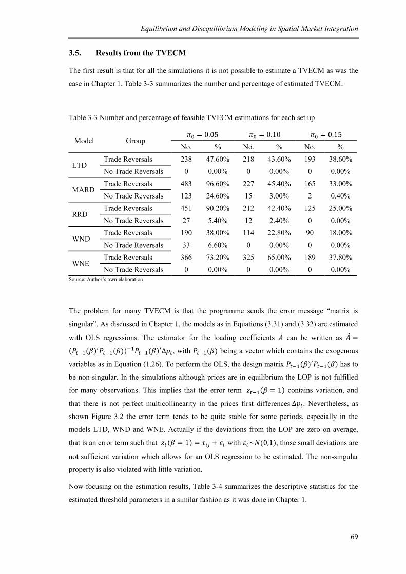
Equilibrium and Disequilibrium Modeling in Spatial Market Integration
69
3.5. Results from the TVECM
The first result is that for all the simulations it is not possible to estimate a TVECM as was the
case in Chapter 1. Table 3-3 summarizes the number and percentage of estimated TVECM.
Table 3-3 Number and percentage of feasible TVECM estimations for each set up
Model Group
No. % No. % No. %
LTD Trade Reversals 238 47.60% 218 43.60% 193 38.60%
No Trade Reversals 0 0.00% 0 0.00% 0 0.00%
MARD Trade Reversals 483 96.60% 227 45.40% 165 33.00%
No Trade Reversals 123 24.60% 15 3.00% 2 0.40%
RRD Trade Reversals 451 90.20% 212 42.40% 125 25.00%
No Trade Reversals 27 5.40% 12 2.40% 0 0.00%
WND Trade Reversals 190 38.00% 114 22.80% 90 18.00%
No Trade Reversals 33 6.60% 0 0.00% 0 0.00%
WNE Trade Reversals 366 73.20% 325 65.00% 189 37.80%
No Trade Reversals 0 0.00% 0 0.00% 0 0.00%
Source: Author’s own elaboration
The problem for many TVECM is that the programme sends the error message “matrix is
singular”. As discussed in Chapter 1, the models as in Equations (3.31) and (3.32) are estimated
with OLS regressions. The estimator for the loading coefficients can be written as
, with being a vector which contains the exogenous
variables as in Equation (1.26). To perform the OLS, the design matrix has to
be non-singular. In the simulations although prices are in equilibrium the LOP is not fulfilled
for many observations. This implies that the error term contains variation, and
that there is not perfect multicollinearity in the prices first differences . Nevertheless, as
shown Figure 3.2 the error term tends to be quite stable for some periods, especially in the
models LTD, WND and WNE. Actually if the deviations from the LOP are zero on average,
that is an error term such that with , those small deviations are
not sufficient variation which allows for an OLS regression to be estimated. The non-singular
property is also violated with little variation.
Now focusing on the estimation results, Table 3-4 summarizes the descriptive statistics for the
estimated threshold parameters in a similar fashion as it was done in Chapter 1.

Equilibrium and Disequilibrium Modeling in Spatial Market Integration
70
Table 3-4 Average estimated threshold parameters descriptive statistics for the five models
Model Threshold
0.05 0.1 0.15 0.05 0.1 0.15 0.05 0.1 0.15
LTD
---- ---- ---- 0.04 -0.07 -0.39 1.16 1.26 1.18
---- ---- ---- 0.84 0.8 0.55 0.43 0.33 0.32
Max ---- ---- ---- 1.52 1.33 0.62 1.97 1.93 1.62
Min ---- ---- ---- -1.54 -1.22 -1.16 0.57 0.57 0.58
MARD
2.32 2.29 2 -0.34 -0.96 -1.05 0.96 0.46 0.89
1.29 0.76 0.54 1.5 1.33 0.75 1.2 1.27 0.79
Max 5.2 4.26 2.38 1.93 1.24 0.24 3.44 2.61 2.07
Min 0.76 1.14 1.62 -7.58 -4.35 -2.97 -3.39 -2.41 -1.52
RRD
1.4 1.14 ---- 0.43 -0.17 -0.79 1.3 0.85 0.47
0.19 0.16 ---- 1.16 1.16 0.96 0.79 0.81 0.75
Max 2.11 1.31 ---- 2.05 1.39 0.95 2.65 2.07 1.77
Min 1.01 0.93 ---- -1.99 -1.99 -1.98 -0.18 -0.18 -0.18
WND
1.4 ---- ---- -0.34 -0.57 -0.54 0.97 1.02 1.16
0.31 ---- ---- 0.92 0.64 0.66 0.63 0.67 0.51
Max 1.68 ---- ---- 1.42 0.94 0.94 1.89 1.91 1.91
Min 1 ---- ---- -2.69 -2.21 -1.95 -0.92 -0.72 -0.59
WNE
---- ---- ---- -0.54 -0.56 -0.75 0.43 0.57 0.46
---- ---- ---- 0.57 0.49 0.67 0.54 0.51 0.64
Max ---- ---- ---- 0.81 0.55 0.67 1.91 1.03 1.76
Min ---- ---- ---- -1.66 -1.66 -1.66 -0.61 -0.55 -0.55
Source: Author’s own elaboration using the R package tsDyn developed by Di Narzo (2009) v. 0.7-60
Apart from the descriptive data, the histograms are of interest in order to see the data frequency.
Figure 3-4 shows the histograms for the upper threshold . The blue line denotes the value of
the true parameter which is equal to two, the red line denotes the average for all the
estimated values reported in Table 3-3

Equilibrium and Disequilibrium Modeling in Spatial Market Integration
71
Figure 3-4 Upper threshold parameter histograms for the five models, trade reversals
Regarding the histograms for the the lower threshold , they are shown in Figure 3-5. The blue
line denotes the value of the true parameter which is equal to minus two, the red line denotes
the average for all the estimated values reported in Table 3-3
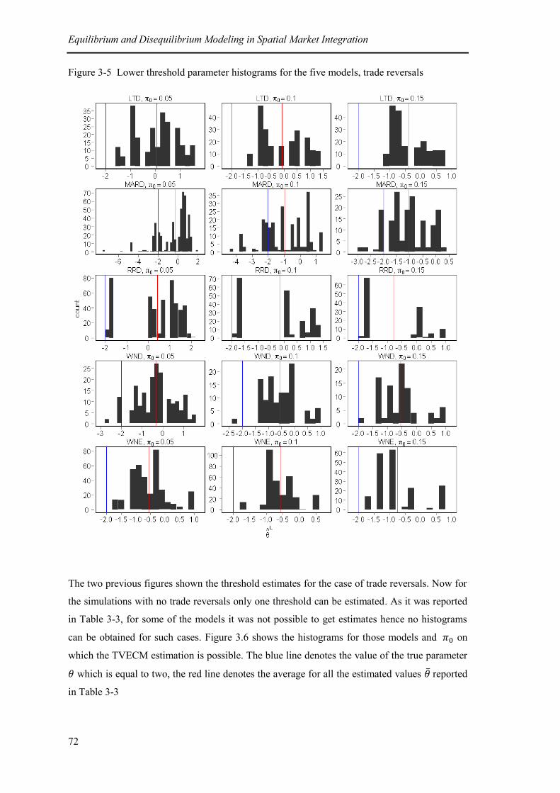
Equilibrium and Disequilibrium Modeling in Spatial Market Integration
72
Figure 3-5 Lower threshold parameter histograms for the five models, trade reversals
The two previous figures shown the threshold estimates for the case of trade reversals. Now for
the simulations with no trade reversals only one threshold can be estimated. As it was reported
in Table 3-3, for some of the models it was not possible to get estimates hence no histograms
can be obtained for such cases. Figure 3.6 shows the histograms for those models and on
which the TVECM estimation is possible. The blue line denotes the value of the true parameter
which is equal to two, the red line denotes the average for all the estimated values reported
in Table 3-3

Equilibrium and Disequilibrium Modeling in Spatial Market Integration
73
Figure 3-6 Threshold parameter histograms for the five models, no trade reversals
As it can be seen from the figures there are differences between the true values and the averages
for the estimates. Following the same methodology as in chapter one, the effect that the
threshold bias has on the neutral band is considered. The neutral band is defined as
and for the case of trade reversals and no trade reversals
respectively; substituting the true values yields and
respectively. The width of the neutral band can be calculated using the expressions
and for the case of trade reversals and no trade reversals, respectively; by
doing so it happens that equals four, and equals two. The idea is to compare the true
values with the estimates. Indeed using the estimated parameters the results for the estimated
neutral band denoted as such that and for the case of trade
reversals and no trade reversals respectively. The results are shown in Table 3-5.

Equilibrium and Disequilibrium Modeling in Spatial Market Integration
74
Table 3-5 Estimated neutral band width for the five model
Source: Author’s own elaboration
Neutral band width LTD MARD RRD WND WNE
0.05 ---- 2.32 1.40 1.40 ----
0.10 ---- 2.29 1.14 ---- ----
0.15 ---- 2.00 ---- ---- ----
0.05 1.12 1.30 0.87 1.31 0.97
0.10 1.33 1.42 1.02 1.59 1.13
0.15 1.57 1.94 1.26 1.70 1.21

Equilibrium and Disequilibrium Modeling in Spatial Market Integration
75
3.6. Discussion
The first outcome, which has been discussed before to some extent, is that even if data in
disequilibrium is observed, a considerable number of the simulations are not suitable for the
estimation of a TVECM. Regarding the groups, the figures are especially low for no trade
reversals. In the absence of trade reversals the price co-movement is more likely to be close to
the LOP, the error term is often found to move around the threshold or the transport
costs, hence the variation of the error term is low. Moreover as
approaches the LOP, the price first differences and are the same and
multicollienarity becomes a problem. The two main problems mentioned previously: low
variation of the error term and multicollienarity between the price first differences
and are frequently observed in the LTD, WND, and WNE Models; hence many
simulations fail in the TVECM estimation. Regarding the trimming parameter , the larger
is, the less the TVECM that can be estimated; this is a general outcome regardless of the group
and model. In general it can be said that three factors will have a negative impact on the
TVECM estimation: a low variation of the error term , multicollienearity between the
price first differences and and a large value for the trimming parameter .
As for the estimation results, it can be observed that having data in disequilibrium produces
biased threshold parameter estimations. For the case of the upper threshold, for all the models
the parameter is underestimated on average. Nevertheless, the Models RRD and MARD
have estimations which are less biased; indeed such models are those for which a larger number
of observations outside the neutral band are observed; furthermore such deviations from the
equilibrium are larger than in the LTD, WND and WNE Models. As for the trimming
parameter, a clear pattern of whether has an impact or not on the bias cannot be derived; the
evidence from the models is mixed. Regarding the lower threshold estimated parameter , the
results show an overestimation for all the models and trimming parameter; yet the MARD
Model has the less biased estimations. As in the upper threshold results, the trimming parameter
does not have an influence on the bias. Finally for the non trade reversals unique threshold
estimated parameter the results suggest an underestimation of the parameter for all the
models. Additionally, regarding the bias of the parameters it is important to observe two
common characteristics on the histograms: (1) different values exhibit high frequencies which
are closer and (2) for some ranges of values no observations are contained; thus the estimated
parameters seem to belong to different distributions.
The individual threshold estimations do not seem to offer much insight on how the type of
model and the trimming parameter affect the bias; thus the neutral band is also analysed. Indeed
the results from the neutral band (Table 3.4) offer a clear picture. First it is possible to observe

Equilibrium and Disequilibrium Modeling in Spatial Market Integration
76
the effect of the trimming parameter: for the group of no trade reversals as the trimming
parameter increases the estimated neutral band width decreases, which is a bias
increase. On the contrary for the trade reversals group as the trimming parameter increases
the estimated neutral band width increases, which is a bias decrease. Furthermore, it can be
observed that overall the MARD Models has the best performance as it exhibits the least biased
results.

Equilibrium and Disequilibrium Modeling in Spatial Market Integration
77
3.7. Concluding Remarks
The estimated parameters results are shown to differ from the true parameters, either when
using pure data in equilibrium or using a combination of data in equilibrium/disequilibrium.
Thus, the revised and modified economic models here proposed remain incompatible with the
Threshold Vector Error Correction Models. The first and more important signal of
incompatibility is the percentage of simulations which allow for estimating a TVECM. Such an
outcome is due to the little variation of the error term and multicolinearity between
the first price differentials and . It has been acknowledged that even though there are
observations contained outside the neutral band such that holds, if such
observation move close to the threshold parameter such that , the OLS
estimations as in the case of the loop fulfilment cannot be performed. Such
econometric results have great implications for the economic analysis. For instance, consider
efficient markets in which the LOP is fulfilled most of the time and markets are cleared fast.
Prices from such markets cannot be represented by a TVECM, as the observations in the outer
regimes will not allow for the econometric estimation to be carried out. Thus, the TVECM is
not a suitable representation of efficient markets. The second sign of incompatibility are the
biased results of the neutral band widths and , for which the trimming parameter has
a counterfactual effect; in the first one there is a negative relation with , while in the second
one the relation is positive. This has to be studied more in detail by accounting for the number
of observations which truly belong to each regime. This confirms the outcome that the TVECM
is not the correct econometric instrument for analyzing efficient markets.
The models implemented here have served to resemble circumstances which create disequilibria
in the markets in a simple manner; such disequilibria have shown to not drift so far from the
equilibrium. Nevertheless, the models can be extended to more realistic situations, i.e. storage,
rationale expectations, production and supply plans, market power and tariffs and quotas,
among others; such implementations can provide a better theoretical understanding of market
efficiency and integration. In the next Chapter a number of models which consider such
scenarios are revised in order to provide plausible directions that research has to follow.

Equilibrium and Disequilibrium Modeling in Spatial Market Integration
78

79
4. ADDRESSING FURTHER RESEARCH IN
ECONOMIC AND ECONOMETRIC THEORY
Following the incompatibility between efficient markets and the Threshold Vector Error
Correction Model (TVECM), alternatives that research ought to follow in order to improve the
understanding of the economic phenomena of Spatial Market Integration are discussed. Further
research should emphasize the improvement of some ambiguous economic and econometric
concepts upon which theory relies on. To do so it seems reasonable that economic and
econometric models should be revised to provide a better understanding of the price formation
process within Spatial Market Integration research. Thus, theoretical economic models can
provide information about the variables which intervene, their relationships and their
properties; from those insights the correct econometric representation can be derived. The
issue deserves more attention; for instance empirical applications often provide evidence that is
counterfactual to the theory, with those empirical studies being the basis for policy
recommendations that are of interest to many stakeholders.

Addressing Further Research in Economic and Econometric Theory
80

Addressing Further Research in Economic and Econometric Theory
81
4.1. Further Theory to be Considered
The fragile understanding of the economic theory and theoretical implications behind the
economic phenomena of Spatial Market Integration was acknowledged by McNew (1996). Part
of the work done in the previous Chapters attempts to provide a better understanding of such
phenomena, while the other part is focused on the compatibility/incompatibility issues between
economic theory and the econometric methods. The general conclusion derived is that for
efficient markets the Threshold Vector Error Correction Model is not an accurate
representation. Yet the issue deserves to be studied more in detail; for instance the previous
models are based on the seminal work done by Takayama & Judge (1964) whereby they solved
the spatial equilibrium as formulated by Samuelson (1952). Their original formulations
included models for a single commodity, as implemented in this research, and for multiple
products nevertheless the models do not have a dynamic nature. Other limitations of the models
implemented here are that they neglect the role of storage, the formation of agents’
expectations, simultaneous trade flows between regions, tariffs and quotas and other price
stabilization schemes, among others. Within the literature there are different models which have
implemented such factors and can serve to provide a better understanding of how price
formation occurs within the context of Spatial Market Integration. Moreover, the fact that the
Spatial Equilibrium Condition cannot be estimated using a TVECM can be an outcome not only
related with the economic theory but with the econometric concept as well; the relevant
question here is how to understand the threshold effects. So far the most used definition of
Threshold Cointegration is the offered by Balke & Fomby (1997), nevertheless the definition
offered by Gonzalo & Pitarakis (2006) appears to be the correct one as it will be discussed.
In the following pages some economic and econometrics considerations are presented in a brief
manner. From the author’s perspective the models and definitions can serve to address future
research and provide a better understanding of the economic phenomena of Spatial Market
Integration.
4.1.1. The Takayama and Judge Spatial and Temporal Price and Allocation
Models
In their seminal paper Takayama & Judge (1964) note that the models they present only cover
the spatial dimension; hence the time dimension is neglected. In order to cope with such a
limitation, seven years later Takayama & Judge (1971) presented new modifications to the
models that incorporated the time dimension as well as other elements to depict more realistic
economic scenarios.

Addressing Further Research in Economic and Econometric Theory
82
Within the static model, Takayama & Judge (1971) introduced a model for which an import
tariff is imposed, and an export subsidy is paid, such that the Net Social Payoff as in
Equation (1.11) can be written as
; (4.1)
note that the tariff has an effect similar to an increase the transport costs while the subsidy has
an effect similar to a reduction in the transport costs.
Another component included in the models is an import-export quota denoted as , such that
the constraint as in Equation (1.12) is rewritten as:
(4.2)
where denotes a matrix containing one for every elements .
Regarding monopolistic behaviour, Takayama & Judge (1971) considered an economic
scenario where two regions trade a single homogeneous good; such a good is produced by a
single producer which has production plants in the regions. The solution is found by
maximizing the profits from the sales which are equal to the total revenue minus the total
costs, including the transport costs from moving the product among regions. The outcome on
such a model is similar to what is obtained when restrictions are included, interestingly the
market prices between regions might differ by more than the transport costs.
For the temporal models the main assumption is similar to what it was done in this research, the
inverse demand and supply functions are time variant such that and
.
Note the absence of the subindices i and j, this is because the model considers a single region,
nonetheless, it can be extended to multiple regions. The product can be transferred between
time periods such that the quantity of trade can be denoted as , with the costs of delivering
a product across time (storage costs, interest, insurance, etc…) denoted as ; moreover
Takayama & Judge (1971) consider storage to be carried out by the government and by
speculators. Another manner to set up a model is to consider adaptive revisions on to a horizon
planning, such that new information available is used, i.e. speculators adapting under a
government’s policy adjustment process; the programming technique for such type of model is
recursive, in a sense this approach is similar to the RRD Model presented in the Chapter Three.
In general, the different models proposed by Takama & Judge (1971) work as extensions of the
original models by depicting more realistic scenarios. Yet they still suffer from some
limitations, for instance, if there are markets at the most trade flows can be observed. In
real life such an assumption is often not fulfilled, i.e. the ethanol trade flow between Brazil and

Addressing Further Research in Economic and Econometric Theory
83
the US goes in both directions. In that regard, an extension of the TJM to the so called
Maxwell-Boltzman Entropy Model was proposed by Yang, et al. (2010) so as to have more than
trade flows.
4.1.2. The Williams & Wright Models
William & Wright (1991) provide sound economic theory for modelling markets for
agricultural commodities. Their approach is to put emphasis on storage as they consider factors
such as future surplus disposal, buffer stocks and supply controls to have either been neglected
or not been studied in detail. Additionally, they point out interesting issues to consider; for
example they consider stocks to not be public, as storage is handled by private agents.
Furthermore they recognize that for storing it is not possible to borrow from the future and that
decisions regarding storage have to be done in an anticipatory manner.
The basic model starts by denoting an individual storing firm for which the costs of storing an
amount from period to period , such that the costs of the total storage are:
(4.3)
where is the constant marginal and average physical storage cost, and the aggregation at the
industry level is:
(4.4)
The collective consumption at period is denoted as , the aggregated realized production is
denoted as such that:
(4.5)
where denotes the available product. Moreover, the consumption is related to the price via
the inverse demand function such that:
(4.6)
There is a constant interest rate denoted as . In order to solve the model one needs to find the
contemporaneous storage to maximize the discounted stream of expected future surplus such
that:
(4.7)

Addressing Further Research in Economic and Econometric Theory
84
is maximized subject to
(4.8)
For every period the surplus is optimized up to the final period; the optimization is done
by backward induction of the final period so that the next solution corresponds to the period
, which can be written as:
(4.9)
and is maximized with respect to . As there cannot be future storage, the problem is solved
by allocating the availability between period and , so that the optimal storage
amount corresponds when the marginal consumption in periods and are equal,
accounting for marginal storage costs and interest.
Based on data obtained from the basic model, William & Wright (1991) provided a useful
insight into the time series properties for theoretical prices in agricultural markets. They studied
autocorrelations and found that prices are correlated with storage, with high storage costs
negatively affecting the correlation. Following the results of the first-order autocorrelations,
William & Wright (1991) explored the presence of a unit root process on the theoretical data;
the findings suggest that for some variables the null of a unit root is often not rejected. In
addition they investigated to what extent the long run is in a steady state or whether the
variables are characterized by booms and busts, the applicability of an ARIMA process
representation and forecasting. In the following 20 years after the publication of such models,
there have been considerable developments of the econometric techniques used in market
analysis. The implementation of theoretical prices using such techniques could serve to
understand what type of data is useful for the analysis, and to find an adequate econometric
instrument for the estimations.
4.1.3. The Rational Expectations Models
Another type of models is focused on the expectation formations of commodities. Examples of
such approaches are the work done by Gilbert & Palaskas (1989); they consider efficient
storage when prices vary very little except when new information is available. In that regard
they argue that expected future prices are likely to differ from expected future conditions as
they are jointly determined with current prices, for that they base their work on Muth’s (1961)
Rational Expectations Model. They conclude that for five commodities there is no evidence of
forward looking behaviour, and point out market intervention as an explanation for such an
outcome. In a similar fashion, Trivedi (1989) derives a model with rational expectations for

Addressing Further Research in Economic and Econometric Theory
85
perennial crops. In this way production is determined on the basis of the past current price
levels whereby inventories include two components: transaction and speculation. Finally, he
also considers the effect of differences between expected and current prices. The role of rational
expectations has been extended to disequilibrium models; examples are the work done by
Maddala (1989) based on Muthian rational expectations or the work done by Palaskas & Gilbert
(1990).
Albeit its popularity, rational expectations have received some criticism as the learning process
is omitted so that the process in which agents process the information and develop their own
forecast is not accounted for (Pesaran, 1987; Rudd & Whelan, 2006).
4.1.4. The Econometric Concept of Threshold Cointegration
At the beginning of the second Chapter, the differences between the concepts of Threshold
Error Correction and Threshold Cointegration were pointed out; moreover the major conclusion
of the Chapter is that the Spatial Equilibrium Condition does not fit whit the concept of
Threshold Error Correction. The problem might be due to the econometric definition, for
instance the idea of Threshold Cointegration as proposed by Gonzalo & Pitarakis (2006) can fit
better with economic theory. Gonzalo & Pitarakis (2006) consider a nonlinear cointegration
relationship between two variables and such that it has a threshold denoted as and can
be written as:
(4.10)
where and such that and is a stationary equilibrium
error. Taking the first differences from Equation (4.10) yields
(4.11)
where . Then the Error Correction Model (ECM) can be denoted as:
. (4.12)
The previous ECM derived is contains the threshold parameter in the long run equilibrium and
not in the error term as the TVECM does. On this regard, the threshold effect on TVECM is
limited to the adjustment process; moreover following the definition of the SEC it is expected
that the estimated loading coefficients in the neutral band to be zero. The results drawn from
the tests suggested incompatibility between the SEC and the TVECM, mainly because the SEC
does not consider any errors to occur. In this regard it might be worth exploring whether the
threshold effect fits better to the economic theory in the long run. For instance, it can be argued
to treat trade as the threshold variable, such that when no trade occurs the long run can be

Addressing Further Research in Economic and Econometric Theory
86
denoted as , which implies that the cointegration vector is time variant and
the relationship is spurious. It is when trade occurs that the long run relationship can be written
as such that the cointegration vector is time invariant and the long run
relationship is stable. Following this idea, the neutral band ought not to be treated as an
adjustment regime of which adjustments are expected to be zero; it is more accurate to refer to
the neutral band as a long run equilibrium relationship with threshold effects: Threshold
Cointegration.

Addressing Further Research in Economic and Econometric Theory
87
4.2. Linking the Economic Theory to the Empirical Applications
The economic and econometric theories addressed in the previous Chapters are the foundations
on which the empirical analyses within Spatial Market Integration rely upon. However,
empirical findings do not often support the theoretical statements. Such is the case of two
studies developed to asses the market integration among maize markets in Mexico and the
United States of America (US).
The first empirical study (Appendix II) is concerned with pure price analyses, partially focused
on addressing the suitability of different linear and non-linear Error Correction Models in the
context of Spatial Market Integration whereby the following three approaches are considered:
Vector Error Correction Models, Asymmetric Price Transmission and Threshold Vector Error
Correction Models. In order to test for the correct model specification the JTT for linear
cointegration, the Hansen & Seo (2003) test for Threshold Error Correction and the F-test for
asymmetric price transmission as in v.Cramon-Taubadel (1998) are implemented. The study
considers prices for maize in five Mexican regions and the aggregated data at the national level
and the prices at the Gulf of Louisiana (US). The cointegration relationships are pair wise, such
that each pair consists of an individual price series for both Mexico and the US. The results
from the test are summarized in the following table:
Table 4-1 Tests’ outcomes
Pair Johansen Trace Test F-Test Hansen & Seo Test
Linear Cointegration Asymmetry Linear Cointegration
Linear Cointegration Asymmetry Linear Cointegration
Linear Cointegration Asymmetry Linear Cointegration
Linear Cointegration Asymmetry Linear Cointegration
Linear Cointegration Linear Cointegration Threshold Error Correction
Linear Cointegration Asymmetry Threshold Error Correction
Source: Araujo-Enciso (2011)
Ideally the Threshold Vector Error Correction is the correct representation of Spatial Market
Integration in terms of the economic theory, yet it is weakly supported in the empirical study.
The results for the first four of pairs are in favour of Asymmetric Price Transmission, for the
fifth model the evidence moves in favour of Threshold Error Correction, for the last model the
evidence is mixed since Asymmetry and Threshold Error Correction appear to hold. Hence,

Addressing Further Research in Economic and Econometric Theory
88
one can ask under which theoretical circumstances linear cointegration or asymmetric
behaviour will hold against the threshold effect. Indeed asymmetries appeal to the idea of
market power, such that prices adjust faster when margins are squeezed rather that when they
are stretched (v.Cramon-Taubadel, 1998) Thus considering monopolies or monopolistic
behaviour in theoretical models can serve to explore the causes and consequences of
asymmetric adjustments. As for the econometric techniques implemented in the application, it
was recommended by one of the reviewers to perform the estimations using a multivariate
approach as pair wise models neglect some interaction among the markets, thus making an
interesting point. So far the TVECM is limited to pair wise analyses; hence during the analyses
information regarding markets relationships can be lost. By deriving artificial prices from a
model considering a network of markets it could be possible to asses the amount of information
lost by limiting the TVECM to the pair wise case.
The second application (Appendix III) is concerned with prices in the form of volatility; the
innovative characteristic is that it makes use of additional information such a trade. The case of
study is as before maize markets in Mexico and the US. The idea behind such research is to
determine whether the supply shocks in the Mexican market can explain price variation in the
form of volatility. Due to the fact that supply is composed of other variables, i.e. stocks,
production and imports, and having information only about the imports, it is only when import
shocks are large enough that their effect causes price variation. Thus, the model for the analysis
is a TVAR as in Lo & Zivot (2001), in which imports and volatility are both treated as
endogenous variables. The hypothesis is that there is an import threshold value which causes
volatility in the Mexican maize prices, in other words international trade causes volatility on the
domestic prices only beyond certain amount of imports. The results of implementing the test
developed by Lo & Zivot (2001) suggest that the models should consider two regimes and one
threshold value. Contrary to the initial assumption, it is not trade that drives volatility but rather
the other way around. The first regime results in trade and volatility to be unrelated; in the
second regime volatility is driving trade, such that when imports go beyond the threshold value
an increasing volatility causes imports to decrease. Additionally, the second regime is
characterized as containing a few observations, roughly 5%, which are import peaks. Although
the relationship between price volatility and trade relies on some theoretical background, the
use of a threshold model is more intuitively justified. Thus no sound theory can underpin the
hypothesis and use of TVAR models. In this regard artificial data obtained by modelling
theoretical markets such as stocks, prices, imports and production can serve to explore
relationships among the variables as already done by William & Wright (1991). From the study
of such relations one can derive which type of econometric model serves to analyse those
variables relationships in empirical applications and which type of data can be useful in

Addressing Further Research in Economic and Econometric Theory
89
understanding market dynamics. Additionally, the theoretical models can be extended to the
study of other issues such as volatility which has gained attention as a consequence of the
recent food and economic crisis.

Addressing Further Research in Economic and Econometric Theory
90
4.3. Summary of Findings and Future Research
Overall the main aim of the author with the present thesis is to provide a first insight on the
compatibility between the economic theory and the econometric methods with regards to
Spatial Market Integration. Therefore, for answering such a question simple models have been
implemented in order to get an overview, but such models are not the definitive answer. To the
author’s knowledge, there are at least two books which provide sound economic theory and
more realistic alternatives for modelling agricultural markets than those implemented here.
Those models proposed by Takayama & Judge (1971) and William & Wright (1991) aim to
create theoretical scenarios which can help to understand the economic phenomena of Spatial
Market Integration. In addition to those models, the Rational Expectations Models can offer
other directions; nevertheless, they are designed for providing a bit of background which
supports econometric techniques rather than for simulating a theoretical scenario. Still, some of
their features fit well whit the economic theory. Such new alternatives proposed for modelling
ought not to be seen as a definitive solution, their limitation in most of the cases is that markets
are considered to be in equilibrium. Although William & Wright (1991) argue that before
attempting to understand the disequilibrium mechanism it is necessary to fully understand the
equilibrium, in the author’s view equilibrium and disequilibrium should be studied together;
indeed that is the approach followed in the present thesis.
To what extent the results here are driven by the simplicity of the models can be questioned.
Nevertheless, the purpose hereby is to create the simplest case for Spatial Market Integration,
which is two markets trading a single homogeneous good with prices bounded by constant
transport costs. Furthermore, such a simple case is the one that often is assumed when
performing empirical analysis due to the econometric model’s limitations. By contrasting the
ideal economic theoretical data with the presumed econometric models it is concluded that
efficient markets cannot be represented as a TVECM; this outcome also holds when
disequilibrium is allowed to occur and such disequilibrium is close to zero. Apart from the
concern regarding the compatibility between the economic theory and econometric models,
there are still further issues remaining to be addressed.
First, the analysis is limited to the case of perfectly integrated markets, the fulfilment of the
LOP, so that the cointegration vector is always restricted to one. By allowing other values for
the cointegration vector, the development of the error term is affected; studying the effect that
the cointegration vector has on the TVECM estimation in more in detail deserves more
attention.
Second, under which circumstances the prices performance lead to the preference of a linear
VECM versus threshold effects, which theoretically is the correct specification, should be

Addressing Further Research in Economic and Econometric Theory
91
investigated. This is closely linked to the results from the empirical application to the Mexican
and US maize markets. If the TVECM itself does not consider the proper threshold effect, then
it will be miss-specified and probably rejected in favour of other specifications. The definition
of Threshold Cointegration offered by Gonzalo & Pitarakis (2006) can provide a better
representation. Additionally a high rejection of Threshold Error Correction is linked to the
econometric properties of the prices; the work done by William & Wright (1991) should be
extended by implementing the current econometric techniques to address this issue.
Third, more variables should be included in order to provide with more realistic scenarios in the
domain of market integration; yet the more variables the more complex the models become. In
order to distinguish the effect that new variables have on the models, such variables have to be
carefully introduced. The idea is to have a controlled experiment that allows understanding the
individual or joint effects of the variables on the equilibrium and other variables. Then the true
relationships among the variables can be observed, such that the proper econometric instrument
can be selected and supported by economic theory.
Finally, the development of sound economic theory is necessary in order to have clear and
unique definitions regarding core concepts which often are used in a misleading manner. Rather
than attempting to dismiss the current research, the author would like to encourage researchers
to improve the foundations of economic theory within Spatial Market Integration research.
Without clear definitions, it seems implausible that the proper econometric techniques can be
selected. Over recent decades Spatial Market Integration has gained relevance, not only for
researchers but also for policy makers, NGO’s, farmers and other stakeholders which are
interested in understanding the price formation process. Having analyses which rely upon
inappropriate econometric representations of the economic phenomena can lead to inaccurate
conclusions.

Addressing Further Research in Economic and Econometric Theory
92

93
REFERENCES
Andreassen, L., 1993. Theoretical and Econometric Modeling of Disequilibrium, s.l.: Central
Bureau of Statistics.
Araujo-Enciso, S. R., 2011. Análisis de Transmisión de Precios Entre los Mercados de Maíz
Mexicanos y el Mercado Estadounidense: Métodos Lineales y No Lineales. Revista Española
de Estudios Agrosociales y Pesqueros, Volume 2, pp. 39-77.
Ardeni, P. G., 1989. Does the Law of One Price Really Hold for Commodity Prices?. American
Journal of Agricultural Economics, 71(3), pp. 661-669.
Balke, N. S. & Fomby, T. B., 1997. Threshold Cointegration. International Economic Review,
August, 38(3), pp. 627-45.
Barrett, C. B., 2001. Measuring Integration and Efficiency in International Agricultural
Markets. Review of Agricultural Economics, 23(1), pp. 19-32.
Barrett, C. B., 2005. Spatial Market Integration. In: L. E. Blume & S. N. Durlauf, eds. The New
Palgrave Dictionary of Economics . 2nd ed. s.l.:London: Palgrave Macmillan.
Barrett, C. B. & Li, J. R., 2002. Distinguishing Between Equilibrium and Integration in Spatial
Price Analysis. American Journal of Agricultural Economics, 84(2), pp. 292-307.
Baulch, B., 1997. Transfer Costs, Spatial Arbitrage, and Testing for Food Market Integration.
American Journal of Agricultural Economics, 79(2), pp. 477-487.
Caner, M. & Hansen, B. E., 2001. Threshold Autoregression With a Unit Root. Econometrica,
69(6), pp. 1555-1596.
Cramon-Taubadel, S. V., 1998. Estimating Asymmetric Price Transmission With the Error
Correction Representation: An Application to the German Pork Market. European Review of
Agricultural Economics, 25(1), pp. 1-18.
Di Narzo, A. F., Aznarte, J. L. & Stigler, M., 2009. tsDyn: Time Series Analysis Based on
Dynamical Systems Theory, s.l.: s.n.
Enders, W. & Siklos, P. L., 2001. Cointegration and Threshold Adjustment. Journal of Business
and Economic Statistics, 19(2), pp. 166-176.
Engle, R. F. & Granger, C. W. J., 1987. Co-integration and Error Correction: Representation,
Estimation, and Testing. Econometrica, March, 55(2), pp. 251-76.
Fackler, P. L. & Goodwin, B. K., 2001. Spatial Price Analysis. In: B. L. Gardner & G. C.
Rausser, eds. Handbook of Agricultural Economics. s.l.:Elsevier, pp. 971-1024.

References
94
Fackler, P. L. & Tastan, H., 2008. Estimating the Degree of Market Integration. American
Journal of Agricultural Economics, 90(1), pp. 69-85.
Fair, R. C. & Jaffee, D. M., 1972. Methods of Estimation for Markets in Disequilibrium.
Econometrica, 40(3), pp. 497-514.
Faminow, M. D. & Benson, B. L., 1990. Integration of Spatial Markets. American Journal of
Agricultural Economics, 72(1), pp. 49-62.
Gilbert, C. L., 2006. Trends and Volatility in Agricultural Commodity Prices. In: A. Sarris & D.
Hallam, eds. Agricultural Commodity Markets and Trade. s.l.:Food and Agriculture
Organization of the United Nations, pp. 31-60.
Gilbert, C. L. & Palaskas, T. B., 1990. Modelling Expectations Formation in Primary
Commodity Markets. In: L. A. Winters & D. Sapsford, eds. Primary Commodity Prices:
Economic Models and Policy. s.l.:Cambridge University Press, pp. 44-61.
Gonzalo, J. & Pitarakis, J.-Y., 2006. Threshold Effects in Cointegrating Relationships. Oxford
Bulletin of Economics and Statistics, Volume 68, pp. 813-833.
Goodwin, B. K., 1992. Multivariate Cointegration Tests and the Law of One Price in
International Wheat Markets. Review of Agricultural Economics, 14(1), pp. 117-124.
Goodwin, B. K., Grennes, T. J. & Wohlgenant, M. K., 1990. A Revised Test of the Law of One
Price Using Rational Price Expectations. American Journal of Agricultural Economics, 72(3),
pp. 682-693.
Goodwin, B. K. & Piggott, N. E., 2001. Spatial Market Integration in the Presence of Threshold
Effects. American Journal of Agricultural Economics, 83(2), pp. 302-317.
Goodwin, B. K. & Schroeder, T. C., 1991. Cointegration Tests and Spatial Price Linkages in
Regional Cattle Markets. American Journal of Agricultural Economics, 73(2), pp. 452-464.
Granger, C. W., 1981. Some Properties of Time Series Data and Their Use in Econometric
Model Specification. Journal of Econometrics, May, 16(1), pp. 121-130.
Greb, F., Cramon-Taubadel, S. v., Krivobokova, T. & Munk, A., 2011. Threshold Estimation in
Price Transmission Analysis, s.l.: s.n.
Green, J. & Laffont, J.-J., 1981. Disequilibrium Dynamics With Inventories and Anticipatory
Price-Setting. European Economic Review, 16(1), pp. 199-221.
Haltiwanger, J. & Waldman, M., 1985. Rational Expectations and the Limits of Rationality: An
Analysis of Heterogeneity. The American Economic Review, 75(3), pp. 326-340.

References
95
Hansen, B. E. & Seo, B., 2002. Testing for Two-Regime Threshold Cointegration in Vector
Error-Correction Models. Journal of Econometrics, 110(2), pp. 293-318.
Johansen, S., 2000. Modelling of Cointegration in the Vector Autoregressive Model. Economic
Modelling, 17(3), pp. 359-373.
Kwiatkowski, D., Phillips, P. C., Schmidt, P. & Shin, Y., 1992. Testing the null hypothesis of
stationarity against the alternative of a unit root: How sure are we that economic time series
have a unit root?. Journal of Econometrics, 54(1-3), pp. 159-178.
Laffont, J.-J. & Garcia, R., 1977. Disequilibrium Econometrics for Business Loans.
Econometrica, 45(5), pp. 1187-1204.
Lo, M. C. & Zivot, E., 2001. Threshold Cointegration and Nonlinear Adjustment to the Law of
One Price. Macroeconomic Dynamics, 5(04), pp. 533-576.
Maddala, G., 1986. Disequilibrium, Self-Selection, and Switching Models. In: Z. Griliches &
M. D. Intriligator, eds. Handbook of Econometrics. s.l.:Elsevier, pp. 1633-1688.
Lütkepohl, H., 2004. Applied Time Series Econometrics. In: H. L. &. M. Krätzig, Hrsg.
s.l.:Cambridge University Press, pp. 8-85.
Maddala, G. S., 1990. Estimation of Dynamic Disequilibrium Models with Rational
Expectations: the Case of Commodity Markets. In: L. A. Winters & D. Sapsford, eds. Primary
Commodity Prices: Economic Models and Policy. s.l.:Cambridge University Press, pp. 21-34.
Maddala, G. S. & Nelson, F. D., 1974. Maximum Likelihood Methods for Models of Markets in
Disequilibrium. Econometrica, November, 42(6), pp. 1013-30.
Martens, M., Kofman, P. & F., T. C., 1998. A Threshold Error-Correction Model for Intraday
Futures and Index Returns. Journal of Applied Econometrics, 13(3), pp. 245-263.
McNew, K., 1996. Spatial Market Integration: Definition, Theory, And Evidence. Agricultural
and Resource Economics Review, April, 25(1), pp. 1-11.
McNew, K. & Fackler, P. L., 1997. Testing Market Equilibrium: Is Cointegration Informative?.
Journal of Agricultural and Resource Economics, 22(02), pp. 191-207.
McNicol, D. L., 1978. Commodity Agreements and Price Stabilization. s.l.:Lexington,
Massachusetts.
Obstfeld, M. & Taylor, A., 1997. Nonlinear Aspects of Goods-Market Arbitrage and
Adjustment: Heckscher's Commodity Points Revisited. Journal of the Japanese and
International Economies, 11(4), pp. 441-479.
References
96
Obstfeld, M. & Taylor, A. M., 1997. Nonlinear Aspects of Goods-Market Arbitrage and
Adjustment: Heckscher's Commodity Points Revisited. Journal of the Japanese and
International Economies, December, 11(4), pp. 441-479.
Officer, L. H., 1986. The law of one price cannot be rejected: Two tests based on the
tradable/nontradable price ratio. Journal of Macroeconomics, 8(2), pp. 159-182.
Palaskas, T. B. & Gilbert, C. L., 1990. Consistent Estimation of a Disequilibrium Model of
Primary Commodity Price Adjustment. Applied Economics, 22(10), pp. 1417-1426.
Pesaran, M. H., 1987. The Limits to Rational Expectations. s.l.:Basic Blackwell, Oxford, U.K..
Pfaff, B., 2008. Analysis of Integrated and Cointegrated Time Series with R. s.l.:Springer New
York.
Ravallion, M., 1986. Testing Market Integration. American Journal of Agricultural Economics,
68(1), pp. 102-109.
Rudd, J. & Whelan, K., 2006. Can Rational Expectations Sticky-Price Models Explain Inflation
Dynamics?. The American Economic Review, 96(1), pp. 303-320.
Samuelson, P. A., 1952. Spatial Price Equilibrium and Linear Programming. The American
Economic Review, 42(3), pp. 283-303.
Seo, M., 2006. Bootstrap Testing for the Null of No Cointegration in a Threshold Vector Error
Correction Model. Journal of Econometrics, 134(1), pp. 129-150.
Srivastava, V. K. & Bhaskara Rao, B., 1990. The Econometrics of Disequilibrium Models.
s.l.:Greenwood Press.
Stigler, M., 2012. Threshold cointegration: Overview and Implementation in R, s.l.: s.n.
Takayama, T. & Judge, G. G., 1964. Spatial Equilibrium and Quadratic Programming. Journal
of Farm Economics, 46(1), pp. 67-93.
Takayama, T. & Judge, G. G., 1971. Spatial and Temporal Price and Allocation Models.
s.l.:North-Holand.
Tong, H., 1978. On a Threshold Model. In: C. C, ed. Pattern recognition and signal processing.
s.l.:Sijthoff \& Noordhoff, Netherlands, pp. 575-586.
Trivedi, P. K., 1990. The Prices of Perennial Crops: The Role of Rational Expectations and
Commodity Stocks. In: L. A. Winters & D. Sapsford, eds. Primary Commodity Prices:
Economic Models and Policy. s.l.:Cambridge University Press, pp. 72-93.
Tsay, R. S., 1989. Testing and Modeling Threshold Autoregressive Processes. Journal of the
American Statistical Association, 84(405), pp. 231-240.

References
97
Vavra, P. & Goodwin, B. K., 2005. Analysis of Price Transmission Along the Food Chain, s.l.:
OECD Publishing.
Weddepohl, C., 1996. A Simulation Study of Disequilibrium Price Dynamics. In: W. A.
Barnett, G. Gandolfo & C. Hillinger, eds. Dynamic Disequilibrium Modeling. s.l.:Cambridge
University Press, pp. 421-443.
Weddepohl, C., 1999. Price Adjustment Models in a Production Economy. Annals of
Operations Research, Volume 89, pp. 149-164.
Williams, J. C. & Wright, B. D., 1991. Storage and Commodity Markets. s.l.:Cambridge
University Press.
Wymer, C., 1996. Role of Continuous Time Disequilibrium Modeling in Macroeconomics. In:
W. A. Barnett, G. Gandolfo & C. Hillinger, eds. Dynamic Disequilibrium Modeling.
s.l.:Cambridge University Press, pp. 67-123.
Yang, C. w., Hung, K. & Chen, C. C., 2010. A Share-Maximizing Marketing Strategy Model of
the Distribution. s.l., s.n., pp. 136-147.

References
98

99
APPENDIX I: GAMS CODES
This section contains the GAMS codes used in generating the artificial data. The parameters in
all the cases were taken from the example provided in the seminal paper by (Takayama &
Judge, 1964).
Simulations in Chapter One and Two are generated using the file “EQ.gms”. The simulations
for Chapter Three depend on several files as following:
Lagged Trade Disequilibrium Model: Files “EQ.gms” and “LTD.gms”
White Noise Disequilibrium Model: File “WND.gms”
Moving Average Restriction Disequilibrium Model: File “MARD.gms”
Restrictive Recursive Disequilibrium Model: Files “EQ.gms”, “R_DES.gms” and
“R_DES_T.gms”
White Noise Equilibrium Model: Files “WNE.gms”

Appendix I: GAMS Codes
100

Appendix I: GAMS Codes
101
File EQ.gms
1 *** This file creates the equilibrium data based on random dynamic parameter: vt(i,t)
2
3
4
5 execseed = gmillisec(jnow);
6
7 ***** The dimensions are declared
8 Sets
9 t Time dimension /1*500/
10 i Supply part /1*2/
11 j Demand part /1*2/
12 same(i,j) Same markets /1.1, 2.2/
13
14 ***** The transport costs are time invariant
15 Table tc(i,j) Transport Costs Table
16 1 2
17 1 0 2
18 2 2 0
19
20 ***** The inverse supply and demand functions parameters are declared
21 ***** All the parameters are time invariant but vt(i,t)
22 Parameters
23 vs(i) Static intercept inverse supply function /1 5, 2 2.5/
24 n(i) Static slope inverse supply function /1 1, 2 0.5/
25 l(j) Static intercept demand function /1 20, 2 20/
26 w(j) Static slope demand function /1 -0.1, 2 -0.2/
27 e(i,t) Error
28 u(i,t) Cumulative error
29 vt(i,t) Dynamic intercept inverse supply function
30 tc(i,j) Transport Costs;
31
32 ***** The parameter vt(i,t) is a random walk which contains a random error
33 ***** e(i,t) normally distributed
34 e(i,t)=normal(0,1);
35 loop(t, e(i,t+1)=e(i,t)+e(i,t+1));
36 u(i,t)=e(i,t);
37 vt(i,t)=vs(i)+u(i,t);
38
39
40 ***** The variables are declared
41 Positive Variables
42 x(i,t) supply
43 y(j,t) demand
44 q(i,j,t) trade
45
46 ***** The objective function is declared
47 Variable
48 CPS Consumer and Producer Surplus;
49
50 ***** The equations, objective function and constrains are declared
51 Equations
52 Supply(i,t) Supply constrain
53 Demand(j,t) Demand constrain
54 MW Maximum Welfare;
55
56 MW.. CPS =E= Sum(t,
57 SUM(j, l(j)*y(j,t)+0.5*w(j)*y(j,t)*y(j,t))
58 -SUM(i, vt(i,t)*x(i,t)+0.5*n(i)*x(i,t)*x(i,t))

Appendix I: GAMS Codes
102
59 -SUM((i,j), tc(i,j)*q(i,j,t)));
60
61 Demand(j,t).. SUM(i, q(i,j,t))-y(j,t)=G=0;
62 Supply(i,t).. -SUM(j, q(i,j,t))+x(i,t)=G=0;
63
64
65 ****** The model is declared and solved
66 MODEL TAKAYAMA /ALL/;
67 takayama.iterlim=10000000;
68 takayama.reslim=2000000;
69 takayama.workspace=100;
70
71 option nlp=coinipopt;
72
73 SOLVE TAKAYAMA USING NLP MAXIMIZING CPS;
74
75 ***** The GDX file is created
76 execute_unload 'EQ' t, j, i, l, w, n, vs, vt, tc, q, x, y, Demand, Supply, u, e;

Appendix I: GAMS Codes
103
File R_DES.gms
1 *** This file takes the parameters and solved variables from the equilibrium (EQ.gdx) as a basis for
setting up a restriction
2 *** The restriction limits trade, and the difference between trade in equilibrium and restricted is used
as feedback on the supply for the next period of time
3
4 execseed = gmillisec(jnow);
5
6 **** Declare the dimensions of the problem
7 Sets
8
9 t Time dimension /1*200/
10 j Supply part /1*2/
11 i Demand part /1*2/
12 Same(j,i) Same markets /1.1, 2.2/
13 alias (t,tt)
14
15 **** Declare the parameters for the inverse demand and supply funtions
16 Parameters
17 vs(j) Static intercept inverse supply function
18 n(j) Static slope inverse supply function
19 l(i) Static intercept demand function
20 w(i) Static slope demand function
21 e(j,t) Error
22 u(j,t) Cumulative error
23 vt(j,t) Dynamic intercept inverse supply function
24 tc(j,i) Transport Costs
25 dt(j,i,t) Shift in the supply curve
26 qe(j,i,t) Trade in Equilibrium as parameter;
27
28 *** The variables are declared
29 Positive Variables
30 xr(j) Supply
31 yr(i) Demand
32 qr(j,i) Trade
33 q(j,i,t) Trade in Equilibrium as variable;
34
35
36 * Load the parameters, the parameters for solving the problem with restriction are the same as
37 * for the problem without restriction
38 Execute_Load 'EQ' l, w, n, vt, tc, u, e, q;
39
40 * Once loaded the parameters the restrictions are generated using the data for trading in the
equilibrium
41 * First the parameters for the restriction are declared
42 Parameters
43 max_qe(j,i) Maximum of trade in equilibrium
44 average_qe(j,i) Average of trade in equilibrium
45 rt(j,i,t) Sorted restriction of trade
46 dt(j,i,t) Shift on the suply curve;
47 qe(j,i,t)=q.l(j,i,t);
48 max_qe(j,i) = smax(t, qe(j,i,t));
49 average_qe(j,i) = sum(t, qe(j,i,t))/200;
50 rt(j,i,t)=uniform(average_qe(j,i),max_qe(j,i));
51
52 display rt;
53
54
55 * Declare the initial values for the parameters

Appendix I: GAMS Codes
104
56 Parameters
57 d(j,i) Initial shift on the supply curve
58 v(j) Initial parameter plus the initial shift
59 r(j,i) Initial restriction
60 tc(j,i) Transport Costs;
61 d(j,i)=0;
62 v(j)=vt(j,"1")-(n(j)*sum(i$(NOT Same(j,i)),d(j,i)));
63 r(j,i)=rt(j,i,"1");
64
65
66 Variable
67
68 CPSr Consumer and Producer Surplus;
69
70
71 *** Declare the new equations
72 Equations
73 Supplyr(j) Supply constrain
74 Demandr(i) Demand constrain
75 Restriction(j,i) Restriction in trade
76 MWr Maximum Welfare;
77
78 MWr.. CPSr =E= SUM((i), l(i)*yr(i)+0.5*w(i)*yr(i)*yr(i))
79 -SUM((j), v(j)*n(j)*xr(j)+0.5*n(j)*xr(j)*xr(j))
80 -SUM((j,i), tc(j,i)*qr(j,i));
81
82 Demandr(i).. SUM(j, qr(j,i))-yr(i)=G=0;
83 Supplyr(j).. -SUM(i, qr(j,i))+xr(j)=G=0;
84
85 **Note that the restriction only takes place for the supply (trade) between different regions and not
the supply within the region
86 Restriction(j,i)$(NOT Same(j,i)).. qr(j,i)=L=r(j,i);
87
88
89 option nlp=coinipopt;
90
91 MODEL TAKAYAMA /ALL/;
92
93 option savepoint=2;
94 takayama.iterlim=0;
95 SOLVE TAKAYAMA USING NLP MAXIMIZING CPSr;
96 takayama.iterlim=1000;
97
98 file meanwhile
99 put meanwhile
100
101 ***** The Model is static, it is the loop where the time dimensions is controlled for
102 loop(t,
103 r(j,i)=rt(j,i,t);
104 d(j,i)=qe(j,i,t)-qr.l(j,i);
105 v(j)=vt(j,t)-(n(j)*sum(i$(NOT Same(j,i)),d(j,i)));
106 display r,d,v;
107 put_utility 'gdxout'/'takayama_p' t.tl:0;
108 put "output to file" t.tl:0 "with sudffix output"/;
109 execute_unload t, j, i, l, w, n, v, tc, d, r, qr, xr, yr, Demandr;
110 SOLVE TAKAYAMA USING NLP MAXIMIZING CPSr;
111 );

Appendix I: GAMS Codes
105
File R_DES_T.gms
1 *** This file retrieves the individual GDX files generated on the code "R_DES.gdx" and put the
results together as a time series
2
3 **** Declare the dimension of the problem
4 Sets
5 t Time dimension /1*200/
6 j Supply part /1*2/
7 i Demand part /1*2/;
8
9
10 **** The dynamic and static parameters are declared
11 parameters
12 Demandr_T(t,i) Price of the good
13 qr_T(t,j,i) Trade among regions restriction
14 xr_T(t,j) Supply
15 yr_T(t,i) Demand
16 l_T(t,i) Intercept demand function
17 w_T(t,j) Slope demand function
18 n_T(t,j) Slope supply function
19 v_T(t,i) Intercept supply function
20 d_T(t,j,i) Shift on the supply curve
21 r_T(t,j,i) Restriction on trade
22 l(i) Intercept demand function
23 w(j) Slope demand function
24 n(j) Slope supply function
25 v(i) Intercept supply function
26 d(j,i) Shift on the supply curve
27 r(j,i) Restriction on trade;
28
29
30 ***** The variables are declared
31 variables
32 xr(j) Output from the supply
33 yr(i) Output from the demand
34 qr(j,i) Output from trade in restriction
35 ;
36
37 ***** Declare the equations to later retrieve the restriction and the prices
38 Equation
39 Demandr(i) Output from price in restriction
40 Restriction(j,i) Restriction on trade;
41
42 xr.l(j)=0; yr.l(i)=0; qr.l(j,i)=0; Demandr.m(i)=0;
43
44 ***** Create the bat file
45 file kcp /kcp.bat/;
46 kcp.nw=0; kcp.nd=0;
47
48 ***** Set up the loop for conciliating the separate static disequilibrium solution into a unique
dynamic solution
49 loop (t,
50 l(i)=0;w(j)=0;n(j)=0;v(i)=0;d(j,i)=0;r(j,i)=0;
51 putclose kcp, 'rm TAKAYAMA_p.gdx'/
52 'cp TAKAYAMA_p', (ord(t)+1),'.gdx TAKAYAMA_p.gdx'/;
53 execute "kcp.bat";
54 execute_loadpoint "TAKAYAMA_p.gdx";
55 Demandr_T(t,i)= Demandr.m(i);
56 qr_T(t,j,i)= qr.l(j,i);

Appendix I: GAMS Codes
106
57 xr_T(t,j)=xr.l(j);
58 yr_T(t,i)=yr.l(i);
59 put_utilities 'GDXIN' /'takayama_p't.tl:0 '.gdx';
60 execute_LOAD l,w,n,v,d,r;
61 l_T(t,i)=l(i);
62 w_T(t,j)=w(j);
63 n_T(t,j)=n(j);
64 v_T(t,i)=v(i);
65 d_T(t,j,i)=d(j,i);
66 r_T(t,j,i)=r(j,i);
67 );
68
69 **** Create the GDX file
70 execute_unload 'RRD' Demandr_T, qr_t, r_t, xr_t, yr_t,l_t,w_t,n_t,v_t,d_t,r_t;

Appendix I: GAMS Codes
107
File WNE.gms
1 *** This file creates the equilibrium data the model works in the same manner as in the EQ.gams file,
the difference is that transport costs are time variant
2
3 execseed = gmillisec(jnow);
4 Sets
5 t Time dimension /1*500/
6 i Supply part /1*2/
7 j Demand part /1*2/
8 same(i,j) Same markets /1.1, 2.2/
9
10 Table tc(i,j) Transport Costs Table
11 1 2
12 1 0 2
13 2 2 0
14
15 Parameters
16 vs(i) Static intercept inverse supply function /1 5, 2 2.5/
17 n(i) Static slope inverse supply function /1 1, 2 0.5/
18 l(j) Static intercept demand function /1 20, 2 20/
19 w(j) Static slope demand function /1 -0.1, 2 -0.2/
20 e(i,t) Error
21 u(i,t) Cumulative error
22 vt(i,t) Dynamic intercept inverse supply function
23 tc(i,j) Transport Costs
24 tct(i,j,t) Transport Costs plus a white noise
25 tu(t) Error in transport costs;
26
27 e(i,t)=normal(0,1);
28 loop(t, e(i,t+1)=e(i,t)+e(i,t+1));
29 u(i,t)=e(i,t);
30 vt(i,t)=vs(i)+u(i,t);
31 **** Here the transport costs are set up with a random white noise component which is normally
distributed
32 tu(t)=normal(0,1);
33 tct(i,j,t)$(NOT same(i,j))=(tc(i,j))+((tu(t)*tu(t))**(0.5));
34
35
36 Positive Variables
37 x(i,t) supply
38 y(j,t) demand
39 q(i,j,t) trade
40
41 Variable
42 CPS Consumer and Producer Surplus;
43
44 Equations
45 Supply(i,t) Supply constrain
46 Demand(j,t) Demand constrain
47 MW Maximum Welfare;
48
49 MW.. CPS =E= Sum(t,
50 SUM(j, l(j)*y(j,t)+0.5*w(j)*y(j,t)*y(j,t))
51 -SUM(i, vt(i,t)*x(i,t)+0.5*n(i)*x(i,t)*x(i,t))
52 -SUM((i,j), tc(i,j)*q(i,j,t)));
53
54 Demand(j,t).. SUM(i, q(i,j,t))-y(j,t)=G=0;
55 Supply(i,t).. -SUM(j, q(i,j,t))+x(i,t)=G=0;

Appendix I: GAMS Codes
108
56
57
58 MODEL TAKAYAMA /ALL/;
59 takayama.iterlim=10000000;
60 takayama.reslim=2000000;
61 takayama.workspace=100;
62
63 option nlp=coinipopt;
64
65 SOLVE TAKAYAMA USING NLP MAXIMIZING CPS;
66
67 execute_unload 'WNE' t, j, i, l, w, n, vs, vt, tc, q, x, y, Demand, Supply, u, e;
68
69 execute '=gdx2xls WNE.gdx';

Appendix I: GAMS Codes
109
File LTD.gms
1 *** This file creates the LTD Model, it relies on the general equilibrium model as in the file EQ.gms
2
3 execseed = gmillisec(jnow);
4 Sets
5 t Time dimension /1*201/
6 i Supply part /1*2/
7 j Demand part /1*2/
8 same(i,j) Same markets /1.1, 2.2/
9
10
11 Parameters
12 n(i) Static slope inverse supply function
13 l(j) Static intercept demand funtion
14 w(j) Static slope demand function
15 vt(i,t) Dynamic intercept inverse supply function
16 tc(i,j) Transport Costs;
17
18 Positive Variables
19 xl(i,t) Supply
20 yl(j,t) Demand
21 q(i,j,t) Trade Equilibrium
22
23 Execute_Load 'EQ' l, w, n, vt, tc, q;
24
25 **** The trade from the equilibrium is loaded, then it first lagged value t-1 is set up as a new
parameter
26 Parameter
27 ql(i,j,t) Lagged Trade;
28 ql(i,j,t)=q.l(i,j,t-1);
29
30
31 Variable
32 CPSl Consumer and Producer Surplus;
33
34 Equations
35 Supplyl(i,t) Supply constrain
36 Demandl(j,t) Demand constrain
37 Restriction(j,i) Restriction
38 MWL Maximum Welfare;
39
40 MWL.. CPSl =E= SUM(t,
41 SUM(j, l(j)*yl(j,t)+0.5*w(j)*yl(j,t)*yl(j,t))
42 -SUM(i, vt(i,t)*xl(i,t)+0.5*n(i)*xl(i,t)*xl(i,t))
43 -SUM((i,j), tc(i,j)*q(i,j,t)));
44
45 Demandl(j,t).. SUM(i, q(i,j,t))-yl(j,t)=G=0;
46 Supplyl(i,t).. -SUM(j, q(i,j,t))+xl(i,t)=G=0;
47 Restriction(j,i,t)$(NOT Same(i,j)).. q(i,j,t)=L=ql(i,j,t);
48
49 MODEL TAKAYAMA /ALL/;
50 takayama.iterlim=10000000;
51 takayama.reslim=2000000;
52 takayama.workspace=100;
53
54 option nlp=coinipopt;
55
56 SOLVE TAKAYAMA USING NLP MAXIMIZING CPSl;
57 execute_unload 'LTD' t, j, i, l, w, n, vt, tc, ql, xl, yl, Demandl, Supplyl;
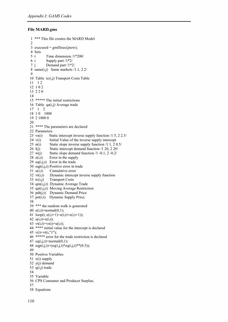
Appendix I: GAMS Codes
110
File MARD.gms
1 *** This file creates the MARD Model
2
3 execseed = gmillisec(jnow);
4 Sets
5 t Time dimension /1*200/
6 i Supply part /1*2/
7 j Demand part /1*2/
8 same(i,j) Same markets /1.1, 2.2/
9
10 Table tc(i,j) Transport Costs Table
11 1 2
12 1 0 2
13 2 2 0
14
15 ***** The initial restrictions
16 Table qa(i,j) Average trade
17 1 2
18 1 0 1000
19 2 1000 0
20
21 **** The parameters are declared
22 Parameters
23 vs(i) Static intercept inverse supply function /1 5, 2 2.5/
24 v(i) Initial Value of the inverse supply intercept
25 n(i) Static slope inverse supply function /1 1, 2 0.5/
26 l(j) Static intercept demand function /1 20, 2 20/
27 w(j) Static slope demand function /1 -0.1, 2 -0.2/
28 e(i,t) Error in the supply
29 eq(i,j,t) Error in the trade
30 eqp(i,j,t) Positive error in trade
31 u(i,t) Cumulative error
32 vt(i,t) Dynamic intercept inverse supply function
33 tc(i,j) Transport Costs
34 qm(i,j,t) Dynamic Average Trade
35 qat(i,j,t) Moving Average Restriction
36 pdt(j,t) Dynamic Demand Price
37 pst(i,t) Dynamic Supply Price;
38
39 *** the random walk is generated
40 e(i,t)=normal(0,1);
41 loop(t, e(i,t+1)=e(i,t)+e(i,t+1));
42 u(i,t)=e(i,t);
43 vt(i,t)=vs(i)+u(i,t);
44 **** initial value for the intercept is declared
45 v(i)=vt(i,"1");
46 ***** error for the trade restriction is declared
47 eq(i,j,t)=normal(0,1);
48 eqp(i,j,t)=(eq(i,j,t)*eq(i,j,t)**(0.5));
49
50 Positive Variables
51 x(i) supply
52 y(j) demand
53 q(i,j) trade
54
55 Variable
56 CPS Consumer and Producer Surplus;
57
58 Equations

Appendix I: GAMS Codes
111
59 Supply(i) Supply constrain
60 Demand(j) Demand constrain
61 Averaget(i,j) Average trade
62 MW Maximum Welfare;
63
64 MW.. CPS =E= SUM(j, l(j)*y(j)+0.5*w(j)*y(j)*y(j))
65 -SUM(i, v(i)*x(i)+0.5*n(i)*x(i)*x(i))
66 -SUM((i,j), tc(i,j)*q(i,j));
67
68 Demand(j).. SUM(i, q(i,j))-y(j)=G=0;
69 Supply(i).. -SUM(j, q(i,j))+x(i)=G=0;
70 Averaget(i,j).. q(i,j)$(NOT same(i,j))=L=qa(i,j)
71
72
73 MODEL TAKAYAMA /ALL/;
74 takayama.iterlim=10000000;
75 takayama.reslim=2000000;
76 takayama.workspace=100;
77
78 option nlp=coinipopt;
79
80 SOLVE TAKAYAMA USING NLP MAXIMIZING CPS;
81
82 **** the static problem is controlled in the loop to have dynamic sets
83 loop (t,
84 v(i)= vt(i,t);
85 qm(i,j,t)=q.l(i,j);
86 qat(i,j,t)=qa(i,j);
87 pdt(j,t)=Demand.m(j);
88 pst(i,t)=Supply.m(i);
89 qa(i,j)=0.5*qm(i,j,t-1)+0.3*qm(i,j,t-2)+0.2*qm(i,j,t-3)+eqp(i,j,t-1);
90 SOLVE TAKAYAMA USING NLP MAXIMIZING CPS;
91 );
92 display qm, qat, pdt, pst;
93
94 execute_unload 'MARD' t, j, i, l, w, n, vs, vt, tc, q, x, y, Demand, Supply, u, e, qm, qat, pdt, pst;

Appendix I: GAMS Codes
112
File WND.gms
1 *** This file creates the WND Model
2
3
4
5 execseed = gmillisec(jnow);
6
7 ***** The dimensions are declared
8 Sets
9 t Time dimension /1*500/
10 i Supply part /1*2/
11 j Demand part /1*2/
12 same(i,j) Same markets /1.1, 2.2/
13
14 ***** The transport costs are time invariant
15 Table tc(i,j) Transport Costs Table
16 1 2
17 1 0 2
18 2 2 0
19
20 ***** The inverse supply and demand functions parameters are declared
21 ***** All the parameters are time invariant but vt(i,t)
22 Parameters
23 vs(i) Static intercept inverse supply function /1 5, 2 2.5/
24 n(i) Static slope inverse supply function /1 1, 2 0.5/
25 l(j) Static intercept demand function /1 20, 2 20/
26 w(j) Static slope demand function /1 -0.1, 2 -0.2/
27 e(i,t) Error
28 u(i,t) Cumulative error
29 vt(i,t) Dynamic intercept inverse supply function
30 tc(i,j) Transport Costs
31 m(i,j,t) Error term in transport costs;
32
33 ***** The parameter vt(i,t) is a random walk which contains a random error
34 ***** e(i,t) normally distributed
35 e(i,t)=normal(0,1);
36 loop(t, e(i,t+1)=e(i,t)+e(i,t+1));
37 u(i,t)=e(i,t);
38 vt(i,t)=vs(i)+u(i,t);
39 ***** The parameter m(i,j,t) is a white noise error
40 m(i,j,t)=normal(0,1);
41
42
43 ***** The variables are declared
44 Positive Variables
45 x(i,t) supply
46 y(j,t) demand
47 q(i,j,t) trade
48
49 ***** The objective function is declared
50 Variable
51 CPS Consumer and Producer Surplus;
52
53 ***** The equations, objective function and constrains are declared
54 Equations
55 Supply(i,t) Supply constrain
56 Demand(j,t) Demand constrain
57
58 MW Maximum Welfare;

Appendix I: GAMS Codes
113
59
60 MW.. CPS =E= SUM(t,
61 SUM(j, l(j)*y(j,t)+0.5*w(j)*y(j,t)*y(j,t))
62 -SUM(i, vt(i,t)*x(i,t)+0.5*n(i)*x(i,t)*x(i,t))
63 -SUM((i,j), tc(i,j)*q(i,j,t)));
64
65 Demand(j,t).. SUM(i, q(i,j,t))-y(j,t)=G=0;
66 Supply(i,t).. -SUM(j, q(i,j,t)+m(i,j,t))+x(i,t)=G=0;
67
68
69 ****** The model is declared and solved
70 MODEL TAKAYAMA /ALL/;
71 takayama.iterlim=10000000;
72 takayama.reslim=2000000;
73 takayama.workspace=100;
74
75 option nlp=coinipopt;
76
77 SOLVE TAKAYAMA USING NLP MAXIMIZING CPS;
78
79 ***** The GDX file is created
80 execute_unload 'WND' t, j, i, l, w, n, vs, vt, tc, q, x, y, Demand, Supply, u, e;

Appendix I: GAMS Codes
114

115
APPENDIX II: EVIDENCE OF NON-LINEAR
PRICE TRANSMISSION BETWEEN MAIZE
MARKETS IN MEXICO AND THE US
This paper was first presented at the 27th Conference of the International Association of
Agricultural Economist, 16-22 August 2009. The final version was published in Spanish
language under the title “Análisis de transmisión de precios entre los mercados de maíz
mexicanos y el mercado estadounidense: métodos lineales y no lineales” in the Revista
Española de Estudios Agrosociales y Pesqueros, No. 229, year 2011. Due to copyright
restrictions here is included the original version, the final one can be downloaded directly from
the following link:
http://www.magrama.es/ministerio/pags/biblioteca/revistas/pdf_REEAP/r229_39_78.pdf
Abstract
The present work provides evidence that non linear price transmission between Mexico and the
US maize prices exists, at country and regional level. The models suggest that Mexican prices
adjust at changes in US prices. Despite asymmetry was statistically rejected, it is likely that it
might occur for thriving parameters different that zero in the error correction term. The results
suggest on which way the research might be improved in order to assess such cointegration
relationship accurately.
Keywords: cointegration, asymmetric price transmission, vector error correction model, error
correction term, loading parameter, Mexico, US, maize.

Appendix II: Evidence of Non-Linear Price Transmission between Maize Markets in Mexico
and the US
116

Appendix II: Evidence of Non-Linear Price Transmission between Maize Markets in Mexico
and the US
117
Introduction and motivation
Maize is the most important agricultural product in Mexico; it occupies the largest share of
cropped area and is the main component of the Mexicans’ diet. Unlike other countries were
maize production is regionalized, in Mexico it is spread all over the territory, as for that the
production systems differ broadly. For example Fiess & Lederman (2004) distinguish two
maize production systems in Mexico: high input (wealthy farmers) and low input (poor
farmers). The two major Maize varieties cropped in Mexico are white and yellow, being white
maize the most important with over 70% of the total production.
The performance of maize production in Mexico has been shaped by a set of complex events
including: the disappearance of the National Company of People´s Subsistence (CONASUPO),
a state company that controlled the domestic market for several crops; the shift of land devoted
to maize to other crops (fruits and vegetables); the abandonment of land; subsidies; and
meteorological phenomena in some cases. Starting in the 80’s a liberalization process started,
allowing maize imports to grow in Mexico in order to satisfy domestic demand, this caused a
shift on the Mexican maize market toward an integration with international markets, mainly the
US. Later with the NAFTA (North American Free Trade Agreement) enforcement, the field
was prepared for free markets in Agricultural products including maize. For instance over the
period 2000-2006, the volume of imports from the US equalled roughly 23% of total domestic
maize production (73% of yellow maize production) highlighting Mexico´s incapacity to
produce enough maize, mainly yellow. Despite both varieties, maize and yellow, differs on their
usage under some circumstances they become substitutes. Given the high amount of yellow
maize imports from the US, one might expect to find cointegration between maize yellow US
prices and white maize prices in Mexico. Furthermore, the US yellow maize price is used as the
reference price for calculating subsidies to maize producers in Mexico.
Before and after total liberalization of maize markets between Mexico and the US took place in
January 2008, there has been a strong controversy regarding the effects of maize imports on
Mexican production. It is often argued that imports from US have negatively influenced
domestic prices and destroyed domestic production systems. Fanjul & Fraser (2003) argue that
maize producers’ prices in Mexico have fallen due to increasing imports and dumping; this
argument is strongly supported by other authors such as Calva (1996) and Vega & Ramirez
(2004). Furthermore, it is argued that emigration from rural into urban areas and the US was
enhanced by income reduction, which was mainly based on maize production (Richter, et al.,
2007; Yunez-Naude, 1998).
Some authors have tried to measure the price relation for maize in Mexico and the US. Fiess &
Lederman (2004) found prices in Mexico and the US to be co-integrated; nonetheless other

Appendix II: Evidence of Non-Linear Price Transmission between Maize Markets in Mexico
and the US
118
authors such as Araujo-Enciso (2008) & Motamed, et al. (2008) have found that the estimated
Vector Error Correction Model (VECM) are weak to assert for market integration. Plausible
reasons for that is the use of a linear approach. The aim of this paper is to fill the gap in the
literature and to test whether US maize prices have an impact on the Mexican maize prices, and
to study the study of this impact using time series econometric techniques.

Appendix II: Evidence of Non-Linear Price Transmission between Maize Markets in Mexico
and the US
119
Methods
Maize is traded between Mexico and the US under a set of variables, observable and
unobservable, that shape the prices’ performance. Under many circumstances prices are the
solely source of information for markets; therefore the linkage between markets might be
measured using such prices.
The previous weak findings of cointegration between maize markets in Mexico and the US,
does not necessarily implies no market integration; for instance the assumption of a linear
relationship might cause misleading results as well as regional data aggregation. The following
research is based on the so called Vector Error Correction Model, which considers a linear
relationship, and the Asymmetric Price Transmission analysis which allow for a certain type of
non-linearity.
Linear error correction
The approach followed for the first analysis is to use a standard linear vector error correction
model (VECM). The endogenous variables are the logarithm of the maize prices for Mexico
and the US, denoted as and
respectively. The linear VECM is:
Where is a matrix with a rank value of r, it goes from 0 to p, and denotes the number of long-
run relationships. Matrix can be decomposed into:
,
Being β a matrix containing all the long-run relationships parameters, and α the short-run
adjustment coefficient or loading factors.
Two variables are said to be co-integrated if they are of order one (I (1)), and they have a linear
combination I(0). The Augmented Dicked-Fuller Test (ADF) is used to determine the order of
the series, being the null hypothesis a Unit Root (I (1)), versus the alternative of a stationary
process (I(0)). In order to perform the ADF is necessary to include the number of lagged
variables, which is selected following the Akaike Info (AIC), and/or Hannan-Quinn (HQC),
and/or Schwarz (SC) criterions.
The following step is to test for cointegration between the series. The Johancen Trace (JTT)
approach serves for determining the cointegration rank r. It tests for the null hypothesis of
exactly r positive eigenvalues, versus the null hypothesis of more positive r eigenvalues. As in

Appendix II: Evidence of Non-Linear Price Transmission between Maize Markets in Mexico
and the US
120
the ADF, it is necessary to include the lagged variables following one or more of the three
criterions below.
A limitation of the present model is the basic assumption of a unique loading factor among the
two variables. For instance some circumstances might cause non linearity behaviour on the
model. On the present studies it is considered the so called Asymmetric Price Transmission
(APT) as an alternative to improve the results.
Asymmetric error correction.
When price transmission differs between a positive or negative value on the deviations from the
equilibrium, an asymmetric behaviour or process is present (Meyer & Cramon-Taubadel, 2004).
Such behaviour might occur either in the long-run equilibrium or the short run adjustment.
Following Meyer & Cramon-Taubadel (2004), the model for Asymmetric Price Transmission
(APT) in the short run has the following form:
Were the error correction term (ECT) or long-run equilibrium is first estimated as a simple
linear autoregressive (VAR) form with zero lags:
being u the deviation between the prices, which is corrected in the short run by the loading
factors. Rearranging (4) is obtained:
Therefore splitting u into its positive and negative values is equivalent to separate the ECT. In
that regard by doing so is possible to estimate ATP as in equation (3). Although the approach
followed by the ATP is different from the VECM, the assumptions of non-stationary (ADF test)
and cointegration (JTT approach) must be hold for the pair of series.

Appendix II: Evidence of Non-Linear Price Transmission between Maize Markets in Mexico
and the US
121
Data
The Mexican Ministry of Agriculture (SAGARPA) publishes annual average rural prices at the
national and regional levels starting from 1980. However, 27 years (observations) is insufficient
for carrying out a cointegration analysis. Fiess & Lederman (2004) and Araujo-Enciso (2008)
generated monthly prices from these annual series using monthly deflators; however, this
method is clearly fraught with difficulties. An alternative is to use consumer level maize
prices, collected by the Ministry of Economy (SNIIM). The main concern with such data is that
is that consumer prices might differ from processor or producer prices on their performance.
Nevertheless, since the data is gathered on a weekly basis at several sales points in the country,
from a statistical point of view it might be rich in information. The US maize prices are export
prices free on board at the Louisiana Gulf port reported on a weekly basis obtained from the
USDA. The data covers the period from the 1st week of 2000 until the 20
th week of 2009 (488
observations). The prices are transformed to logarithms in order to interpret the estimated
parameters as elasticises.
Figure 2. Logarithms of the weekly maize prices Mexico and US
Source: USDA and SNIIM. Prices for Mexico were converted to USD using the weekly average exchange rate from Banxico
Figure 2 shows the aggregated prices at country level for Mexico, and prices for USA. The
Mexican average price is gotten from the figures in the thirty two states that compromise the
country. As the Mexican Ministry of Agriculture classifies the thirty two states in five
-2.75
-2.5
-2.25
-2
-1.75
-1.5
-1.25
-1
-0.75
0 50 100 150 200 250 300 350 400 450 500
Lo
g M
aiz
e P
ric
es
in U
SD
Weeks (1/52 2000 - 20/52 2009)
Ln PUS
Ln PMX

Appendix II: Evidence of Non-Linear Price Transmission between Maize Markets in Mexico
and the US
122
geographical regions, the aggregated prices for the five regions were calculated as well (Figure
3).
Figure 3. Logarithms of the weekly maize prices in Mexico by region (2000 week 1 - 2007
week 26)
Source: Prices for were converted to USD using the weekly average exchange rate from Banxico
As Figure 3 shows the performance of the prices among regions is quite different in some
periods of time. The major concern of this is that data aggregation leads to loss of information
and misleading results in the price transmission analysis as showed by Cramon-Taubadel, et al.
(2006). On that regard, the use of regional data might offer a more reliable result than country
level data.
-1.8
-1.6
-1.4
-1.2
-1
-0.8
-0.6
-0.4
0 100 200 300 400 500
Lo
g M
aiz
e P
rice
s in
US
D
Weeks (1/52 2000 - 20/52 2009)
Ln Region 1
Ln Region 2
Ln Region 3
Ln Region 4
Ln Region 5

Appendix II: Evidence of Non-Linear Price Transmission between Maize Markets in Mexico
and the US
123
Data analysis and results
Results for the ADF test shows that all the times series, except prices for Region III, were
unitary root process, either with or without a constant and /or trend (Appendix B). As the
estimated models consist on bivariate analysis for each of the six Mexican prices series with the
maize prices in the US, for each pair it was performed the JTT (Appendix C). The results
exhibit cointegration for all of them except for Regions IV and V, with and without trend.
Despite this results it was decided to perform the VECM analysis, its results are shown in Table
1.
Table 1. Estimated long-run equilibrium (ECT) from the VECM
Model 1 Model 2 Model 3 Model 4 Model 5 Model 6
LogPMX
LogPMX I
LogPMX II
LogPMX III
LogPMX IV
LogPMX V
LogPUS
-0.565*** -0.509*** -0.526*** -0.515*** -0.593*** -0.631***
test
statistics -9.393 -9.586 -9.684 -7.889 -7.021 -7.943
0.06 0.053 0.054 0.065 0.084 0.079
Constant
c 0.215* 0.382** 0.287** 0.16 0.183 0.069
test
statistics 1.656 3.329 2.442 1.134 1.005 0.402
0.13 0.115 0.117 0.141 0.182 0.172 Source: own estimations using J-multi software developed by Lütkepohl & Krätzig (2004)
The results suggest that prices in the US share a common long run relationship with prices in
Mexico at country and regional level since the estimated parameters are significant. The
estimated 's, values less than one, are interpreted as Mexican prices being greater than US
prices.

Appendix II: Evidence of Non-Linear Price Transmission between Maize Markets in Mexico
and the US
124
Table 2. Estimated loading parameters from the VECM
Model Variable Loading Parameters
test statistics
Model 1 LogP
MX -0.061*** -4.198 0.015
LogPUS 0.033** 2.160 0.015
Model 2 LogP
MX_I -0.159*** -5.910 0.027
LogPUS 0.012 0.874 0.014
Model 3 LogP
MX_II -0.096*** -4.161 0.023
LogPUS 0.042** 2.600 0.016
Model 4 LogP
MX_III -0.141*** -6.532 0.022
LogPUS 0.021** 2.067 0.01
Model 5 LogP
MX_IV -0.040*** -3.233 0.012
LogPUS 0.022 1.536 0.014
Model 6 LogP
MX_V -0.057*** -3.511 0.016
LogPUS 0.023* 1.657 0.014
Source: own estimations using Jmulti software developed by Lütkepohl & Krätzig (2004)
The loading parameters and trend results (Table 2) suggest that prices for Mexico at country
and regional level adjust to the equilibrium, while US prices in some cases do not adjust. With
such evidence it might be plausible to say that US prices to some extend are exogenous and not
determined by prices in Mexico.
With prices in Mexico as endogenous variable, and price in the US as exogenous variables, it is
estimated the long run equilibrium with a VAR model. The results exhibit again prices in the
US to be statistically significant, and that prices in Mexico are higher than in the US (Table 3).
Table 3. Estimated long-run equilibrium with VAR
Model 1 Model 2 Model 3 Model 4 Model 5 Model 6
LogPMX
LogPMX_I
LogPMX_II
LogPMX_III
LogPMX_IV
LogPMX_V
LogPUS
0.495*** 0.49*** 0.497*** 0.444*** 0.502*** 0.554***
test statistics 38.821 32.434 39.27 21.297 36.711 38.855
0.013 0.015 0.013 0.021 0.014 0.014
Constant
c -0.358*** -0.425*** -0.352*** -0.297*** -0.38*** -0.241***
test statistics -13.018 -13.015 -12.897 -6.595 -12.859 -7.823
0.028 0.033 0.027 0.045 0.03 0.031 Source: own estimations using Jmulti software developed by Lütkepohl & Krätzig (2004)
In order to estimate the ATP, the residuals from the VAR models are split on positive and
negative value. Using the model from equation (3), the new estimation shows the following
(Table 4).

Appendix II: Evidence of Non-Linear Price Transmission between Maize Markets in Mexico
and the US
125
Table 4. Estimated loading parameters from the APT
Variable ECT
+ ECT
-
Test
statistic Test
statistic
Model 1’ LogPMX
-0.086*** -4.207 -0.037* -1.654
Model 2’ LogPMX_I
-0.217*** -6.185 -0.083** -2.07
Model 3’ LogPMX_II
-0.095*** -2.98 -0.098*** -3.051
Model 4’ LogPMX_III
-0.193*** -7.319 -0.038 -1.015
Model 5’ LogPMX_IV
-0.047*** -2.615 -0.035* -1.937
Model 6’ LogPMX_V
-0.056** -2.484 -0.061** -2.475
Source: own estimations using Jmulti software developed by Lütkepohl & Krätzig (2004)
It is noticeable that the positive adjustment is always significant, while the negative adjustment
is not. With such results it is not possible to assert that there is or not asymmetry. For doing so,
it was performed an F test comparing the restricted model (VECM) with the unrestricted (APT).
The null hypothesis states as “positive and negative adjustments are equal and jointly
significant” (Table 5).
Table 5. F-tests for asymmetry
Models compared Test
Statistics
5 %
Critical F
Model 1’(ATP) vs Model 1 (VECM) 2.51 3.84
Model 2’(ATP) vs Model2 (VECM) 6.39** 3.84
Model 3’(ATP) vs Model 3 (VECM) 0.17 3.84
Model 4’(ATP) vs Model 4 (VECM) 10.67** 3.84
Model 5’(ATP) vs Model 5 (VECM) 0.02 3.84
Model 6’(ATP) vs Model 6 (VECM) -0.30 3.84 Source: own estimations
The results suggest the presence of asymmetries for Models 2 and 4; nonetheless for Model 4,
due the fact that the negative adjustment is not significant (Table 4) also the asymmetry is
rejected.

Appendix II: Evidence of Non-Linear Price Transmission between Maize Markets in Mexico
and the US
126
Discussion
The results from the VECM and VAR/APT suggest that there is cointegration between maize
markets in Mexico and the US. Nonetheless some issues should be regarded with more attention
before drawing any conclusion.
The long run equilibrium estimated on the VECM and VAR suggest that either at country or
regional level prices for Mexico share a common trend with US prices. Nonetheless it is
unexpected that VECM suggest US prices also adjust to changes in the Mexican prices. Such
event might be quite debatable; despite the fact that Mexico is the destination for 15% of the US
maize total exports; the force that drives US maize prices is more likely to be the international
markets rather than solely the Mexican market. For instance cointegration between both
markets might have a non-linear performance. Furthermore as the estimated VECM is bivariate,
it neglects the interaction among the five Mexican regions; therefore it is not possible to
conclude that the adjustments measured are definitive. Regardless of the previous outcome is
important to stress that the VECM suggest that both markets are integrated, either at regional or
country level. As for that changes in the US prices will pass to the Mexican counterpart. The
evidence for such argument is that adjustment parameters for prices changes in Mexico are
significant, even using a level of confidence of one percent; furthermore the speed of
adjustment for Mexican prices seems to be greater than adjustments in the US. In that regard
the previous assumption of Mexican maize prices being affected or determined by the US
markets might be suggested.
The APT results exhibit a weak evidence for asymmetry, only Model 2 can account for real
asymmetry. These might be explained on the basis of the estimated VAR. From Table 3 is
possible to see the high values of the t-statistics; such values exhibit estimation problems on the
parameters, which although not biased might be misleading. Despite the outcome regarding
asymmetry rejection, the results exhibit a plausible direction in future research. For instance the
non-significance of negative adjustment might be read as Threshold cointegration, that is for
some periods prices are co-integrated while in other periods not. Other possible limitation of the
asymmetry might deal with the thriving parameter, which for the present research is not
estimated but established as zero. There is the necessity to explore if asymmetries or non-linear
price transmission occur with other values; on this regard the approach of Goetz & Cramon-
Taubadel (2008) following Gonzalo & Pitarakis (2006) might be used to estimate a thriving
parameter, furthermore such methodology allows for asymmetry in the ECT estimation as well.
Regarding the models in general, there is a main concern; they do not assume any structural
break. Such assumption is clearly unrealistic given the results of the stability tests (Appendix E)
which shows that both, the VECM and the ECT (VAR), are unstable. Such outcome stresses

Appendix II: Evidence of Non-Linear Price Transmission between Maize Markets in Mexico
and the US
127
again the importance of accounting for some non-linearity in the long and short run equilibrium
in order to improve the results.
Another limitation of the results has to do with data aggregation. As prices either at country
level and regional level are the average of regional prices, the assumption of constant
aggregation must be hold in order to get reliable results (Cramon-Taubadel, et al., 2006).
Unfortunately for the data the cross sectional aggregation is not constant (Appendix F) therefore
to some extend the average prices might not represent the performance of all the states
compromising the Regions. As data aggregation causes loses of information, an alternative is
modelling with the so called generalized autoregressive conditional heteroskedasticity
(GARCH) models, which might capture volatility; nonetheless if the loss is concerning positive
and negative changes of two prices averaging, the best option is the use of non-aggregated data.
A final word of caution has to be made regarding the present study. Despite the maize prices
used here are at consumer level, maize is not consumed as a grain but as a processed good,
mainly as “Tortilla”. Indeed more than 50% of the Mexican maize production is devoted for
the “Tortilla” industry (Galarza Mercado, 2005). Weather such increases might have either a
positive or negative effect on the consumers depends on the price transmission from maize to
tortilla. The elasticities derived from the previous models might provide some insight of the
effects at producers and processors levels, but not for consumers.

Appendix II: Evidence of Non-Linear Price Transmission between Maize Markets in Mexico
and the US
128
Conclusion
The present work provides a first insight on the way future research should develop in order to
fill the gap in the current literature for maize markets cointegration between Mexico and the
US. The relationship among US prices and Mexican prices at different levels is hard to capture
by a simple linear model. The results exhibits that there is strong evidence that maize market in
Mexico and the US are integrated, and that prices share a common relationship. An accurate
measure of such relationship and its dynamics can be drawn with the help of advanced
techniques such as thresholds, structural breaks, smoothness, or conditional heteroskedasticity.
The advantage of such techniques lays on its non-linear nature.

Appendix II: Evidence of Non-Linear Price Transmission between Maize Markets in Mexico
and the US
129
References
Araujo-Enciso, S. R., 2008. Impacts of the NAFTA and bio-ethanol production in the Mexican
maize market: a price transmission analysis, s.l.: s.n.
Calva, J. L., 1996. La Economía Nacional y la Agricultura de México a Tres Años de
Operación del TLCAN. s.l., s.n.
Cramon-Taubadel, S., Loy, J.-P. & Meyer, J., 2006. The impact of cross-sectional data
aggregation on the measurement of vertical price transmission: An experiment with German
food prices. Agribusiness, 22(4), pp. 505-522.
Fanjul, G. & Fraser, A., 2003. Dumping Without Borders: How US agricultural policies are
destroying the livelihoods of Mexican corn farmers. In: Oxfam Briefing Papers. s.l.:Oxfam
International.
Fiess, N. & Lederman, D., 2004. Mexican Corn: The Effects of NAFTA. Trade Note,
September, Volume 18, pp. 1-7.
Galarza Mercado, J. M., 2005. Situación Actual y Perspectiva del Maíz en México 1996-2012,
s.l.: s.n.
Goetz, L. & Cramon-Taubadel, S. v., 2008. Considering threshold effects in the long-run
equilibrium in a vector error correction model: An application to the German apple market,
s.l.: s.n.
Gonzalo, J. & Pitarakis, J.-Y., 2006. Threshold Effects in Cointegrating Relationships. Oxford
Bulletin of Economics and Statistics, Volume 68, pp. 813-833.
Lütkepohl, H. & Krätzig, M. Hrsg., 2004. Applied Time Series Econometrics. Cambridge:
Cambridge University Press.
Meyer, J. & Cramon-Taubadel, S., 2004. Asymmetric Price Transmission: A Survey. Journal of
Agricultural Economics, 55(3), pp. 581-611.
Motamed, M., Foster, K. A. & Tyner, W. E., 2008. Applying cointegration and error correction
to measure trade linkages: maize prices in the United States and Mexico. Agricultural
Economics, 39(1), pp. 29-39.
Richter, S. M., Taylor, J. E. & Yúnez-Naude, A., 2007. Impacts of Policy Reforms on Labor
Migration from Rural Mexico to the United States. In: G. J. Borjas, ed. Mexican Immigration to
the United States. s.l.:University of Chicago Press, pp. 269-288.

Appendix II: Evidence of Non-Linear Price Transmission between Maize Markets in Mexico
and the US
130
Vega Valdivia, D. D. & Ramirez Moreno, P., 2004. Situación y perspectivas del Maíz en
México, s.l.: s.n.
Yunez-Naude, A., 1998. Small-Scale Corn And Livestock Mexican Farmers, s.l.: s.n.

Appendix II: Evidence of Non-Linear Price Transmission between Maize Markets in Mexico
and the US
131
Appendix A. Acronyms
ADF. Augmented Dicked-Fuller Test
AIC. Akaike Info Criteria
ATP. Asymmetric Price Transmission
Banxico. Central Bank of Mexico
BLS. U.S. Berau of Labor Statistics.
CONASUPO. National Company of People´s Subsistence
ECT. Error Correction Term
HQC. Hannan-Quinn Criteria
JTT. Johancen Trace Test
NAFTA. North American Free Trade agreement
OLS. Ordinary Least Squares
SAGARPA. Mexican Ministry of Agriculture, Livestock, Rural Development, Fishery and
Nourishment
SC. Schwarz Criteria
SNIIM. National System of Markets Information of the Mexican Ministry of Economy.
USDA. United States Department of Agriculture.
VECM. Vector Error correction Model.

Appendix II: Evidence of Non-Linear Price Transmission between Maize Markets in Mexico
and the US
132
Appendix B. Unit root test results: Augmented Dicked-Fuller Test
Variable Constant Trend Criterion Lags
Test
Statistics
Critical
value
LogPUS
No No AIC, HQC, SC 1 -0.9542 -1.94
Yes No AIC, HQC, SC 1 -1.1559 -2.86
Yes Yes AIC, HQC, SC 1 -2.5690 -3.41
LogPMX
No No AIC, HQC 4 -0.5277 -1.94
Yes No AIC 4 -0.9586 -2.86
Yes Yes AIC 4 -2.5126 -3.41
LogPMXI
No No AIK, HQC 6 -0.6562 -1.94
Yes No AIK, HQC 6 -1.5289 -2.86
Yes Yes AIC 6 -2.5229 -3.41
LogPMXII
No No AIC 7 -0.5792 -1.94
Yes No AIC 7 -1.4127 -2.86
Yes Yes AIC 7 -3.3358 -3.41
LogPMXIII
No No AIC, HQC 3 -0.0309 -1.94
Yes No AIC, HQC 3 -3.9758 -2.86
Yes Yes AIC, HQC 3 -7.4070 -3.41
LogPMXIV
No No AIC, HQC, SC 1 -0.6637 -1.94
Yes No AIC, HQC, SC 1 -1.1661 -2.86
Yes Yes AIC, HQC, SC 1 -2.0621 -3.41
LogPMXV
No No HQC 2 -0.9446 -1.94
Yes No AIC, HQC 2 -1.1246 -2.86
Yes Yes AIC, HQC 2 -1.8952 -3.41

Appendix II: Evidence of Non-Linear Price Transmission between Maize Markets in Mexico
and the US
133
Appendix C. Cointegration test results: Johancen Trace test
Model Constant Trend Criterion Lags Ho Statistics
Critical
value
5%
Critical
value
10%
LogPUS
-
LogPMXI
Yes No AIC, HQC, SC 2 r=0 36.62 20.16 17.98
AIC, HQC, SC 2 r=1 1.96 9.14 7.60
Yes Yes AIC, HQC, SC 2 r=0 41.10 25.73 23.32
AIC, HQC, SC 2 r=1 6.46 12.45 10.68
LogPUS
-
LogPMXII
Yes No AIC, HQC, SC 2 r=0 26.21 20.16 17.98
AIC, HQC, SC 2 r=1 2.08 9.14 7.60
Yes Yes AIC, HQC, SC 2 r=0 29.56 25.73 23.32
AIC, HQC, SC 2 r=1 5.45 12.45 10.68
LogPUS
-
LogPMXIII
Yes No AIC, HQC 3 r=0 54.51 20.16 17.98
AIC, HQC 3 r=1 1.25 9.14 7.60
Yes Yes AIC, HQC 3 r=0 67.77 25.73 23.32
AIC, HQC 3 r=1 7.04 12.45 10.68
LogPUS
-
LogPMXIV
Yes No AIC, HQC, SC 2 r=0 14.89 20.16 17.98
AIC, HQC, SC 2 r=1 1.50 9.14 7.60
Yes Yes AIC, HQC, SC 2 r=0 19.80 25.73 23.32
AIC, HQC, SC 2 r=1 4.16 12.45 10.68
LogPUS
-
LogPMXV
Yes No HQC, SC 2 r=0 17.59 20.16 17.98
HQC, SC 2 r=1 1.76 9.14 7.60
Yes Yes AIC, HQC, SC 2 r=0 22.99 25.73 23.32
AIC, HQC, SC 2 r=1 3.98 12.45 10.68
LogPUS
-
LogPMX
Yes No AIC, HQC, SC 2 r=0 23.21 20.16 17.98
AIC, HQC, SC 2 r=1 1.17 9.14 7.60
Yes Yes AIC, HQC, SC 2 r=0 28.79 25.73 23.32
AIC, HQC, SC 2 r=1 6.82 12.45 10.68

Appendix II: Evidence of Non-Linear Price Transmission between Maize Markets in Mexico
and the US
134
Appendix D. Estimated Error Correction Term (ECT) from the Vector Error Correction
Model (VECM) and the Vector Autoregressive Model (VAR)/Asymmetric Price
Transmission (APT) split in positive and negative values.
-0.3
-0.2
-0.1
0
0.1
0.2
0.3
0.4
0 100 200 300 400 500
EC
T
Weeks (3/52 2000 - 19/52 2009 )
Model 1: LogPUS-LogPMX
ECT VECM
ECT VAR Positive
ECT VAR Negative
-0.3
-0.2
-0.1
0
0.1
0.2
0.3
0.4
0.5
0.6
0.7
0 100 200 300 400 500
EC
T
Weeks (3/52 2000 - 19/52 2009 )
Model 2: LogPUS-LogPMXI
ECT VECM
ECT VAR Negative
ECT VAR Positive
-0.25
-0.2
-0.15
-0.1
-0.05
0
0.05
0.1
0.15
0.2
0.25
0.3
0 100 200 300 400 500
EC
T
Weeks (3/52 2000 - 19/52 2009 )
Model 3: LogPUS-LogPMXII
ECT VECM
ECT VAR Negative
ECT VAR Positive
-0.4
-0.2
0
0.2
0.4
0.6
0.8
1
1.2
0 100 200 300 400 500
EC
T
Weeks (3/52 2000 - 19/52 2009 )
Model 4: LogPUS-LogPMXIII
ECT VECM
ECT VAR Negative
ECT VAR Positive
-0.3
-0.2
-0.1
0
0.1
0.2
0.3
0 100 200 300 400 500
EC
T
Weeks (3/52 2000 - 19/52 2009 )
Model 5: LogPUS-LogPMXIV
ECT VECM
ECT VAR Negative
ECT VAR Positive
-0.4
-0.3
-0.2
-0.1
0
0.1
0.2
0.3
0.4
0 100 200 300 400 500
ECT
Weeks (3/52 2000 - 19/52 2009 )
Model 6: LogPUS-LogPMXV
ECT VECM
ECT VAR Negative
ECT VAR Positive

Appendix II: Evidence of Non-Linear Price Transmission between Maize Markets in Mexico
and the US
135
Appendix E. Stability tests for the long run equilibrium (ECT/VAR) and the VECM
00.05
0.10.15
0.20.25
0.30.35
0.40.45
0.50.55
0.60.65
0.70.75
0.80.85
0.9
0 50 100 150 200 250 300 350 400 450 500
p-v
alu
e
Weeks (5/52 2000 - 19/52 2009 )
Model 1: LogPUS-LogPMX
ECT/VAR
VECM
00.05
0.10.15
0.20.25
0.30.35
0.40.45
0.50.55
0.60.65
0.70.75
0.8
0 50 100 150 200 250 300 350 400 450 500
p-v
alu
e
Weeks (5/52 2000 - 19/52 2009 )
Model 2: LogPUS-LogPMXI
ECT/VAR
VECM
00.05
0.10.15
0.20.25
0.30.35
0.40.45
0.50.55
0.60.65
0.70.75
0.80.85
0.90.95
1
0 50 100 150 200 250 300 350 400 450 500
p-v
alu
e
Weeks (5/52 2000 - 19/52 2009 )
Model 3: LogPUS-LogPMXII
ECT/VAR
VECM
0
0.05
0.1
0.15
0.2
0.25
0.3
0.35
0.4
0.45
0.5
0.55
0 50 100 150 200 250 300 350 400 450 500 p
-va
lue
Weeks (5/52 2000 - 19/52 2009 )
Model 4: LogPUS-LogPMXIII
ECT/VAR
VECM
00.05
0.10.15
0.20.25
0.30.35
0.40.45
0.50.55
0.60.65
0.70.75
0.8
0 50 100 150 200 250 300 350 400 450 500
p-v
alu
e
Weeks (5/52 2000 - 19/52 2009 )
Model 5: LogPUS-LogPMXIV
ECT/VAR
VECM
00.05
0.10.15
0.20.25
0.30.35
0.40.45
0.50.55
0.60.65
0.70.75
0.80.85
0.90.95
0 50 100 150 200 250 300 350 400 450 500
p-v
alu
e
Weeks (5/52 2000 - 19/52 2009 )
Model 6: LogPUS-LogPMXV
ECT/VAR
VECM

Appendix II: Evidence of Non-Linear Price Transmission between Maize Markets in Mexico
and the US
136
Appendix F. Cross-sectional data aggregation for calculating the average regional prices
-0.05
0
0.05
0.1
0.15
0.2
0.25
0.3
0.35
0.4
0.45
0.5
0
0.2
0.4
0.6
0.8
1
1.2
1.4
1.6
0 100 200 300 400 500
Sta
nd
ar D
ev
iati
on
Pric
es
in U
SD
Weeks (1/52 2000 - 20/52 2009)
Data Agregation Prices Region III (PMXIII)
Baja California
Baja California Sur
Sinaloa
Sonora
Average
Standard Deviation
-0.01
0
0.01
0.02
0.03
0.04
0.05
0.06
0.07
0
0.05
0.1
0.15
0.2
0.25
0.3
0.35
0.4
0.45
0.5
0 100 200 300 400 500
Sta
nd
ar d
ev
iati
on
Pric
es
in U
SD
Weeks (1/52 2000 -20/52 2009)
Price Mexico Region IV(PMXIV)
Distrito Federal
Hidalgo
México
Morelos
Puebla
Average
Standard Deviation
0
0.01
0.02
0.03
0.04
0.05
0.06
0.07
0.08
0
0.05
0.1
0.15
0.2
0.25
0.3
0.35
0.4
0.45
0.5
0 100 200 300 400 500
Sta
nd
ar D
ev
iati
on
Pric
es
in U
SD
Weeks (1/52 2000 -20/52 2009)
Price Mexico Region V(PMXV)
Chihuahua
Coahuila
Durango
Nuevo León
Tamaulipas
Average
Standard Deviation
0
0.05
0.1
0.15
0.2
0.25
0
0.1
0.2
0.3
0.4
0.5
0.6
0.7
0.8
0.9
1
0 100 200 300 400 500
Sta
nd
ard
Dev
iati
on
Pric
e in
US
D
Weeks (1/52 2000 - 20/52 2009)
Data Agregation Prices Region I (PMXI)
Aguascalientes
Colima
Guanajuato
Jalisco
Michoacán
Nayarit
Querétaro
San Luis Potosí
Average
Standard Deviation 0
0.05
0.1
0.15
0.2
0.25
0
0.1
0.2
0.3
0.4
0.5
0.6
0.7
0.8
0.9
1
0 100 200 300 400 500
Sta
nd
ard
Dev
iati
on
Pric
e in
US
D
Weeks (1/52 2000 - 20/52 2009)
Data Agregation Prices Region I (PMXI)
Aguascalientes
Colima
Guanajuato
Jalisco
Michoacán
Nayarit
Querétaro
San Luis Potosí
Average
Standard Deviation

Appendix II: Evidence of Non-Linear Price Transmission between Maize Markets in Mexico
and the US
137
Appendix E. Descriptive statistics of the prices series
Region Variable Mean Min Max Standard
Deviation
Region I
PMX I
0.233436 0.177525 0.394806 0.047012
LogPMX I
-1.472630 -1.728640 -0.929362 0.182679
LogPMX I
0.000764 -0.498360 0.565100 0.062081
Region II
PMX II
0.247339 0.178377 0.393163 0.046624
LogPMX II
-1.413630 -1.723860 -0.933531 0.175514
LogPMX II
0.001021 -0.353978 0.357573 0.045809
Region III
PMX III
0.293320 0.207142 0.642614 0.065026
LogPMX III
-1.246090 -1.574350 -0.442211 0.196975
LogPMX III
-0.000611 -0.729380 0.632768 0.077808
Region IV
PMX IV
0.238138 0.189239 0.400493 0.047241
LogPMX IV
-1.452320 -1.664750 -0.915060 0.180416
LogPMX IV
0.000458 -0.212727 0.251179 0.026766
Region V
PMX V
0.245684 0.191933 0.417436 0.053752
LogPMX V
-1.424700 -1.650610 -0.873624 0.196265
LogPMX V
0.000807 -0.214443 0.244306 0.038054
Mexico
country level
PMX
0.246581 0.197613 0.396189 0.047441
LogPMX
-1.416440 -1.621450 -0.925865 0.175431
LogPMX
0.000422 -0.178157 0.200119 0.029819
US
PUS
0.124393 0.073032 0.304528 0.045003
LogPUS
-2.137400 -2.616860 -1.188990 0.308191
LogPUS
0.001448 -0.143548 0.111435 0.030886

Appendix II: Evidence of Non-Linear Price Transmission between Maize Markets in Mexico
and the US
138
Appendix F. Regions within Mexico
Region States Region States
1- West
Aguascalientes
3 -Northwest
Baja California
Colima Baja California
Sur
Guanajuato Sinaloa
Jalisco Sonora
Michoacán
4 -Centre
Distrito Federal
Nayarit Hidalgo
Querétaro México
San Luis
Potosí Morelos
Zacatecas Puebla
2 -South
Campeche
5 - Northeast
Tlaxcala
Chiapas Chihuahua
Guerrero Coahuila
Oaxaca Durango
Quintana Roo Nuevo León
Tabasco Tamaulipas
Veracruz
Yucatán
Source: taken from Galarza Mercado (2005)
2
3
4
1
5

139
APPENDIX III: THE RELATIONSHIP BETWEEN
TRADE AND PRICE VOLATILITY IN THE
MEXICAN AND US MAIZE MARKETS
This paper originated with the idea of including information about trade in the price
transmission analysis. It was presented at the 123th EAAE Seminar “Price Volatility and Farm
Income Stabilisation Modelling Outcomes and Assessing Market and Policy Based Responses”
held in Dublin, Ireland in February 23-24, 2012. The current version, which is included is still
under development.
Abstract
The supply of maize in the Mexican market depends to a large extent from the US imports which
represent a large share of the domestic consumption. Furthermore imports exhibit a seasonal
pattern, and peaks are often found close to low levels of domestic production and stocks. The
present research suggests that there is a link between imports and prices volatility. Below a
threshold value, imports and volatility are not related, but beyond the threshold it is volatility
the variable driving imports. From the results one can argue that imports have served as a
measure to stabilize prices when the domestic supply is scarce.
Keywords: Volatility, Maize, Imports, Mexico
JEL classification: Q11, Q17.

Appendix III: The Relationship between Trade and Price Volatility in the Mexican and US
Maize Markets
140

Appendix III: The Relationship between Trade and Price Volatility in the Mexican and US
Maize Markets
141
Introduction
Albeit price variation has been a characteristic of the agricultural markets, the dramatic
increases for many commodities during the 2007-2008 food crisis has made researchers, policy
makers, NGO’s and other stakeholders to pay attention to the issue. The discussion in the
academia has not only been centered on the consequences of high volatility, but also in the
causes for it.
Unlike other type of goods, agricultural commodities are demand inelastic, thus large changes
in the prices lead to short changes in the demand; on the contrary agricultural commodities
prices are quite sensible to shocks in the supply (Gilbert, 2006), thus weather shocks have a
large impact on prices behavior (Gilbert & Morgan, 2011). The current literature offers several
explanations for volatility and variables affecting it. For instance Balcombe (2011) and Tothova
(2011) summarizes some factors which are likely to affect volatility such as past volatility,
trends, yields, stock levels, weather, speculation, policy, exchange rates, oil and energy prices,
investment, interest rate and structural change. Those factors and their relation with volatility
have been studied more in detail by other authors, being much of the research done between
volatility and biofuel linkages. Recent research suggests that there is evidence that the
increasing amount of agricultural goods devoted to the produce biofuel, i.e. maize and rapeseed
has created a link between energy and food prices. For instance Baffes (2011), Buse, et al.
(2011), Du, et al. (2011), and Ji & Fan (2012) found that for some agricultural commodities the
relationship between agricultural goods and energy prices has increased in the last years. The
problem is not such a link itself, it is rather that energy markets exhibit higher volatilities than
other commodities (Plourde & Watkins, 1998), thus volatility spillovers are passed through the
agricultural markets. Other research has centered on how policy instruments serve to prevent
excessive volatility. Specifically in the European case O’Connor & Keane (2011) and
Velazquez (2011) argue that the current CAP instruments which have served to stabilize prices
should be revised and improved; this should be done properly in order to avoid volatility peaks
in international markets. Concerning developing countries, policy instruments to ensure price
stabilization have been the reduction of the tariffs and custom fees (Demeke, et al., 2011),
which has lead to an increase in trade. This exposure to international markets, although might
serve to alleviate high prices and volatility, exposes regional markets in developing countries to
international shocks. Using information from the international markets Stigler & Prakash
(2011) found that volatility is linked to low levels of stocks. Indeed for many developing
countries such stocks depend on imports. From this perspective trade might serve to understand
volatility in the agricultural markets. To the knowledge of the author no study had found
empirical evidence that relates trade and volatility. Knowing if international trade serves either

Appendix III: The Relationship between Trade and Price Volatility in the Mexican and US
Maize Markets
142
to alleviate or increase volatility can serve to implement the adequate policies. The question
turns more interesting when one of the markets is a developing country with an open economy,
for instance Mexico.

Appendix III: The Relationship between Trade and Price Volatility in the Mexican and US
Maize Markets
143
Maize production in Mexico
For Mexico one of the most, if not the most, important agricultural commodity is maize.
Between 1996 and 2006, 51% of the agricultural land in Mexico was used for producing maize,
it accounted for 7.6% of the total agricultural production volume and 30% of the total
agricultural production value (Galarza Mercado, 2005). The importance of the maize is not only
from the production/supply side perspective, but from the consumer perspective as well. In rural
areas for 2006 on average 5.9% of the total expenditures are made on cereals (Urzúa, 2008),
from which maize represents more than 50%. Another important consumer of maize is the feed
industry which share of the total domestic demand is 50%. Nevertheless feed industry and
human consumption require different types of maize; for human consumption the main product
is white maize, for the feed industry the main product is yellow maize. From the labour markets
perspective maize is also important. For 2005 it was required more than 20 millions of workers
for producing maize (Galarza Mercado, 2005). Also in the same year the maize processing
industry occupied nearly 150,000 workers. Indeed maize production value is close to one
percent of the national GDP.
Despite being in the top five maize producers in the world, Mexico is also in the top maize
importers in the world; being most of the imports from the neighbour US. Indeed yellow maize
accounts for more than 90% of maize imports in Mexico. Figure 1 shows the development of
monthly production, stocks, imports and demand for maize between 2002 and 2009.
Figure 1.Development of monthly maize stocks, production, imports and demand for the period
2002-2009
Source: Own elaboration with data from the Mexican Ministry of Agriculture
0
1000
2000
3000
4000
5000
6000
7000
8000
Feb-02 Jun-03 Nov-04 Mar-06 Aug-07 Dec-08
Th
ou
san
d M
etri
c T
on
nes
Initial Stock Production Imports Consumption

Appendix III: The Relationship between Trade and Price Volatility in the Mexican and US
Maize Markets
144
For the period 2002-2009 imports represented 48% of the domestic production, 33% of the
domestic demand, and 20% of the initial stocks. Being the imports from the US relevant for the
domestic supply in the Mexican market, one can expect that the volatility of the US markets
prices will influence volatility in the Mexican markets prices.

Appendix III: The Relationship between Trade and Price Volatility in the Mexican and US
Maize Markets
145
Volatility and Trade in the Mexican and US maize markets
The agricultural commodities prices, as many other commodities, are characterized by price
fluctuations which if big lead to periods of high volatility. In 2007-2008 the so called food
crises was characterized by large increases in food prices, having as a consequence high
volatility periods. The maize markets were exposed to such crises as well as Figure 2 shows.
Figure 2. Prices in USD per kilogram and four-week period volatility for yellow maize at the
Lousiana Gulf port (Period January 2000 – May 2009)
Source: Own elaboration with data from the USDA
Thus from figure 2 it is clear that the increases in maize prices in 2008 are also linked to the
highest volatility values; nevertheless other periods of high fluctuations before the food crisis
can be observed. The question is to what extend the volatility in the US markets affect the
prices in Mexico.
In theory, perfectly cointegrated markets in equilibrium exhibit the same volatility as their
changes over the time are proportionally the same. Although in the long run markets should
reach equilibrium, in the short run it can be violated. Nevertheless arbitrage brings markets to
the equilibrium. In the case of Mexican and US maize markets the violations of its equilibrium
relationship are corrected by means of the trade among them. Thus as trade occurs prices in the
markets adjust following the same path, hence exhibiting similar volatility. Figure 3 shows the
historical volatility for the Mexican maize markets.
0
0.2
0.4
0.6
0.8
1
1.2
1.4
0
0.05
0.1
0.15
0.2
0.25
0.3
0.35
Jan-00 May-01 Oct-02 Feb-04 Jun-05 Nov-06 Mar-08
His
tori
cal V
ola
tili
ty
US
D/K
g
Price Volatility

Appendix III: The Relationship between Trade and Price Volatility in the Mexican and US
Maize Markets
146
Figure 3.Maize prices and four-week period historical volatility in Mexico (Period January
2000 – May 2009)
Source: Own elaboration with data from the Mexican Ministry of Economy
From Figure 3 one can see that Mexican markets are characterized by larger fluctuations than in
the US. This is perhaps linked to the production systems in both countries. For instance in
Mexico a large share of the domestic supply comes from small farmers (non-irrigation
production) which depend on the weather conditions. Thus by comparing figures 2 and 3 one
can observe that volatility in Mexico and the US is quite different. This outcome is closely
related to the markets cointegration. For instance Araujo-Enciso (2011) found Mexican markets
to have mixed degrees of cointegration with the US markets ranging from 0.27 to 0.93, with a
value close to 0.5 at national level. An approach suggested to evaluate the relationship between
volatility spillovers was suggested by Zhao & Goodwin (2011); their approach is to find
volatility spillovers with a VAR model rather than with the typical GARCH models. Their
research is done for soybeans and maize markets, for which there is evidence of spillovers.
Nevertheless both products are likely to have a strong cointegration, for instance Marsh (2007)
considers an effect on the maize prices by the soybeans supply in the livestock and poultry
industries; also Zhang, et al. (2009) found Granger causality between soybean and maize prices.
As it was mentioned before, the evidence of cointegrated prices between Mexico and the US is
not strong, hence an analysis of volatility spillover is not really promising. Instead of doing that
an alternative approach is to evaluate the impact of imports on the volatility by means of a VAR
model. Figure 4 depicts the maize imports from the US on a weekly basis.
0
0.02
0.04
0.06
0.08
0.1
0.12
0.14
0.16
0.18
0
0.05
0.1
0.15
0.2
0.25
0.3
0.35
0.4
0.45
Jan-00 Jun-01 Oct-02 Mar-04 Jul-05 Dec-06 Apr-08
Hit
ori
cal
Vola
tili
ty
Pri
ce U
SD
/Kg
Price USD Volatility

Appendix III: The Relationship between Trade and Price Volatility in the Mexican and US
Maize Markets
147
Figure 4. Mexican yellow maize imports (Period January 2000 – May 2009)
Source: Own elaboration with data from the USDA
The weekly maize imports serve to capture seasonality changes in the supply, which are
assumed to be one plausible source of volatility in the Mexican maize markets.
0
50
100
150
200
250
300
350
400
450
Jan-00 May-01 Oct-02 Feb-04 Jun-05 Nov-06 Mar-08
Tra
de
(Th
ou
san
d M
etri
c T
on
nes
)
Trade

Appendix III: The Relationship between Trade and Price Volatility in the Mexican and US
Maize Markets
148
Methods and Results
Methods
Let considered a Vector Autoregressive Model (VAR) of order p whit K endogenous
variables . The VAR(p) process is defined as
(1)
where are coefficient matrices for and is a K-dimensional white noise
process.
For instance one can consider the vector , with denoting the maize prices
volatility in the Mexico, and the maize imports between Mexico and the US at national level.
Such a model would serve to understand a linear relationship between volatility and trade.
Nevertheless one can consider a non-linear approach such as the so called Threshold Vector
Autoregressive Model (TVAR). The TVAR(p) process can be written as
(2)
where is the selected lagged value for the threshold variable, is the threshold value and
the superscripts U and L denote the upper and lower regimes respectively. The idea behind a
threshold model is to consider different relationships between the variables depending on a
threshold value.
In order to estimate a TVAR model one needs to set up a variable which will serve as the
threshold which for this research are the imports. The reason is that imports are a source of
shifts on the supply, nonetheless they are not the unique source as domestic production and
stocks also play a role, hence it is only when the imports are beyond a certain threshold value
that the shift in the supply becomes large enough to cause fluctuations in prices (volatility).
The selection of a TVAR versus a VAR can be done by using the sup-LR statistics proposed
by Lo & Zivot (2001) which can be written as
(3)
where and denote the estimated residual covariance matrix from the restricted (linear)
and unrestricted (threshold) models respectively. The previous test can be extended to test
models with more than one threshold, for instance two threshold and three regimes. Three
criterions are done in order to select the number of lags: Akaike Info Criterion (AIC), Hannan-

Appendix III: The Relationship between Trade and Price Volatility in the Mexican and US
Maize Markets
149
Quinn Criterion (HQC) and the Schwarz Criterion (SC). The selected value is the one that
serves to estimate the most parsimonious model.
The analyses consist on pair-wise models for the volatility data in the five regions in Mexico
and at national level, and the maize imports.
Criterion results
The first step consists on determining the number of lags to include in the models. Table 1
summarizes the results of the three criterions for the six models.
Table 1: Lags to include suggested by the criterions results for the six VAR models
Criterion Lags
AIC 9
HQC 9
SC 5
Source: own elaboration
The results suggest that in order to estimate the most parsimonious model the choice is 5 lags
for all the models.
Testing for linear and threshold models results
In order to test if the model is linear or non-linear first one has to select the threshold variable,
which on this set up is the imports variable , nevertheless as the model includes five lags one
has to select which of the lags is the threshold. The imports used on the analysis have a delivery
time of 30 days; hence one expects that the shock in the supply will occur with 30 days of
delay, which in weeks is approximately four. Nonetheless that is the delivery time at the port of
entry. There is also a time for carrying out the maize to the final destination which has to be
accounted for. Following this idea the lagged selected for the threshold was of five weeks,
which is also the maximum number of lags considered for the models.
After selecting the threshold variable one has to test for the threshold models, for doing so it is
used the Lo & Zivot (2001) test implemented in the tsDyn package by Di Narzo, et al. (2009).
Testing threshold models consider more than one null hypothesis. The following sets of
hypothesis are tested: the null H01:linearity versus the alternative Ha
1: one threshold with two
regimes; the H02:linearity versus the alternative Ha
2: two thresholds with three regimes; and the
null H03: one threshold with two regimes versus the alternative Ha
3: two thresholds with three

Appendix III: The Relationship between Trade and Price Volatility in the Mexican and US
Maize Markets
150
regimes. The results are summarized in table 2. For the entire test 250 bootstraps were
performed to get the distribution.
Table 2: P-values for the Lo & Zivot (2011) test
Threshold variable Hypotheses P-value
H01 vs. Ha
1 0.02
H02 vs. Ha
2 0.01
H03 vs. Ha
3 0.10
Source: own elaboration
Following the results the model to estimate is a TVAR(5) with one threshold and two
regimes
Estimations from the TVAR model
The estimation is done using the package tsDyn implemented in R by Di Narzo, et al. (2009).
The estimated threshold value is . The percentage of observations in the lower
regime is 94.8, and 5.2 for the upper regime. The estimated coefficients are summarized in
Table 3.
The results suggest that in the Lower Regime, where most of the observations belong, the
lagged terms of the volatility doe not have en effect on the imports, on the same way the lagged
terms of imports do not have an effect on the volatility. Therefore in the lower regime, both
variables are unrelated. Nevertheless in the Upper Regime, which accounts for nearly five
percent of the observations, the lagged terms of the volatility have a significant impact on trade,
on the contrary only one lagged term of the imports has a significant impact on volatility at 10%
level. Hence one can conclude that when the amount of trade is lower than 252.66 thousand
metric tonnes, the variables volatility and trade do not have an effect each on other, nevertheless
when the trade amounts goes beyond the lagged terms of the volatility drive the performance of
the imports. This is to some extent contrary to what was assumed, one could assume that
imports by means of shifts on the supply curve causes prices to fluctuate, hence causing
volatility. Nonetheless the fact that volatility is driven imports is plausible. The figure 1 shows
that between 2002 and 2007, peaks on the amount of imports are close to low levels of stock
and low level of production. On this regard one can argue that low production and low stocks
shifts the supply down causing prices to fluctuate (increase), as a measure to alleviate such a
fluctuation and in order to stabilize prices imports increase. Following this idea, on average,

Appendix III: The Relationship between Trade and Price Volatility in the Mexican and US
Maize Markets
151
exposure of the Mexican markets to the world markets by means of trade (imports) seems to
have served as tool not only to drop the domestic prices, but also to stabilize them when
production and stocks levels are low.
Table 3: Estimated parameters from the TVAR(5) model
Variables Lower Regime Upper Regime
Intercept 0.0354 31.3763 0.0925 -113.4385
(0.0096)*** (7.7721)*** (0.1715) (139.3942)
1.0182 -30.2241 0.4694 -2072.3451
(0.0437)*** (35.5191) (0.5671) (461.0869)***
-0.00002 0.4884 -0.0002 1.2725
(6.3e-05) (0.0511)*** (0.0005) (0.4177)**
-0.1817 80.8839 0.1784 1722.7369
(0.0596)** (48.4743) (0.6641) (539.8975)**
-0.000082 0.2326 -0.0001 -0.2603
(6.1e-05) (0.0496)*** (0.0002) (0.1754)
0.1652 -57.1883 -0.0604 -799.1242
(0.0601)** (48.8404) (0.6789) (551.9462)
0.0000036 0.0679 -0.0002 0.2958
(6.2e-05) (0.0503) (0.0002) (0.1923)
-0.4976 11.4253 -0.1282 1789.8152
(0.0597)*** (48.5445) (0.5826) (473.6871)***
-0.00005 -0.01 0.0008 0.1266
(5.9e-05) (0.0482) (0.0003)* (0.2576)
0.3339 29.9835 0.0839 -1536.6734
(0.0424)*** (34.4909) (0.4947) (402.2132)***
0.000056 -0.0586 -0.0002 -0.0952
(5.5e-05) (0.0447) (0.0003) (0.2345)
Source: own elaboration
Note: standard errors are in parentheses, ***, **, and * denote the significance levels at 1%, 5% and 10% respectively.
The measurement of impact of the volatility on imports cannot be analyzed by simply looking
at individual estimated coefficients; it has to be done by looking at the impulse response
functions which is left for future research.
Besides it could be interesting to perform the analysis not only with imports, but also with the
stocks and production variables. Nonetheless there is data limitation, as for those two later
variables the data frequency is in months. Hence the time horizon of the analysis should be
extended in order to allow estimating a TVAR model with monthly data.

Appendix III: The Relationship between Trade and Price Volatility in the Mexican and US
Maize Markets
152
Concluding Remarks
The maize imports of maize in Mexico from the US have served as a tool to stabilize
prices. Import peaks are often found close to low levels of production and stocks, hence when
the low supply causes prices to fluctuate, the imports increase. Furthermore such mechanism is
not frequently observed as it accounts roughly five percentage of the observations.
Further research has to be done by including more variables affecting the supply,
additionally the impulse response functions can provide a better understanding on how imports
and volatility are related.

Appendix III: The Relationship between Trade and Price Volatility in the Mexican and US
Maize Markets
153
References
Araujo-Enciso, S. R., 2011. Análisis de Transmisión de Precios Entre los Mercados de Maíz
Mexicanos y el Mercado Estadounidense: Métodos Lineales y No Lineales. Revista Española
de Estudios Agrosociales y Pesqueros, Band 2, pp. 39-77.
Baffes, J., 2011. The Energy/Non-energy Price Link: Channels, Issues and Implications. In: I.
Piot-Lepetit & R. M'Barek, Hrsg. Methods to Analyse Agricultural Commodity Price Volatility.
s.l.:Springer New York, pp. 31-44.
Balcombe, K., 2011. The nature and determinants of volatility in agricultural prices: an
empirical study. In: A. Prakash, Hrsg. Safeguarding Food Security in Volatility Global Markets.
s.l.:Food and Agriculture Organization of the United Nations (FAO).
Buse, S., Brümmer, B. & Ihle, R., 2011. Emerging linkages between price volatilities in energy
and agricultural markets. In: A. Prakash, Hrsg. Safeguarding Food Security in Volatility Global
Markets. s.l.:Food and Agriculture Organization of the United Nations (FAO).
Demeke, M., Pangrazio, G. & Maetz, M., 2011. Country responses to turmoil in global food
markets. In: A. Prakash, Hrsg. Safeguarding Food Security in Volatility Global Markets.
s.l.:Food and Agriculture Organization of the United Nations (FAO).
Di Narzo, A. F., Aznarte, J. L. & Stigler, M., 2009. tsDyn: Time Series Analysis Based on
Dynamical Systems Theory, s.l.: s.n.
Du, X., Yu, C. L. & Hayes, D. J., 2011. Speculation and volatility spillover in the crude oil and
agricultural commodity markets: A Bayesian analysis. Energy Economics, 33(3), pp. 497-503.
Galarza Mercado, J. M., 2005. Situación Actual y Perspectiva del Maíz en México 1996-2012,
s.l.: s.n.
Gilbert, C. L., 2006. Trends and Volatility in Agricultural Commodity Prices. In: A. Sarris & D.
Hallam, Hrsg. Agricultural Commodity Markets and Trade. s.l.:Food and Agriculture
Organization of the United Nations, pp. 31-60.
Gilbert, C. L. & Morgan, C. W., 2011. Food Price Volatility. In: I. Piot-Lepetit & R. M'Barek,
Hrsg. Methods to Analyse Agricultural Commodity Price Volatility. s.l.:Springer New York, pp.
45-61.
Ji, Q. & Fan, Y., 2012. How does oil price volatility affect non-energy commodity markets?.
Applied Energy, 89(1), pp. 273-280.
Lo, M. C. & Zivot, E., 2001. Threshold Cointegration and Nonlinear Adjustment to the Law of
One Price. Macroeconomic Dynamics, 5(04), pp. 533-576.

Appendix III: The Relationship between Trade and Price Volatility in the Mexican and US
Maize Markets
154
Marsh, J. M., 2007. Cross-Sector Relationships Between the Corn Feed Grains and Livestock
and Poultry Economies. Journal of Agricultural and Resource Economics, 32(1), pp. 93-114.
O’Connor, D. & Keane, M., 2011. Empirical Issues Relating to Dairy Commodity Price
Volatility. In: I. Piot-Lepetit & R. M'Barek, Hrsg. Methods to Analyse Agricultural Commodity
Price Volatility. s.l.:Springer New York, pp. 63-83.
Plourde, A. & Watkins, G., 1998. Crude oil prices between 1985 and 1994: how volatile in
relation to other commodities?. Resource and Energy Economics, 20(3), pp. 245-262.
Stigler, M. & Prakash, A., 2011. The role of low stocks in generating volatility and crisis. In: A.
Prakash, Hrsg. Safeguarding Food Security in Volatility Global Markets. s.l.:Food and
Agriculture Organization of the United Nations (FAO).
Tothova, M., 2011. Main Challenges of Price Volatility in Agricultural Commodity Markets.
In: I. Piot-Lepetit & R. M'Barek, Hrsg. Methods to Analyse Agricultural Commodity Price
Volatility. s.l.:Springer New York, pp. 13-29.
Urzúa, C. M., 2008. Evaluación de los Efectos Distributivos y Espaciales de las Empresas con
Poder de Mercado en México, s.l.: s.n.
Velazquez, B., 2011. Dealing with Volatility in Agriculture: Policy Issues. In: I. Piot-Lepetit &
R. M'Barek, Hrsg. Methods to Analyse Agricultural Commodity Price Volatility. s.l.:Springer
New York, pp. 207-216.
Zhang, Z., Lohr, L., Escalante, C. & Wetzstein, M., 2009. Ethanol, Corn, and Soybean Price
Relations in a Volatile Vehicle-Fuels Market. Energies, 2(2), pp. 320-339.
Zhao, J. & Goodwin, B. K., 2011. Volatility Spillovers in Agricultural Commodity Markets: An
Application Involving Implied Volatilities from Options Markets, s.l.: s.n.