Economics 2010a Game Theory Section Notes

Jetlir Duraj(based on an extended version of section notes first produced by Kevin He)∗

December 4, 2018

∗These are an expanded version of the section notes by Kevin He. They contain additional exercises and material from olderproblem sets of Jerry Green, from the Book Game Theory by Maschler, Solan and Zamir and from the graduate book with thesame title of Roger Myerson. Send comments, critique to duraj@g.harvard.edu

Economics 2010a . Section 1 : Welcome to Game Theory1 10/23/2018∣∣∣∣ (0) Welcome; (1) Course outline; (2) Normal form games; (3) Extensive form games; (4) Strategies in

extensive form games; (5) Optional: on the absent-minded driver.∣∣∣∣

TF: Jetlir Duraj (duraj@g.harvard.edu)

0 Welcome

“But I don’t want to go among mad people,” Alice remarked.“Oh, you can’t help that,” said the Cat: “we’re all mad here. I’m mad. You’re mad.”“How do you know I’m mad?” said Alice.“You must be,” said the Cat, “or you wouldn’t have come here.”

— Alice in Wonderland, on mutual knowledge of irrationality.2

1 Course Outline via a Taxonomy of Games

1.1 A taxonomy of games. The second half of Economics 2010a is organized around several types ofgames of interest in economics, paying particular attention to (i) relevant solution concepts in thedifferent settings we will consider, and (ii) some key economic applications belonging to these settings. Tounderstand the course outline, it is helpful to first introduce some non-rigorous binary classification schemesthat give rise to the game types we will consider in this course.Rigorous definitions of the following terminologies are not feasible without first laying down some background,so at this point we will instead appeal to hopefully familiar games to illustrate the classifications.A game may have...

• Simultaneous moves (eg. rock-paper-scissors) or sequential moves (eg. chess)

• Complete information (eg. chess) or incomplete information (eg. poker)

• Chance moves (eg. Backgammon) or no chance moves (eg. Reversi)

• Finite horizon (eg. tic-tac-toe) or infinite horizon (eg. Gomoku on an infinite board)

• Zero-sum payoff structure (eg. poker) or non-zero-sum payoff structure (eg. the usual model ofprisoner’s dilemma)

1.2 Course outline. Roughly, the course can be divided into 4 units. Each unit is focused on one type ofgame, studying first its solution concepts then some important examples and applications.game type 1: simultaneous move games with complete information

• theory: Nash equilibrium and its extensions, rationalizability

• application: Nash implementation

game type 2: simultaneous move games with incomplete information

• theory: Bayesian Nash equilibrium

• application: Global Games, Auctions1These are an expanded version of the Section Notes first compiled by Kevin He. They contain additional exercises and

material from older problem sets of Jerry Green, from the Book Game Theory by Maschler, Solan and Zamir and from thegraduate book with the same title of Roger Myerson. Send comments, critique to duraj@g.harvard.edu. Figure 1 is due toHaluk Ergin. Figures for Example 11 and Example 12 are adapted from Maschler, Solan, and Zamir (2013): Game Theory [1].

2And on being accepted to Harvard for grad school.

1

game type 3: sequential move games with complete information

• theory: Subgame perfect equilibrium

• application: Bargaining games, repeated games

game type 4: sequential move games with incomplete information

• theory: Perfect Bayesian equilibrium, sequential equilibrium, strategically stable equilibrium, etc

• application: Signaling games

1.3 About sections. Sections are optional. We will review lecture material and work out additional examples.Questions, remarks or critique related to these notes are very welcome.

2 Normal Form Games

2.1 Interpreting the payoff matrix. Here is the familiar payoff matrix representation of a two-player game.

L R

T 1,1 0,0B 0,0 2,2

Player 1 (P1) chooses a row (Top or Bottom) while player 2 (P2) chooses a column (Left or Right). Eachcell contains the payoffs to the two players when the corresponding pair of strategies is played. The firstnumber in the cell is the payoff to P1 while the second number is the payoff to P2. (By the way, this gameis sometimes called the “game of assurance”.)Two important things to keep in mind:(1) In a normal form game it is usually assumed, that players choose their strategies simultaneously. Thatis, P2 cannot observe which row P1 picks when choosing his column. In this case it is irrelevant when theactual decisions are taken, as long as no player can observe her opponents’ decisions.3

(2) The terminology “payoff matrix” is slightly misleading. The numbers that appear in a payoff matrixare actually Bernoulli utilities, not monetary payoffs. To spell out this point in painstaking details: theset of possible outcomes of the game is X := TL, TR,BL,BR. Each player j has a preference %j over∆(X), the set of distributions on this 4 point set. Assume %j is complete and transitive and satisfies thevNM axioms of Independence and Continuity. Then, due to the vNM representation theorem, we find that%j is represented by a utility function Uj : ∆(X)→ R , given by

Uj(p) = pTL · uj(TL) + pTR · uj(TR) + pBL · uj(BL) + pBR · uj(BR).

We then enter uj(TL), uj(TR), uj(BL), uj(BR) into the payoff matrix cells, which happen to be 1, 0, 0, 2.In particular, in computing the expected utility of each player under a mixed strategy profile, we simply takea weighted average of the matrix entries – there is no need to apply a “utility function” to the entries beforetaking the average as they are already denominated in utils. Furthermore, it is important to remember thatlinearity is only given in probabilities, and in particular it does not imply risk-neutrality of the players. It israther a property of the vNM representation.4Finally, as was just established, we will use the Expected Utility paradigm when modeling Choice underUncertainty throughout this course. This is by far not the only way to model Choice under Uncertainty and

3But note that this statement has a hidden assumption: that players’s preferences are stable and don’t change with time.4In fact, mixed strategies in game theory provided one of the motivations for von Neumann and Morgenstern’s work on

their representation theorem for preference over lotteries. Von Neumann’s 1928 theorem on the equality between maxmin andminmax values in mixed strategies for zero-sum games assumed players choose the mixed strategy giving the highest expectedvalue. But why should players choose between mixed strategies based on expected payoff rather than median payoff, mean payoffminus variance of payoff, or say the 4th moment of payoff? The vNM representation theorem finds sufficient and necessaryconditions on their preference over lotteries, which yield the expected utility representation. Note, that utilities are (1) notobservable and (2) not even scale invariant, but choices indeed are observable. The latter is true at least in principle and inmany cases in reality as well.

2

doing game theory with other classes of preferences remains an open area of research, but Expected Utilityis the standard paradigm and so we stick to it in this introductory course.2.2 General definition of a normal form game. The payoff matrix representation of a game is convenient,but it is not sufficiently general. In particular, it seems unclear how we can represent games in which playershave infinitely many possible strategies, such as a Cournot duopoly. Thus the following, more generaldefinition.

Definition 1. A normal form game G = 〈N , (Sk)k∈N , (uk)k∈N 〉 consists of:

• A finite collection of players5 N = 1, 2, ..., N

• A set of pure strategies Sj for each j ∈ N

• A (Bernoulli) utility function uj : ×Nk=1Sk → R for each j ∈ N

To interpret, the pure strategy set Sj is the set of actions that player j can take in the game. Wheneach player chooses an action simultaneously from their own pure strategy set, we get a strategy profile(s1, s2, ..., sN ) ∈ ×Nk=1Sk. Players derive payoffs by applying their respective utility functions to the strategyprofile.The payoff matrix representation of a game is a specialization of this definition. In a payoff matrix for 2players, the elements of S1 and S2 are written as the names of the rows and columns, while the values of u1and u2 at different members of S1 × S2 are written in the cells. If S1 = sA1 , sB1 and S2 = sA2 , sB2 , thenthe game G = 〈1, 2, (A1, A2), (u1, u2)〉 can be written in a payoff matrix:

sA2 sB2

sA1 u1(sA1 , sA2 ), u2(sA1 , sA2 ) u1(sA1 , sB2 ), u2(sA1 , sB2 )sB1 u1(sB1 , sA2 ), u2(sB1 , sA2 ) u1(sB1 , sB2 ), u2(sB1 , sB2 )

Conversely, the game of assurance can be converted into the standard definition by taking N = 1, 2,S1 = T,B, S2 = L,R, u1(T, L) = 1, u1(B,R) = 2, u1(T,R) = u1(B,L) = 0, u2(T, L) = 1, u2(B,R) = 2,u2(T,R) = u2(B,L) = 0,The general definition has the advantage of allowing us to write down games with infinite strategy sets. Ina duopoly setting where firms choose own production quantity, their choices are not taken from a finite setof possible quantities, but are in principle allowed to be any positive real number. So, consider a game withS1 = S2 = [0,∞),

u1(s1, s2) = p(s1 + s2) · s1 − C(s1)

u2(s1, s2) = p(s1 + s2) · s2 − C(s2)

where p(·) and C(·) are inverse demand function and cost function, respectively. Interpreting s1 and s2 asthe quantity choices of firm 1 and firm 2, this is Cournot competition formulated as a normal form game.

3 Extensive Form Games

3.1 Definition of an extensive form game. The rich framework of extensive form games can incorporatesequential moves, incomplete and perhaps asymmetric information, randomization devices such as dice andcoins, etc. It is one of the most powerful modeling tools of game theory, allowing researchers to formally studya wide range of economic interactions. Due to this richness, however, the general definition of an extensiveform game is somewhat cumbersome. An extensive form game can be thought of as a tree endowed withsome additional structures. These additional structures formalize the rules of the game: the timingand order of play, the information of different players, randomization devices relevant to the game, outcomesand players’ preferences over these outcomes, etc.

5From now on: by convention, players 1, 3, 5, ... are female while players 2, 4, 6, ... are male.

3

Definition 2. A finite-horizon extensive form game Γ has the following components:

• A finite-depth tree with vertices V and terminal vertices Z ⊆ V .

• A set of players N = 1, 2, ..., N.

• A player function J : V \Z → N ∪ c.

• A set of available moves Mj,v for each v ∈ J−1(j), j ∈ N . Each move in Mj,v is associated with aunique child of v in the tree.

• A probability distribution f(·|v) over v’s children for each v ∈ J−1(c).

• A (Bernoulli) utility function uj : Z → R for each j ∈ N .

• An information partition Ij of J−1(j) for each j ∈ N , whose elements are information setsIj ∈ Ij . It is required that v, v′ ∈ Ij ⇒Mj,v = Mj,v′ .

The game tree captures all possible states of the game. When players reach a terminal vertex z ∈ Z ofthe game tree, the game ends and each player j receives utility uj(z). The player function J indicates whomoves at each non-terminal vertex. The move might belong to an actual player j ∈ N , or to chance, “c”.Note that J−1(j) refers to the set of all vertices where player j has the move. If a player j moves at vertexv, she gets to pick an element from the set Mj,v and play proceeds along the corresponding edge. If chancemoves, then play proceeds along a random edge chosen according to f(·|v).An information set Ij of player j refers to a set of vertices that player j cannot distinguish between.6It might be useful to imagine the players conducting the game in a lab, mediated by a computer. At eachvertex v ∈ V \Z, the computer finds the player J(v) who has the move and informs her that the game hasarrived at the information set IJ(v) 3 v. In the event that this IJ(v) is a singleton, player J(v) knows exactlyher location in the game tree. Else, she knows only that she is at one of the vertices in IJ(v), but she doesnot know for sure which one.7 The requirement that two vertices in the same information set must have thesame sets of moves is needed to prevent a player from gaining additional information by simply examiningthe set of moves available to her. Otherwise, the idea that the player supposedly cannot distinguish betweenany of the vertices in the same information set would be defeated. For convenience, we also write Mj,Ij forthe common move set for all vertices v ∈ Ij .There are two conventions for indicating an information set Ij in game tree diagrams. Either all of thevertices in Ij are connected using dashed lines, or all of the vertices are encircled in an oval.

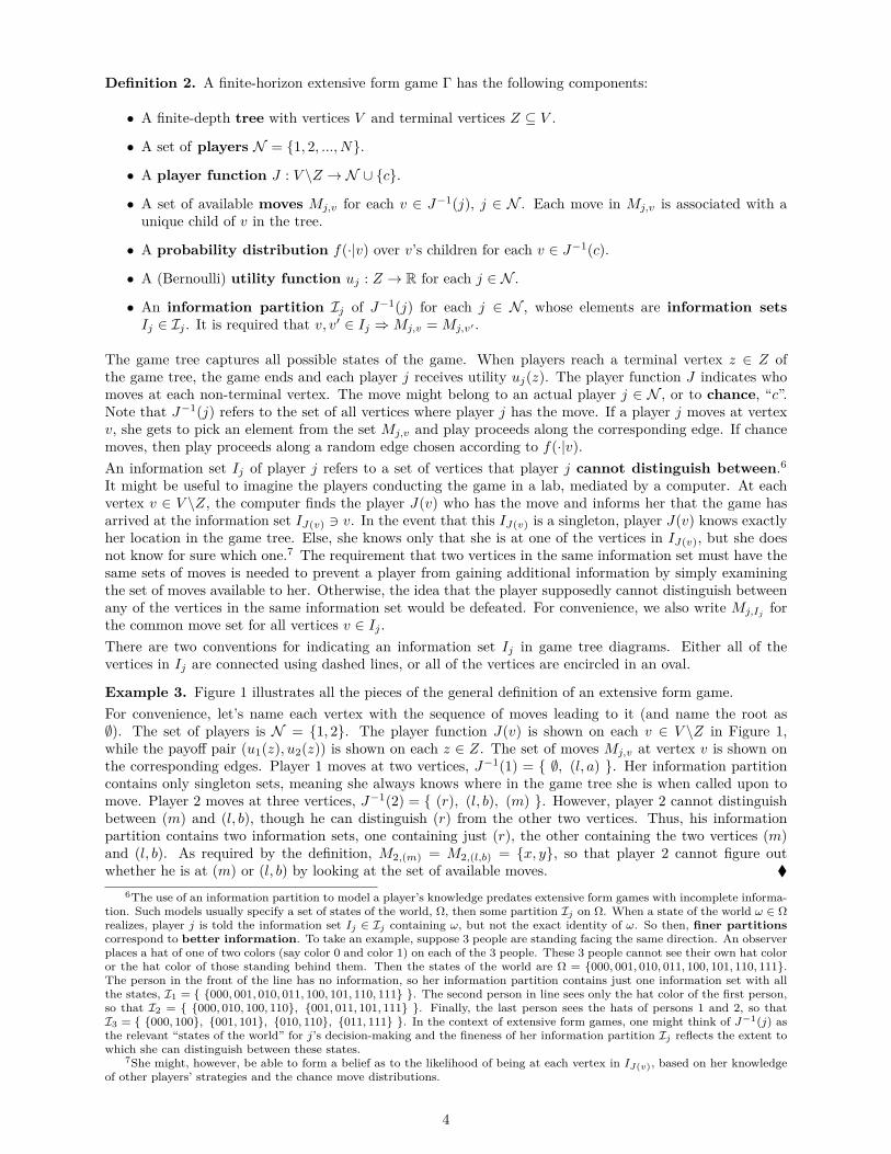
Example 3. Figure 1 illustrates all the pieces of the general definition of an extensive form game.For convenience, let’s name each vertex with the sequence of moves leading to it (and name the root as∅). The set of players is N = 1, 2. The player function J(v) is shown on each v ∈ V \Z in Figure 1,while the payoff pair (u1(z), u2(z)) is shown on each z ∈ Z. The set of moves Mj,v at vertex v is shown onthe corresponding edges. Player 1 moves at two vertices, J−1(1) = ∅, (l, a) . Her information partitioncontains only singleton sets, meaning she always knows where in the game tree she is when called upon tomove. Player 2 moves at three vertices, J−1(2) = (r), (l, b), (m) . However, player 2 cannot distinguishbetween (m) and (l, b), though he can distinguish (r) from the other two vertices. Thus, his informationpartition contains two information sets, one containing just (r), the other containing the two vertices (m)and (l, b). As required by the definition, M2,(m) = M2,(l,b) = x, y, so that player 2 cannot figure outwhether he is at (m) or (l, b) by looking at the set of available moves.

6The use of an information partition to model a player’s knowledge predates extensive form games with incomplete informa-tion. Such models usually specify a set of states of the world, Ω, then some partition Ij on Ω. When a state of the world ω ∈ Ωrealizes, player j is told the information set Ij ∈ Ij containing ω, but not the exact identity of ω. So then, finer partitionscorrespond to better information. To take an example, suppose 3 people are standing facing the same direction. An observerplaces a hat of one of two colors (say color 0 and color 1) on each of the 3 people. These 3 people cannot see their own hat coloror the hat color of those standing behind them. Then the states of the world are Ω = 000, 001, 010, 011, 100, 101, 110, 111.The person in the front of the line has no information, so her information partition contains just one information set with allthe states, I1 = 000, 001, 010, 011, 100, 101, 110, 111 . The second person in line sees only the hat color of the first person,so that I2 = 000, 010, 100, 110, 001, 011, 101, 111 . Finally, the last person sees the hats of persons 1 and 2, so thatI3 = 000, 100, 001, 101, 010, 110, 011, 111 . In the context of extensive form games, one might think of J−1(j) asthe relevant “states of the world” for j’s decision-making and the fineness of her information partition Ij reflects the extent towhich she can distinguish between these states.

7She might, however, be able to form a belief as to the likelihood of being at each vertex in IJ(v), based on her knowledgeof other players’ strategies and the chance move distributions.

4

Chance move distributions: f(a|(l)) = f(b|(l)) = 0.5.Information partitions: I1 = ∅, (l, a) , I2 = (r), (l, b), (m) .

Figure 1: An extensive form game with incomplete information and chance moves.

1

2

(1,1)

L

(0,0)

R

T

2

(0,0)

L

(2,2)

R

B

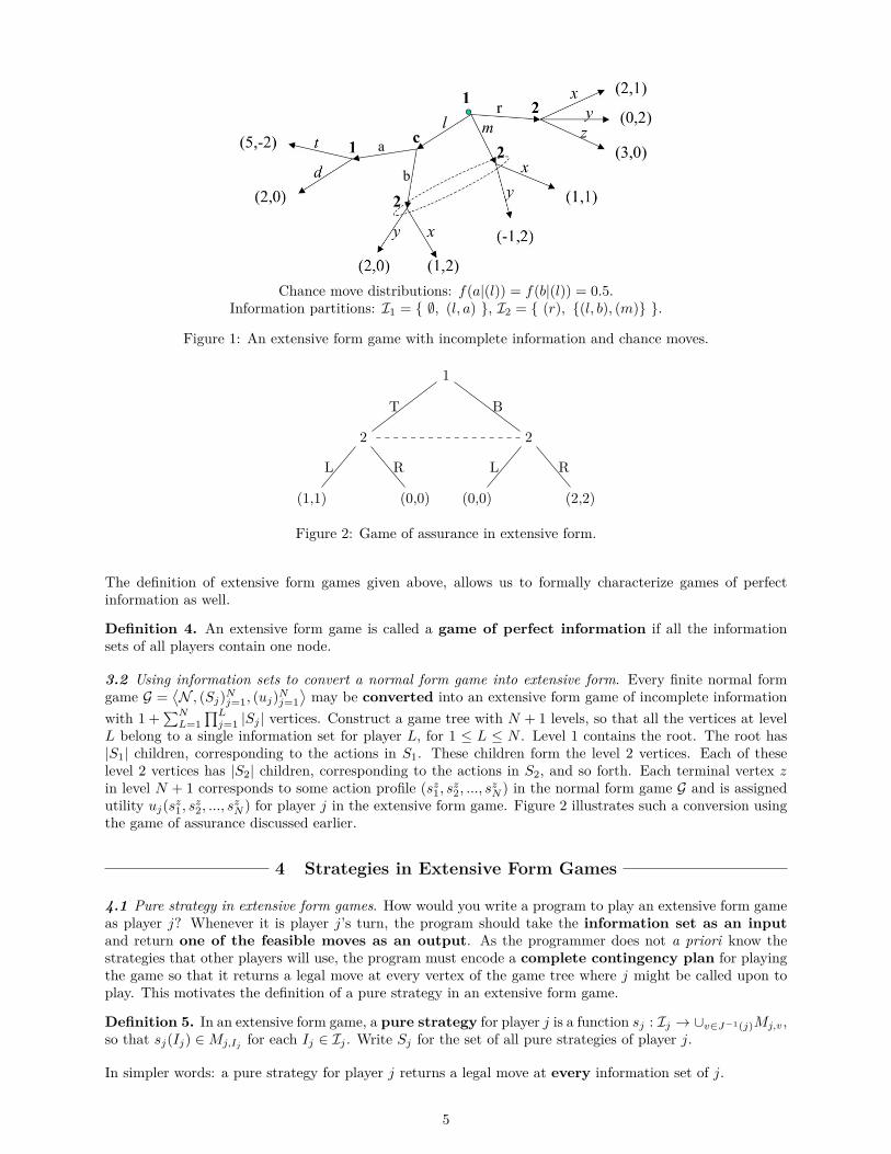
Figure 2: Game of assurance in extensive form.

The definition of extensive form games given above, allows us to formally characterize games of perfectinformation as well.

Definition 4. An extensive form game is called a game of perfect information if all the informationsets of all players contain one node.

3.2 Using information sets to convert a normal form game into extensive form. Every finite normal formgame G =

⟨N , (Sj)Nj=1, (uj)Nj=1

⟩may be converted into an extensive form game of incomplete information

with 1 +∑NL=1

∏Lj=1 |Sj | vertices. Construct a game tree with N + 1 levels, so that all the vertices at level

L belong to a single information set for player L, for 1 ≤ L ≤ N . Level 1 contains the root. The root has|S1| children, corresponding to the actions in S1. These children form the level 2 vertices. Each of theselevel 2 vertices has |S2| children, corresponding to the actions in S2, and so forth. Each terminal vertex zin level N + 1 corresponds to some action profile (sz1, sz2, ..., szN ) in the normal form game G and is assignedutility uj(sz1, sz2, ..., szN ) for player j in the extensive form game. Figure 2 illustrates such a conversion usingthe game of assurance discussed earlier.

4 Strategies in Extensive Form Games

4.1 Pure strategy in extensive form games. How would you write a program to play an extensive form gameas player j? Whenever it is player j’s turn, the program should take the information set as an inputand return one of the feasible moves as an output. As the programmer does not a priori know thestrategies that other players will use, the program must encode a complete contingency plan for playingthe game so that it returns a legal move at every vertex of the game tree where j might be called upon toplay. This motivates the definition of a pure strategy in an extensive form game.

Definition 5. In an extensive form game, a pure strategy for player j is a function sj : Ij → ∪v∈J−1(j)Mj,v,so that sj(Ij) ∈Mj,Ij for each Ij ∈ Ij . Write Sj for the set of all pure strategies of player j.

In simpler words: a pure strategy for player j returns a legal move at every information set of j.

5

Example 6. In Figure 1, one of the strategies of P1 is s1(∅) = m, s1(l, a) = d. Even though playing m atthe root means the vertex (l, a) will never be reached, P1’s strategy must still specify what she wouldhave done at (l, a). This is because some solution concepts we will study later in the course require us toexamine parts of the game tree which are unreached when the game is actually played. Intuitively, thisis necessary because the optimality of an action for a player at some information set may depend on whatshe/he and her/his opponents would have played on an information set which would be reached only if theplayer chooses differently than the strategy under consideration.One of the strategies of P2 is s2((l, b), (m)) = y, s2(r) = z. In every pure strategy P2 must play the sameaction at both (l, b) and (m), as pure strategies are functions of information sets, not individual vertices.In total, P1 has 6 different pure strategies in the game and P2 has 6 different pure strategies.

4.2 Two definitions of randomization. There are at least two natural notions of ’randomizing’ in an extensiveform game: (1) Player j could enumerate the set of all possible pure strategies, Sj , then choose an elementof Sj at random; this corresponds to picking a probability distribution over Sj . (2) Player j could pick arandomization over Mj,Ij for each of her information sets Ij ∈ Ij . These two notions of randomization leadto two different classes of strategies that incorporate stochastic elements:

Definition 7. A mixed strategy for player j is an element σj ∈ ∆(Sj).

Definition 8. A behavioral strategy for player j is a collection of distributions bIjIj∈Ij ,where bIj ∈ ∆(Mj,Ij ).

Strictly speaking, mixed strategies and behavioral strategies form two distinct classes of objects. Wemay, however, talk about the equivalence between a mixed strategy and a behavioral strategy in the followingway:

Definition 9. Say a mixed strategy σj and a behavioral strategy bIj are equivalent if they generatethe same distribution over terminal vertices regardless of the strategies used by opponents, which may bemixed or behavioral.

Note that in this definition for both the behavioral and the mixed case, opponents of j are assumed to playindependently of each other.

Example 10. In Figure 1, a behavioral strategy for P1 is: b∗∅(l) = 0.5, b∗∅(m) = 0, b∗∅(r) = 0.5, b∗(l,a)(t) =0.7, b∗(l,a)(d) = 0.3. That is, P1 decides that she will play m and r each with 50% probability at theroot of the game. If she ever reaches the vertex (l, a), she will play t with 70% probability, d with 30%probability. Now, consider the following 4 pure strategies: s(1)

1 (∅) = l, s(1)1 (l, a) = t; s(2)

1 (∅) = l, s(2)1 (l, a) = d;

s(3)1 (∅) = r, s

(3)1 (l, a) = t; s(4)

1 (∅) = r, s(4)1 (l, a) = d and construct the mixed strategy σ∗j so that σ∗j (s(1)

1 ) =0.35, σ∗j (s(2)

1 ) = 0.15, σ∗j (s(3)1 ) = 0.35, σ∗j (s(4)

1 ) = 0.15. Then the behavioral strategy b∗ is equivalent to themixed strategy σ∗j .

It is often “nicer” to work with behavioral strategies than mixed strategies, for at least two reasons. First,behavioral strategies are easier to write down and usually involve fewer parameters than mixed strategies.Second, it feelsmore realistic for a player to randomize at each decision node than to choose a “grand plan”at the start of the game. In general, however, neither the set of mixed strategies nor the set of behavioralstrategies is a “subset” of the other, as we now demonstrate.

Example 11. (A mixed strategy without an equivalent behavioral strategy) Consider an absent-mindedcity driver who must make turns at two consecutive intersections. Upon encountering the second inter-section, however, she does not remember whether she turned left (T ) or right (B) at the first intersection.The mixed strategy σ1 putting probability 50% on each of the two pure strategies T1T2 and B1B2 generatesthe outcome O1 50% of the time and the outcome O4 50% of the time. However, this outcome distributioncannot be obtained using any behavioral strategy. That is, if the driver chooses some probability of turningleft at the first intersection and some probability of turning left at the second intersection, and furthermorethese two randomizations are independent, then she can never generate the outcome distribution of 50% O1,50% O4.

6

Example 12. (A behavioral strategy without an equivalent mixed strategy) Consider an absent-mindedhighway driver who wants to take the second highway exit. Starting from the root of the tree, x1, he wantsto keep left (L) at the first highway exit but keep right (R) at the second highway exit. Upon encounteringeach highway exit, however, he does not remember if he has already encountered an exit before. The driverhas only two pure strategies: always L or always R. It is easy to see no mixed strategy can ever achieve theoutcome O2. However, the behavioral strategy of taking L and R each with 50% probability each time hearrives at his information set gets the outcome O2 with 25% probability.

These two examples are “strange” in the sense that the drivers “forget” some information that they knewbefore. The city driver forgets what action she took at the previous information set. The highway driverforgets what information sets he has encountered. The definition of perfect recall rules out these twopathologies.

Definition 13. An extensive form game has perfect recall if whenever v, v′ ∈ Ij , the two paths leadingfrom the root to v and v′ pass through the same sequence of information sets and take the same actions atthese information sets.

Intuitively, a game of perfect recall makes it impossible for a player who can remember all the informationabout the path of play she gathered in previous stages (i.e. never forgets anything) to find out in which nodeof any non-singleton information set she is located.In the examples above: the city driver game fails perfect recall since taking two different actions from theroot vertex lead to two vertices in the same information set. The highway driver game fails perfect recallsince vertices x1 and x2 are in the same information set, yet the path from root to x1 is empty while thepath from root to x2 passes through one information set.Kuhn’s theorem states that in a game with perfect recall, it is without loss to analyze only behavioralstrategies. Its proof is beyond the scope of this course.

Theorem 14. (Kuhn 1957) In a finite extensive game with perfect recall, (i) every mixed strategy has anequivalent behavioral strategy, and (ii) every behavioral strategy has an equivalent mixed strategy.

5 Optional food for thought: on the absent-minded driver.

The two types of analyses presented here are intuitively nearer to the concepts of Bayesian Nash Equilibriumand Correlated Equilibrium we will cover in later parts of the lecture. They are based on “The absent-mindeddriver”, Aumann et al., Games and Economic Behavior 1997, Vol. 20 pp. 102-116.Consider the absent-minded driver game we saw in the lecture.

7

Y

1

4

continue

exit

Xexit

0

continue

start

We calculated in the lecture, that the optimal behavioral strategy puts probability of p = 23 on Continue.

Here, in the first part we consider another approach to the same problem, which takes beliefs of the driverabout her location within the info set into account, while in the second part we show that with the helpof simple correlating devices it is possible to achieve an even higher payoff than with mixed or behavioralstrategies.

(1) A Bayesian perspective.For the following analysis we assume

1. The driver makes a decision at each intersection through which he passes. Moreover, when at oneintersection, she can determine the action only there, and not at the other intersection–where she isn’t.

2. Since she can’t distinguish between intersections, whatever reasoning obtains at one intersection mustobtain also at the other, and she is aware of this.

This implies the following.

• The optimal decision is the same at both intersections; it is pinned down by the probability of choosingContinue at each intersection. Call it p∗.

• Therefore, at each intersection, the driver believes that p∗ is chosen at the other intersection.

• The driver has a belief over her location within her information set. At each intersection, the driveroptimizes her decision given her beliefs. Therefore, choosing p at the current intersection she is located,must be optimal given the belief that p∗ is chosen at the other intersection. Moreover, her belief mustbe derived from the strategy she chooses.

By the principle of insufficient reason, without any information about the strategy chosen, the prior prob-ability of being at X will be 1

2 . Denote α(p∗) the belief the driver has about being at the intersection X,given her strategy of choosing p∗ at the other intersection. The reasoning above and Bayes rule implies, that

α(p∗) =12

12 + 1

2p∗ .

Given her beliefs about the behavior at the other node, the payoff of choosing p at the current node is

h(p, p∗) = α(p∗)[(1− p) · 0 + p(1− p∗) · 4 + pp∗ · 1] + (1− α(p∗))[(1− p) · 4 + p · 1].

The first part on the r.h.s. of this expression is the probability of being at X times the payoff from strategyp, conditional on being at X, while the second expression is the probability of being at Y times the payofffrom strategy p, conditional on being at Y . p must be chosen optimally, given the belief p∗ and moreover, pmust be equal to p∗, since the agent doesn’t distinguish between the nodes and any beliefs she has must bederived from the strategy chosen in equilibrium. That is, p∗ must fulfill

p∗ ∈ arg maxp∈[0,1]

h(p, p∗). (1)

8

For the function h(p, q) = 11+q [(1 − p) · 0 + p(1 − q) · 4 + pq · 1] + q

1+q [(1 − p) · 4 + p · 1] = (4−6q)p+4q1+q , we

maximize p for fixed q. The solution as a function of q satisfies

p =

0 if q > 2

3any value in [0, 1] if q = 2

31 if q < 2

3 .

This shows that the solution to (1) is unique and equal to p∗ = 23 . The same as for the optimal behavioral

strategy! Recall that the payoff of the optimal behavioral strategy was 43 .

(2)The handkerchief solution. Assume the driver has a handkerchief in her pocket. Whenever she goesthrough an intersection, she ties a knot in the handkerchief, if there was no knot; or she unties the knot, ifthere was one. At the beginning, i.e. at start it is equally probable that the handkerchief had or did nothave a knot. The driver-absent-minded as she is-cannot remember which was the case. Thus, at each one ofthe two intersections, the probability of having a knot in the handkerchief is 1

2 . Therefore, seeing a knot ornot at each intersection does not reveal any information about the intersection.Nevertheless, consider the following strategy for the driver: exit if there is a knot, continue if there is not.The payoff of this simple strategy is 1

2 · 0 + 12 · 4 = 2: with probability 1

2 the handkerchief had a knot, so thatthe driver exits and the payoff is 0 and with probability 1

2 the handkerchief had no knot so that the drivercontinues and ties a knot; at the next node, seeing the knot the driver exits so that the payoff realized is4. Note that the path of play induced by this strategy can not be replicated using a behavioral strategy:the handkerchief has allowed the driver to avoid ever reaching the last node with payoff 1. Note also, that2 > 4

3 , the payoff from the best behavioral strategy. The handkerchief has served as a coordination devicebetween the forgetful selves in the different nodes and has achieved a higher payoff than the best behavioralstrategy!Question to ponder: what is ‘strange’ in this solution ?

Trivia: “Alice’s adventures in Algebra: Wonderland solved”, Bayley, M. in New Scientist, 2009 containsmore about the mathematics which inspired Lewis Carroll’s book.

9

Economics 2010a . Section 2 : Nash Equilibrium and Its Properties 10/29/2018∣∣∣∣ (1) Strategies in normal form games; (2) Nash equilibrium and some properties; (3) Solving for NE;∣∣∣∣

TF: Jetlir Duraj (duraj@g.harvard.edu)

1 Strategies in Normal Form Games

1.1 Recurring notations. The following notations are common in game theory but usually go unexplained.If X1, X2, ..., XN is a sequence of sets with typical elements x1 ∈ X1, x2 ∈ X2, ..., then:

• X−i means ×1≤k≤N,k 6=iXk

• X is sometimes understood to mean ×Nk=1Xk.

• (xi) refers to a vector8 (x1, x2, ..., xN ). So (xi) is an element in ×Nk=1Xk. The parentheses are used todistinguish it from xi, which is an element of Xi.

• x−i is an element in X−i, i.e. in ×1≤k≤N,k 6=iXk. Confusingly, usually no parentheses are used aroundx−i.

To see an example of these notations, suppose we are studying a three player game

G = 〈1, 2, 3, (S1, S2, S3), (u1, u2, u3)〉

Then “s−2” usually refers to a vector containing strategies from P1 and P3, but not P2. It is an element ofS1 × S3, also written as S−2.1.2 Mixed strategies in normal form games. A player who uses a mixed strategy in a game intentionallyintroduces randomness into her play. Instead of picking a deterministic action as in a pure strategy, amixed strategy user tosses a coin to determine what action to play. Game theorists are interested in mixedstrategies for at least two reasons: (i) mixed strategies correspond to how humans play certain games,such as rock-paper-scissors; (ii) the space of mixed strategies represents a “convexification” of the actionset Si and convexity is required for many existence results.

Definition 15. Suppose G = 〈N , (Sk)k∈N , (uk)k∈N 〉 is a normal form game where each Sk is finite.9 Thena mixed strategy σi is a member of ∆(Si).

Sometimes the mixed strategy putting probability p1 on action s(1)1 and probability 1− p1 on action s(2)

1 iswritten as p1s

(1)1 ⊕ (1− p1)s(2)

1 . The “⊕” notation (in lieu of “+”) is especially useful when s(1)1 , s

(2)1 are real

numbers, as to avoid confusing the mixed strategy with an arithmetic expression to be simplified.Two remarks:

• When two or more players play mixed strategies, their randomizations are assumed to be independent.

• Technically, pure strategies also count as mixed strategies – they are simply degenerate distri-butions on the action set. The term “strictly mixed” is usually used for a mixed strategy that putsstrictly positive probability on every action.

When a profile of mixed strategies (σk)Nk=1 is played, the assumption on independent mixing, together withprevious week’s discussion on payoff matrix entries as Bernoulli utilities in a vNM representation, imply thatplayer i gets utility: ∑

(s′k)∈×kSk

ui(s′

1, ..., s′

N ) · σ1(s′1) · ... · σN (s′N )

We will abuse notation and write ui(σi, σ−i) for this utility, extending the domain of ui into mixed strategies.8Sometimes also called a “profile”.9We can also define mixed strategies when the set of actions Sk is infinite. However, we would need to first equip Sk with

sigma-algebra, then define the mixed strategy as a probability measure on this sigma-algebra.

10

1.3 What does it mean to “solve” a game? A detour into combinatorial game theory. Why are economistsinterested in Nash equilibrium, or solution concepts in general? As a slight aside, you may want to knowthat there actually exist two areas of research that go by the name of “game theory”. The full namesof these two areas are “combinatorial game theory” and “equilibrium game theory”. Despite thesimilarity in name, these two versions of game theory have quite different research agendas. The mostsalient difference is that combinatorial game theory studies well-known board games like chess where thereexists (theoretically) a “winning strategy” for one player. Combinatorial game theorists aim to find thesewinning strategies, thereby ultimately solving the game. On the other hand, no “winning strategies” (usuallycalled “dominant strategies” in our lingo) exist for most games studied by equilibrium game theorists.10

In the Battle of the Sexes, for example, due to the simultaneous move condition, there is no one strategythat is optimal for P1 regardless of how P2 plays, in contrast to the existence of such optimal strategies in,say, tic-tac-toe.If a game has a dominant strategy for one of the players, then it is straight-forward to predict its outcomeunder optimal play. The player with the dominant strategy will employ this strategy and the other playerwill do the best they can to minimize their losses. However, predicting outcome in a game without dominantstrategies requires the analyst to make assumptions. These assumptions are usually called equilibrium as-sumptions and give “equilibrium game theory” its name. One of the most common equilibrium assumptionsin normal form games with complete information is the Nash equilibrium, which we now study.

2 Nash Equilibrium

2.1 Defining Nash equilibrium. A Nash equilibrium11 is a strategy profile where no player can improve uponher own payoff through a unilateral deviation, taking as given the actions of others. This leads to the usualdefinition of pure and mixed Nash equilibria.

Definition 16. In a normal form game G = 〈N , (Sk)k∈N , (uk)k∈N 〉, a Nash equilibrium in pure strate-gies is a pure strategy profile (s∗k)k∈N such that for every player i, ui(s∗i , s∗−i) ≥ ui(s′i, s∗−i) for all s′i ∈ Si.

Definition 17. In a normal form game G = 〈N , (Sk)k∈N , (uk)k∈N 〉, a Nash equilibrium in mixedstrategies is a mixed strategy profile (σ∗k)k∈N such that for every player i, ui(σ∗i , σ∗−i) ≥ ui(s′i, σ∗−i) for alls′i ∈ Si.

In the definition of a mixed Nash equilibrium, we required no profitable unilateral deviation to any purestrategy, s′i. It would be equivalent to require no profitable unilateral deviation to any mixed strategy, dueto the following fact.

Fact 18. For any fixed σ−i, the map σi 7→ ui(σi, σ−i) is affine, in the sense thatui(σi, σ−i) =

∑si∈Si σi(si) · ui(si, σ−i).

That is, the payoff to playing σi against opponents’ mixed strategy profile σ−i is some weighted average ofthe |Si| numbers (ui(si, σ−i))si∈Si , where the weights are given by the probabilities that σi assigns to thesedifferent actions. So, if there is some profitable mixed strategy deviation σ′i from a strategy profile (σ∗i , σ∗−i),then it must be the case that for at least one s′i ∈ Si with σ′i(s′i) > 0, we have ui(s′i, σ∗−i) > ui(σ∗i , σ∗−i).

Example 19. Consider the game of assurance,

L R

T 1,1 0,0B 0,0 2,2

We readily verify that both (T, L) and (B,R) are pure strategy Nash equilibria. Note one of these two NEsPareto dominates the other. In general, NEs need not be Pareto efficient. This is because the definitionof NE only accounts for the absence of profitable unilateral deviations. Indeed, starting from the strategyprofile (T, L), if P1 and P2 can contract on simultaneously changing their strategies, then they would bothbe better off. However, these sorts of simultaneous deviations by a “coalition” are not allowed.

10The one-shot prisoner’s dilemma is an exception here.11John Nash called this equilibrium concept “equilibrium point” but later researchers referred to it as “Nash equilibrium”.

11

But wait, there’s more! Suppose P1 plays 23T ⊕

13B. Suppose P2 plays 2

3L⊕13R. This strategy profile is

also a mixed NE. The reasoning is surprisingly simple. When P1 is playing 23T ⊕

13B, P2 gets an expected

payoff of 23 from playing L and an expected payoff of 2

3 from playing R. Therefore, P2 has no profitableunilateral deviation because every strategy he could play, pure or mixed, would give the same payoff of 2

3 .Similarly, P2’s mixed strategy 2

3L ⊕13R means P1 gets an expected payoff of 2

3 whether she plays T or B,so P1 does not have a profitable deviation either.

2.2 Nash equilibrium as a fixed-point of the best response correspondence. Nash equilibrium embodies theidea of stability. To make this point clear, it is useful to introduce an equivalent view of the Nash equilibriumthrough the lens of best response correspondence.

Definition 20. The individual pure best response correspondence for player i is BRi : S−i ⇒ Si12

whereBRi(s−i) := arg max

si∈Siui(si, s−i).

The pure best response correspondence involves putting the N pure best response correspondencesinto a vector: BR : S ⇒ S where BR(s) := (BR1(s−1) ... BRN (s−N )).Analogously, the individual mixed best response correspondence for player i is BRi :

∏k 6=i ∆(Sk)⇒

∆(Si) whereBRi(σ−i) := arg max

σi∈∆(Si)ui(σi, σ−i).

The mixed best response correspondence involves putting the N mixed best response correspondencesinto a vector: BR :

∏i ∆(Si)⇒

∏i ∆(Si) where BR(σ) := (BR1(σ−1) ... BRN (σ−N )).

To interpret, the individual best response correspondences return the argmax of each player’s utility functionwhen opponents plays some known strategy profile. Depending on others’ strategies, the player may havemultiple maximizers, all yielding the same utility. As a result, we must allow the best responses to becorrespondences rather than functions. Then, it is easy to see that:

Proposition 21. A pure strategy profile is a pure NE iff it is a fixed point of BR. A mixed strategy profileis a mixed NE iff it is a fixed point of BR.

Fixed points of the best response correspondences reflect stability of NE strategy profiles, in the sense thateven if player i knew what others were going to play, she still would not find it beneficial to change her actions.This rules out cases where a player plays in a certain way only because she held the wrong expectationsabout other players’ strategies. We might expect such outcomes to arise initially when inexperienced playersparticipate in the game, but we would also expect such outcomes to vanish as players learn to adjust theirstrategies to maximize their payoffs over time. That is to say, we expect non-NE strategy profiles to beunstable.

2.3. Three properties of Nash equilibria.Property 1: the indifference condition in mixed NEs.In Example 19, we saw that each action that player i plays with strictly positive probability yields the sameexpected payoff against the mixed strategy profile of the opponent. Turns out this is a general phenomenon.

Proposition 22. Suppose (σ∗i ) is a mixed Nash equilibrium. Then for any si ∈ Si such that σ∗i (si) > 0, wehave ui(si, σ∗−i) = ui(σ∗i , σ∗−i).

Proof. Suppose we may find si ∈ Si so that σ∗i (si) > 0 but ui(si, σ∗−i) 6= ui(σ∗i , σ∗−i). In the event thatui(si, σ∗−i) > ui(σ∗i , σ∗−i), we contradict the optimality of σ∗i in the maximization problem arg max ui(σi, σ∗−i),for we should have just picked σi = si, the degenerate distribution on pure strategy si. In the event thatui(si, σ∗−i) < ui(σ∗i , σ∗−i), we enumerate Si = s(1)

i , ..., s(r)i and use the Fact 18 to expand:

ui(σ∗i , σ∗−i) =r∑

k=1σ∗i (s(k)

i ) · ui(s(k)i , σ∗−i)

The term ui(si, σ∗−i) appears in the summation on the right with a strictly positive weight, so if ui(si, σ∗−i) <ui(σ∗i , σ∗−i) then there must exist another s′i ∈ Si such that ui(s′i, σ∗−i) > ui(σ∗i , σ∗−i). But now we have againcontradicted the fact that σ∗i is a best mixed response to σ∗−i.

12The notation f : A⇒ B is equivalent to f : A→ 2B .

12

Property 2: Nash payoffs are greater or equal than the maxmin values of each player.

Definition 23. In a normal form game the maxmin value of a player is defined by

maxσi

minσ−i

ui(σi, σ−i),

while the minmax value of a player is defined by

minσ−i

maxσi

ui(σi, σ−i).

The interpretation of these two values is straightforward:- the maxmin of i is the smallest utility value agent i can ensure if she best responds to the strategies of theother players, while- the minmax of i is the lowest utility the other players can push player i down to, if she best responds totheir strategy.We showed in the lecture, that for two player, zero-sum (or actually constant-sum) games, these two valuesare identical for both players. It turns out that in any game of finite players, any Nash equilibrium payoffof each player is at least as large as his minmax or maxmin value.

Proposition 24. In each normal form game G = (N , (Si)i∈N , (ui)i∈N ) with a finite set of players, for everyNash equilibrium σ∗ = (σ∗1 , . . . , σ∗n) and for every player i it holds

ui(σ∗) ≥ maxσi

minσ−i

ui(σi, σ−i), ui(σ∗) ≥ minσ−i

maxσi

ui(σi, σ−i).

Proof. Note that σ∗ being a Nash equilibrium can be written as

ui(σ∗i , σ∗−i) ≥ ui(si, σ∗−i) (2)

for all si ∈ Si and all players i ∈ N . Due to the properties of Expected Utility this is equivalent to thestatement

ui(σ∗i , σ∗−i) ≥ ui(pi, σ∗−i) (3)

for all pi ∈ ∆(Si): One direction is clear, since pure strategies are a particular case of mixed strategies; theother direction is proven by taking mixtures and noticing that the LHS of both (2) and (3) doesn’t dependon resp. si and pi.(1) Note then, that

ui(σ∗) = maxσi

ui(σi, σ∗−i) ≥ minσ−i

maxσi

ui(σi, σ−i),

where the first equality comes from the definition of Nash equilibrium and the second from the definition ofmin of a function.(2) Furthermore,

ui(σ∗) = maxσi

ui(σi, σ∗−i) ≥ maxσi

minσ−i

ui(σi, σ−i),

because for each fixed σi we have that ui(σi, σ∗−i) ≥ minσ−i ui(σi, σ−i), i.e. we have two functions of σi,where the first always dominates the second at each σi. This implies that the maximum of the first isgreater-equal to the maximum of the second function.These two arguments complete the proof.

Property 3: Never play strictly dominated strategies.

Definition 25. In a normal form game G = (N , (Si)i∈N , (ui)i∈N ) call a pure strategy si ∈ Si of player istrictly dominated if there exists a mixed strategy σi ∈ ∆(Si) so that for every σ−i we have

ui(σi, σ−i) > ui(si, σ−i).

Do not confuse this definition with the one from Nash equilibrium: here, the inequality is strict and shouldhold for every possible play of the other players. It turns out, that recognizing strictly dominated strategiescan help analyze the Nash equilibria of a game, since no player would ever employ them in a Nash equilibriumstrategy.

13

Proposition 26. If σ∗ is a Nash equilibrium of the normal form game G = (N , (Si)i∈N , (ui)i∈N ), then noplayer puts positive probability on a strictly dominated strategy. In other words:

si strictly dominated for i and σ∗ is Nash =⇒ σ∗i (si) = 0.

Proof. Let σ∗ be Nash and assume, that si is strictly dominated by σi for i. This means in particular, that

ui(σi, σ∗−i) > ui(si, σ∗−i).

The definition of Nash equilibrium implies then, that

ui(σ∗i , σ∗−i) > ui(si, σ∗−i),

while the indifference principle implies that if σ∗i (s′i) > 0, then ui(s′i, σ∗−i) = ui(σ∗) > ui(si, σ∗−i). If it were,that σ∗(si) > 0, this would mean that there is some s′i with σ∗i (s′i) > 0 and ui(s′i, σ∗−i) = ui(σ∗) > ui(si, σ∗−i)whose probability σ∗i (s′i) could be increased and which would yield a higher payoff for player i. This wouldbe a contradiction to Nash equilibrium definition! Thus, it has to be σ∗i (si) = 0.

2.4 Mathematical properties of the set of Nash equilibria. The set NE of Nash equilibria of a finite normalform game G is a subset of the product space of strategy profiles ∆(S1)×∆(S2)× · · · ×∆(Sn), where n isthe number of the players. This set is compact, because it is a bounded and closed set of an euclidean space:

• If |S| =∏ni=1 |Si| is the cardinality of the set of pure strategies of the game, then ∆(S1) × ∆(S2) ×

· · · ×∆(Sn) can be mapped uniquely to a bounded set of R|S| and thus is bounded.

• Let σm be a sequence of Nash equilibria of the game such that it converges to a strategy profile σ, i.e.σm→σ as m→∞. We then have

ui(σm,i, σm,−i) ≥ ui(si, σm,−i)

for all players i, strategies si ∈ Si. But the payoff functions are continuous in their arguments, so thatpassing to the limit m→∞ we have

ui(σi, σ−i) ≥ ui(si, σ−i)

for all players i, strategies si ∈ Si. But this is just the definition of σ being a Nash equilibrium profile!This argument shows that the set NE of equilibria is closed.

The set NE of Nash equilibria is in general not convex. Consider as a counterexampe the Battle of the Sexesgame:

Opera Football

Opera 3,2 0,0Football 0,0 2,3

You can check that there are three Nash equilibria for this game: two in pure strategies (Opera,Opera),(Football, Football) and one in mixed strategies ( 3

5Opera ⊕25Football,

25Opera ⊕

35Football).

13 Take themixture with probability 1

2 of the two pure Nash equilibria, i.e. consider ( 12Opera ⊕

12Football,

12Opera ⊕1

2Football). But note that player 1 gets a utility of 32 by playing Opera and a utility of 1 by playing

Football and thus would deviate to playing Opera with probability one. This means, that the set NE ofNash equilibria doesn’t contain ( 1

2Opera⊕12Football,

12Opera⊕

12Football) and thus it is not convex.

Question: Can you think of a (trivial) case where the set of Nash equilibria is indeed convex ?Hint: Think of Prisoner’s Dilemma.

Example 27. Consider the three player game in which every player has two pure strategies; Player 1 choosesa row (T or B), Player 2 chooses a column (L or R) and player 3 chooses the matrix (W or E). The followingmatrices show only the payoff function of player 1.

13Please, please make sure you can indeed find these Nash equilibria on your own – if the concept of Nash equilibria iscompletely new, this is good practice! See also below if you have difficulties characterizing the set of Nash equilibria here.

14

L R

T 0 1B 1 1

matrix W

L R

T 1 1B 1 0

matrix E

What is the maxmin and the minmax value of player 1 in mixed strategies ?

Solution. Assume P1 uses x⊕ (1− x), P2 uses y ⊕ (1− y) and P3 z ⊕ (1− z). Then P1s payoff is

U1(x, y, z) = 1− xyz − (1− x)(1− y)(1− z).

and maxmin-ing this expression leads to

v1 = maxx

miny,z

U1(x, y, z) = 12 .

To see this, note that U1(x, 1, 1) = x ≤ 12 for every x ≤ 1

2 . Also, U1(x, 0, 0) = 1− x ≤ 12 for every x ≥ 1

2 . Itfollows miny,z U1(x, y, z) ≤ 1

2 . But U1( 12 , y, z) ≥

12 for each y.

Next we calculate the minmax of P1.

v1 = miny,z

maxx

U1(x, y, z)

= miny,z

maxx

(1− xyz − (1− x)(1− y)(1− z))

= miny,z

maxx

(1− (1− y)(1− z) + x(1− y − z))

One can see that the (inner) maximum is achieved x = 1 if 1− y − z ≥ 0 and at the extreme point x = 0 if1− y − z ≤ 0. It follows

maxx

(1− (1− y)(1− z) + x(1− y − z)) =

1− (1− y)(1− z), y + z ≥ 11− yz, y + z < 1.

By going case-by-case and using symmetry we see that the (outer) optimum is attained at y = z = 12 . It

followsv1 = 3

4 .

Note that in this example we havev1 = 1

2 <34 = v1.

2.5 Symmetric Games. A game in normal form G = (N , (Si)i∈N , (ui)i∈N ) is called a symmetric game if

• Each player has the same set of strategies: Si = S for all i ∈ N .

• The payoff functions satisfy for each pair of players i, j with i < j

ui(s1, s2, . . . , sn) = uj(s1, . . . , si−1, sj , si+1, . . . , sj−1, si, sj+1, . . . , sn).

Examples of symmetric games are Bertrand duopoly or Cournot duopoly with identical costs, Prisoner’sDilemma, etc. An example of a non-symmetric game is the Battle of the sexes.One can adapt the proof of Nash’s existence Theorem to show that every finite symmetric game has asymmetric Nash equilibrium in mixed strategies: a Nash equilibrium σ = (σi)i∈N satisfying σi = σjfor each i, j ∈ N .This fact can come in handy when solving games. Moreover, the assumption of symmetric play is naturalgiven that symmetric games are so that the players are interchangeable, i.e. their exact identity doesn’tmatter for the game play.

15

3 Solving for Nash Equilibria

The following steps may be helpful in solving for NEs of two-player games.

1. Use iterated elimination of strictly dominated strategies to simplify the problem.14

2. Find all the pure strategy Nash equilibria by considering all cells in the payoff matrix.

3. Look for a mixed Nash equilibrium where one player is playing a pure strategy while the other isstrictly mixing.

4. Look for a mixed Nash equilibrium where both players are strictly mixing.

Example 28. (December 2013 Final Exam) Find all NEs, pure and mixed, in the following payoff matrix.

L R Y

T 2, 2 −1, 2 0, 0B −1,−1 0, 1 1,−2X 0, 0 −2, 1 0, 2

Solution:Step 1: Strategy X for P1 is strictly dominated by 1

2T ⊕12B. Indeed, u1(X,L) = 0 < 0.5 = u1( 1

2T ⊕12B,L),

u1(X,R) = −2 < −0.5 = u1( 12T⊕

12B,R), and u1(X,Y ) = 0 < 0.5 = u1( 1

2T⊕12B, Y ). But having eliminated

X for P1, strategy Y for P2 is strictly dominated by R: u2(T, Y ) = 0 < 2 = u2(T,R), u2(B, Y ) = −2 < 1 =u2(B,R). Hence we can restrict attention to the smaller, 2x2 game in the upper left corner.Step 2: (T, L) is a pure Nash equilibrium as no player has a profitable unilateral deviation. (The deviationL → R does not strictly improve the payoff of P2, so it doesn’t break the equilibrium.) At (T,R), P1deviates T → B, so it is not a pure strategy Nash equilibrium. At (B,L), P2 deviates L → R. At (B,R),no player has a profitable unilateral deviation, so it is a pure strategy Nash equilibrium. In summary, thegame has two pure strategy Nash equilibria: (T, L) and (B,R).Step 3: Now we look for mixed Nash equilibria where one player is using a pure strategy while the other isusing a strictly mixed strategy. As discussed before, if a player strictly mixes between two pure strategies,then they must be getting the same payoff from playing either of these two pure strategies.Using this indifference condition, we quickly realize it cannot be the case that P2 is playing a purestrategy while P1 strictly mixes. Indeed, if P2 plays L then u1(T, L) > u1(B,L). If P2 plays R thenu1(B,R) > u1(T,R).Similarly, if P1 is playing B, then the indifference condition cannot be sustained for P2 since u2(R,B) >u2(L,B).Now suppose P1 plays T . Then u2(T, L) = u2(T,R). This indifference condition ensures that any strictlymixed strategy of P2 pL⊕(1−p)R for p ∈ (0, 1) is a mixed best response to P1’s strategy. However, to ensurethis is a mixed Nash equilibrium, we must also make check P1 does not have any profitable unilateraldeviation. This requires:

u1(T, pL⊕ (1− p)R) ≥ u1(B, pL⊕ (1− p)R)

that is to say,

2p+ (−1) · (1− p) ≥ (−1) · p+ 0 · (1− p)4p ≥ 1

p ≥ 14

14Next section will focus more on IESDS and its properties. Regarding the relation of never best response property to theproperty of being strictly dominated for strategies: these two concepts are equivalent for two-player games. For games withmore than two players, they are in general not equivalent under the assumption that opponents of a player cannot correlatetheir strategies.

16

Therefore, (T, pL⊕ (1− p)R) is a mixed Nash equilibrium where P2 strictly mixes when p ∈ [ 14 , 1).

Step 4: There are no mixed Nash equilibria where both players are strictly mixing. To see this, notice ifσ∗1(B) > 0, then

u2(σ∗1 , L) = 2 · (1− σ∗1(B)) + (−1) · (σ∗1(B)) < 2 · (1− σ∗1(B)) + (1) · (σ∗1(B)) = u2(σ∗1 , R)

So it cannot be the case that P2 is also strictly mixing, since P2 is not indifferent between L and R.In total, the game has two pure Nash equilibria, (T, L) and (B,R), as well as infinitely many mixed Nashequilibria, (T, pL⊕ (1− p)R) for p ∈ [ 1

4 , 1).

Sometimes, iterated elimination of strictly dominated strategy simplifies the game so much that the solutionis immediate after Step 1. The following example illustrates.

Example 29. (Guess two-thirds the average, also sometimes called the beauty contest game15) Considera game of 2 players G(1) where S1 = S2 = [0, 100], ui(si, s−i) = −

(si − 2

3 ·si+s−i

2

)2. That is, each player

wants to play an action as close to two-thirds the average of the two actions as possible. We claim that foreach player i, every action in (50, 100] is strictly dominated by the action 50. To see this, for any opponentaction s−i ∈ [0, 100], we have 2

3 ·50+s−i

2 ≤ 50, so the guess 50 is already too high:

50− 23 ·

50 + s−i2 ≥ 0

At the same time, ddsi

[si − 2

3 ·si+s−i

2

]= 2

3 > 0. Hence we conclude playing any si > 50 exacerbates theerror relative to playing 50,

si −23 ·

si + s−i2 > 50− 2

3 ·50 + s−i

2 ≥ 0

so then −(si − 2

3 ·si+s−i

2

)2< −

(50− 2

3 ·50+s−i

2

)2for all si ∈ (50, 100] and we have the claimed strict

dominance.This means we may delete the set of actions (50, 100] from each Si to arrive at a new game G(2) whereeach player is restricted to using only [0, 50]. The game G(2) will have the same set of NEs as the originalgame. But the same logic may be applied again to show that in G(2), for each player any action in (25, 50]is strictly dominated by the action 25. We may continue in this way iteratively to arrive at a sequenceof games (G(k))k≥1, so that in the game G(k+1), player i’s action set is

[0,( 1

2)k · 100

]. All of the games

G(1),G(2),G(3), ... have the same NEs. This means any NE of G(1) must involve each player playing an actionin

∞⋂k=1

[0,(

12

)k· 100

]= 0

Hence, (0, 0) is the unique NE.

Example 30. Consider the following three player game, where the first player chooses rows, the secondcolumns and the third chooses the matrix.

A L R

T 1,1,1 0,1,3B 1,3,0 1,0,1

C L R

T 3,0,1 1,1,0B 0,1,1 0,0,0

We claim, that there is only one mixed Nash equilibrium and it is in pure strategies: (T, L,A).Solution:Step 1: There is only one Nash equilibrium in pure strategies. Note, that domination argumentsdon’t help here, because no pure strategy of any player is dominated. It is easy to see, that (T, L,A) is a

15The name “beauty contest game” comes from an old newspaper game where readers pick the 6 faces they consider themost beautiful from a set of 100 portraits. The readers who pick the six most popular choices won a prize.

17

pure Nash equilibrium: if players 1, 2 play (T, L), then player 3 is indifferent and so might as well choose A.Note also, that (T, L) is a Nash equilibrium of the two-player game created by taking matrix A and deletingall payoffs of player 3. In this restricted game, there is also the pure Nash where players 1, 2 play (B,L),but then player 3 would like to switch matrix. If we restrict matrix B to the payoffs of players 1, 2 only, wesee that there is only one pure Nash in the two-player induced game: (T,R). but then player 3 would liketo switch matrix to A. In all, there is only one pure Nash and it is (T, L,A).Step 2: There are no Nash equilibria, where two players play pure and the remaining playercompletely mixes.- Assume there is a Nash equilibrium where players 1, 2 play pure and player 3 completely mixes. But wesaw that in A players 1, 2 would then play either (T,L) or (B,L). In the second case, player 3 would liketo switch matrix, so it must be (T, L). But then player 2 would better switch to R, since when matrixA is played he gets 1 in any case and when matrix C is played with positive probability, he gets 1 > 0.Contradiction.- Assume there is a Nash equilibrium where players 1,3 play pure and player 2 completely mixes. Assumefirst, that player 3 plays A. Then any completely mixed strategy of player 2 will induce player 1 to playB, because then she can make sure she gets 1 instead than less than 1. But if player 1 plays B, player 2would want to play L with probability 1, which contradicts the fact that he is completely mixing. Assumethen, that player 3 is playing C. Here player 1 would want to play T with probability 1, because B gives herstrictly less utility, no matter what the strategy of player 2 is. But player 1 playing T would make player 2play L with probability 1, contradicting the hypothesis that he completely mixes.- Assume there is a Nash equilibrium where players 2,3 play pure and player 1 completely mixes. Assumefirst, that player 3 plays A. We know from the induced game between players 1, 2 that then player 1 wouldwant to completely mix only if player 2 is playing L, because otherwise player 1 could increase payoff byplaying B. But then player 3 would want to switch to C to ensure a payoff of 1 contradicting the assumptionthat she plays A. Assume then, that player 3 plays C. Here player 1 would never completely mix, becauseno matter the strategy of player 2 she gets strictly more by playing T rather than B. This contradicts theassumption that player 1 completely mixes and concludes this case.Step 3: There are no Nash equilibria, where one player plays pure and the remaining playerscompletely mix.- Assume it is player 1 who plays pure. Assume first, she plays T . Let p, q ∈ (0, 1) the probabilities withwhich, resp. player 2 plays L and player 3 plays A in equilibrium. Player 3 would choose q ∈ (0, 1) only ifshe is indifferent between the two matrices, i.e. p has to fulfill

p+ 3(1− p) = p+ 0(1− p).

But this implies p = 1, a contradiction. Assume then, that player 1 instead plays B. Let p, q ∈ (0, 1) theprobabilities with which, resp. player 2 plays L and player 3 plays A in equilibrium. Player 2 would wantto completely mix only if he is indifferent between L,R. It follows, that q has to fulfill

3q + 1(1− q) = 0q + 0(1− q),

which is impossible.- Assume now there is a Nash equilibrium where player 2 is the only player who plays pure. Assume heis playing L. Player 1 would want to completely mix only if player 3 was playing A; otherwise, she wouldchoose T with probability 1, which is a contradiction. Assume then, that player 2 is playing R. But thenplayer 3 would play A with probability one, because no matter what the play of player 1 is, she is better offwith A.- Assume finally, for this step, that it is player 3 who plays pure and the other two players completely mix.We can see that it can’t be the case that player 3 plays C because then, player 1 would choose T withprobability 1. So it must be that player 3 plays A. But here again, we know that player 1 would want tocompletely mix if and only if player 2 is playing L, because otherwise by choosing B she can ensure a payoffof 1. This contradicts the assumption that player 2 is completely mixing.Step 4: There are no Nash equilibria, where all players completely mix.16

Assume there is a completely mixed Nash equilibrium where player 1 plays T with probability p, player 2plays L with probability q and player 3 plays A with probability r. Then we must have that players are allindifferent between their resp. pure strategies. For player 1 this means that r, q must fulfill (besides beingin (0, 1))

qr + 0 + 3q(1− r) + (1− q)(1− r) = r + 0.16There are several ways to do this step, this is just one of them.

18

Here, the LHS is player 1 payoff from playing T and the RHS is her payoff from playing B. Simple algebrashows that this indifference condition can be written as

3q(1− r) = (1− q)(2r − 1). (4)

Note that this implies in particular, that r ∈ ( 12 , 1). Similar algebra for players 2 and 3 shows that their

indifference conditions can be written as

3r(1− p) = (1− r)(2p− 1) (5)

for player 2 and3p(1− q) = (1− p)(2q − 1) (6)

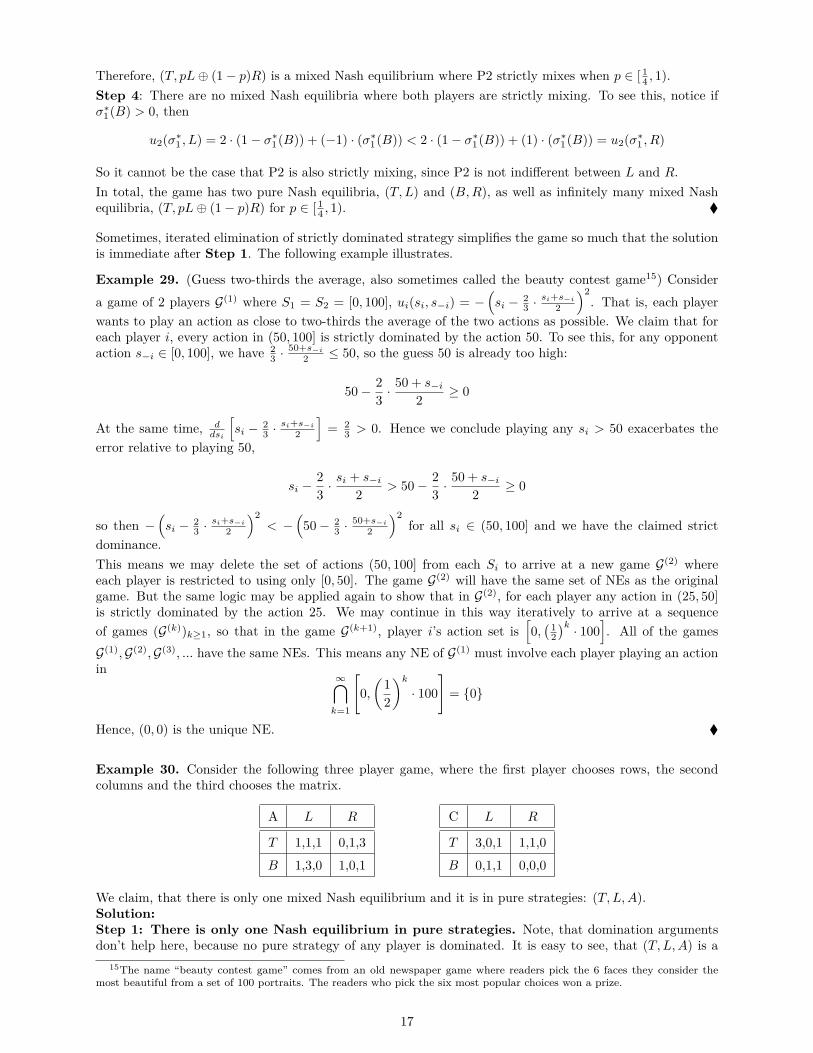
for player 3.17 Now multiply equations (4),(5) and (6) side by side to arrive (using that p, q, r ∈ ( 12 , 1)) at

27pqr = (2p− 1)(2q − 1)(2r − 1).

The RHS of this equation is smaller than 1, while the LHS is greater than 278 > 2, so we have a contradiction!

In all, there can’t be a completely mixed Nash equilibrium.

Example 31. Consider the following normal form game and show that there is a unique Nash equilibriumin mixed strategies.

L R

Rr 0,0 1,-1Rf 0.5,-0.5 0,0Fr -0.5,0.5 1,-1Ff 0,0 0,0

Solution: Step 1: Ff is dominated. For this, compare its payoff to any strict mixture of Rr and Rf .IESDS stops here since no more strategies can be deleted for any of the players.Step 2: There are no pure Nash equilibria. This is easily seen by checking the remaining six sells ofthe matrix, once Ff is deleted. By Nash’s existence theorem there is at least one mixed Nash equilibrium.Step 3: There is no Nash equilibrium where P2 doesn’t strictly randomize. Assume that P2 playsL with probability one. Then P1 would best respond by playing Rf with probability 1. But this means we’dhave a pure NE which contradicts Step 2. Assume that P2 plays R with probability 1. Then P1 is indifferentbetween Rr and Fr and thus plays a mixture between the two. But this profile of strategies gives -1 to P2,which he can improve upon by deviating to L (it would give him a positive payoff).Step 4: There is no Nash equilibrium where P1 puts positive probability on Fr. To see this, itsuffices to note that Fr is weakly dominated by Rr. If P2 strictly mixes in a NE (which we established inStep 3), it follows that Rr always gives a better payoff than playing Fr with positive probability.Step 5: Finding the mixed Nash. We know now that any mixed Nash equilibrium has P2 mix betweenL and R. For this, P1 would have to strictly mix between Rr and Rf . This happens only if she is indifferentbetween the two strategies in equilibrium. Let p be the probability that P2 chooses L. The payoff of P1 fromplaying Rr is 1− p, while that of playing Rf is 0.5p. Equalizing these yields p = 2

3 .Let q be the probability that P1 chooses Rr. The payoff of P2 from playing L is 0.5(1− q), while the payofffrom playing R is q. Equalizing these and solving for q yields q = 1

3 .We have showed that any Nash equilibrium has strict mixing between Rr and Rf for P1 and L and R forP2 and we have found unique mixing probabilities by employing the indifference conditions needed for Nashequilibrium. It follows that the unique Nash equilibrium is

(13 ⊕

23 ⊕ 0⊕ 0; 2

3 ⊕13).

17You can also use the symmetry of the game to write down these conditions without going through the algebra.

19

Example 32. Consider the following normal form game and find its unique Nash equilibrium.

L C R

T 0, 0 7, 6 6, 7M 6, 7 0, 0 7, 6B 7, 6 6, 7 0, 0

Solution. It is easy to see that no strategy is strictly dominated and that there are no Nash equilibria whereonly one of the players plays a pure strategy. Assume that P2 randomizes between L and C only. Then thebest response of P1 is to play B with probability one. But then P2 would optimally decide to not randomizeand play C with probability 1. A similar argument, using symmetry of the game, shows that there is nomixed Nash equilibrium where at least one of the players mixes between two pure strategies. Thus all Nashequilibria of the game have to be equilibria where both players strictly mix between all their three strategies.Since this is a symmetric game, it has a symmetric Nash equilibrium, which per above involves strict mixingbetween all pure strategies. It is therefore given by(

(13 ⊕

13 ⊕

13); (1

3 ⊕13 ⊕

13)).

It is easy to see that, under the constraint that the opponent mix between all three strategies, only uniformmixing as here can make a player indifferent between all three of her pure strategies. This finishes the proofthat the symmetric mixed Nash is the unique Nash.

Example 33. (from MWG) Consumers are uniformly distributed along a boardwalk that is 1 mile long.Ice-cream prices are regulated, so consumers go to the nearest vendor because they dislike walking (assumethat at the regulated prices all consumers will purchase an ice-cream even if they have to walk a full mile).If more than one vendor is at the same location, they split the business evenly.(a) Consider a game in which two vendors pick their locations simultaneously. Show that there exists aunique pure Nash equilibrium where both vendors locate at the midpoint of the boardwalk.(b) Show that with three vendors no pure Nash equilibrium exists.Solution. (a) Let x1 be the location of vendor 1 and x2 the location of vendor 2. Thus, we can associate astrategy for Player i with xi ∈ [0, 1]. First, let us find out the payoff function for each of the vendors. Sincethe price of ice-cream is regulated (thus fixed), we can identify the profit of each vendor with the number ofcustomers she gets. Suppose that x1 < x2. In this case, all consumers located to the left (below) x1+x2

2 willpurchase from vendor 1, while all customers located to the right of x1+x2

2 will buy ice-cream from vendor 2.Thus

u1(x1, x2) = x1 + x2

2 , u2(x1, x2) = 1− x1 + x2

2 .

We can derive a similar result for x2 < x1:

u1(x1, x2) = 1− x1 + x2

2 , u2(x1, x2) = x1 + x2

2 .

In the case that x1 = x2 the vendors split the business so that u1(x1, x2) = u2(x1, x2) = 12 .

It is straightforward to check that ( 12 ,

12 ) constitutes a NE (just check that no deviation is strictly profitable).

To show uniqueness, suppose first that x1 = x2 <12 . Then any firm can do better by moving by ε > 0 to the

right, since it will sell almost 1− x1 >12 units rather than 1

2 units. Similarly, one shows that there’s no NEwith x1 = x2>

12 . Suppose now that x1 < x2. Then firm 1 can do better by moving to x2 − ε, with ε > 0,

therefore this could not have been a NE. Similarly it can be shown that x1 > x2 does not constitute a NE.(b) Suppose that an equilibrium exists given by (x∗1, x∗2, x∗3). Suppose first that x∗1 = x∗2 = x∗3. Then eachfirm sells 1

3 . But any firm can increase its sales by moving to the right (if x∗1 = x∗2 = x∗3 <12 ) or the left

(if x∗1 = x∗2 = x∗3 ≥ 12 ), a contradiction. Suppose that two firms locate at the same point, say x∗1 = x∗2. If

x∗1 = x∗2 < x∗3 then firm 3 can do better by moving to x∗1 + ε for ε > 0 small. If x∗1 = x∗2 > x∗3 then firm 3can do better by moving to x∗1 − ε for ε > 0 small enough, a contradiction. Finally, suppose that all three 3firms are located at different points. But then the firm that is located the farthest on the right will be able

20

to increase sales by moving to the left by ε > 0, a contradiction. Thus, there exists no pure strategy NE inthis game.

21

Economics 2010a . Section 3 : Misc. Topics 11/7/2016∣∣∣∣ (1) More actions can be worse; (2) Correlated Equilibrium; (3) Rationalizability;∣∣∣∣

TF: Jetlir Duraj (duraj@g.harvard.edu)

1 More actions can lower equilibrium payoffs

It is well known that a single rational agent with classical preferences cannot be made worse off by enlargingthe set of possible actions she possesses in a decision problem. The following example shows that this is notthe case anymore in strategic situations, even if we keep the assumption of classical preferences.

Example. Recall the Battle of the Sexes game from last section.

Opera Football

Opera 3,2 0,0Football 0,0 2,3

We showed that it has three Nash equilibria and that all of them have strictly positive payoffs for the agents.Now add a third action: stay home and suppose the game matrix changes into

Opera Football Stay Home

Opera 3, 2 0, 0 −1, 4Football 0, 0 2, 3 −1, 4

Stay Home 4,−1 4,−1 0, 0

Note now that the only Nash is for both players to stay home and it has payoff zero for both players. Addingchoices has led to lower utilities in equilibrium.

2 Correlated Equilibrium

Let’s begin with the definition of a correlated equilibrium in a normal form game.

Definition 34. In a normal form game G = 〈N , (Sk)k∈N , (uk)k∈N 〉, a correlated equilibrium (CE)consists of:

• A finite set of signals Ωi for each i ∈ N . Write Ω := ×k∈NΩk.

• A joint distribution p ∈ ∆(Ω), so that the marginal distributions satisfy pi(ωi) > 0 for each ωi ∈ Ωi.18

• A signal-dependent strategy s∗i : Ωi → Si for each i ∈ N

such that for every i ∈ N , ωi ∈ Ωi, si ∈ Si,∑ω−i

p(ω−i|ωi) · ui(s∗i (ωi), s∗−i(ω−i)) ≥∑ω−i

p(ω−i|ωi) · ui(si, s∗−i(ω−i))

A correlated equilibrium envisions the following situation. At the start of the game, an N -dimensionalvector of signals ω realizes according to the distribution p. Player i observes only the i-th dimension of thesignal, ωi, and plays an action s∗i (ωi) as a function of the signal she sees. Whereas a pure Nash equilibriumhas each player playing one action and requires that no player has a profitable unilateral deviation, in a

18This is without loss of generality since any 0 probability signal of player i may be deleted to generate a smaller signalspace.

22

correlated equilibrium each player may take different actions depending on her signal. Correlatedequilibrium requires that no player can strictly improve her expected payoffs after seeing any of her signals.More precisely, seeing the signal ωi leads her to have some belief over the signals that others must haveseen, formalized by the conditional distribution p(·|ωi) ∈ ∆(Ω−i). Since she knows how these opponentsignals translate into opponent actions through s∗−i, she can compute the expected payoffs of taking differentactions after seeing signal ωi. She finds it optimal to play the action s∗i (ωi) instead of deviating to any othersi ∈ Si after seeing signal ωi.Four important remarks about the definition of correlated equilibria.(1) The signal space and its associated joint distribution, (Ω, p), are not part of the game G, but partof the equilibrium. That is, a correlated equilibrium constructs an information structure under which aparticular outcome can arise.(2) There is no institution compelling player i to play the action s∗i (ωi), but i finds it optimal to do soafter seeing the signal ωi. It might be helpful to think of the traffic lights as an analogy for a correlatedequilibrium. The light color that a player sees as she arrives at the intersection is her signal and imaginea world where there is no traffic police or cameras enforcing traffic rules. Each driver would neverthelessstill find it optimal to stop when she sees a red light, because she infers that her seeing the red light signalmust mean the driver on the intersecting street received the green light signal, and further the other driveris playing the strategy of going through the intersection if he sees a green light. Even though the red light(ωi) merely recommends an action (s∗i (ωi)), i finds it optimal to obey this recommendation given howothers are acting on their own signals.(3) A Nash equilibrium is always a correlated equilibrium. Indeed, if the strategies σ∗i of each player fulfillthe requirements of the Nash equilibrium in the normal form game G = 〈N , (Sk)k∈N , (uk)k∈N 〉 constructΩ = ×k∈NSk,Ωi = Si and p ∈ ∆(Ω) by

p(s1, . . . , sn) = σ1(s1) · σ2(s2) · · · · σn(sn).

Finally, define the signal dependent strategies s∗i : Ωi→Si by s∗i (si) = si.It is trivial to see that this gives a correlated equilibrium. In particular, they always exist.(4) The set of correlated equilibria of a finite normal form game is convex.19 To see this intuitively, considera collection ((Ωli)i∈N , pl, (s∗li )i∈N ) for l = 1, . . . , k, all correlated equilibria of the game and consider weightspl ≥ 0, . . . , pk ≥ 0 with

∑l pl = 1. Construct the new correlated equilibrium by first flipping a ’coin’ or

k-faced dice if you will, which falls on l with probability pl and instruct the players to play the l-th correlatedequilibrium if face l arises as outcome. Once they see the instruction of the dice, the players will play thel-th correlated equilibrium. This is true because of it being a correlated equilibrium in the first place! In all,it is not hard to see then, that this two-stage process gives a correlated equilibrium of the game, which is amixture with weights pl, l = 1, . . . , n of the original correlated equilibria.

Example 35. Consider the usual coordination game, given by the payoff matrix:

L R

L 1,1 0,0R 0,0 1,1

The following is a correlated equilibrium: Ω1 = Ω2 = l, r, p(l, l) = 0.3, p(l, r) = 0.1, p(r, l) = 0.2,p(r, r) = 0.4, s∗i (l) = L and s∗i (r) = R for each i ∈ 1, 2. We can check that no player has a profitabledeviation after any signal. For instance, after P1 sees the signal l, he knows that p(ω2 = l|ω1 = l) = 3

4 ,p(ω2 = r|ω1 = l) = 1

4 . Since s∗2(l) = L, s∗2(r) = R, the expected payoff for P1 to playing L is 3

4 · 1 + 14 · 0 = 3

4 ,whereas the expected payoff to playing R is 3

4 ·0 + 14 ·1 = 1

4 . As such, P1 does not want to deviate to playingR after seeing signal l. Similar arguments can be made for P1 after signal r, P2 after signal l, and P2 aftersignal r.Here’s another correlated equilibrium: Ω1 = Ω2 = l, r, p(l, l) = 0.8, p(r, r) = 0.2, p(l, r) = 0, p(r, l) = 0,s∗i (l) = L and s∗i (r) = R for each i ∈ 1, 2. Note that the signal structures of different correlated equilibrianeed not be the same.In this second equilibrium, the signal structure is effectively a coordination device that picks the (L,L) Nash

19Recall, that this wasn’t true for Nash equilibria.

23

equilibrium 80% of the time, the (R,R) Nash equilibrium 20% of the time. Since each equilibrium chosenis, being Nash, self-enforcing, it is as if the agents are using a randomization device which is public, in thesense, that every player sees the signals of all players. This method to ‘correlate’ among Nash equilibria canbe made more general.

Example 36. (Public randomization device) Fix any normal form game G and fix K of its pure Nashequilibria, E1, ..., EK , where each Ek abbreviates some pure strategy profile (s(k)

1 , ..., s(k)N ). Then, for any

K probabilities p1, ..., pK with pk > 0,∑Kk=1 pk = 1, consider the signal structure with Ωi = 1, ...,K,

p(k, ..., k) = pk for each 1 ≤ k ≤ K, and p(ω) = 0 for any ω where not all N dimensions match. Consider thestrategies s∗i (k) = s

(k)i for each i ∈ N , 1 ≤ k ≤ K. Then (Ω, p, s∗) is a correlated equilibrium. Indeed, after

seeing the signal k, each player i knows that others must be playing their part of the k-th Nash equilibrium,(s(k)

1 , ..., s(k)N ). As such, her best response must be s(k)

i , so s∗i (k) = s(k)i is optimal.

Example 37. (Coordination game with an eavesdropper) Three players Alice (P1), Bob (P2), and Eve (P3,the “eavesdropper”) play a zero-sum game. Alice and Bob win only if they show up at the same location,and furthermore Eve is not there to spy on their conversation. The payoffs are given below. Alice chooses arow, Bob chooses a column, and Eve chooses a matrix.

L R

L -1,-1,2 -1,-1,2R -1,-1,2 1,1,-2

matrix L

L R

L 1,1,-2 -1,-1,2R -1,-1,2 -1,-1,2

matrix R

The following is a correlated equilibrium. Ω1 = Ω2 = Ω3 = l, r, p(l, l, l) = 0.25, p(l, l, r) = 0.25, p(r, r, l) =0.25, p(r, r, r) = 0.25, s∗i (l) = L and s∗i (r) = R for all i ∈ 1, 2, 3. The information structure models asituation where Alice and Bob jointly observe some randomization device unseen by Eve20 and use it tocoordinate on either both playing L or both playing R. Eve’s signals are uninformative of Alice and Bob’sactions. Indeed, after seeing either ω3 = l or ω3 = r, Eve thinks the chances are 50-50 that Alice and Bob areboth playing L or both playing R, so she has no profitable deviation from the prescribed actions s∗3(l) = L,s∗3(r) = R. On the other hand, after seeing ω1 = l, Alice knows for sure that Bob is playing L while Eve hasa 50-50 chance of playing L or R. Her payoff is maximized by playing the recommended s∗1(l) = L. (You cancheck the other deviations similarly.)Eve’s expected payoff in this correlated equilibrium is 1

2 · 2 + 12 · (−2) = 0. However, if Alice and Bob were

to play independent mixed strategies, then Eve’s best response leaves her with an expected payoff ofat least 1. To see this, suppose Alice plays L with probability qA and Bob plays L with probability qB . IfqA · qB ≥ (1 − qA) · (1 − qB), so that it is more likely that Alice and Bob coordinate on L than on R, Evemay play L to get an expected payoff of:

(−2) · (1− qA) · (1− qB)︸ ︷︷ ︸Alice and Bob meet without Eve

+ (2) · [1− (1− qA) · (1− qB)]︸ ︷︷ ︸otherwise

≥ (−2) · 14 + (2) · 3

4 = 1

where we used the fact that qA ·qB ≥ (1−qA) ·(1−qB)⇒ qA+qB ≥ 1⇐⇒1−qA ≤ qB ⇒ (1−qA) ·(1−qB) ≤(1− qB)qB ≤ 1

4 .On the other hand, if qA · qB ≤ (1− qA) · (1− qB), then Eve may play R to get an expected payoff of at least1.

Example 38. We calculate in this example all correlated equilibria of the following version of Battle of theSexes.

O F

O 1,2 0,0F 0,0 2,1

20Perhaps an encrypted message.

24

Solution. Denote a probability distribution over the pure strategy profiles by p = (p(O,O), p(O,F ), p(F,O), p(F, F )).Graphically, this can be written as

O F

O p(O,O) p(O,F)F p(F,O) p(F,F)

The following inequalities need to be satisfied for p to be a correlated equilibrium.21

p(O,O)u1(O,O) + p(O,F )u1(O,F ) ≥ p(O,O)u1(F,O) + p(O,F )u1(F, F )p(F,O)u1(F,O) + p(F, F )u1(F, F ) ≥ p(F,O)u1(O,O) + p(F, F )u1(O,F )p(O,O)u2(O,O) + p(F,O)u2(F,O) ≥ p(O,O)u2(O,F ) + p(F,O)u2(F, F )p(O,F )u2(O,F ) + p(F, F )u2(F, F ) ≥ p(O,F )u2(O,O) + p(F, F )u2(F,O)

p(O,O) + p(F,O) + p(O,F ) + p(F, F ) ≥ 0p(O,O), p(O,F ), p(F,O), p(F, F ) ≥ 0.

Replacing the Bernoulli utility values and simplifying we arrive at

2p(O,O) ≥ p(O,F ), p(F, F ) ≥ 2p(F,O), 2p(F, F ) ≥ p(O,F ), p(O,O) ≥ 2p(F,O). (7)

You can check easily, that these are the only restrictions, which correlated equilibrium puts on the proba-bilities, i.e. for all possible vectors p = (p(O,O), p(O,F ), p(F,O), p(F, F )) as above, (7) specify a correlatedequilibrium. Recall, that the Nash equilibria of this game have the payoffs (1, 2), (2, 1) and ( 2

3 ,23 ). With

some drawing you can check that in this game, the set of possible payoffs achieved by correlated equilibriais equal to the convex hull of the set of the Nash payoffs. Recall that the previous example illustrated thatthis is not always the case.

Example 39 (Optional). In the following game, find the correlated equilibrium which maximizes the ex-pected sum of the players’ payoff.

O F

O 5,1 0,0F 4,4 1,5

Solution. With the notation for probabilities we used in the previous example the expected sum of theplayers’ utilities is

6p(O,O) + 0 · p(O,F ) + 8p(F,O) + 6p(F, F ).This is maximized w.r.t. the ‘obedience’ constraints that a correlated equilibrium needs to satisfy. Theseare the following.

(5− 4)p(O,O) + (0− 1)p(O,F ) ≥ 0 (8)(4− 5)p(F,O) + (1− 1)p(F, F ) ≥ 0 (9)(1− 0)p(O,O) + (4− 5)p(F,O) ≥ 0 (10)(0− 1)p(O,F ) + (5− 4)p(F, F ) ≥ 0. (11)

Using a Lagrange program or better still R or MatLab or other numerical program one finds the solution22

p(O,F ) = 0, p(O,O) = p(F,O) = p(F, F ) = 13 .

Intuitively, the correlated equilibrium with the highest utility needs to have a very low probability on (O,F),as long as the incentives can be combined so that obedience of the correlated strategies is assured. As itturns out, it is possible here to push p(O,F ) all the way to zero without destroying incentives.

21Recall, that w.l.o.g. we can make the identification of signal spaces with the pure strategy spaces. Also, here we havemultiplied each equation by the respective probability of the signal the respective player is recommended to play; to return thefirst inequality to the formulation in the definition, for example, one just needs to divide the whole inequality by p(O,O)+p(O,F ).

22You can also use algebra and some patience of course.

25

3 Rationalizability

1.1 Two algorithms. Consider a normal-form game G. Here we review the two main algorithms of iterativestrategy elimination for normal form games.

Algorithm 40. (Iterated elimination of strictly dominated strategies, “IESDS”) Put S(0)i := Si for each i.

Then, having defined S(t)i for each i, we define S(t+1)

i in the following way:

S(t+1)i :=

si ∈ S(t)

i : 6 ∃σi ∈ ∆(S

(t)i

)s.t. ui(σi, s−i) > ui(si, s−i) ∀s−i ∈ S(t)

−i

Finally, define S∞i :=

⋂t≥0 S

(t)i .

The idea behind IESDS is that if some mixed strategy σi yields strictly more payoff than the action siregardless of what other players do, then i will never use the action si. The “iterated” part comes fromrequiring that (i) the dominating mixed strategy must be supported on i’s actions that survived theprevious rounds of eliminations; (ii) the conjecture of what other players might do must be taken fromtheir strategies that survived the previous rounds of eliminations.

Algorithm 41. (Iterated elimination of never best responses, “IENBR”) Put S(0)i := Si for each i. Then,

having defined S(t)i for each i, we define S(t+1)

i in the following way:

S(t+1)i :=

si ∈ S(t)

i : ∃σ−i ∈ ∆(S

(t)−i

)s.t. ui(si, σ−i) ≥ ui(s′i, σ−i) ∀s′i ∈ S

(t)i

Finally, define S∞i :=

⋂t≥0 S

(t)i .

It is important to note that ∆(S

(t)−i

)6= ×k 6=i∆

(S

(t)k

).23 The left-hand-side is the set of correlated mixed

strategies of players other than i, i.e. the set of all joint distributions on S(t)−i . Such a correlated mixed

strategy might be generated, for example, using a signal-space kind of setup as in correlated equilibrium. Theelimination of never best responses can be viewed as asking each action of player i to “justify its existence”by naming a correlated mixed strategy24 of opponents for which it is a best response. The “iterated” partcomes from requiring that this conjecture of correlated opponents’ strategy have support in their strategiesthat survived the previous rounds of eliminations.Another view on these two algorithms is that they make progressively sharper predictions about thegame’s outcome by making more and more levels of rationality assumptions. A “rational” player i issomeone who maximizes the utility function ui as given in the normal form game G. Rational players arecontrasted against the so-called “crazies” present in some models of reputation from other areas of gametheory we will touch upon later, who are mad in the sense of either maximizing a different utility functionthan normal players, or in not choosing actions based on utility maximization at all. From the analysts’perspective, knowing that every player is rational allows us to predict that only actions in S(1)

i (equivalently,S

(1)i ) will be played by i, since playing any other action is incompatible with maximizing ui. But we cannot

make more progress unless we are also willing to assume what i knows about j’s rationality. If i is rationalbut i thinks that j might be mad, in particular that j might take an action in Sj\S(1)

j , then the step forconstructing S(2)

i for i does not make sense. As it is written in Algorithm 40, we should eliminate any actionof i that does strictly worse than a fixed mixed strategy against all action profiles taken from S

(1)−i , which in

particular assumes that j must be playing something in S(1)j . In general, the t-th step for each of Algorithm

40 and Algorithm 41 rests upon assumptions of the form “i knows that j knows that ... that k is rational”with length t.1.2 Equivalence of the two algorithms. In fact, Algorithm 40 and Algorithm 41 are the equivalent, as wenow demonstrate.

23When there are only two players, ∆(S

(t)−i

)= ×k 6=i∆

(S

(t)k

). This is because −i refers to exactly 1 player, not a group of

players, so we do not get anything new by allowing −i to “correlate amongst themselves”. As such, we did not have to worryabout correlated vs. independent opponent strategies when we computed rationalizable strategy profiles for a two-player gamein lecture.

24This correlated opponents’ strategy might reflect i’s belief that opponents are colluding and coordinating their actions, orit could reflect correlation in i’s subjective uncertainty about what two of her opponents might do.

26

Proposition 42. S(t)i = S

(t)i for each i ∈ N and t = 0, 1, 2, ... In particular, S∞i = S∞i .

In view of this result, we call S∞i the “(correlated) rationalizable strategies of player i”, but note that it canbe computed through either IENBR or IESDS.

Proof. Do induction on t. When t = 0, S(0)i = S

(0)i = Si by definition. Suppose for each i ∈ N , S(t)

i = S(t)i .

To establish that S(t+1)i ⊆ S

(t+1)i , take some s∗i ∈ S

(t+1)i . By definition of IENBR, there is some σ−i ∈

∆(S

(t)−i

)s.t. ui (s∗i , σ−i) ≥ ui(s′i, σ−i) ∀s′i ∈ S

(t)i . The inductive hypothesis lets us replace all tildes with

hats, so that there is some σ−i ∈ ∆(S

(t)−i

)s.t. ui (s∗i , σ−i) ≥ ui(s′i, σ−i) ∀s′i ∈ S

(t)i . If s∗i were strictly

dominated by some σi ∈ ∆(S

(t)i

), then ui(s∗i , σ−i) < ui(σi, σ−i), because the same strict inequality holds at

every s−i in the support of σ−i. By Fact 18, there exists some si ∈ Si with σi(si) > 0 so that ui(s∗i , σ−i) <ui(si, σ−i), contradicting s∗i being a best response to σ−i.Conversely, suppose s∗i ∈ S

(t+1)i . Combining definition of IESDS and the inductive hypothesis shows that

for each σi ∈ ∆(S

(t)i

), there corresponds some s−i ∈ S(t)

−i so that ui (s∗i , s−i) ≥ ui(σi, s−i). Now enumerate

S(t)−i =

s

(1)−i , ..., s

(d)−i

and hence construct the following subset of of Rd:

V :=v ∈ Rd : ∃σi ∈ ∆

(S

(t)i

)s.t. vk ≤ ui

(σi, s

(k)−i

)∀1 ≤ k ≤ d

that is, every σi ∈ ∆

(S

(t)i

)gives rise to a point

(ui(σi, s(1)

−i ) ... ui(σi, s(d)−i ))∈ Rd and V is the region to

the “lower-left” of this collection of points. We can verify that V is convex and non-empty. Now considerthe singleton set W =

(ui(s∗i , s

(1)−i ) ... ui(s∗i , s

(d)−i ))

. We must have W ∩ int(V ) = ∅, where int(V ) isthe interior of V . As such, separating hyperplane theorem implies there is some q ∈ Rd\0 with q ·(ui(s∗i , s

(1)−i ) ... ui(s∗i , s

(d)−i ))≥ q · v for all v ∈ V . Since V includes points with arbitrarily large negative

numbers in each coordinate, we must in fact have q ∈ Rd+\0. So then, q may be normalized so that itsdimensions are weakly positive numbers that add up to 1, i.e. it can be viewed as some correlated mixedstrategy σ∗−i ∈ ∆

(S

(t)−i

). This strategy has the property that ui

(s∗i , σ

∗−i)≥ ui

(σi, σ

∗−i)for all σi ∈ ∆

(S

(t)i

),

showing that in particular s∗i is a best response to σ∗i amongst S(t)i , hence s∗i ∈ S

(t+1)i . This establishes the

reverse inclusion S(t+1)i ⊆ S(t+1)

i and completes the inductive step.

Optional: For more than 2 players correlated mixing by opponents is needed in Prop. 42.To see this, you can look at Exercise 8.C.4 in MWG. If you want to solve that exercise keep in mind thefollowing typo there: The lower left cell should have π + 4ε instead of µ+ 4ε.25

1.3 Rationalizability and equilibrium concepts. In some sense, the collection of rationalizable strategies is asuperset of the collection of correlated equilibrium strategies. To be more precise,

Proposition 43. If (Ω, p, s∗) is a correlated equilibrium, then s∗i (ωi) ∈ S∞i for every i, ωi ∈ Ωi.

Proof. We show for any player k and any sk such that sk ∈ range(s∗k), sk ∈ S(t)k for every t. This statement

is clearly true when t = 0. Suppose this statement is true for t = T . Then, for each player i and each signalωi ∈ Ωi, consider the correlated opponent strategy σ∗−i constructed by

σ∗−i(s−i) := p[ω−i : s∗−i(ω−i) = s−i | ωi

]By definition of CE, s∗i (ωi) best responds to σ∗−i. Furthermore, σ∗−i ∈ ∆

(S

(T )−i

)by inductive hypothesis.

Therefore, si ∈ S(T+1)i , completing the inductive step.

Therefore, we see that correlated equilibria (and in particular, Nash equilibria) embed the assumptionof common knowledge of rationality: not only is Alice rational, but also Alice knows Bob is rational,and Alice knows that Bob knows Alice is rational, etc.

25This is mentioned in old slides of Jerry Green for Ec2010a.

27

1.4 Nested solution concepts. Here we summarize the inclusion relationships between the several solutionconcepts we have seen until now. For a normal form game G,

Rat(G) ⊇ CE(G) ⊇ NE(G)

28

Economics 2010a . Section 4 : Nash Implementation + Bayesian Games 11/07/2018∣∣∣∣ (1) Nash Implementation; (2) Bayesian Games;∣∣∣∣

TF: Jetlir Duraj (duraj@g.harvard.edu)

1 Mechanism Design and Nash Implementation

2.1 Mechanism design as a decentralized solution to the information problem.

Definition 44. A mechanism design problem (MDP) consists of the following:

• A finite collection of players N = 1, ..., N

• A set of states of the world Θ

• A set of outcomes A

• A state-dependent utility ui : A×Θ→ R for each player i ∈ N

• A social choice rule f : Θ⇒ A

Every MDP presents an information problem. Consider a Central Authority who is omnipotent (all-powerful) but not omniscient (all-knowing). It can choose any outcome x ∈ A. However, the outcomeit wants to pick depends on the state of the world. When the state of the world is θ, Central Authority’sfavorite outcomes are f(θ). While every player knows the state of the world, the Central Authority does not.Think of, for example, a town hall (Central Authority) trying to decide how much taxes to levy (outcomes)on a community of neighbors (players), where the optimal taxation depends on the productivities of differentneighbors, a state of the world that every neighbor knows but the town hall does not.Due to Central Authority’s ignorance of θ, it does not know which outcome to pick and must proceed moreindirectly. The goal of the Central Authority is to come up with an incentive scheme, called a mechanism,that induces self-interested players to choose one of the Central Authority’s favorite outcomes. The mecha-nism enlists the help of the players, who know the state of the world, in selecting an outcome optimal fromthe point of view of the Central Authority.More precisely,

Definition 45. Given a MDP, a mechanism is a set of pure strategies (Si)i∈N for each player and a mapg : S → A.

The Central Authority announces a set of pure strategies Si for each player and a mapping between theset of profiles of pure strategies and the outcome set. The Central Authority promises to implement theoutcome g(s1, ..., sN ) when players choose the strategy profile (s1, ..., sN ).In state θ, the mechanism 〈(Sk)k∈N , g〉 gives rise to a normal form game, G(θ), where the set of actionsof player i is Si and the payoff i gets from strategy profile (s1, ..., sN ) is ui(g(s1, ..., sN ), θ). The mechanismsolves the Central Authority’s information problem if playing the game G(θ) yields the same outcomes asf(θ). To predict what agents will do when they play the game G(θ), the Central Authority must pick asolution concept for the game. We will use Nash equilibrium.

Definition 46. The mechanism 〈(Sk)k∈N , g〉 Nash-implements social choice rule f if g(NE(G(θ))) = f(θ)for every θ ∈ Θ.

If the Central Authority wants to use a solution concept other than Nash equilibrium, then it would simplyreplace “NE” in the above definition.We can also represent the definition of implementation diagramatically. Suppose for the sake of simplicitythat f is a (single-valued) function. Then Θ, A, and a function f between them is given by the MDP. TheCentral Authority chooses (Sk)k∈N and g : S → A. The choice of the mechanism induces a function NE(G(θ))giving the Nash equilibrium (assumed unique for simplicity) in each state of the world. Then, mechanism〈(Sk)k∈N , g〉 Nash-implements f if the final, NE G arrow makes the following diagram commute.

29

Θ

NEG

f

S

g// A

Loosely speaking, mechanism design is “reverse game theory”. Whereas a game theorist takes the gameas given and analyzes its equilibria, a mechanism designer takes the social choice rule as given and acts as a“Gamemaker”, aiming to engineer a game with suitable equilibria.2.2 Maskin monotonicity and Nash implementation. It is natural to ask which MDP’s admit Nash imple-mentations. As we saw in lecture the following pair of conditions are important.

Definition 47. A social choice rule f satisfies Maskin monotonicity (MM)26 if for all θ, θ′ ∈ Θ, whenever(1) x ∈ f(θ), and (2) y : ui(y, θ) ≤ ui(x, θ) ⊆ y : ui(y, θ′) ≤ ui(x, θ′) for every i, then x ∈ f(θ′) too.

In words, if f chooses x in state θ, then f should also choose x when the set of outcomes weakly worse thanx expands for everyone.

Definition 48. A social choice rule f satisfies no veto power if for any i ∈ N and any x ∈ A, uj(x, θ) ≥uj(y, θ) for all j 6= i and all y ∈ A implies x ∈ f(θ).

In words, if in a state θ an outcome is preferred by all but one agent then that outcome is picked by f instate θ.

Theorem 49. If f is Nash-implementable, then it satisfies MM. If N ≥ 3 and f satisfies MM and no vetopower, then f is Nash-implementable.

Proof. See lecture.

Example 50. (A social choice rule satisfying no veto power but not MM) Suppose N ≥ 3 and individualshave strict preferences over outcomes A in any state of the world. Consider the social choice rule “top-rankedrule” f top, where x ∈ f top(θ) iff for all z ∈ A,

#i : ui(x, θ) > ui(y, θ) for all y 6= x ≥ #i : ui(z, θ) > ui(y, θ) for all y 6= z

That is, f top chooses the outcome(s) top-ranked by the largest number of individuals. Then f top satisfiesno veto power. Indeed, uj(x, θ) ≥ uj(y, θ) for all j 6= i and all y ∈ A, together with the assumption that allpreferences are strict, implies that

#i : ui(x, θ) > ui(y, θ) for all y 6= x ≥ N − 1

While for any z 6= x,

#i : ui(z, θ) > ui(y, θ) for all y 6= z ≤ 1

Since N ≥ 3, x ∈ f(θ).However, consider the following preferences: In state θ, u1(x, θ) > u1(y, θ) > u1(z, θ), u2(y, θ) > u2(z, θ) >u2(x, θ), and u3(z, θ) > u3(y, θ) > u3(x, θ); in state θ′, the preferences are unchanged except that u3(y, θ) >u3(z, θ) > u3(x, θ). Then outcome x did not drop in ranking relative to any other outcome for any individualfrom θ to θ′, yet f top(θ) = x, y, z while f top(θ′) = y. This shows f top does not satisfy MM, hence byTheorem 49 it is not Nash-implementable.

Example 51. (A social choice rule satisfying MM but not NVP) Suppose individuals have strict preferencesover outcomes A in any state of the world. Consider the social choice rule “dictator’s rule” fD, where fD

simply chooses the top-ranked outcome of player 1, a dictator. Then fD satisfies MM. To see this, x ∈ fD(θ)implies u1(x, θ) > u1(y, θ) for any y 6= x, but in any state of the world θ′ where x does not fall in rankingrelative to any other outcome for any individual, it remains true that u1(x, θ′) > u1(y, θ′) for any y 6= x.

26What Eric Maskin called “monotonicity” in lecture is usually referred to as “Maskin monotonicity” in the literature, cf.Footnote 11.

30

As such, x ∈ fD(θ′) also. However, fD does not satisfy no veto power. If A = x, y, N = 3, then in astate of the world with u1(x, θ) = 1, u1(y, θ) = 0, u2(x, θ) = 0, u2(y, θ) = 1, u3(x, θ) = 0, u3(x, θ) = 1, wehave y being top-ranked for all individuals except 1, yet fD(θ) = x. Theorem 49 does not say whetherfD is Nash-implementable or not. However, it is easy to see that a mechanism with Si = x, y for i ∈ Nand g(s1, ..., sN ) = s1 Nash-implements fD. The mechanism elicits a message from each player but onlyimplements the action of player 1 while ignoring everyone else. This example shows MM plus no veto powerare sufficient for Nash-implementability when N ≥ 3, but they are not necessary.

Example 52 (The electoral college rule.). Consider a society made up of three states: A, B and C. Thevoters in each state will vote over the set of candidates H,T, J. State A has 10 voters and 6 electors, stateB has 7 voters and 5 electors, while state C has 3 voters and 2 electors. Once a candidate wins the state, theelectors will vote according to the winning candidate in their state. Overall, the candidate wins who winsthe most electoral votes.Assume that in state of the world θ all 10 voters of state A have preferences HTJ , all 7 voters of state Bhave preferences THJ , while in state C one voter has the preferences HJT , while the two remainingvoters have JTH. In θ then H carries state A and has 6 electors, T carries state B and has 5 electors,while J carries state C with two electors. Overall, candidate H wins with 6 electoral votes.Consider now state of the world θ′, which is the same as state of the world θ except, that in state C thetwo last individuals have preferences TJH (instead of JTH). Then H hasn’t fallen relatively to theother candidates for any voter, but now candidate T wins the electoral college, by carrying states B and Cwith 7 electors in all.This shows, that this rule is not Maskin monotonic. Note, that by simple popular vote, H would win in bothstates of the world, since she has 11 voters assured, while the most that T could hope to get is 9 votes (instate of the world θ′).Nevertheless, popular vote is also susceptible to failure of Maskin monotonicity. Can you think of an example?

Example 53 (Final Exam December 2016). Suppose that n = 3 and A = a, b, c. Assume that individuals’rankings are strict. For every tuple (1,2,3) of strict rankings of a, b, c assume there exists θ ∈ Θ suchthat for all agents i ui(·, θ) represents i. Let social choice rule f : Θ→A be the rank-order voting. That is,an alternative gets 3 points every time it is ranked first by some individual, 2 every time it is ranked second,and 1 point every time it is ranked third. Points are summed across individuals, and f(θ) consists of thealernative(s) with the highest overall point total. Prove that f is not implementable in Nash equilibrium.

Solution. Let Rθi (x) ∈ 1, 2, 3 be the ranking alternative x gets from agent i in state θ. Then the rule weare considering is

f(θ) = x ∈ A|3∑i=1

Rθi (x) ≥3∑i=1

Rθi (y), y ∈ A.

If f were Nash implementable, it would be Maskin Monotonic according to lecture. Consider then state θ,where agent 1 has the ranking a > c > b, agent 2 the ranking b > a > c and finally agent 3 has the rankingc > b > a. Then each of the alternatives in 1, 2, 3 gets a payoff of 6. Pick a ∈ f(θ) and consider the stateof the world θ′, where the preferences of agents 2 and 3 are the same and agent 1’s preferences are insteada > b > c. Then f(θ′) = b because b gets 7 points. This gives a contradiction to Maskin Monotonicity, sothat f is not Nash-implementable.

2 Bayesian Games

3.1 The common prior model of a Bayesian game. In our brief encounter with mechanism design, weconsidered a setting where the Central Authority is uncertain as to the state of the world θ ∈ Θ, but everyplayer knows θ perfectly. Many economic situations involve uncertainty about payoff-relevant state of theworld amongst even the players themselves. To take some examples:

• Auction participants are uncertain about other bidders’ willingness to pay

• Investors are uncertain about the profitability of a potential joint venture

• Traders are uncertain about the value of a financial asset at a future date

31

How should a group of Bayesian players confront such uncertainty? While there exist some more generalapproaches (see the optional material on the universal type space, for example), most models of incomplete-information games you will encounter will impose the common prior assumption.

Definition 54. A Bayesian game with common prior assumption (CPA) is

B = 〈N , (Sk)k∈N , (Θk)k∈N , µ, (uk)k∈N 〉

consisting of:

• A finite collection of players N = 1, 2, ..., N

• A set of actions Si for each i ∈ N

• A set of states of the world Θ = ×Nk=1Θk.

• A common prior µ ∈ ∆(Θ)

• A Bernoulli utility function ui : ×Nk=1Sk ×Θ→ R for each i ∈ N

Definition 55. A pure strategy of player i in a Bayesian game is a function si : Θi → Si.A mixed strategy of player i in a Bayesian game is a function σi : Θi → ∆(Si).

When mixed strategies are used, we assume again that players, for each realization of the state of the world,randomize independently of each other. For ease of exposition, for now we will focus on the case where Θis finite. (The CPA Bayesian game model can also accommodate games with infinitely many states of theworld, such as auctions with a continuum of possible valuations for each bidder.)A CPA Bayesian game (or just “Bayesian game” for short) proceeds as follows. A state of the world θ isdrawn according to µ. Player i learns the i-th dimension, θi, then takes a pure action from her strategy setSi or a mixed action from ∆(Si) . The utility of player i depends on the profile of actions as well as thestate of the world θ, so in particular it might depend on the dimensions of θ that i does not observe. Thesubset of Bayesian games where the Bernoulli utility ui does not depend on θ−i are called private valuesgames.Player i’s strategy is a function of θi, not of θ, for i can only condition her action on her partial knowledgeof the state of the world. For reasons we make clear later, Θi is often called the type space of i and oneoften describes a strategy of i as “type θ′i does X, while type θ′′i does Y”.A strategy profile in a Bayesian game might remind you of a correlated equilibrium. Indeed, in bothsetups each player observes some realization (her signal in CE, her type in Bayesian game), then performsan action dependent on her observation. However, unlike (Ω, p) in the definition of a correlated equilibrium,the (Θ, µ) in a Bayesian game is part of the game, not part of the solution concept. Furthermore, whilethe signal profile ω ∈ Ω in a CE is only a coordination device that does not by itself affect players’ payoffs(as in an unenforced traffic light), the state of the world in a Bayesian game is usually payoff-relevant.

Example 56. (August 2013 General Exam) Two players play a game. With probability 0.5, the payoffs aregiven by the left payoff matrix. With probability 0.5, they are given by the right payoff matrix. P1 knowswhether the actual game is given by the left or right matrix, while P2 does not. Model this situation as aBayesian game.

L C R

T -2,-2 -1,1 0,0M 1,-1 3,5 3,4B 0,0 4,2 2,4

L C R

T 0,0 0,0 0,0M 0,0 0,0 0,0B 0,0 1,0 4,4

Solution: Let Θ1 = l, r, Θ2 = 0, µ ∈ ∆(Θ) with µ(l, 0) = µ(r, 0) = 0.5. In state (l, 0), the payoffs aregiven by the left matrix. In state (r, 0), they are given by the right matrix. There are thus two types of P1:the type who knows that the payoffs are given by the left matrix, and the type who knows that the payoffsare given by the right one. There is only one type of P2. The utility of each player depends on (s1, s2, θ),

32

for example u2(B,C, (l, 0)) = 2 while u2(B,C, (r, 0)) = 0. In particular, the payoff to P2 depends on θ1, sothis is not a private values game.A pure strategy of P1 in this Bayesian game is a function s1 : Θ1 → S1, in other words the strategy mustspecify what the l-type and r-type of P1 will do. A strategy of P2 is a function s2 : Θ2 → S2, but since Θ2is just a singleton P2 has just one action in each of her pure Bayesian game strategies.A mixed strategy for P1 is a function σ1 : Θ1 → ∆(S1), i.e. it must specify two probability distributions overT,M,B, one for the left matrix and one for the right. A mixed strategy for P2 is a function s2 : Θ2 → ∆(S2)and it specifies a unique probability distribution over L,C,R. This is because P2 does not know which ofthe two matrices is being played.

3.2 Bayesian Nash equilibrium. Here’s the most common equilibrium concept for Bayesian games.

Definition 57. A pure Bayesian Nash equilibrium (pBNE) is a strategy profile (s∗i ) in a Bayesiangame, such that for each player i ∈ N , each type θi ∈ Θi,

s∗i (θi) ∈ arg maxsi∈Si

∑θ−i

ui(si, s∗−i(θ−i), (θi, θ−i)) · µ(θ−i|θi)

A mixed Bayesian Nash equilibrium (BNE) is a mixed strategy profile (σ∗i ) in a Bayesian game, such thatfor each player i ∈ N , each type θi ∈ Θi,

σ∗i (θi) ∈ arg maxσi∈∆(Si)

∑θ−i

∑si∈Si

∑s−i∈S−i

ui(si, s−i, (θi, θ−i)) · σi(si) · σ∗−i(θ−i)(s−i) · µ(θ−i|θi)

This might look complicated, but the argument of the argmax is just the Expected Utility player i of typeθi gets by playing σi ∈ ∆(Si), when all other players and their types play the equilibrium strategies σ∗−i.The probability that an action profile (si, s−i) comes about, from the perspective of player i with type θi,is calculated as the sum of the probabilities of events that can induce (si, s−i). Any such event is of theform: θ−i is realized and the randomization in the chosen mixed strategies gets resolved to (si, s−i). Suchan event is believed to happen with probability µ(θ−i|θi) times the respective probabilities of si and s−i,namely σi(θi)(si) and σ∗i (θ−i)(s−i).

Example 58. (August 2013 General Exam) Find all the BNEs in Example 56.Solution: We focus first on pure BNE. The best way to do this is to systematically check all strategyprofiles. Since P2 has only one type, it is easiest to organize things by P2’s action in equilibrium.

• Can there exist a BNE where s∗2(0) = L? In any such BNE, we must have s∗1(l) = M since the type-lP1 knows for sure that P2 is playing L and that payoffs are given by the left matrix, leading to aunique best response of M. Yet this means P2 (of type 0) has a profitable deviation. Playing C yieldsan expected payoff of 1

2 · 5 + 12 · 0 = 2.5 (regardless of what s∗1(r) is), which is better than playing L

and getting an expected payoff of 12 · (−1) + 1

2 · 0 = −0.5. Therefore, there is no BNE with s∗2(0) = L.

• Can there exist a BNE where s∗2(0) = C? In any such BNE, we must have s∗1(l) = s∗1(r) = B for similarreasoning as above. But that means P2 gets an expected payoff of 1

2 · 2 + 12 · 0 = 1 by playing C, yet

he can get 12 · 4 + 1

2 · 4 = 4 by playing R. Therefore, there is no BNE with s∗2(0) = C.

• Can there exist a BNE where s∗2(0) = R? In any such BNE, we must have s∗1(l) = M, s∗1(r) = B forsimilar reasoning as above. As such, P2 gets an expected payoff of 1

2 · 4 + 12 · 4 = 4 from playing R.

By comparison, he would get an expected 12 · (−1) + 1

2 · 0 = −0.5 from playing L and an expected12 · 5 + 1

2 · 0 = 2.5 from playing C. (It is not feasible for P2 to “play C in the left matrix, play R inthe right matrix” since he can only condition his action on his type. P2 has only one type since heknows only the prior probabilities of the two matrices, but not which one is actually being played.)Therefore, we see that s∗1(l) = M, s∗1(r) = B, s∗2(0) = R is the unique pure BNE of the game.

Now we focus on mixed BNE’s. First, we notice that P1 would never play T in matrix l. She knows thematrix being played and knows that M would give her a higher payoff no matter what the play of P2. Note,that we cannot continue here the IESDS procedure with P2 because it is not common knowledge (or even

33

knowledge) that he knows which matrix is being played. In general IESDS needs common knowledge of thenormal form being played, and in a Bayesian game this is not given.Let p, 1−p be P1’s probabilities of playingM or B in state (l, 0) and q1, q2, 1−q1−q2 the resp. probabilitiesof playing T,M,B in state (r, 0) in a mBNE. Let r1, r2, 1 − r1,−r2 be the probabilities of playing resp.L,C,R for P2 in a mBNE.

• Consider first whether P2 could mix strictly between L,C. This would imply that he is indifferentbetween L,C and so

−1 · 12p+ 0 = 5 · 1

2p+ 2 · 12(1− p) + 0.

This implies 2p+ 1 = 0 which is nonsense. So there isn’t any mBNE where P2 strictly mixes betweenL and C.

• Consider whether P2 could mix strictly between C and R. Then P2 would have to be indifferentbetween the two strategies. This imposes the following restriction on the mixed strategy of P1.

5 · 12p+ 2 · 1

2(1− p) + 0 = 4 · 12 + 4 · 1

2(1− q1 − q2).

This simplifies to (!) p = 2 − 43 (q1 + q2). But note that P2 strictly mixing between R and C implies

that in state of the world (r, 0) P1 would play B with probability one. In particular q1 + q2 = 0 andwe get a contradiction to (!). So there isn’t any mBNE where P2 strictly mixes between C and R only.

• The case of P2 strictly mixing between all of his actions doesn’t need to be considered, since we alreadyshowed that P2 would not strictly mix between L and C.

In all, we showed that there is only one BNE in this game and that it is in pure strategies.

Example 59. (From old problem sets of Jerry Green) Two players are working together to complete aproject. When players 1 and 2 choose effort levels e1, e2 ∈ [0, 1], the probability that the project is successfullycompleted is 1

2 (1 + e1)e2. Assume that players receive one util if the project is successful, and that theyincur a quadratic disutility of effort which makes their expected payoff in the game equal to

ui(e1, e2; c1, c2) = 12(1 + e1)e2 − cie2

i .

Assume that c2 = 1 is common knowledge, but that c1 is known only to player 1, with player 2’s prior beingthat nature chooses c1 according to the probability function,

f(x) = 25x, if x ∈ [2, 3] and 0 otherwise.

Find all (pure and mixed) BNE of this game.Solution Player 1’s type is given by his cost parameter c1 ∈ [2, 3]. Player 2 has a single type.To find BNE we note that in a BNE player 2’s effort level will be fixed (a function of her single type), soplayer 1 can respond to it. Player 1’s maximization problem is,

maxe1

u1(e1, e2; c1, c2) = 12(1 + e1)e2 − c1e2

1.

This is strictly concave in e1 and the maximum is attained at

BR1(e2; c1) = e2

4c1.

In contrast, player 2 must play a best response given expectations, since in equilibrium she has uncertaintyabout player 1s effort level. Her maximization problem is

maxe2

Ee1 [u2] = maxe2

Ee1 [ 12(1 + e1)e2 − e22] = max

e2

(12(1 + E[e1])e2 − e2

2

).

This is again strictly concave in e2 and the maximum is attained at

BR2e1 = 1 + E[e1]4 .

34

In a BNE the strategies (e∗1(c1), e∗2) are best responses to each other. That is

e∗1 = e∗24c1

, e∗2 = 1 + E[e∗1]4 .

To solve we calculate first

Ec1 [BR1(e∗2)] =∫ 3

2

(e∗24c1

)25c1dc1 = e∗2

10

∫ 3

2dc1 = e∗2

10 .

Plugging this into the best response function for player 2 yields

e∗2 =1 + e∗2

104 .

Solving we find e∗2 = 1039 . Plugging this into the equation of player 1 we get

e∗1(c1) = 104 · 39c1

= 578c1

.

Since each player’s maximization problem is strictly concave, the best response correspondences are single-valued (for fixed strategy of the other player). From this it follows there are no other BNEs.In all, the unique BNE is

(e∗1(c1), e∗2) =(

578c1

,1039

).

Example 60. (from MWG) The Alphabeta research and development consortium has two (non-competing)members, firms 1 and 2. The rules of the consortium are that any independent invention by one of the firmsis shared fully with the other. Suppose that there is a new invention, the ‘Zigger’, that either of the twofirms could potentially develop. To develop this new product costs c ∈ (0, 1). The benefit of the Zigger toeach firm is known only to that firm. Formally, each firm i has a type θi that is independently drawn froma uniform distribution over [0, 1], and its benefit in case of type θi is θ2

i . The timing is as follows: The twofirms privately observe their type. Then they each both simultaneously decide to develop or not.Find the pure Bayesian Nash equilibrium of this game.Solution. We write si(θi) = 1 if firm i develops and si(θi) = 0 otherwise. If firm i develops when her typeis θi then her payoff is θ2

i − c, regardless of the action of the other firm. If firm i decides to not develop whenher type is θi her expected payoff is θ2

i Pθj (sj(θj) = 1). Hence, one calculates easily that developing is a bestresponse for type θi of i if and only if

θi ≥[

c

1− Pθj (sj(θj) = 1)

] 12

.

This inequality shows that the strategies in any potential BNE take the form of a cut-off rule: develop ifand only if own type is higher than a threshold. Let θi, i = 1, 2 be the cut-offs in a BNE. Given the cutoffstrategies, we have pθj (sj(θj) = 1) = 1− θj so that the thresholds satisfy the equations

θ1(θ2)2 = c, θ2(θ1)2 = c.

This implies that θ1 = θ2, i.e. any BNE is symmetric. We can then solve to get θi = θ = c13 . This gives a

unique potential BNE. It is then straightforward to check that the threshold strategies with threshold equalto θ = c

13 are indeed a BNE.

Example 61. (From MWG) Consider the usual Cournot model with two firms, linear demand p(Q) = a−bQand identical constant marginal costs of production c. Now assume that the costs can take either a highvalue cH with probability 1− µ or a low value cL with probability µ. Here cH > cL. Solve for the BNE.Solution. A type i ∈ H,L of firm 1 will maximize

35

maxq1i

(1− µ)[(a− b(q1i + q2

H)− ci)q1i ] + µ[(a− b(q1

i + q2L)− ci)q1

i ].

The FOC reads (1−µ)[a−b(2q1i +q2

H)−ci]+µ[a−b(2q1i +q2

L)−ci] = 0. In a symmetric BNE: q1H = q2

H = qHand q1

L = q2L = qL. We plug these into the FOCs to get

(1− µ)[a− 3bqH − cH ] + µ[a− b(2qH + qL)− cH ] = 0,(1− µ)[a− b(qH + 2qL)− cL] + µ[a− 3qL − cL] = 0.

Solving we obtain

qH = 13b

[a− cH + µ

2 (cL − cH)], qL = 1

3b

[a− cL + 1− µ

2 (cH − cL)].

Example 62 (Purification of mixed strategies). 1) Find the unique Nash equilibrium of the following normalform game.

L R

T 0,0 0,-1B 1,0 -1,3

2) Consider now the following perturbed version where ε > 0 is a small number and a, b are independent anduniformly distributed in [0, 1].

L R

T εa, εb εa,−1B 1, εb −1, 3

Assume P1 sees the draw of a but not of b and P2 sees the draw of b but not of a. Find the essentiallyunique Bayesian Nash equilibrium for fixed ε.3) What happens as ε goes to zero ? Interpret.

Solution. 1) It easy to see that there is no Nash equilibrium in pure strategies. It is also easy to see thatthere cannot be a Nash equilibrium where only one of the players strictly mixes.27 By Nash’s existencetheorem there are mixed Nash equilibria. By using the usual indifference conditions we arrive at the uniqueNash equilibrium

(34 ⊕

14 ; 1

2 ⊕12).

2) Note that for a fixed strategy of P2, as a becomes larger and larger T becomes more and more attractivein comparison to B. There is thus a threshold value for a, call it p, so that P1 chooses T whenever a > pand B whenever a < p. The same logic applies to P2 and thus there is a threshold q for him so that L ischosen if b > q and R if b < q.From the perspective of P1, at the threshold p the two pure strategies should be indifferent. Given thethreshold strategy of P2 this implies that for a = p

εp = 1 · (1− q) + (−1) · q.

A similar indifference condition holds for P2:

εq = −1 · (1− p) + 3 · p.27These first two ‘insights’ come from the fact that best responses to any pure strategy are unique.

36

We can solve this system in the two unknowns (p, q) to get

(p, q) = ( 2 + ε

8 + ε2,

4− ε8 + ε2

).

Thus, any Bayesian equilibrium satisfies

s1(a) =T if a > 2+ε

8+ε2

B if a < 2+ε8+ε2 ,

s2(b) =L if b > 4−ε

8+ε2

R if b < 4−ε8+ε2 .

To fully specify a BNE we need to specify strategies for the cases where a = p and b = q. We can takeany possible specification of strategies for these cases, because they happen with probability zero fromthe perspective of the other player28, and the relevant optimality calculations involve comparing expecta-tions/averages which don’t depend on changes made in zero-probability events. Thus, up to strategies pickedfor the cases a = p and b = q, the BNE strategies are unique.3) Note that as ε goes to zero, (p, q) converges to ( 1

4 ,12 ). These thresholds give precisely the mixed NE

calculated in 1). To see this, take for example P1 and see that the strategy s1 specified in 2) implies thatT will be picked whenever the event a > 1

4 occurs, which given the assumption on the distribution of ahas probability 3

4 . A similar calculation happens for P2. Thus we see that play in the limit of the BNE’sconverges to the play of the unique Nash equilibrium in 1). These kinds of perturbation arguments to supportmixed Nash equilibria are well-known since seminal work from Harsanyi who was trying to ‘micro-found’ whyplayers in a game as in 1), which has a unique mixed Nash, would pick the ‘right’ probabilities to randomizewith, given their indifference between the pure strategies in equilibrium. One possible story to tell is thus:the players perceive the game ‘perturbed’ as above and are actually playing a pure BNE in a Bayesian gamewhose play converges to the mixed Nash of the unperturbed game, as the perturbation goes to zero.

3 Optional: The Universal Type Space

This is purely for those of you who want to learn more about what happens when we drop the common priorassumption. It won’t come up on the exams.4.1 Higher orders of belief. We have considered a Bayesian game with CPA as a model of how a group ofBayesian players confront uncertainty. But the CPA model makes several assumptions: (1) Θ is assumedto have a product structure; (2) it is common knowledge that θ is drawn according to µ. That is tosay, everyone knows µ, everyone knows that everyone else knows µ, etc. What if we relax the common priorassumption? That is to say, how should a group of Bayesian players in general behave when confrontinguncertainty Θ?If there is only one player, then the answer is simple. The Bayesian player comes up with a prior µ ∈ ∆(Θ)through introspection, then chooses some s1 ∈ S1 as to maximize

∫θ∈Θ u1(s1, θ)dµ(θ). The prior µ is trivially

a common prior, since there is only one player.However, in a game involving two players29, the answer becomes far more complex. P1 is uncertain notonly about state of the world Θ, but also about P2’s belief over state of the world. P2’s belief mattersfor P1’s decision-making, since P1’s utility depends on the pair (P1’s action, P2’s action) while P2’s actiondepends on his belief. As a Bayesian must form a prior distribution over any relevant uncertainty, P1 shouldentertain not only a belief about state of the world, but also a belief about P2’s belief, which is alsounknown to P1.To take a more concrete example, suppose there are two players Alice and Bob and the states of the worldconcern the weather tomorrow, Θ = sunny, rain. Alice believes that there is a 60% chance that it issunny tomorrow, 40% chance that it rains, so we say she has a first order belief µ(1)

Alice ∈ ∆(Θ) withµ

(1)Alice(sunny) = 0.6, µ(1)

Alice(rain) = 0.4. Now Alice needs to form a belief about Bob’s belief regardingtomorrow’s weather. Alice happens to know that Bob is a meteorologist who has access to more weatherinformation than she does. In particular, Alice believes Bob’s belief about weather tomorrow is correlatedwith the actual weather tomorrow. Either it is the case that tomorrow will be sunny and Bob believestoday that it will be sunny tomorrow with probability 90%, or it is the case that tomorrow will rain andtoday Bob believes it will be sunny with probability 20%. Alice assigns 60-40 odds to these two cases.

28a is distributed according to a continuous distribution from the perspective of P2 and similarly for b and P1.29All of this extends to games with 3 or more players, but with more cumbersome notations.

37

We say Alice has a second order belief µ(2)Alice ∈ ∆(Θ × ∆(Θ)), where µ(2)

Alice is supported on two points(sunny, µ(1)

case 1), (rain, µ(1)case 2) with µ(2)

Alice

[sunny, µ(1)

case 1

]= 0.6, µ(2)

Alice

[rain, µ(1)

case 2

]= 0.4. Here µ(1)

case 1 and

µ(1)case 2 are elements of ∆(Θ) and µ(1)

case 1(sunny) = 0.9 while µ(1)case 2(sunny) = 0.2. We are not finished. Surely

Bob, like Alice, also holds some second order belief. Alice is uncertain about Bob’s second order belief, soshe must form a third order belief

µ(3)Alice ∈ ∆( Θ×∆(Θ)×∆(Θ×∆(Θ)) )

that is a joint distribution over (i) the weather tomorrow; (ii) Bob’s first order belief about the weather; (iii)Bob’s second order belief about the weather. Alice further needs a fourth order belief, fifth order belief, andso on.We highlight the following features of the above example, which will be relevant to the subsequent theoryon the universal type space:

• Alice entertains beliefs of order 1, 2, 3, ... about the state of the world, where k-th order belief is ajoint distribution over state of the world, Bob’s first order belief, Bob’s second order belief, ..., Bob’s(k − 1)-th order belief.

• Alice’s second order belief is consistent with her first order belief, in the sense that whereas µ(1)Alice

assigns probability of 60% to sunny weather tomorrow, µ(2)Alice marginalized to a distribution only over

the weather also says there is a 60% chance that it is sunny tomorrow.

• There is no common prior over the weather and no signal structure is explicitly given.

Harsanyi first conjectured [2] in 1967 that for each specification of states of the world Θ, there correspondsan object now called the “universal type space”30, say T . Points in the universal type space correspondto all “reasonable” hierarchies of first order belief, second order belief, third order belief, ... that a playercould hold about Θ. Furthermore, there exists a “natural” homeomorphism

f : T → ∆(Θ× T )

so that each universal type t encodes a joint belief f(t) over the state of the world and opponent’s universaltype. The universal type space is thus “universal” in the senses of (i) capturing all possible hierarchies ofbeliefs that might arise under some signal structure about Θ; (ii) putting an end to the seemingly infiniteregress of having to resort to (k+ 1)-th order beliefs in order to model beliefs about k-th order beliefs, thenhaving to discuss (k+2)-th order beliefs to describe beliefs about the (k+1)-th order beliefs just introduced,etc.4.2 Constructing the universal type space. Mertens and Zamir first constructed the universal type space in1985 [3]. Brandenburger and Dekel gave an alternative, simpler construction31 in 1993, which we sketch here[4].There are two players, i and j. The states of the world Θ is a Polish space (complete, separable metricspace). For each Polish space Z, write ∆(Z) for the set of probability measures on Z’s Borel σ-algebra. It isknown that ∆(Z) is metrizable by the Prokhorov metric, which makes ∆(Z) a Polish space of its own right.Iteratively, define X0 := Θ, X1 := Θ × ∆(X0), X2 := Θ × ∆(X0) × ∆(X1), etc. Each player has a firstorder belief µ(1)

i , µ(1)j ∈ ∆(X0) that describes her belief about state of the world, a second order belief

µ(2)i , µ

(2)j ∈ ∆(X1) that describes her joint belief about state of the world and opponent’s first order belief,

and in general a k-th order belief µ(k)i , µ

(k)j ∈ ∆(Xk−1) = ∆(Θ×∆(X0)× ...×∆(Xk−2)) that describes her

joint belief about state of the world, opponent’s first order belief, ... and opponent’s (k − 1)-th order belief.Since X0 is Polish, each Xk is Polish.A hierarchy of beliefs is a sequence of beliefs of all orders, (µ(1)

i , µ(2)i , ...) ∈ ×∞k=0∆(Xk) =: T0. Note that

there is a great deal of redundancy within the hierarchy. Indeed, as µ(k)i is a distribution over the first k

30Harsanyi initially called members of such space “attribute vectors”. The word “type” only appeared in a later draft afterHarsanyi discussed his research with Aumann and Maschler, who were also working on problems in information economics.

31Brandenburger and Dekel’s construction was based on a slightly different set of assumptions than that of Mertens andZamir. For instance, Mertens and Zamir assumed Θ is compact, but Brandenburger and Dekel required Θ to be a complete,separable metric space. Neither is strictly stronger.

38

elements of Θ,∆(X0),∆(X1), ..., each µ(k)i can be appropriately marginalized to obtain a distribution over

the same domain as µ(k′)i for any 1 ≤ k′ < k. Call a hierarchy of beliefs consistent if each µ(k)

i marginalizedon all except the last dimension equals µ(k−1)

i and write T1 ⊂ T0 for the subset of consistent hierarchies.Then, Kolmogorov extension theorem implies for each consistent hierarchy (µ(1)

i , µ(2)i , ...), there exists a

measure f(µ(1)i , µ

(2)i , ...) over the infinite product Θ × (×∞k=0∆(Xk)) such that f(µ(1)

i , µ(2)i , ...) marginalized

to Θ × ... × ∆(Xk−1) equals µ(k)i for each k = 0, 1, 2, ... But Θ × (×∞k=0∆(Xk)) is in fact Θ × T0, so that

f associates each consistent hierarchy with a joint belief over state of the world and (possibly inconsistent)hierarchy of the opponent. Further, this association is natural in the sense that f(µ(1)

i , µ(2)i , ...) describes the

same beliefs and higher order beliefs about Θ as the hierarchy (µ(1)i , µ

(2)i , ...). We may further verify the map

f : T1 → ∆(Θ× T0) is bijective, continuous, and has a continuous inverse, so that it is a homeomorphism.To close the construction, define a sequence of decreasing subsets of T1,

Tk := t ∈ T1 : f(t)(Θ× Tk−1) = 1

That is, Tk is the subset of consistent types who put probability 1 on opponent’s type being in the subsetTk−1. Let T := ∩kTk, which is the class of types with “common knowledge of consistency”: i “knows”32

j’s type is consistent, i “knows” that j “knows” i’s type is consistent, etc. This is the universal typespace over Θ. The map f can be restricted to the subset T to given a natural homeomorphism from T to∆(Θ× T ).4.3 Bayesian game as a belief-closed subset of the universal type space. Here we discuss how the Bayesiangame model relates to the universal type space.Take a CPA Bayesian game B = 〈N , (Sk)k∈N , (Θk)k∈N , µ, (uk)k∈N 〉 and suppose for simplicity there are twoplayers, i and j. Each θ∗i ∈ Θi corresponds to a unique point in the universal type space T over Θ, whichwe write as t(θ∗i ) ∈ T . To identify t(θ∗i ), note that i of the type θ∗i has a first order belief µ(1)

i [θ∗i ] ∈ ∆(Θ),such that for E1 ⊆ Θ,

µ(1)i [θ∗i ](E1) := µ(E1|θ∗i )

where µ(·|θ∗i ) ∈ ∆(Θ) is the conditional distribution on Θ derived from the common prior, given that θi = θ∗i .Furthermore, θ∗i also leads to a second order belief µ(2)

i [θ∗i ] ∈ ∆(Θ×∆(Θ)), where for E1 ⊆ Θ, E2 ⊆ ∆(Θ),

µ(2)i [θ∗i ] (E1 × E2) := µ

(θ ∈ Θ : θ ∈ E1 and µ(1)

j [θj ] ∈ E2

|θ∗i)

here µ(1)j : Θj → ∆(Θ) is defined analogously to µ(1)

i . One may similarly construct the entire hierarchyt(θ∗i ) = (µ(k)

i [θ∗i ])∞k=1 and verify that it satisfies common knowledge of consistency. Hence, t(θ∗i ) ∈ T . Thisjustifies calling elements of Θi “types” of P1, for indeed they correspond to universal types over the statesof the world.The set of universal types present in the Bayesian game B, namely

T (B) := t(θ∗k) : θ∗k ∈ Θk, k ∈ i, j

is a belief-closed subset of T . That is, each t ∈ T (B) satisfies f(t) (Θ× T (B)) = 1, putting probability 1on the event that opponent is drawn from the set of universal types T (B).

32More precisely, “knows” here means “puts probability 1 on”.

39

Economics 2010a . Section 5 : Auctions 11/20/2018∣∣∣∣ (1) The Auction Model; (2) Solving for Auction BNEs; (3) Revenue Equivalence: Theorem and Applica-

tions∣∣∣∣

TF: Jetlir Duraj (duraj@g.harvard.edu)

1 The Auction Model

HERE!! 1.1 Definition of an auction. In section, we will make a number of simplifying assumptions insteadof studying the most general auction model. We will assume that: (1) auctions are private values, so thetypes of −i do not matter for i’s payoff; (2) the type distribution is symmetric and independent acrossplayers; (3) there is one seller who sells one indivisible item; (4) players are risk neutral, so gettingthe item with probability H and having to pay P in expectation gives a player i with type θi a utility ofθi ·H − P .

Definition 63. An auction A =⟨N , F, [0, θ], (Hk)k∈N , (Pk)k∈N

⟩consists of:

• A finite set of bidders N = 1, ..., N

• A type distribution F over [0, θ] ⊆ R, which admits a continuous density f with f(θi) > 0 for allθi ∈ [0, θ].

• For each i ∈ N , an allocation rule Hi : RN+ → [0, 1] that specifies the probability that player i getsthe item for every profile of N bids

• For each i ∈ N , a payment rule Pi : RN+ → R that specifies the expected payment of player i forevery profile of N bids

At the start of the auction, each player i learns her own valuation θi. The valuations of different playersare drawn i.i.d. from F , which is supported on the interval [0, θ]. Each player simultaneously submits anonnegative real number as her bid. When the profile of bids (s1, ..., sN ) is submitted, player i gets the itemwith probability Hi(s1, ..., sN ) and pays Pi(s1, ..., sN ) in expectation.1.2 Some examples of (H,P ) pairs. In lecture, we showed that a number of well-known auction formats– namely, first-price and second-price auction – can be written in terms of some (allocation rule, paymentrule) pairs. Now, we turn to a number of unusual auctions to further illustrate the definition33.

• Raffle. Each player chooses how many raffle tickets to buy. Each ticket costs $1. A winner is selectedby drawing a raffle ticket at random. This corresponds to Hi(s1, ..., sN ) = si∑

ksk, Pi(s1, ..., sN ) = si.

Unlike the usual auction formats like first-price and second-price auctions, the allocation rule Hi

involves randomization for almost all profiles of “bids”.

• War of attrition. A strategic territory is contested by two generals. Each general chooses how muchresources to use in fighting for this territory. The general who commits more resources destroys allof her opponents’ forces and wins the territory, but suffers as much losses as the losing general. Thiscorresponds to

Hi(s1, s2) =

1 if si > s−i

0 if si < s−i

0.5 if si = s−i

and Pi(s1, s2) = min(s1, s2), so it is as if two bidders each submits a bid and everyone pays the losingbid.

• All-pay auction. Each player submits a bid and the highest bidder gets the item. Every player, winor lose, must pay her own bid. Here, Hi(s1, ..., sN ) is the same as in first-price auction, but thepayment rule is Pi(s1, ..., sN ) = si.

33Some of these examples may seem to have nothing to do with auctions at a first glance, yet our definition of an auction interms of (H,P ) is general enough to apply to them. Here, as elsewhere in Economics, theory allows us to unify our modelingand understanding of seemingly disparate phenomena under a single framework.

40

1.3 Auctions as private-value Bayesian games. Auctions form an important class of examples inBayesian games. As defined above, an auction is a private value Bayesian game with a continuum of typesfor each player. Referring back to Definition 54, an auction A =

⟨N , F, [0, θ], (Hk)k∈N , (Pk)k∈N

⟩can be

viewed as a Bayesian game B = 〈N , (Sk)k∈N , (Θk)k∈N , µ, (uk)k∈N 〉, where:

• N is the set of players

• Player i’s action set is Si = R+, interpreted as bids

• States of the world is Θ = [0, θ]N , where the i-th dimension is the valuation of player i

• The common prior µ on Θ is the product distribution on [0, θ]N derived from F

• Utility function ui specifies ui(s1, ..., sN , θ) = θi ·Hi(s1, ..., sN )− Pi(s1, ..., sN )

As such, many terminologies from general Bayesian games carry over to auctions. A strategy of bidder i isa function si : Θi → R+, mapping i’s valuation to a nonnegative bid. A BNE in an auction is a strategyprofile (s∗k)k∈N such that for each player i and valuation θi ∈ Θi,

s∗i (θi) ∈ arg maxsi∈R+

Eθ−i[θi ·Hi(si, s∗−i(θ−i))− Pi(si, s∗−i(θ−i))

]As usual in a BNE, player i of type θi knows themapping from opponent’s types θ−i to their actions s∗−i(θ−i),i.e. how each opponent would bid as a function of their valuation, but she does not know opponents’ realizedvaluations. She does know the distribution over opponents’ valuations, so she can compute the expectedpayoff of playing different bids, with expectation34 taken over opponents’ types.

2 Solving for Auction BNEs

Given an auction, here are two approaches for identifying some of its BNEs. But be warned: an auctionmay have multiple BNEs and the following methods may not find all of them.2.1 Weakly dominant BNEs. The following holds in general for private-value Bayesian games.

Definition 64. In a private-value Bayesian game, a strategy si : Θi → Si is weakly dominant for i if forall s−i ∈ S−i and all θi ∈ Θi,

si(θi) ∈ arg maxsi∈Si

ui(si, s−i, θi)

Proposition 65. In a private-value Bayesian game, consider a strategy profile (s∗k)k∈N where for eachi ∈ N , s∗i is weakly dominant for i. Then (s∗k)k∈N is a BNE.

Proof. For each i ∈ N and θi ∈ Θi, definition of weakly dominant strategy says

s∗i (θi) ∈ arg maxsi∈Si

ui(si, s−i, θi)

for every s−i ∈ S−i, so in particular s∗i (θi) maximizes si 7→ ui(si, s∗−i(θ−i), θi) for each θ−i ∈ Θ−i. But thismeans s∗i (θi) must also maximize the expectation of ui(si, s∗−i(θ−i), θi) taken over θ−i,

si 7→ Eθ−i[ui(si, s∗−i(θ−i), θi)

]since it maximizes the integrand pointwise in θ−i.

As a result, if we can identify a weakly dominant strategy for each player in an auction, then a profile ofsuch strategies forms a BNE.

Example 66. Consider a second-price auction with a reserve price. The seller sets reserve price r ∈ R+,then every bidder submits a bid simultaneously.

34This is analogous to Definition 57. However, in Definition 57 we spelled out a weighted sum over θ−i ∈ Θ−i instead ofwriting an expectation. This was possible since we focused on the case of a finite Θ in that section.

41

• If every bid is less than r, then no bidder gets the item and no one pays anything.

• If the highest bid is r or higher, then the highest bidder pays either the bid of the second highest bidderor r, whichever is larger. If several players tie for the highest bidder, then one of these high biddersis chosen uniformly at random, gets the item, and pays the second highest bid (which is equal to herown bid).

We argue that s∗i (θi) = θi is a weakly dominant strategy.If θi < r, then against any profile of opponent bids s−i, ui(θi, s−i, θi) = 0 since i will never win the itemfrom a bid less than the reserve price. Yet, any other bid can only get expected utility no larger than 0,since any bid that wins must be larger than r, which is larger than i’s valuation.If θi ≥ r, then profiles of opponent bids s−i may be classified into 3 cases.Case 1: highest rival bid is y ≥ θi. Then ui(θi, s−i, θi) = 0, while any other bid either loses the item orwins the item at a price of y, which can only lead to non-positive payoffs in the event of winning.Case 2: highest rival bid is y ∈ [r, θi). Then ui(θi, s−i, θi) = ui(si, s−i, θi) = θi − y > 0 for any si ∈ (y,∞),since all bids higher than y lead to winning the item at a price of y. Bidding y leads to an expected payoffno larger than 1

2 (θi − y) from tie-breaking , which is worse than θi − y. Bidding less than y loses the itemand gets 0 utility.Case 3: highest rival bid is y < r. Then ui(θi, s−i, θi) = ui(si, s−i, θi) = θi − r > 0 for any si ∈ [r,∞).Bidding less than the reserve price r loses the item and gets 0 utility.Therefore, we have verified that playing s∗i (θi) = θi is optimal for type θi, regardless of opponents’ bidprofile. This means bidding own valuation is weakly dominant. By Proposition 65, every player bidding ownvaluation is therefore a BNE.

2.2 The FOC approach. In the BNE of an auction, fixing i and an interior valuation θi ∈ (0, θ) we have:

s∗i (θi) ∈ arg maxsi∈R+

Eθ−i[θi ·Hi(si, s∗−i(θ−i))− Pi(si, s∗−i(θ−i))

](12)

so in particular,

θi ∈ arg maxθi∈Θi

Eθ−i[θi ·Hi(s∗i (θi), s∗−i(θ−i))− Pi(s∗i (θi), s∗−i(θ−i))

](13)

because (13) restricts the optimization problem in (12) to the domain of s∗i (Θi) ⊆ R+. Consider now theobjective function of this second optimization problem,

θi 7→ Eθ−i[θi ·Hi(s∗i (θi), s∗−i(θ−i))− Pi(s∗i (θi), s∗−i(θ−i))

](14)

If it is differentiable (which will hold provided Hi, Pi, and the distribution F are “nice enough”) and θi ∈(0, θ), then first order condition (FOC) of optimization implies

d

dθi

Eθ−i

[θi ·Hi(s∗i (θi), s∗−i(θ−i))− Pi(s∗i (θi), s∗−i(θ−i))

](θi) = 0

In auctions without a weakly dominant strategy, sometimes this FOC can help identify a BNE by giving usa closed-form expression of s∗i (θi) after manipulation.

Example 67. Consider a first-price auction with two bidders. The two bidders’ types are distributed i.i.d.with θi ∼ Uniform[0, 1]. Each bidder submits a nonnegative bid and whoever bids higher wins the item andpays her own bid. If there is a tie, then each bidder gets to buy the item at her bid with equal probability.It is known that this auction has a symmetric BNE where (i) s∗i (θi) is differentiable, strictly increasing inθi; (ii) the associated Equation (14) is differentiable. Find a closed-form expression for s∗i (θi).Solution: In the BNE (s∗i )i=1,2, the expected probability of P1 winning the item by playing the BNEstrategy of type θ1 is θ1. This is because s∗2 is strictly increasing and symmetric to s∗1, so that bidding s∗1(θ1)wins is exactly when θ2 < θ1, which happens with probability θ1 since θ2 ∼ Uniform[0, 1]. At the same time,the expected payment for submitting the BNE bid of type θi is θi · s∗i (θi), because bidding s∗i (θi) wins withprobability θi and pays s∗i (θi) in the event of winning. The relevant optimization problem is therefore

42

maxθi∈[0,θ]

θi · θi − θi · s∗i (θi)

FOC implies that θi− s∗i (θi)− θi · (s∗i )′(θi) = 0. This is a first-order differential equation in θi that holds forθi ∈ (0, θ). We may rearrange it to get

θi = s∗i (θi) + θi · (s∗i )′(θi)

Integrating both sides,

12θ

2i + C = θi · s∗i (θi) (15)

Evaluating at θi = 0 recovers35 the constant of integration C = 0. Therefore, s∗i (θi) = 12θi is the desired

symmetric BNE.

3 Revenue Equivalence: Theorem and Applications

3.1 The revenue equivalence theorem. While you may be familiar with statements like “first-price auctionand second-price auction are revenue equivalent” before taking this course, it is important to gain a moreprecise understanding of the revenue equivalence theorem (RET). To see how a cursory reading of the RETmight lead you astray, consider the asymmetric second-price auction BNE from lecture, where bidder 1always bids θ and everyone else always bids 0, regardless of their types. The seller’s expected revenue is 0!Strictly speaking, RET is not a statement comparing two potentially different auction formats, but a state-ment comparing two equilibria of two auction formats. “Revenue” is an equilibrium property and anauction game might admit multiple BNEs with different expected revenues.So let a BNE (s∗k)k∈N of auction game A be given36. Let us define two functions Gi, Ri : Θi → R for eachplayer i, so that Gi(θi) and Ri(θi) give the expected probability of winning and expected paymentwhen bidding as though valuation is θi.

Gi(θi) := Eθ−i[Hi(s∗i (θi), s∗−i(θ−i))

]Ri(θi) := Eθ−i

[Pi(s∗i (θi), s∗−i(θ−i))

]The expectations are taken over opponents’ types. Importantly, Gi and Ri are dependent on the BNE(s∗k)k∈N .37 If we consider a different BNE of the same auction, then we will have a different pair Gi, Ri.To illustrate, consider the symmetric BNE we derived in the two-player auction in Example 67, wheres∗i (θi) = θi

2 . It should be intuitively clear that Gi(θi) = θi and Ri(θi) = θi · θi2 = θ2i

2 . We can also derivethese expressions from definition,

G1(θ1) =∫ θ2=1

θ2=0H1

(θ1

2 ,θ2

2

)dθ2 =

∫ θ1

01 dθ2 +

∫ 1

θ1

0 dθ2 = θ1

R1(θ1) =∫ θ2=1

θ2=0R1

(θ1

2 ,θ2

2

)dθ2 =

∫ θ1

0

θ1

2 dθ2 +∫ 1

θ1

0 dθ2 = θ212

As we have seen in lecture, the celebrated RET is just a corollary of the following nameless result:

Proposition 68. (Nameless Result) Fix a BNE (s∗k)k∈N of the auction game. Under regularity conditions,Ri(θi) =

∫ θi0 xG′i(x)dx+Ri(0) for all i and θi.

35Even though the FOC only applies for interior θi ∈ (0, θ), continuity of s∗i implies Equation (15) holds even at the boundarypoints. (This is sometimes called “value matching”.)

36We can in fact define Gi and Ri for any arbitrary profile of strategies (s∗k)k∈N , without imposing that it is a BNE. However,Proposition 68 only holds when (s∗k)k∈N is a BNE.

37So they more correctly notated as G(s∗k

)k∈Ni , R

(s∗k

)k∈Ni , but such notation is too cumbersome.

43

Proof. See lecture.

This result expresses the expected payment of an arbitrary type of player i in a BNE as a function of: (i)expected payment of the lowest type of player i in this BNE; (ii) the expected probabilities of winningfor various types of player i in this BNE. It then follows that:

Corollary 69. (Revenue equivalence theorem) Under regularity conditions, for two BNEs of two auctionssuch that Gi(θi) = Gi (θi) for all i, θi and Ri(0) = Ri (0) for all i, we have Ri(θi) = Ri (θi) for all i, θi.

This follows directly from Proposition 68. Since in BNE the expected payment of an arbitrary type is entirelydetermined by the winning probabilities of different types and the expected payment of the lowest type, twoBNEs where these two objects match must have the same expected payment for all types.Here are two examples where RET is not applicable due to Gi and Gi not matching up for two BNEs.

Example 70. In a second-price auction, the asymmetric BNE does not satisfy the conditions of RET whencompared to the symmetric BNE of bidding own valuation. In the asymmetric equilibrium, Gi(θi) = 0 forall i 6= 1, θi ∈ [0, θ], since bidders other than P1 never win. Therefore, we cannot conclude from RET thatthese two BNEs yield the same expected revenue. (In fact, they do not.)

Example 71. In Example 66, we showed that bidding own valuation is a BNE in a second-price auctionwith reserve price. When reserve price is r > 0, this BNE does not satisfy the conditions of RET whencompared to the BNE of bidding own valuation in a second-price auction without reserve price. In theformer BNE, Gi(θi) = 0 for any θi ∈ (0, r), whereas in the latter BNE these types have a strictly positiveprobability of winning the item. Therefore, we cannot conclude from RET that these two BNEs in twoauction formats yield the same expected revenue. (In fact, different reserve prices may lead to differentexpected revenues.)

3.2 Using RET to solve auctions. Sometimes, we can use RET to derive a closed-form expression of theBNE strategy profile (s∗i ).

Example 72. As in Example 67, consider a first-price auction with two bidder whose valuations are i.i.d.with θi ∼ Uniform[0, 1]. Assume this auction has a symmetric BNE where s∗i (θi) strictly increasing inθi. Then this BNE is revenue equivalent to the BNE of second price auction where each player bids ownvaluation. To see this, since both BNEs feature strategies strictly increasing in type, i of type θi winsprecisely when player −i has a type θ−i < θi. That is to say, Gi(θi) = θi = Gi (θi). At the same time, theexpected payment from type 0 is 0 in both BNEs – in particular, the type 0 bidder in first-price auctionnever wins since bids are strictly increasing in type, so never pays anything.But in the bid-own-valuation BNE of the second price auction, Ri (θi) = θi · (θi/2), where θi is probability ofbeing the highest bidder and θi/2 is expected rival bid in the event of winning. By RET, Ri(θi) = θi · (θi/2)also. In first-price auction, i pays own bid s∗i (θi) whenever she wins, which happens with probability θi.Hence s∗i (θi) = Ri(θi)/θi = θi

2 . This is the same as what we found using FOC in Example 67.

While in the above example we used RET to verify a result we already knew from FOC, RET can also beused in lieu of FOC to find BNEs. This can be particularly helpful when the differential equation from theFOC approach is harder to solve.

Example 73. (December 2012 Final Exam) Suppose there are two risk-neutral potential buyers of anindivisible good. It is common knowledge that each buyer i’s valuation is drawn independently from thesame distribution on [0, 1] with distribution function F (θ) = θ3, but the realizations of the θi’s are privateinformation. Calculate the expected payment Ri(θi) that a buyer with reservation price θi makes in theunique symmetric equilibrium of a second-price auction. Then, using the revenue equivalence theorem, findthe equilibrium bid function in a first-price auction in the same setting.Solution: In the second-price auction, it is a weakly dominant BNE to bid own valuation. In this BNE,

Ri(θi) =∫ θi

0θj · f(θj) dθj =

∫ θi

0θj · (3θ2

j ) dθj =[

34θ

4j

]θj=θiθj=0

= 34θ

4i

This symmetric BNE of second-price auction is revenue equivalent to any BNE in first-price auction wherebid increases strictly with own type. This is because in these BNEs, Gi(θi) = Gi (θi) = θ3

i (since i of typeθi wins exactly when −i is of type lower than θi) and Ri(0) = Ri (0) = 0 (since type 0 never wins, so neverpays). But in first-price auction, Ri (θi) = s∗i (θi) ·Gi (θi), so then s∗i (θi) =

( 34θ

4i

)/θ3i = 3

4θi.

44

Example 74 (December 2016 Final Exam). Consider the high-bid auction with one indivisible good forsale assuming the seller sets a reserve price of 1

2 . There are two risk-neutral buyers whose valuations aredrawn independently from a distribution on [0, 1] with c.d.f. F (t) = t2. Find the buyers’ bid function in thesymmetric Bayes Nash equilibrium of this auction game. Don’t forget to justify your answer.

Solution. From results in this Section we know, that si (θ) = θ, θ ∈ [0, 1] is a BNE in weakly dominantstrategies of the Second-Price Auction with reservation price 1

2 (henceforth SPAr). We conjecture that thereis a symmetric BNE of the first-price auction with reservation price (henceforth FPAr) with si = s, i = 1, 2,s(θ) = 0, θ < 1

2 , s(12 ) = 1

2 and s(θ) strictly increasing for θ ∈ [ 12 , 1].

Note, that in both BNE, type θ = 0 produces 0 revenue in expectation: R(0) = R(0) = 0. Furthermore, inboth BNE we have for the interim probability of being assigned the good G(θ) = G(θ) = 0, θ ∈ [0, 1

2 ) andG(θ) = G(θ) = θ2, θ ∈ [ 1

2 , 1]. In all, the conditions for applying RET are satisfied. We calculate for thecase of the BNE of SPAr: R(θ) = 0 for θ < 1

2 and for θ ≥ 12

R(θ) =∫ 1

2

0

12 · 2ydy +

∫ θ

12

y · 2ydy + 0 = 23θ

3 + 124 .

Meanwhile, we have R(θ) = θ2s(θ) for FPAr. Equating R(θ) = R(θ) it follows in all, that

s(θ) =

0 if θ < 12

23θ + 1

24θ2 if θ ≥ 12 .

We check by calculating, that indeed s( 12 ) = 1

2 and that s′(θ) = 23 −

112θ3 > 0, which is true for θ > 1

2(precisely in the region where we need it).Finally, we check that the candidate is indeed a BNE of FPAr. It is obvious that types θ ≤ 1

2 don’t haveany profitable deviation: if they bid so as to have positive probability of winning the action they will havea negative expected payoff, which is worse than 0 they are getting in equilibrium. We focus now on typesθ > 1

2 . It is obvious that they wouldn’t deviate to some s > s(1), which is the highest possible rival bid. Ifthey were to bid s ≤ 1

2 , then payoff would be zero, while the equilibrium payoff is

θ2 · θ − θ2 · (23θ + 1

24θ2 ) = 13(θ3 − 1

8),

which is ≥ 0 if and only if θ ≥ 12 . Thus, it remains to consider deviations to s ∈ ( 1

2 , s(1)]. Deviating tosuch s is equivalent to imitating some type in ( 1

2 , 1]. This follows because the candidate equilibrium biddingfunction is strictly increasing in that range. The payoff from imitating θ ∈ ( 1

2 , 1] is

θ2θ − θ2(23 θ + 1

24θ2).

This is a strictly concave function in θ ∈ ( 12 , 1] and the FOC condition w.r.t. θ is

2θθ − 2θ2 = 0,

which implies θ = θ. In all, no type θ would want to deviate from s(θ).

45

Economics 2010a . Section 6 : Dynamic Games38 11/19/2018∣∣∣∣ (1) Subgame-perfect equilibrium; (2) Infinite-horizon games and one-shot deviation; (3) Bargaining; (4)

Intro. to repeated games; (5) Statement of Folk Theorem (infinitely repeated);∣∣∣∣

TF: Jetlir Duraj (duraj@g.harvard.edu)

1 Subgame-Perfect Equilibrium

1.1 Nash equilibrium in finite-horizon games. Recall the definition of a finite-horizon extensive-form gameand the definition of a strategy in extensive-form games from Section 1.

Definition 75. A finite-horizon extensive-form game Γ has the following components:

• A finite-depth tree with vertices V and terminal vertices Z ⊆ V .

• A set of players N = 1, 2, ..., N.

• A player function J : V \Z → N ∪ c.

• A set of available moves Mj,v for each v ∈ J−1(j), j ∈ N . Each move in Mj,v is associated with aunique child of v in the tree.

• A probability distribution f(·|v) over v’s children for each v ∈ J−1(c).

• A (Bernoulli) utility function uj : Z → R for each j ∈ N .

• An information partition Ij of J−1(j) for each j ∈ N , whose elements are information setsIj ∈ Ij . It is required that v, v′ ∈ Ij ⇒Mj,v = Mj,v′ .

Definition 76. In an extensive-form game, a pure strategy for player j is a function sj : Ij → ∪v∈J−1(j)Mj,v,so that sj(Ij) ∈ Mj,Ij for each Ij ∈ Ij . Write Sj for the set of all pure strategies of player j. A mixedstrategy of player j, σj , is a probability distribution over Sj , i.e. an element from ∆(Sj).

Recall from Section 1 the equivalency between mixed strategies and behavioral strategies in extensive-formgames. This still holds here due to the standing assumption we have kept in the course: all games we lookat have perfect recall.A pure strategy profile (sk)k∈N induces a distribution over terminal vertices Z, where any randomness onlycomes from moves of nature; the same holds true for a mixed strategy (σk)k∈N profile, where now therandomness comes from moves of nature and the (still independent) randomization of the players. We writep(·|(σk)) ∈ ∆(Z) for the implied distribution over terminal vertices in both cases. Given this, we may defineUi : ×k∈N∆(Sk)→ R where

Ui(σi, σ−i) := Ez∼p(·|(sk)) [ui(z)] .

In all, the extensive-game payoff to player i is defined as her expected utility from terminal vertices, accordingto her Bernoulli utility ui and the distribution over terminal vertices induced by the strategy profile andpossible moves of Nature. Recall here also, that we always assume that Nature randomizes independentlyfrom the players. A Nash equilibrium in extensive-form game is defined in the natural way: a strategy profilewhere no player has a profitable unilateral deviation, where potential deviations are different extensive-formgame strategies.

Definition 77. A Nash equilibrium in finite-horizon extensive-form game is a strategy profile (σ∗k)k∈Nwhere Ui(σ∗i , σ∗−i) ≥ Ui(σi, σ∗−i) for all σi ∈ ∆(Si).

Example 78. Figure 3 shows the game tree of an ultimatum game, Γ. It models an interaction betweenP1 and P2 who must split two identical, indivisible items. P1 proposes an allocation. Then, P2 acceptsor rejects the allocation. If the allocation is accepted, it is implemented. If it is rejected, then neither playergets any of the good. We focus here on pure strategies.

38Figure 11 is adapted from Osborne and Rubinstein (1994): A Course in Game Theory [5].

46

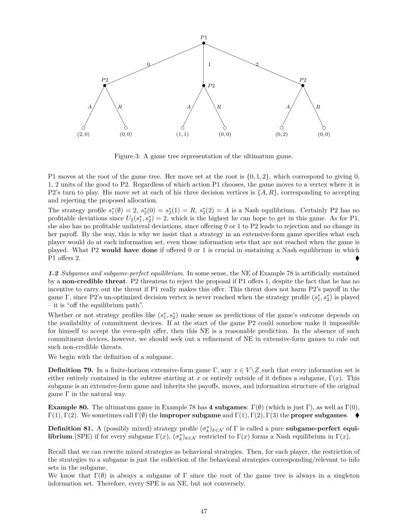
P1

P2

(2, 0)

A

(0, 0)

R

0

P2

(1, 1)

A

(0, 0)

R

1

P2

(0, 2)

A

(0, 0)

R

2

Figure 3: A game tree representation of the ultimatum game.

P1 moves at the root of the game tree. Her move set at the root is 0, 1, 2, which correspond to giving 0,1, 2 units of the good to P2. Regardless of which action P1 chooses, the game moves to a vertex where it isP2’s turn to play. His move set at each of his three decision vertices is A,R, corresponding to acceptingand rejecting the proposed allocation.The strategy profile s∗1(∅) = 2, s∗2(0) = s∗2(1) = R, s∗2(2) = A is a Nash equilibrium. Certainly P2 has noprofitable deviations since U2(s∗1, s∗2) = 2, which is the highest he can hope to get in this game. As for P1,she also has no profitable unilateral deviations, since offering 0 or 1 to P2 leads to rejection and no change inher payoff. By the way, this is why we insist that a strategy in an extensive-form game specifies what eachplayer would do at each information set, even those information sets that are not reached when the game isplayed. What P2 would have done if offered 0 or 1 is crucial in sustaining a Nash equilibrium in whichP1 offers 2.

1.2 Subgames and subgame-perfect equilibrium. In some sense, the NE of Example 78 is artificially sustainedby a non-credible threat. P2 threatens to reject the proposal if P1 offers 1, despite the fact that he has noincentive to carry out the threat if P1 really makes this offer. This threat does not harm P2’s payoff in thegame Γ, since P2’s un-optimized decision vertex is never reached when the strategy profile (s∗1, s∗2) is played– it is “off the equilibrium path”.Whether or not strategy profiles like (s∗1, s∗2) make sense as predictions of the game’s outcome depends onthe availability of commitment devices. If at the start of the game P2 could somehow make it impossiblefor himself to accept the even-split offer, then this NE is a reasonable prediction. In the absence of suchcommitment devices, however, we should seek out a refinement of NE in extensive-form games to rule outsuch non-credible threats.We begin with the definition of a subgame.

Definition 79. In a finite-horizon extensive-form game Γ, any x ∈ V \Z such that every information set iseither entirely contained in the subtree starting at x or entirely outside of it defines a subgame, Γ(x). Thissubgame is an extensive-form game and inherits the payoffs, moves, and information structure of the originalgame Γ in the natural way.

Example 80. The ultimatum game in Example 78 has 4 subgames: Γ(∅) (which is just Γ), as well as Γ(0),Γ(1), Γ(2). We sometimes call Γ(∅) the improper subgame and Γ(1),Γ(2),Γ(3) the proper subgames.

Definition 81. A (possibly mixed) strategy profile (σ∗k)k∈N of Γ is called a pure subgame-perfect equi-librium (SPE) if for every subgame Γ(x), (σ∗k)k∈N restricted to Γ(x) forms a Nash equilibrium in Γ(x).

Recall that we can rewrite mixed strategies as behavioral strategies. Then, for each player, the restriction ofthe strategies to a subgame is just the collection of the behavioral strategies corresponding/relevant to infosets in the subgame.We know that Γ(∅) is always a subgame of Γ since the root of the game tree is always in a singletoninformation set. Therefore, every SPE is an NE, but not conversely.

47

Example 82. The NE (s∗1, s∗2) from Example 78 is not an SPE, since (s∗1, s∗2) restricted to the subgame Γ(1)is not an NE. However, the following is an SPE: s1(∅) = 1, s2(0) = R, s2(1) = s2(2) = A. It is easy tosee that restricting (s1, s2) to each of the subgames Γ(0),Γ(1),Γ(2) forms an NE. Furthermore, (s1, s2) is aNE in Γ(∅) = Γ. P1 gets U1(s1, s2) = 1 under this strategy profile, while offering 0 leads to rejection and apayoff of 0, offering 2 leads to acceptance but again a payoff of 0. For P2, changing s2(0) and s2(2) do notchange payoff in Γ, since these two vertices are never reached. Changing s2(1) from A to R hurts payoff.

Finally, note the following immediate consequence of the definition of SPE: if an extensive form game has aSPE, then each subgame of it has a SPE as well.

1.3 Backwards induction. Backwards induction is an algorithm for finding an SPE in a finite-horizonextensive-form game of perfect information. The idea is to successively replace subgames with terminalvertices corresponding to SPE payoffs of the deleted subgames.Start with a non-terminal vertex furthest away from the root of the game, say v. Since we have picked thedeepest non-terminal vertex, all of J(v)’s moves at this vertex must lead to terminal vertices. Choose oneof J(v)’s moves, m∗, that maximizes her payoff in Γ(v), then replace the subgame Γ(v) with the terminalvertex corresponding to m∗. Repeat this procedure, working backwards from the vertices further away fromthe root of the game. Eventually, the game tree will be reduced to a single terminal vertex, whose payoffwill be an SPE payoff of the extensive-form game, while the moves chosen throughout the deletion processwill form a SPE strategy profile.

P1

P2

P1

(5, 3)

L

(0, 4)

R

L

P1

(0, 0)

L

(1, 4)

R

R

L

P2

P1

(2, 2)

L

(1, 3)

R

L

P1

(1, 4)

L

(3, 0)

R

R

R

Figure 4: A extensive-form game in the game tree representation.

48

P1

P2

(5, 3)

L

P1

(0, 0)

L

(1, 4)

R

R

L

P2

P1

(2, 2)

L

(1, 3)

R

L

P1

(1, 4)

L

(3, 0)

R

R

R

Figure 5: Backwards induction replaces subgames with terminal nodes associated with the SPE payoffs inthose subgames. Here is the resulting game tree after one step of backwards induction.

P1

P2

(5, 3)

L

(1, 4)

R

L

P2

(2, 2)

L

(3, 0)

R

R

Figure 6: Backwards induction in progress. All nodes at depth 3 in the original tree have been eliminated.

P1

(1, 4)

L

(2, 2)

R

Figure 7: Backwards induction in progress. Only nodes with depth 1 remain.

49

(2, 2)

Figure 8: Backwards induction finds the unique SPE payoff in this game.

If ui(z) 6= ui(z′) for every i and z, z′ ∈ Z with z 6= z′, then backwards induction finds the unique SPEof the extensive-form game. Otherwise, the game may have multiple SPEs and backwards induction mayinvolve choosing between several indifferent moves. Depending on the moves chosen during the tie-breaking,backwards induction may lead to different SPEs.

Example 83. (From MWG - this is a prelude to repeated games, which are covered later in the course)Consider a game in which the following simultaneous-move game is played twice. The players observe theactions chosen in the first period before they play in the second period. What are the pure SPNE of thisgame ?

b1 b2 b3

a1 10, 10 2, 12 0, 13a2 12, 2 5, 5 0, 0a3 13, 0 0, 0 1, 1

Solution. The pure NE of the one-shot game are (a2, b2) and (a3, b3). Thus any SPNE involves playingeither of these in the second period. We conjecture the following four classes of SPE:

1. Player 1 plays ai and player 2 plays bi in both periods, i ∈ 2, 3.

2. Player 1 plays ai in the first period and aj in the second period; player 2 plays bi in the first periodand bj in the second period, i, j ∈ 1, 2 and i 6= j.

3. Player 1’s strategy: play ai, i ∈ 1, 2, 3 in period 1; play a2 in period 2 if player 2 played b1 in period1, otherwise play b3.Player 2’s strategy: play b1 in period 1. Play b2 in period 2 if player 1 played ai in period 1, otherwiseplay b3.

4. Player 2’s strategy: play bi, i ∈ 1, 2, 3 in period 1; play b2 in period 2 if player 1 played b1 in period1, otherwise play b3.Player 1’s strategy: play a1 in period 1. Play a2 in period 2 if player 1 played bi in period 1, otherwiseplay a3.

To see that these are indeed SPNE, note that by deviating a player loses 4 in the second period (no dis-counting) and no player can gain more than 3 in any of the described strategy profiles. Equilibrium classes3 and 4 are implemented through ’punishment for deviations’.

Example 84. (From MWG) Consider a game with two players, player 1 and player 2, in which each playeri can choose an action from a finite set Mi that contains mi actions. Player i’s payoffs if the action choicesare (m1,m2) is given by φi(mi,m2). Suppose player 1 moves first and that player 2 can observe the moveof player 1 before choosing her move.(a) Suppose this game has multiple SPNEs. Show that if this is the case then there exists two pairs of moves(m1,m2) 6= (m′1,m′2) such that either

1. φ1(m1,m2) = φ1(m′1,m′2) or

2. φ1(m1,m2) = φ1(m′1,m′2).

(b) Suppose that for any two pairs (m1,m2) 6= (m′1,m′2) we have condition 2. in (a) is violated (i.e. player2 is never indifferent between pairs of moves). Suppose also that there exists a pure Nash equilibrium in thegame in which the two players play simultaneously and denote by π1 player’s 1 payoff in that Nash. Show

50

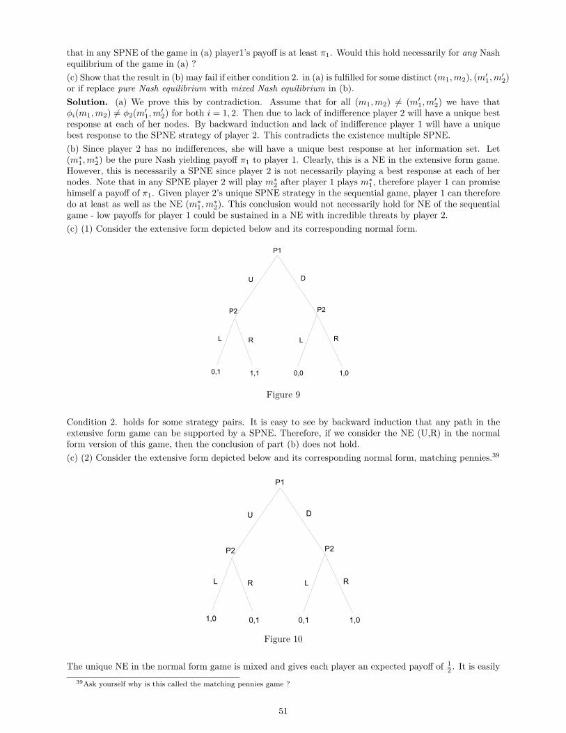
that in any SPNE of the game in (a) player1’s payoff is at least π1. Would this hold necessarily for any Nashequilibrium of the game in (a) ?(c) Show that the result in (b) may fail if either condition 2. in (a) is fulfilled for some distinct (m1,m2), (m′1,m′2)or if replace pure Nash equilibrium with mixed Nash equilibrium in (b).Solution. (a) We prove this by contradiction. Assume that for all (m1,m2) 6= (m′1,m′2) we have thatφi(m1,m2) 6= φ2(m′1,m′2) for both i = 1, 2. Then due to lack of indifference player 2 will have a unique bestresponse at each of her nodes. By backward induction and lack of indifference player 1 will have a uniquebest response to the SPNE strategy of player 2. This contradicts the existence multiple SPNE.(b) Since player 2 has no indifferences, she will have a unique best response at her information set. Let(m∗1,m∗2) be the pure Nash yielding payoff π1 to player 1. Clearly, this is a NE in the extensive form game.However, this is necessarily a SPNE since player 2 is not necessarily playing a best response at each of hernodes. Note that in any SPNE player 2 will play m∗2 after player 1 plays m∗1, therefore player 1 can promisehimself a payoff of π1. Given player 2’s unique SPNE strategy in the sequential game, player 1 can thereforedo at least as well as the NE (m∗1,m∗2). This conclusion would not necessarily hold for NE of the sequentialgame - low payoffs for player 1 could be sustained in a NE with incredible threats by player 2.(c) (1) Consider the extensive form depicted below and its corresponding normal form.

0,1 1,1 0,0 1,0

P1

P2P2

U D

RL L R

Figure 9

Condition 2. holds for some strategy pairs. It is easy to see by backward induction that any path in theextensive form game can be supported by a SPNE. Therefore, if we consider the NE (U,R) in the normalform version of this game, then the conclusion of part (b) does not hold.(c) (2) Consider the extensive form depicted below and its corresponding normal form, matching pennies.39

1,0 0,1 0,1 1,0

P1

P2P2

U D

RL L R

Figure 10

The unique NE in the normal form game is mixed and gives each player an expected payoff of 12 . It is easily

39Ask yourself why is this called the matching pennies game ?

51

seen, however, that the only two SPNE in the extensive form game are (U, (R,L)) and (L, (R,L)). Theygive to player 1 a payoff of 0.

2 Infinite-Horizon Games and One-Shot Deviation

2.1 Infinite-horizon games. So far, we have only dealt with finite-horizon games. These games are repre-sented by finite-depth game trees and must end within M turns for some M ∈ N. But games such as theRubinstein-Stahl bargaining are not finite horizon, for players could reject each other’s offers forever. Wemodify Definition 75 to accommodate such infinite-horizon games. For simplicity, we assume the game hasperfect information and no chance moves.Definition 85. An extensive-form game with perfect information and no chance moves has thefollowing components:

• A possibly infinite-depth tree with vertices V and terminal vertices Z ⊆ V .

• A set of players N = 1, 2, ..., N.

• A player function J : V \Z → N .

• A set of available moves Mj,v for each v ∈ J−1(j), j ∈ N . Each move in Mj,v is associated with aunique child of v in the tree.

• A (Bernoulli) utility function uj : Z ∪H∞ → R for each j ∈ N , where H∞ refers to the set of allinfinite length paths.

When an infinite-horizon game is played, it might end at a terminal vertex (such as when one player acceptsthe other’s offer in the bargaining game), or it might never reach a terminal vertex (such as whenboth players use a strategy involving never accepting any offer in the bargaining game). Therefore, eachplayer must have a preference not only over the set of terminal vertices, but also over the set of infinitehistories. In the bargaining game, for instance, it is specified that uj(h) = 0 for any h ∈ H∞, j = 1, 2, thatis to say every infinite history in the game tree (i.e. never reaching an agreement) gives 0 utility to eachplayer.Many definitions from finite-horizon extensive-form games directly translate into the infinite-horizon setting.For instance, any nonterminal vertex x in the perfect-information infinite-horizon game defines a subgameΓ(x). NE is defined in the obvious way, taking into account distribution over both terminal vertices andinfinite histories induced by a strategy profile. SPE is still defined as those strategy profiles that form anNE when restricted to each of Γ’s (possibly infinitely many) subgames.2.2 One-shot deviation principle. It is often difficult to verify directly from definition whether a givenstrategy profile forms an SPE in an infinite-horizon game. Indeed, given an SPE candidate (s∗k)k∈N of gameΓ, we would have to consider each subgame Γ(x), which is potentially an infinite-horizon extensive-formgame of its own right, and ask whether player i can improve her payoff in Γ(x) by choosing a differentextensive-form game strategy si, modifying some or all of her choices at various vertices in J−1(i) relativeto s∗i . This is not an easy task since i’s set of strategies in Γ(x) is a very rich set. The one-shot deviationprinciple says for extensive-form games satisfying certain regularity conditions, we need only check that idoes not have a profitable deviation amongst a very restricted set of strategies in each subgame Γ(x),namely those that differ from s∗i only at x.Theorem 86. (One-shot deviation principle) If Γ fulfills certain regularity requirements40, then a strategyprofile (s∗k)k∈N is an SPE of Γ iff for every player i, every subgame Γ(x) with J(x) = i, and every strategysi of Γ(x) such that s∗i (v) = si(v) at every v ∈ J−1(i) except possibly at v = x,

UΓ(x)i (s∗i , s∗−i) ≥ U

Γ(x)i (si, s∗−i),

where UΓ(x)i denotes the payoff of i in subgame Γ(x).

The regularity conditions required for the Theorem are satisfied by all finite-horizon extensive-form games, aswell as all infinite-horizon games studied in lecture, including bargaining and repeated games. Under theseconditions, to verify whether (s∗k)k∈N is an SPE we need only examine each subgame Γ(x) and considerwhether J(x) can improve her payoff in Γ(x) by changing her move only at x (a “one-shot deviation”).

40More details: if it is consistent and continuous at infinity.

52

3 Rubinstein-Stahl Bargaining

3.1 Bargaining as an extensive-form game. TheRubinstein-Stahl bargaining game, or simply “bargaininggame”41 for short, is an important example of infinite-horizon, perfect-information extensive-form game. Itis comparable to the ultimatum game from Example 78, but with two important differences: (i) the game isinfinite-horizon, so that first rejection does not end the game. Instead, players alternate in making offers;(ii) the good that players bargain over is assumed infinitely divisible, so that any allocation of the form(x, 1− x) for x ∈ [0, 1] is feasible.

Figure 11: Part of the bargaining game tree, showing only some of the branches in the first two periods.The root ∅ has (uncountably) infinitely many children of the form (x1, 1− x1) for x1 ∈ [0, 1]. At each suchchild, P2 may play R or A. Playing A leads to a terminal node with payoffs (x1, 1 − x1), while playing Rcontinues the game with P2 to make the next offer.

Let’s think about what a strategy in the bargaining game looks like. Figure 11 shows a sketch of thebargaining game tree. P1’s strategy specifies s1(∅), that is to say what P1 will offer at the start of thegame. For each x1 ∈ [0, 1], P2’s strategy specifies s2((x1, 1 − x1)) ∈ A,R, that is whether he accepts orrejects a period 1 offer of (x1, 1 − x1). In addition, P2’s strategy must also specify s2((x1, 1 − x1), R) foreach x1 ∈ [0, 1], that is what he offers in period t = 2 if he rejected P1’s offer in t = 1.42 This offer couldin principle depend on what P1 offered in period t = 1. Now for every x1, x2 ∈ [0, 1], P1’s strategy mustspecify s1((x1, 1− x1), R, (x2, 1− x2)) ∈ A,R, which could in principle depend on what she herself offeredin period t = 1, as well as what P2 offered in the current period, (x2, 1− x2).3.2Asymmetric bargaining power. Here is a modified version of the bargaining game that introduces asym-metric bargaining power between the two players.

Example 87. P1 gets to make offers in periods 3k + 1 and 3k + 2 for k ∈ N, while P2 gets to make offersin periods 3k + 3 for k ∈ N. As in the usual bargaining game, reaching an agreement of (x, 1− x) in periodt yields the payoff profile (δt−1 · x, δt−1 · (1− x)). If the players never reach an agreement, then payoffs are(0, 0).

Consider the following strategy profile: whenever P1 makes an offer in period 3k+1, she offers(

1+δ1+δ+δ2 ,

δ2

1+δ+δ2

).

Whenever P1 makes an offer in period 3k+ 2, she offers(

1+δ2

1+δ+δ2 ,δ

1+δ+δ2

). Whenever P2 makes an offer, he

offers(

δ+δ2

1+δ+δ2 ,1

1+δ+δ2

). Whenever P2 responds to an offer in period 3k + 1, he accepts iff he gets at least

δ2

1+δ+δ2 . Whenever P2 responds to an offer in period 3k+ 2, he accepts iff he gets at least δ1+δ+δ2 . Whenever

P1 responds to an offer, she accepts iff she gets at least δ+δ2

1+δ+δ2 . You may verify that this verbal description41Not to be confused with axiomatic Nash bargaining, which you will study in 2010b.42Remember, an extensive-form game strategy for j is a complete contingency plan that specifies a valid move at any vertex

in the game tree where it is j’s turn to play, even those vertices that would never be reached due to how j plays in previousrounds. Even if P2’s strategy specifies accepting every offer from P1 in t = 1, P2 still needs to specify what he would do aftera history of the form ((x1, 1− x1), R) for each x1 ∈ [0, 1].

53

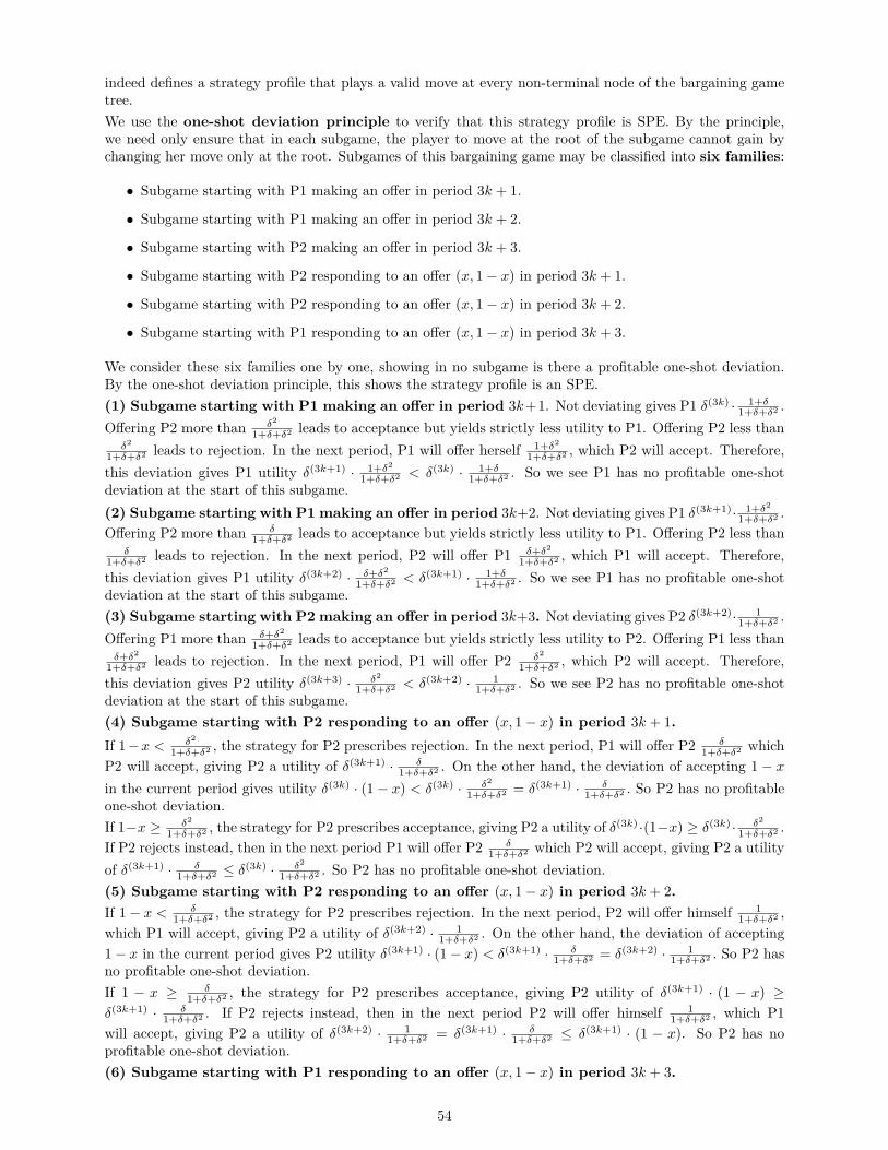
indeed defines a strategy profile that plays a valid move at every non-terminal node of the bargaining gametree.We use the one-shot deviation principle to verify that this strategy profile is SPE. By the principle,we need only ensure that in each subgame, the player to move at the root of the subgame cannot gain bychanging her move only at the root. Subgames of this bargaining game may be classified into six families:

• Subgame starting with P1 making an offer in period 3k + 1.

• Subgame starting with P1 making an offer in period 3k + 2.

• Subgame starting with P2 making an offer in period 3k + 3.

• Subgame starting with P2 responding to an offer (x, 1− x) in period 3k + 1.

• Subgame starting with P2 responding to an offer (x, 1− x) in period 3k + 2.

• Subgame starting with P1 responding to an offer (x, 1− x) in period 3k + 3.

We consider these six families one by one, showing in no subgame is there a profitable one-shot deviation.By the one-shot deviation principle, this shows the strategy profile is an SPE.(1) Subgame starting with P1 making an offer in period 3k+1. Not deviating gives P1 δ(3k) · 1+δ

1+δ+δ2 .Offering P2 more than δ2

1+δ+δ2 leads to acceptance but yields strictly less utility to P1. Offering P2 less thanδ2

1+δ+δ2 leads to rejection. In the next period, P1 will offer herself 1+δ2

1+δ+δ2 , which P2 will accept. Therefore,this deviation gives P1 utility δ(3k+1) · 1+δ2

1+δ+δ2 < δ(3k) · 1+δ1+δ+δ2 . So we see P1 has no profitable one-shot

deviation at the start of this subgame.(2) Subgame starting with P1 making an offer in period 3k+2. Not deviating gives P1 δ(3k+1)· 1+δ2

1+δ+δ2 .Offering P2 more than δ

1+δ+δ2 leads to acceptance but yields strictly less utility to P1. Offering P2 less thanδ

1+δ+δ2 leads to rejection. In the next period, P2 will offer P1 δ+δ2

1+δ+δ2 , which P1 will accept. Therefore,this deviation gives P1 utility δ(3k+2) · δ+δ2

1+δ+δ2 < δ(3k+1) · 1+δ1+δ+δ2 . So we see P1 has no profitable one-shot

deviation at the start of this subgame.(3) Subgame starting with P2 making an offer in period 3k+3. Not deviating gives P2 δ(3k+2)· 1

1+δ+δ2 .Offering P1 more than δ+δ2

1+δ+δ2 leads to acceptance but yields strictly less utility to P2. Offering P1 less thanδ+δ2

1+δ+δ2 leads to rejection. In the next period, P1 will offer P2 δ2

1+δ+δ2 , which P2 will accept. Therefore,this deviation gives P2 utility δ(3k+3) · δ2

1+δ+δ2 < δ(3k+2) · 11+δ+δ2 . So we see P2 has no profitable one-shot

deviation at the start of this subgame.(4) Subgame starting with P2 responding to an offer (x, 1− x) in period 3k + 1.If 1−x < δ2

1+δ+δ2 , the strategy for P2 prescribes rejection. In the next period, P1 will offer P2 δ1+δ+δ2 which

P2 will accept, giving P2 a utility of δ(3k+1) · δ1+δ+δ2 . On the other hand, the deviation of accepting 1 − x

in the current period gives utility δ(3k) · (1− x) < δ(3k) · δ2

1+δ+δ2 = δ(3k+1) · δ1+δ+δ2 . So P2 has no profitable

one-shot deviation.If 1−x ≥ δ2

1+δ+δ2 , the strategy for P2 prescribes acceptance, giving P2 a utility of δ(3k) ·(1−x) ≥ δ(3k) · δ2

1+δ+δ2 .If P2 rejects instead, then in the next period P1 will offer P2 δ

1+δ+δ2 which P2 will accept, giving P2 a utilityof δ(3k+1) · δ

1+δ+δ2 ≤ δ(3k) · δ2

1+δ+δ2 . So P2 has no profitable one-shot deviation.(5) Subgame starting with P2 responding to an offer (x, 1− x) in period 3k + 2.If 1− x < δ

1+δ+δ2 , the strategy for P2 prescribes rejection. In the next period, P2 will offer himself 11+δ+δ2 ,

which P1 will accept, giving P2 a utility of δ(3k+2) · 11+δ+δ2 . On the other hand, the deviation of accepting

1− x in the current period gives P2 utility δ(3k+1) · (1− x) < δ(3k+1) · δ1+δ+δ2 = δ(3k+2) · 1

1+δ+δ2 . So P2 hasno profitable one-shot deviation.If 1 − x ≥ δ

1+δ+δ2 , the strategy for P2 prescribes acceptance, giving P2 utility of δ(3k+1) · (1 − x) ≥δ(3k+1) · δ

1+δ+δ2 . If P2 rejects instead, then in the next period P2 will offer himself 11+δ+δ2 , which P1

will accept, giving P2 a utility of δ(3k+2) · 11+δ+δ2 = δ(3k+1) · δ

1+δ+δ2 ≤ δ(3k+1) · (1 − x). So P2 has noprofitable one-shot deviation.(6) Subgame starting with P1 responding to an offer (x, 1− x) in period 3k + 3.

54

If x < δ+δ2

1+δ+δ2 , the strategy for P1 prescribes rejection. In the next period, P1 will offer herself 1+δ1+δ+δ2 , which

P2 will accept, giving P1 a utility of δ(3k+3) · 1+δ1+δ+δ2 . On the other hand, the deviation of accepting x in

the current period gives P1 utility δ(3k+2) · (x) < δ(3k+2) · δ+δ2

1+δ+δ2 = δ(3k+3) · 1+δ1+δ+δ2 . So P1 has no profitable

one-shot deviation.If x ≥ δ+δ2

1+δ+δ2 , the strategy for P1 prescribes acceptance, giving P1 utility of δ(3k+2) · (x) ≥ δ(3k+3) · 1+δ1+δ+δ2 .

If P1 rejects instead, then in the next period P1 will offer herself 1+δ1+δ+δ2 , which P2 will accept, giving P1 a

utility of δ(3k+3) · 1+δ1+δ+δ2 ≤ δ(3k+2) · (x). So P1 has no profitable one-shot deviation.

Along the equilibrium path, P1 offers(

1+δ1+δ+δ2 ,

δ2

1+δ+δ2

)in t = 1 and P2 accepts. This is a better outcome

for P1 than in the symmetric bargaining game where P1 gets 11+δ . P1’s SPE payoff improves when she has

more bargaining power.One can also show, that the payoffs of this SPE are the unique SPE payoffs of the game (see solutions toPSet 3). The proof idea is to consider three bargaining games: Γ1, Γ2 and Γ3. Γ1 is the barganining gameexhibited in the statement of the problem. Γ2 is the bargaining game, where P1 makes an offer in periodone, P2 makes an offer in period two and if P1 rejects the bargaining game Γ1 is played. Γ3 is the bargaininggame where P2 makes the first offer in period one and if P1 rejects the bargaining game Γ1 is played. Thegame in the statement of the problem is then just the repetition of these types of bargaining subgames:Γ1,Γ2,Γ3,Γ1,Γ2,Γ3, . . .One defines then minimal, maximal SPE payoffs for both players and all three types of bargaining gamesand uses an analysis similar to lecture to find necessary inequalities these minimal, maximal SPE payoffshave to satisfy. Ultimately, one arrives at ’enough’ inequalities so that a combination of them gives a tightcharacterization showing that the minimal and maximal SPE payoffs for both players are equal to the payoffsin the SPE considered in this Example.

4 Introduction to Repeated Games

1.1 What is a repeated game? Many of the normal-form and extensive-form games studied so far can beviewed as models of one-time encounters. After players finish playing Rubinstein-Stahl bargaining orhigh-bid auction, they part ways and never interact again. In many economic situations, however, a group ofplayers may play the same game again and again over a long period of time. For instance, a customermight approach a printing shop every month with a major printing job. While the printing shop has anincentive to shirk and produce low-quality output in a one-shot version of this interaction, in a long-runrelationship the shop might never shirk as to avoid losing the customer in the future. In general, repeatedgames study what outcomes can arise in such repeated interactions.Formally speaking, repeated games (with perfect monitoring43) form an important class of examples withinextensive-form games with finite - or infinite - horizon, depending on the length of repetition.

Definition 88. For a normal-form game44 G = 〈N , (Ak)k∈N , (uk)k∈N 〉 and a positive integer T , denoteby G(T ) the extensive-form game where G is played in every period for T periods and players observe theaction profiles from all previous periods. G is called the stage game and G(T ) the (T -times) repeatedgame. Terminal vertices of G(T ) are of the form (a1, a2, ..., aT ) ∈

(×Nk=1Ak

)T =: AT and payoff to playeri at such a terminal vertex is

∑Tt=1 ui(at). A pure strategy for player i maps each non-terminal history of

action profiles to a stage game action, si : ∪T−1k=0A

k → Ai.

Definition 89. For a normal form game G = 〈N , (Ak)k∈N , (uk)k∈N 〉 and a δ ∈ [0, 1), denote by Gδ(∞)the extensive-form game where G is played in every period for infinitely many periods and players act likeexponential discounters with discount rate δ. This is called the (infinitely) repeated game with discountrate δ. An infinite history of the form (a1, a2, ..., ) ∈ A∞ gives player i the payoff

∑∞t=1 δ

t−1ui(at). A purestrategy for player i maps each finite history of action profiles to a stage game action, si : ∪∞k=0A

k → Ai.

A strategy for player i in G(T ) or Gδ(∞) must specify a valid action of the stage game G after any non-terminal history (a1, ..., ak) ∈ Ak, including those histories that would never be reached under i’s strategy.

43That is to say, actions taken in previous periods are common knowledge. There exists a rich literature on repeated gameswith coarser monitoring structures – for instance, all players observe an imperfect public signal of each period’s action profile,or each player privately observes such a signal – and folk theorems in these generalized settings have been proved as well.

44When discussing repeated games, we use Ai (for “actions”) to denote i’s pure strategies in the stage game G as to avoidconfusion with i’s pure strategies in the repeated game G(T ), which we write as Si.

55

For example, even if P1’s strategy in repeated prisoner’s dilemma is to always play defect, she still needs tospecify s1((C,C), (C,C)), that is what she will play in period 3 if both players cooperated in the first twoperiods.As defined above, our treatment of repeated games focuses on the the simplest case where payoffs in periodt are independent of actions taken in all previous periods. This rules out, for instance, investmentgames where players choose a level of contribution every period and the utility in period t depends on thesum of all accumulated capital up to period t.When discussing repeated games, we are often interested in the “average” stage game payoff under a repeatedgame strategy profile. The following definitions are just normalizations: they ensure that if i gets payoff cin every period, then she is said to have an average payoff of c.

Definition 90. In G(T ), the average payoff to i at a terminal vertex a = (a1, a2, ..., aT ) ∈ AT is U(a) =1T

∑Tt=1 ui(at). In Gδ(∞), the (discounted) average payoff to i at the infinite history a = (a1, a2, ...) ∈ A∞

is U(a) = (1− δ) ·∑∞t=1 δ

t−1ui(at).

1.2 Some immediate results. We first require some additional definitions.

Definition 91. Given a normal-form game G, the set of feasible payoffs is defined as co(u(a) : a ∈ A) ⊆RN , where co is the convex hull operator.

These are the payoffs that can be obtained if players use a public randomization device to correlate theiractions. Specifically, as every v ∈ co(u(a) : a ∈ A) can be written as a weighted average v =

∑rk=1 pk ·u(ak)

where pk ≥ 0,∑rk=1 pk = 1 and ak ∈ A for each k, one can construct a correlated strategy profile where all

players observe a public random variable that realizes to k with probability pk, then player i plays aki uponobserving k. The expected payoff profile under this correlated strategy profile is v.This public randomization device will be used in the construction of the equilibrium in two ways.First, to realize specific feasible payoffs in certain periods as described above.45 That agents will follow theprescriptions of the public randomization device, follows from the optimization property of the equilibrium(i.e. the incentives are given by the continuation play encoded in the equilibrium strategies).Second, to construct SPEs, which have as payoffs a mixture of the payoffs from two (or more) SPEs. Anillustrative example is as follows: imagine that we have two SPE profiles, a(1), a(2) which give SPE payoffprofiles U(a(1)), U(a(2)). Then, given λ ∈ (0, 1), agents can achieve the SPE payoff profile λU(a(1)) + (1 −λ)U(a(2)) by using the public randomization device and replicating a toss of a biased coin (probability headsof λ) at time t = 0 before play starts: if heads, then play the SPE a(1), otherwise play a(2). This is again aSPE, albeit now constructed by public randomization, because no matter what the public outcome of thecoin, the agents will follow its prescription due to the SPE property of a(1), a(2).

Definition 92. In a normal-form game G, player i’s minimax payoff is defined as

vi := minα−i∈∆(A−i)

maxai∈Ai

ui(ai, α−i)

Call a payoff profile v ∈ RN individually rational if vi ≥ vi for every i ∈ N . Call v strictly individuallyrational if vi > vi for every i ∈ N .

Two technical remarks which you can skip:(1) The outer minimization in minimax payoff is across the set of correlated strategy profiles of −i. Asdemonstrated in the coordination game with an eavesdropper (Example 37), the correlated minimax payoffof a player could be strictly lower than her independent minimax payoff (when opponents in −i playindependently mixed actions). This distinction is not very important for this course, as we will almostalways consider two-player stage games when studying repeated games, so that the set of “correlated”strategy profiles of −i is just the set of mixed strategies of −i.(2) We claimed to have described repeated games with perfect monitoring in Definitions 89 and 90, butthe monitoring structure as written was less than perfect. Players only observe past actions and cannotalways detect deviations from mixed strategies or correlated strategies, so in particular they donot know for sure if everyone is faithfully playing a correlated minimax strategy profile against i. (Evenwhen there are only 2 players, the minimax strategy against P1 might be a purely mixed strategy of P2. By

45For example on equilibrium path, but not only.

56

observing only past actions, P1 does not know if P2 is really randomizing with the correct probabilities.)To remedy this problem, we can assume that every coalition (including singleton coalitions) observes acorrelating signal at the start of every period, which they use to implement correlated strategies and mixedstrategies. Furthermore, the realizations of such correlating signals become publicly known at the end ofeach period, so that even correlated strategies and mixed strategies are “observable”. This remark is againnot very important for this course, for the minimax action profile turns out to be pure in most stage gameswe examine. In addition, Fudenberg and Maskin showed that their 1986 folk theorem continues to hold,albeit with a modified proof, even when players only observe past actions and not the realizations of pastcorrelating devices.The following two results are now immediate.

Proposition 93. Suppose (s∗k)k∈N is an NE for G(T ) or Gδ(∞). Then the average payoff profile associatedwith (s∗k)k∈N is feasible and individually rational for the stage game G.

Proof. Evidently, the payoff profile in every period of the repeated game must be in co(u(a) : a ∈ A). InG(T ), the average payoff profile under (s∗k)k∈N is the simple average of T such points, while in Gδ(∞) it is aweighted average of countably many such points, so in both cases the average payoff profile must still be inco(u(a) : a ∈ A) by the convexity of this set. Suppose now player i’s average payoff is strictly less than vi.Then consider a new repeated game strategy si for i, where si(h) best responds to the (possibly correlated)action profile s∗−i(h) after every non-terminal history h. Then playing si guarantees i at least vi in everyperiod, so that his average payoff will be at least vi. This would contradict the optimality of s∗i in the NE(sk)k∈N .

Proposition 94. If G has a unique NE, then for any finite horizon T the repeated game G(T ) has a uniqueSPE. In this SPE, players play the unique stage game NE after every non-terminal history.

Proof. Let (s∗k)k∈N be a SPE of G(T ). For any history hT−1 of length T − 1, (s∗k(hT−1)) must be the uniqueNE of G. Else, some player must have a strictly profitable deviation in the subgame starting at hT−1. So wededuce (s∗k)k∈N plays the unique NE of G in period T regardless of what happened in previous periods. Butthis means (s∗k(hT−2)) must also be the unique NE of G for any history hT−2 of length T − 2. Otherwise,consider the subgame starting at hT−2. If (s∗k(hT−2)) does not form an NE, some player i can improve herpayoff in the current period by changing s∗i (hT−2), and furthermore this change does not affect her payoffin future periods, since we have argued the unique NE of G will be played in period T regardless of whathappened earlier in the repeated game. So we have found a strictly profitable deviation for i in the subgame,contradicting the fact that (s∗k)k∈N is an SPE. Hence, we have shown (s∗k)k∈N plays the unique NE of Gin the last two periods of G(T ), regardless of what happened earlier. Continuing this argument with theprevious periods shows the unique NE of G is played after any non-terminal history.

5 Folk Theorem for Infinitely Repeated Games

2.1 The folk theorem for infinitely repeated games under perfect monitoring. It is natural to ask what payoffprofiles can arise in Gδ(∞). Write E(Gδ(∞)) for the set of average payoff profiles attainable in SPEs ofGδ(∞). Since every SPE is an NE, in view of Proposition 93, the most we could hope for are results of thefollowing form: “limδ→1 E(Gδ(∞)) equals the set of feasible, individually rational payoffs of G.” Theoremsalong this line are usually called “folk theorems”, for such results were widely believed and formed part ofthe economic folklore long before anyone obtained a formal proof.It is important to remember that folk theorems are not merely efficiency results. They are more correctlycharacterized as “anything-goes results”. Not only do they say that there exist SPEs with payoff profilesclose to the Pareto frontier, but they also say there exist other SPEs with payoff profiles close to players’minimax payoffs.The following is a folk theorem for infinitely repeated games with perfect monitoring.

Theorem 95. (Fudenberg and Maskin 1986 [6]) Write V ∗ for the set of feasible, strictly individually rationalpayoff profiles of G. Assume G has full dimensionality. For any v∗ ∈ V ∗, there corresponds a δ ∈ (0, 1) sothat v∗ ∈ E(Gδ(∞)) for all δ ∈ (δ, 1).

Proof. See lecture.

57

2.2 Rewarding minimaxers. The proof of Theorem 95 is constructive and explicitly defines an SPE withaverage payoff v∗. To ensure subgame-perfection, the construction must ensure that −i have an incentiveto minimax i in the event that i deviates. It is possible that the minimax action against i hurts some otherplayer j 6= i so much that j would prefer to be minimaxed instead of minimaxing i. The solution, as we sawin lecture, is to promise a reward of ε > 0 in all future periods to players who successfully carry outtheir roles as minimaxers.46 This way, at a history that calls for players to minimax i, deviating from theminimax action loses an infinite stream of ε payoffs. As players become more patient, this infinite stream ofstrictly positive payoffs matters far more than the utility cost from finitely many periods of minimaxing i.

46The strategy profile used in Fudenberg and Maskin (1986) is often called the “stick and carrot strategy”. If a player deviatesduring the normal phase, the deviator is hit with a “stick” for finitely many periods. Then, all the other players are given a“carrot” in all subsequent periods for having carried out this sanction.

58

Economics 2010a . Section 7 : Repeated Games (continued) + Refinements ofNE 11/24/2018∣∣∣∣ (1) Folk theorem, infinitely repeated: 2-players; (2) Folk theorem, finitely repeated; (3) Refinements of

NE in extensive- and normal-form games; (4) Signaling games∣∣∣∣

TF: Jetlir Duraj (duraj@g.harvard.edu)Sometimes, no complicated rewards schemes as in the general Folk Theorem are necessary. This is the casewhen minimaxing i is not particularly costly for her opponents, as the following example demonstrates.

Example 96. (December 2012 Final Exam) Consider an infinitely repeated game with the following sym-metric stage game.

L C R

T -4,-4 12,-8 3,1M -8,12 8,8 5,0B 1,3 0,5 4,4

Construct a pure strategy profile of the repeated game with the following properties: (i) the strategy profileis an SPE of the repeated game for all δ close enough to 1; (ii) the average payoffs are (8, 8); (iii) in everysubgame, both players’ payoffs are nonnegative in each period.Solution: We quickly verify that each player’s pure minimax payoff (i.e. when minimaxers are restrictedto using pure strategies; this will only relax the minmax constraint for payoffs) is 1. P1 minimaxes P2 withT , who best responds with R, leading to the payoff profile (3, 1). Symmetrically, P2 minimaxes P1 with L,who best responds with B, giving us the payoff profile (1, 3). So, (8, 8) is feasible and strictly individuallyrational, even when restricting attention to pure strategies.However, we cannot directly recite the Fudenberg-Maskin SPE, for their construction uses a public random-ization device in several places – for instance to give the ε > 0 reward to minmiaxers – but the question asksfor a pure strategy profile. Even if we are allowed to use public randomizations, we still face the additionalrestriction that we cannot let any player get a negative payoff in any period, even off-equilibrium. If wepublicly randomize over some action profiles, then we are restricted to those action profiles in the lower rightcorner of the payoff matrix in all subgames.Perhaps the easiest solution is to build a simpler SPE and forget about giving the ε > 0 reward tominimaxers altogether. This is possible because for this particular stage game, the minimaxer gets utility 3while the minimaxee gets utility 1, so it is better to minimax than to get minimaxed. Consider an SPE givenby three phases: in normal phase, play (M,C); in minimax P1 phase, play (B,L); in minimax P2phase, play (T,R). If player i deviates during normal phase, go to minimax Pi phase. If player j deviatesduring minimax Pi phase, go to minimax Pj phase, where possibly j = i. If minimax Pi phase completeswithout deviations, go to normal phase.We verify this strategy profile is an SPE for δ near enough 1 using one-shot deviation principle. Due tosymmetry, it suffices to verify P1 has no profitable one-shot deviation in any subgame. For any subgame innormal phase, deviating gives at most47

12 + δ · 1 + δ2

1− δ · 8 (16)

while not deviating gives

8 + δ · 8 + δ2

1− δ · 8 (17)

47Recall that for δ ∈ [0, 1),• 1 + δ + δ2 + ... = 1

1−δ

• 1 + δ + δ2 + ...+ δT = 1−δT+1

1−δ

59

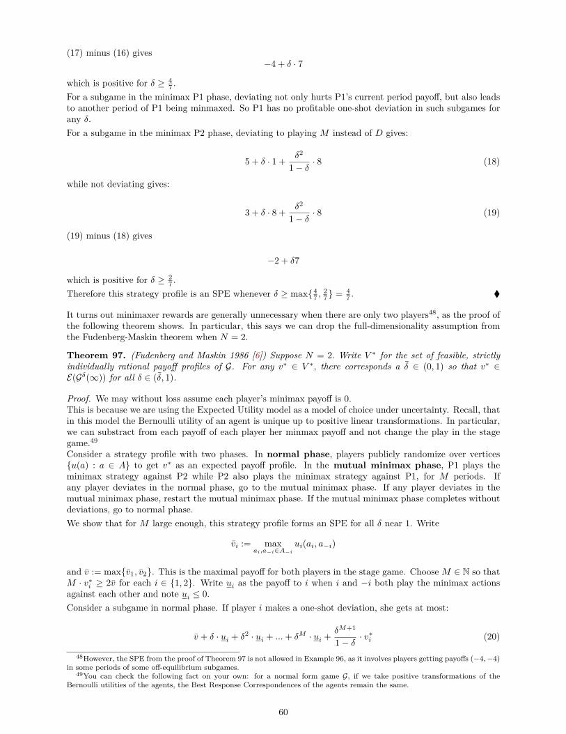
(17) minus (16) gives−4 + δ · 7

which is positive for δ ≥ 47 .

For a subgame in the minimax P1 phase, deviating not only hurts P1’s current period payoff, but also leadsto another period of P1 being minmaxed. So P1 has no profitable one-shot deviation in such subgames forany δ.For a subgame in the minimax P2 phase, deviating to playing M instead of D gives:

5 + δ · 1 + δ2

1− δ · 8 (18)

while not deviating gives:

3 + δ · 8 + δ2

1− δ · 8 (19)

(19) minus (18) gives

−2 + δ7

which is positive for δ ≥ 27 .

Therefore this strategy profile is an SPE whenever δ ≥ max 47 ,

27 = 4

7 .

It turns out minimaxer rewards are generally unnecessary when there are only two players48, as the proof ofthe following theorem shows. In particular, this says we can drop the full-dimensionality assumption fromthe Fudenberg-Maskin theorem when N = 2.

Theorem 97. (Fudenberg and Maskin 1986 [6]) Suppose N = 2. Write V ∗ for the set of feasible, strictlyindividually rational payoff profiles of G. For any v∗ ∈ V ∗, there corresponds a δ ∈ (0, 1) so that v∗ ∈E(Gδ(∞)) for all δ ∈ (δ, 1).

Proof. We may without loss assume each player’s minimax payoff is 0.This is because we are using the Expected Utility model as a model of choice under uncertainty. Recall, thatin this model the Bernoulli utility of an agent is unique up to positive linear transformations. In particular,we can substract from each payoff of each player her minmax payoff and not change the play in the stagegame.49

Consider a strategy profile with two phases. In normal phase, players publicly randomize over verticesu(a) : a ∈ A to get v∗ as an expected payoff profile. In the mutual minimax phase, P1 plays theminimax strategy against P2 while P2 also plays the minimax strategy against P1, for M periods. Ifany player deviates in the normal phase, go to the mutual minimax phase. If any player deviates in themutual minimax phase, restart the mutual minimax phase. If the mutual minimax phase completes withoutdeviations, go to normal phase.We show that for M large enough, this strategy profile forms an SPE for all δ near 1. Write

vi := maxai,a−i∈A−i

ui(ai, a−i)

and v := maxv1, v2. This is the maximal payoff for both players in the stage game. Choose M ∈ N so thatM · v∗i ≥ 2v for each i ∈ 1, 2. Write ui as the payoff to i when i and −i both play the minimax actionsagainst each other and note ui ≤ 0.Consider a subgame in normal phase. If player i makes a one-shot deviation, she gets at most:

v + δ · ui + δ2 · ui + ...+ δM · ui + δM+1

1− δ · v∗i (20)

48However, the SPE from the proof of Theorem 97 is not allowed in Example 96, as it involves players getting payoffs (−4,−4)in some periods of some off-equilibrium subgames.

49You can check the following fact on your own: for a normal form game G, if we take positive transformations of theBernoulli utilities of the agents, the Best Response Correspondences of the agents remain the same.

60

while conforming gives:

v∗i + δ · v∗i + δ2 · v∗i + ...+ δM · v∗i + δM+1

1− δ · v∗i (21)

(21) minus (20) gives:

v∗i − v + (δ + ...+ δM ) · (v∗i − ui) ≥ −v + (δ + ...+ δM ) · (v∗i )

where we used v∗i > 0, ui ≤ 0. But for δ close to 1, δ+...+δM ≥M/2, hence implying −v+(δ+...+δM )·(v∗i ) ≥0 by choice of M . So for δ ≥ δ, there are no profitable one-shot deviations in normal phase.Consider a subgame in the first period of the mutual minimax phase. If player i deviates, she gets at most:

0 + δ · ui + δ2 · ui + ...+ δM · ui + δM+1

1− δ · v∗i (22)

where −i playing the minimax strategy against i implies her payoff in the period of deviation is bounded by0. On the other hand, conforming gives:

ui + δ · ui + δ2 · ui + ...+ δM · v∗i + δM+1

1− δ · v∗i (23)

(23) minus (22) gives:

(1− δM ) · ui + δM · v∗i

But ui ≤ 0 while v∗i > 0, so for δ sufficiently close to 1 this expression is positive. This shows i does nothave a profitable one-shot deviation in the first period of the mutual minimax phase. A fortiori, she cannothave a profitable one-shot deviation in later periods of the mutual minimax phase either.

Example 98 (From Old Problem Sets of Jerry Green). Consider the infinitely repeated game whose stagegame is as below and whose common discount factor is 1

2 .

A D

A 2,3 1,5D 0,1 0,1

Show that ((A,A), (A,A), . . . ) cannot be sustained in any subgame perfect equilibrium path.

Solution. On the equilibrium path player 1 gets on average 2 and player 2 gets 3. Player 1 cannot gain byany deviation since she already gets her highest feasible payoff.Moreover, since A dominates D in the stage game, it is easy to see that there cannot be any subgame whereplayer 1 plays D for all eternity (call this Claim (!)).We need to check the incentives of player 2. For this we can use the one-shot deviation principle. The mostprofitable one-shot deviation of player 2 is to D and it gives a current gain of 2. The heaviest punishmentfor the deviation is minmaxing the player 2 forever after the deviation which gives a per-period loss of -2.Due to the discount factor being 1

2 , the deviation to D in a single period, followed by the punishment of‘minmax forever’ gives a utility difference of

(1− 12)(+2) + 1

2(−2) = 0.

Any weaker punishment (in terms of giving a higher continuation payoff) would cause player 2 to deviate.But since the strongest punishment of ‘minmax forever’ requires player 1 to play D for eternity after adeviation, we arrive at a contradiction to the previous claim (!).

Example 99 (Final Exam December 2016). Consider the three player game given by the following twotables (player 3 chooses the matrix).

61

a3 a2 b2

a1 2,2,2 1,1,1b1 1,1,1 1,1,1

b3 a2 b2

a1 1,1,1 1,1,1b1 1,1,1 2,2,2

What is the set of payoff triplets that can arise as average equilibrium payoffs of the infinitely repeated gamewith discount factor δ when δ is close to 1? Justify your answer.

Solution. Note that the version of the Folk Theorem from lecture doesn’t help here, because the set offeasible payoffs is one-dimensional and there are three players. This set is equal to the segment connectingN1 = (2, 2, 2) and N2 = (1, 1, 1). The solution presented here doesn’t need the assumption that mixedstrategies are observable.Note, that (2, 2, 2) is a Nash-payoff of the stage game and so automatically attainable as a SPE payoff,irrespective of the discount factor.Denote by α the lowest SPE payoff of a player (from symmetry this is the same for all players). Take aprofile of SPE strategies (a′1, a′2, a′3) which imply the payoff profile (α, α, α) in the repeated game. Giventhe probabilities (p1, p2, p3) of the players playing their respective first actions in the stage game in the firstperiod that are prescribed by (a′1, a′2, a′3) a player can deviate and get at least 5

4 .For example, if p2, p3 ≥ 1

2 , then P1 could play p1 = 1 to get at least

2 · p2 · p3 + 1 · (1− p2p3) = 1 + p2p3 ≥ 1 + 12 ·

12 = 5

4 .

The calculation is similar for the cases p2, 1 − p3 ≥ 12 , 1 − p2, p3 ≥ 1

2 and 1 − p2, 1 − p3 ≥ 12 . There is no

deviation from (a′1, a′2, a′3) only if the deviation of one of the players which assures her at least 54 , followed

by play of (a′1, a′2, a′3) from period 2 on is strictly better than playing (a′1, a′2, a′3). Thus it should hold

α ≥ (1− δ)54 + δα.

This is equivalent to α ≥ 54 . Now note that ( 5

4 ,54 ,

54 ) is an SPE payoff. This is because this payoff profile is

attained in the stage game by playing the mixed Nash where each player mixes with probabilities 12 between

her two strategies and infinite repetition of this Nash profile is a SPE.Recall, that the set of SPE payoffs has to be a subset of the set of feasible payoffs, which is the straight linebetween (2, 2, 2) and (1, 1, 1). Also, due to available public randomization the set of SPE payoffs is a convexset. In all, we have that the set of possible SPE payoffs is the straight line between ( 5

4 ,54 ,

54 ) and (2, 2, 2),

both vertices included.

1 Folk Theorem for Finitely Repeated Games

In view of Proposition 94, the stage game G must have multiple NEs for G(T ) to admit more than one SPE.The following result is not the most general one, but it shows how one can use the multiplicity of NEs in thestage game to incentivize cooperative behavior for most of the T periods.

Proposition 100. Suppose G has a pair of NEs a(i) and a(i) for each player i ∈ N such that ui(a(i)) >ui(a(i)). Write di := maxai,ai∈Ai,a−i∈A−i ui(ai, a−i)− ui(ai, a−i) for an upperbound on deviation utility to iin the stage game and set Mi ∈ N with Mi · (ui(a(i))−ui(a(i))) ≥ di. For any feasible payoff profile v∗ wherev∗i ≥ ui(a(i)) for each i and T ≥

∑k∈N Mk, there exists an SPE of G(T ) where the average payoff for all

except the last∑k∈N Mk periods is v∗.

Unlike an infinitely repeated game, a finitely repeated game “unravels” because some NE must be playedin the last period. However, if G has multiple NEs, then conditioning which NEs get played in the lastfew periods of G(T ) on players’ behavior in the early periods of the repeated game provides incentives forcooperation. This is the main intuition behind this and similar results in the literature for finitely repeatedgames.

Proof. Consider the following strategy profile. In the first T −∑k∈N Mk periods, if no one has deviated so

far, publicly randomize so that expected payoff profile is v∗. If some players have deviated and player i wasthe first to deviate, then play a(i). In the last

∑k∈N Mk periods, if no one deviated in the first T−

∑k∈N Mk

62

periods, then play a(1) for M1 periods, followed by a(2) for M2 periods, ..., finally a(N) for MN periods. Ifsomeone deviated in the first T −

∑k∈N Mk periods and i was the first to deviate, then do the same as

before except play a(i) for Mi periods instead of a(i).

We use the one-shot deviation principle to argue this strategy profile forms an SPE. At a subgame startingin the first T −

∑k∈N Mk periods without prior deviations, suppose i deviates. Compared with conforming

to the SPE strategy, i gains at most di in the current period, but gets weakly worse payoffs for the remainderof these first T −

∑k∈N Mk periods as v∗i ≥ ui(a(i)). In addition, i loses at least di across Mi periods in

the last∑k∈N Mk periods of the game by choice of Mi. Therefore, i does not have a profitable one-shot

deviation.At a subgame starting in the first T −

∑k∈N Mk periods with prior deviation, the SPE specifies playing

some NE action profile of the stage game. Deviation can only hurt current period payoff with no effect onthe payoffs of any future priods. Similarly for subgames starting in the last

∑k∈N Mk periods.

Example 101. (December 2013 Final Exam) Suppose the following game is repeated T times and eachplayer maximizes the sum of her payoffs in these T plays. Show that, for every ε > 0, we can choose T bigenough so that there exists an SPE of the repeated game in which each player’s average payoff is within ε of2.

A B C

A 2,2 -1,3 0,0B 3,-1 1,1 0,0C 0,0 0,0 0,0

Solution: For given ε > 0, choose large enough T such that 2(T−1)+1T > 2 − ε. Consider the following

strategy profile: in period t < T , play A if (A,A) has been played in all previous periods, else play C. Inperiod T , play B if (A,A) has been played in all previous periods, else play C. At a history in period t < Twhere (A,A) has been played in all previous periods, a one-shot deviation at most gains 1 in the currentperiod but loses 2 in each of periods t + 1, t + 2, ...T − 1, and finally loses 1 in period T . At a history inperiod t < T with prior deviation, one-shot deviation hurts current period payoff and does not change futurepayoffs. At a history in period T , clearly there is no profitable one-shot deviation as this is the last periodof the repeated game and the strategy profile prescribes playing a Nash equilibrium of the stage game.

2 Refinements of NE in Extensive- and Normal-Form Games

1.1 Four refinements. In lecture we studied four refinements of NE for extensive-form games: perfectBayesian equilibrium (PBE), sequential equilibrium (SE), trembling-hand perfect equilibrium (THPE), andstrategically stable equilibrium (SSE). Whereas specifying an NE or SPE just requires writing down a profileof strategies, PBE and SE are defined in terms of not only a strategy profile, but also a belief system –that is, a distribution πj(·|Ij) over the vertices in information set Ij for each information set of each playerj. They differ in terms of some consistency conditions they impose on the belief system.

Definition 102. A perfect Bayesian equilibrium (PBE) is a behavioral strategy profile (pj)j∈N togetherwith a belief system (πj(·|Ij))j∈N ,Ij∈Ij so that:

• pj(Ij) maximizes expected payoffs starting from information set Ij according to belief πj(·|Ij), for eachj ∈ N , Ij ∈ Ij

• beliefs are derived from Bayes’ rule at all on-path information sets (an information set is called on-pathif it is reached with strictly positive probability under (pj)j∈N . Else, it is called off-path.)

If an information set Ij is reached with strictly positive probability under (pj)j∈N , then the conditionalprobability of having reached each vertex v ∈ Ij given that Ij is reached is well-defined. This is πj(v|Ij). Onthe other hand, we cannot use Bayes’ rule to compute the conditional probability of reaching various verticesin an off-path information set, as we would be dividing by 0. As such, PBE places no restrictions onthese off-equilibrium beliefs. In particular, one could use this additional ’degree of freedom’ to construct

63

PBE by picking off-path beliefs as needed to support on-path play. As we saw in the lecture, this can be a’weakness’ of the solution concept when analyzing certain games.When checking Definition 102 one should not forget to check the first requirement for players whose infor-mation sets are all singletons. These players don’t need to form beliefs, so for them the second requirementof PBE is vacuous, but given the strategy of the other players they should not have a unilateral deviation.This is the only implication of the first requirement of PBE for these kinds of players.

Definition 103. A sequential equilibrium (SE) is a behavioral strategy profile (pj)j∈N together with abelief system (πj(·|Ij))j∈N ,Ij∈Ij so that:

• pj(Ij) maximizes expected payoffs starting from information set Ij according to belief πj(·|Ij), for eachj ∈ N , Ij ∈ Ij .

• there exists a sequence of strictly mixed behavioral strategies (p(m)j )j so that limm→∞(p(m)

j )j = (pj)j ,and furthermore limm→∞(π(m)

j )j = (πj)j , where (π(m)j )j is the unique belief system consistent with

(p(m)j )j .

Though it is not part of the definition, it is easy to show that in an SE, all on-path beliefs are given byBayes’ rule, just as in PBE.Compared to PBE, SE places some additional restrictions on off-equilibrium beliefs. Instead ofallowing them to be completely arbitrary, SE insists that these off-equilibrium beliefs must be attainableas the limiting beliefs of a sequence of strictly mixed strategy profiles that converge to (pj)j∈N – hencethe name sequential equilibrium. Given a strictly mixed (p(m)

j )j∈N , every information set is reached withstrictly positive probability. Therefore, the belief system (π(m)

j )j∈N is well-defined, as there exists exactlyone such system consistent with the behavioral strategies (p(m)

j )j∈N under Bayes’ rule.

Importantly, there are no assumptions of rationality/optimization on the sequence of strategies (p(m)j )j .

It is merely a device used to justify how the belief system (πj)j might arise. In particular, there is norequirement that (p(m)

j )j forms any kind of equilibrium under beliefs (π(m)j )j .

There is one special case where a PBE is automatically a SE.

Proposition. If a PBE is so, that all non-singleton information sets of all players are on the equilibriumpath of the PBE, then that PBE is a SE.

Proof sketch. Any information set on equilibrium path is reached with positive probability. Therefore,Bayes rule is applicable and there is for each player i and information set Ii of i a unique belief πi(·|Ii) aboutthe location of player i in info set Ii. Moreover, since Bayes rule is continuous in probabilities wheneverit is applicable, it follows that there will exist a sequence of small perturbations of the PBE strategies, ofthe completely mixed type, converging to the PBE strategy, such that Bayes rule remains applicable alongthe perturbed sequence and the belief systems induced by the perturbation sequence converge to the beliefsystem of the PBE. Since no information sets are outside of the equilibrium path, there will be no degree offreedom in choosing beliefs off-paths (they never occur!). This shows that the PBE is in fact a SE.

Relatedly, there is a case where Nash equilibria are automatically SE. The logic of the proof is similar toabove and left as an exercise.50

Proposition. In an extensive form game let (pj)j∈N be a completely mixed Nash equilibrium in behavioralstrategies. Let (πj(·|Ij))j∈N ,Ij∈Ij be the belief system derived from (pj)j∈N through Bayes’ rule at eachinformation set. Then the pair

((pj)j∈N , (πj(·|Ij))j∈N ,Ij∈Ij

)is a SE of the extensive form game.

The next two equilibrium concepts, THPE and SSE, are defined in terms of trembles. A tremble ε in anextensive-form game associates a small, positive probability to each move in each information set, interpretedas the minimum weight that any strategy must assign to all valid moves. The strategy profile (pj , p−j) issaid to be an ε−equilibrium if at each information set Ij and with respect to belief πj(·|Ij), pj maximizesj’s expected utility subject to the constraint of minimum weights from the tremble ε.

50Or you can ask me in the OHs.

64

Definition 104. A trembling-hand perfect equilibrium (THPE) is a behavioral strategy profile(pj)j∈N so that there exists a sequence of trembles ε(m) converging to 0 and a sequence of strictly mixedbehavioral strategies (p(m)

j )j , such that (p(m)j )j is an ε(m)-equilibrium and limm→∞(p(m)

j )j = (pj)j .

Definition 105. A strategically stable equilibrium (SSE) is a behavioral strategy profile (pj)j∈N sothat for every sequence of trembles ε(m) converging to 0, there exists a sequence of strictly mixed behavioralstrategies (p(m)

j )j such that (p(m)j )j is an ε(m)-equilibrium and limm→∞(p(m)

j )j = (pj)j .

THPE and SSE are also defined for normal-form games, where the tremble ε specifies minimum weights forthe different actions of various players.The following table summarizes some of the key comparisons between these four equilibrium concepts.

belief at on-path info. set belief at off-path info. set robustness to trembles

PBE determined by Bayes’ rule no restriction noneSE determined by Bayes’ rule limit of beliefs associated with

strictly mixed profilesnone

THPE N/A N/A robust to one sequence oftrembles

SSE N/A N/A robust to any sequence oftrembles

A useful result concerning THPE is the following.Proposition. Every Nash equilibrium in completely mixed strategies in a finite normal form game is aTHPE.

Proof. Let σ be a completely mixed Nash equilibrium of the game G = (N , (Si)i∈N , (ui)i∈N ) and let

c = mini∈N ,si∈Si

σi(si) > 0.

c is strictly positive by the requirement in the statement.Take a sequence of perturbations ε(m),m ∈ N going to zero.51 It follows that there is M ∈ N s.t. allcomponents of all ε(m),m ≥ M are strictly below c. But this means that σ is a feasible strategy profile inthe restricted game where the minimal probability put to any pure strategy of any player is at least as largeas the lowest component found in the perturbation ε(m),m ≥M . Modify the perturbation by letting it startin m ≥M , cutting off the previous finite string of perturbations. Since σ, being Nash in the original game,consists of mutually best responses in the unrestricted game, it is also a mixed ε(m)-equilibrium, i.e. a Nashequilibrium of the restricted game. Defining thus p(m) = σ,m ≥M we have that this trivially converges andtherefore all requirements of Definition of THPE for σ are fulfilled.

Another very useful result you can easily prove on your own is the following.Proposition. In every THPE, every weakly dominated strategy is chosen with probability zero.Finally here are some other useful facts:

Fact 106. For extensive-form game Γ, the following inclusions52 hold:

NE(Γ) ⊇PBE(Γ)SPE(Γ)

⊇ SE(Γ) ⊇ THPE(Γ) ⊇ SSE(Γ)

There is no inclusion relationship between PBE(Γ) and SPE(Γ).

Fact 107. For a finite extensive-form game Γ, THPE(Γ) 6= ∅, though it is possible that SSE(Γ) = ∅.51Note that this is a sequence of vectors.52Inclusion in terms of strategy profiles. Technically, NE does not belong to the same universe as PBE, SE, etc., as these

latter objects require a belief system in addition to a strategy profile.

65

P1

(0, 2)

Out

Chance

P2

(1, 1)

A

(−1,−1)

F

(−9,−9)

FF

good (50%)

P2

(1, 1)

A

(−1, 2)

F

(−9,−9)

FF

bad (50%)

In

Figure 12: A modified market entry game.

That is, there is always at least one THPE in a finite extensive-form game (but it may be in behavioralstrategies, not pure strategies). The immediate implication is that SE, SPE, PBE, and NE are also non-emptyequilibrium concepts in finite games.1.2 Some examples. We illustrate these refinement concepts through two examples. The first example showsan extensive-form game where we have strict inclusions NE(Γ) ) PBE(Γ) ) SE(Γ).

Example 108. Consider the following modification to the entry game. The entrant (P1) chooses whetherto stay out or enter the market. If she enters, nature then determines whether her product is good or bad,each with 50% probability. Incumbent (P2) observes entry decision, but not whether the product is good orbad. If entrant enters, the incumbent can choose (A) to allow entry, (F) to f ight, or (FF) to f ight f iercely.This extensive game is depicted in Figure 12. Let’s write I for P2’s information set and abbreviate strategiesin the obvious way (eg. (Out, F) is the strategy profile where P1 plays Out, P2 plays F) rather than writingthem out in formal notations. Restrict attention to pure equilibria.What are the pure NEs of this game?

• It is easy to see that (Out, F), (Out, FF) are NEs. P2’s action has no effect on his payoff, since P1never enters. P1 does not have a profitable deviation either, as playing In gets an expected utility of-1 if P2 is playing F, -9 if P2 is playing FF.

• In addition, (In, A) is also an NE. P2 does not have a profitable deviation to F, since doing so yieldsan expected payoff of 0.5 · (−1) + 0.5 · (2) = 0.75. P2 does not have a profitable deviation to FF, sincedoing so yields an expected payoff of -9.

What are the pure PBEs of this game?

• These must form a subset of pure NEs.

• There cannot be a PBE with strategy profile (Out, FF). No matter what off-equilibrium belief P2holds, he will find it strictly better to play A rather than FF.

• However, for any belief π2(bad|I) ≥ 23 , ((Out, F), π2(·|I)) forms a PBE.53 Recall that P2 is allowed to

hold arbitrary beliefs at I since this information set is off-path under strategy profile (Out, F).53This PBE is not an SPE since the strategy profile does not form an NE when restricted to the subgame starting with the

chance move. Recall in lecture we saw an example of an SPE that is not a PBE. This shows neither the set of SPEs nor the setof PBEs nests the other one.

66

• In addition, ((In, A), π2(bad|I) = 0.5) is another PBE. In fact, this is the only PBE featuring strategyprofile (In, A), since the information set I is on-path for this strategy profile and so π2(·|I) must bederived from Bayes’ rule.

What are the pure SEs of this game?

• These must form a subset of pure PBEs.

• There is no SE of the form ((Out, F), π2(·|I)). This is because, in every strictly mixed behavioralstrategy profile (p(m)

i ), the information set I is reached with strictly positive probability, meaningBayes’ rule requires π(m)

2 (bad|I) = 0.5. But SE requires that limm→∞ π(m)2 (bad|I) = π2(bad|I), so we

see in any SE of this form we must have π2(bad|I) = 12 .

• We finally check that ((In, A), π2(bad|I) = 0.5) is an SE.54 It is straightforward to verify that actionsmaximize expected payoff at each information set given belief in ((In, A), π2(bad|I) = 0.5). Now,consider a sequence of strictly mixed behavioral strategy profiles (p(m)

i ) where in the m-th profile,P1 plays Out with probability 1

m , plays In with probability 1 − 1m , P2 plays each of F and FF with

probability 12m and plays A with probability 1 − 1

m . It is easy to see that limm→∞(p(m)i ) = (In, A).

Furthermore, for each such profile, π(m)2 (bad|I) = 0.5, so we get limm→∞ π

(m)2 (·|I) = π2(·|I).

The second example is from a general exam and concerns PBEs.

Example 109 (General Exam Spring 2009 (difficult)). 1. Consider the following two-period game betweena supervisor and a worker. In period t = 1, 2 the worker has type θt = 1 with probability 0.9 and θ = 0 withprobability 0.1; θ1 and θ2 are independent. Each period, the worker observes θt, and then decides whetherto pay a cost j > 0 to prevent the supervisor from observing θt. If the worker pays the cost, the supervisorcannot make the report. If the worker does not pay the cost, the supervisor observes θt and then decideswhether or not to report it to the firm. The supervisor is either a ‘normal’ type or a ‘silent’ type who isunable to report. The supervisor’s type is the same in both periods; the prior probability that the supervisoris silent is s, where s < 1− j. The normal type of the supervisor and the worker both try to maximize theexpected value of the sum of their period-by-period payoffs, which are given in the following table, wherethe row player is the worker and the column player is the supervisor.

Report Don′tReport

Pay θt − j, 0 θt − j, 0Don′tpay 0, wt θt, 0

Assume 0 < w1 < 0.9w2 and (1− j)2 < s.

1. Is there a pure-strategy perfect Bayesian equilibrium in which the worker never pays in the first period,and the normal supervisor reports the agent when the first period type is θ1 = 1 ?

2. Is there a pure-strategy perfect Bayesian equilibrium in which the worker never pays in the first period,and the normal supervisor never reports in the first period ?

3. Is there a pure-strategy perfect Bayesian equilibrium in which the worker never pays in the first period,and the supervisor reports with some probability strictly between 0 and 1(whenever he can make thereport)? Hint: When there is such a PBE, what can you say about the probability with which a θ2 = 1worker pays in the second period following first period outcome of (don’t report, don’t pay) ?

Solution: Before solving the respective parts note the following facts:54This does not follow from the non-emptiness of SE as an equilibrium concept, since we have restricted attention to pure

equilibria. The game could have a unique mixed SE but no pure SE.

67

• If not paid costs in second period, normal supervisor will report.

• If θ2 = 1 and worker knows supervisor is normal, he’ll pay costs.

• If θt = 0 worker never pays costs.

1. Given the strategy of the normal supervisor, upon observing θ1 = 1 and observing report in t = 1, workerknows that supervisor is normal and so worker of type θ2 = 1 will pay cost in second period. Thus normalsupervisor’s payoff after seeing θ1 = 1, given the strategies, is 0.1ω2 in second period. By pretending to be asilent type in t = 1 after seeing θ1 though, normal supervisor gets 0 that period and w2 in the second period(since upon not observing a report in t = 1 worker of any type in t = 2 thinks he’s facing a silent supervisor).Since ω1 + 0.1ω2 < ω2 we have a profitable deviation.2. If no info is revealed in first period of the supervisor type, then in second period payoff of θ2 = 1 workerfrom not paying costs is s · 1 + 0, which is smaller than the payoff from paying costs: 1− j. It follows θ2 = 1worker will pay costs. With play in t = 2 fixed, in t = 1, given play of normal supervisor, worker of typeθ1 = 1 also doesn’t pay.Now consider the normal supervisor. He currently only has expected payoff of 0.1ω2. But this is always thecase, no matter the action in t = 1 so the normal supervisor has an incentive to report in t = 1 as well.3. Yes. Suppose the normal supervisor doesn’t report in t = 1 with probability p ∈ (0, 1). Let q be theprobability that θ2 = 1 worker in t = 2 doesn’t pay following history (don’t pay, don’t report). Normalsupervisor needs to satisfy

ω1 + 0.1ω2 = 0.91ω2 + 0.1ω2.

LHS is payoff from reporting in t = 1, RHS is payoff from not reporting in t = 1 for normal supervisor.It follows q = ω1

0.9ω2∈ (0, 1). This needs worker of type θ2 = 1 to be indifferent betweeen paying costs or

not. Formally:1− j = s

s+ (1− s)p .

LHS is payoff from paying costs, RHS is payoff from not paying costs: in this case, normal supervisor willreport. Note from here: p = 1, 0 yields contradictions to the parametric assumptions.This implies

p = sj

(1− j)(1− s) . (24)

Since s < 1− j, we have p ∈ (0, 1).Finally, need to check that θ1 = 1 doesn’t want to pay costs in period one as conjectured. If he does pay, hedoesn’t learn and then payoff is (1− j) + 0.9(1− j) (because in t = 2 the θ2 = 1 worker will pay costs dueto s < 1− j). If he doesn’t pay costs, then payoff in period one is (1− s)p+ s, which is the probability thathe’s not reported. In period 2, there are two cases: either he was reported, which happens with probability(1− s)(1− p), in which case his second period payoff is 0.9(1− j), or he wasn’t, in which case, from above,we have the payoff 0.9(1 − j) again (we are located after the history (don’t pay, don’t report)). In all, thepayoff of not paying costs is

((1− s)p+ s)(1 + 0.9(1− j)) + (1− p)(1− s)0.9(1− j) = ((1− s)p+ s) + 0.9(1− j)

This has to be larger than (1− j)(1 + 0.9). By replacing for the found p from (24), this holds if and only if

s

1− j > 1− j.

This is precisely the parametric assumption s > (1− j)2.

The third example comes from MWG.

Example 110. (from MWG) A buyer and a seller are bargaining. The seller owns an object for which thebuyer has value v (the seller’s value is zero). v is known to the buyer but not to the seller. The value’s priordistribution is common knowledge. There are two periods of bargaining. The seller makes a take-it-or-leaveit offer (i.e. names a price) at the start of each period that the buyer might accept or reject. The gameends when an offer is accepted or after two periods, whichever comes first. Both players discount period 2

68

payoffs by δ ∈ (0, 1). Assume throughout that the buyer always accepts the offer whenever she is indifferentbetween accepting and rejecting.(a) Characterize the pure strategy PBE for the case in which v takes vL, vH with vH > vL > 0 and whereλ = Prob(vH).(b) Do the same for the case in which v is distributed uniformly over [v, v].Solution. (a) For given values of λ, δ we look at two separate cases.Case 1. λ[(1− δ)vH + δvL] + (1− λ)δvL ≥ vL. In this case the seller will demand a price (1− δ)vH + δvLin the first period and vL in the second period. A buyer of type L will buy the good if the price is at mostvL. A buyer of type H will buy the good in the first period if the price is at most (1 − δ)vH + δvL and inthe second period if the price is at most vH .To show that these strategies constitute an equilibrium suppose the high type buyer deviates and does notbuy in the first period. Then he will buy the good in the second period and obtain a payoff of δ(vH − vL).Buying in the first period gives her a payoff of vH − (1− δ)vH − δvL = δ(vH − vL). Thus she is indifferent.A buyer of type L does not benefit by deviating and accepting in the first period, since she would obtaina negative payoff. The seller will not benefit by demanding a higher price in the first period since nobodywill buy at that price (both types will then buy in the second period). Suppose he offers a lower price.If this price is higher than vL then only the higher type buyer will buy and the seller obtains a lowerprice without increasing the trade volume. Suppose he offers the good for vL. Then both types will buythe good and the seller will make a profit of vL. If he uses the above strategy he will make a profit ofλ[(1− δ)vH + δvL] + (1− λ)δvL = vL. Therefore he will not deviate.Case 2. λ[(1 − δ)vH + δvL] + (1 − λ)δvL < vL. In this case the seller will offer the good for vL in bothperiods and both types will buy the good in period one.Both types of buyers cannot profit from deviation, given the strategies of the seller, since they obtain thegood for the lowest price compatible with profit maximization. The analysis in Case 1 shows that the sellerwill not deviate with the assumption of Case 2.

(b) Suppose in equilibrium the seller offers the good for price x in the first period and y in the second period.Clearly x, y ∈ [v, v]. Then there exists a unique type v∗ who is indifferent between buying in the first andsecond period. It is defined by the relation v∗ − x = δ(v∗ − y). Rewritten this is

v∗(x, y) = x− δy1− δ .

Under the condition that all types v ≥ v∗ will buy the good in period one, in equilibrium y must be so thatit maximizes second period profits. These are

y · Prob(v ≥ y|v < v∗) = y ·(

1− y − vv∗ − v

)= y(v∗ − y)

v∗.

The FOC implies the optimum y = v∗

2 . Plugging this into the expression for v∗ we get

v∗(x) = x

1− δ2.

These expressions imply that if the seller charges x in the first period he will charge x2−δ in the second period,

all buyers of type v ≥ v∗ = x1− δ2

will buy in the first period, and all types with x1− δ2

≥ v ≥ x2−δ will buy in

the second period (while the rest is excluded from trade). The seller’s profit will thus be for a fixed x

Π =[v − x

1− δ2

]· x+ δ · x

2− δ

[x

1− δ2− x

2− δ

]=[v − x

1− δ2

]· x+ δ

[x

2− δ

]2

We find the optimal selling price for the first period by maximizing w.r.t. x. This yields x = v(2−δ)2

8−6δ .Plugging in the formula for y we get y = v(2−δ)

8−6δ .

The fourth example illustrates THPE and SSE in a normal-form game.

Example 111. (December 2013 Final Exam) In Example 28, we considered the normal-form game

69

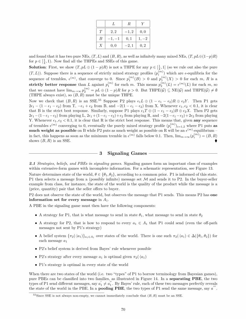
L R Y

T 2, 2 −1, 2 0, 0B −1,−1 0, 1 1,−2X 0, 0 −2, 1 0, 2

and found that it has two pure NEs, (T, L) and (B,R), as well as infinitely many mixed NEs, (T, pL⊕(1−p)R)for p ∈ [ 1

4 , 1). Now find all the THPEs and SSEs of this game.Solution: First, we show (T, pL⊕ (1− p)R) is not a THPE for any p ∈ [ 1

4 , 1] (so we rule out also the pure(T, L)). Suppose there is a sequence of strictly mixed strategy profiles (p(m)

i ) which are ε-equilibria for thesequence of trembles, ε(m), that converge to 0. Since p(m)

1 (B) > 0 and p(m)1 (X) > 0 for each m, R is a

strictly better response than L against p(m)1 for each m. This means p(m)

2 (L) = ε(m)(L) for each m, sothat we cannot have limm→∞ p

(m)2 = pL ⊕ (1 − p)R for p > 0. But THPE(G) ⊆ NE(G) and THPE(G) 6= ∅

(THPE always exist), so (B,R) must be the unique THPE.Now we check that (B,R) is an SSE.55 Suppose P2 plays ε1L ⊕ (1 − ε1 − ε2)R ⊕ ε2Y . Then P1 gets2ε1 − (1− ε1 − ε2) from T, −ε1 + ε2 from B, and −2(1− ε1 − ε2) from X. Whenever ε1, ε2 < 0.1, it is clearthat B is the strict best response. Similarly, suppose P1 plays ε1T ⊕ (1 − ε1 − ε2)B ⊕ ε2X. Then P2 gets2ε1−(1−ε1−ε2) from playing L, 2ε1 +(1−ε1−ε2)+ε2 from playing R, and −2(1−ε1−ε2)+2ε2 from playingY. Whenever ε1, ε2 < 0.1, it is clear that R is the strict best response. This means that, given any sequenceof trembles ε(m) converging to 0, eventually the purely mixed strategy profile (p(m)

i )i=1,2 where P1 puts asmuch weight as possible on B while P2 puts as much weight as possible on R will be an ε(m)-equilibrium –in fact, this happens as soon as the minimum tremble in ε(m) falls below 0.1. Then, limm→∞(p(m)

i ) = (B,R)shows (B,R) is an SSE.

3 Signaling Games

2.1 Strategies, beliefs, and PBEs in signaling games. Signaling games form an important class of exampleswithin extensive-form games with incomplete information. For a schematic representation, see Figure 13.Nature determines state of the world, θ ∈ θ1, θ2, according to a common prior. P1 is informed of this state.P1 then selects a message from a (possibly infinite) message setM and sends it to P2. In the buyer-sellerexample from class, for instance, the state of the world is the quality of the product while the message is a(price, quantity) pair that the seller offers to buyer.P2 does not observe the state of the world, but observes the message that P1 sends. This means P2 has oneinformation set for every message in A1.A PBE in the signaling game must then have the following components:

• A strategy for P1, that is what message to send in state θ1, what message to send in state θ2

• A strategy for P2, that is how to respond to every a1 ∈ A1 that P1 could send (even the off-pathmessages not sent by P1’s strategy)

• A belief system π2(·|a1)a1∈A1 over states of the world. There is one such π2(·|a1) ∈ ∆(θ1, θ2) foreach message a1

• P2’s belief system is derived from Bayes’ rule whenever possible

• P2’s strategy after every message a1 is optimal given π2(·|a1)

• P1’s strategy is optimal in every state of the world

When there are two states of the world (i.e. two “types” of P1 to borrow terminology from Bayesian games),pure PBEs can be classified into two families, as illustrated in Figure 14. In a separating PBE, the twotypes of P1 send different messages, say a′1 6= a

′′

1 . By Bayes’ rule, each of these two messages perfectly revealsthe state of the world in the PBE. In a pooling PBE, the two types of P1 send the same message, say a′′′ .

55Since SSE is not always non-empty, we cannot immediately conclude that (B,R) must be an SSE.

70

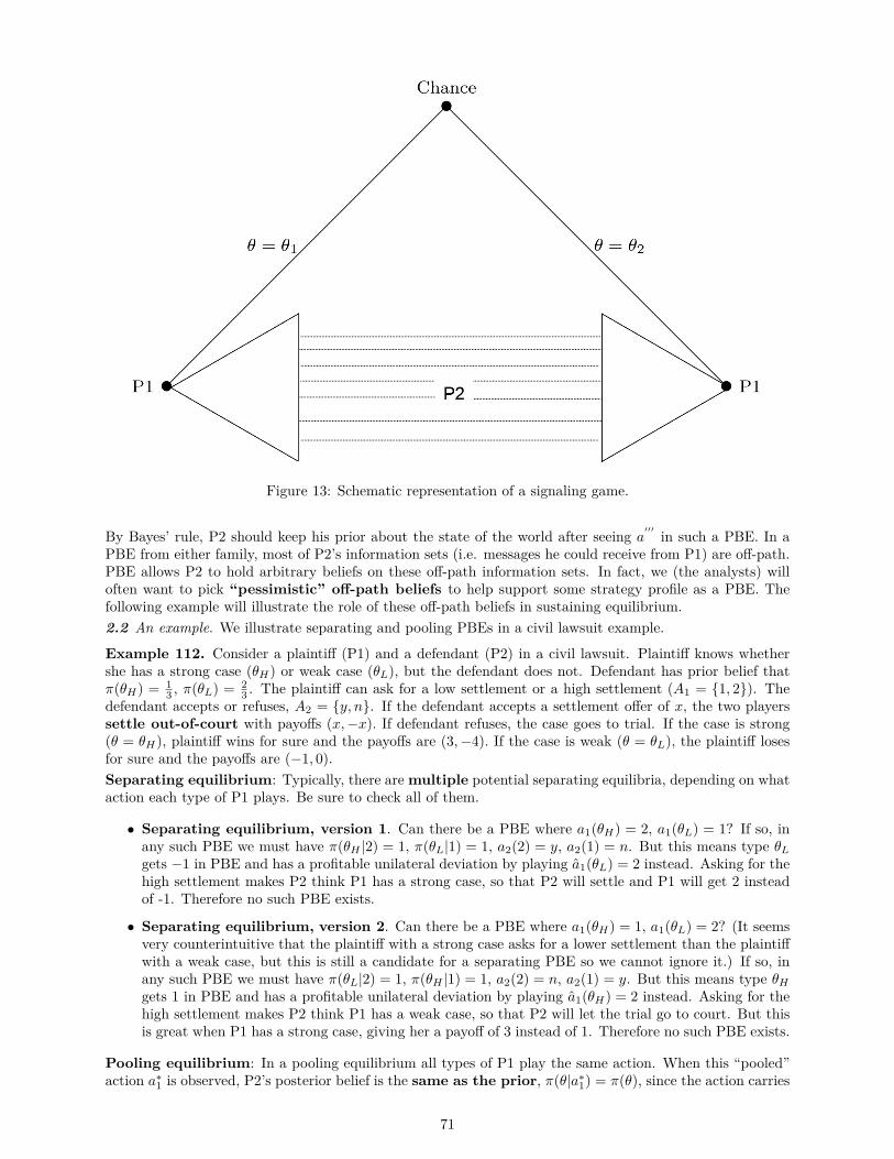
Figure 13: Schematic representation of a signaling game.

By Bayes’ rule, P2 should keep his prior about the state of the world after seeing a′′′ in such a PBE. In aPBE from either family, most of P2’s information sets (i.e. messages he could receive from P1) are off-path.PBE allows P2 to hold arbitrary beliefs on these off-path information sets. In fact, we (the analysts) willoften want to pick “pessimistic” off-path beliefs to help support some strategy profile as a PBE. Thefollowing example will illustrate the role of these off-path beliefs in sustaining equilibrium.2.2 An example. We illustrate separating and pooling PBEs in a civil lawsuit example.

Example 112. Consider a plaintiff (P1) and a defendant (P2) in a civil lawsuit. Plaintiff knows whethershe has a strong case (θH) or weak case (θL), but the defendant does not. Defendant has prior belief thatπ(θH) = 1

3 , π(θL) = 23 . The plaintiff can ask for a low settlement or a high settlement (A1 = 1, 2). The

defendant accepts or refuses, A2 = y, n. If the defendant accepts a settlement offer of x, the two playerssettle out-of-court with payoffs (x,−x). If defendant refuses, the case goes to trial. If the case is strong(θ = θH), plaintiff wins for sure and the payoffs are (3,−4). If the case is weak (θ = θL), the plaintiff losesfor sure and the payoffs are (−1, 0).Separating equilibrium: Typically, there aremultiple potential separating equilibria, depending on whataction each type of P1 plays. Be sure to check all of them.

• Separating equilibrium, version 1. Can there be a PBE where a1(θH) = 2, a1(θL) = 1? If so, inany such PBE we must have π(θH |2) = 1, π(θL|1) = 1, a2(2) = y, a2(1) = n. But this means type θLgets −1 in PBE and has a profitable unilateral deviation by playing a1(θL) = 2 instead. Asking for thehigh settlement makes P2 think P1 has a strong case, so that P2 will settle and P1 will get 2 insteadof -1. Therefore no such PBE exists.

• Separating equilibrium, version 2. Can there be a PBE where a1(θH) = 1, a1(θL) = 2? (It seemsvery counterintuitive that the plaintiff with a strong case asks for a lower settlement than the plaintiffwith a weak case, but this is still a candidate for a separating PBE so we cannot ignore it.) If so, inany such PBE we must have π(θL|2) = 1, π(θH |1) = 1, a2(2) = n, a2(1) = y. But this means type θHgets 1 in PBE and has a profitable unilateral deviation by playing a1(θH) = 2 instead. Asking for thehigh settlement makes P2 think P1 has a weak case, so that P2 will let the trial go to court. But thisis great when P1 has a strong case, giving her a payoff of 3 instead of 1. Therefore no such PBE exists.

Pooling equilibrium: In a pooling equilibrium all types of P1 play the same action. When this “pooled”action a∗1 is observed, P2’s posterior belief is the same as the prior, π(θ|a∗1) = π(θ), since the action carries

71

Figure 14: Schematic representations of separating and pooling PBEs.

72

no additional information about P1’s type. When any other action is observed (i.e. an off-equilibrium actionis observed), PBE allows P2’s belief to be arbitrary. Every member of A1 could serve as a pooled action,so we need to check for all of them systematically.

• Pooling on low settlement. Can there be a PBE where a1(θH) = a1(θL) = 1? If so, in anysuch PBE we must have π(θH |1) = 1

3 . Under this posterior belief, P2’s expected payoff to a2 = n is13 (−4) + 2

3 (0) = − 43 , while playing a2 = y always yields −1. Therefore in any such PBE we must have

a2(1) = y. But then the θH type of P1 has a profitable unilateral deviation of a1(θH) = 2, regardlessof what a2(2) is! If a2(2) = y, that is P2 accepts the high settlement, then type θH P1’s deviationgives her a payoff of 2 rather than 1. If a2(2) = n, that is P2 refuses the high settlement, then this iseven better for the type θH P1 as she will get a payoff of 3 when the case goes to court. Therefore nosuch PBE exists.

• Pooling on high settlement. Can there be a PBE where a1(θH) = a1(θL) = 2? If so, in anysuch PBE we must have π(θH |2) = 1

3 . Under this posterior belief, P2’s expected payoff to a2 = n is13 (−4) + 2

3 (0) = − 43 , while playing a2 = y always yields −2. Therefore in any such PBE we must have

a2(2) = n. In order to prevent a deviation by type θL, we must ensure a2(1) = n as well. Else, if P2accepts the low settlement offer, θL would have a profitable deviation where offering the low settlementinstead of following the pooling action of high settlement yields her a payoff of 1 instead of -1. Butwhether a2(1) = n is optimal for P2 depends on the belief, π(θH |1). Fortunately, this is an off-equilibrium belief and PBE allows such beliefs to be arbitrary. Suppose π(θH |1) = λ ∈ [0, 1]. ThenP2’s expected payoff to playing a2(1) = n is λ(−4) + (1 − λ)(0) = −4λ, while deviating to a2(1) = yyields −1 for sure. Therefore to ensure P2 does not have a profitable deviation at the information setof seeing a low settlement offer, we need λ ≤ 1

4 . If P2’s off-equilibrium belief is that P1 has a strongcase with probability less than 1

4 upon seeing a low-settlement offer, then it is optimal for P2 to rejectsuch low-settlement offers and θL will not have a profitable deviation. At the same time, since P2rejects all offers, the strong type θH of P1 does not have a profitable deviation either, since whicheveroffer she makes the case will go to court. In summary, there is a family of pooling equilibria wherea1(θH) = a1(θL) = 2, a2(1) = a2(2) = n, π(θH |2) = 1

3 , π(θH |1) = λ where λ ∈ [0, 14 ]. Crucially, it is

the judicious choice of off-equilibrium belief π(·|1) that sustains an action of a2(1) = n, which inturn sustains the pooling equilibrium.

All of these pooling PBEs also satisfy the intuitive criterion. Recall that:

Definition 113. Say a PBE (a1(θ), a2(a1)), π2(·|a1) satisfies Intuitive Criterion if there do not exist(a1, a2, θ) such that:(C1) a1 /∈ (a1(θ1), a1(θ2))(C2) u1(a1, a2, θ) > u1(a1(θ), a2(a1(θ)), θ)(C3) u1(a1, a2, θ) < u1(a1(θ), a2(a1(θ)), θ) for all a2 ∈ A2, θ 6= θ

(C4) a2 ∈ arg maxa2∈A2

u2(a1, a2, θ)

In words: there is no deviation for any type θ of P1, s.t. given the best response of P2 to the deviation, typeθ strictly prefers the deviation and no other type θ 6= θ wants to (weakly) imitate θ-s deviation.Intuitively, if type θ of P1 proposes to P2 the action profile (a1, a2), this should break the equilibrium,because type θ of P1 is better off than in the equilibrium and P2 is truly optimizing by playing a2, since heknows, that only type θ of P1 would have a strict incentive to propose to break the equilibrium.

Note, that the definition given here of Intuitive Criterion doesn’t say anything about how off-path beliefsabout the type of player 1 should be updated when the PBE doesn’t satisfy the definition above. In literature,there are more specified versions of Intuitive Criterion which do this step as well. The version given herecan be used to ’kill off’ PBEs in terms of behavior, i.e. in terms of equilibrium actions played, rather thaneliminating unwanted off-path beliefs for the case that equilibrium actions are OK.

In the lawsuit game, only off-equilibrium message a1 in the pooling PBE is the low settlement offer.Suppose (a1, a2, θ) = (1, a2, θL). Then by (C4), a2 = n. But this shows (C2) must not hold, since θL getsthe same payoff in the PBE as under (a1, a2, θ) – the defendant rejects the settlement in both cases.

73

Suppose (a1, a2, θ) = (1, a2, θH). Then by (C4), a2 = y. But this shows (C2) must not hold, since θHwas actually getting higher payoff in PBE when defendant rejects settlement than under (a1, a2, θ), wheredefendant accepts settlement.So there are no (a1, a2, θ) satisfying (C1) through (C4), meaning the high settlement pooling PBEs satisfythe Intuitive Criterion.

We close with the following remark: the intuitive criterion as defined above can be used also for gameswithout types. Imagine a two-player game where player 1 moves first and player 2 doesn’t see every move ofplayer 1. Then either of the moves player 1 might have played but can’t be observed by player 2 might beconsidered his ‘type’ and the analysis as above may apply to this case as well. The sender in this situationis then player 1 and the receiver player 2.

4 The End

"Begin at the beginning," the King said, very gravely, "and go on till you come to the end: then stop."

— Alice in Wonderland, on how to survive grad school at Harvard.

74

0 References

[1] M. Maschler, E. Solan, and S. Zamir, Game Theory, 1st ed. Cambridge: Cambridge University Press,May 2013.

[2] J. C. Harsanyi, “Games with Incomplete Information Played by Bayesian Players, I-III Part I. The BasicModel,” Management Science, vol. 14, no. 3, pp. 159–182, Nov. 1967.

[3] P. J.-F. Mertens and P. S. Zamir, “Formulation of Bayesian Analysis for Games with Incomplete Infor-mation,” Int J Game Theory, vol. 14, no. 1, pp. 1–29, Mar. 1985.

[4] A. Brandenburger and E. Dekel, “Hierarchies of Beliefs and Common Knowledge,” Journal of EconomicTheory, vol. 59, no. 1, pp. 189–198, Feb. 1993.

[5] M. J. Osborne and A. Rubinstein, A Course in Game Theory. Cambridge: The MIT Press, Jul. 1994.

[6] D. Fudenberg and E. Maskin, “The Folk Theorem in Repeated Games with Discounting or withIncomplete Information,” Econometrica, vol. 54, no. 3, pp. 533–554, May 1986. [Online]. Available:http://www.jstor.org/stable/1911307

75