Economics 448: Human Capital and GrowthModels

September 20, 2012

Need to augment Solow Model

Thus we will enrich model, by questioning and weakening theexogeneity assumptions.

On to endogenous growth models. Endogenous because the rate ofgrowth of driving variables (e.g., technical change) are internal tothe model (endogenous).

T.W.Schultz and Human Capital

T. W. Schultz pioneered the idea of “human capital” investment inhuman beings.

I Interestingly, the importance of human capital (late 1940s)came to him as he realized that models of economic growthdidn’t explain differences in per capita income (acrosscountries). Contemporary view (following Marshall) labor wasa homogenous lump, only the amount mattered.

I Schultz recognized investment opportunities to increase skillsand capabilities. Thus investment in people another form ofcapital, human capital.

Human Capital

Human capital any form of investment in people. Important thatthe capital is embodied in the person. Thus, the owner of capitalcares about working conditions.

I Schooling

I Training programs

I Experience (on the job training)

I Health

I Migration – an investment to leave a poor labor market andmove to a good labor market. Pay fixed cost today for higherwages, earnings “tomorrow”.

I Premarket and pre schooling investments by parents (e.g.,child care, Head Start). “Early life investments” all the ragetoday.

Consequences of Embodiment

Should note that human capital being embodied in people hasconsequences.

I Can not use human capital as a form of collateral. Slaveryoutlawed.

I Gives rise to incomplete markets. Can not write a contract toindenture self for educational/training loans.

I May have market failure. Provides justification forgovernment intervention.

Modeling Human Capital

Will extend the Solow growth model to include human capital.

D. Ray makes a number of simplifying assumptions to keep themodel tractable.

Assumes population growth and depreciation are zero (n = δ = 0).

Importantly, there is only skilled labor, measured by the humancapital per capita.

Common to think of two kinds of labor, skilled and unskilled. Toreduce model to only skilled labor highlights the importance ofhuman capital, but comes at a price.

Human and Physical Capital

Can think of there being two types of capital, physical and humancapital.

Human capital is deliberately accumulated, not just the outcomeof population growth (which is zero) or exogenously specifiedtechnological progress.

Model with Human Capital

Retaining notation as before let per capita output (income) be

y = kαh1−α

y and k are per capita output and physical capital, h is per capitahuman capital.

As before some of output is consumed and the remainder can beused to create new physical capital sy and human capital qy . Soconsumption is c = (1− s − q)y .

Law of Motion: Physical and Human Capital

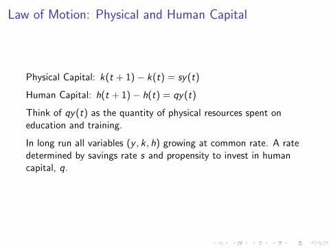
Physical Capital: k(t + 1)− k(t) = sy(t)

Human Capital: h(t + 1)− h(t) = qy(t)

Think of qy(t) as the quantity of physical resources spent oneducation and training.

In long run all variables (y , k , h) growing at common rate. A ratedetermined by savings rate s and propensity to invest in humancapital, q.

Common rate

Let r = h(t)/k(t) then

k(t + 1)− k(t)

k(t)= sy

k = skαh1−α

k

= sr1−α

h(t + 1)− h(t)

h(t)= qy

k = qkαh1−α

k

= qrα

Solve for r yields

r = q/s

Closing the Model

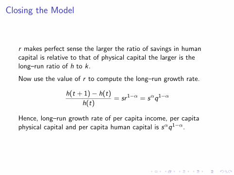
r makes perfect sense the larger the ratio of savings in humancapital is relative to that of physical capital the larger is thelong–run ratio of h to k .

Now use the value of r to compute the long–run growth rate.

h(t + 1)− h(t)

h(t)= sr1−α = sαq1−α

Hence, long–run growth rate of per capita income, per capitaphysical capital and per capita human capital is sαq1−α.

Implications of Human Capital

There are five implications.

1. Physical capital may exhibit diminishing returns yet there maybe no convergence in per capita income.

2. Constancy of returns. Now s and q now have growth rateeffects, and not just level effects as in the Solow model.

3. Growth effects in item (2) related constancy of physical andhuman capital combined.

4. Introduction of human capital helps to explain why rates ofreturn to physical capital may not be as high in poor countriesas the simple Solow model predicts.

5. The model predicts no tendency toward unconditionalconvergence (even if parameters all the same).

Implications of Human Capital

There are five implications.

1. Physical capital may exhibit diminishing returns yet there maybe no convergence in per capita income.

2. Constancy of returns. Now s and q now have growth rateeffects, and not just level effects as in the Solow model.

3. Growth effects in item (2) related constancy of physical andhuman capital combined.

4. Introduction of human capital helps to explain why rates ofreturn to physical capital may not be as high in poor countriesas the simple Solow model predicts.

5. The model predicts no tendency toward unconditionalconvergence (even if parameters all the same).

Implications of Human Capital

There are five implications.

1. Physical capital may exhibit diminishing returns yet there maybe no convergence in per capita income.

2. Constancy of returns. Now s and q now have growth rateeffects, and not just level effects as in the Solow model.

3. Growth effects in item (2) related constancy of physical andhuman capital combined.

4. Introduction of human capital helps to explain why rates ofreturn to physical capital may not be as high in poor countriesas the simple Solow model predicts.

5. The model predicts no tendency toward unconditionalconvergence (even if parameters all the same).

Implications of Human Capital

There are five implications.

1. Physical capital may exhibit diminishing returns yet there maybe no convergence in per capita income.

2. Constancy of returns. Now s and q now have growth rateeffects, and not just level effects as in the Solow model.

3. Growth effects in item (2) related constancy of physical andhuman capital combined.

4. Introduction of human capital helps to explain why rates ofreturn to physical capital may not be as high in poor countriesas the simple Solow model predicts.

5. The model predicts no tendency toward unconditionalconvergence (even if parameters all the same).

Implications of Human Capital

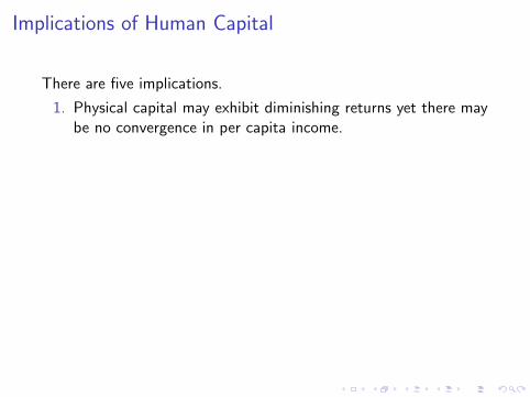
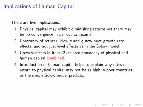
There are five implications.

1. Physical capital may exhibit diminishing returns yet there maybe no convergence in per capita income.

2. Constancy of returns. Now s and q now have growth rateeffects, and not just level effects as in the Solow model.

3. Growth effects in item (2) related constancy of physical andhuman capital combined.

4. Introduction of human capital helps to explain why rates ofreturn to physical capital may not be as high in poor countriesas the simple Solow model predicts.

5. The model predicts no tendency toward unconditionalconvergence (even if parameters all the same).

Implications of Human Capital

There are five implications.

1. Physical capital may exhibit diminishing returns yet there maybe no convergence in per capita income.

2. Constancy of returns. Now s and q now have growth rateeffects, and not just level effects as in the Solow model.

3. Growth effects in item (2) related constancy of physical andhuman capital combined.

4. Introduction of human capital helps to explain why rates ofreturn to physical capital may not be as high in poor countriesas the simple Solow model predicts.

5. The model predicts no tendency toward unconditionalconvergence (even if parameters all the same).

Empirical Predictions of HC Growth Model

The model has two predictions

1. Conditional convergence after controlling for human capital.By conditioning on the level of human capital, poor countrieshave a tendency to grow faster.

2. Conditional divergence after controlling for initial level of percapita income. By conditioning on the level of per capitaincome, countries with more human capital grow faster.

Empirical Evidence on HC Model

Barro (1991) paper in the QJE. (famous)

Discussion by Ray concludes that the model with human capitalprovides a better fit than do the models with exogenous factors.Specifically, does a better job of predicting the growth of some ofsub–Saharan countries (with very low levels of human capital inthe sample period (1960–1985).

However the model with human capital still fails to accountsatisfactorily for the magnitudes of growth displayed by Korea andTaiwan.

Growth & Development Accounting

A way to measure technical progress. Same basic idea used ingrowth and development accounting.

Growth Accounting used with time series data (e.g., annualinformation on a single country).

Development Accounting used to compare two countries at thesame point in time. Typically use cross–sectional data (oncountries, geographical regions).

Basic Idea: Think of production as composed of two parts:

Output = Productivity× Factors of Production

Growth Acct, with Cobb Douglas PF

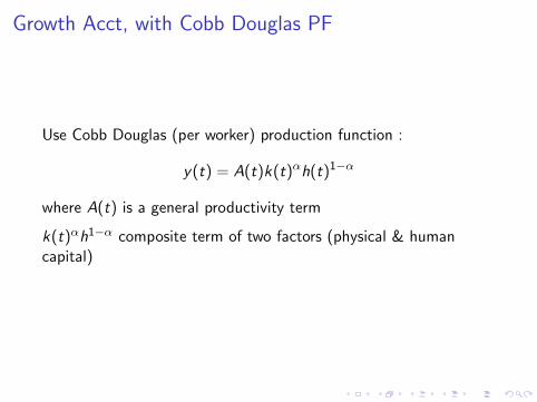
Use Cobb Douglas (per worker) production function :

y(t) = A(t)k(t)αh(t)1−α

where A(t) is a general productivity term

k(t)αh1−α composite term of two factors (physical & humancapital)

Growth Accounting (Cont)

Take logs

ln y(t) = ln A(t) + α ln k(t) + (1− α) ln h(t)

Recall that the time derivative of ln(z(t)) = d ln(z(t)dt = 1

zdzdt

Growth Accounting (Cont)

Take derivative w.r.t. time t

1

y

dy

dt=

1

A

dA

dt+ α

1

k

dk

dt+ (1− α)

1

h

dh

dt

Represent time derivative by a dot above the variable, z = dzdt .

Use “carrot”to denote a percent change zz = z .

y = A + αk + (1− α)h

Recall that α is the income share of capital while 1− α is theincome share of human capital.

Growth Accounting (end)

Thus the rate of growth of output is the sum of productivitygrowth and the share weight sum the growth of factors ofproduction.

We observe: y , k , h. Requires effort and much attention to detail.Calculation where the devil is in the details.

Direct measurement of the rate of growth of productivity is notcredible. (You could try, but no matter the estimate, no one wouldbelieve it.)

Hence, “measure” growth rate of productivity as residual

A = y − αk − (1− α)h

Growth Accounting

The above formulation assumes data on education (to measureHC) is available.

Show for yourself that if the production function is:

Y (t) = A(t)K (t)αP(t)1−α

then the growth accounting equation is:

y = αk + (1− α)P + A

Comparison with Textbook

y = αk + (1− α)P + A

Textbook:

∆Y (t)

Y (t)= σk(t)

∆K (t)

K (t)+ σP(t)

∆P(t)

P(t)+ TFPG(t)

TFPG = A

Ray’s formulation allows income shares of capital and labor to varyover time.

Comments on TFP

Important P(t) should be the working population. Sometimes wellapproximated by total population, sometimes times not.

Total population not accurate for labor force if major changes inlabor force composition (entry by women, or longer schoolingperiod or declining retirement age).

TFP Growth

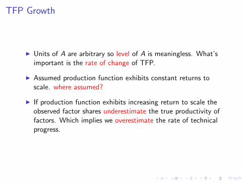
I Units of A are arbitrary so level of A is meaningless. What’simportant is the rate of change of TFP.

I Assumed production function exhibits constant returns toscale. where assumed?

I If production function exhibits increasing return to scale theobserved factor shares underestimate the true productivity offactors. Which implies we overestimate the rate of technicalprogress.

Development Accounting

Start with same basic idea:

Output = Productivity× Factors of production

Assume each country i = 1, 2 has Cobb–Douglas productionfunction

drop time subscript as doing calculation at the same t

Yi = AiKαi N

(1−α)i

where Ni is working population or human capital in country i

Ai measure of productivityKα

i N1−αi composition factor of production

Development Acct (cont)

Divide p.f of country 1 by p.f. country 2:

y1

y2=

A1Kα1 N1−α

1

A2Kα2 N1−α

2

y1

y2=

[A1

A2

](Kα

1 N1−α1

Kα2 N1−α

2

)

Q = P × F

or

P =QF

=y1/y2

Kα11 N1−α

1 /Kα22 N1−α2

2

Example:

Table: Data to Compare Productivity

Country y k h

1 24 27 82 1 1 1

Example - Calculation

Assume that countries have same technology with income share ofcapital α = 1/3 and 1− α = 2/3 the income share of humancapital.

A1

A2=

241

271/3×82/3

11/3×12/3

=24

3×41

= 2.

Hence, Country 1 has twice the productivity of Country 2.

Table

Table 7.2 (ed 2)

Table 1: Development Accounting (2006)

Country y k h FoP=k1/3h2/3 A

US 1.00 1.00 1.00 1.00 1.00Norway 0.92 1.08 0.97 1.01 0.92UK 0.76 0.69 0.97 0.87 0.87Canada 0.75 0.86 1.01 0.96 0.79Japan 0.69 1.10 0.99 1.02 0.67S.Korea 0.54 0.73 0.93 0.86 0.63Mexico 0.29 0.27 0.79 0.56 0.52Peru 0.14 0.12 0.82 0.44 0.32India 0.13 0.10 0.74 0.38 0.35Cameroon 0.10 0.036 0.58 0.23 0.44Zambia 0.034 0.032 0.65 0.24 0.14

1