1

ECOSYSTEM C STORAGE ON THE MARCELL EXPERIMENTALFOREST, MINNESOTA

D.F. GrigalForestry/Soils Consulting

Roseville, MN 55113

June 2009

Background Paper for Marcell Experimental Forest 50th Anniversary Symposium

2

ABSTRACT …………………………………………………………………….. 4TABLES AND FIGURES …………………………………………………… 5

Tables …………………………………………………………………….. 5Figures ……………………………………………………………………. 8

INTRODUCTION ……………………………………………………………… 9OBJECTIVE …………………………………………………………………… 9METHODS ………………………………………………………………………. 9

Location …………………………………………………………………. 9Field ………………………………………………………………………. 10Laboratory ……………………………………………………………… 12Spatial data ……………………………………………………………… 12Numerical and statistical ………………………………………………. 16

Field ……………………………………………………………….. .. 16Categorical C estimates ……………………………………………. 16

Vegetation type …………………………………………….. 16Soil mapping unit …………………………………………… 17

Laboratory…………………………………………………………….. 18C vs. LOI …………………………………………………….. 18Bulk density vs. LOI ………………………………………… 18

C mass …………………………………………………………..…. 19Soil …………………………………………………….……... 19

Forest floor ……………………………………………. 19Mineral ………………………………………………….. 19Peat …………………………………………………….. 20

Vegetation …………………………………………………….. 20Tree biomass ……………………………………………. 20Understory biomass ……………………………………… 20

CWD …………………………………………………..…… 24Landscape attributes ……………………………………………..… 24

Available data …………………………………………………. 25Peatland probability ………………………………………… 30Forested probability …………………………………………… 31Estimation ………………………………………………….. 31

RESULTS …………………………………………………………………………. 31Field ………………………………………………………………… 32Categorical C estimates ……………………………………………. 35

Vegetation type ……………………………………………. 35Soil mapping unit ………………………………………….. 37

3

Laboratory …………………………………………………………. 40C vs. LOI ……………………………………………………. 40Bulk density vs. LOI ………………………………………… 43

C mass ……………………………………………………………… 45Soil …………………………………………………………. 45

Forest floor …………………………………………. 45Mineral …………………………………………….. 47Peat ………………………………………………… 48

Vegetation …………………………………………………. 49Tree biomass …………………………………………… 49Understory biomass ……………………………………… 50

CWD ……………………………………………………….. 52Landscape attributes ……………………………………… ……… 56

Peatland probability ……………………………………….… 56Forested probability ………………………………………… 57Estimation equations ……………………………………….. 58

Explanatory power ……………………………………… 64Another check ……………………………………… 64

Application to MEF ……………………………………………….… 65

ACKNOWLEDGEMENTS ……………………………………………………… 70

LITERATURE CITED ………………………………………………………..… 71

4

ABSTRACT

We determined the magnitude and spatial patterns of ecosystem carbon (C) storage (soil, forestfloor, coarse woody debris (CWD), and standing biomass) across landscapes at the USDA ForestService Marcell Experimental Forest (MEF) in northern Minnesota. The MEF is a 950-ha tractwhose morainic landscape is typical of those in the Upper Great Lakes Region, providinggenerality for the results of the study. The landscape is a mosaic of uplands and peatlands, thelatter varying from fens with regional groundwater influence to perched bogs with little or nosuch influence. We used a combination of data gathered via sampling with field transects,mapping by vegetation cover type and soil mapping unit, and a digital elevation model (DEM)with 10-m resolution based on a topographic map with 1.2-m contour intervals to estimate Cstorage. We used two methods to estimate C storage. We used published information toestimate C for vegetation and soil mapping units, and extrapolated to the entire area. We alsodeveloped estimation equations based on mapped and landscape variables and applied them toindividual cells of the DEM. Estimates of C based on simple extrapolation from map units wasabout 210 Mg ha-1 for soil C (to 100 cm) and 50 Mg ha-1 for vegetation C. Final estimationequations for the DEM cells had R2s ranging from 0.13 (coarse woody debris logs) to 0.66 (treeC), with mean R2s for soil-related variables averaging about 0.20, for vegetation-relatedvariables averaging 0.50, and for CWD-related variables averaging about 0.20. When theequations were applied to random subsamples of data that had not been used to develop theequations, R2s ranged from 0.01 (coarse woody debris logs) to 0.61 (tree C), with mean R2s forsoil-related variables averaging about 0.16, for vegetation-related variables averaging 0.46, andfor CWD-related variables averaging about 0.17. The average estimates for the DEM cells wereabout 170 Mg ha-1 for soil C (to 100 cm), 60 Mg ha-1 for vegetation C, and 20 Mg ha-1 for CWDC. Soil C mass differed little among mineral soils (about 100 Mg ha-1) but was significantlydifferent than that for organic soils (400 Mg ha-1). Vegetation C and CWD C did not differappreciably among soil groups, so that the major differences in C storage among those groupswas related to differences in soil C. When estimates of C storage in organic soils are extendedbeyond 100 cm to the mineral substrate, that C mass is over 1000 Mg ha-1. When the DEM datawere considered by vegetation group, nearly all groups differed from one another in livevegetation C with highest C in the plantation-derived pine type. Because of the dominance ofsoil C to ecosystem C storage, vegetation groups on organic soils all had ecosystem C between300 and 400 Mg ha-1 compared to about 150 to 250 Mg ha-1 for groups on mineral soils.

5

TABLES AND FIGURES

Tables

Table 1. Description of the decay classes of logs used in the inventory of CWD on the MarcellExperimental Forest.

Table 2. Description of the decay classes of snags used in the inventory of CWD on the MarcellExperimental Forest.

Table 3. Vegetation types delineated on map of Marcell Experimental Forest.

Table 4. Estimated merchantable volume for forested types on the Marcell Experimental Forest.

Table 5. Soil mapping units delineated on the Marcell Experimental Forest (Nyberg1987).

Table 6. Vegetation strata used in estimation of biomass for Marcell Experimental Forest .

Table 7. Cover type groups used for estimation of understory biomass on Marcell ExperimentalForest.

Table 8. Vegetation codes used as categorical variables in topographic analysis.

Table 9. Soil codes used as categorical variables in topographic analysis.

Table 10. Data for each inventory point. Landscape attributes were calculated from a 10-mDEM interpolation of 1.2 m contour data for Marcell Experimental Forest.

Table 11. Results of linear regression between re-measurements (x) and original measurements(y) for field data collected at Marcell Experimental Forest.

Table 12. Results of a paired two-tailed t-test to test the significance of differences between re-measurements (x) and original measurements (y) for field data collected at Marcell ExperimentalForest.

Table 13. Factors used to convert mapped merchantable volume to total aboveground biomassfor forested cover types on the Marcell Experimental Forest.

Table 14. Estimated aboveground biomass for forested size class 1 (0 to 12.4 cm dbh) mappedon the Marcell Experimental Forest.

Table 15. Aboveground biomass estimates for nonforested vegetation types mapped on theMarcell Experimental Forest.

6

Table 16. Carbon estimates for vegetation types mapped on the Marcell Experimental Forest,based on a categorical analysis.

Table 17. Organic matter content of the soil mapping units of the Marcell Experimental Forest,based wholly on data in the county soil survey report (Nyberg 1987).

Table 18. Organic carbon content of the soil mapping units of the Marcell Experimental Forest,based on detailed soil characterization data for individual taxonomic units within mapping units.

Table 19. C mass of soil variables from intensive points sampled on Marcell ExperimentalForest.

Table 20. Independent variables and multipliers used to extrapolate C from intensive toreconnaissance sample points.

Table 21. Understory estimation equations and basic statistics used on Marcell ExperimentalForest. Estimates in units of kg ha-1.

Table 22. Estimates of biomass C for all sampled points on the Marcell Experimental Forest.Biomass includes both above- and belowground trees, shrubs, forbs, and ground cover.

Table 23. Vegetation types (CWD types) used in analysis of CWD on Marcell ExperimentalForest, and intercepts (INT) used in the relationship predicting log biomass for the originalinventory points.

Table 24. Estimated C mass of CWD from inventory points on Marcell Experimental Forest.

Table 25. Values for categorical variables used to predict probability that an observation is non-forested (i.e., open).

Table 26. Independent variables used to predict soil carbon.

Table 27. Independent variables used to predict vegetation-related carbon.

Table 28. Independent variables used to predict woody-debris-related carbon.

Table 29. Descriptive statistics and details of estimation equations.

Table 30. Estimates of C mass for Marcell Experimental Forest, categorized by soil groups.Estimates in Mg ha-1. Analysis of variance indicated significant difference among means for allvariables. Area in ha.

7

Table 31. Estimates of C mass for Marcell Experimental Forest, categorized by vegetationgroups. Estimates in Mg ha-1. Analysis of variance indicated significant difference amongmeans for all variables. Area in ha.

8

Figures

Fig. 1. Relationship of C to LOI in mineral soil samples. Best-fit line indicated.

Fig. 2. Relationship of C to LOI in forest floor samples. Best-fit line indicated.

Fig. 3. Relationship of C to LOI in organic soil samples. Best-fit line indicated.

Fig. 4. Relationship of Db calculated from the tabulated mean LOI for each von Posthumification class to tabulated Db for each class (Malterer et al. 1992). Humification classesindicated.

Fig. 5. Relationship between tree height and dbh on the Marcell Experimental Forest.

Fig. 6. Root mass as a function of tree dbh, with data from Perala and Alban (1994), Santantonioet al. (1977), and Whittaker and Marks (1975), and the average of those relationships.

Fig. 7. Observed versus predicted mass of log CWD from CWD inventory of MarcellExperimental Forest. Predictions based on Eq. [14] and Eq. [15].

Fig. 8. Estimates of C mass for Marcell Experimental Forest, categorized by soil groups.Groups are peatlands, organic soil = 0; outwash, ~ 5% clay = 1; outwash/moraine complexes, ~8% clay = 2; and moraine, ~ 10% clay = 3. “Soil (100)” includes sum of forest floor and mineralsoil or organic soil to 100 cm depth, “Vegetation” includes above- and below-ground livingvegetation, and “CWD” includes both snags and logs. Fisher’s least significant difference (p =0.05) based on sum of components indicated (lsd).

Fig. 9. Estimates of C mass for Marcell Experimental Forest, categorized by vegetation groups.Groups are aspen-birch = AB, black spruce = BS, lowland conifers = LC, lowland hardwoods =LH, open = O, pine = PI, spruce-fir = SF, shrubs = SH, and upland hardwoods = UH. “Soil(100)” includes sum of forest floor and mineral soil or organic soil to 100 cm depth,“Vegetation” includes above- and below-ground living vegetation, and “CWD” includes bothsnags and logs. Fisher’s least significant difference (p = 0.05) based on sum of componentsindicated (lsd).

9

INTRODUCTION

Carbon (C) storage and its change are central issues in global change, but the magnitude ofstorage in forested systems is uncertain. Spatial patterns of carbon storage on the landscape,including soil organic carbon and biomass C, are important both from a carbon inventoryperspective and for understanding the biophysical processes that affect carbon fluxes. Althoughnumerous estimates of C storage have been made, the regional (e.g., Grigal and Ohmann 1992,Homann et al. 1995, Johnson and Kern 2003, Kulmatiski et al. 2004, Simmons et al. 1996) andnational (Birdsey and Heath 1995, Birdsey and Lewis 2003) estimates are often tentative becausethey are based on a specific subset of sites on the landscape or on broad-based mean values thatare extrapolated over the entire land base. The patterns and processes affecting ecosystem C willvary considerably among different landscapes, limiting extrapolation across broad climatic-geomorphic regions.

Estimates of C storage for specific watersheds or other forested tracts (e.g., Arrouayes et al.1998, Bell et al. 2000, Thompson and Kolka 2005) can provide metrics to evaluate these broaderestimates. Region-specific studies are therefore warranted at appropriate spatial scales tounderstand specific processes affecting C fluxes. We believe that the appropriate landscape unitfor study in humid region landscapes is the hillslope because hydrologic processes active inhillslopes lead to considerable differences in soil characteristics, including the depth anddarkness of the A horizon; highly correlated with soil C (Thompson and Bell 1996). Theseconsistent hillslope relationships are embodied in the catena concept, firmly established in soilscience. Although the concept is firmly established, quantification of changes in soil C withlandscape position, especially in forests, is lacking. This is especially true in more recentlyglaciated regions such as the northern Great Lakes States, northern New York, and much ofsouth-central Canada, where climate and a poorly-developed drainage network have led toabundant peatlands, occupying 10-30% of most basins. Quantification of the C stored in theseimmature landscapes, the pools in which it is stored, and the relationship of that storage tolandscape features will all aid in predicting the magnitude of C response to various scenarios ofglobal change.

OBJECTIVE

The overall objective of our research is to better understand the mechanisms responsible for Csequestration at landscape scales. Although not our ultimate goal, the predictive mapping of Cstorage is a necessary first step in this understanding. Our specific objective for this study was toquantify the magnitude and spatial patterns of ecosystem carbon storage (soil, forest floor,standing biomass, coarse woody debris) across landscapes at the USDA Forest Service MarcellExperimental Forest (MEF) in northern Minnesota.

METHODS

Location

10

The MEF is a 950-ha tract located 40 km north of Grand Rapids, Minnesota (47 o 32' N, 93 o 28'W). The Forest has been reserved for long-term research with the cooperation of the USDAForest Service North Central Forest Experiment Station, the Chippewa National Forest,Minnesota Department of Natural Resources, Itasca County and a private landowner.Watersheds at the MEF consist of an upland portion and a peatland; streams originate in thepeatlands. The peatlands vary from fens with regional groundwater influence to perched bogswith little or no such influence, providing a range of sites for C storage. The landscape of theMEF is typical of morainic landscapes in the Upper Great Lakes Region, providing generality forstudy. Soils of the MEF have been mapped; predominant upland soils are Warba sandy loams(Glossic Eutroboralfs) (Nyberg 1987). The MEF is of particular interest because it has a largehistorical database concerning hydrology (Nichols and Brown 1980; Boelter and Verry 1977)and chemical cycling and transport (Grigal 1991; Kolka et al. 2001, Urban et al. 1989; Verry andTimmons 1982; Verry 1981). Climate and hydrological data have been collected continuouslysince 1960. The climate of the MEF is subhumid continental, with wide and rapid diurnal andseasonal temperature fluctuations. The mean annual air temperature is 2 C, with extremes of -46 C and 40 C. Average January and July temperatures are -14 C and 19 C, respectively(Verry 1984). Mean annual precipitation is 78 cm with 75% occurring in the snow-free period(mid-April to early November).

Field

Samples and descriptions of soils, vegetative cover, and organic debris at the soil surface,referred to hereafter as forest floor, were collected along 20 transects crossing topographicchanges and the major vegetation types of MEF. We sampled at two levels of intensity. Allsample points were included in a reconnaissance data set. Points were located at 25-mincrements along the transects (approximately 600 points). We recorded landscape position andtopography (position on slope, slope gradient, curvature, and aspect). Four categories of positionon slope (upper slope, midslope, lower slope, and depressional) were used to describe thelocation of the point. Slope gradient was measured with a clinometer at the greatest slopethrough the point. Both profile curvature (curvature parallel to the greatest slope) and plancurvature (perpendicular to the greatest slope) were estimated using three categories: concave,convex, and flat. Aspect was measured as the compass direction down the greatest slope.

Stand basal area was measured using a variable radius plot. Diameter at breast height andcondition of each "in" tree (those 2.5 cm diameter) were recorded. Dead “in” trees wereassigned to one of four condition classes, ranging from 1 (recently dead, with virtually all leavesand twigs intact) to 4 (standing bole without branches). Average tall shrub cover was estimatedto the nearest 5% based on the proportion of ground area that was shaded or covered by shrubs.Height of the tall shrub canopy was estimated visually to the nearest 0.5 m. Low shrub and forbcover was estimated to the nearest 5% based on the proportion of ground area that each stratumshaded. Forest floor and thickness of the A horizon were both measured to the nearest 0.5 cm. Ifpresent, depth of organic soils (peat) was measured to the nearest 5 cm using a McCauley peat

11

auger. Degree of humification was estimated using the von Post scale, with 1 beingundecomposed and 10 being fully humified (Malterer et al. 1992). Location of the beginningpoint, end point, and some of the intermediate points along the transect were recorded using aglobal positioning system.

Approximately one-third of the reconnaissance points were randomly selected for intensivesampling. At intensively-sampled points, samples of soil, forest floor and peat were collected.Soil samples were collected at three locations 3 m from the point center and oriented at 120 ,240 , and 360 . The forest floor depth was measured, and it was sampled quantitatively within astainless steel ring (12.3 cm diameter) at each location; the three samples were aggregated forlaboratory analysis. Similarly, three 0-25 cm depth mineral soil samples were collected from thesame locations using a bucket auger, and the samples were aggregated for laboratory analysis. Asingle mineral soil sample from 26-100 cm was also collected for analysis. For organic soils,single samples for return to the laboratory were collected from the 0-50 cm and 50-100 cmdepths, and from each additional meter thereafter with the peat auger. Depth sampling oforganic soils continued until the soils were impenetrable with the auger.

A total of 596 points were sampled; with 219 of those being intensively sampled. In addition, 30points (including 10 intensively-sampled points) were re-visited to assess variability in datacollection.

The initial inventory of the MEF as described above (carried out in 1992 and 1993) did notinclude complete sampling of coarse woody debris (CWD). Although snags (standing deadtrees) were included in the inventory, logs (fallen branches and boles) on the forest floor werenot included. In 2003, we inventoried logs following the methods outlined in Duvall (1997),based in part on techniques described by Van Wagner (1968).

Sampling was along 28 transects that roughly followed the same bearings and lengths as theoriginal transects used in the C inventory of MEF. Sample points were located at 25-m intervalsalong each transect, with from 4 to 82 points per transect and a total of 566 points. We made noattempt to exactly overlap the sample points with the points from the earlier inventory for tworeasons. First, even if points exactly overlapped, the resulting data would not be directlycomparable with that from the earlier inventory because of successional and disturbance-relatedchanges in forest composition during the approximate decade-long interval between samplings.Secondly, exact overlap would require substantially more field time with GPS to assure theprecise location. Our goal was to collect sufficient data at each sampling point so that we coulddevelop an algorithm for estimating log CWD on MEF.

Each sample point served as the center of a line-transect for the log inventory (Van Wagner1968). Line-transects were 10 m in length, and were oriented along the bearing of the overalltransect. A diameter limit of 2.5 cm was used for logs (at the plane of intersection between a linetransect and log). This provided an inventory of nearly all dead wood too large to be included inthe forest floor sampling. Four classes were used to categorize log decay (Duvall 1997 – Table1). As with the original sampling of MEF, stand basal area was also measured using a variable

12

radius plot centered at each sample point. Diameter at breast height and condition of each "in"tree (those 2.5 cm diameter) was recorded. Dead “in” trees were assigned one of three decayclasses (Duvall 1997 – Table 2).

Table 1. Description of the decay classes of logs used in the inventory of CWD on the MarcellExperimental Forest.

Class Bark Soundness Shape

1 on sound round

2 partially off partially decayed round

3 off decayed round to oval

4 none very decayed and friable oval (moss covered)

Table 2. Description of the decay classes of snags used in the inventory of CWD on the MarcellExperimental Forest.

Class Bark Soundness Twigs and branches

1 on sound all present

2 partially off partially decayed no twigs, branches present

3 off decayed nearly all missing

About 6% of the points were re-visited, and line-transects for log sampling were orientedperpendicular to the bearing of the overall transect rather than at the original bearing. Theseperpendicular transects were also 10 m in length, with the mid-point coinciding with the samplepoint.

Laboratory

All samples of forest floor, mineral soil, and organic soil were kept cool in the field in a largefoam chest, and were sent to the laboratory within 48 hours. Upon receipt in the lab, mineral andorganic soil samples were frozen until further processing. The moist mass of the forest floorsamples was determined, and a subsample was removed to determine moisture content. Theremainder of the sample was then frozen. After thawing, subsamples of forest floor, mineral andorganic soil were analyzed for loss on ignition (LOI) by ashing at 450 C for 12 hours. LOI wasdetermined on all of the forest floor, mineral soil, or peat samples from the intensive points.Total C was determined on about 20% of the samples using a LECO CR-12 analyzer (David1988).

Spatial data

13

We developed a geographic database that included a digital terrain model, vegetation cover type,and soils from an order II soil survey. The information was stored in a raster format using 10-mgrid cells. Scales for input data ranged from 1:15,000 to 1:24,000. Surface topography wasdigitized from an existing topographic map with 1.2-m (four-foot) elevation contours derivedfrom a ground survey of the MEF.

Vegetation type was interpreted from 1:15,840 color infrared airphotos, dated May 1990. Typewas delineated onto a Mylar sheet, and vegetation class and ground control points were handdigitized from the Mylar overlay. Units on the map included 12 forest types and 10miscellaneous types including permanent water (Table 3). The forested types were furthercharacterized by the average diameter breast height (dbh) in English units in three classes, withthe metric equivalents of 1 = 0 to 12.4 cm dbh; 2 = 12.5 to 22.6 cm dbh; and 3 = 22.7 to 37.8 cmdbh. Cover types in size class 1 were further characterized in terms of the stocking, or thepercent of area occupied, in classes of 1 = 10 to 39% stocking; 2 = 40 - 69% stocking; and 3 =>70% stocking. For the larger size classes, the merchantable volume was estimated in Englishunits (cords acre-1) (Table 4).

14

Table 3. Vegetation types delineated on map of Marcell Experimental Forest.

NumericalCode

Type

2 red pine

3 jack pine

11 balsam fir

12 white spruce

21 black spruce

22 tamarack

23 northern white cedar

30 northern hardwoods

40 lowland hardwoods

42 black ash

50 aspen

52 birch

80 upland grass

82 upland brush

85 lowland grass

86 lowland brush

88 beaver pond

90 marsh

91 muskeg

92 permanent water

94 stagnant spruce

95 stagnant tamarack

15

Table 4. Estimated merchantable volume for forested types on the Marcell Experimental Forest.

Merchantable VolumeDiameter class(cords acre-1) (m3 ha-1)

1 3 - 7 17 - 392 7 - 13 39 - 733 13 - 17 73 - 954 17 - 23 95 - 1295 23 - 27 129 - 1516 27 - 33 151 - 1857 33 - 37 185 - 2078 37 - 43 207 - 2419 > 43 > 241

Soil map unit delineations were digitized from a 1:24,000 NRCS order II soil survey (ItascaCounty – Nyberg 1987). Sixteen soil mapping units were recognized on the MEF (Table 5).

The transect sampling locations and digital geographic database were registered to standardgeographic coordinates (universal transverse mercator) such that vegetation type, soil map unit,and topographic attributes were derived for each field sampling point based on geographiclocation.

16

Table 5. Soil mapping units delineated on the Marcell Experimental Forest (Nyberg1987).

Soil Mapping Unit Symbol Area(ha)

Borosaprists, depressional 995 51Cathro muck 544 7Greenwood peat 549 48Loxely peat 533 4Menahga and Graycalm soils, 0 to 8% slopes 867 B 135Menahga loamy sand, 10 to 30% slopes 458 E 71Mooselake and Lupton mucky peats 797 35Nashwauk fine sandy loam, 1 to 10% slopes 622 B 159Nashwauk-Menahga complex, 1 to 10% slopes 1826 B 45Nashwauk-Menahga complex, 10 to 25% slopes 1826 D 96Sago and Roscommon soils 798 8Seelyeville-Bowstring association 799 42Warba fine sandy loam, 1 to 8% slopes 240 B 153Warba fine sandy loam, 10 to 25% slopes 240 D 54Water W 56Sum 964

Numerical and statistical

Field

As described earlier, 30 points (including 10 intensively-sampled points) were re-visited for re-sampling to assess variability in data collection. For the continuous variables measured in thefield, variability was measured as reproducibility using both linear regression and testingsignificance of differences between the original and the re-measurements using a paired two-tailed t-test.

Categorical C estimates

Vegetation type

Although the vegetation type mapping did not directly focus on C, biomass and hence Cestimates can be derived from it. Biomass estimates for the larger size classes of the forestedtypes were based on extrapolation of the mapped merchantable volume to total biomass by covertype group, using data from Grigal and Bates (1992). The geometric mean volume of each classwas computed and multiplied by the appropriate conversion factor to estimate total above-groundtree biomass. Biomass estimates for the smallest diameter class of the aspen-birch forested typeswas primarily based on Perala (1972), with comparisons for reasonableness from Silkworth(1980) and Alban and Perala (1992). For the smallest diameter class of the conifer forest types,including pine, spruce-fir, lowland conifers, and black spruce, biomass was estimated with datafrom Berry (1987) and Methven (1983). Finally, biomass for hardwoods other than aspen-birch

17

was taken to be the geometric mean of those for aspen-birch and conifer. Biomass estimates forthe non-forest cover types were based on a variety of studies in Minnesota.

Belowground biomass estimates were simply a ratio of the aboveground biomass estimates. Forforested types, we based our belowground estimates on a compilation of information bySantantonio et al. (1977) with additional information from Whittaker and Marks (1975) andPerala and Alban (1994). For shrubs, we used an average root:shoot ratio based on data fromGrigal et al. (1985), Johnston et al. (1996), and Perala and Alban (1994). For forbs, the ratiowas based on data from Abrahamson (1979), Ashmun et al. (1985), Grigal et al. (1985), Gross etal. (1983), Nihlgard (1972), Paavilainen (1980), and Remezov and Pogrebnak (1969). Toconvert biomass to C, a ratio of 1:0.474 was used (Raich et al. 1991).

Soil mapping unit

We made two different but related estimates of soil C on MEF using categorical data from thesoil map. One estimate was wholly based on information contained in the published soil surveyreport (Nyberg 1987). Based on the verbal descriptions in the report, the average composition ofeach soil map unit in terms of proportion of taxonomic units was tabulated. The table in thereport, Physical and chemical properties of the soils, provided estimates of soil properties bymajor layers (e.g., surface, subsurface, subsoil, and underlying material) for each taxonomic unit.Properties include thickness of each layer, its range of bulk density, and, for surface layers, itsrange of organic matter. Based on its taxonomic composition and the average bulk density andorganic matter for each layer, these data were used to compute the organic matter content of thesurface layer of each soil mapping unit in units of mass per unit land area. Although the soilsurvey report only reported organic matter in the surface layer (horizon), lower horizons alsocontain organic matter. To estimate the organic matter content of lower soil layers, afundamental relationship between soil organic matter and bulk density was used. We used theapproach of Federer et al. (1993), which assumes that the bulk densities of organic and mineralmatter are constant, and the bulk density of any soil sample is based on the additive volumes ofeach fraction. Thus

Db = (Dbm Dbo)/[Fo Dbm + (1 - Fo) Dbo] [1]

where Db is the soil bulk density (Mg m-3), Fo is the organic fraction (kgo kg-1), Dbo is the bulkdensity when Fo = 1 (i.e., the bulk density of the organic fraction), and Dbm is the bulk densitywhen Fo = 0 (i.e., the bulk density of the mineral fraction).

For organic soils (i.e., Histosols), the mineral fraction is assumed to have negligible volume(Gosselink et al. 1984) according to the relationship

Db = (Dbo/Fo) [2]

where variables are as described above.

18

We used the bulk density and organic matter data for the surface layers of the taxonomic unitsthat constituted the mapping units on the MEF as described in the soil survey report (Nyberg1987) and nonlinear least squares (Wilkinson 1986) to determine Dbm and Dbo. We alsodetermined Dbo for organic soils (OM > 10%) as the simple average of the Dbos of the 10Histosols in the report. The resulting computed densities and the tabulated densities, wherepresent, were used to estimate organic matter for the deeper soil horizons. Based on itstaxonomic composition, and the tabulated or estimated bulk density for each layer, these datawere used to compute the organic matter content of the “surface” upper 25 cm and upper meterof each mapping unit as mass per unit land area.

Because the data in the county soil survey report are relatively general, we used more detaileddata to develop another estimate of organic carbon content of the soil mapping units found on theMEF. The goal was to arrive at a more accurate estimate than that based exclusively on the datawithin the soil survey report. Detailed data for 73 pedons, representing 16 taxonomic units, wascollected from a variety of sources but primarily from the soil characterization database of theNatural Resources Conservation Service (NRCS) (Soil Survey Staff 1997) and fromcharacterization data from the University of Minnesota Department of Soil, Water, and Climate.Other sources, for specific taxonomic units, included Balogh (1983), Grigal et al. (1974), Kolka(1993), and Alban and Perala (1990). For some pedons, bulk density data were missing, and in afew cases C data were missing for some mineral horizons. Where bulk density data weremissing, we again used the approach of Federer et al. (1993) to calculate the bulk densities oforganic and mineral matter from the 100 horizons with both organic carbon and bulk densitydata. These data were used to estimate bulk density for each soil horizon where it was missing.For the few subsurface horizons without C data, we estimated C with a general relationship formineral horizons. Organic carbon was then computed for both the upper 25 cm and the uppermeter of the pedons in the detailed database. These data were then extrapolated to the soilmapping units of the MEF based on their tabulated taxonomic composition.

Laboratory

C vs. LOI

As described, we had LOI and C data for forest floor, peat, and mineral soil from MEF. Inaddition, we had similar data gathered from another site in Minnesota in a companion study (Bellet al. 1996, Bell et al. 2000). We combined the data, and simple linear regressions weredeveloped for each sample type relating LOI (%) as the independent variable and C (%) as thedependent variable.

Bulk density vs. LOI

Mineral soil bulk density was estimated from LOI using the approach of Federer et al. (1993)(Eq. [1]). We developed our relationship from the data collected in a transect of forested sitesacross the north-central United States (Ohmann and Grigal 1991). For forest floor, we used aslightly different approach. In materials high in organic matter, such as forest floor and peat,

19

mineral matter adds little to the bulk volume of soils (Gosselink et al. 1984) (Eq. [2]). Ourobjective was to obtain estimates of forest floor mass per unit area, and we had estimates offorest floor thickness, LOI, and mass from the intensively sampled points. We therefore solvedthe least-square estimate for Dbo from the relationship

FFm = (Dbo/Fo) T K [3]

where FFm is mass of forest floor in kg ha-1, T is forest floor thickness, and K is the appropriateconstant for unit conversion. For peat, we solved Eq. [2] using a nonlinear least-square routine(Wilkinson 1986) and an extensive database of peat Db collected in MEF and other peatlands innorthern Minnesota (Buttleman 1982).

C mass

Soil

Forest floor

Forest floor had been quantitatively sampled at each intensive point, and LOI of that materialwas determined in the laboratory. Mass per unit area was calculated and converted to C per unitarea using the equation relating C to LOI.

The detailed sampling of forest floor only occurred on the intensive points, and we used thosedata to extrapolate estimates of forest floor C to the reconnaissance points. As noted above, thefield data included landscape position and topography (slope gradient, curvature, and aspect) andforest floor and A-horizon thickness. We only had one measurement of forest floor thickness atthe reconnaissance points compared to three for the intensive points. We transformed the aspectto more closely reflect biological reality by the relationship

ASPCOD = [1 + cos (ASP-225 )]/2 [4]

where ASP is the measured aspect in degrees and ASPCOD is the transformed value, whichreaches a maximum value of 1 at 225 (SW) and a minimum value of 0 at 45 (NE). This issimilar to the transformation suggested by Beers et al. (1966), but with a different maximum andminimum. We also added conifer and broadleaf live tree basal area to the data for each point.We randomly chose a subsample of 10% of the data (15 points of the total 152) to be used toevaluate the uncertainty of the final extrapolation equations.

Mineral soil

The C mass of mineral soils requires C concentration, bulk density, and thickness. Using theLOI data from the intensive points, we calculated mineral soil C and Db. These data were thenused to calculate mineral soil C mass for the surface 0 to 25 cm and for the subsurface 26 to 100cm for the intensive points.

20

As with forest floor, we extrapolated those data to the reconnaissance points. We used the samedata to extrapolate, including landscape position and topography, forest floor and A-horizonthickness, transformed aspect data, and the conifer and broadleaf basal area for each point. Werandomly chose a subsample of 10% of the data (15 points of the total 161) to be used toevaluate the uncertainty of the final extrapolation equations. These were the same pointsselected for evaluating the forest floor extrapolation.

Peat

As with mineral soil, calculation of C mass of peat requires C concentration, bulk density, andthickness. However, because we related LOI to both C concentration and bulk density, aconsequence is that C content can be computed as a direct function of LOI and thickness. Usingthese relationships, C mass was calculated for all points with organic soils. Because we haddetermined depth at all points with organic soils, both intensive and reconnaissance, we had noneed to extrapolate data between the two classes of points.

Vegetation

Tree biomass

Overstory (tree) biomass was based on the tree diameter at breast height (dbh) collected at eachpoint. For aboveground biomass, we used estimation equations from Alemdag (1983, 1984).Those equations use both tree dbh and total height as independent variables. Although ourvegetation sampling did not include determination of tree height, we developed a relationshipbetween dbh and height for trees on the MEF.

We did not have a comprehensive set of estimation equations, such as those from Alemdag(1983, 1984), for belowground tree biomass. We based our belowground estimates on acompilation of information by Santantonio et al. (1977) with additional information fromWhittaker and Marks (1975) and Perala and Alban (1994). Santantonio et al. (1977) tabulatedroot biomass estimation equations from a large number of studies and also provided a figure withindividual data points showing the relationship between tree dbh and root mass. Using data fromNew Hampshire, Whittaker and Marks (1975) provided an estimation equation for root mass thatwas based on aboveground mass. Perala and Alban (1994) provided an estimation equationusing Minnesota data, but only with 17 observations. We expressed root mass as a function oftree dbh using the relationships from Whittaker and Marks (1975) and Perala and Alban (1994),from the figure in Santantonio et al. (1977), and from the mean of the tabulated equations(Santantonio et al. 1977), using those developed for genera likely to be found in northernMinnesota.

Understory biomass

21

Although understory strata (below the canopy) are a relatively minor proportion of total standbiomass in closed forest (about 5% – Ohmann and Grigal 1985a, Swanson and Grigal 1991),they may constitute the majority of mass as canopies become more open. We developedbiomass estimation equation for understory strata using data from two comprehensive studiesfrom northern Minnesota, one of uplands (Ohmann and Grigal 1985b) and the other of peatlands(Swanson 1988). Both studies, using different methods, determined the biomass of overstoryand understory in plant communities. The original data from these studies was extracted,yielding a total of 446 stands (211 from Ohmann and Grigal (1985b) and 235 from Swanson(1988)). Although these studies had sampled most of the forest types that are found on the MEF,the data set only included one upland hardwood (i.e., northern hardwood) stand. As a result, datafor an additional seven upland hardwood stands from east-central Minnesota were added(Suhartoyo 1991). Understory biomass was estimated for nine strata in the original data (Table6). These nine strata were aggregated into three understory groups and an overstory group(Table 6).

22

Table 6. Vegetation strata used in estimation of biomass for Marcell Experimental Forest.

Original data Grouped data

moss ground cover

lichens ground cover

ferns and fern allies forbs

grasses and forbs forbs

low shrubs forbs

tall shrubs shrubs

seedlings shrubs

saplings trees

trees trees

The data were further summarized into cover type groups. Cover types for the data fromOhmann and Grigal (1985b) were assigned to broad groups based on the majority (in a fewcases, plurality) of overstory biomass (Table 7). One type in those data, the lichen type, lackedany overstory. The data from Swanson (1988) had been assigned to physiognomic groups andthose groups were reassigned to the cover type groups (Table 7).

23

Table 7. Cover type groups used for estimation of understory biomass on Marcell ExperimentalForest.

Cover Type Group Abbreviation From Ohmann and Grigal(1985b)

From Swanson (1988)

Aspen-Birch AB Aspen-BirchBlack Spruce BS Black Spruce High-density Treed Bog

Low-density Treed BogLowland Conifers LC Lowland Conifers Conifer Swamp

Treed FenLowland Hardwoods LH Lowland Hardwoods Hardwood SwampPine PI PineSpruce-Fir SF Spruce-FirUpland Hardwoods UH Upland HardwoodsLichen LI LichenOpen Bog OB Open Bog

Shrub SH Thicket SwampShrub Fen

Grass GR Graminoid Fen

The resulting 11 groups (Table 7) were reduced to 10 by the elimination of the lichen type,which does not occur on the MEF. Estimation equations were based on a regression, wherebiomass of the understory strata (Table 6) was a function of the conifer overstory biomass, thedeciduous overstory biomass, and the cover type group as a dummy variable. The regressionestimates can be considered to be the solution at a mean cover for forbs and mean cover andheight for shrubs. In our field sampling, we had recorded the cover of the forb and tall shrubstrata, and the mean height of the tall shrubs. The cover and height data were used to refine themean estimates. Understory mass tends to increase allometrically (log-log) with cover and(shrub) height (Ohmann et al. 1981, Buech and Rugg 1995). For each cover type group, therange of the natural logarithm of cover (or cover and height) for the understory from our fieldsampling was linearly scaled to the range of the logarithm of understory biomass from ourbiomass data set. In the case of the field data, the full range of cover and height observationswere used. In the case of the biomass data, the scaling ranged over the 67% confidence interval(equal to one standard deviation above and below the mean) to avoid the influence of outliers.The scaled values were used as the biomass estimates. In other words, observations of cover andheight at a point that were higher than the mean for that type increased the biomass estimate forthat point. Similarly, lower cover and height decreased the biomass estimate.

The cover type group of forested points from our inventory (Table 7) was assigned by dominant(majority) basal area of living trees. Those points with no or minimal tree cover were assigned

24

to cover type groups based on field notes. Field notes were consulted for all points with basalarea less than or equal to 5 m2 ha-1 (two “in” trees per plot), or with average tree diameter of lessthan or equal to 5 cm. Both notes and the composition of the tree strata, including living anddead trees if present, were used to assign cover type groups. One of the most common situationswas recently-cut areas. Variable-radius data from points in these areas, which in most cases hadbeen aspen-birch cover type, may contain a residual red maple tree that would have led to theirassignment into the upland hardwood cover type group, or may contain a balsam fir tree leadingto spruce-fir cover type group. Instead, in those cases field notes helped assign the appropriatecover type group. Field notes were also used to assign the shrub, open bog, and grass cover typegroups. The latter group (grass) included a few upland points that fell within small clearings inthe forest, such as old logging landings.

In all cases, we converted living biomass to C using a ratio of 1:0.475 (Raich et al. 1991).

CWD

Dead tree (snag) aboveground biomass was calculated using the same procedure as with livingtrees (Alemdag’s equations --1983, 1984, and our height-dbh relationship). After the whole treemass was computed, it was adjusted for the condition class. The original inventory of MEF hadfour condition classes; for deciduous trees in condition class 1 we multiplied live biomass by0.98, for class 2, by 0.88, for class 3 by 0.79, and for class 4 by 0.40. For conifers, the multiplierfor class 1 = 0.94, 2 = 0.88, and 3 = 0.81, and 4 = 0.40. The CWD inventory carried out in 2003only used three decay classes. In that case, the multiplier for both deciduous and conifer trees indecay class 1 = 0.98, for class 2 = 0.84, and for class 3 = 0.40. Multipliers were based on ratiosof whole tree mass to that of component parts (Alemdag 1983, 1984).

Log volumes were calculated using techniques described by Van Wagner (1968). The biomassand C content of log CWD in each stand was estimated by combining the volume with estimatesof CWD density and C concentration reported by Duvall (1997). His data include density for 29classes of CWD: combinations of decay-class and species group. Four species groups wereused: red pine, softwoods (conifers other than red pine), aspen (Populus sp.), and hardwoods(broadleaf trees other than aspen). Carbon concentration for both snags and logs was tabulatedas a function of decay class (Duvall 1997).

We estimated log CWD for the points in the original inventory using the data collected in 2003.Points were placed into nine CWD types, and a regression equation was developed using bothCWD type and the continuous variables that we had collected at each point. That equation wasthen applied to the data from the original inventory of the MEF.

Data from the perpendicular transects were divided into upland and peatland, and paired t-testswere used to determine if there were significant differences between log C based on the transectdirection.

Landscape attributes

25

Available data

We used the C data from the inventory of Marcell and landscape attributes to estimate C over theentire Marcell landscape. The estimation equations were based on landscape attributes for a 10m by 10 m cell associated with each inventory point. Attributes were calculated from the digitalelevation model (DEM) for the MEF. The 10-m resolution DEM for MEF was based on thetopographic map. All DEM processing was completed in Arc/Info, mostly with the TOPOGRIDcommand. Both primary and secondary landscape attributes were calculated for this analysis.Primary landscape attributes are those that are calculated directly from the DEM. All primaryattributes are based on a kernel, or window of at least nine individual grid cells. The kernel ispassed across the DEM as a "moving window" (Lillesand and Kiefer 1999). Secondaryattributes are calculated by combining certain primary attributes. Primary attributes calculatedincluded elevation (ELEV), aspect (ASP), flow accumulation (specific catchment area – SCA),plan/profile curvature (PLCURV/PROCURV), and slope (SLOPE). Secondary attributescalculated included both compound topographic index (CTI) and stream power index (SPI). Alllandscape attributes were calculated in Arc/Info's GRID module.

The aspect code (ASPCOD – Eq. [4]) was calculated from ASP for all the data. In some cases,CTI was coded as a missing value. The computation of CTI is based on the log (base 10) ofSCA divided by SLOPE. In those cases where CTI was coded as missing, SCA had the value =0 because it was only reported in whole increments of m2 (i.e., 0, 1, 2, etc.). It is not likely thatSCA was actually = 0. To provide an estimate of SCA and CTI for those cases, a frequencydistribution of the values of SCA was developed,

log10 (n) = 2.18 - 0.149 SCA, n = 10, r2 = 0.95, [5]

where SCA is the value of SCA and log10 (n) is the logarithm, base 10, of the number ofobservations with that value. The ten classes of SCA values used in Eq. [5] represented a total of356 points. Based on Eq. [5], and on the number of observations of SCA that were coded as = 0(126 points), the new estimated value for SCA for those observations was changed from 0 to 0.5m2, and CTI was then re-calculated for those points. Based on scatterplots, distributions of CTI,SCA, and SPI appeared to be log-normal and so natural logs of those variables were calculated.In the case of CTI and SPI, + 2 was added to the values before the logarithms were determined toeliminate negative values.

Next, we merged the appropriate C data from various sources for each inventory point. The soil-related data included estimates of forest floor (FFC), mineral soil C in the 0 - 25 cm increment(SURFC), mineral soil C in the 0 - 100 cm increment (SUMINC), SOILC as the sum of FFC andSUMINC, and peat C to both 100 cm (PEAT100) and to total peat depth (PEATC). Vegetation-related C included aboveground tree C (AGTREC), belowground tree C (ROOTC), estimatedshrub aboveground C (SHRBAGC), estimated forb aboveground C (FORBAGC), estimatedground layer C (GRNDC), and AGVEGC as the sum of AGTREC, SHRBAGC, FORBAGC, and

26

GRNDC. Finally, coarse-woody debris C included standing dead tree C (SNAGC), estimatedlog C (LOGC) and CWDC as the sum of SNAGC and LOGC.

The overlay of the soil and forest cover type maps also provided the map attributes (ascategorical variables) overstory type (OVER_TYPE) (Table 8), overstory size in classes of 1 to 3(OVER_SIZE), overstory density in classes of 1 to 9 (OVER_DENS), and soil mapping unitsymbol (MUSYM) (Table 9). Both OVER_SIZE and OVER_DENS did not have values fornon-forested types such as upland brush. Those data were coded to = 0 (so the final classes were0 to 3 for density and 0 to 9 for size).

27

Table 8. Vegetation codes used as categorical variables in topographic analysis.

OVER_TYPE Descriptor FORTYP2 red pine PI3 jack pine PI

11 balsam fir SF12 white spruce SF

21 black spruce BS

22 tamarack LC23 northern white cedar LC94 stagnant spruce LC95 stagnant tamarack LC

30 northern hardwoods UH

40 lowland hardwoods LH42 black ash LH

50 aspen AB52 birch AB

80 upland grass O82 upland brush O85 lowland grass O88 beaver pond O90 marsh O

86 lowland brush SH91 muskeg SH

92 permanent water W

28

Table 9. Soil codes used as categorical variables in topographic analysis.

Soilcode Map UnitSymbol

Map Unit Name

0 533 Loxley Peat544 Cathro muck549 Greenwood Peat797 Mooselake and Lupton Mucky Peats798 Sago and Roscommon Soils799 Seelyeville-Bowstring Association995 Borosaprists, Depressional

1 867B Menahga and Graycalm Soils, 0 to 8 Percent Slopes458E Menahga Loamy Sand, 10 to 30 Percent Slopes

2 803D Warba-Menahga Complex, 10 to 25 Percent Slopes1826D Nashwauk-Menahga Complex, 10 to 25 Percent Slopes1826B Nashwauk-Menahga Complex, 1 to 10 Percent Slopes

3 240B Warba Fine Sandy Loam, 1 to 8 Percent Slopes240D Warba Fine Sandy Loam, 10 to 25 Percent Slopes622B Nashwauk Fine Sandy Loam, 1 to 10 Percent Slopes

The C data were merged with the landscape attributes to create a single database. The semi-finaldata for each point included landscape variables, map attributes, and dependent variables (Ccontent of ecosystem components) (Table 10).

29

Table 10. Data for each inventory point. Landscape attributes were calculated from a 10-mDEM interpolation of 1.2 m contour data for Marcell Experimental Forest.

Attribute DescriptionPOINT Transect pointNORTHING LocationEASTING LocationELEV Elevation in mASP Aspect direction, in degrees (0-360)CTI Compound topographic indexPLCURV Curvature measured in the plan directionPROCURV Curvature measured in the profile directionSCA Specific catchment area (also known as flow accumulation)SPI Stream power indexSLOPE Slope in degreesLEGEND_NUM Numerical code for combination of overstory, size, and densityOVER_TYPE Overstory type numberOVER_SIZE Overstory sizeOVER_DENS Overstory densitySPECIES Species group or covertype – alphaMUSYM Soil mapping unit symbolLVL Level of field sampling; 1 = reconnaissance, 2 intensiveFFC Forest floor CSURFC Mineral C, 0 - 25 cmSUMINC Mineral C, 0 - 100 cmSOILC Sum FFC + SUMINCPEATDPTH Peat depth, cmPEATC Peat C to mineral substratePEAT100 Peat C to 100 cmFF MEAS Forest floor mass was determined (1) or estimated (0)MIN MEAS Mineral soil mass was determined (1) or estimated (0)COVTYP Cover type based on measured basal areaC/D Conifer or deciduous basal area majority?AGTREC Aboveground tree CROOTC Belowground tree CSHRBAGC Estimated shrub aboveground CFORBAGC Estimated forb aboveground CGRNDC Estimated ground layer aboveground CAGVEGC Sum AGTREC + SHRBAGC + FORBAGC + GRNDCLOGC Estimated log CWD CSNAGC Standing dead tree CCWDC Sum LOGC + SNAGCASPCOD Computed aspect codeLNCTI Natural log (CTI+2)LNSCA Natural log SCALNSPI Natural log (SCI+2)SOILCODE Coalescence of soil mapping units into 4 categoriesFORTYP Coalescence of overstory type into 10 categoriesOVSZCOD Coalescence of overstory size into 4 categoriesOVDNCOD Coalescence of overstory density into 4 categories

30

The number of classes of categorical variables were also reduced by combining them into majorgroups. In the case of the soil data, four categories were produced, roughly based on acombination of physiography and associated surface soil texture (soilcode 0 = peatlands, organicsoil; soilcode 1 = outwash, ~ 5% clay; soilcode 2 = outwash/moraine complexes, ~ 8% clay;soilcode 3 = moraine, ~ 10% clay) (Table 9).

In the case of overstory type, the data were similarly combined into 10 groups (Table 8).Overstory size was originally coded as three (1 to 3) classes for forest types, and overstorydensity into nine classes. In the case of size class 1 (trees less than 12 cm dbh), density classeswere based on % stocking; for larger size classes density was based on estimated wood volumeper unit area. We set up OVSZCOD = 0 and OVDNCOD = 0 for nonforest types (O or SH) andOVSZCOD = 1 and OVDNCOD = 0 for size class 1. For size classes 2 and 3, OVSZCOD wasnumerically equal to the classes, and OVDNCOD ranged from 1 (density classes 1 and 2) to 2(density classes 3, 4, and 5) to 3 (density classes 6 through 9).

Some points had landscape attributes but no field data (7 points) while others had field data butno landscape attributes (those points were therefore off the map) (54 points), and all those pointswere eliminated from the analyses. The final result was 541 points for which we had a full set ofdata. A random subset of 50 points, to serve as a check for resulting estimation equations, wasremoved from the data, yielding 491 points upon which we based our estimation equations.

Extensive data screening was conducted to determine the best overall set of independentvariables to use to estimate C in the various ecosystem compartments. This screening consistedof analyses of variance to determine the relative influence of the categorical variables (soil andforest type) on C, and stepwise regression to determine the influence of the continuous variables(landscape attributes). Based on the results of this screening, two decisions were made. In thecase of all the soil variables, and in the case of many of the vegetative variables, preliminaryanalyses with the entire data set led to relationships with very low explanatory power.Scatterplots indicated that subdivision of the data into peatland and non-peatland, in the case ofsoil, or into forested and non-forested, in the case of vegetation, would enhance the explanatorypower of some relationships.

Peatland probability

Any point on MEF was associated with a set of landscape attributes, a vegetation type, and thesoil mapping unit. However, peatland occurrence could not be simply based on a specific subsetof those data because there is uncertainty associated with each of them, either through simpleerrors or through lack of sufficient mapping resolution (minimum map unit size). We thereforeused logistic regression to predict the probability that a point was likely to be a peatland.Logistic regression uses a mix of categorical and continuous variables to predict probabilities ofa binary response variable. To predict the probability of peatland at a point, we used itselevation, a continuous landscape attribute, and whether or not it occurred in a vegetation typeassociated with wetlands and a soil mapping unit likely to be peatland (categorical variables).

31

The vegetation types considered to be associated with wetlands and therefore potentiallyindicating the presence of peatland included black ash, black spruce, lowland brush, lowlandgrass, lowland hardwoods, marsh, muskeg, northern white cedar, and tamarack. The soilmapping units considered to potentially indicate presence of peat included Loxley peat, Cathromuck, Greenwood peat, Mooselake and Lupton mucky peats, the Seelyeville-Bowstringassociation, Sago and Roscommon soils, and Depressional Borosaprists.

Measurable peat depth had been recorded at 113 inventory points. However, 15 of those pointslanded outside the (unmarked) boundaries of MEF and we therefore had no landscape attributesfor those points. We therefore had peat observations on 98 points with associated landscapeattributes. Landscape attributes were also computed for 443 upland points, or a total of 541observed points with attributes. We randomly removed 50 points from the data set to act as atest set after peat presence/absence was predicted.

Forested probability

A logistic regression, primarily using categorical variables, was also developed to estimate theprobability that a data point either was or was not forested (i.e., had a forest canopy). Thecriterion that was used for presence/absence of a canopy was approximately 5 m2 ha-1 basal areaof living trees. Based on a relationship between aboveground biomass and basal area for MEF, abasal area of < 5 m2 ha-1 was equivalent to < 7.5 Mg ha-1 of aboveground tree C. A logisticequation was therefore developed to predict the probability that a point had < 7.5 Mg ha-1 ofaboveground tree C, using the categorical variables OVSZCOD, OVDNCOD, and SOILCODE.

Estimation

The final estimation equations for soil-related C for MEF were based on a common set ofindependent variables, and the separation of points into peatland (in which case, PEATC wascalculated) or non-peatland (with calculation of FFC, SURFC, SUMINC, and SOILC). The finalestimation equations for C in other ecosystems components (AGTREC, ROOTC, SHRBAGC,FORBAGC, GRNDC, AGVEGC, LOGC, SNAGC, and CWDC) used a different but commonset of independent variables, and for some dependent variables the data were divided into non-forested and forested categories. An estimate of shrub belowground C was based on a simpleratio to SHRBAGC (1.3, sources as described earlier). Forb belowground C was similarly basedon a simple ratio to FORBAGC (2.0).

The final equations were applied to each cell of the 10-m DEM describing MEF (approximately100,000 cells). Statistical tests were conducted to determine the significance of differences in Cestimates among mapped vegetation types and among the summarized vegetation groups, andamong soil mapping units and among the summarized soil groups.

RESULTS

32

Field

The results of the assessment of variability in field data collection have been documented(Kolka, R.K. undated. Analysis of field variability of transect data. Department of Soil, Water,and Climate; University of Minnesota, St. Paul. mimeo. 29 p.), and they will be brieflysummarized here. As described earlier, variability for the continuous variables measured in thefield was assessed as reproducibility using both linear regression and by testing significance ofdifferences between the original measurements and the re-measurements using a paired two-tailed t-test. For categorical variables, only general comparisons were made among data sets.

The linear regressions generally indicated a close relationship between the two sets of fieldmeasurements (slopes near 1) except in the cases of peat depth, peat humification, and to a lesserextent forest floor thickness (Table 11). Only the differences between the two pairs ofmeasurements for shrub and forb cover, A thickness, and peat humification were likely to besignificant (Table 12).

33

Table 11. Results of linear regression between re-measurements (x) and original measurements(y) for field data collected at Marcell Experimental Forest.

Variable Units Intercept Slope r2

Slope % -0.075 1.00 0.81

Aspecta 0.10 0.94 0.84

Shrub cover % 3.38 1.00 0.76

Shrub height m 0.050 0.98 0.69

Forb cover % 3.86 0.99 0.82

Basal area m2 ha-1 0.11 1.01 0.95

A thickness cm 0.64 0.98 0.55

Forest floor cm 0.28 0.87 0.30

Peat depth cm -15.2 1.13 0.53

Peat humificationb 0.63 0.56 0.48

a Linear transform (Beers et al. 1966), data range 0 to 2b Von Post scale (Malterer et al. 1992), data range 1 to 6

34

Table 12. Results of a paired two-tailed t-test to test the significance of differences between re-measurements (x) and original measurements (y) for field data collected at Marcell ExperimentalForest.

Variable Units df (x - y) t Probability

Slope % 21 0.045 0.085 0.933

Aspecta 21 -0.020 -0.391 0.700

Shrub cover % 29 -3.333 -1.941 0.062

Shrub height m 29 -0.017 -0.273 0.787

Forb cover % 29 -3.167 -1.897 0.068

Basal area m2 ha-1 29 -0.23 -0.451 0.655

A thickness cm 37 -0.553 -2.043 0.048

Forest floor cm 37 -0.066 -0.361 0.720

Peat depth cm 7 -6.25 -0.525 0.616

Peathumificationb

5 0.833 2.712 0.042

a Linear transform (Beers et al. 1966), data range 0 to 2b Von Post scale (Malterer et al. 1992), data range 1 to 6

In the cases of peat depth and peat humification, it is unlikely that re-sampling occurred atexactly the same point as the original sampling. The two sample points may have varied inlocation from one to a few meters. In addition, the low number of observations for bothvariables affected the results of the statistical tests (Table 12).

In the case of shrub and forb cover, re-measurements were made during the second week ofSeptember when autumnal senescence and leaf fall was occurring. In the case of both variables,the re-measurements were lower than the original measurements, as is likely to occur duringsenescence (Table 11, 12).

Differences in both A and forest floor thickness are partially related to the field variability inboth parameters, even within a few meters (Grigal et al. 1991), and the fact that samples were notcollected at exactly the same location. Variability is also introduced by the difficulty inconsistently choosing a boundary between the forest floor and the A horizon because that zone isoften a diffuse gradient. Finally, forest floor thickness can be affected by the time of year,decreasing in late summer. In spite of those problems, the average difference in A horizonmeasurements was only about 0.5 cm (Table 12), which was the smallest increment used for thatmeasurement; difference in forest floor thickness was even less.

35

Because they were estimated in classes, only general comparisons were made among data setsfor both profile and plan curvature. There was a 52% agreement between original and re-measured points for profile curvature, and a 74% agreement for plan curvature. Similarly, therewas a 90% agreement between original and re-measurement for estimation of position on slope.

Categorical C estimates

Vegetation type

Extrapolation of the mapped merchantable volume of the forested types to total above-groundtree biomass yielded a range from about 500 to 1000 kg ha-1 per m3 ha-1 (Table 13). In closedstands, understory biomass is a small fraction of total biomass, about 5% (Ohmann and Grigal1985a), and so it was disregarded.

Table 13. Factors used to convert mapped merchantable volume to total aboveground biomassfor forested cover types on the Marcell Experimental Forest.

NumericalCode

Cover Type Cover TypeGroupa

Abbreviation Conversion

(kg ha-1 per m3ha-1)

2 red pine pine PI 510

3 jack pine pine PI 510

11 balsam fir spruce-fir SF 560

12 white spruce spruce-fir SF 560

21 black spruce black spruce BS 650

22 tamarack lowland conifer LC 630

23 northern whitecedar

lowland conifer LC 630

30 northernhardwoods

uplandhardwood

UH 1160

40 lowland hardwoods lowlandhardwood

LH 840

42 black ash lowlandhardwood

LH 840

50 aspen aspen-birch AB 660

52 birch aspen-birch AB 660

a Grigal and Bates (1992)

36

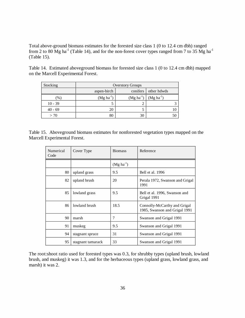
Total above-ground biomass estimates for the forested size class 1 (0 to 12.4 cm dbh) rangedfrom 2 to 80 Mg ha-1 (Table 14), and for the non-forest cover types ranged from 7 to 35 Mg ha-1

(Table 15).

Table 14. Estimated aboveground biomass for forested size class 1 (0 to 12.4 cm dbh) mappedon the Marcell Experimental Forest.

Stocking Overstory Groupsaspen-birch conifers other hdwds

(%) (Mg ha-1) (Mg ha-1) (Mg ha-1) 10 - 39 5 2 3 40 - 69 20 5 10 > 70 80 30 50

Table 15. Aboveground biomass estimates for nonforested vegetation types mapped on theMarcell Experimental Forest.

NumericalCode

Cover Type Biomass Reference

(Mg ha-1)

80 upland grass 9.5 Bell et al. 1996

82 upland brush 20 Perala 1972, Swanson and Grigal1991

85 lowland grass 9.5 Bell et al. 1996, Swanson andGrigal 1991

86 lowland brush 18.5 Connolly-McCarthy and Grigal1985, Swanson and Grigal 1991

90 marsh 7 Swanson and Grigal 1991

91 muskeg 9.5 Swanson and Grigal 1991

94 stagnant spruce 31 Swanson and Grigal 1991

95 stagnant tamarack 33 Swanson and Grigal 1991

The root:shoot ratio used for forested types was 0.3, for shrubby types (upland brush, lowlandbrush, and muskeg) it was 1.3, and for the herbaceous types (upland grass, lowland grass, andmarsh) it was 2.

37

The results indicated an average of 50 Mg ha-1 of C stored in the vegetation of MEF (Table 16).This result, based as described on a categorical analysis, is likely to have high uncertainty.

Table 16. Carbon estimates for vegetation types mapped on the Marcell Experimental Forest,based on a categorical analysis.

Vegetation type Area C C

(ha) (Mg) (Mg ha-1)

aspen 482 32371 67.1

balsam fir 4 197 56.0

birch 26 917 35.3

black ash 3 51 17.8

black spruce 75 1441 19.1

jack pine 23 1553 68.3

lowland brush 17 341 20.2

lowland grass 2 24 13.5

lowland hardwoods 18 1276 69.1

marsh 17 174 10.0

muskeg 103 1071 10.4

northern hardwoods 59 5087 86.1

northern white cedar 7 184 27.9

permanent water 51

red pine 33 969 29.5

stagnant spruce 9 176 19.1

stagnant tamarack 7 150 20.3

tamarack 28 391 13.9

upland grass 3 40 13.5

white spruce 26 140 5.5

Sum 966 46554 49.4a

a Not including area of permanent water

Soil mapping unit

In our first approach to estimating the C content of the soils of the MEF, that using informationwholly in the soil survey report, the nonlinear least squares fit yielded Dbm = 1.54 Mg m-3, andDbo = 0.226 Mg m-3 (R2 = 0.95) (variables as described in Eq. [1]). The Dbm is the upper limit, at

38

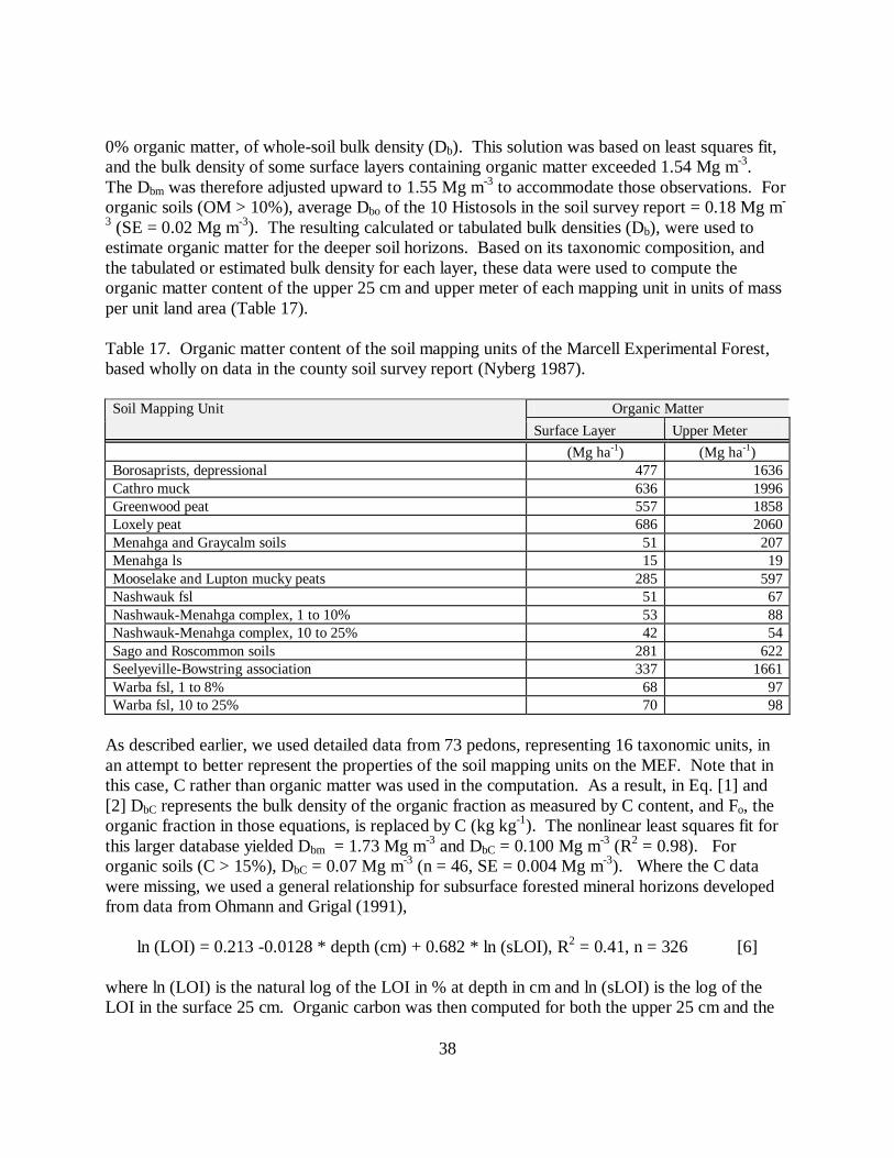
0% organic matter, of whole-soil bulk density (Db). This solution was based on least squares fit,and the bulk density of some surface layers containing organic matter exceeded 1.54 Mg m-3.The Dbm was therefore adjusted upward to 1.55 Mg m-3 to accommodate those observations. Fororganic soils (OM > 10%), average Dbo of the 10 Histosols in the soil survey report = 0.18 Mg m-

3 (SE = 0.02 Mg m-3). The resulting calculated or tabulated bulk densities (Db), were used toestimate organic matter for the deeper soil horizons. Based on its taxonomic composition, andthe tabulated or estimated bulk density for each layer, these data were used to compute theorganic matter content of the upper 25 cm and upper meter of each mapping unit in units of massper unit land area (Table 17).

Table 17. Organic matter content of the soil mapping units of the Marcell Experimental Forest,based wholly on data in the county soil survey report (Nyberg 1987).

Organic MatterSoil Mapping UnitSurface Layer Upper Meter

(Mg ha-1) (Mg ha-1)Borosaprists, depressional 477 1636Cathro muck 636 1996Greenwood peat 557 1858Loxely peat 686 2060Menahga and Graycalm soils 51 207Menahga ls 15 19Mooselake and Lupton mucky peats 285 597Nashwauk fsl 51 67Nashwauk-Menahga complex, 1 to 10% 53 88Nashwauk-Menahga complex, 10 to 25% 42 54Sago and Roscommon soils 281 622Seelyeville-Bowstring association 337 1661Warba fsl, 1 to 8% 68 97Warba fsl, 10 to 25% 70 98

As described earlier, we used detailed data from 73 pedons, representing 16 taxonomic units, inan attempt to better represent the properties of the soil mapping units on the MEF. Note that inthis case, C rather than organic matter was used in the computation. As a result, in Eq. [1] and[2] DbC represents the bulk density of the organic fraction as measured by C content, and Fo, theorganic fraction in those equations, is replaced by C (kg kg-1). The nonlinear least squares fit forthis larger database yielded Dbm = 1.73 Mg m-3 and DbC = 0.100 Mg m-3 (R2 = 0.98). Fororganic soils (C > 15%), DbC = 0.07 Mg m-3 (n = 46, SE = 0.004 Mg m-3). Where the C datawere missing, we used a general relationship for subsurface forested mineral horizons developedfrom data from Ohmann and Grigal (1991),

ln (LOI) = 0.213 -0.0128 * depth (cm) + 0.682 * ln (sLOI), R2 = 0.41, n = 326 [6]

where ln (LOI) is the natural log of the LOI in % at depth in cm and ln (sLOI) is the log of theLOI in the surface 25 cm. Organic carbon was then computed for both the upper 25 cm and the

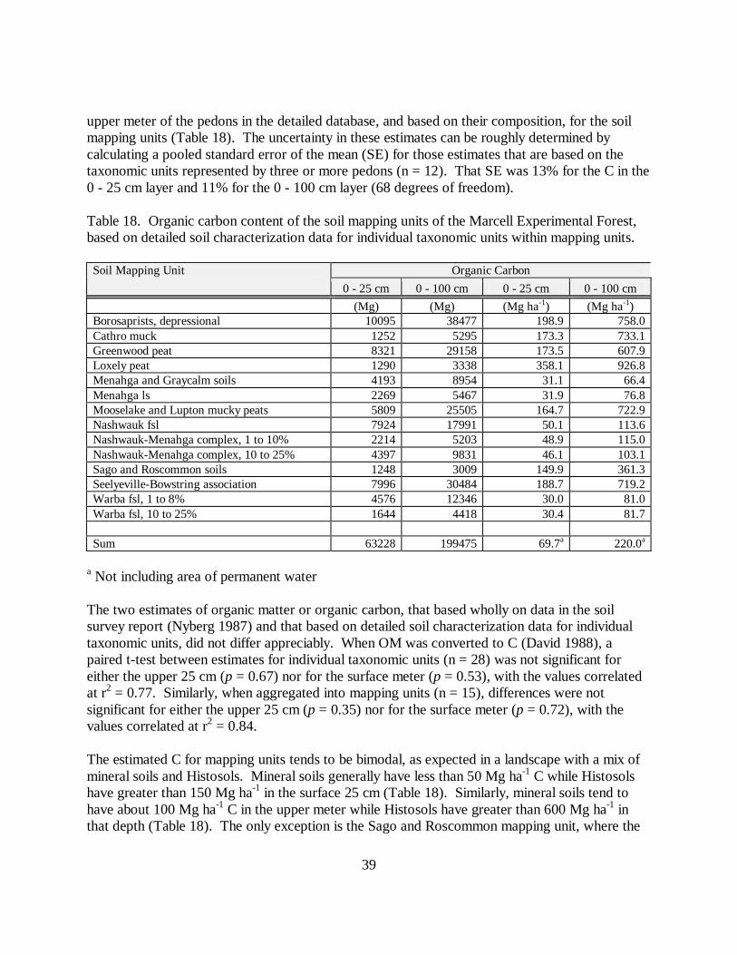
39

upper meter of the pedons in the detailed database, and based on their composition, for the soilmapping units (Table 18). The uncertainty in these estimates can be roughly determined bycalculating a pooled standard error of the mean (SE) for those estimates that are based on thetaxonomic units represented by three or more pedons (n = 12). That SE was 13% for the C in the0 - 25 cm layer and 11% for the 0 - 100 cm layer (68 degrees of freedom).

Table 18. Organic carbon content of the soil mapping units of the Marcell Experimental Forest,based on detailed soil characterization data for individual taxonomic units within mapping units.

Organic CarbonSoil Mapping Unit0 - 25 cm 0 - 100 cm 0 - 25 cm 0 - 100 cm

(Mg) (Mg) (Mg ha-1) (Mg ha-1)Borosaprists, depressional 10095 38477 198.9 758.0Cathro muck 1252 5295 173.3 733.1Greenwood peat 8321 29158 173.5 607.9Loxely peat 1290 3338 358.1 926.8Menahga and Graycalm soils 4193 8954 31.1 66.4Menahga ls 2269 5467 31.9 76.8Mooselake and Lupton mucky peats 5809 25505 164.7 722.9Nashwauk fsl 7924 17991 50.1 113.6Nashwauk-Menahga complex, 1 to 10% 2214 5203 48.9 115.0Nashwauk-Menahga complex, 10 to 25% 4397 9831 46.1 103.1Sago and Roscommon soils 1248 3009 149.9 361.3Seelyeville-Bowstring association 7996 30484 188.7 719.2Warba fsl, 1 to 8% 4576 12346 30.0 81.0Warba fsl, 10 to 25% 1644 4418 30.4 81.7

Sum 63228 199475 69.7a 220.0a

a Not including area of permanent water

The two estimates of organic matter or organic carbon, that based wholly on data in the soilsurvey report (Nyberg 1987) and that based on detailed soil characterization data for individualtaxonomic units, did not differ appreciably. When OM was converted to C (David 1988), apaired t-test between estimates for individual taxonomic units (n = 28) was not significant foreither the upper 25 cm (p = 0.67) nor for the surface meter (p = 0.53), with the values correlatedat r2 = 0.77. Similarly, when aggregated into mapping units (n = 15), differences were notsignificant for either the upper 25 cm (p = 0.35) nor for the surface meter (p = 0.72), with thevalues correlated at r2 = 0.84.

The estimated C for mapping units tends to be bimodal, as expected in a landscape with a mix ofmineral soils and Histosols. Mineral soils generally have less than 50 Mg ha-1 C while Histosolshave greater than 150 Mg ha-1 in the surface 25 cm (Table 18). Similarly, mineral soils tend tohave about 100 Mg ha-1 C in the upper meter while Histosols have greater than 600 Mg ha-1 inthat depth (Table 18). The only exception is the Sago and Roscommon mapping unit, where the

40

major taxonomic components are Histic and Mollic Aquepts, respectively. These wet mineralsoils with surface organic accumulations group with the Histosols in the surface 25 cm, but havereduced organic matter in deeper horizons and so fall between mineral and organic soils at 100cm (Table 18).

When the data are extrapolated to the entire landscape of MEF, it illustrates the importance ofthe organic soils in influencing landscape total C storage. The overall C mass in Mg ha-1, even inthe 0 to 25 cm layer, is higher than that of all vegetation strata both above- and below-ground.When deeper soil layers are considered, then differences are even greater.

Laboratory

C vs. LOI

Laboratory duplicate analyses for LOI were run on 89 pairs of samples; 23 of forest floor, 49 ofmineral, and 17 of peat. The mean LOI of those 178 samples (89 x 2 per pair) was 32.0%, with apooled within-pair standard deviation of 4.2% and a pooled coefficient of variation of 0.13%. Inthe case of C, duplicates were run on 25 pairs of samples; 8 of forest floor, 10 of mineral, and 7of peat. In this case the mean C of those 50 samples was 16.2%, with a pooled within-pairstandard deviation of 1.0% and a pooled coefficient of variation of 0.06%.

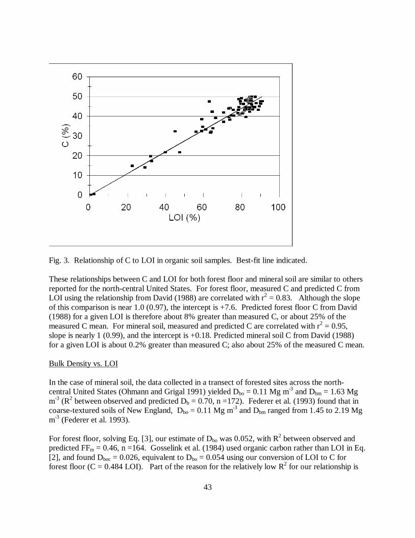
We combined the LOI and C data for forest floor, peat, and mineral soil from both the MEF andthe site of the companion study (Bell et al. 1996, Bell et al. 2000). Simple linear regressionswere developed for each sample type, where x = LOI (%) and y = C (%). The results were

FF C (%) = 0.45 * LOI (%) + 2.21, n = 129, r2 = 0.84,. [7]

Peat C (%) = 0.53 * LOI (%) + 1.94, n = 82, r2 = 0.91, and [8]

Min C (%) = 0.50 * LOI (%) - 0.15, n = 229, r2 = 0.95 (Fig. 1). [9]

41

Fig. 1. Relationship of C to LOI in mineral soil samples. Best-fit line indicated.

For peat, the y-intercept was not significantly different than 0, and for forest floor, it wasmarginally significant (at about the 5% probability). Both those regressions were re-run, forcingthe intercept through 0. The results were:

FF C (%) = 0.484 * LOI (%), n = 129, with r2 = 0.84 (Fig. 2), and [10]

Peat C (%) = 0.55 * LOI (%), n = 82, with r2 = 0.91 (Fig. 3). [11]

42

Fig. 2. Relationship of C to LOI in forest floor samples. Best-fit line indicated.

43

Fig. 3. Relationship of C to LOI in organic soil samples. Best-fit line indicated.

These relationships between C and LOI for both forest floor and mineral soil are similar to othersreported for the north-central United States. For forest floor, measured C and predicted C fromLOI using the relationship from David (1988) are correlated with r2 = 0.83. Although the slopeof this comparison is near 1.0 (0.97), the intercept is +7.6. Predicted forest floor C from David(1988) for a given LOI is therefore about 8% greater than measured C, or about 25% of themeasured C mean. For mineral soil, measured and predicted C are correlated with r2 = 0.95,slope is nearly 1 (0.99), and the intercept is +0.18. Predicted mineral soil C from David (1988)for a given LOI is about 0.2% greater than measured C; also about 25% of the measured C mean.

Bulk Density vs. LOI

In the case of mineral soil, the data collected in a transect of forested sites across the north-central United States (Ohmann and Grigal 1991) yielded Dbo = 0.11 Mg m-3 and Dbm = 1.63 Mgm-3 (R2 between observed and predicted Db = 0.70, n =172). Federer et al. (1993) found that incoarse-textured soils of New England, Dbo = 0.11 Mg m-3 and Dbm ranged from 1.45 to 2.19 Mgm-3 (Federer et al. 1993).

For forest floor, solving Eq. [3], our estimate of Dbo was 0.052, with R2 between observed andpredicted FFm = 0.46, n =164. Gosselink et al. (1984) used organic carbon rather than LOI in Eq.[2], and found Dboc = 0.026, equivalent to Dbo = 0.054 using our conversion of LOI to C forforest floor (C = 0.484 LOI). Part of the reason for the relatively low R2 for our relationship is

44

because FFm is a function of both Db and thickness (T) and variations in both contribute touncertainty. Within-plot variation in T was high, with a pooled coefficient of variation of about42%, based on 3 measurements per point on 164 points.

Our estimate of Dbo for surface peat (< 50 cm depth) (using Eq. [2]) was 0.069 with R2 betweenobserved and predicted = 0.11, n =157, and for subsurface peat (> 50 cm depth) Dbo was 0.092with R2 between observed and predicted Db = 0.23, n =104. The high variability in therelationship between LOI and Db is commonly observed. For example, Nichols and Boelter(1984) found an r2 of 0.17 for the linear relationship between ash content (= 1 - LOI) and Db for176 samples of peat collected from 38 peatlands from the north central U.S. They found that Dbovaried with the particle-size distribution of peat fibers. The Dbos that we determined for surfaceand subsurface peat were significantly different (95% confidence intervals did not overlap) andreflect the influence of compaction leading to higher densities in subsurface peats. A similardifference was recognized by Grigal et al. (1989). Though they used a different nonlinearrelationship between LOI and Db, they also found that subsurface peat had higher Db forequivalent LOI. If their nonlinear relationship is solved using Eq. [2], Dbo for surface peat is0.061 and for subsurface peat is 0.099, very similar to the values that we determined.

In addition to collecting samples for LOI determination at our intensive sampling points, we alsoestimated the Von Post humification class (Malterer et al. 1992). The Db calculated from themean LOI of each humification class was closely related to the tabulated Db for each class(Malterer et al. 1992) (r2 = 0.92), with an intercept of 0.02 and slope of 1.04 for surface and anintercept of 0.03 and slope of 1.38 for subsurface peat (Fig. 4). We therefore consider ourestimates of mass for organic soils to be reasonable.

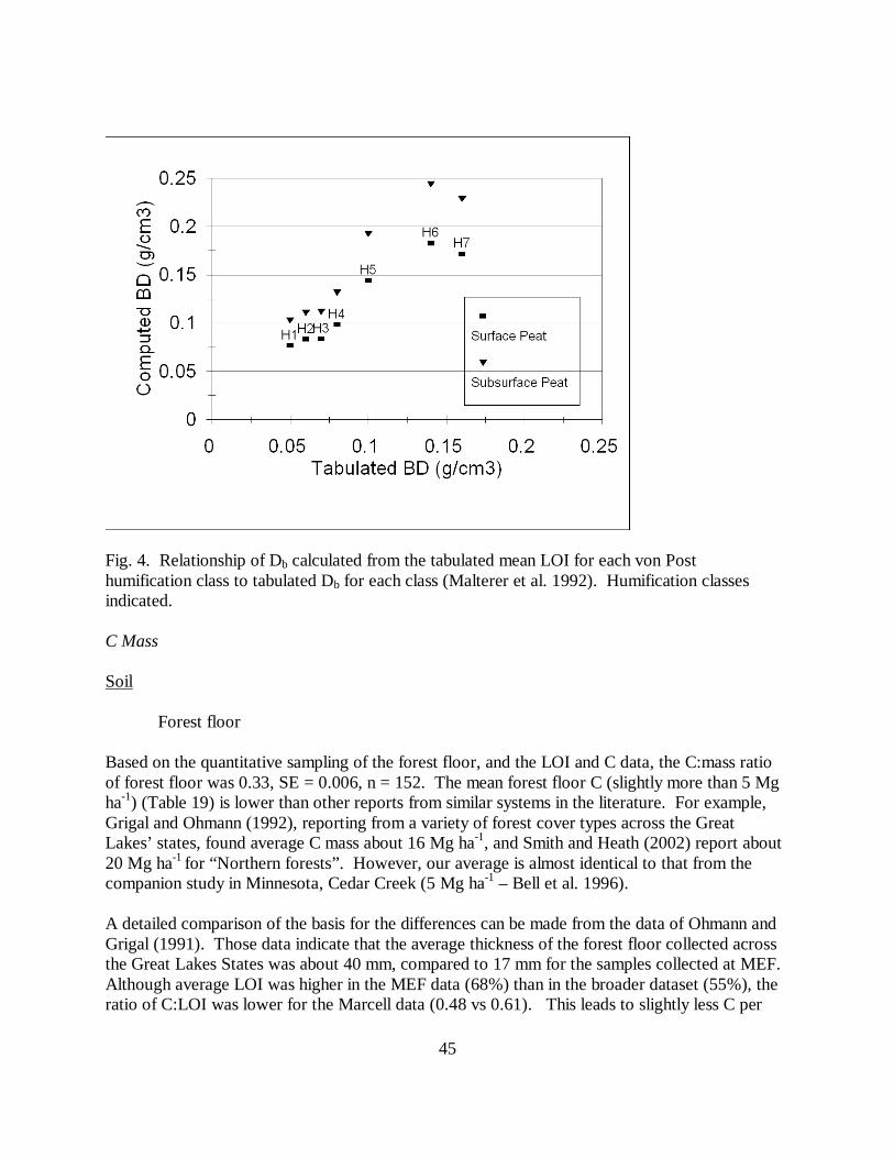
45

Fig. 4. Relationship of Db calculated from the tabulated mean LOI for each von Posthumification class to tabulated Db for each class (Malterer et al. 1992). Humification classesindicated.

C Mass

Soil

Forest floor

Based on the quantitative sampling of the forest floor, and the LOI and C data, the C:mass ratioof forest floor was 0.33, SE = 0.006, n = 152. The mean forest floor C (slightly more than 5 Mgha-1) (Table 19) is lower than other reports from similar systems in the literature. For example,Grigal and Ohmann (1992), reporting from a variety of forest cover types across the GreatLakes’ states, found average C mass about 16 Mg ha-1, and Smith and Heath (2002) report about20 Mg ha-1 for “Northern forests”. However, our average is almost identical to that from thecompanion study in Minnesota, Cedar Creek (5 Mg ha-1 – Bell et al. 1996).

A detailed comparison of the basis for the differences can be made from the data of Ohmann andGrigal (1991). Those data indicate that the average thickness of the forest floor collected acrossthe Great Lakes States was about 40 mm, compared to 17 mm for the samples collected at MEF.Although average LOI was higher in the MEF data (68%) than in the broader dataset (55%), theratio of C:LOI was lower for the Marcell data (0.48 vs 0.61). This leads to slightly less C per

46

unit mass of forest floor at MEF than in the broader dataset. The most important reason for thedifference in C mass between the two datasets, however, is the difference in thickness.

Table 19. C mass of soil variables from intensive points sampled on Marcell ExperimentalForest.

VariableMineral C Peat

Descriptor UnitsForest floor

0 - 25 cm 0 - 100 cmAll pointsn 152 161 161 113mean (Mg ha-1) 5.31 34.36 115.23 962.60std dev (Mg ha-1) 3.75 9.62 35.99 751.57

Basis of equationsn 137 146 146mean (Mg ha-1) 5.27 34.56 116.70std dev (Mg ha-1) 3.64 9.58 36.16R2 0.64 0.42 0.29s y.x (Mg ha-1) 2.23 7.41 31.12

Check of equationsn 15 15 15mean (Mg ha-1) 5.72 32.43 100.94std dev (Mg ha-1) 4.80 10.22 31.93r2 0.30 0.60 0.45s y.x (Mg ha-1) 4.17 6.68 24.55

The extrapolation of the forest floor C mass from the intensive to the reconnaissance points wasbased on the variables that we had for each point, including C mass per unit area (intensivepoints), slope gradient, aspect code, profile curvature (perpendicular to the contour), planarcurvature (parallel to contour), position on slope, forest floor thickness (3 observations onintensive points, one on reconnaissance points), conifer tree basal area, and broadleaf tree basalarea.

In the preliminary analysis, planar curvature (p = 0.97), position on slope (p = 0.22), andbroadleaf tree basal area.(p = 0.16) were not significant predictor variables. The remainingvariables were significant, and the final regression had an R2 = 0.64 (Table 19). For the randomsubsample used to evaluate uncertainty, the correlation between the observed and predicted Cwas r2 = 0.30 (Table 19). A paired t-test indicated no significant difference (p = 0.45) betweenthe observed and predicted forest floor C of that subsample (n = 15).

The influence of the landscape attributes on forest floor was somewhat straightforward. Aswould be expected, forest floor mass increased with its thickness, with an increase in conifer tree

47

basal area, and with a decrease in slope gradient. As less expected, warmer aspects (toward thesouthwest) had greater forest floor mass, and the greatest mass was found where profilecurvature was convex, less where flat, and least where it was concave (Table 20). Althoughsome of these relationships are contrary to accepted paradigms, they may have rationalexplanations. For example, the decline of forest floor mass as the profile curvature becomesmore concave may be associated with its increased incorporation into the surface mineral soil atthose positions. Other relationships may simply be due to the idiosyncracies of these data.

Table 20. Independent variables and multipliers used to extrapolate C from intensive toreconnaissance sample points.

Dependent VariableIndependentVariable

CategoryFFC SURFC SUMMINC

CONSTANT 2.11404 20.03691 79.12565A THICK 0 1.74934 3.86738FF THICK 2.34652 2.57550 6.26430SLOPE -0.08497 0 0ASPECT CODE 1.06827 0 0CONIFER BA 0.14723 -0.34956 -1.26828SLOPE POSa L 0 6.63870 29.24091SLOPE POSa M 0 0.67222 4.13547SLOPE POSa U 0 0 0PROF CURVb F -1.60952 0 0PROF CURVb V -2.16793 0 0PROF CURVb X 0 0 0

a Position on slope (L= lower, M = midddle, U = upper)b Profile curvature; perpendicular to the contour (F = flat, V = concave, X = convex)

Mineral soil

As was the case with forest floor, our estimate of mineral soil C to 100 cm (115 Mg ha-1) (Table19) is lower than the reports for similar soils from Gailbraith et al. (2003), Grigal and Ohmann(1992), and Johnson and Kern (2003) (almost 125 Mg ha-1). Our estimate is higher, however,than that from the companion study in Minnesota, Cedar Creek (40 Mg ha-1 – Bell et al. 1996).Consistent with that lower overall mass, our estimate for C mass in surface soil (34 Mg ha-1)(Table 19) is also lower than that based on reports of similar soils (about 65 Mg ha-1 – Grigaland Ohmann 1992, Johnson and Kern 2003). Our surface estimate was slightly lower than themean of the mineral soil mapping units on MEF based on detailed data (38 Mg ha-1) , but our Csum to 100 cm was slightly higher (mapping units = 91 Mg ha-1) (Table 18). It appears thatthese forest soils, on the western edge of the eastern forests, have low soil C.

The extrapolation of the mineral soil C mass from the intensive to the reconnaissance points wasbased on the same variables that we used for extrapolation of forest floor C. In the preliminary

48

analysis, profile curvature (p = 0.25 for surface soil and p = 0.51 for 0 - 100 cm), planarcurvature (p = 0.16 for surface and p = 0.11 for 0 - 100 cm), broadleaf tree basal area (p = 0.47for surface and p = 0.92 for 0 - 100 cm), aspect code (p = 0.69 for surface and p = 0.72 for 0 -100 cm), and slope gradient (p = 0.11 for surface and p = 0.82 for 0 - 100 cm) were notsignificant predictor variables. The remaining variables were significant, and the final regressionfor surface soil had an R2 = 0.42 (Table 19). For the random subsample used to evaluateuncertainty, the correlation between the observed and predicted C was r2 = 0.60 (Table 19). Apaired t-test indicated no significant difference (p = 0.51) between the observed and predicted Cof that subsample (n = 15). For the sum of mineral C to 100 cm, the final regression had an R2 =0.29 (Table 19) and the correlation between the observed and predicted C for the randomsubsample was r2 = 0.45 (Table 19). A paired t-test indicated no significant difference (p = 0.15)between the observed and predicted C of the random subsample (n = 15).

The influence of the landscape attributes on mineral soil C was somewhat straightforward. Aswould be expected, mineral C mass increased with A thickness and was lowest in upper slopepositions, increasing downslope. Mineral C mass also increased with forest floor thickness anddecreased with increase in conifer tree basal area (Table 20). The increase with forest floorthickness is interesting but inexplicable. There was no relationship between forest floorthickness and A thickness (r2 = 0.01) so they are not simply positively-related covariables. Thedecrease in mineral C mass with increase in conifer basal area may be related to a generaltendency for conifers to occur on coarser-textured soils than broadleaf deciduous trees. It mayalso be related to the positive relationship of forest floor C mass with conifer basal area; moreforest floor C may be associated with less mineral C. Or the relationships may simply be due tothe idiosyncracies of these data.

Peat

As with mineral soil, calculation of C mass of peat requires C concentration, bulk density, andthickness. However, because C concentration was directly related to LOI (Eq. [11]) and bulkdensity was inversely related to LOI (Eq. [2]), the consequence of the two relationships is that Ccontent is a direct function of LOI and thickness. These relationships were used to calculate Cmass for all points with organic soils. Carbon mass of surface peat (< 50 cm depth) was 3.80 Mgha-1 cm-1 and of subsurface peat (> 50 cm depth) was 5.06 Mg ha-1 cm-1.

In contrast to C mass in both forest floor and mineral soil, our estimates of C mass in peat (about960 Mg ha-1 – Table 19) are in the range of most literature values. Our estimates, however, arefor mass from the surface to contact with the mineral substrate, which averaged about 200 cm.Our estimate of C mass to 100 cm is approximately 445 Mg ha-1. Gailbraith et al. (2003), innorthern New York, only reported about 200 Mg ha-1 to 100 cm in Histosols, while Johnson andKern (2003) reported 830 Mg ha-1 to 100 cm from the NRCS database. Our estimate is lowerthan that from the companion study in Minnesota, Cedar Creek (630 Mg ha-1 to 100 cm – Bell etal. 1996). Our estimate is also lower than the mean of the organic soil mapping units on MEF,based on detailed data (590 Mg ha-1 to 100 cm) (Table 18). It appears that these northern

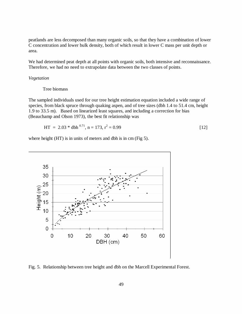
49

peatlands are less decomposed than many organic soils, so that they have a combination of lowerC concentration and lower bulk density, both of which result in lower C mass per unit depth orarea.

We had determined peat depth at all points with organic soils, both intensive and reconnaissance.Therefore, we had no need to extrapolate data between the two classes of points.

Vegetation

Tree biomass

The sampled individuals used for our tree height estimation equation included a wide range ofspecies, from black spruce through quaking aspen, and of tree sizes (dbh 1.4 to 51.4 cm, height1.9 to 33.5 m). Based on linearized least squares, and including a correction for bias(Beauchamp and Olson 1973), the best fit relationship was

HT = 2.03 * dbh 0.71, n = 173, r2 = 0.99 [12]

where height (HT) is in units of meters and dbh is in cm (Fig 5).

Fig. 5. Relationship between tree height and dbh on the Marcell Experimental Forest.

50

Our expression of root mass as a function of tree dbh was the average of the literature sources,yielding

ROOT = 0.031 * dbh 2.39,

where ROOT is root biomass in kg and dbh is in cm (Fig. 6). The relationship conformedrelatively closely to the literature relationships (Fig. 6). Goodness of fit statistics are not relevantfor this equation because it is simply a average of other relationships.

Fig. 6. Root mass as a function of tree dbh, with data from Perala and Alban (1994), Santantonioet al. (1977), and Whittaker and Marks (1975), and the average of those relationships.

Understory biomass

The understory estimation equations, where biomass of the understory was a function of theconifer and the deciduous overstory biomass, with cover type as a dummy variable, were allhighly significant (Table 21).

51

Table 21. Understory estimation equations and basic statistics used on Marcell ExperimentalForest. Estimates in units of kg ha-1.

IndependentVariable

Category Dependent Variable

Herb Shrub GroundCover

CONSTANT 560.540 1110.201 1312.904CONIFER BA -4.687 -6.255 -3.136DECID BA -1.693 -0.937 -6.870COVER TYPE AB 151.704 1566.797 237.122

BS 991.573 -340.866 3405.001GR 2276.742 544.799 -118.230LC 1146.398 2042.110 2232.669LH 808.574 586.941 -1.464OB 1714.758 -928.618 4081.574PI 502.873 1064.341 698.963SF 182.806 1118.949 547.550SH 1099.586 4925.412 272.118UH 0 0 0

R2 0.67 0.32 0.50F 84.1 18.6 38.7Sy.x (kg ha-1) 574.9 2195.0 1552.5

Number of obs 436 436 436Mean (kg ha-1) 1118.9 2040.9 2150.6SE (kg ha-1) 48.5 126.3 103.9

Because we had a tree inventory for all points, both reconnaissance and intensive, we had alarger dataset for tree biomass than for soils. The data indicated a mean biomass C of about 51Mg ha-1 (Table 22). This is very near the areally-weighted mean C based on the vegetationcover-type map (50 Mg ha-1 – Table 16). Of course, one estimate is based on tabular materialand maps, and the other on a sample of points with collection of continuous data, but thecorrespondence is heartening.

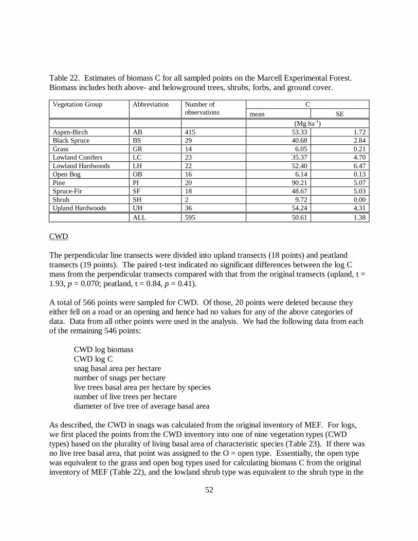
52

Table 22. Estimates of biomass C for all sampled points on the Marcell Experimental Forest.Biomass includes both above- and belowground trees, shrubs, forbs, and ground cover.

CVegetation Group Abbreviation Number ofobservations mean SE

(Mg ha-1)Aspen-Birch AB 415 53.33 1.72Black Spruce BS 29 40.68 2.84Grass GR 14 6.05 0.21Lowland Conifers LC 23 35.37 4.70Lowland Hardwoods LH 22 52.40 6.47Open Bog OB 16 6.14 0.13Pine PI 20 90.21 5.07Spruce-Fir SF 18 48.67 5.03Shrub SH 2 9.72 0.00Upland Hardwoods UH 36 54.24 4.31

ALL 595 50.61 1.38

CWD

The perpendicular line transects were divided into upland transects (18 points) and peatlandtransects (19 points). The paired t-test indicated no significant differences between the log Cmass from the perpendicular transects compared with that from the original transects (upland, t =1.93, p = 0.070; peatland, t = 0.84, p = 0.41).

A total of 566 points were sampled for CWD. Of those, 20 points were deleted because theyeither fell on a road or an opening and hence had no values for any of the above categories ofdata. Data from all other points were used in the analysis. We had the following data from eachof the remaining 546 points:

CWD log biomassCWD log Csnag basal area per hectarenumber of snags per hectarelive trees basal area per hectare by speciesnumber of live trees per hectarediameter of live tree of average basal area

As described, the CWD in snags was calculated from the original inventory of MEF. For logs,we first placed the points from the CWD inventory into one of nine vegetation types (CWDtypes) based on the plurality of living basal area of characteristic species (Table 23). If there wasno live tree basal area, that point was assigned to the O = open type. Essentially, the open typewas equivalent to the grass and open bog types used for calculating biomass C from the originalinventory of MEF (Table 22), and the lowland shrub type was equivalent to the shrub type in the

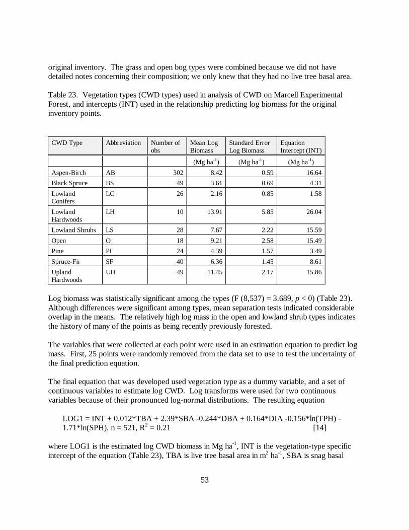
53

original inventory. The grass and open bog types were combined because we did not havedetailed notes concerning their composition; we only knew that they had no live tree basal area.

Table 23. Vegetation types (CWD types) used in analysis of CWD on Marcell ExperimentalForest, and intercepts (INT) used in the relationship predicting log biomass for the originalinventory points.

CWD Type Abbreviation Number ofobs

Mean LogBiomass

Standard ErrorLog Biomass

EquationIntercept (INT)

(Mg ha-1) (Mg ha-1) (Mg ha-1)Aspen-Birch AB 302 8.42 0.59 16.64Black Spruce BS 49 3.61 0.69 4.31LowlandConifers

LC 26 2.16 0.85 1.58

LowlandHardwoods

LH 10 13.91 5.85 26.04

Lowland Shrubs LS 28 7.67 2.22 15.59Open O 18 9.21 2.58 15.49Pine PI 24 4.39 1.57 3.49Spruce-Fir SF 40 6.36 1.45 8.61UplandHardwoods

UH 49 11.45 2.17 15.86

Log biomass was statistically significant among the types (F (8,537) = 3.689, p < 0) (Table 23).Although differences were significant among types, mean separation tests indicated considerableoverlap in the means. The relatively high log mass in the open and lowland shrub types indicatesthe history of many of the points as being recently previously forested.

The variables that were collected at each point were used in an estimation equation to predict logmass. First, 25 points were randomly removed from the data set to use to test the uncertainty ofthe final prediction equation.

The final equation that was developed used vegetation type as a dummy variable, and a set ofcontinuous variables to estimate log CWD. Log transforms were used for two continuousvariables because of their pronounced log-normal distributions. The resulting equation

LOG1 = INT + 0.012*TBA + 2.39*SBA -0.244*DBA + 0.164*DIA -0.156*ln(TPH) -1.71*ln(SPH), n = 521, R2 = 0.21 [14]

where LOG1 is the estimated log CWD biomass in Mg ha-1, INT is the vegetation-type specificintercept of the equation (Table 23), TBA is live tree basal area in m2 ha-1, SBA is snag basal

54

area in m2 ha-1, DBA is basal area of live deciduous trees per ha, DIA diameter of the live tree ofmean basal area in cm, ln(TPH) is the natural logarithm of the number of trees per ha, andln(SPH) is the natural logarithm of the number of snags per hectare. Equation [14] had astandard error within vegetation types of 3.4 Mg ha-1.

Examination of the predicted versus observed mass, however, indicated that points with highobserved log mass were especially underpredicted (because of the weighting of the equation bythe relatively large number of points with no or very low CWD). In order to account for some ofthis deviation, a simple quadratic equation was fitted using the predicted CWD as theindependent variable and the observed CWD as the dependent variable. Although there wassome improvement in the fit to the data, the minima of the relationship was at 1.7 Mg ha-1 (thatis, the minimum predicted mass was > 0). The quadratic was then recomputed with a 0 intercept,with a resulting relationship

LOG = 0.628 LOG1 + 0.015 LOG12, R2 = 0.24, n = 521, [15]

where LOG is estimated log CWD biomass in Mg ha-1 and LOG1 is the preliminary estimatefrom Eq. [14] (Fig. 7). Equation [15] had with a standard error within vegetation types of 3.3Mg ha-1.

55

Fig. 7. Observed versus predicted mass of log CWD from CWD inventory of MarcellExperimental Forest. Predictions based on Eq. [14] and Eq. [15].

That relationship was then tested against the 25 observations that had been randomly removedfrom the data set. The equation(s) explained 33% of the variation in those data.

The resulting relationships (Eq. [14] and [15]) were therefore used to predict log mass for theoriginal Marcell inventory points. Because some points in that inventory had no live tree norsnag basal area, application of Eq. [14] resulted in the estimated log CWD equal to the INT(Table 24). In an attempt to more accurately estimate log CWD in those cases, we calculated themean log CWD by CWD type of all points without snags or live trees in the CWD inventory.The overall mean log CWD biomass on those points was 22.3 Mg ha-1, indicating that in manycases lack of standing live or dead trees was a transitory phenomenon. We used the average ofthose two estimates (intercept and mean) by CWD type, and considered that value to be theestimated log biomass CWD for those points without standing trees or snags.

The equations (Eq. [14] and [15]) for log CWD resulted in estimates of biomass, not C. We hadboth log biomass and log C for individual points. We ran an analysis of variance to determine ifthe ratio of biomass to C differed among CWD types. It did (F (8,493) = 2.010, p = 0.043) sothe appropriate ratio for each type was used to convert log CWD biomass to log CWD C. Theresulting estimates of C mass in CWD fell within the literature values (Table 24).

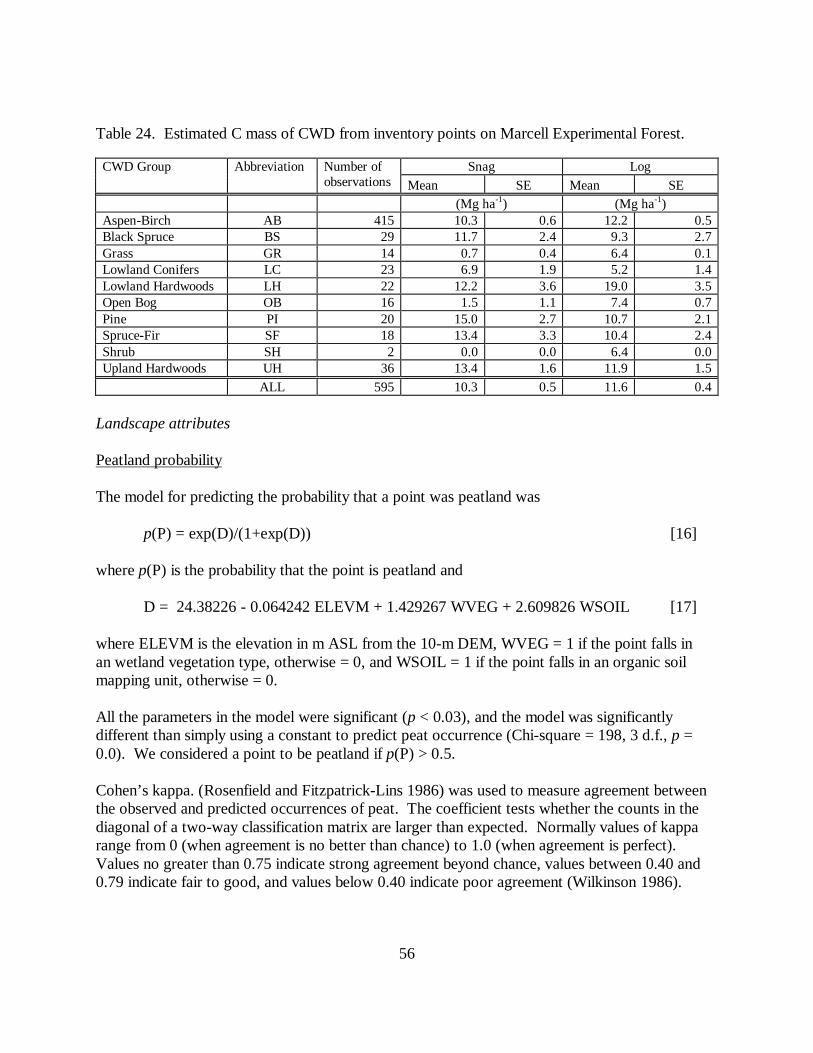
56

Table 24. Estimated C mass of CWD from inventory points on Marcell Experimental Forest.

Snag LogCWD Group Abbreviation Number ofobservations Mean SE Mean SE

(Mg ha-1) (Mg ha-1)Aspen-Birch AB 415 10.3 0.6 12.2 0.5Black Spruce BS 29 11.7 2.4 9.3 2.7Grass GR 14 0.7 0.4 6.4 0.1Lowland Conifers LC 23 6.9 1.9 5.2 1.4Lowland Hardwoods LH 22 12.2 3.6 19.0 3.5Open Bog OB 16 1.5 1.1 7.4 0.7Pine PI 20 15.0 2.7 10.7 2.1Spruce-Fir SF 18 13.4 3.3 10.4 2.4Shrub SH 2 0.0 0.0 6.4 0.0Upland Hardwoods UH 36 13.4 1.6 11.9 1.5

ALL 595 10.3 0.5 11.6 0.4

Landscape attributes

Peatland probability

The model for predicting the probability that a point was peatland was

p(P) = exp(D)/(1+exp(D)) [16]

where p(P) is the probability that the point is peatland and

D = 24.38226 - 0.064242 ELEVM + 1.429267 WVEG + 2.609826 WSOIL [17]

where ELEVM is the elevation in m ASL from the 10-m DEM, WVEG = 1 if the point falls inan wetland vegetation type, otherwise = 0, and WSOIL = 1 if the point falls in an organic soilmapping unit, otherwise = 0.

All the parameters in the model were significant (p < 0.03), and the model was significantlydifferent than simply using a constant to predict peat occurrence (Chi-square = 198, 3 d.f., p =0.0). We considered a point to be peatland if p(P) > 0.5.

Cohen’s kappa. (Rosenfield and Fitzpatrick-Lins 1986) was used to measure agreement betweenthe observed and predicted occurrences of peat. The coefficient tests whether the counts in thediagonal of a two-way classification matrix are larger than expected. Normally values of kapparange from 0 (when agreement is no better than chance) to 1.0 (when agreement is perfect).Values no greater than 0.75 indicate strong agreement beyond chance, values between 0.40 and0.79 indicate fair to good, and values below 0.40 indicate poor agreement (Wilkinson 1986).

57

Kappa between observed and predicted occurrences of peat for the large data set that was thebasis of the model was 0.644, and for the 50-point test data set was 0.555. Presence of anorganic soil mapping unit had the strongest statistical influence on the prediction of peatoccurrence.

Forested probability

As described, we considered a point to be open (non-forested) if live tree basal area was < 5 m2

ha-1. The input data did not include tree basal area, but did include living tree biomass for eachpoint. We developed a relationship between aboveground biomass and basal area,

AGTREC (Mg ha-1) = -4.057 + 2.311 BA (m2 ha-1), n = 595, r2 = 0.81 [18]

where AGTREC is aboveground tree C and BA is stand basal area.

Based on Eq. [18], a basal area of < 5 m2 ha-1 was equivalent to < 7.5 Mg ha-1 of abovegroundtree C.

The model predicting probability of a point being non-forested (< 7.5 Mg ha-1 aboveground treeC) was similar to that for peatland Eq. [16], but in this case

D = 2.918 + (categorical variable values) [19]

where the appropriate categorical variable values are as defined in Table 25.

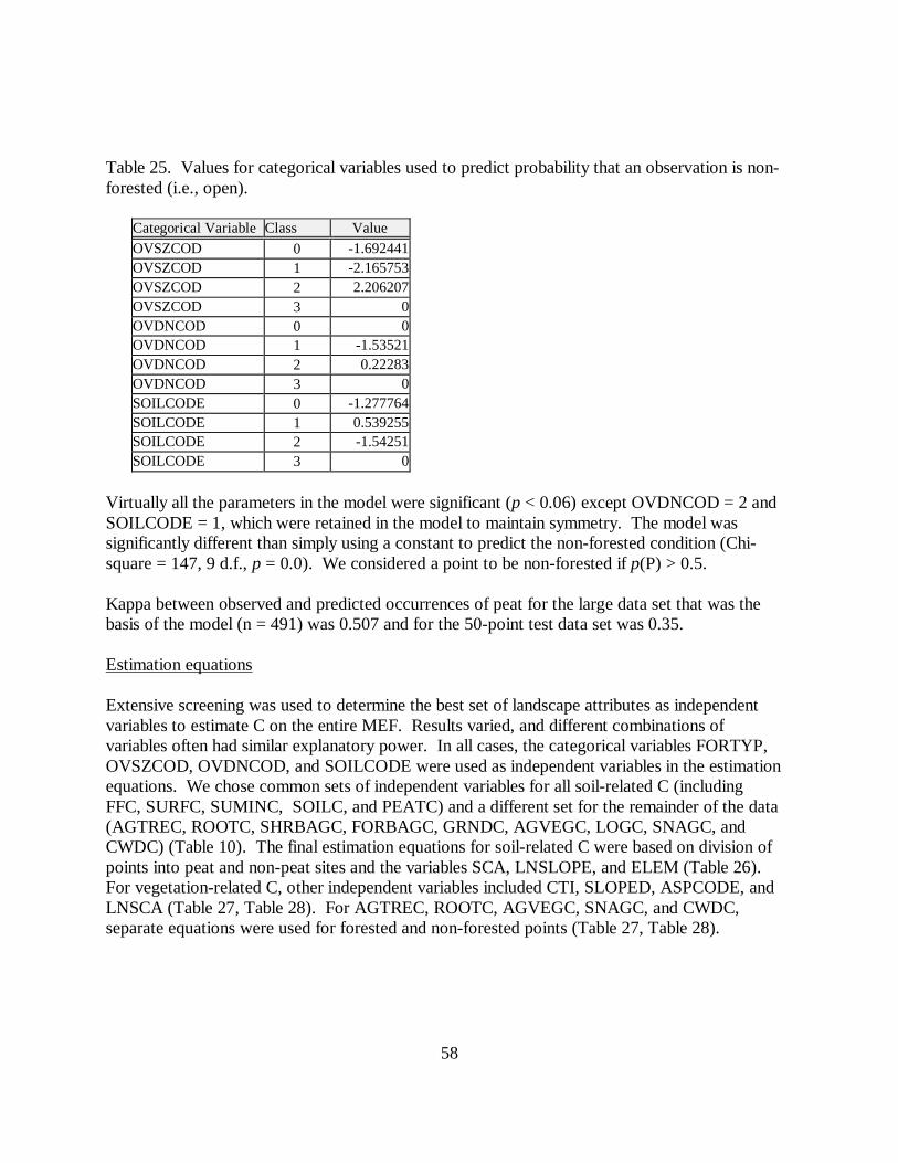
58

Table 25. Values for categorical variables used to predict probability that an observation is non-forested (i.e., open).

Categorical Variable Class ValueOVSZCOD 0 -1.692441OVSZCOD 1 -2.165753OVSZCOD 2 2.206207OVSZCOD 3 0OVDNCOD 0 0OVDNCOD 1 -1.53521OVDNCOD 2 0.22283OVDNCOD 3 0SOILCODE 0 -1.277764SOILCODE 1 0.539255SOILCODE 2 -1.54251SOILCODE 3 0

Virtually all the parameters in the model were significant (p < 0.06) except OVDNCOD = 2 andSOILCODE = 1, which were retained in the model to maintain symmetry. The model wassignificantly different than simply using a constant to predict the non-forested condition (Chi-square = 147, 9 d.f., p = 0.0). We considered a point to be non-forested if p(P) > 0.5.

Kappa between observed and predicted occurrences of peat for the large data set that was thebasis of the model (n = 491) was 0.507 and for the 50-point test data set was 0.35.

Estimation equations

Extensive screening was used to determine the best set of landscape attributes as independentvariables to estimate C on the entire MEF. Results varied, and different combinations ofvariables often had similar explanatory power. In all cases, the categorical variables FORTYP,OVSZCOD, OVDNCOD, and SOILCODE were used as independent variables in the estimationequations. We chose common sets of independent variables for all soil-related C (includingFFC, SURFC, SUMINC, SOILC, and PEATC) and a different set for the remainder of the data(AGTREC, ROOTC, SHRBAGC, FORBAGC, GRNDC, AGVEGC, LOGC, SNAGC, andCWDC) (Table 10). The final estimation equations for soil-related C were based on division ofpoints into peat and non-peat sites and the variables SCA, LNSLOPE, and ELEM (Table 26).For vegetation-related C, other independent variables included CTI, SLOPED, ASPCODE, andLNSCA (Table 27, Table 28). For AGTREC, ROOTC, AGVEGC, SNAGC, and CWDC,separate equations were used for forested and non-forested points (Table 27, Table 28).

59

Table 26. Independent variables used to predict soil carbon.

IndependentVariable

Category Dependent Variable

FFC SURFC SUMMINC

SOILC PEATC

CONSTANT 18.5391 151.0127 400.4220 418.9611 6121.3760SCA 0.0151 0.1618 0.4301 0.4452 -4.3170LNSLOPED 0.0682 -1.0780 -4.6847 -4.6165 -292.7490ELEM -0.0561 -0.3117 -0.7612 -0.8173 -12.2220FORTYP W 0 0 0 0 0FORTYP AB 8.5789 14.7283 39.2619 47.8408 166.1660FORTYP BS 8.1420 14.4724 64.2565 72.3985 764.1440FORTYP LC 7.8665 5.8607 25.0006 32.8671 311.8470FORTYP LH 9.7775 12.5389 41.5320 51.3095 737.9880FORTYP O 3.6434 1.1713 12.4067 16.0501 642.6150FORTYP PI 10.3821 6.3843 16.6309 27.0130 474.6050FORTYP SF 6.8655 13.9894 50.3195 57.1850 0FORTYP SH 3.4767 8.4392 26.0027 29.4794 1063.5900FORTYP UH 8.6065 14.8434 49.4584 58.0649 0OVSZCOD 0 0 0 0 0 0OVSZCOD 1 0.0434 5.1139 12.7404 12.7838 483.1480OVSZCOD 2 -0.0127 7.4917 15.9969 15.9842 904.7070OVSZCOD 3 0 0 0 0 0OVDNCOD 0 5.3253 13.5880 31.2996 36.6249 -612.1630OVDNCOD 1 1.0949 -2.1155 -13.9009 -12.8060 -1175.9500OVDNCOD 2 0.5437 0.1215 -0.4123 0.1314 -769.8270OVDNCOD 3 0 0 0 0 0SOILCODE 0 -0.3258 -3.1361 -5.7889 -6.1147 328.6580SOILCODE 1 1.6374 0.5892 -1.4626 0.1748 -52.2010SOILCODE 2 -0.9125 -0.5454 -8.2841 -9.1966 -129.9250SOILCODE 3 0 0 0 0 0

run R2 0.146 0.146 0.174 0.161 0.379check R2 0.069 0.060 0.067 0.036 0.549

60

Table 27. Independent variables used to predict vegetation-related carbon.Independent

VariableCategory Dependent Variable

AGTREEC ROOTC SHRUBC FORBC GRNDC AGVEG Copen forest open forest open forest

CONSTANT 1.5862 99.9477 0.8052 24.2647 1.1515 0.0023 0.5076 2.8867 102.0217CTI -0.7081 12.2751 -0.2077 2.8719 -0.0612 0.0134 0.0390 -0.6190 12.2215SLOPED -0.0289 0.7890 -0.0028 0.1843 0.0010 -0.0028 -0.0053 -0.0109 0.7798ASPCODE 0.8591 0.9074 0.2316 0.4904 0.0472 -0.0349 -0.1567 0.5497 0.7982LNSCA 0.2181 -5.2876 0.0565 -1.2555 0.0283 0.0071 0.0257 0.2510 -5.2171FORTYP W 0 0 0 0 0 0 0 0 0FORTYP AB -1.0260 -25.4146 -0.6067 -7.2907 -0.1169 0.2798 -0.0041 -0.6324 -25.7290FORTYP BS 1.1560 -23.2451 0.2964 -7.0488 -0.3275 0.3413 0.7531 2.9974 -22.9318FORTYP LC 0 -21.5143 -0.2223 -5.9455 -0.1223 0.2709 0.5889 0 -21.1688FORTYP LH 0 -49.2510 0 -11.2321 -0.1505 0.2234 -0.0562 0 -49.5560FORTYP O -2.3281 -30.1191 -0.7103 -6.0866 -0.4119 0.7368 0.7499 -2.2713 -29.9871FORTYP PI -3.4895 -28.9820 -1.2225 -7.6344 -0.2607 0.2586 0.0818 -4.4499 -29.3066FORTYP SF -1.1083 -30.5552 -0.6187 -8.2258 -0.0449 0.2638 0.2158 -0.0262 -30.6433FORTYP SH -0.1407 -34.3298 0 -7.9973 -0.1912 0.3512 0.7098 -0.0669 -33.7355FORTYP UH 0 -42.1063 0 -10.9564 -0.2147 0.3438 0.2444 0 -42.1631OVSZCOD 0 0 0 0 0 0 0 0 0 0OVSZCOD 1 -1.6572 -37.0357 -0.2681 -6.8552 0.1129 0.0533 0.1928 -2.9212 -36.7057OVSZCOD 2 -3.1632 -10.1458 -0.8540 -1.6859 -0.0953 0.0176 0.1284 -4.1121 -10.0396OVSZCOD 3 0 0 0 0 0 0 0 0 0OVDNCOD 0 0.5908 -21.3851 0.0351 -5.2757 0.0757 0.0120 -0.4952 1.4645 -22.1133OVDNCOD 1 -0.3722 -11.5952 -0.3028 -2.3384 -0.0925 0.0335 -0.1303 0.1178 -11.7766OVDNCOD 2 1.6420 -6.1394 0.4776 -1.3285 -0.0479 0.0216 0.0198 2.9372 -6.1887OVDNCOD 3 0 0 0 0 0 0 0 0 0SOILCODE 0 -1.0294 -14.6317 -0.3589 -3.0505 -0.2243 0.2211 0.5151 -0.7941 -14.2407SOILCODE 1 -0.8688 7.5450 -0.2044 2.1034 -0.0676 -0.0247 -0.0238 -0.7821 7.3628SOILCODE 2 0.7865 -3.9203 0.3686 -0.9968 -0.0155 0.0469 0.0166 0.6301 -3.9242SOILCODE 3 0 0 0 0 0 0 0 0 0run R2 0.289 0.405 0.324 0.341 0.242 0.429 0.505 0.294 0.404combined R2 0.613 0.606 0.582check R2 0.660 0.653 0.163 0.374 0.230 0.660

61

Table 28. Independent variables used to predict woody-debris-related carbon.

IndependentVariable

Category Dependent Variable

SNAGC LOG C CWDCopen forest open forest

CONSTANT -1.6285 10.4414 1.4344 3.4746 13.7826CTI -1.8595 -0.3516 -1.3581 -4.2732 -1.0395SLOPED -0.0321 -0.0880 -0.0547 -0.1151 -0.1376ASPCODE 0.8479 0.4239 1.3562 2.1832 1.2706LNSCA 0.7455 0.3974 0.5650 1.6982 0.8734FORTYP W 0 0 0 0 0FORTYP AB 10.8675 5.9959 12.1016 23.6796 16.7143FORTYP BS 14.7354 9.3717 13.2145 26.7675 20.8539FORTYP LC 5.6079 1.4700 4.1999 11.0150 5.8104FORTYP LH 0.0000 -2.8654 4.7958 0 0.5379FORTYP O 0.0000 -4.7751 -1.6597 0.6985 -8.3971FORTYP PI 6.8836 9.9095 14.4154 18.4225 23.1790FORTYP SF 12.3110 0.6950 13.8685 23.7860 8.4738FORTYP SH 0.8667 1.9264 1.4639 0 4.4123FORTYP UH 0 2.7589 7.3172 0 9.1037OVSZCOD 0 0 0 0 0 0OVSZCOD 1 -3.8937 -7.4448 -4.7525 -4.0027 -11.8868OVSZCOD 2 4.6432 -2.3203 0.5636 16.1305 -2.2277OVSZCOD 3 0 0 0 0 0OVDNCOD 0 0.4755 0.0539 7.3671 0.4503 6.8623OVDNCOD 1 -9.4483 -2.5587 -2.5863 -17.9006 -5.6814OVDNCOD 2 -9.0795 -1.1732 -1.7116 -21.7482 -2.4339OVDNCOD 3 0 0 0 0 0SOILCODE 0 -0.0241 -1.7276 -1.4595 0.3100 -3.7546SOILCODE 1 -6.9661 1.2908 0.3775 -12.1689 2.1782SOILCODE 2 2.2992 5.4717 2.8310 2.9544 9.9025SOILCODE 3 0 0 0 0 0

run R2 0.283 0.146 0.127 0.320 0.140combined R2 0.267 0.242check R2 0.367 0.006 0.144

62

The C data upon which the estimation equations were based were highly variable across theMEF (Table 29). For the 443 non-peat points, the coefficient of variation (CV) was nearly 80%for FFC, and about 25% for mineral soil C. For the 98 peat points, the CV for PEATC wassimilar to that for FFC, about 80%. Although FFC was significantly different amongSOILCODEs (p = 0), only SOILCODE = 1, outwash (C = 5.9 Mg ha-1), was significantlydifferent than the others which had overlapping confidence intervals (C = 3.6 Mg ha-1). In thecase of SURFC, there was no significant difference among SOILCODEs (p = 0.13) (C = 34.1Mg ha-1). For SUMINC, there was a significant difference among SOILCODEs (p = 0.014), butin this case only the highest mean, for moraines (C = 115.7 Mg ha-1) differed from the lowest,outwash (C = 104.5 Mg ha-1), but they did not significantly differ from the means foroutwash/moraine complexes nor organic soils. Finally, SOILC as the sum of FFC and SUMINC,was significantly different among SOILCODEs (p = 0.066), but according to the lsd test, none ofthe means differed from each other (C = 116.4 Mg ha-1). PEATC was significantly differentamong SOILCODEs (p = 0.0), but the key difference was the high C in organic soils (C = 1156Mg ha-1) as compared to the average PEATC in the other mapping units (C = 468 Mg ha-1). Onthe basis of those tests, the major difference in soil C among locations in Marcell is whether ornot it is an organic soil; if not, soil C (to 100 cm) scarcely differs.

Vegetation-related C was similarly highly variable. For all sample points (n = 541, with n = 443for mineral soil and n = 98 for peat), the CV was near 100% for CWD and 80% for vegetation C(Table 29). Analysis of variance for AGVEGC and CWDC indicated that both signficantlydiffered among FORTYPs and OVSZCODs, but not among OVDNCODs. In both cases, theprobability of significant differences was lower (that is, type 1 errors were less likely), amongOVSZCODs. As would be expected, AGVEGC was significantly highest in OVSZCOD = 3,with C = 55.2 Mg ha-1). In the case of CWDC, the highest C was in OVSZCOD = 0 (C = 25.3Mg ha-1). Although this may seem anomalous (that is, the smallest size overstory having thehighest CWDC), those points included recently harvested areas with abundant slash-relatedCWD.

63

Table 29. Descriptive statistics and details of estimation equations.

All Points Basis of Equations Check of Equations

Variable n mean std dev n mean std dev R2 s y.x n mean std dev R2 s y.x

(Mg ha-1) (Mg ha-1) (Mg ha-1) (Mg ha-1) (Mg ha-1) (Mg ha-1) (Mg ha-1) (Mg ha-1)

FFC 443 4.00 3.19 401 4.08 3.27 0.146 3.10 42 3.24 2.24 0.069 2.18SURFC 443 34.10 10.55 401 34.35 10.85 0.146 10.29 42 31.78 6.72 0.060 6.60SUMINC 443 112.52 28.96 401 112.79 29.48 0.174 27.47 42 109.89 23.65 0.067 50.44SOILC 443 116.52 29.13 401 116.87 29.66 0.161 27.65 42 113.13 23.76 0.039 50.49PEATC 98 966.60 785.39 90 977.50 804.70 0.379 709.74 8 843.80 544.80 0.549 395.36AGTREC 541 38.43 33.05 491 39.19 32.93 0.613 20.50 50 31.01 33.60 0.660 19.80ROOTC 541 9.57 7.56 491 9.74 7.47 0.606 4.70 50 7.96 8.27 0.653 4.92SHRBAGC 541 1.03 0.38 491 1.04 0.38 0.242 0.34 50 1.00 0.39 0.163 0.36FORBAGC 541 0.34 0.24 491 0.33 0.23 0.429 0.18 50 0.39 0.30 0.374 0.24GRNDC 541 0.64 0.53 491 0.64 0.54 0.505 0.39 50 0.65 0.42 0.230 0.37AGVEGC 541 40.45 32.66 491 41.20 32.54 0.612 20.30 50 33.03 33.26 0.660 19.60LOGC 541 11.75 9.83 491 11.75 9.91 0.127 9.46 50 11.79 9.13 0.006 9.19SNAGC 541 10.46 11.64 491 10.64 11.84 0.267 10.14 50 8.75 9.47 0.367 7.62CWDC 541 22.21 20.65 491 22.39 20.98 0.213 18.64 50 20.54 17.17 0.144 16.05

64

Explanatory power

In general, the landscape relationships used to predict soil-related C did not have highexplanatory power (Table 28, 29). Relationships only explained about 15% of the variation inboth forest floor and mineral soil C, and about 38% of the peat C (n = 401 for non-peat points, n= 90 for peat points). Using the check data, the relationships only explained about 7% of thevariation in both forest floor and mineral soil C, but about 55% of the peat C (n = 42 for non-peat points, n = 8 for peat points) (Table 29). It is clear that mineral soil C is not easilypredictable over the MEF.

For vegetation-related C, the landscape relationships had a higher explanatory power than forsoils (Table 27, 29). Relationships explained about 61% of the variation in AGTREC andROOTC, 24% of the variation in SHRBAGC, 43% in FORBAGC, and 51% in GRNDC (n=491).Using the check data, the relationships explained about 65% of the variation in AGTREC andROOTC, 16% of the variation in SHRBAGC, 37% in FORBAGC, and 23% in GRNDC. Thesum of above-ground vegetation C (AGVEGC) had 58% of the variation explained in theestimation data set and 66% in the check data (Table 27, 29). Vegetation-related C is betterpredicted than is soil C, in part because vegetation cover type information was used as anindependent variable.

As with soil C, CWD C was generally not well predicted by the estimation equations.Relationships explained about 28% of the variation in SNAGC, 13% of the variation in LOGC,and 24% of the variation in their sum, CWDC (n=491) (Table 28, 29). Using the check data, therelationships explained about 37% of the variation in SNAGC, less than 1% of the variation inLOGC, and 14% of the variation in CWDC (Table 28, 29). In part, this is due to the highvariability of CWD across the landscape. Over all sample points, the CV was 110% forSNAGC, 84% for LOGC, and 93% for CWDC.

Another check

Another check was run on the estimation relationships. We had complete data for 237intensively-sampled points along the transects. At those points either peat depth was determined,or forest floor and soil C were sampled and returned to the laboratory for determination oforganic content (98 points with peat; 139 with forest floor and mineral soil). Data from some ofthese points had been used in determination of the estimation equations; data for others had beenused as part of the data set to check the equations. We ran that data set through the entireprocedure for estimation of ecosystem C using the landscape attributes.

First, we used the logistic equation to estimate which points were peat and which were mineralsoil. In that analysis, 84% were correctly assessed with a kappa = 0.65 (Rosenfield andFitzpatrick-Lins 1986). The estimation equations were then run on the data; peat C for pointswith a probability > 0.5 of being peatland, and mineral soil C for other points. For the 69 pointspredicted to have peat, r2 between measured and estimated PEATC was 0.27 (in part because of

65

5 mineral soil points with PEATC = 0). For the 168 points predicted to be mineral soil, FFC r2 =0.15, SURFC r2 = 0.01, and SUMINC r2 = 0.01 (in part because of 34 peat points with mineralsoil C = 0). Total soil C as either PEATC or SOILC had an r2 = 0.63, n = 237, sy.x = 390 Mg Cha-1.

Secondly, we used the logistic equation to estimate which points were forested and which wereopen. In that analysis, 80% were correctly assessed with a kappa = 0.43. The estimationequations were then run on the data. For the 237 points, the results were AGTREC r2 = 0.37,ROOTC r2 = 0.33, SHRBAGC r2 = 0.30, FORBAGC r2 = 0.52, GRNDC r2 = 0.52, and forAGVEGC r2 = 0.37 (n = 237, sy.x = 24.7 Mg C ha-1).

For CWD, using the same separation of data into forested and open, LOGC r2 = 0.09, SNAGCr2 = 0.12, and CWDC r2 = 0.11 (n = 237, sy.x = 19.5 Mg C ha-1).

Application to MEF

Application of the estimation equations to the approximately 100,000 10-m cells in the MEFDEM (actually about 94,000) yielded estimates of C mass for the various ecosystemcomponents. When the C estimates were computed for the cells, some that had been designatedas “W” (water) in either the vegetation or soil mapping had landscape attributes. As a result,ecosystem C was computed for those cells. In either the vegetation or soil mapping, those cellsrepresented small areas of MEF (about 12 ha or 1.3% of the area of MEF in the case ofvegetation mapping, about 5 ha or 0.5% of the area in the case of soil mapping).

Analysis of variance, testing whether or not differences in C in various ecosystem componentswere significant among categories of soils or vegetation, invariably indicated that the differencesexceeded those arising by chance. This was due, in part, to the size of the differences but also tothe number of cells in each class being tested. The significance of the differences betweenestimates in any two vegetation or soil classes was evaluated by Fisher’s least significantdifference (p = 0.05), and in some cases indicated that the differences between some classes werenot significant.

When grouped by soils, the sum of soil C to 100 cm was about 100 Mg ha-1 for mineral soils and400 Mg ha-1 for organic soils (Table 30, Fig. 8), with the C mass of the mineral soils differinglittle statistically (Table 30). Cells classified as “W” but with landscape attributes had high soilC (Table 30). Because these cells were generally along the perimeter of lakes, their attributes oflow elevation and subdued topography led to high probability that they had organic soils, andhence high soil C. Vegetation and CWD C did not differ appreciably among mineral soil groupswith somewhat less on organic soils, so that the major differences in C storage among soilgroups were almost exclusively related to soil differences.

66

Table 30. Estimates of C mass for Marcell Experimental Forest, categorized by soil groups.Estimates in Mg ha-1. Analysis of variance indicated significant difference among means for allvariables. Area in ha.

Dependent variableSoilgroupa

Soil (100)b C (100)c All Cd

Areae

0 402 446 1159 1931 115 217 217 2022 106 180 180 1393 119 209 209 355W 429 457 1337 5

mean 179 259 417pooled SDf 52 61 271lsdg 3 4 16

a 1 = outwash, ~ 5% clay; 2 = outwash/moraine complexes, ~ 8% clay; 3 = moraine, ~ 10% clay;0 = peatlands, organic soil; W = water.b Soil C to 100 cm, including both mineral and organic soils.c Sum of vegetation, CWD, and soil C to 100 cm.d Sum of vegetation, CWD, and soil C to 100 cm for mineral soils and to total depth of organicsoils.e Does not include 47 ha of open water.f Pooled standard deviation from analysis of variance among soil groups.g Fisher’s least significant difference (p = 0.05)

67

Fig. 8. Estimates of C mass for Marcell Experimental Forest, categorized by soil groups.Groups are peatlands, organic soil = 0; outwash, ~ 5% clay = 1; outwash/moraine complexes, ~8% clay = 2; and moraine, ~ 10% clay = 3. “Soil (100)” includes sum of forest floor and mineralsoil or organic soil to 100 cm depth, “Vegetation” includes above- and below-ground livingvegetation, and “CWD” includes both snags and logs. Fisher’s least significant difference (p =0.05) based on sum of components indicated (lsd).

When the data are grouped by vegetation type, nearly all the types differ from one another in livevegetation C (Fig. 9, Table 31). Highest live vegetation C is in the pine type. Virtually all of thepine types on the MEF are plantations, and their uniform stocking leads to the highest tree andtherefore vegetation C. Ironically, the lowest vegetation C is found in the upland spruce-fir type(Table 31). Nearly all of the upland spruce-fir on MEF are also plantations, but in those casesthe plantations are very young, with associated low tree C (Table 31). The biggest contribution toC among vegetation types, however, is the soil, and more specifically organic soils (Fig. 9).Vegetation types on organic soils, including shrubs, lowland conifers and lowland hardwoods,open, and black spruce, all had high ecosystem C (Fig 9, Table 31).

68

Table 31. Estimates of C mass for Marcell Experimental Forest, categorized by vegetationgroups. Estimates in Mg ha-1. Analysis of variance indicated significant difference amongmeans for all variables. Area in ha.

Dependent variableVegetationtypea

Vegetationb CWDc C (100)d All Ce

Areae

AB 69 25 94 233 507BS 48 23 71 1140 75LC 38 12 50 557 51LH 46 10 56 609 21O 24 9 33 849 22PI 82 34 116 277 55SF 17 12 28 224 29SH 19 11 30 1092 63UH 62 21 82 222 58W 35 11 46 436 12Mean 58 22 259 417pooled SDf 28 8 93 354lsdg 1 0 4 17

a AB = aspen-birch, BS = black spruce, LC = lowland conifers, LH = lowland hardwoods, O =open, PI = pine, SF = spruce-fir, SH = shrubs, UH = upland hardwoods, W = water.b Living vegetation, both above and below-ground.c Coarse woody debris, including logs and snags.d Sum of vegetation, CWD, and soil C to 100 cm.e Does not include 47 ha of open water.f Pooled standard deviation from analysis of variance among vegetation groups.g Fisher’s least significant difference (p = 0.05)

69

Fig. 9. Estimates of C mass for Marcell Experimental Forest, categorized by vegetation groups.Groups are aspen-birch = AB, black spruce = BS, lowland conifers = LC, lowland hardwoods =LH, open = O, pine = PI, spruce-fir = SF, shrubs = SH, and upland hardwoods = UH. “Soil(100)” includes sum of forest floor and mineral soil or organic soil to 100 cm depth,“Vegetation” includes above- and below-ground living vegetation, and “CWD” includes bothsnags and logs. Fisher’s least significant difference (p = 0.05) based on sum of componentsindicated (lsd).

70

ACKNOWLEDGEMENTS

Because this project continued over an extensive period, it has involved numerous individuals.Initial data collection was funded by the USDA Forest Service Northern Stations Global ChangeProgram and the Minnesota Agricultural Experiment Station under project 25-054. Individualsinvolved in that portion of the study included Pete Bates, Jacob Fleck, Linda Kernik, and RandyKolka. Collection of the CWD data was primarily carried out by Jason McClure, with fundingby the Forest Service North Central Forest Experiment Station. Data summarization was carriedout under Joint Venture Agreement 02-JV-11231300-073 between the North Central ForestExperiment Station and David Grigal. Spatial analysis, including all GIS work, was carried outby the Soil Landscape Analysis Lab of the University of Minnesota under the direction of JoelNelson. Dr. Randall Kolka has been the unifying force in bringing the effort to closure.

71

LITERATURE CITED

Abrahamson, W.G. 1979. Patterns of resource allocation in wildflower populations of fields andwoods. American Journal Botany 66:71-79.

Alban, D.H. and Perala, D.A., 1990. Impact of aspen timber harvesting on soils. p. 377-391. InGessel, S.P., Lacate, D.S., Weetman, G.F., and Powers, R.F. (Eds.), Sustained Productivity ofForest Soils. Univ. of British Columbia, Faculty of Forestry, Vancouver, BC.

Alban, D.H. and D.A. Perala. 1992. Carbon storage in Lake States aspen ecosystems. CanadianJournal of Forest Research 22:1107-1110.

Alemdag, I.S. 1983. Mass equations and merchantability factors for Ontario softwoods.Canadian Forestry Service, Petawawa National Forestry Institute. Information Report PI-X-23.

Alemdag, I.S. 1984. Total tree and merchantable stem biomass equations for Ontariohardwoods. Canadian Forestry Service, Petawawa National Forestry Institute. InformationReport PI-X-46.

Arrouays, D., J. Daroussin, L. Kicin, and P. Hassika. 1998. Improving topsoil carbon storageprediction using a digital elevation model in temperate forest soils of France. Soil Sci. 163:103–108.

Ashmun, J.W., R.L. Brown, and L.F. Pitelka. 1985. Biomasa allocation in Aster acuminatus:variation within and among populations over 5 years. Canadian Journal Botany 63:2035-2043.

Balogh, J. C. 1983. Tall shrubs in Minnesota. Ph.D. thesis, University of Minnesota, St. Paul.327 p.

Beauchamp, J.J. and J.S. Olson. 1973. Corrections for bias in regression estimates afterlogarithmic transformation. Ecology 54:1403-1407.

Beers, T.W., P.E. Dress, and L.C. Wensel. 1966. Aspect transformation in site productivityresearch. Journal Forestry 64:691-692.

Bell, J.C., D.F. Grigal, P.C. Bates, and C.A. Butler. 1996. Spatial patterns in carbon storage in aLake States' landscape. p. 198-202. In Hom, J., R. Birdsey, and K. O'Brian, eds. Proceedings,1995 Meeting of the Northern Global Change Program; 1995 March 14-16; Pittsburgh, PA.USDA Forest Service General Technical Report NE-214. 238 p.

72

Bell, J.C., D.F. Grigal, and P.C. Bates. 2000. A soil-terrain model for estimating spatial patternsof soil organic carbon. Chapter 12, p. 295-310. In Terrain analysis: Principles and applications.(J.P. Wilson and J.C. Gallant, eds.). John Wiley and Sons, New York.

Berry, A.B. 1987. Plantation white spruce variable density volume and biomass yield tablesto age 60 at the Petawawa National Forestry Institute. Petawawa National Forestry Institute,Canadian Forestry Service, Chalk River, Ontario. Information report PI-X-71.

Birdsey, R.A. and L.S. Heath. 1995. Carbon changes in U.S. forests. p. 56-70. In L.A. Joyce(ed.) Productivity of America's forests and climate change. USDA Forest Service GeneralTechnical Report RM-GTR-271.

Birdsey, R.A. and G.M. Lewis. 2003. Carbon in U.S. forests and wood products, 1987-1997:State-by-state estimates. USDA Forest Service General Technical Report NE-310. 42 p.

Boelter, D. H., and E. S. Verry. 1977. Peatland and water. USDA For. Serv. Gen. Tech. Rep.NC-31. 22 p.

Buech, R.R.and D.J. Rugg. 1995. Biomass relations for components of five Minnesota shrubs.USDA Forest Service Res. Pap. NC-325.

Buttleman, C.G. 1982. Use of Rb/K ratio to define nutrient linkages between a perched bog andits surrounding upland. M.S. thesis, University of Minnesota. St. Paul. 143 p.

Connolly-McCarthy, B. J. and D. F. Grigal. 1985. Biomass of shrub-dominated wetlands inMinnesota. Forest Science 31:1011-1017.

David, M.B. 1988. Use of loss-on-ignition to assess soil organic carbon in forest soils. Commun.Soil Sci. Plant Anal. 19:1593- 1599.

Duvall, M.D., and Grigal, D.F. 1999. Effects of timber harvesting on coarse woody debris in redpine forests across the Great Lakes states, U.S.A. Canadian Journal Forest Research 29:1926-1934.

Duvall, M.D. 1997. Effects of timber harvesting on the distribution of coarse woody debris in redpine forests of the western Great Lakes region. M.S. thesis, University of MinnesotaMinneapolis,MN.

Federer, C.A., D.E. Turcotte, and C.T. Smith. 1993. The organic fraction — bulk densityrelationship and the expression of nutrient content in forest soils. Canadian Journal ForestResearch 23:1026-1032.

73

Galbraith, J.M, P.J.A. Kleinman, and R.B. Bryant. 2003. Sources of uncertainty affecting soilorganic carbon estimates in northern New York. Soil Science Society America Journal 67:1206-1212.

Gosselink, J.G., R. Hatton, and C.S. Hopkinson. 1984. Relationship of organic carbon andmineral content to bulk density in Louisiana marsh soils. Soil Science 137:177-180.Grigal, D.F. 1991. Elemental dynamics in forested bogs in northern Minnesota. CanadianJournal of Botany 69: 539-546.

Grigal, D.F. and P.C. Bates. 1992. Forest soils. A technical paper for a Generic EnvironmentalImpact Statement on Timber Harvesting and Forest Management in Minnesota. Jaakko PoyryConsulting, Inc. Tarrytown, NY. 155 p.

Grigal, D. F. and L. F. Ohmann. 1992. Carbon storage in upland forests of the Lake States. SoilScience Society America Journal 56:935-943.

Grigal, D.F., S.L. Brovold, W.S. Nord, and L.F. Ohmann. 1989. Bulk density of surface soilsand peat in the North Central United States. Canadian Journal Soil Science 69:895-900.

Grigal, D. F., C. G. Buttleman and L. K. Kernik. 1985. Biomass and productivity of the woodystrata of forested bogs in northern Minnesota. Canadian Journal of Botany 63:2416-2424.

Grigal, D. F., L. M. Chamberlain, H. R. Finney, D. V. Wroblewski and E. R. Gross. 1974. Soilsof the Cedar Creek Natural History Area. Minn. Agr. Exp. Sta. Misc. Rep. 123. 47 p.

Grigal, D. F., R. E. McRoberts, and L. F. Ohmann. 1991. Spatial variation in chemicalproperties of forest floor and surface mineral soil in the North Central United States. SoilScience 151:282-290.

Gross, K.L., T. Berner, E. Marschall, and C. Tomcko. 1983. Patterns of resource allocationamong five herbaceous perennials. Bulletin Torrey Botanical Club 110:345-352.

Homann, P.S., P. Sollins, H.N. Chappell, and A.G. Stangenberger. 1995. Soil organic carbon in amountainous, forested region: Relation to site characteristics. Soil Science Society AmericaJournal 59: 1468-1475.

Johnson, M.G. and J.S. Kern. 2003. Quantifying the organic carbon held inforested soils of theUnited States and Puerto Rico. P. 47-72. In J.M. Kimble, L.S. Heath, R.A. Birdsey, and R. Lal(Eds.), The potential of U.S. forest soils to sequester carbon and mitigate the greenhouse effect.CRC Press, Boca Raton.

74

Johnston, M.H., P.S. Homann, J.K. Engstrom, and D.F. Grigal. 1996. Changes in ecosystemcarbon storage over 40 years on an old-field/forest landscape in east-central Minnesota. ForestEcology and Management 83:17-26.

Kolka, R.K. 1993. Cation release rates from weathering of five Upper Great Lakes forest soils.M.S. thesis, University of Minnesota, St. Paul. 169 p.

Kolka, R.K., D.F. Grigal, E.A. Nater, and E.S. Verry. 2001. Hydrologic cycling of mercury andorganic carbon in a forested upland-bog watershed. Soil Science Society America Journal65:897-905.

Kulmatiski, A., D.J. Vogt, T.G. Siccama, J.P. Tilley, K. Kolesinskas, T.W. Wickwire and B.C.Larson. 2004. Landscape determinants of soil carbon and nitrogen storage in southern NewEngland. Soil Sci. Soc. Am. J. 68:2014-2022.

Larson, D.A. 1997. Soil survey of Clearwater County area, Minnesota. USDA Natural ResourcesConservation Service, Washington, DC.

Lillesand, T. M. and R.W. Kiefer. 1999. Remote sensing and image interpretation, 4th Edition.John Wiley & Sons, Inc, New York.

Malterer, T.J., E.S. Verry, and J. Erjavec. 1992. Fiber content and degree of decomposition inpeats: Review of national methods. Soil Science Society America Journal 56:1200-1211.

Methven, I.R. 1983. Tree biomass equations for young plantation-grown red pine (Pinusresinosa) in the maritime lowlands ecoregion [New Brunswick]. Maritimes Forest ResearchCentre, Canadian Forestry Service, Fredericton, New Brunswick. Information report M-X-147.

Nichols, D.S. and D.H. Boelter. 1984. Fiber size distribution, bulk density, and ash content ofpeats in Minnesota, Wisconsin, and Michigan. Soil Science Society America Journal 48:1320-1328.

Nichols, D. S., and J. M. Brown. 1980. Evaporation from a sphagnum moss surface. Jour.Hydrology 48: 289-302.

Nihlgård, B. 1972. Plant biomass, primary production and distribution of chemical elements in abeech and planted spruce forest in South Sweden. Oikos 23:69-81.

Nyberg, P.R. 1987. Soil survey of Itasca County, Minnesota. USDA Soil Conservation Service.Government Printing Office, Washington, DC.

Ohmann, L.F. and D.F. Grigal. 1985a. Biomass distribution of unmanaged upland forests inMinnesota. Forest Ecology and Management 13:205-222.

75

Ohmann, L. F. and D. F. Grigal. 1985b. Plant species biomass estimates for 13 upland plantcommunity types of northeastern Minnesota. USDA Forest Service Resource Bulletin NC-88.52 p.

Ohmann, L. F. and D. F. Grigal. 1991. Properties of soils and tree wood tissue across a LakeStates sulfate deposition gradient. USDA Forest Service Resource Bulletin NC-130.

Ohmann, L. F., D. F. Grigal and L. L. Rogers. 1981. Estimating plant biomass for undergrowthspecies of northern Minnesota. USDA Forest Service Gen. Tech. Rep. NC-61. 10 p.

Paavilainen, E. 1980. Effect of fertilization on plant biomass and nutrient cycle on a draineddwarf shrub pine swamp. Commun. Inst. For. Fenn. 98: 1-71.

Perala, D.A. 1972. Stand equations for estimating aerial biomass, net productivity, and stemsurvival of young aspen suckers on good sites. Canadian Journal of Forest Research 3:288-292.

Perala, D.A. and D.H. Alban. 1994. Allometric biomass estimators for aspen-dominatedecosystems in the Upper Great.Lakes. USDA Forest Service Research Paper NC-314.

Raich, J.W., E.B. Rastetter, J.M. Melillo, D.W. Kicklighter, P.A. Steudler, B.J. Peterson, A.L.Grace, and C.J. Vorosmarty. 1991. Potential net primary productivity in SouthAmerica:application of a global model. Ecological Applications 1:399-429.

Remezov, N.P.and P.S. Pogrebnak. 1969. Forest soil science. Translated from Russion. IsraelProgram for Scientific Translations, Jerusalem. 261 p.

Rosenfield, G.H. and K. Fitzpatrick-Lins. 1986. A coefficient of agreement as a measure ofthematic classification accuracy. Photogrammetric Engineering and remote Sensing 52:223-227.Santantonio, D., R.K. Hermann, and W.S. Overton. 1977. Root biomass studies in forestecosystems. Pedobiologia 17:1-31.

Silkworth, D. R. 1980. Leaching losses of nutrients following whole-tree harvesting of aspen.M.S. thesis, University of Minnesota, St. Paul. 163 p.

Simmons, J.A., I.J. Fernandez, R.D. Briggs, and M.T. Delaney. 1996. Forest floor carbon poolsand fluxes along a regional climate gradient in Maine, USA. For. Ecol. Manage. 84:81-95.

Smith, J.E. and L.S. Heath. 2002. A model of forest floor carbon mass for United States foresttypes. USDA Forest Service Res. Pap. NE-722. 37 p.

Soil Survey Staff. 1997. National characterization data, Soil Survey Laboratory, National SoilSurvey Center. USDA Natural Resources Conservation Service, Lincoln, NE.

76

Suhartoyo, H. 1991. Analysis of vegetation of the Cedar Creek Natural History Area usingmethods of classification and ordination. M.S. thesis, University of Minnesota, Minneapolis.125 p.

Swanson, D. K. 1988. Properties of peatlands in relation to environmental factors in Minnesota.Ph.D. thesis, University of Minnesota. St. Paul. 210 p.

Swanson, D. K. and D. F. Grigal. 1991. Biomass, structure and trophic environment of peatlandvegetation in Minnesota. Wetlands 11:279-302.

Thompson, J.A. and J.C. Bell. 1996. A color index for identifying hydric conditions forseasonally-saturated prairie soils in Minnesota. Soil Science Society America Journal 60:1979-1988.

Thompson, J.A. and R.K. Kolka. 2005. Soil carbon storage estimation in a forested watershedusing quantitative soil-landscape modeling. Soil Sci. Soc. Am. J. 69:1086–1093.

Urban, N.R., S.E. Bayley, and S.J. Eisenreich. 1989. Export of dissolved organic carbon andacidity from peatlands. Water Resources Res. 25(7): 1619-1628.

Van Wagner, C.E. 1968. The line intersect method in forest fuel sampling. For. Sci. 14: 20–26.

Verry, E.S. 1981. Acidity of lakes and impoundments in north-central Minnesota. USDA For.Serv. Res. Note NC-273. 4 p.

Verry, E.S. and D. R. Timmons. 1982. Waterborne nutrient flow through an upland-peatlandwatershed in Minnesota. Ecology 63(5): 1456-1467.

Whittaker, R.H. and P.L. Marks. 1975. Methods of assessing terrestrial productivity. p. 55-118.In H. Lieth and R.H. Whittaker (ed.) Primary productivity of the biosphere. Springer-Verlag,New York.

Wilkinson, L. 1986. SYSTAT: The system for statistics. SYSTAT, Inc. Evanson, IL.