Edge Foci Interest Points

C. Lawrence ZitnickMicrosoft Research

Redmond, WAlarryz@microsoft.com

Krishnan RamnathMicrosoft Research

Redmond, WAkramnath@microsoft.com

Abstract

In this paper, we describe an interest point detector us-ing edge foci. Unlike traditional detectors that computeinterest points directly from image intensities, we use nor-malized intensity edges and their orientations. We hypothe-size that detectors based on the presence of oriented edgesare more robust to non-linear lighting variations and back-ground clutter than intensity based techniques. Specifically,we detect edge foci, which are points in the image that areroughly equidistant from edges with orientations perpendic-ular to the point. The scale of the interest point is definedby the distance between the edge foci and the edges. Wequantify the performance of our detector using the inter-est point’s repeatability, uniformity of spatial distribution,and the uniqueness of the resulting descriptors. Results arefound using traditional datasets and new datasets with chal-lenging non-linear lighting variations and occlusions.

1. IntroductionIdentifying local features is a critical component to many

approaches in object recognition, object detection, imagematching and 3D reconstruction. In each of these scenar-ios, a common approach is to use interest point detectorsto estimate a reduced set of local image regions that areinvariant to occlusion, orientation, illumination and view-point changes. The interest point operator defines these re-gions by their spatial locations, orientations, scales and pos-sibly affine transformations. Descriptors are then computedfrom these image regions to find reliable image-to-image[19, 23] or image-to-model matches [5, 22]. It is desirablethat a good interest point detector has the following threeproperties: (1) The interest points are repeatable, (2) the de-scriptors produced from them are unique and (3) they arewell-distributed spatially and across scales.

An interest point is defined based on some function ofthe image, typically a series of filtering operations followedby extrema detection. Some of the techniques that workbased on this principle are the Harris corner detector [7], theDifference of Gaussian DoG detector [11], the Laplacian

Figure 1. Illustration (a) of the position of edge foci (red dots) rel-ative to edges (blue line). Grey ellipses show the area of positiveresponse for the orientation dependent filters. Peak aggregated fil-ter responses for a small scale (b) and large scale (c).

detector [10], and their variants including Harris-Laplace[14, 16] and Hessian-Laplace detectors [17]. Detectors thatfind affine co-variant features [17] have also been proposedsuch as Harris-affine [1, 15], Hessian-affine [17], Maxi-mally Stable Extremal Regions MSER [13] and salient re-gions [8]. Most of these approaches perform a series oflinear filtering operations on the image’s intensities to de-tect interest point positions. However, filtering intensitiesdirectly can result in reduced repeatability under non-linearlighting variations that commonly occur in real world sce-narios. Furthermore, when detecting objects in a scene,changes in the background will also result in non-linearintensity variations along object boundaries, resulting in asimilar reduction in repeatability.

In this paper, we propose detecting interest points us-ing edge foci. We define the set of edge focus points oredge foci, as the set of points that lie roughly equidistant toa set of edges with orientations perpendicular to the point,shown as red dots in Figure 1(a). The detection of edgefoci is computed from normalized edge magnitudes, and isnot directly dependent on the image’s intensities or abso-lute gradient magnitudes. Compared to image intensities,we hypothesize that the presence of edges and their orien-tations is more robust to non-linear lighting variations andbackground clutter [18, 4, 25]. Edge foci are detected by ap-plying different filters perpendicular and parallel to an edge.

The filter parallel to the edge determines the edge’s scaleusing a Laplacian of a Gaussian. The second filter blursthe response perpendicular to the edge centered on the pre-dicted positions of the foci, shown as grey ellipses in Figure1(a). Aggregating the responses from multiple edges resultsin peaks at edge foci. Figures 1(b,c) show examples of twodetected foci at different scales.

As described in Section 3, our detector has three stages.First, we compute locally normalized edge magnitudes andorientations. Second, we perform orientation dependent fil-tering on the resulting edges, and aggregate their results.Finally, we find local maxima in the resulting aggregatedfilter responses in both spatial position and scale. In Section4, experimental results show the increased repeatability ofour detector and its competitive performance on real worldtasks. Given the non-linear operations performed by the de-tector, our approach does require increased computationalresources over more traditional approaches [7, 11]

2. Previous workInterest point detectors can be categorized based on the

transformations for which they are co-variant. The earli-est interest points were corner detectors [7] that detectedthe positions of corner-like features in the image. Scale co-variant features were later introduced by Lindeberg [10] andpopularized by Lowe [11] using Laplacian or Difference ofGaussian filters. Recently, several interest points detectorshave been proposed that are co-variant with affine transfor-mations. Matas et al. [13] detects stable regions of intensity,while Kadir et al. [8] detects salient regions. Combinationsof either Harris or Hessian corner detectors, followed byLaplacian scale selection and affine fitting were proposedby Mikolajczyk et al.[15] and Baumberg et al. [1]. A com-parison of the affine co-variant interest point detectors canbe found in [17]. Computationally efficient detectors havealso been proposed, including SURF [2], FAST [21] andCenSurE [12].

The use of edges for interest point detection has receivedless attention. Mikolajczyk et al. [18] proposed an inter-est point detector that finds points equidistant from edges.Unlike our approach, they do not consider edge orientationin their filter response, resulting in numerous peaks that arenot well localized. Mikolajczyk et al. [17] also proposedan affine co-variant edge-based region detector using Har-ris corners [7] to locate positions. Canny edges [4] deter-mined the remaining affine parameters. However, it under-performed the authors’ other detectors.

3. ApproachIn this section, we describe our approach to interest point

detection. We begin by describing the computation of nor-malized edges and orientations (Figure 2(b)), followed byorientation dependent filtering (Figure 2(c,d)). Finally, wediscuss approaches to computing the filter responses across

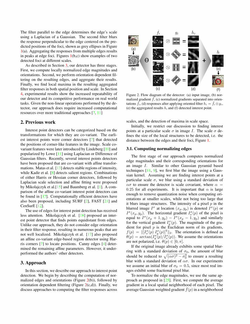
Figure 2. Flow diagram of the detector: (a) input image, (b) nor-malized gradient f̂ , (c) normalized gradients separated into orien-tations f̂i, (d) responses after applying oriented filter hi = f̂i⊗gi,(e) the aggregated results h, and (f) detected interest point.

scales, and the detection of maxima in scale space.Initially, we restrict our discussion to finding interest

points at a particular scale σ in image I . The scale σ de-fines the size of the local structures to be detected, i.e. thedistance between the edges and their foci, Figure 1.

3.1. Computing normalizing edges

The first stage of our approach computes normalizededge magnitudes and their corresponding orientations foran image I . Similar to other Gaussian pyramid basedtechniques [11, 9], we first blur the image using a Gaus-sian kernel. Assuming we are finding interest points at aparticular scale σ, we blur using a standard deviation ofασ to ensure the detector is scale covariant, where α =0.25 for all experiments. It is important that α is largeenough to remove quantization noise when computing ori-entations at smaller scales, while not being too large thatit blurs image structures. The intensity of a pixel p in theblurred image Iσ at location (xp, yp) is denoted Iσ(p) orIσ(xp, yp). The horizontal gradient Iσx (p) of the pixel isequal to Iσ(xp + 1, yp) − Iσ(xp − 1, yp) and similarlyfor the vertical gradient Iσy (p). The magnitude of the gra-dient for pixel p is the Euclidean norm of its gradients,f(p) = ‖[Iσx (p) Iσy (p)]T‖2. The orientation is defined asθ(p) = arctan(Iσy (p)/Iσx (p)). We assume the orientationsare not polarized, i.e. θ(p) ∈ [0, π].

If the original image already exhibits some spatial blur-ring with a standard deviation of σ0, the amount of blurshould be reduced to

√(ασ)2 − σ2

0 to ensure a resultingblur with a standard deviation of ασ. In our experimentswe assume an initial blur of σ0 = 0.5, since most real im-ages exhibit some fractional pixel blur.

To normalize the edge magnitudes, we use the same ap-proach as proposed in [25]. First, we compute the averagegradient in a local spatial neighborhood of each pixel. Theaverage Gaussian weighted gradient f̄(p) in a neighborhood

N of p is:

f̄(p) =∑q∈N

f(q)G(q − p;ασ

√(λ2 − 1)

), (1)

where G(x; s) is a normalized Gaussian evaluated at x withzero mean and a standard deviation of s. We set λ = 1.5 forall our experiments. Next, we divide f by the mean gradientf̄ to compute our normalized gradient f̂ :

f̂(p) =f(p)

max(f̄(p), ε/σ), (2)

where ε = 10 is used to ensure the magnitude of f̄(p) isabove the level of noise. An example of the normalizedgradients is shown in Figure 2(b).

3.2. Orientation dependent filteringOur next stage computes a series of linear filters on the

normalized gradients f̂ based on their orientations θp, Fig-ure 2(c,d). We apply different filters perpendicular and par-allel to the edges. As shown in Figure 3(e), a Laplacianis applied parallel to an edge to determine the edge’s scaleor length. Gaussian filters modeling the predicted positionsof edge foci are applied on either side perpendicular to theedge. The responses of all edges are summed together to getthe final filter response, Figure 2(e). As a result, edges thatare equidistant and perpendicular to edge foci will reinforceeach others’ responses.

The filter applied parallel to an edge attempts to deter-mine the scale of the edge, i.e. the linear length of theedge segment. A filter known for superior detection of scale[15, 9] is the Laplacian of Gaussian filter. As stated in [9],this filter will produce a maximal response at the correctscale without producing extraneous or false peaks. Our 1Dfilter is defined as:

u(x, σ) = −σ2u∇2G(x;σu), (3)

where σu =√

(βσ)2 − (ασ)2 to account for the blurringalready applied to the image. Scaling by a factor of σ2

u isrequired for true scale co-variance as shown by [9]. Varyingthe value of β will affect the size of the area around the edgefoci that is reinforced by the individual edge responses, asshown in Figure 3(a,b,c). A value too large, Figure 3(a)will blur structural detail, while a value too small may suf-fer from aliasing artifacts and create multiple peaks if theedges are not exactly aligned perpendicular to the foci, Fig-ure 3(c). We choose an intermediate value of β = 0.5 that isrobust to noise, but does not overly blur detail, Figure 3(b).

The filter applied perpendicular to the edge allows edgesof similar lengths to reinforce each others’ responses at po-tential edge foci, as shown in Figure 1. We assume edgefoci exist at a distance of σ perpendicular to the edge. As aresult, our filter is the summation of two Gaussians centeredat −σ and σ:

v(x, σ) = G(x− σ;σv) + G(x+ σ;σv). (4)

(a) (b) (c)

(d) (e)

Figure 3. (a,b,c) illustration of different values of β for edges form-ing a circle. Grey ellipses represent the area of positive responsefor filter (e) applied perpendicular to the edges. (d) illustration ofthe computation of ϑ on a set of edges forming a circle, and over-lapping Gaussian with Laplacian having twice the standard devi-ation. (e) the filter response g that is applied to normalized edgeimages.

The value of σv may be assigned based on the pre-dicted variance of the edge foci. However, setting σv =√

(βσ)2 − (ασ)2 the same value as σu provides compu-tational advantages. As we discuss in Section 3.2.1, the2D filter resulting from convolving equations (3) and (4),shown in Figure 3(e), can be computed using steerable fil-ters that are linearly separable.

For computational efficiency, we only evaluate the filters(3) and (4) at a discrete number of orientations θi, where i ∈Nθ, (Nθ = 8). For each orientation θi, we create an edgeorientation image f̂i that only contains normalized edgeswith orientations similar to θi. We softly assign edges to anedge orientation image f̂i using:

f̂i(p) = f̂(p)G(θ(p)− θi;ϑ), (5)

where ϑ = sin−1(β)/2, and θi = iπ/Nθ. As illustrated inFigure 3(d), our Laplacian filter has a zero crossing at βσ,and we assume the edge focus point is a distance σ from theedge. For an object with locally constant non-zero curva-ture we can assign a value of sin−1(β)/2 to ϑ to match thewidths of the Gaussian in equation (5) to the center of theLaplacian in (3), i.e. the standard deviation of the Gaussianis half the Laplacian, inset Figure 3(d).

As shown in Figure 2 and 3(e), if gi is our 2D filter foundby convolving our vertical filter (3) with our horizontal filter(4) and rotated by θi, we can compute our final responsefunction h using:

h =1

Nθ

∑i

hi (6)

where hi = f̂i ⊗ gi.

3.2.1 Steerable filters

In this section, we describe how in practice we computehi = f̂i ⊗ gi for all i. Naively convolving f̂i with the 2Dfilter gi is computationally expensive. Since filter (4) is thesummation of two identical Gaussians, we can apply a sin-gle Gaussian blur and sum the result at two different offsets:

hi(p) = h̃i(p− p′) + h̃i(p+ p′) (7)

where p′ = {σ cos(θi), σ sin(θi)} and h̃i = f̂i ⊗ Gi2. Gi2is the second derivative edge filter with orientation θi re-sulting from the convolution of a Gaussian and its secondderivative. If σu = σv , Gi2 combined with (7) results in thesame response as applying the filters (3) and (4). It is known[6] that Gi2 can be computed as a set of three 2D filters thatare linearly separable:

G2a(x, y) = σ2uG(y;σu)∇2G(x;σu) (8)

G2b(x, y) = σ2u∇G(x;σu)∇G(y;σu) (9)

G2c(x, y) = σ2uG(x;σu)∇2G(y;σu). (10)

Using equations (8), (9) and (10), we can compute Gi2 =ka(θi)G2a + kb(θi)G2b + kc(θi)G2c with:

ka(θi) = − cos2(−θi + π/2)kb(θi) = 2 sin(θi) cos(−θi + π/2)kc(θi) = − sin2(−θi + π/2)

. (11)

In practice, Gi2 may also be computed by first rotatingthe image by−θi, applyingG0

2 and rotating back. However,artifacts due to resampling may reduce the quality of theresponse. Computational requirements are similar for bothtechniques.

3.3. Scale spaceIn the previous section, we described how to compute

a single filter response function hk at the scale σk, wherek ∈ K is the set of computed scales. There are sev-eral methods for computing interest points across multiplescales depending on how image resampling is performed.For instance, a naive approach is to apply increasing valuesof σ to the original image to compute each scale. Howeverat large values of σ, computing the filter responses can beexpensive.

We use a popular approach that creates an octave imagepyramid, in which the image size is constant in an octaveof scale space and resized by half between octaves [11, 10].An octave refers to a doubling in size of σ. This approachreduces artifacts resulting from resampling, while beingcomputationally efficient due to the reduced image size atlarger scales. Since we perform non-linear operations onour image, such as computing orientations and normalizinggradients, we are required to recompute f̂ and θ to producehk at each scale k. Unlike our approach, methods based on

linear filters such as the DoG interest point detector [11],may progressively blur filter responses for additional effi-ciency. Following [11] we compute three levels per octave,i.e. σk+1/σk = 21/3. Two additional padding scales arecomputed per level to aid in peak detection.

3.4. Maxima detectionGiven a set of response functions hk over scales k ∈ K

we want to find a set of unique and stable interest point de-tections. To accomplish this, we use the standard approachproposed in [11] for finding maxima in the responses spa-tially and across scales. A pixel p is said to be a peak if itsresponse is higher than its neighbors in a 3 × 3 × 3 neigh-borhood, i.e. its 9 neighbors in hk−1 and hk+1, and its 8neighbors in hk. In addition to being a maxima, the re-sponse must also be higher than a threshold τ = 0.2.

As first proposed by Brown and Lowe [3], we refine ourinterest point locations by fitting a 3D quadratic function tothe local response hk in the same 3 × 3 × 3 neighborhood.The computed offset x̂ from the original position x is foundusing:

x̂ = −∂2h−1

∂x2∂h

∂x. (12)

4. Experimental ResultsIn this section, we show experimental results to illustrate

the performance of edge foci interest points based on threedifferent metrics: First, we provide an entropy measure tostudy the distribution both spatially and across scales ofthe interest points. Second, we score the interest points’repeatability, i.e. whether corresponding regions are cho-sen between images. Finally, we measure the uniquenessof the descriptors computed by the interest points to esti-mate the amount of ambiguity present during matching. Wealso evaluate the detectors on image alignment and retrievaltasks.

We compare the performance of our detector againstsome of the most commonly used detectors such as the Har-ris [7], Hessian [17], Harris/Hessian Laplace [17], MSER[13] and DoG [11] detectors1 on a set of new datasets thatcapture non-linear illumination variations and changes inbackground clutter. Homographies are computed using tenor more hand labeled points to provide correspondences be-tween pairs of images. We assume the scenes are eitherplanar or taken at a far distance so correspondences can bewell approximated by a homography. Figure 4 shows twoexample images from the 8 datasets used in this paper. Thedatasets Boat, Graffiti and Light were provided by and de-scribed in [17]. When required, the rotation of the interestpoints are computed using the method of [11].

Before we present quantitative experimental results, weshow the response of our detector in comparison with the

1For the all the detectors except DoG we use the binariesfrom http://www.featurespace.org/, for DoG the binaries provided athttp://www.cs.ubc.ca/˜lowe/keypoints/ generate better results.

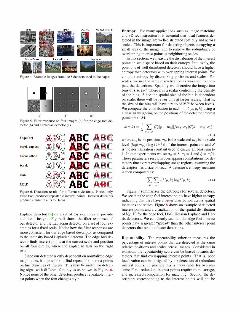
Figure 4. Example images from the 8 datasets used in the paper.

(a) (b) (c)

Figure 5. Filter response on four images (a) for the edge foci de-tector (b) and Laplacian detector (c).

Figure 6. Detection results for different style fonts. Notice onlyEdge Foci produces repeatable interest points. Hessian detectorsproduce similar results to Harris.

Laplace detector[10] on a set of toy examples to provideadditional insight. Figure 5 shows the filter responses ofour detector and the Laplacian detector on a set of four ex-amples for a fixed scale. Notice how the filter responses aremore consistent for our edge based descriptor as comparedto the intensity based Laplacian detector. The edge foci de-tector finds interest points at the correct scale and positionon all four circles, where the Laplacian fails on the righttwo.

Since our detector is only dependent on normalized edgemagnitudes, it is possible to find repeatable interest pointson line drawings of images. This may be useful for detect-ing signs with different font styles as shown in Figure 6.Notice none of the other detectors produce repeatable inter-est points when the font changes style.

Entropy For many applications such as image matchingand 3D reconstruction it is essential that local features de-tected in the image are well-distributed spatially and acrossscales. This is important for detecting objects occupying asmall area of the image, and to remove the redundancy ofoverlapping interest points at neighboring scales.

In this section, we measure the distribution of the interestpoints in scale space based on their entropy. Intuitively, thepositions of well distributed detectors should have a higherentropy than detectors with overlapping interest points. Wecompute entropy by discretizing positions and scales. Forscales, we use the same discretization as was used to com-pute the detections. Spatially we discretize the image intobins of size ξσk where ξ is a scalar controlling the densityof the bins. Since the spatial size of the bin is dependenton scale, there will be fewer bins at larger scales. That is,the size of the bins will have a ratio of 21/3 between levels.We compute the contribution to each bin b(x, y, k) using aGaussian weighting on the positions of the detected interestpoints m ∈M:

b(p, k) =1

Z

∑m∈M

G(‖p−mp‖/mσ;σx)G(k −mk;σl)

(13)wheremp is the position,mσ is the scale andmk is the scalelevel (log(mσ)/ log (21/3)) of the interest point m, and Zis the normalization constant used to ensure all bins sum to1. In our experiments we set σx = 8, σl = 1 and ξ = σ/4.These parameters result in overlapping contributions for de-tectors that extract overlapping image regions, assuming thedescriptor has a size of 4mσ . A detector’s entropy measureis then computed as:∑

p

∑k

−b(p, k) log b(p, k) (14)

Figure 7 summarizes the entropies for several detectors.We see that the edge foci interest points have higher entropyindicating that they have a better distribution across spatiallocations and scales. Figure 8 shows an example of detectedinterest points and a visualization of the spatial distributionof b(p, k) for the edge foci, DoG, Hessian Laplace and Har-ris detectors. We can clearly see that the edge foci interestpoints have a greater “spread” than the other interest pointdetectors that tend to cluster detections.

Repeatability The repeatability criterion measures thepercentage of interest points that are detected at the samerelative positions and scales across images. Considered inisolation, the repeatability score can be biased towards de-tectors that find overlapping interest points. That is, poorlocalization can be mitigated by the detection of redundantinterest points. In practice this is undesirable for two rea-sons: First, redundant interest points require more storage,and increased computation for matching. Second, the de-scriptors corresponding to the interest points will not be

Figure 7. Entropy of interest point detectors across variousdatasets.

Figure 8. Visualization of the interest points and their spatial dis-tributions for various detectors on Yosemite image.

unique, increasing the difficultly of matching and nearestneighbor techniques.

Two interest points, m and m′, that are detected in dif-ferent images are said to pass the traditional repeatabilitycriterion [11, 16] if their relative positions and scales arewithin some scale normalized distance:

(‖mp −m′p‖ − ε)/mσ < τp (15)

‖mk −m′k‖ < τk. (16)

where τp = 0.4, τk = log(1.3) and ε = 2 to accountfor small errors in the homography estimation. We normal-ize the distances by scale since the variance in the interestpoints’ descriptors are related to scale normalized distancesand not fixed distances. To ensure the consistent measure-ment of scale, the scales of all detectors were calibrated ona test image with various sizes of circles. If the projectedinterest points lie outside the other image, they are not usedto compute the repeatability score.

We modify the traditional measure of repeatability to ad-ditionally penalize overlapping detections. Using the set ofinterest pointsM∗ that passed the traditional repeatabilitycriterion, we compute a distribution B(p, k) using equa-tion (13) similar to b(p, k) used for our entropy measure.To only penalize detections resulting in descriptors that aremore than half overlapping, we reduce the value of σx to 4.We assume a standard descriptor region size of 4 times theinterest point scale. Our final measure of repeatability thatencourages well distributed detections is:

1

#M∗∑p

∑k

min (t, B(p, k)) (17)

where #M∗ is the size ofM∗ and t is the product of theGaussian normalization constants in Equation (13), t =1/(2πσxσk). Using Equation (17), if none of the interestpoints inM∗ overlap, the repeatability score is the same asusing a traditional repeatability criterion [11, 16]. However,if two interest points in M∗ do overlap, their contributionis truncated by Equation (17) reducing the overall score.

For our experiments, we compare the repeatability ofour Edge Foci interest points with the interest points gen-erated from the Harris[7], Hessian[17], Harris/Hessian-Laplace[16, 17], MSER [13] and DoG detector [11] on thedifferent datasets described in section 4. We tune each de-tector to generate approximately the same number of inter-est points per test image ranging from 700 to 2, 500 points.Figure 9 shows the repeatability measures for each dataset.Across the various datasets the edge foci detectors per-form well, especially in those containing significant light-ing variation (Inspiration point, Notre Dame, Mt. Rush-more, Painted Lady) and occlusion (Obama). MSER per-forms best on severe affine transformations (Graffiti). Hes-sian Laplace and Harris Laplace are generally within thetop three performers, while Harris and Hessian typicallyperform worse due to poor scale localization. For compar-ison, the traditional repeatability scores averaged over thedatasets without penalizing overlap [16] are EdgeFoci 24%,DOG 12%, HarLap 25%, Harris 17%, HesAff 18%, HesLap22%, Hessian 19% and MSER 18%.

Descriptor uniqueness In the previous section, we mea-sured performance based on repeatability of the detectors.While the repeatability measure describes how often we canmatch the same regions in two images, it does not measurethe uniqueness of the interest point descriptors. Unique de-scriptors are essential for avoiding false matches, especiallyin applications with large databases. As stated before, re-dundant interest points across scales may create similar de-scriptors. Interest points that are only detected on very spe-cific image features may also reduce the distinctiveness ofdescriptors.

We compute descriptor uniqueness using the state-of-the-art daisy descriptor [24] to describe the image regionsfor all detectors (similar results are achieved with SIFT[11].) Given the image descriptors for a pair of images, wefind the nearest neighbors for each descriptor in the otherimage. Using our repeatability criterion described above,it is determined whether each pair of nearest neighbor de-tections correspond. Each pair is either assigned to a pos-itive (repeatable) set of detections or a negative set. In thenegative detections we also include the second best nearestneighbor match to obtain a better estimate of the distribu-tion of negative matches. Finally, we create an ROC curveby varying the threshold on the descriptor distance ratio [11]and compute the number of false positives and true positivesbelow the threshold. The distance ratio is the ratio betweenthe distance of the best match and second best match in an

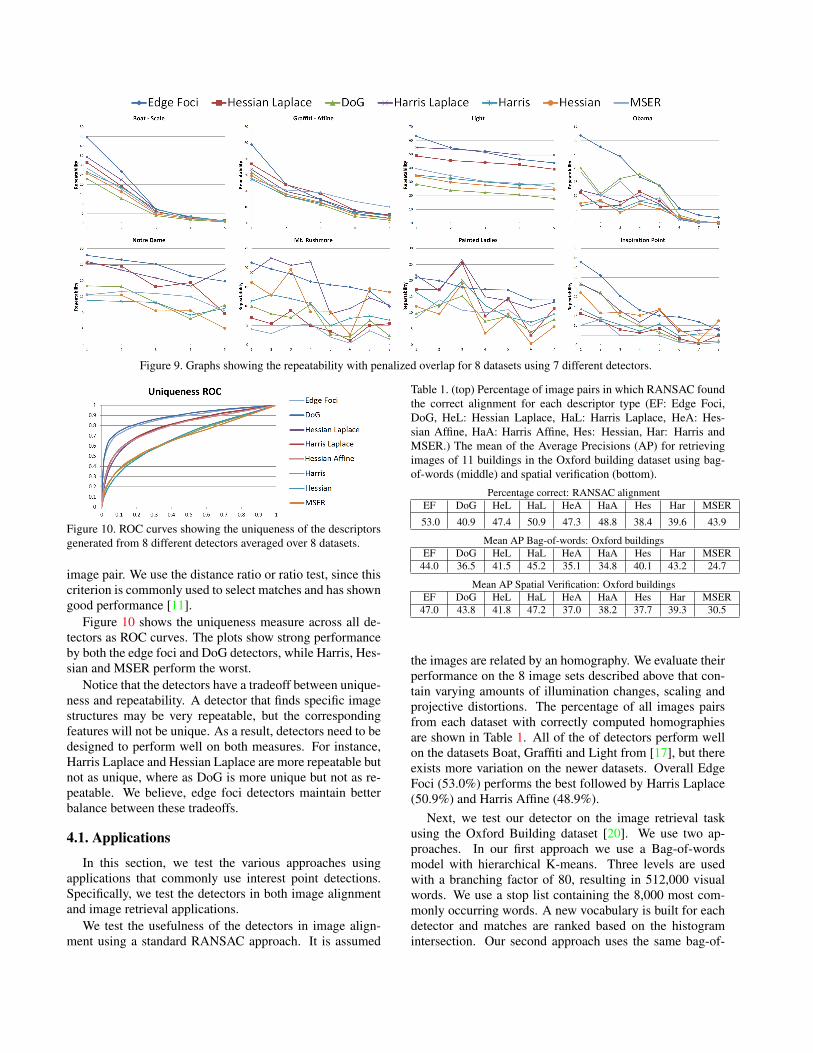
Figure 9. Graphs showing the repeatability with penalized overlap for 8 datasets using 7 different detectors.

Figure 10. ROC curves showing the uniqueness of the descriptorsgenerated from 8 different detectors averaged over 8 datasets.

image pair. We use the distance ratio or ratio test, since thiscriterion is commonly used to select matches and has showngood performance [11].

Figure 10 shows the uniqueness measure across all de-tectors as ROC curves. The plots show strong performanceby both the edge foci and DoG detectors, while Harris, Hes-sian and MSER perform the worst.

Notice that the detectors have a tradeoff between unique-ness and repeatability. A detector that finds specific imagestructures may be very repeatable, but the correspondingfeatures will not be unique. As a result, detectors need to bedesigned to perform well on both measures. For instance,Harris Laplace and Hessian Laplace are more repeatable butnot as unique, where as DoG is more unique but not as re-peatable. We believe, edge foci detectors maintain betterbalance between these tradeoffs.

4.1. Applications

In this section, we test the various approaches usingapplications that commonly use interest point detections.Specifically, we test the detectors in both image alignmentand image retrieval applications.

We test the usefulness of the detectors in image align-ment using a standard RANSAC approach. It is assumed

Table 1. (top) Percentage of image pairs in which RANSAC foundthe correct alignment for each descriptor type (EF: Edge Foci,DoG, HeL: Hessian Laplace, HaL: Harris Laplace, HeA: Hes-sian Affine, HaA: Harris Affine, Hes: Hessian, Har: Harris andMSER.) The mean of the Average Precisions (AP) for retrievingimages of 11 buildings in the Oxford building dataset using bag-of-words (middle) and spatial verification (bottom).

Percentage correct: RANSAC alignmentEF DoG HeL HaL HeA HaA Hes Har MSER

53.0 40.9 47.4 50.9 47.3 48.8 38.4 39.6 43.9

Mean AP Bag-of-words: Oxford buildingsEF DoG HeL HaL HeA HaA Hes Har MSER

44.0 36.5 41.5 45.2 35.1 34.8 40.1 43.2 24.7

Mean AP Spatial Verification: Oxford buildingsEF DoG HeL HaL HeA HaA Hes Har MSER

47.0 43.8 41.8 47.2 37.0 38.2 37.7 39.3 30.5

the images are related by an homography. We evaluate theirperformance on the 8 image sets described above that con-tain varying amounts of illumination changes, scaling andprojective distortions. The percentage of all images pairsfrom each dataset with correctly computed homographiesare shown in Table 1. All of the of detectors perform wellon the datasets Boat, Graffiti and Light from [17], but thereexists more variation on the newer datasets. Overall EdgeFoci (53.0%) performs the best followed by Harris Laplace(50.9%) and Harris Affine (48.9%).

Next, we test our detector on the image retrieval taskusing the Oxford Building dataset [20]. We use two ap-proaches. In our first approach we use a Bag-of-wordsmodel with hierarchical K-means. Three levels are usedwith a branching factor of 80, resulting in 512,000 visualwords. We use a stop list containing the 8,000 most com-monly occurring words. A new vocabulary is built for eachdetector and matches are ranked based on the histogramintersection. Our second approach uses the same bag-of-

words model with the addition of spatial verification. Spa-tial verification is achieved using a three degree of freedom(position and scale) voting scheme between correspondinginterest points. Using the code supplied by [20], we com-pute the mean of the average precision scores for each de-tector across all 11 buildings in the dataset. The results forboth methods are shown in Table 1. Both Edge Foci andHarris Laplace achieve good results in both tests. It is inter-esting to notice that detectors with good localization (EdgeFoci, DoG, MSER, etc.) get a larger performance boostfrom spatial verification than those with poor localization(Hessian, Harris).

Examining the performance of each query in isolation,it is clear that the accuracy of the detector is dependent onthe content of the scene. While Harris Laplace and EdgeFoci share similar average accuracies, the results on eachquery can vary significantly. For instance, Harris Laplaceperforms better on the ”ashmolean” Oxford building, whileEdge Foci performs significantly better on ”bodleian” and”pitt rivers”. For best results, it may be beneficial to usemultiple detectors.

5. DiscussionOrientation dependent filtering is critical for localizing

interest points using edge information. If a standard spatialfilter such as a Laplacian is used directly on the edge re-sponses [18], numerous false peaks and ridges occur. Dueto the peakiness of our filter, we found it unnecessary to fil-ter local maxima based on the ratio of principle curvaturesas proposed by [11]. While not shown in this paper, the fil-ter responses could be used for affine fitting similar to [16].

Due to the non-linear operations performed by our fil-ter, and orientation dependent filtering, our detector ismore computationally expensive than previous approaches[11, 13, 17]. The average run time for our detector on a640× 480 image is 4.25 seconds on a 2.53GHz Intel CPU.However, the filters applied to the images could easily bemapped to a GPU. The filters applied to the oriented nor-malized edge images f̂i may also be computed in parallel.

In conclusion, we propose a method for detecting inter-est points using edge foci. The positions of the edge fociare computed using normalized edges that are more invari-ant to non-linear lighting changes and background clutter.We show improved results over previous works on numer-ous datasets with significant variation in lighting and occlu-sions.

References[1] A. Baumberg. Reliable feature matching across widely sep-

arated views. In IEEE Proc. of CVPR, 2000. 1, 2[2] H. Bay, T. Tuytelaars, and L. Van Gool. Surf: Speeded up

robust features. In IEEE Proc. of ECCV. 2006. 2[3] M. Brown and D. Lowe. Invariant Features from Interest

Point Groups. In BMVC, 2002. 4

[4] J. Canny. A computational approach to edge detection. IEEETrans. on PAMI, 8(6), 1986. 1, 2

[5] R. Fergus, P. Perona, and A. Zisserman. Object class recog-nition by unsupervised scale-invariant learning. IEEE Proc.of CVPR, 2, 2003. 1

[6] W. T. Freeman and E. H. Adelson. The design and use ofsteerable filters. IEEE Trans. on PAMI, 13, 1991. 4

[7] C. Harris and M. Stephens. A combined corner and edgedetector. In Proc. of the Alvey Vision Conference, 1988. 1, 2,4, 6

[8] T. Kadir, A. Zisserman, and M. Brady. An affine invariantsalient region detector. In IEEE Proc. of ECCV. 2004. 1, 2

[9] T. Lindeberg. Scale-space theory: A basic tool for analysingstructures at different scales. Journal of Applied Statistics,21, 1994. 2, 3

[10] T. Lindeberg. Feature detection with automatic scale selec-tion. Int’l J. of Computer Vision, 30, 1998. 1, 2, 4, 5

[11] D. G. Lowe. Distinctive image features from scale-invariantkeypoints. Int’l J. of Computer Vision, 60, 2004. 1, 2, 4, 5,6, 7, 8

[12] M. R. B. M. Agrawal, K. Konolige. Censure: Center sur-round extremas for realtime feature detection and matching.In IEEE Proc. of ECCV, 2008. 2

[13] J. Matas, O. Chum, M. Urban, and T. Pajdla. Robust wide-baseline stereo from maximally stable extremal regions. Im-age and Vision Computing, 22(10), 2004. 1, 2, 4, 6, 8

[14] K. Mikolajczyk and C. Schmid. Indexing based on scaleinvariant interest points. In IEEE Proc. of ICCV, 2001. 1

[15] K. Mikolajczyk and C. Schmid. An affine invariant interestpoint detector. In IEEE Proc. of ECCV, 2002. 1, 2, 3

[16] K. Mikolajczyk and C. Schmid. Scale and affine invariantinterest point detectors. Int’l J. of Computer Vision, 60, 2004.1, 6, 8

[17] K. Mikolajczyk, T. Tuytelaars, C. Schmid, A. Zisserman,J. Matas, F. Schaffalitzky, T. Kadir, and L. Gool. A compar-ison of affine region detectors. Int’l J. of Computer Vision,65, 2005. 1, 2, 4, 5, 6, 7, 8

[18] K. Mikolajczyk, A. Zisserman, and C. Schmid. Shape recog-nition with edge-based features. In BMVC, 2003. 1, 2, 8

[19] D. Nister and H. Stewenius. Scalable recognition with a vo-cabulary tree. IEEE Proc. of CVPR, 2006. 1

[20] J. Philbin, O. Chum, M. Isard, J. Sivic, and A. Zisser-man. Object retrieval with large vocabularies and fast spatialmatching. In IEEE Proc. of CVPR, 2007. 8

[21] E. Rosten and T. Drummond. Machine learning for high-speed corner detection. In IEEE Proc. of ECCV. 2006. 2

[22] F. Rothganger, S. Lazebnik, C. Schmid, and J. Ponce. 3dobject modeling and recognition using local affine-invariantimage descriptors and multi-view spatial constraints. Int’l J.of Computer Vision, 66, 2006. 1

[23] N. Snavely, S. M. Seitz, and R. Szeliski. Photo tourism: Ex-ploring photo collections in 3d. In SIGGRAPH, 2006. 1

[24] S. Winder, G. Hua, and M. Brown. Picking the best daisy.IEEE Proc. of CVPR, 2009. 6

[25] C. L. Zitnick. Binary coherent edge descriptors. IEEE Proc.of ECCV, 2010. 1, 2