edge stabilization and consistent tying of constituents at

INTERNATIONAL JOURNAL FOR NUMERICAL METHODS IN ENGINEERINGInt. J. Numer. Meth. Engng 2017; 110:1142–1172Published online 25 April 2017 in Wiley Online Library (wileyonlinelibrary.com). DOI: 10.1002/nme.5446

Edge stabilization and consistent tying of constituents at Neumannboundaries in multi-constituent mixture models

Harishanker Gajendran1, Richard B. Hall2 and Arif Masud1,*,†

1Department of Civil and Environmental Engineering, University of Illinois at Urbana–Champaign, Urbana,IL 61801-2352, USA

2Materials and Manufacturing Directorate, Air Force Research Laboratory, Wright–Patterson Air Force Base,OH 45433-7750, USA

SUMMARY

A mixture-theory-based model for multi-constituent solids is presented where each constituent is governedby its own balance laws and constitutive equations. Interactive forces between constituents that emanate frommaximization of entropy production inequality provide the coupling between constituent-specific balancelaws and constitutive models. The deformation of multi-constituent mixtures at the Neumann boundariesrequires imposing inter-constituent coupling constraints such that the constituents deform in a self-consistentfashion. A set of boundary conditions is presented that accounts for the non-zero applied tractions, and avariationally consistent method is developed to enforce inter-constituent constraints at Neumann boundariesin the finite deformation context. The new method finds roots in a local multiscale decomposition of thedeformation map at the Neumann boundary. Locally satisfying the Lagrange multiplier field and subsequentmodeling of the fine scales via edge bubble functions result in closed-form expressions for a generalizedpenalty tensor and a weighted numerical flux that are free from tunable parameters. The key novelty isthat the consistently derived constituent coupling parameters evolve with material and geometric nonlinear-ity, thereby resulting in optimal enforcement of inter-constituent constraints. Various benchmark problemsare presented to validate the method and show its range of application. Copyright © 2016 John Wiley &Sons, Ltd.

Received 24 April 2016; Revised 30 August 2016; Accepted 4 October 2016

KEY WORDS: mixture theory; coupled deformation of constituents; stabilized methods; interfaces andinterphases; finite strains; composite materials

1. INTRODUCTION

In the manufacturing of fibrous composites, the fiber–resin mixture is subjected to a cure cycle thatinitiates cross-linking polymerization in resin to produce a structurally hard material. The propertiesof the final product as well as its performance characteristics depend on the properties of the con-stituents as well as the properties of the interphase zone formed in the constituent interface region.Theoretical models and numerical methods employed to model material evolution at the microscalelevel need to accurately represent the behavior of the individual constituents as well as their cou-pled interactions in an integrated fashion. This paper employs a mixture-theory-based model fora representative infinitesimal volume element of dense mixture of multi-constituent solids whereeach constituent is governed by its own balance laws and constitutive equations. Interactive forcesbetween constituents that emanate from maximization of entropy production inequality provide thenecessary coupling between the balance laws and constitutive models and therefore between theconcurrent and overlapping constituents of the mixture.

*Correspondence to: Arif Masud, Department of Civil and Environmental Engineering, University of Illinois at Urbana–Champaign, Urbana, IL 61801-2352, USA.

†E-mail: [email protected]

Copyright © 2016 John Wiley & Sons, Ltd.

CONSISTENT TYING OF CONSTITUENTS AT NEUMANN BOUNDARIES 1143

A literature review reveals that the mixture theory proposed by Truesdell [1] has been widelyemployed in the modeling of fluid–fluid and solid–fluid mixtures. Comprehensive review articlesby Atkin and Craine [2] and Green and Naghdi [3, 4] and a book by Rajagopal and Tao [5] pro-vide a good exposition to the mixture theory and associated constitutive relations. Mixture theoryideas have been used to model various phenomena such as classical viscoelasticity [6], swellingof polymers [7], thermo-oxidative degradation of polymer composites [8, 9], growth of biologi-cal materials [10] and crystallization of polymers [11], to name a few. Mixture theories have alsobeen employed to model the multi-constituent elastic solids; e.g., Bowen and Wiese [12] presenteda thermomechanical theory for diffusion in mixtures of elastic materials. Bedford and Stern [13]proposed a multi-continuum theory for composite materials where the material particles of differ-ent constituents are grouped together in the reference configuration to define a composite particle.Although these constituent particles occupy different spatial points as the material deforms, theinteractions between constituents are evaluated in the reference configuration using the compositeparticle. Hall and Rajagopal [14, 15] proposed a mixture model for diffusion of chemically react-ing fluids through anisotropic solids based on the maximization of the rate of entropy productionconstraint, considering anisotropic effective reaction rates and the limits of diffusion-dominated (dif-fusion of the reactants is far more rapid than the reaction) and reaction-dominated (the reaction isfar more rapid than the diffusion of the reactants) processes. In the present work, the theory by Halland Rajagopal [14, 15] is enhanced to the case of a mixture of two interacting solid constituents,and an edge-stabilized method is developed to numerically model mixture-based fibrous compositesystems.

A general preface of the mixture theory is that the constituents are assumed to coexist over eachother at every point in the domain, a condition that arises because of the volumetric homogenizationof each constituent over the composite/mixture domain. As the constituents deform with respectto each other, the domain boundary of the mixture needs to be constrained via continuity condi-tions so that the constituents deforms in a unified way. Enforcing continuity between constituentsat the boundary is analogous to the interface treatment in domain decomposition methods, contactproblems, and material interfaces. Amongst the various numerical techniques that enforce continu-ity conditions and traction equilibrium at the interface, a classical approach is the unconstrainedoptimization problem wherein a Lagrange multiplier field is employed to enforce continuity at theinterface. The stability issues that arise in this dual-field formulation in its discretized form arewell known [16], where the interpolation functions for the primary field and Lagrange multipliersneed to be chosen such that the celebrated Babuska–Brezzi condition is not violated. In addition,the computational cost increases because of the introduction of additional variables associated withthe Lagrange multipliers. This however can be addressed via a primal field formulation that canbe derived by defining the Lagrange multipliers through penalty parameter and the continuity con-ditions. The disadvantage of the penalty method is that it attains optimal convergence only as thepenalty parameter approaches infinity, which however leads to ill conditioning of the matrix system.A consistent penalty formulation was introduced by Nitsche [17] to enforce a Dirichlet boundarycondition weakly on the boundaries. This primal formulation is consistent and symmetric, whereinthe Lagrange multiplier fields are approximated by the numerical fluxes at the boundary. The Nitschemethod was subsequently extended to handle interfaces that arise in domain decomposition meth-ods, embedded finite element methods, and physical interfaces. The penalty parameter in the Nitschemethod needs to be defined to ensure the coercivity of the method, and there have been many worksto define this parameter through the following: (i) an a priori analysis, (ii) solving of global or localeigenvalue problems, and (iii) bubble functions approach [18–22]. Masud and coworkers [23–28]have developed a unified formulation for interface coupling and frictional contact modeling wherethe penalty parameter is derived through variational multiscale (VMS) framework, and a Lagrangemultiplier field is approximated as a simple average of fluxes. Truster and Masud [29] have extendedthis framework to finite deformations where the stabilization tensor is consistently derived and is afunction of both material and geometric nonlinearity.

The deformation of multi-constituent mixtures at the Neumann boundaries requires imposingconstraint conditions such that the constituents deform in a self-consistent fashion. In the presentwork, a set of boundary conditions are presented that are then modified to account for the non-

Copyright © 2016 John Wiley & Sons, Ltd. Int. J. Numer. Meth. Engng 2017; 110:1142–1172DOI: 10.1002/nme

1144 H. GAJENDRAN, R. B. HALL AND A. MASUD

zero applied tractions. Following the line of thought in [23–28], a numerical method is developedthat draws from the stabilized discontinuous Galerkin method for finite strain kinematics with anunderlying Lagrange multiplier interface formulation. The derivation of the new method hingesupon a multiscale decomposition of the deformation map locally at the Neumann boundary andsubsequent modeling of the fine scales via edge bubble functions. The resulting terms enable thecondensation of the multiplier field from the formulation in addition to providing an edge-basedstabilization of the method. Closed-form expressions are derived for the stabilization tensor andthe weighted numerical flux that are free from tunable stability parameters. The key novelty is thatthe consistently derived stability tensors automatically evolve with evolving material and geometricnonlinearity at the boundaries.

The outline of the paper is as follows. In Section 2, we present the governing equations and theconstitutive relations for two solid-constituent mixtures for the modeling of composites. Boundaryconditions and a procedure to determine the material properties of the constituents are presentedin Section 3. The stabilized formulation for the imposition of continuity and traction equilibriumconditions is derived in Section 4. Section 5 presents a series of numerical test cases, and results arecompared with analytical solutions and published data that are available in literature. Conclusionsare drawn in Section 6.

2. MIXTURE THEORY GOVERNING EQUATIONS

Although mixture theory provides a general framework for modeling an N constituent mixture, wepresent mixture equations in the context of two constituents, namely, matrix and fiber, where bothconstituents are assumed to be in the solid phase. The underlying idea in mixture theory for themodeling of composites is that the constituents are assumed to coexist concurrently at every point inthe domain. This assumption arises due to the volumetric homogenization of each constituent overthe composite/mixture domain.

Let us consider a microstructure of a composite as shown in Figure 1. A microscopic volume inthe mixture domain represents an average behavior of the constituents. Assuming certain periodicityin the microstructure, the microscopic volume can be represented by a unit cell that is comprisedof fibers with a given orientation that are embedded in the matrix material. These constituents aresegregated and homogenized over the mixture volume and are assigned an apparent density property,which is defined as the ratio of the mass of the constituent over the mixture volume. Thus, thecomposite density is the sum addition of the constituent apparent densities:

� D �m C �r (1)

where �m and �r are the matrix and fiber apparent densities, respectively, and �c is the compositedensity.

Figure 1. Mixture theory homogenization.



RemarkThe effective properties of a composite are orthotropic owing to fiber orientation and fiber–matrixinteraction even when the constituents by themselves are isotropic. In mixture theory, as the con-stituents are homogenized at the individual level in a volumetric sense over the mixture volume,the effective orthotropic properties of the composite are obtained by modeling the domain ofhomogenized fibers as an orthotropic material.

Consider an open-bounded region of the mixture �c in the reference configuration as shown inFigure 2, where a matrix reference domain �m and a fiber reference domain �r coexist over eachother. It should be noted that in the reference configuration, �r D �m D �c . The boundaries ofthe fiber, matrix, and the composite domains are denoted by �r , �m, and �c , respectively, where�r D �m D �c because every point on the boundary is concurrently occupied by the fiber andmatrix. For a compact presentation of ideas, the kinematic and kinetic quantities of the fiber, matrix,and composite will be denoted by a superscript ˛, where ˛ 2 ¹r;m; cº. For a given point X inthe material configuration of the composite, there exists a particle of fiber, X r , and that of matrixXm, with same material coordinates. Although X r D Xm D X c , for the sake of clarity, theseconstituent material points are shown in two separate domains in Figure 2. As explained earlier,the fiber domain �r and the matrix domain �m coexist over each other in the composite domain�c . When the mixture domain is subjected to external loadings, the reference configuration of theconstituent ˛,�˛ , deforms to the current configuration�˛' under the deformation map, '˛ .X˛; t /.Thus, the deformation gradient of each constituent ˛ is given as

F ˛ D@'˛ .X˛; t /

@X(2)

From Figure 2, it can be seen that the coexisting material pointsX r andXm of the constituents inmaterial configuration map to two different spatial points in the current configuration. The interac-tion between these homogenized constituents as they deform with respect to each other is a functionof the relative stretch and rotation of these two spatial points. For any point in one of the constituentspatial configurations, the corresponding spatial point from the other constituent can be obtained viaa pull-back and push-forward mapping as given in the following:

xr D 'r .X r ; t / D 'r .Xm; t / D 'r�'m�1

.xm; t / ; t�

(3)

Figure 2. Mixture kinematics.



The balance of mass and balance of linear momentum of the constituents in the current configurationare given as follows:

Balance of mass:@�˛

@tCr �

��˛v˛

�D m˛ (4)

Balance of linear momentum: r � .T ˛/TC �˛b˛ C I˛ D 0 (5)

where �˛ is the apparent density in the current configuration and m˛ is the rate of mass transferredby chemical reaction to constituent ˛, T ˛ is the partial Cauchy stress, b˛ is the body force per unitmass, and I˛ is the interactive force per unit mixture volume of the concurrent constituents definedin the reference configuration as the constituents deform with respect to each other in the currentconfiguration. Newton’s third law requires that

Ir C Im D 0 (6)

RemarkInteractive force is a unique feature of mixture theory that models the interaction between the con-stituents as they deform with respect to each other. Because of homogenization of the constituentsover the unit cell, this force is a homogenized quantity that captures the interactions at the fiber–matrix interface through constitutive relations. This force identifies spatial zones in the compositewhere fiber–matrix interfaces are under higher shear stresses. Interfacial debonding that is usuallytriggered when the induced shear stresses exceed the stress transfer capacity of the interfaces islikely to initiate in such regions.

In the absence of mass exchange between the constituents, the balance of mass equations reducesto an algebraic form

�˛J ˛ D �˛R (7)

where �˛R is the apparent density in the reference configuration.

RemarkAlthough it has been assumed that there is no mass transfer between the matrix and fiber, the theorystill allows the modeling of the material interface evolution in the composite by postulating that thematerial evolves in the boundary layer of the matrix domain at the fiber–matrix interface.

The constitutive relations for the mixture theory are obtained through maximization of the rateof dissipation constraint with respect to state variables sŒt � D ¹Fm;F r ; �m; �rº Œt �. Details for thisderivation can be seen in [14, 15]. Here, we present the summary of the constitutive relations, wherethe volume additivity constraint is not imposed.

Constitutive relations:

T m D �Fm�@

@Fm

�T� �mgm1C �

@�

@Lm(8)

T r D �F r�@

@F r

�T� �rgr1 (9)

Im D gm�r

�r�m � gr

�m

�r�r C

�r�m

�

�@ m

@FmW rFm �

@ r

@F rW rF r

�

�mm.vm � vr/ � .r�/�m�r

�.m � r/ � �Av.vm � vr/

(10)



�@�

@ P�D ��

�@

@�C

�(11)

� �

�@

@�0

�D �

@�

@ P�0(12)

where P�0 is the reaction rate, � is the rate of dissipation, � is the Lagrange multiplier enforcing themaximum rate of dissipation constraint, ˛ is the entropy, g˛ is the chemical potential of the ˛thcomponent of the mixture, and 1 is the identity tensor.

Assuming isothermal conditions and chemically non-reactive nonlinear elastic constituents, wecan reduce the constitutive relations for the matrix stress, fiber stress, and fiber interactive forcegiven in (8)–(10) to

T m D Fm�@.� /

@Em

�.Fm/T (13)

T r D F r�@.� /

@E r

�.F r/T (14)

Im D�r�m

�

�@ m

@FmW rFm �

@ r

@F rW rF r

�(15)

RemarkInteractive force is required for force balance of a given constituent as obtained from both the surfacetractions on a representative element and the interacting constituents within the element. Interactiveforce in the matrix domain under isothermal conditions is given by (15) and is a function of bothmatrix and fiber displacement fields. The constitutive relation for the interactive force is a higherorder relation as it involves second-order derivatives of the displacement fields. As indicated byHall [15], the components of the interactive forces reflect a change of sign when the constituents areinterchanged.

3. BOUNDARY CONDITIONS AND MATERIAL PROPERTIES FOR THE MIXTURE MODEL

In this section, we specify the boundary conditions and the material properties of the constituentsthat are needed to complete the definition of the mixture boundary value problem. In the single-continuum theories for solids, the definitions of the Dirichlet and Neumann boundary conditionsare well posed. However, in the mixture theory, as the constituents deform relative to each other inthe spatial domain, the definitions of the boundary conditions are unclear because of two reasons.First, given a composite traction field, one needs an equivalent matrix and fiber traction boundarycondition to complete the matrix and fiber boundary value problem. Second, because of finite defor-mation kinematics, the constituent boundaries can have different spatial mappings, thereby makingit difficult to impose consistent boundary conditions.

3.1. Consistent split of the traction fields

In the mixture theory literature, a volumetric split of the traction fields is usually proposed, whichhowever has the drawback of inconsistent deformation of the constituent boundaries. Followingalong the lines of the strategy adopted in the interface problems where continuity in the traction anddisplacement fields are weakly imposed, we propose a set of equations for Dirichlet and Neumann



boundary conditions that ensures displacement continuity and traction equilibrium at the boundaryof each constituent, which can be written in the spatial configuration as

'm � 'r D 0 on �h''r D 'm D 'c on �g'

T rnr C T mnm D hc on �'

(16)

where nr and nm are the unit normal vectors to the domain boundary �' for the two constituents rand m, respectively. hc is the domain normal component of the stress field at the boundary of thecomposite �' , and this field disappears at the inter-constituent boundaries �'n

®�g' [ �

h'

¯, while

'c is the specified composite displacement field at �g' .

RemarkCompatibility condition induced by displacement continuity at the composite boundary precludesrelative displacement between fiber and matrix at the boundary and therefore fracture or delam-ination of the fiber–matrix system. This is however not a restriction on the theoretical model orits numerical implementation. This can be relaxed by introducing a slip function that can permit arelative slip between 'm and 'r at �h' .

3.2. Modeling of homogeneous fiber constituent

A basic premise of the mixture theory is that the constituents coexist and are homogenized over themixture volume. While each of the constituents, i.e., the matrix and the fiber, may be homogenousand isotropic, the structural layout of the fibers makes the homogenized fiber material as beingtransversely isotropic.

The constitutive models for the transversely isotropic composites are developed by first definingthe Helmholtz free energy functions r and m for the fiber and the matrix, respectively, and thenapplying the concept of constituent volume fraction c D �r r C �m m, where

r D1

�rT

´12r .tr ŒE r �/2 C �rT tr

h.E r/

2iC ˛r

�m0 � ŒE r �m0

�tr ŒE r �

C2��rL � �

rT

�m0 � ŒE r �

2m0 C 1

2ˇr�m0 �E rm0

�2μ

(17)

m D1

�mT

²1

2m .tr ŒEm�/2 C �mtr

h.Em/

2i³

(18)

Consequently, the total Helmholtz free energy function of the transversely isotropic compositemixture can be written as

c D�m

�mT

²1

2m .tr ŒEm�/2 C �mtr

h.Em/

2i³

C�r

�rT

´12r .tr ŒE r �/2 C �rT tr

h.E r/

2iC ˛r

�m0 � ŒE r �m0

�tr ŒE r �

C2��rL � �

rT

�m0 � ŒE r �

2m0 C 1

2ˇr�m0 �E rm0

�2μ (19)

where �mT and �rT are the matrix and fiber true density, respectively; m and �m are matrix materialconstants; r , ˛r , �rL, �rT , and ˇr are fiber material constants; and m0 is the fiber direction inthe reference coordinates. For a transversely isotropic composite, the Helmholtz free energy of thecomposite based on single-continuum homogenization (sch) can be written as

sch ŒX ; t � D

8̂<:̂12sch

�trhE sch

i�2C �schT tr

��E sch

�2C ˛sch

�m0 �

hE sch

im0�

trhE sch

iC2

��schL � �schT

�m0 �

hE sch

i2m0 C 1

2ˇsch

�m0 �E schm0

�29>=>;

(20)



where sch, ˛sch, �schL , �schT , and ˇsch are single-continuum homogenization composite mate-rial constants [30, 31]. For the homogenized composite, the five independent material constantsin (20) can be obtained from the literature for various material classes. The material constantsassociated with the mixture matrix in (19) are obtained using the true matrix material parame-ters available in the literature. The constitutive coefficients for the homogenized oriented fibermaterial for use in the mixture model are obtained by comparing the coefficients of the five straininvariants in (19) and (20) for the case of equally strained composite and its constituents. Forexample, for E r D Em D E sch we have .trŒE r �/2 D .trŒEm�/2 D .trŒE sch�/2, which yieldssch D

��m=�mT

�mC

��r=�rT

�r . This expression provides the value of r for the mixture model.

4. VARIATIONAL MULTISCALE FRAMEWORK FOR THE MIXTURE THEORY

This section starts with a Lagrange multiplier formulation for imposing continuity constraints givenin Equation (16) on the constituent boundaries. Then, employing VMS ideas, we transform theLagrange multiplier formulation into a stabilized primal formulation in the finite deformation con-text, wherein the closed-form approximations for the numerical flux and stabilization parameter areconsistently derived. This derivation is a generalization of the stabilized primal formulation for theinterfaces that was developed to accommodate material discontinuity and possible non-conformingmeshes in [26, 29].

In order to make the presentation of ideas precise, we carry out the developments in the referenceconfiguration, as is the usual practice in developing finite element methods in the finite deformationcontext. We consider the balance of linear momentum equations of the constituents together withthe boundary conditions as defined in the reference configuration.

DIV P˛ C �˛RB˛ C J ˛I˛ D 0 in �˛; ˛ 2 ¹r;mº (21)

PrN r CPmNm D H c on �

'm � 'r D 0 on �h

'r D 'm D 'c on �g(22)

whereP˛ is the first Piola–Kirchhoff stress tensor,N ˛ is the unit outward normal to the constituentboundary �˛ , B˛ is the body force, I˛ is the interactive force field, and '˛ is the deformation mapof constituent ˛. We write this boundary value problem as an unconstrained minimization problemvia the Lagrange multiplier method.

….'r ;'m;�/ DX˛Dr;m

24 Z�˛

˛ .F ˛/ d� �Z�˛

�˛RB˛ � '˛d� �

Z�˛

J ˛I˛ � '˛d�

35

�

Z�c

H c � 'cd� �Z�c

� ��'r � 'm

�d� D 0

(23)

where ˛ is the Helmholtz free energy function of the constituent ˛. 'c is a variationally consis-tent mapping of the composite boundary �c , and � is the Lagrange multiplier field defined on theboundary to enforce the continuity constraints in (22). Employing the continuity conditions in thework performed by the surface traction term in (23) and also considering the fact that the sum ofthe volume fraction of the constituents is unity, Equation (23) can be rewritten as

….'r ;'m;�/ DX˛Dr;m

24 Z�˛

˛ .F ˛/ d� �Z�˛

�˛RB˛ � '˛d� �

Z�˛

J ˛I˛ � '˛d�

35

�

Z�c

H c � .V r'r C V m'm/ d� �Z�c

� ��'r � 'm

�d� D 0

(24)



The associated weak form is obtained by taking a variational derivative [32] of (24) with respectto .'r ;'m;�/ and is stated as follows. For all ¹�ro;�

mo ;�º 2 Vr � Vm � Q , find .'r ;'m;�/ 2

Sr � Sm �Q , such that

W' DX˛Dr;m

24 Z�˛

rX�˛o � P

˛d� �Z�˛

�˛o � �˛RB

˛d� �Z�˛

�˛o � J˛I˛d�

35

�

Z�c

�V r�ro C V

m�mo�� H cd� �

Z�c

� ��ro � �

mo

�d� D 0

W� D

Z�c

� ��'r � 'm

�d� D 0

(25)

where the functional spaces are defined as follows:

S˛ D°'˛j'˛ 2

H 2 .�˛/

�nsd; det .F ˛ .'˛// > 0; '˛j�g D '

c±

V˛ D°�˛o j�

˛o 2

H 2 .�˛/

�nsd; �˛o j�g D 0

±

Q˛ D²�j� 2

hH�1=2 .�c/

insd³(26)

The functional spaces for the kinematically admissible constituent deformation field and the corre-sponding variational field lie in the H 2 .�˛/ Sobolev space. This requirement arises because of theconstitutive relation obtained for the interactive force through the maximization of rate of dissipa-tion constraint. As seen in Equation (15) , the interactive force is a function of the spatial gradientof the deformation gradient.

RemarkAn interactive force field enforces local force equilibrium between the fiber and the matrix domain,and therefore, it is a function of the kinematics of the physical problem. It is non-zero only if thedisplacement field produced under an arbitrary loading is atleast quadratic in order and is zero for alinear displacement field. In addition, the shape functions that are required to expand the interactiveforce field in the discrete representation must be quadratic or higher order as well.

RemarkThe appearance of a GRAD-F term makes the theory higher order, which requires that the functionsas well as their derivatives be continuous across inter-element boundaries. However, consideringthat in the interactive force field there is only one term that has GRAD-F , we have opted to ignorethe continuity of the derivatives across the elements.

4.1. Multiscale decomposition

Although the Lagrange multiplier formulation consistently enforces the constraint at the constituentboundary, it leads to a mixed form for which the admissible spaces of functions for the displace-ment and the Lagrange multiplier fields must satisfy the Babuska–Brezzi condition [16]. In thissection, we present a synopsis of the stabilized discontinuous Galerkin formulation that is thenextended to the case of a two-constituent mixture by employing the VMS framework presentedin [29].

In the VMS framework, the underlying field is decomposed into a coarse-scale field and a fine-scale field. The coarse-scale field represents the part of the solution that is represented by the givennumerical discretization, and the fine-scale field represents the unresolved part of the solution. Inthe finite deformation context, it leads to a split of the total deformation map '˛ of each constituent,



which is written as a composition of fine-scale deformation map Q'˛ over the coarse-scaledeformation map '˛ ,

'˛ D Q'˛ ı '˛ .X˛; t /

D X˛ C u˛ C Qu˛(27)

where u˛ is the coarse-scale displacement field and Qu˛ is the fine-scale displacement field. Bysubstituting (27) in (2), we obtain the multiplicative split of the total deformation gradient.

F ˛ D QF˛� F

˛(28)

where QF˛

is the fine-scale deformation gradient and F˛

is the coarse-scale deformation gradient.Substituting the multiscale decomposition of the solution and the weighting function fields in theweak form (25) and by employing the standard arguments regarding the linearity of the weightingfunction slot, we obtain the coarse-scale and fine-scale sub-problems as follows:

Coarse-scale sub-problem

W' DX˛Dr;m

24 Z�˛

rX�˛o � P

˛d� �Z�˛

�˛o � �˛Rb

˛d� �Z�˛

�˛o � J˛I˛d�

35

�

Z�c

�V r�ro C V

m�mo�� H cd� �

Z�c

� ��ro � �

mo

�d� D 0

W� D

Z�c

� ��'r � 'm

�d� D 0

(29)

Fine-scale sub-problem

QW' DX˛Dr;m

24 Z�˛

rX Q�˛o � P

˛d� �Z�˛

Q�˛o � �˛Rb

˛d� �Z�˛

Q�˛o � J˛I˛d�

35

�

Z�c

�V r Q�ro C V

m Q�mo�� H cd� �

Z�c

� ��Q�ro � Q�

mo

�d� D 0

(30)

To obtain a primal formulation, we follow along the derivations presented in [29] and first solve thefine-scale problem to obtain a closed-form approximation for the incremental fine-scale field, whichin the present context also incorporates an interactive force term and a mixture boundary tractionterm. We consider a finite element discretization of the constituent domain, where the union ofelements represent the domain,

SnelemeD1 �˛e D �

˛ . Although the formulation allows the modeling ofnon-conforming meshes between the constituents, for the sake of clarity and ease of implementationof the mixture theory, we assume a conforming mesh between the matrix and the fiber, 8e;�re D�me . Similarly, the boundary of the constituent domain can be written as

SnsegsD1 �

˛e D �˛ , where

nseg is the total number of boundary segments. The union of the elements attached to these boundarysegments is denoted as

SnsegeD1 !

˛e D !

˛ .As a modeling step, the fine scales are assumed to exist close to the boundary and asymptote to

zero beyond the elements attached to the boundary and in the direction of unit normal to the bound-ary. Thus, the nonlinear fine-scale problem can be written as a series of local problems defined overthe pair of elements across the interface. The fine scales are modeled using edge bubble functionsand can be written as

Q'˛ D b˛s .X/ˇ˛ Q�˛o D b

˛s .X/�

˛ (31)

where b˛s .X/ is the edge bubble function that is non-zero on the boundary segment and vanishesalong the remaining boundaries of the element, ˇ˛ is the unknown fine-scale degrees of freedom



(DOF) of the ˛th constituent. Thus, the fine-scale problem (30) can be rewritten as a local problemover the matching pair of boundary elements:

QR'�'˛; Q'˛;�I Q�˛o

�D

X˛Dr;m

264Z!˛e

rX Q�˛o � P

˛d� �Z!˛e

Q�˛o � �˛Rb

˛d� �Z!˛e

Q�˛o � J˛I˛d�

375

�

Z�˛e

�V r Q�ro C V

m Q�mo�� H cd� �

Z�˛e

� ��Q�ro � Q�

mo

�d� D 0

(32)

As Equation (32) is a nonlinear problem, we first linearize this equation about the fine-scalesolution field,

QR'�'˛; 0;�I Q�˛o

�CD QR'

�'˛; 0;�I Q�˛o

�� Qu˛ D 0 (33)

X˛Dr;m

264Z!˛e

rX Q�˛o W A

˛ W rX� Qu˛d� �

Z!˛e

Q�˛o � D ŒJ ˛I˛� � � Qu˛d�

375 D � QR' �'˛; 0;�I Q�˛o�

(34)where D is the directional derivative, � Qu˛ is the incremental fine-scale displacement field, and A˛

is the acoustic tensor moduli and is given as

A˛iIaA D S˛AI ıia C F

˛iJC˛IJKAF

˛aK (35)

where S ˛ is the second Piola–Kirchhoff stress tensor and C˛is the tensor of material moduli inthe reference configuration. The second term in (34) represents the stiffness contribution from theinteractive force and is obtained by taking the variational derivative of (15) with respect to the fine-scale field. The expressions for the variational derivative of the interactive force with respect to thefine-scale field are given in Appendix A.

Now, by substituting the incremental form of the fine-scale fields (31) and integrating by parts theright-hand side of (34), we obtain the linearized fine-scale problem:

�r :

264Z!re

�r .be/ W Ar W �r .be/ d� �Z!re

beBrmd�

375�ˇr

C�m :

264Z!me

�m .be/Am�m .be/ d� �Z!me

beBmrd�

375�ˇm

D �r :

264Z!re

be�DIVPr C �rRb

r C J rIr�

d�CZ�re

be .� �PrN r C V rH c/ d�

375

C�m :

264Z!me

be�DIVPm C �mRb

m C JmIm�

d�CZ�me

be .�� PmNm C V mH c/ d�

375 D 0

(36)

where �r .be/ is the third-order tensor of the bubble function. Brm and Bmr are second-orderstiffness tensors obtained by substituting the fine-scale fields given in (31) in the variational deriva-tive of the interactive force expressions provided in Appendix A. By employing the arbitrarinessof the fine-scale weighting functions, we extract the incremental fine-scale displacement field for



both constituents.

�ˇru D �rs :

264Z!re

be�DIVPr C �rRb

r C J rIr�

dCZ�re

be .� �PrN r C V rH c/ d�

375

�ˇmu D �ms :

264Z!me

be�DIVPm C �mRb

m C JmIm�

d�CZ�me

be .�� PmNm C V mH c/ d�

375

(37)where the stabilization tensor for each constituent is given as

�rs D

264Z!re

�r .be/ W Ar W �r .be/ d �Z!re

beBrmd

375�1

�ms D

264Z!me

�m .be/ W Am W �m .be/ d� �Z!me

beBmrd�

375�1 (38)

In order to simplify the formulation, we introduce certain assumptions along the lines of [29]. Weassume that the bubble functions are orthogonal to the functions employed to expand coarse-scaleresidual, and this results in wiping out the bulk contribution in (37). Although this assumption maynot be strictly enforced by polynomial bubble functions, it has been shown in [26, 29] that we obtaina stable algorithm for a wide variety of problems in both small and finite deformation contexts.Thus, the incremental fine-scale displacement fields reduce to

�ˇru D �rs �

Z�re

be�� PrN r C V rH c

�d�

�ˇmu D �ms �

Z�me

be .�� PmNm C V mH c/ d�(39)

Further, by employing the mean value theorem, we extract the traction residual out of the integralover the boundary, and the incremental fine-scale displacement fields become

� Qur D �r � .� �PrN r C V rH c/

� Qum D �m � .�� PmNm C V mH c/(40)

The stabilization tensor of each constituent in the preceding equation is given as

�r Dmeas

��re��1

0B@Z�re

bsd�

1CA2

�rs

�m Dmeas

��me��1

0B@Z�me

bsd�

1CA2

�ms

(41)

where the average value of the bubble function over the interface is employed.

RemarkIn this formulation, the edge fine scales are displacement based and therefore take on the notion of‘stretching or compression of nonlinear springs’. From local equilibrium at the edge, this stretching



or compression of nonlinear springs associated with each constituent needs to be self-equilibratedlocally; consequently, Lagrange multipliers take the notion of a nonlinear force that is needed forself-consistent proportioning of the edge tractions at the Neumann boundaries.

4.2. Variational embedding in the coarse-scale problem

To obtain a stabilized primal formulation for the solid-constituent mixture theory, we first embed theincremental fine scales in the continuity Equation (29) with the objective of obtaining a closed-formexpression for the Lagrange multiplier in terms of the coarse-scale displacement fields. Accordingly,we first consider the displacement continuity equation.

W� D �

Z�c

� ��'r � 'm

�d� D 0 (42)

We linearize (42) with respect to the fine-scale fields, and by substituting the incremental finescales for each constituent as given in Equation (40), we obtain the linearized continuity problem,

�

Z�c

� ��'r�'mC�r � .� �PrN r C V rH c/��m � .�� PmNm C V mH c/

�d� D 0 (43)

where � � � is the jump operator. The third and fourth terms in (43) are the Lagrange multiplierenforcement of the boundary constraints that are written in terms of normal tractions while account-ing for any externally applied forces. Equation (43) holds for all �. Because of the edge-basedstabilization facilitated by the fine-scale equations, we can employ an arbitrary combination of inter-polation functions for the displacement and Lagrange multiplier fields. Assuming that the Lagrangemultipliers belong to the space of discontinuous L2 functions, we can localize (43) to the sum ofelement interiors. Following along the lines of Truster and Masud [29], we solve for � locally andobtain a closed-form expression for the Lagrange multiplier field � on each segment along theNeumann boundary. Accordingly, a pointwise expression for the Lagrange multiplier field at theboundary can be written as

� D ırs � .PrN r � V rH c/ � ıms � .P

mNm � V mH c/ � �s � �'r � 'm� (44)

where the flux weighting tensors ı˛s and the stabilization tensors �s are given as

ı˛s D �s � �˛s �s D

��rs C �

ms

��1(45)

By substituting (44) into the incremental fine-scale displacement fields (40), the fine-scale fieldsare written as a function of coarse-scale displacement fields:

� Qur D �ıs � .PrN r CPmNm �H c/ �

�ırs�T� �'r � 'm�

� Qum D �ıs � .PrN r CPmNm �H c/C

�ıms�T� �'r � 'm� (46)

wherein we have employed the symmetry of the tensors �˛s to enable the substitution.ı˛s /

T D �˛s � �s . The additional stability tensor ı˛s that arises during stabilization is definedas follows.

ıs D �rs � ı

ms D �

ms � ı

rs (47)

RemarkIt is important to note that in general .ı˛s /

T ¤ ı˛s .



Now we return to the coarse-scale problem to obtain the final multiscale weak form by embeddingthe expressions obtained for the incremental fine-scale fields and the Lagrange multiplier field. Wefirst linearize the coarse-scale problem in Equation (29) with respect to the fine-scale fields.

R'�'˛; 0;�I Q�˛o

�CDR'

�'˛; 0;�I Q�˛o

�� Qu˛ D 0 (48)

where

DR'�'˛; 0;�I Q�˛o

�� Qu˛ D �

Z�˛

DIVrX�

˛o W A

˛�� Qu˛d�

C

Z�˛

�rX�

˛o W A

˛�� N ˛

�� Qu˛d� �

Z�˛

�˛o � D ŒJ ˛I˛� � � Qu˛d�(49)

Following along the assumptions presented earlier for the fine-scale problem, we neglect the bulkterm and the interactive force contribution in Equation (49) for computational expediency to obtainthe final stabilized form.

X˛Dr;m

24Z�˛

rX�˛o � P

˛d��Z�˛

�˛o : �˛Rb

˛d��Z�˛

�˛o � J˛I˛d�

35�Z

�˛

�V r�ro C V

m�mo�� H cd�

�

Z�˛

� ��ro � �

mo

�d� C

Z�˛

�rX�

˛o W A

˛�� N ˛

�� Qu˛d� D 0

(50)By embedding the expressions for the Lagrange multiplier field from Equation (44) and incre-

mental fine-scale displacement field from Equation (46) into Equation (50), we obtain the finalmultiscale weak form in the primal variables for self-consistent imposing of the tractions at theNeumann boundaries.

X˛Dr;m

24Z�˛

rX�˛o � P

˛d��Z�˛

�˛o � �˛Rb

˛d��Z�˛

�˛o � J˛I˛d�

35�Z

�˛

�V r�ro C V


�

Z�˛

��ro � �

mo

��ırs � .P

rN r � V rH c/ � ıms � .PmNm � V mH c/

�d�

C

Z�˛

��ro � �

mo

�� s �

�'r � 'm

�d�

�

Z�˛

�rX�

ro W A

r�� N r

��ırs�T �

'r � 'm�

d�

C

Z�˛

�rX�

mo W A

m�� Nm

��ıms�T �

'r � 'm�

d�

�

Z�˛

�rX�

ro W A

r�� N r

�� ıs ŒP

rN r CPmNm � V rH c � d�

�

Z�˛

�rX�

mo W A

m�� Nm

�� ıs ŒP

rN r CPmNm � V rH c � d� D 0

(51)The last two terms are the contributions from the stress jump. By employing the standard notationsfrom the discontinuous Galerkin method literature and by neglecting the last two terms in (51) to



improve computational efficiency, we obtain the simplified final multiscale form:

X˛Dr;m

24Z�˛

rX�˛o � P

˛d��Z�˛

�˛o � �˛Rb

˛d��Z�˛

�˛o � J˛I˛d�

35 � Z

�˛

�V r�ro C V


�

Z�˛

��ro � �

mo

�� ¹PN º d� �

Z�˛

¹.rX�o W A/ � N º ��'r � 'm

�d�

C

Z�˛

��ro � �

mo

�� s �

�'r � 'm

�d� D 0

(52)where the average flux operators are given as

¹P :N º D ırs � .PrN r � V rH c/ � ıms � .P

mNm � V mH c/

¹.rX�o W A/ � N º D�rX�

ro W A

r�� N r

��ırs�T��rX�

mo W A

m�� Nm

��ıms�T (53)

The set of the first three bracketed terms in (52) is the weak form of momentum balance for themixture model wherein the third term is the contribution to momentum balance from the interactiveforce field. The fourth term is a self-consistent weak form for boundary tractions. The fifth and sixthterms are the stabilization terms that arise because of the variational gap in the weighting functionfields of matrix and fiber to enforce the displacement continuity and traction continuity. Similarly,the last integral is the stabilization term that accounts for the variation in the material moduli ofthe matrix and fiber to enforce displacement continuity. A consistent tangent corresponding to thestabilized multiscale form (52) is presented in Appendix B. Furthermore, an outline of the algorithmfor numerical implementation of the proposed approach is presented in Appendix C.

5. NUMERICAL RESULTS

This section presents numerical results obtained for several three-dimensional problems by employ-ing the proposed VMS-based formulation of mixture theory for the modeling of composites. Ourobjective is to account for more features at the micromechanics level than are facilitated by thehomogenization theories that smear away any local effects in the interest of producing computa-tionally economic models. Specifically, the present theory brings in the interactive force field thatarises because of relative deformation or evolution of the constituents that were related in their cor-responding reference configurations. This micromechanics-based interactive force field serves as ameasure of the local interactions between constituents and can serve as an indicator of the regionwhere fiber–matrix interfaces are under higher stresses.

Section 5.1 presents axial stretching of a four-ply symmetric laminate, which has traditionallyserved as a benchmark problem, and the results are compared with the works of Pipes and Pagano[33] and Reddy [34]. In Section 5.2, we consider a graphite–epoxy lamina plate with a hole, whichis subjected to a given axial pressure field. In this problem, the ratio of the hoop stress along thecircumference of the hole to the applied pressure at the composite boundary is compared with theanalytical solution provided by Lekhnitskii [35]. In Section 5.3, we present the solution for the bend-ing of a four-ply laminate subjected to a transverse pressure load, and the results are compared withthe first-order shear deformation (FSDT) theory [36]. We conclude the section with pure bendingof the rectangular composite block to highlight the finite deformation capability of the method. Asall the numerical problems presented are solved in the context of mixture theory, each lamina con-sists of overlapping and coexisting matrix and fiber domains. The matrix material is modeled as ahomogenous isotropic material, and the fiber as a transversely isotropic material. The correspondingconstitutive model is given in (19).

The matrix and fiber domains are discretized using structured hexahedral meshes that are com-prised of 27-noded Lagrange elements. The volume and surface integrals are evaluated with asufficiently high Gauss quadrature rule to accurately integrate all the terms. The significant features



of mixture theory are the constituent stresses and the interactive force field that are highlightedthroughout.

5.1. Four-ply laminate, ŒC45= � 45�s

We consider a graphite–epoxy laminate of dimensions 60 � 20 � 2:5 mm with ŒC45= � 45�s asshown in Figure 3. The laminate consists of four plies, where each ply is of 0.625 mm thickness. Thetop and bottom plies have a fiber orientation of C45ı, and the middle plies have an orientation of�45ı with respect to the longitudinal axis. As the laminate is modeled using mixture theory, everynode has six DOFs, namely, three displacement DOFs for the matrix and 3 DOFs for the fiber. Thematerial properties of the matrix and fiber are given in Table I. The boundary of the laminate, i.e.,the matrix, and the fiber boundary are tied with the interface formulation as explained in Section 4.This ensures variationally consistent tying of the constituent at Neumann boundaries.

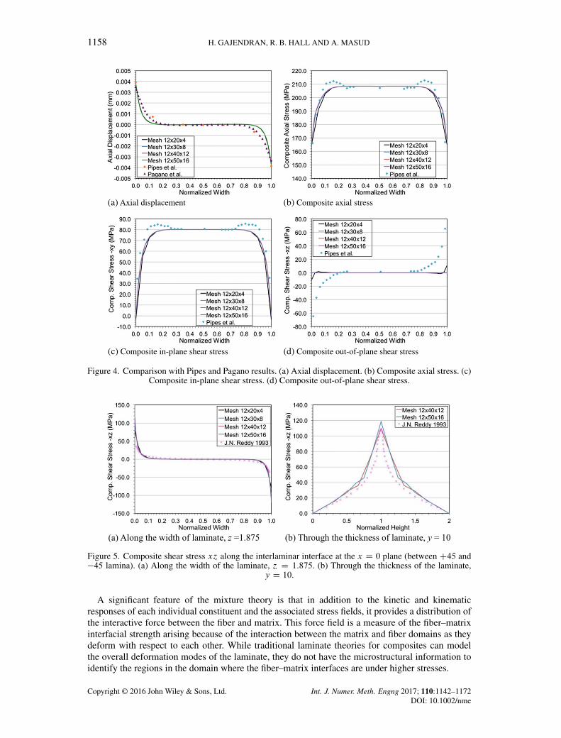
The laminate is subjected to an axial displacement of 0.3 mm at the x D ˙30 mm plane. Thenodes at the x D 0 plane are appropriately constrained to avoid rigid-body motions. This axialstretching problem is solved with four successively refined meshes, and the results are comparedwith those of Pipes and Pagano [33] and Reddy [34]. Figure 4 shows the axial displacement, com-posite axial stress, in-plane shear stress, and out-of-plane shear stress at the top surface along thewidth of the laminate at the x D 0 plane obtained from the mixture theory. It can be seen that theresults obtained from mixture theory converge with mesh refinement along the width and the thick-ness of the laminate and follow the trends observed by Pipes and Pagano [33]. The in-plane shearstress along the width of the laminate at the interlaminar interface (i.e., ´ D 1:875) between C45and �45 at the x D 0 plane is shown in Figure 5a. A steep boundary layer effect is observed alongthe axial direction at the interlaminar interface, and a good comparison for the in-plane shear stressis obtained with Reddy [34]. Figure 5b shows the through-the-thickness variation of the compositeshear stress x´ at .x; y/ D .0; 10/.

Figure 6 shows the axial stress and in-plane shear stress of the composite. As predicted by theclassical laminate theory, we observe a uniform state of stress in the bulk region of the laminate,while there are gradients in the stress fields close to the boundary signifying edge effects due to thefinite width of the laminate. Figures 7–9 show the axial stress and in-plane shear stress of the fiberand matrix, respectively. From Figure 7b, it can be observed that the fiber in-plane shear stress inthe top and bottom plies is tensile, while it is compressive in the middle plies. This is an artifact ofthe angle ply laminate configuration. From Figure 8, it can be seen that the matrix stress exhibits theeffect of the fiber orientation at the boundaries, although the matrix is modeled as a homogeneousisotropic material. This effect arises because of the tying of the constituent boundaries, where thesurface tractions at the boundaries are distributed between the constituents in a consistent fashion.

Figure 3. Four-ply laminate.

Table I. Material properties of the laminate.

˛ ˇ �L �T � Volume(MPa) (MPa) (MPa) (MPa) (MPa) (kg/mm3) fraction

Fiber 4.424EC03 1.203EC03 2.467EC05 1.039EC04 1.039EC04 1550E�09 0.5Matrix 1.990EC03 — — 1.327EC03 — 1200E�09 0.5



(a) Axial displacement (b) Composite axial stress

(c) Composite in-plane shear stress (d) Composite out-of-plane shear stress

Figure 4. Comparison with Pipes and Pagano results. (a) Axial displacement. (b) Composite axial stress. (c)Composite in-plane shear stress. (d) Composite out-of-plane shear stress.

Figure 5. Composite shear stress x´ along the interlaminar interface at the x D 0 plane (between C45 and�45 lamina). (a) Along the width of the laminate, ´ D 1:875. (b) Through the thickness of the laminate,

y D 10.

A significant feature of the mixture theory is that in addition to the kinetic and kinematicresponses of each individual constituent and the associated stress fields, it provides a distribution ofthe interactive force between the fiber and matrix. This force field is a measure of the fiber–matrixinterfacial strength arising because of the interaction between the matrix and fiber domains as theydeform with respect to each other. While traditional laminate theories for composites can modelthe overall deformation modes of the laminate, they do not have the microstructural information toidentify the regions in the domain where the fiber–matrix interfaces are under higher stresses.



Figure 6. Composite stress in the domain. (a) Axial stress. (b) In-plane shear stress.

Figure 7. Fiber stress in the domain. (a) Axial stress. (b) In-plane shear stress.

Figure 8. Matrix stress in the domain. (a) Axial stress. (b) In-plane shear stress.

Figure 9. Matrix interactive force in the domain. (a) Interactive force in the Z direction. (b) Zoomed viewat the corner.

RemarkAs mixture theory provides matrix, fiber, and composite stress fields in addition to interactive forcefield, this information can be employed to develop a comprehensive failure theory for modelingfailure in the matrix and fiber and at the fiber–matrix interface.

Figure 9 shows that the matrix interactive force field in the Z direction achieves its maximum andminimum along the interlaminar interface close to the boundary at the y D ˙10 mm plane. Thisinteractive force has a maximum value of 5.97 N/mm3 directed along the positive Z axis for the



top ply (C45ı) and a value of �5.97 N/mm3 directed along the negative Z axis for the middle ply(�45ı), which tends to peel apart the two plies. A similar pattern is observed along the interfaceplane between the bottom two plies.

RemarkFiber–matrix interaction is a function of the loading, the boundary conditions, the material ori-entation, and the mode of deformation. Therefore, sections with higher interactive force indicatethe regions where fiber–matrix interfaces are under higher stresses and therefore debonding can beinitiated. This provides crucial micromechanical insight into the potential onset of damage in thematerial system.

RemarkFrom (6), it can be deduced that the fiber interactive force is equal and opposite to the matrixinteractive force. Thus, for conciseness, fiber interactive force plots are not shown here.

RemarkThe computational cost of the mixture model scales with the number of constituents that are indi-vidually represented via the constituent governing equations. In the context of displacement-basedformulation, each additional constituent adds three DOFs per node (in the 3D context). However,unlike the pre-homogenized theories that modify the constitutive tensor and are not cognizant ofindividual constituents, mixture theory provides constituent-level micromechanical information aswell. In this context, mixture theory can be viewed as a ‘reduced-order model’ that provides micro-scopic material response in addition to the mesoscopic structural response at substantially reducedcomputational cost as compared to standard approaches that have to discretely model individualfibers to obtain this information.

5.2. Single-ply lamina with a hole

Next, we consider the axial stretching of a single-ply lamina with a hole at the center that results instress concentration and therefore local wrinkling and potential delamination in the case of multipleplies. A rectangular prismatic domain of dimensions 60� 20� 2:5mm is considered with a circularhole of radius of 1.0 mm. The composite is comprised of epoxy matrix and graphite fibers withmaterial properties that are provided in Table II. The lamina is subjected to an axial traction of200 MPa at x D ˙30 mm planes in the axial direction. The domain is discretized using 27-nodedLagrange elements, and the nodes are appropriately constrained at the x D 0 plane to avoid rigid-body motion.

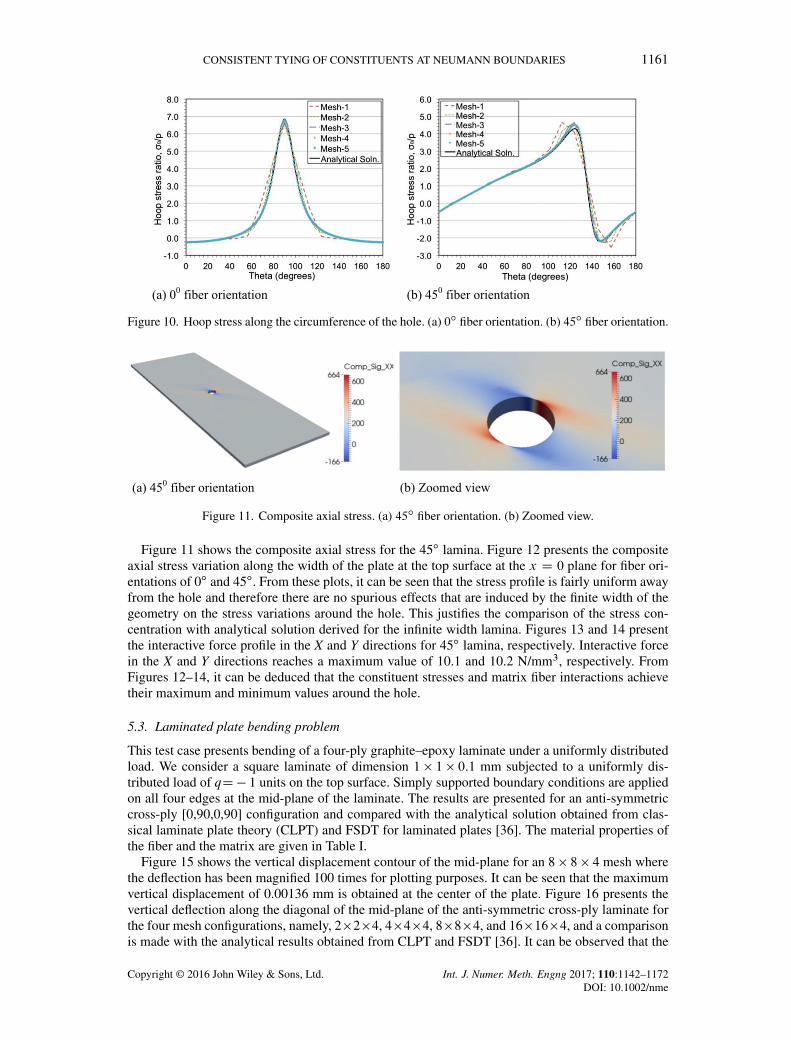
Stress concentration, which is defined as the ratio of the hoop stress and the applied traction,is plotted along the circumference of the hole. A closed-form solution for the stress concentrationaround the hole for an infinite width laminate for a given axial load and for an arbitrary fiber orien-tation is derived in Leknitskii [35]. Figure 10 shows that the stress concentration obtained from themixture theory compares well with the analytical solution for both 0ı and 45ı fiber orientations thatare considered in the simulations presented here. It can also be observed that with mesh refinement,the finite element solution variationally converges monotonically to the exact solution, which is anumerical validation of the variational consistency of the method. For the fiber orientation of 0ı,the stress concentration reaches a maximum value of 6.8 at 90ı along the circumference of the hole,while a fiber orientation of 45ı reduces the stress concentration in the lamina to 4.4. The location ofthe maximum stress concentration also shifts from 90ı to 123ı.

Table II. Material properties of the lamina.

˛ ˇ �L �T � Volume(MPa) (MPa) (MPa) (MPa) (MPa) (kg/mm3) fraction

Fiber 1.314EC03 �3.86EC03 2.252EC05 9.674EC03 3.531EC03 1550E�09 0.7Matrix 1.990EC03 — — 1.327EC03 — 1200E�09 0.3



Figure 10. Hoop stress along the circumference of the hole. (a) 0ı fiber orientation. (b) 45ı fiber orientation.

Figure 11. Composite axial stress. (a) 45ı fiber orientation. (b) Zoomed view.

Figure 11 shows the composite axial stress for the 45ı lamina. Figure 12 presents the compositeaxial stress variation along the width of the plate at the top surface at the x D 0 plane for fiber ori-entations of 0ı and 45ı. From these plots, it can be seen that the stress profile is fairly uniform awayfrom the hole and therefore there are no spurious effects that are induced by the finite width of thegeometry on the stress variations around the hole. This justifies the comparison of the stress con-centration with analytical solution derived for the infinite width lamina. Figures 13 and 14 presentthe interactive force profile in the X and Y directions for 45ı lamina, respectively. Interactive forcein the X and Y directions reaches a maximum value of 10.1 and 10.2 N/mm3, respectively. FromFigures 12–14, it can be deduced that the constituent stresses and matrix fiber interactions achievetheir maximum and minimum values around the hole.

5.3. Laminated plate bending problem

This test case presents bending of a four-ply graphite–epoxy laminate under a uniformly distributedload. We consider a square laminate of dimension 1 � 1 � 0:1 mm subjected to a uniformly dis-tributed load of qD� 1 units on the top surface. Simply supported boundary conditions are appliedon all four edges at the mid-plane of the laminate. The results are presented for an anti-symmetriccross-ply [0,90,0,90] configuration and compared with the analytical solution obtained from clas-sical laminate plate theory (CLPT) and FSDT for laminated plates [36]. The material properties ofthe fiber and the matrix are given in Table I.

Figure 15 shows the vertical displacement contour of the mid-plane for an 8 � 8 � 4 mesh wherethe deflection has been magnified 100 times for plotting purposes. It can be seen that the maximumvertical displacement of 0.00136 mm is obtained at the center of the plate. Figure 16 presents thevertical deflection along the diagonal of the mid-plane of the anti-symmetric cross-ply laminate forthe four mesh configurations, namely, 2�2�4, 4�4�4, 8�8�4, and 16�16�4, and a comparisonis made with the analytical results obtained from CLPT and FSDT [36]. It can be observed that the



Figure 12. Composite axial stress variation along the width of the plate at the top surface. (a) 0ı fiberorientation. (b) 45ı fiber orientation.

Figure 13. Interactive force in the X direction. (a) 45ı fiber orientation. (b) Zoomed view.

Figure 14. Interactive force in the Y direction. (a) 45ı fiber orientation. (b) Zoomed view.

Figure 15. Vertical deflection of the mid-plane for an 8 � 8 � 4 mesh.



Figure 16. Comparison of vertical deflection along the diagonal between mixture theory and plate theory.CLPT, classical laminate plate theory; FSDT, first-order shear deformation theory.

Figure 17. Composite stress through the thickness at .x; y/ D .0:25; 0:25/. (a) Composite axial stress. (b)Composite in-plane shear stress. FSDT, first-order shear deformation theory.

finite element solution of the vertical deflection converges monotonically with mesh refinement. Asthe CLPT assumes that the transverse normal and shear stresses are negligible, it underpredicts thedisplacement of the laminate. The vertical deflection compares well with the results obtained witha coarse mesh, which corresponds to a stiff behavior. As the FSDT accounts for constant transverseshear stress, we can see from Figure 16 that the FSDT solution compares well with the 16 � 16 � 4mesh. Figure 17a and b shows the composite axial stress through the thickness and composite in-plane shear stress at .x; y/ D .0:25; 0:25/, respectively. In both cases, a good correlation with FSDTis attained. Figure 18a presents the surface projection of the Z component of the interactive forcefor the 8 � 8 � 4 mesh. It can be observed from the side-edge surface that the second ply fromthe bottom, which has a 90ı fiber orientation, has an interactive force directed along the negative Zdirection, while the third ply, where the fiber orientation is at 0ı, has an interactive force directedalong the positive Z direction. Figure 18b and c shows the common interface between the top surfaceof the second ply and the bottom surface of the third ply and further substantiates this insight. Asthe second and third plies show an opposite interactive force in the Z direction, one of the potentialfailure modes for anti-symmetric cross-ply laminate is delamination along the mid-plane interfaceat the center of the edges.



Figure 18. Surface projection of the Z-component of the interactive force. (a) Four-ply laminate Œ0; 90; 0; 90�.(b) Top interfacial surface of the bottom two plies. (b) Bottom interfacial surface of the top two plies.

5.4. Large deformation bending of a composite beam

This section investigates the finite deformation features of the proposed numerical method underplane strain conditions. A graphite–epoxy lamina of dimensions 8� 1� 1 mm is considered, wherethe fibers are oriented along the axial direction. This finite deformation pure bending problem isadapted from Ogden [37] and Truster et al. [29] where the exact solution and corresponding firstPiola–Kirchhoff stress is provided for incompressible and compressible neo-Hookean materials,respectively. The deformation map of the matrix and fiber constituents for an arbitrary bending angleof is given as

x D

24 r cos�r sin�Z

35 ; r .X/ D

s2LX

CR2o �

LH

; � .Y / D

Y

L(54)

whereRo is the outer radius, while L and H are the length and the width of the domain, respectively.In Ogden [37], the following equations are employed to impose the incompressibility constraint:

�R2o �R

2i

�D 2HL

RoRi D

�L

�2 (55)

where Ri is the inner radius of the deformed domain. Using (54) and (55), we can rewrite thedeformation map as

x D

24 r cos�r sin�Z

35 ; r .X/ D

vuut2LX

C

sL2H 2

2CL4

4; � .Y / D

Y

L(56)



and give the deformation gradient and its inverse as

F D

264

L r

cos� � rL

sin� 0L r

sin� rL

cos� 00 0 1

375 ; F �1 D

24

rL

cos� rL

sin� 0� L r

sin� L r

cos� 00 0 1

35 (57)

It can be observed from (56) that the deformation map is only a function of the bending angle .Ignoring the interactive forces and employing the material model given in (19), we can solve for thebody force that satisfies the equilibrium equations in both the constituents. The expressions for thebody force and the first Piola–Kirchhoff stress for the fiber are given in Appendix D.

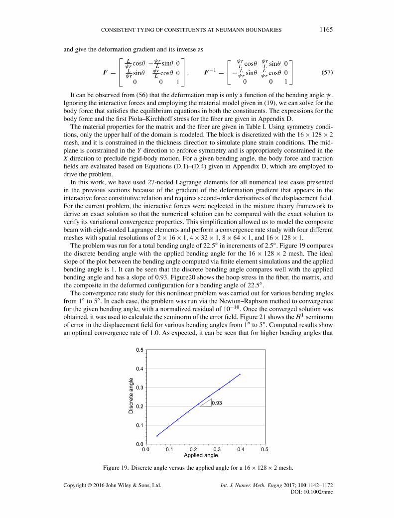
The material properties for the matrix and the fiber are given in Table I. Using symmetry condi-tions, only the upper half of the domain is modeled. The block is discretized with the 16 � 128 � 2mesh, and it is constrained in the thickness direction to simulate plane strain conditions. The mid-plane is constrained in the Y direction to enforce symmetry and is appropriately constrained in theX direction to preclude rigid-body motion. For a given bending angle, the body force and tractionfields are evaluated based on Equations (D.1)–(D.4) given in Appendix D, which are employed todrive the problem.

In this work, we have used 27-noded Lagrange elements for all numerical test cases presentedin the previous sections because of the gradient of the deformation gradient that appears in theinteractive force constitutive relation and requires second-order derivatives of the displacement field.For the current problem, the interactive forces were neglected in the mixture theory framework toderive an exact solution so that the numerical solution can be compared with the exact solution toverify its variational convergence properties. This simplification allowed us to model the compositebeam with eight-noded Lagrange elements and perform a convergence rate study with four differentmeshes with spatial resolutions of 2 � 16 � 1, 4 � 32 � 1, 8 � 64 � 1, and 16 � 128 � 1.

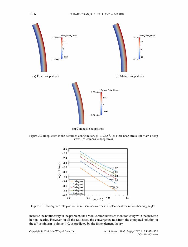
The problem was run for a total bending angle of 22.5ı in increments of 2.5ı. Figure 19 comparesthe discrete bending angle with the applied bending angle for the 16 � 128 � 2 mesh. The idealslope of the plot between the bending angle computed via finite element simulations and the appliedbending angle is 1. It can be seen that the discrete bending angle compares well with the appliedbending angle and has a slope of 0.93. Figure20 shows the hoop stress in the fiber, the matrix, andthe composite in the deformed configuration for a bending angle of 22.5ı.

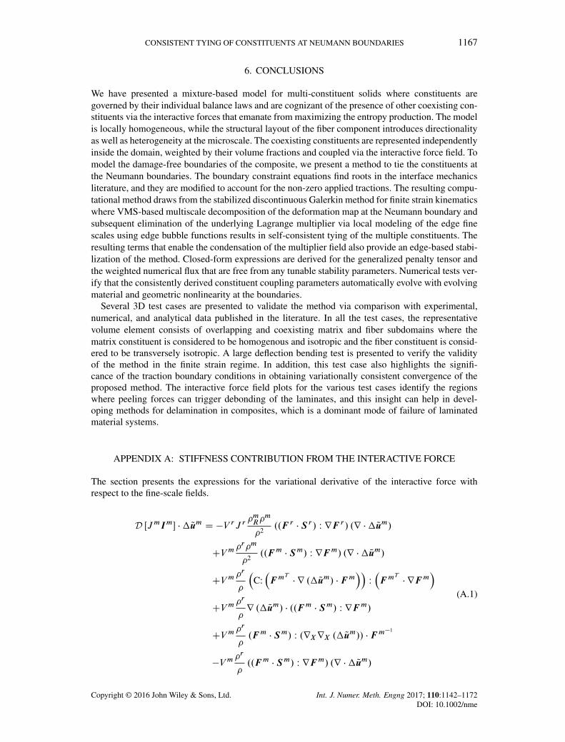
The convergence rate study for this nonlinear problem was carried out for various bending anglesfrom 1ı to 5ı. In each case, the problem was run via the Newton–Raphson method to convergencefor the given bending angle, with a normalized residual of 10�10. Once the converged solution wasobtained, it was used to calculate the seminorm of the error field. Figure 21 shows the H1 seminormof error in the displacement field for various bending angles from 1ı to 5ı. Computed results showan optimal convergence rate of 1.0. As expected, it can be seen that for higher bending angles that

Figure 19. Discrete angle versus the applied angle for a 16 � 128 � 2 mesh.



Figure 20. Hoop stress in the deformed configuration, D 22:50. (a) Fiber hoop stress. (b) Matrix hoopstress. (c) Composite hoop stress.

Figure 21. Convergence rate plot for the H1 seminorm error in displacement for various bending angles.

increase the nonlinearity in the problem, the absolute error increases monotonically with the increasein nonlinearity. However, in all the test cases, the convergence rate from the computed solution inthe H1 seminorm is almost 1.0, as predicted by the finite element theory.



6. CONCLUSIONS

We have presented a mixture-based model for multi-constituent solids where constituents aregoverned by their individual balance laws and are cognizant of the presence of other coexisting con-stituents via the interactive forces that emanate from maximizing the entropy production. The modelis locally homogeneous, while the structural layout of the fiber component introduces directionalityas well as heterogeneity at the microscale. The coexisting constituents are represented independentlyinside the domain, weighted by their volume fractions and coupled via the interactive force field. Tomodel the damage-free boundaries of the composite, we present a method to tie the constituents atthe Neumann boundaries. The boundary constraint equations find roots in the interface mechanicsliterature, and they are modified to account for the non-zero applied tractions. The resulting compu-tational method draws from the stabilized discontinuous Galerkin method for finite strain kinematicswhere VMS-based multiscale decomposition of the deformation map at the Neumann boundary andsubsequent elimination of the underlying Lagrange multiplier via local modeling of the edge finescales using edge bubble functions results in self-consistent tying of the multiple constituents. Theresulting terms that enable the condensation of the multiplier field also provide an edge-based stabi-lization of the method. Closed-form expressions are derived for the generalized penalty tensor andthe weighted numerical flux that are free from any tunable stability parameters. Numerical tests ver-ify that the consistently derived constituent coupling parameters automatically evolve with evolvingmaterial and geometric nonlinearity at the boundaries.

Several 3D test cases are presented to validate the method via comparison with experimental,numerical, and analytical data published in the literature. In all the test cases, the representativevolume element consists of overlapping and coexisting matrix and fiber subdomains where thematrix constituent is considered to be homogenous and isotropic and the fiber constituent is consid-ered to be transversely isotropic. A large deflection bending test is presented to verify the validityof the method in the finite strain regime. In addition, this test case also highlights the signifi-cance of the traction boundary conditions in obtaining variationally consistent convergence of theproposed method. The interactive force field plots for the various test cases identify the regionswhere peeling forces can trigger debonding of the laminates, and this insight can help in devel-oping methods for delamination in composites, which is a dominant mode of failure of laminatedmaterial systems.

APPENDIX A: STIFFNESS CONTRIBUTION FROM THE INTERACTIVE FORCE

The section presents the expressions for the variational derivative of the interactive force withrespect to the fine-scale fields.

D ŒJmIm� �� Qum D �V rJ r�mR�

m

�2..F r � S r/ W rF r/ .r �� Qum/

CV m�r�m

�2..Fm � Sm/ W rFm/ .r �� Qum/

CV m�r

�

�C:�Fm

T

� r .� Qum/ � Fm��W�Fm

T

� rFm�

CV m�r

�r .� Qum/ � ..Fm � Sm/ W rFm/

CV m�r

�.Fm � Sm/ W .rXrX .� Qu

m// � Fm�1

�V m�r

�..Fm � Sm/ W rFm/ .r �� Qum/

(A.1)



D ŒJ rIr � �� Qur D �V mJm�rR�

r

�2..Fm � Sm/ W rFm/ .r �� Qur/

CV r�r�m

�2..F r � S r/ W rF r/ .r �� Qur/

C V r�m

�

�C:�F r

T

� r .� Qur/ � F r��W�F r

T

� rF r�

C V r�r

�r .� Qur/ � ..F r � S r/ W rF r/

C V r�m

�.F r � S r/ W .rXrX .� Qu

r// � F r�1

� V r�m

�..F r � S r/ W rF r/ .r �� Qur/

(A.2)

By substituting the incremental form of (31) into (A.1) and (A.2), we can write a concise form ofthe consistent tangent stiffness tensors Bmr and Brm that arise due to the matrix and fiber interactiveforce as follows: D ŒJmIm� �� Qum D Bmr�ˇm and D ŒJ rIr � �� Qur D Brm�ˇr .

The gradient of the fine-scale weighting field can be expressed in terms of bubble functions asQ�˛a;A D �

˛aAu .b

e/ˇ˛u. The matrix form of this equation is given as follows:8̂̂̂ˆ̂̂<ˆ̂̂̂̂:̂

�˛1;1�˛2;2�˛3;3�˛1;2�˛2;3�˛3;1

9>>>>>>=>>>>>>;D

266666664

@be@x

0 0

0 @be@y

0

0 0 @be@´

@be@y

0 0

0 @be@´

0

0 0 @be@x

377777775

8<:ˇ˛1ˇ˛2ˇ˛3

9=; (A.3)

APPENDIX B: CONSISTENT LINEARIZATION

This subsection provides consistent linearization of the final multiscale weak form, Equation (52).It can be observed that Equation (52) is a function of both matrix and fiber displacement fields. Tosolve this problem in a fully coupled fashion using the Newton–Raphson scheme, we linearize thestabilized primal formulation with respect to both the constituents. The tangent stiffness matrix ofthe final multiscale weak form given in (52) can be written in symbolic form as

K�'r ;'m;�I�ro;�

mo

�D DR'

�'r ;'m;�I Q�ro; Q�

mo

�: �ur CDR'

�'r ;'m;�I Q�ro; Q�

mo

�: �um

(B.1)The variational derivative of the coarse-scale residual with respect to both the constituents in

reference configuration is given as

K�'r ;'m;�I�ro;�

mo

�D

X˛Dr;m

24Z�˛

rX�˛o W A

˛ W rX�u˛d� �

Z�˛

�˛o :D ŒJ ˛I˛� � �u˛d�

35

�X˛Dr;m

24Z�˛

��ro � �mo � � D Œ¹PN º� � �u˛d�

35

C

Z�˛

��ro � �

mo

�� s �

��ur ��um

�d�

�

Z�res2

¹.rX�o W A/ � N º � ��ur ��um�d�

�

Z�res2

D Œ¹.rX�o W A/ � N º� � �u˛ ��'r � 'm

�d�

(B.2)



The weighted average of the flux term in the preceding equation can be further simplified as

D Œ¹PN º� � �u˛ D ırs � .D ŒPr � � �ur/N r � ıms � .D ŒPm� � �um/Nm

D ¹.A W rX�u/N º(B.3)

and the linearization of the acoustic tensor term is written as

D Œ¹.rX�o W A/ � N º� � �u˛ D�rX�

ro W „

r W rX�ur�� N r

��ırs�T

��rX�

mo W „

m W rX�um�� Nm

��ıms�T

D ¹.rX�o W „ W rX�u/ � N º

(B.4)

where „˛ is the sixth-order tensor of material moduli and is defined as

„˛ D@3 ˛

@F ˛@F ˛@F ˛(B.5)

The final consistent tangent stiffness matrix contribution due to the constituent ˛ can be writtenin the material configuration as

DR'�'˛;'˛;�I Q�˛o

�� u˛D

X˛Dr;m

24Z�˛

rX�˛o W A

˛ W rX�u˛d��

Z�˛

�˛o � D ŒJ ˛I˛� � �u˛d�

35

�

Z�˛

��ro � �

mo

�� ¹.A W rX�u/N º d�

C

Z�˛

��ro � �mo � � �s � ��ur ��um�d�

�

Z�res2

¹.rX�o W A/ � N º � ��ur ��um�d�

�

Z�res2

¹.rX�o W „ W rX�u/ � N º � �'r � 'm�d�(B.6)

We now push forward the residual of the governing equations and the consistent tangent stiffnessterms to the current configuration as follows.

Residual vector:

X˛Dr;m

264Z�˛'

r�˛ � ˛d�'�Z�˛'

�˛ � �˛b˛d�'�Z�˛'

�˛ � I˛d�'

375�Z

�˛'

.V r�rCV m�m/ � hcd�'

�

Z�˛'

��r � �m

��ırs � .

rnr � V rhc/ � ıms � .mnm � V mhc/

�d�'

C

Z�˛'

��r � �m

�� s �

�'r � 'm

��Ad�'

�

Z�'

°Œ.r�r W ar/ � nr � �

�ırs�T� Œ.r�m W am/ � nm� �

�ıms�T ±��'r � 'm

�d�' D 0

(B.7)



Stiffness matrix:

DR'�'˛;'˛;�I Q�˛o

��u˛D

X˛Dr;m

264Z�˛'

r�˛ Wa˛ Wr�u˛d�'�Z�˛'

�˛ �1

J ˛D ŒJ ˛I˛� ��u˛d�'

375

C

Z�˛'

��r � �m

�� s � ��ur ��um��Ad�'

�

Z�r'

¹.r� W a/ � nº ��ur ��um�d�'

�

Z�˛'

��r � �m

�� ¹.a W r�u/ � nº d�'

�

Z�r'

¹.r� W d W r�u/ � nº ��'r � 'm

�d�'

(B.8)

APPENDIX C: OUTLINE OF THE ALGORITHM FOR IMPLEMENTATION OF THEPROPOSED APPROACH

Initialize VariablesLoop over Load-step

Loop until ConvergenceLoop over Bulk elements

Compute the bulk stabilization tensor for matrix and fiber

Compute F˛; rF˛

Compute T˛; I˛

Compute elemental residual (Equation (B.6)) and tangent stiffness matrix(Equation (B.7)) of constituentsAssemble global residual and tangent stiffness matrix

End loop

Loop over Boundary Interface elementsCompute edge stabilization tensor for matrix and fiber (Equation (41))

Compute F˛; rF˛

Compute T˛; I˛

Compute corresponding contribution (i.e., boundary interface terms) toresidual and tangent stiffness matrix (in Equations (B.6) and (B.7), respectively)Assemble global residual and tangent stiffness matrix

End loopApply boundary conditionsSolve for incremental fiber and matrix displacement fields

End loop (Convergence)End loop (Load-step)



APPENDIX D: BODY FORCE AND TRACTION FIELD FOR LARGE DEFORMATIONBENDING OF THE COMPOSITE BEAM

For the case of fiber orientation along the axial direction, the first Piola–Kirchhoff stress and bodyforce of the fiber are given as follows:

PrDV r�rT

24�u3 � u

�cos�

�t � t3

�sin� 0�

u3 � u�

sin��t3 � t

�cos� 0

0 0 0

35C 1

2V r˛r

24 .t � u/ cos�

�t � t3

�sin� 0

.t � u/ sin��t3 � t

�cos� 0

0 0�t2 � 1

�35

C1

2V rr

24�u3 C t � 2u

�cos�

�2t � u � t3

�sin� 0�

u3 C t � 2u�

sin��uC t3 � 2t

�cos� 0

0 0�u2 C t2 � 2

�35

C1

2V r˛r

24 0

��u � t3 C 2t

�sin� 0

0�uC t3 � 2t

�cos� 0

0 0 0

35C 1

2V rˇr

24 0

�t � t3

�sin� 0

0�t3 � t

�cos� 0

0 0 0

35

(D.1)Accordingly, the three components of the body force are given by

�rBr1DVr�rT cos�

�3u4

r�u2

r

�C1

2V rrcos�

�3u4

r�u

r�2u2

r

�C1

2V r˛rcos�

��u

r�u2

r

�

C

�V r�rT C

1

2V rr C

1

2V rˇr

� �t3 � t

�cos�

L

C1

2V rr

��2t C uC t3

�cos�

LC1

2V r˛r

�uC t3 � 2t

�cos�

L(D.2)

�rBr2DVr�rT sin�

�3u4

r�u2

r

�C1

2V rr sin �

�3u4

r�u

r�2u2

r

�C1

2V r˛rsin�

��u

r�u2

r

�

C

�V r�rT C

1

2V r˛r C

1

2V rˇr

� �t3 � t

�sin�

L

C1

2V rr

��2t C uC t3

�sin�

LC1

2V r˛r

��2t C uC t3

�sin�

L(D.3)

�rBr3 D 0 (D.4)

where u D L r

and t D rL

.

REFERENCES

1. Truesdell C, Noll W. The Non-linear Field Theories of Mechanics. Springer: Berlin, 2004.2. Atkin R, Craine R. Continuum theories of mixtures: basic theory and historical development. The Quarterly Journal

of Mechanics and Applied Mathematics 1976; 29(2):209–244.3. Green AE, Naghdi PM. On basic equations for mixtures. The Quarterly Journal of Mechanics and Applied

Mathematics 1969; 22(4):427–438.4. Green AE, Naghdi PM. A theory of mixtures. Archive for Rational Mechanics and Analysis 1967; 24(4):243–263.5. Rajagopal KR, Tao L. Mechanics of Mixtures. World Scientific Publishing Company, Incorporated: Singapore, 1995.6. Rajagopal KR, Srinivasa A. On the thermomechanics of materials that have multiple natural configurations. Part

I: viscoelasticity and classical plasticity. Zeitschrift für angewandte Mathematik und Physik ZAMP 2004; 55(5):861–893.

7. Rajagopal KR. Diffusion through polymeric solids undergoing large deformations. Materials Science and Technology2003; 19(9):1175–1180.

8. Karra S. Modeling the diffusion of a fluid through viscoelastic polyimides. Mechanics of Materials 2013; 66:120–33.9. Karra S, Rajagopal KR. A model for the thermo-oxidative degradation of polyimides. Mechanics of Time-dependent

Materials 2012; 16(3):329–342.



10. Humphrey J, Rajagopal KR. A constrained mixture model for growth and remodeling of soft tissues. MathematicalModels and Methods in Applied Sciences 2002; 12(03):407–430.

11. Rao I, Rajagopal KR. A thermodynamic framework for the study of crystallization in polymers. Zeitschrift fürangewandte Mathematik und Physik ZAMP 2002; 53(3):365–406.

12. Bowen RM, Wiese JC. Diffusion in mixtures of elastic materials. International Journal of Engineering Science 1969;7(7):689–722.

13. Bedford A, Stern M. Toward a diffusing continuum theory of composite materials. Journal of Applied Mechanics1971; 38(1):8–14.

14. Hall RB, Rajagopal KR. Diffusion of a fluid through an anisotropically chemically reacting thermoelastic body withinthe context of mixture theory. Mathematics and Mechanics of Solids 2012; 17(2):131–164.

15. Hall RB. A theory of coupled anisothermal chemomechanical degradation for finitely-deforming composite mate-rials with higher-gradient interactive forces. In Challenges in Mechanics of Time Dependent Materials, Antoun B,et al. (eds.), Conference Proceedings of the Society for Experimental Mechanics Series, vol. 2. Springer, 2017.(Available from: https://doi.org/10.1007/978-3-319-41543-7_13).

16. Brezzi F, Fortin M. Mixed and Hybrid Finite Element Methods. Springer Science & Business Media: New York,2012.

17. Nitsche J. Über ein Variationsprinzip zur Lösung von Dirichlet-Problemen bei Verwendung von Teilräumen, diekeinen Randbedingungen unterworfen sind. In Abhandlungen aus dem mathematischen Seminar der UniversitätHamburg 1971 Jul 1 (Vol. 36, No. 1, pp. 9–15). Springer, Berlin.

18. Hansbo A, Hansbo P. An unfitted finite element method, based on Nitsche’s method, for elliptic interface problems.Computer Methods in Applied Mechanics and Engineering 2002; 191(47):5537–52.

19. Dolbow J, Harari I. An efficient finite element method for embedded interface problems. International Journal forNumerical Methods in Engineering 2009; 78(2):229–52.

20. Sanders JD, Dolbow JE, Laursen TA. On methods for stabilizing constraints over enriched interfaces in elasticity.International Journal for Numerical Methods in Engineering 2009; 78(9):1009.

21. Embar A, Dolbow J, Harari I. Imposing Dirichlet boundary conditions with Nitsche’s method and spline-based finiteelements. International Journal for Numerical Methods in Engineering 2010; 83(7):877–98.

22. Annavarapu C, Hautefeuille M, Dolbow JE. A robust Nitsche’s formulation for interface problems. ComputerMethods in Applied Mechanics and Engineering 2012; 225:44–54.

23. Masud A, Truster TJ, Bergman LA. A variational multiscale a posteriori error estimation method for mixed form ofnearly incompressible elasticity. Computer Methods in Applied Mechanics and Engineering 2011; 200(47):3453–81.

24. Masud A, Scovazzi G. A heterogeneous multiscale modeling framework for hierarchical systems of partialdifferential equations. International Journal for Numerical Methods in Fluids 2011; 65(1-3):28–42.

25. Masud A, Truster TJ, Bergman LA. A unified formulation for interface coupling and frictional contact modeling withembedded error estimation. International Journal for Numerical Methods in Engineering 2012; 92(2):141–77.

26. Masud A, Truster TJ. A framework for residual-based stabilization of incompressible finite elasticity: stabilized for-mulations and methods for linear triangles and tetrahedra. Computer Methods in Applied Mechanics and Engineering2013; 267:359–99.

27. Truster TJ, Masud A. Primal interface formulation for coupling multiple PDEs: a consistent derivation via thevariational multiscale method. Computer Methods in Applied Mechanics and Engineering 2014; 268:194–224.

28. Truster TJ, Masud A. A Discontinuous/continuous Galerkin method for modeling of interphase damage in fibrouscomposite systems. Computational Mechanics 2013; 52(3):499–514.

29. Truster TJ, Chen P, Masud A. Finite strain primal interface formulation with consistently evolving stabilization.International Journal for Numerical Methods in Engineering 2015; 102(3-4):278–315.

30. Masud A, Tham CL, Liu WK. A stabilized 3-D co-rotational formulation for geometrically nonlinear analysis ofmulti-layered composite shells. Computational Mechanics 2000; 26(1):1–2.

31. Masud A, Panahandeh M. Finite-element formulation for analysis of laminated composites. Journal of EngineeringMechanics 1999; 125(10):1115–24.

32. Marsden JE, Hughes TJR. Mathematical Foundations of Elasticity. Prentice-Hall: Englewood Cliffs, NJ, 1983.33. Pipes RB, Pagano NJ. Interlaminar stresses in composite laminates under uniform axial extension. Journal of

Composite Materials 1970; 4(4):538–48.34. Reddy JN. An evaluation of equivalent-single-layer and layerwise theories of composite laminates. Composite

Structures 1993; 25(1-4):21–35.35. Leknitskii SG. Theory of Elasticity of an Anisotropic Elastic Body. Holden-Day: San Francisco, 1963.36. Reddy JN. Mechanics of Laminated Composite Plates and Shells: Theory and Analysis. CRC Press: Boca Raton,

2004.37. Ogden RW. Non-Linear Elastic Deformations. Courier Corporation: New York, 1997.


https://doi.org/10.1007/978-3-319-41543-7_13

edge stabilization and consistent tying of constituents at

Documents