editorial and business address: chemical engineering...
TRANSCRIPT

Summer 2002 177
Chemical Engineering Education Volume 36 Number 3 Summer 2002
CHEMICAL ENGINEERING EDUCATION (ISSN 0009-2479) is published quarterly by the Chemical EngineeringDivision, American Society for Engineering Education, and is edited at the University of Florida. Correspondenceregarding editorial matter, circulation, and changes of address should be sent to CEE, Chemical Engineering Department,University of Florida, Gainesville, FL 32611-6005. Copyright © 2002 by the Chemical Engineering Division, AmericanSociety for Engineering Education. The statements and opinions expressed in this periodical are those of the writers and notnecessarily those of the ChE Division, ASEE, which body assumes no responsibility for them. Defective copies replaced ifnotified within 120 days of publication. Write for information on subscription costs and for back copy costs and availability.POSTMASTER: Send address changes to Chemical Engineering Education, Chemical Engineering Department., Universityof Florida, Gainesville, FL 32611-6005. Periodicals Postage Paid at Gainesville, Florida and additional post offices.
EDITORIAL AND BUSINESS ADDRESS:Chemical Engineering Education
Department of Chemical EngineeringUniversity of Florida • Gainesville, FL 32611
PHONE and FAX : 352-392-0861e-mail: [email protected]
EDITORTim Anderson
ASSOCIATE EDITORPhillip C. Wankat
MANAGING EDITORCarole Yocum
EDITORIAL ASSISTANTChristina Smart
PROBLEM EDITORJames O. Wilkes, U. Michigan
LEARNING IN INDUSTRY EDITORWilliam J. Koros, Georgia Institute of Technology
• CHAIRMAN •E. Dendy Sloan, Jr.
Colorado School of Mines
• MEMBERS •Pablo Debenedetti
Princeton University
Dianne DorlandRowan University
Thomas F. EdgarUniversity of Texas at Austin
Richard M. FelderNorth Carolina State University
Bruce A. FinlaysonUniversity of Washington
H. Scott FoglerUniversity of Michigan
William J. KorosGeorgia Institute of Technology
David F. OllisNorth Carolina State University
Ronald W. RousseauGeorgia Institute of Technology
Stanley I. SandlerUniversity of Delaware
Richard C. SeagraveIowa State University
C. Stewart SlaterRowan University
James E. SticeUniversity of Texas at Austin
Donald R. WoodsMcMaster University
� EDUCATOR
178 L.K. Doraiswamy of Iowa State University,Thomas D. Wheelock, Peter J. Reilly
� LABORATORY
182 Experimental Projects for the Process Control Laboratory,Siong Ang, Richard D. Braatz
198 An Introduction to Drug Delivery for Chemical Engineers,Stephanie Farrell, Robert P. Hesketh
216 Mass Transfer and Cell Growth Kinetics in a Bioreactor, Ken K.Robinson, Joshua S. Dranoff, Christopher Tomas, Seshu Tummala
226 Integrating Kinetics Characterization and Materials Processing in theLab Experience,
Dennis J. Michaud, Rajeev L. Gorowara, Roy L. McCullough
� CLASSROOM
188 Using Test Results for Assessment of Teaching and Learning,H. Henning Winter
212 Rubric Development and Inter-Rater Reliability Issues in AssessingLearning Outcomes,
James A. Newell, Kevin D. Dahm, Heidi L. Newell
232 Scaling of Differential Equations: “Analysis of the Fourth Kind,”Paul J. Sides
236 The Use of Software Tools for ChE Education: Students’ Evaluations,Abderrahim Abbas, Nader Al-Bastaki
242 Teaching Process Control with a Numerical Approach Based onSpreadsheets, Christopher Rives, Daniel J. Lacks
� CURRICULUM
192 Is Process Simulation Used Effectively in ChE Courses?Kevin D. Dahm, Robert P. Hesketh, Mariano J. Savelski
222 Teaching ChE to Business and Science Students, Ka M. Ng
� RANDOM THOUGHTS
204 FAQs. v. Designing Fair Tests, Richard M. Felder, Rebecca Brent
� CLASS AND HOME PROBLEMS
206 Boiling-Liquid Expanding-Vapor Explosion (BLEVE): An Introduc-tion to Consequence and Vulnerability Analysis, C. Téllez, J.A. Peña
231 Errata
PUBLICATIONS BOARD

178 Chemical Engineering Education
L. K. Doraiswamyof Iowa State University
THOMAS D. WHEELOCK, PETER J. REILLY
Iowa State University • Ames, IA 50011
LK. Doraiswamy came to Iowa State University (ISU)in a most unusual manner. One of the authors (PR)was attending a meeting in New Delhi in 1984 and,
since he had previously helped two scientists at the NationalChemical Laboratory (NCL) in Pune with some chromatog-raphy for a project of theirs, he asked if he could visit themthere. He took the train to Pune during the dry season, arriv-ing a bit hot and dusty, but quite exhilarated after experienc-ing one of the world’s great train rides—the climb throughthe Western Ghats. He and a former graduate student werepicked up by two NCL scientists on their motor scooters andwere delivered to the laboratory, where they were eventuallyushered into the baronial office of the NCL Director, occu-pied in fine style by one L.K. Doraiswamy. Although L.K. waschagrined that the visitors had not been met by an air-condi-tioned NCL car, things went so well after that, the ISU visitorended by participating in a joint enzyme project with the NCL.
Some years later, L.K. (as he is known to his friends andcolleagues, except at Wisconsin-Madison where he goes byDorai) arrived by very small plane in Des Moines to see howthe ISU end of the joint project was progressing. During thatvisit L.K. was asked by his host what he planned to do afterhis (imminent) NCL retirement. L.K. mentioned how muchhe liked small midwestern university towns, and sensing avery good thing, the host passed this word on to his depart-ment chair (Dick Seagrave). Soon an appointment was hur-tling through the university hierarchy in record time.
That first appointment, in 1989, was the Glenn MurphyChair, meant for a distinguished visiting professor in theCollege of Engineering. It was followed by the Departmentof Chemical Engineering’s Herbert Stiles Chair in 1992, andthen in 1996 L.K. became Anson Marston Distinguished Pro-fessor in Engineering. His first office was anything but baro-nial, being the standard 120 ft2 with hardly any window area,but eventually a nice office opened up when Sweeney Hallwas expanded. L.K. still occupies it, even after his retire-ment from ISU in December 2000.
EARLY STIRRINGSL.K. was born in Bangalore in 1927 to L.S. and Kamala
Krishnamurthy, the only boy of four children. His father ledthe Hyderabad Branch of the Geological Survey of India. Forpart of his childhood, L.K. and his family lived in the smallvillage of Lingsagur. Later they moved to Hyderabad, thestate capital, where L.K. graduated from Methodist Boys HighSchool. He studied chemistry at Nizam College in Hyderabad,part of the University of Madras, and then was faced withseveral opportunities for further education. One was to studyorganic chemistry, a subject he thoroughly enjoyed. But therapidly developing field of chemical engineering also attractedhim, and he ultimately decided to study it at the AlgappeChettiar College of Technology, also part of the Universityof Madras. Such an opportunity was very rare in India at thetime, since only two schools with limited enrollments andvery high entrance standards offered chemical engineering.
ON TO WISCONSIN
As a result of his successful record in pursuing chemicalengineering at Madras, L.K. received a scholarship from theHyderabad government to study in the United States. An unclewith a Wisconsin PhD in chemistry suggested that he applythere—he did, he was accepted, and he arrived during thewinter cold of December 1948.
L.K. was lucky enough to secure Olaf Hougen as his majorprofessor, and after he earned his MS in 1950 and his Indianscholarship had expired, Hougen convinced the Hyderabad gov-ernment to continue funding L.K. for a PhD (which he receivedin 1952). His dissertation was on semichemical pulping, doneunder the joint supervision of Hougen and John McGovern ofthe USDA Forest Products Laboratory in Madison.
Hougen’s perception that he had found a promising chemi-cal engineer was even truer than he thought—in 1987 L.K.became the Olaf Hougen Visiting Professor of Chemical En-gineering at Wisconsin, an honor given to only five otherdistinguished educators. Then in 1991, he received an honor-© Copyright ChE Division of ASEE 1999
ChE educator

Summer 2002 179
(Top) L.K. evinced a clearpenchant for things mechanical
at an early age.
(Above) L.K. and his wifeRajalakshmi (now deceased)after their 1952 wedding.
(Right) Today’s L.K.
(Below) L.K.’s present family;left to right, Rahul, Sandhya,Sankar, L.K., Deepak, andPriya.
ary DSc from Wisconsin to go with his 1982 hon-orary DSc from Salford in England.
BACK HOME TO THE NATIONALCHEMICAL LABORATORY
After graduating from Wisconsin, L.K. workedon emulsion paints for a year at Carlisle Chemicaland Manufacturing in Brooklyn. Although thecompany urged him to stay, L.K. believed he couldmake a greater contribution in India, and in 1954he joined the NCL as a senior scientist. He roserapidly through the ranks, becoming Assistant Di-rector and head of the Division of Organic Inter-mediates and Dyes in 1961, Deputy Director andhead of the Division of Chemical Engineering andProcess Development in 1966, and finally becom-ing Director in 1978. He was the fifth director andthe first nonchemist to head the NCL, and he ledit until he retired in 1989. After his retirement, hecame to the United States to be nearer to his chil-dren and grandchildren, and (not incidentally) tocontinue his research career without the burden ofadministrative duties.
L.K. had a tremendous impact on NCL, both asa tireless and innovative researcher and as a highlyrespected and visionary leader who promoted re-search excellence. When he retired he received ascroll that reviewed his accomplishments andsummed up his contributions by stating, “Youepitomize the finest in scientific research, man-agement, planning, and execution. We will alwaysremember you, as a compassionate human beingwho combined in himself the attributes of greatscholarship and visionary leadership.” His contri-butions to the growth of the Indian chemical in-dustry were also cited, as was his extensive ser-vice as an advisor to the Indian government andas a member of various key committees.
Early in his NCL tenure, L.K. established astrong base of fundamental and applied research,especially in chemical reaction engineering. Un-der his leadership, many commercially importanttechnologies were developed, including fluidized-bed processes for making chloromethanes andmethylchlorosilanes, continuous processes fordimethylaniline and ethylenediamine, a new pro-cess for vitamin B
6, and a complete process for
methyl, ethyl, butyl, and 2-ethylhexyl acrylates.The dimethylaniline technology was the first va-por-phase catalytic process for making that prod-uct, while that for ethylenediamine was apparentlythe first continuous organic chemical process de-veloped in India. His teams also developed zeo-
L.K. and six of his seven ISU doctoral students. From theleft, Leigh Hagenson Thompson, L.K., Sanjeev Naik, Holger
Glatzer, Jennifer Anderson, Ore Sofekun, and SridharDesikan. Missing is Justinus Satrio.

180 Chemical Engineering Education
Students andfaculty at the
Wisconsin summerlaboratory course
in 1977, with L.K. atthe far right
and Roger Altpeterand Richard
Grieger-Block atthe far left.
Wisconsonians,and others,
beyond a certainage will enjoyidentifying theothers pictured
here.
lite catalysts and processes for xylene isomerization and formaking alkylating benzene with alcohols. Many of these de-velopments led to awards from the Indian ChemicalManufacturer’s Association.
L.K. lavished care and attention on the NCL by streamlin-ing departments, doing what was needed to attract the bestpeople, and attending to the needs of the whole community.His son Deepak tells us that on occasion this involved suchmatters as “compassionate appointments” for poor or recentlywidowed employees, special housing allotments for deserv-ing cases, and investment of resources for welfare purposessuch as the local school and a shopping center (which hassince become a major attraction in the city and is namedafter his late wife).
To highlight his human side, one instance is worth specialmention. One night, a poor family was evicted from the NCLcampus for building and occupying an illegal accommoda-tion. L.K., moved by their plight (and against the administra-tive officer’s advice), gave them permission to stay overnightuntil they could make other arrangements. This eventuallyled to a protracted legal battle and illustrates how his softerside sometimes leads him to take risks.
His professionalism concerning matters such as punctual-ity, returning phone calls, meeting deadlines, and making al-lowances for potential mistakes in planning is also a hall-mark of his character. His approach is simply “to get andmaintain the best,” and it has led to a legacy of excellencethat he is especially proud of. He maintains that “excellenceis a state of mind” and he never tires of repeating it.
While at NCL, L.K. wrote a book on catalytic reactors andreactions (Pergamon, 1991) and was coauthor of two vol-
umes on heterogeneous reactions with his close friend M.M.Sharma at the University of Bombay (Wiley, 1984) and oneon stochastic modeling with his NCL colleague B.D. Kulkarni(Gordon and Breach, 1987). He also edited or coedited fourbooks and contributed chapters to six others. L.K. personallyguided the thesis research of 45 students who received PhDsfrom various Indian universities and collaborated with thelate Tony Holland at Salford in guiding fifteen others andwith Mike Davidson at Edinburgh in an additional two. Hehas been author or coauthor of some 155 international jour-nal articles. They were mainly on adsorption and catalysis;gas-solid, gas-liquid, solid-solid, and slurry reactions; fluidi-zation; and stochastic modeling and analysis of reacting sys-tems. For five years he also served as editor of the IndianChemical Engineer.
L.K. is reputed to have received every major scientific andtechnical award in India open to chemical engineers. Amongthe most noteworthy are the Om Prakash Bhasin Award forScience and Technology, given by Indian President Zail Singhin 1986, the Jawaharlal Nehru Award for lifetime achieve-ment in engineering and technology (1987), and the Repub-lic Day honor Padma Bhushan presented by Indian PresidentR. Venkataraman in 1990. Notable awards from outside ofIndia but honoring his work there are election to the ThirdWorld Academy of Science in 1997, the Richard H. WilhelmAward from AIChE in 1990, and the Personal Achievementin Chemical Engineering Award in 1988 from ChemicalEngineering magazine.
THE FAMILY MANSoon after returning to India, L.K. married his wife
Rajalakshmi. She was always a source of great emotional
Summer 2002 181
strength and happiness to him, and her early death after aprolonged and painful illness was a devastating blow. L.K.has two children, Sandhya and Deepak, who remember theirdad teaching them by gentle example and with the adage thatdiscipline is doing what you don’t like to do. Sandhya com-pleted a MPhil at the University of Poona and became a CPAafter she arrived in the United States. She and her husbandSankar Raghavan have two children, Rahul and Priya, theapples of their grandfather’s eyes. L.K.’s son Deepak receiveda PhD in chemical engineering from Delaware after earninga BTech from the University of Bombay. He completed apostdoctoral fellowship in the Rutgers Department of Ceram-ics and Materials Engineering and then joined the DuPontExperimental Station in Wilmington, Delaware. He is alsoan adjunct professor at West Virginia University. L.K.’s chil-dren and the department at ISU engage in a gentle tug-of-warover where L.K. will live in retirement. So far, to our delight,he remains in Ames, with frequent trips east.
Deepak tells us that true to his sense of filial and familyresponsibility, L.K. took under his wing his parents, an un-married sister, and a widowed sister and her children, all whilesupporting his own young wife and two small children.
L.K. is a lover of the English language, both written andspoken. He writes beautifully and his spoken English is freeof slang and interjections. He is a purist about word usageand delights in good sentence construction. As a child, hisschool principal advised him to become an author, if pos-sible, and he managed to do that, although certainly not inthe manner the former expected.
A SECOND CAREERStarting a second career at ISU in 1989 did not slow L.K.’s
pace at all. In fact, relinquishing administrative duties at theNCL gave him a second wind. He has continued to thrivethrough his writing, lecturing, teaching, and research. Hetaught undergraduate and graduate chemical reaction en-gineering courses, established a new research programfrom scratch, and guided the research of seven ISU doc-toral students.
L.K.’s research has focused primarily on chemical reac-tion engineering, especially on rate enhancement strategiesin organic synthesis. His group was worked on phase trans-fer catalysis and has showed that many of its problems canbe overcome by immobilizing the catalyst on a polymer sup-port. They have developed and published new mathematicalmodels and have investigated the effect of ultrasound on solid-liquid reactions mediated by phase transfer catalysts. In ad-dition to his own seven doctoral students, L.K. collaboratedwith Terry King and Tom Wheelock in supervising two oth-ers. He worked with the late Mauri Larson on developingand validating a microphase-assisted reaction model, and hecontinues to develop an advanced calciuim-based sorbent fordesulfurizing hot coal gas with Tom Wheelock.
Writing and publishing continue to draw much of L.K.’sattention. He has published 25 research papers and severalcomprehensive reviews, mainly in Chemical EngineeringScience and IEC Research, while at ISU. At the same time,he was absorbed in writing his 26-chapter Organic SynthesisEngineering, published by Oxford University Press in 2001.The book integrates synthetic organic chemistry with chemi-cal engineering through many illustrative examples, so it willbenefit both chemists and engineers who work together onmanufacturing processes.
L.K. was also honored by a special session at the 1997AIChE Annual Meeting in Los Angeles and by the publica-tion of special collections of research papers written by manyof his colleagues and friends. One of these collections ap-peared as the “L.K. Doraiswamy Festschrift,” which honoredhis 70th birthday and filled the June 1998 issue of IEC Re-search. The Indian Academy of Sciences published an ear-lier collection, titled “Reactions and Reaction Engineering,”to mark his 60th birthday. In spite of these accolades, L.K.remarked in the preface to Organic Synthesis Engineering:“If the truth be told, I am not sure to this day whether I learnedmore from my students at NCL and ISU or they from me.”
To further honor L.K.’s contributions in both the UnitedStates and India, ISU and NCL established a DoraiswamyHonor Lectureship, filled by a distinguished chemical engi-neer who annually delivers lectures at both places. The firstthree lecturers have been Jimmy Wei (Princeton), Alex Bell(UC Berkeley), and Klavs Jensen (MIT). It was the first ex-posure to India for all three.
Along with L.K.’s ISU Distinguished Professorship camethe Margaret Ellen White Graduate Faculty Award (2000) forsuperior mentoring of graduate students. Selection for thishonor reflects the sentiments of a former student, who wrote“The dedication, persistence, and attention to detail that Ilearned from Dr. Doraiswamy has guided me in more waysthan I ever dreamed possible.” L.K. not only has a high re-gard for students but also enjoys assisting and working withthem without completely solving their technical problems.He is well known for inviting groups of students to his homefor serious as well as humorous discussions of science, phi-losophy, and politics, subjects in which he has deep interest.
One of his graduate students sums up quite nicely the men-tor-teacher-friend we know as L.K.: “In addition to being afine research mentor, I found Dr. Doraiswamy to be a caringindividual. I was able to talk with him about other thingsoutside my research—even some personal matters. The well-being of his students was also Dr. Doraiswamy’s concern.There was a period of time when I had been struggling withmy health. Whenever we met, Dr. Doraiswamy would askme about my health. When I mentioned this to a researchgroup colleague, he said ‘That’s funny. Dr. Doraiswamy al-ways asks me whether my old car is running.’” ❐

182 Chemical Engineering Education
EXPERIMENTAL PROJECTSFOR THE
PROCESS CONTROL LABORATORY
SIONG ANG, RICHARD D. BRAATZ
University of Illinois at Urbana-Champaign • Urbana, IL 61801
Digital control has been used in the Department ofChemical Engineering at the University of Illinoismore than twenty-five years, but the process control
laboratory underwent a major renovation and expansion from1994-2000, in which the total number of control apparatuseswas increased from a dozen to twenty-six (some of the appa-ratuses are duplicates). The cost for lab renovation was ap-proximately $100,000, and the lab is maintained by a teach-ing assistant working fewer than ten hours per week. Thisexpansion enabled all University of Illinois seniors (approxi-mately 80 students/4 lab sections) to take the process controlcourse in one semester, working in groups of two studentsduring lab. Also, a modern control interface was designedand implemented in HP-VEE, which is a modern visual pro-gramming environment for instrument control.[1] The twenty-six control apparatuses include
1. Temperature control in an air bath2. Water-flow control under oscillatory load disturbances3. Single-tank pH control4. Interacting water-tank level control5. Temperature control with variable-measurement time
delay6. Integrating tank-level control7. Cascade control of temperature in a water tank8. Dye-concentration control with load disturbances9. Four-tank water-level control
10. Temperature and level control in a water tank11. Multitank pH control
The experiments were designed based on three underlyingprinciples. First, the experiments should emulate real indus-trial processes and the control problems associated with thoseprocesses. Second, collectively the apparatuses should teachstudents a wide variety of techniques for addressing chemi-cal process control problems. Third, the students should com-municate with the apparatuses via a modern control inter-face.[1] Following these principles ensures that the studentsreceive the appropriate training to productively solve controlproblems they may encounter in the industry.
The last three control apparatuses are the most sophisti-cated. Control apparatus #9 is similar to an apparatus in Pro-fessor Frank Doyle’s control lab at the University of Dela-ware[2] and in a control lab at the Lund Institute of Technol-ogy.[3] The apparatus is used to teach multiloop and decouplingcontrol and to illustrate how the controller design becomesmore difficult as the interactions increase. Control apparatus#10 uses two oversized valves as the final actuation devicesand temperature, water level, and two flow rates as the mea-sured variables. This two-input four-output process is con-trolled using multivariable cascade control. Control appara-tus #11, the multitank pH control apparatus, is a novel labapparatus that exhibits significant nonlinearity.[4] In additionto a multiloop control strategy, students can also applyfeedforward-feedback control loops and observe the dependenceof their performance on the accuracy of disturbance models.
SOFTWARE AND HARDWARE IN THEPROCESS CONTROL LABORATORY
A laboratory course in process control constitutes an im-portant component of a chemical engineer’s education.[5,6]
It should provide hands-on training in the application ofcontrol to real processes. The design of the process con-trol laboratory is instrumental to the quality of a chemi-cal engineering education.
Figure 1 shows the flow of information between the com-puter hardware and the physical apparatus. Each computer isconnected to a wet-lab experiment and an air-bath experi-
© Copyright ChE Division of ASEE 2002
ChE laboratory
Siong Ang received his BS in chemical engineering from the University ofIllinois in 2000 under a Singapore Armed Forces Overseas Merit Scholar-ship. He received an MS degree in chemical engineering at Stanford Uni-versity in 2001 and is now serving in the Singapore Armed Forces.Richard Braatz received his BS from Oregon State University and his MSand PhD from the California Institute of Technology. After a postdoctoralyear at DuPont, he joined the faculty of chemical engineering at the Uni-versity of Illinois. His main research interests are in complex systems theoryand its application.

Summer 2002 183
ment. Modern industrial process installations have graphicoperator interfaces for communication between the processcontrol engineer and the industrial process. Undergraduateengineers should be exposed to such a graphic user interfaceand be provided with experience in controlling real processesusing such interfaces.[5,6] The interfaces are designed to havethe professional look and feel of real industrial operator in-terfaces, exposing students to a realistic control environment.
The Hewlett Packard Visual Engineering Environment (HP-VEE) is a visual programming language designed for instru-mental control.[7] This software uses boxes to represent pro-cesses and controllers, and lines to represent informationflows. The software has advantages over traditional program-ming languages. The visual interface of HP-VEE allows nov-
ice users to quickly mas-ter its programming lan-guage and therefore en-courages more activestudent participation.Getting the program towork in a certain man-ner merely requireschanging line connec-tions between boxes ormodifying control struc-tures. Every change is a
Figure 1. Computer hardware/software architecture.
few mouse clicks away. The program is also equipped withdebugging capabilities with direct reference to the errorsource, thus reducing time spent for debugging. More ad-vanced algorithms such as model predictive control[8] can beimplemented by linking to compiled programs written inpopular languages such as Fortran or Visual Basic. For iden-tification, the data are imported to Excel, and the parametersare fit using a variety of fitting routines. To assist the stu-dents in programming, an HP-VEE program is stored inthe server for reference. The latest version of HP-VEE iscalled Agilent VEE.
DESCRIPTION OF THE UNDERGRADUATEPROCESS CONTROL COURSE
The control class covers a broad range of control topicsrelevant in industrial problems encountered today. The syl-labus includes first-principles modeling, process identifica-tion, and both single-loop and multivariable control systems.Students are exposed to a wide variety of real-life controlrestrictions such as time delays, non-minimum phase zeros,model uncertainties, unmeasured disturbances, measurementnoise, and ill-conditioning.
Students have three hours of lectures and three hours oflaboratory per week. The students spend about four hoursper week outside of class to study for this course. The allo-cated lab time is sufficient for students to complete the lab.
Students apply techniques inthe laboratory shortly after theyare covered in a lecture. Table1 shows how the lecture topicsare coordinated with lab ex-periments. The first series oflaboratory sessions are devotedto an air-bath experiment fromwhich students gain familiar-ity with the HP-VEE software,first-principles modeling, pa-rameter estimation, filtering,on-off control, and single-loopPID control. This training pre-pares them for the second se-ries of laboratory sessions,which are more open-endedand demanding. The studentsare split into several teams,with one wet-lab project as-signed to each team. Duringthe first three weeks of theseexperiments, the students writea visual program in HP-VEEto control the wet-lab experi-ment and carry out open-loopidentification experiments. In
TABLE 1Course Schedule
Week Lecture Lab
1 Introductory concepts
2 Review: mathematical modeling & Laplace transform Introduction to control labReview of lab equipment
3 Building transfer function models On/off control of air bathDynamics of simple processes
4 Higher-order dynamic behavior Response of a shielded thermocoupleStability
5 Nonlinear systems, linearization Response of a shielded thermocoupleParameter estimation
6 Feedback control, introduction to PID PID air bath temperature control
7 Closed-loop time response and stability PID air bath temperature control
8 Direct synthesis PID air bath temperature controlIntroduction to frequency domain
9 Frequency domain identification and analysis Group project: open-loop identification
10 Cascade control Group project: open-loop identificationFeedforward/ratio control
11 Review Group project: open-loop identification
12 Introduction to MIMO systems Group project: model, design, and implement controllersInteraction Analysis
13 Design of decouplers Group project: model, design, and implement controllersModel predictive control
14 On-line optimization Group project: model, design, and implement controllersStatistical process control
15 Case study: distillation columns, packed-bed reactors
184 Chemical Engineering Education
TABLE 2Proposed Schedule for Wet-Lab Experiments
Week 1 • Familiarize with the equipment for the wet-lab experiment.• Construct a block diagram showing all equipment.• Derive transfer function models for all the blocks and clearly
identify which model parameters can be looked up or directlymeasured and which must be determined from process reactioncurves.
• Propose a control strategy that will satisfy the given controlobjectives and further familiarize yourself with the software.
Weeks 2/3 • Make changes in the visual program to record all measurements,send all manipulated variable moves computed by the controllerto the laboratory apparatus, save all variables of interest to thedata file, plot all variables in the correct units.
• Implement open-loop step responses.
Week 4 • Construct models from process response curve experiments.
Week 5 • Implement control algorithms and collect closed-loop responsedata.
Week 6 • Analyze data and compare theory with both open-loop andclosed-loop experiments.
• Write lab report.
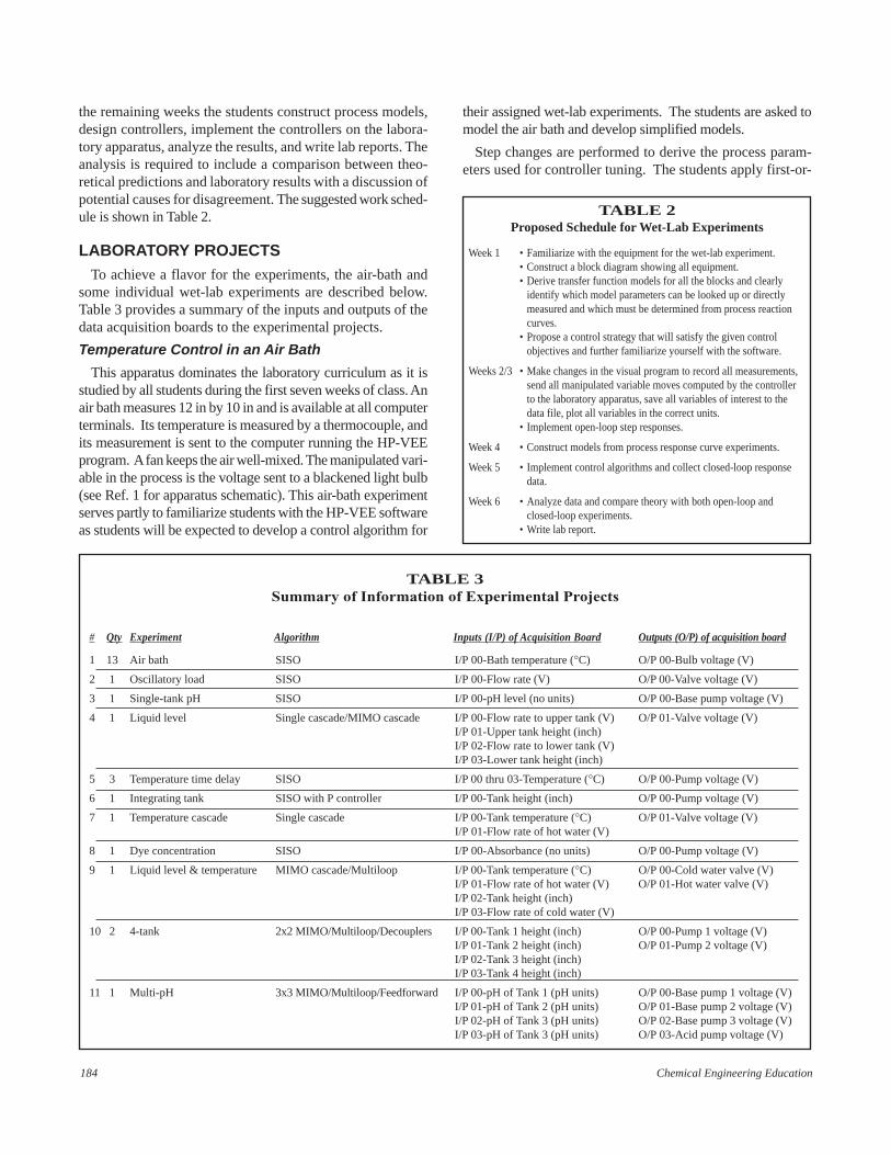
TABLE 3Summary of Information of Experimental Projects
# Qty Experiment Algorithm Inputs (I/P) of Acquisition Board Outputs (O/P) of acquisition board
1 13 Air bath SISO I/P 00-Bath temperature (°C) O/P 00-Bulb voltage (V)
2 1 Oscillatory load SISO I/P 00-Flow rate (V) O/P 00-Valve voltage (V)
3 1 Single-tank pH SISO I/P 00-pH level (no units) O/P 00-Base pump voltage (V)
4 1 Liquid level Single cascade/MIMO cascade I/P 00-Flow rate to upper tank (V) O/P 01-Valve voltage (V)I/P 01-Upper tank height (inch)I/P 02-Flow rate to lower tank (V)I/P 03-Lower tank height (inch)
5 3 Temperature time delay SISO I/P 00 thru 03-Temperature (°C) O/P 00-Pump voltage (V)
6 1 Integrating tank SISO with P controller I/P 00-Tank height (inch) O/P 00-Pump voltage (V)
7 1 Temperature cascade Single cascade I/P 00-Tank temperature (°C) O/P 01-Valve voltage (V)I/P 01-Flow rate of hot water (V)
8 1 Dye concentration SISO I/P 00-Absorbance (no units) O/P 00-Pump voltage (V)
9 1 Liquid level & temperature MIMO cascade/Multiloop I/P 00-Tank temperature (°C) O/P 00-Cold water valve (V)I/P 01-Flow rate of hot water (V) O/P 01-Hot water valve (V)I/P 02-Tank height (inch)I/P 03-Flow rate of cold water (V)
10 2 4-tank 2x2 MIMO/Multiloop/Decouplers I/P 00-Tank 1 height (inch) O/P 00-Pump 1 voltage (V)I/P 01-Tank 2 height (inch) O/P 01-Pump 2 voltage (V)I/P 02-Tank 3 height (inch)I/P 03-Tank 4 height (inch)
11 1 Multi-pH 3x3 MIMO/Multiloop/Feedforward I/P 00-pH of Tank 1 (pH units) O/P 00-Base pump 1 voltage (V)I/P 01-pH of Tank 2 (pH units) O/P 01-Base pump 2 voltage (V)I/P 02-pH of Tank 3 (pH units) O/P 02-Base pump 3 voltage (V)I/P 03-pH of Tank 3 (pH units) O/P 03-Acid pump voltage (V)
the remaining weeks the students construct process models,design controllers, implement the controllers on the labora-tory apparatus, analyze the results, and write lab reports. Theanalysis is required to include a comparison between theo-retical predictions and laboratory results with a discussion ofpotential causes for disagreement. The suggested work sched-ule is shown in Table 2.
LABORATORY PROJECTSTo achieve a flavor for the experiments, the air-bath and
some individual wet-lab experiments are described below.Table 3 provides a summary of the inputs and outputs of thedata acquisition boards to the experimental projects.
Temperature Control in an Air Bath
This apparatus dominates the laboratory curriculum as it isstudied by all students during the first seven weeks of class. Anair bath measures 12 in by 10 in and is available at all computerterminals. Its temperature is measured by a thermocouple, andits measurement is sent to the computer running the HP-VEEprogram. A fan keeps the air well-mixed. The manipulated vari-able in the process is the voltage sent to a blackened light bulb(see Ref. 1 for apparatus schematic). This air-bath experimentserves partly to familiarize students with the HP-VEE softwareas students will be expected to develop a control algorithm for
their assigned wet-lab experiments. The students are asked tomodel the air bath and develop simplified models.
Step changes are performed to derive the process param-eters used for controller tuning. The students apply first-or-
Summer 2002 185
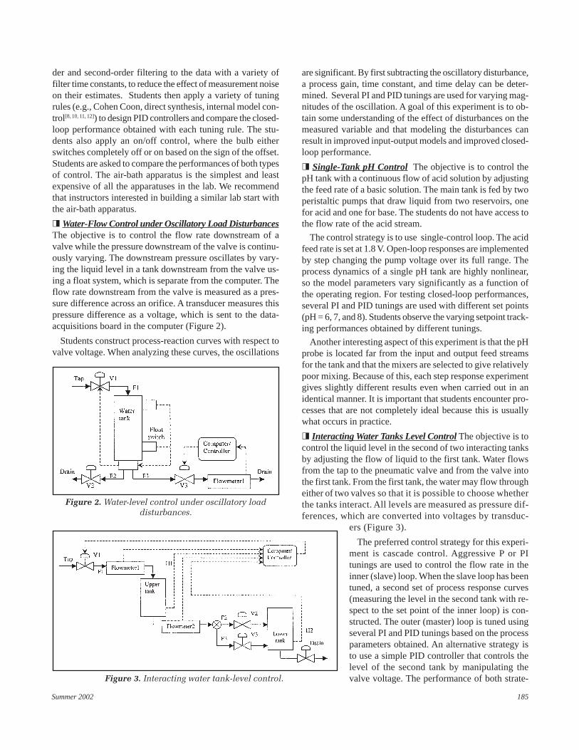
Figure 2. Water-level control under oscillatory loaddisturbances.
Figure 3. Interacting water tank-level control.
der and second-order filtering to the data with a variety offilter time constants, to reduce the effect of measurement noiseon their estimates. Students then apply a variety of tuningrules (e.g., Cohen Coon, direct synthesis, internal model con-trol[8, 10, 11, 12]) to design PID controllers and compare the closed-loop performance obtained with each tuning rule. The stu-dents also apply an on/off control, where the bulb eitherswitches completely off or on based on the sign of the offset.Students are asked to compare the performances of both typesof control. The air-bath apparatus is the simplest and leastexpensive of all the apparatuses in the lab. We recommendthat instructors interested in building a similar lab start withthe air-bath apparatus.
� Water-Flow Control under Oscillatory Load DisturbancesThe objective is to control the flow rate downstream of avalve while the pressure downstream of the valve is continu-ously varying. The downstream pressure oscillates by vary-ing the liquid level in a tank downstream from the valve us-ing a float system, which is separate from the computer. Theflow rate downstream from the valve is measured as a pres-sure difference across an orifice. A transducer measures thispressure difference as a voltage, which is sent to the data-acquisitions board in the computer (Figure 2).
Students construct process-reaction curves with respect tovalve voltage. When analyzing these curves, the oscillations
are significant. By first subtracting the oscillatory disturbance,a process gain, time constant, and time delay can be deter-mined. Several PI and PID tunings are used for varying mag-nitudes of the oscillation. A goal of this experiment is to ob-tain some understanding of the effect of disturbances on themeasured variable and that modeling the disturbances canresult in improved input-output models and improved closed-loop performance.
� Single-Tank pH Control The objective is to control thepH tank with a continuous flow of acid solution by adjustingthe feed rate of a basic solution. The main tank is fed by twoperistaltic pumps that draw liquid from two reservoirs, onefor acid and one for base. The students do not have access tothe flow rate of the acid stream.
The control strategy is to use single-control loop. The acidfeed rate is set at 1.8 V. Open-loop responses are implementedby step changing the pump voltage over its full range. Theprocess dynamics of a single pH tank are highly nonlinear,so the model parameters vary significantly as a function ofthe operating region. For testing closed-loop performances,several PI and PID tunings are used with different set points(pH = 6, 7, and 8). Students observe the varying setpoint track-ing performances obtained by different tunings.
Another interesting aspect of this experiment is that the pHprobe is located far from the input and output feed streamsfor the tank and that the mixers are selected to give relativelypoor mixing. Because of this, each step response experimentgives slightly different results even when carried out in anidentical manner. It is important that students encounter pro-cesses that are not completely ideal because this is usuallywhat occurs in practice.
� Interacting Water Tanks Level Control The objective is tocontrol the liquid level in the second of two interacting tanksby adjusting the flow of liquid to the first tank. Water flowsfrom the tap to the pneumatic valve and from the valve intothe first tank. From the first tank, the water may flow througheither of two valves so that it is possible to choose whetherthe tanks interact. All levels are measured as pressure dif-ferences, which are converted into voltages by transduc-
ers (Figure 3).
The preferred control strategy for this experi-ment is cascade control. Aggressive P or PItunings are used to control the flow rate in theinner (slave) loop. When the slave loop has beentuned, a second set of process response curves(measuring the level in the second tank with re-spect to the set point of the inner loop) is con-structed. The outer (master) loop is tuned usingseveral PI and PID tunings based on the processparameters obtained. An alternative strategy isto use a simple PID controller that controls thelevel of the second tank by manipulating thevalve voltage. The performance of both strate-

186 Chemical Engineering Education
Figure 4. Dye concentration controlwith load disturbances.
gies can be compared. A goal of this experiment is to recognizethe performance improvement obtainable by cascade control.
� Temperature Control with Variable-Measurement TimeDelay The objective is to control the temperature at one ofseveral thermocouples downstream from a mixing tank. Themanipulated variable is the hot-water feed rate into the mix-ing tank. A reservoir provides a constant head for a cold-water feed, and a peristaltic pump transfers hot water from areservoir into the mixing tank. Four thermocouples are lo-cated downstream from the outlet of the mixing tank.
Students construct process reaction curves with respect topump voltage for each of the four thermocouples downstream.They should observe that the time delay in their step responsesis greater for thermocouples located further downstream. PIand PID controllers are implemented using each of the ther-mocouples as the measured variable. Students investigate theeffect of changing the time delay on the closed-loop stabilityand performance by using one thermocouple’s tuning rulesfor the other thermocouples.
� Integrating Tank-Level Control The water level in anintegrating tank is the control variable. This tank receives aconstant flow of water from the tap. The water level in thetank is measured as a pressure difference signal. Water is re-moved from the tank by a peristaltic pump under the controlof the computer. An interesting feature is that the HP-VEEsoftware assumes that the gain of the process is positive.This would be true if the pump was feeding water into thetank. In the integrating tank, however, the pump drains wa-ter away from the tank; therefore, the sign of the controllergain should be negative.
Step changes in the pump voltage are implemented to de-termine the model parameters, which the students use to tuneP, PI, and PID controllers. The integrating characteristics ofthe tank do not require integral action in the controller tohave zero steady-state closed-loop error. Hence, this particu-lar process can be controlled using a single-loop P controller,which can be tuned using direct synthesis. The controller istuned so that the closed-loop response is as fast as possible,without too much overshoot. Students can test the disturb-ing response of their controller parameters by implement-ing the controller under conditions in which the tapwaterfeed rate changes.
� Cascade Control of Temperature in a Water Tank Theobjective is to control the temperature in a stirred tank byadjusting a hot-water flow rate. Cold water is supplied to themixing tank from a reservoir that uses an overflow to main-tain a constant level. Hot water flows through a pneumaticvalve, and a computer records its temperature and flow rate.The flow rate is measured as a pressure difference across anorifice by a transducer with output in units of volts.
The preferred method is to implement a single cascade loop.Open-loop responses for the flow rate of hot water into the
tank are constructed by making a step change in the valvevoltage. After determining the gain, time constant, and timedelay, students can try several P and PI tunings for the inner(slave) loop to control the flow rate. For tuning the masterloop, the steps are the same except that a new set of processresponse curves is constructed by measuring the temperatureof the tank with respect to the set point of the inner loop.Using the same control parameters from the tuning, a singlePID controller is implemented and compared with a cascadecontroller in terms of closed-loop performance.
� Dye Concentration Control with Load Disturbances Theobjective is to control the dye concentration in a tank underload disturbances by changing the voltage to the feed pump.The 3-liter tank is drained both from the bottom and from anoverflow pipe. A pump takes in water from the bottom of thetank and sends it through a colorimeter, which measures theabsorbance of the solution using the tap water as a reference,with the outlet of the colorimeter returned to the tank. A peri-staltic pump sets the flow rate of dye into the tank (Figure 4).
This process can be controlled using PI or PID control.The absorbance of the solution is measured and compared toa concentration setpoint. The voltage to the dye feed pump isthe manipulated variable. Besides determining the setpointtracking performance, students perform disturbancechanges by decreasing the water-feed rate by partiallyclosing the valve at the faucet.
� 4-Tank Water-Level Control The objective is to controlthe water levels in the bottom two tanks (Tanks 1 and 2) withthe levels at least two-thirds of the maximum height. On eachside, water is pumped upward from a cylindrical beaker andsplit into two channels at a Y-junction. The relative amountof water entering the two split tubings can be adjusted manu-ally. All liquid levels are measured by pressure transducers.The two pumps adjust the flow of water to the tanks accord-ing to voltage signals sent by the PID controllers.
A straightforward control strategy is to use two PID loopsto control the process. Both pumps must be calibrated beforereliable data can be obtained. By making step changes to thepumps, the process reaction curves for the tank levels are

Summer 2002 187
obtained. The gains, time constants, and time delays of eachprocess are determined. Each PID loop is tuned separately sothat the closed-loop speed of response is as fast as possible,without too much overshoot. After tuning the two single loops,the control loops are implemented simultaneously, and the in-teractions between the loops are observed. To provide adequatesetpoint tracking, the two loops are detuned as necessary.
Decouplers are capable of reducing loop interactions. Stu-dents can use the HP-VEE software to implement partialdecouplers and assess any improvements/deterioration in theclosed-loop performance.
� Temperature and Level Control in a Water Tank Theobjective is to control the liquid level and temperature in atank by adjusting the pneumatic valves on hot and cold waterfeed-flow rates. Both the feed-flow rates and liquid level inthe tank are indirectly measured as pressure differences bytransducers, which output in units of volts. The presence oftwo possible actuators suggests the possibility of implement-ing multiple loops. Since it is possible to receive four mea-sured signals, two cascade-control loops can be used. Stu-dents construct process reaction curves for the flow rates intothe tank with respect to the voltage sent to the valves. Thegain, time constant, and time delay for each of the four trans-fer functions can then be defined.
The inner (slave) loops should be tuned aggressively with-out excessive overshoot to control the flow rates. After ob-taining good tuning parameters, a second set of process re-sponse curves measuring the level and temperature in the tankwith respect to the set points of the inner loops is constructed.The process gain, time constant, and time delay for each ofthe four transfer functions are collected. At this stage, stu-dents should be able to assess the level of interaction betweenthe two loops and decide on the pairing. Another possiblestrategy is to implement two simple PID controllers, controllevel and temperature, and manipulate the valve voltages.Students can observe and compare the difference inclosed-loop performance between the cascade controllersand the PID controllers.
� Multitank pH Control The objective is to control the pHof an acid stream, which flows through three tanks connectedin series. This is accomplished by adjusting the feed rates ofa basic solution. Three tanks are connected in series. The acidstream enters a pulse dampener before a pH probe measuresits pH. The acid stream will enter Tank 1, Tank 2, and Tank 3before it is drained into a safety reservoir. Each tank has itsbase flow regulated by one base pump. In addition, a pH probeis located in each tank to measure the pH of the solution (seeRef. 4 for apparatus schematic).
Pumps are calibrated, and their threshold voltages are de-termined. Step changes should be made in the range boundedby the threshold voltages. The acid flow rate is set through-out the experiment. There are many ways to design a cascadecontrol loop with one master and two slave loops. Yet an-
other way is to implement a full multivariable controller withthree inputs and three outputs, and to use partial decouplingfollowed by multiloop control. Regardless of strategies, stu-dents should be able to report any loop interactions. The closed-loop performance is compared with different set points for thethird tank (pH = 6, 7, and 8). Since this experiment can be con-trolled by different strategies, it is especially suited for chal-lenging students to consider and test various control strategies.
� Integration of Experiments with Control Curriculum Thecontrol apparatuses, coupled with the use of a HP-VEE asthe control software, have been designed to equip seniors witha practical experience in process control. With emphasis onproject-based learning, students are given the opportunity toapply theoretical concepts on real industrial processes. Theyare exposed to the phenomena that limit the achievable closed-loop performance, including process nonlinearity, time de-lays, disturbances, measurement noise, valve hysteresis, andloop interactions. This provides them with experience in han-dling real physical systems and practice in applying theoreti-cal concepts to the real process.
Students rated the organization of this course highly butindicated that too much effort was involved in writing the labreport. Based on student feedback over the years, severalimprovements have been made to the course, including ashorter lab report requirement.
ACKNOWLEDGMENTSThe Dreyfus Foundation, DuPont, and the University of Illi-
nois IBHE program are acknowledged for support of this project.
REFERENCES 1. Braatz, R.D., and M.R. Johnson,“Process Control Laboratory Educa-
tion Using a Graphical Operator Interface,” Comp. Appl. Eng. Ed., p. 6(1998)
2. Gatzke, E.P., E.S. Meadows, C. Wang, and F.J. Doyle, III, “Model-BasedControl of a Four-Tank System,” Comp. & Chem. Eng., 24, p. 1503(2000)
3. Johansson, K.H., and J.L.R. Nunes, “A Multivariable Laboratory Pro-cess with an Adjustable Zero,” Proc. of the Amer. Cont. Conf., IEEEPress, Piscataway, NJ, p. 2045 (1998)
4. Siong, A., M.R. Johnson, and R.D. Braatz, “Control of a MultivariablepH Neutralization Process,” Proc. of the Educational Topical Conf.,AIChE Annual Meeting, Los Angeles, CA, Paper 61a. (2000)
5. Skliar, M., J.W. Price, and C.A. Tyler, “Experimental Projects in Teach-ing Process Control,” Chem. Eng. Ed., 34, p. 254 (1998)
6. Rivera, D.E., K.S. Jun, V.E. Sater, and M.K. Shetty, “Teaching ProcessDynamics and Control Using an Industrial-Scale Real-Time Comput-ing Environment,” Comp. Appl. Eng. Ed., 4, p. 191 (1996)
7. Heisel, R., Visual Programming with HP-VEE, 2nd ed., Prentice HallPTR, Upper Saddle River, NJ (1997)
8. Ogunnaike, B.A., and W.H. Ray, Process Dynamics, Modeling, andControl, Oxford University Press, New York, NY (1994)
9. <http://www.get.agilent.com/gpinstruments/products/vee/support/>10. Skogestad, S., and I. Postlethwaite, Multivariable Feedback Control --
Analysis and Design, Wiley, New York, NY (1996)11. Braatz, R.D., “Internal Model Control,” in Control Systems Fundamen-
tals, ed. by W.S. Levine, CRC Press, Boca Raton, FL, p. 215 (2000)12. Morari, M., and E. Zafiriou, Robust Process Control, Prentice-Hall,
Englewood Cliffs, NJ (1989) ❐

188 Chemical Engineering Education
Using Test Results for ASSESSMENT OF
TEACHING AND LEARNING
H. HENNING WINTER
University of Massachusetts • Amherst, MA 01003
Examination time can be filled with anxiety. Teachersdesign a mid-term or final exam to cover the mostimportant subjects of their courses and expect the stu-
dent to apply the learned material successfully. Most gratify-ing for teacher and student alike is an exam in which thestudent answers all questions and receives a top grade. In-complete or wrong answers generate dissatisfaction with boththe student and the teacher. Reality is somewhere betweenthese extremes, depending on the degree of success of theteaching and student committment. The exam results oftensuggest that the teaching needs to be improved, but the ques-tions are where it can be improved and how. Direction cancome from an assessment of exams. They contain a wealth ofinformation, much more than just a grade for the student.[1]
Methods have been developed for assessing entire engi-neering programs, curricula as well as individual courses, andeducational research projects.[2,3] Student portfolios[2,3] allowquantitative assessment of the students’ work during the yearwith feedback to the campus community. This report describesa teaching tool that works on the assumption that the educa-tional program as a whole has already been assessed and thata plan exists for individual courses. Instead of the large-scaleapproach, this paper will focus on methods of analyzing asingle exam and generating direct feedback for the teachingof a course with well-defined objectives.
I have introduced the concept of a “grading matrix” foranalyzing the results of tests in chemical engineering. Thegrading matrix has the purpose of detecting academicstrengths and weaknesses of individual students as well asstrengths and weaknesses of teaching. Most important is theidentification of weaknesses so that they can be corrected inthe classroom (or outside) and possibly re-assessed. The in-creased interest in teaching assessment has motivated me to
describe the grading matrix in this report. Until now, I haveused it by myself in all undergraduate and graduate teachingfor over a decade and have gradually refined it. The matrixmethod is somewhat related to the Primary Trait Analysis ofLoyd-Jones,[5] which was recently pointed out to me. But, inaddition to student performance, the grading matrix also as-sesses teaching success. This paper briefly describes the grad-ing matrix together with suggestions for its use in teachingand curriculum development.
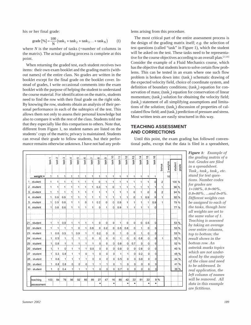
THE GRADING MATRIXThe definition and use of the grading matrix can be seen in
Figure 1. The example is deliberately kept simple: a typicalwritten test is broken down into N individual subtopics (task
1
to task16
since N=16 was chosen for this test) shown acrossthe top of the matrix. Student names appear on the left side.Separately for each of the subtopics, the student’s exam isevaluated on a scale from 0% to 100%. Grades are finelyvaried between 0% and 100% or, in yes/no fashion of aquiz, with either 1 or 0 in the matrix. This choice dependson the nature of the test or quiz. A row of grades acrossthe matrix shows the strengths and weaknesses of thatindividual student. The average over the row constitutes
© Copyright ChE Division of ASEE 2002
ChE classroom
H. Henning Winter is Distinguished Univer-sity Professor of Chemical Engineering at theUniversity of Massachusetts at Amherst. Hehas degrees from Stanford University (MS)and the University of Stuttgart (Dr. Ing). Hisresarch includes experimental rheology, poly-mer gelation, and crystallization.
Summer 2002 189
his or her final grade:
gradeN
task task task taskN%[ ] = + + +( ) ( )10011 2 3 K
where N is the number of tasks (=number of columns inthe matrix). The actual grading process is complete at thispoint.
When returning the graded test, each student receives twoitems: their own exam booklet and the grading matrix (with-out names) of the entire class. No grades are written in thebooklet except for the final grade on the booklet cover. In-stead of grades, I write occasional comments into the exambooklet with the purpose of helping the student to understandthe course material. For identification on the matrix, studentsneed to find the row with their final grade on the right side.By knowing the row, students obtain an analysis of their per-sonal performance in each of the subtopics of the test. Thisallows them not only to assess their personal knowledge butalso to compare it with the rest of the class. Students told methat they especially like this comparison to others. Note that,different from Figure 1, no student names are listed on thestudents’ copy of the matrix; privacy is maintained. Studentscan reveal their grade to fellow students, but their perfor-mance remains otherwise unknown. I have not had any prob-
lems arising from this procedure.
The most critical part of the entire assessment process isthe design of the grading matrix itself; e.g. the selection oftest questions (called “task” in Figure 1), which the studentwill be asked on the test. These tasks need to be representa-tive for the course objectives according to an overall plan.[2,3,6]
Consider the example of a Fluid Mechanics course, whichhas the objective that students learn to solve certain flow prob-lems. This can be tested in an exam where one such flowproblem is broken down into: (task
1) schematic drawing of
the expected velocity field, choice of coordinate system, anddefinition of boundary conditions; (task
2) equation for con-
servation of mass; (task3) equation for conservation of linear
momentum; (task4) solution for obtaining the velocity field;
(task5) statement of all simplifying assumptions and limita-
tions of the solution; (task6) discussion of properties of cal-
culated flow field; and (task7) prediction of pressure and stress.
Most written tests are easily structured in this way.
TEACHING ASSESSMENTAND CORRECTIONS
Until this point, the exam grading has followed conven-tional paths, except that the data is filed in a spreadsheet,
Figure 1: Example ofthe grading matrix of atest. Grades are filedin a spreadsheet.Task1, task2, task3, etc.stand for test ques-tions. Number codesfor grades are1=100%, 0.9=90%,0.8=80%, ...and 0=0%.Different weights canbe assigned to each ofthe tasks, though hereall weights are set tothe same value of 1.Teaching is assessedby taking an averageover entire columns,top to bottom; theresult shows in thebottom row. Anasterisk marks topicswhich are not under-stood by the majorityof the class and needto be addressed. Inreal application, theleft column of nameswill be removed. Alldata in this exampleare fictitious.

190 Chemical Engineering Education
Figure 2:
This is the samegrading matrix as
in Figure 1, butspecific weights areassigned to each of
the tasks. Thisaffects the
calculation of thegrade as defined in
Equation 2.Everything else,
including theteaching
assignment,remains unchanged
by the weightingsystem. Weights
have littleeffect on thegrade of top
students but canmake a large
difference for aweaker student.
ready for further assessment. Some of the most importantinformation is contained in the columns of the grading ma-trix of Figure 1. A column with mostly high marks (1 = high-est mark) top to bottom shows that all students know the sub-ject, at least at the level of the exam question. If a column,however, has mostly “0” marks, something went wrong. Rea-sons can be deep-rooted or only superficial (i.e., the questionwas confusing or the students ran out of time). Discussionsbetween teacher and students often bring clarification, andplans for further action are easily devised. Technical defi-ciencies and/or misunderstandings are recognized and canbe addressed, for instance, in a special help session or in thenext homework assignment. Experiments can be added orcomputer animation can be used to help visualize abstractconcepts. Teachers have an opportunity to become very cre-ative as soon as the problem is defined. This definition of theproblem is the main purpose of the grading matrix.
Correction of weaknesses can then be re-assessed in thenext test. This is typically done by including appropriate ques-tions in the next exam, preferably within the same courseand/or in the next homework assignment. Teaching shouldbe corrected further if necessary. Often it is too late to intro-duce corrections in the same semester or quarter. If changescannot be made in time, the weakness in one course will bepassed on to the teacher of the following course. This
teacher should be alerted to the problem so that correc-tions can be made there.
The grading matrix provides a record, which can be usedeven if another teacher teaches the course the following year.Adjustments can be made then and can be re-assessed untilteaching weaknesses are resolved. I can imagine, however, aproblem with the existence of such records, since they have apotential for misuse in the form of over-coaching of teach-ers. This would interfere with the learning environment andimpair the matrix method. Access to the grading matrixshould be restricted to the teachers and students who aredirectly involved.
FEEDBACKTO STUDENTS
Advising individual students is enhanced by the diagnosticproperty of a grading matrix. The teacher sees individualweaknesses of students and can suggest corrective measures.(e.g., specific reading material or exercises). This does notrequire further preparation on the teacher’s part. Informationis available instantly when a student comes to the office forconsultation. The matrix row of grades, in combination withother observations (attendance, participation during class,etc.), provides a quantitative basis for a discussion.

Summer 2002 191
...thispaper
[focuses]on methods
ofanalyzinga singleexamand
generatingdirect
feedback...
CURRICULUM DEVELOPMENTWeaknesses in student learning, as detected in the grading
matrices of a course (two midterms and a final, for example)should be assessed in the context of the entire curriculum.There is a possibility that students may not be sufficientlyprepared for a specific class. Prevailing weak-nesses should, in this case, be addressed by chang-ing the course content of the responsible preced-ing course. Relevant results from the gradingmatrix can be integrated into the systematic cur-riculum development.[3] Discussions along theselines are in progress in our department.
ADAPTATIONOF THE MATRIX METHOD
There are many ways of integrating the infor-mation from the grading matrix into personalapproaches to teaching and student advising. Itgoes without saying that assessment of test per-formance as reported here needs to be integratedwith classroom assessment. This is a dynamicprocess, which differs from year to year, sinceeach group of students interacts differently andvaries in its needs. As the learning processevolves, teachers adapt in their classroom assess-ment and in their creative teaching approaches. The integra-tion of the grading matrix in day-to-day teaching works wellfor me, but a general discussion of this topic would exceedthe scope of this report.
Obviously, the matrix itself can be tailored in many differ-ent ways, and adaptations are straightforward. A few will bementioned here. It is possible, for instance, to emphasize se-lected parts of an exam by adding weight to some of the tasks.While I normally give uniform weight to all questions (seetop row of the matrix in Figure 1), more important questionscan be given an increased weight, as shown in Figure 2. Therow of grades across the matrix needs to be rescaled accord-ingly when calculating the final grade:
grade
weight task
weight
i ii
N
ii
N%[ ] =⋅
( )=
=
∑
∑100 21
1
where N is the number of columns. Additional bonus pointscan be added wherever appropriate. The overall scale of thetest will not be affected by assigning bonus points to indi-vidual students.
The concept of a grading matrix is introduced here with achemical engineering example and on the most straightfor-ward type of test. The proposed method for assessment ofteaching is applicable at many levels, however. It is equallyuseful for students and teachers outside of engineering. Similar
questions arise in high school teaching and even in elemen-tary schools where standardization of tests is considered.[7]
The matrix method can also be adapted to examinations ofmuch wider scope, such as oral presentations or essay-typeexams. Oral exams or essays tend to be less uniform in their
structure than the written tests discussed above.This, however, does not make their grading lessamenable to matrix format. New categoriesneed to be added to the list of tasks, such asstyle and expression, logic of argument, depthof discussion, format of graphs, validity of con-clusions, and more. The choice of categoriesneeds to be explained to the students well inadvance of the exam.
SUMMARYThe three main functions of the grading ma-
trix are providing a grade for the student, label-ing areas of weakness in the student’s knowl-edge, and labeling areas of weakness in theteaching. For me personally, the grading ma-trix helped to fairly assess the abilities of stu-dents since my grading became more uniform,something I tried with less success with othergrading methods. The grading matrix alsoalerted me to problems that students encoun-
tered with course material. It labeled weaknesses in my teach-ing so that I could devise different teaching methods whenneeded. I feel that, during office hours, my advice becamebetter directed to the needs of individual students. The de-sign of test content with the matrix structure in mind and thefeedback from tests have positively affected my teaching andmy continued search for ways to motivate students. While stillbeing a stressful experience for the students, examinations haveturned into an effective instrument for improved teaching.
ACKNOWLEDGMENTSSupport from the von Humboldt Foundation, many lively
discussions with colleagues and students, and helpful sug-gestions from the reviewers are gratefully acknowledged.
REFERENCES1. Walvoord, G. and V.J. Anderson, Effective Grading: A Tool for Learn-
ing and Assessment, Jossey-Bass, San Francisco, CA (1998)2. Olds, B.M. and R.L. Miller, “An Assessment Matrix for Evaluating
Engineering Programs,” J. Eng. Ed., 87, p. 173 (1998)3. McNeill B. and L. Bellamy, “The Articulation Matrix, a Tool for De-
fining and Assessing a Course.” Chem. Eng. Ed., 33, p. 122 (1999)4. Taylor, R. Basic Principles of Curriculum and Instruction, University
of Chicago Press. Chicago, IL (1949)5. Loyd-Jones, R. “Primary Trait Analysis” in Cooper C. and L. Odell
(eds.) Evaluating Writing: Describing, Measuring, Judging. Urbana,IL Council of Teachers of English, Urbana (1977)
6. Olds, B.M. and R.L. Miller, “Using Portfolios to Assess a ChemicalEngineering Program,” Chem. Eng. Ed., 33, p. 110 (1999)
7. Saltet, J.K. “How is my Child Doing?” J. Waldof Education, 10(2), p.5 (2001) ❐
192 Chemical Engineering Education
IS PROCESS SIMULATIONUSED EFFECTIVELY IN ChE
COURSES?KEVIN D. DAHM, ROBERT P. HESKETH, MARIANO J. SAVELSKI
Rowan University • Glassboro, NJ 08028
Process simulators are becoming basic tools in chemi-cal engineering programs. Senior-level design projectstypically involve the use of either a commercial simu-
lator or an academic simulator such as ASPENPLUS,ChemCAD, ChemShare, FLOWTRAN, HYSYS, and ProIIw/PROVISION. Many design textbooks now include exer-cises specifically prepared for a particular simulator. For ex-ample, the text by Seider, Seader, and Lewin[1] has exampleswritten for use with ASPENPLUS, HYSYS, GAMS,[2] andDYNAPLUS.[3] Professor Lewin has prepared a new CD-ROM version of this courseware giving interactive self-pacedtutorials on the use of HYSYS and ASPEN PLUS through-out the curriculum.[4,5]
This paper will analyze how effective it is to include com-puting (particularly process simulation) in the chemical en-gineering curriculum. Among the topics of interest will bevertical integration of process simulation vs. traditional usein the senior design courses, the role of computer program-ming in the age of sophisticated software packages, and thereal pedagogical value of these tools based on industry needsand future technology trends. A course-by-course analysiswill present examples of specific methods of effective use ofthese tools in chemical engineering courses, both from theliterature and from the authors’ experience.
DISCUSSION
In the past, most chemical engineering programs viewedprocess simulation as a tool to be taught and used solely insenior design courses. Lately, however, the chemical engi-neering community has seen a strong movement toward ver-tical integration of design throughout the curriculum.[6-9] Someof these initiatives are driven by the new ABET criteria.[10]
This integration could be highly enhanced by early introduc-tion to process simulation.
Process simulation can also be used in lower-level coursesas a pedagogical aid. The thermodynamics and separationsareas have a lot to gain from simulation packages. One of theadvantages of process simulation software is that it enables
the instructor to present information in an inductive manner.For example, in a course on equilibrium staged operations,one concept a student must learn is the optimum feed loca-tion. Standard texts such as Wankat[11] present these conceptsin a deductive manner. The inductive presentation used atRowan University is outlined below in the section on equi-librium staged separations.
Some courses in chemical engineering, such as processdynamics and control and process optimization, are computerintensive and can benefit from dynamic process simulatorsand other software packages. Henson and Zhang[12] presentan example problem in which HYSYS.Plant (a commercialdynamic simulator) is used in the process control course. Theprocess features the production of ethylene glycol in a CSTRand purification of the product through distillation. The au-thors use this simple process to illustrate concepts such asfeedback control and open-loop dynamics. Clough[13] presentsa good overview of the use of dynamic simulation in teach-ing plantwide control strategies.
A potential pedagogical drawback to simulation packagessuch as HYSYS and ASPEN is that it is possible for studentsto successfully construct and use models without really un-derstanding the physical phenomena within each unit opera-tion. Clough emphasizes the difference between “studentsusing vs. students creating simulations.” Care must be takento insure that simulation enhances student understanding,rather than simply providing a crutch that allows them to solve
Kevin D. Dahm is Assistant Professor of Chemical Engineering at RowanUniversity. He received his BS from Worcester Polytechnic Institute in 1992and his PhD from Massachusetts Institute of Technology in 1998.
Robert P. Hesketh is Professor of Chemical Engineering at Rowan Uni-versity. He received his BS in 1982 from the University of Illinois and hisPhD from the University of Delaware in 1987. Robert’s teaching and re-search interests are in reaction engineering, freshman engineering, andseparations.
Mariano J. Savelski is Assistant Professor of Chemical Engineering atRowan University. He received his BS in 1991 from the University of BuenosAires, his ME in 1994 from the University of Tulsa, and his PhD in 1999from the University of Oklahoma. His technical research is in the area ofprocess design and optimization.
© Copyright ChE Division of ASEE 2002
ChE curriculum

Summer 2002 193
CACHE survey, Kantor and Edgar[15] observed that comput-ing was generally accepted as an integral component of teach-ing design, but that it had not significantly permeated the restof the curriculum. The survey results suggest that this per-ception is outdated. Table 1 shows that only 20% of depart-ments reported that process simulation software is used ex-clusively in the design course, and Tables 2 and 3 show thatit is particularly prevalent in the teaching of equilibrium stagedseparations, process control, and thermodynamics. It mustbe noted, however, that the survey did not ask respondents toquantify the extent of use; a “yes” response could indicate aslittle as a single exercise conducted using a simulator.
Table 1 also indicates that over one-fourth of the respond-ing departments felt that their faculty have “an overall, uni-formly applied strategy for teaching simulation to their stu-dents that starts early in the program and continues in subse-quent courses.” Many other respondents acknowledged themerit of such a plan but cited interpersonal obstacles, withcomments such as
With each faculty member having their own pet piece of software,it’s tough to come to a consensus.
Not many faculty use ASPEN in their courses because they haven’tlearned it, think it will take too much time to learn, and aren’tmotivated to do so.
I would like to see the use of flowsheet simulators expanded toother courses in our curriculum but haven’t been able to talkanybody else into it yet.
At Rowan University, the incorporation of mini-modules(described further in the next section) into sophomore-and-junior-level courses has proved to be an effective solution tothis problem. They require only limited knowledge of thesimulation package on the part of the instructor because theyemploy models that contain only a single unit operation.
Table 4 (next page) summarizes the responses to a ques-tion on motivation for using simulation software. Four op-
tions were given, and the respondentwas asked to check all that apply. Themost common choice was “It’s a toolthat graduating chemical engineersshould be familiar with, and is thustaught for its own sake.” A total of83% of the respondents selected thisoption, and in 15% of the responses itwas the only one chosen.
TABLE 1Responses to:
“Which of these best describes your department’s useof process simulation software?”
Response % Yes
� The faculty has an overall, uniformly applied strategy forteaching simulation to their students that starts early in theprogram and continues in subsequent courses. 27%
� There is some coordination between individual facultymembers, but the department as a whole has notadopted a curriculum-wide strategy. 35%
� Several instructors use it at their discretion, but thereis little or no coordination. 18%
� Only the design instructor requires the use of chemicalprocess simulation software. 20%
� No professor currently requires simulation in under-graduate courses. 1%
TABLE 2Responses to:
“Please indicate the courses inwhich professors require the useof steady-state chemical process
simulation programs.”
Course % Yes
� Design I and/or II 94%
� Process Safety 4%
� Process Dynamics and Control 10%
� Unit Operations 31%
� Equilibrium Staged Separations 57%
� Chemical Reaction Engineering 19%
� ChE Thermodynamics 36%
� Fluid Mechanics 7%
� Heat Transfer 13%
� Chemical Principles 29%
TABLE 3Responses to:
“Please indicate the courses inwhich professors require the use
of dynamic chemical processsimulation programs.”
Course % Yes
� Design I and/or II 12%
� Process Dynamics and Control 52%
problems with only a surface understanding of the processesthey are modeling. This concern about process simulatorsmotivated development of the phenomenological modelingpackage ModelLA.[14] This package allows the user to de-clare what physical and chemical phenomena are operativein a process or part of a process. Examples include choosinga specific model for the finite rate of interphase transport orthe species behavior of multiphase equilibrium situations. Oneuses engineering science in a user-selected hierarchical sequenceof modeling decisions. The focus is on physical and chemicalphenomena, and equations are derived by the software.
Despite these concerns, the survey results discussed in thenext section indicate that HYSYS, ASPEN, and ProII remainthe primary simulation packages currently in use.
SURVEY: COMPUTER USE IN CHEMICALPROCESS SIMULATION
In 1996, CACHE conducted a study discussing the role ofcomputers in chemical engineering education and practice.The study surveyed both faculty members and practicing en-gineers, but little emphasis was placed on the specific use ofprocess simulation. To fill this gap and obtain up-to-date re-sults, a survey on computer use in the chemical engineeringcurriculum was distributed to U.S. chemical engineering de-partment heads in the spring of 2001. It addressed how ex-tensively simulation software is used in the curriculum, aswell as motivation for its use. The use of mathematical soft-ware and computer programming was also examined. A totalof 84 responses was received, making the response rate approxi-mately 48%. Tables 1-7 summarize the results. The wording ofquestions and responses in the tables is taken verbatim from thesurvey. The survey also provided a space for written commentsand some of these are presented throughout this paper.
In a 1996 publication that discussed the results of the
194 Chemical Engineering Education
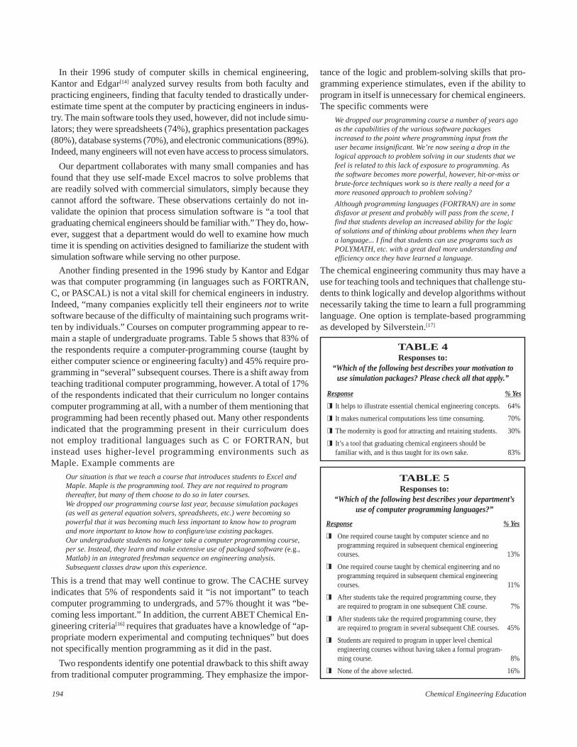
TABLE 4Responses to:
“Which of the following best describes your motivation touse simulation packages? Please check all that apply.”
Response % Yes
� It helps to illustrate essential chemical engineering concepts. 64%
� It makes numerical computations less time consuming. 70%
� The modernity is good for attracting and retaining students. 30%
� It’s a tool that graduating chemical engineers should befamiliar with, and is thus taught for its own sake. 83%
TABLE 5Responses to:
“Which of the following best describes your department’suse of computer programming languages?”
Response % Yes
� One required course taught by computer science and noprogramming required in subsequent chemical engineeringcourses. 13%
� One required course taught by chemical engineering and noprogramming required in subsequent chemical engineeringcourses. 11%
� After students take the required programming course, theyare required to program in one subsequent ChE course. 7%
� After students take the required programming course, theyare required to program in several subsequent ChE courses. 45%
� Students are required to program in upper level chemicalengineering courses without having taken a formal program-ming course. 8%
� None of the above selected. 16%
In their 1996 study of computer skills in chemical engineering,Kantor and Edgar[14] analyzed survey results from both faculty andpracticing engineers, finding that faculty tended to drastically under-estimate time spent at the computer by practicing engineers in indus-try. The main software tools they used, however, did not include simu-lators; they were spreadsheets (74%), graphics presentation packages(80%), database systems (70%), and electronic communications (89%).Indeed, many engineers will not even have access to process simulators.
Our department collaborates with many small companies and hasfound that they use self-made Excel macros to solve problems thatare readily solved with commercial simulators, simply because theycannot afford the software. These observations certainly do not in-validate the opinion that process simulation software is “a tool thatgraduating chemical engineers should be familiar with.” They do, how-ever, suggest that a department would do well to examine how muchtime it is spending on activities designed to familiarize the student withsimulation software while serving no other purpose.
Another finding presented in the 1996 study by Kantor and Edgarwas that computer programming (in languages such as FORTRAN,C, or PASCAL) is not a vital skill for chemical engineers in industry.Indeed, “many companies explicitly tell their engineers not to writesoftware because of the difficulty of maintaining such programs writ-ten by individuals.” Courses on computer programming appear to re-main a staple of undergraduate programs. Table 5 shows that 83% ofthe respondents require a computer-programming course (taught byeither computer science or engineering faculty) and 45% require pro-gramming in “several” subsequent courses. There is a shift away fromteaching traditional computer programming, however. A total of 17%of the respondents indicated that their curriculum no longer containscomputer programming at all, with a number of them mentioning thatprogramming had been recently phased out. Many other respondentsindicated that the programming present in their curriculum doesnot employ traditional languages such as C or FORTRAN, butinstead uses higher-level programming environments such asMaple. Example comments are
Our situation is that we teach a course that introduces students to Excel andMaple. Maple is the programming tool. They are not required to programthereafter, but many of them choose to do so in later courses.We dropped our programming course last year, because simulation packages(as well as general equation solvers, spreadsheets, etc.) were becoming sopowerful that it was becoming much less important to know how to programand more important to know how to configure/use existing packages.Our undergraduate students no longer take a computer programming course,per se. Instead, they learn and make extensive use of packaged software (e.g.,Matlab) in an integrated freshman sequence on engineering analysis.Subsequent classes draw upon this experience.
This is a trend that may well continue to grow. The CACHE surveyindicates that 5% of respondents said it “is not important” to teachcomputer programming to undergrads, and 57% thought it was “be-coming less important.” In addition, the current ABET Chemical En-gineering criteria[16] requires that graduates have a knowledge of “ap-propriate modern experimental and computing techniques” but doesnot specifically mention programming as it did in the past.
Two respondents identify one potential drawback to this shift awayfrom traditional computer programming. They emphasize the impor-
tance of the logic and problem-solving skills that pro-gramming experience stimulates, even if the ability toprogram in itself is unnecessary for chemical engineers.The specific comments were
We dropped our programming course a number of years agoas the capabilities of the various software packagesincreased to the point where programming input from theuser became insignificant. We’re now seeing a drop in thelogical approach to problem solving in our students that wefeel is related to this lack of exposure to programming. Asthe software becomes more powerful, however, hit-or-miss orbrute-force techniques work so is there really a need for amore reasoned approach to problem solving?
Although programming languages (FORTRAN) are in somedisfavor at present and probably will pass from the scene, Ifind that students develop an increased ability for the logicof solutions and of thinking about problems when they learna language... I find that students can use programs such asPOLYMATH, etc. with a great deal more understanding andefficiency once they have learned a language.
The chemical engineering community thus may have ause for teaching tools and techniques that challenge stu-dents to think logically and develop algorithms withoutnecessarily taking the time to learn a full programminglanguage. One option is template-based programmingas developed by Silverstein.[17]

Summer 2002 195
TABLE 7Responses to:
“Please indicate allapplicable steady-state
Chemical Process Simula-tion programs currently
being used in yourdepartment’s undergraduate
courses. Check all thatapply.”
Response % Yes
� ProII/Provision 12%
� HYSYS or Hysim 32%
� Aspen Plus 45%
� ChemCAD 32%
� Other 13%
TABLE 6Responses to:
“Indicate the mathematicalapplications software required
of chemical engineeringundergraduates.
Check all that apply.”
Response % Yes
� POLYMATH40 37%
� MATLAB 65%
� Maple 24%
� MathCAD 37%
� EZ-Solve 5%
� Spreadsheets 82%
� Mathematica 13%
� Other 15%
EXAMPLES OF CHEMICAL PROCESSSIMULATORS IN CHEMICAL ENGINEERING
In this section of the paper we give some practical ideas onhow to effectively implement chemical process simulatorsinto courses other than the capstone design course.
Freshman Engineering
At Rowan University, an inductive approach has been usedto introduce freshmen and sophomores to chemical processsimulators. The methodology used was
♦ Show the students a heat exchanger. This can be either alaboratory unit or part of a cogeneration plant.[18] The stu-dents are asked to record their observations of fluid flowrateand temperatures.
♦ Next, have the students start a process simulator and putthese experimental results into a simple heat-exchange unitoperation of a process simulator to determine the heat duty.
♦ Finally, have the students conduct an energy balance by handon the system. In this manner the students have first seenthe equipment and then modeled it using a simulator on handcalculations. This helps to familiarize them with what a simu-lator actually does and what sort of problem can be tackledwith simulation.
Chemical Principles or Stoichiometry
In many programs with vertical integration of designthroughout the curriculum, the design project starts in thistypically sophomore-level course. Many project examples canbe found in the literature. Bailie, et al., [19] proposed a designexperience for the sophomore and junior years. In the firstsemester of the sophomore year, the students are given a singlechemical design project, and they focus on material balancesand simple economic evaluations such as raw material costand the products’ selling prices. Throughout the sequence,the students must apply newly acquired knowledge to im-prove and optimize the process. The ultimate goal is to pro-duce a fully sized and optimized design, including the analy-
sis of the capital and operating costs by the end of the junioryear. This approach is comparable to problem-based learning.[20]
There have been other contributions to this vertical approach.[21-
23] In the above work it is unclear how process simulators arebeing used and it is not mentioned if the simulators are usedin the early stages of integration. Process simulators cer-tainly can be used for such problems, however, since theyprovide an efficient way to evaluate many variations on asingle design concept.
Chemical Principles—Energy Balances
In Felder and Rousseau[24] (a standard text for this course),the chapter on multiphase systems introduces the concepts ofbubble and dew points. An inductive method of teaching theseconcepts is to start with an experiment on a binary system, us-ing a 1L distillation unit or an interactive computer module[25]
with a visual examination of the bubble and dewpoint. Thesemethods result in the students examing their data by using abinary T-x-y diagram. The next step is to use the process simu-lator to predict bubble and dewpoints for binary and multicom-ponent systems. In using HYSYS, the dewpoint temperature isautomatically calculated after specifying the vapor fraction as1.0 (dewpoint), the compositions, and pressure in a singlestream. The calculations for multicomponent systems are usu-ally reserved for an equilibrium staged operations course.
In new editions of many textbooks for the chemical processprinciples course there are chapters on process simulation.[24-26]
They give examples with solutions done by calculators, Excelspreadsheets, and FORTRAN. This gives the students an ex-cellent reference on how a system of equations is used by chemi-cal process simulators. In section 10.4 of Felder & Rousseau,commercial process-simulation packages are discussed, but noexamples are given. The last problem in the chapter suggests,however, that any of the other fourteen homework problemscould be solved by a chemical process simulator. This could beanother starting point for introducing commercial process simu-lators in this course.
Equilibrium Staged Operations
In teaching distillation, the standard modeling approach is touse the McCabe-Thiele graphical method. This is an excellenttool for introducing students to binary distillation problems.Before extensive use of the computer became feasible, the nextstep was to add the energy balance and use the Ponchon-Savaritmethod. Many professors no longer teach this method, usingthe simulator instead. This decreasing use of Ponchon-Savarithas been promoted by Wankat, et al.,[27] and recently publishedtextbook descriptions of the method have been shortened.[28]
Using simulators throughout the curriculum requires that fac-ulty have knowledge of the simulator that the students are us-ing. In the discussion of the survey results, there were concernsabout the faculty time and motivation required to be come pro-ficient in using a simulator. One possible solution is to imple-ment mini-modules of the type used at Rowan University. In
196 Chemical Engineering Education
equilibrium staged operations, a student must learn the opti-mum feed location and the improved separation resulting fromincreasing reflux ratio for a given number of stages; in an ap-proach that has been used at Rowan University
♦ The instructor prepares a complete HYSYS model of a distillation col-umn and distributes it to the class.
♦ The class receives a brief (less than five minutes) tutorial on modelingcolumns with HYSYS—just enough to tell them how to change specificparameters such as the reflux ratio and where to locate the resultingstream compositions and other output parameters of interest.
♦ The students take a column through a series of configurations, vary-ing the reflux ratio, number of stages, and feed stage location, andthen answers a series of questions about the results. The students arethus introduced to concepts in an inductive manner.
♦ Subsequent classroom instruction further examines the “whys” of theresults. This is used as a starting point in deductive derivation of theMcCabe-Thiele model.
Mini-modules analogous to this have been integrated through-out the course, as well as in thermodynamics and principles ofchemical processes. The primary purpose of the modules is thatthe HYSIS model provides a time-efficient and effective wayfor students to examine the cause-effect relationships amongcolumn operational parameters. The modules also serve a cur-ricular purpose in that they begin to introduce process simula-tion. This is accomplished with a minimal requirement of facultytime. It is not necessary for professors to learn all aspects of thesimulation package; they merely need to learn how to model oneparticular unit operation.
Other forms of mini-modules have been proposed where stu-dents learn the process simulator in self-paced tutorials.[1,4] Theproposal is that these modules be given to the students—theprofessor does not need to prepare time-consuming tutorialsand may not need to learn how to use the simulator. Anotherpaper by Chittur[29] discusses preparing tutorials for ASPEN Plussimulators using HTML. Finally, the University of Floridamaintains a web site for ASPEN where tutorials are available.[30]
Chemical Engineering Thermodynamics
Judging from the survey results, it seems that process simu-lators are now widely used in thermodynamics (see Table 2).This is fertile ground for a pedagogical use of the process simu-lators, and the first thing a new user of a simulator faces is thevariety of thermodynamics packages that are available. The newuser will quickly learn that an incorrect choice of a thermody-namic model will yield meaningless results regardless of theconvergence of the simulation case. Unfortunately, there are somany thermodynamics models in commercial simulators thatit is impossible to educate our students in each one of them.Elliott and Lira[31] present a decision tree for the proper selec-tion of the thermodynamic model.
Traditionally, students are taught how to perform equilibriumand properties calculations by hand or, in the best scenario, withthe aid of custom-made software programs for hand calcula-tors or computers. The increasing influence of process simula-tors opens up a completely new spectrum of possibilities. Sincesimulation results are only as good as the thermodynamic pack-
age chosen, there is value in teaching the fundamental as-pects that will permit students to pick the right thermody-namic package for a system. Simulators also offer the advan-tages of combining thermodynamic models in the same simu-lation and picking different models for certain propertieswithin the overall process model; PRO II with Provision isvery versatile in this respect. For instance, an equation ofstate such as Soave-Redlich-Kwong (SRK) is chosen asthe overall simulation package, but it is modified so liq-uid density is calculated using the American PetroleumInstitute (API) equation.
In many cases, professors have been taught thermodynam-ics using earlier versions of Sandler[32] and Smith and VanNess,[33] which did not emphasize predictions of thermody-namic properties based on an equation of state. More recentversions of both texts and new texts such as Elliott and Liranow contain at least one chapter devoted to predicting ther-modynamic properties from other equations of state. One ofthe fundamental aspects of a modern chemical thermodynam-ics course is not only to teach students how to use these equa-tions, but also which equation of state they should select fora particular problem. An example of the prediction of theenthalpy of a single component where values of the correlat-ing parameters of a=f(T) and b are from the Peng-Robinsonequation of state is
H H
RTZ n
Z B
Z B
A
B
Tig
r−( )
= − −+ +( )+ −( )
⎡
⎣
⎢⎢
⎤
⎦
⎥⎥
+⎡
⎣⎢⎢
⎤
⎦⎥⎥
11 2
1 2 81l
κα
where B ≡bP/RT and A ≡aP/(RT)2
From the above equations it is easily seen how compli-cated these predictions can become compared to a table or agraph in a standard handbook.[34,35] Many recent thermody-namic textbooks have included computer programs that al-low the reader to use various equations of state to solve home-work problems. The drawback of these programs is that astudent will only use them for the thermodynamics course.Instead of using these textbook computer programs, a pro-fessor can encourage use of the thermodynamic packagescontained in the chemical process simulators. In this manner,the students can become familiar with the available optionsin the various simulators.
Chemical Reaction Engineering
In the current chemical reaction engineering course, moststudents are familiar with ODE solvers found in POLYMATHor MatLab. The philosophy given by Fogler[36] is to have thestudents use the mole, momentum, and energy balances ap-propriate for a given reactor type. In this manner a fairly de-tailed model of industrial reactors can be developed for de-sign projects.[37] By using POLYMATH or MatLab, a studentcan easily see the equations used to model the reactor. In mod-ern process simulators there are several reactors that can beused. For example, in HYSYS 2.2 there are the two ideal

Summer 2002 197
TABLE 8
Reaction Type Description
Conversion F F F Xi i A A= −0 0
Equilibrium K f Teq = ( ) ; equilibrium-based on reaction stoichiometry; Keq predicted or specified.
Gibbs minimization of Gibbs free energy of all components
Kinetic r k C C k C CA f A B rev R S= − +α β φ γ where the reverse rate parameters must be thermody-
namically consistent and rate constants are given by k AT E RTn= −( )exp /
Heterogeneous Catalytic Yang and Hougen form, which includes Langmuir-Hinshelwood, Eley-Rideal and Mars-van Krevelen, etc.
− =
−
+
⎛
⎝⎜⎞
⎠⎟
∑r
k C CC C
K
K CA
Aa
Bb R
rSs
i iy i1
Simple Rate r k C CC C
KA f A B
R S
eq
= − −⎛
⎝⎜⎞
⎠⎟α β
φ γ
in which Keq is predicted from equilibrium data
reactor models of a CSTR and a PFR. The CSTR model is astandard algebraic model that has been in simulation pack-ages for a number of years. The ODE’s of the PFR are a re-cent addition to simulation packages and are solved by di-viding the volume into small segments and then finding asequential solution for each volume element. In these morerecent models, the reactors not only include energy balances,but pressure drop calculations are also a standard feature forpacked-bed reactors.
With the above set of reactions, chemical reaction engi-neering courses can easily use the process simulator. Simula-tion can be integrated throughout the course and used in par-allel with the textbook, or it can be introduced in the latterstages of the course, after the students have developed profi-ciency in modeling these processes by hand. As mentionedin the discussion section, the primary dilemma is how to in-sure that the simulator is used to help teach the material ratherthan simply giving students a way to complete the assign-ment without learning the material. Taking care that assign-ments require synthesis, analysis, and evaluation in additionto simple reporting of numerical results will help in this re-gard. Requiring that students do calculations by hand willensure that they understand what the simulator is actually do-ing. The professor can select chemical compounds that are notin the simulator database to ensure that these are done by hand.
Rate-Based Separations
An example of an integrated approach to teaching rate-basedseparations with design is given by Lewin, Seider, and Seader(1998).[38] In this paper the authors state that while designcourses fully use advances in modern computing through theprocess simulators, many other courses in the curriculum stilluse methods employed over sixty years ago. Many modern
computing methods are visual and are thus very useful in teach-ing chemical engineering concepts. The authors suggest thatprofessors who teach junior course(s) in separations, equilib-rium-stage operations, rate-based operations, and/or mass trans-fer consider including
♦ Approximate methods (Fenske-Underwood-Gililand and Kremser al-gebraic method)
♦ Rigorous multicomponent♦ Enhanced distillation using triangular diagrams♦ Rate-based methods contained in the ChemLSep program and the
RATEFRAC program of Aspen Plus♦ Adsorption, ion exchange, chromatography♦ Membrane separations
which are similar to Chapters 9 through 12 in the new Seaderand Henley text.[28]
One major drawback in current process simulators is a lackof standard unit operations for membrane and other novel sepa-rators. This can be partially addressed by importing programsinto the process simulators. For example, on the HYSYS website, an extension program can be downloaded for a membraneseparator and other operations.[39] As simulators develop, webelieve that more unit operations will become available.
CONCLUSIONSChemical process simulation is currently underused in the
chemical engineering curriculum at many schools. Accordingto survey results, process simulators are used in essentially alldesign courses and are also heavily used in equilibrium stageoperations, primarily with respect to multicomponent distilla-tion. But many respondents acknowledge that the role of simu-lators could be beneficially expanded in their curriculum. Pro-cess-simulation designers can make their products more valu-able to chemical engineering educators by adding new and in-
novative unit operations while theycontinue to improve their thermody-namic models.
This paper contains practical sug-gestions and references for imple-menting a unified strategy for teach-ing simulation to their students, start-ing early in the program and continu-ing in subsequent courses. We be-lieve that simulation packages are afundamental tool for the futurechemical engineer.
REFERENCES1. Seider, Warren D., J.D. Seader, and Daniel R.
Lewin, Process Design Principles: Synthesis,Analysis and Evaluation, John Wiley and Sons,New York, NY(1999)
2. GAMS, see<http://www.che.utexas.edu/cache/newslet-ters/fall97_art2.pdf>
3. Aspen Technology, Inc.
Continued on page 203.

198 Chemical Engineering Education
AN INTRODUCTION TODRUG DELIVERY
FOR CHEMICAL ENGINEERS
STEPHANIE FARRELL, ROBERT P. HESKETH
Rowan University • Glassboro, NJ 08028-1701
© Copyright ChE Division of ASEE 2002
ChE laboratory
Rowan University is pioneering a progressive engineer-ing program that uses innovative methods of teachingand learning to prepare students for a rapidly changing
and highly competitive marketplace, as recommended byASEE.[1] Key features of the program include
• Multidisciplinary education through collaborative laboratory andcourse work
• Teamwork as the necessary framework for solving complexproblems
• Incorporation of state-of-the-art technologies throughout thecurricula
• Creation of continuous opportunities for technical communica-tion.[2]
The Rowan program emphasizes these essential features in aneight-semester, multidisciplinary, engineering clinic sequencethat is common to the four engineering programs (civil, chemi-cal, electrical, and mechanical).
A two-semester Freshman Clinic sequence introduces allfreshmen engineering students to engineering at Rowan Uni-versity. The first semester of the course focuses onmultidisciplinary engineering experiments using engineeringmeasurements as a common thread. In the spring semester, stu-dents are immersed in a semester-long project that focuses onthe reverse engineering of a product or a process. In addition tointroducing engineering concepts, the Freshman Clinic incor-porates the four key features mentioned above.
This paper describes an experiment that was performed bothin our Freshman Clinic to introduce students to drug delivery,and in a senior-level elective on pharmaceutical and biomedi-cal topics to apply concepts of mass transfer and mathematicalmodeling. Drug delivery is a burgeoning field that representsone of the major research and development focus areas of thepharmaceutical industry today, with new drug delivery systemsales exceeding $10 billion per year.[3] With projected double-digit growth, the market is expected to reach $30 billion peryear by 2005.[4] Drug delivery is an inherently multidisciplinaryfield that combines knowledge from fields of medicine, phar-maceutical sciences, engineering, and chemistry. Chemical en-
gineers play an important role in this exciting field by apply-ing their knowledge of physical and chemical properties,chemical reactions, mass transfer rates, polymer materials, andsystem models to the design of drug-delivery systems, yet un-dergraduate chemical engineering students are rarely exposedto drug delivery through their coursework.
This experiment introduces freshman engineering studentsto chemical engineering principles and their application tothe field of drug delivery. Students are introduced to concen-tration measurements and simple analysis of rate data.Through this experiment, students explore concepts and toolsthat they will use throughout their careers, such as
• Novel application of chemical engineering principles• Concentration measurement• Calibration• Material balances• Use of spreadsheets for calculations and graphing• Parameter evaluation• Semi-log plots and trendlines• Comparison of experimental concentration data to predicted concentrations• Testing a transient model at the limits of initial time and infinite time• Development of a mathematical model (in the senior level class)
BACKGROUNDPeriodic administration of a drug by conventional means,
such as taking a tablet every four hours, can result in con-stantly changing systemic drug concentrations with alternat-ing periods of ineffectiveness and toxicity. Controlled-releasesystems attempt to maintain a therapeutic concentration of adrug in the body for an extended time by controlling its rateof delivery. A comparison of systemic drug profiles estab-
Stephanie Farrell is Associate Professor of Chemical Engineering atRowan University. She received her BS in 1986 from the University ofPennsylvania, her MS in 1992 from Stevens Institute of Technology, andher PhD in 1996 from New Jersey Institute of Technology. Her teachingand research interests are in controlled drug delivery and biomedical en-gineering.Robert Hesketh is Professor of Chemical Engineering at Rowan Univer-sity. He received his BS in 1982 from the University of Illinois and his PhDfrom the University of Delaware in 1987. His research is in the areas ofreaction engineering, novel separations, and green engineering.

Summer 2002 199
lished by conventional administration and controlled releaseis shown in Figure 1.
Historically, drug-delivery systems were developed prima-rily for traditional routes of administration, such as oral andintravenous, but recently there has been an explosion in re-search on delivery by so-called nonconventional routes, suchas transdermal (skin), nasal, ocular (eyes), and pulmonary(lung) administration. Drug-delivery applications have ex-panded from traditional drugs to therapeutic peptides, vac-cines, hormones, and viral vectors for gene therapy. Thesesystems employ a variety of rate-controlling mechanisms,including matrix diffusion, membrane diffusion, biodegra-dation, and osmosis. To design and produce a new drug-de-livery system, an engineer must fully understand the drugand its material properties as well as processing variables thataffect its release from the system. This requires a solid graspof the fundamentals of mass transfer, reaction kinetics, ther-modynamics, and transport phenomena. The engineer mustalso be skilled in characterization techniques and physicalproperty testing of the delivery system, and practiced in analy-sis of the drug-release data.
We present a simple experiment in which students are in-troduced to the basic concepts of drug delivery by studyingthe dissolution of a lozenge into water. This is the type ofexperiment that would be performed by a drug company todetermine the rate of drug release from a dissolution-limitedsystem. As the lozenge dissolves, the drug is released (alongwith a coloring agent added by the manufacturer) into thesurrounding water. Students observe the increasing color in-tensity of the water and are able to measure the increasingdrug concentration periodically using a spectrophotometer.After calculating the mass of drug released at any time t, theyplot a release profile. They must calculate by material bal-
ance the mass of drug remaining in the lozenge at any time.They are also able to compare their data to a model after evalu-ating a single parameter in the model.
Through this experiment, students are exposed to the excit-ing field of drug delivery and are introduced to some basicprinciples of chemical engineering. They perform a calibra-tion that enables them to determine the concentration of drugin their samples. A spreadsheet is used to perform calculationsnecessary to determine the release profile, and a plot of therelease profile of drug from their lozenge is created. Finally,they evaluate what is needed to apply a model to their sys-tem, and they compare their experimental release profileto that described by the model.
The experiment begins with a short lecture of drug deliveryin which students are introduced to the two main objectives todrug delivery: drug targeting (to deliver a drug to the desiredlocation in the body), and controlled release (to deliver a drugat a desired rate for a desired length of time). These two objec-tives are illustrated through familiar examples of drug-deliv-ery systems, and the important role of chemical engineers indesigning drug-delivery systems is explained to the students.The release mechanism of three commercial drug-deliverysystems are explored in the lecture: enteric coated aspirin,Efidac® 24-hour-nasal decongestant, and Contac® 12-hourcold capsules. The experiment explores drug release froman analgesic throat lozenge.
The objective of drug targeting is illustrated by enteric-coatedaspirin, which accomplishes a drug targeting objective byavoiding dissolution of the aspirin in the stomach where it cancause irritation. The enteric coating (such as hydroxypropylmethylcellulose or methacrylic acid copolymer) is specificallydesigned to prevent dissolution in the low pH of the stomach,
so that the aspirin tablet passes intact to the intes-tine. In the more neutral environment of the intes-tine, the coating dissolves, allowing the aspirin todissolve as well. The absorption of drugs in thesmall intestine is usually quite good due to the largesurface area available. The function of the enteric-coating is illustrated by placing one enteric-coatedaspirin tablet in an environment simulating thestomach (hydrochloric acid, pH 2), and another en-teric-coated aspirin tablet in an environment simu-lating the intestine (sodium hydroxide, pH 8). Stu-dents see that within about thirty seconds the tabletin the intestine environment has begun to dissolve,while the tablet in the stomach environment remainsintact. Within a couple of minutes, the tablet in theintestine has essentially disintegrated, but the othertablet remains completely unchanged for the entireclass period (and for several weeks thereafter).
The second objective of drug delivery or con-trolled release (or the release of a drug at a desiredrate for a desired time) is illustrated through famil-
Figure 1. A comparison of systemic drug profiles established byconventional administration and controlled release.
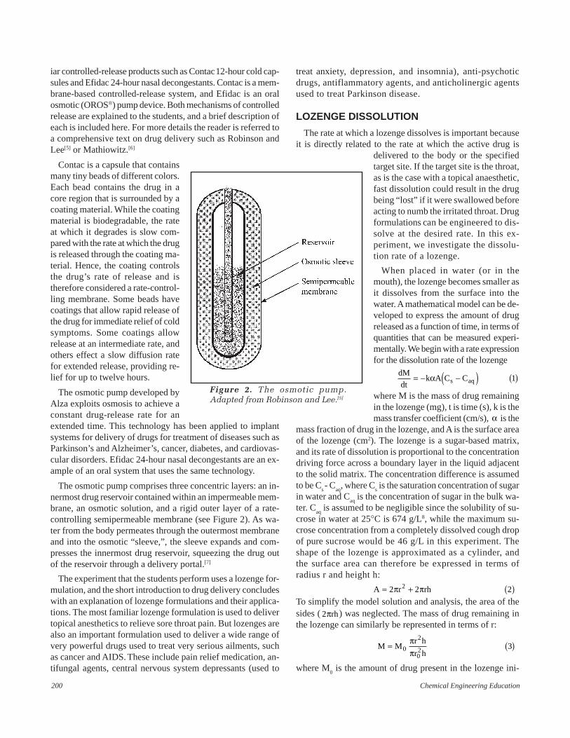
200 Chemical Engineering Education
Figure 2. The osmotic pump.Adapted from Robinson and Lee.[5]
iar controlled-release products such as Contac 12-hour cold cap-sules and Efidac 24-hour nasal decongestants. Contac is a mem-brane-based controlled-release system, and Efidac is an oralosmotic (OROS®) pump device. Both mechanisms of controlledrelease are explained to the students, and a brief description ofeach is included here. For more details the reader is referred toa comprehensive text on drug delivery such as Robinson andLee[5] or Mathiowitz.[6]
Contac is a capsule that containsmany tiny beads of different colors.Each bead contains the drug in acore region that is surrounded by acoating material. While the coatingmaterial is biodegradable, the rateat which it degrades is slow com-pared with the rate at which the drugis released through the coating ma-terial. Hence, the coating controlsthe drug’s rate of release and istherefore considered a rate-control-ling membrane. Some beads havecoatings that allow rapid release ofthe drug for immediate relief of coldsymptoms. Some coatings allowrelease at an intermediate rate, andothers effect a slow diffusion ratefor extended release, providing re-lief for up to twelve hours.
The osmotic pump developed byAlza exploits osmosis to achieve aconstant drug-release rate for anextended time. This technology has been applied to implantsystems for delivery of drugs for treatment of diseases such asParkinson’s and Alzheimer’s, cancer, diabetes, and cardiovas-cular disorders. Efidac 24-hour nasal decongestants are an ex-ample of an oral system that uses the same technology.
The osmotic pump comprises three concentric layers: an in-nermost drug reservoir contained within an impermeable mem-brane, an osmotic solution, and a rigid outer layer of a rate-controlling semipermeable membrane (see Figure 2). As wa-ter from the body permeates through the outermost membraneand into the osmotic “sleeve,”, the sleeve expands and com-presses the innermost drug reservoir, squeezing the drug outof the reservoir through a delivery portal.[7]
The experiment that the students perform uses a lozenge for-mulation, and the short introduction to drug delivery concludeswith an explanation of lozenge formulations and their applica-tions. The most familiar lozenge formulation is used to delivertopical anesthetics to relieve sore throat pain. But lozenges arealso an important formulation used to deliver a wide range ofvery powerful drugs used to treat very serious ailments, suchas cancer and AIDS. These include pain relief medication, an-tifungal agents, central nervous system depressants (used to
treat anxiety, depression, and insomnia), anti-psychoticdrugs, antiflammatory agents, and anticholinergic agentsused to treat Parkinson disease.
LOZENGE DISSOLUTION
The rate at which a lozenge dissolves is important becauseit is directly related to the rate at which the active drug is
delivered to the body or the specifiedtarget site. If the target site is the throat,as is the case with a topical anaesthetic,fast dissolution could result in the drugbeing “lost” if it were swallowed beforeacting to numb the irritated throat. Drugformulations can be engineered to dis-solve at the desired rate. In this ex-periment, we investigate the dissolu-tion rate of a lozenge.
When placed in water (or in themouth), the lozenge becomes smaller asit dissolves from the surface into thewater. A mathematical model can be de-veloped to express the amount of drugreleased as a function of time, in terms ofquantities that can be measured experi-mentally. We begin with a rate expressionfor the dissolution rate of the lozenge
dM
dtk A C Cs aq= − −( ) ( )α 1
where M is the mass of drug remainingin the lozenge (mg), t is time (s), k is themass transfer coefficient (cm/s), α is the
mass fraction of drug in the lozenge, and A is the surface areaof the lozenge (cm2). The lozenge is a sugar-based matrix,and its rate of dissolution is proportional to the concentrationdriving force across a boundary layer in the liquid adjacentto the solid matrix. The concentration difference is assumedto be C
s - C
aq, where C
s is the saturation concentration of sugar
in water and Caq
is the concentration of sugar in the bulk wa-ter. C
aq is assumed to be negligible since the solubility of su-
crose in water at 25°C is 674 g/L8, while the maximum su-crose concentration from a completely dissolved cough dropof pure sucrose would be 46 g/L in this experiment. Theshape of the lozenge is approximated as a cylinder, andthe surface area can therefore be expressed in terms ofradius r and height h:
A r rh= + ( )2 2 22π πTo simplify the model solution and analysis, the area of thesides ( 2πrh) was neglected. The mass of drug remaining inthe lozenge can similarly be represented in terms of r:
M Mr h
r h= ( )0
2
02 3
ππ
where M0 is the amount of drug present in the lozenge ini-
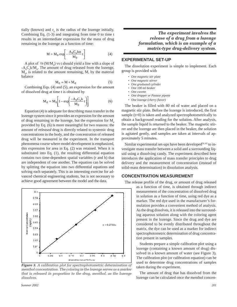
Summer 2002 201
The experiment involves therelease of a drug from a lozenge
formulation, which is an example of amatrix-type drug-delivery system.
Figure 3. A calibration plot for spectrophotometric determination ofmenthol concentration. The coloring in the lozenge serves as a markerthat is released in proportion to the drug, menthol, as the lozengedissolves.
tially (known) and r0 is the radius of the lozenge initially.
Combining Eq. (1-3) and integrating from time 0 to time tresults in an intermediate expression for the mass of drugremaining in the lozenge as a function of time:
M MA C k
Mts= −
⎡
⎣⎢
⎤
⎦⎥ ( )0
0
04exp
α
A plot of ln (M/M0) vs t should yield a line with a slope of
-A0C
sk/M
0. The amount of drug released from the lozenge,
Md, is related to the amount remaining, M, by the material
balance
M M Md0 5= + ( )Combining Eqs. (4) and (5), an expression for the amount
of dissolved drug at time t is obtained by
M MA C k
Mtd
s= −−⎛
⎝⎜⎞⎠⎟
⎡
⎣⎢⎢
⎤
⎦⎥⎥
( )00
01 6exp
Equation (4) is adequate for describing mass transfer in thelozenge system since it provides an expression for the amountof drug remaining in the lozenge, but the expression for M
d
provided by Eq. (6) is more meaningful for two reasons: theamount of released drug is directly related to systemic drugconcentrations in the body, and the concentration of releaseddrug will be measured in the experiment. In the transportphenomena course where model development is emphasized,this expression for area in Eq. (2) was retained. When it issubstituted into Eq. (1), the resulting differential equationcontains two time-dependent spatial variables (r and h) thatare independent of one another. The equation can be solvedby splitting the equation into two differential equations andsolving each separately. This is an interesting exercise for ad-vanced chemical engineering students, but is not necessary toachieve good agreement between the model and the data.
EXPERIMENTAL SET-UPThe dissolution experiment is simple to implement. Each
group is provided with
• One magnetic stir plate• One magnetic stirrer• One graduated cylinder• One 100-ml beaker• One cuvette• One dropper or Pasteur pipette
• One lozenge (cherry flavor)
The beaker is filled with 80 ml of water and placed on amagnetic stir plate. Before the lozenge is introduced, the firstsample (t=0) is taken and analyzed spectrophotometrically toobtain a background reading for the solution. After analysis,the sample liquid is returned to the beaker. The magnetic stir-rer and the lozenge are then placed in the beaker, the solutionis agitated gently, and samples are taken at intervals of ap-proximately 5 minutes.
Similar experimental set-ups have been developed[9,10] to in-vestigate mass transfer between a solid and a surrounding liq-uid using a dissolving candy. The experiment described hereintroduces the application of mass transfer principles to drugdelivery and the measurement of concentration (instead ofsolid-mass determination) in dissolution analysis.
CONCENTRATION MEASUREMENTThe release profile of the drug, or amount of drug released
as a function of time, is obtained through indirectmeasurement of the concentration of dissolved drugin solution as a function of time, using red dye as amarker. The red dye used in the manufacturer’s for-mulation provides a convenient method of analysis.As the drug dissolves, it is released into the surround-ing aqueous solution along with the coloring agentpresent in the lozenge. Since the drug and dye areconsidered to be evenly distributed throughout thematrix, the dye can be used as a marker for indirectspectrophotometric determination of drug concentra-tion present in samples.
Students prepare a simple calibration plot using alozenge (containing a known amount of drug) dis-solved in a known amount of water (see Figure 3).The calibration plot (or calibration equation) can beused to determine drug concentrations of samplestaken during the experiment.
The amount of drug that has dissolved from thelozenge can be calculated once the menthol concen-
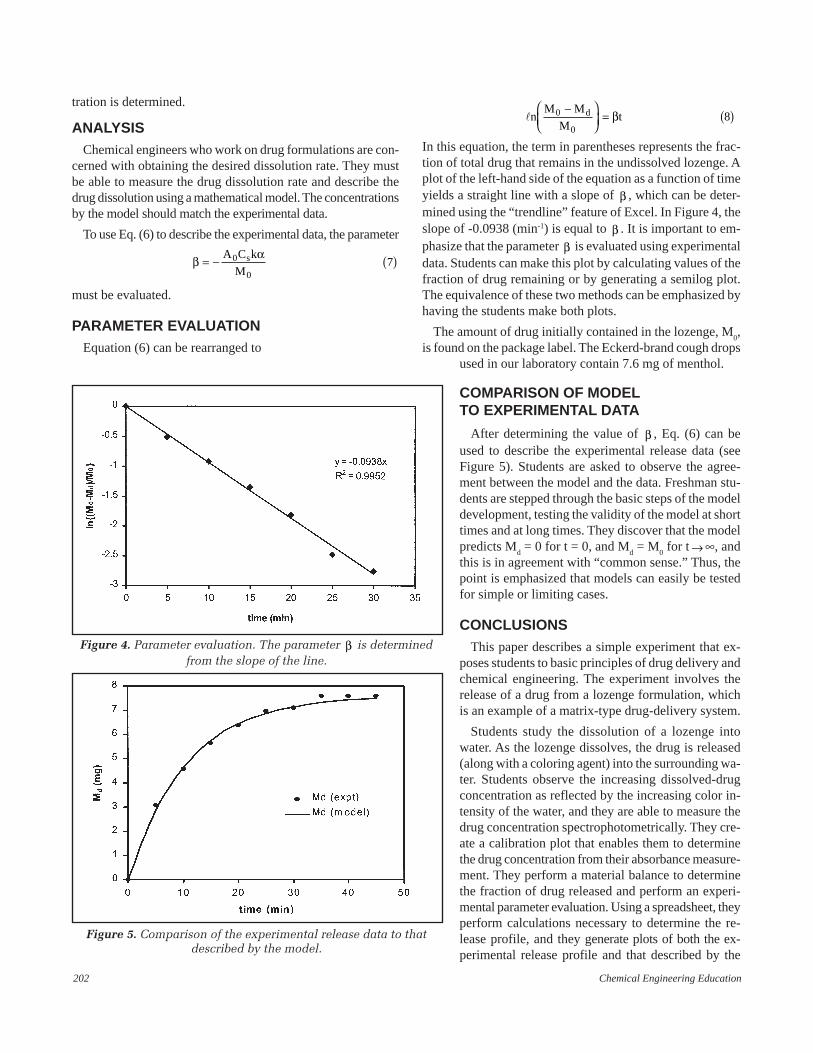
202 Chemical Engineering Education
Figure 4. Parameter evaluation. The parameter β is determinedfrom the slope of the line.
Figure 5. Comparison of the experimental release data to thatdescribed by the model.
tration is determined.
ANALYSISChemical engineers who work on drug formulations are con-
cerned with obtaining the desired dissolution rate. They mustbe able to measure the drug dissolution rate and describe thedrug dissolution using a mathematical model. The concentrationsby the model should match the experimental data.
To use Eq. (6) to describe the experimental data, the parameter
βα
= − ( )A C k
Ms0
07
must be evaluated.
PARAMETER EVALUATIONEquation (6) can be rearranged to
lnM M
Mtd0
08
−⎛⎝⎜
⎞⎠⎟= ( )β
In this equation, the term in parentheses represents the frac-tion of total drug that remains in the undissolved lozenge. Aplot of the left-hand side of the equation as a function of timeyields a straight line with a slope of β , which can be deter-mined using the “trendline” feature of Excel. In Figure 4, theslope of -0.0938 (min-1) is equal to β . It is important to em-phasize that the parameter β is evaluated using experimentaldata. Students can make this plot by calculating values of thefraction of drug remaining or by generating a semilog plot.The equivalence of these two methods can be emphasized byhaving the students make both plots.
The amount of drug initially contained in the lozenge, M0,
is found on the package label. The Eckerd-brand cough dropsused in our laboratory contain 7.6 mg of menthol.
COMPARISON OF MODELTO EXPERIMENTAL DATA
After determining the value of β , Eq. (6) can beused to describe the experimental release data (seeFigure 5). Students are asked to observe the agree-ment between the model and the data. Freshman stu-dents are stepped through the basic steps of the modeldevelopment, testing the validity of the model at shorttimes and at long times. They discover that the modelpredicts M
d = 0 for t = 0, and M
d = M
0 for t→∞, and
this is in agreement with “common sense.” Thus, thepoint is emphasized that models can easily be testedfor simple or limiting cases.
CONCLUSIONSThis paper describes a simple experiment that ex-
poses students to basic principles of drug delivery andchemical engineering. The experiment involves therelease of a drug from a lozenge formulation, whichis an example of a matrix-type drug-delivery system.
Students study the dissolution of a lozenge intowater. As the lozenge dissolves, the drug is released(along with a coloring agent) into the surrounding wa-ter. Students observe the increasing dissolved-drugconcentration as reflected by the increasing color in-tensity of the water, and they are able to measure thedrug concentration spectrophotometrically. They cre-ate a calibration plot that enables them to determinethe drug concentration from their absorbance measure-ment. They perform a material balance to determinethe fraction of drug released and perform an experi-mental parameter evaluation. Using a spreadsheet, theyperform calculations necessary to determine the re-lease profile, and they generate plots of both the ex-perimental release profile and that described by the
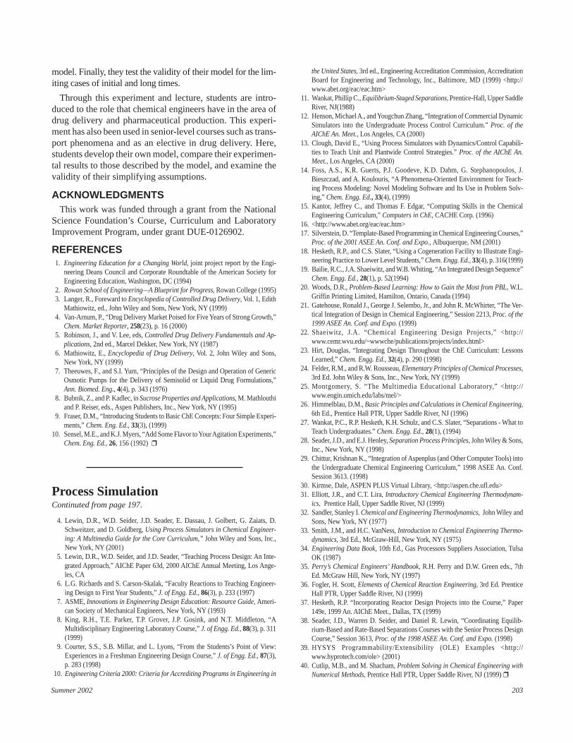
Summer 2002 203
model. Finally, they test the validity of their model for the lim-iting cases of initial and long times.
Through this experiment and lecture, students are intro-duced to the role that chemical engineers have in the area ofdrug delivery and pharmaceutical production. This experi-ment has also been used in senior-level courses such as trans-port phenomena and as an elective in drug delivery. Here,students develop their own model, compare their experimen-tal results to those described by the model, and examine thevalidity of their simplifying assumptions.
ACKNOWLEDGMENTSThis work was funded through a grant from the National
Science Foundation’s Course, Curriculum and LaboratoryImprovement Program, under grant DUE-0126902.
REFERENCES1. Engineering Education for a Changing World, joint project report by the Engi-
neering Deans Council and Corporate Roundtable of the American Society forEngineering Education, Washington, DC (1994)
2. Rowan School of Engineering—A Blueprint for Progress, Rowan College (1995)3. Langer, R., Foreward to Encyclopedia of Controlled Drug Delivery, Vol. 1, Edith
Mathiowitz, ed., John Wiley and Sons, New York, NY (1999)4. Van-Arnum, P., “Drug Delivery Market Poised for Five Years of Strong Growth,”
Chem. Market Reporter, 258(23), p. 16 (2000)5. Robinson, J., and V. Lee, eds, Controlled Drug Delivery Fundamentals and Ap-
plications, 2nd ed., Marcel Dekker, New York, NY (1987)6. Mathiowitz, E., Encyclopedia of Drug Delivery, Vol. 2, John Wiley and Sons,
New York, NY (1999)7. Theeuwes, F., and S.I. Yum, “Principles of the Design and Operation of Generic
Osmotic Pumps for the Delivery of Semisolid or Liquid Drug Formulations,”Ann. Biomed. Eng., 4(4), p. 343 (1976)
8. Bubnik, Z., and P. Kadlec, in Sucrose Properties and Applications, M. Mathlouthiand P. Reiser, eds., Aspen Publishers, Inc., New York, NY (1995)
9. Fraser, D.M., “Introducing Students to Basic ChE Concepts: Four Simple Experi-ments,” Chem. Eng. Ed., 33(3), (1999)
10. Sensel, M.E., and K.J. Myers, “Add Some Flavor to Your Agitation Experiments,”Chem. Eng. Ed., 26, 156 (1992) ❐
4. Lewin, D.R., W.D. Seider, J.D. Seader, E. Dassau, J. Golbert, G. Zaiats, D.Schweitzer, and D. Goldberg, Using Process Simulators in Chemical Engineer-ing: A Multimedia Guide for the Core Curriculum,” John Wiley and Sons, Inc.,New York, NY (2001)
5. Lewin, D.R., W.D. Seider, and J.D. Seader, “Teaching Process Design: An Inte-grated Approach,” AIChE Paper 63d, 2000 AIChE Annual Meeting, Los Ange-les, CA
6. L.G. Richards and S. Carson-Skalak, “Faculty Reactions to Teaching Engineer-ing Design to First Year Students,” J. of Engg. Ed., 86(3), p. 233 (1997)
7. ASME, Innovations in Engineering Design Education: Resource Guide, Ameri-can Society of Mechanical Engineers, New York, NY (1993)
8. King, R.H., T.E. Parker, T.P. Grover, J.P. Gosink, and N.T. Middleton, “AMultidisciplinary Engineering Laboratory Course,” J. of Engg. Ed., 88(3), p. 311(1999)
9. Courter, S.S., S.B. Millar, and L. Lyons, “From the Students’s Point of View:Experiences in a Freshman Engineering Design Course,” J. of Engg. Ed., 87(3),p. 283 (1998)
10. Engineering Criteria 2000: Criteria for Accrediting Programs in Engineering in
the United States, 3rd ed., Engineering Accreditation Commission, AccreditationBoard for Engineering and Technology, Inc., Baltimore, MD (1999) <http://www.abet.org/eac/eac.htm>
11. Wankat, Phillip C., Equilibrium-Staged Separations, Prentice-Hall, Upper SaddleRiver, NJ(1988)
12. Henson, Michael A., and Yougchun Zhang, “Integration of Commercial DynamicSimulators into the Undergraduate Process Control Curriculum.” Proc. of theAIChE An. Meet., Los Angeles, CA (2000)
13. Clough, David E., “Using Process Simulators with Dynamics/Control Capabili-ties to Teach Unit and Plantwide Control Strategies.” Proc. of the AIChE An.Meet., Los Angeles, CA (2000)
14. Foss, A.S., K.R. Guerts, P.J. Goodeve, K.D. Dahm, G. Stephanopoulos, J.Bieszczad, and A. Koulouris, “A Phenomena-Oriented Environment for Teach-ing Process Modeling: Novel Modeling Software and Its Use in Problem Solv-ing,” Chem. Engg. Ed., 33(4), (1999)
15. Kantor, Jeffrey C., and Thomas F. Edgar, “Computing Skills in the ChemicalEngineering Curriculum,” Computers in ChE, CACHE Corp. (1996)
16. <http://www.abet.org/eac/eac.htm>17. Silverstein, D. “Template-Based Programming in Chemical Engineering Courses,”
Proc. of the 2001 ASEE An. Conf. and Expo., Albuquerque, NM (2001)18. Hesketh, R.P., and C.S. Slater, “Using a Cogeneration Facility to Illustrate Engi-
neering Practice to Lower Level Students,” Chem. Engg. Ed., 33(4), p. 316(1999)19. Bailie, R.C., J.A. Shaeiwitz, and W.B. Whiting, “An Integrated Design Sequence”
Chem. Engg. Ed., 28(1), p. 52(1994)20. Woods, D.R., Problem-Based Learning: How to Gain the Most from PBL, W.L.
Griffin Printing Limited, Hamilton, Ontario, Canada (1994)21. Gatehouse, Ronald J., George J. Selembo, Jr., and John R. McWhirter, “The Ver-
tical Integration of Design in Chemical Engineering,” Session 2213, Proc. of the1999 ASEE An. Conf. and Expo. (1999)
22. Shaeiwitz, J.A. “Chemical Engineering Design Projects,” <http://www.cemr.wvu.edu/~wwwche/publications/projects/index.html>
23. Hirt, Douglas, “Integrating Design Throughout the ChE Curriculum: LessonsLearned,” Chem. Engg. Ed., 32(4), p. 290 (1998)
24. Felder, R.M., and R.W. Rousseau, Elementary Principles of Chemical Processes,3rd Ed. John Wiley & Sons, Inc., New York, NY (1999)
25. Montgomery, S. “The Multimedia Educational Laboratory,” <http://www.engin.umich.edu/labs/mel/>
26. Himmelblau, D.M., Basic Principles and Calculations in Chemical Engineering,6th Ed., Prentice Hall PTR, Upper Saddle River, NJ (1996)
27. Wankat, P.C., R.P. Hesketh, K.H. Schulz, and C.S. Slater, “Separations - What toTeach Undergraduates.” Chem. Engg. Ed., 28(1), (1994)
28. Seader, J.D., and E.J. Henley, Separation Process Principles, John Wiley & Sons,Inc., New York, NY (1998)
29. Chittur, Krishnan K., “Integration of Aspenplus (and Other Computer Tools) intothe Undergraduate Chemical Engineering Curriculum,” 1998 ASEE An. Conf.Session 3613. (1998)
30. Kirmse, Dale, ASPEN PLUS Virtual Library, <http://aspen.che.ufl.edu>31. Elliott, J.R., and C.T. Lira, Introductory Chemical Engineering Thermodynam-
ics, Prentice Hall, Upper Saddle River, NJ (1999)32. Sandler, Stanley I. Chemical and Engineering Thermodynamics, John Wiley and
Sons, New York, NY (1977)33. Smith, J.M., and H.C. VanNess, Introduction to Chemical Engineering Thermo-
dynamics, 3rd Ed., McGraw-Hill, New York, NY (1975)34. Engineering Data Book, 10th Ed., Gas Processors Suppliers Association, Tulsa
OK (1987)35. Perry’s Chemical Engineers’ Handbook, R.H. Perry and D.W. Green eds., 7th
Ed. McGraw Hill, New York, NY (1997)36. Fogler, H. Scott, Elements of Chemical Reaction Engineering, 3rd Ed. Prentice
Hall PTR, Upper Saddle River, NJ (1999)37. Hesketh, R.P. “Incorporating Reactor Design Projects into the Course,” Paper
149e, 1999 An. AIChE Meet., Dallas, TX (1999)38. Seader, J.D., Warren D. Seider, and Daniel R. Lewin, “Coordinating Equilib-
rium-Based and Rate-Based Separations Courses with the Senior Process DesignCourse,” Session 3613, Proc. of the 1998 ASEE An. Conf. and Expo. (1998)
39. HYSYS Programmability/Extensibility (OLE) Examples <http://www.hyprotech.com/ole> (2001)
40. Cutlip, M.B., and M. Shacham, Problem Solving in Chemical Engineering withNumerical Methods, Prentice Hall PTR, Upper Saddle River, NJ (1999) ❐
Process SimulationContinuted from page 197.

204 Chemical Engineering Education
The subject that sets off the most heated discussions inour workshops is testing. When we suggest giving teststhat can be finished in the allotted time by most of the
students, contain only material covered in lectures or assign-ments, involve no unfamiliar or tricky solution methods, andhave average grades in the 70–75 range, a few participantsalways leap up to raise objections:
1. What’s wrong with tests that only the best studentshave time to finish?Engineers constantly have to face deadlines; besides,if you really understand course material you should beable to solve problems quickly.
2. Why do I have to teach everything on the test?We shouldn’t spoon-feed the students—they need tolearn to think for themselves!
3. If I curve grades, what difference does it make if myaverages are in the 50’s?
Let’s consider these questions, starting with the first one.One problem with long tests is that students have differentlearning and test-taking styles.[2] Some (“intuitors”) tend towork quickly and are not inclined to check their calculations,even if they have enough time. Fortunately for them, theirstyle doesn’t hurt them too badly on tests: they are usuallyfast enough to finish and their careless mistakes only lead tominor point deductions. Others (“sensors”) are characteristi-cally methodical and tend to go over their calculations ex-haustively. They may understand the material just as well asthe intuitors do, but their painstaking way of working oftenleads to their failing exams they could have passed with fly-ing colors if they had more time.
Being methodical and careful is not exactly a liability in anengineer, and sensors are every bit as likely as intuitors tosucceed in engineering careers. (Frankly, we would prefer
them to design the bridges we drive across and the planes wefly in, even if their insistence on checking their results re-peatedly slows them down compared to the intuitors.) Stud-ies have shown, however, that sensors tend to get signifi-cantly lower grades than intuitors in engineering courses[2]
and that minimizing speed as a factor in test performancemay help level the playing field.[3]
Tests that are too long thus discriminate against some stu-dents on the basis of an attribute that has little to do withconceptual understanding or aptitude for engineering. (True,engineers have deadlines, but not on a time scale of minutesfor the types of problems on most engineering exams.) More-over, while overlong tests inevitably frustrate and demoral-ize students, there is not a scrap of research evidence thatthey either predict professional success or help students tobecome better or faster problem solvers.
FAQS.V.
DESIGNING FAIR TESTS[1]
© Copyright ChE Division of ASEE 2002
Random Thoughts . . .
RICHARD M. FELDER AND REBECCA BRENT
North Carolina State University • Raleigh, NC 27695
Richard M. Felder is Hoechst Celanese Pro-fessor Emeritus of Chemical Engineering atNorth Carolina State University. He received hisBChE from City College of CUNY and his PhDfrom Princeton. He is coauthor of the text El-ementary Principles of Chemical Processes(Wiley, 2000) and codirector of the ASEE Na-tional Effective Teaching Institute
Rebecca Brent is an education consultant spe-cializing in faculty development for effective uni-versity teaching, classroom and computer-based simulations in teacher education, and K-12 staff development in language arts and class-room management. She co-directs the SUC-CEED Coalition faculty development programand has published articles on a variety of topicsincluding writing in undergraduate courses, co-operative learning, public school reform, andeffective university teaching.

Summer 2002 205
How long is too long? Unless problems are trivial, studentsneed time to stop and think about how to solve them whilethe author of the problems does not. A well-known rule-of-thumb is that if a test involves quantitative problem solving,the author should be able to work out the test in less thanone-third of the time the students have to do it (and less thanone-fourth or one-fifth if particularly complex or computa-tion-heavy problems are included). If a test fails to meet thiscriterion, it should be shortened by eliminating some ques-tions, giving some formulas instead of requiring their deriva-tions, or asking for some solution outlines rather than requir-ing all the algebra and arithmetic to be worked out in detail.
How about those problems with unfamiliar twists that sup-posedly show whether the students can think independently?The logic here is questionable, to say the least. Figuring out anew way to tackle a quantitative problem on a time-limitedtest reflects puzzle-solving ability as much as anything else.If tricky problems count for more than about 10–15% of atest, the good puzzle-solvers will get high grades and the poorones will get low grades, even if they understand the coursecontent quite well. This outcome is unfair.
But (a workshop participant protests) shouldn’t engineer-ing students learn to think for themselves? Of course, butpeople learn through practice and feedback, period; no onehas ever demonstrated that testing unpracticed skills teachesanyone anything.Therefore, there should be no surprises ontests: no content should appear that the students could nothave anticipated, no skill tested that has not been taught andrepeatedly practiced. To equip students to solve problems thatrequire, say, critical or creative thinking, try working throughone or two such problems in class, then put several more onhomework assignments, and then put one on the test. If forsome reason you want students to be faster problem solvers,give speed drills in class and on assignments and then givelonger tests. The test grades will be higher—not becauseyou’re lowering standards, but because you’re teaching thestudents the skills you want them to have (which is, after all,what teachers are supposed to do).
Finally, what’s wrong with a test on which the average gradeis 55, especially if the grades are curved? It is that given thehurdles students have to jump over to matriculate in engi-neering and survive the freshman year, an entire engineer-ing class is unlikely to be incompetent enough to deservea failing average grade on a fair test. If most students in aclass can only work out half of a test correctly, it is prob-ably because the test was poorly designed (too long, tootricky) or the instructor didn’t do a good job of teaching
the necessary skills. Either way, there’s a problem.
One way to make tests fair without sacrificing their rigor isto post a detailed study guide before each one. The guideshould include statements of every type of question that mightshow up on the test, especially the types that require high-level thinking skills.[4] The statements should begin with ob-servable action words (explain, identify, calculate, derive,design, formulate, evaluate,...) and not vague terms such asknow, learn, understand, or appreciate. (You wouldn’t askstudents to understand something on a test—you wouldask them to do something to demonstrate their understand-ing.) A typical study guide for a mid-semester test mightbe between one and two pages long, single-spaced. Draw-ing from the study guides when planning lectures and as-signments and constructing tests makes the course bothcoherent and effective.
Peter Elbow observes that faculty members have two con-flicting functions—gatekeeper and coach.[5] As gatekeepers,we set high standards to assure that our students are qualifiedfor professional practice by the time they graduate, and ascoaches we do everything we can to help them meet and sur-pass those standards. Tests are at the heart of both functions.We fulfill the gatekeeper role by making our tests compre-hensive and rigorous, and we satisfy our mission as coachesby ensuring that the tests are fair and doing our best to pre-pare our students for them. The suggestions given in this pa-per and its predecessor[1] address both sets of goals. Adopt-ing them may take some effort, but it is hard to imagine aneffort more important for both our students and the profes-sions they will serve.
REFERENCES1. This column is based on R.M. Felder, “Designing Tests to Maximize
Learning,” J. Prof. Issues in Engr. Education & Practice, 128(1), 1–3(2002). Available at<http://www.ncsu.edu/felder-public/Papers/TestingTips.htm>.
2. R.M. Felder, “Reaching the Second Tier: Learning and Teaching Stylesin College Science Education,” J. College Science Teaching, 23(5),286-290 (1993). Available at<http://www.ncsu.edu/felder-public/Learning_Styles.html>.
3. R.M. Felder, G.N. Felder, and E.J. Dietz, “The Effects of PersonalityType on Engineering Student Performance and Attitudes,” J. Engr.Education, 91(1), 3–17 (2002). Available at<http://www.ncsu.edu/felder-public/Learning_Styles.html>.
4. R.M. Felder and R. Brent, “Objectively Speaking,” Chemical Engi-neering Education, 31(3), 178–179 (1997). Available at <http://www.ncsu.edu/felder-public/Columns/Objectives.html>. Illustrativestudy guides may be found at <http://www.ncsu.edu/felder-public/che205site/guides.html>
5. P. Elbow, Embracing Contraries: Explorations in Learning and Teach-ing, New York, Oxford University Press, 1986.
All of the Random Thoughts columns are now available on the World Wide Web athttp://www.ncsu.edu/effective_teaching and at http://che.ufl.edu/~cee/

206 Chemical Engineering Education
© Copyright ChE Division of ASEE 2002
ChE class and home problems
BOILING-LIQUID EXPANDING-VAPOREXPLOSION (BLEVE)
An Introduction to Consequence andVulnerability Analysis
C. TÉLLEZ, J.A. PEÑA
University of Zaragoza • Zaragoza, Spain
The chemical engineering curriculum should includeinformation on safety, health, and loss prevention inthe chemical industries.[1-4] A special sensitivity has
developed in the industry as a result of the real possibility ofaccidents of catastrophic proportions, such as
• The Flixborough accident (1974) at the Nypro plant inthe United Kingdom when an unconfined vapor cloudexplosion of cyclohexane resulted in 28 deaths andhundreds of injuries.
• The Sevesso (Italy, 1976) accident, where a runawayreaction caused toxic emissions of dioxin and methylisocynate that caused animal deaths, dried vegetation,and affected 2000 people.
• The Bophal (India, 1984) accident, which is thegreatest industrial disaster in the world to date, withabout 2,500 deaths and between 100,000 and 250,000injuries.
• The Mexico (1984) accident at St. J. Ixhuatepec wherea BLEVE (Boiling Liquid Expanding Vapor Explo-sion) of a storage tank of LPG produced more than500 deaths and 4,500 injuries.
After the Sevesso accident, developed countries establishedcompulsory legislation regulating declarations of risk by in-dustry,[5] developed emergency plans inside plants and in thesurrounding areas, and created coordinating organizations foremergency events. In the European community, the SevessoI (formerly) and the Sevesso II (currently) directives cover
Carlos Téllez received his PhD in 1998 at theUniversity of Zaragoza, where he is currentlyAssistant Professor teaching chemical engi-neering fundamentals. His research is focusedon fundamental studies in the preparation ofzeolite membranes and inorganic membranesfor pervaporation and gas separation.
Jose Angel Peña is Associate Professor ofChemical Engineering at the University ofZaragoza. His research interests include de-velopment of new methods for hydrogen stor-age and transport, development of a new sys-tem of indicators to estimate the risk of majoraccidents involving chemical reactors, and im-proved systems for early detection of runawayreactions.
The object of this column is to enhance our readers’ collections of interesting and novel prob-lems in chemical engineering. Problems of the type that can be used to motivate the student bypresenting a particular principle in class, or in a new light, or that can be assigned as a novel homeproblem, are requested, as well as those that are more traditional in nature and that elucidatedifficult concepts. Manuscripts should not exceed ten double-spaced pages if possible and shouldbe accompanied by the originals of any figures or photographs. Please submit them to ProfessorJames O. Wilkes (e-mail: [email protected]), Chemical Engineering Department, University ofMichigan, Ann Arbor, MI 48109-2136.
Summer 2002 207
such actions, while in the United States, legislation has re-quired development of both external and internal emergencyplans. OSHA has published laws regarding industrial healthand safety for the last thirty years, while other federal agen-cies, such as EPA, DOE, DOT, and associations such asAPI and AIChE, have developed their own legislation andcodes for good practice.
Universities should act as a mirror for society, and duringthe past few decades the chemical engineering curriculumhas made an effort to develop awareness of safety, health,and loss prevention, but there is still a need for greater aware-ness. The Center for Chemical Process Safety (CCPS), cre-ated in 1985, is an industry-driven center affiliated with theAmerican Institute of Chemical Engineers (AIChE) that ini-tiated a close relationship with engineering schools in 1992by creating the Safety and Chemical Engineering Educationprogram (SACHE). It provides teaching materials and pro-grams that bring elements of process safety into the curricu-lum <http://www.aiche.org/sache/>. The AIChE <http://www.aiche.org/education/crsindex.asp> and the Institution ofChemical Engineers in the United Kingdom <http://www.icheme.org/she/tps/index.html> also provide a varietyof safety courses for the chemical engineering curriculum. InSpain, a legislative article (R.D. 923/92) of the year 1992,established a degree of chemical engineering, and while somesubjects on health and safety were included as obligatory, itis clearly insufficient.
To increase knowledge of safety during the undergraduateyears of chemical engineering, several solutions have beenproposed in the U.S.[6,7] The first proposal is to introduce anobligatory safety course, but that would increase the lengthof the curriculum and would be difficult for departments andABET to agree upon. A second possibility, already incorpo-rated in some programs, is to include safety courses as elec-tives for undergraduates. The third proposal, perhaps moreuseful and easier to incorporate, is to give the students small“pills” of safety during their studies. One useful pill for show-ing students how to improve the safety of a process is the so-called “risk analysis.” This technique gives a quantitativeestimation of the risk involved in a given process.
In Spain, some knowledge of risk has been included asobligatory as a part of some courses on safety and/or health,and some universities have this program separated as elec-tive options. For example, the University of Zaragoza has anelective course titled “Analysis and Risk Reduction in theChemical Industry.”
The objective of this article is to familiarize the student
with risk analysis. The case selected for this is a boiling-liquid expanding-vapor explosion (BLEVE) of a tank truckof liquid propane. A brief introduction to consequence andvulnerability analysis models is included.
BRIEF DESCRIPTION OF THE CASEA tank truck of 50 m3 containing 19,000 kg of liquefied
propane under its vapor pressure was discharging inside afactory. Due to unknown reasons, the tank developed a leakand propane gas discharged into the atmosphere. About fiveminutes later, some propane and oxygen (from the atmo-sphere) produced a mixture within the LFL (lower flamma-bility limit) and the UFL (upper flammability limit). An un-known ignition source produced a weak explosion and starteda fire close to the tank. The heat flux coming from the fireincreased the temperature of the tank wall and the liquid pro-pane within it. The liquid propane tracked its boiling pointcurve (p0 vs T), substantially increasing the pressure in thetank. As a consequence, the tank ruptured catastrophically.This kind of phenomenon is a BLEVE (Boiling-LiquidExpanding-Vapor Explosion). At the moment of the acci-dent, the ambient temperature was 36°C and the atmo-spheric pressure and relative humidity were 760 mm Hgand 41%, respectively.
The students should
• Use consequence analysis models to study thepossibility of a BLEVE occurrence and its effects(fireball radiation, damage due to overpressure) onthe surrounding area.
• Use the Probit methodology for vulnerabilityanalysis to speculate on the percentage of victims(deaths, injuries, etc.) for a given area.
INTRODUCTION TOCONSEQUENCE ANALYSIS MODELS
STAGE 1
Is It Possible for a BLEVE to Take Place?
A BLEVE is the worst possible outcome when an LPG tankis exposed to fire. The possibility of a BLEVE occuring canbe checked by using Reid’s “massive nucleation theory.”[9]
This theory is based on the phenomenon of “spontaneousnucleation” that consists of a massive, instantaneous forma-tion of tiny bubbles within the liquid mass, caused by a sud-den depressurization of the vessel contents. When this phe-nomenon takes place, the possibility of a BLEVE occurs.
Universities should act as a mirror for society, and during the past few decades the chemicalengineering curriculum has made an effort to develop awareness of safety, health,
and loss prevention, but there is still a need for greater awareness.

208 Chemical Engineering Education
TABLE 1Fireball Characteristic Parameters as Calculated
by Different Authors(M) Initial Mass of Flammable Liquid [kg]
(Dmax
) = maximum diameter of the fireball [m](H
BLEVE) = height at the center of fireball [m]
(tBLEVE
) = duration of fireball [s]
CCPS [10] CCPS [19]
Dmax = 6.48 M0.325 = 159.3 m D*max = 5.8 M1/3 = 154.8 m
tBLEVE = 0.825 M0.26 = 10.7 s t*BLEVE = 0.45 M1/3 = 12 s
HBLEVE
= 0.75 DMAX
= 119.5 m
TABLE 2Flow of Radiation Per Unit of Surface Area and Time (I)
for Different Models
CCPS Model[10] Elia Model[12] Pape, et al., Model[13]
I(kW/m2) 336 301 306
Figure 1. Vapor pressure vs. temperature diagram showingthe zone of spontaneous nucleation for propane, as
described by Reid’s Theory.[9]
The zone of spontaneous nucleation can be seen in thepressure vs. temperature diagram shown in Figure 1. Itrepresents the liquid-gas equilibrium as mathematicallydescribed by the appropriate Antoine equation for the ma-terial being used (e.g., propane). (The equilibrium rela-tionship, as well as the critical temperature and pressurefor such material, can be obtained from the literature.[8])From the critical point (e.g., the critical temperature andpressure), a tangent line to the p0-vs.-T curve must be tracedup to a point where the ordinate represents the atmosphericpressure. The squared dot in Figure 1 shows the condi-tions inside the tank before the fire engulfment. As de-scribed by the Reid theory, every point located to the rightof this imaginary vertical line (dashed and arrowed) thatconnects the above described tangent line at atmosphericpressure, is a suitable scenario for a BLEVE. This meansthat when the tank is exposed to a fire, the heat comingfrom it will increase the temperture (and correspondinglythe pressure) inside the vessel, and the original conditionswill begin to ascend, following the p0-vs.-T curve. Thisprogressive heating will lead to a point where the above-mentioned vertical line will be trespassed. Once this con-dition has been achieved, a sudden rupture of the vesselwould lead to a BLEVE because of the suddendepresurization.
STAGE 2
Mathematical Models that
Describe the Effects of BLEVEs
The literature describes three types of BLEVE effects:the shock wave (overpressure effects), the thermal radia-tion, and the fragment projection. This paper focuses onthe shock wave and thermal effects as the main events in aBLEVE scenario.
Thermal Effects • The thermal effects of a BLEVE arerelated to radiation coming from the fireball. They are usu-ally accounted for through empirical equations related tothe quantity of substance involved in the BLEVE. Table 1shows expressions that have been proposed by differentauthors to calculate the maximum diameter of the fireball,D
max[m], the duration of the fireball, t
BLEVE[s], and the height
at the center of the fireball, HBLEVE
[m], as well as the re-sults obtained with them for the given case.
The flow of radiation per unit of emissive surface areaand time (I) in kW/m2 can be calculated using
CCPS[10]
IF H M
D t
R comb
BLEVE
=−( )
( )( )Δ
π max2 1
Elia model[12]
IM H P
D t
comb
BLEVE
=−( )
( )( )
0 2720
0 32
2
. .
max
Δ
π
Pape, et al., model[13]
I Pv= ( )235 30 39.
where FR is defined as the ratio between the energy emitted by
radiation and the total energy released by the combustion (thesuggested value as stated in the literature[10] ranges from 0.25 to0.4); -ΔH
comb is the heat of combustion of the material [kJ/kg];
P0 is the initial pressure at which the liquid is stored [MPa]; and
Pv is the vapor pressure of the stored liquid [MPa].

Summer 2002 209
Figure 2. Radiation received by a vertical surface as afunction of distance.
Typical radiation values of fireballs associated with BLEVEsare quoted in the range of 200 to 350 kW/m2. Taking a value ofF
R = 0.325, the heat of combustion from reference 14, and the
pressure inside the tank (1976 kPa) calculated as the vapor pres-sure of liquid propane at its superheat temperature (331 Kusing a Redlich-Kwong EOS approximation), the results areshown in Table 2. The value is inside the typical range forBLEVEs and close to the values reported by CCPS[10] (350kW/m2) for the intensity of radiation emitted by propane inBLEVE experiments.
The radiation received by a surface at a distance X from theemitting point can be calculated once the geometric view factor(F
vg) and the fraction of energy transmitted (atmospheric trans-
missivity, τ ) are known:
I I FR vg= ( )τ 4
In this respect, when considering the vulnerability of people tothe effects of a BLEVE, it is appropriate to use a geometricview factor corresponding to a surface perpendicular to a sphere:
FvgD
X= ( )
2
245
Considering only the partial pressure of water present in theatmosphere at the moment of the accident, τ can be calculatedapproximately by[20]
τ = ( ) ( )−2 02 0 096. .
P Xw
where Pw is the partial pressure of the water at ambient tem-
perature [Pa].
Another, simpler, model has been proposed by Roberts[11]
where the intensity of radiation received by a surface at a dis-tance X is given by an expression depending only on the massof fuel:
I M XR = − ( )828 0 771 2 7.
Overpressure Effects • Overpressures are difficult to pre-dict in the event of a BLEVE. The vaporization and pres-surization prior to the receptacle’s collapse, and the dura-tion of the rupture-depressurization, is extremely difficultto quantify. Experiments with explosives have demon-strated that the overpressure can be estimated using anequivalent mass of TNT. An approximate way to calculatethe equivalent weight of TNT (W
TNT) for a BLEVE has
been described by Prugh[15] as
WTNT
k
kPV
k P=
−− ⎛⎝
⎞⎠
⎡
⎣
⎢⎢⎢
⎤
⎦
⎥⎥⎥
( )−
0 0241
11
8
1
.*
where P is the pressure existing in the receptacle beforethe rupture [bar]. V* is given as
V V Vv ll
vf
D
D* = +
⎛⎝⎜
⎞⎠⎟
( )9
where Vv and V
l are the volumes of vapor and liquid [m3]
in the vessel before the explosion; Dl and D
v are the densi-
ties of liquid and vapor at the pressure and temperature ofthe system before the explosion; k is the ratio of Cp andCv; and f is the fraction of liquid that flashes after depres-surization. This can be calculated by the simple energybalance
f em
mv
Cp T T
Hb
v= = −−
−( )( )
01
0
10Δ
where m0 and m
v are the initial mass of liquid and the
amount vaporized in the flash, respectively, T0 is the ini-
tial temperature, Tb is the normal boiling temperature, C
p
is the heat capacity, and ΔHv is the heat of vaporization.
This expression to calculate f usually gives values on theorder of two times smaller than those observed experimen-tally,[16] concluding that a flash fraction well above 20%might be considered as a total vaporization.
To calculate the equivalent TNT mass, the following datacan be used:
• Liquid and vapor density are taken from reference 14
• Values for Cp (2.64 kJ/kg.K) and ΔH
v (430 kJ/kg) are
taken from reference 5.
• Boiling temperature of propane at atmosphericpressure is 231 K
The value of f obtained with these data is 0.38. It has beenmentioned that a more realistic value of the fraction thatflashes is two times the value obtained with Eq. (10); there-fore, the final estimation of f = 0.76 is close to 1. With fequal to 1, the equivalent TNT is 423.6 kg.
The TNT model is based on an empirical law establishedfrom trials using explosives.[17] This “cubic root law” es-

210 Chemical Engineering Education
Figure 4. Probability and Probit units relationship.
TABLE 3Probit Correlations for a
Variety of Causes and Effects[18,21]
Cause Effect k1 k2 V
Explosion Lung hemorrhage -77.1 6.91 Overpressure peak(1)
Explosion Eardrum rupture -15.6 1.93 Overpressure peak(1)
Explosion Structural damages -23.8 2.92 Overpressure peak(1)
Explosion Glass breakage -18.1 2.79 Overpressure peak(1)
Thermal effects Mortality -38.5 2.56 IR
4/3*t(2)
Thermal effects Second-degree burns -39.8 3.02 IR
4/3*t(2)
Thermal effects First-degree burns -43.1 3.02 IR
4/3t(2)
(1) Overpressure expressed in [Pa](2) I
R the intensity of radiation level received [W/m2]
and t the exposure time [s]
Figure 3. Overpressure along distance for the BLEVEproposed scenario.
tablishes equivalent overpressure effects for explosions oc-curring at the same normalized distances, expressed as
zR
WTNT
=( )
( )1 3 11/
where z is the normalized distance [m.kg-1/3] and R is thereal distance [m]. The experimental relation between over-pressure and normalized distance for unconfined explo-sions can be found in several references.[5,18] Figure 3shows the overpressure profile along distance for theproposed scenario.
INTRODUCTION TOVULNERABILITY ANALYSIS
The objective is to calculate the vulnerability to personsor installations expressed as the number of individuals orinstallations that could possibly be affected to a certainlevel of injury because of an accident. A possible methodfor estimating vulnerability consists of relating the dosereceived with the effect considered. This can be achievedfrom empirical evidence showing that individuals whohave been subjected to a certain dose of the injuring agent(e.g., a certain radiation intensity level during a given time)have suffered a particular effect (e.g., death by burn).Therefore, the methods that relate causes directly with ef-fects are hardly used, and the approximations to the prob-lem of estimation of vulnerability generally follow a proba-bilistic approach. The Probit scale is a way of dealing withsuch approximations. The connection between Probit units(Y) and probability (P) is given by
P e duuY
=−
−∞
−
∫ ( )1
212
2
25
π
The result of this expression is the Probit distribution withmean 5 and variance 1. The curve relating percentages andProbit units is shown in Figure 4.
Given the characteristics of the Probit variable, the fol-lowing relationship can be written
Y k k n V= + ( )1 2 13l
where Y is the number of Probit units, k1 and k
2 are em-
pirical constants depending on the causative factor and thelevel of damage to be analyzed, and V measures the inten-sity of the damage causative factor. The way in which V isexpressed depends on the type of effect studied. Table 3shows some values of the empirical constants (k
1 and k
2)
and the expression related with V.
The Probit expressions for prediction of the effects pro-duced by a given radiation intensity level during a giventime use a causative factor, V, proportional to the productt.I
R4/3 (t is the exposure time and I
R is the intensity of radia-
tion level). Regarding vulnerability to explosions, V is the

Summer 2002 211
Figure 5. Percentage of people and installations affectedby different effects and causes at a given point:
overpressure effects (solid line) andthermal effects (dotted line).
TABLE 4Distance at which 1% and 50% of the Population
(People or Objects) are Affected
Cause Effect Distance Distance[m] 50% [m] 1%
Explosion Lung hemorrhage 18.8 22.3
Explosion Eardrum rupture 34.4 63.0
Explosion Structural damages 51.6 84.7
Explosion Breakage of glass 162 321
Thermal effects Mortality due to thermal radiation 153 212
Thermal effects Second-degree burns(1) 222 293
Thermal effects First-degree burns(2) 329 436
(1) Epidermis and part of the dermis are burned(2) A superficial burn in which the top layer of skin (part of the epidermis) hasbeen slightly burned
overpressure at a given point.
Figure 5 shows the percentage of people and installations af-fected by different effects and causes. The values of overpres-sure and radiation intensity received by a surface at a distanceX (Elia model) obtained in the previous section (consequenceanalysis models) were used; the exposure time was taken astBLEVE
obtained with the Elia model.[12] Table 4 shows the esti-mated distances at which 1% and 50% of the population or struc-tures can be affected by a given effect. The limit at which 1% ofthe population may die is called “mortality threshold.”
CONCLUSIONSRisk analysis of major accidents is a useful tool for future
chemical engineers; it gives not only a quantitative estimationof the risk involved in a given process, but also a suitable methodfor estimation of possible victims (environment, persons, and
properties). A boiling-liquid expanding-vapor explosion(BLEVE) of a tank truck of liquid propane has been usedto demonstrate this technique, and the blast and thermaleffects have been calculated with several methods. The vul-nerability of persons and/or installations affected in bothcases has been calculated using the Probit methodology.
REFERENCES1. Lane, A.M., “Incorporating Health, Safety, Environmental, and Ethi-
cal Issues into the Curriculum,” Chem. Eng. Ed., 23, 70 (1989)
2. Cohen, Y., W. Tsai, and S. Chetty, “A Course on Multimedia Envi-ronmental Transport, Exposure, and Risk Assessment,” Chem. Eng.Ed., 24, 212 (1990)
3. Gupta, J.P., “A Chemical Plant Safety and Hazard Analysis Course,”Chem. Eng. Ed., 23, 194 (1989)
4. Mannan, M.S., A. Akgerman, R.G. Anthony, R. Darby, P.T. Eubank,and R.K. Hall, “Integrating Process Safety into the Education andResearch,” Chem. Eng. Ed., 33, 198 (1999)
5. Santamaria, J.M., and P.A. Braña, “Risk Analysis and Reductionin the Chemical Process Industry,” Blackie Academic & Profes-sional (1998)
6. Golder, A., “Safety Relevance in Undergraduate Education,”SACHE News, Spring 4 (2000)
7. Rossignol, A.M., and B.H. Hanes, “Introducing Occupational Safetyand Health Material into Engineering Courses,” Eng. Ed., 80, 430(1990)
8. Reid, R.C., J.M. Prausnitz, and B.E. Poling, The Properties of Gasesand Liquids, McGraw-Hill, New York, NY (1987)
9. Reid, R.C., “Possible Mechanism for Pressurized-Liquid Tank Ex-plosions or BLEVEs,” Science, 3, 203 (1979)
10. CCPS (Center for Chemical Process Safety), Guidelines for Chemi-cal Process Quantitative Risk Analysis, AIChE, New York, NY(1989)
11. Roberts, A.F., “Thermal Radiation Hazards from Release of LPGFires from Pressurized Storage,” Fire Safety J., 4, 197 (1982)
12. Elia, F., Risk Assessment and Risk Management for the ChemicalProcess Industry, H.R. Greenberg and J.J. Cramer, eds., VanNostrand Reinhold, New York, NY (1991)
13. Pape, R.P., et al., “Calculation of the Intensity of Thermal Radia-tion from Large Fires,” Loss. Prev. Bull., 82, 1 (1988)
14. Perry, R.H., and D. Green, eds, Perry’s Chemical Engineer’s Hand-book, 6th ed., McGraw-Hill, New York, NY (1984)
15. Prugh, R.W., “Quantify BLEVE Hazards,” Chem. Eng. Prog., 87,66 (1991)
16. Kletz, T. “Unconfined Vapor Explosions,” Loss Prevention 11,Chem. Eng. Prog. Tech. Manual, AIChE, New York, NY (1977)
17. Hopkinson, B., British Ordnance Board Minutes 13565 (1915)
18. Crowl, D.A., and J.F. Louvar, Chemical Process Safety: Funda-mentals with Applications, Prentice Hall, Englewood Cliffs, NJ(1990)
19. CCPS (Center for Chemical Process Safety): “Guidelines for Evalu-ating the Characteristics of Vapor Cloud Explosions, Flash Fires,and BLEVEs,” AIChE, New York, NY (1994)
20. Pietersen, C.M., and S.C. Huerta, “Analysis of the LPG Incident inSan Juan Ixhuapetec, Mexico City, 19-11-84,” TNO Report B4-0222, TNO, Directorate General of Labor, 2273 KH Vooburg, Hol-land (1985)
21. TNO, “Methods for the Determination of Possible Damage toPeople and Objects Resulting from Release of Hazardous Materi-als,” CPR 16E, Vooburg, Holland (1992) ❐

212 Chemical Engineering Education
RUBRIC DEVELOPMENT ANDINTER-RATER RELIABILITY ISSUES
In Assessing Learning Outcomes
JAMES A. NEWELL, KEVIN D. DAHM, AND HEIDI L. NEWELL
Rowan University • Glassboro, NJ 08028
With the increased emphasis placed by ABET[1] onassessing learning outcomes, many facultystruggle to develop meaningful assessment instru-
ments. In developing these instruments, the faculty membersin the Chemical Engineering Department at Rowan Univer-sity wanted to ensure that each instrument addressed the threefundamental program tasks as specified by Diamond:[2]
� The basic competencies for all students must be stated interms that are measurable and demonstrable.
� A comprehensive plan must be developed to ensure thatbasic competencies are learned and reinforced throughoutthe time the students are enrolled in the institution.
� Each discipline must specify learning outcomes congruentwith the required competencies.
Like many other institutions,[3] Rowan University’s Chemi-cal Engineering Department chose to use items that addressmultiple constituencies including alumni, industry, and thestudents themselves. Assessment data from these groups wereobtained through alumni surveys, student peer-reviews, andemployer surveys. These instruments were fairly straightfor-ward to design and could be mapped directly to the educa-tion objectives specified in Engineering Criteria 2000 (Crite-rion 3, A-K) as well as the AIChE requirements and otherdepartment-specific goals. Regrettably, over-reliance on sur-vey data often neglects those most qualified to assess studentperformance—the faculty themselves.
The faculty agreed that student portfolios would provide avaluable means of including faculty input into the process. Thedifficulty arose when the discussion turned to evaluating theportfolios. Paulson, et al.,[4] define portfolios as a “purposefulcollection of student work that exhibits the students’ efforts,progress, and achievement.” As Rogers and Williams[5] noted,however, there is no single correct way to design a portfolioprocess. Essentially everyone agreed that a portfolio shouldcontain representative samples of work gathered primarilyfrom junior- and senior-year courses. The ABET educationalobjectives are summative rather than formative in nature, so
the faculty decided to focus on work generated near the endof the student’s undergraduate career. A variety of assign-ments would be required to ensure that all of the diverse cri-teria covered in Criterion 3 could be addressed by at leastsome part of the portfolio. At the same time, we were acutelyaware that these portfolios would be evaluated every year andwere understandably interested in minimizing the total amountof work collected. Ultimately, we selected the following items:
� A report from a year-long, industrially sponsored researchproject through the Junior/Senior Clinics
� The Senior Plant Design final report� A hazardous operations (haz-op) report� One final examination from a junior-level chemical
engineering class (Reaction Engineering or Heat Transfer)� One laboratory report from the senior-level Unit Opera-
tions Laboratory Course
These items were all constructed-response formats[6-8] in whicha student furnished an authentic response to a given assign-ment or test question. This format was selected over multiplechoice selected response formats because it better representsrealistic behavior.[9] The selected-response format presentsalternative responses from which the student selects the cor-rect answer; specific selected response formats include true-false, matching, or multiple choice exams, while constructedresponse formats include essay questions or mathematical
James Newell is Associate Professor of Chemical Engineering at RowanUniversity. He is currently Secretary/Treasurer of the Chemical Engineer-ing Division of ASEE. His research interests include high performance poly-mers, outcomes assessment and integrating communication skills throughthe curriculum.
Kevin Dahm is Assistant Professor of Chemical Engineering at RowanUniversity. He received his PhD in 1998 from Massachusetss Institute ofTechnology. Before joining the faculty of Rowan University, he served asAdjunct Professor of Chemical Engineering at North Carolina A&T StateUniversity.
Heidi Newell is the Assessment Consultant for the College of Engineeringat Rowan University. She holds a PhD in Educational Leadership from theUniversity of North Dakota, a MS in Industrial/Organizational Psychol-ogy from Clemson University, and a BA in Sociology from BloomsburgUniversity of Pennsylvania.
© Copyright ChE Division of ASEE 2002
ChE classroom

Summer 2002 213
problem solving.[10] Although the items contained in the port-folio provided a wide range of work samples, they could notbe as neatly mapped to the ABET criteria. There was simplyno way to look at a laboratory report and assign a numberevaluating the student’s ability to apply math, science, andengineering. The immediate question that arose from the fac-ulty was, “Compared to whom?” A numerical ranking com-paring Rowan University’s chemical engineering students toundergraduates from other schools may be very different thanone comparing students to previous classes. It became clearthat specific descriptions of the performance level in eacharea would be required so that all faculty could understandthe difference between a 4 and a 2. As Banta[11] stated, “Thechallenge for assessment specialists, faculty, and administra-tors is not collecting data but connecting them.” The chal-lenge became one of developing rubrics that would help mapstudent classroom assignments to the educational objectivesof the program. The four-point assessment rubric also fol-lowed the format developed by Olds and Miller[12] forevaluating unit operations laboratory reports at the Colo-rado School of Mines.
COURSE VS PROGRAMMATIC ASSESSMENTOther chemical engineering departments are also develop-
ing rubrics for other purposes. In their exceptional (and Mar-tin-Award winning) paper on developing rubrics for scoringreports in a unit operations lab, Young, et al.,[13] discuss thedevelopment of a criterion-based grading system to clarifyexpectations to students and to reduce inter-rater variabilityin grading, based on the ideas developed by Walvoord andAnderson.[14] This effort represents a significant step forwardin course assessment. The goals of course assessment andprogram assessment are quite different, however.
For graded assignments to capture the programmatic ob-jectives, a daunting set of conditions would have to be met.Specifically,
� Every faculty member must set proper course objectivesthat arise exclusively from the program’s educationalobjectives and fully encompass all of these objectives
� Tests and other graded assignments must completelycapture these objectives
� Performance on exams or assignments must be a directreflection of the student’s abilities and not be influenced bytest anxiety, poor test-taking skills, etc.
If all of these conditions are met, there should be a directcorrelation between student performance in courses and thestudent’s overall learning. Moreover, much of the pedagogi-cal research warns of numerous pitfalls associated with us-ing evaluative instruments (grades on exams, papers, etc.)within courses as the primary basis for program assessment.[15]
One of the immediate difficulties is that many criteria areblended into the grade. A student with terrific math skills couldhandle the partial differential equations of transport phenom-ena but might never understand how to apply the model to
practical physical situations. Another student might under-stand the physical situation perfectly but struggle with themath. In each case, the student could wind up with a C on anexam, but for very different reasons. This is not a problem fromthe perspective of the evaluation; both students deserve a C.But, from an assessment standpoint, the grade does not provideenough data to indicate areas for programmatic improvement.
Moreover, if exams or course grades are used as the pri-mary assessment tool, the impact of the entire learning experi-ence on the student is entirely ignored[16]. Community activi-ties, field trips, service projects, speakers, and campus activi-ties all help shape the diverse, well-rounded professional withleadership skills that industry seeks. The influence of these non-classroom factors cannot be measured by course grades alone.
The goal of our rubrics was to map student work directlyto the individual learning outcomes. This also put us in a po-sition to more directly compare our assessment of studentwork with the assessment of performance provided by stu-dent peer reviews, employers, and alumni.
RUBRIC DEVELOPMENTThe first step was to take each educational objective and
develop indicators, which are measurable examples of anoutcome through phrases that could be answered with “yes”or “no.” A specific educational objective and indicator isshown below.
Goal 1, Objective 1: The Chemical Engineering Programat Rowan University will produce graduates who demon-strate an ability to apply knowledge of mathematics, sci-ence, and engineering (ABET-A).
Indicators:
1. Formulates appropriate solution strategies2. Identifies relevant principles, equations, and data3. Systematically executes the solution strategy4. Applies engineering judgment to evaluate answers
Once the indicators for each objective were developed, thenext task involved defining the levels of student achievement.Clearly, the lowest level should be what a novice demon-strates when confronted with a problem. The highest levelshould show metacognition,[16] the students’ awareness of theirown learning skills, performance, and habits. To achieve thehighest level, students not only have to approach the prob-lem correctly, but they must also demonstrate an understand-ing of their problem-solving strategies and limitations. Theintermediate scores represent steps between a metacognitiveexpert and a novice. It is important to note that the numbersare ordinal rather than cardinal. A score of four does not im-ply “twice as good” as a score of two.
All of the other assessment instruments used by the Chemi-cal Engineering Department had a five-point Likert scale,so a faculty team set out to develop meaningful scoring ru-brics using a five-point scoring system. Initially, the scorescontained labels (5 = excellent, 4 = very good, 3 = good, 2 =marginal, 1 = poor), but the qualitative nature of the descrip-

214 Chemical Engineering Education
TABLE 14 3 2 1
Formulates appropriate solution Can easily convert word Forms workable Has difficulty in Has difficulty gettingstrategies problems to equations; strategies, but may not be planning an approach; beyond the given unless
sees what must be done optimal; occasional tends to leave some directly instructedreliance on brute force problems unsolved
Identifies relevant principles, Consistently uses relevant Ultimately identifies relevant Indentifies some principles Cannot identify and assembleequations, and data items with little or no items but may start with but seems to have difficulty relevant information
extraneous efforts extraneous information in distinguishing what is needed
Systematically executes the Consistently implements strategy; Implements well; Has some difficulty in solving Often is unable to solvesolution strategy gets correct answers occasional minor errors the problem when data are problem, even when all data
may occur assembled; frequent errors are given
Applies engineering judgment Has no unrecognized Has no more than one, if any, Attempts to evaluate answers Makes little, if any, effortto evaluate answers implausible answers unrecognized implausible but has difficulty; recognizes to interpret results; numbers
answers; if any, it is minor that numbers have meaning appear to have little meaningand obscure but cannot fully relate
TABLE 24 3 2 1
Solutions based upon Has no unrecognized Has no more than one, if any, Attempts to evaluate answers Makes little, if any, effort tochemical engineering principles implausible answers unrecognized implausible answers; but has difficulty; recognizes interpret results; numbersare reasonable if any, it is minor and obscure that numbers have meaning appear to have little meaning
but cannot fully relate.
tive phrases should stand alone, without the need for additionalclarifiers. Ultimately, it was decided to eliminate all labels.
It became apparent that a four-point scale allowed for moremeaningful distinctions in developing the scoring rubrics forthe portfolios. Providing four options instead of five elimi-nates the default “neutral” answer and forces the evaluator tochoose a more definitive ranking. The four-option scale alsomade it easier to write descriptive phrases that were meaning-fully different from the levels above and below. In developingthese phrases, the following heuristic was used: for the four-point phrases, the writer attempted to describe what ametacognitive expert would demonstrate; for the three-pointphrases, the target was what a skilled problem solver who lackedmetacognition would display; for the two-point words, the writ-ers attempted to characterize a student with some skills, butwho failed to display the level of performance required for anengineering graduate; the one-point value captured the perfor-mance of a novice problem solver.
To evaluate a given indicator, professors would read the left-most description. If it did not accurately describe the perfor-mance of the student, they would continue to the next block tothe right until the work was properly described. A sample ru-bric is shown in Table 1.
RUBRIC TESTINGAND INTER-RATER RELIABILITY
Once the lengthy process of developing scoring rubrics foreach objective was completed, the rubrics needed testing. C.Robert Pace[17] succinctly stated the challenge of accurateassessment, saying “The difficulty in using faculty for the
assessment of student outcomes lies in the fact that differentprofessors have different criteria for judging students’ per-formance.” The intent of the rubrics was to create specificand uniform assessment criteria so that the role of subjectiveopinions would be minimized. The ideal result would be thatall faculty members using the rubrics would assign the samescores every time to a given piece of student work.
To evaluate if the rubrics were successful in this respect,six samples of student work (four exams and two engineer-ing clinic reports) were distributed to the entire faculty (sevenmembers at that time). All of them assigned a score of 1,2,3,4, or “not applicable” to every student assignment for everyindicator. This produced 160 distinct score sets (excludingthose that were all “not applicable”) that were examinedfor inter-rater reliability.
The results, in general, were excellent. Every faculty mem-ber scored the items within one level of each other in 93% ofthe items. In 47% of the score sets (75 of 160), agreementwas perfect—all faculty members assigned exactly the samescore. In another 46%, all assigned scores were within 1.Rubrics for which this level of agreement was not achievedwere examined more closely for possible modification. Afterall of the scoring sheets had been compared, the faculty metto discuss discrepancies in their evaluations.
The primary example of a rubric that required modifica-tion is shown in Table 2. “Solutions based on chemical engi-neering principles are reasonable,” in the originally devel-oped scheme, was an indicator that applied to a number ofdifferent educational objectives. This was the only rubric for

Summer 2002 215
which scores were not routinely consistent. One heat-trans-fer exam received a range of scores that included multipleoccurrences of both 4 and 1.
In the ensuing discussion, we found that the difficulty withthis exam was that nothing recognizable as a final answerwas presented for any question. The student formulated asolution strategy and progressed through some work but neverfinished solving the equations. Interpreting the rubric word-ing in one way, some faculty chose to assign 4. This interpre-tation is understandable because no answer was given, andthere was no “unrecognized implausible answer.” By the let-ter of the criteria, the student earned a 4. Some faculty inter-preted the criteria differently, however, resulting in the as-signment of 1. This interpretation is also reasonable—sincethere were no results, there was no attempt to interpret theresults. The rubric was simply re-written to specify that arating of N/A be given if no recognizable “final answer” wasprovided, and the discrepancies in scoring were not presentin subsequent evaluations.
In addition to pointing out necessary revisions, this testingprovided a good measure of inter-rater reliability. Havingevery faculty member review every item in an annual assess-ment portfolio would be a laborious task. Consequently, theresults of this test were examined to determine what level ofaccuracy could be expected when a group of three facultyreviewed an item. For example, in the score set 2, 2, 2, 2, 1,3, 2; the mean score assigned by the faculty was 2, and themean of a three-score subset could be 1.67, 2, or 2.33. Thismeans that any panel of three faculty members would haveassessed this sample of work with a score within 0.5 of thatassigned by the entire faculty. We found (after one rubric wasrevised as described above) that 95% (153 of 160) of the scoresets showed this level of consistency. Thus, we concluded thatwhen using the rubrics, a randomly constituted panel of threefaculty members would be reasonably representative of the de-partment. Detailed rubrics are available through the web at
<http://engineering.eng.rowan.edu/~newell/rubrics>
CLOSING THE LOOPUltimately, the purpose of gathering detailed assessment
data is to improve student learning. Once each year, we re-view the data in a two-day assessment meeting[3] where wediscuss all aspects of the program, including the data fromeach tool. We identify strengths and areas for improvementand make decisions affecting curriculum and policies. Spe-cific changes resulting from these meetings have includeda decision to introduce product engineering and econom-ics earlier in the curriculum and to adjust topical cover-age in thermodynamics.
THE NEXT LEVELThe next goal is to use the rubrics to help guide selection
of course objectives across the curriculum. With detailed edu-
cational objectives in place and rubrics to assist in their as-sessment, we hope improved course objectives will be de-veloped that more directly link classroom activities and evalu-ations with the program goals. The rubrics described in thispaper should provide the basis for a more in-depth, forma-tive assessment. Although the ABET criteria are summative,the educational process itself centers around formativechanges, incrementally enhancing a student’s knowledge, skillset, and problem-solving capabilities.
CONCLUSIONSA complete set of rubrics was developed and tested that
maps student performance of a variety of junior/senior-levelassignments directly to program educational objectives. Theserubrics were tested for inter-rater reliability and were shownto yield the same mean (within 0.5) regardless of which setof three faculty members evaluated the material. These re-sults, in conjunction with input from alumni, employers, andthe students themselves, serve as a basis for assessment ofthe chemical engineering program.
REFERENCES
1. Engineering Accreditation Commission, Engineering Criteria 2000, Ac-creditation Board for Engineering and Technology, Inc., Baltimore (1998)
2. Diamond, R.M., Designing and Assessing Courses and Curricula: A Prac-tical Guide,” Jossey-Bass Inc., San Francisco (1998)
3. Newell, J.A., H.L. Newell, T.C. Owens, J. Erjavec, R. Hasan, and S.P.K.Sternberg, “Issues in Developing and Implementing an Assessment Plan inChemical Engineering Departments,” Chem. Eng. Ed., 34(3), p. 268 (2000)
4. Paulson, L.F., P.R. Paulson, and C. Meyer, “What Makes a Portfolio aPortfolio?” Educational Leadership, 48(5), p. 60 (1991)
5. Rogers, G.M., and J.M. Williams, “Asynchronous Assessment: Using Elec-tronic Portfolios to Assess Student Outcomes,” Proc. of the 1999 ASEENat. Mtng., Session 2330, Charlotte (1999)
6. Morris, L.L., C.T. Fitz-Gibbon, and E. Lindheim, How to Measure Per-formance and Use Tests, Sage Publishers, Newberry Park, CA (1987)
7. Roid, G.H., and T.M. Haladyna, A Technology for Test-Item Writing, Aca-demic Press, San Diego (1982)
8. Robertson, G.J., “Classic Measurement Work Revised: An Interview withEditor Robert L. Linn,” The Score, p.1 (1989)
9. Fitzpatrick, R., and E.J. Morrison, “Performance and Product Evaluation,”in Educational Measurement, R. Thorndike ed., American Council of Edu-cation, Washington DC (1989)
10. Erwin, T. Dary, Assessing Student Learning and Development, Jossey-Bass, San Francisco (1991)
11. Banta, T.W., J.P. Lund, K.E. Black, and F.W. Oblander, Assessment in Prac-tice, Jossey-Bass Inc., San Francisco (1996)
12. Olds, B.M., and R.L. Miller, “Using Portfolios to Assess a ChE Program,”Chem. Eng. Ed., 33(2), 110 (1999)
13. Young, V.L., D. Ridgway, M.E. Prudich, D.J. Goetz, B.J. Stuart, “Crite-rion-based Grading for Learning and Assessment in the Unit OperationsLaboratory,” Proc. of the 2001 ASEE Nat. Mtng., Albuquerque (2001)
14. Walvoord, B.E., and V.J. Anderson, Effective Grading: A Tool for Learn-ing and Assessment, Jossey-Bass Inc., San Francisco (1998)
15. Terzini, P.T., and E.T. Pascarella, How College Affects Students: Findings andInsights from Twenty Years of Research, Jossey-Bass Inc., San Francisco (1991)
16. Angelo, T.A., and K.P. Cross, Classroom Assessment Techniques: A Hand-book for College Teachers, 2nd ed., Jossey Bass Inc., San Francisco (1993)
17. Pace, C.R., “Perspectives and Problems in Student Outcomes Research,”in Assessing Educational Outcomes, Peter Ewell ed., Jossey-Bass Inc.,San Francisco (1985) ❐

216 Chemical Engineering Education
MASS TRANSFER AND CELL GROWTH KINETICS
IN A BIOREACTOR
KEN K. ROBINSON, JOSHUA S. DRANOFF, CHRISTOPHER TOMAS, SESHU TUMMALA
Northwestern University • Evanston, IL 60208-3120
Ken Robinson is a Lecturer at Northwestern University with primary re-sponsibility for the undergraduate chemical engineeirng laboratory. Hereceived his BS and MS from the University of Michigan and his DSc fromWashington University. He has worked in industry for both Amoco andMonsanto.Joshua Dranoff is Professor of Chemical Engineering at NorthwesternUniversity. He received his BE degree from Yale University and his MSEand PhD from Princeton University. His research interests are in chemicalreaction engineering and chromatographic separations.Christopher Tomas is a PhD candidate at Northwestern University work-ing under the direction of Professor E. Terry Papoutsakis. He received hisBS in Chemical Engineering from the University of Illinois, Urbana-Champaign, in 1996, and his MS in Biotechnology from NorthwesternUniversity in 1998.Seshu Tummala is a PhD candidate at Northwestern University workingunder the direction of Professor E. Terry Papoutsakis. He received his BSdegree from The Johns Hopkins University in 1996 and his MS degreefrom Northwestern University in 1999, both in chemical engineering.
Biotechnology is an increasingly important factor inthe chemical process industries. The last decade hasseen rapid growth in the resources committed to the
development of biologically based processes. At the sametime, the market value of new products generated by biologi-cal means has continued to grow at an accelerating rate. Ac-cordingly, more and more chemical engineers are being em-ployed in the development, design, and operation ofbioprocesses for production of pharmaceuticals, foods, andspecialty chemicals, with no indication that the demands andopportunities in this area will moderate in the future.
In recognition of this trend, we have developed a new “bio-technology experiment” for Northwestern’s senior laboratorycourse.[1] This experiment is aimed at giving our students anopportunity to become familiar with various factors involvedin the implementation of bioprocesses and some of the atten-dant technologies. We hope this will introduce them to thisbroad field while they are still at Northwestern and also en-hance their attractiveness to potential employers.
The experiment provides a means for studying two basicchemical engineering operations (mass transfer and cellgrowth kinetics) that occur in a three-liter stirred fermenta-
tion reactor. The initial part of the experiment involves thestudy of oxygen transfer rates from gas to liquid phases; tran-sient dissolved oxygen profiles resulting from step changesin feed gas oxygen concentration are measured with a dis-solved oxygen probe. The growth kinetics of Escherichia coliare then studied in the same reactor under standard condi-tions. Cell growth is monitored by spectrophotometric analy-sis of samples removed from the reactor at specific times.The complete experiment is normally run in two successivelaboratory sessions, each about eight hours long, separatedby one week. It is also necessary to perform some short pre-parative steps the day prior to the second laboratory session.
EXPERIMENT SETUP
Equipment • The principal apparatus used is an Applikonthree-liter glass stirred bioreactor. It was obtained as part of acomplete package that included a number of ancillary items,such as temperature, pH, and oxygen probes and control sys-tems. Additional major items obtained for this purpose in-cluded an Innova 4200 shaken-cell incubator and a basic spec-trophotometer (Spectronic 20+). The approximate cost of thisequipment is indicated in Table1. Not included in the indi-cated cost, but of critical importance for this experiment, is asteam sterilizer large enough to accommodate the fermenta-tion reactor. We had access to such a unit in our department(AMSCO Eagle 2300 Autoclave) and assume that similarequipment is likely to be available in chemical engineeringor related departments at other institutions.
A sketch of the reactor is shown in Figure 1. It is stirredwith dual turbine blade impellers on a single shaft, driven byan electrical motor with an adjustable speed control. The re-actor top is a stainless steel disk equipped with multiple portsfor sampling, introduction of inoculum, gas feed and outletlines, and insertion of temperature, pH, and dissolved oxy-gen measuring probes. Additional specifications are indi-cated in the Appendix.
© Copyright ChE Division of ASEE 2002
ChE laboratory

Summer 2002 217
TABLE 1Major Equipment Needed for Experiment
� Applikon 3-liter fermentor, with control system and $15,000oxygen, temperature, and pH probes
� Innova 4200 Incubator $ 5,000
� Spectronic Instruments 20+ Spectrophotometer $ 1,700
Total Cost $21,700
Gas is fed into the reactor and dispersed into the liquidthrough an L-shaped sparger tube that has multiple holes alongthe horizontal section that is located near the bottom of thereactor vessel. Outlet gas passes through a small water-cooledcondenser tube that serves to prevent evaporation of waterfrom the normally warm liquid contents of the reactor.
Temperature in the vessel is sensed by a type-J thermo-couple inserted through one of the reactor ports and controlledby a simple electronic control system. An electrically heatedjacket provides required heat input, while cooling water canbe simultaneously circulated through a small cooling coilimmersed in the reactor liquid. Stable control of the reactortemperature at 37°C is easily achieved with this system.
The bioreactor can be fed with three different gases. Air issupplied by an air pump with an inlet microfilter; pure oxy-gen and nitrogen are provided from pressurized cylinders.The nitrogen is used in calibrating and spanning the dissolvedoxygen probe and in the oxygen transfer-rate experiments.Air and oxygen are used in the cell-growth kinetics studies inconjunction with the dissolved oxygen (DO) controller. Dur-ing a typical cell-growth experiment, air is continuouslysparged into the liquid medium in the reactor with the con-troller set point at 70% of total saturation relative to pure air.Whenever the measured oxygen concentration falls below70%, a three-way valve is actuated automatically to switchthe sparging gas from air to pure oxygen. This control schemeis normally quite effective in returning the DO level back tothe set point within a few minutes, except during the highoxygen uptake portion of the cell-growth curve (exponential
phase described below). At such times, the stirrer speed canbe increased from 250 rpm (normal operating level) to 350rpm in order to increase the gas-liquid interfacial area enoughto permit increased oxygen transfer to the liquid phase. Op-eration at these stirrer speeds was found to be convenientand minimized foam formation during experiments (no anti-foaming agents were used).
Expendable Supplies • To perform the following experi-ments, a number of reagents and other expendable suppliesare required. They include sodium chloride, Ampicillin,Tryptone, yeast extract, Agar, ethanol, deionized water, andbleach, as well as disposable gas-line filters.
DESCRIPTION OF THE EXPERIMENTS(A) Determination of the Oxygen Transfer Coefficient
The first quantity measured with this system is the com-bined mass transfer coefficient for oxygen transfer from thegas to the liquid phase, k
La. (Since the interfacial area avail-
able for mass transfer cannot be readily determined in theseexperiments, it has been incorporated in the definition of thecoefficient in the usual fashion.) This simple experiment pro-vides an opportunity for the student to become familiar withvarious parts of the apparatus while illustrating an importantchemical engineering principle.
� The reactor is assembled and filled with 2 liters of deion-ized water. With the stirring speed set at 250 rpm, the tem-perature control system is activated and the system is allowedto reach a steady temperature of 37°C.
� The DO probe, having been previously polarized by op-eration for two hours in deionized water, is connected. Thereactor is sparged with nitrogen at a rate of approximately0.5 liters/minute until the DO signal has stabilized (normallyabout 30-45 minutes), at which point the zero of the DO con-troller is set to read 0% oxygen. The nitrogen flow is thenreplaced by air at the same volumetric rate and flow is main-tained until the DO probe output remains constant. At thispoint the controller span is adjusted to read 100% (i.e., satu-ration with respect to the oxygen content of air).
� The feed gas is then rapidly switched back to nitrogen(step down in feed gas oxygen concentration), and the DOconcentration is recorded every 30 seconds to 1 minute untilit returns to 0%. The feed is then rapidly switched back to air(step up in feed gas oxygen concentration), and DO concen-tration is recorded every minute until it returns to 100%. These“step-up” and “step-down” data are then analyzed as indi-cated below to determine k
La.
(B) Determination of Cell Growth Kinetics
This is the more difficult and demanding part of the ex-periment, especially for students unfamiliar with the proto-cols used in biochemical research. It involves two separateoperations: the preparation of a stock culture of active cellsand the subsequent measurement of cell growth kinetics.Figure 1. Fermentation reactor.

218 Chemical Engineering Education
Figure 2. Typical oxygen transfer data: Dissolved oxygenconcentration vs. time.
Throughout this portion of the experiment, emphasis is placedon the need to maintain sterility and cleanliness of the appa-ratus and the work area.
� (1) Preparation of stock culture. This part of the proce-dure is normally carried out during the first laboratory ses-sion along with the oxygen transfer measurements describedearlier. Steps involved include:
• Preparation of Luria-Bertani (LB) culture media (seealso the Discussion section).
Liquid LB medium is a mixture of sodium chloride,Tryptone, yeast extract, and deionized water (compositiongiven in the Appendix).
Solid LB medium is a mixture of sodium chloride, Tryptone,yeast extract, Agar, and deionized water (composition givenin the Appendix).
Each of these media is placed in an Erlenmeyer flask that isthen covered with aluminum foil and autoclaved for 20minutes in the sterilizer. The liquid medium can be used inthe reactor as prepared.
The solid medium is used to prepare solid culture plates.After the initial sterilization, the solutions are allowed toequilibrate at 55°C and then antibiotic solution is added(see the Appendix for composition of antibiotic solution).The medium is then poured into sterile culture plates thatare stacked and allowed to solidify in a sterile hood atroom temperature (several hours).
• Preparation of Cell Cultures. The cells used in theseexperiments are from an E.coli strain, ER 2275, furnishedby New England Bio Labs, Beverly, Massachusetts, andmodified (pImP1) as described by Mermelstein, et al.[2]
A stock of E.coli on the solid medium is prepared bystreaking a fresh solid medium plate with a colony ofE.coli and then incubating the plate at 37°C overnight. Ifindividual colonies of E.coli are then easily visible on theplate, it is placed in the refrigerator for storage. If not,another plate is streaked and incubated, as above. Thisprocess has proven to be easily reproducible.
• Preparation of inoculum. The inoculum is a solutioncontaining living cells that is used to initiate the growthprocess within the bioreactor. It is prepared the day priorto the fermentation experiment. An individual colony froma stock plate is combined in a 250-ml. Erlenmeyer flaskwith 200 ml of liquid LB medium equilibrated at 37°C,antibiotic solution is added, and the inoculum is allowedto grow overnight (for approximately 12 hours) with shak-ing at 200 rpm in the incubator.
� (2) Preparation of the Reactor for Growth KineticsStudies. The reactor vessel is assembled and filled with deion-ized water and then autoclaved for approximately 20 min-utes along with a supply of liquid LB medium prepared asdescribed above. After the reactor has cooled to room tem-perature, the water is pumped out and replaced by 1.8 liters
of the LB medium. The reactor is then allowed to come tothermal equilibrium at 37°C and the control systems are acti-vated. (The DO probe must first be polarized and calibrated,as described above.)
� (3) Growth Kinetics Studies. When the system is ready,200 ml of the inoculum solution is pumped into the reactorand the DO level is set to approximately 70%. A small sample(10-15 ml) of the reactor contents is then removed every 10-15 minutes and its turbidity measured in the spectrophotom-eter (at a wavelength of 600 nm). If the cell concentrationgets too high, the sample is first diluted in order to keep itwithin the mid-range of the spectrophotometer. The experi-ment is concluded when the fermentation appears to havereached the stationary phase (see below). This normally re-quires 4 to 6 hours.
The final liquid medium still left in the reactor is auto-claved before disposal, and all equipment is carefullycleaned with bleach and soap.
DATA ANALYSIS(A) Determination of Oxygen Transfer Coefficient
Typical data obtained in the “step-down” (nitrogen feed)and “step-up” (air feed) experiments described above areshown in Figure 2. These data were obtained with a reactorvolume of 2.0 liters, a gas flow rate of 0.38 liters per minute,and a mixer rpm of 250. The data clearly exhibit an initialtime lag that is the same for both experiments. This lag isapparently due to dynamic response of the dissolved oxygenprobe itself. Since it was consistent and relatively small com-pared to the overall time scale of the experiment, the responsedata have been corrected by subtracting a lag of 1.5 minutesfrom the measured time in each transient experiment.
For either experiment, the oxygen transfer rate per unitvolume of liquid (OTR) is given by the following equation,which also defined the volumetric liquid phase mass transfercoefficient:
OTR k a C CL= −( ) ( )* 1
where

Summer 2002 219
Figure 3. Typical Oxygen transfer data: Determination ofkLa with nitrogen sparging.
Figure 4. Typical oxygen transfer data: Determination ofkLa with air sparging.
C* saturated dissolved oxygen concentration at the gas-liquid interface, mmol/L
C dissolved oxygen concentration in the bulk liquidphase, mmol/L
kLa liquid phase oxygen mass transfer coefficient, 1/
minuteOTR oxygen transfer rate, mmol/L/minute
The transfer coefficient typically depends on the gas flowrate, the bioreactor working volume, and the power input tothe agitator (or stirrer speed). It may also depend on the pa-rameters of the reactor design, such as impeller and spargerdesign and configuration, and the physical properties of theculturing medium, such as viscosity and interfacial tension.
A transient oxygen balance for the reactor volume is
dC
dtOTR k a C CL= = −( ) ( )* 2
Considering the experiment in which the initially oxygen-free solution is contacted with oxygen containing gas, Eq.(2) must be integrated with initial concentration = 0 and con-centration C* held constant. The well-known result is
lnC C
Ck atL
*
*
−( ) = − ( )3
For the reverse experiment in which the solution is initiallysaturated at concentration C* and the gas concentration is =0, the solution is
lnC
Ck atL*
= − ( )4
Logarithmic plots of the corrected step-down and step-updata according to Eqs. (3) and (4) are shown in Figures 3 and4, respectively. It can be seen that the data conform quitewell to the expected form, yielding the values for the masstransfer coefficient of 0.155 min-1 for the nitrogen spargingor step-up experiment, and 0.145 min-1 for the air sparging orstep-down experiment, for an average value of 0.15 min-1.
One other measurement of kLa was made with air sparging
into the OB medium prior to the beginning of the cell-growthexperiments. In this case, the mixer speed was set to 150 rpmwhile the other conditions remained as before. It was foundthat the data once again showed a time lag of 1.5 minutes andfit the expected exponential decay similar to Figure 4. Thevalue of k
La determined, however, was 0.075 min-1. Thus, it
is clear that this mass transfer coefficient is a strong func-tion of the degree of agitation in the vessel and the prop-erties of the liquid.
It should be noted that Roberts, et al.,[3] previously describeda laboratory experiment to measure oxygen transfer in a 1-liter stirred fermentor. In that case, the stirring rate was con-siderably higher (500 to 700 rpm) and the method of deter-mining k
La was different; those authors measured the quasi-
steady-state rate of oxygen consumption by yeast in the ab-sence of oxygen feed (the vessel contents were previouslysaturated with air). Although conditions were quite differentin that experiment compared to the present case, the masstransfer coefficients reported were of the same order of mag-nitude—approximately 0.6 min-1 at a stirrer speed of 500 rpm.Using their exponent of 2.75 for the effect of mixer rpm, theexpected value of k
La at 250 rpm would be 0.089 min-1, which
is unexpectedly close to the value of 0.15 min-1 found hereunder considerably different conditions.
(B) Determination of Cell Growth Kinetics
The immediate objective of the second part of the experi-ment is to measure the specific growth rate of the E.coli cul-ture in the batch fermentation reactor system. Typically, suchbacteria growing in a batch culture exhibit four distinct growthphases following inoculation with an active culture. As shownin Figure 5, growth usually begins with a very slow lag phaseas cells introduced into the inoculum adjust to their new en-vironment. This is followed by a rapid, exponential phase asacclimated cells reproduce via binary fission as quickly asnutrient and oxygen concentrations within the medium per-mit. This phase is followed by a stationary phase where therate of oxygen supplied to the cells equals their rate of oxy-gen consumption. Finally, the cell concentration falls duringthe death phase due to the depletion of nutrients and thebuildup of toxic byproducts.
The specific growth rate ( μ ) of the cells is determined dur-ing the exponential binary fission phase. This process is au-

220 Chemical Engineering Education
Figure 5. Typical batch culture growth phases.
Figure 7. Determination of specific cell-growth rate.
Figure 6. E.coli growth data: solution absorbance vs. time.
tocatalytic and is usually represented as a first-order reac-tion, i.e.,
dX
dtX= ( )μ 5
Integration of this differential cell balance yields
X t X t to o( )= −( )[ ] ( )exp μ 6
whereX cell concentration, number/volumet time, minutesμ cell specific growth rate, 1/minuteo as a subscript refers to initial conditions
In the present experiments, cell concentration in the reac-tor is monitored at 10- to 15-minute intervals by measure-ment of the absorbance (at 600 mm) of a small sample ofsolution using the spectrophotometer. According to the usualBeer-Lambert law, the light transmitted through a solution isrelated to the incident light and the concentration of absorb-ing species, as shown in
I
Icl
o= −( ) ( )exp ε 7
whereI/I
ofractional light intensity relative to incident intensity
c concentration of absorbing species, number per unit volumel length of light path through solutionε extinction coefficient of absorbing species, area per number
Strictly speaking, for the present experiments ε should beregarded as an appropriate fitting parameter since changes inmeasured light intensity are no doubt due to a combinationof absorption and scattering.
Since absorbance A is defined as -log10
(I/Io), it follows from
Eqs. (6) and (7) that
Alc lX
t too= = −( )[ ] ( )ε ε
μ2 303 2 303
8. .
exp
Taking natural logs of Eq. (8) yields
l ln nA t tlX
oo( ) = −( ) + ⎛
⎝⎜⎞⎠⎟ ( )μ
ε2 303
9.
Thus, a plot of ln A( ) against time should be linear with aslope equal to the specific cell-growth rate ( μ ) during theexponential growth phase. A cell doubling time, t
d, can be
calculated once the growth rate is determined, according to
td = ( ) ( )ln 210
μ
Figure 6 shows typical data obtained over a 4-hour periodfollowing the experimental procedure described earlier. Thesedata indicate an expected initial lag of 15 minutes, followedby an apparent exponential growth phase that levels off some-time after 200 minutes. When these data are plotted in accordwith Eq. (9), a good fit to the exponential model is obtained,as shown in Figure 7. The corresponding specific growth rate
of the E.coli in this experiment was 0.013 min-1. This is equiva-lent to a doubling time t
d of 53 minutes. This relatively long
doubling time confirms that the E.coli strain, while adequatefor these experiments, is not particularly robust.
The only difficulty encountered in carrying out the cell-growth experiments has been maintaining the dissolved oxy-gen concentration at 70%. Large swings in the oxygen level(between 50% and 90% of saturation) have been observedeven with increases in gas-flow rate and stirring speed. Thesevariations, however, apparently do not have any significanteffect on the observed growth rates.

Summer 2002 221
DISCUSSIONThe experiments described here have provided a means for
introducing senior students to some aspects of bioprocessing.During the course of this experiment, students are exposed tostandard procedures for preparing and handling a bacterialculture, including preparation of growth media, developmentof active bacterial colonies, and incubation and sterilizationprocesses. They also become aware of the mass transfer pro-cesses involved, the underlying theoretical analysis, and rel-evant methods of data analysis, as well as the relatively longtime scale of the experiments. The latter is not a serious prob-lem in our laboratory since we are able to devote two 8-hoursessions to this experiment. Some compromises, such as morepre-lab preparations carried out by the instructors, wouldundoubtedly be necessary in order to perform similar experi-ments in a shorter laboratory session.
In designing this experiment, we have attempted to includeas many of the preparative and analytical steps mentionedabove as possible without unduly burdening the students, sinceour goal is to provide opportunies for “hands-on” experienceswhenever possible. At the same time, we are not attemptingto develop research-level competencies in our students bythis means. Selection of LB culture media as opposed tochemically defined media is a case in point. While the formermay yield somewhat less reproducible results from one stu-dent group to another, the LB media have proven to be robustand easy to use. Some lack of reproducibility was not con-sidered to be a significant drawback in the present context.
A related laboratory experiment[4] used the growth of yeast(Saccharomyces cerevisiae) and involved the simultaneoususe of two fermenters. The rate of oxygen transfer to the liq-uid phase was studied with and without cell growth, and therates of cell growth during the exponential phase were alsomeasured under aerobic conditions with various concentra-tions of added ethanol. No performance data were presented,so a more direct comparison to the present experiment is notpossible. It should be noted, however, that while the overallgoals of these two experiments are similar, the systems ofchoice and the methods of data analysis differ somewhat.
Another experiment[5] based on ethanol production usingSaccharomyces cerevisiae yeast used 1 liter fermentors andmeasured CO
2 generated during fermentation to follow the
course of the process. As in the above-mentioned case, theoverall objective of the experiment is similar to the presentcase, although it is much more limited in scope.
We have now run this experiment successfully for two years,with increasing numbers of students and with very positiveresults. While the immediate and ancillary equipment requiredto mount such an experiment is not trivial or inexpensive,such equipment is becoming relatively common and is likelywithin reach of most chemical engineering departments in-terested in providing some direct introduction to biotechnol-ogy in their curricula. Of even greater importance than equip-
ment in the successful development of such an experimentare skilled and experienced people who can help in the earlyplanning and implementation stages. We were particularlyfortunate to be able to call on Professors E.T. Papoutsakisand W.M. Miller and some of their graduate students for tech-nical assistance and encouragement.
ACKNOWLEDGEMENTSWe wish to thank the following Northwestern graduate students
for their assistance and advice during the development and start-upof this experiment: Kathy Carswell, Dominic Chow, Rick Desai,Sanjay Patel, Albert Schmelzer, and Vivian DeZengotita. We alsothank the recent undergraduate laboratory group whose data wereused to illustrate the features of this experiment: Michael Gerlach,Julie Nguyen, Edward Ruble, and Chris Spelbring. Finally, we areespecially thankful to Kraft, Abbott Laboratories, and the MurphySociety of the McCormick School of Engineering and Applied Sci-ence for the financial support that made it possible to develop andbring this new experiment to full realization.
REFERENCES1. Robinson, K.K., and J.S. Dranoff, Chem. Eng. Ed., 30, 98 (1996)2. Mermelstein, L.D., N.E. Welker, C.N. Bennett, and E.T. Papoutsakis,
Bio/Technology, 10, 190 (1992)3. Roberts, R.S., J.R. Kastner, M. Ahmad, and D.W. Tedder, Chem. Eng.
Ed., 26, 142 (1992)4. Shuler, M.L., N. Mufti, M. Donaldson, and R. Taticek, Chem. Eng.
Ed., 28, 24(1994)5. Badino, Jr., A.C., and C.O. Hokka, Chem. Eng. Ed., 33, 54 (1999)
Useful references for this general area are:Biochemical Engineering, by Harvey W. Blanch and Douglas S. Clark,Dekker (1996)Biochemical Engineering Fundamentals, 2nd ed., by James E. Baileyand David F. Ollis, McGraw-Hill (1986)Bioprocess Engineering: Basic Concepts, by M. L. Shuler and F. Kargi,Prentice-Hall (1992) ❐
APPENDIX
1. Composition of Luria-Bertani liquid medium:Per liter of solution: NaCl 10 grams
Tryptone 10 gramsYeast extract 5 gramsDeionized water 1 liter
2. Composition of Luria-Bertani solid medium:Per liter of solution NaCl 10 grams
Tryptone 10 gramsYeast extract 5 gramsAgar 15 gramsDeionized water 1 liter
3. Composition of antibiotic solution:Ampicillin 1 gram dissolved in 1 ml of deionized waterAdded to LB medium at concentration of 100 micrograms/ml
4. Reactor dimensionsType: 3 liter, dished bottomInside diameter: 130 mmImpeller: Two 6-bladed Rushton turbines
Turbine diameter: 45 mmTurbine distance from vessel bottom: 45 mm and 75 mm
Baffles: Three, equally spaced baffles, each 220 mm long

222 Chemical Engineering Education
TEACHING ChE TOBUSINESS AND SCIENCE STUDENTS
KA M. NG
Hong Kong University of Science and Technology • Clear Water Bay, Hong Kong
The chemical processing industries (CPI) have under-gone profound changes, and companies are under con-siderable pressure to restructure and innovate in a glo-
bal environment where information, technology, capital, andhuman resources flow easily. Supply chain management ande-business is used to improve the overall efficiency of anenterprise, and there is a tendency to farm out non-core tech-nologies. For example, recognizing that drug discovery is theirmain business, pharmaceutical firms tend to outsource theproduction of active pharmaceutical ingredient intermediates.There is increasing emphasis on product design, which isclosely linked to market demands.[1,2] This creates new busi-ness opportunities and the need for better understanding ofthe global issues of chemical processing. In response, thereis considerable effort to broaden chemical engineering edu-cation to include emphasis on entrepreneurship, lifelong learn-ing, management, business, international experience, etc.
Obviously, chemical engineering is not the only professionreacting to the challenges of the new global environment.Other disciplines also strive to enhance the depth and breadthof their curriculum in order to expand employment opportu-nities for students. A case in point is an elective course aboutchemical engineering offered to business and science studentsat the Hong Kong University of Science and Technology(HKUST). Here, the semester system is identical to that of
© Copyright ChE Division of ASEE 2002
the US, and all classes are conducted in English. There aretwo similar but separate courses: one for business and onefor science students. The course for business students coversmore basic chemistry, while the one for science students ismore detailed in business concepts. We will discuss what weteach and why, how the students respond to the course, andwhat we can learn from this experience.
COURSE OBJECTIVESHong Kong (a Special Administrative Region of China since
1997) is a vibrant, international city of 6.7 million inhabit-ants from all over the world. It is located in the heart of theAsia-Pacific region where chemical processing industrieshave been growing at a rate in excess of 10% per year. HongKong has a strong financial sector with an interest in chemi-cal-related businesses. While the manufacturing sector withinHong Kong is comparatively small, extensive manufactur-ing takes place north of Hong Kong in Shenzhen, Guangzhou,Zhuhai, Huizhou, and other municipalities. Also, since theGNP per capita of Hong Kong is comparable to that of otherdeveloped countries, there is keen interest in chemical prod-ucts that can offer a higher return on assets. Of particularinterest are high-value-added chemicals and pharmaceuti-cals. The allure is clear when one compares the 8% profitmargin in a typical chemical firm to the 20% figure of aUS drug company.[3]
The overall goal of the course is to provide business andscience students with an overview of chemical engineering.Specifically, the student is expected to gain an appreciationof
• The CPI products• How chemicals are manufactured• The cost of building and operating a typical chemical
plant
ChE curriculum
Ka M. Ng is Professor and Head of ChemicalEngineering and Director of the Consortiumof Chemical Products and Processes atHKUST. He obtained his BS and PhD degreesat Minnesota and Houston, respectively. From1980 to 2000 he was Professor of ChemicalEngineering at the University of Massachu-setts. His research interests are in processsystems engineering involving reactions, crys-tallization, and solids processing of high-value-added products.
Summer 2002 223
• The organization and finance of a typical chemicalcompany
• Product-centered processing• The history of chemical engineering• The global chemical business
COURSE DESIGNThe course, consisting of six sections (see Table 1) starts
by introducing the students to the US and HK economies.[4,5]
In the late ‘70s , the breakdown of the HK GNP was similarto that of the US. Gradually, financing, insurance, and realestate have become dominant industries in Hong Kong. Incontrast, the US CPI is one of the largest among manufactur-ing sectors such as electronic and electric equipment, motorvehicles, and parts, etc. We show how the return on assets
and profit margins of the CPI have fluctuated with time alongwith the overall economy. Innovations such as nylon andpolyester have created new markets for chemical products.
In Section 2 of the course, we discuss selected chemicalproducts.[6] Table 2 lists the products we have considered sofar. Petroleum is normally the first product to be discussed.The students can easily appreciate the various uses of petro-leum and the concept of distillation. Soaps and detergents isanother business to which the students can readily relate. Theylearn about the composition of a typical detergent formula-tion, surfactants, detergent builders, bleaching agents, andenzymes, and how detergency works. There is a wealth ofinformation on the World Wide Web from the Soap and De-tergent Association[7] as well as from companies such asProcter and Gamble and Unilever. A typical assignment is toread a product report in Chemical and Engineering News.[8]
The students gain an appreciation for both the need for dif-ferentiated products that drive reformulations and the chal-lenges faced by suppliers of detergent ingredients. We con-sider the replacement of sodium tripolyphosphate with zeo-lites from an environmental viewpoint, and we use picturesand samples of chemical products such as cellulose triacetate(for cigarette filters), spandex, sugar esters, superabsorbents(for diapers), etc., to stimulate students’ interest in the sub-ject. Oils and fats is another business of interest to Hong Kongstudents. We discuss the nature of those products, the sourceof raw materials, and manufacturing processes.[9,10,11]
Next we show the students that all of these products origi-nate from three sources in our environment: air and water;substances from the ground (which include gas, petroleum,and minerals); and living things (including plants and ani-mals). We show the primary reaction for conversion of onecompound (or compounds) to another.[12] For example, ureais manufactured from ammonia and carbon dioxide; polyes-ter results from a polycondensation reaction between ethyl-ene glycol and terephthalic acid, which is in turn obtainedfrom the oxidation of paraxylene; and cellulose triacetatecomes from cotton linters. We expected the students to gainan appreciation of the complexity of the chemical supply chainand also introduced the concept of mass balance. We pointout the kind of companies that add value to different seg-ments of the suppy chain, such as oil companies, chemicalcompanies, specialized engineering firms, pharmaceuticalcompanies, consumer goods companies, etc.
In Section 3 of the course, we turn our attention to the pro-duction of chemicals using Douglas’ hierarchical approach.[13]
After covering input-output, recycle structure, and separa-tion systems, we discuss chemical engineering unit opera-tions. These include reaction, evaporation, drying, distilla-tion, absorption, extraction, crystallization, adsorption, fil-tration, etc.[14] We discuss basic principles but omit equationsfor equipment design. We use The Visual Encyclopedia ofChemical Engineering Equipment developed at the Univer-
TABLE 1Outline of Topics
Section1. Introduction
• The economy and the chemical processing industries (CPI)• Diversity and complexity of products from the CPI• Characteristics of the CPI
2. Chemicals and Their Sources• Basic chemistry• Chemicals in our daily lives• The chemical supply chain• The chemical business hierarchy
3. The Production of Chemicals• The chemical plant and its unit operations• Project evaluation• The cost of manufacture• The criteria of economic performance
4. The Financial Performance of Chemical Corporations• Financial metrics• Financial statements• Capital budgeting
5. Product Design• Approaches to product design• Product-centered process synthesis and development
6. The Modern Chemical Processing Industries• Development of CPI in the UK, Germany, US, and Japan• The scale and economics of the CPI today• The CPI in Asia
TABLE 2Chemicals in Our Daily Lives
• Petroleum• Fibers• Soaps and detergents• Plastics• Oils and fats• Natural products• Traditional Chinese medicines

224 Chemical Engineering Education
Figure 1. The production of towngas by catalytic reformingof naphtha using steam.
sity of Michigan to supplement the lectures. The animatedequipment operations are very helpful to the non-engineer-ing students. At this point, we briefly discuss safety and en-vironment issues related to chemical processing in order toraise the students’ awareness of these issues.
We use a chemical plant in Hong Kong to illustrate pro-cessing concepts. Towngas, produced by catalytic reactionof naphtha with steam, is often the example of choice (seeFigure 1). The first stage of the desulfurization unit convertsorganic sulfur compounds to hydrogen sulfide, and the sec-ond stage removes hydrogen sulfide with zinc oxide. In thereaction system, the desulfurized naptha is converted to meth-ane and hydrogen, and carbon monoxide is converted to car-bon dioxide and hydrogen. The carbon dioxide and water isremoved in the gas purification and drying system. Projectevaluation follows Douglas’ book. The students do not havemuch difficulty in grasping the details of direct costs, indi-rect costs, working capital, etc. We also cover (particularlyfor science students) the time value of money and the dis-counted cash-flow rate of return on investment. Normally,we assign a project in which the students perform cost evalu-ation of a chemical plant. The flowsheet and all major equip-ment sizes and operating conditions are given, assuming thatthis input information has been obtained from chemical en-gineers in a consulting firm.
Next we turn our attention to the financial performance ofchemical corporations. Various measurements, such as returnon net assets, after-tax profit margin, sales growth, and con-trolled fixed-cost productivity, are introduced. We usuallyexamine the financial statements of two US corporations;recently, we have discussed those of DuPont in class whilethose of Eastman Chemical are analyzed in a homework as-signment. One objective is to learn how to read the balancesheet, the income statement, and the statement of changes infinancial position. More importantly, we emphasize an ap-preciation of the financial position of a typical chemical com-pany in terms of profit margin, new investments,amount of assets on the ground, etc. This reinforcesthe notion that CPI is a capital-intensive business.To emphasize decision-making in chemical busi-nesses, we venture into capital budgeting,[15] butthis segment can be skipped if the students havepreviously learned these concepts in their businessclasses. Retrofit projects, as well as proposals toconstruct a grassroots plant, are considered.
Product design is of great interest to Hong Kong.We discuss a typical product development cycle—concept development, design and prototype, pro-cess planning, piloting, and plant startup. We ex-plain the use of Quality Function Deployment(QFD); this is further refined for chemical prod-ucts where market trends lead to product attributes,which are in turn decided by material properties
and processing conditions (see Figure 2). We identify thedesired performance of the product, both functional and sen-sorial, and select the requisite ingredients. The processflowsheet and the operating conditions are then identified.
We study the modern CPI in Section 6.[4] It begins with areview of the manufacture of soda ash, dyes, and sulfuricacid in the UK and Germany as well as the emergence of theCPI in America in the 1900s and in Japan in the 1950s. Thenwe turn our attention to today’s CPI. Its global enormity isevident when one compares the global chemical shipment of$1.59 trillion in 1999 to the HK GDP equivalent of approxi-mately $200 billion.
We then examine the financial performance of the top glo-bal chemical companies, emphasizing the top twenty-fivechemical-selling countries in 1999 (see Table 3).[3] It is evi-dent from the statistics that chemical production per capita inAsia is below the world average, but (unsurprisingly) it israpidly gaining ground. Singapore is a net exporter compet-ing in the international market. Although China is not ex-pected to be self-sufficient, its rapid development and pur-chasing decisions can significantly affect the global CPI. Weexamine the recent JVs and investment projects in order toappreciate the dynamics of the market in this region.[16]
COURSE EVALUATION
The impact of the course has been assessed by its students.While the course is intended for undergraduates, it generallyhas around 25% graduate students from all science and busi-ness disciplines. With rankings ranging from very bad to verygood, about 85% of the respondents ranked the overall courseas good or very good. Most of them expressed that they ac-quired a good knowledge of chemical engineering. Also,throughout the semester we hold a 10-to-15 minute oral quizevery week in order to challenge them to think about interre-lationships among different decisions. Most students felt that

Summer 2002 225
Figure 2. Step-by-step procedure for product-centeredprocess synthesis and development.
1. U.S. 4352. Japan 2053. Germany 1044. China 915. France 786. United Kingdom 507. South Korea 508. Italy 499. Brazil 36
10. Belgium 3511. India 3112. Spain 3013. Taiwan 30
TABLE 3Top Twenty-Five Chemical-Selling Countries in 1999
(in US$ billions)[3]
14. Netherlands 2815. Switzerland 2616. Russia 2517. Canada 2118. Mexico 1519. Australia `1420. Argentina 1021. Sweden 922. Malaysia 823. Poland 624. Singapore 525. Thailand 5
they have been encouraged to express ideas (84% ranked asgood and very good) and have improved their ability to think(76% ranked as good and very good).
REFLECTIONS ONCHEMICAL ENGINEERING EDUCATION
With the reshaping of the global economic landscape, thedemarcation between disciplines has become blurred. It ishighly desirable to have an appreciation of contemporary glo-
bal economic issues while keeping our core competencies inchemical engineering practice. The strategy and financialdealings of the various companies in the global CPI coveredin this course can also serve as an interesting topic in a typi-cal chemical engineering process design course. In fact, someof these business concepts were covered in the senior designcourse at the University of Massachusetts.
In addition to synthesizing, simulating, and costing a chemi-cal plant, it is interesting to investigate whether or not a pro-posed retrofit project or a new investment adds to the share-holder value. Indeed, it is not uncommon to request that theengineers and researchers in a company justify an R&D pro-posal in terms of potential return on investment as well as onits technical merits. Similarly, the lectures on product-cen-tered process synthesis and development is suitable for chemi-cal engineering process design. In this case, the student learnshow market demands dictate what to make, how to make it,and where to make it, thus gaining an appreciation of theeconomic consequences of these decisions in a much widercontext than in a traditional process design course.
ACKNOWLEDGMENTS
I would like to thank Bruce Vrana for his teachings on cor-porate finance during my stay at DuPont Central R&D,Francis Lui for providing the HK economics data, and ChiMing Chan for teaching the section on product design.
REFERENCES1. Cussler, E.L., and J.D. Moggridge, Chemical Product Design, Cam-
bridge University Press, Cambridge, UK (2001)2. Wibowo, C., and K.M. Ng, “Product-Oriented Process Synthesis and
Development: Creams and Pastes,” AIChE J., 47, 2746 (2001)3. “Facts and Figures from the Chemical Industry,” C&EN, June 26, p.
48 (2000)4. Arora, A., R. Landau, and N. Rosenberg, Chemicals and Long-Term
Economic Growth, John Wiley and Sons (1998)5. “Estimates of Gross Domestic Product 1961 to 1997,” Government of
Hong Kong, Feb. (1998)6. Chenier, P.J., Survey of Industrial Chemistry, 2nd ed., John Wiley &
Sons (1992)7. <http://www.sdahq.org/>8. Ainsworth, S.J., “Soaps and Detergents,” C&EN, Jan 24, p. 34 (1994)9. Hamm, W., and R.J. Hamilton, eds., Edible Oil Processing, CRC Press
(2000)10. Hoffmann, G., The Chemistry and Technology of Edible Oils and Fats
and Other High Fat Products, Academic Press (1989)11. O’Brien, R.D., Fats and Oils Formulating and Processing for Appli-
cations, Technomic Publishing Co., Lancaster, PA (1998)12. Rudd, D.F., S. Fathi-Afshar, A.A. Trevino, and M.A. Stadtherr, Petro-
chemical Technology Assessment, John Wiley and Sons (1981)13. Douglas, J.M., Conceptual Design of Chemical Processes, McGraw-
Hill, New York, NY (1988)14. Walas, S.M., Chemical Process Equipment: Selection and Design,
Butterworths, Boston, MA (1988)15. Ross, S.A., R.W. Westfield, and B.D. Jordan, Fundamentals of Cor-
porate Finance, 5th ed., McGraw Hill, New York, NY (2000)16. Bank of America’s Guide to Petrochemicals in Asia, EFP International,
Hong Kong (1997) ❐

226 Chemical Engineering Education
INTEGRATINGKINETICS CHARACTERIZATION
AND MATERIALS PROCESSING IN THELAB EXPERIENCE
DENNIS J. MICHAUD, RAJEEV L. GOROWARA, ROY L. MCCULLOUGH
University of Delaware • Newark, DE 19716
At the University of Delaware, we have developed anintegrated sequence of two undergraduate laboratoryexperiments (spanning the junior and senior years)
in which the students investigate different aspects of batchprocess design. The design task assigned to the students is toidentify adequate processing conditions to produce a qualityone-inch-thick composite laminate within a limited timeframe. Thick-sectioned thermoset composites can be diffi-cult to process correctly due to the exothermic nature ofthe polymerizing resin and the low thermal conductivityof the laminate.
The Resin Transfer Molding (RTM) process incorporates anumber of core chemical engineering concepts within a labo-ratory exercise while at the same time introducing studentsto the manufacture and properties of composite materials. Anumerical cure simulation of the RTM process,[1] developedwithin the Center for Composite Materials at the Universityof Delaware, is used during each lab’s design component toevaluate different processing scenarios. Figure 1 outlines theimportant features of the two experiments and illustrates themanner in which they are integrated.
In the first experiment, the juniors characterize the resin’spolymerization kinetics and heat of reaction using differen-tial scanning calorimetry (DSC). Using an empirical nonlin-ear kinetic model for the thermosetting resin,[2] the data iscorrelated to establish the model parameters needed by theprocess simulation. The simulation is then used for a pre-liminary design of the processing conditions required to suc-cessfully produce a one-inch-thick composite laminate withina two-hour processing window. The sensitivity of their de-sign to kinetic parameter variability is also investigated.
Dennis J. Michaud is currently Lecturer of Chemical Engineering at theUniversity of Delaware. He received his BS from Northeastern Universityand was awarded a PhD in Chemical Engineering at the University ofDelaware in 2000 for his work in the optimization and control of thick-sectioned RTM composite processing.Rajeev L. Gorowara received his PhD in Chemical Engineering underthe direction of Professor McCullough at the University of Delaware in2001, focusing on interphase formation in glass-fiber vinyl-ester compos-ites. He received his BS and MS from Ohio State University. He is cur-rently a Consulting Engineer in the DuPont Engineering Particle Scienceand Technology Group.Roy L. McCullough was Professor of Chemical Engineering at the Uni-versity of Delaware until his death in December of 2001. He received hisundergraduate chemistry training at Baylor University and was awarded aPhD in Chemistry by the University of New Mexico in 1960. He publishednumerous technical papers and organized symposia in the areas of poly-mer science and composite materials.
The senior composite laboratory experience continues thesimulation-based sensitivity analysis of the RTM process byincluding variations of the simulation’s heat transfer modelparameters. The students implement their initial design, pro-ducing a ten-inch-square composite laminate with a one-inchthrough-thickness. Density, void fraction, and mechanicaltests of the laminate help students evaluate the success (orfailure) of their experiment. By comparing measurementsfrom thermocouples embedded within the composite andthose predicted by the simulation, the students make modifi-cations to the simulation’s model parameters (heat transferand kinetic) to improve the simulation’s accuracy.
Armed with an improved process simulation and moreknowledge of the process, the students then generate a newset of processing conditions and again implement it experi-mentally, producing a new (and hopefully improved) com-posite laminate. The students then use a combined evalua-tion of the simulation’s model parameters and their process-
ChE laboratory
© Copyright ChE Division of ASEE 2002

Summer 2002 227
ing experience to propose a final design in their written report.
THICK-SECTIONED COMPOSITE MANUFACTURINGThe specific problem given to students concerns the manufacture of
thick (greater than one-half inch through-thickness) composite materialsvia RTM. This nontraditional subject matter allows students to applyclassroom knowledge of kinetics and transport phenomena while alsointroducing process control and the limitations of mathematical models.Processing thick-sectioned composites is challenging due to the exo-thermic nature of the reacting resin and the heat transfer limitationsof the polymer and glass fiber composite.[1,3] Unfavorable process-ing conditions of the composite part can lead to poor part quality,including cases where the laminate cracks internally due to residualstresses within the part.
The primary design problem for thick-sectioned composite is to iden-tify an acceptable temperature trajectory (or “cure cycle”) that balances
the heat necessary to initiate the polymerizationreaction (cure) with the heat transfer limitations ofthe composite once the reaction begins, while alsomaintaining a processing time that is economicallyfeasible. The example cure cycle presented in Fig-ure 2 shows experimentally measured heater andcomposite (measured at the center of a one-inch-thick laminate) temperatures. The cure cycle isbroken up into different stages, each with a spe-cific heater set-point.
For the experiment shown in Figure 2, the firstset-point was 62°C and the second set-point for thepost-cure was 90°C. Due to the low thermal con-ductivity of the composite, almost 60 minutes ofprocessing is required for the center of the com-posite to reach the heater set-point, but once theresin at the center begins to cure, the heat gener-ated from the reaction quickly raises the composite’stemperature and drives the polymerization reactionto completion. A lower temperature curing stagereduces the temperature gradient within the part aswell as residual stresses, but also increases process-ing time. Since the surface temperature of the com-posite remains much closer to the heater set-point,a post-cure is generally required to ensure the sur-faces of the composite are adequately cured for re-moval of the part from the mold.
LABORATORY FORMATAND EDUCATIONAL OBJECTIVES
At Delaware, the undergraduate chemical engi-neering laboratory is a two-course sequence, takenin the spring of the junior year and the fall of thesenior year. Initially, all students attend fivebackground lectures in laboratory safety, mea-surement techniques, statistics, report writing,and oral presentation.
In the junior course, student groups go throughthree experimental cycles, with each cycle center-ing around a design problem using informationgathered during a laboratory experiment. Over afour-week period, the students must learn about theproblem, perform the experiment, analyze thedata, prepare a preliminary data report, revisethe data analysis, and complete the design prob-lem in a final report.
In the first week of a cycle, the students preparefor the lab by reviewing the experiment and labo-ratory procedures with the teaching assistant (TA).They prepare an experimental proposal, and dur-
Figure 1. Schematic of integrated undergraduatelaboratory experiments.
Figure 2. Example cure cycle and correspondinginternal composite temperature.

228 Chemical Engineering Education
Figure 3. Example heat flow of a differential scanningcalorimetry (DSC) experiment.
ing the graded pre-lab conference they present it to the su-pervising faculty member, who must be convinced that valu-able “research facility” time should be spent on the prob-lem. The students must also show an understanding ofthe safety issues involved.
In the second week the students perform the experimentunder the guidance of the TA, and in the third week they con-clude the data analysis andpreliminary data report.The students then use theirlab data during the fourthweek for the design prob-lem and present the finalreport for the cycle to thefaculty member.
At the conclusion of thecourse, the individualgroups orally present one oftheir experiments to theircolleagues and faculty andthen critique their video-taped performance. Theformat of the senior-yearcourse is very similar inapproach, but has only twoexperiment cycles. A longersix-week sequence allowsthe students to return to thelab after their first experiment and either extend or correcttheir experimental data.
The integrated lab format allows us to address the entirehierarchy of educational objectives outlined by Bloom andcolleagues in their famous taxonomy.[4] These objectives in-clude analysis, synthesis, and evaluation, referred to as“higher-level skills” by Felder, et al.[5] The fundamental ob-jectives of knowledge, comprehension, and application arereferred to as “lower-level skills.”
We agree with Miller, et al.,[6] that the engineering labora-tory is an ideal setting to help students become better engi-neering practitioners and to enhance their higher-level think-ing skills. Since the time of Professor Robert Pigford, it hasbeen the tradition at the University of Delaware to focus thechemical engineering laboratories not only on the determi-nation of experimental data, but also on a design problemusing that data. In the terms of Bloom’s taxonomy, the higher-level objectives are not only analysis, but also the synthesisof this new information into an engineering design. We findthe design problem’s requirements to be an excellent motiva-tion for the laboratory experiments, and that the synthesisstep reinforces the need to succeed in the lower-level skills.
We add the integrated lab to this tradition, as it creates asituation that stresses evaluation, based on the student’s own
depth of experience: evaluation of the validity of experimen-tal data in comparison to the other groups; evaluation of theirprocess design in the second experiment; and (after revisingtheir process model based on the second experiment) evalua-tion of their ability to evaluate. The supervising professorfocuses on the higher-level skills, guiding students in ana-lyzing their data, using it in the synthesis of a new process
design, and evaluating thatdesign in the process ex-periment.
The TA tends to focus onthe lower-level skills:knowledge of polymeriza-tion kinetics and compos-ites processing; compre-hension of the experimen-tal methods; and applica-tion of that knowledge toextract model parametersfrom the experimental data.
KINETICS OFTHERMOSETPOLYMER CURE(JUNIOR YEAR)
The junior-level com-posite laboratory experi-ment requires that the stu-
dents evaluate the resin’s kinetic parameters necessary to pre-dict the resin curing behavior within a thick-sectioned com-posite and to develop a preliminary design of the processingconditions for a one-inch-thick composite laminate. The stu-dents investigate the resin-curing process of pure (neat) resinsamples using differential scanning calorimetry (DSC), whichaccurately measures the heat evolved from the reaction andthe reaction temperature.[7] They are challenged to consis-tently prepare the small (8 to 12 mg) resin samples and tointerpret the DSC’s baseline and endpoint data. The DSC isused to measure the isothermal heat release rate, dQ/dt, whichis related to the polymerization reaction rate, d dtα , by
∂∂
= ( )αt H
dQ
dtult
11
and the extent of ploymerization (cure), α
α tH
dQ
dtdt
ult t
t
( ) = ⎛⎝
⎞⎠ ( )∫
12
0
where Hult
is the total heat of reaction given by
H H HdQ
dtdt
dQ
dtdtult rxn residual
t
t
t
tf isothermal
f isothermal
= + = ⎛⎝
⎞⎠ + ⎛
⎝⎞⎠
( )
∫ ∫∞
0
3
,
,

Summer 2002 229
The Resin Transfer Molding (RTM)
process incorporates a number of core
chemical engineering concepts within a
laboratory exercise while at the same time
introducing students to the manufacture and
properties of composite materials.
Hult
is determined by summing the heat measured during theisothermal cure of the resin with the residual heat measuredat the conclusion of an isothermal run. Using Figure 3 ofexperimentally measured heat flows as an example, the valueof H
rxn is evaluated from t
0 = 3.2 minutes (when the DSC pan
is added to the cell) to the final isothermal time point, tf,isothermal
,of 20 minutes. The temperature of the DSC cell is then rampedat 5°C/min until no residual heat is observed.
For the students to simulate resin cure in an actual part,they need to be able to describe the reaction in a non-isother-mal cure. The kinetics of the free-radical polymerization canbe described using the popular autocatalytic model[2,8] shownin Eq. (4), which gives the reaction rate, d dtα , as a functionof the fractional extent of cure, α , the maximum extent ofcure, αmax , and an overall reaction order of 2
d
dtk m mα α αα= ⋅ −( ) ( )−
max2
4
and
α α
αt
m k tm
( )+ −( ) ⋅ ⋅[ ]
( )= −( )max
max/
1 15
1 1
An Arrhenius expression is used to account for the tempera-ture dependence of the rate constant, k
k AE
RTa= −⎛⎝⎜⎞⎠⎟ ( )exp 6
For the incomplete curing case in which vitrification occursbefore complete reaction, the maximum extent of cure, αmax ,for an isothermal curing temperature is less than one, and alinear relationship may be used to approximate the effect oftemperature, T, on αmax .
α αmax max= + ⋅ < ( )a a T for0 1 1 7
We have used the resin Derakane 411-C50 (Dow Chemi-cal), a free-radical polymerizing resin that is 50 wt% DGEBA-based vinyl ester and 50 wt% styrene, since we use it in otherprojects.[1,9] Alternative resin systems can easily be imple-mented, however. We have also used a variety of initiatorsand accelerators to alter the kinetic performance of the resin.
From heat rate and time data, the students estimate theresin’s kinetic parameters (H
ult, A, E
a, m, a
0, and a
1) required
by the cure simulation. We recommend that the students firstdetermine H
ult, then αmax (T), and then k(T) and m at each
cure temperature, using nonlinear regression. We make avail-able for their use KaleidaGraph (Synergy Software), whichallows curve fits of nonlinear functions. To help ensure rea-sonable curve fitting results, we ask the students to usetheir derived kinetic model to predict the extent of cure(α ) as a function of time and compare that to the experi-mental extent of cure data.
The students estimate the error for some of the parameters
based on the nonlinear regression fitting of the data, and theerror for the others is determined by propagation of experi-mental measurement errors. The melting of a standard In-dium sample is used to estimate error in the DSC heat flowand temperature measurements.
Once the students submit their preliminary data reports,the data from all of the groups (including previous cycles) iscirculated via memos in order to provide a larger estimate ofvariability from the pooled data. This gives the students anintroduction to the statistical treatment of data, including theuse of significance testing (i.e., t-test) to determine if theirdata is within the norm. There is generally a lot of variabilitybetween groups, and this exercise gives the students an ap-preciation of these statistical techniques as well as refiningthe data they will need during the design component. Thestudents are asked to use these estimates as bounds for thesensitivity analysis on the simulation parameters.
SIMULATION-BASEDPROCESS CYCLE DESIGN(INTEGRATED DESIGN PROBLEM)
As part of the junior lab, the students are introducted tosimulation-based batch-process cycle design, focusing pri-marily on the effects of the resin’s kinetic parameters. TheRTM process cure simulations are provided via a coursehomepage.* Before their prelab meeting, the students use afast, but imperfect, neural net version of the simulation toexplore the dynamics of the system and get a “feel” for theirdesign problem. Once they have experimentally determinedthe resin’s kinetic parameters, they use the more accurate fi-nite difference cure simulation[1] for their design.
We define the problem of cure-cycle design as the properselection of the composite’s time-temperature cycle (similarto Figure 2), within the limits of available equipment, to makea high-quality part while completing the cure process in asshort a period of time as possible to reduce the productioncost. We define a successful cure cycle in terms of severalquality criteria, such as achieving an acceptable degree ofcure while minimizing void content, thermal degradation,and residual stresses.
* <http://www.che.udel.edu/cheg445/composite/>

230 Chemical Engineering Education
Figure 4. Diagram of resin transfer molding (RTM) equipment.
The students are informed of the different process param-eters that must be controlled to meet the product design lim-its. For example, void formation is affected by the vaporiza-tion of styrene, and therefore the students must calculate thistemperature limit at process pressures (approximately 20psig). To avoid thermal degradation, the student’s proposedtemperature cycle should minimize the peak temperatureobserved in the center of the composite. To minimize residualstresses, the students should ensure that the composite curesinside/out once the resin’s gel-point is reached. The resinshrinks 8% during cure, and significant curing on the outsideof the composite before thecenter begins to cure resultsin large internal stresses(and possible delamina-tions) once the resin at thecenter begins to polymerize.
In terms of minimizingprocessing time, the stu-dents are given the goal ofcuring the composite(αsurface > 0.75) in less than2 hours. The juniors presenttheir proposed design intheir final report for theDSC experiment. In theirsenior year, they again visitthe simulation-based designproblem, but with a newemphasis on the materialproperties of the composite(resin content, compositedensity, thermal conductivity, etc.), heat transfer coeffi-cients within the mold, and the effect of fibers on the ki-netic behavior of the resin.
DESIGN AND MANUFACTURE OF THICK-SECTIONED RTM COMPOSITES(SENIOR YEAR)
After an introduction to composite processing in the juniorlab, the seniors are given an opportunity to manufacture acomposite laminate. While they previously only investigatedthe kinetic behavior of neat resins, they soon discover thatthe heterogeneous nature of composite materials, as well asother manufacturing realities, can complicate a situation.
One of the challenges they find with manufacturing thick-sectioned composites is that extrapolating kinetic data downto the lower temperatures necessary for thick-sectioned curecan result in significant error.[1] Other complications includethe change in the resin’s kinetic behavior in the presence offibers and the effect of inhibitors within the resin system thatare not currently modeled by the simulation. Lastly, the stu-
dents are responsible for measuring and/or estimating thephysical properties of the composite and the mold environ-ment (e.g., volume fraction of the resin, composite densityand thermal conductivity, and effective heat transfer coeffi-cients). The students are given the pure component proper-ties for the resin and glass fibers for their calculations. Heatcapacity of the composite is estimated using the “rule of mix-tures,” and its thermal conductivity can be predicted using anumber of techniques.[10,11]
The seniors begin their composite laboratory sequence witha tour of the compositemanufacturing equipmentand an overview of the ex-perimental procedure andsafety issues. The experi-mental RTM equipment isshown in Figure 4. Usingtheir experience from thejunior lab, students use theon-line simulation to iden-tify the cure cycle they willimplement experimentally.The simulation is also usedto analyze the effect of pos-sible model parametervariations on the cure cycle(i.e., sensitivity analysis).
The lab begins with thestudents filling the stainlesssteel mold with a predeter-mined volume fraction of
glass fiber reinforcement. The particular fiber reinforcementhas varied over the years to include woven sheets, randommats, and stitched layers of different fabric types, which canaffect the resulting volume fraction of resin and thecomposite’s thermal conductivity. During the placement ofthe fibers, six J-type thermocouples are placed between thefabric layers to provide internal temperature data during manu-facturing. The entire mold assembly is placed within a heatpress to seal the mold components and to provide the heatnecessary to cure the composite. The catalyzed resin, con-tained within a pressurized pot, is injected into the room-temperature mold until no air bubbles are seen exiting fromthe mold. Once the mold has been filled with resin, the flowof resin is stopped and the cure cycle is begun.
As discussed earlier, the cure cycle is defined by the tem-perature set-point of the heat press. A representative cure cyclefor a one-inch-thick composite laminate is shown in Figure2. LabView® is used to observe and collect the internal com-posite temperatures during processing. When the observedtemperatures do not match those generated by the simula-tion, the students are challenged with modifying the cure cycleon-line according to insights from their sensitivity analysis.

Summer 2002 231
Once the cure cycle is completed and the mold is cooled, thecomposite is removed from the mold and cut into test samples.The students estimate the composite’s quality according toASTM standards for density (D792), void fraction (D2584/D2734), and short-beam shear strength (D2344).
Although some material and heat transfer model param-eters of the composite and the mold can be measured, a fewof them (e.g., thermal conductivity and the simulation’sboundary condition) must be estimated by the students in orderto improve the accuracy of the cure simulation. By compar-ing the simulated composite temperatures with those mea-sured at the beginning of the cure cycle when no resin curehas occurred, the students identify which of the estimatedheat transfer model parameters is most likely responsible forthe mismatch, and they can then estimate new values. Like-wise, the students compare simulated composite temperaturesto those measured during the curing phase of the resin to iden-tify possible changes in kinetic parameters due to lower pro-cessing temperatures and the effect of fibers.
As is shown in Figure 2, the numerical simulation gener-ally underpredicts the length of time necessary to cure thecomposite when the default model parameters are used (neatresin kinetics and predicted heat transfer parameters). Sincethere are a number of parameters within the simulation thatcan be altered to improve the fit of the simulated temperatureprofile, the students must defend their choices by using knowl-edge they have gained about the system and by performing asensitivity analysis.
Once the students have improved the simulation, they useit to redesign their cure cycle (while understanding that theydo not have a perfect model of the system) and use it to manu-facture another composite part. The experimental results fromthis second experiment are then used to further improve theestimate of the simulation’s model parameters. Using modelparameters derived from both experiments and their newlyacquired knowledge of composite processing, the studentsgenerate a final cure-cycle design as part of their written re-port of the lab. This report also includes a sensitivity analysisof their final design and recommendations as to how the simu-lation and the experiments might be improved in order tobetter generate an “optimal” cure cycle design that can ac-count for observed batch-to-batch variability.
CONCLUSION
The double sequence of junior and senior laboratory ex-periments described in this paper has been implemented suc-cessfully at the University of Delaware for the past five years.In order to understand the goals of the experiments and com-plete the design portion, students are required to integrate anumber of important engineering concepts, including kinet-ics, heat and mass transfer, and some process control. Bothexperiments also provide a good basis for implementing a
statistical treatment of the data. Furthermore, the students areintroduced (through the simulation-based design component)to the reality of process-model mismatch and the effect ofsignificant process variabilities on their design.
As a whole, each laboratory sequence allows the studentsto demonstrate many of the outcomes defined within theABET Engineering Criteria 2000. Unlike many other labora-tory experiences, the ability to take a piece of the final prod-uct home with them (e.g., a composite paperweight) has beenwell received by the students. We believe that the integratedconcept of this lab and its design aspect in each phase pro-vides an invaluable experience for the students.
ACKNOWLEDGEMENT
The paper is dedicated to the memory of Professor Roy L.McCullough, coauthor, educator, mentor, and friend, whopassed away unexpectedly in December of 2001.
REFERENCES
1. Michaud, D.J., A.N. Beris, and P.S. Dhurjati, “Curing Behavior ofThick-Sectioned RTM Composites,” J. of Comp. Mats., 32(14), 1273(1998)
2. Lam, P.W.K., H.P. Plauman, and T. Tran, “An Improved Kinetic Modelfor the Autocatalytic Curing of Styrene-Based Thermoset Resins,” J.of Appl. Polymer Sci., 41, 3043 (1990)
3. Ciriscioli, P.R., Q. Wang, and G.S. Springer, “Autoclave Curing: Com-parisons of Model and Test Results,” J. of Comp. Mats., 26(1), 90(1992)
4. Bloom, B.S., ed., Taxonomy of Educational Objectives, David McKayCo., New York, NY (1956)
5. Felder, R.M., D.R. Woods, J.E. Stice, and A. Rugarcia, “The Future ofEngineering Education: II. Teaching Methods that Work,” Chem. Eng.Ed., 34(1), 26 (2000)
6. Miller, R.L., J.F. Ely, R.M. Baldwin, B.M. Olds, “Higher-Order Think-ing in the Unit Operations Laboratory,” Chem. Eng. Ed., 32(2), 146(1998)
7. Willard, H.H., L.L. Merritt, Jr., J.A. Dean, and F.A. Settle, Instrumen-tal Methods of Analysis, 7th ed., John Wiley & Sons, New York, NY(1988)
8. Kamal, M.R., and S. Sourour, “Kinetics and Thermal Characteriza-tion of Thermoset Cure,” Polymer Eng. and Sci., 13(1), 59 (1973)
9. Gorowara, R.L., S.H. McKnight, and R.L. McCullough, “Effect ofGlass Fiber Sizing Variation on Interphase Degradation in Glass Fi-ber-Vinyl Ester Composites upon Hygrothermal Exposure,” Compos-ites Part A, accepted for publication
10. Springer, G.S., and S.W. Tsai, “Thermal Conductivities of Unidirec-tional Materials,” J. of Comp. Mats., 1, 166 (1967)
11. Farmer, J.D., and E.E. Covert, “Thermal Conductivity of an Anisotro-pic Thermosetting Advanced Composite During Cure,” Am. Inst. ofAeron. and Astron.:Structures, Structural Dynamics, and Materials,
5(56), 2939 (1995) ❐
ERRATA
The phrase “to appear in” in citations 4 and 7 of “Devel-oping Troubleshooting Skills in the Unit Operations Labo-ratory,” by Aziz M. Abu-Khalaf, published in CEE, 36(2),p. 122, (2002), should be omitted.

232 Chemical Engineering Education
SCALING OFDIFFERENTIAL EQUATIONS
“Analysis of the Fourth Kind”
Paul J. Sides is currently Professor of Chemi-cal Engineering at Carnegie Mellon Univer-sity. He received his BSChE from the Univer-sity of Utah in 1973 and his PhD in ChemicalEngineering from the University of Californiaat Berkeley in 1981. He joined the faculty ofthe Department of Chemical Engineering atCarnegie Mellon in 1981. He has publishedarticles in electrochemical engineering, growthof advanced materials, and data storage tech-nology.
© Copyright ChE Division of ASEE 2002
PAUL J. SIDES
Carnegie Mellon University • Pittsburgh, PA 15213
What does it mean to solve a differential equation?The answer might be in closed form, or it can bean infinite series. A numerical simulation might
also provide the answer. The first kind of answer is preferredbut not always available or even possible. The second answeris useful if the series converges well, but this is not guaranteedin all cases. The third kind of answer is the least flexible, anddoubt about the exactness of the simulation can remain.
This paper concerns a fourth kind of analysis, where a so-lution per se is not found, but the student learns about thedependence of the solution on relevant parameters and/or ob-tains an order of magnitude estimate of various meaningfulquantities, such as the approximate thickness of a boundarylayer. This answer is the result of natural scaling of the dif-ferential equation; it provides insight into an equation evenwhen the solution to the equation or set of equations is un-known. This process of deducing relationships among thephysical properties and significant dimensions of the problemaccelerates physical understanding of its nature. The answersfrom this type of analysis often guide experiments, reducingtheir number to a minimum. Finally, the analysis can demon-strate that effects are important or unimportant.
The goal is to present an approach for arriving at the fourthkind of answer. The procedure is called “all-natural scaling”of the equation. There is at least one contribution in the lit-erature on a similar topic. Hellums and Churchill[1] describeda general method for analyzing equations; their method re-veals cases where similar solutions are found and at least in-dicates minimum numbers of parameters and variables. Theirapproach is formal and aimed more at deducing constraints onproblems than on deducing physically meaningful quantities.
What need does this contribution fill? It is not a scientificadvance, because scaling of equations has been around for along time; scaled equations are the standard form in journalpublications. For most undergraduates, the limited need forthis understanding and the modest potential for comprehen-sion of its significance are not compelling arguments for in-
troducing them to it. Likewise, this contribution is not in-tended for the experienced analyst who performs these op-erations subconsciously or has seen them all.
This method is intended primarily for advanced undergradu-ates or first-year graduate students who find themselves inclasses where the professor conjures dimensionless groupswithout arguing their origins. I introduce this technique tothe students in our core graduate math and transport courses;they seem not to have seen a direct discussion of this processbefore. This contribution is intended to fill that gap.
EXAMPLE 1Viscous Heating and the Brinkman Number
Consider first the classic problem of viscous heating ap-pearing in Figure 1. A warm viscous liquid flows laminarlyin a pipe and is cooled by contact with the cold wall; theconcern is whether or not viscous heating of the liquid is im-portant. For simplicity, it is assumed that axial convection ofenergy dominates axial conduction, so that the important heattransfer terms are radial conduction, and viscous dissipation.The following equation governs convective heat transfer inlaminar pipe flow under these circumstances:
ρ μc vz
kr r
rT
r
v
rp zz∂
∂= ∂
∂∂∂
⎛⎝⎜
⎞⎠⎟
⎡
⎣⎢
⎤
⎦⎥ +
∂∂
⎛⎝⎜
⎞⎠⎟
( )11
2
where T = temperature, To = incoming temperature, T
w = wall
ChE classroom

Summer 2002 233
temperature, vz = axial velocity in laminar pipe flow, ρ = den-
sity of the fluid, μ = viscosity, cp = heat capacity, k = thermal
conductivity, r = radial position, and z = axial position.
Equation 1 is the convective conduction equation for thelaminar flow of fluid in a pipe plus a term describing thelocal dissipation of mechani-cal energy into thermal en-ergy.[2] Before going to thetrouble of solving the equa-tion, or looking up the an-swer, we can use a scalinganalysis to estimate the im-portance of the effect. Thisexample illustrates the pro-cess of natural scaling and the deduction of the pertinent di-mensionless group.
First, we pick all sensible length scales for the independentvariables in the governing equation. R is obvious for radius,but there is no obvious choice for axial distance. We there-fore temporarily give the axial length scale a name and de-duce it during the derivation. This lets the equation exhibitappropriate relations among the physical properties. Finally,we define a dimensionless dependent variable preferably sothat its value varies from zero to unity, when its range isknown.
ξ ζ θ≡ ≡ ≡−−
( )r
R
z
z
T T
T To
w
o w2
For laminar pipe flow: v vz = < > −( )2 1 2ξ
Substitute these definitions into the equation using the chainrule for derivatives. The first crucial step is to divide by thecoefficient of an important term in the equation. In this case,we are exploring the importance of the viscous heating term,so its coefficient must float. Axial convection of energy isobviously an important term, so one divides through the equa-tion by the convective energy transport coefficient
2 3ρc vT T
zpo w
o< >
−⎛⎝⎜
⎞⎠⎟
( )
The result is
1
2
1 16
2
4
2
2 22
−( ) ∂ =
< >∂∂
∂∂
⎛⎝⎜
⎞⎠⎟
⎡
⎣⎢⎢
⎤
⎦⎥⎥+
< >−( )
( )
ξ θθζ
ρ ξ ξξ θ
ξμ
ρξ
kz
c v R
v z
c R T To
p
o
p o w
Dividing the energy equation by Eq. (3) “scales” the axialconvection term to 0(1); it declares axial convection to beimportant. The choice of which term to use in scaling theequation seems arbitrary at first. (Hellums and Churchill,[1]
for example, use the coefficient of the diffusive term to scaletheir Eqs. 10-12 but do not comment on the choice.) This
Figure 1. Laminar flow of a viscous liquid in a pipe ofcircular cross section.
choice is not often critical as long as the term chosen is im-portant in the problem. The first exercise of the Appendix ofthis contribution illustrates this point.
The radial conduction term is also important; after all, thisis how the thermal energy escapes the pipe. Thus, the con-
duction term is scaled to 0(1) byequating its coefficient to unityand solving for the unknownlength scale.
zv R c
kop≡
< >( )
25
2ρ
With the inclusion of this axiallength scale, the overall energy
equation can now be written as
11
16 62 2−( ) ∂∂ = ∂∂
∂∂
⎛⎝⎜
⎞⎠⎟
⎡
⎣⎢⎢
⎤
⎦⎥⎥+ ( )ξ θ
ζ ξ ξξ θ
ξξBr
where
Brv
k T To w≡ < >
−( ) ( )μ 27
The analysis yields two results. First, the temperature of theincoming fluid changes substantially toward the wall tem-perature over a distance z
o that is calculable from known quan-
tities of the problem. Second, the resulting parameter in Eq.7, (Br), is a dimensionless group that governs the importanceof viscous heating;[2] i.e., we can now quickly determine thesignificance of viscous heating relative to the ability of thesystem to dissipate the irreversible energy released. If thethermal conductivity is high relative to heating by viscousdissipation, the latter is unimportant. The effect of viscousheating is proportional to the viscosity and the square of thevelocity, and inversely proportional to conductivity of the liq-uid. If 16Br is very small, we can ignore viscous heating— theusual case; otherwise, we should consult the published work.[2]
Guidelines � The method used in the previous exampleconsisted of several steps.
1) Write the governing equation including effects of interest.2) Make position variables dimensionless with distances over
which the dependent variable assumes the full range of itspossible values. Where there is no obvious appropriate dis-tance, give it a name and try to deduce it as part of the analy-sis (remember R and z
o).
3) Nondimensionalize the dependent variables with their full scalevalues.
4) Substitute the definitions into the differential equation using thechain rule for derivatives. Once students do this a couple oftimes, they easily write down the substituted form by inspection.
5) Identify a term of known importance and divide the equationby the coefficient of that term. This forces that term to orderunity importance in the equation and scales the rest of theequation to that term. The equation becomes dimensionless.
6) Inspect the remaining terms of the equation. Whenever a co-

234 Chemical Engineering Education
Figure 2. Geometry for natural convection near a heated wall.
efficient contains only one unknown distance or other nor-malizing quantity and is also a known important term, set thecoefficient to unity and solve for the unknown quantity (i.e., weknew the conduction in the radial direction was important, sowe found z
o with the coefficient of the conduction term.)
7) Collect remaining terms into as few coefficients as possible.These terms are generally dimensionless ratios that appearas parameters of the final solution.
These steps should be considered general guidelines. Forthe student, it is useful to try scaling the same equations bythe coefficients of various terms to see the effect on the re-sults. This process develops insight and experience that makethe analysis meaningful. If one plans to solve the complete equa-tion in closed form, the choice of reference distances does notmatter. If we plan to solve the equation numerically, it can makea great deal of difference if the equation is properly scaled.
EXAMPLE 2
Natural Convection Near a Vertical Heated Surface
How much can be said about a classic case of natural con-vection without actually solving the governing equations indetail? Consider a heated vertical plate immersed in a fluidof infinite extent as shown in Figure 2. The well-known equa-tions for the laminar case (GrPr < 109) are the following:
Continuity∂∂
+ ∂∂
= ( )v
y
v
zy z 0 8
Motion
ρ μ ρ βvv
yv
v
z
v
y
v
zg T Ty
zz
z z zc
∂∂
+ ∂∂
⎛⎝⎜
⎞⎠⎟= ∂
∂+ ∂
∂
⎛
⎝⎜⎞
⎠⎟+ −( ) ( )
2
2
2
2 9
Energy
ρc vT
yv
T
zk
T
y
T
zp y z
∂∂
+ ∂∂
⎛⎝⎜
⎞⎠⎟= ∂
∂+ ∂∂
⎛
⎝⎜⎞
⎠⎟( )
2
2
2
2 10
where vy = y velocity, v
z = z velocity, T = temperature, T
h =
wall temperature, Tc = bulk fluid temperature, c
p = thermal
heat capacity, k = thermal conductivity, g = gravity, β = co-efficient of expansion, ρ = density, μ = viscosity, y = hori-zontal position, and z = vertical position.
For completeness, no assumption has been made about therelative importance of cunduction or convection in the direc-tion parallel to the wall. The first step is to identify scalingparameters for the independent variables, in this case y andz. The scaling distance for z is obviously H; the scaling dis-tance for y is unclear since the domain is infinite in that di-rection. Thus, define a distance y
o as the appropriate scale for
y. This distance is essentially a characteristic hydrodynamicboundary-layer thickness. Then define the dependent vari-able over its range
ζ η θ≡ ≡ ≡−−
( )z
H
y
y
T T
T To
c
h c11
Likewise, there are no natural reference velocities for thevertical and horizontal velocities, so give them names as well( φ φz z oz y y oyv v v v≡ ≡/ , / ) and define B g T Tw c= −( )ρ β .After inserting them into the momentum equation, we obtain
ρφ φ
ηρ
φ φζ
μ φη
μ φζ
θ
v v
y
v
H
v
y
v
HB
oy oz
oy
z ozz
z
oz
o
z oz z
∂∂
⎛⎝⎜
⎞⎠⎟+ ∂
∂⎛⎝⎜
⎞⎠⎟=
∂∂
⎛
⎝⎜⎞
⎠⎟+ ∂
∂
⎛
⎝⎜⎞
⎠⎟+ ( )
2
2
2
2 2
2
2 12
The convection of momentum in the direction parallel to thewall is surely important; scale the equation by dividingthrough by that term’s coefficient
Hv
y v
H
y v Hv
BH
v
oy
o ozy
zz
z
o oz
z
oz
z
oz
φ φη
φ φζ
ν φη
ν φζ ρ
θ
∂∂
⎛⎝⎜
⎞⎠⎟+ ∂
∂=
∂∂
⎛
⎝⎜⎞
⎠⎟+ ∂
∂
⎛
⎝⎜⎞
⎠⎟+ ( )2
2
2
2
2 2 13
At this point, there are two terms that contain only one of theunknown reference variables—the second and third terms onthe right-hand side. Typically, diffusion of momentum is neg-ligible compared to convection of momentum in the primarydirection of flow, thus it would not be prudent to base thedefinition of the reference velocity in the z-direction on thecoefficient of this term. Furthermore, we know that for natu-ral convection, the source term for momentum must be O(1)or the problem does not make sense. Force the coefficient ofthis term to unity. We conclude that a reference velocity forthe flow parallel to the vertical wall should be
vBH
oz ≡ ( )ρ
14
Having this definition, we can now define other referencequantities by forcing the coefficients of other important termsto unity. The coefficient of the y-directed momentum diffu-sion terms yields
yH
Band v
B
Ho oy=
⎛
⎝⎜⎞
⎠⎟=⎛
⎝⎜⎞
⎠⎟( )μ
ρμρ
2 1 4 2
3
1 4
15
/ /
and the differential equation becomes
φ φη
φ φζ
φη
μρ
φζ
θyz
zz z z
H B
∂∂
+ ∂∂
= ∂∂
+ ∂∂
⎛
⎝⎜⎞
⎠⎟+ ( )
2
2
2
3
2
2 16

Summer 2002 235
This is as it should be. The typically important boundary-layer type terms are all of order unity along with the sourceterm driving them. The axial diffusion of momentum is mul-tiplied by a coefficient that allows its importance to be as-sessed. For even very modest temperature differences betweenthe wall and the bulk fluid, or for large H, this term is small.The H-3 dependence of this parameter is very strong.
We now insert the definitions obtained into the energy equa-tion and obtain
φ θη
φ θζ
θη
α ρ θζy z
H B
∂∂
⎛⎝⎜
⎞⎠⎟+ ∂
∂⎛⎝⎜
⎞⎠⎟= ∂
∂
⎛
⎝⎜⎞
⎠⎟+⎛
⎝⎜⎞
⎠⎟∂∂
⎛
⎝⎜⎞
⎠⎟( )117
2
2
2
3
1 2 2
2Pr
/
The equation contains two parameters—Pr and a coefficientmultiplying the axial diffusion term. Assuming that the axialdiffusion of energy can be neglected, we find that the Prandtlnumber is the sole parameter of the system of Eqs.(8,9)
What happened to the Grashof number? Why does it notappear in this equation? To see how Gr arises, examine theflux of heat at the vertical wall, using the derived definitionsto make it dimensionless
q h T T
kT
yNu
hy
k
h
k
H
B
w c
y
o
≡ −( ) =
− ∂∂
⇒ = =⎛
⎝⎜⎞
⎠⎟= − ∂
∂( )
= =0
2 1 4
0
18μρ
θη η
/
Still no Grashof number appears. Note that the appropriatescaling distance for heat flux normal to the wall is the hydro-dynamic boundary-layer thickness y
o. The Nusselt number,
i.e., the dimensionless flux of heat, remains solely a functionof Pr. The only way that Gr appears in the equation is if weconvert this “all natural” scaling to one based on H as thelength parameter. Then the flux equation becomes
q h T T kT
yNu
NuH
y
B
H
H
w cy
H
yo
o
≡ −( ) = − ∂∂
⇒ =
= − ∂∂
⎛
⎝⎜⎞
⎠⎟( )
=
=
0
02
1 4
119
θη
ρμη
/
The coefficient on the far right-hand side is recognizable asGr so that the definition of Nu
H becomes
Nu GrH = − ∂∂
( )=
θη η 0
1 4 20/
The dimensionless temperature gradient at the wall is a func-tion solely of the Pr number, as we found scaling of the sys-tem of coupled equations and is most often written as
− ∂∂
≡ ( )=
θη η 0
1 4 21f(Pr) Pr /
where f(Pr) is a slowly varying function of Pr. This definitionleads to the tidy form
Nu f GrH = ( )( ) ( )Pr Pr /1 4 22
which is the one commonly encountered.
As in the first example, there are several useful results. First,we now have estimates of the velocities achieved in the prob-lem and the boundary layer thickness (Eqs. 14, 15). Second,we show that if axial diffusion of momentum and energy issmall, the solution to the problem is only a function of Pr.Third, the origin of the Grashof number in this problem isclearly demonstrated.
CONCLUSIONSScaled equations are the standard for most journal publica-
tions, but apart from this standard, the process of scaling dif-ferential equations is a way to learn about their nature andbuild arguments about what terms can be neglected. Themethod requires that the student be able to read the equationsat hand; in the examples, the student needs to recognize dif-fusive and convective terms. We suggest that this perspec-tive be imparted concurrently with the method where neces-sary. We hope the method presented here helps advancedundergraduates and first-year graduate students become ac-customed to the practice of scaling equations and, most ofall, to understand the origin of dimensionless numbers, theshorthand of our profession.
APPENDIX: Suggested Further Examples1) Repeat example 1, but divide through by the conductive term
rather than the convective term; compare the results to Eq. 7.2) One might object and say that it is strange to force all the
terms to unity in example 2, that this must create an imbal-ance in the equation. We can check for suitability by insertingthe definitions into the continuity equation. Problems with thescaling might appear there. Put the given definitions for thereference quantities into the continuity equation and deduceits form. Does a problem appear?
3) Consider the classic problem of flow of a free stream that meetsand flows parallel to a flat plate. Include the axial diffusion ofmomentum. Deduce a parameter that allows one to estimatethe minimum plate length for which axial diffusion of mo-mentum can be neglected. Deduce an estimate of the thick-ness of the hydrodynamic boundary layer for a plate of lengthL. A close approximation to the exact answer is 5 νL v/ ∞ .How does your answer compare to this?
4) Write the energy equation for the above example, includingthe axial conduction term. Use the reference distances devel-oped in Prob. 1. Deduce a parameter that allows estimation ofthe lengths below which axial conduction must be considered.
5) Instead of using the hydrodynamic boundary layer thicknessin the energy equation, as in the previous problem, define anew reference length in the direction normal to the plate forthe energy equation. Deduce an estimate of the thermal bound-ary layer thickness. Show that the ratio of the hydrodynamiclayer thickness to the thermal layer thickness is given by Pr1/2.
REFERENCES1. Hellums, J.D. and S. W. Churchill, AICHE J., 10, p. 110, (1964).2. Brinkman, H.C., Appl. Sci. Research, A2, p. 120, (1951).
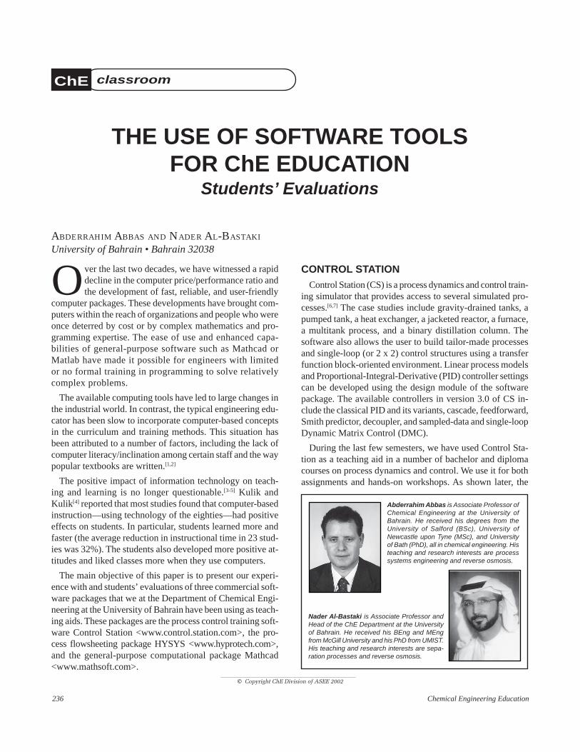
236 Chemical Engineering Education
THE USE OF SOFTWARE TOOLSFOR ChE EDUCATION
Students’ Evaluations
© Copyright ChE Division of ASEE 2002
ChE classroom
ABDERRAHIM ABBAS AND NADER AL-BASTAKI
University of Bahrain • Bahrain 32038
Over the last two decades, we have witnessed a rapiddecline in the computer price/performance ratio andthe development of fast, reliable, and user-friendly
computer packages. These developments have brought com-puters within the reach of organizations and people who wereonce deterred by cost or by complex mathematics and pro-gramming expertise. The ease of use and enhanced capa-bilities of general-purpose software such as Mathcad orMatlab have made it possible for engineers with limitedor no formal training in programming to solve relativelycomplex problems.
The available computing tools have led to large changes inthe industrial world. In contrast, the typical engineering edu-cator has been slow to incorporate computer-based conceptsin the curriculum and training methods. This situation hasbeen attributed to a number of factors, including the lack ofcomputer literacy/inclination among certain staff and the waypopular textbooks are written.[1,2]
The positive impact of information technology on teach-ing and learning is no longer questionable.[3-5] Kulik andKulik[4] reported that most studies found that computer-basedinstruction—using technology of the eighties—had positiveeffects on students. In particular, students learned more andfaster (the average reduction in instructional time in 23 stud-ies was 32%). The students also developed more positive at-titudes and liked classes more when they use computers.
The main objective of this paper is to present our experi-ence with and students’ evaluations of three commercial soft-ware packages that we at the Department of Chemical Engi-neering at the University of Bahrain have been using as teach-ing aids. These packages are the process control training soft-ware Control Station <www.control.station.com>, the pro-cess flowsheeting package HYSYS <www.hyprotech.com>,and the general-purpose computational package Mathcad<www.mathsoft.com>.
CONTROL STATIONControl Station (CS) is a process dynamics and control train-
ing simulator that provides access to several simulated pro-cesses.[6,7] The case studies include gravity-drained tanks, apumped tank, a heat exchanger, a jacketed reactor, a furnace,a multitank process, and a binary distillation column. Thesoftware also allows the user to build tailor-made processesand single-loop (or 2 x 2) control structures using a transferfunction block-oriented environment. Linear process modelsand Proportional-Integral-Derivative (PID) controller settingscan be developed using the design module of the softwarepackage. The available controllers in version 3.0 of CS in-clude the classical PID and its variants, cascade, feedforward,Smith predictor, decoupler, and sampled-data and single-loopDynamic Matrix Control (DMC).
During the last few semesters, we have used Control Sta-tion as a teaching aid in a number of bachelor and diplomacourses on process dynamics and control. We use it for bothassignments and hands-on workshops. As shown later, the
Abderrahim Abbas is Associate Professor ofChemical Engineering at the University ofBahrain. He received his degrees from theUniversity of Salford (BSc), University ofNewcastle upon Tyne (MSc), and Universityof Bath (PhD), all in chemical engineering. Histeaching and research interests are processsystems engineering and reverse osmosis.
Nader Al-Bastaki is Associate Professor andHead of the ChE Department at the Universityof Bahrain. He received his BEng and MEngfrom McGill University and his PhD from UMIST.His teaching and research interests are sepa-ration processes and reverse osmosis.

Summer 2002 237
feedback from the students on the use of the program wasvery positive. The program made it easier for them to under-stand process control material and concepts in a shorter timethan traditional lecture-only classes. It also helped the stu-dents relate theory to practice.
Two workshop examples of how CS can be used to teachcontrol concepts are shown in Figures 1 and 2. Figure 1 il-lustrates why the derivative action should not be employedfor processes having noisy measurements; the addition of thederivative action to a PI controller leads to a deterioration
Figure 2.
Effect of
interaction
on
SISO
loops
(Control
Station).
Figure 1.
Impact
of noise
on
derivative
action
(Control
Station).

238 Chemical Engineering Education
Figure 3. Simulation of an ammonia reactor (HYSYS).
Figure 4. Methanol synthesis loop (HYSYS).
(not an improvement) of the closed-loop response. Also,the derivative term leads to unacceptable fast movementof the control valve.
The use of CS significantly contributes to teaching advancedcontrol strategies such as feedforward, cascade, and
decoupling control to undergraduate students. Figure 2 illus-trates the effect of process interaction on the performance ofconventional controllers in multi-input/multi-output pro-cesses. The distillate composition controller results in goodclosed-loop performance when the bottoms composition con-

Summer 2002 239
TABLE 1Students’ Evaluation Forms
1. Justification for the use of program in the course(1 = unjustified; 5 = absolutely justified)
2. Contribution to study of the subject by program use(1 = irrelevant; 5 = very effective)
3. Ease of achieving the goal (1 = difficult; 5 = easy)
4. Clarity in the means used to convey knowledge(1 = confusing; 5 = absolutely clear)
5. Relationship between the complexity of the concept given andthe resources supplied (1 = inadequate; 5 = absolutely adequate)
6. Number of resources (information) simultaneously presented onscreen (1 = excessive; 5 = balanced)
7. Computer skills required (1 = excessive; 5 = null)
8. General quality of presentation (1 = poor; 5 = excellent)
9. Effectiveness of the resources used: graphics, tables, and texts(1 = ineffective; 5 = very effective)
10. Ease of operation (1 = complex; 5 = very easy)
11. Documentation for user (1 = deficient, 5 = excellent)
12. Clarity of the goal (1 = confusing, 5 = perfectly defined)
13. Correspondence between program and knowledge conveyed inclass (1 = absolute disconnection; 5 = highly related)
14. Amount of specific knowledge required about subject forprogram use (1 = excessive; 5 = reasonable)
15. Degree of interaction between user and program(1 = passive schemes; 5 = very interactive)
16. Time needed for program execution (1 = excessive; 5 = suitable)
Comment on the reasons for which you felt attracted to or boredby the program.
The use of multimedia and softwarepackages enhances teaching and learning.
. . . the students learn more and faster,allowing the teacher to cover
more material . . .
troller is on manual mode. Closing this latter loop leads to adeterioration of the performance of the first loop due to the“fight” or interaction between the two controllers. The stu-dents are usually asked to check the loops’ interaction by cal-culating the relative gain array[8] and to design and test adecoupler for the distillation column.
HYSYSHYSYS is a modular commercial process flowsheeting
program that is widely used by universities and industry (par-ticularly hydrocarbon-related companies). It is capable of do-ing material and energy balances for static and dynamic con-ditions and is a very powerful tool for process simulation. Ithas built-in routines to solve many specialized unit opera-tions. One of the important features of HYSYS is the avail-ability of an “Oil Manager” option dedicated to support re-finery simulations. A comprehensive library of thermody-namic property packages is supplied with HYSYS to enablethe user to design and solve many types of problems. At theChemical Engineering Department of the University ofBahrain, HYSYS is used as an effective teaching tool in anumber of courses including process analysis (material andenergy balances), plant design, and the senior projects.
In the process analysis course, students follow a system-atic approach in which they effectively analyze the systemsand develop comprehensive degree-of-freedom tables to de-termine if a problem is correctly specified and also the orderof solving the various units. The basic concepts used in modu-lar simulation packages are thoroughly discussed. Among theproblems associated with modular solution is the presence ofrecycle streams, which necessitate the iterative tear streamsolution. Determining the number of tear streams, their posi-tions, the convergence techniques, and the order or sequencesof their converging are basic issues that we clarify.
Figures 3 and 4 show flow diagrams of simple HYSYScase studies that the students were requested to develop. InFigure 3, the effect of operating parameters such as tempera-ture, pressure, and composition of inerts on the productionrate are evaluated for an equilibrium-type ammonia reactor(parametric analysis). The variation of ammonia output com-position with the operating pressure is shown in Figure 3.The significance of the recycle loop and the selection of thesuitable convergence acceleration method are emphasized bythe second case study on a methanol synthesis loop (Figure4). Solving this problem also gives students insight into thephilosophy of the modular flowsheeting programs and thenature of the sequential solution strategy.
MATHCADMathcad is one of the four most popular computational
packages used in industry and academia; the other three pro-grams are Matlab, Maple, and Mathematica. Mathcad com-bines some of the best features of spreadsheets (like MS Ex-cel) and symbolic math programs. It provides a good graphi-cal user interface and can be used to efficiently manipulatelarge data arrays, to perform symbolic calculations, and toeasily construct graphs. One of the useful features of Mathcadthat is not found in the aforementioned programs is its abilityto perform calculations with units; this is indeed an impor-tant feature for engineering students. In a recent survey con-ducted by the discussion group on Computer Applications inChemical Engineering <http://www.che-comp.org/>,Mathcad was the preferred computational package for 16.2%of participants. The survey included a large number of knownpackages, and the only two programs preferred by morepeople were MS Excel (35.3%) and Matlab (23.4%).
As a general programming package, Mathcad is being usedin the Chemical Engineering Department in several coursesincluding process analysis, process modeling and simulation,

240 Chemical Engineering Education
TABLE 2Evaluation Results for
Control Station (10 students)
Question Mean Standard Deviation
1 4.10 0.99
2 3.70 0.82
3 3.20 1.03
4 3.30 0.95
5 3.50 0.97
6 3.90 0.88
7 3.40 1.07
8 3.50 0.71
9 3.90 0.74
10 3.40 1.17
11 2.90 1.20
12 3.10 0.88
13 3.90 0.99
14 3.00 0.47
15 3.40 0.84
16 4.10 0.99
Comment on the reasons for which you feltattracted to or bored by the program.
TABLE 3Overall Marks for Control Station
Category Mean Standard Deviation
Content and teaching methodology 3.56 0.97
Program design characteristics 3.62 0.92
Users’ reaction 3.40 0.99
Overall 3.52 0.96
TABLE 4Evaluation Results forHYSYS (21 students)
Question Mean Standard Deviation
1 3.59 1.33
2 4.00 1.07
3 3.50 0.91
4 3.41 1.14
5 3.36 1.05
6 3.59 1.18
7 3.59 1.05
8 3.57 1.16
9 4.27 0.83
10 3.05 1.05
11 2.86 1.08
12 4.18 0.80
13 3.82 1.22
14 3.32 1.09
15 3.32 0.99
16 3.09 1.34
TABLE 5Overall Marks for HYSYS
Category Mean Standard Deviation
Content and teaching methodology 3.57 1.11
Program design characteristics 3.61 1.11
Users’ reaction 3.43 1.17
Overall 3.53 1.12
Figure 5. Overall marks for the three packages. CTM = Con-tent and Teaching Methodology, PCC = Program DesignCharacteristics, and UR = Users’ Reaction.
equipment and plant design and the senior projects.
STUDENTS’ EVALUATIONSTo measure the usefulness and effectiveness of the consid-
ered software packages, students filled out the evaluation formshown in Table 1 at the end of the course for which the soft-ware was used. The sixteen questions were selected from thelist of 24 questions proposed by Iglesias, et al.[9] Eight ques-tions were dropped based on the recommendations of theauthors and the inability of students to clearly understandsome of them. Iglesias and co-workers classified the ques-tions in three categories: teaching content and methodology(questions 1-5), software and design features (questions 6-10), and user reaction (questions 11-16).
The first class attempts to test the usefulness of the educa-tional software in terms of subject content and design fea-tures, as well as the teaching methodology used in the course.The second category evaluates mainly the user interface (num-ber of resources presented, quality and effectiveness of graph-ics, tables, animation, etc.) andease of use of the package. Thethird class tests the user’s reac-tion to the program by consider-ing aspects such as documenta-tion for user, degree of interac-tion between user and program,and time needed for program ex-ecution. Note that the three cat-egories are not totally indepen-dent and distinct. The question-naire ends by asking students tocomment on the reasons theyfelt attracted to or bored by theprogram.
The students’ evaluations forthe three considered packages areshown in Tables 2 to 7. The over-all results are presented in Figure5. Control Station and Mathcadwere, respectively, evaluated bythe process control and processanalysis undergraduate classes.HYSYS was evaluated by stu-

Summer 2002 241
TABLE 6Evaluation Results forMathcad (6 students)
Question Mean Standard Deviation
1 3.50 1.52
2 3.33 1.51
3 3.33 1.03
4 3.67 1.21
5 3.33 0.82
6 4.50 0.55
7 3.67 0.52
8 4.00 1.10
9 4.00 0.63
10 4.00 1.10
11 3.17 1.17
12 3.50 1.05
13 4.17 1.60
14 4.50 0.84
15 3.67 1.37
16 3.50 1.05
TABLE 7Overall Marks for Mathcad
Category Mean Standard Deviation
Content and teaching methodology 3.43 1.17
Program design characteristics 4.03 0.81
Users’ reaction 3.75 1.20
Overall 3.74 1.10
dents from process systems engineering courses. As the tablesand Figure 5 show, the students’ evaluations of all three soft-ware packages were highly favorable; the overall marks var-ied within a relatively narrow range (3.52 to 3.74).
For the case of control station, questions 1 and 13 receivedhigh marks, indicating a strong correlation between the soft-ware and the knowledge conveyed in the class, and also thatthe use of computer workshops in the course is highly justi-fied. Question 14 received the second lowest mark (3.0). Thiswas expected since chemical engineering students do gener-ally feel that their first process control course includes morematerial than an average course and that it is rather difficult.This is due to the well-known fact that process control is muchdifferent from traditional chemical engineering courses andthat it includes a significant number of new theories and terms.
For HYSYS, questions 2, 9, and 12 received the highestmarks, indicating that the students found the software re-sources to be very effective and that the program has signifi-cantly contributed to their study of the courses considered.Note that prior to the availability of process flowsheetingpackages, the students had to manually carry out lengthy de-
sign calculations. The students gave their lower ratings toquestions 10 (3.05) and 16 (3.09), i.e., they felt that the pro-gram was not very easy to operate and that the time for simu-lating case studies was too long. The speed of execution is,of course, dependent on the size of the problem at hand. WithHYSYS being a commercial flowsheeting package, evensimple problems include a significant number of details.
High marks were given to questions related to Mathcaddesign characteristics; the overall mark is 4.03 (see Table 7).This is not surprising since the package is truly user-friendlyand the fact that prior to using Mathcad, the students wereprogramming in FORTRAN. For all three programs, the stu-dents evaluated the programs’ documentation as above aver-age (see question 11). Although we feel that the materialhanded out to the students was very good, this issue is cur-rently being addressed by conducting more tutorials on theuse of the packages, supplying the students with more copiesof shorter versions of the users’ guides, and preparing sim-pler getting-started handouts.
CONCLUDING REMARKS
The computer has become an integral part of engineeringeducation. As the power of both hardware and software con-tinues to rapidly increase, we expect the use of informationtechnology in the classroom/laboratory to grow at a muchfaster rate in the near future.
The use of multimedia and software packages enhancesteaching and learning. In particular, the students learn moreand faster, allowing the teacher to cover more material in thetime allocated for the course. Of course, the information tech-nology tools have a large number of benefits that are not withinthe scope of this paper. For example, they are invaluable toolsfor web-based education and distance learning and training.
REFERENCES1. Kantor, J.C., T.F. Edgar, “Computing Skills in the Chemical Engineer-
ing Curriculum,” in B. Carnahan (Ed.), Computers in Chemical Engi-neering Education, CACHE Corporation, p. 9, (1996)
2. Benyahia, F., “Process Simulation Packages in Undergraduate Chemi-cal Engineering Courses,” The 1998 IchemE Research Event, CD-ROM(ISBN 0 85295 400 X)
3. Edgar, T.F., “Information Technology and ChE Education: Evolutionor Revolution?” Chem. Eng. Ed., 34(4), p. 290, (2000)
4. Kulik, J.A. and C.C. Kulik, Contemporary Education Psychology, 12,p. 222, (1987)
5. Montgomery, S., H.S. Fogler, “Interactive Computer-Aided Instruc-tion,” In B. Carnahan (Ed.), Computers in Chemical Engineering Edu-cation, CACHE Coproration, p. 57, (1996)
6. Cooper D., D. Dougherty, “Enhancing Process Control Education withControl Station Training Simulator,” Compt Appl Eng Edu, 7, p. 203,(1999)
7. Cooper, D.J., N. Sinha, “Picles + Digest = Control StationTM for Win-dows,” CACHE News, 44, p. 14, (1997)
8. Bristol, E.H., “On a New Measure of Interactions for MultivariableProcess Control,” IEEE Trans Auto Control AC-11, 133, p. 133, (1966)
9. Iglesias, O.A., C.N. Paniagua, R.A. Pessacq, “Evaluation of Univer-sity Educational Software,” Compt Appl Eng Edu, 5, p. 181, (1997) ❐
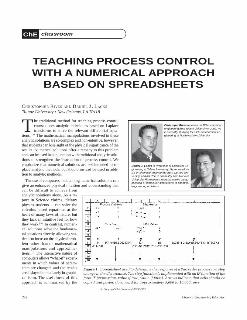
242 Chemical Engineering Education
TEACHING PROCESS CONTROLWITH A NUMERICAL APPROACH
BASED ON SPREADSHEETS
CHRISTOPHER RIVES AND DANIEL J. LACKS
Tulane University • New Orleans, LA 70118
The traditional method for teaching process controlcourses uses analytic techniques based on Laplacetransforms to solve the relevant differential equa-
tions.[1-9] The mathematical manipulations involved in theseanalytic solutions are so complex and non-intuitive, however,that students can lose sight of the physical significance of theresults. Numerical solutions offer a remedy to this problemand can be used in conjunction with traditional analytic solu-tions to strengthen the instruction of process control. Weemphasize that numerical solutions are not intended to re-place analytic methods, but should instead be used in addi-tion to analytic methods.
The use of computers in obtaining numerical solutions cangive an enhanced physical intuition and understanding thatcan be difficult to achieve fromanalytic solutions alone. As a re-port in Science claims, “Manyphysics students ... can solve thecalculus-based equations at theheart of many laws of nature, butthey lack an intuitive feel for howthey work.[10] In contrast, numeri-cal solutions solve the fundamen-tal equations directly, allowing stu-dents to focus on the physical prob-lem rather than on mathematicalmanipulations and approxima-tions.[11] The interactive nature ofcomputers allows “what-if” experi-ments in which values of param-eters are changed, and the resultsare dislayed immediately in graphi-cal form. The usefulness of thisapproach is summarized by the
© Copyright ChE Division of ASEE 2002
Figure 1. Spreadsheet used to determine the response of a 2nd order process to a stepchange in the disturbance. The step function is implemented with an IF function of theform IF (expression, value if true, value if false). Arrows indicate that cells should becopied and pasted downward for approximately 5,000 to 10,000 rows.
ChE classroom
Christoper Rives received his BS in chemicalengineering from Tulane University in 2002. Heis currently studying for a PhD in chemical en-gineering at Northwestern University.
Daniel J. Lacks is Professor of Chemical En-gineering at Tulane University. He received hisBS in chemical engineering from Cornell Uni-versity, and his PhD in chemistry from HarvardUniversity. His research interests involve the ap-plication of molecular simulations to chemicalengineering problems.
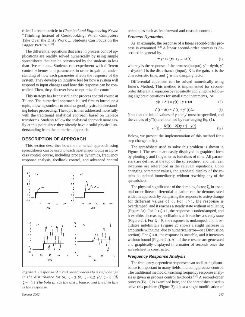
Summer 2002 243
title of a recent article in Chemical and Engineering News:“Thinking Instead of Cookbooking: When ComputersTake Over the Dirty Work ... Students Can Focus on theBigger Picture.”[12]
The differential equations that arise in process control ap-plications are readily solved numerically by using simplespreadsheets that can be constructed by the students in lessthan five minutes. Students can experiment with differentcontrol schemes and parameters in order to gain an under-standing of how each parameter affects the response of thesystem. They develop an intuitive feel for how a system willrespond to input changes and how this response can be con-trolled. Then, they discover how to optimize the control.
This strategy has been used in the process control course atTulane. The numerical approach is used first to introduce atopic, allowing students to obtain a good physical understand-ing before proceeding. The topic is then addressed more fullywith the traditional analytical approach based on Laplacetransforms. Students follow the analytical approach more eas-ily at this point since they already have a solid physical un-derstanding from the numerical approach.
DESCRIPTION OF APPROACHThis section describes how the numerical approach using
spreadsheets can be used to teach most major topics in a pro-cess control course, including process dynamics, frequencyresponse analysis, feedback control, and advanced control
techniques such as feedforward and cascade control.
Process Dynamics
As an example, the response of a linear second-order pro-cess is examined.[1-9] A linear second-order process is de-scribed in general by
τ ζτ2 2 1y y y Kf t" '+ + = ( ) ( )where y is the response of the process (output), y' = dy/dt, y"= d2y/dt2, f is the disturbance (input), K is the gain, τ is thecharacteristic time, and ζ is the damping factor.
Differential equations can be solved numerically usingEuler's Method. This method is implemented for second-order differential equation by repeatedly applying the follow-ing algebraic equations for small time increments, Δt :
y t t y t y t t+( ) = ( ) + ( ) ( )Δ Δ' 2
y t t y t y t t' ' "+( ) = ( ) + ( ) ( )Δ Δ 3
Note that the initial values of y and y' must be specified, andthe values of y"(t) are obtained by rearranging Eq. (1).
y tKf t y t y t
a"'( ) = ( ) − ( ) − ( ) ( )2
12ζττ
Below, we present the implementation of this method for astep change in f(t).
The spreadsheet used to solve this problem is shown inFigure 1. The results are easily displayed in graphical formby plotting y and f together as functions of time. All param-eters are defined at the top of the spreadsheet, and their celllocations are referenced in the relevant equations. Uponchanging parameter values, the graphical display of the re-sults is updated immediately, without rewriting any of thespreadsheet.
The physical significance of the damping factor, ζ , in a sec-ond-order linear differential equation can be demonstratedwith this approach by comparing the response to a step changefor different values of ζ . For ζ > 1, the response isoverdamped, and it reaches a steady state without oscillating(Figure 2a). For 0 1< <ζ , the response is underdamped, andit exhibits decreasing oscillations as it reaches a steady state(Figure 2b). For ζ = 0 , the response is undamped, and it os-cillates indefinitely (Figure 2c shows a slight increase inamplitude with time, due to numerical error—see Discussionsection). For ζ < 0 , the response is unstable, and it increaseswithout bound (Figure 2d). All of these results are generatedand graphically displayed in a matter of seconds once thespreadsheet is constructed.
Frequency Response Analysis
The frequency-dependent response to an oscillating distur-bance is important in many fields, including process control.The traditional method of teaching frequency response analy-sis is given in process control textbooks.[1-9] A second-orderprocess (Eq. 1) is examined here, and the spreadsheet used tosolve this problem (Figure 3) is just a slight modification of
Figure 2. Response of a 2nd order process to a step changein the disturbance for (a) ζ = 3 (b) ζ = 0 2. (c) ζ = 0 (d)
ζ = −0 1. The bold line is the disturbance, and the thin lineis the response.

244 Chemical Engineering Education
Figure 3. Spreadsheet used to determine the response of a 2nd order process to anoscillating disturbance. Arrows indicate that cells should be copied and pasted down-ward for approximately 5,000 to 10,000 rows.
Figure 4. Response of a 2nd order process to an oscillatingdisturbance for (a) ζ = 1 5. , ω = 0 1. ; (b) ζ = 1 5. , ω = 0 3. ; (c)ζ = 1 5. , ω = 2 ; (d) ζ = 0 5. , ω = 0 2. . The bold line is thedisturbance, and the thin line is the response.
the spreadsheet used for the stepfunction input (only the disturbanceis different).
The frequency response of the sys-tem can be addressed by comparingthe response obtained with differentvalues of the angular frequency, ω .When the frequency is small, the sys-tem has sufficient time to react to thechanging disturbance, and the re-sponse is nearly in phase with thedisturbance (Figure 4a). When thefrequency is increased, however, thesystem does not have sufficient timeto react, and the response increas-ingly lags behind the disturbance(Figures 4b and 4c). Additionally,the amplitude of the response usu-ally decreases with increasing frequency (Figures 4a, 4b, and4c). For ζ < 1 and small frequencies, however, the behaviorof a linear second-order system is unusual in that the ampli-tude increases with increasing frequency (Figure 4d). Notethat the immediate graphical results allow students to quicklyand easily experiment with different values of ω and ζ .
Feedback Control
A feedback control mechanism measures the output of theprocess, compares it to the desired value (the set point), andthen alters an input to the process in order to bring the outputcloser to the desired value.[1-9]
The output of a proportional-integral-derivative (PID) con-troller is given by
y KK
dt Kd
dtc cc
l
t
c D= + + ( )∫ετ
ε τ ε
0
4
where ε = −y ysp , ysp is the set point, and y is the output ofthe process. When the system is not under any control, thevalues of Kc and τD are set equal to zero, while τ l is setequal to infinity. The integral term can be calculated numeri-cally as
ε ε0
5t
iidt t t∫ ∑= ( ) ( )Δ
and the derivative term can be calculated numerically as
d t
dt
t t t
t
ε ε ε( ) = ( ) − −( ) ( )ΔΔ
6
The numerical approach is applied here to the feedback con-trol of a process consisting of three first-order systems in se-ries. The dynamics of the other parts of the control loop (e.g.,measuring device) are not included for simplicity, but caneasily be included if desired (as pointed out in the Discussionsection). A process consisting of three first-order systems in
series is described by three coupled first-order differentialequations,
τ
τ
i i i i p c
i i i i i l
y y K f K y i
y y K y i
'
' ,
+ = + = ( )
+ = = ( )−
1 7
2 3 8
where i is the system number. These coupled differential equa-tions are numerically integrated using Euler's method by re-peatedly applying the algebraic equations
y t t y t y t t ii i i+( ) = ( ) + ( ) = ( )Δ Δ' , ,1 2 3 9

Summer 2002 245
Fig
ure
5. S
pre
adsh
eet
use
d t
o d
eter
min
e th
e re
spon
se o
f a
pro
cess
con
sist
ing
of t
hre
e1s
t or
der
sys
tem
s in
ser
ies
wit
h f
eed
back
con
trol
(P
ID c
ontr
olle
r).
Arr
ows
show
th
atce
lls
shou
ld b
e co
pie
d a
nd
pas
ted
dow
nw
ard
for
5,0
00-1
0,00
0 ro
ws.
Figure 6. Response of a process consisting of three first-order systems inseries with feedback control to a step change in the disturbance. (a) P-only, Kc = 1 ; (b) P-only, Kc = 4 ; (c) P-only, Kc = 15 ; (d) PI: Kc = 1 , τ l = 5; (e)PI: Kc = 1 , τ l = 1 3. , (f) PID: Kc =1, τ l = 1 3. , τD = 15 . The bold line is the dis-turbance, and the thin line is the response.
where the y ti' ( ) are obtained from Equations 7 and 8. The spreadsheet
used to solve this problem is shown in Figure 5.
By experimenting with different values of the control parameters( Kc, τ l and τD ), the relationship between each control parameterand the response can be determined. If proportional-only control isused (i.e., τD = 0 and τ l = a large number that approximates ∞), theresponse is offset from the set point (Figure 6a). Increasing the valueof Kc will minimize this offset (Figure 6b), but the system can be-come unstable if Kc is too large (Figure 6c). Adding integral control(i.e., decreasing τ l from ∞ ) will eliminate this offset (Figure 6d).But if the value of τ l is too small, the system becomes unstable (Fig-ure 6e). Adding derivative control (i.e., increasing τD from 0) stabi-lizes the system (Figure 6f). This stabilization allows a larger Kc anda smaller τ l to be used, but a large τD value also slows the response.
The values of the control parameters should be chosen such that aquick response with small oscillations and no offset is achieved. TheZeigler-Nichols tuning method is one way to obtain advantageousvalues for the three control parameters, in which
KK
a
Pb
Pc
cc
lu
Du
= ( )
= ( )
= ( )
max
.1 710
210
810
τ
τ
where Kcmax is the maximum value of Kc for which the response is
stable with a proportional-only controller, and Pu is the period of os-cillation of the response at Kc
max . The value of Kcmax is found by trial

246 Chemical Engineering Education
Fig
ure
8.
Sp
read
shee
t u
sed
to
det
erm
ine
the
resp
onse
of
a p
roce
ss c
onsi
stin
g of
th
ree
firs
t-or
der
sys
tem
s in
ser
ies
wit
h f
eed
forw
ard
con
trol
. Arr
ows
ind
icat
e th
at c
ells
sh
ould
be
cop
ied
an
d p
aste
d d
own
war
d f
or a
pp
roxi
mat
ely
5,00
0 to
10,
000
row
s.
Figure 9. Response of a process consisting of three first-or-der systems in series with feedforward control to a step changein the disturbance. (a) A K K Kp= =1 0 8422 3/ ( ) . andB K Kl p= =/ .0 625 ; (b) A = 0.842 and B = 0 5. . The bold lineis the disturbance; the thin line is the response.
Figure 7. Tuning of PID parameters with Ziegler-Nicholsmethod, for a process consisting of three first-order systems inseries with feedback control. (a) Determination of Kc
max andPu ; (b) PID with Ziegler-Nichols parameters: Kc = 3 7. , τ l = 5 4. ,τD = 1 4. . The bold line is the disturbance, and the thin line isthe response.
and error to be 6.3 (Figure 7a), and the value of Pu is observedto be 10.8. The response using the Ziegler-Nichols parametersis shown in Figure 7b.
Feedforward Control
A feedforward control mechanism measures the disturbanceand uses this measured value to adjust an input variable withthe goal of keeping the process output at the desired value.[1]
The output of a simple feedforward controller is given by
y Ay Bfc sp= − ( )11
where A and B are controller parameters that will depend on theparticular process to be controlled.
The numerical approach is applied here to the feedforwardcontrol of a process consisting of three first-order systems inseries (Eq. 7 and 8). The spreadsheet for this problem is shownin Figure 8. Perfect control can be obtained by choosing theparameters such that the system is at steady state with the pro-cess output at the set point (i.e., y y y1 2 3 0' ' '= = = and y ysp3 = ).From equations 7 and 8, it is easily found that the parametervalues that yield perfect control are A K K Kp= 1 2 3/ ( ) and

Summer 2002 247
Fig
ure
10.
Sp
read
shee
t u
sed
to
det
erm
ine
the
resp
onse
of
a p
roce
ss c
onsi
stin
g of
th
ree
firs
t-or
der
sys
tem
s in
ser
ies
wit
hca
scad
e co
ntr
ol. A
rrow
s in
dic
ate
that
cel
ls s
hou
ld b
e co
pie
d a
nd
pas
ted
dow
nw
ard
for
5,0
00 t
o 10
,000
row
s.
Figure 11. Response of a process consist-ing of three first-order systems in serieswith cascade control to a step change inthe disturbance (primary controller: Kc=2and τ l =5, secondary controller: Kc=10).The bold line is the disturbance, and thethin line is the response.
B K Kl p= / . As shown in Figure 9a, perfect control is indeed achievedwith these parameters. Perfect control is no longer achieved whenA K K Kp≠ 1 2 3/ ( ) or B K Kl p≠ / (as shown in Figure 9b). Since realprocesses are generally not simple with accurately known parameters,perfect control is only idealistic, not practical.
Cascade Control
Cascade control uses two control loops (primary and secondary).[1] Theprimary control compares the process output to the desired value (setpoint), yielding a second set point to be used for a secondary control.The secondary control compares an intermediate quantity to this secondset point to determine how to alter an input variable.
The example of a process consisting of three first-order systems inseries (Eq. 7 and 8) is used to examine cascade control. The intermediatequantity used in the secondary control loop is the output of the first-order process ( yl ). A proportional-integral controller is used for theprimary controller, and a proportional-only controller is used for thesecondary controller. The spreadsheet used to solve this problem isshown in Figure 10.
The response of the system with cascade control is shown in Figure 11- this response is superior to the response with feedback control (Figure7b). (Note that this example is somewhat artificial in that the secondarycontrol loop consists of only a first-order process and will be stable forany value of the secondary controller gain. Therefore, an arbitrarily largevalue of the secondary controller gain can be used to make the responsearbitrarily fast. This arbitrarily fast response is not possible in gen-eral, e.g., if the secondary loop includes dead time or a process higherthan second-order).
DISCUSSIONImplementation of Approach
This numerical approach using spreadsheets was implemented in theprocess control course at Tulane as follows: first, a topic is introduced ina lecture, and the governing equations are derived; next, the class moveson to our computer lab, where students solve the governing equationsnumerically (all students do this individually on separate comput-ers), and the physical significance of the results is discussed; finally,the traditional analytic solutions based on Laplace transforms aretaught, in lecture format.
Homework assignments include problems requiring numerical solu-tions using spreadsheets, problems requiring analytical solutions, andproblems that use the Control Station software package.[13] Some prob-
lems require that students compare resultsfrom numerical solutions to results fromanalytical solutions. For example, one

248 Chemical Engineering Education
homework problem requires that students find the maximumvalue of a controller gain for a proportional-only controllerin a certain process by three methods: by trial and error withnumerical solutions, by deriving the transfer function and find-ing the gain that leads to positive real parts of its poles, andby the Bode stability criterion using analytical expressionsfor phase lags and amplitude ratios. The students comparethe results for the maximum controller gain from thesedifferent methods and find them to be the same (withinnumerical error).
The exams test the students' knowledge of applying nu-merical methods to process control problems, in addition tothe traditional process control material. One of the examsincludes a computer part (given in class in our computer com-puter lab), where students solve a problem numerically witha spreadsheet and turn in the printed result. The other examshave problems in which students must show how to set up aspreadsheet to numerically solve a given problem, providingall of the relevant equations.
Students found the numerical approach using spreadsheetsto be extremely useful in understanding the concepts under-lying process control. In unsolicited comments on the courseevaluations, two-thirds of the students remarked that the nu-merical approach was the most valuable aspect of the course.
The students also seemed to genuinely enjoy this approach.When problems were solved with this method in the com-puter lab, students were often so eager to discover the ef-fects of changing some parameters that they would proceedahead of the discussion. They would also occasionally con-tinue experimenting with the effects of different parametersafter the class had ended.
Other Issues
The numerical approach is more general than the analyticapproach, in that it can also be applied to nonlinear differen-tial equations, i.e., a linearization approximation is not nec-essary as it is for the analytic approach based on Laplacetransforms. To emphasize this point, a homework problemwas given in which students investigate the frequency re-sponse for a process described by the nonlinear differentialequation y y fa' + = (where a is the number of letters in theirlast name divided by five), and then use the results to con-struct Bode and Nyquist diagrams.
A concern with the numerical approach, of course, is thatthere is numerical error in the results. Students should beaware of the numerical error and that the error can be re-duced by decreasing the time step Δt or by using a moresophisticated integration method (e.g., Runge-Kutta or a pre-dictor-corrector method). A reasonable time step for theseproblems is Δt = τ / 100 , where τ is the smallest characteris-tic time for the system.
Although excluded here for simplicity, it is straightforwardto include in this approach the dynamics of other elements of
the control loop, such as actuators (e.g., valves) and measur-ing devices. Including the dynamics of these elements wouldamount to including a few more coupled differential equations, whichtranslates to a few more columns on the spreadsheet.
Dead time is also straightforward to include in this approach.To introduce dead time to a variable y, a new variable, y dead+ ,is defined such that y t y t tdead dead+ ( ) = −( ) . The values fory dead+ are obtained in the spreadsheet from the values of y,by setting the cell for y dead+ at the time, t, equal to the valueof the cell for y at the time t tdead− (i.e., t tdead / Δ rows abovein the spreadsheet).
The present approach is different than, but complementaryto, an approach that uses packaged software (such as ControlStation[13]) for teaching process control. In the present ap-proach, students are in fact solving the governing equationsthemselves, with a numerical method rather than an analyticalmethod. In contrast, the Control Station software[13] presentsresults without requiring that students solve the equations.
CONCLUSIONIn the usual method for teaching process control, students
are taught to solve the relevant differential equations analyti-cally by using Laplace transforms. This method involves com-plex mathematical manipulations, which can cause studentsto lose sight of the physical significance of the problem. Themain goal of a process control course should be to provide ageneral understanding and intuitive feel for how physical pro-cesses behave and how they can be controlled. Numericalsolutions for process control problems are extremely easy toobtain using spreadsheets created by students themselves. Thisapproach allows students to concentrate on what is physi-cally happening as opposed to the complex mathematics, yetthe students solve the problems themselves (i.e., the solu-tion is not given to them by packaged software). This ap-proach has been used in the Process Control course at Tulane,and student feedback has been extremely positive.
REFERENCES1. Stephanopolous, G., Chemical Process Control, Prentice Hall, Englewood Cliffs,
NJ (1984).2. Riggs, J.B., Chemical Process Control, Ferret, Lubbock, TX (1999).3. Marlin, T.E., Process Control, McGraw-Hill, New York, NY (1995).4. Marlin, T.E., Process Control, 2nd ed., McGraw-Hill, New York, NY (2000).5. Smith, C.A., and A.B. Corripio, Principles and Practice of Automatic Process
Control, John Wiley & Sons, New York, NY (1985).6. Seborg, D.E., T.F. Edgar, and D.A. Mellichamp, Process Dynamics and Con-
trol, John Wiley & Sons, New York, NY (1989).7. Shinskey, F.G., Process Control Systems, 4th ed., McGraw-Hill, New York, NY
(1996).8. Luyben, W.L., Essentials of Process Control, McGraw-Hill, New York, NY
(1997).9. Coughanowr, D.R., Process Systems Analysis and Control, 2nd ed., Mc-Graw-
Hill, New York, NY (1991).10. Gibbons, W., Science, 266, 893 (1994).11. De Vries, P.L., American Journal of Physics, 64, 364 (1996).12. Wilson, E.K., Chemical and Engineering News, May 26, p. 33 (1997).13. Cooper, D.J., Control Station for Windows, Version 2.5 (2000) ❐