editorial - the comprehensive r archive network

NewsThe Newsletter of the R Project Volume 3/3, December 2003

Editorialby Friedrich Leisch

Another year is over and it is time for change in theeditorial board of R News. Thomas Lumley will takeover as Editor-in-Chief for 2004, and Paul Murrellwill join him and Doug Bates as board members.

Three years ago, in the editorial of issue 1/1, KurtHornik and I outlined possible topics for articles inthe newsletter; I am pleased to say that issue 3/3 cov-ers all of these types of topics and much more.

This issue starts with an introductory guide ondimension reduction for data mapping, followed bytwo articles on applications that describe how R canbe used as a simulation tool in empirical ecology andfor the analysis of student achievements over time.Of interest to many users is creation of web pagesfrom within R, the topic of the R2HTML package arti-cle. For programmers and those interested in gettinga little bit more out of R we have a Programmer’sNiche column on regular expressions, an introduc-tion to a new debugging facility, and an introductionto the lmeSplines package.

Certainly one of the key strengths of R is the pack-aging system. We now have about 300 packages onCRAN and another 50 in the Bioconductor reposi-tory, and the lists keep growing faster and faster. Thiswealth of packages can have a down side. In my ex-

perience the distinction between a “package” and a“library” or why it is hard to install a “source” pack-age on Windows are confusing issues, especially forbeginners. This issue’s Help Desk column clarifiesthis vocabulary and has many upseful tips on howto make your R installation easier to maintain.

At the Technische Universität Wien we areeagerly anticipating the first R users conference,useR! 2004, which will be held here in May. Overthe last few years we had several developer confer-ences but this will be the first meeting primarily forthose interested in using R for data analysis withoutnecessarily writing software (although, in S, a soft-ware user often quickly becomes a developer). Sev-eral R core members will give keynote lectures on im-portant features of R; in addition we hope to attracta large number of contributions from which we cancompile an attractive program. In some sense thiswill be a conference version of R News, with bits andpieces for all R users from novices to seasoned pro-grammers.

Looks like 2004 will be another good year for theR project. Best wishes to everyone!

Friedrich LeischTechnische Universität Wien, [email protected]

Contents of this issue:

Editorial . . . . . . . . . . . . . . . . . . . . . . 1Dimensional Reduction for Data Mapping . . . 2R as a Simulation Platform in Ecological Mod-

elling . . . . . . . . . . . . . . . . . . . . . . . 8Using R for Estimating Longitudinal Student

Achievement Models . . . . . . . . . . . . . . 17lmeSplines . . . . . . . . . . . . . . . . . . . . . 24

Debugging Without (Too Many) Tears . . . . . 29The R2HTML Package . . . . . . . . . . . . . . 33R Help Desk . . . . . . . . . . . . . . . . . . . . 37Programmer’s Niche . . . . . . . . . . . . . . . 40Recent Events . . . . . . . . . . . . . . . . . . . 41Upcoming Events . . . . . . . . . . . . . . . . . 42Changes in R 1.8.1 . . . . . . . . . . . . . . . . . 43Changes on CRAN . . . . . . . . . . . . . . . . 43R Foundation News . . . . . . . . . . . . . . . . 45

mailto:[email protected]

Vol. 3/3, December 2003 2

Dimensional Reduction for Data MappingA practical guide using R

by Jonathan Edwards and Paul Oman

Introduction

Techniques that produce two dimensional mapsof multi-variate data are of increasing importance,given the recent advances in processing capability,data collection and storage capacity. These tech-niques are mostly used in an exploratory capacity, tohighlight relationships within the data-set, often as aprecursor to further analysis. An example usage ona data-set of shape descriptors is given in Edwardset al. (2003). There are many statistical approachesto this problem, and this article serves as an initialoverview and practical guide to their application inR. A small comparative study is also presented, tohighlight the ease with which the analysis can be per-formed, and to demonstrate the capabilities of sev-eral of the more established techniques. The inter-ested reader is directed to Ripley (1996) for thoroughtreatments and derivations.

Principal component analysis

Principal Component Analysis (PCS, Pearson, 1901)is the most widely used general dimension reduc-tion technique, and can easily be applied to mappingmulti-variate data. PCA is a centring (to mean), scal-ing (to variance) and rotation (to principal axes) pro-duced by an orthogonal linear transform (equation 1)of the data ({x}n

i=1 ∈ RD), with the aim of generatinga series of uncorrelated variables (y).

y = UT(x− x) (1)

A standard solution to finding UT, and hence y,is the spectral decomposition (Σ = UΛUT) of the co-variance matrix 1 (Σ = IE((x− x)(x− x)T)), whereΛ

is the diagonal eigenvalue matrix, with eigenvaluesordered λ1 ≥ λ2 ≥ . . . ≥ λp. For dimension re-duction to dimension L (for mapping, normally 2),PCA has the desirable property that in a linear sense,the largest variance is explained by the first L com-ponents. Due to its ubiquity and also because itforms a basis for other approaches, many packagesimplement PCA. In practice they mainly rely on thebase routines of svd and eigen to perform eigen-decomposition 2. The author’s preferred implemen-tations are the prcomp and princomp (with formulainterface) functions supplied by the mva package

(The interested reader should also examine the ade4package). These functions make the application ofPCA to dataframes a trivial task. The following linesof R code perform PCA on the data-set g54 (whichis used as data in all the proceeding examples, seesection “data generation” at the end of this article fordetails):

> out.pca <- prcomp(g54[,1:4])

If we want to use correlations instead of covari-ances, scaling is required, so the function call be-comes prcomp(g54[,1:4], scale=TRUE).

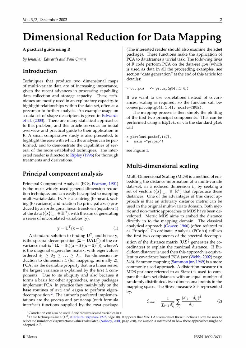
The mapping process is then simply the plottingof the first two principal components. This can beperformed using a biplot, or via the standard plotcall

> plot(out.pca$x[,1:2],

+ main ="prcomp")

see Figure 1.

Multi-dimensional scaling

Multi-Dimensional Scaling (MDS) is a method of em-bedding the distance information of a multi-variatedata-set, in a reduced dimension L, by seeking aset of vectors ({x}n

i=1 ∈ RL) that reproduce thesedistances. One of the advantages of this direct ap-proach is that an arbitrary distance metric can beused in the original multi-variate domain. Both met-ric and non-metric approaches to MDS have been de-veloped. Metric MDS aims to embed the distancedirectly in to the mapping domain. The classicalanalytical approach (Gower, 1966) (often referred toas Principal Co-ordinate Analysis (PCoA)) utilisesthe first two components of the spectral decompo-sition of the distance matrix (UΣ

12 generates the co-

ordinates) to explain the maximal distance. If Eu-clidean distance is used then this approach is equiva-lent to covariance based PCA (see (Webb, 2002) page346). Sammon mapping (Sammon jnr, 1969) is a morecommonly used approach. A distortion measure (inMDS parlance referred to as Stress) is used to com-pare the data-set distances with an equal number ofrandomly distributed, two-dimensional points in themapping space. The Stress measure S is representedby,

Ssam =1

∑i< j d2i j

∑i< j

(di j − di j)2

di j(2)

1Correlation can also be used if one requires scaled variables in x2These techniques are O(D3) (Carreira-Perpinan, 1997, page 10). It appears that MATLAB versions of these functions allow the user to

select the number of eigenvectors/values calculated (Nabney, 2001, page 230), the author is interested in how these approaches might beadopted in R.

R News ISSN 1609-3631


−2 −1 0 1

−2−1

01

2

prcomp

−0.5 0.0 0.5

−0.5

0.0

0.5

cmdscale

−1.0 −0.5 0.0 0.5 1.0

−0.5

0.0

0.5

1.0

sammon s= 0.0644

−5 0 5

−50

5

isoMDS, s= 23.6937

−2 −1 0 1 2

−2−1

01

2

fastICA

Figure 1: Maps of the Gaussian5 data-set (5 multivariate Gaussian clusters in 4-dimensional space)

di j is the distance vectors i and j,d is the estimateddistance in dimension L. Ssam is minimised usingan appropriate iterative error minimisation scheme,Sammon proposed a pseudo-Newtonian methodwith a step size, α normally set to 0.3. Ripley ((Rip-ley, 1996) page 309) discusses a crude but extremelyeffective line search for step size, which appears tosignificantly enhance the optimisation process.

Non-Metric MDS produces a map that main-tains the rank of distances within the original data-set. The most widely known approach is due toKruskal (Kruskal, 1964) which uses a similar iterativeStress function minimisation to the Sammon map,the stress function

Skruskal =

√√√√∑i< j(di j − di j)2

∑i< j d2i j

(3)

which is again minimised, using a suitable gradientdescent technique.

All the MDS techniques discussed above (includ-ing Ripley’s adaptive step-size optimisation scheme)are supported in R as a part of the mva and MASSpackages (classical MDS (cmdscale), Sammon map-ping (sammon) and non metric MDS (isoMDS)). Ad-ditionally, a further implementation of the Sammonmap is available in the multiv package, however, thisappears to be less numerically stable. All the MDSfunctions utilise a distance matrix (normally gener-ated using the function dist) rather than a matrix ordata.frame, hence there is considerable flexibility to

employ arbitrary distance measures. Although thefunction’s defaults are often adequate as a first pass,the two iterative techniques tend to require a moreforceful optimisation regime, with a lower “desired”stress, and more iterations, from a random initialconfiguration, to achieve the best mapping. The Rcode below performs all three mapping techniques,using the more rigorous optimisation strategy

> dist.data <- dist(g54[,1:4])

> out.pcoa <- cmdscale(dist.data)

> randstart <- matrix(runif(nrow(g54[,1:4])*2),

+ nrow(g54[,1:4]),2)

> out.sam <- sammon(dist.data,y=randstart,

+ tol=1e-6,niter=500)

> out.iso <- isoMDS(dist.data,y=randstart,

+ tol=1e-6,maxit=500)

Again, plotting can be done with the standard R plot-ting commands.

> plot(out.pcoa, main="cmdscale")

> plot(out.sam$points), ,ylab="",xlab="",

+ main=paste("sammon s=",as.character(

+ round(out.sam$stress,4))))

> plot(out.iso$points,xlab="",ylab="",

+ main=paste("IsoMDS, s=",

+ as.character(round(out.iso$stress,4))))

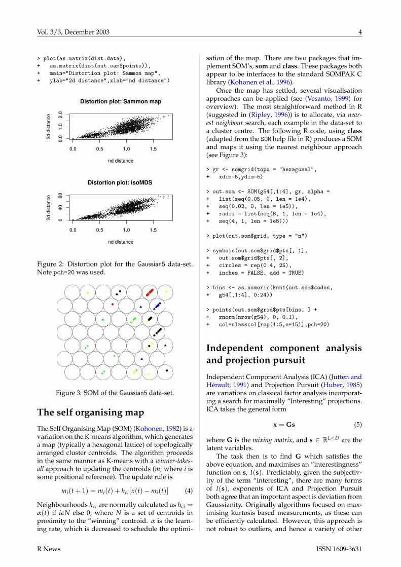
It is also worthwhile to produce a distortion plot(see Figure 2), this plots the original distances againstthe mapped distances, and can be used to assess theaccuracy of distance reproduction in L.



> plot(as.matrix(dist.data),

+ as.matrix(dist(out.sam$points)),

+ main="Distortion plot: Sammon map",

+ ylab="2d distance",xlab="nd distance")

0.0 0.5 1.0 1.5

0.0

1.0

2.0

Distortion plot: Sammon map

nd distance

2d d

ista

nce

0.0 0.5 1.0 1.5

040

80

Distortion plot: isoMDS

nd distance

2d d

ista

nce

Figure 2: Distortion plot for the Gaussian5 data-set.Note pch=20 was used.

Figure 3: SOM of the Gaussian5 data-set.

The self organising map

The Self Organising Map (SOM) (Kohonen, 1982) is avariation on the K-means algorithm, which generatesa map (typically a hexagonal lattice) of topologicallyarranged cluster centroids. The algorithm proceedsin the same manner as K-means with a winner-takes-all approach to updating the centroids (mi where i issome positional reference). The update rule is

mi(t + 1) = mi(t) + hci[x(t)−mi(t)] (4)

Neighbourhoods hci are normally calculated as hci =α(t) if iεN else 0, where N is a set of centroids inproximity to the “winning” centroid. α is the learn-ing rate, which is decreased to schedule the optimi-

sation of the map. There are two packages that im-plement SOM’s, som and class. These packages bothappear to be interfaces to the standard SOMPAK Clibrary (Kohonen et al., 1996).

Once the map has settled, several visualisationapproaches can be applied (see (Vesanto, 1999) foroverview). The most straightforward method in R(suggested in (Ripley, 1996)) is to allocate, via near-est neighbour search, each example in the data-set toa cluster centre. The following R code, using class(adapted from the SOM help file in R) produces a SOMand maps it using the nearest neighbour approach(see Figure 3):

> gr <- somgrid(topo = "hexagonal",

+ xdim=5,ydim=5)

> out.som <- SOM(g54[,1:4], gr, alpha =

+ list(seq(0.05, 0, len = 1e4),

+ seq(0.02, 0, len = 1e5)),

+ radii = list(seq(8, 1, len = 1e4),

+ seq(4, 1, len = 1e5)))

> plot(out.som$grid, type = "n")

> symbols(out.som$grid$pts[, 1],

+ out.som$grid$pts[, 2],

+ circles = rep(0.4, 25),

+ inches = FALSE, add = TRUE)

> bins <- as.numeric(knn1(out.som$codes,

+ g54[,1:4], 0:24))

> points(out.som$grid$pts[bins, ] +

+ rnorm(nrow(g54), 0, 0.1),

+ col=classcol[rep(1:5,e=15)],pch=20)

Independent component analysisand projection pursuit

Independent Component Analysis (ICA) (Jutten andHérault, 1991) and Projection Pursuit (Huber, 1985)are variations on classical factor analysis incorporat-ing a search for maximally “Interesting” projections.ICA takes the general form

x = Gs (5)

where G is the mixing matrix, and s ∈ RL<D are thelatent variables.

The task then is to find G which satisfies theabove equation, and maximises an “interestingness”function on s, I(s). Predictably, given the subjectiv-ity of the term “interesting”, there are many formsof I(s), exponents of ICA and Projection Pursuitboth agree that an important aspect is deviation fromGaussianity. Originally algorithms focused on max-imising kurtosis based measurements, as these canbe efficiently calculated. However, this approach isnot robust to outliers, and hence a variety of other



approaches have been suggested (see (Hyvärinen,1999b) for discussion on why non-Gaussianity is in-teresting, weaknesses of kurtosis and survey of alter-native “interestingness” functions). A standard ro-bust approach, which has been discussed in the lit-erature of both Projection Pursuit and ICA, is to es-timate (via approximation) the minimum mutual in-formation via maximisation of the negentropy.

J(s) = (IE f (s)− IE f (v))2 (6)

where v is a standard Normal r.v, and f is f (u) =log cosh a1u (a1 ≥ 1 is a scaling constant). Thismethod is used in the fastICA implementation ofICA (Hyvärinen, 1999a), and can be applied andplotted by the following R function calls:

> out.ica <- fastICA(g54[,1:4], 2,

+ alg.typ = "deflation",

+ fun = "logcosh", alpha = 1,

+ row.norm = FALSE, maxit = 200,

+ tol =0.0001)

again, the first two components (out.ica$[,1:2])areplotted. XGobi and Ggobi (Swayne et al., 1998) areadditional methods of performing Projection Pur-suit, which although not strictly a part of R can becalled using the functions in the R interface pack-age Rggobi. This has less flexibility than a tradi-tional R package, however there are some attractivefeatures that are worth considering for exploratorymulti-variate analysis, particularly the grand tour ca-pability, where the data-set is rotated along each ofit’s multivariate axes.

A small comparative study

−4 −2 0 2 4

−1.0

−0.5

0.0

0.5

1.0

prcomp

−10 −5 0 5 10

−1.0

−0.5

0.0

0.5

1.0

cmdscale

−4 −2 0 2 4

−10

−50

510

sammon s= 0

−4 −2 0 2 4 6

−50

5

isoMDS, s= 0

−1.0 −0.5 0.0 0.5 1.0

−1.5

−0.5

0.5

1.0

1.5

fastICA

Figure 4: Maps for the Line data-set.

Data-set n,s c DescriptionLine 9,9 x line in 9d

Helix 3,30 x 3d spiralGaussian54 4,75 X 5 Gaussians in a 4d simplex

Iris 4,150 X classic classifier problem

Table 1: The data sets, n, s are dimension and size.

To illustrate the capabilities of the above tech-niques (SOMs were not included as there are prob-lems visualising geometric structures) a series of ex-ample maps have been generated using the data-setsfrom Sammon’s paper (Sammon jnr, 1969)(see Ta-ble 1) 3. These data-sets are used as they are easilyunderstood and contrast the mapping performance.Interpretation of these results is fairly objective, forthe geometric functions one requires a sensible repro-duction, for data-sets with class information (labeled’c’ in the table) a projection that maintains cluster in-formation is desirable. For the iterative MDS tech-niques I will admit repeating the mapping process afew times (maximum 4!).

−1 0 1 2

−1.0

−0.5

0.0

0.5

1.0

prcomp

−10 −5 0 5 10

−1.0

−0.5

0.0

0.5

1.0

cmdscale

−5 0 5

−6−4

−20

24

sammon s= 0.001

−30 −20 −10 0 10 20 30

−15

−50

510

isoMDS, s= 0.0096

−1.0 −0.5 0.0 0.5 1.0

−1.5

−0.5

0.5

1.5

fastICA

Figure 5: Maps for the Helix data-set.

Results

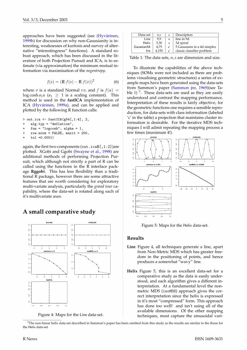
Line Figure 4, all techniques generate a line, apartfrom Non-Metric MDS which has greater free-dom in the positioning of points, and henceproduces a somewhat “wavy” line.

Helix Figure 5, this is an excellent data-set for acomparative study as the data is easily under-stood, and each algorithm gives a different in-terpretation. At a fundamental level the non-metric MDS (isoMDS) approach gives the cor-rect interpretation since the helix is expressedin it’s most “compressed” form. This approachhas done too well! and isn’t using all of theavailable dimensions. Of the other mappingtechniques, most capture the sinusoidal vari-

3The non-linear helix data-set described in Sammon’s paper has been omitted from this study as the results are similar to the those forthe Helix data-set



ation (especially PCA), and hence subjectivelypresent a better “story”.

Gaussian5 Figure 1, again this data is excellent forhighlighting the power of MDS techniques. Ifa reasonable minima can be found - MDS tech-niques offer a significant advantage in main-taining clustering information. One of the maincharacteristics of a cluster is that members tendto be relatively close together, hence MDS, fun-damentally a distance based approach, has agreater capacity to maintain this relationship.

Iris Figure 6, there appears to be only minor differ-ence in the maps produced. Of note perhapsis the tighter clustering in the MDS based ap-proaches.

−2 −1 0 1 2 3

−2−1

01

2

prcomp

−3 −2 −1 0 1 2 3 4

−1.0

0.0

0.5

1.0

cmdscale

−2 −1 0 1 2

−3−2

−10

12

3

sammon s= 0.0048

−15 −5 0 5 10 15

−40

−20

020

40

isoMDS, s= 4.1909

−1.5 −0.5 0.5 1.0 1.5

−2−1

01

23

fastICA

Figure 6: Maps of the Iris data-set.

Summary

As the results of the above study show, R is an excel-lent tool to perform dimension reduction and map-ping. The mva package in particular provides an ex-cellent set of classical approaches which often givethe most revealing results, particularly when datacontains class information. fastICA and the SOMfunction from class provide a welcome addition tothe repertoire, even if they are perhaps aimed moreat alternative problems. Clearly, there is scope to ex-tend the number of projection pursuit indices, in linewith those implemented in XGobi.

Dimensional reduction is an extremely activearea of research, mainly within the Neural Networkcommunity. Few comparative practical studies ofthe application of recent techniques to mapping exist(particularly between newer techniques and “classi-cal” MDS approaches), hence there is no strong in-dication of what might be usefully ported to R. Afree MATLAB implementation of many of the newertechniques (Probabilistic Principal Component Anal-ysis (Tipping and Bishop, 1997) (PPCA) mixtures ofPPCA (Tipping and Bishop, 1999), Generative Topo-graphic Mapping (GTM) (Bishop et al., 1998) andNeuroScale (Tipping and Lowe, 1998)), with excel-lent supporting documentation is provided by theNETLAB package (Nabney, 2001). This highlightssome of the advances that have yet to appear inR, most notably techniques that are derived froma Bayesian prospective. Further notable omissionsare Local Linear Embedding (Saul and Roweis, 2003)and Isomap (Tenenbaum et al., 2000) which gener-ate a series of local representations, which are thenlinked together into a global mapping.

Data generation

The data-sets used in this study were generated us-ing the following functions:

helix <- function( size = 30 ){# input : size, sample size# output: 3d helix

t <- 0:(size-1)z <- sqrt(2)/2*ty <- sin(z)x <- cos(z)cbind(x,y,z)

}

gauss54 <- function ( s=15 , sig=0.02 ){# input : s, sample size (per Gaussian)# sigma, cluster _covariance_# output: 5 4d Gaussian clusters

simp4d <- matrix( c(0,0,0,0,1,0,0, 0, 1/2, sqrt(3)/2, 0, 0, 1/2,sqrt(3)/6 ,sqrt(2/3),0 ,1/2 ,sqrt(3)/6 ,sqrt(2)/(4*sqrt(3)),sqrt(5/8)),5,4,byrow=T)#simplex4d can easily be checked#using 'dist'

rbind(mvrnorm(simp4d[1,],S=diag(4)*sig,n=s),mvrnorm(simp4d[2,],S=diag(4)*sig,n=s),mvrnorm(simp4d[3,],S=diag(4)*sig,n=s),mvrnorm(simp4d[4,],S=diag(4)*sig,n=s),mvrnorm(simp4d[5,],S=diag(4)*sig,n=s))}



l9 <- matrix(rep(1:9,9),9,9)h30 <- helix()#g54, last column is class labelg54 <- cbind(gauss54(),rep(1:5,e=15))#iris data is a standard data-setdata(iris)#check for duplicates else#distance algorithms 'blow up'

iris.data <- unique(iris[,1:4])iris.class <- iris[row.names(iris.data),5]#some colours for the mapsclasscol <- c("red","blue","green","black","yellow")

Bibliography

C. M. Bishop, M. S., and C. K. I. Williams. GTM: Thegenerative topographic mapping. Neural Computa-tion, 10(1):215–234, 1998. URL citeseer.nj.nec.com/bishop98gtm.html. 6

M. Carreira-Perpinan. A review of dimension reduc-tion techniques. Technical Report CS–96–09, Dept.of Computer Science, University of Sheffield, Jan-uary 1997. 2

J. Edwards, K. Riley, and J. Eakins. A visual compar-ison of shape descriptors using multi-dimensionalscaling. In CAIP 2003, the 10th interantional con-ference on computer analysis of images and patterns,pages 393–402, 2003. 2

J. C. Gower. Some distance properties of latent rootand vector methods used in multivariate analysis.Biometrika, (53):325–328, 1966. 2

P. Huber. Projection pursuit. The Annals of Statistics,13(2):435–475, 1985. 4

A. Hyvärinen. Fast and robust fixed-point algo-rithms for independent component analysis. IEEETransactions on Neural Networks, 10(3):626–634,1999a. URL citeseer.nj.nec.com/hyv99fast.html. 5

A. Hyvärinen. Survey on independent compo-nent analysis. Neural Computing Surveys, 2:94–128,1999b. 5

C. Jutten and J. Hérault. Blind separation of sources.Signal Processing, 24:1–10, 1991. 4

T. Kohonen. Self-organized formation of topologi-cally correct feature maps. Biological Cybernetics,43:59–69, 1982. 4

T. Kohonen, J. Hynninen, J. Kangas, and J. Laak-sonen. Som pak: The self-organizing map pro-gram package, 1996. URL citeseer.nj.nec.com/kohonen96som.html. 4

J. Kruskal. Multidimensional scaling by optimizinggoodness of fit to a nonmetric hypothesis. Psy-chometrika, 1-27(29):115–129, 1964. 3

I. Nabney. NETLAB: Algorithms for Pattern Recogni-tion. Springer, 2001. 2, 6

K. Pearson. Principal components analysis. LondonEdinburgh and Dublin Philosophical Magazine andJournal, 6(2):559, 1901. 2

B. Ripley. Pattern Recognition and Neural Networks.Cambridge University Press, 1996. 2, 3, 4

J. Sammon jnr. A nonlinear mapping for data struc-ture analysis. IEEE Transactions on Computers, C-18:401–409, 1969. 2, 5

L. K. Saul and S. T. Roweis. Think globally, fit lo-cally: Unsupervised learning of low dimensionalmanifolds. Journal of Machine Learning Research, 4:119–155, 2003. 6

D. F. Swayne, D. Cook, and A. Buja. XGobi: Inter-active dynamic data visualization in the X Win-dow System. Journal of Computational and GraphicalStatistics, 7(1):113–130, 1998. URL citeseer.nj.nec.com/article/swayne98xgobi.html. 5

J. B. Tenenbaum, V. Silva, and J. C. Langford. Aglobal geometric framework for nonlinear dimen-sionality reduction. Science, 290(22):2319–2323,2000. 6

M. Tipping and C. Bishop. Probabilistic prin-cipal component analysis. Technical ReportNCRG/97/010, Neural Computing ResearchGroup, Aston University, 1997. 6

M. Tipping and D. Lowe. Shadow targets: a novel al-gorithm for topographic projections by radial basisfunctions. Neurocomputing, 19(1):211–222, 1998. 6

M. E. Tipping and C. M. Bishop. Mixtures of prob-abilistic principal component analysers. NeuralComputation, 11(2):443–482, 1999. URL citeseer.nj.nec.com/tipping98mixtures.html. 6

J. Vesanto. SOM-based data visualization meth-ods. Intelligent-Data-Analysis, 3:111–26, 1999. URLciteseer.nj.nec.com/392167.html. 4

A. Webb. Statistical Pattern Recognition. Wiley, 2002.ISBN 0470845139. 2

Jonathan Edwards & Paul OmanDepartment of Informatics, University of NorthumbriaNewcastle upon tyne, UK{jonathan.edwards,paul.oman}@unn.ac.uk


citeseer.nj.nec.com/bishop98gtm.html

citeseer.nj.nec.com/bishop98gtm.html

citeseer.nj.nec.com/hyv99fast.html

citeseer.nj.nec.com/hyv99fast.html

citeseer.nj.nec.com/kohonen96som.html

citeseer.nj.nec.com/kohonen96som.html

citeseer.nj.nec.com/article/swayne98xgobi.html

citeseer.nj.nec.com/article/swayne98xgobi.html

citeseer.nj.nec.com/tipping98mixtures.html

citeseer.nj.nec.com/tipping98mixtures.html

citeseer.nj.nec.com/392167.html

mailto:protect T1extbraceleft jonathan.edwards,paul.omanprotect T1extbraceright @unn.ac.uk


R as a Simulation Platform in EcologicalModellingThomas Petzoldt

Introduction

In recent years, the R system has evolved to a matureenvironment for statistical data analysis, the devel-opment of new statistical techniques, and, togetherwith an increasing number of books, papers and on-line documents, an impressing basis for learning,teaching and understanding statistical techniquesand data analysis procedures.

Moreover, due to its powerful matrix-orientedlanguage, the clear interfaces and the overwhelmingamount of existing basic and advanced libraries, Rbecame a major platform for the development of newdata analysis software (Tierney, 2003).

Using R firstly for post-processing, statisticalanalysis and visualization of simulation model re-sults and secondly as a pre-processing tool for exter-nally running models the question arose, whether Rcan serve as a general simulation platform to imple-ment and run ecological models of different types,namely differential equation and individual-basedmodels.

From the perspective of an empirical ecologist,the suitability of a simulation platform is oftenjudged according to the following properties:

1. learning curve and model development time,

2. execution speed,

3. readability of the resulting code,

4. applicability to one special model type only orto a wide variety of simulation methods,

5. availability of libraries, which support modeldevelopment, visualization and analysis ofsimulation results,

6. availability of interfaces to external code andexternal data,

7. portability and licensing issues.

While questions 5 to 7 can be easily answeredin a positive sense for the R system, e.g. portabil-ity, free GNU Public License, the availability of ex-ternal interfaces for C, Fortran and other languagesand numerous methods to read and write externaldata, the remaining questions can be answered onlywith some practical experience. As a contribution, Ipresent some illustrative examples on how ecological

models can be implemented within R and how theyperform. The documented code, which can be easilyadapted to different situations will offer the readerthe possibility to approach their own questions.

Examples

The examples were selected to show different typesof ecological models and possible ways of implemen-tation within R. Although realism and complexityare limited due to the intention to give the full sourcecode here, they should be sufficient to demonstrategeneral principles and to serve as an onset for fur-ther work1.

Differential equations

The implementation of first-order ordinary differ-ential equation models (ODEs) is straightforwardand can be done either with an integration algo-rithm written in pure R, for example the classicalRunge-Kutta 4th order method, or using the lsodaalgorithm (Hindmarsh, 1983; Petzold, 1983), whichthanks to Woodrow Setzer are both available in theodesolve-library. Compared to other simulationpackages this assortment is still relatively limited butshould be sufficient for Lotka-Volterra type and othersmall and medium scale ecological simulations.

As an example I present the implementation ofa recently published Lotka-Volterra-type model (Bla-sius et al., 1999; Blasius and Stone, 2000), the con-stant period – chaotic amplitude (UPCA) model. Themodel consists of three equations for resource u, her-bivorous v, and carnivorous w animals:

dudt

= au−α1 f1(u, v) (1)

dvdt

= −bv +α1 f1(u, v)−α2 f2(v, w) (2)

dwdt

= −c(w− w∗) +α2 f2(v, w) (3)

where f1, f2 represent either the Lotka-Volterraterm fi(x, y) = xy or the Holling type II termfi(x, y) = xy/(1 + kix) and w∗ is an important stabi-lizing minimum predator level when the prey popu-lation is rare.

To run the model as an initial value simulationwe must provide R with (1) the model written as anR-function, (2) a parameter vector, (3) initial (start)values, and (4) an integration algorithm.

1Supplementary models and information are available on http://www.tu-dresden.de/fghhihb/petzoldt/modlim/


http://www.tu-dresden.de/fghhihb/petzoldt/modlim/


After loading the required libraries, the modelequations (the Holling equation f and the derivativesmodel), can be written very similar to the mathemat-ical notation. To make the code more readable, thestate vector xx is copied to named state variables andthe parameters are extracted from the parameter vec-tor parms using the with-environment. The results ofthe derivative function are returned as list.

library(odesolve)

library(scatterplot3d)

f <- function(x, y, k){x*y / (1+k*x)} #Holling II

model <- function(t, xx, parms) {

u <- xx[1]

v <- xx[2]

w <- xx[3]

with(as.list(parms),{

du <- a * u - alpha1 * f(u, v, k1)

dv <- -b * v + alpha1 * f(u, v, k1) +

- alpha2 * f(v, w, k2)

dw <- -c * (w - wstar) + alpha2 * f(v, w, k2)

list(c(du, dv, dw))

})

}

As a next step, three vectors have to be de-fined: the times vector for which an output valueis requested, the parameter vector (parms), and thestart values of the state variables (xstart) where thenames within the vectors correspond to the namesused within the model function.

times <- seq(0, 200, 0.1)

parms <- c(a=1, b=1, c=10,

alpha1=0.2, alpha2=1,

k1=0.05, k2=0, wstar=0.006)

xstart <- c(u=10, v=5, w=0.1)

Now the simulation can be run using either rk4or lsoda:

out <- as.data.frame(lsoda(xstart, times,

model, parms))

This should take only two seconds on a standardcomputer and finally we can plot the simulation re-sults as time series or state trajectory (fig. 1):

par(mfrow=c(2,2))

plot(times, out$u, type="l", col="green")

lines(times, out$v, type="l", col="blue")

plot(times, out$w, type="l", col="red")

plot(out$w[-1], out$w[-length(out$w)], type="l")

scatterplot3d(out$u, out$v, out$w, type="l")

Of course, similar results can be obtained withany other simulation package. However, the greatadvantage using a matrix oriented language like Ror Octave2 is, that the core model can be easily inte-grated within additional simulation procedures. As

an example a bifurcation (Feigenbaum)-diagram ofthe chaotic amplitude of the predator population canbe computed. First a small helper function whichidentifies the peaks (maxima and minima) of the timeseries is needed. Within a vectorized environmentthis can be implemented very easily by selecting allthose values which are greater (resp. lower for min-ima) as their immediate left and right neighbours:

peaks <- function(x) {

l <- length(x)

xm1 <- c(x[-1], x[l])

xp1 <- c(x[1], x[-l])

x[x > xm1 & x > xp1 | x < xm1 & x < xp1]

}

As a next step the integration procedure is in-cluded within a main loop which increments thevariable parameter b, evaluates the peaks and up-dates the plot:

plot(0,0, xlim=c(0,2), ylim=c(0,1.5),

type="n", xlab="b", ylab="w")

for (b in seq(0.02,1.8,0.02)) {

parms["b"] <- b

out <- as.data.frame(lsoda(xstart, times,

model, parms, hmax=0.1))

l <- length(out$w) %/% 3

out <- out[(2*l):(3*l),]

p <- peaks(out$w)

l <- length(out$w)

xstart <- c(u=out$u[l], v=out$v[l], w=out$w[l])

points(rep(b, length(p)), p, pch=".")

}

After a stabilization phase only the last third ofthe detected peaks are plotted to show the behavior“at the end” of the time series. The resulting bifurca-tion diagram (fig. 2) shows the dependence of theamplitude of the predator w in dependence of theprey parameter b which can be interpreted as emigra-tion parameter or as predator independent mortality.The interpretation of this diagram is explained in de-tail by Blasius and Stone (2000), but from the techni-cal viewpoint this simulation shows, that within thematrix-oriented language R the integration of a sim-ulation model within an analysis environment canbe done with a very small effort of additional code.Depending on the resolution of the bifurcation dia-gram the cpu time seems to be relatively high (sev-eral minutes up to one hour) but considering that inthe past such computations were often done on su-percomputers, it should be acceptable on a personalcomputer.

2http://www.octave.org


http://www.octave.org


0 20 40 60 80 100

4

6

8

10

12

14

time

u (g

reen

), v

(blu

e)

0 20 40 60 80 100

0.0

0.2

0.4

0.6

0.8

1.0

time

w

0.0 0.2 0.4 0.6 0.8 1.0

0.0

0.2

0.4

0.6

0.8

1.0

wt−1

wt

2 4 6 8 10 12 14 160.00.20.40.60.81.01.2

2 4 6 8 10 12

x

vw

Figure 1: Simulation of an UPCA model, top left: resource (green) and prey (blue), top right: predator, bottomleft: predator with lagged coordinates, bottom right: three dimensional state trajectory showing the chaoticattractor.

0.0 0.5 1.0 1.5 2.0

0.0

0.5

1.0

1.5

b

w

Figure 2: Bifurcation diagram for the predator w independence of prey parameter b.

Individual-based models

In contrast to ODE models, which in most caseswork on an aggregated population level (abundance,biomass, concentration), individual based modelsare used to derive population parameters from thebehavior of single individuals, which are commonlya stochastic sample of a given population. During thelast decade this technique, which is in fact a creative

collection of discrete event models, became widelyused in theoretical and applied ecology (DeAngelisand Gross, 1992, and many others). Among them arevery different approaches, which are spatially aggre-gated, spatially discrete (grid-based or cellular au-tomata), or with a continuous space representation(particle diffusion type models).

Up to now there are different simulation toolsavailable, which are mostly applicable to a rela-tively small class of individual-based approaches,e.g. SARCASim3 and EcoBeaker4 for cellular au-tomata or simulation frameworks like OSIRIS (Mooijand Boersma, 1996). However, because the ecologi-cal creativity is higher than the functionality of someof these tools, a large proportion of individual-basedmodels is implemented using general-purpose lan-guages like C++ or Delphi, which in most cases, re-quires the programmer to take care of data input andoutput, random number generators and graphical vi-sualization routines.

A possible solution of this tradeoff are matrix ori-ented languages like Matlab5 (for individual-basedmodels see Roughgarden, 1998), Octave or the S lan-guage. Within the R system a large collection offundamental statistical, graphical and data manipu-

3http://www.collidoscope.com/ca/4http://www.ecobeaker.com/5http://www.mathworks.com/


http://www.collidoscope.com/ca/

http://www.ecobeaker.com/

http://www.mathworks.com/


lation functions is readily available and therefore itis not very difficult to implement individual-basedmodels.

Individual-based population dynamics

The population dynamics of a Daphnia (water flee)population is shown here as an example. Daphniaplays an important role for the water quality of lakes(e.g. Benndorf et al., 2001), can be held very easilyin the laboratory and the transparent skin makes itpossible to observe important life functions using themicroscope (e.g. food in the stomach or egg numbersin the brood pouch), so the genus Daphnia became anoutstanding model organism in limnology, compara-ble to Drosophila in genetic research.

Figure 3: Parthenogenetic life cycle of Daphnia.

Under normal circumstances the life cycle ofDaphnia is asexual (parthenogenetic) and begins withone new-born (neonate) female which grows up tothe size of maturity (fig. 3). Then a number of asex-ual eggs are deposited into the brood pouch (spawn-ing) which then grow up to neonates and which arereleased after a temperature-dependent time spaninto the free water (hatching). There are several ap-proaches to model this life cycle in the literature (e.g.Kooijman, 1986; Gurney et al., 1990; Rinke and Pet-zoldt, 2003). Although the following is an absolutelyelementary one which neglects food availability andsimplifies size-dependent processes, it should be suf-ficient to demonstrate the principal methodology.

For the model we take the following assumptions(specified values taken from Hülsmann and Weiler(2000) and Hülsmann (2000)):

• The egg depelopment time is a function ofwater temperature according to Bottrell et al.(1976).

• Neonates have a size of 510 µm and the size ofmaturity is assumed to be 1250 µm.

• Juvenile length growth is linear with a growthrate of 83 µm d−1 and due to the reproductiveexpense the adult growth rate is reduced to80% of the juvenile value.

• The clutch size of each individual is taken ran-domly from an observed probability distribu-tion of the population in Bautzen Reservoir(Germany) during spring 1999.

• The mortality rate is set to a fixed size-independent value of 0.02 d−1 and the maxi-mum age is set to a fixed value of 30 d.

The implementation consists of six parts. Afterdefining some constants, the vector with the cumu-lative distribution of the observed egg-frequencies,the simulation control parameters (1) and necessaryhelper functions, namely a function for an inversesampling of empiric distributions (2), the life func-tions (3) of Daphnia: grow, hatch, spawn and dieare implemented. Each individual is represented asone row of a data frame inds where the life func-tions either update single values of the individualsor add rows via rbind for each newborn individual(in hatch) or delete rows via subset for dead indi-viduals. With the exception of the hatch functionall procedures are possible as vectorized operationswithout the need of loops.

Now the population data frame is created (4) withsome start individuals either as a fixed start popula-tion (as in the example) or generated randomly. Thelife loop (5) calls each life function for every time stepand, as the inds data frame contains only one actualstate, collects the desired outputs during the simula-tion, which are analysed graphically or numericallyimmediately after the simulation (6, see fig. 4). Theexample graphics show selected population statis-tics: the time series of abundance with an approx-imately exponential population growth, the meanlength of the individuals as a function of time (in-dicating the presence of synchronized cohorts), thefrequency distribution of egg numbers of adult indi-viduals and a boxplot of the age distribution.

Additionally or as an alternative it is possible tosave logfiles or snapshot graphics to disk and to anal-yse and visualise them with external programs.

#===============================================

# (1) global parameters

#===============================================

# cumulative egg frequency distribution

eggfreq <- c(0.39, 0.49, 0.61, 0.74,

0.86, 0.95, 0.99, 1.00)

son <- 510 # um

primipara <- 1250 # um

juvgrowth <- 83 # um/d

adgrowth <- 0.8*juvgrowth # um/d

mort <- 0.02 # 1/d

temp <- 15 # deg C

timestep <- 1 # d

steps <- 40

#

# template for one individual

newdaphnia <- data.frame(age = 0,

size = son,



eggs = 0,

eggage = 0)

#===============================================

# (2) helper functions

#===============================================

botrell <- function(temp) {

exp(3.3956 + 0.2193 *

log(temp)-0.3414 * log(temp)^2)

}

# inverse sampling from an empiric distribution

clutchsize <- function(nn) {

approx(c(0,eggfreq), 0:(length(eggfreq)),

runif(nn), method="constant", f=0)$y

}

#===============================================

# (3) life methods of the individuals

#===============================================

grow <- function(inds){

ninds <- length(inds$age)

inds$age <- inds$age + timestep

inds$eggage <- ifelse(inds$size > primipara,

inds$eggage + timestep, 0)

inds$size <- inds$size + timestep *

ifelse(inds$size < primipara,

juvgrowth, adgrowth)

inds

}

die <- function(inds) {

subset(inds,

runif(inds$age) > mort & inds$age <= 30)

}

spawn <- function(inds) {

# individuals with size > primipara

# and eggage==0 can spawn


neweggs <- clutchsize(ninds)

inds$eggs <- ifelse(inds$size > primipara

& inds$eggage==0,

neweggs, inds$eggs)

inds

}

hatch <- function(inds) {

# individuals with eggs

# and eggage > egg development time hatch


newinds <- NULL

edt <- botrell(temp)

for (i in 1: ninds) {

if (inds$eggage[i] > edt) {

if (inds$eggs[i] > 0) {

for (j in 1:inds$eggs[i]) {

newinds <- rbind(newinds,

newdaphnia)

}

}

inds$eggs[i] <- 0

inds$eggage[i] <- 0

}

}

rbind(inds, newinds)

}

#===============================================

# (4) start individuals

#===============================================

inds <- data.frame(age = c(7, 14, 1, 11, 8,

27, 2, 20, 7, 20),

size = c(1091, 1339, 618, 1286,

1153, 1557, 668, 1423,

1113, 1422),

eggs = c(0, 0, 0, 5, 0,

3, 0, 3, 0, 1),

eggage = c(0, 0, 0, 1.6, 0,

1.5, 0, 1.7, 0, 1.2))

#===============================================

# (5) life loop

#===============================================

sample.n <- NULL

sample.size <- NULL

sample.eggs <- NULL

sample.agedist <- NULL

for (k in 1:steps) {

print(paste("timestep",k))

inds <- grow(inds)

inds <- die(inds)

inds <- hatch(inds)

inds <- spawn(inds)

sample.n <- c(sample.n,

length(inds$age))

sample.size <- c(sample.size,

mean(inds$size))

sample.eggs <- c(sample.eggs,

inds$eggs[inds$size >

primipara])

sample.agedist <- c(sample.agedist,

list(inds$age))

}

#===============================================

# (6) results and graphics

#===============================================

par(mfrow=c(2,2))

plot(sample.n, xlab="time (d)",

ylab="abundance", type="l")

plot(sample.size, xlab="time (d)",

ylab="mean body length (tm)", type="l")

hist(sample.eggs, freq=FALSE, breaks=0:10,

right=FALSE, ylab="rel. freq.",

xlab="egg number", main="")

time <- seq(1,steps,2)

boxplot(sample.agedist[time],

names=as.character(time), xlab="time (d)",

ylab="age distribution (d)")

Particle diffusion models

In individual based modelling two different ap-proaches are used to represent spatial movement:cellular automata and continuous coordinates (diffu-sion models). Whereas in the first case movement isrealized by a state-transition of cells depending ontheir neighbourhood, in diffusion models the indi-viduals are considered as particles with x and y coor-dinates which are updated according to a correlatedor a random walk. The movement rules use polar co-ordinates with angle (α) and distance (r) which canbe converted to cartesian coordinates using complex



0 10 20 30 40

5010

015

020

0

time (d)

abun

danc

e

0 10 20 30 40

1000

1100

1200

1300

time (d)

mea

n bo

dy le

ngth

(µm

)

egg number

rel.

freq.

0 2 4 6 8 10

0.00

0.10

0.20

0.30

1 5 9 15 21 27 33 39

05

1015

2025

30

time (d)

age

dist

ribut

ion

(d)

Figure 4: Results of an individual-based Daphnia model: exponential growth of abundance (top left), fluctu-ation of the mean body length indicating synchronised hatching (top right), simulated egg counts of adultindividuals (bottom left), boxplot of age distribution as a function of time (bottom right).



numbers or sine and cosine transformation, what isessentially the same. Changes in direction are real-ized by adding a randomly selected turning angle tothe angle of the time step before. An angle which isuniformly distributed within the interval (0, 2π) re-sults in an uncorrelated random walk, whereas anangle of less than a full circle or a non-uniform (e.g.a normal) distribution leads to a correlated randomwalk. To keep the individuals within the simulationarea either a wrap around mode or reflection at theborders can be used.

The example shows a diffusion example with acoordinate system of x, y = (0, 100) and an areaof decreased movement speed in the middle y =(45, 55), which can be interpreted as refugium (e.g. ahedge within a field for beatles), a region of increasedfood availability (the movement speed of herbivo-rous animals is less while grazing than foraging) oras a diffusion barrier (e.g. reduced eddy diffusionwithin the thermocline of stratified lakes).

The implementation is based on a data frame ofindividuals (inds) with cartesian coordinates (x,y)and a movement vector given as polar coordinates(a, r), the movement rules and the simulation loop.

The simulation runs fast enough for a real-timevisualization of several hundred particles and givesan impression, how an increased abundance withinrefugia or diffusion barriers, observed very often inthe field, can be explained without any complicatedor intelligent behavior, solely on the basis of randomwalk and variable movement speed (fig. 5). Thismodel can be extended in several ways and may in-clude directed movement (sedimentation), reproduc-tion or predator-prey interactions6. Furthermore, theprinciple of random walk can be used as a startingpoint for more complex theoretical models or, com-bined with population dynamics or bioenergeticalmodels, as models of real-world systems (e.g. Hölkeret al., 2002).

#===============================================

# simulation parameters and start individuals

#===============================================

n <- m <- 100 # size of simulation area

nruns <- 2000 # number of simulation runs

nind <- 100 # number of inds

inds <- data.frame(x = runif(nind)*n,

y = runif(nind)*m,

r = rnorm(nind),

a = runif(nind)*2*pi)

#===============================================

# Movement

#===============================================

move <- function(inds) {

with(inds, {

## Rule 1: Refugium

speed <- ifelse(inds$y > 45

& inds$y < 55, 0.2, 2)

## Rule 2: Random Walk

inds$a <- a + 2 * pi / runif(a)

dx <- speed * r * cos(a)

dy <- speed * r * sin(a)

x<-inds$x + dx

y<-inds$y + dy

## Rule 3: Wrap Around

x<-ifelse(x>n,0,x)

y<-ifelse(y>m,0,y)

inds$x<-ifelse(x<0,n,x)

inds$y<-ifelse(y<0,m,y)

inds

})

}

#===============================================

# main loop

#===============================================

for(i in 1:nruns) {

inds <- move(inds)

plot(inds$x, inds$y, col="red", pch=16,

xlim=c(0, n), ylim=c(0, m),

axes=FALSE, xlab="", ylab="")

}

0 20 40 60 80 100

0

20

40

60

80

100

x

y

frequency

0 10 20 30 40 50

Figure 5: State of the particle diffusion model after2000 time steps.

Cellular automata

Cellular automata (CA) are an alternative approachfor the representation of spatial processes, widelyused in theoretical and applied ecological modelling.As one of the most fundamental systems the well-known deterministic CA “Conway’s Game of Life”(Gardner, 1970) is often used as an impressive simu-lation to show, that simple rules can lead to complexbehavior. To implement a rectangular CA within R,a grid matrix (z), state transition rules implementedas ifelse statements and the image plot function arethe essential building blocks. Furthermore a function(neighbourhood) is needed, which counts the num-ber of active (nonzero) cells in the neighbourhood ofeach cell. In the strict sense only the eight adjacentcells are considered as neighbours, but in a more gen-eral sense a weighted neighbourhood matrix can beused. The neighbourhood count has to be evaluatedfor each cell in each time step and is therefore a com-putation intensive part, so the implementation as an

6see supplementary information



external C-function was necessary and is now avail-able as part of the experimental simecol package.

Using this, Conway’s Game of Life can be imple-mented with a very short piece of code. Part (1) de-fines the grid matrix with a set of predefined or ran-dom figures respectively, and part (2) is the life loop,which contains only the call of the neighbourhoodfunction, the state transition rules and the visualiza-tion. The simulation is much slower than specializedConway-programs (20 s on an AMD Athlon 1800+for the example below) but still fast enough for real-time animation (0.2 s per time step). Approximately85% of the elapsed time is needed for the visualiza-tion, only 3% for the neighbourhood function and therest for the state transition rules.

Figure 6: Initial state of matrix z before the simu-lation (left) and state after the first simulation step(right) .

However, despite the slower simulation speedit is a great advantage of this implementation, thatstate matrices and transition rules are under fullcontrol of the user and that the system is com-pletely open for extension towards grid-based mod-els with an ecological background. Furthermore theneighbours-function of the simecol-package allowsthe use of a generalized neighbourhood via a weightmatrix to implement e.g. random or directed move-ment of animals, seed dispersal, forest fire propaga-tion or epidemic models.

library(simecol)

#===============================================

# (1) start individuals

#===============================================

n <- m <- 80

z <- matrix(0, nrow=n, ncol=m)

z[40:45,20:25] <-1 # filled square 6x6 cells

z[51:70,20:21] <-1 # small rectangle 20 x 2 cells

z[10:12,10] <-1 # short bar 3x1 cells

z[20:22,20:22] <- c(1,0,0,0,1,1,1,1,0) # glider

z[1:80,51:80] <-round(runif(2400)) # random

image(z, col=c("wheat", "navy"), axes=FALSE)

#===============================================

# (2) life loop

#===============================================

for (i in 1:100){

nb <- eightneighbours(z)

## survive with 2 or 3 neighbours

zsurv <- ifelse(z > 0 & (nb == 2 | nb ==3), 1, 0)

## generate for empty cells with 3 neigbors

zgen <- ifelse(z == 0 & nb == 3, 1, 0)

z <- matrix((zgen + zsurv), nrow=n)

image(z, col=c("wheat","navy"),

axes=FALSE, add=TRUE)

}

Conclusions

The examples described so far, plus the experiencewith R as data analysis environment for measure-ment and simulation data, allows to conclude thatR is not only a great tool for statistical analysis anddata processing but also a general-purpose simula-tion environment, both in research and especially inteaching.

It is not only an advantage to replace a lot of dif-ferent tools on the modelers PC for different typesof models, statistical analysis and data managementwith one single platform. The main advantage lies inthe synergistic effects, which result from the combi-nation and integration of these simulation models to-gether with powerful statistics and publication qual-ity graphics.

Being an interpreted language with a clear syn-tax and very powerful functions, R is easier to learnthan other languages and allows rapid prototypingand and interactive work with the simulation mod-els. Due to the ability to use vectorized functions, theexecution speed is fast enough for non-trivial simu-lations and for real-time animation of teaching mod-els. In many cases the code is compact enough todemonstrate field ecologists the full ecological func-tionality of the models. Furthermore, within a work-group where field ecologists and modellers use thesame computing environment for either statisticaldata analysis or the construction of simulation mod-els, R becomes a communication aid to discuss eco-logical principles and to exchange ideas.

Acknowledgements

I am grateful to my collegues Karsten Rinke, StephanHülsmann, Robert Radke and Markus Wetzel forhelpful discussions, to Woodrow Setzer for imple-menting the odesolve package and to the R Devel-opment Core Team for providing the great R system.

Bibliography

Benndorf, J., Kranich, J., Mehner, T., and Wagner, A.(2001). Temperature impact on the midsummer de-cline of Daphnia galeata from the biomanipulatedBautzen Reservoir (Germany). Freshwater Biology,46:199–211. 11

Blasius, B., Huppert, A., and Stone, L. (1999).Complex dynamics and phase synchronization in



spatially extended ecological systems. Nature,399:354–359. 8

Blasius, B. and Stone, L. (2000). Chaos and phase syn-chronization in ecological systems. InternationalJournal of Bifurcation and Chaos, 10:2361–2380. 8,9

Bottrell, H. H., Duncan, A., Gliwicz, Z. M., Gry-gierek, E., Herzig, A., Hillbricht-Ilkowska, A.,Kurasawa, H., Larsson, P., and Weglenska, T.(1976). A review of some problems in zooplanktonproduction studies. Norvegian Journal of Zoology,24:419–456. 11

DeAngelis, D. L. and Gross, L. J., editors (1992).Individual-Based Models and Approaches in Ecol-ogy: Populations, Communities, and Ecosystems.,Knoxwille, Tennessee. Chapmann and Hall. Pro-ceedings of a Symposium/Workshop. 10

Gardner, M. (1970). The fantastic combinations ofJohn Conway’s new solitaire game ’life’. ScientificAmerican, 223:120–123. 14

Gurney, W. C., McCauley, E., Nisbet, R. M., and Mur-doch, W. W. (1990). The physiological ecology ofDaphnia: A dynamic model of growth and repro-duction. Ecology, 71:716–732. 11

Hindmarsh, A. C. (1983). ODEPACK, a systematizedcollection of ODE solvers. In Stepleman, R., editor,Scientific Computing, pages 55–64. IMACS / North-Holland. 8

Hölker, F., Härtel, S. S., Steiner, S., and Mehner, T.(2002). Effects of piscivore-mediated habitat useon growth, diet and zooplankton consumption ofroach: An individual-based modelling approach.Freshwater Biology, 47:2345–2358. 14

Hülsmann, S. (2000). Population Dynamics of Daphniagaleata in the Biomanipulated Bautzen Reservoir: Life

History Strategies Against Food Deficiency and Preda-tion. PhD thesis, TU Dresden Fakultät Forst-, Geo-,Hydrowissenschaften, Institut für Hydrobiologie.11

Hülsmann, S. and Weiler, W. (2000). Adult, not juve-nile mortality as a major reason for the midsum-mer decline of a Daphnia population. Journal ofPlankton Research, 22(1):151–168. 11

Kooijman, S. (1986). Population dynamics on the ba-sis of budgets. In Metz, J. and Diekman, O., edi-tors, The dynamics of physiologically structured popu-lations, pages 266–297. Springer Verlag, Berlin. 11

Mooij, W. M. and Boersma, M. (1996). An object ori-ented simulation framework for individual-basedsimulations (OSIRIS): Daphnia population dynam-ics as an example. Ecol. Model., 93:139–153. 10

Petzold, L. R. (1983). Automatic selection of meth-ods for solving stiff and nonstiff systems of ordi-nary differential equations. Siam J. Sci. Stat. Com-put., 4:136–148. 8

Rinke, K. and Petzoldt, T. (2003). Modelling theeffects of temperature and food on individualgrowth and reproduction of Daphnia and their con-sequences on the population level. Limnologica,33(4):293–304. 11

Roughgarden, J. (1998). Primer of Ecological Theory.Prentice Hall. 10

Tierney, L. (2003). Name space management for R. RNews, 3(1):2–6. 8

Thomas PetzoldtDresden University of TechnologyInstitute of HydrobiologyDresden, [email protected]




Using R for Estimating LongitudinalStudent Achievement Modelsby J.R. Lockwood1, Harold Doran and Daniel F. McCaf-frey

Overview

The current environment of test-based accountabilityin public education has fostered increased interest inanalyzing longitudinal data on student achievement.In particular, “value-added models” (VAM) thatuse longitudinal student achievement data linkedto teachers and schools to make inferences aboutteacher and school effectiveness have burgeoned.Depending on the available data and desired infer-ences, the models can range from straightforwardhierarchical linear models to more complicated andcomputationally demanding cross-classified models.The purpose of this article is to demonstrate how R,via the lme function for linear mixed effects modelsin the nlme package (Pinheiro and Bates, 2000), canbe used to estimate all of the most common value-added models used in educational research. Afterproviding background on the substantive problem,we develop notation for the data and model struc-tures that are considered. We then present a se-quence of increasingly complex models and demon-strate how to estimate the models in R. We concludewith a discussion of the strengths and limitationsof the R facilities for modeling longitudinal studentachievement data.

Background

The current education policy environment of test-based accountability has fostered increased interestin collecting and analyzing longitudinal data on stu-dent achievement. The key aspect of many suchdata structures is that students’ achievement dataare linked to teachers and schools over time. Thispermits analysts to consider three broad classes ofquestions: what part of the observed variance instudent achievement is attributable to teachers orschools; how effective is an individual teacher orschool at producing growth in student achievement;and what characteristics or practices are associatedwith effective teachers or schools. The models usedto make these inferences vary in form and complex-ity, and collectively are known as “value added mod-els” (VAM, McCaffrey et al., 2004).

However, VAM can be computationally demand-ing. In order to disentangle the various influences on

achievement, models must account simultaneouslyfor the correlations among outcomes within studentsover time and the correlations among outcomes bystudents sharing teachers or schools in the currentor previous years. The simplest cases have studentoutcomes fully nested within teachers and schools,in which case standard hierarchical linear models(Raudenbush and Bryk, 2002; Pinheiro and Bates,2000) are appropriate. When students are linked tochanging teachers and/or schools over time, morecomplicated and computationally challenging cross-classified methods are necessary (Bates and DebRoy,2003; Raudenbush and Bryk, 2002; Browne et al.,2001). Although the lme function of the nlme libraryis designed and optimized for nested structures, itssyntax is flexible enough to specify models for morecomplicated relational structures inherent to educa-tional achievement data.

Data structures

The basic data structures supporting VAM estima-tion are longitudinal student achievement data Yk =(Yk0, . . . , YkT) where k indexes students. Typicallythe data represent scores on an annual standardizedexamination for a single subject such as mathemat-ics or reading, with t = 0, . . . , T indexing years.For clarity, we assume that all students are fromthe same cohort, so that year is coincident withgrade level. More careful consideration of the dis-tinction between grade level and year is necessarywhen modeling multiple cohorts or students who areheld back. We further assume that the scores rep-resent achievement measured on a single develop-mental scale so that Ykt is expected to increase overtime, with the gain scores (Ykt − Yk,t−1) represent-ing growth along the scale. The models presentedhere can be estimated with achievement data that arenot scaled as such, but this complicates interpreta-tion (McCaffrey et al., 2004).

As noted, the critical feature of the data under-lying VAM inference is that the students are linked,over time, to higher-level units such as teachers andschools. For some data structures and model spec-ifications, these linkages represent a proper nestingrelationship, where outcomes are associated with ex-actly one unit in each hierarchical level (e.g. out-comes nested within students, who are nested withinschools). For more complex data, however, the

1This material is based on work supported by the National Science Foundation under Grant No. 99-86612. Any opinions, findingsand conclusions or recommendations expressed in this material are those of the author(s) and do not necessarily reflect the views of theNational Science Foundation.



stuid schid y0.tchid y1.tchid y2.tchid y0 y1 y2

1 1 3 102 201 557 601 6292 1 3 101 203 580 632 6603 1 2 102 202 566 620 654

· · ·287 4 14 113 215 590 631 667288 4 14 114 213 582 620 644289 4 13 113 214 552 596 622

· · ·

Table 1: Sample records from wdat

linkages represent a mixture of nested and cross-classified memberships. For example, when studentschange teachers and/or schools over time, the re-peated measures on students are associated with dif-ferent higher-level units. Complicating matters isthat some models may wish to associate outcomeslater in the data series with not only the current unit,but past units as well (e.g. letting prior teachers af-fect current outcomes).

Depending on the type of model being fit, thedata will need to be in one of two formats foruse by lme. In the first format, commonly called“wide” or “person-level” format, the data are storedin a dataframe where each student has exactly onerecord (row), and repeated measures on that stu-dent (i.e. scores from different years) are in dif-ferent fields (columns). In the other form, com-monly called “long” or “person-period” format, re-peated measures on students are provided in sep-arate records, with records from the same studentin consecutive, temporally ordered rows. Intercon-version between these formats is easily carried outvia the reshape function. In some settings (partic-ularly with fully nested data structures) making thedataframe a groupedData object, a feature providedby the nlme library, will simplify some model specifi-cations and diagnostics. However, we do not use thatconvention here because some of the cross-classifieddata structures that we discuss do not benefit fromthis organization of the data.

Throughout the article we specify models interms of two hypothetical dataframes wdat and ldatwhich contain the same linked student achievementdata for three years in wide and long formats, re-spectively. For clarity we assume that the outcomedata and all students links to higher level units arefully observed; we discuss missing data at the endof the article. In the wide format, the outcomes forthe three years are in separate fields y0, y1, and y2.In the long format, the outcomes for all years are inthe field yt, with year indicated by the numeric vari-able year taking on values of 0, 1 and 2. The studentidentifiers and school identifiers for both dataframesare given by stuid and schid, respectively, which weassume are constant across time within students (i.e.students are assumed to be nested in schools). For

the wide format dataframe, teacher identifiers are inseparate fields y0.tchid, y1.tchid, and y2.tchidwhich for each student link to the year 0, 1 and 2teachers, respectively. These fields will be used tocreate the requisite teacher variables of the long for-mat dataframe later in the discussion. All identi-fiers are coded as factors, as this is required by someof the syntax presented here. Finally, in order tospecify the cross-classified models, it is necessary toaugment ldat with a degenerate grouping variabledumid that takes on a single value for all records inthe dataframe. This plays the role of a highest-levelnesting variable along which there is no variation inthe data. Sample records from the two hypotheticaldataframes are provided in Tables 1 and 2.

stuid schid dumid year yt

1 1 1 0 5571 1 1 1 6011 1 1 2 6292 1 1 0 5802 1 1 1 6322 1 1 2 660

· · ·287 4 1 0 590287 4 1 1 631287 4 1 2 667288 4 1 0 582288 4 1 1 620288 4 1 2 644

· · ·Table 2: Sample records from ldat

Model specifications

In this section we consider three increasingly com-plex classes of VAM, depending on the dimensionof the response variable (univariate versus multivari-ate) and on the relational structure among hierarchi-cal units (nested versus cross-classified). We havechosen this organization to span the range of mod-els considered by analysts, and to solidify, throughsimpler models, some of the concepts and syntaxrequired by more complicated models. All of themodels discussed here specify student, teacher andschool effects as random effects. We focus on spec-ification of the random effects structures, providing



a discussion of fixed effects for student, teacher orschool-level characteristics in a later section. It is out-side of the scope of this article to address the manycomplicated issues that might threaten the validity ofthe models (McCaffrey et al., 2004); rather we focuson issues of implementation only. It is also outside ofthe scope of this article to discuss the variety of func-tions, both in R in general and in the nlme library inparticular, that can be used to extract relevant diag-nostics and inferences from model objects. The bookby Pinheiro and Bates (2000) provides an excellenttreatment of these topics.

In specifying the statistical models that follow, forclarity we use the same symbols in different mod-els to draw correspondences among analogous terms(e.g. µ for marginal means, ε for error terms) butit should be noted that the actual interpretations ofthese parameters will vary by model. Finally, we usesubscripts i, j, k to index schools, teachers and stu-dents, respectively. To denote linkages, we use nota-tion of the form m(n) to indicate that observations orunits indexed by n are associated with higher-levelunits indexed by m. For example, j(k) denotes theindex j of the teacher linked to an outcome from stu-dent k.

1. Nested univariate models

Though VAM always utilizes longitudinal studentlevel data linked to higher level units of teachers,schools and/or districts, analysts often specify sim-ple models that reduce the multivariate data to aunivariate outcome. They also reduce a potentiallycross-classified membership structure to a nested oneby linking that outcome with only one teacher orschool. Such strategies are most commonly em-ployed when only two years of data are available,though they can be used when more years are avail-able, with models being repeated independently foradjacent pairs of years. As such, without loss of gen-erality, we focus on only the first two years of thehypothetical three-year data.

The first common method is the “gain scoremodel” that treats Gk1 = (Yk1 − Yk0) as outcomeslinked to current year (year 1) teachers. The formalmodel is:

Gk1 = µ +θ j1(k) +εk1 (1)

where µ is a fixed mean parameter, θ j1 are iidN(0,σ2

θ1) random year one teacher effects and εk1 iidN(0,σ2

ε1) year one student errors. Letting g1 denotethe gain scores, the model is a simple one-way ran-dom effects model specified in lme by

lme(fixed=g1~1,data=wdat,random=~1|y1.tchid)

In the traditional mixed effects model notation Yk =Xkβ + Zkθk + εk (Pinheiro and Bates, 2000), thefixed argument to lme specifies the response andthe fixed effects model Xkβ, and the random argu-ment specifies the random effects structure Zkθk. The

fixed argument in the model above specifies that thegain scores have a grand mean or intercept commonto all observations, and the random argument spec-ifies that there are random intercepts for each yearone teacher.

The other common data reduction strategy formultivariate data is the “covariate adjustment”model that regresses Yk1 on Yk0 and current yearteacher effects:

Yk1 = µ + βYk0 +θ j1(k) +εk1 (2)

This model is also easily specified by

lme(fixed=y1~y0,data=wdat,random=~1|y1.tchid)

As a matter of shorthand notation used throughoutthe article, in both the fixed and random argumentsof lme, the inclusion of a covariate on the right sideof a tilde implies the estimation of the correspondingintercept even though the +1 is not explicitly present.

Both of these models are straightforwardly ex-tended to higher levels of nesting. For example, inthe covariate adjustment model Equation (2) it maybe of interest to examine what part of the marginalteacher variance lies at the school level via the model:

Yk1 = µ + βYk0 +θ j1(k) +εk1

θ j1 = γi( j1) + e j1 (3)

with γi, e j1 and εk1 independent normal randomvariables with means 0 and variances σ2

γ , σ2e1 and σ2

ε1respectively. Thusσ2

θ1 from the previous model is de-composed into the between-school variance compo-nent σ2

γ and the within-school variance componentσ2

e1. Using standard nesting notation for statisticalformulae in R this additional level of nesting is spec-ified with

lme(fixed=y1~y0,data=wdat,random=~1|schid/y1.tchid)

where the random statement specifies that there arerandom intercepts for schools, and random inter-cepts for year one teachers within schools.

2. Nested multivariate models

The next most complicated class of models directlytreats the longitudinal profiles Yk = (Yk0, . . . , YkT)as outcomes, rather than reducing them to univari-ate outcomes, and the challenge becomes modelingthe mean and covariance structures of the responses.In this section we assume that the multivariate out-comes are fully nested in higher level units; in thehypothetical example, students are nested in schools,with teacher links ignored (in actual data sets teacherlinks are often unavailable). For multivariate model-ing of student outcomes, it is common for analyststo parameterize growth models for the trajectories



of the outcomes, and to examine the variations ofthe parameters of the growth models across studentsand schools.

The class of models considered here is of the form

Ykt = µt + sit(k) +εkt (4)

where µt is the marginal mean structure, sitare school-specific growth trajectories, and εkt arestudent-specific residual terms which may them-selves contain parameterized growth trajectories.For clarity and conciseness we focus on a limitedcollection of linear growth models only. Other lin-ear growth models, as well as nonlinear modelsspecified with higher-order or piecewise polynomialterms in time, can be specified using straightforwardgeneralizations of the examples that follow.

The first growth model that we consider assumesthat in Equation (4), µt = α + βt and sit = αi + βit.This model allows each school to have its own lin-ear growth trajectory through the random interceptsαi and random slopes βi, which are assumed to bebivariate normal with means zero, variances σ2

α andσ2

β, and covariance σαβ. This model is specified as

lme(fixed=yt~year,data=ldat,random=~year|schid)

Note that because the model is multivariate, the longdata ldat is necessary.

This model is probably inappropriate because itassumes that deviations of individual student scoresfrom the school-level trajectories are homoskedasticand independent over time within students. Morerealistically, the student deviations εkt are likely tobe correlated within students, and potentially havedifferent variances across time. These features canbe addressed either through student-specific randomeffects, or through a richer model for the within-student covariance structure. To some extent thereis an isomorphism between these two pathways; theclassic example is that including random student in-tercepts as part of the mean structure is equivalent tospecifying a compound symmetry correlation struc-ture. Which of the two pathways is more appropriatedepends on the application and desired inferences,and both are available in lme.

As an example of including additional randomstudent effects, we consider random student lineargrowth so that εkt = γk + δkt + ξkt. Like (αi , βi) atthe school level, (γk, δk) are assumed to be bivariatenormal with mean zero and an unstructured covari-ance matrix. The random effects at the different lev-els of nesting are assumed to be independent, andthe residual error terms ξkt are assumed to be inde-pendent and homoskedastic. The change to the syn-tax from the previous model to this models is veryslight:

lme(fixed=yt~year,data=ldat,random=~year|schid/stuid)

The random statement is analogous to that used inestimating the model in Equation (3); in this case, be-cause there are two random terms at each level, lmeestimates two (2× 2) unstructured covariance matri-ces in addition to the residual variance.

The other approach to modeling dependencein the student terms εkt is through their covari-ance structure. lme accommodates heteroskedastic-ity and within-student correlation via the weightsand correlation arguments. For the weights ar-gument, a wide variety of variance functions that«««< vam.tex can depend on model covariates asdescribed in Pinheiro and Bates Pinheiro and Bates(2000) are available. For the basic models we are======= can depend on model covariates as de-scribed in Pinheiro and Bates (2000) are available.For the basic models we are »»»> 1.2 consideringhere, the most important feature is to allow the resid-ual terms to have different variances in each year. Forthe correlation argument, all of the common resid-ual correlation structures such as compound symme-try, autoregressive and unrestricted (i.e. general pos-itive definite) are available. The model with randomgrowth terms at the school level and an unstructuredcovariance matrix for εk = (εk0,εk1,εk2) shared byall students is specified by

lme(fixed=yt~year,data=ldat,random=~year|schid,weights=varIdent(form=~1|year),correlation=corSymm(form = ~1|stuid))

A summary of the model object will report the esti-mated residual standard deviation for year 0, alongwith the ratio of the estimated residual standard de-viations from other years to that of year 0. It willalso report the estimate of the within-student corre-lation matrix. The functions varIdent and corSymmcombine to specify the unstructured covariance ma-trix; other combinations of analogous functions canbe use to specify a broad array of other covariancestructures (Pinheiro and Bates, 2000).

3. Cross classified multivariate models

All of the models in the previous two sections in-volved only fully nested data structures: observa-tions nested within students, who are nested inhigher level units such as schools. Modeling crosseddata structures – e.g., accounting for the successiveteachers taught by a student – is more challenging.The two most prominent examples of cross-classifiedmodels for longitudinal student achievement dataare «««< vam.tex that of the Tennessee Value AddedAssessment System (TVAAS) Ballou et al. (2004) andthe cross-classified model of Raudenbush and BrykRaudenbush and Bryk (2002). Both models have the======= that of the Tennessee Value Added As-sessment System (TVAAS, Ballou et al., 2004) and



the cross-classified model of Raudenbush and Bryk(2002). Both models have the »»»> 1.2 property thatthe effects of teachers experienced by a student overtime are allowed to “layer” additively, so that pastteachers affect all future outcomes.

The TVAAS layered model is the most ambitiousVAM effort to date. The full model simultaneouslyexamines outcomes on multiple subjects, from mul-tiple cohorts, across five or more years of testing. Weconsider a simplified version of that model for threeyears of testing on one subject for one cohort. Themodel for the outcomes of student k is as follows:

Yk0 = µ0 +θ j0(k) +εk0

Yk1 = µ1 +θ j0(k) +θ j1(k) +εk1

Yk2 = µ2 +θ j0(k) +θ j1(k) +θ j2(k) +εk2 (5)

The random effects for teachers in year t, θ jt, are as-sumed to be independent and normally distributedwith mean 0 and variance σ2

θt. The within studentresidual terms εk = (εk0,εk1,εk2) are assumed to benormally distributed with mean 0 and unstructuredpositive definite covariance matrix Σε. The residu-als are independent across students and are indepen-dent of the teacher effects.

Because the model deals directly with the cross-classified structure of the data, special syntax is re-quired to fit the model with lme. The main challengesare building the teacher links and specifying the dis-tribution of the teacher random effects. The first stepis to augment the long dataframe with binary vari-ables for each teacher with the property that for eachrecord, the new variable takes on the value 1 if theteacher’s random effect is part of that score under themodel and zero otherwise. That is, if there are n stu-dents in the data set, and if there are Jt teachers inyear t with J = J0 + J1 + J2, then one must augmentthe long dataframe with a (3n × J) matrix Z with el-ements of 1 where linkages occur and 0 otherwise.Note that in most settings, the matrix is large withprimarily entries of 0, which is why sparse matrixtechniques are likely to be a beneficial line of compu-tational development for these models.

There are several ways to construct this matrixbut one straightforward method is to build it fromsimple assignment matrices of size (n × Jt) usingthe teacher identifier fields y0.tchid, y1.tchid andy2.tchid from the wide format dataframe. The fol-lowing code carries this out for the hypothetical com-pletely observed dataset; modifications are necessaryin the presence of missing data:

it<-rep(1:n,each=3)z0<-model.matrix(~y0.tchid-1,data=wdat)[it,]z1<-model.matrix(~y1.tchid-1,data=wdat)[it,]z2<-model.matrix(~y2.tchid-1,data=wdat)[it,]i0<-seq(from=1,to=(3*n-2),by=3)z1[i0,]<-0z2[c(i0,i0+1),]<-0ldat<-data.frame(ldat,cbind(z0,z1,z2))

The calls to model.matrix result in (n × Jt) assign-ment matrices, which are then expanded to dupli-cated rows via the index it. Then, the appropriaterows of z1 and z2 are set to zero to indicate that laterteachers are not associated with prior scores. The fi-nal call augments the long dataframe with the newvariables.

The next step is to specify the distribution of the Jteacher random effects. Recall that the teacher effectsare assumed to be independent and normally dis-tributed, with different variances in each year. Thatis, the covariance matrix of the joint distribution of allteacher random effects (where teachers are blockedby year) is

Var(θ) =

σ2θ0 IJ0 0 0

0 σ2θ1 IJ1 0

0 0 σ2θ2 IJ2

(6)

Communicating this structure to lme requires a rel-atively sophisticated random argument. To constructthis argument it is necessary to make use of nlme’spdMat classes, which allow specification of a flexi-ble class of positive definite covariance structures forrandom effects. The specific classes that are requiredare pdIdent, which refers to matrices of the formσ2 I,and pdBlocked, which creates a block diagonal ma-trix from its list argument. To build the pdIdentblocks it is necessary to construct a formula of theform

~tchid1 + tchid2 + ... + tchidJ -1

for each year; this is used to allow a separate randomeffect for each teacher. A common way to build sucha formula from a vector of character strings is

fmla0<-as.formula(paste("~",paste(colnames(z0),collapse="+"),"-1"))

Letting fmla1 and fmla2 refer to the analogous for-mulas for years 1 and 2, the covariance structure inEquation (6) is specified as:

mat<-pdBlocked(list(pdIdent(fmla0),pdIdent(fmla1),pdIdent(fmla2)))

This covariance structure is then passed to lme in thecall to fit the layered model:

lme(fixed=yt~factor(year)-1,data=ldat,random=list(dumid=mat),weights=varIdent(form=~1|year),correlation=corSymm(form = ~1|dumid/stuid))

Because the layered model allows a separate meanfor each year, it is necessary to treat year as a factor;including the -1 in the fixed effects specification re-moves the intercept so that the yearly means are esti-mated directly. The random argument makes use of atrick that is necessary to force lme to deal with cross-classified data when it is designed for nested data.



In brief, lme assumes that units are nested in hierar-chical levels, and it allows a vector of random coeffi-cients for each higher-level unit that affects the out-comes of all lower-level units nested in that higher-level unit. Because students are not nested in teach-ers, and thus in principle the random effects for anyteacher are eligible to contribute to the responses forany student, it is necessary to impart an artificialnesting structure on the data. This is the role of thedumid variable which takes on the same value for allrecords in the dataset. Students are trivially nested indumid, and teachers are assumed to be attributes ofdumid that have random coefficients, thus allowingany teacher to affect any student. Finally, as in theprevious section, the weights and correlation ar-guments allow an unstructured residual covariancematrix within students; note that in the correlationargument it is necessary to respect the artificial nest-ing of students in dumid.

The cross-classified specification of the model af-fects the form of the model output in one notableway: a summary of the model object will report a sep-arate estimated standard deviation component foreach teacher. However, those values will be commonacross all teachers in the same year, as required bythe pdIdent specifications.

The Raudenbush and Bryk cross-classified modeluses the same layering of the teacher effects asthe TVAAS layered model, but specifies an explicitmodel for student growth rather than an unstruc-tured student-level covariance matrix. Specifically,the model for the outcomes of student k is

Yk0 = (µ + µk) +θ j0(k) +εk0

Yk1 = (µ + µk) + (β + βk) +θ j0(k) +θ j1(k) +εk1

Yk2 = (µ + µk) + 2(β + βk)+ θ j0(k) +θ j1(k) +θ j2(k) +εk2 (7)

Here the residualsεkt are assumed to be independentand homoskedastic both within and across students.The student random intercepts and slopes (µk, βk)have a bivariate normal distribution with mean zero,variances σ2

µ and σ2β and covariance σµβ. The dis-

tributions of teacher random effects are the same asthose assumed by the TVAAS layered model.

In order to specify this model in lme one needsto perform the same steps regarding the teacherrandom effects as were necessary with the layeredmodel, culminating in the creation of the object matabove. The resulting call to lme is:

lme(fixed=yt~year,data=ldat,random=list(dumid=mat,stuid=~year))

Note that here year is treated as numeric, with themodel estimating a marginal linear trend in time.The random statement needs to specify the randomeffects structure at each of the two levels of nesting:the teacher effects at the degenerate highest-level ofnesting have covariance matrix mat, and the random

intercepts and slopes for the students have an unre-stricted covariance matrix.

Practical Considerations for Cross-Classified Mod-els: Although this article has shown how lme canbe used to estimate the most prominent cross-classified models in educational achievement mod-eling, it is important to bear in mind that it is nei-ther designed nor optimized for such models. Some-times, particularly with larger cross-classified mod-els, lme will be exceedingly memory intensive andmay not converge. To increase the likelihood of con-vergence in practical settings, particularly with un-structured student-level correlation, it is useful tostart the algorithm at the empirical correlation ofthe data via the value argument of the corClassesconstructor functions. Also in some circumstanceswe have found that replacing the unstructured stu-dent correlation matrix with compound symmetry(via corCompSymm) greatly enhances the stability ofthe estimation. In our experience with actual stu-dent achievement data, compound symmetry is of-ten a reasonable assumption and the impact of thisrestriction on model inferences is generally minimal.Finally, in our experience with lme, the TVAAS lay-ered model is more likely to converge than the Rau-denbush and Bryk cross-classified model.

Another practical constraint is that to our knowl-edge, lme does not allow there to be more than 200random effects associated with any one unit at anyone level of nesting. This implies, for example, thatthe layered or cross-classified cannot be fit as speci-fied above when the total number of teachers exceeds200, because teachers are assumed to be attributesof dumid each with a separate random coefficient. Aclever way to sidestep this boundary is to make useof additional, “higher-level” degenerate nesting vari-ables. Although all such variables take on only a sin-gle value in the dataset, they are still trivially nested,and it is technically possible to specify up to 200 ran-dom effects at each of these levels. With three yearsof cross-classified data in (for example) the TVAASlayered model, this can be used to expand the capa-bilities of lme from 200 total teachers to 600 via thefollowing syntax, where the additional degeneratenesting variables dumid2 and dumid3 have been ap-pended to ldat:

lme(fixed=Y~factor(year)-1,data=ldat,random=list(dumid=pdIdent(fmla1),

dumid2=pdIdent(fmla2),dumid3=pdIdent(fmla3)),

weights=varIdent(form=~1|year),correlation=corSymm(form =~1|dumid/dumid2/dumid3/stuid))

Although such structuring in principle increases thecapabilities lme, our experience is that models withsignificantly more than 200 teachers often do not con-vergence.



Extensions and other issues

Incomplete data

The hypothetical examples assumed fully observeddata: all student outcomes and all appropriate linksof units to higher level units are known. In practi-cal applications this will seldom be true. Studentsmay be missing scores, links to teachers, or both. Forthe nested univariate models, it is common (thoughpotentially not advisable) to use only complete cases;this is achieved by passing na.action=na.omit as anadditional argument to lme. The multivariate mod-els can use incomplete records, though the specificassumptions and models necessary to do so requirecareful substantive consideration. Incomplete dataalso make some of the pre-processing operations re-quired to fit cross-classified models somewhat moretedious; in particular, adjustments to the Z matrix toaccount for missing scores and/or missing teacherlinks are required.

Multivariate annual outcomes

In some cases it might be of interest to model simul-taneously the outcomes on multiple assessments in agiven year, either on the same or different subjects.Generally this would be done only in the context ofthe multivariate models, where then one must con-sider appropriate mean and covariance structuresfor outcomes both contemporaneously and acrosstime. It is beyond the scope of this article to explorethe details of such specifications, but for some dataand model structures (particularly with nested ratherthan cross-classified data) it is possible to specify andestimate such models with lme.

Covariates

Although the bulk of this article focused on the speci-fications of the random effects structures of the mod-els, which can be used to estimate student, teacheror school effects, in practical settings it is often of in-terest to augment the models with covariates at oneor more levels of the data. The relationships of suchvariables to outcomes may be of substantive inter-est, they may be used to explain variation in randomeffects, or they may be used to make more normal-ized comparisons among estimated unit-specific ef-fects. In most applications, such variables are mod-eled with fixed effects, and thus are simply speci-fied by passing standard R model formulae as thefixed argument to lme for any of the models spec-ified above. The syntax seamlessly handles variablesat any level of the multilevel data structure.

Conclusion

lme is an excellent tool for the many applications oflongitudinal student achievement modeling in edu-

cation research. In many research problems involv-ing moderately sized data sets, it is possible to es-timate all of the models that are commonly usedto make inferences about teacher and school effectsas well as the relationships of outcomes with edu-cator practices and characteristics. The current pri-mary limitation is the size of the dataset, particu-larly with cross-classified models. Although largecross-classified models are outside the current scopeof the nlme package, theoretical and practical devel-opments are underway to broaden the size and scopeof such models that can be estimated (Bates and De-bRoy, 2003; Browne et al., 2001).

The examples presented previously can be gen-eralized to handle some additional complications ofthe data such as team teaching and multiple studentcohorts. More complex models involving student-by-teacher interactions and unknown persistence ofteacher effects (such as that described in McCaffreyet al. (2004)) are currently beyond the reach of lme aswell as other standard packages.

Bibliography

D. Ballou, W. Sanders, and P. Wright. Controlling forstudent background in value-added assessment ofteachers. Journal of Educational and Behavioral Statis-tics, 2004. to appear. 20

D. Bates and S. DebRoy. Linear mixed models andpenalized least squares. Journal of MultivariateAnalysis, 2003. Submitted for publication. 17, 23

W. J. Browne, H. Goldstein, and J. Rasbash. Multi-ple membership multiple classification (MMMC)models. Statistical Modelling: An International Jour-nal, 1(2):103–124, 2001. 17, 23

D. McCaffrey, J. Lockwood, K. D., T. Louis, andL. Hamilton. Models for value-added modeling ofteacher effects. Journal of Educational and BehavioralStatistics, 2004. to appear. 17, 19, 23

J. C. Pinheiro and D. M. Bates. Mixed-Effects Models inS and S-PLUS. Statistics and Computing. Springer,2000. 17, 19, 20

S. Raudenbush and A. Bryk. Hierarchical Linear Mod-els: Applications and Data Analysis Methods. SagePublications, Newbury Park, CA, second edition,2002. 17, 20, 21

J.R. Lockwood, Daniel F. McCaffreyThe RAND [email protected], [email protected]

Harold C. DoranNew American [email protected]






lmeSplinesAn R package for fitting smoothing spline terms inLME models

by Rod Ball

Smoothing splines can be formulated in terms of lin-ear mixed models. Corresponding to any smoothingspline term there is a mixed model with a set of ran-dom effects, a covariance structure, and a Z-matrixlinking the random effects back to observations inthe users dataframe. For a smoothing spline model asingle variance component is estimated which is in-versely proportional to the smoothing parameter forthe smoothing spline. The lmeSplines package pro-vides functions for generating and manipulating thenecessary Z-matrices corresponding to sets of ran-dom effects. Using the Choleski decomposition ofthe covariance matrix, the random effects are trans-formed to an independent set of random effects, en-abling the model to be fitted in lme with existingpdMat classes. Model predictions can be obtainedat the data points and, by interpolation in the Z-matrices, at alternate points using predict.lme.

Smoothing splines

Smoothing splines are a parsimonious representa-tion (only one variance parameter is fitted) of a non-parametric curve. Compared with non-linear mod-els, smoothing splines offer a number of advantages:

• Avoiding the need to find a parametric model.

• Avoiding strong model assumptions about theform of the curve.

• Avoiding problems e.g. in longitudinal datawhere some individuals don’t follow the stan-dard curves.

• Can be used to test for smooth departures froma given model.

• A non-linear mixed model can be replaced witha linear model giving more rapid convergenceof model fits, and hence enabling more com-plex and realistic variance structures to be fit-ted.

Smoothing splines as mixed models

Our package is based on the formulation given inVerbyla et al (1999), and extends the capabilities ofthe NLME package for fitting linear and non-linearmixed models. Readers interested in trying NLMEare recommended to read the excellent book (Pin-heiro and Bates 2000). The NLME package is sub-stantial, with comprehensive on-line documentation,

however it helps to have worked through the exam-ples, and have an overview understanding of the sys-tem to fully appreciate its potential.

In the one dimensional case, the smoothing splinefor fitting a function of the form y = g(t) + ε, isfound by maximising the penalised likelihood:

penalised likelihood = log likelihood−λ

∫g′′(t)2dx

(1)Restricting to the observed data points, the choice

of g from an infinite dimensional space reduces to afinite dimensional problem, which can be expressedas a linear mixed model. The mixed model has theform:

y = Xsβs + Zsus +ε (2)

where β are fixed effects with intercept and slopecoefficients, us is a set of random effects with us ∼N(0, Gsσ

2s ), and ε ∼ N(0,σ2). The matrices Q and

Gs depend only on the the spacings between the timepoints (see Verbyla et al p. 278), where Q is denotedby ∆), Zs is given by

Zs = Q(QtQ)−1, (3)

and the smoothing spline parameter λ is related tothe mixed model parameters by

λ =σ2

σ2s

. (4)

We transform to a set of independent random ef-fects u′s with

us = Lu′s, Z′s = ZsL, (5)

where L is the Choleski decomposition of Gs, LL′ =Gs, giving

y = Xsβs + Z′su′s +ε (6)

with u′s ∼ N(0, Iσ2s ).

For further information on the historical contextof representing smoothing splines as mixed modelsand related approaches to smoothing see the discus-sion (Verbyla et al p. 276), and the other references.

Fitting smoothing spline models

The package provides 3 functions: the functionsmspline() calculates the matrix Z′

s in (6), (hence-forth referred to as the Z-matrix, or simply Z), withcolumns corresponding to the unique values of the‘time’ covariate, except for the two endpoints. Thefunction smspline.v() returns a list containing thematrices X, Q, Z, Gs which can be used for furthercalculations in the smoothing spline framework. A



third function approx.Z is used for transforming thespline basis (columns of the Z-matrix).

The function smspline() is used to calculate theZ-matrix. A smoothing spline is fitted by including aterm (or block) of the form pdIdent(~ Z - 1) in theLME random effects structure.

In the first example a smoothing spline is fit to acurve with measurements made on 100 time points.This takes less than a second to fit on a 2 Ghz LinuxPC.

Example 1.

> library{lmeSplines}> data(smSplineEx1)> # variable ‘all’ for top level grouping> smSplineEx1$all <- rep(1,nrow(smSplineEx1))> # setup spline Z-matrix> smSplineEx1$Zt <- smspline(~ time,+ data=smSplineEx1)> fit1s <- lme(y ~ time, data=smSplineEx1,+ random=list(all=pdIdent(~Zt - 1)))

Note:

1. LME has several methods for specifyingthe covariance structure for random effectswhich can be confusing to new users. Wewill use only one: consisting of a namedlist with each element corresponding toa level of grouping, specified by a for-mula, such as ~ time, or a ‘pdMat’ objectsuch as pdIdent(~Zt - 1), or a list of suchobjects wrapped up with pdBlocked e.g.pdBlocked(list(~time,pdIdent(~Zt - 1))).

2. Where there is no grouping structure, or wewish to use the ’top-level’ grouping, consistingof the whole dataset, we introduce the variableall consisting of a vector of ones.

3. The structure smSplineEx1 is a dataframe with100 rows. We have added the matrix Zt whichis a matrix with 100 rows.

> str(smSplineEx1)‘data.frame’: 100 obs. of 5 variables:$ time : num 1 2 3 4 5 6 7 8 9 10 ...$ y : num 5.80 5.47 4.57 3.65 ...$ y.true: num 4.24 4.46 4.68 4.89 ...$ all : num 1 1 1 1 1 1 1 1 1 1 ...$ Zt : num [1:100, 1:98] 1.169 ...

Fortunately the R dataframes and model for-mulae can contain matrix terms. Using ~ Ztin a model formula is equivalent to specifyingevery column of Zt as a term.

4. The ‘ -1’ in pdIdent(~Zt - 1) stops R fromadding an intercept term. Thus there are 98random effects specified, one for every column

of Zt, i.e. one for every unique time point ex-cept the ends.

The LME fitted model is summarised as:-

> summary(fit1s)Linear mixed-effects model fit by REMLData: smSplineEx1AIC BIC logLik282 292 -137

Random effects:Formula: ~Zt - 1 | allStructure: Multiple of an Identity

Zt1 Zt2 Zt3 Zt4StdDev: 0.0163 0.0163 0.0163 0.0163. . .

Zt97 Zt98 ResidualStdDev: 0.0163 0.0163 0.86

Fixed effects: y ~ timeValue Std.Error DF t-value

(Intercept) 6.50 0.173 98 37.5time 0.04 0.003 98 13.0

p-value(Intercept) <.0001time <.0001Correlation:

(Intr)time -0.868

Standardized Within-Group Residuals:Min Q1 Med Q3 Max

-2.889 -0.581 0.116 0.659 1.784

Number of Observations: 100Number of Groups: 1

We read off the estimate of σs = 0.0163 (standarddeviation parameters for Zt1, Zt2,. . . ), and the es-timate of σ = 0.86 (residual standard deviation),and hence the smoothing parameter is estimated asλ = (σ/σs)2 = (0.0163/0.86)2 = 3.6 × 10−4 repre-senting quite a smooth curve. (Cf Figure 1).

Comparison with B-splines and Flexi

We compare the smoothing spline fit to B-splinemodels with 3 and 5 knots (fit1bs3, fit1bs5 re-spectively) viz:-

> fit1bs3 <- update(fit1s, random=list(all=+ ~bs(time,3)-1))> fit1bs5 <- update(fit1s, random=list(all=+ ~bs(time,5)-1))> anova(ex1.fit1s,ex1.fit1bs3,ex1.fit1bs5)

Model df AIC BIC logLik L.Rat Pvalfit1s 1 4 282 292 -137fit1bs3 2 13 298 332 -136 1.86 0.99fit1bs5 3 24 316 378 -134 4.54 0.95



A plot of the smoothing spline fit is shown in Fig-ure 1, with B-spline fits with 3 and 5 knots are shownfor comparison. Output from Flexi, a Bayesiansmoother (Upsdell 1994,1996; Wheeler and Upsdell1997) is also shown. The Flexi and smoothing splinecurves appear similar with Flexi giving slightly lessof a ‘hump’ near the end. The B-spline models usedmany more degrees of freedom, took longer to fit (2sec and 10 sec for 3 and 5 knot points respectively)and gave poorer fits by either AIC of BIC criteria—note the polynomial type wobbles.

0 20 40 60 80 100

46

810

time

y

truesm.splinebs(time,3)bs(time,5)flexi

Figure 1: Spline fits. Curves fitted include: the‘true’ curve, from which deviations were simulated,a smoothing spline, B-splines with 3,5 knots, andFlexi, a Bayesian smoother.

Aside: Discussion of mixed model formu-lation in LME, GENSTAT and SAS

By using the variable ’all’ we see that models withno grouping structure are a special case of modelswith a grouping structure. This makes it possible tofit any models, such as commonly fitted in GENSTATor SAS, where there is no grouping structure (un-less specifically requested using a ‘repeated’ or ‘ran-dom’ statement in SAS), albeit without taking advan-tage of the efficiency gains possible from LME’s treat-ment of grouping. Model formulae in LME are of-ten more cumbersome than the corresponding GEN-STAT REML or SAS PROC MIXED formulae, be-cause LME assumes a general positive definite sym-metric covariance matrix for all effects in a formula,while GENSTAT and SAS assume independent setsof random effects for each term in a formula. Sup-pose that a,b are factors, and we want random termsfor a, b, and the interaction, with different variancesfor different levels of b. In GENSTAT this would befitted with:

vcomp random = a + b + a.bvstruct[term=b]factor=b; model=diagvstruct[term=a.b]factor=a,b; model=id,diag

In LME, using the levels of a as groups, this wouldbecome

random=list(all=pdBlocked(list(pdIdent(~1),pdIdent(~a-1),pdDiag(~b-1))),

a = pdDiag(~b-1))

LME is still lacking some ‘pdMat’ classes corre-sponding to the separable (i.e. tensor product) struc-tures in GENSTAT. In many cases, one of the covari-ance matrices in a tensor product is the identity, andcan be modelled using the factor with the identitystructure as a grouping factor, as above. If, however,a in the GENSTAT model had a general symmetriccovariance matrix Va and b had a diagonal matrix Db,the tensor product covariance matrix Va ⊗ Db for theinteraction between a and b would be fitted in GEN-STAT with:

vcomp random = a + b + a.bvstruct a; symmvstruct b; diagvstruct a.b; symm,diag

which currently has no equivalent in LME.Of course LME has the major advantage that any-

one can write a new pdMat class.

Fitting with alternate sets of time points

The fitted curve in Fig. 1 was obtained using fittedvalues from the NLME fitted model object viz:-

lines(smSplineEx1$time,fitted(fit1s),col=2)

If the observed data are irregular or more points areneeded, predictions at other points can be obtainedin principle from the spline model using the matri-ces Xs, Q, Gs. We have not implemented these calcu-lations, rather, we use a third function approx.Z()for transforming the spline basis to alternate sets ofpoints (e.g. finer or coarser grids) for modellingand/or prediction. For example to fit the model on acoarser grid:-

# fit model on coarser gridtimes20 <- seq(1,100,length=20)Zt20 <- smspline(times20)smSplineEx1$Zt20 <- approx.Z(Zt20,times20,

smSplineEx1$time)fit1s20 <- lme(y ~ time, data=smSplineEx1,

random=list(all=pdIdent(~Zt20 - 1)))

Predictions with alternate sets of timepoints

For model predictions we need to generate a newdataargument for predict.lme() which contains all theterms in the model including the Z-matrix (hereZt20). This means we need a replacement for



Zt20 with values for each time point in the predic-tion dataset. This is obtained by calling the func-tion approx.Z which uses linear interpolation in thecolumns of the Z-matrix.

# get model predictions on a finer gridtimes200 <- seq(1,100,by=0.5)pred.df <- data.frame(all=rep(1,

length(times200)),time=times200)pred.df$Zt20 <- approx.Z(Zt20,times20,

times200)yp20.200 <- predict(fit1s20,newdata=pred.df)

Note: Linear interpolation is a good approximationhere because the spline basis functions (columns ofthe Z-matrix, i.e. the matrix Z′

s after the transforma-tion (5)) are approximately piecewise linear.

Models with multiple levels of grouping

More general models can contain multiple smooth-ing spline terms at different levels of groupingand/or with different time covariates.

This is illustrated in the second example. TheSpruce dataset contains size measurements takenover time on 13 different trees from each of 4 differ-ent plots.

Example 2.

data(Spruce)Spruce$Zday <- smspline(~days, data=Spruce)spruce.fit2 <- lme(logSize ~ days,data=Spruce, random=list(all=pdIdent(~Zday - 1),plot=pdBlocked(list(

~ days, pdIdent(~Zday - 1))),Tree = ~1))

Fixed or random? Note the inclusion of interceptand slope terms as random effects at the plot level.The smoothing spline model (6) specifies fixed effectsfor the slope and intercept. We recommend that thechoice of random or fixed effects should be madeprior to consideration of fitting a smoothing splineterm—whether these should be fixed or random fol-lows the same logic regardless of whether a smooth-ing spline term is added. We specify random effectssince plot effects come from a population of plots,which gives rise to a population of spline curves.

The pdBlocked construction at the plot level givesa variance structure in two mutually independentblocks. The first block contains two random ef-fects (intercept and slope) for each plot with a gen-eral symmetric 2×2 covariance matrix, and the sec-ond contains 11 independent random effects for thesmoothing spline.

Alternate possible models include adding linearterms at the tree level, or linear and spline terms.However, for these data a single overall spline termgave the best fit.

Much more complex models can be fitted. Re-cently we have fitted models for the spatial dis-tribution of wood density in tree stems. Therewere measurements made for each annual ringof each of a number of discs taken from logends (at approximately 5m intervals) on 2 treesper clone for each of 10 clones, for a total sam-ple size of around 2650. There were four levelsof grouping: all/clone/tree/disc. The modelcontained linear terms, smooth trends representedby pdIdent(~Zr-1), pdIdent(~Zh-1), in ring num-ber and height, and deviations represented by e.g.pdIdent(~factor(ring)-1), at each level, as appro-priate, additionally with an AR(1) correlation struc-ture for within group errors. The LME model fittedwas:

Example 3.

lme(density ~ ring + height, random=list(all = pdBlocked(list(

pdIdent(~Zr-1),pdIdent(~factor(ring) -1),pdIdent(~Zh-1),pdIdent(~factor(height)-1))),

clone = pdBlocked(list(~ ring + height,pdIdent(~factor(ring) -1),pdIdent(~Zh-1),pdIdent(~factor(height)-1))),

tree = pdBlocked(list(~ ring + height,pdIdent(~factor(ring) -1),pdIdent(~Zh-1),pdIdent(~factor(height)-1))),

disc = pdBlocked(~ ring, pdIdent(~Zr -1)),cor=corAR1(form= ~ring))

The smoothing spline models fit relativelyquickly, but with additional within group correlationstructures the model fits take a number of hours. Fur-ther details will be reported elsewhere.

References

Ball, R. D. (2003) Experiences with LME, smooth-ing splines, and application to Pinus radiatawood density. New Zealand Statistical Asso-ciation Annual Conference, Massey University,Palmerston North.

Green, P. J. and Silverman, B. W. (1994) Nonpara-metric Regression and Generalized Linear Models.Chapman and Hall, London.

Guo, W. (2002) Inference in smoothing spline anal-ysis of variance. J. Royal Stat. Soc. B 64(4) 887–898.



Kimeldorf, G.S. and Wahba, G. (1970) A correspon-dence between Bayesian estimation on stochas-tic processes and smoothing by splines. Ann.Math. Statist., 41, 495–502.

Pinheiro, J. C. and Bates, D. M. (2000) Mixed-EffectsModels in S and S-PLUS Springer-Verlag, NewYork.

Silverman, B. W. (1985) Some aspects of the splinesmoothing approach to non parametric regres-sion curve fitting (with discussion). J.R. Statist.Soc. B, 47, 1–52.

Speed, T. P. (1991) Discussion of “That BLUP is agood thing: the estimation of random effects”by G. K. Robinson. Statist. Sci., 6, 42–44.

Upsdell, M. P. (1994) Bayesian smoothers as an ex-tension of nonlinear regression. The NewZealand Statistician, 29, pp.66–81

Upsdell, M. P. (1996) Choosing an AppropriateCovariance Function in Bayesian Smoothing,Bayesian Statistics 5, pp.747-756, Oxford Univer-sity Press, Oxford.

Verbyla, A., Cullis, B. R., Kenward, M. G., andWelham, S. J. (1999) The analysis of designed

experiments and longitudinal data by usingsmoothing splines. Appl. Statist. 48(3) 269–311.

Wahba, G. (1978) Improper priors, spline smooth-ing and the problem of guarding against modelerrors in regression. J.R. Statist. Soc. B, 40, 364–372.

Wahba, G. (1983) Bayesian “confidence intervals”for the cross-validated smoothing spline. J.R.Statist. Soc.B 45, 2133–150.

Wecker, W. P. and Ansley, C. F. (1983) The signal ex-traction approach to nonlinear regression andspline smoothing. J. Am. Statist. Ass., 78, 81–89.

Wheeler, D. M. and Upsdell, M. P (1997)Flexi 2.4 reference manual. New ZealandPastoral Agriculture Research InstituteLtd, Ruakura, Hamilton, New [email protected]

Rod Ball,Forest Research, Rotorua, New [email protected]



www.agresearch.co.nz



Debugging Without (Too Many) TearsNew packages: debug and mvbutils

by Mark Bravington

“Man is born unto trouble, as surely as the sparks fly up-ward”1; and writing functions leads surely to bugs,even in R. Although R has a useful debugging facilityin trace and browser, it lacks some of the sophisti-cated features of debuggers for languages like C. Thenew package debug offers:

• a visible code window with line-numberedcode and highlighted execution point;

• the ability to set (conditional) breakpoints inadvance, at any line number;

• the opportunity to keep going after errors;

• multiple debugging windows open at once(when one debuggee calls another, or itself);

• full debugging of on.exit code;

• the ability to move the execution point aroundwithout executing intervening statements;

• direct interpretation of typed-in statements, asif they were in the function itself.

I often use the debugger on other people’s codeas well as my own: sometimes to see exactly whatwent wrong after typing something, and sometimesmerely to see how another function actually works.And sometimes— just sometimes— because there’sa bug!

Although this article is mostly about debug, itmakes sense to briefly mention another new pack-age, mvbutils, which is required by debug. Besidesits many miscellaneous utilities, mvbutils supports:

• hiearchical, searchable project organization,with workspaces switchable inside a single Rsession;

• function editing (interface to text editors), withmultiple simultaneous edits, an “unfrozen” Rprompt, and automatic backup;

• function code and plain-text documentationstored in the same R object, and editable in thesame file;

• informal plain-text documentation via help,and conversion to Rd format;

• nested sourceing, and interspersal of R codeand data in the same file;

• macro-like functions, executing inside theircaller’s environment;

• untangling and display of “what calls what”within groups of functions.

Once the packages are installed and loaded,detailed documentation can be obtained viaREADME.debug() and README.mvbutils(). The codeof debug— which is written entirely in R itself— re-veals quite a bit about the workings of R, and willform the subject of a future Programmer’s Niche ar-ticle. The rest of this article is a basic introduction tousage.

Using the debugger

Consider this function, which is laboriously trying tocalculate a factorial:

f <- function(i) {if (i<0)i <- NA

elsefor(j in (i-1):2)i <- i * j

i}

This doesn’t quite work: f(3) is rightly 6, butf(2) is 4 not 2. To prepare for debugging, typemtrace(f), then f(2) to actually start. A windowcontaining the line-numbered code of f will appearat the bottom of the screen, looking like a wider ver-sion of Figure 1. You may need to resize your R win-dow to see it. In the R command window, you’ll seea prompt2 D(1)>. The debugger is awaiting your in-put.

Figure 1: The code window at the start of debuggingfunction f

In the R window, press <ENTER> to execute thebright green highlighted statement and print the re-sult. The FALSE value comes from the conditionaltest in the if statement. The highlight will move

1Book of Job, 5:72The 1 is the current frame number, which matches the number in the title bar of the code window; see “The code window”.



into the else block, to the for loop at line 3. Press<ENTER> again, and the values that the index willloop through are printed. The intention is obviouslynot to do the loop at all for i<=2, but instead you’llsee [1] 1 2 because the “:” is going the “wrong”way3.

If you were really debugging this function, youwould probably exit with qqq() at this point, andthen edit f. For now, though, type go(5). The de-bugger will begin executing statements in f contin-uously, without pausing for input. When line 5 isreached, it will be highlighted in the code window,and the D(1)> prompt will return in the R commandwindow. At the prompt, type i to see its value. Youcan type any R statement (including assignments)at the prompt; it will be evaluated in the function’sframe, and the result will be printed in the R com-mand window. The pending statement in your func-tion will stay pending, i.e. it won’t be executed yet.To see all this, try hand-tweaking the result by typ-ing i<- 2. Then type go() (without a line numberthis time) to run through the rest of the function andreturn the correct value at the normal R prompt.

If you type something at the D(...)> prompt thatleads to an error, the error message will be printedbut the D(...)> prompt will return, with the line thatled to the error highlighted in the code window. Youcan carry on as if the error didn’t happen; type somecommands to patch the problem, or mtrace anotherfunction inside which the error occurred, or skip toanother statement (see below), or type qqq() to finishdebugging.

Special debugging functions

The “big five” are: mtrace to prepare or unpreparedebugging, bp to manage breakpoints, go to executestatements continuously, skip to move the executionpoint without actually executing any code, and qqqto halt the debugging session and return you to theusual R prompt (with a “non-error” message). Thelast three can only be called inside the debugger, thefirst two from inside or outside. go and qqq havealready featured, and there isn’t much more to sayabout them. As for the others:

• mtrace(f) does two things. First, it storesdebugging information about f in tracees$f.The list tracees has one element for eachfunction currently mtraced; it lives in themvb.session.info environment, shown bysearch(). This environment is created whenmvbutils is loaded, and lasts until the end ofthe R session. It is never written to disk, and isused to store session information, like “frame0” in Splus.

Second, mtrace overwrites f with a modifiedversion that calls the debugger. This doesnot change f’s source attribute, so you willsee no apparent change if you type f (but trybody(f)). However, if you save an mtracedfunction and then load it into a new R ses-sion, you’ll see an error when you invoke thefunction. Before saving, type mtrace(f,F)to untrace f, or mtrace.off() to untrace alltracees— or consult ?Save for a shortcut.

mtraceing a function should not affect editingoperations. However, after the function is readback into R, it will need to be mtraced again(unless you use fixr in mvbutils). All previ-ous breakpoint will be cleared, and a new onewill be set at line 1.

• To illustrate skip, type f(-5) to start debug-ging again, and press <ENTER>. The if test willbe TRUE, so execution will move to line 2. Atthis point, you might decide that you want torun the loop anyway. Type skip(3) to movethe execution point to the start of the for loop,and i to confirm that the value has not been al-tered. skip(1) will move you back to the startof the function, ready to start over. However,note that skipping backwards doesn’t undoany changes.

• bp(5) will set a breakpoint at line 5 (if the de-bugger is already running), as shown by thered asterisk that appears to the left of line 5.Type go(); the highlight should re-appear online 5. Now clear the line 1 breakpoints bybp(1,F)— the upper asterisk will disappear.Press <ENTER> to execute line 5 and finish thefunction, then f(2) again to restart the debug-ger. This time, when the code window appears,the highlight will be on line 5. Because the line1 breakpoint was cleared, execution has pro-ceeded continuously until the breakpoint online 5 triggers. If all breakpoints are cleared,the entire function will run without the codewindow ever appearing, unless an error occurs(try f(’oops’)). Clearing all breakpoints canbe useful when a function will be invoked re-peatedly.

Conditional breakpoints can be set by e.g.bp(4,i<=j). The second argument is an (un-quoted) expression which will be evaluated inthe function frame whenever line 4 is reached;if the expression evaluates to anything exceptFALSE, the breakpoint will trigger. Such break-points are mainly useful inside loops, or whena function is to be called repeatedly. Be-cause everything in a breakpoint expression

3One solution to this common loop bug, is to replace the “:” with the %downto% operator from mvbutils: for( j in (i-1) %downto%

2). A far better way to calculate vectorized factorials, though, is based on cumprod(1 %upto% max(x))[x], and there is alwaysround(exp(lgamma(i+1))).



gets evaluated in the function frame, includ-ing assignments, conditional breakpoints canbe used for “invisible mending” of code. Putthe “patch” statement followed by FALSE in-side braces, as in the following hack to get fworking OK:

bp( 4, { if(i<3) break; FALSE})

The FALSE at the end prevents the breakpointfrom triggering, so that execution continueswithout pause. f(2) and f(1) will now workOK, giving possibly the world’s worst factorialfunction.

Breakpoints are usually set inside the debug-ger, after the code window has appeared.However, they can also be set in advance. Un-less you are clearing/setting at line 1, you willneed to check the line list, which can be seen intracees$f$line.list.

Debugging on.exit code

Code set in on.exit statements can be debugged justlike normal body code. At the end of the main bodycode, the code window displays a section marked##### ON EXIT #####. Until an on.exit statementgets executed, this section just contains a NULL state-ment. When on.exit is invoked (either in the func-tion, or from the prompt), the code window willchange to show the new exit code. You can set break-points in the exit code and step through it just as ifit were body code. The exit code will normally bereached when there are no more statements to exe-cute in the body code, or following a return state-ment. Without the debugger, the exit code will alsobe run after an error; however, with the debugger, er-rors switch the debugger into step mode, but do notmove the execution point.

If you quit the debugger via qqq(), the exit codewill not be executed. To avoid this, skip to the start ofthe exit code, go to the line number of the final NULL,and then type qqq().

Every statement that is executed or typed inwhile in the body code, will update the return value(except debug-specific commands such as go()).Once the debugger has moved into the exit code, thereturn value does not change. You can find out thereturn value by typing get.retval(). To forciblychange it, first skip back to any line in the body code,then call return to set the value and return to the exitcode block.

Note that if your function completes (i.e. the de-bugger leaves it without you calling qqq()), the re-turn value will be passed on OK and execution willcarry on as normal, even if there were error messagesduring the execution of your function.

Which statements can be traced?

The basic unit of execution in debug is the numberedline. Certain statements get individual lines, whileother statements are grouped together in a singleline, and therefore can’t be stepped into. Groupedstatements comprise:

• The test expressions in if, while and switchstatements.

• The lists of items to be looped over in for state-ments.

• Calls to “normal” (non-flow-control) functions.You can usually mtrace the function in ques-tion if you want to see what’s happening.

• Assignments. If you write code such as x<- {for( i in 1:5) y<- i/y+y/i; y}, you’re onyour own!

The code window

In the present version of debug, all you can do in thecode window is look at your code. You can scroll upor down and select lines, but this has no effect on de-bugging. Several code windows can be open at once,not necessarily for different functions (try calling ffrom within f), and can be distinguished by the func-tion name and frame number in the title. The win-dow whose number matches the D(...)> prompt iscurrently “active”. Some aspects of window positionand appearance can be controlled via options; seethe package documentation.

Strategies for debugging

There are no rules for how to go about debugging,but in most cases I begin by following one of tworoutes.

When faced with an actual error message, I firstcall traceback() to see where the error occurred; of-ten, this is not in my own functions, even if one ofthem is ultimately responsible. I then call mtraceeither on my function, or on the highest-numberedfunction from traceback for which the cause of erroris mysterious. Next, I simply retype whatever gavethe error, type go() when the code window appears,and wait for the crash. The debugger highlights theerror line, and I can inspect variables. If it’s still notobvious why the crash occurred, I mtrace whicheverfunction is invoked by the error line— say glm.. ThenI press <ENTER> to take me into glm, and either exam-ine the arguments, or type go() again to take me tothe error line in glm, etc. etc.

If there’s no error but f is giving strange results,then I mtrace and invoke f, and step through thecode with <ENTER>, watching intermediate resultsand printing any variables I’m curious about. Ifthere is an unproblematic block of code at the start



of f, then it’s faster to use go(N) (or bp(N) followedby go()) to get to line number N after the block;sometimes N will be the first line of the exit code.Once I understand roughly where the problem is—as shown by a variable taking on an unexpectedvalue— I will either qqq() or patch things up, by set-ting variables directly from the keyboard and/or us-ing skip, just to check that the next few statementsafter the bug are OK.

The fancier features, such as conditional break-points and bp(1,F), are used less, but can be invalu-able timesavers where loops are involved.

Speed issues

Functions do run slower when mtraced, though thisis only likely to be a problem if a lengthy loop has toexecute before reaching the interesting code. You canspeed things up by wrapping innocuous code nearthe start in an evalq({...}) call. For instance, if youmtrace and run this function

slowcrash <- function( x) {for( i in 1:(10^5)) x <- x+1crash <- x + "oops!"

}

then you’ll be waiting a long time before go ar-rives at the accident scene. Instead, try mtraceingand running this:

fastcrash <- function( x) {evalq({ for( i in 1:(10^5)) x <- x+1 })crash <- x + "oops!"

}

If an error occurs in a complex statement inside aloop, but only after a large number of loop iterationshave completed, you can try a different trick. Put theloop contents into an mlocal “macro” function (seemvbutils) called e.g. loopee; replace the guts of theloop with a call to loopee(); make sure loopee is un-traced; invoke f; and type go(). When the debuggerstops at the offending iteration, on the loopee() line,call mtrace(loopee) and press <ENTER> to step intoloopee.

Omissions and limitations

1. try(...) statements work fine, but can’t yetbe stepped into (it’s on the to-do list). Fancy er-ror handling via tryCatch etc. isn’t explicitlyhandled, and I don’t know how the debuggerwill respond.

2. The debugger endeavours to invisibly re-place certain commands with “debug-friendly”equivalents, both in function code and inkeyboard input. It is possible to de-feat this with really strange code such aseval(parse(text=’next’)). If you write thatsort of code, you’ll get what you deserve...

3. A few key base functions (and most functionsin the debugger) can’t be debugged directly. Aworkaround is to copy them to a new variableand mtrace that.

4. There is no “watch window” and no “globalexpression-triggered breakpoint” facility. Bothcould be added (the Splus version of debug didhave a watch window at one point), but wouldtake me some time.

5. Loss of breakpoints after editing is annoying;the Splus version tries harder to keep them,and I might implement the same for R.

6. The code window is very unsophisticated, re-flecting my TCL/TK abilities; mark-and-copywould be nice, for example.

7. S4 methods aren’t handled (though S3 methodsare, even hidden ones); I have no plans to writemy own S4 methods, and hope not to have todebug anyone else’s!

Feedback on debug and mvbutils is welcome. Iwill fix bugs, and will try to add feasible enhance-ments as time permits.

Mark BravingtonCSIRO Mathematics and Information SciencesHobart, Tasmania, [email protected]




The R2HTML PackageFormatting HTML output on the fly or by using atemplate scheme

By Eric Lecoutre

Statistics is not only theory and methodology, butalso computing and communication. Applied statis-ticians are aware that they have to pay particular at-tention to the last step of an analysis: the report. Avery elegant way to handle the final report with R isto use the wonderful Sweave system (Leisch, 2002a)in package tools: not only does it allow professionalquality reports by using LATEX, but it also stores thecode that is used for the report within the document,which is very useful when returning to the analysislater on. This solution, however, is not always ap-plicable, as the user may not be familiar with LATEXor may need another format to communicate with aclient, who, in many cases, will expect a report thathe can edit or to which he can add some details. RTFformat is ideal for this type of communication, as itcan be opened on many platforms and allows someformatting enhancements (bold, tables, . . . ). Never-theless, it is not easy to produce and does not enablethe user to embed graphs. Another universal formatwhich can achieve our goal is HTML: it is lightweight,readable on almost all platforms, editable, and al-lows graphs. Moreover, it can easily be exported toother formats.

This document describes the R2HTML packagewhich provides some support for writing formattedHTML output. Although some knowledge of HTMLis desirable for those who wish to customize the out-put, the package can be used successfully withoutthis background. We will create several web pages,which the reader can find at the following address:http://www.stat.ucl.ac.be/R2HTML/.

Introduction to HTML and theR2HTML package

According to the W3 Consortium, HTML is the lin-gua franca for publishing hypertext on the WorldWide Web. It is a non-proprietary format based uponSGML, and can be created and processed by a widerange of tools, from simple plain text editors to so-phisticated WYSIWYG authoring tools. HTML usesso-called tags to structure text into headings, para-graphs, lists, hypertext links and to apply a format.For example the <b> tag is used to start bold text, andthe </b> tag to stop bold text. The tag with the slash(/) is known as the closing tag. Many opening tagsneed to be followed by a closing tag, but not all ofthem do.

Consequently, the only required knowledge in or-der to write basic HTML documents is the list of ex-isting tags and their functionality. By way of illus-tration, here is the structure of a (rather basic) HTMLdocument:

<html>

<h1>My first HTML page </h1>

<p>This is some basic text with a

<b>bold</b> word.</p>

<p>It uses h1, and p tags which allows to create

a title and to define a paragraph</p>

</html>

Now, we have a very easy way to create our firstwebpage from R: simply using the cat function towrite text into an external file. In the following ex-ample, consider how we call the cat function sever-all times having set the append argument to TRUE inorder to add information to the page.

> htmlfile = file.path(tempdir(),

+ "page1.html")

> cat("<html><h1>My first HTML page from R</h1>",

+ file = htmlfile)

> cat("\n<br>Hello Web World!",

+ append = TRUE, file = htmlfile)

> cat("\n</html>", append = TRUE,

+ file = htmlfile)

The package R2HTML contains a collection ofwrapper fynctions that call the cat function to writeHTML codes. The main functions are:

• HTML() Main generic function with methodsfor all classic classes (matrix, lm, summary.xxx,. . . ).

• HTMLbr() Inserts a <br> HTML tag, which re-quires a new line to be started.

• HTMLhr() Inserts an <hr> HTML tag, a horizon-tal rule to separate pieces of text.

• HTMLInsertGraph() Inserts an <img> HTML tagto add an existing graph to the report. Thegraph should have been created before in asuitable web format such as GIF, JPEG or PNG.

Basically, the R2HTML package contains ageneric HTML() function that behaves like the inter-nal cat function. Common arguments are appendand file, the default file is set by the hidden vari-able .HTML.file:

> .HTML.file = file.path(tempdir(),

+ "page2.html")

> HTML(as.title("Title of my report"),

+ append = FALSE)

> HTMLhr()

> HTML("3 dimensions identity matrix")

> HTML(diag(3))


http://www.stat.ucl.ac.be/R2HTML/


Generating HTML output on the fly

The first way to use the R2HTML package is to gen-erate automatic HTML output during an interactivesession. This is especially convenient for teaching,as students can then keep a log of the commandsthey asked for and the corresponding outputs, withgraphs incorporated. For a dynamic session to besuccessful, two commands have to be processed:

• HTMLStart()

• HTMLStop()

Here is a sketch of the way those commandswork. When calling HTMLStart(), several actions areperformed:

• Three HTML files are written into the tempo-rary directory of the session (or in the direc-tory specified in an option). The main file‘index.html’ is linked to the other two, by in-corporating them within HTML frames. Thismakes it possible to have the commands on theleft of the screen and the corresponding out-puts on the right.

• A new environment, called HTMLenv, is cre-ated, where some internal variables are stored.Those variables make it possible to store thepath of the output files, and to know which ac-tion has been performed with the latest submit-ted command.

• A new fix function is assigned to the globalenvironment, masking the internal one. Whencalling the "new" fix, a boolean is set to TRUEin the HTMLenv environment, so that we knowthat the latest action was to edit a function.

• addTaskCallback is called, adding a task toeach submitted command. This task, handledby the function ToHTML (not visible to the user)is the core of the process, as it exports the lastmanipulated object. This function also testswhether a stored boolean indicates that a func-tion has been edited and, if so, exports theedited function. When doing so, a new file iscreated, so that at the end of the process, onecan keep track of all the versions of the func-tion at the different stages of the work.

• Finally, as a side effect, the prompt is changedto HTML> so as a signal that outputs are cur-rently being redirected.

From this moment on, every command is treatedtwice: first it is evaluated and then the result goesthrough the ToHTML function which writes it into theHTML output.

As there is no convenient way to know whena graph has been performed (or modified, think of

lines, points, . . . ) and as it is not desirable to exportevery graph, the user has to explicitly ask for the in-sertion of the current active graph to the output, bycalling the HTMLplot() function.

When necessary, a call to the HTMLStop() func-tion stops the process and removes all the temporaryvariables created.

The following example only works in an interac-tive R session:

> HTMLStart(filename = "dynamic",

+ echo = TRUE)

*** Output redirected to directory: C:\tmp

*** Use HTMLStop() to end redirection.[1] TRUE

HTML> sqrt(pi)

[1] 1.772454

HTML> x = rnorm(10)

HTML> x^2

[1] 2.91248574 0.21033662

[3] 0.16120327 1.56429808

[5] 0.02863139 3.47605227

[7] 1.36348399 0.30152315

[9] 0.73402896 0.77886722

HTML> myfunction = function(x)

+ return(summary(x))

### try to fix the function

HTML> myfunction(x)

Min. 1st Qu. Median Mean

-1.7070 -0.3017 0.6291 0.3878

3rd Qu. Max.

1.0960 1.8640

HTML> plot(x)

HTML> HTMLplot()

[1] TRUE

HTML> HTMLStop()

[1] "C:\\.../dynamic_main.html"

Creating personalized reports

A simple analysis

For anyone who knows the basics of HTML, theR2HTML package offers all the necessary materialto develop fast routines in order to create one’s ownreports. But even users without knowledge of HTMLcan easily create such reports. What we propose hereis a so-called template approach. Let us imagine thatwe have to perform a daily analysis whose outputconsists of some summary tables and graphs.

First, we collect in a list all the objects necessaryfor writing the report. An easy way to do so is tocreate a user function MyAnalysis that returns sucha list. In addition, we assign a user-defined class tothis object.

MyAnalysis = function(data) {

table1 = summary(data[,1])

table2 = mean(data[, 2])

dataforgraph1 = data[,1]

output = list(tables =



list(t1 = table1, t2 = table2),

graphs = list(d1 = dataforgraph1))

class(output) = "MyAnalysisClass"

return(output)

}

We then provide a new HTML function, based onthe structure of our output object and correspondingto its class:

HTML.MyAnalysisClass = function(x,

file = "report.html", append = TRUE,

directory = getwd(), ...) {

file = file.path(directory, file)

cat("\n", file = file,

append = append)

HTML.title("Table 1: summary for

first variable",file = file)

HTML(x$tables$t1, file = file)

HTML.title("Second variable",

file = file)

HTML(paste("Mean for second",

"variable is: ",

round(x$tables$t2,3),

sep = ""),file = file)

HTMLhr(file = file)

png(file.path(directory,

"graph1.png"))

hist(x$graphs$d1,

main = "Histogram for 1st variable")

dev.off()

HTMLInsertGraph("graph1.png",

Caption = "Graph 1 - Histogram",

file = file)

cat(paste("Report written: ",

file, sep = ""))

}

If we want to write the report, we simply have todo the following:

> data = matrix(rnorm(100), ncol = 2)

> out = MyAnalysis(data)

> setwd(tempdir())

> HTML(out, file = "page3.html")

Report written: C:/.../page3.html

The advantage of this approach is that we store allthe raw material of the analysis within an object, andthat we dissociate it from the process that creates thereport. If we keep all our objects, it is easy to modifythe HTML.MyAnalysisClass function and generate allthe reports again.

A template scheme to complete the report

What we wrote before is not a real HTML file,as it does not even contain standard headers<html>...</html>. As we see it, there are two dif-ferents ways to handle this, each with its pros andcons. For this personalization, it is indispensable tohave some knowledge of HTML.

First, we could have a pure R approach, byadding two functions to our report, such as:

MyReportBegin = function(file = "report.html",

title = "My Report Title") {

cat(paste("<html><head><title>",

title, "</title></head>",

"<body bgcolor=#D0D0D0>",

"<img=logo.gif>", sep = ""),

file = file, append = FALSE)

}

MyReportEnd = function(file = "report.html") {

cat("<hr size=1></body></html>",

file = file, append = TRUE)

}

MyReport = function(x, file = "report.html") {

MyReportBegin(file)

HTML(x, file = file)

MyReportEnd(file)

}

Then, instead of calling the HTML function directly,we would consider it as an internal function and, in-stead, call the MyReport function.

> out = MyAnalysis(data)

> MyReport(out, file = "page4.html")

Report written: C:/.../page4.html

The advantage is that we can even personalize theheader and the footer of our report on the basis ofsome R variables such as the date, the name of thedata or anything else.

If we do not need to go further than that andonly need hard coded content, we can build the re-port on the basis of two existing files, header.htmland footer.html, which can be modified to suit ourneeds. To work properly, the following piece of codesupposes that those two files do exist in the workingdirectory:

MyReport = function(x, file = "report.html",

headerfile = "header.html",

bottomfile = "footer.html") {

header = readLines(headerfile)

cat(paste(header, collapse = "\n"),

file = file, append = FALSE)

HTML(x, file = file, append = TRUE)

bottom = readLines(bottomfile)

cat(paste(bottom, collapse = "\n"),

file = file, append = TRUE)

}

Going one step further with CSS

Cascading Style Sheets (CSS) compensate for some ofthe deficiencies of HTML language. CSS add to eachstandard HTML element its own style, which is de-fined in an external file. Thus, when the inhousestylebook of the report is changed, one need onlymodify the definition of the classes in a single placeto change the look of all the reports - past or future -that rely on the defined classes.

The use of cascading style sheets makes it possi-ble to:



• give a homogeneous look to all generated re-ports

• change the look of a bunch of reports at onetime

• produce lighter reports, as formatting instruc-tions are kept separate

• download and view reports more rapidly

for details about CSS see http://www.w3.org/Style/CSS/.

All functions of package R2HTML rely on CSSand a given sample CSS file, R2HTML.CSS. This fileis used by HTMLStart. In order to work properly,the CSS file must located in the same directory asthe report and one simply has to add the follow-ing line to it <link rel=stylesheet type=text/csshref=R2HTML.css>. This job is performed by theHTMLCSS() function. It is a good idea to systemati-cally start a report with this function, as CSS files arevery powerful. So, in its last version, our reportingfunction yields:

MyReport = function(x, file = "report.html",

CSSfile = "R2HTML") {

MyReportBegin(file)

HTMLCSS(file = file, CSSfile = CSSfile)

HTML(x, file = file)

MyReportEnd(file)

}

Summary

The R2HTML package provides functions to exportmany base R objects to HTML. In this paper we havedescribed a simple mechanism to use these functionsin order to write HTML reports for statistical analy-ses performed with R. The mechanism is flexible andallows customizations in many ways, mainly by us-ing a template approach (separating the body of thereport from the wrapper, i.e., header and footer) andby using an external CSS file.

Bibliography

F. Leisch. Sweave: Dynamic generation of statisticalreports using literate data analysis. In W. Härdleand B. Rönz, editors, Compstat 2002 — Proceedingsin Computational Statistics, pages 575–580. PhysikaVerlag, Heidelberg, Germany, 2002a. ISBN 3-7908-1517-9.

33

Eric LecoutreInstitut de statistique, UCL, [email protected]


http://www.w3.org/Style/CSS/

http://www.w3.org/Style/CSS/



R Help DeskPackage Management

Uwe Ligges

Preface

A huge number of packages dedicated to wide rangeof applications is available for R. Writing this article,there are more than 300 packages: base and recom-mended packages, CRAN1 packages, packages fromthe Omegahat2 and BioConductor3 projects, as wellas a couple of other packages. This shows that pack-age management is really important. A recent sum-mary of existing packages is published in the R FAQby Hornik (2003).

Convenient tools for developing, checking, in-stalling, updating and removing packages are avail-able in R. Therefore, users and developers can easilyhandle packages. This is one of the main reasons forR’s rapid growth.

In this article, the procedures to install, update,and manage packages in (more than) one libraryare described. In particular, this article summarizesand extends the existing documentation on packagemanagement.

Documentation on package man-agement

Package management is described in several docu-ments, because handling packages is fundamentalfor users of R. The “R Installation and Administra-tion” manual (R Core, 2003a) is the main resource forusers who want to install packages. Among othertopics it explains the terminology. In particular, it isimportant to distinguish between a package and a li-brary:

“A package is loaded from a library by thefunction library(). Thus a library is a direc-tory containing installed packages; ...”

“The R FAQ” (Hornik, 2003) devotes a section topackage management. The complementary “R forWindows FAQ” (Ripley, 2003) explains a couple ofspecific Windows issues related to package manage-ment. For users of the Macintosh, the “RAqua FAQ”(Iacus, 2003) might be extended by a correspondingsection in a future versions.

The manual “Writing R Extensions” (R Core,2003b) is devoted to the development of packages,hence of minor interest for the user who tries to in-stall or update a package.

Libraries

If you have installed a released version of R, thebase and recommended packages can be found inthe main library: R_HOME/library, where R_HOME de-notes the path to your version of R, e.g. /usr/local/lib/R or c:\Programs\rw1081.

By default, further packages will be installed intoR_HOME/library as well.

It may be sensible to have more than one library,depending on the purpose of the system R has beeninstalled on.

Let’s consider the following situation: R has beeninstalled on a server, and the regular user does nothave any write access to R’s main library. There isno need to ask the administrator to install a pack-age from CRAN. The user can easily install the pack-age into another library to which he has write ac-cess, e.g.: /home/user/myRstuff/library. More-over, it might be convenient to have a third librarycontaining packages the user is maintaining himself,e.g.: /home/user/myRstuff/mylibrary.

In the example given above, Unix file paths havebeen used, but the idea is applicable to arbitrary op-erating systems. As an example, consider our de-partment’s Windows system: R is installed on a net-work share, say s:\R (no write access for the regularuser). If a user has write access to, say, d:\user, thend:\user\myRstuff\library might be a good choicefor a library containing private packages.

Since R does not know about any further li-braries than the default one, the environment vari-able R_LIBS must be set appropriately. This can bedone in the usual way for setting environment vari-ables on your operating system, or even better byspecifying it in one of the environment files R pro-cesses on its startup, see ?Startup for details. Forexample, in order to tell R that a second library/home/user/myRstuff/mylibrary is available, youmight want to add the line

R_LIBS=/home/user/myRstuff/mylibrary

to the file ‘.Renviron’ (see ?Startup). More librariescan be specified as a semicolon separated list.

During R’s startup, the library search path is ini-tialized by calling the function .libPaths() on thedirectories defined in R_LIBS (the main library is al-ways included). If .libPaths() is called withoutany arguments, the current library search path is re-turned.

1http://cran.r-project.org2http://www.omegahat.org3http://www.bioconductor.org


http://cran.r-project.org

http://www.omegahat.org

http://www.bioconductor.org


Source vs. binary packages

Packages may be distributed in source or binaryform.

Source packages are platform independent,i.e. independent of hardware (CPU, ...) and oper-ating system, as long as the package author doesnot implement platform specific details — and, ofcourse, as long as R is available on the particular plat-form. Installing source packages requires a couple oftools to be installed (e.g. Perl, and depending on thepackage: C compiler, Fortran compiler, ...). In orderto provide packages to a large group of users, devel-opers must submit their packages in source form toCRAN4

For users working on Unix-like systems (includ-ing Linux, Solaris, ...), it is quite easy to install pack-ages from source, because their systems generallyhave (almost) all of the required tools installed.

Binary packages are platform specific. They mayalso depend on the R version — in particular, if com-piled code has been linked against R. To install a bi-nary package, no special tools are required, becausethe shared object files (as known as DLL5 under Win-dows), help pages (HTML, text, ...), etc. already havebeen pre-compiled in a binary package.

In order to make package installation as conve-nient as possible for the user, binary versions ofCRAN packages are provided for some platforms (inparticular these are currently MacOS X, SuSE Linux,and Windows) and the most recent versions of R.For example, binary versions of packages for Win-dows regularly appear within two days after the cor-responding source package on CRAN — given thereis no special dependence or need for manual config-uration.

By convention, source packages regularly havethe file extension ‘.tar.gz’, binary packages for Win-dows ‘.zip’, and those for Linux ‘.deb’ or ‘.rpm’.Both extensions ‘.tar.gz’ and ‘.zip’ indicate archivesfiles (an archive contains files in compressed form)packed by different tools. Hence, it’s a fast but alsounsafe way to decide by looking at file extensions:Omegahat source packages still end in ‘.zip’, MacOSX binary packages end in ‘.tar.gz’. You can alwayscheck whether a package contains folders help andhtml. If it does, it is almost certainly a binary pack-age.

Installing and updating sourcepackages

If you have more than one library, you need to spec-ify the library to/in/from which a package is to beinstalled, updated, removed, etc. The syntax to in-

stall source packages on Unix using the commandline is

$ R CMD INSTALL -l /path/to/library package

The part used to specify the library, -l/path/to/library, can be omitted. In that case thefirst library in the environment variable R_LIBS isused if set, otherwise the main library. Note that file‘.Renviron’ is not read by R CMD. A Section describingthe syntax for Windows can be found below.

For example, a source package mypackage_0.0-1.tar.gz can be installed to the library /home/user/myRstuff/mylibrary using the command

$ R CMD INSTALL -l /home/user/myRstuff/mylibrary

mypackage_0.0-1.tar.gz

In most cases an alternative approach is muchmore convenient: Packages can be downloadedand installed from within R using the functioninstall.packages(). In order to install a pack-age package from CRAN into the library /path/to/library from an appropriate CRAN mirror6 (whichmight not be the US mirror given below), the calllooks like:

R> options(CRAN="http://cran.us.r-project.org/")

R> install.packages("package",

R+ lib = "/path/to/library")

Analogously to the command line version, the spec-ification of a library may be omitted when the pack-age is to be installed into the first library of the librarysearch path. More specifically, install.packages()looks for available source packages on CRAN, down-loads the latest version of the requested source pack-age, and installs it via R CMD INSTALL.

The function update.packages() helps to keeppackages on a system up to date. According to RCore (2003a), update.packages()

“... downloads the list of available packagesand their current versions, compares it withthose installed and offers to fetch and installany that have later versions on CRAN.”

Note that, instead of the current package man-agement tools, packageStatus() (see its help page?packageStatus for details) is intended to becomethe default package manager for future versions of R.Both packageStatus() and the package reposToolsfrom the BioConductor project are expected to be-come great tools for modern package managementin R.

On Windows, install.packages() andupdate.packages() are used to install binary ver-sions of packages rather than source packages (seebelow).

See R Core (2003a) for an explanation how to re-move packages.

4Note that submissions of any binary packages to CRAN will not be accepted.5dynamic link libraries6For a list of mirrors see http://cran.r-project.org/mirrors.html


http://cran.r-project.org/mirrors.html


Package management on the Mac-intosh

Recent versions of R only support MacOS X. On thisoperating system’s command line, R behaves as un-der Unix.

For users of RAqua, the GUI has menus for the in-stallation and update of source and binary packages.Also, there are separate menus for CRAN packagesand packages from the BioConductor project, as wellas for packages from local directories.

Functions like install.packages() for manag-ing source packages behave as on Unix, but there arealso functions for managing binary packages avail-able in RAqua. Instead of ending on .packages,names of these functions end on .binaries. Hence,install.binaries() installs binary packages, etc.A corresponding binary repository for RAqua isavailable on CRAN at yourCRANmirror/bin/macosx/MajVer/ where MajVer is, e.g., ‘1.8’ for R-1.8.1.

Package management on Windows

Package management on Windows is special in away: On the typical Windows system many of therequired tools to install packages from source aremissing. Moreover, the operating system’s commandshell is quite different from typical Unix commandshells.

Therefore, R’s command line tools are slightlydifferent on Windows. For example, the commandto install the source package called mypackage infile ‘mypackage 0.0-1.tar.gz’ to the library path c:\myRstuff\mylibrary using the command line is:

c:\> Rcmd INSTALL -l c:\myRstuff\mylibrary

mypackage_0.0-1.tar.gz

How to collect the required tools and how to set upthe system in order to be able to install packages fromsource is described in the file R_HOME/src/gnuwin32/readme.packages within the R sources. It is highlyrecommended to read that file very carefully line byline, because almost every line is important to getRcmd INSTALL working. Those who have alreadycompiled their version of R from source also have setup their system and tools correctly to install sourcepackages.

The R functions install.packages(),update.packages() and friends work differentlyon Windows than on Unix (with the same syntax,though). On Windows, these functions look at the listof binary packages (rather than of source packages)and download the latest version of the requestedbinary package.

The repository in which these functionsare looking for binary packages is located at

yourCRANmirror/bin/windows/contrib/MajVer/where MajVer is, e.g., ‘1.8’ for R-1.8.1. The ReadMefiles in these directories (and also the one inyourCRANmirror/bin/windows/contrib/ReadMe)contain important information on availability ofpackages and how special circumstances (e.g. whathappens when packages do not pass the quality con-trol, Rcmd CHECK) are handled.

If you are using R’s GUI (‘RGui.exe’) on Win-dows, you will find a menu called “Packages”that provides a GUI interface to the functionsinstall.packages(), update.packages() andlibrary(). Besides the CRAN repository, the Bio-Conductor repository is also accessible via the menu,as well as the installation of local files.

Note that it is not possible to install to anotherlibrary than that one in the first place of the librarysearch path (.libPaths()[1]) using the menu. Con-sider using install.packages() directly in order toinstall to a different library. For example, in order toinstall a binary version of the package mypackage,available as a local zip file c:\myRstuff\mypackage_0.0-1.zip, into the library c:\myRstuff\mylibrary,we can use

R> install.packages(

R+ "c:/myRstuff/mypackage_0.0-1.zip",

R+ lib = "c:/myRstuff/mylibrary", CRAN = NULL)

Note that you have to escape the backslash, or usenormal slashes as above, to specify a path within Rfor Windows.

Bibliography

Hornik, K. (2003): The R FAQ, Version 1.8-28. http://www.ci.tuwien.ac.at/~hornik/R/ ISBN 3-900051-01-1. 37

Iacus, S. (2003): RAqua FAQ/DOC, Version for R1.8.x. http://cran.r-project.org/bin/macosx/RAqua-FAQ.html. 37

R Development Core Team (2003a): R Installation andAdministration. URL http://CRAN.R-project.org/manuals.html. ISBN 3-900051-02-X. 37, 38

R Development Core Team (2003b): Writing RExtensions. URL http://CRAN.R-project.org/manuals.html. ISBN 3-900051-04-6. 37

Ripley, B.D. (2003): R for Windows FAQ, Versionfor rw1081. http://cran.r-project.org/bin/windows/rw-FAQ.html. 37

Uwe LiggesFachbereich Statistik, Universität Dortmund, [email protected]


http://www.ci.tuwien.ac.at/~hornik/R/

http://www.ci.tuwien.ac.at/~hornik/R/

http://cran.r-project.org/bin/macosx/RAqua-FAQ.html

http://cran.r-project.org/bin/macosx/RAqua-FAQ.html

http://CRAN.R-project.org/manuals.html




http://cran.r-project.org/bin/windows/rw-FAQ.html

http://cran.r-project.org/bin/windows/rw-FAQ.html



Programmer’s NicheLittle Bits of String

by Thomas Lumley

Character strings occupy an unusual position in R.They are treated as atomic types — little bits of string— by all the subscripting functions. On the otherhand, in most cases where the programmer really istreating strings as atomic objects it would be betterto use factors instead.

The decision not to treat strings as vectors of char-acters makes sense when you consider what sorts ofoperations we do on strings. The vectorised opera-tions in R mostly deal with operating on the sameentry in multiple vectors. With two strings, the ‘samecharacter’ is more likely to be defined relative to pat-terns in the string rather than by counting charac-ters from the beginning. The most useful operationson strings are not elementwise operations on theircharacters, but pattern matching and replacementoperations. In the Unix world these pattern match-ing operations are described by regular expressions.R provides two implementations of regular expres-sions, which allow quite complex text manipulation,though for efficient processing of very large quanti-ties of text a specialised tool such as Perl is better. Iwill discuss only some features of one of the R imple-mentations. A more complete description of regularexpressions in R is given by help(regex) and the ref-erences it cites.

A regular expression is a small program thatmatches one or more strings. For example, the reg-ular expression a regular expression matches thesingle string “a regular expression”. R providesfunctions grep, sub, gsub, regexpr, and strsplitthat take a regular expression and a string and lookfor any of the possible outputs of the regular ex-pression in the string. This can be useful evenwith very simple regular expressions, for example,apropos("file") returns all the currently definedobjects that have the string "file" in their names.

As the example shows, most characters in a regu-lar expression just match themselves as output. Thepower of regular expressions comes from the specialcharacters that do more than this. The first two are ^and $, which represent the beginning and end of thestring respectively. The regular expression ^printmatches “print” at the beginning of the string,which is found in the strings "print.data.frame"and "printer.type" but not in "dev.print". Insimpler times the function methods, which lists themethods available for a given generic function, couldjust use a regular expression of this sort to find allfunctions whose name began with the name of thegeneric; things are much more complicated now.

In addition to representing a single character, wecan represent a class of characters. At the extreme,the character . matches any character, but more re-stricted patterns are often more useful. For exam-ple, the regular expression [[:alpha:]] matches anysingle uppercase or lowercase letter, [[:digit:]]matches any digit, and [[:space:]] matches any ofthe white-space characters. Other square-bracket ex-pressions specify other character classes. You maysee [A-Z] for specifying ranges of characters (be-tween A and Z in this example), but this should beused with care (for example, in Danish the letters Æ,Ø, and Å are not between A and Z).

The special characters present a problem whenyou need an actual . or $, say, in a string. To preventtheir being interpreted as special they must be pre-ceded by a backslash and, given the familiar prob-lems with C strings, this means typing a doublebackslash. To match “.sgml” at the end of a string(identifying S help files) we need the regular expres-sion \\.sgml$ (as a convenience, the R functions thataccept regular expressions mostly accept an argu-ment fixed=TRUE to specify that all special charactersshould be interpreted as ordinary characters).

The real power of regular expressions comes fromspecifying repetitions of characters or sets of charac-ters. The qualifiers ?, +, and * specify that the pre-vious character should be repeated at most once, atleast once, or any number of times. For example,^[[:space:]]* matches any amount of empty spaceat the start of a string, so

sub("^[[:space:]]*", "", string)

will remove any leading whitespace characters fromthe strings (that is, replace it with nothing). Paren-theses create groups that can be repeated together, sothat (".+",[[:space:]]*)* matches any number ofterms in quotation marks, separated by commas andoptionally by space. Even trickier things are possiblewith parentheses:

([[:alpha:]]+)[[:space:]]\\1

matches repeated words. The backreference \\1means ‘the string that the first set of parenthesesmatched’. We could remove repeated words from astring with

> gsub("([[:alpha:]]+)[[:space:]]*\\1", "\\1","the the end is is nigh")

[1] "the end is nigh"

The Sweave tools (Leisch, 2002) provide a nice exam-ple of the integration of regular expressions into Rprograms. The underlying R code can process inputfiles in multiple formats, with the necessary descrip-tions of the formats given by regular expressions (e.g.tools::SweaveSyntaxNoweb1)

1in future versions of R this will be utils::SweaveSyntaxNoweb



Despite this power, the main use I make of reg-ular expressions is in simple script processing. Forexample, in porting a package written for S-PLUS re-cently I wrote a function to find all the SGML docu-mentation files in the package, strip the version con-trol comments from the beginning of each file, andfeed them to R CMD Sd2Rd to make Rd files. Thiscould have been done in Perl or probably with a sim-ple shell script, but it seemed easier just to use R.

An interesting exercise for the reader: Creat-ing a namespace for an existing package that usesS3 methods requires registering the methods inthe NAMESPACE file. That is, for a function suchas print.coxph, the NAMESPACE file should containS3method(print, coxph). How would you writea function that looked for methods for a list ofcommon generic functions and created the neces-sary S3method calls? You would probably needto use the functions either strsplit and paste or

regexpr and substr, and would need to rememberthat the generic name need not be a single word(is.na.Surv springs to mind). Some hand edit-ing would still be required, for example to deter-mine whether t.test.formula was a method for tor t.test or neither.

References

Leisch, F. (2002) Sweave, Part I: Mixing R and LATEX.R News 2(3): 28–31.

Thomas LumleyBiostatistics, University of [email protected]

Recent EventsR at the Statistics Canada Sympo-sium

R was one of the software packages demonstratedat the 2003 Statistics Canada Symposium, an annualevent organized by Statistics Canada and presentednear Ottawa, Ontario. The event is attended largelyby the methodologists (statisticians) who work hereand at other national statistical agencies, such as theUS Census Bureau. This year’s symposium was the20th edition of the conference. The four day eventhad two days of software demonstrations with dif-ferent packages being shown each day. Out of the 10different packages being demonstrated, 7 were de-veloped at Statistics Canada for very specific tasks.

Although the software demonstrations were hid-den in a room out of sight from the main proceed-ings, there were still several curious visitors to the Rdemo computer. We showed some basic demos of

R at work in sampling and in simulation problems,emphasizing both the simplicity of the code and theresults that can be produced. We also used the built-in graphics demo, which impressed many people. Asmost people working for Statistics Canada use SAS,many of our discussions were about why one woulduse R instead of SAS (besides the fact that R is free).We had many discussions on programming struc-ture, creating plots, dealing with large amounts ofdata and general ease of use. All our visitors, whenshown the software, seemed to like it and were notadverse to the idea of using it instead of SAS. In fact,they couldn’t understand why we were not alreadyusing it more widely.

Krisztina FilepSocial Survey Methods DivisionStatistics CanadaOttawa, Ontario, [email protected]





Upcoming EventsuseR! 2004

The first international R user conference ‘useR! 2004’will take place at the Technische Universität Wien inVienna, Austria from 2004-05-20 to 2004-05-22. ThisR user conference will

• give an overview of the new features of therapidly evolving R project and

• provide a platform for R users to discuss andexchange ideas how R can be used to do sta-tistical computations, data analysis, visualiza-tion, teaching and exciting applications in var-ious fields.

Keynote lectures

A huge amount of exciting features and innovationscame up in the last releases of R. How these featurescan be used efficiently will be presented in the fol-lowing keynote lectures given by R core team mem-bers:

• R Key Features & Innovations

– grid Graphics and Programming, by PaulMurrell

– Namespaces & Byte Compilation, by LukeTierney

– S4 Classes and Methods, by FriedrichLeisch

• Users Become Developers

– Good Programming Practice, by MartinMächler

– Language Interfaces (.Call & .External), byPeter Dalgaard

– Packaging, Documentation, Testing, byKurt Hornik

• Topics of Current Interest

– Datamining: Large Databases and Meth-ods, by Brian D. Ripley

– Multilevel Models in R: Present & Future,by Douglas Bates

User-contributed presentations

A major goal of the useR! conference is to bringusers from various fields together and provide a plat-form for discussion and exchange of ideas: both inthe official presentations as well as in Vienna’s wineand beer pubs, cafes and restaurants. The formalpart of the conference will consist of both oral andposter user-contributed presentations reflecting thewide range of fields in which R is used to analyzedata such as: biostatistics & medical statistics; vi-sualization & graphics; spatial statistics; graphicalmodels; time series, econometrics & finance; R onWindows and MacOS; office integration & user in-terfaces; teaching with R and many, many more...

Further information on the program, submissionof abstracts and registration details are available on-line on the conference web page at http://www.ci.tuwien.ac.at/Conferences/useR-2004/.

See you in Vienna!

For the organizing committee:Torsten Hothorn, ErlangenAchim Zeileis and David Meyer, [email protected]

COMPSTAT 2004

COMPSTAT 2004, the 16th Symposium of theInternational Association for Statistical Comput-ing (IASC, http://www.cbs.nl/isi/iasc.htm), willtake place at Charles University in Prague, Czech Re-public, from 2004-08-23 to 2004-08-27.

As at previous COMPSTATs, the scientific pro-gram will cover all aspects of the link between sta-tistical theory and applied statistics provided by sta-tistical computing, from the development and im-plementation of new statistical ideas through to userexperiences and software evaluation. The programshould appeal to anyone working in statistics andusing computers, whether in universities, industrialcompanies, government agencies, research institutesor as software developers. On Aug 22, I will de-liver a half-day pre-conference tutorial on “R: TheNext Generation”, introducing the key innovationsin the R 2.0 release scheduled for 2004. There are nokeynote lectures or invited organized sessions specif-ically dedicated to R.

The conference web site (http://compstat2004.cuni.cz/) has more details.

Kurt HornikWirtschaftsuniversität Wien, [email protected]


http://www.ci.tuwien.ac.at/Conferences/useR-2004/

http://www.ci.tuwien.ac.at/Conferences/useR-2004/


http://www.cbs.nl/isi/iasc.htm

http://compstat2004.cuni.cz/

http://compstat2004.cuni.cz/



Changes in R 1.8.1by the R Core Team

New features

• There is now a “Complex” S3 group generic(a side-effect of fixing up the corresponding S4group generic).

• help("regex") now gives a description of theregular expressions used in R.

• The startup message now shows the R Foun-dation as copyright holder, and includes theR ISBN number and a pointer to the newcitation() function.

• The solve() function now uses the ‘tol’ argu-ment for all non-complex cases. The defaulttolerance for LINPACK is 1e-7, as before. ForLAPACK it currently is .Machine$double.epsbut may be changed in later versions of R.

• help.search() now defaults to agrep =FALSE when keyword= is specified, since noone wants fuzzy matching of categories.

• Function texi2dvi() in package tools can beused to compile latex files from within R.

• Objects with formal S4 classes saved in pre-1.8versions and loaded into the current versionhave incompatible class attributes (no packageinformation). A new function, fixPre1.8() inpackage methods, will fix the class attributes.See the help for this function.

• heatmap() allows Rowv/Colv = NA, suppress-ing the corresponding dendrogram.

• An “antifeature”: Tcl 8.0 is now officially un-supported. In 1.8.0 it just didn’t work. Thisvery old version lacks several features that areneeded for the new version of the tcltk pack-age. R will still build the tcltk package againstTcl 8.0 but the resulting package will not load.

The above lists only new features, see the ‘NEWS’file in the R distribution or on the R homepage for alist of bug fixes.

Changes on CRANby Kurt Hornik and Friedrich Leisch

New contributed packages

CDNmoney Components of Canadian MonetaryAggregates with continuity adjustments. ByPaul Gilbert.

HI Simulation from distributions supported bynested hyperplanes, using the algorithm de-scribed in Petris & Tardella, “A geometricapproach to transdimensional Markov chainMonte Carlo”, Canadian Journal of Statistics,v.31, n.4, (2003). Also random direction mul-tivariate Adaptive Rejection Metropolis Sam-pling. By Giovanni Petris and Luca Tardella.

asypow A set of routines written in the S languagethat calculate power and related quantities uti-lizing asymptotic likelihood ratio methods. Soriginal by Barry W. Brown, James Lovato andKathy Russel. R port by Kjetil Halvorsen.

concord Measures of concordance and reliability. ByJim Lemon.

covRobust The cov.nnve() function for robust co-variance estimation by the nearest neighbor

variance estimation (NNVE) method of Wangand Raftery (2002,JASA). By Naisyin Wang andAdrian Raftery with contributions from ChrisFraley.

digest The digest package provides two functionsfor the creation of ‘hash’ digests of arbitraryR objects using the md5 and sha-1 algorithmspermitting easy comparison of R language ob-jects. The md5 algorithm by Ron Rivest isspecified in RFC 1321. The SHA-1 algorithmis specified in FIPS-180-1. This packages usestwo small standalone C implementations (thatwere provided by by Christophe Devine) of themd5 and sha-1 algorithms. Please note thatthis package is not meant to be used for cryp-tographic purposes for which more compre-hensive (and widely tested) libraries such asOpenSSL should be used. By Dirk Eddelbuet-tel.

fda Analysis of functional data, that is data wherethe basic observation is a function of somesort—an area involving the generalization ofthe techniques of multivariate data analysis tofunctional data. By Jim Ramsay.

fork This library provides a simple wrapper around



the Unix process management API calls: fork,wait, waitpid, kill, and _exit. These com-mands allow construction of programs that uti-lize multiple concurrent processes. By GregoryR Warnes.

labstatR This package contains sets of functions de-fined in “Laboratorio di Statistica con R”, Iacus& Masarotto, MacGraw-Hill Italia, 2003. Func-tion names and docs are in italian as well. ByStefano M.Iacus and Guido Masarotto.

lazy By combining constant, linear, and quadraticlocal models, lazy estimates the value of an un-known multivariate function on the basis of aset of possibly noisy samples of the function it-self. This implementation of lazy learning au-tomatically adjusts the bandwidth on a query-by-query basis through a leave-one-out cross-validation. By Mauro Birattari and GianlucaBontempi.

ldDesign R package for design of experiments forassociation studies for detection of linkage dis-equilibrium. Uses an existing deterministicpower calculation for detection of linkage dise-quilibrium between a bi-allelic QTL and a bi-allelic marker, together with the Spiegelhal-ter and Smith Bayes factor to generate designswith power to detect effects with a given Bayesfactor. By Rod Ball.

lmm Some improved procedures for linear mixedmodels. S original by Joseph L. Schafer, R portby Jing hua Zhao.

magic A variety of methods for creating magicsquares of any order greater than 2, and vari-ous magic hypercubes. Includes sundry magicsquare amusements and is intended as a rebut-tal to the often-heard comment “I thought Rwas just for statistics”. By Robin K. S. Hankin.

mapproj Converts latitude/longitude into projectedcoordinates. By Doug McIlroy. Packaged for R

by Ray Brownrigg and Thomas P Minka.

pan Multiple imputation for multivariate panel orclustered data. S original by Joseph L. Schafer,R port by Jing hua Zhao.

pheno Provides some easy-to-use functions for timeseries analyses of (plant-) phenological datasets. These functions mainly deal with the es-timation of combined phenological time seriesand are usually wrappers for functions thatare already implemented in other R packagesadapted to the special structure of phenologi-cal data and the needs of phenologists. By Jo-erg Schaber.

phyloarray Software to process data from phyloge-netic or identification microarrays. At presentstate, it is rather limited and focuss was on afast and easy way for calculating backgroundvalues by interpolation and plotting meltingcurves. The functions for reading the data aresimilar to those used in package sma (statisticalmicroarray analysis). By Kurt Sys.

rgdal Provides bindings to Frank Warmerdam’sGeospatial Data Abstraction Library (GDAL)(>= 1.1.8) - this version with new-style classes.The GDAL library is external to the package,and must be correctly installed first. By Timo-thy H. Keitt and Roger Bivand.

Other changes

• Package normix was renamed to nor1mix.

Kurt HornikWirtschaftsuniversität Wien, [email protected]

Friedrich LeischTechnische Universität Wien, [email protected]





R Foundation Newsby Bettina Grün

Donations

• Brian Caffo (USA)

• Department of Economics, University of Mi-lano (Italy)

• Hort Research Institute (New Zealand)

• Biostatistics and Research Decision Sciences,Merck Research Laboratories (USA)

• Minato Nakazawa (Japan)

• Bill Pikounis (USA)

• James Robison-Cox (USA)

• Boris Vaillant (Germany)

New supporting institutions

• Department of Biostatistics, Johns HopkinsUniversity, Maryland, USA

• Loyalty Matrix Inc., California, USA

New supporting members

Adelchi Azzalini (Italy)Paul J. Brewer (Hong Kong)Olaf Bürger (Germany)James Curran (New Zealand)Davide Fiaschi (Italy)John Field (Australia)John R. Gleason (USA)Darlene Goldstein (Switzerland)Eugène Horber (Switzerland)Graham Jones (UK)Christian Keller (Switzerland)Shigeru Mase (Japan)Daniel Mathews (USA)Roger Peng (USA)Bill Pikounis (USA)Michael Tiefelsdorf (USA)Harald Weedon-Fekjær (Norway)Bernd Weiß (Germany)Brandon Whitcher (UK)

Bettina GrünTechnische Universität Wien, [email protected]

Editor-in-Chief:Friedrich LeischInstitut für Statistik und WahrscheinlichkeitstheorieTechnische Universität WienWiedner Hauptstraße 8-10/1071A-1040 Wien, Austria

Editorial Board:Douglas Bates and Thomas Lumley.

Editor Programmer’s Niche:Bill Venables

Editor Help Desk:Uwe Ligges

Email of editors and editorial board:firstname.lastname @R-project.org

R News is a publication of the R Foundation for Sta-tistical Computing, communications regarding thispublication should be addressed to the editors. Allarticles are copyrighted by the respective authors.Please send submissions to regular columns to therespective column editor, all other submissions tothe editor-in-chief or another member of the edi-torial board (more detailed submission instructionscan be found on the R homepage).

R Project Homepage:http://www.R-project.org/

This newsletter is available online athttp://CRAN.R-project.org/doc/Rnews/



http://www.R-project.org/

http://CRAN.R-project.org/doc/Rnews/

editorial - the comprehensive r archive network

Documents