tikzdevice: latex graphics for r - the comprehensive r archive
TRANSCRIPT
Tik
ZD
ev
ice LATEX Graphics for R
Charlie Sharpsteen
Cameron Bracken
NAhttps://github.com/yihui/tikzDevice
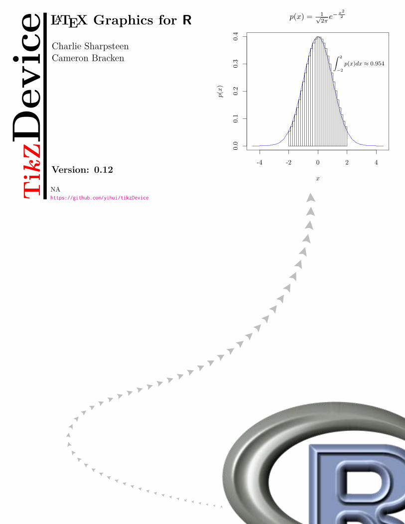
Version: 0.12-4 -2 0 2 4
0.0
0.1
0.2
0.3
0.4
x
p(x
)
p(x) = 1√
2π
e−x
2
2
∫2
−2
p(x)dx ≈ 0.954
Contents i
Contents
1 Introduction 11.1 Acknowledgements . . . . . . . . . . . . . . . . . . . . . . . . . . . . . . . . . . . . . . . . . . . . . . 2
I Usage and Examples 3
2 Loading the Package 42.1 Options That Affect Package Behavior . . . . . . . . . . . . . . . . . . . . . . . . . . . . . . . . . . . 5
The tikzDefaultEngine Option . . . . . . . . . . . . . . . . . . . . . . . . . . . . . . . . . . . . . . . 5The tikzLatex, tikzXelatex and tikzLualatex Options . . . . . . . . . . . . . . . . . . . . . . . . . . . 5The tikzMetricsDictionary Option . . . . . . . . . . . . . . . . . . . . . . . . . . . . . . . . . . . . . 5The tikzDocumentDeclaration Option . . . . . . . . . . . . . . . . . . . . . . . . . . . . . . . . . . . 6The tikzLatexPackages, tikzXelatexPackages and tikzLualatexPackages Options . . . . . . . . . . . 6The tikzMetricPackages and tikzUnicodeMetricPackages Options . . . . . . . . . . . . . . . . . . . . . 7The tikzFooter Option . . . . . . . . . . . . . . . . . . . . . . . . . . . . . . . . . . . . . . . . . . . . . 7The tikzSanitizeCharacters and tikzReplacementCharacters Options . . . . . . . . . . . . . . . . . . . 7The tikzLwdUnit Option . . . . . . . . . . . . . . . . . . . . . . . . . . . . . . . . . . . . . . . . . . . . 7The deprecated tikzRasterResolution Option . . . . . . . . . . . . . . . . . . . . . . . . . . . . . . . 8The tikzPdftexWarnUTF Option . . . . . . . . . . . . . . . . . . . . . . . . . . . . . . . . . . . . . . 8
3 The tikz Function 83.1 Description . . . . . . . . . . . . . . . . . . . . . . . . . . . . . . . . . . . . . . . . . . . . . . . . . . 83.2 Usage . . . . . . . . . . . . . . . . . . . . . . . . . . . . . . . . . . . . . . . . . . . . . . . . . . . . . 83.3 Font Size Calculations . . . . . . . . . . . . . . . . . . . . . . . . . . . . . . . . . . . . . . . . . . . . 9
UTF-8 Output . . . . . . . . . . . . . . . . . . . . . . . . . . . . . . . . . . . . . . . . . . . . . . . . 103.4 Examples . . . . . . . . . . . . . . . . . . . . . . . . . . . . . . . . . . . . . . . . . . . . . . . . . . . 10
Default Mode . . . . . . . . . . . . . . . . . . . . . . . . . . . . . . . . . . . . . . . . . . . . . . . . . 10bareBones Mode . . . . . . . . . . . . . . . . . . . . . . . . . . . . . . . . . . . . . . . . . . . . . . . 12standAlone Mode . . . . . . . . . . . . . . . . . . . . . . . . . . . . . . . . . . . . . . . . . . . . . . . 14console output Mode . . . . . . . . . . . . . . . . . . . . . . . . . . . . . . . . . . . . . . . . . . . . . 15Using X ELATEX . . . . . . . . . . . . . . . . . . . . . . . . . . . . . . . . . . . . . . . . . . . . . . . . 15Annotating Graphics with TikZ Commands . . . . . . . . . . . . . . . . . . . . . . . . . . . . . . . . . 17tikz vs. pdf for plotmath symbols and Unicode characters . . . . . . . . . . . . . . . . . . . . . . . . 20
4 The getLatexCharMetrics and getLatexStrWidth Functions 214.1 Description . . . . . . . . . . . . . . . . . . . . . . . . . . . . . . . . . . . . . . . . . . . . . . . . . . . 214.2 Usage . . . . . . . . . . . . . . . . . . . . . . . . . . . . . . . . . . . . . . . . . . . . . . . . . . . . . . 214.3 Examples . . . . . . . . . . . . . . . . . . . . . . . . . . . . . . . . . . . . . . . . . . . . . . . . . . . . 21
II Installation Guide 24
5 Obtaining a LATEX Distribution 255.1 Windows . . . . . . . . . . . . . . . . . . . . . . . . . . . . . . . . . . . . . . . . . . . . . . . . . . . 255.2 UNIX/Linux . . . . . . . . . . . . . . . . . . . . . . . . . . . . . . . . . . . . . . . . . . . . . . . . . 255.3 Mac OS X . . . . . . . . . . . . . . . . . . . . . . . . . . . . . . . . . . . . . . . . . . . . . . . . . . . 255.4 Installing TikZ and Other Packages . . . . . . . . . . . . . . . . . . . . . . . . . . . . . . . . . . . . 25
Using a LATEX Package Manager . . . . . . . . . . . . . . . . . . . . . . . . . . . . . . . . . . . . . . 26Manual Installation . . . . . . . . . . . . . . . . . . . . . . . . . . . . . . . . . . . . . . . . . . . . . . 26
TikZDevice LATEX Graphics for R
Contents ii
IIIPackage Internals 28
6 Introduction and Background 29
7 Anatomy of an R Graphics Device 297.1 Drawing Routines . . . . . . . . . . . . . . . . . . . . . . . . . . . . . . . . . . . . . . . . . . . . . . 297.2 Font Metric Routines . . . . . . . . . . . . . . . . . . . . . . . . . . . . . . . . . . . . . . . . . . . . . 307.3 Utility Routines . . . . . . . . . . . . . . . . . . . . . . . . . . . . . . . . . . . . . . . . . . . . . . . . 30
8 Calculating Font Metrics 30Character Metrics . . . . . . . . . . . . . . . . . . . . . . . . . . . . . . . . . . . . . . . . . . . . . . . 31Calling R Functions from C Functions . . . . . . . . . . . . . . . . . . . . . . . . . . . . . . . . . . . . 31Implementing a System Call to LATEX . . . . . . . . . . . . . . . . . . . . . . . . . . . . . . . . . . . 33
9 On the Importance of Font and Style Consistency in Reports 379.1 The pgfSweave Package and Automatic Report Generation . . . . . . . . . . . . . . . . . . . . . . . . 37
Bibliography 38
TikZDevice LATEX Graphics for R
Introduction 1
Introduction
Chapter 1
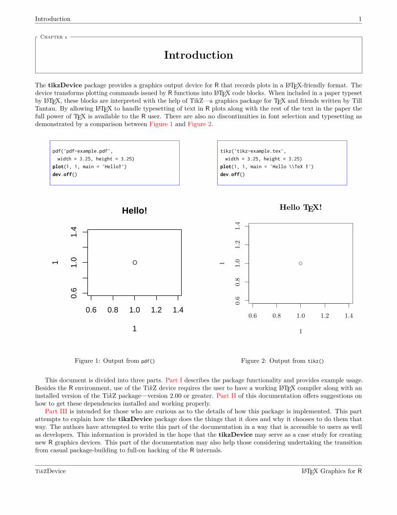
The tikzDevice package provides a graphics output device for R that records plots in a LATEX-friendly format. Thedevice transforms plotting commands issued by R functions into LATEX code blocks. When included in a paper typesetby LATEX, these blocks are interpreted with the help of TikZ—a graphics package for TEX and friends written by TillTantau. By allowing LATEX to handle typesetting of text in R plots along with the rest of the text in the paper thefull power of TEX is available to the R user. There are also no discontinuities in font selection and typesetting asdemonstrated by a comparison between Figure 1 and Figure 2.
pdf('pdf-example.pdf',
width = 3.25, height = 3.25)
plot(1, 1, main = 'Hello!')
dev.off()
●
0.6 0.8 1.0 1.2 1.4
0.6
1.0
1.4
Hello!
1
1
Figure 1: Output from pdf()
tikz('tikz-example.tex',
width = 3.25, height = 3.25)
plot(1, 1, main = 'Hello \\TeX !')
dev.off()
0.6 0.8 1.0 1.2 1.4
0.6
0.8
1.0
1.2
1.4
Hello TEX!
1
1
Figure 2: Output from tikz()
This document is divided into three parts. Part I describes the package functionality and provides example usage.Besides the R environment, use of the TikZ device requires the user to have a working LATEX compiler along with aninstalled version of the TikZ package—version 2.00 or greater. Part II of this documentation offers suggestions onhow to get these dependencies installed and working properly.
Part III is intended for those who are curious as to the details of how this package is implemented. This partattempts to explain how the tikzDevice package does the things that it does and why it chooses to do them thatway. The authors have attempted to write this part of the documentation in a way that is accessible to users as wellas developers. This information is provided in the hope that the tikzDevice may serve as a case study for creatingnew R graphics devices. This part of the documentation may also help those considering undertaking the transitionfrom casual package-building to full-on hacking of the R internals.
TikZDevice LATEX Graphics for R
Introduction 2
1.1 Acknowledgements
This package would not have been possible without the hard work and ingenuity of many individuals. This packagestraddles the divide between two great open source communities—the R programming language and the TEXtypesetting system. It is our hope that this work will make it easier for users to leverage the strengths of bothsystems.
First off, we would like to thank the R Core Team for creating such a wonderful, open and flexible programmingenvironment. Compared to other languages we have used, creating packages and extensions for R has always been aliberating experience.
This package started as a fork of the PicTEX device created by Valerio Aimale which is part of the R core graphicssystem. Without access to this simple, compact example of implementing a graphics device we likely would haveabandoned the project in its infancy. We would also like to thank Paul Murrell for all of his work on the R graphicssystem and especially for his research and documentation concerning the differences between the font systems usedby TEX and R.
This package also owes its existence to Friedrich Leisch’s work on the Sweave system and Roger D. Peng’scacheSweave extension. These two tools got us interested in the concept of Literate Programming and developmentof this package was driven by our desire to achieve a more seamless union between our reports and our code.
The performance of this package is also enhanced by the database capabilities provided by Roger D. Peng’sfilehash package. Without this package, the approach to calculating font metrics taken by the tikzDevice wouldbe infeasible.
Last, but certainly not least, we would like to thank Till Tantau, Mark Wibrow and the rest of the PGF/TikZteam for creating the LATEX graphics package that makes the output of this device meaningful. We would also like toexpress deep appreciation for the beautiful documentation that has been created for the TikZ system.
As always, there are many more who have contributed in ways too numerous to list.
Thank you!—The tikzDevice Team
TikZDevice LATEX Graphics for R
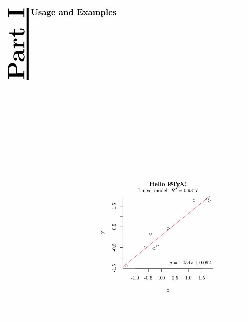
Part
I Usage and Examples
-1.0 -0.5 0.0 0.5 1.0 1.5
-1.5
-0.5
0.5
1.5
Hello LATEX!
x
y
Linear model: R2 = 0.9377
y = 1.054x + 0.092
Loading the Package 4
Loading the Package
Chapter 2
The functions in the tikzDevice package are made accessible in the R environment by using library():
library(tikzDevice)
Upon loading, the package will search for the following LATEX compilers:
• pdfLATEX
• X ELATEX
• LuaLATEX
Access to LATEX is essential for the device to produce output as the compiler is queried for font metrics whenconstructing plots that contain text. For more information on why communication between the device and LATEX isnecessary, see Part III. The package will fail to load if pdfLATEX cannot be located. The presence of the X ELATEX andLuaLATEX compilers is optional. When the package loads successfully, a startup message will be printed that lookssimilar to the following:
Loading required package: filehash
filehash: Simple key-value database (2.2 2011-07-21)
tikzDevice: R Graphics Output in LaTeX Format (v0.7)
LaTeX found in the PATH using the command: pdflatex
XeLaTeX found in the PATH using the command: xelatex
LuaLaTeX found in the PATH using the command: lualatex
If a working pdfLATEX compiler cannot be found, the tikzDevice package will fail to load and a warning messagewill be displayed:
Error : .onLoad failed in loadNamespace() for 'tikzDevice', details:
call: fun(libname, pkgname)
error:
An appropriate LaTeX compiler could not be found.
Access to LaTeX is required in order for the TikZ device
to produce output.
The following places were tested for a valid LaTeX compiler:
the global option: tikzLatex
the environment variable: R_LATEXCMD
the environment variable: R_PDFLATEXCMD
the global option: latexcmd
the PATH using the command: pdflatex
the PATH using the command: latex
the PATH using the command: /usr/texbin/pdflatex
...
Error: loading failed
TikZDevice LATEX Graphics for R
Loading the Package 5
In this case, tikzDevice has done its very best to locate a working compiler and came up empty. If you havea working LATEX compiler, the next section describes how to inform the tikzDevice package of its location. Forsuggestions on how to obtain a LATEX compiler, see Part II.
2.1 Options That Affect Package Behavior
The tikzDevice package is influenced by a number of options that may be set locally in your R scripts or in theR console or globally in a .Rprofile file. All of the options can be set by using options(<option> = <value>). Theseoptions allow for the use of custom documentclass declarations, LATEX packages, and typesetting engines (e.g. X ELATEXor LuaLATEX).
For convenience the function setTikzDefaults() is provided which sets all the global options back to their originalvalues.
The proper placement of a .Rprofile file is explained in the R manual page ?Startup. For the details of why callingthe LATEX compiler is necessary, see Part III.
A lot of power is given to you through these global options, and with great power comes great responsibility.For example, if you do not include the TikZ package in the tikzLatexPackages option then all of the string metriccalculations will fail. Or if you use a different font when compiling than you used for calculating metrics, strings maybe placed incorrectly. There are innumerable ways for packages to clash in LATEX so be aware.
The tikzDefaultEngine Option
This option specifies which typesetting engine the tikzDevice package will prefer. Current possible values are pdftex,xetex or luatex which will respectively trigger the use of the pdfLATEX, X ELATEX or LuaLATEX compilers.
options(tikzDefaultEngine = 'pdftex')
Default
options(tikzDefaultEngine = 'xetex')
options(tikzDefaultEngine = 'luatex')
Choosing the TEX engine
The tikzLatex, tikzXelatex and tikzLualatex Options
Specifies the location of the LATEX, X ELATEX and LuaLATEX compilers to be used by tikzDevice. Setting a defaultfor this option may help the package locate a missing compiler:
options(tikzLatex = '/path/to/pdflatex')
options(tikzXelatex = '/path/to/xelatex')
options(tikzLualatex = '/path/to/lualatex')
Setting default compilers in .Rprofile
The tikzMetricsDictionary Option
When using the graphics device provided by tikzDevice, you may notice that R appears to “lag" or “hang” whencommands such as plot() are executed. This is because the device must query the LATEX compiler for string widthsand font metrics. For a normal plot, this may happen dozens or hundreds of times—hence R becomes unresponsivefor a while. The good news is that the tikz() code is designed to cache the results of these computations so theyneed only be performed once for each string or character. By default, these values are stored in a temporary cachefile which is deleted when R is shut down. Using the option tikzMetricsDictionary, a permanent cache file may bespecified:
TikZDevice LATEX Graphics for R
Loading the Package 6
options(tikzMetricsDictionary = '/path/to/dictionary/location')
Setting a location in .Rprofile for a permanent metrics dictionary
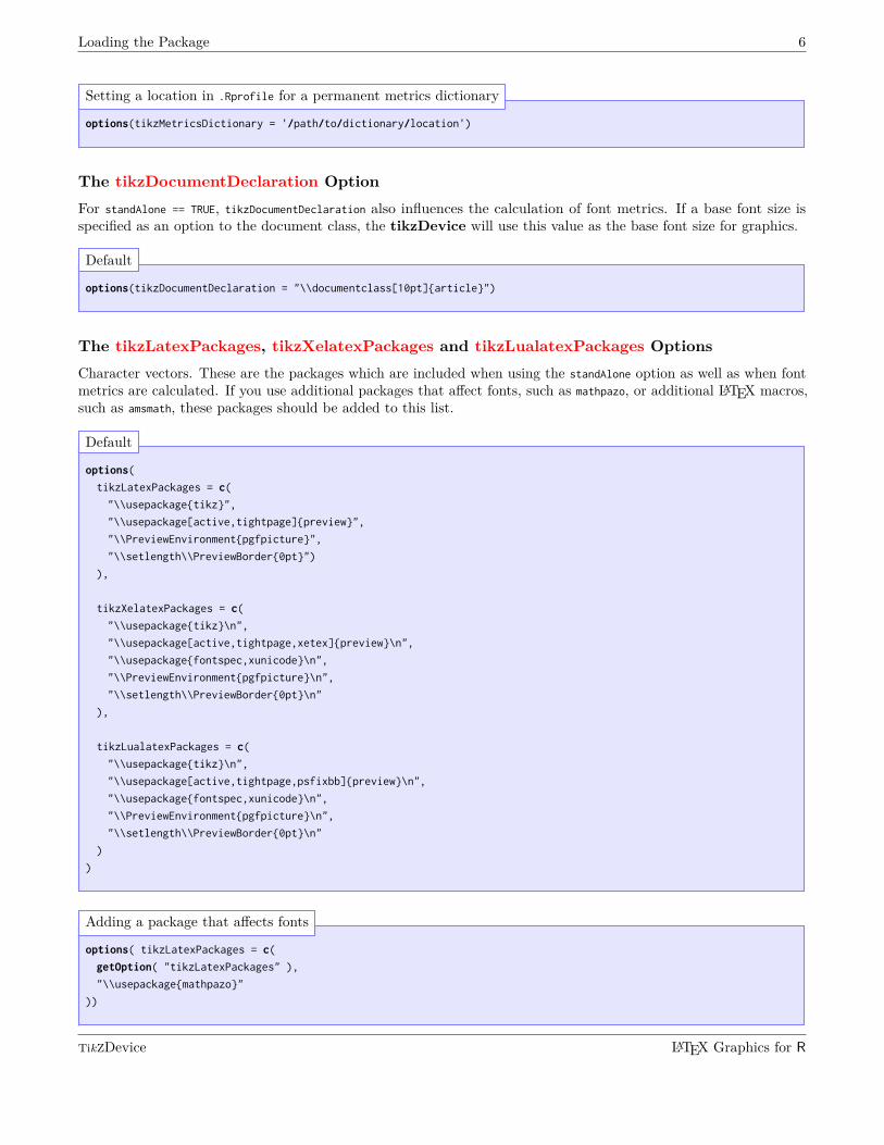
The tikzDocumentDeclaration Option
For standAlone == TRUE, tikzDocumentDeclaration also influences the calculation of font metrics. If a base font size isspecified as an option to the document class, the tikzDevice will use this value as the base font size for graphics.
options(tikzDocumentDeclaration = "\\documentclass[10pt]{article}")
Default
The tikzLatexPackages, tikzXelatexPackages and tikzLualatexPackages Options
Character vectors. These are the packages which are included when using the standAlone option as well as when fontmetrics are calculated. If you use additional packages that affect fonts, such as mathpazo, or additional LATEX macros,such as amsmath, these packages should be added to this list.
options(
tikzLatexPackages = c(
"\\usepackage{tikz}",
"\\usepackage[active,tightpage]{preview}",
"\\PreviewEnvironment{pgfpicture}",
"\\setlength\\PreviewBorder{0pt}")
),
tikzXelatexPackages = c(
"\\usepackage{tikz}\n",
"\\usepackage[active,tightpage,xetex]{preview}\n",
"\\usepackage{fontspec,xunicode}\n",
"\\PreviewEnvironment{pgfpicture}\n",
"\\setlength\\PreviewBorder{0pt}\n"
),
tikzLualatexPackages = c(
"\\usepackage{tikz}\n",
"\\usepackage[active,tightpage,psfixbb]{preview}\n",
"\\usepackage{fontspec,xunicode}\n",
"\\PreviewEnvironment{pgfpicture}\n",
"\\setlength\\PreviewBorder{0pt}\n"
)
)
Default
options( tikzLatexPackages = c(
getOption( "tikzLatexPackages" ),
"\\usepackage{mathpazo}"
))
Adding a package that affects fonts
TikZDevice LATEX Graphics for R
Loading the Package 7
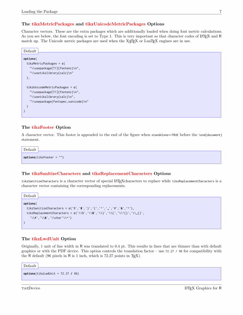
The tikzMetricPackages and tikzUnicodeMetricPackages Options
Character vectors. These are the extra packages which are additionally loaded when doing font metric calculations.As you see below, the font encoding is set to Type 1. This is very important so that character codes of LATEX and R
match up. The Unicode metric packages are used when the X ETEX or LuaTEX engines are in use.
options(
tikzMetricPackages = c(
"\\usepackage[T1]{fontenc}\n",
"\\usetikzlibrary{calc}\n"
),
tikzUnicodeMetricPackages = c(
"\\usepackage[T1]{fontenc}\n",
"\\usetikzlibrary{calc}\n",
"\\usepackage{fontspec,xunicode}\n"
)
)
Default
The tikzFooter Option
A character vector. This footer is appended to the end of the figure when standAlone==TRUE before the \end{document}
statement.
options(tikzFooter = "")
Default
The tikzSanitizeCharacters and tikzReplacementCharacters Options
tikzSanitizeCharacters is a character vector of special LATEXcharacters to replace while tikzReplacementCharacters is acharacter vector containing the corresponding replacements.
options(
tikzSanitizeCharacters = c('%','$','}','{','^','_','#','&','~'),
tikzReplacementCharacters = c('\\%','\\$','\\}','\\{','\\^{}','\\_{}',
'\\#','\\&','\\char`\\~')
)
Default
The tikzLwdUnit Option
Originally, 1 unit of line width in R was translated to 0.4 pt. This results in lines that are thinner than with defaultgraphics or with the PDF device. This option controls the translation factor – use 72.27 / 96 for compatibility withthe R default (96 pixels in R is 1 inch, which is 72.27 points in TEX).
options(tikzLwdUnit = 72.27 / 96)
Default
TikZDevice LATEX Graphics for R
The tikz Function 8
The deprecated tikzRasterResolution Option
When tikz is requested to add a raster to a graphic, the raster is written to a PNG file which is then included bythe LATEX code. In the current version, the raster is always written “as is” (after mirroring has been applied) usingpng::writePNG() (Urbanek, 2013). No resampling or transformation of any kind are applied in this process, rotationand interpolation are carried out by LATEX.
The tikzPdftexWarnUTF Option
A TRUE/FALSE value that controls whether warnings are printed if Unicode characters are sent to a device using thepdfTEX engine.
options(tikzPdftexWarnUTF = TRUE)
Default
The tikz Function
Chapter 3
3.1 Description
The tikz function provides most of the functionality of the tikzDevice package. This function opens an R graphicsdevice that records plots as a series of TikZ commands. The device supports many levels of output that range fromstand-alone LATEX documents that may be compiled into figures to code chunks that must be incorporated intoexisting LATEX documents using the \include{} macro.
3.2 Usage
The tikz function opens a new graphics device and may be called with the following arguments:
tikz(file = ifelse(onefile, "./Rplots.tex", "./Rplot%03d.tex"), width = 7,
height = 7, onefile = TRUE, bg = "transparent", fg = "black",
pointsize = 10, lwdUnit = getOption("tikzLwdUnit"), standAlone = FALSE,
bareBones = FALSE, console = FALSE, sanitize = FALSE,
engine = getOption("tikzDefaultEngine"),
documentDeclaration = getOption("tikzDocumentDeclaration"), packages,
footer = getOption("tikzFooter"),
symbolicColors = getOption("tikzSymbolicColors"),
colorFileName = "%s_colors.tex",
maxSymbolicColors = getOption("tikzMaxSymbolicColors"),
timestamp = TRUE, verbose = interactive())
file A character string indicating the desired path to the output file. It is recommended, but not required,that the filename end in .tex.
width The width of the output figure, in inches.
height The height of the output figure, in inches.
onefile Controls whether output should be directed to a single file containing one tikzpicture environment perplot or split into multiple files each containing a single tikzpicture environment.
TikZDevice LATEX Graphics for R
The tikz Function 9
bg The starting background color for the plot.
fg The starting foreground color for the plot.
pointsize Base pointsize used in the LaTeX document. This option is only referenced if a valid pointsize cannotbe extracted from the value of getOption("tikzDocumentDeclaration"). See Section 3.3 for more details.
lwdUnit The number of pts in LaTeX that lwd=1 in R is translated to. Defaults to 0.4 (LaTeX and TikZ default);for compatibility with R default, please use 72.27/96 (96 pixels in R is 1 inch, which is 72.27 points inTeX). See also Section 2.1, “Options That Affect Package Behavior.”
standAlone A logical value indicating whether the resulting file should be suitable for direct processing byLATEX.
bareBones A logical value indicating whether TikZ code is produced without being placed within a tikzpicture
environment.
console Controls whether output is directed to the R console. This is useful for dumping TikZ output directlyinto a LATEX document via sink. If TRUE, the file argument is ignored. Setting file=´´ is equivalent tosetting console=TRUE.
sanitize Should special latex characters be replaced (Default FALSE). See Section 2.1, “Options That AffectPackage Behavior” for which characters are replaced.
engine A string specifying which TEX engine to use. Possible values are ’pdftex’, ’xetex’ and ’luatex’.
documentDeclaration See Section 2.1, “Options That Affect Package Behavior.”
packages See Section 2.1, “Options That Affect Package Behavior.”
footer See Section 2.1, “Options That Affect Package Behavior.”
The first six options should be familiar to anyone who has used the default graphics devices shipped with R. Theoptions standAlone and bareBones are specific to the tikz() graphics device and affect the structure the output file.Using these options tikz supports three modes of output:
• Graphics production as complete LATEX files suitable for compilation.
• Graphics production as complete figures suitable for inclusion in LATEX files.
• Graphics production as raw figure code suitable for inclusion in an enclosing tikzpicture environment in a LATEXfile.
3.3 Font Size Calculations
The overarching goal of the tikzDevice is to provide seamless integration between text in R graphics and the text ofLATEX documents that contain those graphics. In order to achieve this integration the device must translate font sizesspecified in R to corresponding font sizes in LATEX. The issue is that font sizes in LATEX are controlled by a “base fontsize” that is specified at the beginning of the document—typically 10pt. There is no easy way in LATEX to change thefont size to a new numerical value, such as 16pt for a plot title. Fortunately, the TikZ graphics system allows text tobe resized using a scaling factor. The tikzDevice calculates a scaling factor used to approximate other font sizesusing the following three inputs:
• The “base font size” specified when the graphics device is created.
• The “character expansion factor” parameter, specified using the ‘cex’ argument to functions such as describedin the documentation of the R function par.
• The “font size” parameter, specified using the ‘ps’ argument to functions such as par or the ‘fontsize’ argumentto functions such as gpar.
TikZDevice LATEX Graphics for R
The tikz Function 10
The calculation used is:
Scaling Factor = cex ·
ps
base font size
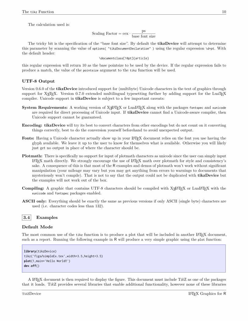
The tricky bit is the specification of the “base font size”. By default the tikzDevice will attempt to determinethis parameter by scanning the value of options( "tikzDocumentDeclaration" ) using the regular expression \d+pt. Withthe default header:
\documentclass[10pt]{article}
this regular expression will return 10 as the base pointsize to be used by the device. If the regular expression fails toproduce a match, the value of the pointsize argument to the tikz function will be used.
UTF-8 Output
Version 0.6.0 of the tikzDevice introduced support for (multibyte) Unicode characters in the text of graphics throughsupport for X ETEX. Version 0.7.0 extended multilingual typesetting further by adding support for the LuaTEXcompiler. Unicode support in tikzDevice is subject to a few important caveats:
System Requirements: A working version of X ELATEX or LuaLATEX along with the packages fontspec and xunicode
are required for direct processing of Unicode input. If tikzDevice cannot find a Unicode-aware compiler, thenUnicode support cannot be guaranteed.
Encoding: tikzDevice will try its best to convert characters from other encodings but do not count on it convertingthings correctly, best to do the conversion yourself beforehand to avoid unexpected output.
Fonts: Having a Unicode character actually show up in your LATEX document relies on the font you use having theglyph available. We leave it up to the user to know for themselves what is available. Otherwise you will likelyjust get no output in place of where the character should be.
Plotmath: There is specifically no support for input of plotmath characters as unicode since the user can simply inputLATEX math directly. We strongly encourage the use of LATEX math over plotmath for style and consistency’ssake. A consequence of this is that most of the R examples and demos of plotmath won’t work without significantmanipulation (your mileage may vary but you may get anything from errors to warnings to documents thatmysteriously won’t compile). That is not to say that the output could not be duplicated with tikzDevice butthe examples will not work out of the box.
Compiling: A graphic that contains UTF-8 characters should be compiled with X ELATEX or LuaLATEX with thexunicode and fontspec packages enabled.
ASCII only: Everything should be exactly the same as previous versions if only ASCII (single byte) characters areused (i.e. character codes less than 132).
3.4 Examples
Default Mode
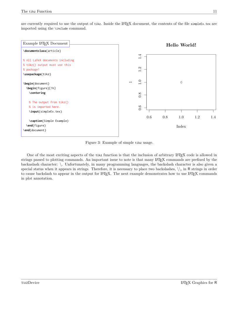
The most common use of the tikz function is to produce a plot that will be included in another LATEX document,such as a report. Running the following example in R will produce a very simple graphic using the plot function:
library(tikzDevice)
tikz('figs/simpleEx.tex',width=3.5,height=3.5)
plot(1,main='Hello World!')
dev.off()
A LATEX document is then required to display the figure. This document must include TikZ as one of the packagesthat it loads. TikZ provides several libraries that enable additional functionality, however none of these libraries
TikZDevice LATEX Graphics for R
The tikz Function 11
are currently required to use the output of tikz. Inside the LATEX document, the contents of the file simpleEx.tex areimported using the \include command.
\documentclass{article}
% All LaTeX documents including
% tikz() output must use this
% package!
\usepackage{tikz}
\begin{document}
\begin{figure}[!h]
\centering
% The output from tikz()
% is imported here.
\input{simpleEx.tex}
\caption{Simple Example}
\end{figure}
\end{document}
Example LATEX Document
0.6 0.8 1.0 1.2 1.4
0.6
0.8
1.0
1.2
1.4
Hello World!
Index1
Figure 3: Example of simple tikz usage.
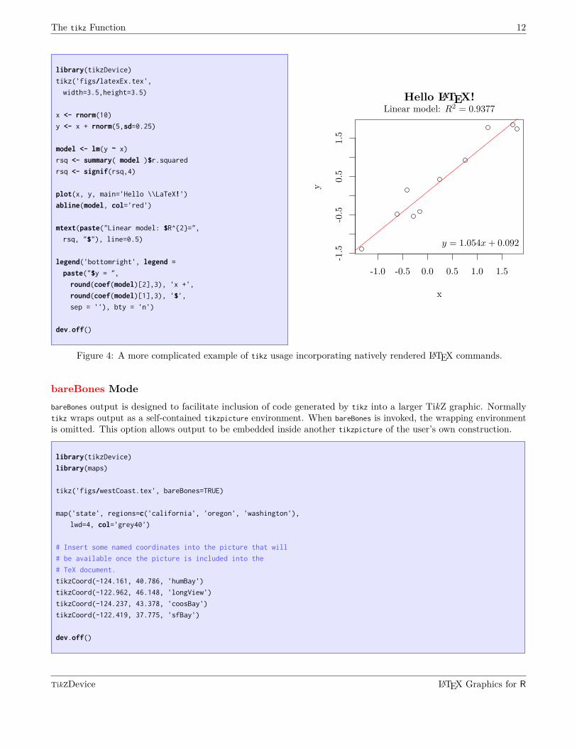
One of the most exciting aspects of the tikz function is that the inclusion of arbitrary LATEX code is allowed instrings passed to plotting commands. An important issue to note is that many LATEX commands are prefixed by thebackaslash character: \. Unfortunately, in many programming languages, the backslash character is also given aspecial status when it appears in strings. Therefore, it is necessary to place two backslashes, \\, in R strings in orderto cause backslash to appear in the output for LATEX. The next example demonstrates how to use LATEX commandsin plot annotation.
TikZDevice LATEX Graphics for R
The tikz Function 12
library(tikzDevice)
tikz('figs/latexEx.tex',
width=3.5,height=3.5)
x <- rnorm(10)
y <- x + rnorm(5,sd=0.25)
model <- lm(y ~ x)
rsq <- summary( model )$r.squared
rsq <- signif(rsq,4)
plot(x, y, main='Hello \\LaTeX!')
abline(model, col='red')
mtext(paste("Linear model: $R^{2}=",
rsq, "$"), line=0.5)
legend('bottomright', legend =
paste("$y = ",
round(coef(model)[2],3), 'x +',
round(coef(model)[1],3), '$',
sep = ''), bty = 'n')
dev.off()
-1.0 -0.5 0.0 0.5 1.0 1.5
-1.5
-0.5
0.5
1.5
Hello LATEX!
x
y
Linear model: R2 = 0.9377
y = 1.054x + 0.092
Figure 4: A more complicated example of tikz usage incorporating natively rendered LATEX commands.
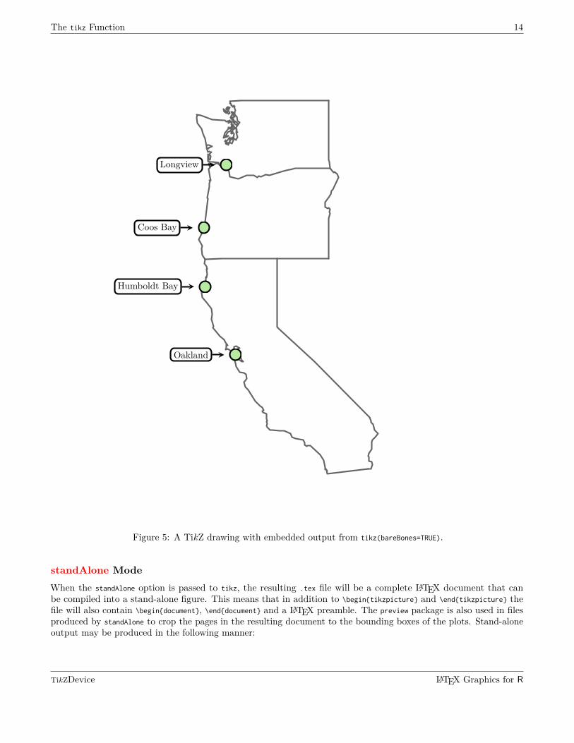
bareBones Mode
bareBones output is designed to facilitate inclusion of code generated by tikz into a larger TikZ graphic. Normallytikz wraps output as a self-contained tikzpicture environment. When bareBones is invoked, the wrapping environmentis omitted. This option allows output to be embedded inside another tikzpicture of the user’s own construction.
library(tikzDevice)
library(maps)
tikz('figs/westCoast.tex', bareBones=TRUE)
map('state', regions=c('california', 'oregon', 'washington'),
lwd=4, col='grey40')
# Insert some named coordinates into the picture that will
# be available once the picture is included into the
# TeX document.
tikzCoord(-124.161, 40.786, 'humBay')
tikzCoord(-122.962, 46.148, 'longView')
tikzCoord(-124.237, 43.378, 'coosBay')
tikzCoord(-122.419, 37.775, 'sfBay')
dev.off()
TikZDevice LATEX Graphics for R
The tikz Function 13
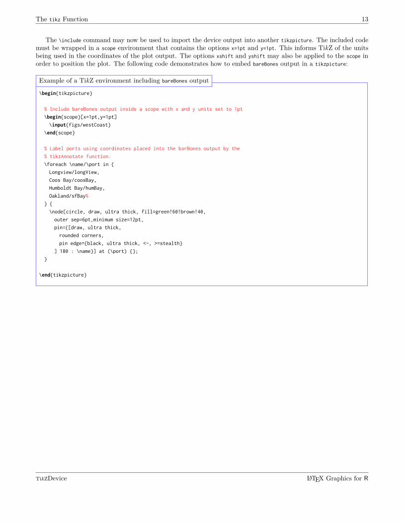
The \include command may now be used to import the device output into another tikzpicture. The included codemust be wrapped in a scope environment that contains the options x=1pt and y=1pt. This informs TikZ of the unitsbeing used in the coordinates of the plot output. The options xshift and yshift may also be applied to the scope inorder to position the plot. The following code demonstrates how to embed bareBones output in a tikzpicture:
\begin{tikzpicture}
% Include bareBones output inside a scope with x and y units set to 1pt
\begin{scope}[x=1pt,y=1pt]
\input{figs/westCoast}
\end{scope}
% Label ports using coordinates placed into the barBones output by the
% tikzAnnotate function.
\foreach \name/\port in {
Longview/longView,
Coos Bay/coosBay,
Humboldt Bay/humBay,
Oakland/sfBay%
} {
\node[circle, draw, ultra thick, fill=green!60!brown!40,
outer sep=6pt,minimum size=12pt,
pin={[draw, ultra thick,
rounded corners,
pin edge={black, ultra thick, <-, >=stealth}
] 180 : \name}] at (\port) {};
}
\end{tikzpicture}
Example of a TikZ environment including bareBones output
TikZDevice LATEX Graphics for R
The tikz Function 14
Longview
Coos Bay
Humboldt Bay
Oakland
Figure 5: A TikZ drawing with embedded output from tikz(bareBones=TRUE).
standAlone Mode
When the standAlone option is passed to tikz, the resulting .tex file will be a complete LATEX document that canbe compiled into a stand-alone figure. This means that in addition to \begin{tikzpicture} and \end{tikzpicture} thefile will also contain \begin{document}, \end{document} and a LATEX preamble. The preview package is also used in filesproduced by standAlone to crop the pages in the resulting document to the bounding boxes of the plots. Stand-aloneoutput may be produced in the following manner:
TikZDevice LATEX Graphics for R
The tikz Function 15
library(tikzDevice)
tikz('standAloneExample.tex',standAlone=TRUE)
plot(sin,-pi,2*pi,main="A Stand Alone TikZ Plot")
dev.off()
Note that files produced using the standAlone option should not be included in LATEX documents using the \input
command! Use \includegraphics or load the pdfpages package and use \includepdf.
console output Mode
Version 0.5.0 of tikzDevice introduced the console option. With this option, tikz will send output to stdout insteadof a file. This kind of output can be redirected to a file with sink or spit out directly into a TEX document from aSweave file so that the TEX file is self contained and does not include other files via \input. (Including the chunkoption strip.white=FALSE was necessary for some versions of tikzDevice prior to 0.7.2.)
\documentclass{article}
\usepackage{tikz}
\begin{document}
\begin{figure}[ht]
\centering
<<inline,echo=FALSE,results='tex'>>=
require(tikzDevice)
tikz(console=TRUE,width=5,height=5)
x <- rnorm(100)
plot(x)
dummy <- dev.off()
@
\caption{caption}
\label{fig:inline}
\end{figure}
\end{document}
Catching tikz output inside Sweave
Using X ELATEX
It is also possible to use other typesetting engines like X ELATEX by using the global options provided by tikzDevice.The following example was inspired by Dario Taraborelli and his article The Beauty of LaTeX.
# Set options for using XeLaTeX font variants.
options(tikzXelatexPackages = c(
getOption('tikzXelatexPackages'),
"\\usepackage[colorlinks, breaklinks]{hyperref}",
"\\usepackage{color}",
"\\definecolor{Gray}{rgb}{.7,.7,.7}",
"\\definecolor{lightblue}{rgb}{.2,.5,1}",
"\\definecolor{myred}{rgb}{1,0,0}",
"\\newcommand{\\red}[1]{\\color{myred} #1}",
TikZDevice LATEX Graphics for R
The tikz Function 16
"\\newcommand{\\reda}[1]{\\color{myred}\\fontspec[Variant=2]{Zapfino}#1}",
"\\newcommand{\\redb}[1]{\\color{myred}\\fontspec[Variant=3]{Zapfino}#1}",
"\\newcommand{\\redc}[1]{\\color{myred}\\fontspec[Variant=4]{Zapfino}#1}",
"\\newcommand{\\redd}[1]{\\color{myred}\\fontspec[Variant=5]{Zapfino}#1}",
"\\newcommand{\\rede}[1]{\\color{myred}\\fontspec[Variant=6]{Zapfino}#1}",
"\\newcommand{\\redf}[1]{\\color{myred}\\fontspec[Variant=7]{Zapfino}#1}",
"\\newcommand{\\redg}[1]{\\color{myred}\\fontspec[Variant=8]{Zapfino}#1}",
"\\newcommand{\\lbl}[1]{\\color{lightblue} #1}",
"\\newcommand{\\lbla}[1]{\\color{lightblue}\\fontspec[Variant=2]{Zapfino}#1}",
"\\newcommand{\\lblb}[1]{\\color{lightblue}\\fontspec[Variant=3]{Zapfino}#1}",
"\\newcommand{\\lblc}[1]{\\color{lightblue}\\fontspec[Variant=4]{Zapfino}#1}",
"\\newcommand{\\lbld}[1]{\\color{lightblue}\\fontspec[Variant=5]{Zapfino}#1}",
"\\newcommand{\\lble}[1]{\\color{lightblue}\\fontspec[Variant=6]{Zapfino}#1}",
"\\newcommand{\\lblf}[1]{\\color{lightblue}\\fontspec[Variant=7]{Zapfino}#1}",
"\\newcommand{\\lblg}[1]{\\color{lightblue}\\fontspec[Variant=8]{Zapfino}#1}",
"\\newcommand{\\old}[1]{",
"\\fontspec[Ligatures={Common, Rare},Variant=1,Swashes={LineInitial, LineFinal}]{Zapfino}",
"\\fontsize{25pt}{30pt}\\selectfont #1}%",
"\\newcommand{\\smallprint}[1]{\\fontspec{Hoefler Text}
\\fontsize{10pt}{13pt}\\color{Gray}\\selectfont #1}"
))
# Set the content using custom defined commands
label <- c(
"\\noindent{\\red d}roo{\\lbl g}",
"\\noindent{\\reda d}roo{\\lbla g}",
"\\noindent{\\redb d}roo{\\lblb g}",
"\\noindent{\\redf d}roo{\\lblf g}\\\\[.3cm]",
"\\noindent{\\redc d}roo{\\lblc g}",
"\\noindent{\\redd d}roo{\\lbld g}",
"\\noindent{\\rede d}roo{\\lble g}",
"\\noindent{\\redg d}roo{\\lblg g}\\\\[.2cm]"
)
# Set the titles using custom defined commands, and hyperlinks
title <- c(
paste(
"\\smallprint{D. Taraborelli (2008),",
"\\href{http://nitens.org/taraborelli/latex}",
"{The Beauty of \\LaTeX}}"
), paste(
"\\smallprint{\\\\\\emph{Some rights reserved}.",
"\\href{http://creativecommons.org/licenses/by-sa/3.0/}",
"{\\textsc{cc-by-sa}}}"
))
# Draw the graphic
tikz('xelatexEx.tex',
standAlone=TRUE,width=5,height=5,
engine = 'xetex')
lim <- 0:(length(label)+1)
plot(lim,lim,cex=0,pch='.',xlab = title[2],ylab='', main = title[1])
for(i in 1:length(label))
text(i,i,label[i])
TikZDevice LATEX Graphics for R
The tikz Function 17
dev.off()
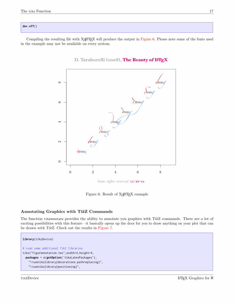
Compiling the resulting file with X ELATEX will produce the output in Figure 6. Please note some of the fonts usedin the example may not be available on every system.
..
0
.
2
.
4
.
6
.
8
.
0
.
2
.
4
.
6
.
8
.
D. Taraborelli (2008), The Beauty of LATEX
.Some rights reserved. - y-s
.
droog
.
droog
.
droog
.
droog
.
droog
.
droog
.
droog
.
droog
Figure 6: Result of X ELATEX example
Annotating Graphics with TikZ Commands
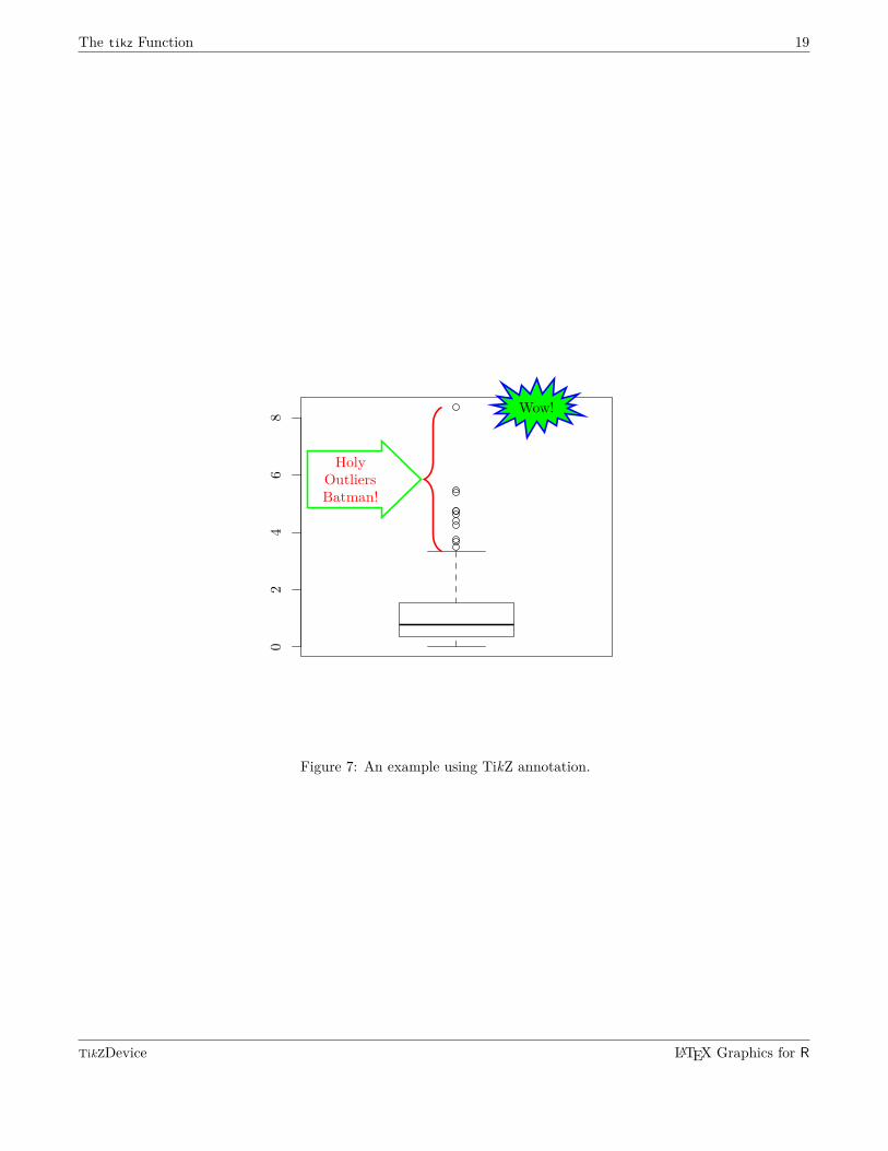
The function tikzAnnotate provides the ability to annotate you graphics with TikZ commands. There are a lot ofexciting possibilities with this feature—it basically opens up the door for you to draw anything on your plot that canbe drawn with TikZ. Check out the results in Figure 7.
library(tikzDevice)
# Load some additional TikZ libraries
tikz("figs/annotation.tex",width=4,height=4,
packages = c(getOption('tikzLatexPackages'),
"\\usetikzlibrary{decorations.pathreplacing}",
"\\usetikzlibrary{positioning}",
TikZDevice LATEX Graphics for R
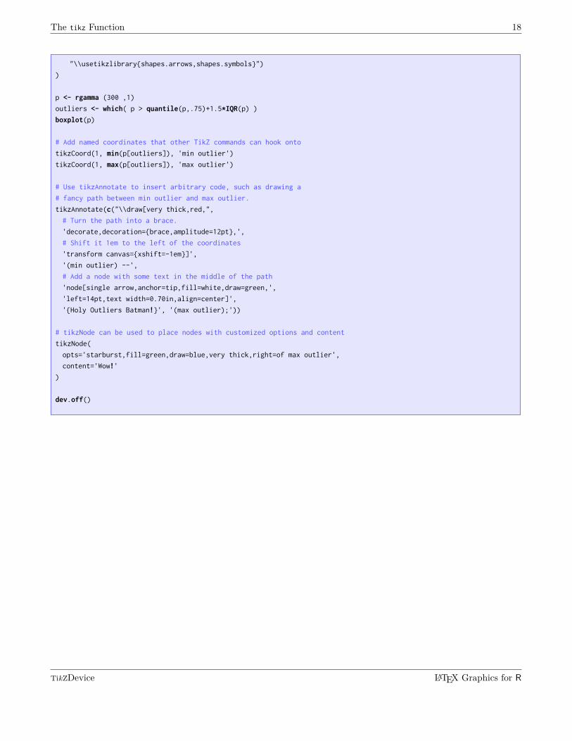
The tikz Function 18
"\\usetikzlibrary{shapes.arrows,shapes.symbols}")
)
p <- rgamma (300 ,1)
outliers <- which( p > quantile(p,.75)+1.5*IQR(p) )
boxplot(p)
# Add named coordinates that other TikZ commands can hook onto
tikzCoord(1, min(p[outliers]), 'min outlier')
tikzCoord(1, max(p[outliers]), 'max outlier')
# Use tikzAnnotate to insert arbitrary code, such as drawing a
# fancy path between min outlier and max outlier.
tikzAnnotate(c("\\draw[very thick,red,",
# Turn the path into a brace.
'decorate,decoration={brace,amplitude=12pt},',
# Shift it 1em to the left of the coordinates
'transform canvas={xshift=-1em}]',
'(min outlier) --',
# Add a node with some text in the middle of the path
'node[single arrow,anchor=tip,fill=white,draw=green,',
'left=14pt,text width=0.70in,align=center]',
'{Holy Outliers Batman!}', '(max outlier);'))
# tikzNode can be used to place nodes with customized options and content
tikzNode(
opts='starburst,fill=green,draw=blue,very thick,right=of max outlier',
content='Wow!'
)
dev.off()
TikZDevice LATEX Graphics for R
The tikz Function 19
02
46
8
HolyOutliersBatman!
Wow!
Figure 7: An example using TikZ annotation.
TikZDevice LATEX Graphics for R
Thetikz
Function
20
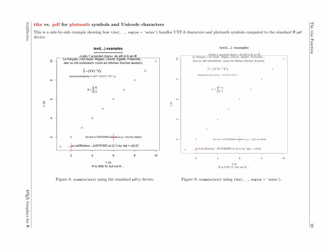
tikz vs. pdf for plotmath symbols and Unicode characters
This is a side-by-side example showing how tikz(..., engine = ’xetex’) handles UTF-8 characters and plotmath symbols compared to the standard R pdf
device.
2 4 6 8 10
24
68
10
text(...) examples
~~~~~~~~~~~~~~
R is GNU ©, but not ® ...
1:10
1:10
«Latin-1 accented chars»: éè øØ å<Å æ<Æ
the text is CENTERED around (x,y) = (6,2) by default
or Left/Bottom - JUSTIFIED at (2,1) by 'adj = c(0,0)'
β^ = (XtX)−1Xty
expression(hat(beta) == (X^t * X)^{-1} * X^t * y)
x =∑i=1
n xi
n
Le français, c'est façile: Règles, Liberté, Egalité, Fraternité...
Jetz no chli züritüütsch: (noch ein bißchen Zürcher deutsch)
Figure 8: example(text) using the standard pdf() device.
..
2
.
4
.
6
.
8
.
10
.
2
.
4
.
6
.
8
.
10
.
text(...) examples
.. R is GNU ©, but not ® ....1:10
.1:
10.
«Latin-1 accented chars»: éè øØ å<Å æ<Æ
.
the text is CENTERED around (x,y) = (6,2) by default
.
or Left/Bottom - JUSTIFIED at (2,1) by ’adj = c(0,0)’
.
β̂ = (XtX)−1Xty
.
\displaystyle\hat{\beta} = (XˆtX)ˆ{-1}Xˆty
.
x̄ =n∑
i=1
xi
n
.
Le français, c’est façile: Règles, Liberté, Egalité, Fraternité...
.
Jetz no chli züritüütsch: (noch ein bißchen Zürcher deutsch)
Figure 9: example(text) using tikz(..., engine = ’xetex’).
Tik
ZD
evice
LAT
EX
Grap
hics
forR
The getLatexCharMetrics and getLatexStrWidth Functions 21
The getLatexCharMetrics and getLatexStrWidth Functions
Chapter 4
4.1 Description
These two functions may be used to retrieve font metrics through the interface provided by the tikzDevice package.Cached values of the metrics are returned if they have been calculated by the tikzDevice before. If no cached valuesexist, a LATEX compiler will be invoked to generate them.
4.2 Usage
The font metric functions are called as follows:
getLatexStrWidth( texString, cex = 1, face= 1)
getLatexCharMetrics( charCode, cex = 1, face = 1 )
texString A string for which to compute the width. LATEX commands may be used in the string, however allbackslashes will need to be doubled.
charCode An integer between 32 and 126 which indicates a printable character in the ASCII symbol table usingthe T1 font encoding.
cex The character expansion factor to be used when determining metrics.
face An integer specifying the R font face to use during metric calculations. The accepted values are asfollows:
1: Text should be set in normal font face.
2: Text should be set in bold font face.
3: Text should be set in italic font face.
4: Text should be set in bold italic font face.
5: Text should be interpreted as plotmath symbol characters. Requests for font face 5 are currently ignored.
4.3 Examples
The getLatexStrWidth function may be used to calculate the width of strings containing fairly arbitrary LATEX commands.For example, consider the following calculations:
getLatexStrWidth( "The symbol: alpha" )
[1] 82.5354
getLatexStrWidth( "The symbol: $\\alpha$" )
[1] 65.08636
TikZDevice LATEX Graphics for R
The getLatexCharMetrics and getLatexStrWidth Functions 22
For the first calculation, the word “alpha” was interpreted as just a word and the widths of the characters ‘a’, ‘l’,‘p’, ‘h’ and ‘a’ were included in the string width. For the second string, \alpha was interpreted as a mathematicalsymbol and only the width of the symbol ‘α’ was included in the string width.
The getLatexCharWidth function must be passed an integer corresponding to an ASCII character code and returnsthree values:
• The ascent of the character. This is the distance between the baseline and the highest point of the character’sglyph.
• The descent of the character. This is the distance between the baseline and the lowest point of the character’sglyph.
• The width of the character.
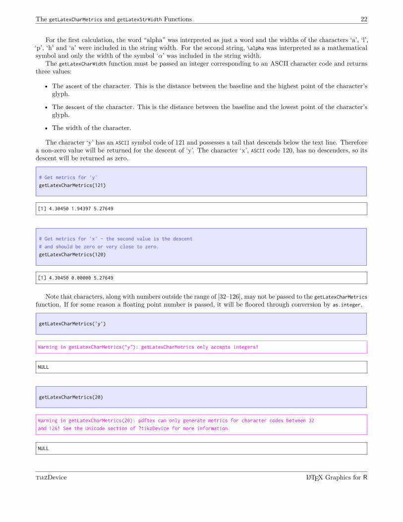
The character ‘y’ has an ASCII symbol code of 121 and possesses a tail that descends below the text line. Thereforea non-zero value will be returned for the descent of ‘y’. The character ‘x’, ASCII code 120, has no descenders, so itsdescent will be returned as zero.
# Get metrics for 'y'
getLatexCharMetrics(121)
[1] 4.30450 1.94397 5.27649
# Get metrics for 'x' - the second value is the descent
# and should be zero or very close to zero.
getLatexCharMetrics(120)
[1] 4.30450 0.00000 5.27649
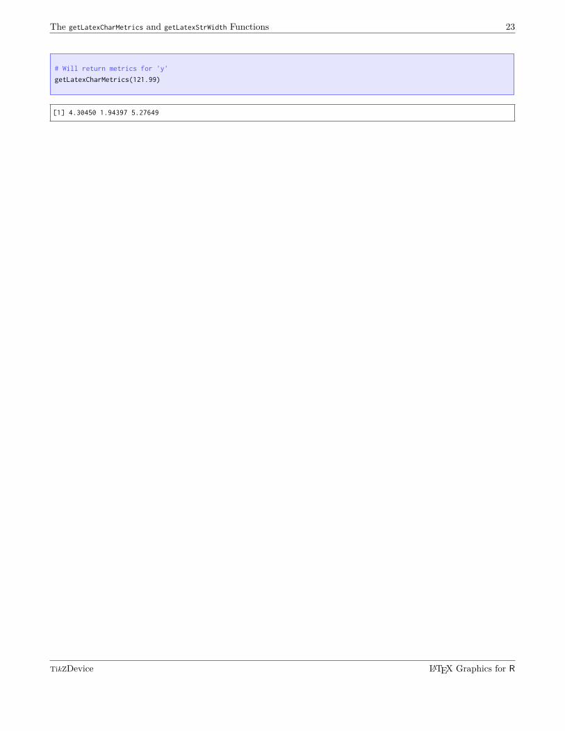
Note that characters, along with numbers outside the range of [32–126], may not be passed to the getLatexCharMetrics
function. If for some reason a floating point number is passed, it will be floored through conversion by as.integer.
getLatexCharMetrics('y')
Warning in getLatexCharMetrics("y"): getLatexCharMetrics only accepts integers!
NULL
getLatexCharMetrics(20)
Warning in getLatexCharMetrics(20): pdftex can only generate metrics for character codes between 32
and 126! See the Unicode section of ?tikzDevice for more information.
NULL
TikZDevice LATEX Graphics for R
The getLatexCharMetrics and getLatexStrWidth Functions 23
# Will return metrics for 'y'
getLatexCharMetrics(121.99)
[1] 4.30450 1.94397 5.27649
TikZDevice LATEX Graphics for R

Part
IIInstallation Guide
Obtaining a LATEX Distribution 25
Obtaining a LATEX Distribution
Chapter 5
This section offers pointers on how to obtain a LATEX distribution if there is not one already installed on your system.The distributions detailed in this section are favorites of the tikzDevice developers as they provide integratedpackage managers which greatly simplify the process of installing additional LATEX packages. Currently this section isnot, and may never be, a troubleshooting guide for LATEX installation. For those unfortunate situations we refer theuser to the documentation of each distribution.
A LATEX distribution provides the packages and support programs required by the tikzDevice and the documentsthat use its output. In addition to a LATEX compiler, a few extension packages are required. Section 5.4 describeshow to obtain and install these packages.
5.1 Windows
Windows users will probably prefer the MiKTeX distribution available at http://www.miktex.org. An amazing featureof the MiKTeX distribution is that it contains a package manager that will attempt to install missing packageson-the-fly. Normally when LATEX is compiling a document that tries to load a missing package it will wipe out with awarning message. When the MiKTeX compilers are used compilation will be suspended while the new package isdownloaded.
5.2 UNIX/Linux
For users running a Linux or UNIX operating system, we recommend the TeX Live distribution which is availableat http://www.tug.org/texlive/acquire.html. TeX Live is maintained by the TeX Users Group and a new version isreleased every year. We recommend using TeX Live 2008 or higher as the tlmgr package manager was introduced inthe 2008 distribution. Using tlmgr greatly simplifies the adding and removing packages from the distribution. Thewebsite offers an installation package, called install-tl.tar.gz or something similar, that contains a shell script thatcan be used to install an up-to-date version of the TeX Live distribution. Note that the version of TeX Live providedby many Linux package management systems sometimes lags behind the version provided directly by the TeX UsersGroup.
5.3 Mac OS X
For users running Apple’s OS X, we recommend the Mac TeX package available at http://www.tug.org/mactex/. MacTeX is basically TeX Live packaged inside a convenient OS X installer along with a few add-on packages. One strikingdifference between the Mac TeX and TeX Live installers is that the installer for Mac TeX includes the whole TeXLive distribution in the initial download- for TeX Live 2013 this amounts to approximately 2.3 GB. This is quite alarge download that contains several packages that the average or even advanced user will never ever use. To conservetime and space we recommend installing from the basic installer at http://www.tug.org/mactex/morepackages.html andusing the tlmgr utility to add desired add-on packages.
Adam R. Maxwell has created a very nice graphical interface to tlmgr for OS X called the TeX Live Utility. Itmay be obtained from http://code.google.com/p/mactlmgr/ and we highly recommend it.
5.4 Installing TikZ and Other Packages
Unsurprisingly, tikzDevice requires the TikZ package to be installed and available in order to function properly.TikZ is an abstraction of a lower-level graphics language called PGF and both are distributed as the the pgf package.Users who do no have a full TEX installation will also need to install a few more required packages:
pgf As mentioned, provides TikZ.
TikZDevice LATEX Graphics for R
Obtaining a LATEX Distribution 26
preview Used to crop documents in order to produce standalone figures.
ms Martin Schröder’s LaTeX packages. everyshi.sty lets us run commands at every shipped page.
graphics LATEX’s general-purpose graphics inclusion functionality.
pdftex-def Device-specific colour and graphics definitions when running pdfTEX/pdfLATEX.
oberdiek infwarerr.sty provides info/error/warning messages
ec (Font metrics for) the default font, European Computer Modern.
xcolor Used by TikZ to specify colors.
fontspec Used by LuaTEX and X ETEX to select fonts.
xunicode Assists LuaTEX and X ETEX with UTF-8 characters.
Using a LATEX Package Manager
The easiest way to install LATEX packages is by using a distribution that includes a package manager such as MiKTeXor TeX Live/Mac TeX. For Windows users, the MiKTeX package manager usually handles package installationautomagically during compilation of a document that is requesting a missing package. The MiKTeX package manager,mpm, can also be run manually from the command prompt:
mpm --install packagename
Using mpm to install packages
For versions of TeX Live and Mac TeX dated 2008 or newer, the tlmgr package manager is used in an almostidentical manner:
tlmgr install packagename
Using tlmgr to install packages
Manual Installation
Sometimes an automated package manager cannot be used. Common reasons may be that one is not available, as isthe case with the TeX Live 2007 distribution, or that when running the package manager you do not have writeaccess to the location where LATEX packages are stored, as is the case with accounts on shared computers. If this isthe case, a manual install may be the best option for making a LATEX package available.
Generally, the best place to find LATEX packages is the Comprehensive TeX Archive Network, or CTAN locatedat http://www.ctan.org. In the case of the PGF/TikZ package, the project homepage at http://www.sourceforge.net/
projects/pgf is also a good place to obtain the package—especially if you would like to play with the bleeding-edgedevelopment version.
Generally speaking, all LATEX packages are stored in a specially directory called a texmf folder. Most TEXdistributions allow for each user to have their own personal texmf folder somewhere in their home path. The mostusual locations, and here usual is an unfortunately loose term, are as follows:
~/texmf
For UNIX/Linux
~/Library/texmf
For Mac OS X
TikZDevice LATEX Graphics for R
Obtaining a LATEX Distribution 27
# None predefined. However the following command will open
# the MiKTeX options panel and a new texmf folder may be assigned
# under the "Roots" tab.
mo
For Windows, using MiKTeX
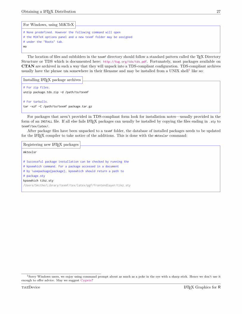
The location of files and subfolders in the texmf directory should follow a standard pattern called the TEX DirectoryStructure or TDS which is documented here: http://tug.org/tds/tds.pdf. Fortunately, most packages available onCTAN are archived in such a way that they will unpack into a TDS-compliant configuration. TDS-compliant archivesusually have the phrase tds somewhere in their filename and may be installed from a UNIX shell1 like so:
# For zip files.
unzip package.tds.zip -d /path/to/texmf
# For tarballs.
tar -xzf -C /path/to/texmf package.tar.gz
Installing LATEX package archives
For packages that aren’t provided in TDS-compliant form look for installation notes—usually provided in theform of an INSTALL file. If all else fails LATEX packages can usually be installed by copying the files ending in .sty totexmf/tex/latex/.
After package files have been unpacked to a texmf folder, the database of installed packages needs to be updatedfor the LATEX compiler to take notice of the additions. This is done with the mktexlsr command:
mktexlsr
# Successful package installation can be checked by running the
# kpsewhich command. For a package accessed in a document
# by \usepackage{package}, kpsewhich should return a path to
# package.sty
kpsewhich tikz.sty
/Users/Smithe/Library/texmf/tex/latex/pgf/frontendlayer/tikz.sty
Registering new LATEX packages
1Sorry Windows users, we enjoy using command prompt about as much as a poke in the eye with a sharp stick. Hence we don’t use it
enough to offer advice. May we suggest Cygwin?
TikZDevice LATEX Graphics for R
Part
III Package Internals
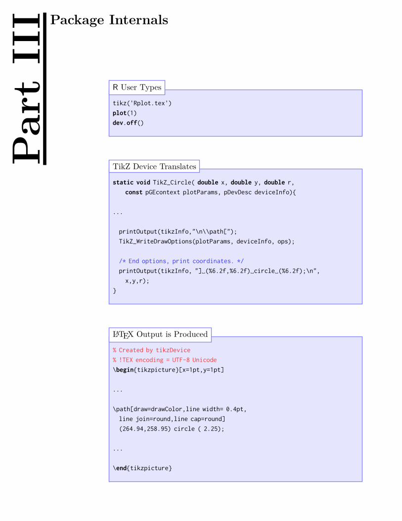
tikz('Rplot.tex')
plot(1)
dev.off()
R User Types
static void TikZ_Circle( double x, double y, double r,
const pGEcontext plotParams, pDevDesc deviceInfo){
...
printOutput(tikzInfo,"\n\\path[");
TikZ_WriteDrawOptions(plotParams, deviceInfo, ops);
/* End options, print coordinates. */
printOutput(tikzInfo, "]␣(%6.2f,%6.2f)␣circle␣(%6.2f);\n",
x,y,r);
}
TikZ Device Translates
% Created by tikzDevice
% !TEX encoding = UTF-8 Unicode
\begin{tikzpicture}[x=1pt,y=1pt]
...
\path[draw=drawColor,line width= 0.4pt,
line join=round,line cap=round]
(264.94,258.95) circle ( 2.25);
...
\end{tikzpicture}
LATEX Output is Produced
Introduction and Background 29
We will encourage you to developthe three great virtues of aprogrammer: laziness, impatience,and hubris.
Programming Perl
–Larry Wall
Introduction and Background
Chapter 6
We learn best through working with examples. When it comes to programming languages this involves taking workingcode that someone else has written, breaking it in as many places at it can possibly be broken, and then trying tobuild something out of the wreckage. Open source software facilitates this process wonderfully by ensuring the sourcecode of a project is always available for inspection and experimentation. The tikzDevice its self was created bydisassembling and then rebuilding Valerio Aimale’s PicTEX device driver which is a part of the R core codebase.
This section is our attempt to help anyone who may be experimenting with our code, and by extension theinternals of the R graphics system. There may also be useful, or useless, tidbits concerning building R packages andinteracting with the core R language. The R language can be extended in so many interesting and useful ways and itis our hope that the following documentation may provide a case study for anyone attempting such an extension.
We will make an attempt to assume no special expertise with any of the systems or programming languagesleveraged by this package and described by this documentation. Therefore, if you are an experienced developer andfind yourself thinking “My god, are they really about to launch into a description of how C header files work?”, pleasefeel free to skip ahead a few paragraphs. We received our formal introduction to computer programming in a collegeengineering program—therefore our programming background is rooted in Fortran (or, if you prefer, fortran). Weare attempting to write the sort of documentation that we would have found invaluable at the start of this project
Therefore, this section is for all the budding developers like ourselves out there—people who have done someprogramming and who are starting to take a close look at the nuts and bolts of the R programming environment. Ifyou feel like you are wandering through a vast forest getting smacked in the face by every branch then maybe thissection will help pull some of those branches out of the way...
...then again we have a lot of material to cover: R, C, LATEX, TikZ , typography and the details of computerizedfont systems. Our grip may fail and send those branches flying back with increased velocity.
We wish you luck!-The tikzDevice Team
Anatomy of an R Graphics Device
Chapter 7
The core of an R graphics device is a collection of functions, written in C, that perform various specialized tasks. Adescription of some of these functions can be found in the R Internals manual while the main documentation is in the C
header file GraphicsDevice.h. For most R installations this header file can be found in the directory R_HOME/include/R_ext.For copies of R distributed in source code form, GraphicsDevice.h is located inside R-version/src/include/R_ext. Thefollowing is a description of the functions each graphics device is expected to provide:
7.1 Drawing Routines
circle This function is required to draw a circle cen-tered at a given location with a given radius.
clip This function specifies a rectangular area tobe used a a clipping boundary for any deviceoutput that follows.
TikZDevice LATEX Graphics for R
Calculating Font Metrics 30
line This function draws a line between two points.
polygon This function draws lines between a list ofpoints and then connects the first point to thelast point.
polyline This function draws lines between a list ofpoints.
rect This function is given a lower left corner andan upper right corner and draws a rectanglebetween the two.
text This function inserts text at a given location.
7.2 Font Metric Routines
metricInfo This function is given the name of a single char-acter and reports the ascent, descent and widthof that character.
strWidth This function is given a text string and reportsthe width of that string.
7.3 Utility Routines
activate This function is called when the device is desig-nated as the active output device—i.e. by usingdev.set() in R
close This function is called when the device is shutdown—i.e. by using dev.off() in R
deactivate This function is called when another device isdesignated as the active output device.
locator This function is mainly used by devices witha GUI window and reports the location of amouseclick.
mode This function is called when a device beginsdrawing output and again when the device fin-ishes drawing output.
newPage This function initiates the creation of a newpage of output.
size This function reports the size of the canvas thedevice is drawing on.
Calculating Font Metrics
Chapter 8
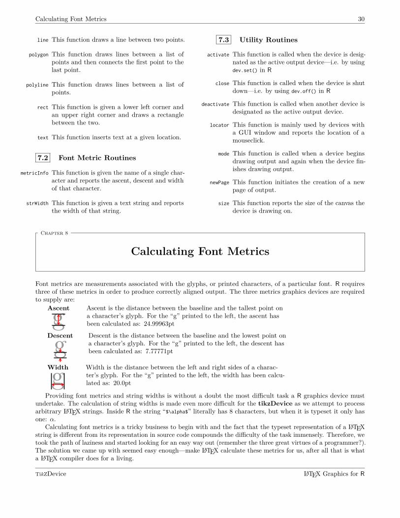
Font metrics are measurements associated with the glyphs, or printed characters, of a particular font. R requiresthree of these metrics in order to produce correctly aligned output. The three metrics graphics devices are requiredto supply are:
Ascent
gAscent is the distance between the baseline and the tallest point ona character’s glyph. For the “g” printed to the left, the ascent hasbeen calculated as: 24.99963pt
Descent
gDescent is the distance between the baseline and the lowest point ona character’s glyph. For the “g” printed to the left, the descent hasbeen calculated as: 7.77771pt
Width
gWidth is the distance between the left and right sides of a charac-ter’s glyph. For the “g” printed to the left, the width has been calcu-lated as: 20.0pt
Providing font metrics and string widths is without a doubt the most difficult task a R graphics device mustundertake. The calculation of string widths is made even more difficult for the tikzDevice as we attempt to processarbitrary LATEX strings. Inside R the string “$\alpha$” literally has 8 characters, but when it is typeset it only hasone: α.
Calculating font metrics is a tricky business to begin with and the fact that the typeset representation of a LATEXstring is different from its representation in source code compounds the difficulty of the task immensely. Therefore, wetook the path of laziness and started looking for an easy way out (remember the three great virtues of a programmer?).The solution we came up with seemed easy enough—make LATEX calculate these metrics for us, after all that is whata LATEX compiler does for a living.
TikZDevice LATEX Graphics for R
Calculating Font Metrics 31
Now, how to do that?
Character Metrics
As a starting point, let’s examine the interface of the C function that R calls in order to determine character metrics:
void (metricInfo)(int c, const pGEcontext gc,
double* ascent, double* descent, double* width,
pDevDesc dd);
Function declaration for metricInfo
The most important variables involved in the function are c, ascent, descent and width. The incoming variable isc, which contains the character for which R is requesting font metrics. Interestingly, c is passed as an integer, nota character as one might expect. What’s up with that? Well, the short answer is that R passes the ASCII or UTF8
symbol code of a character and not the character itself. How to use that character code to recover a character will beexplained later.
The outgoing variables are ascent, descent and width. The asterisks, ‘*’, in their definitions mean these variablesare passed as pointers as opposed to values. A complete discussion of the differences between pointers and valuescould, and has, filled up several chapters of several programming books. The important distinction in context of themetricInfo function is that when a number is assigned to a pointer variable, that number is available elsewhere afterthe function terminates. In contrast, when a number is assigned to a value variable, that number disappears whenthe function ends unless it is explicitly sent back out to the wide world through the return statement. So, the maintask of the metricInfo function is to assign values to ascent, descent and width.
The other two variables present in the function are the pGEcontext variable gc and the pDevDesc variable dd. gc
contains information such as the font face, foreground color, background color, character expansion factor, ect.currently in use by the graphics system. dd is the object which contains R’s representation of the graphics device. Forthe sake of simplifying the following discussion, we will ignore these variables.
So, to recap—we have an integer c coming in that represents a code for a character in the ASCII or UTF8 symboltables (for the sake of the following discussion, we will assume ASCII characters only). Our overall task is to somehowturn that integer into three numbers which can be assigned to the pointer variables ascent, descent and width. And,since we’re being lazy, we’ve decided that the best way to do that is to ask the LATEX compiler to compute thenumbers for us.
Recovering these numbers from the LATEX compiler involves the execution of three additional tasks:
1. We must write a LATEX input file that contains instructions for calculating the metrics.
2. We call the LATEX compiler to process that input file.
3. We must read the compiler’s output in order to recover the metrics.
Each of these tasks could be executed from inside our C function, metricInfo. However, we will run into somedifficulties—namely with step 2, which involves calling out to the operating system with orders to run LATEX. Eachoperating system handles these calls a little differently and our package must attempt to get this job done whether itis running on Windows, UNIX, Linux or Mac OS X.
Portable C code could be written to handle each of these situations, but that is starting to sound like work andwe’re trying to be lazy here. What we need is to be able to work at a higher level of abstraction. That is—instead ofusing C, we need to be working inside a language that shields us from such details as what operating system is beingused. R may have called this C function to calculate font metrics, but we really want to do the actual computationsback inside R.
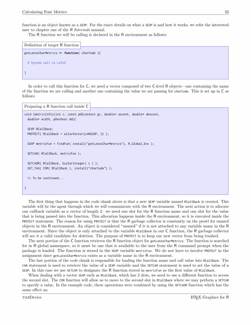
Calling R Functions from C Functions
The “Ritual of the Calling of the R Function” is easy enough to perform as long as you don’t have burning need toknow all the details of the objects you are handling. The C level representation of a R object such as a variable or
TikZDevice LATEX Graphics for R
Calculating Font Metrics 32
function is an object known as a SEXP. For the exact details on what a SEXP is and how it works, we refer the interesteduser to chapter one of the R Internals manual.
The R function we will be calling is declared in the R environment as follows:
getLatexCharMetrics <- function( charCode ){
# System call to LaTeX
}
Definition of target R function
In order to call this function for C, we need a vector composed of two C-level R objects—one containing the nameof the function we are calling and another one containing the value we are passing for charCode. This is set up in C asfollows:
void (metricInfo)(int c, const pGEcontext gc, double* ascent, double* descent,
double* width, pDevDesc dd){
SEXP RCallBack;
PROTECT( RCallBack = allocVector(LANGSXP, 2) );
SEXP metricFun = findFun( install("getLatexCharMetrics"), R_Global_Env );
SETCAR( RCallBack, metricFun );
SETCADR( RCallBack, ScalarInteger( c ) );
SET_TAG( CDR( RCallBack ), install("charCode") );
\\ To be continued...
}
Preparing a R function call inside C
The first thing that happens in the code chunk above is that a new SEXP variable named RCallBack is created. Thisvariable will be the agent through which we will communicate with the R environment. The next action is to allocateour callback variable as a vector of length 2– we need one slot for the R function name and one slot for the valuethat is being passed into the function. This allocation happens inside the R environment, so it is executed inside thePROTECT statement. The reason for using PROTECT is that the R garbage collector is constantly on the prowl for unusedobjects in the R environment. An object is considered “unused” if it is not attached to any variable name in the R
environment. Since the object is only attached to the variable RCallBack in our C function, the R garbage collectorwill see it a valid candidate for deletion. The purpose of PROTECT is to keep our new vector from being trashed.
The next portion of the C function retrieves the R function object for getLatexCharMetrics. The function is searchedfor in R global namespace, so it must be one that is available to the user from the R command prompt when thepackage is loaded. The function is stored in the SEXP variable metricFun. We do not have to involve PROTECT in theassignment since getLatexCharMetrics exists as a variable name in the R environment.
The last portion of the code chunk is responsible for loading the function name and call value into RCallBack. TheCAR statement is used to retrieve the value of a SEXP variable and the SETCAR statement is used to set the value of aSEXP. In this case we use SETCAR to designate the R function stored in metricFun as the first value of RCallBack.
When dealing with a vector SEXP such as RCallBack, which has 2 slots, we need to use a different function to accessthe second slot. The CDR function will allow us to move to the second slot in RCallBack where we may perform a SETCAR
to specify a value. In the example code, these operations were combined by using the SETCADR function which has thesame effect as:
TikZDevice LATEX Graphics for R
Calculating Font Metrics 33
SETCAR( CDR(RCallBack), ScalarInteger( c ) );
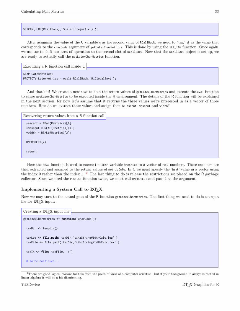
After assigning the value of the C variable c as the second value of RCallBack, we need to “tag” it as the value thatcorresponds to the charCode argument of getLatexCharMetrics. This is done by using the SET_TAG function. Once again,we use CDR to shift our area of operation to the second slot of RCallBack. Now that the RCallBack object is set up, weare ready to actually call the getLatexCharMetrics function.
SEXP LatexMetrics;
PROTECT( LatexMetrics = eval( RCallBack, R_GlobalEnv) );
Executing a R function call inside C
And that’s it! We create a new SEXP to hold the return values of getLatexCharMetrics and execute the eval functionto cause getLatexCharMetrics to be executed inside the R environment. The details of the R function will be explainedin the next section, for now let’s assume that it returns the three values we’re interested in as a vector of threenumbers. How do we extract these values and assign then to ascent, descent and width?
*ascent = REAL(RMetrics)[0];
*descent = REAL(RMetrics)[1];
*width = REAL(RMetrics)[2];
UNPROTECT(2);
return;
Recovering return values from a R function call
Here the REAL function is used to coerce the SEXP variable RMetrics to a vector of real numbers. These numbers arethen extracted and assigned to the return values of metricInfo. In C we must specify the ‘first’ value in a vector usingthe index 0 rather than the index 1. 2 The last thing to do is release the restrictions we placed on the R garbagecollector. Since we used the PROTECT function twice, we must call UNPROTECT and pass 2 as the argument.
Implementing a System Call to LATEX
Now we may turn to the actual guts of the R function getLatexCharMetrics. The first thing we need to do is set up afile for LATEX input:
getLatexCharMetrics <- function( charCode ){
texDir <- tempdir()
texLog <- file.path( texDir,'tikzStringWidthCalc.log' )
texFile <- file.path( texDir,'tikzStringWidthCalc.tex' )
texIn <- file( texFile, 'w')
# To be continued...
Creating a LATEX input file
2There are good logical reasons for this from the point of view of a computer scientist—but if your background in arrays is rooted in
linear algebra it will be a bit disorienting.
TikZDevice LATEX Graphics for R
Calculating Font Metrics 34
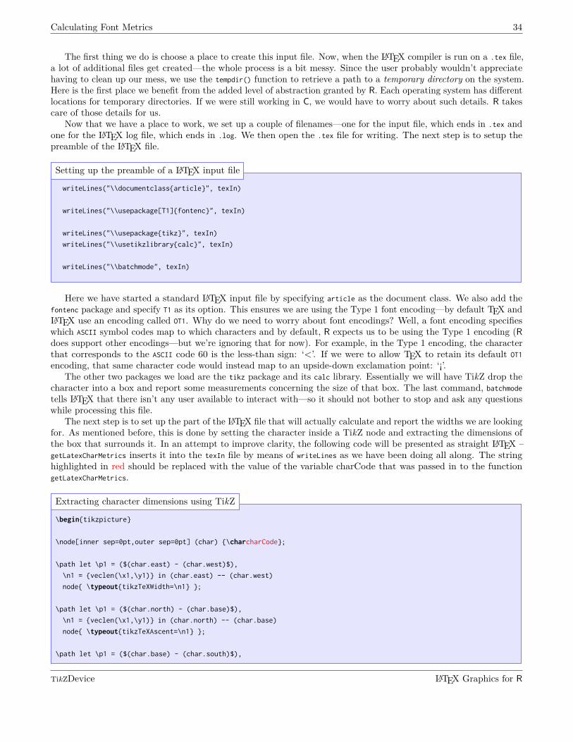
The first thing we do is choose a place to create this input file. Now, when the LATEX compiler is run on a .tex file,a lot of additional files get created—the whole process is a bit messy. Since the user probably wouldn’t appreciatehaving to clean up our mess, we use the tempdir() function to retrieve a path to a temporary directory on the system.Here is the first place we benefit from the added level of abstraction granted by R. Each operating system has differentlocations for temporary directories. If we were still working in C, we would have to worry about such details. R takescare of those details for us.
Now that we have a place to work, we set up a couple of filenames—one for the input file, which ends in .tex andone for the LATEX log file, which ends in .log. We then open the .tex file for writing. The next step is to setup thepreamble of the LATEX file.
writeLines("\\documentclass{article}", texIn)
writeLines("\\usepackage[T1]{fontenc}", texIn)
writeLines("\\usepackage{tikz}", texIn)
writeLines("\\usetikzlibrary{calc}", texIn)
writeLines("\\batchmode", texIn)
Setting up the preamble of a LATEX input file
Here we have started a standard LATEX input file by specifying article as the document class. We also add thefontenc package and specify T1 as its option. This ensures we are using the Type 1 font encoding—by default TEX andLATEX use an encoding called OT1. Why do we need to worry about font encodings? Well, a font encoding specifieswhich ASCII symbol codes map to which characters and by default, R expects us to be using the Type 1 encoding (Rdoes support other encodings—but we’re ignoring that for now). For example, in the Type 1 encoding, the characterthat corresponds to the ASCII code 60 is the less-than sign: ‘<’. If we were to allow TEX to retain its default OT1
encoding, that same character code would instead map to an upside-down exclamation point: ‘¡’.The other two packages we load are the tikz package and its calc library. Essentially we will have TikZ drop the
character into a box and report some measurements concerning the size of that box. The last command, batchmode
tells LATEX that there isn’t any user available to interact with—so it should not bother to stop and ask any questionswhile processing this file.
The next step is to set up the part of the LATEX file that will actually calculate and report the widths we are lookingfor. As mentioned before, this is done by setting the character inside a TikZ node and extracting the dimensions ofthe box that surrounds it. In an attempt to improve clarity, the following code will be presented as straight LATEX –getLatexCharMetrics inserts it into the texIn file by means of writeLines as we have been doing all along. The stringhighlighted in red should be replaced with the value of the variable charCode that was passed in to the functiongetLatexCharMetrics.
\begin{tikzpicture}
\node[inner sep=0pt,outer sep=0pt] (char) {\charcharCode};
\path let \p1 = ($(char.east) - (char.west)$),
\n1 = {veclen(\x1,\y1)} in (char.east) -- (char.west)
node{ \typeout{tikzTeXWidth=\n1} };
\path let \p1 = ($(char.north) - (char.base)$),
\n1 = {veclen(\x1,\y1)} in (char.north) -- (char.base)
node{ \typeout{tikzTeXAscent=\n1} };
\path let \p1 = ($(char.base) - (char.south)$),
Extracting character dimensions using TikZ
TikZDevice LATEX Graphics for R
Calculating Font Metrics 35
\n1 = {veclen(\x1,\y1)} in (char.base) -- (char.south)
node{ \typeout{tikzTeXDescent=\n1} };
What the heck just happened? Well, first we instructed LATEX to enter the TikZ picture environment using\begin{tikzpicture}. Then we ordered TikZ to create a node named “char” containing the command \char followed bythe value of charCode. For example, if we were passed ‘103’ as the character code, which corresponds to the character‘g’, the node line should be:
\node[inner sep=0pt,outer sep=0pt] (char) {\char103};
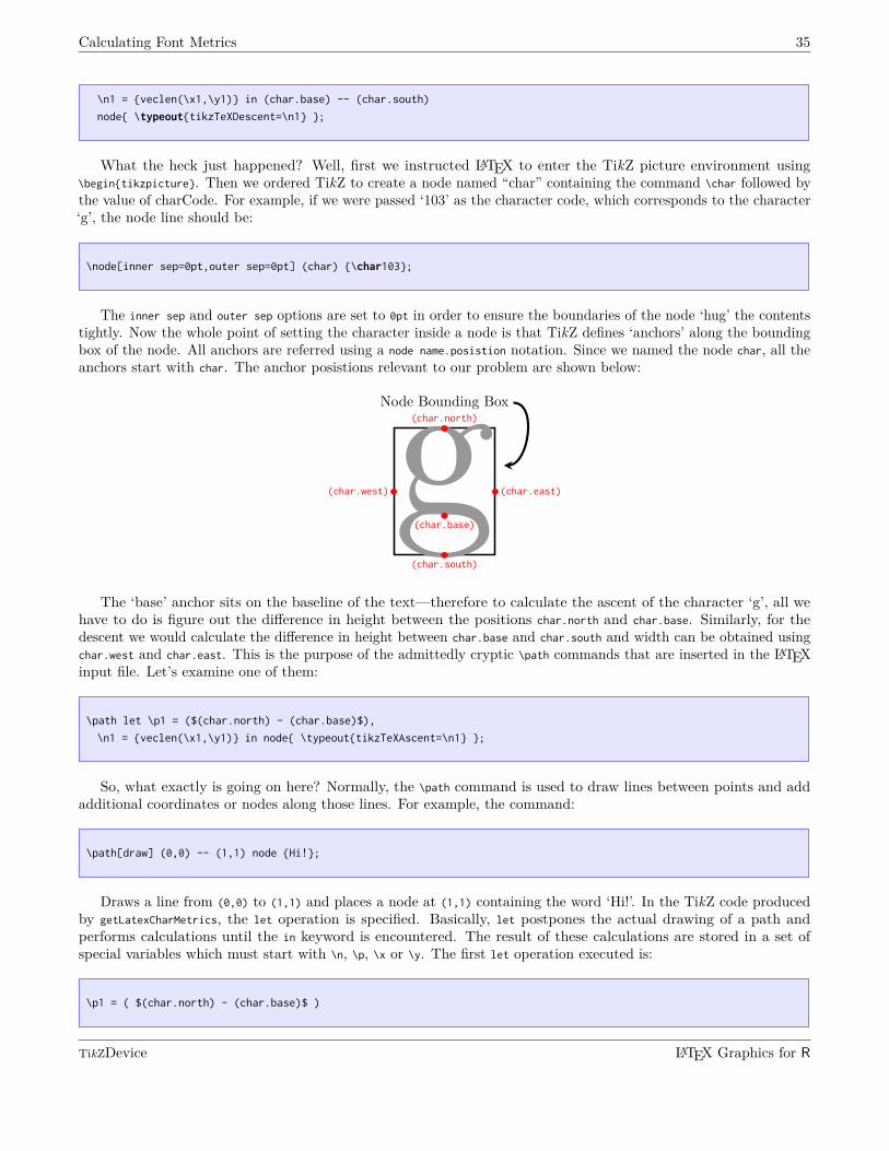
The inner sep and outer sep options are set to 0pt in order to ensure the boundaries of the node ‘hug’ the contentstightly. Now the whole point of setting the character inside a node is that TikZ defines ‘anchors’ along the boundingbox of the node. All anchors are referred using a node name.posistion notation. Since we named the node char, all theanchors start with char. The anchor posistions relevant to our problem are shown below:
g(char.north)(char.south)
(char.base)
(char.east)(char.west)
Node Bounding Box
The ‘base’ anchor sits on the baseline of the text—therefore to calculate the ascent of the character ‘g’, all wehave to do is figure out the difference in height between the positions char.north and char.base. Similarly, for thedescent we would calculate the difference in height between char.base and char.south and width can be obtained usingchar.west and char.east. This is the purpose of the admittedly cryptic \path commands that are inserted in the LATEXinput file. Let’s examine one of them:
\path let \p1 = ($(char.north) - (char.base)$),
\n1 = {veclen(\x1,\y1)} in node{ \typeout{tikzTeXAscent=\n1} };
So, what exactly is going on here? Normally, the \path command is used to draw lines between points and addadditional coordinates or nodes along those lines. For example, the command:
\path[draw] (0,0) -- (1,1) node {Hi!};
Draws a line from (0,0) to (1,1) and places a node at (1,1) containing the word ‘Hi!’. In the TikZ code producedby getLatexCharMetrics, the let operation is specified. Basically, let postpones the actual drawing of a path andperforms calculations until the in keyword is encountered. The result of these calculations are stored in a set ofspecial variables which must start with \n, \p, \x or \y. The first let operation executed is:
\p1 = ( $(char.north) - (char.base)$ )
TikZDevice LATEX Graphics for R
Calculating Font Metrics 36
This performs a vector subtraction between the coordinates of char.north and char.base. The resulting x and ycomponents are stored in the ‘point’ variable \p1. The second operation executed is:
\n1 = {veclen(\x1,\y1)}
This let operation treats the coordinates stored in \p1 as a vector and calculates its magnitude. The ‘1’ appendedto the \x and \y variables specifies that we are accessing the x and y components of \p1. This result is stored in the‘number’ variable \n1. Now, that our metric is stored in \n1, our final task is to ensure it makes it into the LATEX .log
file—this is done by adding a node containing the \typeout command. The contents of the node:
\typeout{tikzTexAscent=\n1}
cause the phrase ‘tikzTexAscent=’ to appear in the .log file—followed by the ascent calculated using the node anchors.After the ascent, descent and width have been calculated the LATEX compiler may be shut down, this is done byadding the final two lines to the input file:
writeLines("\\makeatother", texIn)
writeLines("\\@@end", texIn)
close(texIn)
Terminating a LATEX compilation
Now that the input file has been prepped, we must process it using the LATEX compiler and load the contents ofthe resulting .log so that we may search for the metrics we dumped using \typeout.
latexCmd <- getOption('tikzLatex')
latexCmd <- paste( latexCmd, '-interaction=batchmode',
'-output-directory', texDir, texFile)
silence <- system( latexCmd, intern=T, ignore.stderr=T)
texOut <- file( texLog, 'r' )
logContents <- readLines( texOut )
close( texOut )
Terminating a LATEX compilation
The LATEX compiler is executed through the system function which handles the details of implementing a systemcall on whatever operating system we happen to be using. We assign the return value of the system function to adummy variable called silence so that no output floods the user’s screen. The last task is to extract our metrics fromthe text of the .log we loaded.
match <- logContents[ grep('tikzTeXWidth=', logContents) ]
width <- gsub('[=A-Za-z]','',match)
Parsing the .log file text
TikZDevice LATEX Graphics for R
On the Importance of Font and Style Consistency in Reports 37
match <- logContents[ grep('tikzTeXAscent=', logContents) ]
ascent <- gsub('[=A-Za-z]','',match)
match <- logContents[ grep('tikzTeXDescent=', logContents) ]
descent <- gsub('[=A-Za-z]','',match)
return( as.double( c(ascent,descent,width) ) )
Here we use the grep function to search through the log output for the tags ‘tikzTeXWidth=’, ‘tikzTeXAscent=’and ‘tikzTeXDescent=’ that we specified when we used \typeout. After we recover a line containing one of these tags,we use the gsub command to remove the letters and the equals sign from the text line—leaving just the number we’reinterested in. These values are then coerced using as.double and set as the return value of getLatexCharMetrics.
On the Importance of Font and
Style Consistency in Reports
Chapter 9
If you haven’t figured it out by now, we are quite picky about the way our graphics and reports look. We are especiallypicky about the consistency in fonts (both sizes and shapes). Without launching into a diatribe about this, we justwant to say with tools like tikzDevice you no longer have to settle for what is “just okay.” So go nuts, be pickyabout how your text and graphics look. Don’t be afraid to snub your nose at reports which pay no attention to detail.Be that person who says “NO! I wont settle for half rate graphics, I want the best!”
9.1 The pgfSweave Package and Automatic Report Generation
Now for a little shameless self promotion. The authors of tikzDevice have another package called pgfSweave whichprovides a driver for Sweave. pgfSweave started as an interface to eps2pgf and its ability to interpret strings in epsfiles as LATEX. This was used to much the same effect as tikzDevice. The problem was the conversion from eps topgf was SLOW. Long story short, by combining this functionality with the externalization feature of pgf and thecacheSweave we were able to achieve bearable compilation speed and nice looking graphics. pgfSweave is in theprocess of getting pumped up by interfacing with the tikzDevice package. We hope that the combination will be aself-caching, consistency-inducing, user-empowering tool for high quality reports.
TikZDevice LATEX Graphics for R
Bibliography 38
Bibliography
Murrell, P. (2005), Using Computer Modern Fonts in R Graphics, http://www.stat.auckland.ac.nz/~paul/R/CM/CMR.html.
Peng, R. D. (2006), Interacting with data using the filehash package, R News, 6 (4), 19–24.
R Development Core Team (2009), R Internals: Version 2.9.1.
Tantau, T. (2008), The TikZ and PGF Packages: Manual for version 2.00.
Urbanek, S. (2013), png: Read and write PNG images, r package version 0.1-7.
TikZDevice LATEX Graphics for R