edr design guidelines hvac simulation

Part 1: Underfloor Air Distribution and Thermal Displacement

Ventilation

Introduction to Part 1 . . . . . . . . . . . . . . . . . . . . . . . . . . . . . . . . . . . . . . . . . . . . . . . . . .1

What are Underfloor Air Distribution and Thermal Displacement Ventilation? . . .1

What differentiates UFAD and TDV systems from overhead distribution systems? .

. . . . . . . . . . . . . . . . . . . . . . . . . . . . . . . . . . . . . . . . . . . . . . . . . . . . . . . . . . . . . . . . 2

Barriers to Modeling UFAD and TDV in DOE-2 . . . . . . . . . . . . . . . . . . . . . . . . . . . . .3

• Calculation of cooling loads isn’t available . . . . . . . . . . . . . . . . . . . . . . . . . . . . .4

Thermal Displacement Ventilation and Underfloor Air Distribution Modeling . . . .4

Modeling Issues . . . . . . . . . . . . . . . . . . . . . . . . . . . . . . . . . . . . . . . . . . . . . . . . . . . . . . .6

• System Selection . . . . . . . . . . . . . . . . . . . . . . . . . . . . . . . . . . . . . . . . . . . . . . . . . .7

• Supply Air Temperature . . . . . . . . . . . . . . . . . . . . . . . . . . . . . . . . . . . . . . . . . . . .8

• Dehumidification . . . . . . . . . . . . . . . . . . . . . . . . . . . . . . . . . . . . . . . . . . . . . . . . . .8

• Air Volume . . . . . . . . . . . . . . . . . . . . . . . . . . . . . . . . . . . . . . . . . . . . . . . . . . . . . . .8

• Static Pressure . . . . . . . . . . . . . . . . . . . . . . . . . . . . . . . . . . . . . . . . . . . . . . . . . . . .8

• Economizer Controls . . . . . . . . . . . . . . . . . . . . . . . . . . . . . . . . . . . . . . . . . . . . . . .9

• Building Skin Loads . . . . . . . . . . . . . . . . . . . . . . . . . . . . . . . . . . . . . . . . . . . . . . . .9

• Perimeter Systems . . . . . . . . . . . . . . . . . . . . . . . . . . . . . . . . . . . . . . . . . . . . . . . . .9

Modeling Methodology . . . . . . . . . . . . . . . . . . . . . . . . . . . . . . . . . . . . . . . . . . . . . . . .10

• Modeling TDV and UFAD in DOE-2.1e . . . . . . . . . . . . . . . . . . . . . . . . . . . . . . .10

• Modeling TDV and UFAD in eQUEST . . . . . . . . . . . . . . . . . . . . . . . . . . . . . . . 14

Table of Contents

• Defining TDV or UFAD for Title-24 Comparisons . . . . . . . . . . . . . . . . . . . . . .15

• Modeling TDV and UFAD in EnergyPro . . . . . . . . . . . . . . . . . . . . . . . . . . . . . .16

• Revising the Lighting, Equipment, and Occupant Inputs Directly in DOE-2 .16

Part 2: Energy Efficient Chillers

Introduction to Part 2 . . . . . . . . . . . . . . . . . . . . . . . . . . . . . . . . . . . . . . . . . . . . . . . .18

How Chiller Performance is Specified in DOE-2 . . . . . . . . . . . . . . . . . . . . . . . . . .19

• CAPFT - Chiller Capacity as a Function of Temperature . . . . . . . . . . . . . . . . .20

• EIRFT - Energy Input Ratio as a Function of Temperature . . . . . . . . . . . . . .20

• EIRFPLR - Energy Input Ratio as a Function of Part Load Ratio . . . . . . . . .21

Improved Models for Variable Speed Chillers in DOE-2.2 . . . . . . . . . . . . . . . . . .24

Data Required for Specifying Chiller Performance Curves in Doe-2 . . . . . . . . .25

Obtaining Data Required for Chiller Performance Curves . . . . . . . . . . . . . . . . . .26

Methods for Creating Custom DOE-2 Chiller Models . . . . . . . . . . . . . . . . . . . . . .27

Methods for Including Chiller Data in DOE-2 Performance Curves . . . . . . . . . .29

• Calculating the CAPFT Curve in DOE-2 . . . . . . . . . . . . . . . . . . . . . . . . . . . . . .29

• Calculating the EIRFT Curve in DOE-2 . . . . . . . . . . . . . . . . . . . . . . . . . . . . . . .32

• Calculating the EIRFPLR Curve in DOE-2 . . . . . . . . . . . . . . . . . . . . . . . . . . . .33

Guidelines for Creating Accurate Custom Chillers . . . . . . . . . . . . . . . . . . . . . . . .42

Summary . . . . . . . . . . . . . . . . . . . . . . . . . . . . . . . . . . . . . . . . . . . . . . . . . . . . . . . . . . .42

Part 3: Advanced Control Sequences

Introduction to Part 3 . . . . . . . . . . . . . . . . . . . . . . . . . . . . . . . . . . . . . . . . . . . . . . . .45

Variable Speed Drive Control Sequences . . . . . . . . . . . . . . . . . . . . . . . . . . . . . . . .46

• Variable Primary Flow Chilled Water Distribution . . . . . . . . . . . . . . . . . . . . . .46

• Primary/Secondary Chilled Water Distribution . . . . . . . . . . . . . . . . . . . . . . . .48

• Cautions for Modeling Variable-Speed Pumps and Variable-Chilled Water . . .

Flow in eQUEST . . . . . . . . . . . . . . . . . . . . . . . . . . . . . . . . . . . . . . . . . . . . . . . . .53

• Variable Flow Condenser Water System . . . . . . . . . . . . . . . . . . . . . . . . . . . . . .54

Condenser Water System Operation . . . . . . . . . . . . . . . . . . . . . . . . . . . . . . . . . . . . .55

• Cooling Tower Cell Control . . . . . . . . . . . . . . . . . . . . . . . . . . . . . . . . . . . . . . . . .55

• Cooling Tower Capacity Control . . . . . . . . . . . . . . . . . . . . . . . . . . . . . . . . . . . . .55

• Condenser Water Temperature Reset . . . . . . . . . . . . . . . . . . . . . . . . . . . . . . . .57

• Modeling Condenser Water Load Reset in eQUEST . . . . . . . . . . . . . . . . . . . .58

Chilled Water Loop Temperature Reset . . . . . . . . . . . . . . . . . . . . . . . . . . . . . . . . .59

• Defining Chilled Water Temperature Reset in eQUEST . . . . . . . . . . . . . . . . . .59

Hot Water Loop Temperature Reset . . . . . . . . . . . . . . . . . . . . . . . . . . . . . . . . . . . . .59

Prepared for Pacific Gas and Electric Company by CTG Energetics, Inc. for the statewide

Energy Design Resources program (www.energydesignresources.com).

This report was funded by California utility customers under the auspices of the California

Public Utilities Commission.

Neither Pacific Gas and Electric Company nor any of its employees and agents:

1. Makes any written or oral warranty, expressed or implied, regarding this report,

including, but not limited to those concerning merchantability or fitness for a particular

purpose.

2. Assumes any legal liability or responsibility for the accuracy, completeness, or usefulness

of any information, apparatus, product, process, method, or policy contained herein.

3. Represents that use of the report would not infringe any privately owned rights,

including, but not limited to, patents, trademarks or copyrights.

Underfloor air distribution (UFAD) and thermal displacement ventilation (TDV)

have become increasingly common in commercial new construction because they

are energy-efficient, enhance indoor air quality, and increase flexibility for space

reconfiguration. However, conflicting opinions exist concerning the benefits of

UFAD and TDV. This often leads to inappropriate analysis and unrealistic cus-

tomer expectations. There are many different notions regarding the energy effi-

ciency of UFAD and TDV systems, with some people claiming that these systems

save little or no energy, while others suggest that they can cut HVAC energy

usage by fifty percent or more. To help the energy modeler evaluate the energy

benefits of UFAD and TDV, this simulation guidebook identifies the key charac-

teristics that distinguish UFAD and TDV systems from traditional overhead sys-

tems and presents a logical, engineering-based method for analyzing UFAD and

TDV with DOE-2-based simulation programs.

This simulation guidebook is concerned with methods for analyzing air distribution systems

that deliver cooling and heating air at floor level instead of from the ceiling. An example

of such a system is underfloor air distribution (UFAD), where conditioned air is delivered at

a moderate velocity (650 to 800 feet-per-minute) via a 10” to 16” plenum space underneath

an access floor system (Figure 1a). Another example is a Thermal Displacement Ventilation

(TDV) system that delivers supply air horizontally at low velocity (50 to 100 feet-per-minute)

from wall-mounted diffusers without using an underfloor plenum (Figure 1b).

1part 1: underfloor air distribution and thermal displacement ventilation

PART 1: Underfloor Air Distribution and

Thermal Displacement Ventilation

What are Underfloor Air Distribution andThermal Displacement Ventilation?

Diffuser for Underfloor Air Distribution System1 (1a-left) versus Diffuser for

Thermal Displacement System2 (1b-right)

While there are differences in the performance characteristics between UFAD and TDV sys-

tems, the modeling methodology described in this simulation guidebook applies to both.

Energy modelers must exercise judgment to adjust the methods to suit either system.

Guidelines are provided throughout this guidebook that can be applied to account for dif-

ferences between the two systems.

Traditional space conditioning systems supply heated or cooled air from diffusers mounted

in a suspended ceiling grid. The design assumption made is that supply air completely

mixes with the air in the room, and as a result, all of the air within the conditioned space

reaches a homogeneous temperature (Figure 2).

Designers go to great effort to select diffusers that promote this mixing effect so that cold

air does not “dump” onto the occupants below. In an overhead mixing system, cold sup-

ply air mixes with hot air that accumulates near the ceiling as a result of heat generated

2 simulation guidebook vol. 1

What differentiates UFAD and TDV systems from overhead distribution systems?

Figure 1:

(a) A typical underfloor

air distribution system

consists of a raised

access floor, a 10” to

16” underfloor plenum,

and air delivery dif-

fusers. (b) A thermal

displacement ventila-

tion system delivers

low velocity air at

floor level. An access

floor is not usually

employed for such a

system.

1Source: Tate Access Floors

2 Source: Halton Group

by people, lights, and equipment. While an overhead mixing system concept can provide

good occupant comfort, it wastes energy by providing comfortable conditions from the floor

all the way to the ceiling. It would be more efficient to limit the distribution of heated or

cooled air only to the lower volume (for example, up to seven feet above the floor) of the

room where the occupants are located.

Overhead Air Delivery Provides Homogeneous Temperature Distribution3

Thermal Displacement Ventilation Encourages Stratification4

Uniform temperatures are assumed throughout the entire conditioned spaceMost simulation programs based on DOE-2.1e or DOE-2.2 (such as eQUEST and EnergyPro)

determine space cooling loads as a summation of all heat losses and heat gains within a

space, without regard to how the loads are influenced by airflow patterns and the buoyan-

cy of warm air. Stated another way, most simulation programs are not aware that hot air

rises, and therefore assume a uniform temperature throughout the conditioned volume.

Figure 2:

Traditional overhead

air distribution sys-

tems are designed to

completely mix supply

air with room air. The

goal is to provide a

uniform temperature

distribution from

floor to ceiling.


Figure 3:

By delivering cool air

at floor level and

drawing warmer air

from the ceiling, TDV

encourages thermal

stratification.

3 Source: CTG Energetics, Inc.4 Source: CTG Energetics, Inc.

Barriers to Modeling UFAD and TDV in DOE-2

For example, consider the following internal load calculation:

People (sensible + latent)

30 occupants x 500 Btu/hr-person 15,000 Btu/hr

Lights

900 SF x 1.5 W/SF x 3.413 Btu/hr-W 4,608 Btu/hr

Equipment

900 SF x 1.0 W/SF x 3.413 Btu/hr-W 3,072 Btu/hr

TOTAL 22,680 Btu/hr

Most simulation programs calculate the required cooling capacity to meet these internal

loads as the sum of the loads. The fact that hot air rises (producing warmer temperatures

near the ceiling and cooler temperatures near the floor) is not accounted for. For overhead

mixing-type air distribution this approach is satisfactory because overhead diffusers are

selected and placed to promote mixing of supply air and room air. The flow of supply air

from the ceiling pushes the hot air near the ceiling down to the level of occupants.

Calculation of cooling loads isn’t availableWhen conditioned air is delivered at floor level at low velocity, it does not significantly mix

with the hot ceiling air. Accordingly, floor-supplied air is not as disruptive to thermal strati-

fication as overhead delivery (Figure 3). This is advantageous because the hot ceiling air

can be drawn directly into the return air system and exhausted from the space instead of

neutralized by mixing with cold air. The effect of thermal stratification is that cooling loads

are reduced relative to those of overhead delivery systems, but most simulation programs

do not reflect this change. Referring to the previous load calculation example, a UFAD sys-

tem would reduce the cooling load resulting from internal heat gains by nearly 50 percent.

More complex and time-consuming analysis methods, such as computational fluid dynam-

ics (CFD), must be employed if one wishes to calculate cooling loads that account for ther-

mal stratification. In most cases it is not practical to perform CFD analysis, and such analy-

sis cannot be submitted to show Title 24 compliance.

The strategy for modeling TDV and UFAD systems is to move a portion of the heat gain

from people, lights and equipment from the conditioned space to an unconditioned plenum

space. While project-specific information about how much of each internal load should be

apportioned to the plenum is highly desirable, such data is infrequently available. Table 1

provides reasonable estimates for both UFAD and TDV systems. Figure 4 and Figure 5

The effect of thermal

stratification is that

cooling loads are

reduced relative to

those of overhead

delivery systems, but

most simulation pro-

grams do not reflect

this change.

Thermal Displacement Ventilation and Underfloor AirDistribution Modeling


show how lighting and receptacle loads would be redistributed in a typical underfloor air

system. A similar approach would be employed for occupant heat gain.

Internal Load Distribution Values for Typical Underfloor Air and Thermal

Displacement Ventilation Encourages Systems5

Room Cross Section with Loads in Space6

Table 1


Figure 4:

Cross-section view of

typical room showing

conditioned and

unconditioned spaces,

with typical lighting

power density (LPD)

and equipment power

density (EPD). The

total internal heat

gain from these

sources is 1.95 W/ft2.

5Source: CTG Energetics, Inc.6Source: CTG Energetics, Inc.

Room Cross Section with Loads in Plenum7

There are a number of issues that must be considered when modeling thermal displacement

or underfloor air distribution systems. These issues include:

• System Selection

• Supply Air Temperature

• Dehumidification

• Air Volume

• Static Pressure

• Economizer Controls

• Building Skin Loads

• Perimeter Systems

Modeling Issues


7Source: CTG Energetics, Inc.

Figure 5:

To simulate the

reduced heat gain

from lighting and

receptacle loads, much

of the load is reas-

signed to the uncondi-

tioned return air

plenum. The effect is

that cooling loads in

the conditioned space

are reduced while the

return air temperature

is increased. The total

gain from lights and

receptacles is

unchanged; however,

it has been appor-

tioned differently

between conditioned

and unconditioned

space.

System SelectionThe energy modeler must take care to choose the appropriate HVAC system type from

those available within the simulation program. The exact system choice should reflect

whether the system operates in constant or variable-volume fashion, the source of heating

and cooling, and the way that outside air ventilation is managed. The following are

examples of potential system selections:

Example #1: Access Floor System with Manually Adjustable Diffusers. This sort of system,

which may include a large number of round, manually adjustable “swirl” diffusers

(approximately one diffuser per 75 to 100 ft2of conditioned area), has become increasing-

ly common in office buildings. Because occupants have some control over the airflow in

their workspace - but cannot completely shut off the air supply - the system operates

essentially as a variable-air-volume system with a high minimum airflow rate. Such sys-

tems are most commonly employed as part of a chilled water cooling system. In the

DOE-2 simulation environment, such a system could be modeled using system type VAVS

(variable-air-volume, with chilled water cooling). The minimum airflow rate (MIN-CFM-

RATIO) would be set high to reflect the diversity of loads in the conditioned space and

also the limited turndown offered to occupants. It is common for turndown ratios to be 70

to 80 percent of full flow, though modeling assumptions should be verified with the HVAC

engineer. In many cases, a 100% outside-air-economizer cycle will be employed and the

specific program inputs should reflect the fact that the cooling requirements can be met

using warmer air than with overhead systems (i.e. 64ºF to 67ºF).

Example #2: Access Floor System with Thermostatically Controlled VAV Zone Terminals.

This system is similar in some respects to Example #1, but the large number of “swirl”

diffusers is replaced with a reduced number of thermostatically-controlled VAV terminals

located in the underfloor plenum. Zoning for such systems is often comparable to

overhead systems in terms of the average area per zone. Such systems usually offer higher

turndown than the manual “swirl” diffusers and are automatically controlled based on space

temperature. As a result, the minimum airflow ratio (MIN-CFM-RATIO) will frequently be

lower with this air distribution strategy. Reviewing the zone schedule prepared by the

mechanical engineer should provide information about the minimum airflow for each VAV

terminal. Without such data, it is reasonable to assume a minimum airflow ratio of 50

percent until more detailed information is available.

Example #3: Thermal Displacement System with Constant Volume Delivery. This system

design is most frequently used in classrooms or other assembly areas. A common configu-

ration for thermal displacement systems consists of four-pipe fan coil units for each zone (or

classroom), with a central air-handling unit distributing outside air to each unit. The fan coil

units deliver constant volume supply air horizontally at low velocities from wall-mounted

diffusers. The system can be modeled in DOE-2 using system type FPFC (four-pipe fan coil).

The energy model system inputs should reflect the supply air temperature and volume

design conditions associated with TDV, and fan energy inputs for each fan coil should

account for the contributions from the central outside air supply unit.

The energy modeler

must take care to

choose the appropri-

ate HVAC system type

from those available

within the simulation

program.


Supply Air TemperatureSince TDV and UFAD generally introduce conditioned air in close proximity to the build-

ing occupants, the air is delivered at a temperature only slightly (5ºF to 10ºF) below space

temperature set points. This corresponds to a 64ºF to 67ºF supply air temperature set

point (MIN-SUPPLY-T or COOL-SET-T) as opposed to a 55ºF set point for traditional mix-

ing systems.

DehumidificationDue to the elevated supply air temperature associated with TDV and UFAD, the mechani-

cal designer must give close attention to humidity control for these systems. With the

exception of cool, dry climates, cooling coils provide inadequate removal of latent load

when cooling to only 64ºF or 67ºF. Consequently, most TDV and UFAD designs need to

implement supplemental humidity control features to avoid the decreased comfort and

indoor air quality associated with high space humidity conditions. In a common TDV or

UFAD humidity control scheme, the chilled water coil cools a mixture of outside air and

return air down to 55ºF, and this conditioned air is then mixed with the remainder of the

return air to increase the temperature back up to the supply air temperature set point.

Although the limitations of DOE-2 prevent the accurate modeling of this humidity control

scheme, energy modelers should keep in mind that this form of humidity control will

achieve less energy savings than projected by a DOE-2 model with a high supply-air tem-

perature set point.

Air VolumeDesign supply airflow calculations for the space must account for both the elevated sup-

ply air temperature and the redistribution of a portion of the occupant, plug and lighting

loads from the space to the return air. Ignoring the high supply-air temperature for TDV

and UFAD systems will result in an underestimation of supply air volume, and neglecting

to redistribute a portion of the space loads to the plenum will result in supply air-flow

rates that are up to two times greater than the amount required to condition the space.

Typically, supply air flows for a true TDV system exceed those of a corresponding over-

head mixing system by only five to twenty percent.8 Supply air flow rates for UFAD sys-

tems range from twenty-five percent less to fifteen percent more than traditional overhead

systems.9

Static PressureIn most UFAD systems, the underfloor plenum serves as the primary source of air distribu-

tion. Consequently, UFAD systems generally use far less ductwork than corresponding

overhead systems, resulting in reduced static pressure at the supply fans when compared

against standard overhead systems. However, due to the wide variance in UFAD

With the exception of

cool, dry climates,

cooling coils provide

inadequate removal of

latent load when cool-

ing to only 64ºF or

67ºF.


8“Underfloor Air Distribution and Access Floors.” Energy Design Resources Design Brief.

9Webster, Tom, Bauman, Fred, and Reese, Jim. “Underfloor Air Distribution: Thermal

Stratification.” ASHRAE Journal. May 2002. Vol. 44, No. 5, Pg. 34.

design, energy analysts should confirm estimated values for static pressure with the mechan-

ical designer prior to modeling savings associated with reduced fan static pressure. The fan

energy savings linked to lower fan static pressures will generally not be reflected in Title-24,

since the standard case changes with the proposed case for inputs related to fan power.

Economizer ControlsTDV and UFAD systems can often take advantage of increased hours of economizer oper-

ation due to the higher temperature of air delivered to the space. In most California cli-

mate zones, raising the supply air temperature from 55ºF to 65ºF can extend economizer

operation by 2,000-2,500 hours per year.10

However, the humidity control requirements in

many of these climates will limit the hours of additional economizer operation, resulting in

reduced free cooling benefits. In climate zones that require additional dehumidification,

the economizer operation must be integrated with the humidity control to maintain proper

humidity conditions. This requires differential enthalpy-based economizer operation to

ensure that the humidity of the outside air remains lower than that of the return air. In

DOE-2, differential enthalpy control is modeled using the ENTHALPY keyword for OA-

CONTROL at the system level.

Building Skin LoadsIf return grilles are located directly above the windows in perimeter spaces served by

UFAD or TDV systems, a significant portion of the convective cooling load associated with

the building skin can be funneled directly into the return air plenum.11 A precise energy

model for UFAD and TDV systems can account for the energy savings associated with this

phenomenon by reapportioning some of the glazing and exterior walls in the occupied

space to the adjacent plenum. However, this methodology may result in the loss of legiti-

mate automated daylighting control savings in DOE-2-based programs. Furthermore, this

modeling approach has not yet been approved for demonstrating UFAD system savings in

2005 Title-24.

Perimeter SystemsPerimeter system approaches vary widely for both UFAD and TDV systems. In some

cases, perimeter underfloor air plenums for UFAD systems are separated from interior

underfloor air plenums with dividers; in another approach, underfloor ductwork provides

perimeter spaces with a separate source of supply air, and sometimes perimeter spaces are

entirely served by overhead systems. Baseboard heating can also be provided as the pri-

mary heating source for perimeter zones served by TDV or UFAD systems. The

Underfloor Air Distribution Design Guide (ASHRAE, 2003) provides a good overview of

In most California cli-

mate zones, raising

the supply air tempera-

ture from 55ºF to 65ºF

can extend economizer

operation by 2,000-

2,500 hours per year.


10“The Case for TDV in California Schools.” California Energy Commission’s Public

Interest Energy Research (PIER) Program. http://www.archenergy.com/ieq-k12/ther-mal_displacement/thermal_displace_background.htm

11Bauman, Fred S. and Daly, Alan. Underfloor Air Distribution (UFAD) Design Guide.

Atlanta: ASHRAE, 2003.

the range of perimeter system designs commonly applied in conjunction with underfloor

air distribution. Energy analysts should use their judgment to select the type of space

heating and zone terminal units in DOE-2 that most closely represent the perimeter system

design for their project.

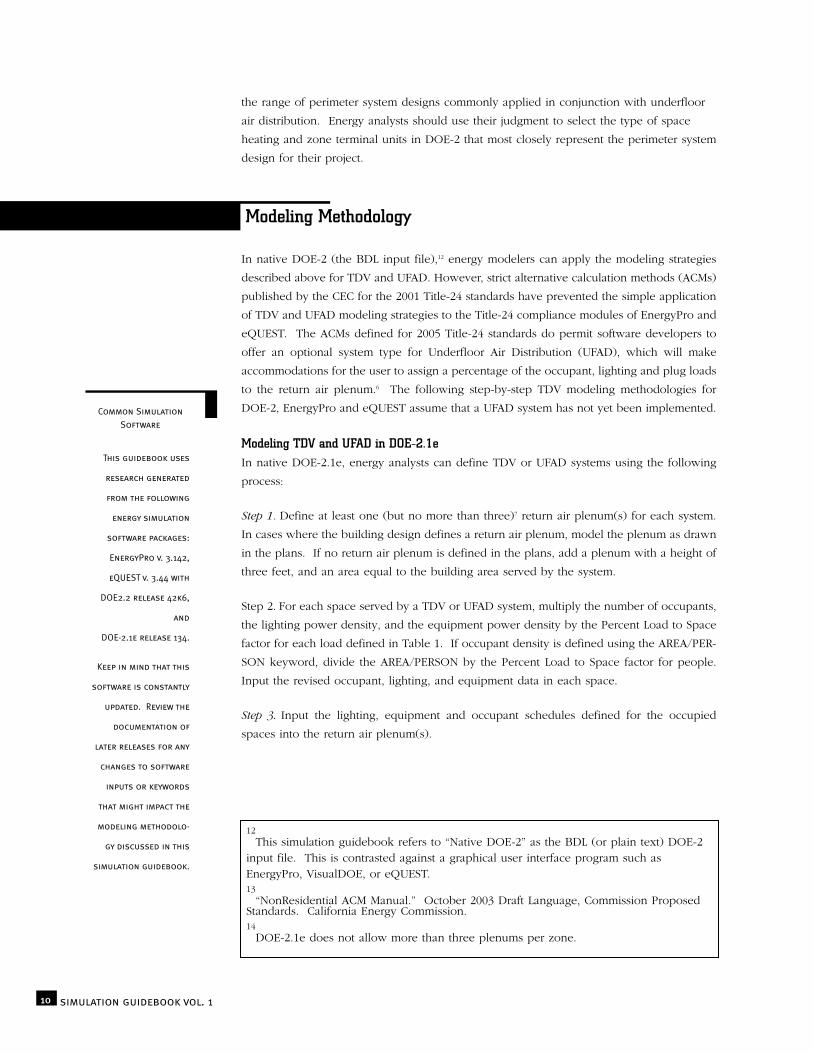
In native DOE-2 (the BDL input file),12 energy modelers can apply the modeling strategies

described above for TDV and UFAD. However, strict alternative calculation methods (ACMs)

published by the CEC for the 2001 Title-24 standards have prevented the simple application

of TDV and UFAD modeling strategies to the Title-24 compliance modules of EnergyPro and

eQUEST. The ACMs defined for 2005 Title-24 standards do permit software developers to

offer an optional system type for Underfloor Air Distribution (UFAD), which will make

accommodations for the user to assign a percentage of the occupant, lighting and plug loads

to the return air plenum.6 The following step-by-step TDV modeling methodologies for

DOE-2, EnergyPro and eQUEST assume that a UFAD system has not yet been implemented.

Modeling TDV and UFAD in DOE-2.1eIn native DOE-2.1e, energy analysts can define TDV or UFAD systems using the following

process:

Step 1. Define at least one (but no more than three)7 return air plenum(s) for each system.

In cases where the building design defines a return air plenum, model the plenum as drawn

in the plans. If no return air plenum is defined in the plans, add a plenum with a height of

three feet, and an area equal to the building area served by the system.

Step 2. For each space served by a TDV or UFAD system, multiply the number of occupants,

the lighting power density, and the equipment power density by the Percent Load to Space

factor for each load defined in Table 1. If occupant density is defined using the AREA/PER-

SON keyword, divide the AREA/PERSON by the Percent Load to Space factor for people.

Input the revised occupant, lighting, and equipment data in each space.

Step 3. Input the lighting, equipment and occupant schedules defined for the occupied

spaces into the return air plenum(s).

Common Simulation

Software

This guidebook uses

research generated

from the following

energy simulation

software packages:

EnergyPro v. 3.142,

eQUEST v. 3.44 with

DOE2.2 release 42k6,

and

DOE-2.1e release 134.

Keep in mind that this

software is constantly

updated. Review the

documentation of

later releases for any

changes to software

inputs or keywords

that might impact the

modeling methodolo-

gy discussed in this

simulation guidebook.

Modeling Methodology


12This simulation guidebook refers to “Native DOE-2” as the BDL (or plain text) DOE-2

input file. This is contrasted against a graphical user interface program such asEnergyPro, VisualDOE, or eQUEST.13

“NonResidential ACM Manual.” October 2003 Draft Language, Commission ProposedStandards. California Energy Commission. 14

DOE-2.1e does not allow more than three plenums per zone.

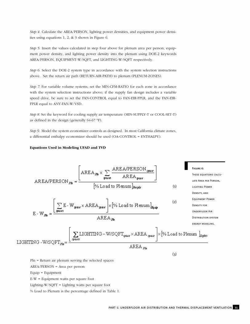
Step 4. Calculate the AREA/PERSON, lighting power densities, and equipment power densi-

ties using equations 1, 2, & 3 shown in Figure 6.

Step 5. Insert the values calculated in step four above for plenum area per person, equip-

ment power density, and lighting power density into the plenum using DOE-2 keywords

AREA/PERSON, EQUIPMENT-W/SQFT, and LIGHTING-W/SQFT respectively.

Step 6. Select the DOE-2 system type in accordance with the system selection instructions

above. Set the return air path (RETURN-AIR-PATH) to plenum (PLENUM-ZONES).

Step 7. For variable volume systems, set the MIN-CFM-RATIO for each zone in accordance

with the system selection instructions above; if the supply fan design includes a variable

speed drive, be sure to set the FAN-CONTROL equal to FAN-EIR-FPLR, and the FAN-EIR-

FPLR equal to ANY-FAN-W/VSD.

Step 8. Set the keyword for cooling supply air temperature (MIN-SUPPLY-T or COOL-SET-T)

as defined in the design (generally 64-67 ºF).

Step 9. Model the system economizer controls as designed. In most California climate zones,

a differential enthalpy economizer should be used (OA-CONTROL = ENTHALPY).

Equations Used in Modeling UFAD and TVD

Figure 6:

These equations calcu-

late Area per Person,

Lighting Power

Density, and

Equipment Power

Density for

Underfloor Air

Distribution system

energy modeling.


(1)

(2)

(3)

Pln = Return air plenum serving the selected spaces

AREA/PERSON = Area per person

Equip = Equipment

E-W = Equipment watts per square foot

Lighting-W/SQFT = Lighting watts per square foot

% Load to Plenum is the percentage defined in Table 1.

DOE-2.1e Sample Text for an Access Floor System with Manually Adjustable

Diffusers

$ SAMPLE SPACE-DEFINITION - OFFICE WITH UNDERFLOOR AIR CONDITIONING:

$ E. Office $

ZONE-1 = SPACE

ZONE-TYPE = CONDITIONED

PEOPLE-SCHEDULE = SCHED-26

LIGHTING-SCHEDULE = SCHED-25

EQUIP-SCHEDULE = SCHED-24

INF-SCHEDULE = SCHED-23

AREA/PERSON = 133 $ AREA/PERSON = 100/75% = 133

$ where 75% = Percent to space factor

PEOPLE-HG-SENS = 250

PEOPLE-HG-LAT = 200

LIGHTING-W/SQFT = 0.871 $ LIGHTING-W/SQFT = 1.3 * 67% = 0.871


EQUIPMENT-W/SQFT = 1.0 $ EQUIPMENT-W/SQFT = 1.5 * 67% = 1.0


EQUIP-SENSIBLE = 1.0

EQUIP-LATENT = 0.0

INF-METHOD = AIR-CHANGE

AIR-CHANGES/HR = 0.2027

AREA = 1710

VOLUME = 17100

..

$ SAMPLE ZONE-DEFINITION - OFFICE WITH UNDERFLOOR AIR CONDITIONING,

UFAD DIFFUSERS WITH VSD ON FANS

ZONE-1 = ZONE

ZONE-TYPE = CONDITIONED

DESIGN-HEAT-T = 70.0

DESIGN-COOL-T = 74.0

THROTTLING-RANGE = 4.0

HEAT-TEMP-SCH = SCHED-20

COOL-TEMP-SCH = SCHED-19

OA-CFM-PER = 15

SIZING-OPTION = ADJUST-LOADS

INDUCED-AIR-ZONE = ZONE-1

TERMINAL-TYPE = SVAV

MIN-CFM-RATIO = 0.75 $ MINIMUM CFM SET TO 75%

..

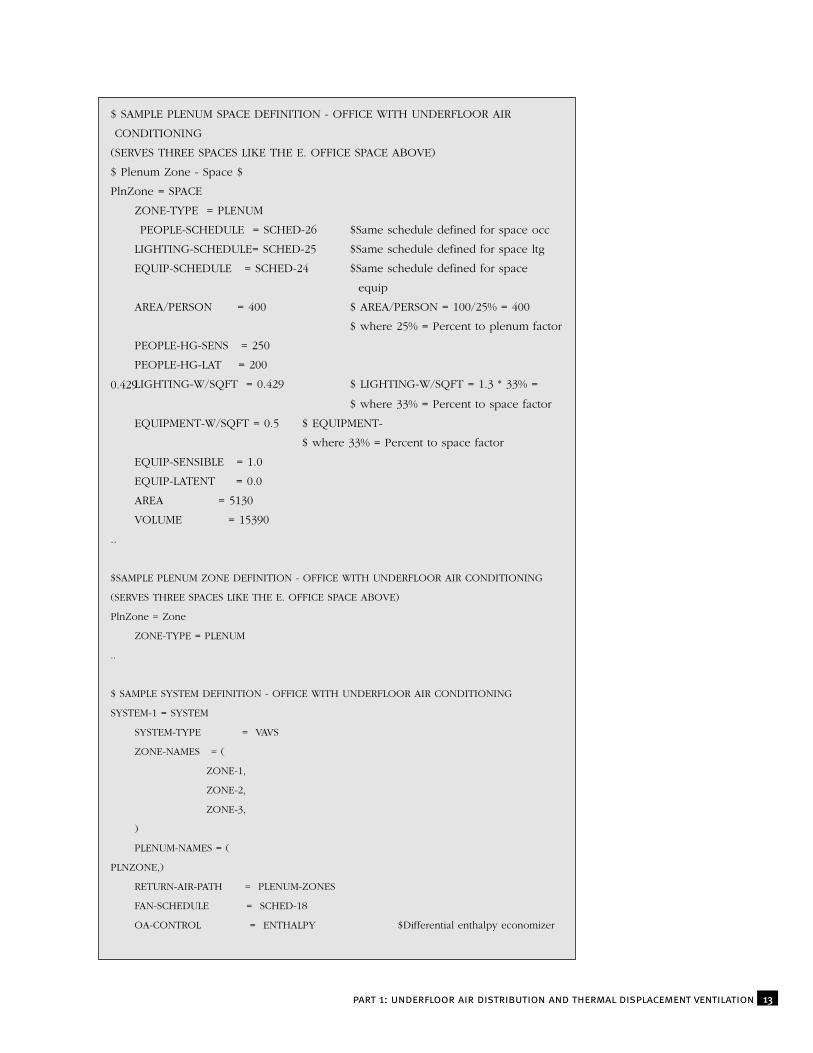
Figure 7:

The system that corre-

sponds to this sample

text serves three

spaces and is modeled

with a return air

plenum to simulate the

impacts of underfloor

air distribution. One

third of the lighting

and equipment loads

and one quarter of the

occupant load is redis-

tributed to the

plenum. The system

operates with a vari-

able speed fan and a

differential enthalpy

economizer and sup-

plies air at an elevated

supply air temperature.

The minimum air flow

to the space is

assumed to be 75%.



$ SAMPLE PLENUM SPACE DEFINITION - OFFICE WITH UNDERFLOOR AIR

CONDITIONING

(SERVES THREE SPACES LIKE THE E. OFFICE SPACE ABOVE)

$ Plenum Zone - Space $

PlnZone = SPACE

ZONE-TYPE = PLENUM

PEOPLE-SCHEDULE = SCHED-26 $Same schedule defined for space occ

LIGHTING-SCHEDULE= SCHED-25 $Same schedule defined for space ltg

EQUIP-SCHEDULE = SCHED-24 $Same schedule defined for space

equip

AREA/PERSON = 400 $ AREA/PERSON = 100/25% = 400

$ where 25% = Percent to plenum factor

PEOPLE-HG-SENS = 250

PEOPLE-HG-LAT = 200

LIGHTING-W/SQFT = 0.429 $ LIGHTING-W/SQFT = 1.3 * 33% =0.429


EQUIPMENT-W/SQFT = 0.5 $ EQUIPMENT-


EQUIP-SENSIBLE = 1.0

EQUIP-LATENT = 0.0

AREA = 5130

VOLUME = 15390

..

$SAMPLE PLENUM ZONE DEFINITION - OFFICE WITH UNDERFLOOR AIR CONDITIONING

(SERVES THREE SPACES LIKE THE E. OFFICE SPACE ABOVE)

PlnZone = Zone

ZONE-TYPE = PLENUM

..

$ SAMPLE SYSTEM DEFINITION - OFFICE WITH UNDERFLOOR AIR CONDITIONING

SYSTEM-1 = SYSTEM

SYSTEM-TYPE = VAVS

ZONE-NAMES = (

ZONE-1,

ZONE-2,

ZONE-3,

)

PLENUM-NAMES = (

PLNZONE,)

RETURN-AIR-PATH = PLENUM-ZONES

FAN-SCHEDULE = SCHED-18

OA-CONTROL = ENTHALPY $Differential enthalpy economizer

Modeling TDV and UFAD in eQUESTIf eQUEST users are not using the Title-24 compliance module, they can define TDV and

UFAD systems using the following process:

Step 1. If the building design includes a return air plenum, model the plenum in the

Building Footprint screen of the eQUEST wizard by selecting floor-to-floor height and floor-

to-ceiling height as shown in the plans. If no return air plenum is defined in the plans, a

plenum must be defined in the eQUEST detailed edit interface. The plenum should have a

height of three feet, and an area equal to the building area served by the system.

Step 2. From the Occupied Loads by Activity Area screen of the eQUEST wizard, multi-

ply the installed lighting power density and the equipment power density for each occu-

pancy type by the Percent Load to Space factor for each load defined in Table 1. Input

the revised lighting and equipment data in each space.

Step 3. From the HVAC System Definitions screen, select the system type as outlined in

the system selection guidelines above.

Step 4. From the HVAC Zones: Temperatures and Air Flows screen, set the supply air

temperature as defined in the plans. For VAV systems, define the VAV minimum flow for

both core and perimeter spaces, as described in the system selection guidelines.

Step 5. Switch to Detailed Edit Mode by selecting File / Mode / Detailed Edit Mode.

Step 6. From the Internal Loads module, select the Spreadsheet tab, and then select

Occupancy. Divide the AREA/PERSON for each space by the Percent Load to Space factor

for people defined in Table 1. Input the revised data in each space. In the return air

plenum space, select the occupancy schedule to be the same as the occupied spaces.


ECONO-LOCKOUT = NO

MAX-OA-FRACTION = 1.0

FAN-CONTROL = FAN-EIR-FPLR

FAN-EIR-FPLR = ANY-FAN-W/VSD $Variable Speed Fan Controls

MIN-FAN-RATIO = 0.30

SUPPLY-CFM = 5000

SUPPLY-KW = 0.001

SUPPLY-DELTA-T = 2.79

DUCT-AIR-LOSS = 0.00

COOL-CONTROL = RESET

COOL-RESET-SCH = COLD-DECK-RESET

COOLING-CAPACITY = 153000

COOL-SH-CAP = 122400

MIN-SUPPLY-T = 65 $ ELEVATED SUPPLY AIR TEMPERATURE

..

Use equation 1 to calculate the AREA/PERSON for the plenum.

Step 7. Again from the Spreadsheet tab, select Lighting. In the return air plenum, select

the same lighting schedule as is defined for the occupied spaces. Use equation 3 to calcu-

late the lighting power density for the plenum. Repeat this process for Equipment, using

equation 2 to calculate the plenum equipment power density.

Sample eQuest Input Screen

Defining TDV or UFAD for Title-24 ComparisonsWhen using the Title-24 compliance module, eQUEST users must define TDV or UFAD

inputs using a slightly more complex process:

Step 1. Complete steps 1, 3, and 4 described above for the eQUEST non-compliance TDV

and UFAD modeling process.

Step 2. Run the Title-24 simulation using the Perform Compliance Analysis option.

Step 3. Load the DOE-2 input file for the Title-24 proposed case (titled [FileName]- T24

Proposed Building.inp) into eQUEST by selecting File / Open / Files of Type / DOE-2.2

BDL Input Files, and then selecting the appropriate file.

Step 4. From the Internal Loads module, select the Spreadsheet tab, and then select

Occupancy. Divide the AREA/PERSON for each space by the Percent Load to Space fac-

tor for people defined in Table 1. Input the revised data in each space. In the return air

plenum space, select the occupancy schedule to be the same as the occupied spaces. Use

equation 1 to calculate the AREA/PERSON for the plenum.

Step 5. Again from the Spreadsheet tab, select Lighting. Multiply the installed lighting

power density for each space by the Percent Load to Space factor for defined in Table 1.

Input the revised lighting power density in each space. In the return air plenum, select the

same lighting schedule as is defined for the occupied spaces. Use equation 3 to calculate

Figure 8:

eQuest zone tempera-

ture and air flow

selections for an

access floor systems

with manually

adjustable diffusers.


the lighting power density for the plenum.

Step 6. Repeat the process above for Equipment using the equipment power densities,

equipment schedules, and calculating the plenum equipment power density with equation

2.

Step 7. Rerun the energy model to obtain a revised Title-24 proposed case. The Title-24

standard case should remain the same. As an error-checking routine, the energy modeler

should confirm that the lighting and equipment energy usage for the original Title-24 pro-

posed case is equal to those shown in the revised Title-24 proposed case.

Modeling TDV and UFAD in EnergyProAn energy modeler can simulate TDV or UFAD with EnergyPro by:

• Inputting system inputs directly in EnergyPro;

• Using the EnergyPro Win/DOE module to generate a DOE-2 input file, and

• Revising the lighting, equipment, and occupant inputs directly in DOE-2. This step is

explained below.

Revising the Lighting, Equipment, and Occupant Inputs Directly in DOE-2 Step 1. Define at least one but no more than three return air plenums for each system. In

cases where the building design defines a return air plenum, model the plenum as drawn

in the plans. If no return air plenum is defined in the plans, add a plenum with a height of

three feet, and an area equal to the building area served by the system.

Step 2. Select the DOE-2 system type as outlined in the system selection instructions above.

Set the cooling supply air temperature in the cooling tab for each system. Model the econ-

omizer type as designed (often differential enthalpy for TDV systems). For each system, con-

firm that any variable speed fans are appropriately defined under the Fans tab.

Step 3. For variable volume systems, select a zonal system from the mechanical tab for each

zone, with minimum air flow set in accordance with the system selection guidelines.

Step 4. From the File menu, select Calc Manager / Options / Win/DOE. Confirm that

Delete DOE files after run is unchecked.

Step 5. To generate the DOE-2 files, select Calc Manager / Calculate.

Step 6. From your EnergyPro Win/DOE directory, open the Title-24 proposed input file

titled [FileName]-Proposed.doe (where filename is the name you entered for the project in

EnergyPro).

Step 7. Complete steps 2-5 for Modeling TDV in DOE-2 as outlined above.

Step 8. Create a text file in your Win/DOE directory using the following syntax: doe21e


“[FileName]-Proposed.doe” [EnergyProWeatherPath]\[WeatherFile]. [FileName] represents the

name of your project, [EnergyProWeatherPath] represents the path to the EnergyPro weath-

er directory, and [WeatherFile] represents the name of the weather file used for your project.

For example, the text file for a project titled Office and located in Sacramento, CA (climate

zone 12) would contain the text doe21e “office-Proposed.doe”

C:\EP3\Weather\CZ12RV2.WY2, assuming that the EnergyPro directory was located in

C:\EP3.

Step 9. Change the extension of the text file to .bat to create a batch file that can run your

project in MS DOS. (To run the simulation, navigate to the .bat file using either Windows

Explorer or My Computer, and double-click on the .bat file)

Step 10. As an error-checking routine, the energy modeler should confirm that the lighting

and equipment energy usage for the original Title-24 proposed case are equal to those

shown in the revised Title-24 proposed case.


Advances in heat transfer surface technology, digital control, and variable frequency drives

have resulted in chillers that are much more efficient at part load and low lift conditions

than those available ten years ago. For example, many chillers equipped with Variable

Frequency Drives (VSDs) perform up to three times better at 30-50% load when chilled

water supply temperature is raised and entering condenser water temperature is lowered.

At present, VSDs are only available on centrifugal chillers.

To achieve any savings, condenser water temperature must be lowered on centrifugal

chillers with VSDs. This is due to the fact that these chillers operate with both inlet vanes

and VSDs to achieve both capacity reduction and to keep out of surge. If the entering con-

denser water temperature is kept high (high chiller lift), the capacity control is entirely with

the inlet vanes, and the chiller will be less efficient than the same chiller without a VSD due

to the drive losses.

DOE-2-based simulation programs have the capability to accurately model the chiller per-

formance if the programmer specifies appropriate performance curves. However, this

approach is often overlooked by building simulation programmers, who opt to use default

chiller performance curves rather than develop curves calibrated for the specific chillers

under investigation. This significantly limits the effectiveness of the energy model as a tool

for chiller selection and optimization. By developing chiller performance curves to match

the performance of the specific chillers being modeled, energy modelers can accurately

reflect the product capabilities of each chiller, and avoid the over or underestimation of sav-

ings that commonly occurs with default curves.

Accordingly, this simulation guidebook addresses the following topics to present strategies

for modeling customized chiller curves in DOE-2-based simulation programs:

• Chiller curves used to define chiller performance data in DOE-2;

• Two methods for developing chiller curves and implementing them into the DOE-2

model, and

18part 2: energy efficient chillers

PART 2: Energy Efficient Chillers

COMMON SIMULATION

SOFTWARE

This guidebook uses

research generated from

the following energy sim-

ulation software pack-

ages:

EnergyPro v. 3.142,

eQUEST v. 3.44 with

DOE2.2 release 42k6, and




updated. Review the docu-

mentation of later

releases for any changes

to software inputs or

keywords that might

impact the modeling

methodology discussed

in this simulation guide-

book.

• Manufacturer’s data necessary to generate chiller curves.

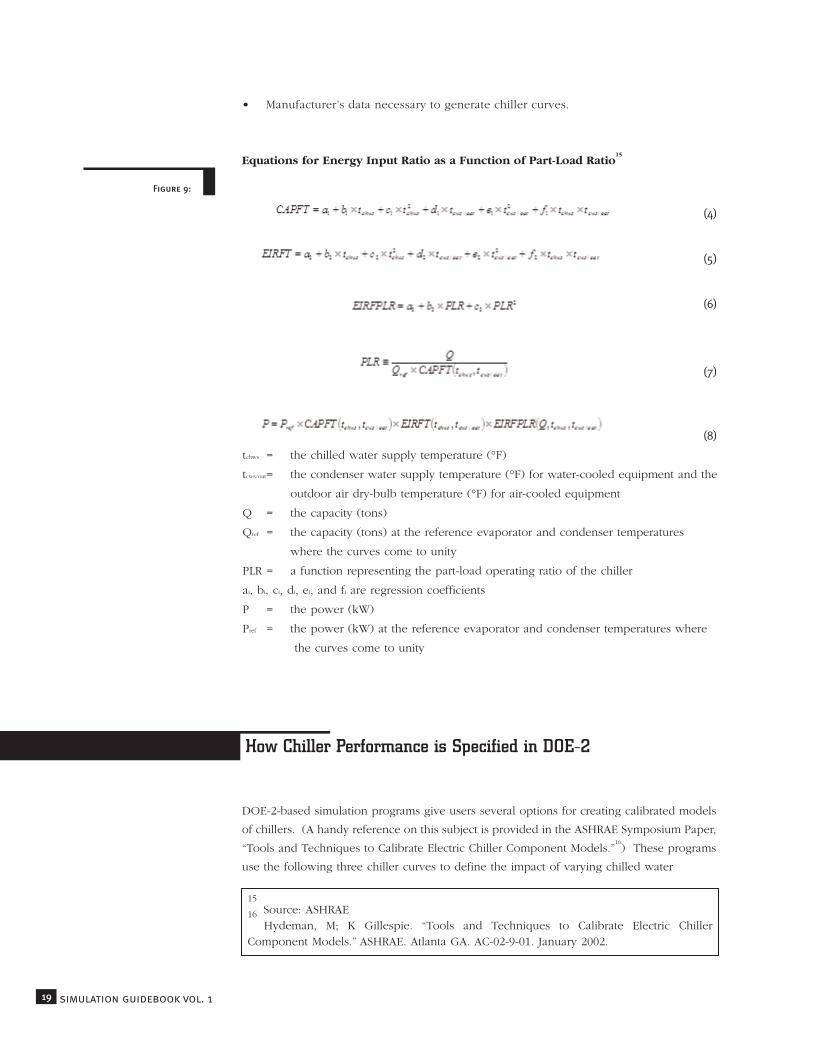
Equations for Energy Input Ratio as a Function of Part-Load Ratio15

DOE-2-based simulation programs give users several options for creating calibrated models

of chillers. (A handy reference on this subject is provided in the ASHRAE Symposium Paper,

“Tools and Techniques to Calibrate Electric Chiller Component Models.”16) These programs

use the following three chiller curves to define the impact of varying chilled water


How Chiller Performance is Specified in DOE-2

Figure 9:

15Source: ASHRAE16 Hydeman, M; K Gillespie. “Tools and Techniques to Calibrate Electric Chiller

Component Models.” ASHRAE. Atlanta GA. AC-02-9-01. January 2002.

(4)

(5)

(6)

(7)

(8)

tchws = the chilled water supply temperature (°F)

tcws/oat= the condenser water supply temperature (°F) for water-cooled equipment and the

outdoor air dry-bulb temperature (°F) for air-cooled equipment

Q = the capacity (tons)

Qref = the capacity (tons) at the reference evaporator and condenser temperatures

where the curves come to unity

PLR = a function representing the part-load operating ratio of the chiller

ai, bi, ci, di, ei, and fi are regression coefficients

P = the power (kW)

Pref = the power (kW) at the reference evaporator and condenser temperatures where

the curves come to unity

temperature, condenser temperature, and load on chiller performance and capacity:

• CAPFT - Capacity as a Function of Temperature. This curve adjusts the available

capacity of the chiller as a function of evaporator and condenser temperatures (or lift).

• EIRFT - Energy Input Ratio as a Function of Temperature. This curve adjusts the

efficiency of the chiller as a function of evaporator and condenser temperatures (or lift).

• EIRFPLR - Energy Input Ratio as a Function of Part-Load Ratio. This curve adjusts the

efficiency of the chiller as a function of part-load operation.

The format of these curves is shown in Figure 9. Using Equations (4) to (7), the power

under any conditions of load and temperature can be found from equation 8 (see Figure

9). Each of these curves is described below:

CAPFT- Chiller Capacity as a Function of TemperatureThis curve defines how chiller cooling capacity changes with different refrigerant lift con-

ditions. The curve can be directly calculated in the DOE-2 program by entering an array

of data points that each contains three numbers: the chilled water supply temperature,

the condenser temperature, and the corresponding value of CAPFT. For example, the data

point (44, 85, 1.0) for a water-cooled chiller translates as, “...when the chiller is producing

44 degree F chilled water and the entering condenser water temperature is 85 degrees F,

the chiller provides 100% of its rated capacity.” This would make sense to many mechani-

cal engineers because 44 and 85 correspond to the ARI rating conditions under which

chiller capacity and integrated part load value (IPLV) are calculated. All data for the

CAPFT curve assumes the chiller is operating at 100% of motor load.

CAPFT is defined from equation 7 above at the point where the “part-load ratio” (PLR) is

unity. This is shown in equation 9:

(9)

EIRFT- Energy Input Ratio as a Function of TemperatureThis curve defines how chiller efficiency changes with different refrigerant lift conditions.

The curve can be directly calculated in the DOE-2 program by entering an array of data

points that each contains three numbers: the chilled water supply temperature, the con-

denser temperature, and the EIRFT. For example, the data point (44, 85, 1.0) translates as,

“...when the chiller is producing 44 degree F chilled water and the entering condenser

water temperature is 85 degrees F, the chiller operates at its nominal full-load efficiency.”

All data for the CAPFT curve assumes the chiller is operating at 100% of motor load.

EIRFT is defined from equation 8 above at the point where the “energy input ratio as a func-

tion of part-load ratio” (EIRFPLR) is unity. This is shown in equation 10:

(10)


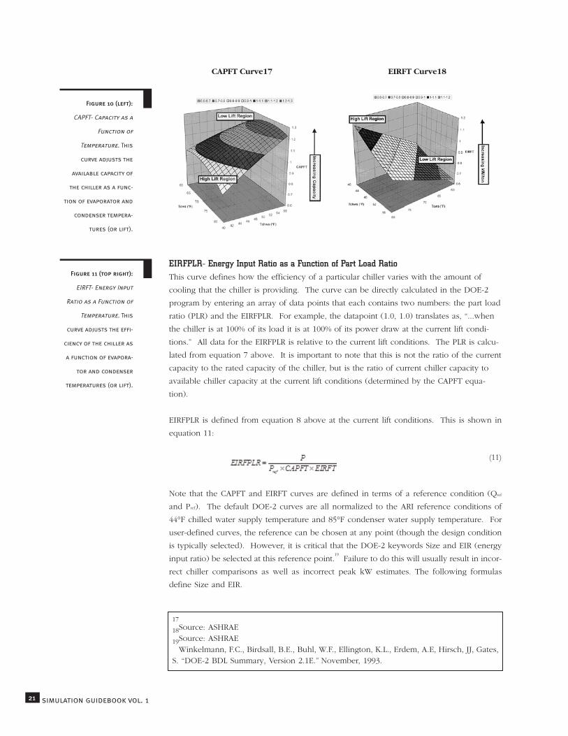
Figure 10 (left):

CAPFT- Capacity as a

Function of

Temperature. This

curve adjusts the

available capacity of

the chiller as a func-

tion of evaporator and

condenser tempera-

tures (or lift).


CAPFT Curve17 EIRFT Curve18

EIRFPLR- Energy Input Ratio as a Function of Part Load RatioThis curve defines how the efficiency of a particular chiller varies with the amount of

cooling that the chiller is providing. The curve can be directly calculated in the DOE-2

program by entering an array of data points that each contains two numbers: the part load

ratio (PLR) and the EIRFPLR. For example, the datapoint (1.0, 1.0) translates as, “...when

the chiller is at 100% of its load it is at 100% of its power draw at the current lift condi-

tions.” All data for the EIRFPLR is relative to the current lift conditions. The PLR is calcu-

lated from equation 7 above. It is important to note that this is not the ratio of the current

capacity to the rated capacity of the chiller, but is the ratio of current chiller capacity to

available chiller capacity at the current lift conditions (determined by the CAPFT equa-

tion).

EIRFPLR is defined from equation 8 above at the current lift conditions. This is shown in

equation 11:

(11)

Note that the CAPFT and EIRFT curves are defined in terms of a reference condition (Qref

and Pref). The default DOE-2 curves are all normalized to the ARI reference conditions of

44°F chilled water supply temperature and 85°F condenser water supply temperature. For

user-defined curves, the reference can be chosen at any point (though the design condition

is typically selected). However, it is critical that the DOE-2 keywords Size and EIR (energy

input ratio) be selected at this reference point.19

Failure to do this will usually result in incor-

rect chiller comparisons as well as incorrect peak kW estimates. The following formulas

define Size and EIR.

Figure 11 (top right):

EIRFT- Energy Input

Ratio as a Function of

Temperature. This

curve adjusts the effi-

ciency of the chiller as

a function of evapora-

tor and condenser

temperatures (or lift).

17Source: ASHRAE18Source: ASHRAE19Winkelmann, F.C., Birdsall, B.E., Buhl, W.F., Ellington, K.L., Erdem, A.E, Hirsch, JJ, Gates,

S. “DOE-2 BDL Summary, Version 2.1E.” November, 1993.

• Size - Nominal Rated Output Capacity. This input for nominal chiller capacity,

expressed in units of one million Btu’s per hour (Mbtu/hr), is used to normalize the

CAPFT curve.

(12)

Most DOE-2.1e user interfaces such as EnergyPro or VisualDOE allow the user to input

nominal chiller capacity in units of tons.

• ELEC-INPUT-RATIO, or EIR- Electric Input to Nominal Capacity Ratio. This input is

used to define the efficiency of the chiller at the reference conditions. The EIR is

calculated as follows:

(13)

This data is generally entered in unit of kW/ton in DOE-2.1e- based programs such as

EnergyPro and VisualDOE.

DOE-2.1e Sample Text for Chiller Inputs


Figure 12

INPUT PLANT ..

CHWPlnt = PLANT-ASSIGNMENT ..

$ *********************************************************************** $

$ General Chiller Inputs $

$ *********************************************************************** $

$ electric centrifugal chiller #1

CHILLER1 = PLANT-EQUIPMENT

TYPE = OPEN-CENT-CHLR $ Selections available are described in

$ DOE-2.1e BDL summary, Page 50 (Nov 1993)

SIZE = 2.393 $ SIZE = Capacity * 0.012 MBTU/hr / ton

$ where capacity is expressed in units

$ of tons

INSTALLED-NUMBER = 1

MAX-NUMBER-AVAILABLE = 1

..

$ part load ratio for electric centrifugal chiller #1

PART-LOAD-RATIO

TYPE = OPEN-CENT-CHLR

ELEC-INPUT-RATIO = 0.199 $ EIR = kW/ton * 3413 Btu/kW / 12,000 Btu/ton

$ EIR should be defined using the same

$ conditions for CHWT & CWT as SIZE

MIN-RATIO = .1

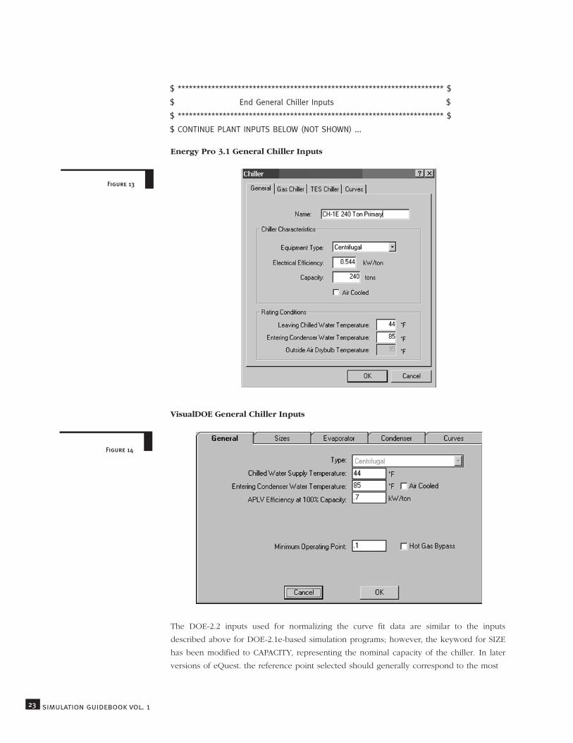
Energy Pro 3.1 General Chiller Inputs

VisualDOE General Chiller Inputs

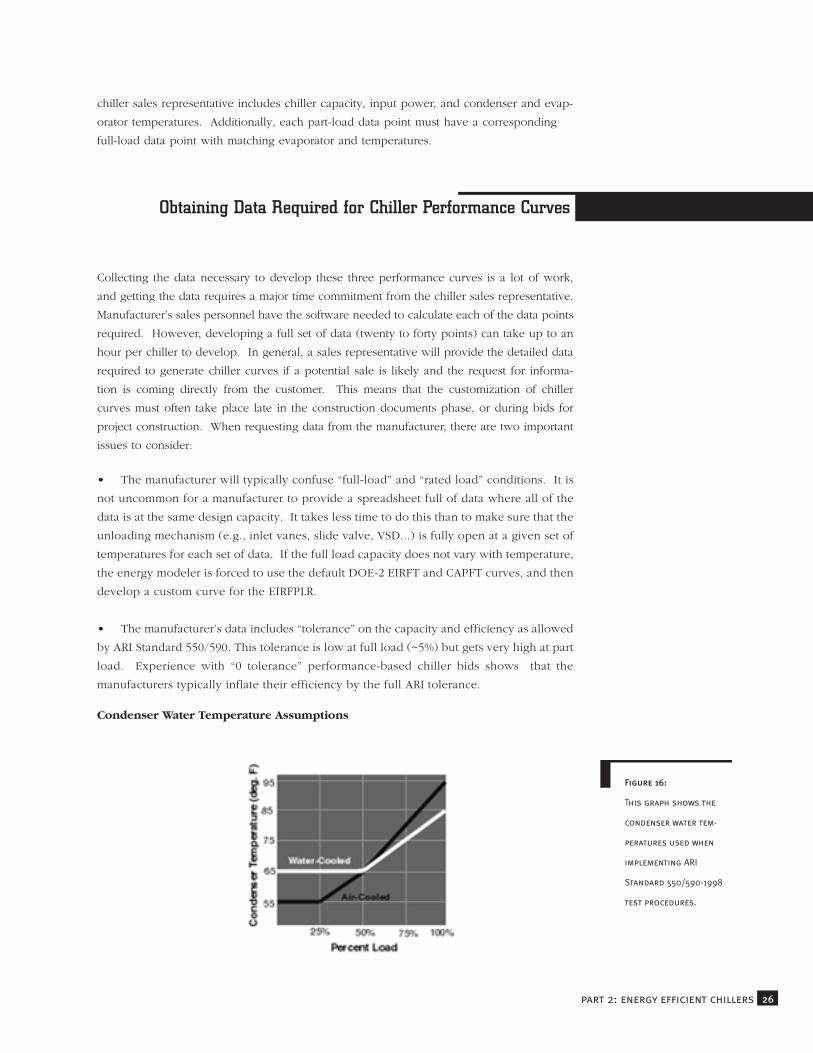
The DOE-2.2 inputs used for normalizing the curve fit data are similar to the inputs

described above for DOE-2.1e-based simulation programs; however, the keyword for SIZE

has been modified to CAPACITY, representing the nominal capacity of the chiller. In later

versions of eQuest. the reference point selected should generally correspond to the most


Figure 13

$ *********************************************************************** $

$ End General Chiller Inputs $

$ *********************************************************************** $

$ CONTINUE PLANT INPUTS BELOW (NOT SHOWN) ...

Figure 14

Figure 15


common operating condition (which is typically not at ARI-rated conditions).

DOE-2.2 offers an improved model for variable-speed-driven chillers that includes temper-

ature terms in the EIRFPLR equations. This model was based on research reported in the

ASHRAE Symposium paper, “Development and Testing of a Reformulated Regression Based

Electric Chiller Model.”20

The research reported in this paper demonstrates the accuracy of

the DOE-2 model in predicting the performance of all electric chiller types over a wide range

of operating conditions. The two main shortcomings of the original DOE-2 (2.1E) model

are the part-load efficiency of variable speed driven chillers over a range of temperatures,

and the performance of these models where the condenser water flow varies through the

chiller. The variable speed model has been improved in DOE-2.2; however, the variable

flow condenser water performance21

was not fixed.

The format of the revised EIRFPLR curve for variable speed chillers in DOE-2 is shown in

Figure 15.

Improved Equations for Energy Input Ratio as a function of Part-Load Ratio (EIRF-

PLR)

The variable speed chiller EIRFPLR curve can be calculated in DOE-2.2 by entering an array

of data points that each contains three numbers: the part load ratio (PLR), the difference

between the entering condenser water temperature and the leaving chilled water tempera-

ture (dT), and the EIRFPLR (defined in Equation 11 above). For example, the

Improved Models for Variable Speed Chillers in DOE-2.2

(14)

PLR is defined in equation 7 above

(15)

a3, b3, c3, d3, e3, and f3 are regression coefficients

dT = tcws/oat - tchws

20Hydeman, M.; N. Webb; P. Sreedharan; S. Blanc. “Development and Testing of a

Reformulated Regression Based Electric Chiller Model.” ASHRAE, Atlanta GA. HI-02-18-02.2002.21

Hydeman,Mark. Personal Interview. 20 Apr. 2004.

data point (1.0, 41, 1.0) translates as, “...when the chiller is at 100% of its load, and there is

a 41-degree temperature difference between the condenser temperature and the leaving

chilled water temperature, the chiller is at 100% of its power draw at the current lift condi-

tions.”

To develop curves that accurately model chiller operation, the energy modeler needs access

to at least twenty to thirty records of data which fully cover the range of conditions that will

be simulated.22

The required data consists of one subset of full-load data and a second sub-

set of part-load data. The modeler is cautioned to ensure that the data covers the full range

of conditions under which the chiller will be modeled.

During the simulation, if the chiller is subjected to conditions outside of the range of tuning

data, very unpredictable and inaccurate results can occur.

Full-load data used for defining the CAPFT and EIRFT curves must represent the entire range

of condenser and chilled water supply temperatures that will be evaluated by the energy

model. For water-cooled chillers, condenser temperature is defined as the entering con-

denser water temperature; for air-cooled chillers, the condenser temperature is defined as

the outside air drybulb temperature. To generate the full-load curves, there must be at least

six full-load data points, with at least two different values for both chilled water and con-

denser temperatures, and the data points must include both the minimum and maximum

chilled water and condenser temperature values that will be evaluated by the model. The

information required for each full-load data point includes chiller capacity, input power,

chilled water temperature, and condenser temperature. Although the energy modeler can

generate full-load curves with as little as six data points, a significantly greater number of

distinct full-load data points (i.e., 10 to 20 points) should be used to avoid skewed or inac-

curate results.

Part-load data used for defining the EIRFPLR curve must represent the complete range of

chiller unloading that will be analyzed within the energy model. At least three distinct data

points are required in order to develop the EIRFPLR curve, but a significantly larger num-

ber of points (i.e., 6 to 10 points) should be used to improve the accuracy of the chiller

curve. In DOE-2.2, at least six distinct points are required when defining the EIRFPLR curve

for VSDs, and additional data should be included whenever possible. For each data point

defined in any EIRFPLR curve, the minimum amount of information needed from the

With the exception of

cool, dry climates,

cooling coils provide

inadequate removal of

latent load when cool-

ing to only 64ºF or

67ºF.


22Hydeman, Mark, and Gillespie, Kenneth L. Jr., pp.3.

Data Required for Specifying Chiller Performance Curves inDOE-2

chiller sales representative includes chiller capacity, input power, and condenser and evap-

orator temperatures. Additionally, each part-load data point must have a corresponding

full-load data point with matching evaporator and temperatures.

Collecting the data necessary to develop these three performance curves is a lot of work,

and getting the data requires a major time commitment from the chiller sales representative.

Manufacturer’s sales personnel have the software needed to calculate each of the data points

required. However, developing a full set of data (twenty to forty points) can take up to an

hour per chiller to develop. In general, a sales representative will provide the detailed data

required to generate chiller curves if a potential sale is likely and the request for informa-

tion is coming directly from the customer. This means that the customization of chiller

curves must often take place late in the construction documents phase, or during bids for

project construction. When requesting data from the manufacturer, there are two important

issues to consider:

• The manufacturer will typically confuse “full-load” and “rated load” conditions. It is

not uncommon for a manufacturer to provide a spreadsheet full of data where all of the

data is at the same design capacity. It takes less time to do this than to make sure that the

unloading mechanism (e.g., inlet vanes, slide valve, VSD...) is fully open at a given set of

temperatures for each set of data. If the full load capacity does not vary with temperature,

the energy modeler is forced to use the default DOE-2 EIRFT and CAPFT curves, and then

develop a custom curve for the EIRFPLR.

• The manufacturer’s data includes “tolerance” on the capacity and efficiency as allowed

by ARI Standard 550/590. This tolerance is low at full load (~5%) but gets very high at part

load. Experience with “0 tolerance” performance-based chiller bids shows that the

manufacturers typically inflate their efficiency by the full ARI tolerance.

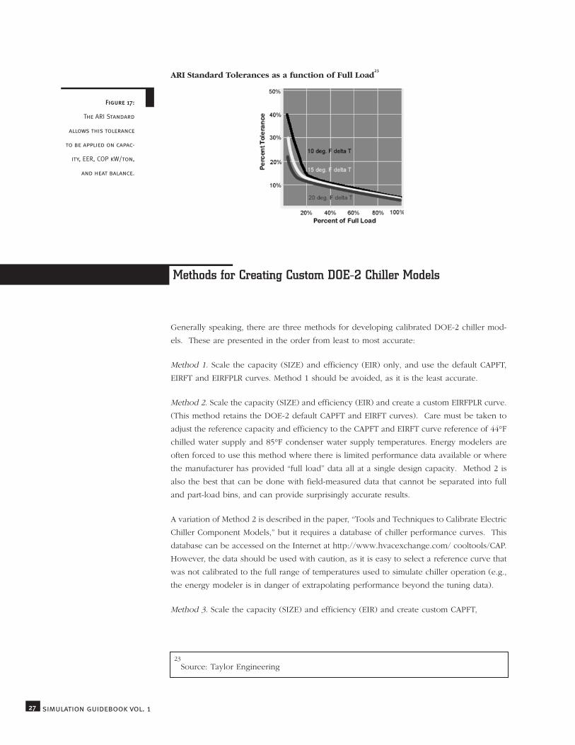
Condenser Water Temperature Assumptions

Figure 16:

This graph shows the

condenser water tem-

peratures used when

implementing ARI

Standard 550/590-1998

test procedures.


Obtaining Data Required for Chiller Performance Curves

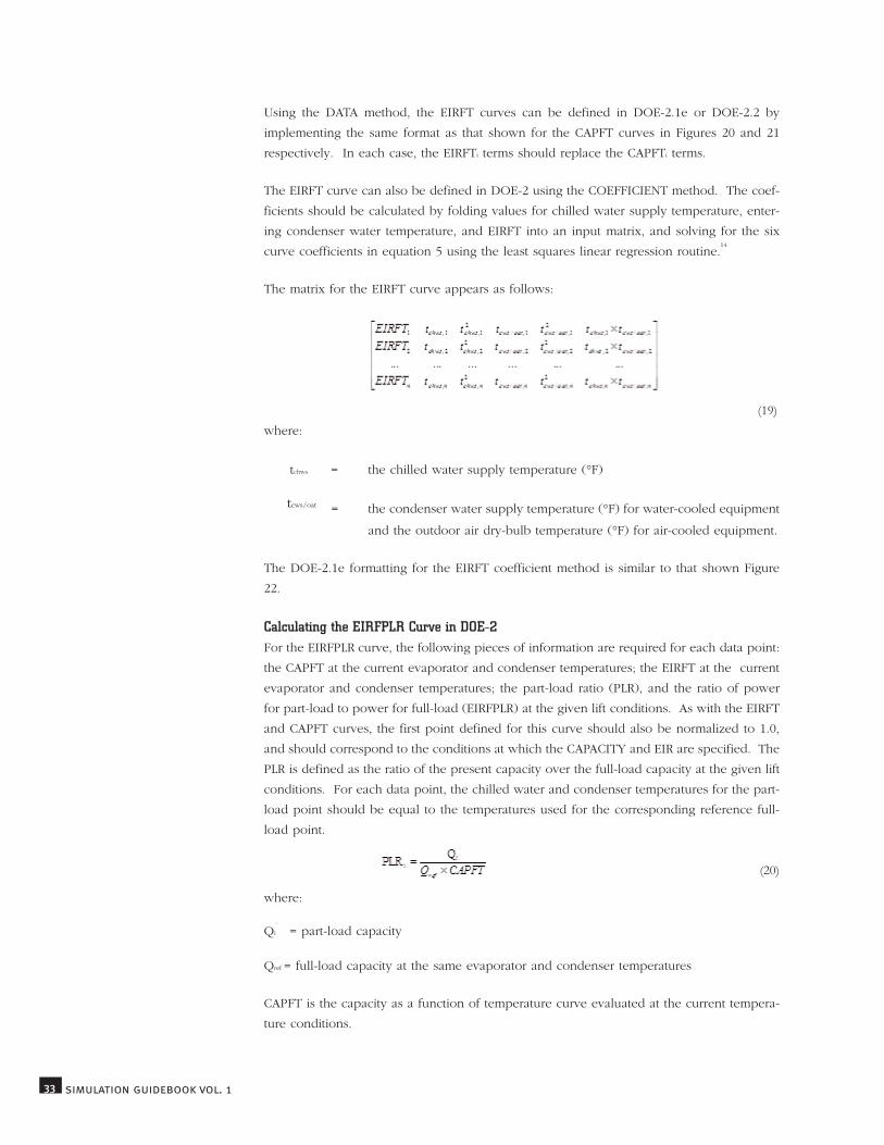
ARI Standard Tolerances as a function of Full Load23

Generally speaking, there are three methods for developing calibrated DOE-2 chiller mod-

els. These are presented in the order from least to most accurate:

Method 1. Scale the capacity (SIZE) and efficiency (EIR) only, and use the default CAPFT,

EIRFT and EIRFPLR curves. Method 1 should be avoided, as it is the least accurate.

Method 2. Scale the capacity (SIZE) and efficiency (EIR) and create a custom EIRFPLR curve.

(This method retains the DOE-2 default CAPFT and EIRFT curves). Care must be taken to

adjust the reference capacity and efficiency to the CAPFT and EIRFT curve reference of 44°F

chilled water supply and 85°F condenser water supply temperatures. Energy modelers are

often forced to use this method where there is limited performance data available or where

the manufacturer has provided “full load” data all at a single design capacity. Method 2 is

also the best that can be done with field-measured data that cannot be separated into full

and part-load bins, and can provide surprisingly accurate results.

A variation of Method 2 is described in the paper, “Tools and Techniques to Calibrate Electric

Chiller Component Models,” but it requires a database of chiller performance curves. This

database can be accessed on the Internet at http://www.hvacexchange.com/ cooltools/CAP.

However, the data should be used with caution, as it is easy to select a reference curve that

was not calibrated to the full range of temperatures used to simulate chiller operation (e.g.,

the energy modeler is in danger of extrapolating performance beyond the tuning data).

Method 3. Scale the capacity (SIZE) and efficiency (EIR) and create custom CAPFT,

Methods for Creating Custom DOE-2 Chiller Models


23Source: Taylor Engineering

Figure 17:

The ARI Standard

allows this tolerance

to be applied on capac-

ity, EER, COP kW/ton,

and heat balance.

EIRFT and EIRFPLR curves. This is the preferred method for developing calibrated DOE-2

chiller models.

Manufacturer’s Data Request Form

Figure 18:

The data request form

shown provides a sim-

ple means for

requesting chiller

curve input data from

chiller manufactur-

ers. A more substan-

tial manufacturer’s

data request form is

available at

http://www.hvacex-

change.com/cooltool

s/CAP/. You may

access it by clicking

the “Excel spread-

sheets for site sur-

veys and manufactur-

er’s data requests”

link.


g

DOE-2 offers two methods for creating chiller curves: the DATA method and the COEFFI-

CIENT method. In the DATA method, the programmer defines each data point directly in

DOE-2. In the COEFFICIENT method, the programmer calculates the regression coefficients

for each curve based on the available data, and inputs these regression coefficients into the

model. VisualDOE and eQUEST support both methods for defining chiller curves, while the

current version of EnergyPro supports only the COEFFICIENT method. The COEFFICIENT

method is much more time-consuming than the DATA method, yet produces the same

results. Therefore, the most time-efficient method for modeling custom chiller curves for

EnergyPro projects may be to generate a DOE-2 input file from EnergyPro, modify the input

file with the custom chiller curves, and run the input file directly in DOE-2.

Calculating the CAPFT Curve in DOE-2The CAPFT curve requires three pieces of data per point: the CAPFT, the chilled water

supply temperature, and the condenser temperature. Each CAPFT point is calculated as

follows:

(16)

Where:

= chiller capacity at specified temperature conditions

= reference capacity, which can be selected based on either the design

capacity or the ARI-rated capacity of the chiller, but must be equal to

the nominal capacity defined for the chiller in DOE-2.

To define CAPFT curves using the DATA method in DOE-2.1e, the energy modeler should

group together the corresponding chilled water temperature, condenser temperature, and

CAPFTi for each point by enclosing these three values into a single set of parentheses. The

first point in the curve must be normalized to 1.0, and must correspond to the conditions at

which the CAPACITY and EIR are specified. A sample DOE-2.1e CAPFT curve is shown in

Figure 20.

In DOE-2.2, curves are defined by grouping all the data for a given input parameter into a

single array. For example, in the CAPFT curve, the chilled water leaving temperatures are


Methods for Including Chiller Data in DOE-2 PerformanceCurves

Qi

Qref

listed in the “INDEPENDENT-1” array, the condenser temperatures are listed in the “INDE-

PENDENT-2” array, and the calculated values for CAPFTi are listed in the “DEPENDENT”

array. The sample DOE-2.1e CAPFT curve shown in Figure 20 below would be defined in

DOE-2.2 as shown in Figure 21.

eQuest Chiller Curve- DATA Method

DOE-2.1e CAPFT Curve- DATA Method


Figure 19:

The screen shot

shows how to define a

chiller curve in

eQuest using the Data

Method.

$********************************************************$

$ DOE-2.1e CAPFT Curve - DATA Method $

$********************************************************$

$ Insert curve under PLANT-ASSIGNMENT in the PLANT portion of

$ the DOE-2 input file

TYP-CAPPFT = CURVE-FIT

TYPE = BI-QUADRATIC

DATA

$ (CHWSi, CWSi, CAPFTi)

DATA (44,85,1.000) (42,85,0.981)(40,85,0.946) (38,85,0.911)

(42,75,1.035)(40,75,1.035) (38,75,0.989)

(50,65,1.035) (42,65,1.035)(40,65,1.035) (38,65,1.035)

$*****************************************************************$ $ END DOE-2.1e CAPFT Curve - DATA Method $$*****************************************************************$

Figure 20

DOE-2.2 CAPFT Curve- DATA Method

In the COEFFICIENT method, the inputs for chilled water supply temperature, entering con-

denser water temperature, and CAPFT are folded into an input matrix which can be solved

for the six regression coefficients in equation 4 using the least squares linear regression rou-

tine.13

The matrix for the CAPFT curve appears as follows:

(17)

Where:


tcws/oat = the condenser water supply temperature (°F) for water-cooled equipment and

the outdoor air dry-bulb temperature (°F) for air-cooled equipment

A typical CAPFT curve in DOE-2.1e using the COEFFICIENT method would be defined as

shown in Figure 22.


Figure 21

$********************************************************$

$ DOE-2.2 CAPFT Curve - DATA Method $

$********************************************************$

$ Insert curves after the last input for SPACE

“TYP-CAPFT” = CURVE-FIT

TYPE = BI-QUADRATIC-T

INPUT-TYPE = DATA

INDEPENDENT-1 =

(44,42,40,38,42,40,38,50,42,40,38)

$Independent-1 defines chilled water leaving temperature

INDEPENDENT-2 =

(85,85,85,85,75,75,75,65,65,65,65)

$Independent-2 defines condenser water entering temperature

DEPENDENT =

( 1.000,0.981,0.946,0.911,1.035,1.035,0.989,

1.035,1.035,1.035,1.035)

$Dependent defines calculated values for CAPFTi

..

$*********************************************************$

$ END DOE-2.2 CAPFT Curve - DATA Method $

$*********************************************************$

DOE-2.1e CAPFT Curve- COEFFICIENTS Method

Calculating the EIRFT Curve in DOE-2

The EIRFT curve is similar to the CAPFT curve, but replaces the “CAPFT” term with a term

for “EIRFT”. Similarly to the CAPFT curve, the first point in the EIRFT curve must be nor-

malized to 1.0, and must correspond to the conditions at which the CAPACITY and EIR are

specified. When implemented correctly, this curve should show the best chiller performance

at low lift conditions and the worst performance at high lift conditions. Each EIRFT point

is calculated as follows:

(18)

where:

Qi and Qref are defined in equation 16, and

Pi = chiller input power at specified temperature conditions

Pref = reference input power which can be selected based on either the design capacity or

the ARI-rated capacity of the chiller; but must use the same conditions as Qref.


Figure 22

$**************************************************************$

$ DOE-2.1e CAPFT Curve - COEFFICIENTS Method $

$**************************************************************$



TYP-CAPFT = CURVE-FIT

TYPE = BI-QUADRATIC

$ COEF = (a2, b2, c2)

COEF=( -0.38924542, -0.02195141, -0.00027343

0.04974775, -0.00053441, 0.00067295)

..

$*******************************************************************$

$ END DOE-2.1e CAPFT Curve - COEFFICIENTS Method $

$*******************************************************************$

Using the DATA method, the EIRFT curves can be defined in DOE-2.1e or DOE-2.2 by

implementing the same format as that shown for the CAPFT curves in Figures 20 and 21

respectively. In each case, the EIRFTi terms should replace the CAPFTi terms.

The EIRFT curve can also be defined in DOE-2 using the COEFFICIENT method. The coef-

ficients should be calculated by folding values for chilled water supply temperature, enter-

ing condenser water temperature, and EIRFT into an input matrix, and solving for the six

curve coefficients in equation 5 using the least squares linear regression routine.14

The matrix for the EIRFT curve appears as follows:

(19)where:


= the condenser water supply temperature (°F) for water-cooled equipment

and the outdoor air dry-bulb temperature (°F) for air-cooled equipment.

The DOE-2.1e formatting for the EIRFT coefficient method is similar to that shown Figure

22.

Calculating the EIRFPLR Curve in DOE-2For the EIRFPLR curve, the following pieces of information are required for each data point:

the CAPFT at the current evaporator and condenser temperatures; the EIRFT at the current

evaporator and condenser temperatures; the part-load ratio (PLR), and the ratio of power

for part-load to power for full-load (EIRFPLR) at the given lift conditions. As with the EIRFT

and CAPFT curves, the first point defined for this curve should also be normalized to 1.0,

and should correspond to the conditions at which the CAPACITY and EIR are specified. The

PLR is defined as the ratio of the present capacity over the full-load capacity at the given lift

conditions. For each data point, the chilled water and condenser temperatures for the part-

load point should be equal to the temperatures used for the corresponding reference full-

load point.

(20)

where:

Qi = part-load capacity

Qref = full-load capacity at the same evaporator and condenser temperatures

CAPFT is the capacity as a function of temperature curve evaluated at the current tempera-

ture conditions.


tcws/oat


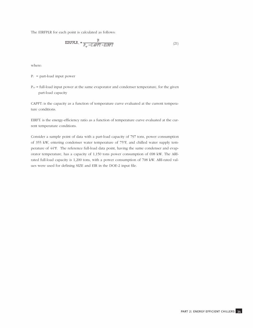
The EIRFPLR for each point is calculated as follows:

(21)

where:

Pi = part-load input power

Pref = full-load input power at the same evaporator and condenser temperature, for the given

part-load capacity

CAPFTi is the capacity as a function of temperature curve evaluated at the current tempera-

ture conditions.

EIRFTi is the energy-efficiency ratio as a function of temperature curve evaluated at the cur-

rent temperature conditions.

Consider a sample point of data with a part-load capacity of 797 tons, power consumption

of 355 kW, entering condenser water temperature of 75ºF, and chilled water supply tem-

perature of 44ºF. The reference full-load data point, having the same condenser and evap-

orator temperature, has a capacity of 1,150 tons power consumption of 698 kW. The ARI-

rated full-load capacity is 1,200 tons, with a power consumption of 708 kW. ARI-rated val-

ues were used for defining SIZE and EIR in the DOE-2 input file.

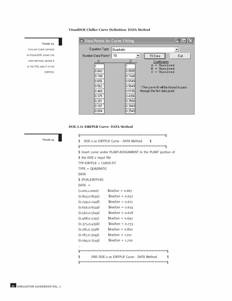
Figure 24


VisualDOE Chiller Curve Definition- DATA Method

DOE-2.1e EIRFPLR Curve- DATA Method

$********************************************************$

$ DOE-2.1e EIRFPLR Curve - DATA Method $

$********************************************************$



TYP-EIRFPLR = CURVE-FIT

TYPE = QUADRATIC

DATA

$ (PLRi,EIRFPLRi)

DATA =

(1.000,1.0000) $kw/ton = 0.667

(0.843,0.8595) $kw/ton = 0.637

(0.749,0.7448) $kw/ton = 0.621

(0.656,0.6549) $kw/ton = 0.624

(0.562,0.5649) $kw/ton = 0.628

(0.468,0.5195) $kw/ton = 0.693

(0.375,0.4396) $kw/ton = 0.733

(0.281,0.3598) $kw/ton = 0.800

(0.187,0.3049) $kw/ton = 1.017

(0.094,0.2549) $kw/ton = 1.700

..

$*********************************************************$

$ END DOE-2.1e EIRFPLR Curve - DATA Method $

$*********************************************************$

Figure 23:

Chiller Curve defined

in VisualDOE using the

data method, where X

is the PLR, and Z is the

EIRFPLR.


The CAPFT evaluated at the current temperature conditions would be calculatedas:

The EIRFT evaluated at the current temperature conditions would be calculated as:

The EIRFPLR point would be calculated as:

Using the DATA method, a typical EIRFPLR curve in DOE-2.1e would be defined shown in

Figure 24.

The same EIRFPLR curve, representing part-load chiller performance for a chiller without a

Variable Speed Drive (VSD), should be entered in DOE-2.2 as shown in Figure 25.

DOE-2.1e EIRFPLR Curve without VSD- DATA Method

$********************************************************$

$ DOE-2.2 EIRFPLR Curve without VSD - DATA Method $

$********************************************************$

$ Insert curve after the last entry for SPACE

“TYP-EIRFPLR” = CURVE-FIT

TYPE = QUADRATIC

INPUT-TYPE = DATA

INDEPENDENT = (1.000, 0.843, 0.749, 0.656, 0.562,

0.468, 0.375, 0.281, 0.187, 0.094)

$ independent dataset includes all PLRi terms

DEPENDENT = (1.000, 0.8595, 0.7488, 0.6549, 0.5649

.5195, 0.4396, 0.3598, 0.3049, 0.2549)

$ dependent dataset includes all EIRFPLRi terms

..

$************************************************************$

$ END DOE-2.2 EIRFPLR Curve without VSD - DATA Method $

$************************************************************$

Figure 25:

A sample DOE2.2 EIRF-

PLR curve for a chiller

with a VSD that is

shown in figure 30.

In the COEFFICIENT method, inputs for PLR and EIRFPLR are folded into an input matrix

which can be solved for the three curve coefficients using the least squares linear regres-

sion routine.24

The format for the EIRFPLR curve is as follows:

` (22)

Where a1, b1, and c1 are the regression coefficients for the curve.

The matrix for the EIRFPLR curve appears as follows:

(23)

The EIRFPLR curve should be defined in DOE-2.1e as shown in Figure 26.

DOE-2.1e EIRFPLR Curve- Coefficients Method

In DOE-2.2, the EIRFPLR curve for VSDs should be modified to include a third value for

each point of data that indicates the differential between the condenser and chilled water

supply temperatures.24

The curve type should be selected as “BI-QUADRATIC-RATIO&dt,”

where the first independent dataset lists the values for PLRi, the second independent dataset

lists the values for the temperature differential between the condenser and entering chilled

water, and the dependent dataset lists the values for EIRFPLR. The sample code shown in

Figure 30 demonstrates the format for defining this curve in DOE-2.2.

Once the three chiller curves have been defined, they should each be attached to the cor-

responding chiller. In DOE-2.1e, this is accomplished by associating each chiller curve


24More details regarding the definition of this curve, defined as a “BI-QUADRATIC-

RATIO&dT” curve can be found in the “New Features,” Volume 6 manual by JamesHirsch (see footnote 3 from chapter 1).

$********************************************************$

$ DOE-2.1e EIRFPLR Curve - COEFFICIENTS Method $

$********************************************************$



TYP-EIRFPLR = CURVE-FIT

TYPE = QUADRATIC

$ COEF = (a1, b1, c1)

COEF=(0.27715900,-0.02504500,0.73693600)

..

$*********************************************************$

$ END DOE-2.1e EIRFPLR Curve - COEFFICIENTS Method $

$*********************************************************$

Figure 26

Figure 28:

Chiller curve defined

in Energy Pro using

the coefficients

method.


eQuest Chiller Curve Definition

with the corresponding chiller type. For example, for an open centrifugal chiller, selected as

OPEN-CENT-CHLR, the curves would be attached under EQUIPMENT-QUAD using the key-

words OPEN-CENT-CAP-FT for the CAPFT curve, OPEN-CENT-EIR-FT for the EIRFT curve,

and OPEN-CENT-EIR-FPLR for the EIRFPLR curve (see Figure 31).

Energy Pro Chiller Curve Definition- COEFFICIENTS Method

Figure 27:

Define EIRFPLR curve

for variable speed

chiller as”Bi-

Quadratic in Ratio &

dT” in eQuest.

eQuest Chiller Curve Definition- DATA Method


Figure 29:

Insert points for EIRF-

PLR curve for Variable

Speed Chiller in

eQuest.

DOE-2.2 EIRFPLR Curve for Chillers with Variable Speed Drives- DATA Method

Figure 30


$**************************************************************$

$ DOE-2.2 EIRFPLR Curve - DATA Method $

$ (TO BE USED FOR CHILLERS WITH VARIABLE SPEED DRIVES) $

$**************************************************************$

$ Insert curves after the last input for SPACE

“VSD-EIRFPLR” = CURVE-FIT

TYPE = BI-QUADRATIC-RATIO&dt

INPUT-TYPE = DATA

INDEPENDENT-1 = (1.000,0.900,0.751,0.630,0.540

0.450,0.360,0.270,0.180,0.141)

$ independent dataset # 1 includes all PLRi terms

INDEPENDENT-2 = (41.000,37.000,33.000,29.000,25.000

21.000,21.000,21.000,21.000,21.000)

$ independent dataset # 2 includes all dti terms

DEPENDENT = (1.000,0.828,0.673,0.542,0.440

0.367,0.330,0.259,0.203,0.184)

$ dependent dataset includes all EIRFPLRi terms

..

$*************************************************************$

$ END DOE-2.2 EIRFPLR Curve - DATA Method for VSD Chillers $

$*************************************************************$

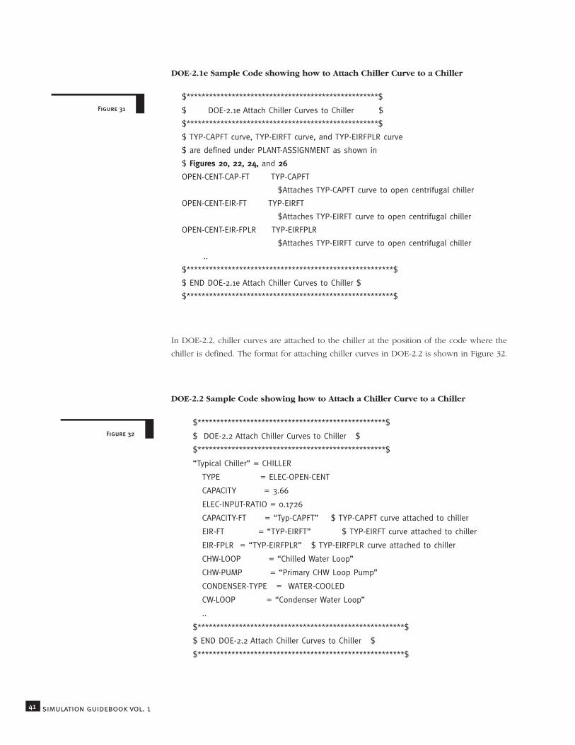
DOE-2.1e Sample Code showing how to Attach Chiller Curve to a Chiller

In DOE-2.2, chiller curves are attached to the chiller at the position of the code where the

chiller is defined. The format for attaching chiller curves in DOE-2.2 is shown in Figure 32.

DOE-2.2 Sample Code showing how to Attach a Chiller Curve to a Chiller


$**************************************************$

$ DOE-2.2 Attach Chiller Curves to Chiller $

$**************************************************$

“Typical Chiller” = CHILLER

TYPE = ELEC-OPEN-CENT

CAPACITY = 3.66

ELEC-INPUT-RATIO = 0.1726

CAPACITY-FT = “Typ-CAPFT” $ TYP-CAPFT curve attached to chiller

EIR-FT = “TYP-EIRFT” $ TYP-EIRFT curve attached to chiller

EIR-FPLR = “TYP-EIRFPLR” $ TYP-EIRFPLR curve attached to chiller

CHW-LOOP = “Chilled Water Loop”

CHW-PUMP = “Primary CHW Loop Pump”

CONDENSER-TYPE = WATER-COOLED

CW-LOOP = “Condenser Water Loop”

..

$*******************************************************$

$ END DOE-2.2 Attach Chiller Curves to Chiller $

$*******************************************************$

$***************************************************$

$ DOE-2.1e Attach Chiller Curves to Chiller $

$***************************************************$

$ TYP-CAPFT curve, TYP-EIRFT curve, and TYP-EIRFPLR curve

$ are defined under PLANT-ASSIGNMENT as shown in

$ Figures 20, 22, 24, and 26

OPEN-CENT-CAP-FT TYP-CAPFT

$Attaches TYP-CAPFT curve to open centrifugal chiller

OPEN-CENT-EIR-FT TYP-EIRFT

$Attaches TYP-EIRFT curve to open centrifugal chiller

OPEN-CENT-EIR-FPLR TYP-EIRFPLR

$Attaches TYP-EIRFT curve to open centrifugal chiller

..

$*******************************************************$

$ END DOE-2.1e Attach Chiller Curves to Chiller $

$*******************************************************$

Figure 32

Figure 31

Due to the complexity involved in creating custom chiller curves, energy modelers have

been known to improperly develop them and end up with results that are less accurate

than those available using default curves. To ensure the greatest accuracy when modeling

custom chiller curves, follow these important guidelines:

• Get accurate data from the chiller manufacturer. Make sure that the “full load” data

is truly at an operating point with the chiller fully loaded.

• Derate the data based on the ARI tolerance curve. Do not derate the capacity, but use

the full tolerance to derate the stated power at each point of operation.

• Make sure that the data points used for the curves extends over the full range of

simulated operation. If you extrapolate performance beyond the data points, you will

get useless results.

• Use sufficient amounts of data. Results will increase in accuracy as the number of data

points is increased, provided that the data points cover the full range of conditions

that will be simulated in the energy analysis program.

• Pay attention to the order of data input. Whether using the COEFFICIENT method or

the DATA method to define chiller curves, the order of the data input must be entered

as outlined in this simulation guidebook. For example, in the EIRFPLR curve,

information for PLR should be listed first in the data pair, and EIRFPLR should be listed

second. If the order of the data is reversed, then the energy efficiency of the chiller

at various part-load conditions will be calculated incorrectly, and therefore, overall

chiller energy use will be inaccurate.

Using the chiller modeling methodology described in this guidebook, energy modelers can

assist the design team in developing chiller plants with tremendous potential savings. When

energy modelers combine the advanced control sequences modeling strategies discussed in

the third section of this simulation guidebook with these strategies for modeling chiller

curves, the energy model can become a particularly effective tool for optimizing chilled

water plant performance. For example, an article entitled “Commissioning Tools &

Techniques Used in a Large Chilled Water Plant Optimization Project,”17


25Hydeman, M.; S. Tylor; C. Speck; and K. Gillespie. “Commissioning Tools &

Techniques Used in a Large Chilled Water Plant Optimization Project.” Proceedings ofthe 7

thNational Conference on Building Commissioning. PECI, Portland Oregon. May

1999.

Summary

Guidelines for Creating Accurate Custom Chillers

reported a 6.5 GWH/year reduction in plant energy through chiller replacement and con-

trols in a 17,000 ton chiller plant. Careful development of calibrated energy models for this

plant enabled the team to analyze the various design options, and achieve the maximum

possible energy and cost savings for the plant. These savings were verified by post-retrofit

monitoring.

Steps for Creating Custom Chiller Curves in DOE-2-Based Programs

1. Procure 20-40 points of data from chiller manufacturers, where each point includes con-denser temperature, chilled water supply temperature, chiller capacity, input power,and percent loading. Data should include both part-load and full-load data over thefull range of condenser and chilled water temperatures for which the chiller will oper-ate.

2. Select the reference point by which the chiller curves will be normalized. For DOE-2.1e, the reference point should be selected at ARI-rated conditions. For recent ver-sions of DOE-2.2, the reference point should correspond to the most common full-loadoperating conditions.

3. Generate CAP-FT Curve

a. For each set of full-load data, calculate CAPFTi, defined in equation 16 above.

b. DATA Method: Enter each set of full load data points for the CAPFT curve into aDOE-2 based simulation program, where each point includes a term for chilledwater temperature, condenser temperature, and CAPFTi. Confirm that the CAPFTifor the first point is normalized to 1.0 based on the reference point identified inStep # 2 above. Figure 20 defines the format for entering CAPFT curves in DOE-2.1e, and Figure 21 indicates the format for DOE2.2 CAPFT curves.

c. COEFFICIENTS Method: Input each set of full load data points including chilledwater temperature, condenser temperature, and CAPFTi into the matrix shown inequation 17, and solve for the six regression coefficients. Define the curve coeffi-cients in DOE-2.1e using the format shown in Figure 22.

4. Generate EIR-FT Curve

a. For each set of full-load data, calculate EIRFTi, defined in equation 18 above.

b. DATA Method: Enter each set of full load data points for the EIRFT curve into aDOE-2 based simulation program, where each point includes a term for chilledwater temperature, condenser temperature, and EIRFTi. Confirm that the EIRFTifor the first point is normalized to 1.0 based on the reference point identified inStep # 2 above. Figure 20 defines the format for entering EIRFT curves in DOE-2.1e, and Figure 21 indicates the format for DOE2.2 EIRFT curves (where in eachcase the term for EIRFTi replaces the term for CAPFTi).

c. COEFFICIENTS Method: Input each set of full load data points including chilledwater temperature, condenser temperature, and CAPFTi into the matrix shown inequation 19, and solve for the six regression coefficients. Define the curve coeffi-cients in DOE-2.1e using the format shown in Figure 22.


5. Generate EIR-FPLR Curve

a. For each set of part-load data, calculate the PLRi and EIRFPLRi as defined in equa-tions 20 and 21 respectively. Note that you will need to calculate the CAPFTi andEIRFTi at each point in order to calculate the PLRi and EIRFPLRi. If you are defin-ing a curve for a variable speed chiller in DOE2.2, you should also calculate dT asdefined in equation 15.

b. DATA Method: Enter each set of full load data points for the EIRFPLR curve into aDOE-2 based simulation program, where each point includes a term for PLRi andEIRFPLRi. Confirm that the PLRi and EIRFPLRi for the first point are normalized to1.0 based on the reference point identified in Step # 2 above. For curves definedin DOE-2.1e, use the format shown in Figure 24. For chillers without variablespeed drives, defined in DOE-2.1e, use the format shown in Figure 25. For chillerswith variable speed drives defined in DOE2.2, include terms for PLRi, dT, andEIRFPLRi as demonstrated in Figure 30.

c. COEFFICIENT method: Input the data for PLRi and EIRFPLRi into the matrix shownin equation 23, and solve for the three regression coefficients. Enter the curve coef-ficients in DOE-2.1e using the format shown in Figure 26.

6. Attach the custom chiller curves to the appropriate chiller using Figure 31 for DOE-2.1e,and Figure 32 for DOE2.2.


The recent widespread use of digital controls in building construction has greatly expand-

ed the opportunities for optimizing building efficiency. Using digital controls provides more

accurate sensing of data and enhances flexibility for modifying control logic. However, rel-

atively few buildings that use digital control technologies attain their full potential for cost-

effectively minimizing energy demand and consumption. Common problems that prevent

the use of efficient digital control technologies include:

• Misinformation regarding the risks and benefits of the technology;

• An inadequate understanding of the energy and cost benefits associated with these

strategies, and

• Complete ignorance regarding the availability of such strategies.

Energy models that accurately demonstrate the operating cost benefits of these technologies

can present decision makers with compelling reasons for implementing the strategies into

the project design. Accordingly, this simulation guidebook highlights the following digital

control strategies and sequences that may improve efficient operation of water-side systems.

The guidebook also provides a guide for modeling each technology in EnergyPro, native

DOE-2.1e, and eQUEST:

• Variable primary flow chilled water distribution (page 46)

• Primary/secondary chilled water distribution (page 48)

• Variable flow condenser water system (page 54)

• Cooling tower cell control (page 55)

• Cooling tower capacity control (page 55)

• Condenser water temperature reset (page 57)

• Chilled water temperature reset (page 59)

• Hot water temperature reset (page 60)

45part 3: advanced control sequences

PART 3: Advanced Control Sequences

COMMON SIMULATION

SOFTWARE

This guidebook uses

research generated from

the following energy sim-

ulation software pack-

ages:

EnergyPro v. 3.142,

eQUEST v. 3.44 with

DOE2.2 release 42k6, and




updated. Review the docu-

mentation of later

releases for any changes

to software inputs or

keywords that might

impact the modeling

methodology discussed

in this simulation guide-

book.

When controlled correctly, variable speed drives (VSDs) installed on fan, pump, and com-

pressor motors can significantly limit equipment energy usage by optimizing the part-load

performance of the equipment. In recent years, VSDs have become an increasingly com-

mon option for HVAC system equipment due to the improved reliability of VSD technology

and more stringent energy code requirements. However, design teams often only specify

equipment with VSDs when this technology is required to minimally comply with energy

code standards. To promote further use of these efficient technologies, California Title-24

2005 standards prescriptively require variable speed controls for pumps over 5 hp that serve

variable-flow systems.

Using DOE-2 simulation programs to model variable-speed control sequences for waterside

systems is often difficult due to (a) the limited modeling capabilities of DOE-2.1e-based soft-

ware (i.e. EnergyPro), and (b) the vast range of available inputs in DOE-2.2 programs such

as eQUEST. This portion of the simulation guidebook discusses methods for modeling the

following variable-speed control strategies in EnergyPro, native DOE-2.1e, and eQUEST:

• Variable Primary Flow Chilled Water Distribution

• Primary/Secondary Chilled Water Distribution

• Variable Flow Condenser Water System

Note that the variable-speed, variable-flow-pumping algorithms in the LBNL/USDOE version

of DOE-2.1e (which is used as the simulation engine for EnergyPro), provide only a rough

approximation of actual variable speed pumping control, whereas later versions of DOE-

2.1e, and DOE-2.2 incorporate much more accurate simulation of variable-speed pumping

control.

Variable Primary Flow Chilled Water DistributionIn a variable primary flow chilled water distribution system, VSDs on the primary chilled

water pumps vary the flow through the chillers and out to the chilled water coils based

on demand. These systems generally include a bypass loop to ensure minimum flow

through the chiller. When properly implemented, variable primary pumping generally pro-

vides the most cost-effective and energy-efficient option for chilled water distribution. In

EnergyPro, variable primary flow is modeled by defining the primary chilled water pump

data under the secondary chilled water pump tab according to the following process:

• From the Plant / Chilled Water tab, click each chiller to view the primary pump inputs.

Set Flow Rate per Pump, Pump Multiplier, and Design Power to a value of zero. Close

the chiller window.

• Select the Secondary Pumps window by clicking the graphic titled either No

Secondary Pumps or Secondary Pumps. Select the pump type as Variable Speed, and

then enter the appropriate Minimum Flow Per Pump, as well as all the other relevant inputs


Variable Speed Drive Control Sequences

Following Through on

Control Strategies

Each control strategy simu-

lated in the final building

energy model MUST match

the equipment data and con-

trol schemes defined in the

plans and control

sequences for the building.

Unfortunately, control

strategies are often recom-

mended based on initial

energy models and incorpo-

rated into the final estimat-

ed energy savings for the

building, but are excluded

from final plans or control

sequences. A building com-

missioning process should

be used to confirm that

control sequences

described in the design

document are used in the

final building design, and

to confirm that the control

sequences function proper-

ly when the building is com-

pleted.


pertaining to the primary chilled water pumps. In DOE-2.1e, energy modelers can simulate

variable primary chilled water flow by setting CCIRC-PUMP-TYPE to VARIABLE-SPEED, and

specifying the minimum electricity consumption as a fraction of full load consumption

(CCIRC-MIN-PLR).

Variable Primary Flow Inputs for the Variable Primary Flow Inputs for the

Chiller Window in EnergyPro Secondary Chilled Water Pumps in EnergyPro

DOE-2.1e Variable Primary Chilled Water Flow

Figure 33 (Far left):

To define variable pri-

mary flow in

EnergyPro, set the val-

ues for flow, pump

multiplier, and design

power to 0 in the

chiller window.

Figure 34 (top right):

Define variable primary

inputs in the sec-

ondary chilled water

pump window in

EnergyPro.

Figure 35

PLANT-PARAMETERS

$Chilled Water Variable Primary CHW Pumps

CCIRC-PUMP-TYPE = VARIABLE-SPEED $ defines primary flow as

$ variablespeed; (FIXED-SPEED

$ is the DOE-2default)

CCIRC-MIN-PLR = 0.300 $ Minimum electricity

$ consumption as fraction of

$ full-load consumption

CCIRC-HEAD = 100 $ Defines the head pressure

$ of the CHW loop

CCIRC-IMPELLER-EFF = .7 $ CHW pump impeller

$ efficiency

CCIRC-MOTOR-EFF = .85 $ CHW pump motor efficiency

$ Other Plant Parameters not shown

..

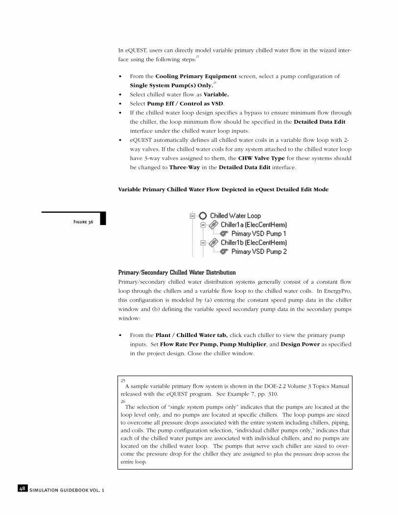
Figure 36


In eQUEST, users can directly model variable primary chilled water flow in the wizard inter-

face using the following steps:25

• From the Cooling Primary Equipment screen, select a pump configuration of

Single System Pump(s) Only.26

• Select chilled water flow as Variable.

• Select Pump Eff / Control as VSD.

• If the chilled water loop design specifies a bypass to ensure minimum flow through

the chiller, the loop minimum flow should be specified in the Detailed Data Edit

interface under the chilled water loop inputs.

• eQUEST automatically defines all chilled water coils in a variable flow loop with 2-

way valves. If the chilled water coils for any system attached to the chilled water loop

have 3-way valves assigned to them, the CHW Valve Type for these systems should

be changed to Three-Way in the Detailed Data Edit interface.

Variable Primary Chilled Water Flow Depicted in eQuest Detailed Edit Mode

Primary/Secondary Chilled Water DistributionPrimary/secondary chilled water distribution systems generally consist of a constant flow

loop through the chillers and a variable flow loop to the chilled water coils. In EnergyPro,

this configuration is modeled by (a) entering the constant speed pump data in the chiller

window and (b) defining the variable speed secondary pump data in the secondary pumps

window:

• From the Plant / Chilled Water tab, click each chiller to view the primary pump

inputs. Set Flow Rate Per Pump, Pump Multiplier, and Design Power as specified

in the project design. Close the chiller window.

25A sample variable primary flow system is shown in the DOE-2.2 Volume 3 Topics Manual

released with the eQUEST program. See Example 7, pp. 310.26

The selection of “single system pumps only” indicates that the pumps are located at theloop level only, and no pumps are located at specific chillers. The loop pumps are sizedto overcome all pressure drops associated with the entire system including chillers, piping,and coils. The pump configuration selection, “individual chiller pumps only,” indicates thateach of the chilled water pumps are associated with individual chillers, and no pumps arelocated on the chilled water loop. The pumps that serve each chiller are sized to over-come the pressure drop for the chiller they are assigned to plus the pressure drop across theentire loop.

• Select the Secondary Pumps window by clicking the graphic titled either No

Secondary Pumps or Secondary Pumps. Select the Pump Type as Variable

Speed, and input the appropriate minimum flow per pump, as well as all the other

relevant inputs pertaining to the secondary chilled water pumps.

Variable Primary Chilled Water Floor Defined in eQuest Wizard

Although the primary/secondary pumping configuration cannot be directly modeled in DOE-

2.1e, the energy usage of primary/secondary chilled water distribution systems can be

approximated by (a) entering data for the variable flow secondary loop under the chilled

water pump inputs and (b) inputting the primary constant flow loop data under the con-

denser pump inputs.27

The effective head (TWR-PUMP-HEAD) for the combined condenser

water pump(s) and primary chilled water pump(s) can be calculated by summing the prod-

ucts of the individual pump head and flow rate, and dividing by the net system flow rate

through the condenser and evaporator (see Figure 38).28

Motor efficiency and impeller efficiency for the pumps should be calculated using the flow-

weighted averages for the condenser water and primary chilled water pumps. This is shown

in Figure 39.

In eQUEST, energy modelers can define primary/secondary flow by (a) entering the sec-

ondary chilled water loop inputs in the wizard interface and then (b) completing the pri-

mary chilled water loop inputs in the detailed interface:

• From the Cooling Primary Equipment wizard screen, select a pump configuration

of Single System Pump(s) Only.

• Select CHW Loop Flow as VVaarriiaabbllee and Pump Control for the loop as VSD.

• When all wizard inputs have been entered, switch to Detailed Edit Mode by clicking

Mode /Detailed Data Edit.


Figure 37

27This modeling approach assumes that condenser water pumps are constant speed.28“Procedures for Modeling Buildings to MNECB and CBIP.” Version 2.0, November, 2002.

Equations for Calculating Effective Head for Combined Condenser Water Pump(s) as

an Input for DOE-2.1e.


Figure 38(24)

(25)

(26)

Where:

= Net System Flow Rate through the condenser and evaporator (in gpm).

= Flow Rate through the evaporator for each chiller (in gpm)

= Flow Rate through each condenser water pump (in gpm)

= Flow Rate through each primary chilled water pump (in gpm)

= Flow Rate through the condenser for each chiller (in gpm)

(DOE-2 keyword: TWR-PUMP-HEAD) = Effective head for the system (in feet)

= Pump head for each condenser water pump

= Pump head for each CHW pump

= Capacity of each chiller in tons

COMP-TO-TWR-WATER = DOE-2 Keyword to define flow (in gpm/ton)

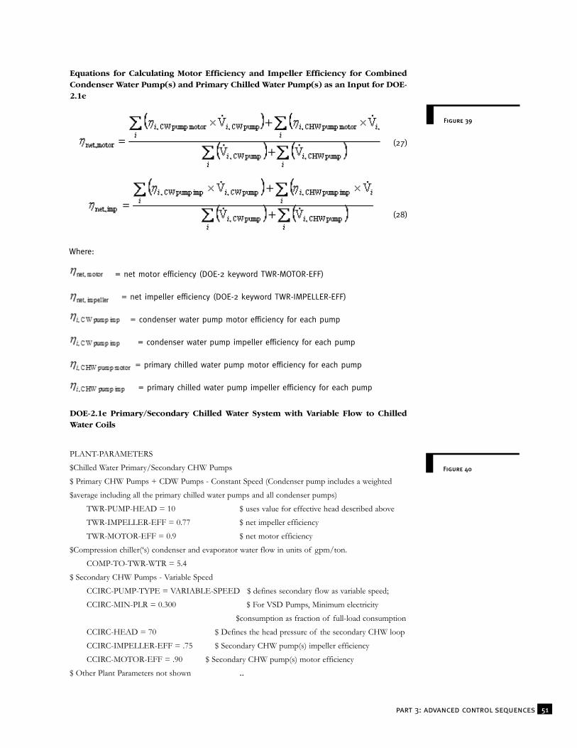
Figure 39


Equations for Calculating Motor Efficiency and Impeller Efficiency for CombinedCondenser Water Pump(s) and Primary Chilled Water Pump(s) as an Input for DOE-2.1e

DOE-2.1e Primary/Secondary Chilled Water System with Variable Flow to ChilledWater Coils

(27)

(28)

Where:

= net motor efficiency (DOE-2 keyword TWR-MOTOR-EFF)

= net impeller efficiency (DOE-2 keyword TWR-IMPELLER-EFF)

= condenser water pump motor efficiency for each pump

= condenser water pump impeller efficiency for each pump

= primary chilled water pump motor efficiency for each pump

= primary chilled water pump impeller efficiency for each pump

Figure 40

PLANT-PARAMETERS$Chilled Water Primary/Secondary CHW Pumps$ Primary CHW Pumps + CDW Pumps - Constant Speed (Condenser pump includes a weighted $average including all the primary chilled water pumps and all condenser pumps)

TWR-PUMP-HEAD = 10 $ uses value for effective head described aboveTWR-IMPELLER-EFF = 0.77 $ net impeller efficiencyTWR-MOTOR-EFF = 0.9 $ net motor efficiency

$Compression chiller(‘s) condenser and evaporator water flow in units of gpm/ton.COMP-TO-TWR-WTR = 5.4

$ Secondary CHW Pumps - Variable SpeedCCIRC-PUMP-TYPE = VARIABLE-SPEED $ defines secondary flow as variable speed;CCIRC-MIN-PLR = 0.300 $ For VSD Pumps, Minimum electricity

$consumption as fraction of full-load consumptionCCIRC-HEAD = 70 $ Defines the head pressure of the secondary CHW loopCCIRC-IMPELLER-EFF = .75 $ Secondary CHW pump(s) impeller efficiencyCCIRC-MOTOR-EFF = .90 $ Secondary CHW pump(s) motor efficiency

$ Other Plant Parameters not shown ..

• Right-click the Project icon in the Waterside HVAC module, and then select Create

Pump. Assign a name to the pump, and then select Create from Scratch. Enter the

appropriate data for the primary pump(s) in the resulting pop-up window. Use

caution to leave the pump capacity control as One-Speed Pump.

• Right-click the Project icon again, and then click Create Circulation Loop. Assign

a name to the loop, and select Create from Scratch. Select Circulation Loop Type

as Chilled Water. Enter the appropriate data for the primary chilled water loop in the

resulting pop-up window. Select Loop Pump as the primary pump(s) just created.

• Double-click each chiller and change the Loop Assignment for CHW to the primary

chiller loop created in the previous step.

• Double-click the Secondary Loop and set Loop Subtype to Secondary. Select the

Primary Chilled Water Loop as the Attached Primary Loop, and then set Head

Setpoint Control to Fixed or Valve-Reset, depending on the actual controls scheme

that will be used in the building. In the resulting pop-up window, keep Valve-Type

as Three Way, and enter any other pertinent information.

eQuest Detailed Interface for Primary/Secondary Chilled Water Loop

To create new pumps, or a new chilled water circulation loop in eQuest, right-click

on the Project icon and select the appropriate icon.


Figure 41:

Final appearance of

primary/secondary

chilled water loop in

eQuest detailed inter-

face.

Figure 42

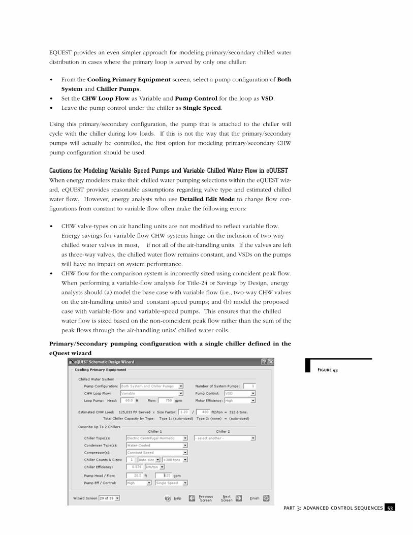
EQUEST provides an even simpler approach for modeling primary/secondary chilled water

distribution in cases where the primary loop is served by only one chiller:

• From the Cooling Primary Equipment screen, select a pump configuration of Both

System and Chiller Pumps.

• Set the CHW Loop Flow as Variable and Pump Control for the loop as VSD.

• Leave the pump control under the chiller as Single Speed.

Using this primary/secondary configuration, the pump that is attached to the chiller will

cycle with the chiller during low loads. If this is not the way that the primary/secondary

pumps will actually be controlled, the first option for modeling primary/secondary CHW

pump configuration should be used.

Cautions for Modeling Variable-Speed Pumps and Variable-Chilled Water Flow in eQUESTWhen energy modelers make their chilled water pumping selections within the eQUEST wiz-

ard, eQUEST provides reasonable assumptions regarding valve type and estimated chilled

water flow. However, energy analysts who use Detailed Edit Mode to change flow con-

figurations from constant to variable flow often make the following errors:

• CHW valve-types on air handling units are not modified to reflect variable flow.

Energy savings for variable-flow CHW systems hinge on the inclusion of two-way

chilled water valves in most, if not all of the air-handling units. If the valves are left

as three-way valves, the chilled water flow remains constant, and VSDs on the pumps

will have no impact on system performance.

• CHW flow for the comparison system is incorrectly sized using coincident peak flow.

When performing a variable-flow analysis for Title-24 or Savings by Design, energy

analysts should (a) model the base case with variable flow (i.e., two-way CHW valves

on the air-handling units) and constant speed pumps; and (b) model the proposed

case with variable-flow and variable-speed pumps. This ensures that the chilled

water flow is sized based on the non-coincident peak flow rather than the sum of the

peak flows through the air-handling units’ chilled water coils.

Primary/Secondary pumping configuration with a single chiller defined in the

eQuest wizard

Figure 43


Variable Flow Condenser Water SystemDOE-2.1e-based programs such as EnergyPro do not provide a means for effectively mod-

eling variable-condenser water flow. Energy modelers can evaluate the impact of variable

speed-condenser water flow control on building performance by using VSD manufacturer’s

software to calculate the annual energy consumption associated with variable speed versus

constant speed-condenser water pumps, and integrating these values into the energy model

outputs during post-processing of the results. However, the California Energy Commission

has not approved this approach for demonstrating compliance with Title-24 standards.

In eQUEST, variable-condenser water flow is modeled in Detailed Data Edit Mode as fol-

lows:29

• When all wizard data has been finalized, select Mode /Detailed Data Edit.

• From the Water-Side HVAC module, select the condenser water loop pump(s) from

the condenser water loop.

• Set Capacity Controll as Variable Speed Pump, and then enter the appropriate data

for the minimum speed of the pump.

• Select each chiller served by the condenser water loop. From the LLoooopp AAttttaacchhmmeennttss

tab, set Condenser Water Flow Control as Variable Flow. Select the Minimum

Condenser Water Flow, defined as the “minimum allowable fraction of the design

flow through the condenser,” as specified in the control sequences. This minimum

flow should be sufficiently high to maintain turbulent flow through the condenser.

Variable Condenser Flow defined in eQuest


29Variable condenser water flow can only be defined in recent versions of eQuest.

Figure 44

Although the variable condenser water flow strategies discussed above will generally

improve the efficient operation of the chilled water plant, this strategy typically affords the

greatest benefit when used with other condenser water system control strategies. The fol-

lowing section of the simulation guidebook discusses modeling techniques for three addi-

tional condenser water system control strategies:

• Cooling tower cell control

• Cooling tower capacity control

• Condenser water temperature reset

Cooling Tower Cell ControlCentral plant designs specifying multiple cooling towers or multi-cell cooling towers can

capitalize on the energy savings associated with variable speed tower fans by implementing

control sequences to operate the maximum possible number of cells at any given time. In

the Max Cells sequence, the control system enables the greatest number of cells that can

operate above their specified minimum flow ratios at a given time, and spreads the load

equally across these cells. Cooling tower applications designed to provide very low flow

will see the greatest energy savings from Max Cells controls.

In EnergyPro, the software hard-codes the Max Cells option into the DOE-2 input file when-

ever multiple cell cooling towers are defined. In DOE-2.1e, cooling tower cell control can

be defined under plant parameters by changing TWR-CELL-CTRL from MIN-CELLS to MAX-

CELLS. The energy modeler should also check DOE-2 inputs for minimum part load ratios

to confirm that they match the ratios defined in the system control sequences. In eQUEST,

multi-cell cooling towers and cooling tower cell control sequences should be selected from

the Detailed Data Edit mode as follows:

• Double-click the Cooling Tower icon in the Water-Side HVAC module. Enter the

total number of cooling tower cells shown in the plans.

• Set Cell Control as Maximum Cells. Define the cell minimum flow as the smallest

ratio of flow compared against the nominal flow for which each cell can operate.

Cooling Tower Capacity ControlCooling tower capacity control describes the method used for regulating the exit tempera-

ture for the water leaving the cooling tower. The four options most commonly seen in exist-

ing and new buildings include:30

• Fluid Bypass: a three-way valve bypasses water around the cooling tower, modulating

as needed to maintain capacity. This is the least efficient control option, since

cooling tower fans run continuously.


Condenser Water System Operation

30A full description of each cooling tower fan capacity control keyword is included in

EnergyPro, DOE-2.1e and eQuest documentation.

eQuest Detailed Edit mode input for maximum cell control

• One-Speed Fan: the fan cycles on and off to maintain the set-point temperature.

• Two-Speed Fan: the fan cycles between Off, Low-Speed, and High-Speed to regulate

the exit water temperature.

• Variable-Speed Fan: a variable-speed drive controls fan speed, so that the heat

rejection capacity exactly matches the load at the desired set-point. This is the most efficient

option, and generally reduces wear and tear on the fan motor associated with one or two-

speed fan operation.

In EnergyPro, the energy modeler can identify fan capacity control as follows:

Cooling Tower Capacity Control Selections in EnergyPro

• From the Plant / Chilled Water tab, double-click the cooling tower icon. A water-

cooled chiller must be defined on the Chilled Water tab before the cooling tower icon

will appear.

• Click Cooling Tower in the pop-up window, and then select an existing tower to edit,

or create a new cooling tower. Select the capacity control to match the controls shown

on the plans.


Figure 45

Figure 46

In DOE-2.1e, energy modelers can define cooling tower capacity in the PLANT-ASSIGN-

MENT section as follows:

• TWR-CAP-CTRL to FLUID-BYPASS, ONE-SPEED-FAN, TWO-SPEED-FAN, or

VARIABLE-SPEED-FAN as defined in the plans.

• For two-speed fan control, enter the air flow ratio and fan power ratio for the low-

speed setting as defined in equations 29 and 30:

(29)

(30)

• For variable-speed fan control, use the DOE-2 keyword TWR-MIN-FAN-SPEED to

enter the minimum fraction of nominal fan speed at which the fan can operate.

eQuest Detailed Edit Mode Inputs Associated with Variable Speed Fan Control

eQUEST includes fan capacity control selections from the Heat Rejection screen of the wiz-

ard. When wizard selections indicate two-speed or variable speed control, eQUEST gener-

ates default assumptions for minimum fan speed and power. The Detailed Data Edit mode

allows the option for modifying these assumptions in the Water-Side HVAC module:

• For variable speed fan control, the Min Fan Speed represents the minimum fraction

of fan speed where the fan can operate.

• Two-speed fan control, Fan Low Flow and Fan Low Elec are defined according to

equations 29 and 30, respectively.

Condenser Water Temperature Reset

Chillers operate most efficiently when at low lift conditions where the differential between

chilled water supply temperature and entering condenser water temperature reaches its min-

imum. Therefore, reducing condenser water supply temperatures at chiller part-load condi-

tions results in demonstrable compressor energy savings. The condenser water reset strate-

gies simulated in DOE-2.1e-based programs are limited to wetbulb temperature reset


Figure 47

control, which reduces condenser water set point temperatures based on outside air wet-

bulb temperatures. This strategy rarely results in substantial energy savings. In contrast, a

reset control that varies the cooling tower fan speed based on chiller load allows the leav-

ing condenser water temperature to float with both wetbulb temperature and chiller load,

producing sizable chiller energy savings. To demonstrate the energy benefit of condenser

water load reset controls in EnergyPro or other DOE-2.1e-based programs, energy modelers

can perform a separate analysis of these controls, and then integrate their findings into the

DOE-2 results during post-processing of the models. However, the California Energy

Commission has not approved this modeling approach for documenting Title-24 compli-

ance.

Modeling Condenser Water Load Reset in eQUEST

eQUEST lets energy modelers select condenser water load reset and further refine the

assumptions for load reset controls in the Detailed Edit Mode:

• From the Primary Heat Rejection screen, set Temperature Control as Reset,

identify the Minimum Condenser Water temperature as defined in the control

sequences, and then select the appropriate option for Cooling Tower Fan

Capacity control. The system design must specify Two-Speed or Variable-Speed

cooling tower fans for the load reset control strategy to function properly.

• When the project design employs condenser water load reset controls in conjunction

with variable-condenser water flow, adjust inputs for minimum reset part-load ratio

and maximum reset speed to reflect the actual control sequences defined in the system.

From the Detailed Data Edit mode, double-click the cooling tower, and then specify

the Min Reset PLR as the minimum part load of the fan at which the minimum

condenser water flow occurs. Also define the Max Reset Speed as the maximum speed

of the cooling tower fan during load reset operation.

eQuest Detailed Edit Mode Inputs Associated with Condenser Water Systems


Figure 48:

Enter the information

shown in this graphic

when both condenser

water load reset and

variable condenser

water flow are imple-

mented into the pro-

ject design.

If implemented carefully, chilled water (CHW) temperature reset controls can reduce chiller

energy usage as well as the losses associated with chilled water distribution by increasing

the chilled water supply temperature set-point with decreasing load. The mechanical engi-

neer should carefully examine chiller constraints when identifying the appropriate CHW

reset schedule, since optimum efficiencies for different chillers can vary greatly for any given

CHW temperature, CW temperature, and percentage load conditions. For example, constant

speed centrifugal chillers reach maximum efficiencies when loaded to greater than 80%,

while the same chiller model equipped with a VSD performs best at 30-50% load with a rel-

atively high chilled water temperature. A chilled water temperature control strategy for the

constant speed chiller would have a very low reset range, whereas the variable-speed chiller

may have a reset temperature range of greater than 10ºF. For variable-flow chilled water

loops, the design team must also be careful to optimize the chilled water flow and temper-

ature reset controls to minimize combined chiller and CHW pump energy usage. EnergyPro

does not provide a means for modeling chilled water temperature reset controls directly in

the program interface. However, by modifying the input file generated from EnergyPro, and

running the simulation directly in DOE-2.1e, the energy modeler can simulate the approxi-

mate impact of this strategy on building performance. The temperature range for chilled

water reset control is defined in DOE-2.1e using the keyword CHILL-WTR-THROTTLE. To

increase the chilled water temperature with decreasing load, a negative value must be

entered for this keyword. For example, to specify a reset temperature range of 10ºF, the

CHILL-WTR-THROTTLE should be -10ºF. While this modeling strategy loosely represents

chilled water reset controls, the DOE-2 simulation results for this strategy are not exact.

Defining Chilled Water Temperature Reset in eQUESTThe eQUEST wizard interface provides a simple method for defining chilled water reset con-

trols from the Chilled Water System Control and Schedule screen:

• Set Setpoint as Reset.

• Enter the appropriate values for CHW Minimum and CHW Maximum temperatures.

• When the chilled water circulation loop is a variable-flow loop, the loop flow reset

should also be defined as follows:

• From the Detailed Data Edit mode, double-click the chilled water circulation loop

in the water-side HVAC module.

• Select the Controls tab from the pop-up window, and then set the appropriate

Loop-Flow Reset. The chilled water reset control sequence should use Variable-

Speed Pump controls to limit the flow to the percentage defined for loop-flow-

reset, and then hold the water flow constant while implementing the CHW reset

control strategies.

eQuest Wizard Inputs for CHW Temperature Reset Controls


Chilled Water Loop Temperature Reset

Figure 49

Hot Water (HHW) temperature reset controls generally reduce boiler energy usage and dis-

tribution losses by decreasing the hot water supply temperature set-point with decreasing

load. Hot water reset control strategies cannot be modeled directly in DOE-2.1e or

EnergyPro. However, in eQUEST, hot water reset is modeled similarly to chilled water reset;

the energy modeler can select Reset Control from the Hot Water System Control and

Schedule screen of the eQUEST wizard. For variable-flow loops, the energy modeler can

enter data in Detailed Data Edit mode to define the loop flow reset ratio for the pumps,

where hot water flow will be held constant as the hot water reset control strategy takes

effect.

eQuest Wizard Inputs for HHW Temperature Reset Controls


Hot Water Loop Temperature Reset

Figure 50

edr design guidelines hvac simulation

Documents