simulation of a building and its hvac system with an ... · 1 simulation of a building and its hvac...
TRANSCRIPT

1
Simulation of a Building and its HVAC system with an equation
solver: Application to benchmarking.
BERTAGNOLIO Stéphane 1*
, LEBRUN Jean 1
Thermodynamics Laboratory, University of Liège
Campus du Sart-Tilman, Bâtiment B49 (P33)
B-4000 LIEGE, BELGIUM
Tel : 32-(0)-366 48 00 Fax : 32-(0)-366 48 12
This paper has been published in “Building Simulation: An International Journal” © Tsinghua
Press and Springer-Verlag 2008.
Paper DOI: 10.1007/s12273-008-8219-4
The original publication is available at www.springerlink.com
The correct citation of the paper is:
Bertagnolio, S., Lebrun, J. (2008) Simulation of a building and its HVAC system with
an equation solver: Application to benchmarking. Building Simulation: An
International Journal. 1(3): 234-250.
2
ABSTRACT
The today - availability of powerful engineering equation solvers is opening very new
possibilities in technical component modelling and in system simulation.
The simulation models, the “user guide” and the “reference guide” are all included in a same
file. Reliable “reference” and “simplified” models are currently available for the building
zone and for most HVAC components. Focus is given here on “simplified” models and on a
simulation tool, called “Benchmark”. This tool should help an auditor to make the best use of
the limited information usually available about actual fuel and electricity consumptions and to
get a very first evaluation of the actual performances of a given HVAC system. An example
of such use is presented.
Another simulation tools and more information about the modelling of HVAC components
will be presented in a further paper.
KEYWORDS
Building modelling, HVAC system modelling, Building Energy Audit, Benchmarking

3
LIST OF SYMBOLS
albedo albedo
A wall area (m²)
C thermal capacity (J/K)
CO2 or water capacity (kg)
CLF cooling load factor
cp specific heat (J/kg-K)
ELF electrical load factor
F correction or increase factor
h combined convective – radiative heat transfer coefficient (W/m²-K)
HLF heating load factor
H& enthalpy flow rate (W)
I solar radiation (W/m²)
M mass (kg)
MM molar mass (g/mol)
nocc number of occupants
P∆ Pressure drop (Pa)
Q& heat flux or thermal power (W)
R thermal resistance (K/W)
SF solar factor
t temperature (C)
U internal energy (J)
V volume (m³)
V& volumetric flow rate (m³/s)
w humidity ratio (kg/kg)

4
W& electrical power (W)
X volumetric concentration, or control variable
α solar absorbance
ε effectiveness
η efficiency
ρ density (kg/m³)
τ time (s)
Subscripts
1 initial value
a air
appl appliance
c consumed
cd condenser
CO2 carbon dioxide
dp dewpoint
el electricity
ev evaporator
ex exhaust
exfiltr exfiltration
f fictitious
FCU fan coil unit
in indoor
inf infiltration
n nominal
occ occupancy

5
out outdoor
r refrigerant
red reduced
s sensible
sh shaft
su supply
surf surface
tot total
twb wet bulb temperature
TU terminal unit
u useful
vent ventilation
w water
wb wet bulb
w water

6
MAIN TEXT
1. Introduction
Early developments of simulation tools were mostly oriented towards supporting system
design, i.e. mainly the selection and sizing of HVAC components (Lebrun and Liebecq,
1988). The usefulness of simulation tools in further stages of the building life cycle appeared
later, among others with the apparition of friendly engineering equation solvers and of reliable
simulation models. Energy simulation may help all along the building life cycle, from early
design until last audit and retrofit actions. Building and HVAC simulation models should
therefore be continuously available, but in different forms, according to what is expected from
the simulation and according to the information actually available.
Today, the simulation bottleneck is no more the computer, but the understanding of the user.
Simulation models have therefore to be designed in such away to make easier this
understanding.
Hopefully the equation solvers presently available (Klein, 2008) open the way to the
development of fully transparent and fully adaptable simulation models, with all equations
written as in a text book. This means that a simulation program, its user guide and its
reference guide can be combined into only one file, fully readable and directly executable.
Reference and detailed models of HVAC components may help a lot in the commissioning
process, among others for functional performance testing (Visier and Jandon, 2004). These
detailed models may also help a lot in the daily system management, among others for fault
detection and diagnosis (Jagpal, 2006). More global (and simplified) simulation can be used
in real time to “emulate” building energy management systems (Lebrun and Wang, 1993).
New simulation capabilities are also appearing today in the domain of energy audit (Auditac,
2007; Harmonac, 2008).
In this paper, special attention is paid to this last use of building energy simulation tools.
7
2. Use of simulation tools for energy auditing
Audit is required, among others, to identify the most efficient and cost-effective Energy
Conservation Opportunities (ECOs), consisting in more efficient use or in (partial or global)
replacement of the existing components.
Four audit stages are generally distinguished (André et al., 2006a):
1. The “benchmarking” helps in deciding if it is necessary to launch a complete
audit procedure; it’s based mainly on energy bills and basic calculations. A
direct use of such global data would not allow the auditor to identify “good”,
“average” and “bad” energy performances. The experimental identification of
HVAC consumptions is often almost impossible: these consumptions are, most
of the time, not directly measured, but “mixed” with other ones (lighting,
appliances etc.). Simulation is then of great help to define some, even very
provisory, reference performances (or “benchmarks”), in view of a first
qualification of the current building performances.
Without simulation, some arbitrary normalization had been required before any
comparison of the recorded data on the studied installation with reference
values deduced from case studies or from statistics.
2. The aim of the “pre-audit” (also called “Walk-through Audit” or “Inspection”)
is to identify the main defects and “energy conservation opportunities”
(ECO’s). Its results are supposed to orient the future “detailed” audit. The
inspection consists in a visual verification of HVAC equipment, in an analysis
of operating data records and in a systematic disaggregation of recorded energy
consumptions. Thanks to parametric tuning, the building-HVAC simulation
model can be fitted on the records actually available (very often no more than
monthly fuel and electricity bills) in such a way to become a “baseline”

8
simulation model, allowing the auditor to identify the main energy consumers
(lighting, appliances, fans, pumps, chiller…) and to analyse the actual
performance of the building
3. The “detailed” audit consists in a detailed and comparative evaluation of the
ECOs previously selected. At this step even more, simulation is the key tool.
4. The “investment grade” audit concerns the detailed technical and economical
engineering studies, justifying the costs of the retrofits.
This fourth audit stage brings the system (building + HVAC) to a new life cycle: new design,
call for tenders, submissions, evaluations, installations, commissioning, etc.
Several simulation tools are being developed in the frame of the HARMONAC project
(2008).
Focus is given, in the present paper, to a first one, called "BENCHMARK". This tool is used
to compute the "theoretical" (or « reference ») consumptions of the building, supposed to be
equipped with a “typical” HVAC system, including air quality, temperature and humidity
control. The building is seen as a unique zone, described by a very limited number of
parameters. This first simulation tool should help the auditor in getting, a very first impression
about the performances of the system considered. Other simulations tools will be described in
further papers.

9
3. Modelling
For benchmarking, as for further audit actions, the simulation tool must handle with realism:
- building (static and dynamic) behaviour,
- weather and occupancy loads,
- comfort requirements and control strategies (air quality, air temperature and
humidity),
- full air conditioning process and characteristics of all HVAC system components
(terminal units, Air Handling Units, air and water distribution, plants)
The level of detail required for the calculation of heating/cooling demands can vary a lot from
case to case:
- For heating calculations, the major issues are a correct description of the building
envelope and an accurate evaluation of air renewal.
- For cooling calculations, the fenestration area and orientation, the intensity and
distribution of internal gains, the ventilation rates and the geographical location
appear as critical issues.
At benchmarking stage mainly, the simulation tools have also to be usable with a limited
quantity of information only, depending on data actually available. These tools must be easy-
to-use, transparent, reliable, sufficiently accurate and robust.
The simulation tool presented here after includes models of both the building and the HVAC
equipment. These models are submitted to different loads and interact at each time step with a
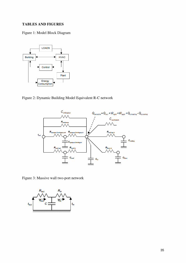
control module (Figure 1).
The main phenomena involved in building dynamics are considered in order to compute
realistic heating and cooling demands. Indeed, the indoor conditions of the zone come from
the equilibrium established among many different influences. A compromise is made between
the number of influences taken into account and the simplicity of the model: transient heat

10
transfer through walls, energy storage in slabs, internal generated gains, solar gains through
windows, infrared losses and, of course, ventilation and heating/cooling devices, are actually
taken into account.
3.1. Inputs, outputs and parameters
The outputs, inputs and parameters must be selected according to the specific needs of the
user. As in some other softwares, as TRNSYS for instance (Klein et al., 2004), the parameters
are here defined as selected inputs which are not supposed to vary during the simulation.
The main outputs of the tool presented here are:
- Air quality and hygro-thermal comfort achievements: CO2 contamination,
temperature, humidity, predicted percentage of dissatisfied (PPD), and predictd
mean vote (PMV);
- Global power and energy consumptions : Fuel and Electricity consumptions;
- HVAC components specific demands;
- Performances of the mechanical equipments: COP, efficiencies...
The main inputs are:
- Weather data : hourly values of temperature, humidity, global and diffuse
radiations;
- Nominal occupancy loads (in W/m²), occupancy and installation functioning rates;
- Comfort requirements: air renewal, temperature and humidity set points;
- Control strategies : feedback on indoor temperature and relative humidity,
feedforward on occupancy schedules and calendar.
The main parameters are:
- Dimensions, orientation and general characteristics of the building envelope (e.g.
“heavy”, “medium” or “light” thermal mass and walls U values).
- Sizing factors of the main HVAC components
11
The main parameters described above are entered through the control panels. The other
parameters of the model, as HVAC system characteristics, nominal performances and
capacities are automatically computed through a pre-sizing calculation, or defined on the basis
of default values, given in European standards prEN 13053 (2003) and prEN 13773 (2007).
Other information as weather data and occupancy rate are provided in “lookup tables”.
3.2. Building Modelling
3.2.1. Indoor Conditions
The indoor conditions (CO2 contamination, global temperature and humidity) are computed
by means of three different mass and energy balances. Indoor comfort indexes (PMV and
PPD) are evaluated at each time step through classical Fanger’s equations (1970).
3.2.1.3 Sensible heat balance
A sensible heat balance is made on the indoor node to compute the combined convective -
radiative indoor temperature.
A mono-zone building model is used here. It’s based on a simplified equivalent R-C network
including five thermal masses (Figure 2; Masy, 2006), corresponding to a large occupancy
zone, surrounded by external glazed and opaque walls. This scheme corresponds to a typical
office building, mainly composed of lattice structure and slabs.
The heat flow emitted by the surfaces of the walls (roof, floor, opaque frontages and
windows), the enthalpy flow rate corresponding to ventilation and infiltration air and the
internal sensible gains (including local heating/cooling and internal generated gains) are
summed (eq. 1), in order to compute the energy storage inside the indoor environment (eq. 2
and 3). This energy storage is computed by the means of a first order differential equation. A
correction factor (Fa,in, eq. 4) has to be applied to the air capacity in order to take into account
the effect of the vertical air temperature gradient in the zone (Lebrun, 1978; Laret, 1980).
inssventswindowsinsurffrontagesopaqueinsurffloorinsurfroofin
QHHQQQQd
dU,inf,,,,,,,,,
&&&&&&& ++++++=τ
(1)

12
∫=∆
2
1
τ
τ
ττ
dd
dUU
inin
( )1,,,* inainainin ttCU −=∆
apaininain cVFC ,, *** ρ=
3.2.1.2 CO2 Balance
A first mass balance is used to compute the CO2 concentration in the indoor environment.
The CO2 flow rate entering the zone is due to two main contributions (eqs. 5 to 11) :
- CO2 brought by ventilation (eq. 6), positive infiltration and negative exfiltration
air flow rates (eq. 7),
- CO2 produced by the occupants (function of the occupant metabolic rate, eq. 8).
Treated ventilation air CO2 concentration is given as an output of the HVAC system model,
while, for infiltration, it corresponds to outdoor air input data.
inCOCOventCOinCO
MMMd
dM,inf,,
,222
2
&&& ++=τ
inCO
a
COreturnductsuaplyductexCO
a
COplyductexaventCO X
MM
MMMX
MM
MMMM ,,,sup,,sup,,, **** 2
2
2
2
2&&& −=
inCO
a
COexfiltraoutCO
a
COaCO X
MM
MMMX
MM
MMMM ,,,inf,inf, **** 2
2
2
2
2&&& −=
tperoccupanCOoccoccCOinCO MnMM ,,, * 222&&& ==
∫=∆
2
1 22
τ
τ
ττ
dd
dMM
inCOinCO
,,
a
COinainCO
MM
MMMC 2
2 *,, =
( )12222 ,,,,, * inCOinCOinCOinCO XXCM −=∆
(2)
(3)
(4)
(5)
(6)
(11)
(7)
(8)
(9)
(10)

13
The “CO2 capacity” introduced in equation 10 is here supposed to correspond to the mass of
the air contained in the zone. A correction factor might be also introduced in order to take into
account of CO2 absorption in the building materials (walls and furniture).
3.2.1.3. Water Balance
A second mass balance is made to compute the water content of the indoor air. The water
flow rate entering the zone is due to three main contributions (eq. 12) :
- water brought by ventilation, positive infiltration and negative exfiltration air flow
rates (eq.16 and 17),
- water produced by the occupants or local humidification devices (eq.18),
- water condensed by local cooling devices (eq. 18).
Water exchanges between air and walls or materials are roughly estimated in the present
software. A correction factor (Fw,in) is here also applied to the air capacity; it’s supposed to
take into account of the effect of hygroscopic materials contained in the zone (Woloszyn,
1999).
inwwventwinw
MMMd
dM,inf,,
,
&&& ++=τ
∫=∆
2
1
τ
τ
ττ
dd
dMM
inwinw
,,
( )1,,, * inininwinw wwCM −=∆
aininwinw VFC ρ**,, =
inreturnductsuaplyductexplyductexaventw wMwMM ** ,,sup,sup,,,&&& −=
inexfiltraoutaw wMwMM ** ,inf,inf,&&& −=
coolingTUwheatingTUwoccwinw MMMM ,,,,&&&& −+=
(12)
(13)
(14)
(16)
(17)
(18)
(15)

14
3.2.2. Walls thermal models
A 2RC 1st order “two-port networks” model (Figure 3) is associated to each massive wall
(Laret, 1980). The wall network (Figure 2) corresponds either to imposed temperature
boundary conditions (for ‘external’ massive walls in contact with outdoor conditions) or to
null heat flow boundary conditions (for ceiling and floor slabs separating two heated zones
characterized by similar temperature profiles). The parameters of each “two-port network” are
tuned through a frequency analysis based on the computation of the zone admittance matrix
(Masy, 2006).
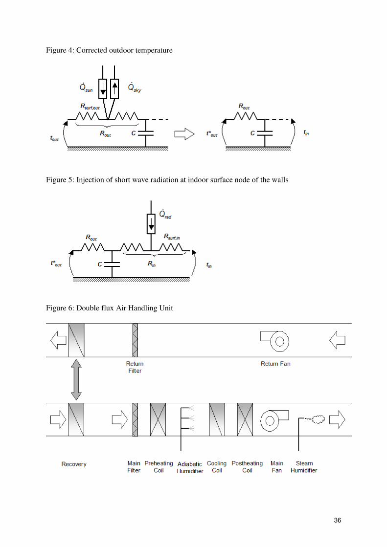
In the case of an “isothermal wall” (massive opaque frontage or roof slab), the absorbed solar
radiation is injected on the outdoor surface node (Figure 4).
A correction heat flow (Bliss, 1961) varying from 45 to 100 W/m², is also used to take into
account that the sky temperature is below the outdoor air temperature. These two effects
(solar and sky radiations) are included in the corrected outdoor (“sol-air”) temperature
*
outt (eq. 19).
( ) outsurfskysunoutout RQQtt ,
* *&& −+=
Solar radiation absorbed by the wall is computed as follow :
wallsunwallwallsun IAQ ,**α=&
diffglobwallbeamwallsun IalbedoIII ***,,2
1
2
1++=
where,
walldiffglobwallbeam FIII *)(, −=
Fwall is the weighted average of the projection factors of all opaque walls facing different
orientations. The hourly values of these projections factors are pre-computed all along the
year as function of the incidence angles (for the latitude considered) and are provided as
inputs for the model.
(19)
(20)
(21)
(22)
15
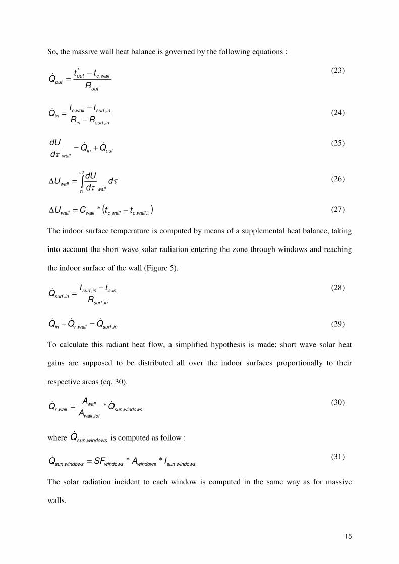
So, the massive wall heat balance is governed by the following equations :
out
wallcout
outR
ttQ ,
* −=&
insurfin
insurfwallc
inRR
ttQ
,
,,
−
−=&
outinwall
QQd
dU && +=τ
∫=∆
2
1
τ
τ
ττ
dd
dUU
wallwall
( )1,,,* wallcwallcwallwall ttCU −=∆
The indoor surface temperature is computed by means of a supplemental heat balance, taking
into account the short wave solar radiation entering the zone through windows and reaching
the indoor surface of the wall (Figure 5).
insurf
inainsurf
insurfR
ttQ
,
,,
,
−=&
insurfwallrin QQQ ,,&&& =+
To calculate this radiant heat flow, a simplified hypothesis is made: short wave solar heat
gains are supposed to be distributed all over the indoor surfaces proportionally to their
respective areas (eq. 30).
windowssun
totwall
wallwallr Q
A
AQ ,
,
, * && =
where windowssunQ ,& is computed as follow :
windowssunwindowswindowswindowssun IASFQ ,, **=&
The solar radiation incident to each window is computed in the same way as for massive
walls.
(23)
(24)
(25)
(26)
(27)
(28)
(29)
(30)
(31)

16
In the case of an “adiabatic wall” (floor, ceiling or party walls; Figure 2), the two-port
network can be reduced to a simple branch composed of one resistance and one capacity. The
same method is applied to compute solar heat gains reaching these walls.
Each light wall (as, for example, a window) is modelled with only one resistance, connected,
on one side, to the indoor temperature node and, on the other side, to a node of corrected
outdoor temperature, taking into account of sky radiation effect.
3.2.3. Sensible Heat Gains
Except for the solar radiation transmitted through the windows which is “injected” to the
indoor surfaces, all sensible heat gains are injected to the indoor node (Figure 2) through the
sensible heat balance of equation 8. They include three contributions :
- sensible heat generated by electrical devices (lighting and appliances),
- sensible heat generated by occupants (function of the metabolic rate),
- sensible heat generated or absorbed by heating or cooling terminal units.
This give :
coolingsheatingsappllightoccsins QQWWQQ ,,,,&&&&&& −+++=
where heatingsQ ,& and coolingsQ ,
& are output variables of the terminal units models.
3.2.4. Ventilation, infiltration and exfiltration sensible enthalpy flow rates
The air leaving the zone (through ventilation exhaust and/or through exfiltration) is supposed
to be at indoor temperature (due to a perfect “mixing” inside the zone). Ventilation air
temperature is given as an output of the HVAC system model, while infiltrated air is at
outdoor temperature.
Supply and exhaust state variables are used to define the CO2 (eq. 2), sensible enthalpy (eq.
33) and water (eq. 16) flow rates carried by the ventilation and infiltration/exfiltration:
inaapreturnductsuaplyductexaapplyductexavents tcMtcMH ,,,,sup,,,sup,,, **** &&& −=
(32)
(33)

17
inaapexfiltraoutapas tcMtcMH ,,,,inf,inf, **** &&& −=
3.2.5. Validation
The thermal aspects of this simple dynamic building zone model have been validated
(Bertagnolio et al., 2008) through analytical tests, empirical tests and through BESTEST
comparative procedure (Judkoff and Neymark, 1995).
3.3. HVAC System Model
The building zone model presented here above can be easily connected to a complete
“typical” HVAC system model, including, for example, a Constant Air Volume (CAV) Air
Handing Unit (AHU), some local heating and/or cooling Terminal Units and a heating and
cooling plant.
The system model actually available includes most of the classical HVAC components
currently used (fans, air-to-air static recovery systems, coils, fan coils, pumps…).
Considering that the building model is a mono-zone model, most of components (AHUs, TUs,
pumps,…) are aggregated into “global” components. The different locations of the terminal
units and of the air diffusers are not yet considered.
Two different modelling levels are distinguished for the HVAC system (André et al., 2006b;
Lebrun et al., 2006a):
- So-called “mother” (“first principle”, or “mechanistic”) models, containing all the
(present) understanding of the physical phenomena, are used as references;
- So-called “daughter” (“simplified” and very often polynomial) model, generated with
help of the help of the previous ones, are preferred to simulate large system on long
time periods.
“Mother” models are preferred in some other domains of use, as, for instance, to support
experimental work (design of the experiment and analysis of experimental results) or to
characterize some specific equipment. “Daughter” models only are used in Benchmark.
(34)

18
3.3.1. Air Handling Unit
The AHU considered may include a return fan, a return filter, a recovery system, a supply
filter, a preheating coil, an adiabatic humidifier, a cooling coil, a post heating coil, a main fan
and a steam humidifier (Figure 6). Of course, these components are usually not included all
together (for example, both adiabatic and steam humidifiers don’t have to be selected at same
time).
In “Benchmark”, the CAV AHU is supposed to provide a constant hygienic flow rate to the
zone and to ensure humidity control (by humidification and/or dehumidification).
Temperature control is then ensured by terminal units, as described hereafter.
3.3.1.1. Fans
The different pressure drops of the components are taken into account to compute the fans
consumptions and the corresponding air heating-up.
The equations related to the return (or extraction) fan give, for instance:
returnfans
returnfanreturnfanreturnfan
PVW
,
*ε
∆= &&
where,
eryreturnreomizerreturneconerreturnfiltreturnductreturnfan PPPPP cov∆+∆+∆+∆=∆
and,
returnfana
returnfanreturnfansuareturnfanexa
C
Wtt
,
,,,, &
&
+=
Similar equations are used to model the main supply fan.
3.3.1.2. Heating Coils
Heating coils are simulated by using a simplified ε-NTU model. In the classical ε-NTU
model, the simultaneous calculations of air and water evolutions would consume more
(35)
(36)
(37)

19
computational time. The simplification proposed here consists in not taking into account what
happens on the water side; the heating coil is characterized by its air-side effectiveness only.
When the control valve is fully open and for a constant air flow rate, the air-side effectiveness
is expressed as:
a
lheatingcoilheatingcoiaC
C
&
&min
, *εε =
For a constant air flow rate, the maximal air exhaust temperature ta,ex,heatingcoil,max is supposed
to be reached when the valve is fully open:
( )lheatingcoisualheatingcoisuwlheatingcoialheatingcoisualheatingcoiexa tttt ,,,,,,,max,,, * −+= ε
The control variable is then used to compute the required exhaust temperature ta,ex,heatingcoil:
( )lheatingcoisualheatingcoiexalheatingcoilheatingcoisualheatingcoiexa ttXtt ,,max,,,,,,, * −+=
where X is the control variable (cf. § 3.3.6).
The heating power actually provided by the coil is then computed:
)(* ,,,,, lheatingcoisualheatingcoiexalheatingcoialheatingcoi ttCQ −= &&
This simplification allows to avoid the computation of the thermal exchange on water side.
Only the characteristics of the coil in nominal regime are required to compute the air-side
effectiveness.
3.3.1.3. Cooling Coil
Lemort et al. (2008) have used the same approach to build a simplified cooling coil model.
They propose to do as if the cooling coil exhaust air temperature was controlled by its contact
temperature (in place of the refrigerant flow rate). This control is described by equation 41.
The exhaust air temperature is first compared to its set point. The control variable (comprised
between 0 and 1) is then used to adjust the contact temperature (cf. §3.3.6).
( )min,,,,,,,, . coilccoilsuacontrolcoilcoilsuacoilc ttXtt −−=
(38)
(40)
(41)
(39)
20
For given supply air temperature, contact effectiveness and contact temperature, the exhaust
air temperature can be defined as follows:
( )coilccoilsuacoilccoilsuacoilexa tttt ,,,,,,,, . −−= ε
The coil contact effectiveness is defined by the equation 43.
)exp(1 ,,,, wetcoilcwetcoilc NTU−−=ε
with
coilacoila
wetcoilcCR
NTU,,
,,.
1
&=
This means that (as Ra and aC& ), the contact effectiveness is only depending on the air flow
rate. The exhaust air humidity is determined by equation 45.
( )( )wetcoilccoilsucoilccoilsucoilex wwMAXww ,,,,,, .,0 −−= ε
Once the exhaust air temperature and humidity are known, the sensible and latent heat outputs
of the coil can be calculated.
The minimal value of the contact temperature (corresponding to the full opening of the
control valve) must be determined as a function of both supply temperatures: the temperature
of the refrigerant and the (dry bulb or wet bulb) temperature of the air (according to the
regime :dry or wet):
).( ,,,,
,
,,
,,min,,, coilsurcoilsua
coilc
drycoila
coilsuadrycoilc tttt −−=ε
ε
).( ,,,,
,
,,
,,min,,, coilsurcoilsuwb
coilc
wetcoila
coilsuwbwetcoilc tttt −−=ε
ε
In these equations, εa,coil,dry and εa,coil,wet are the “air-side” effectiveness’s, defined in dry and
wet regimes respectively.
In each regime, the “air side” effectiveness is related to the actual coil effectiveness:
drya
drycoil
drycoildrycoilaC
C
,
,min,
,,, .&
&
εε =
(42)
(43)
(44)
(45)
(46)
(47)
(48)

21
fa
wetcoil
wetcoilwetcoilaC
C
,
,min,
,,, .&
&
εε =
with,
coilfapcoilafa cMC ,,,,, *&& =
The fictitious specific heat, cp,af is defined by the equation 51 (Lebrun et al., 1990).
wetcoilexwbcoilsuwb
wetcoilexacoilsua
coilfaptt
hhc
,,,,,
,,,,,
,,,−
−=
These effectiveness’s are defined with the valve fully open. If the air flow rate is varying, its
effect has to be pre-identified with the help of the reference model.
The coil is supposed to work in dry regime, if the dew point temperature at cooling coil
supply is lower than the minimum contact temperature. If not, it is supposed to be in wet
regime:
If wetcoilccoilsudp tt min,,,,, < , drycoilccoilc tt min,,,min,, =
If wetcoilccoilsudp tt min,,,,, > , wetcoilccoilc tt min,,,min,, =
Lemort et al. (2008) have shown that the agreement between results of both reference and
simplified models is very good. A comparative test between the reference and the simplified
models proofs that the simplified model can be used without any significant loss of accuracy
on the cooling load calculation. Moreover the calculation time dramatically reduced and no
numerical instability is encountered.
3.3.1.4. Humidifiers
Both adiabatic and steam humidification are modelled in the present simulation tool.
Adiabatic humidification is supposed to be controlled by means of the preheating coil and is
modelled by the following equations:
( )adiabhumsuadiabhumtwbsadiabhumadiabhumsuadiabhumex wwww ,,,,, * −+= ε
( )adiabhumsuaadiabhumsuwbadiabhumadiabhumsuaadiabhumexa tttt ,,,,,,,, * −+= ε
(49)
(50)
(51)
(52)
(53)

22
Steam humidification is modelled by means of water and energy balances:
steamhuma
steamhumsusteam
steamhumsusteamhumexM
Mww
,
,,
,, &
&
+=
steamhumsusteam
steamhuma
steamhumsusteam
steamhumsuasteamhumexa hM
Mwh ,,
,
,,
,,,, *&
&
+=
The exhaust air humidity ratio is then calculated by using the following control law :
max,,,, * steamhumsteamhumsteamhumexsteamhumex wXww ∆+= 0
With Xsteamhum as control variable (see hereafter)
3.3.2. Terminal Units
In Benchmark, room sensible heating and cooling are ensured by a classical fan coil unit.
In first and simple approach, this unit is characterized by its heat transfer coefficient only. The
fan electrical power is defined as a percentage of the nominal heating/cooling power. The
main outputs of this model are the heating/cooling power actually delivered and the related
fan consumption.
In heating mode, for example, the heating power delivered by the fan coil is defined as
follow:
)(** ,,,,,,, inaFCUheatingsuwFCUheatingFCUheatingFCUheating ttKXQ −=&
Kheating,FCU is the equivalent heat transfer coefficient of the fan coil unit:
min, *CK FCUheating&ε=
This term is defined for the nominal water flow rate (valve fully open) and for the fan rotation
speed considered (usually selected by the occupant). Xheating,FCU is the control variable (this
control is supposed to consist in a tuning of the water flow rate).
The cooling power is defined in the same way. Possible water condensation inside the fan coil
is not yet taken into account in Benchmark, but it could be easily included by using a model
similar to the one used for the cooling coil of the Air Handling Unit.
(54)
(55)
(56)
(57)
(58)

23
3.3.3. Hot and cold water distributions
Water networks are modelled in such a way to take both pressure drops and heat exchanges
into account.
In Benchmark, a first approximation consists in characterizing each water distribution
network with only one equivalent thermal efficiency.
Equivalent nominal water flow rates are defined on the basis of nominal heating and cooling
powers and of nominal temperature variations. For the hot water distribution, for example:
nntheatingplawwp
nntheatingpla
strhotwaterdiwtc
QM
,,,
,
,* ∆
=&
&
The so-defined “primary” water flow rate is kept constant in the simulation.
Both heating-up through the pump and heat exchanges along the distribution network are
taken into account. For hot water distribution, for example, this gives:
−+=
wpnstrhotwaterdiw
lossstrhotwaterdimphotwaterpush
sthotwaterdisuwstrhotwaterdiexwcM
QWtt
,,,
,,
,,,,*&
&&
( ) andheatingdemstrhotwaterdilossstrhotwaterdi QQ && *, η−= 1
The primary water pump consumption is defined as follows:
mphotwaterpushsw
strhotwaterdiw
nstrhotwaterdiwmphotwaterpush
PMW
,,
,
,,,*
*ερ
∆= &&
mphotwaterpu
mphotwaterpush
mphotwaterpu
WW
η
,&
& =
Similar equations are used to model the chilled water network and its pump.
3.3.4. Heat Production
In the present version of Benchmark, heat is supposed to be produced by a classical fuel-oil
boiler with ON/OFF control.
(59)
(60)
(61)
(62)
(63)

24
The “daughter” boiler model used here is derived from the reference (“mother”) model
developed by Bourdouxhe et al. in the ASHRAE HVAC1 Toolkit (1999).
In the mother model, the boiler is represented by an assembly of a supposed to be adiabatic
combustion chamber and two (gas-water and water-environment) heat exchangers (Figure 7).
At constant water supply temperature, the fuel oil boiler submitted to ON/OFF control has a
very linear behaviour as shown in Figure 8. This suggests that a double linear correlation can
be used as simplified model. Consumed power is plotted as function of useful power and a
linear fit is made on this curve.
Applying the same methodology to the same boiler for different values of water supply
temperature (e.g. from 50°C to 80°C) , and using reduced variables, the following correlation
is established (eq. 66).
onnu
uredu
Q
,,
, &
&
& =
onnc
credc
Q
,,
, &
&
& =
reduredc qCCq ,, * &&10 +=
The values of C0 and C1 can be correlated with the water supply temperature as follows:
boilersuwtCCC ,,,, *10000 +=
boilersuwtCCC ,,,, *11011 +=
If there is no mixing valve or if it’s fully open, the boiler water supply temperature
corresponds to the heating plant return water temperature:
wpstrhotwaterdiw
andheatingdem
strhotwaterdiexwntheatingplareturnwcM
Qtt
,,
,,,,*&
&
−=
In Benchmark, the boiler is only submitted to weather control: the exhaust water temperature
set point is fixed according to the outdoor temperature.
(64)
(65)
(66)
(67)
(68)
(69)
25
Of course, it may occur that this set point stay above the maximal temperature achievable; in
such case, the boiler is running in full load.
3.3.5. Cold Production
For the chiller, various simplified “daughter” models are available (Lebrun et al., 2006a). The
simplest one consists in expressing the chiller “capacity” (full load cooling power) and the
corresponding electrical consumption as polynomial functions of two independent variables:
1) the temperature of the secondary fluid supplying (or leaving) the evaporator
2) the temperature of the secondary fluid supplying the condenser (Figures 9).
The part load regime can be described with the help of Heating, Cooling and Electrical load
factors (eq. 70, 71 and 72):
,maxcd
cd
Q
QHLF
&
&
=
max,ev
ev
Q
QCLF
&
&
=
max,el
el
W
WELF
&
&
=
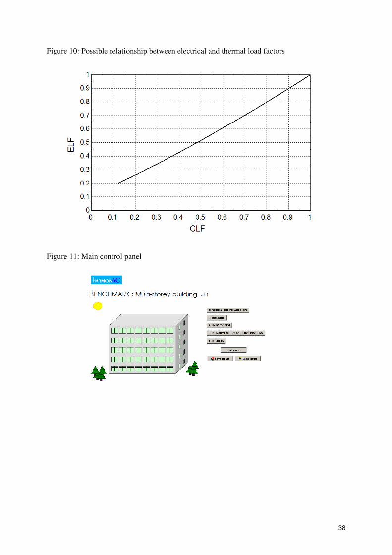
Simple polynomial laws can also be used to correlate electrical and cooling load factors to
each other (Figure 10).
A better, but still very simple, approach consists in using the evaporation and condensation
temperatures (in place of the secondary fluid temperatures) in the two first polynomial laws
(which then concern the compressor and the refrigeration cycle only). Separate semi-
isothermal heat exchanger models can then be used to deal with the evaporator and with the
condenser. The definitions of the part load factors stay the same as for the first model. This is
the approach preferred in Benchmark.
In ideal control conditions, the simulation will determine the chilled water supply
temperatures “required” by both air handling and terminal units. These temperatures will be
(70)
(71)
(72)
26
generated by the (real or fictitious) proportional controls of both units. The minimum between
these two temperatures will become the set point of the chiller control.
Of course, it may occur that this set point stay below the minimal temperature achievable, in
such case, the chiller is running in full load.
3.3.6. HVAC system control
When having to deal with a complex system simulation, a good engineer approach consists in
starting with idealistic hypotheses and going progressively to more realism, according to what
is looked for. Ideal control allows using simpler simulation models, gives easier access to
benchmarks and indicates clearly the maximal performances that could be reached.
A simple proportional control laws is used for each component, with a non dimensional
control variable Xcontrol, varying between 0 and 1 in proportion of the difference observed
between the set point and the controlled variable:
)))(*,(,( int ttCMAXMINX tsepocontrolcontrol −= 01
The control “gain”, Ccontrol, is arbitrarily fixed as a realistic compromise between accuracy and
robustness.
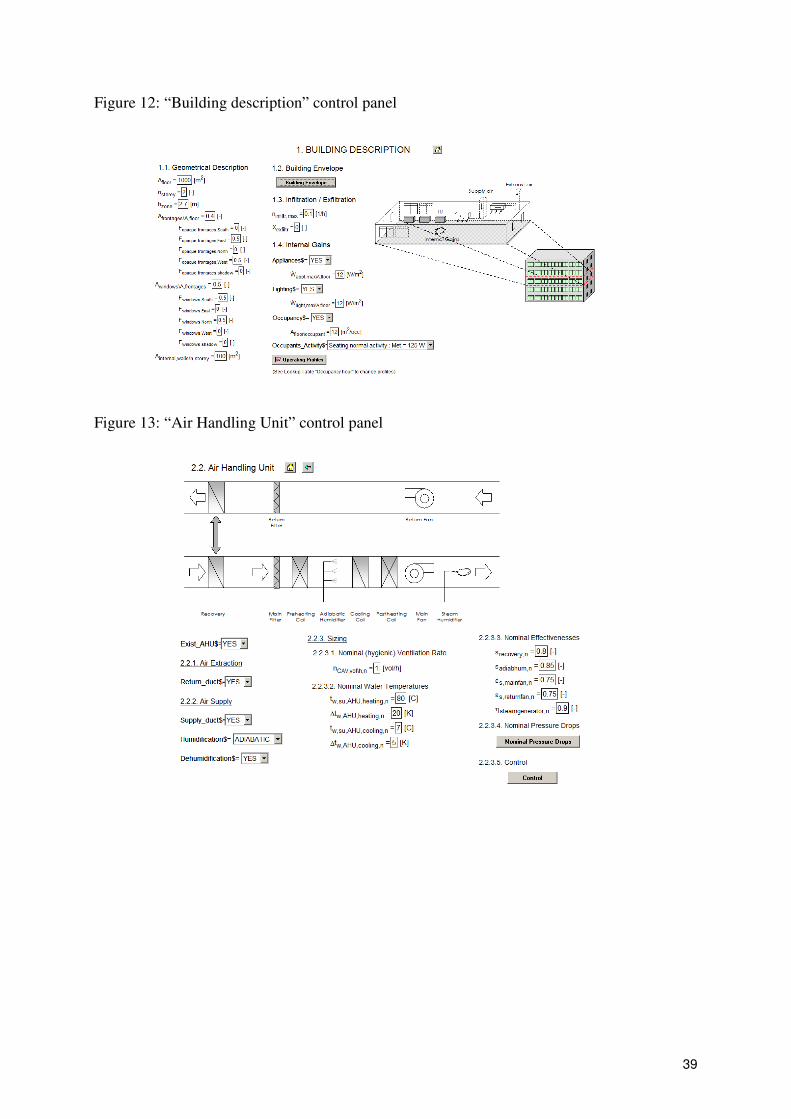
3.4. Interface and Implementation
In Benchmark, all the parameters asked to the user have to be provided by means of control
panels. A main control panel (Figure 11) is used to access the other ones. The “Building
description” panel (Figure 12) is used to fix the geometry of the building, the characteristics
of the envelope and the internal gains (occupancy, lighting and appliances). The “Air
Handling Unit” panel (Figure 13) is used to select the main characteristics of this subsystem
(existence of a mechanical ventilation, hygienic ventilation flow rate, type of humidification
system, water nominal temperature regimes and nominal fan efficiencies). The temperature
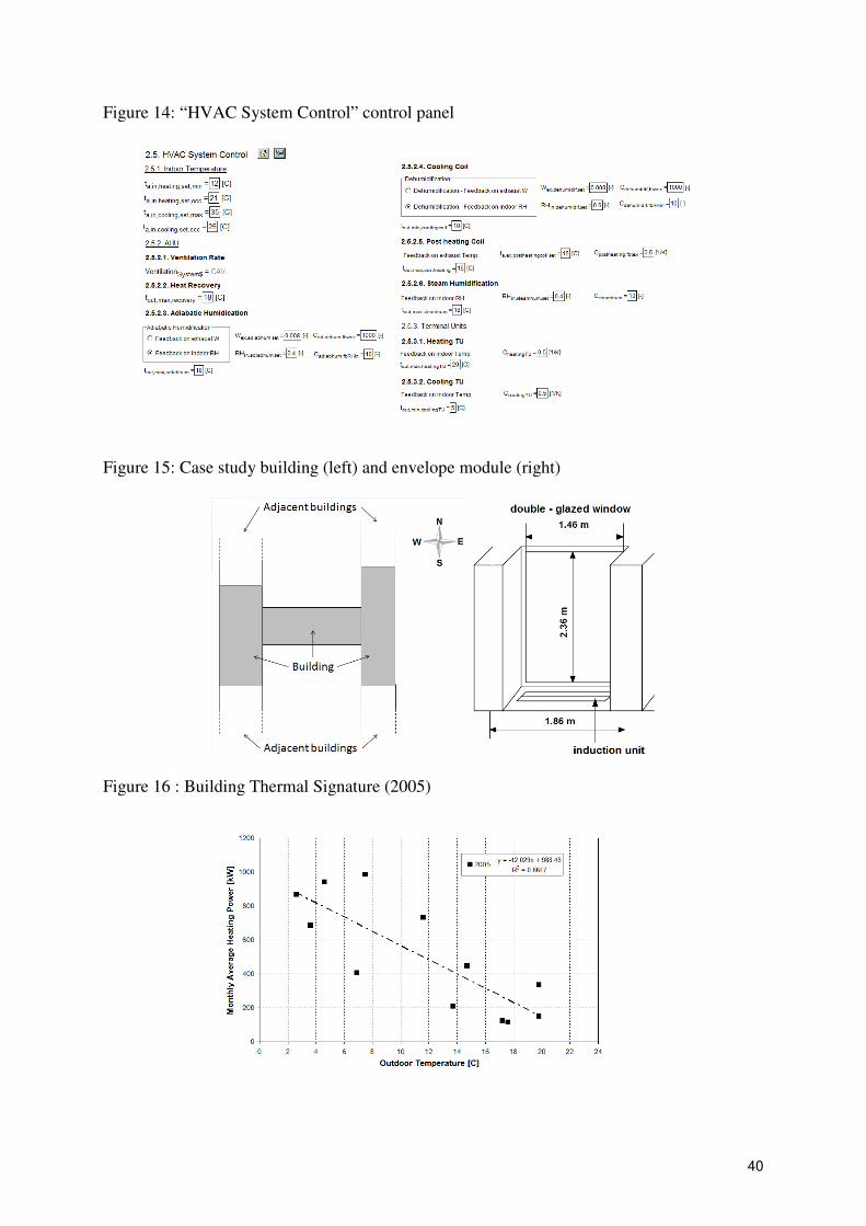
and humidity set points and the control laws can be modified in the “HVAC System Control”
panel (Figure 14).
27
4. Example of Use
4.1. Building description
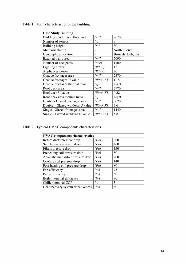
The model presented here above is applied to an existing medium-size office building (around
26700 m² of air-conditioned floor area), erected in Brussels at the end of the sixties (Lebrun et
al., 2006b). The building is composed of three blocks, has a “H” shape (figure 15) and is
North-South oriented. Eight storeys of the building include landscaped offices and meeting
rooms and are occupied by about 1100 people, between 8 am and 18 pm. The five
underground levels are dedicated to cars parking. The frontages of the lobby are made of
single-glazed windows. The rest of building envelope is made of about 1000 double-glazed
modules as shown in figure 15. The main characteristics of the envelope are given in table 1.
About 1000 four-pipes heating and cooling induction units are installed in the offices. The
CAV Air Handling Units provide together a total of about 190000 m³/h of fresh air per hour,
75 hours per week, to the conditioned zones (from level 0 to 8). Vitiated air is rejected in the
underground storeys to ensure ventilation of the parking. This ventilation flow rate
corresponds to about 2.4 air renewals per hour. According to the outdoor weather conditions,
the supplied air can be heated, adiabatically humidified, or cooled and dehumidified. Heat
production is ensured by four fuel-oil boilers, giving together a nominal heating capacity of
about 4 MW. Chilled water production is ensured by four water cooled chillers, coupled to
two cooling towers, giving a total cooling capacity of about 2.1MW.
Recorded monthly fuel consumptions are available from 1975 to 2005 and monthly records of
electricity consumption are available from September 2004 to February 2006.
Classical thermal signature based on recorded data (2005) can be built by expressing the
monthly average heating powers as function of the average outdoor temperature (Figure 16).
The slope of this signature (about 42 kW/K), should correspond to the global heat transfer
28
coefficient of the building. However, the interpretation of this curve stays quite difficult
because of the very global data used and the poor correlation factor (R²=0.6647).
Electricity signatures can also be built by expressing the monthly electrical power demand
(2005) as function of the outdoor temperature. As shown in Figure 17, no significant
correlation can be established between the two variables: the electricity consumption stays
quite constant all along the year.
Such information is too limited to be directly used, but much more can be learned through the
use of simulation model tuned on the available data.
4.2. Use of “BENCHMARK”
The software presented above is applied to the nine conditioned storeys of the building (from
level 0 to 8), simulated as a unique zone. Parking zone is not considered in the study. The
actual characteristics of the building envelope, the estimated internal generated gains, the
actual occupancy schedules and temperature and humidity setpoints are entered in the
software. The first approach consists in supposing that the studied building is coupled to the
“typical” HVAC system described above. The performances of this system (pressure drops
and HVAC components efficiencies) are estimated according to the standards prEN 13053
and 13773 (table 2). The constant hygienic ventilation flow rate is fixed to 45 m³/h of fresh air
per hour and per occupant.
This first simulation gives the results plotted in Figure 18 and 19. To allow a fair comparison
between measured and computed data, monthly fuel consumptions are here averaged on the
30 years of available data. This method tends to minimize the error due to the use of a typical
set of weather data, based on averages carried out over thirty years of measurements, realized
in Uccle (Belgium). For electricity consumption, the values of 2005 are used as reference.

29
It appears that monthly computed and measured consumptions are very different. Mostly the
fuel, but also the electricity consumptions are largely underestimated by the software. This
suggests the existence of important energy savings potentials.
4.3. Calibration
In this second phase of the study, a more complete tool using the same bases has to be used.
This second tool is very similar to the first one, but includes additional HVAC components
models as induction unit, radiator, cooling ceiling models, etc. These additional components
models will be described in further papers.
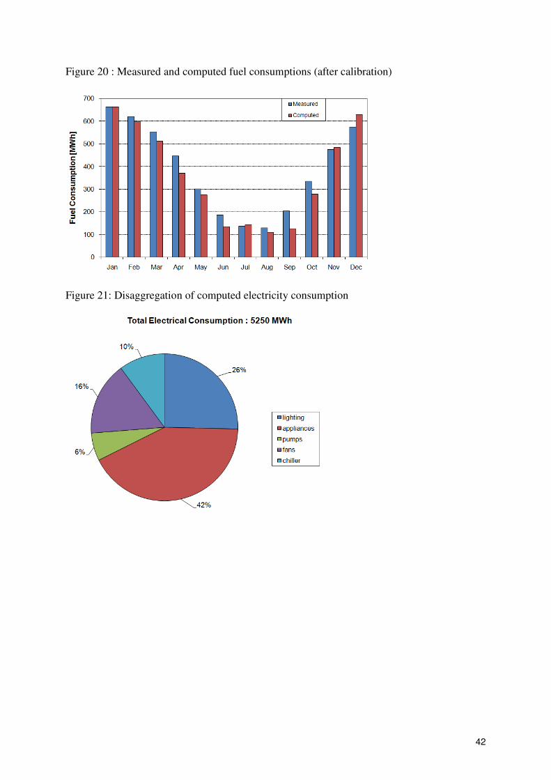
With more realistic hypotheses (much higher ventilation flow rate) and a description of the
actual HVAC system (four-pipes induction units, no heat recovery system,...) and its
performances and operating conditions, the software gives the results shown in Figure 20.
The computed and measured monthly consumptions are now in fair agreement.
After this calibration, the tool can be used to disaggregate the electricity consumption and to
identify the main energy consumers (Figure 21). This indicates that an important part of the
electricity consumption is due to lighting and appliances. Fans and pumps are in charge of
about 22 % of the global electrical consumption, while chiller part is only of about 10 %.
Finally, some selected ECO’s would be evaluated on economical and environmental bases.
This second part of the work will be described in further papers.
5. Advantages and limitations of equation solvers
The presented model is implemented on an Engineering equation solver (Klein, 2008). This
implementation ensures also a full transparency for the user and makes easier the continuous
improvement and development of the tools. Indeed, model’s equations are directly readable
and easy to modify by any user (Figure 22). It is also very easy to develop additional HVAC
components models and to connect them to the existing ones. Moreover, the present equation

30
solver is very well adapted to solve differential equations systems as used to model the
thermal behaviour of the building zone.
Of course, the use of an equation solver to solve complex equation systems implies longer
computation time than other simulation softwares, but the continuous increase of computer
performances tends to reduce this inconvenience. At present time, about 20 minutes are
necessary to simulate a mono-zone building and its complete HVAC system (including AHU,
terminal units and heat and cold production and distribution) hour by hour on one year with a
classical computer equipped with a 2.00GHz processor.
6. Conclusion
Fairly detailed and realistic simulations are possible today in the field of buildings and
HVAC. The use of an equation solver makes the models fully transparent and easy to improve
whenever required.
HVAC equipment modelling can be performed at different levels: The most simplified
models with very few parameters can be of great help in the first stage of an energy audit. The
“Benchmark” tool presented in this paper is an example of such simulation model. It allows
the auditor to get a first impression about energy saving potentials.
Then, a calibrated but still simplified simulation tool is used to disaggregate the electricity
consumption and to allow a better interpretation of on site records.
Finally, more detailed and specific simulation tools should be used to allow a safe
identification and an assessment of the most promising retrofit opportunities. More detailed
and complete simulation tools will be presented in further papers.
31
ACKNOWLEDGMENTS
This work is performed with the support of the Walloon Region of Belgium and of Intelligent
Energy Europe programme. The sole responsibility for the content of this document lies with
the authors. It does not represent the opinion of the Community. The European Commission is
not responsible for any use that may be made of the information contained therein.
REFERENCES
André P, Lebrun J, Adam C, Aparecida Silva C, Hannay J, Lemort V (2006). A contribution
to the audit of an air-conditioning system : modelling, simulation and benchmarking. In:
Proceedings of the 7th
International Conference on System Simulation in Buildings, Liège,
Belgium.
André P, Lebrun J, Adam C, Georges B, Lemort V, Teodorese I (2006). From model
validation to production of reference simulations : how to increase reliability and applicability
of building and HVAC simulation models. In: Proceedings of the 7th
International Conference
on System Simulation in Buildings, Liège, Belgium.
AuditAC (2007). AuditAC project : field benchmarking and market development for audit
methods in air conditioning. AuditAC Final report. Intelligent Energy Europe programme.
Bertagnolio S, Masy G, Lebrun J, André P (2008). Building and HVAC System simulation
with the help of an engineering equation solver. Paper presented at the Simbuild 2008
Conference, Berkeley, USA.
Bliss R (1961). Atmospheric radiation near the surface of the ground: a summary for
engineers. Solar Energy. 5: 103-120.
32
Bourdouxhe J-P, Grodent M, Lebrun J, Saavedran C (1999). ASHRAE HVAC1 Toolkit : A
Toolkit for Primary System Energy Calculation. Atlanta : American Society of Heating,
Refrigerating and Air-Conditioning Engineers, Inc.
European Standard prEN13053 (2003) Ventilation for buildings - Air handling units - Ratings
and performance for units, components and sections.
European Standard prEN13779 (2007) Ventilation for non-residential buildings –
Performance requirements for ventilation and room-conditioning systems.
Fanger P (1970). Thermal Comfort – Analysis and Applications in Environmental
Engineering. Copenhagen: Danish Technical Press.
Harmonac (2008). Harmonac project : Harmonizing Air Conditioning Inspection and Audit
Procedures in the Tertiary Building Sector. Intelligent Energy Europe programme.
Jagpal R (2006). International Energy Agency – Energy Conservation in Buildings and
Community Systems Annex 34 : Computer Aided Evaluation of HVAC System Performance.
Synthesis Report.
Judkoff R, Neymark J (1995). International Energy Agency - Building Energy Simulation
Test (BESTEST) and Diagnostic Method. National Renewable Energy Laboratory, U.S.
D.O.E.

33
Klein SA (2008). EES: Engineering Equation Solver, User manual. F-chart software.
Madison: University of Wisconsin-Madison, USA.
Klein SA, Beckman WA, Mitchell, JW, Duffie JA (2004). TRNSYS 16-a TraNsient System
Simulation program, User manual. Solar Energy Laboratory. Madison: University of
Wisconsin-Madison, USA.
Laret L (1980). Use of general models with a small number of parameters, Part 1: Theoritical
analysis. In: Proceedings of Conference Clima 2000, Budapest, 263-276.
Lebrun J (1978). Etudes expérimentales des regimes transitoires en chambres climatiques.
Ajustement des méthodes de calcul. Journées Bilan et Perspectives Génie Civil, INSA Lyon,
France. (in French).
Lebrun J, Liebecq G (1988). International Energy Agency – Energy Conservation in
Buildings and Community Systems Annex 10: Building HVAC System Simulation. Synthesis
Report.
Lebrun J, Ding X, Eppe J-P, Wasacz M (1990). Cooling Coil Models to be used in Transient
and/or Wet Regimes. Theoretical Analysis and Experimental Validation. In: Proceedings of
the 3rd
International Conference on System Simulation in Buildings, Liège, Belgium.
Lebrun J, Wang S (1993). International Energy Agency – Energy Conservation in Buildings
and Community Systems Annex 17: Building Energy Management Systems – Evaluation and
Emulation Techniques. Synthesis Report.

34
Lebrun J, André P, Aparecida Silva C, Hannay J, Lemort V, Teodorese V (2006). Simulation
of HVAC systems : development and validation of simulation models and examples of
practical applications. In: Proceedings of the Mercofrio 2006 Conference, Porto Alegre,
Brazil.
Lebrun J, André P, Hannay J, Aparecida Silva C (2006). Example of audit of an air
conditioning system. In: Proceedings of the Klimaforum Conference, Godovic, Slovenia.
Lemort V, Cuevas C, Lebrun J, Teodorese I (2008). Development of Simple Cooling Coil
Models for Simulation of HVAC Systems. ASHRAE Transactions 114(1).
Masy G (2006). Dynamic Simulation on Simplified Building Models and Interaction with
Heating Systems. In: Proceedings of the 7th
International Conference on System Simulation in
Buildings, Liège, Belgium.
Visier, J.C., Jandon, M. 2004. International Energy Agency – Energy Conservation in
Buildings and Community Systems Annex 40: Commissioning of Building HVAC Systems
for Improved Energy Performances. Synthesis Report.
Woloszyn M (1999). Moisture-Energy-Airflow modelling of multizone buildings. PhD
Dissertation. CETHIL Laboratory, INSA Lyon, France.
35
TABLES AND FIGURES
Figure 1: Model Block Diagram
Figure 2: Dynamic Building Model Equivalent R-C network
Figure 3: Massive wall two-port network
36
Figure 4: Corrected outdoor temperature
Figure 5: Injection of short wave radiation at indoor surface node of the walls
Figure 6: Double flux Air Handling Unit

37
Figure 7: Boiler Model Components
Figure 8: Boiler consumption as function of its useful thermal power at constant water supply
temperature (ON/OFF control).
Figure 9: Cooling capacity as function of secondary fluids temperatures
38
Figure 10: Possible relationship between electrical and thermal load factors
Figure 11: Main control panel
39
Figure 12: “Building description” control panel
Figure 13: “Air Handling Unit” control panel
40
Figure 14: “HVAC System Control” control panel
Figure 15: Case study building (left) and envelope module (right)
Figure 16 : Building Thermal Signature (2005)

41
Figure 17: Building Electrical Signature
Figure 18: Measured and computed fuel consumptions (first run)
Figure 19: Measured and computed electricity consumptions (first run)
42
Figure 20 : Measured and computed fuel consumptions (after calibration)
Figure 21: Disaggregation of computed electricity consumption

43
Figure 22 : Formatted equations as appearing in the software
44
Table 1 : Main characteristics of the building
Case Study Building
Building conditioned floor area [m²] 26700
Number of storeys [-] 9
Building height [m] 30
Main orientation - North / South
Geographical location - Brussels, Belgium
External walls area [m²] 7090
Number of occupants [occ] 1100
Lighting power [W/m²] 15
Appliances power [W/m²] 20
Opaque frontages area [m²] 2570
Opaque frontages U value [W/m²-K] 1.15
Opaque frontages thermal mass [-] Light
Roof deck area [m²] 2970
Roof deck U value [W/m²-K] 0.32
Roof deck area thermal mass [-] Light
Double - Glazed frontages area [m²] 3020
Double – Glazed windows U value [W/m²-K] 3.6
Single - Glazed frontages area [m²] 1440
Single – Glazed windows U value [W/m²-K] 5.8
Table 2 : Typical HVAC components characteristics
HVAC components characteristics
Return ducts pressure drop [Pa] 300
Supply ducts pressure drop [Pa] 400
Filters pressure drop [Pa] 150
Preheating coil pressure drop [Pa] 80
Adiabatic humidifier pressure drop [Pa] 200
Cooling coil pressure drop [Pa] 140
Post-heating coil pressure drop [Pa] 80
Fan efficiency [%] 75
Pump efficiency [%] 50
Boiler nominal efficiency [%] 90
Chiller nominal COP [-] 3
Heat recovery system effectiveness [%] 80