ee401 (semester 1, 2011) jitkomut songsiri 1. review of

EE401 (Semester 1, 2011) Jitkomut Songsiri

1. Review of Probability

• Random Experiments

• The Axioms of Probability

• Conditional Probabilty

• Independence of Events

• Sequential Experiments

• Discrete-time Markov chain

1-1

Random Experiments

An experiment in which the outcome varies in an unpredictable fashionwhen the experiment is repeated under the same conditions

Examples:

• Select a ball from an urn containing balls numbered 1 to n

• Toss a coin and note the outcome

• Roll a dice and note the outcome

• Measure the time between page requests in a Web server

• Pick a number at random between 0 and 1

Review of Probability 1-2

Sample space

Sample space is the set of all possible outcomes, denoted by S

• obtained by listing all the elements, e.g., S = {H,T}, or

• giving a property that specifies the elements, e.g., S = {x | 0 ≤ x ≤ 3}

Same experimental procedure may have different sample spaces

y

x

0

1

1

S1

y

x

0

1

1

S2

• Experiment 1: Pick two numbers at random between zero and one

• Experiment 2: Pick a number X at random between 0 and 1, then picka number Y at random between 0 and X


Three possibilities for the number of outcomes in sample spaces

finite, countably infinite, uncountably infinite

Examples:

S1 = {1, 2, 3, . . . , 10}

S2 = {HH,HT,TT,TH}

S3 = {x ∈ Z | 0 ≤ x ≤ 10}

S4 = {1, 2, 3, . . .}

S5 = {(x, y) ∈ R× R | 0 ≤ y ≤ x ≤ 1}

S6 = Set of functions X(t) for which X(t) = 0 for t ≥ t0

Discrete sample space: if S is countable (S1, S2, S3, S4)

Continuous sample space: if S is not countable (S5, S6)


Events

Event is a subset of a sample space when the outcome satisfies certainconditions

Examples: Ak denotes an event corresponding to the experiment Ek

E1 : Select a ball from an urn containing balls numbered 1 to 10

A1 : An even-numbered ball (from 1 to 10) is selected

S1 = {1, 2, 3, . . . , 10}, A1 = {2, 4, 6, 8, 10}

E2 : Toss a coin twice and note the sequence of heads and tails

A2 : The two tosses give the same outcome

S2 = {HH,HT,TT,TH}, A2 = {HH,TT}


E3 : Count # of voice packets containing only silence from 10 speakers

A3 : No active packets are produced

S3 = {x ∈ Z | 0 ≤ x ≤ 10}, A3 = {0}

Two events of special interest:

• Certain event, S, which consists of all outcomes and hence alwaysoccurs

• Impossible event or null event, ∅, which contains no outcomes andnever occurs


Review of Set Theory

• A = B if and only if A ⊂ B and B ⊂ A

• A ∪B (union): set of outcomes that are in A or in B

• A ∩B (intersection): set of outcomes that are in A and in B

• A and B are disjoint or mutually exclusive if A ∩B = ∅

• Ac (complement): set of all elements not in A

• A ∪B = B ∪A and A ∩B = B ∩A

• A ∪ (B ∪ C) = (A ∪B) ∪ C and A ∩ (B ∩ C) = (A ∩B) ∩ C

• A∪ (B ∩C) = (A∪B)∩ (A∪C) and A∩ (B ∪C) = (A∩B)∪ (A∩C)

• DeMorgan’s Rules

(A ∪B)c = Ac ∩Bc, (A ∩B)c = Ac ∪Bc


Axioms of Probability

Probabilities are numbers assigned to events indicating how likely it is thatthe events will occur

A Probability law is a rule that assigns a number P (A) to each event A

P (A) is called the the probability of A and satisfies the following axioms

Axiom 1 P (A) ≥ 0

Axiom 2 P (S) = 1

Axiom 3 If A ∩B = ∅ then P (A ∪B) = P (A) + P (B)


Probability Facts

• P (Ac) = 1− P (A)

• P (A) ≤ 1

• P (∅) = 0

• If A1, A2, . . . , An are pairwise mutually exclusive then

P

(

n⋃

k=1

Ak

)

=

n∑

k=1

P (Ak)

• P (A ∪B) = P (A) + P (B)− P (A ∩B)

• If A ⊂ B then P (A) ≤ P (B)


Conditional Probability

The probability of event A given that event B has occured

The conditional probability, P (A|B), is defined as

P (A|B) =P (A ∩B)

P (B), for P (B) > 0

If B is known to have occured, then A can occurs only if A ∩B occurs

Simply renormalizes the probability of events that occur jointly with B

Useful in finding probabilities in sequential experiments


Example: Tree diagram of picking balls

Selecting two balls at random without replacement

Outcome of first draw

Outcome of second draw

B1

B2B2

W1

W2W2

3

5

2

5

1

4

3

42

4

2

4

1

10

3

10

3

10

3

10

B1, B2 are the events of getting a black ball in the first and second draw

P (B2|B1) =1

4, P (W2|B1) =

3

4, P (B2|W1) =

2

4, P (W2|W1) =

2

4

The probability of a path is the product of the probabilities in the transition

P (B1 ∩B2) = P (B2|B1)P (B1) =1

4

2

5=

1

10


Example: Tree diagram of Binary Communication

Input

Output 00

0

11

1

p1− p

εε 1− ε1− ε

(1− p)(1− ε) (1− p)ε pε p(1− ε)

Ai: event the input was i, Bi: event the reciever was i

P (A0 ∩B0) = (1− p)(1− ε)

P (A0 ∩B1) = (1− p)ε

P (A1 ∩B0) = pε

P (A1 ∩B1) = p(1− ε)


Theorem on Total Probability

Let B1, B2, . . . , Bn be mutually exclusive events such that

S = B1 ∪B2 ∪ · · · ∪Bn

(their union equals the sample space)

Event A can be partitioned as

A = A ∩ S = (A ∩B1) ∪ (A ∩B2) ∪ · · · ∪ (A ∩Bn)

Since A ∩Bk are disjoint, the probability of A is

P (A) = P (A ∩B1) + P (A ∩B2) + · · ·+ P (A ∩Bn)

or equivalently,

P (A) = P (A|B1)P (B1) + P (A|B2)P (B2) + · · ·+ P (A|Bn)P (Bn)


Example: revisit the tree diagram of picking two balls

Outcome of first draw

Outcome of second draw

B1

B2B2

W1

W2W2

3

5

2

5

1

4

3

42

4

2

4

1

10

3

10

3

10

3

10

Find the probability of the event that the second ball is white

P (W2) = P (W2|B1)P (B1) + P (W2|W1)P (W1)

=3

4·2

5+

1

2·3

5=

3

5


Bayes’ Rule

The conditional probablity of event A given B is related to the inverseconditional probability of event B given A by

P (A|B) =P (B|A)P (A)

P (B)

• P (A) is called a priori probability

• P (A|B) is called a posteriori probability

Let A1, A2, . . . , An be a partition of S

P (Ai|B) =P (B|Ai)P (Ai)

∑n

k=1P (B|Ak)P (Ak)


Example: Binary Channel

OutputInput

00

11

ε

ε

1− ε

1− εAi event the input was i

Bi event the receiver output was i

Input is equally likely to be 0 or 1

P (B1) = P (B1|A0)P (A0)+P (B1|A1)P (A1) = ε(1/2)+(1−ε)(1/2) = 1/2

Applying Bayes’ Rule, we obtain

P (A0|B1) =P (B1|A0)P (A0)

P (B1)=

ε/2

1/2= ε

If ε < 1/2, input 1 is more likely than 0 when 1 is observed


Independence of Events

Events A and B are independent if

P (A ∩B) = P (A)P (B)

• Knowledge of event B does not alter the probability of event A

• This implies P (A|B) = P (A)

��

��

��

��

0

1

1

A

B

x

y

��

��

��

��

0

1

1

A

C x

y

A and B are independent A and C are not independent


Example: System Reliability

Controller Unit 1

Unit 2

Unit 3

• System is ’up’ if the controller and atleast two units are functioning

• Controller fails with probability p

• Peripheral unit fails with probability a

• All components fail independently

• A: event the controller is functioning

• Bi: event unit i is functioning

• F : event two or more peripheral units are functioning

Find the probability that the system is up


The event F can be partition as

F = (B1 ∩B2 ∩Bc3) ∪ (B1 ∩Bc

2 ∩B3) ∪ (Bc1 ∩B2 ∩B3) ∪ (B1 ∩B2 ∩B3)

Thus,

P (F ) = P (B1)P (B2)P (Bc3) + P (B1)P (Bc

2)P (B3)

+ P (Bc1)P (B2)P (B3) + P (B1)P (B2)P (B3)

= 3(1− a)2a+ (1− a)3

P (system is up) = P (A ∩ F ) = P (A)P (F )

= (1− p)P (F ) = (1− p){3(1− a)2a+ (1− a)3}


Sequential Independent Experiments

• Consider a random experiment consisting of n independent experiments

• Let A1, A2, . . . , An be events of the experiments

• We can compute the probability of events of the sequential experiment

P (A1 ∩A2 ∩ · · · ∩An) = P (A1)P (A2) . . . P (An)

• Example: Bernoulli trial

– Perform an experiment and note if the event A occurs– The outcome is “success” or “failure”– The probability of success is p and failure is 1− p


Binomial Probability

• Perform n Bernoulli trials and observe the number of successes

• Let X be the number of successes in n trials

• The probability of X is given by the Binomial probability law

P (X = k) =

(

nk

)

pk(1− p)n−k

for k = 0, 1, . . . , n

• The binomial coefficient

(

nk

)

=n!

k!(n− k)!

is the number of ways of picking k out of n for the successes


Example: Error Correction Coding

OutputInput

00

11

ε

ε

1− ε

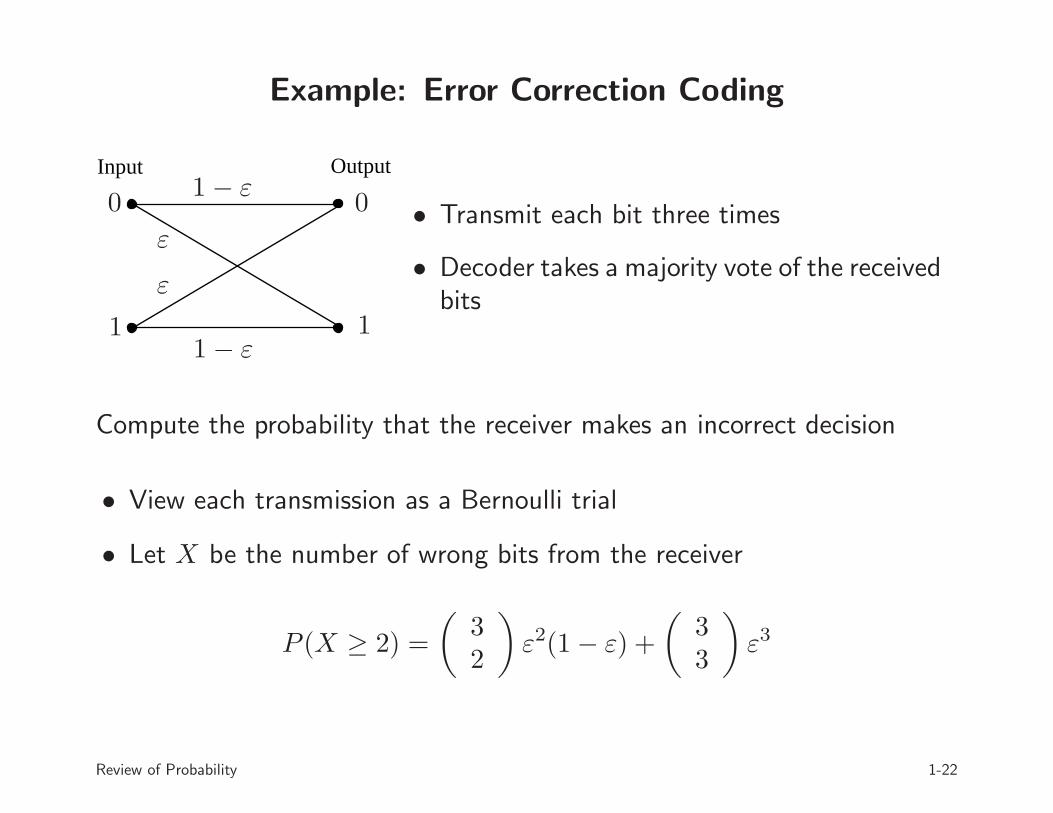
1− ε• Transmit each bit three times

• Decoder takes a majority vote of the receivedbits

Compute the probability that the receiver makes an incorrect decision

• View each transmission as a Bernoulli trial

• Let X be the number of wrong bits from the receiver

P (X ≥ 2) =

(

32

)

ε2(1− ε) +

(

33

)

ε3


Mutinomial Probability

• Generalize the binomial probability law to the occurrence of more thanone event

• Let B1, B2, . . . , Bm be possible events with

P (Bk) = pk, and p1 + p2 + · · ·+ pm = 1

• Suppose n independent repetitions of the experiment are performed

• Let Xj be the number of times each Bj occurs

• The probability of the vector (X1,X2, . . . ,Xm) is given by

P (X1 = k1, X2 = k2, . . . , Xm = km) =n!

k1!k2! . . . km!pk11 pk22 · · · pkmm

where k1 + k2 + · · ·+ km = n


Geometric Probability

• Repeat independent Bernoulli trials until the the first success occurs

• Let X be the number of trials until the occurrence of the first success

• The probability of this event is called the geometric probability law

P (X = k) = (1− p)k−1p, for k = 1, 2, . . .

• The geometric probabilities sum to 1:

∞∑

k=1

P (X = k) = p∞∑

k=1

qk−1 =p

1− q= 1

where q = 1− p

• The probability that more than n trials are required before a success

P (X > n) = (1− p)n


Example: Error Control by Retransmission

• A sends a message to B over a radio link

• B can detect if the messages have errors

• The probability of transmission error is q

• Find the probability that a message needs to be transmitted more thantwo times

Each transmission is a Bernoulli trial with probability of success p = 1− q

The probability that more than 2 transmissions are required is

P (X > 2) = q2


Sequential Dependent Experiments

Sequence of subexperiments in which the outcome of a givensubexperiment determine which subexperiment is performed next

Example: Select the urn for the first draw by flipping a fair coin

1

0

11

1

1

01

0

0 1

Draw a ball, note the number on the ball and replace it back in its urn

The urn used in the next experiment depends on # of the ball selected


Trellis Diagram

Sequence of outcomes

...

H

T000

0000000

111

111

1111

Probability of a sequence of outcomes

...

2/3

1/3

5/6

2/3 2/3

1/3 1/3

1/6 1/6

5/6 5/6

1/2

1/21/6

0000

1111

is the product of probabilities along the path


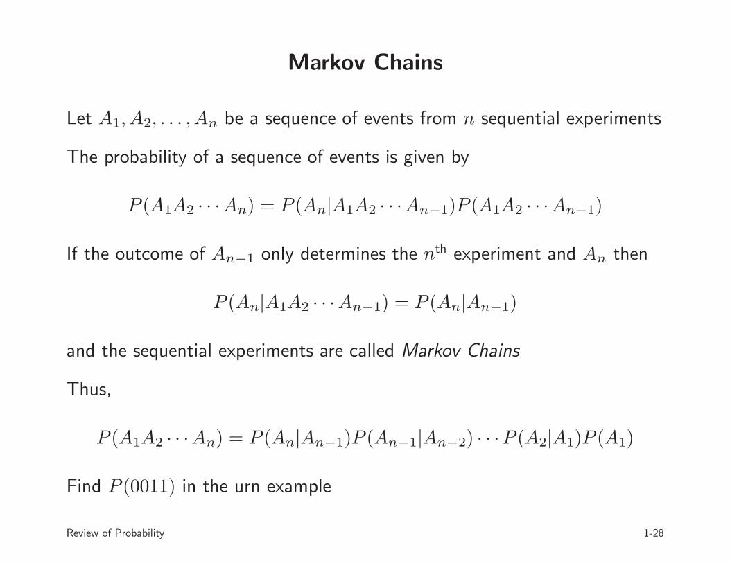
Markov Chains

Let A1, A2, . . . , An be a sequence of events from n sequential experiments

The probability of a sequence of events is given by

P (A1A2 · · ·An) = P (An|A1A2 · · ·An−1)P (A1A2 · · ·An−1)

If the outcome of An−1 only determines the nth experiment and An then

P (An|A1A2 · · ·An−1) = P (An|An−1)

and the sequential experiments are called Markov Chains

Thus,

P (A1A2 · · ·An) = P (An|An−1)P (An−1|An−2) · · ·P (A2|A1)P (A1)

Find P (0011) in the urn example


The probability of the sequence 0011 is given by

P (0011) = P (1|1)P (1|0)P (0|0)P (0)

where the transition probabilities are

P (1|1) =5

6, P (1|0) =

1

3, P (0|0) =

2

3

and the initial probability is given by

P (0) =1

2

Hence,

P (0011) =5

6·1

3·2

3·1

2=

5

54


Discrete-time Markov chain

a Markov chain is a random sequence that has n possible states:

x(t) ∈ {1, 2, . . . , n}

with the property that

prob( x(t+ 1) = i | x(t) = j ) = pij

where P = [pij] ∈ Rn×n

• pij is the transition probability from state j to state i

• P is called the transition matrix of the Markov chain

• the state x(t) still cannot be determined with certainty


example:

a customer may rent a car from any of three locations and return to any ofthe three locations

Rented from location

1 2 3

0.8 0.3 0.2 1

0.1 0.2 0.6 2

0.1 0.5 0.2 3

Returned to location

1

0.1

0.5

0.6

0.2

0.10.3

0.2 0.2

0.8

3 2


Properties of transition matrix

let P be the transition matrix of a Markov chain

• all entries of P are real nonnegative numbers

• the entries in any column are summed to 1 or 1TP = 1T :

p1j + p2j + · · ·+ pnj = 1

(a property of a stochastic matrix)

• 1 is an eigenvalue of P

• if q is an eigenvector of P corresponding to eigenvalue 1, then

P kq = q, for any k = 0, 1, 2, . . .


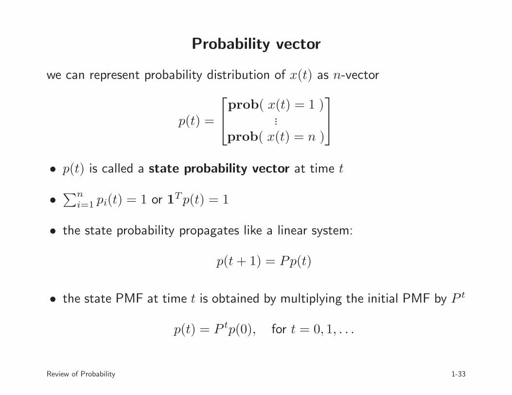
Probability vector

we can represent probability distribution of x(t) as n-vector

p(t) =

prob( x(t) = 1 )...

prob( x(t) = n )

• p(t) is called a state probability vector at time t

•∑n

i=1pi(t) = 1 or 1Tp(t) = 1

• the state probability propagates like a linear system:

p(t+ 1) = Pp(t)

• the state PMF at time t is obtained by multiplying the initial PMF by P t

p(t) = P tp(0), for t = 0, 1, . . .


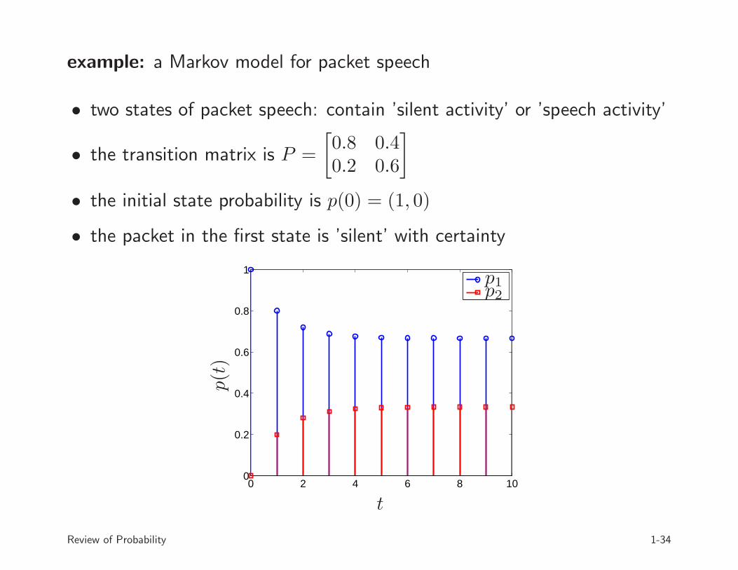
example: a Markov model for packet speech

• two states of packet speech: contain ’silent activity’ or ’speech activity’

• the transition matrix is P =

[

0.8 0.40.2 0.6

]

• the initial state probability is p(0) = (1, 0)

• the packet in the first state is ’silent’ with certainty

0 2 4 6 8 100

0.2

0.4

0.6

0.8

1

t

p(t)

p1p2


• eigenvalues of P are 1 and 0.4

• calculate P t by using ’diagonalization’ or ’Cayley-Hamilton theorem’

P t =

[

(5/3)(0.4 + 0.2 · 0.4t) (2/3)(1− 0.4t)(1/3)(1− 0.4t) (5/3)(0.2 + 0.4t+1)

]

• P t →

[

2/3 2/31/3 1/3

]

as t → ∞ (all columns are the same in limit!)

• limt→∞ p(t) =

[

2/3 2/31/3 1/3

] [

p1(0)1− p1(0)

]

=

[

2/31/3

]

p(t) does not depend on the initial state probability as t → ∞


what if P =

[

0 11 0

]

?

• we can see that

P 2 =

[

1 00 1

]

, P 3 =

[

0 11 0

]

, . . .

• P t does not converge but oscillates between two values

under what condition p(t) converges to a constant vector as t → ∞ ?

Definition: a transition matrix is regular if some integer power of it hasall positive entries

Fact: if P is regular and let w be any probability vector, then

limt→∞

P tw = q

where q is a fixed probability vector, independent of t


Steady state probabilities

we are interested in the steady state probability vector

q = limt→∞

p(t) (if converges)

• the steady-state vector q of a regular transition matrix P satisfies

limt→∞

p(t+ 1) = P limt→∞

p(t) =⇒ Pq = q

(in other words, q is an eigenvector of P corresponding to eigenvalue 1)

• if we start with p(0) = q then

p(t) = P tp(0) = 1tq = q, for all t

q is also called the stationary state PMF of the Markov chain


example: weather model (’rainy’ or ’sunny’)

probabilities of weather conditions given the weather on the preceding day:

P =

[

0.4 0.20.6 0.8

]

(probability that it will rain tomorrow given today is sunny, is 0.2)

given today is sunny with probability 1, calculate the probability of a rainyday in long term


References

Chapter 2 inA. Leon-Garcia, Probability, Statistics, and Random Processes for

Electrical Engineering, 3rd edition, Pearson Prentice Hall, 2009


ee401 (semester 1, 2011) jitkomut songsiri 1. review of

Documents