eet toolbox: eeg and eye tracker integration ting xiao

EET Toolbox: EEG and Eye tracker integration

data recording and analysis toolbox

by

Ting Xiao

(Under the Direction of Tianming Liu)

Abstract

Current research on the combination with the EEG and Eye Tracker is only simply to run

the stimuli and devices on different platforms to collect the human biomedical information.

There is a requirement to unify them into a same platform to avoid the timestamp correction

and perform the data analysis effectively and accurately.

The present study describes the framework and the implementation of EEG-Eye Tracker

Toolbox (EET), which can integrate the EEG and Eye-tracking device together to record

raw biomedical data of the brain and eyes, and support general output to do the different

post data analysis. The EET toolbox is developed by using the MATLAB and can be easily

launched on multiple operating systems where MATLAB is installed.

I complete the EET by integrating the mono-channel EEG (Neurosky MindWave Mobile)

and Eye Tracker (Tobii X2-30), and then test it with a set of movie trailers as an experiment.

Index words: EEG, Eye Tracking, Multimedia, MATLAB, Visualization



by

Ting Xiao

B.S., Donghua University, China,2006

B.A., Donghua University, China,2006

A Dissertation Submitted to the Graduate Faculty

of The University of Georgia in Partial Fulfillment

of the

Requirements for the Degree

Master Science

Athens, Georgia

2014

c©2014

Ting Xiao

All Rights Reserved



by

Ting Xiao

Approved:

Major Professor: Tianming Liu

Committee: Suchi BhandarkarKang Li

Electronic Version Approved:

Julie CoffieldInterim Dean of the Graduate SchoolThe University of GeorgiaDecember 2014

EET Toolbox: EEG and Eye Tracker Integration

Data Recording and Analysis Toolbox

Ting Xiao

November 29, 2014

Acknowledgments

I would like to thank William Olive and Dr.Miller for helping with the implementation and

test on the EEG machine in the Bio-image Research Center. Thanks for the help from the

friends in the CAID lab as the volunteers to test this toolbox and give me a lot of suggestions.

At the same time, I appreciate the great support from Andrews M Rogers, the Manager of

Global Web & Social Media in Elekta. Without their support I cannot complete this thesis.

iv

Contents

1 Introduction 1

1.1 EEG Technology . . . . . . . . . . . . . . . . . . . . . . . . . . . . . . . . . 1

1.2 Eye Tracking Technology . . . . . . . . . . . . . . . . . . . . . . . . . . . . . 3

1.3 Motivation of Combining EEG and Eye Tracking . . . . . . . . . . . . . . . 4

2 EET System Design 6

2.1 System Architecture . . . . . . . . . . . . . . . . . . . . . . . . . . . . . . . 6

2.2 Workflow . . . . . . . . . . . . . . . . . . . . . . . . . . . . . . . . . . . . . 8

2.3 Data Structure . . . . . . . . . . . . . . . . . . . . . . . . . . . . . . . . . . 8

3 Methods 9

3.1 Experiment Function . . . . . . . . . . . . . . . . . . . . . . . . . . . . . . . 9

3.2 Post Experiment Analysis Function . . . . . . . . . . . . . . . . . . . . . . . 10

4 Case Study 15

4.1 Experiment Method . . . . . . . . . . . . . . . . . . . . . . . . . . . . . . . 15

4.2 Experiment Result . . . . . . . . . . . . . . . . . . . . . . . . . . . . . . . . 16

5 Conclusion 28

6 Future Study 30

Bibliography 31

v

Appendix A Function Source Code 33

A.1 EET_Experiment.m . . . . . . . . . . . . . . . . . . . . . . . . . . . . . . . 33

A.2 getFrameToShotDetection.m . . . . . . . . . . . . . . . . . . . . . . . . . . . 37

A.3 getSegment.m . . . . . . . . . . . . . . . . . . . . . . . . . . . . . . . . . . . 40

A.4 getVideoFeature.m . . . . . . . . . . . . . . . . . . . . . . . . . . . . . . . . 41

A.5 getAudioFeature.m . . . . . . . . . . . . . . . . . . . . . . . . . . . . . . . . 42

A.6 getEEGFeature.m . . . . . . . . . . . . . . . . . . . . . . . . . . . . . . . . . 43

A.7 getEYEFeature.m . . . . . . . . . . . . . . . . . . . . . . . . . . . . . . . . . 45

A.8 getEYEGaze.m . . . . . . . . . . . . . . . . . . . . . . . . . . . . . . . . . . 47

vi

List of Tables

I Movie Trailers Used In Experiment . . . . . . . . . . . . . . . . . . . . . . . 16

vii

List of Figures

1.1 Mono-channel EEG(NeuroSky MindWave Mobile) . . . . . . . . . . . . . . . 2

1.2 Multi-channel EEG . . . . . . . . . . . . . . . . . . . . . . . . . . . . . . . . 2

1.3 10-20 Electrode Position . . . . . . . . . . . . . . . . . . . . . . . . . . . . . 3

1.4 Tobii X2-30 Eye Tracker . . . . . . . . . . . . . . . . . . . . . . . . . . . . . 4

2.1 EET Architecture . . . . . . . . . . . . . . . . . . . . . . . . . . . . . . . . . 7

2.2 EET Workflow . . . . . . . . . . . . . . . . . . . . . . . . . . . . . . . . . . 8

3.1 EET Data Structure For Video Stimuli . . . . . . . . . . . . . . . . . . . . . 11

3.2 Shot Detection Comparison For The Bucket List . . . . . . . . . . . . . . . . 12

4.1 Visualization Result of Video Features(Group1) . . . . . . . . . . . . . . . . 18

4.2 Visualization Result of Video Features(Group2) . . . . . . . . . . . . . . . . 19

4.3 Visualization Result of Audio Features(Group1) . . . . . . . . . . . . . . . . 20

4.4 Visualization Result of Audio Features(Group2) . . . . . . . . . . . . . . . . 21

4.5 Comparison Result of EEG-Eye Feature (Zombie Nation) . . . . . . . . . . . 23

4.6 Comparison Result of EEG-Eye Feature (Bounty Killer) . . . . . . . . . . . 24

4.7 Comparison Result of EEG-Eye Feature (Watchman) . . . . . . . . . . . . . 25

4.8 Comparison Result of EEG-Eye Feature (Die Hard 5) . . . . . . . . . . . . . 26

4.9 Gaze Data for One Segment in TED . . . . . . . . . . . . . . . . . . . . . . 27

viii

Chapter 1

Introduction

This chapter introduces the background for this thesis, the current situation of EEG and

Eye tracking technology, and the motivation of combining both of them to do the research.

1.1 EEG Technology

Humans never stop to understand themselves, especially the brain. In 1931,Hans Berger, a

German physician, discovered the electroencephalogram (EEG). After that, EEG becomes a

powerful research method in the field of neurology and clinical neurophysiology, for example,

to observe the damage of the brain, monitor brain activities,use the different brain waves

from human frontal to evaluate the TV commercial [2],pick out relative band from the EEG

raw data to analyze the emotional response of human beings [3], and promote the use of

brain computer interfaces(BCI) for gaming based on the EEG data [8].

The basic idea of Encephalographic measurements is that the electrodes read the signal

from the human’s head surface, amplifiers bring the microvolt signals into the range where

they can be digitalized accurately, converter signals from analog to digital form, and the

computer stores and displays the obtained data. Minimal configuration for mono channel

EEG measurement consists of one active electrode, one reference and one ground electrode,

like the NeuroSky MindWave Mobile EEG Sensor(Figure 1.1), while the multi-channel EEG

1

Figure 1.1: Mono-channel EEG(NeuroSky MindWave Mobile)

Figure 1.2: Multi-channel EEG

can comprise up to 128 or 256 active electrodes(Figure 1.2).

In 1958, International Federation in Electroencephalography and Clinical Neurophysiol-

ogy adopted standardization for electrode placement called 10-20 electrode placement sys-

tem. This system standardized physical placement and designations of electrodes on the

scalp. The head is divided into proportional distances from prominent skull landmarks (na-

sion, preauricular points, inion) to provide adequate coverage of all regions of the brain.

Label 10-20 designates proportional distance in percents between ears and nose where points

for electrodes are chosen. Electrode placements are labeled according adjacent brain areas:

F (frontal), C (central), T (temporal), P (posterior), and O (occipital). Odd numbers at the

2

Figure 1.3: 10-20 Electrode Position

left side of the head and with even numbers accompanies the letters on the right side (Figure

1.3). [10]

1.2 Eye Tracking Technology

Conversely, the principle of eye tracker is relatively simple.Recently it has become a tool in

scientific fields addressing the study of human vision perception and has been used in differ-

3

Figure 1.4: Tobii X2-30 Eye Tracker

ent research areas such as neuroscience, psychology, human and computer interaction.Figure

1.4 shows one of the low sampling-rate eye trackers manufactured by Tobii. The gaze co-

ordination information is the only raw data recorded by eye tracker. Depending on it, we

can compute the gaze data, pupil size from the eyes of subject. Many researchers identified

different fixation algorithms to analyze the eye-movement pattern.

1.3 Motivation of Combining EEG and Eye Tracking

In M.Teplan study [10], an important result about the EEG signal was achieved, that is,

most of the people are remarkably sensitive to the phenomenon of eye closing, when they

close their eyes, their EEG wave patterns significantly change from beta into alpha waves. It

is also a good reason for combining the EEG with Eye tracking to understanding the brain

activities.

However, there are still a lot of challenges to integrate both technologies together.On

the EEG side is how to explain those signals of the brain.Different researches are based on

different band of the signals.For instance, one study selected Delta: 1.375 - 4.125 Hz; Theta:

4

4.125 - 6.875 Hz; Alpha1: 6.875 - 9.625 Hz;Alpha2: 9.625 - 12.375 Hz; Beta1: 12.375 - 17.875

Hz; Beta2: 17.875 - 34.375 Hz as the EEG frequency ranges to perform their neurocode-

tracking method [5].While Erik referred the Delta: 0.5 - 2.75 Hz; Theta: 3.5 - 6.75Hz; Alpha1:

7.5 - 9.25 Hz;Alpha2: 10 - 11.75 Hz; Beta1: 13 - 16.75 Hz; Beta2: 18 - 29.75 Hz;Gamma1:31-

39.75Hz;Gamma2:41-49.75Hz to design the brain computer interface(BCI) of the snake of

game [8]. On the other hand, commercial software platforms of the eye tracker are usually

proprietary, and it cannot be extended or modified for particular analysis algorithms. So

far, I only found one open source tool named EYE-EEG plugin [4], which must be used with

EEGLAB [12] platform.

It is hard to explain which standard for the EEG band is right or wrong, but other

biomedical data can be added to help us to understand those activities. Therefore, there is a

requirement to implement an open source for the EEG and Eye tracking integration system

used in different research fields.In my study, a new toolbox integrating the EEG and Eye

tracking will be developed and named as EET(EEG and Eye Tracking Toolbox), running

independently for experiment multimedia stimuli presentation and post experimental data

analysis. EET is designed to implement on the MATLAB, therefore it can be used flexibly

on the Windows OS, Linux and Mac OS X, where MATLAB is preinstalled.Furthermore, it

can also be extended based on different experiment requirement.

5

Chapter 2

EET System Design

This chapter explains the system architecture, workflow and data structure of the EET for

supporting different devices and extending the function in the future as an open source.

2.1 System Architecture

Currently, the EET is only considered to load the EEG and Eye tracking equipment at

the same platform, and there is no communication component between these two types of

devices. Figure2.1 illustrates the entire architecture of the EET and the function of each

component.

(1) Stimuli Presentation: In order to do a good experiment for the specific research, operator

should prepare different kind of stimulus for the participant, such as one static picture,

some slides, and an audio or video clip. And display them in different approaches.

(2) Data Connection and Recording: This part includes a lot of interface function of the

devices that are chosen in EET system. Most of EEG and Eye-tracking devices supports

the API in different platform.Check their developer or manual book before will be very

helpful. The signal values are recorded as matrix object and saved in the end of the

experiment.

6

Figure 2.1: EET Architecture

7

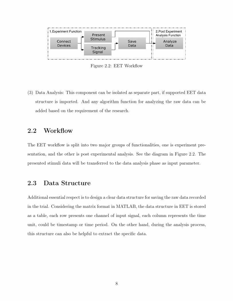
Figure 2.2: EET Workflow

(3) Data Analysis: This component can be isolated as separate part, if supported EET data

structure is imported. And any algorithm function for analyzing the raw data can be

added based on the requirement of the research.

2.2 Workflow

The EET workflow is split into two major groups of functionalities, one is experiment pre-

sentation, and the other is post experimental analysis. See the diagram in Figure 2.2. The

presented stimuli data will be transferred to the data analysis phase as input parameter.

2.3 Data Structure

Additional essential respect is to design a clear data structure for saving the raw data recorded

in the trial. Considering the matrix format in MATLAB, the data structure in EET is stored

as a table, each row presents one channel of input signal, each column represents the time

unit, could be timestamp or time period. On the other hand, during the analysis process,

this structure can also be helpful to extract the specific data.

8

Chapter 3

Methods

This chapter focuses on the implementation of EET by using the script language of MAT-

LAB. Current supporting EEG device is Neurosky Mobile Set and eye tracking device is

Tobii X2-30.

3.1 Experiment Function

The Tobii X2-30 [15] [14] supports the MATLAB platform. The modules that process the

connection, calibration and data tracking will be used into EET to record the eyes’ position.

On the other hand, the EEG data is recorded by using the Neurosky MindWave Mobile.

There is no toolbox support on the MATLAB platform directly. However, NeuroSky provides

the interface on .NET, Mac OS X, iOS and Android [11]. The COM technology for Windows

OS and dylib for the Mac OS X and Linux is used to merge the connection, tracking interface

into EET toolbox.

Furthermore, in order to avoid using the VideoReader methods of MATLAB, the experi-

ment stimulus is present by the third media player application on the operating system. On

Window OS 7, I choose the Media Player by COM interface, while on Mac OS X by using

the command line tools to recall the QuickTime.

In the end, both EEG and Eye tracking data will be saved as matrix file directly for the

9

next process. Function named EET_Experiment is listed in the appendix.

3.2 Post Experiment Analysis Function

For the purpose of analyzing the video stimuli with EEG and Eye tracking biomedical in-

formation, I separate the analysis process into 4 steps: 1 shot detection, 2 segment all the

signal channels based on key frames, 3 extract the low feature for each segmentation, 4 vi-

sualization. The specific design data structure for doing the video trial described in Figure

3.1.

(a) the video feature vector (VF) for each key frame of one video signal

(b) the audio feature vector (AF) for each audio channel.

(c) the electrical signal vector for each EEG channel.

(d) the eye feature vector (EF) such as validate eyes position and the its moving distances

for each video segmentation.

Step1 Shot Detection: The algorithm I used in this step is present online [13].Its

principle idea is to select the abrupt transition scene from continuous video frame sequence

depending on the intensity histogram difference of each frame. However, this algorithm is

not good for picking out the transition scenes in the continuous frame, I added a threshold

to search a proper boundary for segmentation. In order to clarify the question, I use a trailer

named The Bucket List that was also used in the case study to illustrate. In Figure 3.2(a),

those frames shown in the top are the first few key frames result of the shot detection. From

No. 300 to No 304 is the cluster of transition scene in the trailer. If these frames were not

filtered, the audio segmentation would fail in the next step. I set the threshold number of

search range as 10, which means if there is no other transition scenes before or after 10 frames

to the current frame, it is marked as key frame.Figure 3.2(b) shows the result of filtering the

transition scenes in the same video stimulus. Function named getFrameToShotDetection is

10

Figure 3.1: EET Data Structure For Video Stimuli

11

(a) Shot Detection Result Before Improvement

(b) Shot Detection Result After Improvement

Figure 3.2: Shot Detection Comparison For The Bucket List

12

listed in appendix.

Step2 Segmentation: According to the result of the previous step, the principle of

segmentation step is to use the FFmpeg [1], which is a multimedia platform to record,

convert and stream audio and video. The MATLAB script supports the Linux or DOS

command line. Therefore, original video would be segment into small clips and saved as

MP4 and MP3 format, which will be used to extract the low-level features for the next step.

The source code getSegment.m implemented in the appendix part.

Step3 Low Feature Extraction: Based on these segmentation results, in the third

step, I will extract the low feature for each channel of the video, audio, EEG, eye, and

combine the data into a structure I mentioned in the beginning of this chapter. Four func-

tions complete this process: getVideoFeature.m, getAudioFeature.m, getEEGFeature.m, and

getEYEFeature.m. And the following low features parameters are defined in EET.

(a) Video Feature (VF): extract color feature including brightness, colorfulness, contrast

and simplicity for each segmentation.

(b) Audio Feature (AF): extract the dynamic, rhythm, timbre and pitch features for each

audio clips by the MIRtoolbox [9], referring to the research method used in game music

[7].

(c) EEG Feature(EEGF):since the original power value of every channel into the dataset

to do later statistic, I only focused on collecting the sum, average and variance of EEG

power value in each shot.

(d) Eye Movement Feature(EYEF):Based on the investigation report in Filippakopoulou

paper for designing their own toolbox [6], we can know that there are lot of software to

analyze the raw data recorded by different eye trackers, however, they do not show any

inner algorithm to analyze those position. For EET, I only collect the validate position

of the eyes and calculate the distance of the eyes movement based on the raw record.

13

Step4 Visualization: Rely on the designed data structure, it is very easy to visualize

the data to select specific one to compare in the final step. In this study, I focus on observing

the EEG and eye moving changes to the same stimulus.The visualization result will be shown

in next chapter.

14

Chapter 4

Case Study

For the purpose of testing the EET, the Neurosky MindWave Mobile and Tobii X2-30 were

installed as the Figure 4.1. I will introduce the experiment and the result of each step in

this chapter.

4.1 Experiment Method

The experiment was conducted on 10 subjects. They were sitting in sofa and requested to

watch some movie trailers in relaxed, as they would watch film at home. 20 movie trailers

were selected, which had been released in previous years in U.S. The 10 were good movie

trailers (group1) and the others were bad ones (group2) with lower score in the YouTube

and based on the evaluation result from the Department of Theatre and Film Studies. Those

movie trailer names are list in Table 1, and would be randomly shown in different order for

each subject. Neurosky MindWave Mobile and Tobii X2-30 recorded his/her brain and eye

activities.

15

Table I: Movie Trailers Used In Experiment

NO. Movie Trailer Name(Group1:Bad) Movie Trailer Name(Group2:Good)

1 Chairman of the Board Watchman

2 The Double Pirates of the Caribbean 3

3 Young Adult TED

4 Zombie Nation Seven Psychopaths

5 Sharknado Hitchcock

6 Assault on Wall Street The Bucket List

7 Cosmopolis Jack the Giant Killer

8 The Wicked Wrath Of The Titans

9 The Room Mud

10 Bounty Killer Die Hard 5

4.2 Experiment Result

I generated various visualizations for all the low features saved in the EET to analyze exper-

iment result. The general result is the good trailers have more segmentations than the bad

ones. Additionally, those good segments have even intervals.

Video Feature of Movie Trailers

First,the video feature visualizations of twenty movie trailers in two groups are list in

Figure 4.1 and Figure 4.2. The x-axis represents the frame number of the video stimuli and

the y-axis indicates the feature value. Each black frame includes five color feature plots for

one movie trailer, from left to right, top to bottom. They are brightness, contrast, saturation,

colorfulness and simplicity. Compared the plots in group, most of the trailers have more

variations in Group 2 than the Group 1.Take an extreme example in Group 1: No.4 trailer

named Zombie Nation, which only has 5 key segmentations,each color feature changed evenly

and smooth. The same situation occurs in the No.10(Bounty Killer), No.8(The Wicked), and

16

No.5(Sharknado). However, it is hard to find any similar example in the good edit trailers,

all of color features are varied with each film montage.

Audio Feature of Movie Trailers

Accordingly, I visualized the audio features in the same way as the video features in

Figure 4.3 and Figure 4.4.In each black frame, there are nine audio feature plots for one

movie trailer, from left to right, top to bottom, they are dynamic, rhythm, timbre and

pitch. The unusual value is the average tempo value, some segment have no tempo value, for

example, the No.1,2,3,6,7 movie trailers in Group1 and the No. 3,4,5,6,8,10 movie trailers

in Group 2.Every tailer has different variations depended on the different features.However,

if we combine the audio and video changes together, the good and bad edit trailers can be

separated more quickly. That is good trailers should have totally different sound editing with

video clips. Using the No.10 Die Hard 5 trailer as an example, from around 900th frame to

1000th frame, there are dramatic changes in color features, while among the audio features,

the varied range is small, even the tempo value cannot be detected. In contrast, those

trailers in Group1, for instance, No.7 Cosmopolis, the color feature variations concentrated

in a frame interval from 1000th to 2000th frame, the same trend on the audio features.

EEG and Eye Feature

Video and audio features can only represent the feature level of the stimuli. While

comparing the EEG and Eye signals can help us to find more useful watch models for how

people capture the information from multimedia. I spread out all subjects visualization

results of EEG(Fpz Channel) and Eye movement distance for analyzing the trailer edit

influence.

First of all, that those 10 subjects always have high EEG power value and long eye moving

distance value at the beginning of seeing the trailer stimulus, after that the EEG power signal

became lower, and the eye moving distances were much shorter than the beginning. When

the subject was seeing the good trailers, the variation tendency of EEG average power is

very similar as the convergence function but the same regulation can hard be found in the

17

Figure 4.1: Visualization Result of Video Features(Group1)

18

Figure 4.2: Visualization Result of Video Features(Group2)

19

Figure 4.3: Visualization Result of Audio Features(Group1)

20

Figure 4.4: Visualization Result of Audio Features(Group2)

21

bad trailers, less frames, few segmentations and uneven changes cannot help people to keep

pace of the video content.

Second, people are sensitive to any feature variation no matter it is good or bad trailer.

Select the third column, the variance of the EEG signal value and eye moving feature,

to compare the corresponding stimuli features, for example, the No.4 trailer: Zombie Na-

tion(Figure 4.5), even though the color features changed smoothly, the subjects’ EEG signal

varied sharply. as well as the No.10 Bounty Killer(Figure 4.6).Taking the example in the

Group 2, the No10 trailer: Die Hard 5(Figure 4.7), those low features changes of the stimuli

always bring the fluctuation in the EEG signal.

Eye Gaze Data Visualization

Figure 4.9 shows the partial gaze data of each subject when he/she was seeing the TED

movie trailer. Obviously, in this particular segmentation, some subjects haven’t focus on

this scene any more, such as subject 5 and subject 10. On the other hand, the gaze intensity

is so different among the other subjects. Which means the gaze intensity could be added to

the future study.

22

Figure 4.5: Comparison Result of EEG-Eye Feature (Zombie Nation)

23

Figure 4.6: Comparison Result of EEG-Eye Feature (Bounty Killer)

24

Figure 4.7: Comparison Result of EEG-Eye Feature (Watchman)

25

Figure 4.8: Comparison Result of EEG-Eye Feature (Die Hard 5)

26

Figure 4.9: Gaze Data for One Segment in TED

27

Chapter 5

Conclusion

The result indicates that the EET toolbox can be executed and support the analysis the

EEG and Eye tracking data for multimedia stimuli.Therefore,the primary contributions in

this thesis are:

1. The presentation of the basic architecture of the integration system.It can work for

any products if they provide proper MATLAB interface.

2. The development of each functionality design.

Since all the source codes are written in MATLAB script, it can work on any machine

installed with MATLAB, I test the system on MATLAB_2013a_Student on Mac OS

X 10.10 and MATLAB_2013b_Student on Windows OS 7. It executed well on the

both operating systems.

3. One specific multimedia movie trailer experiment was executed and analyzed.

There is few research on the movie trailer experiment with the EEG and Eye Tracking

so far. The following result shows the shot detection based multimedia analysis, which

also combining with the EEG and Eye tracking can help us to study more useful vision

and brain activity model.

a)Bad trailer always has few frame numbers, few segmentation and even variations in

28

color features changed.

b)Good trailer not only has more frame numbers, more clips, frequent changes in color

features, but also combing with a stark contrast change in audio feature.

In one word, to make a good trailer, we should use dynamic editing methods to make

sure both video and audio features change differently.

29

Chapter 6

Future Study

First step, to test the EET with 256 channels EEG device in Bio-image Research Center

in UGA by using the same experiment set, thus to get more details of brain activities by

other channel information. Secondly, to add the event synchronize for the whole trial will be

helpful for searchers to set the interesting events mark for observing the brain activities in

real time. Third,focus on adding more algorithms for eye features in the feature-extraction

phase.

30

Bibliography

[1] Ffmpeg. https://www.ffmpeg.org/.

[2] Mathieu Bertin, Rie Tokumi, Ken Yasumatsu, Makoto Kobayashi, and Akihiro Inoue.

Application of eeg to tv commercial evaluation. Biomedical Informatics and Technol-

ogy Communications in Computer and Informtion Science, 404:277–282, 2014.

[3] Danny Oude Bos. EEG-based Emotion Recognition The Influence of Visual and Audi-

tory Stimuli. PhD thesis, University of Twente, 2006.

[4] O. Dimigen. Eye-eeg plugin. http://www2.hu-berlin.de/eyetracking-eeg/.

[5] Wilfried Dimpfel and Hans Carlos Hofmann. Neurocode-tracking based on quantita-

tive fast dynamic eeg recording in combination with eye-tracking. World Journal of

Neuroscience, 4:106–119, May 2014.

[6] Vassiliki Filippakopoulou and Byron Nakos. Eyemmv toolbox: An eye movement

post-analysis tool based on a two-step spatial dispersion threshold for fixation iden-

tification. Journal of Eye Movement Research, 7(1):1–10, 2014.

[7] Raffaella Folgieri, Mattia G. Bergomi, and Simone Castellani. EEG-based Brain-

Computer Interface for Emotional Involvement in Games through Music. Number

205-236 in Digital Da Vinci. Springer, 04 2014.

[8] Erik Andreas Larsen. Classification of eeg signals in a brain-computer interface sys-

tem. Master’s thesis, Norwegian University of Science and Technology, June 2011.

31

[9] Olivier Lartillot, Petri Toiviainen, and Tuomas Eerola. Mirtoolbox.

https://www.jyu.fi/hum/laitokset/musiikki/en/research/coe/materials/mirtoolbox.

[10] M.Teplan. Foundamentals of eeg measurement. Measurement Science Review, 2, 2002.

[11] Neurosky. Neurosky sdk, 10 2014.

http://developer.neurosky.com/docs/doku.php?id=start.

[12] University of California San Diego. Eeglab toolbox. http://sccn.ucsd.edu/eeglab/.

[13] Roman. Video boundary detection. http://www.roman10.net/video-boundary-

detectionpart-1-abrupt-transitions-and-its-matlab-implementation/.

[14] Tobii. Tobii Toolbox for Matlab. Tobii, 1.1 edition, 07 2010.

[15] Tobii. Users’ Manual Tobii X2-30 Eye Tracker. Tobii, 1.0.3 edition, 06 2014.

32

Appendix A

Function Source Code

A.1 EET_Experiment.m

% EET_Experiment.m% Ting Xiao% 10/24/2014% Test on Tobii X2-30 and NeuroSky MindSet Mobileclcclear allclose allname = input(’What is your name? :’,’s’);movienum = input(’which number you like:1-10:’);% *************************************************************************% NeuroSky Define% *************************************************************************portnum1 = 3; %COM Port #comPortName1 = sprintf(’\\\\.\\COM%d’, portnum1);% Baud rate for use with TG_Connect() and TG_SetBaudrate().TG_BAUD_57600 = 57600;% Data format for TG_Connect() and TG_SetDataFormat().TG_STREAM_PACKETS = 0;% Data type for TG_GetValue().TG_DATA_RAW = 4;% *************************************************************************% Load SDK% 1) Tobii% 2) NeuroSky

33

% *************************************************************************addpath(’functions’);addpath(’tetio’); % Eye Tracker SDKaddpath(’NeuroSky’);% EEG SDK%load thinkgear dllloadlibrary(’Thinkgear.dll’);fprintf(’Thinkgear.dll loaded\n’);%get dll versiondllVersion = calllib(’Thinkgear’, ’TG_GetDriverVersion’);fprintf(’ThinkGear DLL version: %d\n’, dllVersion );% *************************************************************************% Initialization and connection to the Tobii Eye-tracker% *************************************************************************disp(’Initializing tetio...’);tetio_init();% Set to tracker IDtrackerId = ’your eye tracker ID’;if ( strcmp(trackerId, ’NotSet’) )

warning(’tetio_matlab:EyeTracking’,’ NO TrackerId.’);disp(’Browsing for trackers...’);trackerinfo = tetio_getTrackers();for i = 1:size(trackerinfo,2)

disp(trackerinfo(i).ProductId);endtetio_cleanUp();

endtetio_connectTracker(trackerId)% *************************************************************************% Initialization and connection to the NeuroSky% *************************************************************************% Get a connection ID handle to ThinkGearconnectionId1 = calllib(’Thinkgear’, ’TG_GetNewConnectionId’);if ( connectionId1 < 0 )

error( sprintf( ’ERROR: ...TG_GetNewConnectionId() returned %d.\n’, connectionId1 ) );

end;% Set/open stream (raw bytes) log file for connectionerrCode = calllib(’Thinkgear’, ...’TG_SetStreamLog’, connectionId1, ’streamLog.txt’ );if( errCode < 0 )

error( sprintf( ’ERROR: ...TG_SetStreamLog() returned %d.\n’, errCode ) );

end;% Set/open data (ThinkGear values) log file for connectionerrCode = calllib(’Thinkgear’, ...

34

’TG_SetDataLog’, connectionId1, ’dataLog.txt’ );if( errCode < 0 )

error( sprintf( ’ERROR: ...TG_SetDataLog() returned %d.\n’, errCode ) );

end;% = connection ID handle to serial port "COM#"errCode = calllib(’Thinkgear’, ...’TG_Connect’, connectionId1,...comPortName1,TG_BAUD_57600,TG_STREAM_PACKETS );if ( errCode < 0 )

error( sprintf( ’ERROR:...TG_Connect() returned %d.\n’, errCode ) );

endfprintf( ’Connected. Reading Packets from MindSet...\n’ );% *************************************************************************%% Prepare a stimulus% call for mediaplayer to show the Movie%% *************************************************************************close all;movie_name = sprintf(’Hello-good%d.avi’, movienum);movie_path = fullfile([pwd],movie_name);mov = VideoReader( movie_name );movDuration = mov.Duration;%unit: secondh=actxserver(’WMPlayer.OCX.7’);

hold on;% *************************************************************************%% Check the subject’s eye status and calibration%% *************************************************************************SetCalibParams;% Display the track status window (to position the participant).TrackStatus;% Perform calibrationHandleCalibWorkflow(Calib);close all% *************************************************************************%% Start tracking and plot the gaze data read from the tracker.%% *************************************************************************tetio_startTracking;

35

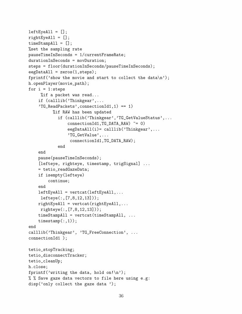
leftEyeAll = [];rightEyeAll = [];timeStampAll = [];%set the sampling ratepauseTimeInSeconds = 1/currentFrameRate;durationInSeconds = movDuration;steps = floor(durationInSeconds/pauseTimeInSeconds);eegDataAll = zeros(1,steps);fprintf(’show the movie and start to collect the data\n’);h.openPlayer(movie_path);for i = 1:steps

%if a packet was read...if (calllib(’Thinkgear’,...’TG_ReadPackets’,connectionId1,1) == 1)

%if RAW has been updatedif (calllib(’Thinkgear’,’TG_GetValueStatus’,...

connectionId1,TG_DATA_RAW) ~= 0)eegDataAll(i)= calllib(’Thinkgear’,...’TG_GetValue’,...connectionId1,TG_DATA_RAW);

endendpause(pauseTimeInSeconds);[lefteye, righteye, timestamp, trigSignal] ...= tetio_readGazeData;if isempty(lefteye)

continue;endleftEyeAll = vertcat(leftEyeAll,...lefteye(:,[7,8,12,13]));

rightEyeAll = vertcat(rightEyeAll,...righteye(:,[7,8,12,13]));

timeStampAll = vertcat(timeStampAll, ...timestamp(:,1));

endcalllib(’Thinkgear’, ’TG_FreeConnection’, ...connectionId1 );

tetio_stopTracking;tetio_disconnectTracker;tetio_cleanUp;h.close;fprintf(’writing the data, hold on!\n’);% % Save gaze data vectors to file here using e.g:disp(’only collect the gaze data ’);

36

[gazex,gazey]=DisplayData(leftEyeAll, rightEyeAll );resultEYEfile = sprintf(’result-EYE%s%d.mat’,...name, movienum);save(resultEYEfile, ’leftEyeAll’, ’rightEyeAll’, ...’timeStampAll’, ’gazex’, ’gazey’);save(resultEEGfile, ’eegDataAll’);%hold on;scatter (gazex,gazey,50,’filled’);axis([0 1 1 0]);resultEYEPosition = sprintf(’result-EYE%s%d’,...name, movienum);saveas(gcf, resultEYEPosition, ’fig’);

A.2 getFrameToShotDetection.m

% getFrameToShotDetection.m% Ting Xiao% 11/7/2014% Attempt to get the shot for movie trailerclc;close all;clear all;DataSet = {...

’Movie1’,...’Movie2’};

for iFile=1:numel(DataSet)% *************************************************************************% Get Frames from FrameFolder% *************************************************************************

dataName = cellstr(DataSet(iFile));%reading video clipsrcdir = [pwd];tempPath = fullfile(srcdir,dataName,’\*.png’);dircontent = dir(tempPath{1});nfiles = length(dircontent);if(nfiles==0) warning(’No files found.’); return; end;frameIndice = zeros(1,nfiles);tempName = sprintf(’%s.mp4’,dataName{1});videoName = fullfile(srcdir,dataName{1},tempName);

% *************************************************************************% Get video metadata

37

% *************************************************************************mov = VideoReader(videoName);frameRate = mov.FrameRate;frameHeight = mov.Height;frameWidth = mov.Width;

% *************************************************************************% Compute the color histogram% *************************************************************************

B = 5; %there will be 2^B binsnumOfBins = 2^B;numOfFrames = nfiles;colorInt = 256/numOfBins;GrayH = zeros(numOfFrames, numOfBins);stdGray = zeros(1, numOfFrames);for i=1:numOfFrames

%I don’t use videoreader, use the frames I savedframePNGName = sprintf(’%3.3d.png’,i);framepath = fullfile(srcdir,dataName{1},...framePNGName);%read image info for each framelFrame = imread(framepath);%RGBlRFrame = lFrame(:,:,1);lGFrame = lFrame(:,:,2);lBFrame = lFrame(:,:,3);%get the intensitylGray = 0.299*lRFrame + 0.587*lGFrame + 0.114*lBFrame;lGrayReshaped = reshape(lGray, 1, ...frameHeight*frameWidth);stdGray(i) = std(double(lGrayReshaped), 0, 2);lindexGray = uint8(floor(double(lGray)./colorInt + 1));for j=1:1:frameHeight

for k=1:1:frameWidthGrayH(i, lindexGray(j, k)) = GrayH(i, ...lindexGray(j, k)) + 1;

endend

end%calculate the histogram differenceGrayHD = [zeros(1, numOfFrames-1)];for i=1:1:numOfFrames-1

GrayHD(i) = sum(sum(abs(GrayH(i, :) -...GrayH(i+1, :))));

end% *************************************************************************

38

%calculate the mean and variance of the frame-to-frame difference%compute the threshold of Tb = mean + alpha*variance% *************************************************************************

alpha = 3;mu = mean(GrayHD);sigma = std(GrayHD);Tb = mu + alpha*sigma;DHNumOfBins = 100;IntDH = max(GrayHD)/DHNumOfBins + 1;HistD = zeros(1, DHNumOfBins);for i=1:1:numOfFrames-1

index = uint8(floor(double(GrayHD(i))/IntDH+1));HistD(index) = HistD(index) + 1;

endmxHistD = max(HistD);mxIndex = find(HistD==mxHistD);Ts = max((mxIndex+2)*IntDH, mu);

% *************************************************************************% Plot the result% *************************************************************************

%rescale stdGray for better plotscaleF = Tb/max(stdGray);stdGray = stdGray.*scaleF;figure, plot(1:numOfFrames-1, GrayHD, ...1:numOfFrames-1, Tb,...

1:numOfFrames-1, Ts(1,1));% *************************************************************************% Get Key Frame Result and Save as Mat format% *************************************************************************

keyFrame = [];keyFrameIndex =1;keyFrame(1,keyFrameIndex)=1;for i=1:1:numOfFrames-1

if (GrayHD(i) > Tb)highCnt = 1;for j=2:1:10%starting from 2 to avoid the cut transition with 2 frames

if ((i-j >=1) & (GrayHD(i-j) > Tb/3) &...GrayHD(i-j) > 5000)

highCnt = highCnt + 1;endif ((i+j < numOfFrames-1) & (GrayHD(i+j) > Tb/3)...& GrayHD(i+j) > 5000)

highCnt = highCnt + 1;end

39

endif((highCnt<2)& i>2)

keyFrameIndex = keyFrameIndex+1;keyFrame(1,keyFrameIndex)= i-1;

endend

endkeyFrameIndex = keyFrameIndex+1;keyFrame(1,keyFrameIndex)= numOfFrames;

moviename = cellstr(DataSet_movie(iFile))resultname = sprintf(’%s-%s.mat’,moviename{1},’keyframes’);save(resultname,’keyFrame’);

end

A.3 getSegment.m

% getSegment.m% Ting Xiao% 11/7/2014% segment video into clips based on the result of shot detectionDataSet={’movielist};movieFolder = ’set your work path’;for iFile=1:numel(DataSet)

dataName = cellstr(DataSet(iFile));srcdir = [pwd];movName = sprintf(’%s.mp4’,dataName{1});movPath = fullfile(srcdir,movName);segName = sprintf(’%s-Video-Seg.mat’,dataName{1});tempSegData = load(segName,’vidSegData’);segData = tempSegData.(’vidSegData’);nSegSize=size(segData,1);for iSegNum=1:nSegSize

start_T=segData(iSegNum,1);end_T=segData(iSegNum,2);duration_T=end_T-start_T;

% *************************************************************************% Change time format before use command% *************************************************************************

start_Format = datestr(start_T/86400,’HH:MM:SS.FFF’);if(duration_T==0)

dur_Format=datestr(0.10/86400,’HH:MM:SS.FFF’);

40

elsedur_Format=datestr(duration_T/86400,’HH:MM:SS.FFF’);

endcommad1 =sprintf(’/usr/local/bin/ffmpeg -i ...

%s -ss %s -t %s -async 1 %s-cut%d.mp4’,...movName,start_Format,dur_Format,...dataName{1},iSegNum);

commad2 =sprintf(’/usr/local/bin/ffmpeg -i ...%s -ss %s -t %s -async 1 %s-cut%d.mp3’,...movName,start_Format,dur_Format,...dataName{1},iSegNum);

unix(commad1);unix(commad2);

endend

A.4 getVideoFeature.m

%getVideoFeature.m% Ting Xiao% 11/7/2014% extract the color feature of each segmentationclc;close all;clear all;srcdir = [pwd];dircontent = dir( [srcdir ’/*.mp4’] );nfiles = length(dircontent);if(nfiles==0) warning(’No avi files found.’); return; end;for i=1:nfiles

clear fbri fcon fsat fcol fsimdisp([’THIS IS ’ num2str(i) ’th file’]);VideoName= sprintf(’*.mp4’,i)videopath = fullfile(srcdir,VideoName);vidframes = videoread(videopath);fnumber= size(vidframes,4);for j=1:fnumber

frgb=double(vidframes(:,:,:,j));fhsv=rgb2hsv(frgb);l=(max(frgb,[],3)+min(frgb,[],3))/2;pixnum=size(frgb,1)*size(frgb,2);

41

%frame brightnessfbri(j)=sum(sum(fhsv(:,:,3)))/pixnum;%frame contrastfcon(j)=std(l(:),0);%frame saturationfsat(j)=sum(sum(fhsv(:,:,2)))/pixnum;%frame colorfulnessrg=frgb(:,:,1)-frgb(:,:,2);yb=(frgb(:,:,1)+frgb(:,:,2))/2-frgb(:,:,3);sig=sqrt(std(rg(:),1)^2+std(yb(:),1)^2);my=sqrt(mean(rg(:))^2+mean(yb(:))^2);fcol(j)=sig+0.3*my;%frame simplicityrgbhist=zeros(1,4096);for x=1:size(frgb,1)

for y=1:size(frgb,2)rind=floor(frgb(x,y,1)/16);gind=floor(frgb(x,y,2)/16);bind=floor(frgb(x,y,3)/16);rgbhist(1,rind*16^2+gind*16+bind+1)=...rgbhist(1,rind*16^2+gind*16+bind+1)+1;

endendcount=find(rgbhist>=0.01*max(rgbhist));fsim(j)=size(count,2)/4096;

endvbri(i,1)=mean(fbri);vcon(i,1)=mean(fcon);vsat(i,1)=mean(fsat);vcol(i,1)=mean(fcol);vsim(i,1)=mean(fsim);

endvcolor=[vbri,vcon,vsat,vcol,vsim];color_feature=vcolor’;save(’vcolor.mat’,’color_feature’);

A.5 getAudioFeature.m

% getAudioFeature.m% Ting Xiao% 11/7/2014

42

% extract the audio feature for each segmentation% import MIRtoolbox first(important)clear,clc%dynamic featurerms = mirrms(’Folder’);lowenergy = mirlowenergy(’Folder’);%rhythmfluc = mirfluctuation(’Folder’);%beat = mirbeatspectrum(’Folder’);onsets = mironsets(’Folder’);evtdnsty = mireventdensity(’Folder’);tempo = mirtempo(’Folder’);%Timbrezerocross = mirzerocross(’Folder’);%Pitchpitch = mirpitch(’Folder’);mirexport(’audiofeature.txt’,rms,lowenergy,fluc,...onsets,evtdnsty,tempo,zerocross,pitch);audioFeature = dlmread(’audiofeature.txt’,’\t’,1,1);save(’Hello-good3-audiofeature.mat’,’audioFeature’);

A.6 getEEGFeature.m

%getEEGFeature% Ting Xiao% 11/7/2014% Analysis the Movie Trailers used in the experimentclc;close all;clear all;DataSet_movie = {...

’Movie1’,...’Movie2’ };

DataSet_subject = {...’subject name1’,...’subject name2’};

% *************************************************************************% Get Segmentation Resutl% *************************************************************************segmentFoldler = ’set path first’;for iFile = 1:numel(DataSet_subject)

43

%get segment informationsubName=cellstr(DataSet_subject(iFile))for iNum=1:10

eegdatafile = sprintf(’result-EEG%s%d.mat’,...subName{1},iNum);tempEEGData = load(eegdatafile,’eegDataAll’);eegData=tempEEGData.(’eegDataAll’);clear tempEEGData;movName = DataSet_movie{iNum};segdatafile = sprintf(’%s\\%s-EEG-Seg.mat’,...segmentFoldler,movName);tempSegData = load(segdatafile,’eegSegData’);segData=tempSegData.(’eegSegData’);clear tempSegData;ncount = 0;segnum = size(segData,1);feature_eegsum=zeros(1,segnum);feature_eegmean=zeros(1,segnum);feature_eegstd=zeros(1,segnum);for iseg=1:segnum

seg_start=segData(iseg,1);seg_end=segData(iseg,2);nsize = seg_end-seg_start;d_set=zeros(1,nsize);for ieeg=seg_start:(seg_end-1)

size_eeg=size(eegData,2);if ieeg>=size_eeg

v=0;else

v=eegData(ieeg);endd_set(1,ieeg)=v;

endeeg_sum =sum(d_set);eeg_mean = mean(d_set);eeg_std = std(d_set);feature_eegsum(1,iseg)=eeg_sum;feature_eegmean(1,iseg)=eeg_mean;feature_eegstd(1,iseg)=eeg_std;clear d_set;

endresultname = sprintf(’%s-%s-EEGFeature.mat’,...movName,subName{1});save(resultname,’feature_eegsum’,...’feature_eegmean’,’feature_eegstd’);

44

endend

A.7 getEYEFeature.m

%getEYEFeature% Ting Xiao% 11/7/2014% get eye moving feature for each segmentationclc;close all;clear all;DataSet_movie = {...

’Movie1’,...’Movie2’};


clc;close all;clear all;% *************************************************************************% Get Segmentation Resutl% *************************************************************************segmentFoldler = ’set path first’;for iFile = 1:numel(DataSet_subject)


eyedatafile = sprintf(’result-EYE%s%d.mat’,...subName{1},iNum);tempEyeData = load(eyedatafile,’gazex’,’gazey’);gazex=tempEyeData.(’gazex’);gazey=tempEyeData.(’gazey’);clear tempEyeData;movName = DataSet_movie{iNum};segdatafile = sprintf(’%s\\%s-EYE-Seg.mat’,...segmentFoldler,movName);tempSegData = load(segdatafile,’eyeSegData’);segData=tempSegData.(’eyeSegData’);clear tempSegData;

45

ncount = 0;segnum = size(segData,1);feature_dsum=zeros(1,segnum);feature_dmean=zeros(1,segnum);feature_dstd=zeros(1,segnum);for iseg=1:segnum

seg_start=segData(iseg,1);seg_end=segData(iseg,2);nsize = seg_end-seg_start;d_set=zeros(1,nsize);for ieye=seg_start:(seg_end-1)

size_gazex=size(gazex,1);if ieye>=size_gazex

x1=0;y1=0;x2=0;y2=0;

elsex1=gazex(ieye);y1=gazey(ieye);x2=gazex(ieye+1);y2=gazey(ieye+1);

endd=(x1-x2)^2+(y1-y2)^2;d_set(1,ieye)=d;

endd_sum =sum(d_set);d_mean = mean(d_set);d_std = std(d_set);feature_dsum(1,iseg)=d_sum;feature_dmean(1,iseg)=d_mean;feature_dstd(1,iseg)=d_std;clear d_set;

endresultname = sprintf(’%s-%s-EYEFeature.mat’,...movName,subName{1});save(resultname,’feature_dsum’,...’feature_dmean’,’feature_dstd’);

endend

46

A.8 getEYEGaze.m

%getEYEGaze% Ting Xiao% 11/7/2014% get gaze data for each segmentationclc;close all;clear all;

DataSet_movie = {...’Movie1’,...’Movie2’};


clc;close all;clear all;% *************************************************************************% Get Segmentation Resutl% *************************************************************************segmentFoldler = ’set path first’;for iFile = 1:numel(DataSet_subject)


eyedatafile = sprintf(’result-EYE%s%d.mat’,...subName{1},iNum)tempEyeData = load(eyedatafile,’gazex’,’gazey’);gazex=tempEyeData.(’gazex’);gazey=tempEyeData.(’gazey’);clear tempEyeData;movName = DataSet_movie{iNum};segdatafile = sprintf(’%s\\%s-EYE-Seg.mat’,...segmentFoldler,movName);%segdatafile = sprintf(’%s/%s-EYE-Seg.mat’,...segmentFoldler,movName);tempSegData = load(segdatafile,’eyeSegData’);segData=tempSegData.(’eyeSegData’);clear tempSegData;ncount = 0;segnum = size(segData,1);

47

feature_dsum=zeros(1,segnum);feature_dmean=zeros(1,segnum);feature_dstd=zeros(1,segnum);for iseg=1:segnum

seg_start=segData(iseg,1);seg_end=segData(iseg,2);nsize = seg_end-seg_start;%postion set for this segmentationp_set=zeros(nsize,2);for ieye=seg_start:(seg_end-1)

size_gazex=size(gazex,1);if ieye>=size_gazex

x1=0;y1=0;

elsex1=gazex(ieye);y1=gazey(ieye);

endp_set(ieye,1)=x1;p_set(ieye,2)=y1;

end%save eye position for each segmentresultname = sprintf(’%s-%s-EP-seg%d.mat’,...movName,subName{1},iseg);save(resultname,’p_set’);

endend

end

48

eet toolbox: eeg and eye tracker integration ting xiao

Documents