efﬁcient cohomology computation for electromagnetic...

Copyright © 2010 Tech Science Press CMES, vol.60, no.3, pp.247-277, 2010

Efficient Cohomology Computation for ElectromagneticModeling

Paweł Dłotko1 and Ruben Specogna2

Abstract: The systematic potential design is of high importance in computa-tional electromagnetics. For example, it is well known that when the efficient eddy-current formulations based on a magnetic scalar potential are employed in problemswhich involve conductive regions with holes, the so-called thick cuts are needed tomake the boundary value problem well defined. Therefore, a considerable efforthas been invested over the past twenty-five years to develop fast and general algo-rithms to compute thick cuts automatically. Nevertheless, none of the approachesproposed in literature meet all the requirements of being automatic, computation-ally efficient and general. In this paper, an automatic, computationally efficientand provably general algorithm is presented. It is based on a rigorous algorithmto compute a cohomology basis of the insulating region with state-of-art reduc-tions techniques—the acyclic sub-complex technique, among others—expresslydesigned for cohomology computations over simplicial complexes. Its effective-ness is demonstrated by presenting a number of practical benchmarks. The auto-matic nature of the proposed approach together with its low computational timeenable the routinely use of cohomology computations in computational electro-magnetics.

Keywords: Cell Method (CM), Finite Integration Technique (FIT), Finite Ele-ment Method (FEM), eddy-currents, potential design, thick cuts, computationalcohomology, reduction methods, acyclic sub-complex technique.

1 Introduction

This paper considers the numerical solution of magneto-quasi-static Boundary ValueProblems (BVP)—also called eddy-current problems—which are obtained by ne-glecting the displacement current in Ampère–Maxwell’s equation [Maxwell (1891)].1 Jagiellonian University, Institute of Computer Science, Łojasiewicza 6, 30348 Kraków, Poland,[email protected].

2 Università di Udine, Dipartimento di Ingegegneria Elettrica, Gestionale e Meccanica (DIEGM),via delle Scienze 208, 33100 Udine, Italy, [email protected].

248 Copyright © 2010 Tech Science Press CMES, vol.60, no.3, pp.247-277, 2010

It is well known that two families of formulations for magneto-quasi-static prob-lems exist, depending on the set of potentials chosen, see for example [Bossavit(1984)]. In this paper, the attention is focused on the so-called h-formulations,which are based on a magnetic scalar potential. The reason for this choice isthat h-formulations are more efficient with respect to the complementary familyof b-formulations, since they usually require about an order of magnitude less un-knowns.

Nonetheless, when h-oriented formulations are employed in problems which in-volve conductive regions with holes, the design of potentials is not straightforwardsince the so-called thick cuts need to be introduced to make the BVP well defined,see for example [Dłotko, Specogna, and Trevisan (2009); Specogna, Suuriniemi,and Trevisan (2008); Ren (2002); Henrotte and Hameyer (2003)]1.

In this paper, the so-called Discrete Geometric Approach (DGA) is used as workingframework. In the last years, the DGA gained popularity, becoming an attractivemethod to solve BVP arising in various physical theories, see for example [Weiland(1977); Bossavit (1998); Bossavit and Kettunen (2000); Tarhasaari, Kettunen, andBossavit (1999); Specogna and Trevisan (2008); Specogna, Suuriniemi, and Tre-visan (2008); Dłotko, Specogna, and Trevisan (2009); Codecasa, Specogna, andTrevisan (2009, 2010)]. The DGA presents some pedagogical and computationaladvantages with respect to the widely used Finite Element Method (FEM). First ofall, the exploitation of the topological nature of Maxwell’s equations and the geo-metric structure behind them, allows to reformulate the mathematical descriptionof physical laws of electromagnetism directly in algebraic form. Such a reformula-tion can be elegantly formalized by using algebraic topology [Branin (1966); Tonti(1975, 1998)]. Taking advantage of this formalism, physical variables are modeledas cochains and Maxwell’s laws are enforced by means of the coboundary opera-tor. The information about the metric and the material properties are encoded inthe constitutive relations, that are modeled as discrete counterparts of the Hodgestar operator [Tarhasaari, Kettunen, and Bossavit (1999)] usually called constitu-tive matrices. Then, by combining Maxwell’s laws formulated by means of thecoboundary operator together with constitutive matrices, an algebraic system ofequations is directly obtained, yielding to a simple, accurate and efficient numeri-cal technique. Nonetheless, considering the DGA as working framework does not

1 Other definitions of cuts have been introduced in the literature, due to the use of the old FEM nodalbasis functions. In particular, the so-called thin cuts have been introduced both rigorously bymeans of homology [Kotiuga (1987, 1988, 1989); Suuriniemi (2004); Gross and Kotiuga (2004)]or by heuristic homotopy-based approaches, see for example [Harold and Simkin (1985); Leonard,Lai, Hill-Cottingham, and Rodger (1993); Simkin, Taylor, and Xu (2004); Dular (2005)]. Thealgorithms that generate thin cuts cannot be used for the thick cut extraction in general, as describedin [Dłotko, Specogna, and Trevisan (2009)].

Efficient Cohomology Computation for Electromagnetic Modeling 249

limit the generality of the results contained in this paper, since the Finite ElementMethod (FEM) and the Finite Differences (FD) can be easily reinterpreted in theDGA framework as well, see for example [Bossavit (1998); Tarhasaari, Kettunen,and Bossavit (1999)]. Consequently, the algorithms introduced in this paper canbe employed, without any modification, for the automatic potential design in thecorresponding widely used FEM formulation.

The originality of the approach induced by the DGA lies in the fact that the designof potentials is tackled directly within a discrete topological setting. In fact, thanksto the reformulation of Maxwell’s laws by using the coboundary operator, homol-ogy and cohomology with integer coefficients are employed for the potential designin place of the continuous theory known as de Rham cohomology, routinely usedespecially in the FEM context, see for example [Ren (2002); Gross and Kotiuga(2004); Kotiuga (1987, 1988, 1989); Henrotte and Hameyer (2003); Specogna, Su-uriniemi, and Trevisan (2008)].

It has been already shown in [Dłotko, Specogna, and Trevisan (2009)] that thethick cuts are generators of the 1-st cohomology group with integer coefficients ofthe insulating region. Even though a considerable effort has been made in the com-putational electromagnetic community to develop fast and general algorithms toproduce thick cuts, all the proposed algorithms, reviewed in Section 4, are not sat-isfactory in practice, whether because they are not automatic, require an unaccept-able amount of computational time or because of provable theoretical limitationsin their generality.

A general algorithm for the computation of a basis of the 1-st cohomology groupover integers is well known since many decades ago and it is based on the cele-brated Smith Normal Form [Munkres (1984)] computation. The problem of thisalgorithm is that its computational complexity is hyper-cubical with the best im-plementation available [Storjohann (1996)] and consequently it cannot be used inpractice even on extremely coarse meshes. Hence, some reductions techniques[Mrozek and Batko (2009); Mrozek, Pilarczyk, and Zelazna (2008); Kaczynski,Mrozek, and Slusarek (1998)] are used to reduce the complex before the Smith Nor-mal Form computation is run. Once the cohomology generators are found on thereduced complex via the standard Smith Normal Form algorithm, they are restoredinto the original complex by the so-called pull-back operation [Mrozek and Wan-ner (2010)]. These reduction techniques have proved to be efficient for homologycomputations [Dłotko, Specogna, and Trevisan (2009); Kaczynski, Mischaikow,and Mrozek (2004)], but we are not aware of any attempt to make a cohomologycomputation by using reduction techniques. In particular, a so-called shaving forcohomology is desired, which enables a reduction of the complex without the needof pulling-back the generators. This is due to the property that the cohomology


generators of the shaved complex are generators also of the original complex.

The aim of this paper is to present an original, automatic, general, and efficientalgorithm to compute cohomology generators and use it as a tool for the thick cutscomputation in computational electromagnetics. The presented algorithm uses asshavings the reduction procedures presented in [Mrozek, Pilarczyk, and Zelazna(2008); Mrozek and Batko (2009)]. The presented method is tested over a numberof practical benchmarks. An intuitive introduction to the computational aspects ofhomology and cohomology theory is provided in addition.

The 1-st cohomology group generators have been shown to be useful also to couplethe geometric A-χ formulation with electric circuits, see [Dłotko, Specogna, andTrevisan (2010)]. Hence, the techniques presented in this paper can be also usedfor this purpose.

Recently, cohomology generators have been shown to be very useful also in com-puter science, being employed, for example, in global mesh parametrization, tex-ture mapping, shape matching and shape morphing [Gu and Yau (2002); Gu, Wang,and Yau (2003); Guo, Li, Bao, Gu, and Qin (2006); Desbrun, Kanso, and Tong(2008)]. In all of these applications, fast algorithms to obtain the cohomology gen-erators are needed. The methods presented in this paper can be used to obtain them.

The paper is structured as follows. In Section 2, a survey of the relevant topics ofalgebraic topology together with a link to electromagnetic modeling is provided. InSection 3, the need of a 1-st cohomology group basis for electromagnetic potentialdesign is recalled. In Section 4, previous approaches to solve the problem of thethick cut computations are reviewed. In the Section 5, a detailed and intuitivepresentation of the algorithms used in cohomology computations is addressed. Inthe Section 6, real-sized numerical examples are provided to show the efficiencyand robustness of the presented method. Finally, in the Section 7, the conclusionsare drawn.

2 Computational topology and computational electromagnetism

2.1 Geometrical mesh and simplicial complex

We assume that the domain of interest is meshed with a tetrahedral Finite Elementmesh. The mesh is generated, from the considered geometry of the problem, byone of the standard mesh generators, for example [Schöberl (1997)]. Since we areconcerned about computer algorithms, the mesh is assumed to be finite.

Although eddy-current formulations need the mesh of the whole computationaldomain (conductive plus insulating regions), cohomology generators have to becomputed in the insulating region only [Dłotko, Specogna, and Trevisan (2009)].


Therefore, in the rest of the paper, we consider the restriction of the mesh in theinsulating region only, which we denote as M .

Since in this paper we are going to work on a discrete level only, it is important todistinguish two different concepts. The first one is the geometrical mesh M . Thesecond one is the simplicial complex, denoted in this paper by K , which is goingto be used in the presented algorithms.

We assume that the geometrical mesh M , obtained by the mesh generator, consistsof a set of tetrahedra. For each tetrahedron, the coordinates of its vertices areknown. Each vertex, for simplicity, is uniquely determined by its unique integerlabel. Moreover, we assume that M is conformal, i.e. the intersection of any twotetrahedra is either empty, or its common vertex, edge or face.

Starting from the geometrical mesh M , a structure called simplicial complex isconstructed. A finite collection K of finite, non-empty sets is called a simplicialcomplex2, if for every set S ∈ K and for every T ⊂ S one has that T ∈ K . Inother words, a simplicial complex is a set of sets closed to the operation of takinga subset. The elements of K are referred to as simplices. A simplex S ∈K suchthat the cardinality of S is equal to k+1 is referred to as k-simplex. The set of all k-simplices in K is denoted by Kk. Moreover, for the sake of simplicity, we assumethat the elements of the simplices in K are integer numbers being the labels ofthe vertices in M . For a simplex S ∈ Kk by a face of S we mean any simplexK ∈Kk−1 such that K ⊂ S. When K is a face of S we say that S is a coface of K.We would like to point out that the presented definition of simplicial complex canbe automatically used as a data structure to be stored in a computer. This, in fact,is described in the Section 5. The geometrical mesh M is a geometric object. Weassume here that the set-theoretic sum of the tetrahedra in it forms the insulatingregion of the considered domain which is a subset of R3 having non-trivial 1-sthomology group3. The simplicial complex K is a combinatorial structure usedto effectively store the topological information about the mesh M in a computer,disregarding all the metric information in it. An algorithm that converts M into Kis presented in Section 5.1.

2.2 Oriented simplices, chains and cochains

Let us assume that a simplicial complex K is given. In this Section, the basicconcepts of algebraic topology are reviewed.

2 Usually, in the mathematical literature, K is referred to as abstract simplicial complex. However,since this is the only complex considered in this paper, we decided to simplify the notation and callit simplicial complex.

3 In this case there is a need for thick cuts. If the 1-st homology group of K is trivial, no thick cutis needed.


It turns out that simplices in a simplicial complex, being plain sets, are too generalto introduce the definitions of the boundary and coboundary operators used in alge-braic topology. There is the need of some kind of ordering of each simplex. Hence,the concept of oriented simplex is now introduced.

Let us consider all orderings of the k + 1 elements of a given k-simplex S. Theordering of S is an arbitrary bijection σ : 0, . . . ,k → S. Two orderings σ and σ ′

of S are said to be equivalent, if they differ by an even permutation. Therefore,the presented equivalence relation divides the set of all orderings of S into twoequivalence classes. Such a class of ordering is called an (inner) orientation of S.By oriented simplex we mean a simplex with a chosen ordering. From now on, letus fix the orientation for each simplex and let us work on the oriented simplicesonly. For a k-simplex S, we fix the increasing ordering of the labels of the verticesin S, which (with a little abuse of notation) is denoted by S = [x0,x1, . . . ,xn], wherexi < xi+1 holds for i ∈ 0, . . . ,n−14.

In standard textbooks on algebraic topology, cohomology theory is always treatedin a very abstract and hardly accessible way. Namely, it is introduced as a theorywhich is dual to the homology theory.

In this paper, we would like to present an algorithm-oriented approach which dra-matically simplifies the exposition. For the standard approach to cohomology the-ory one can consult the book [Hatcher (2002)]. Moreover, in this paper we consideronly homology and cohomology groups with integer coefficients. In fact, it is astandard result in algebraic topology that (co)homology with integer coefficients isthe most general one (for a demonstration see for example Th. 3.2 and Th. 3.A.3in [Hatcher (2002)]).

Let us introduce first the concept of elementary cochain. For a fixed oriented sim-plex S ∈K , an elementary cochain S is a map:

S(K) =

1 if S = K ,0 for all K ∈K \S .

A k-chain is a formal combination of oriented k-simplices with integer coefficients.The group of k-chains of K is denoted by Ck(K ). For c ∈ Ck(K ) we writec = ∑S∈Kk

αSS. It is very natural and easy to store chains in a computer. In fact,the set of all k-simplices in K with the chosen orientation forms a basis of Ck(K )and therefore the chain c = ∑S∈Kk

αSS can be stored as an array in which the value

4 This, rather technical assumption, fruitfully simplifies the implementation. When computing theboundary and coboundary of each simplex there is the need to restrict the considered simplices.According to this convention, the considered ordering ensures that the orientation of the simplex[x0,x1, . . . ,xi−1,xi,xi−1, . . . ,xn], restricted to the sub-simplex [x0,x1, . . . ,xi−1,xi−1, . . . ,xn], is theorientation of the considered sub-simplex.


αS is stored in the place corresponding5 to the simplex S. For a chain c ∈Ck(K )such that c = ∑S∈Kk

αSS, the support of c is |c|= S ∈Kk such that αS 6= 0.A k-cochain c∗ is a map c∗ : Ck(K )→ Z. The group of all k-cochains is denotedby Ck(K ). Therefore, from the algorithmic point of view, the k-cochain c∗ assignsto each k-chain c ∈Ck(K ) an integer value. Of course, there are infinitely manypossible k-chains. So, the basic question is: Is there a way to store a k-cochain (amap with an infinite domain!) in a computer? It is straightforward to see that theset of elementary k-cochains S for all S ∈ Kk forms a basis of Ck(K ). In otherwords, the value of the k-cochain on a k-chain is uniquely determined by the valueson the oriented simplices and a cochain c∗ can be written as ∑S∈Kk

αSS. Therefore,it is straightforward to see that k-cochains—as well as k-chains—can be stored intoarrays. This property allows us to tailor without radical changes the existing code tocompute homology groups and generators [capd.ii.u j.edu.pl (2010)], to computecohomology groups and generators. For a cochain c∗ = ∑S∈Kk

αSS, the support ofc∗ is defined as |c∗|= S ∈Kk such that αS 6= 0.In this Section we have talked about the groups of chains and cochains. The groupis a formal mathematical structure with an operation (addition in our case). In agroup there has to exist the neutral element of the operation (the chain cz withall αS = 0, the cochain c∗z being the zero map) and each element has to posses aninverse element with respect to the operation (for a chain c = ∑S∈K αSS the inverseelement is simply −c = ∑S∈K −αSS, for a cochain c∗ the inverse is −c∗).

2.3 (Co)boundary operator and (co)homology

For T ∈Kk such that T = [x0, . . .xi−1,xi,xi+1 . . . ,xk] and S ∈Kk−1 such that S =[x0, . . . ,xi−1,xi+1 . . . ,xk], we define κ(T,S) := (−1)i. In the other case, we defineκ(T,S) := 0.

For k ≥ 1, the boundary operator ∂k : Ck(K )→Ck−1(K ) is defined. For S ∈Kkone has ∂ k(S) = ∑T∈Kk−1

κ(S,T )T .

For k ≥ 1, the coboundary operator δ k : Ck−1(K )→Ck(K ) is defined. For S ∈Kk−1 one has δ k(S) = ∑T∈Kk

κ(T,S)T .

The idea behind the coboundary operator is presented in Fig. 1 by means of anexample.

It is straightforward to verify that δ k+1 δ k = 0, as well as ∂k ∂k+1 = 0. The proofof this fact is very easy and can be found in every standard textbooks dealing withcohomology theory like [Hatcher (2002)].

The k-coboundary operator gives rise to a classification of cochains. From δ k+1

5 It is easy to provide some enumeration of all simplices in Kk.


1

23

4

5

Figure 1: Let us consider the complex K illustrated in the picture above con-sisting of four 2-simplices, eight 1-simplices and five 0-simplices. In this case,δ 1[1] = −[1,2] − [1,3] − [1,4] − [1,5]. Consequently, δ 2δ 1[1] = −δ 2[1,2] −δ 2[1,3]− δ 2[1,4]− δ 2[1,5] = −[1,2,4]− [1,2,3] + [1,2,3]− [1,3,5] + [1,2,4]−[1,4,5]+ [1,3,5]+ [1,4,5] = 0. Analogously, ∂2[1,4,5] = [4,5]− [1,5]+ [1,4] and∂1∂2[1,4,5] = ∂1[4,5]−∂1[1,5]+∂1[1,4] = [5]− [4]− [5]+ [1]+ [4]− [1] = 0.

δ k = 0, it is straightforward to verify that image of δ k is a sub-group of kernelof δ k+1. imδ k is denoted as k-coboundary (Bk(K )) and kerδ k+1 is denoted ask-cocycle (Zk(K )).The k-cohomology group is defined as the quotient group Hk(K )= Zk(K )/Bk(K ).An analogous situation holds for the chains. Therefore, the k-cycles Zk(K ), k-boundaries Bk(K ) and the k-homology group Hk(K ) = Zk(K )/Bk(K ) can bedefined.

The dimension of the k-cohomology group is referred to as k-th Betti number(βk(K ) = dimHk(K )) 6.

We would like to point out that the cohomology group is a quotient group. There-fore, its elements are equivalence classes of cocycles. Two k-cocycles c1,c2 arein the same cohomology class if there exists a (k− 1)-cocycle w such that c1 =c2 +δ kw. Each element of the cohomology class is referred to as a representant ofthe cohomology class.

In the algorithms we cannot deal with the whole equivalence class, but it sufficeto have one representant for each cohomology class. Our algorithms, designed for

6 Usually in homology theory by Betti number the dimension of homology group is denoted. Due tothe homology-cohomology duality shown in Dłotko, Specogna, and Trevisan (2009), the presenteddefinition is equivalent to the standard one in case of simplicial complexes embedded in R3.


cohomology computations, return both the Betti numbers and the representativesof the generators (one for each element of the cohomology basis).

The obvious question now is if the cohomology of all finite simplicial complex canbe computed. In other words, can happen that Betti numbers are infinite or thatthere are infinitely many Betti numbers? In such a case, for obvious reasons, thecohomology computations would be futile. Fortunately, this is not the case. It isshown in [Kaczynski, Mischaikow, and Mrozek (2004)] that the cohomology groupof a finite simplicial complex is a finitely generated abelian group7. Therefore,there is just a finite number of Betti numbers and all of them are finite. But wehave even more. In our setting, as it is shown in [Dłotko and Specogna (2010)],the homology and cohomology groups are free groups8. Moreover, it is standard inalgebraic topology that, for a simplicial complex of dimension 3, the cohomologygroup may be non-trivial only in dimensions 0, 1 and 2. Therefore, the output of the(co)homology computations is always finite. In Section 5, the original algorithmsto compute cohomology groups introduced in this paper are presented.

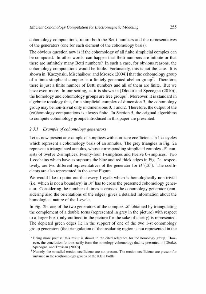
2.3.1 Example of cohomology generators

Let us now present an example of simplices with non-zero coefficients in 1-cocycleswhich represent a cohomology basis of an annulus. The grey triangles in Fig. 2arepresent a triangulated annulus, whose corresponding simplicial complex K con-sists of twelve 2-simplices, twenty-four 1-simplices and twelve 0-simplices. Two1-cochains which have as supports the blue and red thick edges in Fig. 2a, respec-tively, are two different representatives of the generator for H1(K ). The coeffi-cients are also represented in the same Figure.

We would like to point out that every 1-cycle which is homologically non-trivial(i.e. which is not a boundary) in K has to cross the presented cohomology gener-ator. Considering the number of times it crosses the cohomology generator (con-sidering also the orientations of the edges) gives a detailed information about thehomological nature of the 1-cycle.

In Fig. 2b, one of the two generators of the complex K obtained by triangulatingthe complement of a double torus (represented in grey in the picture) with respectto a larger box (only outlined in the picture for the sake of clarity) is represented.The depicted green edges lie in the support of one of the two 1-st cohomologygroup generators (the triangulation of the insulating region is not represented in the

7 Being more precise, this result is shown in the cited reference for the homology group. How-ever, the conclusion follows easily form the homology-cohomology duality presented in [Dłotko,Specogna, and Trevisan (2009)].

8 Namely, the so-called torsion coefficients are not present. The torsion coefficients are present forinstance in the (co)homology groups of the Klein bottle.


-1

1

1

1

1

1

a)

t1

b)

Figure 2: Examples of 1-st cohomology group generators.

picture for the sake of clarity).

3 Cohomology in electromagnetic modeling

In this Section, we intuitively explain why cohomology theory is useful in compu-tational electromagnetics. For a more detailed explanation please refer to [Dłotko,Specogna, and Trevisan (2009); Dłotko and Specogna (2010)].

Let us concentrate on the design of potentials in the insulating region K for h-oriented eddy-current formulations9. The discrete Ampére’s law in the insulatingregion can be written as

δF = I = 0,

where I is the complex-valued electric current 2-cochain10—being zero by the hy-pothesis since K models the insulating region—and F is the magneto-motive force

9 We assume to solve the eddy-current problem in frequency domain. If the eddy-current problem issolved in time domain, the group of reals has to be used in place of the group of complex numberswithout any further changes.

10 It is straightforward to define the complex-valued chains and cochains by using the group of com-plex numbers C in place of Z which has been used in the integer-valued chains and cochains def-inition. In this way, the complex-valued homology Hk(K ,C) and cohomology Hk(K ,C) groupcan be introduced.


(m.m.f.) complex-valued 1-cochain. Thanks to the discrete Ampére’s law, F is a1-cocycle in K , hence F ∈ Z1(K ,C).Consequently, the 1-cocycle F can be expressed by the sum of a 1-coboundaryB1(K ,C) and a basis of the 1-st cohomology group H1(K ,C). The 1-coboundaryB1(K ,C) can be obtained by taking the 0-coboundary of a complex-valued 0-cochain magnetic scalar potential Ω. Hence we have

F = δΩ+β1(K )

∑j=1

T jcut ,

where the T jcut

β1(K )j=1 are the representatives of the 1-st cohomology group H1(K ,C)

generators.

It is demonstrated in [Dłotko and Specogna (2010)] how fixing the basis for thecohomology group T j

cutβ1(K )j=1 , fixes also the dot product (see [Hatcher (2002)]) of

each cohomology generator over the generators c jβ1(K )j=1 of the dual 1-st complex

homology group H1(K ,C) basis

〈T jcut ,ci〉= i j δi j,

where, thanks to Ampére’s law, the dot product of F over the homology generatorc j have to match the electric current i j linked by c j

〈F,c j〉= 〈β1(K )

∑i=1

Ticut ,c j〉= 〈T j

cut ,c j〉= i j,

see [Dłotko, Specogna, and Trevisan (2009)].

Now, from the Universal Coefficient Theorem for cohomology, as explained in[Dłotko and Specogna (2010)], each T j

cutβ1(K )j=1 can be written as

T jcut = i j t j,

where t j is a representative of the 1-st cohomology group basis over integers.

Therefore it is straightforward to see that, in order to be able to design the potentialin the insulating region, one needs the representatives of the H1(K ) generatorsover integers. Efficient algorithms to obtain them are provided in Section 5.

4 Previous approaches for thick cuts generation

Few algorithms to generate thick cuts have been presented in the literature.


The chronologically first one has been introduced in [Ren (2002)]. It is a homotopy-based algorithm which is supposed to produce thick cuts. It is based on the intuitiveidea of “growing a simply-connected bubble inside K ”. Then, at the end of thisprocess, the “complement of the bubble” is claimed to be the union of the sup-ports of all the thick cuts. However, the lack of necessary details does not allowa serious analysis of the algorithm. In particular, it is not straightforward a) howthe bubble is grown, b) how to find the coefficients of the edges for each thick cutseparately from the complement of the bubble and c) how to discriminate cycles inthe surface whose support form loops around holes from the ones that form loopsaround branches of the conductive region. Theoretical evidences can prove that thisalgorithm is unreliable in practice.

In [Henrotte and Hameyer (2003)], an algorithm which the Authors call Gener-alized Spanning Tree Technique (GSTT) has been introduced. This algorithm at-tempts to generate a basis for the 1-st cohomology group, once a basis for the 1-sthomology group is given as input. In [Henrotte and Hameyer (2003)], homologygenerators have been constructed “by hand” and no discussion about the termi-nation of the algorithm has been addressed. In [Dłotko, Specogna, and Trevisan(2009)], the Authors describe an efficient algorithm to automatically produce thehomology generators and in [Dłotko and Specogna (2010)] a detailed analysis ofthe GSTT has been presented. In particular, in [Dłotko and Specogna (2010)],many problems are highlighted which are very difficult to solve in practice.

We would like also to point out that, as already shown in [Dłotko, Specogna, andTrevisan (2009)], all algorithms which compute the so-called thin cut, like the onesdescribed in [Kotiuga (1987, 1988, 1989); Suuriniemi (2004); Gross and Kotiuga(2004); Harold and Simkin (1985); Leonard, Lai, Hill-Cottingham, and Rodger(1993); Simkin, Taylor, and Xu (2004); Dular (2005)], are not useful for thick cutcomputation in general.

5 Algorithms

In this Section, the algorithms to obtain 1-st cohomology group generators are pre-sented. Our implementation heavily bases on the CAPD code [capd.ii.u j.edu.pl(2010)] for homology computations. The detailed explanation of homology compu-tations for cubical complexes can be found in [Kaczynski, Mischaikow, and Mrozek(2004)].

Homology and cohomology theories have a long stand history. They have beenfruitfully used to compute the so-called Conley index in the theory of dynami-cal systems [Mischaikow and Mrozek (1995)]. The main problem with the stan-dard approach to homology and cohomology computations is the complexity of the


standard algorithm, which is hyper-cubical [Storjohann (1996)] with respect to thenumber of simplices in K . Therefore, it cannot be used in practical applications.Some faster approaches need to be found to make the cohomology computations vi-able in practice. The idea of the reduction algorithms (see [Kaczynski, Mischaikow,and Mrozek (2004); Kaczynski, Mrozek, and Slusarek (1998); Mrozek and Batko(2009); Mrozek, Pilarczyk, and Zelazna (2008)]) turned out to be a breakthrough.In fact, how to make a hyper-cubical algorithm feasible in practice? The answeris: Make the input of the algorithm as small as possible in a way that interest-ing information are preserved. Therefore, reduction algorithms are design as apre-processing stage for the standard (co)homology algorithm11. During this pre-processing stage some simplices from the initial complex K are removed in a waythat the cohomology group of the complex does not change.

Most of the reduction algorithms are design in order to obtain just the Betti num-bers, because this was needed for the Conley index computations. Therefore, oncea random reduction method is applied to the complex K , usually cohomology gen-erators in the reduced complex cannot be used as a cohomology generators in theinitial complex. Since our need is to find exactly the representatives of cohomologygenerators, we would like to use in the computations a special class of reductiontechniques referred to as shaving. When a shaving is applied to the complex K , co-homology generators in the reduced complex are also cohomology generators in theinitial complex. Such an approach makes the computation of cohomology genera-tors faster. The speed-up is so sensible that—with these techniques—cohomologycomputations can be routinely used in practice. In this Section, apart form present-ing standard algorithms for cohomology computations, we describe in details sucha shaving procedures for cohomology computations.

5.1 Simplicial complex

In this Section, the data structure Simplex used to store simplices is presented. Inorder to be able to effectively apply shaving procedures, each Simplex is equippedwith a pointer to its boundary and coboundary elements12. Moreover, during theshaving some elements are removed from the complex K . In order not to changethe whole structure of the Simplicial Complex when some elements are re-moved, the so-called lazy delete approach is used. In this case, every Simplexis also equipped with a boolean flag called isDeleted. This flag indicates if theSimplex is still in the complex (when it is set to false) or if it was already re-moved (when it is set to true). When presenting the algorithms, we use C++-like

11 By a standard (co)homology algorithm we mean the Smith Normal Form algorithm which is es-sentially the same for homology and cohomology computations.

12 By a coboundary element of a simplex A we mean a simplex B which has A in its boundary.


object-oriented programming style.

class Simplex

1. set <Simplex∗> boudanry;

2. set <Simplex∗> coboundary;

3. boolean isDeleted;

4. set < integer > vertices;

5. Simplex(set < integer > v)

(a) this−>vertices = v;

(b) this−>isDeleted = false;

Table 1: The Simplex data structure.

It is assumed that the default value of the flag isDeleted is false. The datastructure Simplicial Complex used to keep the simplicial complex in a computeris a simple aggregation of pointers to the Simplex data structure. We would like topoint out that both in the class Simplex and in the class Simplicial Complex inthe lists and sets we keep only the pointers to the Simplex data structure.

To be able to distinguish two data structures S1,S2 of a type Simplex one canimplement a subroutine which compare the sets S1.vertices and S2.vertices. Infurther algorithms, for the sake of simplicity, this subroutine is not used explicitlybeing hidden into a set data structure13.

Now, the algorithm to convert the geometrical mesh M to the Simplicial ComplexK is presented in Table 3. It is presented as the constructor of the class SimplicialComplex. We assume that the vertices of each tetrahedron are marked with integernumbers as it is done in [Schöberl (1997)].

The operations on the sets can be effectively implemented. One can, for instance,use one of the standard template library implementations like [Josuttis (1999)].After that the algorithm presented in Table 3 runs, the Simplicial Complex Kis returned14.13 Adding to the set S an element that is already in S does not have any effect. Therefore the set data

structure have to be able to compare elements, and this is where the subroutine is used.14 Since the data structure Simplicial Complex returned by the algorithm is directly inspired by


class Simplicial Complex

1. set <Simplex∗> ZeroDimSimpl;

2. set <Simplex∗> OneDimSimpl;

3. set <Simplex∗> TwoDimSimpl;

4. set <Simplex∗> ThreeDimSimpl;

5. Simplicial Complex( Geometrical mesh M )

Table 2: The Simplicial Complex data structure.

5.2 Shaving procedures

Let us assume that the Simplicial Complex K has been created as described inSection 5.1. In this Section, the details of the shaving procedures for cohomologycomputations are presented.

The so-called acyclic sub-complex method [Mrozek, Pilarczyk, and Zelazna (2008)]is a shaving for cohomology computation (the detailed mathematical proof of thisfact will be published elsewhere). By an acyclic sub-complex A of a complex Kwe mean a set A having trivial homology in all dimensions except from dimensionzero15. The dimension of 0-th homology group of A is 1. The idea of the acyclicsub-complex method is to remove from the simplicial complex K the largest pos-sible acyclic sub-complex A . We do not want to go into theoretical details here,but before we proceed to the algorithms themselves, let us present in Figure 3 anexample which shows that the acyclic sub-complex algorithm is indeed a shavingfor cohomology computations.

In the following, two essentially different algorithms to find the acyclic sub-complexare presented. The first one bases on the idea of building the acyclic space aspresented in [Mrozek, Pilarczyk, and Zelazna (2008)]. The second one uses theso-called coreduction algorithm [Mrozek and Batko (2009)] to remove the acyclicsub-complex form the initial complex K .

the abstract definition of simplicial complex K presented in Section 5.1, further on in this paperwe use the notation K to indicate both the mathematical simplicial complex and the data structureSimplicial Complex returned by the Algorithm 3.

15 The dimension of 0-th homology group measures the number of connected components of thecomplex.


Simplicial Complex( Geometrical mesh M )

1. Let K be an empty Simplicial Complex;

2. for every tetrahedron T ∈M

(a) sort the integers representing T in increasing ordering[x0,x1,x2,x3];

(b) for every i ∈ 0,1,2,3K .ZeroDimSimpl∪ new Simplex(xi);

(c) for every i, j ∈ 0,1,2,3 such that i < j K .OneDimSimpl ∪newSimplex(xi,x j);

(d) for every i, j,k ∈ 0,1,2,3 such that i < j < kK .TwoDimSimpl∪ newSimplex(xi,x j,xk);

(e) K .TreeDimSimpl∪ newSimplex(x0,x1,x2,x3);

3. for every pair of Simplex S,P ∈K

(a) if S is a face of P, then

i. S.co f ace∪P;ii. P. f ace∪S;

4. return K ;

Table 3: The constructor of the Simplicial Complex class being the conversionof the geometrical mesh to the Simplicial Complex data structure.

5.3 Direct acyclic sub-complex computation

Let us give an idea on how the sub-complex A is created. The algorithm, whichis inspired by the Algorithm 2 in [Mrozek, Pilarczyk, and Zelazna (2008)], can befound in Table 4. For each 3-simplex T , let n(T ) denotes a simple subroutine thatreturns all the neighbors of T in K 16.

The details of the procedure checkAcyclicity(A ,T ) are provided further on. Forthe moment, let us only assume that it exhibits a constant complexity and once itreturns true, then the set A ∪T remains acyclic. The analysis of the complexityof the prototype of the algorithm presented in Table 4 can be found in [Mrozek,

16 By a neighbor of a 3-simplex T we mean any 3-simplex W having non-empty intersection with T .


a) b)

Figure 3: On the left, the simplicial complex representing an annulus is shown. Thesupport of the cohomology generators is presented with the red thick edges. On theright, the blue 2-simplices are the simplices in the acyclic sub-complex A . Wewould like to indicate that A is a closed complex (i.e. if an element is in A , thenall its faces are in A ). Therefore, the red edges which indicate the support of thecohomology generator in the reduced complex are the only edges remained in thereduced complex. This example illustrates that the acyclic sub-complex algorithmis indeed a shaving procedure for cohomology computations.

Pilarczyk, and Zelazna (2008)]. In fact, in case of simplices, it remains exactly thesame. Therefore, for n0 = maxT∈K3 card n(T ), the complexity of the algorithmis bounded by n0 cardK3 c, where c is the complexity of checkAcyclicity(A ,T )procedure. Since in all meshes which are considered to be acceptable in electro-magnetic modeling the number n0 is a constant (i.e. does not grow for a fixedgeometry when a sequence of refined meshes of this geometry are considered),then the complexity of the above algorithm may be considered to be linear.

Let us now discuss the details of the checkAcyclicity(A ,T ) procedure. In theacyclicity tests, as it is indicated in [Mrozek, Pilarczyk, and Zelazna (2008)], itis possible to use the corollary from the Mayer-Vietoris [Hatcher (2002)] Theorem.It roughly says that, if two sets A, B of simplices are acyclic and their intersectionA∩B is acyclic, then the sum A∪B is also acyclic. But we know that the set Ais acyclic. It is also straightforward that every tetrahedron T is acyclic. Therefore,if one confirms that the intersection A ∩T is also acyclic, then from the Mayer-Vietoris Theorem one has that A ∪ T is acyclic. As it it indicated in [Mrozek,Pilarczyk, and Zelazna (2008)], the simplest and straightforward way of check-ing the acyclicity of the intersection A ∩T is simply by computing homology of


1. A := /0;

2. Let Q be empty set of pointers to Simplex;

3. Pick any T ∈K .ThreeDimSimpl; A := A ∪T ;

4. Q := Q ∪n(T );

5. while (Q 6= /0)

(a) T := dequeue(Q);

(b) if checkAcyclicity(A ,T ) then

i. A := A ∪T ;ii. for each P ∈ n(T )∩ (K \A )

A. if P 6∈Q then Q :=Q ∪P;

6. for every T ∈A

(a) T .isDeleted = true;

(b) for every W being a boundary element of T set W .isDeleted =true;

7. return A ;

Table 4: Acyclic sub-complex algorithm.

A ∩T . Since this intersection would consists only of some boundary elements ofT —that is, at most 14 elements—this test can be done in a constant time from thepoint of view of complexity analysis (although the constant would be reasonablylarge).

Therefore, we would like to present here two alternative approaches.

The first one, presented in Section 5.3.1, is based on the so-called coreduction algo-rithm [Mrozek and Batko (2009)]. In many practical cases, it enables to reduce thecomplex up to its homology generators. To do coreductions, similarly to the caseof the acyclic sub-complex method, a more general structure with respect to themathematical simplicial complex is needed. This is because the complex obtainedduring and after removing the acyclic sub-complex or by applying coreduction isnot a simplicial complex anymore (the non-delted simplices in this complex do not


have to have all its faces being non-deleted17). The detailed theoretical explanationof the coreduction algorithm can be found in [Mrozek and Batko (2009)]. Here, inthe Figure 4, we would like to present the intuitive idea of the algorithm.

The second one, described in Section 5.3.2, is based on the idea of lookup tablesfor simplices, presented in [Mrozek, Pilarczyk, and Zelazna (2008)] for cubicalcomplexes.

5.3.1 checkAcyclicity via local coreduction algorithm

Since removing coreduction pairs does not change the first and higher (co)homologygroups (see [Mrozek and Batko (2009)]) of the simplicial complex, it is straight-forward that if all the elements in A ∩T are removed with the coreductions, thenA ∩T is an acyclic set. Consequently, in such case, T can be added to the set A .

After introducing the method itself, let us present the algorithm in Table 5.

Intuitively, the algorithm presented in Table 5 puts to the set A all the elementsin A ∩T , applies the coreductions on those elements, and then, after detecting ifall the elements in A ∩ T are reduced, change back the fields isDeleted in allSimplex data structure elements in A.

It is straightforward that the presented algorithm works in linear time (the detailedproof can be found in [Mrozek and Batko (2009)]). Since the cardinality of theconsidered set A is bounded by 14 (the number of all boundary elements of atetrahedron), the whole algorithm checkAcyclicity(A ,T ) works in constant time.Therefore, the total complexity of finding the maximal acyclic sub-complex A islinear with respect to the number of simplices in the complex K . The experimentsshown that this technique is much faster with respect to the pure Smith NormalForm computations.

5.3.2 checkAcyclicity via lookup tables

Despite the efficiency of the method presented in Section 5.3.1, no proof has beengiven that the algorithm presented in Table 5 returns true if and only if the inter-section A ∩ T is acyclic. One can only be sure that if it returns true, then theconsidered intersection is acyclic. Therefore another algorithm, which gives if andonly if criterion, and which is faster than algorithm presented in Table 5, is nowprovided. It is based on a simple idea: Since the intersection A ∩ T contains atmost 14 elements, it is possible to check all the possible configurations of bound-ary elements of the 3-simplex T and list them all in a table as it is done in [Dłotko(2010)]. Then, for a given configuration, one is able to verify in a constant time ifthe considered configuration is acyclic or not by checking the suitable entry in the

17 However, due to the isDeleted flag, this situation can easily be handled by our implementation.


a) b)

c) d)

e) f)

Figure 4: a) The complex having two 2-simplices, seven 1-simplices and five 0-simplices is presented. The idea of coreduction algorithm can be understood ascomputing the so-called reduced homology. b) In the first step, a single vertex isremoved from the complex (the removed vertex is marked with red). Then, in aloop, as long as possible, the so-called coreduction pairs are removed. A simplex Sis said to be a free coface, if it has only one non deleted simplex T in its boundary.In this case, the pair (S,T ) is said to be a coreduction pair. In the pictures c), d) ande), the following steps of the coreduction algorithm are indicated. The coreductionpairs are indicated in blue. The deleted simplices are indicated in red. After allthe pairs are removed, there is only one non deleted 1-simplex in the complex(indicated in bold black in the picture f)). In this case, we say that this simplexrepresents a 1-st homology generator in the reduced complex.

lookup table (in the suitable entry of the lookup table a boolean value indicates theacyclicity of the considered configuration).


boolean checkAcyclicity(A ,T )

1. Let a list L = /0, set A := A ∩T and an boolean value isAcyclic begiven;

2. Let I ∈ A represents a 0-simplex;

3. I.isDeleted = true;

4. for every S ∈ I.coboundary∩A do L := L∪S;

5. while (L 6= /0)

(a) S :=pop_front(L);

(b) if S is a free coface in A, and T ∈ A is its unique face havingT.isDeleted=false

i. T.isDeleted = S.isDeleted = true;ii. for every W ∈ T.coboundary∩A such that

W.isDeleted=false if W is a free coface do L := L∪W ;

(c) else for every W ∈ S.coboundary∩A such thatW.isDeleted=false and W is a free coface do L := L∪W ;

6. if for every S ∈ A S.isDeleted=true then isAcyclic := true

7. else isAcyclic := false;

8. for every S ∈ A do S.isDeleted=false;

9. return isAcyclic;

Table 5: CheckAcyclicity algorithm.

The presented method has turned out to be the fastest one. However, we decidedto present also the other methods because to effectively use the lookup tables oneneeds to be able, for a given 3-simplex T , to return all its boundary element inthe order presented in Table 6. This is an extra constraint which in case of somesimplicial complex implementations may be problematic to achieve.


boolean checkAcyclicityByLookupTable(A ,T )

1. Let L be the lookup table obtained from Dłotko (2010);

2. Let T = [v1,v2,v3,v4] such that v1 < v2 < v3 < v4;

3. Let N be the vector of boundary elements of T ordered as follows :[v1], [v2], [v3], [v4], [v1,v2], [v1,v3], [v1,v4], [v2,v3], [v2,v4], [v3,v4],[v1,v2,v3], [v1,v2,v4], [v1,v3,v4], [v2,v3,v4];

4. Let W be the vector, such that W [i] ∈ 0,1. Let W [i] = 1 if and only ifN[i] ∈A ∩T ;

5. integer index := ∑13i=0 2iW [i];

6. return L[index];

Table 6: CheckAcyclicity algorithm by using lookup table.

5.4 Acyclic sub-complex via coreduction algorithm

Let us now present the second way to obtain the acyclic sub-complex. It can bedemonstrated that the set B removed from the initial complex K by the coreduc-tion algorithm as in Figure 4 is acyclic. In fact, the coreduction algorithm is adifferent version of the acyclic sub-complex algorithm presented above. Therefore,one can alternatively use the coreduction algorithm as a shaving for cohomologycomputations. The shaving algorithm using coreduction is presented in Table 7.

As it has been already shown in Section 6, the complexity of the algorithm in Ta-ble 7 is linear with respect to the cardinality of K . The presented method is slowerwith respect to the ones presented in Section 5.3.1 or in Section 5.3.1. However, itis very easy to implement and the general and efficient template implementationsof the coreduction algorithm are available.

5.5 Cohomology computations

The reduction algorithms presented in Section 5.2 turn out to be very efficient inpractice. After one of the two shaving procedure is applied, usually there is only theneed for minor algebraic computations with respect to the algebraic computationsnecessary for the initial complex.

Let K be the initial complex and A be the acyclic sub-complex found by one of the


Acyclic_Sub-complex_via_coreduction( Simplicial Complex K )

1. Let A := /0, L be an empty list;

2. Let I ∈K represents 0-simplex;

3. I.isDeleted = true;

4. A := A ∪ I;

5. for every S ∈ I.coboundary L := L∪S;

6. while L 6= /0

(a) S :=pop_front(L);

(b) if S is a free coface, and T is its unique face havingT.isDeleted=false

i. T.isDeleted = S.isDeleted = true;ii. A := A ∪T,S

iii. for every W ∈ T.coboundary such thatW.isDeleted=false if W is a free coface do L := L∪W ;

(c) else for every W ∈ S.coboundary such thatW.isDeleted=false and W is a free coface do L := L∪W ;

7. return A ;

Table 7: Acyclic sub-complex via coreduction algorithm.

shaving procedures presented in Section 5.2. Now it is time to turn all the elementsin K \A into the coboundary matrix data structure18. We would like to remind thatthe idea of shaving is to exclude some elements from the complex K , which arenot important from the point of view of information about cohomology. Therefore,the coboundary operator restricted to the set K \A is considered further on duringalgebraic computations.

Before turning into standard Smith Normal Form algorithm, we use the KMS algo-

18 In homology computations, boundary matrices are created at this point, whereas, during coho-mology computations, coboundary matrices—which are the transposed boundary matrices—areneeded.


rithm [Kaczynski, Mrozek, and Slusarek (1998)] to minimize the amount of alge-braic computations. The procedure of cohomology computation and pulling-backthe generators19 is exactly the same as in the case of homology computations. Sincethese techniques are clearly and elegantly presented in [Kaczynski, Mischaikow,and Mrozek (2004)], we decided not to repeat them here.

For the implementation of the considered algebraic procedures, the code [capd.ii.u j.edu.pl(2010)] has been used. The only difference with respect to the homology computa-tions is that the coboundary operator is provided to the code instead of the boundaryoperator. This minor change allows to use the standard software designed to com-pute homology for cohomology computations.

6 Numerical examples

The proposed algorithms have been applied to the thick cut computations for real-sized industrial eddy-current problems without experimenting any difficulty. Forexample, a micro inductor and a micro transformer are considered, see Figs. 5 and6, respectively. To visualize the thick cuts produced by the algorithms proposed inthis paper for the considered examples, one may represent the set of edges in thesupport of each thick cut, see for example Fig. 2b. To gain more insight, it is usefulto plot the dual faces dual with respect to the set of edges in the support of eachthick cut, see [Dłotko, Specogna, and Trevisan (2009)]. Such a sets of dual facesfor the two considered examples are shown in Figs. 7 and 8. The convergence ofthe inductance value of the micro inductor with mesh refinement is shown in Fig.9. The eddy-current problems have been solved by the two complementary formu-lations on the same meshes. The same algorithm used to produce thick cuts forthe T -Ω formulation in the insulating region can be applied to produce thick cutsin the conducting region needed to couple A-χ formulation with electric circuits,see [Dłotko, Specogna, and Trevisan (2010)]. From an engineering viewpoint, be-ing able to us both complementary formulations is very important, since the meanvalue obtained by the two formulations is quite accurate even for coarse meshes.In Figs. 10 and 11 the execution times obtained by using various algorithms arecompared for the micro inductor and micro transformer example, respectively.

The algorithms presented in this paper do not take any assumptions on the topologyof the input mesh, being the algorithms provably general. The algorithms have alsobeen applied with success in eddy-current problems consisting of knotted conduc-tors. For example Fig. 12 shows a trefoil knot conductor and the thick cut for this

19 Since a shaving was used, there is no need to pull-back the reductions back to K . One needsonly to find the cohomology generators in K \A . In this case, after all algebraic computations,one needs to pull-back only the KMS reductions [Kaczynski, Mrozek, and Slusarek (1998)]. Thissubroutine is already a part of the [capd.ii.u j.edu.pl (2010)] software.


Figure 5: A micro inductor.

Figure 6: A micro transformer.


Figure 7: The thick cut for the micro inductor.

Figure 8: The two thick cuts for the micro transformer.


4.6 4.8 5 5.2 5.4 5.6 5.8 6 6.2 6.4

0.21

0.22

0.23

0.24

0.25

0.26

0.27

log10 (number of tetrahedra)

L [n

H]

A−χ formulationT−Ω formulationmean

Figure 9: Convergence of the inductance value of the micro inductor with meshrefinement.

0

100

200

300

400

500

600

700

800

900

4,4 4,6 4,8 5 5,2 5,4 5,6

log(number of tetrahedra)

time

(s)

b101_accb101_coreb101_table

Figure 10: Execution times obtained by using various reduction techniques for themicro inductor example.


0

500

1000

1500

2000

2500

3000

3500

4000

4500

5000

4,5 4,7 4,9 5,1 5,3 5,5 5,7

log(number of tetrahedra)

time

(s)

b102_accb102_coreb102_table

Figure 11: Execution times obtained by using various reduction techniques for themicro transformer example.

example is shown in Fig. 13.

7 Conclusion

In this paper, a new automatic, general and efficient technique for the 1-st coho-mology group computation over integers has been introduced. All of the algo-rithms have been described in detail. This technique turned out to be fundamental,among the other applications of cohomology computation, for the generation ofthe thick cuts, needed for the potential design in eddy-current h-formulations. Thefeasibility of the presented technique with real-sized industrial problems has beendemonstrated by concrete examples. We believe that the presented approach shouldbe routinely included in the next-generation electromagnetic solvers.

Acknowledgement: The Authors would like to thank Marian Mrozek for manydiscussions and help without which this paper could not be written.

References

Bossavit, A. (1984): Two dual formulations of the 3d eddy currents problem.COMPEL, vol. 4, pp. 103–116.

Bossavit, A. (1998): How weak is the weak solution in finite elements methods?IEEE Trans. Mag., vol. 34, pp. 2429–2432.


Figure 12: A trefoil knot massive conductor.

Figure 13: The thick cut for the trefoil knot massive conductor.


Bossavit, A.; Kettunen, L. (2000): Yee-like schemes on staggered cellular grids:A synthesis between fit and fem approaches. IEEE Trans. Mag., vol. 36, pp. 861–867.

Branin, F. (1966): The algebraic-topological basis for network analogies andthe vector calculus. Proceedings of the Symposium on Generalized Networks,Polytechnic Press, Brooklin, NY, pp. 453–491.

capd.ii.u j.edu.pl (2010): The capd library, 2010.

Codecasa, L.; Specogna, R.; Trevisan, F. (2009): Base functions and discreteconstitutive relations for staggered polyhedral grids. Comput. Meth. Appl. Mech.Eng., vol. 198, no. 9–12, pp. 1117–1123.

Codecasa, L.; Specogna, R.; Trevisan, F. (2010): A new set of basis functionsfor the discrete geometric approach. in press, 2010.

Desbrun, M.; Kanso, E.; Tong, Y. (2008): Discrete differential forms forcomputational modeling. Oberwolfach Seminars, Discrete Differential Geometry,Birkhäuser, Basel, Switzerland, vol. 28, pp. 287–324.

Dłotko, P. (2010): Acyclic configurations for boundary of 3 and 4 dimensionalsimplices, www.ii.u j.edu.pl/ dlotko/acccon f .html, 2010.

Dłotko, P.; Specogna, R. (2010): Critical analysis of the spanning tree techniques.submitted to SIAM Journal on Numerical Analysis, 2010.

Dłotko, P.; Specogna, R.; Trevisan, F. (2009): Automatic generation of cutssuitable for the t-ω geometric eddy-current formulation. Comput. Meth. Appl.Mech. Eng., vol. 198, pp. 3765–3781.

Dłotko, P.; Specogna, R.; Trevisan, F. (2010): Voltage and current sources formassive conductors suitable with the a−χ geometric formulation. IEEE Transac-tions on Magnetics, vol. 46.

Dular, P. (2005): Curl-conform source fields in finite element formulations: Au-tomatic construction of a reduced form. COMPEL, vol. 24, pp. 364–373.

Gross, P.; Kotiuga, P. (2004): Electromagnetic Theory and Computation: ATopological Approach. Cambridge University Press.

Gu, X.; Wang, Y.; Yau, S.-T. (2003): Multiresolution computation of conformalstructures of surfaces. Journal of Systemics, Cybernetics and Informatics, vol. 1,pp. 45–50.

Gu, X.; Yau, S. (2002): Computing conformal structures of surfaces. Communi-cations in Information and Systems, vol. 2, pp. 121–146.


Guo, X.; Li, X.; Bao, Y.; Gu, X.; Qin, H. (2006): Meshless thin-shell simulationbased on global conformal parameterization. IEEE Trans. Vis. Comput. Gr., vol.12, pp. 375–385.

Harold, C.; Simkin, J. (1985): Cutting multiply connected domains. IEEETrans. Magn., vol. 21, pp. 2495–2498.

Hatcher, A. (2002): Algebraic topology. Cambridge University Press, Cam-bridge, UK.

Henrotte, F.; Hameyer, K. (2003): An algorithm to construct the discrete coho-mology basis functions required for magnetic scalar potential formulations withoutcuts. IEEE Trans. Magn., vol. 39, pp. 1167–1170.

Josuttis, N. M. (1999): The C++ Standard Library: A Tutorial and Reference.Addison-Wesley U.S.A.

Kaczynski, T.; Mischaikow, K.; Mrozek, M. (2004): Computational Homology.Springer-Verlag, New York, USA.

Kaczynski, T.; Mrozek, M.; Slusarek, M. (1998): Homology computation byreduction of chain complexes. Computers and Mathematics, vol. 35, pp. 59–70.

Kotiuga, P. (1987): On making cuts for magnetic scalar potentials in multiplyconnected regions. J. Appl. Phys., vol. 61, pp. 3916–3918.

Kotiuga, P. (1988): Toward an algorithm to make cuts for magnetic scalar poten-tials in finite element meshes. J. Appl. Phys., vol. 63, pp. 3357–3359.

Kotiuga, P. (1989): An algorithm to make cuts for magnetic scalar potentials intetrahedral meshes based on the finite element method. IEEE Trans. Magn, vol.25, pp. 4129–4131.

Leonard, P.; Lai, H.; Hill-Cottingham, R.; Rodger, D. (1993): Automaticimplementation of cuts in multiply connected magnetic scalar region for 3-D eddycurrent models. IEEE Trans. Magn., vol. 29, pp. 1368–1371.

Maxwell, J. (1891): A Treatise on Electricity and Magnetism. Oxford : Claren-don Press.

Mischaikow, K.; Mrozek, M. (1995): Chaos in lorenz equations: a computerassisted proof. Bull. Amer. Math. Soc. (N.S.), vol. 33, pp. 66–72.

Mrozek, M.; Batko, B. (2009): Coreduction homology algorithm. Discrete andComputational Geometry, vol. 41, pp. 96–118.

Mrozek, M.; Pilarczyk, P.; Zelazna, N. (2008): Homology algorithm based onacyclic subspace. Computers and Mathematics, vol. 55, pp. 2395–2412.


Mrozek, M.; Wanner, T. (2010): Coreduction homology algorithm for inclusionsand persistent homology. Preprint available online, 2010.

Munkres, J. R. (1984): Elements of Algebraic Topology. Addison-Wesley.

Ren, Z. (2002): t-ω formulation for eddy-current problems in multiply connectedregions. IEEE Trans. Magn., vol. 38, pp. 557–560.

Schöberl, J. (1997): Netgen - an advancing front 2d/3d-mesh generator based onabstract rules. Computing and Visualization in Science, vol. 1, pp. 41–52.

Simkin, J.; Taylor, S.; Xu, E. (2004): An efficient algorithm for cutting multiplyconnected regions. IEEE Trans. Magn., vol. 40, pp. 707–709.

Specogna, R.; Suuriniemi, S.; Trevisan, F. (2008): Geometric t-ω approach tosolve eddy-currents coupled to electric circuits. Int. J. Numer. Meth. Eng., vol. 74,pp. 101–115.

Specogna, R.; Trevisan, F. (2008): Eddy-currents computation with T -Ω discretegeometric formulation for a NDE problem. IEEE Trans. Mag., vol. 44, pp. 698–701.

Storjohann, A. (1996): Near optimal algorithms for computing smith normalform of integer matrices. Proceedings of the 1996 international symposium onsymbolic and algebraic computation, ISAAC 1996, pp. 267–274.

Suuriniemi, S. (2004): Homological computations in electromagnetic modeling.PhD Thesis, Tampere University of Technology.

Tarhasaari, T.; Kettunen, L.; Bossavit, A. (1999): Some realizations of a dis-crete Hodge operator: a reinterpretation of finite element techniques. IEEE Trans.on Mag., vol. 35, pp. 1494–1497.

Tonti, E. (1975): On the formal structure of physical theories. Quaderni deiGruppi di Ricerca Matematica del CNR.

Tonti, E. (1998): Algebraic topology and computational electromagnetism.Fourth International Workshop on the Electric and Magnetic Fields (EMF): fromNumerical Models to Industrial Applications, Marseille, France, pp. 284–294.

Weiland, T. (1977): A numerical method for the solution of the eigenvalue prob-lem of longitudinally homogeneous waveguides. Electronics and Communication(AE), vol. 31, pp. 308–311.

efﬁcient cohomology computation for electromagnetic...

Documents