efﬁcient skyline computation for large volume data in...

Efficient Skyline Computation for Large Volume Data inMapReduce Utilising Multiple Reducers

Kasper MullesgaardAalborg UniversityAalborg, Denmark

[email protected]

Jens Laurits PedersenAalborg UniversityAalborg, Denmark

[email protected]

ABSTRACTA skyline query is useful for extracting a complete set of in-teresting tuples from a large data set according to multiplecriteria. The sizes of data sets are constantly increasing andthe architecture of backends are switching from single nodeenvironments to cluster oriented setups. Previous work haspresented ways to run the skyline query in these setups usingthe MapReduce framework, but the parallel possibilities arenot taken advantage of since a significant part of the queryis always run serially. In this paper, we propose the novel al-gorithm MapReduce - Grid Partitioning Multiple ReducersSkyline (MR-GPMRS) that runs the entire query in paral-lel. This means that MR-GPMRS scales well for large datasets and large clusters. We demonstrate this using experi-ments showing that MR-GPMRS runs several times fasterthan the alternatives for large data sets with high skylinepercentages.

1. INTRODUCTIONSkyline queries have a wide application domain ranging

from e-commerce and quality based service selection, tostock trading and, generally speaking, any process involv-ing multi-attribute decision making. Skyline query process-ing is computationally intensive. In order to handle thishigh computation cost, commodity computing can be used.Commodity computing is a paradigm where a high numberof low cost computers are connected in a cluster to run de-manding computations across multiple nodes. Commoditycomputing is deployed by several notable companies [1, 7,8, 9, 11].

When using commodity clusters, the idea is to to take ad-vantage of the high number of nodes by processing queriesparallelly. High fault tolerance is a requirement since ma-chines can fail, and a larger cluster have a higher probabilityof machines faulting. MapReduce is designed specifically forhigh fault tolerance parallel computing.

The problem of this article is to develop a MapReducealgorithm that finds the skyline of a large volume data set

efficiently. Similar work on this subject has been done be-fore but previous work presents solutions that uses only asingle reducer to find the global skyline, failing to utlilise theMapReduce framework to its full potential. To the best ofour knowledge, applying multiple reducers to find the globalskyline is unprecedented when finding the skyline for largedata sets, and it is the focus of the work presented here.

As a solution to the problem, the MapReduce - Grid Parti-tioning Multiple Reducers Skyline (MR-GPMRS) algorithmis proposed. The basis of the MR-GPMRS algorithm is, asthe name suggests, to partition the input data set using agrid. A bitstring is used to keep track of which partitionsin the grid are non-empty, which makes it possible to makedecisions based on the distribution of the entire data set.How dominance in the skyline query works combined withthe grid partitioning scheme allows splitting the data intoparts that can be processed independently of each other,which means that these parts can be processed by differentreducers. The goal of MR-GPMRS is to minimise the queryresponse time for data sets with high skyline percentages.To measure this, it is compared to other skyline query pro-cessing algorithm that applies the MapReduce framework.

The rest of this paper is organized as follows: Section2 contains the preliminaries. In Section 3 we introduceMapReduce - Grid Partitioning Single Reducers Skyline(MR-GPSRS): Our bitstring based grid partitioning algo-rithm for skyline query processing in the MapReduce frame-work. In Section 4 we introduce MR-GPMRS, a novel exten-sion to MR-GPSRS that allows processing skyline queries inMapReduce using multiple reducers. In Section 6 we presentexperimental evaluation of the proposed solutions comparedwith algorithms from the litterature, and finally, in Section7, we conclude the paper and propose future directions forresearch.

2. PRELIMINARIESIn this section, the skyline query and the MapReduce

framework is described. A table of common symbols usedthroughout this paper is shown in Table 1.

2.1 The Skyline QueryGiven a set of multi-dimensional tuples R, the skyline

query returns a set of tuples SR, such that SR consists of allthe tuples in R that are not dominated by any other tuplein R [3].

Definition 1. A tuple ri dominates another tuple rj , de-noted by ri ≺ rj , if and only if, for all dimensions, the value

1

Table 1: A list of common terms.

Symbol InterpretationR A set of tuplesSR The skyline of the set of tubles Rt A tuplen Partitions per dimension (PPD)d Dimensionalityp A partition of the dataP A set of partitionsBS A bitstringIG A group of independent partitions

Reduce1

Map1

Reduce2

Map2

Reducek

Mapn...

...

Input

Output

Figure 1: This figure shows the MapReduce process. Theinput is split between the mappers. The mappers pro-cess their input split and output the results to the reduc-ers. The reducers process the results from the mappers,generating the final output.

of ri is not worse than the corresponding value of rj , andfor at least one dimension, the value of ri is better than thevalue of rj [3].

Whether a value is better or worse than another value isdetermined by the configuration of the skyline query. Typ-ically, a value v1 has to be either larger or smaller thananother value v2 for v1 to be better than v2. In this paperit is assumed that a smaller value is better.

2.2 The MapReduce FrameworkMapReduce is a framework for distributed computing. It

is based on a Map and a Reduce function [6]. The Mapfunction is invoked for each record in the input file and itproduces a list of key-value pairs. The Reduce function isthen invoked once for each unique key and the associatedlist of values. This produces key-value pairs that are the re-sult of the MapReduce job, i.e., Map(k1, v1) → list(k2, v2)and Reduce(k2, list(v2)) → list(k3, v3). Several MapRe-duce jobs can be chained together, later phases being ableto refine and/or use the results from earlier phases. TheMapReduce process is illustrated in Figure 1.

A distributed file system is used to store the data pro-cessed and produced by the MapReduce job. The inputfile(s) is split up, stored, and possibly replicated on the dif-ferent nodes in the cluster. The nodes are then able to accesstheir local splits when processing data. When the data fromthe Map function has been processed by the different nodes,the results are shuffled between the nodes so the requireddata can be accessed locally when the Reduce function isinvoked.

It can be necessary to replicate some data across all nodes.In Hadoop [2], the implementation of MapReduce used forthis paper, the Distributed Cache can be used for this pur-pose. In the beginning of a MapReduce job, data written

to the Distributed Cache is transferred to all nodes, makingit accessible in the Map and Reduce functions. This paperassumes that the Distributed Cache, or something similar,is available.

2.3 Skyline Query Processing in MapReduceIn an article by Zhang et al. [12] skyline algorithms

are adapted for the MapReduce framework. Three differ-ent algorithms are presented: MapReduce - Block NestedLoop (MR-BNL), MapReduce - Sort Filter Sort (MR-SFS),and MR-Bitmap. MR-BNL uses BNL and grid partitioning.The second algorithm, MR-SFS, modifies MR-BNL withpresorting, but it is shown to perform worse than MR-BNL.MR-Bitmap is based on a bitmap which is used to determinedominance. It is fast computationally but requires a largeamount of disk space and is only viable for data sets with fewdistinct values. A single reducer is used to calculate the fi-nal resulting skyline in MR-BNL and MR-SFS. MR-Bitmapdoes use multiple reducers, and is the only MapReduce al-gorithm for finding the skyline of a data set we know of todo so. However, as mentioned, it can only handle data setswith low data distinction. In [12], it was not tested on datasets with more than ten thousand distinct values, which isbelow the threshold for data sets used for testing in thisarticle.

Angular partitioning is a different partitioning techniqueproposed by Vlachou et al. [10]. Angular partitioning isbased on making partitions by dividing the data space upusing angles. The idea is based on the observation thatskyline tuples are located near the origin. So by dividingthe data space up using angles, skyline tuples should bedistributed into several partitions while non-skyline tuplesshould be grouped with skyline tuples that dominates them.The technique is shown to be effective but the global skylineis found using a single node. In an article by Chen et al. [4]the angular partitioning technique is adapted to MapReduceresulting in the algorithm MapReduce - Angle (MR-Angle).The results are comparable to those in [10], and the globalskyline is found using a single reducer.

3. GRID PARTITIONING BASED SINGLEREDUCER SKYLINE COMPUTATION

In this section, a skyline algorithm for MapReduce is pro-posed. The algorithm utilises grid partitioning and bit-strings in order to prune dominance checks between tuples.

3.1 Grid PartitioningGrid partitioning is a method of splitting up a space where

each dimension is divided into n parts, referred to as the Par-titions per Dimension (PPD). This gives a regular grid of nd

partitions, termed as P , where d is the dimensionality of thedata set. In the context of skyline queries, the dominatingrelationship between the partitions p1, p2, . . . , pnd ∈ P canbe exploited to exclude dominance checks between tuples.Partitions have a dominating relationship with each othersimilar to that between tuples. The main difference is thata dominating relationship between two partitions pi and pjis based on their maximum corners pi.max and pj .max, andminimum corners, pi.min and pi.min. The maximum cor-ner of a partition is defined as the corner of the partitionthat has the highest (worst) values. Similarly, the minimumcorner of a partition is defined as the corner of the partitionthat has the lowest (best) values.

2

Figure 2: An example of partitions and their offsets.Non-empty partitions are marked with crosses and thedominating (dark grey) and anti-dominating (light grey)regions of the partition with offset 4 (circle) are shown.

Definition 2. A partition pi dominates another partitionpj , denoted by pi ≺ pj , if and only if pi.max dominatespj .min. This ensures that all tuples in pi dominates alltuples in pj .

pi ≺ pj ⇔pi.max ≺ pj .min (1)

If this is not the case, pi does not dominate pj , denoted bypi ⊀ pj .

The dominating relationships between the partitions canbe expressed using their individual dominating (Cui et al.[5]) and anti-dominating regions.

Definition 3. Given a partition pi, its dominating regionpi.DR contains all partitions dominated by pi:

pi.DR = {pj | pj ∈ P ∧ pi ≺ pj} (2)

Meanwhile, pi’s anti-dominating region pi.ADR contains allpartitions that can have tuples that dominates pi.max:

pi.ADR = {pj | pj ∈ P ∧ pj .min ≺ pi.max} (3)

Figure 2 shows an example of the dominating and anti-dominating region of the partition marked as 4 in a twodimensional data set. The non-empty partitions are markedwith a cross. The dominating region of partition 4 containspartition 8 and the anti-dominating region contains parti-tions 0, 1, and 3.

3.2 Bitstring RepresentationIn grid partitioning, the only partitions of interest are

those that are non-empty, i.e. {pi | pi ∈ P ∧ pi 6= ∅}.The partitioning scheme can be represented as a bitstringBS(0, 1, 2, . . . , nd − 1) where for 0 ≤ i ≤ nd − 1:

BS[i] =

{1 if p 6= ∅0 otherwise

(4)

The resulting bitstring can be constructed using eitherrow-major order or column-major order, the only differencebeing how the offset of a partition in the bitstring is calcu-lated. Column-major order is used in this paper. For exam-ple, the offset of the partitions of the two dimensional dataset in Figure 2 is indicated by the digit in their lower leftcorner of the partitions, resulting in the bitstring 011110100.

...

R

BSR

R1 BSR1 R2 BSR2 Rn BSRm

BSR1∪BSR2∪...∪BSRm BSR

Figure 3: The data flow of the bitstring generation phaseof MR-GPSRS with the data set R.

...

R, BSR

SR

R1 SR1 R2 SR2 Rn SRm

BSR

SR1∪SR2∪...

SRm SR

BSR BSR BSR

Figure 4: The data flow of the skyline computation phaseof MR-GPSRS with the data set R and the bitstring BSR.

The bitstring can be traversed to prune partitions suchthat fewer partitions and data tuples are involved in theskyline computation. This can be done by using the domi-nating relationships between partitions. If pi ≺ pk for pi,pk ∈ P then the value of pk in the bitstring is set to 0,thereby eliminating it from further consideration. If n sub-sets R1, R2, . . ., Rn ⊂ R are partitioned with the same gridscheme, this will result in n bitstrings BS(R1), BS(R2), . . .,BS(Rn). Two or more of these bitstrings can be merged us-ing bitwise or, and if R1 ∪ R2 ∪ . . . ∪ Rn = R then BS(R1)∨ BS(R2) ∨ . . . ∨ BS(Rn) = BS(R).

3.3 MR-GPSRS AlgorithmThe algorithm is divided into two phases: The bitstring

generation phase and the skyline computation phase.In the mappers of the bitstring generation phase, shown

in Algorithm 1, a bitstring BSRi is initialized (line 1), thestatus of the partitions of the tuples in Ri are set to 1 inBSRi (lines 2-5), and all mappers send their BSRi to a singlereducer (line 6. In the reducer (Algorithm 2) the global bit-string BSR is initialized (line 1). A logical OR operation isthen performed on the global bitstring BSR and each of thebitstrings received from the mappers BSS (lines 2-4). Thebitstring is then traversed and pruned (lines 5-7) for domi-nated partitions. The data flow of the bitstring generationphase of MR-GPSRS is represented in Figure 3 where it isshown how the data set R is split into subsets [R1, Rm] thatare processed by the mappers into local bitstrings [BSR1,BSRm]. The reducer then finds the global bitstring BSR

using [BSR1, BSRm] and outputs BSR.In the skyline computation phase, shown in Algorithm 3,

the mappers partition their subset Ri of the data set R (lines1-2). By using the bitstring BSR from the bitstring genera-

3

Algorithm 1 Mapper of the bitstring generation phase

Input: A subset Ri of the data set R, the dimensionalityof the data set d, and the PPD n.

Output: A bitstring BSRi of the empty and non-emptystatus of the partitions in the data set RS.

1: Initialize a bitstring BSRi with length nd where all bitsare set to 0

2: for each t ∈ Ri do3: Decide the partition p that t belongs to4: Set the bit that represents the status of p in

bitstring BSRi to 15: end for6: Output(null, BSRi)

Algorithm 2 Reducer of the bitstring generation phase

Input: A set of local bistrings BSS, the dimensionality ofthe data set d, and the PPD n.

Output: BSR, the bitstring of the data set R.1: Initialize a bitstring BSR with length nd where all bits

are set to 02: for each BSRi ∈ BSS do3: BSR ← BSR ∨ BSRi[i]4: end for5: for each partition p with status 1 in BSR do6: set status of partitions in p.DR to 0 in BSR

7: end for8: Output(null, BSR)

tion phase, the tuples belonging to partitions that have beenpruned are discarded (line 3). The InsertTuple function (Al-gorithm 5) is then called on the remaining tuples (line 4),where a tuple t is inserted into a partition p and t is com-pared with all tuples in p, such that only the local skylineof p is maintained. The mappers, after all tuples have beenpartitioned, compute their local skyline (lines 7-9) by call-ing the ComparePartitions function (Algorithm 4), wherethe dominating relationships of the partitions, as specifiedin Definition 3 (Section 3.1), are used to remove any tuplesdominated by other tuples local to that mapper. Each map-per then outputs their set of local partitions P to a singlereducer (line 10). At this point in the algorithm, P is equalto SRi, the skyline of the mappers local subset Ri of thedata set R.

In Algorithm 6, the reducer receives the local skylines, inthe form of a set of partition sets LS, from the mappersand merges them (lines 1-8). Merging the partitions usesthe same function for inserting tuples into partitions as inAlgorithm 3, where only the local skyline is maintained ineach partition. The reducer then calculates and outputsSR, the skyline of R, by iterating through the partitions andcomparing them with the partitions in their anti-dominatingregions (lines 9-11).

The data flow of the skyline computation phase ofMR-GPSRS is represented in Figure 4 where it is shown howthe data set R is split into subsets [R1, Rm] that are pro-cessed by the mappers into local skylines [SR1, SRm]. Thereducer then finds the global skyline SR using [SR1, SRm]and outputs SR.

Algorithm 3 Mapper of MR-GPSRSSkyline Computation

Input: A subset Ri of the data set R and the bitstringBSR.

Output: A set of local partitions SRi where each partitioncontains local skyline tuples.

1: for each t ∈ Ri do2: decide the partition p in the set of local

partitions P that t belongs to3: if status of p in BSR is 1 then4: p← InsertTuple(t, p)5: end if6: end for7: for each p ∈ P do8: p← ComparePartitions(p, P )9: end for

10: Output(null, P )

Algorithm 4 ComparePartitions(partition p,set of partitions P)

Input: A partition p and a set of partitions POutput: Returns p such that all tuples in p dominated by

a tuple in any partition in P are removed.1: ADR = p.ADR ∩ P2: for each p′ ∈ ADR do3: remove from p tuples that are dominated

by tuples in p′

4: end for5: return p

Algorithm 5 InsertTuple(tuple t, partition p)

Input: A tuple t and a partition pOutput: Returns p such that it contains t if t is not dom-

inated by any tuples in p. If t dominates any tuples inp, they are removed.

1: check = true2: for each t′ ∈ p do3: if t ≺ t′ then4: remove t′ from p5: end if6: if t′ ≺ t then7: check = false8: break9: end if

10: end for11: if check then12: add t to p13: end if14: return p

4

Algorithm 6 Reducer of MR-GPSRSSkyline Computation

Input: The set of local skylines from all the mappers LSin the form of a set of partition sets.

Output: The global skyline SR.1: for each P ∈ LS do2: for each p ∈ P do3: for each t ∈ p do4: decide the partition p′ in the set of global

partitions PG that t belongs to5: p′ ← InsertTuple(t, p′)6: end for7: end for8: end for9: for each p′ ∈ PG do

10: ComparePartitions(p′, PG)11: end for12: for each p′ ∈ PG do13: Output(null, p′)14: end for

3.3.1 Choosing the Number of Partitions per Dimen-sion

The PPD is a parameter that is significant for the per-formance of the algorithm. The reason the PPD is impor-tant is that it determines the number of Tuples per Parti-tion (TPP). TPP is important since if there are too fewTPP, then the process of comparing each set of partitions isnot worthwhile compared to checking the tuples in the par-titions. Conversely, if there are too many TPP, the grid istoo rough and the number of partitions that can be prunedwhen comparing partitions becomes less than optimal.

What the optimal PPD is depends on the cardinality, dis-tribution, and dimensionality of the data set, as well as thenumber of active mappers. Without having extensive knowl-edge of the algorithm and the data set, choosing the optimalPPD, or even a good PPD, is guesswork. To avoid this, anextension to MR-GPSRS is proposed where the algorithmchooses the PPD itself.

The extension is based on a guess of a good PPD n madein the mappers. This guess is based on the data sets cardi-nality c, dimensionality d, and the desired TPP. The num-ber of TPP in a given grid can be approximated with thefollowing expression:

c

nd= TPP (5)

From this, n can be isolated:

d

√c

TPP= n (6)

It is then necessary to determine the desired TPP. For thedata sets in this article, 100/d was found to be a good num-ber. This takes into account the number of dimensions,which affects the time it takes to compare them. Whatthis number should be in different setups might vary. Fromthe guess n, several bitstrings are generated. For example,a bitstring based on n and then four more bitstrings basedon PPD values 1 and 2 higher and lower than n. The valuesshould only be used if 2 ≤ n ∧ nd < c.

The set of bitstrings generated by each mapper, as well asthe number of points each mapper processed, is then send

...

...

R, BSR

S1∪S2∪...

∪Sn SR

R1 SR1BSR R2 SR2

BSR Rn SRnBSR

SR1.2∪SR2.2∪...

∪SRn.2 S2BSR

SR1.r∪SR2.r∪...

∪SRn.r SnBSR

SR1.1∪SR2.1∪...

∪SRn.1 S1BSR

Figure 5: The data flow of the second phase ofMR-GPMRS with the bitstring BSr of the data set R

to a reducer. To get the global bitstrings, the reducer runsa logical OR operation on the bitstrings from the differentmappers that are based on the same n. The reducer thenmakes an estimate on the number of TPP for each bitstringby dividing the number of non-empty partitions, taken fromthe bitstring, with the number of tuples processed by eachmapper. The reducer can then estimate the remaining tu-ples each bitstring would have after pruning by using theestimated TPP and the difference in the number of set bitsin the bitstrings before and after pruning. The remainingnumber of tuples and the number of non-empty partitionsin each bitstring after pruning are then used by the reducerto make a final estimate of the TPP in each bitstring afterpruning. The one that is closest to the desired TPP is thenchosen as the final global bitstring used in the rest of thealgorithm. This extension is used for the experiments inSection 6.

4. GRID PARTITIONING BASEDMULTIPLE REDUCERS SKYLINECOMPUTATION

In this section, an extension to MR-GPSRS is proposedthat utilises multiple reducers. MR-GPSRS relies on a singlereducer for computing the global skyline, which increasinglybecomes a bottleneck when the skyline of the data set be-comes larger.

This bottleneck is alleviated by utilising the fact that thegrid partitioning technique can be used to identify subsetsof partitions for which the skyline can be computed inde-pendently, allowing the use of multiple reducers.

4.1 Skyline Query Processing Using GridPartitioning With Multiple Reducers

In the current methods of computing skyline in MapRe-duce, the final step of the algorithms require the local sky-lines from the mappers to be merged into the global skylineby a single reducer. This is due to the inability of map-pers to communicate with each other, thereby not having aglobal awareness of the data set, and that with some par-titioning methods, it is not possible to distribute partitionsinto groups that can be processed independently.

The issue of communication between the mappers is ad-dressed by utilising the bitstring to ensure that the neces-sary information is available to the mappers. The issue ofidentifying independent groups of partitions is addressed by

5

Figure 6: An example showing the distribution of non-empty partitions on two mappers (cross and circle), thepartitions belonging to an independent group (grey), andthe replicated partitions (dark grey).

utilising the anti-dominating relationship between the par-titions in the grid partitioning scheme. The combination ofthese methods allows the mappers in the algorithm to unan-imously decide how the partitions are to be sent to multiplereducers. In order for the mappers to output their parti-tions to reducers they need to be aware of which partitionsare non-empty. A single mapper mapper1 is aware of whichpartitions are non-empty in its subset. This is, however, notenough for the mapper to decide how the partitions are to besent, as the distribution of non-empty partitions in anothermapper mapper2 might be different. The decision on howto send the partitions made by mapper1 might be differentthan that made by mapper2, which results in a partitionp not being compared with all the partitions in its globalanti-dominating region p.ADR.

For example, Figure 6 illustrates the non-empty parti-tions of the mappers mapper1 = {p1, p2, p6} and mapper2 ={p2, p3, p4, p6}. A decision is made by mapper1 to sendthe partitions p1 and p2 to reducer1 and partition p6 toreducer3. Meanwhile, mapper2 decides to send partition p2to reducer1, partitions p3 and p4 to reducer2, and partitionsp3 and p6 to reducer3. In this example, reducer2 would needpartition p1 because p1 ∈ p4.ADR. Since mapper1 does notknow that p4 is non-empty, however, it has no way of know-ing that it should send p1 to reducer2. A global bitstring isa way to resolve this problem, since it allows the mappersto know the empty or non-empty status of all partitions.

4.1.1 Grouping PartitionsThe grid partitioning scheme allows for identifying inde-

pendent groups: Sets of partitions that can be processedindependently to obtain the skyline of those partitions.

Definition 4. A set of partitions IG is independent if andonly if the following holds:

{∀p ∈ IG | p.ADR ⊆ IG} (7)

Independent groups makes it possible for the combined out-put of multiple reducers to be the global skyline while onlyhaving each reducer process a subset of the data set. Thefollowing lemma provides a general way to identifying inde-pendent groups.

Lemma 1. Any group of partitions that consists of a par-tition p, and the partitions in p.ADR, is independent.

Proof. Consider three partitions p1, p2, p3 that are partof the same regular grid for which the following statementshold:

p2.min ≺ p1.max (8)


Since the grid partitions p1, p2, p3 belong to is regular, fromStatements 8 and 9, it follows that:


Considering Definition 3 (Section 3.1), from Statements 8,9, and 10 it follows that:

p2 ∈ p1.ADR ∧ p3 ∈ p2.ADR⇒ p3 ∈ p1.ADR (11)

which can be generalized as:

p2 ∈ p1.ADR⇒ p2.ADR ⊆ p1.ADR (12)

Considering Definition 4, it follows that the set of partitionsP is independent if:

P = p1.ADR ∪ p1 (13)

Generating independent groups should not be done us-ing arbitrarily chosen partitions and their anti-dominatingregions, since this does not exclude the possibility of the in-dependent groups being subsets of each other. One way toidentify independent groups from a set of partitions P , thatcannot be subsets of each other, is by using the maximumpartitions in P .

Definition 5. A partition pmax ∈ P is a maximum parti-tion if and only if the following holds:

{∀p ∈ P | pmax /∈ p.ADR} (14)

When a group of partitions consists of a maximum parti-tion pmax, and the partitions in pmax.ADR, it is indepen-dent and it cannot be a subset of another independent group.

For example, consider Figure 6. The partition p2 is amaximum partition because it is not in the anti-dominatingregion of another partition . Making an independent groupIG1 from p2 and p2.ADR gives IG1 = {p1, p2}. Similarly,partitions p4 and p6 are also maximum partitions and mak-ing independent groups IG2, IG3 from p4 and p4.ADR andp6 and p6.ADR respectively, gives IG2 = {p1, p3, p4} andIG3 = {p3, p6}. Since these groups are made based on max-imum partitions, they are not subsets of each other.

It is necessary to replicate some partitions among the in-dependent groups as they lie in the anti-dominating regionsof partitions in multiple groups, e.g. p1, p3. The skyline tu-ples in a replicated partition are only output by one of thereducers to which the partition is sent. The mappers decideswhich reducers are responsible for outputting the replicatedpartitions.

4.1.2 Merging Independent GroupsThe number of maximum partitions in a data set can be

high, and therefore the number of independent groups thatcan be generated will also be high. If the number of inde-pendent groups is higher than the number of cluster nodes,multiple independent groups will be send to the same nodes,

6

and because partitions can be present in multiple indepen-dent groups, this will cause partitions to be sent to the samenodes multiple times.

Consider the previous example from Figure 6 withthe three independent groups IG1 = {p1, p2}, IG2 ={p1, p3, p4}, IG3 = {p3, p6}. In a scenario where IG1 andIG2 are sent to the same node, for example, partition p1is send twice. It is notable that the overlap between parti-tions becomes more prominent in higher dimensions wherethe number of replicated partitions increases, since the di-mensionality of the anti-dominating regions of the partitionsalso increases.

The independent groups can be merged, however, to avoidsending the same partitions to the same nodes multipletimes. The two groups IG1 and IG2 can be merged to formthe group IGmerged ={p1,p2,p3,p4}. These merged groupsare then able to be send to reducers without any duplicationin their list of partitions, and are called reducer groups. Themerging of independent groups influences both the commu-nication cost and the balancing of computation cost betweenthe reducers. One method of merging is based on optimizingthe communication cost: Independent groups that have themost partitions in common are merged. This method, how-ever, does not guarrenty any balance of the computationsamong the reducers as this could leave some reducer groupswith more unique partitions than other groups. Considerthe previous example, the reducer group IGmerged consistsof 3 unique partitions and IG3 consists of 1 unique par-tition. This would result in a larger amount of computa-tions for IGmerged, assuming uniform amount of tuples inthe partitions, as it is forced to compute the skyline forthe 3 partitions as they are not present in any other reducergroup. Preliminary tests have shown that a merging methodbased on balancing the computations cost between the re-ducers performed the best, and it was therefore the one usedthroughout this paper.

How many reducer groups that should be generated de-pends on the size of the data set, the size of the cluster,and the available memory in the nodes. The reducer part ofthe skyline generation phase requires that the skyline of thelocal data set is kept in memory.

This means that if the number of reducer groups is settoo low compared to the size of the data set, the memorymay overflow which will cause the runtime to increase sig-nificantly. If the number of reducer groups is set too high,the same partitions can be sent to the same node severaltimes, or be sent to multiple nodes unnecessarily, causingadditional communication. A balance between the two isdesirable, such that memory does not overflow and commu-nication cost is not unnecessarily high. In this paper, thenumber of generated reducer groups is set to be equal to thenumber of nodes in the cluster r. This is fitting since thelocal skylines of the data sets tested for fits in the mem-ory of the nodes and any unnecessary communication costis avoided. For larger clusters or larger data sets, generatinga number of reducer groups equal to the number of nodesmight not be optimal.

4.1.3 Outputting Replicated PartitionsSince partitions are replicated in different reducer groups,

it is necessary to control which reducers output the repli-cated partitions. When a reducer is responsible for out-putting the skyline tuples in a partition, the reducer group

of that reducer is referred to as being responsible for thatpartition. A reducer group is responsible for all the parti-tions unique for that reducer group. If a partition is presentin more than one reducer group, one of the reducer groups inwhich it is present is designated as being responsible for thatpartition. The reducer group chosen to be responsible for areplicated partition is based on a calculation of how manycomparisons are made between the partitions it contains.The number of comparisons necessary for each partition thereducer group is responsible for is calculated based on thebitstring and added up. In order to balance the computa-tion cost for each reducer group, the reducer group with thelowest number of calculated partition comparisons is maderesponsible for a replicated partition until responsibility ofevery partition has been given to some reducer group. Sincethe mappers use the bitstring to form reducer groups, theallocation of responsibility is identical across all mappers.

4.2 GPMRS AlgorithmThe MR-GPMRS algorithm has two phases; the bitstring

generation phase and the skyline computation phase, wherethe bitstring generation phase is the same as in MR-GPSRS.The skyline computation phase of MR-GPMRS, Algo-rithm 7, is the same as the skyline computation phase ofMR-GPSRS until line 9. There after the independent groupsare found (line 10), grouped together (line 11), and responsi-bility of replicated partitions are assigned (lines 12-16). Thereducer groups are then sent to the reducers (lines 17-21).

Algorithm 7 Mapper of MR-GPMRSSkyline computation

Input: A subset Ri of the data set R, the bitstring BSR,and the number of reducers r.

Output: A set of reducer groups RG containing local par-titions with the local skyline.

1: for each t ∈ Ri do2: Decide the partition p in the set of local partitions

P that t belongs to3: if status of p in BSR is 1 then4: p← InsertTuple(r, p)5: end if6: end for7: for each p ∈ P do8: p← ComparePartitions(p, P )9: end for

10: IG← IndependentGroups(P,BSR)11: RG← ReducerGroups(IG, r)12: while BSR contains set bits do13: rgmin ← a reference to rg ∈ RG with

the lowest amount of computations14: Assign responsibility of a single p ∈ rgmin

to rgmin

15: Set index of p in BSR to 016: end while17: i = 018: for each rg ∈ SRi ← RG do19: Output(i, rg)20: i + +21: end for

In order to maintain consistency throughout the mappers,the bitstring is used to generate the independent groups.In Algorithm 8, the independent groups are generated by

7

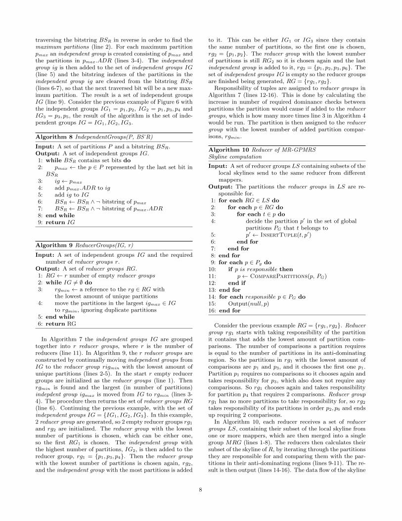
traversing the bitstring BSR in reverse in order to find themaximum partitions (line 2). For each maximum partitionpmax an independent group is created consisting of pmax andthe partitions in pmax.ADR (lines 3-4). The independentgroup ig is then added to the set of independent groups IG(line 5) and the bitstring indexes of the partitions in theindependent group ig are cleared from the bitstring BSR

(lines 6-7), so that the next traversed bit will be a new max-imum partition. The result is a set of independent groupsIG (line 9). Consider the previous example of Figure 6 withthe independent groups IG1 = p1, p2, IG2 = p1, p3, p4 andIG3 = p3, p5, the result of the algorithm is the set of inde-pendent groups IG = IG1, IG2, IG3.

Algorithm 8 IndependentGroups(P, BS˙R)

Input: A set of partitions P and a bitstring BSR.Output: A set of independent groups IG.1: while BSR contains set bits do2: pmax ← the p ∈ P represented by the last set bit in

BSR

3: ig ← pmax

4: add pmax.ADR to ig5: add ig to IG6: BSR ← BSR ∧ ¬ bitstring of pmax

7: BSR ← BSR ∧ ¬ bitstring of pmax.ADR8: end while9: return IG

Algorithm 9 ReducerGroups(IG, r)

Input: A set of independent groups IG and the requirednumber of reducer groups r.

Output: A set of reducer groups RG.1: RG← r number of empty reducer groups2: while IG 6= ∅ do3: rgmin ← a reference to the rg ∈ RG with

the lowest amount of unique partitions4: move the partitions in the largest igmax ∈ IG

to rgmin, ignoring duplicate partitions5: end while6: return RG

In Algorithm 7 the independent groups IG are groupedtogether into r reducer groups, where r is the number ofreducers (line 11). In Algorithm 9, the r reducer groups areconstructed by continually moving independent groups fromIG to the reducer group rigmin with the lowest amount ofunique partitions (lines 2-5). In the start r empty reducergroups are initialized as the reducer groups (line 1). Thenrgmin is found and the largest (in number of partitions)indepdent group igmax is moved from IG to rgmin (lines 3-4). The procedure then returns the set of reducer groups RG(line 6). Continuing the previous example, with the set ofindependent groups IG = {IG1, IG2, IG3}. In this example,2 reducer group are generated, so 2 empty reducer groups rg1and rg2 are initialized. The reducer group with the lowestnumber of partitions is chosen, which can be either one,so the first RG1 is chosen. The independent group withthe highest number of partitions, IG2, is then added to thereducer group, rg1 = {p1, p3, p4}. Then the reducer groupwith the lowest number of partitions is chosen again, rg2,and the independent group with the most partitions is added

to it. This can be either IG1 or IG3 since they containthe same number of partitions, so the first one is chosen,rg2 = {p1, p2}. The reducer group with the lowest numberof partitions is still RG2 so it is chosen again and the lastindependent group is added to it, rg2 = {p1, p2, p3, p6}. Theset of independent groups IG is empty so the reducer groupsare finished being generated, RG = {rg1, rg2}.

Responsibility of tuples are assigned to reducer groups inAlgorithm 7 (lines 12-16). This is done by calculating theincrease in number of required dominance checks betweenpartitions the partition would cause if added to the reducergroups, which is how many more times line 3 in Algorithm 4would be run. The partition is then assigned to the reducergroup with the lowest number of added partition compar-isons, rgmin.

Algorithm 10 Reducer of MR-GPMRSSkyline computation

Input: A set of reducer groups LS containing subsets of thelocal skylines send to the same reducer from differentmappers.

Output: The partitions the reducer groups in LS are re-sponsible for.

1: for each RG ∈ LS do2: for each p ∈ RG do3: for each t ∈ p do4: decide the partition p′ in the set of global

partitions PG that t belongs to5: p′ ← InsertTuple(t, p′)6: end for7: end for8: end for9: for each p ∈ Pg do

10: if p is responsible then11: p← ComparePartitions(p, PG)12: end if13: end for14: for each responsible p ∈ PG do15: Output(null, p)16: end for

Consider the previous example RG = {rg1, rg2}. Reducergroup rg1 starts with taking responsibility of the partitionit contains that adds the lowest amount of partition com-parisons. The number of comparisons a partition requiresis equal to the number of partitions in its anti-dominatingregion. So the partitions in rg1 with the lowest amount ofcomparisons are p1 and p3, and it chooses the first one p1.Partition p1 requires no comparisons so it chooses again andtakes responsibility for p3, which also does not require anycomparisons. So rg1 chooses again and takes responsibilityfor partition p4 that requires 2 comparisons. Reducer grouprg1 has no more partitions to take responsibility for, so rg2takes responsibility of its partitions in order p2, p6 and endsup requiring 2 comparisons.

In Algorithm 10, each reducer receives a set of reducergroups LS, containing their subset of the local skyline fromone or more mappers, which are then merged into a singlegroup MRG (lines 1-8). The reducers then calculates theirsubset of the skyline of R, by iterating through the partitionsthey are responsible for and comparing them with the par-titions in their anti-dominating regions (lines 9-11). The re-sult is then output (lines 14-16). The data flow of the skyline

8

Table 2: A list of common terms.

Symbol Interpretationptotal(n, d) Partitions in a gridprem(n, d) Remaining partitions in a grid after

pruning dominated partitionspdom(n, d) Partition dominance checks for a

single partitions(n, d) Partition dominance checks for a

single surface in a gridgmapper(n, d) Partition dominance checks for a

single mappergreducer(n, d) Partition dominance checks for the

reducer with the most partitiondominance checks

computation phase of MR-GPMRS is represented in Figure5 where it is shown how the data set R is split into subsetsR1, R2, . . . Rn that are processed by the mappers into localskylines SR1, SR2, . . . SRn. The reducers then find subsetsof the global skyline S1, S2, . . . Sn using subsets of the localskylines {{SR1.1, . . . , SR1.n},{SR2.1,. . . ,SR2.n},{SRn.1,. . . ,S1,. . .Sn}} which are then combined to produce the globalskyline SR as output.

5. COST ESTIMATIONIn this section estimations of the cost of MR-GPMRS are

made. A table of common terms is shown in Table 2.

5.1 Partition-wise Dominance Tests EstimateThe purpose of this section is to estimate the number

of dominance checks performed between partitions in theMR-GPMRS algorithm. Specifically, what is estimated ishow many times the line 3 in Algorithm 4 is executed. Dueto several uncertainties of the algorithm, it is necessary tomake some assumptions.

• Every partition in every mapper is non-empty.The data distribution is an important factor of theestimation. It is necessary to assume that there areno empty partitions in order to predict the requirednumber of comparisons. It is comparable to uniformdata distribution where it can be expected that mostpartitions are non-empty.

• The dominance checks between partitions inthe mappers do not lower the number of non-empty partitions. In practice, the partition checksin the mappers are likely to leave some partitionsempty. This is unpredictable and is therefore not ac-counted for.

These assumptions mean that the scenario for which theestimations are made is a worst case scenario for a dataset with a uniform data distribution. When every partitionis non-empty, after the grid has been pruned, the locationand amount of the remaining partitions is predictable us-ing the dimensionality d and the PPD n. A d dimensionalgrid has a number of d − 1 dimensional surfaces equal tod × 2. Half of these surfaces, i.e. d surfaces, are filled withremaining partitions. The remaining part of the other halfof the surfaces, as well as the rest of the partitions, are

dominated. For example, consider Figure 6. In this 2 di-mensional, 3 PPD grid, there are d × 2 = 4 surfaces witha dimensionality of d − 1 = 1. These four surfaces consistsof the partitions surf1 = {p2, p1, p0}, surf2 = {p0, p3, p6},surf3 = {p6, p7, p8}, and surf4 = {p8, p5, p2}. If everypartition were non-empty, the partitions p4, p5, p7, and p8would be dominated and pruned. This would leave d = 2 in-tact surfaces, surf1 and surf2. There is an overlap betweenthe surfaces that must be considered. In this case, the over-lap between the remaining surfaces surf1 and surf2 is p0.

The number of remaining partitions after pruning a gridwhere every partition is non empty prem(n, d) can be cal-culated by finding the total number of partitions in a gridparttotal(n, d) and subtracting a grid one PPD smaller:

ptotal(n, d) = nd (15)

prem(n, d) = parttotal(n, d)− parttotal(n− 1, d) (16)

From the previous example, the pruned partitions, p4, p5,p7, and p8, can be contained by a d = 2 dimensional n −1 = 2 PPD grid. This means the the number of remainingpartitions after pruning a 2 dimensional, 3 PPD grid can becalculated as 32−22 = 5. The dominance checks to be doneby a single partition p depends on its anti-dominating region.A partition pi performs dominance checks against anotherpartition pj if pj ∈ pi.ADR. The number of dominancechecks pdom(n, d) for a partition p is equal to its grid positionvalues multiplied with each other minus one:

pdom(n, d) = p.pos.d1 × p.pos.d2 × . . .× p.pos.dd − 1 (17)

The position of a partition in a grid is how many parti-tions, including itself, from the origin a partition is locatedin the different dimensions.

For example, in Figure 6 the partition p2, for the firstdimension, has the position p2.pos.d1 = 3, and for the seconddimension it has the position p2.pos.d2 = 1. Summing thisup to get the number of partition checks for every partitionin a surface s(n, d) yields the following expression:

s(n, d) =

n∑i1=1

n∑i2=1

. . .

n∑id=1

(i1 × i2 × . . .× dn − 1) (18)

To get the number of partition checks for all surfaces, theoverlap between surfaces, where they meet on the axes, hasto be considered. The first surface is calculated as above.The second surface is also calculated as above but with theoverlap between the first and the second surface removed.The overlap between the first and the third surface and theoverlap between the second and the third surface has to besubtracted from the third surface, and so on. To accountfor this, the start index i of one of the summations is incre-mented for each surface that is calculated. So the number ofdominance checks gmap(n, d) between partitions in a singlemapper for all surfaces of a grid is as follows:

s1(n, d) =

n∑i1=1

n∑i2=1

. . .

n∑id−1=1

(i1 × i2 × . . .× id−1 − 1) (19)

9

s2(n, d) =

n∑i1=2

n∑i2=1

. . .

n∑id−1=1

(i1 × i2 × . . .× id−1 − 1) (20)

s3(n, d) =

n∑i1=2

n∑i2=2

. . .

n∑id−1=1

(i1 × i2 × . . .× id−1 − 1) (21)

. . .

sd(n, d) =

n∑i1=2

n∑i2=2

. . .

n∑id−1=2

(i1 × i2 × . . .× id−1 − 1) (22)

gmap(n, d) =

d∑i=1

si(n, d) (23)

For the reducer, only a single surface has to be considered.The reason for this is that each surface is an independentgroup that can be calculated individually by the reducers.The reducer with the most dominance checks is the one thathas the biggest surface, which is the one where no overlapis considered. This allows the surface calculation from be-fore to be reused when calculating the number of partitiondominance checks greducer(n, d) in the reducer with the mostdominance checks:

greducer(n, d) = s1(n, d) (24)

6. EXPERIMENTSIn this section, the results from experimental runs of the

algorithms are presented. A cluster of thirteen commoditymachines have been used for the experiments. Twelve of themachines have an Intel Pentium D 2.8 GHz Core2 proces-sor. Three of these have a single gigabyte of RAM, four ofthem have two, and five of them have three. The last ma-chine has an Intel Pentium D 2.13 GHz Core2 processor andtwo gigabytes of RAM. The machines are connected with a100 Mbit/s LAN connection. The operating system used isUbuntu 12.04 and the version of Hadoop is 1.1.0. The algo-rithms are implemented in Java. Tests are performed on thealgorithms MR-GPMRS, MR-GPSRS, MR-BNL from [12],and MR-Angle from [4]. The tests are performed on severaldifferent data sets, with varying cardinality, dimensionality,and data distribution.

1 5 9 13 17Reducers

0

100

200

300

400

500

Runt

ime

[s]

8 Dimensions (Anti-Correlated)8 Dimensions (Uniform)

Figure 7: The graph shows the runtime of the algorithmMR-GPMRS run on an anti-correlated data set with adimensionality of 8 and with a cardinality of 1×106. Thenumber of reducers used is varied. The result for onereducer is the runtime of MR-GPSRS.

2 3 4 5 6 7 8 9 10Dimensionality

0

1

2

3

4

5

6

Compa

rison

s

1e6

Mapper(Anti−correlated)Mapper(Uniform)

Estimate(Anti−correlated)Estimate(Uniform)

(a) Mappers

2 3 4 5 6 7 8 9 10Dimensionality

0.0

0.2

0.4

0.6

0.8

1.0

1.2

1.4

Compa

rison

s

1e6

Reducer(Anti−correlated)Reducer(Uniform)

Estimate(Anti−correlated)Estimate(Uniform)

(b) Reducers

Figure 8: The estimated and actual number of domi-nance checks between partitions for data sets when runon a data set with a cardinality of 1 × 106 and varyingdimensionality.

The cardinalities are 1×105, 5×105, 1×106, 2×106, and3 × 106. The dimensionality range is [2 . . . 10]. The distri-butions are anti-correlated and uniform. For the test runsof MR-GPMRS for comparison with the other algorithms,MR-GPMRS is set to use one reducer per node, i.e. thirteen.To see the effect of the number of reducers, MR-GPMRS hasbeen run on select data sets with varying number of reduc-ers.

6.1 Effect of DimensionalityThe runtime results for uniform data sets with varying

dimensionality are shown in Figure 9. The results for anti-correlated data sets are shown in Figure 10.

As can be seen from the uniform data set results (Figure9), the MR-GPMRS algorithm runs a little slower for thelower dimensions (2 − 5). For the rest of the dimensions(6 − 10), however, the runtime of MR-GPMRS increaseslinearly, while the runtime of the other algorithms increasesexponentially. The exception is MR-GPSRS that runs fasterthan MR-GPMRS even for higher dimensions. The differ-ence is marginal but consistent. The reason for these resultsare that for the low dimensionalities, the skyline percentageis so low that the runtime of the algorithms is dominatedby the communication cost and the time it takes to read thedata set. This overhead in MR-GPMRS is slightly largerthan the other algorithms, which is why the runtime is a bithigher. For the higher dimensions, when the skyline percent-age becomes more significant, MR-GPMRS is able to obtainthe skyline more efficiently than MR-Angle and MR-BNL.MR-GPSRS is the fastest algorithm for all uniform datasets, which shows that the pruning power of the grid parti-tioning scheme used in both MR-GPSRS and MR-GPMRSis superior, and that using multiple reducers is not worththe extra communication cost when the skyline percentageis low.

For the anti-correlated data sets (Figure 10), MR-GPMRSis superior for all dimensions, except to MR-GPSRS whichis better for the dimensionalities less than 5. It is clear thatMR-GPMRS scales well for higher dimensionalities even forlarge cardinalities, having a runtime of less than ten minutesfor a data set with a cardinality of 2×106 and 10 dimensions.Results for MR-Angle and MR-BNL are not shown for thehigher dimensionalities since they are not able to terminatein a reasonable amount of time. MR-GPSRS is running sig-nificantly slower than MR-GPMRS for the low cardinalityand high dimensionality data sets. For the higher cardinal-ity, the difference is more clear and MR-GPSRS does not

10

2 3 4 5 6Dimensionality

50

55

60

65

70

75

80

Runtim

e [s]

MR−BNLMR−AngleMR−GPSRSMR−GPMRS

(a) 2-6 dimensionality1× 105 cardinality

7 8 9 10Dimensionality

0

100

200

300

400

500

600

Runtim

e [s]


(b) 7-10 dimensionality1× 105 cardinality


5060708090

100110120130140

Runtim

e [s]


(c) 2-6 dimensionality2× 106 cardinality


100

200

300

400

500

600

700

Runtim

e [s]


(d) 7-10 dimensionality2× 106 cardinality

Figure 9: Each graph shows the run time of the algorithms MR-BNL, MR-Angle, MR-GPSRS, and MR-GPMRS runon uniform data sets with varying dimensionality.


0

100

200

300

400

500

600

Runtim

e [s]


(a) 2-6 dimensionality1× 105 cardinality


100

150

200

250

300

Runtim

e [s]


(b) 7-10 dimensionality1× 105 cardinality


0100200300400500600700800900

Runtim

e [s]


(c) 2-6 dimensionality2× 106 cardinality


200

400

600

800

1000

1200

1400

1600

1800

Runtim

e [s]


(d) 7-10 dimensionsilty2× 106 cardinality

Figure 10: Each graph shows the run time of the algorithms MR-BNL, MR-Angle, MR-GPSRS, and MR-GPMRSrun on anti-correlated data sets with varying dimensionality.

terminate in a reasonable amount of time for the highestdimensionalities. The reason here is that in anti-correlateddata sets, the skyline is significant even when the dimen-sionality is low, and it increases quickly for higher dimen-sionalities.

This means that the ability of MR-GPMRS to find theskyline more efficiently outweighs its increased overhead.For higher dimensionalities, this is even more evident. ThatMR-GPSRS performs better than MR-GPMRS for the lowerdimensionalities continues to show that using multiple re-ducers is not worth the extra communication cost when theskyline percentage is below a certain point.

6.2 Effect of CardinalityThe results for varying cardinality is shown in Figure 11.

For uniform data, MR-GPMRS is slowest for all cardinal-ities when the dimensionality is 3, almost 20 seconds at acardinality of 3 × 106. MR-GPSRS has the best runtimefor all cardinalities, MR-Angle tying with it for the cardi-nalities 1 × 106 and 3 × 106. For the higher dimensional-ity of 8, MR-GPMRS and MR-GPSRS has the fastest run-times, MR-GPSRS being a bit faster given the small skylinepercentage of the uniform data where the multiple reduc-ers are not an improvement given the extra communicationcost. What these results show is that using multiple reduc-ers consistently causes a slower runtime when the skylinepercentage of the data set is low.

For anti-correlated data, MR-GPMRS and MR-GPSRSis superior for all cardinalities and both dimensionalities.For the lower dimensionality of 3, MR-GPSRS is marginallybetter than MR-GPMRS, but for the higher dimensionalityof 8, MR-GPSRS fails to terminate in a reasonable amountof time for the highest cardinality and is consistently worsethan MR-GPMRS.

6.3 Effect of Number of ReducersFigure 7 shows how the runtime of MR-GPMRS changes

when the number of reducers used is varied. What can beseen from the runtimes of the anti-correlated data set isthat it lowers when the number of reducers is increased.For this particular data set the runtime is best when thenumber of reducers is at the highest. It is better even whenthe number of reducers is higher than the number of nodes.The reason for this is that Hadoop is able to utilise themultiple cores in the nodes to parallelize multiple reducerson the same node. This is not necessarily the case for otherdata sets, as evident from the results where MR-GPSRSoutperforms MR-GPMRS. The skyline percentage needsto be high enough for the extra communication cost themultiple reducers causes for the high number of reducersto be useful. The runtime for the data set with uniformdistribution almost does not change when the number ofreducers is increased. There is a small increase, caused bythe additional overhead of multiple reducers. This uniformdata set has a much smaller skyline than the anti-correlatedone, which means that the use of multiple reducers is notworthwhile given the extra overhead.

6.4 Evaluation of EstimateFigure 8 shows the estimated number of dominance checks

between partitions, as described in Section 5, comparedwith the measured number of partition comparisons inMR-GPMRS. The measured numbers has been taken fromthe mapper and the reducer that had the highest numberof comparisons. The results for the mappers show that theestimate does not deviate far from the measured numberwhen the data distribution is uniform, and in some casesthere is no deviation. The estimate, however, is inaccurate

11

0.1 0.5 1.0 2.0 3.0Cardinality 1e6

40

50

60

70

80

90

Runtim

e [s]


(a) Uniform3 dimensionality

0.1 0.5 1.0 2.0 3.0Cardinality 1e6

0

100

200

300

400

500

600

700

Runtim

e [s]


(b) Anti-correlated3 dimensionality

0.1 0.5 1.0 2.0 3.0Cardinality 1e6

0100200300400500600700800900

Runtim

e [s]


(c) Uniform8 dimensionality

0.1 0.5 1.0 2.0 3.0Cardinality 1e6

0

200

400

600

800

1000

Runtim

e [s]


(d) Anti-correlated8 dimensionality

Figure 11: The graphs show the runtime of the algorithms MR-BNL, MR-Angle, MR-GPSRS, and MR-GPMRS runwith a dimensionality of 3 and with varying cardinality.

when estimating the number of partition dominance checksfor mappers run on the anti-correlated data set. This is to beexpected as the estimation was done on the premise that thedata set is uniform. It is notable that the estimated num-ber of dominance checks is above the measured one in everycase, which means that the estimate can be still be used as aworst case estimate for anti-correlated data sets. The resultsfor the reducers show that the estimate is inaccurate for thereducers, both for the uniform and the anti-correlated dataset. The reason that the estimate is inaccurate even for theuniform data set, is that no way was found to mathemati-cally predict the way the reducer groups are generated, soinstead a number was used that was ensured to be the worstcase.

7. CONCLUSIONIn this paper, two novel algorithms, MR-GPSRS and

MR-GPMRS, for skyline query processing in MapReduceare proposed. The main feature of the algorithms are thatthey allow decision making across mappers and reducers.This is accomplished by using a bitstring describing the par-titions empty and non-empty state across the entire data set.In addition, the common bottleneck of having the final sky-line computed at a single node is avoided in the MR-GPMRSalgorithm by utilizing the bitstring to partition the final sky-line computation among multiple reducers.

The experiments conducted show that the algorithms pro-posed in this paper consistently outperforms existing algo-rithms and they scale well with the skyline and data setsize. Which of the two proposed algorithms performs bet-ter depends on the data set. When the skyline percent-age is high, MR-GPMRS performs significantly better whileMR-GPSRS performs marginally better when the skylinepercentage is low. Running test on a large cluster would beinteresting in order investigate how well MR-GPMRS scalesfor large numbers of reducers.

The increased communication cost incurred by having re-ducers receive replicated partitions is a consequence of themethod that allows for the utilization of multiple reducers.One research direction, therefore, is to develop a schemethat balances the reducer groups in MR-GPMRS such thatthe computations is balanced across the reducers and thecommunication cost is minimized at the same time.

As the results show, using multiple reducers is not thebest option when the skyline percentage is low. So for thealgorithm to perform optimally for any data set, it is neces-sary to develop a scheme that allows MR-GPMRS to intel-ligently decide how many reducers to use. It is possible that

the method for choosing the PPD in the proposed algorithmcan be improved.

The method does not incur a noticeable amount of extraruntime, and it chose a viable PPD for all the data setstested for. It did not necessarily choose the optimal PPD,however, so finding a method that is guaranteed to choosethe optimal PPD for any data set would be a significantimprovement.

8. REFERENCES[1] Amazon. Amazon elastic compute cloud.

http://aws.amazon.com/ec2/.

[2] Apache. Welcome to apacheTMhadoop R©!http://http://hadoop.apache.org//.

[3] S. Brzsnyi, D. Kossmann, and K. Stocker. The skylineoperator. 17th Internation Conference on DataEngineering, 2001.

[4] L. Chen, K. Hwang, and J. Wu. Mapreduce skylinequery processing with a new angular partitioningapproach. 26th International Parallel and DistributedProcessing Symposium Workshops & PhD Forum,2012.

[5] B. Cui, H. Lu, Q. Xu, L. Chen, Y. Dai, and Y. C.Zhou. Parallel distributed processing of constrainedskyline queries by filtering. 24th ICDE, 2008.

[6] J. Dean and S. Ghemawat. Mapreduce: Simplifieddata processing on large clusters. OSDI, 2004.

[7] Facebook. Hive - a petabyte scale data warehouseusing hadoop. https://www.facebook.com/note.php?note_id=89508453919.

[8] LinkedIn. A professional network built with javatechnologies and agile practices.http://www.slideshare.net/linkedin/

linkedins-communication-architecture.

[9] Twitter. Hadoop at twitter. http://engineering.twitter.com/2010/04/hadoop-at-twitter.html.

[10] A. Vlachou, C. Doulkeridis, and Y. Kotidis.Angle-based space partitioning for efficient parallelskyline computation. SIGMOD ’08, 2008.

[11] Yahoo. Hadoop at yahoo!http://developer.yahoo.com/hadoop/.

[12] B. Zhang, S. Zhou, and J. Guan. Adapting skylinecomputation to the mapreduce framework: Algorithmsand experiments. DASFAA Workshops, 2011.

12

efﬁcient skyline computation for large volume data in...

Documents