group skyline computation - ntuagtsat/collection/skylines/infosci2012.pdf · group skyline...

Information Sciences 188 (2012) 151–169

Contents lists available at SciVerse ScienceDirect

Information Sciences

journal homepage: www.elsevier .com/locate / ins

Group skyline computation

Hyeonseung Im, Sungwoo Park ⇑Pohang University of Science and Technology (POSTECH), Republic of Korea

a r t i c l e i n f o

Article history:Received 22 October 2010Received in revised form 13 October 2011Accepted 10 November 2011Available online 22 November 2011

Keywords:Skyline computationDynamic algorithm

0020-0255/$ - see front matter � 2011 Elsevier Incdoi:10.1016/j.ins.2011.11.014

⇑ Corresponding author. Tel.: +82 54 279 2386.E-mail addresses: [email protected] (H. Im),

a b s t r a c t

Given a multi-dimensional dataset of tuples, skyline computation returns a subset of tuplesthat are not dominated by any other tuples when all dimensions are considered together.Conventional skyline computation, however, is inadequate to answer various queries thatneed to analyze not just individual tuples of a dataset but also their combinations. In thispaper, we study group skyline computation which is based on the notion of dominancerelation between groups of the same number of tuples. It determines the dominance rela-tion between two groups by comparing their aggregate values such as sums or averages ofelements of individual dimensions, and identifies a set of skyline groups that are not dom-inated by any other groups. We investigate properties of group skyline computation anddevelop a group skyline algorithm GDynamic which is equivalent to a dynamic algorithmthat fills a table of skyline groups. Experimental results show that GDynamic is a practicalgroup skyline algorithm.

� 2011 Elsevier Inc. All rights reserved.

1. Introduction

Given a multi-dimensional dataset of tuples, skyline computation [4] returns a subset of tuples that are no worse than, ornot dominated by, any other tuples when all dimensions are considered together. As an example, consider the dataset of sixbasketball players in Fig. 1. Each tuple lists the number of points and the number of rebounds. As we prefer higher values forboth attributes, players p1, p2, and p3 (marked with �) are the best choices which are no worse than any other players, whileplayers p4, p5, and p6 (marked with �) are all inferior choices which are dominated by player p1 or p3. We say that players p1,p2, and p3 are skyline tuples, and refer to the set of skyline tuples as the skyline of the dataset. A skyline algorithm performscomparisons between tuples, or dominance tests, to identify all skyline tuples, or equivalently, to eliminate all non-skylinetuples.

Because of its potential applications in decision making, skyline computation since its inception has drawn a lot of atten-tion in the database community [2,4,5,9,12,13,18,28]. Researchers have also investigated its extensions such as parallel sky-line computation for share-nothing architectures [8,25,27] and multicore architectures [19,21], probabilistic skylinecomputation on uncertain datasets and data streams [1,3,6,20], and skycube computation for finding all possible 2d � 1 sub-space skylines of the given d-dimensional dataset [11].

Conventional skyline computation, however, is inadequate to answer various queries that require us to analyze not justindividual tuples of a dataset but also their combinations. For example, it is not clear how to answer the following queries(on the dataset in Fig. 1) using only conventional skyline computation when we wish to form a team of three players:

� Our team has currently two players p1 and p5. Who is the best player to recruit as a new member?

. All rights reserved.

[email protected] (S. Park).

http://dx.doi.org/10.1016/j.ins.2011.11.014

mailto:[email protected]

mailto:[email protected]

http://dx.doi.org/10.1016/j.ins.2011.11.014

http://www.sciencedirect.com/science/journal/00200255

http://www.elsevier.com/locate/ins

Fig. 1. A dataset of basketball players and the skyline.

152 H. Im, S. Park / Information Sciences 188 (2012) 151–169

� Who is the best player to choose if the other two players in our team are unknown yet? In particular, is non-skyline player p4 abetter choice than skyline player p2 or p3?

In essence, these queries call for an analysis of groups of three players, which is beyond the reach of conventional skylinecomputation.

In this paper, we study group skyline computation which is based on the notion of dominance relation between groups ofthe same number of tuples. It determines the dominance relation between two groups by comparing their aggregate valuesof elements of individual dimensions. We may use any aggregate function that is strictly monotone in each argument [7] suchas sum and average. For the purpose of easy illustration, however, we use the aggregate function sum in all the motivatingexamples in the paper.

As an example of group skyline computation, consider again the dataset in Fig. 1. We wish to find groups of three playerswhose sums of points and rebounds are no worse than any other groups of three players. After examining a total ofC(6,3) = 20 candidate groups, we obtain four such groups:

Group of players
Sum of points Sum of rebounds
{p1,p2,p3}
7 8 {p1,p2,p4} 5 10 {p1,p3,p4} 9 7 {p1,p4,p5} 7 8
We refer to these groups as 3-skyline groups of the dataset where 3 indicates the number of tuples in each group, and refer tothe set of 3-skyline groups as the 3-skyline of the dataset. Given a value of k specifying the number of tuples in each group,group skyline computation finds the k-skyline, or the set of k-skyline groups, of the dataset.

Group skyline computation has a number of potential applications in decision making that need to compare groups oftuples. For example, we can answer the two previous queries using group skyline computation:

� Our team has currently two players p1 and p5. Who is the best player to recruit as a new member?We perform group skyline computation on the dataset to find 3-skyline groups with both p1 and p5. Since there is onlyone such 3-skyline group {p1,p4,p5}, we choose to recruit non-skyline player p4, instead of remaining skyline players p2

and p3. If we perform conventional skyline computation after removing players p1 and p5, we obtain three players p2, p3,and p4 to choose from.� Who is the best player to choose if the other two players in our team are unknown yet? In particular, is non-skyline player p4 a

better choice than skyline player p2 or p3?The goal is to find a player who maximizes the probability that the team with the player belongs to the 3-skyline. Weperform group skyline computation on the dataset and count the number of 3-skyline groups to which each playerbelongs. We rank all the players by these numbers and obtain the following list: p1 (4), p4 (3), p2/p3 (2), p5 (1), p6 (0). Notethat we rank non-skyline player p4 higher than skyline players p2 and p3.

Thus we may exploit group skyline computation to answer various queries that conventional skyline computation eithercannot answer or answers incorrectly.

The main challenge in developing an algorithm for group skyline computation is to overcome its computational complex-ity. Unfortunately the space complexity of group skyline computation is exponential in general and a dataset of n tuples canhave up to Cðn; kÞ ¼ n!

ðn�kÞ!k!k-skyline groups. For example, we can construct such a dataset by placing all tuples in the same

hyperplane. This, in turn, means that its time complexity is also exponential because we have to generate all skyline groupsduring the computation. Since the set of intermediate candidate groups may not fit in memory, we have to generate allcandidate groups in a progressive manner and update the resultant group skyline dynamically. As such, we thus cannot

H. Im, S. Park / Information Sciences 188 (2012) 151–169 153

exploit those techniques, such as index structures R-trees [18] and ZBtrees [13], developed for conventional skylinecomputation.

We develop a group skyline algorithm called GDynamic which exploits key properties of group skyline computation toreduce both the number of intermediate candidate groups and the number of dominance tests between groups. As a preli-minary step, we study a simple group skyline algorithm called GIncremental which is based on the intuition that everyk-skyline group is likely to contain at least one (k � 1)-skyline group. (We prove that the intuition is valid for k 6 3, butnot for k P 4.) After analyzing the properties of GIncremental, we design GDynamic which is equivalent to a dynamic algo-rithm that fills a table of group skylines. Experimental results on both synthetic and real datasets show that GDynamic is apractical group skyline algorithm.

A recent proposal of top-k combinatorial skyline query (k-CSQ) processing by Su et al. [22] is similar in spirit to groupskyline computation in that it also considers combinations of tuples and computes combinations that are not dominatedby any others. However, k-CSQ processing is different in that it reports only those combinations whose aggregate valuesfor a certain attribute are the highest, and thus may miss some important combinations. In contrast, group skyline compu-tation generates all skyline groups, which may be exploited in more complicated decision making processes. Hence its mainchallenge is to find key properties for reducing both the number of intermediate candidate groups and the number of dom-inance tests between groups. Section 6 provides a more detailed discussion on k-CSQ processing.

The remainder of the paper is organized as follows. Section 2 introduces group skyline computation and studies its basicproperties. Sections 3 and 4 develop the algorithm GIncremental and GDynamic, respectively. Section 5 presents experimen-tal results and Section 6 discusses related work. Section 7 concludes.

2. Preliminaries

This section formally defines group skyline computation and studies its basic properties. Fig. 2 summarizes the key nota-tions used throughout the paper. We begin by reviewing conventional skyline computation.

2.1. Skyline computation

Given a dataset, skyline computation retrieves its skyline which consists of tuples not dominated by any other tuples.Under the assumption that larger values are better, a tuple p dominates another tuple q if all elements of p are larger thanor equal to their corresponding elements of q and there exists at least one element of p that is strictly larger than its corre-sponding element of q. Thus the skyline consists of those tuples that are no worse than any other tuples when all dimensionsare considered together.

Let us formally define the skyline of a d-dimensional dataset D. We write p[i] for the i-th element of tuple p where1 6 i 6 d; hence we have p = (p[1], . . . ,p[d]). We write p � q to mean that tuple p dominates tuple q, that is, p[i] P q[i] holdsfor 1 6 i 6 d and there exists a dimension j such that p[j] > q[j]. We also write p ¤ q to mean that p does not dominate q, andp �� q to mean that p and q are incomparable (p ¤ q and q ¤ p). Then the skyline SðDÞ of D is defined as

SðDÞ ¼ fp 2 D j 8q 2 D; q¤pg:

Note that SðDÞ � D and SðSðDÞÞ ¼ SðDÞ hold. We refer to those tuples in the skyline as skyline tuples.The cost of skyline computation increases with the number of dominance tests performed to identify skyline tuples. A

dominance test between two tuples p and q determines whether p dominates q (p � q), q dominates p (q � p), or p and qare incomparable (p �� q). Usually a skyline algorithm reduces the number of dominance tests by exploiting specific

Fig. 2. Summary of key notations.


properties of skyline tuples. For example, transitivity of� allows us to eliminate from further consideration any tuple as soonas we find that it is dominated by another tuple:

Proposition 2.1. If p � q and q � r, then p � r.

2.2. Group skyline computation

Group skyline computation extends the notion of dominance relation to groups of the same number of tuples and iden-tifies a group skyline, or a set of groups that are no worse than any other groups. It determines the dominance relation be-tween two groups by comparing their aggregate values of elements of individual dimensions. Hence we may think of groupskyline computation on a dataset as conventional skyline computation on a derived dataset consisting of all its subsets of thesame size.

For dominance tests, we may use any aggregate function that is strictly monotone in each argument [7]. An aggregatefunction f is monotone if f ðx1; . . . ; xmÞP f ðx01; . . . ; x0mÞ whenever xi P x0i for every i. f is strictly monotone iff ðx1; . . . ; xmÞ > f ðx01; . . . ; x0mÞ whenever xi > x0i for every i. f is strictly monotone in each argument if an increase in any argumentresults in an increase of its value. That is, f is strictly monotone in each argument if f ðx1; . . . ; xi; . . . ; xmÞ > f ðx1; . . . ; x0i; . . . ; xmÞwhenever xi > x0i for some i. For example, sum and average are strictly monotone in each argument, whereas min and maxare not. In the rest of the paper, we write ‘‘aggregate functions’’ to mean those that are strictly monotone in each argument.

Now let us formally define group skylines of a d-dimensional dataset D using an aggregate function f. We refer to a subsetCk of D containing k tuples as a k-group of D and write CkðDÞ for the set of all k-groups of D:

CkðDÞ ¼ fCk j Ck � D; jCkj ¼ kg

As a special case, we have C1ðDÞ ¼ ffpg j p 2 Dg.Given a k-group Ck = {p1, . . . ,pk}, we write f(Ck) for the aggregate tuple (f(p1[1], . . . ,pk[1]), . . . , f (p1[d], . . . ,pk[d])). We define

the dominance relation Ck � C0k between two k-groups Ck and C0k as follows:

Definition 2.2. Suppose Ck = {p1, . . . ,pk} and C0k ¼ fq1; . . . ; qkg. We say that Ck dominates C0k and write Ck � C0k if f ðCkÞ � f ðC0kÞholds, that is, f(p1[i], . . . ,pk[i]) P f(q1[i], . . . ,qk[i]) holds for 1 6 i 6 d and there exists a dimension j such thatf(p1[j], . . . ,pk[j]) > f(q1[j], . . . ,qk[j]).

As in conventional skyline computation, we write Ck¤C0k to mean that Ck does not dominate C0k, and Ck �� C0k to mean thatCk and C0k are incomparable (Ck¤C0k and C0k¤Ck). Then the group skyline of size k, or k-skyline, of D is defined as

GkðDÞ ¼ SðCkðDÞÞ ¼ fCk 2 CkðDÞ j 8C 0k 2 CkðDÞ; C0k¤Ckg:

We refer to those groups in the k-skyline as k-skyline groups and write Gk for a k-skyline group (i.e., Gk 2 GkðDÞ). As a specialcase, we have G1ðDÞ ¼ ffpg j p 2 SðDÞg.

2.3. Basic properties of group skyline computation

A trivial but important property of group skyline computation is that its space complexity is exponential in general. This,in turn, means that its time complexity is also exponential because we have to generate all skyline groups during thecomputation.

Proposition 2.3. For a value of k specifying the size of group skylines, a dataset with n tuples can have up to Cðn; kÞ ¼ n!ðn�kÞ!k!

k-skyline groups. That is, all its k-groups can be in the k-skyline.

Proof. Consider the summation R as an aggregate function and a 2-dimensional dataset D = {(x,�x) j x = 1, . . . ,n}. Everyk-group of D is written as ðRk

i¼1xi; �Rki¼1xiÞ and belongs to the k-skyline. h

Since we cannot achieve a group skyline algorithm of polynomial space or time complexity, we focus on those properties ofgroup skyline computation that enable us to consider fewer intermediate candidate groups on typical datasets not all ofwhose k-groups are in the k-skyline.

Since a k-skyline group collectively represents a single ‘‘good’’ tuple, it is likely to contain skyline tuples. Proposition 2.4,however, shows that a group of k skyline tuples does not necessarily form a k-skyline group:

Proposition 2.4. Suppose Ck � SðDÞ. Then we may have Ck R GkðDÞ.

Proof. Consider the summation R as an aggregate function and a 2-dimensional dataset of 4 tuples: p1 = (0,4), p2 = (1,2),p3 = (2,1), and p4 = (4,0). All tuples are skyline tuples, but {p1,p4} dominates {p2,p3}. h

Proposition 2.5 proves the converse of Proposition 2.4 that a k-skyline group may indeed contain non-skyline tuples:


Proposition 2.5. Suppose Gk 2 GkðDÞ. Then we may have Gk åSðDÞ.

Proof. Consider the summation R as an aggregate function and a 2-dimensional dataset of 3 tuples: p1 = (0,2), p2 = (1,0), andp3 = (2,1). p2 is dominated by p3 and thus is not a skyline tuple, but {p2,p3} is a 2-skyline group. h

Hence group skyline computation needs to consider not only skyline tuples but also non-skyline tuples. This result, how-ever, does not mean that we should treat all non-skyline tuples in the same manner – Proposition 2.6 shows that a k-skylinegroup may contain a non-skyline tuple, but along with all its dominating tuples:

Proposition 2.6. Suppose p 2 Gk 2 GkðDÞ. Then q � p with q 2 D implies q 2 Gk.

Proof. Suppose q R Gk and Gk = {p1, . . . ,pk}. Without loss of generality, assume pk = p. From q � p, we have q[i] P p[i] for every i andthere exists j such that q[j] > p[j]. Then, given an aggregate function f, we have f(p1[i], . . . ,pk�1[i],q[i]) P f(p1[i], . . . ,pk�1[i],p[i]) forevery i by the monotonicity of f. Moreover, by the strict monotonicity in each argument and q[j] > p[j], f(p1[j], . . . ,pk�1[j],q[j]) > f(p1[j], . . . ,pk�1[j],p[j]). Hence, by Definition 2.2, we have (Gk � {p}) [ {q} � Gk, which contradicts Gk 2 GkðDÞ. For example,in Fig. 1, player p5 belongs to a 3-skyline group G3 only if players p1 and p4 both belong to G3. h

Hence a k-skyline group contains at least one skyline tuple.An important corollary to Proposition 2.6 is that for computing a k-skyline, we may safely discard all non-skyline tuples

that are dominated by k or more tuples. We say that a tuple p is k-dominated if it is dominated by k or more tuples in thesame dataset, i.e., if there exists Ck such that q 2 Ck implies q � p.

Corollary 2.7. For a k-dominated tuple p 2 D, there is no k-skyline group Gk 2 GkðDÞ such that p 2 Gk.

Proof. Suppose that a k-skyline group Gk contains a k-dominated tuple p. Then there exist k distinct tuples that dominate p.By Proposition 2.6, Gk should also contain all those k tuples. Since its size is k, Gk cannot contain all k dominating tuples and pat the same time, which contradicts the assumption. h

Proposition 2.6 and Corollary 2.7 are the basis for our group skyline algorithms. Given a dataset D and the size k of thegroup skyline, we first exploit Corollary 2.7 to remove all k-dominated tuples. Then we consider only those k-groups thatsatisfy the condition in Proposition 2.6. Without these two optimizations, even a dataset of moderate size with a small valueof k generates an intractable number of candidate k-groups. For example, a dataset of 1000 tuples with k = 5 generatesC(1000,5) = 8250291250200 candidate 5-groups.

Below we write T kðDÞ for the set of tuples obtained by removing all k-dominated tuples from D. T kðDÞ is the set of can-didate tuples that we need to consider when computing GkðDÞ. We have SðDÞ � T kðDÞ.

3. Incremental group skyline computation

In designing an algorithm for group skyline computation, we need to devise a scheme for dealing with its exponentialspace complexity. In principle, the exponential space complexity is due to the worst-case memory requirement for storingskyline groups, but in practice, the main obstacle lies in storing intermediate candidate groups, which may not fit in memory.Hence a practical group skyline algorithm never generates all candidate groups at once; rather it generates candidate groupsin a progressive manner and updates the resultant group skyline dynamically. This, in turn, means that we cannot exploitthose techniques, such as index structures R-trees [18] and ZBtrees [13], developed for conventional skyline computation.

Since we generate candidate groups in a progressive manner, the speed of a group skyline algorithm depends to someextent on the order in which it examines candidate groups. As a preliminary step to developing our main group skyline algo-rithm in Section 4, we study an intuitive group skyline algorithm and investigate other subtle properties of group skylinecomputation.

3.1. Group skyline algorithm GIncremental

Recall from Section 2 that a k-skyline group consists only of skyline tuples or non-skyline tuples that are dominated by atmost (k � 1) tuples. Since all these k tuples are likely to be ‘‘good’’ tuples, a k-skyline group is also likely to contain at leastone (k � 1)-skyline group as its subset. This intuition leads to a simple group skyline algorithm GIncremental which succes-sively computes GkðDÞ from Gk�1ðDÞ beginning with G1ðDÞ ¼ ffpg j p 2 SðDÞg.

Given (i � 1)-skyline Gi�1, GIncremental generates a candidate i-group by extending an (i � 1)-skyline group Gi�1 with atuple p in T kðDÞ while testing the condition in Proposition 2.6. (To be specific, GIncremental checks whether Gi�1 containsevery tuple that dominates p.) Then it attempts to insert the candidate i-group Gi�1 [ {p} to the current i-skyline Gi. GIncre-mental produces all candidate groups in a progressive manner and considers only one candidate group Gi�1 [ {p} at a time.

Fig. 3. A dataset D in which a 4-skyline group {p1,p2,p3,p4} contains no 3-skyline group.


As a minor optimization, we sort T kðDÞ according to a monotone preference function based on entropy [5] so that pj neverdominates pi if pj is considered later than pi. Hence GIncremental considers ‘‘good’’ tuples early and is likely to generate‘‘good’’ skyline groups dominating many candidate groups early in the computation.

The correctness of the algorithm GIncremental is subject to the conjecture that every k-skyline group contains at least one(k � 1)-skyline group. Proposition 2.6 implies that the conjecture is true for k = 2. Proposition 3.2 below shows that the con-jecture is also true for k = 3 if the aggregate function f is restricted to sum or average. The proof of Proposition 3.2 allowsmulti-sets (e.g., {p,p,r}) and implicitly uses Lemma 3.1, which also allows multi-sets and uses [ to denote the union of mul-ti-sets, for example, {p,p} [ {p,q} = {p,p,p,q}. Note that both proofs of Lemma 3.1 and Proposition 3.2 are valid regardless ofthe dimensionality of the dataset.

Lemma 3.1. Suppose that the aggregate function f is sum or average. Then,

1) if Ci � C0i and Cj � C0j, then Ci [ Cj � C0i [ C0j.2) if Ci � C0i with p 2 Ci and p 2 C0i, then Ci � fpg � C0i � fpg.

Proof. The proof is straightforward by Definition 2.2 and the assumption that f is sum or average. h

Proposition 3.2. Suppose that the aggregate function f is sum or average. Then every 3-skyline group G3 contains a 2-skylinegroup G2 (i.e., G2 � G3).

Proof. See Appendix for the detailed proof. h

Unfortunately the conjecture fails to extend to the case of k P 4.

Proposition 3.3. There exists a dataset D with a 4-skyline group G4 2 G4ðDÞ such that no 3-skyline group is a subset of G4, i.e.,G3 2 G3ðDÞ implies G3 å G4.

Proof. Consider the summation R as an aggregate function. Fig. 3 shows such a dataset D (with dimensionality 18 and car-dinality 12). G4 = {p1,p2,p3,p4} is a 4-skyline group, but no subset of size 3 is a 3-skyline group. For the detailed proof, seeAppendix. h

Proposition 3.3 implies that for k P 4, the algorithm GIncremental is incorrect in general: it may fail to identify all k-sky-line groups. In fact, we observe its incorrectness even on a real dataset. For example, on the three-dimensional NBA dataset(which we use in Section 5), GIncremental misses a 9-skyline group out of a total of 3635 9-skyline groups. Still, however, weregard GIncremental as a practical group skyline algorithm because it usually returns a correct answer unless k is extremelylarge (e.g., k > 8). Even if it fails to return a correct answer, it misses only a very small number of k-skyline groups.

4. Dynamic group skyline computation

Besides its incorrectness, the algorithm GIncremental has another weakness that it generates only one candidate group ata time. Our experiments with GIncremental, however, reveal that it is safe to generate a set of candidate groups at once as faras the set is smaller than the current group skyline.


Below we develop another group skyline algorithm GDynamic which is an improvement over the algorithm GIncremen-tal. Like GIncremental, GDynamic successively computes group skylines of different sizes, but selects a specific tuple p andgenerates all candidate groups containing p at once. The availability of such a set of candidate groups allows us to implementan optimization that would be too expensive if separately applied to individual candidate groups as in GIncremental. GDy-namic is equivalent to a dynamic algorithm that fills a table of group skylines (of different sizes and with different inputdatasets), but its implementation updates just an array of group skylines.

4.1. Basic idea

The basic idea of the algorithm GDynamic is that given a dataset D containing a tuple p, we can compute GkðDÞ fromGkðD� fpgÞ and Gk�1ðD� fpgÞ (where k > 1). Consider a k-skyline group Gk. There are two possibilities:

� If p R Gk, then Gk must be in GkðD� fpgÞ.� If p 2 Gk, then Gk � {p} must be in Gk�1ðD� fpgÞ. Otherwise there exists a (k � 1)-group Gk�1 such that Gk�1 � Gk � {p},

which implies Gk�1 [ {p} � (Gk � {p}) [ {p}, i.e., Gk�1 [ {p} � Gk, contradicting the assumption that Gk is a k-skyline group.

Therefore, in order to compute GkðDÞ, we only have to consider those k-groups in GkðD� fpgÞ and new candidate k-groupsbuilt from Gk�1ðD� fpgÞ:

GkðDÞ ¼ S GkðD� fpgÞ [ Gk�1 [ fpg j Gk�1 2 Gk�1ðD� fpgÞf gð Þ

Note that new candidate k-groups built from Gk�1ðD� fpgÞ are all incomparable with each other. In this way, we try to gen-erate a minimal number of intermediate candidate groups.

Building on this basic idea, GDynamic exploits Corollary 2.7 to examine only those tuples in T kðDÞ and Proposition 2.6 tofurther reduce the number of intermediate candidate groups. Let us assume T kðDÞ ¼ fp1; � � � ; png. We use Gj

i for the i-skylineof a dataset {p1, . . . ,pj}. For i > 1, we compute Gj

i from Gj�1i and Gj�1

i�1 as follows:

Gji ¼ S G

j�1i [ Gi�1 [ fpjg j Gi�1 2 Gj�1

i�1; q � pj implies q 2 Gi�1

n o� �

For i = 1, we compute Gji by inserting {pj} to Gj�1

i if no (singleton) group in Gj�1i dominates {pj}:

Gji ¼ S G

j�1i [ ffpjgg

� �

Thus, after initializing G0i to an empty set for i = 1, . . . ,k, we compute Gj

i for j = 1, . . . ,n until we obtain Gnk . We may think of

computing Gji by GDynamic as filling in a table of group skylines shown below:

4.2. Group skyline algorithm GDynamic

Fig. 4 shows the pseudocode of the algorithm GDynamic. As in GIncremental, it begins by sorting candidate tuples inT kðDÞ according to a monotone preference function based on entropy (line 1). The outer loop (lines 3–12) considers a tuplepj in T kðDÞ at each iteration and computes all group skylines (of sizes 1, . . . , k) of {p1, . . . , pj}. The inner loop (lines 4–11) de-creases the index variable i which specifies the size of the group skyline being computed. For i > 1, the inner loop generates atonce the set Ci of all candidate i-groups that include pj (line 8) and incorporates Ci into an existing group skyline Gi (line 9).Note that decreasing i in the inner loop permits GDynamic to discard Gj�1

i after computing Gji and thus allocate just a single

variable Gi for the entire i-th column in the table shown above.

Fig. 4. Algorithm GDynamic.

Fig. 5. Example of running GDynamic on the dataset of basketball players in Fig. 1.


Fig. 5 shows the result of running GDynamic on the dataset D in Fig. 1 to compute G3ðDÞ using the aggregate function sum.By sorting candidate tuples in T 3ðDÞ by entropy, we obtain {p1,p2,p3,p4,p5} (which excludes player p6).1 Throughout the en-tire computation, GDynamic generates only one candidate group that is later eliminated, namely {p2,p3} (marked with ) whichis included in G3

2, but not in G42. All other candidate groups turn out to be skyline groups. Note that GDynamic exploits Propo-

sition 2.6 when generating candidate groups. For example, when computing G53, it does not generate {p1,p2,p5} and {p1,p3,p5} as

candidate groups because neither group contains player p4, who dominates player p5.To show the correctness of GDynamic, we observe that at the beginning of an iteration of the inner loop, variables Gi�1 and Gi

store (i � 1)-skyline Gj�1i�1 and i-skyline Gj�1

i , respectively (line 4). Then the inner loop terminates the iteration by storingi-skyline Gj

i in variable Gi (line 10). Hence, when the outer loop terminates, variable Gk stores the k-skyline of T kðDÞ, or equiv-alently, of the input dataset D.

In addition to its correctness, GDynamic overcomes the weakness of GIncremental by generating at once the set of allcandidate groups that include a specific tuple (line 8 in Fig. 4). The availability of a set of candidate groups allows us toimplement an optimization that would be too expensive if separately applied to individual candidate groups as in GIncre-mental. For example, to update Gi in line 9 in Fig. 4, our implementation of GDynamic maintains temporary index structures(storing the result of sorting tuples along each individual dimension) for both Gi and Ci. Then, for each i-skyline group Gi in Gi,

1 Players p2 and p3 have the same entropy because we take into consideration maximum and minimum values for each dimension.


we exploit the index structure for Ci in order to determine the minimal number of i-groups in Ci that should be comparedwith Gi. (Similarly for each i-group Ci in Ci.)

The following example illustrates how our implementation of GDynamic exploits temporary index structures, where weuse the aggregate function sum. It concerns the last step in Fig. 5 which merges two sets C3 and G4

3 to obtain G53 (in line 9 in

Fig. 4).

C3

2

C13

C33

C2

2

G23

G13

G33

C13

{p1,p2,p5} (5,9)

C23

{p1,p3,p5} (9,6)

C33

{p1,p4,p5} (7,8)

C3 index

1

C23

C33

C13
3
G43

G13

{p1,p2,p3} (7,8)

G23

{p1,p2,p4} (5,10)

G33

{p1,p3,p4} (9,7)

G43 index

1

G33

G13

G23

GDynamic obtains C3 by adzding a new tuple p5 into each 2-skyline group in G42 (in line 8 in Fig. 4). G4

3 is the 3-skyline of asmaller subset {p1,p2,p3,p4} of the dataset. For each of C3 and G4

3, our implementation of GDynamic maintains a sorted list foreach dimension as an index structure. For example, the first sorted list for C3 stores indexes to 3-groups in C3 in the decreas-ing order of their aggregate values (sums) of elements of the first dimension.

To obtain G53 from G4

3 and C3, we use each 3-group G3 in G43 to remove from C3 all groups dominated by G3, and vice versa.

Suppose that we now examine G23 in G4

3. We perform a binary search on each sorted list for C3 to find the minimum number ofgroups to be compared. By inspecting the first sorted list, we find that G2

3 dominates at most one group, namely C13. Note that

G23 cannot dominate C2

3 and C33 because its aggregate value for the first dimension is smaller than the corresponding values of

C23 and C3

3. Similarly, by inspecting the second list, we find that G23 dominates at most three groups C1

3;C23, and C3

3. By com-bining these two results, G2

3 dominates at most one group C13. Hence GDynamic compares G2

3 only with C13 and dispenses with

two dominance tests. When using each group C3 in C3 to remove from G43 all groups dominated by C3, GDynamic similarly

exploits the index structures for G43.

In conjunction with the basic idea given in Section 4.1, the above optimization results in a considerable difference inspeed and the number of dominance tests, as we will see in the next section.

5. Experiments

This section presents experimental results of running GIncremental and GDynamic on various datasets. In order to mea-sure their relative performance, we use another group skyline algorithm GNaive:


� Given a dataset D, GNaive computes GkðDÞ by exhaustively generating all possible candidate k-groups from T kðDÞ andupdating the set of k-skyline groups in a progressive manner. It does not compute the k-skyline at once after generatingall candidate k-groups, which may not fit in memory. Rather it generates a k-group at a time and compares it with currentk-skyline groups to update the k-skyline. When generating candidate k-groups, GNaive also exploits Proposition 2.6 andCorollary 2.7, and examines tuples in T kðDÞ in the decreasing order of their entropy.

In all our experiments below, we use an aggregate function sum, and GIncremental misses no skyline groups and returnscorrect answers. We implement all the algorithms GIncremental, GDynamic, and GNaive as main-memory algorithms in C.

We do not compare our algorithms with RCA, the algorithm for computing top-k combinatorial skylines, proposed by Suet al. [22]. The reasons are twofold. First RCA requires the user to determine the ranking of every dimension of the dataset,and its performance varies depending on the user preference. Second, while our algorithms compare only groups of the samesize, RCA compares groups of different sizes as well.

5.1. Setup

The experiments use both synthetic datasets and real datasets. We generate synthetic datasets according to independentdistributions or anti-correlated distributions [4]. For independent datasets, we independently generate all tuple elementsusing a uniform distribution. For anti-correlated datasets, we generate tuples in such a way that a good tuple element inone dimension is likely to indicate the existence of bad elements in other dimensions. For real datasets, we use the NBA data-set which contains average records about 1,313 players from 1991 to 2005 (from http://www.nba.com). The NBA datasetroughly follows an anti-correlated distribution.

A dataset D determines two parameters d and n:

� d denotes the dimensionality of the dataset.� n denotes the number of tuples in the dataset, or its size. When reporting the number of tuples, we use K for 1000.

For independent distributions, we use two groups of synthetic datasets. The first group varies the number of tuples in thedataset: we use n = 1K, 2K, 8K, 64K, and d = 4. The second group varies the dimensionality of the dataset: we use d = 2, 3,4, 5, and n = 1K. For anti-correlated distributions, we use n = 50, 100, 200, 400, and d = 4. (Thus we use a total of 11 syntheticdatasets.) In each experiment, we use a parameter k to specify the size of group skylines.

Fig. 6. Results on independent datasets with d = 4, k = 5 (n = 1K,2K,8K,64K).

http://www.nba.com


We compile all the algorithms using gcc 4.4.3 with -O3 option. We run all experiments on Ubuntu Linux with Intel XeonX3363 2.83 GHz and 4 gigabytes of main memory. We use as main performance metrics the elapsed time measured in wallclock seconds, the number of dominance tests, and the number of intermediate candidate groups. All measurements areaveraged over 4 sample runs. For each experiment, we also report the size of T kðDÞ and GkðDÞ of each dataset D.

5.2. Experimental results on synthetic datasets

Fig. 6 shows the effect of the size of independent datasets on (a) the elapsed time, (b) the number of dominance tests, and(c) the number of intermediate candidate groups when n varies from 1K to 64K while d is set to 4; we set k (the size of groupskylines) to 5. All graphs are shown in a logarithmic scale and have a similar pattern. For each algorithm, the elapsed time isapproximately proportional to the total number of dominance tests. Fig. 6(d) shows the size of T kðDÞ and GkðDÞ for each data-set D. Note that because of the use of independent distributions in generating datasets, jT kðDÞj and jGkðDÞj do not increase inproportion to n. For example, while n increases 8-fold from 8K to 64K, both jT kðDÞj and jGkðDÞj increase approximately 2-foldonly.

In Fig. 6, GDynamic outperforms GNaive and GIncremental with respect to all three metrics. For example, in Fig. 6(a), itruns up to 35.59 and 5.93 times faster than GNaive and GIncremental, respectively (n = 64K). In Fig. 6(b), GDynamic signif-icantly reduces the number of dominance tests: 96.56% of GNaive and 88.53% of GIncremental on average. In Fig. 6(c), it alsosignificantly reduces the number of intermediate candidate groups: 98.12% of GNaive and 42.05% of GIncremental on aver-age. Overall GDynamic is much more effective than GNaive and GIncremental in generating candidate groups and avoidingunnecessary dominance tests.

Fig. 7 shows the effect of the dimensionality of independent datasets when d varies from 2 to 5 while n is set to 1K; we setk to 5. All graphs are shown in a logarithmic scale. As in Fig. 6, GDynamic outperforms GNaive and GIncremental with respectto all three metrics. In Fig. 7(a), it runs up to 10.52 and 4.42 times faster than GNaive and GIncremental, respectively (d = 4).Fig. 7(b) and (c) show that GDynamic significantly reduces the number of dominance tests and intermediate candidategroups, respectively: for dominance tests, 94.91% of GNaive and 86.60 % of GIncremental on average (excluding d = 2); forcandidate groups, 95.00% of GNaive and 40.10% of GIncremental on average (excluding d = 2). In Fig. 7(d), since a larger valueof d means more skyline tuples, both jT kðDÞj and jGkðDÞj increase with d, but jGkðDÞj increases much faster than jT kðDÞj. Thatis, the ratio jGkðDÞj

jT kðDÞjincreases with d. For example, jGkðDÞj

jT kðDÞjis 2.35 for d = 2, but 270.47 for d = 5. This result indicates that combi-

nations of candidate tuples (from T kðDÞ) are more likely to form skyline groups in high-dimensional datasets.

Fig. 7. Results on independent datasets with n = 1K, k = 5 (d = 2,3,4,5).


Fig. 8 shows the effect of the size of anti-correlated datasets when n varies from 50 to 400 while d is set to 4; we set k to 5.All graphs are shown in a logarithmic scale. Although we observe a similar pattern, the speedup of GDynamic over GIncre-mental is not as high as in Figs. 6 and 7: it runs only from 1.14 (n = 400) to 3.22 (n = 50) times faster. This is partly becausecombinations of candidate tuples in anti-correlated datasets are more likely to form aggregate tuples whose values are closeto the median values for individual dimensions than in independent datasets. Hence the optimization in GDynamic is not soeffective in anti-correlated datasets – when combining two sets of intermediate candidate groups (line 9 in Fig. 4), GDynamicperforms more dominance tests in anti-correlated datasets than in independent datasets. GDynamic still reduces 66.60% ofdominance tests and 18.83% of candidate groups on average when compared with GIncremental. In Fig. 8(d), the ratio jGkðDÞj

jT kðDÞjranges from 312.59 (n = 200) to 392.04 (n = 50), whereas it ranges only from 75.60 (n = 1K) to 103.94 (n = 8K) in Fig. 6(d). Thisresult indicates that combinations of candidate tuples are more likely to form skyline groups in anti-correlated datasets thanin independent datasets.

Fig. 9 shows the effect of the size of groups when k varies from 2 to 8; we consider the independent dataset with n = 1Kand d = 4. All graphs are shown in a logarithmic scale. We observe that even for a large value of k, GDynamic is much fasterthan GNaive and GIncremental and the most effective in generating candidate groups and avoiding unnecessary dominancetests. Note that jGkðDÞj increases exponentially with k (because the number of k-groups increases exponentially with k).

5.3. Effectiveness of Proposition 2.6

To show the pruning power of Proposition 2.6, we compare GDynamic with a variant that does not exploit it. For the var-iant, we simply remove the condition ‘‘Gi�1 contains every tuple that dominates pj’’ in line 8 in Fig. 4. We use the same data-sets as in Section 5.2.

Fig. 10 shows the reduction percentage of dominance tests and candidate groups due to Proposition 2.6. Fig. 10(a) showsthat the reduction percentage is more than 70% for all datasets, regardless of their size. Fig. 10(b) shows that the reductionpercentage for independent datasets is almost irrelevant to their dimensionality (up to 5). Fig. 10(c) shows that the reductionpercentage for anti-correlated datasets increases with n. Since anti-correlated datasets usually have more skyline tuples thanindependent datasets, the reduction percentage is not as high as in independent datasets. Fig. 10(d) shows that the reductionpercentage increases with k. As the number of k-groups increases exponentially with k, the number of dominance tests andcandidate groups reduced by Proposition 2.6 also increases exponentially with k. Overall Proposition 2.6 is highly effective inreducing the number of dominance tests and intermediate candidate groups.

Fig. 8. Results on anti-correlated datasets with d = 4, k = 5 (n = 50,100,200,400).

Fig. 9. Results on the independent dataset with n = 1K, d = 4 (k = 2,4,6,8).

Fig. 10. Reduction percentage (%) of dominance tests and candidate groups due to Proposition 2.6.


5.4. Experimental results on real datasets

This section shows the experimental results on the NBA dataset with two dimensionalities d = 3, 5. For d = 3, we use aver-age points, assists, and rebounds for each player. For d = 5, we additionally use average steals and blocks.

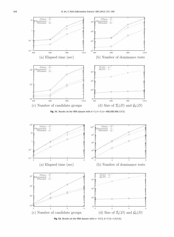
Fig. 11. Results on the NBA dataset with d = 5, k = 5 (n = 400,600,900,1313).

Fig. 12. Results on the NBA dataset with n = 1313, d = 5 (k = 3,4,5,6).


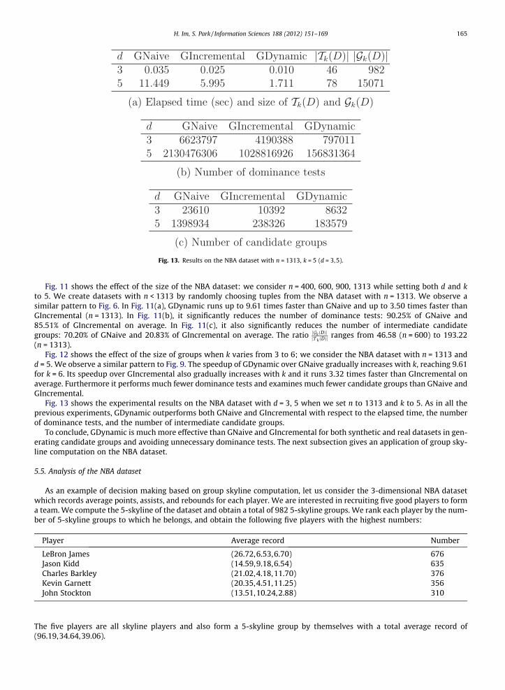
Fig. 13. Results on the NBA dataset with n = 1313, k = 5 (d = 3,5).


Fig. 11 shows the effect of the size of the NBA dataset: we consider n = 400, 600, 900, 1313 while setting both d and kto 5. We create datasets with n < 1313 by randomly choosing tuples from the NBA dataset with n = 1313. We observe asimilar pattern to Fig. 6. In Fig. 11(a), GDynamic runs up to 9.61 times faster than GNaive and up to 3.50 times faster thanGIncremental (n = 1313). In Fig. 11(b), it significantly reduces the number of dominance tests: 90.25% of GNaive and85.51% of GIncremental on average. In Fig. 11(c), it also significantly reduces the number of intermediate candidategroups: 70.20% of GNaive and 20.83% of GIncremental on average. The ratio jGkðDÞj

jT kðDÞjranges from 46.58 (n = 600) to 193.22

(n = 1313).Fig. 12 shows the effect of the size of groups when k varies from 3 to 6; we consider the NBA dataset with n = 1313 and

d = 5. We observe a similar pattern to Fig. 9. The speedup of GDynamic over GNaive gradually increases with k, reaching 9.61for k = 6. Its speedup over GIncremental also gradually increases with k and it runs 3.32 times faster than GIncremental onaverage. Furthermore it performs much fewer dominance tests and examines much fewer candidate groups than GNaive andGIncremental.

Fig. 13 shows the experimental results on the NBA dataset with d = 3, 5 when we set n to 1313 and k to 5. As in all theprevious experiments, GDynamic outperforms both GNaive and GIncremental with respect to the elapsed time, the numberof dominance tests, and the number of intermediate candidate groups.

To conclude, GDynamic is much more effective than GNaive and GIncremental for both synthetic and real datasets in gen-erating candidate groups and avoiding unnecessary dominance tests. The next subsection gives an application of group sky-line computation on the NBA dataset.

5.5. Analysis of the NBA dataset

As an example of decision making based on group skyline computation, let us consider the 3-dimensional NBA datasetwhich records average points, assists, and rebounds for each player. We are interested in recruiting five good players to forma team. We compute the 5-skyline of the dataset and obtain a total of 982 5-skyline groups. We rank each player by the num-ber of 5-skyline groups to which he belongs, and obtain the following five players with the highest numbers:

Player
Average record Number
LeBron James
(26.72,6.53,6.70) 676 Jason Kidd (14.59,9.18,6.54) 635 Charles Barkley (21.02,4.18,11.70) 376 Kevin Garnett (20.35,4.51,11.25) 356 John Stockton (13.51,10.24,2.88) 310
The five players are all skyline players and also form a 5-skyline group by themselves with a total average record of(96.19,34.64,39.06).


Now we wish to form another team to play against the previous team. We find a total of six teams that are incomparablewith the previous team:

Team
Players
1
p1, p2, p3, p4, p5
2
p1, p2, p3, p6, p5
3
p1, p7, p2, p3, p4
4
p1, p7, p2, p3, p6
5
p1, p8, p7, p2, p6
6
p1, p8, p7, p2, p3
Player
Name
p1
Shaquille O’Neal p2 Karl Malone p3 Tim Duncan p4 Dirk Nowitzki p5 Dennis Rodman p6 Chris Webber p7 Michael Jordan p8 Allen Iverson
We have to recruit Shaquille O’Neal who is the only player belonging to all the six teams. Suppose that Dennis Rodman, ChrisWebber, and Allen Iverson refuse to join the new team. Then we choose the team 3 whose total average record is(123.07,17.08,48.41). Interestingly Dirk Nowitzki is not a skyline player as his average record (22.17,2.54,8.66) is dominatedby Karl Malone’s record (24.75,3.99,9.81). (Including Dirk Nowitzki, there are 17 such non-skyline players who belong to 5-skyline groups.)

6. Related work

In this section, we review conventional skyline algorithms and their connection with group skyline computation. Group-byskyline computation in [16] returns skyline sets of multiple groups of tuples and is fundamentally different from group skylinecomputation.

Depending on whether external index structures are used or not, the state-of-the-art skyline algorithms are usu-ally classified into two categories. Those skyline algorithm that do no use external index structures include the block-nested-loop (BNL) algorithm [4] which performs a dominance test between every pair of tuples while maintaining awindow of candidate skyline tuples, the sort-filter-skyline (SFS) algorithm [5] which presorts a dataset according to amonotone preference function so that no tuple is dominated by succeeding tuples in the sorted dataset, LESS (linearelimination sort for skyline) [9] which incorporates two optimization techniques into the external sorting phase ofSFS, and SaLSa (sort and limit skyline algorithm) [2] which presorts a dataset, but unlike SFS and LESS, does notnecessarily inspect every tuple in the sorted dataset. All these algorithms do not take streams of tuples as inputand thus are difficult to adapt for group skyline computation, which needs to generate all candidate groups in a pro-gressive manner.

There are also several skyline algorithms that exploit external index structures. The nearest-neighbor (NN) algorithm [12]and the branch-and-bound skyline (BBS) algorithm [18] use R-trees [10] as their index structures. Lee et al. [13] propose theZSearch algorithm which uses a new variant of B+-tree, called ZBtree, for maintaining the set of candidate skyline tuples inthe increasing order of Z-addresses. Similarly to those algorithms using no external index structures, BBS and ZSearch areinappropriate for group skyline computation because they require an entire dataset in order to build an external indexstructure.

Since group skyline computation generates candidate groups in a progressive manner, we can incorporate into ourgroup skyline algorithms any algorithm for continuous skyline computation on data streams such as [14,17,23]. Forexample, we can replace Gi SðGi [ CiÞ in line 9 in Fig. 4 with an algorithm for continuous skyline computation thatregards Ci as new arrivals in the data stream. Such an algorithm can also take advantage of the property of group sky-line computation that only new groups arrive and no existing groups expire (i.e., the size of the sliding window can beset to infinite).

Recently Su et al. [22] propose top-k combinatorial skyline query (k-CSQ) processing which is similar in spirit to groupskyline computation in that it also considers combinations of tuples. A combination is either a single tuple or a meta-tuple


that combines several tuples using monotone aggregate functions.2 Combinatorial skyline tuples are then defined as the sky-line of all combinations where the maximum number of tuples to be combined is specified by the user. k-CSQ processing returnsk best combinatorial skyline tuples according to a preference order of attributes given by the user. In other words, it returnsthose k combinatorial skyline tuples whose aggregate values for the most preferred attribute are the highest. The preferenceorder is crucial in reducing exponential search space. To find k best combinatorial skyline tuples, it suffices to first sort the data-set according to the user preference and then inspect combinations of only a small number of tuples that appear in the begin-ning of the sorted dataset.

Although Su et al. experimentally show the efficiency of their proposed algorithm for k-CSQ processing, it reports onlythose combinatorial skyline tuples whose aggregate values for a certain attribute are the highest. In contrast, group skylinecomputation considers only groups of the same number of tuples without considering the user preference. Furthermore wefocus on various properties of group skyline computation and efficient generation of all skyline groups by exploiting suchproperties. As discussed in Section 5.5, we may also use skyline groups in more complicated decision making processes.

Another work superficially similar to but clearly different from group skyline computation concerns the problem of cre-ating competitive products proposed by Wan et al. [26]. They also consider combinations of tuples but their objective is tocreate new products that are not dominated by already existing products. A product is a combination of tuples, or compo-nents, each of which comes from a different dataset called a source table and may have distinct attributes. For example, wemay think of laptops as products, and CPUs, memories, and screens as their components. One important property in theproblem of creating competitive products is that when we combine source tables to create new products, it suffices to con-sider only the skyline tuples in each source table, which reduces search space significantly. In contrast to creating compet-itive products which combines tuples of different kinds, group skyline computation combines tuples of the same kind. Hencegroup skyline computation is more appropriate for such problems as recruiting sport players or analyzing stock portfolioswhich deal with homogeneous datasets. Furthermore, as proved in Proposition 2.5, it needs to consider not only skyline tu-ples but also non-skyline tuples, which is the main difference from their work.

7. Conclusion

We have proposed the problem of group skyline computation which is based on dominance tests between groups of thesame number of tuples. After studying its various properties, we have developed a group skyline algorithm GDynamic whichuses the idea of dynamic programming in its design. Through various experiments, we have demonstrated that GDynamic isa practical group skyline algorithm.

Because of the exponential growth in the number of combinations of tuples, group skyline computation is inherentlyexpensive in terms of both time and space. Like previous work on parallel skyline computation [8,19,21,25,27], we may con-sider the parallelization of group skyline computation on distributed or multicore architectures, which is left as future work.As another direction for future work, we may consider a problem of finding a small number of representative skyline groups,similarly to finding a small number of representative skyline tuples [15,24].

Acknowledgments

We thank Hyuk Jun Kweon for the example in Fig. 3 and Sunghwan Kim for the prototype implementation of the groupskyline algorithms. We also thank the anonymous reviewers for their helpful comments. This work was supported by BasicScience Research Program through the National Research Foundation of Korea (NRF) funded by the Ministry of Education,Science and Technology (2009-0077543).

Appendix A

A.1. Proof of Proposition 3.2

Suppose that there exists a 3-skyline group G3 = {p,q,r} that contains no 2-skyline group (where p – q, p – r, q – r). Weshow by contradiction that such a 3-skyline group G3 cannot exist.

Since G3 contains no 2-skyline group, there exists a 2-skyline group that dominates {p,q}. Furthermore such a 2-skylinegroup G2 must include r, since otherwise G2 [ {r} would dominate G3. Hence we assume a 2-skyline group {p0,r} such that{p0,r} � {p,q} with p0 – r. Similarly we assume 2-skyline groups {q0,p} and {r0,q} such that {q0,p} � {q,r} with q0 – p and{r0,q} � {p,r} with r0 – q.

By combining the three dominance relations {p0,r} � {p,q}, {q0,p} � {q,r}, and {r0,q} � {p,r}, we obtain {p0,q0,r0} � {p,q,r}.Since {p,q,r} = G3 is a 3-skyline group, {p0,q0,r0} must contain duplicate tuples. Without loss of generality, we assume thatp0 and q0 are the same tuple (p0 = q0). Then {p0,p} � {q,r} follows from {q0,p} � {q,r}. By combining {p0,p} � {q,r} with {p0,r} �

2 Incidentally their use of monotone aggregate functions is incorrect because Lemma 1 and Theorem 2 in [22] do not hold for the monotone aggregatefunction max. As in this paper, they should use aggregate functions that are strictly monotone in each argument.


{p,q}, we obtain p0 � q and consequently {p,p0,r} � {p,q,r}. Below we show that {p,p0,r} � {p,q,r} contradicts one of theassumptions. We have two cases to consider: (1) p – p0 and (2) p = p0.

Suppose p – p0. Since p – r and p0 – r already hold, {p,p0,r} contains no duplicate tuples and {p,p0,r} � {p,q,r} contradictsthe assumption that {p,q,r} is a 3-skyline group.

Suppose p = p0. From p0 � q, we obtain p � q. From {p0,r} � {p,q}, we obtain r � q. Since p � q and r � q, either {r0,q} is not a2-skyline group by Corollary 2.7 or p = r holds. The former contradicts the assumption that {r0,q} is a 2-skyline group and thelatter the assumption p – r.

Therefore a 3-skyline group always contains a 2-skyline group. h

A.2. Proof of Proposition 3.3

We construct D in such a way that qi and q0i form a pair and correspond to pi for 1 6 i 6 4. Every tuple in D is a skyline tupleand we have T 4ðDÞ ¼ D. We show that G4 = {p1,p2,p3,p4} is a 4-skyline group, but no subset of size 3 is a 3-skyline group.

First we observe that none of {p1,p2,p3}, {p1,p2,p4}, {p1,p3,p4}, and {p2,p3,p4} is a 3-skyline group:

fp1; q1; q01g � fp2;p3;p4g

fp2; q2; q02g � fp1;p3;p4g

fp3; q3; q03g � fp1;p2;p4g

fp4; q4; q04g � fp1;p2;p3g

For example, fp1; q1; q01g � fp2; p3; p4g holds as follows:

Rfp1; q1; q01g ¼ ð1;1;0;0;0;0;0;0;4;9;9;9;5;5;5;8;8;8Þ

Rfp2;p3;p4g ¼ ð0; 0;0;0;0;0;0;0;3;6;6;6;3;3;3;6;6;6Þ

The other three cases are all symmetric because of the way that we construct D. Hence G4 contains no 3-skyline group.Next we show that G4 is indeed a 4-skyline group, that is, no C4 � D dominates G4. There are three mutually exclusive

cases to consider where we assume 1 6 i 6 4 and 1 6 j 6 4.

� For some pair fqi; q0ig, only one of qi 2 C4 and q0i 2 C4 holds. We assume q1 2 C4 and q01 R C4 without loss of generality.

� There is only one pair fqi; q0ig such that both qi 2 C4 and q0i 2 C4 hold. In this case, jC4 \ G4j = 2; otherwise, this case is cov-

ered by the first one. We assume q1 2 C4 and q01 2 C4 without loss of generality.� C4 consists of two pairs fqi; q

0ig and fqj; q

0jg. Without loss of generality, we assume C4 ¼ fq1; q

01; q2; q

02g.

In the first case, we have (RC4)[2] = �1 and (RG4)[2] = 0 and thus C4 ¤ G4. In the second case, we have (RC4)[9] 6 5 and(RG4)[9] = 7 and thus C4 ¤ G4. In the third case, we have (RC4)[13] = 4 and (RG4) [13] = 6 and thus C4 ¤ G4. Hence G4 is a 4-skyline group. h

References

[1] M. Atallah, Y. Qi, Computing all skyline probabilities for uncertain data, in: Proceedings of the 28th ACM SIGMOD-SIGACT-SIGART Symposium onPrinciples of Database Systems, ACM, 2009, pp. 279–287.

[2] I. Bartolini, P. Ciaccia, M. Patella, Efficient sort-based skyline evaluation, ACM Transactions on Database Systems 33 (4) (2008) 1–49.[3] C. Böhm, F. Fiedler, A. Oswald, C. Plant, B. Wackersreuther, Probabilistic skyline queries, in: Proceeding of the 18th ACM Conference on Information and

Knowledge Management, ACM, 2009, pp. 651–660.[4] S. Börzsönyi, D. Kossmann, K. Stocker, The skyline operator, in: Proceedings of the 17th International Conference on Data Engineering, IEEE Computer

Society, 2001, pp. 421–430.[5] J. Chomicki, P. Godfrey, J. Gryz, D. Liang, Skyline with presorting, in: Proceedings of the 19th International Conference on Data Engineering, IEEE

Computer Society, 2003, pp. 717–719.[6] X. Ding, X. Lian, L. Chen, L. Jin, Continuous monitoring of skylines over uncertain data streams, Information Sciences 184 (1) (2012) 196–214.[7] R. Fagin, A. Lotem, M. Naor, Optimal aggregation algorithms for middleware, Journal of Computer and System Sciences 66 (4) (2003) 614–656.[8] A. Cosgaya-Lozano, A. Rau-Chaplin, N. Zeh, Parallel computation of skyline queries, in: Proceedings of the 21st Annual International Symposium on

High Performance Computing Systems and Applications, IEEE Computer Society, 2007, p. 12.[9] P. Godfrey, R. Shipley, J. Gryz, Maximal vector computation in large data sets, in: Proceedings of the 31st International Conference on Very Large Data

Bases, VLDB Endowment, 2005, pp. 229–240.[10] A. Guttman, R-trees: a dynamic index structure for spatial searching, in: Proceedings of the 1984 ACM SIGMOD International Conference on

Management of Data, ACM, 1984, pp. 47–57.[11] G.T. Kailasam, J.-S. Lee, J.-W. Rhee, J. Kang, Efficient skycube computation using point and domain-based filtering, Information Sciences 180 (7) (2010)

1090–1103.[12] D. Kossmann, F. Ramsak, S. Rost, Shooting stars in the sky: an online algorithm for skyline queries, in: Proceedings of the 28th International Conference

on Very Large Data Bases, VLDB Endowment, 2002, pp. 275–286.[13] K.C.K. Lee, B. Zheng, H. Li, W.-C. Lee, Approaching the skyline in Z order, in: Proceedings of the 33rd International Conference on Very Large Data Bases,

VLDB Endowment, 2007, pp. 279–290.[14] X. Lin, Y. Yuan, W. Wang, H. Lu, Stabbing the sky: efficient skyline computation over sliding windows, in: Proceedings of the 21st International

Conference on Data Engineering, IEEE Computer Society, 2005, pp. 502–513.[15] X. Lin, Y. Yuan, Q. Zhang, Y. Zhang, Selecting stars: the k most representative skyline operator, in: Proceedings of the 23rd International Conference on

Data Engineering, IEEE Computer Society, 2007, pp. 86–95.


[16] M-H. Luk, M.L. Yiu, E. Lo, Group-by skyline query processing in relational engines, in: Proceeding of the 18th ACM Conference on Information andKnowledge Management, ACM, 2009, pp. 1433–1436.

[17] M. Morse, J.M. Patel, W.I. Grosky, Efficient continuous skyline computation, Information Sciences 177 (17) (2007) 3411–3437.[18] D. Papadias, Y. Tao, G. Fu, B. Seeger, Progressive skyline computation in database systems, ACM Transactions on Database Systems 30 (1) (2005) 41–82.[19] S. Park, T. Kim, J. Park, J. Kim, H. Im, Parallel skyline computation on multicore architectures, in: Proceedings of the 25th International Conference on

Data Engineering, IEEE Computer Society, 2009, pp. 760–771.[20] J. Pei, B. Jiang, X. Lin, Y. Yuan, Probabilistic skylines on uncertain data, in: Proceedings of the 33rd International Conference on Very Large Data Bases,

VLDB Endowment, 2007, pp. 15–26.[21] J. Selke, C. Lofi, W.-T. Balke, Highly scalable multiprocessing algorithms for preference-based database retrieval, in: Proceedings of the 15th

International Conference on Database Systems for Advanced Applications (DASFAA), 2010, pp. 246–260.[22] I.-F. Su, Y.-C. Chung, C. Lee. Top-k combinatorial skyline queries, in: Proceedings of the 15th International Conference on Database Systems for

Advanced Applications (DASFAA), 2010, pp. 79–93.[23] Y. Tao, D. Papadias, Maintaining sliding window skylines on data streams, IEEE Transactions on Knowledge and Data Engineering 18 (3) (2006) 377–

391.[24] Y. Tao, L. Ding, X. Lin, J. Pei, Distance-based representative skyline, in: Proceedings of the 25th International Conference on Data Engineering, IEEE

Computer Society, 2009, pp. 892–903.[25] A. Vlachou, C. Doulkeridis, Y. Kotidis, Angle-based space partitioning for efficient parallel skyline computation, in: Proceedings of the 2008 ACM

SIGMOD International Conference on Management of Data, ACM, 2008, pp. 227–238.[26] Q. Wan, R.C.-W. Wong, I.F. Ilyas, M.T. Özsu, Y. Peng, Creating competitive products, Proceedings of the VLDB Endowment 2 (1) (2009) 898–909.[27] P. Wu, C. Zhang, Y. Feng, B.Y. Zhao, D. Agrawal, A.E. Abbadi, Parallelizing skyline queries for scalable distribution, in: Proceedings of the 10th

International Conference on Extending Database Technology, 2006, pp. 112–130.[28] S. Zhang, N. Mamoulis, D.W. Cheung, Scalable skyline computation using object-based space partitioning, in: Proceedings of the 35th SIGMOD

International Conference on Management of Data, ACM, 2009, pp. 483–494.

group skyline computation - ntuagtsat/collection/skylines/infosci2012.pdf · group skyline...

Documents