Int J Comput Vis (2008) 77: 175–198DOI 10.1007/s11263-007-0091-7

Efficient Learning of Relational Object Class Models

Aharon Bar-Hillel · Daphna Weinshall

Received: 18 August 2005 / Accepted: 11 September 2007 / Published online: 17 November 2007© Springer Science+Business Media, LLC 2007

Abstract We present an efficient method for learning part-based object class models from unsegmented images repre-sented as sets of salient features. A model includes parts’appearance, as well as location and scale relations betweenparts. The object class is generatively modeled using a sim-ple Bayesian network with a central hidden node containinglocation and scale information, and nodes describing objectparts. The model’s parameters, however, are optimized to re-duce a loss function of the training error, as in discriminativemethods. We show how boosting techniques can be extendedto optimize the relational model proposed, with complexitylinear in the number of parts and the number of features perimage. This efficiency allows our method to learn relationalmodels with many parts and features. The method has anadvantage over purely generative and purely discriminativeapproaches for learning from sets of salient features, sincegenerative method often use a small number of parts andfeatures, while discriminative methods tend to ignore geo-metrical relations between parts. Experimental results aredescribed, using some bench-mark data sets and three setsof newly collected data, showing the relative merits of ourmethod in recognition and localization tasks.

Keywords Object class recognition · Object localization ·Generative models · Boosting · Weakly supervised learning

A. Bar-Hillel (�)Intel Research Israel, P.O.Box 1659, Haifa 31015, Israele-mail: aharon.bar-hillel@intel.com

D. WeinshallComputer Science Department and the Center for NeuralComputation, The Hebrew University of Jerusalem, Jerusalem91904, Israel

1 Introduction

One of the important organization principles of object recog-nition is the categorization of objects into object classes.Categorization is a hard learning problem due to the largeinner-class variability of object classes, in addition to the“common” object recognition problems of varying pose andillumination. Recently, there has been a growing interest inthe task of object class recognition (Fergus et al. 2003, 2005;Agarwal et al. 2004; Opelt et al. 2004b; Csurka et al. 2004;Leibe et al. 2004; Feltzenswalb and Huttenlocher 2005;Fritz et al. 2005; Loeff et al. 2005; Dorkó and Schmid 2005)which can be defined as follows: given an image, deter-mine whether the object of interest appears in the image.In many cases the localization of the object in the image isalso sought.

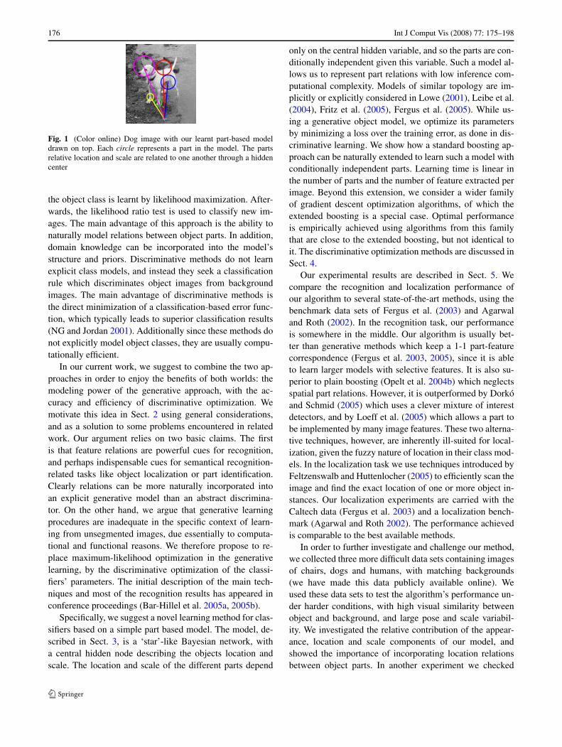
Following previous work (Fergus et al. 2003; Vidal-Naquet and Ullman 2003), we represent an object using apart-based model (see illustration in Fig. 1). Such modelscan capture the essence of most object classes, since theyrepresent both parts’ appearance and invariant relations oflocation and scale between the parts. Part-based models aresomewhat resistant to various sources of variability such aswithin-class variance, partial occlusion and articulation, andthey are potentially convenient for indexing in a more com-plex system (Lowe 2001; Leibe et al. 2004).

Part-based approaches to object class recognition canbe crudely divided into two types: (1) ‘generative’ meth-ods which compute class models (Fergus et al. 2003, 2005;Leibe et al. 2004; Feltzenswalb and Huttenlocher 2005;Fei-Fei et al. 2003; Fritz et al. 2005; Loeff et al. 2005)and (2) ‘discriminative’ methods which do not computeclass models (Opelt et al. 2004a, 2004b; Csurka et al. 2004;Serre et al. 2005; Viola and Jones 2001; Dorkó and Schmid2005). In the Generative approach, a probabilistic model of

176 Int J Comput Vis (2008) 77: 175–198

Fig. 1 (Color online) Dog image with our learnt part-based modeldrawn on top. Each circle represents a part in the model. The partsrelative location and scale are related to one another through a hiddencenter

the object class is learnt by likelihood maximization. After-wards, the likelihood ratio test is used to classify new im-ages. The main advantage of this approach is the ability tonaturally model relations between object parts. In addition,domain knowledge can be incorporated into the model’sstructure and priors. Discriminative methods do not learnexplicit class models, and instead they seek a classificationrule which discriminates object images from backgroundimages. The main advantage of discriminative methods isthe direct minimization of a classification-based error func-tion, which typically leads to superior classification results(NG and Jordan 2001). Additionally since these methods donot explicitly model object classes, they are usually compu-tationally efficient.

In our current work, we suggest to combine the two ap-proaches in order to enjoy the benefits of both worlds: themodeling power of the generative approach, with the ac-curacy and efficiency of discriminative optimization. Wemotivate this idea in Sect. 2 using general considerations,and as a solution to some problems encountered in relatedwork. Our argument relies on two basic claims. The firstis that feature relations are powerful cues for recognition,and perhaps indispensable cues for semantical recognition-related tasks like object localization or part identification.Clearly relations can be more naturally incorporated intoan explicit generative model than an abstract discrimina-tor. On the other hand, we argue that generative learningprocedures are inadequate in the specific context of learn-ing from unsegmented images, due essentially to computa-tional and functional reasons. We therefore propose to re-place maximum-likelihood optimization in the generativelearning, by the discriminative optimization of the classi-fiers’ parameters. The initial description of the main tech-niques and most of the recognition results has appeared inconference proceedings (Bar-Hillel et al. 2005a, 2005b).

Specifically, we suggest a novel learning method for clas-sifiers based on a simple part based model. The model, de-scribed in Sect. 3, is a ‘star’-like Bayesian network, witha central hidden node describing the objects location andscale. The location and scale of the different parts depend

only on the central hidden variable, and so the parts are con-ditionally independent given this variable. Such a model al-lows us to represent part relations with low inference com-putational complexity. Models of similar topology are im-plicitly or explicitly considered in Lowe (2001), Leibe et al.(2004), Fritz et al. (2005), Fergus et al. (2005). While us-ing a generative object model, we optimize its parametersby minimizing a loss over the training error, as done in dis-criminative learning. We show how a standard boosting ap-proach can be naturally extended to learn such a model withconditionally independent parts. Learning time is linear inthe number of parts and the number of feature extracted perimage. Beyond this extension, we consider a wider familyof gradient descent optimization algorithms, of which theextended boosting is a special case. Optimal performanceis empirically achieved using algorithms from this familythat are close to the extended boosting, but not identical toit. The discriminative optimization methods are discussed inSect. 4.

Our experimental results are described in Sect. 5. Wecompare the recognition and localization performance ofour algorithm to several state-of-the-art methods, using thebenchmark data sets of Fergus et al. (2003) and Agarwaland Roth (2002). In the recognition task, our performanceis somewhere in the middle. Our algorithm is usually bet-ter than generative methods which keep a 1-1 part-featurecorrespondence (Fergus et al. 2003, 2005), since it is ableto learn larger models with selective features. It is also su-perior to plain boosting (Opelt et al. 2004b) which neglectsspatial part relations. However, it is outperformed by Dorkóand Schmid (2005) which uses a clever mixture of interestdetectors, and by Loeff et al. (2005) which allows a part tobe implemented by many image features. These two alterna-tive techniques, however, are inherently ill-suited for local-ization, given the fuzzy nature of location in their class mod-els. In the localization task we use techniques introduced byFeltzenswalb and Huttenlocher (2005) to efficiently scan theimage and find the exact location of one or more object in-stances. Our localization experiments are carried with theCaltech data (Fergus et al. 2003) and a localization bench-mark (Agarwal and Roth 2002). The performance achievedis comparable to the best available methods.

In order to further investigate and challenge our method,we collected three more difficult data sets containing imagesof chairs, dogs and humans, with matching backgrounds(we have made this data publicly available online). Weused these data sets to test the algorithm’s performance un-der harder conditions, with high visual similarity betweenobject and background, and large pose and scale variabil-ity. We investigated the relative contribution of the appear-ance, location and scale components of our model, andshowed the importance of incorporating location relationsbetween object parts. In another experiment we checked

Int J Comput Vis (2008) 77: 175–198 177

the contribution of using a large numbers of parts and fea-tures, and demonstrated their relative merits. We experi-mented with a generic interest point detector (Kadir andBrady 2001), as well as with a discriminative interest pointdetector (Gao and Vasconcelos 2004); our results show asmall advantage for the latter. Finally, we showed that theclassifiers learnt perform well against new, unseen back-grounds.

2 Why Mix Discriminative Learning with GenerativeModeling: Motivation and Related Work

In this section we describe the main arguments for combin-ing generative and discriminative methods in the context oflearning from unsegmented images. In Sect. 2.1 we reviewthe distinction between the generative and discriminativeparadigms, and assess the relative merits of each approachin general. We next discuss the specific problem of learningfrom unsegmented images in Sect. 2.2, and characterize it aslearning from unordered feature sets, rather than data vec-tors. In Sect. 2.3 we claim that relations between features,best represented in a generative framework, are useful inthe context of learning from unordered sets, and are specif-ically important for semantical recognition-related tasks.In Sect. 2.4 we argue that generative maximum-likelihoodlearning is highly problematic in the context of learningfrom unsegmented images. Specifically, we argue that suchlearning suffers from inherent computational problems, andthat it is likely to exhibit deficient feature pruning character-istics. To solve these problems while keeping the importantinformation of feature relations, we propose to combine thegenerative treatment of relations with discriminative learn-ing techniques. In Sect. 2.5 we briefly review how featurerelations are handled in related discriminative methods.

2.1 Discriminative and Generative Learning

Generative classifiers learn a model of the probabilityp(x|y) of input x given label y. They then predict the inputlabels by using Bayes rule to compute p(y|x) and choosingthe most likely label. With 2 classes y ∈ {−1,1}, the opti-mal decision rule is the log likelihood ratio test, based onthe statistic:

logp(x|y = 1)

p(x|y = −1)− ν (1)

where ν is a constant threshold. The models p(x|y = 1) andp(x|y = −1) are learnt in a maximum likelihood framework(or maximum-a-posteriori when a useful prior is available).

Discriminative classifiers do not learn probabilistic classmodels. Instead, they learn a direct map from the inputspace X to the labels. The map’s parameters are chosen in

a way that minimizes the training error, or a smooth lossfunction of it. With two labels, the classifier often takes theform sign(f (x)), with the interpretation that f (x) modelsthe log likelihood ratio statistic.

There are several compelling arguments in the learn-ing literature which indicate that discriminative learning ispreferable to generative learning in terms of classificationperformance. Specifically, learning a direct map is consid-ered an easier task than the reliable estimation of p(x|y)

(Vapnik 1998). When classifiers with the same functionalform are learned in both ways, it is known that the asymp-totic error of a reasonable discriminative classifier is loweror equal to the error achievable by a generative classifier(NG and Jordan 2001). In addition, discriminative methodsare often simpler and faster then their generative counter-parts (Ulusoy and Bishop 2005).

However, when we wish to design (or choose) the func-tional form of our classifier, generative models can be veryhelpful. When building a model of p(x|y) we can use ourprior knowledge about the problem’s domain to guide ourmodeling decisions. We can make our assumptions more ex-plicit and gain semantic understanding of the model’s com-ponents. Specifically, the generative framework readily al-lows for the modeling of parts relations, while providingus with a rich toolbox of theory and algorithms for infer-ence and relations learning. It is plausible to expect that acarefully designed classifier, whose functional form is deter-mined by generative modeling, will give better performancethan a classifier from an arbitrary parametric family.

These considerations suggest that a hybrid path may bebeneficial. More specifically, choose the functional form ofthe classifier using a generative model of the data, then learnthe model’s parameters in a discriminative setting. While thearguments in favor of this idea as presented so far are verygeneral, we next claim that when learning from images inparticular, this idea can overcome several problems in cur-rent generative and discriminative approaches.

2.2 Learning from Features Sets

Our primary problem is object class recognition from un-aligned and unsegmented images, which are binary labeledas to whether or not they contain an object from the class.A natural view of this problem is as a binary classificationproblem, where the input is a set of features rather than anordered vector of features, as in standard learning problems.This is an important distinction: vector representation im-plicitly assumes that measurements of the ‘same’ quantitiesare made for all data instances and stored in correspondingindices of the data vectors. The ‘same’ features in differ-ent data vectors are assumed to have the same fixed, simplerelation with the class label (the same ‘role’). Such implicit

178 Int J Comput Vis (2008) 77: 175–198

correspondence is often hard to find in bottom up image rep-resentation, in particular when feature maps or local descrip-tors sets are detected with interest point detectors.

Thus we adopt the view of image representation as a setof features. Each feature has a location index, but unlikean element in a vector, its location does not imply a pre-determined fixed ‘role’ in the representation. Instead, onlyrelations between locations are meaningful. Such represen-tations present a challenge to current learning theory andalgorithms, which are well developed primarily for vectorialinput.

A second inherent problem arises because the relevantfeature set representations usually contain a large number ofspurious features. The images are unsegmented, and there-fore many features may not represent the object of interestat all (but background information), while many other fea-tures may duplicate each other. Thus feature pruning is animportant part of the learning problem.

2.3 Semantics and Part Relations

The lack of feature correspondence between images can behandled in two basic ways: either try to establish correspon-dence, or give it up to begin with. Without correspondence,images are typically represented by some statistical prop-erties of the feature set, without assigning roles to specificimage features. A notable example is the feature histogram,used for example in Csurka et al. (2004), Chan et al. (2004),Thureson and Carlsson (2004) and most of the methods inEveringham et al. (2006). These approaches are relativelysimple and in some cases give excellent recognition results.In addition they tend to have good invariance properties, asthe use of invariant features directly gives invariant classi-fiers. Most of these approaches do not consider feature re-lations, mainly because of their added complexity (an ex-ception is Thureson and Carlsson 2004). The main draw-back of this framework is the complete lack of image se-mantics. While good recognition rates can be achieved, fur-ther recognition related tasks like localization or part iden-tification cannot be done in this framework, as they requireidentifying the role of specific features.

The alternative research choice, which we adopt in thecurrent paper, seeks to identify and correspond featureswith the same ‘role’ in different images. This is done ex-plicitly in some generative modeling approaches (Ferguset al. 2003, 2005; Feltzenswalb and Huttenlocher 2005;Leibe et al. 2004), using the notion of a probabilisticallymodeled ‘part’. The ‘part’ is an entity with a fixed role(probabilistically modeled), and its instantiation in each im-age is a single feature, to be chosen from the set of availableimage features. Discriminative part based methods (Opeltet al. 2004a, 2004b; Agarwal et al. 2004; Vidal-Naquet andUllman 2003), as well as some generative models (Loeff

et al. 2005), use a more implicit ‘part’ notion, and their de-gree of commitment to finding semantically similar featuresin images varies. The important advantage of identifyingparts with fixed roles over the images is the ability to per-form image understanding tasks beyond mere recognition.

When looking in images for parts with fixed roles, fea-ture relations (mainly location and scale relations) providea powerful, perhaps indispensable cue. Basing part identityon appearance criteria alone is possible, and in (Opelt et al.2004a; Serre et al. 2005; Dorkó and Schmid 2005) it leadsto very good recognition results. However, as reported in(Opelt et al. 2004a), the stability of correct part identificationis low, and localization results are mediocre. Specifically, itwas found that typically less than 50% of the instantiatingfeatures were actually located on the object. Instead, manyfeature rely on the difference in background context betweenobject and non-object images. Conversely, good localizationresults are reported for methods based on generative models(Fergus et al. 2003, 2005; Leibe et al. 2004). In Agarwalet al. (2004) a detection task is considered in a discrimina-tive framework. In order to achieve good localization, grosspart relations are introduced as additional features into thediscriminative classifier.

2.4 Learning in Generative Models

We now consider generative model learning when the in-put is a set of unsegmented images. In this scenario, themodel is learnt from a set of object images alone, and itsparameters are chosen to maximize the likelihood of theimage set (sometimes under a certain prior over models).We describe two inherent problems of this maximum like-lihood approach. In Sect. 2.4.1 we claim that such learn-ing involves an essential tradeoff, where computational effi-ciency is traded for weaker modeling which allows repetitiveparts. In Sect. 2.4.2 we review how this problem is handledin some current generative models. In Sect. 2.4.3 we main-tain that generative learning is not well adjusted to featurepruning, and becomes problematic when rich image repre-sentations are used.

2.4.1 The Computational Problem

Assume that the image is represented as a set of features (seeSect. 2.2), that our generative model incorporates part rela-tions, and that we are committed to a notion of ‘part’ instan-tiated by a single image feature, as discussed in Sect. 2.3.Likelihood evaluation and model learning under these con-ditions are hard. Denote the feature set of image I byF(I), and the number of features in F(I) by N . Whilethe input is a feature set, the generative model typicallyspecifies the likelihood P(V |M) for an ordered part vectorV = (f1, . . . , fP ) of P parts. The problem of learning from

Int J Comput Vis (2008) 77: 175–198 179

unordered sets is tackled by considering all the possiblevectors V that can be formed using the feature set.Legitimate part vectors should have no repeated features,and there are O(NP ) such vectors. Thus, the image like-lihood P(I |M) requires marginalization1 over all such vec-tors. Assuming uniform prior over these vectors, we have

P(I |M) =∑

V =(x1,...,xP )∈F(I)P

xi �=xj if i �=j

P (V |M). (2)

Efficient likelihood computation in relational models isonly possible via the decomposition of the joint probabil-ity using conditional independence assumptions, as done ingraphical models. Such decomposition specifies the proba-bility as a product of local terms, each depending on a smallsubset of parts. For a part vector V = (f1, . . . , fP )

P (V |M) =∏

c

�c(V |Sc ) (3)

where Sc ⊂ {1, . . . ,P } are index subsets and V |S = {fi :i ∈ S}. Using dynamic programming, inference and mar-ginalization are exponential in the ‘induced width’ g ofthe related graphical model, which is usually relatively low(note that for trees, g = 2 only).

The summation in (2) does not lend itself easily to suchsimplifications, however. We therefore make the followingapproximation, in which part vectors with repetitive featuresare allowed

P(I |M) =∑

(x1,...,xP )∈F(I)P

xi �=xj for i �=j

∏

c

�c(V |Sc )

≈∑

(x1,...,xP )∈F(I)P

∏

c

�c(V |Sc ). (4)

This approximation is essential to making efficient mar-ginalization possible. If feature repetition is not allowed,global dependence emerges between the features assignedto the different parts (as they cannot overlap). As a result weget global constraints, and efficient enumeration becomesimpossible.

The approximation in (4) may appear minor, which is in-deed the case when a fixed, ‘reasonable’ part based modelis applied to an image. In this case, typically, parts are char-acterized by different appearance and location models, andpart vectors with repetitive parts have low insignificant prob-ability. But during learning, approximation (4) brings abouta serious problem: when vectors with feature repetitions are

1Alternatively, one may approximate the sum in (2) by a max operator,looking for the best model interpretation in the image. This does notaffect the computation considerations discussed here.

Fig. 2 (Color online) A “star” graphical model. Peripheral nodes,shown in blue, are related only via a hidden central node. Such a modelis used in our work, as well as in Fergus et al. (2005). If (i) feature rep-etition is allowed (as in (4)), and (ii) model parameters are chosen tomaximize the likelihood of the best object occurrence, then all the pe-ripheral nodes are optimized to represent the same part

allowed, learning may result in models with many repetitiveparts. In fact, standard maximum likelihood has a strong ten-dency to choose such models. This is because it can easilyincrease the likelihood by choosing the same parts with highlikelihood, over and over again.

The intuition above can be made precise in the simplecase in which a ‘star’ model is used (see Fig. 2) and the sumover all hypotheses is approximated by the single best fea-tures vector. In this extreme case, the maximal likelihood isachieved when all the peripheral parts models are identical.We specifically consider this model in Sect. 3 and prove thelast statement in Appendix 1. The proof doesn’t directly ap-ply when a sum over all the feature vectors is used, but asthis sum is usually dominated by only a few vectors, partrepetition is likely to occur in this case too.

Thus, in conclusion, we see that in the ideal generativeframework, one needs to choose between computational ef-ficiency and the risk of part duplication. One way to escapethis dilemma is by dropping the requirement that a part isinstantiated in a single image feature, as done in (Loeff et al.2005). This, however, leads to a vaguer ‘part’ notion, withlower semantic value. The alternative we suggest here keepsthe ‘part’ notion intact, and gives up generative optimizationinstead.

2.4.2 How is This Computational Problem Handled:Related Work

Several recent approaches use generative modeling for ob-ject class recognition (Fergus et al. 2003, 2005; Fei-Fei et al.2003; Holub et al. 2005; Feltzenswalb and Huttenlocher2005; Loeff et al. 2005). In Fergus et al. (2003), Fei-Fei et al.(2003), Holub et al. (2005) a full relational model is used.The probability P((f1, . . . , fP )|M) in this model cannot bedecomposed into the product of local terms, due to the com-plex probabilistic dependencies between all of the model’sparts (in graphical models terminology the model is a sin-gle large clique). As a result, both learning and recognitionare exponential in the number of model parts, which limitsthe number of parts that can be used (up to 7 in Fergus et al.

180 Int J Comput Vis (2008) 77: 175–198

2003, 4 in Fei-Fei et al. 2003, 3 in Holub et al. 2005), andthe number of features per image (N = 30,20, up to 100 re-spectively). In (Fergus et al. 2005) a decomposable model isproposed with a ‘star’-like topology. This reduces the com-plexity of recognition (i.e., the likelihood evaluation of anexisting model) significantly. However, learning remains es-sentially exponential, in order to avoid part repetition in thelearnt model.

In contrast, the problem (as well as the feature prun-ing problem, discussed in the next section) is completelyavoided in the case of learning from segmented images,as done in Feltzenswalb and Huttenlocher (2005). Here theinput is a set of object images, with manually segmentedparts and manual part correspondence between images. Inthis case learning is reduced to standard maximum likeli-hood estimation of vectorial data. As stated above, Loeffet al. (2005) avoid the computational problem by allowingfor each part to be implemented in many image features.

2.4.3 Feature Pruning

We argued in Sect. 2.2 that feature pruning is necessarywhen learning from images. P , the number of parts in themodel, is often much smaller than the number of featuresper image N . This is usually not the case in classical ap-plications of generative modeling, in which data is typicallydescribed as a relatively small feature vector.

When P � N , maximum likelihood chooses to modelonly parts with high likelihood—often parts which arehighly repetitive in images, with repetitive relations. Thisoptimization policy has a number of drawbacks. On the onehand, it introduces a preference for simple parts, as thesetend to have low variability through images, which givesrise to high likelihood scores. It also introduces preferencefor features which are frequent in natural images, whetherthey belong to the object or not. On the other hand, thereis no explicit preference for discriminative parts, nor anypreference for feature diversity. As a result, certain aspectsof the object may be extensively described, while others areneglected. The problem may be intuitively summarized bystating that generative methods can describe the data, butthey cannot choose what to describe. Additional task relatedsignal, external to the data, is needed, and is most readilyprovided by labels.

In Fergus et al. (2003), Fei-Fei et al. (2003), initial featurepruning is obtained by using the Kadir and Bradey detector(Kadir and Brady 2001), which finds relatively diverse, highentropy regions in the image. Explicit preference is given tofeatures with large scale, which tend to be more discrimina-tive. In addition, they limit the number of features per image(N = 20,30). To some extent, the burden of feature pruningis placed on the pre-learning feature detection mechanisms.However, with such a small number of features per image,

objects do not always get sufficient coverage. In fact, learn-ing is very sensitive to the fine tuning of the feature pruningmechanism.

In Fergus et al. (2005), where a ‘star’-like decomposablemodel is used, more parts and features are used in the gen-erative learning experiments. Surprisingly, the results do notshow obvious improvement. Increasing the number of partsP and features Nf does not typically reduce the error rates,since many of the additional features turn out to be irrel-evant, which makes feature pruning harder. In Sect. 5 weinvestigate the impact that P and Nf have on performancefor models similar to those used by Fergus et al. (2005), butoptimized discriminatively. In our experiments extra infor-mation (increased Nf ) and modeling power (increased P )clearly lead to better performance.

2.5 Relations in Discriminative Methods

Many part based object class recognition methods aremostly discriminative (Opelt et al. 2004b; Vidal-Naquet andUllman 2003; Ullman et al. 2002; Agarwal et al. 2004;Dorkó and Schmid 2005). In most of these methods, spa-tial relations between parts are not considered at all. Whilesome of these systems exhibit state-of-the-art recognitionperformance, they are usually lacking in further, more se-mantical tasks as localization and part identification, as de-scribed in Sect. 2.3. In the ‘fragment based’ approach of(Vidal-Naquet and Ullman 2003; Ullman et al. 2002) rela-tions are not used, but when the same approach is appliedto segmentation, which requires richer semantics, fragmentrelations are incorporated (Borenstein at al. 2004).

One way to incorporate part relations into a discrimina-tive setting is used by the object detection system of Agar-wal et al. (2004). The task is localization, and it requiresthe exact correspondence and the identification of parts. Toachieve this, qualitative location relations between fragmentfeatures are also considered as features, creating a very largeand sparse feature vector. Discriminative learning in thisvery high dimensional space is then done using a specificfeature-efficient learning algorithm. The relational featuresin this scheme are highly qualitative (for example, ‘fragmenta in to the left and bottom of fragment b’). Another problemwith this approach is that supervised learning from high di-mensional sparse vectors is a hard problem, often requiringdimensionality reduction to enable efficient learning.

In this context, our main contribution may be the de-sign of a relatively simple and efficient technique for theintroduction of relational information into the discrimina-tive framework of boosting. As such, our work is relatedto the purely discriminative techniques used in Opelt et al.(2004a, 2004b). In spirit, our work has some resemblanceto the work of (Torralba et al. 2004), in which relationalcontext information is incorporated into a boosting process.

Int J Comput Vis (2008) 77: 175–198 181

However, the techniques we use and the task we considerare quite different.

2.6 Similar Approaches to the Generative-DiscriminativeCombination

In our work, the generative-discriminative combination isaimed at solving a very specific problem: how to allow theefficient learning of part-based models with spatial part re-lations. But when viewed more broadly, it is an instance of amore general recent trend, trying to combine the representa-tion advantage of generative models with the accuracy andgoal-oriented nature of discriminative ones. In many cases,the combination is done by concatenating an initial genera-tive stage, which provides the representation, with a seconddiscriminative stage for the actual classification. In Holubet al. (2005) and Fritz et al. (2005), generative methods (pre-viously presented in Fergus et al. 2003 and Leibe et al. 2004respectively) are augmented with a discriminant SVM-basedsecond stage. This approach is shown to considerably en-hance recognition (Holub et al. 2005) and localization re-sults (Fritz et al. 2005). In these two examples the genera-tive models include spatial relations. Other approaches usea similar 2-stage procedure for a bag-of-features model (Liet al. 2005; Dorkó and Schmid 2005), and obtain excellentrecognition results. In these approaches the set of object im-age features is represented using a Gaussian mixture model,followed by a discriminative procedure which selects infor-mative Gaussian components and uses them for classifica-tion.

In Holub and Perona (2005), Holub et al. present an ob-ject recognition method which, like our proposed scheme,relies on discriminative optimization of a generative modelbased classifier. However, the proposed discriminative op-timization does not solve the computational problem de-scribed in Sect. 2.4.1, and learning is even slower than theparallel generative learning procedure. The models learntare hence limited to 3–4 parts. Note that the 2-stage meth-ods described above (Holub et al. 2005; Fritz et al. 2005) donot solve the computational problem either. Specifically, themethod of Holub et al. (2005) is also limited to 3–4 parts inpractice, and the method of Fritz et al. (2005) learns fromsegmented or highly aligned images.

3 The Generative Model

We represent an input image using a set of local descriptorsobtained using an interest point detector. Some details re-garding this process are given in Sect. 3.1. We then define aclassifier over such sets of features using a generative objectmodel. The model and the resulting classifier are describedin Sects. 3.2 and 3.3 respectively.

3.1 Feature Extraction and Representation

Our feature extraction and representation scheme mostlyfollows the scheme used in Fergus et al. (2003). Initially,images were rescaled to have a uniform horizontal lengthof 200 pixels. We experimented with two feature detec-tors: (1) Kadir & Brady (KB) (Kadir and Brady 2001), and(2) Gao & Vasconcellos (GV) (Gao and Vasconcelos 2004).2

The KB detector is a generic detector. It searches for circu-lar regions of various scales, that correspond to the maximaof an entropy based score in scale space. The GV detectoris a discriminative saliency detector, which searches for fea-tures that permit optimal discrimination between the objectclass and the background class. Given a set of labeled im-ages from two classes, the algorithm finds a set of discrim-inative filters based on the principle of Maximal MarginalDiversity (MMD). It then identifies circular salient regionsat various scales by pooling together the responses of thediscriminative filters.

Both detectors produce an initial set of thousands ofsalient candidates for a typical image (see example inFig. 3a). As in Fergus et al. (2003), we multiply the saliencyscore of each candidate patch by its scale, thus creating apreference for large image patches, which are usually moreinformative. A set of Nf high scoring features with limitedoverlap is then chosen using an iterative greedy procedure.By varying the amount of overlap allowed between selectedfeatures we can vary the number of patches chosen: in ourexperiments we varied Nf between 13 and 513. After theirinitial detection, selected regions are cropped from the im-age and scaled down to 11 × 11 pixel patches. The patchesare then normalized to have zero mean and variance of 1.Finally the patches are represented using their first 15 DCTcoefficients (not including the DC).

To complete the representation, we concatenate 3 addi-tional dimensions to each feature, corresponding to the x

and y image coordinates of the patch, and its scale respec-tively. Therefore each image I is represented using an un-ordered set F(I) of 18 dimensional vectors. Since our sug-gested algorithm’s runtime is only linear in the number ofimage features, we can represent each image using a largenumber of features, typically in the order of several hundredfeatures per image.

3.2 Model Structure

We consider a part-based model, where each part in a spe-cific image Ii corresponds to a patch feature from F(Ii).Denote the appearance, location and scale components of

2We thank Dashan Gao for making his code available to us, and pro-viding useful feedback.

182 Int J Comput Vis (2008) 77: 175–198

Fig. 3 (Color online) a Output of the KB interest point (or feature) de-tector, marked with green circles. b A Bayesian network specifying thedependencies between the hidden variables Cl,Cs and the parts scales

and locations Xkl ,X

ks for k = 1, . . . ,P . The part appearance variables

Xka are independent, and so they do not appear in this network

each vector x ∈ F(I) by xa, xl and xs respectively (with di-mensions 15, 2, 1), where x = [xa, xl, xs]. We can assumethat the appearance of different parts is independent, butthis is obviously not the case with the parts’ scale and lo-cation. However, once we align the object instances with re-spect to location and scale, the assumption of part locationand scale independence becomes reasonable. Thus we intro-duce a 3-dimensional hidden variable C = (Cl,Cs), whichfixes the location of the object and its scale. Our assump-tion is that the location and scale of different parts is con-ditionally independent given the hidden variable C, and sothe joint distribution decomposes according to the graph inFig. 3b.

It follows that for a model with P parts, the joint proba-bility of {Xk}pk=1 and C takes the form

p({Xk}Pk=1,C|�)

= p(C|�)

P∏

k=1

p(Xk|C,θk)

= p(C|�)

P∏

k=1

p(Xka|θk

a )p(Xkl |Cl,Cs, θ

kl )p(Xk

s |Cs, θks ).

(5)

We assume uniform probability for C and Gaussian condi-tional distribution for Xa,Xl,Xs as follows:

P(Xka|θk

a ) = G(Xka|μk

a,�ka),

P (Xkl |Cl,Cs, θ

kl ) = G

(Xk

l − Cl

Cs

∣∣∣∣ μkl ,�

kl

), (6)

P(Xks |Cs, θ

ks ) = G(log(Xk

s ) − log(Cs)|μks , σ

ks ),

where G(·|μ,�) denotes the Gaussian density with meanμ and covariance matrix �. We index the model compo-nents a, l, s as 1,2,3 respectively, and denote the log ofthese probabilities by LG(xj |C,μj ,�j ) for j = 1,2,3.

3.3 A Model Based Classifier

As discussed in Sect. 2.4.1, the likelihood P(I |M) is givenby averaging over all the possible part vectors that can beassembled from the feature set F(I) (see (2)). In our case,we should also average over all the possible values for thehidden variable C. Thus

P(I |M) = K0

∑

C

∑

(x1,...,xp)∈F(I)P

xi �=xj for i �=j

P∏

k=1

P(xk|C,θk) (7)

for some constant K0.In order to allow efficient likelihood assessment we make

the following approximations

P(I |M) ≈ K0

∑

C

∑

(x1,...,xp)∈F(I)P

P∏

k=1

P(xk|C,θk) (8)

≈ K0 maxC,(x1,...,xp)∈F(I)P

P∏

k=1

P(xk|C,θk) (9)

= K0 maxC

P∏

K=1

maxx∈F(I)

P (x|C,θk). (10)

Approximation (8) above was discussed earlier in a moregeneral context (see (4)), and it is necessary in order toeliminate the global dependency between parts. In approx-imation (9), averages are replaced by the likelihood of the

Int J Comput Vis (2008) 77: 175–198 183

best feature vector and best hidden C. This approximationis compelling since as long as the image contains a singleobject from the class, there are rarely two different likelyobject interpretations. In addition, working with the best sin-gle vector uniquely identifies the object’s location and scale,as well as the object’s parts. Such unique identification isrequired for most semantical tasks beyond mere recogni-tion. Finally, the approximated likelihood is decomposedinto separate maxima over C and the different parts in (10).

The decomposition of the maximum achieved in (10) isthe key to the efficient likelihood computation. We discretizethe hidden variable C and consider only a finite grid of lo-cations and scales, with a total of Nc possible values. Us-ing this decomposition the maximum over the Nc · NP

f ar-guments can be computed in O(NcNf P ) operations. How-ever, we cannot optimizing the parameters of such a modelby likelihood maximization. Since feature repetition is al-lowed, the ML solution will choose the same (best) part p

times, as shown in Appendix 1.The natural generative classifier is based on the compari-

son of the LRT statistic to a constant threshold, and it there-fore requires a model of the background in addition to theobject model. Modeling general backgrounds is clearly dif-ficult, due to the diversity of objects and scenes that do notshare simple common features. We therefore approximatethe background likelihood by a constant. Our LRT basedclassifier thus becomes

f (I) = logP(I |M) − log(I |BG) − ν′

= maxC

P∑

k=1

maxx∈F(I)

logp(x|C,θk) − ν (11)

for some constant ν.

4 Discriminative Optimization

Given a set of labeled images {Ii, yi}Ni=1, we wish to find aclassifier f (I) of the functional form given in (11), whichminimizes the exponential loss

L(f ) =N∑

i=1

exp(−yif (Ii)). (12)

This is the same loss minimized by the Adaboost algorithm(Schapire and Singer 1999). Its main advantage in our con-text is that it allows for the determination of the classifierthreshold using a closed form formula, as will be describedin Sect. 4.1.

We have considered two possible techniques for the op-timization of the loss in (12): Boosting and gradient de-

scent. In the boosting context, we view the log probability ofa part

maxx∈F(I)

logp(x|C,θk)

as a weak hypothesis of a specific functional form. However,the classifier form we use in (11) is rather different fromthe traditional classifiers built by boosting, which typicallyhave the form f (I) = ∑P

k=1 αkhk(I ). Specifically, the clas-sifier (11) does not include part weights αk , it has an extrathreshold parameter ν, and it involves a maximization overC, which depends on all the ‘weak’ hypotheses. The thirdpoint is the most problematic, as it requires optimizing overparts with internal dependencies, which is much harder thanoptimization over independent parts as in standard boosting.

In order to simplify the presentation, we assume inSect. 4.1 a simplified model with no spatial relations be-tween the parts, and show how the problems of partsweights and threshold parameters are coped with, with mi-nor changes to the standard boosting framework. In Sect. 4.2we consider the problem of dependent parts, and show howboosting can be naturally extended to handle classifiers as in(11), despite the dependencies between parts due to the hid-den variable C. Finally we consider the optimization froma more general viewpoint of gradient descent in Sect. 4.3.This allows us to introduce several enhancements to the pureboosting technique.

4.1 Boosting of a Probabilistic Model

Let us consider a simplified model with parts appearanceonly (see (6)). We show how such a classifier can berepresented as a sum of weighted ‘weak’ hypotheses inSect. 4.1.1. We then derive the boosting algorithm as an ap-proximate gradient descent in Sect. 4.1.2. This derivation isslightly simpler than similar derivations in the literature, andprovides the basis for our treatment of related parts, intro-duced in Sect. 4.2. In Sect. 4.1.3 we show how the thresholdparameter in our classifier can be readily optimized.

4.1.1 Functional Form of the Classifier

When there are no relations between parts, the classifier (11)takes the following form

f (I) =P∑

k=1

maxx∈F(I)

logp(xa|θka ) − ν. (13)

184 Int J Comput Vis (2008) 77: 175–198

This classifier is easily represented as a sum of weak hy-potheses f (I) = ∑P

k=1 hk(I ) where

hk(I ) = maxx∈F(I)

logG(xa|θka ) − νk (14)

and ν = ∑Pk=1 νk . Weak hypotheses in this form can be

viewed as soft classifiers.We next represent the classifier in an equivalent func-

tional form in which the covariance scale is transformed topart weight. Now f (I) = ∑P

k=1 αkhk(I ) where hk(I ) takesthe form

hk(I ) = maxx∈F(I)

logG(xa|ηka,�

ka) − νk, |�k

a | = 1. (15)

The equivalence of these forms is shown in Appendix 2.

4.1.2 Boosting as Approximate Gradient Descent

Boosting is a common method which learns a classifier ofthe form f (x) = ∑p

k=1 αkhk(x) in a greedy fashion. Sev-eral papers (Friedman et al. 2000; Mason et al. 2000) havepresented boosting as a greedy gradient descent of some lossfunction. In particular, the work of Mason et al. (2000) hasshown that the Adaboost algorithm (Freund and Schapire1996; Schapire and Singer 1999) can be viewed as a greedygradient descent of the exp loss of Eq. (12), in L2 func-tion space. In Friedman et al. (2000) Adaboost is derivedusing a second order Taylor approximation of the exp loss,which leads to repetitive least square regression problems.We suggest here another variation of the derivation, simi-lar to Friedman et al. (2000) but slightly simpler. All threeapproaches lead to an identical algorithm (the discrete Ad-aboost Freund and Schapire 1996) when the weak learn-ers are binary with the range {+1,−1}. For weak learnerswith a continuous output, our approach and the approach ofMason et al. (2000) culminates in the same algorithm, e.g.Adaboost with confidence intervals (Schapire and Singer1999). However, our approach is simpler, and is later usedto derive a boosting version for a model with dependentparts.

Specifically, we derive Adaboost by considering the firstorder Taylor expansion of the exp loss function. In what fol-lows and throughout this paper, we use superscripts to indi-cate the boosting round in which a quantity is measured. Atthe pth boosting round, we wish to extend the classifier f

by f p(x) = f p−1(x)+αphp(x). We first assume that αp isinfinitesimally small, and look for an appropriate weak hy-pothesis hp(X). Since αp is small, we can approximate (12)using the first order Taylor expansion.

To begin with, we differentiate L(f ) w.r.t. αp

dL(f )

dαp= −

N∑

i=1

exp(−yif (xi))yihp(xi). (16)

We denote wi = exp(−yif (xi)), and derive the followingTaylor expansion

L(f p) ≈ L(f p−1) − αp

N∑

i=1

wp−1i yih

p(xi). (17)

Assuming αp > 0, the steepest descent of L(f ) is ob-tained for some weak hypothesis hp which maximizes theweighted correlation score

S(hp(x)) =N∑

i=1

wp−1i yih

p(xi). (18)

This maximization is done by a weak learner, getting as in-put the weights {wp−1

i }Ni=1 and the labeled data points. Afterthe determination of hp(x), the coefficient αp is determinedby the direct optimization of the loss from Eq. (12). Thiscan be done in closed form only for binary weak hypotheseswith output in the range of {1,−1}. In the general case nu-meric methods are employed, such as line search (Schapireand Singer 1999).

4.1.3 Threshold Optimization

Maximizing the linear approximation (17) can be problem-atic when unbounded weak hypotheses are used. In particu-lar, optimizing this criterion w.r.t. to the threshold parameterin hypotheses of the form (14) is ill-posed. Substituting (14)into criterion (17), we get the following expression to opti-mize:

S(h) =N∑

i=1

wiyi

(max

x∈F(I)logG(xi |μa,�a) − ν

)

= C +( ∑

i:yi=−1

wi −∑

i:yi=1

wi

)ν (19)

where C is independent of ν. If∑

i:yi=−1 wi −∑i:yi=1 wi �=

0, S(h) can be increased indefinitely by sending ν to +∞or −∞. Such a choice of ν clearly doesn’t improve the orig-inal (exact) loss (12).

The optimization of the threshold should therefore bedone by considering (12) directly. It is based on the follow-ing lemma:

Lemma 1 Consider a function f : I → R. We wish to min-imize the loss (12) of the function f̃ = f − ν where ν is aconstant. Assume that there are both labels +1 and −1 inthe data set.

1. An optimal ν∗ exists and is given by

ν∗ = 1

2log

[ ∑N{i:yi=−1} exp(f (Ii))

∑N{i:yi=1} exp(−f (Ii))

]. (20)

Int J Comput Vis (2008) 77: 175–198 185

2. The optimal f̃ ∗ = f − ν∗ satisfies

N∑

{i:yi=1}exp(−f̃ ∗(Ii)) =

N∑

{i:yi=−1}exp(f̃ ∗(Ii)). (21)

3. The optimal loss L(f − ν∗) is

2

[N∑

{i:yi=1}exp(−f (Ii)) ·

N∑

{i:yi=−1}exp(f (Ii))

] 12

. (22)

The lemma is proved by direct differentiation of the lossw.r.t. ν, as sketched in Appendix 3.

We use this lemma to determine the threshold after eachround of boosting, when f p(I) = f p−1(I ) + αphp(I).Equation (20) gives a closed form solution for ν oncehp(I) and αp have been chosen. Equation (22) gives theoptimal score obtained, and it is useful when efficient nu-meric search for αp is required. Finally, property (21) im-plies that after threshold update, the coefficient of ν in(19) is nullified (the slope of the linear approximation is0 at the optimum). Hence optimizing the threshold be-fore round p assures that the score S(hp) does not de-pend on νp . We optimize the threshold in our algorithmduring initialization, and after every boosting round (seeAlgorithm 1). The weak learner can therefore effectivelyignore this parameter when choosing a candidate hypothe-sis.

4.2 Relational Model Boosting

We now extend the boosting framework to handle depen-dent parts in a relational model of the form (11). We intro-duce part weights into the classifier by applying the transfor-mation described in (15) to the three model ingredient de-scribed in (6), i.e. appearance, location and scale. The threenew weights are summed into a single part weight, leadingto the following classifier form

f (I) = maxC

P∑

k=1

αkhk(I,C) − ν (23)

where for k = 1, . . . ,P

hk(I,C) = maxx∈F(I)

gk(I,C),

gk(I,C) =3∑

j=1

λkj∑3

j=1 λkj

LG(xkj |C,μk

j ,�kj ), (24)

|�kj | = 1, λk

j > 0, j = 1,2,3.

In this parametrization αk is the sum of componentweights and λi/

∑3j=1 λj measures the relative weights of

the appearance, location and scale. Thus, given an image I ,the computation of f requires the computation of the accu-mulated log-likelihood and its hidden center optimizer, de-noted as follows

ll(I,C) =p∑

k=1

αkhk(I,C),

C∗ = arg maxC

ll(I,C).

(25)

In order to allow tractable maximization over C, we dis-cretize it and consider only a finite grid of locations andscales with Nc possible values. Under these conditions, thecomputation of ll and C∗ amounts to standard MAP mes-sage passing, requiring O(PNf Nc) operations.

Our suggested boosting method is presented in Algo-rithm 1. We derive it by replicating the derivation of standardboosting in (16–18). For f of the form (23), the derivativeof L(f ) w.r.t. αp is now

dL(f )

dαp= −

N∑

i=1

wiyihp(Ii,C

∗i ) (26)

and using the Taylor expansion (17) we get

L(f p) = L(f p−1) − αp

N∑

i=1

wp−1i yih

P (Ii,C∗,p−1i ). (27)

In analogy with the criterion (18), the weak learner

should now get as input {wp−1i ,C

∗,p−1i }N

i=1 and try to max-imize the score

S(hp) =N∑

i=1

wp−1i yih

P (Ii,C∗,p−1i ). (28)

This task is not essentially harder than the weak learner’stask in standard boosting, since the weak learner ‘assumes’that the value of the hidden variable C is known and set toits optimal value according to the previous hypotheses. Inthe first boosting round, when C∗,p−1 is not yet defined, weonly train the appearance component of the hypothesis. Therelational components of this part are set to have low weightsand default values.

Choosing αp after the hypothesis hp(I,C) has been cho-sen is more demanding than in standard boosting. Specifi-cally, αp should be chosen to minimize

L(maxC

[llp−1(I,C) + αphp(I,C)] − ν∗). (29)

186 Int J Comput Vis (2008) 77: 175–198

Algorithm 1 Relational model boosting

Given {(Ii, yi)}Ni=1, yi ∈ {−1,1}, initialize:

ll(i, c) = 0, i = 1, . . . ,N , c in a predefined grid

ν = 1

2log

#{yi = −1}#{yi = 1}

wi = exp(yi · ν), i = 1, . . . ,N

wi = wi

/ N∑

i=1

wi

For k = 1, . . . ,P

1. Use a weak learner to find a part hypothesis hk(I,C)

which maximizes

S(h) =N∑

i=1

wiyih(Ii,C∗i )

(see text for special treatment of round 1).

2. Find optimal αk by minimizing

N∑

{i:yi=1}exp(−f 0(Ii)) ·

N∑

{i:yi=−1}exp(f 0(Ii))

where f 0(I ) = maxC ll(I,C) + αhk(I,C)).Update ll and the optimal center C∗

ll(i, c) = ll(i, c) + αkh(i, c)

[f 0(Ii),C∗i ] = max, arg max

cll(i, c)

3. Update f (Ii) and the weights {wi}Ni=1

ν = 1

2log

[ ∑N{i:yi=−1} exp(f 0(Ii))

∑N{i:yi=1} exp(−f 0(Ii))

]

f (Ii) = f 0(Ii) − ν

wi = exp(−yif (Ii))

wi = wi/

N∑

i=1

wi

Output the final hypothesis

f (I) = maxC

P∑

k=1

αkhk(I,C) − ν

Since the optimal value of C depends on αp , its inferenceshould be repeated whenever a different value is consid-ered for αp (although the messages hp(I,C) can be com-puted only once). After finding the maximum over C, the

loss with the optimal threshold can be computed using (22).The search for the optimal αp can be done using any linesearch algorithm, and we implement it using gradient de-scent as described next in Sect. 4.3.

4.3 Gradient Descent

In this section we combine the relational boosting fromSect. 4.2 with elements from a more general gradient de-scent perspective. In Sect. 4.3.1 we describe our implemen-tation of Algorithm 1, in which the weak learner and thepart weight optimization are gradient based. In Sect. 4.3.2we suggest to supplement Algorithm 1 with feedback ele-ments in the spirit of more traditional gradient descent algo-rithms. Algorithm 2 presents the resulting algorithm for partoptimization.

4.3.1 Gradient-Based Implementation

Current boosting-based object recognition approaches usea version of what we call “selection-based” weak learners(Opelt et al. 2004b; Viola and Jones 2001; Murphy et al.2003). The weak hypotheses family is finite, and hypothe-ses are based on a predefined feature set (Viola and Jones2001) or on the set of features extracted from the trainingimages (Opelt et al. 2004b; Murphy et al. 2003). The weaklearner computes the weighted correlation for all the possi-ble hypotheses and returns the best scoring one. Weak learn-ers of this type, considered in the current paper, sample fea-tures from object images (exhaustive search is too expensivecomputationally); they build part hypotheses based on thefeature and the current estimate of the hidden center C∗ inthe feature’s image. However, as a single feature cannot reli-ably determine the relative weights of the different part com-ponents (the covariance scale of appearance, location andscale), several values of these parameters are considered foreach feature.

As an alternative, we have considered a second type ofweak learners, which we call “gradient-based”. A “gradient-based” weak learner uses a hypothesis supplied by the se-lection learner as its starting point, and tries to improve itsscore using gradient ascent. Unlike the selection based weaklearner, the gradient-based weak learner is not limited toparts based on natural image features, as it searches in thecontinuum of all possible part models. The update rules arebased on the relevant gradient, i.e. the derivative of the scoreS(hp) w.r.t. the part parameters, given by the weighted sum

�θp = ηdS(hp)

dθp= η

N∑

i=1

wp−1i yi

dhp(Ii,C∗,p−1i )

dθp

= η

N∑

i=1

wp−1i yi

dgp(Ii,C∗,p−1i , x

∗,pi )

dθp(30)

Int J Comput Vis (2008) 77: 175–198 187

where η > 0 is a step size and x∗,pi is the best part candidate

in image i

x∗,pi = arg max

x∈F(Ii )

gp(Ii,C∗,p−1i ).

Specifically, θp = {μpj ,�

pj , λ

pj }3

j=1. In order to keep

�pj > 0 during the gradient descent (for j = 1,2) we re-

parameterize (�pj )−1 = (A

pj )tA

pj and descend w.r.t. A

pj .

Dropping the superscript p from all the variables and pa-rameters and denoting gi = gp(Ii,C

∗,p−1i , x

∗,pi ), the gradi-

ents in (30) are given by

dgi

dμj

= −λj�−1j (z∗

i,j − μj ),

dgi

dAj

= −λjAj (z∗i,j − μj )(z

∗i,j − μj )

t ,

(31)

dgi

dλj

= 1/(

3∑

j=1

λj

)[LG(x∗

i,j |C∗i ,μj ,�j )

−3∑

j=1

λj∑3j=1 λj

LG(x∗i,j |C∗

i ,μj ,�j )].

Above x∗i,j stands for the j th component (appearance, loca-

tion or scale) of x∗i and

z∗i,1 = x∗

i,1,

z∗i,2 = (x∗

i,2 − (Cl)∗i )/(Cs)

∗i ,

z∗i,3 = log(x∗

i,3) − log((Cs)∗i ).

The constraints of |�j | = 1 and λj ≥ 0 were enforcedafter each gradient step. Since the gradient depends on thebest part candidates according to the current model, the gra-dient dynamics iterates between gradient steps in the para-meters θp and the re-computation of the best part candidates{x∗,p

i }Ni=1. Pseudo code is given in Step 1 of Algorithm 2.We also use gradient descent dynamics to implement

the line search for the optimal part weight αp . This searchmethod is based on slow, gradual changes in the value of αp ,and hence it allows us to experiment with a feedback mech-anism (see Sect. 4.3.2). The gradient of the loss w.r.t. αp isgiven in (26). Notice that the gradient depends on {C∗

i }Ni=1and {wi}Ni=1, and both are functions of αp . Hence the gra-dient dynamics in this case iterates between gradient stepsof αp , inference of {C∗

i }Ni=1, and updates of {wi}Ni=1. Thisloop is instantiated in Step 3 of Algorithm 2. The loop mustbe preceded by the computation of the messages h(i, c) inStep 2.

Algorithm 2 Optimization of part p

Input : F(Ii), yi , wi , C∗i , i = 1, . . . ,N

ll(i, c), i = 1, . . . ,N, c = 1, . . . ,Nc

initialize weak hypothesis using a selection learner :Choose θ = λj ,μj ,�j , j = 1, . . . ,3, α = 0

Set [h(i,C∗i ), x∗(i)] = max, arg max

x∈F(Ii )

g(x,C∗i )

where g(x, c) = ∑3j=1

λj∑3j=1 λj

LG(xj |c,μj ,�j )

Loop over 1,2,3 K1 iterations

1. Loop over a, b K2 iterations (θ optimization)

(a) Update weak hypothesis parameters

θ = θ + η

N∑

i=1

wiyi

dg(x∗i , c∗

i )

dθ

(b) Update best part candidates for all images

[h(i,C∗i ), x∗

i ] = max, arg maxx∈F(Ii )

g(x,C∗i )

2. Compute for all i, c h(i, c) = maxx∈F(Ii ) g(x, c)

3. Loop over a, b, c K3 iterations (α optimization)

(a) Update α: α = α + η∑N

i=1 wiyih(i,C∗i )

(b) Update hidden center for all images[f 0(Ii),C

∗i ] = max, arg maxc ll(i, c) + αh(i, c)

(c) Update f (Ii) and the weights

ν = 1

2log

[ ∑N{i:yi=−1} exp(f 0(Ii))

∑N{i:yi=1} exp(−f 0(Ii))

]

f (Ii) = f 0(Ii) − ν

wi = exp(−yif (Ii)), wi = wi

/ N∑

i=1

wi

Set llp(i, c) = ll(i, c) + αh(i, c)

Return θ , wi , C∗i , llp(i, c), i = 1, . . . ,N , c = 1, . . . ,Nc.

4.3.2 Gradient-Based Extension

When the determination of both θp and αp are gradi-ent based, the boosting optimization at round p essentiallymakes a specific control choice for a unified gradient descentalgorithm which optimizes αp and θp together. A more tra-ditional gradient descent algorithm can be constructed by (1)differentiating L(f ) directly instead of using its Taylor ap-proximation, and (2) iterating small gradient steps on bothαp and θp in a single loop, instead of two separate loopsas suggested by boosting. In boosting, the optimization ofθp is done before setting αp and there is no feedback be-tween them. Such feedback is plausible in our case, since

188 Int J Comput Vis (2008) 77: 175–198

any change in αp may induce changes in C∗ for some im-ages, and can therefore change the optimal part model ofhp(I,C).

We considered the update steps required for gradient de-scent of the exact loss (12), without the Taylor approxima-tion implied by the boosting strategy. The gradient of αp

(26) and its treatment remain the same, as αp was optimizedw.r.t. the exact loss in the boosting strategy as well. The gra-dient w.r.t. θp is

dL(f )

dθp=

N∑

i=1

wpi yi

dhp(Ii,C∗,pi )

dθp. (32)

While this expression is very similar to (30), there isa subtle difference between them. In (32) wi and C∗

i areno longer constant as they were in (30), but depend on θp

and αp . Exact gradient descent therefore requires the re-computation of wi,C

∗i at each gradient iteration, which is

computationally expensive.We have experimented in the continuum between the

‘boosting’ and the ‘gradient descent’ flavors using Algo-rithm 2, which encloses the optimization loops of hp and αp

in a third ‘feedback’ loop. Setting the outer loop counter K1

to 1 we get the boosting flavor, i.e., Algorithm 2 implementsan inner loop step in Algorithm 1. Setting K1 to some largevalue and K2 = 1, K3 = 1, we get exact gradient descentflavor. We found that a good trade-off between complexityand performance is achieved with a version which is ratherclose to boosting, but still repeats the optimization of αp

and hp several times to allow mutual cross-talk during theestimation of these parameters. Thus, our final optimizationalgorithm involves repeated, sequential calls of Algorithm 2.

5 Experimental Results

We tested our algorithm in recognition tasks using the Cal-tech datasets (Fergus et al. 2003), which are publicly avail-able,3 as well as three more challenging data sets we havecollected specifically for this evaluation. The former areused as a common benchmark, while the latter are designedto measure the performance limits of the algorithm by chal-lenging it with fairly hard conditions. Localization perfor-mance was evaluated using a common benchmark for thistask (Agarwal et al. 2004).4 The datasets are described inSect. 5.1. In Sect. 5.2 we discuss the various algorithm pa-rameters. Recognition results are presented in Sect. 5.3. InSect. 5.4 we report the results of additional experiments,studying the contribution to recognition performance of sev-eral modeling factors in isolation. Finally, we report local-ization results in Sect. 5.5.

3http://www.robots.ox.ac.uk/∼vgg/data.4http://www.pascal-network.org/challenges/VOC/#UIUC.

5.1 Datasets

We compare our recognition results with other methods us-ing the Caltech datasets. Four datasets are used: Motor-cycles (800 images), Cars rear (800), Airplanes (800) andFaces (435). These datasets contain relatively small variancein scale and location, and the background images do not con-tain objects similar to the class objects. In order to test recog-nition performance under harder conditions, we compiled 3new datasets with matching backgrounds.5 These datasetscontain images of Chairs (800 images), Dogs (500) and Hu-mans (593), and are briefly described below. The data setsmentioned above are not well suited for localization experi-ments, since the objects of interest are usually placed in thecenter of the image. We nevertheless present here localiza-tion results for the data sets which include a bounding-boxinformation, which are Airplanes, Motorcycles and Faces.To better estimate the localization ability of our algorithmwe used the UIUC cars side benchmark (Agarwal et al.2004). The training set here is composed of 550 cars im-ages and 500 background images. The test set includes 170images, containing altogether 200 cars, with ground truthbounding boxes.

In the Chairs and Dogs datasets, the objects are seenroughly from the same pose, but include large inner classvariability, as well as some variability in location and scale.For the Chairs dataset we compiled a background datasetof Furniture which contained images of tables, beds andbookcases (200,200,100 images respectively). When possi-ble (for tables and beds), images were aligned to a viewpointisomorphic to the viewpoint of the chairs. As backgroundfor the Dogs dataset, we compiled two animal datasets:‘Easy Animals’ contains 500 images of animals not simi-lar to Dogs; ‘Hard Animals’ contains 250 images from the‘Easy Animals’ dataset, and an additional set of 250 imagesof four-legged animals (such as horses and goats) in a poseisomorphic to the Dogs.

The Humans dataset was designed to include large vari-ability in location, scale and pose. The data contains imagesof 25 different people. Each person was photographed in 4different scales (each 1.5 times larger than its predecessor),at various locations and with several articulated poses of thehands and legs. For each person there are several images inwhich s/he is partially occluded. For this dataset we createda background dataset of 593 images, showing the sites inwhich the Humans images were taken. Figure 4 shows sev-eral images from our datasets.

5.2 Algorithm Parameters

We have run a series of preliminary experiments, in order totune the weak learners’ parameters and compare the results

5The datasets are available at http://www.cs.huji.ac.il/~aharonbh/.

Int J Comput Vis (2008) 77: 175–198 189

Fig. 4 (Color online) Images from the Chairs, Dogs and Humansdatasets and their corresponding backgrounds. Object images appearon the left, background images on the right. In the second row, the twoleftmost background images are of ‘easy animals’ and next are two

‘hard animals’ images. In the third row, the two leftmost object imagesbelong to the easier image subset. The next two images are hard due tothe person’s scale and pose

when using selection-based vs. gradient-based weak learn-ers. The parameters of the selection based weak learner in-clude the number of image patches it samples, and the num-ber of location/scale models used for each sampled patch.The parameters of the gradient based learner include thestep size and stop condition. The gradient based learner isnot limited to hypotheses based on object images, and inmany cases it chooses exaggerated appearance and loca-tion models for the part in order to enhance discriminativepower. In the exaggerated appearance models, the bright-ness contrast is enhanced and the mean patch looks al-most like a Black&White mask (see examples in Fig. 5b).This tendency for exaggerated appearance model is en-hanced when the weight of the location model is relativelyweak.

In exaggerated location models, parts are modeled as be-ing much farther from the center than they are in real objects.An example is given in Fig. 7, showing a chair model wherethe tip of the chair’s leg is located below its mean locationin most images. Still, in most cases gradient based learnersgive lower error rates than their purely selection-based com-petitors. Some examples are given in Fig. 5a. We hence usedgradient based learners in the rest of the recognition experi-ments.

We have also experimented with the learning of covari-ance matrices for the appearance and location models. Asstated in Sect. 4.3.1, we have implemented gradient dynam-ics for the square root of the covariance matrix. However,we have still observed too much over-fitting in the estima-tion of the covariance matrices in our experiments. Theseadditional degrees of freedom tended not to improve the testresults, while achieving lower training error. The problemwas more serious with the appearance covariance matrix,where we have sometimes observed reduced performance,and the emergence of unstable models with covariance ma-trices close to singular. As a result, in the following experi-ments we fix the covariance matrices to σI . We only learn

the covariance scale, which in our model determines the partand component weight parameters.

In the recognition experiments reported in Sect. 5.3, weconstructed models with up to 60 parts using Algorithm 2,with control parameters of K1 = 60, K2 = 100, K3 = 4.Each image was represented using at most Nf = 200 fea-tures (KB detector) or Nf = 240 features (GV detector).The hidden center location values were an equally spacedgrid of 6 × 6 positions over the image. The hidden scalecenter had a single value, or 3 different values with a ra-tio of 0.63 between successive scales, resulting in a totalof Nc = 36,108 values respectively. We randomly selectedhalf of the images from each dataset for training and usedthe remaining half for testing.

For the localization experiments reported in Sect. 5.5we changed several important parameters of the learningprocess. Model accuracy is more important for this task,and we therefore learn smaller models with P = 40 parts,but using a finer location grid of 10 × 10 possible locations(NC = 100) and Nf = 400 features extracted per image.As noted above, the dynamics of the gradient-based loca-tion model tends to produce ‘exaggerated’ models, in whichparts are located too far from the objects center. This ten-dency dramatically reduces the utility of the model for lo-calization. We therefore eliminated the gradient location dy-namics in this context, and modified only the part appear-ance using gradient descent. We found experimentally thatincreasing the weight of the location component uniformlyfor all the parts improves the localization results consider-ably. In the experiments reported below, we multiply thelocation component weights λk

2, k = 1, . . . ,P (see (23) fortheir definition) by a constant factor of 10. Probabilistically,this amounts to smaller location covariance and hence tostricter demands on the accuracy of parts relative locations.Finally, parts without location component (when the loca-tion component weight is 0) are ignored; these parts do notconvey localization information, and therefore add irrelevant‘noise’ to the MAP score.

190 Int J Comput Vis (2008) 77: 175–198

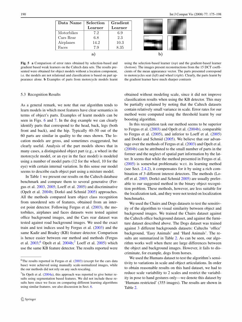
Fig. 5 a Comparison of error rates obtained by selection-based andgradient based weak learners on the Caltech data sets. The results pre-sented were obtained for object models without a location component,i.e. the models are not relational and classification is based on part ap-pearance alone. b Examples of parts from motorcycle models learnt

using the selection-based learner (top) and the gradient-based learner(bottom). The images present reconstructions from the 15 DCT coeffi-cients of the mean appearance vector. The parts presented correspondto motorcycles seat (left) and wheel (right). Clearly, the parts learnt bythe gradient learner have much sharper contrasts

5.3 Recognition Results

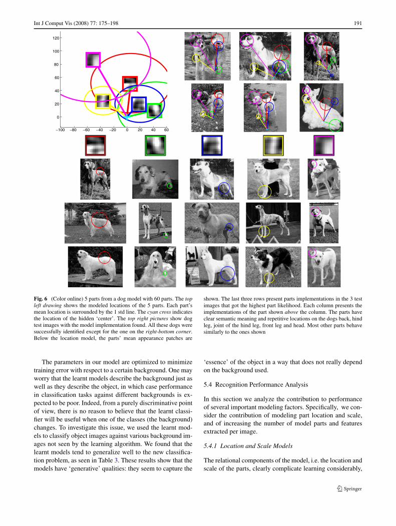
As a general remark, we note that our algorithm tends tolearn models in which most features have clear semantics interms of object’s parts. Examples of learnt models can beseen in Figs. 6 and 7. In the dog example we can clearlyidentify parts that correspond to the head, back, legs (bothfront and back), and the hip. Typically 40–50 out of the60 parts are similar in quality to the ones shown. The lo-cation models are gross, and sometimes exaggerated, butclearly useful. Analysis of the part models shows that inmany cases, a distinguished object part (e.g., a wheel in themotorcycle model, or an eye in the face model) is modeledusing a number of model parts (12 for the wheel, 10 for theeye) with certain internal variation. In this sense our modelseems to describe each object part using a mixture model.

In Table 1 we present our results on the Caltech databasebenchmark and compare them to several generative (Fer-gus et al. 2003, 2005; Loeff et al. 2005) and discriminative(Opelt et al. 2004b; Dorkó and Schmid 2005) approaches.All the methods compared learn object class recognitionfrom unordered sets of features, obtained from an inter-est point detector. Following Fergus et al. (2003), the mo-torbikes, airplanes and faces datasets were tested againstoffice background images, and the Cars rear dataset wastested against road background images. We used the exacttrain and test indices used by Fergus et al. (2003) and thesame Kadir and Bradey (KB) feature detector. Comparisonis hence easier between our method and methods (Ferguset al. 2003;6 Opelt et al. 2004b;7 Loeff et al. 2005) whichuse the same KB feature detector. The results reported were

6The results reported in Fergus et al. (2003) (except for the cars database) were achieved using manually scale-normalized images, whilethe our methods did not rely on any such rescaling.7In Opelt et al. (2004a), this approach was reported to give better re-sults using segmentation based features. We did not include these re-sults here since we focus on comparing different learning algorithmsusing similar features. see also discussion in Sect. 6.

obtained without modeling scale, since it did not improveclassification results when using the KB detector. This maybe partially explained by noting that the Caltech datasetscontain relatively small variance in scale. Error rates for ourmethod were computed using the threshold learnt by ourboosting algorithm.

In this recognition task our method seems to be superiorto Fergus et al. (2003) and Opelt et al. (2004b), comparableto Fergus et al. (2005), and inferior to Loeff et al. (2005)and Dorkó and Schmid (2005). We believe that our advan-tage over the methods of Fergus et al. (2003) and Opelt et al.(2004b) can be attributed to the small number of parts in theformer and the neglect of spatial part information by the lat-ter. It seems that while the method presented in Fergus et al.(2005) is somewhat problematic w.r.t. its learning method(see Sect. 2.4.2), it compensates for it by using a rich com-bination of 3 different interest detectors. The methods (Lo-eff et al. 2005; Dorkó and Schmid 2005) are usually prefer-able to our suggested method in the binary object recogni-tion problem. These methods, however, are less suitable forthe localization task, and they were not tested on localizationbenchmarks.

We used the Chairs and Dogs datasets to test the sensitiv-ity of the algorithm to visual similarity between object andbackground images. We trained the Chairs dataset againstthe Caltech office background dataset, and against the furni-ture dataset described above. The Dogs dataset was trainedagainst 3 different backgrounds datasets: Caltechs ‘office’background, ‘Easy Animals’ and ‘Hard Animals’. The re-sults are summarized in Table 2. As can be seen, our algo-rithm works well when there are large differences betweenthe object and background images. However, it fails to dis-criminate, for example, dogs from horses.

We used the Humans dataset to test the algorithm’s sensi-tivity to variations in scale and object articulations. In orderto obtain reasonable results on this hard dataset, we had toreduce scale variability to 2 scales and restrict the variabil-ity in pose to hand gestures only—we denote this dataset by‘Humans restricted’ (355 images). The results are shown inTable 2.

Int J Comput Vis (2008) 77: 175–198 191

Fig. 6 (Color online) 5 parts from a dog model with 60 parts. The topleft drawing shows the modeled locations of the 5 parts. Each part’smean location is surrounded by the 1 std line. The cyan cross indicatesthe location of the hidden ‘center’. The top right pictures show dogtest images with the model implementation found. All these dogs weresuccessfully identified except for the one on the right-bottom corner.Below the location model, the parts’ mean appearance patches are

shown. The last three rows present parts implementations in the 3 testimages that got the highest part likelihood. Each column presents theimplementations of the part shown above the column. The parts haveclear semantic meaning and repetitive locations on the dogs back, hindleg, joint of the hind leg, front leg and head. Most other parts behavesimilarly to the ones shown

The parameters in our model are optimized to minimizetraining error with respect to a certain background. One mayworry that the learnt models describe the background just aswell as they describe the object, in which case performancein classification tasks against different backgrounds is ex-pected to be poor. Indeed, from a purely discriminative pointof view, there is no reason to believe that the learnt classi-fier will be useful when one of the classes (the background)changes. To investigate this issue, we used the learnt mod-els to classify object images against various background im-ages not seen by the learning algorithm. We found that thelearnt models tend to generalize well to the new classifica-tion problem, as seen in Table 3. These results show that themodels have ‘generative’ qualities: they seem to capture the

‘essence’ of the object in a way that does not really dependon the background used.

5.4 Recognition Performance Analysis

In this section we analyze the contribution to performanceof several important modeling factors. Specifically, we con-sider the contribution of modeling part location and scale,and of increasing the number of model parts and featuresextracted per image.

5.4.1 Location and Scale Models

The relational components of the model, i.e. the location andscale of the parts, clearly complicate learning considerably,

192 Int J Comput Vis (2008) 77: 175–198

Fig. 7 (Color online) 5 parts from a chair model. The model is pre-sented in the same format as Fig. 6. Model parts represent the tip ofthe chairs leg (first part), edges of the back (second and forth parts),

the seat corner (third) and the seat edge (fifth). The location model isexaggerated: The tip of the chairs leg is modeled as being far below itsreal mean position in object images

Table 1 Test error rates over the Caltech dataset, showing the results of our method in 2 conditions—using 7 or 50 parts compared to severalother methods. The algorithm’s parameters were held constant across all experiments

Data name Our model Fergus et al. (2003) Opelt et al. (2004b) Fergus et al. (2005) Loeff et al. (2005) Dorkó and Schmid (2005)

50 parts

Motorbikes 4.9 7.5 7.8 4.0 3.0 0.5

Cars Rear 0.6 9.7 8.9 12.3 2.0 –

Airplanes 6.7 9.8 11.1 6.8 3.0 1.5

Faces 6.3 3.6 6.5 11.9 1.3 0.9

Table 2 Error rates with the new datasets of Chairs, Dogs and Hu-mans. Results were obtained using the KB detector (see text for moredetails)

Data Background Test error

Chairs Office 2.23

Chairs Furniture 15.53

Dogs Office 8.61

Dogs Easy Animals 19.0

Dogs Hard Animals 34.4

Humans Sites 34.3

Humans (resticted) Sites 25.9

and it is important to understand if they give any perfor-mance gain. Table 4 shows comparative results varying themodel complexity. Specifically we present results when us-ing only an appearance model, and when adding locationand scale models, using the GV detector (Gao and Vasconce-

los 2004).8 We can see that although the appearance modelproduces very reasonable results, adding a location modelsignificantly improves performance. The additional contri-bution of the scale model is relatively minor. Additionally,by comparing the results of our full blown model (A+L+S)

to those presented in Tables 1 and 2, we can see that the dis-criminative GV detector usually provides somewhat betterresults than those obtained using the generic KB detector.

5.4.2 Large Numbers of Parts and Features

When hundreds of features are used per image, many fea-tures lie in the background of the image, and learning goodparts implicitly requires feature pruning. Figure 8 gives er-ror rates as a function of the number of parts and features.Significant performance gains are obtained by scaling up

8Similar experiments with the KB detector yielded similar results, butshowed no significant improvement with scale modeling.

Int J Comput Vis (2008) 77: 175–198 193

these quantities, indicating that the algorithm is able to findgood part models even in the presence of many clutter fea-tures. This behavior should be contrasted with the generativelearning of a similar model in Fergus et al. (2005), where in-creasing the number of parts and features does not usuallylead to improved performance. Intuitively, maximum likeli-hood learning chooses to model features which are frequentin object images, even if these are simple clutter featuresfrom the background, while discriminative learning natu-rally tends to selects more distinctive parts.

Table 3 Generalization results of some learnt models to new back-grounds. Each row describes results of a single class model trainedagainst a specific background and tested against other backgrounds.Test errors were computed using a sample of 100 images from eachtest background. The classifiers based on learnt models perform wellin most of the new classification tasks. There is no apparent connec-tion between the difficulty of the training background and successfulgeneralization to new backgrounds

Data Original Motorcycles Airplanes Sites

BG BG BG BG

Cars Road (0.6) 3.0 2.2 6.8

Cars Office (1.6) 1.0 0.8 6.4

Chairs Office (2.2) 8.0 1.4 6.2

Chairs Furniture (15.5) 17.4 4.2 8.4

Dogs Office (8.6) 10.3 4.0 12.3

Dogs Easy animals (19.0) 15.7 5.7 7.7

5.5 Localization Results

Locating an object in a large image is much harder than thebinary present/absent detection task. The latter problem istackled in this paper using a limited set of image features,and a crude grid of possible object locations. For localiza-tion we use a similar framework in learning, but turn to amore exhaustive search at the test phase. While searchingwe do not select representative features, but consider in-stead as part candidates all the possible image patches atevery location and several scales. Object center candidatesare taken from a dense grid of possible image locations. Tosearch efficiently, we use the methods proposed in Ferguset al. (2005), Feltzenswalb and Huttenlocher (2005), whichallow such an exhaustive search in a relatively low compu-tational cost.

Table 4 Errors rates using models of varying complexity. (A) Ap-pearance model alone. (A + L) Appearance and location models.(A + L + S) Appearance, location and scale models. The algorithm’sparameters were held constant across all experiments

Data name A A + L A + L + S

Motorbikes 8.1 3.2 3.5

Cars Rear 4.0 1.4 0.6

Airplanes 15.1 15.1 12.1

Faces 6.1 5.2 3.8

Chairs 16.3 10.8 10.9

Fig. 8 a) Error rate as a function of the number of parts P in the model on the Caltech datasets for Nf = 200. b) Error rate as a function ofthe number of image features Nf on the Cars rear (easy) and Airplanes (Relatively hard) Caltech datasets, with P = 30. In b), the X axis variesbetween 13 and 228 features in log scale, base 2. All the results were obtained using the KB detector

194 Int J Comput Vis (2008) 77: 175–198

The model is applied to an image following a three stageprotocol:

1. Convolve the image with the first 15 filters of the DCTbase at Ns scales, yielding Ns × 15 coefficient ‘activitymaps’. We use Ns = 5, spanning patch sizes between 5and 30 pixels.

2. Compute P ×Ns appearance maps by applying the partsappearance models to the vector of DCT coefficients atevery image location. The coordinate values (x, y) inmap (k, j) contain the log probability of part k with scalej in location (x, y).

3. Apply the relational model to the set of appearance maps,yielding a single log probability map for the ‘hiddencenter’ node. To this end, the Ns appearance maps ofeach part are merged into a single map by choosingat each coordinate the most likely part scale. We thencompute P part message maps, corresponding to themessages hk(I,C) defined in (24), by applying the dis-tance transform (Feltzenswalb and Huttenlocher 2005) tothe merged appearance maps. Finally the ‘hidden cen-ter’ map is formed as a weighted sum of parts messagemaps.

5.5.1 Caltech Data Sets

3 data sets used in the recognition experiments are suppliedwith bounding box information: Airplanes, Motorcycles andFaces. However, only in the latter objects have significantlocation variance, specifically in the X-axis. On these datasets we measure localization accuracy using the distance be-tween the true and the detected object center, normalized bythe bounding box size. These measurements are collectedseparately for the x and y axis (normalized by the x andy sizes of the bounding box respectively), and for the twodimensional Euclidean distance (normalized by the bound-ing box diagonal). Median scores for the three data sets are

Table 5 Median Localization scores for Caltech data sets. The scoresare distances between true and detected object centers, normalized bythe bounding box length in the relevant dimension. In the parenthesisthe same scores are given for the null hypothesis, placing the object atthe image center. We can see that the inaccuracies in median detectionare not larger than 10% of the bounding box size for all categories

Data Name x axis y axis√

(x2 + y2)

Motorbikes 0.0251 (0) 0.0577 (0) 0.0463 (0)

Airplanes 0.0516 (0.0281) 0.1048 (0.0938) 0.0699 (0.0495)

Faces 0.0743 (0.2018) 0.0325 (0.0313) 0.0583 (0.1313)

Fig. 9 (Color online) 5 parts from the car side model used in the lo-calization task. The parts shown correspond to the two wheels, frontand rear ends, and the top-rear corner. The complete model includes38 parts, most of them with clear semantics. While the model is not

symmetric w.r.t. to the x axis, it is not far from being so. It hence hap-pens that a car is successfully detected, but its direction is not properlyidentified

Int J Comput Vis (2008) 77: 175–198 195

Fig. 10 (Color online) Hidden center probability maps and car de-tections. In each image pair, the left image shows the probability mapfor the location of reference point C. The right image shows the 5parts from Fig. 9 superimposed on the detected cars. Top Successfuldetections. Notice that the middle of a gap between two cars tends toemerge as a probable car candidate, as it gains support from both cars.

Bottom Problematic detections. The third example includes a spuriousdetection and a car detected using the model of the ‘wrong’ direction.The bottom example includes a spurious ‘middle car’ between tworeal cars. Values in the probability maps were thresholded and linearlytransformed for visualization

reported in Table 5, as well as median scores for the null hy-pothesis, stating that the object is located at the image center.Clearly the final localization is quite accurate in these exper-iments. Note, however, that these results are only significantfor the faces data set—the only one (in the CalTech data)with any meaningful variation in object location, as can beseen in the scores of the null hypothesis. Similar effects werenoticed in Loeff et al. (2005).

5.5.2 UIUC Cars Side Data

The data includes cars facing both directions (i.e. left-to-right and right-to-left). We therefore flip the training imagesprior to training, such that all cars face the same direction.At the test phase we run the exhaustive search for the learnt

model and its mirror image. We detect local maxima in thehidden center map, sort them according to likelihood, andprune neighboring maxima in a way similar to the neigh-borhood suppression technique suggested in Agarwal et al.(2004). Figure 10 presents some probability maps and de-tected cars, illustrating typical successful and problematicdetections. Each detection is labeled as hit or miss using thecriterion used in Agarwal and Roth (2002) (which is slightlydifferent from the one used in Agarwal et al. (2004)), toallow for a fair comparison with other methods. Figure 11presents a precision-recall curve and a comparison of theachieved localization performance to several recently sug-gested methods. Our results are comparable to those ob-tained by the best methods, and are inferior only to classi-

196 Int J Comput Vis (2008) 77: 175–198

Fig. 11 a Recall-Precision curve for cars side detection, using the model shown in Fig. 9. b Error rates (recall = 1 − precision) obtained on thecars side data by several recent methods. Our performance is comparable to the best methods of weakly supervised learning

fiers learnt using ‘strong’ supervision, in the form of im-ages with parts segmentations (e.g. the stronger classifiersin Leibe et al. 2004). In such a method part identities arenot learnt but chosen manually, and so the learning task issimpler.

6 Discussion

We have presented a method for object class recognition andlocalization, based on discriminative optimization of a rela-tional generative model. The method combines the naturaltreatment of spatial part relations, typical to generative clas-sifiers, with the efficiency and pruning ability of discrimi-native methods. Efficient, scalable learning is achieved byextending boosting techniques to a simple relational modelwith conditionally dependent parts. In a recognition task,our method compares favorably with several purely gener-ative or purely discriminative systems recently proposed. Ina localization task its performance is comparable to the bestavailable methods.

While our recognition results are good, (Opelt et al.2004a; Serre et al. 2005) report better results obtained usingdiscriminative methods which ignore geometric relationsand focus instead on feature representation. Specifically, inOpelt et al. (2004a) segmentation based features are used,while in Serre et al. (2005) features are based on flexibleexhaustive search of ‘code book’ patches. The recognitionperformance of these approaches relies on better feature ex-traction and representation, compared with our simple com-bination of interest point detection and DCT-based repre-sentation. We regard the advances offered by these meth-ods as orthogonal to our main contribution, i.e. the efficientincorporation of geometrical relations. The advantages canbe combined by combining better part appearance modelsand better feature extraction techniques with the relationalboosting technique suggested here. We intend to continueour research along these lines.

The complexity of our suggested learning technique islinear in the number of parts and features per image, butit may still be quite expensive. Specifically, the inferencecomplexity of the hidden center C is O(NcNf P ) where Nc

is the number of considered center locations, and this infer-ence is carried for each image many times during learning.This limits us to a relatively crude grid of possible centerlocations in the learning process, and hence limits the accu-racy of the location model learnt. A possible remedy is toconsider less exhaustive methods for inferring the optimalhidden center, based on part voting or mean shift mode es-timation, as done in (Leibe et al. 2004). Such ‘heuristic’ in-ference solutions may offer enhanced scalability and a morebiologically plausible recognition mechanism.

Finally, leaving technical details aside, we regard thiswork as a contribution to an important debate in learningfrom unprocessed images, regarding the choice of genera-tive vs. discriminative modeling. We demonstrated that com-bining generative relational modeling with discriminativeoptimization can be fruitful and lead to more scalable learn-ing. However, this combination is not free of problems. Ourtechnical problems with covariance matrix learning and thetendency of our technique to produce ‘exaggerated’ modelsare two examples. The method proposed here is a step to-wards the required balance between the descriptive powerof generative models and the task relatedness enforced bydiscriminative optimization.

Acknowledgements We are indebted to Tomer Hertz, who has beeninvolved in the early stages of this research, for his support and his helpin the empirical validation of the method.

Appendix 1: Feature Repetition and ML Optimizationin a Star Model

Allowing feature repetitions, we derived the likelihood ap-proximation (10) for our star model. For a set of object im-

Int J Comput Vis (2008) 77: 175–198 197

ages {Ij }nj=1. This approximation entails the following totaldata likelihoodn∑

j=1

logP(Ij |�)

= n logK0 +n∑

j=1

log

[max

C

P∏

K=1

maxx∈F(Ij )

P (x|C,θk)

]

= n logK0 +n∑

j=1

maxC

P∑

K=1

maxx∈F(Ij )

logP(x|C,θk). (33)

The maximum likelihood parameters � = (θ1, . . . , θP )

are chosen to maximize this likelihood. In this maximiza-tion, we can ignore the constant term n logK0. To simplifyfurther notation let us denote parts’ conditional log likeli-hood terms by gj (C, θk) = maxx∈F(Ij ) P (x|C,θk). Also de-note the vector of the hidden center variables in all imagesby C = (C1, . . . ,Cn).

max�

[ n∑

j=1

maxC

P∑

K=1

gj (C, θk)

]

= max(C1,...,Cn)

[max

�

n∑

j=1

P∑

K=1

gj (Cj , θk)

]

= max C

P∑

K=1

maxθk

[ n∑

j=1

gj (Cj , θk)

]. (34)

For any fixed centers vector C, and any 1 ≤ k ≤ P , theoptimal θk is determined as θk = arg maxθ G(θ, C) whereG(θ, C) = ∑n

j=1 gj (Cj , θ). Hence, for any C, the optimal

part parameters θk are identical, as maxima of the samefunction. Clearly the maximum over C also posses this prop-erty.

The proof can be repeated in a similar way for the starmodel presented in Fergus et al. (2005), in which the centernode is an additional ‘landmark’ part, as long as the sumover all model interpretations in an image is replaced by thesingle maximal likelihood interpretation.

Appendix 2: Part Weights Introduction

Here we establish the functional equivalence between clas-sifiers with and without part weights for weak learners of theform (14). We use the identity

logG(x|μ,�) − ν = α[logG(x|μ′,�′) − ν′] (35)

where

μ′ = μ, �′ = α�,

ν′ = 1

α

[ν + d(1 − α)

2log 2π + 1 − α

2log |�| − αd

2logα

]

to introduce part weights into the classifier. This identity istrue for all α > 0. We apply this identity to each part k in theclassifier (14), with αk = |�k

a |−1/d , to obtain

f (I) =P∑

k=1

maxx∈F(I)

logG(x|μka,�

ka) − νk

=P∑

k=1

αk[ maxx∈F(I)

logG(x|μka,�

k′a ) − νk′ ] (36)

where �k′a = αk�k

a is has a fixed determinant of 1 for allparts. The weights αk therefore (inversely) reflect covari-ance scale.

Appendix 3: Proof of Lemma 1

We differentiate the loss w.r.t. ν

0 = d

dν

N∑

i=1

exp(−yi[f (Ii) − ν])

= −∑

{i:yi=1}exp(−f (Ii) + ν)

+∑

{i:yi=−1}exp(f (Ii) − ν). (37)

For f̃ = f − ν, (37) gives property (21). Solving for ν gives

exp(ν)∑

{i:yi=1}exp(−f (Ii))

= exp(−ν)∑

{i:yi=−1}exp(f (Ii)) (38)

from which (20) follows. Finally, we can compute the lossusing the optimal ν∗

N∑

i=1

exp(−yi[f (Ii) − ν∗])

=[ ∑

{i:yi=−1} exp(f (Ii))∑{i:yi=1} exp(−f (Ii))

] 12 ∑

{i:yi=1}exp(−f (Ii))

+[ ∑

{i:yi=−1} exp(f (Ii))∑{i:yi=1} exp(−f (Ii))

]− 12 ∑

{i:yi=−1}exp(f (Ii))

from which (22) follows.

References

Agarwal, S., Awan, A., & Roth, D. (2004). Learning to detect objectsin images via a sparse, part based representation. Pattern Analysisand Machine Intelligence, 20(11), 1475–1490.

198 Int J Comput Vis (2008) 77: 175–198

Agarwal, S., & Roth, D. (2002). Learning a sparse representation forobject detection. In ECCV (pp. 113–130).

Bar-Hillel, A., Hertz, T., & Weinshall, D. (2005a). Efficient learning ofrelational object class models. In ICCV.

Bar-Hillel, A., Hertz, T., & Weinshall, D. (2005b). Object class recog-nition by boosting a part based model. In CVPR. Los Alamitos:IEEE Computer Society

Borenstein, E., Sharon, E., & Ullman, S. (2004). Combining top-downand bottom-up segmentation. In IEEE workshop on perceptual or-ganization in computer vision (CVPR).

Chan, A. B., Vasconcelos, N., & Moreno, P. J. (2004). A family ofprobabilistic kernels based on information divergence.

Csurka, G., Bray, C., Dance, C., & Fan, L. (2004). Visual categoriza-tion with bags of keypoints. In ECCV.

Dorkó, G., & Schmid, C. (2005, submitted). Object class recognitionusing discriminative local features. IEEE Transactions on PatternAnalysis and Machine Intelligence.

Everingham, M. R., Zisserman, A., Williams, C. K. I., & Van Gool,L. et al. (2006). The 2005 pascal visual object classes challenge.In J. Quinonero-Candela, I. Dagan, B. Magnini, & F. d’Alche-Buc(Eds.), LNAI: Vol. 3944. Machine learning challenges. Evaluatingpredictive uncertainty, visual object classification, and recognis-ing textual entailment (pp. 117–176).

Fei-Fei, L., Fergus, R., & Perona, P. (2003). A bayesian approach tounsupervised one shot learning of object catgories. In ICCV.

Feltzenswalb, P., & Huttenlocher, D. (2005). Pictorial structures forobject recognition. International Journal of Computer Vision, 61,55–79.

Fergus, R., Perona, P., & Zisserman, A. (2003). Object class recog-nition by unsupervised scale invariant learning. In CVPR. LosAlamitos: IEEE Computer Society

Fergus, R., Perona, P., & Zisserman, A. (2005). A sparse object cat-egory model for efficient learning and exhaustive recognition. InCVPR.

Freund, Y., & Schapire, R. E. (1996). Experiments with a new boostingalgorithm. In ICML (pp. 148–156).

Friedman, J. H., Hastie, T., & Tibshirani, R. (2000). Additive logisticregression: a statistical view ofboosting. Annals of Statistics, 28,337–407.

Fritz, M., Leibe, B., Caputo, B., & Schiele, B. (2005). Integrating rep-resentative and discriminant models for object category detection.In ICCV.

Gao, D., & Vasconcelos, N. (2004). Discriminant saliency for visualrecognition from cluttered scenes. In NIPS.

Holub, A. D., & Perona, P. (2005). A discriminative framework formodeling object classes. In CVPR.

Holub, A. D., Welling, M., & Perona, P. (2005). Combining generativemodels and fisher kernels for object class recognition. In ICCV.

Kadir, T., & Brady, M. (2001). Scale, saliency and image description.International Journal of Computer Vision, 45(2), 83–105.

Leibe, B., Leonardis, A., & Schiele, B. (2004). Combined object cat-egorization and segmentation with an implicit shape model. InECCV workshop on statistical learning in computer vision.

Li, Y., Shapiro, L., & Bilmes, J. (2005). A generative /discriminativelearning algorithm for image classification. In ICCV (Vol. 2, pp.1605–1612).

Loeff, N., Arora, H., Sorokin, A., & Forsyth, D. (2005). Efficient un-supervised learning for localization and detection in object cate-gories. In NIPS.

Lowe, D. (2001). Local feature view clustering for 3D object recogni-tion. In CVPR, (pp. 682–688).

Mason, L., Baxter, J., Bartlett, P., & Frean, M. (2000). Boosting algo-rithms as gradient descent in function space. In NIPS (pp. 512–518).

Murphy, K. P., Torralba, A., & Freeman, W. T. (2003). Using the forestto see the trees: a graphical model relating features, objects andscenes. In NIPS.

NG, A. Y., & Jordan, M. I. (2001). On discriminative vs. generativeclassifiers: A comparison of logistic regression and naive bayes.In NIPS.

Opelt, A., Fussenegger, M., Pinz, A., & Auer, P. (2004a). Object recog-nition with boosting (Technical report tr-emt-2004-01). Submittedto PAMI.

Opelt, A., Fussenegger, M., Pinz, A., & Auer, P. (2004b). Weak hy-potheses and boosting for generic object detection and recogni-tion. In ECCV.

Schapire, R. E., & Singer, Y. (1999). Improved boosting usingconfidence-rated predictions. Machine Learning, 37(3), 297–336.

Serre, T., Wolf, L., & Poggio, T. (2005). A new biologically motivatedframework for robust object recognition. In CVPR.

Thureson, J., & Carlsson, S. (2004). Appearance based qualitative im-age description for object class recognition. In ECCV (pp. 518–529).

Torralba, A., Murphy, K., & Freeman, W. T. (2004). Contextual modelsfor object detection using boosted random fields. In NIPS.

Ullman, S., Vidal-Naquet, M., & Sali, E. (2002). Visual features of in-termediate complexity and their use in classification. Nature Neu-roscience, 5, 682–687.

Ulusoy, I., & Bishop, C. M. (2005). Generative versus discriminativemethods for object recognition. In CVPR (Vol. 2, pp. 258–265).

Vapnik, V. N. (1998). Statistical learning theory. New York: Wiley.Vidal-Naquet, M., & Ullman, S. (2003). Object recognition with infor-

mative features and linear classification. In ICCV.Viola, P., & Jones, M. (2001). Rapid object detection using a boosted

cascade of simple features. In CVPR.