effect of varying stepsizes in numerical approximation...
TRANSCRIPT

Applied and Computational Mathematics 2015; 4(5): 351-362
Published online September 8, 2015 (http://www.sciencepublishinggroup.com/j/acm)
doi: 10.11648/j.acm.20150405.14
ISSN: 2328-5605 (Print); ISSN: 2328-5613 (Online)
Effect of Varying StepSizes in Numerical Approximation of Stochastic Differential Equations Using One Step Milstein Method
Sunday Jacob Kayode1, Akeem Adebayo Ganiyu
2, *
1Department of Mathematical Sciences, Federal University of Technology, Akure, Nigeria 2Mathematics Department, Adeyemi College of Education, Ondo, Nigeria
Email address: [email protected] (S. J. Kayode), [email protected] (A. A. Ganiyu)
To cite this article: Sunday Jacob Kayode, Akeem Adebayo Ganiyu. Effect of Varying StepSizes in Numerical Approximation of Stochastic Differential
Equations Using One Step Milstein Method. Applied and Computational Mathematic. Vol. 4, No. 5, 2015, pp. 351-362.
doi: 10.11648/j.acm.20150405.14
Abstract: This paper examines the effect of varying stepsizes in finding the approximate solution of stochastic differential
equations (SDEs). One step Milstein method (MLSTM) for solution of general first order stochastic differential equations
(SDEs) has been derived using Itô Lemma and Euler-Maruyama Method as supporting tools. Two problems in the form of first
order SDEs have been considered. The method of solution used is one step Milstein method. The absolute errors were
calculated using the exact solution and numerical solution. Comparison of varying the stepsizes was achieved using mean
absolute error criterion. The results showed that the mean absolute error due to approximation decreases as the stepsizes
decreases. The order of convergence is approximately 1, which indicates the accuracy of the method. Also, the effect of
varying stepsizes can also be identified using graphical method constructed for various stepsizes.
Keywords: Stochastic Differential Equations, Itô Lemma, Euler-Maruyama Method, Milstein Method, Wiener Process,
Wiener Increment, Black Scholes Option Price Model, StepSizes
1. Introduction
Consider a stochastic differential equation of the form
, (1)
where , are the
drift function and diffusion function respectively. is
Wiener process.
Many researchers have worked on SDE of the form (1),
among these are Platen (1992) who worked on introductory
aspects of SDEs, Higham (2001) who worked on an
algorithmic introduction to numerical simulation of SDEs,
Burrage et al (2000) who worked on numerical solution of
SDEs and discusses stability issues, Burrage (2004) who
worked on the overview of numerical methods for strong
solution of SDEs, Anna (2010) who worked on economic
Runge-Kutta methods with weak second order for SDEs,
Razaeyan and Farnoosh (2010) who worked on analytical
solution of SDEs with application to Kalman-Bucky filter in
modeling RC circuit, Fadugba et al (2013) who worked on
convergence of Euler-Maruyama and Milstein scheme for
solution of stochastic ordinary differential equations, Bokor
(2003) who worked on stochastic stable one step
approximations of solution of SDEs, Sauer (2013) who
worked on computational solution of SDEs and Akinbo et al
(2015) who worked on numerical solution of stochastic
differential equations.
The objective of this paper is to develop one step Milstein
method for solution of SDE (1) and apply it to solve two
problems in the form of first order SDEs. Absolute errors
will be determined at various point in the interval ,
where . The absolute errors will be determined by
finding the absolute value of the difference between the exact
solution and numerical solution of (1) using one-step
Milstein method. Obtaining these values for various values
of will allow us to obtain mean absolute error. The
order of convergence of the method will be determined from
the stepsizes used and the mean absolute error obtained.
Fadugba et al (2013) consider the effect of using single step
( )( ) ( )( ) ( ), ,dX f t X t dt g t X t dW t= + ( )0 0X t X=
:[0, ] n nf T × →ℝ ℝ : [0, ] n n mg T ×× →ℝ ℝ
( )W t
0,T
1T =
[ ]0,t T∈

352 Sunday Jacob Kayode and Akeem Adebayo Ganiyu: Effect of Varying StepSizes in Numerical Approximation of
Stochastic Differential Equations Using One Step Milstein Method
size for solution of SDE (1).
Integrating equation (1) from to , we have the
following integral.
(2)
The first integral at the right hand side of equation (2) is
called Riemman integral while the second integral is called
Itô or stochastic integral.
2. Research Methodology
To determine the solution of SDE (1), we shall use one
step Milstein method (MLSTM). This method was used by
Higham (2001) by considering an autonomous system of
stochastic differential equations. Here, we shall consider the
derivation of one step MLSTM for the solution of general
first order stochastic differential equations (SDEs) of the
form (1). For this derivation, the following Lemma shall be a
vital tool.
Consider a SDE of equation (1).
Also, consider a function . Applying Taylor’s
theorem to , we have
(3)
Substituting (1) into (3), gives
(4)
Here, we can assume that . Also, we can assume as in Oksendal (1998) that as , then
. Also, as , .
Equation (4) then becomes
(5)
Equation (5) is called Itô Lemma (or Stochastic Chain
Rule) obtained from (Stochastic-Taylor series expansion),
that is Taylor series expansion of SDE (1).
3. Derivation of One Step Milstein
Method (MLSTM)
In this paper, forward difference approach shall be
considered instead of backward difference methods of
Higham (2001) and Richardson (2009). MLSTM will be
derived from Itô Lemma (5) by using discritised interval
as . Let be the
stepsize defined as , where are some integer
and . In the integral of equation (5), if it is assumed
that and , the equation becomes
(6)
(7)
(8)
0 t
( ) ( )( ) ( )( ) ( ), ,t t
oo o
X t X f s X s ds g s X s dW s= + +∫ ∫
( )U U X=U
( ) ( )1 22
2...
1! 2!
dX dXdU d UdU
dX dX= + +
( ) ( )( ) ( ){ }, ( ) ,dU
dU f t X t dt g t X t dW tdX
= + ( )( )( ) ( ){ ( )( ) ( )( ) ( )2
2 2
2
1, 2 , ,
2
d Uf t X t dt f t X t g t X t dtdW t
dX+ +
( )( )( ) ( )( ) }2 2
, ...g t X t dW t+ +
( )( ),U U t X t= 0dt →
( )( ) ( )( )2 2
dW t E dW t dt→ = 2 0dt → ( ) 0dtdW t →
( )( ) ( )( )( )2
2
2
1, ,
2
dU d UdU f t X t g t X t dt
dX dX
= +
( )( ) ( ),dU
g t X t dW tdX
+
[ ]0,T 0 1 10 j j Tτ τ τ τ +< < < < < =⋯T
tL
δ =
1: j jtδ τ τ+= − L
j j tτ δ=
t s= jt τ=
( )( ),j
s
dU Xτ
τ τ =∫ ( )( ) ( )( ) ( )( )( ) ( )( )22
2
, ,1, ,
2j
s dU X d U Xf X g X d
dX dXτ
τ τ τ ττ τ τ τ τ
+
∫ ( )( ) ( )( ) ( ),
,j
s dU Xg X dW
dXτ
τ ττ τ τ
+
∫
⇒ ( )( ) ( )( ), ,j jU s X s U Xτ τ= ( )( ) ( )( ) ( )( )( ) ( )( )22
2
, ,1, ,
2j
s dU X d U Xf X g X d
dX dXτ
τ τ τ ττ τ τ τ τ
+ +
∫
( )( ) ( )( ) ( ),
,j
s dU Xg X dW
dXτ
τ ττ τ τ
+
∫
⇒ ( )( ) ( )( ), ,j jU s X s U Xτ τ= ( )( ) ( )( )( ) ( )( )2
2
2
1, , ,
2j
s d df X g X U X d
dX dXττ τ τ τ τ τ τ
+ +
∫
( )( ) ( )( ) ( ), ,j
s dg X U X dW
dXττ τ τ τ τ +
∫
Applied and Computational Mathematics 2015; 4(5): 351-362 353
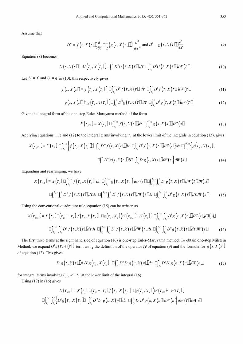
Assume that
and (9)
Equation (8) becomes
(10)
Let in (10), this respectively gives
(11)
(12)
Given the integral form of the one-step Euler-Maruyama method of the form
(13)
Applying equations (11) and (12) to the integral terms involving at the lower limit of the integrals in equation (13), gives
(14)
Expanding and rearranging, we have
(15)
Using the conventional quadrature rule, equation (15) can be written as
(16)
The first three terms at the right hand side of equation (16) is one-step Euler-Maruyama method. To obtain one-step Milstein
Method, we expand term using the definition of the operator of equation (9) and the formula for
of equation (12). This gives
, (17)
for integral terms involving at the lower limit of the integral (16).
Using (17) in (16) gives
( )( ) ( )( )( )2
20
2
1, ,
2
d dD f X g X
dX dXτ τ τ τ= + ( )( )1 ,
dD g X
dXτ τ=
( )( ) ( )( ) ( )( )0, , ,j
s
j jU s X s U X D U X dτ
τ τ τ τ τ= + ∫ ( )( ) ( )1 ,j
s
D U X dWτ
τ τ τ+∫
and U f U g= =
( )( ) ( )( ), ,j jf s X s f Xτ τ= ( )( )0 ,j
s
D f X dτ
τ τ τ+∫ ( )( ) ( )1 ,j
s
D f X dWτ
τ τ τ+∫
( )( ) ( )( ) ( )( )0, , ,j
s
j jg s X s g X D g X dτ
τ τ τ τ τ= + ∫ ( )( ) ( )1 ,j
s
D g X dWτ
τ τ τ+∫
( ) ( ) ( )( )1
1 ,j
jj jX X f s X s ds
τ
ττ τ +
+ = + ∫ ( )( ) ( )1
,j
j
g s X s dW sτ
τ
++∫
jτ
( ) ( )1j jX Xτ τ+ = ( )( ) ( )( ){1 0, ,
j
j j
s
j jf X D f X dτ
τ ττ τ τ τ τ++ +∫ ∫ ( )( ) ( )}1 ,
j
s
D f X dW dsτ
τ τ τ+∫ ( )( ){1
,j
jj j
g Xτ
ττ τ++∫
( )( ) ( )( ) ( )} ( )0 1, ,j j
s s
D g X d D g X dW dW sτ τ
τ τ τ τ τ τ+ +∫ ∫
( ) ( ) ( )( )1
1,
j
jj j j j
X X f X dsτ
ττ τ τ τ+
+ = + ∫ ( )( ) ( )1
,j
jj j
g X dW sτ
ττ τ++∫ ( )( ) ( ) ( )1 1 ,
j
j j
s
D g X dW dW sτ
τ ττ τ τ++∫ ∫
( )( )1 0 ,j
j j
s
D f X d dsτ
τ ττ τ τ++∫ ∫ ( )( ) ( )1 1 ,
j
j j
s
D f X dW dsτ
τ ττ τ τ++∫ ∫ ( )( ) ( )1 0 ,
j
j j
s
D g X d dW sτ
τ ττ τ τ++∫ ∫
( ) ( ) ( ) ( )( )1 1 ,j j j j j jX X f Xτ τ τ τ τ τ+ += + − ( ) ( ) ( )( )1,j j j jg X W Wτ τ τ++ − ( )( ) ( ) ( )1 1 ,j
j j
s
D g X dW dW sτ
τ ττ τ τ++∫ ∫
( )( )1 0 ,j
j j
s
D f X d dsτ
τ ττ τ τ++∫ ∫ ( )( ) ( )1 1 ,
j
j j
s
D f X dW dsτ
τ ττ τ τ++∫ ∫ ( )( ) ( )1 0 ,
j
j j
s
D g X d dW sτ
τ ττ τ τ++∫ ∫
( )( )1 ,D g Xτ τ 1D ( )( ),g s X s
( )( ) ( )( ) ( )( )1 1 0 1, , ,j
s
j jD g X D g X D D g n X n dn
ττ τ τ τ= + ∫ ( )( ) ( )1 1 ,
j
s
D D g n X n dW nτ
+∫
, 0j r rτ + =
( ) ( ) ( ) ( )( )1 1 ,j j j j j jX X f Xτ τ τ τ τ τ+ += + − ( ) ( ) ( )( )1,j j j jg X W Wτ τ τ++ −
( )( ){ ( )( )1 1 0 1, ,j
j j j
s s
j jD g X D D g n X n dn
τ
τ τ ττ τ++ +∫ ∫ ∫ ( )( ) ( )} ( ) ( )1 1
,j
s
D D g n X n dW n dW dW sτ
τ+∫

354 Sunday Jacob Kayode and Akeem Adebayo Ganiyu: Effect of Varying StepSizes in Numerical Approximation of
Stochastic Differential Equations Using One Step Milstein Method
(18)
Expansion of (18) gives
(19)
By definition c.f.(9)
Using (9) in equation (19), this can be written as
(20)
Where, .
The one-step MLSTM follow from the first four terms at the right hand side of equation (20). The method is
(21)
Having evaluated the double integral at the right hand side of equation (21) using Itô formula, we have
(22)
Define , ; , and , .
Equation(22) can now be written as
, . (23)
, (24)
The method in equation (23) was considered by Higham
(2001) using backward difference. In this paper, we shall
apply this method to the SDE (1) using discritised interval
as . Let be the
stepsize defined as , where are some integer
and . The -space path increment
will be approximated by summing the
underlying -space increments as established by Higham
(2001) using
sum (25)
Wiener increment will be generated in MATLAB
( )( )1 0 ,j
j j
s
D f X d dsτ
τ ττ τ τ++∫ ∫ ( )( ) ( )1 1 ,
j
j j
s
D f X dW dsτ
τ ττ τ τ++∫ ∫ ( )( ) ( )1 0 ,
j
j j
s
D g X d dW sτ
τ ττ τ τ++∫ ∫
( ) ( ) ( ) ( )( )1 1 ,j j j j j jX X f Xτ τ τ τ τ τ+ += + − ( ) ( ) ( )( )1,j j j jg X W Wτ τ τ++ − ( )( ) ( ) ( )1 1 ,j
j j
s
j jD g X dW dW sτ
τ ττ τ τ++∫ ∫
( )( ) ( ) ( )1 0 1 ,j
j j j
s s
D D g n X n dn dW dW sτ
τ τ ττ++∫ ∫ ∫ ( )( ) ( ) ( ) ( )1 1 1 ,
j
j j j
s s
D D g n X n dW n dW dW sτ
τ τ ττ++∫ ∫ ∫
( )( )1 0 ,j
j j
s
D f X d dsτ
τ ττ τ τ++∫ ∫ ( )( ) ( )1 1 ,
j
j j
s
D f X dW dsτ
τ ττ τ τ++∫ ∫ ( )( ) ( )1 0 ,
j
j j
s
D g X d dW sτ
τ ττ τ τ++∫ ∫
( )( )1 ,d
D g XdX
τ τ=
( ) ( ) ( ) ( )( )1 1 ,j j j j j jX X f Xτ τ τ τ τ τ+ += + − ( ) ( ) ( )( )1,j j j jg X W Wτ τ τ++ −
( )( ) ( )( ) ( ) ( )1
, ' ,j
j j
s
j j j jg X g X dW dW sτ
τ ττ τ τ τ τ++ ∫ ∫ ( )( ) ( ) ( )1 0 1 ,
j
j j j
s s
D D g n X n dndW dW sτ
τ τ ττ++∫ ∫ ∫
( )( ) ( ) ( ) ( )1 1 1 ,j
j j j
s s
D D g n X n dW n dW dW sτ
τ τ ττ++∫ ∫ ∫ ( )( )1 0 ,
j
j j
s
D f X d dsτ
τ ττ τ τ++∫ ∫
( )( ) ( )1 1 ,j
j j
s
D f X dW dsτ
τ ττ τ τ++∫ ∫ ( )( ) ( )1 0 ,
j
j j
s
D g X d dW sτ
τ ττ τ τ++∫ ∫
( )( ) ( )( )' , ,j j j j
dg X g X
dXτ τ τ τ=
( ) ( ) ( ) ( )( )1 1 ,j j j j j jX X f Xτ τ τ τ τ τ+ += + − ( ) ( ) ( )( )1,j j j jg X W Wτ τ τ++ −
( )( ) ( )( ) ( ) ( )1
, ' ,j
j j
s
j j j jg X g X dW dW sτ
τ ττ τ τ τ τ++ ∫ ∫
( ) ( ) ( ) ( )( )1 1 ,j j j j j jX X f Xτ τ τ τ τ τ+ += + − ( ) ( ) ( )( )1,j j j jg X W Wτ τ τ++ −
( )( ) ( )( ) ( ) ( )( ) ( )( )2
1 1
1, ' ,
2j j j j j j j jg X g X W Wτ τ τ τ τ τ τ τ+ ++ − − −
( )j rX τ + := j rX + 0,1r = ( ) ( )( )1:j j r j rW W Wδ τ τ+ + −= − 1r = ( )1: j r j rtδ τ τ+ + −= − 1r =
( )1 ,j j j jX X t f Xδ τ+ = + ( ),j j jg X Wτ δ+ ( ) ( ) ( ) ( )( ) ( )( )2
1 1
1, ' ,
2j j j j j j j jg X g X W Wτ τ τ τ τ τ+ ++ − − − 0,1, 2, ,j L= ⋯
( ) ( )1, ,
j j j j j j jX X f X t g X Wτ δ τ δ+ = + + ( ) ( ) ( )( )21
, ,2
'j j j j jg X g X dW tτ τ δ+ − 0,1, 2, ,j L= ⋯
[ ]0,T 0 1 10 j j Tτ τ τ τ +< < < < < =⋯T
tL
δ =
1: j jtδ τ τ+= − N
j j tτ δ= tδ
1:j j jdW W W −= −
dt
Winc = ( ( *( 1) 1: * )dW R j R j− +
dW
Applied and Computational Mathematics 2015; 4(5): 351-362 355
over the space intervals by using
.For computational purpose, we
shall assume that
We can now examine the effect of varying step sizes in
numerical approximation of stochastic differential Equations
using one step Milstein Method.
4. Effect of Varying StepSizes in
Numerical Approximation of
Stochastic Differential Equations
Using One Step Milstein Method.
In this section, we will consider two problems in the form
of first order stochastic differential equation (1) to
investigate the effect of varying step sizes when finding the
solution of SDEs using one step MLSTM of equation (24).
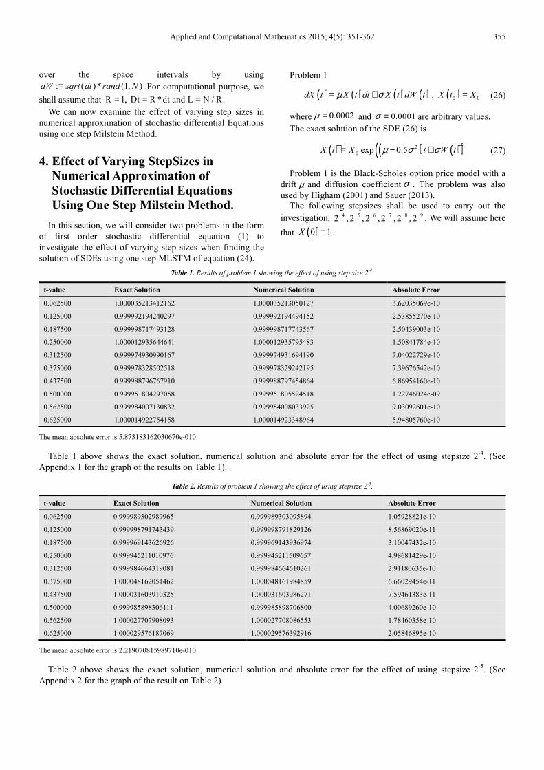
Problem 1
, (26)
where and are arbitrary values.
The exact solution of the SDE (26) is
(27)
Problem 1 is the Black-Scholes option price model with a
drift and diffusion coefficient . The problem was also
used by Higham (2001) and Sauer (2013).
The following stepsizes shall be used to carry out the
investigation, . We will assume here
that .
Table 1. Results of problem 1 showing the effect of using step size 2-4.
t-value Exact Solution Numerical Solution Absolute Error
0.062500 1.000035213412162 1.000035213050127 3.62035069e-10
0.125000 0.999992194240297 0.999992194494152 2.53855270e-10
0.187500 0.999998717493128 0.999998717743567 2.50439003e-10
0.250000 1.000012935644641 1.000012935795483 1.50841784e-10
0.312500 0.999974930990167 0.999974931694190 7.04022729e-10
0.375000 0.999978328502518 0.999978329242195 7.39676542e-10
0.437500 0.999988796767910 0.999988797454864 6.86954160e-10
0.500000 0.999951804297058 0.999951805524518 1.22746024e-09
0.562500 0.999984007130832 0.999984008033925 9.03092601e-10
0.625000 1.000014922754158 1.000014923348964 5.94805760e-10
The mean absolute error is 5.873183162030670e-010
Table 1 above shows the exact solution, numerical solution and absolute error for the effect of using stepsize 2-4
. (See
Appendix 1 for the graph of the results on Table 1).
Table 2. Results of problem 1 showing the effect of using stepsize 2-5.
t-value Exact Solution Numerical Solution Absolute Error
0.062500 0.999989302989965 0.999989303095894 1.05928821e-10
0.125000 0.999998791743439 0.999998791829126 8.56869020e-11
0.187500 0.999969143626926 0.999969143936974 3.10047432e-10
0.250000 0.999945211010976 0.999945211509657 4.98681429e-10
0.312500 0.999984664319081 0.999984664610261 2.91180635e-10
0.375000 1.000048162051462 1.000048161984859 6.66029454e-11
0.437500 1.000031603910325 1.000031603986271 7.59461383e-11
0.500000 0.999985898306111 0.999985898706800 4.00689260e-10
0.562500 1.000027707908093 1.000027708086553 1.78460358e-10
0.625000 1.000029576187069 1.000029576392916 2.05846895e-10
The mean absolute error is 2.219070815989710e-010.
Table 2 above shows the exact solution, numerical solution and absolute error for the effect of using stepsize 2-5
. (See
Appendix 2 for the graph of the result on Table 2).
: ( ) * (1, )dW sqrt dt rand N=R 1, Dt R *dt and L N / R.= = = ( ) ( ) ( ) ( )dX t X t dt X t dW tµ σ= + ( )0 0X t X=
0.0002µ = 0.0001σ =
( ) ( ) ( )( )2
0 exp 0.5X t X t W tµ σ σ= − +
µ σ
4 5 6 7 8 92 ,2 ,2 ,2 ,2 ,2
− − − − − −
( )0 1X =
356 Sunday Jacob Kayode and Akeem Adebayo Ganiyu: Effect of Varying StepSizes in Numerical Approximation of
Stochastic Differential Equations Using One Step Milstein Method
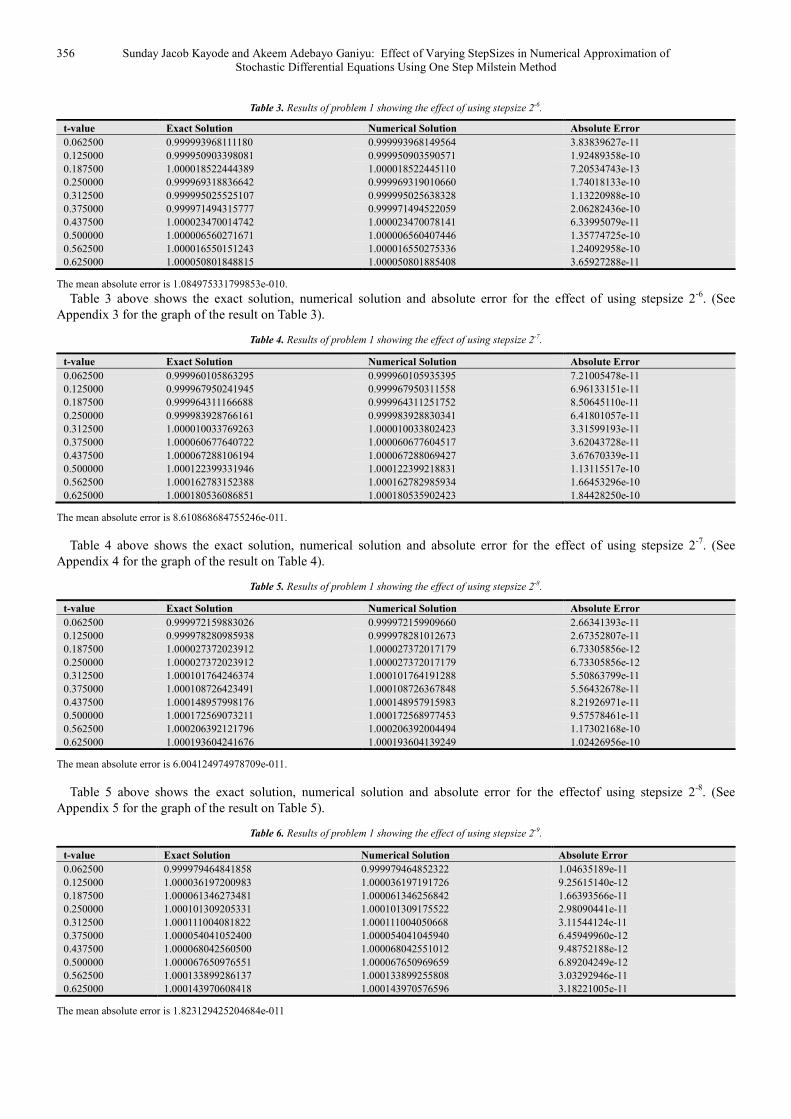
Table 3. Results of problem 1 showing the effect of using stepsize 2-6.
t-value Exact Solution Numerical Solution Absolute Error
0.062500 0.999993968111180 0.999993968149564 3.83839627e-11
0.125000 0.999950903398081 0.999950903590571 1.92489358e-10
0.187500 1.000018522444389 1.000018522445110 7.20534743e-13
0.250000 0.999969318836642 0.999969319010660 1.74018133e-10
0.312500 0.999995025525107 0.999995025638328 1.13220988e-10
0.375000 0.999971494315777 0.999971494522059 2.06282436e-10
0.437500 1.000023470014742 1.000023470078141 6.33995079e-11
0.500000 1.000006560271671 1.000006560407446 1.35774725e-10
0.562500 1.000016550151243 1.000016550275336 1.24092958e-10
0.625000 1.000050801848815 1.000050801885408 3.65927288e-11
The mean absolute error is 1.084975331799853e-010.
Table 3 above shows the exact solution, numerical solution and absolute error for the effect of using stepsize 2-6
. (See
Appendix 3 for the graph of the result on Table 3).
Table 4. Results of problem 1 showing the effect of using stepsize 2-7.
t-value Exact Solution Numerical Solution Absolute Error
0.062500 0.999960105863295 0.999960105935395 7.21005478e-11
0.125000 0.999967950241945 0.999967950311558 6.96133151e-11
0.187500 0.999964311166688 0.999964311251752 8.50645110e-11
0.250000 0.999983928766161 0.999983928830341 6.41801057e-11
0.312500 1.000010033769263 1.000010033802423 3.31599193e-11
0.375000 1.000060677640722 1.000060677604517 3.62043728e-11
0.437500 1.000067288106194 1.000067288069427 3.67670339e-11
0.500000 1.000122399331946 1.000122399218831 1.13115517e-10
0.562500 1.000162783152388 1.000162782985934 1.66453296e-10
0.625000 1.000180536086851 1.000180535902423 1.84428250e-10
The mean absolute error is 8.610868684755246e-011.
Table 4 above shows the exact solution, numerical solution and absolute error for the effect of using stepsize 2-7
. (See
Appendix 4 for the graph of the result on Table 4).
Table 5. Results of problem 1 showing the effect of using stepsize 2-8.
t-value Exact Solution Numerical Solution Absolute Error
0.062500 0.999972159883026 0.999972159909660 2.66341393e-11
0.125000 0.999978280985938 0.999978281012673 2.67352807e-11
0.187500 1.000027372023912 1.000027372017179 6.73305856e-12
0.250000 1.000027372023912 1.000027372017179 6.73305856e-12
0.312500 1.000101764246374 1.000101764191288 5.50863799e-11
0.375000 1.000108726423491 1.000108726367848 5.56432678e-11
0.437500 1.000148957998176 1.000148957915983 8.21926971e-11
0.500000 1.000172569073211 1.000172568977453 9.57578461e-11
0.562500 1.000206392121796 1.000206392004494 1.17302168e-10
0.625000 1.000193604241676 1.000193604139249 1.02426956e-10
The mean absolute error is 6.004124974978709e-011.
Table 5 above shows the exact solution, numerical solution and absolute error for the effectof using stepsize 2-8
. (See
Appendix 5 for the graph of the result on Table 5).
Table 6. Results of problem 1 showing the effect of using stepsize 2-9.
t-value Exact Solution Numerical Solution Absolute Error
0.062500 0.999979464841858 0.999979464852322 1.04635189e-11
0.125000 1.000036197200983 1.000036197191726 9.25615140e-12
0.187500 1.000061346273481 1.000061346256842 1.66393566e-11
0.250000 1.000101309205331 1.000101309175522 2.98090441e-11
0.312500 1.000111004081822 1.000111004050668 3.11544124e-11
0.375000 1.000054041052400 1.000054041045940 6.45949960e-12
0.437500 1.000068042560500 1.000068042551012 9.48752188e-12
0.500000 1.000067650976551 1.000067650969659 6.89204249e-12
0.562500 1.000133899286137 1.000133899255808 3.03292946e-11
0.625000 1.000143970608418 1.000143970576596 3.18221005e-11
The mean absolute error is 1.823129425204684e-011

Applied and Computational Mathematics 2015; 4(5): 351-362 357
Table 6 above shows the exact solution, numerical
solution and absolute error for the effect of using stepsize 2-9
.
(See Appendix 6 for the graph of the result on Table 6)
Problem 2
(28)
Where and .
The true solution is
(29)
Problem 2 was also used by Fadugba et al (2013) with
constant , .
The following step sizes shall be used to carry out the
investigation, . We will assume here
that and for better
accuracy.
Table 7. Results of problem 2 showing the effect of using stepsize 2-4.
t-value Exact Solution Numerical Solution Absolute Error
0.062500 -2.000030639939910 -2.000030642409364 2.46945397e-9
0.125000 -1.999826604550993 -1.999826597757476 6.79351708e-9
0.187500 -1.999771190197802 -1.999771181571479 8.62632321e-9
0.250000 -1.999738855905664 -1.999738846600268 9.30539579e-9
0.312500 -1.999549931800135 -1.999549913990723 1.78094122e-8
0.375000 -1.999485167195670 -1.999485147086992 2.01086778e-8
0.437500 -1.999441604632085 -1.999441583283593 2.13484912e-8
0.500000 -1.999255786341376 -1.999255756647863 2.96935132e-8
0.562500 -1.999277377750062 -1.999277350071063 2.76789982e-8
0.625000 -1.999295108719981 -1.999295082862801 2.58571793e-8
The mean absolute error is 1.696909619486320e-008.
Table 7 above shows the exact solution, numerical solution and absolute error for the effectof using stepsize 2-4
. (See
Appendix 7 for the graph of the result on Table 7).
Table 8. Results of problem 2 showing the effect of using stepsize 2-5.
t-value Exact Solution Numerical Solution Absolute Error
0.062500 -1.999892917380804 -1.999892915172975 2.20782859e-9
0.125000 -1.999846392834979 -1.999846389932891 2.90208790e-9
0.187500 -1.999682499484875 -1.999682492955720 6.52915455e-9
0.250000 -1.999535775997482 -1.999535766271172 9.72630998e-9
0.312500 -1.999579115423757 -1.999579107248484 8.17527313e-9
0.375000 -1.999694550513440 -1.999694545690344 4.82309592e-9
0.437500 -1.999569940134597 -1.999569932666208 7.46838902e-9
0.500000 -1.999357977043176 -1.999357964749685 1.22934911e-8
0.562500 -1.999408364465035 -1.999408353898191 1.05668438e-8
0.625000 -1.999339028019188 -1.999339016188690 1.18304986e-8
The mean absolute error is 7.652297262517039e-009.
Table 8 above shows the exact solution, numerical solution and absolute error for the effectof using stepsize 2-5. (See
Appendix 8 for the graph of the result on Table 8).
Table 9. Results of problem 2 showing the effect of using stepsize 2-6.
t-value Exact Solution Numerical Solution Absolute Error
0.062500 -1.999906910993895 -1.999906910064862 9.29032185e-10
0.125000 -1.999702767364218 -1.999702764118717 3.24550031e-9
0.187500 -1.999830588766838 -1.999830587352560 1.41427758e-9
0.250000 -1.999608061287530 -1.999608057327698 3.95983291e-9
0.312500 -1.999610182559322 -1.999610178860159 3.69916386e-9
0.375000 -1.999464678473431 -1.999464673190970 5.28246158e-9
0.437500 -1.999545553506756 -1.999545549468417 4.03833855e-9
0.500000 -1.999419912678686 -1.999419907305332 5.37335354e-9
0.562500 -1.999374919082127 -1.999374913380986 5.70114156e-9
0.625000 -1.999402649038457 -1.999402643917728 5.12072984e-9
The mean absolute error is 3.876383192213950e-009.
( ) ( )( ) ( )( ) ( )( ) ( )2 2 2 21 (1dX t a b X t X t dt b X t dW t= − + − + −
0.0002, 0.0001, [0,1]a b t= = ∈ ( )0 0X t X=
( ) ( ) ( )( )
( ) ( )( )( )2 2
0 0
2 2
0 0
1 1
1 1
at bW t
at bW t
X e XX t
X e X
− +
− +
+ + −=
+ − +
1a = 2b =
4 5 6 7 8 92 ,2 ,2 ,2 ,2 ,2− − − − − −
0.0002, 0.0001a b= = ( )0 2X = −

358 Sunday Jacob Kayode and Akeem Adebayo Ganiyu: Effect of Varying StepSizes in Numerical Approximation of
Stochastic Differential Equations Using One Step Milstein Method
Table 9 above shows the exact solution, numerical solution and absolute error for the effectof using stepsize 2-6
. (See
Appendix 9 for the graph of the result on Table 9).
Table 10. Results of problem 2 showing the effect of using stepsize 2-7.
t-value Exact Solution Numerical Solution Absolute Error
0.062500 -1.999805341404871 -1.999805340305775 1.09909570e-9
0.125000 -1.999753891446814 -1.999753890143567 1.30324640e-9
0.187500 -1.999668007898771 -1.999668006176140 1.72263093e-9
0.250000 -1.999651870477482 -1.999651868771152 1.70633041e-9
0.312500 -1.999655185128882 -1.999655183560381 1.56850133e-9
0.375000 -1.999732080887753 -1.999732079916673 9.71079883e-10
0.437500 -1.999676933687320 -1.999676932488846 1.19847443e-9
0.500000 -1.999767219155966 -1.999767218638566 5.17400789e-10
0.562500 -1.999813341382202 -1.999813341270112 1.12089893e-10
0.625000 -1.999791597710221 -1.999791597579308 1.30913502e-10
The mean absolute error is 1.032976326698076e-009.
Table 10 above shows the exact solution, numerical solution and absolute error for the effect of using stepsize 2-7
. (See
Appendix 10 for the graph of the result on Table 10).
Table 11. Results of problem 2 showing the effect of using stepsize 2-8.
t-value Exact Solution Numerical Solution Absolute Error
0.062500 -1.999841496174841 -1.999841495738286 4.36554792e-10
0.125000 -1.999784874982539 -1.999784874427676 5.54862600e-10
0.187500 -1.999857131369450 -1.999857131098878 2.70572231e-10
0.250000 -1.999897512575721 -1.999897512489857 8.58642046e-11
0.312500 -1.999930285134005 -1.999930285209092 7.50870477e-11
0.375000 -1.999876177386879 -1.999876177351470 3.54092311e-11
0.437500 -1.999921851349309 -1.999921851515182 1.65873315e-10
0.500000 -1.999917674573231 -1.999917674784625 2.11394457e-10
0.562500 -1.999944122996693 -1.999944123349270 3.52577079e-10
0.625000 -1.999830784974864 -1.999830785031834 5.69697622e-11
The mean absolute error is 2.245164720804382e-010.
Table 11 above shows the exact solution, numerical solution and absolute error for the effectof using stepsize 2-8
. (See
Appendix 11 for the graph of the result on Table 11).
Table 12. Results of problem 2 showing the effect of using stepsize 2-9.
t-value Exact Solution Numerical Solution Absolute Error
0.062500 -1.999863407270136 -1.999863407086074 1.84061877e-10
0.125000 -1.999958592655718 -1.999958592649633 6.08535444e-12
0.187500 -1.999959037106798 -1.999959037130689 2.38906672e-11
0.250000 -2.000003915981924 -2.000003916105223 1.23299593e-10
0.312500 -1.999957999627532 -1.999957999708359 8.08273448e-11
0.375000 -1.999712179640226 -1.999712179366374 2.73852718e-10
0.437500 -1.999679195925699 -1.999679195629594 2.96105140e-10
0.500000 -1.999603058636733 -1.999603058251007 3.85726118e-10
0.562500 -1.999726729199231 -1.999726729035875 1.63356217e-10
0.625000 -1.999681957561421 -1.999681957357425 2.03995709e-10
The mean absolute error is 1.741200739147075e-010.
Table 12 above shows the exact solution, numerical
solution and absolute error for the effect of using stepsize 2-9
.
(See Appendix 12 for the graph of the result on Table 12).
5. Determination of Order of
Convergence of the Method
To determine the accuracy of any numerical method, the
properties of methods of solution of stochastic differential
equations cannot be ignored. Some of the properties peculiar

Applied and Computational Mathematics 2015; 4(5): 351-362 359
to SDEs include convergence and order of convergence. The
issues of convergence of SDEs have been examine by Higham
(2001), Burrage (2004), Lactus (2008), Sauer (2013), Fadugba
et al (2013) and Akinbo et al (2015) for one step method etc.
In this section, mean absolute error (MAE) or Strong Error
of one step MLSTM will be determined to assess the effect of
varying stepsizes. The order of convergence of the method
will be obtained using mean absolute error (MAE) obtained.
Table 13(a) and (b): Results showing MAE of one step
MLSTM applied to problems 1 and 2 with varying stepsizes.
Table 13(a). MAE for Problem 1.
Stepsize Mean Absolute error
2-4 5.87318316e-10
2-5 2.21907082e-10
2-6 1.08497533e-10
2-7 8.61086868e-11
2-8 6.00412497e-11
2-9 1.82312943e-11
Table 13(b). MAE for Problem 2.
Stepsize Mean Absolute error
2-4 1.69690962e-8
2-5 7.65229726e-9
2-6 3.87638319e-9
2-7 1.03297633e-9
2-8 2.24516472e-10
2-9 1.74120074e-10
Using the data in table 13a, the strong order of
convergence for one step MLSTM and the residual for
one step MLSTM with respect to problem 1 can be obtained
by making least squares fit using MALAB commands.
Running the MATLAB commands, the strong convergence
of order while the residual .
Similarly, for problem 2, the strong convergence of order
while the residual .
6. Discussion
We have so far discussed about the method of deriving one
step method of Milstein type. This method was applied to
two SDEs. The method was used to determine the numerical
solution of the given problem. Absolute errors were
calculated using the numerical approximation and the
corresponding exact solution. Mean absolute error were
determined. Using this, comparison of absolute error was
made. To determine the accuracy of the method, strong order
of convergence was obtained for each method. The order of
convergence obtained was approximately 1 which shows the
accuracy of the method.
7. Conclusion
In this paper, two problems in the form of first order SDEs
have been considered.One step Milstein method (MLSTM)
for solution of general first order stochastic differential
equations (SDEs) has been derived. The absolute errors
between the exact solution and numerical solution have been
determined using this method. The mean absolute errors for
varying stepsizes were also determined. The result showed
that the mean absolute error generally decreases as the
stepsizes decreases. The effect of the varying stepsizes can
also be seen by observing the behaviour of the exact solution
and numerical solution using graphical method as indicated
in Appendix 1 to 12. To determine the accuracy of the
method, we also determine the strong order of convergence
of the method. For problem 1 the strong order of
convergence gives while for problem 2, the
strong order of convergence gives . The results
were obtained using MATLAB as a supporting tool.
Appendix 1
Figure 1. Shows the graph of exact solution and one step Milstein Method
with stepsize 2-4.
Appendix 2
Figure 2. Shows the graph of exact solution and one step Milstein Method
with stepsize 2-5.
λ C
0.8868λ ≃ 0.5739C ≃
1.4347λ ≃ 0.6808C ≃
0.8868λ ≃1.4347λ ≃
0 0.1 0.2 0.3 0.4 0.5 0.6 0.7 0.8 0.9 10.9999
1
1
1
1
1
1.0001
1.0001
1.0001
1.0001
t
X(t)
One-Step Mistein Method for Solution of Problem 1 Using Step Size 1/24
Exact Solution
Milstein approximation
0 0.1 0.2 0.3 0.4 0.5 0.6 0.7 0.8 0.9 10.9999
1
1
1
1
1
1.0001
1.0001
1.0001
1.0001
t
X(t)
One-Step Mistein Method for Solution of Problem 1 Using Step Size 1/25
Exact Solution
Milstein approximation

360 Sunday Jacob Kayode and Akeem Adebayo Ganiyu: Effect of Varying StepSizes in Numerical Approximation of
Stochastic Differential Equations Using One Step Milstein Method
Appendix 3
Figure 3. Shows the graph of exact solution and one step Milstein Method
with stepsize 2-6.
Appendix 4
Figure 4. Shows the graph of exact solution and one step Milstein Method
with stepsize 2-7.
Appendix 5
Figure 5. Shows the graph of exact solution and one step Milstein Method
with stepsizes 2-8.
Appendix 6
Figure 6. Shows the graph of exact solution and one step Milstein Method
with stepsizes 2-9.
Appendix 7
Figure 7. Shows the graph of exact solution and one step Milstein Method
with stepsizes 2-4.
Appendix 8
Figure 8. Shows the graph of exact solution and one step Milstein Method
with stepsizes 2-5.
0 0.1 0.2 0.3 0.4 0.5 0.6 0.7 0.8 0.9 10.9999
1
1
1.0001
1.0001
1.0002
1.0002
t
X(t)
One-Step Mistein Method for Solution of Problem 1 Using Step Size 1/26
Exact Solution
Milstein approximation
0 0.1 0.2 0.3 0.4 0.5 0.6 0.7 0.8 0.9 10.9999
1
1
1.0001
1.0001
1.0002
1.0002
1.0003
1.0003
t
X(t)
One-Step Mistein Method for Solution of Problem 1 Using Step Size 1/27
Exact Solution
Milstein approximation
0 0.1 0.2 0.3 0.4 0.5 0.6 0.7 0.8 0.9 10.9999
1
1
1.0001
1.0001
1.0002
1.0002
t
X(t)
One-Step Mistein Method for Solution of Problem 1 Using Step Size 1/28
Exact Solution
Milstein approximation
0 0.1 0.2 0.3 0.4 0.5 0.6 0.7 0.8 0.9 10.9999
1
1
1.0001
1.0001
1.0002
1.0002
1.0003
1.0003
t
X(t)
One-Step Mistein Method for Solution of Problem 1 Using Step Size 1/29
Exact Solution
Milstein approximation
0 0.1 0.2 0.3 0.4 0.5 0.6 0.7 0.8 0.9 1-2.0002
-2
-1.9998
-1.9996
-1.9994
-1.9992
-1.999
-1.9988
-1.9986
-1.9984
-1.9982
t
X(t)
One-Step Milstein Method for Solution of Problem 2 Using Step Size 1/24
Exact Solution
Milstein approximation
0 0.1 0.2 0.3 0.4 0.5 0.6 0.7 0.8 0.9 1-2.0002
-2
-1.9998
-1.9996
-1.9994
-1.9992
-1.999
-1.9988
-1.9986
-1.9984
t
X(t)
One-Step Milstein Method for Solution of Problem 2 Using Step Size 1/25
Exact Solution
Milstein approximation

Applied and Computational Mathematics 2015; 4(5): 351-362 361
Appendix 9
Figure 9. Shows the graph of exact solution and one step Milstein Method
with stepsizes 2-6.
Appendix 10
Figure 10. Shows the graph of exact solution and one step Milstein Method
with stepsizes 2-7.
Appendix 11
Figure 11. Shows the graph of exact solution and one step Milstein Method
with stepsizes 2-8.
Appendix 12
Figure 12. Shows the graph of exact solution and one step Milstein Method
with stepsizes 2-9.
References
[1] Akinbo B.J., Faniran T. and Ayoola E.O. (2015). Numerical Solution of Stochastic Differential Equations. International Journal of Advanced Research in Science, Engineering and Technology.
[2] Anna N. (2010). Economical Runge-Kutta Methods with week Second Order for Stochastic Differential Equations. Int. Contemp. Maths. Sciences, 5(24), 24 1151-1160.
[3] Beretta, M., Carletti, F. and Solimano F. (2000). “On the Effects of Enviromental Flunctuationsin Simple Model of Bscteria- Bacteriophage Interaction, Canad. Appl. Maths. Quart. 8(4)321-366.
[4] Bokor R.H. (2003). “Stochastically Stable One Step Approximations of Solutions of Stochastic Ordinary Differential Equations”, J. Applied Numerical Mathematics 44, 21-39.
[5] Burrage, K. (2004). Numerical Methods for Strong Solutions of Stochastic Differential Equations: An overview. Proceedings: Mathematical Physical and Engineering Science, Published by Royal Society, 460(2041), 373-402.
[6] Burrage, K. Burrage, P. and Mitsui T. (2000). Numerical Solutions of Stochastic Differential Equations-Implementation and Stability Issues. Journalof Computational&Applied Mathematics, 125, 171-182.
[7] Fadugba S.E., Adegboyegun B.J., and Ogunbiyi O.T. (2013). On Convergence of Euler-Maruyama and Milstein Scheme for Solution of Stochastic Differential Equations. International Journal of Applied Mathematics and Modeling@ KINDI PUBLICATIONS.1(1), 9-15. ISSN: 2336-0054.
[8] Higham D.J. (2001). An Algorithmic Introduction to Numerical Simulation of Stochastic Differential Equations. SIAM Review, 43(3), 525-546.
[9] Lactus, M.L. (2008). Simulation and Inference for Stochastic Differential Equations withR Examples. Springer Science + Buisiness Media, LLC, 233 Springer Street, New York,NY10013, USA. Pp 61-62.
0 0.1 0.2 0.3 0.4 0.5 0.6 0.7 0.8 0.9 1-2.0001
-2
-1.9999
-1.9998
-1.9997
-1.9996
-1.9995
-1.9994
-1.9993
t
X(t)
One-Step Milstein Method for Solution of Problem 2 Using Step Size 1/26
Exact Solution
Milstein approximation
0 0.1 0.2 0.3 0.4 0.5 0.6 0.7 0.8 0.9 1-2
-2
-1.9999
-1.9999
-1.9998
-1.9998
-1.9997
-1.9997
-1.9996
-1.9996
-1.9995
t
X(t)
One-Step Milstein Method for Solution of Problem 2 Using Step Size 1/27
Exact Solution
Milstein approximation
0 0.1 0.2 0.3 0.4 0.5 0.6 0.7 0.8 0.9 1-2.0001
-2
-1.9999
-1.9998
-1.9997
-1.9996
-1.9995
-1.9994
-1.9993
-1.9992
t
X(t)
One-Step Milstein Method for Solution of Problem 2 Using Step Size 1/28
Exact Solution
Milstein approximation
0 0.1 0.2 0.3 0.4 0.5 0.6 0.7 0.8 0.9 1-2
-2
-1.9999
-1.9999
-1.9998
-1.9998
-1.9997
-1.9997
-1.9996
-1.9996
-1.9995
t
X(t)
One-Step Milstein Method for Solution of Problem 2 Using Step Size 1/29
Exact Solution
Milstein approximation

362 Sunday Jacob Kayode and Akeem Adebayo Ganiyu: Effect of Varying StepSizes in Numerical Approximation of
Stochastic Differential Equations Using One Step Milstein Method
[10] Oksendal B. (1998). Stochastic Differential Equations. An Introduction with Application, FifthEdition, Springer-Verlage, Berlin, Heidelberge, Italy.
[11] Platen E. (1992). An Introduction to Numerical Methods of Stochastic Differential equations. ActaNumerica, 8, 197-246.
[12] Rezaeyan R. and Farnoosh R. (2010). Stochastic Differential Equations and Application of Kalman-Bucy Filter in Modeling of RC Circuit. Applied Mathematical Sciences, Stochastic Differential Equations 4(33), 1119-1127.
[13] Richardson M. (2009). Stochastic Differential Equations Case
Study. (Unpublished).Sauer T. (2013). Computational Solution of Stochastic Differential Equations. WIRES ComputStat. doi: 10.1002/wics.1272.
[14] Wang P. and Liu Z. (2009). “Stabilized Milstein Type Methods for Stiff Stochastic Systems”. Journal of Numerical Mathematics and Stochastics, Eulidean Press, LLC. 1(1): 33-34.
[15] Yashihiro S. and Taketomo M. (1996). Stability Analysis of Numerical Schemes for Stochastic Differential Equations. SIAM J. Numer. Anal. 33(6), 2254.