homotopy method for solving finite level fuzzy nonlinear...

Applied and Computational Mathematics 2015; 4(4): 245-257

Published online June 26, 2015 (http://www.sciencepublishinggroup.com/j/acm)

doi: 10.11648/j.acm.20150404.13

ISSN: 2328-5605 (Print); ISSN: 2328-5613 (Online)

Homotopy Method for Solving Finite Level Fuzzy Nonlinear Integral Equation

Alan Jalal Abdulqader

University Gadjah mada, Department of Mathematics and atural Science, Faculty MIPA, Yogyakarta, Indonesia

Email address: [email protected]

To cite this article: Alan Jalal Abdulqader. Homotopy Method for Solvind Finite Level Fuzzy Nonlinear Integral Equation. Applied and Computational

Mathematics. Vol. 4, No. 4, 2015, pp. 245-257. doi: 10.11648/j.acm.20150404.13

Abstract: In this paper, non – linear finite fuzzy Volterra integral equation of the second kind (NFVIEK2) is considered. The

Homotopy analysis method will be used to solve it, and comparing with the exact solution and calculate the absolute error

between them. Some numerical examples are prepared to show the efficiency and simplicity of the method.

Keywords: Fuzzy Number, Finite Level, Volterra Integral Equation of Second Kind, Homotopy Analysis Method,

Fuzzy Integral

1. Introduction

In this chapter, we construct a new method to find a

solution of the nonlinear fuzzy integral equation.

u��x� = f�x� + λ � k��x, t�u��t��dt�� (1)

where u�, fandk�arefuzzyfunctions . Park et al., consider

the existence of solution of fuzzy integral equations in

Banach spaces. But unfortunately, we could not see the proof

of the existence theorem, For this reason, we prove the

existence theorem for the solution of fuzzy integral equations

by extending the existence theorems for ordinary integral

equations, and we think that our approach different from the

approach of those authors. So we need some background

material about fuzzy metric space, fuzzy contraction mapping

and related mathematical notions. These notions are

fundamental, and absolutely essential in proving the

existence and uniqueness of (1) .We will discuss some

method in order to find the solutions of nonlinear fuzzy

integral equation of second kind.

2. Basic Concepts

Let X be a space of object , let A" be a fuzzy set in X then

one can define the following concepts related to fuzzy subset

A" of X [1,6] :

1- The support of A" in the universal X is crisp set , denoted

by :

S�A"� = $x ∈ X|μ)"�x� > 0,. 2- The core of a fuzzy set A" is the set of all point x ∈ X,

such that μ)"�x� = 1

3- The height of a fuzzy set A" is the largest membership

grade over X, i.e hgt(A"� = sup0∈1μ)"�x�

4- Crossover point of a fuzzy set A" is the point in X whose

grade of membership in A" is 0.5

5- Fuzzy singleton is a fuzzy set whose support is single

point in X with μ)"�x� = 1

6- A fuzzy set A" is called normalized if it’s height is 1;

otherwise it is subnormal

Note:

A non-empty fuzzy set A" can always be normalized by

dividing

μ)"�x�bysup0∈1μ)"�x�

7-The empty set ϕandXarefuzzyset, then: forallx ∈X, μ7�x� = 0, μ0�x� = 1respectively

8- A = Bifandonlyifμ)�x� = μ9�x�for all x∈ X

9- A ⊆ Bifandonlyifμ)�x� ≤ μ9�x� for all x∈ X

10-A"< is a fuzzy set whose membership function is defined

by μ)"=�x� = 1 − μ)"�x�forallx ∈ X

11-Given two fuzzy sets, A"andB" , their standard

intersection, A"⨅B", andthestandardunionA"⨆B", are fuzzy

sets and their membership function are defined for all

x ∈ X, bytheequations: ∀x ∈ X, μ)∪9�x� = MaxEμ)�x�, μ9�x�F

246 Alan Jalal Abdulqader: Homotopy Method for Solvind Finite Level Fuzzy Nonlinear Integral Equation

∀x ∈ X, μ)∩9�x� = MinEμ)�x�, μ9�x�F

3. H – Cut Sets

Definition 1: (α − cutset� The α-cut set AJ of a fuzzy set

A is made up of membership whose membership is not less

than α, [3,5,9]

AJ = $x ∈ X ∶ μ)�x� ≥ α,, ∀x ∈ X

The following properties are satisfied for all α ∈ E0,1]

i- �A ∪ B�J =AJ ∪ BJ

ii- �A ∩ B�J =AJ ∩ BJ

iii- A ⊆ BgivesAJ ⊆ BJ

iv- A = BiffAJ = BJ, ∀α ∈ E0,1F v- α ≤ αOthenAJ ⊇ AJQ Remarks 3:

1- The set of all level α ∈ E0,1F, that represent distinct α –

cuts of a given fuzzy set [17]

A"iscalledalevelsetofA"

Λ�A"� = $α|μ)"(x) = α, forsomex ∈ X} 2- The support of A" is exactly the same as the strong

α − cut of A" for α = 0, ATU = S�A"�. 3- The core of A" is exactly the same as the α − cutof A" for

α = 1, (i. eAV = core�A"�).

4- The height of A" may also be viewed as the supremum of

α − cut for which Aα ≠ ϕ

5- The membership function of a fuzzy set A" can be

expressed in terms of the characteristic function of it is

α − cuts according to the formula:

μ)"(x) = supJ∈]T,V]Min{α, μ)X(x)} Where

μ)X(x) = Z 1ifx ∈ AJ0, otherwise\ 4. Convex Fuzzy Sets

We can generalize the definition of convexity to fuzzy sets.

Assuming universal set X is defined in the set of real numbers R . If all α − cutsetsareconvex, then the fuzzy set with

these α − cutsets is convex [12, 20]

Definition 2:

A fuzzy set A" on R is convex if and only if [13] :

μ)"(λxV + (1 − λ)x^) ≥ Min{μ)"(xV), μ)"(x^)} forallxV, x^ ∈ R, andallλ ∈ [0,1]

Remarks 4:

Assume that A" is convex for all αandletα =μ)"(xV), μ)"(x^) then if xV, x^ ∈ AJ and moreover λxV +(1 − λ)x^ ∈ AJ for any λ ∈ [0,1] by the convexity of A" .

Consequently

μ)"(λxV + (1 − λ)x^) ≥ α = μ)"(xV) =Min{μ)"(xV), μ)"(x^)}. Assume that A" satisfies equation (1), we need to prove that

For any α ∈ [0,1], AJisconvex. NowforanyxV, x^ ∈ AJ

and for any λ ∈ [0,1] by equation (1)

μ)"(λxV + (1 − λ)x^) ≥ Min{μ)"(xV), μ)"(x^)} ≥ Min{α, α} = α

i.e λxV + (1 − λ)x^ ∈ AJ, thereforeAJisconvexforanyα ∈[0,1], A" is convex.

Definition 3. (Extension of fuzzy set ) Let f: X ⟶ Y, andA

be a fuzzy set defined on X,then we can obtain a fuzzy set f(A)inYbyfandA [14, 23]

∀y ∈ Y, μb())(y) =Zsup{μ)(x)iffcV(y) ≠ ϕ, ∀x ∈ X, y = f(x)}0iffcV(y) = ϕ \

Definition 4: (Extension Principle) We can generalize the

per-explained extension of fuzzy set. Let X be Cartesian

product of universal set X = XV × X^ × ………×XfandAV, A^, …… . . , Af be r- fuzzy sets in the universal set.

Cartesian product of fuzzy sets AV, A^, …… . . , Af yields a

fuzzy set [14,24,19] AV, A^, …… . . , Afdefine as

μ)g,)h,……..,)i(XV × X^ × ………× Xf) =Min(μ)g(XV), ……… . , μ)i(Xf)) Let function f be from space XandY

f(XV × X^ × ………× Xf): X → Y

Then fuzzy set BinY can be obtained by function f and

fuzzy sets AV, A^, …… . . , Af as follows:

μ9(y) = kSup{Min(μ)g(XV), ……… . , μ)i(Xf)|xl ∈ Xl \, i = 1,2,3… . . , n, y = f(xV × … . .× xf)}o, iffcV(y) = ϕ \ Here, fcV(y) is the inverse image of y , μ9(y) is the

membership of = f(xV × … . .× xf) In following example, we will show that fuzzy distance

between fuzzy sets can be defined by extension principle.

5. Intervals

“real number” implies a set containing whole real numbers

and “positive numbers” implies a set holding numbers

excluding negative numbers. “positive number less than

equal to 10 (including 0)” suggests us a set having numbers

from 0 to 10. That is [1,4,11,22]

A={x|0 ≤ x ≤ 10, x ∈ R} Or

μ)(x) = Z1, if0 ≤ x ≤ 10, x ∈ R0, ifx < 0pqr > 10 \ Since the crisp boundary is involved, the outcome of

Applied and Computational Mathematics 2015; 4(4): 245-257 247

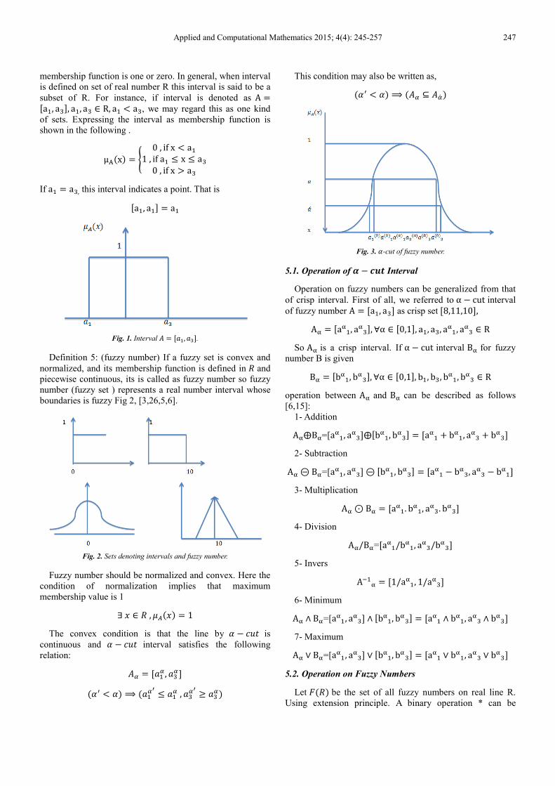
membership function is one or zero. In general, when interval

is defined on set of real number R this interval is said to be a

subset of R. For instance, if interval is denoted as A =[aV, as], aV, as ∈ R, aV < as, we may regard this as one kind

of sets. Expressing the interval as membership function is

shown in the following .

μ)(x) = t 0, ifx < aV1, ifaV ≤ x ≤ as0, ifx > as\

If aV = as, this interval indicates a point. That is

[aV, aV] = aV

Fig. 1. Interval u = [vV, vs]. Definition 5: (fuzzy number) If a fuzzy set is convex and

normalized, and its membership function is defined in w and

piecewise continuous, its is called as fuzzy number so fuzzy

number (fuzzy set ) represents a real number interval whose

boundaries is fuzzy Fig 2, [3,26,5,6].

Fig. 2. Sets denoting intervals and fuzzy number.

Fuzzy number should be normalized and convex. Here the

condition of normalization implies that maximum

membership value is 1

∃r ∈ w, yz(r) = 1

The convex condition is that the line by { − |}~ is

continuous and { − |}~ interval satisfies the following

relation:

u� = [vV� , vs�] ({O < {) ⟹ (vV�Q ≤ vV�, vs�Q ≥ vs�)

This condition may also be written as,

({O < {) ⟹ (u� ⊆ u�)

Fig. 3. {-cut of fuzzy number.

5.1. Operation of H − �� Interval

Operation on fuzzy numbers can be generalized from that

of crisp interval. First of all, we referred to α − cut interval

of fuzzy number A = [aV, as] as crisp set[8,11,10], AJ = [aJV, aJs], ∀α ∈ [0,1], aV, as, aJV, aJs ∈ R

So AJ is a crisp interval. If α − cut interval BJ for fuzzy

number B is given

BJ = [bJV, bJs], ∀α ∈ [0,1], bV, bs, bJV, bJs ∈ R

operation between AJ and BJ can be described as follows

[6,15]:

1- Addition

AJ⨁BJ=[aJV, aJs]⨁[bJV, bJs] = [aJV + bJV, aJs + bJs] 2- Subtraction

AJ ⊝ BJ=[aJV, aJs] ⊝ [bJV, bJs] = [aJV − bJs, aJs − bJV] 3- Multiplication

AJ ⊙ BJ = [aJV. bJV, aJs. bJs] 4- Division

AJ/BJ=[aJV/bJV, aJs/bJs] 5- Invers

AcVJ = [1/aJV, 1/aJs] 6- Minimum

AJ ∧ BJ=[aJV, aJs] ∧ [bJV, bJs] = [aJV ∧ bJV, aJs ∧ bJs] 7- Maximum

AJ ∨ BJ=[aJV, aJs] ∨ [bJV, bJs] = [aJV ∨ bJV, aJs ∨ bJs] 5.2. Operation on Fuzzy Numbers

Let �(w) be the set of all fuzzy numbers on real line R.

Using extension principle. A binary operation * can be


extended into (*) to combine two fuzzy numbers A and B.

Moreover, if yzv��y� are the membership functions of A

and B assumed to be continuous functions on R [2,7,16]

μ)(∗)9(z) = Sup{Min(μ)(x), μ9(y)|∀x, y ∈ R, z = x ∗ y} (2)

Theorem 1: Let A, B and C be a fuzzy numbers. The

following holds [9]:

1- u(�⨁�) = (u. �)⨁(u. �) 2- -(-A)=A

3- A\1=A

4- A/B=A.1/B

5- q(u⨁�) = qu⨁q�

6- (-r)A=-(rA)

7- (-A)B=-(A.B)=A(-B)

8- A/r=(1/r)A

9- u⨁(−�) = u − �

6. Other Types of Fuzzy Numbers

Carrying out computations with fuzzy quantities and in

particular with fuzzy numbers, can be complicated. There are

some special classes of fuzzy numbers for which

computations of their sum, for example .is easy. One such

class is that of triangular fuzzy number, another one is that of

trapezoidal fuzzy number.

In this paper we discuss about new type for fuzzy number

name finite level fuzzy number[11,17,21].

Remarks 5:

Lets talk about the operation of trapezoidal fuzzy number

as in the triangular fuzzy number

1. Addition and Subtraction between trapezoidal

(triangular )fuzzy numbers become trapezoidal

(triangular ) fuzzy number

2. Multiplication, Division and inverse need not be

trapezoidal (triangular) fuzzy numbers

3. Max and Min operation of trapezoidal (triangular) fuzzy

numbers is not always in the form of trapezoidal

(triangular) fuzzy numbers

But in may cases, the operation results from multiplication

or division are approximated trapezoidal shape. As I

triangular fuzzy number, addition and subtraction are simply

defined, and multiplication and division operations should be

done by using membership function

i- u⨁B = [aV, as]⨁[bV, bs] = [aV + bV, as + bs] ii- A ⊖ B = [aV, as] ⊖ [bV, bs] = [aV − bs, as − bV] iii- A ⊙ B = [aV, as] ⊛ [bV, bs] = [aV. bV, as. bs] iv- symmetricimage − (A) = [−as, −aV] The multiplication and the addition of two triangular

( trapezoidal) fuzzy numbers is not a triangular (trapezoidal)

fuzzy number , so it will not form a group structure. Now, we

will construct a new of fuzzy numbers ( which we shall call it

finite level fuzzy numbers), such that the addition and

multiplication of two finite level fuzzy numbers will be also

finite level fuzzy number. The construction of this new type

of fuzzy numbers will as follows [25,14,20]:

Given n ,N be two positive integers n < N, andαV, α^, ……… , α� ∈ [0,1]suchthat αV < α^ < ⋯ . . < α�cV < α� = 1

α� < α�cV < ⋯ . . < α�UV < α� = 1

Let F(R�) be the set of all fuzzy numbers A = {(xl, αl)}�

defined on R , such that xV < x^ < ⋯ . . < x�

The operations of this type of fuzzy numbers can be

defined by

Let AandB ∈ F(R�) such that A = {(xl, αl)}�andB ={(yl, αl)}�

According to equation (2) we have

μ)(∗)9(z) = Sup{Min(μ)(x), μ9(y)|∀x, y ∈ R, z = x ∗ y} = Max{Min(αl, α�)|z = xl ∗ yl} (3)

If we perform the * operation between A and B, we will

get the following table

* �� rV {V{V{V r^ {V{^{^ [Min{{� , { }] r¡

{¡{¡ 1 ¢£¤�¥{� , { ¦§{¨cV{¨cVr¨ {¨{¨{¨

Now, from this table it is clear that the convex of A*B is

yz(∗)�(©) =ª«¬« {V®¯°±g∗²g³´³±h∗²h�hµ¶·¸h∗¹hº»º¸¼∗¹¼..gµ¶·»½¸¾∗¹¾¿¾Àgµ¶·¸¾∗¹¾º»º¸¾Àg∗¹¾Àg..¿Áµ¶·¸ÁÂg∗¹ÁÂgº»º¸Á∗¹Á

\ (4)

According to equation (3 and 4) in this case can be written

as

yz(∗)�(©) = {�, ¤Ã© = r� ∗ Ä� (5)

where

yz(∗)�(©) = 1, ¤Ã© = r¡ ∗ Ä¡

and

©V < ©^ < ⋯… < ©¡ = r¡ ∗ Ä¡v��r¡ ∗ Ä¡ = ©¡ < ©¡UV < ⋯ < ©¡

So Å� = {(©� , {�}¨ is fuzzy number and Å� ∈ �(w¨)

7. Fuzzy Equations

A fuzzy equation is an equation whose coefficients and / or

variable are fuzzy sets of R. The concept of equation can be

extended to deal with fuzzy quantities in several ways.

Consider the simple equation vr + Æ = rÇℎÉqÉ(v, Æ) ∈

w, r¤ÊvqÉvËÌvqÉ¤vÆËÉ, v��v ≠1, Êp~ℎv~~ℎÉ}�¤Í}ÉÊpË}~¤p�¤Êr = ÎVcÏ , then the fuzzy

equation

v�r� + Æ� = r�, v�, Æ� ∈ Ð�(w), r ∈ w (6)

means that the fuzzy set v�r� + Æ� is the same as r�. Note that it

is forbidden to shift terms from one side to another . For


instance, the equation v�r� + Æ� = r� is not equal to v�r� + Æ� −r� = 0 ∶the first may have solution, while the second surely

dose not, since v�r� + Æ� − r� is fuzzy and 0 is scalar.

We can solve the fuzzy equation (6) if we consider the

fuzzy variables and the fuzzy coefficient as a fuzzy numbers

of the form u = {(r� , {�)}¨. In another word[15],

v�, Æ�, r� ∈ �(w¨) v� = {(v� , {�)}¨,Æ� = {(Æ� , {�)}¨, r� = {(r� , {�)}¨ (7)

again using equation (7) to solve equation (6)

v�r� + Æ� = {(v�r� + Æ� , {�)}¨ (8)

Finally the fuzzy equation

v�r� + Æ� = r�

implies that ∀{� ∈ [0,1], ¤ = 1,… . , Ñ

v�r� + Æ� = r� → r� = ÎÒVcÏÒ , v� ≠ 1 (9)

So the solution of the fuzzy equation (6) is a fuzzy number

r� = {( ÎÒVcÏÒ , {� )}¨ (10)

Fuzzy function of crisp Variable

Two points of view can be developed depending on

whether the image of r ∈ Ó is a fuzzy set Ã(r) on Ô, or r is

mapped to Ä through a fuzzy set of functions .

Definition 6:

A fuzzy mapping �� is a mapping from XtothesetnonemptyfuzzysetsonX , namely Ð�(r). In

other words, to each r ∈ Ó , corresponds a fuzzy set ��(r)

defined on Ó, whose membership function is yÕ�(±) and [8]

μÖ"(0): X → I A fuzzy set of mapping F can be constructed in the

following way,

Define a function F: X → P"(x) such that μÖ: R0 → I ,

( where R0 is the set of all functions f: X → R)

μÖ(f) = Inf{μÖ"(0)(f(x)|x ∈ X, Definition 7: Given a fuzzy set of mappings F with

μÖ: R0 → I , we can construct a fuzzy function F�: X →P"�x�suchthatF��x� is a fuzzy set , as follows[21]:

μÖ"�0��y� = Zsup$μÖ�f�|x ∈ fcV�y�, whenfcV ≠ ϕ0, whenfcV = ϕ \

Definition 8:

Given a fuzzy function set Fon X with μÖ: X → I and a

function T: X → Y. Then there exists a fuzzy function

T"�F�: Y → P"�y�withμÚ"�Ö�: Y → I such that[25]

∀Ä ∈ Ô, yÛ��Õ��Ä� = Ü}Ý$yÕ�r�|∀r ∈ Ó, Ä = Þ�r�,

Fig. 4. fuzzy function Þ��. Definition 9: Given a fuzzy set of mappings �

withyÕ: w± → ß and a functional

à: w± → w . Then we can construct a fuzzy functional

à: w�± → w� such that[27]

à�� = à��

Therefore ∀Ä ∈ w

yá�Õ��Ä� = yá��Õ��Ä� = Ü}Ý$yÕ�Ã�|Ã ∈ w± , Ä = à�Ã�,

Fig. 5. fuzzy functional.

Example 1:

Let G be the set of all integrable functions. The integration

� : G ⊆ R0 → R,0 can be considered as a functional where

� f ∈ R.0

Then the fuzzy integral � :R"0 → p��R�0 can be defined the

equation above

Given a fuzzy mapping

F�: X → P"�x�, then∃afuzzymappingFwithμÖ: G ⊆ R0 → I such that

μ� Ö"ã�y� = μ� Öã

�y� = Sup$μÖ�f�|f ∈ R0, y = � f0 , (11)

Definition 10:

Let T be a fuzzy set such that T: X → R,then T will be

finite if supp�T� = $xl,. In another word, T = $�xl, αl�,�

where μÚ�xl� = αl > 0

Definition 11: rewrite the definition 8 , if fuzzy mapping

F�: X → P"�X� is finite , then F�can be written as

F��x� = $�fl�x�, αl�,�

Any fuzzy set of mapping F, constructed from �� also will

be finite , and

μÖ�f� = Inf¥μÖ"�0��f�x��äx ∈ X¦ = αlifandonlyiff = fl This implies that F = $�fl, αl�,�


Now, if given a finite set of mappings F = {(fl, αl)}�, then

we have

μÖ"(0)(y) = Sup{μÖ(f)|y = f(x)

⟹ μÖ"(0)(y) = αlifandonlyify = fl(x)

⟹ F�(x) = {(fl(x), αl)}�

Definition 12:

Given a finite mapping �(r) = {(Ã�(r), {�)}¡ , and a

functionalà: w± → w, then a fuzzy functional in this case ,

can be defined by[27]

μå�Ö"�(y) = μå�(Ö)(y) = Sup{αl|∀i = 1,2, … n, y = ρ(fl) } (12)

Definition 13:

The integral of a finite fuzzy mapping � = {(Ã�, {�)}¡ is

given by

μ� Ö"ã (y) = μ� Öã (y) = Sup{αl|∀i = 1,2,… n, y = � fl0 (13)

Definition 14: Starting from the fuzzy mapping F�: X →P"(x) with μÖ"(0): X → I, for any α ∈ (0,1], we can define the α − cutofF�, denotedbyF�J as follows [17,24]:

∀x ∈ X, F�J(x) = ¥yäμÖ"(0)(y) ≥ α¦ (14)

For a fuzzy set of mappings F with μÖ: R0 → I, theα −cutofFistheordinarysetFJ and it can be constructed

using (13) as

FJ = {f: X → R|∀x ∈ X, f(x) ∈ F�J(x)} {f: X → R|Inf0∈1μÖ"(0)�f(x)� = μÖ(f) ≥ α} (15)

Theorem 2: [19]Let A be a fuzzy set such hat A ∈P"(x), andf: X → Y then

f(A) =∪J αf(AJ) (16)

Theorem 3: [11] let F�: X → P"(x) be a fuzzy function.Due to

above theoerm we always ha

� F� =∪J α(� F�)0 J0 =∪J α(� FJ)0 (17)

8. H- Level Fuzzifying Function ç�(è) Consider a fuzzy function, which shall be integrated over

the crisp interval. The fuzzy function f(x) is supposed to be

fuzzy number; we shall further assume that α - level

curves[3,8,17]:

μb(0) = α, ∀α ∈ [0,1] (18)

have exactly two continuous solutions:

y = fUJ(x)andy = fcJ(x), forallα ≠ 1

and only one solution:

y = f(x)forα = 1 (19)

which is also continuous ; fUJ(x)andfcJ(x) are defined

such that

fUJ(x) ≥ fUJ(x) ≥ f(x) ≥ fcJ(x) ≥ fcJ(x), ∀α, αwithα ≤ αé (20)

These functions will be called α- level curves of f Definition 15:

Let a fuzzy function f(x): [a, b] ⊆ R → R, such that for all x ∈ [a, b], f(x) is a fuzzy number and fUJandfJc are α − levelcurves as defined in equation (20), [22,27]

The fuzzy integral of f(x)over[a, b] is then defined as the

fuzzy set

I(a, b) = {(IcJ + IUJ,α)|α ∈ (0,1]} where IcJ = � fJc(x)dxand�� IUJ = � fUJ�� (x)dx and +

stands for the union opertors

Remark 5:

1- A fuzzy mapping having a one curve will be called a

normalized fuzzy mapping

2- A continuous fuzzy mapping is a fuzzy mapping f(x)suchthatμb(0)(y) is continuous for all x ∈ I ⊂R, andally ∈ R 3- The concept of fuzzy interval is convex, normalized

fuzzy set of R whose membership function is

continuous.

Fig. 6. { −level fuzzifying function.

Definition 16:.A fuzzy mapping F� such that F�: X → p�(X) ,

in other words, to each

x ∈ X, correspondsafuzzyF�(x)deëinedonX,whosemembershipfunctionisμÖ": X → I. A fuzzy set of mapping F can be constructed in the

following way, Define a function F: X → p�(X) such that


μÖ: R0 → I , ( whereR0 is the set of all functions f: X → R). yÖ(Ã) = inf{yÕ�(±)(Ã(r))|r ∈ Ó,\ (21)

9. Fuzzy Operator

In the Eq(21) . we consider a fuzzy mapping �� such that

��: Ó → Ý��Ó� with yÕ: Ó → ß. The functional of à over X was

defined as a fuzzy set à∗��. In this part , we shall deal with the operator of fuzzy

function F, which will denoted ì∗��E5,13,26F In this part , we shall deal with the operator of fuzzy

function F, which will denoted ì∗��E5,13,26F Definition 17 : Given a fuzzy function ��: Ó → Ð��Ó� with

yÕ�: Ó → ß and an operator

ì: w± → w± . Then we can construct a fuzzy operator

ì∗: w�± → w�± such that

ì∗�� = ì��

Therefore ,∀Ä ∈ w, ∀r ∈ Ó

yì∗�Õï��±��Ä� = yì�Õ��±��Ä� = Ü}Ý$yì�Õ��ð�|∀ð ∈ w± , Ä =ð�r�,

= Sup$sup μÖ�f�|∀f, g ∈ R0, y =ì�f�,y = g�x� (21)

When ì is non=-to-one operator then equation (21) will be

μì∗�Ö"��0��y� = Sup$μÖ�f�|∀f ∈ R0, y = ì�f��x�, Lemma1:

Let F be a fuzzy mapping μÖ: X → I, Let T and H be two

operator such that T: X → Y, H: Y → Z , and H is one-to-one

then we have

H"T"�F� = HT�F� (22)

proof:

∀∈ Z

μó"Ú"�z� = Sup$μÚ"�y�|∀y ∈ Y, z ∈ H�y�= Sup$sup$μÖ�x�|∀x ∈ X, y = T�x�, ∀z = H�y�,,

Since H is one –to-one , then

μó"Ú"�z� = Sup$μÖ�x�|∀x ∈ X, z = H�T�x�� = �HT��x�,= μóÚ�z�

Theorem 4: [8]

Let F� be a fuzzy mapping μÖ": X → I , andI, ì be two

operators I, ì: R0 → R0 where ì is one-to-one . Then there

exist a fuzzy operators I∗, ì∗: R"0 → R"0such that

ì∗I∗�F�� = �Iì�∗�F��

Proof:

ì∗I∗�F�� = ì∗�I�F� = ì ôI�F�õ = �Iì�∗�F�� By Lemma , we have

ìI�F� = ìI�F� ì∗I∗�F�� = ìI�F� = ìI�F� = �Iì�∗�F��

Definition 18. Given a finite fuzzy set of mappings

= $�fl, αl�,� , and an operator

ì: R0 → R0. The fuzzy operator ì∗:R"0 → R"0 of F can be

defined by

∀y ∈ R0

μì∗�Ö"��y� = μì�Ö��y� = Sup$αl|foralli = 1, … , ny = ì�fl�, (23)

If ì is a one –to-one equation (90) will be

μì∗�Ö"��y� = μì�Ö��y� = αlifandonlyify = ì�fl� ⟹ ì∗�F�� = ì∗$�fl, αl�,� = $�ì�fl�, αl�,� (24)

Remarks 6:[25]

Given a fuzzy mapping F�andG" . Then we have

i- �F� + G"��x� = F��x� + G"�x�

ii- �F�. G"��x� = F��x�. G"�x�

iii- �cF��x� = cF��x�

Theorem 5: let F�andG" be real fuzzy mapping from X to

the set P"�x� such that

F� = $�fl, αl�,�, G" = $�gl, βl�,�. Then

i- ì∗�F� + G"� = ì∗�F�� + ì∗�G"�

ii- ì∗�� F��x − t�G"�t�dt� =0T ì∗�F��s�. ì∗�G"��s�

Proof :

(i)

�F� + G"��x� = F��x� + G"�x� = $�fl + gl�, γl�, Where γl� =Maxl,�$Min�αl, β��, (ii)

ì∗�ø F��x − t�G"�t�dt� =0

Tì∗�ø �$fl�x − t�, αl,. $gl�x�, β�,�

0

Tdt

= ì∗ ø $fl�x − t�. g��x�, γl�0

T,dt

$ì ø fl�x − t�. g��t��dt,0

Tγl�,


= {ì(fl(x). ì ôg�(t)õ , γl�} = {ì(fl)(s), αl}. {ì(g�(s), β�}

= ì∗�F��(s). ì∗�G"�(s)

Definition 19:

Let R be the set of real number and P"(R) all fuzzy subsets

defined on R . G.Zang defined the fuzzy number a� ∈ F(R) as

follows : a� is normal , that is there exists x ∈ R such that μ��(x) = 1

Foe every α ∈ (0,1], aJ = {x: μ��(x) ≥ α} is closed

interval , denoted by

[acJ, aUJ] Using Zaheh’s notation a� ∈ F(R) is the fuzzy set on R

defined by

a� =∪J∈[T,V] aJ =∪J∈[T,V] α[acJ, aUJ] Definition 20:

Let a�, b�andc� ∈ F(R) we define the following operation as

[1,7,20]:

1- c� = a� + b� ifccJ = acJ + bcJandcUJ = aUJ + bUJ, foreveryα ∈ [0,1] 2- c� = a� − b� ifccJ = acJ − bUJandcUJ = aUJ − bcJ, foreveryα ∈ [0,1] 3- c� = a�. b� ifccJ = Min[acJ. bcJ, acJ. bUJ, aUJ, bcJ, aUJ. bUJ] cUJ =Mxa[acJ. bcJ, acJ. bUJ, aUJ, bcJ, aUJ. bUJ], foreveryα ∈ (0,1] 4- c� = a� b�⁄ ifccJ = Min[acJ ∕ bcJ, acJ ∕ bUJ, aUJ ∕ bcJ, aUJ ∕ bUJ] , cUJ =Mxa[acJ ∕ bcJ, acJ ∕ bUJ, aUJ ∕ bcJ, aUJ ∕bUJ], forevery α ∈ (0,1], excludinghecasebcJ = 0orbUJ = 0

5- forevery k ∈ Randa� ∈ F(R), ka� =∪J∈[T,V] α[kacJ, kaUJ]ifk ≥ 0

= ∪J∈[T,V] α[kaUJ, kacJ]ifk < 0

6- a� ≤ b�ifacJ ≤ bcJandaUJ ≤ bUJforeveryα ∈ (0,1] 7- a� ≤ b�ifacJ ≤ bcJandthereexistsα ∈ (0,1]suchthatacJ < bcJor aUJ < bUJ

8- aUJ = bUJifa� ≤ b�andb� ≤ a�foreveryα ∈ (0,1] Definition 21: Let u ⊂ �(w)

1- If there exists M" ∈ F(R) such that a� ≤ M" for every a� ∈ A", then A" is said to have an upper bound M". 2- If there exists m� ∈ F(R) such that m� ≤ a� for every a� ∈ A" ,then A" is said to have an lower bound m�. 3- A"is said to be bounded if A" has both upper and lower

bounds. Asequence{a��} ⊂ F(R)is said to be bounded if the set {a��|n ∈ N} is bounded

Definition 22: Let(X, d) be a metric space , and let H(x) be

the set of all non-empty compact subset of X. The distance

between A and B , for each A, B ∈ H(x) is defined by the

Hausdorff metric [18,27]

D(A, B) = Max{Sup�∈)Inf�∈9d(a, b), Sup�∈9Inf�∈)d(a, b)} Theorem 6. (H(x),D) is a metric space

Definition 23: A fuzzy set A": X → I is compact if all its

level sets AJ is compact subset in the metric space (X,d)

Definition 24: Let H(F(x)) be the set of all non-empty

compact fuzzy subset of X. the distance between A", B" ∈H(F(x)) defined by

D": H�F(x)� × H�F(x)� → RU ∪ {0} such that

D"�A", B"� = SupT³J³VD(AJ, BJ) = SupT³J³V{Max¥Sup�∈)XInf�∈9Xd(a, b), Sup�∈9XInf�∈)Xd(a, b)¦} where D is the Haousdorff metric defined in H(x)

Theorem 7: (H(F(x), D") is a metric space , if (X, d) is a

metric space

Theorem 8: (H(F(x), D") is complete metric space ,if (X,d)

is a complete metric space.

Now, when X = R and d(u, v) = |u − v|forallu, v ∈ R ,

since for each fuzzy number a� ∈ F(R) we know that a�J is a

closed interval [acJ, aUJ], then a�T is compact , and hence a� is

a non-empty compact subset in R

Definition 23. The distance between fuzzy numbersa�, b� ∈F(R) is given by

D"�a�, b�� = SupT³J³V{Max{Sup�∈[�ÂX,�ÀX]Inf�[∈�ÂX,�ÀX]|a − b|, Sup�∈[�ÂX,�ÀX]Inf�∈[�ÂX,�ÀXd(a, b)|a − b|}} = SupT³J³V{Max{|acJ − bcJ|, |aUJ − bUJ|}}

Theorem 5.(F(R), D") is a metric space

Theorem 6. If a�, b�, c� ∈ F(R)thenD"�a� + c�, b� + c�� = D"(a�, b�)

Proof:

D"�a� + c�, b� + c�� = SupJ∈(T,V](D(a� + c�)J, �b� + c��J) = SupJ∈(T,V](D[acJ + ccJ, aUJ + cUJ)J, [bcJ + ccJ, bUJ + cUJ)J) =SupJ∈(T,V]Max{ä(acJ + ccJ) − (bcJ + ccJ)ä, |(aUJ + cUJ) − (bUJ + cUJ)|}= SupJ∈(T,V]Max{|acJ − bcJ|, |aUJ − bUJ|} =D"(a�, b�)


definition 25. Let {a��} ⊂ F(R), a� ∈ F(R) . Then the sequence {a��} is said to converge to a� in fuzzy distance D", denoted by

lim�→ü a�� = a�

if for any given ε > 0 there exists an integer N >0Ê}|ℎ~ℎv~D"(a��, a�) < þ for n ≥ N. A sequence {a��}inF(R) is said to be a Cauchy sequence if for every ε > 0, there exists an integer N > 0 such that

D"(a��, a��) < þ

For n,m > Ñ. A fuzzy metric space (F(R), D) is called the

complete metric space if every Cauchy sequence in F(R) is

converges .

Theorem 7. The sequence {a��}inF(R) is converge in the

metric D" if and only if {a��}is a Cauchy sequence .

Theorem 8. �F(R), D"�isacompletemetricspace

Definition 26: A fuzzy mapping F�: X → F(R) is called

levelwise continuous at tT ∈ X if the mapping F�J is

continuous at t = tT with respect to the Hausdorff metric Don F(R) for all α ∈ (0,1]. AsaspecialcasewhenX = [a, b] ⊆ R ,

this definition can be generalized to [a, b] × [a, b]asfollows: Definition 27: A fuzzy mapping f: X × X → F(R) is called

levelwise continuous at point (xT, tT) ∈ X × X provided , for

any fixed α ∈ [0,1] and arbitrary ε > 0 there exists δ(ε, α) >0 such that

D(äf(x, t)äJ, äf(xT, tT)äJ) < þ

whenever

|t − tT| < �, |x − xT| < �

for all x, t ∈ X

Definition 28:

Let

F�: X → F�R�, theintegralofF�overX =Ea, bFdenotedby � F��t�dt0 is defined levelwise by the

equation

�ø F��t�dt0

�J= ø F�J�t�dtforall0 < { ≤ 1

0

�ø F�cJ0�t�dt, ø F�UJ�t�dt0

� Theorem 9. If F�: X → F�R� levelwise continuous and

Supp(F�� is bounded , then F is integrable

Proof: Directly from definition (27)

Theorem 10.Let F, G: X → F�R� be integrable and ∈ R .

Then

1- � �F�t� + G�t�dt = � F�t�dt0 + � G�t�dt00

2- � λF�t�dt = λ � F�t�dt00

Theorem 10:

(Existence and uniqueness For a Solution Of fuzzy

nonlinear integral Equation )

Assume the following conditions are satisfied

1 − f: Ea, bF → E�iscountinuousandbounded

2 − K:∆→ E�isacontinuousfunction

3 − ifu, v: Ea, bF→ E�arecontious, thenthelipschitzcondition

DôK�x, t, u�t��,K�x, t, v�t��õ ≤ LD�u�x�, v�x��

issatisëied, with0 < < 1b − a. where∆= $�x, t, u, v�|a ≤ x, t ≤ b, −∞ ≤ v ≤ ∞, −∞ ≤ u ≤

v,.

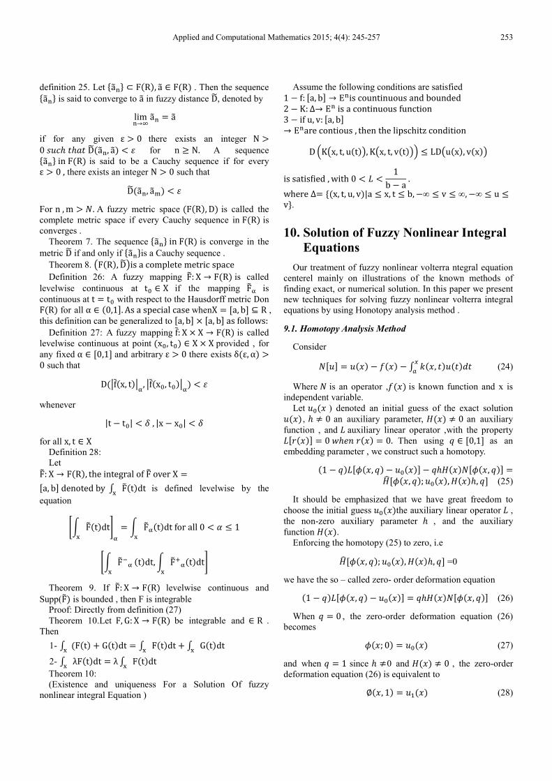
10. Solution of Fuzzy Nonlinear Integral

Equations

Our treatment of fuzzy nonlinear volterra ntegral equation

centerel mainly on illustrations of the known methods of

finding exact, or numerical solution. In this paper we present

new techniques for solving fuzzy nonlinear volterra integral

equations by using Honotopy analysis method .

9.1. Homotopy Analysis Method

Consider

ÑE}F = }�r� − Ã�r� − � ��r, ~�}�~��~±Ï (24)

Where Ñ is an operator ,Ã�r� is known function and x is

independent variable.

Let }T�r ) denoted an initial guess of the exact solution

}�r� , ℎ ≠ 0 an auxiliary parameter, ��r� ≠ 0 an auxiliary

function , and auxiliary linear operator ,with the property Eq�r�F = 0ÇℎÉ�q�r� = 0. Then using Í ∈ E0,1F as an

embedding parameter , we construct such a homotopy.

�1 − Í�E �r, Í� − }T�r�F − Íℎ��r�ÑE �r, Í�F =��E �r, Í�;}T�r�,��r�ℎ, ÍF (25)

It should be emphasized that we have great freedom to

choose the initial guess }T�r�the auxiliary linear operator ,

the non-zero auxiliary parameter ℎ , and the auxiliary

function ��r�.

Enforcing the homotopy (25) to zero, i.e

��E �r, Í�;}T�r�,��r�ℎ, ÍF =0

we have the so – called zero- order deformation equation

�1 − Í�E �r, Í� − }T�r�F = Íℎ��r�ÑE �r, Í�F (26)

When Í = 0 , the zero-order deformation equation (26)

becomes

�r; 0� = }T�r� (27)

and when Í = 1 since ℎ ≠0 and ��r� ≠ 0 , the zero-order

deformation equation (26) is equivalent to

∅�r, 1� = }V�r� (28)


Thus according to (27) and (28), as the embedding

parameter Í increases from 0 to 1, ∅(r, Í) varies

continuously. From the initial }T(r) the exact solution (r).

Such a kind of continuous variation is called deformation in

homotopy .

By Taylor’s theorem ∅(r, Í) can be expanded in power

series of Í as follows

∅(r, Í) = }T(r) + ∑ }�(r)Í�ü��V (29)

Where

}�(r) = V�!

��(±,�)�� |��T (30)

If the initial guess }T(r), the auxiliary linear parameter ,

the non zero auxiliary parameter h , and the auxiliary

function �(r) are property chosen so that the power series

(29) of (r, Í) converges at Í = 1 , we have under these

assumptions the solution series .

}(r) = (r, 1) = }T(r) + ∑ }�(r)Í�ü��V (31)

}�(r) = ��}�cV(r) + ℎ[}�cV(r) − Ã(r)− ø �(r, ~)}�cV(~)�~±

Ï

�� = Z0¤Ã� ≤ 11¤Ã� > 1\ Finaly we get

}T(r) = (r, 0)

}V(r) = −ℎÃ(r)

}�(r) = (1 + ℎ)}�cV(r) − ℎ[ø �(r, ~)}�cV(~)�~±Ï ]

Where

� ≥ 2

Hence , the solution of equation (24)

}(r) = lim�→V }(r, Ý) = � }�(r)ü��V

we denoted the nth- order approximation to solve }�(r) =∑ }�¡��V (r) 9.2. Solve Fuzzy HAM

Consider the fuzzy nonlinear integral equation with fuzzy

difference kernel

}�(r) = Ã(r) + ø ��(r − ~)}�(~)�~±Ï

Where }�(r) = {(}�(r), {�)}¡, Ã(r) = {(Ã�(r), {�)}¡v��(r −~) = {(��(r − ~), {�)}¡

Then

{(}�(r), {�)}¡ = {(Ã�(r), {�)}¡ + ø {(��(r − ~), {�)}¡{(}�(~), {�)}¡�~±

Ï

Now , make use equation (7), we get

{(}�(r), {�)}¡ = {(Ã�(r), {�)}¡+{�ø ��(r±Ï− ~)}�(~)�~ , {��}¡

andbyequation(8) {(}�(r), {�)}¡ = {(Ã�(r) + ø ��(r − ~)}�(~)�~±

Ï , {�)}¡

which implies that for each ∀{� ∈ [0,1] }�(r) = Ã�(r) + � ��(r, ~)}�(~)�~±Ï ∀¤ = 1,2, … . . , � (32)

Now , we can apply the HAM to equation (32) , we get

Ñ[}] = }�(r) − Ã�(r) − ø ��(r, ~)}�(~)�~±Ï

Let Í ∈ [0,1] (1 − Í)[ �(r, Í) − }�T(r)] − Íℎ�(r)Ñ[ �(r, Í)]= ��[ �(r, Í);}�T(r),�(r)ℎ, Í]

��[ �(r, Í);}�T(r),�(r)ℎ, Í] =0

(1 − Í)[ �(r, Í) − }�T(r)] = Íℎ�(r)Ñ[ �(r, Í)] When q=0

�(r; 0) = }�T(r)

when q=1

∅�(r, 1) = }�V(r) ∅�(r, Í) = }�T(r) + � }��(r)Í�ü

��V

Where

}��(r) = 1�¤! �

�� (r, Í)�Í�� |��T

}�(r) = �(r, 1) = }�T(r) + � }��(r)Í��ü��V

}��(r) = ��}��cV(r) + ℎ[}��cV(r) − Ã�(r)− ø ��(r, ~)}��cV(~)�~±Ï

�� = Z0¤Ã� ≤ 11¤Ã� > 1\


Finally we get

}�T(r) = �(r, 0) }�V(r) = −ℎÃ�(r)

}��(r) = (1 + ℎ)}��cV(r) − ℎ[ø ��(r, ~)}��cV(~)�~±Ï ]

Where

� ≥ 2

}�(r) = lim�→V}�(r, Ý) = � }��(r)ü��V

we denoted the nth- order approximation to solve }��(r) =∑ }��¡��V (r), ∀¤ = 1,2… . , �

Example 1

Consider the fuzzy nonlinear integral equation

}�(r) = Ã(r) + ø ��(r, ~)}�^(~)�~±Ï

Ã(r) = {(ÃV, 0.4), (Ã , 1)} ÃV(r) =ln(x+1)+2ln2(1−xln2+x)−2x−

!" ,Ã (r) =sin(πx)

��V(r, ~)}�^V(~) = (r − ~)}V^(~), ��^(r, ~)}�s^(~)= 15 cos(πx) sin(πt)}s^(~)

with the exact solution to equation is }V(r) =ln(x + 1), and

}^(r) = sin(πx) + 20 − √3913 cos(πx)

by using equation (9), and (10)

Where

}�(r) = {(}�(r), {�)}¡, Ã(r) = {(Ã�(r), {�)}¡v��(r − ~)= {(��(r − ~), {�)}¡

Then

{(}�(r), {�)}¡ = {(Ã�(r), {�)}¡ + ø {(��(r − ~), {�)}¡{(}�(~), {�)}¡�~±

Ï

Now , make use equation (7), we get

{(}�(r), {�)}¡ = {(Ã�(r), {�)}¡+{�ø ��(r±Ï− ~)}�(~)�~ , {��}¡

andbyequation(8) {(}�(r), {�)}¡ = {(Ã�(r) + ø ��(r − ~)}�(~)�~±

Ï , {�)}¡

which implies that for each ∀{� ∈ [0,1] }V(r) = ln(x + 1) + 2ln2(1 − xln2 + x) − 2x − 5

4+ ø (r − ~)}V^(~)±Ï �~

by using HAM method to solve this formula , we get

}VT(r) = 0

}VV(r) = −ℎ(ln(x + 1) + 2ln2(1 − xln2 + x) − 2x − 54

}V^(r) = (1 + ℎ)}VV(r) − ø (r − ~)}VV^(~)±Ï �~

}V�(r) = (1 + ℎ)}V�cV(r) − ø (r − ~)}V�cV^(~)±Ï �~

Table 1. shows numerical result calculated according the exact solution and

Homotopy analysis method for }V� , where h=0.5.

&' Exact (�(&) =ln(x +

1), HAM (�)(&) Exact-HAM

0 (0,0.4) (0.00000026768,0.4) 2.56186267595E-

8

0.1 (0.095310179804,0.4) (0.95310206285,0.4) 2.53309949127E-

8

0.2 (0.182321556793,0.4) (0.182321579887,0.4) 2.19432191028E-

8

0.3 (0.262364264467,0.4) (0.262364280170,0.4) 1.45529119865E-

8

0.4 (0.336472236621,0.4) (0.336472248418,0.4) 1.06476171213E-

8

0.5 (0.405465108108,0.4) (0.405465120209,0.4) 1.84023705163E-

8

0.6 (0.470003629245,0.4) (0.470003629794,0.4) 6.84976264597E-

9

0.7 (0.530628251062,0.4) (0.587786677053,0.4) 6.0872384910E-

10

0.8 (0.587786664902,0.4) (0.587786677053,0.4) 3.5510718809E-9

0.9 (0.641853886172,0.4) (0.641853890141,0.4) 2.8196508461E-9

1 (0.693147180559,0.4) (0.693147181293,0.4) 4.163761557E-10

Table 1 solution to the example 1

}^(r) = sin(πx) + ø 15 cos(πx) sin(πt)}s^(~)±Ï �~

at{ = 1

by using the equation (9) and ( 10) , we get

}^T(r) = 0

}^V(r) = −ℎ(sin(πx))

}^^(r) = (1 + ℎ)}^V(r) − ø 15 cos(πx) sin(πt)}^Vs(~)±Ï �~

}^�(r) = (1 + ℎ)}^�cV(r)− ø 15 cos(πx) sin(πt)}^�cVs(~)±Ï �~


Table 2. shows numerical result calculated according the exact solution and

Homotopy analysis method for }^�, where h=0.5.

è* Exact ��(è) =+',(-&) +�.c√/0�/ 12+(-&). HAM ��3(è) Exact-HAM

0 (0.0754266889,1) (0.0754266889,1) 5.53723733531E-

15

0.1 (0.3807520383,1) (0.3807520383,1) 5.21804821573E-

15

0.2 (0.6488067254,1) (0.6488067254,1) 4.55191440096-15

0.3 (0.8533516897,1) (0.8533516897,1) 3.21964677141-15

0.4 (0.9743646449,1) (0.9743646449,1) 1.77635683940-15

0.5 (1.0000000000,1) (1.0000000000,1) 0

0.6 (0.9277483875,1) (0.9277483875,1) 1.77635683940E-

15

0.7 (0.7646822990,1) (0.7646822990,1) 3.21964677141E-

15

0.8 (0.5267637791,1) (0.5267637791,1) 4.55191440096E-

15

0.9 (0.2372819503,1) (0.2372819503,1) 0.52735593669E-

15

1 (-0.0754266889,1) (-0.0754266889,1) 0.55372373353E-

15

Table 2 solution to the example 1

11. Conclusion

The proposed method is a powerful procedure for solving

fuzzy nonlinear integral equations. The examples analyzed

illustrate the ability and reliability of the method presented in

this paper and reveals that this one is very simple and

effective. The obtained solutions, in comparison with exact

solutions admit a remarkable accuracy. Results indicate that

the convergence rate is very fast, and lower approximations

can achieve high accuracy.

References

[1] C. T. H. Baker, A perspective on the numerical treatment of volterra equations, Journal of Computational and Applied Mathematics, 125 (2000), 217-249.

[2] N.Boldik, M. Inc, Modified decomposition method for nonlinear Volterra-Fredholm integral equations, Chaos, Solution and Fractals 33 (2007) 308- 313. http://dr.doi.org/10.1016/j.chaos.2005.12.058

[3] M. I. Berenguer, D. Gamez, A. I. Garralda-Guillem, M. Ruiz Galan and M. C. Serrano Perez, Biorthogonal systems for solving volterra integral equation systems of the second kind, Journal of Computational and Applied Mathematics, 235 (2011), 1875-1883.

[4] A. M. Bica, Error estimation in the approximation of the solution of nonlinear fuzzy fredholmintegral equations, Information Sciences, 178 (2008), 1279-1292.

[5] A. H. Borzabadi and O. S. Fard, A numerical scheme for a class of nonlinear fredholmintegral equations of the second kind, Journal of Computational and Applied Mathematics, 232 (2009), 449-454.

[6] S. S. L. Chang and L. Zadeh, On fuzzy mapping and control, IEEE Trans. System Man Cybernet, 2 (1972), 30-34.

[7] Y. Chen and T. Tang, Spectral methods for weakly singular volterra integral equations with smooth solutions, Journal of Computational and Applied Mathematics, 233 (2009), 938-950.

[8] D. Dubois and H. Prade, Operations on fuzzy numbers, International Journal of Systems Science, 9 (1978), 613-626.

[9] D. Dubois and H. Prade, Towards fuzzy differential calculus, Fuzzy Sets and Systems, 8(1982), 1-7.

[10] A. Kaufmann and M. M. Gupta, Introduction fuzzy arithmetic, Van Nostrand Reinhold, NewYork, 1985.

[11] J. P. Kauthen, Continuous time collocation method for volterra-fredholm integral equations, Numerical Math., 56 (1989), 409-424.

[12] P. Linz, Analytical and numerical methods for volterra equations, SIAM, Philadelphia, PA,1985.

[13] O. Solaymani Fard and M. Sanchooli, Two successive schemes for numerical solution of linearfuzzy fredholm integral equations of the second kind, Australian Journal of Basic Applied Sciences, 4 (2010), 817-825.

[14] L. A. Zadeh, The concept of a linguistic variable and its application to approximate reasoning, Information Sciences, 8 (1975), 199-249.

[15] S. Abbasbandy, E. Babolian and M. Alavi, Numerical method for solving linear fredholm fuzzy integral equations of the second kind, Chaos Solitons & Fractals, 31 (2007), 138-146.

[16] E. Babolian, H. S. Goghary and S. Abbasbandy, Numerical solution of linear fredholm fuzzy integral equations of the second kind by Adomian method, Applied Mathematics and Com-putation, 161 (2005), 733-744.

[17] Alabdullatif, M., Abdusalam, H. A. and Fahmy, E. S., Adomain decomposition method for nonlinear reaction diffusion system of Lotka- Volterra type, International Mathematical Forum, 2, No. 2 (2007), pp. 87-96.

[18] WazWaz, A.-M., The modified decomposition method for analytic treatment of nonlinearintegral equations and system of non-linear integral equations, International Journal of Computer Mathematics, Vol. 82, No. 9(2005), pp. 1107-1115.

[19] R. Goetschel and W. Vaxman, Elementary fuzzy calculus, Fuzzy Sets and Systems, 18 (1986), 31-43.

[20] T. Allahviranloo and M. Otadi, Gaussian quadratures for approximate of fuzzy multipleintegrals, Applied Mathematics and Computation, 172 (2006), 175-187.

[21] Kaleva, O.: A note on fuzzy differential equations, Nonlinear Analysis 64, 895–900 (2006).

[22] O. Kaleva, Fuzzy differential equations, Fuzzy Sets and Systems, 24 (1987), 301-317.

[23] M. Ma, M. Friedman and A. Kandel, A new fuzzy arithmetic, Fuzzy Sets and Systems, 108 (1999), 83-90

[24] G. J. Klir, U. S. Clair and B. Yuan, Fuzzy set theory: foundations and applications, Prentice-Hall, 1997.

[25] W. Congxin and M. Ming, On embedding problem of fuzzy number spaces, Part 1, Fuzzy Setsand Systems, 44 (1991), 33-38.


[26] M. L. Puri and D. Ralescu, Fuzzy random variables, Journal of Mathematical Analysis and Applications, 114 (1986), 409-422.

[27] Eman A.hussain, Existence and uniqueness of the solution of

nonlinear integral equation, Department of mathematics /college of science, university of Al-mustansiriyah Iraq/ Baghdad ,vol.26(2)2013.

homotopy method for solving finite level fuzzy nonlinear...

Documents