effective hydraulic parameters for steady state vertical

Effective hydraulic parameters for steady state vertical flow

in heterogeneous soils

Jianting Zhu and Binayak P. Mohanty

Biological and Agricultural Engineering Department, Texas A&M University, College Station, Texas, USA

Received 8 November 2002; revised 19 May 2003; accepted 23 June 2003; published 30 August 2003.

[1] In hydroclimate and land-atmospheric interaction models, effective hydraulicproperties are needed at large grid scales. In this study, the effective soil hydraulicparameters of the areally heterogeneous soil formation are derived by conceptualizing theheterogeneous soil formation as an equivalent homogeneous medium and assuming thatthe equivalent homogeneous soil will approximately discharge the same total amount offlux and produce same average pressure head profile in the formation. As compared toprevious effective hydraulic property studies, a specific feature of this study is that thederived effective hydraulic parameters are mean-gradient-dependent (i.e., vary acrossdepth). Although areal soil heterogeneity was formulated as parallel homogeneous streamtubes in this study, our results appear to be consistent with the previous findings of mean-gradient unsaturated hydraulic conductivity [Yeh et al., 1985a, 1985b]. Three widely usedhydraulic conductivity models were employed in this study, i.e., the Gardner model, theBrooks and Corey model, and the van Genuchten model. We examined the impact ofparameter correlation, boundary condition (surface pressure head), and elevation above thewater table on the effective saturated hydraulic conductivity and shape parameter. Thecorrelation between the saturated hydraulic conductivity Ks and the shape parameter aincreases the effective saturated hydraulic conductivity, while it does not affect the effectivea. The effective a is usually smaller than the mean value of a, while the effective Ks can besmaller or larger than the mean value depending on no correlation or full correlationbetween Ks and a fields, respectively. An important observation of this study is thatGardner and van Genuchten functions resulted in effective parameters, whereas it isdifficult to define effective parameters for the Brooks Corey model since this model uses apiecewise-continuous profile for hydraulic conductivity. INDEX TERMS: 1875 Hydrology:

Unsaturated zone; 1836 Hydrology: Hydrologic budget (1655); 1869 Hydrology: Stochastic processes; 1833

Hydrology: Hydroclimatology; 1829 Hydrology: Groundwater hydrology; KEYWORDS: effective hydraulic

parameters, heterogeneous soil formation, Gardner’s model, Brooks and Corey model, van Genuchten model

Citation: Zhu, J., and B. P. Mohanty, Effective hydraulic parameters for steady state vertical flow in heterogeneous soils, Water

Resour. Res., 39(8), 1227, doi:10.1029/2002WR001831, 2003.

1. Introduction

[2] Simulations of unsaturated flow and solute transportin soil typically use closed-form functional relationships torepresent water-retention characteristics and unsaturatedhydraulic conductivities. The Gardner and Russo exponen-tial model [Gardner, 1958; Russo, 1988], the Brooks andCorey piecewise-continuous model [Brooks and Corey,1964], and the van Genuchten model [van Genuchten,1980] represent some of the most widely used and practicalhydraulic property models. Basically, based on a point-scalehydrologic process, these parameter models are valid at thepoint or local scale. When these models are used in larger-scale (plot, field, watershed, or regional) processes, majorquestions remain about how to average the spatially variablehydraulic properties over a heterogeneous soil volume [e.g.,Yeh et al., 1985a, 1985b, 1985c; Russo, 1992; Desbarats,1998; Govindaraju et al., 2001] and what averages of

hydraulic property shape parameters to use for thesemodels [e.g., Yeh, 1989; Green et al., 1996]. During thepast 2 decades, many research efforts have been dedicatedto this issue, and the problem is usually analyzed usingstochastic models [e.g., Montoglou and Gelhar, 1987a,1987b, 1987c; Unlu et al., 1990a; Ferrante and Yeh, 1999].[3] Smith and Diekkruger [1996] studied one-dimen-

sional vertical flows through spatially heterogeneous soils.They assumed that there was no cross correlation betweenthe soil characteristic parameters. Green et al. [1996]investigated methods for determining the upscaled water-retention characteristics of stratified soil formations usingthe van Genuchten model for soil hydraulic properties.While they compared the linear volume average (LVA)and the direct parameter average for an upscaled waterretention curve of periodically layered soils, their ap-proach remains to be justified under flow conditions.Chen et al. [1994a, 1994b] developed the spatiallyaveraged Richards equation for the mean water saturationin each horizontal soil layer and the cross covariance of

Copyright 2003 by the American Geophysical Union.0043-1397/03/2002WR001831$09.00

SBH 12 - 1

WATER RESOURCES RESEARCH, VOL. 39, NO. 8, 1227, doi:10.1029/2002WR001831, 2003

the saturated hydraulic conductivity and the water satu-ration in each soil layer in a heterogeneous field. Theirapproach, however, is restricted to the uncertainty fromspatial variability in the saturated hydraulic conductivity.Govindaraju et al. [2001] studied field-scale infiltrationover soils. They only considered the spatial variability ofsaturated hydraulic conductivity, which is represented bya homogeneous correlated lognormal random field. Kim etal. [1997] investigated the significance of soil hydraulicheterogeneity on the water budget of the unsaturated zoneusing the Brooks and Corey model, based on a frame-work of approximate analytical solutions. In their work,the geometrical scaling theory was assumed appropriateand the air entry value (1/aBC) was assumed to bedeterministic.[4] While stochastic analysis of flow through fully

three-dimensional heterogeneous media [e.g., Yeh et al.,1985a, 1985b, 1985c] is most appropriate, one-dimension-al models has been used as approximations for varioussimplified problems under investigation (e.g., shallowsubsurface dominated by vertical flows). For one-dimen-sional analyses, two physical scenarios need to be distin-guished: (1) vertical layering (heterogeneity), wherevariations in soil properties are in the vertical directionsonly [e.g., Yeh, 1989], and (2) vertically homogeneous soilcolumns with variations of the soil properties in thehorizontal plane only [e.g., Rubin and Or, 1993]. Ourstudy focuses on the latter case, where the variability is inthe horizontal plane. The domain is assumed to be com-posed of homogeneous soil columns without mutual inter-action to simplify the analysis while keeping the focuson some of the main process of many practical fieldapplications. For example, in meso-/regional-scale soil-vegetation-atmosphere transfer (SVAT) schemes used inhydroclimatic models, pixel dimensions may range fromseveral hundred square meters to several hundred squarekilometers, while the vertical scale of subsurface process-es near the land-atmosphere boundary (the top fewmeters) is considerably small. In such a large horizontalscale, the areal heterogeneity of hydraulic propertiesdominates. Therefore it is reasonable to consider onlythe areal heterogeneity of soil. On the other hand, theparallel column approach will not apply to scenarioswhere the vadose zone is very deep and vertical hetero-geneity dominates or the topography of the region variesconsiderably and thus mutual interactions between soilcolumns might be significant. Pixel-scale soil hydraulicparameters and their accuracy are critical for the successof hydroclimatic and soil hydrologic models. Our studytries to answer a major question: What will be theeffective/average hydraulic properties for the entire pixel(or footprint of a remote sensor) for a typical soil texturalcombination in a real field condition, if the soil hydraulicproperties can be estimated for each individual texture?[5] Typically, the p-order power average or p-norm has

been used in determining the parameters for the upscaledhydraulic conductivity function [e.g., Green et al., 1996;Korvin, 1982]. It is, however, often difficult to determinep-value, which can range from �/ to +/. Furthermore,most previous studies of similar context usually eitherassumed that the driving force of heterogeneity was solelyfrom saturated hydraulic conductivity or the parameters

considered were statistically independent. In the study ofYeh et al. [1985a, 1985b, 1985c], the perturbation equationof the steady stochastic flow in unsaturated media wassolved by spectral representation techniques, while Zhanget al. [1998] developed first-order stochastic models insecond-order stationary media with both the Brooks-Coreyand the Gardner-Russo constitutive relationships. Whilethe mathematical approaches of Yeh et al. [1985a, 1985b,1985c] and Zhang et al. [1998] were quite generic, theytypically worked well in the deep and unbounded vadosezone where gravity-dominated infiltration is the mainprocess and the mean hydraulic gradient is approximatelyconstant. In this study, we consider the influence ofparameter correlation on upscaled effective parameterswithout using a specific averaging scheme for the hydraulicparameters. The results apply equally well to both infiltrationand evaporation scenarios in the shallow vadose zonebounded by atmospheric boundary. Specifically, we analyzethe effective soil hydraulic parameters of the heterogeneoussoil formation by conceptualizing the areally heterogeneoussoil formation as an equivalent homogeneous mediumand assuming that the equivalent homogeneous soil willapproximately discharge ensemble-mean flux and produceensemble-mean pressure head profile in the heterogeneousformation for the steady state flows. Three widely usedhydraulic conductivity models were employed in the study,i.e., the Gardner model, the Brooks and Corey model, andthe van Genuchten model. We examined the impact ofparameter correlation, boundary condition (surface pressurehead), and elevation above the water table on effectivesaturated hydraulic conductivity and shape parameter a. Inthis study, spatial correlation structure for each parameterfield was assumed absent.

2. Hydraulic Property Models

[6] Soil hydraulic behavior is characterized by the soilwater retention curve, which defines the water content (q) as afunction of the capillary pressure head (y), and the hydraulicconductivity function, which establishes relationship be-tween the hydraulic conductivity (K) and water content orcapillary pressure head. Simulations of unsaturated flow andsolute transport typically use closed-form functions torepresent water-retention characteristics and unsaturatedhydraulic conductivities. It is assumed that the constitutiverelationships apply at every point in the soil and the soilhydraulic property areal variation between sampling pointscan be described by the spatial variations of the parameters inthe hydraulic characteristic functions [e.g., Russo andBouton, 1992]. Some of the commonly used functionalrelationships include the Gardner-Russo model [Gardner,1958; Russo, 1988], the Brooks-Corey model [Brooks andCorey, 1964], and the van Genuchten model [van Genuchten,1980]. A brief review of these models is given below.Interested readers are referred to Leij et al. [1997] for morecomprehensive review and discussion on various closed-formexpressions of hydraulic properties, including the modelsgiven below.

2.1. The Gardner-Russo Model

[7] The unsaturated hydraulic conductivity (K)-capillarypressure head (y) and the reduced water content (Se)-

SBH 12 - 2 ZHU AND MOHANTY: PARAMETERS FOR STEADY STATE VERTICAL FLOW

capillary pressure (y) are assumed to be represented by theGardner model [Gardner, 1958; Russo, 1988]

K ¼ Kse�aGy ð1aÞ

Se yð Þ ¼ e�0:5aGy 1þ 0:5aGyð Þ� �2= ‘þ2ð Þ ð1bÞ

where Ks is the saturated hydraulic conductivity, aG isknown as the pore-size distribution parameter, ‘ is aparameter that accounts for the dependence of the tortuosityand the correlation factors on the water content estimated, tobe about 0.5 as an average for many soils [Mualem, 1976],Se = (q � qr)/(qs � qr) is the effective, dimensionless reducedwater content, q is the total volumetric water content, and qsand qr are the saturated and residual (irreducible) watercontents, respectively. For notational convenience, y for theremainder of this paper is taken positive for unsaturatedsoils (i.e., it denotes suction).

2.2. The Brooks-Corey Model

[8] Brooks and Corey [1964] established the relationshipbetween K and y using the following empirical equationsfrom analysis of a large database:

Se yð Þ ¼ aBCyð Þ�lif aBCy > 1 ð2aÞ

Se yð Þ ¼ 1 if aBCy � 1 ð2bÞ

K yð Þ ¼ Ks aBCyð Þ�bif aBCy > 1 ð2cÞ

K yð Þ ¼ Ks if aBCy � 1 ð2dÞ

where b = l(‘ + 2) + 2. The l is a parameter used by Brooksand Corey to define the relationship between water contentand y (retention function) affecting the slope of theretention function.[9] This model has been used successfully to describe

retention data for relatively homogeneous and isotropicsamples. The model may not describe the data well nearsaturation where the saturation is fixed and a discontinuityoccurs at y = 1/aBC.

2.3. The van Genuchten Model

[10] Van Genuchten [1980] identified an S-shaped func-tion that fits measured water-retention characteristics ofmany types of soil very well. The function was alsocombined with Mualem’s hydraulic conductivity function[Mualem, 1976] to predict unsaturated hydraulic conductiv-ity. Subsequently, the van Genuchten function has becomeone of the most widely used curves for characterizing soilhydraulic properties. The van Genuchten equation of soilwater retention curve can be expressed as follows:

Se yð Þ ¼ 1

1þ avGyð Þn½ mð3Þ

where avG, n, and m are parameters that determine the shapeof the soil water retention curve. Assuming m = 1 � 1/n,

van Genuchten [1980] combined above the soil waterretention function with the theoretical pore-size distributionmodel of Mualem [1976] and obtained the followingrelationships for the hydraulic conductivity in terms of thereduced water content or the capillary pressure head:

K Seð Þ ¼ KsS‘e 1� 1� S1=me

� �mh i2ð4Þ

K yð Þ ¼ Ks 1� avGyð Þmn 1þ avGyð Þn½ �mf g2

1þ avGyð Þn½ m‘ð5Þ

[11] There are then four parameters for the Gardner-Russo model to describe the soil hydraulic characteristicsof each sample: Ks, aG, qs, and qr; five parameters for theBrooks-Corey model: Ks, aBC, l, qs, and qr; and fiveparameters for the van Genuchten model: Ks, avG, n, qs,and qr. A study by Hills et al. [1992] showed that thewater-retention characteristics could be adequately modeledusing either a variable parameter avG with a constant vanGenuchten parameter n, or a variable n with a constant avG,with better results when avG was variable. Because the vanGenuchten n is closely related to the Brooks-Corey l, weshall treat the Brooks-Corey l as a deterministic constant inour subsequent analysis to reduce the number of parametersneeded to describe the spatial distribution of the hydraulicproperties. In the light of their results, we will consider onlythe spatial variability introduced by the spatial variation ofthe parameter Ks and a for both the Gardner-Russo and theBrooks-Corey models. In this study, we adopt a typicalvalue of l = 0.4, Ks = 1.0 � 10�5 (cm/s), CV(Ks) = 0.4, anda = 0.0225(1/cm), CV(a) = 0.4 [e.g., Unlu et al., 1990b].Other values can also be used [e.g., Philip, 1969; Braester,1973; El-Kadi, 1992; Fayer and Gee, 1992; Rawls et al.,1992; Mohanty et al., 1994].[12] There are many studies about the correlation be-

tween characteristic parameters for the hydraulic proper-ties of soil in the literature [e.g., Yeh et al., 1985a, 1985b,1985c; Montoglou and Gelhar, 1987a, 1987b, 1987c;Russo and Bouton, 1992]. Some of their results showno consensus about parameter correlation. For example,after analyzing soil samples gathered on the Krummbachand Eisenbach catchments in northern Germany and froma field experiment near Las Cruces, New Mexico, Smithand Diekkruger [1996] concluded that no significantcorrelation was observed among any of the characteristicparameters and suggested that most random variation insoil characteristic parameters could be treated as indepen-dent. However, in another study, Wang and Narasimhan[1992] indicated that Ks was proportional to a2. In thisresearch, we will study both correlated and independentcases and the significance of their correlation on theensemble behavior of soil dynamic characteristic of un-saturated flow.

3. Steady State Vertical Flow

[13] General equations relating pressure head and eleva-tion above the water table for steady state vertical flows can

ZHU AND MOHANTY: PARAMETERS FOR STEADY STATE VERTICAL FLOW SBH 12 - 3

be expressed as [e.g., Zaslavsky, 1964; Warrick and Yeh,1990]

z ¼Zy0

K yð ÞdyK yð Þ þ q

ð6Þ

where z is the vertical distance above the water table withthe water table location being at z = 0, and q is the steadystate evaporation (positive) or infiltration (negative) rate. Itsdimensionless form can be expressed as

az ¼Zay0

Kr xð ÞdxKr xð Þ þ q0

ð7Þ

where the dimensionless hydraulic conductivity Kr = K/Ks, the dimensionless pressure head x = ay, and thedimensionless flux rate q0 = q/Ks. When the pressure headat the surface, yL, is known, the dimensionless statesteady flux q/Ks can be found out from the followingequation:

aL ¼ZayL

0

Kr xð ÞdxKr xð Þ þ q0

ð8Þ

where L is the elevation of the ground surface above thewater table. From equation (8), it can be seen that thedimensionless steady state flux rate q0 itself is not relatedto the saturated hydraulic conductivity Ks. In other words,the flux rate q is a linear function of Ks. In turn, we caninfer from equation (7) that the capillary pressure head yis not related to the saturated hydraulic conductivity Ks ifthe dimensionless flux q0 is specified.[14] When the Gardner hydraulic conductivity model is

used, the capillary pressure profile (y) and the dimension-less flux rate (q0 = q/Ks) can be analytically expressed as

y ¼ lneaGL � 1

e�aGz þ e�aGyL � e�aGL � e�aG zþyLð Þ

� 1=aG

� L ð9Þ

q0 ¼ 1� e�aG yL�Lð Þ

eaGL � 1ð10Þ

[15] For the Brooks-Corey model, analytical solutions arealso possible, but the evaporation and infiltration cases needto be analyzed separately. The capillary pressure head (y)can be related to the elevation above the water table (z) asthe following series relationship for steady state evaporation[Warrick, 1988]:

aBCz ¼1

bq0ð Þ�1=b � BU

1

b; 1� 1

b

� � bq0

1þ bð Þ 1þ q0ð Þ2

� 2F1 1; 2; 2þ 1

b;

q0

1þ q0

� ð11Þ

where Bu is the incomplete Beta function with u =q0aBC

b yb/(1 + q0aBCb yb) and 2F1 is the Gaussian

hypergeometric function. The relationship between thedimensionless evaporation rate q0 and the surface pressurehead yL can be established iteratively by the followingequation:

aBCL ¼ 1

bq0ð Þ�1=b � BuL

1

b; 1� 1

b

� � bq0

1þ bð Þ 1þ q0ð Þ2

� 2F1 1; 2; 2þ 1

b;

q0

1þ q0

� ð12Þ

where uL = q0aBCb yL

b/(1 + q0aBCb yL

b), while for steady stateinfiltration, the relationship can be established as follows[Zhu and Mohanty, 2002] with p0 = �q0:

aBCz ¼ aBCy � 2F1

1

b; 1; 1þ 1

b; p0ab

BCyb

� þ bp0

1� p0ð Þ 1þ bð Þ

� 2F1 1;1

b; 2þ 1

b; p0

� ð13Þ

The relationship between the dimensionless infiltration ratep0 and the surface pressure head yL can be establishediteratively by the following equation:

aBCL ¼ aBCy � 2F1

1

b; 1; 1þ 1

b; p0ab

BCybL

� þ bp0

1� p0ð Þ 1þ bð Þ

� 2F1 1;1

b; 2þ 1

b; p0

� ð14Þ

[16] These analytical solutions will be required to calcu-late the derivative terms in deriving effective parameters inthe next section. For the van Genuchten model, the integra-tions in equations (7) and (8) were carried out numerically.

4. Effective Hydraulic Parameters

[17] The effective soil hydraulic parameters of theheterogeneous soil formation are derived by conceptualizingthe soil formation as an equivalent homogeneous medium. Itis assumed that the equivalent homogeneous soil willapproximately discharge the same ensemble-mean flux[e.g., Milly and Eagleson, 1987; Kim et al., 1997] andproduce the same ensemble-mean pressure head profile inthe formation. Since y is only related to a based on theprevious discussions for the three functions, approximatingy by the first two terms of a Taylor expansion around themean parameter a and taking the expected value of theresulting equation lead to

y að Þ ¼ y að Þ þ 1

2

@2y@a2

að Þs2a ð15Þ

Since q is a linear function of Ks, a similar operation in termsof q leads to

q Ks;að Þ ¼ Ksq0 að Þ þ Ks

2

@2q0

@a2að Þs2a þ @q0

@aað ÞrsKs

sa ð16Þ

In equations (15) and (16), sKsand sa are the standard

deviations of Ks and a, respectively, and r is the correlationcoefficient of Ks and a, defined as

r ¼ cov Ks;að ÞsKS

sa¼

Ks � Ks

�a� að Þ

sKssa

:


Approximation of y(a) and q(Ks, a) to the first order of aTaylor expansion around the mean parameters yields

y aeffð Þ ¼ y að Þ þ @y@a

að Þ aeff � að Þ ð17Þ

q Kseff ;aeff

�¼Ksq

0 að Þþq0 að Þ Kseff � Ks

�þ Ks

@q0

@aað Þ aeff � að Þ

ð18Þ

In using equations (17) and (18), we made two assumptions.First, it is a Taylor series expansion with higher-order termstruncated. Second, the derivative terms in the expansionsare also evaluated approximately assuming that thederivative terms in the hypothetic layered formation areclosed to those in the homogeneous formation. Bothapproximations require the variance of the randomparameters to be small. Following Milly and Eagleson[1987] and Kim et al. [1997], we set y(aeff) = y að Þ andq(Kseff, aeff) = q Ks;að Þ and use equations (15) through (18),which yield,

aeff ¼ aþ 1

2

@2y@a2

að Þ�

@y@a

að Þ�

s2a ð19Þ

Kseff ¼ Ks þKs

2q0 að Þ@2q0

@a2að Þ

� @q0

@aað Þ=@y

@aað Þ

� �� @2y

@aað Þ�s2a

þ @q0

@aað Þ�

q0 að Þ� �

rsKssa ð20Þ

[18] Since predicting the ensemble-mean flux rate isusually a main concern in most practical soil-vegetation-atmospheric transfer (SVAT) models, we can use an alter-native and simpler approach to derive effective hydraulicparameters by assuming that the equivalent homogeneousmedium will discharge the same amount of flux as theheterogeneous one. Because of the nature of areally hetero-geneous vertical flow, in this study we consider the arithme-tic average (mean) for the saturated hydraulic conductivityas an appropriate effective parameter, i. e., Kseff = Ks,and determine the other effective parameter, aeff, by onlymatching the flux rate q. In this way, by equaling q(Ks, aeff)to q Ks;a

�we have the following simple expression for

effective parameter aeff:

aeff ¼ aþ 1

2

@2q0

@a2að Þ�

@q0

@aað Þ

� �s2a ð21Þ

[19] In this sense, the equivalent homogeneous formationso defined would only deliver approximately ensemble-mean flux, while there would be no guarantee in term ofensemble-average pressure profiles in the formation.

5. Higher-Order Approximation andComparison With Monte Carlo Simulationsand Previous Studies

[20] Using a procedure similar to the first-order approx-imation but truncating the Taylor expansion around the

mean parameters to the second order yields (note y =y(a) and q = Ksq

0(a))

y aeffð Þ ¼ y að Þ þ dyda

að Þ aeff � að Þ þ 1

2

d2yda2

að Þ aeff � að Þ2

ð22Þ

q Kseff ;aeffð Þ ¼Ksq0 að Þ þ q0 að Þ Kseff �Ks

�þ Ks

dq0

daað Þ aeff � að Þ

þ Ks

2

d2q0

da2aeff � að Þ2 þ dq0

daKseff � Ks

�aeff � að Þ

ð23Þ

[21] Setting y(aeff) = y að Þ and q(Kseff, aeff) = q Ks;að Þleads to

aeff ¼ a� dyda

þ dyda

� 2"(

þ d2yda2

� 2

s2a

#1=29=; d2y

da2

�

ifdyda

< 0: ð24Þ

aeff ¼ a� dyda

� dyda

� 2"(

þ d2yda2

� 2

s2a

#1=29=; d2y

da2

�

ifdyda

> 0: ð25Þ

Kseff ¼ Ks

þKs

2d2q0

da2 s2a � aeff � að Þ2h i

þ dq0

da rsKssa � Ks

dq0

da aeff � að Þ

q0 þ dq0

da aeff � að Þð26Þ

[22] We have also conducted Monte Carlo simulationsof 10,000 realizations and compared the results with theresults of both first- and second-order approximations inorder to verify our findings. Both Ks and a are assumedto obey the lognormal distribution. The cross-correlatedrandom fields of the parameters Ks and a were generatedusing the spectral method proposed by Robin et al.[1993]. Random fields were produced with the powerspectral density function, which was based on exponen-tially decaying covariance functions. The coherency spec-trum, given by equation (27), is an indicator of parametercorrelation,

R fð Þ ¼ f12 fð Þf11 fð Þf22 fð Þ½ 1=2

ð27Þ

where f11(f ), f22(f ) are the power spectra of randomfields log(Ks) and log(a), respectively, and f12(f ) is thecross spectrum between log(Ks) and log(a). Having jRj2 = 1indicates perfect linear correlation between the randomfields. The random fields are assumed to be isotropic,


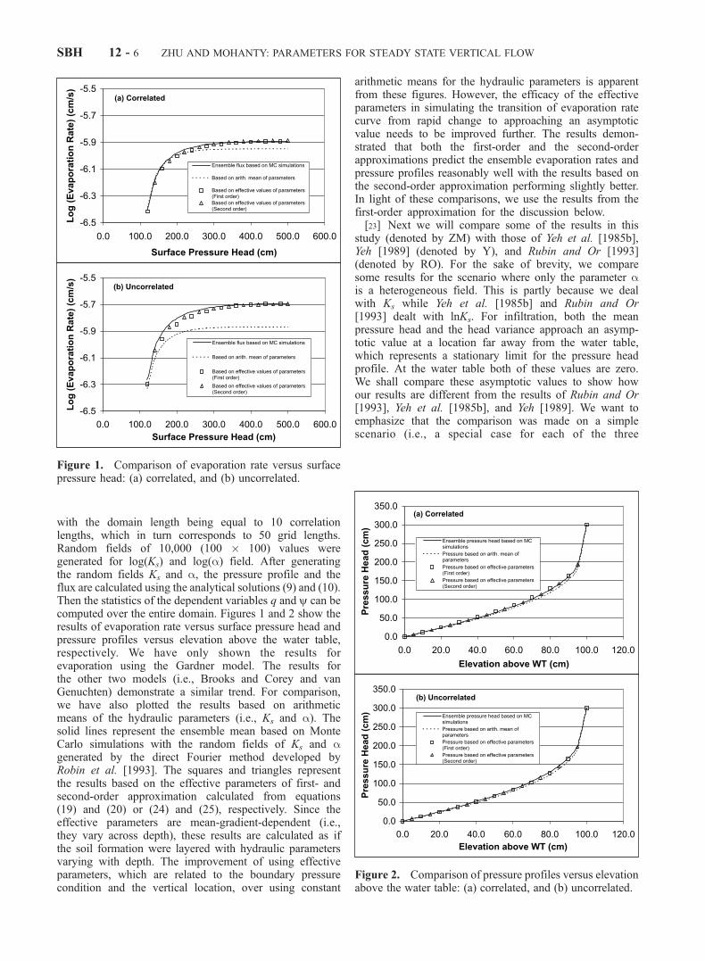
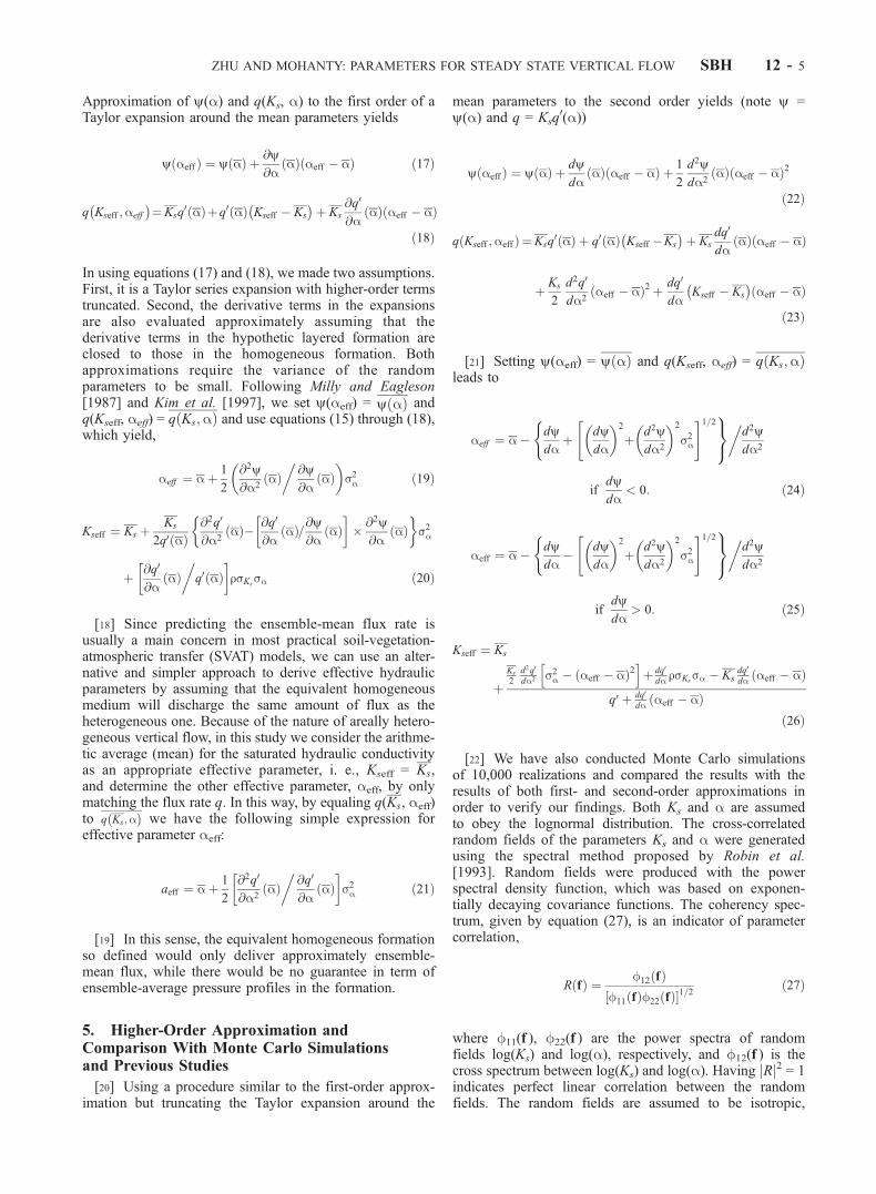
with the domain length being equal to 10 correlationlengths, which in turn corresponds to 50 grid lengths.Random fields of 10,000 (100 � 100) values weregenerated for log(Ks) and log(a) field. After generatingthe random fields Ks and a, the pressure profile and theflux are calculated using the analytical solutions (9) and (10).Then the statistics of the dependent variables q and y can becomputed over the entire domain. Figures 1 and 2 show theresults of evaporation rate versus surface pressure head andpressure profiles versus elevation above the water table,respectively. We have only shown the results forevaporation using the Gardner model. The results forthe other two models (i.e., Brooks and Corey and vanGenuchten) demonstrate a similar trend. For comparison,we have also plotted the results based on arithmeticmeans of the hydraulic parameters (i.e., Ks and a). Thesolid lines represent the ensemble mean based on MonteCarlo simulations with the random fields of Ks and agenerated by the direct Fourier method developed byRobin et al. [1993]. The squares and triangles representthe results based on the effective parameters of first- andsecond-order approximation calculated from equations(19) and (20) or (24) and (25), respectively. Since theeffective parameters are mean-gradient-dependent (i.e.,they vary across depth), these results are calculated as ifthe soil formation were layered with hydraulic parametersvarying with depth. The improvement of using effectiveparameters, which are related to the boundary pressurecondition and the vertical location, over using constant

arithmetic means for the hydraulic parameters is apparentfrom these figures. However, the efficacy of the effectiveparameters in simulating the transition of evaporation ratecurve from rapid change to approaching an asymptoticvalue needs to be improved further. The results demon-strated that both the first-order and the second-orderapproximations predict the ensemble evaporation rates andpressure profiles reasonably well with the results based onthe second-order approximation performing slightly better.In light of these comparisons, we use the results from thefirst-order approximation for the discussion below.[23] Next we will compare some of the results in this

study (denoted by ZM) with those of Yeh et al. [1985b],Yeh [1989] (denoted by Y), and Rubin and Or [1993](denoted by RO). For the sake of brevity, we comparesome results for the scenario where only the parameter ais a heterogeneous field. This is partly because we dealwith Ks while Yeh et al. [1985b] and Rubin and Or[1993] dealt with lnKs. For infiltration, both the meanpressure head and the head variance approach an asymp-totic value at a location far away from the water table,which represents a stationary limit for the pressure headprofile. At the water table both of these values are zero.We shall compare these asymptotic values to show howour results are different from the results of Rubin and Or[1993], Yeh et al. [1985b], and Yeh [1989]. We want toemphasize that the comparison was made on a simplescenario (i.e., a special case for each of the three

Figure 1. Comparison of evaporation rate versus surfacepressure head: (a) correlated, and (b) uncorrelated.

Figure 2. Comparison of pressure profiles versus elevationabove the water table: (a) correlated, and (b) uncorrelated.


approaches, Yeh [1989], Rubin and Or [1993], and thisstudy). In our study, the horizontal stationarity is implicitlyassumed, meaning that the mean and variance are constantin the horizontal directions. Vertically, the hydraulicparameters were assumed homogeneous. Yeh [1989]assumes vertical variability of hydraulic parameters andunit mean gradient; his model can be compared with ourstudy by taking very large values of the vertical integralscales of the random hydraulic parameters. The work ofRubin and Or [1993] also considered the effect of rootwater uptake, which is taken to be zero when comparingwith our study.[24] For this special case, the vertical pressure profile by

using the Gardner hydraulic function can be easily expressedas

y zð Þ ¼ � ln e�az � q0 1� e�azð Þ½ =a ð28Þ

It can be seen that y and sy2 approach an asymptotic limit as

z (the distance from the water table) increases. At a locationfar away from the water table (i.e., unit gradient),

y ¼ � ln �q0ð Þ=a ð29Þ

[25] For a lognormally distributed variable a, its proba-bility distribution function is

f að Þ ¼1ffiffiffiffiffiffiffiffi2px

p exp � lna� mð Þ2

2x2

" #a > 0

0 a � 0

8><>: ð30Þ

with the parameters m and x being determined from themean of a, a, and the coefficient of variations of a, ca, asfollows:

x ¼ffiffiffiffiffiffiffiffiffiffiffiffiffiffiffiffiffiffiffiffiffiln c2a þ 1 �q

ð31Þ

m ¼ lnaffiffiffiffiffiffiffiffiffiffiffiffiffi

c2a þ 1p !

ð32Þ

Then the mean value and the variance of y at a location faraway from the water table can be calculated as

y ¼ � ln q0ð ÞZ10

f að Þdaa

¼ � ln �q0ð Þa

1þ c2a �

ð33Þ

s2y ¼ y2 � yð Þ2¼ ln �q0ð Þa2

� �21þ c2a �2

c2a ð34Þ

The variance of pressure head from this study can beexpressed as

s2y ¼ y að Þ � y aeffð Þ½ 2 ¼ @y@a

� 2

a� aeffð Þ2 ð35Þ

[26] Using the mean pressure head profile of equation (17)and the variance of (35) and evaluating at locations far awayfrom the water table, we have

yZM ¼ y aeffð Þ ¼ � ln �q0ð Þa

1þ c2a �

ð36Þ

s2yZM ¼ ln �q0ð Þa

� �2c2a 1þ c2a �

ð37Þ

It can be seen that the results of this study predict exactmean pressure value (33) and underpredict the headvariance (34) by a factor of (1 + ca

2).[27] The results of Rubin and Or [1993] for the mean and

the variance of the pressure head are as (simplified fromtheir equations (17) and (19) using our notations)

yRO ¼ � ln �q0ð Þa

ð38Þ

s2yRO ¼ ln �q0ð Þa

� �2c2a ð39Þ

The results of Rubin and Or [1993] suggested that the meanpressure head is the pressure head using the mean valueof a.[28] The head variance based on Yeh et al. [1985a, 1985b]

can be expressed as

s2yY ¼ y2Ys

2a=a

2 ð40Þ

[29] The effective value for a from Yeh [1989] for thisspecial case can be simplified by taking a very large valuefor the correlation scale in their results [e.g., Yeh, 1989,equation (16)],

aeff Yð Þ ¼ a� s2aa

¼ a 1� c2a �

ð41Þ

[30] The mean pressure head and the variance can then beobtained by using aeff(Y) into pressure head and varianceexpressions,

yY ¼ � ln �q0ð Þa 1� c2a � ð42Þ

s2yY ¼ ln �q0ð Þ½ 2

a2

c2a

1� c2a �2 ð43Þ

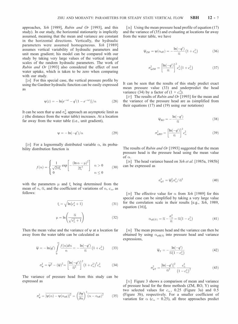
[31] Figure 3 shows a comparison of mean and varianceof pressure head for the three methods (ZM, RO, Y) usingtwo selected values for ca , 0.25 (Figure 3a) and 0.5(Figure 3b), respectively. For a smaller coefficient ofvariation for a (ca = 0.25), all three approaches predict


the mean and variance of the pressure reasonably well.The results of Rubin and Or [1993] underestimate bothmean and variance of the pressure head, suggesting thearithmetic mean is too large as an effective parameter. Theresults based on Yeh et al. [1985b] and Yeh [1989]overestimate both mean and variance of the pressure head.However, the variance based on Yeh [1989] is closest tothe theoretical results. It can be seen that the results of thisstudy predict the mean pressure head exactly and under-estimate the pressure variance.[32] As a caveat, we want to point out that a general

matching of mean pressure head and mean flux does notimply an equally good comparison of other details for agiven scenario. The effective parameter idea developed inthis study means to predict mean flux and pressure head inheterogeneous soils for steady state flows.

6. Results and Discussion

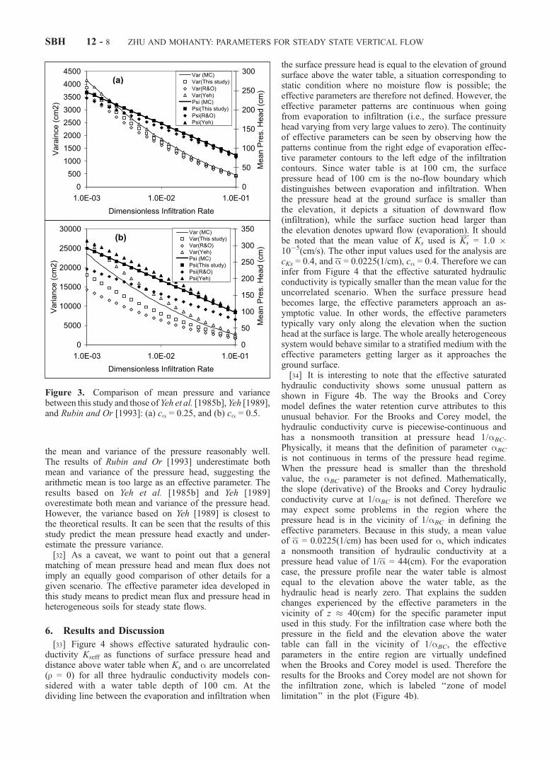
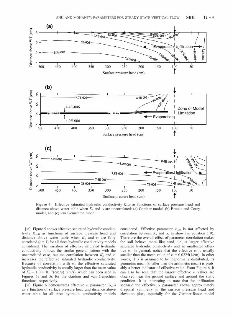
[33] Figure 4 shows effective saturated hydraulic con-ductivity Kseff as functions of surface pressure head anddistance above water table when Ks and a are uncorrelated(r = 0) for all three hydraulic conductivity models con-sidered with a water table depth of 100 cm. At thedividing line between the evaporation and infiltration when

the surface pressure head is equal to the elevation of groundsurface above the water table, a situation corresponding tostatic condition where no moisture flow is possible; theeffective parameters are therefore not defined. However, theeffective parameter patterns are continuous when goingfrom evaporation to infiltration (i.e., the surface pressurehead varying from very large values to zero). The continuityof effective parameters can be seen by observing how thepatterns continue from the right edge of evaporation effec-tive parameter contours to the left edge of the infiltrationcontours. Since water table is at 100 cm, the surfacepressure head of 100 cm is the no-flow boundary whichdistinguishes between evaporation and infiltration. Whenthe pressure head at the ground surface is smaller thanthe elevation, it depicts a situation of downward flow(infiltration), while the surface suction head larger thanthe elevation denotes upward flow (evaporation). It shouldbe noted that the mean value of Ks used is Ks = 1.0 �10�5(cm/s). The other input values used for the analysis arecKs = 0.4, and a = 0.0225(1/cm), ca = 0.4. Therefore we caninfer from Figure 4 that the effective saturated hydraulicconductivity is typically smaller than the mean value for theuncorrelated scenario. When the surface pressure headbecomes large, the effective parameters approach an as-ymptotic value. In other words, the effective parameterstypically vary only along the elevation when the suctionhead at the surface is large. The whole areally heterogeneoussystem would behave similar to a stratified medium with theeffective parameters getting larger as it approaches theground surface.[34] It is interesting to note that the effective saturated

hydraulic conductivity shows some unusual pattern asshown in Figure 4b. The way the Brooks and Coreymodel defines the water retention curve attributes to thisunusual behavior. For the Brooks and Corey model, thehydraulic conductivity curve is piecewise-continuous andhas a nonsmooth transition at pressure head 1/aBC.Physically, it means that the definition of parameter aBC

is not continuous in terms of the pressure head regime.When the pressure head is smaller than the thresholdvalue, the aBC parameter is not defined. Mathematically,the slope (derivative) of the Brooks and Corey hydraulicconductivity curve at 1/aBC is not defined. Therefore wemay expect some problems in the region where thepressure head is in the vicinity of 1/aBC in defining theeffective parameters. Because in this study, a mean valueof a = 0.0225(1/cm) has been used for a, which indicatesa nonsmooth transition of hydraulic conductivity at apressure head value of 1/a = 44(cm). For the evaporationcase, the pressure profile near the water table is almostequal to the elevation above the water table, as thehydraulic head is nearly zero. That explains the suddenchanges experienced by the effective parameters in thevicinity of z � 40(cm) for the specific parameter inputused in this study. For the infiltration case where both thepressure in the field and the elevation above the watertable can fall in the vicinity of 1/aBC, the effectiveparameters in the entire region are virtually undefinedwhen the Brooks and Corey model is used. Therefore theresults for the Brooks and Corey model are not shown forthe infiltration zone, which is labeled ‘‘zone of modellimitation’’ in the plot (Figure 4b).

Figure 3. Comparison of mean pressure and variancebetween this study and those ofYeh et al. [1985b], Yeh [1989],and Rubin and Or [1993]: (a) ca = 0.25, and (b) ca = 0.5.


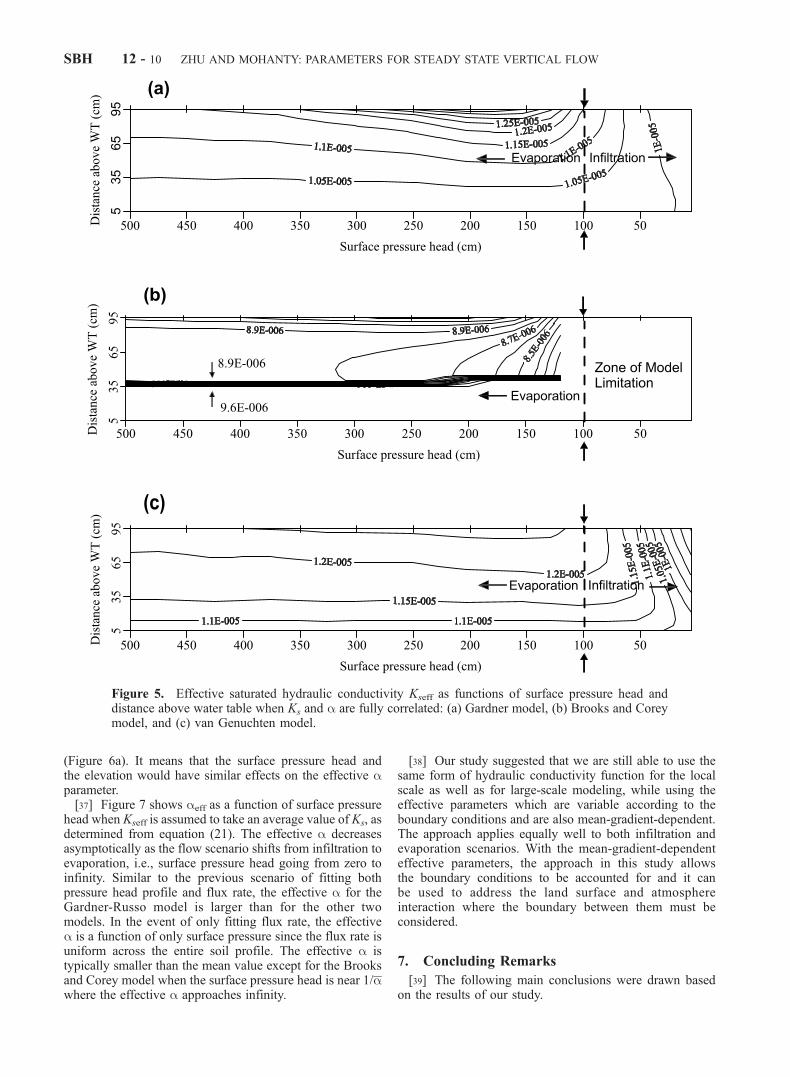
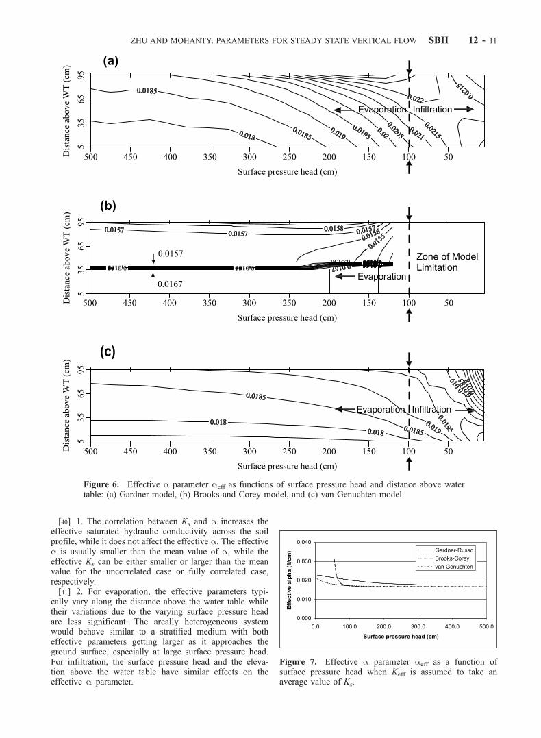
[35] Figure 5 shows effective saturated hydraulic conduc-tivity Kseff as functions of surface pressure head anddistance above water table when Ks and a are fullycorrelated (r = 1) for all three hydraulic conductivity modelsconsidered. The variation of effective saturated hydraulicconductivity follows the similar general pattern with theuncorrelated case, but the correlation between Ks and aincreases the effective saturated hydraulic conductivity.Because of correlation with a, the effective saturatedhydraulic conductivity is usually larger than the mean valueof Ks ¼ 1:0� 10�5ðcm=sÞ (cm/s), which can been seen inFigures 5a and 5c for the Gardner and van Genuchtenfunctions, respectively.[36] Figure 6 demonstrates effective a parameter (aeff)

as a function of surface pressure head and distance abovewater table for all three hydraulic conductivity models

considered. Effective parameter aeff is not affected bycorrelation between Ks and a, as shown in equation (19).Therefore the overall effect of parameter correlation makesthe soil behave more like sand, i.e., a larger effectivesaturated hydraulic conductivity and an unaffected effec-tive a. In general, notice that the effective a is usuallysmaller than the mean value of a = 0.0225(1/cm). In otherwords, if a is assumed to be lognormally distributed, itsgeometric mean (smaller than the arithmetic mean) is prob-ably a better indicator of effective value. From Figure 6, itcan also be seen that the largest effective a values areobserved near the ground surface and around the staticcondition. It is interesting to note that for infiltrationscenario the effective a parameter shows approximatelydiagonal symmetry in the surface pressure head andelevation plots, especially for the Gardner-Russo model

Figure 4. Effective saturated hydraulic conductivity Kseff as functions of surface pressure head anddistance above water table when Ks and a are uncorrelated: (a) Gardner model, (b) Brooks and Coreymodel, and (c) van Genuchten model.


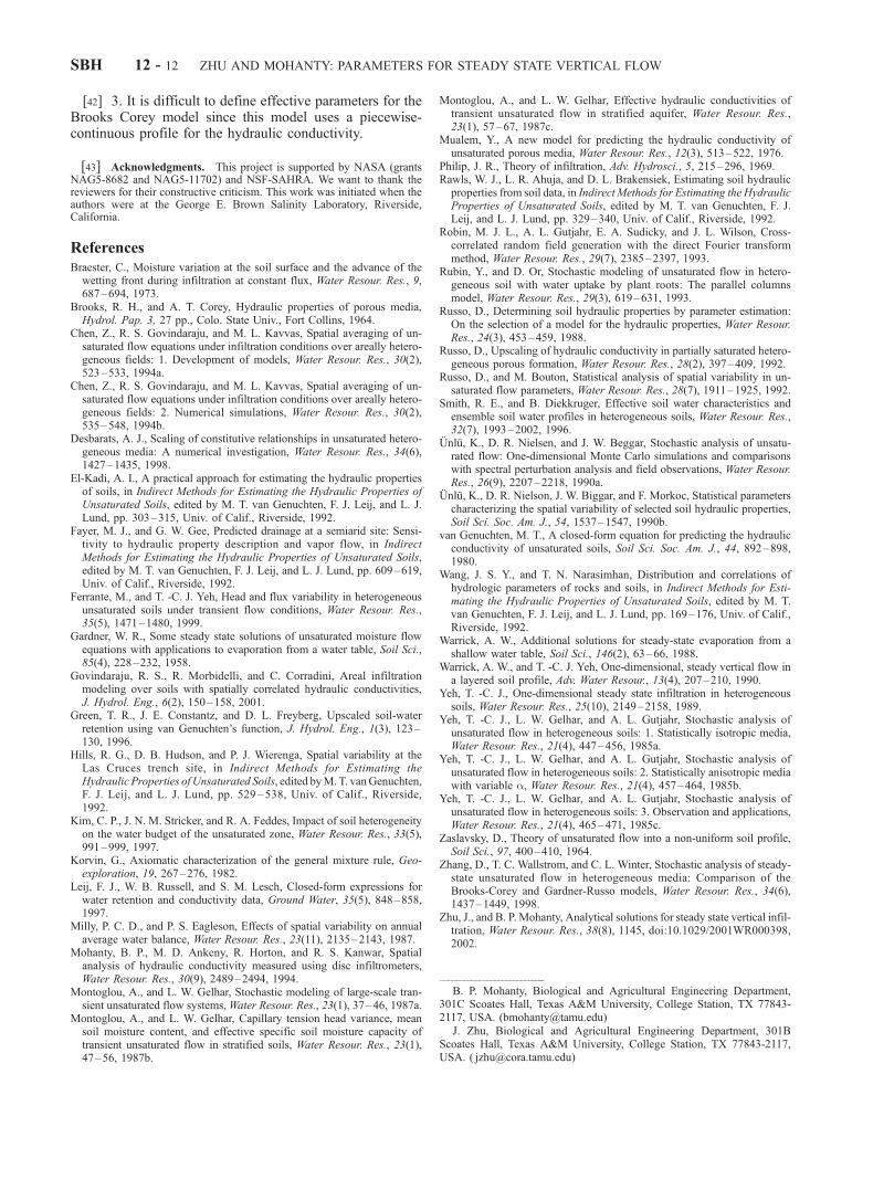
(Figure 6a). It means that the surface pressure head andthe elevation would have similar effects on the effective aparameter.[37] Figure 7 shows aeff as a function of surface pressure

head when Kseff is assumed to take an average value of Ks, asdetermined from equation (21). The effective a decreasesasymptotically as the flow scenario shifts from infiltration toevaporation, i.e., surface pressure head going from zero toinfinity. Similar to the previous scenario of fitting bothpressure head profile and flux rate, the effective a for theGardner-Russo model is larger than for the other twomodels. In the event of only fitting flux rate, the effectivea is a function of only surface pressure since the flux rate isuniform across the entire soil profile. The effective a istypically smaller than the mean value except for the Brooksand Corey model when the surface pressure head is near 1/awhere the effective a approaches infinity.

[38] Our study suggested that we are still able to use thesame form of hydraulic conductivity function for the localscale as well as for large-scale modeling, while using theeffective parameters which are variable according to theboundary conditions and are also mean-gradient-dependent.The approach applies equally well to both infiltration andevaporation scenarios. With the mean-gradient-dependenteffective parameters, the approach in this study allowsthe boundary conditions to be accounted for and it canbe used to address the land surface and atmosphereinteraction where the boundary between them must beconsidered.

7. Concluding Remarks

[39] The following main conclusions were drawn basedon the results of our study.

Figure 5. Effective saturated hydraulic conductivity Kseff as functions of surface pressure head anddistance above water table when Ks and a are fully correlated: (a) Gardner model, (b) Brooks and Coreymodel, and (c) van Genuchten model.


[40] 1. The correlation between Ks and a increases theeffective saturated hydraulic conductivity across the soilprofile, while it does not affect the effective a. The effectivea is usually smaller than the mean value of a, while theeffective Ks can be either smaller or larger than the meanvalue for the uncorrelated case or fully correlated case,respectively.[41] 2. For evaporation, the effective parameters typi-

cally vary along the distance above the water table whiletheir variations due to the varying surface pressure headare less significant. The areally heterogeneous systemwould behave similar to a stratified medium with botheffective parameters getting larger as it approaches theground surface, especially at large surface pressure head.For infiltration, the surface pressure head and the eleva-tion above the water table have similar effects on theeffective a parameter.

Figure 6. Effective a parameter aeff as functions of surface pressure head and distance above watertable: (a) Gardner model, (b) Brooks and Corey model, and (c) van Genuchten model.

Figure 7. Effective a parameter aeff as a function ofsurface pressure head when Keff is assumed to take anaverage value of Ks.


[42] 3. It is difficult to define effective parameters for theBrooks Corey model since this model uses a piecewise-continuous profile for the hydraulic conductivity.

[43] Acknowledgments. This project is supported by NASA (grantsNAG5-8682 and NAG5-11702) and NSF-SAHRA. We want to thank thereviewers for their constructive criticism. This work was initiated when theauthors were at the George E. Brown Salinity Laboratory, Riverside,California.

ReferencesBraester, C., Moisture variation at the soil surface and the advance of thewetting front during infiltration at constant flux, Water Resour. Res., 9,687–694, 1973.

Brooks, R. H., and A. T. Corey, Hydraulic properties of porous media,Hydrol. Pap. 3, 27 pp., Colo. State Univ., Fort Collins, 1964.

Chen, Z., R. S. Govindaraju, and M. L. Kavvas, Spatial averaging of un-saturated flow equations under infiltration conditions over areally hetero-geneous fields: 1. Development of models, Water Resour. Res., 30(2),523–533, 1994a.

Chen, Z., R. S. Govindaraju, and M. L. Kavvas, Spatial averaging of un-saturated flow equations under infiltration conditions over areally hetero-geneous fields: 2. Numerical simulations, Water Resour. Res., 30(2),535–548, 1994b.

Desbarats, A. J., Scaling of constitutive relationships in unsaturated hetero-geneous media: A numerical investigation, Water Resour. Res., 34(6),1427–1435, 1998.

El-Kadi, A. I., A practical approach for estimating the hydraulic propertiesof soils, in Indirect Methods for Estimating the Hydraulic Properties ofUnsaturated Soils, edited by M. T. van Genuchten, F. J. Leij, and L. J.Lund, pp. 303–315, Univ. of Calif., Riverside, 1992.

Fayer, M. J., and G. W. Gee, Predicted drainage at a semiarid site: Sensi-tivity to hydraulic property description and vapor flow, in IndirectMethods for Estimating the Hydraulic Properties of Unsaturated Soils,edited by M. T. van Genuchten, F. J. Leij, and L. J. Lund, pp. 609–619,Univ. of Calif., Riverside, 1992.

Ferrante, M., and T. -C. J. Yeh, Head and flux variability in heterogeneousunsaturated soils under transient flow conditions, Water Resour. Res.,35(5), 1471–1480, 1999.

Gardner, W. R., Some steady state solutions of unsaturated moisture flowequations with applications to evaporation from a water table, Soil Sci.,85(4), 228–232, 1958.

Govindaraju, R. S., R. Morbidelli, and C. Corradini, Areal infiltrationmodeling over soils with spatially correlated hydraulic conductivities,J. Hydrol. Eng., 6(2), 150–158, 2001.

Green, T. R., J. E. Constantz, and D. L. Freyberg, Upscaled soil-waterretention using van Genuchten’s function, J. Hydrol. Eng., 1(3), 123–130, 1996.

Hills, R. G., D. B. Hudson, and P. J. Wierenga, Spatial variability at theLas Cruces trench site, in Indirect Methods for Estimating theHydraulic Properties of Unsaturated Soils, edited byM.T. vanGenuchten,F. J. Leij, and L. J. Lund, pp. 529–538, Univ. of Calif., Riverside,1992.

Kim, C. P., J. N. M. Stricker, and R. A. Feddes, Impact of soil heterogeneityon the water budget of the unsaturated zone, Water Resour. Res., 33(5),991–999, 1997.

Korvin, G., Axiomatic characterization of the general mixture rule, Geo-exploration, 19, 267–276, 1982.

Leij, F. J., W. B. Russell, and S. M. Lesch, Closed-form expressions forwater retention and conductivity data, Ground Water, 35(5), 848–858,1997.

Milly, P. C. D., and P. S. Eagleson, Effects of spatial variability on annualaverage water balance, Water Resour. Res., 23(11), 2135–2143, 1987.

Mohanty, B. P., M. D. Ankeny, R. Horton, and R. S. Kanwar, Spatialanalysis of hydraulic conductivity measured using disc infiltrometers,Water Resour. Res., 30(9), 2489–2494, 1994.

Montoglou, A., and L. W. Gelhar, Stochastic modeling of large-scale tran-sient unsaturated flow systems,Water Resour. Res., 23(1), 37–46, 1987a.

Montoglou, A., and L. W. Gelhar, Capillary tension head variance, meansoil moisture content, and effective specific soil moisture capacity oftransient unsaturated flow in stratified soils, Water Resour. Res., 23(1),47–56, 1987b.

Montoglou, A., and L. W. Gelhar, Effective hydraulic conductivities oftransient unsaturated flow in stratified aquifer, Water Resour. Res.,23(1), 57–67, 1987c.

Mualem, Y., A new model for predicting the hydraulic conductivity ofunsaturated porous media, Water Resour. Res., 12(3), 513–522, 1976.

Philip, J. R., Theory of infiltration, Adv. Hydrosci., 5, 215–296, 1969.Rawls, W. J., L. R. Ahuja, and D. L. Brakensiek, Estimating soil hydraulicproperties from soil data, in Indirect Methods for Estimating the HydraulicProperties of Unsaturated Soils, edited by M. T. van Genuchten, F. J.Leij, and L. J. Lund, pp. 329–340, Univ. of Calif., Riverside, 1992.

Robin, M. J. L., A. L. Gutjahr, E. A. Sudicky, and J. L. Wilson, Cross-correlated random field generation with the direct Fourier transformmethod, Water Resour. Res., 29(7), 2385–2397, 1993.

Rubin, Y., and D. Or, Stochastic modeling of unsaturated flow in hetero-geneous soil with water uptake by plant roots: The parallel columnsmodel, Water Resour. Res., 29(3), 619–631, 1993.

Russo, D., Determining soil hydraulic properties by parameter estimation:On the selection of a model for the hydraulic properties, Water Resour.Res., 24(3), 453–459, 1988.

Russo, D., Upscaling of hydraulic conductivity in partially saturated hetero-geneous porous formation, Water Resour. Res., 28(2), 397–409, 1992.

Russo, D., and M. Bouton, Statistical analysis of spatial variability in un-saturated flow parameters, Water Resour. Res., 28(7), 1911–1925, 1992.

Smith, R. E., and B. Diekkruger, Effective soil water characteristics andensemble soil water profiles in heterogeneous soils, Water Resour. Res.,32(7), 1993–2002, 1996.

Unlu, K., D. R. Nielsen, and J. W. Beggar, Stochastic analysis of unsatu-rated flow: One-dimensional Monte Carlo simulations and comparisonswith spectral perturbation analysis and field observations, Water Resour.Res., 26(9), 2207–2218, 1990a.

Unlu, K., D. R. Nielson, J. W. Biggar, and F. Morkoc, Statistical parameterscharacterizing the spatial variability of selected soil hydraulic properties,Soil Sci. Soc. Am. J., 54, 1537–1547, 1990b.

van Genuchten, M. T., A closed-form equation for predicting the hydraulicconductivity of unsaturated soils, Soil Sci. Soc. Am. J., 44, 892–898,1980.

Wang, J. S. Y., and T. N. Narasimhan, Distribution and correlations ofhydrologic parameters of rocks and soils, in Indirect Methods for Esti-mating the Hydraulic Properties of Unsaturated Soils, edited by M. T.van Genuchten, F. J. Leij, and L. J. Lund, pp. 169–176, Univ. of Calif.,Riverside, 1992.

Warrick, A. W., Additional solutions for steady-state evaporation from ashallow water table, Soil Sci., 146(2), 63–66, 1988.

Warrick, A. W., and T. -C. J. Yeh, One-dimensional, steady vertical flow ina layered soil profile, Adv. Water Resour., 13(4), 207–210, 1990.

Yeh, T. -C. J., One-dimensional steady state infiltration in heterogeneoussoils, Water Resour. Res., 25(10), 2149–2158, 1989.

Yeh, T. -C. J., L. W. Gelhar, and A. L. Gutjahr, Stochastic analysis ofunsaturated flow in heterogeneous soils: 1. Statistically isotropic media,Water Resour. Res., 21(4), 447–456, 1985a.

Yeh, T. -C. J., L. W. Gelhar, and A. L. Gutjahr, Stochastic analysis ofunsaturated flow in heterogeneous soils: 2. Statistically anisotropic mediawith variable a, Water Resour. Res., 21(4), 457–464, 1985b.

Yeh, T. -C. J., L. W. Gelhar, and A. L. Gutjahr, Stochastic analysis ofunsaturated flow in heterogeneous soils: 3. Observation and applications,Water Resour. Res., 21(4), 465–471, 1985c.

Zaslavsky, D., Theory of unsaturated flow into a non-uniform soil profile,Soil Sci., 97, 400–410, 1964.

Zhang, D., T. C. Wallstrom, and C. L. Winter, Stochastic analysis of steady-state unsaturated flow in heterogeneous media: Comparison of theBrooks-Corey and Gardner-Russo models, Water Resour. Res., 34(6),1437–1449, 1998.

Zhu, J., and B. P. Mohanty, Analytical solutions for steady state vertical infil-tration, Water Resour. Res., 38(8), 1145, doi:10.1029/2001WR000398,2002.

��B. P. Mohanty, Biological and Agricultural Engineering Department,

301C Scoates Hall, Texas A&M University, College Station, TX 77843-2117, USA. ([email protected])

J. Zhu, Biological and Agricultural Engineering Department, 301BScoates Hall, Texas A&M University, College Station, TX 77843-2117,USA. ( [email protected])


effective hydraulic parameters for steady state vertical

Documents