LBNL 43723

Effects of Duct Improvement and ENERGYSTAREquipment on Comfort and Energy Efficiency

I. Walker, M. Sherman, J. Siegel, and M. ModeraEnvironmental Energy Technologies Division

Energy Performance of Buildings GroupLawrence Berkeley National Laboratory

Berkeley, CA 94720

July 1999

This study was sponsored by the U.S. Environmental Protection Agency, through the U.S.Department of Energy under Contract No. DE-AC03-76SFOO098. Publication of research resultsdoes not imply EPA endorsement of or agreement with these findings.

DISCLAIMER

This report was prepared as an account of work sponsoredby an agency of the United States Government. Neitherthe United States Government nor any agency thereof, norany of their employees, make any warranty, express orimplied, or assumes any legal liability or responsibility forthe accuracy, completeness, or usefulness of anyinformation, apparatus, product, or process disclosed, orrepresents that its use would not infringe privately ownedrights. Reference herein to any specific commercialproduct, process, or service by trade name, trademark,manufacturer, or otherwise does not necessarily constituteor imply its endorsement, recommendation, or fmmring by

‘~ the United States Government or any agency thereof. Theviews and opinions of authors expressed herein do notnecessarily state or reflect those of the United StatesGovernment or any agency thereof.

DISCLAIMER

Portions of this document may be illegiblein electronic image products. Images areproduced from the best available originaldocument.

Table of Contents

TABLE OF CONTENTS ...................... ..................................................................................................................... 2

EXECUTIVE SUMMARY ......................... ...................................................................... ........... ........ .. .................... 4

INTRODUCTION ... .......................................... .................................................................. ......... .............................. 5

DUCT LEAKAGE AND ENERGYSTAR EQUIPMENT EFFECTS ON COMFORT ....... .. .............................. 5

F~m MEASUREMENTS.......................... .. ........ ........................................................ ..................................................5Diagnostics .................................................................................................................... .. ..................................... 6

House ventilation rates . ............................................................................................................................................... ...... 7Table 1. Summary of House Envelope Leakage Test Results ............................................................................................. 7Table 2. Summary of Tracer Gas Measurements of House Ventilation Rates .................................................................... 7Register and Air Handler F1ows....................................................................................................................................... 7Table 3. System Flows and Register Flows (cfm) ............................................................................................................. 9Duct leakage by prewurization ......................................................................................................................................... 9Boot and Cabinet Letiage .............................................................................................................................................. 10Table 4. Summary of Fan Pressurization Leakage Flows at 25 Pa (cfm25) .................................................................... 11[% of fan flowl] ................................................................................................................................................................. 11Table 5. Added Leaks at operating conditions, cfm [% of fan flow] ................................................................................ 11Duct location and dimensions. ........................................................................................................................................ 11

Continuous Monitoring .................. .............. .. .. ...... ........................................................... .................................. 12Table6. Performance Metrics ........................................................................................................................................... 12~lldown time .................................................................................................................................................................. 12Temperature distribution ................................................................................................................................................ 12Table 7. Pulldown time in different locations in the house ............................................................................................... 13Total tons at the register (TAR) ..................................................................................................................................... 13Table 8. Tons at the register after 30 tinutes .................................................................................................................... 14Table 9. Capacity at the indoor coil after 30 minutes (kW).............................................................................................. 15Comparing Measured and Rated Air Conditioner Capacity ....................................................................................... 15Table 10. System capacity comptisons ........................................................................................................................... 15Air conditioner Coefficient of Performance (COP) ....................................................................................................... 15Table 11. Equipment Coefficient of Performance (COP), Power Consumption and fraction of power consumption due tofan, afier30 tinutes .......................................................................................................................................................... 16System Coefficient of Performance (COP) .................................................................................................................... 16Table 12. Total System Coefficient of Performance (COP) after 30 finutes .................................................................... 17Delivery Effectiveness (DE) ............................................................................................................................................ 17Table 13. Delivery Effectiveness [%] after30 finutes ..................................................................................................... 17

Field Measurement Summa~ ................................................................................... .......................................... 17MODELINGIMPROVEDCOMFORTWITHREGCAP ................................... ............................ .................................... 18

REGCAP Simulation Evacuation .............................................................................. ...................................... .... 19Figure 1: REGCAP Predicted and Measured Attic Temperatures for the Sacramento test house. August 11, 1998.........20Attic Temperature ........................................................................................................................................................... 20Figure 2 REGCAP Predicted and Measured House Air Temperatures for the Sacramento test house. August 11, 199821House Temperatwe ......................................................................................................................................................... 21Figure 3: REGCAP Predicted and Measured Return Duct Air Temperatures for the Sacramento test house. August 11,1998 .................................................................................................................................................................................. 22Return Duct Air Temperature ........................................................................................................................................ 22Figure 4: REGCAP Predicted and Measured Supply Duct Air Temperatures for the Sacramento test house. August 11,1998 .................................................................................................................................................................................. 24Supply Duct Ah Tempe~tire ........................................................................................................................................ 24

REGCAP Simulation Results .................... .......... ................................... ............................................................. 25

2

Figure 5. REGCAP Simulations of pulldowns from 3:00 p.m. on a Sacramento design day. .......................................... 26Table 14. List of REGCAP Simulation Cases .................................................................................................................. 27Table 15. REGCAP Delivered Capacity (TAR) Comparison (System on for 1.75 hours) ............................................... 27

TECHNOLOGY TRANSFER ................................................................................................................................. 2-7

DUCTCLEANmGEFFECTON ~ROSOLSEWT (EPA) . .................................................. .. ...................................... 27HEWTHND S~TYASSESSMENTOFWROSOL SEWT(EPA) .................................... .................. ....................28ASHRAE: RATINGOF DISTRIBUTIONSYSTEMS- ASHRAE 152P ......... ............ ..................................................... 29

ASTM: RATINGOFDUCTSEALANTSANDREWSLNGDUCTLEAKAGEMEASUREMENTMETHODS............................... 29

REFERENCES ...... ..................... ......................... .......................... ........................ .................... .. ......................... ..... 29

APPENDIX A. DETAILED MEASUREMENT RESULTS ..... ............................................ ................................ 31

Table Al. Pulldown time and temperatures in different locations in the house ................................................................ 31Table A2. Temperatures at different locations in the house during pulldown tests ........................................................... 31Table A3. Tons At the Register (T~) .............................................................................................................................. 32Table A4. Capacity at the Indoor Coil .............................................................................................................................. 32Table AS. Equipment Coefficient of Performance (COP) ................................................................................................. 33Table A6 System Power Consumption ............................................................................................................................. 33Table A7. Total System Coefficient of Performance (COP).............................................................................................. 34Table A8. Delivery Effwtiveness ...................................................................................................................................... 34Table A9 Key Temperatures and Enthalpies for Calculating System Petiormmce ........................................................... 34

APPENDIX B. FLOWCHART FOR REGCAP MODEL ... ................ ............ ...... ............................................... 35

3

Executive Summary

This report discusses the results of field tests and computer simulations to evaluate and parameters that influenceenergy efficiency and comfort of forced air cooling systems. The field study was performed in two houses: one inSacramento, CA., and one in Cedar Park, TX. The two house locations were chosen to represent a relatively drycooling climate and a high humidity cooling climate respectively. The two houses were tested with standard SEER10 Ak Conditioning equipment and then with ENERGYSTAR equipment (SEER 13). The field testing combinedcontinuous monitoring of system performance with diagnostic tests of the house and WAC system. The systemperformance was evaluated in terms of effective capacity (both latent and sensible), equipment and system

efficiency, pulldown time room-to-room temperature distribution. Because the weather was cool during the testingin Cedar Park, the following results focus on the Sacramento test results.The key results discussed in this report include:

●

●

●

●

●

●

Poor duct system design and installation significantly affects comfort. An example is the associated room-to-room temperature differences.

The SEER rating was a reasonable numerical guide to Air Conditioner eftlciency].

Ak conditioner name plate capacity ratings alone are a poor indicator of how much cooling will actually bedelivered to the conditioned space. Duct system efficiency can have as large an impact on performance asvariations in SEER.

Duct leakage added approximately 0.2 Air Changes per Hour to the house infiltration rate during systemoperation.

The REGCAP computer simulation showed that it was capable of modeling the dynamic performance of forcedair thermal distribution systems.

The REGCAP simulations showed how improving duct efficiency can allow the use of smaller capacity airconditioning equipment.

1For sensible effects only.

4

Introduction

Residential thermal distribution systems have significant energy and comfort implications due to losses from thedistribution system in the form of leakage and conduction and poor distribution from room-to-room within the house.Aiso, poor mechanical equipment performance, and the interactions between the distribution system and theequipment act to further reduce system capacity and thermal comfort. An example of duct system and equipmentinteraction is the that airflow over the indoor coils changes the efficiency, capacity and humidity removal of thesystem resulting in comfort, energy consumption and efficiency changes. To determine if there are any differences inthe interactions depending on whether or not the equipment is ENERGYSTAR rated, two houses were tested withstandard (SEER lO) air conditioners and then retrofitted with ENERGYSTAR (SEER 13) equipment. In addition, theeffect of duct leakage was examined by adding leaks to the systems under test, The original plan had been to seal theduct systems, but they were found to be not very leaky. Leakage was added in order to show the effect of reducedleakage. Four additional houses were tested as part of a companion study (Walker et al. (1999)) that did not haveequipment changes. Selected measurement results from these houses are presented where appropriate.

This report is in two main parts. The first part discusses the field measurement techniques and results. The secondpart examines efforts to model distribution system performance using a sophisticated computer simulation programcalled REGCAP. REGCAP has been developed to specifically include the interactions of duct systems with theirsurroundings (In this study the duct surroundings are attic spaces). Lastly, a brief summary of related thermaldistribution system research is included at the end of the report.

Duct Leakage and EIVERGYSTAREquipment Effects on Comfort

Three key concepts related to comfort were used to study this issue:1.

2.

3.

Tons at the Register (TAR). Tons at the register is the actual cooling delivered to the conditioned space, i.e.what comes out of the registers. The combined distribution system losses and system capacity at operatingconditions act to determine the TAR of a system.Pulldown. Comfort, and hence occupant acceptability, is determined not only by steady-state temperatures, butby how long it takes to pull down the temperature during cooling start-up, such as when the occupants comehome on a hot summer afternoon. In addition, the delivered tons of cooling at the register during start-upconditions are critical to customer acceptance of equipment downsizing strategies. In this study, the pulldownwas evaluated at different locations within the house to evaluate thermal comfort issues regarding distribution ofcooling within the house.Room-by-room temperature distribution. A well designed and installed system accounts for variations in room-by-room loads by having the appropriate flow through each register in each room. Poor systems have incorrectflows through their registers resulting in room-to-room temperature differences. From a comfort point of view,some occupants may not be happy because some rooms will be either too cool or too hot. From an energy

perspective, this is also poor because to have all occupied parts of the house cooled to a comfortable level(particularly upstairs room sin two-story houses) some parts of the house will be much cooler than necessary.Energy has then been wasted by overcooking parts of the house.

Field measurements

Field measurements were made onCA., and the other in Cedar Park,

air-conditioning systems in two new and unoccupied houses: one in Sacramento,TX. The two house locations were chosen to represent a relatively dry cooling

climate and a high humidity cooling climate, respectively. The measurements included diagnostics to determinebuilding and system characteristics and continuous monitoring over several days to determine system performance.The Sacramento house was cooled with a split system air conditioner and heated with natural gas (using the same airhandler/cabinet and ducts). The Texas house had a heat pump and electric resistance strip heat. The Sacramento

5

house had all of the system in the attic - air handler, equipment cabinet and ducts. The Cedar Park house had the airhandler/cabinet in a closet in the house, with only the supply plenum and supply ducts in the attic. The “return” ductin this house was the space under the platform that supported the air handler cabinet. A large grille was placedthrough the platform wall below the closet door. Flow was somewhat restricted in this system despite its simplicitybecause the water heater was located within the air-handler platform !

The houses were tested in their “as found” configuration and with holes added to the duct systems. The original planwas to test systems in the “as found” condition and then seal the duct systems, however the duct systems in the twotest houses were not very leaky in the “as found” condition. Therefore holes were added instead to enable us to still

examine the effect of leakage on system performance. The holes were added at the system plenums because theselocations provided easy access and large flat areas for placing the holes. The added holes varied in size from systemto system, but they were typically four inches (10 cm) in diameter. At both test houses an attempt was made tomeasure the flow through the added holes directly, rather than inferring the leakage flow from indirect measurementsas used in standard diagnostic tests. At the Sacramento test house, the airflow through these added holes wasmeasured using a vane anemometer during normal system operation. At the Texas house, the holes were calibratedin a laboratory. The airflow was then determined by measuring the pressure difference across the holes at the holelocation during normal system operation.

When the ENERGYSTAR equipment was installed in Sacramento, just the outside compressor unit and the controlsystem were changed. In the Cedar Park house the indoor coil, fan and cabinet (and electric heating system) werealso replaced. In each case the nominal nameplate capacity was the same for both the original and ENERGYSTARequipment.

The continuous monitoring was performed for several days in each system configuration. During this monitoring thesystem was set to stay off until about 3:00 p.m., allowing the house to warm up during the day. Then the system was

turned on and the house temperature was “pulled down” to 74°F (24°C) at the thermostat. Because temperatureswere monitored in each room we were able to determine if the temperature at the thermostat was representative ofother temperatures in the house. In most cases, the thermostat was not the warmest place in the house (it was usuallycentrally mounted in a hallway away from any direct solar gains) and so the pulldown was changed to reduce the

temperature at the thermostat below the original 74°F (24°C) setpoint. The reduced thermostat pulldowntemperature setpoint was varied for each test, depending on the specific temperature differences between the roomsand the thermostat and the weather condhions on the day of the test. In addition, pulldown times were calculated fordifferent parts of the house.

DiagnosticsThe following diagnostics were used to characterize the house and duct system and determine changes in systemperformance (e.g., effect of added leaks on system flows). Also, the results of the diagnostics were used as inputparameters to the REGCAP simulations.

Envelope Leakage.The envelope leakage was measured using a blower door test with the registers uncovered. Therefore, it includesleakage to outside via the duct system. The envelope leakage for the test houses is given in Table 1. The leakage isexpressed in three ways:

in terms of the blower test results, i.e., the flow coefficient and pressure exponent,Specific Leakage Area (SLA), andflow at 50 Pa divided by floor area (Q50/FA).

The SLA and Q50/FA are methods of scaling leakage by house size so that comparisons of envelope air tightness canbe made between houses. In addition, the calculation of SLA allows the comparison of these houses to a “standard’house that would meet California Energy Code (California Energy Commission (1998)). Both these methodsnormalize the leakage by house floor area. SLA uses the effective leakage area (defined at 0.016 in. of water (4 Pa)with a discharge coefficient of 1.0) of the house calculated from the flow coefficient and pressure exponent. Thesehouses had SLAS typical of new construction that were close to the California Energy Code default SLA of 4.9 forhouses with ducted forced air systems. Q50 uses the flow coefilcient and the pressure exponent to calculate theenvelope flow at 0.2 in. of water (50 Pa), i.e. Q50=C(50)”.

House ventilation rates.Ventilation rates were measured using tracer gas decay with the system fan off and with the system fan on. Thedifferences between fan on and fan off results were used to determine any changes in ventilation rate due to ductleakage. The results of these tests are summarized in Table 2. Because of the large variation in ventilation rates withweather conditions, the only significant result is the change in ventilation rate due to system operation. This isbecause the ON/OFF tests took two to three hours to perform and the change in weather driven infiltration over that

time period is usually less than day to day variations. The fractional increases (compared to when the system wasoff) in ventilation due to system operation are only valid for the particular instances of these tests. For example, thelarge fi-actional increase at Cedar Park after holes were added is because the ventilation rate was very low with thesystem off. However, the results shown in Table 2 show that the system operation does have a significant effect on

- the ventilation rate – adding an average of 0.2 Air Changes per Hour (ACH). Previous studies found similar results,with the infiltration rate doubling when the system is turned on (see Cummings et al. (1990), Palmiter and Francisco(1994), Palmiter and Bond (1992) and Modera (1989)).

I Table 1. Summary of House Envelope Leakage Test Results ISite Leakage Pressure SLA Q50/floor area

Coefficient, C Exponent, n (Cfrnlf?)(cfrn/Pan)

Sacramento, I 110 I 0.64 161 1.61 ICA I I I

Cedar Park, 243 0.59 5.2 1.40

I Table 2. Summary of Tracer Gas Measurements of House Ventilation Rates ISite Fan Building ACH Change (fan ACH fan on as multiple of ACH

Mode Ventilation ON - OFF) fan off(off/on) rate (ACH)

Sacramento. ON 0.41 0.18 1.8As Found

OFF 0.23

Cedar Park. ON 0.25 0.12 1.9As Found

OFF 0.13

Cedar Park. ON 0.45 0.37 5.6Added Leaks

OFF 0.08

Register and Air Handler Flows.The supply register flows were measured using a fan assisted flowhood. The return register flows were measuredeither using a flowhood or a vane anemometer traverse. The mean anemometer velocities were combined with anestimate of the open area of the return grille to obtain return flows. The sums of the register flows are summarized inTable 3.

7

All the fan flow results are summarized in Table 3. The fan flows were estimated using three techniques:1. Fan flowmeter operating pressure matching.2. Tracer gas concentration.3. Combining register flows and leakage measurements.

Fan flowmeter:The fan flowmeter test methods used here are based on those in proposed ASHRAE Standard 152P (ASHRAE 1999)and the procedure in Alternative Calculation Manual, Appendix F of the Energy Efficiency Standards for Low-RiseResidential Buildings (California Energy Commission (CEC), (1998)) (often referred to as Title 24). This test usesthe supply ducts as a flowmeter and utilizes the fact that having the same pressure drop across the supply system at

operating conditions and measurement conditions ensures the same flow through the system at the two differentconditions. The pressure difference between the supply plenum and the conditioned space is measured at normal ,operating conditions. The return duct is then blocked off from the rest of the equipment and a combined fan andflowmeter attached at the air handler access. The fan flowmeter is turned on and adjusted until the pressuredifference between the supply plenum and the conditioned space is the same as at normal operating conditions. Theflow through the flowmeter is then the system fan flow at operating conditions. However, the fan flowmeter does notusually produce enough flow to match the supply plenum to conditioned space operating pressure. In these cases thefan flowmeter is operated at maximum output and the flow and supply plenum to conditioned space pressure arerecorded. Assuming a pressure exponent of 0.6 for the duct system, the measured flow at maximum output isextrapolated to the flow at the operating condition pressure difference.

An alternative is to operate the fan flowmeter over a range of flows, recording the flows and supply plenum toconditioned space pressure differences. A least squares fit can then be used to determine a flow coefficient, andpressure exponent for the system and the flow at operating condition pressures is determined from these parameters.

For this fan flow measurement technique one source of error is possible changes in flow patterns in the plenum andduct system, such that the flow through the system when the pressures are matched (or extrapolated to) is not thesame as at normal operating conditions. Another source of error is in mounting the fan flowmeter such that the outletis partially blocked (this is typical if the fan flowmeter is attached directly to the air handler cabinet). This blockingof the outlet changes the flowmeter calibration such that the flowmeter can give significantly incorrect readings. We(and other researchers) are continuing to examine this issue in ongoing work.

Tracer gas:The tracer gas method uses a mass flow meter to release a tracer gas a fixed known rate in to the return grille. Thetracer gas concentration is measured at a supply register and the flow rate calculated from the tracer gasconcentration. The biggest problem with this test method is the requirement that the tracer as be thoroughly mixed inthe supply ducts. In the tests for this study we measured the tracer gas concentrations at several registers (typicallyfour or five) to check for complete mixing (measuring the same concentration at each register confirms the mixing).

Combining supply register flows and pressurization leakage results:In this method the sum of the register flows from the flowhood measurements is added to the measured supply ductleakage taken from pressurization duct leakage tests to determine flow through the system fan. The sum of the supplyregister flows was 1570 less than the fan flow for Sacramento and 17% less than the fan flow for Cedar Park. Notethat not all of this difference is leakage directly to outside – the fraction of leakage to outside will discussed later inthe duct leakage measurements section.

Table 3. System Flows and Register Flows (cfm)

Fan flow Measurement Method Sum of register flows

Site Configuration Tracer Using Flow meter Sum of Supply supply Return (TJaverse orGas Register FIows Flow IJood)

PIUS supplyDuct Leakage

Sacramento – as found 1205 1210 (F F1OWmeter)* 1104 1004 Not performed1361 (S flow meter)**

Sacramento – added 1240 1021 (F flow meter) 1082 928 828 (H)leaks 1231 (S flow meter)Cedar Park -as found None 1408 (F flow meter) 1448 1336 1492 (T)

1614 (S flow meter)1415 (S HVAC)

Cedar Park – with None 1488 (F flow meter) 1499 1430 1543 (T)ENERGYSTAR 1664 (S flow meter)equipment

Cedar Park - added None 1697 (F Flow meter)*** 1559 1458 1415 (T)Ieaks - withENERGYSTAREQUIPMENT* - F tests are fits to data points with a forced intercept of Oflow at O pressure.‘* - S tests use highest measured flow and pressure and extrapolate to operating conditions (n=O.6)●** Flow meter mounted at the return grille, flows were corrected for estimated return and cabinet leakage.

Duct leakage by pressurizationFor these tests the registers are covered and a fan fiowmeter is attached to the duct system to pressurize it. The flowis measured at a reference pressure of 25 Pa and is referred to as cfm25. Duct leakage by pressurization can beseparated into five components: supply, supply boot, return, return boot and cabinet. This was done by connectingthe fan flowmeter at different parts of the duct system and inserting blocking in the ducts to isolate the individualcomponents. For example the test method used to determine supply boot leakage has the following steps:● The supply and return are split by blocking the supply from the return within the equipment cabinet.

● The total supply leakage is then found by covering the supply registers and pressurizing the supply ducts (thisdetermines the combined supply duct and supply boot leakage).

● The registers are then removed and a blockage is placed inside each register upstream of the boot. The supplyducts are then pressurized again to determine the duct only leakage.

● The boot leakage is the difference between these two tests.Note that in these houses the return boot leakage was not separated out from the total return leakage due to theconstruction of these systems. In Sacramento, the filter was at the single return grille and so the return boot wasdepressurized to the same level as the rest of the return system. In addition, it was very difficult to put separators inplace to isolate just the leaks around the return grille connection to the return (effectively the return boot in thiscase). In Cedar Park, there was no return duct – just a grille into side of a platform and therefore no return boot toisolate.

The separation of total leakage fkom leakage to outside was accomplished by simultaneously pressurizing the housewith a blower door to the same pressure (referenced to outside) as the duct system. This means that there will bezero (or a very small) pressure across any leaks from the duct system to inside and only duct leakage to outside willbe measured. At Cedar Park, there was significant return leakage to outside, although there were no return ducts assuch. This was because the closet containing the equipment and the platform return leaked to the attic through holesaround the ceiling penetration for the supply plenum. This shows the necessity for field testing of duct systems

9

because simple observation would have implied that the return leaks were to the closet (essentially the conditionedspace).

The complete pressurization test results are given in Table 4. The system fan flow used to normalize the test resultsis the single point extrapolated fan flowmeter meastirement (the – S – test in Table 3). The exception in the final testat Cedar Park (with added leaks and the ENERGYSTARequipment) where the system fan flow is the flowmeter – F

test. The Sacramento house had a total (combining boots cabinet and ducts leakage to outside) cfm25 of 11% of fanflow. This was increased to 29% of fan flow by adding the holes. The “as found” leakage to inside was about aquarter of the magnitude of the leakage to outside. For the Cedar Park house the “as found” cfm25 was 7% of fanflow and 20’7. with the added holes. The as found leakage to inside was about the same as the leakage to outside. Inthe “as found” condition, these systems were less leaky than the 22% of fan flow for new California houses fromprevious studies by Walker at al. (1997, 1998b) and by Modera and Wilcox (1995).

The original plan was to tighten leaky duct systems to examine the effect of duct leakage. However, the ducts inthese houses gave little scope for reducing leakage by sealing, so both sites had leakage added. The added leaks werecut into the supply and return plenums and resealed after the experiments were finished. The added leakage flowswere individually measured at operating conditions, as well as using the pressurization technique. At Cedar Park theleakage flows at operating conditions were measured directly using a vane anemometer. The added holes were cutprecisely to be the same size as the vane anemometer so that no traverses and interpolations were required. AtSacramento the extra leaks were calibrated in a laboratory and the measured system operating pressures were used toestimate the leakage flows at operating conditions. These added leaks are summarized in Table 5.

Boot and Cabinet LeakageA key question raised in previous duct leakage measurements was the contribution of leaks at boots and the HVACequipment cabinet to the total duct leakage. These two parts of the duct system were examined separately becausethey represent opportunities for duct system leakage reduction that can be fixed by changes in the manufacture ofequipment and by boot inspection and sealing without great expense or effort for the installer/builder. The cabinetleaks include the connection from the cabinet to the plenums, but not the duct connections to the plenums. Thesecabinet leaks are of particular interest because it should be relatively simple to eliminate these leaks with acombination of changes to cabinet construction (tighter tolerances and improved fan access door seals) and moreattention paid to filling knockouts with grommets. Although changing the manufacturing process for system cabinetsmay initially be costly for manufacturers, the significant cabinet leakage means that it has a large potential addedvalue in terms of energy savings and comfort.

The results in Table 4 show that cabinet leakage averaged 24 cfm25 to outside. The supply boots averaged about 40cfm25 to outside. Assuming a pressure exponent of 0.6 and converting these results to the average of the measuredoperating pressures of about 5 Pa for boots and 65 Pa for cabinets results in boot leakage of about 15 cfm andcabinet leakage of about 43 cfm. At both sites, the boot and cabinet leakage was a substantial fraction (25 Y0-50%) ofthe “as found” duct leakage to outside, This means that achieving high levels of air-tightness in ducts (e.g., theleakage requirements for the efficient duct credit in California State Energy Code (CEC (1998))) will require bootand cabinet leaks to be sealed and not just leaks in the ducts themselves.

10

Table 4. Summary of Fan Pressurization Leakage Flows at 25 Pa (cfm25)[% of fan flowl]

I Sacramento

Leakage supply Supply Boots Return Cabinet Totalcondition +Return Boots

As found Total 26 [2] 92 [7] 38 [3] 26 [2] 182 [13]

To Outside 24 [2] 63 [5] 24 [2] 26 [2] 137 [10]

Added Holes Total 145 [12] 92 [7] 134 [11] 26 [2] 397 [32]

To Outside 118 [10] 63 [9] 96 [8] 26 [2] 303 [25]

Cedar Park

Leakage supply Supply Boots Return + Cabinet Totalcondition return Boots

As found Total 40 [2] 33 [2] 163 [10] 22 [1] 258 [16]

To Outside 36 [2] 21 [1] 51 [3] 5 [1] 113 [7]

I With Total 40 [2] 33 [2] 163 [10] 22 (1] 258 [16]ENERGYSTAR To Outside 36 [2] I 21 [1] 51 [3] 42 [3] 150 [9]

equipment

Added leaks – Total 101 [6] 33 [2] 322 [19] 22 [1] 478 [28]with To Outside nla N/a n/a 42 [3]

ENERGYSTARequipment

1-The system fanflow used to normatizethe test resultsis the single pointextrapolatedfan flowmetermeasurement(the– S – test in Table3The exceptionin the final test at CedarPark(withaddedleaks and theENERGYSTARequipment)wherethe system fan flow is the flowmeter– Ftest.

Table 5. Added Leaks at operating conditions, cfm [% of fanflow]

Site supply Return

Sacramento 75 [6] 32 [3]

Cedar Park 32 [2] 73 [4]

Duct location and dimensions.At Sacramento, the entire system of air handler, furnace, cooling coils and supply ducts were all in the attic. At

Cedar Park, the air handler ;nd equipment were in a closet inside~he thermal en~~lope of the house, with the supplyducts in the attic. The return was a simple stand that was part of the closet containing the air handler. The ductsurface areas were estimated by measuring each duct run length and exterior dimensions with a measuring tape. AtSacramento there was 22.5 m2 (243 ft2) of exposed supply ducts and 7 m2 (276 ftz) of return ducts. At Cedar Parkthere was 30.4 m2 (327 ftz) of supply ducts and no return duct in the attic.

11

Continuous MonitoringThe continuous monitoring used computer based data acquisition systems to store data about every 10 seconds. Themonitored parameters were:

. Temperatures at each register, in each room, outdoors, attic, garage, return plenum and supply plenum. Thesupply plenum temperatures were measured at four points in the plenum to account for possible spatial variationin plenum temperatures.

● Weather: wind speed, wind direction, total solar radiation and diffuse solar radiation.

● Humidity: outside, supply air, return air and attic.

● Energy Consumption: Compressor unit (including fan) and distribution fan power.

The measured system temperatures and relative humidities were combined with the register and system fan flow ratesused to calculate the energy flow for each register (tons at each register) and the energy change of the air stream atthe heat exchanger. The supplies were then combined to find the total energy flow (Tons At the Register, or TAR)for the system.

The performance metrics that were calculated from the measured data are listed in Table 6. Except for pulldowntime and temperature distribution, each metric has a sensible and a latent component (reported as a sensible and

total). For all of the metrics except the pulldown time, the value is reported from an average of a minute of data at 5,30, and 60 minutes from when the pulldown test began. This range of times was used because of the significanttransient changes in system performance between the beginning of a cycle and the quasi-steady-state operation

reached later in the pulldown test.

Table 6. Performance Metrics

Pulldown Time and Temperature Variation Time that it takes for a location within the house to reach24°C. Three .pulldown times are reported: for thethermostat (how the system house would normallyrespond), kitchen, and master bedroom. A widedisparity between these times indicates an inadequatedistribution system.

Tons at the register (TAR) Amount of energy delivered to the space.

Air Conditioner Capacity Capacity of the air conditioner calculated fromtemperatures and relative humidities measured in thesupply and return plenums and air handler flow.

Air Conditioner Coefficient of Performance (COP) Air conditioner capacity divided by power consumed byair conditioner, including fan energy

System COP Tons at the register divided by power consumed by airconditioner, including fan energy

Delivery Efficiency Tons at the register divided by air conditioner capacity

Pulldown timePulldown time was significantly reduced by changing the equipment to ENERGYSTAR specifications, as shown inTable 7. The addition of leaks to the system increased the pulldown times in Sacramento. However, in Cedar Park,the added leakage measurements were performed under much milder weather conditions that resulted in very shortpulldown times. The Cedar Park result shows how the pulldown times are sensitive to changes in weatherconditions. At Sacramento, the weather conditions were similar for all three tested conditions.

Temperature distributionThe temperature distribution showed significant room-to-room variations in the test houses and will be discussedhere in terms of how it changes the pulldown time for each room as well as individual room to room temperaturedifferences. Both test houses showed considerable variation (on the order of factors of two or more between the

12

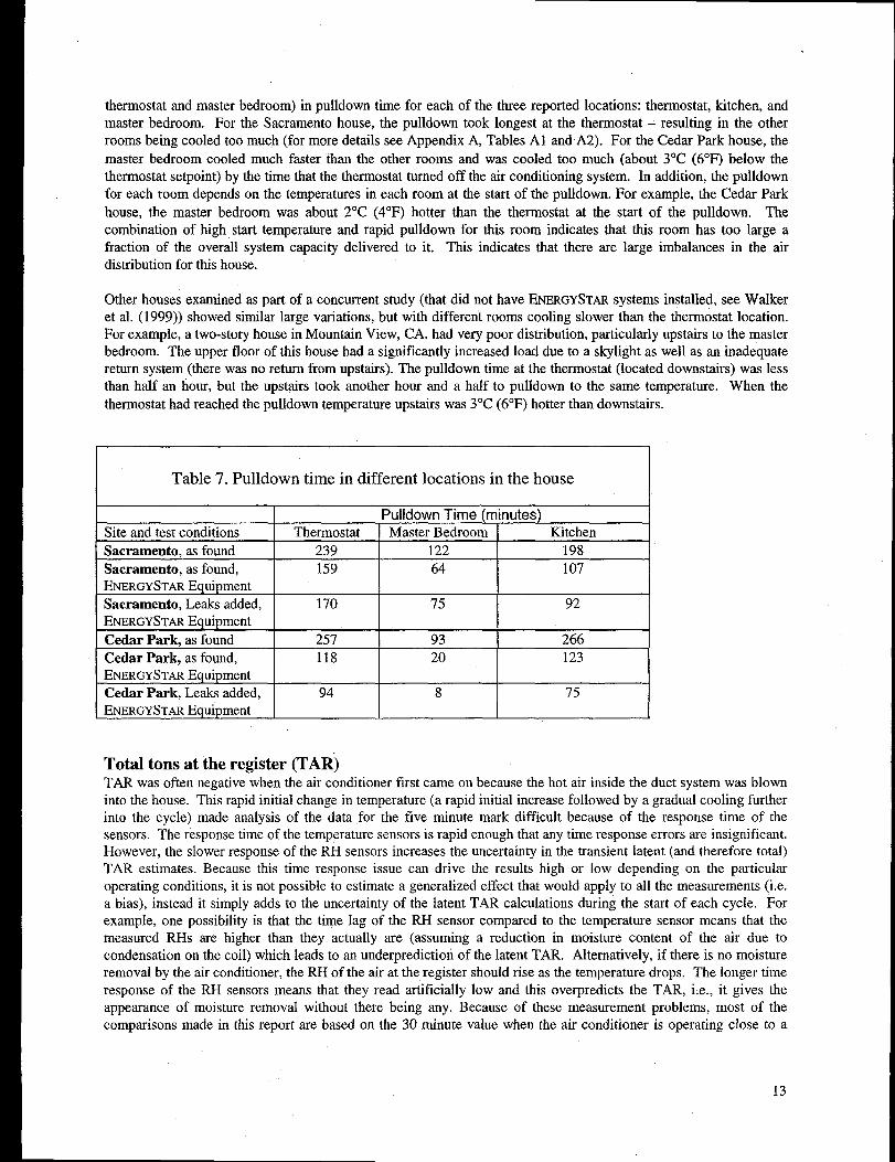
thermostat and master bedroom) in pulldown time for each of the three reported locations: thermostat, kitchen, andmaster bedroom. For the Sacramento house, the pulldown took longest at the thermostat – resulting in the otherrooms being cooled too much (for more details see Appendix A, Tables Al and A2). For the Cedar Park house, the

master bedroom cooled much faster than the other rooms and was cooled too much (about 3°C (6°F) below thethermostat setpoint) by the time that the thermostat turned off the air conditioning system. In addition, the pulldownfor each room depends on the temperatures in each room at the start of the pulldown. For example, the Cedar Park

house, the master bedroom was about 2°C (4”F) hotter than the thermostat at the start of the pulldown. Thecombination of Klgh start temperature and rapid pulldown for this room indicates that this room has too large afraction of the overall system capacity delivered to it. This indicates that there are large imbalances in the airdistribution for this house.

Other houses examined as part of a concurrent study (that did not have ENERGYSTARsystems installed, see Walkeret al. (1999)) showed similar large variations, but with different rooms cooling slower than the thermostat location.For example, a two-story house in Mountain View, CA. had very poor distribution, particularly upstairs to the masterbedroom. The upper floor of this house had a significantly increased load due to a skylight as well as an inadequatereturn system (there was no return from upstairs). The pulldown time at the thermostat (located downstairs) was lessthan half an hour, but the upstairs took another hour and a half to pulldown to the same temperature. When the

thermostat had reached the pulldown temperature upstairs was 3°C (6°F) hotter than downstairs.

Table 7. Pulldown time in different locations in the house

Pulldown Time (minutes) ISite and test conditions Thermostat Master Bedroom Kitchen

Sacramento, as found 239 122 198

Sacramento, as found, 159 64 107ENERGYSTAR Equipment

Sacramento, Leaks added, 170 75 92ENERGYSTAR Equipment

Cedar Park, as found I 257 93 266

Cedar Park as found, 118 20 123ENERGYSTAR Equipment

Cedar Park, Leaks added, 94 8 75ENERGYSTAR Equipment

Total tons at the register (TAR)TAR was often negative when the air conditioner first came on because the hot air inside the duct system was blowninto the house. This rapid initial change in temperature (a rapid initial increase followed by a gradual cooling furtherinto the cycle) made analysis of the data for the five minute mark difficult because of the response time of thesensors. The response time of the temperature sensors is rapid enough that any time response errors are insignificant.However, the slower response of the RH sensors increases the uncertainty in the transient latent (and therefore total)TAR estimates. Because this time response issue can drive the results high or low depending on the particularoperating conditions, it is not possible to estimate a generalized effect that would apply to all the measurements (i.e.a bias), instead it simply adds to the uncertainty of the latent TAR calculations during the start of each cycle. ForexampIe, one possibility is that the time lag of the RH sensor compared to the temperature sensor means that themeasured RHs are higher than they actually are (assuming a reduction in moisture content of the air due tocondensation on the coil) which leads to an underprediction of the latent TAR. Alternatively, if there is no moistureremovaI by the air conditioner, the RH of the air at the register should rise as the temperature drops. The longer time

response of the RH sensors means that they read artificially low and this overpredicts the TAR, i.e., it gives theappearance of moisture removal without there being any. Because of these measurement problems, most of thecomparisons made in this report are based on the 30 minute value when the air conditioner is operating close to a

13

steady state condition.

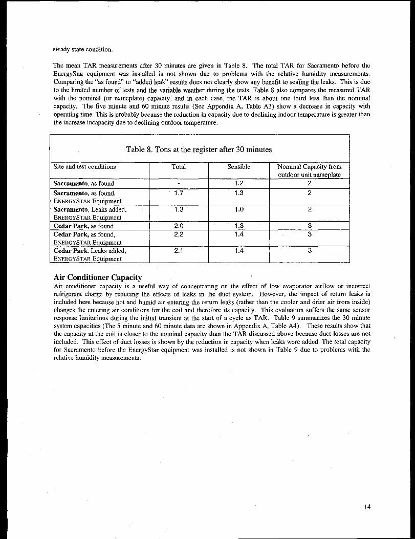
The mean TAR measurements after 30 minutes are given in Table 8. The total TAR for Sacramento before the

EnergyStar equipment was installed is not shown due to problems with the relative humidity measurements.Comparing the “as found” to “added leak” results does not clearly show any benefit to sealing the leaks. This is dueto the limited number of tests and the variable weather during the tests. ‘Table 8 also compares the measured TARwith the nominal (or nameplate) capacity, and in each case, the TAR is about one third less than the nominalcapacity. The five minute and 60 minute results (See Appendix A, Table A3) show a decrease in capacity withoperating time. This is probably because the reduction in capacity due to declining indoor temperature is greater thanthe increase incapacity due to declining outdoor temperature.

Table 8. Tons at the register after 30 minutes

Site and test conditions Total Sensible Nominal Capacity fromoutdoor unit nameplate

Sacramento, as found 1.2 2

Sacramento, as found, 1.7 1.3 2ENERGYSTAREquipment

Sacramento, Leaks added, 1.3 1.0 2ENERGYSTAR Equipment

Cedar Park as found 2.0 1.3 3

Cedar Park as found, 2.2 1.4 3ENERGYSTAR Equipment

Cedar ‘Park Leaks added, 2.1 1.4 3ENERGYSTAR Equipment

Ah Conditioner CapacityAir conditioner capacity is a useful way of concentrating on the effect of low evaporator airflow or incorrectrefrigerant charge by reducing the effects of leaks in the duct system. However, the impact of return leaks isincluded here because hot and humid air entering the return leaks (rather than the cooler and drier air from inside)changes the entering air conditions for the coil and therefore its capacity. This evaluation suffers the same sensorresponse limitations during the initial transient at the start of a cycle as TAR. Table 9 summarizes the 30 minutesystem capacities (The 5 minute and 60 minute data are shown in Appendix A, Table A4). These results show thatthe capacity at the coil is closer to the nominal capacity than the TAR discussed above because duct losses are notincluded. This effect of duct losses is shown by the reduction in capacity when leaks were added. The total capacityfor Sacramento before the EnergyStar equipment was installed is not shown in Table 9 due to problems with therelative humidity measurements.

Table 9. Capacity at the indoor coil after 30 minutes (kW) ISite and test conditions Total Sensible Nominal Capacity from outdoor

trnit nameplate

Sacramento, as found . 5 7

Sacramento, as found, 6.9 5.4 7ENERGYSTAR Equipment

Sacramento, Leaks added, 5.6 4.7 7ENERGYSTAR Equipment

Cedar Park, as found 9.5 6.9 10.5

Cedar Park, as found, 9.9 7.2 10.5ENERGYSTAREquipment

Cedar Park, Leaks added, 9.3 6.7 10.5ENERGYSTAREquipment

Comparing Measured and Rated Air Conditioner CapacityComparisons of measured and rated air conditioner capacity are summarized in Table 10. For each site, the ACCAManual J (1986) sensible load was calculated using the measured house dimensions and construction details. Thiswas compared to data from the manufacturer (nameplate capacity), from the ARI (1999) ratings and the measuredsensible TAR. The measured TAR were the quasi-steady-state values obtained after the equipment had beenoperating for 30 minutes so as not to include transient effects that are not part of the other ratings. These resultsshow that the nameplate capacities far exceed the requirements of the Manual J calculations indicating potentialoversizing. The ARI and measured Maximum Sensible Capacity ratings diminish the oversizing effect but stillreinforce the overrating in the nameplate capacities. The measured TAR is closer to the Manual J estimates and atCedar Park the TAR is less than the Manual J load estimate. These “results illustrate the impact of the systemperformance in converting from what is purchased by the homeowner or contractor (nameplate capacity) and isactually delivered to the conditioned space (TAR). Sacramento has a TAR that is almost the same as the MaximumSensible Capacity of the equipment. This is an unusual result, however, and the other sites examined for thecompanion study (Walker et al. (1999)) have considerable lower TAR than this maximum. Overall, the resultsshown in Table 10 illustrate that nameplate capacity is a poor way of evaluating the capacity of the equipment(compared to Maximum Sensible Capacity) and the system as a whole (TAR). In addition, the apparently grossoversizing of nameplate capacity compared to Manual J is offset by lower actual equipment performance and thermaldistribution system losses

Site

Table 10. System capacity comparisons

Manual J Nameplate ARI MaximumSensible Loadl Capa;ity Capacity Sensible

[Tons] [Tons] [Tons] Capacity

[Tons]

Sacramento 1.02 2 1.9 1.56

Cedar Park 2.28 3 2.9 2.34%’tratthe capacityshouldbe assumingno duct leakage,400cfrn/tonairtlow,perfectrefrigerantcharge,no addition

Air conditioner Coefficient of Performance (COP)Air conditioner COP is a measure of efficiency of an air conditioner,unit. Unlike the COPS presented by the manufacturer, the COPS

Tons at the

Register[Tons~

1.5

1.8safetyfactor.

and it is typically around 2-3 for a residentialreported here include the energy (and heat

15

generation) of the air handler fan. Table 11 summarizes the measured COPS, system power consumption and thefraction of this power drawn by the air handler fan after 30 minutes. System power consumption includes thecompressor, outdoor fan and air handler fan. As with the indoor coil capacity discussed earlier, the addkion of leakstends to reduce the COP. The measured sensible COP for the ENERGYSTARequipment is about 25% higher then the

original equipment in Sacramento and about the same in Cedar Park. In all the tests the fan power consumption wasa significant fraction of the total (l5%-3O’%O). This indicates that there are substantial performance gains to be had byimproving the distribution fan efficiency and reducing system pressure drop, The five and sixty minute results aregiven in Appendix A, Tables A5 and A6.

Table 11. Equipment Coefficient of Performance (COP), Power Consumption andfraction of power consumption due to fan, after 30 minutes

Site and test conditions Sensible Total System Power Air Handler Fan power

COP COP’ Consumption as fraction of total (70)

(kW)

Sacramento, as found 1.8 - 2.9 20

Sacramento, as found, 2.4 3.0 2.4 30’

ENERGYSTAREquipment

Sacramento, Leaks added, 2.2 2.7 2.1 30ENERGYSTAREquipment

Cedar Park, as found 1.9 2.6 3.7 20

Cedar Park, as found, 1.9 2.7 3.7 20

ENERGYSTAREquipment

Cedar Park, Leaks added, I .7 2.4 3.9 15

ENERGYSTAREquipment1-NotshownforSacramentobeforetheEnergyStarequipmentwasinstalledduetoproblemswiththeRH measurements.2 – Largevariationindicatinga variablespee~_compress&.

System Coefficient of Performance (COP)S~stem COP is the most inclusive performance measure: it is a simple ratio of the cooling energy delivered to theconditioned space (TAR) divided by the power consumption of the air conditioner and fan. System COP combinesthe changes in the air conditioner capacity as well as any losseslgains in the distribution system. Table 12 shows thesmall increases in system COP due to installing ENERGYSTAREquipment and the small reduction in system COP dueto adding leaks. Appendix A, Table A7 gives the addkional test results for five and sixty minute data.

16

Table 12. Total System Coefficient of Performance (COP) after 30 minutes

Site and test conditions Sensible Totall

Sacramento, as found 1.5

Sacramento, as found, 2.0 2.5ENERGYSTAREquipment

Sacramento, Leaks added, 1.7 2.1

ENERGYSTAREquipment

Cedar Park, as found 1.2 1.9

Cedar Park, as found, 1.4 2.1ENERGYSTAREquipment

Cedar Park, Leaks added, 1.3 1.9

ENERGYSTAREquipment. . . . .- —1- Notshowntor SacramentobeforetheEnergyStarequipmentwas instatleddue to problemswith the NH measurements.

Delivery Effectiveness (DE)Delivery Effectiveness is the total capacity at the registers divided by the capacity at the air handler and does notinclude arty regain of losses or the energy and comfort implications of duct leakage to inside. DE separates duct onlyeffects from the other system performance parameters included in TAR and COP (e.g., it does not include refrigerantcharge effects). Table 13 shows DE for both sensible and total capacity after the system has been operating for 30minutes. After 30 minutes, the system is operating in quasi-steady-state and the DE will not be significantly affectedby any transient thermal mass effects of the duct system and cooling equipment. Additional results (Shown inAppendix A, Table A8) indicate that DE can be higher after five minutes of operation than the 30 minute values inTable 13. This is mostly because the whole duct system has not cooled down from its initial high temperature in theattic. Because the duct temperatures are higher, the conduction losses are lower, and this is reflected in a highermeasured DE. For Sacramento, the results of sealing the duct system. are much more apparent when looking atdelivery effectiveness rather than the TAR given in Table 8,

I Table 13. Delivery Effectiveness [Yo] after 30 minutes

Site and test conditions Sensible Total

Sacramento, as found 0.85 0.89

Sacramento, as found, 83 85

ENERGYSTAREquipment

Sacramento, Leaks added, 77 79

ENERGYSTAREquipment

Cedar Park, as found 0.67 0.75

Cedar Park, as found, 78 Insufficient data

ENERGYSTAREquipment

Cedar Park, Leaks added, 75 80

ENERGYSTAR Equipment

Field Measu~ement Summary● Improving ducts by reducing leakage can lead to significant energy efficiency gains in addition to increasing the

TAR, and increases comfort by reducing pulldown time.

● Systems can have good efficiency, but not give sufficient comfort to occupants due to poor room-by-roomdistribution.

. Using higher SEER units indicated larger sensible than total energy savings. Sensible performance increased by25% at one site and Iess than 5% at the other. The latent perform~ce was harder to interpret due to

17

uncertainties in Relative Humidity measurements.

● Installed capacity (TAR) is considerably less than nameplate and ARI ratings. In addition, nameplate and ARIratings exceed ACCA Manual J load estimates.

. Thermal distribution system losses and poor equipment installation combine to reduce nameplate and ARIcapacities toward ACCA Manual J load estimates.

. The total duct leakage for the test houses was less than in previous studies and was between the default valueand minimum requirement for duct leakage credit in T24 (2290 and 6tZ0respectively). Because an objective ofthis study was to investigate the interactions between duct losses and equipment operation, leakage was added tothe duct systems to simulate more typically leaky systems.

. Boot and cabinet leakage contributes 25% to 50% of the total duct leakage at operating conditions and aboutthree quarters of the fixed pressure test leakage.

● The duct leaks added an average of 0.2 ACH to the ventilation rates of the tested houses.

Modeling improved Comfort with REGCAPSome of the details of the simulation model (called REGCAP) are given in previous work by Walker et al. (1998aand 1998b) and Walker et al. (1999). A flowchart for the simulation program is shown in Appendix B. The thermaland ventilation parts of REGCAP were adapted from existing models that were specifically developed to examineattic performance. These models of ventilation and heat transfer, excluding the ducts, have been verified withextensive field measurements (Walker (1993)). The airflow modeling for REGCAP combines the existingventilation models for the house and attic with duct register and leakage flows using mass balance of air flowing inand out of the house, attic and duct system. The thermal modeling uses a lumped heat capacity approach so thattransient effects are included. The ventilation and thermal models interact because the house and attic ventilationrates depend on house and attic air temperatures, airflow through duct leaks, and the energy transferred by the ductsystem depends on the attic and house temperatures. Recent model developments made during this study includedadditional airflow paths through duct leaks when the system is not operating and a moisture balance for use in latentload and equipment capacity calculations. A simple thermostat model and the ability to make calculations at smalltimesteps allows the model to be used for examining cyclic effects. REGCAP is a single-zone model and does notperform energy or airflow calculations for every room in the house so the simulation results only apply to “wholehouse” values and cannot be used to estimate room-by-room comfort estimates. The reason for this single zoneapproach is that the information required to perform multi-zone calculations is generally unknown and is difficult todetermine even for case studies like those performed in the field measurement section of this study. For example,characterizing all the potential airflow paths through the envelope of the house and between every room of the houseis essentially impossible.

The comfort delivered by each system was evaluated by simulating pulldown time and TAR at various times duringthe pulldown. In the same way as the measured data, the pulldown was simulated by having the air-conditioner offfrom midnight to 3:00 p.m. Then at 3:00 p.m., the air conditioner was turned on. The simulation model was used tocalculate the system performance in one minute time steps for a whole day (including times when the system is off).In the previous work (Walker et al. (1998a and 1998b), the timesteps had been set to 15 minutes, but this was foundto be too coarse a timestep for capturing all the transient behavior of the systems.

The following list gives the key model input parameters:Envelope leakage. For both house and attic.Envelope thermal parameters. Insulation and construction details for house and attic.Weather. Outside air temperature and relative humidity, wind speed, wind direction and solar loads (totaland diffuse).Refrigerant Charge. The retilgerant change was set to three levels representative of those measured in fieldtesting.Airflow across coil. The airflow was set to two levels representative of those measured in field testing.Duct Leakage. Duct leakage was set to levels representing field test results, CEC ACM compliant and ideal(no leakage) ducts.Alr handler and duct location. This was either the attic (typical of new construction) or inside theconditioned space.Equipment Capacity, The capacity was calculated using an equipment model developed by John Proctor.

18

The equipment model used to predict the capacity of the air conditioners for the REGCAP simulation is an empiricalmodel developed by John Proctor. This model is the only available model that accounts for refrigerant charge leveland is sufficiently general for use in this project. This model has been used in several research projects (Proctor(1997), (1998a) and (1998b)) and is continually updated as new data are collected. Currently, the portion of themodel that accounts for deviation from recommended refrigerant charge is taken directly from Rodriguez et al.(1995) and the rest of the model is from Proctor Engineering Group fieldwork in about one hundred houses. Theequipment model requires the following inputs: nominal (nameplate) capacity, ARI capacity, airflow, outsidetemperature, indoor (return plenum) enthalpy, refrigerant charge level, and expansion valve type (capillarytube/orifice or TXV (thermostatic expansion valve)). The equipment model predicts sensible capacity and, with theassumption of a sensible heat ratio for the unit, latent and/or total capacity can also be predicted. A comparison tothe measured capacities at the two houses in this study (plus another four from the companion study) indicate thatthe model overpredicts capacity by about 10%. There is no obvious reason for this consistent deviation fromProctor’s data, but a possible reason is that most of the Proctor’s verification of the model occurred in very dryclimates, rather than the more humid weather that we encountered during the field testing and the simple assumptionabout latent load requires refining.

REGCAP Simulation EvaluationAn essential part of simulation design and use was verifying that the simulation makes accurate predictions. In thiscase, we were interested in predicting two parameters: tons at the register (delivered capacity) and pulldown time(time to cool down the house). REGCAP was validated by comparing predicted temperatures to measuredtemperatures. Given the same temperatures, other variables used to determine energy flows (e.g., register flowrates)and comfort parameters (e.g., pulldown times) are the same for both modeled and measured data. For this purpose,we examined the temperatures of four air nodes: attic, house, supply duct and return duct.

Over 100 days of measured data at 5 sites were used to evaluate REGCAP (4 in California and 1 in Texas). Overallthere was very good agreement between measured house and attic temperatures and REGCAP predictions. Therewas also good agreement between the duct air temperatures when the air handler fan was on, but not very goodagreement when the air handler was off. In o}der to illustrate these and other strengths and weaknesses of REGCAP,the predicted and measured temperatures are shown for one site and each of the four (house, attic, return and supply)modeled temperatures will be discussed individually. There was no attempt to show data that were either particularlyfavoring or condemning of REGCAP. The following illustrations are included to demonstrate both the strengths andthe weaknesses of the model. The generalized discussion applies to all the comparisons between measured andmodeled data.

19

0 5 10 15 20

Time [Hours]

Figure 1: REGCAP Predicted and Measured Attic Temperatures for the Sacramento test house.August 11, 1998

Attic TemperatureFigure 1 shows good agreement between the REGCAP predicted and the measured attic temperature over the wholeday. The agreement is excellent for the first half of the day and then the predicted temperature drops slightly belowthe measured temperature later in the day. The average absolute difference in temperatures over the day was 2.4°C

(4.3°F). There are several hypotheses that explain this small discrepancy. The most plausible is a problem with themeasured solar radiation input data (the dip in the data when the sun comes up is an indication of this). Anotherpossibility is that the ducts are too strongly coupled with the house so that when the air conditioner comes on theduct leakage cools the attic more in the REGCAP predictions than in the measured case. Another possible problemis that the radiative transfer involving the attic endwalls and the combined mass of wood in the attic was neglected.

20

0

I— Measured I

5 10 , 15 20

Time [Hours]

Figure 2: REGCAP Predicted Wd Measured House Air Temperatures for the Sacramento testhouse. August 11, 1998

House TemperatureThe comparison of house temperatures for the Sacramento tests house is shown in Figure 2. The measuredtemperatures are taken at the location of the thermostat that controls the air conditioner. The house air temperaturesare predicted better than the attic air temperatures. The average absolute difference between the REGCAP predicted

and the measured values is 0.4°C (0.7”F). The predicted temperatures are less smooth than the measuredtemperatures because the modeled house air responds very quickly to changes in weather conditions. Eachdiscontinuity in the predicted temperatures is a change in input weather data (for which we have 15 minute averagesonly). The rapid reaction of indoor temperatures to the change in weather conditions is probably because ofinsufficient coupling between the house air and the house mass. There are two most likely causes of this problem: thefirst is that the interior surface convection heat transfer coefficient is biased towards natural, rather than forcedconvection. This is possibly a poor assumption when the air handler is on. This is a good example of wherereducing an input requirement (i.e. not requiring average air velocity in the house to be known) may lead to a lessaccurate predicted result. The second is that the surface area active in heat exchange between the thermal mass ofthe house and house air is too small in the model. Future work will further investigate the convection heat transfer

21

coefficient thermal mass issue.

Examination of the weather data collected on the day of test indicates very strong winds from about 1lam until 6p.m. This failure of REGCAP to deal with extreme conditions and is probably the cause of the wide temperature

swings evident in the measured data. The REGCAP prediction has a single spike in the temperature when the airconditioner comes on. This is an artifact of the ducts pushing hot air into the house that doesn’t seem to be evidentin the measured data (which was collected every 10 seconds, a finer resolution than the minute long timestep used byREGCAP). Despite these discrepancies, predicted house temperatures reflect the overall shape of the temperaturecurve in each house. An improved house load model will be developed and used in the future.

w 40

30

201

I— Measured I1

b

+

5g 10L J

o 5 10 15 20

Time [Hours]

1Figure 3: REGCAP Predicted and Measured Return Duct Air Temperatures for the Sacramento

test house. August 11, 1998

Return Duct Air TemperatureThe agreement between measured and predicted return duct temperatures shown in Figure 3 is quite good when theair conditioner is on (absolute difference of only 0.3”C). Overall, REGCAP does an adequate job of predicting the

22

return duct air temperature when the air handler fan is on. When the air handler is off, the predicted duct airtemperature is much hotter than the measured temperature (absolute difference of 5.1 ‘C). The REGCAP predictedreturn duct temperature with the system off is close to the attic air temperature, which is expected because the ducts

are in the attic, but the measured results have lower return temperatures. The most likely reasons for this differenceare factors that we have not included in REGCAP (because the input data required to perform the calculations isdifficult to determine) or measurement problems. The two most likely sources of uncertainty are:1. Stratification of air inside the duct such that the measured air temperature is near a cool point.2. Additional indoor airflow through the system due to room-to-room pressure differences caused by air infiltration

flows.

The spatial temperature variation point is one that always occurs with simplified modeling and measurement whenassumptions are made about air being well mixed at the measurement location. Without making more measurements

at more locations we cannot tell if this is a big problem or not. In future work we will need to examine this issue inmore detail. We need to be careful in not tweaking REGCAP to match these measured results in case themeasurements are an anomaly due to large temperature variations.

When the system is off REGCAP does include air flows from the house into the duct due to ventilation (caused bypressure differences due to temperature, wind effects and mechanical ventilation). The measured results could bebetter matched by REGCAP if these airflows were increased. It is possible that the pressure differences betweenrooms in the house may cause additional flows that R.EGCAP does not account for. However, to include these flowswould require detailed multizone modeling for which the inputs (airflow resistance between rooms, including theflow resistance of each individual duct) are not known. These inputs are very difficult to measure for an individualhouse and it is not practical to require them as model input. One possibility is to make up some values and performparametric modeling, however this would not improve the match between measured and modeled data that we arediscussing here. In addition, given the uncertainty in measurement discussed above (due to spatial temperaturevariations) it is not possible to justify this additional modeling effort.

The ducts in contact with the floor could be accounted for by making additional observations of the ducts as installedin the test houses and then adding a conduction path to the house for the attic ducts. This is has been added as anoption for REGCAP. However, it is difficult to estimate the contact area and insulation value for ducts lying on theattic floor.

Although the above discussion shows that there may be some complex heat transfer issues not included in REGCAP,it should be noted that the large discrepancies only apply when the system is off. They would only affect the initialtransient performance of REGCAP and would not significantly change any of the predictions during systemoperation.

23

70

60

50

40

30

20

10

— Measured— — Predicted

I

I

0 5 10 15 20

Time [Hours]

Figure 4: REGCAP Predicted and Measured Supply Duct Air Temperatures for the Sacramento- test house. August 11, 1998

Supply Duct Air TemperatureLike the return duct air temperature, the supply duct air temperatures show good agreement when the air handler fanis on, but poor agreement when the air handler fan is off. When the air handler is off, the REGCAP predicted supplyduct temperature is very strongly influenced by the attic temperature and radiation exchange with the interior atticsurfaces. The agreement is not very good for the supply duct air temperatures when the air handler is off for thesame reasons as for the return ducts.

The lack of air-handler off agreement for the duct temperatures is not particularly significant for the objectives ofthis study: predicting the pulldown time and the tons at the register. The only temperatures that are directly neededfor these calculations are the house air temperature and the supply duct air temperature when the air conditioning fanis on. For this reason, REGCAP is well suited to calculating the performance parameters that are the focus of thisproject.

24

REGCAP Simulation ResultsThe improved model was used to reexamine the pulldown simulations performed previously by Walker et al. (1998and 1998b). In the simulations, eight different thermal distribution systems are used in the same house for the sameweather conditions. The results shown here use a day of TMY data for Sacramento, CA (NCDC (1980)) for whichthe peak temperatures most closely matched the ASHRAE ( 1997) 1% design values. In the previous work thesimulations were used to show how pulldown time changed with duct system performance, different weatherconditions (a typical design day and the maximum load day) and with system capacity.

Table 14 lists the simulation cases that were examined here. The BASE case is typical of new construction inCalifornia. The POOR system represents what is often found at the worst end of the spectrum in existing homes.The BEST system is what could reasonably be installed in new California houses using existing technologies andcareful duct and equipment installation to manufacturers’ specifications. The BEST RESIZED system looks at thepossibility of reducing the equipment capacity while using the best duct system. The INTERIOR system examinesthe gains to be had if duct systems are moved out of the attic and into conditioned space. The INTERIOR RESIZEDsystem examines the system performance when reduced capacity equipment is used together with interior ducts.Lastly, the IDEAL system is an interior duct system that has been installed as well as possible. The IDEALOVERSIZED simulations were included to examine the difference in pulldown if the IDEAL system were sizedusing current sizing methods (i.e., 4 tons).

The simulations were able to show several key results:● A good duct system (with the correct refilgerant charge, little or no leakage and the right flow across the coil)

allowed the capacity of the equipment to be reduced by about one third: from four tons to three tons nameplatecapacity.

. If system nameplate capacity is unchanged, either improving duct systems (to have little leakage) and correctlyinstalling the equipment, or moving the ducts inside the conditioned space results in significant pulldownperformance improvements. In these cases pulldown times were reduced by more than an hour and initial tonsat the register were approximately doubled.

. The model results also showed the wide range of pulldown times for different duct systems.

The large range of pulldown results are illustrated in Figure 5, with each simulation starting at the same time. Thebetter systems were able to pulldown the house in a reasonably short time (under three hours) but the poor systemstook over five hours. The longer pulldown times mean that the house would not be as comfortable for occupantsreturning in the afternoon. For example, the house with the POOR system is still not pulled down at 8:00 p.m. Forthe occupants this may be unacceptable.

Note that pulldown tests focus on capacity at the registers and how this changes the pulldown time. With gooddistribution systems and reduced equipment capacity it maybe better to not turn the system off during the day (set-upfollowed by afternoon pulldown) and allow the system to cycle. In addition, the continuous operation (non-set-up)will be of more use for providing humidity control in humid environments.

25

Start of pulldown -a-- POOR

— BASE... .. “~ “ ““ BEST RESIZED

~ INTERIOR RESIZED. . . . . BEST+ IDEAL+ INTERIOR+ IDEAL OVERSIZED

I

14 15 16 17 18 19 20 21

Time of Day (hours)

Figure 5. REGCAP Simulations of pulldowns from 3:00 p.m. on a Sacramento design day.

Table 15 compares the results of the calculated TAR based on the simulations. Note that for these calculations thesystems have been running for almost two hours and are at quasi-steady-state and do not show the transient capacityreductions at the start of the pulldown. This was done so that we are not unfairly comparing the nameplate capacityto the transient system performance. In other words, we are being as generous as possible in our comparisons byreporting close to the highest system capacities. All but the POOR ducts are better than the BASE case in terms ofdelivered TAR and also TAR as a fraction of the nameplate capacity of the equipment. All of the resized systemshave TAR closer to their nominal capacity than for the BASE case. However in all cases (even the ideal situationwith correct system charge and airflow and minimal duct losses) the equipment capacities are much less than thenameplate rating on the equipment that a home owner, builder or HVAC equipment installer has paid for.

These simulation results reinforce the following conclusions from the previous studies:● Improved ducts and system installation can allow the use of a smaller capacity air conditioner (almost one ton

less in the cases studied here, and at least one ton in more demanding situations) without any comfort penalty interms of pulldown time. As part of the companion study, Walker et al. (1999) also showed that the smallercapacity air conditioners could also have large energy savings (roughly halving energy consumption required forpulldown).

26

● If system nameplate capacity is unchanged, either improving duct systems and correctly installing theequipment, or moving the ducts inside results in significant pulldown time reductions.

. Systems do not provide their nameplate capacity at design conditions, when system capacity is most critical.

Table 14. List of REGCAP Simulation Cases

Duct Duct and NameplateSystem Air Handler Leakage equipment RatedCharge Flow Fraction Location Capacity

p!] [CFM/Ton] p7’0] ~ons]

IASE 85 345 11 Attic 4

‘OOR 70 345 30 Attic 4

lEST 100 400 3 Attic 4

JEST RESIZED 100 400 3 Attic 3

NTERIOR 85 345 0 House 4

NTERIOR RESIZED 85 345 0 House 3

DEAL 100 400 0 House 3

DEAL OVERSIZED 100 400 0 House 4

I Table 15. REGCAP Delivered Capacity (TAR) Comparison (System on for 1.75 hours)I

Nameplate Tons at the Tons at the Register Ratio toCapacity Register Nameplate Capacity Base Case

(TAR)[Tons] [Tons] [%] [%]

BASE 4 1.66 42% 100%

POOR 4 1.51 38% 91%

BEST 4 2.21 55% 133%

BEST RESIZED “3 1.66 55% 133%

INTERIOR 4 1.84 4670 110%

INTERIOR RESIZED 3 1.36 45% 109%

IDEAL 3 1.68 56% 135%

IDEAL OVERSIZED 4 2.28 57% 137%

Technology TransferThe following are duct system technology transfer issues that have been investigated as part of this study.

Duct C/caning effect on aerosol sealant (EPA).An issue that has been raised regarding the aerosol sealant is its resistance to duct cleaning. Ducts are cleaned in

order to remove build-ups of dust that can lead to poor indoor air quality. Unlike sealants applied to the outside ofducts (e.g., duct tape), the aerosol sealant is applies from the inside and maybe more sensitive to abrasion caused byduct cleaning efforts. In order to examine this effect, a sheet metal duct system was sealed with the aerosol sealant

27

and then cleaned by professional duct cleaners. The duct cleaners were local HVAC contractors who cleaned theducts as they would for a regular service call. No attempt was made to change the tasks they performed in order to

make the duct cleaning more effective. The cleaning was about four years after the initial aerosol sealing. The

system was cleaned four times in total.

The first contractor vacuumed duct system supply four times: supply system twice and return system once and bothsystems the same time once. For the first vacuuming, all of the registers were taped and furnace was isolated. An 8“diameter vacuum hose was connected to the supply plenum. The system was vacuumed for about 15 minutes. Thepressure difference between the duct and the house (measured at the furthest part of the duct system from where thevacuum hose was connected) was 35 Pa. The relatively low vacuum pressure was because the cardboard used toisolate the furnace was misplaced and resulted in a blg leak. After this leak was fixed, the pressure differencebetween the duct and the house increased to 254 Pa. The return was vacuumed separately. The two return registerswere taped and the furnace was isolated. The return duct was also vacuumed for about 15 minutes. The pressuredifference between the return duct and the house was 980 Pa falling to 540 Pa at the end of the vacuum. cleaning. Aduct leakage measurement was performed after the above cleaning procedures, and the supply and return leakagewere unchanged - within 0.1 cfm25 of the pre cleaning leakage (Before the system was cleaned the measured leakagewas 6.2 cfm25 supply and 9.3 cfm25 return.).

For the next cleaning an 8“ diameter vacuum hose was connected to the furnace burner access panel. Only arudimentary attempt was made to seal around this connection using a rag wrapped around the hose. All of theregisters were simply covered with pieces of paper rather than being completely sealed. The pressure differencebetween the ducts and the house was about 220 Pa and stayed at the same level during the vacuuming process. Afterthese two vacuumings, the duct leakage was measured to be 6.6 cfm25 for the supply and 9.0 cfm25 for the return.This result shows that the leakage was again unchanged (within the experimental uncertainty of Al cfm) by thevacuuming process.

A second HVAC contractor then vacuumed the duct system with a combination of inserting a spinning brush into theducts at the registers and brushing all the way to plenum if there was no damper to block it. This was a more severetest of the aerosol sealant because it might have been abraded by the brushes. The supply and return duct systemswere isolated and each grille was removed before inserting the spinning brush and then the register was plugged witha piece of foam. The supply duct was depressurized to about 330Pa. After this brushing and vacuuming, themeasured leakage was 7.9 cfm25 for the supply and 9.8 cfin25 for the return. Thk shows a small increase waspossibly caused by a change in the leakage at the boot to wall seal where aerosol deposition was disturbed when thegrille was removed. However this amount of extra leakage (less than 2 cfm) is not significant given the measurementuncertainty.

It should be noted that the vacuuming without the brush did not appear to remove much dust from the system. Thecombination of vacuuming and brushing was much more effective and included the removal of a paper cup and a halfroll of duct tape.

The conclusions drawn from these tests is that duct cleaning of a system sealed using the aerosol sealant does notremove the sealant and there is a large variation between contractors of duct cleaning thoroughness. Further tests arerequired on more systems to determine if the sealant is as durable as these tests indicate.

Health and Safety Assessment of Aerosol Sealant (EPA)As with any new industrial material, concern exists over the potential human health hazards related to exposure tothe aerosol sealant. Potential health and safety issues regarding the duct seal material were evaluated and discussed

by Buchanan (1999). That report examined the characteristics of the sealants individual components based on areview of the current literature. Buchanan indicated that there are three primary means by which exposure couldoccur: ingestion, eyeldermal contact, and inhalation. Each of these possibilities was examined. Exposure and safetyrisks were assessed with regard to the currently known constituents that are believed to pose potential hazards; VAP,VAM, 2EH, and acetaldehyde. Buchanan concluded that the aerosol sealant did not pose any significant health andsafety risks.

28

ASHRAE: Rating”of Distribution Systems - ASHRAE 152PASHRAE 152P has been developed to the point where it has been published by ASHRAE for public review duringMay and June 1999. It is expected that the final draft of this standard will be ready by January 2000. We have alsodeveloped a web-based tool for performing 152P calculations. This tool can be accessed at httv://ducts.lbl. ~ov. Thisweb tool includes many defaults as guides for the uninitiated user that are taken from the appendices of 152P. Thesedefaults are intended to make this web-tool easier to use.

ASTM: Rating of duct sealants and revising duct leakage measurement methodsWe have attended ASTM meetings and corresponded with ASTM to discuss the implementation of an ASTMstandard for longevity testing of duct sealants (ASTM (1999b)). A draft of the standard was prepared and voted onby ASTM E6.41 subcommittee members. Several comments were made on this draft which was then revised andwill be reallotted later this year.

The current duct leakage test measurement in ASTM E1554 is obsolete. That standard has been rewritten, based onthe results of duct leakage test evaluations performed for the last three phases of the current research sponsored byCIEE/CEC, together with input from other ASTM members and the members of ASHRAE SSPC 152P. The newdraft of the standard has two leakage test methods: the DeltaQ test and duct pressurization. The standard alsoincIudes the benefits and drawbacks of the two methods so that the user can select the most appropriate test methodfor the test they are performing. For example the DeltaQ testis better for measuring leaky duct systems for HERStesting, but the pressurization tests are more robust for low leakage compliance testing.

References

ACCA. 1986. Manual J - Load Calculation for Residential Winter and Summer Air Conditioning - Seventh Edition.,Air Conditioning Contractors of America (ACCA), Washington, D.C.

ARI. 1999. Electronic Unitary Directory, ARI UD99S V1 .2. Air Conditioning and Refrigeration Institute, Arlington,VA.

ASHRAE. 1997. Handbook of Fundamentals. ASHRAE, Atlanta, GA.

ASHRAE. 1999. ASHRAE Standard 152P: Method of Test for Determining the Design and Seasonal Ef%ciencies ofResidential Thermal Distribution Systems (public review draft). ASHRAE, Atlanta, GA.

ASTM. 1999. Draft revision to Standard E-1554 – Determining External Air Leakage of Air Distribution Systemsby Fan Pressurization. American Society for Testing and Materials, West Conshohocken, PA.

ASTM. 1999b. Task group draft – Standard Test Method for Longevity Testing of Duct Sealant Methods.American Society for Testing and Materials, West Conshohocken, PA.

Buchanan, C. 1999. Duct Seal Health and Safety Assessment.LBNL43114

California Energy Commission (CEC). 1998. Low-Rise Residential Alternative Calculation Method ApprovalManual for 1998 Energy Eftlciency Standards for Low-Rise Residential Buildings, California EnergyCommission, Sacramento, California.

Cummings, J.B., Tooley, J. J., Moyer, M. and Dunsmore, R. 1990. Impacts of duct leakage on infiltration rates, spaceconditioning energy use and peak electrical demand in Florida houses. Proc. 1990 ACEEE Summer Study,Vol. 9, pp.65-76. ACEEE, Washington , DC.

Modera, M.P., 1989. Residential Duct System leakage: Magnitude, Impacts and Potential for reduction. ASHRAETrans., Vol 95, Part 2, pp.561-569. ASHRAE, Atlanta, GA.

29

Modera, M. P., and Wilcox, B. 1995. Treatment of residential duct leakage in Title 24 energy efficiency Standards.California Energy Commission Contract Report.

NCDC. 1980. Climatography of U. S., #8 1, Monthly Normals of Temperature, Precipitation and Heating and CoolingDegree days 1951-1980. National Climatic Data Center, Federal Building, Asheville, NC.

Palmiter, L. and Francisco, P. 1994. Measured Efficiency of Forced-Air distribution systems in 24 houses. Proc.1994. ACEEE Summer Study, Vol. 3, pp. 177-187. ACEEE, Washington, DC.

Palmiter, L. and Bond, T., 1992. Impact of mechanical systems on ventilation and infiltration in homes. Proc. 1992ACEEE Summer Study, Vol. 2, pp.205-216. ACEEE, Washington, DC.

Proctor, J. 1998a. Monitored In-Situ Performance of residential Air-Conditioning Systems. ASHRAE Trans. Vol.104. Part 1. ASHRAE, Atlanta, GA.

Proctor, J. 1998b. Performance of a Reduced Peak kW Air Conditioner at High Temperatures and Typical FieldConditions. Proc. ACEEE Summer Study on Energy Efficiency in Buildings 1998. Vol. 1 pp.265-274.American Council for an Energy Efilcient Economy, Washington, D.C.

Proctor, J. 1997. “Field Measurements of new residential air conditioners in Phoenix, Arizona.” ASHRAE Trans.Vol. 103 Part 1. ASHRAE, Atlanta, GA.

Rodriguez, A. G., O’Neal, D.L., Bain, J.A., and Davis, M.A. 1995. The Effect of Refrigerant Charge, Duct Leakage,and Evaporator Ak Flow on the High Temperature Performance of Air Conditioners and Heat Pumps.Energy Systems Laboratory report for EPRI, Texas A&M University.

Walker, 1.S. 1993. Attic Ventilation, Heat and Moisture Transfer. Ph.D. Thesis, University of Alberta, Alberta,Canada.

Walker, I, Sherman, M., Modera, M., Siegel, J.Dickerhoff, D. 1997. Leakage Diagnostics, Sealant Longevity, Sizingand Technology Transfer in Residential Thermal Distribution Systems. CIEE Residential ThermalDistribution Systems Phase V Final Report, October 1997, LBNL Report 41118.

Walker, I., Sherman, M., Siegel, J., Wang, D., Buchanan, C. and Modera, M. 1998. eakage Diagnostics, SealantLongevity, Sizing and Technology Transfer in Residential Thermal Distribution Systems: Part II. CIEEResidential Thermal Distribution Systems Phase VI Final Report, October 1997, CIEE, Berkeley, CA.LBNL report 42127.

Walker, I., Brown, K., Siegel, J. and Sherman, M. 1998. Saving Tons at the Register. Proc. ACEEE Summer Study,Vol. 1, pp. 367-383. ACEEE, Washington, DC. LBNL report 41957.

Walker, I., Sherman, M., and Siegel, J. 1999. Distribution Effectiveness and Impacts on Equipment Sizing. CIEEResidential Thermal Distribution Systems Transition Phase Final Report. CIEE, Berkeley, CA. LBNL43’724

Appendix A. Detailed Measurement Results

I Table Al. Pulldown time and temperatures in different locations in the housePulldown Time (minutes) Temperatures PC)

Condition Thermostat Master BR Kitchen Thermostat Master BR KkchenSacramentoas 239 122 198 24.1 21.9 23.2foundSacramentoas 159 64 107 24.0 21.9 23.1found,newcompressorSacramento 170 75 92 24.0 22.1 22.7LeaksaddedCedar Park as 257 93 266 24.0 21.0 24.2foundCedar Park as 118 20 123 23.2 20.3 23.1found,new .

compressor ICedar Park 94 8 75 23.6 22.8 25.2

Table A2. Temperatures at different locations in the house during pulldown tests5

Condition T“

Sacramentoas 30foundSacramentoas 28.6found,newcompressorSacramento 28.1LeaksaddedCedar Park as 26.6foundCedar Park as No datafound,newcompressorCedar Park 24.4leaks added

ninutes 30 minutes 60 minutesMaster Kitchen Thermostat Master Kitchen Thermostat Master KitchenBR [“C] ~c] rc] BR PC] PC] PC] BR ~C] p’c]

26.9 28.1 28.5 26.7 25.9 27.6 26.1 25.0

27.5 26.8 27.0 25.5 24.7 26.1 24.8 23.8

27.0 26.9 26.7 25.1 24.9 26.0 24.4 24.1

30.1 28.0 27.8 28.6 25.5 27.3 28.2 24.7

Nodata No data 27.6 28.4 25.2 27.0 27.7 24.4

26 23.6 23.6 24.5 21.4 22.9 23.7 20.7

31

found leakage,ENERGYSTAR IequipmentSacramento, 2added leaks,ENERGYSTAR I

found leakage,ENERGYSTAR Iequipment

Cedar Park. 3–

Table A. 5minTotalMean

3.1

1.9

1.4

2.8

Nodata

2.8

Tons At the Register (TAR)tes 30 Minutes 60 minutesSensible I Total Sensible Total

Mean I MeanI

Mean I Mean

1.1 3.0 1.2 2.9

1.3 1.7 1.3 1.6

1.0 1.3 1.0 1.4

1.2 2.0 1.3 1.9

Nodata 2.2 i .4 2.0

SensibleMean

1.3

1.3

1.2

1.4

1.4

1.4

Table A4. Capacity at the Indoor Coil5 minutes 30 minutes 60 minutes

Total Sensible Total Sensible Total SensibleCondition KW kW kW kW kW kW

Sacramento as 12.3 4.8 11.7 5 11.5 5.2foundSacramento as 7.6 5.17 6.9 5.4 6.7 5.5found, newcompressorSacramento Leaks 6.1 4.5 5.6 4.7 5.5 4.7addedCedar Park as 12.1 6 9.5 6.9 9.2 7.1foundCedar Park as No data No data 9.9 7.2 9.7 7.4found, newcompressorCedar Park leaks 11.8 6.6 9.3 6.7 9.0 6.8added

32

Table A5. Equipment Coefficient of Performance (COP)Sensible Total

Condition 5 minutes 30 minutes 60 minutes 5 minutes 30 minutes 60 minutesSacramentoas 1.7 1.8 1.9 * * *foundSacramentoas 2.2 2.4 2.4 3.3 3.0 2.9found,newcompressorSacramento 2.2 2.2 2.2 2.9 2.7 2.6LeaksaddedCedarParkas 1.6 1.9 1.9 3.2 2.6found

2.5

CedarParkas Poor data 1.9 2.0 Poor data 2.7 2.6found,newcompressorCedar Park 1.8 1.7 1.8 3.1 2.4 2.3leaks added* - poor RH measurements mean that total COP cannot be accurately estimated.

Table A6 System Power Consumption

5 minutes 30 minutes 60 minutes Air Handler fanpower as fractionof total powerconsumption

Condition KW kW KWSacramento as 2.9 2.9 2.8 0.20foundSacramento as 2.4 2.4 2.3 0.30’found, newcompressorSacramento Leaks 2.1 2.1 2.1 0.30addedCedar Park as 3.7 3.7 3.7 0.20foundCedar Park as Poor data 3.7 3.7 0.20found, newcompressorCedar Park leaks 3.8 3.9 3.9 0.15added1 – Large variation indicating a variable” speed compressor

33

Table A7. Total System Coefficient of Performance (COP)Sensible Total

Gondition 5 minutes 30 minutes 60 minutes 5 minutes 30 minutes 60 minutesSacramentoas 1.4 1.5 1.6 3.9 3.8 3.8foundSacramentoas 1.9 2.0 2.1 2.8 2.5 2.6found,newcompressorSacramento 1.7 1.7 2.0 2.4 2.1 2.4LeaksaddedCedarPark as 1.1 1.2 1.3 2.7 1.9 1.8foundCedar Park as Poor data 1.4 1.4 Poor datafound,new

2.1 2.0

compressorCedar Park 1.4 1.3 1.3 2.6 1.9 1.9leaksadded

Table A8. Delivery EffectivenessSensible Total

Condition 5 minutes 30 minutes 60 minutes 5 minutes 30 minutes 60 minutesSacramentoas 0.85 0.85 0.84 0.88 0.89 0.88foundSacramentoas 0.86 0.83 0.85 0.88 0.85 0.87found,newcompressorSacramento 0.78 0.77 0.90 0.80 0.79 0.90LeaksaddedCedarPark as 0.69 0.67 0.67 0.82 0.75 0.74foundCedar Parkas Poor data 0.78 0.74 Poor datafound,new

Poor data Poor data

compressorCedar Park 0.77 0.75 0.75 0.85 0.80 0.80leaksadded

Table A9 Key Temperatures and Enthalpies for Calculating System Performance5 minutes 30 minutes 60 minutes

Condition Tout’ hreturn’ Tattic’ Tout hreturn Tattic Tout hreturn Taf3ic(“c) (kJ/kg) (“c) (DC) (kJ/kg) fc) f’c) (kJ/kg) (“c)

Sacramento as 36.9 61.4 60.2 36.5 56.1 57.5 35.8 53.6 55.0foundSacramento as 32.2 57.4 56 32.0 52.2 53.4 31.9 49.6 50.6found, newcompressorSacramento Leaks 32.8 55.7 53.6 32.6 51.8 50.9 31.9 49.6 48.1addedCedar Park as 33.7 54.5 53.8 34.0 48.9 54.4 34.3 46.7 53.1foundCedar Park as Poor Poor 38.8 33.4 48.8 48.9 33.8 46.3 50.6found, new data datacompressorCedar Park leaks 27.4 41.8 37.1 27.1 46.4 37.0 27.2 43.6 35.8added1- outside air dry bulb temperature2- enthalpy of air in return3- attic air dry bulb temperature

34

9STARToutput

Options

Appendix B. Flowchart for REGCAP Model

r*

Initialize

Simulation 4

‘=/’ '""'""""""""""""""""""""""""`""""""""""""""""""Weather Data 1

ATEquipment

Model

Mass Flows

Temperatures I

@q--

I I

m

0END

Writeoutput

35