effects of moist froude number and cape on a conditionally

Effects of Moist Froude Number and CAPE on a Conditionally Unstable Flow over aMesoscale Mountain Ridge

SHU-HUA CHEN

Department of Land, Air, and Water Resources, University of California, Davis, Davis, California

YUH-LANG LIN

Department of Marine, Earth, and Atmospheric Sciences, North Carolina State University, Raleigh, North Carolina

(Manuscript received 19 November 2003, in final form 6 August 2004)

ABSTRACT

In this study, idealized simulations are performed for a conditionally unstable flow over a two-dimensional mountain ridge in order to investigate the propagation and types of cloud precipitation systemscontrolled by the unsaturated moist Froude number (Fw) and the convective available potential energy(CAPE). A two-dimensional moist flow regime diagram, based on Fw and CAPE, is proposed for aconditionally unstable flow passing over a two-dimensional mesoscale mountain ridge. The characteristicsof these flow regimes are 1) regime I: flow with an upstream-propagating convective system and an early,slowly moving convective system over the mountain; 2) regime II: flow with a long-lasting orographicconvective system over the mountain peak, upslope, or lee slope; 3) regime III: flow with an orographicconvective or mixed convective and stratiform precipitation system over the mountain and a downstream-propagating convective system; and 4) regime IV: flow with an orographic stratiform precipitation systemover the mountain and possibly a downstream-propagating cloud system. Note that the fourth regime wasnot included in the flow regimes proposed by Chu and Lin and Chen and Lin. The propagation of theconvective systems is explained by the orographic blocking and density current forcing associated with thecold-air outflow produced by evaporative cooling acting against the basic flow, which then determines thepropagation and cloud types of the simulated precipitation systems.

1. Introduction

Understanding the formation and propagation ofprecipitation systems in the vicinity of mesoscale moun-tains is essential in helping forecast orographic rain andthe damages caused by flooding associated with it. Thepropagation of orographic precipitation systems may becontrolled by various factors, such as the basic windspeed (U), moist Brunt–Väisälä frequency (Nw), moun-tain height (h) and width, convective available potentialenergy (CAPE), atmospheric moisture content, andvertical wind shear. Based on idealized numerical simu-lations, Chu and Lin (2000; hereafter CL) identifiedthree moist flow regimes for a two-dimensional condi-tionally unstable flow over a mesoscale mountain ridge:1) regime I: flow with an upstream-propagating convec-tive system; 2) regime II: flow with a quasi-stationaryconvective system over the mountain peak; and 3) re-

gime III: flow with both a quasi-stationary convectivesystem over the mountain peak and a downstream-propagating convective system. They proposed that theunsaturated moist Froude number Fw � U/Nwh mightserve as the control parameter for these flow regimes.In regime I (with low Fw), the quasi-continuous andheavy rainfall is produced over the upslope side of theterrain and adjacent plains as individual convectivecells develop farther upstream at the head of the den-sity current. The convective cells then propagate down-stream once they form. In regime II (with moderate orcritical Fw), the convective system becomes quasi-stationary over the upslope side of the terrain and inthe vicinity of the mountain peak. A balance betweenthe momentum forcing associated with the basic flowand the forcing associated with the cold-air outflow isreached in this flow regime. In regime III (with largeFw), two convective system modes are identified: aquasi-stationary convective system over the mountainridge and a downstream-propagating convective sys-tem. For the quasi-stationary convective system locatedover the mountain, the formation mechanisms are thesame as those for regime II. For the downstream-

Corresponding author address: Dr. Shu-Hua Chen, Departmentof Land, Air, and Water Resources, University of California,Davis, One Shields Avenue, Davis, CA 95616.E-mail: [email protected]

FEBRUARY 2005 C H E N A N D L I N 331

© 2005 American Meteorological Society

JAS3380

propagating convective system, the convective cells aremainly generated by the convergence at the front edgeof the downslope wind, which is located over the leeslope.

Chen and Lin (2004) found that the flow regimesidentified by CL also exist in a three-dimensionalconditionally unstable flow. In their study, themoist Brunt–Väisälä frequency was defined as N2

w �(g/��)��/�z (e.g., see Emanuel 1994), where �� is thevirtual potential temperature and g is the accelerationof gravity, for moist but unsaturated air in order toavoid negative values. In addition, they found thatheavy orographic rainfall might be produced under astrong incoming flow and that the quasi-stationary con-vective system tends to be located over the upslope sideof the terrain, which is more consistent with observa-tions (e.g., see the brief review provided by Lin et al.2001b). Miglietta and Buzzi (2001) studied the role ofmoisture in flow regime transitions, namely between“flow over” and “flow around” a mesoscale mountain.They found that moist processes favor the flow overregime, instead of the flow-around regime. However,Stein (2004) argued that this conclusion is less evidentfor a conditionally unstable flow because the air is un-der the influence of either the dry, moist, or even thenegative Brunt–Väisälä frequency, depending on thesaturation state. Schneidereit and Schär (2000) showedthat, if an east–west oriented, idealized Alpine moun-tain ridge has a western flank (i.e., the existence of aconcave geometry), the flow in the presence of a finite-width southerly jet can undergo transitions between the“go around” and “go over” regimes. In studying the1994 Piedmont flood, Rotunno and Ferretti (2001)found that these flow regimes are also influenced by thehorizontal moisture gradient. By comparing the resultsof Miglietta and Buzzi (2001) with Chen and Lin (2004),it appears that the three-dimensional flow-around re-gime corresponds to regime I as classified by CL, whilethe flow-over regime corresponds to either CL’s regimeII or III. In exploring convective flow regimes over realAlpine topography, Stein (2004) also found the exis-tence of regime II for a conditionally unstable soundingobserved at Cagliari, Sardinia, during the MesoscaleAlpine Program (MAP; see Binder and Schär 1996;Bougeault et al. 2001) Intensive Observation Period-2(IOP-2). In other words, the three-dimensional flow re-gimes are also controlled by the unsaturated moistFroude number.

Although Fw may serve as an effective control pa-rameter for the propagation of orographic precipita-tion, it may not completely represent some flow char-acteristics, especially when the incoming airstream isconditionally unstable. For example, the CAPE associ-ated with a conditionally unstable airstream might bereleased if the orographic forcing is sufficiently large tolift the incoming air parcels in the boundary layer abovethe level of free convection (LFC). Under this situation,CAPE will be released, resulting in the acceleration of

the air parcels upward, which can then generate and/orstrengthen the convective systems over the mountainand its surrounding area. To understand the formationand distribution of orographic rain, we hypothesize thatCAPE can influence the classification of moist flow re-gimes, and it may serve as a control parameter, in ad-dition to Fw. This hypothesis is also consistent with theingredient argument recently proposed by Lin et al.(2001a).

In fact, the preliminary numerical experiments oftwo-dimensional (Chu and Lin 1998) and three-dimensional (Chen and Lin 2004) flow have shown thatflow regimes tend to shift from higher number regimesto lower number regimes when the CAPE is large. Forexample, regime II (III) would shift to regime I (II)when the CAPE is large and the flow regimes are de-fined as in CL. CAPE has also been found to playimportant roles in producing orographic rainfall overthe Alps (e.g., Lin et al. 2001b; Stein 2004). By varyingCAPE and convective inhibition (CINH), Stein (2004)found a flow in which no convection develops. Rather,only stratiform rain, in which the cloud depth is lessthan 4 km, is produced when CAPE and CINH areequal to �200 and 400 J kg�1, respectively (e.g., theircase M3K20). However, more rainfall is produced, andsome convection is triggered away from the center ofthe arc of the Alps. To understand the formation andpropagation of orographic rain more thoroughly, thecomplex dynamics of the flow behavior needs to befurther explored by taking a systematic approach andperforming numerical experiments using idealizedsoundings and mountain geometries.

This paper is organized as follows: The numericalmodel is described and our experimental designs arepresented in section 2. Results of idealized numericalsimulations are then discussed in section 3, which in-cludes verification of the model, effects of CAPE, anddiscussion of the regime diagram based on our two cho-sen control parameters, Fw and CAPE. Concluding re-marks are then made in section 4.

2. Model description and experiment design

The Weather Research and Forecast (WRF) model isa next-generation mesoscale model developed by agroup of scientists from different institutions and re-search centers (Chen and Dudhia 2000; Michalakes etal. 2001; Skamarock et al. 2001). WRF is a fully com-pressible, three-dimensional (3D) nonhydrostaticmodel, and the governing equations are written in fluxform. The terrain-following height coordinate (� � z) isused for this study. The Runge–Kutta third-order timescheme and fifth- and third-order advection schemesare adopted in the horizontal and vertical directions,respectively (Wicker and Skamarock 2002). An open(radiative) lateral boundary condition in the north–south direction, a free-slip lower boundary condition,

332 J O U R N A L O F T H E A T M O S P H E R I C S C I E N C E S VOLUME 62

and a periodic boundary condition in the east–west di-rection are also chosen. The Purdue–Lin (Chen andSun 2002) microphysics parameterization scheme is ac-tivated in all simulations, which is based on Lin et al.(1983) and Rutledge and Hobbs (1984) with somemodifications, and the equivalent ice potential tem-perature is treated as a conserved variable. (Detailedinformation about the WRF model is available onlineat www.wrf-model.org.)

The horizontally homogeneous initial conditions arefrom Schlesinger (1978) with specified wind fields, andthe sounding of the control case (CNTL) has a CAPEabout 3000 J kg�1, which is calculated from the follow-ing formula:

CAPE � �z1

z2 g��p � ��

�dz, �1�

where z1 and z2 are the LFC and level of neutral buoy-ancy (LNB), respectively, g (�9.8 m s�1) is gravita-tional acceleration, � the potential temperature of thesounding (environment), and �p is the potential tem-perature of an air parcel that is lifted from mixed air atthe lowest 500 m. The tropopause of this sounding islocated at approximately 12 km, and the atmosphereabove this level is assumed to be isothermal up to theupper boundary (i.e., 20 km). The unsaturated moistBrunt–Väisälä frequency (Nw) is approximately 0.0095s�1, which is estimated from the surface to approxi-mately 3 km in a column away from the mountain ridgebased on the following formula (Emanuel 1994):

Nw2 �

g

�v

��v

�z, �2�

where �� is the virtual potential temperature and �� isthe mean virtual potential temperature in the layer con-sidered. A uniform southerly flow and temperatureprofile are imposed across the entire model domain.However, different basic wind speeds and temperatureprofiles are also tested for different cases.

In this study, idealized, two-dimensional mountaingeometry is used with the formula for the surface ter-rain (hsfc) as

hsfc �h

1 �x � xo��a�2 . �3�

The parameters for the mountain height (h), half-width(a), and horizontal grid spacing (�x) in the model are2, 30, and 1 km, respectively, and are kept constantthroughout in this study. The horizontal domain has1001 grid points, which spans a physical length of 1000km. The vertical grid interval is stretched from 30 m atthe lowest model level to 500 m near the domain top.There are 50 vertical levels in the model, yielding aphysical domain height of 20 km. A 5-km-deep sponge

layer is added to the upper part of the physical domainto reduce artificial wave reflection. The mountain isintroduced impulsively into the basic flow at the timethe simulation is started, that is, t � 0 s. For all cases,the model time step is 1 s and the model is integratedfor 10 h.

The CNTL (also called CP4F2) experiment uses abasic southerly wind of U � 5 m s�1, which gives Fw �0.262, and the thermodynamic sounding from Schle-singer (1978; Fig. 1), which gives a CAPE of about 3000J kg�1. To investigate the effects of Fw and CAPE on aconditionally unstable flow over a mesoscale mountain,a matrix of numerical experiments is conducted basedon two control parameters, Fw and CAPE. Cases withdifferent Fw are based on the variation of U and aredenoted by (F1, F2, F3, F4, F5, F6) � (0.131, 0.262,0.524, 0.786, 1.048, 1.572), which correspond to U �(2.5, 5, 10, 15, 20, 30 m s�1), respectively. Note thatvariation of Fw may also be accomplished by varyingother dimensional parameters, such as h and Nw. In thisstudy, however, we choose to take the same approachas that of CL by only varying U and keeping h and Nw

constant. This is necessary as the second nondimen-sional control parameter, related to CAPE, may be in-fluenced by variations in h, U, or Nw. The mountainhalf-width is also kept at a constant of 30 km for allcases. Cases with different CAPE are based on thevariation of temperature profile above 2.0 km (see Fig.

FIG. 1. The sounding for the CNTL case, which is identical tothat of Schlesinger (1978). The sounding has a CAPE about 3000J kg�1. The wind is assumed uniform with height and a speed of5 m s�1.


9), in order to keep the low-level CINH constant. Thisvariation is denoted by CP0, CP1, CP2, CP3, CP4, andCP5 and correspond to CAPE � 487, 1372, 1895, 2438,3000, and 3578, respectively. The formulas for modifi-cations of those temperature soundings are as follows:

�T� � 0, z � zb

T� � min �Tpturb, Tpturb�z � zb��zref�, z � zb

, �4�

where T is the modification, zb � 2 km, zref � 5 km,and z is the height measured in km. For cases CP0F2,CP1F2, CP2F2, CP3F2, and CP5F2, Tpturb � 9, 6, 4, 2,and �2, respectively. The basic flow parameters for asubset of numerical experiments, to be discussed inmore detail in the text, and their associated flow re-gimes are summarized in Table 1. A more complete setof experiments, based on two control parameters, Fw

and CAPE, is conducted, and a moist flow regime dia-gram is then proposed.

3. Results

a. Verification of the model and effects of Fw

To verify the model, we perform numerical simula-tions with various unsaturated moist Froude numbersby changing the basic flow speeds and then compare theresults with the 2D flow regimes proposed by CL. Fig-ures 2a and 2b show the vertical velocity and potentialtemperature fields for the control (CNTL/CP4F2) caseafter t � 3 h and t � 7 h, respectively, for a uniform,conditionally unstable flow over a two-dimensionalmountain ridge with h � 2 km, a � 30 km, and U � 5m s�1. The unsaturated moist Froude number (Fw) is0.262. The convective system is initiated at the peak ofthe mountain. During the first 3 h of the simulation, theslowly moving system remains in the vicinity of themountain peak with more convective cells located onthe lee side (Fig. 2a) where the maximum accumulated

rainfall is located (Fig. 3). After t � 3 h, new convectivecells start to develop upstream of the convective sys-tem, which propagates slowly away from the mountain(Fig. 2b). The movement of the system can be seenfrom the temporal evolution of the vertical velocity at aheight of 3.6 km in Fig. 3. At a later time (t � 8 h) untilthe end of simulation, the system becomes muchweaker (w � 4 m s�1), and the rainfall becomes verylight.

The upstream-propagating convective system is pri-marily generated by the low-level convergence associ-ated with the upstream-propagating density currentthat is produced by evaporative cooling. According toCL, this flow belongs to regime I in which a slowlymoving, strong convective system develops early in thevicinity of the mountain peak and subsequently propa-gates upstream. We therefore propose regime I of CLbe modified to include an early, slowly moving convec-tive system in the vicinity of the mountain peak in ad-dition to the upstream-propagating convective system.Note that a weak convective cell associated with lightrainfall appears to be produced by the shallow down-stream-propagating density current, which travelsdownstream rather rapidly at a speed of about 11 m s�1.From Fig. 3, it can be seen that this weak convective cellis not produced numerically by the initial shock; rather,it is produced physically by the low-level convergenceassociated with the density current generated by theevaporative cooling associated with the precipitation ofthe convective system at about t � 1 h.

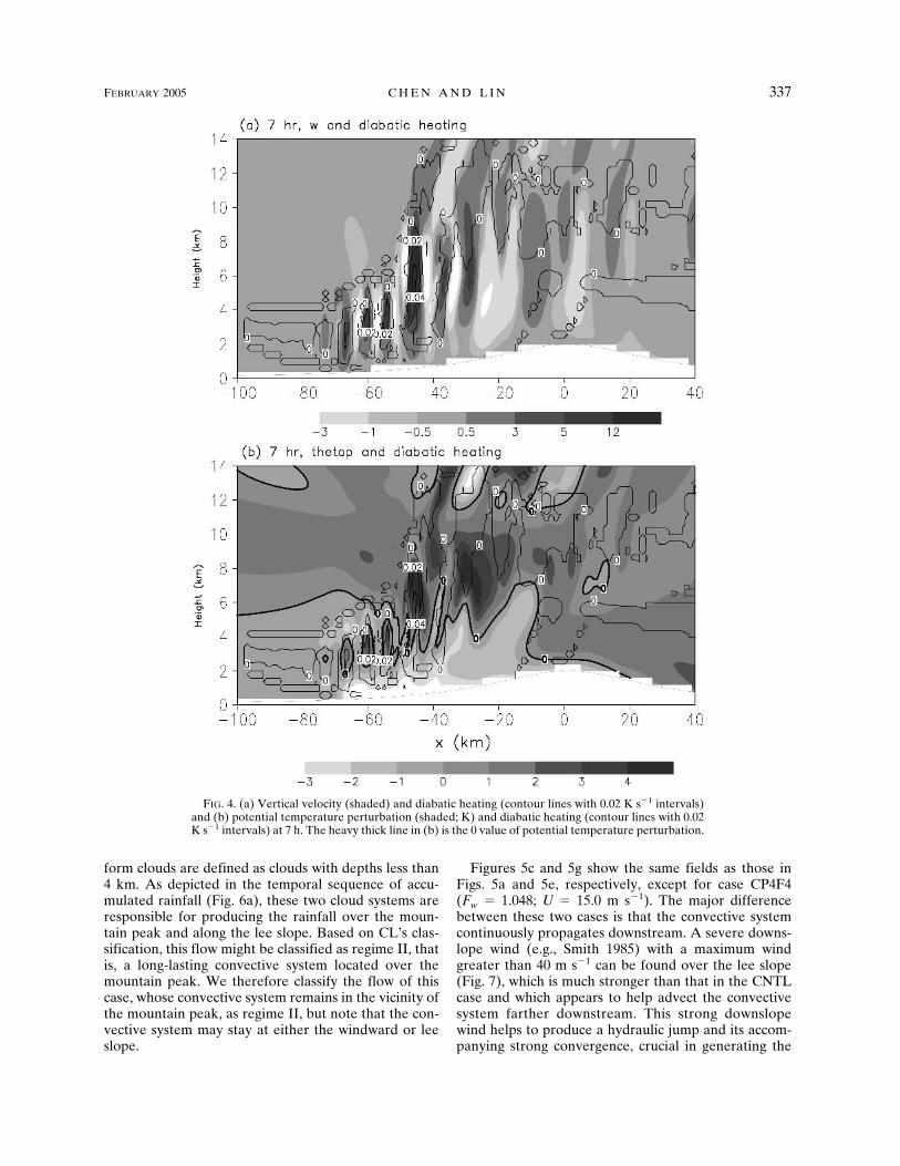
As shown in Fig. 2a, the air is warmed by either thelatent heat generated by the upward motion inside thedeep convective cells or by adiabatic warming associ-ated with the weak, compensated downward motionbetween the deep convective cells. Due to the subsi-dence warming, the diabatic heating coincides betterwith the vertical velocity (Fig. 4a) than with potentialtemperature perturbation (Fig. 4b). It appears that twoconvective cell modes exist during the simulation,

TABLE 1. Flow parameters of the CAPE, basic wind (U), the equivalent vertical velocity (Wmax), the unsaturated moist Brunt–Väisäläfrequency (Nw), and the unsaturated moist Froude number (Fw) for some cases and their associated flow regimes. Wmax � �2CAPE,Nw � (g/��)��/�z, Fw � U/(Nwh), and h � 2 km in all cases except h � 1 km in CP4F6. Cases are named as follows: CP0, CP1, CP2,CP3, CP4, and CP5 mean CAPE � 487, 1372, 1895, 2438, 3000, and 3578 J kg�1, respectively; F1, F2, F3, F4, F5, and F6 mean Fw �0.131, 0.262, 0.524, 0.786, 1.048, and 1.572, respectively.

CAPE(J kg�1)

U(m s�1)

Wmax(m s�1)

Nw

(s�1) Fw Regime

CNTL (CP4F2) 3000 5 77.5 9.54 � 10�3 0.262 ICP4F1 3000 2.5 77.5 9.54 � 10�3 0.131 ICP4F3 3000 10 77.5 9.54 � 10�3 0.524 IICP4F4 3000 15 77.5 9.54 � 10�3 0.786 IIICP4F5 3000 20 77.5 9.54 � 10�3 1.048 IVCP4F6 3000 30 77.5 9.54 � 10�3 1.572 IVCP0F2 487 5 31.2 1.01 � 10�2 0.250 IVCP1F2 1372 5 52.4 9.75 � 10�3 0.256 IICP2F2 1895 5 61.6 9.69 � 10�3 0.258 IICP3F2 2438 5 69.8 9.62 � 10�3 0.260 IICP5F2 3578 5 84.6 9.42 � 10�3 0.265 I


namely, a growing mode and a propagating mode asclassified by Lin et al. (1998) for convective cells em-bedded in a multicell storm. The growing mode (Fig. 4)may also be called a forced mode, which is producedmainly by the latent heating associated with the micro-physical processes of the convective cells, while thepropagating mode behaves like a free gravity wave. Thepropagating mode proposed by Lin et al. (1998) is simi-lar to the trapped gravity mode (developed at a later

stage) in Yang and Houze (1995). The vertical velocityand diabatic heating are in phase with the growingmode, as also assumed in the linear theory developed inYang and Houze (1995). In the present case, after t �7 h, six convective cells located at x � �72, �69, �61,�56, �48, and �38 km (Fig. 4a) may be classified asgrowing or forced modes. Note that the adiabaticwarming associated with subsidence is much weakerthan the warming produced by latent heating associated

FIG. 2. Case CNTL: vertical cross section of the vertical velocity (in m s�1; shaded) and potentialtemperature (solid lines) produced by a uniform, conditionally unstable flow over a two-dimensionalmountain ridge with the mountain peak of 2 km, half-width of 30 km, and basic flow of 5 m s�1. Theunsaturated moist Froude number (Fw) is 0.262. The flow fields are shown at (a) 3 and (b) 7 h. Thecontour interval for potential temperature is 7 K. The cloud boundary is denoted by the thick dottedcurve for total water content greater than 0.0005 g kg�1.


with the convective updrafts. On the other hand, con-vective cells located at (x, z) � (�7 km, 9 km) in Fig. 2aand at (x, z) � (�38 km, 8 km) in Fig. 2b possess quitedifferent characteristics from the convectively forcedmodes (e.g., Lin et al. 1998). Upon closer inspection,one can see that this convective cell has a phase differ-ence between the vertical velocity and potential tem-perature perturbation. More specifically, the updraft islocated 1/4 wavelength behind the maximum tempera-ture perturbation. This relationship is explained by ba-sic linear gravity wave theory (see Lin et al. 1998; Yangand Houze 1995).

In the lower layer near the surface (Fig. 4b), a deepcold pool extending approximately to x � �70 km is

produced by evaporative cooling associated with rain-fall along the windward slope of the mountain. Thecold pool develops into a density current, which pro-pagates against the basic wind. The dynamics associ-ated with the force balance between the cold pool andthe uniform basic wind is controlled by the parameter,U/(Qld)1/3, where Q is the buoyancy depletion orevaporative cooling rate (in K s�1) and l and d are thehorizontal scale and vertical depth of the cooling region(Thorpe et al. 1980). Apparently, the present case be-longs to the subcritical flow regime with respect to theoutflow (i.e., the cold pool); thus a density current canform and propagate upstream against the basic flow. Infact, by comparing the flow fields in Figs. 2a and 2bmore carefully, one can see that in addition to the up-stream propagation of the density current, there areupstream-propagating gravity waves generated by theconvective system, such as the convective cell centeredat (x, z) � (�7 km, 9 km) in Fig. 2a and the one cen-tered at (x, z) � (�38 km, 8 km) in Fig. 2b. Dynami-cally, this flow belongs to a regime subcritical to bothoutflow and gravity waves (Raymond and Rotunno1989; Lin et al. 1993) since both features are able topropagate upstream against the basic wind. Note thatthe propagation of internal gravity waves is controlledby the nondimensional parameter, �U/Nd (Raymondand Rotunno 1989), where N is Brunt–Väisälä fre-quency and d the depth of the prescribed cooling layer.This type of flow is consistent with Fig. 14a in Lin et al.(1993).

Effects of Fw on the moist flow regimes and the re-gime transition may be investigated systematically byvarying Fw, similar to that carried out in CL. The varia-tion of Fw is performed by varying the basic wind ve-locities from 2.5 to 30 m s�1 (for CP4FX cases), whichgives Fw � 0.131 to 1.572. Figure 5 shows the verticalvelocity and potential temperature at 7 h for casesCP4F1, CP4F3, CP4F4, and CP4F6 and the correspond-ing time evolutions of the vertical velocity at 3.6-kmheight and accumulated rainfall. Case CP4F1 (Figs. 5aand 5e) is similar to the CNTL (CP4F2) case exceptwith Fw � 0.131 (U � 2.5 m s�1). As in the CNTL case,in addition to a slowly moving convective system atearlier times over the mountain peak, there is an up-stream-propagating convective system after t � 3 h.Apparently, this flow belongs to regime I, as in theCNTL case. After t � 7 h, the system starts to weakenrapidly (Fig. 3a) and keeps propagating upstream. Fig-ures 5b and 5f show the same fields as those in Figs. 5aand 5e, respectively, except for case CP4F3 (Fw �0.524; U � 10.0 m s�1). A long-lasting convective sys-tem remains on the lee side near the mountain peakduring the simulation period, and the maximum rainfallis located on the lee slope in the region between x � 50km and x � 100 km. Near the top of the windward slopethere exists another mixed type of cloud system (tran-sition between convective and stratiform) during theentire simulation period. Following Stein (2004), strati-

FIG. 3. Case CNTL: (a) Time evolution of the vertical velocityat 3.6-km height (contour lines are shown at �3, –1, 1, and 3 ms�1) and accumulated rainfall and (b) an enlarged figure of (a)around x � 0 km. Rainfall greater than 0.1 mm is shaded. Dottedlines indicate elevation (200, 1000, and 1800 m) where the moun-tain peak is at x � 0 km.


form clouds are defined as clouds with depths less than4 km. As depicted in the temporal sequence of accu-mulated rainfall (Fig. 6a), these two cloud systems areresponsible for producing the rainfall over the moun-tain peak and along the lee slope. Based on CL’s clas-sification, this flow might be classified as regime II, thatis, a long-lasting convective system located over themountain peak. We therefore classify the flow of thiscase, whose convective system remains in the vicinity ofthe mountain peak, as regime II, but note that the con-vective system may stay at either the windward or leeslope.

Figures 5c and 5g show the same fields as those inFigs. 5a and 5e, respectively, except for case CP4F4(Fw � 1.048; U � 15.0 m s�1). The major differencebetween these two cases is that the convective systemcontinuously propagates downstream. A severe downs-lope wind (e.g., Smith 1985) with a maximum windgreater than 40 m s�1 can be found over the lee slope(Fig. 7), which is much stronger than that in the CNTLcase and which appears to help advect the convectivesystem farther downstream. This strong downslopewind helps to produce a hydraulic jump and its accom-panying strong convergence, crucial in generating the

FIG. 4. (a) Vertical velocity (shaded) and diabatic heating (contour lines with 0.02 K s�1 intervals)and (b) potential temperature perturbation (shaded; K) and diabatic heating (contour lines with 0.02K s�1 intervals) at 7 h. The heavy thick line in (b) is the 0 value of potential temperature perturbation.


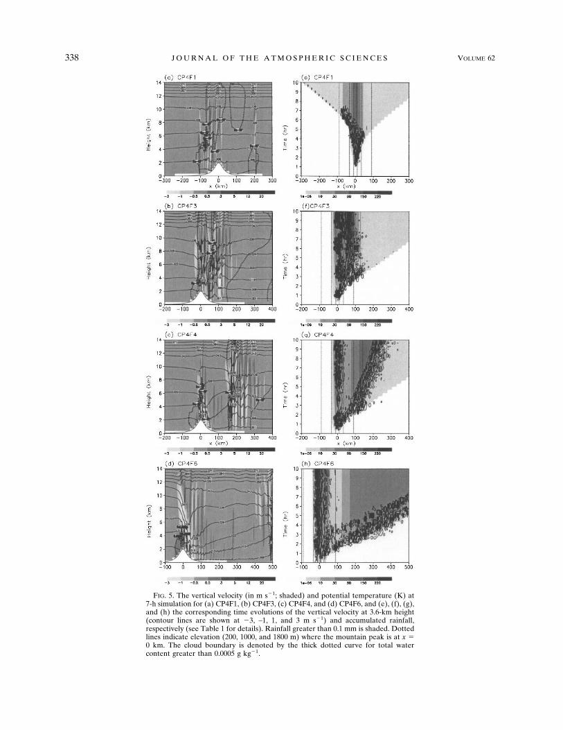
FIG. 5. The vertical velocity (in m s�1; shaded) and potential temperature (K) at7-h simulation for (a) CP4F1, (b) CP4F3, (c) CP4F4, and (d) CP4F6, and (e), (f), (g),and (h) the corresponding time evolutions of the vertical velocity at 3.6-km height(contour lines are shown at �3, –1, 1, and 3 m s�1) and accumulated rainfall,respectively (see Table 1 for details). Rainfall greater than 0.1 mm is shaded. Dottedlines indicate elevation (200, 1000, and 1800 m) where the mountain peak is at x �0 km. The cloud boundary is denoted by the thick dotted curve for total watercontent greater than 0.0005 g kg�1.


downstream-propagating convective system along itsfront edge. From the temporal sequence of accumu-lated rainfall (Fig. 6b), one can clearly see that a long-lasting convective system, which is a mixed type of cloudsystem (transition between convective and stratiform),remains close to the top of the mountain during thesimulation in addition to a convective system whichpropagates downstream. This flow belongs to regime III.

The setting of case CP4F6 (Figs. 5d and 5h) is similarto that of CP4F4 but with a larger unsaturated moistFroude number (Fw � 1.572; U � 30 m s�1). The flowcharacteristics in this case are different from those inCP4F4 during the simulation period. In this case(CP4F6), the updraft over the mountain peak is tiltedupstream, and only straiform-type clouds exist. How-ever, in CP4F4 (regime III), the orographic cloud is amixed type (transition between convective and strati-form), and the updraft is deeper and more erect (thiscan also be seen from the potential temperature field

above the mountain peak). Therefore, CP4F6 is catego-rized as a new flow regime, that is, regime IV.

One may raise the following question: why is an oro-graphic stratiform cloud, instead of a convective type(e.g., CP4F3), formed over the mountain in CP4F6?Whether convective or stratiform types of cloud areformed may be determined by the advection time andthe cloud growth time. The advection time can be esti-mated by a/U, where a is the mountain half-width. Thecloud growth time is controlled by the microphysicalprocesses, which are rather complicated and difficult toestimate (e.g., Jiang and Smith 2003). Assuming thecloud growth time is 20 min (e.g., Stein 2004), the ad-vection time for CP4F6 is about 16 min, which is barelyenough for a deep (convective) cloud to develop. Onthe other hand, the advection time for CP4F3 is about50 min, which is long enough for a convective cloud todevelop. Another relevant time scale is the orographicperturbation growth time. The orographic perturbationgrowth time is related to the strength of the conditionalinstability. Assuming the mountain is high enough tolift the impinging conditionally unstable airstream tothe LFC, then the orographic perturbation growth timeis related to CAPE and may be estimated by clouddepth, and the averaged vertical velocity induced by theconditional instability. Along this line of thinking, wemay roughly estimate the orographic perturbationgrowth time to be (zLNB � zLFC)/Wave, where Wave may

FIG. 6. Spatial distribution of total accumulated rainfall (mm)after 4-h (thin solid line), 6-h (thick solid line), 8-h (thin dashedline), and 10-h (thick dashed line) simulations for (a) CP4F3 and(b) CP4F4. The environmental thermodynamic sounding is thesame as CNTL case.

FIG. 7. Vertical cross section of zonal flow (in m s�1) with abasic flow of 20 m s�1 after a 7-h simulation. The unsaturatedmoist Froude number (Fw) is 0.786 (CP4F4). The contour intervalfor zonal flow is 10 m s�1.


be estimated by half the value of Wmax � �2CAPE. Arough estimate gives the orographic perturbationgrowth time of about 4 min for both CP4F6 and CP4F3,which is apparently short enough for air parcels to pen-etrate to the tropopause but is too short compared withthe cloud growing time for these two cases and is lessrelevant to the cloud development. Thus, in this situa-tion, the cloud type (i.e., convective versus stratiform)will be determined by the advection time and the cloudgrowing time.

Based on Fig. 5, varying Fw tends to produce transi-tion from regime I to II, III, and then to IV. One mightbe able to draw an analogy between the moist flow andthe dry flow regimes by linking the current regime I toblocked dry flow with columnar disturbance, regimes IIand III to breaking dry mountain wave, and regime IVto the quasi-linear dry flow. The downstream-propa-gating convective system in regime III is triggered bythe convergence associated with the hydraulic jump;thus it is linked to the breaking dry mountain wavesince the generation of a hydraulic jump over the leeslope is related to the wave breaking (e.g., see Smith1985). Lin and Wang (1996) presented a series of fig-ures showing the flow regime transition for dry flowover mountains, which may be used for comparison.

Figure 8 shows the spatial distribution of total accu-mulated rainfall after a 10-h simulation with CAPE �3000 J kg�1 and different basic flow velocities. For allcases, there is an area of local maximum rainfall nearthe mountain peak, which is associated with the oro-

graphic lifting. The accumulated rainfall spreads (or theprecipitating system propagates) upstream for casesCP4F1 and CNTL (CP4F2) but downstream for theother cases. The simulated convective system is able toconsistently propagate farther downstream when thebasic flow speed increases.

As found in CL and Chen and Lin (2004), the flowtends to shift to a higher number flow regime as Fw

increases while using the thermodynamic soundingshown in Fig. 1. In addition, we have identified one newflow regime (regime IV). The definition of regime I asproposed by CL has also been modified to include anearly, slowly moving convective system in the vicinity ofthe mountain peak, in addition to the upstream-propagating convective system, which possibly weakensbefore the end of the numerical simulation. Regime II,as proposed by CL, is modified to have a long-lastingconvective system remaining in the vicinity of themountain peak, but the convective system may stay ateither the windward or lee slope.

b. Effects of CAPE

The speed of the density current, which is propor-tional to the strength of the cold pool, can help deter-mine the propagation speed of the convective system.The strength of the evaporative cooling, which is one ofthe major factors in determining the strength of thecold pool, is in turn closely related to the magnitude ofCAPE in a conditionally unstable flow. Therefore, thepropagation of a convective system might be strongly

FIG. 8. Total accumulated rainfall (mm) after 10-h simulation for CP4F1 (thick dotted line),CNTL (CP4F2; thick long-dashed line), CP4F3 (thin dotted line), CP4F4 (thick solid line),CP4F5 (thin solid line), and CP4F6 (thin long-dashed line). The environmental thermody-namic sounding for all cases is the same as the CNTL case, and the CAPE is about 3000 J kg�1.


correlated to the magnitude of CAPE in the atmo-sphere. In addition, CAPE is correlated to the satu-rated moist Froude number by Nm, which might be animportant variable in the second nondimensional con-trol parameter (still unknown at the time of research),as it is derived here. The definition of CAPE in Eq. (1)may also be written as (e.g., see Emanuel 1994)

CAPE � �z1

z2

Bdz, �5�

where B is the buoyancy and z1 and z2 are the LFC andthe LNB, respectively. In cloudy air, the buoyancy isrelated to the saturated Brunt–Väisälä frequency (Nm),which is related to B by N2

m � ��B/�z. Thus, CAPE isrelated to the saturated Brunt–Väisälä frequency by

CAPE � �z1

z2 ��Nm2 dz� dz � �

12

Nm2 �z2

2 � z12�,

�6�

where Nm is the column-averaged saturated Brunt–Väisälä frequency. Note that N2

m � 0 for a staticallyunstable, moist air. Thus, roughly speaking, CAPE isdirectly proportional to |N2

m |. The vertical accelerationof cloudy air is related to the saturated Brunt–Väisäläfrequency by (e.g., Emanuel 1994)

d2� z

dt2 Nm

2 � z � 0, �7�

where the first term is the vertical acceleration of amoist air parcel and �z is the vertical displacement ofthe air parcel from its undisturbed level. Therefore, thelarger the CAPE, the stronger the vertical accelerationand the stronger the convective system. However, it isworth mentioning that the strength of convective sys-tems can also be modified by the orographic forcing.

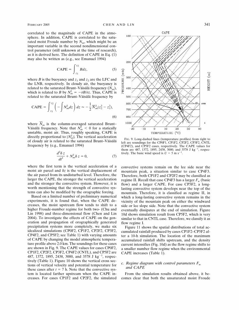
Based on a limited number of preliminary numericalexperiments, it is found that, when the CAPE de-creases, the moist upstream flow tends to shift to ahigher Froude-number regime for both two- (Chu andLin 1998) and three-dimensional flow (Chen and Lin2004). To investigate the effects of CAPE on the gen-eration and propagation of orographically generatedprecipitation systems more completely, we make sixidealized simulations (CP0F2, CP1F2, CP2F2, CP3F2,CP4F2, and CP5F2; see Table 1) with varying amountsof CAPE by changing the model atmospheric tempera-ture profile above 2.0 km. The soundings for these casesare shown in Fig. 9. The CAPE values for cases CP0F2,CP1F2, CP2F2, CP3F2, CP4F2 (CNTL), and CP5F2 are487, 1372, 1895, 2438, 3000, and 3578 J kg�1, respec-tively (Table 1). Figure 10 shows the vertical cross sec-tions of vertical velocity and potential temperature forthese cases after t � 7 h. Note that the convective sys-tem is located farther upstream when the CAPE in-creases. For cases CP1F2 and CP2F2, the simulated

convective systems remain on the lee side near themountain peak, a situation similar to case CP4F3.Therefore, both CP1F2 and CP2F2 may be classified asregime II. Recall that case CP4F3 has a larger Fw (basicflow) and a larger CAPE. For case CP3F2, a long-lasting convective system develops near the top of themountain. Therefore, it is classified as regime II, inwhich a long-lasting convective system remains in thevicinity of the mountain peak on either the windwardside or lee slope side. Note that the convective systemeventually dissipates at the end of simulation. Figure10d shows simulation result from CP5F2, which is verysimilar to that in CNTL case. Therefore, we classify it asflow regime I.

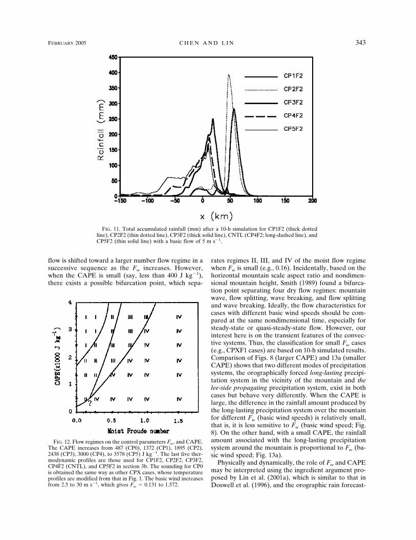
Figure 11 shows the spatial distributions of total ac-cumulated rainfall produced by cases CP1F2–CP5F2 af-ter a 10-h simulation. The location of the maximumaccumulated rainfall shifts upstream, and the densitycurrent intensifies (Fig. 10d) as the flow regime shifts toa smaller number flow regime when the environmentalCAPE increases (Table 1).

c. Regime diagram with control parameters Fwand CAPE

From the simulation results obtained above, it be-comes clear that both the unsaturated moist Froude

FIG. 9. Long-dashed lines (temperature profiles) from right toleft are soundings for the CP0F1, CP1F2, CP2F2, CP3F2, CNTL(CP4F2), and CP5F2 cases, respectively. The CAPE values forthem are 487, 1372, 1895, 2438, 3000, and 3578 J kg�1, respec-tively. The basic wind speed is U � 5 m s�1.


number and CAPE may serve as control parameters forthe classification of flow regimes. However, two impor-tant results may be questioned and they are relateddynamically: 1) The flow tends to shift to a higher num-ber flow regime when the unsaturated moist Froudenumber increases for a given thermodynamic sounding,and 2) the flow regime shifts to a lower number flowregime when the CAPE increases. To address theseissues, we conduct a series of experiments (36 membersin total) and vary two control parameters, Fw and

CAPE, to help determine the two-dimensional flow re-gime diagram. In these experiments, Fw is varied bychanging the basic wind speed from 2.5 to 30 m s�1

(CPXF1–CPXF6). The CAPE varies from 487 to 3578 Jkg�1 for CP0FX –CP5FX.

Based on Fw and CAPE, we have constructed a moistflow regime diagram, presented in Fig. 12, analogous tothe dry flow regime proposed in Smith (1989). From thefigure, we can see that with a relatively large and fixedCAPE (e.g., greater than 1800 J kg�1 in this study), the

FIG. 10. Vertical cross section of the vertical velocity (in m s�1; shaded) and potential temperature (solid lineswith a contour interval of 7 K) for (a) CP1F2, (b) CP2F2, (c) CP3F2, and (d) CP5F2 after 7-h simulation. The basicwind speed is 5 m s�1.


flow is shifted toward a larger number flow regime in asuccessive sequence as the Fw increases. However,when the CAPE is small (say, less than 400 J kg�1),there exists a possible bifurcation point, which sepa-

rates regimes II, III, and IV of the moist flow regimewhen Fw is small (e.g., 0.16). Incidentally, based on thehorizontal mountain scale aspect ratio and nondimen-sional mountain height, Smith (1989) found a bifurca-tion point separating four dry flow regimes: mountainwave, flow splitting, wave breaking, and flow splittingand wave breaking. Ideally, the flow characteristics forcases with different basic wind speeds should be com-pared at the same nondimensional time, especially forsteady-state or quasi-steady-state flow. However, ourinterest here is on the transient features of the convec-tive systems. Thus, the classification for small Fw cases(e.g., CPXF1 cases) are based on 10-h simulated results.Comparison of Figs. 8 (larger CAPE) and 13a (smallerCAPE) shows that two different modes of precipitationsystems, the orographically forced long-lasting precipi-tation system in the vicinity of the mountain and thelee-side propagating precipitation system, exist in bothcases but behave very differently. When the CAPE islarge, the difference in the rainfall amount produced bythe long-lasting precipitation system over the mountainfor different Fw (basic wind speeds) is relatively small,that is, it is less sensitive to Fw (basic wind speed; Fig.8). On the other hand, with a small CAPE, the rainfallamount associated with the long-lasting precipitationsystem around the mountain is proportional to Fw (ba-sic wind speed; Fig. 13a).

Physically and dynamically, the role of Fw and CAPEmay be interpreted using the ingredient argument pro-posed by Lin et al. (2001a), which is similar to that inDoswell et al. (1996), and the orographic rain forecast-

FIG. 12. Flow regimes on the control parameters Fw, and CAPE.The CAPE increases from 487 (CP0), 1372 (CP1), 1895 (CP2),2438 (CP3), 3000 (CP4), to 3578 (CP5) J kg�1. The last five ther-modynamic profiles are those used for CP1F2, CP2F2, CP3F2,CP4F2 (CNTL), and CP5F2 in section 3b. The sounding for CP0is obtained the same way as other CPX cases, whose temperatureprofiles are modified from that in Fig. 1. The basic wind increasesfrom 2.5 to 30 m s�1, which gives Fw � 0.131 to 1.572.

FIG. 11. Total accumulated rainfall (mm) after a 10-h simulation for CP1F2 (thick dottedline), CP2F2 (thin dotted line), CP3F2 (thick solid line), CNTL (CP4F2; long-dashed line), andCP5F2 (thin solid line) with a basic flow of 5 m s�1.


ing models of Alpert (1986) and Smith (2003). The totalprecipitation (P) associated with an orographic precipi-tating system may be estimated as (see, e.g., Lin et al.2001a)

P � ��w� E�woro wenv�qD, �8�

where � is the low-level air density, �w the liquid waterdensity, E the precipitation efficiency, woro the upwardmotion induced by the orography, wenv the upward mo-tion induced by the environment (such as conditionalinstability, convective instability, etc.), q the low-levelmixing ratio of water vapor, and D the duration of the

precipitating system. Roughly, woro may be estimatedby U�h/�x for flow over a two-dimensional mountainridge. For a conditionally unstable airstream, wenv maybe estimated by the idealized equivalent vertical veloc-ity, Wmax, which is roughly equal to �2CAPE. Notethat the relationship between woro and wenv may notnecessarily be linear since the convective systems in-duced by these two types of forcing are highly nonlin-ear and may interact with each other. Additionally,these two values should not be compared quantita-tively but qualitatively since woro (�U�h/�x) is just anestimation of the vertical velocity at the surface, while

FIG. 13. Total accumulated rainfall (mm) after 10-h simulation (a) for CP0F1 (thick dottedline), CP0F2 (thin dotted line), CP0F3 (thick solid line), CP0F4 (thin solid line), and CP0F5(long-dashed line) with CAPE � 487 J kg�1, and (b) for CP0F5 (thick dotted line), CP1F5(thin dotted line), CP2F5 (thick solid line), CP3F5 (thin solid line), CP4F5 (thick long-dashedline), and CP5F5 (thin long-dashed line) with a basic wind speed of 20 m s�1.


wenv (��2CAPE) is an estimation of the maximumvertical velocity inside the convective cell for a condi-tionally unstable flow. It is worth mentioning that thevertical moisture profile in the model atmosphere iskept the same for all cases studied here (only the basicwind speed or temperature profile is changed).

Consider the situation with relatively large CAPE(e.g., Figure 8). In this case, wenv will dominate thevertical motion, but a modest woro may be able to in-duce an orographic convective system associated withthe long-lasting mode in the vicinity of the mountain, aslong as the LFC is reached. Hence, the rainfall amountwill be less sensitive to the magnitude of woro, or ratherthe basic wind speed because the slope steepness (�h/�x) is fixed in this case. On the other hand, for the casewith small CAPE (e.g., Fig. 13a), the vertical velocityinduced by the conditional instability might be rela-tively small, and the orographic rainfall amount will bemore sensitive to the basic wind since woro � U�h/�x.Thus, orographic rainfall amount is roughly propor-tional to the basic wind speed, or Fw, if the mountainslope remains unchanged. Implicitly, this indicates thatconditional instability does not play an important rolein producing orographic rainfall when the basic windspeed is large (Fig. 13b). Therefore, with small CAPEand large basic wind speed, the long-lasting orographicprecipitation system over the mountain belongs to thestratiform type, instead of the convective type, due to theclassical stable accent mechanism (e.g., see reviews bySmith 1979, Houze 1993, and Chu and Lin 2000). Thisis evidenced by the vertical velocity, potential tempera-ture, and shallow cloud fields for the case with U � 20m s�1and CAPE � 1372 J kg�1 (see Fig. 14d). As men-tioned earlier, the stratiform cloud is defined as havinga cloud depth less than 4 km. Under this condition,since the convective precipitation system is dominatedby the orographically induced vertical motion, it shouldreflect the structure of the mountain shape. Here thevertical motion field reveals a hydrostatic mountainwave (Fig. 14d). The-lee-side propagating convective orcloud system is very weak, and therefore this flow re-gime may be referred to as a long-lasting orographicstratiform precipitation system over the mountain andpossibly a downstream-propagating cloud system. Notethat this is a new flow regime (regime IV), which wasnot discussed in CL and Chen and Lin (2004).

From a fundamental physics point of view, one mightbe curious to know why a deep, orographic convectivesystem cannot develop when the basic wind is strongand the environmental CAPE is small. For the CP1F2sounding (Fig. 9), the LFC is located at about 820 hPa,which is about 1.8 km. With a 2-km-high mountain, onewould anticipate that the mountain is high enough tolift most of the low-level air parcels to their LFCs andrelease the instability even though the CAPE is notvery large. Indeed, this is true. If one inspects caseCP1F1, Fw � 0.131 and CAPE � 1372 J kg�1 (Fig. 14b),a deep convective system can be triggered in the vicin-

ity of the mountain under a small CAPE condition.This may be explained as follows: for weak basic flow,such as in CP1F1 (2.5 m s�1), the advection time forairflow to cross the mountain is long enough for a deepcloud to develop over the mountain (Jiang and Smith2003) due to the small CAPE (1372 J kg�1). The kineticenergy (KE) associated with the cold pool produced byevaporative cooling is comparable to the KE associatedwith the weak basic flow. Thus, a quasi-steady, criticalstate is reached and convection is able to develop. Inother words, the flow is critical to the cold-air outflow.On the other hand, for stronger wind and smallerCAPE (Fig. 14d), the deep convective cloud has insuf-ficient time to grow over the mountain (small advectiontime). Since the KE associated with the cold air outflowis much smaller than the KE associated with the basicwind, the precipitating system will be advected down-stream by the basic wind and no strong deep clouds canexist over the mountain area. In other words, the flowis supercritical to the cold-air outflow.

A similar situation also occurs with variation ofCAPE when Fw (basic flow speed) is kept constant.When the basic flow is weak (say, e.g., less than orequal to 5 m s�1 in this study), the flow is shifted to asmaller number flow regime (i.e., the system moves up-stream; see Fig. 11) as the CAPE increases (Fig. 12).This can be interpreted as follows: a stronger system onthe lee side of the mountain can develop when an air-stream has a larger CAPE and a weak basic flow (longadvection time) and, therefore, the cold pool producedby the system is relatively stronger. Thus, under thissituation the convective system on the lee slope is ableto propagate upstream against the basic flow and shiftsthe flow to a smaller number flow regime. This, in away, is analogous to the decrease in Fw (incoming windspeed) for a fixed CAPE.

The above discussions may be depicted by using thevertical velocity, potential temperature, and cloudfields in Fig. 14 and the temporal evolution of accumu-lated rainfall and the vertical velocity at 3.6-km heightin Fig. 15 from four cases (CP1F1, CP5F1, CP1F5, andCP5F5). Based on Figs. 14a and 15a, the flow may beclassified as regime I, which is characterized as a flowwith an upstream-propagating convective system and atransient convective system existing in the vicinity ofthe mountain, which may potentially weaken at latertimes. Using Figs. 14b and 15b, the flow is classified asregime II.

From Figs. 14c and 15c, the flow is classified as re-gime III, which was characterized by a long-lasting oro-graphic precipitation system near the mountain peakand a downstream-propagating convective system(CL). A closer inspection reveals that the long-lastingorographic precipitation system is a mixed stratiformand convective precipitation system (Fig. 14c). Notethat, if the basic wind is weaker, then the long-lastingorographic precipitation system may be a convectivetype (e.g., Figs. 11 and 12 of CL) instead of a mixed


type. In addition, due to the strong wind, an upward-propagating hydrostatic wave is produced, which can beseen clearly in the isentropes (Fig. 14c). From Fig. 15c,one can clearly see that the orographic precipitationsystem redevelops by t � 4 h, after the first convectivesystem is advected downstream by the strong basicwind.

The flow shown in Figs. 14d and 15d was not identi-fied in CL and Chen and Lin (2004); thus it is a new

flow regime as discussed above. This flow regime maybe classified as regime IV and is characterized by along-lasting orographic stratiform precipitation systemand possibly a downstream-propagating cloud system.An upward-propagating hydrostatic mountain waveis produced by the strong basic flow. It is noted that anew downstream-propagating system is triggered atabout 120 km (Fig. 15d) after 1.5-h simulation andstarts generating light rainfall at 170 km after 2.5-h

FIG. 14. Vertical velocity and potential temperature fields for (Fw, CAPE) � (a) (0.131, 3578 J kg�1); (b) (0.131,1372 J kg�1); (c) (1.048, 3578 J kg�1), and (d) (1.048, 1372 J kg�1) after 7-h simulations. The cloud boundary isdenoted by the thick dotted curve for total water content greater than 0.0005 g kg�1.


simulation. This is why there is no rainfall between 70and 180 km.

4. Concluding remarks

Based on idealized simulations of conditionally un-stable flow passing over a two-dimensional mountainridge, we found four moist flow regimes, which may be

characterized as (Fig. 16) 1) regime I: flow with an up-stream-propagating convective system and a transientconvective system existing in the vicinity of the moun-tain at an earlier time; 2) regime II: flow with a long-lasting orographic convective system over the mountainpeak, upslope or downslope; 3) regime III: flow with along-lasting orographic convective or mixed convectiveand stratiform precipitation system over the mountain

FIG. 15. Time evolution of the vertical velocity at 3.6-km height (contour lines are shown at �3, –1, 1, and 3m s�1) and accumulated rainfall for cases shown in Fig. 14. Rainfall greater than 0.1 mm is shaded. Dotted linesindicate elevation (200, 1000, and 1800 m), where the mountain peak is at x � 0 km.


peak and a downstream-propagating convective sys-tem; and 4) regime IV: flow with a long-lasting oro-graphic stratiform precipitation system over the moun-tain and possibly a downstream-propagating cloud sys-tem. Based on idealized simulations with variations inFw and CAPE, a regime diagram is constructed. Thefirst three flow regimes are the same as those found inCL and Chen and Lin (2004), but with modifications.Regime I proposed by CL has been modified to includea convective system in the vicinity of the mountain peakat an earlier time in addition to the upstream-propagating convective system, which may possiblyweaken at later times. In regime II, the long-lasting

convective system may exist over the mountain peak,upslope, or lee slope instead of just over the mountainpeak, as proposed by CL. For regime III, we found thatthe long-lasting orographic precipitation system overthe mountain peak may become a mixed convectiveand stratiform precipitation system instead of just con-vective precipitation system proposed in CL. Note thatthe variation of Fw is carried out by varying U only. Thefourth flow regime is new and was not discussed in CLand Chen and Lin (2004). The long-lasting orographicstratiform precipitation system in regime IV is ex-plained by comparing the small advection time withcloud growing time; in addition, the kinetic energy of

FIG. 16. Schematic of the flow regimes I–IV found in this study. 1) regime I: flow with upstream-propagatingconvective system and a transient convective system existing in the vicinity of the mountain at earlier time; 2)regime II: long-lasting orographic convective system over the mountain peak; 3) regime III: downstream-propagating convective system and long-lasting orographic convective or mixed convective and stratiform precipi-tation system; and 4) regime IV: a long-lasting orographic stratiform precipitation system over the mountain peakand possibly a downstream-propagating cloud system. Here, FD is assumed to be a proxy of CAPE. Symbols C, S,and N denote convective, stratiform, and no cloud types, respectively. Outline (filled) arrow denotes the propa-gation direction of the precipitation system (cold-air outflow).


the basic flow is much larger than that associated withthe cold outflow produced by evaporative cooling; thusthe precipitating system is advected downstream and astrong, deep convective system cannot develop over theupslope.

When the Fw (or basic wind speed) increases and theCAPE is fixed, the flow tends to shift to a higher num-ber of the flow regime. Conversely, when the CAPEincreases and the Fw (i.e., basic wind speed in thisstudy) is fixed, the flow shifts to a lower regime. Whenthe CAPE is large, the orographic rainfall amounts withdifferent basic wind speeds are comparable (i.e., notsensitive to the basic wind speed) but the precipitationtypes can be different (i.e., convective versus strati-form). However, when the CAPE is small, the oro-graphic rainfall amount is strongly dependent on thestrength of the basic wind speed—the stronger thewind, the larger the amount of rainfall. The formationand propagation of different flow regimes may be in-terpreted by the competition between the forcing asso-ciated with the basic flow (Fw) and the forcing associ-ated with the cold outflow or the density current (FD),as shown in Fig. 16. The forcing associated with the coldoutflow, FD, is related to the CAPE. A more preciserelationship between FD and CAPE needs to be ex-plored. The propagation and cloud types (convective,stratiform, or a mixed convective and stratiform) of theprecipitation systems are determined by the time scal-ing (i.e., advection time and cloud growing time) andrelative strength of the basic wind and the cold outflow,which may be represented by CAPE for a conditionallyunstable flow.

In addition to Fw and CAPE, additional parametersmay come into play to influence the moist flow regimesfor a conditionally unstable flow over a mesoscalemountain. For example, the mountain height and widthaspect ratio may serve as an important control param-eter. To make a more complete moist flow regime dia-gram, a more complete coverage of the control param-eters, which includes h/a, should be carried out. We willleave this for future studies. The readers are also re-minded that our moist regime diagram is constructedbased on reasonably long time simulated results, butnot necessarily for steady or quasi-steady solutions.Longer time simulations, such as 20 h, for small Fw

cases (e.g., CPXF1 cases) are also tested and the flowbehavior is very similar to those for 10-h simulations (aspresented) except for the CP5F1 case (Fw � 0.131 andCAPE � 3578 J kg�1). In case CP5F1, a convectivesystem redevelops near the peak of the mountain aftera 13-h simulation and stays there until the end of thesimulation. Thus, the moist flow regimes proposed inthis study are based on transient, instead of quasi-steady state, numerical solutions. We have also testedthe sensitivity of the moist flow to the initial orographysetup by activating the microphysics processes after 10h for some cases (CP2F1, CP0F2, and CP4F3). Thereexist some differences between these cases (20-h simu-

lations) and their counterpart experiments (e.g., cloudstrength and cloud lifetime) that activate microphysicsat t � 0 h. However, since we are interested in thetransient moist flow regimes, our regime classificationsfor these new cases are still valid. Physically, this maybe equivalent to a sudden increase of the environmen-tal wind, such as the passage of a trough over the Alpsin fall.

Acknowledgments. This work is supported by USNSF Grant ATM-0096876. The authors would like toacknowledge the WRF model development team fortheir efforts in developing this model. Comments byDr. R. P. Weglarz in the Department of Physics, As-tronomy, and Meteorology at Western ConnecticutState University are greatly appreciated. We would alsolike to thank Heather Reeves and James Thurman forproofreading the manuscript.

REFERENCES

Alpert, P., 1986: Mesoscale indexing of the distribution of oro-graphic precipitation over high mountains. J. Climate Appl.Meteor., 25, 532–545.

Binder, P., and C. Schär, Eds., 1996: MAP design proposal. Me-teoSwiss, 75 pp. [Available from the MAP Programme Of-fice, MeteoSwiss, CH-8044, Zurich, Switzerland.]

Bougeault, P., and Coauthors, 2001: The MAP special observingperiod. Bull. Amer. Meteor. Soc., 82, 433–462.

Chen, S.-H., and J. Dudhia, 2000: Annual report: WRF physics.Air Force Weather Agency, 38 pp. [Available online at http://wrf-model.org.]

——, and W.-Y. Sun, 2002: A one-dimensional time-dependentcloud model. J. Meteor. Soc. Japan, 80, 99–118.

——, and Y.-L. Lin, 2004: Orographic effects on a conditionallyunstable flow over an idealized three-dimensional mesoscalemountain. Meteor. Atmos. Phys., in press.

Chu, C.-M., and Y.-L. Lin, 1998: Effects of orography on thegeneration and propagation of mesoscale convective systems.Preprints, Eighth Conf. on Mountain Meteorology, Flagstaff,AZ, Amer. Meteor. Soc., 302–309.

——, and ——, 2000: Effects of orography on the generation andpropagation of mesoscale convective systems in a two-dimensional conditionally unstable flow. J. Atmos. Sci., 57,3817–3837.

Doswell, C. A., III, H. Brooks, and R. Maddox, 1996: Flash floodforecasting: An ingredient-based methodology. Wea. Fore-casting, 11, 560–581.

Emanuel, K. A., 1994: Atmospheric Convection. Oxford Univer-sity Press, 580 pp.

Houze, R. A., Jr., 1993: Cloud Dynamics. Academic Press, 573 pp.Jiang, Q., and R. B. Smith, 2003: Cloud timescales and orographic

precipitation. J. Atmos. Sci., 60, 1543–1559.Lin, Y.-L., and T. A. Wang, 1996: Flow regimes and transient

dynamics of two-dimensional stratified flow over an isolatedmountain ridge. J. Atmos. Sci., 53, 139–158.

——, R. D. Farley, and H. D. Orville, 1983: Bulk parameterizationof the snow field in a cloud model. J. Climate Appl. Meteor.,22, 1065–1092.

——, T.-A. Wang, and R. P. Weglarz, 1993: Interaction betweengravity waves and cold air outflows in a stably stratified uni-form flow. J. Atmos. Sci., 50, 3790–3816.

——, R. L. Deal, and M. S. Kulie, 1998: Mechanisms of cell re-generation, development, and propagation within a two-dimensional multicell storm. J. Atmos. Sci., 55, 1867–1886.

——, S. Chiao, T.-A. Wang, M. L. Kaplan, and R. P. Weglarz,


2001a: Some common ingredients for heavy orographic rain-fall. Wea. Forecasting, 16, 633–660.

——, J. A. Thurman, and S. Chiao, 2001b: Influence of synopticand mesoscale environments on heavy orographic rainfall as-sociated with MAP IOP2B and IOP8. MAP Newsletter, No.15, 72–75. [Available online at http://www.map.ethz.ch/newsletter15.htm.]

Michalakes, J., S.-H. Chen, J. Dudhia, L. Hart, J. Klemp, J.Middlecoff, and W. Skamarock, 2001: Development of a nextgeneration regional weather research and forecast model.Developments in Teracomputing: Proceedings of the NinthECMWF Workshop on the Use of High Performance Com-puting in Meteorology, W. Zwieflhofer and N. Kreitz, Eds.,World Scientific, 269–276.

Miglietta, M. M., and A. Buzzi, 2001: A numerical study of moiststratified flows over isolated topography. Tellus, 53A, 481–499.

Raymond, D. J., and R. Rotunno, 1989: Responses of a stablystratified flow to cooling. J. Atmos. Sci., 46, 2830–2837.

Rotunno, R., and R. Ferretti, 2001: Mechanisms of intense Alpinerainfall. J. Atmos. Sci., 58, 1732–1749.

Rutledge, S. A., and P. V. Hobbs, 1984: The mesoscale and mi-croscale structure and organization of clouds and precipita-tion in midlatitude cyclones. XII: A diagnostic modelingstudy of precipitation development in narrow cloud-frontalrainbands. J. Atmos. Sci., 41, 2949–2972.

Schlesinger, R. E., 1978: A three-dimensional numerical model ofan isolated thunderstorm: Part I. Comparative experimentsfor variable ambient wind shear. J. Atmos. Sci., 35, 690–713.

Schneidereit, M., and C. Schär, 2000: Idealised numerical experi-ments of Alpine flow regimes and southside precipitationevents. Meteor. Atmos. Phys., 72, 233–250.

Skamarock, W. C., J. B. Klemp, and J. Dudhia, 2001: Prototypesfor the WRF (Weather Research and Forecast) model. Pre-prints, Ninth Conf. on Mesoscale Processes, Fort Lauderdale,FL, Amer. Meteor. Soc., J11–J15.

Smith, R. B., 1979: The influence of mountains on the atmo-sphere. Advances in Geophysics, Vol. 21, Academic Press,87–230.

——, 1985: On severe downslope winds. J. Atmos. Sci., 42, 2597–2603.

——, 1989: Hydrostatic airflow over mountains. Advances in Geo-physics, Vol. 31, Academic Press, 1–41.

——, 2003: A linear upslope-time-delay model for orographic pre-cipitation. J. Hydrol., 282, 2–9.

Stein, J., 2004: Exploration of some convective regimes over theAlpine orography. Quart. J. Roy. Meteor. Soc., 130, 481–502.

Thorpe, A., M. J. Miller, and M. W. Moncrieff, 1980: Dynamicalmodels of two-dimensional downdraughts. Quart. J. Roy. Me-teor. Soc., 106, 463–484.

Wicker, L. J., and W. C. Skamarock, 2002: Time-splitting methodsfor elastic models using forward time schemes. Mon. Wea.Rev., 130, 2088–2097.

Yang, M.-J., and R. A. Houze Jr., 1995: Multicell squall line struc-ture as a manifestation of vertically trapped gravity waves.Mon. Wea. Rev., 123, 641–660.


effects of moist froude number and cape on a conditionally

Documents