LEI Wageningen UR is one of the world’s leading independent socio-economic research institutes. LEI’s unique data, models and knowledge offer clients insight and integrated advice on policy and decision-making in an innovative manner, and ultimately contribute to a more sustainable world. LEI is part of Wageningen UR (University and Research centre), forming the Social Sciences Group together with the Department of Social Sciences and Wageningen UR Centre for Development Innovation.

The mission of Wageningen UR (University & Research centre) is ‘To explore the potential of nature to improve the quality of life’. Within Wageningen UR, nine specialised research institutes of the DLO Foundation have joined forces with Wageningen University to help answer the most important questions in the domain of healthy food and living environment. With approximately 30 locations, 6,000 members of staff and 9,000 students, Wageningen UR is one of the leading organisations in its domain worldwide. The integral approach to problems and the cooperation between the various disciplines are at the heart of the unique Wageningen Approach.

LEI Wageningen URP.O. Box 297032502 LS Den HaagThe NetherlandsE publicatie.lei@wur.nlwww.wageningenUR.nl/lei

REPORT LEI 2015-145ISBN 978-90-8615-726-6

Hans van Oostenbrugge, Diana Slijkerman, Katell Hamon, Oscar Bos, Marcel Machiels, Olga van de Valk, Niels Hintzen, Ernst Bos, Jan Tjalling van der Wal and Joop Coolen

A Cost Benefit Analysis

Effects of seabed protection on the Frisian Front and Central Oyster Grounds

Effects of seabed protection on the Frisian Front and Central Oyster Grounds

A Cost Benefit Analysis

Hans van Oostenbrugge1, Diana Slijkerman2, Katell Hamon1, Oscar Bos2, Marcel Machiels2, Olga van de Valk1,

Niels Hintzen2, Ernst Bos1, Jan Tjalling van der Wal2 and Joop Coolen2

1 LEI Wageningen UR

2 IMARES Wageningen UR

This study was carried out by LEI Wageningen UR in cooperation with IMARES and was commissioned and

financed by the Dutch Ministry of Infrastructure and the Environment.

LEI Wageningen UR

Wageningen, December 2015

REPORT

LEI 2015-145

ISBN 978-90-8615-726-6

Van Oostenbrugge, Hans, Diana Slijkerman, Katell Hamon, Oscar Bos, Niels Hintzen, Ernst Bos,

Jan Tjalling van der Wal and Joop Coolen, 2015. Effects of seabed protection on the Frisian Front and

Central Oyster Grounds; A Cost Benefit Analysis. Wageningen, LEI Wageningen UR (University &

Research centre), LEI Report 2015-145. 168 pp.; 41 fig.; 37 tab.; 74 ref.

This report provides an overview of the important benefits and costs for six variant closures for the

protection of the benthic ecosystem on the Frisian Front and the Central Oyster Grounds. The

proposed closures lead to a range of ecological benefits and economic costs. The current study

facilitates an informed discussion about an optimal allocation of the closures.

Dit rapport geeft een overzicht van de belangrijke kosten en baten voor zes varianten voor

gebiedssluitingen voor de bescherming van het benthische ecosysteem op het Friese Front en de

Centrale Oestergronden. De voorgestelde afsluitingen leiden tot een reeks ecologische baten en

economische kosten. De huidige studie faciliteert daarmee een geïnformeerde discussie over een

optimale allocatie van deze afsluitingen.

Key words: Cost Benefit Analysis, Fisheries

This report can be downloaded for free at the E-depot http://edepot.wur.nl or at

www.wageningenUR.nl/en/lei (under LEI publications).

© 2015 LEI Wageningen UR

P.O. Box 29703, 2502 LS The Hague, The Netherlands, T +31 (0)70 335 83 30,

E informatie.lei@wur.nl, www.wageningenUR.nl/en/lei. LEI is part of Wageningen UR (University &

Research centre).

For its reports, LEI utilises a Creative Commons Attributions 3.0 Netherlands license.

© LEI, part of DLO Foundation, 2015

The user may reproduce, distribute and share this work and make derivative works from it. Material

by third parties which is used in the work and which are subject to intellectual property rights may not

be used without prior permission from the relevant third party. The user must attribute the work by

stating the name indicated by the author or licensor but may not do this in such a way as to create the

impression that the author/licensor endorses the use of the work or the work of the user. The user

may not use the work for commercial purposes.

LEI accepts no liability for any damage resulting from the use of the results of this study or the

application of the advice contained in it.

LEI is ISO 9001:2008 certified.

LEI 2015-145 | Project code 2282600085

Cover photo: Shutterstock

Contents

Preface 7

Summary 8

S.1 Key findings 8 S.2 Complementary results 11 S.3 Method 12

Samenvatting 13

S.1 Belangrijkste uitkomsten 13 S.2 Overige uitkomsten 16 S.3 Methode 17

1 Introduction 18

2 Application of Cost Benefit Analysis to closed areas 21

3 Variants 25

4 Ecological benefits 28

4.1 Methodology 28 4.1.1 Ecological cost and benefits and the ecosystem approach 28 4.1.2 Introduction to the ecopoint valuation method 29 4.1.3 Adapted ecopoint valuation for the Frisian Front and Central

Oyster Grounds 30 4.2 Methodology 31

4.2.1 Step 1: Area quantity 31 4.2.2 Step 2: Area quality indicators 31 4.2.3 Step 3 Weighting factors 33 4.2.4 Step 4 Calculation of ecopoints 40 4.2.5 Step 5 Test of the robustness/sensitivity of the analysis 40

4.3 Results Ecopoints 41 4.3.1 Step 1. Area quantity 41 4.3.2 Step 2. Area quality indicators 41 4.3.3 Step 3. Weighting factors 44 4.3.4 Step 4. Ecopoints 46 4.3.5 Step 5. Test of robustness/sensitivity 50

4.4 Ecosystem development: Qualitative description 50 4.4.1 Quality indicators: limited benthos approach 50 4.4.2 Artificial hard substrata as proxy for biodiversity 51 4.4.3 Baseline descriptions and ecosystem development after measures are

implemented 52 4.4.4 Generic effects of displacement on ecology 54 4.4.5 Ecosystem services and ecosystem valuation 56

4.5 Discussion and conclusions 57 4.5.1 Summary of ecopoint scores 57 4.5.2 Ranking the variants on ecopoint scores 58 4.5.3 Scaling of quality indicators 60 4.5.4 Sensitivity and robustness 60

5 Fishing activities in the areas 61

5.1 Methodology 61 5.1.1 Fishing activities of Dutch vessels 61 5.1.2 Fishing activities of foreign vessels 63

5.2 Data 64 5.2.1 Fishing activities of Dutch vessels 64 5.2.2 Fishing activities of Foreign vessels 64

5.3 Results 64 5.3.1 Value for Dutch fishing vessels 64 5.3.2 Fishing activities foreign vessels 72

5.4 Discussion 75 5.4.1 Fishing activities Dutch vessels 75 5.4.2 Fishing activities foreign vessels 76

6 Costs for Dutch fisheries 78

6.1 Methodology 78 6.1.1 Scenarios for policy, economy and innovation 78 6.1.2 Displacement scenarios 82 6.1.3 Calculation of net present value 87 6.1.4 Sensitivity analysis 88

6.2 Results 88 6.2.1 Fishing activities in Policy, Economy and Innovation scenarios 89 6.2.2 Displacement costs 92 6.2.3 Sensitivity analysis 101

6.3 Discussion 105

7 Social effects on fisheries and their communities 106

7.1 Methodology 106 7.2 Results 107 7.3 Discussion and conclusions 110

8 Effects on enforcement and monitoring 112

8.1 Methodology 112 8.2 Results 112

8.2.1 Control 112 8.2.2 Monitoring 114

8.3 Discussion 115

9 Synthesis 116

References and websites 125

Glossary 129 Appendix 1

Biodiversity maps 130 Appendix 2

Availability of ecological data 137 Appendix 3

Ecopoint calculations per subarea 138 Appendix 4

Data sources for direct economic effects on fishing sector 144 Appendix 5

Gear Codes 145 Appendix 6

Characteristics of the Dutch activities in the sub-areas of all Appendix 7

variants 146

Seasonal patterns of landings value for various gears 148 Appendix 8

Classification fishing harbours for stress analysis 152 Appendix 9

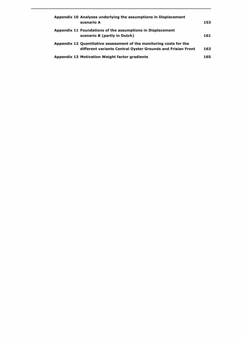
Analyses underlying the assumptions in Displacement Appendix 10

scenario A 153

Foundations of the assumptions in Displacement Appendix 11

scenario B (partly in Dutch) 161

Quantitative assessment of the monitoring costs for the Appendix 12

different variants Central Oyster Grounds and Frisian Front 163

Motivation Weight factor gradients 165 Appendix 13

LEI Report 2015-145 | 7

Preface

This report gives an overview of the potential benefits and costs of six variants for fishery closures on

the Frisian Front and the Central Oyster Grounds within the framework of a Cost Benefit Analysis. The

effects of fisheries closures on both the ecology and the fishing sector have been widely discussed but

a lot remains unknown, especially when comparing specific closures as is done here. The authors have

been working on the cutting edge of science, combining scientific knowledge with new analyses and

assumptions made on expert knowledge and stakeholder information. The results do not provide a

clear choice for policy makers, but facilitate the discussion on preferences and possible compromises

between stakeholders and managers. In this discussion the present study shows the most recent

knowhow on the costs and benefits of the different variants. The methods and outcomes have been

intensely discussed during the process and many persons and institutions have given valuable

contributions. Most importantly the authors want to thank the representatives of the Dutch fisheries

and the NGOs for their comments, discussions and time spent during the various stakeholder events.

Moreover we want to thank the NVWA and the Ministry of I&M for their information on control and

monitoring costs. The colleagues from sister fisheries institutes in Denmark (DTU-aqua), Germany

(Von Thünen), Belgium (ILVO) and the UK (CEFAS) are thanked for their contribution on the effort

estimates for the foreign fleets.

Prof.dr.ir. Jack G.A.J. van der Vorst

General Director Social Sciences Group - Wageningen UR

8 | LEI Report 2015-145

Summary

S.1 Key findings

The various proposed closures for protection of the benthic communities of the Frisian Front

and the Central Oyster grounds (Figure S.1) lead to a range of ecological benefits and

economic costs (Table S.1). The current study provides an overview of benefits and costs

and therewith facilitates an informed discussion about an optimal allocation of the closures.

Figure S.1 Maps of different variants taken into consideration

Source: Ministry of I&M, processed by LEI.

LEI R

eport 2

015-1

45 | 9

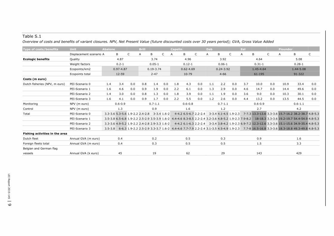
Table S.1

Overview of costs and benefits of variant closures. NPV, Net Present Value (future discounted costs over 30 years period); GVA, Gross Value Added

Type of costs/benefits Unit Abalone

Brill

Capelin

Dab

Eel

Flounder

Displacement scenario A B C A B C A B C A B C A B C A B C

Ecologic benefits Quality 4.87 3.74 4.96 3.92 4.64 5.08

Weight factors 0.2-1 0.05-1 0.12-1 0.06-1 0.31-1 0.28-1

Ecopoints/km2 0.97-4.87 0.19-3.74 0.62-4.69 0.24-3.92 1.45-4.64 1.44-5.08

Ecopoints total 12-59 2-47 10-79 4-66 61-195 91-322

Costs (m euro)

Dutch fisheries (NPV, m euro) PEI-Scenario 0 1.4 3.4 0.0 0.8 1.4 0.0 1.8 4.3 0.0 1.1 2.2 0.0 3.7 10.0 0.0 10.9 33.4 0.0

PEI-Scenario 1 1.6 4.6 0.0 0.9 1.9 0.0 2.2 6.1 0.0 1.3 2.9 0.0 4.6 14.7 0.0 14.4 49.6 0.0

PEI-Scenario 2 1.4 3.0 0.0 0.8 1.3 0.0 1.8 3.9 0.0 1.1 1.9 0.0 3.6 9.0 0.0 10.3 30.1 0.0

PEI-Scenario 3 1.6 4.1 0.0 0.9 1.7 0.0 2.2 5.5 0.0 1.2 2.6 0.0 4.4 13.2 0.0 13.5 44.5 0.0

Monitoring NPV (m euro) 0.6-0.9 0.7-1.1 0.6-0.8 0.7-1.1 0.6-0.9 0.6-1.1

Control NPV (m euro) 1.3 0.9 1.6 1.2 2.7 4.2

Total PEI-Scenario 0 3.3-3.6 5.3-5.6 1.9-2.2 2.4-2.8 3-3.4 1.6-2 4-4.2 6.5-6.7 2.2-2.4 3-3.4 4.1-4.5 1.9-2.3 7-7.3 13.3-13.6 3.3-3.6 15.7-16.2 38.2-38.7 4.8-5.3

PEI-Scenario 1 3.5-3.8 6.5-6.8 1.9-2.2 2.5-2.9 3.5-3.9 1.6-2 4.4-4.6 8.3-8.5 2.2-2.4 3.2-3.6 4.8-5.2 1.9-2.3 7.9-8.2 18-18.3 3.3-3.6 19.2-19.7 54.4-54.9 4.8-5.3

PEI-Scenario 2 3.3-3.6 4.9-5.2 1.9-2.2 2.4-2.8 2.9-3.3 1.6-2 4-4.2 6.1-6.3 2.2-2.4 3-3.4 3.8-4.2 1.9-2.3 6.9-7.2 12.3-12.6 3.3-3.6 15.1-15.6 34.9-35.4 4.8-5.3

PEI-Scenario 3 3.5-3.8 6-6.3 1.9-2.2 2.5-2.9 3.3-3.7 1.6-2 4.4-4.6 7.7-7.9 2.2-2.4 3.1-3.5 4.5-4.9 1.9-2.3 7.7-8 16.5-16.8 3.3-3.6 18.3-18.8 49.3-49.8 4.8-5.3

Fishing activities in the area

Dutch fleet Annual GVA (m euro) 0.4 0.2 0.5 0.3 0.9 1.6

Foreign fleets total Annual GVA (m euro) 0.4 0.3 0.5 0.5 1.5 3.3

Belgian and German flag

vessels Annual GVA (k euro) 45 19 62 29 143 429

10 | LEI Report 2015-145

From the compiled overview of costs and benefits (Table S.1) the variants (named after fish) can be

characterised as follows:

Abalone

The total area is 1,204 km2 and comprises two subareas. Together with Brill this is the smallest

variant, and represents the lower boundary of the government objective for the closing of areas for

seabed protection. The costs for the Dutch fishery related to this variant are low to intermediate and

the costs for control are relatively low. The ecologic benefits depend on the expression of ecopoints

and the weighting factors applied. Abalone results in the upper range when ecopoints are expressed

per km2, which depends on the weighting factor applied. Using the weighting factor ‘hard substrate’

results in a lowest score among all variants; applying weighting factors related to front and gradient

results in relatively high scores. Ecopoints expressed at the total area fit in the upper range of the four

smaller variants compared to Eel and Flounder. The impact of the weighting factors are the same as in

the results of ecopoints/km2.

Brill

The total area is 1,263 km2 and comprises four subareas. Together with Abalone this is the smallest

variant. The two larger subareas are located on sandy substrate, below the Frisian Front. The two

smaller subareas are located within the Frisian Front and the Central Oyster Grounds. This variant

results in relatively low costs for both the Dutch fishing sector and for control. The ecological benefits

are in the lower range, compared to the other variants, except when using the weighting factor ‘hard

substrate’ (highest score in ecpopoints/km2, mid range when expressed as total ecopoints).

Capelin

The total area is 1,597 km2 and comprises four subareas. The four subareas are of similar size: three

are located in the Frisian Front and one at the Central Oyster Grounds. The gradients in the Frisian

Front are covered over the three subareas, but not as a continuous area. The Central Oyster Grounds

area is approximately of comparable size, location and quality value to the variants Abalone, Brill and

Dab, scoring high for long-living species and species richness. This variant results in intermediate

costs for both the Dutch fisheries and for control. The number of ecopoints per km2 is in the mid-

range, for most of the weighting factors applied. Ecopoints expressed at the total area fit in the upper

range of the four smaller variants. Weighting factors vary for this variant and they have similar

impacts on the results of ecopoints/km2 and total ecopoints.

Dab

The total area is 1,683 km2 and comprises four subareas. This variant is an extended version of Brill

and consists of two large subareas that are partly situated in the sandy sediment, below the Frisian

Front, and two smaller subareas within the Frisian Front and the Central Oyster Grounds. This variant

results in low to intermediate costs for the Dutch fisheries and intermediate control costs. The ecologic

benefits are in a mid to lower range when ecopoints are expressed per km2, depending on the

weighting factor applied. However, using the weighting factor ‘hard substrate’ results in highest scores

when expressed in ecopoints/km2. Also ‘number of habitats’ results in relatively higher scores.

Depending on the weighting factors it is in the mid to low range but higher than Brill. The impact of

the weighting factors is the same as in the results of ecopoints/km2.

Eel

The total area is 4,206 km2 and comprises four subareas. The four large subareas vary in size from

700 to 1,400 km2, and are distributed throughout the search area, from the sandy substrate to the

Central Oyster Grounds. In this way, a suite of habitat types is protected, while allowing for fishing in

between the areas. The size of the Central Oyster Grounds subarea is considerably larger than that

within the variants Abalone to Dab. This variant results in intermediate to high costs for both the

Dutch fisheries and for control, and it scores in an overall higher range in terms of both ecopoints/km2

and total ecopoints. The actual value depends on the weighting factor applied. Using the weighting

factor ‘hard substrate’, and % in the parallolgram results in lower ecopoints/km2, applying weighting

factors related to gradient, results in relatively mid-range to high scores for both ecopoints/km2 and

total ecopoints.

LEI Report 2015-145 | 11

Flounder

The total area is 6,339 km2 and comprises of two subareas. This is the largest variant. The two

subareas, cover fully the Frisian Front and Central Oyster Grounds. Therefore it fully protects all

(a)biotic gradients on the Frisian Front and scores highest for species richness. This variant results in

both highest costs for both the Dutch fisheries and for control, and highest scores for ecopoints/km2,

except when hard substrates are taken into account (in terms of ecopoints/km2). When ecopoints are

expressed on the total area, Flounder has the overall highest scores.

In case no long-term costs of fisheries displacement are assumed to be 0 (displacement scenario C)

the relative ranking of the various variants remains similar with low costs for Brill and Dab,

intermediate costs for Abalone and Capelin and high costs for Eel and Flounder. The reason for this is

the assumption that control costs are related to the amount of fishing activities in the areas.

This study does not provide a clear answer to the question on the optimal management choice. Having

said that, the outcomes have a value as a characterisation of the aspects of the areas under study

that will be affected by a closure. As such, the present study can provide useful information in a

discussion on preferences and possible compromises between stakeholders and mangers. In these

discussions, the present study shows the most recent knowhow on the different variants and

distinguishes between facts and fiction for the topics under study.

S.2 Complementary results

The ecopoint method has been applied to assess the ecological benefits of the closures. The ecopoints

are based on the current status of the benthic ecosystem. The weighting factors applied resemble

various management priorities that are taken from the current management. The choice of used

weighting factors is of prime importance for the results, together with the size of the closed area. See

Chapter 4.

The economic effects of closures on the Dutch fishing sector using four Policy, Economy and

Innovation scenarios (PEI scenarios) and three displacement scenarios. The PEI scenarios include

effects of external developments such as fish prices, stock developments and other area closures. The

displacement scenarios are based on scientific insights into displacement effects (A), the fishing

sectors’ point of view (B), and the assumption that because of alternative fishing opportunities the

long-term costs of displacement will be negligible (C). The scenarios result in a wide range of costs

with substantial overlap between the various variants. The displacement scenario based on the fishing

sectors view results in significantly higher costs than the two other scenarios. See Chapter 6.

The total importance of the areas for foreign fleets is in four variants comparable and in two variants

larger than for the Dutch fleet. Landings value and GVA are similar in case of variants Abalone, Brill,

Capelin and Dab and in case of Eel and Flounder foreign values are higher. Because part of the foreign

vessels is owned by Dutch enterprises the effects on foreign fleets will also affect the Dutch economy

but is not taken into account in the costs in this study. See Chapter 5.

The closures will have an effect on social aspects in fisheries and their communities. Most of these

aspects cannot be attributed to one of the variants but have been described. See Chapter 7.

Costs for monitoring and control are non-distinctive for most of the variants as the uncertainty in the

costs is high. See Chapter 8.

Although the current study provides an overview of the benefits and costs of protecting the seabed in

the different variants, many of the costs and benefits are not comparable and the outcomes are quite

uncertain See Chapter 9.

The main reason for this is:

Uncertainty in the data and assumptions underlying the scenarios

The scope of the study that result in the fact that e.g. the effects on flag vessels have not been fully

assessed.

12 | LEI Report 2015-145

The absence of clear and measurable management objectives to which the costs and benefits can be

compared with

The inability to assess potential future changes in the importance of these areas for ecology and the

economy.

S.3 Method

The Frisian Front and Central Oyster Grounds have been selected for area protection measures under

the Marine Strategy Framework Directive (MSFD, EU, 2008) because of their high benthic biodiversity

scores (Bos et al., 2011) relative to the rest of the Dutch North Sea. The aim of the Dutch government

for the Dutch part of the North Sea is to protect 10-15% of the Dutch Continental Shelf against

appreciably disrupting by human activities, with a minimum impact for the fishermen (Ministry of I&M,

Ministry of EZ, 2012). The fishery measures in Natura 2000 areas (North Sea Coastal Zone, Vlakte van

de Raan, Voordelta, Dogger Bank and Cleaver Bank) contribute to this aim partly. The closures on the

Frisian Front and Central Oyster Grounds should help to reach the 10-15% and contribute to the

targets as defined in the Dutch Marine Strategy Part 1 (Table 1.1, Ministry of I&M, Ministry of EZ,

2012). During a stakeholder process 6 possible variants for closed areas have been developed

(Figure S1.1). The question of the ministry is what the costs and benefits are for each of these six

variants. See Chapter 1.

An MKBA provides a thorough method to compare costs and benefits of interventions. As such this

method has been used to compare the costs and benefits of the closures. See Chapter 2.

For all direct consequences of the closures on the ecosystem, fisheries and monitoring and control the

consequences for all variants were assessed using a range of methods. The ecologic benefits were

assessed using the ecopoint method, focusing on the current status of the benthic ecosystem and

possible focus areas in the management. The effects of closures on the fisheries were assessed by an

analysis of the historic fishing activities in the areas combined with scenario analysis. Social effects

have been assessed through interviews with fishermen and the costs for monitoring and control have

been estimated. See Chapter 4-8.

LEI Report 2015-145 | 13

Samenvatting

S.1 Belangrijkste uitkomsten

De diverse voorgestelde afsluitingen voor bescherming van de benthische gemeenschappen

van het Friese Front en de Centrale Oestergronden (figuur S.1) leiden tot een reeks

ecologische baten en economische kosten (tabel S.1). De huidige studie geeft een overzicht

van de baten en kosten en faciliteert daarmee een geïnformeerde discussie over een

optimale allocatie van deze afsluitingen.

Figure S.1 Kaarten van de verschillende overwogen varianten

Bron: Ministerie van Infrastructuur en Milieu, bewerkt door het LEI.

14 |

LEI R

eport 2

015.1

45

Tabel S.1

Overzicht van de baten en kosten van afsluitingsvarianten. NPV, Netto Contante Waarde (toekomstige contant gemaakte kosten over een periode van 30 jaar); BTW, Bruto

Toegevoegde Waarde

Type kosten/baten Eenheid Abalone

Brill

Capelin

Dab

Eel

Flounder

Verplaatsingscenario A B C A B C A B C A B C A B C A B C

Ecologische baten Kwaliteit 4.87 3.74 4.96 3.92 4.64 5.08

Weeg factoren 0.2-1 0.05-1 0.12-1 0.06-1 0.31-1 0.28-1

Ecopunten/km2 0.97-4.87 0.19-3.74 0.62-4.69 0.24-3.92 1.45-4.64 1.44-5.08

Ecopunten totaal 12-59 2-47 10-79 4-66 61-195 91-322

Kosten (m euro)

Nederlandse visserij (NPV BTW*,

m euro)

PEI-Scenario 0

1.4 3.4 0.0 0.8 1.4 0.0 1.8 4.3 0.0 1.1 2.2 0.0 3.7 10.0 0.0 10.9 33.4 0.0

PEI-Scenario 1 1.6 4.6 0.0 0.9 1.9 0.0 2.2 6.1 0.0 1.3 2.9 0.0 4.6 14.7 0.0 14.4 49.6 0.0

PEI-Scenario 2 1.4 3.0 0.0 0.8 1.3 0.0 1.8 3.9 0.0 1.1 1.9 0.0 3.6 9.0 0.0 10.3 30.1 0.0

PEI-Scenario 3 1.6 4.1 0.0 0.9 1.7 0.0 2.2 5.5 0.0 1.2 2.6 0.0 4.4 13.2 0.0 13.5 44.5 0.0

Monitoring NPV (m euro) 0.6-0.9 0.7-1.1 0.6-0.8 0.7-1.1 0.6-0.9 0.6-1.1

Controle NPV (m euro) 1.3 0.9 1.6 1.2 2.7 4.2

Totaal PEI-Scenario 0 3.3-3.6 5.3-5.6 1.9-2.2 2.4-2.8 3-3.4 1.6-2 4-4.2 6.5-6.7 2.2-2.4 3-3.4 4.1-4.5 1.9-2.3 7-7.3 13.3-13.6 3.3-3.6 15.7-16.2 38.2-38.7 4.8-5.3

PEI-Scenario 1 3.5-3.8 6.5-6.8 1.9-2.2 2.5-2.9 3.5-3.9 1.6-2 4.4-4.6 8.3-8.5 2.2-2.4 3.2-3.6 4.8-5.2 1.9-2.3 7.9-8.2 18-18.3 3.3-3.6 19.2-19.7 54.4-54.9 4.8-5.3

PEI-Scenario 2 3.3-3.6 4.9-5.2 1.9-2.2 2.4-2.8 2.9-3.3 1.6-2 4-4.2 6.1-6.3 2.2-2.4 3-3.4 3.8-4.2 1.9-2.3 6.9-7.2 12.3-12.6 3.3-3.6 15.1-15.6 34.9-35.4 4.8-5.3

PEI-Scenario 3 3.5-3.8 6-6.3 1.9-2.2 2.5-2.9 3.3-3.7 1.6-2 4.4-4.6 7.7-7.9 2.2-2.4 3.1-3.5 4.5-4.9 1.9-2.3 7.7-8 16.5-16.8 3.3-3.6 18.3-18.8 49.3-49.8 4.8-5.3

Visserij activiteiten in gebied

Dutch fleet BTW* (m euro) 0.4 0.2 0.5 0.3 0.9 1.6

Nederlandse vloot BTW* totaal (m euro) 0.4 0.3 0.5 0.5 1.5 3.3

Buitenlandse vloot BTW* BEL en DUI

vlagschepen (k euro) 45 19 62 29 143 429

LEI Report 2015-145 | 15

Op basis van het samengestelde overzicht van kosten en baten (Tabel S.1) zijn de varianten als volgt

te karakteriseren:

Abalone

Het totale gebied heeft een oppervlak van 1.204 km2 en omvat twee subgebieden. Abalone is samen

met Bril de kleinste variant en vertegenwoordigt de ondergrens van de overheidsdoelstelling voor het

afsluiten van gebieden ter bescherming van de zeebodem. Deze variant leidt tot lage tot gemiddelde

kosten voor de Nederlandse visserij en lage kosten voor controle. De ecologische voordelen zijn

afhankelijk van de uitdrukking van ecopunten per km2 of voor het hele gebied en van de toegepaste

wegingsfactoren. Abalone scoort bovengemiddeld wanneer ecopunten worden uitgedrukt per km2,

maar dit is afhankelijk van de toegepaste wegingsfactor. Het gebruik van de wegingsfactor ‘hard

substraat’ resulteert in de laagste score van alle varianten, terwijl toepassing van wegingsfactoren

met betrekking tot front en gradiënt resulteert in relatief hoge scores. Ecopunten uitgedrukt voor het

totale gebied zijn voor Abalone bovengemiddeld ten opzichte van de vier kleinere varianten. De impact

van de wegingsfactoren is hetzelfde als bij de resultaten van ecopunten/km2.

Brill

Het totale gebied heeft een oppervlak van 1.263 km2 en omvat vier subgebieden. Samen met abalone

is dit de kleinste variant. De twee grotere subgebieden bevinden zich op zandsubstraat, ten zuiden

van het Friese Front. De twee kleinere subgebieden liggen binnen het Friese Front en de Centrale

Oestergronden. Deze variant leidt tot relatief lage kosten voor zowel de visserij als voor controle.

Vergeleken met de andere varianten liggen de ecologische voordelen hier in het onderste bereik,

behalve wanneer de wegingsfactor ‘hard substraat’ wordt toegepast (hoogste score voor de ecopunten

per km2, gemiddeld voor het totale aantal ecopunten).

Capelin

Het totale gebied heeft een oppervlak van 1.597 km2 en omvat vier subgebieden. De vier subgebieden

zijn van vergelijkbare omvang: drie ervan bevinden zich in het Friese Front en één in de Centrale

Oestergronden. De gradiënten in het Friese Front beslaan de drie subgebieden, echter niet als een

aaneengesloten gebied. Het gebied in de Centrale Oestergronden is ongeveer van vergelijkbare

omvang, locatie en kwaliteitswaarde als voor de varianten Abalone, Brill en Dab, en scoort hoog voor

langlevende soorten en biodiversiteit. Deze variant leidt tot middelhoge kosten voor zowel de

Nederlandse visserij als ook voor controle. Het aantal ecopunten per km2 bevindt zich voor de meeste

toegepaste wegingsfactoren in het middenbereik. Ecopunten uitgedrukt voor het totale gebied vallen

in het bovenste bereik van de vier kleinere varianten. De wegingsfactoren variëren voor deze variant

en hun impact op de resultaten van ecopunten/km2 en het totale aantal ecopunten is vergelijkbaar.

Dab

Het totale gebied heeft een oppervlak van 1.683 km2 en omvat vier subgebieden. Deze variant is een

uitgebreide versie van Brill (griet) en bestaat uit twee grote subgebieden die zich deels in het

zandfundament bevinden, onder het Friese Front, en twee kleinere subgebieden binnen het Friese

Front en de Centrale Oestergronden. Deze variant leidt tot lage tot middelhoge kosten voor de

Nederlandse visserij en gemiddelde kosten voor controle. De ecologische baten liggen in een

gemiddeld tot laag bereik wanneer ecopunten worden uitgedrukt per km2, afhankelijk van de

toegepaste wegingsfactor. Gebruik van de wegingsfactor ‘hard substraat’ resulteert echter in de

hoogste score wanneer ecopunten worden uitgedrukt per km2. Ook ‘aantal habitats’ resulteert in

relatief hoge scores. Afhankelijk van de wegingsfactoren ligt dit in het middelhoge tot lage bereik,

maar hoger dan griet. De impact van de wegingsfactoren is hetzelfde als bij de resultaten van

ecopunten/km2.

Eel

Het totale gebied heeft een oppervlak van 4.206 km2 en omvat vier subgebieden. De vier grote

subgebieden variëren in grootte van 700 tot 1.400 km2 en liggen verspreid over het gehele

zoekgebied, van het zandige gronden in het zuiden tot de Centrale Oestergronden. Op deze manier

wordt een suite van habitatsoorten beschermd, terwijl vissen tussen deze gebieden in is toegestaan.

De omvang van het subgebied in de Centrale Oestergronden is aanzienlijk groter dan het betreffende

16 | LEI Report 2015-145

subgebied binnen de varianten Abalone tot Dab. Deze variant leidt tot middelhoge tot hoge kosten

voor zowel de Nederlandse visserij als de controle, en scoort ook in het algeheel hoger, zowel wat

betreft ecopunten/km2 als wat betreft het totale aantal ecopunten. De daadwerkelijke waarde is

afhankelijk van de toegepaste wegingsfactor. Gebruik van de wegingsfactor ‘hard substraat’ en ‘% in

het parallellogram’ resulteert in minder ecopunten/km2, terwijl gebruik van gradiëntgerelateerde

wegingsfactoren resulteert in relatief middelhoge tot hoge scores, zowel voor ecopunten/km2 als voor

het totale aantal ecopunten.

Flounder

Het totale gebied heeft een oppervlak van 6.339 km2 en omvat twee subgebieden. Dit is de grootste

variant. De twee subgebieden dekken het Friese Front en de Centrale Oestergronden in hun geheel.

Daarom beschermt deze variant alle (a)biotische gradiënten op het Friese Front en scoort hij het

hoogste voor biodiversiteit. Deze variant leidt zowel tot de hoogste kosten voor zowel de Nederlandse

visserij als de controle, als ook tot de hoogste scores voor ecopunten/km2, behalve wanneer harde

substraten worden meegerekend (in termen van ecopunten/km2). Wanneer ecopunten worden

uitgedrukt voor het totale gebied, heeft Flounder de hoogste totaalscores.

Ook als ervan uit wordt gegaan de lange termijn kosten voor de verplaatsing van visserijactiviteiten 0

is (Verplaatsingsscenario C) verandert dat de rangschikking van de varianten niet. De kosten van Brill

en Dab zijn laag, de kosten van Abalone en Capelin gemiddeld en de kosten voor Eel en Flounder

hoog. De reden hiervoor is de aangenomen afhankelijkheid van de controle kosten van de mate van

visserijactiviteiten in de gebieden.

Deze studie karakteriseert de gebieden die voor sluiting in aanmerking komen en de effecten die

afsluiting op die gebieden zal hebben op basis van de meest recente kennis over de kosten en baten

van de diverse varianten. Het onderzoek biedt daarmee geen eenduidig antwoord op de vraag wat de

optimale managementkeuze is maar kan wel een goede basis vormen voor discussie over voorkeuren

en mogelijke compromissen tussen stakeholders en managers.

S.2 Overige uitkomsten

Het ecopuntensysteem is toegepast om de ecologische baten van de afsluitingen te beoordelen. De

ecopunten zijn gebaseerd op de huidige status van het benthische ecosysteem. De toegepaste

wegingsfactoren komen overeen met diverse beheersprioriteiten die zijn afgeleid van het huidige

beheer. De keuze welke wegingsfactoren worden gebruikt, speelt een cruciale rol in de resulterende

voordelen, samen met de grootte van het afgesloten gebied. Zie hoofdstuk 4.

De economische effecten van afsluitingen op zowel de Nederlandse visserij zijn beraamd met behulp

van vier beleids-, economische en innovatiescenario’s (PEI-scenario’s) en drie verplaatsingsscenario’s.

De PEI-scenario’s houden rekening met effecten van externe ontwikkelingen zoals visprijzen,

ontwikkeling van voorraden en afsluitingen van andere gebieden. De verplaatsingsscenario’s zijn

gebaseerd op wetenschappelijke inzichten in de effecten van verplaatsing (A), en het standpunt van

de visserijsector (B) en de aanname dat door alternatieve visserijmogelijkheden de lange termijn

kosten voor verplaatsing verwaarloosbaar zijn (C). De scenario’s resulteren in een brede bandbreedte

van kosten met substantiële overlap tussen de diverse varianten. Het verplaatsingsscenario dat is

gebaseerd op het standpunt van de visserijsector leidt tot aanzienlijk hogere kosten dan de twee

andere scenario’s. Zie hoofdstuk 6.

Het totale belang van de gebieden voor buitenlands vloten is vergelijkbaar/groter dan voor de

Nederlandse vloot. Aanvoerwaarde en de Bruto Toegevoegde waarde zijn vergelijkbaar voor de

varianten Abalone, Brill, Capelin en Dab en in het geval van Eel en Flounder liggen deze parameters

voor de buitenlandse vloten hoger. Omdat een deel van de buitenlandse schepen eigendom is van

Nederlandse ondernemingen zullen effecten op buitenlandse vloten ook hun weerslag vinden in de

Nederlandse economie. Dit effect is niet meegenomen in de huidige studie. Zie hoofdstuk 5.

LEI Report 2015-145 | 17

De afsluitingen zullen gevolgen hebben voor maatschappelijke aspecten van de visserij en hun

gemeenschappen. De meeste van deze aspecten kunnen niet worden toegeschreven aan een van de

varianten, maar zijn beschreven. Zie hoofdstuk 7.

Kosten voor het monitoren en controleren zijn niet-onderscheidend voor de meeste varianten omdat

de onzekerheid van de kosten hoog is. Zie hoofdstuk 8.

Hoewel het huidige onderzoek een overzicht biedt van de kosten voor en baten van de verschillende

varianten voor het beschermen van de zeebodem, zijn veel van deze kosten en baten niet

vergelijkbaar en zijn de uitkomsten vrij onzeker. Zie hoofdstuk 9.

De voornaamste reden hiervoor is:

onzekerheid van de gegevens en aannames die ten grondslag liggen aan de scenario’s

de scope van het onderzoek, wat tot gevolg heeft dat bijvoorbeeld de effecten op vlagschepen niet

volledig zijn meegenomen

het ontbreken van duidelijke en meetbare managementdoelstellingen om de kosten en baten mee te

vergelijken

het onvermogen om potentiële toekomstige veranderingen van het belang van deze gebieden voor

ecologie en economie te beoordelen.

S.3 Methode

Het Friese Front en de Centrale Oestergronden zijn geselecteerd voor

gebiedsbeschermingsmaatregelen onder de Europese Kaderrichtlijn Mariene Strategie (KRM, 2008)

vanwege hun hoge scores op het gebied van benthische biodiversiteit (Bos et al., 2011) ten opzichte

van de rest van de Nederlandse Noordzee. De doelstelling van de Nederlandse regering voor het

Nederlandse deel van de Noordzee is om 10 tot 15% van het Nederlandse continentale plat te

beschermen tegen merkbare verstoring door menselijke activiteiten, met een minimale impact voor de

vissers (Ministerie van I&M, Ministerie van EZ, 2012). De visserijmaatregelen in Natura 2000-gebieden

(Noordzeekustzone, Vlakte van de Raan, Voordelta, Doggersbank en Klaverbank) dragen deels bij aan

deze doelstelling. De afsluitingen van het Friese Front en de Centrale Oestergronden moeten helpen

deze 10-15% te bereiken en leveren een bijdrage aan deze doelstellingen zoals gedefinieerd in de

Nederlandse Mariene Strategie Deel 1 (tabel 1.1, Ministerie van I&M, Ministerie van EZ, 2012).

Gedurende een stakeholderproces zijn zes mogelijke varianten ontwikkeld voor afgesloten gebieden

(figuur S1.1). De vraag van het ministerie is wat de kosten en baten zijn voor elk van deze zes

varianten. Zie hoofdstuk 1.

Een MKBA vormt een systematisch methode om kosten en baten van interventies te vergelijken. Als

zodanig is deze methode gebruikt om de kosten en baten van de afsluitingen te vergelijken. Zie

hoofdstuk 2.

Voor alle directe gevolgen van de afsluitingen op het ecosysteem, visserij en monitoring en controle

werden de gevolgen voor alle varianten beoordeeld met behulp van een reeks methoden. De

ecologische voordelen werden beoordeeld met behulp van de ecopuntenmethode, uitgaande van de

huidige status van het benthische ecosysteem en mogelijke focusgebieden in het management. De

effecten van afsluitingen voor de visserij werden beoordeeld door een analyse van de historische

visactiviteiten in het gebied in combinatie met een scenarioanalyse. Van de beoordeelde effecten op

de aanvoerwaarde is ook een schatting gemaakt van de effecten voor visafslagen en de

visverwerkende sector. Maatschappelijke effecten zijn beoordeeld aan de hand van interviews met

vissers, de kosten voor monitoring en controle zijn geschat. Zie hoofdstuk 4-8.

18 | LEI Report 2015-145

1 Introduction

Hans van Oostenbrugge and Diana Slijkerman

Protection of the Frisian Front and Central Oyster Grounds area

The Frisian Front and Central Oyster Grounds have been selected for area protection measures under

the Marine Strategy Framework Directive (MSFD, EU, 2008). This directive requires EU member states

to come forward with a national Marine Strategy. In the Netherlands, the Marine Strategy Part 1

(Ministry of I&M, Ministry of EZ, 2012) describes the current status of the Dutch North Sea (initial

assessment), the good ecological status to be reached in 2020 (GES), and the indicators to measure

the change from the current status to the good ecological status. Part 2 (Ministry of I&M, Ministry of

EZ, 2014) describes the monitoring plan to obtain data for the indicators. In part 3 (due end of 2015),

the operational measures will be described that are needed to reach GES. One of the measures in the

Dutch North Sea will be the closure of (a part of) the Frisian Front and Central Oyster Grounds area

for seabed disturbing fisheries, in order to protect the benthic community.

The Frisian Front and Central Oyster Grounds (Figure 1.1) have been selected for area protection

measures under the MSFD because of high benthic biodiversity scores (Bos et al., 2011) relative to the

rest of the Dutch North Sea (see maps in Appendix 2). The deep silty benthic habitat and the front

system present in the central North Sea (Frisian Front, Central Oyster Grounds) is characterised by a

high species richness, high biomass, high density, the presence of vulnerable species and large

growing species, but is not listed in the Habitat Directive Annex I and is therefore excluded from

Natura 2000 protection measures.

The overall aim of the Dutch government for the Dutch part of the North Sea is to protect 10-15% of

the Dutch Continental Shelf against appreciably disrupting by human activities, with a minimum

impact for the fishermen (Ministry of I&M, Ministry of EZ, 2012). The fishery measures in Natura 2000

areas (North Sea Coastal Zone, Vlakte van de Raan, Voordelta, Dogger Bank and Cleaver Bank) partly

contribute to this aim. The closures on the Frisian Front and Central Oyster Grounds should help to

reach the 10-15% and contribute to the targets as defined in the Dutch Marine Strategy Part 1

(Table 1.1, Ministry of I&M, Ministry of EZ, 2012).

Table 1.1

The overall objective of area closures on the Frisian Front and Central Oyster Grounds as defined in

the Dutch Marine Strategy Part 1 (Ministry of I&M, Ministry of EZ, 2012)

Main target: structure of the ecosystem:

The interim target for 2020 is to reverse the trend of degradation of the marine ecosystem due to damage to seabed

habitat and to biodiversity towards a development of recovery. This constitutes a first step towards a situation in which the

marine ecosystem in the Dutch part of the North Sea can (in part) recover in the long term. This implies a structure in

which the relative proportions of the ecosystem components (habitats and species) are in line with prevailing

physiographic, geographic and climatic conditions.

Subtargets:

Benthos

a) Improvement of the size, quality and distribution of populations of long-living and/or vulnerable (i.e. sensitive to

physical disturbance) benthic species.

Habitats

l) Supplementary improvement of the quality of the deeper, silty parts and deeper, non-dynamic sandy seabeds in the

Netherlands part of the North Sea. The quality of the habitats applies to the physical structure, ecological function and

diversity and structure of the associated species communities.

m) 10-15% of the seabed of the Netherlands part of the North Sea is not appreciably disrupted by human activities.

Source: Ministry of I&M.

LEI Report 2015-145 | 19

To determine which areas would contain the highest biodiversity at minimal costs for the fishermen, a

number of preparatory studies has been conducted. First an overview was made of available ecological

and fishery knowledge for the Frisian Front and Central Oyster Grounds (Slijkerman et al., 2013).

Next, studies to explore area closure measures using Marxan (Slijkerman et al., 2014) and an expert

judgement workshop on the potential for recovery of the area after closure (Jongbloed et al., 2013)

were conducted. In addition, recent trends and possible future developments in the Dutch fishing

sector were described (Kuhlman and Van Oostenbrugge, 2014).

Figure 1.1 Area use in the Dutch part of the North sea, showing optional locations for fisheries

restricting measures in the Central Oyster Grounds and the Frisian Front

Source: adapted from Ministry of I&M, Ministry of EZ (2014b).

20 | LEI Report 2015-145

In 2014 a stakeholder process was started by the Dutch Ministry of I&M involving the fishery sector,

NGOs and scientists. This led to additional studies: a study on the effects of closures on fisheries and

exploited stocks (Van Kooten et al., 2014), one on the effects of fisheries on benthic traits (Van

Kooten et al., 2015), a study on the effects of displacement of fisheries after closures (De Vries et al.,

2015), a study on the ecological importance of the Frisian Front (Lindeboom et al., 2015), and an

evaluation of flyshoot fisheries (Rijnsdorp et al., 2015). In June 2015, after a number of stakeholder

meetings, six different variants for area closures to bottom fisheries were put forward by the ministry

of Infrastructure & Environment, three of them based on propositions by the stakeholders (see

Chapter 2).

To facilitate the decision-making process on the choice of a variant for implementation of protection

measures for the sea bottom substrate and to comply with the MSFD, the present study aims to

quantify the benefits and costs of each of the six proposed variants. This is done using the Dutch

guidance on Cost Benefit Analyses (CBA)(Romijn and Renes, 2013) (See Chapter 2).

The product of this project will facilitate the discussions on the choice of the closures with stakeholders

in 2016.

The project has been carried out by LEI and IMARES for the Ministry of I&M from February 2015 to

December 2015.

Chapter 2 describes the general application of the CBA guidelines and selection of costs and benefits

that have been taken into account in the study. Chapter 3 shows the main characteristics of the

variants. In Chapter 4-9 the main effects of the proposed closures are analysed. Each of the chapters

include a section on the specific methodology used, the results and a discussion of the results. Chapter

10 integrates all findings and discussed these in the context of the general aims of the study.

LEI Report 2015-145 | 21

2 Application of Cost Benefit Analysis to

closed areas

Hans van Oostenbrugge and Ernst Bos

General methodology Cost Benefit Analysis

The analyses are done in accordance with the Dutch guidance on CBA (Romijn and Renes, 2013). The

guidance specifies various steps in the CBA (Figure 2.1) in order to come to a complete and

comparable overview of all costs and benefits. After a problem analysis (see Chapter 1), a description

of the autonomous developments in ecology and in fisheries (Step 2) in the area have already been

carried out in preparation of this study (Slijkerman et al., 2013, Kuhlman and Van Oostenbrugge,

2014). For the fisheries, the data have been updated as described in Chapter 5). A description of the

variants (Step 3) is given in Chapter 3. In the following chapters (Chapter 4 – 8) the effects of the

alternative measures are described in more detail and quantified (Step 4 and 5). While most of the

costs are relatively easy to quantify and value, the monetarisation of ecological effects requires

indirect valuation techniques (Buisman and de Vos, 2010). An example of such methodology applied

to marine ecosystems can be found in Borger et al 2014. Although application of such valuation

methodology would enable to get a rough idea about social benefits from assumed ecological changes,

this technique was not applied as the resolution of the variants is too low and furthermore, the

technique itself is yet to be found to be too uncertain and not suitable to diversify among the variants.

Ecological benefits have been quantified as the current ecological values of the different variants, and

not the future ecological benefits. Moreover, some additional effects have been analysed that are

complementary to the valuable costs and benefits (e.g. social effects).

22 | LEI Report 2015-145

Figure 2.1 Overview of the steps in the Cost Benefit Analysis

Source: Dutch guidance on Cost Benefit Analyses (Romijn and Renes, 2013).

For most effects, an analysis of the uncertainty (Step 6) is carried out and included in the Chapter on

the quantification. Chapter 10 provides an overview of the benefits and costs (Step 7) and draws

conclusions.

Identification of possible effects of management measures

The overall aim of the management measures under study is to protect the continental shelf against

appreciably disruption by human activities. In order to do so, management will reduce the the bottom-

contact fisheries in the areas. As a consequence, the measures will directly affect the fish cluster and

the ecology of the area. Other activities (e.g. shipping, tourism, navy) will not be affected directly by

the management action, but might benefit indirectly as a consequence of changes in ecology in the

areas. In addition ecological changes in the area might also affects fishing opportunities (Van

Denderen, 2015). However, these indirect effects are highly uncertain and as such are not the subject

of this study.

This study focusses on the direct effects of management measures in the areas in accordance with the

guidance on Cost Benefit Analyses (Romijn and Renes, 2013). Figure 2.2 summarises of the various

effects of the closures. The direct effects of the closures include effects on the protected benthic

ecosystem, the affected fishing sector and the costs for monitoring the ecological developments and

the costs for control.

LEI Report 2015-145 | 23

Figure 2.2 Main effects of area closures and the way in which these effects were taken into account

in this study.

The closures aim is to protect the benthic ecosystem from the effects of bottom fisheries. The absence

of fishing pressure is assumed to have a positive effect on the development of the benthic community

(see Chapter 4). The ecological benefits are studied taking into account the value of the areas and

possible management aims using the ecopoint method. The analysis has been limited to the current

status of the ecology in the area. The main reason for this is the fact that the effects of the closures

on the ecology in the area are highly uncertain and the valuation of such ecological developments by

means of indirect valuation techniques also adds uncertainty to the estimates, which makes a

comparative analysis of the variants of little added value.

As fishing using bottom gears is forbidden in the closed areas, the affected fishermen need to

reallocate their fishing activities to other locations. This reallocation may affect their economic

performance, social welfare and the amount of fish produced. This applies both to Dutch fishing

vessels as well as to foreign vessels. The effects on the economic performance of the Dutch fleet are

studied most extensively (Chapter 6); the value of the areas to the fisheries are quantified and the

effects of closures are estimated under various scenarios and assumptions for the costs of

displacement. The scenarios assess the effects of possible external developments on the consequences

of the closures. Furthermore, the future costs are discounted and a sensitivity analysis is carried out

for all major effects. Additionally, effects for the employment in the fishing sector are quantified. For

the foreign fleets, the analysis is restricted to the quantification of the current value of the areas to

the fisheries. The effects of external factors and possibilities for displacement depend on the national

contexts of each of the foreign fleets and the analyses of those contexts are outside the scope of the

study. The displacement of fishing activities to other (and possibly new) fishing grounds also might

result in social consequences such as longer trips, other landing harbours etc. The social effects of

closures for the fishing sector have been mapped using interviews (Chapter 7).

In order to monitor the developments in the benthic community and to enforce the closures extra

monitoring and control costs need to be made (Chapter 8). The costs for monitoring and enforcement

have been valued and discounted, but because of the simplicity of the estimation method no

sensitivity analysis has been included.

In the first inventory of the possible effects, also the effects on the Dutch auctions and the fish

processing sector were identified as effects of closures. The vast majority of the fish caught in the

areas is sold to the Dutch processing sector through Dutch auctions. According to the Dutch guidelines

24 | LEI Report 2015-145

for Cost Benefit Analyses, these effects should not be considered in an formal Cost Benefit Analysis.

The reasons for this are (Romijn and Renes, 2013):

The auction and processing sector are indirectly affected by the closure of the areas

Potential effects on the sector are small. Based on previous studies on the value of the areas for

the Dutch fishing sector it was concluded that the value of the total area of the Frisian Front and

the Central Oyster Grounds 2% of the total value of the fish landed by the Dutch demersal

fisheries. Moreover Beukers, (2015) stated that the dependency of the Dutch processing sector on

the Dutch fisheries was around 50% (based on the value of landings of sole and plaice). Taking this

into account, the potential effect on the raw material for the processing industry would be 1% at

max which can be regarded as a small effect. The dependency of the auctions on foreign vessels is

not known, but also for the auctions it can be concluded that the maximal effect on auctions will be

small.

The sector functions in a well-functioning market. The markets for the raw material for both the

auctions and the processing industry are open markets that are very transparent. Fishermen are

free to choose the auction where to land there fish and a considerable proportion of the fish is

transported by truck to fish auctions other than the auction of the harbour where the fish is landed

to be sold at a (presumably) better price. Most auctions publish price and landings data daily in

order to inform their customers on the fish landings and there are multiple sellers and buyers.

Based on this information it can be concluded that the market for raw fish are well functioning

markets.

Stakeholder involvement

During the project several stakeholder meetings were organised. The meetings provided in discussions

on the methodology and possible additions to the study.

Separate meetings with both fisheries representatives and NGO representatives took place at the

IMARES office on respectively July 28th and August 25th. Topics discussed with fisheries

representatives were to include additional weighting factors (wrecks, fisheries pressure- see chapter

4) and to clarify the need to include weighting factors for frontal area and connected gradients. Topics

discussed with NGO representatives were related to the scope of the benthic ecosystem, which was

discussed to be a limited scope. Furthermore the need was expressed and discussed to evaluate

additional aspects representing the ecosystem based approach and ecosystem services and how these

could be included in the methodology.

For the costs, meetings were held to discuss the PEI scenario’s (16th June), methods for estimating the

economic value of fishing activities in the areas (2nd July) and a workshop on the effects of

displacement (27th August). These meetings resulted in the addition of a special analysis for the value

of the areas for foreign fleets and adaptations in the scenarios for the costs of effort displacement in

case of closure. After the presentation of the concept results, the stakeholders had the opportunity to

provided additional comments, which have been taken into account in this version.

LEI Report 2015-145 | 25

3 Variants

Hans van Oostenbrugge and Diana Slijkerman

This study compares the effects of six variants of closures of (parts of) the Central Oyster Grounds

and the Frisian Front. Boundaries of the Frisian Front and the Central Oyster Grounds have been

defined differently in various contexts. In the management context the Frisian Front has been defined

as in Figure 3.1 (Flounder) as a protection zone for birds. These boundaries and the boundaries of the

Central Oyster Grounds as shown in Figure 3.1 (Flounder) have also been used in previous studies on

the ecological and economic value of the areas (e.g. Kuhlman and Van Oostenbrugge, 2014;

Slijkerman et al., 2014). In the context of the MSFD the boundaries of the optional locations for

fisheries restricting measures in the Central Oyster Grounds and the Frisian Front have been combined

into one organically shaped area (Ministry of I&M, Ministry of EZ, 2014b, Figure 1.1).

In the spring of 2015 a stakeholder process was set up by the Ministry of I&M to develop variants for

the closures. This was done based on insights of previous studies about the ecology in the area and

the fishing patterns and developments (Slijkerman et al., 2013, Kuhlman and Van Oostenbrugge,

2014) and these insights were discussed during so called ‘Knowledge meetings’. This process

culminated in a maptable session on the 17th of April. The stakeholders were asked to provide their

preferences and IMARES and LEI facilitated the discussion by providing maps on ecological patterns

and fishing activities. After the meeting the variants were proposed by the ministry (variants Abalone,

Capelin and Eel), the fisheries sector (variants Brill and Dab) and the NGOs (variant Flounder). To

increase the readability of the report, the variants were ordered in increasing surface area and named

after fish species from A (Abalone) to F (Flounder). The proposed variants all consist of several

subareas in both the Central Oyster Grounds and the Frisian Front as well as outside these areas. They

vary in the positioning of the subareas, the total size and the total perimeter. Table 3.1 and Figure 3.1

summarise the main characteristics of the variants and subareas.

26 | LEI Report 2015-145

Figure 3.1 Maps of different variants taken into consideration

Source: Ministry of I&M, processed by LEI.

LEI Report 2015-145 | 27

Table 3.1

Main characteristics of the variants under study in the CBA

Variant 1 No. in Figure 3.1 Subarea coding Surface area (km2) Perimeter area (km)

Abalone A1 FF 800 138

Abalone A2 CO 404 81

Total 1,204 219

Brill B1 CO 207 63

Brill B2 FFSW 632 129

Brill B3 FFSE 319 97

Brill B4 FFC 105 41

Total 1,263 330

Capelin C1 FFSW 398 88

Capelin C2 FFSE 398 88

Capelin C3 FFNO 398 88

Capelin C4 CO 404 81

Total 1,597 345

Dab D1 CO 304 91

Dab D2 FFSW 772 135

Dab D3 FFSE 501 112

Dab D4 FFC 105 41

Total 1,683 380

Eel E1 FFSE 700 106

Eel E2 FFSW 1,050 133

Eel E3 COS 1,050 133

Eel E4 CON 1,406 150

Total 4,206 521

Flounder F1 FF 2,882 249

Flounder F2 CO 3,457 267

Total 6,339 516

1 Dutch translations of variant names: Abalone, zeeoor; Brill, griet; Capelin, lodde; Dab, schar; Eel, aal; Flounder, bot.

Source: Ministry of I&M.

28 | LEI Report 2015-145

4 Ecological benefits

Diana Slijkerman, Oscar Bos, Jan Tjalling van der Wal and Joop Coolen

4.1 Methodology

4.1.1 Ecological cost and benefits and the ecosystem approach

As described in Section 1.1.1., the area closure(s) will serve as spatial protection measures in addition

to Natura 2000 areas and are needed to move forward to a Good Environmental Status (GES) in 2020.

The interim target for 2020 is to reverse the trend of degradation of the marine ecosystem due to

damage to seabed habitat and to biodiversity towards a development of recovery, and these closures

will contribute to that target. Although the target of the closures in the FF/CO area are to protect

vulnerable benthic species, their ecological benefits could be larger, and it would be wise to take these

additional benefits into account.

The main question to be answered in this chapter is: what are the ecological benefits of closing one or

more areas to bottom fisheries and how do they compare between the 6 variants? First of all,

ecological benefits are difficult to express in terms of euros, although monetary values have been

assigned to ocean services such as ‘lifecycle maintenance’, ‘gene pool protection’, ‘food’, ‘climate

regulation’ within ecosystem services project (e.g. the TEEB project, Van der Ploeg and De Groot,

2010). The general assumption is that area closures are beneficial for the environment. From an

ecosystem approach point of view, the benefits of area closures could therefore be expressed in terms

of an increase in biodiversity (biomass, density, or species numbers of benthic fauna, commercial and

non-commercial fish, birds, marine mammals, etc.). In general, this seems to be the case. Fox et al.

(2011) report that no-take protection typically results in increases of organism sizes, higher densities,

higher biomass, and higher species richness. They further report that such effects vary by taxa and

are most dramatic for species targeted by fisheries. However, the effects of (partial) closures may also

be different from the expected results. The Plaice Box for example does not protect young plaice,

because the plaice left the area. This is probably because of a rise of water temperatures and of

lowered eutrophication, rather than a change in fishing regime (Beare et al., 2013). Effects on food

webs may take longer - sometimes decades - because top predators are long-lived and slow growing

(Fox et al., 2011). Also benefits of area closures for ecosystem functions (spawning grounds, feeding

grounds, etc.) should be considered. The benefits of area closures for the ecosystem will probably

largely depend on the size of the closure: the larger the size, the better. To get a grip on the supposed

benefits, the ministries of I&M, EZ and WWF have funded a number of studies that provide insight into

this matter:

Comparison of the ecology of the Frisian Front with Oyster Grounds, now and in the future. Read

this study if you would like to compare expected developments in both areas. Jongbloed et al.

(2013) (http://edepot.wur.nl/288777)

Proposed Marine Protected Areas in the Dutch North Sea: An exploration of potential effects on

fisheries and exploited stocks. Read this study if you want to know more about the potential effects

of the closures on the fisheries. Report for WWF: Van Kooten et al. (2014)

An exploratory analysis of environmental conditions and trawling on species richness and benthic

ecosystem structure in the Frisian Front and Central Oyster Grounds. Read this study to understand

how fisheries affects biodiversity: Van Kooten et al. (2015).

In Section 4.5 and further these costs and benefits are discussed in more detail.

In this report the focus is not on the entire area, but on 6 different variants. General ideas on how the

larger area could profit ecologically cannot be expressed quantitatively on the scale of the proposed

closures and they cannot be compared among the 6 variants. For example, it is not known what

LEI Report 2015-145 | 29

minimum size the area should have to serve as a spawning ground, and it is not known either where

exactly spawning grounds are located. To answer the question how the 6 variants will differ in their

potential to serve as spawning grounds is therefore impossible. In the discussion section, we elaborate

on this.

Data that can be compared among the different variants are those on the current status of the

biodiversity (biomass, density, species numbers, etc.), for which Bos et al. (2011) have provided an

overview, in combination with data on the variants’ sizes (km2) and other characteristics (e.g. habitat

diversity) (see also Appendix 3). Therefore, the ecological part of the cost-benefit analysis is in this

report just a comparison of current biodiversity values among the variants, because future biodiversity

values, as well as contributions of the closures to the rest of the ecosystem (ecosystem approach)

unfortunately cannot be predicted on the level of the variants.

In the following sections, we will therefore only compare the current benthic biodiversity values of the

different variants. Strictly speaking this is therefore not an analysis of ecological benefits, but of

existing and already heavily fisheries influenced benthic ecological values.

4.1.2 Introduction to the ecopoint valuation method

To analyse the costs and benefits, a quantitative method was needed and proposed. One way to

express biodiversity values per variant, is the ecopoint valuation method (Sijtsma et al., 2009).

The ecopoint valuation method (Sijtsma et al., 2009) is used to calculate ecological values or gain in

values of a certain area before and after implementation of measures. It is an extension of the Natural

Capital Index (Ten Brink et al., 2002), which is defined as the product of nature quantity (%) and

quality (%). The ecopoint method takes into account the same formula, but adds a weighting factor,

based on the fraction of the total biodiversity that is represented by the specific ecosystem or habitat

(Sijtsma et al., 2009). The weighting factor is often a calculated value representing habitat rarity

which in turn represents the importance of the specific habitat for maintaining overall biodiversity

(Liefveld et al., 2011). The method has been applied in previous cost-benefit studies and evaluated to

be feasible to quantify ecological features such as biodiversity and the impact of measures (Sijtsma

et al., 2009; Liefveld et al., 2011). Ecological values per measure are expressed as dimensionless

values, based on available biodiversity data and habitat information, instead of using qualitative data

(e.g. plusses and minuses).

The principle of the ecopoint method is that the amount of biodiversity within an area with multiple

habitats is evaluated by three factors: 1) quantity of the habitat (area), 2) quality of the habitat (i.e.

number of species) and 3) a weighting factor per habitat. Ecopoints are calculated as:

Ecopoint total = ∑all habitats(Area * Quality* Weighting factor)per habitat

Ecopoints versus quality gain

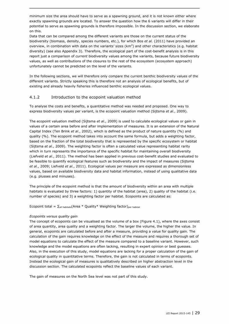
The concept of ecopoints can be visualised as the volume of a box (Figure 4.1), where the axes consist

of area quantity, area quality and a weighting factor. The larger the volume, the higher the value. In

general, ecopoints are calculated before and after a measure, providing a value for quality gain. The

calculation of the gain requires knowledge on the effect of the measure and requires a thorough set of

model equations to calculate the effect of the measure compared to a baseline variant. However, such

knowledge and the model equations are often lacking, resulting in expert opinion or best guesses.

Also, in the execution of this study, model equations are lacking for a proper calculation of the gain of

ecological quality in quantitative terms. Therefore, the gain is not calculated in terms of ecopoints.

Instead the ecological gain of measures is qualitatively described on higher abstraction level in the

discussion section. The calculated ecopoints reflect the baseline values of each variant.

The gain of measures on the North Sea level was not part of this study.

30 | LEI Report 2015-145

Figure 4.1 Visualisation of ecopoints (blue) before measure and gain in ecopoints (green) after

measure (after Liefveld et al., 2011)

Source: after Liefveld et al. (2011).

A weighting factor is applied to express the importance, threat or rarity of different habitats (Liefveld

et al., 2011). The basic methodology can be retrieved in Sijtsma et al. (2009) and Liefveld et al.

(2011).

4.1.3 Adapted ecopoint valuation for the Frisian Front and Central Oyster Grounds

In the current study, the ecopoint method of Sijtsma et al. (2009) was adapted to the specific purpose

of this study, i.e. to select for closed areas (variants) that contribute most to the targets of the Dutch

Marine Strategy. In the ecopoint calculation formula shown above, the first factor, the area, is the size

of each of the 6 proposed closures (variants), expressed in km2. The second factor in the equation,

habitat quality, is expressed as a biodiversity value, calculated on the basis of benthic biodiversity

maps as published in Bos et al. (2011), which are based on the MSFD criteria for biodiversity

indicators (EU, 2010). The weighting factor is generically used to express the importance of the

specific habitat for maintaining overall biodiversity. In this study a number of weighting factors are

defined to differentiate the benthic ecological values of the variants resulting from various ecological

viewpoints. The following aspects were taken into account:

1. The weighting factor should contribute to the aims of the closure with respect to the improvement

of the quality of deeper, silty seabeds and deeper, non-dynamic sandy seabeds.

2. The weighting factor should select for habitat rarity (rare habitats are more in need of protection

than common habitats).

3. The weighting factor should reflect the general MSFD ecosystem approach (favour all species

groups and important ecosystem characteristics where possible).

4. The weighting factor should favour one larger single area over a combination of many smaller

areas (rationale in Section 4.2.3.2)

Since it is not very clear how to create one weighting factor that encompasses all of these aspects, we

have constructed different weighting factors that each address one or more of these points. We thus

provide results for a number of different weighting factors and compare their effects on the ecopoint

score for the variants. We also provide data per subarea to be able to compare results within a variant

and between subareas.

To highlight the rarity or importance of certain habitats over others within the search area, the

characteristics of the local ecosystems need to be compared. Such a comparison between the Frisian

Front and Central Oyster Grounds has been made by Jongbloed et al. (2013) during an expert

workshop. Both areas are characterised by deep muddy habitats and are highly biodiverse (Bos et al.,

LEI Report 2015-145 | 31

2011). The Frisian Front, however, is a front system, is more productive, has a higher biodiversity,

higher heterogeneity, has depth gradients resulting in hydrographical and sedimentological gradients,

has little stratification and has a large variation in angle of inclination (Lindeboom et al., 2015). In the

Central Oyster Grounds there is little variation in depth, there is a longer and more gradual gradient of

sediment, less variation in depth and stability of stratification and there is little energy input in the

system (Jongbloed et al., 2013).

4.2 Methodology

In this project, 6 different variants for combinations of closed areas in the Frisian Front/Central Oyster

Grounds area are compared in terms of ecopoints. Ecopoints are calculated for the ‘baseline’ situation

only, as explained in the introduction (Section 4.1.1), according to the following formula:

Ecopoint total = Area * Quality* Weighting factor

In the subsequent sections, each of these factors are discussed in more detail. Based on the

commonly applied methodology of ecopoint derivation (e.g. Sijtsma et al., 2009; Liefveld et al., 2014;

Van Gaalen et al., 2011), area describes the total surface area, quality describes the quality of an

habitat in terms of species or biodiversity, and weighting factors describe the areas’ relative

importance or uniqueness to maintain overall biodiversity.

In this study, several options to derive ecopoints are presented. In these options, the area (km2) per

variant and quality factors are kept constant, while a number of weighting factors are defined which

can be used to differentiate the ecological score of the variants. The list of weighting factors comprise

different alternatives of which it can be debated which one is most relevant for the final assessment.

This latter depends e.g. on policy ambition.

The following steps were taken to obtain information that allows for calculation of the ecopoints:

Step 1: Area quantity calculation

Step 2: Area quality calculation

2a: Selection of relevant quality indicators

2b: Calculation quality indicator values

2c: Scaling of quality indicators to values between 0 and 1

Step 3: Weighting factor

3a: Selection of weighting factors

3b: Calculation of weighting factors

Step 4: Calculation of ecopoints

Step 5: Evaluation of data robustness and effect on outcome

4.2.1 Step 1: Area quantity

The area (km2) per variant is calculated as the sum of the subareas (see Table 4.1 and Figure 4.1).

4.2.2 Step 2: Area quality indicators

4.2.2.1 Step 2a: Selection of area quality indicators

Quality indicators in the ecopoint methodology refer to species lists or biodiversity values, expressed

as abundance of typical species listed on a national species list (e.g. at N2000 qualifying species lists,

combined with a goal per species) (Sijtsma et al., 2009; Liefveld et al., 2011). In the context of the

MSFD and this study, the area closures to bottom impact by fisheries should contribute to the recovery

of habitats and biodiversity, and improve the size, quality and distribution of long-lived and or

vulnerable benthic species.

The area quality indicators should therefore inform on biodiversity values, with emphasis on benthos,

and in particular long-lived and/or vulnerable benthic species. The search area (Frisian Front and

Central Oyster Grounds) was selected for benthic protection measures based on high benthic

32 | LEI Report 2015-145

biodiversity values, as presented in Bos et al. (2011). In this study we therefore use the same data

(see Appendix 2) to calculate the area quality.

The indicators calculated by Bos et al. (2011) represent different aspects of biodiversity, including

density of species, biomass and condition, corresponding to the requirements for MSFD indicators (EU,

2010). These maps have been constructed with the best possible data available (see discussion). The

methodology of kriging (interpolating) to obtain the coloured areas between sampling points is

described in Bos et al. (2011). The following maps and data are used for this study (see maps in

Appendix 2):

Macrobenthos (BIOMON)1

Species richness

Species biomass

Species density

Species evenness

Long-lived benthic species

Large growing species

Megabenthos (triple D)2

Species richness

Species biomass

Species density

Since quality indicators should be independent of one another to avoid a ‘double counting’ of

indicators, the quality indicator ‘rare species’ (see map in Appendix 2) was excluded, since this is a

subset of the data on ‘species richness’ and therefore strongly correlates with ‘species richness’. The

other quality indicators represent different aspects of biodiversity that are independent of one another.

To avoid double counting of aspects within the overall equation, a clear distinction is made between

quality aspects and weighting factor aspects. Abiotic habitat characteristics are used to derive

weighting factors, whereas species information is used to calculate quality indicators.

4.2.2.2 Step 2b. Calculation of quality indicator values

Biodiversity data were obtained from maps in Bos et al. (2011) which consist of scaled data, with each

class containing more or less the same number of data on a Dutch Continental Shelf (DCS) scale. In

Bos et al. (2011) these values per sampling station were kriged (extrapolated over space) in GIS so

that colours represent classes, (see maps in Appendix 2). In this study, these maps are used to obtain

biodiversity values for each of the 6 variants, by calculating the average value of an indicator within a

variant, using GIS. Basically, this follows Liefveld et al. (2011), except, in this study, we concentrate

only on benthos and do not calculate the gain (rationale see Section 4.1.2). As such this is a Limited

Benthos Approach (LBA) and not an overall ecosystem approach.

For example, if a variant would consist of 2 subareas (Figure 4.2), subarea 1 of 400 km2 and subarea

2 of 800 km2, the following calculation is made:

If the first subarea consisted for 100% of a biodiversity quality value 3 (orange colour) the quality

value for the first subarea would be 3*400=1,200. The second subarea of 800 km2 would have a value

of 70% of value 3 and 30% of value 2, with a total biodiversity value of (0.7*3+0.3*2)*800=2,160.

Then the average biodiversity value would be (1,200+2,160)/(400+800)=2.8.

1 BIOMON is the biological monitoring program (BIOMON) of Rijkswaterstaat, in which data on macrobenthos are collected

at the Dutch Continental Shelf. Macrobenthos consists of the organisms that live at the bottom and are larger than

~0.5 mm. 2 Triple D is the monitoring device of NIOZ, applied in benthic monitoring on the North Sea in several research

programmes. Provides complementary benthic data to BIOMON because another part of the seafloor is sampled. Sampling

focuses on larger benthos species than in BIOMON, such as larger infauna and the epifauna.

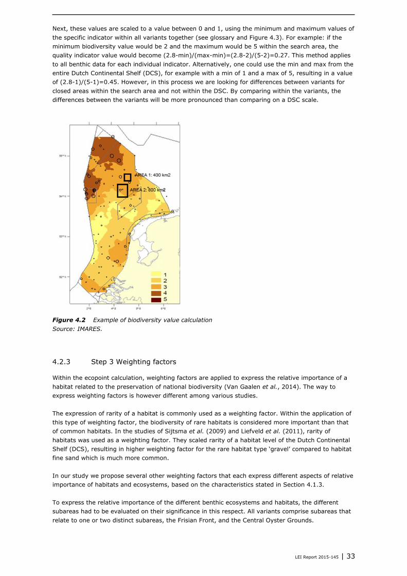
LEI Report 2015-145 | 33

Next, these values are scaled to a value between 0 and 1, using the minimum and maximum values of

the specific indicator within all variants together (see glossary and Figure 4.3). For example: if the

minimum biodiversity value would be 2 and the maximum would be 5 within the search area, the

quality indicator value would become (2.8-min)/(max-min)=(2.8-2)/(5-2)=0.27. This method applies

to all benthic data for each individual indicator. Alternatively, one could use the min and max from the

entire Dutch Continental Shelf (DCS), for example with a min of 1 and a max of 5, resulting in a value

of (2.8-1)/(5-1)=0.45. However, in this process we are looking for differences between variants for

closed areas within the search area and not within the DSC. By comparing within the variants, the

differences between the variants will be more pronounced than comparing on a DSC scale.

Figure 4.2 Example of biodiversity value calculation

Source: IMARES.

4.2.3 Step 3 Weighting factors

Within the ecopoint calculation, weighting factors are applied to express the relative importance of a

habitat related to the preservation of national biodiversity (Van Gaalen et al., 2014). The way to

express weighting factors is however different among various studies.

The expression of rarity of a habitat is commonly used as a weighting factor. Within the application of

this type of weighting factor, the biodiversity of rare habitats is considered more important than that

of common habitats. In the studies of Sijtsma et al. (2009) and Liefveld et al. (2011), rarity of

habitats was used as a weighting factor. They scaled rarity of a habitat level of the Dutch Continental

Shelf (DCS), resulting in higher weighting factor for the rare habitat type ‘gravel’ compared to habitat

fine sand which is much more common.

In our study we propose several other weighting factors that each express different aspects of relative

importance of habitats and ecosystems, based on the characteristics stated in Section 4.1.3.

To express the relative importance of the different benthic ecosystems and habitats, the different

subareas had to be evaluated on their significance in this respect. All variants comprise subareas that

relate to one or two distinct subareas, the Frisian Front, and the Central Oyster Grounds.

34 | LEI Report 2015-145

Within the North Sea, the Frisian Front area has been judged to be ecologically more valuable than the

Central Oyster Grounds (Jongbloed et al., 2013; Lindeboom et al., 2015), because of its relative

higher production, higher bioturbation, greater connectivity due to the presence of a frontal area, as

well as a higher potential for recovery after closure for fisheries compared to the Central Oyster

Grounds (Jongbloed et al., 2013). Definition of additional weighting factors to reflect the ecosystem of

the Central Oyster Grounds was debated but found not relevant. The Central Oyster Grounds in itself

is a relevant benthic ecosystem, but compared to the Frisian front ecosystem less unique in the North

Sea (Lindeboom et al., 2015).

Some weighting factors emphasise more or less the same aspects, and differ only in detail. This seems

redundant, but is not the case. As each weighting factor is applied individually, no redundancy exists:

it is either factor A or B, not both. The choice for a certain weighting factor will depend on the policy

ambition. For example, if the ambition is to close a large single area versus several smaller areas,

then the decision maker should look at the results of the corresponding weighting factor. Furthermore,

no combinations of weighting factors are applied in this study to be able to compare them

independently, except for factor 5 which includes gradient and front together (see Figure 4.3). Also,

multiplying different factors would result in redundancy.

The different weighting factors express not only the overall score of a variant, but can be used to

evaluate the importance of one subarea over another.

4.2.3.1 Step 3a Selection of weighting factors

The weighting factors are grouped into the following categories (additional details and calculation are

explained in 4.2.3.2 and Figure 4.3):

Generic weighting factors including weighting factors based on habitat rarity (following Sijtsma

et al., 2010 and Liefveld et al., 2011) and habitat diversity in general. Weighting factors 1 and 2

highlight the variants with a lot of rare or diverse habitats and are explained in more detail below

In addition, weighting factors are included that take the ‘border effect’ into account (see Section

4.2.3.2, weighting factor 3, following Lindeboom et al., 2015). Decision makers can choose to use

these weighting factors if they want to be able to compare e.g. the value of one larger area versus

several smaller areas.

Weighting factors emphasising the frontal area and gradients within this area. The emphasise on the

frontal area follows from the arguments by Lindeboom et al. (2015) in which it is described how and

why the frontal area could be evaluated as ecological more significant than other regions in the

North Sea. The weighting factors from this category apply to all subareas but will favour those

subareas positioned within the Frisian Front region.

Weighting factor reflecting the density of artificial hard substrate within variants. This weighting

factor is proposed in the stakeholder process, and is assumed to be a proxy for biodiversity. This

weighting factor benefits the variants with higher density of artificial substrates. A rationale

regarding this weighting factor is included in section 4.4.3.2.

Weighting factor in which fisheries pressure within a variant is used as a proxy for benthic habitat

damage due to fisheries and potential habitat recovery when fisheries would be excluded. Based on

the rationale that fishing pressure negatively relates to benthic biodiversity (see section 4.4.1). This

weighting factor benefits variants with high fisheries pressure over variants with lower fisheries

pressure based on the assumption that the higher the current pressure, the larger the recovery can

be.

The weighting factors are summarised below and described in more detail in the following section

(Section 4.2.3.2).

Generic weighting factors:

Weighting factor 1: rarity of habitats (average rarity of habitats within area)

­ This basic method (Liefveld et al., 2011) allows to select for variants that have more rare habitats

than others and thus better contribute to the maintenance of the overall biodiversity.

Weighting factor 2: diversity of habitats (N habitats/ area)

­ This factor selects for the variants with the highest habitat diversity (all habitats count evenly)

LEI Report 2015-145 | 35

Weighting factors emphasising the net effective area (larger over smaller and border effects):

Weighting factor 3a: border effect (border/area of an area relative to that of a circle)

­ This factor selects for fewer larger areas over more smaller areas, in order to compensate for

ineffective protection: A single large area will have less a border length than multiple small areas

of the same size (for details see below) and is more effective in its net protection compared to

smaller areas (Lindeboom et al., 2015).

Weighting factor 3b: effective area (effective area relative to that within a buffer of 1 km around

­ Similar to 3a, with the additional ecological motivation that benthic fauna may migrate to outside

the area, so that a buffer zone is needed to protect them efficiently.

Weighting factor 3c: effective area (effective area relative to that within a buffer of 2,5 km around)

­ Similar to 3a, with an additional ecological motivation (larger buffer zone)

Weighting factors emphasising frontal area and gradients:

Weighting factor 4a: importance of central front within the FF expressed by the central front system

(% of 20% silt area within subarea) (rationale in Lindeboom et al., 2015).

­ This factor selects for variants that are located in the centre of the Frisian Front, the central and

most silty part.

Weighting factor 4b: importance of FF expressed as influenced ecosystem around the central front

system (% Frisian Front parallelogram within closed area) (rationale in Lindeboom et al., 2015)

­ This factor selects for variants that are influenced by the central front in the Frisian Front, i.e.

located in the Frisian Front area as defined in Lindeboom et al. (2005)

Weighting factor 5a: importance of abiotic gradients (max N habitats within highest scoring subarea

within parallelogram Frisian Front)

­ This factors selects for variants that are within the Frisian Front and contain a gradient (nature

types)

Weighting factor 5b: importance of benthic gradients (max N connected benthic zones within Frisian

Front)

­ Similar to 5a. This weighting factor selects for variants that cover a gradient in silt content,

corresponding to benthic zones (see below)

Weighting factor 5c: importance of benthic gradients including the front (max N connected benthic

zones within Frisian Front- including the front)

­ Similar to 5b. This weighting factor selects for variants that are located in the central part of the

Frisian Front, and that cover a gradient.

Weighting factor emphasising the presence of artificial hard substrates

Weighting factor 6:

­ This factor reflects the relative abundance of artificial hard substrate located based on the number

of wrecks and oil and gas facilities providing substrate for organisms to settle on.

Weighting factor reflecting fisheries pressure and potential recovery

Weighting factor 7:

­ This factor reflects the potential recovery of the benthic ecosystem within a variant based on the

fisheries pressure (in fishing days- see Table 5.5)

4.2.3.2 Step 3b. Calculation of weighting factors

Figure 4.3 presents each of the weighting factors and their differences. Thereafter, for each weighting

factor the calculation method is described.

36 | LEI Report 2015-145

Figure 4.3 Graphic representations of the weighting factors. Left: generic weighting factors, right:

weighting factors emphasising the frontal area and gradients and hard substrate

Source: IMARES.

Generic weighting factors

Weighting factor 1: Habitat rarity

This weighting factor takes into account the rarity of the habitats on the DCS, where the protection of

rare habitats is considered more important than the protection of common habitats (according to

Sytsma et al., 2009 and Liefveld et al., 2011). The rationale is that rare habitats contain a different

biodiversity than more generic habitats and should be included in protected areas. The habitat types

used in this weighting factor are the ‘nature types’ (Bos et al., 2011), consisting of combinations of

depth classes (0-10 m, 10-20, 20-30, 30-40, >40), sediment size classes (<150 um, 150-210; 210-

420; >420), absence/presence of silt (>15%), absence/presence of stratification. This weight

indicator ‘Presence of rare habitats’ is expressed as the average rarity based on the nature type map

published in Bos et al. (2011) where rarity is defined as (1-occurence) (see Appendix 2). In this way,

a rare habitat type will be given a greater importance than a common habitat type. For example, if a

habitat type covers 5% of the DCS, the rarity is (1-0.05)=0.95. The data were thereafter scaled based

on the minimum and maximum values related to this indicator. The most common habitat type in the

Dutch North Sea is sandy sediment, which covers 28% of the seafloor (rarity = 1-0.28=0.72). In this

example rarity is scaled on a scale ranging from 0.72 (which is the min) to 1 (which is the max).

For example, a closed area consists of 20% of habitat type A and 80% of habitat type B. The coverage

of habitat type A at the DCS-scale is 5% (or 0.05) (rarity value: 1-0.05=0.95) and of habitat B is 25%

(rarity value of 0.75). The rarity values are first rescaled between the minimum (0.72) and the

maximum (1). Thus the rarity of habitat type A becomes (0.95-0.72)/(1-0.72))=0.89. Of type B:

(0.75-0.72)/(1-0.72))=0.11. Then the weighting factor becomes 20%*0.89+80%*0.11=0.73.

Weighting factor 2: Habitat diversity

Weighting factor 3 takes into account the diversity of habitats within a closed area, where multiple

habitats (‘nature types’ based on Bos et al., 2011. See Appendix 2) are preferred over a single one.

The assumption is that a combination of different habitats potentially results in higher biodiversity

than a single habitat. It is expressed as the number of nature types (combinations of depth, sediment

size, absence/presence of silty, absence/presence of stratification) to express the importance of

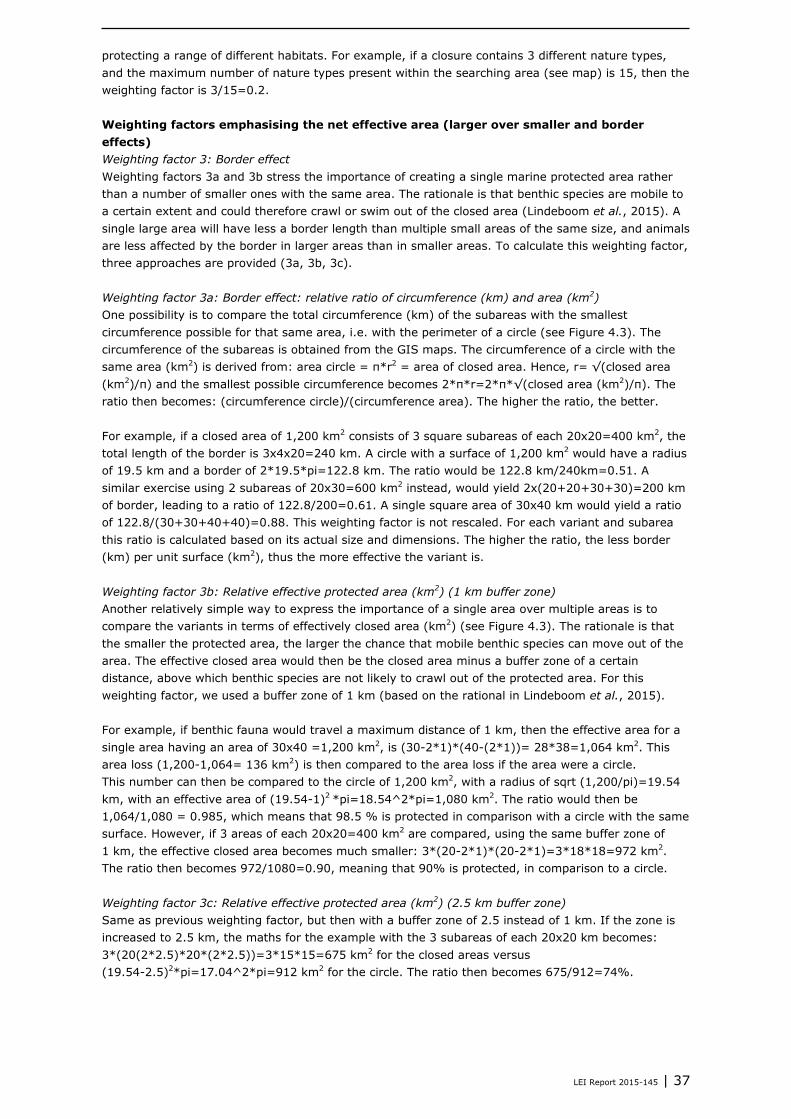
LEI Report 2015-145 | 37

protecting a range of different habitats. For example, if a closure contains 3 different nature types,

and the maximum number of nature types present within the searching area (see map) is 15, then the

weighting factor is 3/15=0.2.

Weighting factors emphasising the net effective area (larger over smaller and border

effects)

Weighting factor 3: Border effect

Weighting factors 3a and 3b stress the importance of creating a single marine protected area rather

than a number of smaller ones with the same area. The rationale is that benthic species are mobile to

a certain extent and could therefore crawl or swim out of the closed area (Lindeboom et al., 2015). A

single large area will have less a border length than multiple small areas of the same size, and animals

are less affected by the border in larger areas than in smaller areas. To calculate this weighting factor,

three approaches are provided (3a, 3b, 3c).

Weighting factor 3a: Border effect: relative ratio of circumference (km) and area (km2)

One possibility is to compare the total circumference (km) of the subareas with the smallest

circumference possible for that same area, i.e. with the perimeter of a circle (see Figure 4.3). The

circumference of the subareas is obtained from the GIS maps. The circumference of a circle with the

same area (km2) is derived from: area circle = π*r2 = area of closed area. Hence, r= √(closed area

(km2)/π) and the smallest possible circumference becomes 2*π*r=2*π*√(closed area (km2)/π). The

ratio then becomes: (circumference circle)/(circumference area). The higher the ratio, the better.

For example, if a closed area of 1,200 km2 consists of 3 square subareas of each 20x20=400 km2, the

total length of the border is 3x4x20=240 km. A circle with a surface of 1,200 km2 would have a radius

of 19.5 km and a border of 2*19.5*pi=122.8 km. The ratio would be 122.8 km/240km=0.51. A

similar exercise using 2 subareas of 20x30=600 km2 instead, would yield 2x(20+20+30+30)=200 km

of border, leading to a ratio of 122.8/200=0.61. A single square area of 30x40 km would yield a ratio

of 122.8/(30+30+40+40)=0.88. This weighting factor is not rescaled. For each variant and subarea

this ratio is calculated based on its actual size and dimensions. The higher the ratio, the less border

(km) per unit surface (km2), thus the more effective the variant is.

Weighting factor 3b: Relative effective protected area (km2) (1 km buffer zone)

Another relatively simple way to express the importance of a single area over multiple areas is to

compare the variants in terms of effectively closed area (km2) (see Figure 4.3). The rationale is that

the smaller the protected area, the larger the chance that mobile benthic species can move out of the

area. The effective closed area would then be the closed area minus a buffer zone of a certain

distance, above which benthic species are not likely to crawl out of the protected area. For this

weighting factor, we used a buffer zone of 1 km (based on the rational in Lindeboom et al., 2015).

For example, if benthic fauna would travel a maximum distance of 1 km, then the effective area for a

single area having an area of 30x40 =1,200 km2, is (30-2*1)*(40-(2*1))= 28*38=1,064 km2. This

area loss (1,200-1,064= 136 km2) is then compared to the area loss if the area were a circle.

This number can then be compared to the circle of 1,200 km2, with a radius of sqrt (1,200/pi)=19.54

km, with an effective area of (19.54-1)2 *pi=18.54^2*pi=1,080 km2. The ratio would then be

1,064/1,080 = 0.985, which means that 98.5 % is protected in comparison with a circle with the same

surface. However, if 3 areas of each 20x20=400 km2 are compared, using the same buffer zone of

1 km, the effective closed area becomes much smaller: 3*(20-2*1)*(20-2*1)=3*18*18=972 km2.

The ratio then becomes 972/1080=0.90, meaning that 90% is protected, in comparison to a circle.

Weighting factor 3c: Relative effective protected area (km2) (2.5 km buffer zone)

Same as previous weighting factor, but then with a buffer zone of 2.5 instead of 1 km. If the zone is

increased to 2.5 km, the maths for the example with the 3 subareas of each 20x20 km becomes:

3*(20(2*2.5)*20*(2*2.5))=3*15*15=675 km2 for the closed areas versus

(19.54-2.5)2*pi=17.04^2*pi=912 km2 for the circle. The ratio then becomes 675/912=74%.

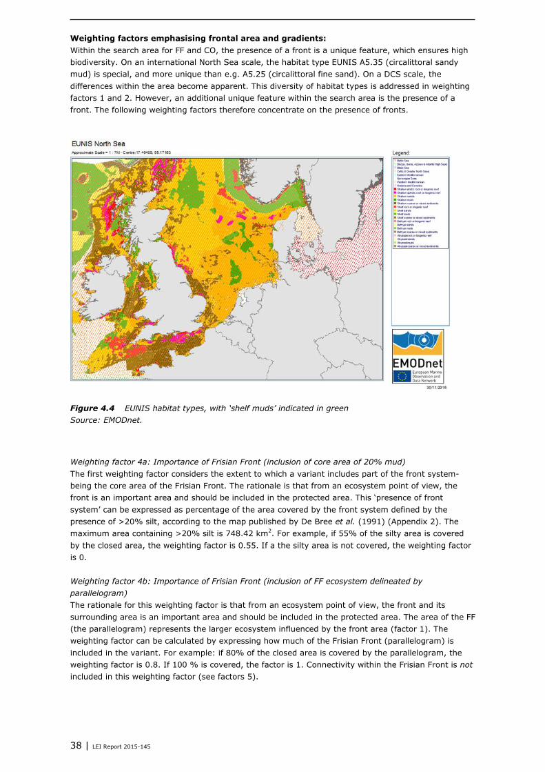
38 | LEI Report 2015-145

Weighting factors emphasising frontal area and gradients:

Within the search area for FF and CO, the presence of a front is a unique feature, which ensures high

biodiversity. On an international North Sea scale, the habitat type EUNIS A5.35 (circalittoral sandy

mud) is special, and more unique than e.g. A5.25 (circalittoral fine sand). On a DCS scale, the

differences within the area become apparent. This diversity of habitat types is addressed in weighting

factors 1 and 2. However, an additional unique feature within the search area is the presence of a

front. The following weighting factors therefore concentrate on the presence of fronts.

Figure 4.4 EUNIS habitat types, with ‘shelf muds’ indicated in green

Source: EMODnet.

Weighting factor 4a: Importance of Frisian Front (inclusion of core area of 20% mud)

The first weighting factor considers the extent to which a variant includes part of the front system-

being the core area of the Frisian Front. The rationale is that from an ecosystem point of view, the

front is an important area and should be included in the protected area. This ‘presence of front

system’ can be expressed as percentage of the area covered by the front system defined by the

presence of >20% silt, according to the map published by De Bree et al. (1991) (Appendix 2). The

maximum area containing >20% silt is 748.42 km2. For example, if 55% of the silty area is covered

by the closed area, the weighting factor is 0.55. If a the silty area is not covered, the weighting factor

is 0.

Weighting factor 4b: Importance of Frisian Front (inclusion of FF ecosystem delineated by

parallelogram)

The rationale for this weighting factor is that from an ecosystem point of view, the front and its

surrounding area is an important area and should be included in the protected area. The area of the FF

(the parallelogram) represents the larger ecosystem influenced by the front area (factor 1). The

weighting factor can be calculated by expressing how much of the Frisian Front (parallelogram) is

included in the variant. For example: if 80% of the closed area is covered by the parallelogram, the

weighting factor is 0.8. If 100 % is covered, the factor is 1. Connectivity within the Frisian Front is not

included in this weighting factor (see factors 5).

LEI Report 2015-145 | 39

Weighting factor 5a. Importance of abiotic gradients

The rationale for this weighting factor is that the front is the most important ecosystem within the

search area, and that within the front it ecologically assumed to be of importance to protect a

continues gradient, based on Lindeboom et al. (2015).

First, the number of nature types within the Frisian Front parallelogram within a subarea are counted.

Next, the score of the subarea containing most nature types is taken to calculate a weighting factor.

We have calculated the maximum number of connected nature types and not the average number of

nature types, since the weighting factor should express the maximum gradient, in terms of the

number of connected nature types. Averaging would results in less interpretable results. The score is

scaled by using the minimum (0) and maximum number of nature types (14) that can be enclosed

within the parallelogram.

For example, if subarea number 1 is located within the parallelogram, and contains 4 nature types,

and if subarea number 2 is half located in the parallelogram, and contains 2 nature types, the score of

4 is taken for further calculations, because this is the maximum number of connected nature types

Next, the weighting factor is calculated as: (4-min)/(max-min)=4/(14-0)=0.29. The maximum of the

weighting factor is 1, the minimum is 0 (see Figure 4.3)

Weighting factor 5b. Importance of benthos gradients

This weighting factor is calculated by counting the number of zones (Creutzberg et al., 1984) within a

subarea within the parallelogram (see Appendix 2). The zones have been found by Creutzberg et al.

(1984) to represent distinct benthic zones and are situated in parallel. The difference with the previous

factor is that these zones are based on mud content, while the nature types include more abiotic

characteristics (see glossary). The rationale is that the front is the most important ecosystem within

the search area, and that within the front it is important to protect a continues gradient. These zones

reflect the change in mud content and each zone more or less coincides with peaks of certain species.

The weighting factor is based on the maximum number of connected zones within the Frisian Front

parallelogram. The rationale for including a continuous gradient is provided in Appendix 13. The score

is obtained by counting the zones from the map. The weighting factor is calculated by scaling the

score between the minimum (0) and maximum (8) number of benthos zones, yielding a number

between 0 and 1.

For example, if a closed area consists of 2 subareas, and subarea number 1 covers 2 benthos zones,

while subarea number 2 covers 4 zones, then the score is 4. The weighting factor becomes 4/(max-

min)=4/(8-0)=0.5.

Weighting factor 5c. Importance of benthos gradients

Same as 5b, but in this case it is obligatory to include the core of the front (20% mud) as the centre

of the gradient.

Weighting factor emphasising the presence of artificial hard substrates

Weighting factor 6. Artificial hard substrate

This weighting factor is suggested by stakeholders. The rationale is that artificial hard substrate

provides substrate for organisms to settle on. It is assumed that the more artificial hard substrate a

variant has, the higher the biodiversity can be. The factor is calculated by counting all artificial hard

substrata objects (wrecks and oil/gas facilities) within the variants.

Wreck positions are retrieved from the website http://www.wrecksite.eu. The retrieved dataset

includes a total of 16,726 wrecks in the North Sea, of which 180 lay within the various variants.

Based on NLOG datasets3 which provide positions of oil and gas facilities in the North Sea, the number

of facilities is counted per variant. A total of 38 facilities are positioned within all variants together.

The sum of number of wrecks and oil and gas facilities per variant is taken as the total number of

3 http://www.nlog.nl/nl/mappingDatasets/mappingDatasets.html retrieved on November 17 2015

40 | LEI Report 2015-145

artificial hard substrata. The number is then divided by the total surface of the variant to obtain the

density. Next, the weighting factor is scaled between 0-1 based on the density range that was

theoretically possible (min = 0, max = highest density within search area (max total number of hard

substrate items (218)/lowest possible surface (1,204 km2)).

Maps of both wreck and oil and gas facilities are presented in Appendix 2.

Weighting factor reflecting fisheries pressure and potential recovery

Weighting factor 7: Fisheries pressure

This factor reflects the fact that the present ecosystem is already heavily influenced by fisheries.

Duineveld et al. showed that the impact of bottom trawl fisheries depends on the fishing intensity.

This is different for the different scenario’s and therefor a weighing factor taking this into account

was introduced. At the same time if a heavily influenced area is closed to fisheries the potential

recovery of the benthic ecosystem is higher. Both effects were taken into account within a variant

based on the fisheries pressure (in fishing effort in days- see Table 5.5). The weighting factor is

calculated as the proportion of the maximum pressure: the maximum fishing pressure of 0.12 gives

a weighting factor of 1, the fishing pressure of 0.8, being 67% becomes 0.67, etc.

4.2.4 Step 4 Calculation of ecopoints

Ecopoints are expressed in two ways:

per km2 (quality x weighting factor) per (total) variant and subareas to obtain a weighted ecopoint

value /km2 (since size difference largely and steers outcome). Total score is calculated on the

whole/total area, following the methodology as described above. It is not a sum nor an average of

the subareas.

per area (area/100* quality* weighting factor) per variant and subareas to obtain the total amount

of ecopoints, according to the formula shown in Section 4.2. This method follows descriptions in

Liefveld et al. (2011). By dividing the area (km2) per variant by 100, the multiplication factor is in

the same order of magnitude as the sum of the quality indicators, which range from 3.72 to 5.08

(see Table 4.2). For example, if a variant would have a total area of 1,200 km2, the multiplication

factor becomes 1,200/1,00=12. This number is in the same order of magnitude as the total sum of

the quality factors. The total score is calculated on the whole/total area, following the methodology

as described above. It is not a sum nor an average of the subareas.

4.2.5 Step 5 Test of the robustness/sensitivity of the analysis

To test the influence of each contributing element to the outcome, a sensitivity analysis can be

performed. In this study, a sensitivity analysis is not done by means of statistical analysis, but based

on minimum and maximum ranges. Of each quality factor, weighting factor, and area factor the range

between minimum and maximum ecopoint value across the different variants is presented, including

the factor describing the effect of this range. For example, Abalone has a surface of 1,204 km2, while

Flounder has a surface of 6,339 km2 (see Table 3.1). This means that, based on surface area alone,

the smallest variant already scores (6,339/1,204=) 5.26 times lower than the largest variant. In the

same way, the quality factor and the weighting factor are evaluated. The set of quality indicators

accumulate into one quality value, which all add to the final quality indicator. Also these individual

contributions are evaluated. An overview of these ranges and factors is presented in the results

section.

In addition, the scores of each subarea provide insights on how the weighted score of the overall

variant is a result of similar scores of the subareas, or that large differences between the subareas are

present. That is why all subarea values are presented as well to be transparent on the subvalues,

resulting in a weighted average total score for each variant.

LEI Report 2015-145 | 41

4.3 Results Ecopoints

In this section, the results per calculation step of the ecopoint calculations are presented in tables and

figures. In Chapter 4.5 the meaning of the results is discussed. In Appendix 4, the scores for the

subareas are presented.

4.3.1 Step 1. Area quantity

In Table 4.1, the area quantity per variant and per subarea is presented. This information is used for

the ecopoint calculation (step 4). The total surfaces are divided by 100 (see Liefveld et al., 2011) in

order to obtain values in the same order of magnitude.

Table 4.1

Area quantity per variant and per subarea (km2)

Variant 1 Variant code Subarea coding Surface area (km2)

Abalone A FF 800

Abalone A CO 404

Total 1,204

Brill B CO 207

Brill B FFSW 632

Brill B FFSE 319

Brill B FFC 105

Total 1,263

Capelin FFSW 398

Capelin C FFSE 398

Capelin C FFNO 398

Capelin C CO 404

Total 1,597

Dab D CO 304

Dab D FFSW 772

Dab D FFSE 501

Dab D FFC 105

Total 1,683

Eel E FFSE 700

Eel E FFSW 1,050

Eel E COS 1,050

Eel E CON 1,406

Total 4,206

Flounder F FF 2,882

Flounder F CO 3,457

Total 6,339

Source: Ministry of I&M.

4.3.2 Step 2. Area quality indicators

In Table 4.2 the biodiversity quality indicator are shown for the 6 variants, per subarea and for the

total area. These values are calculated on the basis of maps, as explained in Section 4.2.2. and

represent different aspects of species biodiversity. Rarity’ is set at 0 for the indicators because rarity is

strongly correlated with species richness.

42 | LEI Report 2015-145

Table 4.3 shows the rescaled values to a value between 0 and 1 for the quality indicators. Figure 4.5

presents an overview of the summed quality for each variant. The highest possible score was 9. The

overall quality score for these variants ranges from 3.74-5.08. Overall, Flounder represents the

highest quality score, and Brill lowest.

LEI Report 2015-145 | 43

Table 4.2

Area quality indicators

Macrobenthos Megabenthos

Variant

bio

mass

even

ness

larg

e_

sp

ecie

s

lon

g-l

ived

sp

ecie

s

sp

ecie

s

ric

hn

ess

rarit

y

den

sit

y

bio

mass

den

sit

y

rarit

y

ric

hn

ess

Abalone 5.33 4.31 5.43 5.16 7.01 2.18 5.62 5.88 6.62 4.99 6.54

Brill 5.72 4.10 4.66 3.56 5.25 1.98 5.75 5.24 5.41 3.57 5.20

Capelin 5.30 4.35 5.55 4.99 6.77 2.23 5.78 5.46 6.80 5.28 7.25

Dab 5.71 4.04 4.75 3.73 5.43 2.00 5.90 5.41 5.60 3.74 5.41

Eel 5.11 4.33 5.62 5.88 7.06 2.53 5.72 4.58 5.50 5.07 6.51

Flounder 5.00 4.40 5.86 6.09 7.69 2.60 5.45 4.62 6.57 5.81 7.63

Min 4.00 3.00 4.00 2.00 2.00 1.00 4.00 2.00 1.00 2.00 3.00

Max 7.00 6.00 7.00 9.00 9.00 4.00 8.00 8.00 9.00 9.00 9.00

Table 4.3

Re-scaled values of quality indicators

Macrobenthos Megabenthos

Variant

bio

mass

even

ness

larg

e_

sp

ecie

s

lon

g-l

ived

sp

ecie

s

sp

ecie

s

ric

hn

ess

rarit

y

den

sit

y

bio

mass

den

sit

y

rarit

y

ric

hn

ess

su

m a

rea

qu

ali

ty

Abalone 0.44 0.44 0.48 0.45 0.72 0 0.40 0.65 0.70 0 0.59 4.87

Brill 0.57 0.37 0.22 0.22 0.46 0 0.44 0.54 0.55 0 0.37 3.74

Capelin 0.43 0.45 0.52 0.43 0.68 0 0.44 0.58 0.73 0 0.71 4.96

Dab 0.57 0.35 0.25 0.25 0.49 0 0.47 0.57 0.57 0 0.40 3.92

Eel 0.37 0.44 0.54 0.55 0.72 0 0.43 0.43 0.56 0 0.59 4.64

Flounder 0.33 0.47 0.62 0.58 0.81 0 0.36 0.44 0.70 0 0.77 5.08

Table 4.3 shows the rescaled values for the quality indicators (see Section 4.2.2). The final quality is

the sum of the 9 different biodiversity indicators.

Figure 4.5 Quality of each variant (sum of 9 scaled biodiversity indicators)

44 | LEI Report 2015-145

4.3.3 Step 3. Weighting factors

In Table 4.4 the weighting factors are presented as original - not scaled values. The factors are scaled

to a value between 0 and 1 (see methodology in Section 4.2.2.2). The scaled values are presented in

Table 4.5 and Figure 4.6.

Remarks regarding the total scores corresponding to each of the weighting factors:

1. habitat rarity: rarity of the total area (not average of subareas, nor sum of subarea)

2. N habitat: total per area = number unique habitat types in total area

3a. relative border: total is compared to circle. NB subareas are compared to subcircles

3b. Effective protect.-1 km: total is compared to circle with same area (km2) minus 1 km buffer

zone

3c. Effective protect.-2.5km: total is compared to circle with same area (km2) minus 2.5 km buffer

zone

4a. 20%FFmud: total per area = sum of subareas

4b. %FFparallelogram: total per area = sum of subareas

5a. Abiotic gradients: Total is max within subareas

5b. Benthic gradients: Total is max within subareas

5c. Gradients including centre: Total is max within subareas

6. Artificial hard substrate: total number of artificial hard substrate/km2

7: fisheries pressure: fishing effort in days/km2

Overall, the highest weighting factors are related to the factors representing the ecological significance

of the Frisian Front (4 and 5). Flounder, Eel and Abalone qualify for the highest weighting factors

(factor of 1), whereas Brill and Dab qualify for the lowest factors.

Taking into account the generic weighting factors (1-3), it depends largely on the specific weighting

factor which variant qualifies for highest or lowest factor.

Table 4.4

Weighting factors, original values (see Section 4.2.2.2 for method)

Variant

1.

hab

ita

t rarit

y

2.

N h

ab

itats

3a.

rela

tive b

ord

er

3b

. E

ffecti

ve p

ro

tect.

-1

km

3c.

Eff

ecti

ve p

ro

tect.

-

2.5

km

4a.

20

%FFm

ud

4b

. %

FFp

arall

elo

gram

5a.

Ab

ioti

c g

rad

ien

ts

5b

. B

en

thic

grad

ien

ts

5c.

Grad

ien

ts i

ncl

cen

tre

6.

Arti

ficia

l h

ard

su

bstr

ate

7.

Fis

hery p

ressu

re

Abalone 89.91 9 56% 92% 78% 25% 20% 8 8 8 0.02 0.12

Brill 81.57 9 38% 84% 58% 13% 5% 4 3 3 0.06 0.08

Capelin 91.63 11 41% 87% 67% 12% 35% 6 5 4 0.03 0.12

Dab 82.86 15 38% 86% 63% 13% 6% 4 3 3 0.05 0.08

Eel 92.13 15 44% 93% 82% 35% 31% 8 8 8 0.02 0.09

Flounder 94.41 14 55% 96% 90% 100% 100% 14 8 8 0.02 0.12

Table 4.5 shows the rescaled values of Table 4.4, according to the methods described in Section

3.2.3.2. The minimum and maximum values of the weighting factors shown in Table 4.5 are used to

scale the weighting factors between 0 and 1.

LEI Report 2015-145 | 45

Table 4.5

Scaled weighting factors (see Section 4.2.2.2 for method)

Variant

1.

hab

ita

t rarit

y

2.

N h

ab

itats

3a.

rela

tive b

ord

er

3b

. E

ffecti

ve p

ro

tect.

-1

km

3c.

Eff

ecti

ve p

ro

tect.

-

2.5

km

4a.

20

%FFm

ud

4b

. %

FFp

arall

elo

gram

5a.

Ab

ioti

c g

rad

ien

ts

5b

. B

en

thic

grad

ien

ts

5c.

Grad

ien

ts i

ncl

cen

tre

6.

Arti

ficia

l h

ard

su

bstr

ate

7.

Fis

hery p

ressu

re

Abalone 0.61 0.57 0.63 0.83 0.55 0.25 0.20 0.57 1.00 1.00 0.28 1.00

Brill 0.29 0.57 0.43 0.67 0.15 0.13 0.05 0.29 0.38 0.38 1.00 0.67

Capelin 0.68 0.71 0.46 0.74 0.35 0.12 0.35 0.43 0.63 0.50 0.43 1.00

Dab 0.34 1.00 0.43 0.71 0.26 0.13 0.06 0.29 0.38 0.38 0.81 0.67

Eel 0.70 1.00 0.50 0.86 0.65 0.35 0.31 0.57 1.00 1.00 0.35 0.75

Flounder 0.79 0.93 0.61 0.92 0.81 1.00 1.00 1.00 1.00 1.00 0.28 1.00

Figure 4.6 Visual presentation of the scaled weighting factors for each variant

46 | LEI Report 2015-145

4.3.4 Step 4. Ecopoints

First the ecopoints per km2 are shown in Table 4.6. These numbers are obtained by multiplying the

quality factors with the weighting factors as explained in Section 3.2.4, resulting in ecopoints per km2.

In the next table, these numbers are multiplied with the area.

Overall, Brill and Dab score lowest in ecopoints, and Flounder scores highest. The way of expression

(per km2, of per variant) does not influence this result (see overview in Table 4.7B).

Table 4.6

Calculated ecopoints per km2 for each variant, depending on the applied weighting factor

Variant

0.

no

weig

hti

ng

facto

r

1.

hab

ita

t rarit

y

2.

N h

ab

itats

3a.

rela

tive b

ord

er

3b

. E

ffecti

ve p

ro

tect.

-1

km

3c.

Eff

ecti

ve p

ro

tect.

-

2.5

km

4a.

20

%FFm

ud

4b

. %

FFp

arall

elo

gram

5a.

Ab

ioti

c g

rad

ien

ts

5b

. B

en

thic

grad

ien

ts

5c.

Grad

ien

ts i

ncl

cen

tre

6.

Hard

su

bstr

ate

7.

Fis

hery p

ressu

re

Abalone 4.87 2.98 2.78 3.07 4.06 2.70 1.24 0.97 2.78 4.87 4.87 1.34 4.87

Brill 3.74 1.10 2.14 1.61 2.51 0.58 0.48 0.19 1.07 1.40 1.40 3.74 2.50

Capelin 4.96 3.37 3.55 2.29 3.69 1.73 0.62 1.74 2.13 3.10 2.48 2.12 4.96

Dab 3.92 1.34 3.92 1.69 2.80 1.02 0.49 0.24 1.12 1.47 1.47 3.18 2.61

Eel 4.64 3.24 4.64 2.30 3.99 2.99 1.62 1.45 2.65 4.64 4.64 1.61 3.48

Flounder 5.08 4.00 4.72 3.12 4.70 4.09 5.08 5.08 5.08 5.08 5.08 1.44 5.08

In Table 4.7A, the ecopoints are calculated, according the formula (area/100) x quality x weighting

factor (see Section 4.3.4). In Table 4.7B the ranking of the ecopoints is shown (1=lowest, 6=highest)

Table 4.7A

Calculated ecopoints for each variant, depending on the applied weighting factor

Variant

0.

no

weig

hti

ng

facto

r

1.

hab

ita

t rarit

y

2.

N h

ab

itats

3a.

rela

tive b

ord

er

3b

. E

ffecti

ve p

ro

tect.

-

1 k

m

3c.

Eff

ecti

ve p

ro

tect.

-

2.5

km

4a.

20

%FFm

ud

4b

. %

FFp

arall

elo

gram

5a.

Ab

ioti

c g

rad

ien

ts

5b

. B

en

thic

grad

ien

ts

5c.

Grad

ien

ts i

ncl

cen

tre

6.

Hard

su

bstr

ate

7.

Fis

hery p

ressu

re

Abalone 59 36 33 37 49 32 15 12 33 59 59 16 59

Brill 47 14 27 20 32 7 6 2 14 18 18 47 32

Capelin 79 54 57 37 59 28 10 28 34 50 40 34 79

Dab 66 23 66 28 47 17 8 4 19 25 25 53 44

Eel 195 136 195 97 168 126 68 61 111 195 195 68 146

Flounder 322 253 299 198 298 260 322 322 322 322 322 91 322

LEI Report 2015-145 | 47

Table 4.7B

Ranking of calculated ecopoints for each variant, depending on the applied weighting factor

Variant

0.

no

weig

hti

ng

facto

r

1.

hab

ita

t rarit

y

2.

N h

ab

itats

3a.

rela

tive b

ord

er

3b

. E

ffecti

ve p

ro

tect.

-

1 k

m

3c.

Eff

ecti

ve p

ro

tect.

-

2.5

km

4a.

20

%FFm

ud

4b

. %

FFp

arall

elo

gram

5a.

Ab

ioti

c g

rad

ien

ts

5b

. B

en

thic

grad

ien

ts

5c.

Grad

ien

ts i

ncl

cen

tre

6.

Hard

su

bstr

ate

7.

Fis

hery p

ressu

re

Abalone 2 3 2 4 3 4 4 3 3 4 4 1 3

Brill 1 1 1 1 1 1 1 1 1 1 1 3 1

Capelin 4 4 3 3 4 3 3 4 4 3 3 2 4

Dab 3 2 4 2 2 2 2 2 2 2 2 4 2

Eel 5 5 5 5 5 5 5 5 5 5 5 5 5

Flounder 6 6 6 6 6 6 6 6 6 6 6 6 6

In Figures 4.7 and 4.8, the ecopoints values are presented in figures. The Y-axes represent the

ecopoint value. For each variant the values of each of the 10 different calculations of ecopoints are

given in bars. Figure 4.6 represents the ecopoint score per km2, whereas Figure 4.7A represents the

ecopoints per variant (including total surface). The difference between the two figures emphasises the

effect of surface within the ecopoint derivation.

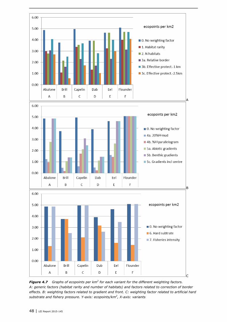
48 | LEI Report 2015-145

A

B

C

Figure 4.7 Graphs of ecopoints per km2 for each variant for the different weighting factors.

A: generic factors (habitat rarity and number of habitats) and factors related to correction of border

effects. B: weighting factors related to gradient and front. C: weighting factor related to artificial hard

substrate and fishery pressure. Y-axis: ecopoints/km2, X-axis: variants

LEI Report 2015-145 | 49

A

B

C

Figure 4.8 Graphs of total Ecopoints per variant for each weighting factor. Y-axis: ecopoints,

X-axis: variants. A: generic factors (habitat rarity and number of habitats) and factors related to

correction of border effects. B: weighting factors related to gradient and front. C: weighting factor

related to artificial hard substrate and weighting factor Fisheries pressure

50 | LEI Report 2015-145

4.3.5 Step 5. Test of robustness/sensitivity

Table 4.8 provides an overview of the contribution of each quality indicator and weighting factor to the

ecopoint score. From this table it becomes clear that the outcome of the ecopoint equation is largely

determined by surface area (km2) and some weighting factors. Surface area determines the score

largely because it is relatively large compared to the sum of the quality indicators. The total sum of

quality indicators can theoretically add up to 9 (based upon 9 indicators). In this study however, the

maximum ‘quality’ for the subareas is 5.89 (Table 3.1). Compared to the range of values of surface

area (12-63) the outcome of the equation will always be steered by area size and not by quality.

Within the selection of weighting factors, ‘% parallelogram’ (factor 20), ‘% mud’ (factor 8.3), and

‘effective area (2.5 km border)’ (factor 6.3) have the largest contribution in discriminating between

variants.

Looking into detail within the quality indicators, species richness, long-lived species and large species

have the largest contribution in discriminating the score.

Table 4.8

Range of scaled values (min - max) for each element in the equation (individual quality indicators,

surface area and weighting factors) including the difference, and the factor min/max as an indication

for contribution of each element in the equation

Min value Max value Difference Factor min/max

surface area area size 12 63.00 51.00 5.3

Quality

indic

ato

rs

biomass 0.37 0.57 0.20 1.5

eveness 0.35 0.47 0.12 1.3

large_species 0.22 0.62 0.40 2.8

long-lived species 0.25 0.58 0.33 2.3

species richness 0.46 0.81 0.35 1.8

density 0.36 0.47 0.11 1.3

biomass 0.43 0.65 0.22 1.5

density 0.55 0.73 0.18 1.3

richness 0.37 0.77 0.40 2.1

sum of quality indicators 3.36 5.67 2.31 1.7

Weig

hting f

acto

r

1. habitat rarity 0.29 0.93 0.64 3.2

2. N habitats 0.57 1.00 0.43 1.8

3a. relative border 0.43 1.00 0.57 2.3

3b. Effective protect.-1 km 0.67 0.97 0.30 1.5

3c. Effective protect.-2.5km 0.15 0.93 0.78 6.2

4a. 20%FFmud 0.12 1.00 0.88 8.3

4b. %FFparallelogram 0.05 1.00 0.95 20.0

5a. Abiotic gradients 0.29 1.00 0.71 3.4

5b. Benthic gradients 0.38 1.00 0.62 2.6

5c. Gradients incl centre 0.38 1.00 0.62 2.6

6. Artificial hard substrate 0.28 1.00 0.72 3.6

7. Fisheries pressure 0.67 1.00 0.33 1.5

4.4 Ecosystem development: Qualitative description

4.4.1 Quality indicators: limited benthos approach

The MSFD follows the ecosystem approach and therefore it can be discussed whether the applied

selection of benthic quality indicators is broad enough to assess the overall ecological benefit of the

area closures. Various ecosystem components (species groups other than benthos) and ecosystem

services were considered whether they could be part of the assessment (Appendix 3). These other

LEI Report 2015-145 | 51

ecosystem aspects include the function of the area in terms of e.g. connectivity, breeding area,

foraging area, or export of larvae. Connectivity within ecosystems and between ecosystems are very

relevant aspects to consider.

Jongbloed et al. (2013) reported that the Frisian Front ecosystem is relatively more connected to other

regions compared to Central Oyster Grounds due to its geographical position in combination with local

currents. In general, import and export of larvae are assumed to be larger from and to the Frisian

Front than to and from the Central Oyster Grounds (Jongbloed et al., 2013). The studies listed in

Appendix 3 did however not contain spatial biodiversity data on the level of the variants.

Since the area closures should contribute to the protection of vulnerable benthic species it would have

been useful to include data on vulnerable species for both mega benthos (Triple D data), and macro

benthos (box core data). However, Bos et al. (2011) and other studies could not provide such maps

for mega benthos, making this only a Limited Benthos Approach (LBA). On the other hand, adding 1

more quality indicator to a suit of 9 indicators will probably not result in large changes in the final

ecopoint calculations between the variants (see Section 4.4.3).

Closure of areas will most probably not only be beneficial to benthic species, but also to other species

groups, ecological functions and ecosystem services (see Section 4.4.5). This depends on the size and

position of the area. Variants habitat characteristics, and connectivity to the region are important

aspects for additional benefits for e.g. fish. Data on fish were however not included, because fish are

very mobile, and closed areas of relatively small sizes will in general not contribute to restoring fish

populations of vulnerable species such as sharks or rays. Closed areas of > 3,600 km2 (60 x 60 km2)

are mentioned by Bergman et al. (1991) to provide protection for fish. This is approximately the size

of an ICES rectangle. Although included quality indicators did not contain the fish component of the

ecosystem, the larger variants (Eel and Flounder, covering > 3,600 km2) are expected to contribute to

recovery or protection of some less mobile or homing fish species (maybe including rays).

4.4.2 Artificial hard substrata as proxy for biodiversity

Artificial hard substrata such as shipwrecks and oil & gas facilities contribute to the total biodiversity of

a predominantly muddy or sandy area, since they provide hard substrate which attracts a different

group of species. Up to 90% of the species present on shipwrecks in the Belgian part of the North Sea

was found to be absent in the surrounding sandy bottom (Zintzen, 2007). Van Moorsel (2014)

reviewed the species present on artificial and natural hard substrata in the international North Sea. He

reports 417 species that are specific for hard substrata and concluded that these form an important

part of the benthic life in the North Sea. Of these species, 113 were found exclusively on artificial hard

substrata.

A relevant function of artificial hard substrata in the context of seabed protection could be that it

serves as a single-point refugium, since species in the immediate surroundings are probably less

affected by bottom trawling fisheries. The distance of trawling to wrecks however depends largely on

the type of fisheries. Cod and seabass fisheries using trawled nets fish as close to wrecks as possible

to catch fish. Fishing in the 500 m exclusion zone around oil and gas installations is prohibited and it is

likely to be of low intensity around shipwrecks. Without detailed knowledge on their biodiversity, the

estimated number of shipwrecks and oil and gas facilities could therefore either be used as a proxy of

hard substrate biodiversity and as a proxy of the number of refugia and serve as an additional quality

indicator.

A wreck’s potential for contributing to biodiversity depends on many additional factors: Size, age and

level of decay, vertical position (%under of above sediment, type of habitat), material (steel, wood,

iron). Biodiversity data or data on the ecological function of shipwrecks in the area of interest are

lacking to present better estimations. Although in 2013 the biodiversity of 10 shipwrecks was

investigated (Lengkeek et al., 2013) and scuba divers collected data on the biodiversity of ~100

wrecks in the North Sea in 2010-2015 (see e.g. Gittenberger et al., 2013; Lengkeek et al., 2013;

Schrieken et al., 2013; Coolen et al., 2015), data in the search area are too limited for specific

shipwreck biodiversity values per variant. Finally, the wrecks’ status and size, which vary a great deal,

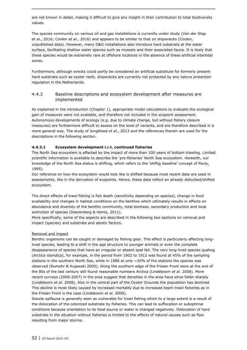
52 | LEI Report 2015-145

are not known in detail, making it difficult to give any insight in their contribution to total biodiversity

values.

The species community on various oil and gas installations is currently under study (Van der Stap

et al., 2016; Coolen et al., 2016) and appears to be similar to that on shipwrecks (Coolen,

unpublished data). However, many O&G installations also introduce hard substrata at the water

surface, facilitating shallow water species such as mussels and their associated fauna. It is likely that

these species would be extremely rare at offshore locations in the absence of these artificial intertidal

zones.

Furthermore, although wrecks could partly be considered an artificial substitute for formerly present

hard substrata such as oyster reefs, shipwrecks are currently not protected by any nature protection

regulation in the Netherlands.

4.4.3 Baseline descriptions and ecosystem development after measures are

implemented

As explained in the introduction (Chapter 1), appropriate model calculations to evaluate the ecological

gain of measures were not available, and therefore not included in the ecopoint assessment.

Autonomous developments of ecology (e.g. due to climate change, but without fishery closure

measures) are furthermore difficult to assess on the level of variants, and are therefore described in a

more general way. The study of Jongbloed et al., 2013 and the references therein are used for the

descriptions in the following section.

4.4.3.1 Ecosystem development i.r.t. continued fisheries

The North Sea ecosystem is affected by the impact of more than 100 years of bottom trawling. Limited

scientific information is available to describe the ‘pre-fisheries’ North Sea ecosystem. Herewith, our

knowledge of the North Sea status is shifting, which refers to the ‘shiftig baseline’ concept of Pauly,

1995).

Our reference on how the ecosystem would look like is shifted because most recent data are used in

assessments, like in the derivation of ecopoints. Hence, these data reflect an already disturbed/shifted

ecosystem.

The direct effects of trawl fishing is fish death (sensitivity depending on species), change in food

availability and changes in habitat conditions on the benthos which ultimately results in effects on

abundance and diversity of the benthic community, total biomass, secondary production and local

extinction of species (Deerenberg & Heinis, 2011).

More specifically, some of the aspects are described in the following two sections on removal and

impact (species) and substrate and abiotic factors.

Removal and impact

Benthic organisms can be caught or damaged by fishing gear. This effect is particularly affecting long-

lived species, leading to a shift in the age structure to younger animals or even the complete

disappearance of species that have an irregular or absent spat fall. The very long-lived species quahog

(Arctica islandica), for example, in the period from 1902 to 1912 was found at 45% of the sampling

stations in the southern North Sea, while in 1986 at only ~20% of the stations the species was

observed (Rumohr & Kujawski 2000). Along the southern edge of the Frisian Front were at the end of

the 80s of the last century still found reasonable numbers Arctica (Lindeboom et al. 2008). More

recent surveys (2006-2007) in the area suggest that densities in the area have since fallen sharply

(Lindeboom et al. 2008). Also in the central part of the Oyster Grounds the population has declined.

This decline is most likely caused by increased mortality due to increased beam trawl fisheries as in

the Frisian Front is the case (Lindeboom et al. 2008).

Sessile epifauna is generally seen as vulnerable for trawl fishing which to a large extent is a result of

the dislocation of the colonized substrate by fisheries. This can lead to suffocation or suboptimal

conditions because orientation to its food source or water is changed negatively. Dislocation of hard

substrate in the situation without fisheries is limited to the effects of natural causes such as flow

resulting from major storms.

LEI Report 2015-145 | 53

In addition, smaller species are less impacted by fisheries than larger species which is explained by

the generally slower recovery of larger species (Hiddink et al. 2006). The study indicates that a

reduction in species diversity is primarily caused by the loss of large species. Regarding the succession

and age structure of species, fisheries will result in a reset of the succession sequence to an earlier

stage. The consequences can be seen in the age structure and the presence of species that are

indicative of soil disturbance, ie that benefit from it (e.g. Van Kooten et al., 2015).

Alteration of substrate and abiotic factors

The structure of the bottom substrate can be affected by the trawled gears. There are two effects to

distinguish (Heinis & Deerenberg, 2011) :

• The removal of abiotic and biotic structures, such as sand ribs and biogenic reefs, so that also the

related biota is affected.

• The homogenization of the soil structure.

The structure of the substrate for the slopes to the deep silty areas more important than for shallow

sandy soils (references in Jak et al., 2009).

Trawl fishing causes a re-suspension of fine sediments (see van der Molen et al., 2013)). Via direct

and indirect effects decomposition processes result in increased oxygen consumption. In combination

with the reduced oxygen tension by the summer stratification, this may lead to additional oxygen

stress and increased mortality. The model study of Van der Molen et al. (2013) suggests that the

effects of bottom fisheries and climate change are additive but that the effects on nutrient fluxes in

the Central Oyster Grounds are relatively small.

In conclusion, fishing leads to set backs of the succession of ecosystem development to an earlier

stage. The consequences are observed in the age structure and the presence of species that are

indicative of soil disturbance, or benefiting from them. Continued fisheries will result in sustained

setbacks of ecosystem succession, preventing the ecosystem to recover and develop into a state with

long-lived and vulnerable species.

4.4.3.2 Ecosystem development after exclusion of fisheries

Generic development

In an expert workshop in 2013, various researchers discussed the possible ecological development of

the Frisian Front and the Central Oyster Grounds given the hypotheses that fisheries would be

excluded. The results are described by Jongbloed et al. (2013) and the included literature (e.g.

Duineveld et al., (2007)) and summarised in this section.

After exclusion of trawl fishing in an area, it is expected that seabed structure will change towards

natural intrinsic conditions, resulting in an increase in natural bioturbation4 combined with the

increased influence of occasional storms on the one hand and increased stabilisation of the sediment

on the other hand. A benthic community can develop in which epifauna has a larger role and share.

Biodiversity may increase and this may be a recovery towards a natural situation. The prevalence of

worms will decrease, and bivalves and burrowing sea urchins can increase. The biomass of epi- and

infauna will potentially increase, but a prediction on actual numbers is hard as it depends on various

uncontrolled factors. It is expected that the age distribution and densities of the species will change.

Which specific species this will be, and how they will affect the soil is speculation. Some experts

expect that biodiversity will increase if top predators also have more opportunities in the North Sea.

Biogenic structures and their associated soil fauna can recover. Habitats associated with these

structures are more heterogeneous. An increase in the density of shellfish and species diversity of soil

fauna is expected. The period over which a benthic community recovers cannot be exactly determined.

On the basis of various studies, it is expected that this may be in the order of 5 to 25 years. The

presence of a source population outside the area (connectivity) is one of the important factors for

recovery. This is however regarded by experts as an unpredictable factor. A restored seabed is of

ecological value to the region as well (Jongbloed et al., 2013).

4 Bioturbation is the reworking of sediments by animals or plants. Its effects include e.g. changing texture of sediments

54 | LEI Report 2015-145

Development on the Central Oyster Grounds and Frisian Front

In the study of Jongbloed et al. (2013), the Frisian Front and the Central Oyster Grounds are similar in

assumed development with regard to the following developments after stopping trawl fishing-

assuming the whole area is closed:

Assumed biodiversity increase of benthos, development of biogenic structures, decrease of

scavengers, equal in worms, increase of crustaceans and bivalves, increase of sensitive fish species

and predatory fish and large specimens of certain species.

The Frisian Front and the Central Oyster Grounds differ with respect to the following assumed

developments:

Frisian Front ecosystem has a faster recovery of benthic fauna (for a start situation which is a result of

a greater impact of fisheries and dynamism, heterogeneity and dynamics of the landscape), higher

potential for growth of long-lived benthic (individuals and species), higher potential for growth of

biomass, higher potential for increasing biodiversity, higher potential for several types of big fish.

In addition, return of the historical ecosystem of the Central Oyster Grounds (where oyster beds were

key elements) is not expected in the foreseeable future due to the absence of hard structures.

However, reintroduction of native flat oysters may lead to a partial restoration. It is also noted by

Jongbloed et al., (2013) that this is not an end in itself, the viewing direction should be recovery from

the current situation, and not historic. It was noted that the potential natural oyster beds may develop

again, provided there is hard substrate present when the oyster larvae settle. There are shell

remnants (which can serve as a hard substrate) present. There may, in principle, only few hard

structure to be present in order to allow formation of oyster- beds and other biogenic structures.

The supply of oyster larvae will also determine whether oysters can return to the area. There is no

record of where potential source populations are located. In future, the quahog can spread in the

northern part of the Central Oyster Grounds, potentially making a major contribution to the status of

local biomass and long lived species.

Next to the assumptions from the experts as summarised above, a technical evaluation study was

performed on the effect of a partial fisheries closure in an area close by the FF and CO - the Plaice Box

(PB). Beare et al. (2013) evaluated whether the PB has been an effective management measure. The

changes in the ecosystem (plaice, demersal fish, benthos) and fisheries were analysed to test whether

the observed changes are due to changes in the environment unrelated to the PB or to the PB closure.

Data showed that juvenile growth rate of plaice decreased and juveniles moved to deeper waters

outside the PB. Demersal fish biomass decreased, whereas the abundance of epibenthic predators

(seastars and brown crab) increased in the PB. Polychaetes and small bivalves, the main food items of

plaice, remained stable or decreased both inside and outside the PB. Beare et al. (2013) concluded

that the observed changes were most likely related to changes in the North Sea ecosystem, which

may be related to changes in eutrophication and temperature. It is less likely that observed changes

are related to the change in fishing.

4.4.4 Generic effects of displacement on ecology

Slijkerman and Tamis (2015) provided an overview of recent literature on ecological effects of

displacement. Displacement of fishing effort to other areas could lead to effects on habitats and/or

species, depending on:

fishing effort prior and after closure

amount of effort displaced, as well as the gear type

homogeneity of trawling effort after closure

protected species within the closed area, i.e. fish- or benthic species

additional management measures

4.4.4.1 Displacement- generic ecological effects

Understanding the spatial-temporal patterns of fishing-effort allocation around closed areas is

essential for assessing their effectiveness (Forcada et al., 2010). As described by Slijkerman and

Tamis (2015) there are many factors influencing fisheries distribution after area closure. Also the

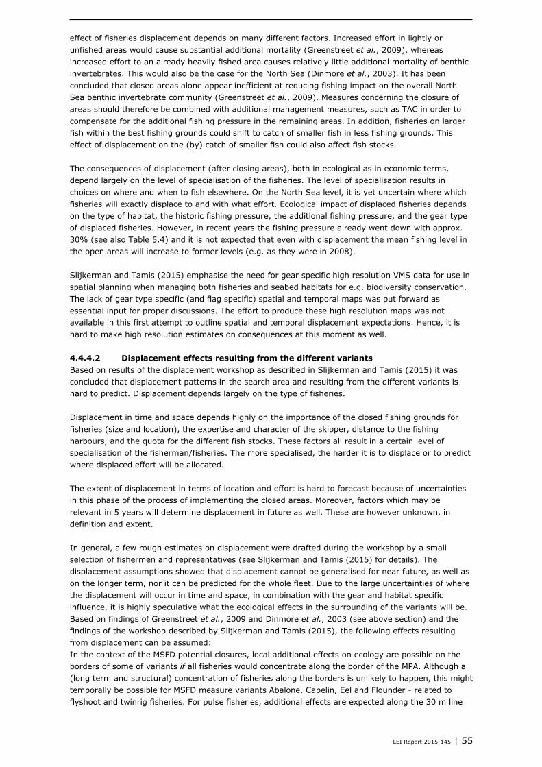
LEI Report 2015-145 | 55

effect of fisheries displacement depends on many different factors. Increased effort in lightly or

unfished areas would cause substantial additional mortality (Greenstreet et al., 2009), whereas

increased effort to an already heavily fished area causes relatively little additional mortality of benthic

invertebrates. This would also be the case for the North Sea (Dinmore et al., 2003). It has been

concluded that closed areas alone appear inefficient at reducing fishing impact on the overall North

Sea benthic invertebrate community (Greenstreet et al., 2009). Measures concerning the closure of

areas should therefore be combined with additional management measures, such as TAC in order to

compensate for the additional fishing pressure in the remaining areas. In addition, fisheries on larger

fish within the best fishing grounds could shift to catch of smaller fish in less fishing grounds. This

effect of displacement on the (by) catch of smaller fish could also affect fish stocks.

The consequences of displacement (after closing areas), both in ecological as in economic terms,

depend largely on the level of specialisation of the fisheries. The level of specialisation results in

choices on where and when to fish elsewhere. On the North Sea level, it is yet uncertain where which

fisheries will exactly displace to and with what effort. Ecological impact of displaced fisheries depends

on the type of habitat, the historic fishing pressure, the additional fishing pressure, and the gear type

of displaced fisheries. However, in recent years the fishing pressure already went down with approx.

30% (see also Table 5.4) and it is not expected that even with displacement the mean fishing level in

the open areas will increase to former levels (e.g. as they were in 2008).

Slijkerman and Tamis (2015) emphasise the need for gear specific high resolution VMS data for use in

spatial planning when managing both fisheries and seabed habitats for e.g. biodiversity conservation.

The lack of gear type specific (and flag specific) spatial and temporal maps was put forward as

essential input for proper discussions. The effort to produce these high resolution maps was not

available in this first attempt to outline spatial and temporal displacement expectations. Hence, it is

hard to make high resolution estimates on consequences at this moment as well.

4.4.4.2 Displacement effects resulting from the different variants

Based on results of the displacement workshop as described in Slijkerman and Tamis (2015) it was

concluded that displacement patterns in the search area and resulting from the different variants is

hard to predict. Displacement depends largely on the type of fisheries.

Displacement in time and space depends highly on the importance of the closed fishing grounds for

fisheries (size and location), the expertise and character of the skipper, distance to the fishing

harbours, and the quota for the different fish stocks. These factors all result in a certain level of

specialisation of the fisherman/fisheries. The more specialised, the harder it is to displace or to predict

where displaced effort will be allocated.

The extent of displacement in terms of location and effort is hard to forecast because of uncertainties

in this phase of the process of implementing the closed areas. Moreover, factors which may be

relevant in 5 years will determine displacement in future as well. These are however unknown, in

definition and extent.

In general, a few rough estimates on displacement were drafted during the workshop by a small

selection of fishermen and representatives (see Slijkerman and Tamis (2015) for details). The

displacement assumptions showed that displacement cannot be generalised for near future, as well as

on the longer term, nor it can be predicted for the whole fleet. Due to the large uncertainties of where

the displacement will occur in time and space, in combination with the gear and habitat specific

influence, it is highly speculative what the ecological effects in the surrounding of the variants will be.

Based on findings of Greenstreet et al., 2009 and Dinmore et al., 2003 (see above section) and the

findings of the workshop described by Slijkerman and Tamis (2015), the following effects resulting

from displacement can be assumed:

In the context of the MSFD potential closures, local additional effects on ecology are possible on the

borders of some of variants if all fisheries would concentrate along the border of the MPA. Although a

(long term and structural) concentration of fisheries along the borders is unlikely to happen, this might

temporally be possible for MSFD measure variants Abalone, Capelin, Eel and Flounder - related to

flyshoot and twinrig fisheries. For pulse fisheries, additional effects are expected along the 30 m line

56 | LEI Report 2015-145

or along the borders of the Frisian Front. The extent of the additional impact is however hard to

quantify due to limited information in this phase of the study. Flyshoot fisheries exploring e.g. the

Skagerrak will most probably display a heterogeneous distribution, resulting in a low or negligibly

additional ecological impact on the benthic community.

Economically, the consequences are drafted in the following chapters. Yet, we can state, that

fishermen without experience in the open remaining areas will be affected more compared to

fishermen with experience and more generalised way of fishing (exploring and adapting).

4.4.5 Ecosystem services and ecosystem valuation

During the stakeholder process various ecological factors were suggested to include in the

assessment. These aspects are discussed in this section.

The use of environmental valuation and cost-benefit analysis is done more and more by policymakers

(Borger et al., 2014). This means that policy-makers, regulators and stakeholders are placing

increasing demands on economists and ecologists to supply such values for use in policy analysis and

management (Hanley et al., 2014). There is also a growing emphasis on basing environmental

analysis and management on the ecosystem services (ES) approach (e.g. Fisher et al., 2008, Keeler

et al., 2012).

Ecosystem services are the benefits people obtain from ecosystems. These services include

provisioning, regulating, and cultural services that directly affect people and supporting services

needed to maintain other services. A clear example of a provisioning ecosystem service is the value of

fisheries. Examples of other services are resilience to climate change, mining sources for all kind of

compounds (e.g. medical, industrial or spiritual) and tourism.

There is still a lack of recognition and quantification of uncertainty in valuation of ecosystem services,

and furthermore, techniques for assessing and monetising non-use values are still widely criticised

(e.g. Parks and Gowdy, 2013; Bateman and Mawby, 2004; Gómez-Baggethun et al., 2014).

Quantification of ecosystem services (except for fisheries value which is quantified in Chapter 5) is an

upcoming science in which various techniques are being developed and tested. Some case studies

show interesting examples on the application of e.g. choice experiments, or so-called ‘willingness to

pay’ methods in which the total economic value of non-marketable goods are assessed. For the

Doggersbank valuation scenarios have been assessed using these methods (Borger et al., 2014).

The scientific knowledge on how to express ecosystem services using ecological data is also relatively

new. Hussain et al. (2010) demonstrated that the benefit estimation of ecosystem services is

complicated by scientific uncertainty and data gaps that hinder the development of a bottom-up

valuation of the ecosystem services. Overall, there are many issues related to economic valuation of

ecosystem services that require further research and discussion. Unfortunately, the lack to account for

the ecosystem services because of the difficulty associated with their valuation (Chan et al., 2012),

both economically as ecologically, exclude these important issues from the cost-benefit analysis in this

project so far.

LEI Report 2015-145 | 57

4.5 Discussion and conclusions

4.5.1 Summary of ecopoint scores

Table 4.9 and Table 4.10 present a summary of the previous tables for each variant. For each

weighting factor, the range of values is supported with a shading. The shading intensity categories are

applied within each column, in order to provide a quick overview of highest and lowest scores per

weighting factor. The intensity follows a gradual relation. The intensity of the grey colour indicates the

ranking of the ecopoints: the more intense the shading, the higher the ecopoint value and thus

ecological benefit. It becomes clear that when the ecopoints per km2 are multiplied by ‘area

(km2/100)’, that variant Flounder has most ecopoints, independent of the applied weighting factor.

Variant Brill has the lowest ecopoint total- except for ecopoints/km2 when hard substrates are

included. Averages and variation on the totals are not provided as the total scores are calculated as

weighted scores. To obtain some sense of variation we refer to Appendix 4 in which the scores of the

subareas are presented.

Table 4.9

Summary of ecopoints per km2 for each variant. Shading intensity indicates the order of the values

within columns

Table 4.10A

Summary of ecopoints per variant. Shading intensity indicates the relative values within columns

Var

ian

t

0. N

o w

eigh

tin

g fa

cto

r

1. H

abit

at r

arit

y

2. N

hab

itat

s

3a.

Rel

ativ

e b

ord

er

3b

. Eff

ecti

ve p

rote

ct.-

1 k

m

3c.

Eff

ecti

ve p

rote

ct.-

2.5

km

4a.

20

%FF

mu

d

4b

. %FF

par

alle

logr

am

5a.

Ab

ioti

c gr

adie

nts

5b

. Ben

thic

gra

die

nts

5c.

Gra

die

nts

incl

cen

tre

6. H

ard

su

btr

ate

7. F

ish

erie

s in

ten

sity

Abalone 4.87 2.98 2.78 3.07 4.06 2.70 1.24 0.97 2.78 4.87 4.87 1.34 4.87

Brill 3.74 1.10 2.14 1.61 2.51 0.58 0.48 0.19 1.07 1.40 1.40 3.74 2.50

Capelin 4.96 3.37 3.55 2.29 3.69 1.73 0.62 1.74 2.13 3.10 2.48 2.12 4.96

Dab 3.92 1.34 3.92 1.69 2.80 1.02 0.49 0.24 1.12 1.47 1.47 3.18 2.61

Eel 4.64 3.24 4.64 2.30 3.99 2.99 1.62 1.45 2.65 4.64 4.64 1.61 3.48

Flounder 5.08 4.00 4.72 3.12 4.70 4.09 5.08 5.08 5.08 5.08 5.08 1.44 5.08

Var

ian

t

0. n

o w

eigh

tin

g fa

cto

r

1. H

abit

at r

arit

y

2. N

hab

itat

s

3a.

Rel

ativ

e b

ord

er

3b

. Eff

ecti

ve p

rote

ct.-

1 k

m

3c.

Eff

ecti

ve p

rote

ct.-

2.5

km

4a.

20

%FF

mu

d

4b

. %FF

par

alle

logr

am

5a.

Ab

ioti

c gr

adie

nts

5b

. Ben

thic

gra

die

nts

5c.

Gra

die

nts

incl

cen

tre

6. H

ard

su

btr

ate

7. F

ish

erie

s in

ten

sity

Abalone 59 36 33 37 49 32 15 12 33 59 59 16 59

Brill 47 14 27 20 32 7 6 2 14 18 18 47 32

Capelin 79 54 57 37 59 28 10 28 34 50 40 34 79

Dab 66 23 66 28 47 17 8 4 19 25 25 53 44

Eel 195 136 195 97 168 126 68 61 111 195 195 68 146

Flounder 322 253 299 198 298 260 322 322 322 322 322 91 322

58 | LEI Report 2015-145

Table 4.10B

Ranking of ecopoints per variant. Shading intensity indicates the relative values. 11= lowest rank, 6 =

highest rank

4.5.2 Ranking the variants on ecopoint scores

Independent of the method of expressing the ecopoints - average per km2 or total for the area -

variant Flounder yields the most ecopoints, and thus highest ecological benefit compared to the other

variants (Tables 4.9 and 4.10). The subsequent ranking of the other variants depends on the way of

expressing the ecopoints, and the weighting factor applied. In the section below each contributing

factor to the ecopoint score is discussed. In Chapter 9 a synthesis of the highlights per variant is

presented.

4.5.2.1 Ecopoints per km2

Variant Flounder has the highest score- except of the ecopoints related to weighting factor ‘hard

substrate’. The high score on ecopoints is due to its large size- all factors are co-related with the

larger size- even if total area is not taken into account in the calculation. The larger areas contain

more habitats, species and score relatively good on weighting factors and consequently have more

ecopoints per km2.

The second best scoring variant depends on the applied weighting factor: most times it is either

variant Abalone or Eel. In general, variants Brill and Dab score lowest on ecopoints, except for

weighting factors hard substrate and number of habitats. The overall quality score of these variants

was lowest.

4.5.2.2 Ecopoints per area

When multiplying the values (quality * weighting factor) with the area (km2/100), variant Flounder

has the highest score (Table 4.9). Variant Eel ranks second. Comparing the ranking of variants of

approximately equal size shows that variant Abalone has a much higher score than Brill (both ~1200

km2), and variant Capelin has a higher rank than variant Dab (both ~1,600 km2).

4.5.2.3 Effect of weighting factors on ecopoints

In contrast to the quality indicators, the weighting factors can, to some extent, be used to select for a

variant that contributes more to the protection of the ecosystem as a whole than others. However,

different lines of thinking can be followed. If artificial hard substrate is considered an important part of

the ecosystem (see section on hard substrate), then weighting factor 6 should be considered in the

decision making process. If the aim is to protect a diverse and unique area with numerous functions

on a North Sea wide scale, then weighting factors considering the inclusion of the frontal area should

be given importance. If the aim is to emphasise benthic biodiversity values, then it would make sense

to look at the quality alone, and not use a weighting factor. When fisheries pressures is set as a proxy

for relative recovery, weight factor 7 should be considered. And if it is considered important that a

single large area is chosen, to avoid benthic animals to leave the protected area, or to make sure that

Var

ian

t

0. n

o w

eigh

tin

g fa

cto

r

1. H

abit

at r

arit

y

2. N

hab

itat

s

3a.

Rel

ativ

e b

ord

er

3b

. Eff

ecti

ve p

rote

ct.-

1 k

m

3c.

Eff

ecti

ve p

rote

ct.-

2.5

km

4a.

20

%FF

mu

d

4b

. %FF

par

alle

logr

am

5a.

Ab

ioti

c gr

adie

nts

5b

. Ben

thic

gra

die

nts

5c.

Gra

die

nts

incl

cen

tre

6. H

ard

su

btr

ate

7. F

ish

erie

s in

ten

sity

Abalone 2 3 2 4 3 4 4 3 3 4 4 1 3

Brill 1 1 1 1 1 1 1 1 1 1 1 3 1

Capelin 4 4 3 3 4 3 3 4 4 3 3 2 4

Dab 3 2 4 2 2 2 2 2 2 2 2 4 2

Eel 5 5 5 5 5 5 5 5 5 5 5 5 5

Flounder 6 6 6 6 6 6 6 6 6 6 6 6 6

LEI Report 2015-145 | 59

certain ecosystem functions have a higher change to be restored, then weighting factor 3 could be

important. Of course the size of the closed areas themselves is of large importance, but they are not a

weighting factor as this is expressed by the ecopoints for the total area. The average or sum of all

separate ecopoints combined can be sued to evaluate the overall score for a variant.

The generic weighting factors differentiate the scores of ecopoints as follows (score/km2). Flounder

has highest ecopoint scores, and Brill has lowest ecopoint scores. The ranking in between depends on

the weighting factor of interest. Weighting factors ‘habitat rarity’ and ‘habitat diversity’ rank Abalone,

Dab, Capelin, and Eel differently than weighting factors expressing the effective area. Effective area

rank Dab and Brill lowest, whereas Dab scores relatively high when applying the number of habitats as

a weighting factor.

When looking at the total score- in which area is taken into account as well, the highest and lowest

score are attributed to Flounder and Brill as well. Variant Eel is always second in rank, independent of

the weighting factor.

The weighting factors emphasising the frontal area and gradients rank the variants differently than the

generic factors. Although Flounder still scores highest and Brill lowest, the ranking in between differs

significantly, as well the relative scores. Taking into account the score per km2, variant Abalone

benefits from the weighting factors in which gradients are taken into account. Its overall score

increases compared to the other variants. The way of expressing the gradient - with or without the

frontal area as an obligatory aspect - does not influence its rank. Overall it is clear that variant

Abalone scores relatively higher and thus reflect more ecological benefit when taking into account the

ecological significance of gradients and the frontal area. Variant Capelin scores relatively lower

compared to Abalone.

The weighting factor reflecting the density of artificial hard substrate rank the variants totally different

compared to the other factors. When expressed as ecopoint/km2 Brill scores highest, followed by Dab

and Capelin. Abalone and Flounder score lowest.

The weighting factor reflecting fisheries pressure rank the variant more or less the same as the

generic weighting factor 0 (no weighting factor), 1 (habitat rarity) and factor 3 (effective protection).

Brill scores lowest, and Flounder highest when fisheries pressure- as a proxy for habitat recovery- is

taken into account.

4.5.2.4 Sum of quality at the subarea level

Ecopoints are a sum of the equation to which habitat quantity (area), habitat quality (biodiversity) and

weighting factors contribute. In this section, the influence of the quality per subarea is discussed.

These values are presented in Appendix 4. Values for hard substrate and fisheries pressure were not

included on the subarea level.

Overall, the sum of the quality (see Table 4.2 and 4.3 and Figure 4.4) is highest for variant Flounder,

followed by Capelin. Lowest quality score have variants Brill and Dab. The overall quality score ranges

from 3.74-5.08. The highest possible score was 9. The highest quality of a subarea is obtained by the

Frisian Front subarea.

Taking into account the scores of subareas it is obvious that the quality score per subarea is

determined by different indicators. In general, subareas covering the Central Oyster Grounds score

relatively high on ‘large species’, ‘long-lived species’ and species richness of the macrobenthos

compared to Frisian Front subareas, while Frisian Front subareas in general score relatively high on

quality indicators ‘biomass’ and ‘density’. Furthermore, the megabenthos values for species richness,

density and biomass are relatively higher for Frisian Front areas compared to Central Oyster Ground

subareas.

Long-lived species scores are highest for Eel and Abalone, and Eel scores highest for large species as

well. These scores are all related to the Central Oyster Ground subareas. Species richness of the

macrobenthos is highest for Flounder and Brill CO subareas. Capelin Frisian Front subareas scores

relatively high on megabenthos density and richness, followed in rank by Flounder Frisian Front

subarea and Brill and Dab Frisian Front subareas.

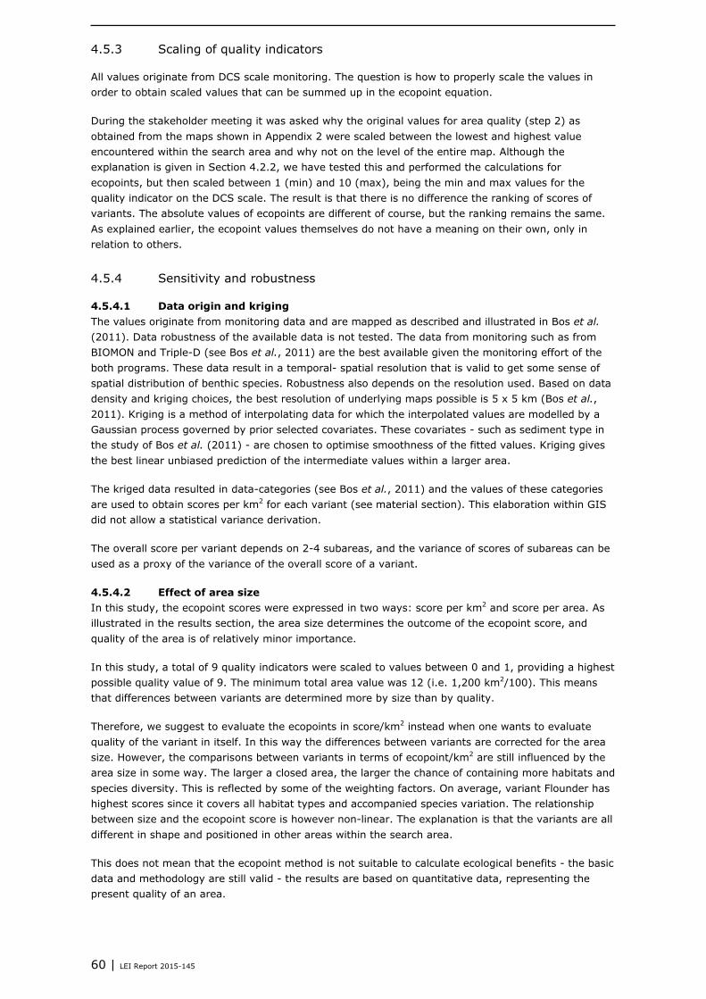
60 | LEI Report 2015-145

4.5.3 Scaling of quality indicators

All values originate from DCS scale monitoring. The question is how to properly scale the values in

order to obtain scaled values that can be summed up in the ecopoint equation.

During the stakeholder meeting it was asked why the original values for area quality (step 2) as

obtained from the maps shown in Appendix 2 were scaled between the lowest and highest value

encountered within the search area and why not on the level of the entire map. Although the

explanation is given in Section 4.2.2, we have tested this and performed the calculations for

ecopoints, but then scaled between 1 (min) and 10 (max), being the min and max values for the

quality indicator on the DCS scale. The result is that there is no difference the ranking of scores of

variants. The absolute values of ecopoints are different of course, but the ranking remains the same.

As explained earlier, the ecopoint values themselves do not have a meaning on their own, only in

relation to others.

4.5.4 Sensitivity and robustness

4.5.4.1 Data origin and kriging

The values originate from monitoring data and are mapped as described and illustrated in Bos et al.

(2011). Data robustness of the available data is not tested. The data from monitoring such as from

BIOMON and Triple-D (see Bos et al., 2011) are the best available given the monitoring effort of the

both programs. These data result in a temporal- spatial resolution that is valid to get some sense of

spatial distribution of benthic species. Robustness also depends on the resolution used. Based on data

density and kriging choices, the best resolution of underlying maps possible is 5 x 5 km (Bos et al.,

2011). Kriging is a method of interpolating data for which the interpolated values are modelled by a

Gaussian process governed by prior selected covariates. These covariates - such as sediment type in

the study of Bos et al. (2011) - are chosen to optimise smoothness of the fitted values. Kriging gives

the best linear unbiased prediction of the intermediate values within a larger area.

The kriged data resulted in data-categories (see Bos et al., 2011) and the values of these categories

are used to obtain scores per km2 for each variant (see material section). This elaboration within GIS

did not allow a statistical variance derivation.

The overall score per variant depends on 2-4 subareas, and the variance of scores of subareas can be

used as a proxy of the variance of the overall score of a variant.

4.5.4.2 Effect of area size

In this study, the ecopoint scores were expressed in two ways: score per km2 and score per area. As

illustrated in the results section, the area size determines the outcome of the ecopoint score, and

quality of the area is of relatively minor importance.

In this study, a total of 9 quality indicators were scaled to values between 0 and 1, providing a highest

possible quality value of 9. The minimum total area value was 12 (i.e. 1,200 km2/100). This means

that differences between variants are determined more by size than by quality.

Therefore, we suggest to evaluate the ecopoints in score/km2 instead when one wants to evaluate

quality of the variant in itself. In this way the differences between variants are corrected for the area

size. However, the comparisons between variants in terms of ecopoint/km2 are still influenced by the

area size in some way. The larger a closed area, the larger the chance of containing more habitats and

species diversity. This is reflected by some of the weighting factors. On average, variant Flounder has

highest scores since it covers all habitat types and accompanied species variation. The relationship

between size and the ecopoint score is however non-linear. The explanation is that the variants are all

different in shape and positioned in other areas within the search area.

This does not mean that the ecopoint method is not suitable to calculate ecological benefits - the basic

data and methodology are still valid - the results are based on quantitative data, representing the

present quality of an area.

LEI Report 2015-145 | 61

5 Fishing activities in the areas

Hans van Oostenbrugge, Katell Hamon Niels Hintzen and Marcel Machiels

The first step in order to assess the effects of the closures on the fishing sector is the quantification of

the historic fishing activities in the areas. This is important for the estimation of the costs of closures

as historic data provide the basis for any analysis of effects of closures and the effect of closures

depend on the extent of fishing activities, the type of fisheries in the area and the dependency of

these fisheries on the area. This was done for the period from 2008-2014 for the Dutch fishing vessels

and from 2011-2014 for foreign vessels. Fishing activities in the areas were quantified in terms of

effort, landings volume, landings value and contribution to the Gross Value Added (GVA). The GVA is

especially important as this metric indicates the value of the fishing activities to society: the returns

on the invested capital (fishing vessel) and labour by the crew. For the Dutch fishing vessels also the

dependency on the areas was estimated per vessel as this is important for the effects of closures on

the fishing practices and herewith on the potential costs (see also Chapter 6).

5.1 Methodology

5.1.1 Fishing activities of Dutch vessels

5.1.1.1 Total fishing activities

The methods applied and the data used to assess the fishing activities in the areas were similar to

those used for the previous studies (e.g. Van Oostenbrugge et al., 2010). In addition some extra data

checks were included and another data processing platform was used for part of the analysis. Because

of the large similarity in the method, this report contains a limited description focusing on small

adjustments that have been made. A complete description can be found in Van Oostenbrugge et al.,

2010.

Several steps were needed to process the Dutch data for the analysis. First of all, the Vessel

Monitoring Data (VMS data) were processed and the patterns in fishing efforts were determined. To

clean up the VMS data set, the R package VMStools was used (Hinzen et al., 2011). Duplicated points,

points in harbour, points on land and points with impossible speed/location (<1% of total) were

removed.

Next, the fishing efforts were used to distribute the catches between the various points. The method

used is illustrated by the example included in Table 5.1. The fishing vessel carries out a fishing trip

from 14:00 to 19:00 hours on 21 August. First, the vessel speed was used to determine whether the

vessel was fishing or steaming at each VMS point based on speed thresholds derived from South et al.

(2009) and an analysis of frequency distribution of VMS-speed data by vessel and year.

62 | LEI Report 2015-145

Table 5.1

Example of a calculation of the catch at the VMS positions during one trip of a vessel of 300 hp using

Otter board Trawl (OTB)

DH1 time Speed Time since last

position

catch

21-aug 14:00 0.2

21-aug 15:00 5.6 1:00 0

21-aug 17:00 3.4 2:00 1,200

21-aug 18:00 3.2 1:00 600

21-aug 19:00 0 1:00 0

Total catch 1.800

In Table 5.1 the speed of VMS point at time 14:00 is too low to be fishing. At the second VMS point

(15:00) the speed is too high to be fishing. Therefore neither of these points get catch attributed. The

next two VMS points (17:00 and 18:00) have a speed that falls within speed range for which we

assume the vessel to be fishing. Next, the duration was determined for each position (the time

interval between the current and previous position). The catch (kg) was distributed on the basis of the

duration at the various positions at which the vessel was fishing.

Table 5.2 shows the thresholds per gear determining fishing and steaming activities. Any gears

missing in this table were assigned the activity Unknown.

Table 5.2

Determination fishing and steaming activity

Gear Fishing Steaming

Gill nets, Danish seines speed<0.3 speed>=0.3

Scottish seine speed<7 speed>=7

Beam trawl, shrimp trawl Speed within 3 to 6 Speed<3 or speed>6

Otter board trawl 0-300hp Speed within 3 to 5 Speed<3 or speed>5

Otter board trawl >300hp Speed within 3 to 4 Speed<3 or speed>4

Twin trawl 0-300hp Speed within 3 to 5 Speed<3 or speed>5

Twin trawl >300hp Speed within 3 to 4 Speed<3 or speed>4

Source: South et al. (2009).

The example in Table 5.1 illustrates the ideal situation where a trip is comprised of a number of fishing

and/or steaming VMS points and the day catch is available. This was not always the case. Several

factors could complicate the distribution of catch over the VMS points. For example in a number of

cases a vessel was sailing at all the available VMS positions on a day or data were lacking, for example

on the fishing gear, HP and speed, which made it not possible to allocate an activity to a VMS point.

To still be able to allocate catch to VMS locations a number of assumptions needed to be made in the

case of missing data. The distribution methods used in these cases are summarised in Table 5.3.

LEI Report 2015-145 | 63

Table 5.3

Distribution catch in several situations (see text for further explanation

Day catch recorded for trip Day catch

recorded on day

Type of Activity Distribution

Yes Yes Fishing and other Fishing time/fishing time on

fishing day

Yes Yes Only steaming Catch not distributed

Yes Yes Only unknown Time unknown/time on fishing

day unknown

Yes Yes Steaming and Unknown Catch not distributed

Yes No All combinations Catch not distributed

No No Fishing and other Fishing time/fishing time on

fishing day

No No Only steaming Catch not distributed

No No Only unknown Time unknown/time on trip

unknown

No No Steaming an unknown Catch not distributed

The VMS data do not provide full coverage. This is, in particular, due to vessels with a length less than

12 meters and which consequently do not have on-board VMS as well as an inability to fully distribute

all the catches between VMS points. Moreover some landings cannot be distributed because of the

specifics of the VMS data of a trip (see Table 5.3). This was corrected by increasing the landings at

each location by a factor based on coverage percentages per gear and type of vessel. So for example

if for a certain gear type the coverage was 95%, the total catches with this gear type were multiplied

by a factor (1/0.95). This approach facilitated the distribution of all catches found in the VIRIS logbook

data.

The catches and average auction prices were used to determine the value of the catches at the various

VMS points. Finally, the contribution to the gross value added was calculated on the basis of the

average cost structure for each year, type of vessel and type of fishery, as known in LEI’s Farm

Accountancy Data Network.

This described method is in agreement with the methods used in earlier LEI reports on the estimation

of the value of fishing areas (such as Van Oostenbrugge et al., 2010).

5.1.1.2 Dependency analysis

For each vessel and year combination the level of dependency on the closed areas was calculated as

the percentage of the annual revenue coming from each of the proposed closed areas in the various

variants. Average dependencies over the time period were calculated for each vessel. The individual

dependency levels were aggregated in so called stress profiles, showing the distribution of vessels

over the various dependency levels. Dependency levels have been calculated on both annual and

quarterly level.

5.1.2 Fishing activities of foreign vessels

Recent trends in the fishing intensity in the areas has been assessed for the Danish, German, Belgian

and UK fishing fleets. This was done by analysing the Vessel Monitoring System datasets available at

the national fisheries institutes and estimating the effort in each of the variants. Because the VMS

data are available in a uniform data format (EFLALO), this could be done by using a uniform analysis

script written in R.5 To estimate the effort in the areas, the same methodology was used as for the

Dutch fishing fleet. For the German and Belgian fleet it was possible to distinguish between vessels

owned by foreign companies and those owned by Dutch companies (flag vessels). This was done

based on a list of these vessels provided by the fisheries sector. For the UK fleet merging the list of

5 R is an open-source statistical software package that is widely used in fisheries science.

64 | LEI Report 2015-145

flag vessels was not possible. These analyses resulted in the amount of effort (sea days) per gear,

vessel length class and nationality in each of the variants. In order to assess the landings, landings

value and the GVA of the foreign fleets, the effort data were combined with information on catch

composition and economic information from the database of the Annual Economic Report of 2015

(STECF 2015). In this database, catch information (landing volume and value) is only available at the

level of gear and ICES subarea (e.g. Central North Sea). Because of this, the landings and landings

value was estimated by combining the effort information with average landings and landings values for

each gear type in the Central North Sea. The GVA was estimated using the proportion of landing and

GVA for the fishing fleet in question.

5.2 Data

5.2.1 Fishing activities of Dutch vessels

Several data sources were used in the evaluation. The data sources used were Vessel Monitoring

System (VMS) data, catch data from VIRIS (Fish Registration and Information System), Fleet data

from the Netherlands Register of Fishing Vessels (NRV), average monthly price data per species

collected by the Productschap Vis (Netherlands Fish Product Board) and economic data (The LEI

panel). The datasets used and the data coverage are described in more detail in Appendix 5.

5.2.2 Fishing activities of Foreign vessels

Effort data on foreign fleets were used from the EFLALO datasets of the sister institutes in Denmark,

Germany, Belgium and the UK. Data on landings volume, value and economic performance of foreign

fleets were taken from the database of the Annual Economic Report of the EU fishing fleets (AER

2015).

5.3 Results

5.3.1 Value for Dutch fishing vessels

5.3.1.1 Recent fishing activities

Over the last seven years the amount of fishing activities has been quite different in the various

variants and from year to year (Table 5.4). Variant Flounder shows by far the highest level of fishing

activities; on average the Dutch fleet spent around 730 days fishing in these areas creating a total

Gross Added Value (GVA) of around 1.6m euros. The amount of fishing activities in variant Brill was

the lowest (100 fishing days and a total GVA of around 0.2m euros), less than 15% of the fishing

activity in Flounder. The other variants show intermediate levels of activity. Variant Abalone and Dab

show comparable levels of effort and landings (around 140 fishing days and 320 tonnes of fish

annually). However, the value of landings and GVA for Abalone were around 20% higher (1m euros

and 0.35m euros, respectively) than for Dab (0.77m euros and 0.28m euros, respectively). The

number of fishing activities of Capelin is approximately twice the number of activities for Brill (190

fishing days and a total GVA of around 0.5m euros) and the fishing activities in Eel are approx. four

times the activities for Brill (360 fishing days and a total GVA of around 0.9m euros). The average

total value of the landings by the Dutch demersal fishing sector amounted approximately 250m euros

per year in the same period (www.visserijincijfers.nl). The values for the various subareas can be

found in Appendix 7.

LEI Report 2015-145 | 65

Table 5.4

Overview of effort, landings and values and gross value added of the Dutch fishing sector in the areas

of the different variants

Variant 2008 2009 2010 2011 2012 2013 2014 Average

Effort (fishing days)

Abalone 165 194 160 118 168 106 91 143

Brill 156 143 124 63 113 75 34 101

Capelin 221 261 241 193 155 156 124 193

Dab 230 217 156 78 135 94 46 136

Eel 505 481 428 268 344 292 214 362

Flounder 835 871 809 762 723 600 524 732

Landings (tonnes)

Abalone 295 345 328 166 640 209 321 329

Brill 184 223 182 67 616 236 82 227

Capelin 411 406 441 282 643 375 336 413

Dab 291 321 237 98 799 346 123 316

Eel 876 866 864 695 1,568 886 519 896

Flounder 1,535 1,459 1,618 1,686 2,372 1,359 1,377 1,630

Value (1000 euros)

Abalone 1,229 1,287 1,093 663 1,453 700 572 1,000

Brill 824 619 581 237 961 354 169 535

Capelin 1,681 1,523 1,451 1,095 1,398 1,017 816 1,283

Dab 1,337 996 744 307 1,259 506 243 770

Eel 3,467 2,970 2,741 1,796 3,296 2,201 1,436 2,558

Flounder 5,714 5,250 5,147 5,108 5,663 3,966 3,358 4,887

Gross Value Added (1,000 euros)

Abalone 403 548 400 225 412 274 199 352

Brill 300 268 216 74 290 139 62 193

Capelin 564 657 532 364 371 392 281 452

Dab 472 430 277 98 382 196 90 278

Eel 1183 1,279 1,000 510 922 772 516 883

Flounder 2015 2,270 1,883 1,572 1,418 1,428 1,199 1,684

a) preliminary estimates;

Source: Logbook data and VMS data, processed by LEI

Table 5.5

Average fishing intensity per km2 of the Dutch fishing sector in the variants over the period of 2008-

2014. Stdev is the standard deviation of the average over the years

Effort (fishing

days/km2)

Landings (kg/km2) Value (euros/km2) Gross Value Added

(euros/km2)

average stdev average stdev average stdev average stdev

Abalone 0.12 0.03 273 127 830 291 292 103

Brill 0.08 0.04 180 145 423 235 153 80

Capelin 0.12 0.03 259 71 803 195 283 84

Dab 0.08 0.04 188 139 458 263 165 93

Eel 0.09 0.03 213 77 608 183 210 72

Flounder 0.12 0.02 257 55 771 140 266 60

Source: Logbook data and VMS data, processed by LEI.

Although the size of the areas in the variants is a major determinant of the total level of fishing

activities, the fishing intensity per km2 also varies substantially (Table 5.5). Variants Abalone, Capelin

and Flounder show similar, relatively high fishing intensities; around 0.12 fishing days/km2 and a GVA

between 260-300 euros/km2. Fishing intensities for Brill and Dab are 30-50% lower; around

0.08 fishing days/km2 and a GVA between 150- 170 euros/km2. Eel shows intermediate fishing

intensity (around 0.09 fishing days/km2 and a GVA of 210 euros/km2.

66 | LEI Report 2015-145

Figure 5.1 Historical trends of the fishing activities by the Dutch fleet in the areas of the variants.

Effort, landings, value of landings and GVA are given by gear groups as specified in the European DCF.

Source: Logbook data and VMS data, processed by LEI.

For all variants the fishing activities have decreased substantially during the seven years taken into

consideration (Figure 5.1). On average, the effort, landings value and the GVA decrease around 50-

60%. The reductions in landings volume are considerably less; around 30% for all variants. This is

mainly due to the general increase in fishing opportunity in the North Sea and decreasing prices.

Variants Brill and Dab show the highest reduction in activities: effort, landings value and GVA are

reduced by around 75% and landings volume by around 60%. The reduction in fishing activity in

Flounder is lowest; around 40% in effort, landings value and GVA and less than 10% in landings

volume.

The main gear types used in the area are bottom gears such as beam trawl and its innovative

successors (puls trawl, pulswing and SumWing) and other types of bottom trawls. Over the period

2008-2014 beam trawls (including puls gears) accounted for 62% of the total effort and 64% of the

GVA. Other bottom trawls and seines were on average less important, accounting for 34% of the total

effort and 30% of the GVA. However, whereas the fishing activity of the beam trawls has decreased,

the fishing activities of other bottom trawls and seines such as otter trawl and twin trawl have been

stable or even increased. Because of this as from 2013 onwards beam trawls were no longer the

dominant gear used in the areas, but other bottom trawls and seines became more important. In 2012

Abalone Brill Capelin Dab Eel Flounder

0

250

500

750

0

500

1,000

1,500

2,000

0

2

4

0.0

0.5

1.0

1.5

2.0

Effo

rt (fishin

g d

ays)

Landin

gs (to

nnes)

Valu

e (m

illion e

uro

s)

GV

A (m

illion e

uro

s)

2008 2012 2008 2012 2008 2012 2008 2012 2008 2012 2008 2012

year

Gear Beam trawlers Demersal trawlers or seiners Pelagic trawlers Nets Others

LEI Report 2015-145 | 67

considerable catches of pelagic fish have been caught in the areas, but these catches were incidental

and they represent a low value because of the low prices of pelagic fish. Nets and other gears

(dredges or shrimp trawls) are hardly used in the areas.

Figure 5.2 Historical trends of the fishing activities by the Dutch beam trawl fleet (including

traditional and pulse trawls gears) in the areas of variants. Effort, landings, value of landings and GVA

are given by gear type; TBB, traditional beam trawl; TBS, shrimp trawl.

Source: Logbook data and VMS data, processed by LEI.

Activity levels of beam trawl fisheries (including puls gears) in the areas of the variants show similar

patterns as the total Dutch fisheries in the North Sea (Figure 5.2). The level of fishing activities are

lowest for variant Brill (average 62 fishing days and GVA of 0.13m euros), Abalone and Dab show

comparable levels of activity (around 90 fishing days and GVA of 0.18-0.24m euros) and Capelin, Eel

and Flounder show higher levels of fishing activity (resp. 120, 250 and 410 fishing days and GVA of

0.30m, 0.62m and 1.0m euros). In all variants the total fishing activity level of beam trawls has

decreased substantially but especially for Brill and Dab, the decrease has been very large (more than

90% for both fishing days and GVA). For other variants the decrease in fishing activity level was

around 70-80%. Within the beam trawls a partial shift has taken place from the traditional beam trawl

to the pulse wing gear. Was in 2008 100% of the fishing activity still carried out by traditional beam

trawl, in 2012 and 2013 this gear only contributed around one third of the effort and GVA in the areas.

Abalone Brill Capelin Dab Eel Flounder

0

200

400

600

0

250

500

750

1,000

1,250

0

1

2

3

4

0.0

0.5

1.0

1.5

2.0

Effo

rt (fishin

g d

ays)

Landin

gs (to

nnes)

Valu

e (m

illion e

uro

s)

GV

A (m

illion e

uro

s)

2008 2012 2008 2012 2008 2012 2008 2012 2008 2012 2008 2012

year

Gear Pulskor Pulswing Sumwing TBB TBS

68 | LEI Report 2015-145

In 2014 however, the relative importance of the traditional beam trawl increased again for some of

the variants; for Abalone Capelin and Flounder the importance of the traditional beam trawl increased

this year to around 60%. Good fishing opportunities for plaice and relatively low fuel prices might have

contributed to this development. For Dab and Eel, the pulse gears have become the most important

gears used with a relative importance of around 60% but total fishing intensity decreased substantially

in these variants from 2013 and 2014.

Figure 5.3 Historical trends of the fishing activities by the Dutch demersal trawlers in the areas of

the different variants. Effort, landings, value of landings and GVA are given by gear type: OTB, otter

trawl bottom; OTT, twin trawl; PTB, pair trawl bottom; SSC, Scottish seine (fly shoot fishery) (see also

Appendix 6).

Source: Logbook data and VMS data, processed by LEI.

Activity levels of ‘other trawls and seiners’ have been relatively high in all variants during the last

years and have become the most important gear type used in the area (Figure 5.3). Average fishing

activity level lowest in Brill and Dab. In these variants, the effort was around 15 and 20 fishing days

and the contribution of the areas to the GVA was 36 and 52 kEur. In the other variants fishing

activities ranged from 50 fishing days for Abalone, 70 fishing days for Capelin, 100 fishing days for Eel

to 310 fishing days for Flounder. The patterns in GVA resembled those in effort and relative

Abalone Brill Capelin Dab Eel Flounder

0

100

200

300

400

0

200

400

600

800

0.0

0.5

1.0

1.5

2.0

0.0

0.2

0.4

0.6

0.8

Effo

rt (fishin

g d

ays)

Landin

gs (to

nnes)

Valu

e (m

illion e

uro

s)

GV

A (m

illion e

uro

s)

2008 2012 2008 2012 2008 2012 2008 2012 2008 2012 2008 2012

year

Gear OTB OTT PTB SSC

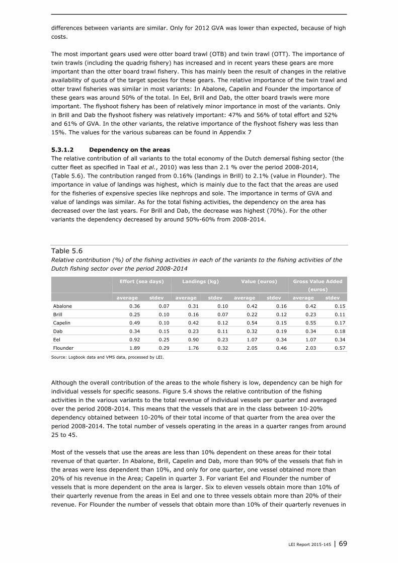
LEI Report 2015-145 | 69

differences between variants are similar. Only for 2012 GVA was lower than expected, because of high

costs.

The most important gears used were otter board trawl (OTB) and twin trawl (OTT). The importance of

twin trawls (including the quadrig fishery) has increased and in recent years these gears are more

important than the otter board trawl fishery. This has mainly been the result of changes in the relative

availability of quota of the target species for these gears. The relative importance of the twin trawl and

otter trawl fisheries was similar in most variants: In Abalone, Capelin and Founder the importance of

these gears was around 50% of the total. In Eel, Brill and Dab, the otter board trawls were more

important. The flyshoot fishery has been of relatively minor importance in most of the variants. Only

in Brill and Dab the flyshoot fishery was relatively important: 47% and 56% of total effort and 52%

and 61% of GVA. In the other variants, the relative importance of the flyshoot fishery was less than

15%. The values for the various subareas can be found in Appendix 7

5.3.1.2 Dependency on the areas

The relative contribution of all variants to the total economy of the Dutch demersal fishing sector (the

cutter fleet as specified in Taal et al., 2010) was less than 2.1 % over the period 2008-2014,

(Table 5.6). The contribution ranged from 0.16% (landings in Brill) to 2.1% (value in Flounder). The

importance in value of landings was highest, which is mainly due to the fact that the areas are used

for the fisheries of expensive species like nephrops and sole. The importance in terms of GVA and

value of landings was similar. As for the total fishing activities, the dependency on the area has

decreased over the last years. For Brill and Dab, the decrease was highest (70%). For the other

variants the dependency decreased by around 50%-60% from 2008-2014.

Table 5.6

Relative contribution (%) of the fishing activities in each of the variants to the fishing activities of the

Dutch fishing sector over the period 2008-2014

Effort (sea days) Landings (kg) Value (euros) Gross Value Added

(euros)

average stdev average stdev average stdev average stdev

Abalone 0.36 0.07 0.31 0.10 0.42 0.16 0.42 0.15

Brill 0.25 0.10 0.16 0.07 0.22 0.12 0.23 0.11

Capelin 0.49 0.10 0.42 0.12 0.54 0.15 0.55 0.17

Dab 0.34 0.15 0.23 0.11 0.32 0.19 0.34 0.18

Eel 0.92 0.25 0.90 0.23 1.07 0.34 1.07 0.34

Flounder 1.89 0.29 1.76 0.32 2.05 0.46 2.03 0.57

Source: Logbook data and VMS data, processed by LEI.

Although the overall contribution of the areas to the whole fishery is low, dependency can be high for

individual vessels for specific seasons. Figure 5.4 shows the relative contribution of the fishing

activities in the various variants to the total revenue of individual vessels per quarter and averaged

over the period 2008-2014. This means that the vessels that are in the class between 10-20%

dependency obtained between 10-20% of their total income of that quarter from the area over the

period 2008-2014. The total number of vessels operating in the areas in a quarter ranges from around

25 to 45.

Most of the vessels that use the areas are less than 10% dependent on these areas for their total

revenue of that quarter. In Abalone, Brill, Capelin and Dab, more than 90% of the vessels that fish in

the areas were less dependent than 10%, and only for one quarter, one vessel obtained more than

20% of his revenue in the Area; Capelin in quarter 3. For variant Eel and Flounder the number of

vessels that is more dependent on the area is larger. Six to eleven vessels obtain more than 10% of

their quarterly revenue from the areas in Eel and one to three vessels obtain more than 20% of their

revenue. For Flounder the number of vessels that obtain more than 10% of their quarterly revenues in

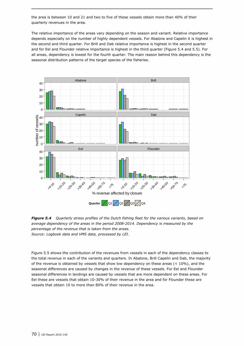
70 | LEI Report 2015-145

the area is between 10 and 21 and two to five of these vessels obtain more than 40% of their

quarterly revenues in the area.

The relative importance of the areas vary depending on the season and variant. Relative importance

depends especially on the number of highly dependent vessels. For Abalone and Capelin it is highest in

the second and third quarter. For Brill and Dab relative importance is highest in the second quarter

and for Eel and Flounder relative importance is highest in the third quarter (Figure 5.4 and 5.5). For

all areas, dependency is lowest for the fourth quarter. The main reason behind this dependency is the

seasonal distribution patterns of the target species of the fisheries.

Figure 5.4 Quarterly stress profiles of the Dutch fishing fleet for the various variants, based on

average dependency of the areas in the period 2008-2014. Dependency is measured by the

percentage of the revenue that is taken from the areas.

Source: Logbook data and VMS data, processed by LEI.

Figure 5.5 shows the contribution of the revenues from vessels in each of the dependency classes to

the total revenue in each of the variants and quarters. In Abalone, Brill Capelin and Dab, the majority

of the revenue is obtained by vessels that show low dependency on these areas (< 10%), and the

seasonal differences are caused by changes in the revenue of these vessels. For Eel and Flounder

seasonal differences in landings are caused by vessels that are more dependent on these areas. For

Eel these are vessels that obtain 10-30% of their revenue in the area and for Flounder these are

vessels that obtain 10 to more than 80% of their revenue in the area.

Abalone Brill

Capelin Dab

Eel Flounder

0

10

20

30

40

0

10

20

30

40

0

10

20

30

40

>0-10

>10-2

0

>20-3

0

>30-4

0

>40-5

0

>50-7

5

>75

>0-10

>10-2

0

>20-3

0

>30-4

0

>40-5

0

>50-7

5

>75

% revenue affected by closure

nu

mb

er

of ve

sse

ls

Quarter Q1 Q2 Q3 Q4

LEI Report 2015-145 | 71

Figure 5.5 Average revenue (*1,000 euros) per quarter over the period 2008-2014 in each of the

variants a)

a) The various colours show the level to which the vessel depend on the areas. E.g. almost the

complete revenue in quarter 2 for variant Brill is obtained by vessels that are less than 10%

dependent on these areas.

Source: Logbook data and VMS data, processed by LEI.

Seasonal patterns in utilisation of the area vary among gear types. Appendix 8 shows the patterns for

the most important gear types.

On an annual basis the dependency is lower than on an quarterly basis. Figure 5.6 shows that for the

first four variants, almost none of the vessels obtain more than 10% of their income from the area.

Only in case of Eel and Flounder, the number of vessels that obtain more than 10% is larger: 7 for Eel

and 19 for Flounder. This means that the vessels utilising the areas vary between seasons and that

although fishermen perceive dependency on the area at the quarterly level, the average dependency

on an annual level is limited. On the other hand it shows that low a low level of dependency at the

annual level, may still be an indication of seasonal dependency on the area. This information has been

used in the assumptions for the estimation of the possible displacement effects.

Most of the vessels that fish in the areas are registered in Wieringen and Urk (Figure 5.6). Some other

vessels come from the province of Friesland and Groningen, but their dependency is lower than 10%.

Nearly all vessels with high dependency levels (>20%) come from the previously mentioned two

fishing communities. Although the dependency levels vary among the various variants, the regional

distribution is similar in all variants. As the vessels utilising the area mostly originate from the

communities of Urk and Wieringen, these communities will also be most affected by possible

consequences of fisheries measures in the areas. This is discussed in Chapter 8 and 10.

Abalone Brill Capelin

Dab Eel Flounder

0

500

1,000

1,500

0

500

1,000

1,500

Q1

Q2

Q3

Q4

Q1

Q2

Q3

Q4

Q1

Q2

Q3

Q4

Quarter

ave

rag

e r

eve

nu

e a

ffe

cte

d b

y c

losu

re 2

00

8-2

01

4

RevenueDependency

>0-10

>10-20

>20-30

>30-40

>40-50

>50-75

>75

72 | LEI Report 2015-145

Figure 5.6 Stress profile of the Dutch fishing fleet for the various variants, based on average annual

dependency of the areas in the period 2008-2014, aggregated by region of registration of the vessel

(e.g. UK220 is registered in Urk). North, harbours in Groningen and Friesland; Holland, harbours in

Noord- and Zuid-Holland. A specification of the classification of fishing harbours is presented in

Appendix 9. Dependency is measured by the percentage of the revenue that is taken from the areas.

Source: Logbook data and VMS data, processed by LEI.

5.3.2 Fishing activities foreign vessels

For the foreign fishing fleets, the areas under study also have provided considerable fishing

opportunities over the last 5 years (Table 5.7). In variant Brill fishing intensity is lowest with around

60 fishing days and an average GVA of around 0.25m euros. In Abalone fishing intensity is approx.

50% higher resulting in an average GVA of around 0.37m euros. Capelin and Dab show comparable

levels of fisheries activities resulting in GVAs around 0.5m euros and as for the Dutch fleet fishing

activity is highest for Eel and Flounder (GVAs 1.5 and 3.3m euros, respectively).

Abalone Brill Capelin

Dab Eel Flounder

0

20

40

60

0

20

40

60

>0-10

>10-2

0

>20-3

0

>30-4

0

>40-5

0

>50-7

5

>75

>0-10

>10-2

0

>20-3

0

>30-4

0

>40-5

0

>50-7

5

>75

>0-10

>10-2

0

>20-3

0

>30-4

0

>40-5

0

>50-7

5

>75

% revenue affected by closure

nu

mb

er

of ve

sse

ls

Region Urk North Holland Zeeland

LEI Report 2015-145 | 73

Table 5.7

Overview of the average fishing activities by foreign fishing fleets in the areas of the variants,

distinguishing between vessels owned by foreign owners and by Dutch owners (so called flag vessels)

Abalone Brill Capelin Dab Eel Flounder

Foreign owned vessels (including all UK vessels)

Fishing days 75 48 100 86 344 716

Landings (tonnes) 790 616 1,052 1,452 3,188 6,567

Landings value (kEuro) 712 455 987 890 3,264 6,695

GVA (kEuro) 329 234 430 497 1,379 2,831

Dutch owned vessels

Fishing days 20 10 31 14 66 194

Landings (tonnes) 39 19 55 30 126 366

Landings value (kEuro) 92 44 134 65 393 863

GVA (kEuro) 45 19 62 29 143 429

Total

Fishing days 95 58 131 100 410 910

Landings (tonnes) 829 636 1,107 1,483 3,314 6,934

Landings value (kEuro) 804 499 1,121 956 3,557 7,558

GVA (kEuro) 374 252 492 526 1,523 3,260

Source: Logbook data and VMS data and data from the Annual Economic report (STECF 2015), processed by LEI, CEFAS, ILVO, Von Thünen and

DTU. *All UK vessels are assumed to be foreign owned.

The majority of the fishing activities in the areas are carried out by the UK fleet which contributes to

more than 50% of the effort in all variants (Figure 5.7). The landings volume of the Danish fleet is

relatively high, but these are predominantly low price species, caught in large quantities. As a result

the contribution of the Danish fleet to the total effort and landings value is relatively low, between

8-17% in effort. The effort levels of the German fleet and Belgian fleet are generally comparable to

the Danish ones, but differences exist for specific years and variants. E.g. the Belgian fleet spend only

5 days fishing in Dab, whereas the Danish fleet spend 30 days.

The time series of the foreign fleets do not show a clear trend. In Eel and Flounder fishing activities

seem to be stable over time and for the other variants, fishing activities are highly variable among

years.

74 | LEI Report 2015-145

Figure 5.7 Historical trends of the fishing activities by the foreign fishing fleets (including foreign

owned and Dutch owned vessels) in the areas of the variants. Effort, landings, value of landings and

GVA are given by country of origin

Source: Logbook data and VMS data and data from the Annual Economic report (STECF 2015),

processed by LEI, CEFAS, ILVO, VTI and DTU.

The relative importance of the fishing activities of flag vessels (Dutch owned vessels) in the area in

the foreign fleets seems limited (Table 5.7). However, the values presented here are underestimating

the contribution of flag values to the total fishing activities of foreign fleets as the data for UK flag

vessels is missing. This is due to the fact that for the UK the information on fishing activity could be

matched only partly with the vessel information from the Dutch sector. For other countries the

information could be matched completely. Dutch flag vessels under Belgian and German flag operating

in the areas contribute minimal 20% to the total effort and 4% to the GVA of foreign fleets over the

period 2010-2014. The total effort of all flag vessels ranges from 10 fishing days for Brill to 194 fishing

days for Flounder. Large differences exist from one to another country, (Figure 5.8): whereas no

Danish flag vessel (Dutch owned Danish vessel) is operating in any of the areas, 80% of the effort

from German vessels and 60% of the effort of Belgian vessels is made by flag vessels.

Based on the current data, the German flag fleet in the area is more important than the Belgian flag

fleet in all of the variants. The contribution of these vessels to the total effort of flag vessels ranges

from 56% in Flounder to 85% in Brill. Belgian flag vessels are found in all variants as well but their

relative importance is much lower: from 15% in Brill to 44% in Capelin.

For Eel and Flounder fishing activities of Belgian and German flag vessels have been increasing over

the period 2010-2014. Efforts nearly doubled in the areas and value of landings and GVA more than

Abalone Brill Capelin Dab Eel Flounder

0

250

500

750

1000

0

2000

4000

6000

8000

0.0

2.5

5.0

7.5

0

1

2

3

Effo

rt (fishin

g d

ays)

Landin

gs (to

nnes)

Valu

e (m

illion e

uro

s)

GV

A (m

illion e

uro

s)

2010 2013 2010 2013 2010 2013 2010 2013 2010 2013 2010 2013

year

Gear Belgium Denmark Germany United Kingdom

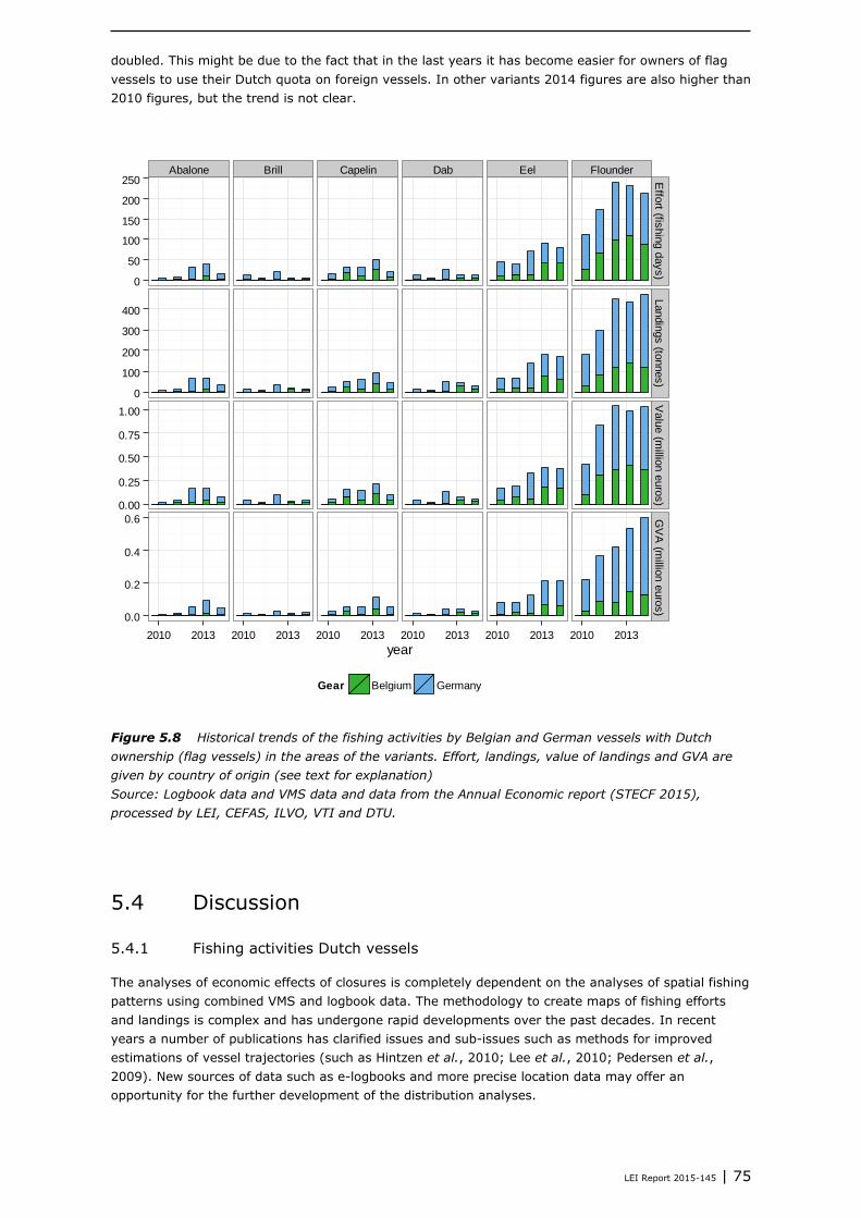
LEI Report 2015-145 | 75

doubled. This might be due to the fact that in the last years it has become easier for owners of flag

vessels to use their Dutch quota on foreign vessels. In other variants 2014 figures are also higher than

2010 figures, but the trend is not clear.

Figure 5.8 Historical trends of the fishing activities by Belgian and German vessels with Dutch

ownership (flag vessels) in the areas of the variants. Effort, landings, value of landings and GVA are

given by country of origin (see text for explanation)

Source: Logbook data and VMS data and data from the Annual Economic report (STECF 2015),

processed by LEI, CEFAS, ILVO, VTI and DTU.

5.4 Discussion

5.4.1 Fishing activities Dutch vessels

The analyses of economic effects of closures is completely dependent on the analyses of spatial fishing

patterns using combined VMS and logbook data. The methodology to create maps of fishing efforts

and landings is complex and has undergone rapid developments over the past decades. In recent

years a number of publications has clarified issues and sub-issues such as methods for improved

estimations of vessel trajectories (such as Hintzen et al., 2010; Lee et al., 2010; Pedersen et al.,

2009). New sources of data such as e-logbooks and more precise location data may offer an

opportunity for the further development of the distribution analyses.

Abalone Brill Capelin Dab Eel Flounder

0

50

100

150

200

250

0

100

200

300

400

0.00

0.25

0.50

0.75

1.00

0.0

0.2

0.4

0.6

Effo

rt (fishin

g d

ays)

Landin

gs (to

nnes)

Valu

e (m

illion e

uro

s)

GV

A (m

illion e

uro

s)

2010 2013 2010 2013 2010 2013 2010 2013 2010 2013 2010 2013

year

Gear Belgium Germany

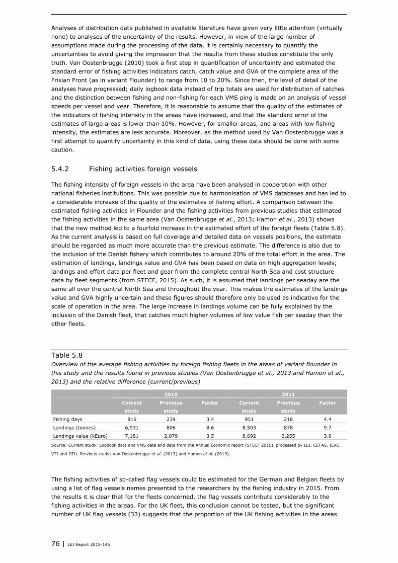
76 | LEI Report 2015-145

Analyses of distribution data published in available literature have given very little attention (virtually

none) to analyses of the uncertainty of the results. However, in view of the large number of

assumptions made during the processing of the data, it is certainly necessary to quantify the

uncertainties to avoid giving the impression that the results from these studies constitute the only

truth. Van Oostenbrugge (2010) took a first step in quantification of uncertainty and estimated the

standard error of fishing activities indicators catch, catch value and GVA of the complete area of the

Frisian Front (as in variant Flounder) to range from 10 to 20%. Since then, the level of detail of the

analyses have progressed; daily logbook data instead of trip totals are used for distribution of catches

and the distinction between fishing and non-fishing for each VMS ping is made on an analysis of vessel

speeds per vessel and year. Therefore, it is reasonable to assume that the quality of the estimates of

the indicators of fishing intensity in the areas have increased, and that the standard error of the

estimates of large areas is lower than 10%. However, for smaller areas, and areas with low fishing

intensity, the estimates are less accurate. Moreover, as the method used by Van Oostenbrugge was a

first attempt to quantify uncertainty in this kind of data, using these data should be done with some

caution.

5.4.2 Fishing activities foreign vessels

The fishing intensity of foreign vessels in the area have been analysed in cooperation with other

national fisheries institutions. This was possible due to harmonisation of VMS databases and has led to

a considerable increase of the quality of the estimates of fishing effort. A comparison between the

estimated fishing activities in Flounder and the fishing activities from previous studies that estimated

the fishing activities in the same area (Van Oostenbrugge et al., 2013; Hamon et al., 2013) shows

that the new method led to a fourfold increase in the estimated effort of the foreign fleets (Table 5.8).

As the current analysis is based on full coverage and detailed data on vessels positions, the estimate

should be regarded as much more accurate than the previous estimate. The difference is also due to

the inclusion of the Danish fishery which contributes to around 20% of the total effort in the area. The

estimation of landings, landings value and GVA has been based on data on high aggregation levels;

landings and effort data per fleet and gear from the complete central North Sea and cost structure

data by fleet segments (from STECF, 2015). As such, it is assumed that landings per seaday are the

same all over the central North Sea and throughout the year. This makes the estimates of the landings

value and GVA highly uncertain and these figures should therefore only be used as indicative for the

scale of operation in the area. The large increase in landings volume can be fully explained by the

inclusion of the Danish fleet, that catches much higher volumes of low value fish per seaday than the

other fleets.

Table 5.8

Overview of the average fishing activities by foreign fishing fleets in the areas of variant flounder in

this study and the results found in previous studies (Van Oostenbrugge et al., 2013 and Hamon et al.,

2013) and the relative difference (current/previous)

2010 2011

Current

study

Previous

study

Factor Current

study

Previous

study

Factor

Fishing days 816 239 3.4 951 218 4.4

Landings (tonnes) 6,931 806 8.6 8,503 878 9.7

Landings value (kEuro) 7,181 2,079 3.5 8,692 2,255 3.9

Source: Current study: Logbook data and VMS data and data from the Annual Economic report (STECF 2015), processed by LEI, CEFAS, ILVO,

VTI and DTU. Previous study: Van Oostenbrugge et al. (2013) and Hamon et al. (2013).

The fishing activities of so-called flag vessels could be estimated for the German and Belgian fleets by

using a list of flag vessels names presented to the researchers by the fishing industry in 2015. From

the results it is clear that for the fleets concerned, the flag vessels contribute considerably to the

fishing activities in the areas. For the UK fleet, this conclusion cannot be tested, but the significant

number of UK flag vessels (33) suggests that the proportion of the UK fishing activities in the areas

LEI Report 2015-145 | 77

carried out by Dutch vessels can be substantial. In case 50% of the fishing activities of the UK vessel

would be carried out by Dutch owned vessels, the economic value of the Flag vessels would be around

75% of the value for the Dutch fleet. From the trends it seems that the fishing intensity by flag

vessels in the area has been increasing over the last years. This is most probably a true trend, but it

could also be partly due to the inaccuracy of the list for the previous years.

78 | LEI Report 2015-145

6 Costs for Dutch fisheries

Hans van Oostenbrugge and Katell Hamon

6.1 Methodology

The costs of the closures for the Dutch fisheries depend both on the future value of the designated

areas to the fishery and the possibilities for the fisheries to displace their activities to other locations in

case of closures. Because both the future value of the areas and the possibilities for displacement are

highly uncertain, scenarios have been designed for both aspects to get some idea of potential costs.

First Policy, Economy and Innovation scenarios were developed to show the effects of externalities on

the fishing activities in the areas. Subsequently the effects of reallocation of the fishing activities in

case of closures were estimated, by developing displacement scenarios.

6.1.1 Scenarios for policy, economy and innovation

6.1.1.1 Defining Policy, Economy and Innovation scenarios

The fisheries sector in Europe is currently in a very dynamic period because of all kinds of internal and

external developments. The most important ones are:

Price changes (fish prices and fuel price)

Changes in fish abundance (MSY targets of management)

Implementation of the landing obligation

Technical innovations

Restriction of the fishing area by nature conservation, wind parks etc.

In the previous study on developments in the Dutch demersal fishing sector (Kuhlman and van

Oostenbrugge, 2014) an inventory of these developments and their potential economic effects on the

fisheries sector was made. These developments are used and combined into four Policy, Economy and

Innovation scenarios (PEI scenarios). These PEI scenarios are used to evaluate the value of the

potentially closed areas under different external developments. The developments were combined in

the PEI-scenarios in such a way that the PEI scenarios would resemble extreme outcomes: PEI

scenario one and two combine all developments that will have either positive (PEI scenario 1) or

negative (PEI scenario 2) consequences for the overall economic performance of the Dutch fishing

sector. PEI scenario 0 resembles the situation as it was during the reference period (business as

usual). In PEI scenario 3, all developments have been combined.

The specifics of the four scenarios are given in Table 6.1 and the background and implementation of

each of the factors is described below.

LEI Report 2015-145 | 79

Table 6.1

Overview of the combination of external developments used in each of the Policy, Economy and

Innovation scenarios. See text for explanation

Factors taken into

account

Scenarios

0 1 2 3

Fish stocks X X

Fish prices a) 1 2 1+2

Fuel prices X X

Technical innovation X X

Landing obligation X X

Area closures X X

a) 1, positive price scenario (see text); 2, negative price scenario. See text for more explanation.

Fish Stocks

Recently, the key fish stocks in the North Sea (especially sole and plaice) have been growing. The

fishing effort (mortality) is for sole and plaice at the level of MSY (Maximum Sustainable Yield), and

the stock size increases for both species (ICES, 2013). For plaice, this has also led to increased fishing

opportunities in recent years and the prospects are that this trend will continue. If fishing pressure will

stay at a sustainable levels (MSY), the stock size will potentially grow to over 1m tonnes. This would

mean that the catches could increase approximately by a factor two compared to the level of 2012,

which is close to the average of the seven years. For sole, the situation is different (ICES, 2013). Due

to the large recruitment to the stock in recent years, it is expected that the current stock size is larger

than usual. Because of this, future catches will not be able to increase in order to sustainably use the

stock, but will remain constant or even decline slightly compared with the 2012 level. Based on this, it

is assumed that in PEI scenario 1 and 3 catch levels will increase for plaice catches by 100% and will

stay constant for sole. For other species catch levels are assumed to increase by 25%. This can be

either read as the development in the complete stocks, but also as the development of the stocks in

the area. In PEI scenario 2 catches of all species are assumed equal to the level in the base year.

Fish prices

Two possible price developments have been implemented in the scenarios. Price development one

originates from the so-called Delta-Groei scenario (Bruggeman and Dammers, 2013). The Delta

Scenarios have been developed as possible directions for the future (2050 with a view through to

2100) based on future (WLO) scenarios of CPB and PBL (Janssen et al., 2006) and show four possible

development directions, based on two dimensions: from moderate to rapid climate change and socio-

economic contraction to growth. For this study it is particularly important what bandwidth these

scenarios provide for the most relevant external variables of the fishing sector. For example, the Delta

Scenarios for 2050 indicate a population of Netherlands ranging from 15 to 20m, and an average

growth of the gross domestic product of 1-2.5%. In comparison, the WLO scenarios were based on a

population of 16-20m in 2040 and economic growth of 0.7 to 2.6% per year. In 2012 CPB performed

an update of the WLO scenarios from 2006, and the conclusion is that the ranges are still realistic

(Huizinga, 2012). Using the assumed growth in the domestic product of 2.5% and an income elasticity

on demand for fish of 0.27 (Lechene, 2000), and constant imports of fish from outside the EU, the

Delta-Groei scenario results in price increases for sole (+4%) plaice (+1%) and others (+2%).

The second price development is based on EU information on population growth and economic growth.

The total EU population is expected to grow between 2013 and 2050 by 3.6% (Eurostat). This

corresponds to 0.1% per year. Economic growth is the most important for the growth in the demand

for fish. Assuming a somewhat conservative estimate of the per capita income growth of 1.5% per

year and the same demand elasticity as for the previous scenario, this amounts to an increase in

demand for fish from about 0.5% per year. Undoubtedly, competition from farmed fish will increase

rather than decrease. It is therefore likely that the EU demand for wild fish the next 15 years will

stagnate at best, and likely fall slightly. This also means pressure on prices. Therefore, it is assumed

that the sale price of fish for the fishing sector will decrease by 10% for all species.

80 | LEI Report 2015-145

The two possible price developments are implemented in PEI scenario 1 and 2. In PEI scenario 3 the

two price effects are combined. This results in a (hypothetic) price reduction.

Technical innovation

In the past decade a series of new fishing gears were developed as replacement for the traditional

beam trawl. It is assumed that these new fishing techniques such as pulse trawl and pulswing will find

further passage and will further replace the beam trawling in the coming years. It is also possible that

the landing obligation will provide an incentive for changes in fishing techniques and shifts in the

targeted species. Together with further fuel savings it will reduce the impact of higher fuel prices and

tighter emission restrictions. The simplest calculation of the effects of this development is an increase

in the cost of maintenance of fishing gear and a decrease in fuel consumption. Based on recent studies

(Marlen et al., 2014) it is assumed that technical innovation will increase gear costs by 50% and

decrease fuel consumption by 25% in the beam trawl fleet. As the innovative pulse gears are not

allowed above 55 degrees latitude, all beam trawl effort above this border is assumed to reallocate to

more southern areas. This effort is distributed proportionally to the existing effort south of 55 degrees

latitude. The effects of technical innovation are expected to have a positive effect on the economic

performance of the sector and as such are included in PEI scenario 2 and 3.

Landing obligation

The effects of the landing obligation (discard ban) in the longer term are still very unclear. The landing

obligation might lead to an increase in the cost, but how high this increase is depends on a number of

factors:

the type and size of adjustment of the (bycatch) quota

the possible exemptions of certain species/fisheries

the options for discard reduction by means of technical measures and changes in fishing patterns

the price that can be obtained for bycatch

the additional costs to be incurred for processing and landing of catches

reduced fishing because of the extra catches and limits in storage capacity on board

the extra labour needed on board to sort out the catches.

Buisman et al. (2013) estimated that in case fishing behaviour will not change and quota are not

increased, the net cost to the Dutch cutter sector will be about 22-26m euros per year. This is mainly

caused by the fact that some of the bycatch quota will limit the fishing activities of the fleet. With an

adjustment of quotas (in which current discards would be added to the future quota) costs are

estimated to be much lower; 6-12m euros (Buisman et al., 2013.). In this study the effects of the

landing obligation are assumed to be similar to those in Buisman et al., 2013 (Table 6.2) with an

adjustment of the quota.

Table 6.2

Overview of constants used in estimating the effects of the landings obligation (from Buisman et al.,

2013)

Variable Value

Discard rate (% of the total catch):

Euro cutters (engine power <300 hp) 95%

Large cutters (engine power >= 300 hp) 80%

Price discards (Euro/kg) 0.2

Landings costs discards (Euro/kg) 0.3

Extra labour costs (%):

Euro cutters (engine power <300 hp) 20

Large cutters (engine power >= 300 hp) 25

Extra steaming costs for Euro cutters (%) 6

The effects of the discard ban are included in PEI scenario 2 and 3. The inclusion of this effect in the

scenarios can also be explained as the effect of different levels of discards in the area, with 0 discards

LEI Report 2015-145 | 81

for PEI scenario 1 and average discard levels in PEI scenario 2 and 3 while the discard ban applies to

all scenarios.

Area closures

Competition for space on the North Sea with other space users, particularly wind farms and protected

areas has increased and will further increase. This will potentially lead to lower fishing efficiency

because fishermen need to reallocate fishing activities. To what extent the loss of fishing grounds also

leads to lower catches is uncertain: on the one hand the displacement effect leads to greater

pressures elsewhere, and thus possibly to lower catch per unit effort (see also Rijnsdorp et al., 2000).

On the other hand, there are potential (but uncertain) benefits of the closed areas in the development

of resources (van Denderen, 2015). Because of this uncertainty, only the direct effects of effort

displacement on the effort in the areas of the closures are taken into account. An inventory of all

closures in the North Sea with their specific conditions is outside the scope of this study. Therefore,

the inventory of possible closures carried out in the North Sea in the EU project Vectors is used to

estimate the total effort in all possible closure areas (Marchal et al., 2014). In the overview

(Figure 6.1) potential MPA’s but especially potential areas for wind farm development are depicted.

However, in the UK and Denmark these so called wind farm search areas are very large and when

taking into account that only in smaller sub-areas actual wind farms will be developed fisheries

displacement will be much less than indicated by the areas shown in Figure 6.1. Furthermore, in the

UK the government is considering the possibilities to allow fishing within wind farms resulting in less

displacement.

To calculate the effects of displacement by future MPA’s and wind farms we assumed that on the

German shelf in the coming decades 50 % of the indicated search areas will actually be developed,

while in Denmark and the UK about 10% of these areas will be developed such that this leads to

fisheries displacement. The effects of closures have been included in PEI scenario 2 and 3 and can be

read as the potential effects of effort allocation due to area closures.

Figure 6.1 Potential area closures in the North Sea from Marchal et al., 2014. These area closures

were used as a proxy for all area closures (see also text).

Source: Logbook data and VMS data, processed by LEI.

82 | LEI Report 2015-145

6.1.1.2 Implementation of PEI scenarios

The effects of the scenarios were estimated for each vessel and each year in the time series

individually. In case of effort displacement (in technical developments and area closures) the

proportion of effort from these areas is estimated for each vessel and this proportion is redistributed in

the remaining fishing grounds proportional to the existing effort pattern. This means that in case a

vessel fishes 20% in potential closed areas, the effort of this vessel on all other fishing grounds,

including the Frisian Front and the Central Oyster Grounds will increase by 20%. In this way the

variations in effort distribution, gear use, fish prices, species composition etc. of each vessel and year

were taken into account in the estimation of the value of the variants in each of the PEI scenarios.

After the estimation at the individual level the results were aggregated. All of the scenarios analyses

implemented in R.

6.1.2 Displacement scenarios

Effort displacement is a complex issue and effects are hard to quantify. Yet these effects are crucial for

the economic consequences of closures for fisheries and essential for assessing the effectiveness of

closures (Forcada et al., 2010). In order to get an idea about possible displacement mechanisms and

the resulting effects for the closure of these areas, another project about effort displacement was

carried out in parallel with the current project. The parallel project included a desk study on the

general aspects of displacement, a case study on the displacement effects of closures in the North Sea

and a workshop with fishermen to discuss the results of the desk study and consequences for the

effects of closures (Slijkerman and Tanis, 2015, De Vries et al., 2015).

Displacement effects resulting from the different variants

Based on results of the displacement workshop as described in Slijkerman and Tamis (2015) it was

concluded that displacement patterns resulting from the different variants are hard to predict and that

displacement depends largely on the type of fisheries. Moreover, displacement depends highly on the

importance of the closed fishing grounds (size and place), the expertise and character of the skipper,

distance to the fishing harbours, and the quota for the different fish stocks. These factors all result in

a certain level of dependency of the fisherman/fisheries. The more dependent the fishermen are, the

harder it is to displace or to predict where displaced effort will be allocated.

The extent of displacement in terms of location and effort is hard to forecast because of uncertainties

in this phase of the process of implementing the closed areas. Moreover, factors which may be

relevant in 5 years will determine displacement in future as well. These are however unknown, in

definition and extent.

Nevertheless, a few rough estimates on displacement were drafted during the workshop by a small

selection of fishermen and representatives. It should be emphasised that these conclusions have not

been widely discussed and confirmed within the fisheries sector, and reflect only a first attempt to

qualify displacement (more information in Slijkerman and Tamis, 2015).

Twinrig nephrops fishermen might first explore near/at the borders of the closed area, in case this is

nearby their original grounds. Displacement will probably be explorative and heterogeneous in the

remaining open areas when fishing grounds are all closed. After exploring, fisheries will concentrate

in areas when proper fishing grounds are found.

Flyshoot fishermen may follow the fish on their route and displaced fisheries depend on these

routes. As a result, the Frisian Front is an important area for these fisheries in the period May - July.

Displacement probably focuses on the open areas, nearby the optimum concentration of fish stocks.

Displacement also depends on the amount of quotas. In case of enough plaice quota fishermen

might be able to displace to the Dogger Bank although fishing opportunities are also limited there

because of closures. With sufficient cod quota they might be able to displace to areas like

Skagerrak.

Pulse fisheries may displace to the remaining open areas of 30 m depth. This depth line goes right

through the Frisian front and is the border between harder and softer grounds. Fishermen that are

highly dependent on the area probably have little idea where to displace to.

LEI Report 2015-145 | 83

Based on the outcomes of the workshop a methodology for the estimation of economic effects of

displacement was developed. Elements that were taken from the results of the workshop were:

There are three different situations with respect to use of the areas:

Use by dependent fishermen

Use by fishermen that depend on the area for a large proportion of their fishing activities. This can

also be seasonal, because of distribution patterns of target species.

Use by independent fishermen

Use by fishermen that are fishing in different areas and fish in the area once in a while.

Fishing through the area

Use by fishermen that are on their way to other fishing areas and fish through the area. This was

only mentioned as a problem in case the whole Frisian Front was closed (variant Flounder).

The options for reallocation of the fishing activities and their effects on the economic performance of

the fisheries depend on the type of use and the fishery that is conducted in the area. The main gear

types differ in respect to the use of the area (see Chapter 5) and alternative fishing possibilities as

explained below.

Figure 6.2 Schematic approach to assess the effects of displacement of fishing activities. The

value for the various percentages are given in Table 6.3

Figure 6.2 shows the approach taken to estimate the effects of the closures.

Distinction is made between the three types of use mentioned during the workshop; specific use of the

areas by dependents and independents, and fishing through. The last type of use (fishing through)

was only mentioned to become a problem in variant Flounder for the fishing activities in the Frisian

Front, because in this variant large area is closed for fishing without corridors that fishermen can use

to fish through the area from north to south and vice versa.

For the estimation of the effects of displacement the following assumptions are made:

If a fisherman spends more than 10% of his annual fishing time using a specific gear in the area, he

is dependent on the area. This percentage is based on the observation that considerable seasonal

dependency occurs and translates into lower dependency on an annual basis.

If a fisherman spends less than 10% of his annual fishing time using a specific gear in the area, he

is not dependent on the area.

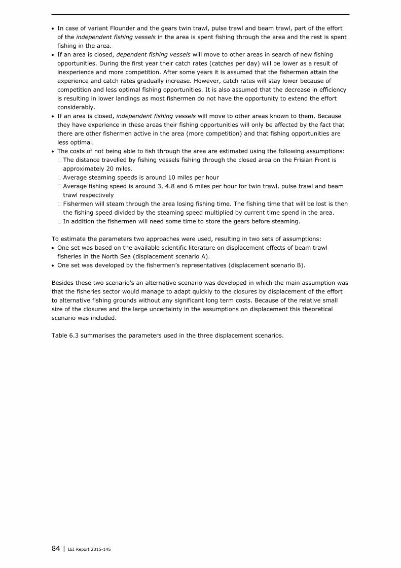
84 | LEI Report 2015-145

In case of variant Flounder and the gears twin trawl, pulse trawl and beam trawl, part of the effort

of the independent fishing vessels in the area is spent fishing through the area and the rest is spent

fishing in the area.

If an area is closed, dependent fishing vessels will move to other areas in search of new fishing

opportunities. During the first year their catch rates (catches per day) will be lower as a result of

inexperience and more competition. After some years it is assumed that the fishermen attain the

experience and catch rates gradually increase. However, catch rates will stay lower because of

competition and less optimal fishing opportunities. It is also assumed that the decrease in efficiency

is resulting in lower landings as most fishermen do not have the opportunity to extend the effort

considerably.

If an area is closed, independent fishing vessels will move to other areas known to them. Because

they have experience in these areas their fishing opportunities will only be affected by the fact that

there are other fishermen active in the area (more competition) and that fishing opportunities are

less optimal.

The costs of not being able to fish through the area are estimated using the following assumptions:

­ The distance travelled by fishing vessels fishing through the closed area on the Frisian Front is

approximately 20 miles.

­ Average steaming speeds is around 10 miles per hour

­ Average fishing speed is around 3, 4.8 and 6 miles per hour for twin trawl, pulse trawl and beam

trawl respectively

­ Fishermen will steam through the area losing fishing time. The fishing time that will be lost is then

the fishing speed divided by the steaming speed multiplied by current time spend in the area.

­ In addition the fishermen will need some time to store the gears before steaming.

To estimate the parameters two approaches were used, resulting in two sets of assumptions:

One set was based on the available scientific literature on displacement effects of beam trawl

fisheries in the North Sea (displacement scenario A).

One set was developed by the fishermen’s representatives (displacement scenario B).

Besides these two scenario’s an alternative scenario was developed in which the main assumption was

that the fisheries sector would manage to adapt quickly to the closures by displacement of the effort

to alternative fishing grounds without any significant long term costs. Because of the relative small

size of the closures and the large uncertainty in the assumptions on displacement this theoretical

scenario was included.

Table 6.3 summarises the parameters used in the three displacement scenarios.

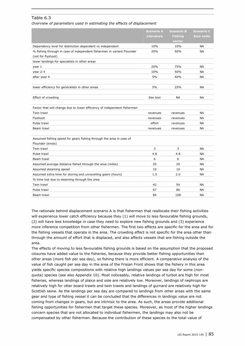
LEI Report 2015-145 | 85

Table 6.3

Overview of parameters used in estimating the effects of displacement

Scenario A

Literature

Scenario B

Fishing

sector

Scenario C

Zero costs

Dependency level for distinction dependent vs independent 10% 10% NA

% fishing through in case of independent fishermen in variant Flounder

(not for flyshoot)

20% 50% NA

lower landings for specialists in other areas

year 1 20% 75% NA

year 2-4 10% 50% NA

after year 4 5% 40% NA

lower efficiency for generalists in other areas 5% 25% NA

Effect of crowding See text NA NA

Factor that will change due to lower efficiency of independent fishermen

Twin trawl revenues revenues NA

Flyshoot revenues revenues NA

Pulse trawl effort revenues NA

Beam trawl revenues revenues NA

Assumed fishing speed for gears fishing through the area in case of

Flounder (knots)

Twin trawl 3 3 NA

Pulse trawl 4.8 4.8 NA

Beam trawl 6 6 NA

Assumed average distance fished through the area (miles) 20 20 NA

Assumed steaming speed 10 10 NA

Assumed extra time for storing and unravelling gears (hours) 1.5 2.0 NA

% time lost due to steaming through the area

Twin trawl 42 54 NA

Pulse trawl 67 86 NA

Beam trawl 84 108 NA

The rationale behind displacement scenario A is that fishermen that reallocate their fishing activities

will experience lower catch efficiency because they (1) will move to less favourable fishing grounds,

(2) will have less knowledge in case they need to explore new fishing grounds and (3) experience

more inference competition from other fishermen. The first two effects are specific for the area and for

the fishing vessels that operate in the area. The crowding effect is not specific for the area other than

through the amount of effort that is displaced, and also affects vessels that are fishing outside the

area.

The effects of moving to less favourable fishing grounds is based on the assumption that the proposed

closures have added value to the fisheries, because they provide better fishing opportunities than

other areas (more fish per sea day), so fishing there is more efficient. A comparative analysis of the

value of fish caught per sea day in the area of the Frisian Front shows that the fishery in this area

yields specific species compositions with relative high landings values per sea day for some (non-

quota) species (see also Appendix 10). Most noticeably, relative landings of turbot are high for most

fisheries, whereas landings of plaice and sole are relatively low. Moreover, landings of nephrops are

relatively high for otter board trawls and twin trawls and landings of gurnard are relatively high for

Scottish seine. As the landings per sea day are compared to landings from other areas with the same

gear and type of fishing vessel it can be concluded that the differences in landings value are not

coming from changes in gears, but are intrinsic to the area. As such, the areas provide additional

fishing opportunities for fishermen that target these species. Moreover, as most of the higher landings

concern species that are not allocated to individual fishermen, the landings may also not be

compensated by other fishermen. Because the contribution of these species to the total value of

86 | LEI Report 2015-145

landings in the areas is relatively small (10-20% for Turbot and gurnard combined), the effect of the

overall lower catch efficiency will also be small, but it will continue to exists in time in case it is

assumed that fish distribution patterns in space will not change. As such it is assumed that the

closures will lead to a permanent reduction in VPUE of 5%.

The effects of crowding have been studied for beam trawl fisheries in the North Sea by Rijnsdorp et al

2000. They found that a reduction in fishing intensity led to higher catch rates during the week of

prayer in Urk (10% higher catch rates in week with 75% reduction in fishing effort) and concluded

that increased fishing intensity in a fishing area will have an negative effect on catch efficiency

through crowding. As the effort of the fishing vessels is displaced from the closed areas to alternative

areas with other vessels operating, fishing intensity in other areas will increase affecting the catch

efficiency of all vessels. As such the effect of crowding can only be estimated on a fleet level. The

overall effect on catch efficiency is estimated using the relationship between effort and catch efficiency

by Rijnsdorp et al and the relative amounts of effort in the closures (See Table 5.6)(see also

Appendix 10). The reductions in catch efficiency are assumed to result in lower landings and higher

costs and resulting reductions in GVA in the same way as for the affected fishing vessels (e.g. higher

costs for sole fisheries and lower landings for other fisheries).

Rijnsdorp et al. (2007) assessed the effects of a temporal large area closure in the North Sea for the

beam trawl fishery and included a comparison of the landings of resident fishermen and newcomers.

The study concluded that in the northern part of the North Sea the newcomers had lower catch rates:

on average 20% lower with a maximum of 40% in one week.

Figure 6.3 Effects of reallocation effort for the fishing vessels operating inside the closures and the

vessels operating outside the closures as assumed in displacement scenario A.

For fishermen that depend on the closed area the reduction in catch efficiency is assumed to be higher

as they also have less knowledge on the local fishing circumstances in the alternative areas. As the

reduction in catch efficiency applies to a whole year, and the reduction in Poos and Rijnsdorp was only

for a number of weeks, the extra reduction in catch efficiency was assumed to be smaller than in Poos

and Rijnsdorp (15%) as fishermen will probably increase their catch efficiency over the time period by

getting more experience on the new fishing grounds. This results in a total reduction in catch

efficiency of 20% in the first year for the fishing activities that fishermen would need reallocate.

During the years after the closure it is assumed that the dependent displaced fishermen will become

as efficient as the independent displaced fishermen and the reduction in catch efficiency will decrease

to 5%. Moreover it is assumed that depending on the most limiting factor for the fisheries, fishermen

LEI Report 2015-145 | 87

will compensate lost fishing opportunities (lower efficiency or lost fishing time) either by making more

sea days or landing less fish:

For pulse trawl (targeting sole) it is assumed that the amount of sole quota is limiting (as is has

been during the last years), so that the number of fishing days and costs will increase.

For other gears it is assumed that the amount of fishing days will be limiting, so the catches and

revenues will decrease.

The calculation of the time lost due to fishing through the area results in the maximum fishing time

lost. Moreover, currently fishermen that fish through the area will not always take the shortest route

as there is no reason to do so. Because of this a conservative estimate of the percentage of fishing

days that were spend fishing through the area has been used (20%)

The rationale behind displacement scenario B has been based on expert opinion from the fishermen.

A complete rationale can be found in Appendix 11. The reductions in catch efficiency are much higher

than the ones in scenario A, based on the conviction that the fishermen will not only lose fish because

of lack of knowledge and more competition, but that the catch efficiency on these fishing grounds is

much higher than on alternative grounds that could be utilised by the affected fishermen. It is stated

that the 75% reduction in catch efficiency for specialists in the first year is an proxy for the fact that a

limited number of fishermen will stop completely because of the closures. Further, the effect of

steaming through the area is larger than for displacement scenario A. Another difference is that in

displacement scenario B it is assumed that the resulting lower catch efficiency by the closures will not

be compensated by making longer trips.

6.1.3 Calculation of net present value

Calculating a net present value concerns discounting future costs and benefits. Costs and benefit may

occur at various moments in time. Examples are yearly income, continuing maintenance costs and

‘once only’ costs such as investment costs. In order to evaluate various plan alternatives - such as

scenarios for protecting areas - by means of a CBA, costs and benefits that occur at different moments

in time are being converted into a single metric, namely a net present value (NPV). The NPV concerns

a weighted aggregation of all relevant costs and benefits. Thereby, costs/benefits that occur later in

time have a smaller weight in the summation. This weighting of costs and benefits is also referred to

as discounting costs and benefits.

In this study the following parameters have been used:

a discount rate of 5.5 %

a time horizon of 30 years.

The discount rate is based on the recommendations of the Werkgroep Actualisatie Discontovoet. The

time horizon is chosen to be 30 years as an indication of the closed period.

Then the formula for calculating the net present value is:

T (Bt - Ct)

NPV= Σ (1 + r )t ,

t = 0

where:

T = time horizon

Bt = benefits in year t

Ct = costs in year t

r = discount rate

88 | LEI Report 2015-145

6.1.4 Sensitivity analysis

A sensitivity analysis was carried out for all main effects taken into account in the scenario analyses.

Table 6.4 provides the original value and the adjusted values for all parameters that were adjusted in

the sensitivity analysis. The sensitivity analysis was not carried out for each of the parameters

separately, but the parameters of each type of development were tested in combination.

Table 6.4

Overview of the factors that were tested in the sensitivity analysis and the relative changes

Factors tested Original value for

Scenario 3

Changed value

(10% increase)

Value in the areas:

Extra effort in each of the areas variable +10%

Technical innovation:

Relative fuel decrease (%) 25 27.5

Relative gear costs increase (%) 50 55

Area closures due to nature conservation and wind farms:

Effort increase in the areas 10% extra closures

Relative increase fish density (%)

Plaice 100 110

Sole 0 10%

Other fish 25 27.5

Landing obligation

Discard rate:

Euro cutters (<300 hp) 95 104.5

large cutters (>300 hp) 80 88

Discard price (euro per kg discards) 0.2 0.22

Landings costs discards (per kg discards) 0.3 0.33

Relative increase in labour costs (%)

Euro cutters (<300 hp) 20 22

large cutters (>300 hp) 25 27,5

Relative increase steaming costs for Euro cutters 6 6,6

Relative change in fish prices (%)

Plaice price -9.1 -10.0

Sole price -6.4 -7.0

Price other fish -8.2 -9.0

Economic results in the area

Relative increase fuel price (%) 20 22

6.2 Results

In the results section first the effects of the PEI scenarios on the fishing intensity in the areas and the

resulting value are presented. Second the effects of the displacement scenarios are presented in

combination with the PEI scenarios.

LEI Report 2015-145 | 89

6.2.1 Fishing activities in Policy, Economy and Innovation scenarios

The outcomes of the PEI scenarios illustrate the uncertain future for the Dutch fishing fleet.

Dependening on the developments taken into account the fishing activities in the areas and their

resulting economic performance can vary significantly.

Figure 6.4 Consequences of the Policy, Economy and Innovation scenarios for the fishing activities

of the Dutch fleet in the areas of various variants (annual totals) in case the areas are not closed

Source: Logbook data and VMS data, processed by LEI.

All scenarios indicate that fishing activities in the areas increase and that the value and volume of

landings will be larger than in the current situation (scenario 0, Figure 6.4). This is realistic, based on

the fact that the fishing area will get smaller and the fish stocks and thereby the possible landings will

increase. Effort increases due to area closures and the change to pulse gears that are not allowed

north of 55 degrees latitude. This causes an effort increase of 4 to 7% in scenario 3, depending on the

variant. The increase is highest for Flounder and Eel (7% for both in scenario 3) and lowest for Brill

and Dab (4% for both in scenario 3). Abalone and Capelin show intermediate increases (5 and 6% in

scenario 3). For scenario 1 and 2 the increases are lower, but the ranking of the variants stays the

same. The difference between relative increases in effort for the variants indicate that the vessels

active in the variants differ in their spatial fishing patterns. Apparently, vessels that are fishing in

variant Flounder are more active in other areas that have been identified as closures in the PEI

scenarios than vessels that are active in variant Brill.

Landings increase significantly in all PEI scenarios ranging from 60% to 270%. This leads to total

landings that range from 400 tonnes for Brill to 5,200 tonnes for Flounder in PEI scenario 3. The main

reasons for this increase are the increase of fish biomass in PEI scenario 1 and the inclusion of

discards that have to be landed in PEI scenario 2. Also the increase in effort contributes to the

increased landings. The differences between the PEI scenarios are large, but despite the large

changes, the ranking of the variants is stable. In case of Flounder and Eel the relative changes are

Fishing days Value (1,000 euro)

Landings (tonnes) GVA (1,000 euro)

200

400

600

800

2,000

4,000

6,000

0

1,000

2,000

3,000

4,000

5,000

0

1,000

2,000

3,000

AbaloneBrill Capelin Dab EelFlounder AbaloneBrill Capelin Dab EelFlounder

AbaloneBrill Capelin Dab EelFlounder AbaloneBrill Capelin Dab EelFlounder

variant

scenario

Scenario 0

Scenario 1

Scenario 2

Scenario 3

90 | LEI Report 2015-145

largest (around 370% in scenario 3). For the other variants the increases are quite similar, around

310% for Brill and Dab and 330% for Abalone and Capelin.

Landings value also increases in al PEI scenarios and variants, but the change is much smaller than for

landings volume. This is mainly due to the low price of discards and the fact that the biomass of sole is

assumed to be stable. Because of this the vast majority of extra fish that is caught has a relative low

value, especially in PEI scenario 2. As for the landings volume the effects are largest for the largest

variants (Eel and Flounder) and the ranking does not change.

GVA is influenced most by all the assumed changes in the PEI scenarios and shows that depending on

external developments, economic performance in the variants might vary considerably. In PEI

scenario 1 the GVA increases by 130-160% of the original value and in PEI-scenario 2 the GVA

decreases of 61-71%. In PEI scenario 3 these opposite effects partly mitigate each other, and the

overall effects of all developments result in an increase of the GVA in all variants of 50-80%.

In addition to the overall effects on the fishing activities in the area and the resulting economic

performance, the PEI scenarios hardly affect the dependency of individual fishermen on the areas for

their fisheries. Figures 6.5 to 6.8 show that although the average landings value affected by the

closures of the main fisheries changes considerably, the patterns in dependency are highly consistent.

This is mainly due to the fact that the maximum increase in the fishing intensity due to other closed

areas is around 6%. In PEI scenario 2 and 3 the dependency increase for all variants, due to area

closures elsewhere. In most variants, the effect is however negligible because of the general low level

of dependency. In case of Flounder, one would expect that the dependency change is largest as the

basic dependency is highest, but the effects are too small to see in the graphs. However, the amounts

of fish caught by dependent fishermen do increase substantially in scenario 2 and 3.

Figure 6.5 Average revenue of the Dutch fleet (kEuro per year) affected by the closure of the main

fisheries in scenario 0 (no change) in each of the variants The various colours show the level to which

the vessels generating the revenues depend on the areas on an annual basis. E.g. almost the

complete revenue for TBB/sumwing in variant Abalone is obtained by vessels that are less than 10%

dependent on these areas.

Source: Logbook data and VMS data, processed by LEI

Abalone Brill Capelin

Dab Eel Flounder

0

1,000

2,000

0

1,000

2,000

OT

B/O

TT

Puls

e

SS

C

TB

B/S

um

win

g

OT

B/O

TT

Puls

e

SS

C

TB

B/S

um

win

g

OT

B/O

TT

Puls

e

SS

C

TB

B/S

um

win

g

Gear

ave

rag

e r

eve

nu

e a

ffe

cte

d b

y c

losu

re 2

00

8-2

01

4

RevenueDependency

>0-10

>10-20

>20-30

>30-40

>40-50

>50-75

>75

LEI Report 2015-145 | 91

Figure 6.6 Average revenue of the Dutch fleet (kEuro per year) affected by the closure of the main

fisheries in scenario 1 in each of the variants. The various colours show the level to which the vessels

generating the revenues depend on the areas on an annual basis. E.g. the complete revenue for

TBB/sumwing in variant Abalone is obtained by vessels that are less than 10% dependent on these

areas.

Source: Logbook data and VMS data, processed by LEI.

Figure 6.7 Average revenue of the Dutch fleet (kEuro per year) affected by the closure of the main

fisheries in scenario 2 in each of the variants. The various colours show the level to which the vessels

generating the revenues depend on the areas on an annual basis. E.g. the complete revenue for

TBB/sumwing in variant Abalone is obtained by vessels that are less than 10% dependent on these

areas.

Source: Logbook data and VMS data, processed by LEI.

Abalone Brill Capelin

Dab Eel Flounder

0

1,000

2,000

3,000

4,000

0

1,000

2,000

3,000

4,000O

TB

/OT

T

Puls

e

SS

C

TB

B/S

um

win

g

OT

B/O

TT

Puls

e

SS

C

TB

B/S

um

win

g

OT

B/O

TT

Puls

e

SS

C

TB

B/S

um

win

g

Gear

ave

rag

e r

eve

nu

e a

ffe

cte

d b

y c

losu

re 2

00

8-2

01

4

RevenueDependency

>0-10

>10-20

>20-30

>30-40

>40-50

>50-75

>75

Abalone Brill Capelin

Dab Eel Flounder

0

1,000

2,000

0

1,000

2,000

OT

B/O

TT

Puls

e

SS

C

TB

B/S

um

win

g

OT

B/O

TT

Puls

e

SS

C

TB

B/S

um

win

g

OT

B/O

TT

Puls

e

SS

C

TB

B/S

um

win

g

Gear

ave

rag

e r

eve

nu

e a

ffe

cte

d b

y c

losu

re 2

00

8-2

01

4

RevenueDependency

>0-10

>10-20

>20-30

>30-40

>40-50

>50-75

>75

92 | LEI Report 2015-145

Figure 6.8 Average revenue of the Dutch fleet (kEuro per year) affected by the closure of the main

fisheries in scenario 3 in each of the variants. The various colours show the level to which the vessels

generating the revenues depend on the areas on an annual basis. E.g. the complete revenue for

TBB/sumwing in variant Abalone is obtained by vessels that are less than 10% dependent on these

areas.

Source: Logbook data and VMS data, processed by LEI.

6.2.2 Displacement costs

As a consequence of area closures a vessel can either increase its effort and costs or decrease its

landings and income. Which option is chosen depends on the dependency of the vessels, the variant

and the gear used. Because these characteristics vary among vessels, the two effects can occur

simultaneously within the fleet; for some vessels income will be lower, while for others costs will

increase.

Table 6.5 and Figures 6.9-6.14 show the effects of displacement of the fishing activities from the

closed areas. For displacement scenario A only the effects on the vessels affected by the closures are

shown. As displacement scenario C results in 0 costs for the fisheries, these have not been presented

in the graphs, but have been mentioned in the graphs and tables headers.

Abalone Brill Capelin

Dab Eel Flounder

0

1,000

2,000

3,000

4,000

0

1,000

2,000

3,000

4,000O

TB

/OT

T

Puls

e

SS

C

TB

B/S

um

win

g

OT

B/O

TT

Puls

e

SS

C

TB

B/S

um

win

g

OT

B/O

TT

Puls

e

SS

C

TB

B/S

um

win

g

Gear

ave

rag

e r

eve

nu

e a

ffe

cte

d b

y c

losu

re 2

00

8-2

01

4

RevenueDependency

>0-10

>10-20

>20-30

>30-40

>40-50

>50-75

>75

LEI Report 2015-145 | 93

Table 6.5

Net effects of effort displacement in case of area closures for the Dutch fleet in the first, second and

fifth year after the closure for PEI scenario 0 and displacement scenario A and B. For displacement

scenario A only the costs for affected vessels are shown. For displacement scenario C the

changes in effort, landings, value and Gross Value Added are 0

Effort (sea days) Landings (tonnes) Value (1,000 euros) Gross Value Added

(1,000 euros)

Displacement scenario A B A B A B A B

Abalone

Year 1 0.9 0.0 -11 -64 -40 -237 -42 -220

Year 2 0.9 0.0 -11 -63 -40 -236 -42 -219

Year 5 0.9 0.0 -11 -63 -40 -236 -42 -219

Brill

Year 1 0.2 0.0 -6 -31 -19 -102 -18 -94

Year 2 0.2 0.0 -6 -31 -19 -101 -18 -94

Year 5 0.2 0.0 -6 -31 -19 -101 -18 -94

Capelin

Year 1 0.7 0.0 -16 -84 -55 -306 -54 -284

Year 2 0.7 0.0 -16 -84 -55 -306 -54 -283

Year 5 0.7 0.0 -16 -84 -55 -306 -54 -283

Dab

Year 1 0.3 0.0 -9 -46 -29 -155 -28 -144

Year 2 0.3 0.0 -9 -46 -28 -154 -28 -143

Year 5 0.3 0.0 -9 -45 -28 -153 -27 -142

Eel

Year 1 1.6 0.0 -57 -260 -188 -874 -183 -810

Year 2 1.6 0.0 -41 -220 -133 -736 -132 -682

Year 5 1.6 0.0 -33 -205 -106 -681 -106 -631

Flounder

Year 1 6.5 0.0 -251 -919 -832 -3108 -805 -2882

Year 2 6.5 0.0 -179 -740 -588 -2498 -579 -2316

Year 5 6.5 0.0 -143 -668 -466 -2254 -465 -2090

Source: Logbook data and VMS data, processed by LEI

Table 6.5 shows that the overall pattern in the effects of effort displacement for scenarios A and B is

comparable to that of the PEI scenarios. The consequences of displacement are lowest for variant Brill

and Dab. Variant Abalone and Capelin show intermediate values and the values of Eel and Flounder

are by far the highest. For nearly all variants, the effects of displacement in scenario B are around 5 to

6 times higher than those in displacement scenario A. This accounts for the landings volume, landings

value and the resulting GVA. Only in case of variant Flounder, displacement scenario B results are 3.5-

5 times higher than displacement scenario A. This is because in case of variant Flounder, a

considerable part of the effect is due to costs of steaming through the area. The difference in this

effect between the two displacement scenarios is much smaller than the difference in costs of

displacement of fishing in the area (see also Table 6.3). Another difference between the scenarios is

the assumption in displacement scenario B that the closures will not lead to extra effort. This effect is

however small because the extra effort is limited. In case of displacement scenario C there is no

difference in the resulting costs of the variants as for all variants, the costs are 0.

In both displacement scenario A and B the effect of displacement is largest in the first year after the

closure as the vessels that are dependent on the closed areas experience the greatest reduction in

fishing efficiency. Only in case of variant Eel and Flounder the results show a considerable decrease

over the years, because only for these two variants a considerable proportion of the fishing activities is

carried out by vessels that are categorised as dependent on the areas. In case of displacement

scenario C there is no reduction in the effects of displacement over time.

Next figures show effects of displacement for independent and dependent vessels for the various PEI

scenarios and displacement scenarios A and B.

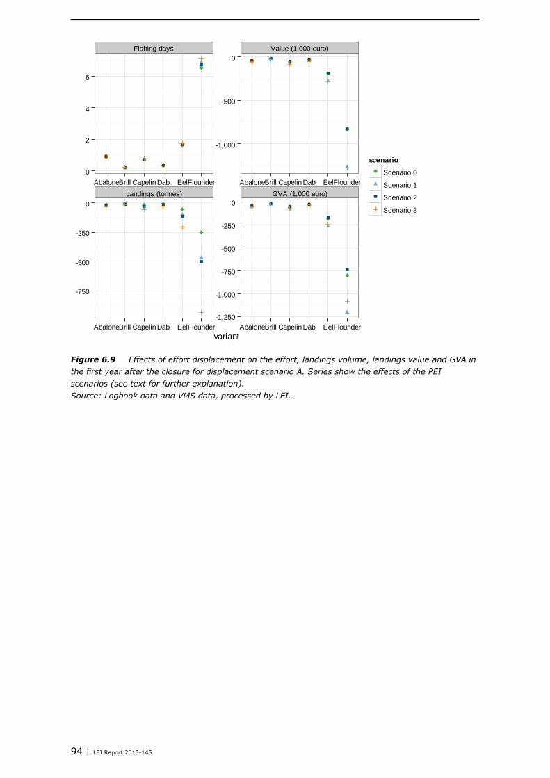
94 | LEI Report 2015-145

Figure 6.9 Effects of effort displacement on the effort, landings volume, landings value and GVA in

the first year after the closure for displacement scenario A. Series show the effects of the PEI

scenarios (see text for further explanation).

Source: Logbook data and VMS data, processed by LEI.

Fishing days Value (1,000 euro)

Landings (tonnes) GVA (1,000 euro)

0

2

4

6

-1,000

-500

0

-750

-500

-250

0

-1,250

-1,000

-750

-500

-250

0

AbaloneBrill Capelin Dab EelFlounder AbaloneBrill Capelin Dab EelFlounder

AbaloneBrill Capelin Dab EelFlounder AbaloneBrill Capelin Dab EelFlounder

variant

scenario

Scenario 0

Scenario 1

Scenario 2

Scenario 3

LEI Report 2015-145 | 95

Figure 6.10 Effects of effort displacement for independent vessels on the effort, landings volume,

landings value and GVA in the first year after the closure for displacement scenario A. Series show the

effects of the PEI scenarios (see text for further explanation).

Source: Logbook data and VMS data, processed by LEI

Fishing days Value (1,000 euro)

Landings (tonnes) GVA (1,000 euro)

0

2

4

6

-500

-400

-300

-200

-100

0

-300

-200

-100

0

-400

-300

-200

-100

0

AbaloneBrill Capelin Dab EelFlounder AbaloneBrill Capelin Dab EelFlounder

AbaloneBrill Capelin Dab EelFlounder AbaloneBrill Capelin Dab EelFlounder

variant

scenario

Scenario 0

Scenario 1

Scenario 2

Scenario 3

96 | LEI Report 2015-145

Figure 6.11 Effects of effort displacement for dependent vessels on the effort, landings volume,

landings value and GVA in the first year after the closure for displacement scenario A. Series show the

effects of the PEI scenarios (see text for further explanation).

Source: Logbook data and VMS data, processed by LEI.

Fishing days Value (1,000 euro)

Landings (tonnes) GVA (1,000 euro)

-0.50

-0.25

0.00

0.25

0.50

-800

-600

-400

-200

0

-600

-400

-200

0

-600

-400

-200

0

AbaloneBrill Capelin Dab EelFlounder AbaloneBrill Capelin Dab EelFlounder

AbaloneBrill Capelin Dab EelFlounder AbaloneBrill Capelin Dab EelFlounder

variant

scenario

Scenario 0

Scenario 1

Scenario 2

Scenario 3

LEI Report 2015-145 | 97

Figure 6.12 Effects of effort displacement on the effort, landings volume, landings value and GVA in

the first year after the closure for displacement scenario B. Series show the effects of the PEI

scenarios (see text for further explanation).

Source: Logbook data and VMS data, processed by LEI.

Fishing days Value (1,000 euro)

Landings (tonnes) GVA (1,000 euro)

-0.50

-0.25

0.00

0.25

0.50

-4,000

-3,000

-2,000

-1,000

0

-3,000

-2,000

-1,000

0

-4,000

-3,000

-2,000

-1,000

0

AbaloneBrill CapelinDab EelFlounder AbaloneBrill CapelinDab EelFlounder

AbaloneBrill CapelinDab EelFlounder AbaloneBrill CapelinDab EelFlounder

variant

scenario

Scenario 0

Scenario 1

Scenario 2

Scenario 3

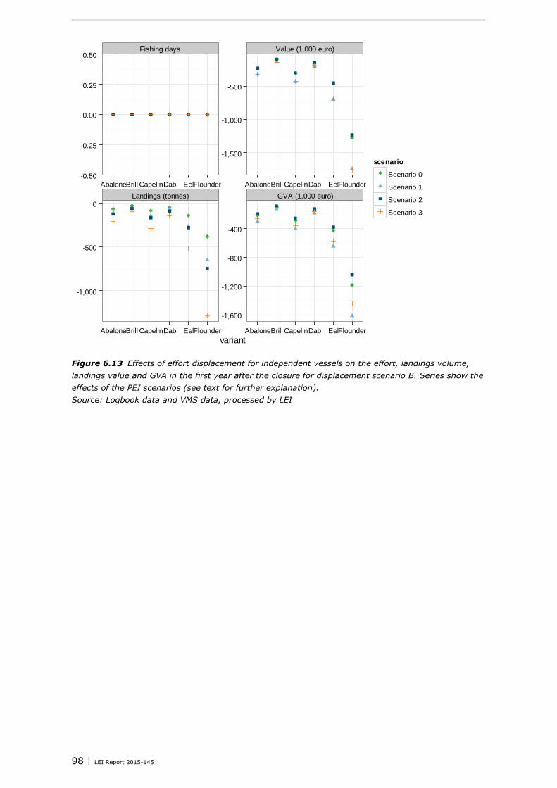
98 | LEI Report 2015-145

Figure 6.13 Effects of effort displacement for independent vessels on the effort, landings volume,

landings value and GVA in the first year after the closure for displacement scenario B. Series show the

effects of the PEI scenarios (see text for further explanation).

Source: Logbook data and VMS data, processed by LEI

Fishing days Value (1,000 euro)

Landings (tonnes) GVA (1,000 euro)

-0.50

-0.25

0.00

0.25

0.50

-1,500

-1,000

-500

-1,000

-500

0

-1,600

-1,200

-800

-400

AbaloneBrill CapelinDab EelFlounder AbaloneBrill CapelinDab EelFlounder

AbaloneBrill CapelinDab EelFlounder AbaloneBrill CapelinDab EelFlounder

variant

scenario

Scenario 0

Scenario 1

Scenario 2

Scenario 3

LEI Report 2015-145 | 99

Figure 6.14 Effects of effort displacement for dependent vessels on the effort, landings volume,

landings value and GVA in the first year after the closure for displacement scenario B. Series show the

effects of the PEI scenarios (see text for further explanation).

Source: Logbook data and VMS data, processed by LEI

The graphs show the differences in impact of the closures to vessels that have been classified as

dependent and independent for displacement scenario A and B. For the variants Abalone, Brill, Capelin

and Dap hardly any of the vessels are dependent and their contribution to the total costs is negligible.

On the contrary, for Eel and Flounder, the dependent vessels cause much higher costs of

displacement. The displacement costs of dependent vessels contribute approximately half of the total

costs for variant Eel and Flounder in case of displacement scenario A. In displacement scenario B the

costs for the dependent vessels are more important and dominate the total costs. The graphs only

show the effects of the first year after closure in which the costs made by dependent vessels are

highest. In later years, the differences between dependent and independent vessels are smaller and

disappear completely after four years in case of displacement scenario A. For displacement scenario C

the distinction between dependent and independent vessels is not relevant as neither of the two

categories has costs.

The differences between outcomes of the PEI scenarios are largest for variant Flounder and Eel. The

relative difference between the maximum and minimum reduction in GVA are for these variants more

than twice the difference for other variants. This is mainly due to effects on the dependent vessels. In

PEI-scenario 2 and 3, the reduction in landings are relatively high, but this is mainly due to landed

discards.

In case of displacement scenario A additional costs are estimated for the whole fleet, based on the

crowding effect. Table 6.6 summarises the effects of crowding for the whole Dutch fleet, based on the

effort increase in the remaining open area for each of the PEI scenarios. The effect of increased

crowding ranges from 0.5 m euros in variant Brill in PEI-scenario 0 to 3.4 m euros in variant Flounder

in PEI-scenario 3 and is almost proportional to the amount of effort displaced. For Abalone, Brill and

Dab the effect of displacement is relatively small. For Capelin the effect is intermediate and for Eel and

Fishing days Value (1,000 euro)

Landings (tonnes) GVA (1,000 euro)

-0.50

-0.25

0.00

0.25

0.50

-3,000

-2,000

-1,000

0

-2,000

-1,500

-1,000

-500

0

-2,000

-1,000

0

AbaloneBrill CapelinDab EelFlounder AbaloneBrill CapelinDab EelFlounder

AbaloneBrill CapelinDab EelFlounder AbaloneBrill CapelinDab EelFlounder

variant

scenario

Scenario 0

Scenario 1

Scenario 2

Scenario 3

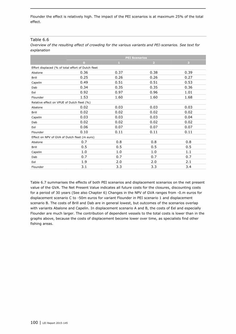
100 | LEI Report 2015-145

Flounder the effect is relatively high. The impact of the PEI scenarios is at maximum 25% of the total

effect.

Table 6.6

Overview of the resulting effect of crowding for the various variants and PEI-scenarios. See text for

explanation

PEI Scenarios

0 1 2 3

Effort displaced (% of total effort of Dutch fleet

Abalone 0.36 0.37 0.38 0.39

Brill 0.25 0.26 0.26 0.27

Capelin 0.49 0.51 0.51 0.53

Dab 0.34 0.35 0.35 0.36

Eel 0.92 0.97 0.96 1.01

Flounder 1.53 1.60 1.60 1.68

Relative effect on VPUE of Dutch fleet (%)

Abalone 0.02 0.03 0.03 0.03

Brill 0.02 0.02 0.02 0.02

Capelin 0.03 0.03 0.03 0.04

Dab 0.02 0.02 0.02 0.02

Eel 0.06 0.07 0.07 0.07

Flounder 0.10 0.11 0.11 0.11

Effect on NPV of GVA of Dutch fleet (m euro)

Abalone 0.7 0.8 0.8 0.8

Brill 0.5 0.5 0.5 0.5

Capelin 1.0 1.0 1.0 1.1

Dab 0.7 0.7 0.7 0.7

Eel 1.9 2.0 2.0 2.1

Flounder 3.1 3.3 3.3 3.4

Table 6.7 summarises the effects of both PEI scenarios and displacement scenarios on the net present

value of the GVA. The Net Present Value indicates all future costs for the closures, discounting costs

for a period of 30 years (See also Chapter 6) Changes in the NPV of GVA ranges from -0.m euros for

displacement scenario C to -50m euros for variant Flounder in PEI scenario 1 and displacement

scenario B. The costs of Brill and Dab are in general lowest, but outcomes of the scenarios overlap

with variants Abalone and Capelin. In displacement scenario A and B, the costs of Eel and especially

Flounder are much larger. The contribution of dependent vessels to the total costs is lower than in the

graphs above, because the costs of displacement become lower over time, as specialists find other

fishing areas.

LEI Report 2015-145 | 101

Table 6.7

Net effects of effort displacement on the net present value of the GVA (million euros) in the various

scenarios and displacement scenarios

PEI scenario 0 PEI scenario 1 PEI scenario 2 PEI scenario 3

Displacement

scenario

A B C A B C A B C A B C

Abalone -1.4 -3.4 0 -1.6 -4.6 0 -1.4 -3.0 0 -1.6 -4.1 0

Brill -0.8 -1.4 0 -0.9 -1.9 0 -0.8 -1.3 0 -0.9 -1.7 0

Capelin -1.8 -4.3 0 -2.2 -6.1 0 -1.8 -3.9 0 -2.2 -5.5 0

Dab -1.1 -2.2 0 -1.3 -2.9 0 -1.1 -1.9 0 -1.2 -2.6 0

Eel -3.7 -10.0 0 -4.6 -14.7 0 -3.6 -9.0 0 -4.4 -13.2 0

Flounder -10.9 -33.4 0 -14.4 -49.6 0 -10.3 -30.1 0 -13.5 -44.5 0

Source: Logbook data and VMS data, processed by LEI

6.2.3 Sensitivity analysis

Fishing activity in areas

The level of fishing activity in the areas provides the basic data for all analysis. As such all effects and

scenario outcomes are highly dependent on changes in these basic data. A 10% increase in the

estimated effort in the variants causes in some scenarios and variants even a more than proportional

increase in the outcomes (see Figure 6.15 and 6.16, panel 10% extra area use) e.g. the effect for

variant Brill in displacement scenario B is 13%. This is mainly due to the fact that an increase in the

effort in the area also increases the dependency on the area and thereby the costs of displacement. In

case of Flounder a large part of the costs of displacement are already from dependent fishing vessels,

so here the effect of increased dependence is smaller.

Scenario parameters

The sensitivity analyses carried out on the parameters as mentioned in Table 6.4 for the main effects

in the scenarios show that the results are relative robust to many of the parameters in the scenarios.

Moreover the analyses show that changing the overall values of most parameters affect the scenario

outcomes similarly. Changes in fuel price and technical innovation hardly have any effect on the

outcomes of the scenarios. Fuel costs are only part of the total costs and technical innovation

decreases fuel costs, but increases gear costs. A 10% extra decrease if the fish price results in a 1%

lower NPV of the GVA for PEI scenario 2 and 3 and a 10% increase of the effects of the landings

obligation has a comparable effect. Extra closures and extra fish density lead to increases in the value

for all the variants. A 10% increase in the other area closures as assumed in the PEI scenarios leads

to increased effort in each of the variants, thereby enhancing the value, but the effect is small. A 10%

increase in the fish density has a large effect on the outcomes and causes changes in outcome (NPV of

GVA) between 5 and 7%. The effect is largest for Brill and Dab and smallest for Abalone, Capelin and

Flounder. The effects of parameter changes are hardly influenced by the differences in the two

displacement scenarios.

102 | LEI Report 2015-145

Figure 6.15 Relative effects of 10% changes in selected parameters (see 6.4) on the net present

value of GVA for displacement scenario A. Series show the effects in each of the PEI scenarios.

10%extraLOeffect, 10% extra costs due to the landing obligation (see text for further explanation).

Source: Logbook data and VMS data, processed by LEI

Figure 6.16 Relative effects of 10% changes in selected parameters (see Table 6.4) on the net

present value of GVA for displacement scenario B. Series show the effects in each of the PEI scenarios.

10%extraLOeffect, 10% extra costs due to the landing obligation (see text for further explanation).

Source: Logbook data and VMS data, processed by LEI.

10%extrafuelprice 10%lowerfishprice 10%extraLOeffect 10%extraFishdensity

10%extraTechnInnov 10%extravectorsClosure 10%ExtraAreaUse

0

5

10

0

5

10

Abalone Brill Capelin Dab Eel Flounder Abalone Brill Capelin Dab Eel Flounder Abalone Brill Capelin Dab Eel Flounder

variant

NP

V G

VA

% o

f b

ase

scenario Scenario 0 Scenario 1 Scenario 2 Scenario 3

10%extrafuelprice 10%lowerfishprice 10%extraLOeffect 10%extraFishdensity

10%extraTechnInnov 10%extravectorsClosure 10%ExtraAreaUse

0

5

10

0

5

10

Abalone Brill Capelin Dab Eel Flounder Abalone Brill Capelin Dab Eel Flounder Abalone Brill Capelin Dab Eel Flounder

variant

NP

V G

VA

% o

f b

ase

scenario Scenario 0 Scenario 1 Scenario 2 Scenario 3

LEI Report 2015-145 | 103

Reference period

As mentioned above, the outcomes of the analyses are highly sensitive to changes in fishing activity in

the variants. Because of this historic changes in spatial patterns in effort and landings might have an

important effect on the costs of closures for the fishing sector. In order of quantify the effects of the

definition of the reference period on the study results the time trends for the fishing activities in the

ICES rectangles containing the possible closures were analysed. Figure 6.17 shows the trends in

effort, landings and landings value and shows that over the last decades, total effort, landings and

value of landings have been decreasing. Moreover, the area including the Frisian Front and the Central

Oyster ground has become less important to the Dutch fishing sector than before. The relative

importance of the landings value from this area decreased from around 10% in 1999 to around 7% in

2014. However, the averages of the period up to 2014 show a much lower decrease than the values of

individual years. This is because the relative importance of individual years that are added to the

average decreases as the time series grow larger; e.g. the weight of 2013 data in the average of

2013 -2014 is half of the total value, but the weight of 2005 data in the average of 2005-2014 is only

10%. Never the less, extending the time series backwards increases the average landings volume by

2% and the landings value by 3% for each year that is included. It is unclear whether this trend is

indicative for the fishing activities in all variants and whether this would lead to higher estimated costs

for the closures. The effects on GVA might be lower than expected, because the overall profitability of

the fleet was low during the period from 2003 - 2007 (Taal et al., 2010).

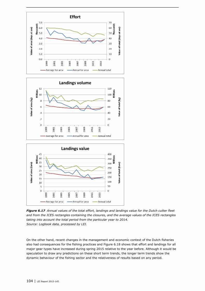
104 | LEI Report 2015-145

Figure 6.17 Annual values of the total effort, landings and landings value for the Dutch cutter fleet

and from the ICES rectangles containing the closures, and the average values of the ICES rectangles

taking into account the total period from the particular year to 2014.

Source: Logbook data, processed by LEI.

On the other hand, recent changes in the management and economic context of the Dutch fisheries

also had consequences for the fishing practices and Figure 6.18 shows that effort and landings for all

major gear types have increased during spring 2015 relative to the year before. Although it would be

speculation to draw any predictions on these short term trends, the longer term trends show the

dynamic behaviour of the fishing sector and the relativeness of results based on any period.

LEI Report 2015-145 | 105

Figure 6.18 Effort, landings and landings value for the major gear types of the Dutch fleet from the

ICES rectangles containing the closures in the first half year of 2014and 2015.

Source: Logbook data, processed by LEI.

6.3 Discussion

The analysis for the costs of closures for the fishing sector is based on simple scenarios including

policy, innovation and economic developments and effects of displacement. In the synthesis the

general consequences of making these assumptions is discussed.

The sensitivity analyses carried out show that individual factors taken into account in the scenario

analysis do not have a large effect on the outcome of the scenarios and do not change the relative

differences between areas. One should be aware that this is mainly due to the simplicity of the

scenarios, that assume similar effects of future developments in all areas:

Fish distribution patterns are assumed constant

Discard rates are assumed equal in all areas

Effort distribution patterns are assumed constant

Relative prices of fish species other than place and sole are assumed constant

No behavioural changes to the implementation of the discard ban.

The PEI scenarios 1 and 2 provide a range of extreme outcomes that include direct effects of changes

in these assumptions: e.g. PEI scenario one assumes that there is no effect of the discard ban on the

fishery in the area which can be explained that discard rates in the areas are negligible. In this way

the scenarios seem to provide some kind of range of possible outcomes. However, the scenarios only

take into account direct effects of the developments, which limit the value of these scenarios. E.g. the

fact that discard rates in the area are low (as suggested by some of the fishermen) could attract more

fishermen to the area when the landing obligation is implemented. This could potentially increase the

value of areas considerably.

As for the effects of displacement, these are mostly based on expert opinion and stakeholder

consultation. Although these results provide some indication of possible effects, they do not take into

account the complexity of the fishing practice. As a result the actual outcomes could be higher or

lower than shown here. This also applies to the PEI scenarios.

Despite the above mentioned uncertainties it can be concluded from the ranges in outcomes of the

various PEI and displacement scenarios that variants Brill and Dab will most probably result in relative

low costs for the fishing sector, Abalone and Capelin in intermediate costs and Eel and Flounder in

relative high costs.

106 | LEI Report 2015-145

7 Social effects on fisheries and their

communities

Olga van der Valk and Hans van Oostenbrugge

7.1 Methodology

A list of vessels was composed that in the last 7 years (2008-2014) had the highest score of sea days

spent in the proposed closure areas (all variations) was composed. The list was ranked according to

the average of effort since 2008, with yearly average above 10% including at least the last four years

(2011-2014). (See Table 7.1). Of the 10 cutters that are most dependent on the proposed areas, most

are registered in Urk (6) and Wieringen (2). Also for the top 20, Urk prevails: 9 cutters against 6 from

Wieringen. All vessels are most affected (e.g. have the highest dependency score) for variant

Flounder, with one exception. From this list, crew was approached for an interview. In total

4 interviews were conducted (highlighted in Table 8.1). In addition to information from the interviews

information on safety aspects has been incorporated as stated during the workshop on displacement

effects (Slijkerman and Tamis, 2015).

Table 7.1

Ranking of vessels with the highest dependency on the areas, from which the respondents for the

interviews were selected (highlighted)

Ranking Provenance Average

annual

dependency

Time period Highest

annual

dependency

Year Variant

1 Wieringen 32% '08-'14 75% 2008 f

2 Urk 32% '08-'14 45% 2009 f

3 Urk 32% '08-'14 39% 2009 f

4 Goedereede 25% '08-'14 59% 2011 f

5 Texel 24% '08-'09 38% 2009 e,f

6 Urk 22% '11-'14 27% 2011 f

7 Urk 22% '08-'11 26% '08-'09 f

8 Urk 20% 2013 20% 2013 f

9 Wieringen 18% '08-'14 27% 2010 f

10 Urk 17% '08-'14 32% 2009 f

11 Wieringen 17% '08-'14 27% 2011 f

12 Lemmer 17% '08-'11 19% 2011 f

13 Wieringen 15% '08-'14 30% 2011 b,d

14 Tholen 15% 08-'09-'10-'14 23% 2010 f

15 Urk 13% '08-'14 22% 2013 f

16 Wieringen 13% '08-'14 22% 2011 f

17 Urk 12% '08-'14 24% 2008 f

18 Wieringen 11% '08-'14 25% 2011 f

19 Urk 11% '08-'14 22% 2009 f

20 Lemmer 17% '08-'11 19% 2011 f

Source: Logbook data and VMS data, processed by LEI

Research results are based on qualitative interviews, which are not necessarily representative of the

entire sector, but give a good indication of what is happening within the fishing communities. One

interview was a double interview: two crewmembers of one cutter. The interviewees were all male, in

different stages of their lives: young men (25-35 yrs.) with and without (young) family and working as

LEI Report 2015-145 | 107

crew on a vessel of father / uncle; a skipper-owner (40-50 yrs.) whose children are young teenagers;

and retired skippers- owners (45-55 yrs.), on shore, still regularly sailing. Used fishing gear was

twinrig and beam trawl; the targeted species were langoustine, prawns and plaice / sole / turbot.

During the interviews the fishermen were shown the six variants in proposed area closures, but no

specific attention was given to how these variations differ. Interview questions focused on the social

impact of area closure in general (e.g. their experiences with earlier closures) and on the areas they

fish the most.

To assess social costs and benefits because of area closure, a list of topics was used, distinguishing

impact / relevance at company and at community level.

Table 7.2

Social consequences of variants discussed during the interviews

Company level Community level

Company succession Changes in landing port

Knowledge transfer / loss of experience Competition with other fishing communities

Working conditions / job satisfaction Social cohesion at community / national level

Employment

Previous / expected public policy

7.2 Results

Company level

Working conditions / job satisfaction

In the case of plaice / sole vessels from, respondents from Urk indicated a direct negative effect of

area closure on their working conditions and daily operations insomuch it reduces their options to fish

near their hometown. Fishing in areas further away signifies a different working schedule, that is, not

returning home for the weekend. Landing the fish further away means having to realise a higher

volume to cover transportation cost of bringing the fish to the auction, so the bottom line is that crew

members have to work harder for the same income, while time to spend with the family is reduced.

Thus, area closure limits the options to choose fishing areas, including those that allow the vessel to

return weekly. Nevertheless, the Urker respondents did not give area closure as main criteria for

displacement, but available quota, fishing price and expected gross turnover (quantity and quality of

fish based on information from other vessels).

The preference for regular working hours depends on the profile of the entrepreneur: how he values

family life, family tradition of fishing at the same spot for generations; and religiosity as basis for daily

activities. These entrepreneurs are most area-dependent and less prone to diversification of target

species.

Well, if we would lose the Frisian Front that is a disaster, that would really be a disaster. Because we fish there for a

100%, we always fish there. I grew up there, in turn I got the knowledge from my father. So I am making myself

acquainted with that area, that is familiar, one knows how to fish there. So I mean, as long as I have been at sea,

that’s how I sail, and my knowledge of other fishing areas is, to be very frank, not that great. [..]Most dart out on

Sunday night, but both of us, my cousin and I are the only ones left in the harbour on Monday morning. [..] One

has the responsibility for the family, the children, you can only raise them once.

Deteriorated working conditions are seen to be important for crewmembers that have no personal

connection with the vessels more than for those who belong to the upcoming generation, prospective

successors in family business. The level of commitment and loyalty of the latter is high.

Respondents indicated that imbalance between working hours and earnings may cause crewmembers

to giving up the fishing profession if job alternatives are more attractive. Nevertheless, respondents

indicate that mutual loyalty between skipper and crew is high and well looked upon by society; even

to the point that having to let go of a crewmember / co-skipper for financial reasons burdens both

108 | LEI Report 2015-145

parties emotionally, creating tension in family relationships. As a result, there is little turnover of crew

among vessels.

When you’ve worked for 10 years under the same captain, you do not easily say ‘I quit’, because you’ve

experienced the good years. Though it is difficult when you have a large family. You still remain true to your skipper

and your company where you work. If the crew is suffering, then the skipper is even suffering more. It’s not

because of the skipper filling his pockets that crew members quit.

Operational decision making, succession and knowledge transfer

Respondents indicate that there are two levels of decision making: operational and strategic. The

skipper on board consults with the crew and decides on the fishing tracks and daily operations, as well

as the areas the vessel will go to fish. The ‘skippers-on-shore’, vessel owners and mostly retired,

decide when to change target species, switch fishing gear and leave to a different area to fish. They

also have a major say in succession. As for selling the vessel, in the interviews the old generation’s

(lack of) motivation (because of ‘fickle’ public policy) was recurrently mentioned as a criteria in

strategic decision making. Nonetheless, comments and previous research shows that main reasons for

quitting are economic. No direct link with area closure is apparent. One respondent noted that for

fishing on the Doggerbank, area-specific knowledge will make a difference in volume of fish caught,

where this is less so for other areas (coastal range, Cleaverbank).

In knowledge transfer, the older respondents view the importance of experience and knowledge

transfer in a different light than the new generation:

‘That is all of their knowledge of the past, and the fish is moving again, so basically there is no telling what will

happen. Every year is different. Skagerrak is a good example. There always used to be small fish, always small

sorting, always plaice 4. This year, they were big, that’s never happened since I have started fishing. Fisheries is

really changeable.’

‘The disappearance of knowledge has an effect on the employment of the community. A father transferred his

company to his son, the son had to take over, but the father was not motivated because of all the regulations

coming… I have transferred my knowledge fanatically to my skipper. And he takes it up fanatically. If I transfer my

knowledge in a ‘la-la-la’ way, they also grasp it in a ‘la-la-la’ way. And I have seen it happening with the younger

generation as they take over: nothing comes out of it, and the company is sold or goes bankrupt. I can recall more

than 10 cases when these things have happened.’

Respondents indicate that knowledge transfer is not one-sided, it is practice based (the active younger

skipper handling the new technologies) versus experience based (knowledge on weather, fish

migration, seasonal cycle by the older skipper). The skipper with a young teenager son worried about

the fact that he would not be able to support his son with his advice, that the son would have to find

out all by himself through trial and error.

Community level

Changes in landing port

Respondents indicated that changes in landing ports will occur, as a result of area closure. One

respondent stated that he would probably need to land fish in Danish harbours with higher costs

because of changes in fishing grounds, but also at national level the fishermen indicated they might go

to other Dutch ports. This is mainly the case for plaice/sole (beam, pulse), not for langoustine

(twinrig).

Taking a historical longer term perspective on the importance of knowledge for the local economy, one

respondent mentioned that the decimated fleet and disappearance of fisheries related knowledge has

led to weakened industry (providers, processing) and innovative capacity of Urk. With the decreasing

fleet, supplying industries are diversifying activities (offshore; inland shipping); and specialized

expertise on fisheries technologies are sought elsewhere where fishing is economically dominant, like

in Denmark and Spain.

Employment and social cohesion at community level

The changes in community life have been different for Wieringen or Urk. In Urk the respondents note

the carpet industry and offshore activities offers employment opportunities and retain the youth.

Wieringen on the other hand is a noticeably ageing community, and young people move to Amsterdam

for study and a job. Surprisingly, respondents comment that the fleet crew is not ageing in neither

LEI Report 2015-145 | 109

locality. There are start-ups by young fisherman in both communities, mainly with smaller vessels for

shrimps. And while the respondents from Urk mark the decreasing local fishing economy (decreased

turnover by the auction; fleet shrinking from 300 to 37 vessels); those from Wieringen conclude that

their way of doing business (not going along with past trends of bigger and larger vessels) has made

the difference to maintain a stable fleet. Respondents foresee that closure of fishing grounds will lead

to a loss of employment.

We will have a very small area, if they close the Frisian Front and the Dogger Bank. I have the image that again

cutters will fall out, while this year… no, there was no ship building, but cutters, as good as new, did join.

In both communities the fleet has used foreign workers; in Wieringen only from Poland, in Urk also

from the Philippines. Also with regard to previous comments on the desirability of a steady crew,

seasonal employment occurs in prosperous times for the fisheries. Foreign people are employed as

crewmember; but skipper, boatswain and engineer are preferably Dutch. Mainly the larger companies

employ foreigners.

Social cohesion is very high among fishermen. This is not different for the young or the old. Social life

hardly involves people from other professions, and the topic of conversation is fishing. They

acknowledge the difficulties that their prolonged absence cause for the families on shore. This in turn

gives strong networking and cohesion amongst fishermen girlfriends and wives. Strong social bonding

makes it easier for fishermen to go to sea. Social cohesion determines the choice for the fisheries

sector, besides the earlier mentioned balance. As said before, the priorities in the balance between

earnings, working conditions and family life are decided by the individual fisherman. Area closure may

force him towards a different balance in order to survive as business.

‘If we were the only fishermen amongst our friends, they would say ‘you’re crazy’ Fishermen draw to each other,

you can see that amongst the young people as well. We have a separate team that isolates us a bit from the rest.

Because during the weekend, yeah that sounds a bit boring, but we also talk about fishing, others do not

understand. [..] But at Urk the women are used to it, they know how it is like. But most of the women’s father was

also a fisherman so they know’

Unfair competition

Fishermen feel that area closure has the opposite effect of what the measure aims at, as it will

increase the density of cutters in a certain area, and with it the risk of local resource depletion. While

they do not believe that this will create less collegiality amongst fishermen from the different

communities, they do foresee more tension among individual vessels, even internationally.

Furthermore, respondents express worry and indignation about the increasing amount of areas that

are closed for fisheries activities, whether because of fast shipping lanes, windmill parks, oilrigs or ‘the

placing of rocks’.

‘Areas that are taken away from us, we just never get them back, and it causes a considerable impact. At a certain

moment we will sail with less vessels but we are forced to bring them to the same fishing grounds. Pulse and beam

trawls will move to the areas of twin rig fishing and the two cannot interact, because twin rig fishing occurs at

3 knot, and beam trawling at 6 knots. So the latter chases the fish away for the twinrigger. You are driving others

away from their fishing grounds. If we go further south with the Urker flag vessels, the people in Arnemuiden will

not appreciate our coming to their fishing grounds, I think.’ [..]

Do you think that the Danish are happy with the presence of the Dutch? The same thing you can see with the

French. Not so much the Belgian as they practise the same kind of fisheries. With the French we have rows already;

tires are being punched and all.. You will see that happening next, when we move more to English and German

territory, that they [authorities] will start extra rigorous inspections to check the amount of discards.’

Society level

Legitimacy of public policy is low and decreasing

First and utmost the respondents were keen on ventilating their position towards policy and the

regulation of closed areas, recurrently remarking on its demotivating effect, which they consider an

important ‘social effect’ of the regulation. The interviews show that policymaking procedures cause

incomprehension, unbelief and cynicism amongst stakeholders.

Low legitimacy of public policy negatively influences the willingness to change behaviour and will

increase the cost of policy enforcement. Fishermen are not always negative towards restrictive policy

110 | LEI Report 2015-145

interventions, e.g. all respondents speak positively about the introduction of quotas, which was

described by a skipper as ‘acquired rights to the sea.’ Nevertheless, support for area closure is very

low. Regarding the quota as legitimate regulating system, they question the need for area closures.

Fishermen give several reasons for the limited support for closed areas, which is also influenced by

their view on public policy formulation in general:

1. Doubts about the effectiveness of measures decreases credibility of policy. Fishermen question the

‘usefulness’ of area closure (increased fish stocks, biodiversity); because they do not see

compliance with policy objectives at sea, - rather the contrary -, while scientific proof that fish

stock or biodiversity is increasing, is missing. (Plaice Box, being a recurrent example in all

interviews).

2. Discontent regarding the policymaking (governance) process. Fishermen express frustration about

always being consulted without it leading to changes. ‘We indicate, please move the area a bit. It is

received, you may have your say, but it is not used. There is nothing more frustrating than when it goes like

this. With the same speed it gets rejected. But it concerns [areas] where we have to make our money.’

3. Feelings of loss because decisions affect the flexibility and autonomy of the fishing profession

which are never reversed. ‘The Plaice Box would be a temporary solution, but it is still there. Every area that

we surrender, is lost to us.’ Fishermen consider that the ‘theoretical’ fundament of policies does not

correspond to (the need for flexible) practice at sea that is dependent on nature, not on planning

procedures. ‘One storm does more than 10 times fishing there. You do not know what’s going on at the

bottom. While we experience it every week.’ ‘You’re dealing with the theory and practice, and they differ a lot.

That is the fishing life, you talk about a certain freedom, yes, but you’re just very nature dependent. And that is

also the challenge.’

Fishermen also experience that they do not control their own destiny anymore. ‘Too many parties

who want to have a say regarding the sea.’ Respondents gave examples of how fishermen have been

adapting their vessels and fishing practices throughout the decades, and nevertheless see their

options for continuation of fisheries diminishing. ‘It is time that they look us straight in the eye and tell

us that they want us off the North Sea, instead of slowly strangling us.’

4. Experienced overload in quantity and unpredictability of regulations, which mainly gives rise to

demotivation and stress. ‘The frustrating thing is: at the moment we are making money, but

everybody has fear in the back of their head about how long will the gasoil price be so cheap, and

what will happen next, what more is there in store for us?’ ‘If only it would stop. But additional

regulations keep coming every year. We have nowhere left to go. It must stop. You will hear this

everywhere: you will hear it in Urk, Texel, in Stellendam. But it does not stop and at a certain

moment it breaks your spirit’.

Safety aspects

During the stakeholder process (e.g. the workshop on effects of effort displacement, Slijkerman and

Tamis, 2015) it was repeatedly stated by the fisheries representatives that the choice of a variant also

affects the safety on board fishing vessels. Two aspects are mentioned in particular:

The areas south of the Frisian Front of variants Brill and Dab overlap with shipping corridors, where

shipping intensity is high and chance on collision is higher than average. Closing these areas for

fishing would help to prevent such accidents

Closure of the Frisian Front area completely, as in variant Flounder, would urge fishermen to steam

through the area on their way to more Northern fishing grounds. During bad weather this could lead

to extra safety risks as fishing vessels are less stable in case fishing gears are stored.

7.3 Discussion and conclusions

The comments made by the respondents show that fishermen do not consider the closure of fishing

areas as a separate measure, but in the light of a whole package of regulations introduced by the

government, in which they fail to see a consistent vision for the fisheries sector. This creates anger,

bewilderment and disillusion, particularly as most measures that fishermen have adapted to, do have

negative economic effects, only to find that new ones are introduced.

LEI Report 2015-145 | 111

Respondents regard fisheries as a ‘hunter’s’ activity. Fishermen cannot control the conditions that

makes fish thrive. The presence of fish in a certain area, as well as the success of fishing practices,

are defined by nature, not by man. Conditions are highly variable, such as (increasing) sea

temperature, weather and wind conditions, and catches depend on fish migration, soil fertility and -

structure. To survive as a food providing company, fishermen ask for flexibility in how they organise

their fishing practices. The expanding and increasingly complex legal framework seems to reduce that

flexibility to a level that fishermen consider inoperable, and economically unfeasible, not to mention a

disregard for the complexity of their profession.

The interviews make clear that changing one aspect in fisheries conditions will generate direct and

indirect changes in a complex system, that may be cumulative and totally unforeseen. Most effects are

at company level: having to change target species, means reallocation of quota, changing gear, nets,

lengths of trips and ultimately may signify a changed family life. Changes in fisheries practices also

affect feasibility of other Dutch (and European) fishing companies, as it intervenes in the supply and

demand of fishing rights (quota prices) which may be the final blow to an individual vessel elsewhere.

Interviewees moreover hint at unexpected (negative) consequences for the ecosystem in and outside

protected areas.

That brings us to the conclusion that the effects, social and economic, of area closure are very case

specific. Categorising fishing companies is difficult, as fishing practices depend on family tradition, the

character and social values of the fisherman, his entrepreneurship, and even his (and his partner’s)

personal ability to combine profession with family life. More than other measures, area closure directly

and indirectly affects customary rights of fishermen who have fished on the same spots, sometimes

exclusively, for generations. Individual fishermen are struggling to conserve their way of life and, as

sector representatives already had marked upon, the interviews confirm that many a company

termination is also a personal tragedy.

112 | LEI Report 2015-145

8 Effects on enforcement and

monitoring

Hans van Oostenbrugge

8.1 Methodology

Besides the effects on the fisheries and the ecological effects, two important effects of implementation

of these area closures have been taken into account: effects on costs for control/enforcement and

effects on monitoring of ecological development in the areas. The effects on control/enforcement have

been assessed by means of telephone interviews with experts from the Netherlands Food and

Consumer Product Safety Authority (NVWA) and the concept texts have been reviewed by them.

The effects on monitoring have been assessed by experts from by Rijkswaterstaat and Informatiehuis

marien and provided to the team as a memo that is presented in Appendix 12. No additional data sets

were used for the analysis of these effects.

8.2 Results

8.2.1 Control

The control and enforcement of closed areas is carried out by the NVWA in cooperation with the Coast

Guard and Department of Public Works. NVWA has a Fisheries Monitoring Centre (FMC): from this

centre all vessel movements of the fishery are monitored 24/7. Currently, the capacity of this centre is

reduced. The control is carried out by means of VMS (Vessel Monitoring System) and AIS (Automatic

Identification System). The VMS system will, in principle, receive every 2 hours, the location, speed

and direction of the vessel but can also be activated from the FMC to transmit actual data. Since May

2014 also the AIS is mandatory for fishing vessels over 15 meters. This system transmits continuously

information about the position of the ship, but the strength of the signal (selection between high and

low strength is up to the skipper) is not always large enough to capture the information on land and to

monitor vessels in this manner.

Currently fishing vessels are only forbidden to fish in protected areas. Because of this, to prove an

offense (fishing in a closed area) there must also be evidence of fishing activities in addition to a

location observation. This evidence can only be collected on the spot by means of inspection by a

vessel or an aircraft. If there are indications of a breach by VMS and AIS data, the NVWA can decide in

consultation with the Coast Guard / Rijkswaterstaat seek additional evidence and carry out spot

checks. The decision for this is partly dependent on the position and course of the fishing vessel with

respect to the area and the position and plans of the units of the Coast Guard (flight plan, etc.). In

case a spot check indicates that there has been a breach (e.g. by Photos from an aircraft) formal

report may be made. In that case, there are costs associated with the settlement of the offense.

Respondents from the NVWA stated that the total budget for control of closures is hardly dependent

on the size of the closures and the fishing activities. From 2015 to 2016 the budget was reduced,

whereas additional control tasks were added (Dogger Bank, Cleaver bank). Because of this it is

assumed that the total control costs will remain constant and there will be some kind of allocation

mechanism by which the budget is divided over the various areas.

In 2014, in the coastal zone a number of areas have been closed to fishing under the N2000

regulations (VIBEG areas). These closures are enforced by the NVWA. In total the enforcement costs

for NVWA amounted around 500 kEuro during 2015. Out of 300 suspicions only 20 were acted upon

by means of air surveillance. The costs of this were approx. 200 kEuro during 2015.

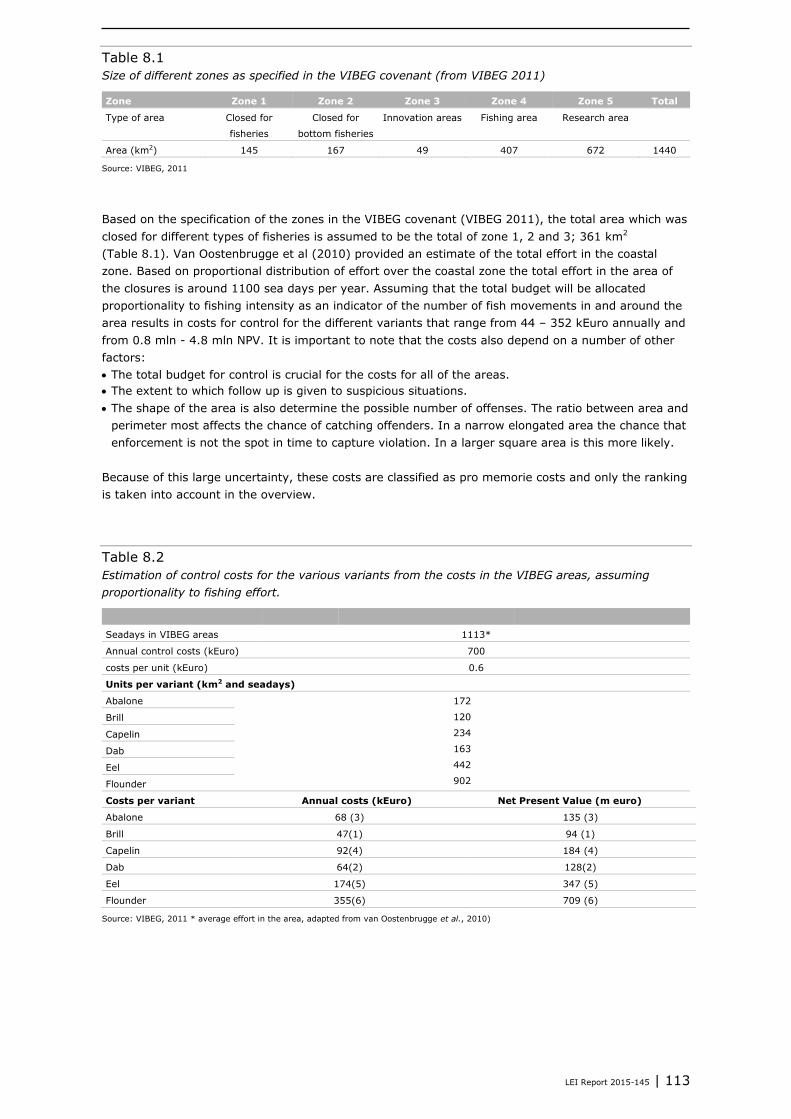
LEI Report 2015-145 | 113

Table 8.1

Size of different zones as specified in the VIBEG covenant (from VIBEG 2011)

Zone Zone 1 Zone 2 Zone 3 Zone 4 Zone 5 Total

Type of area Closed for

fisheries

Closed for

bottom fisheries

Innovation areas Fishing area Research area

Area (km2) 145 167 49 407 672 1440

Source: VIBEG, 2011

Based on the specification of the zones in the VIBEG covenant (VIBEG 2011), the total area which was

closed for different types of fisheries is assumed to be the total of zone 1, 2 and 3; 361 km2

(Table 8.1). Van Oostenbrugge et al (2010) provided an estimate of the total effort in the coastal

zone. Based on proportional distribution of effort over the coastal zone the total effort in the area of

the closures is around 1100 sea days per year. Assuming that the total budget will be allocated

proportionality to fishing intensity as an indicator of the number of fish movements in and around the

area results in costs for control for the different variants that range from 44 – 352 kEuro annually and

from 0.8 mln - 4.8 mln NPV. It is important to note that the costs also depend on a number of other

factors:

The total budget for control is crucial for the costs for all of the areas.

The extent to which follow up is given to suspicious situations.

The shape of the area is also determine the possible number of offenses. The ratio between area and

perimeter most affects the chance of catching offenders. In a narrow elongated area the chance that

enforcement is not the spot in time to capture violation. In a larger square area is this more likely.

Because of this large uncertainty, these costs are classified as pro memorie costs and only the ranking

is taken into account in the overview.

Table 8.2

Estimation of control costs for the various variants from the costs in the VIBEG areas, assuming

proportionality to fishing effort.

Seadays in VIBEG areas 1113*

Annual control costs (kEuro) 700

costs per unit (kEuro) 0.6

Units per variant (km2 and seadays)

Abalone 172

120

234

163

442

902

Brill

Capelin

Dab

Eel

Flounder

Costs per variant Annual costs (kEuro) Net Present Value (m euro)

Abalone 68 (3) 135 (3)

Brill 47(1) 94 (1)

Capelin 92(4) 184 (4)

Dab 64(2) 128(2)

Eel 174(5) 347 (5)

Flounder 355(6) 709 (6)

Source: VIBEG, 2011 * average effort in the area, adapted from van Oostenbrugge et al., 2010)

114 | LEI Report 2015-145

8.2.2 Monitoring

Rijkswaterstaat is responsible for monitoring of the status of the North sea ecosystem in the context of

the Marine Strategy. A detailed description of the assessment of the monitoring costs is provided in

Appendix 12. An assessment of the benthic ecosystem in the areas under study is carried out every

third year. The design of the monitoring of the Frisian Front and Central Oyster Grounds is based on

two separate areas (see Annex 5 of Part 2 of the Marine Strategy, Ministry of I&M, Ministry of EZ,

2014a). The measurement strategy is designed in such a way that a change in spatial distribution of

indicator species of the Marine strategy within the area of at least 50% change can be observed

between two measurement moments with a confidence level of 95%. The design of the measurement

strategy does not take into account the imposition of measures (i.e. closing areas) and because of that

additional activities need to be carried out in order to incorporate the areas in the monitoring system

and assess the developments inside and outside the closures. These activities are specified below and

summarised in Table 9.3.

Variant Flounder corresponds with the areas as defined in the Marine Strategy Part 2. The

measurement strategy has been prepared to monitor change in the area without taking into account

possible measures. Based on this premise an initial assessment (T0) has been performed in spring

2015. Closing the complete area raises the question of whether the measurement strategy still

qualifies or whether it should be adapted to include reference areas outside the closures. This means

that there may be additional costs in this variant. These costs will be determined on the basis of

expert opinion, but could potentially be as high as the costs for T0, causing a doubling of the

monitoring costs.

Variant Eel corresponds significantly to the areas in the Marine Strategy Part 2 (Ministry of I&M,

Ministry of EZ, 2014a); approximately half of the Central Oyster Grounds and the Frisian Fronts is

closed. For the area between CO and FF a measurement strategy has to be set up and a TO has to be

carried out. The regular monitoring costs will be higher than now as the intermediate area must be

monitored as well.

Variant Capelin appears to cover with three small areas in the Frisian Front about half of the area. It

should be examined whether this coverage is in accordance with the current measurement strategy or

that more points should be added. The closed area in the CO is (much) smaller than in the original

plan. For this area the measurement strategy has to be adjusted and a T0 must be performed again.

For the Central Oyster Grounds of variant Abalone the same applies as in Variant Capelin. Also for the

Frisian Front the measurement strategy has to be adjusted and a T0 has to be performed again. The

area is smaller than in the current monitoring plan, and also partly located in a different area.

Variant Brill and Dab differ most from the original monitoring plan. This means that the measurement

strategy and T0 should be performed again. The areas in Variant Brill are smaller, which may cost

more than Variant Dab because more measurements points will be needed. However, this cannot be

concluded based on these data.

For the variants Abalone -Eel and possibly Flounder a new measurement strategy need to be

established (cost approximately € 5,000 - € 10,000). For these variants also T0 also needs to be

adapted/redone, but the extent differs per variant. Because T0 was already carried out in a specific

way in spring 2015, the costs for complementary monitoring to complete T0 are not comparable

among the variants. Therefore, the costs of T0 have been left out in the calculation of the monitoring

costs.

For each of the variants the Net present value has been estimated using a time period of 30 years and

a discount rate of 5.5%.

LEI Report 2015-145 | 115

Table 8.3

Monitoring costs for the various variants (follow up monitoring) and an estimate of the Net Present

Value of future follow up monitoring costs (every 3rd year)

Variant Costs follow up monitoring (kEuro) NPV (kEuro)

Abalone 130 - 200 570 - 877

Brill 150 - 250 658 - 1,097

Capelin 130 - 180 570 - 790

Dab 150 - 250 658 - 1,097

Eel 130 - 210 570 - 921

Flounder 130 - 250 570 - 1,097

Source: RWS 2015

The NPV of total monitoring costs for the various variants ranges from 0.6 to 1.1m euros (Table 8.3).

Monitoring costs seem highest for Brill and Dab and Founder. Abalone and Capelin and Eel show

somewhat lower cost levels. For each of the variants, however, the estimate of the monitoring costs is

quite uncertain. The relative difference between the upper and lower estimate ranges from 38% for

Capelin to 92% for Flounder. As a result there is large overlap between the ranges of monitoring costs

for the different variants and it is not clear whether the actual costs of monitoring differ among

variants.

8.3 Discussion

Both control and monitoring costs of these closures have been made based on expert knowledge and

show high levels of uncertainty. As such it is hard to distinguish between the various variants,

especially between Abalone, Brill, Capelin and Dab. In addition costs for monitoring and control may

not only depend on the choice of the variant, but also on budget availability within the responsible

ministries. If this dependency on budget is high, choosing a variant for which estimated costs are

higher might not affect total costs but the intensity of the monitoring and control practices. In both

control and monitoring this can have consequences for the effects on (perceived) biodiversity and

fisheries practices.

116 | LEI Report 2015-145

9 Synthesis

Hans van Oostenbrugge and Diana Slijkerman

This study has assessed the major costs and benefits of six variants of closures for the bottom

fisheries in the areas of the Central Oyster Grounds and the Frisian Front (Figure 9.1). Table 9.1

presents a summary of the various costs and benefits.

Figure 9.1 Maps of different variants taken into consideration.

Source: Ministry of I&M, processed by LEI

Ecopoints per km2 and total ecopoints for the closures have been used as proxies for the ecological

benefits. These numbers resemble the current ecological values of the different variants, and not the

future ecological benefits as an quantitative assessment of the ecological effects is not feasible.

Therefore, this is no standard cost-benefit analysis. To compare the six variants, the ecopoint method

was used, which calculates Area* Quality* Weighting factor. The quality is the value of the species

biodiversity, expressed as the sum of the values of a number of benthic biodiversity indicators, which

can be calculated per variant. The weighting factors express the importance of e.g. the rarity of the

habitats covered by the closures, the presence of hard substrate, the presence of a front, the ratio

between size and circumference, etc. In this way, the results of different ways of thinking and the

effects of different preferences and management objectives can be compared. The future effects of

closures on the ecosystem can only be described in a qualitative way. For example, it is expected that

LEI Report 2015-145 | 117

a large closed area could result in restoration of species size distributions (e.g. of benthos or fish), but

it is impossible to predict and compare such expected values on the scale of the six variants (see also

Chapter 4).

The costs for the Dutch fishing sector have been estimated using historic data on fishing activities in

the variants and different PEI scenarios (Policy, Economics and Innovation scenarios)and displacement

scenarios. The PEI scenarios have been developed to assess potential effects of external developments

on the fishing activities in the areas. The displacement scenarios are used to estimate the costs in

case the areas are closed. Each of the three displacement scenarios is based on a specific set of

assumptions: Displacement scenario A is based on scientific insights on the specific fishing

opportunities in the areas (for non-quota species), the effects of crowding and the effect of

fishermen’s knowledge. Displacement scenario B is based on the view of fishermen’s representatives

and also includes costs for some vessels that will stop fishing. Displacement scenario C assumes that

the costs of the closures are negligible because fishermen will quickly adapt and find new fishing

opportunities. Comparison of the results of the various PEI-scenarios shows that the relative rating of

the closures in each of the scenario’s is quite stable. However, the sensitivity analyses show that the

outcomes are quite sensitive for some of the assumptions made, so some care should be taken into

account when focussing on the outcomes per PEI-scenario. The three extreme displacement scenarios

exemplify that there is large uncertainty around the possible outcomes of the closures dependent on

the assumed behavioural changes by the fishing sector. The results are presented as the Net Present

Value (NPV) of the Gross Value Added (GVA) (See also Chapter 6). The Net Present Value indicates all

future costs for the closures, discounting costs for a period of 30 years (See also Chapter 6).Because

most of the affected vessels are from Urk and Wieringen, the economic impacts of closures will also be

highest for these communities.

As the estimation of the effects of the closures are very context specific the effects of closures have

not been estimated for the foreign fleets, but the average annual GVA from the variants is presented

as an indication of the economic importance of the areas for these fishing fleets (See also Chapter 5).

The estimates shown here are much higher than in previous studies that were only based on partial

analysis. The economic importance of the areas to foreign fleets is for most of the variants comparable

to the importance for the Dutch fleet. For variant Eel and Flounder the importance for the foreign

fleets is larger. The annual GVA for Belgian and German flag vessels is also included as these vessels

are owned by Dutch entrepreneurs and contribute to the Dutch economy. For the UK vessels the

proportion of the fishing activities carried out by Dutch owned vessels could not be estimated.

However it is known that a considerable part of the UK fleet is in Dutch hands and this is the most

important foreign fleet operating in the area. Assuming a share of 50% of the UK vessels owned by

Dutch companies would result in economic returns from the closures which are approximately 75% of

the returns from Dutch fishing activities. In case the relative costs of displacement would be similar to

those of the Dutch fleet the total costs for Dutch owned vessels could be significantly higher than the

costs as stated in Table 10.1. As such, the foreign fleet activities are important and should be taken

into account in the discussion between stakeholder and managers. As the GVA of foreign and flag

vessels is presented as a number it seems that the uncertainty in the number is small. It should be

noted that the numbers presented here are merely indications of the scale of operation of foreign

fleets in the variants (see also 5.4.2).

Social aspects of the closures have been mapped using interviews of the most affected fishermen. The

interviews show that the effects of closures on the working conditions of fishermen are very context

specific and that changing one aspect in fisheries conditions will generate direct and indirect changes

in a complex system, that may be cumulative and totally unforeseen. Although social costs have not

been specified for each of the variants, safety aspects were mentioned for specific variants during the

stakeholder interactions. Safety for fishermen could be enhanced in case of variant Brill and Dab

because of smaller risks of collision with cargo vessels. In case of Flounder the practice of steaming

through the area could increase safety risks in case of bad weather conditions (See also Chapter 7).

The analysis of the dependency of fishing vessels shows that most fishermen affected come from

either Wieringen and Urk. Because of this, economic consequences will be concentrated in these two

fishing communities. Most of the fish coming from the community fishing fleets of especially Urk is

sold via the local auction and Urk also has as considerable fish processing and trade cluster. It is not

118 | LEI Report 2015-145

clear to what extent the closures will affect these sectors, but changes in the availability of fish for the

local fish cluster will affect its economy.

For the monitoring costs a range is presented of the net present value comparable to the one for the

fishing sector. and for the control costs a point estimate is given. It should be stated that also this

estimate is uncertain as it depends on the total budget for NVWA and the need for other control

activities (See also Chapter 8).

Comparison of the various types of costs shows that for the larger variants and for displacement

scenario B the costs of the fisheries comprise the majority of the costs. Fort the smaller closures,

however the costs for control and monitoring are of similar importance as the costs of fisheries.

LEI R

eport 2

015-1

45 | 1

19

Table 9.1

Overview of costs and benefits of variant closures

Type of costs/benefits Unit Abalone

Brill

Capelin

Dab

Eel

Flounder

Displacement scenario A B C A B C A B C A B C A B C A B C

Ecologic benefits Quality 4.87 3.74 4.96 3.92 4.64 5.08

Weight factors 0.2-1 0.05-1 0.12-1 0.06-1 0.31-1 0.28-1

Ecopoints/km2 0.97-4.87 0.19-3.74 0.62-4.69 0.24-3.92 1.45-4.64 1.44-5.08

Ecopoints total 12-59 2-47 10-79 4-66 61-195 91-322

Costs (m euro)

Dutch fisheries (NPV, m euro) PEI-Scenario 0 1.4 3.4 0.0 0.8 1.4 0.0 1.8 4.3 0.0 1.1 2.2 0.0 3.7 10.0 0.0 10.9 33.4 0.0

PEI-Scenario 1 1.6 4.6 0.0 0.9 1.9 0.0 2.2 6.1 0.0 1.3 2.9 0.0 4.6 14.7 0.0 14.4 49.6 0.0

PEI-Scenario 2 1.4 3.0 0.0 0.8 1.3 0.0 1.8 3.9 0.0 1.1 1.9 0.0 3.6 9.0 0.0 10.3 30.1 0.0

PEI-Scenario 3 1.6 4.1 0.0 0.9 1.7 0.0 2.2 5.5 0.0 1.2 2.6 0.0 4.4 13.2 0.0 13.5 44.5 0.0

Monitoring NPV (m euro) 0.6-0.9 0.7-1.1 0.6-0.8 0.7-1.1 0.6-0.9 0.6-1.1

Control NPV (m euro) 1.3 0.9 1.6 1.2 2.7 4.2

Total PEI-Scenario 0 3.3-3.6 5.3-5.6 1.9-2.2 2.4-2.8 3-3.4 1.6-2 4-4.2 6.5-6.7 2.2-2.4 3-3.4 4.1-4.5 1.9-2.3 7-7.3 13.3-13.6 3.3-3.6 15.7-16.2 38.2-38.7 4.8-5.3

PEI-Scenario 1 3.5-3.8 6.5-6.8 1.9-2.2 2.5-2.9 3.5-3.9 1.6-2 4.4-4.6 8.3-8.5 2.2-2.4 3.2-3.6 4.8-5.2 1.9-2.3 7.9-8.2 18-18.3 3.3-3.6 19.2-19.7 54.4-54.9 4.8-5.3

PEI-Scenario 2 3.3-3.6 4.9-5.2 1.9-2.2 2.4-2.8 2.9-3.3 1.6-2 4-4.2 6.1-6.3 2.2-2.4 3-3.4 3.8-4.2 1.9-2.3 6.9-7.2 12.3-12.6 3.3-3.6 15.1-15.6 34.9-35.4 4.8-5.3

PEI-Scenario 3 3.5-3.8 6-6.3 1.9-2.2 2.5-2.9 3.3-3.7 1.6-2 4.4-4.6 7.7-7.9 2.2-2.4 3.1-3.5 4.5-4.9 1.9-2.3 7.7-8 16.5-16.8 3.3-3.6 18.3-18.8 49.3-49.8 4.8-5.3

Fishing activities in the area

Dutch fleet Annual GVA (m euro) 0.4 0.2 0.5 0.3 0.9 1.6

Foreign fleets total Annual GVA (m euro) 0.4 0.3 0.5 0.5 1.5 3.3

Belgian and German flag

vessels Annual GVA (k euro) 45 19 62 29 143 429

120 | LEI Report 2015-145

From the compiled overview of costs and benefits the variants can be characterised as follows:

Abalone

The total area is 1,204 km2 and comprises of 2 subareas. Together with Brill this is the smallest

variant, and represents the lower boundary of the government objective for the closing of areas for

sea bed protection.

The subarea on the FF covers an important abiotic south-north gradient, from shallow to deep and

from sand to mud, and contributes to the quality specifically in terms of species richness and biomass.

The subarea on the CO, is of highest value compared to the other variants because of relative high

number of vulnerable species, such as long-lived species. The overall score for the CO subarea is

comparable to the CO subareas of the variants Brill, Capelin and Dab. In terms of ecopoints per km2,

this variant scores in the mid-range, and better than Brill which is equal in size. An exception is the

ecopoint value with hard substrate as weighting factor where Abalone scores lowest of all variants.

When weighting factors for fronts and gradients are applied, this variant scores second highest, next

to Flounder. Abalone scores (depending on the weighting factor applied) on average similar as

Capelin, which is however larger in size. When ecopoints are expressed on the total area Abalone

scores in general higher then Brill and Dab and Capelin, the difference however which depends on the

weighting factor of interest. Compared to Eel and Flounder this variant scores lower when ecopoints

are expressed on ecopoints/km2 and on the area level.

The fishing intensity of the Dutch fleet and the value of landings per km2 are relatively high, but

because of the small size, the costs of the closure to the Dutch fisheries are low to intermediate in

case long-term displacement costs are assumed (displacement scenario A and B). The costs for the

fishery are comparable with those for Capelin and the range also overlap with those of variant Brill and

Dab. The value for foreign fleets is among the lowest of all variants, together with those for variant

Brill. This is caused by the fact that in these variants smaller areas are closed where foreign fishermen

are active. Control costs seem to be relatively low for this variant.

In conclusion, the costs for the Dutch fishery related to this variant are low to intermediate. The

ecologic benefits depends on the expression of ecopoints and the weighting factors applies. Abalone

results in the upper range when ecopoints are expressed per km2, which depends on the weighting

factor applied. Using the weighting factor ‘hard substrate’ results in a lowest score, applying weighting

factors related to front and gradient, results in relatively high scores. Ecopoints expressed at the total

area fit in the upper range of the four smaller variants compared to Eel and Flounder. Impact of the

weighting factors are the same as in the results of ecopoints/km2.

Brill

The total area is 1,263 km2 and comprises 4 subareas. Together with Abalone this is the smallest

variant. The 2 larger subareas are located on sandy substrate, below the Frisian Front. The 2 smaller

subareas are located within the Frisian Front and the Central Oyster Grounds.

The overall value of ecological quality scores is lowest of all variants; the small subarea within the FF

however has the highest quality score of all subareas of all variants. The overall score for the CO

subarea is comparable to the CO subareas of the variants Abalone, Capelin and Dab. In general, this

variant scores lowest in terms of eco-points per km2, for almost all weighting factors. Only when ‘hard

substrate’ is taken into account as a weighting factor, the score per km2 is highest.

The closure of variant Brill also has a relatively low impact on the Dutch fisheries, together with the

closure of variant Dab. The fishing intensity and the value of landings per km2 are relatively low for the

Dutch fleet, and due to the small size, the costs of the closure to the Dutch fisheries are among the

lowest of all variants in case long-term displacement costs are assumed (displacement scenario A and

B). The costs for Dutch fisheries are comparable with those for Dab and the range also shows some

overlap with variant Abalone. The value for foreign fleets is among the lowest of all variants, together

with those for variant Abalone. This variant might also result in safety benefits for the fishing sector

because it lowers interaction with shipping. Control costs seem to be relatively low for this variant.

LEI Report 2015-145 | 121

In conclusion, this variant results in relatively low costs. The ecological benefits are in the lower range,

compared to the other variants, except when using the weighting factor ‘hard substrate’ (highest in

ecopoints/km2).

Capelin

The total area is 1,597 km2 and comprises 4 subareas. The 4 subareas are of similar size: 3 are

located in the FF and 1 at the CO. The gradients in the FF are covered over the 3 subareas, but not as

a continuous area. The CO area is approximately of comparable size, location and quality value to the

variants Abalone, Brill and Dab, scoring high for long-living species and species richness.

The ecological quality value is the second highest, as a result of relatively high scores for all

indicators. In terms of eco-points, this variant scores comparable to variant Abalone, which is smaller.

Capelin scores in the mid-range when weighting factors for continuous gradients are taken into

account. Compared to Dab, which is equal in size, Capelin has higher ecopoints, except when hard

substrate and number of habitats are included as weighting factor.

The costs of closure for this variant to the Dutch fisheries are intermediate. This is mainly due to the

fishing intensity and the value of landings per km2 which are among the highest of all variants, and the

intermediate size. The costs for fishery are comparable with those for Abalone and the range also

overlap with variant Dab and also Eel for displacement scenario A and B. The value for foreign fleets

also has an intermediate level, together with those for variant Dab. Costs for control are intermediate

as well for this variant.

In conclusion, this variant results in intermediate costs, and the number of ecopoints per km2 are in

the mid-range, for most of the weighting factors applied. Ecopoints expressed at the total area fit in

the upper range of the four smaller variants. Weighting factors vary for this variant and their impact

on the results of ecopoints/km2 and total ecopoints is similar.

Dab

The total area is 1,683 km2 and comprises 4 subareas. This variant is an extended version of Brill and

consists of 2 large subareas that are partly situated in the sandy sediment, below the FF, and 2

smaller subareas within the FF and the CO.

The quality value is one-but-lowest, except for the subarea in the centre of the Frisian Front (see

Brill). The overall score for CO subarea is comparable to the CO subareas of the variants Abalone,

Capelin and Brill, scoring high for long-lived species and species richness. In general, this variant

scores one-but-lowest in terms of ecopoints per km2, but scores highest when weighting factor

“number of habitats” and second highest when hard substrate are applied.

The fishing intensity of the Dutch fisheries and the value of landings per km2 are similarly low to those

of variant Brill, but because this variant is 30% larger the costs of closure are also somewhat higher

but somewhat lower than the other variants. Because of the uncertainty in outcomes, the ranges in

resulting costs of the two variants overlap substantially for displacement scenario A and B. The range

of costs also overlaps with those of Abalone, Brill and Capelin. The value for foreign fleets has an

intermediate level, together with that for variant Capelin. This variant might also result in safety

benefits for the fishing sector because it lowers interaction with shipping. Costs for control are

intermediate.

In conclusion, this variant results in low to intermediate costs. The ecologic benefits are in a mid to

lower range when ecopoints are expressed per km2, depending on the weighting factor applied. Using

the weighting factor ‘hard substrate’ or ‘number of habitats’ results in higher scores, other weighting

factors result in lower scores. Depending on the weighting factors it is in the mid- to low-range but

higher than Brill. Impact of the weighting factors are the same as in the results of ecopoints/km2.

Eel

The total area is 4,206 km2 and comprises 4 subareas. The 4 large subareas vary in size from 700 to

1,400 km2, and are distributed throughout the search area, from the sandy substrate to the CO. In

122 | LEI Report 2015-145

this way, a suite of habitat types is protected, while allowing for fishing in between the areas. The size

of the CO subarea is considerably larger than that within the variants Abalone to Dab.

The quality value of Eel is relatively low compared to other variant because a part of the variant

covers the sandy substrate with lower biodiversity values. In general the values of the weighting

factors are relatively high for this variant, except for hard substrate. However, while the quality factor

value is slightly below that of Abalone, Capelin and Founder, this variant scores the second highest

number of ecopoints/km2, for most weighting factors - except for hard substrates and fisheries

pressure.

The fishing intensity of the Dutch fisheries is relatively low for this variant and the effort per km2 is

almost equal to that of variants Brill and Dab. Because of the large size however, the total costs of the

closure of this variant for the Dutch fisheries in scenario A and B are higher than those of the previous

variants. This is also because some of the fishermen are classified as being dependent on the area

(more than 10% of their annual revenues from the area). Therefore, they are assumed to have higher

costs for reallocating their effort to other fishing grounds. The range of costs for the Dutch fishery

shows some overlap with the ranges for variant Capelin and with the range for variant Flounder. The

value for foreign fleets Is relatively high. Because of the higher value to the fisheries the control costs

are also relatively high.

In conclusion, this variant results in intermediate to high costs, and it scores in an overall higher range

in terms of both ecopoints/km2 and total ecopoints. The actual value depends on the weighting factor

applied. Using the weighting factor ‘hard substrate’ results in lower ecopoints/km2, applying weighting

factors related to gradient, results in relatively mid-range to high scores for both ecopoints/km2 and

total ecopoints.

Flounder

The total area is 6,339 km2 and comprises of 2 subareas. This is the largest variant. The 2 subareas

fully cover the FF and CO. Therefore it fully protects all (a)biotic gradients on the FF and scores

highest for species richness.

Overall, this variant scores the highest quality value, the highest weighting factors, and therefore also

the highest number of ecopoints, for all but one applied weighting factor (hard substrate in terms of

ecopoints/km2). Besides the high scores for quality and weighting factors, the size of the area is very

determining for the final result.

The costs of closure for the Dutch fisheries are by far the highest of all variants in case long-term

displacement costs are assumed (displacement scenario A and B). This results from both the large size

of the area and the high fishing intensity in the area (mainly on the Frisian Front). In addition, the

variant has the highest proportion of fishing vessels that are classified as dependent on this area and

that are assumed to have extra difficulties in reallocating their activities. Finally, closing the complete

Frisian Front also removes the possibility for fishermen to fish through the area on their way to

northern fishing grounds or back to the harbour. Fisheries representatives have stated that this can

also lead to potential safety risks in case of bad weather. Also for the foreign fleets, the value of the

areas is by far the largest for this variant. The costs for control will be highest of all variants.

In conclusion, this variant results in both highest costs, and highest scores for ecopoints/km2, except

when hard substrates are taken into account. When ecopoints are expressed on the total area,

Flounder has overall highest scores.

In case no long-term costs of fisheries displacement are assumed to be 0 the relative ranking of the

various variants remains similar with low costs for Brill and Dab, intermediate costs for Abalone and

Capelin and high costs for Eel and Flounder. The reason for this is the assumption that control costs

are related to the amount of fishing activities in the areas.

Although the current study provides a characterisation of the benefits and costs of protecting the

seabed in the different variants, many of the costs and benefits are not comparable and the outcomes

LEI Report 2015-145 | 123

are quite uncertain. As such this study does not provide clear answers as to which variant is most

likely to fulfil the management objective most efficiently. The main reasons for this are described

below.

Uncertainty in the data

Part of the high variability in the outcome of the study is due to uncertainty in the basic data that is

used for the analysis. Statistical data such as the basic ecological data and the distribution of landings

from the fishery is uncertain as it is based on incomplete observations of the reality. As such these

estimates are unbiased, but contain some degree of uncertainty. On the other hand stakeholder

dependent information is used in the analyses of various effects (e.g. costs of control, displacement

effects, social effects). Stakeholders have another perception of the developments. First of all they

look at the developments from another point of view (Densen, 2001). The fishermen that were

interviewed and were present at the displacement workshop stressed that the consequences of a

closure are vessel specific and depend on many aspects such as gear, quota availability, distribution

patterns, social background etc. Therefore it is hard to get a good overview of possible effects of

closures on fishing operations. Second, the closure studied here is only one of several (policy)

developments that affect their position and its consequences might be of little importance in the light

of other developments. The large range in outcomes of the PEI scenarios confirm this. This makes it

even harder to specify the consequences of this specific management measure. In addition to the

fishing sector this might also apply to other stakeholders such as the NVWA, which stated that the

costs of enforcement are also driven to by budget limitations. However, the current stakeholder

consultation gives stakeholders the opportunity to try and influence the policy by means of strategic

behaviour. As such their estimates of effects are uncertain and might also be biased. In this study, the

uncertainty is assessed by means of scenario analysis and sensitivity analysis. This enables the reader

to get an idea about the uncertainty, but at the same time complicates the choice for an optimal

solution solely based on this analysis. A specific discussion on the effects of displacement is provided

in the previous chapters. More information on specific uncertainties in the data/assumptions are

provided in the discussions of the various chapters. An increased knowledge base about the

mechanisms behind fishermen’s behaviour and the effects of closures on this would help to create

more certainty. The study by de Vries et al (2015) on the effects of the Voordelta closures can be a

good starting point for this.

Scope of the study

Limitations in the scope of the study also limits the possibilities to come to a complete evaluation of an

optimal solution. These limits can be seen at two levels. First, the different types of effects still have

different dimensions (e.g. ecopoints, ecopoints per km2 and euros) which complicates comparison of

costs and benefits between scenarios. In scientific literature various methods exist to monetarise

different types of effects (Buisman en Vos, 2010) or to compare effects with different dimensions by

means of a multi criteria analysis (Soma et al., 2013). These techniques may provide valuable insights

into preferences, but they also add assumptions and thereby uncertainty to the already highly

uncertain outcome of the current analysis. Moreover, such studies are only useful in case differences

in the ecological effects of the variants could be analysed, which is not possible based on the current

knowledge. As such the added value in the application of such techniques in the current context to find

‘the best variant’ might be questionable.

Besides, the effects of the closures on the foreign fisheries activities have only been partially analysed.

This is mainly because the effects on these fleets largely depend on local circumstances and it would

be very complex and time consuming (if not impossible) to get reliable (quantitative) results for the

effects for all of these fishing vessels. Nevertheless, this study shows that the value of the areas for

the foreign fleets is approximately twice the value for the Dutch fisheries. Therefore, the choice of the

variant will also have a significant effect on foreign fishing vessels. Because part of these vessels are

Dutch owned and part land their catches in Dutch harbours, this will probably also affect the Dutch

fish cluster indirectly. The extent of this is, however, highly uncertain.

Complex multiple objectives

The uncertainty in the outcomes of the study is also partly due to the fact that the policy objectives

are complex, include multiple sub-objectives which are not (or cannot be) clearly defined in

124 | LEI Report 2015-145

measurable units, e.g. an X% increase in the biomass of these species. In the current study a number

of weighting factors are used in case of the ecological benefits, emphasising various characteristics of

the closure. The results provide valuable input for a discussion on the pros and cons of each of the

variants, but also result in considerable variation in the outcome of the study (see Table 10.1) without

clear-cut answers. On the economic side, the choice of the net present value of the GVA as an

indicator of economic costs indicates a macroeconomic approach, which assumes that the total returns

on invested capital and labour should be optimised. Depending on the policy objectives one could also

choose to focus on the effects on employment, income of the crew, or total landings value or volume.

All of these variables might show different aspects of the economic effects, while the actual effect on

the economy will be a combination of all of them.

Future effects of closures

Last but not least the current study tries to assess potential future effects of closing areas based on

current knowledge and historical data. This raises two questions:

Is the reference period correct?

Can analysing data from this period tell us something about future potential?

The reference period for ecological data has been based on the most recent available survey data and

for fisheries it has been based on data availability of VMS data. These time series have been used to

provide a number of years that is representative of recent developments. For the Dutch fishing sector

the time series in Chapter 5 show a decreasing trend in both effort, landings and value. A sensitivity

analysis on the extension of the time series (Section 6.2.3) suggest that extending the time series to

previous years has little effect on the outcomes. Reducing the reference period (e.g. to 2010-2014)

would result in lower values. However, it is questionable whether these years are more representative

for a normal than the years before. The period between 2010 and 2014 has been a time of transition

for the Dutch fisheries to other, more innovative, cost efficient and more eco-friendly ways of fishing

(e.g. van Marlen et al., 2014). Moreover, the analysis of the 2015 data (Section 6.2.3) shows that for

all gears effort, landings and value increased in the area that includes the potential closures. Because

of this, the reference period, including both the transition period and some years before, is regarded

as being a proper reference period.

The question whether historical data can tell us something about future effects is not specific for the

current study. However, it should be noted that any attempt to provide estimations of future effects

will include a great amount of uncertainty, especially in case differences are sought on a detailed level

as in this study. The future potential of the areas for both economy and ecology will be highly

dependent on the natural and economic context. The ecological analysis in this study focuses on the

current situation in the variants and does not assess effects of closing the areas. This is because at the

scale of this study, no reliable tools for estimation of ecologic effects of closures are available (see

Chapter 4). For the fisheries effects, scenarios do not provide optional future effects but the indicate

what possible effects various developments might have on the current situation. From the sensitivity

analyses it is clear that the various assumptions made in the analyses have considerable effects on the

outcomes. Moreover, the fact that most assumptions are similar for all variants might create an

erroneous sense of certainty that the effects of future developments will be similar for all variants.

However, this is incorrect because future changes in fish distribution for example are not taken into

account in the scenarios, but will have a significant effect on the relative costs for closing one or

another area. Changes in relative fish prices or discard rates can have similar effects. As such, the

outcomes of the scenarios for the fisheries effects for each of the variants should rather be seen as a

measure of uncertainty of the outcomes than of different sets of variant outcomes that can be used to

compare variants.

Because of the points mentioned above, this study does not provide a clear answer to the question on

the optimal management choice. Having said that, the outcomes have a value as a characterisation of

the aspects of the areas under study that will be affected by a closure. As such, the present study can

provide useful information in a discussion on preferences and possible compromises between

stakeholders and mangers. In these discussions, the present study shows the most recent knowhow

on the costs and benefits of the different variants and distinguishes between facts and fiction for the

topics under study.

LEI Report 2015-145 | 125

References and websites

Beare, D., A.D. Rijnsdorp, M. Blaesberg, U. Damm, J. Egekvist, H. Fock, M. Kloppmann, C. Röckmann,

A. Schroeder, T. Schulze, I. Tulp, C. Ulrich, R. van Hal, T. van Kooten, M. Verweij (2013):

Evaluating the effect of fishery closures: Lessons learnt from the Plaice Box. Journal of Sea

Research 84: 49-60.

Bergman, M.J.N. (1991): Beschermde gebieden Noordzee: noodzaak en mogelijkheden. Report 1991-

3, NIOZ, Den Burg, Texel, The Netherlands.

Beukers, R. (2015): De Nederlandse visverwerkende industrie en visgroothandel; Economische

analyse van de sector, ontwikkelingen en trends. Wageningen, LEI Wageningen UR (University &

Research centre), LEI Report 2014-026. 84 blz.; 20 fig.; 44 tab.; 7 ref.

Blancher, P., E. Catalon, C. Wallis, M. Menard, L. Girard, B. Maresca, A. Dujin, F. Fondrinier, X.

Mordret, I. Borowski-maaser, M. Saladin, E. Interwies, S. Görlitz, M. Da Conceição Cunha (2013):

ESAWADI: Utilizing The Ecosystem Services Approach For Water Framework Directive

Implementation. Synthesis Report Work Package 5: Synthesis And Policy Recommendations.

Borger, T., C. Hattam, D. Burdon, J. Atkins, M. Austen (2014): Valuing the conservation benefits of

offshore marine protected areas. Ecological Economics. 108, 229-249.

Bos, O.G., R. Witbaard, M. Lavaleye, G. van Moorsel, L.R. Teal, R. van Hal, T. van der Hammen, R. ter

Hofstede, R. van Bemmelen, R.H. Witte, S. Geelhoed, E.M. Dijkman (2011): Biodiversity hotspots

on the Dutch Continental Shelf: A Marine Strategy Framework Directive perspective, IMARES

report C071/11 (http://edepot.wur.nl/174045).

Bruggeman, W., E. Dammers, G.J. van den Born, B. Rijken, B. van Bemmel, A. Bouwman, K.

Nabielek, J. Beersma, B. van den Hurk, N. Polman, V. Linderhof, C. Folmer, F. Huizinga, S.

Hommes, A. te Linde (2013): Deltascenario’s voor 2050 en 2100 Nadere uitwerking 2012-2013.

Deltares Delft, 2013 - 65 p.

Buisman, E., H. van Oostenbrugge, R. Beukers (2013): Economische effecten van een aanlandplicht

voor de Nederlandse visserij LEI-rapport 2013-062. ISBN/EAN: 978-90-8615-657-3.

Buisman, F.C., B.I. de Vos (2010): Maatschappelijke kosten-batenanalyse voor de visserij. Een

verkenning naar een MKBA in een mariene omgeving. LEI Rapport 2008-005. ISBN/EAN

9789086152261. LEI, Den Haag.

Coolen, J.W.P., W. Lengkeek, S. Degraer, F. Kerckhof, H.J. Lindeboom (in prep): Separation by habitat

preference: Distribution of the invasive Caprella mutica and native Caprella linearis on artificial

hard substrata in the North Sea. submitted.

Coolen, J.W.P., W. Lengkeek, G. Lewis, O.G. Bos, L. van Walraven, U. van Dongen (2015): First

record of Caryophyllia smithii in the central southern North Sea: artificial reefs affect range

extensions of sessile benthic species. Marine Biodiversity Records. 8 (e140). p.p. 4 pages.

Creutzberg, F., P. Wapenaar, G. Duineveld, N. Lopez Lopez (1984): Distribution and density of the

benthic fauna in the southern North Sea in relation to bottom characteristics and hydrographic

conditions (http://www.vliz.be/imisdocs/publications/14729.pdf). Rapp P -v Réun Cons int Explor

Mer 183:101-110.

De Gee, A., M.A. Baars, H.W. van der Veer (1991): De ecologie van het Friese Front. Waarnemingen

aan een biologisch-rijke zone in de Noordzee, gelegen tussen de zuidelijke bocht en de

Oestergronden (www.vliz.be/imisdocs/publications/263191.pdf). Report 1991-2, NIOZ.

Deerenberg, C., F. Heinis (2011). Passende beoordeling boomkorvisserij op vis in de Nederlandse

kustzone. IMARES rapport C130/11.

Densen, W.L.T. van (2001): On the perception of time trends in resource outcome. Its importance in

fisheries co-management, agriculture and whaling. PhD thesis. Twente University. 299 p.

De Vries, P., N.T. Hintzen, D.M.E. Slijkerman (2015): Fisheries displacement effects of managed

areas: a case study of De Voordelta. IMARES Report number C136/15.

Dinmore, T.A., D.E. Duplisea, B.D. Rackham, D.L. Maxwell, S. Jennings (2003): Impact of a large-

scale area closure on patterns of fishing disturbance and the consequences for benthic

communities. ICES Journal of Marine Science, 60: 371e380.

126 | LEI Report 2015-145

Duineveld, G. C. A., Bergman, M. J. N. & Lavaleye, M. S. S. (2007). Effects of an area closed to

fisheries on the composition of the benthic fauna in the southern North Sea. – ICES Journal of

Marine Science, 64: 899–908.EU (2010): 2010/477/EU. Commission Decision of 1 September

2010 on criteria and methodological standards on good environmental status of marine waters

(notified under document C(2010) 5956). Online: http://eur-

lex.europa.eu/LexUriServ/LexUriServ.do?uri=OJ:L:2010:232:0014:0024:EN:PDF.

Fisher, B. (2008): Ecosystem services and economic theory: integration for policy-relevant research.

Ecological Applications. 18, 2050-2067.

Forcada, A., C. Valle, J.L. Sánchez-Lizaso, J.T. Bayle-Sempere, F. Corsi (2010): Structure and spatio-

temporal dynamics of artisanal fisheries around a Mediterranean marine protected area. ICES

Journal of Marine Science 67: 191-203.

Fox, H.E., M.B. Mascia, X. Basurto, A. Costa, L. Glew, D. Heinemann, L.B. Karrer, S.E. Lester,

A.V. Lombana, R.S. Pomeroy, C.A. Recchia, C.M. Roberts, J.N. Sanchirico, L. Pet-Soede, A.T.

White (2012): Reexamining the science of marine protected areas: linking knowledge to action.

Conservation Letters 5:1-10.

Gittenberger, A., N. Schrieken, J.W.P. Coolen, W. Vlierhuis (2013): The Jewel anemone Corynactis

viridis, a new order for The Netherlands (Cnidaria: Corallimorpharia). Nederlandse Faunistische

Mededelingen. 41. p. pp. 35 - 42.

Greenstreet, S.P.R., H.M. Fraser, G.J. Piet (2009): Using MPAs to address regional-scale ecological

objectives in the North Sea: modelling the effects of fishing effort displacement. ICES Journal of

Marine Science 66: 90-100.

Hamon, K., J.A.E. van Oostenbrugge, H. Bartelings (2011): Fishing activities on the Frisian Front and

the Cleaver Bank. Historic developments and effects of management. LEI Memorandum 13-050.

May 2013.

Hanley, N., S. Hynes, N. Jobstvogt, D.P. Paterson (2014): Economic Valuation of Marine and Coastal

Ecosystems: Is it currently fit for purpose? Working Paper 2014-11, Department of Geography and

Sustainable Development, University of St Andrews.

Hiddink, J.G., S. Jennings, M.J. Kaiser, A.M. Queiros, D.E. Duplisea, G.J. Piet (2006): Cumulative

impacts of seabed trawl disturbance on benthic biomass, production, and species richness in

different habitats. Canadian Journal of Fisheries and Aquatic Sciences 63 (4) - p 721 – 736

Hintzen, N.T., G.J. Piet, T. Brunel (2010): Improved estimation of trawling tracks using cubic Hermite

spline interpolation of position registration data In: Fisheries Research 101 (1-2): pp. 108-115.

Huizinga, F. (2012): Actualiteit WLO scenario’s. CPB Notitie 8 mei 2012.

Janssen, L.H.J.M., V.R. Okker, J. Schuur (eds.) (2006): Welvaart en Leefomgeving: Een scenariostudie

voor Nederland in 2040, Den Haag/Bilthoven, Centraal Planbureau, Milieu- en Natuurplanbureau

en Ruimtelijk Planbureau.

Jongbloed, R.H., D.M.E. Slijkerman, R. Witbaard, M.M.S. Lavaleye (2013): Ontwikkeling

zeebodemintegriteit op het Friese Front en de Centrale Oestergronden in relatie tot

bodemberoerende visserij: Verslag expert workshop (http://edepot.wur.nl/288777). Report

C212/13, IMARES.

Keeler, B.L. et al. (2012): Linking water quality and well-being for improved assessment and valuation

of ecosystem services. PNAS. 109, 18619-18624.

Kuhlman, J.W., J.A.E. van Oostenbrugge (2014): Bodemberoerende visserij op de Noordzee; Huidige

situatie, recente ontwikkelingen en toekomstscenario’s. Wageningen, LEI Wageningen UR

(University & Research Centre), LEI Report 2014-024.

Lechene, V. (2000): Chapter 6: Income and Price Elasticities of Demand for Foods Consumed in the

Home, National Food Survey: 2000, available at

http://statistics.defra.gov.uk/esg/publications/nfs/2000/Section6.pdf.

Lee, J., A.B. South, S. Jennings, (2008): Developing reliable, repeatable, and accessible methods to

provide high-resolution estimates of fishing-effort distributions from vessel monitoring system

(VMS) data.ICES Journal of Marine Science 67: 1260-1271.

Lengkeek, W., J.W.P. Coolen, A. Gittenberger, N. Schrieken (2013): Ecological relevance of shipwrecks

in the North Sea. Nederlandse Faunistische Mededelingen. 40 (6). p. pp. 49-58.

Lengkeek, W., K. Didderen, M. Dorenbosch, S. Bouma, H.W. Waardenburg (2013): Biodiversiteit van

kunstmatige substraten. Een inventarisatie van 10 scheepswrakken op het NCP. Report 13-226,

Bureau Waardenburg, Culemborg.

LEI Report 2015-145 | 127

Liefveld, W., K. Didderen, W. Lengkeek, W. Japink, S. Bouma, M.M. Visser (2011): Evaluating

biodiversity of the North Sea using Ecopoints: Testing the applicability for MSFD assessments,

Bureau Waardenburg.

Lindeboom, H., A.D. Rijnsdorp, R. Witbaard, D. Slijkerman, M. Kraan (2015): Het ecologisch belang

van het Friese Front. IMARES rapport C137/15.

Lindeboom, H.J., R. Witbaard, O.G. Bos, H.W.G. Meesters (2008): Gebiedsbescherming Noordzee;

Habitattypen, instandhoudingsdoelen en beheersmaatregelen. Wageningen, Wettelijke

Onderzoekstaken Natuur & Milieu, WOtwerkdocument 114.

Marchal, P., H. Bartelings, F. Bastardie, J. Batsleer, A. Delaney, R. Girardin, P. Gloaguen, K. Hamon, E.

Hoefnagel, C. Jouanneau, S. Mahévas, R. Nielsen, J. Piwowarczyk, J.J. Poos, T. Schulze, E. Rivot,

S. Simons, A. Tidd, Y. Vermard, M. Woillez (2014): Mechanisms of change in human behaviour.

Deliverable 2.3.1. VECTORS of Change in Oceans and Seas Marine Life, Impact on Economic

Sectors. http://archimer.ifremer.fr/doc/00223/33377/31802.pdf.

Marlen, B. van, J.A.M. Wiegerinck, E. van Os-Koomen, E. van Barneveld (2014): Catch comparison of

flatfish pulse trawls and a tickler chain beam trawl Fisheries Research 151 (2014). - ISSN 0165-

7836 - p. 57 - 69.

Ministry of I&M, Ministry of EZ (2012): Marine Strategy for the Netherlands part of the North Sea

2012-2020, Part 1

(http://www.noordzeeloket.nl/images/Marine%20Strategy%20for%20the%20Netherlands%20par

t%20of%20the%20North%20Sea%202012-2020,%20Part%201_683.pdf), Ministry of

Infrastructure and the Environment, Ministry of Economic Affairs.

Ministry of I&M, Ministry of EZ (2014a): Mariene Strategie voor het Nederlandse deel van de Noordzee

2012-2020, Deel 2 KRM-monitoringprogramma

(http://www.noordzeeloket.nl/images/Mariene%20Strategie%20voor%20het%20Nederlandse%20

deel%20van%20de%20Noordzee%202012-2020%2C%20Deel%202%20KRM-

monitoringprogramma_3335.pdf).

Ministry of I&M, Ministry of EZ (2014b): Mariene Strategie voor het Nederlandse deel van de Noordzee

2012-2020, Deel 3; KRM-programma van maatregelen.

(http://www.noordzeeloket.nl/images/Ontwerp%20Mariene%20Strategie%20voor%20het%20Ned

erlandse%20deel%202012-2020%20(deel%203)_3918.pdf).

Pedersen, S.A., H.O. Fock, A.F. Sell (2009): Mapping fisheries in the German exclusive economic zone

with special reference to offshore Natura 2000-sites. Marine Policy 33: pp. 571-590, 2009.

Poos, J.J, A.D. Rijnsdorp (2007): An ‘experiment’ on effort allocation of fishing vessels: The role of

interference competition and area specialization. Can. J. Fish. Aquat. Sci. 64: 304-313.

Rijnsdorp, A.D., W. Dol, M. Hoyer, M.A. Pastoors (2000a): Effects of fishing power and competitive

interactions among vessels on the effort allocation on the trip level of the Dutch beam trawl fleet.

ICES Journal of Marine Science, 57: 927-937.

Rijnsdorp, A.D., P.L. van Maurik Broekman, E.G. Visser (2000b): Competitive interactions among

beam trawlers exploiting local patches of flatfish in the North Sea. ICES Journal of Marine Science,

57: 894-902.

Rijnsdorp A.D., O.G. Bos, D.M.E. Slijkerman (2015): Impact Assessment of the Flyshoot fishery in

Natura 2000 and MSFD areas of the Dutch continental shelf. Rapport C000/15.

Romijn, G., G. Renes (2013): Algemene leidraad voor maatschappelijke kosten-batenanalyse. © CPB /

PBL. Den Haag, 2013. ISBN: 978-90-5833-619-4.

Rumohr, H., T. Kujawski (2000): The impact of trawl fishery on the epifauna of the southern North

Sea. ICES Journal of Marine Science 57:1389-1394.

Schrieken, N., A. Gittenberger, J.W.P. Coolen, W. Lengkeek (2013): Marine fauna of hard substrata of

the Cleaver Bank and Dogger Bank. Nederlandse Faunistische Mededelingen. 41. p.pp. 69-78.

Sijtsma, F.J., A. van Hinsberg, S. Kruitwagen, F.J. Dietz (2009): Natuureffecten in de MKBA’s van

projecten voor integrale gebiedsontwikkeling. Planbureau voor de Leefomgeving.

Slijkerman, D.M.E., O.G. Bos, J.T. van der Wal, J.E. Tamis, P. de Vries (2013): Zeebodemintegriteit en

visserij op het Friese Front en de Centrale Oestergronden: Beschikbare kennis en eerste

uitwerkingen (http://edepot.wur.nl/258211). Report C078/13, IMARES.

Slijkerman, D.M.E., J.E. Tamis (2015): Fisheries displacement effects of closed areas: a literature

review of relevant aspects. IMARES Report number C000/15.

128 | LEI Report 2015-145

Slijkerman, D.M.E., J.T. van der Wal, R. Witbaard, M.S.S. Lavaleye (2014): Verkenning

zoneringsmaatregelen met Marxan: Kaderrichtlijn Marien op het Friese Front en de Oestergronden

(http://edepot.wur.nl/292232). Report C005/14, IMARES/NIOZ.

Soma, K., J. Ramos, Ø. Bergh, T. Schulze, H. van Oostenbrugge, A.P. van Duijn, K. Kopke, V.

Stelzenmüller, F. Grati, T. Mäkinen, C. Stenberg, E. Buisman (2013): The ‘mapping out’ approach:

effectiveness of marine spatial management options in European coastal waters. - ICES Journal of

Marine Science, doi:10.1093/icesjms/fst193.

South, A., J. Lee, C. Darby, N. Hintzen, E. LeBlonde, M. Laurans, N. Campbell (2009): Spatial and

temporal analysis of VMS data to provide standardised estimates of fishing effort in consultation

with the fishing industry. Developing standard European protocol for estimating fishing effort from

VMS data. Report from EU Lot7 workshop. Cefas Lowestoft 6-7 April, 2009.

Scientific, Technical and Economic Committee for Fisheries (STECF) (2015): The 2015 Annual

Economic Report on the EU Fishing Fleet (STECF-15-07). Publications Office of the European

Union, Luxembourg, 434 pp.

Taal, C., H. Bartelings, R. Beukers, A.J. Klok, W.J. Strietman (2010): Visserij in cijfers 2010. LEI-

rapport 2010-057. ISBN 9789086153763. LEI, Den Haag 130 p.

Ten Brink, B.J.E., A. van Hinsberg, M. de Heer, D.C.J. van der Hoek, B. de Knegt, O.M. Knol, W.

Ligtvoet, R. Rosenboom & M.J.S.M. Reijnen (2002): Technisch ontwerp Natuurwaarde en

toepassing in Natuurverkenning 2. RIVM report 408657007. Bilthoven.

Van der Molen, J., J.N. Aldridge, C. Couglan, E.R. Parker, D. Stephens, P. Ruardij (2013): ‘Modelling

marine ecosystem response to climate change and trawling in the North Sea.’ Biogeochemistry

113: 213-236.

Van der Stap, T., J.W.P. Coolen, H.J. Lindeboom (in press): Marine fouling assemblages on Offshore

Gas Platforms in the southern North Sea: Effects of depth and distance from shore on biodiversity.

submitted.

Van Denderen, P.D. (2015): Ecosystem effects of bottom trawl fishing. PhD thesis.

Van Gaalen F., A. van Hinsberg, R. Franken, M. Vonk, P. van Puijenbroek, R. Wortelboer (2014):

Natuurpunten: kwantificering van effecten op natuurlijke ecosystemen en biodiversiteit in het

Deltaprogramma. Planbureau voor de Leefomgeving. Den Haag, 2014. PBL-publicatienummer:

1263.

Van Hal, R., O.G. Bos, R.G. Jak (2011): Noordzee: systeemdynamiek, klimaatverandering,

natuurtypen en benthos: achtergronddocument bij Natuurverkenning 2011

(http://edepot.wur.nl/189129). Wageningen: Wettelijke Onderzoekstaken Natuur & Milieu,

(Werkdocument / Wettelijke Onderzoekstaken Natuur & Milieu 255).

Van Kooten T., C. Deerenberg, R.G. Jak, R. van Hal and M.A.M. Machiels (2014): Proposed Marine

Protected Areas in the Dutch North Sea: An exploration of potential effects on fisheries and

exploited stocks. Report for WWF. Report C093/14, IMARES.

Van Kooten T., P.D. van Denderen, S. Glorius, R. Witbaard, P. Ruardij, M. Lavaleye, D.M.E. Slijkerman

(2015): An exploratory analysis of environmental conditions and trawling on species richness and

benthic ecosystem structure in the Frisian Front and Central Oyster Grounds. Report C037/15,

IMARES/NIOZ.

Van Moorsel, G.W.N.M. (2014): Biodiversiteit kunstmatig hard substraat in de Nederlandse Noordzee,

vergelijking met natuurlijk substraat. Doorn.

Van Oostenbrugge, J.A.E., H. Bartelings, F.C. Buisman (2010): Distribution maps for the North Sea

fisheries Methods and application in Natura 2000 areas. LEI report 2010-067. ISBN/EAN: 978-90-

8615-459-3.

Van Oostenbrugge, J.A.E., H. Bartelings, K. Hamon (2013): Fishing activities on the Central Oyster

Grounds. LEI Memorandum 13-049. May 2013.

Van der Ploeg, S., R.S. de Groot (2010): The TEEB Valuation Database - a searchable database of

1310 estimates of monetary values of ecosystem services. Foundation for Sustainable

Development, Wageningen, The Netherlands.

VIBEG akkoord (2011): Vissen binnen de grenzen van Natura 2000, Afspraken over het visserijbeheer

in de Noordzeekustzone en Vlakte van de Raan voor de ontwikkeling van natuur en visserij.

December 2011.

Zintzen, V. (2007): Biodiversity of shipwrecks from the Southern Bight of the North Sea. University of

Louvain.

LEI Report 2015-145 | 129

Glossary Appendix 1

Closed area Area that is proposed to be closed for fisheries. Can refer to both the whole

variant or a subarea

CO Central Oyster Grounds

Displacement scenario Scenario used to assess the economic consequences of the closures and the

resulting reallocation of fishing activities

FF Frisian Front

GVA Gross Value Added; indicator for the economic returns from an activity on

investments in labour and capital

MSFD Marine Strategy Framework Directive

Nature type A habitat type, defined as a combination of abiotic characteristics: depth,

sediment size, stratification and silt content (details in Bos et al., 2011)

NPV Net Present Value; aggregation of future costs/benefits in which these are

discounted (see also Chapter 6)

OTB Otter board trawls

OTT Otter Twin Trawls

PEI scenario Policy, economy and innovation Scenario used to show the possible effects

of external developments on the value

Search area Area including the Frisian Front and Central Oyster Grounds in which the

closed area should be situated (see Figure 1.1 on page 12)

SSC Scottish Seines

Subarea One of the closed areas within a variant

Variant Proposal for a closed area to bottom fisheries. Consist of 1 or more

subareas

VMS Vessel Monitoring System (using satellites)

130 | LEI Report 2015-145

Biodiversity maps Appendix 2

Biodiversity maps (Bos et al., 2011). Macrobenthos: BIOMON data; Megabenthos = Triple D data. For

details on the sampling and mapping methodology, see Bos et al. (2011).

6°E5°E4°E3°E

55°N

54°N

53°N

52°N

Macrobenthos density

Macrobenthos biomass

6°E5°E4°E3°E

55°N

54°N

53°N

52°N

6°E5°E4°E3°E

55°N

54°N

53°N

52°N

6°E5°E4°E3°E

55°N

54°N

53°N

52°N

Kriged macrobenthos density

Kriged macrobenthos biomass

N/m²

0 - 749

750 - 1500

1500 - 2500

2500 - 3000

> 3000

N/m²

0

|

|

|

|

|

|

|

|

>3000

g AFDW/m²

0 - 10

11 - 15

16 - 20

20 - 31

> 31

g AFDW/m²

0

|

|

|

|

|

|

|

|

>31

6°E5°E4°E3°E

55°N

54°N

53°N

52°N

Macrobenthos rarity

Macrobenthos rarity

6°E5°E4°E3°E

55°N

54°N

53°N

52°N

6°E5°E4°E3°E

55°N

54°N

53°N

52°N

6°E5°E4°E3°E

55°N

54°N

53°N

52°N

Kriged macrobenthos rarity

Kriged macrobenthos rarity

N ind.

0

1

2

3

>3

N ind.

0

|

|

|

>3

N species

0

1

2

3

>3

N species

0

|

|

|

>3

LEI Report 2015-145 | 131

6°E5°E4°E3°E

55°N

54°N

53°N

52°N

Macrobenthos richness

Macrobenthos evenness

6°E5°E4°E3°E

55°N

54°N

53°N

52°N

6°E5°E4°E3°E

55°N

54°N

53°N

52°N

6°E5°E4°E3°E

55°N

54°N

53°N

52°N

Kriged macrobenthos richness

Kriged macrobenthos evenness

N taxa

<60

60 - 75

76 - 85

86 - 95

>= 95

N taxa

<60

|

|

|

|

|

|

|

|

>=95

Shannon

<2.5

2.5 - 2.75

2.75 - 3

3 - 3.25

> 3.25

Shannon

< 2.5

|

|

|

|

|

|

|

|

>= 3.25

6°E5°E4°E3°E

55°N

54°N

53°N

52°N

Macrobenthos large species (>1000mg, indiv.)

Macrobenthos large species (ind. AFDW>1g)

6°E5°E4°E3°E

55°N

54°N

53°N

52°N

6°E5°E4°E3°E

55°N

54°N

53°N

52°N

6°E5°E4°E3°E

55°N

54°N

53°N

52°N

Kriged macrob. large species (>1000mg indiv.)

Kriged macrob. large species (ind. AFDW>1g)

N ind.

0 - 7

8 - 12

13 - 15

16 - 19

>= 20

N ind.

0

|

|

|

|

|

|

|

|

=> 20

N species

0 - 3

4

5

6

7 - 9

N species

1

|

|

|

|

|

|

|

|

5

132 | LEI Report 2015-145

6°E5°E4°E3°E

55°N

54°N

53°N

52°N

Megabenthos density

Megabenthos biomass

6°E5°E4°E3°E

55°N

54°N

53°N

52°N

6°E5°E4°E3°E

55°N

54°N

53°N

52°N

6°E5°E4°E3°E

55°N

54°N

53°N

52°N

Kriged megabenthos density

Kriged megabenthos biomass

N/m²

1.8 - 9.8

9.9 - 15.7

15.9 - 29.4

29.7 - 60.1

60.5 - 878.6

N/m²

1.8

|

|

|

|

|

|

|

|

878.6

g AFDW/m²

0.68 - 4.41

4.45 - 6.06

6.14 - 8.99

9.04 - 14.93

14.99 - 315.93

g AFDW/m²

0.68

|

|

|

|

|

|

|

|

315.93

6°E5°E4°E3°E

55°N

54°N

53°N

52°N

Megabenthos rarity

Megabenthos richness

6°E5°E4°E3°E

55°N

54°N

53°N

52°N

6°E5°E4°E3°E

55°N

54°N

53°N

52°N

6°E5°E4°E3°E

55°N

54°N

53°N

52°N

Kriged megabenthos rarity

Kriged megabenthos richness

N spec/sample

0 - 2

2.1 - 3.9

4 - 5

6 - 7

8 - 14

N spec/sample

0

|

|

|

|

|

|

|

|

14

N spec/sample

4 - 19

20 - 23

23.4 - 27

28 - 32

33 - 48

N spec/sample

4

|

|

|

|

|

|

|

|

48

6°E5°E4°E3°E

55°N

54°N

53°N

52°N

Megabenthos Shannon-Wiener index

Megabenthos total

6°E5°E4°E3°E

55°N

54°N

53°N

52°N

6°E5°E4°E3°E

55°N

54°N

53°N

52°N

6°E5°E4°E3°E

55°N

54°N

53°N

52°N

Kriged megabenthos Shannon-Wiener index

Kriged megabenthos total

0.535 - 1.666

1.669 - 1.804

1.805 - 1.909

1.910 - 2.012

2.014 - 2.275

0.535

|

|

|

|

|

|

|

|

2.275

3 - 7

8 - 11

12 - 15

16 - 20

21 - 25

3 - 7

7 - 10

10 - 12

12 - 14

14 - 16

16 - 17

17 - 18

18 - 20

20 - 22

22 - 25

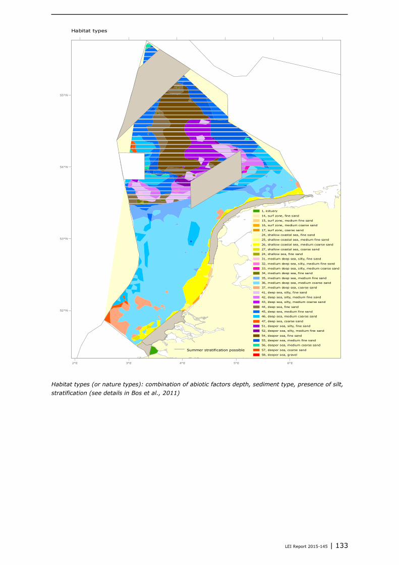
LEI Report 2015-145 | 133

Habitat types (or nature types): combination of abiotic factors depth, sediment type, presence of silt,

stratification (see details in Bos et al., 2011)

Habitat types

6°E5°E4°E3°E2°E

55°N

54°N

53°N

52°N

1, estuary

14, surf zone, fine sand

15, surf zone, medium fine sand

16, surf zone, medium coarse sand

17, surf zone, coarse sand

24, shallow coastal sea, fine sand

25, shallow coastal sea, medium fine sand

26, shallow coastal sea, medium coarse sand

27, shallow coastal sea, coarse sand

24, shallow sea, fine sand

31, medium deep sea, silty, fine sand

32, medium deep sea, silty, medium fine sand

33, medium deep sea, silty, medium coarse sand

34, medium deep sea, fine sand

35, medium deep sea, medium fine sand

36, medium deep sea, medium coarse sand

37, medium deep sea, coarse sand

41, deep sea, silty, fine sand

42, deep sea, silty, medium fine sand

43, deep sea, silty, medium coarse sand

44, deep sea, fine sand

45, deep sea, medium fine sand

46, deep sea, medium coarse sand

47, deep sea, coarse sand

51, deeper sea, silty, fine sand

52, deeper sea, silty, medium fine sand

54, deeper sea, fine sand

55, deeper sea, medium fine sand

56, deeper sea, medium coarse sand

57, deeper sea, coarse sand

58, deeper sea, gravel

Summer stratification possible

134 | LEI Report 2015-145

Frisian Front showing the 20% silt (red) and 15% silt (orange red) areas (De Bree et al., 1991)

6°E5°E4°E3°E

55°N

54°N

53°N

52°N

Habitat rarity %

%

5.71 - 27.6

2.15 - 5.7

0.34 - 2.14

0.13 - 0.33

0 - 0.12

LEI Report 2015-145 | 135

Digitised version of the map presented by De Bree et al. (1991) (see previous figure)

Georeferenced map of Creutzberg et al. (1984), combined with location of front (>20% silt) according

to De Bree et al. (1991) (see previous figure)

136 | LEI Report 2015-145

Map of all oil and gas facilities in the area and within the variants. Retrieved on November 17 2015

from http://www.nlog.nl/nl/mappingDatasets/mappingDatasets.html (dataset dated 2015-03-03)

Map of all known wrecks in the area and within the variants.

Data collected by IMARES (sources: website http://www.wrecksite.eu;

http://www.nlog.nl/nl/mappingDatasets/mappingDatasets.htm)

LEI Report 2015-145 | 137

Availability of ecological data Appendix 3

Availability of data and possible elements to describe the different variants, based on the studies

prepared for the stakeholder process.

Qualitative Quantitative

Study on biodiversity Dutch Continental Shelf (Bos et al.,

2015)

Macro/megabenthos biomass, density, species richness, evenness,

long-lived species, large growing species, etc.

x

Birds, fish, marine mammals x

Study on Ecological function (report on species traits, Van

Kooten et al., 2015)

Restoration of species richness X

Restoration of species size distribution (% population molluscs) X

Proportion of benthic species with brood care X

Proportion of predatory species (e.g. sea star) X

Proportion of deep burrying species (e.g. mud shrimp) X

Proportion of bioturbating species X

Proportion of mobile benthic species (free living) X

Proportion of subsurface deposit feeders (e.g. worms) X

Position in sediment (0-5cm, e.g. Sabellaria) X

Proportion of species with benthic egg development (e.g. whelk or

squid)

X

Study on benefits for fishery (Van Kooten et al., 2014) X

Export of larvae (from closed area) X

Export of commercial fish (from closed area) X

Export of less mobile species (from border of closed area) X

Study on potential for recovery of the area after closure

(Jongbloed et al., 2013)

X

Benthos: Increase of bioturbation and biogenic structures X

Benthos: Increase biodiversity: shift of biomass, increase bivalves,

increase crustaceans, decrease worms

X

Benthos: Increase of density and age classes, decrease of

scavengers (crabs, worms, sea stars), shifts in biomass and

abundance

X

Benthos: increase of whelk X

Benthos: increase of long-lived species such as Artica islandica,

Mya truncata, Thracia convexa

X

Fish: Increase of rays and sharks X

Fish: Increase of larger specimens within fish species X

Proportion of species with exoskeleton (e.g. crab, mud shrimp, but

not bivalves) X

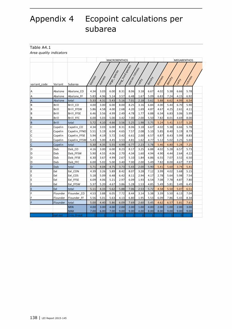
138 | LEI Report 2015-145

Ecopoint calculations per Appendix 4

subarea

Table A4.1

Area quality indicators

MACROBENTHOS MEGABENTHOS

variant_code Variant Subarea biom

ass

even

ess

larg

e_sp

ecie

slo

ng_l

ived

spe

cies

spec

ies

rich

ness

rarit

y

dens

ity

biom

ass

dens

ity

rarit

y

rich

ness

A Abalone Abalone_CO 4.34 3.03 6.00 8.31 8.06 3.18 6.67 4.02 5.38 6.66 5.78

A Abalone Abalone_FF 5.83 4.96 5.14 3.57 6.48 1.67 5.09 6.83 7.24 4.15 6.92

A Abalone total 5.33 4.31 5.43 5.16 7.01 2.18 5.62 5.88 6.62 4.99 6.54 3 A Abalone A total 0.44 0.44 0.48 0.45 0.72 0 0.40 0.65 0.70 0 0.59 4.87 sum area quality

B Bril l Bril l_CO 4.00 3.00 6.00 8.00 8.25 3.16 6.84 4.00 5.44 6.70 5.90

B Bril l Bril l_FFSW 5.86 4.58 4.00 2.68 4.20 1.69 4.87 4.67 4.25 2.61 4.11

B Bril l Bril l_FFSE 6.46 3.56 4.99 2.49 4.78 1.77 6.88 6.34 6.83 3.06 5.99

B Bril l Bril l_FFC 6.00 5.03 5.00 3.42 7.00 2.00 5.50 7.82 8.01 4.69 8.00

B Bril l total 5.72 4.10 4.66 3.56 5.25 1.98 5.75 5.24 5.41 3.57 5.20

C Capelin Capelin_CO 4.34 3.03 6.00 8.31 8.06 3.18 6.67 4.02 5.38 6.66 5.78

C Capelin Capelin_FFNO 5.51 5.19 6.04 4.65 7.57 2.08 5.10 5.85 8.40 5.19 8.79

C Capelin Capelin_FFSE 5.94 4.19 5.72 3.42 6.61 2.00 6.57 6.87 8.43 5.99 8.83

C Capelin Capelin_FFSW 5.43 5.00 4.45 3.53 4.81 1.62 4.77 5.12 5.02 3.25 5.60

C Capelin total 5.30 4.35 5.55 4.99 6.77 2.23 5.78 5.46 6.80 5.28 7.25

D Dab Dab_CO 4.16 3.00 6.00 8.23 8.17 3.25 6.88 4.02 5.28 6.57 5.73

D Dab Dab_FFSW 5.90 4.55 4.06 2.70 4.34 1.60 4.94 4.90 4.44 2.64 4.22

D Dab Dab_FFSE 6.30 3.67 4.99 2.67 5.10 1.84 6.86 6.55 7.07 3.52 6.50

D Dab Dab_FFC 6.00 5.02 5.00 3.40 7.00 2.00 5.49 7.82 8.00 4.67 7.97

D Dab total 5.71 4.04 4.75 3.73 5.43 2.00 5.90 5.41 5.60 3.74 5.41

E Eel Eel_CON 4.39 3.26 5.89 8.42 8.07 3.28 7.12 3.99 4.02 5.68 5.15

E Eel Eel_COS 5.18 5.09 6.48 6.42 8.11 2.94 4.17 2.78 5.64 5.98 7.54

E Eel Eel_FFSE 6.09 4.06 5.21 2.97 6.09 1.93 6.54 7.08 7.78 4.87 7.80

E Eel Eel_FFSW 5.37 5.20 4.67 3.86 5.28 1.53 4.85 5.49 5.81 3.49 6.45

E Eel total 5.11 4.33 5.62 5.88 7.06 2.53 5.72 4.58 5.50 5.07 6.51

F Flounder Flounder_CO 4.53 3.88 6.05 7.72 8.44 3.14 5.38 3.39 5.50 6.13 7.04

F Flounder Flounder_FF 5.56 5.01 5.63 4.13 6.80 1.95 5.53 6.09 7.86 5.43 8.34

F Flounder total 5.00 4.40 5.86 6.09 7.69 2.60 5.45 4.62 6.57 5.81 7.63

MIN 4.00 3.00 4.00 2.00 2.00 1.00 4.00 2.00 1.00 2.00 3.00

MAX 7.00 6.00 7.00 9.00 9.00 4.00 8.00 8.00 9.00 9.00 9.00

opt out 1=in, 0=out 1 1 1 1 1 0 1 1 1 0 1

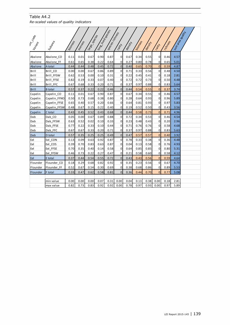
LEI Report 2015-145 | 139

Table A4.2

Re-scaled values of quality indicators

Varia

nt_c

ode

Varia

nt

Suba

rea

biom

ass

even

ess

larg

e_sp

ecie

slo

ng_l

ived

spe

cies

spec

ies

rich

ness

rarit

y

dens

ity

biom

ass

dens

ity

rarit

y

rich

ness

sum

are

a qu

alit

y

Abalone Abalone_CO 0.11 0.01 0.67 0.90 0.87 0 0.67 0.34 0.55 0 0.46 4.57

Abalone Abalone_FF 0.61 0.65 0.38 0.22 0.64 0 0.27 0.80 0.78 0 0.65 5.01

Abalone A total 0.44 0.44 0.48 0.45 0.72 0 0.40 0.65 0.70 0 0.59 4.87 sum area quality

Bril l Bril l_CO 0.00 0.00 0.67 0.86 0.89 0 0.71 0.33 0.56 0 0.48 4.50

Bril l Bril l_FFSW 0.62 0.53 0.00 0.10 0.31 0 0.22 0.45 0.41 0 0.18 2.81

Bril l Bril l_FFSE 0.82 0.19 0.33 0.07 0.40 0 0.72 0.72 0.73 0 0.50 4.48

Bril l Bril l_FFC 0.67 0.68 0.33 0.20 0.71 0 0.37 0.97 0.88 0 0.83 5.64

Bril l B total 0.57 0.37 0.22 0.22 0.46 0 0.44 0.54 0.55 0 0.37 3.74

Capelin Capelin_CO 0.11 0.01 0.67 0.90 0.87 0 0.67 0.34 0.55 0 0.46 4.57

Capelin Capelin_FFNO 0.50 0.73 0.68 0.38 0.80 0 0.28 0.64 0.93 0 0.96 5.89

Capelin Capelin_FFSE 0.65 0.40 0.57 0.20 0.66 0 0.64 0.81 0.93 0 0.97 5.83

Capelin Capelin_FFSW 0.48 0.67 0.15 0.22 0.40 0 0.19 0.52 0.50 0 0.43 3.56

Capelin C total 0.43 0.45 0.52 0.43 0.68 0 0.44 0.58 0.73 0 0.71 4.96

Dab Dab_CO 0.05 0.00 0.67 0.89 0.88 0 0.72 0.34 0.53 0 0.46 4.54

Dab Dab_FFSW 0.63 0.52 0.02 0.10 0.33 0 0.23 0.48 0.43 0 0.20 2.96

Dab Dab_FFSE 0.77 0.22 0.33 0.10 0.44 0 0.71 0.76 0.76 0 0.58 4.68

Dab Dab_FFC 0.67 0.67 0.33 0.20 0.71 0 0.37 0.97 0.88 0 0.83 5.63

Dab D total 0.57 0.35 0.25 0.25 0.49 0 0.47 0.57 0.57 0 0.40 3.92

Eel Eel_CON 0.13 0.09 0.63 0.92 0.87 0 0.78 0.33 0.38 0 0.36 4.48

Eel Eel_COS 0.39 0.70 0.83 0.63 0.87 0 0.04 0.13 0.58 0 0.76 4.93

Eel Eel_FFSE 0.70 0.35 0.40 0.14 0.58 0 0.64 0.85 0.85 0 0.80 5.31

Eel Eel_FFSW 0.46 0.73 0.22 0.27 0.47 0 0.21 0.58 0.60 0 0.58 4.12

Eel E total 0.37 0.44 0.54 0.55 0.72 0 0.43 0.43 0.56 0 0.59 4.64

Flounder Flounder_CO 0.18 0.29 0.68 0.82 0.92 0 0.35 0.23 0.56 0 0.67 4.70

Flounder Flounder_FF 0.52 0.67 0.54 0.30 0.69 0 0.38 0.68 0.86 0 0.89 5.53

Flounder F total 0.33 0.47 0.62 0.58 0.81 0 0.36 0.44 0.70 0 0.77 5.08

min value 0.00 0.00 0.00 0.07 0.31 0.00 0.04 0.13 0.38 0.00 0.18 2.81

max value 0.82 0.73 0.83 0.92 0.92 0.00 0.78 0.97 0.93 0.00 0.97 5.89

140 | LEI Report 2015-145

Table A4.3

Weighting factors, original values

Varia

nt_c

ode

Varia

nt

Suba

rea

1. H

abita

t rar

ity

2. N

hab

itats

3a. R

elat

ive

bord

er3b

. Eff

ectiv

e pr

otec

t.-1

km

3c. E

ffec

tive

pro

tect

.-2.5

km

4a. 2

0%FF

mud

4b. %

FFpa

ralle

logr

am5a

. Abi

otic

gra

dien

ts

5b. B

enth

ic g

radi

ents

5c. G

radi

ents

incl

cen

tre

6. H

ard

subs

trat

e7.

Fis

hery

inte

nsity

Abalone Abalone_CO 91.89 2 88% 97% 92% 0% 0% 0 0 0

Abalone Abalone_FF 88.91 8 73% 95% 85% 25% 20% 8 8 8

Abalone total 89.91 9 56% 92% 78% 25% 20% 8 8 8 0.02 0.12

Bril l Bril l_CO 91.76 1 81% 93% 79% 0% 0% 0 0 0

Bril l Bril l_FFSW 73.97 2 69% 93% 82% 0% 1% 2 1 0

Bril l Bril l_FFSE 84.86 4 65% 87% 57% 0% 0% 0 0 0

Bril l Bril l_FFC 97.27 4 89% 94% 80% 13% 4% 4 3 3

Bril l total 81.57 9 38% 84% 58% 13% 5% 4 3 3 0.06 0.08

Capelin Capelin_CO 91.89 2 88% 97% 92% 0% 0% 0 0 0

Capelin Capelin_FFNO 97.18 6 80% 95% 86% 0% 14% 6 3 3

Capelin Capelin_FFSE 98.24 6 80% 95% 86% 12% 13% 6 4 4

Capelin Capelin_FFSW 79.19 4 80% 95% 86% 0% 9% 4 5 0

Capelin total 91.63 11 41% 87% 67% 12% 35% 6 5 4 0.03 0.12

Dab Dab_CO 91.76 1 68% 89% 64% 0% 0% 0 0 0

Dab Dab_FFSW 74.09 2 73% 95% 85% 0% 3% 2 1 0

Dab Dab_FFSE 87.93 6 71% 92% 76% 0% 0% 0 0 0

Dab Dab_FFC 97.27 4 89% 94% 80% 13% 4% 4 3 3

Dab total 82.86 15 38% 86% 63% 13% 6% 4 3 3 0.05 0.08

Eel Eel_CON 93.05 4 89% 99% 97% 0% 0% 0 0 0

Eel Eel_COS 95.55 5 87% 98% 95% 0% 0% 0 0 0

Eel Eel_FFSE 94.04 9 88% 98% 95% 11% 11% 8 4 4

Eel Eel_FFSW 86.18 8 87% 98% 95% 24% 20% 8 8 8

Eel total 92.13 15 44% 93% 82% 35% 31% 8 8 8 0.02 0.09

Flounder Flounder_CO 93.65 5 78% 98% 95% 0% 0% 0 0 0

Flounder Flounder_FF 95.32 14 76% 98% 94% 100% 100% 14 8 8

Flounder total 94.41 14 55% 96% 90% 100% 100% 14 8 8 0.02 0.12

MIN 73.97 1 0% 50% 50% 0% 0% 0 0 0 0.00 0.00

MAX 99.95 15 89% 100% 100% 100% 100% 14 8 8 0.06 0.12

LEI Report 2015-145 | 141

Table A4.4

Weighting factors, scaled values

Varia

nt_c

ode

Varia

nt

Suba

rea

1. H

abita

t rar

ity

2. N

hab

itats

3a. R

elat

ive

bord

er3b

. Eff

ectiv

e pr

otec

t.-1

km

3c. E

ffec

tive

pro

tect

.-2.5

km

4a. 2

0%FF

mud

4b. %

FFpa

ralle

logr

am5a

. Abi

otic

gra

dien

ts5b

. Ben

thic

gra

dien

ts5c

. Gra

dien

ts in

cl c

entr

e

6. H

ard

subs

trat

e7.

Fis

hery

inte

nsity

AbaloneAbalone_CO 0.69 0.07 0.99 0.95 0.85 0.00 0.00 0.00 0.00 0.00

AbaloneAbalone_FF 0.57 0.50 0.82 0.90 0.71 0.25 0.20 0.57 1.00 1.00

Abalonetotal 0.61 0.57 0.63 0.83 0.55 0.25 0.20 0.57 1.00 1.00 0.28 1.00

Bril l Bril l_CO 0.68 0.00 0.91 0.87 0.58 0.00 0.00 0.00 0.00 0.00

Bril l Bril l_FFSW 0.00 0.07 0.78 0.87 0.63 0.00 0.01 0.14 0.13 0.00

Bril l Bril l_FFSE 0.42 0.21 0.73 0.75 0.13 0.00 0.00 0.00 0.00 0.00

Bril l Bril l_FFC 0.90 0.21 1.00 0.89 0.60 0.13 0.04 0.29 0.38 0.38

Bril l total 0.29 0.57 0.43 0.67 0.15 0.13 0.05 0.29 0.38 0.38 1.00 0.67

CapelinCapelin_CO 0.69 0.07 0.99 0.95 0.85 0.00 0.00 0.00 0.00 0.00

CapelinCapelin_FFNO 0.89 0.36 0.90 0.91 0.73 0.00 0.14 0.43 0.38 0.38

CapelinCapelin_FFSE 0.93 0.36 0.90 0.91 0.73 0.12 0.13 0.43 0.50 0.50

CapelinCapelin_FFSW 0.20 0.21 0.90 0.91 0.73 0.00 0.09 0.29 0.63 0.00

Capelintotal 0.68 0.71 0.46 0.74 0.35 0.12 0.35 0.43 0.63 0.50 0.43 1.00

Dab Dab_CO 0.68 0.00 0.76 0.78 0.28 0.00 0.00 0.00 0.00 0.00

Dab Dab_FFSW 0.00 0.07 0.82 0.90 0.70 0.00 0.03 0.14 0.13 0.00

Dab Dab_FFSE 0.54 0.36 0.80 0.85 0.53 0.00 0.00 0.00 0.00 0.00

Dab Dab_FFC 0.90 0.21 1.00 0.89 0.60 0.13 0.04 0.29 0.38 0.38

Dab total 0.34 1.00 0.43 0.71 0.26 0.13 0.06 0.29 0.38 0.38 0.81 0.67

Eel Eel_CON 0.73 0.21 1.00 0.97 0.93 0.00 0.00 0.00 0.00 0.00

Eel Eel_COS 0.83 0.29 0.97 0.96 0.90 0.00 0.00 0.00 0.00 0.00

Eel Eel_FFSE 0.77 0.57 0.99 0.96 0.90 0.11 0.11 0.57 0.50 0.50

Eel Eel_FFSW 0.47 0.50 0.97 0.96 0.90 0.24 0.20 0.57 1.00 1.00

Eel total 0.70 1.00 0.50 0.86 0.65 0.35 0.31 0.57 1.00 1.00 0.35 0.75

FlounderFlounder_CO 0.76 0.29 0.88 0.96 0.90 0.00 0.00 0.00 0.00 0.00

FlounderFlounder_FF 0.82 0.93 0.86 0.96 0.89 1.00 1.00 1.00 1.00 1.00

Floundertotal 0.79 0.93 0.61 0.92 0.81 1.00 1.00 1.00 1.00 1.00 0.28 1.00

min value 0.00 0.00 0.43 0.67 0.13 0.00 0.00 0.00 0.00 0.00 0.28 0.67

max value 0.93 1.00 1.00 0.97 0.93 1.00 1.00 1.00 1.00 1.00 1.00 1.00

142 | LEI Report 2015-145

Table A4.5

Calculated ecopoints per km2 for each variant and subareas, depending on the applied weighting factor

5. Ecopoints per km2ecopoints (per km2) = area quality (per km2)* weight factor

Varia

nt_c

ode

Varia

nt

Suba

rea

0. N

o w

eigh

ting

fact

or

1. H

abita

t rar

ity

2. N

hab

itats

3a. R

elat

ive

bord

er3b

. Eff

ectiv

e pr

otec

t.-1

km

3c. E

ffec

tive

pro

tect

.-2.5

km

4a. 2

0%FF

mud

4b. %

FFpa

ralle

logr

am5a

. Abi

otic

gra

dien

ts5b

. Ben

thic

gra

dien

ts

5c. G

radi

ents

incl

cen

tre

6. H

ard

subs

trat

e7.

Fis

hery

inte

nsity

A Abalone Abalone_CO 4.57 3.15 0.33 4.52 4.33 3.88 0.00 0.00 0.00 0.00 0.00

A Abalone Abalone_FF 5.01 2.88 2.51 4.09 4.50 3.54 1.28 1.00 2.87 5.01 5.01

A Abalone total 4.87 2.98 2.78 3.07 4.06 2.70 1.24 0.97 2.78 4.87 4.87 1.34 4.87

B Bril l Bril l_CO 4.50 3.08 0.00 4.09 3.91 2.62 0.00 0.00 0.00 0.00 0.00

B Bril l Bril l_FFSW 2.81 0.00 0.20 2.18 2.44 1.79 0.00 0.04 0.40 0.35 0.00

B Bril l Bril l_FFSE 4.48 1.88 0.96 3.28 3.34 0.60 0.00 0.00 0.00 0.00 0.00

B Bril l Bril l_FFC 5.64 5.06 1.21 5.63 5.01 3.39 0.72 0.21 1.61 2.12 2.12

B Bril l total 3.74 1.10 2.14 1.61 2.51 0.58 0.48 0.19 1.07 1.40 1.40 3.74 2.50

C Capelin Capelin_CO 4.57 3.15 0.33 4.52 4.33 3.88 0.00 0.00 0.00 0.00 0.00

C Capelin Capelin_FFNO 5.89 5.26 2.10 5.32 5.34 4.30 0.02 0.81 2.53 2.21 2.21

C Capelin Capelin_FFSE 5.83 5.45 2.08 5.27 5.28 4.25 0.70 0.74 2.50 2.92 2.92 C Capelin 23 22 8 21 21 17 3 3 10 12 12

C Capelin Capelin_FFSW 3.56 0.72 0.76 3.22 3.22 2.60 0.00 0.31 1.02 2.23 0.00

C Capelin total 4.96 3.37 3.55 2.29 3.69 1.73 0.62 1.74 2.13 3.10 2.48 2.12 4.96

D Dab Dab_CO 4.54 3.11 0.00 3.46 3.53 1.26 0.00 0.00 0.00 0.00 0.00

D Dab Dab_FFSW 2.96 0.01 0.21 2.42 2.65 2.06 0.00 0.08 0.42 0.37 0.00

D Dab Dab_FFSE 4.68 2.51 1.67 3.72 3.97 2.48 0.00 0.00 0.00 0.00 0.00

D Dab Dab_FFC 5.63 5.05 1.21 5.62 5.00 3.38 0.71 0.21 1.61 2.11 2.11

D Dab total 3.92 1.34 3.92 1.69 2.80 1.02 0.49 0.24 1.12 1.47 1.47 3.18 2.61

E Eel Eel_CON 4.48 3.29 0.96 4.46 4.36 4.17 0.00 0.00 0.00 0.00 0.00

E Eel Eel_COS 4.93 4.09 1.41 4.80 4.75 4.44 0.00 0.00 0.00 0.00 0.00

E Eel Eel_FFSE 5.31 4.10 3.03 5.28 5.11 4.77 0.58 0.57 3.03 2.65 2.65

E Eel Eel_FFSW 4.12 1.94 2.06 4.01 3.97 3.71 0.99 0.84 2.35 4.12 4.12

E Eel total 4.64 3.24 4.64 2.30 3.99 2.99 1.62 1.45 2.65 4.64 4.64 1.61 3.48

F Flounder Flounder_CO 4.70 3.56 1.34 4.13 4.54 4.26 0.00 0.00 0.00 0.00 0.00

F Flounder Flounder_FF 5.53 4.55 5.14 4.75 5.30 4.91 5.53 5.53 5.53 5.53 5.53

F Flounder total 5.08 4.00 4.72 3.12 4.70 4.09 5.08 5.08 5.08 5.08 5.08 1.44 5.08

LEI Report 2015-145 | 143

Table A4.6

Calculated ecopoints for each variant and subarea, depending on the applied weighting factor

5. Ecopoints per area (km2)ecopoints = (area(km2)/100)* area quality (per km2)* weight factor

7. F

ishe

ry in

tens

ity

Varia

nt_c

ode

Varia

nt

Suba

rea

0. N

o w

eigh

ting

fact

or

1. H

abita

t rar

ity

2. N

hab

itats

3a. R

elat

ive

bord

er3b

. Eff

ectiv

e pr

otec

t.-1

km

3c. E

ffec

tive

pro

tect

.-2.5

km

4a. 2

0%FF

mud

4b. %

FFpa

ralle

logr

am

5a. A

biot

ic g

radi

ents

5b. B

enth

ic g

radi

ents

5c. G

radi

ents

incl

cen

tre

6. H

ard

subs

trat

e7.

Fis

hery

inte

nsity

A Abalone Abalone_CO 18 13 1 18 17 16 0 0 0 0 0

A Abalone Abalone_FF 40 23 20 33 36 28 10 8 23 40 40

A Abalone total 59 36 33 37 49 32 15 12 33 59 59 16 59

B Bril l Bril l_CO 9 6 0 8 8 5 0 0 0 0 0

B Bril l Bril l_FFSW 18 0 1 14 15 11 0 0 3 2 0

B Bril l Bril l_FFSE 14 6 3 10 11 2 0 0 0 0 0

B Bril l Bril l_FFC 6 5 1 6 5 4 1 0 2 2 2

B Bril l total 47 14 27 20 32 7 6 2 14 18 18 47 32

C Capelin Capelin_CO 18 13 1 18 17 16 0 0 0 0 0

C Capelin Capelin_FFNO23 21 8 21 21 17 0 3 10 9 9

C Capelin Capelin_FFSE23 22 8 21 21 17 3 3 10 12 12

C Capelin Capelin_FFSW14 3 3 13 13 10 0 1 4 9 0

C Capelin total 79 54 57 37 59 28 10 28 34 50 40 34 79

D Dab Dab_CO 14 9 0 11 11 4 0 0 0 0 0

D Dab Dab_FFSW 23 0 2 19 20 16 0 1 3 3 0

D Dab Dab_FFSE 23 13 8 19 20 12 0 0 0 0 0

D Dab Dab_FFC 6 5 1 6 5 4 1 0 2 2 2

D Dab total 66 23 66 28 47 17 8 4 19 25 25 53 44

E Eel Eel_CON 63 46 13 63 61 59 0 0 0 0 0

E Eel Eel_COS 52 43 15 50 50 47 0 0 0 0 0

E Eel Eel_FFSE 37 29 21 37 36 33 4 4 21 19 19

E Eel Eel_FFSW 43 20 22 42 42 39 10 9 25 43 43

E Eel total 195 136 195 97 168 126 68 61 111 195 195 68 146

F Flounder Flounder_CO163 123 46 143 157 147 0 0 0 0 0

F Flounder Flounder_FF160 131 148 137 153 142 159 160 160 160 160

F Flounder total 322 253 299 198 298 260 322 322 322 322 322 91 322

144 | LEI Report 2015-145

Data sources for direct Appendix 5

economic effects on fishing

sector

VIRIS data

The catch data originates from the VIRIS (Fish Registration and Information System) database that

contains records of all landings by vessels sailing under the Dutch flag and all landings by vessels

sailing under a non-Dutch flag landing fish at ports in the Netherlands. These records are based on the

logbooks kept by the fishermen. The catches of each species controlled by quota must be entered in

this logbook per sailing day and ICES quadrant. Records of the catches of species not controlled by

quota are kept per trip.

Fleet data

The catch data for the various types of fisheries was calculated using the technical data listed in the

NRV (Netherlands Register of Fishing Vessels). The combination of NRV data and VIRIS data yielded

information about the technical specifications of the vessel on each trip. Not all the technical

specifications of non-Dutch vessels are known.

VMS data

Since 1 January 2000, an increasingly large proportion of fishing vessels are under the obligation to

operate an onboard VMS system (Vessel Monitoring System) within the context of the European

inspection policy. This VMS system transmits the position of the vessel, vessel identification code and

the vessel’s sailing speed to a central computer about once every two hours. The computer stores this

data (EU Regulation 2244/2003). The vessel’s sailing speed can be used to make a distinction between

the various activities (fishing, sailing and at anchor). Although this distinction cannot be made

completely, the potential error is small relative to the total number of records. Information about the

presence of non’Dutch vessels in the Dutch section of the North Sea is also available.

Price data

The value of the catches was determined using the average monthly price data per species collected

by the Productschap Vis (Netherlands Fish Product Board). Price data is not collected for all the species

listed in VIRIS. When specific price data was not available for fish species then the value of the

catches was determined using the average price of less specific market categories (for example, ‘other

seafish’). In addition, prices from other sources were used for a number of fish species (in particular,

sprat and herring, grey mullet and smelt) (requested from fishers and collected from the accounts of

the high-sea fisheries) since these species are rarely traded on the fish auctions and the auction prices

are not representative of the actual prices paid for the fish. The average auction price of catches by

vessels with fixed fishing gear were increased by 15%: an analysis of a limited dataset with price data

for the fisheries with fixed fishing gear and discussions with fishermen revealed that these fisheries’

catches are, in general, traded at higher auction prices due to a different market grading (in general,

larger sole) and quality (fresh fish with less damage as compared to fish caught with beam trawls).

Economic data

The LEI panel has economic data for the various fisheries over the entire period of the study. The data

contains the total annual proceeds of the Dutch cutter fisheries in the various fisheries and the

relationships between the total proceeds and the gross value added. However, these data are not

classified by fishing area. Consequently, the economic data need to be combined with catch data to

arrive at an estimate of the contribution each fishing area makes to the economy.

LEI Report 2015-145 | 145

Gear Codes Appendix 6

Table A6.1

Gear codes used in the report and the gears

Gear code Gear type

FPO Pots

GN Gillnets (not specified)

GNC Encircling gillnets

GND Drift nets

GNS Set gillnets (anchored)

GTN Combined gillnets-Trammel nets

GTR Trammel nets

LHP Hand-lines and pole-lines (hand operated)

LL Longlines (not specified)

LLD Drifting longlines

LLS Set lines (longlines set)

LN Lift nets (not specified)

MIS MISCELLANEOUS GEAR

OTB Otter trawls bottom

OTM Otter trawls midwatter

OTT Otter twin trawls

PTB Pair trawls bottom

PTM Pair trawls mid-water

SDN Danish seines

SSC Scottish seines

TBB Beam trawls

TBS Shrimp trawls

146 | LEI Report 2015-145

Characteristics of the Dutch Appendix 7

activities in the sub-areas of

all variants

Table A7.1

Overview of landings and values of the Dutch fishing sector in the different areas and locations of the

possible variants

Variant Location 2008 2009 2010 2011 2012 2013 2014 Average

Landings volume (tonnes)

Abalone FF 256 326 295 160 534 157 281 287

Abalone CO 39 19 34 6 107 52 40 42

Brill CO 33 13 17 3 68 31 25 27

Brill FFSW 96 84 45 18 65 16 9 48

Brill FFSE 32 79 54 35 338 173 31 106

Brill FFC 23 48 65 11 146 17 17 47

Capelin FFSW 90 70 78 28 147 95 20 75

Capelin FFSE 206 189 168 79 277 148 45 159

Capelin FFNO 76 129 161 170 112 80 231 137

Capelin CO 39 19 34 6 107 52 40 42

Dab CO 37 15 22 4 75 43 30 32

Dab FFSW 171 149 71 22 79 45 15 79

Dab FFSE 60 110 81 62 499 242 61 159

Dab FFC 23 47 63 11 147 16 17 46

Eel FFSE 229 261 232 102 693 278 90 269

Eel FFSW 323 274 232 173 392 220 124 248

Eel COS 221 270 302 384 248 264 190 268

Eel CON 103 61 98 36 235 124 115 110

Flounder FF 975 1,182 1,220 956 1,655 934 836 1,108

Flounder CO 560 277 397 730 717 426 542 521

Landings value (kEuro)

Abalone FF 1,136 1,255 1,037 648 1,315 621 511 932

Abalone CO 93 33 56 15 138 78 61 68

Brill CO 79 22 31 7 87 48 39 45

Brill FFSW 489 349 185 93 172 64 25 197

Brill FFSE 161 71 148 107 494 164 63 171

Brill FFC 94 185 221 30 208 78 42 123

Capelin FFSW 399 293 286 99 317 293 81 252

Capelin FFSE 873 712 584 275 563 338 149 499

Capelin FFNO 316 485 525 707 381 308 525 464

Capelin CO 93 33 56 15 138 78 61 68

Dab CO 88 27 39 8 100 65 45 53

Dab FFSW 852 607 289 114 256 119 46 326

Dab FFSE 304 189 210 155 694 247 109 270

Dab FFC 93 182 215 30 209 74 42 121

Eel FFSE 1,008 868 739 298 1,179 457 215 679

Eel FFSW 1,403 1,033 797 365 976 702 394 810

Eel COS 815 962 1,049 1,046 789 858 626 878

Eel CON 241 111 164 87 352 185 201 192

Flounder FF 4,096 4,470 4,179 3,409 4,280 3,107 2,280 3,689

Flounder CO 1,618 782 967 1,699 1,383 859 1,078 1,198

Effort (fishing days)

Abalone FF 152 188 152 116 156 94 82 134

Abalone CO 13 6 7 2 12 12 9 9

Brill CO 10 5 4 1 8 7 6 6

LEI Report 2015-145 | 147

Variant Location 2008 2009 2010 2011 2012 2013 2014 Average

Brill FFSW 94 95 50 24 38 15 6 46

Brill FFSE 35 18 42 32 50 44 16 34

Brill FFC 18 25 28 6 17 10 6 15

Capelin FFSW 49 45 45 17 27 39 11 33

Capelin FFSE 116 124 99 51 53 46 22 73

Capelin FFNO 43 86 90 123 63 59 81 78

Capelin CO 13 6 7 2 12 12 9 9

Dab CO 12 5 5 1 10 10 7 7

Dab FFSW 136 132 66 29 49 21 9 63

Dab FFSE 64 55 58 42 60 55 25 51

Dab FFC 17 25 27 6 16 9 5 15

Eel FFSE 147 153 126 61 99 67 36 98

Eel FFSW 186 160 121 47 103 90 50 108

Eel COS 140 149 160 150 105 107 102 130

Eel CON 33 19 21 10 38 28 26 25

Flounder FF 577 741 658 556 541 476 374 560

Flounder CO 258 130 151 206 182 124 150 172

a) preliminary estimates.

Source: Logbook data and VMS data, processed by LEI.

148 | LEI Report 2015-145

Seasonal patterns of landings Appendix 8

value for various gears

Seasonal patterns in utilisation of the area vary among gear types. For the traditional beam trawl and

Sumwing fishery the first quarter is most important in most of the variants and highest dependencies

are seen there. Only in case of Brill and Dab the second quarter is slightly more important. Only in

case of Flounder vessels are highly dependent (>30% of the quarterly revenue) on the areas. This

high dependency occurs mainly during first quarter when some vessels obtain more than 50% of their

revenue from the area. For Abalone, Brill and Dab nearly all of the revenue in the area is obtained by

vessels that fish occasionally in the area (<10% of the revenue).

Figure A8.1 Average revenue (kEuro) of the beam trawl and sumwing fishery per quarter over the

period 2008-2014 in each of the variants. The various colours show the level to which the vessel

depend on the area’s E.g. almost the complete revenue in quarter 2 for variant Brill is obtained by

vessels that are less than 10% dependent on these areas.

Source: Logbook data and VMS data, processed by LEI

The fishing season for twin trawl and otter board trawl fisheries is during the third quarter. In all

variants, the revenues from the area are highest for this period and also the highest dependencies

occur then. In most of the variants dependency is low, especially in Brill and Dab. In Flounder,

however, some vessels depend heavily (>50%) on the revenues from the area. This high dependency

also occurs during the fourth quarter, although the total revenue is much lower.

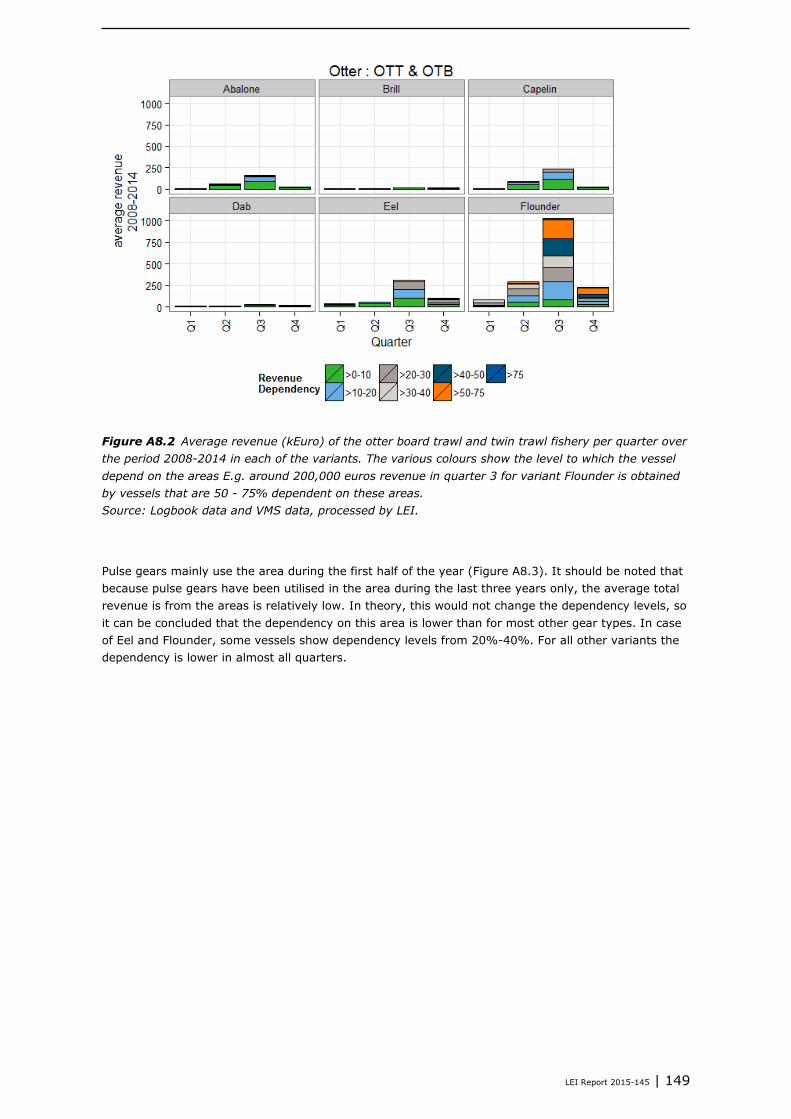
LEI Report 2015-145 | 149

Figure A8.2 Average revenue (kEuro) of the otter board trawl and twin trawl fishery per quarter over

the period 2008-2014 in each of the variants. The various colours show the level to which the vessel

depend on the areas E.g. around 200,000 euros revenue in quarter 3 for variant Flounder is obtained

by vessels that are 50 - 75% dependent on these areas.

Source: Logbook data and VMS data, processed by LEI.

Pulse gears mainly use the area during the first half of the year (Figure A8.3). It should be noted that

because pulse gears have been utilised in the area during the last three years only, the average total

revenue is from the areas is relatively low. In theory, this would not change the dependency levels, so

it can be concluded that the dependency on this area is lower than for most other gear types. In case

of Eel and Flounder, some vessels show dependency levels from 20%-40%. For all other variants the

dependency is lower in almost all quarters.

150 | LEI Report 2015-145

Figure A8.3 Average revenue (kEuro) of the pulse fisheries per quarter over the period 2008-2014 in

each of the variants. The various colours show the level to which the vessel depend on the area’s E.g.

the complete revenue in quarter 2 for variant Dab is obtained by vessels that are less than 10%

dependent on these areas.

Source: Logbook data and VMS data, processed by LEI.

Flyshoot vessels (SSC) mainly utilise the areas of variant Brill, Dab and Eel during the second quarter

(Figure A8.4). Dependency on the areas is low in general, with the exception of Dab and Eel. In these

variants around 15% of the revenues are generated by vessels that are more than 20% dependent on

these areas (Figure 5.9). The total revenue generated in the variants by this fisheries is however low

for all variants; on average less than 70 kEuroper quarter.

LEI Report 2015-145 | 151

Figure A8.4 Average revenue (kEuro) of the flyshoot fisheries per quarter over the period 2008-2014

in each of the variants. The various colours show the level to which the vessel depend on the area’s

E.g. the complete revenue in quarter 2 for variant Dab is obtained by vessels that are less than 10%

dependent on these areas.

Source: Logbook data and VMS data, processed by LEI.

152 | LEI Report 2015-145

Classification fishing Appendix 9

harbours for stress analysis

Table A9.1

Classification of harbour codes in regions for the stress analysis

Harbour code Region Harbour code Region

ARM Zeeland MS Zeeland

BIW Holland NB Holland

BR Zeeland NZ Zeeland

BRU Zeeland OD Holland

BU Holland OH Holland

BZ Zeeland OL North

DM Holland SCH Holland

DZ North SL Holland

EH Holland ST North

FL North TH Zeeland

GM North TM North

GO Holland TS North

GOE Zeeland TX North

HA North UK Urk

HD Holland UQ North

HI North VD Holland

HK Holland VL Zeeland

HL North VLI Zeeland

HN Holland VLL North

HON Zeeland WK North

IJM Holland WL North

KG Zeeland WON North

KL Zeeland WR Holland

KW Holland WSW Zeeland

LE North YE Zeeland

LO North ZK North

ME Holland ZL Zeeland

MO Holland ZZ Zeeland

LEI Report 2015-145 | 153

Analyses underlying the Appendix 10

assumptions in Displacement

scenario A

Figure A10.1 Characterisation of the relative Value per sea day (VPUE) of individual species in the

area of the Frisian Front by vessels using Otter board trawls (OTB) with engines larger than 300 hp

(Big). Upper panel displays the comparison between the average in the area and the overall average,

during the quarters (2 and 3) in which the landings from the areas are most important (diamonds)

and the relative amount of effort in alternative fishing grounds (ICES rectangles) for which the VPUE is

higher. Lower panel provides the Average VPUE in the area of the Frisian Front as a means to show

the relative importance of the species. FAO species codes are: BLL, brill; COD, cod; DAB, dab; FLE,

flounder; GUU, Gurnard; NEP, Nephrops; PLE, plaice; SOL, sole; TUR, turbot, ZTH, Other.

Conclusion: of the important species Nephrops VPUE is relative high in the area, turbot is

also relative high in quarter 2.

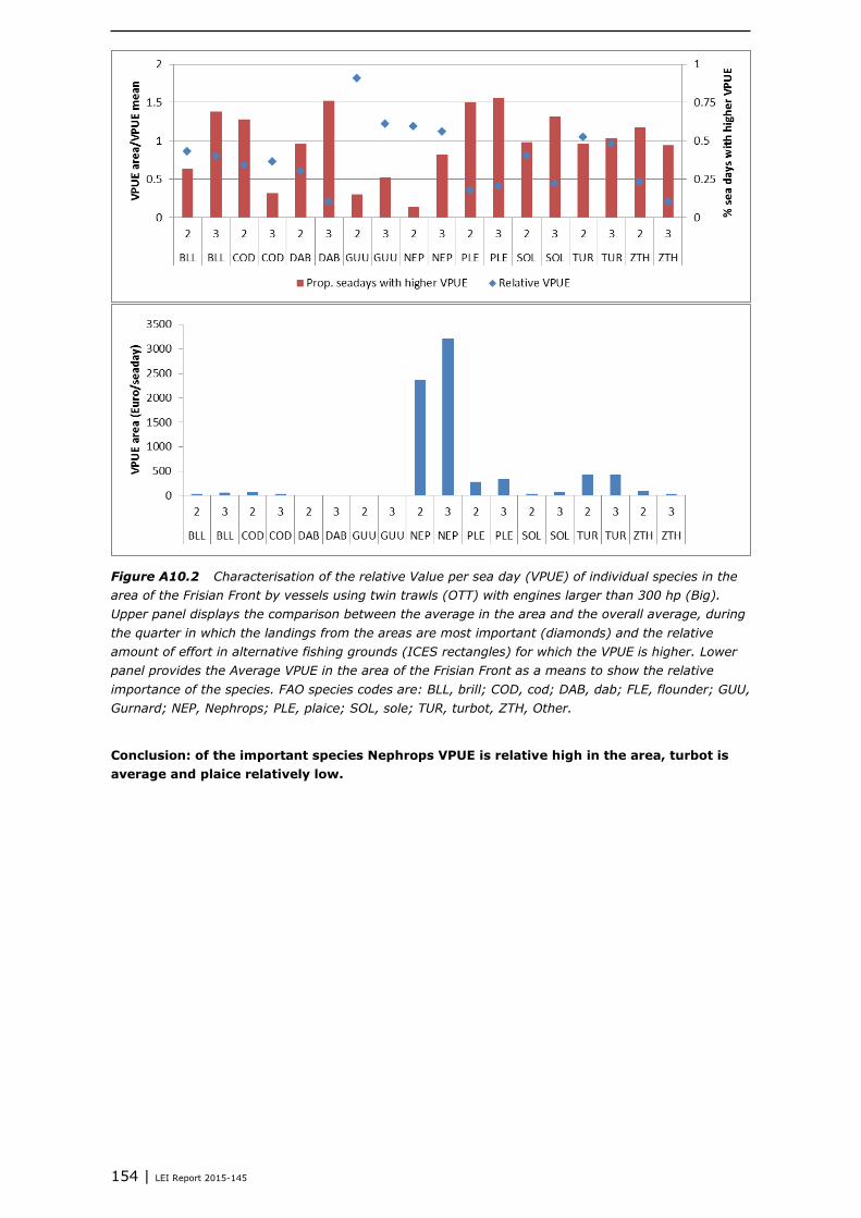
154 | LEI Report 2015-145

Figure A10.2 Characterisation of the relative Value per sea day (VPUE) of individual species in the

area of the Frisian Front by vessels using twin trawls (OTT) with engines larger than 300 hp (Big).

Upper panel displays the comparison between the average in the area and the overall average, during

the quarter in which the landings from the areas are most important (diamonds) and the relative

amount of effort in alternative fishing grounds (ICES rectangles) for which the VPUE is higher. Lower

panel provides the Average VPUE in the area of the Frisian Front as a means to show the relative

importance of the species. FAO species codes are: BLL, brill; COD, cod; DAB, dab; FLE, flounder; GUU,

Gurnard; NEP, Nephrops; PLE, plaice; SOL, sole; TUR, turbot, ZTH, Other.

Conclusion: of the important species Nephrops VPUE is relative high in the area, turbot is

average and plaice relatively low.

LEI Report 2015-145 | 155

Figure A10.3 Characterisation of the relative Value per sea day (VPUE) of individual species in the

area of the Frisian Front by vessels using Scottish seines (SSC) with engines larger than 300 hp (Big).

Upper panel displays the comparison between the average in the area and the overall average, during

the quarter in which the landings from the areas are most important (diamonds) and the relative

amount of effort in alternative fishing grounds (ICES rectangles) for which the VPUE is higher. Lower

panel provides the Average VPUE in the area of the Frisian Front as a means to show the relative

importance of the species. FAO species codes are: BLL, brill; COD, cod; DAB, dab; FLE, flounder; GUU,

Gurnard; NEP, Nephrops; PLE, plaice; SOL, sole; TUR, turbot, ZTH, Other.

Conclusion: of the important species gurnard VPUE and plaice VPUE are relative high in the

area, other species is relatively low.

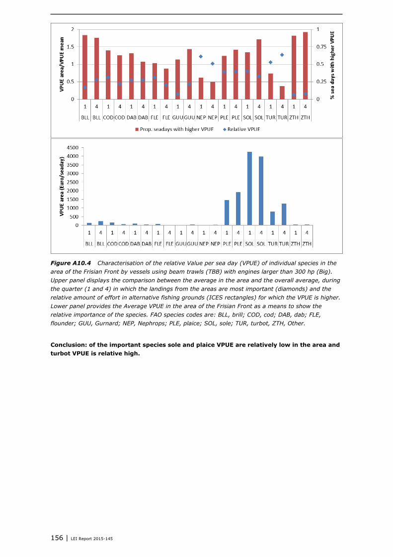
156 | LEI Report 2015-145

Figure A10.4 Characterisation of the relative Value per sea day (VPUE) of individual species in the

area of the Frisian Front by vessels using beam trawls (TBB) with engines larger than 300 hp (Big).

Upper panel displays the comparison between the average in the area and the overall average, during

the quarter (1 and 4) in which the landings from the areas are most important (diamonds) and the

relative amount of effort in alternative fishing grounds (ICES rectangles) for which the VPUE is higher.

Lower panel provides the Average VPUE in the area of the Frisian Front as a means to show the

relative importance of the species. FAO species codes are: BLL, brill; COD, cod; DAB, dab; FLE,

flounder; GUU, Gurnard; NEP, Nephrops; PLE, plaice; SOL, sole; TUR, turbot, ZTH, Other.

Conclusion: of the important species sole and plaice VPUE are relatively low in the area and

turbot VPUE is relative high.

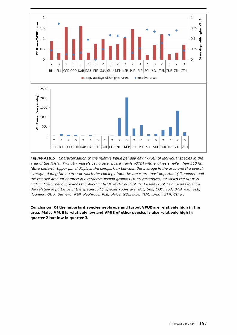
LEI Report 2015-145 | 157

Figure A10.5 Characterisation of the relative Value per sea day (VPUE) of individual species in the

area of the Frisian Front by vessels using otter board trawls (OTB) with engines smaller than 300 hp

(Euro cutters). Upper panel displays the comparison between the average in the area and the overall

average, during the quarter in which the landings from the areas are most important (diamonds) and

the relative amount of effort in alternative fishing grounds (ICES rectangles) for which the VPUE is

higher. Lower panel provides the Average VPUE in the area of the Frisian Front as a means to show

the relative importance of the species. FAO species codes are: BLL, brill; COD, cod; DAB, dab; FLE,

flounder; GUU, Gurnard; NEP, Nephrops; PLE, plaice; SOL, sole; TUR, turbot, ZTH, Other.

Conclusion: Of the important species nephrops and turbot VPUE are relatively high in the

area. Plaice VPUE is relatively low and VPUE of other species is also relatively high in

quarter 2 but low in quarter 3.

158 | LEI Report 2015-145

Figure A10.6 Characterisation of the relative Value per sea day (VPUE) of individual species in the

area of the Frisian Front by vessels using twin trawls (OTT) with engines smaller than 300 hp (Euro

cutters). Upper panel displays the comparison between the average in the area and the overall

average, during the quarter in which the landings from the areas are most important (diamonds) and

the relative amount of effort in alternative fishing grounds (ICES rectangles) for which the VPUE is

higher. Lower panel provides the Average VPUE in the area of the Frisian Front as a means to show

the relative importance of the species. FAO species codes are: BLL, brill; COD, cod; DAB, dab; FLE,

flounder; GUU, Gurnard; NEP, Nephrops; PLE, plaice; SOL, sole; TUR, turbot, ZTH, Other.

Conclusion: of the important species Nephrops VPUE is average in the area, and plaice VPUE

is relative low. Turbot VPUE is relatively high in quarter 2 and average in quarter 3.

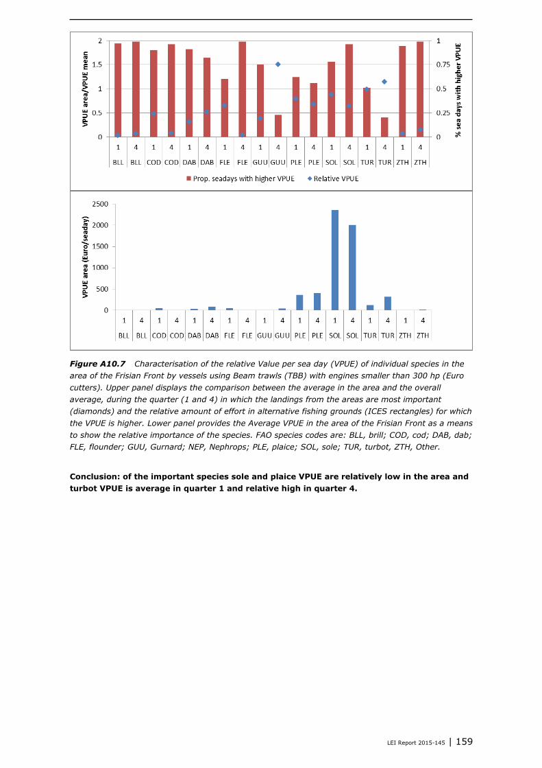
LEI Report 2015-145 | 159

Figure A10.7 Characterisation of the relative Value per sea day (VPUE) of individual species in the

area of the Frisian Front by vessels using Beam trawls (TBB) with engines smaller than 300 hp (Euro

cutters). Upper panel displays the comparison between the average in the area and the overall

average, during the quarter (1 and 4) in which the landings from the areas are most important

(diamonds) and the relative amount of effort in alternative fishing grounds (ICES rectangles) for which

the VPUE is higher. Lower panel provides the Average VPUE in the area of the Frisian Front as a means

to show the relative importance of the species. FAO species codes are: BLL, brill; COD, cod; DAB, dab;

FLE, flounder; GUU, Gurnard; NEP, Nephrops; PLE, plaice; SOL, sole; TUR, turbot, ZTH, Other.

Conclusion: of the important species sole and plaice VPUE are relatively low in the area and

turbot VPUE is average in quarter 1 and relative high in quarter 4.

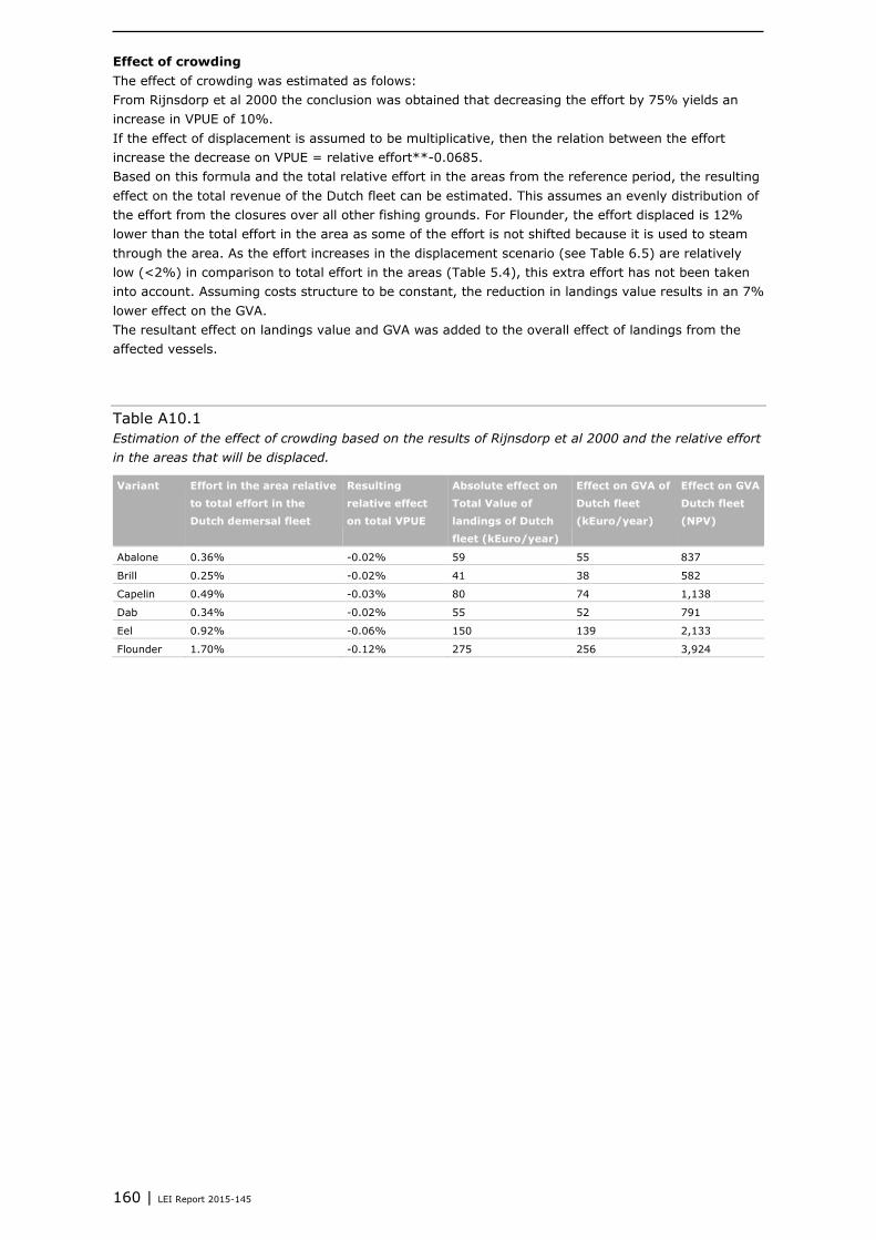
160 | LEI Report 2015-145

Effect of crowding

The effect of crowding was estimated as folows:

From Rijnsdorp et al 2000 the conclusion was obtained that decreasing the effort by 75% yields an

increase in VPUE of 10%.

If the effect of displacement is assumed to be multiplicative, then the relation between the effort

increase the decrease on VPUE = relative effort**-0.0685.

Based on this formula and the total relative effort in the areas from the reference period, the resulting

effect on the total revenue of the Dutch fleet can be estimated. This assumes an evenly distribution of

the effort from the closures over all other fishing grounds. For Flounder, the effort displaced is 12%

lower than the total effort in the area as some of the effort is not shifted because it is used to steam

through the area. As the effort increases in the displacement scenario (see Table 6.5) are relatively

low (<2%) in comparison to total effort in the areas (Table 5.4), this extra effort has not been taken

into account. Assuming costs structure to be constant, the reduction in landings value results in an 7%

lower effect on the GVA.

The resultant effect on landings value and GVA was added to the overall effect of landings from the

affected vessels.

Table A10.1

Estimation of the effect of crowding based on the results of Rijnsdorp et al 2000 and the relative effort

in the areas that will be displaced.

Variant Effort in the area relative

to total effort in the

Dutch demersal fleet

Resulting

relative effect

on total VPUE

Absolute effect on

Total Value of

landings of Dutch

fleet (kEuro/year)

Effect on GVA of

Dutch fleet

(kEuro/year)

Effect on GVA

Dutch fleet

(NPV)

Abalone 0.36% -0.02% 59 55 837

Brill 0.25% -0.02% 41 38 582

Capelin 0.49% -0.03% 80 74 1,138

Dab 0.34% -0.02% 55 52 791

Eel 0.92% -0.06% 150 139 2,133

Flounder 1.70% -0.12% 275 256 3,924

LEI Report 2015-145 | 161

Foundations of the Appendix 11

assumptions in Displacement

scenario B (partly in Dutch)

Table A11.1

Overview of constants used in estimating the effects of displacement

Dependency level for distinction between dependent and non dependent fishermen 10%

Groep gaat akkoord met 10% als onderscheidingsniveau.

% fishing through in case of generalists in variant Flounder (not for flyshoot) 50%

Groep vindt 50% een goede aanname en merkt op dat vanwege de ligging zeer veel doorheen wordt gevist op

weg naar en van bestekken elders.

lower landings for specialists in other areas

year 1 75%

year 2-4 50%

after year 4 40%

lower efficiency for generalists in other areas 25%

Groep acht de getallen zoals door LEI voorgesteld te laag; daarom deze verhoging.

[ingevoegd na reactie LEI] LEI geeft aan de 75% onrealistisch te vinden omdat ze verwacht dat bij meer dan

50% reductie het vissen onrendabel wordt. Dit komt echter wel overeen met het beeld vanuit de sector. Die

geeft namelijk aan te verwachten dat voor enkele van de ‘specialisten’ die er zeer veelvuldig komen, het

vissen inderdaad onrendabel gaat worden en dat zij zullen moeten stoppen. De 75% moet dan zo gezien

worden dat deze schepen hierin opgenomen zijn: het gemiddelde wordt wat opgetrokken. De schepen welke

wel nog kunnen vissen komen ook met een hoog percentage te zitten, maar niet in de verliesgevende cijfers.

Er is sprake van een leereffect, dus afname van visverlet in periode na sluiting is aannemelijk. Dit is in de

getallen behouden. Er zal echter sprake blijven van visverlet omdat de gronden waarheen verplaatst wordt

minder gunstig zijn (anders viste men op voorhand op de verkeerde plaats en dat is onaannemelijk) en

vanwege de toegenomen druk op deze gronden. Dit is eveneens in de getallen behouden.

Naast de verwachte verlaging van de vangst tijdens de trek zelf kwam een aanvullend punt ter sprake. Het

gebied zal niet alleen effect hebben op trekken uitgevoerd in de tijd die in de uitgangssituatie binnen het te

sluiten gebied zou zijn gevist. Een visreis wordt namelijk gepland als serie trekken (visplan) die van elkaar

afhankelijk zijn. Er wordt bijvoorbeeld, alvorens naar de visafslag terug te keren op het eind van een week,

een serie van vijf trekken doorheen het gebied en de omgeving gepland waarbinnen de verwachte vangst

wordt geoptimaliseerd. Een groot gesloten gebied relatief nabij de afslag heeft tot gevolg dat velerlei van dit

soort trips geheel anders ingepland zal moeten worden, waarbij ook bij de overige trekken in de serie een

lagere vangst mag worden verwacht.

Eveneens wordt gewezen op het cumulatieve effect van andere gebiedssluitingen, waaronder Natura 2000 en

hernieuwbare energieprojecten. Daardoor neemt de druk op de uitwijkgebieden verder toe dan alleen door

uitwijk vanuit het voorliggende gebied. Wanneer dit in MKBA’s van individuele gebiedssluitingen niet wordt

meegerekend, vallen de gevolgen van deze aanvullende druk tussen wal en schip.

Factor that will change due to lower efficiency of generalists

Twin trawl revenues

Flyshoot revenues

Pulse trawl revenues

Beam trawl revenues

Groep acht de redenering niet reëel dat schepen die met de pulskor vissen zullen compenseren voor de lagere

efficiëntie in de uitwijkgebieden door langer door te vissen. De groep verwacht dat schippers en bemanningen

dat niet zullen doen omdat ze niet op de schaarse vrije tijd in willen boeten door langer van huis te zijn.

Daarom stelt de groep dat voor puls net als voor de andere tuigen de effecten in opbrengst (niet in

inspanning) moeten worden uitgedrukt.

Na de bijeenkomst geeft LEI aan de berekening op basis van inspanning te hebben verkozen omdat uitsluitend

op vlootniveau wordt gerekend. Dit is één manier van weergave; het is voor de visserijondernemers echter

162 | LEI Report 2015-145

van belang dat eveneens de effecten voor vissers die in dit gebied vissen worden gekwantificeerd.

Verder wordt opgemerkt dat voor langoustinevisserij nog een aanvullend effect optreedt. Deze vissers hebben

een drietal bestekken waar zij vooral vissen, waarvan de andere twee verder weg liggen. Omdat het kleine

scheepjes betreft zijn zij sterk afhankelijk van de weersomstandigheden. Als het slecht weer is of de

voorspelling slecht weer aangeeft, dan gaat men niet naar de verder weg gelegen bestekken en is men sterk

afhankelijk van de bestekken in het betreffende gebied bij het Friese Front. Dit zou nog ergens tot uitdrukking

moeten komen.

Assumed fishing speed for gears fishing through the area in case of Flounder (knots)

Twin trawl 3

Pulse trawl 4.8

Beam trawl 6

Assumed steaming speed 10

Snelheden worden door de groep als een goede schatting gezien; geen wijzigingen.

% time lost due to steaming through the area

Twin trawl 30

Pulse trawl 48

Beam trawl 60

Berekening lijkt correct wanneer puur stoomtijd met vistijd wordt vergeleken. De groep geeft echter aan dat

tevens tijd voor handelingen aan de tuigage moet worden meegerekend.

Besproken wordt dat wanneer door het gebied moet worden gestoomd eerst de tuigage moet worden

opgeborgen, en na doorvaart weer moet worden uitgepakt. Dat kost bij mooi weer (40% van de dagen) naar

schatting 1 uur (opbergen + uitpakken), en bij matig weer (40% van de dagen) naar schatting 1.5 uur. Bij

slecht weer (20% van de dagen) kan het voorkomen dat opbergen en uitpakken niet mogelijk is. Er wordt dan

zoveel mogelijk met tuig overboord gevaren vanwege de veiligheid: stabiliteit van het schip; zwaaien van

loshangende zaken etc. Het is dan te verwachten dat stomen wordt vermeden en er een verlies van zo’n 5 uur

gerekend moet worden omdat er om het gebied heen gevaren wordt met tuig overboord.

Bovendien geeft de groep aan dat deze handelingen niet tot de routine behoren tijdens het vissen en dus een

risico inhouden. Opgemerkt wordt dat ongelukken bij het vissen over het algemeen tijdens afwijkingen van de

routine voorkomen.

LEI Report 2015-145 | 163

Quantitative assessment of Appendix 12

the monitoring costs for the

different variants Central

Oyster Grounds and Frisian

Front

IenM / RWS, November 25, 2015

The design of the monitoring of the Frisian Front (FF) and Central Oyster Grounds (CO) is based on

two separate areas (see Annex 5 of Part 2 of the Marine Strategy). The measurement strategy is

designed in such a way that on the basis of probability at least 50% change in spatial distribution of

indicator species6 within the area can be observed between two measurement moments (three years

in between) with a confidence level of 95%. The design of the measurement strategy does not take

into account the imposition of measures (i.e. closing areas).

In 2015, on the basis of this measurement strategy, a baseline monitoring (T0) has taken place on

Frisian Front and Central Oyster Grounds as part of the overall baseline for the marine strategy.

Subsequently, every three years monitoring will take place. The costs of T0 on Frisian Front and

Central Oyster Grounds is budgeted at approximately €130,000, =. In an unmodified implementation

of the monitoring program, the monitoring program will cost every three years €130,000,=. The cost

of preparing the measurement strategy for the different variants are not distinctive. If the

measurement strategy has to be adjusted this can be done with very limited additional non-recurring

costs (€5,000 - €10,000, =).

The variants for the measures lead to assumptions other than those made in the measurement

strategy for T0: variants have almost all different shapes and sizes and are sometimes (partly) outside

the area covered by the T0. That means, that for proper monitoring of each variant the measurement

strategy must be adapted to a greater or lesser extent, and possibly the TO has to take place again.

This is subject to the following principles:

The more a variant differs from the defined areas in the Marine Strategy Part 2, the greater the

additional T0 is which has to be done again;

Each area with measures needs to have an equally large area without measures as a reference, with

the same EUNIS-3 habitat.

Monitoring of a large area is more cost effective than monitoring of several small areas with the

same surface area. Due to the chosen statistical frameworks, it is not possible to simply add a

number of small areas up to a large area. For instance, three small areas probably need more data

points than one large area of the same size.

Based on these principles the cost of monitoring of each variant can be estimated.

A comparison of the monitoring costs of the six variants is given below, based upon a cost estimate of

the T0 of €130,000. In order to compare the different variants with each other, the costs of the initial

T0 has not been taken into account.

6 As defined in Part 2 of the Marine Strategy for Frisian Front and Central Oyster Grounds

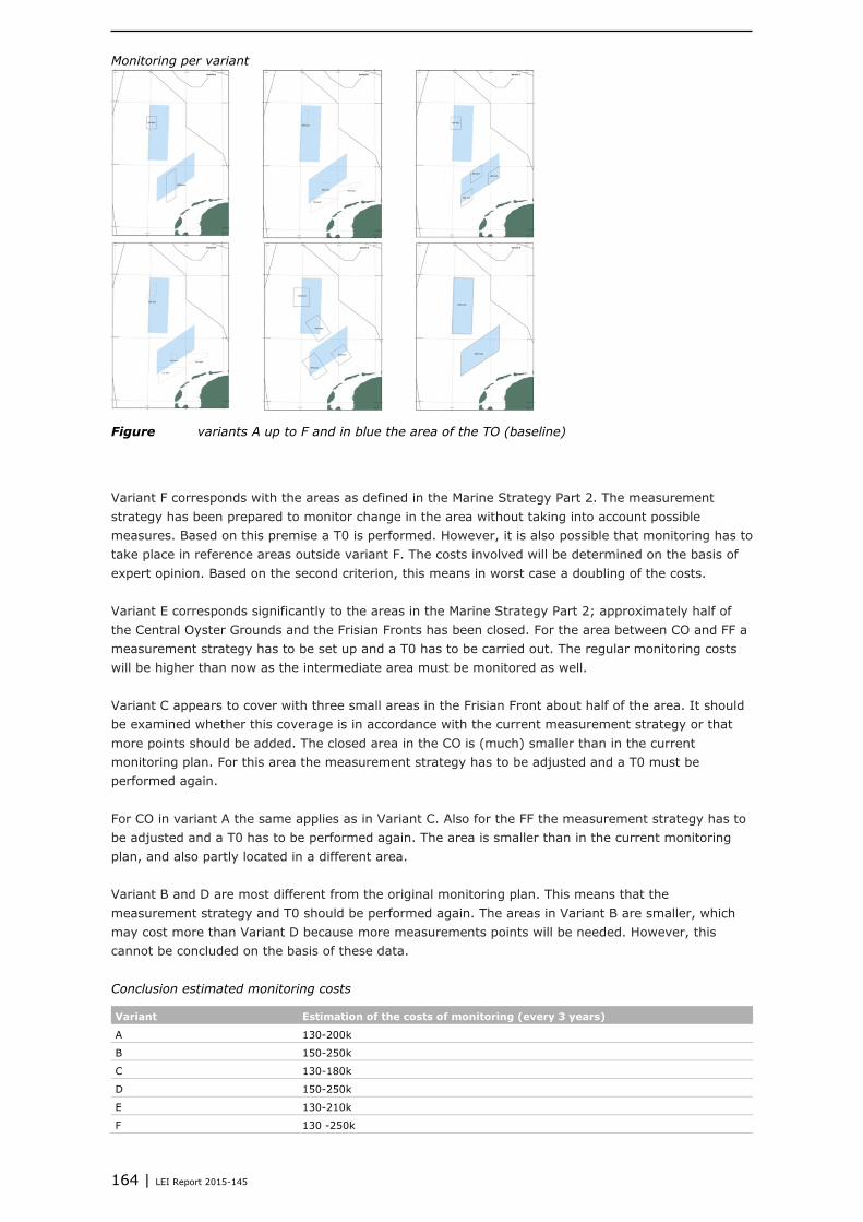
164 | LEI Report 2015-145

Monitoring per variant

Figure variants A up to F and in blue the area of the TO (baseline)

Variant F corresponds with the areas as defined in the Marine Strategy Part 2. The measurement

strategy has been prepared to monitor change in the area without taking into account possible

measures. Based on this premise a T0 is performed. However, it is also possible that monitoring has to

take place in reference areas outside variant F. The costs involved will be determined on the basis of

expert opinion. Based on the second criterion, this means in worst case a doubling of the costs.

Variant E corresponds significantly to the areas in the Marine Strategy Part 2; approximately half of

the Central Oyster Grounds and the Frisian Fronts has been closed. For the area between CO and FF a

measurement strategy has to be set up and a T0 has to be carried out. The regular monitoring costs

will be higher than now as the intermediate area must be monitored as well.

Variant C appears to cover with three small areas in the Frisian Front about half of the area. It should

be examined whether this coverage is in accordance with the current measurement strategy or that

more points should be added. The closed area in the CO is (much) smaller than in the current

monitoring plan. For this area the measurement strategy has to be adjusted and a T0 must be

performed again.

For CO in variant A the same applies as in Variant C. Also for the FF the measurement strategy has to

be adjusted and a T0 has to be performed again. The area is smaller than in the current monitoring

plan, and also partly located in a different area.

Variant B and D are most different from the original monitoring plan. This means that the

measurement strategy and T0 should be performed again. The areas in Variant B are smaller, which

may cost more than Variant D because more measurements points will be needed. However, this

cannot be concluded on the basis of these data.

Conclusion estimated monitoring costs

Variant Estimation of the costs of monitoring (every 3 years)

A 130-200k

B 150-250k

C 130-180k

D 150-250k

E 130-210k

F 130 -250k

LEI Report 2015-145 | 165

Motivation Weight factor Appendix 13

gradients

During sessions with fishermen it has become clear that there are disadvantages related to large

closed areas. Large closed areas can be an obstacle for fishermen to arrive to their fishing grounds

when they are not allowed to fish while steaming through these closed areas.

There are several ways to design protected/closed areas. The question in this process is whether

contiguous areas are important to consider, and as part thereof, whether the aspect of ‘gradients’ is

an essential criterion to distinguish areas regarding effectivity in protection.

Lindeboom et al. (2015) reflect on a number of ecological considerations related to this matter in

which sub division of areas and effective protection were part of the elaboration. The proposed

‘penalty’ factor is a practical advise to compensate for these aspects. Weighting factor 3 of the

ecopoint calculation, which reflects this penalty, has a generic character, in which the size/perimeter

ratio is the steering element. In a further specification of the penalty additional features are included

to compensate for ineffectiveness in protection related to total surface to due species mobility. The

gradient of the Frisian Front has no role in this weighting factor.

With regard to the Frisian Front, Lindeboom et al., (2015) discusses the determining elements for the

uniqueness of the Frisian Front. One of the unique aspects is the North-South gradient of sediment

types with corresponding ecological characteristics. The question is whether this gradient must be

contiguous, or whether it can be disconnected zones, and if there is a preference for one of these

based on ecological arguments.

As stated in Lindeboom et al. (2015) one of the ways to include the uniqueness and the whole range

of niches of the Frisian Front into the ecopoint calculation is to apply a weighting factor that reflects

the entire gradient between sand -in the south-, the core area with high silt (15-20%) into the deeper

silty areas in the north.

In this viewpoint, it is assumed that the ecological values of the Frisian Front are represented to the

maximum (picture A). Studies in which the relationships of each zone on the Frisian Front (in abiotic

and biotic terms) are investigated in detail are however lacking. Lindeboom et al., 2015 state that the

ecological value of the different zones within the gradient on the Frisian Front is more than the sum of

its parts. The front and its related area actually covers a wider range of valuable circumstances in

which many different species may find their potential niche. The optimum niche for a species is a

combination of these factors, and species will associate with the optimum combination of factors in

space and time. It depends on the species and its traits how tolerant its population will be and

whether it is capable of (long-term) survival within sub-optimal combination of factors.

If one wants to protect areas on the Frisian Front optimally, an area with a continuous gradient is

preferred (picture A). If the closed area is split into different parts, the protection will be reduced even

if all zones are included (because some are less in surface and not present in each sub-area) (B).

Because each zone is characterized by its own benthic community, the border effect will reduce the

protection of those zones that lay on the border of the closed area. Subdivision of areas can be

compensated for this latter effect by choosing the closed sub areas in such a way that the zones laying

at the border are included in both sub –areas (picture C).

166 | LEI Report 2015-145

Figure A13.1 Schematic representation of interpretation of continuous gradients and division into

sub-areas. In the text A, B and C are explained

LEI Wageningen UR

P.O. Box 29703

2502 LS The Hague

The Netherlands

T +31 (0)70 335 83 30

E publicatie.lei@wur.nl

www.wageningenUR.nl/en/lei

REPORT

LEI 2015-145

LEI Wageningen UR is one of the world’s leading independent socio-economic

research institutes. LEI’s unique data, models and knowledge offer clients

insight and integrated advice on policy and decision-making in an innovative

manner, and ultimately contribute to a more sustainable world. LEI is part of

Wageningen UR (University and Research centre), forming the Social

Sciences Group together with the Department of Social Sciences and

Wageningen UR Centre for Development Innovation.

The mission of Wageningen UR (University & Research centre) is ‘To explore

the potential of nature to improve the quality of life’. Within Wageningen UR,

nine specialised research institutes of the DLO Foundation have joined forces

with Wageningen University to help answer the most important questions in

the domain of healthy food and living environment. With approximately 30

locations, 6,000 members of staff and 9,000 students, Wageningen UR is one

of the leading organisations in its domain worldwide. The integral approach

to problems and the cooperation between the various disciplines are at the

heart of the unique Wageningen Approach.

LEI Wageningen UR is one of the world’s leading independent socio-economic research institutes. LEI’s unique data, models and knowledge offer clients insight and integrated advice on policy and decision-making in an innovative manner, and ultimately contribute to a more sustainable world. LEI is part of Wageningen UR (University and Research centre), forming the Social Sciences Group together with the Department of Social Sciences and Wageningen UR Centre for Development Innovation.

The mission of Wageningen UR (University & Research centre) is ‘To explore the potential of nature to improve the quality of life’. Within Wageningen UR, nine specialised research institutes of the DLO Foundation have joined forces with Wageningen University to help answer the most important questions in the domain of healthy food and living environment. With approximately 30 locations, 6,000 members of staff and 9,000 students, Wageningen UR is one of the leading organisations in its domain worldwide. The integral approach to problems and the cooperation between the various disciplines are at the heart of the unique Wageningen Approach.

LEI Wageningen URP.O. Box 297032502 LS Den HaagThe NetherlandsE publicatie.lei@wur.nlwww.wageningenUR.nl/lei

REPORT LEI 2015-145ISBN 978-90-8615-726-6

Hans van Oostenbrugge, Diana Slijkerman, Katell Hamon, Oscar Bos, Marcel Machiels, Olga van de Valk, Niels Hintzen, Ernst Bos, Jan Tjalling van der Wal and Joop Coolen

A Cost Benefit Analysis

Effects of seabed protection on the Frisian Front and Central Oyster Grounds