effects of wintertime polluted aerosol on cloud over the ... · pdf file1 effects of...

1

Effects of wintertime polluted aerosol on cloud over the Yangtze 1

River Delta: case study 2

3

Chen Xua, Junyan Duana, Yanyu Wang a, Yifan Wang a, Hailin Zhu a, 4

Xiang Li a *, Lingdong Kong a, Qianshan He b, Tiantao Cheng a *, Jianmin 5

Chen a 6

a. Shanghai Key Laboratory of Atmospheric Particle Pollution and Prevention 7

(LAP3), Department of environmental science and engineering, Fudan University, 8

Shanghai 200433, China; 9

b. Shanghai Meteorological Bureau, Shanghai 200030, China; 10

11

* Corresponding authors: Tiantao Cheng, Xiang Li 12

Tel: (86) 21-6564 3230; fax: (86) 21-6564 2080; 13

Email: [email protected], [email protected] 14

15

Abstract 16

The effects of polluted aerosol on cloud are examined over the Yangtze 17

River Delta (YRD) using three-month satellite data during wintertime 18

from December 2013 to January 2014. The relationships between aerosol 19

properties and cloud parameters are analyzed in detail to clarify the 20

differences of cloud development under varying aerosol and meteorology 21

conditions. Complex relationships between aerosol optical depth (AOD) 22

and cloud droplet radius (CDR), liquid water path (LWP) and cloud 23

optical thickness (COT) exists in four sub-regions. High aerosol loading 24

(AOD) does not obviously affect the distributions of cloud LWP and COT. 25

Atmos. Chem. Phys. Discuss., doi:10.5194/acp-2016-968, 2016Manuscript under review for journal Atmos. Chem. Phys.Published: 7 December 2016c© Author(s) 2016. CC-BY 3.0 License.

2

In fact, an inhibiting effect of aerosol occurs in coastal area for low- and 1

medium-low clouds, more pronounced in low clouds (<5km) than high 2

clouds. Low aerosol loading (AOD) plays a positive role in promoting 3

COTs of high- and low-clouds in areas dominated by marine aerosol. The 4

most significant effect presents in valley and coal industry districts for 5

clouds except high-cloud. The smallest values and variations of cloud 6

parameters are observed in dry-polluted area, which suggests that dust 7

aerosol makes little difference on clouds properties. Synoptic conditions 8

also cast strong impacts on cloud distribution, particularly the unstable 9

synoptic condition leads to cloud development at larger horizontal and 10

vertical scales. The ground pollution enhances the amount of low-level 11

cloud coverage even under stable condition. Aerosol plays an important 12

role in cloud evolution for the low layers of troposphere (below 5km) in 13

case of the stable atmosphere in wintertime. 14

Keywords: Aerosol, Cloud, Pollution, the Yangtze River Delta 15

16

1. Introduction 17

Aerosol is the solid or liquid particles of 0.001-10 microns in diameter 18

suspended in the atmosphere. Aerosol can influence regional and global 19

climates by direct and indirect effects (Ackerman et al., 2000; Forest et 20

al., 2002; Knutti et al., 2002; Anderson et al., 2003; Lohmann and 21

Feichter, 2005; Satheesh et al., 2006), and cause great harm to 22


3

atmospheric environment and human health (Monks et al., 2009; Pöschl, 1

2005). Actually, aerosol can act as cloud condensation nuclei (CCN) or 2

ice nuclei (IN) to affect cloud droplet size, number and albedo, and as a 3

result, delaying the collision and coalescence in warm clouds (Twomey, 4

1974). Aerosol also affects precipitation and cloud lifespan, and 5

eventually cloud coverage and regional climate (Albrecht, 1989; 6

Rosenfeld, 2000; Ramanathan et al., 2001; Quaas et al., 2004). In the 7

process of cloud formation, aerosol probably influences cloud physical 8

characteristics, such as cloud thickness and cloud amount (Hansen et al., 9

1997). 10

The Yangtze River Delta (YRD) is a fast growing and densely 11

populated area in East China, hence experiencing relatively high aerosol 12

loadings for decades because of large amount of black carbon and sulfate 13

emissions (Wolf and Hidy, 1997; Streets et al., 2001; Xu et al., 2003; 14

Bond et al., 2004; Lu et al., 2010). Due to human activities and special 15

geographies, this region suffers a lot from natural and anthropogenic 16

aerosols. In addition to industrial aerosol caused by human activities, the 17

other major types are marine aerosol from sea surface brought by winds 18

and dust transported occasionally from deserts in northern China mostly 19

in winter and spring (Jin and Shepherd, 2008). All these factors may 20

result in a more complex aerosol-cloud-precipitation interaction over this 21

region. 22


4

In recent years, increasing attention has been paid on aerosol and its 1

radiative effects in the YRD district (Xia et al., 2007; Liu et al., 2012). 2

For instance, He et al. (2012) explored that a notable increase of annual 3

mean aerosol optical depth (AOD) takes place during 2000-2007, 4

maximum in summer dominated by fine particles and minimum in winter 5

by coarse mode particles mostly. Other studies have focused on aerosol 6

indirect effect (AIE) and attempt to assess the impact of aerosol on 7

precipitation in eastern China. For example, Leng et al. (2014) pointed 8

out that aerosol is more active in hazy days in Shanghai. Tang et al. (2014) 9

analyzed the variability of cloud properties induced by aerosol over East 10

China from satellite data, and compared land with ocean areas to 11

understand AIE discrepancy under different meteorological conditions. 12

Menon et al. (2002) proposed that the fact of anthropogenic aerosol 13

increasing precipitation in southeastern China but suppressing in 14

northeastern China is likely attributable to the absorption radiation by 15

AOD distribution. Zhao et al. (2006) examined the feedback of 16

precipitation and aerosol over the eastern and central China, and revealed 17

that precipitation significantly reduces whereas atmospheric visibility 18

increases during the last 40 years. Despite of the above-mentioned studies, 19

up to now, the influence of polluted aerosol on cloud and precipitation on 20

different underlying surfaces over the YRD is not intensively examined. 21

Since the winter of 2013, a widely reported air pollution named haze 22


5

has arisen in different areas of China, and has been characterized by 1

long-lasting, large-scale and highly polluted features. In the YRD, haze 2

occurred persistently at the wintertime from December 2013 to February 3

2014. In order to understand the formation of haze, Leng et al. (2015) 4

analyzed the synoptic situation, boundary layer and pollutants of haze 5

that happened in December 2013, and Hu et al. (2016) profiled the 6

chemical characteristics of single particle sampled in Shanghai. Kong et 7

al. (2015) observed the variation of polycyclic aromatic hydrocarbons in 8

PM2.5 during haze periods around the 2014 Chinese Spring Festival in 9

Nanjing. More efforts are needed to focus on the relationship between 10

aerosol types and macro-/micro-physical properties of clouds under 11

different atmospheric conditions. 12

This paper presents the spatio-temporal variations of aerosol and 13

cloud over the YRD region from December 2013 to February 2014 based 14

on satellite retrievals and the method used by Costantino et al. (2013). 15

The aim is to provide insights into the influence of aerosol on cloud 16

microphysical properties under highly polluted conditions. The results are 17

helpful to in-depth understanding of aerosol indirect effects in Asian 18

fast-growing areas. 19

2. Data and methods 20

Clouds and Earth’s Radiant Energy System (CERES), part of the 21

NASA’s Earth Observing System (EOS), is an instrument aboard Aqua 22


6

satellite to measure the upwelling short- and long-wave radiations on 1

about 20×20 km2 horizontal resolution (Wielicki et al., 1996; Loeb and 2

Manalo-Smith, 2005). In this study, the cloud and aerosol parameters of 3

CERES-SYN1deg, Edition 3A 3-hour data from satellites of Terra and 4

Aqua were used for the YRD domain (26.5-35.5°N, 115.5-122.5°E) 5

between December 2013 and February 2014. Cloud properties include 6

cloud liquid water path (LWP), cloud effective droplet radius (CDR), 7

cloud optical thickness (COT), cloud top pressure (CTP) and cloud 8

fraction (CLF) retrieved from the 3.7 µm (mid-IR) channel with the 9

horizontal resolution of 1°×1° (Minnis et al., 2004). The daily average 10

was computed based on the 3-hour values of the corresponding day from 11

the SYN1deg-3hour products (also for monthly average). Depending on 12

three-month mean AODs at 0.55μm (as proxy of aerosol loading) and 13

underlying surface conditions, the YRD was divided into four sub-regions 14

(Fig.1). If one grid has more than 2/3 area falling in certain sub-region, 15

we consider this grid as one part of such sub-region. 16

The CERES-SYN retrieval includes MODIS-derived cloud and aerosol 17

properties (Minnis et al., 2004; Remer et al., 2005) and 18

geostationary-derived cloud properties. It uses 3-hour cloud property data 19

from geostationary (GEO) imagers for modelling more accurately the 20

variability between CERES observations. Computations use MODIS and 21

geostationary satellite cloud properties along with atmospheric profiles 22


7

provided by the Global Modeling and Assimilation Office (GMAO). 1

Furthermore, the CDR and COT of MOD04 are generally smaller than 2

that in MOD06 products (Minnis et al., 2004; Platnick et al., 2003) 3

because of the MODIS algorithm tends to classify very thick aerosol 4

layers as clouds and no-aerosols (Remer et al., 2006). Thus, MODIS 5

probably under estimates the total AOD. Overall, the properties of cloud 6

and aerosol are best retrieval in the CERES-SYN (Jones et al., 2009). 7

MODIS products are derived from cloud-free 500m resolution data and 8

then aggregated to a 10 km footprint (20×20 pixels) by the MODIS level2 9

aerosol product (MOD04). The fine mode fraction (FMF) of aerosol at 10

0.55 µm was used to determine the effect of aerosol types on cloud 11

properties. In this study, the simple method, which is utilized by Barnaba 12

and Gobbi (2004) based on the combination of AOD and FMF, was 13

implemented to separate aerosol types. This method defines aerosol as 14

marine type with AOD< 0.3 and FMF< 0.8, dust with AOD> 0.3 and 15

FMF< 0.7, and continental type with AOD< 0.3 and FMF > 0.8 or AOD> 16

0.3 and FMF > 0.7. By the way, aerosol type pixels were created 17

following the resolution of CERES products. 18

The aerosol and cloud products are retrieved by the CALIPSO lidar 19

instrument, which provides height-resolved information globally since 20

2006, including the layer fraction of aerosol and cloud and aerosol 21

vertical feature mask (Winker et al., 2009, 2010). In order to examine 22


8

atmospheric stability, surface lifted index (SLI) and sea level pressure 1

(SLP) from the National Center for Environmental Prediction (NCEP) 2

Reanalysis (Kalnay et al., 1996) were used. The frequency of 3

precipitation was calculated by precipitation rate from reanalysis data. 4

The Hybrid Single Particle Lagrangian Integrated Trajectory 5

(HYSPLIT) model (Draxler and Rolph 2003; Rolph 2003; 6

www.arl.noaa.gov/ready.html) was used to calculate 72-h air mass 7

forward and backward trajectories every six hours at 9 key sites in the 8

YRD. The meteorological input is from the FNL dataset, reprocessed 9

from the final analysis data of NOAA’s NCEP by Air Resources 10

Laboratory. Additionally, the data of PM2.5 concentration comes from the 11

on-line monitoring and analysis platform of air quality in China 12

(http://www.aqistudy.cn/). 13

3. Results and discussion 14

3.1 Aerosol spatial variation 15

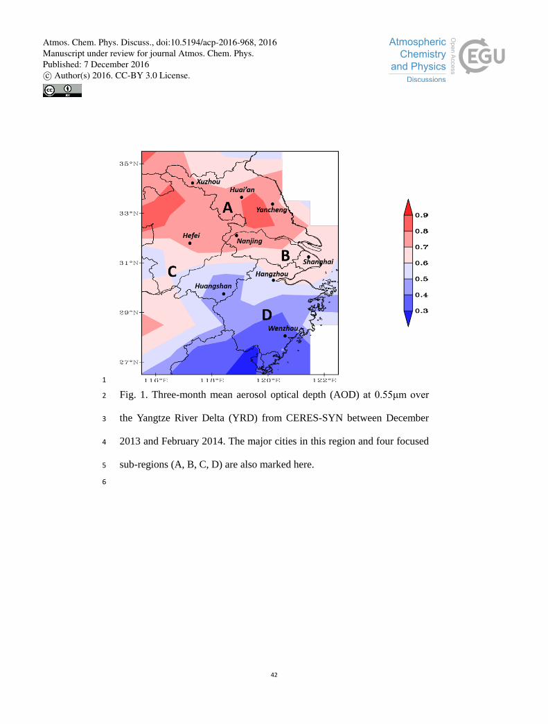
Figure 1 displays the spatial distribution of 3-h mean AODs over the 16

YRD region from December 2013 to February 2014. AODs range in 17

0.3-0.9, lower than the annual average (0.5-1.3) (Kourtidis et al., 2015), 18

and show obviously inhomogeneous due to different surface conditions 19

from north to south. High AODs almost scatter in plains and valleys, 20

particularly the densely populated and industrialized locations, while low 21

AODs are mainly in hills and mountains. AODs higher than 0.7 are 22


9

concentrated in the north of the YRD, the central and northern parts of 1

Jiangsu Province and the northern part of Anhui Province, traditional 2

agricultural areas, here which are defined as sub-region A. Furthermore, 3

high AODs of 0.5-0.7 are found in Shanghai and the northeastern part of 4

Zhejiang Province, typical urban industrial areas, named as sub-region B. 5

The Yangtze River valley in Anhui Province, surrounded by Dabie and 6

Tianmu mountains, is categorized into sub-region C. AODs lower than 7

0.5 are observed in mountainous areas throughout the south and west 8

parts of Zhejiang province and the Mount Huang in Anhui province, 9

referred to as sub-region D. The 3-month mean AODs are 0.76, 0.62, 0.57, 10

0.44 in the sub-region A, B, C, and D, respectively. This feature of 11

aerosol spatial distribution is in accordance with the result concluded by 12

Tan et al. (2015) using 10-year data that aerosol concentration is higher in 13

north and lower in south, whereas FMF is just opposite to AOD. 14

According to AOD~FMF classification method (Barnaba and Gobbi, 15

2004), aerosols of the sub-region A are probably categorized into marine, 16

dust and continental types, mainly generated from local urban/industrial 17

emissions and biomass burning. Also, this sub-region is vulnerable to 18

dust blowing from the North China (Fu et al., 2014). In the sub-region B, 19

besides fine mode particles from urban/industrial emissions, coarse mode 20

particulate pollutants have marine aerosols brought by northeastern 21

airflows and dust floating long distance from the north. The large aerosol 22


10

loading of the Jiaozhou Bay is probably attributed to coarse mode 1

particles due to the humidity swelling of sea salt (Xin et al., 2007). A 2

plenty of construction and industrial activities also contribute numerous 3

dust-like particles to the atmosphere (He et al., 2012). Similar with the 4

aerosol types in the sub-region B, the sub-region C is home to more than 5

one million people, numerous copper-melting industry and coalmines, 6

which are the major sources of local emissions. The sub-region C is 7

viewed as one of the main channels for aerosol transported from the west 8

(He et al., 2012). On the other hand, the surrounding mountains could 9

prevent long-distance transportation of dust originated from the north. 10

The sub-region D is dominated by continental and marine aerosols, most 11

of which can be easily detected close to their sources (He et al., 2012). 12

Overall, dust and anthropogenic pollutants often influence the columnar 13

optical properties of aerosol in all parts of northern the YRD. 14

3.2 Aerosol and cloud properties 15

3.2.1 Cloud optical thickness (COT) 16

Figure 2 shows the distribution of COTs varying with AODs, which are 17

averaged over every constant bin AOD (0.02) from 0.2 to 1. Clearly, 18

COTs are notably uni-modal in the sub-region B, C and D, and almost 19

reach to maximum at AODs of 0.6-0.74. The peaks of COTs are close to 20

17 in the sub-region C, D and smaller 15 in the sub-region B. A possible 21

reason is that clouds turn thicker in mountainous areas (e.g. sub-region C 22


11

and D) as a result of new particles’ activation (Bangert et al., 2011). In 1

contrast, COTs ascend slowly, and multi-modal peaks appear in the 2

sub-region A, such as COTs 7.1, 8.4 in corresponding to AODs at 0.44 3

and 0.88, respectively. 4

In the sub-region A, COTs grow as aerosols increase, and particularly 5

COTs of the clouds below 4.6km is correlated with AODs below 0.6 6

(Table S1). COTs and AODs are positive-correlated at low-level AODs 7

(<0.6) in the sub-region B, C and D and negative-correlated at high-level 8

AODs (0.6-1.0). In the sub-region B, COTs are greatly sensitive to AODs, 9

and COTs of all height-type clouds are affected equally by AODs at 10

low-level. As for high-clouds, the inhibiting effect of aerosol on COTs is 11

more outstanding (R2=0.47) than the promoting effect. In the sub-region 12

C, except for high-clouds, the influence of low-level AODs on COTs of 13

other type clouds is relatively stronger than that in the sub-region B, 14

while high-level AODs are less influential in the sub-region B than the 15

sub-region C and basically cast no evident impacts on high-clouds. In the 16

sub-region D, COTs and AODs show a significant positive correlativity at 17

low-level AODs, for example, a steep slope (3.58) appears in high-clouds. 18

Generally, COT links closely with AOD, in particular of low- and 19

medium-low clouds in the sub-region A, low- and high-clouds in the 20

sub-region B and D, and other types except high-clouds in the sub-region 21

C. 22


12

3.2.2 Cloud liquid water path (LWP) 1

Kourtidis et al. (2015) point out that the impact of AODs on cloud 2

cover would greatly overestimated unless water vapor is considered in the 3

YRD, where AODs and water vapor have similar seasonal variations. In 4

addition, recent studies have focused on the possible impacts of 5

meteorological parameters on AOD–COT relationships, such as water 6

vapor (Ten Hoeve et al., 2011) and relative humidity (Koren et al., 2010; 7

Grandey et al., 2013). 8

Water vapor influence is discussed using LWPs averaged over a 9

constant bin of AODs (Figure 3). The relationship of LWP-AOD is 10

somewhat similar to that of COT-AOD (Figure 2), and AODs of 0.6-0.74 11

correspond to peak LWPs in the sub-region B, C and D. In the sub-region 12

C, LWPs rise up about 14 times as AODs increase from 0.22 to 0.66, 13

which is the largest increase among these sub-regions. Otherwise, in the 14

sub-region A, although LWPs grow smoothly with AODs on the whole, 15

no distinct peaks are detected, and the amount of cloud water increases by 16

425% as AODs increase from 0.2 to 0.96. The growth rate of LWPs in the 17

sub-region A is similar to that of the sub-region B, but the promoting 18

effects of AOD zones are quite different between them (0.2-1 vs 0.2-0.6). 19

This discrepancy is responsible for a large amount of non-hygroscopic 20

aerosols in the sub-region A (Liu and Wang, 2010). 21

Generally, LWPs increase with AODs when AODs are at low levels in 22


13

the four sub-regions. LWPs and AODs are negative-correlated at 1

high-level AODs in the sub-region B, C and D, but weakly positive- 2

correlated in the sub-region A. Specifically, in the sub-region A, the 3

promotion of aerosol positive effect slows down with cloud height 4

growing and AOD increasing. Although aerosol plays equal roles in all 5

height-type clouds in the sub-region B, the best-fit slopes at high-level 6

AODs are twice as large as those at low-level AODs, and correlation 7

coefficients for the clouds below 4.6km are larger than clouds in higher 8

layers (Table S1). In other words, for each level of clouds, LWPs increase 9

slowly (AOD<0.6) but decrease sharply (AOD>0.6) with AODs growing. 10

Opposite to the sub-region B, the promoting effect of AOD on LWP in the 11

sub-region C at low AODs is marked, while the inhibiting effect is not 12

significant at high AODs (Table S1). In addition, the promoting effect of 13

low clouds in the sub-region C is most outstanding. In the sub-region D, 14

the pronounced effect of AOD on LWP mainly works on low- and high- 15

clouds at low-level AODs (Table S1). Particularly, the best-fit slope of 16

high-clouds, such as 2.53 at low-level AODs and -3.46 at high-level 17

AODs, is much higher than that of other height-type clouds. 18

Many studies have also displayed the correlation of LWP and AOD in 19

other regions of the world. For instance, a report over Pakistan (Alam et 20

al., 2010), where aerosol is dominated by coarse particles, is similar to 21

our results of the sub-region A, where positive correlations of LWP-AOD 22


14

are found mainly due to their common seasonal patterns. LWP plays an 1

important role in AIE (L’Ecuyer et al., 2009), and findings confirm that 2

high-aerosol conditions tend to decrease LWP, and the magnitude of LWP 3

reduction is greater in the unstable environment of non-precipitating 4

clouds (Lebsock et al., 2008). Moreover, the fact that increasing LWP is 5

not systematically associated with increasing AOD (Fig.3) indicates there 6

is no definite relationship between AOD and LWP. 7

3.2.3 Cloud droplet radius (CDR) 8

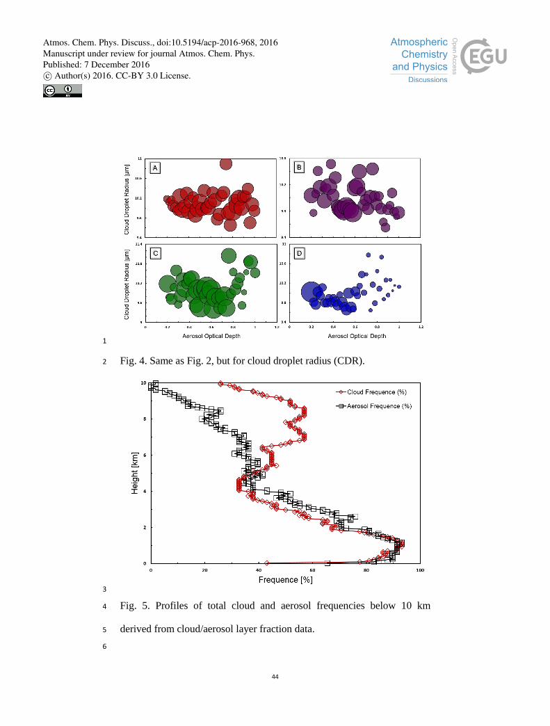
Fig.4 presents mean CDRs averaged over a constantbin (0.02) of AODs. 9

Basically, CDRs vary between 9.5μm and 11μm in all 4 sub-regions. For 10

the sub-region A, two sections indicate weak positive correlation between 11

CDR and AOD. For the sub-region B, however, it is of negative 12

correlation for these two sections. As for the sub-region C and D, CDRs 13

have a similar pattern that it decreases as AOD increases at low-level 14

AODs and constantly increases at high-level AODs. Therefore, CDRs 15

show an insignificant dependence on AODs (Table S1). Consistent with 16

the Twomey effect and similar to the findings by Brenguier et al. (2003), 17

AODs and CDRs are negative-correlated for cloud types, at low-level 18

AODs in the sub-region B, C and D, which agrees with the observation in 19

Oklahoma atmospheric radiation measurement site by Feingold et al. 20

(2003) and Penner et al. (2004). It is interesting to find that CDR 21

increases with AOD in the sub-region A, C and D, but this tendency is not 22


15

obvious among different height-type clouds (Table S1). As a whole, CDR 1

shows little exponential dependence on AOD, consequently, simply the 2

exponential presentation is difficult to entirely reflect their complex 3

relationship. 4

In order to understand AOD-CDR, variables of cloud height and 5

cloud water content are controlled to evaluate their potentials in different 6

height-type clouds by correlation coefficients of cloud parameters (e.g. 7

CDR, LWP, COT) (Table S1). Firstly, it is notable that a considerable 8

portion of relatively high correlation coefficients mostly occurs in low 9

clouds. Figure 5 shows frequencies of occurrence of total cloud and 10

aerosol below 10km over the entire YRD. The cloud frequency is 11

multi-modal, ranging from 93% around 1km to 26% around 10km, 12

among which most exceeding 50% obviously occur at the low (< 3km) 13

and high (6-9km) layers. As for aerosol layer fraction, it turns out high 14

frequency occurs below 3.6km above sea level, maximum around 1.2km, 15

and the frequency decreases to zero with increasing heights. Overall, both 16

of cloud and aerosol most frequently appear below 3km, indicating that 17

low-cloud (latitude from the surface to 2.8km) plays an important role in 18

AIE within every sub-region. Thereby, we use 3-h average data of 19

low-cloud from CERES in the following analyses. 20

Water vapor (WV) has a great effect on CDR. Yuan et al. (2008) 21

summarized that 70% of variability between AOD and CDR is due to 22


16

changes of atmospheric water content. Moreover, statistics suggests that 1

WV has an evidently stronger impact on cloud cover than AOD over the 2

YRD (Kourtidis et al., 2015). Therefore, we introduce LWP and divide it 3

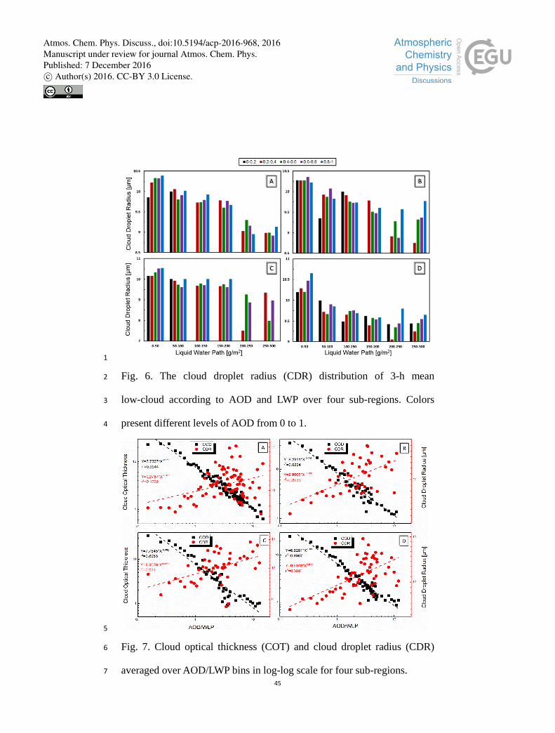
into six grades for analysis of CDR changes with AOD. In Figure 6, 4

CDRs present different tendencies as AOD changes at different levels of 5

cloud water content. When cloud water content is low (i.e. thin cloud, 6

LWP<50 g/m2), CDRs increase gradually with AODs. The CDRs in the 7

sub-region A and B increase with AODs synchronously at LWPs of 50 8

-100, but decrease in the sub-region C and D. Overall，it is indicated that 9

in a mountainous area full of water vapors, the inhibiting effect appears 10

as the aerosol loading increases. When LWP is growing, however, the 11

trend of CDR changes with AODs turns ambiguous. 12

Meanwhile, some of CDRs show clearly decreasing tendency with 13

LWPs at constant AODs under LWP <200 g/m2, such as higher AODs 14

(AOD>0.6) in the sub-region D and medium aerosol loading 15

(0.4<AOD<0.6) in the sub-region B. Conversely, for LWP >200 g/m2, 16

there are no obvious changes with growing LWPs because of limited data. 17

The increasing tendency has been observed in Amazon because of 18

difference meteorological and biosphere conditions (Yu et al., 2007; 19

Michibata et al., 2014). 20

In this study, we use AOD/LWP to reflect the proportion of aerosol and 21

water content. Figure 7 shows COTs and CDRs averaged over a constant 22


17

bin (0.1) of AOD/LWP in log-log scale, in which AODs are adjusted to 1

LWPs in same magnitude. COTs decrease with AOD/LWP, while CDRs 2

increase with it in all sub-regions. However, the ranges of COT, CDR, 3

and AOD/LWP values are changeable in different sub-regions. In the 4

sub-region A, AOD/LWP maximum (15) is larger than that in other 5

sub-regions, indicating a polluted-dry condition. Correspondingly, COTs 6

decrease from 22.8 toward 0.6 with AOD/LWP and shows a strong 7

correlation. Nevertheless, the weakest tendency (-0.84) indicates that the 8

inhibiting effect on COTs is not as strong as other sub-regions. For the 9

clear-wet sub-region D, COTs are larger than that in the sub-region A at 10

same AOD/LWP values. Also, CDRs vary between 9 and 11, showing a 11

weak dependence on AOD/LWP (Figure 7). Many studies have revealed 12

other factors on CDR variation, such as functions of different aerosol 13

components and cloud physical dynamics (Sardina et al., 2015; Chen et 14

al., 2016). 15

Furthermore, the relationship between aerosol and precipitation is 16

complex as well. The increase of aerosol may reduce CDR, thus, 17

precipitation will be inhibited under dry conditions. For humid regions or 18

seasons, however, the more particles, the more frequently it is going to 19

rain. Therefore, factors of seasons and locations cannot be neglected. 20

Obviously, precipitation is seasonally and regionally different under 21

various aerosol loadings. Thus, in the research, we divide the YRD into 4 22


18

sub-regions as aforementioned during wintertime, and a is defined as a 1

slight pollution status (AOD < 0.5) and b as a severe pollution status 2

(AOD > 0.5) (Figure 8). If it is severely polluted in the sub-region A, it 3

rains much more frequently, whereas the frequency of precipitation does 4

not differ too much in the sub-region B and C in terms of different 5

pollution levels. Furthermore, it rains much more heavily in a more 6

severely polluted situation, illustrating that aerosols present the 7

promoting effect on precipitation in the north and central YDR. In an area 8

of severe pollution, the sub-region A enjoys a large proportion of high 9

AODs, explaining the reason of particularly high precipitation frequency. 10

In converse, both frequency and amount of precipitation under the 11

condition of low AODs are greater than those under the condition of high 12

AODs in the sub-region D, presenting a negative effect of AODs on 13

precipitation. The discrepancy between the sub-region A and D can 14

possibly be owed to different dominant aerosol types, featuring different 15

conversion rate (from cloud water to rainwater) (Sorooshian et al., 2013). 16

The amount of precipitation increases slowly at low CDR of 10-15μm but 17

rapidly at higher values of 15-25μm (Michibata et al., 2014). Since there 18

are few CDRs of high values in the study, the low frequency of big rain 19

becomes explanatory. On the whole, the result is in agreement with 20

Sorooshian et al. (2009), who believe that clouds with low LWP (<500 21

g/m2) generate little rain and are not strongly susceptible due to aerosol. 22


19

3.2.4 Cloud fraction (CLF) 1

Cloud parameter of cloud top pressure (CTP) can roughly estimate 2

cloud vertical development. Its role in AOD-CLF interactions has been 3

investigated in previous studies in eastern Asia (Alam et al., 2014; Wang 4

et al., 2014). Moreover, the hygroscopicity of aerosols and 5

meteorological/climatic conditions matters a lot in aerosol–cloud 6

interactions as well (Gryspeerdt et al., 2014). In this study, the AODs 7

dominantly drive the variation of CTP over all the sub-regions, 8

irrespective of the pressure system and water amount (Fig. 9 and 10). 9

Figure 9 shows scatter plot of daily averaged CLF and CTP in four 10

sub-regions at different AODs. CERES daily product data is also sorted 11

into five categories based on AODs at constant interval of 0.2. We draw 12

two trend lines of different aerosol loadings, the yellow one is on subset 13

0-0.3 and the blue one is on subset 0.8-1. Notably, in the sub-region A and 14

C, the cloud coverage under the condition of high-level AODs are 15

generally larger than that under the condition of low-level AODs. There 16

often exist positive relationships between AOD and CLF even 17

considering WV and synoptic variability (Kourtidis et.al, 2015). 18

Compared with the sub-region A and C, the lower AODs of the 19

sub-region B and D not only have more remarkably positive effects on 20

cloud evolvement, but also possess lager cloud fraction if CTP is less than 21

700hPa. 22


20

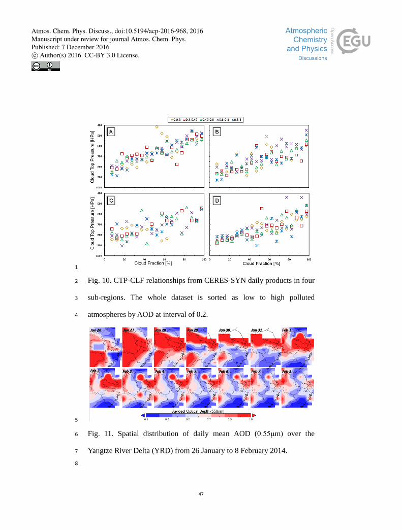
Meanwhile, Figure 10 shows CTPs have small differences with AODs 1

among four sub-regions. CLF-CTP under the condition of different AODs 2

is almost cumulatively distributed in one line in the sub-region A, as well 3

as in the sub-region D when the CLF <40%. With regard to the 4

sub-region B, C and D (CLF >40%), high-level AODs are not always 5

associated with small cloud top pressure, suggesting that aerosol-cloud 6

interaction do not lead to the variations of CTP. The possible reasons is 7

that aerosols influence horizontal extension of clouds rather than the 8

vertical distribution (Costantino et al., 2013). 9

3.2.5 Aerosol types and low clouds 10

In fact, most of aerosol particles float in the low atmosphere of 11

stagnant conditions during wintertime. To explore relationships between 12

cloud parameters and aerosol types (table 1), we analyzed low clouds due 13

to ample amounts of clouds appear at low altitudes as previously 14

described (Jones et al., 2009). This is a simple consequence of 15

transportation from north by prevailing northern wind in winter over the 16

YRD. As a result, the air mainly saturated with burning fossil fuels and 17

the quality of air is deteriorated. At the same time, partial areas of the 18

YRD are affected by air mass flowing from the highly polluted areas in 19

the Sichuan Basin. 20

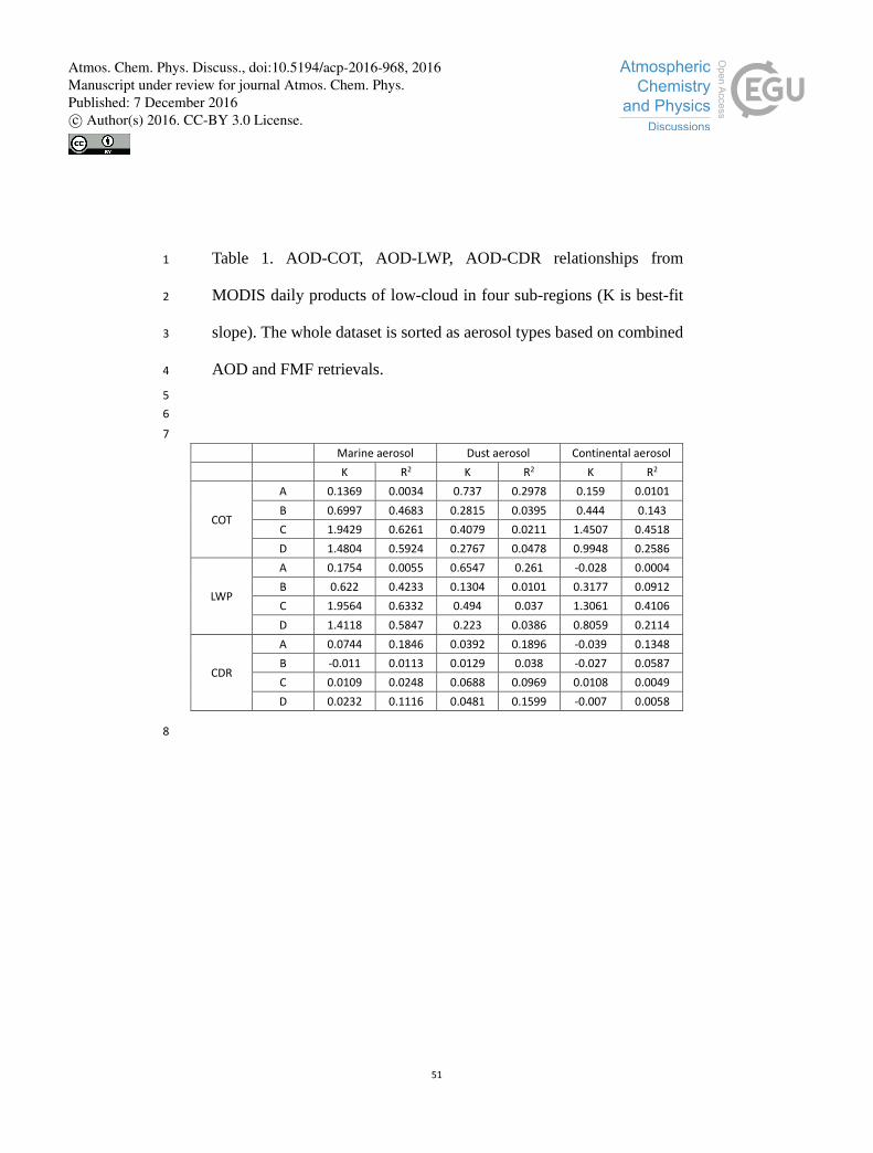
Although dust accounts for a large portion of AOD, marine and 21

continental aerosols make notable effects on COT and LWP in all 22


21

sub-regions except sub-region A. It is mainly because that, as a kind of 1

poor hygroscopic aerosols, dust is less likely to be mixed with water 2

vapor and become CCN. Marine aerosols, comprising both organic and 3

inorganic components from primary and secondary sources, have equal 4

impacts on COT and LWP in the sub-region C and D, and furthermore, 5

thicken the clouds. Nevertheless, dust aerosols just have slight impact on 6

COT and LWP in the sub-region A. Probably, dust particles can be coated 7

with hygroscopic material (i.e. sulfate) in polluted regions, greatly 8

increasing their ability to act as effective CCN (Satheesh et al., 2006; 9

Karydis et al. 2011). 10

The correlation coefficients, as for CDR, between different aerosol 11

types are close. It is worth noting that negative values of K (best-fit slope) 12

only appear in marine aerosol of the sub-region B and continental aerosol 13

of the sub-region A, B and D. In other words, CDRs decrease along with 14

increasing marine/continental aerosols in the sub-region B and 15

continental aerosol in the sub-region A and D. Additionally, small values 16

of correlation coefficient (R2) demonstrate that precise analysis can 17

hardly be done only aerosol types are taken into consideration. 18

3.3 Polluted aerosol and cloud development 19

Fig. 11 shows the daily average of AODs from 26 January to 8 20

February, covering both the growing and mitigating process of one 21

pollution event over the YRD region. High AODs mainly scatter in a 22


22

large domain, involving Shanghai, Anhui Province, northeastern Jiangxi 1

Province, southern and western Jiangsu Province, and northwestern 2

Zhejiang Province on 27 January. Since then, the polluted areas gradually 3

reduce to Shanghai and Jiangsu Province until 2 February. Obviously, 4

AODs increase from 27 January to 1 February in the north of Jiangsu 5

Province, but decrease from 2 to 8 February. The traditional Chinese New 6

Year is just within this period. 7

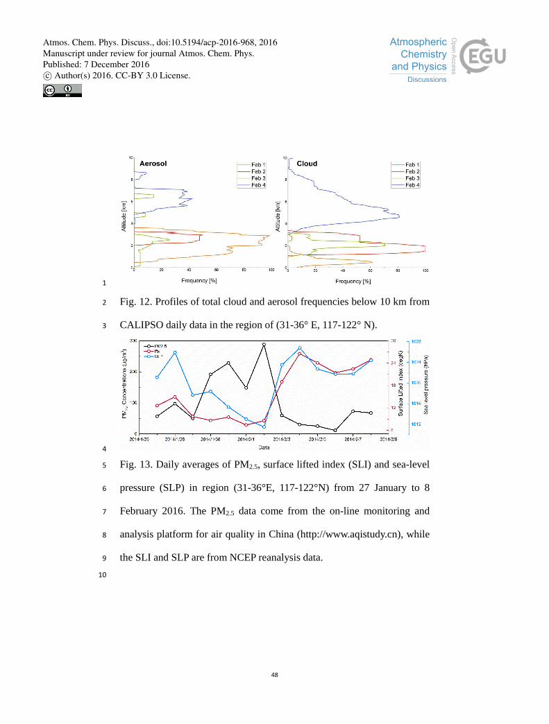
In order to understand aerosol and cloud vertical distributions during 8

the above mentioned period, frequency profiles of aerosol and cloud 9

calculated by layer fraction from CALIPSO daily data is drawn below 10 10

km in the region of (31-36°E, 117-122°N). As shown in Fig. 12, where 11

four days are chosen for case study and the data of aerosol and cloud 12

layers comes from CALIPSO. It displays that aerosol reaches high 13

frequency (>70%) between the height of 1.2 and 3km on 1 February 14

(Brown line). Meanwhile, cloud layers develop from relatively low 15

occurrence frequency (<60%) below height of 1km to high frequency (the 16

maximum reaches 100%) between the height of 1.2 and 3 km. With the 17

major decline of aerosol at the same altitude on 2 and 3 February, 18

occurrence frequency of clouds clearly deceases by nearly 30% at the 19

height of 2.5km on 3 February. Furthermore, it is noticed that the peaks of 20

aerosol occurrence frequency arise at higher altitudes, around 4.8km and 21

6.5km on 3 February as well as 5.6 to 7km on 4 February. 22


23

Correspondingly, the clouds develop in the vertical. 1

The daily averages of surface lifted index (SLI), sea level pressure 2

(SLP) and PM2.5 concentrations are shown in Fig. 13. SLI, calculated by 3

temperature at surface and 500hPa, is applied to indicate the stability 4

status of atmosphere. In addition, the SLP<1008hPa represents the core 5

of low-pressure systems and descending motions of air on 30 January and 6

1 February, a typical atmospheric circulation in case of weak 7

low-pressure systems. The time series of SLI variation display a sharp 8

increase from 2.6 to 26.5 degK on 3 and 4 February. With the strong 9

synoptic system of lower SLP, it proves that the air mass ascends in these 10

days. The concentration of PM2.5, sharply declining from 288 μg/m3 to 11

30.5 μg/m3, is coincident with air mass updrafts and horizontal 12

transmission. 13

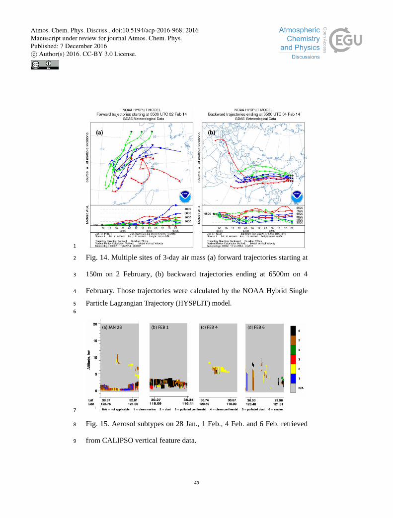
In addition, to identify the movement path and vertical distribution of 14

aerosol and cloud layers, the air mass forward trajectories matrix from 15

NOAA’s HYSPLIT model are shown in Fig.14a, beginning on 2 February 16

and at 150m height. Most of these forward trajectories show that aerosols 17

are transmitted to southwest at first. Then blue lines at two locations 18

(33.5°E-119.5°N, 33.5°E-122°N) direct to northeast, while air mass flows 19

back and is elevated to 3500m or higher on 4 February. In contrast, 20

backward trajectories at 6500m height on 4 February (Fig.14b), will take 21

air horizontal and vertical movements into consideration. With sharp 22


24

decline of low-cloud fraction and unremarkable variation of high-cloud 1

parameters (Fig.16), it can be inferred that the enhanced high-cloud 2

fraction is mainly caused by transmission. In other words, the occurrence 3

of high aerosol layer on 4 February is mainly caused by vertical elevation 4

of air mass from polluted ground and long-distance horizontal 5

transportation from west. 6

Air mass transportation has great influences on aerosol 7

micro-properties (e.g. particle size, shape, composition) and then cloud 8

development. For example, smoke and polluted dust occur on 1 February 9

(Fig.15) below the height of 3km. There are significant influences on the 10

size distribution and chemical composition of aerosols mixed with dust 11

and polluted particles (Wang et al., 2007; Sun et al., 2010), particularly 12

smoke (Ackerman et al., 2003). The polluted aerosol is likely to be 13

produced by fireworks during the Spring Festival. Additionally, the YRD 14

is an area with significant black carbon (Streets et al., 2001; Bond et al., 15

2004) and sulfate (Akimoto et al., 1994; Streets et al., 2000; Lu et al., 16

2010) emissions. Thus, dust particles in this aerosol mass coated with 17

water-soluble materials can easily evolve into CCN. Moreover, an evident 18

increase of cloud amount (Fig.12), is just the same as the results shown 19

by Yu et al. (2007), with a decrease of CDR and an increase of COT 20

appearing in adjacent clouds (low- and mid-low clouds) on the following 21

day (2 February). These factors amplify the cooling effect at the surface 22


25

and the top of atmosphere (TOA), consequently, the relatively stable 1

atmosphere appears at low altitude. With the low values of SLI and SLP 2

(Fig.13), large concentrations of PM2.5 are left on the ground in these two 3

days. Atmosphere suddenly becomes unstable from 3 February (Fig.13) 4

as AODs and aerosol layer fractions decrease on 2 February. Also, as 5

shown in Fig. 16, from 4 to 7 February, LWPs of low- and mid-low 6

clouds increase systemically from noon to midnight. Under these 7

conditions, with more water vapor and stronger air updraft, it could 8

reduce the critical super-saturation for droplet growth and relatively favor 9

the activation of aerosol particles into CCN, hence, more effectively 10

decreasing the droplet size (Feingold et al., 2003; Kourtidis et al., 2015). 11

4. Conclusion 12

The AIE of polluted aerosol over the YRD is analyzed using three- 13

month data (from December 2013 to February 2014) of AODs and cloud 14

parameters from the CERES product. Statistical analyses present that a 15

complex relationship exists between aerosol loadings and 16

micro-/macro-physical parameters of clouds. Aerosol exhibits an 17

important role in complication of cloud evolution in the low layers of 18

troposphere over four typical sub-regions. 19

The correlations of CDR-AOD, LWP-AOD and COT-AOD tell that 20

although minor differences in four sub-regions, AIE is in good agreement 21

with Twomey’s hypothesis at low-level AODs. With increasing cloud 22


26

height, the significance level between aerosol and cloud recedes, and AIE 1

mainly stays active at low troposphere (below 5km) in case of the stable 2

atmosphere in wintertime. The ground pollution possibly increase low 3

cloud cover. Synoptic conditions also have significant impact on cloud 4

cover. For instance, the unstable synoptic condition stimulate clouds to 5

develop larger and higher. 6

In general, meteorological and geographical conditions have strong 7

impact on cloud cover (Norris, 1998). Most studies of AIE do not 8

deliberate that these parameters result in the deviation of cloud quantity 9

and quality. Moreover, airflow brings uncertainty to the assessment of 10

AIE factors based on satellite observation. Further, we need to improve 11

the understanding of physical and thermos-dynamic in clouds, which play 12

an important role in cloud development but is not considered in this paper. 13

The classifications of aerosol and cloud are still rough, which cannot 14

accurately illustrate the relationships between aerosol types and different 15

clouds. In addition, a profound interference of geographical factors as 16

well as aerosol climatic impact need further investigation. 17

18

Acknowledgements 19

This research is supported by the National Key Research and 20

Development Program (2016YFC0202003), the National Key 21

Technology R&D Program of Ministry of Science and Technology 22

(2014BAC16B01), and the National Natural Science Foundation of China 23


27

(41475109, 21577021, 21377028), and partly by the Jiangsu 1

Collaborative Innovation Center for Climate Change. 2

3

References 4

Ackerman, A. S., Toon, O. B., Stevens, D. E., Heymsfield, A. J., 5

Ramanathan, V., &Welton, E. J. (2000). Reduction of tropical 6

cloudiness by soot. Science, 288(5468), 1042-1047. 7

Ackerman, A. S., Toon, O. B., Stevens, D. E., &Coakley, J. A. (2003). 8

Enhancement of cloud cover and suppression of nocturnal drizzle in 9

stratocumulus polluted by haze. Geophysical research letters, 30(7). 10

http://dx.doi.org/10.1029/2002GL016634. 11

Akimoto, H., & Narita, H. (1994). Distribution of SO2, NOx and CO2 12

emissions from fuel combustion and industrial activities in Asia with 13

1× 1 resolution. Atmospheric Environment, 28(2), 213-225. 14

Alam, K., Iqbal, M. J., Blaschke, T., Qureshi, S., & Khan, G. (2010). 15

Monitoring spatio-temporal variations in aerosols and aerosol–cloud 16

interactions over Pakistan using MODIS data. Advances in Space 17

Research, 46(9), 1162-1176. 18

Alam, K., Khan, R., Blaschke, T., &Mukhtiar, A. (2014). Variability of 19

aerosol optical depth and their impact on cloud properties in Pakistan. 20

Journal of Atmospheric and Solar-Terrestrial Physics, 107, 104-112. 21

Albrecht, B. A. (1989). Aerosols, cloud microphysics, and fractional 22


28

cloudiness. Science, 245, 1227–1230. 1

Anderson, A. K., &Sobel, N. (2003). Dissociating intensity from valence 2

as sensory inputs to emotion. Neuron, 39(4), 581-583. 3

Bangert, M., Kottmeier, C., Vogel, B., & Vogel, H. (2011). Regional scale 4

effects of the aerosol cloud interaction simulated with an online 5

coupled comprehensive chemistry model. Atmospheric Chemistry and 6

Physics, 11(9), 4411-4423. 7

Barnaba, F., &Gobbi, G. P. (2004). Aerosol seasonal variability over the 8

Mediterranean region and relative impact of maritime, continental and 9

Saharan dust particles over the basin from MODIS data in the year 10

2001.Atmospheric Chemistry and Physics, 4(9/10), 2367-2391. 11

Bond, T. C., Streets, D. G., Yarber, K. F., Nelson, S. M., Woo, J. H., 12

&Klimont, Z. (2004). A technology‐based global inventory of black 13

and organic carbon emissions from combustion. Journal of 14

Geophysical Research: Atmospheres, 109(D14). 15

http://dx.doi.org/10.1029/2003JD003697. 16

Brenguier, J. L., Pawlowska, H., &Schüller, L. (2003). Cloud 17

microphysical and radiative properties for parameterization and 18

satellite monitoring of the indirect effect of aerosol on climate. Journal 19

of Geophysical Research: Atmospheres, 108(D15). 20

http://dx.doi.org/10.1029/2002JD002682. 21

Bréon, F. M., Tanré, D., &Generoso, S. (2002). Aerosol effect on cloud 22


29

droplet size monitored from satellite. Science, 295(5556), 834-838. 1

Chan, C. K., & Yao, X. (2008). Air pollution in mega cities in China. 2

Atmospheric environment, 42(1), 1-42. 3

Chen, S., Bartello, P., Yau, M. K., Vaillancourt, P. A., & Zwijsen, K. 4

(2016). Cloud Droplet Collisions in Turbulent Environment: Collision 5

Statistics and Parameterization. Journal of the Atmospheric 6

Sciences, 73(2), 621-636. 7

Costantino, L., &Bréon, F. M. (2013). Aerosol indirect effect on warm 8

clouds over South-East Atlantic, from co-located MODIS and 9

CALIPSO observations. Atmospheric Chemistry and Physics, 13(1), 10

69-88. 11

Draxler, R. R., &Rolph, G. D. (2003). HYSPLIT (HYbrid Single-Particle 12

Lagrangian Integrated Trajectory) model access via NOAA ARL 13

READY website (http://www. arl. noaa. gov/ready/hysplit4. html). 14

NOAA Air Resources Laboratory, Silver Spring. 15

Feingold, G., Eberhard, W. L., Veron, D. E., &Previdi, M. (2003). First 16

measurements of the Twomey indirect effect using ground‐based 17

remote sensors. Geophysical Research Letters, 30(6). 18

http://dx.doi.org/10.1029/2002GL016633. 19

Forest, C. E., Stone, P. H., Sokolov, A. P., Allen, M. R., & Webster, M. D. 20

(2002). Quantifying uncertainties in climate system properties with the 21

use of recent climate observations. Science, 295(5552), 113-117. 22


30

Fu, X., Wang, S. X., Cheng, Z., Xing, J., Zhao, B., Wang, J. D., &Hao, J. 1

M. (2014). Source, transport and impacts of a heavy dust event in the 2

Yangtze River Delta, China, in 2011. Atmospheric Chemistry and 3

Physics, 14(3), 1239-1254. 4

Grandey, B. S., Stier, P., & Wagner, T. M. (2013). Investigating 5

relationships between aerosol optical depth and cloud fraction using 6

satellite, aerosol reanalysis and general circulation model 7

data. Atmospheric Chemistry and Physics, 13(6), 3177-3184. 8

Gryspeerdt, E., Stier, P., & Partridge, D. G. (2014). Satellite observations 9

of cloud regime development: the role of aerosol 10

processes. Atmospheric Chemistry and Physics, 14(3), 1141-1158. 11

Hansen, J., Sato, M., &Ruedy, R. (1997). Radiative forcing and climate 12

response. Journal of Geophysical Research: Atmospheres, 102(D6), 13

6831-6864. 14

He, Q., Li, C., Geng, F., Lei, Y., & Li, Y. (2012). Study on long-term 15

aerosol distribution over the land of East China using MODIS 16

data. Aerosol and Air Quality Research, 12(3), 304-319. 17

Hu, Q., Fu, H., Wang, Z., Kong, L., Chen, M., & Chen, J. (2016). The 18

variation of characteristics of individual particles during the haze 19

evolution in the urban Shanghai atmosphere. Atmospheric 20

Research, 181, 95-105. 21

Jin, M., & Shepherd, J. M. (2008). Aerosol relationships to warm season 22


31

clouds and rainfall at monthly scales over east China: Urban land 1

versus ocean. Journal of Geophysical Research: 2

Atmospheres, 113(D24). http://dx.doi.org/10.1029/2008JD010276. 3

Jones, T. A., Christopher, S. A., & Quaas, J. (2009). A six year 4

satellite-based assessment of the regional variations in aerosol indirect 5

effects. Atmospheric Chemistry and Physics, 9(12), 4091-4114. 6

Kalnay, E., Kanamitsu, M., Kistler, R., Collins, W., Deaven, D., Gandin, 7

L., et al. (1996). The NCEP/NCAR 40-year reanalysis project. Bulletin 8

of the American meteorological Society, 77(3), 437-471. 9

Karydis, V. A., Kumar, P., Barahona, D., Sokolik, I. N., &Nenes, A. 10

(2011). On the effect of dust particles on global cloud condensation 11

nuclei and cloud droplet number. Journal of Geophysical Research: 12


Knutti, R., Stocker, T. F., Joos, F., &Plattner, G. K. (2002). Constraints on 14

radiative forcing and future climate change from observations and 15

climate model ensembles. Nature, 416(6882), 719-723. 16

Kong, S., Li, X., Li, L., Yin, Y., Chen, K., Yuan, L., et al. (2015). 17

Variation of polycyclic aromatic hydrocarbons in atmospheric PM 2.5 18

during winter haze period around 2014 Chinese Spring Festival at 19

Nanjing: Insights of source changes, air mass direction and firework 20

particle injection. Science of the Total Environment, 520, 59-72. 21

Koren, I., Feingold, G., & Remer, L. A. (2010). The invigoration of deep 22


32

convective clouds over the Atlantic: aerosol effect, meteorology or 1

retrieval artifact?. Atmospheric Chemistry and Physics, 10(18), 2

8855-8872. 3

Kourtidis, K., Stathopoulos, S., Georgoulias, A. K., Alexandri, G., 4

&Rapsomanikis, S. (2015). A study of the impact of synoptic weather 5

conditions and water vapor on aerosol–cloud relationships over major 6

urban clusters of China. Atmospheric Chemistry and Physics, 15(19), 7

10955-10964. 8

L'Ecuyer, T. S., Berg, W., Haynes, J., Lebsock, M., &Takemura, T. (2009). 9

Global observations of aerosol impacts on precipitation occurrence in 10

warm maritime clouds. Journal of Geophysical Research: 11


Lebsock, M. D., Stephens, G. L., &Kummerow, C. (2008). Multisensor 13

satellite observations of aerosol effects on warm clouds. Journal of 14


http://dx.doi.org/10.1029/2008JD009876. 16

Leng, C., Zhang, Q., Tao, J., Zhang, H., Zhang, D., Xu, C., et al. (2014). 17

Impacts of new particle formation on aerosol cloud condensation 18

nuclei (CCN) activity in Shanghai: case study. Atmospheric Chemistry 19

and Physics, 14(20), 11353-11365. 20

Leng, C., Duan, J., Xu, C., Zhang, H., Zhang, Q., Wang, Y., et al. (2015). 21

Insights into a historic severe haze weather in Shanghai: synoptic 22


33

situation, boundary layer and pollutants. Atmospheric Chemistry & 1

Physics Discussions, 15(22). 2

Liu, J., Zheng, Y., Li, Z., Flynn, C., &Cribb, M. (2012). Seasonal 3

variations of aerosol optical properties, vertical distribution and 4

associated radiative effects in the Yangtze Delta region of 5

China. Journal of Geophysical Research: 6

Atmospheres, 117(D16).http://dx.doi.org/10.1029/2011JD016490. 7

Liu, X., & Wang, J. (2010). How important is organic aerosol 8

hygroscopicity to aerosol indirect forcing?.Environmental Research 9

Letters, 5(4), 044010. 10

Loeb, N. G., & Manalo-Smith, N. (2005). Top-of-atmosphere direct 11

radiative effect of aerosols over global oceans from merged CERES 12

and MODIS observations. Journal of Climate, 18(17), 3506-3526. 13

Lohmann, U., &Feichter, J. (2005). Global indirect aerosol effects: a 14

review. Atmospheric Chemistry and Physics, 5(3), 715-737. 15

Lu, Z., Streets, D. G., Zhang, Q., Wang, S., Carmichael, G. R., Cheng, Y. 16

F., et al. (2010). Sulfur dioxide emissions in China and sulfur trends in 17

East Asia since 2000. Atmospheric Chemistry and Physics, 10(13), 18

6311-6331. 19

Menon, S., Hansen, J., Nazarenko, L., &Luo, Y. (2002). Climate effects 20

of black carbon aerosols in China and India. Science, 297(5590), 21

2250-2253. 22


34

Michibata, T., Kawamoto, K., &Takemura, T. (2014). The effects of 1

aerosols on water cloud microphysics and macrophysics based on 2

satellite-retrieved data over East Asia and the North 3

Pacific. Atmospheric Chemistry and Physics, 14(21), 11935-11948. 4

Minnis, P., Young, D. F., Sun-Mack, S., Heck, P. W., Doelling, D. R., 5

&Trepte, Q. Z. (2004, February). CERES cloud property retrievals 6

from imagers on TRMM, Terra, and Aqua. In Remote Sensing (pp. 7

37-48). International Society for Optics and Photonics. 8

http://dx.doi.org/10.1117/12.511210. 9

Monks, P. S., Granier, C., Fuzzi, S., Stohl, A., Williams, M. L., Akimoto, 10

H., et al. (2009). Atmospheric composition change–global and regional 11

air quality. Atmospheric environment, 43(33), 5268-5350. 12

Norris, J. R. (1998). Low cloud type over the ocean from surface 13

observations. Part I: Relationship to surface meteorology and the 14

vertical distribution of temperature and moisture. Journal of Climate, 15

11(3), 369-382. 16

Norris, J. R. (1998). Low cloud type over the ocean from surface 17

observations. Part II: Geographical and seasonal variations. Journal of 18

Climate, 11(3), 383-403. 19

Penner, J. E., Dong, X., & Chen, Y. (2004). Observational evidence of a 20

change in radiative forcing due to the indirect aerosol 21

effect. Nature,427(6971), 231-234. 22


35

Platnick, S., King, M. D., Ackerman, S. A., Menzel, W. P., Baum, B. A., 1

Riédi, J. C., & Frey, R. A. (2003). The MODIS cloud products: 2

Algorithms and examples from Terra. IEEE Transactions on 3

Geoscience and Remote Sensing, 41(2), 459-473. 4

Pöschl, U. (2005). Atmospheric aerosols: composition, transformation, 5

climate and health effects. Angewandte Chemie International Edition, 6

44(46), 7520-7540. 7

Quaas, J., Boucher, O., & Bréon, F. M. (2004). Aerosol indirect effects in 8

POLDER satellite data and the Laboratoire de Météorologie 9

Dynamique–Zoom (LMDZ) general circulation model. Journal of 10


http://dx.doi.org/10.1029/2003JD004317. 12

Ramanathan, V., Crutzen, P. J., Lelieveld, J., Mitra, A. P., Althausen, D., 13

Anderson, J., et al. (2001). Indian Ocean Experiment: An integrated 14

analysis of the climate forcing and effects of the great Indo‐Asian 15

haze. Journal of Geophysical Research: Atmospheres, 106(D22), 16

28371-28398. 17

Remer, L. A., Kaufman, Y. J., Tanré, D., Mattoo, S., Chu, D. A., Martins, 18

J. V., et al. (2005). The MODIS aerosol algorithm, products, and 19

validation. Journal of the atmospheric sciences, 62(4), 947-973. 20

Remer, L. A., & Kaufman, Y. J. (2006). Aerosol direct radiative effect at 21

the top of the atmosphere over cloud free ocean derived from four 22


36

years of MODIS data. Atmospheric Chemistry and Physics, 6(1), 1

237-253. 2

Rolph, G. D. (2003). Real-time Environmental Applications and Display 3

sYstem (READY) Website (http://www. arl. noaa. gov/ready/hysplit4. 4

html). NOAA Air Resources Laboratory, Silver Spring. Md. 5

Rosenfeld, D. (2000). Suppression of rain and snow by urban and 6

industrial air pollution. Science, 287(5459), 1793-1796. 7

Sardina, G., Picano, F., Brandt, L., & Caballero, R. (2015). Continuous 8

growth of droplet size variance due to condensation in turbulent clouds. 9

Physical review letters, 115(18), 184501. 10

Satheesh, S. K., Moorthy, K. K., Kaufman, Y. J., &Takemura, T. (2006). 11

Aerosol optical depth, physical properties and radiative forcing over 12

the Arabian Sea. Meteorology and Atmospheric Physics, 91(1-4), 13

45-62. 14

Sorooshian, A., Feingold, G., Lebsock, M. D., Jiang, H., & Stephens, G. 15

L. (2009). On the precipitation susceptibility of clouds to aerosol 16

perturbations. Geophysical Research Letters, 36(13). 17

http://dx.doi.org/10.1029/2009GL038993. 18

Sorooshian, A., Wang, Z., Feingold, G., &L'Ecuyer, T. S. (2013). A 19

satellite perspective on cloud water to rain water conversion rates and 20

relationships with environmental conditions. Journal of Geophysical 21

Research: Atmospheres, 118(12), 6643-6650. 22


37

Streets, D. G., &Waldhoff, S. T. (2000). Present and future emissions of 1

air pollutants in China: SO2, NOx, and CO. Atmospheric 2

Environment, 34(3), 363-374. 3

Streets, D. G., Gupta, S., Waldhoff, S. T., Wang, M. Q., Bond, T. C., 4

&Yiyun, B. (2001). Black carbon emissions in China. Atmospheric 5

environment, 35(25), 4281-4296. 6

Sun, Y., Zhuang, G., Huang, K., Li, J., Wang, Q., Wang, Y., et al. (2010). 7

Asian dust over northern China and its impact on the downstream 8

aerosol chemistry in 2004. Journal of Geophysical Research: 9

Atmospheres,115(D7). http://dx.doi.org/10.1029/2009JD012757. 10

Tan, C., Zhao, T., Xu, X., Liu, J., Zhang, L., & Tang, L. (2015). Climatic 11

analysis of satellite aerosol data on variations of submicron aerosols 12

over East China. Atmospheric Environment, 123, 392-398. 13

Tang, J., Wang, P., Mickley, L. J., Xia, X., Liao, H., Yue, X., et al. (2014). 14

Positive relationship between liquid cloud droplet effective radius and 15

aerosol optical depth over Eastern China from satellite 16

data. Atmospheric Environment, 84, 244-253. 17

Ten Hoeve, J. E., Remer, L. A., & Jacobson, M. Z. (2011). Microphysical 18

and radiative effects of aerosols on warm clouds during the Amazon 19

biomass burning season as observed by MODIS: impacts of water 20

vapor and land cover. Atmospheric Chemistry and Physics, 11(7), 21

3021-3036. 22


38

Twomey, S. (1974). Pollution and the planetary albedo. Atmospheric 1

Environment (1967), 8(12), 1251-1256. 2

Wang, Y., Zhuang, G., Tang, A., Zhang, W., Sun, Y., Wang, Z., &An, Z. 3

(2007). The evolution of chemical components of aerosols at five 4

monitoring sites of China during dust storms. Atmospheric 5

Environment, 41(5), 1091-1106. 6

Wang, F., Guo, J., Wu, Y., Zhang, X., Deng, M., Li, X., et al. (2014). 7

Satellite observed aerosol-induced variability in warm cloud properties 8

under different meteorological conditions over eastern 9

China. Atmospheric Environment, 84, 122-132. 10

Wielicki, B. A., Barkstrom, B. R., Harrison, E. F., Lee III, R. B., Louis 11

Smith, G., & Cooper, J. E. (1996). Clouds and the Earth's Radiant 12

Energy System (CERES): An earth observing system 13

experiment. Bulletin of the American Meteorological Society, 77(5), 14

853-868. 15

Winker, D. M., Vaughan, M. A., Omar, A., Hu, Y., Powell, K. A., Liu, Z., 16

et al. (2009). Overview of the CALIPSO mission and CALIOP data 17

processing algorithms. Journal of Atmospheric and Oceanic 18

Technology,26(11), 2310-2323. 19

Winker, D. M., Pelon, J., CoakleyJr, J. A., Ackerman, S. A., Charlson, R. 20

J., Colarco, P. R., ... &Kubar, T. L. (2010). The CALIPSO mission: A 21

global 3D view of aerosols and clouds. Bulletin of the American 22


39

Meteorological Society, 91(9), 1211. 1

Wolf, M. E., &Hidy, G. M. (1997). Aerosols and climate: Anthropogenic 2

emissions and trends for 50 years. Journal of Geophysical Research: 3

Atmospheres, 102(D10), 11113-11121. 4

Xia, X., Li, Z., Holben, B., Wang, P., Eck, T., Chen, H., et al. (2007). 5

Aerosol optical properties and radiative effects in the Yangtze Delta 6

region of China. Journal of Geophysical Research: 7


Xin, J., Wang, Y., Li, Z., Wang, P., Hao, W. M., Nordgren, B. L., et al. 9

(2007). Aerosol optical depth (AOD) and Ångström exponent of 10

aerosols observed by the Chinese Sun Hazemeter Network from 11

August 2004 to September 2005. Journal of Geophysical Research: 12

Atmospheres, 112(D5). 13

Xu, J., Bergin, M. H., Greenwald, R., & Russell, P. B. (2003). Direct 14

aerosol radiative forcing in the Yangtze delta region of China: 15

Observation and model estimation. Journal of Geophysical Research: 16


Yu, H., Fu, R., Dickinson, R. E., Zhang, Y., Chen, M., & Wang, H. (2007). 18

Interannual variability of smoke and warm cloud relationships in the 19

Amazon as inferred from MODIS retrievals. Remote Sensing of 20

Environment, 111(4), 435-449. 21

Yuan, T., Li, Z., Zhang, R., & Fan, J. (2008). Increase of cloud droplet 22


40

size with aerosol optical depth: An observation and modeling 1

study. Journal of Geophysical Research: 2


Zhao, C., Tie, X., & Lin, Y. (2006). A possible positive feedback of 4

reduction of precipitation and increase in aerosols over eastern central 5

China. Geophysical Research Letters, 33(11). 6


41

Figure captions: 1

Fig. 1. Three-month mean aerosol optical depth (AOD) at 0.55μm over the Yangtze 2 River Delta (YRD) from CERES-SYN between December 2013 and February 2014. 3 The major cities in this region and four focused sub-regions (A, B, C, D) are also 4 marked here. 5 Fig. 2. Cloud optical thickness (COT) averaged over AOD bins for four sub-regions. 6 The area of circle represents sample number in each bin. 7 Fig. 3. Same as Fig. 2, but for liquid water path (LWP). 8 Fig. 4. Same as Fig. 2, but for cloud droplet radius (CDR). 9 Fig. 5. Profiles of total cloud and aerosol frequencies below 10 km derived from 10 cloud/aerosol layer fraction data. 11 Fig. 6. The cloud droplet radius (CDR) distribution of 3-h mean low-cloud according 12 to AOD and LWP over four sub-regions. Colors present different levels of AOD from 13 0 to 1. 14 Fig. 7. Cloud optical thickness (COT) and cloud droplet radius (CDR) averaged over 15 AOD/LWP bins in log-log scale for four sub-regions. 16 Fig. 8. Frequency of precipitation amount under clean and polluted conditions in four 17 sub-regions. Colors show different precipitation amount (mm). The a and b in 18 x-coordinate indicate AOD <0.5 and >0.5, respectively. 19 Fig. 9. CLF-CTP relationships from CERES-SYN daily products in four sub-region. 20 The whole dataset is sorted as low to high polluted atmospheres by AOD at interval of 21 0.2. 22 Fig. 10. CTP-CLF relationships from CERES-SYN daily products in four sub-regions. 23 The whole dataset is sorted as low to high polluted atmospheres by AOD at interval of 24 0.2. 25 Fig. 11. Spatial distribution of daily mean AOD (0.55μm) over the Yangtze River 26 Delta (YRD) from 26 January to 8 February 2014. 27 Fig. 12. Profiles of total cloud and aerosol frequencies below 10 km from CALIPSO 28 daily data in the region of (31-36° E, 117-122° N). 29 Fig. 13. Daily averages of PM2.5, surface lifted index (SLI) and sea-level pressure 30 (SLP) in region (31-36°E, 117-122°N) from 27 January to 8 February 2016. The 31 PM2.5 data come from the on-line monitoring and analysis platform for air quality in 32 China (http://www.aqistudy.cn), while the SLI and SLP are from NCEP reanalysis 33 data. 34 Fig. 14. Multiple sites of 3-day air mass (a) forward trajectories starting at 150m on 2 35 February, (b) backward trajectories ending at 6500m on 4 February. Those trajectories 36 were calculated by the NOAA Hybrid Single Particle Lagrangian Trajectory 37 (HYSPLIT) model. 38 Fig. 15. Aerosol subtype on 28 Jan., 1 Feb., 4 Feb. and 6 Feb. retrieved from 39 CALIPSO vertical feature data. 40 Fig. 16. Time series of cloud property parameters (CF, COT, LWP and CDR) from 41 CERES-SYN 3-h data between 27 Jan. to 28 Feb. 2014. Colors represent clouds at 42 different altitudes. 43


42

1

Fig. 1. Three-month mean aerosol optical depth (AOD) at 0.55μm over 2

the Yangtze River Delta (YRD) from CERES-SYN between December 3

2013 and February 2014. The major cities in this region and four focused 4

sub-regions (A, B, C, D) are also marked here. 5

6


43

1

Fig. 2. Cloud optical thickness (COT) averaged over AOD bins for four 2

sub-regions. The area of circle represents sample number in each bin. 3

4

Fig. 3. Same as Fig. 2, but for liquid water path (LWP). 5

6


44

1

Fig. 4. Same as Fig. 2, but for cloud droplet radius (CDR). 2

3

Fig. 5. Profiles of total cloud and aerosol frequencies below 10 km 4

derived from cloud/aerosol layer fraction data. 5

6


45

1

Fig. 6. The cloud droplet radius (CDR) distribution of 3-h mean 2

low-cloud according to AOD and LWP over four sub-regions. Colors 3

present different levels of AOD from 0 to 1. 4

5

Fig. 7. Cloud optical thickness (COT) and cloud droplet radius (CDR) 6

averaged over AOD/LWP bins in log-log scale for four sub-regions. 7


46

1 2 3 4 5 6 7 8 9 10 11 12 13 14

Fig. 8. Frequency of precipitation amount under clean and polluted 15

conditions in four sub-regions. Colors show different precipitation 16

amount (mm). The a and b in x-coordinate indicate AOD <0.5 and >0.5, 17

respectively. 18

19

Fig. 9. CLF-CTP relationships from CERES-SYN daily products in four 20

sub-region. The whole dataset is sorted as low to high polluted 21

atmospheres by AOD at interval of 0.2. 22


47

1

Fig. 10. CTP-CLF relationships from CERES-SYN daily products in four 2

sub-regions. The whole dataset is sorted as low to high polluted 3

atmospheres by AOD at interval of 0.2. 4

5

Fig. 11. Spatial distribution of daily mean AOD (0.55μm) over the 6

Yangtze River Delta (YRD) from 26 January to 8 February 2014. 7

8


48

1

Fig. 12. Profiles of total cloud and aerosol frequencies below 10 km from 2

CALIPSO daily data in the region of (31-36° E, 117-122° N). 3

4

Fig. 13. Daily averages of PM2.5, surface lifted index (SLI) and sea-level 5

pressure (SLP) in region (31-36°E, 117-122°N) from 27 January to 8 6

February 2016. The PM2.5 data come from the on-line monitoring and 7

analysis platform for air quality in China (http://www.aqistudy.cn), while 8

the SLI and SLP are from NCEP reanalysis data. 9

10


49

1

Fig. 14. Multiple sites of 3-day air mass (a) forward trajectories starting at 2

150m on 2 February, (b) backward trajectories ending at 6500m on 4 3

February. Those trajectories were calculated by the NOAA Hybrid Single 4

Particle Lagrangian Trajectory (HYSPLIT) model. 5 6

7

Fig. 15. Aerosol subtypes on 28 Jan., 1 Feb., 4 Feb. and 6 Feb. retrieved 8

from CALIPSO vertical feature data. 9


50

1

Fig. 16. Time series of cloud property parameters (CF, COT, LWP and 2

CDR) from CERES-SYN 3-h data between 27 Jan. to 28 Feb. 2014. 3

Colors represent clouds at different altitudes. 4

5

6


51

Table 1. AOD-COT, AOD-LWP, AOD-CDR relationships from 1

MODIS daily products of low-cloud in four sub-regions (K is best-fit 2

slope). The whole dataset is sorted as aerosol types based on combined 3

AOD and FMF retrievals. 4

5 6

7 Marine aerosol Dust aerosol Continental aerosol K R2 K R2 K R2

COT

A 0.1369 0.0034 0.737 0.2978 0.159 0.0101 B 0.6997 0.4683 0.2815 0.0395 0.444 0.143 C 1.9429 0.6261 0.4079 0.0211 1.4507 0.4518 D 1.4804 0.5924 0.2767 0.0478 0.9948 0.2586

LWP

A 0.1754 0.0055 0.6547 0.261 -0.028 0.0004 B 0.622 0.4233 0.1304 0.0101 0.3177 0.0912 C 1.9564 0.6332 0.494 0.037 1.3061 0.4106 D 1.4118 0.5847 0.223 0.0386 0.8059 0.2114

CDR

A 0.0744 0.1846 0.0392 0.1896 -0.039 0.1348 B -0.011 0.0113 0.0129 0.038 -0.027 0.0587 C 0.0109 0.0248 0.0688 0.0969 0.0108 0.0049 D 0.0232 0.1116 0.0481 0.1599 -0.007 0.0058

8


effects of wintertime polluted aerosol on cloud over the ... · pdf file1 effects of...

Documents