efficiency in corporate takeovers
TRANSCRIPT

EFFICIENCY IN CORPORATE TAKEOVERS

ISBN 978 90 361 0391 6
Cover design: Crasborn Graphic Designers bno, Valkenburg a.d. Geul
This book is no. 585 of the Tinbergen Institute Research Series, established through
cooperation between Thela Thesis and the Tinbergen Institute. A list of books
which already appeared in the series can be found in the back.

Efficiency in Corporate Takeovers
Efficiency bij Bedrijfsovernames
Proefschrift
ter verkrijging van de graad van doctor aan de
Erasmus Universiteit Rotterdam
op gezag van de rector magnificus
Prof.dr. H.A.P. Pols
en volgens besluit van het College voor Promoties.
De openbare verdediging zal plaatsvinden op
vrijdag 23 Mei 2014 om 09:30 uur
door
Yun Dai
geboren te Wuxi, China
Promotiecommissie:
Promotor: Prof.dr. J.T.J. Smit
Overige leden:
Prof.dr. B.E. Eckbo
Prof.dr. H.P.G. Pennings
Prof.dr. P. Verwijmeren
Copromotor: Dr. S. Gryglewicz

To Te and Wenxin,
my precious


i
Preface
As a milestone in my academic life, this dissertation concludes my three-year hard work,
as well as provides a precious opportunity for me to thank all of those who companied,
encouraged, and helped me through all the process.
My first gratitude goes to my excellent supervisors – Han Smit and Sebastian
Gryglewicz. I still remember the first time that I met Han. At the first sight, I was so
impressed by his warm smile that I felt I was already one member of his research team. His
pleasant personality soon becomes an indispensable part of our research project. His
passion for research cheers every meeting with excitement. His supportive attitude
strengthens my determination to overcome difficulties. His deep knowledge of practical
finance turns complicated mathematics into vivid reflection of finance activity. By Han’s
introduction, I got to know Sebastian, another intelligent scholar. Sebastian owns every
merit of a great supervisor. He is insightful, good at finding the key questions. He is smart,
with excellent skill in modeling. He is diligent, with high attention to details. He is also
easy-going, caring and supportive, willing to share his experience and give advice
whenever I need. Han’s contagious enthusiasm and Sebastian’s patient guidance as well as
their outstanding research skills constitute perfect mentorship, which makes my PhD life
not only joyful but also fruitful. I am glad to publish our first joint paper before my
graduation, and my research ability has developed and grown during this process, which
will surely become a valuable asset of my life.
Someone once told me that, doing a PhD was similar to running a start-up. It begins
with finding a promising project, and requires investment of numerous time and effort. If
the R&D turns successful (i.e. a paper is written), you need to learn how to present your

ii
product (by conference presentation) and sell it to the market (by publication of the paper).
Sometimes, this course can be tedious and lonely because you need to do it all by yourself.
Fortunately, my PhD journey is never boring thanks to the company of my fellow
researchers. I am grateful to Agbeko, Christel, Gosia, Jiangyu, Liting, Natalya, Noemie,
Olivier, Philipe, Xinying, and Yang for the delightful discussions and cooperation in the
study groups for TI courses. To Kyle, Marc, Patrick, Remco, Sander, Xiaoming, and
Xiaoyu for their inspiring comments on my research. To Joris, Guangyao, Tiantian, and
Zhenxing for their help on my students’ thesis defenses. To Pinar and Ona for their nice
presence as good officemates. To Lerby for the incentive he offered to my swimming
learning. To Leontine for her help on my Dutch. To Chen, Dan, Guangyuan, Hong,
Jiansong, Jindi, Lin, Mike, Qibai, Ran, Siyu, Wei, Xiye, Xiaolong, Xin, Xuedong, Yijing,
Yu, Yue, Yueshen, Zhenzhen, Zhengyuan, and Zhiling, for the wonderful time that we
spent together.
Finally, I would like to thank my family for their endless love and unconditional
support. I am greatly indebted to my parents for their understanding when I decided to
study in the Netherlands, to my sister for her devotion to family, and to my parents-in-law
for their generous help. My deepest gratitude goes to my husband, Te: meeting him is the
most beautiful thing that ever happened to me. Without Te’s support, I would have not
come so far. This dissertation is dedicated to Te and Wenxin (our daughter), who brighten
my life, fuel my energy and encourage me to discover the best out of life.

iii
Contents
CHAPTER 1 INTRODUCTION ................................................................................................................... 1
1.1. RESEARCH QUESTIONS ..................................................................................................................... 1
1.2. OUTLINE ........................................................................................................................................... 7
CHAPTER 2 SIMILAR BIDDERS IN TAKEOVER CONTESTS ........................................................... 9
2.1. INTRODUCTION ................................................................................................................................. 9
2.2. A MODEL OF TAKEOVER CONTESTS ................................................................................................. 15
2.2.1. Bidders and target values ...................................................................................................... 15
2.2.2. Bidding and payoffs ............................................................................................................... 16
2.2.3. Informational externalities and competition ......................................................................... 19
2.3. BIDDERS’ STRATEGIES AND EQUILIBRIUM ....................................................................................... 21
2.3.1. Bidder A: to preempt or to accommodate ............................................................................. 21
2.3.2. Bidder B: to participate or to stay out .................................................................................. 23
2.3.3. Equilibrium ........................................................................................................................... 25
2.4. MODEL IMPLICATIONS .................................................................................................................... 28
2.5. THE EXPERIMENTAL SETUP ............................................................................................................. 30
2.5.1. Treatments and hypotheses ................................................................................................... 30
2.5.2. Experiment implementation ................................................................................................... 32
2.6. EXPERIMENTAL RESULTS ................................................................................................................ 35

iv
2.6.1. H1: proportion of single-bidder contests .............................................................................. 36
2.6.2. H2: prices in single-bidder contests ...................................................................................... 38
2.6.3. H3: prices in two-bidder contests ......................................................................................... 40
2.6.4. Dynamic session-effects ........................................................................................................ 41
2.7. CONCLUSIONS................................................................................................................................. 45
CHAPTER 3 THE LEARNING EFFECT IN TAKEOVERS WITH TOEHOLDS .............................. 53
3.1. INTRODUCTION ............................................................................................................................... 53
3.2. DATA DESCRIPTION ........................................................................................................................ 57
3.2.1. Sample construction .............................................................................................................. 57
3.2.2. Sample Characteristics ......................................................................................................... 58
3.2.3. Takeover efficiency measures ................................................................................................ 61
3.3. EFFICIENCY CHANGE IN TOEHOLD STRATEGIES ............................................................................... 63
3.4. THE LEARNING EFFECT WITH A SELF-SELECTION MODEL ................................................................ 69
3.4.1. Subsample division ................................................................................................................ 70
3.4.2. Self-selection model............................................................................................................... 73
3.5. IS MONITORING AN IMPORTANT QUALIFICATION FOR AN EFFICIENT TOEHOLD STRATEGY? ............. 78
3.6. ROBUSTNESS CHECK ....................................................................................................................... 82
3.6.1. Different specifications of institutional holdings................................................................... 82
3.6.2. Merger wave.......................................................................................................................... 85
3.7. CONCLUSION .................................................................................................................................. 88

v
CHAPTER 4 ARE CORPORATE GOVERNANCE MECHANISMS COMPLEMENTS? EVIDENCE
FROM FAILED TAKEVOERS ................................................................................................................... 91
4.1. INTRODUCTION ............................................................................................................................... 91
4.2. HYPOTHESES DEVELOPMENT .......................................................................................................... 95
4.3. DATA .............................................................................................................................................. 97
4.3.1. Sample construction .............................................................................................................. 97
4.3.2. Definition of variables and summary statistics ................................................................... 100
4.4. RESULTS ....................................................................................................................................... 106
4.4.1. Changes in investment and capital structure policies ......................................................... 106
4.4.2. Stock performance around failed takeovers ........................................................................ 112
4.4.3. New results after matching .................................................................................................. 113
4.5. CONCLUSION ................................................................................................................................ 120
SUMMARY .................................................................................................................................................. 123
SAMENVATTING (SUMMARY IN DUTCH) ........................................................................................ 125
BIBLIOGRAPHY ....................................................................................................................................... 127


1
Chapter 1
Introduction
1.1. Research Questions
Corporate takeover is a very important economic activity that generates profound
consequences on many classes of market participants. The great financing needs and
transaction costs directly change the wealth of both shareholders and creditors. The
corporate restructuring induced by the takeover results in a significant impact on the
welfare of management, employees, and customers. The reshaped industrial map due to the
takeover further influences the competition strategies of other firms. Moreover, the
changes in the taxable revenues when the takeover happens across the industry can also
affect the tax income to the government. The paramount impact on corporations and the
economy highlights the importance of studying the efficiency in corporate takeovers. This
dissertation contributes to the discussion on takeover efficiency by exploring three key
questions.
The first question is about the optimal bidding strategy in takeover contests. Since
corporate takeover is a costly process, it is critical to make the right decisions on (1)
Whether to enter a takeover contest or (2) How to select an optimal bid. Following

2
Fishman (1988), we model the takeover contests as auctions with sequential entry, and find
that the optimal entry and bidding strategies depend heavily on the similarity level of
acquirers’ valuations of the target. When acquirers’ valuations are dissimilar, the first bid
of the first bidder is mainly about their own value. The following bidder is easily deterred
by a high first bid, because it signals the high value of the first bidder. However, when the
similarity level increases, the first bid is embedded with higher information externality. A
high first bid not only signals the high value of the first bidder, but also implies the high
value of the following bidder. It becomes harder to deter the competition, and the first
bidder needs to offer a higher first bid to pre-empt others. However, when the similarity
level exceeds a certain threshold, the competition between very similar acquirers becomes
so severe that pre-emption becomes easier and the first bidder can use a lower first bid to
deter the following bidders. These non-monotonic effects of similarity on acquirers’ entry
and bidding decisions are further confirmed in controlled laboratory experiments.
The second question is about the efficiency evaluation of takeover strategies. Different
from the static viewpoint in most studies, we introduce a dynamic framework in answering
this question. By studying how the efficiency of takeovers with toeholds1 changes over
time, we propose that an evolutionary perspective is important in evaluating the
performance of a takeover strategy. Although the toehold bidding is accompanied with
worse performance than the non-toehold bidding in the early 1990s, its efficiency is
improving over time. From 1990 to 2006, takeovers with toeholds experience significant
increases in terms of returns to bidders and synergy value created through transactions. The
discovery of a significant time pattern in the toehold bidding shows that the dynamic
1 Toeholds refer to the minority ownership of the target’s shares owned by the acquirer before a takeover is
initiated.
3
perspective is very important in evaluating the efficiency of takeover strategies.
Overlooking it may lead to biased or inaccurate conclusions.
The third question is how to improve firms’ performance in corporate takeovers. This
question can be divided into two sub-questions: (1) How to improve acquirers’ efficiency
in carrying out corporate takeovers; and (2) How to improve targets’ response to takeover
threats. Related literatures suggest that corporate governance can be a promising candidate
(Shleifer, and Vishny, 1986; Schranz 1993; Nickell et al, 1997; Allen et al., 2000; Gillan
and Stark, 2000; Hartzell and Stark, 2003; Gaspar et al., 2005; Chen et al., 2007). We
therefore, examine the interaction between the firms’ performance and their corporate
governance qualities. In the study on the efficiency of toehold bidding, we introduce
institutional ownership as a measure of monitoring strength, and investigate its impact on
the toehold performance. We find that the magnitude of the institutional investment well
explains the efficiency evolution in toehold performance, which suggests that the
monitoring from institutional investors can enhance acquirers’ ability to benefit from the
toehold bidding. We further examine the relationship between the target firms’ response to
takeover threats and two different governance mechanisms—monitoring from institutional
investors and product market competition. We find little impact of corporate governance
on the target firms’ post-takeover restructuring. The influence of both the internal
monitoring (the institutional ownership) and the external discipline (the product market
competition) is very limited. Neither of them can result in a systematic improvement in
firms’ performance after takeovers. The difference in the impacts of corporate governance
on the performance of acquirers and targets is illuminating. It suggests that the
effectiveness of corporate governance depends on whether the firms have the initiative.
When a firm is actively participating in the corporate takeover, that is, as an acquirer, its
4
corporate governance can help in making wise decisions. On the contrary, when a firm is
passively involved in a takeover, that is, as a target, the takeover threat is so strong that it is
forced to make changes regardless of its corporate governance quality.
In addition to exploring the efficiency in corporate takeovers, this dissertation tries to
provide innovative thinking on several interesting puzzles or issues in takeover literature.
The first puzzle is the insignificant relationship between the number of bidders and
takeover returns. Although the number of the bidders is usually regarded as an intuitive
measure of competition intensity, previous studies (Kale et al., 2003; Betton et al., 2008;
Boone and Mulherin, 2008) show that it cannot explain the variation in prices and returns
in corporate takeovers. Our study points out a new measure of the competition level in
takeovers; that is, the similarity in bidders’ valuations, which is a key consideration in
bidders’ entry decisions and bidding strategies. The single-bidder contests are more likely
to occur when the similarity level is either low or high, compared with the case of the
intermediate similarity level. The acquisition prices are higher at the intermediate
similarity level than at the low or high similarity level. Hence, multiple-bidder contests are
most likely at the intermediate level of similarity at which expected prices in multiple-
bidder contests are the highest, whereas single-bidder acquisitions are most likely at very
low and very high levels of similarity when expected prices in single-bidder contests are
lower. Furthermore, given the level of similarity, targets’ returns can be higher in single-
bidder acquisitions than in multiple-bidder contests, because a premium is offered to deter
competition. This non-monotonic impact of the similarity level explains the unclear
relationship between the number of bidders and the prices and returns in takeovers.
Without controlling for the level of similarity, the relationship between the number of
bidders and target returns can show either signs in a cross-section study of acquisitions.

5
The second puzzle is the well-known toehold puzzle in takeover literature. Toehold
refers to the acquirer’s ownership of the target’s share before a takeover is initiated.
Theoretically, toeholds can grant the owner a favorable position. They strengthen the
toehold owner’s competitiveness by mitigating the free-rider problem, increasing the
winning probability and accumulating insider information (Shleifer and Vishny, 1986;
Burkart 1995; Singh 1998; Bulow et al., 1999). However, in the past decades, less than 10%
of acquisitions were acquired with toeholds. The sharp contradiction between the attractive
merits of the toehold acquisition strategy and its scare adoption constitutes a “toehold
puzzle.” We propose that the “learning effect” in takeovers with toeholds can be a possible
explanation, where qualified acquirers learn to use the strategy effectively, whereas
unqualified acquirers have learned to walk away. As discussed earlier, we find a significant
efficiency improvement in the toehold performance from 1990 to 2006. However, the
decline in the popularity of the toehold strategy indicates that this improvement is not
unconditional. As suggested by the adverse impact of toeholds in the early period, the
toehold bidding does not guarantee beneficial outcomes, and to properly use toeholds to
generate higher returns requires some qualifications. Bidders gradually learn their
qualifications while using the toehold strategy, and they self-select to stay or give up this
strategy increases. With the passing of time, the proportion of qualified acquirers using the
toehold strategy, which results in a co-existence of a decrease in the frequency of toehold
acquisitions and an improvement in the toehold performance. Using self-selection models,
we identify and confirm this learning effect in takeovers with toeholds, which for explains
the toehold puzzle from a new evolutionary perspective.
The third controversial topic is the interplay among different mechanisms of
corporate governance: whether they are complements or substitutes? There is no
6
conclusive answer. Some research supports the complements view (Denis and Serrano,
1996; Hadlock and Lumer, 1997; Mikkelson and Parch, 1997); some speak for the
substitutes view (Giroud and Mueller, 2010; Atanassov 2013); and other studies
demonstrate no interaction between the internal and external governance mechanism
(Huson, Parrino, and Starks, 2001; Denis and Kruse 2000). To contribute to this discussion,
I select a special group of firms—targets in failed takeovers and their industry peers—to
examine the impact of different governance mechanisms on firms’ responses to takeover
threats. The special feature of this sample is that it differentiates between two cases with
different strengths of takeover threats: target firms facing direct and strong threats and peer
firms facing indirect and weak threats. This enables me to investigate the complements
argument in a comprehensive manner. Are governance mechanisms complementary to the
takeover threat in their disciplinary power? If so, do their roles differ in the presence of
strong or weak takeover threats? The results show that corporate governance is a weak
complement to takeover threats. First, its impact is limited to a few post-takeover policy
changes. There is no general or comprehensive enhancement on restructuring outcomes.
Second, the market perception reflected by stock performance does not differ in the
governance quality. Furthermore, the limited impact of corporate governance mainly
occurs with regard to target firms’ performance, that is, when the takeover threat is strong.
Corporate governance cannot increase peer firms’ sensitivity to takeover threats or make a
difference in firms’ post-takeover restructuring.
Lastly, the contribution of the thesis is also methodological. It combines theory,
experimental and empirical studies while addressing different questions. There has been a
large experimental literature on asset pricing pioneered by Smith et al. (1988), whereas
little experimental work was done on topics related to corporate finance. By introducing
7
experimental methods to the study on corporate takeovers, the dissertation adds more
evidence to experimental corporate finance. Besides the experimental method, the
perspective from learning and evolutionary selection in studying toehold puzzles is also
innovative.
1.2. Outline
This dissertation studies three interesting questions in takeover contests related to
efficiency in corporate takeovers. The results are reported in three chapters. Each chapter is
self-contained, with its own introductions, conclusions, and appendix.
Chapter 2 is developed from the paper “Similar Bidders in Takeover Contests” (Dai,
Gryglewicz, Smit, and De Maeseneire, 2013, Games and Economic Behavior). It studies
the optimal bidding strategies in corporate takeovers when an acquirer is facing a
similar/dissimilar competing acquirer. With a theoretical model, we show that the
similarity level in acquirers’ valuations about the target has two implications. On the one
hand, it affects the information content of bids. On the other hand, it determines the
competition intensity between acquirers. As a result, the acquisition prices and the
probability of multiple-bidder contests are predicted to be the highest for intermediately
similar acquirers. The non-monotonic effects of similarity with regard to prices and the
frequency of multiple-bidder contests are further confirmed by a laboratory experiment in
which we control the similarity between bidders and ask subjects to choose their bidding
and entry decisions.
Chapter 3 is based on a working paper “The Learning Effect in Takeovers with
Toeholds” (Dai, Gryglewicz and Smit, 2013). It investigates the evolution in the toehold
performance and proposes a new explanation to the toehold puzzle. With four efficiency

8
measures, we show that the performance of the toehold strategy is improving over time,
though the frequency of toehold acquisitions is decreasing. The discrepancy between the
toeholds efficiency and its popularity can be attributed to an improvement in the self-
selection procedure, where qualified acquirers learn to use this strategy whereas
unqualified acquirers learn to walk away. With self-selection models, we provide strong
and significant support to the improved efficiency of self-selection in toehold acquisition.
Furthermore, corporate governance, such as institutional holdings, improves outcomes in a
toehold acquisition strategy, and indicates that firms with better monitoring quality can
become more qualified toehold acquirers.
Chapter 4, “Are corporate governance mechanisms complements? Evidence from
Failed Takeovers” (Dai, 2013), studies the impact of corporate governance on firms’
responses to control threats. By restricting the sample to failed takeovers, I identify firms
who received concrete control threats but without a change in corporate control, and
investigate whether their operational change will be affected by the quality of their
corporate governance. Furthermore, I use the stock performance and analysts’ forecast to
check whether the investors expect different responses from firms with good/bad corporate
governance. The result shows that, in the presence of strong control threats, corporate
governance has little influence on firms’ restructuring, and investors do not differentiate
between firms with different corporate governance while trading on stocks facing takeover
threat.
9
Chapter 2
Similar Bidders in Takeover Contests2
2.1. Introduction
Returns in mergers and acquisitions for acquirer and target not only depend on the value
that is created, but also on acquisition premium that is paid. Empirical research indicates
that, overall, acquisitions do create value (Andrade, Mitchell and Stafford, 2001; Bargeron,
Schlingemann, Stulz, and Zutter, 2008; Betton, Eckbo, and Thorburn, 2008) but gains
accrue mostly to targets. Acquiring firms’ returns are, on average, close to zero and exhibit
large variation (Stulz, Walkling, and Song, 1990; Leeth, and Borg, 2000; Fuller, Netter,
and Stegemoller, 2002; Moeller, Schlingemann, and Stulz, 2005). Taken together, the
evidence suggests that acquisition prices are determinative for the division of takeover
surplus.
2 This chapter is based on Dai, Grylewicz, Smit and De Maeseneire (2013).

10
The underlying causes of this variation in prices and returns have been subject to
continuous scrutiny in the empirical literature. Surprisingly, the level of competition as
measured by the number of bidders does not seem to explain this variation (Boone and
Mulherin, 2008).3
However, characteristics of buyers do appear to be successful in
explaining returns.4
Guided by this evidence, we develop a model of takeover contests in which the
characteristics of potential acquirers matter and affect the intensity of competition. We
want to take into account that potential acquirers can be similar or dissimilar because they
may have very similar or very unique resources, capabilities, and post-acquisition
strategies. More specifically, we analyze a model of two potential bidders that may
sequentially enter a takeover contest. If the bidders are similar, their private values of a
target are correlated. After observing the initial bid, the second bidder may decide to pay
an entry cost to learn its valuation and to participate in the contest. Entering takeover
contests is costly since information on target value requires due diligence costs such as fees
for consultants, lawyers and investment bankers. The first bidder may offer a high
(preemptive) bid in an attempt to deter the competing firm from entering. Alternatively, a
low (accommodating) offer by the first bidder may induce entry by the second bidder and
3 Boone and Mulherin (2008) use an extensive data set on potential bidders and control for the endogeneity
between returns and the level of competition. Some earlier studies using less detailed data sets show either no
significant relation (Kale, Kini, and Ryan, 2003; Betton, Eckbo, and Thorburn, 2008) or mixed results
(Schwert, 2000).
4 Bidder size is responsible for a large portion of variation in returns (Moeller, Schlingemann, and Stulz,
2004, 2005). Acquirers with more uncertain growth prospects gain less in acquisitions (Moeller,
Schlingemann, and Stulz, 2007). Furthermore, the premiums paid to targets depend significantly on the
public status of acquirers and whether acquirers are operating firms or private equity funds (Bargeron,
Schlingemann, Stulz, and Zutter, 2008). Among operating firms, acquirer returns depend on the strategic
objectives of acquiring firms (such as vertical integration, horizontal integration, or diversification) (Walker,
2000).
11
start a competitive auction. The signaling effect of an opening offer depends critically on
the similarity between bidders.
The interdependence of bidders’ valuations has two opposing effects on contest
participation. On the one hand, a bid from a bidder that is similar creates a greater
informational externality and thereby encourages entry by a rival. On the other hand, if
bidders are more closely related, the bidding contest is expected to be more competitive.
The resulting high prices reduce expected payoffs from participation and thus discourage
entry. We show that neither of the effects is dominant but their relative strengths depend on
the level of similarity and radically affect bidding strategies, price, and bidders’
participation. Our analysis provides several important new insights and implications.
First, conditional on observing a takeover, the probability of single-bidder acquisitions
and multiple-bidder contests varies in similarity between potential bidders. Multiple-bidder
contests are most likely between intermediately similar competitors, due to the strength of
informational externalities of initial bids that attracts followers. Initial bids from very
similar bidders promise an even higher expected target value, but also indicate a fierce
bidding competition. As a result, single-bidder contests are expected mostly between
dissimilar (when informational externalities are low) and very similar competitors (when
potential competition is high).
Second, expected prices for targets demonstrate an inverted U-shape in the level of
bidder similarity. This pattern applies for prices in both single-bidder acquisitions and in
multiple-bidder contests. The initial bid embeds informational externalities that signal
value, making it attractive for competitors to enter. In single-bidder acquisitions, this
means that high preemptive bids are required to deter a competitor that shares some of the
sources of value. However, if bidders become very similar, the competition effect on prices
12
starts to dominate informational externalities, and deterrence is possible with a relatively
low preemptive bid. When multiple-bidder contests occur, competitive bidding yields
higher prices when rivals are more similar. However, when rivals are almost identical, the
initial bidder will accommodate only if its valuation is low, but this means that the
expected price in the contest will be low as well.
Third, our analysis indicates that in an environment with interdependent values, the
similarity of potential bidders is an important measure of competition intensity. Targets’
returns are higher in single-bidder acquisitions than in multiple-bidder contests for any
given level of similarity because a premium is required to preempt a rival. However, this
does not necessarily imply that empirical data should demonstrate higher target returns in
single-bidder acquisitions. As discussed above, multiple-bidder contests are most likely at
intermediate levels of similarity at which expected prices are the highest. Conversely,
single-bidder acquisitions are most likely at very low and very high levels of similarity
when expected prices are lower. This implies that, in a cross-section of acquisitions, the
relation between the number of bidders and target returns may show either signs if the
level of similarity is not controlled for.
The theoretical predictions of the model are difficult to test empirically using historical
acquisition data because information about the identity of preempted bidders, and so their
similarity with acquirers, is not readily observable by researchers. To overcome this
difficulty, we employ a laboratory experiment with financially well-trained subjects.
Relative to tests using field data where many relevant factors change simultaneously,
controlled environments of laboratory experiments allow for clear comparative static tests.
At the same time, laboratory experiments raise questions about external validity—is the
behavior of students-subjects informative about investment strategies of firms? We believe

13
that the experiment can inform us about the validity of our theory. First, the academic
literature on takeovers shows that individuals play an important role in investment and
acquisition decisions. CEOs, like all other people, have behavioral biases and these biases
not only drive takeovers (Roll, 1986; Berkovitch and Narayanan, 1993), but also affect
premiums paid in acquisition (Hayward and Hambrick, 1997; Malmendier and Tate, 2008;
Levi, Li and Zhang, 2010). Second, human behavior often deviates from theoretical
predictions even in simple auctions [see Kagel (1995) for a survey]. People in general
demonstrate systematic biases that may intensify some predicted forces and weaken others.
The aim of our experiment is to verify if people respond to the tradeoffs in our model. As
such, a laboratory test is a first and important step to validate the relevance of our
theoretical predictions to corporate environments.5
The experimental design replicates the model specification. Two groups of subjects
play the roles of first or second bidder in an auction for a target. Their valuations are
correlated with a correlation coefficient called “similarity level”. The first bidder chooses
his first bid and the second bidder can decide to enter or not depending on the first bid and
the similarity level. In this way, we collect data about preemptive bidding behavior and
conditional entry decisions.
The experimental results support the main insights of the model. Our first observation is
that high first bids deter second bidders from entering in line with the preemption
arguments. We then find that the frequency of multiple-bidder contests demonstrates a
non-monotonic pattern in similarity levels. Furthermore, prices in both single- and
5 Several other papers also use experiments to test corporate takeovers theories, e.g., Kale and Noe (1997),
Weber and Camerer (2003), Croson, Gomes, McGinn and Nöth (2004), Gillette and Noe (2006), and Kogan
and Morgan (2010).
14
multiple-bidder contents first increase in similarity and then decrease, as predicted by the
theory.
This paper is related to the literature on sequential bidding in takeover contests initiated
by Fishman (1988). With sequential entry, there is information externality from initial bids.
Hence, a high first bid, which signals a high value of initial bidders for the target, can deter
competition. Others have extended this model in various directions. Fishman (1989) shows
that the medium of exchange can be a supplementary tool for preemption in addition to a
high bid. Chowdhry and Nanda (1993) claim that issuing debt commits the bidder to
overbidding, which can be preemptive. Burkart (1995), Singh (1998), Bulow, Huang and
Klemperer (1999), and Ravid and Spiegel (1999) study overbidding induced by toeholds.
Hirshleifer and Png (1989), Daniel and Hirshleifer (1998) explore takeovers from the
perspective of efficiency, and find that, although preemption reduces competition, it may
raise expected social welfare if bidding is costly. Che and Lewis (2007) apply the
preemption model to a policy analysis of lockups, and discuss how lockups affect
competition levels and allocation efficiency. Bulow and Klemperer (2009) compare
simultaneous auctions and sequential-entry takeover contests and rationalize the target’s
preference for auctions rather than for sequential bidding by showing how preemptive bids
transfer surplus from sellers to buyers. The model presented here differs from all these
papers in that it investigates the impact of similarity between bidders on equilibrium bids,
participation, and returns by assuming private correlated values. Our experiment is the first
direct test in a controlled environment of the underling model of sequential-entry takeover
contrasts.
15
2.2. A model of takeover contests
2.2.1. Bidders and target values
Two potential bidders, firms A and B, compete to acquire a target.6 The private values of
the target for the two bidders are allowed to be interdependent. The valuation of firm i is
denoted by iv , ,i A B . Both valuations are drawn from normal distributions with equal
means, 0v , standard deviations, σ , and are correlated with coefficient 0.ρ if and iF
denote probability density and cumulative distribution functions of iv . Below we use the
notation Av and Bv for the random values and Av and Bv for their realizations to clarify
the distinction. The bidders know the distributions of both values, but can observe the
realizations of their own values only after conducting costly valuation and cannot directly
observe the value realizations of the opponent. Target value without a takeover is equal to
0v . This means that uninformed bidders expect neither to create nor to destroy value in the
takeover. The target accepts any offer at or above 0v .
We model the interdependence of values using non-negative correlation instead of the
commonly-used affiliation, mostly because correlation is easier to understand for the
subjects in our experiment.7 It is important to understand how to interpret different levels
6 Our focus on the single-bidder and two-bidder contests should be not seen as very limiting as few contests
have more than two bidders. Bradley, Desai, and Han (1988) report only eight instances of more than two
public bidders in their sample of 286 contests. The number of potential bidders may be higher, but Boone
and Mulherin (2008), who also identify potential bidders that did not publicly place a bid, provide evidence
that our assumption is close to reality in most situations. They show that the average number of potential
buyers (those signing confidentiality agreements to access non-public information about the target) is 3.14
(median 1), of private-bid bidders is 1.24 (median 1) and of public-bid bidders is 1.12 (median 1). The low
numbers also indicate that it should be relatively easy for firms to identify other potential buyers.
7 Note that affiliation is a subset of positive correlation.

16
of the correlation coefficient. The correlation between bidders’ valuations reflects the
degree of similarity of the rival bidders’ resources, capabilities, and post-acquisition
strategies. More specifically, we have the following examples in mind. Private equity
funds often have very similar post-acquisition strategies and are therefore likely to face
high correlation between valuations. For example, in leveraged buyouts, the added value is
mainly generated by tax shields, high managerial participation, improved monitoring
stemming from concentrated ownership and the disciplining effect of leverage. These value
drivers are relatively homogenous and can be obtained by a number of capable investors.
Strategic buyers are more heterogeneous as they may have built up unique assets and are
likely to create unique synergies that depend on the bidders’ assets and resources and their
match with the target. Clearly, in some such cases the correlation may be positive and high
(e.g., two industry competitors competing for a horizontal merger with a third firm), but in
other situations it can be much lower (e.g., an industry leader aiming at horizontal
integration and industry consolidation competing against an industry supplier aiming at
limiting bargaining power). Zero correlation can be expected if two bidders derive values
from a completely different match of resources or industry forces, for example, a hostile
bidder with an asset-stripping strategy and a strategic bidder valuing the target as a going
concern.
2.2.2. Bidding and payoffs
We consider the following bidding contest. First, bidder A finds a potential target that is
suitable for acquisition. Following Fishman (1989), we assume that there are few potential
targets so that it is not profitable for acquirers to perform costly due diligence on random
firms. Bidder A pays entry cost Ac to get informed about its private valuation Av of the

17
target. Next, if Av exceeds the seller’s reservation price, 0v , then bidder A places an initial
offer .b If bidder A does not place a bid, the contest is over, as bidder B does not know the
potential target. After observing ,b bidder B decides whether to enter the contest and to
learn its valuation Bv of the target. We denote bidder B’s decision by {0,1}Be , where
0Be indicates that bidder B does not enter the contest and 1Be indicates that bidder B
pays entry cost Bc and learns Bv . Finally, if bidder B enters, the price is determined by an
English auction. This means that the bidder with the highest valuation wins the auction and
pays the value of the losing bidder.8,9
Entry is assumed to be costly. The entry costs of both bidders include due diligence
costs required to learn the value of the target in acquisition. This includes fees to
consultants and investment bankers but also other costs such as disclosure costs, financing
fees, or opportunity cost of management time. In effect, we assume that a bidder can
participate in the takeover contest only if it pays the entry cost. We simplify the analysis
and assume that the entry cost of bidder A, Ac , is sufficiently low so that bidder A always
performs due diligence if it identifies a potential target. Because the game is trivial if
bidder A does not place a bid, this is with little loss of generality.
In the game after bidder A’s entry, we derive equilibrium decisions of bidder A to
place the initial bid and of bidder B to enter the takeover contest. This signaling game can
8 English auction is also assumed to represent a sequential bidding contest in takeovers in other related
studies (Fishman, 1988; Chowdhry and Jegadeesh, 1994; Burkart, 1995; Bulow, Huang, and Klemperer,
1999; and Ravid and Spiegel, 1999; Che and Lewis, 2007). English auction in our model also ensures that the
target is sold to the bidder with highest valuation. This is consistent with legal requirements on target
management to solicit the highest tender price (see Che and Lewis, 2007).
9 We note that in our setup a clock auction and an action allowing for jump bidding are equivalent; it is
always a dominant strategy to bid up to one’s value.
18
have multiple equilibria. We focus on the perfect Bayesian equilibrium that is most
profitable for bidder A. This is equivalent to selecting the perfect sequential equilibrium or
the one satisfying the credibility refinement.10
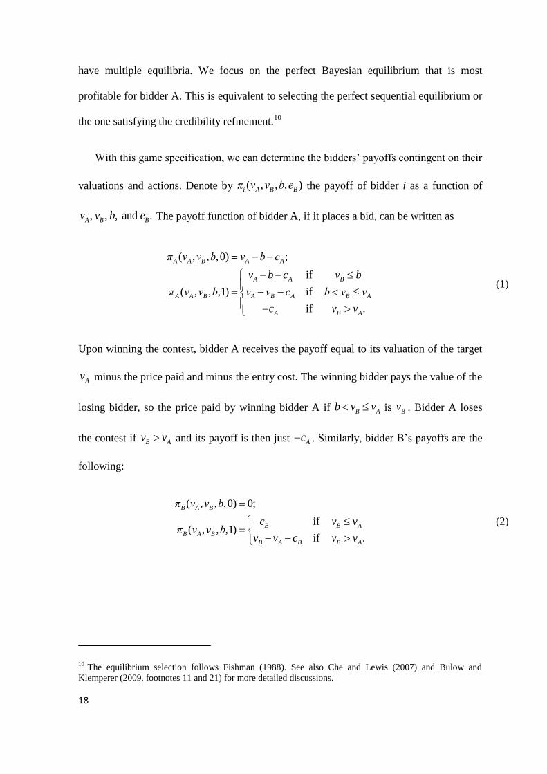
With this game specification, we can determine the bidders’ payoffs contingent on their
valuations and actions. Denote by ( , , , )i A B Bπ v v b e the payoff of bidder i as a function of
, , , and .A B Bv v b e The payoff function of bidder A, if it places a bid, can be written as
( , , ,0) ;
if
( , , ,1) if
if .
A A B A A
A A B
A A B A B A B A
A B A
π v v b v b c
v b c v b
π v v b v v c b v v
c v v
(1)
Upon winning the contest, bidder A receives the payoff equal to its valuation of the target
Av minus the price paid and minus the entry cost. The winning bidder pays the value of the
losing bidder, so the price paid by winning bidder A if B Ab v v is Bv . Bidder A loses
the contest if B Av v and its payoff is then just Ac . Similarly, bidder B’s payoffs are the
following:
( , , ,0) 0;
if( , , ,1)
if .
B A B
B B A
B A B
B A B B A
π v v b
c v vπ v v b
v v c v v
(2)
10 The equilibrium selection follows Fishman (1988). See also Che and Lewis (2007) and Bulow and
Klemperer (2009, footnotes 11 and 21) for more detailed discussions.
19
2.2.3. Informational externalities and competition
We take a first look at the influence of bidder A’s offer on bidder B’s beliefs and payoff.
An important observation is that the expected payoff may either increase or decrease in the
level of similarity between the valuations. Intuition suggests that there are two effects due
to correlated valuations. First, if valuations are dependent, then the second bidder can infer
some information about its own value of the target from the first offer. Second, if both
bidders enter the contest, the level of similarity will affect the competitiveness of the
contest and the price paid by the winning bidder. We refer to the former effect as the
informational externality effect and to the latter as the competition effect.
Suppose now that bidder A’s strategy is fully revealing. From observing a bid b ,
bidder B can exactly infer the realization of bidder A’s value .Av In other words, we
assume here that bidder A’s strategy is separating and each valuation realization stipulates
a different bid. Because Av and Bv are correlated, information about the realization of Av
affects the posterior distribution of Bv . Given bidder A’s value ,Av the posterior
distribution of the value of bidder B is again normal with probability density function
denoted by |B Af . The expected value is updated to
| 0| (1 ) .B A B A Aμ E v v ρv ρ v (3)
It follows from (3) that the informational externality effect of increasing ρ on bidder B’s
expected value is positive for all ρ as long as 0Av v . Because bidder A places a bid only
if Av exceeds 0v , the informational externality effect encourages bidder B to participate
and bidder B is better off with a correlation with bidder A that is as high as possible.
20
The posterior standard deviation of Bv is updated to 2
| 1B Aσ σ ρ . It is the largest at
0ρ and decreases as the value of ρ increases. The posterior standard deviation is related
to the competition effect and it works through the expected payoff that bidder B obtains
from entering the contest. If bidder B knows the realization of Av , this payoff is given by
| |
2
( , , ,1) ( ) ( )
1 ( ) (1 Φ( )) ,
A
A
v
B A B B B A A B B A
v
A A A B
E π v v b c f v dv v v c f v dv
σ ρ z z z c
(4)
where | |( ) /A A B A B Az v μ σ , and and Φ denote probability density and cumulative
distribution functions of the standard normal distribution.
To isolate the competition effect, we set 0Av v , at which the informational externality
effect is absent. Taking the derivative of (4) with respect to ρ , we obtain
2
.21
ρ σ
πρ
(5)
The sign of this expression—reflecting the competition effect of similarity—is negative if
0ρ . When taking into account only the competition effect, bidder B prefers the
correlation to be equal to zero. Intuitively, if both bidders enter the contest and their
valuations are not dispersed, then they outbid each other to the point that the expected price
paid by the winning bidder is close to its value. In other words, given the mean of its
valuation, bidder B prefers to have the highest variance. The effect is caused by the
convexity of bidder B’s payoff function in its valuation of the target, so that a higher
posterior variance 2
|B Aσ leads to higher expected payoffs.
21
With the assumption of this subsection that Av is observable, neither the informational
externality effect nor the competition effect dominates for all levels of similarity. The
derivate of the expected payoff of bidder B from entering (given in (4)) with respect to ρ
includes both effects and is given by
2
( ) (1 ) 1 Φ( ) .1
A A A
σρ z ρ z z
ρ
(6)
It is easy to establish that this expression is positive for relatively small positive ρ (the
positive informational externality effect dominates the negative competition effect), and is
negative for large positive ρ (the negative competition effect dominates the positive
informational externality effect).
The preceding discussion clearly conveys the intuition for the two effects of similarity,
but the separating strategy of bidder A that fully reveals its valuation cannot be sustained
by an equilibrium. The next section analyzes strategies of both bidders that can form
equilibrium.
2.3. Bidders’ strategies and equilibrium
2.3.1. Bidder A: to preempt or to accommodate
We restrict our attention to cut-off pure strategies in which bidder A with valuations within
a certain set places a specified bid. These strategies have a clear interpretation in our
bidding game: preemption and accommodation. With a preemptive bid, the expected
payoff for the second bidder is sufficiently low so that it is deterred from entering. An
accommodating bid does not attempt to limit participation of the follower. If bidder A
preempts with a bid b, its expected payoff is given by
22
[ ( , , ,0)] .A A B A AE π v v b v b c (7)
If bidder A accommodates, it cannot gain anything from bidding above the reservation
value, so its bid is equal to 0v and its expected payoff is
0
0
0 0 | 0 |
| |
2
0 0 0
[ ( , , ,1)] ( , , ,1) ( ) ( ) ( )
( ) ( ) ( )
1 ( ) ( ) Φ( ) Φ( ) ,
A
A
v
A A B A A B A A A B A
v
A A B A A B A
v v
A A A A
E π v v v π v v v f v dv v v c f v dv
v v c f v dv c f v dv
σ ρ z z z z z z c
(8)
where | |( ) /A A B A B Az v μ σ and 0 0 | |( ) /B A B Az v μ σ .
Bidder A will be willing to preempt with a bid b if the expected payoff from
preemption exceeds or equals the expected payoff from accommodation, that is if
0( , ) [ ( , , ,0)] [ ( , , ,1)] 0.A A A B A A BV v b E π v v b E π v v v (9)
Conversely, if ( , ) 0AV v b , then bidder A is better off with accommodation. Denote by
( )Ab v the maximum bid that bidder A with value Av is willing to offer to preempt bidder
B. This means that with a bid at ( )Ab v , the condition in (9) holds in equality. Substituting
(7) and (8) into (9), we obtain that
2
0 0 0( ) 1 ( ) ( ) Φ( ) Φ( ) .A A A A Ab v v σ ρ z z z z z z (10)
For a given preemptive bid ,b bidder A’s incentive for accommodation or preemption
depends on the realized value of Av . If ( ),Ab b v then the expected payoff from
23
preemption is larger than that from accommodation, and the opposite relation holds if
( ).Ab b v In the Appendix we prove that the following result holds given that 0ρ .
Lemma 1. ( )Ab v increases in 0.Av v
The implication of the lemma is that for a given preemptive bid b , such that ( )b b v ,
bidder A with valuation larger than or equal to v prefers to preempt rather than to
accommodate. This observation justifies our focus on cut-off accommodation and
preemption strategies of bidder A.
2.3.2. Bidder B: to participate or to stay out
We consider here bidder B’s expected payoff when bidder A uses a cut-off strategy.
Suppose a bid b is chosen if the realized valuation of bidder A lies in between some v and
v . Denote by ( , )W v v bidder B’s expected payoff if it decides to enter the contest (as long
as bid b is lower than v , which is the case in equilibrium, this value depends only on the
implied valuations of bidder A, not on the bid itself). Then
1
( , ) [ ( , , ,1)] ( )( ) ( )
v
B A B A A A
A A v
W v v E π v v b f v dvF v F v
. (11)
Bidder B is deterred by the set of bidder A with valuations in ( , )v v if ( , ) 0.W v v If this
is the case, then bidder B’s payoff from entering falls below its payoff from staying out,
which is equal to zero.
From Section 3.1 we know that for 0ρ , bidder A’s incentives to preempt increase in
its own valuation. Therefore bidder A uses a preemptive strategy if its valuations are above

24
some v . A preemptive strategy works only if it implies that bidder B does not enter, that is,
that the expected payoff of bidder B from entering W is non-positive. The following
lemma shows that the cheapest such strategies (with W equal to zero) are unique.
Lemma 2. There exists at most one 0v v that solves ( , ) 0W v .
Let us define Lv such that ( , ) 0.LW v Lv is the lowest value such that information
that A Lv v deters bidder B from the contest.
The incentives of bidder B to enter are influenced by the informational externality and
competition effects. If the negative effects of similarity dominate, bidder B may easily be
deterred. In particular, in some cases, bidder B may be deterred by information that Av
exceeds the reservation value, 0Av v , inferred from observing bidder A placing any bid.
The following lemma specifies when this is the case.
Lemma 3. Let 2 /BR πc σ and assume that 2 1R . If bidder B believes that 0Av v ,
then bidder B does not enter the contest whenever 1 1 2ρ ρ R R or
2 1 2ρ ρ R R .
We assume from now on that 2 1R to focus on interesting cases. If this condition is
not satisfied, then bidder B does not participate after a bid from A for any possible value of
ρ .11
Lemma 3 states that if bidder B’s only information is that bidder A’s valuation
exceeds the reservation price 0v , it may still be sufficient as a deterrent if the valuations
11 The condition is a result of the requirement that 0( , )W v is positive at least for some values of ρ .
25
are interdependent with a low correlation coefficient, 1ρ ρ , or if the valuations are
strongly positively correlated, 2ρ ρ . Intuitively, a high value of Av together with a low
correlation promises a low expected value of Bv . For example, consider the extreme case
with 1ρ . Then 0Av v implies 0Bv v and bidder B makes sure losses with any
positive entry cost. On the other hand, a high value of Av with a high correlation leaves
little profit to be earned in the subsequent auction, because values of both bidders are
expected to be similar. At the extreme point as 1ρ , Bv is equal to Av with probability
one, and after entry the price paid is equal to the value, which leaves no profit. At very low
and very high correlation, expected payoffs do not compensate the entry cost. We note that
for positive Bc and 2 1R , both 1ρ and 2ρ are inside the domain for a correlation
coefficient and are such that 1 21 0.5 1ρ ρ .
2.3.3. Equilibrium
Equilibrium strategies consist of bidder A’s initial bidding strategy b and bidder B’s entry
strategy Be . In the previous subsections, we outlined the derivation of the strategies in the
signaling equilibrium involving the most profitable outcome for bidder A. These strategies
can be interpreted as accommodation with a bid at the reservation price that induces entry
of the competitor and as preemption with a bid at a premium over the reservation price that
deters the other contestant. In some cases, a deterring bid is placed that, while low at the
reservation price, effectively deters the competitor.
For example, in the case of the preemptive outcome, the equilibrium is constructed as
follows. We have shown that there is a threshold Lv such that bidder A with A Lv v places
26
a preemptive bid and deters bidder B. For this bid not to be imitated by bidder types with
A Lv v , it must be at least ( )Lb v . Bidder A with valuations A Lv v cannot match this bid
and offers the lowest price 0v which invites the second bidder. These results are gathered
in the following proposition.12
Proposition 4. In the game after bidder A enters, there exists equilibrium * *( , )Bb e in cut-
off strategies with the following properties. If 0Av v , then bidder A places a bid and there
are two cases.
1. If 20 ρ ρ , then
*
0 0
( ) if( )
if ,
L A L
A
A L
b v v vb v
v v v v
* 1 if ( )( )
0 if ( );
L
B
L
b b ve b
b b v
2. If 2ρ ρ , then *
0( )Ab v v and * ( ) 0Be b .
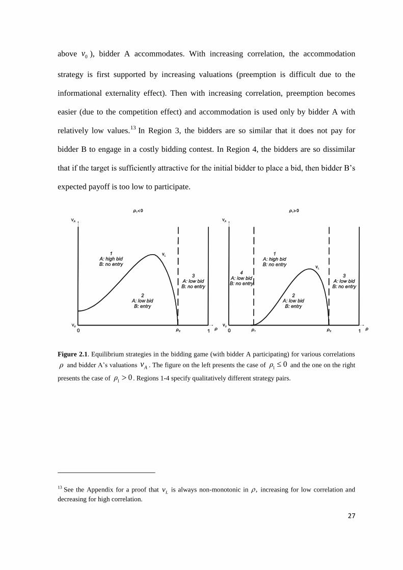
Figure 2.1 presents how the equilibrium strategies depend on the level of correlation
between the valuations. There are four possible scenarios depending on the correlation ρ
and the first bidder’s valuation Av . In Region 1 at intermediate levels of correlation, bidder
A preempts bidder B with a high bid. This happens for sufficiently high values Av such
that A Lv v . In Region 2 at intermediate levels of correlation and at low valuations (but
12 For transparency, Proposition 4 is stated for the case 1 0ρ . Using Lemma 3, it holds if 2 1R . The
proposition can be adapted to the other case in the obvious way.
27
above 0v ), bidder A accommodates. With increasing correlation, the accommodation
strategy is first supported by increasing valuations (preemption is difficult due to the
informational externality effect). Then with increasing correlation, preemption becomes
easier (due to the competition effect) and accommodation is used only by bidder A with
relatively low values.13
In Region 3, the bidders are so similar that it does not pay for
bidder B to engage in a costly bidding contest. In Region 4, the bidders are so dissimilar
that if the target is sufficiently attractive for the initial bidder to place a bid, then bidder B’s
expected payoff is too low to participate.
Figure 2.1. Equilibrium strategies in the bidding game (with bidder A participating) for various correlations
ρ and bidder A’s valuations Av . The figure on the left presents the case of 10ρ and the one on the right
presents the case of 10ρ . Regions 1-4 specify qualitatively different strategy pairs.
13 See the Appendix for a proof that Lv is always non-monotonic in , increasing for low correlation and
decreasing for high correlation.
28
2.4. Model implications
Similarity between bidders generates the trade-off between the informational externality of
the initial bid and competition intensity. The interaction of these two forces leads to a non-
monotonic relationship of the correlation coefficient on acquisition strategies and returns.
Figure 2.2 presents numerical comparative statics with respect to the correlation coefficient
between bidders’ valuations. Other exogenous parameters are set at 20σ , 2Bc , and
0 50v . These parameters are later used in our experiments. Figures 2.2.A and 2.2.B
present the probabilities of observing either a single-bidder contest or a multiple-bidder
contest conditional on observing a takeover. The probability of single-bidder contests is
non-monotonic and has a U-shape. The complementing probability of two-bidder contests
is then also non-monotonic and has an inverted U-shape. The two-bidder contests are
mostly observed at intermediate positive correlation. The intuition is that it is most difficult
to deter the second bidder at these levels of correlation—the information externality is
strong enough to attract followers and the post-entry competition is not yet to fierce—and
only the highest valuations of the first bidder can serve as an effective deterrent.
Figures 2.2.C and 2.2.D plot the expected prices paid for the target in single-bidders
contests and multiple-bidder contests. Contingent on observing a single-bidder contest, the
offered price has an inverted U-shape in bidder similarity. This non-monotonic effect is
driven by the fact that low initial bids may deter competition if the potential competitors
are very similar (post-entry bidding competition makes entry unattractive) or very
dissimilar (the initial bid does not convey much of positive information to potential
followers about their valuation of the target). Similarly, contingent on observing a two-
bidder contest, the expected price paid by the winning bidder has an inverted U-shape in
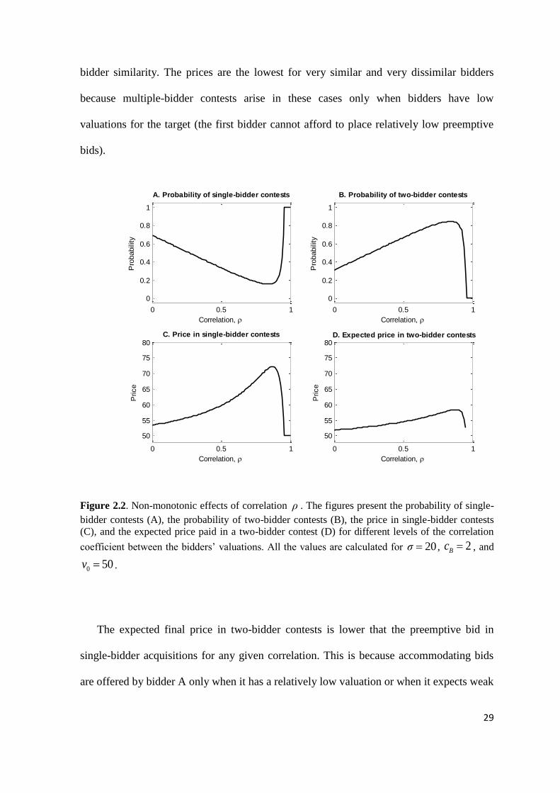
29
bidder similarity. The prices are the lowest for very similar and very dissimilar bidders
because multiple-bidder contests arise in these cases only when bidders have low
valuations for the target (the first bidder cannot afford to place relatively low preemptive
bids).
Figure 2.2. Non-monotonic effects of correlation ρ . The figures present the probability of single-
bidder contests (A), the probability of two-bidder contests (B), the price in single-bidder contests
(C), and the expected price paid in a two-bidder contest (D) for different levels of the correlation
coefficient between the bidders’ valuations. All the values are calculated for 20σ , 2Bc , and
0 50v .
The expected final price in two-bidder contests is lower that the preemptive bid in
single-bidder acquisitions for any given correlation. This is because accommodating bids
are offered by bidder A only when it has a relatively low valuation or when it expects weak
0 0.5 1
0
0.2
0.4
0.6
0.8
1
Correlation,
Pro
babili
ty
A. Probability of single-bidder contests
0 0.5 1
0
0.2
0.4
0.6
0.8
1
Correlation, P
robabili
ty
B. Probability of two-bidder contests
0 0.5 1
50
55
60
65
70
75
80
Correlation,
Price
C. Price in single-bidder contests
0 0.5 1
50
55
60
65
70
75
80
Correlation,
Price
D. Expected price in two-bidder contests
30
competition. However, two-bidder contests are most likely when the expected prices in
two-bidder contests are high, and single-bidder contests are most likely when the prices in
single-bidder contests are low. This may explain why empirical evidence of the effects of
competition measured by the number of bidders on target returns is inconclusive and
frequently demonstrates a puzzling lack of any significant relation. The analysis indicates
that the effect of the number of bidders should be controlled for the level of similarity.
2.5. The experimental setup
As discussed in the introduction, testing the model’s predictions with historical field data is
difficult because the identity of preempted bidders, and so their similarity with acquirers, is
not observable to researchers. To address this problem and to offer a first test of the
model’s trade-offs, we use experimental data in which we can control the combinations of
competing bidders and other characteristics of the environment. Specifically, we design a
computerized laboratory experiment in which we recreate the exact setting of the model. In
different treatments, we change only the level of interdependence between bidders’
valuations and keep all other variables constant.
2.5.1. Treatments and hypotheses
The parameters in the experiment are chosen to replicate a takeover opportunity with
uncertain value and with sufficient potential profits to make the investment attractive. The
mean target value is set at 0 50v , the standard deviation of the bidders’ valuation, σ ,
equals 20, and the entry cost, c , equals 2. When there is no rival, this parameter setting
leads to an expected payoff of about 30 to a bidder if he or she enters. With competing
bidders, the expected payoff of the initial bidder will vary depending on the intensity of
competition and the strategies bidders adopt.
31
We set up three treatments that differ in the level of correlation between bidders’
valuations. The correlations are 0, 0.5, and 0.95. These levels are sufficiently different to
represent three typical takeover contests. In the low similarity treatment (with correlation
equal to 0), bidders’ valuations are independent. This is as in the standard Fishman (1988)
model and we interpret this case as a contest between a strategic bidder and a financial
bidder. The intermediate similarity treatment (with correlation equal to 0.5) represents the
case of two strategic bidders. The high similarity treatment (with correlation equal to 0.95)
represents the case in which bidders’ valuation are highly dependent with each other as in
bidding between two financial bidders.
The three treatments generate qualitatively distinctive equilibrium strategies. Table 2.1
reports the theoretical predictions for equilibrium strategies and outcomes. At low
similarity, the minimum bid that can preempt bidder B is 53 and when bidder A’s value is
above 58, he chooses to offer this preemptive bid. This implies that single-bidder contests
are expected in 66% of observed takeovers and that the average price in two-bidder
contests is about 51. At intermediate similarity, bidder A makes a preemptive bid equal to
60 when his value is above 69 and the proportion of single-bidder contests is significantly
lower at 30%, while prices in two-bidder contests are higher at 54. At high similarity, the
proportion of single-bidder contests increases to 70%, bidder A will make a preemptive bid
of 56 when his value is above 58, and the average price in two-bidder contests decreases
slightly to 53. The model predicts a non-monotonic pattern in the proportion of single-
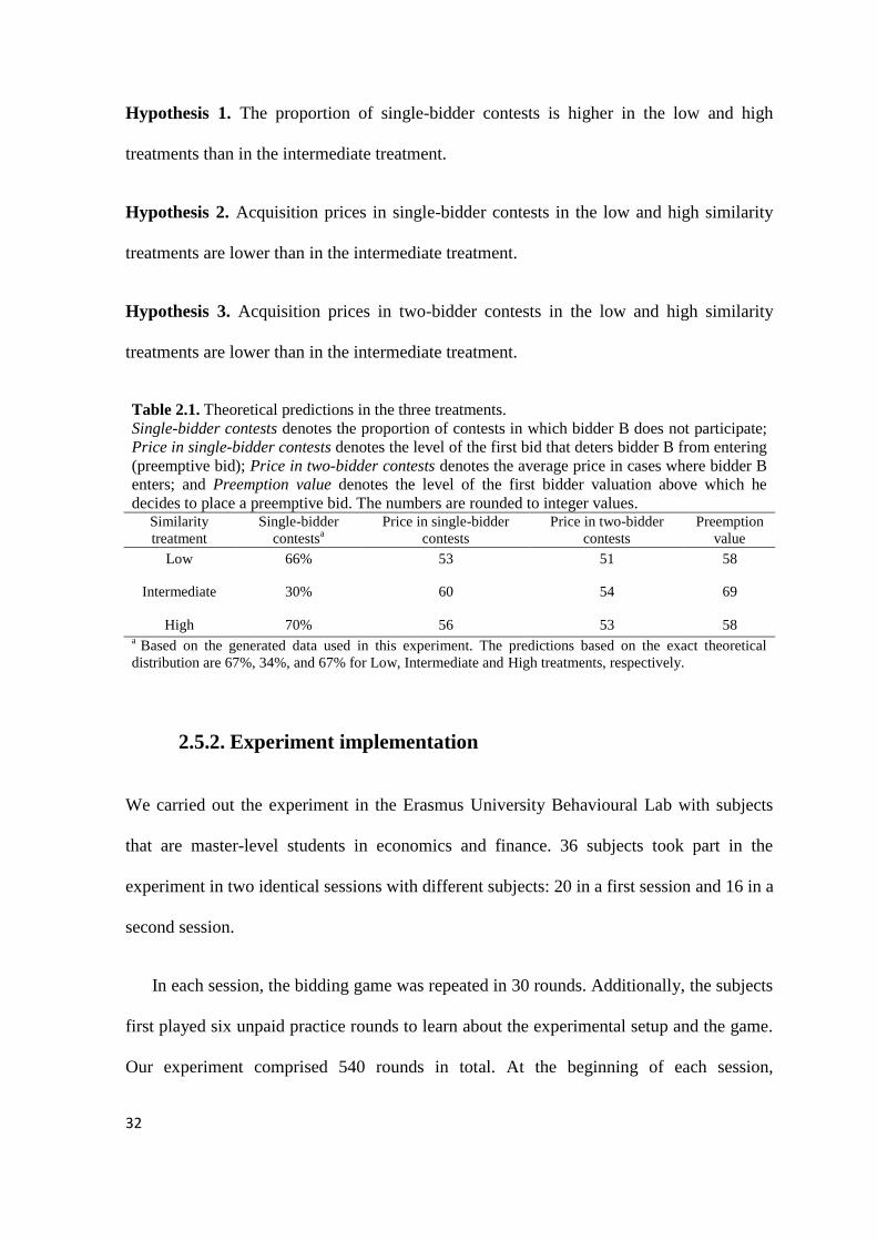
bidder contests and acquisition prices. This leads to three testable hypotheses.14
14 We do not specify a separate hypothesis for preemption values. First, preemption values used by bidder A
are not directly observable in the experiment. Second, in the theory, preemption values measure the same
behavior as the proportion of single-bidder contests. The proportion of single-bidder contests is the
proportion of bidder A’s distribution that falls above preemption value.
32
Hypothesis 1. The proportion of single-bidder contests is higher in the low and high
treatments than in the intermediate treatment.
Hypothesis 2. Acquisition prices in single-bidder contests in the low and high similarity
treatments are lower than in the intermediate treatment.
Hypothesis 3. Acquisition prices in two-bidder contests in the low and high similarity
treatments are lower than in the intermediate treatment.
Table 2.1. Theoretical predictions in the three treatments.
Single-bidder contests denotes the proportion of contests in which bidder B does not participate;
Price in single-bidder contests denotes the level of the first bid that deters bidder B from entering
(preemptive bid); Price in two-bidder contests denotes the average price in cases where bidder B
enters; and Preemption value denotes the level of the first bidder valuation above which he
decides to place a preemptive bid. The numbers are rounded to integer values. Similarity
treatment
Single-bidder
contestsa
Price in single-bidder
contests
Price in two-bidder
contests
Preemption
value
Low 66% 53 51 58
Intermediate 30% 60 54 69
High 70% 56 53 58
a Based on the generated data used in this experiment. The predictions based on the exact theoretical
distribution are 67%, 34%, and 67% for Low, Intermediate and High treatments, respectively.
2.5.2. Experiment implementation
We carried out the experiment in the Erasmus University Behavioural Lab with subjects
that are master-level students in economics and finance. 36 subjects took part in the
experiment in two identical sessions with different subjects: 20 in a first session and 16 in a
second session.
In each session, the bidding game was repeated in 30 rounds. Additionally, the subjects
first played six unpaid practice rounds to learn about the experimental setup and the game.
Our experiment comprised 540 rounds in total. At the beginning of each session,
33
participants were randomly assigned to play a role throughout the entire session: either
"first bidder" or "second bidder". Each first bidder was randomly paired with a second
bidder in each round to avoid learning bidder characteristics. This was aimed to facilitate
the perception of a series of one-shot games.
The sequence of the game was as follows. At the beginning, both bidders were
informed about the level of their similarity. The first bidder was assigned his or her
valuation of the target and the entry fee was deducted from its account. Next, the first
bidder submitted a bid. After observing the first bid and similarity level, the second bidder
chose whether to enter or not. If he entered, the entry fee was deducted from his current
account and his valuation of the target was revealed. Then the outcome of the auction was
automatically determined by an English auction rule – the bidder with the highest valuation
bought the target for the second highest bid.15
If instead the second bidder chose not to
enter, the game ended and the first bidder bought the target with his first bid.
Each bidder’s valuation of the target was private information. The similarity level and
the distribution of bidders’ valuations were known to both bidders. It was also known that
the target would not sell below a reservation price of 50. In every round, the first bidder
was assigned a new random valuation drawn from normal distribution with a mean of 50
and a standard deviation of 20. The first bidder will only observe his value if it is no less
than 50, because otherwise no contest is initiated.16
The value for the second bidder was
drawn from another normal distribution with a mean of 50 and a standard deviation of 20.
15 The second highest bid is defined as the second highest value in {the first bidder’s valuation, the second
bidder’s valuation, the first bid}.
16 Alternatively, we could have used a full normal distribution and removed half of the rounds which
involved no actions and had no information.
34
The second bidder’s valuation was correlated with the normal distribution underlying the
first bidder’s valuation with a coefficient equal to the similarity level. To ensure that
participants understood the distribution of bidders’ valuations and their interdependent
nature, numerical examples were given for different similarity levels.17
Each pair of bidders in each round was assigned with a new similarity level drawn
from the set {0, 0.5, 0.95} with equal probability. To control for learning across different
similarity levels, the sequence of similarity levels was selected randomly. The
experimental sessions lasted about two hours and the final payoffs in the experiment were
determined by the performance of the participants and by their roles. The accumulated
payoffs were recorded by points they earned or lost, with a conversion rate of €1 for every
20 points. Because of the entry fee, the bidders that lost an auction incurred a net loss. To
prevent bankruptcy, each bidder was given 60 initial points, which was just sufficient to
cover the entire entry fee if he bid in every round. Furthermore, the second bidders were
given an additional fixed payment of €5 to compensate for their disadvantaged initial
position compared to the first bidders. The range of actual earnings paid to the first bidder
was €5.90-17.00, with a mean of €9.00; the range of actual earnings paid to the second
bidder was €7.70-10.90, with a mean of €9.0018
.
17 The full experiment instructions can be found at the online appendix.
18 The payment level in our experiment is not high. As experimental literature shows that subject
performance can be affected by compensation level (Smith, Walker, 1993; Gneezy, Rustichini, 2000), we add
one more session by increasing conversion rate between experimental points and euro from 20:1 to 8:1.
Sixteen subjects participated in this new session, and the payment ranges from €13.9 to € 33.6 with an
average of € 22.3. Results are similar to the original sessions, which suggest non-monotonic patterns in entry
and bidding behaviour. Because of the different compensation structure, experiment outcome from high
payment session is not reported here. Extra analysis on these additional data will be provided upon request.

35
2.6. Experimental results
We start with an overview of aggregate bidder behavior in different treatments. Table 2.2
presents descriptive statistics of the results. Panel A shows that the first bid in the single-
bidder contests is higher than that in the two-bidder contests. The differences are highly
significant in all treatments. We take this finding as reassurance that first bids can be
preemptive and most subjects were responding sensibly within our experiment.
Table 2.2. Descriptive statistics of the experimental results.
Statistics are calculated from 540 experimental observations. In Panel A, the data are split into two
subgroups depending on the number of bidders active in the contest. Columns report the percentage
of the two types of contests (Proportion) and the mean of the first bids (First bid) and prices across
the three treatments. The last two columns present the difference in first bids across the two types of
contests and t-statistics for differences between means. Panel B reports t-statistics for differences
between means of the proportion of and prices paid in two types of contests across the three
treatments. Parentheses report number of observations or standard errors.
Panel A: Statistics for each contest outcome
Similarity
treatment
Single-bidder contests
Two-bidder contests
First bid
difference
Proportion First bid
[=Price] Proportion First bid Price Mean t-stat
Low 27% 56
73% 52.48 55.97
3.52
4.47 (N=48) (0.93) (N=132) (0.33) (0.56) (0.79)
Intermediate 22% 58.79
78% 53.81 57.82
4.99
4.73 (N=39) (1.28) (N=141) (0.43) (0.73) (1.05)
High 39% 60.8
61% 56.04 61.78
4.76
3.31 (N=70) (1.42) (N=110) (0.71) (0.95) (1.44)
Panel B: Differences between treatments
Comparison pair
Proportion of
Price in
Price in
single-bidder contests single-bidder contests two-bidder contests
Mean t-stat Mean t-stat Mean t-stat
Low – 5% 1.11
-2.79 -1.81
-1.85 -2.01
Intermediate (4.50%) (1.54) (0.92)
High – 17%
3.56 2.01
0.94 3.96
3.38 Intermediate (4.80%) (2.13) (1.17)
Panel B of Table 2.2 provides some support to the theoretical predictions for the
proposed effects of similarity between bidders. The proportion of single-bidder contests is
moderately lower in the intermediate similarity treatment compared to the low similarity
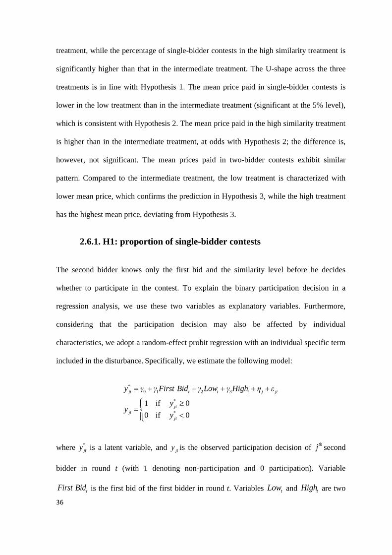
36
treatment, while the percentage of single-bidder contests in the high similarity treatment is
significantly higher than that in the intermediate treatment. The U-shape across the three
treatments is in line with Hypothesis 1. The mean price paid in single-bidder contests is
lower in the low treatment than in the intermediate treatment (significant at the 5% level),
which is consistent with Hypothesis 2. The mean price paid in the high similarity treatment
is higher than in the intermediate treatment, at odds with Hypothesis 2; the difference is,
however, not significant. The mean prices paid in two-bidder contests exhibit similar
pattern. Compared to the intermediate treatment, the low treatment is characterized with
lower mean price, which confirms the prediction in Hypothesis 3, while the high treatment
has the highest mean price, deviating from Hypothesis 3.
2.6.1. H1: proportion of single-bidder contests
The second bidder knows only the first bid and the similarity level before he decides
whether to participate in the contest. To explain the binary participation decision in a
regression analysis, we use these two variables as explanatory variables. Furthermore,
considering that the participation decision may also be affected by individual
characteristics, we adopt a random-effect probit regression with an individual specific term
included in the disturbance. Specifically, we estimate the following model:
*
0 1 2 3
*
*
1 if 0
0 if 0
jt t t t j jt
jt
jt
jt
y γ γ First Bid γ Low γ High η ε
yy
y
where *
jty is a latent variable, and jty is the observed participation decision of thj second
bidder in round t (with 1 denoting non-participation and 0 participation). Variable
tFirst Bid is the first bid of the first bidder in round t. Variables tLow and tHigh are two
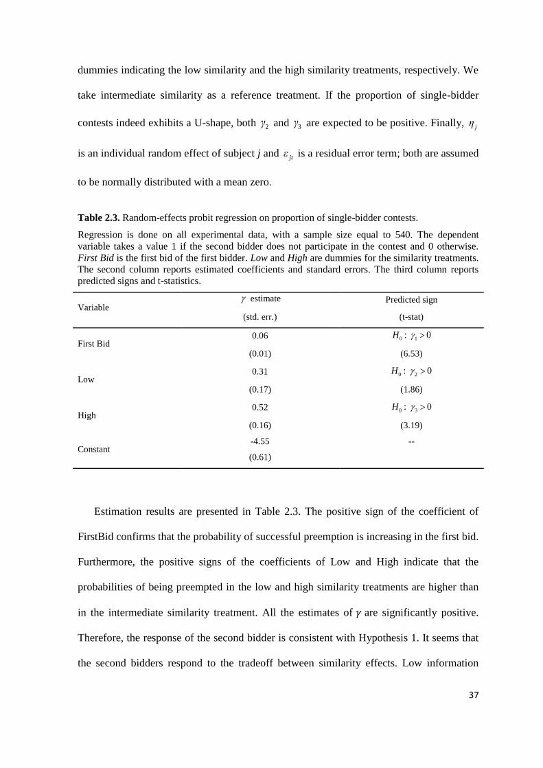
37
dummies indicating the low similarity and the high similarity treatments, respectively. We
take intermediate similarity as a reference treatment. If the proportion of single-bidder
contests indeed exhibits a U-shape, both 2γ and 3γ are expected to be positive. Finally, jη
is an individual random effect of subject j and jtε is a residual error term; both are assumed
to be normally distributed with a mean zero.
Table 2.3. Random-effects probit regression on proportion of single-bidder contests.
Regression is done on all experimental data, with a sample size equal to 540. The dependent
variable takes a value 1 if the second bidder does not participate in the contest and 0 otherwise.
First Bid is the first bid of the first bidder. Low and High are dummies for the similarity treatments.
The second column reports estimated coefficients and standard errors. The third column reports
predicted signs and t-statistics.
Variable estimate Predicted sign
(std. err.) (t-stat)
First Bid 0.06 0 1: 0H
(0.01) (6.53)
Low 0.31 0 2: 0H
(0.17) (1.86)
High 0.52 0 3: 0H
(0.16) (3.19)
Constant -4.55 --
(0.61)
Estimation results are presented in Table 2.3. The positive sign of the coefficient of
FirstBid confirms that the probability of successful preemption is increasing in the first bid.
Furthermore, the positive signs of the coefficients of Low and High indicate that the
probabilities of being preempted in the low and high similarity treatments are higher than
in the intermediate similarity treatment. All the estimates of are significantly positive.
Therefore, the response of the second bidder is consistent with Hypothesis 1. It seems that
the second bidders respond to the tradeoff between similarity effects. Low information
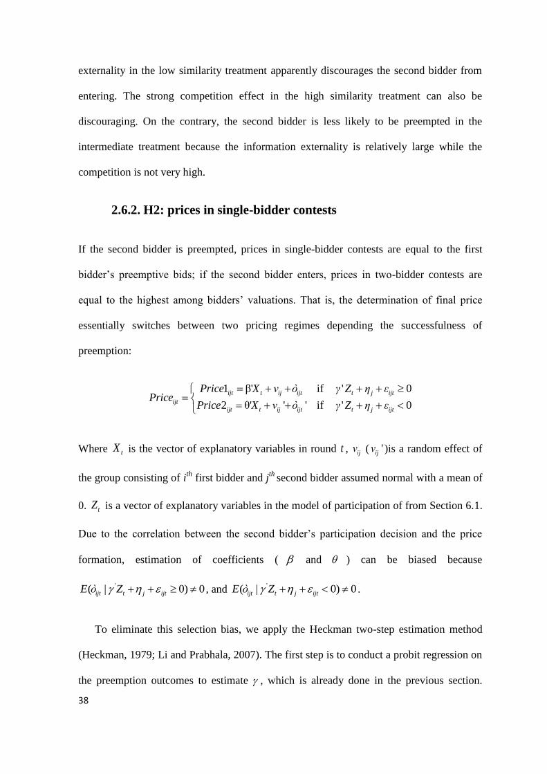
38
externality in the low similarity treatment apparently discourages the second bidder from
entering. The strong competition effect in the high similarity treatment can also be
discouraging. On the contrary, the second bidder is less likely to be preempted in the
intermediate treatment because the information externality is relatively large while the
competition is not very high.
2.6.2. H2: prices in single-bidder contests
If the second bidder is preempted, prices in single-bidder contests are equal to the first
bidder’s preemptive bids; if the second bidder enters, prices in two-bidder contests are
equal to the highest among bidders’ valuations. That is, the determination of final price
essentially switches between two pricing regimes depending the successfulness of
preemption:
1 β' if ' 0
2 θ' ' ' if ' 0
ijt t ij ijt t j ijt
ijt
ijt t ij ijt t j ijt
Price X ν γ Z η εPrice
Price X ν γ Z η ε
ò
ò
Where tX is the vector of explanatory variables in round t , ijν ( 'ijν )is a random effect of
the group consisting of ith
first bidder and jth
second bidder assumed normal with a mean of
0. tZ is a vector of explanatory variables in the model of participation of from Section 6.1.
Due to the correlation between the second bidder’s participation decision and the price
formation, estimation of coefficients ( and ) can be biased because
'( | 0) 0ijt t j ijtE Z ò , and '( | 0) 0ijt t j ijtE Z ò .
To eliminate this selection bias, we apply the Heckman two-step estimation method
(Heckman, 1979; Li and Prabhala, 2007). The first step is to conduct a probit regression on
the preemption outcomes to estimate , which is already done in the previous section.
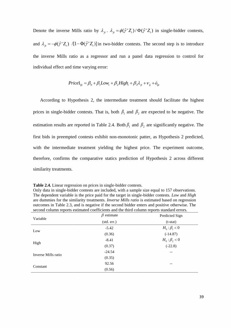
39
Denote the inverse Mills ratio by jt . ˆ ˆ( ' ) / ( ' )jt t tZ Z in single-bidder contests,
and ˆ( ' )jt tZ ˆ/[1 Φ( ' )]tZ in two-bidder contests. The second step is to introduce
the inverse Mills ratio as a regressor and run a panel data regression to control for
individual effect and time varying error:
0 1 2 31ijt t t jt ij ijtPrice Low High ò
According to Hypothesis 2, the intermediate treatment should facilitate the highest
prices in single-bidder contests. That is, both 1β and 2β are expected to be negative. The
estimation results are reported in Table 2.4. Both 1β and 2β are significantly negative. The
first bids in preempted contests exhibit non-monotonic patter, as Hypothesis 2 predicted,
with the intermediate treatment yielding the highest price. The experiment outcome,
therefore, confirms the comparative statics prediction of Hypothesis 2 across different
similarity treatments.
Table 2.4. Linear regression on prices in single-bidder contests.
Only data in single-bidder contests are included, with a sample size equal to 157 observations.
The dependent variable is the price paid for the target in single-bidder contests. Low and High
are dummies for the similarity treatments. Inverse Mills ratio is estimated based on regression
outcomes in Table 2.3, and is negative if the second bidder enters and positive otherwise. The
second column reports estimated coefficients and the third column reports standard errors.
Variable estimate Predicted Sign
(std. err.) (t-stat)
Low -5.42 0 1: 0H
(0.36) (-14.87)
High -8.41 20 : 0H
(0.37) (-22.8)
Inverse Mills ratio -24.54 --
(0.35)
Constant 92.56 --
(0.56)
40
2.6.3. H3: prices in two-bidder contests
The next step is to check prices in two-bidder contests. According to Hypothesis 3, the
intermediate treatment boasts the highest average price compared to low and high
treatments. To test it, we run a similar self-selection regression as above, but the dependent
variable changes to prices in two-bidder contests and we use only observations with two-
bidder contests. The regression equation is as follows:
0 1 2 3 '2ijt t t jt ij ijtPrice θ θ Low θ High θ λ ν ò
ijtPrice2 denotes prices in two-bidder contests, and tLow and tHigh are two similarity
indicators. Again, we control an random effect of group ij, 'ijν , assumed to be normal with
a mean of 0.
Table 2.5. Linear regression on prices in two-bidder contests.
Only data in two-bidder contests are analyzed, which include 383 observations. The dependent
variable is the price paid for the target in two-bidder contests. Low and High are dummies for the
similarity treatments. Inverse Mills ratio is estimated based on regression outcomes in Table 2.3,
and is negative if the second bidder enters and positive otherwise. The second column reports
estimated coefficients and standard errors. The third column reports predicted signs and t-statistics.
Variable estimate Predicted Sign
(std. err.) (t-stat)
Low -3.67 0 1: 0H
(0.86) (-4.28)
High -3.13 20 : 0H
(1.06) (-2.95)
Inverse Mills ratio -24.08 --
(1.92)
Constant
51.40 --
(0.81)
As Hypothesis 3 predicts that prices in two-bidder contests in the low and high
treatments are lower than in the intermediate treatment, both 1θ and 2θ are expected to be
41
negative. Regression results in Table 2.5 provide confirmative evidence to this prediction.
Both 1θ and 1θ are significantly negative. Again, non-monotonic pattern in prices is
supported in two-bidder contests. In addition, coefficients of inverse Mills ratio are both
significant at 1% level in Table 2.4 and Table 2.5, which indicate the self-selection effect
plays a role in determining prices.
2.6.4. Dynamic session-effects
There are two sessions in our experiment. Observations across subjects of a given session
might be more correlated than observations across subjects from different sessions. One
possible source of the higher correlation can be that subjects adjust their strategy according
to the feedbacks from their previous actions. For example, a successful low bid in a
previous round can make the first bidder more likely to submit a low bid in the following
round, and a successful entry decision can induce the second bidder to enter. If this is the
case, there can be some interdependence among observations within one session, which is
named as “dynamic session effects” in experimental economics (Frechette, 2012). 19
Ignoring dynamic session effects can bias the variance computation of estimators,
resulting in incorrect conclusion on accepting or rejecting null hypothesis. To mitigate this
session effects problem, we employ two solutions suggested by Frechette (2012), one by
clustering, and the other by identifying the source of interdependence among observations.
Because the interdependence among observations is within sessions, one simple
solution is to cluster the variance computation at the session level. Table 2.6 presents the
new estimates by clustering. All of our previous findings hold with the new regression
19 The discussion on dynamic session effects is inspired by the comment from an anonymous referee.
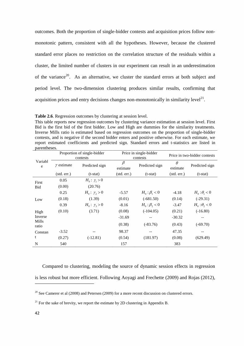
42
outcomes. Both the proportion of single-bidder contests and acquisition prices follow non-
monotonic pattern, consistent with all the hypotheses. However, because the clustered
standard error places no restriction on the correlation structure of the residuals within a
cluster, the limited number of clusters in our experiment can result in an underestimation
of the variance20
. As an alternative, we cluster the standard errors at both subject and
period level. The two-dimension clustering produces similar results, confirming that
acquisition prices and entry decisions changes non-monotonically in similarity level21
.
Table 2.6. Regression outcomes by clustering at session level.
This table reports new regression outcomes by clustering variance estimation at session level. First
Bid is the first bid of the first bidder. Low and High are dummies for the similarity treatments.
Inverse Mills ratio is estimated based on regression outcomes on the proportion of single-bidder
contests, and is negative if the second bidder enters and positive otherwise. For each estimate, we
report estimated coefficients and predicted sign. Standard errors and t-statistics are listed in
parentheses.
Variabl
e
Proportion of single-bidder
contests
Price in single-bidder
contests Price in two-bidder contests
estimate Predicted sign
estimate Predicted sign
estimate
Predicted sign
(std. err.) (t-stat) (std. err.) (t-stat) (std. err.) (t-stat)
First
Bid
0.05 0 1: 0H
(0.00) (20.76)
Low
0.25 0 2: 0H -5.57 0 1: 0H -4.18 0 1: 0H
(0.18) (1.39) (0.01) (-681.50) (0.14) (-29.31)
High
0.39 0 3: 0H -8.16 20 : 0H -3.47 20 : 0H
(0.10) (3.71) (0.08) (-104.05) (0.21) (-16.80)
Inverse
Mills
ratio
-31.69 -- -30.32 --
(0.38) (-83.76) (0.43) (-69.70)
Constan
t
-3.52 -- 98.37 -- 47.35 --
(0.27) (-12.81) (0.54) (181.97) (0.08) (629.49)
N 540
157
383
Compared to clustering, modeling the source of dynamic session effects in regression
is less robust but more efficient. Following Aoyagi and Frechette (2009) and Rojas (2012),
20 See Camerer et al (2008) and Petersen (2009) for a more recent discussion on clustered errors.
21 For the sake of brevity, we report the estimate by 2D clustering in Appendix B.
43
we modify previous regression in several ways to capture the characteristics of dynamic
session effects. The first modification is to assume the individual random effect jη follow
an independent normal distribution ( , )jN . j is equal to the entry choice of second
bidder j in the first round of each similarity treatment, which serves as a proxy for bidder
j ’s tendency to enter. and are common parameters across subjects, and can be
estimated from the data. Similarly, ijν and 'ijν follow independent normal distribution
( , )v ij vN and ( ' ', ')v ij vN , respectively. ij ( 'ij ) is set to be equal to the first
acquisition price in single-bidder contests (two-bidder contests) in a paired bidder group in
each similarity treatment. This specification is introduced to deal with the initial-conditions
problem (Chamberlain, 1980; Heckman, 1981; Wooldridge, 2002). Moreover, we add two
variables, namely Successful entry in previous round, and Successful first bid in previous
round, to reflect the idea that previous successful experience can influence consequent
decision-making. Variable Period is introduced to see whether there is evolution of
bidding outcomes over time, and variable First Round is added to check what’s in common
in subjects’ first action.
New estimates are presented in Table 2.7. Most of our findings remain under the new
specification, except that 2θ becomes insignificantly positive. Considering the predicted
difference in acquisition prices in two-bidder contests is very small between intermediate
and high similarity treatment22
, this estimate of 2θ can still be viewed as consistent with
model prediction.
22 The predicted price in two-bidder contests in intermediate treatment is 54, while it is 53 for high treatment.
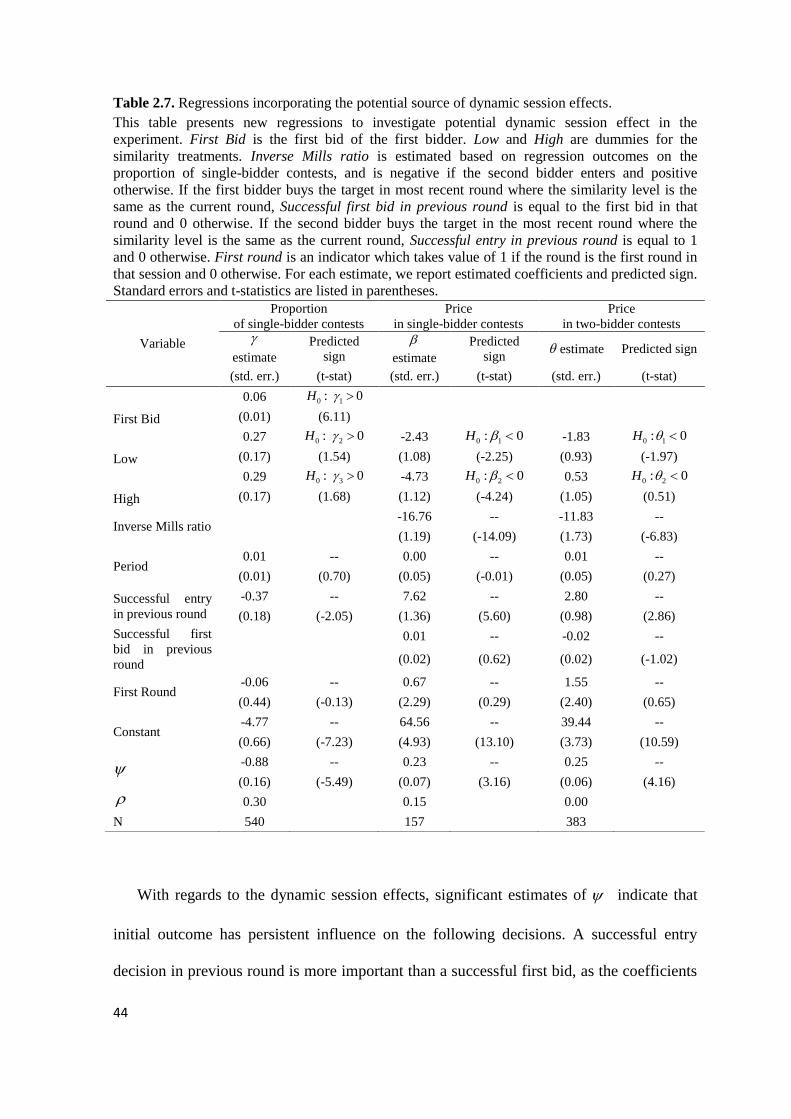
44
With regards to the dynamic session effects, significant estimates of indicate that
initial outcome has persistent influence on the following decisions. A successful entry
decision in previous round is more important than a successful first bid, as the coefficients
Table 2.7. Regressions incorporating the potential source of dynamic session effects.
This table presents new regressions to investigate potential dynamic session effect in the
experiment. First Bid is the first bid of the first bidder. Low and High are dummies for the
similarity treatments. Inverse Mills ratio is estimated based on regression outcomes on the
proportion of single-bidder contests, and is negative if the second bidder enters and positive
otherwise. If the first bidder buys the target in most recent round where the similarity level is the
same as the current round, Successful first bid in previous round is equal to the first bid in that
round and 0 otherwise. If the second bidder buys the target in the most recent round where the
similarity level is the same as the current round, Successful entry in previous round is equal to 1
and 0 otherwise. First round is an indicator which takes value of 1 if the round is the first round in
that session and 0 otherwise. For each estimate, we report estimated coefficients and predicted sign.
Standard errors and t-statistics are listed in parentheses.
Variable
Proportion
of single-bidder contests
Price
in single-bidder contests
Price
in two-bidder contests
estimate
Predicted
sign
estimate
Predicted
sign estimate Predicted sign
(std. err.) (t-stat) (std. err.) (t-stat) (std. err.) (t-stat)
First Bid
0.06 0 1: 0H
(0.01) (6.11)
Low
0.27 0 2: 0H -2.43 0 1: 0H -1.83 0 1: 0H
(0.17) (1.54) (1.08) (-2.25) (0.93) (-1.97)
High
0.29 0 3: 0H -4.73 20 : 0H 0.53 20 : 0H
(0.17) (1.68) (1.12) (-4.24) (1.05) (0.51)
Inverse Mills ratio -16.76 -- -11.83 --
(1.19) (-14.09) (1.73) (-6.83)
Period 0.01 -- 0.00 -- 0.01 --
(0.01) (0.70) (0.05) (-0.01) (0.05) (0.27)
Successful entry
in previous round
-0.37 -- 7.62 -- 2.80 --
(0.18) (-2.05) (1.36) (5.60) (0.98) (2.86)
Successful first
bid in previous
round
0.01 -- -0.02 --
(0.02) (0.62) (0.02) (-1.02)
First Round -0.06 -- 0.67 -- 1.55 --
(0.44) (-0.13) (2.29) (0.29) (2.40) (0.65)
Constant -4.77 -- 64.56 -- 39.44 --
(0.66) (-7.23) (4.93) (13.10) (3.73) (10.59)
-0.88 -- 0.23 -- 0.25 --
(0.16) (-5.49) (0.07) (3.16) (0.06) (4.16)
0.30
0.15
0.00
N 540
157
383
45
of the former are all significant while the coefficients of the later are not significant at all.
Evolution of bidding over time is not supported as all of the coefficients of Period are not
significant. In addition, insignificant coefficients of First Round suggest that bidders do not
behave differently in the first round from what they do in other rounds.
In sum, the new estimates in Table 2.7 indicate the existence of dynamic session effects,
and the hypotheses of non-monotonic entry and bidding cannot be rejected after controlling
for dynamic session effects.
2.7. Conclusions
This paper has shown that interdependence (or similarity) in bidders’ private valuations has
significant effects on the strategies and outcomes in sequential-entry takeover contests.
With interdependent valuations, the initial bid not only conveys information about the first
bidder’s valuation but also about other potential bidders’ valuations. Besides this
information externality, similarity levels indicate the intensity of bidding competition if
both bidders enter the contest. The information externality and the intensity of competition
determine the chances of preemption and equilibrium acquisition prices. Our theory for
takeover contests predicts that the information externality effect dominates at low levels of
similarity and the competition effect dominates at high levels of similarly. The interplay of
these two forces generates a non-monotonic effect of similarity: the proportion of multiple-
bidder versus single-bidder contests and the level of acquisition prices are the highest at
intermediate levels of similarity.
To verify whether these predictions hold, we carried out a controlled laboratory
experiment. Subjects participated in three treatments that differed in the level of
interdependence between valuations. The comparative statics prediction with respect to the

46
proportion of single-bidder contests and acquisition prices are strongly supported by the
data, indicating that subjects reacted strategically to the effects of information externality
and competition intensity in the way predicted by our model. Our findings on the
differences between takeover contests with different similarity levels between bidders can
be summarized as follows. Contests between dissimilar potential acquirers (e.g., a strategic
bidder against a financial bidder) have low prices and are relatively often single-bidder
contests. Contests between intermediately similar bidders (e.g., two strategic bidders)
generate high prices and are frequently competitive with two bidders placing bids. Contests
in which potential acquirers are very similar (e.g., two financial bidders) have low prices
and are seldom with more than one bidder.
In conclusion, this paper reveals a strong influence of bidders’ similarity on takeover
strategies. The theory and the experiment imply that, in addition to the number of bidders,
the similarity in bidders’ characteristics is an important measure of competition intensity
which should be accounted for in empirical studies of returns in takeovers.
47
Appendix 2.A. Proofs
Proof of Lemma 1: Taking the derivative of (10) with respect to Av we obtain
0 0
0 0
( ) 1 Φ( ) 1 (Φ( ) Φ( ))
1 Φ( ) (Φ( ) Φ( )) 1 Φ( ) 0.
A A
A A
b v z ρ z z
z z z z
(12)
In the first inequality we use that 0Az z and 0.ρ □
Proof of Lemma 2: Let : ( , ) 0v v W v . We will show that v is unique if it exists.
By (11) ( , ) 0W v is equivalent to
( , , ,1) ( ) 0.B A B A A
v
E π v v b f v dv
(13)
Note that ( , , ,1)B A BE π v v b (given in (4)) is negative for large Av ,
[ ( , , ,1)] 0B B BE π v b c . Since ( )Af v is always positive, ( , , ,1)B A BE π v v b must be
positive for some ,Av v for the root v in (13) to exist. Because ( , , ,1)B A BE π v v b is
decreasing in Av :
2
2
|
[ ( , , ,1)]1 ( ) 1 Φ( ) ( )
(1 )1 Φ( ) 1 0,
B A B AA A A A A
A A
A
B A
E π v v b dzσ ρ z f z z z f z
v dv
ρσ ρ z
σ
it must be then that
[ ( , , ,1)] 0.B BE π v v b (14)

48
Suppose now that v exists so that (14) holds. Then the derivative of ( , )W v with
respect to v evaluated at v is negative:
2
( ) ( )( , ) ( , , ,1) ( ) ( , , ,1)
1 ( )1 ( )
( )( , ) ( , , ,1)
1 ( )
( )( , , ,1)
1 ( )
0.
B A B A A B Bv v
v
B B
B B
d f v f vW v E π v v b f v dv E π v v b
dv F vF v
f vW v E π v v b
F v
f vE π v v b
F v
Since ( , )W v is a continuous function, it follows that it must have at most one root.
Therefore the solution to ( , ) 0W v is unique if it exists. □
Proof of Lemma 3: We will use the following integrals for some constants m , n , and h :
Φ( ) Φ( )( ) ( ) ,
2
Φ( ) ( ) Φ( ) Φ( ) ( )Φ( ) ( )Φ( ),2
n
m
n
m
Hn Hmhx x dx
H π
hx hx x dx Hn Hm m hm n hm
H π
(15)
where 21H h . Then
2
1( , ) [ ( , , ,1)] ( )
( ) ( )
11 ( ) (1 Φ( )) ( )
( ) ( )
(Φ( ) Φ( )) ( )(1 Φ( )) ( )(1 Φ( )) ,Φ( ) Φ( ) 2
v
B A B A A A
A A v
v
A A A B A A A
A A v
B
W v v E π v v b f v dvF v F v
σ ρ z z z c f v dvF v F v
σ σρ HHy H y y hy y hy c
y y h π
(16)
49
where 0( ) /y v v σ , 0( ) /y v v σ , 2(1 ) / 1h ρ ρ and 21H h . In the second
line of (16) we use (4) and the third line follows from (15).
If bidder A’s valuation is above 0v , then bidder B’s expected payoff from entering is
equal to
0
1( , ) 2(1 ) (1 ) .
2BW v σ ρ σ ρ c
π
The expression follows from (16). Bidder B does not enter if 0( , ) 0W v . Solving this
quadratic inequality for ρ , yields 1ρ and 2ρ given in the proposition. They exist and are
distinct under the assumption that 2 1R . □
Proof of the non-monotonic shape of Lv in ρ : We show that Lv increases in ρ at low ρ
and decreases in ρ at high .ρ Since Lv is defined by ( , ) 0,LW v we have that
/ / /L Ldv dρ W ρ W v . As shown in the proof of Lemma 2, / LW v is negative,
so /Ldv dρ has the same sign as /W ρ . Differentiating (16), we obtain
( , )
1 Φ( ) ( ) 1 Φ( )1 Φ( ) 2 2
LL L L
L
W v σ HHy y hy
ρ y h π
, (17)
where 0( ) /L Ly v v σ .
Suppose first that 1 0ρ . Then the lowest ρ that supports preemption is 1ρ . At 1ρ ρ ,
0Lv v and so 0Ly . We have

50
1
10
1
2(1 ) 1( , )0.
2 2(1 )ρ ρ
ρW v σ
ρ π ρ
The inequality holds because 1 0.5ρ and thus 12(1 )ρ >1.
Suppose next that 1 0ρ . Then preemption is possible at 0ρ . At 0ρ , 0Lv v and
so 0Lv . When 0ρ , 1h and 2H , and (17) becomes
0
( , ) 1( ) 1 Φ( ) 1 Φ( 2 )
1 Φ( ) 2
LL L L
Lρ
W v σy y y
ρ y π
.
which has the same sign as ( )LG y , where
1( ) ( ) 1 Φ( ) 1 Φ( 2 )
2L L L LG y y y y
π .
Because 0Ly ,
2( 2 )
'( ) ( ) 1 Φ( ) ( ) ( ) 1 Φ( ) 02
L L L L L L L L
yG y y y y y y y y
π
.
In addition, (0) 1/ (2 2 ) 1/ (4 ) 0G π π and ( ) 0G . It follows that the sign of
function ( )LG y is always positive, which means that 0/ |ρW ρ is positive. The signs of
the derivatives at 1ρ ρ (if 1 0ρ ) and 0ρ (if 1 0ρ ) show that the preemptive value
first increases in similarity level.
The highest ρ that supports preemption is 2ρ . At 2ρ ρ ,
51
2
20
2
2(1 ) 1( , )0.
2 2(1 )ρ ρ
ρW v σ
ρ π ρ
The sign is negative because 12(1 )ρ >1. This shows that the preemptive value Lv
decreases in ρ at high ρ .
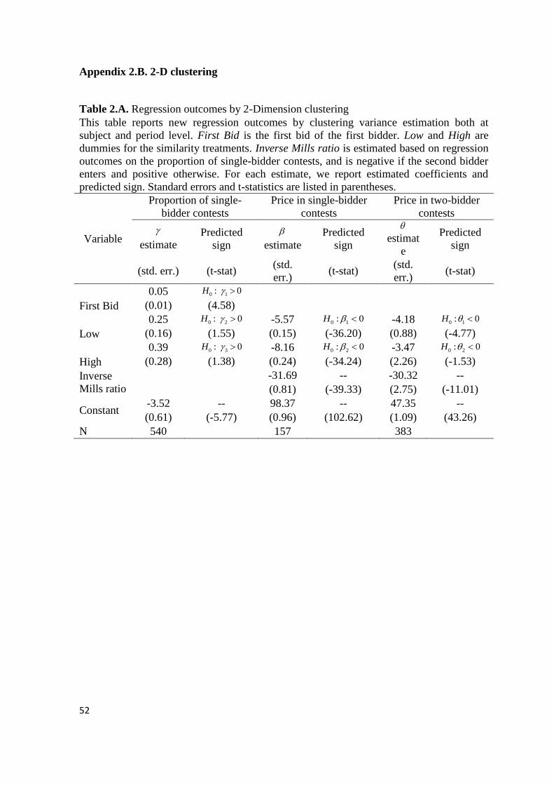
52
Appendix 2.B. 2-D clustering
Table 2.A. Regression outcomes by 2-Dimension clustering
This table reports new regression outcomes by clustering variance estimation both at
subject and period level. First Bid is the first bid of the first bidder. Low and High are
dummies for the similarity treatments. Inverse Mills ratio is estimated based on regression
outcomes on the proportion of single-bidder contests, and is negative if the second bidder
enters and positive otherwise. For each estimate, we report estimated coefficients and
predicted sign. Standard errors and t-statistics are listed in parentheses.
Variable
Proportion of single-
bidder contests
Price in single-bidder
contests
Price in two-bidder
contests
estimate Predicted
sign
estimate
Predicted
sign
estimat
e
Predicted
sign
(std. err.) (t-stat) (std.
err.) (t-stat)
(std.
err.) (t-stat)
First Bid
0.05 0 1: 0H
(0.01) (4.58)
Low
0.25 0 2: 0H -5.57 0 1: 0H -4.18 0 1: 0H
(0.16) (1.55) (0.15) (-36.20) (0.88) (-4.77)
High
0.39 0 3: 0H -8.16 20 : 0H -3.47 20 : 0H
(0.28) (1.38) (0.24) (-34.24) (2.26) (-1.53)
Inverse
Mills ratio
-31.69 -- -30.32 --
(0.81) (-39.33) (2.75) (-11.01)
Constant -3.52 -- 98.37 -- 47.35 --
(0.61) (-5.77) (0.96) (102.62) (1.09) (43.26)
N 540
157
383
53
Chapter 3
The Learning Effect in Takeovers with Toeholds23
3.1. Introduction
In corporate takeovers, “toeholds” refer to the ownership of target’s shares before initiating
a takeover. Theoretically, the acquisition of a toehold in a target can grant its owner several
advantages in acquiring full control. It can mitigate the free-rider problem24
(Shleifer and
Vishny, 1986); it signals the acquirer’s valuation and facilitates the efficient allocation of
targets to acquirers owning high value of the targets (Hirshleifer and Titman, 1990); it
increases the probability of the owner of a toehold stake winning a takeover contest even
when competing with a stronger rival bidder (Burkart 1995, and Singh 1998); and, in
23 This draft is based on Dai, Gryglewicz, and Smit (2013).
24 Free-rider problem was firstly discussed in Grossman and Hart (1980). Given a tender offer, the target’s
shareholders must balance between two possible payoffs – one is what they can gain by selling their shares to
an acquirer, the other is to enjoy the post-takeover synergy if the tender offer is accepted by the majority. As
every shareholder wants to free-ride the synergy value created by a successful takeover, the tender offer will
only be accepted when it offers the whole synergy value, which is likely to make takeovers unprofitable for
acquirers.

54
common value auctions, it also enables toehold-owners to win auctions cheaply because of
their information advantage and their potential position as sellers (Bulow et al., 1999).
Probably due to a combination of these benefits, the toehold acquisition strategy was
popular in the early 1980s, when over 60% of tender offers were acquired via toehold
strategies. However, the proportion of toehold strategies to total acquisitions has decreased
rapidly over time to below 10% in the past decade (Betton et al., 2009a). The declining
popularity and scare adoption of the strategy in the market for corporate control contradicts
sharply with its attractive merits as noted in takeover literature. This constitutes a “toehold
puzzle”: If the use of toeholds improves acquisition performance, why do fewer acquirers
buy them?
The current literature on the toehold puzzle provides several alternative
explanations for the infrequent adoption of staged toehold strategies. Chowdhry and
Jegadeesh (1994) view toeholds as a signal of acquirers’ value and show that it is not
optimal for “low value” acquirers to purchase toeholds, while Ravid and Spiegel (1999)
show that market liquidity and merger legislation decrease toehold bids. The decision to
acquire a toehold can be greatly affected by its information externality (Bris, 2002;
Goldman and Qian, 2005), and Betton et al. (2009a) focus on merger negotiation processes,
and show toeholds can only be effective when their sizes exceed certain thresholds. The
contribution of this paper to these studies is the detection of learning in the evolution of
efficiency in toehold strategies, which adds a new and truly dynamic perspective to the
existing explanations to the toehold puzzle.
In our proposed learning explanation, toehold owners need to posses certain
qualifications to achieve a better outcome from a toehold strategy. If it is the case,
acquirers can be categorized into two types: “qualified” bidders, who can use toeholds to

55
their benefit, and “unqualified” bidders, who cannot benefit from such strategies. Because
of its public context, 25 and its similarity to sunk costs, toeholds in the hands of the
“unqualified” bidders can lead to acquisition pitfalls such as over-commitment or
escalation errors26. After their initial investment, managers can become insensitive to new
inflows of bad news (Haunschild et al., 1994) or may deliberately stick to bad investments
to hinder their release of private information about their human capital (Kanodia et al.,
1989). If pitfalls associated with the execution of a toehold strategy become increasingly
understood by market participants, acquirers will walk away from toehold strategies to
avoid their adverse impacts: only “qualified” acquirers, with high levels of rationality or
whose decisions are well-monitored, will stay. So, by mitigating these pitfalls and
increasing the efficiency, self-selection gradually improves, resulting in a declining
proportion of toehold strategies being adopted, but – at the same time – in their increasing
performance over time.
Testing the dynamic learning hypothesis of the toehold puzzle calls for detailed
investigation of 1) the evolution of toehold performance over time and 2) self-selection of
the qualified acquirers. First, we look into four measures to analyze toehold performance:
the return to acquirers, the acquisition premium, the combined return, and the completion
rate – in aiming to provide a thorough description of a toehold’s role in the success of
mergers and acquisitions. We divide our sample into two periods to see whether toehold
strategies perform consistently overtime. Our results confirm that toeholds are not always
25 Under the 1968 Williams Act, toehold acquisitions that exceed 5% threshold are required for mandatory
disclosure. The 1976 Hart-Scott-Radino Antitrust Improvements Act also requires that share purchases over a
certain threshold trigger notification to the anti-trust agency.
26 For general discussion about how sunk cost can result in over-commitment or escalation errors, refer to
Staw (1976), Thaler (1980), Laughhunn and Payne (1984), Arkes and Blumer (1985), and Staw and Ross
(1986).

56
beneficial to acquirers – and in fact can work against the interest of their owners, by
lowering their return, leading them to select worse targets, and decreasing the completion
rate of deals. However, as time passes by, we find that toehold strategies perform better in
all four measures, implying an improvement in their efficiency over time. The adverse
impact of toehold strategies in all aspects in the early period seems to disappear in the later
period.
Second, we propose an improved self-selection procedure – which we refer to as a
“learning effect” – as a possible explanation of the co-existence of declining popularity and
efficiency improvement of toehold strategies. We use the Heckman two-step estimation
process to confirm that such self-selection is an important factor in determining toehold
strategies’ performance, but also that their efficiency improved over time, which is
consistent with our learning hypothesis. To identify which forces contribute to learning
about toehold strategies, we use monitoring strength – proxy by institutional holdings – to
separate the market-wide improvement of toehold performance and the efficiency
improvements associated with high-quality acquirers. Our regression results show that
acquirers’ quality is a better explanation, and also identifies qualified acquirers as those
with better monitoring.
The rest of this paper is organized as follows. Section 3.2 describes our sample
construction, deal characteristics and efficiency measures in our data. Section 3.3 reports
separate regression results on four efficiency measures and identifies a time pattern in the
toehold performance. Section 3.4 divides the sample into two sub-samples to verify the
existence of a learning effect in toeholds’ performance with self-selection models. Section
3.5 checks whether monitoring can explain this learning effect. Section 3.6 performs
robustness check and section 3.7 concludes.
57
3.2. Data description
3.2.1. Sample construction
To construct our sample, we begin with all the Mergers and Acquisitions announced by US
public acquirers for US public targets between 1990 and 200627
extracted from the
Security Data Corporation (SDC) database. We require all bids to be aimed at obtaining
major control of a target, so acquirers are restricted to those who own less than 50% of the
target’s shares before the takeover and intend to gain control (i.e., have more than 50%)
after the transaction. Financial acquirers and financial targets are removed, so that
measurements of combined returns28
are comparable across all takeovers. Special
transactions marked as spinoffs, exchange offers, self-tenders, repurchases,
recapitalizations, acquisitions of remaining interest, minority stake purchases, and
privatizations are excluded, and we delete all the deals announced as rumors. We also
require data about both targets and acquirers to be available from the Center for Research
in Security Prices (CRSP), to insure takeover performance is measurable. To make sure the
transactions have substantial impact on acquirers’ performance, targets are required to have
a market valuation no less than 5% of that of acquirers 42 days before announcement date.
Meeting all these requirements resulted in a sample of 2118 bids.
27 In mid-1980s, the widespread adoption of takeover defenses such as ‘poison pill’ tactics led to a decline in
hostile takeovers, where toehold is much more common in hostile takeovers than in friendly takeovers.
(Betton et al., 2008). To leave this structural change out of our sample, we only collected deals from 1990
onwards.
28 Combined returns can serve as a measure of the synergy created by merging target and acquirer if both
parties are operating firms, but the meaning of combined return in cases where a financial firm acquires an
operating target is not clear, as financial acquirers usually focus on a target’s financial aspects, aiming to
benefit from higher prices when exiting via IPO, or by selling the target to second buyer, i.e. synergy value is
not a major motivation for financial acquirers initiating a takeover.
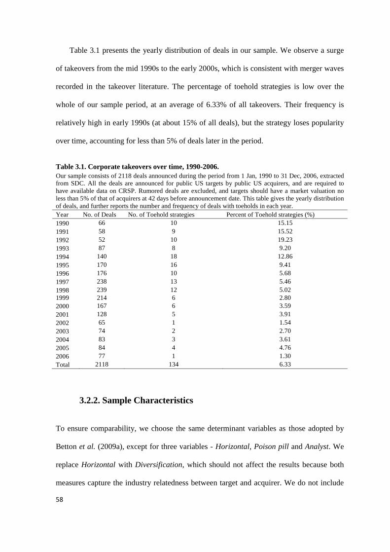
58
Table 3.1 presents the yearly distribution of deals in our sample. We observe a surge
of takeovers from the mid 1990s to the early 2000s, which is consistent with merger waves
recorded in the takeover literature. The percentage of toehold strategies is low over the
whole of our sample period, at an average of 6.33% of all takeovers. Their frequency is
relatively high in early 1990s (at about 15% of all deals), but the strategy loses popularity
over time, accounting for less than 5% of deals later in the period.
Table 3.1. Corporate takeovers over time, 1990-2006.
Our sample consists of 2118 deals announced during the period from 1 Jan, 1990 to 31 Dec, 2006, extracted
from SDC. All the deals are announced for public US targets by public US acquirers, and are required to
have available data on CRSP. Rumored deals are excluded, and targets should have a market valuation no
less than 5% of that of acquirers at 42 days before announcement date. This table gives the yearly distribution
of deals, and further reports the number and frequency of deals with toeholds in each year.
Year No. of Deals No. of Toehold strategies Percent of Toehold strategies (%)
1990 66 10 15.15
1991 58 9 15.52
1992 52 10 19.23
1993 87 8 9.20
1994 140 18 12.86
1995 170 16 9.41
1996 176 10 5.68
1997 238 13 5.46
1998 239 12 5.02
1999 214 6 2.80
2000 167 6 3.59
2001 128 5 3.91
2002 65 1 1.54
2003 74 2 2.70
2004 83 3 3.61
2005 84 4 4.76
2006 77 1 1.30
Total 2118 134 6.33
3.2.2. Sample Characteristics
To ensure comparability, we choose the same determinant variables as those adopted by
Betton et al. (2009a), except for three variables - Horizontal, Poison pill and Analyst. We
replace Horizontal with Diversification, which should not affect the results because both
measures capture the industry relatedness between target and acquirer. We do not include
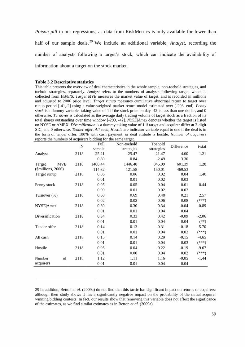
59
Poison pill in our regressions, as data from RiskMetrics is only available for fewer than
half of our sample deals.29
We include an additional variable, Analyst, recording the
number of analysts following a target’s stock, which can indicate the availability of
information about a target on the stock market.
Table 3.2 Descriptive statistics This table presents the overview of deal characteristics in the whole sample, non-toehold strategies, and
toehold strategies, separately. Analyst refers to the numbers of analysts following target, which is
collected from I/B/E/S. Target MVE measures the market value of target, and is recorded in millions
and adjusted to 2006 price level. Target runup measures cumulative abnormal return to target over
runup period [-41,-2] using a value-weighted market return model estimated over [-293, end]. Penny
stock is a dummy variable, taking value of 1 if the stock price on day -42 is less than one dollar, and 0
otherwise. Turnover is calculated as the average daily trading volume of target stock as a fraction of its
total shares outstanding over time window [-293, -42]. NYSE|Amex denotes whether the target is listed
on NYSE or AMEX. Diversification is a dummy taking value of 1 if target and acquirer differ at 2-digit
SIC, and 0 otherwise. Tender offer, All cash, Hostile are indicator variable equal to one if the deal is in
the form of tender offer, 100% with cash payment, or deal attitude is hostile. Number of acquirers
reports the numbers of acquirers bidding for the same target.
N
Full
sample
Non-toehold
strategies
Toehold
strategies Difference t-stat
Analyst 2118 25.21 25.47 21.47 4.00 1.21
0.80 0.84 2.49 3.30
Target MVE
($millions, 2006)
2118 1408.44 1446.48 845.09 601.39 1.28
114.32 121.58 150.01 469.53
Target runup 2118 0.06 0.06 0.02 0.04 1.40
0.01 0.01 0.02 0.03
Penny stock 2118 0.05 0.05 0.04 0.01 0.44
0.00 0.01 0.02 0.02
Turnover (%) 2118 0.68 0.69 0.48 0.21 2.57
0.02 0.02 0.06 0.08 (***)
NYSE|Amex 2118 0.30 0.30 0.34 -0.04 -0.89
0.01 0.01 0.04 0.04
Diversification 2118 0.34 0.33 0.42 -0.09 -2.06
0.01 0.01 0.04 0.04 (**)
Tender offer 2118 0.14 0.13 0.31 -0.18 -5.70
0.01 0.01 0.04 0.03 (***)
All cash 2118 0.15 0.14 0.29 -0.15 -4.65
0.01 0.01 0.04 0.03 (***)
Hostile 2118 0.05 0.04 0.22 -0.19 -9.67
0.01 0.00 0.04 0.02 (***)
Number of
acquirers
2118 1.12 1.11 1.16 -0.05 -1.44
0.01 0.01 0.04 0.04
29 In addition, Betton et al. (2009a) do not find that this tactic has significant impact on returns to acquirers:
although their study shows it has a significantly negative impact on the probability of the initial acquirer
winning bidding contests. In fact, our results show that removing this variable does not affect the significance
of the estimates, as we find similar estimates as in Betton et al. (2009a).
60
Table 3.2 provides an overview of the deal characteristics of the full sample of non-
toehold and acquisitions with toeholds separately. There are about 25 analysts (on average)
following stock activity in targets taken over by acquirers without using toehold strategies,
slightly more than in acquisitions following toeholds (21 analysts on average). The average
target size is larger for acquisitions without toeholds, about US$1,446m (at 2006 values),
but only US$ 845m for targets acquired using toeholds. Cumulative abnormal return to the
targets over the run-up period [-41, -2] are higher for non-toeholds than for acquisitions
with toeholds (0.06 compared to 0.02), and average daily turnovers of target shares before
takeovers without toeholds is 0.69%, which is significantly higher than for takeovers with
toeholds (with an average turnover is 0.48%). Other liquidity measures of target stocks,
such as whether they are ‘‘penny stocks’ (i.e., priced at less than $1), and whether they are
listed on major exchanges (such as NYSE and Amex) seem not to differ across takeover
types. About 42% of takeovers using toeholds are cross-industry, but only 33% of
takeovers without toeholds are for diversification purposes. Acquirers buying with
toeholds are more likely to place their bids in the form of tender offers, and pay 100% in
cash. Toehold strategies are also more frequently associated with hostile takeovers.
Twenty-two percent of the takeovers with toeholds are hostile, while the figure is only four
percent for takeovers without toeholds. Finally, most of the takeovers in our sample are
single bidder contests: the proportions of multiple acquirers are low for both takeovers
with or without toeholds. In general, based on significance, we find toehold strategies are
commonly used for acquiring targets of lower turnover, more frequently for diversification
purposes, in the form of tender offers, with 100% cash payment, and with hostile attitudes.
61
3.2.3. Takeover efficiency measures
We explore takeover efficiency using four measures: returns to acquirers, acquisition
premiums, combined returns to target and acquirer, and completion rates. The first two
measures aim to evaluate acquirers’ benefits and costs in takeovers; combined returns
serves as measures of the synergy created by takeovers, and also reflects acquirers’ ability
for select targets; completion rate, checks whether adopting a toehold strategy can help an
acquirer win a takeover contest.
In particular, we measure returns by cumulative abnormal returns over total contest
window [-41, end], where the end date is defined as the earlier of the bid’s effective date
and the target stock delisting date, plus 126 trading days. The total contest window can be
further divided into three event periods - the run-up period [-41,-2]; the announcement
period [-1, 1]; and the post-announcement period [2, end]. We estimate daily abnormal
returns, jkAR , for each event period, by the method described in Betton et al. (2008).
enddaytdARrr jt
K
k
ktjkmtjjjt ,...,293,1
where jtr is the excess return to firm j at day t ; mtr is the value-weighted market return
adjusted by risk-free rate; and ktd is a dummy variable that takes a value of one if day t is
in the kth event window and zero otherwise. Stock returns are obtained from CRSP, and
market return and risk-free rates from the Fama French & Liquidity Factor provided by
Wharton Research Data Services (WRDS). To be included in the sample, a firm should
have at least 100 return observations over the whole event window. Our estimation method
applies ordinary least squares with White’s heteroskedastic-consistent covariance matrix.
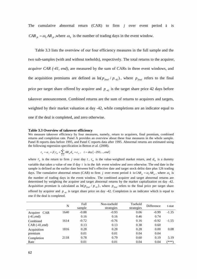
62
The cumulative abnormal return (CAR) to firm j over event period k is
jkkjk ARCAR ,where k is the number of trading days in the event window.
Table 3.3 lists the overview of our four efficiency measures in the full sample and the
two sub-samples (with and without toeholds), respectively. The total returns to the acquirer,
acquirer CAR (-41, end), are measured by the sum of CARs in three event windows, and
the acquisition premiums are defined as 42ln( / )finalp p
, where finalp refers to the final
price per target share offered by acquirer and 42p is the target share price 42 days before
takeover announcement. Combined returns are the sum of returns to acquirers and targets,
weighted by their market valuation at day -42, while completions are an indicator equal to
one if the deal is completed, and zero otherwise.
Table 3.3 Overview of takeover efficiency We measure takeover efficiency by four measures, namely, return to acquirers, final premium, combined
returns and completion rate. Panel A provides an overview about these four measures in the whole sample.
Panel B reports data before 1995, and Panel C reports data after 1995. Abnormal returns are estimated using
the following regression specification in Betton et al. (2008).
1
, 293,...,K
jt j j mt jk kt jt
k
r r AR d t day end
where jtr is the return to firm j over day t , mtr is the value-weighted market return, and
ktd is a dummy
variable that takes a value of one if day t is in the kth event window and zero otherwise. The end date in the
sample is defined as the earlier date between bid’s effective date and target stock delist date plus 126 trading
days. The cumulative abnormal return (CAR) to firm j over event period k isjk k jk
CAR AR , where k is
the number of trading days in the event window. The combined acquirer and target abnormal returns are
determined by weighting the acquirer and target abnormal returns by the market capitalization on day -42.
Acquisition premium is calculated as 42ln( / )finalp p , where finalp refers to the final price per target share
offered by acquirer and 42p is target share price on day -42. Completion is an indicator which is equal to
one if the deal is completed.
N Full
sample
Non-toehold
strategies
Toehold
strategies Difference t-stat
Acquirer CAR
(-41,end)
1640 -0.88 -0.93 0.06 -0.99 -1.35
0.16 0.16 0.46 0.74
Combined
CAR (-41,end)
1614 -0.72 -0.76 0.16 -0.92 -1.55
0.13 0.13 0.38 0.60
Acquisition
premium
1816 0.28 0.28 0.28 0.00 0.08
0.01 0.01 0.04 0.04
Completion
Rate
2118 0.78 0.79 0.60 0.19 5.19
0.01 0.01 0.04 0.04 (***)
63
Over the whole sample, takeovers executed with the use of toeholds generate higher
returns to acquirers. Acquirer CARs (-41, end) are negative for takeovers executed without
toeholds, but positive for those with toeholds (-0.93 v.s. 0.06). Combined CARs (-41, end)
are negative for acquisition without toehold strategies, but positive in acquisitions with
toehold strategies (-0.76 compared to 0.16). Acquisition premiums are almost the same
(about 0.28) for both types of takeovers. Toehold strategies also have lower average
completion rates – at about 60% of deals, while about 79% of takeovers without toeholds
are completed. Although none of the differences are significant except for the completion
rate, this rough comparison shows the use of toehold strategies does not significant
enhance takeover efficiency: on the contrary, their adoption can be a clue of bad
performance, being associated, for instance, with lower completion rates.
3.3. Efficiency change in toehold strategies
Table 3.4 presents regression results on the four efficiency measures with three different
specifications. The first specification is the same as used in Betton et al. (2009a), where
year dummies are not included as explanatory variables. In the second specification, we
add year dummies into the regression to control for year effects, while in the third
specification, an interaction term, Toehold size*Time, is also added to see whether there is
a consistent time trend in toehold performance.
The first efficiency measure we investigate is cumulative abnormal returns to acquirer
during the event window [-41, end]. Without control for year effects, toehold strategies
seem to have no significant impact on acquirers’ returns, which are negatively correlated
with turnover rate of targets’ stocks, and higher if the target’s run-up is larger, its stock
price is less than one dollar, or it is listed on NYSE or Amex. In contrast, target size, daily
64
turnover of its stock, and takeovers with diversification purpose are associated with lower
returns: all these findings are consistent with those in Betton et al. (2009a). We also find
that the existence of multiple bidders leads to higher acquirer returns. However, since all
these estimates only concern completed deals, acquirers in the regression are actually
“winning acquirers” in takeover contests. Winning a takeover contest by defeating others
can be viewed as a strong market signal of acquirers’ competiveness, which explains why
the indicator of multiple acquirers has a positive coefficient on the acquirers’ returns.
The introduction of year dummies in the second specification does not change the
estimates much – they remain much as before, in terms of coefficient signs, magnitude and
significant levels. The only exceptions are that the coefficients for Toehold size and Tender
offer increase in significance levels to become significantly positive. This new evidence on
the positive influence of toehold size on acquirers’ return is significant, as the efficiency of
toehold is the focus of our paper. When controlling for year effects, toehold seems
beneficial to acquirers, bringing them higher abnormal returns. This change in significance
suggests that there is a time pattern in toehold performance, implying that ignoring it can
lead to inaccurate conclusions about toeholds’ impacts.
The addition of the estimation of Toehold size*Time in the third specification further
confirms the importance of time patterns in measuring the efficiency of toehold strategies.
The term has a coefficient of 0.006 at the 1% significance level, which shows that this time
pattern not only exists, but also follows a consistent trend. In the early sample period, the
use of toeholds has an adverse impact on acquirer’s return – as suggested by the
significantly negative coefficient of Toehold size (which is equal to -0.035) – but, as time
passes, the toehold strategy performs better and better. The positive coefficient of the
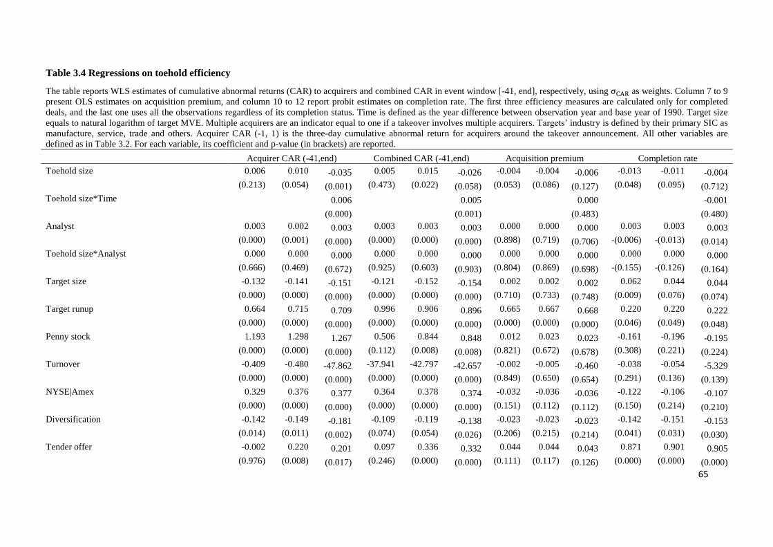
65
Table 3.4 Regressions on toehold efficiency
The table reports WLS estimates of cumulative abnormal returns (CAR) to acquirers and combined CAR in event window [-41, end], respectively, using as weights. Column 7 to 9
present OLS estimates on acquisition premium, and column 10 to 12 report probit estimates on completion rate. The first three efficiency measures are calculated only for completed
deals, and the last one uses all the observations regardless of its completion status. Time is defined as the year difference between observation year and base year of 1990. Target size
equals to natural logarithm of target MVE. Multiple acquirers are an indicator equal to one if a takeover involves multiple acquirers. Targets’ industry is defined by their primary SIC as
manufacture, service, trade and others. Acquirer CAR (-1, 1) is the three-day cumulative abnormal return for acquirers around the takeover announcement. All other variables are
defined as in Table 3.2. For each variable, its coefficient and p-value (in brackets) are reported.
Acquirer CAR (-41,end) Combined CAR (-41,end) Acquisition premium Completion rate
Toehold size 0.006 0.010 -0.035 0.005 0.015 -0.026 -0.004 -0.004 -0.006 -0.013 -0.011 -0.004
(0.213) (0.054) (0.001) (0.473) (0.022) (0.058) (0.053) (0.086) (0.127) (0.048) (0.095) (0.712)
Toehold size*Time 0.006 0.005 0.000 -0.001
(0.000) (0.001) (0.483) (0.480)
Analyst 0.003 0.002 0.003 0.003 0.003 0.003 0.000 0.000 0.000 0.003 0.003 0.003
(0.000) (0.001) (0.000) (0.000) (0.000) (0.000) (0.898) (0.719) (0.706) -(0.006) -(0.013) (0.014)
Toehold size*Analyst 0.000 0.000 0.000 0.000 0.000 0.000 0.000 0.000 0.000 0.000 0.000 0.000
(0.666) (0.469) (0.672) (0.925) (0.603) (0.903) (0.804) (0.869) (0.698) -(0.155) -(0.126) (0.164)
Target size -0.132 -0.141 -0.151 -0.121 -0.152 -0.154 0.002 0.002 0.002 0.062 0.044 0.044
(0.000) (0.000) (0.000) (0.000) (0.000) (0.000) (0.710) (0.733) (0.748) (0.009) (0.076) (0.074)
Target runup 0.664 0.715 0.709 0.996 0.906 0.896 0.665 0.667 0.668 0.220 0.220 0.222
(0.000) (0.000) (0.000) (0.000) (0.000) (0.000) (0.000) (0.000) (0.000) (0.046) (0.049) (0.048)
Penny stock 1.193 1.298 1.267 0.506 0.844 0.848 0.012 0.023 0.023 -0.161 -0.196 -0.195
(0.000) (0.000) (0.000) (0.112) (0.008) (0.008) (0.821) (0.672) (0.678) (0.308) (0.221) (0.224)
Turnover -0.409 -0.480 -47.862 -37.941 -42.797 -42.657 -0.002 -0.005 -0.460 -0.038 -0.054 -5.329
(0.000) (0.000) (0.000) (0.000) (0.000) (0.000) (0.849) (0.650) (0.654) (0.291) (0.136) (0.139)
NYSE|Amex 0.329 0.376 0.377 0.364 0.378 0.374 -0.032 -0.036 -0.036 -0.122 -0.106 -0.107
(0.000) (0.000) (0.000) (0.000) (0.000) (0.000) (0.151) (0.112) (0.112) (0.150) (0.214) (0.210)
Diversification -0.142 -0.149 -0.181 -0.109 -0.119 -0.138 -0.023 -0.023 -0.023 -0.142 -0.151 -0.153
(0.014) (0.011) (0.002) (0.074) (0.054) (0.026) (0.206) (0.215) (0.214) (0.041) (0.031) (0.030)
Tender offer -0.002 0.220 0.201 0.097 0.336 0.332 0.044 0.044 0.043 0.871 0.901 0.905
(0.976) (0.008) (0.017) (0.246) (0.000) (0.000) (0.111) (0.117) (0.126) (0.000) (0.000) (0.000)
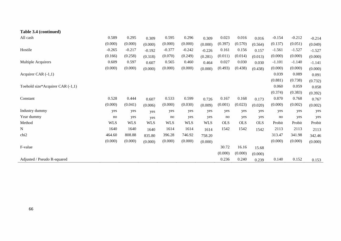
66
Table 3.4 (continued)
All cash 0.589 0.295 0.309 0.595 0.296 0.309 0.023 0.016 0.016 -0.154 -0.212 -0.214
(0.000) (0.000) (0.000) (0.000) (0.000) (0.000) (0.397) (0.570) (0.564) (0.137) (0.051) (0.049)
Hostile -0.265 -0.217 -0.192 -0.377 -0.242 -0.226 0.161 0.156 0.157 -1.561 -1.527 -1.527
(0.166) (0.258) (0.318) (0.070) (0.249) (0.281) (0.011) (0.014) (0.013) (0.000) (0.000) (0.000)
Multiple Acquirers 0.609 0.597 0.607 0.565 0.460 0.464 0.027 0.030 0.030 -1.101 -1.140 -1.141
(0.000) (0.000) (0.000) (0.000) (0.000) (0.000) (0.493) (0.438) (0.438) (0.000) (0.000) (0.000)
Acquirer CAR (-1,1)
0.039 0.089 0.091
(0.881) (0.738) (0.732)
Toehold size*Acquirer CAR (-1,1)
0.060 0.059 0.058
(0.374) (0.383) (0.392)
Constant 0.528 0.444 0.607 0.533 0.599 0.726 0.167 0.168 0.173 0.870 0.768 0.767
(0.000) (0.041) (0.006) (0.000) (0.030) (0.009) (0.001) (0.023) (0.020) (0.000) (0.002) (0.002)
Industry dummy yes yes yes yes yes yes yes yes yes yes yes yes
Year dummy no yes yes no yes yes no yes yes no yes yes
Method WLS WLS WLS WLS WLS WLS OLS OLS OLS Probit Probit Probit
N 1640 1640 1640 1614 1614 1614 1542 1542 1542 2113 2113 2113
chi2 464.60 808.88 835.80 396.28 746.92 758.20
313.47 341.98 342.46
(0.000) (0.000) (0.000) (0.000) (0.000) (0.000)
(0.000) (0.000) (0.000)
F-value
30.72 16.16 15.68
(0.000) (0.000) (0.000) Adjusted / Pseudo R-squared
0.236 0.240 0.239 0.140 0.152 0.153

67
interaction term between Toehold size and Time implies a yearly improvement of 17.14%
(=0.006/0.035), which is economically significant. In sum, the above finding suggests a
negative impact of the toehold strategy on acquirers’ return at the beginning of our sample
(year 1990) as the stand-alone Toehold size has a negative coefficient of -0.035. However,
at the end of sample period (year 2006), toehold acquisitions generate beneficial outcomes
to acquirers, with a positive impact of 0.057 (calculated as stand-alone toehold
performance + yearly change * time, -0.035+ 0.006*(2006-1990)).
While return to acquirers measures net benefits to acquirers, combined return can be
viewed as a measure of takeover synergy between target and acquirer. Columns 4 to 6 in
Table 3.4 present regressions in which the dependent variable is the combined return.
Without year dummies (Column 4), the link between toeholds and synergy value is weak
and insignificant. It becomes effective in identifying better targets and is positively
correlated with higher combined returns after introducing year dummies (Column 5).
Furthermore, the coefficient of Toehold size*Time in the regression in Column 6 again
confirms an upward trend in toehold performance: while toehold size alone is negative
correlated with combined returns, the interaction term loads a positive and significant
coefficient so that, as above, this upward yearly change results in positive impacts of
toeholds by the end of our sample period.
Next, we look at the effect of toeholds on acquisition premiums. The regression
excluding year effects in Column 7 reports a significantly negative impact of toehold size
on acquisition premium (as found in Betton et al., 2009a). This impact remains significant
after controlling for year effects in the second pooled regression, but after introducing the
interaction term between toehold size and time, estimates of this impact become

68
insignificant. The coefficient of Toehold size*Time is also indistinguishable from zero,
which shows the time pattern in acquisition premium is not as strong as in return measures.
The final efficiency measure of toehold strategies that we tested is the completion rate
of takeovers: we use a probit regression to estimate determinants of completion rates. As
Chen et al. (2007) suggested, acquirers can update their belief in targets’ quality with
perceived announcement CAR (i.e. CAR over announcement window [-1, 1]), which can
change their determination to complete a takeover deal. According to their argument,
higher announcement returns to acquirers reflect better market perceptions of such deals,
which are good signals of project quality. Witnessing market reaction during
announcement period, acquirers will re-evaluate their target selection and is likely to
withdraw from bad projects (i.e. those with low announcement return) and complete good
ones (i.e. those with high announcement return). To accommodate this information
updating, we introduce two additional determinants of completion rate (Acquirer CAR (-
1,1), and Toehold size * Acquirer CAR (-1,1)) in related regressions. The first variable is
the cumulative abnormal return to acquirers over the announcement window [-1, 1], and
tracks sensitivity of completion rate to deal quality, and the second is an interaction term
which records additional sensitivity of completion rate to deal quality when a toehold is
involved. If the toehold strategy facilitates the updating of information, the coefficient of
Toehold size * Acquirer CAR (-1,1) is expected to be positive.
The estimates in column 10 to 12 suggest a weak time pattern in completion rates. In
general, toeholds lower the probability of completing a deal: but this negative impact loses
its significance at the 5% significance level after introducing year dummies. The
coefficient of Toehold size*Acquirer CAR (-1,1) is not significant at all, which indicates

69
the use of a toehold strategy does not help acquirers to withdraw from bad takeover
projects.
The term Toehold size*Analyst is not significant in any estimate of the four efficiency
measures, which implies acquirers cannot use toeholds to compensate for the lack of
availability of information about targets on public market.
To summarize, we find that toehold strategies have time-varying impacts on takeover
performance. In particular, their efficiency in terms of enhancing acquirers’ returns and
success in choosing targets with higher synergistic value improves over time. However,
this improvement cannot be explained by better information or its updating during the
announcement period.
3.4. The learning effect with a self-selection model
As is shown in the previous section, toehold efficiency improves in generating higher
returns to acquirers and enabling them to select better targets over time, though the number
of acquirers who use toehold strategies is still declining at the same time. This
phenomenon is puzzling if we assume that acquirers are homogeneous with regards to their
ability to implement toehold strategies. Under that assumption, the improvement in the
efficiency of such strategies would apply to all acquirers, and the natural outcome of the
improving efficiency of toehold strategies should be an accompanying increase in their use.
However, empirical evidence points to a contradictory result – the co-existence of
improving toehold’s efficiency and their declining popularity. This indicates that the
impact of toeholds varies across different acquirers – i.e., acquirers are heterogeneous in
their ability to benefit from using toehold acquisition strategies.

70
To put this puzzle in a dynamic framework, the heterogeneity of acquirers and the
efficiency improvements in toehold’s performance suggest a self-selection process in
toehold strategy. Suppose there are two types of acquirers with respect to their ability to
use toeholds, qualified acquirers and unqualified acquirers. At first, if acquirers (especially
unqualified ones) are not conscious about the qualifications needed to produce favorable
outcomes with toeholds, both qualified and unqualified acquirers may buy toeholds,
attracted by their theoretical appeal. This would result in a pooling effect, where toeholds’
efficiency when used by qualified acquirers is moderated by the inefficiency generated by
their use by unqualified acquirers. Over time, it becomes clear that successful
implementation of toehold strategies requires certain qualities in acquirers, so unqualified
acquirers start to withdraw from using them, while qualified acquirers stick with them.
Gradually, this self-selection process transforms the pooled population of toehold bidders
into separate populations, where most toehold acquirers are qualified, which is reflected by
enhanced toehold performance in later periods. The learning effect of this self-selection
process successfully explains the co-existence of toehold strategies’ improving
performance and declining popularity.
3.4.1. Subsample division
As improving self-selection can be a possible explanation of improved efficiency
improvement in toehold performance, the next step is to check whether there is indeed a
difference in selection outcomes. To facilitate this comparison, we divide our sample into
two sub-samples, using year 1995 as the cutting point. The first sub-sample includes
observations prior to and including 1995, and the second all observations after 1995. 1995
was chosen as the cut-off point because the percentage of acquisitions using toehold
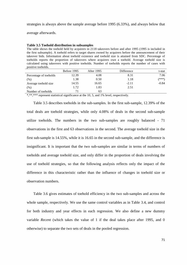
71
strategies is always above the sample average before 1995 (6.33%), and always below that
average afterwards.
Table 3.5 Toehold distribution in subsamples The table shows the toehold held by acquirers in 2118 takeovers before and after 1995 (1995 is included in
the first subsample). A toehold refers to target shares owned by acquirers before the announcement of their
takeover bids. Information about toehold existence and toehold size is attained from SDC. Percentage of
toeholds reports the proportion of takeovers where acquirers own a toehold. Average toehold size is
calculated using takeovers with positive toeholds. Number of toeholds reports the number of cases with
positive toeholds.
Before 1995 After 1995 Difference t-stat
Percentage of toeholds 12.39 4.08 8.31 7.06
(%) 1.38 0.50 1.18 (***)
Average toehold size 14.55 16.65 -2.11 -0.84
(%) 1.72 1.83 2.51
Number of toeholds 71 63
*,**,*** represent statistical significance at the 10, 5, and 1% level, respectively.
Table 3.5 describes toeholds in the sub-samples. In the first sub-sample, 12.39% of the
total deals are toehold strategies, while only 4.08% of deals in the second sub-sample
utilize toeholds. The numbers in the two sub-samples are roughly balanced - 71
observations in the first and 63 observations in the second. The average toehold size in the
first sub-sample is 14.55%, while it is 16.65 in the second sub-sample, and the difference is
insignificant. It is important that the two sub-samples are similar in terms of numbers of
toeholds and average toehold size, and only differ in the proportion of deals involving the
use of toehold strategies, so that the following analysis reflects only the impact of the
difference in this characteristic rather than the influence of changes in toehold size or
observation numbers.
Table 3.6 gives estimates of toehold efficiency in the two sub-samples and across the
whole sample, respectively. We use the same control variables as in Table 3.4, and control
for both industry and year effects in each regression. We also define a new dummy
variable Recent (which takes the value of 1 if the deal takes place after 1995, and 0
otherwise) to separate the two sets of deals in the pooled regression.
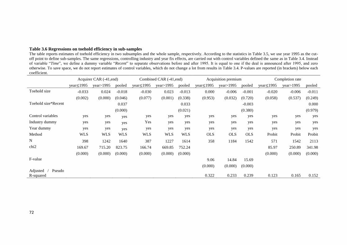
72
Table 3.6 Regressions on toehold efficiency in sub-samples The table reports estimates of toehold efficiency in two subsamples and the whole sample, respectively. According to the statistics in Table 3.5, we use year 1995 as the cut-
off point to define sub-samples. The same regressions, controlling industry and year fix effects, are carried out with control variables defined the same as in Table 3.4. Instead
of variable “Time”, we define a dummy variable “Recent” to separate observations before and after 1995. It is equal to one if the deal is announced after 1995, and zero
otherwise. To save space, we do not report estimates of control variables, which do not change a lot from results in Table 3.4. P-values are reported (in brackets) below each
coefficient.
Acquirer CAR (-41,end) Combined CAR (-41,end) Acquisition premium Completion rate
year 1995 year>1995 pooled year 1995 year>1995 pooled year 1995 year>1995 pooled year 1995 year>1995 pooled
Toehold size -0.033 0.024 -0.018 -0.030 0.023 -0.013 0.000 -0.006 -0.001 -0.020 -0.006 -0.011
(0.002) (0.000) (0.046) (0.077) (0.001) (0.338) (0.953) (0.032) (0.720) (0.058) (0.537) (0.249)
Toehold size*Recent
0.037
0.033
-0.003
0.000
(0.000)
(0.021)
(0.380)
(0.979)
Control variables yes yes yes yes yes yes yes yes yes yes yes yes
Industry dummy yes yes yes Yes yes yes yes yes yes yes yes yes
Year dummy yes yes yes yes yes yes yes yes yes yes yes yes
Method WLS WLS WLS WLS WLS WLS OLS OLS OLS Probit Probit Probit
N 398 1242 1640 387 1227 1614 358 1184 1542 571 1542 2113
chi2 169.67 715.20 823.75 166.74 669.85 752.24
85.97 250.89 341.98
(0.000) (0.000) (0.000) (0.000) (0.000) (0.000)
(0.000) (0.000) (0.000)
F-value
9.06 14.84 15.69
(0.000) (0.000) (0.000) Adjusted / Pseudo
R-squared
0.322 0.233 0.239 0.123 0.165 0.152
73
On the whole, we find the same efficiency improvements in toehold performance with
respect to both acquirer’s return and target quality. Before 1995, toehold strategies appear
to have adverse impacts in takeover outcomes, lowering acquirers’ benefits (with a
significantly negative coefficient of -0.033), and tending to be associated with the selection
of worse targets (its impact on combined return is negative and significant at 10% level).
But the situation changes after 1995: when toehold size is associated with higher returns to
acquirers and combined returns: both these effects are positive and highly significant at 1%
level. This efficient improvement is further confirmed by the coefficients of Toehold
size*Recent, which are significantly positive. Looking at acquisition premiums and
completion rates in the two subsamples, we find additional evidence of improvement in
toehold performance. Toehold’s impact on acquisition premium is indistinguishable from
zero before 1995, but becomes significantly negative after (with a coefficient of -0.006 and
p-value of 0.032), showing that they help to lower the prices paid by acquirers in the
‘recent’ period. Furthermore, the use of toehold strategies in acquisitions bids decreases the
probability of the deal being completed successfully before 1995, but this negative effect
loses its significance thereafter. But the time differences in acquisition premiums and
completion rates are slight, as their insignificant estimates in the pooled regression indicate.
3.4.2. Self-selection model
To test the learning hypothesis empirically, we introduce a self-selection model as in
Betton et al. (2009b), where the acquisition of a toehold is modeled as an endogenous
decision which is determined by a mix of both publicly available information (such as
acquirer’s characteristics) and private information (such as CEO’s self-restrain from
empire building, which is unobservable). The following specification describes the
interplay between the self-selection of a toehold strategy and toehold performance.
74
0
0
' iff ' 0
' ' iff ' 0
toe
toe
Performance X Z
Performance X Z
where is the vector of explanatory variables for toehold performance, which are the same
as in Table 3.4. The following conditions describe the decision to adopt a toehold strategy.
An acquirer buys a toehold if the sum of and is positive, and not otherwise. The
vector contains factors known to influence toehold strategy. represents any
unmeasured characteristics and is assumed to be jointly normally distributed with ( ' ).
The correlation between and ( ' ) mean that the estimation of can be biased because
( ' 0) 0E Z and ( ' 0) 0E Z . To eliminate this selection bias, we
introduce the inverse Mills ratio, using the “Heckman two-step” method (Heckman, 1979;
Li and Prabhala, 2007; Betton et al., 2009b).
The first step is to conduct a probit regression on the decision to adopt a toehold strategy
(Table 3.7) to estimate 'Z , which defines the inverse Mills ratios as .
( ' ) ( ' )Z Z in toehold strategies, and ( ' ) 1 ( ' )Z Z in non-toehold
strategies. In particular, we introduce two instruments- Target age and Acquirer’s equity
investment - to mitigate the potential multi-collinearity issue in self-selection models30
.
Target age denotes the number of years between the target list date as a public company
and announcement date: the longer a target has been listed on exchange, the more time the
acquirer has had to accumulate its shares. Acquirer’s equity investment refers to the ratio of
an acquirer’s equity holdings in investment assets to its total assets. If an acquirer is prone
30 Strictly speaking, extra instruments are not necessary in the Heckman selection model, because the inverse
Mills ratio is a nonlinear function of variables. But if the selection variables and explanatory variables in
the second step are identical, it’s likely that the inverse Mills ratio has very little variation relative to ,
which may lead to multicollinearity problems.
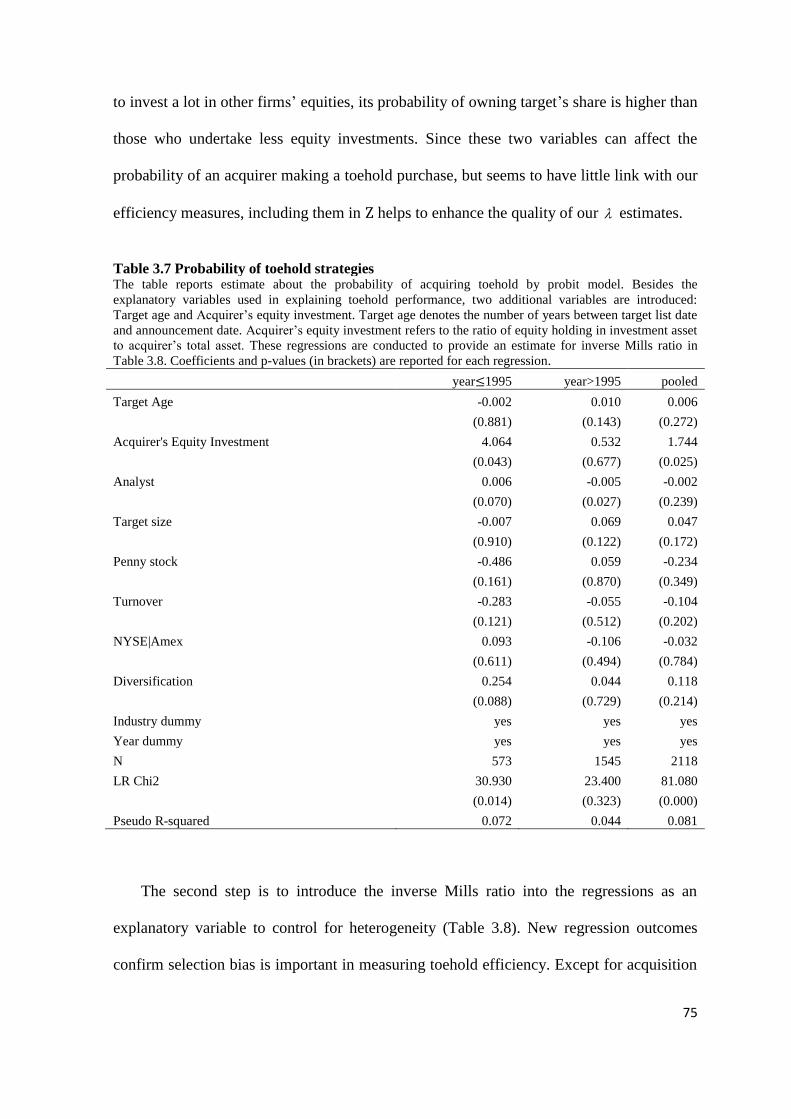
75
to invest a lot in other firms’ equities, its probability of owning target’s share is higher than
those who undertake less equity investments. Since these two variables can affect the
probability of an acquirer making a toehold purchase, but seems to have little link with our
efficiency measures, including them in helps to enhance the quality of our estimates.
Table 3.7 Probability of toehold strategies The table reports estimate about the probability of acquiring toehold by probit model. Besides the
explanatory variables used in explaining toehold performance, two additional variables are introduced:
Target age and Acquirer’s equity investment. Target age denotes the number of years between target list date
and announcement date. Acquirer’s equity investment refers to the ratio of equity holding in investment asset
to acquirer’s total asset. These regressions are conducted to provide an estimate for inverse Mills ratio in
Table 3.8. Coefficients and p-values (in brackets) are reported for each regression.
year 1995 year>1995 pooled
Target Age -0.002 0.010 0.006
(0.881) (0.143) (0.272)
Acquirer's Equity Investment 4.064 0.532 1.744
(0.043) (0.677) (0.025)
Analyst 0.006 -0.005 -0.002
(0.070) (0.027) (0.239)
Target size -0.007 0.069 0.047
(0.910) (0.122) (0.172)
Penny stock -0.486 0.059 -0.234
(0.161) (0.870) (0.349)
Turnover -0.283 -0.055 -0.104
(0.121) (0.512) (0.202)
NYSE|Amex 0.093 -0.106 -0.032
(0.611) (0.494) (0.784)
Diversification 0.254 0.044 0.118
(0.088) (0.729) (0.214)
Industry dummy yes yes yes
Year dummy yes yes yes
N 573 1545 2118
LR Chi2 30.930 23.400 81.080
(0.014) (0.323) (0.000)
Pseudo R-squared 0.072 0.044 0.081
The second step is to introduce the inverse Mills ratio into the regressions as an
explanatory variable to control for heterogeneity (Table 3.8). New regression outcomes
confirm selection bias is important in measuring toehold efficiency. Except for acquisition
76
premiums, coefficients of Inverse Mills ratio are significant in most estimation. For the
other three efficiency measures, self-selection process seems to produce a different impact
on the two sub-samples. In the early period, selection is accompanied with lower returns to
acquirer and lower synergy values, but brings favorable outcomes in the later period,
where its generates higher acquirer returns and is associated with the selection of better
targets, as suggested by the significant coefficient of Inverse Mill’s ratio*Recent. This
improvement in selection efficiency is consistent with a transformation from a pooling of
toehold strategies to a separated situation, where only qualified acquirers buy toeholds. But
when it comes to completion rates, selection is associated with a higher probability of
failure: it does not affect completion rates before 1995 (with an insignificant coefficient of
-0.210) but reduces them after 1995, with a significant estimate of -0.438. This difference
is further confirmed by the interaction term between Inverse Mill’s ratio and the dummy
variable Recent in the pooled regression, whose coefficient is -0.384 and significant at 5%
level.
But caution is needed in interpreting this as evidence of the inefficiency of self-
selection on the probability of deal completion. As toehold strategies are much more
common in hostile takeovers than in friendly ones (Betton et al., 2008), it is natural to
expect that completion rates are lower in takeovers with toeholds. Some empirical studies,
such as Jennings and Mazzeo (1993), claim toehold strategies have a two-fold impact on
completion rates: they find that their existence increases the possibility of target resistance,
but also that the size of toehold is negatively associated with the likelihood of such
resistance. We make similar findings seeing a positive correlation between completion
rates and toehold size, regardless of the negative correlation between completion rates and
Inverse Mill’s ratio (which represents the hidden information involved in the toehold).
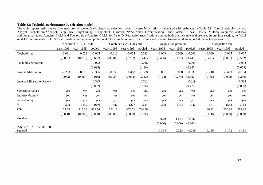
77
Table 3.8 Toeholds performance by selection model The table reports estimates on four measures of toehold's efficiency by selection model. Inverse Mills ratio is calculated with estimates in Table 3.9. Control variables include
Analyst, Toehold size*Analyst, Target size, Target runup, Penny stock, Turnover, NYSE|Amex, Diversification, Tender offer, All cash, Hostile, Multiple Acquirers, and two
additional variables, Acquirer CAR3 and Toehold size*Acquirer CAR3, for Panel D. Regression specifications and methods are the same as those used in previous section, i.e. WLS
model for return analysis, OLS for acquisition premium and probit model for completion rate. Coefficients and p-values (in brackets) are reported for each regression.
Acquirer CAR (-41,end) Combined CAR (-41,end) Acquisition premium Completion rate
year 1995 year>1995 pooled year 1995 year>1995 pooled year 1995 year>1995 pooled year 1995 year>1995 pooled
Toehold size -0.021 0.023 -0.005 -0.011 -0.004 0.013 -0.003 -0.009 -0.003 -0.009 0.025 -0.007
(0.091) (0.013) (0.657) (0.581) (0.702) (0.442) (0.456) (0.027) (0.448) (0.471) (0.091) (0.562)
Toehold size*Recent
0.022
-0.016
-0.005
0.034
(0.095)
(0.410)
(0.347)
(0.069)
Inverse Mill's ratio -0.293 0.019 -0.306 -0.355 0.468 -0.388 0.061 0.058 0.039 -0.210 -0.438 -0.134
(0.033) (0.867) (0.016) (0.035) (0.003) (0.012) (0.124) (0.264) (0.332) (0.135) (0.002) (0.300)
Inverse Mill's ratio*Recent
0.323
0.761
0.019
-0.384
(0.052)
(0.000)
(0.770)
(0.036)
Control variables yes yes yes yes yes yes yes yes yes yes yes yes
Industry dummy yes yes yes yes yes yes yes yes yes yes yes yes
Year dummy yes yes yes yes yes yes yes yes yes yes yes yes
N 398 1242 1640 387 1227 1614 358 1184 1542 571 1542 2113
chi2 174.23 715.23 829.56 171.16 678.71 764.89
88.22 260.99 357.82
(0.000) (0.000) (0.000) (0.000) (0.000) (0.000)
(0.000) (0.000) (0.000)
F-value
8.79 14.34 14.86
(0.000) (0.000) (0.000)
Adjusted / Pseudo R-
squared
0.324 0.233 0.239 0.126 0.172 0.159

78
After controlling for self-selection, toehold has a greater impact on completion rates in the
recent period than in the early one. The positive estimate of Toehold size*Recent indicates
such strategies become much more beneficial over time in facilitating acquirers to
complete deals. On the whole, as Table 3.8 shows, the efficiency improvement in toehold
performance can be explained to some extent by self-selection procedure. Except for
completion rates31, the coefficient of the interaction term between Toehold size and the
dummy variable Recent becomes less significant after controlling for self-selection
outcomes.
3.5. Is monitoring an important qualification for an efficient toehold
strategy?
According to the M&A literature, the takeover field is severely affected by agency
problems (Mueller, 1969; Amihud and Lev, 1981; Berkovitch, and Narayanan, 1993).
However, concentrated ownership, especially institutional holdings, helps monitor
managers’ actions and bring good outcomes for takeovers (Shleifer, and Vishny, 1986;
Schranz 1993; Allen et al., 2000; Gaspar et al., 2005; Chen et al., 2007). Inspired by these
studies, we start to wonder: whether the better monitoring provided by institutional
investors qualifies acquirers to use toeholds efficiently.
One possible explanation could be as follows. The adverse impact of toeholds in the
early period can be viewed as evidence of agency problems in takeovers, but the
involvement of institutional investors can mitigate such adverse impacts by monitoring
managers to act in shareholders’ interest. As time pass, the inappropriate usage of toeholds
31 As discussed above, the relation between toehold and completion rate is complicated, which is greatly
affected by the endogenous interaction between management resistance and toehold strategy, so it’s hard to
use self-selection procedure alone to identify all the impacts of toehold strategies on completion rate.
79
is reduced because of increased monitoring power. If this explanation holds, the
introduction of institutional holdings into our previous regressions could capture the
improvement of toehold’s efficiency performance over time.
We define Institutional holdings as the percentage of shares held by institutional
investors, and collect this data from Thomson Reuters. Table 3.9 shows new estimates of
our four efficiency measures after introducing this new variable and its interaction term
with toehold size. Again, a two-step method that controls for selection bias and
heterogeneity is conducted. Compared to results in the previous section, the greatest
changes occur on estimates for the recent period (after 1995) and the interaction term
between toehold size and the recent dummy. For returns to acquirers in the recent period,
the coefficient of Toehold size decreases from significantly positive (0.023 in Table 3.5) to
significantly negative (-0.047), i.e., even worse than in the early period (-0.030). This
adverse impact of stand-alone toehold strategies is further confirmed by the insignificant
coefficients of the interaction term, Toehold size*Recent, in the last two pooled regressions.
Similar changes happen to estimation results for combined returns, acquisition premiums,
and completion rates. The relative better performance of toehold strategies in the recent
period disappears in the presence of institutional holdings and its interaction terms. Apart
from completion rates, where all coefficients of Toehold size are insignificant, stand-alone
toeholds load with estimates of the same sign both before and after 1995. This change
further helps to exclude the alternative explanation for the learning effect, i.e., a growing
market acknowledgement of toehold’s impact over time. If improvement in toehold’s
efficiency was attributed to better market perception of toehold strategies, coefficients of
stand-alone Toehold size should remain time varying, rather than have the same sign
across the two sub-samples. Toeholds owned by acquirers without institutional investors
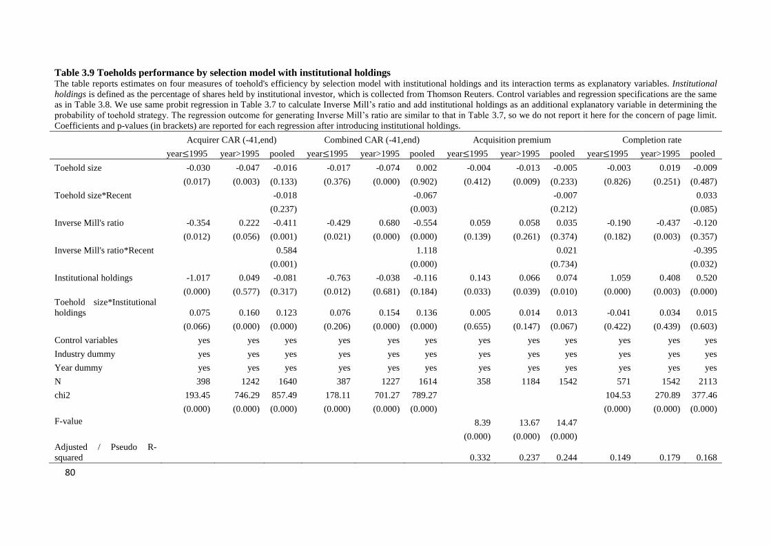
80
Table 3.9 Toeholds performance by selection model with institutional holdings The table reports estimates on four measures of toehold's efficiency by selection model with institutional holdings and its interaction terms as explanatory variables. Institutional
holdings is defined as the percentage of shares held by institutional investor, which is collected from Thomson Reuters. Control variables and regression specifications are the same
as in Table 3.8. We use same probit regression in Table 3.7 to calculate Inverse Mill’s ratio and add institutional holdings as an additional explanatory variable in determining the
probability of toehold strategy. The regression outcome for generating Inverse Mill’s ratio are similar to that in Table 3.7, so we do not report it here for the concern of page limit.
Coefficients and p-values (in brackets) are reported for each regression after introducing institutional holdings.
Acquirer CAR (-41,end) Combined CAR (-41,end) Acquisition premium Completion rate
year 1995 year>1995 pooled year 1995 year>1995 pooled year 1995 year>1995 pooled year 1995 year>1995 pooled
Toehold size -0.030 -0.047 -0.016 -0.017 -0.074 0.002 -0.004 -0.013 -0.005 -0.003 0.019 -0.009
(0.017) (0.003) (0.133) (0.376) (0.000) (0.902) (0.412) (0.009) (0.233) (0.826) (0.251) (0.487)
Toehold size*Recent
-0.018
-0.067
-0.007
0.033
(0.237)
(0.003)
(0.212)
(0.085)
Inverse Mill's ratio -0.354 0.222 -0.411 -0.429 0.680 -0.554 0.059 0.058 0.035 -0.190 -0.437 -0.120
(0.012) (0.056) (0.001) (0.021) (0.000) (0.000) (0.139) (0.261) (0.374) (0.182) (0.003) (0.357)
Inverse Mill's ratio*Recent
0.584
1.118
0.021
-0.395
(0.001)
(0.000)
(0.734)
(0.032)
Institutional holdings -1.017 0.049 -0.081 -0.763 -0.038 -0.116 0.143 0.066 0.074 1.059 0.408 0.520
(0.000) (0.577) (0.317) (0.012) (0.681) (0.184) (0.033) (0.039) (0.010) (0.000) (0.003) (0.000)
Toehold size*Institutional
holdings 0.075 0.160 0.123 0.076 0.154 0.136 0.005 0.014 0.013 -0.041 0.034 0.015
(0.066) (0.000) (0.000) (0.206) (0.000) (0.000) (0.655) (0.147) (0.067) (0.422) (0.439) (0.603)
Control variables yes yes yes yes yes yes yes yes yes yes yes yes
Industry dummy yes yes yes yes yes yes yes yes yes yes yes yes
Year dummy yes yes yes yes yes yes yes yes yes yes yes yes
N 398 1242 1640 387 1227 1614 358 1184 1542 571 1542 2113
chi2 193.45 746.29 857.49 178.11 701.27 789.27
104.53 270.89 377.46
(0.000) (0.000) (0.000) (0.000) (0.000) (0.000)
(0.000) (0.000) (0.000)
F-value
8.39 13.67 14.47
(0.000) (0.000) (0.000)
Adjusted / Pseudo R-
squared
0.332 0.237 0.244 0.149 0.179 0.168

81
persist in being inefficient over time, indicating that market do not perceive toehold
strategies in a more positive light as time passes.
Compared to Table 3.8, the efficiency improvement indicated by coefficients of
Toehold size*Recent become even weaker after adding Institutional holdings into the
regression. The positive change in acquirer’s return becomes insignificantly negative, and
the period difference in combined return changes from insignificant to significantly
negative. Efficiency improvements in these two return measures cease to exist after
controlling for monitoring power. Estimates of Toehold size*Institutional holdings are
more significant for deals taking place after 1995 than those for earlier deals, especially for
Acquirer CAR (-41,end) and Combined CAR (-41,end), showing that Institutional holdings
function better in improving toehold performance in the recent period. As with the
pervious findings, time-variance in acquisition premiums is indistinguishable from zero,
and better monitoring does not help to reduce the costs paid by acquirers (coefficients of
Toehold size*Institutional holdings are insignificant in two subsamples, and significantly
positive for the pooled regression). Institutional holdings also increase takeover completion
rates - as all the estimates of Institutional holdings are significant at 1% level - but it does
not help to improve toehold’s performance in this respect, as none of their interaction
terms are significant.
In sum, efficiency improvement in toehold performance ceases to exist after
controlling for institutional holdings, as indicated by its similar impact on deals in the two
sub-samples. It implies that better monitoring power can be a candidate to help toehold-
owners to use such strategies properly to benefit them.
82
3.6. Robustness check
3.6.1. Different specifications of institutional holdings
As Institutional holdings is a general measure of shares owned by all institutional investors,
it cannot reflect concentration of share ownership. To address this issue, we repeat our
regressions in Table 3.10 using shares held by top five institutional investors in acquirer
firms (defined as variable Top five) and its interaction terms with Toehold size and Recent
to replace Institutional holdings and corresponding interaction terms.
Table 3.10 presents the same result as in Table 3.9, and shows that concentrated
holdings by top five institutional investors reduces time-variance in toehold efficiency. The
impacts of the size of stand-alone toeholds are of the same sign in two sub-samples,
strengthening the evidence that firms with higher institutional holdings are the more
qualified toehold acquirers.
As well as the concentration of share ownership, the type of institutional investors also
matters. Previous studies show that public pension funds are more active in monitoring
their portfolios than other investors (Del Guercio and Hawkins, 1999; Gompers and
Metrick, 2001) and use the percentage of a firm’s shares owned by public pension fund as
a measure of corporate governance (Atanassov, 2012; Dittmar and Mahrt-Smith, 2007).
We follow these studies in using public pension fund ownership as an alternative measure,
and use the list assembled by Dittmar and Mahrt-Smith (2007) to identify them from the
pool of institutional investors in our data. Table 3.11 shows similar results as the
robustness check with shares held by top five institutional investors, confirming that good
corporate governance can enhance toehold performance, and mitigate differences in
toehold efficiency over time.
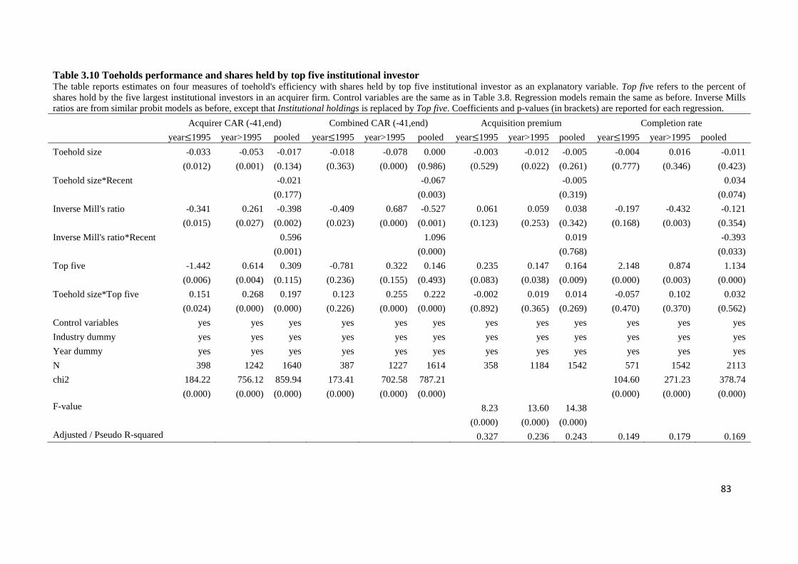
83
Table 3.10 Toeholds performance and shares held by top five institutional investor The table reports estimates on four measures of toehold's efficiency with shares held by top five institutional investor as an explanatory variable. Top five refers to the percent of
shares hold by the five largest institutional investors in an acquirer firm. Control variables are the same as in Table 3.8. Regression models remain the same as before. Inverse Mills
ratios are from similar probit models as before, except that Institutional holdings is replaced by Top five. Coefficients and p-values (in brackets) are reported for each regression.
Acquirer CAR (-41,end) Combined CAR (-41,end) Acquisition premium Completion rate
year 1995 year>1995 pooled year 1995 year>1995 pooled year 1995 year>1995 pooled year 1995 year>1995 pooled
Toehold size -0.033 -0.053 -0.017 -0.018 -0.078 0.000 -0.003 -0.012 -0.005 -0.004 0.016 -0.011
(0.012) (0.001) (0.134) (0.363) (0.000) (0.986) (0.529) (0.022) (0.261) (0.777) (0.346) (0.423)
Toehold size*Recent
-0.021
-0.067
-0.005
0.034
(0.177)
(0.003)
(0.319)
(0.074)
Inverse Mill's ratio -0.341 0.261 -0.398 -0.409 0.687 -0.527 0.061 0.059 0.038 -0.197 -0.432 -0.121
(0.015) (0.027) (0.002) (0.023) (0.000) (0.001) (0.123) (0.253) (0.342) (0.168) (0.003) (0.354)
Inverse Mill's ratio*Recent
0.596
1.096
0.019
-0.393
(0.001)
(0.000)
(0.768)
(0.033)
Top five -1.442 0.614 0.309 -0.781 0.322 0.146 0.235 0.147 0.164 2.148 0.874 1.134
(0.006) (0.004) (0.115) (0.236) (0.155) (0.493) (0.083) (0.038) (0.009) (0.000) (0.003) (0.000)
Toehold size*Top five 0.151 0.268 0.197 0.123 0.255 0.222 -0.002 0.019 0.014 -0.057 0.102 0.032
(0.024) (0.000) (0.000) (0.226) (0.000) (0.000) (0.892) (0.365) (0.269) (0.470) (0.370) (0.562)
Control variables yes yes yes yes yes yes yes yes yes yes yes yes
Industry dummy yes yes yes yes yes yes yes yes yes yes yes yes
Year dummy yes yes yes yes yes yes yes yes yes yes yes yes
N 398 1242 1640 387 1227 1614 358 1184 1542 571 1542 2113
chi2 184.22 756.12 859.94 173.41 702.58 787.21
104.60 271.23 378.74
(0.000) (0.000) (0.000) (0.000) (0.000) (0.000)
(0.000) (0.000) (0.000)
F-value
8.23 13.60 14.38
(0.000) (0.000) (0.000)
Adjusted / Pseudo R-squared
0.327 0.236 0.243 0.149 0.179 0.169
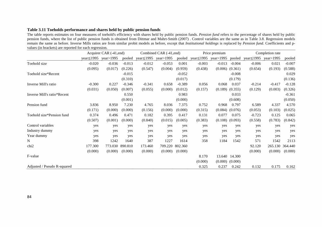
84
Table 3.11 Toeholds performance and shares held by public pension funds The table reports estimates on four measures of toehold's efficiency with shares held by public pension funds. Pension fund refers to the percentage of shares held by public
pension funds, where the list of public pension funds is obtained from Dittmar and Mahrt-Smith (2007) . Control variables are the same as in Table 3.8. Regression models
remain the same as before. Inverse Mills ratios are from similar probit models as before, except that Institutional holdings is replaced by Pension fund. Coefficients and p-
values (in brackets) are reported for each regression.
Acquirer CAR (-41,end) Combined CAR (-41,end) Price premium Completion rate
year 1995 year>1995 pooled year 1995 year>1995 pooled year 1995 year>1995 pooled year 1995 year>1995 pooled
Toehold size -0.020 -0.036 -0.013 -0.012 -0.053 0.001 -0.003 -0.013 -0.004 -0.006 0.021 -0.007
(0.095) (0.017) (0.226) (0.547) (0.004) (0.959) (0.438) (0.006) (0.361) (0.654) (0.193) (0.588)
Toehold size*Recent
-0.015
-0.052
-0.008
0.029
(0.310)
(0.017)
(0.179)
(0.136)
Inverse Mill's ratio -0.300 0.227 -0.346 -0.341 0.658 -0.389 0.056 0.068 0.037 -0.214 -0.417 -0.128
(0.031) (0.050) (0.007) (0.055) (0.000) (0.012) (0.157) (0.189) (0.355) (0.129) (0.003) (0.326)
Inverse Mill's ratio*Recent
0.550
0.983
0.033
-0.361
(0.001)
(0.000)
(0.608)
(0.050)
Pension fund 3.836 8.950 7.230 4.765 8.036 7.375 0.752 0.968 0.797 6.589 4.337 4.570
(0.171) (0.000) (0.000) (0.156) (0.000) (0.000) (0.315) (0.084) (0.076) (0.053) (0.103) (0.025)
Toehold size*Pension fund 0.374 0.496 0.471 0.182 0.395 0.417 0.131 0.077 0.075 -0.723 0.125 0.065
(0.507) (0.001) (0.000) (0.840) (0.015) (0.005) (0.383) (0.108) (0.093) (0.558) (0.783) (0.842)
Control variables yes yes yes yes yes yes yes yes yes yes yes yes
Industry dummy yes yes yes yes yes yes yes yes yes yes yes yes
Year dummy yes yes yes yes yes yes yes yes yes yes yes yes
N 398 1242 1640 387 1227 1614 358 1184 1542 571 1542 2113
chi2 177.300 773.030 890.810 173.460 709.220 802.360
92.120 265.130 364.440
(0.000) (0.000) (0.000) (0.000) (0.000) (0.000)
(0.000) (0.000) (0.000)
F-value
8.170 13.640 14.300
(0.000) (0.000) (0.000)
Adjusted / Pseudo R-squared
0.325 0.237 0.242 0.132 0.175 0.162

85
3.6.2. Merger wave
Our sample contains observations during the recent merger wave between the mid-1990s
and the early 2000s. Although both of our sub-samples cover a portion of this merger wave,
more years belong to the merger wave period in the recent sub-sample than in the early
sub-sample. To separate the impact of market abnormalities associated with the merger
wave, we exclude data from the wave period from our sample and divide the rest into two
subsamples, i.e. before the merger wave (1990-1993), and after it (2002-2006). Using
observations before the wave as the benchmark, we define one dummy variable ‘after’ to
denote those made after the wave.
Panel A in Table 3.12 presents estimates similar to Table 3.6, where we compare
differences in toehold performance before and after the merger wave. In general, the
changes in toeholds’ efficiency in Table 3.6 still persist in the sample without the presence
of a merger wave. Toehold strategies perform better in the later period than they did in the
early period, especially in terms of increasing acquirers’ returns and success in selecting
good targets. There is little change in acquisition premiums. Before the merger wave,
toeholds reduce the probability of completing deals, but this negative correlation
disappears after the wave, although the insignificant coefficient of Toehold size*After
indicates this time variance is not significant, which is consistent with previous findings.
Panel B in Table 3.12 reports new estimates after introducing the self-selection
procedure and institutional holdings as additional regressors. Due to fewer observations,
most estimates are less significant as before, but we can still observe that the self-selection
model has similar explanatory power as it had before. Time differences in toehold
efficiency disappear, indicated by insignificant estimates of all the interaction terms
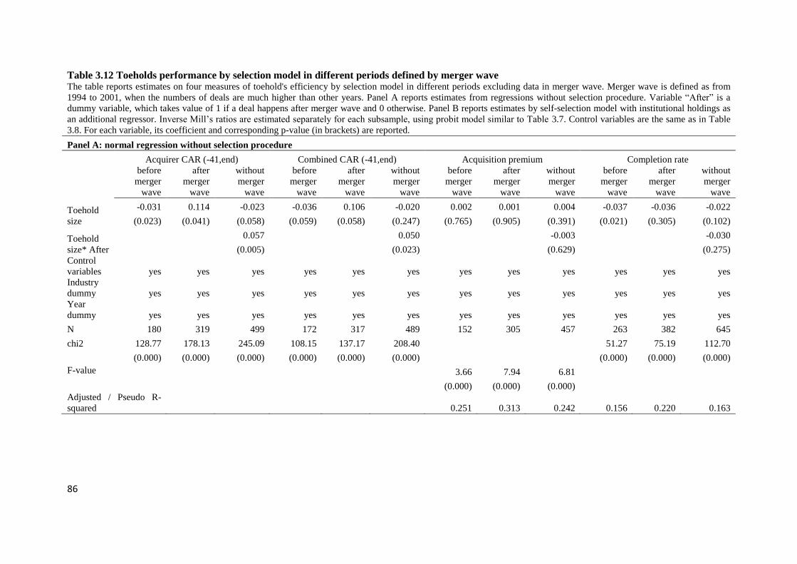
86
Table 3.12 Toeholds performance by selection model in different periods defined by merger wave The table reports estimates on four measures of toehold's efficiency by selection model in different periods excluding data in merger wave. Merger wave is defined as from
1994 to 2001, when the numbers of deals are much higher than other years. Panel A reports estimates from regressions without selection procedure. Variable “After” is a
dummy variable, which takes value of 1 if a deal happens after merger wave and 0 otherwise. Panel B reports estimates by self-selection model with institutional holdings as
an additional regressor. Inverse Mill’s ratios are estimated separately for each subsample, using probit model similar to Table 3.7. Control variables are the same as in Table
3.8. For each variable, its coefficient and corresponding p-value (in brackets) are reported.
Panel A: normal regression without selection procedure
Acquirer CAR (-41,end) Combined CAR (-41,end) Acquisition premium Completion rate
before
merger
wave
after
merger
wave
without
merger
wave
before
merger
wave
after
merger
wave
without
merger
wave
before
merger
wave
after
merger
wave
without
merger
wave
before
merger
wave
after
merger
wave
without
merger
wave
Toehold
size
-0.031 0.114 -0.023 -0.036 0.106 -0.020 0.002 0.001 0.004 -0.037 -0.036 -0.022
(0.023) (0.041) (0.058) (0.059) (0.058) (0.247) (0.765) (0.905) (0.391) (0.021) (0.305) (0.102)
Toehold
size* After
0.057
0.050
-0.003
-0.030
(0.005)
(0.023)
(0.629)
(0.275)
Control
variables yes yes yes yes yes yes yes yes yes yes yes yes
Industry
dummy yes yes yes yes yes yes yes yes yes yes yes yes
Year
dummy yes yes yes yes yes yes yes yes yes yes yes yes
N 180 319 499 172 317 489 152 305 457 263 382 645
chi2 128.77 178.13 245.09 108.15 137.17 208.40
51.27 75.19 112.70
(0.000) (0.000) (0.000) (0.000) (0.000) (0.000)
(0.000) (0.000) (0.000)
F-value
3.66 7.94 6.81
(0.000) (0.000) (0.000)
Adjusted / Pseudo R-
squared
0.251 0.313 0.242 0.156 0.220 0.163
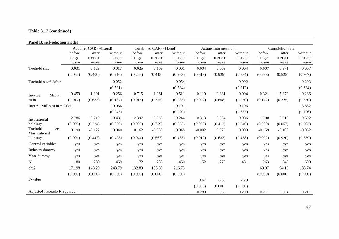
87
Table 3.12 (continued)
Panel B: self-selection model
Acquirer CAR (-41,end) Combined CAR (-41,end) Acquisition premium Completion rate
before
merger
wave
after
merger
wave
without
merger
wave
before
merger
wave
after
merger
wave
without
merger
wave
before
merger
wave
after
merger
wave
without
merger
wave
before
merger
wave
after
merger
wave
without
merger
wave
Toehold size -0.031 0.123 -0.017 -0.025 0.109 -0.001 -0.004 0.003 -0.004 0.007 0.371 -0.007
(0.050) (0.400) (0.216) (0.265) (0.445) (0.963) (0.613) (0.929) (0.534) (0.793) (0.525) (0.767)
Toehold size* After
0.052
0.054
0.002
0.293
(0.591)
(0.584)
(0.912)
(0.334)
Inverse Mill's
ratio
-0.459 1.391 -0.256 -0.715 1.061 -0.511 0.119 -0.381 0.094 -0.321 -5.379 -0.236
(0.017) (0.683) (0.137) (0.015) (0.755) (0.033) (0.092) (0.608) (0.050) (0.172) (0.225) (0.250)
Inverse Mill's ratio * After
0.066
0.101
-0.106
-3.682
(0.945)
(0.920)
(0.637)
(0.126)
Institutional
holdings
-2.786 -0.210 -0.481 -2.397 -0.053 -0.244 0.313 0.034 0.086 1.700 0.612 0.692
(0.000) (0.224) (0.000) (0.000) (0.759) (0.063) (0.028) (0.412) (0.046) (0.000) (0.057) (0.003)
Toehold size
*Institutional
holdings
0.190 -0.122 0.040 0.162 -0.089 0.048 -0.002 0.023 0.009 -0.159 -0.106 -0.052
(0.001) (0.447) (0.403) (0.044) (0.567) (0.435) (0.919) (0.633) (0.458) (0.092) (0.920) (0.539)
Control variables yes yes yes yes yes yes yes yes yes yes yes yes
Industry dummy yes yes yes yes yes yes yes yes yes yes yes yes
Year dummy yes yes yes yes yes yes yes yes yes yes yes yes
N 180 289 469 172 288 460 152 279 431 263 346 609
chi2 171.98 148.29 248.79 132.89 135.80 216.73
69.07 94.13 138.74
(0.000) (0.000) (0.000) (0.000) (0.000) (0.000)
(0.000) (0.000) (0.000)
F-value
3.67 8.33 7.29
(0.000) (0.000) (0.000)
Adjusted / Pseudo R-squared
0.280 0.356 0.298 0.211 0.304 0.211
88
between Toehold size and After. Apart for completion rates, the impact of the self-
selection procedure - as reflected by the coefficient of Inverse Mill’s ratio - is adverse for
the rest of the efficiency measures before the merger waves, but this negative effect ceases
to exist afterwards. The overall result shows that the existence of a merger wave does not
introduce significant bias into our original analysis.
3.7. Conclusion
By investigating performance of toehold strategies in terms of return to acquirers,
acquisition premiums, combined returns and completion rates, we find their efficiency
improves over time, which indicates there is a time difference in the performance of
acquisitions which use such strategies. This is in sharp contrast with the decline in
popularity of minority stake acquisitions. We believe that – in addition to existing
explanations – a dynamic perspective is required to understand the evolution of this puzzle.
This explanation can be an improving self-selection outcome from learning the
qualifications needed to use toehold strategies properly in executing acquisitions. We test
this by building a self-selection model, and our outcomes support this argument.
Furthermore, we show the better monitoring provided by institutional investors helps to
overcome pitfalls in implementing toehold strategies, and can be seen as part of an
acquirer’s qualification to use them successfully.
This interplay between toehold performance and monitoring quality has practical
implications, especially in mitigating agency problems in corporate investment. Driven by
incentives to control more resources, managers can be highly motivated to expand their
firms without maximizing shareholder’s interest, which can lead to zero - or even negative
- takeover payoffs. The adverse impacts of toehold strategies can be one consequence of

89
this distorted incentive. Good corporate governance can be an effective mechanism to
mitigate this principal-agent problem. Improvements in toehold performance show the
rewards of strengthening monitoring: as a measure of external monitoring strength,
institutional holdings demonstrate their important role in enhancing takeover performance,
and suggest a similar role for internal monitoring mechanisms such as, for example, board
independence.
This interplay between toehold performance and monitoring quality has theoretical
and empirical implications. A dynamic model under agency considerations can more
rigorously and realistically explain the suboptimal execution of minority stake, where
unqualified bidders execute their acquisitions before the optimal threshold. An in-depth
exploration of the relationship between internal monitoring and toehold performance is left
for future work.


91
Chapter 4
Are Corporate Governance Mechanisms
Complements? Evidence from Failed Takeovers
4.1. Introduction
Corporate governance is a set of disciplinary forces that is used to control companies and
reduce agency cost. Takeover threats from potential acquirers are usually considered a very
strong external governance mechanism in the management team. In the context of failed
takeovers, this chapter investigates the interplay among different corporate governance
mechanisms, which aims at shedding some light on the following questions. Are different
corporate governance mechanisms complements or substitutes? In particular, is the quality
of a firm’s response to takeover threat positively correlated to the quality of other aspects
of the firm’s corporate governance? Previous studies have generated a lot of results and
insights on this topic, but not yet reached a conclusive answer.
92
Some research supports the complements view. Hadlock and Lumer (1997) and
Mikkelson and Parch (1997) find that the internal disciplinary pressure on the top
managers is weaker when the threat of takeover is low. Denis and Serrano (1996) show
that the post-contest internal restructuring is more value enhancing in the presence of an
outside blockholder. Giroud and Mueller (2010) and Atanassov (2013) speak for the
substitutes view. Their papers show that the adverse impact of the anti-takeover legislation
is weaker in the presence of better internal governance. Other studies find neither
complementary nor substitutional effect between the internal and external governance.
Huson, Parrino, and Starks (2001) find that the intensity of the takeover threats does not
affect the sensitivity of forced CEO turnover to firm performance, and conclude that
takeover does not influence the internal corporate control. Denis and Kruse (2000) also
find no change in CEO turnover and a firm’s restructuring after the great decline in
takeover activities in the late 1980s.
In this article, I focus on three aspects of corporate governance: monitoring by
institutional investors, product market competition, and takeover threats. Monitoring by
institutional investors is an internal and direct disciplinary mechanism that can actively
affect corporate operation by proxy voting (Gillan and Stark, 2000; Hartzell and Stark,
2003). Product market competition is an external and relatively weak governance
mechanism that facilitates a comparison of managerial performance (Nickell et al, 1997).
Takeover threat poses a strong dismissal threat to management, and is therefore a powerful
external disciplinary mechanism (Shleifer and Vishny, 1997; Bertrand and Mullainathan,
2003). The investigation into the interplay among these three governance mechanisms aims
at providing a comprehensive understanding of their interactions. In particular, I want to
address the following two questions:
93
Question (1): Can monitoring by institutional investors promote the effectiveness of
the target firms’ response to takeover threats? (Are monitoring by institutional investors
and takeover threats complements?)
Question (2): Can competition in product markets enhance the effectiveness of firms’
response to takeover threats? (Are competition in product markets and takeover threats
complements?)
In particular, I consider failed takeovers as the ground to identify the relationship
between different governance mechanisms. The key advantage of using the data on failed
takeovers is that although the failed takeover creates a concrete control threat to the target
firm, it does not actually shift in corporate control in the end. However, the threat is so
strong that target firms may respond with substantial restructuring. Denis and Serrano
(1996) report high management turnover among poorly performing firms after
unsuccessful control contests. Franks and Mayer (1996) observe a high board turnover and
an increase in asset disposals in target firms after unsuccessful hostile takeovers.
Safieddine and Titman (1999) find that the target firms significantly increase leverage after
the termination of takeovers.
Furthermore, I restrict the failed takeovers to those with a hostile or an unsolicited
deal attitude. As argued by Morck et al (1989), Lambrecht and Myers (2007), and Servaes
and Tamayo (2013), hostile takeovers are more likely to occur in troubled industries than
in healthy industries. This grants hostile takeovers with the information externality, as it
can signal poor performance of the whole industry. Since the inefficiency occurs industry
wide, peer firms are expected to take similar corrective actions as the target firms (Servaes
and Tamayo, 2013). They find significant changes in peer firms’ investment and financing
policies. Relative to target firms, control threats facing the peer firms are weaker and less
94
direct. As a result, peer firms’ responses to control threats may vary with the quality of
their governance. Examining peer firms’ responses enables me to investigate whether
corporate governance can enhance firms’ sensitivity to inefficiency signals embedded in
failed takeovers.
The effectiveness of firms’ responses is measured from two perspectives. The first is
the changes in firms’ investment and financing decisions. As discussed in Servaes and
Tamayo (2013), as hostile takeovers identify industries with overinvestment problems,
peer firms respond to this signal by cutting down their investment and increasing leverage.
To make the analysis comparable to their study, I follow Servaes and Tamayo (2013) to
focus on the changes in the capital spending and debt levels. The second perspective is to
look at stock performance. It reflects a market’s view on firms’ profitability. By examining
both operational decisions and market expectations, my result can provide a
comprehensive picture of the influence of corporate governance on the effectiveness of
firms’ responses in failed takeovers.
The findings suggest that these three corporate governance mechanisms are, at most,
weak complements. Although monitoring from institutional investors helps decrease target
firms’ free cash, it does nothing in improving firms’ financing decisions or stock
performance. Competition in product markets does not have a strong impact either.
Although it brings higher abnormal returns to peer firms, its impact disappears after
matching target and peer firms by their probability of being taken over. This means that the
influence of product market competition is derived from its implication of the strength of
takeover threat, rather than its disciplinary power. Overall, the quality of firms’ responses
to failed takeovers (the effectiveness of takeover threats as an external governance
mechanism) does not have a strong correlation with either the monitoring by institutional
95
investors (internal governance) or competition in the product market (anther external
governance).
This article contributes to the literature on the interplay among different corporate
governance mechanisms. Hadlock and Lumer (1997), Mikkelson and Parch (1997), Giroud
and Mueller (2010), Atanassov (2013), Huson, Parrino, and Starks (2001), and Denis and
Kruse (2000) investigate this topic under the context of declined takeover threat, whereas I
complement the evidence by examining the interactions in the presence of strong takeover
threats. The inclusion of both target and peer firms further decomposes takeover threats
into two levels: strong and concrete threats to target firms, and indirect signals of industry-
wide inefficiency to peer firms. This decomposition enables me to investigate the role of
corporate governance under different strengths of control threats, which is a unique feature
of failed takeovers.
The rest of this article is organized as follows. Section 4.2 develops the hypotheses.
Section 4.3 describes the sample construction, variable definitions, and hypotheses to test.
Section 4.4 reports the results, and section 4.5 is the conclusion.
4.2. Hypotheses development
Target firms and peer firms are subject to different strengths of takeover threats. Therefore,
their responses are expected to be different in terms of the magnitudes. The target firms
directly receive takeover bids. Although they successfully defend themselves, the takeover
attempts indicate external recognition of inefficiency in their operations. As a reaction,
they can either improve their performance or adopt takeover defenses. Whether the post-
takeover restructuring is value enhancing or increasing management entrenchment will
depend on the quality of other aspects of corporate governance. If the other aspects of
96
governance mechanisms are complements to takeover threats, the target firms’ post-
takeover performance should be higher for firms that are better in those aspects of
corporate governance. This leads to hypothesis 1 and 2:
Hypothesis 1: Firms with higher monitoring from institutional investors make better
responses to takeover threats, and perform better in the stock market.
Hypothesis 2: Firms facing more competition in the product market make better responses
to takeover threats, and perform better in the stock market.
Peer firms are not directly involved in takeovers. However, takeovers have
information externality, implying industry-wide inefficiency (Morck et al, 1989;
Lambrecht and Myers, 2007; Servaes and Tamayo, 2013). Peer firms can respond to this
inefficiency signal by adopting similar actions as target firms. Since this signal is weaker
than the shock received by target firms, whether peer firms can fully recognize it is not
guaranteed. If other governance mechanisms are complements to takeover threats, they
should improve peer firms’ sensitivity to the inefficiency signal sent by takeover threats.
After the failed takeover attempts, peer firms with better governance in other aspects are
more likely to consider takeover threat a signal of operational inefficiency. Corporate
governance is further expected to determine how well the peer firms can do after takeovers.
Based on these arguments, I formulate the following testable hypotheses:
Hypothesis 3: Peer firms with higher monitoring from institutional investors make better
financial and investment decisions after the takeover threats on the target firm, and
perform better in the stock market.
97
Hypothesis 4: Peer firms facing more competitive pressure in the product market make
better financial and investment decisions after the takeover threats on the target firm, and
perform better in the stock market.
Finally, since the takeover threat influences the target firm directly, and the peers of the
target firms only indirectly, I hypothesize that the magnitude of the response by the peer
firms is to a lesser extent than the target firm, and if that leads to improved stock market
performance, the improvement on the peers’ stocks should be smaller than the target’s
improvement.
Hypothesis 5: The response to the takeover threat by the peer firms should be of a smaller
magnitude than the target firms. The change/improvement of stock performance (if any)
should also be smaller for the peer firms than for the target firms.
4.3. Data
4.3.1. Sample construction
Two samples of firms are constructed: a group of targets and a group of peers. The target
sample is collected from the Security Data Corporation (SDC). To be included in the
sample, a takeover attempt should meet the following criteria:
The deal is announced for U.S. public non-financial targets during the period from
1 January 198732
to 31 December 2008;
The deal status is withdrawn, and the deal attitude is hostile or unsolicited33
;
32 I choose 1987 as the starting year, because this article uses historical SIC codes from Compustat to identify
peer firms, and the earliest historical SIC codes provided by Compustat start from 1987.

98
Acquirers are seeking to own more than 50% of target shares, and the percentage
owned by acquirers before the takeover attempts is less than 50%;
The following deal types are excluded: privatization, spinoffs, recapitalizations,
exchange offers, repurchases, debt restructuring, target bankrupt, and acquirer
involves management;
The deal is announced at least one year after the last completed bid and one year
before the next completed bid;
The target has available accounting data from Compustat and available stock data
from CRSP in the announcement year.
If one target received multiple withdrawn bids satisfying the earlier criteria, it is
counted as one single takeover attempt with the announcement equal to that of the earliest
bid and the withdrawn date equal to that of the last bid. In the end, there are 270 failed
takeover attempts in the target sample.
The sample of industry peers is identified by historical 4-digit SIC codes from
Compustat.34
To exclude the impact from other takeovers, firms receiving takeover bids
within 3 years around the corresponding failed takeover are removed. This requirement
also effectively removes targets from the sub-sample of peer firms. Furthermore, to be
included in the peer sample, firms should have available data on both Compustat and
CRSP. These requirements result in 1849 firms in the peer sample.
33 Servaes and Tamayo (2013) focus only on hostile takeovers, whereas I also include unsolicited takeovers
because of the limited number of unsuccessful hostile takeovers (only 125 deals meeting the selection criteria
are hostile). Furthermore, unsolicited takeovers are expected to be similar to hostile takeovers, as they are not
invited by target firms and reflect external investors’ opinions on the efficiency of target firms’ operation.
34 According to Guenther and Rosman (1994) and Kahle and Walkling (1996), Compustat SIC codes are
more reliable than CRSP SIC codes.
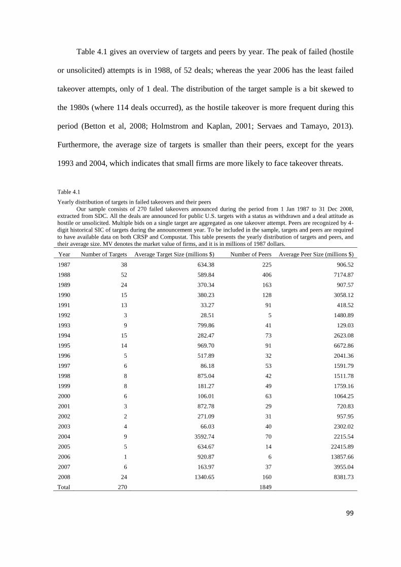
99
Table 4.1 gives an overview of targets and peers by year. The peak of failed (hostile
or unsolicited) attempts is in 1988, of 52 deals; whereas the year 2006 has the least failed
takeover attempts, only of 1 deal. The distribution of the target sample is a bit skewed to
the 1980s (where 114 deals occurred), as the hostile takeover is more frequent during this
period (Betton et al, 2008; Holmstrom and Kaplan, 2001; Servaes and Tamayo, 2013).
Furthermore, the average size of targets is smaller than their peers, except for the years
1993 and 2004, which indicates that small firms are more likely to face takeover threats.
Table 4.1
Yearly distribution of targets in failed takeovers and their peers
Our sample consists of 270 failed takeovers announced during the period from 1 Jan 1987 to 31 Dec 2008,
extracted from SDC. All the deals are announced for public U.S. targets with a status as withdrawn and a deal attitude as
hostile or unsolicited. Multiple bids on a single target are aggregated as one takeover attempt. Peers are recognized by 4-
digit historical SIC of targets during the announcement year. To be included in the sample, targets and peers are required
to have available data on both CRSP and Compustat. This table presents the yearly distribution of targets and peers, and
their average size. MV denotes the market value of firms, and it is in millions of 1987 dollars.
Year Number of Targets Average Target Size (millions $) Number of Peers Average Peer Size (millions $)
1987 38 634.38
225 906.52
1988 52 589.84
406 7174.87
1989 24 370.34
163 907.57
1990 15 380.23
128 3058.12
1991 13 33.27
91 418.52
1992 3 28.51
5 1480.89
1993 9 799.86
41 129.03
1994 15 282.47
73 2623.08
1995 14 969.70
91 6672.86
1996 5 517.89
32 2041.36
1997 6 86.18
53 1591.79
1998 8 875.04
42 1511.78
1999 8 181.27
49 1759.16
2000 6 106.01
63 1064.25
2001 3 872.78
29 720.83
2002 2 271.09
31 957.95
2003 4 66.03
40 2302.02
2004 9 3592.74
70 2215.54
2005 5 634.67
14 22415.89
2006 1 920.87
6 13857.66
2007 6 163.97
37 3955.04
2008 24 1340.65
160 8381.73
Total 270 1849

100
Most of the firms in the target sample are involved in only one failed takeover. The
maximum number of failed takeover attempts for a target firm is two, and only eight target
firms appeared twice in the sample. The average number of peer firms per deal is 7.12,
ranging from zero for 22 deals to 40 for two deals.
With regard to the distribution of the deal sample across industries, Table 4.2 shows
that 27 deals occurred in the business service sector according to Fama-French 48-industry
categories, whereas the retail sector scored the second with 20 deals in the sample. All the
other industries have less than 20 deals.
Table 4.2
Distribution of deals in Fama-French 48-industry categories
This table gives the distribution of deals in our sample by Fama-French 48-industry categories.
Fama-French 48-industry categories Number of deals
Business service 27
Retail 20
Constrution materials 15
Restaurants, hotels, motels 14
Computers 13
Electronic equipment 13
Healthcare 11
Apparel 10
Other 147
4.3.2. Definition of variables and summary statistics
To provide a comprehensive picture of the interplay between different corporate
governance mechanisms, I use two measures of corporate governance. One is the
percentage shares held by institutional investors, institutional holdings. They are well
grounded in the corporate governance theory that the institutional investors as blockholders
can strengthen the monitoring power on corporate management. (Shleifer and Vishny,
1986; Brickley, Lease, and Smith, 1988; Agrawal and Mandelker, 1990). The institutional

101
holdings are computed from Thomson Reuters as the sum of the percentage of shares held
by institutional investors. Greater institutional holdings of a target firm imply more active
monitoring from shareholders.
The other measure of corporate governance is the Herfindahl–Hirschman index
(HHI). The HHI captures the intensity from product market competition. As shown by
Giroud and Mueller (2010) and Atanassov (2013), product market competition can
mitigate weakened discipline of management resulted from the enactment of antitakeover
laws. The HHI is defined as the sum of squared market shares of all firms in a given three-
digit SIC industry,35
where market shares are calculated from firms’ sales. A higher HHI
implies weaker competition.
The firms’ performance in failed takeovers is measured at two levels. The first level
is the corporate level. Previous studies show that corporate takeover plays an important
role in correcting managerial failure. In particular, it has a disciplining function on
managers’ tendency to overinvest. In failed takeovers, firms often reduce investments and
increase the amount of debt in their capital structure (Franks and Mayer 1996; Safieddine
and Titman, 1999; Servaes and Tamayo, 2013). Following previous studies, I mainly look
at firms’ responses to takeover threats in terms of investment and capital structure policies.
The main measures of investment policies are the capital spending and the level of free
cash flow relative to assets. The capital spending is measured as the ratio of capital
expenditure to assets. The level of free cash flow is defined as “operating income – interest
payments – tax payments – dividend payments” (Lehn and Poulsen, 1989; Servaes and
Tamayo, 2013), and its ratio to total assets can be viewed as a proxy for post-tax cash flow
35 To make results comparable to Giround and Mueller (2010), I define the industry by a three-digit SIC code
similar to the one in their paper.

102
that is not distributed to stakeholders. If firms view takeover attempts as signals of their
overinvestment, they will reduce their capital spending and the levels of free cash flow.
The main measure of capital structure policy is the ratio of long-term debt to total assets.
As argued widely in earlier literature, high leverage helps align the interests of managers
and shareholders, as it increases the probability that the manager is fired for poor
performance (Grossman and Hart, 1982; Jensen, 1986). If the firms want to signal their
commitment to correct overinvestment, they will borrow more debt to increase leverage.
Second, I use stock performance to depict investors’ expectations on firms’
profitability. If the changes in firms’ financial policies are correct and effective, the stock
of the firm should experience high abnormal returns around the takeovers. Considering the
uncertainty and noise in choosing the proper event window, I calculate two measures of
abnormal returns, CAR(-1,1) and CAR(-42, end), to describe stock performance in both
short and long horizons. Furthermore, I use analysts’ forecasts on EPS to show how
professionals, who are assumed to have better investment knowledge, view the efficiency
of firms’ reactions in failed takeovers.
Table 4.3 presents the summary statistics of all the performance measures. In
addition to aggregating observations by the firms’ identity (targets or peers), each firm
group is further divided into four subgroups according to the level of institutional holdings
and HHI, respectively. I use the differences between two-year averages of each accounting
measure before and after the takeovers to measure the changes in investment and capital
structure policies. Targets experienced greater changes in investment and capital structure
policies, higher abnormal returns, and larger decreases in EPS forecast than their peers.
Scaled by total assets, targets on average reduce their capital spending by 1%, increase
long-term debt by 4%, and increase free cash flow by 3.4% after failed takeovers; whereas

103
the corresponding changes for peers are only 0.6%, 3.7%, and 2%, respectively. Moreover,
the takeover events result in positive and significant abnormal returns for targets, whereas
the CARs for peers are insignificantly negative. For an inter-subgroup comparison, t-
statistics are insignificant for all but two of the differences. Targets with high institutional
holdings only suffer a slight decrease in EPS forecast, of 0.75%; whereas those with low
institutional holdings experience a decrease of 2.88%. Furthermore, peers with high
institutional holdings reduce their capital expenditures by 1.07%, whereas those with low
institutional holdings only cut their capital spending by 0.23%.
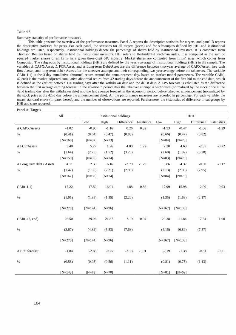
104
Table 4.3
Summary statistics of performance measures
This table presents the overview of the performance measures. Panel A reports the descriptive statistics for targets, and panel B reports
the descriptive statistics for peers. For each panel, the statistics for all targets (peers) and for subsamples defined by HHI and institutional
holdings are listed, respectively. Institutional holdings denote the percentage of shares held by institutional investors. It is computed from
Thomson Reuters based on shares held by institutional investors. HHI refers to Herfindahl–Hirschman index. It is computed as the sum of
squared market shares of all firms in a given three-digit SIC industry. Market shares are computed from firms’ sales, which comes from
Compustat. The subgroups by institutional holdings (HHI) are defined by the yearly average of institutional holdings (HHI) in the sample. The
variables Δ CAPX/Asset, Δ FCF/Asset, and Δ Long-term Debt/Asset are the difference between two-year average of CAPX/Asset, free cash
flow / asset, and long-term debt / Asset after the takeover attempts and their corresponding two-year average before the takeovers. The variable
CAR(-1,1) is the 3-day cumulative abnormal return around the announcement day, based on market model parameters. The variable CAR(-
42,end) is the market-adjusted cumulative abnormal return from 42 trading days before the announcement of the first bid to the end date, which
is defined as the earliest between 126 trading days after the withdrawn date and the delist date. Δ EPS forecast is calculated as the difference
between the first average earning forecast in the six-month period after the takeover attempt is withdrawn (normalized by the stock price at the
42nd trading day after the withdrawn date) and the last average forecast in the six-month period before takeover announcement (normalized by
the stock price at the 42nd day before the announcement date). All the performance measures are recorded in percentage. For each variable, the
mean, standard errors (in parentheses), and the number of observations are reported. Furthermore, the t-statistics of difference in subgroups by
HHI and s are reported.
Panel A: Targets
All Institutional holdings HHI
Low High Difference t-statistics Low High Difference t-statistics
Δ CAPX/Assets -1.02 -0.90 -1.16 0.26 0.32 -1.53 -0.47 -1.06 -1.29
% (0.41) (0.64) (0.47) (0.83) (0.66) (0.47) (0.82)
[N=160] [N=87] [N=73] [N=84] [N=78]
Δ FCF/Assets 3.40 5.27 1.26 4.00 1.22 2.28 4.63 -2.35 -0.72
% (1.64) (2.75) (1.52) (3.28) (2.60) (1.92) (3.28)
[N=159] [N=85] [N=74] [N=83] [N=76]
Δ Long term debt / Assets 4.11 2.38 6.16 -3.79 -1.29 3.86 4.37 -0.50 -0.17
% (1.47) (1.96) (2.21) (2.95) (2.13) (2.03) (2.95)
[N=162] [N=88] [N=74] [N=84] [N=78]
CAR(-1,1) 17.22
17.89 16.01 1.88 0.86
17.99 15.98 2.00 0.93
% (1.05)
(1.39) (1.55) (2.20)
(1.35) (1.68) (2.17)
[N=270]
[N=174] [N=96]
[N=167] [N=103]
CAR(-42, end) 26.50
29.06 21.87 7.19 0.94
29.38 21.84 7.54 1.00
% (3.67)
(4.82) (5.53) (7.68)
(4.16) (6.89) (7.57)
[N=270]
[N=174] [N=96]
[N=167] [N=103]
Δ EPS forecast -1.84
-2.88 -0.75 -2.13 -1.91
-2.19 -1.38 -0.81 -0.71
% (0.56)
(0.95) (0.56) (1.11)
(0.81) (0.75) (1.13)
[N=143]
[N=73] [N=70]
[N=81] [N=62]
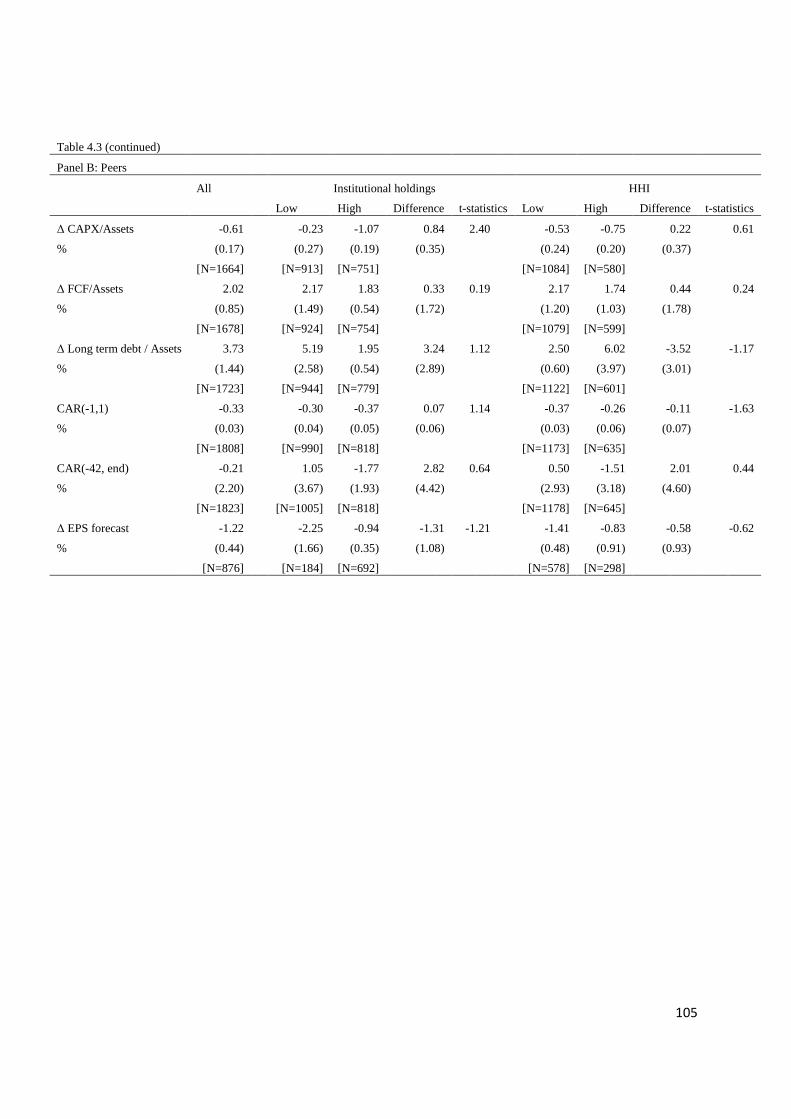
105
Table 4.3 (continued)
Panel B: Peers
All Institutional holdings HHI
Low High Difference t-statistics Low High Difference t-statistics
Δ CAPX/Assets -0.61 -0.23 -1.07 0.84 2.40 -0.53 -0.75 0.22 0.61
% (0.17) (0.27) (0.19) (0.35) (0.24) (0.20) (0.37)
[N=1664] [N=913] [N=751] [N=1084] [N=580]
Δ FCF/Assets 2.02 2.17 1.83 0.33 0.19 2.17 1.74 0.44 0.24
% (0.85) (1.49) (0.54) (1.72) (1.20) (1.03) (1.78)
[N=1678] [N=924] [N=754] [N=1079] [N=599]
Δ Long term debt / Assets 3.73 5.19 1.95 3.24 1.12 2.50 6.02 -3.52 -1.17
% (1.44) (2.58) (0.54) (2.89) (0.60) (3.97) (3.01)
[N=1723] [N=944] [N=779] [N=1122] [N=601]
CAR(-1,1) -0.33
-0.30 -0.37 0.07 1.14
-0.37 -0.26 -0.11 -1.63
% (0.03)
(0.04) (0.05) (0.06)
(0.03) (0.06) (0.07)
[N=1808]
[N=990] [N=818]
[N=1173] [N=635]
CAR(-42, end) -0.21
1.05 -1.77 2.82 0.64
0.50 -1.51 2.01 0.44
% (2.20)
(3.67) (1.93) (4.42)
(2.93) (3.18) (4.60)
[N=1823]
[N=1005] [N=818]
[N=1178] [N=645]
Δ EPS forecast -1.22
-2.25 -0.94 -1.31 -1.21
-1.41 -0.83 -0.58 -0.62
% (0.44)
(1.66) (0.35) (1.08)
(0.48) (0.91) (0.93)
[N=876]
[N=184] [N=692]
[N=578] [N=298]

106
4.4. Results
4.4.1. Changes in investment and capital structure policies
In this section, I examine how a firm changes its capital spending, free cash flow, and
long-term debt after a failed takeover, and the influence of institutional holdings and
industry competition (HHI) on the changes.
The yearly observations of CAPX/Assets, FCF/Assets, and Long-term debt/Assets
are accumulated for a window ranging from three years before the takeover announcement
to three years after the takeover withdrawal. The variable “After” is introduced to separate
observations before and after takeovers. It is a dummy variable that uses a value of one for
the years after the year of withdrawn, and zero otherwise. Its interactions with
“institutional holdings” and “HHI” are the key variables in this section. These interactions
describe the interplay between takeover threat and corporate governance. In particular, the
following panel data regression is performed:
1 2 3
4 5
* * * * *
* * *
it it it it it it
it it it i it
Ratio a After a Institutional holding After a HHI After
a Institutional holding a HHI b X e
,
where itX is a vector of control variables, b is a vector of regression coefficients on the
control variables, and i is an unobservable individual effect that is estimated by the fixed
effect. To make the results comparable, I use the same sets of control variables as in
Sevaes and Tamayo (2013) and list them explicitly for each ratio in the Appendix. Along
with control variables, the noise in measuring the firms’ policy changes is reduced, as the
impact of changes on firms’ fundamentals is identified. Furthermore, the fixed-effect
107
specification in panel regression captures the unobserved time-invariant heterogeneity in
firms’ investment and capital structure policies, which makes the estimates more efficient.
Panel A of Table 4.4 contains the main results for target firms. Column 1 shows the
effect of failed takeovers on target firms’ capital spending, and whether the change in
CAPX/Assets is different for firms with high and low institutional holdings, and for firms
in competitive and non-competitive industries. The coefficient of the After dummy is -2.12
(with a standard error of 0.68). It is significant at the 1% level, implying that CAPX/Assets
drop by 2.12% points on average. Given that the average CAPX/Assets of target firms is
8.62%, it implies a drop in CAPX/Assets by 24.6% for the average firm, which is very
large economically. The interaction term between the After dummy and the institutional
holdings has a coefficient of 0.74 (with a standard error of 0.95), which implies that the
change in CAPX/Assets is not affected by the percentage of shares held by institutional
investors. For the impact of industry competition, the interaction term between the After
dummy and the HHI has a coefficient of 2.61 (standard error of 1.46), and it is significant
at the 10% level. It implies that the drop in CAPX/Assets is larger for firms in competitive
industries. As for the economic magnitude of the effect, a decrease in the HHI by one
standard deviation is associated with a drop in CAPX/Assets by 2.61%*0.156=0.407%, or
a drop in CAPX/Asset of 4.72% for the average firm. Both the stand-alone institutional
holdings and HHI have insignificant coefficients, meaning they do not influence a target
firm’s capital spending without the takeover threat.
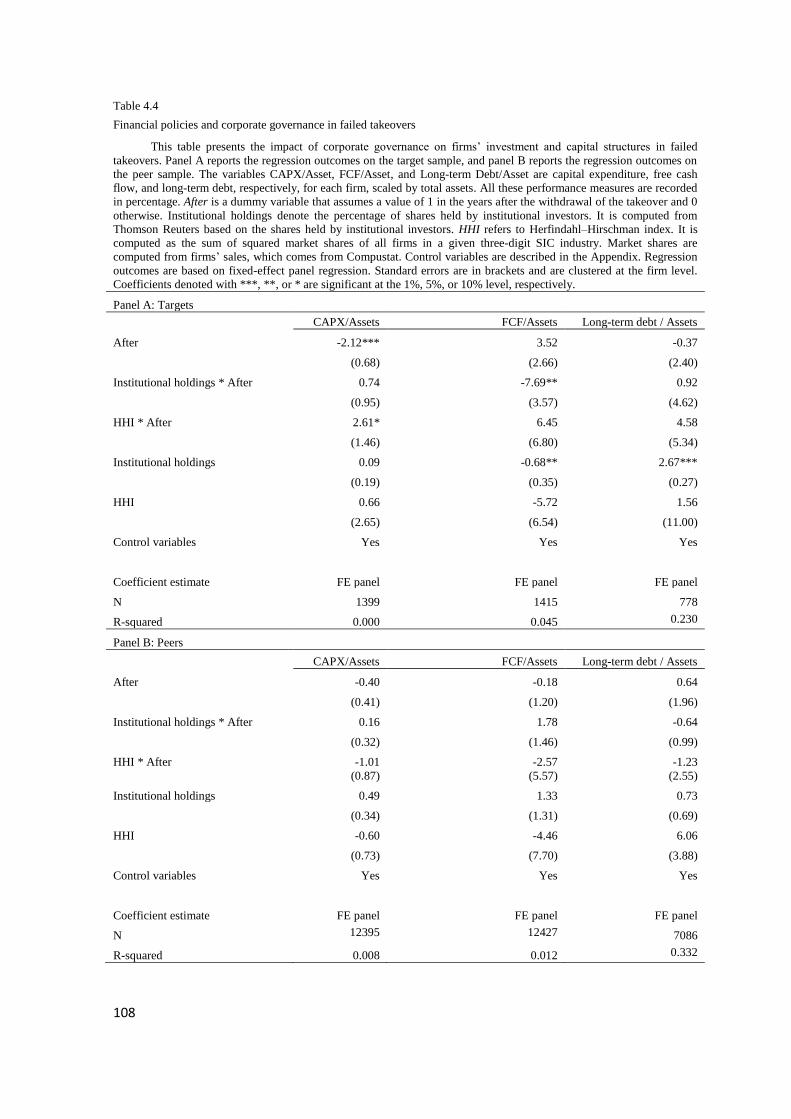
108
Table 4.4
Financial policies and corporate governance in failed takeovers
This table presents the impact of corporate governance on firms’ investment and capital structures in failed
takeovers. Panel A reports the regression outcomes on the target sample, and panel B reports the regression outcomes on
the peer sample. The variables CAPX/Asset, FCF/Asset, and Long-term Debt/Asset are capital expenditure, free cash
flow, and long-term debt, respectively, for each firm, scaled by total assets. All these performance measures are recorded
in percentage. After is a dummy variable that assumes a value of 1 in the years after the withdrawal of the takeover and 0
otherwise. Institutional holdings denote the percentage of shares held by institutional investors. It is computed from
Thomson Reuters based on the shares held by institutional investors. HHI refers to Herfindahl–Hirschman index. It is
computed as the sum of squared market shares of all firms in a given three-digit SIC industry. Market shares are
computed from firms’ sales, which comes from Compustat. Control variables are described in the Appendix. Regression
outcomes are based on fixed-effect panel regression. Standard errors are in brackets and are clustered at the firm level.
Coefficients denoted with ***, **, or * are significant at the 1%, 5%, or 10% level, respectively.
Panel A: Targets
CAPX/Assets FCF/Assets Long-term debt / Assets
After -2.12*** 3.52 -0.37
(0.68) (2.66) (2.40)
Institutional holdings * After 0.74 -7.69** 0.92
(0.95) (3.57) (4.62)
HHI * After 2.61* 6.45 4.58
(1.46) (6.80) (5.34)
Institutional holdings 0.09 -0.68** 2.67***
(0.19) (0.35) (0.27)
HHI 0.66 -5.72 1.56
(2.65) (6.54) (11.00)
Control variables Yes Yes Yes
Coefficient estimate FE panel FE panel FE panel
N 1399 1415 778
R-squared 0.000 0.045 0.230
Panel B: Peers
CAPX/Assets FCF/Assets Long-term debt / Assets
After -0.40 -0.18 0.64
(0.41) (1.20) (1.96)
Institutional holdings * After 0.16 1.78 -0.64
(0.32) (1.46) (0.99)
HHI * After -1.01 -2.57 -1.23
(0.87) (5.57) (2.55)
Institutional holdings 0.49 1.33 0.73
(0.34) (1.31) (0.69)
HHI -0.60 -4.46 6.06
(0.73) (7.70) (3.88)
Control variables Yes Yes Yes
Coefficient estimate FE panel FE panel FE panel
N 12395 12427 7086
R-squared 0.008 0.012 0.332
109
Column 2 in Panel A of Table 4.4 studies target firms’ free cash flows. As claimed
by Servaes and Tamayo (2013), hostile takeovers signal industry-wide overinvestment. If
target firms think in this manner, the correct response is to reduce the level of free cash
flows. The coefficient of the After dummy does not support this argument, as it is
insignificant and positive. However, consistent with the over-investment story, high
institutional holdings decrease the level of free cash flow after takeover, as the coefficient
of the interaction term between the After dummy and the institutional holdings is
significantly negative. An increase in the institutional holdings by one standard deviation is
associated with a reduction in FCF/Assets by 7.69%*0.188=1.45%. Since the average
FCF/Assets in the target sample is 2.36%, it equals a decline of 61.4% in FCF/Assets for
the average target firm, which is highly economically significant. Furthermore, the stand-
alone institutional holdings appear effective in cutting the level of free cash flow. Its
coefficient is -0.68, which implies that high institutional holdings can mitigate the over-
investment problem in target firms.
The third column in Panel A of Table 4.4 examines the debt levels in target firms.
Neither the After dummy nor its interaction terms with the institutional holdings or the
HHI has significant coefficients. It seems that neither monitoring from institutional
investors nor the discipline from product competition can encourage target firms to
increase their leverage more after a failed takeover. When it comes to stand-alone
institutional holdings, they are positively associated with debt level, as it has a positive
coefficient of 2.67, which is significant at a 1% level. If a target firm increases its
institutional holdings by one standard deviation, the ratio between long-term debt and total
assets will increase by 2.67%*0.188=0.50%. The coefficient of the HHI is insignificant.
110
Panel B of Table 4.4 presents the regression outcomes for peer firms. None of the
variables in concern has a significant coefficient. It seems that the peer firms do not
consider failed takeover attempts to industry counterparts as a concrete control threat, or, at
least, they are not sensitive to this threat. The insignificant coefficient of the interaction
terms between the After dummy and the institutional holdings (the HHI) shows that the
corporate governance cannot enhance the peer firms’ response to weak potential control
threats. We can summarize these findings in Result 1:
Result 1: The estimation results provide some support for Hypothesis 1, and weak support
for Hypothesis 2. Higher institutional holding is a complement to takeover threat in terms
of reducing free cash flows; there is weak evidence that more competition in the product
market is a complement (the coefficient is only significant at a 10% level) to takeover in
terms of cutting down capital expenditure. The result does not support neither Hypothesis
3 nor 4. The financial decision by the peer firms does not seem to be affected by the
takeover threat, and it is, therefore, possible to identify interaction terms of takeover threat
and institutional holding, or competition in the product market. This result is supportive of
Hypothesis 5, namely, since the takeover threat has a direct impact on the target firm, but
only indirect impact on the peers, it improves the financial decision by the targets, whereas
it generates barely any influence on the financial decision of the peers.
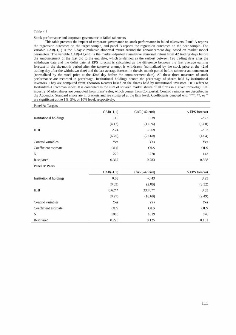
111
Table 4.5
Stock performance and corporate governance in failed takeovers
This table presents the impact of corporate governance on stock performance in failed takeovers. Panel A reports
the regression outcomes on the target sample, and panel B reports the regression outcomes on the peer sample. The
variable CAR(-1,1) is the 3-day cumulative abnormal return around the announcement day, based on market model
parameters. The variable CAR(-42,end) is the market-adjusted cumulative abnormal return from 42 trading days before
the announcement of the first bid to the end date, which is defined as the earliest between 126 trading days after the
withdrawn date and the delist date. Δ EPS forecast is calculated as the difference between the first average earning
forecast in the six-month period after the takeover attempt is withdrawn (normalized by the stock price at the 42nd
trading day after the withdrawn date) and the last average forecast in the six-month period before takeover announcement
(normalized by the stock price at the 42nd day before the announcement date). All these three measures of stock
performance are recorded in percentage. Institutional holdings denote the percentage of shares held by institutional
investors. They are computed from Thomson Reuters based on the shares held by institutional investors. HHI refers to
Herfindahl–Hirschman index. It is computed as the sum of squared market shares of all firms in a given three-digit SIC
industry. Market shares are computed from firms’ sales, which comes from Compustat. Control variables are described in
the Appendix. Standard errors are in brackets and are clustered at the firm level. Coefficients denoted with ***, **, or *
are significant at the 1%, 5%, or 10% level, respectively.
Panel A: Targets
CAR(-1,1) CAR(-42,end) Δ EPS forecast
Institutional holdings 1.10 0.39 -2.22
(4.17) (17.74) (3.80)
HHI 2.74 -3.69 -2.02
(6.75) (22.60) (4.04)
Control variables Yes Yes Yes
Coefficient estimate OLS OLS OLS
N 270 270 143
R-squared 0.362 0.283 0.568
Panel B: Peers
CAR(-1,1) CAR(-42,end) Δ EPS forecast
Institutional holdings 0.03 -0.43 3.25
(0.03) (2.89) (3.32)
HHI 0.62** 33.70** 3.53
(0.27) (16.60) (2.49)
Control variables Yes Yes Yes
Coefficient estimate OLS OLS OLS
N 1805 1819 876
R-squared 0.229 0.125 0.151
112
4.4.1. Stock performance around failed takeovers
In this section, I investigate the impact of corporate governance on firms’ stock
performance around failed takeovers. In particular, firms’ abnormal returns and the
changes in analysts’ EPS forecast are studies that examine how the market expects the
profitability of the firm to develop after a failed takeover, and how the presence of an
institutional investor and the competition in the product market affect this expectation.
Panel A of Table 4.5 presents the results for target firms. None of the estimated
coefficients is significant. This suggests that investors and professional analysts do not
expect different performance of target firms after failed takeovers, irrespective of the level
of the institutional holding in the firm, or the competitiveness in the product market. Panel
B of Table 4.5 reports the result for peer firms. Similar to an earlier finding, the
institutional holdings do not affect CARs or changes in the forecast of EPS after in failed
takeovers. However, the intensity of product market competition is negatively associated
with abnormal stock returns of peer firms, as the coefficients of the HHI are significantly
positive. For CAR(-1,1), the HHI has a coefficient of 0.62, with a standard error of 0.27.
As for the economic magnitude of the effect, an increase in the HHI by one standard
deviation is associated with an increase in CAR(-1,1) by 0.62%*0.156=0.097%. Since the
average CAR(-1,1) in the sample of the peer firms is 0.59%, it equals an increase of 16.44%
in CAR(-1,1) for the average firm. This positive correlation between the market
competition and abnormal returns also holds for a longer event window. For CAR(-42,end),
the HHI has a coefficient of 33.70 (standard error of 16.60); that is, an increase in the HHI
by one standard deviation will increase CAR(-42,end) by 33.70%*0.156=5.257%. Given
the average CAR(-42,end) in the sample of the peer firm is -0.212%, the impact of the HHI
is large both statistically and economically. Nevertheless, one should be cautious in
113
interpretation of the relationship between product market competition and CARs for peer
firms. The HHI is highly determined by the number of firms in the same product industry.
In addition to product market competition, it also reflects the size of the potential target
pool in a certain industry. Within a highly concentrated market, a failed takeover may
result in high attention toward peer firms, as they are likely to be the next target if the
acquirer aims at buying assets from the same industry. If this is the case, the positive
correlation between the HHI and CARs cannot be treated as the positive correlation
between market competition and CARs. Instead, it only demonstrates a stronger spill-over
effect of failed takeover in a more concentrated market. The results can be summarized in
Result 2:
Result 2: The result of simple regression suggests that institutional holding has no impact
on post-failed-takeover stock performance of either the target or the peers. Competition in
the product market does not influence the post-failed-takeover stock performance of the
target, but it lowers the stock return of the peers, which is quite counter-intuitive.
4.4.2. After matching
In the earlier sections, the samples of target and peer firms are separated, and the
relationship between corporate governance and firms’ performance in failed takeovers is
examined separately for each sample, because the sizes of the target sample and peer
sample differ a lot, 270 targets vs. 1849 peers. In this section, I match peer firms with
target firms by their takeover probability, and use the pooled sample to re-investigate the
hypotheses.
Matching is introduced for two reasons. First, it can create a balanced pooled sample
in which the groups of target and peer firms have a similar size. Second, by leveling the
114
possibility of being acquired, it can be more certain that the impact of HHI and institutional
holdings comes from their roles as a measurement of corporate governance, rather than
other alternative implications such as the industry concentration or the similarity with the
target firms. Peer firms are identified by the industry classification of target firms, and
there can be huge heterogeneity in industry characteristics, which will affect firms’
sensitivity to takeover threats. For instance, the industry concentration varies in different
industries. It is natural that a peer firm in a wide-spread industry is less sensitive to a failed
takeover targeted at a remote target firm, compared with a peer firm in a concentrated
industry facing the same signal, because the concentration of an industry can affect both
the dissemination and perception of the signal conveyed by failed takeover threats. In a
concentrated industry, the likelihood of a peer firm to become the next target is higher than
in the case of a wide-spread industry, which will lead to different responses of peer firms
in industries with different levels of concentration. This concern can cause serious
problems if not treated well, because one key variable in this article, HHI, is a common
measure of the industry concentration and indicates the intensity of product market
competition. The previous finding shows that HHI has a significant impact on peer firms’
stock performance, but it is doubtful as to whether this impact comes from the effect of
corporate governance or the industry concentration measured by HHI. In order to reduce
the noise brought about by multiple implications of HHI, I include HHI as one of the
dependent variables to calculate the propensity score of firms. Moreover, peer firms
sharing the common characteristics with target firms are more likely to become the next
target, and, thus, respond more strongly to takeover threats. Since ownership structure is a
critical characteristic, institutional holdings are also included as a dependent variable in the
estimation of propensity score, to control for its impact on the likelihood of a peer firm
becoming the next target.
115
The model I used to pair target and peer firms is propensity score matching (PSM). It
was first introduced by Rosenbaum and Rubin (1983), and further developed by Heckman
et al (1997). It is a widely applied approach that is used to estimate causal treatment effects
(Dehejia and Wahba, 1999; Perkins et al, 2000; Hitt and Frei 2002; Davies and Kim, 2003;
Brand and Halaby 2006; Caliendo and Kopeinig, 2008). Based on firms’ asset
characteristics, I calculate the probability of being the target in failed takeovers for each
firm in the sample. Specifically, the propensity score is estimated from a probit regression
with the control variables in section 4.1 (those for CAPX/Assets, FCF/Assets, and Long-
term debt/Assets) as independent variables and the target dummy as the dependent variable.
In particular, I use nearest-neighbor matching by using a propensity score. Table 4.6
presents the propensity scores (pscore) for target and peer firms before and after matching.
After matching, the distribution of pscore in target and peer samples becomes more similar,
and the sample size becomes the same, both with 103 firms.
Table 4.6
Pscores of targets and peers before and after matching
This table presents the distribution of propensity scores (pscores) for targets and peers before and after matching.
The estimation of the propensity scores is estimated from a probit regression with control variables for CAPX/Assets,
FCF/Assets, and Long-term debt/Assets, plus HHI and the institutional holdings.
Panel A: pscores before matching
N Mean Std. Dev. Min Max
Targets 106 0.114 0.045 0.038 0.265
Peers 998 0.094 0.042 0.000 0.287
Panel B: pscores after matching
N Mean Std. Dev. Min Max
Targets 103 0.111 0.039 0.038 0.215
Peers 103 0.111 0.039 0.038 0.216
Table 4.7 reports new regression results in pooled sample after matching. More
interaction terms are introduced to separate the impact for target and peer firms. Panel A
shows new estimates for investment and capital structure policies. The interaction term
116
between the institutional holdings and the After dummy has a positive coefficient of 1.70
for capital expending, and a negative coefficient of -12.71 for FCF/Assets. It indicates that
monitoring from institutional investors can motivate target firms to spend more on capital
investment and to reduce more on undistributed capital after failed takeovers. If a firm
increases its institutional holdings by one standard deviation, its CAPX/Assets will
increase by 1.70%*0.188=0.320%, and its free cash flow/Assets will decrease by
12.71*0.188=2.389%. Different from previous findings, the interaction term between the
HHI and the After dummy loses the significance on its coefficient for regression on
CAPX/Assets. Furthermore, the interaction term between the institutional holdings (the
HHI), the After dummy, and the Peer dummy does not have any significant coefficient in
Panel A, which means that corporate governance does not make any difference in peer
firms’ responses to failed takeovers in their investment and capital structure policies.
Panel B of Table 4.7 reports new estimates for stock performance. Different from the
finding in section 4.2, the HHI does not have a significant coefficient for CARs any more,
neither does the stand-alone HHI nor the interaction term between the HHI and the Peer
dummy. This suggests that the positive correlation between the HHI and CARs in section
4.2 can be attributed to the link between the product market competition and the
probability of becoming a target. Since the peer firms in more concentrated markets are
more likely to become the next target,36
they experience higher abnormal returns after
failed takeovers. Once controlled for the probability of being acquired, the impact of the
product competition on CARs disappears. Moreover, the monitoring from institutional
investors stays trivial in determining firms’ stock performance. Neither the stand-alone
36 In fact, in the probit regression that estimates propensity score, the HHI has a positive coefficient of 0.822
with a p-value of 0.016.
117
institutional holdings nor their interaction term with the Peer dummy has a significant
coefficient. This indicates that the difference in the institutional investors’ presence in a
firm’s ownership does not form different expectations of future profitability among
investors and professional analysts after a failed takeover. Though Panel A of Table 4.7
suggests that the monitoring from institutional investors changes target firms’ decisions on
capital spending and free cash flow, it appears too weak to affect stock performance. These
results can be summarized in Result 3:
Result 3: When an improved estimation is made, taking into account the influence of the
two corporate governance variables on the probability of a peer firm to be acquired, only
institutional holding is found to be a complement to takeover threat in cutting down free
cash flows (both target and peers). Competition in the production market does not improve
the firm’s response to takeover threats. Neither institutional holding nor competition in the
production market has a significant impact on the post-failed-takeover stock performance
of the firm. These findings provide support for Hypothesis 1, but not for Hypotheses 2–5.
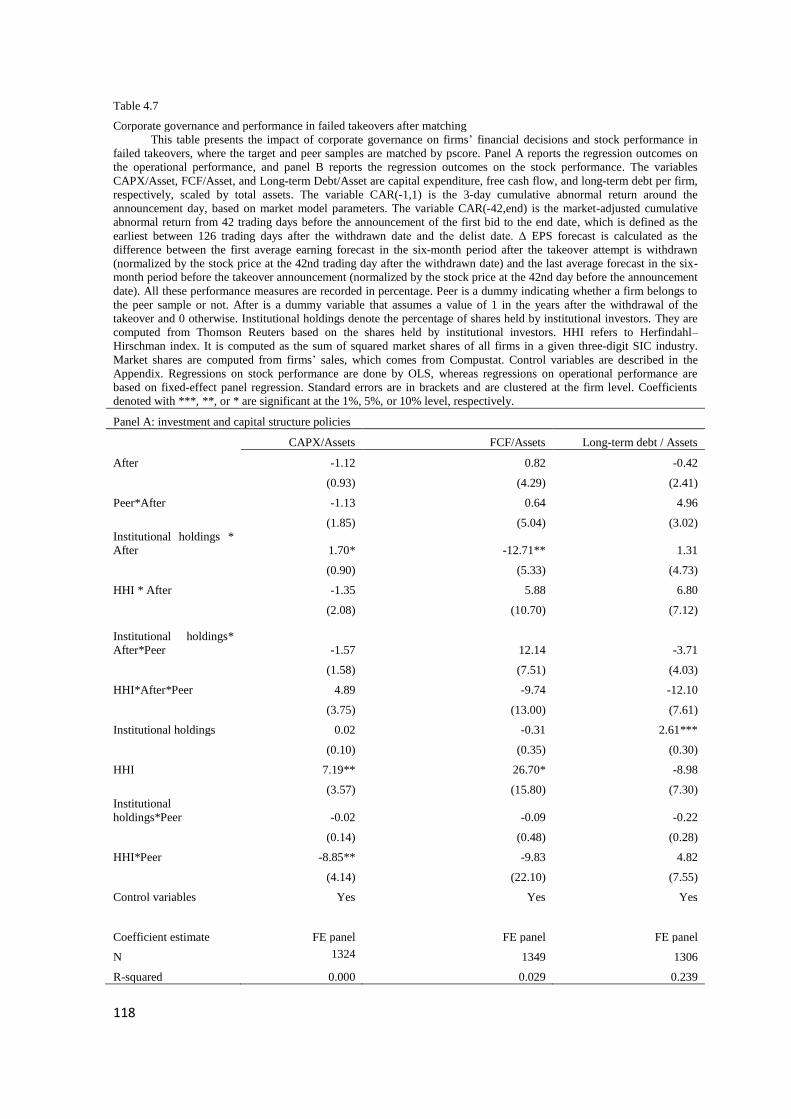
118
Table 4.7
Corporate governance and performance in failed takeovers after matching
This table presents the impact of corporate governance on firms’ financial decisions and stock performance in
failed takeovers, where the target and peer samples are matched by pscore. Panel A reports the regression outcomes on
the operational performance, and panel B reports the regression outcomes on the stock performance. The variables
CAPX/Asset, FCF/Asset, and Long-term Debt/Asset are capital expenditure, free cash flow, and long-term debt per firm,
respectively, scaled by total assets. The variable CAR(-1,1) is the 3-day cumulative abnormal return around the
announcement day, based on market model parameters. The variable CAR(-42,end) is the market-adjusted cumulative
abnormal return from 42 trading days before the announcement of the first bid to the end date, which is defined as the
earliest between 126 trading days after the withdrawn date and the delist date. Δ EPS forecast is calculated as the
difference between the first average earning forecast in the six-month period after the takeover attempt is withdrawn
(normalized by the stock price at the 42nd trading day after the withdrawn date) and the last average forecast in the six-
month period before the takeover announcement (normalized by the stock price at the 42nd day before the announcement
date). All these performance measures are recorded in percentage. Peer is a dummy indicating whether a firm belongs to
the peer sample or not. After is a dummy variable that assumes a value of 1 in the years after the withdrawal of the
takeover and 0 otherwise. Institutional holdings denote the percentage of shares held by institutional investors. They are
computed from Thomson Reuters based on the shares held by institutional investors. HHI refers to Herfindahl–
Hirschman index. It is computed as the sum of squared market shares of all firms in a given three-digit SIC industry.
Market shares are computed from firms’ sales, which comes from Compustat. Control variables are described in the
Appendix. Regressions on stock performance are done by OLS, whereas regressions on operational performance are
based on fixed-effect panel regression. Standard errors are in brackets and are clustered at the firm level. Coefficients
denoted with ***, **, or * are significant at the 1%, 5%, or 10% level, respectively.
Panel A: investment and capital structure policies
CAPX/Assets FCF/Assets Long-term debt / Assets
After -1.12 0.82 -0.42
(0.93) (4.29) (2.41)
Peer*After -1.13 0.64 4.96
(1.85) (5.04) (3.02)
Institutional holdings *
After 1.70* -12.71** 1.31
(0.90) (5.33) (4.73)
HHI * After -1.35 5.88 6.80
(2.08) (10.70) (7.12)
Institutional holdings*
After*Peer -1.57 12.14 -3.71
(1.58) (7.51) (4.03)
HHI*After*Peer 4.89 -9.74 -12.10
(3.75) (13.00) (7.61)
Institutional holdings 0.02 -0.31 2.61***
(0.10) (0.35) (0.30)
HHI 7.19** 26.70* -8.98
(3.57) (15.80) (7.30)
Institutional
holdings*Peer -0.02 -0.09 -0.22
(0.14) (0.48) (0.28)
HHI*Peer -8.85** -9.83 4.82
(4.14) (22.10) (7.55)
Control variables Yes Yes Yes
Coefficient estimate FE panel FE panel FE panel
N 1324 1349 1306
R-squared 0.000 0.029 0.239
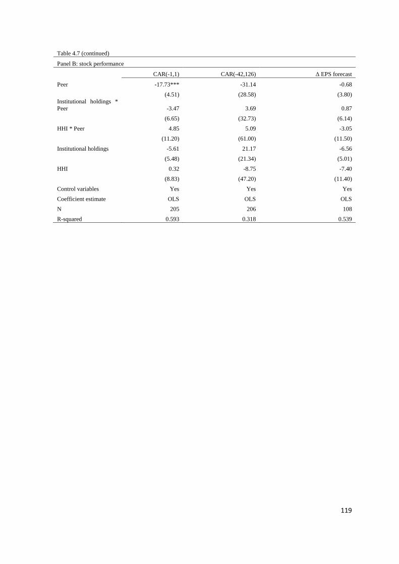
119
Table 4.7 (continued)
Panel B: stock performance
CAR(-1,1) CAR(-42,126) Δ EPS forecast
Peer -17.73*** -31.14 -0.68
(4.51) (28.58) (3.80)
Institutional holdings *
Peer -3.47 3.69 0.87
(6.65) (32.73) (6.14)
HHI * Peer 4.85 5.09 -3.05
(11.20) (61.00) (11.50)
Institutional holdings -5.61 21.17 -6.56
(5.48) (21.34) (5.01)
HHI 0.32 -8.75 -7.40
(8.83) (47.20) (11.40)
Control variables Yes Yes Yes
Coefficient estimate OLS OLS OLS
N 205 206 108
R-squared 0.593 0.318 0.539

120
4.5. Conclusion
This article studies whether different corporate governance mechanisms are complements
or substitutes in improving firms’ decisions and stock market performance. More
specifically, I study how monitoring by institutional investors and competition from the
product market affect firms’ responses in failed takeovers. In the context of failed
takeovers, I investigate the impact of monitoring by institutional investors and competition
in the product market on the firms’ performance in terms of operational performance and
market recognition, which has not been studied earlier.
The result provides weak evidence on the complement argument for corporate
governance mechanisms, in particular in terms of firms’ financial decisions. Institutional
holdings have a mixed impact on reducing overinvestment in target firms and have no
impact on peer firms’ operational decisions. For the target firms, it decreases free cash
flow on the one hand, but increases capital spending on the other hand. Furthermore, it has
no impact on the stock performance—for either target firms or peer firms—around the
takeovers, which indicates no difference in investors’ view on firms’ performance with
different institutional holdings. Competition in the product market also shows no influence
on firms’ responses. Although it affects peer firms’ stock returns around takeovers, this
influence is attributed to the positive correlation between industry concentration and the
strength of takeover threat.
The result has important policy implications. Since governance mechanisms are not
good complements, they suggest little spill-over effect by improving corporate governance
in alternative forms in the presence of a well-functioning governance force. Thus, more
effort should be directed to places where one form of corporate governance is weak. For

121
example, it can be more beneficial to improve governance quality in non-competitive
industries than in competitive industries.
This study focuses on three aspects of corporate governance. Future work can be
extended to how other corporate governance mechanisms, such as monitoring by large
non-institutional holders or the board, influence a target firm’s response to takeover threats,
or the interaction between internal governance mechanisms when the firm is not faced with
a takeover initiative.

122
Appendix 4.A
Control variables
This table gives a summary of control variables used in this article. The control variables used for accounting
measures (CAPX/Assets, Long-term Debt/Assets, and FCF/Assets) are similar to those in Servaes and Tamayo (2013),
and the control variables used for stock performances (CARs and delta EPS forecast) are similar to those in Dai,
Gryglewicz, and Smit (2013).
Dependent variable Control variables
CAPX/Assets lagged Tobin’s q, measured as (book value of assets - book value of equity + deferred taxes +
market value of equity) / book value of assets;
Long term debt /
Assets i. EBIT / assets;
ii. net property, plant and equipment / assets;
iii. log assets;
iv. R&D / assets;
v. selling, general and administrative expenses / assets.
FCF / Assets log assets.
CAR(-1,1),
CAR(-42, end),
and Δ EPS forecast
i. size of toeholds;
ii. number of analysts making one-year-ahead earnings forecasts in the announcement year;
iii. Log of market value at the 42nd trading day before the announcement date normalized at
the price level of 1987;
v. the average of the daily turnovers over the window [-166, -42] ;
iv. a dummy equal to 1 if the stock price is less than one dollar at the 42nd trading day before
the announcement date;
vi. a dummy equal to 1 if the stock is listed on NYSE or AMEX;
vii. a dummy equal to 1 if it is a tender offer.
viii. a dummy equal to 1 if the takeover is paid by 100% cash;
ix. a dummy equal to 1 if the deal attitude is hostile;
x. a dummy equal to 1 if there are multiple bidders;
xi. a dummy equal to 1 if the firm is incorporated in an antitakeover state;
xii. year dummies;
xiii. industry dummies (using 48 Fama-French industries).
123
Summary
This dissertation investigates three key questions about efficiency in corporate takeovers.
They are 1) What are the optimal decisions in takeover contests? 2) How to measure the
efficiency of a takeover strategy? and 3) How to improve firms’ performance in takeovers?
Three chapters, in this dissertation, are written to provide our thoughts on these questions.
Chapter 2 proposes that the level of similarity in bidders’ valuations is an important
factor that determines bidders’ entry and bidding decisions. When bidders in a
corporate takeover have related resources and post-acquisition strategies, their valuations
of a target are likely to be interdependent. This chapter analyzes sequential-
entry takeover contests in which similar bidders have correlated private valuations. The
level of similarity affects information content of bids and bidding competition. Our model
predicts that expected acquisition prices and the probability of multiple-bidder contests are
the highest for intermediately similar bidders. We test these predictions in laboratory
experiments in which we control the similarity between bidders. The experimental data
confirm the non-monotonic effects of similarity on prices and on the frequency of
multiple-bidder contests.
Chapter 3 introduces a dynamic perspective in evaluating the takeover strategy with
toeholds37
. Despite their decreasing popularity, toehold strategies to acquire targets do, in
fact, perform better overtime. We propose a new explanation for the improved execution of
37 Toeholds refer to the minority ownership of the target’s shares owned by the acquirer before a takeover.

124
the toehold strategy: Qualified acquirers learn to use the strategy effectively, while
unqualified acquirers have learned to walk away, because of the pitfalls involved in
bidding with toeholds. Evidence, using self-selection models, supports this notion.
Corporate governance, such as institutional holdings, also appear successful in improving
outcomes in a toehold acquisition strategy, suggesting that firms with better monitoring are
the more qualified toeholds acquirers.
In the context of failed takeovers, chapter 4 investigates whether internal (i.e.
monitoring from institutional investors) and external governance mechanisms (i.e.
competition form product markets) can improve firms’ response to takeover threats and
their stock performance. I collect data for two groups of firms (1) targets that are faced
with strong threats and (2) peers that are faced with weak threats. The results indicate that
governance mechanisms are at most weak complements to takeover threats in terms of
promoting firms’ performance. The internal and external governance mechanisms can
improve targets’ restructuring decisions (i.e. on free cash flow) to some extent, but cannot
enhance peer firms’ response. Furthermore, both governance mechanisms fail to bring
higher stock performance for firms.

125
Samenvatting (Summary in Dutch)
Dit proefschrift onderzoekt drie belangrijke vragen over efficiency bij bedrijfsovernames.
Deze zijn: 1) Wat zijn optimale beslissingen bij bedrijfsovernames? 2) Hoe kan de
efficiency van een overnamestrategie worden gemeten? 3) Hoe kan de prestatie van
bedrijven bij een overname verbeterd worden? Deze vragen worden in drie opeenvolgende
hoofdstukken van dit proefschrift nader uitgewerkt.
Hoofdstuk 2 stelt dat de mate waarin de waardebepaling van verschillende bieders
overeenstemt een belangrijke factor is, die zowel de beslissing van een bieder om mee te
dingen als de hoogte van het uitgebrachte bod bepaalt. Wanneer de bieders vergelijkbare
middelen en post-acquisitiestrategieën hebben, dan is het waarschijnlijk dat er een
interdependentie is van hun waardebepaling van het overnamedoelwit. Dit hoofdstuk
analyseert overnames waarbij de beslissing om mee te bieden sequentieel (opeenvolgend)
is en waarbij er een correlatie is tussen de individuele waardebepalingen van op elkaar
lijkende bieders. De mate van gelijkenis beïnvloedt het informatiegehalte van de biedingen
en de biedstrijd. Ons model voorspelt dat de verwachte acquisitieprijs en de kans dat er een
biedingenstrijd tussen meerdere bieders ontstaat hoger is wanneer er sprake is van een
beperkte mate van gelijkenis tussen de bieders. We testen deze voorspelling met
laboratoriumexperimenten waarbij we de mate waarin bieders op elkaar lijken laten
variëren. De resultaten van het experiment bevestigen het bestaan van niet-monotone
effecten die dermate van gelijkenis heeft op zowel de acquisitieprijs, als op de kans dat een
overnamestrijd ontstaat.

126
Hoofdstuk 3 introduceert een dynamisch perspectief waarbij een ‘toehold’ strategie
gehanteerd wordt. Dit betekent dat de bieder voorafgaand aan een overnamestrijd al een
minderheidsbelang heeft in het overnamedoelwit. In weerwil van hun afnemende
populariteit blijkt dat ‘toeholds’ uiteindelijk een beter resultaat opleveren. Wij vinden een
nieuwe verklaring voor de betere resultaten van een toehold strategie: kopers met goede
kwalificaties leren hoe ze de strategie optimaal kunnen inzetten, terwijl kopers met slechte
kwalificaties leren om de overnamestrijd niet aan te gaan, vanwege de valkuilen die
gepaard gaan met toehold biedingen. Resultaten van zelf-selectiemodellen ondersteunen
deze hypothese. Governance maatregelen, zoals institutioneel aandeelhouderschap, lijken
ook te leiden tot betere resultaten van een toehold strategie, wat suggereert dat bedrijven
met een betere monitoring ook beter gekwalificeerde kopers zijn.
In het kader van gefaalde overnames onderzoekt hoofdstuk 4 of interne governance
mechanismen (zoals institutioneel aandeelhouderschap) en externe governance
mechanismen (zoals concurrentie op de productmarkt) een positief effect hebben op de
reactie van een bedrijf op een overnamedreiging en op de aandelenkoers. We verzamelen
informatie voor twee groepen bedrijven: 1) “overnamedoelwitten” die een sterke
overnamedreiging voelen en 2) een controlegroep met vergelijkbare bedrijven die een
zwakke overnamedreiging voelen. Uit de resultaten blijkt dat governance mechanismen
hooguit een zwak complement voor een overnamedreiging vormen bij het verbeteren van
de aandelenkoers van het bedrijf. Interne en externe governance mechanismen kunnen de
herstructureringsbeslissing van een overnamedoelwit (bijvoorbeeld vrije cash flows)
enigszins verbeteren, maar verbetert niet de respons van de controlegroep op een
overnamedreiging. Tenslotte resulteren geen van beide governance mechanismen in een
hogere aandelenkoers.

127
Bibliography
[1] Agrawal, A. and G.N. Mandelker, 1990. “Large shareholders and the monitoring of
managers: the case of antitakeover charter amendments,” Journal of Financial and
Quantitative Analysis 25, 143-161.
[2] Allen F., A.E. Bernardo, and I. Welch, 2000. “A theory of dividends based on tax
clienteles,” The Journal of Finance 55, 2499-2536.
[3] Amihud Y., and B. Lev, 1981. “Risk reduction as a managerial motive for
conglomerate mergers,” The Bell Journal of Economics 12, 605-617.
[4] Andrade, G., M. Mitchell, and E. Stafford, 2001. “New evidence and perspectives
on mergers,” Journal of Economic Perspectives 15, 103–120.
[5] Aoyagi, M., and G. Frechette, 2009. “Collusion as public monitoring becomes
noisy: experimental evidence,” Journal of Economic Theory 144, 1135-1165.
[6] Arkes H.R., and C. Blumer, 1985. “The psychology of sunk cost,” Organizational
Behavior and Human Decision Process 35, 124-140.
[7] Atanassov, J., 2013. “Do hostile takeovers stifle innovation? Evidence from
antitakeover legislation and corporate patenting,” The Journal of Finance 68, 1097-
1131.
[8] Bargeron, L., F. Schlingemann, R. Stulz, and C. Zutter, 2008. “Why do private
acquirers pay so little compared to public acquirers?” Journal of Financial
Economics 89, 375–390.
128
[9] Berkovitch, E., and M. Narayanan, 1993. “Motives for takeovers: an empirical
investigation,” The Journal of Financial and Quantitative Analysis 28, 347-362.
[10] Bertrand, M. and S. Mullainathan, 2003. “Enjoying the quite life? Corporate
governance and managerial preferences,” Journal of Political Economy 111, 1043-
1075.
[11] Betton S., and B.E. Eckbo, 2000. “Toeholds, bid jumps, and expected payoffs in
takeovers,” The Review of Financial Studies 13, 841-882.
[12] Betton S., B.E. Eckbo, and K.S. Thorburn, 2008. “Corporate takeovers,” in
Handbook of Empirical Corporate Finance, Vol. 2, edited by B.E. Eckbo. North-
Holland: Elsevier press.
[13] Betton S., B. E. Eckbo, and K. S. Thorburn, 2009a. “Merger negotiations and the
toehold puzzle,” Journal of Financial Economics 91, 158-178.
[14] Betton S., B.E. Eckbo, and K.S. Thorburn, 2009b. “Markup pricing revisited,”
working paper.
[15] Boone, A., and J. Mulherin, 2008. “Do auctions induce a winner's curse: new
evidence from the corporate takeover market,” Journal of Financial Economics 89,
1–19.
[16] Bradley, M., A. Desai, and E. Kim, 1988. “Synergistic gains from corporate
acquisitions and their division between the stockholders of target and acquiring
firms,” Journal of Financial Economics 21, 3–40.
129
[17] Brand, J.E. and C.N. Halaby, 2006. “Regression and matching estimates of the
effects of elite college attendance on educational and career achievement,” Social
Science Research 35, 749-770.
[18] Brickley, J.A., R.C. Lease, and C.W. Smith, Jr., 1988. “Ownership structure and
voting on antitakeover amendments,” Journal of Financial Economics 20, 267-291.
[19] Bris A., 2002. “Toeholds, takeover premium, and the probability of being acquired,”
Journal of Corporate Finance 8, 227-253.
[20] Bulow J., M. Huang and P. Klemperer, 1999. “toeholds and takeovers,” Journal of
Political Economy 107, 427-454.
[21] Bulow, J., and P. Klemperer, 2009. “Why do sellers (usually) prefer auctions,”
American Economic Review 99, 1544–1575.
[22] Burkart M., 1995. “Initial shareholdings and overbidding in takeover contests,” The
Journal of Finance, 50, 1491-1515.
[23] Caliendo, M. and S. Kopeinig, 2008. “Some practical guidance for the
implementation of propensity score matching,” Journal of Economic Surveys 22,
31-72.
[24] Cameron, A., J. Gelbach, and D. Miller, 2008. “Bootstrap-based improvements for
inference with clustered errors,” Review of Economics and Statistics 90, 414-427.
[25] Chamberlain, G., 1980. “Analysis of covariance with qualitative data,” Review of
Economic Studies 47, 225-238.
130
[26] Che, Y., and T. Lewis, 2007. “The role of lockups in takeover contests,” RAND
Journal of Economics 38, 648–669.
[27] Chen X., J. Harford, and K. Li, 2007. “Monitoring: Which institutions matter?”
Journal of Financial Economics 86, 279-305.
[28] Chowdhry B., and N. Jegadeesh, 1994. “Pre-tender offer share acquisition strategy
in takeovers,” The Journal of Financial Quantitative Analysis 29, 117-129.
[29] Chowdhry, B., and V. Nanda, 1993. “The strategic role of debt in takeover
contests,” Journal of Finance 48, 731–745.
[30] Croson, R., A. Gomes, K. McGinn, and M. Nöth, 2004. “Mergers and acquisitions:
an experimental analysis of synergies, externalities and dynamics,” Review of
Finance 8, 481–514.
[31] Dai, 2013. "Are corporate governance mechamisms complements? Evidence from
failed takeovers," Working paper.
[32] Dai, Y., S. Gryglewicz and H.T.J. Smit, 2013. “The learning effect in takeovers with
toeholds,” Working paper.
[33] Dai, Y., S. Gryglewicz, H.T.J. Smit and W. de Maeseneire, 2013. “Similar bidders
in takeover contests,” Games and Economic Behavior 82, 544-561.
[34] Daniel, K., and D. Hirshleifer, 1998. “A theory of costly sequential bidding,”
Working paper. Kellogg Graduate School of Management.
[35] Davies, R. and S. Kim, 2003. “Matching and the estimated impact of interlisting,”

131
Discussion Paper in Finance No. 2001-11, ISMA Center, Reading.
[36] Dehejia, R.H. and S. Wahba, 1999. “Causal effects in nonexperimental studies:
reevaluating the evaluation of training programs,” Journal of the American
Statistical Association 97, 1053-1062.
[37] Del Guercio D., and J. Hawkins, 1999. “The motivation and impact of pension fund
activism,” Journal of Financial Economics 52, 293-340.
[38] Denis D.J. and J.M. Serrano, 1996. “Active investors and management turnover
following unsuccessful control contests,” Journal of Financial Economics 40, 239-
266.
[39] Denis, D.J. and T.A. Kruse, 2000. “Mangerial discipline and corporate restructuring
following performance decline,” Journal of Financial Economics 55, 391-424.
[40] Dittmar A., and J. Mahrt-Smith, 2007. “Corporate governance and the value of cash
holdings,” Journal of Financial Economics 83, 599-634.
[41] Fishman, M., 1988. “A theory of preemptive takeover bidding,” RAND Journal of
Economics 19, 88–101.
[42] Fishman M., 1989. “Preemptive bidding and the role of the medium of exchange in
acquisitions,” Journal of Finance 44, 41–57.
[43] Franks J. and C. Mayer, 1996. “Hostile takeovers and the correction of managerial
failure,” Journal of Financial Economics 40, 163-181.
[44] Frechette, G., 2012. “Session-effects in the laboratory,” Experimental Economics
132
15, 485-498.
[45] Fuller, K., J. Netter, and M. Stegemoller, 2002. “What do returns to acquiring firms
tell us: evidence from firms that make many acquisitions,” Journal of Finance 57,
1763–1793.
[46] Gaspar J.M., M. Massa, and P. Matos, 2005. “Shareholder investment horizons and
the market for corporate control,” Journal of Financial Economics 76, 135-165.
[47] Gillan, S.L. and L.T. Starks, 2000. “Corporate governance proposals and
shareholder activism: the role of institutional investors,” Journal of Financial
Economics 57, 275-305.
[48] Gillette, A., and T. Noe, 2006. “If at first you don’t succeed: an experimental
investigation of the impact of repetition options on corporate takeovers and the
provision of public goods,” Review of Financial Studies 19, 561–603.
[49] Giroud, X. and H.M. Mueller, 2010. “Does corporate governance matter in
competitive industries?” Journal of Financial Economics 95, 312-331.
[50] Gneezy, U., and A. Rustichini, 2000. “Pay enough or don’t pay at all,” The
Quarterly Journal of Economics 115, 791-810.
[51] Goldman E., and J. Qian, 2005. “Optimal toeholds in takeover contests,” Journal of
Financial Economics 77, 321-346.
[52] Gompers P., and A. Metrick, 2001. “Institutional investors and equity prices,”
Quartly Journal of Economics 116, 229-259.
133
[53] Grossman, S.J. and O.D. Hart, 1982. “Corporate financial structure and managerial
incentives,” in The Economics of Information and Uncertainty, edited by J. McCall.
University of Chicago Press.
[54] Guenther, D.A. and A.J. Rosman, 1994. “Difference between Compustat and CRSP
SIC Codes and related effects on research,” Journal of Accounting and Economics
18, 115-128.
[55] Hadlock, C.J., and G.B. Lumer, 1997. “Compensation, turnover and top
management incentives: Historical evidence,” Journal of Business 70, 153-187.
[56] Hartzell, J.C. and L.T. Starks, 2003. “Institutional investors and executive
compensation,” The Journal of Finance 58, 2351-2374.
[57] Haunschild, P.R., A. Davis-Blake, and M. Fichman, 1994. “Managerial
overcommitment in corporate acquisition processes,” Organization Science 5, 528-
540.
[58] Hayward, M., and D. Hambrick, 1997. “Explaining the premiums paid for large
acquisitions: Evidence of CEO hubris,” Administrative Science Quarterly 42, 103-
127.
[59] Heckman J.J., 1979. “Sample selection bias as a specification error,” Econometrica
47, 153-161.
[60] Heckman, J.J., 1981. “Structural analysis of discrete data with econometric
applications,” In The incidental parameters problem and the problem of initial
conditions in estimating a discrete time-discrete data stochastic process, 179-195.
134
Cambridge: MIT Press.
[61] Heckman, J.J., H. Ichmura, and R.E. Todd, 1997. “Evaluation estimator: Evidence
from evaluating a job training programme,” Review of Economic Studies 64, 605-
654.
[62] Hirshleifer, D., and I. Png, 1989. “Facilitation of competing bids and the price of a
takeover bid,” Review of Financial Studies 2, 587–606.
[63] Hirshleifer D., and S. Titman, 1990. “Share tendering strategies and the success of
hostile takeover bids,” The Journal of Political Economy 98, 295-324.
[64] Hitt, L. and F. Frei, 2002. “Do better customers utilize electronic distribution
channels? The case of PC banking,” Management Science 48, 732-748.
[65] Holmstrom, B., and S.N. Kaplan, 2001. “Corporate governance and merger activity
in the United States: Making sense of the 1980s and 1990s,” Journal of Economic
Perspectives 15, 121-144.
[66] Huson, Parrino and Starks, 2001. “Internal monitoring mechanisms and CEO
turnover: A long-term perspective,” The Journal of Finance 56, 2265-2297.
[67] Jennings R.H., and M.A. Mazzeo, 1993. “Competing bids, target management
resistance, and the structure of takeover bids,” The Review of Financial Studies 6,
883-909.
[68] Jensen, M.C., 1986. “Agency costs of free cash flow, corporate finance, and
takeovers,” American Economic Review 76, 323-329.

135
[69] Kagel, J., 1995. “Auctions: a survey of experimental research,” In: Kagel J., Roth A.
(Eds.), The Handbook of Experimental Economics. Princeton, NJ: Princeton
University Press.
[70] Kahle, K.M. and R.A. Walkling, 1996. “The impact of industry classifications on
financial research,” Journal of Financial and Quantitative Analysis 31, 309-335.
[71] Kale, J., O. Kini, and H. Ryan, 2003. “Financial advisors and shareholder wealth
gains in corporate takeovers,” Journal of Financial and Quantitative Analysis 38,
475–501.
[72] Kale, J., and T. Noe, 1997. “Unconditional and conditional takeover offers:
experimental evidence,” Review of Financial Studies 10, 735–766.
[73] Kanodia C., R. Bushman, and J. Dickhaut, 1989. “Escalation errors and the sunk
cost effect: An explanation based on reputation and information asymmetries,”
Journal of Accounting Research 27, 59-77.
[74] Kogan, S., and J. Morgan, 2010. “Securities auctions under moral hazard: an
experimental study,” Review of Finance 14, 477–520.
[75] Lambrecht, B.M. and S.C. Myers, 2007. “A theory of takeovers and disinvestment,”
The Journal of Finance 62, 809-845.
[76] Laughhunn D., and J.W. Payne, 1984. “The impact of sunk outcomes on risk choice
behavior,” Canadian Journal of Operational Research and Information Processing
22, 155-181.

136
[77] Leeth J., and J. Borg, 2000. “The impact of takeovers on shareholder wealth during
the 1920s merger wave,” Journal of Financial and Quantitative Analysis 35, 217–
238.
[78] Levi M., K. Li, and F. Zhang, 2010. “Deal or no deal: Hormones and the mergers
and acquisitions game,” Management Science 56, 1462-1483.
[79] Li K., and N. Prabhala, 2007. “Self-selection models in corporate finance,” in
Handbook of Empirical Corporate Finance, Vol. 1, edited by B.E. Eckbo. North-
Holland: Elsevier.
[80] Malmendier, U., and G. Tate, 2008. “Who makes acquisitions? CEO overconfidence
and the market’s reaction,” Journal of Financial Economics 89, 20-43.
[81] Mikkelson, W.H. and M.M. Partch, 1997. “The decline of takeovers and disciplinary
managerial turnover,” Journal of Financial Economics 44, 205-228.
[82] Moeller, S., F. Schlingemann, and R. Stulz, 2004. “Firm size and the gains from
acquisitions,” Journal of Financial Economics 73, 201–228.
[83] Moeller, S., F. Schlingemann, and R. Stulz, 2005. “Wealth destruction on a massive
scale: a study of acquiring firm returns in the recent merger wave,” Journal of
Finance 60, 757–782.
[84] Moeller, S., F. Schlingemann, and R. Stulz, 2007. “How do diversity of opinion and
information asymmetry affect acquirer returns,” Review of Financial Studies 20,
2047–2078.
137
[85] Morck, R., A. Shleifer, and R.W. Vishny, 1989. “Alternative mechanisms for
corporate control,” American Economic Review 79, 842-852.
[86] Mueller D.C., 1969. “A theory of conglomerate mergers,” Quarterly Journal of
Economics 16, 643-659.
[87] Nickell, S., D. Nicolitsas, and N. Dryden, 1997. “What makes firms perform well?”
European Economic Review 41, 783-796.
[88] Perkins, S.M., W. Tu, M.G. Underhill, X. Zhou and M.D. Murray, 2000. “The use
of propensity scores in pharmacoepidemiologic research,” Pharmacoepidemiolog
and Drug Safety 9, 93-101.
[89] Petersen, M., 2009. “Estimating standard errors in finance panel data sets:
comparing approaches,” The Review of Financial Studies 22, 435-480.
[90] Ravid S.A., and M. Spiegel, 1999. “Toehold strategies, takeover laws and rival
acquirers,” Journal of Banking & Finance 23, 1219-1242.
[91] Rojas, C., 2012. “The role of demand information and monitoring in tacit collusion,”
RAND Journal of Economics 43, 78-109.
[92] Roll, R., 1986. “The hubris hypothesis of corporate takeovers,” Journal of Business
59, 197-216.
[93] Rosenbaum, P.R. and D.B. Rubin, 1983. “The central role of the propensity score in
observational studies for causal effects,” Biometrika 70, 41-55.
[94] Safieddine A. and S. Titman, 1999. “Leverage and corporate performance: evidence
138
from unsuccessful takeovers,” The Journal of Finance 54, 547-580.
[95] Schranz M.S., 1993. “Takeovers improve firm performance: Evidence from the
banking industry,” Journal of Political Economy 101, 299-326.
[96] Schwert, W., 2000. “Hostility in takeovers: in the eyes of the beholder,” Journal of
Finance 55, 2599–2640.
[97] Servaes, H. and A. Tamayo, 2013. “How do industry peers respond to control
threats?” Mangement Science, forthcoming.
[98] Shleifer, A. and R.W. Vishny, 1986. “Large shareholders and corporate control,”
Journal of Political Economy 94, 461-488.
[99] Shleifer, A. and R.W. Vishny, 1997. “A survey of corporate governance,” The
Journal of Finance 52, 737-783.
[100] Singh R., 1998. “Takeover bidding with toeholds: The case of the owner’s curse,”
The Review of Financial Studies 11, 679-704.
[101] Smith, V. L., and J.M. Walker, 1993. “Monetary rewards and decision cost in
experimental economics,” Economic Inquiry 31, 245-261.
[102] Staw B.M., 1976. “Knee deep in the big muddy: A study of escalating commitment
to a chosen course of action,” Organizational Behavior and Human Performance 16,
26-44.
[103] Staw B. M., and J. Ross, 1986. “Behavior in escalation situations: Antecedents,
prototypes, and solutions,” in Research in Organizational Behavior, edited by S.

139
Cummings and B. Staw. Greenwich, Conn.: JAI Press.
[104] Stulz, R., R. Walkling, and M. Song, 1990. “The distribution of target ownership
and the division of gains in successful takeovers,” Journal of Finance 45, 817–833.
[105] Thaler R., 1980. “Towards a positive theory of consumer choice,” Journal of
Economic Behavior and Organization 1, 39-60.
[106] Walker, M., 2000. “Corporate takeovers, strategic objectives, and acquiring-firm
shareholder wealth,” Financial Management 29, 53–66.
[107] Weber R.A., and C.F. Camerer C. F., 2003. “Cultural conflict and merger failure: an
experimental approach,” Management Science 49, 400-415.
[108] Wooldridge, J.M., 2002. “Econometric analysis of cross section and panel data,”
Cambridge: MIT Press.

141
TINBERGEN INSTITUTE RESEARCH SERIES
The Tinbergen Institute is the Institute for Economic Research, which was founded in 1987
by the Faculties of Economics and Econometrics of the Erasmus University Rotterdam,
University of Amsterdam and VU University Amsterdam. The Institute is named after the
late Professor Jan Tinbergen, Dutch Nobel Prize laureate in economics in 1969. The
Tinbergen Institute is located in Amsterdam and Rotterdam. The following books recently
appeared in the Tinbergen Institute Research Series:
535 A. KOTHIYAL, Subjective Probability and Ambiguity
536 B. VOOGT, Essays on Consumer Search and Dynamic Committees
537 T. DE HAAN, Strategic Communication: Theory and Experiment
538 T. BUSER, Essays in Behavioural Economics
539 J.A. ROSERO MONCAYO, On the importance of families and public
policies for child development outcomes
540 E. ERDOGAN CIFTCI, Health Perceptions and Labor Force Participation
of Older Workers
541 T.WANG, Essays on Empirical Market Microstructure
542 T. BAO, Experiments on Heterogeneous Expectations and Switching
Behavior
543 S.D. LANSDORP, On Risks and Opportunities in Financial Markets
544 N. MOES, Cooperative decision making in river water allocation problems
545 P. STAKENAS, Fractional integration and cointegration in financial time

142
series
546 M. SCHARTH, Essays on Monte Carlo Methods for State Space Models
547 J. ZENHORST, Macroeconomic Perspectives on the Equity Premium
Puzzle
548 B. PELLOUX, the Role of Emotions and Social Ties in Public On Good
Games: Behavioral and Neuroeconomic Studies
549 N. YANG, Markov-Perfect Industry Dynamics: Theory, Computation, and
Applications
550 R.R. VAN VELDHUIZEN, Essays in Experimental Economics
551 X. ZHANG, Modeling Time Variation in Systemic Risk
552 H.R.A. KOSTER, The internal structure of cities: the economics of
agglomeration, amenities and accessibility.
553 S.P.T. GROOT, Agglomeration, globalization and regional labor markets:
micro evidence for the Netherlands.
554 J.L. MÖHLMANN, Globalization and Productivity Micro-Evidence on
Heterogeneous Firms, Workers and Products
555 S.M. HOOGENDOORN, Diversity and Team Performance: A Series of
Field Experiments
556 C.L. BEHRENS, Product differentiation in aviation passenger markets:
The impact of demand heterogeneity on competition
557 G. SMRKOLJ, Dynamic Models of Research and Development
558 S. PEER, The economics of trip scheduling, travel time variability and
traffic information
559 V. SPINU, Nonadditive Beliefs: From Measurement to Extensions
560 S.P. KASTORYANO, Essays in Applied Dynamic Microeconometrics

143
561 M. VAN DUIJN, Location, choice, cultural heritage and house prices
562 T. SALIMANS, Essays in Likelihood-Based Computational Econometrics
563 P. SUN, Tail Risk of Equidity Returns
564 C.G.J. KARSTEN, The Law and Finance of M&A Contracts
565 C. OZGEN, Impacts of Immigration and Cultural Diversity on Innovation
and Economic Growth
566 R.S. SCHOLTE, The interplay between early-life conditions, major events
and health later in life
567 B.N.KRAMER, Why don’t they take a card? Essays on the demand for
micro health insurance
568 M. KILIÇ, Fundamental Insights in Power Futures Prices
569 A.G.B. DE VRIES, Venture Capital: Relations with the Economy and
Intellectual Property
570 E.M.F. VAN DEN BROEK, Keeping up Appearances
571 K.T. MOORE, A Tale of Risk: Essays on Financial Extremes
572 F.T. ZOUTMAN, A Symphony of Redistributive Instruments
573 M.J. GERRITSE, Policy Competition and the Spatial Economy
574 A. OPSCHOOR, Understanding Financial Market Volatility
575 R.R. VAN LOON, Tourism and the Economic Valuation of Cultural
Heritage
576 I.L. LYUBIMOV, Essays on Political Economy and Economic
Development
577 A.A.F. GERRITSEN, Essays in Optimal Government Policy
578 M.L. SCHOLTUS, The Impact of High-Frequency Trading on Financial
Markets
144
579 E. RAVIV, Forecasting Financial and Macroeconomic Variables:
Shrinkage, Dimension reduction, and Aggregation
580 J. TICHEM, Altruism, Conformism, and Incentives in the Workplace
581 E.S. HENDRIKS, Essays in Law and Economics
582 X. SHEN, Essays on Empirical Asset Pricing
583 L.T. GATAREK, Econometric Contributions to Financial Trading,
Hedging and Risk Measurement
584 X. LI, Temporary Price Deviation, Limited Attention and Information
Acquisition in the Stock Market
585 Y. DAI, Efficiency in Corporate Takeovers