eindhoven university of technology master h-infinity ... · fk control as applied to torsional...

Eindhoven University of Technology

MASTER

H-infinity control as applied to torsional drillstring dynamics

Serrarens, A.F.A.

Award date:1997

DisclaimerThis document contains a student thesis (bachelor's or master's), as authored by a student at Eindhoven University of Technology. Studenttheses are made available in the TU/e repository upon obtaining the required degree. The grade received is not published on the documentas presented in the repository. The required complexity or quality of research of student theses may vary by program, and the requiredminimum study period may vary in duration.

General rightsCopyright and moral rights for the publications made accessible in the public portal are retained by the authors and/or other copyright ownersand it is a condition of accessing publications that users recognise and abide by the legal requirements associated with these rights.

• Users may download and print one copy of any publication from the public portal for the purpose of private study or research. • You may not further distribute the material or use it for any profit-making activity or commercial gain

Take down policyIf you believe that this document breaches copyright please contact us providing details, and we will remove access to the work immediatelyand investigate your claim.

Download date: 08. Jul. 2018

fk Control as Applied to Torsional Drillstring Dynamics

A.F.A. Serrarens

Report number: WFW 97.020

Mas ter Thesis

Committee: Prof. dr. ir j. Kok (TUB) dr. ir. R. van de Molengraft (TUE) dr. ir. A. de Jager (TUE) ir. L. van den Steen (SIEP) ir. M. Heertjes (TUE)

Author: A.F. A.Serrarens Institution: Mentors:

Report number: WFW 97.020 Date: March 1997

Shell International Exploration & Production (SIEP) ir. L. van den Steen (SIEP); ir. R. van de Molengraft (TUE)

Nm Control as Applied to Torsional Drillstring Dynamics

A.F.A. Serrarens

March 19, 1997

bummary

In the field of gas- and oil well drilling often use is made of drillstrings made out of thin-walled pipe sections screwed to one another. The drillstring is exerted by an electric motor connected by a gear system to the drillstring. The lower sections of this drillpipe have a larger wall thickness to provide sufficient pressure, without buckling, on the drilling bit that is connected to the string at the very bottom end. As of the combination of this heavy thick-walled section referred to as the Bottom Hole Assembly (BHA) and the drillstring possessing finite torsional stiffness, a torsional vibration system can be identified. Generally, this vibration system is poorly damped and due to a non-linear nature of the friction at the BHA and drilling bit the system undergoes self-excited oscillations preferably ocurring around the fundamental mode.

These self-excited vibrations are driven by the difference between the friction coefficient at near- zero bit speed and average speeds, respectively. This difference is referred to as the backlash torque. In particular, the friction at near-zero bit speed is considerably higher than at average bit speed settlings. Due to this non-linearity, a disturbance at the bit can bring it to a temporary standstill (stiction) alternated with periods of large acceleration and deceleration in the bit speed (slip). The behaviour can be compared with the textbook example of a rigid mass on a running conveyer-belt where the mass is connected to a wall by a spring. oscillations. For drilling systems it is very detrimental and ways to avoid or kill these self-excited vibrations could result in significant cost savings.

A commercially available control system, the Soft Torque Rotary System, developed to control the drillstring vibrations has proved to be successful in many field implementations. The STRS is an example of a damped dynamic vibration csbsorber possessing limited performance. In this report a controller based on linear 31, -control techniques is designed to improve 1) the handling ef stick-slip oscillations and 2) Vit speed settling behavioiir, and 3) prevent a specific problem induced by the STRS. This specific problem is associated with the electric motor having a limited torque output. The total momentum in the rotating non-controlled system is often high enough to overcome stiction torques that are temporarily higher than the maximum motor torque. Due to the damping nature of the STRS it substracts too much momentum out of the drilling system such that such high friction loads can not be overcome.

From simulation results it becomes clear that the designed X m -controller is able to handle backlash torques almost twice as high as the STRS. The settling behaviour is significantly improved and the specific problem is not ocurring anymore. The controller is robustly stable and shows robust performance in the face of parameter- and higher order model uncertainities. Preliminary lab-scale experiments support a few of these reported improvements.

V

Acknowledgements

The underlying research of this report is performed at Shell International Exploration & Produc- tion Laboratory (SIEP) in Rijswijk Z.H., The Netherlands.

I would like to thank a number of people for their contributions to this work.

First of all, I want to express my gratitude to Leon van den Steen (SIEP) for the many fruitful conversations and directions in the field of drilling and other, more airy subjects.

I will thank René van de Molengraft (Eindhoven University of Technology) for his contributions, directions and many questions which forced me to remain critical about my findings.

Furthermore, I am grateful to prof. Jan Kok (Eindhoven University of Technology) for spending precious time on visits to SIEP during my stay there.

I want to thank the student Remco Leine (Delft University of Technology) and the ir. Remco Leine (Eindhoven University of Technology) for the useful discussions about stick-slip phenomena.

Moreover, I would like to thank all the students present at SIEP during my stay for the joyful time we spent after working hours.

Finally, I am grateful to the staff and personnel of Shell International Exploration & Production who gave me the opportunity and helped me to perform this work.

vii

... v111

Contents

1 Introduction 1

1.1 Rotary Drilling System . . . . . . . . . . . . . . . . . . . . . . . . . . . . . . . . . . 1

1.2 Stick-Slip in Drilling Systems . . . . . . . . . . . . . . . . . . . . . . . . . . . . . . 4

1.3 Specific Problems and Objectives . . . . . . . . . . . . . . . . . . . . . . . . . . . . 5

1.4 Outline . . . . . . . . . . . . . . . . . . . . . . . . . . . . . . . . . . . . . . . . . . 6

2 Design of an 31. Drillstring Controller 9

2.1 Preliminaries on linear 31. control . . . . . . . . . . . . . . . . . . . . . . . . . . . 9

2.2 Control Synthesis Model . . . . . . . . . . . . . . . . . . . . . . . . . . . . . . . . . 12

2.2.1 the nominal plant . . . . . . . . . . . . . . . . . . . . . . . . . . . . . . . . 13

2.2.2 the generalized plant . . . . . . . . . . . . . . . . . . . . . . . . . . . . . . . 13

2.2.3 interconnection structure . . . . . . . . . . . . . . . . . . . . . . . . . . . . 14

2.2.4 weighting functions . . . . . . . . . . . . . . . . . . . . . . . . . . . . . . . . 15

2.3 Closed loop design . . . . . . . . . . . . . . . . . . . . . . . . . . . . . . . . . . . . 17

2.3.1 the weighting W, . . . . . . . . . . . . . . . . . . . . . . . . . . . . . . . . . 18

2.3.2 the weighting VTOB . . . . . . . . . . . . . . . . . . . . . . . . . . . . . . . 18

2.3.3 the weighting W, . . . . . . . . . . . . . . . . . . . . . . . . . . . . . . . . . 19

2.4 Computing the 31, controller . . . . . . . . . . . . . . . . . . . . . . . . . . . . . . 20

3 Analysis of the Closed Loop Properties 23

3.1 Frequency domain performance . . . . . . . . . . . . . . . . . . . . . . . . . . . . . 23

3.1.1 quantifying A, (s) . . . . . . . . . . . . . . . . . . . . . . . . . . . . . . . . 24

3.1.2 refined performance analysis . . . . . . . . . . . . . . . . . . . . . . . . . . . 25

3.2 Time domain performance . . . . . . . . . . . . . . . . . . . . . . . . . . . . . . . . 27

3.2.1 specifications . . . . . . . . . . . . . . . . . . . . . . . . . . . . . . . . . . . 28

3.2.2 comparison with the STRS . . . . . . . . . . . . . . . . . . . . . . . . . . . 30

3.2.3 stick-slip handling . . . . . . . . . . . . . . . . . . . . . . . . . . . . . . . . 32

3.3 Robustness . . . . . . . . . . . . . . . . . . . . . . . . . . . . . . . . . . . . . . . . 34

3.3.1 parameter perturbations . . . . . . . . . . . . . . . . . . . . . . . . . . . . . 34

3.3.2 higher order perturbations . . . . . . . . . . . . . . . . . . . . . . . . . . . . 37

ix

4 Experiments on a Lab-Scale Simulator 41

4.1 Implementation issues . . . . . . . . . . . . . . . . . . . . . . . . . . . . . . . . . . 41

4.1.1 re-definition of the control input . . . . . . . . . . . . . . . . . . . . . . . . 41

4.1.2 stability . . . . . . . . . . . . . . . . . . . . . . . . . . . . . . . . . . . . . . 43

4.i.3 measurements . . . . . . . . . . . . . . . . . . . . . . . . . . . . . . . . . . . 47

4.1.4 simulation . . . . . . . . . . . . . . . . . . . . . . . . . . . . . . . . . . . . . 48

4.2 Experimental setup . . . . . . . . . . . . . . . . . . . . . . . . . . . . . . . . . . . . 49

4.2.1 scaling the setup . . . . . . . . . . . . . . . . . . . . . . . . . . . . . . . . . 50

4.3 Experiments . . . . . . . . . . . . . . . . . . . . . . . . . . . . . . . . . . . . . . . . 51

4.3.1 stick-slip experiment . . . . . . . . . . . . . . . . . . . . . . . . . . . . . . . 51

4.3.2 results on stick-slip control . . . . . . . . . . . . . . . . . . . . . . . . . . . 52

5 Closure 55

5.1 Discussion . . . . . . . . . . . . . . . . . . . . . . . . . . . . . . . . . . . . . . . . . 55

5.2 Conclusions . . . . . . . . . . . . . . . . . . . . . . . . . . . . . . . . . . . . . . . . 57

5.3 Recommendations . . . . . . . . . . . . . . . . . . . . . . . . . . . . . . . . . . . . 57

A Robustness Theorems 59

B Modelling the Drillstring 63

B.l Transmission line modelling . . . . . . . . . . . . . . . . . . . . . . . . . . . . . . . 63

B.2 67 The Finite Element Method applied to torsional drillstring dynamics . . . . . . . .

C Stick-Slip Phenomena 73

C.l Non-linear friction characteristic . . . . . . . . . . . . . . . . . . . . . . . . . . . . 73

C.2 Stick-slip limit cycles in the phase plane . . . . . . . . . . . . . . . . . . . . . . . . 75

C.3 St&i!ity of the se!f excited stick-slip vibration . . . . . . . . . . . . . . . . . . . . . ??

D A Generalized State Space Solution to the 3t. Control Problem 81

X

Introduction

A linear torsional-dynamics model of common drilling equipment for the preparation of wells for oil and gas production is derived. Furthermore, the stick-slip phenomenon, as observed in such drilling systems, is discussed together with a more specific problem. A framework is presented in which to design a controller to eliminate stick-slip oscillations, and finally the outline of the report is presented

1.1 Rotary Drilling System

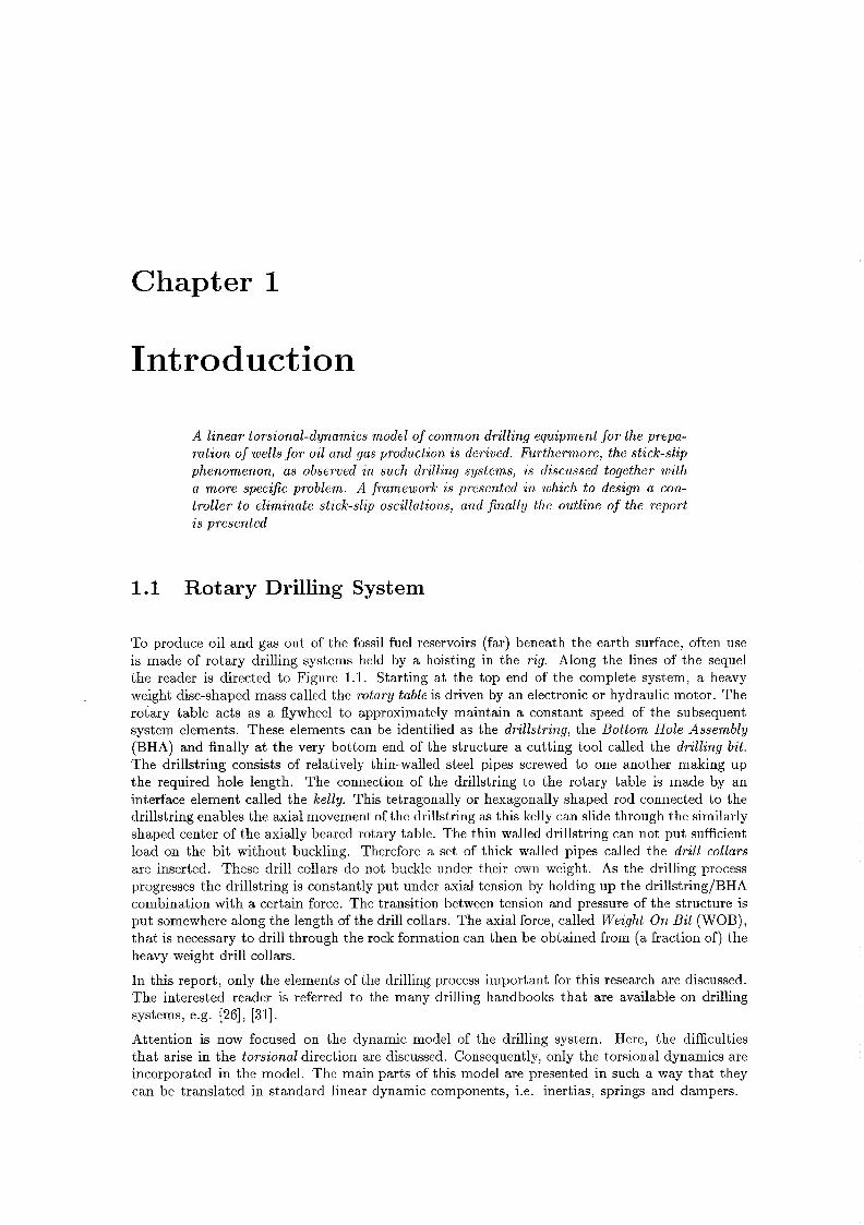
To produce oil and gas out of the fossil fuel reservoirs (far) beneath the earth surface, often use is made of rotary drilling systems held by a hoisting in the rig. Along the lines of the sequel the reader is directed to Figure 1.1. Starting at the top end of the complete system, a heavy weight disc-shaped mass called the rotary table is driven by an electronic or hydraulic motor. The rotary table acts as a flywheel to approximately maintain a constant speed of the subsequent system elements. These elements can be identified as the drillstring, the Bottom Hole Assembly (BHA) and finally at the very bottom end of the structure a cutting tool called the drilling bit. The drillstring consists of relatively thin-walled steel pipes screwed to one another making up the required hole length. The connection of the drillstring to the rotary table is made by an interface element called the kelly. This tetragonally or hexagonally shaped rod connected to the drillstring enables the axial movement of the drillstring as this kelly can slide through the similarly shaped center of the axially beared rotary table. The thin walled drillstring can not put sufficient load on the bit without buckling. Therefore a set of thick walled pipes called the drill collars are inserted. These drill collars do not buckle under their own weight. As the drilling process progresses the drillstring is constantly put under axial tension by holding up the drillstring/BHA combination with a certain force. The transition between tension and pressure of the structure is put somewhere along the length of the drill collars. The axial force, called Weight On Bit (WOB), that is necessary to drill through the rock formation can then be obtained from (a fraction of) the heavy weight drill collars.

In this report, only the elements of the drilling process important for this research are discussed. The interested reader is referred to the many drilling handbooks that are available on drilling systems, e.g. [26], [31].

Attention is now focused on the dynamic model of the drilling system. Here, the difficulties that arise in the torsional direction are discussed. Consequently, only the torsional dynamics are incorporated in the model. The main parts of this model are presented in such a way that they can be translated in standard linear dynamic components, i.e. inertias, springs and dampers.

2 CHAPTER 1, INTRODUCTION

Neutral

\ I

Transition Point

I I

Tension *+b Pressure

WOB

-

30-80 m

1-8 krn

BHA 100-300 rn

Figure 1.1: Drilling equipment

See Figure 1.2 and 1.3 for a schematic view of the model.

An electric motor assumed to possess linear dynamics drives the damped -by ca- rotary table inertia Jrot. The drillstring is simply modelled as a single linear torsional spring with stiffness k . Finally, the BHA, that is the drill collars together with the bit, is modelled as a damped -by cl- inertia Ji. The friction at the bit, which is better known as the Torque On Bit (TOB), can be modelled to be of any appropriate shape always working in the opposite bit speed direction. The inertia of the motor and the rotary table can be combined as Jz = Jrot + n2J,. The motor constant K , is combined with the gear ratio as K = nK,. The rotary speed and the bit speed are defined as Q2 and Q1, respectively, and finally the twist of the drillstring ( p z - pi) is defined as 4. The model of the electric motor pertains to a standard separately excited DC motor, and therefore contains an induction L and a resistance RI which are electro-mechanically coupled in series with the rotor inertia J,. The electro-mechanical coupling is considered as a linear relationship between a load voltage, better known as the back-electro-motive force (back-emf), and the speed of the rotor. This linear relationship is characterized by the motor constant K,. The rotor speed is n times the rotary table speed Q2 if the gear box is considered to be infinitely stiff. The motor is fed

1.1 ROTARY DRILLING SYSTEM 3

- A-

Figure 1.2: Rotary drilling system isolated from the rig

by an external voltage V,. The rotary table and motor inertia, combined in 5 2 , are driven by a torque T2 from the gear box, which is the product of the motor current I and the combined motor constant li'. Furthermore, the motion is considered to be damped by bearings and other rotor-dynamical parts in the motor, gear box and at the rotary table. This damping is lumped into the damping coefficient ca. The drillstring is modelled as a single torsional spring with stiffness k . The numerical value of k as a model parameter can be obtained as an equivalent system property of the drillstring calculated by the virtual work approach, see [21]. If a constant speed source is mai!ab!e-b&er known as the dynamically clamped condition- the system- param-eters J1 and c1 are determined as follows. The lumped inertia 51 at the bit is estimated from that of the BHA and one third of the distributed drillstring inertia ([SI). The same goes for the lumped damping c1 calculated as the damping at the bit and one third of the damping along the drill shaft. An error is made in the consistency of the model components 51, c1, J2, and ca if the rotary table is considered not to rotate at a constant speed. Therefore, a more consistent approach such as the finite element method or transmission line modelling should be applied if arbitrary speed fluctuations of the rotary table-either by controlling or by disturbances-are considered. A more in-depth discussion of these modelling approaches together with the relative errors in the method used here can be found in appendix B of this report. In the sequel, the modelling assumptions made in the foregoing are used to build a set of differential equations. The differential equations can be readily derived along the simple linear description of the drilling system (Figure 1.3), i.e.

4 CHAPTER 1. INTRODUCTION

L I __c +- I

% i,, I- ’ TOB

Figure 1.3: Modelling in standard linear components

1.2 Stick-Slip in Drilling Systems

Having the model of the drilling system, the problem of stick-slip occurring at the bit is briefly discussed in this section, and forms the basis of the discussions to come.

Here, stick-slip can be viewed as a marginally stable oscillation of the bit due to a characteristic nonlinear friction behavior at near zero speed of the bit. There are many models available for this TOB characteristic, either for simulation or analysis (see [i], [24] and [16]). All of them describe a more or less increasing friction force at mar zero speeds, at, least seen from. higher to lower speeds (also see left part of Figure 1.4). This implies that low bit speeds will even get lower, possibly down till zero. At this moment a period of clamping - stiction - of the bit occurs while the rotary table continues rotating. Consequently, the drillstring receives nearly all the torque from the rotary table without being able to dissipate it at the bit as slip-friction heat. Instead, the potential energy in the drillstring is being built up as it behaves like a torsional spring. This goes on until the maximum friction torque that “clamps” the bit is exceeded. At that moment the bit is released from its stiction and the potential energy in the drillstring is transformed into kinetic energy of the bit as its speed increases rapidly to a peak value far above the nominal rotary table speed. After that, the bit speed decreases rapidly again as the kinetic energy is dissipated by the slipping of the bit. Lacking sufficient damping, the bit speed becomes zero again and the cycle starts all over. A few of such stick-slip cycles can be seen in the right part of Figure 1.4. In this diagram field measurements are presented in case of a reference speed of 50 RPM (5.24 rad/sec). The curve labeled ‘surface) describes the rotary table speed and the curve labeled ‘downhole’ describes the rotary speed of the bit. The figure illustrates that in practice the stick- slip oscillations indeed occur in a consistent manner and that rotary table speed is hardly affected by these oscillations (the reference speed of 50 RPM is approximately maintained by the rotary table).

The stick-slips cycle only occur under certain circumstances. As already mentioned, the friction at

1.3 SPECIFIC PROBLEMS AND OBJECTIVES 5

rotary speed [RPM]

250 I

SufiaCe downhole 200 I I I

O 10 20 30 40 50

time [SI

Figure 1.4: left: T O B as a function of the bit speed RI. right: typical sticlc-slip behavior measured in the field

near zero speeds must be higher than at normal reference speed. The drillstring/BHA combination must have a low first eigen frequency, which comes down to long drillstrings (low stiffness k ) combined with the heavy weight BHA (high inertia J1). The reference speed of the rotary table is below a certain threshold at which the stick-slip vibrations may be initialized, and finally, the damping down-hole is relatively low; at least not high enough to eliminate the stick-sip vibrations.

At unchanged conditions, the oscillation continues to exist. Therefore, it is also called a self-excited vibration. Hence, this oscillation can be labeled as marginally stable, although by itself it never becomes unstable since the overall energy is dissipated at the slipping intervals. More detailed discussions on this phenomenon and its interesting properties (in an academic sense) can be found in Appendix C. Here, the notion of stick-slip and general characteristics of the T O B is enough to proceed with the solution to counteract these oscillations. This is of major importance because they can give considerable wear to the bit, BHA and the drillstring, which can even suffer from a twist-off. Moreover, the rate-of-penetration decreases and the diameter, shape and direction of the bore-hole is poorly controllable.

1.3 Specific Problems and Objectives

During the eighties until today, one has become aware of the torsional stick-slip vibrations in relationship to system properties (see [4] [5 ] , [7], [18] [25] and [32] ). A lot of effort has been put into the solution of this problem. The most practical solution up till now is probably the introduction of damping at the top end of the structure. In [22] a combination of a damper and a spring between the drive and rotary table was introduced to dampen the vibrations in the drillstring. This spring/damper behaviour is electronically mimicked by a feedback circuit measuring the motor current I and controlling the speed input voltage V,. This configuration has been proved to be a successful way to kill the stick-slip vibrations in the field, and is commercially available as the “Soft Torque Rotary System” (STRS).

Nevertheless, problems - which did not occur before - arose in case of high peak T O B loads. The motor constantly puts energy into the rotary table, which acts as a flywheel delivering its torque to the mechanical structure below. This structure is affected by the (heavy) T O B fluctuations


and other dissipative processes. These loads have to be overcome by the combination of motor torque and the instantaneous momentum of the rotary table, drillstring and BHA. Because of the limited power of the electronic motor-drive, loads beyond this power limit can only be overcome if the total kinetic energy in the drilling structure is sufficient at any moment. Such high peak loads may be, for example, the torque that clamps the bit at zero speed. Without any additional control systems such as the spring/damper combination explained above, the kinetic energy is in nlost cases siiR.cieicient8 to release the sticking bit. On the other hand, applying a damping system such as the STRS introduces extra dissipation of kinetic energy in the total structure, especially the rotary table. At the high peak loads this can reduce the kinetic energy to such extent that too less buffered energy is left to overcome the difference between the very high T O B and the maximum motor torque. In those situations, the bit comes to a complete stand-still, better known as stalling.

Leaving the STRS there, a new control concept is developed in this report to control the vibrations keeping the high peak load problem in mind. The control method applied to this system is the ?im control theory as one of the solutions to the robust control problem ( [as] ) . For the following, the reader is directed to the left part of Figure 1.4. In this figure, TOBdyn stands for the friction torque at normal speed levels, that is at a fully dynamic bit speed situation. The torque indicated by TOB,,, represents the maxzmum friction torque that the bit/formation- interaction can generate after which it decreases rapidly to TOBd,, implying that the bit is released from stiction. The difference TOB,,, - TOBd,, is labeled as the backlash torque. From now on, these definitions will be used throughout the report, without further reference. A list of global requirements/restrictions, not yet specified in numerical or analytical measures, have to be defined by way of a reference framework in which an 31, controller has to be designed, i.e.

o Because of the aggressive environmental conditions in practice, neither torque- nor speed- measurements are performed at the rotary table. Instead, measurements and control actions have to be performed in terms of motor signals, that is the motor current and the motor input voltage V, .

o The ability of the system itself to overcome peak loads higher than the maximum motor torque should not be violated by adding a control system of any kind. The ability to overcome the indicated extreme load situations should preferably be improved by the control system.

o Up to a threshold in stepwise changes of the TO&,, as high as possible the control system sho~!d he able to prever,$ the bit from initializing a stickslip oscillation. Moreover, up to an even higher threshold of the backlash torque, the closed loop system should be able to eliminate stick-slip oscillations.

o Above requirements have to be met in the presence of uncertainty in the system model, of external disturbances and of disturbances in measurements. For obvious reasons, the rotary table speed is restricted, which should be considered in the controller design. The to-be- synthesized controller should result in a robust closed loop- and controller stability in the face of model uncertainties and/or unmodelled system dynamics. Moreover the bit speed must be controlled resulting in a smoothening behaviour. This comes down to limited settling times and overshoot after step- or impulse- like TOB or Q-,f changes. The commonly defined restriction, that the closed loop performance should be met with minimal control actuation power, is dropped here to be able to account for the highly fluctuating T O B disturbances.

1.4 Outline

The report is organized as follows. Chapter 1 to 5 hold the core discussion about the design and implementation of a linear ?im controller to control the torsional drillstring vibrations. The

1.4 OUTLINE 7

subsequent appendices have a supplementary purpose. They present some topics that have no direct connection with the controller design, though are interesting in an academic sense.

Chapter 2 presents some preliminaries on the ?i, control setup. It discusses the choices of the weighting functions reflecting performance requirements and TOB input characteristics. Further- more, attention is given to the interconnection structure of the the generalized plant with which a controller is computed.

Chapter 3 gives a comprehensive analysis of both the frequency- and time-domain performance of the closed loop system. Directions for improvements are discussed aiong the perÎormance- and stability analysis in the time domain.

Chapter 4 presents a method to implement the controller in terms of motor quantities. Aspects of stability and influence of measurement imperfections are discussed. Time-domain simulation results show that this implementation does not degrade the performance. The implementation has been tested in a lab-scale drilling system simulator of which the the results are shown.

Chapter 5 summarizes the preceding chapters and lists a number of conclusions with respect to the results obtained. Moreover, it discusses directions for future research.

Appendix A gives an overview of important theorems in the field of 'Hm control.

Appendix B presents a few model concepts for the drillstring dynamics.

Appendix C discusses the T O B non-linearity and its implication in a one-mode model for the drillstring.

Finally, Appendix D closes this report, presenting a general approach to the state space solution of 3, control problems. The method comprises the solution to both linear system models and a class of non-linear system models.

Design of an 7& Drillstring Controller

This chapter discusses the application of the 31, control concept to control torsional drillstring vibrations of any kind. The control theory is applied in a linear sense. Consequently, a linear control model of the system wall be defined that explicitly accounts for the TOB disturbance and performance specifications by dynamically weighting the relevant in- and output signals along the frequency axis. The chapter is closed presenting computational aspects.

2.1 Preliminaries on linear 3-1, control

A MIMO linear 31, controller tries to minimize the interaction between exogenous inputs, e.g. disturbancesfreference signals, and outputs, e.g. objectives, of a closed loop transfer function matrix (TFM) by minimizing the infinity norm 1 1 . I(, of this TFM. The infinity norm of a TFM can be computed as IITFMII, := supwEx F(TFM(jw)), where a(.) denotes the maximum singular value operator to an arbitrarily dimensioned TFM (see [15]). In the 31, setup, the control problem

Figure 2.1: Standard 31, controller design setup

can be generally presented as depicted in Figure 2.1, where s represents the complex frequency j w in the Laplace domain, and where all systems indicated by a block are proper, linear, time- invariant transfer function matrices. In this figure w is a set of reference/disturbance inputs, z a

10 CHAPTER 2. DESIGN OF AN 31, DRILLSTRING CONTROLLER

set of to-be-controlled variables (objectives), y are the measurements, u is the control input, q is the input to the uncertainty block A(s) and finally TI is a disturbance input to the plant generated by A(s). P ( s ) and G(s) are both denoted as the plant model, and K ( s ) is the dynamic controller.

P ( s ) is defined as the nominal plant model. The meaning of G(s) will become clear later on. As mentioned above, A(s) is a TFM representing the dynamic uncertainties in the model of the plant. Hence, the combination of the plant and the uncertainty forms the exact plant dynamics (which are not known). The controiier N(sj is to be designed for this reai piant by using the piant model, i.e. P ( s ) or G(s) . The controlled plant model (closed loop p h t model) is defined by W ( s ) arid is indicated by the dashed frame-box in Figure 2.1.

In this setup, no restrictions concerning magnitude or structure are put on the uncertainties in A(s) yet. However, in the 31, design the magnitude of the uncertainty block is assumed to be restricted such that IIA(s)lloo 5 1. This, and restricting A(s) to be internally stable, implies that closing the upper loop will never introduce instability by itself as it does not magnify the signal q to v. Instability can then only be introduced by the closed loop plant. A very simple, though illustrative example of this is envisaged by the following block diagram. If the 1 1 . llm-

W

Figure 2.2: Simple example of closed loop stability notion

norm of the closed loop plant H ( s ) is equal to 2 and the system H ( s ) is already a (nominally) stabilized system, then a sufficient (but not necessary) condition to guarantee stability of the perturbed closed loop plant is that the 11 . Il,-norm of A(s) should be smaller than i (provided that A(s) is internally stable). In the 31, theory there is consensus about defining the restriction IIA(s)llm 5 1. Hence, a sufficient restriction to guarantee stability is to force the perturbed closed loop system having llH(s)llm < 1 (at least if H ( s ) was already stable) for all stable perturbations A(s) : IIA(s)llm 5 1. In many cases this restriction is too heavy and less demanding assumptions would guarantee stability for the perturbed plant as well. On the other hand, the restriction to H ( s ) made here provides a safe upper bound which is exactly the goal in the design of a robust closed loop. The restriction put on the uncertainty block can be manipulated by augmenting the nominal plant with dynamic weighting functions. Note that in the simple example above, this consensus can be achieved by weighting H ( s ) by 4. In fact these weighting functions reflect the amount of uncertainty the closed loop system eventually can handle along the frequency axis such that it remains stable in the normed sense explained above and can therefore be labeled as design functions.

An augmented version of the block diagram in Figure 2.1 would also close z to w by a fictitious uncertainty block A, ( s ) . This block represents the uncertainties in the model in case they could be described as a feedback TFM between z and w. The reason why such a block is also considered is to be able to measure both robustness of the closed loop stability (q-w feedback) and robustness of the closed loop performance (z-w feedback) in the same way. Aspects of these kind will be discussed in Chapter 3. Again, the unity restriction on the infinity norm of A,(s) would be necessary to hold and again this could be achieved by the use of weighting functions. In the controller design discussed in this report most attention is paid to the weighting functions associated with the performance as the system does not have to be stabilized.

Assuming that the appropriate weighting functions are incorporated, the resulting augmented version of the nominal plant is defined as the generalized plant G(s), which in the standard setup of Figure 2.1 replaces the nominal plant P(s) . To design an appropriate controller, this generalized

2.1 PRELIMINARIES ON LINEAR ‘?im CONTROL 11

plant will be thought of as the to-be-controlled plant The robust control problem can then be defined as to find a controller K ( s ) such that

o the generalized closed loop system H ( s ) is nominally stable, and

Although it seems that twc separate specifications have to be w-et, in fact the second specification implies the first one. This will be argued later on in this section. The second requirement can be generalized by demanding that the closed loop infinity norm should be smaller than an arbitrary number y. There exists a y = yo such that IIHIIm = yo is the optimal solution to the X, control problem. This optimal solution represents the controller K ( s ) = Ko(s ) for which the closed loop infinity norm has reached a global minimum. For a general non-square MIMO TFM this optimum is hard to find. A more practical solution can be found by defining a sub-optimal version of the 31, control problem. In this case IIHIIm must be simply smaller than y : yo 5 y 5 1.

In this report, the famous state-space solution presented in [14] and [lo] to the linear %, control problem, as one of the many possibilities (loopshaping, nyquist criteria, pole-placement, Quantita- tive Feedback Theory, Model-Matching Equivalence, etc) to achieve the two conditions, is applied. The state-space method results in a sub-optimal solution of the ?lm controller in a sense that it explicitly uses a provided y. An iterative procedure of alternately computing the controller (meeting the stability and norm requirements) and adjusting y can be used to search for a y arbitrarily close to the optimal value yo.

The state-space synthesis is based on the ‘size’ of quantities (states, outputs, inputs) rather than the ‘size’ of transfer functions. In the following it will be shown that the 31, problem formulation can be presented in such quantities.

The closed loop system H ( s ) maps the disturbance inputs w into the objectives z , i.e.

z = H w (2.1)

Generally, z represents objective signals that have to be minimized. Examples of such signals are tracking errors, positioning errors, etc. On the other hand, it may represent any other quantity for which certain performance requirements are defined. The goal is to get the infinity norm of H ( s ) smaller than some value for y. Regarding (2.1), achieving such a infinity norm for H ( s ) will reduce the influence (in a normed sense) of the disturbances w on the objectives z down to a level less than y. Note that this choice of the control problem does not explicitly account for desired (time domain) solutions for the objectives z . Such desired solutions have to be reflected by the already mentioned weighting functions, which in most cases is not a straightforward procedure as the system model may generally be MIMO and of high order.

In order to use the state-space method for H ( s ) , the two goals (robustly stabilizing it and minimizing its co-norm) must be formulated in the time domain. It can be be verified that the following property holds (see: [13])

where 1 1 . 112 is the 2-norm defined as Ila(-t)ll2 = ,/- and L2 is the set of all functions that have a finite 2-norm. In fact (2.2) is the definition of the infinity-norm. In words it says that there exists a bounded (in La sense) exogenous input w(t) such that the transfer from w to z is maximal.

12 CHAPTER 2. DESIGN O F AN ‘ h ! ~ DRILLSTRING CONTROLLER

At this stage, a time domain representation of the XW problem is available. The sub-optimal solution to the Xm problem can be formulated as:

where “stab K” denotes (‘for all stabilizing controllers K”. The last inequality in (2.3) can be viewed as a cost integral function reminiscent of the LQG-control problem formulation. Therefore, the solution to the LQG-control problem (or ‘h!~ control problem) and the 31, control problem have great similarities which are discussed profoundly in [lo].

The state-space method to find the optimal or sub-optimal solution of the ‘A!, optimization problem (2.3) resulting in a static state feedback law assumes that the complete state 2 is available. The measurement vector y generally has a lower dimension than the dimension of the state vector 2. This implies that not all state components are measured (due to physical limitations or cost aspects, etc). Hence, it is necessary to reconstruct the remaining components of the state out of the measurements y in some way. Assuming that this can be performed appropriately, the reconstructed state can be used to determine the static feedback function. It appears that the reconstruction problem can be treated as a dual of the feedback control problem. The feedback control synthesis tries to make the output of the actual system follow the output of the model system in the face of external input disturbances to the actual system. Reversely, the filter synthesis tries to make the input to the model system follow the control input to the actual system in the face of output disturbances to the actual system (measurement errors and/or noise) , [28]. Due to this duality, the setup of- and solution to the reconstruction problem can be performed in an equivalent manner as the state feedback control problem. ‘Assembling’ of the two separate structures results in a controller in the form of a linear dynamic system with input y and output u. The computation of the optimum according to inequality in (2.3) involves solving two Matrix Riccati equations: one for the (robust) static feedback law and one for the (robust) reconstruction of the state by the measurements in y. The state-space solution is presented in Appendix D within a more general, non-linear framework where the linear solution forms a subset, either by working out the problem for a linear system model or finding local solutions for the non-linear system model using local linearizations.

First, a proper nominal model and weighting functions have to be available in order to force the performance specifications for the closed loop, which are defined in Chapter 1 to be met. This is the subject of the next two sections.

2.2 Control Synthesis Model

Already implicitly indicated in the previous section, the resulting ‘Hm controller derived here will be one of the observer-based controller type. This implies that the controller in itself will also be a dynamic system, typically having the model order. The controller system consists of a reconstruction part, in order to reconstruct the systems’ state “as good as possible,” and of a static feedback part that is applied to the reconstructed state. This is also known as the separation structure of a dynamic controller. The separation of the reconstruction and control part enables the use of the 31, approach as a stand-alone procedure for either filter- or full state feedback control problems, respectively. Hence, combinations with other control or reconstruction techniques are possible issues if the state-space approach is followed, [34].

A suitable control model of the plant for both the reconstruction and computation of the feedback law will be presented in order to derive a satisfying robust controller.

‘Although an 31, controller is derived here as o n e of the solutions to a r o b u s t c o n t r o l problem, that controller is interchangeably denoted as both a robust- and ‘Hm controller.

2.2 CONTROL SYNTHESIS MODEL 13

2.2.1 the nominal plant

In the previous chapter, a typical simulation model was derived. This model is not very useful for the design of a dynamic controller for several reasons. Firstly, the dynamics of the motor are at least an order of magnitude faster than those of the drilling system. Secondly, the dynamics of the drilling system and motor are only slightly coupled (see [al]). This implies that including the motor dynamics would result in an unnecessarily higher order of the nominal model and consequently the dynamic controller. Moreover, the motor dynamics can be controlled separately from the main drillstring control problem, provided that the bandwidth of the controlled motor is sufficiently high to prevent instability, when combined with the drillstring controller. If a more sophisticated plant model is desired it is better to emphasize on higher order drillstring dynamics rather than including the motor dynamics. Topics on higher order modelling of the drillstring are discussed Appendix B.

Considering above assumptions, a simpler, linear, time-invariant state-space control model description can be defined as:

-c1 k

T O B Q 2 - -

J 2 J 2 J2

in shorthand 5(t) = A x ( t ) + B 1 W ( t ) + 3 2 ~ ( t ) , x(to) = ZO

Hence, the state is defined as x = [RI 4 aalT, the external reference signals/disturbances w = [Q,,, TOBIT and finally the control input u is the torque T2 exerted to the rotary table. Compared to ( l . l ) , the only new variable in this description is the reference speed setting QT,f to be used by the controller as a reference signal. Moreover, it can be seen in equations (2.4) that the damping at the rotary table c2 is accounted for by feed-forwarding the reference speed ar,f with this damping coefficient. Note that by equations (2.4) not the complete state of the system model-topologically mimicked in Figure 1.3-is described. The two degrees of freedom p1 and (p2 are combined in the twist 4 = p 2 - p l . Even though for control purpose these two DOF’S defined as separate state variables are not required, they could not be reconstructed with model (2.4) anyway as the initial condition at t = t o of pi and p 2 are not prescribed in 20. The nominal plant description (2.4) forms the basis for the generalized plant described next.

2.2.2 the generalized plant

In this paragraph, the generalized plant G(s) denoted in the premise is defined in terms of an interconnection structure in which the weighting functions are inserted. Interconnection structures describe a model in terms of causal block diagrams, where blocks hold transfer functions or TFM’s and arrows indicate signals or columns of signals. Omitting the perturbation interaction of A(s), in Figure 2.1 two types of inputs and outputs can be identified. The inputs are separated as the referenceldisturbance inputs w and control inputs u, respectively, and the outputs are specified as to be the objective outputs z and measured outputs y, respectively. A general controller canonical state-space representation of the necessarily proper generalized plant will therefore be partitioned as (the time argument is dropped for convenience):

14 C H A P T E R 2. DESIGN OF AN ‘?I!- DRILLSTRING C O N T R O L L E R

The state-space solution of the controller will eventually be formulated in terms of the time domain matrices in (2.5) ’. On the other hand, the performance and stability specifications reflected by the weighting functions first have to be specified in the frequency domain after which they are converted into the time domain. In principle, the time domain specifications could be directly incorporated in the state-space representation (2.5). Unfortunately, this appears not to be a straightforward procedure as the solutions of the state z in time are given in transcendental formulae, typically cûmbir,atims ~f enpenentia! and trigonometric fmxtionc [E], in which specifications cannot he inserted easily. Therefore, the frequency domain is preferred as the design space because in this space the relation between signals are given in terms of straightforward complex-valued polynomial (algebraic) functions.

In equations (2.5) it is assumed that the model is time-invariant. On the other hand, the real plant depends on time as the drillstring length increases during the proceeding drilling process. The equivalent drillstring stiffness IC will decrease while the lumped inertia Ji will increase. In the controller design discussed in this report only one nominal configuration of the drillstring is considered and the robustness towards variations (e.g. longer drillstring or higher order simulation model) of this nominal design will be considered in Chapter 3.

2.2.3 interconnection structure

The state 2, disturbances/references w and control input u for the drillstring control problem are already defined. Regarding (2.5), the remaining quantities to be defined are the objectives z and the measurements y, i.e.

Hence, the remaining matrices left in equations (2.5) are:

Cl = [ -1 o o 0 o 0 1 ; D i l = [ ; o ] ; D 1 2 = [ ; ] ;

(2.7)

The component WTOB in D21 will be explained further on. The first performance objective in z is defined as the difference between the reference-or desired speed-and the actual bit speed. Thus, this is a typical error signal objective. The second objective is the control input u. It is assumed that by the to-be-designed weighting functions the control input-or equivalently the controller K(s)-can be manipulated along the frequency axis such that the limited output of the motor is accounted for. This is the reason why the control input is chosen as an objective signal, although it is not a typical error signal of which one desires it to be zero in the ideal case.

In the measurement vector y, the first measurement is the difference of the reference speed and the rotary table speed. The second measurement is the twist 4. In fact this quantity cannot be measured in practice. On the other hand, it represents the torque that the drillstring exerts to the rotary table, that is k 4 for the one-mode model under consideration, scaled by the lumped drillstring stiffness IC. Thus, y2 = b 4/IC = 4. In more practical approaches-in which the simple modelling by a single torsional spring is less appropriate-this measurement would simply be the scaled torque that the rotary table “feels” from the drillstring. In the model under consideration

2The required formulation in state-space matrices demands for the generalized plant to be proper, otherwise a description such as in (2.5) can not be formed.

2.2 CONTROL SYNTHESIS MODEL 75

the twist 4 is defined as this scaled drillstring torque. It is assumed that the measurements are not corrupted by error signals such as noise and offsets. Later on, during the synthesis of an implementation version of the controller for experimental purpose, above measurement aspects will be given attention.

Having the definitions of states, inputs and outputs, the interconnection structure of the control desigri setup in Figure 2.1 is unfolded into the block diagrarr, of Figure 2.3, where the V- and

U

Figure 2.3: Interconnection structure with shaping filters

W - functions are dynamic weighting functions dependent of the frequency w . The effect of these weighting functions will be discussed in the next paragraph. In Figure 2.3, the nominal plant described in state-space quantities by equations (2.4) and (2.6) is indicated as P and the controller is denoted as IC. In this figure, the second measurement y2 is defined as the discussed scaled drillstring torque summed with a weighted version of the TOB disturbance. The state-space method, [14], demands for D21 in (2.5) to have full row rank as will be discussed further on. Consequently, the method expects that the w2 is also measured in some sense although this is not possible in practice. Imposing a very small weight WTOB (e.g. on the fictive T O B measurement will suffice for the state-space method to compute a controller without considerably changing the nominal model description in which the TOB is/can not measured.

2.2.4 weighting functions

The discussion of Figure 2.3 is completed by specifying the weighting functions Kef , VTOB, W, and Wu. Restricting the order of controller, the weighting functions are limited to be at most second order stable, proper transfer functions. Note that the “V-functions” denote the input weightings and the “W-functions” are the output weightings. Also note that by imposing the weighting functions, w and z are transformed into weighted versions of their former definitions. To avoid yet new symbol definitions, the naming of w and z is maintained without loss of generality.

The augmented plant G(s ) can be represented by the following open-loop map of plant inputs to plant outputs:

16 CHAPTER 2. DESIGN OF AN ?7!m DRILLSTRING CONTROLLER

For the system under consideration this is expanded to:

where p l ( s ) = J1s2 + q s + k , p2(s) = J2s2 + C ~ S + k and d(s) = pl(s)p2(s) - le2. The fractions of G in (2.8) can be readily identified in (2.9). Hence, closing G(s) by K ( s ) gives rise to the closed loop TFM H ( s ) , which can be represented as a so-called lower Linear Fractional Transformation (LFT) of G(s) and K ( s ) :

H ( s ) = Ei(G(s), K ( s ) ) Gii(s) + G12(~)1{(~)(1 - Gzz(s )K(s ) ) -~Gz~(s ) , (2.10)

yielding

(2.11)

If H*(s) E Fl(P(s), K( s ) ) , the nominal closed loop, is defined then the following holds for the relation between the generalized and nominal closed loop

(2.12)

The way the controller interacts with the system is implicitly envisaged by the LFT in (2.10) and therefore implicitly shows the limitations in the solution of a controller. One of these limitations is the poor direct influence of the controller K ( s ) on the feed-through of w to z , that is the fraction GlI(s). In fact the combination of G21Ií7(I - G22K)-’G21 preferably must have the same order of magnitude, though with opposite sign, as that of Gil at every frequency to keep the magnitude of the closed loop system H ( s ) small for every frequency. This implies that K ( s ) must regulate the four other TFM’s and stabilize the closed loop, which can only compromisingly be achieved.

As mentioned earlier, the weighting functions Wp(s) , Wu(s) V,,f and VTOB, which have to be specified in the frequency domain, are design functions in order to obtain a satisfactory time domain performance under the stability restriction. Generally, the W-functions refiect the desired closed loop character of the underlying signal, while the V-functions reflect important a priori knowledge of the disturbance input. The mechanisms of the weighting functions influencing the transfer design have simple principles, although the exact (numerical) characterization of these weighting functions is not always straightforward, especially in multi-variable and/or high order systems. The simple principles of the weighting function mechanism is best explained by an illustrating example. Suppose it is required to shape (and minimize) a closed loop transfer Hi* along the frequency axis by a controller Ki. The closed loop transfer has a generalized representation by the use of weighting functions: WiH:L$ with which to establish this shaping. For clarity, it is assumed that the closed loop is SISO and the weighting functions are scalar functions. As already mentioned in Section 2.1, the controller design is based on this weighted closed loop in the sense that it tries to reduce its gain to a level lower than y (under the stability restriction), that is

]Wi(S)Hi*(S)K(S)J < y vw E 3 (2.13)

where y is as small as possible. Equivalently, this minimization can be written as

(2.14)

2.3 CLOSED LOOP DESIGN 17

An ‘optimal’ controller design can in principle be established by shaping the magnitude of Hi* (s) to the right-hand side of (2.14) as close as possible. This implies that IH:(s)l can be large (small) where l/lWi(s)K(s)I is large (small). If, for example, at some frequency interval of interest l/lWi(s)x(s)l is chosen small to reflect a certain specification then lWi(s)&(s)l is large and IH:l has to be ‘pushed down’ in that interval in order to ensure inequality (2.13) to hold.

It is clear that the shaping principles sketched in above example indeed provide the possibilities to insert design specifications and a priori knowledge of the disturbances into the generaiized piant concept and hence into the controller synthesis. In the next section the choices of the weighting functions will be discussed given a number of design specifications.

2.3 Closed loop design

Recalling the rough design specifications and restrictions in Section 1.3, the weighting functions have to be designed such that the following refined design specifications will be met:

1. The bit speed response to a 5 rad/sec step in the reference speed should lie within a 1% error band around the reference speed after T d seconds, where T d denotes the period time of the eigen frequency wd of the drillstring/BHA combination: wd = fi. This is a settling time specification towards steps in the reference speed ‘disturbance input’

2. The final accuracy of the bit speed to a 5 rad/sec step in the reference speed must be better than 0.5 rad/sec.

3. At a reference speed of 10 rad/sec, the magnitude of the closed loop transfer between the T O B disturbance input (wa) and the bit speed error ( 2 1 ) at the eigen frequency must be equal or smaller than the magnitude of the non-controlled transfer function between w2 and 21

in case the damping c1 in this transfer function is just high enough to result in a marginal stick-slip oscillation for the case the backlash torque is set at 5 kNm. A marginal stick- slip oscillation occurs if the conditions are such that the system just sustains the stick-slip oscillation. Provided a certain reference speed and persistent backlash torque, every slight increase of c1 would make the stick-slip oscillation damp out. Assuming that the plant has no damping at the BHA, i.e c1 = 0, this specification is defined to ensure sufficient damping at the eigen frequency in order to kill stick-slip oscillations at least up to 5 kNm in the backlash torque for fit,,f = 10 rad/sec.

4. The closed loop system must at least sustain stick-slip oscillations instead of complete stalling for TOB loads which are temporarily 10% higher than the maximum available motor torque. This comes down io 55 kNm (e.g. TOB,,, in severe stick-slip situations) for the system under consideration.

Note that in above specifications no attention is paid to the settling behaviour of the bit speed to (step-wise) T O B disturbances. On the other hand, it is assumed that satisfying settling behaviour is obtained whenever spec 1. and 2. are met. Moreover, if the ‘substitute damping’ to kill the stick-slip oscillations indicated in spec 3. is performing well it can also be expected that the settling behaviour of the bit speed after step-wise TOB changes (without inducing stick-slip) is satisfying. These aspects will be investigated in the comprehensive time-domain analysis of Chapter 3.

In the three subsections to come the weighting functions W,, VTOB and W, wil1 be successively designed given the four specifications listed above. The reference speed weighting function is set V,,f = 1 because the reference speed-which is usually set somewhere between O and 15 rad/sec- does not necessarily have to be scaled or normalized.

i8 C H A P T E R 2. DESIGN OF AN 31, DRILLSTRING C O N T R O L L E R

2.3.1 the weighting W,

This weighting function W, must penalize the transfer function H;, and H;2 in equation (2.12). To design W,, attention is only paid to H;, and is assumed that Hr2 can be properly shaped by V-OB as will be discussed in the next subsection. Preferably, there must hold:

where-according to design inequality (2.14)-y is set to 1 and V,,f = 1 as already mentioned. In [42] similar specifications as 1. and 2. were translated into the associated weighting W,. Here, the same procedure will be followed. The specification is written in the form:

(2.16) s + ai - - K-. 1

W,(S) s + a a

In case no overshoot is assumed, the settling time specification 1. is met if a2 2 - ln(O.Ol/tc)/Td, where the factor '0.01' denotes the 1% error band. For the case under consideration K = 100 is chosen, which implies together with Td = 5.6 rad/sec that a2 > 1.65 should be chosen. As the system will most likely show overshoot a higher parameter a2 = 5 is chosen to account for the oscillatory behaviour of the bit speed before it remains within the 1% error band. The parameter a1 determines the final accuracy or equivalently the steady-state error. If al is set to zero then it is specified that steady-state errors are not allowed. Here, a less restrictive specification is demanded namely that the steady state error must be less than 0.5 rad/sec for step-wise changes in the reference speed of 5 rad/sec (spec 2.). In this case there must hold a1 < ( 0 . 5 . a 2 ) / ( 5 . ~ ) = 5.0.10-3. Here, a1 = 2.5. is chosen to ensure the specification to be met. Resumably, the weighting W, becomes:

s + 5 Wp(s) = 100s + 0.25'

(2.17)

2.3.2 the weighting VTOB

The specification 3. determines the weighting VTOB. Utilizing spec 3., the appropriate transfer function to penalize is HT2 as this transfer function describes the dynamic relation between TOB inputs and the bit speed (-error) response. Preferably there most hold:

(2.18)

In [2l] an analysis is performed resulting in an approximate expression for the threshold reference speed as a function of the damping e1 and the backlash torque TOB,,, - TOBd,, for which the drilling system will operate showing a marginal stick-slip oscillation. The approximation is given as

(2.19)

where C = C1/2J lwd. For a fixed c1 and backlash torque the expression (2.19) gives the minimal reference speed above which stick-slip will just damp out. The expression can also be used reversely,

30vershoot will not occur if the damping e1 2 2 J l w d = 750, which is an unrealisticly high damping coefficient. In fact, stick-slip would vanish immediately at such a high dampingat the BHA. From field experience, such smooth behaviour is not reported at a regular basis. Hence, a damping c1 high enough to circumvent overshoot is not likely to occur.

2.3 CLOSED LOOP DESIGN 19

that is, determining the threshold damping for a fixed reference speed and backlash torque. For Q,,f = 10 rad/sec and TOB,,, - TOBd,, = 5 kNm given in spec 3., the threshold damping of e1 = 50 Nms/rad can be found. Now, the goal is to match the right-hand side of inequality (2.18) with the uncontrolled transfer function between (S2,,f - S21) and TOB at the eigen frequency in case the damping is set at e1 = 50 Nms/rad. It is assumed that the matching is only necessary around the eigen frequency of the drilling system as the stick-slip oscillations preferably occur in this frequency region (see Chapter i)

Regardless of whateveï dynamic function will Se chosen for VTOB it wil always be scaled by a factor 50 . lo3. This factor equals the maximum avai!able motor torque and determines an appropriate scaling of the TOB-disturbance because higher TOB’s can not be handled properly anyway. Note that TOB’s higher than the maximum available motor torque will be accounted for by means of the weighting function W,, which will be discussed in the next subsection.

The following structure for VTOB is chosen:

s 2 + s + w ;

S 2 + Q S + W & = 50 . io3 (2.20)

This structure enables the magnitude of VTOB to maintain the scaling of 50 . lo3 at frequencies lower and higher than w,. The parameter cy causes IVTOBI to have a local maximum at w = w, if a < 1 and a local minimum at w = w, if a! > 1. To reflect the problematic system’s eigen frequency, the frequency w, in the VTOB structure could be chosen equal to this eigen frequency wd. On the other hand, from simulations it has become clear that if w, is slightly shifted to a lower frequency better results are obtained both in settling behaviour as well as stick-slip handling. In the nominal plant upon which the controller design is based, the eigen frequency is w d = 1.125 rad/sec and w, is chosen to be 0.9 rad/sec. The only parameter left to design is a. If Q = 40 then the discussed match is achieved, hence rise is given to the following function for VTOB:

s2 + s + 0.8 s2 + 40s + 0.8’

v ~ ~ ~ ( ~ ) = 50 . io3 (2.21)

2.3.3 t he weighting W,

The appropriate transfer function to account for the fourth specification is H;2 as it describes the transfer between the TOB disturbance and the control input u. Preferably there must hold:

(2.22)

Although it is required that the controller gain must remain sufficiently high at frequencies around the eigen frequency, that is at frequencies were stick-slip is likely to occur, the bandwidth of the controller must remain limited. This restriction is made to avoid high frequency components in u, which can occur for step-wise changes in the disturbance vector 20, unmodelled higher order dynamics, and/or possible high frequency noise components in the measurements y. For the inverse of W, , the following structure is chosen

1 s + P -- WU(S) -[- S

(2.23)

In this structure j3 specifies the frequency above which the control input u must be penalized. Here, b = 25 rad/sec is chosen which is well above the eigen frequency (1.125 rad/sec) while input signals with a frequency above 25 rad/sec should be filtered out by the controller. The parameter 5 determines the final controller gain and is merely based on trial and error. Meeting spec 4. it is considered that the situation at the eigen frequency is again most important. The control

CHAPTER 2. DESIGN OF AN 31, DRILLSTRING CONTROLLER

input is expected to resemble the TOB disturbance if the left-hand side in (2.22) equals 1. On the other hand, to meet specification 4. the control input should be higher than the T O B to force the motor into its saturation whenever extreme TOB loads occur. This can be established if the combined weight at the right-hand side of inequality (2.22) is chosen to be greater than 1 at least around the problematic eigen frequency. This gives the transfer H& room to locally enable a larger transfer gain from TOB disturbances to control input which could result in meeting spec 4. In thzt czse E mwt at !east he chosen greater than 50. Out of a trial-and-errir procedure hy alternately computing a controller and verifying the time domain performance, E = 500 appears to be the appropriate choice to meet spec 4. (without violating the other specs). Hence, the weighting W, becomes:

S

500(s + 25) WU(.) = (2.24)

This completes the discussion about designing the weighting functions and in the next section computation aspects of the X, controller using the weighted plant (generalized plant) as a controller model will be the topic.

2.4 Computing the 7-Lw controller

As explained in Section 2.1 the goal is to find a controller K ( s ) which, firstly (robustly) stabilizes the closed loop system, and, secondly minimizes the 'H, norm of the closed loop TFM H ( s ) from w to z . It was shown for the sub-optimal approach that in the time domain this comes down to finding a stabilizing controller K ( s ) such that the inequality (2.3) holds. The computation of this problem involves the solution of two Riccati equations which explicitly make use of the system matrices of (2.5) and a user-defined value for y. The computation can be extended to iteratively lowering the given y and computing the X, controller until a solution ceases to exist due to not conforming to the closed loop (robust) stability restriction. For satisfying solutions though, y can be iterated arbitrarily close to the optimal yo, i.e. that y for which the norm (2.3) reaches a global minimum.

In [lo] the computation of an 31, controller using the state-space method is discussed for a number of standard configurations of (2.5). Moreover, conditions for the computation of a stabilizing controller are presented for each case. The most important conditions are summarized here:

i The pair (A , Bz) is stabilizable and the pair (C2, A) is detectable, which is required for the exzstence of a stabilizing controller;

2 Dl2 has full column rank and D21 has full row rank, which ensures the controllers to be proper (not valid in all cases);

A - j W r B2 ] has full column rank for all w; [ Cl Dl2

A - jW' Bi ] has full row rank for all w . [ C2 Dzi

The block of system matrices in condition 3 are associated with the state-space system affected by the control input u. The block of system matrices in condition 4 are associated with the state- space system affected by the exogenous disturbance input w. It appears in the state-space solution of the X, control that both the 'best' control input u as well as the 'worst' disturbance w (which replaces the concept of worst perturbations A(s) in case the state-space solution is considered) affect the system by full state feedback. The assumptions 3 and 4 ensure that the Xfls-control

2.4 COMPUTING THE 31, CONTROLLER 21

problem (LQG-control problem) solution of the two subsystems result in asymptotically stable closed loops. This appears to be appropriate for the solution of the 31, control problem as well.

The discussion about the interconnection structure of the generalized plant in paragraph 2.2.3 already anticipated for the second restriction in which was stated that D21 must have full row rank. This was achieved by inserting a weighted TOB disturbance to the second measurement. The fact that D21 should have full row rank indicates the necessity to observe a sufficient number of disturbances in the column w in order to be abie to reconstruct the compiete state 2 out of the measurements y. The condition on D21 can therefore be interpreted as a state-observability condition in the presence of disturbances/unknown inputs. Given the generalized plant G(s) as partitioned in (2.8), above requirements for the computation of the 31, controller all hold, consequently no further assumptions on G(s) have to be made and the 31, optimization can be performed using G(s) as it is.

The synthesis of the controller is executed utilizing the ,u-Analysis and Synthesis TOOLBOX, operating in the MATLAB environment, [2]. With the resulting controllers the system should achieve Robust Performance in the sense that the system remains stable and meets the performance specifications in the presence of uncertainties. In the next chapter Robust Performance and other robustness notions will be discussed profoundly. In the face of stability robustness, no explicit attention is paid to uncertainties in the modelling of the nominal plant P ( s ) , e.g. by weighting functions. Therefore, analysis of the closed loop system in both the time and frequency domain has to determine what stability robustness-level is attained. The robustness towards model uncertainties can be extended by the use of a so called D-K iteration, also provided by the TOOLB BOX . This iteration assumes that the uncertainty matrix block A(s) in Figure 2.1 is structured in the sense that its sub-blocks Ai(s) form the set of uncertainties restricted to A(s) = diag{Ai(s)}. For such structured perturbations a structured singular wdue p a ( H ) is defined for the closed loop H ( s ) in the face of uncertainties A(s) of the denoted kind. The exact definition of ,Y is not given here but will be a topic in Appendix A. A loose interpretation of p , though, is that it defines the smallest structured uncertainty A(s) for which the controlled system closed by this A(s) (such as in Figure 2.2) will make the perturbed closed loop unstable. By its definition p must be as small as possible to attain a robustness towards structured model uncertainties as large as possible.

Leaving the papproach for the moment, attention is focussed on the resulting Xm controller in case only use is made of the y iteration towards a sub-optimal design. The controller K ( s ) for the defined open loop generalized plant G(s ) is computed as:

(2.25)

I T 1.82~6 + 2.36.102~5 + 1.01.104~4 + ~ 4 6 . 1 0 5 ~ 3 + 3.67.105~2 + 7.52.105~ - 2.64.103 & [ -1.52. 103s6 - 9.50. 104s5 - 1.27. 106s4 + 4.15. 106s3 + 5.77. 106s2 + 1.19. 106s + 2.94. lo3

d ~ ( s ) = s7 + 1.06. 102s6 + 2.98. 103s5 + 8.39. 103s4 + 1.28. 104s3 + 8.85. 103s2 + 2.51. 103s + 6.22

The gains and phases as a function of the frequency of the controller fractions in equation (2.25) are depicted in Figure 2.4. In this figure, the gain fraction IK11 feeds back the measurement y1 ,

that is the rotary table speed error. It is clear that this gain is maintained up to about the system’s eigen frequency wd = 1.125 rad/sec. The gain IK21 feeds back the measurement y2, the scaled drillstring torque. This gain shows a local maximum around wd to account for the severe stick-slip oscillations preferably ocurring around this frequency.

As defined earlier in Section 2.1, under the stability condition the robust control problem is solved successfully if ~ ~ H ( s ) ~ ~ , 5 1. In case of the computed controller (2.25), the closed loop achieves an infinity-norm of 0.88, hence sufficient robustness according to the definition is indeed reached. Analysis has to show out if the time domain performance is satisfactory too, that is, the closed loop should satisfy the four specifications listed in Section 2.3. This will be investigated in the next chapter. Comparison of differences in the time domain performance as a result of different

22 C H A P T E R 2. DESIGN OF AN Xm DRILLSTRING C O N T R O L L E R

200 I I I I I I I I I

K1 - - K 2 . . . _ _

50 - -

-

LKi -50 - -

-100 -150 -200 -250 - -300

- -

- - -

- ... ......... ..... - . .... -

I I I I I I I I I

le4 I I I I I I I I I I

! I

le3 le2 l e l

le0 le-1 le-2 le-3

le-4 le-5

le-5 le-4 le-3 le-2 le-1 le0 l e l le2 le3 le4 le5 w [rad/sec]

Figure 2.4: Gains and phases of controller fractions Ki , i = 1, 2

realizations of the weighting functions, and consequently the controller, will also be discussed there.

The stability of the generalized closed loop with this controller is of course guaranteed, otherwise the iteration would not have found the presented K ( s ) . To what extent the stability is guaranteed has to be analyzed considering perturbations A(s) of the closed loop. In the next chapter an extended analysis of the closed loop robustness in the Stability- and performance sense is performed.

Analysis of the Closed Loop Properties

In this chapter, an extensive closed loop analysis of the linear X, controlled system is performed. In the first section, the frequency domain performance properties are investigated. In analogy, the second section discusses the time domain performance. The last section contributes to the (stability-) robustness of the closed loop in the face of model uncertainties/perturbations

3.1 Frequency domain Performance

The frequency domain robustness properties of the closed loop drilling system can be divided into two parts, i.e. Nominal Performance and Robust Stability. The combination of the two notions is often called Robust Performance and holds the complete notion of robustness of (multi- variable) linear, time-invariant closed loop systems towards model uncertainties that might result in instability or lack of performance of a specified type. For clarity, three definitions commonly applied as quantitative measures for above notified robustness properties are presented next, [ll].

Consider the right perturbed dosed loop block diagram of Figure 3.1. In the block diagrams of Figure 3.1 the definitions are the same as in Figure 2.1. Furthermore, the fictitious perturbation block Af(.s) is introduced, which closes the controlled plant from the objectives z to the disturbancelreference inputs w. Consecutively, the definitions of the robustness notions are:

Nominal Performance is achieved if in the absence of A(s), and the presence of A,(s) for the closed loop system H ( s ) holds that: H ( s ) is nominally stable, and l l H ( ~ ) 1 1 ~ < 1 for all fictitious perturbations A,(s) with IlA,(s)IJco 5 1.

Robust Stabilityis achieved if in the absence of A,(s), and the presence of A(s) for the closed loop system H ( s ) holds that H ( s ) is nominally stable, and llH(s)11, < 1 for all perturbations A(s) with IIA(s)llrn 5 1.

Robust Performance is achieved if in the presence of both A,(s) and A(s) the closed loop system H ( s ) is nominally stable, and llH(s)llm < 1 for all perturbations A,(s) and A(s) with IlA,(s)lt, 5 1 and IIA(s)llrn 5 1, respectively.

In the sequel of this section, only the first notion will be investigated for the closed loop drilling system. The last two notions will be given attention in Section 3.3. Hence, only use is made of the

24 CHAPTER 3. ANALYSIS OF THE CLOSED LOOP PROPERTIES

r - - - I r - - - I

U

Figure 3.1: Standard block diagram to clarify X, robustness notion

fictitious perturbation A,(s). A,(s) does not hold uncertainties of the nominal plant that can be physically described in terms of equations or parameter perturbations. It is only there to be able to measure the nominal performance in the same way as the stability robustness towards physical model uncertainties, casted into A(s), is measured. This is the reason why A,(s) is denoted as ‘fictitious’.

3.1.1 quantifying A, ( s )

As already discussed in Chapter 2, computing an 3c, controller with the weighting functions designed in subsections 2.3.1 to 2.3.3 results in an X, norm of 0.88 achieved at 1.24 rad/s for the generalized plant G(s) , and 1.84 achieved at 0.72 rad/s for the nominal plant P ( s ) . Performance notions are generally said to be met if the restrictions listed above hold in the face of the generalized plant G(s) closed by I l ( s ) . Hence, the closed loop H ( s ) in question is formed by the iower LFT

For this H ( s ) the Nominal Performance notion can be identified by closing the performance objectives z to w by the fictitious perturbation block A,(s) and determining the maximally allowable norm of A,(s) for which the perturbed loop gain remains bounded, i.e. ~ ~ H ( s ) A ~ ( s ) ~ ~ , 5 1 (recall Section 2.1). The infinity-norm from w to z of the generalized closed loop was 0.88, implying that the robustness of the nominal performance reaches up to perturbations IlA,(s)11, 5 &jj = 1.136. What exactly the absolute perturbations of the closed loop H ( s ) may be, depends on the definition of the perturbed plant. Here, two most commonly used definitions are presented. Within the robustness notion discussed here, these uncertainties are viewed as perturbations to the nominal plant and it is to be analyzed up to what extent the controller can handle such perturbations in a robust sense, that is llH(s)Aj(s)\l, 5 1 must hold. The terms perturbations and plant uncertainties are used interchangeably without confusion as long as robustness properties are analysed. The exact closed loop H p (perturbed closed loop) is considered to be described by either of the two forms:

4(G(s) , Ic(s)) .

3.1 FREQUENCY DOMAIN PERFORMANCE 25

where Ai(s) is the input multiplicative perturbation applied at the plant input, and Ao(s) is the output multiplicative perturbation applied at the plant output. Either of the perturbation forms can equal the fictitious perturbation A, (s). Conceivably, there holds:

(3.3) (3.4)

for the two perturbatiori Miodels (3.1) and (3.21, respectively. Hence, for the compted c!osed loop, the norm (or 'size') of the absolute perturbation llHp - HIIm may be at most 113.6 % of the nominal IIHllco to satisfy the Nominal Performance notion.

3.1.2 refined performance analysis

The Nominal Performance notion is a rather rigorous way to characterize the performance qualities as it ranges the complete frequency domain and the multi-variable properties into one number. Therefore, it provides more insight if the frequency dependency of the generalized transfer functions defined in equality (2.11) are contemplated. Even more insight is obtained if all transformation fractions in the nominal closed loop are observed which are related the generalized functions through equality (2.12). By the weighting functions W, and W, performance requirements of R,,, - RI and u = T2 respectively, are forced along the frequency axis. The input weighting VTOB was defined to model some characteristics and order of magnitude of the TOB. Note that the input weighting Kef to Q r e f was set to 1 (it will not be mentioned anymore for that reason). H;, defines the transformation from the reference speed to the bit speed error, which in fact can be interpreted as a relative bit speed error. Weighting function W, was chosen to reflect performance requirements of this transfer. Hr2 defines the transformation from T O B disturbances to the absolute bit speed error. For this sensitivity] the combined weighting W, VTOB was introduced. HS1 defines the transformation from the reference speed to the control input u. The weighting function most appropriate for this relation is W, . Finally, HS2 defines the transformation from the T O B to the control input. The weighting for this relation is the combined weighting W U V ~ o ~ . The performance specifications reflected in the weighting functions are met in the frequency domain if holds that:

for all w E 3. This test is graphically illustrated in Figure 3.2. In this figure the gains of the subsequent closed loop transfer functions as well as the specification functions at the right- hand sides of inequalities (3.5) to (3.8). In the upper left and right plots also a third gain is depicted] that is, P11 and P 1 2 respectively. These resemble the uncontrolled response functions, of reference speed inputs and T O B disturbances to the bit speed error, respectively. Such gains are not displayed for the lower two plots as they do not exist (note the two zero entries in the matrix (2.9)). Considering Figure 3.2, several interesting conclusions can be drawn. First of all, it is obvious that the performance specifications are met for all fractions except for HT2. This fraction lies above rad/s. For such low frequencies though, this will not degrade the closed loop performance substantially as most specifications are concerned with the problematic eigen frequency at wd = 1.125 rad/sec. Secondly, the closed loop behaviour

for O < - w < 4 .


1

1 c a 0

.-

1

IH*ll I, IIíWpl, ..... IP11 I

c a w .-

1

omega [radísec]

Figure 3.2: TFM fractions and inverse weighting functions

of the transmissions H;, and HI2 is improved remarkably around the eigen frequency of the drilling system. This can be seen more precisely in the two plots of Figure 3.3. In this figure, the transmission gains of the H;, and H;, closed loop fractions are compared with their respective non-controlled versions. For completeness, the associated inverse weighting functions are also displayed. The left plot shows that the resonance peak of the transmission from reference speeds to the bit speed error has decreased by a factor 4 (=12 dB). In analogy, the right plot shows that the resonance peak of the transmission gain from TOB inputs to bit speed errors is decreased by u. fxt,or 12 (=ai UB) and is slightly shifted to I rad/s. This ana!ysis shows that the damping of oscillations around the eigen frequency is considerably increased, possibly contributing to a satisfying stick-slip handling. This is investigated in the time-domain simulations of next section.

Thirdly, note the anti-resonance dip exactly at the system’s eigen frequency and consequently the two peaks at either side of the dip in the closed loop fraction HS,, that is the transfer between Q,f and T2. The two peaks force the control input T2 to actuate at a dominating frequency which is slightly shifted to a lower or higher frequency than the problematic eigen frequency. In the time-domain analysis of the next section it will be shown that the torsional oscillations preferably occurring at the eigen frequency of the ‘drillstring/BHA-oscillator’ will be attracted to these slightly shifted control frequencies. This process will disturb the drillstring/BHA-oscillator’s eigen mode which apparently will phase-out the oscillations at a relatively fast rate. The genesis of attractors and there dynamic phenomena are beyond the scope of this report and the reader is directed to the extensive amount of literature available on this subject.

Finally, it can be seen in Figure 3.2 that the performance specifications defined by the weighting functions are met with moderate optimality at least around the eigen frequency. This can be clarified if one observes the area between the specifications (weighting functions) and the closed

‘The term ‘optimality’ is used here as direct opponent of ‘conservativeness’, a commonly used term to denote the ‘tameness’ of a controller design

3.2 TIME DOMAIN PERFORMANCE 27

-IHl l I , _.-ll/Wpl, ..... IP111 IH121, IlNVpVtobl, ..... IP121

/ '

/' / '

/ ,:i - - .

/ . . . , :; -.. I '. . ; : : ':

10' .

/

/.

._ c /' c - % ' . / a -

o> ._

. /'

l o4 ' ' ' " "" ' ' ' " " - lo-' ' ' " " " ' ' ' ""- 1 O-' 1 oo 1 o' 1 O-' 1 oo 1 o'

omega [radkec] omega [radkec]

Figure 3.3: Details H11, H12, Pi l , P12 and inverse weighting functions

loop gain within the small interval of interest, say 0.1 - 10 rad/s. It is obvious that especially for HT2 and the specifications are 'tracked' almost perfectly, which is a direct notion of optimality of the design at least in this (most important) frequency region.

For completeness, the two singular values and the two principal gains of the generalized closed loop are depicted in the plot of Figure 3.4. In this plot ü and 0 are the maximal and minimal principal gain, respectively. 1x1 I and 1x2 I are the maximal and minimal characteristic gains, respectively. The principal gains, mathematically defined as the singular values, of H ( s ) always "sandwich" the characteristic gains, mathematically defined as the absolute eigenvalues of H ( s ) , see [as]. The plot clearly illustrates this property. The ñ!, norm of H ( s ) , i.e. supwEaF(H(s)), can be easily identified in this plot, measuring approximately 0.9 at 1.2 rad/s. This was indeed the result for the X, controller computed for this problem (recall: 0.88 at 1.24 rad/sec).

Wi!kinsm, [O3] , argues thst the sensitivity of the eigenvalues of a matrix to pertiirbations of its elements is minimized if the matrix is ortho-normal. If a matrix i s ortho-normal then there holds:

In the case here, the matrix H ( s ) shows near-ortho-normality within a small interval around the systems' eigen frequency and for frequencies higher than 500 rad/s since the associated principal- and characteristic gains lie very close to each other there. Consequently, the low sensitivity of the closed loop eigen values to parameter variations/uncertainties at the problematic eigen frequency sure is an attendant advantage. Moreover, the same can be said about the high frequency range as higher order dynamics, which could as well be modelled by chosing different system parameters at these frequencies, will have minimal influence to the closed loop properties. This completes the Nominal Performance analysis.

3.2 Time domain performance

In this section, time domain simulations are presented from which the performance is analyzed. It is shown whether the specifications listed in Section 2.3 are met. The performance of the ñ!, and


l e l

le0

le-1

le-2

le-3

le-4

le-5

le-6

gains

I I I I I I I I I - g- g . . - -

1x11 - 1x21

. . . - -

< . . . -

. . . . . . . . . . . . . . . m .

. . - . . . . _ _ . _ . . . . '..

-

- -

- -

I I I I I I I I I

Figure 3.4: Principal- and characteristic gains of generalized closed loop

the conventional STR-controller are compared. Moreover, the influence of adjusting VSOB to the stick-slip handling will be shown. In the simulations to come, no use is made of actuator and measurement dynamics. Directions to the implementation of the controller using the motor (-dynamics) to generate the control torque T2 are discussed in the next chapter.

All simulations are based on the same nominal drilling system configuration as used in Chapter 2. For clarity, the configuration data is repeated here. The drilling system consists of a rotary table where J2 = 2122 Nms2 and ca = 424.5 Nms/rad, a 2000 m drillstring lumped into a single torsional stiffness L = 473 Nm/rad, and finally the BHA with one third of the drillstring inertia lumped into i t , leading to 51 = 374 Nms2 while the damping at the BHA is set to its worst case value of e1 = O Nms/rad.

Moreover, the nonlinear relation between the T O B and the bit speed sZ1 is modelled by the function:

(3.10)

in which ai, i = 1,2 ,3 are real positive constants characterizing the shape of the non-linearity within the proposed transcendental structure. In Appendix C, this non-linear T O B functionality is envisaged and the influences of the parameters ai to its shape are discussed. In the simulations of this section, the parameters are set to a1 = 9.5, a2 = 2.2 and o3 = 35.0 which makes TOB,,, = 2 . TOBd,, .

3.2.1 specifications

In this subsection it is investigated if the time domain requirements enumerated in Section 2.3 are met simply by doing the associated time-domain simulations with the nominal model closed by the 'H, controller (2.25)

The time simulation associated with the first and second specification is depicted in Figure 3.5. In this figure, the response of the bit speed to a step-wise increase of Q,.,j from 5 rad/sec to 10 rad/sec, which occurs at t = 50 sec, is plotted. The period time of the eigen frequency T d is indicated by the interval marked by the short vertical lines. The 1% error band around the final

3 . 2 TIME DOMAIN PERFORMANCE 29

Ql [rad/sec]

4 I I I I I I I I I

46 48 50 52 54 56 58 60 62 64 66 time [sec]

Figure 3.5: Response of the bit speed to 5 rad/sec step-wise change of Rref

reference speed is formed by the area between the two dotted horizontal lines. From this graph it is clear that spec 1. is just met as after Td seconds the response just remains within the 1% error band. The second spec is also met because the final accuracy after the 5 rad/sec step in Rr,j is clearly smaller than 0.5 radjsec (note that the error band indicates 0.1 rad/sec error a t either side of the final steady-state bit speed).

In Figure 3.6 the response of the bit speed and rotary table speed to a step-wise change of the TOB form O kNm to 5 kNm is plotted. In Figure 3.7, the control torque T2 is plotted together with the changes in the TOB due to its step-wise increase from O kNm to 5 kNm at t = 60 sec and step-wise decrease from 10 kNm (= TOB,,,) to 5 kNm (= TOB&,,) at the moment the bit is released from its stiction which approximately occurs at t = 63 sec. It is interesting to follow the stick-slip mechanism in these two plots. At t = 60 sec, the step-wise increase in the TOB causes the bit speed to decrease rapidly to a zero speed at which a period of stiction starts. At that moment the TOB-which first shows impulse-like changes due to the relatively large deceleration of R1 at the moment the bit falls into stiction-increases almost linearly with time maintaining a static equilibrium of forces (increasing drillstring torque vs. TOB) at the bit. This increase persists until TOB,,, is reached beyond which the TOB finds no way to keep the bit in stiction. Hence, the bit is released from its zero speed and rapidly increases consuming the potential energy that was accUmulated in the drillstring during the stick-period. As the Sit is abruptly slipping again, the TOB is decreased almost perfectly step-wise from TOB,,, to TOBd,,.

Clearly, the induced stick-slip oscillation is damped out immediately after the first period of stiction. Although spec 3 . was defined in the frequency domain, its underlying purpose was to force stick-slip oscillations (in the time-domain) to die out for Q.,f = 10 rad/sec and a backlash torque of 5 kNm. Regarding the results in Figure 3.6 and 3.7, this requirement is indeed met. It can be verified that stick-slip oscillations induced at Q r e j = 10 rad/sec by a backlash torque even slightly higher than 6 kNm can be phased out by the closed loop. In the next two paragraphs it will be argued to what extent this performance is an improvement compared to the non-controlled and STR-controlled drilling system.

A few other remarks can be made about the simulation envisaged in Figures 3.6 and 3.7. Although the settling specifications 1. and 2 . were defined for the transfer between Rr,f-inputs and the bit speed error, the response of the bit speed to TOB-inputs appears to have satisfying settling


I I I I I I - . 25000

20000 - TOB - -

15000 -

T2 . . ._

-

.. . . torque [Nm] - .... .......................... - .

TOBdun . . . . . . . - . . . . .. -

-5000 I I I I I I

I I I I I I

[rad/sec]

55 60 65 70 75 80 85 90 time [sec]

Figure 3.6: Response of the bit speed to 5 kNm step-wise change of T O B

Figure 3.7: Response of the control input to 5 kNm step-wise change of T O B

behaviour as well. Considering the last step-wise change in the T O B at t M 63 sec, the bit speed has restored again to Q,,f = 10 rad/sec without persisting oscillatory behaviour approximately 2 . T d after the step. The rotary table speed remains within its operating area, that is between O and 20 rad/sec. The control torque inpiit T2 shows large excursions, i.e. changes iri T2 are about two times as high as the changes in TOB. This was expected as of the way the weighting W, was designed. On the other hand, the frequency of the oscillations in Tz are rather low (< w d )

regarding the high frequency-components that might have been induced by the step-wise changes in the TOB. This is advantageous in the face of the implementation using the electro-motor having its main dynamics an order of magnitude above the dynamics that are required to phase out the oscillations (Figure 3.7).

3.2.2 comparison with the STRS

In this subsection a comparative time domain simulation is performed to illustrate the performance improvements of the %, controlled drilling system over the conventional STRS-controlled drilling system. See Figure 3.8 to 3.10 for the simulation results in which the bit speed, rotary table speed

3 .2 TIME DOMAIN PERFORMANCE 3 1

and control torque are subsequently plotted for both closed loops. The reference speed is set at i0 rad/sec, the backlash torque is 2 kNm and the worst case damping e1 = O Nms/rad is applied. Up to 50 sec the controllers are disabled in both cases (thus, in both cases the non-controlled drilling system) and a phase of persistent stick-slip oscillations dominate the dynamic behaviour driven by the mentioned backlash torque. At t = 50 sec both controllers are switched on and in both cases the stick-slip vanishes. The bit speed settling behaviour (Figure 3.8) of the 31, controller

oscillatory behaviour and the bit speed has just become in a 10% error band around the steady- state speed while the X, controlled bit speed is almost completely damped out there lying within a 1% error band. From Figure 3.9 it is clear that in case of the X, controller, the excursions of the rotary table speed are larger just after the switching-on. On the other hand, they decrease more rapidly to much lower oscillations than the tamely decreasing STR-controlled rotary table speed oscillations. The same can be said about the control input torque T2 in Figure 3.10.

Interestingly, at the moment the controllers are switched on, they both show the same 'strategy' to kill the stick-slip. Except for a difference in magnitude the curves coincide between 50 and approximately 60 sec. Within this interval, the bit is not returning into a new period of stiction, hence the non-linear stick-slip dynamics are not influencing the behaviour anymore (TOB remains TOBdYn). This implies that after t M 60 sec the bit speed shows 'normal' transient settling behaviour in both cases, which makes the differences between the 31, and STR-controller very transparent. The key to clarify these differences can be found in the rationale behind the design of the STR-system and will be discussed next.

Already briefly notified in Chapter 1, the STR-system comprises a (mechanically) parallel combination of a damper and spring behaviour. They are thought to be placed between the rotary table and a reference speed source of infinite bandwidth. In the actual implementation, they are electronically mimicked in terms of the motor quantities 1 and V,. The tuning of the two STR-components is based on the two single-mode vibration systems that arise from this implementation. The first one holds the torsional spring modelling the leading vibration mode of the drillstring when combined with the lumped BHA/drillstring inertia. The second system comprises the spring/damper combination of the STR coupled with the rotary table inertia. In [39] it is shown that the drillstring vibration mode, and the STR-vibration mode, maximally exchange energy if all poles of the two systems coincide. In fact, the combination of the two subsystems exchange energy at a faster rate than if the subsystems are isolated. The maximal energy exchange is the resulting phenomenon of the original design criterion, which was to make the two subsystems equally important. In that case the poorest damping should be maximized. This is referred to as the Maximized Minimum Damping criterion. At some point in the tuning-when the poles coincide-the damping of the two systems become equal, meaning that above criterion is met. Using this criterion, very simple formulae for the tuning of the spring/damper components in the STR can be derived. For the damping and spring coefficients in the STR-system according to the Maximized Minimum Damping criterion the following expressions can be found, respectively:

is clea.,rly silperior to t,he STR--ront,roller, -At. f = 7.5 sec the C;TR"-contro]!ed system shows

CSTR = 2m (3.11)

(3.12)

The coinciding poles, or equivalently, maximal exchange of energy, imply that-without change of the dominating (eigen) frequency-the phase shift between fl1 and Cl2 is 90" in case of oscillations. On the other hand, the 31, controller excites the system such that it slightly disturbs the eigen frequency as was already notified in the previous section. This can be explained best by Figure 3.10. In this figure, from t M 60 sec, the frequency of the oscillating control input T2 in case of the 31, controller is slightly higher than that of the STR-controller (this can best be seen by the maxima and minima of the 31, control input which are slightly more shifted after every period). This will attract the transient behaviour of the drillstring oscillations, or better: the free undamped eigen mode, towards the slightly higher frequency. This disturbance of eigen frequency apparently


I

31, : Q2 - - STR: Q2 - * * -

-

-

... _ . _

has an important positive effect on the settling behaviour of the bit speed-, and consequently all other occurring oscillations. This property of the 31, controller is definitely the mayor advantage over the STR-controller. In fact, the 31, controller can be said to possess servo- capabilities rather than the total-system-damping capabilities of the STR-system.

25 I I I I I 1

Q2

20

15

[rad/sec] 10

5

O

-5 ’ I I I I I

30 40 50 60 70 80 90 time [sec]

Figure 3.8: Comparison of the bit speed response for ?iw and STR-controller

[rad/sec]

14

13

12

11

10

9

8

7

6 30 40 50 60 70 80 90

time [sec]

Figure 3.9: Comparison of the rotary table speed response for ñ!, and STR-controller

3.2.3 stick-slip handling

In this paragraph, the influence of adjusting the weighting functions to the stick-slip handling performance will be discussed. More specifically, the second parameter in the denominator of

3.2 TIME DOMAIN PERFORMANCE 33

14000 I I I I I I I

12000

10000

8000

6000

4000

2000

O

[Nml

30 40 50 60 70 80 90 time [sec]

Figure 3.10: Comparison of the control input for X, and STR-controller

VTOB will be adjusted. By doing so, it will become clear that this forms an excellent way to manipulate the handling performance of stick-slip oscillations. “Handling of stick-slip” is simply decided by the ability of the system to kill the stick-slip oscillations (or: force the stick-slip limit cycle to die out) after which the reference speed setting is achieved again within a finite time interval. VTOB is written again as:

s2 + s + 0.8 s2 + as + 0.8 vTOB = 50. i o 3 (3.13)

In the Table 3.1 the influence of the a parameter is listed. This table is the result of simulations using a T O B vs. 81 functionality in equation (3.10). 1.4. For the peak value in this function holds TOB,,, = 2 TOBd,, , hence the backlash torque can be derived as TOB,,, -TûBd,, = TOBd,, .

a 0.1 0.5

0 . X 1.0 2.5 5.0

10.0 25.0 50.0

100.0 250.0 500.0

1000.0

backlash torque [kNm] 11.0 12.0 11.2 10.3 7.8 7.2 6.5 6.3 6.4 6.7 6.6 4.7 4.6

maximally achievable TOB,,, BNm] 50.0 52.0 53.6 55.2 56.0 56.0 56.0 56.0 56.0 56.2 57.0 58.0 60.0

Table 3.1: Stick-slip handling performance as a function of a

?im norm 60.9 44.9 36.3 29.8 13.5 6.9 3.5 1.4

0.69 0.35 0.16 0.12 0.11

The maximally achievable TOB is the maximum value of TOB,,, that the controlled drilling system can overcome in the face of the motor saturation. The maximally available motor torque is 50 kNm. The system will not be able to kill stick-slip at such high TOB,,,’s, but is at least able to sustain it instead of falling into a complete standstill (better known as stalling). For completeness, the ?i, norm of the Nominal Performance notion is also included. The reference speed is kept


constant at S2,.,f = 10 rad/s. The rotary table speed is not allowed to become negative or higher than 20 rad/s. The presented results have little meaning when not compared with, for example, the STR-system and the non-controlled drilling system. The maximum backlash torque that still can be handled by the STR-system in the presented configuration is 3.5 kNm. The maximally achievable T O B is 50 kNm (just the maximally available motor torque). The non-controlled system can handle backlash torques up till 2.5 kNm and the maximally achievable T O B is 56.0 kNm. It is obvious that nearly for all presented values of a the ZE controlled system achieves a higher stick-slip handling than the STR-controlled system. For values of a greater than 100.0, the maximally achievable TOB,,, is greater than 56.0 kNm implying that the controlled system performs as well or even better than the non-controlled system as far as the stalling problem is concerned . A very important recommendation already stated here, is that the maximally achievable TOB,,, can be increased even more if the (lumped) damping ca at the rotary table is decreased, for example by better construction techniques, lubricants and bearings in the motor, gear box and rotary table. Simulations assuming these improvements are not shown, though it is quite trivial that if less momentum at the rotary table has to be ‘spilled’ on dissipative processes, the net momentum left to overcome TOB,,, will increase.

From Table 3.1 it can be concluded that the best compromise between stick-slip handling, maximally achievable T O B and an acceptable Y, norm, i.e. close to 1, is obtained for 2.5 < Q < 250.0. Within this interval, the threshold backlash torque beyond which stick-slip will not vanish 5 about two times as high as the STR-controller can handle. Moreover, spec 3. in Section 2.3 is met more than strictly necessary. The maximally achievable TOB,,, within this interval all meet spec 4. Finally, above performance measures are met with a closed loop infinity-norm relatively close to 1. For all analyses to come, the controller computed for a = 100 will be used (instead of Q = 40 used throughout the premise) as the ‘optimal’ design.

.

3.3 Robustness

In this section the stability- and performance robustness towards model uncertainties are analyzed. In Section 3.1, a general treatment of the Robust Stability notion was implied by computing the infinity norm of the closed loop in the face of stable perturbations A(s) having an infinity norm smaller than 1. At first glance, it is not clear what physically identifiable signals the columns q and v in Figure 3.1 may hold in order to get a perturbation structure A(s) that makes sense. For that reason, it is better to investigate up to what extent to closed loop keeps meeting the listed specifications and/or remains stable in the face of parameter perturbations or structured higher order perturbations. The item “and/or” divides the robustness analysis in the treatment of the Robust Performance (and) and Robust Stability (or) notions, though in a different sense than defined in Section 3.1. If above perturbations are considered than q , v and A(s) can almost automatically be identified.

3.3.1 parameter perturbations

An important shortcoming of the modelling assumptions made in Chapter 1 is that the model is time-invariant. On the other hand, the real drilling system is far from time-invariant. As the drilling process proceeds, the drillstring length is extended continuously by screwing new pipe-segments at the top-end of the string. Consequently, the dynamic properties of the system change as the total inertia increases and the (lumped) stiffness decreases. Hence, to investigate the robustness of the closed loop towards perturbations in the drillstring length, J i and k are the appropriate parameters to utilize. The damping at the rotary table ca, was assumed to be a fixed value. On the other hand, as it holds the lumping of many different complicated dissipative processes (see Chapter l), it most likely will be time-variant and non-linear (e.g. as a function of the rotary speed). For this reason, the damping parameter c2 will also be perturbed for robustness

3.3 ROBUSTNESS 35

analysis. The damping at the BHA c1, can be given the same interpretation, though, because a worst-case analysis is performed, this damping is kept at O Nms/rad. Larger damping will make the system only 'more stable' because the associated system poles will lie further into the left-half complex plane. The BHA-inertia JBHA (see Figure 1.3) and the rotary table inertia are fixed and well-known parameters and will therefore not be perturbed.

Resumably, rise is given to the perturbed nominal system description:

1 O

Ji + AJi O O

O c2 + Ac2 I J 2

in shorthand:

[ % ] + O

(3.14)

and the outputs:

(3.15)

where C1, C2, D11,D12, D21 and 0 2 2 as inequations (2.7). The parameters k+Ak and J l+AJ i are coupled through the drillstring length L d s , which reduces the number of perturbation parameters to be one less. If the computed dynamic controller K ( s ) (with a = 100) is written in the state- space controller canonical form:

(3.16)

where X K is the internal state-vector of the controller, then the closed loop is described by

] [ : K I + [ BhLgl]w X A + A A B ~ C K [ X K ] = [ B K C ~ AK

z = [ ci D12CK ] [ 3c", ] +DllW (3.17)

The augmented state x = [x .KIT is defined and the perturbed closed loop in equations (3.17) are written in shorthand as:

(3.18)

The perturbed closed loop transfer matrix H p ( s ) from the disturbances w to the output z is described in the Laplace domain by:

Hp(s ) = C, (SI - A,)-' B, + D, E H * ( s ) ( I + A(s)), (3.19)


1500 m 27.0 sec 0.09 rad/s 6.0 kNm 2000 m 5.6 sec 0.04 rad/s 6.3 kNm 2500 m 22.0 sec 0.05 rad/s 4.5 kNm

where H * ( s ) = Fl(P(s) , K ( s ) ) , the nominal closed loop. The last equality in (3.19) is defined for the class of multipZicatiue perturbations (recall equations (3.1) and (3.2)). As H p ( s ) maps w(s) into z(s ) , it is easily shown that in the face of Figure 3.1 the choices

54 kNm 56 kNm 60 kNm

(3.20) (3.21)

irideed estsblishes this map, that is, the to-be-controlled output becomes z = H* (w + w) = H p w.

Hp(s ) will become unstable if det(s1- A,) = O for some w or, equivalently, if for some eigenvalue X i of A, holds that Re(&) > O. It is verified that the closed loop remains stable for at least the range:

425 5 ca 5 5000 Nms/rad 0 < L d s 5 3400 m (3.22)

The range obtained for the drillstring length is quite satisfying if one recalls that the controller was designed for L d s = 2000 m. On the other hand, the closed loop is never stable for c2 < 425 Nms/rad, where this lower bound equals the value for the nominal controller design. From numerous other controller computations using different c2-values in the nominal design model, it appears that the closed loop is just stable for damping coefficients c2 equal or greater than the nominal design value. Therefore it is wise to compute a controller with a (nominal) c2 that is measured in the field as a lower bound. For damping coefficients ca and/or drillstring lengths L d s outside the range (3.221, always one unstable real-valued pole is obtained. This pole lies relatively close to the imaginary axis in the right-half complex plane. This implies that the result of the possible instability will most likely not lead to destructive behaviour. It is verified by time- simulations that the unstable mode will gently increase the control input (without oscillations because the unstable pole is real-valued) towards its saturation.

The performance specifications can not all be met if the nominally computed controller is applied to a perturbed model (provided it is closed loop stable). For example, the results for specs 1 to 4 in case of a 500 m perturbed drillstring length (thus 2500 m or 1500 m instead of 2000 m) are listed in Table 3.2. In this table the performance of the two perturbed closed loop models

for a drillstring length of 1500 and 2500 respectively are compared with the nominal simulation model, i.e. L d s = 2000 m. The quantities associated with the four specifications comparatively determine the performance robustness of the '?Lm controller. In case of L d s = 1500 m, the settling is with almost 5 times as high quite disappointing, while the state error is more than satisfying. The backlash torque still meets spec 3. more than necessary. The maximally achievable TOB,,, does not satisfy spec 4, although it is still better than the STR-system. For L d s = 2500 m, the settling behaviour is with 4 times as high also quite disappointing. The steady state error meets spec 2. The backlash torque that still can be handled is only just 10% lower than required in spec 3. The maximally achievable TOB,,, is considerably increased, implying that meeting spec 4. is also more than satisfying. The reason why higher TOB,,, can be reached is simply because the total inertia has increased implying that more momentum will be buffered during slipping phases, which will be used to overcome even higher TOB,,, during stiction. The opposite reasoning can

3.3 ROBUSTNESS 37

be applied for the 1500 m drillstring. An overall conclusion of this analysis is that perturbations of the drillstring length of 500 m about the nominal 2000 m length violates half the specifications although the obtained performance is still satisfying. An equivalent analysis for c2 is not presented here but it can be verified that merely spec 4. is violated considerably for damping coefficients higher than the nominal value (for lower values the system is unstable as shown before). This can be easily explained because for higher c2 rnore energy is dissipated and less will be left to overcome high peak TOR'S.

3.3.2 higher order perturbations

To illustrate the performance of the Zm controller in a more realistic setup, a higher order simulation model is built using the Finite Element Method (FEM). The drillstring is treated as a finite number of masses, springs and dampers, which are (mechanically) parallel- and partly cross-coupled. The BHA and rotary table are still modelled as rigid masses. Details of modelling the drillstring as such are presented in Appendix B. The N-mode drillstring model according to the FEM-concept can be presented by the following equations (see [48]) :

1 6 2 3

- -

...

...

O 1 6

...

...

2 3 1 6

- -

where li, is the drillstring element length, j t is the torsional drillstring inertia per unit length, ct is the torsional drillstring damping per unit length, and kt is the torsional drillstring stiffness per unit length. The DOF's <pi and p 2 are the bit angle and rotary angle, respectively, and (Pdsi, i = 1, ..., N - 1 are the intermediate DOF's. JBWA is the inertia ofjust the BHA and CBHA

is its damping coefficient. In the right hand part of the equation, the same inputs that have been used throughout, can be identified.

Equations (3.23) can be written in shorthand as

in which the new variable Q can be readily identified as well as the matrices J t , Ct, K t , F1 and F2. The implicit state-space form can easily be obtained, i.e.

(3.25)


Pds3 r ----I 4

Figure 3.11: Partitioned drillstring model

After defining the state vector xt = [& @IT , the explicit state-space form is derived:

xt = A xt + BI w + B2 u , with (3.26)

Jt 0 -I o O I

The state xt can be divided into the nominal state x in equation (2.4) and the state xh associated with the higher order modes. Proceeding like this the following partition of (3.26) is made:

(3.27)

in which the following definitions hold: Ai1 = A + AA, B I , = B I + AB1 and Bzi = B2 + AB2, where A, B1 and B2 as in equation (2.4). Applying the controller structure (3.16), the perturbed closed loop becomes

In shorthand this is written as

(3.28)

(3.29)

(3.30) (3.31)

3.3 ROBUSTNESS 39

Assuming the multiplicative perturbation model again, the perturbed closed loop can be described as

H,*(s) = Cx+ (SI - Ax*)-’ Bx* + Dx* 5 H * ( s ) ( l + A*(s)), (3.32)

where H* is again the nominal closed loop. The perturbation model according to Figure 3.1 has the same form as (3.20) and (3.21): i.e.

q z w

v E A*(s) q (3.33) (3.34)

It appears that-by ad hoc inserting more states x h in the structure (3.28)-higher order perturbations have no effect on the closed loop stability. Such stability tests are executed up to 100 higher order states in the vector z h . Hence, the nominal closed loop is robust (read: stable) for higher order perturbations of the form (3.28) derived from FEM-analysis at least up to 50 higher order modes.

An example of higher order perturbed closed loop is discussed in case 5 modes are assumed. The partitioned drillstring in Figure 3.11 is illustrative for the DOF’S of the five-mode FEM model. In Figure 3.12, the transmissions H;, and Pi1 between the R,,j-input and the al-output are depicted in the left part and the transmissions H1*2 and P12 between the TOB input, and the Q1-output in the right part. Hfl and HT2 are the transmissions associated with the controlled five-mode system while PI1 and PI2 are those associated with the non-controlled five-mode model. The inverse weighting functions l/W, and l / W p V ~ ~ ~ are also plotted to show that Nominal Performance is still achieved everywhere in the frequency range of interest for which the curves are plotted in Figure 3.12. The five eigen modes are clearly visible in the right plot of Figure 3.12. The first eigen mode is perfectly damped, as expected, while all higher order modes show no improvements.

Figure 3.12: Details Hf,, HT2, P I I , Pi2 and inverse weighting functions For the one-mode ?ím controller closing a jive-mode drillstring model

In Figure 3.13 the response to a 9.0 kNm step in the backlash torque is given for the closed loop five-mode model. If one reads out the entry for a = 100 in Table 3.1, then such a large step in the


I I I I I I I I I

modes 1 5

O ' I II I I I I I I

40 45 50 55 60 65 70 75 80 85 90 time [sec]

spec i. spec 2. spec 3. spec 4. 5.6 sec 0.04 rad/s 6.3 kNm 56 kNm 13.0 sec 0.05rad/s 9.ûkNm 55 kNm

Figure 3.13: Response of Jive-mode model to a 9.0 kNm step in the backlash torque

backlash torque could not be handled by the one-mode model. On the other hand, Figure 3.13 implies that such high backlash torques can be handled better by the more realistic higher order plant model. Obviously, the higher order dynamics introduce disturbances to the persistently performing stick-slip oscillation in the first mode such that this can be killed more easily. This conclusion can also be drawn for the STR-system, although the denoted lower performance towards stick-slip handling still holds.

In the step-response of Figure 3.13, the second eigen mode at about 5 rad/s (see right part of Figure 3.12) can be clearly identified in the low-amplitude vibration induced at the stick-slip cycle. Further fine-tuning of the controller by means of the weighting functions, could result in a satisfying handling performance of this frequency too. Most likely, the structures of the weighting functions have to be chosen considerably different than those used here, as these completely emphasize the stick-slip problems in relation with the first eigen mode. Such a procedure is not presented here and is left for further investigation. The time-domain performance ef the me-xode and five-mode model are compared and the results can be found in Table 3.3. Except for the first

spec all other specs are met which makes the performance robustness in the face of higher order perturbations (here up to 5 modes) quite satisfying.

This completes the time domain analysis. In the next chapter the implementations of the X, controller in the drive model and in an actual experimental setup are discussed.

Chapter 4

Experiments on a Lab-Scale Simulator

In this chapter, the Y,, controller for ct = 100, designed and analyzed in the previous chapters, is tested on a lab-scale simulator. Prior to that, the control input is reformulated in terms of motor quantities I and V,. The simulator emulates the torsional dynamics of a vertical drilling system. Moreover, the non-linear TOB function (3.íO) can be applied in the setup, making comparison between different controller designs and with theory unambiguous

4.1 Implement at ion issues

In this section the 2-input/l-output controller structure (see Figure 2.3) is reformulated such that it evolves to a simple SISO feedback structure in terms of the motor quantities V, and I . Stability conditions for the implementation of such a reformulated controller are discussed. Finally, some simulations will show that this implementation approximately results in the same time-domain responses when compared to the direct torque input assumption used throughout the foregoing.

4.1.1 re-definition of the control input

Figure 4.1 shows the rotary table inertia 52 with its damping c2, isolated from the drilling structure and the drive system. Instead, the interacting torques are thought to excite the rotary table externally. Because fluctuations on top of the (constant) reference speed are to be controlled, the rotary speed is redefined as h2 E CL2 - C L 2 , , f . The associated control torque is labeled T2, and finally the torque-fluctuations exerted by the drilling structure is ?ds. Firstly, it is shown that the appropriate control action f " can be derived by just measuring the rotary speed fluctuation 6 2 ,

resulting in exactly the same synthesis. Secondly, this formulation will be used to implement the controller in terms of V, and I.

Recalling equations (l.l), the equation of motion for the rotary table is repeated here in the speed fluctuation form, i.e.

J262 + ~ 2 6 2 + k$ = ?2,

( ~ 5 2 + ~ 2 ) f i 2 ( ~ ) + k&s) = ?2(s),

(4.1)

or in terms of Laplace transformed quantities (this will be maintained from now on):

(4.2)

42 CHAPTER 4. EXPERIMENTS ON A LAB-SCALE SIMULATOR

where s denotes the complex Laplace variable iw. Note that the same variables are used for both the time domain and the Laplace domain quantities. This is unusual, but it does not affect the oncoming derivations. The term k$(s) equals the load torque stemming from the drillstring-

4 c2

Figure 4.1: Rotary table with load- and control torques

and BHA dynamics on top of the static load in case of the one-mode model. Generally, higher order modes apply to the drilling system and therefore it gains more insight if the load from the drillstring is denoted by T d s . For the implementation, the details of the dynamics resulting in T d s

are not important. The result of it is simply the torque ?ds , which, in principle, can be measured. As was already stated in Chapter 2, the one-mode model, resulting in ?ds = k.4, where 4 is the twist of torsional spring, may be an overly simplified representation of the drillstring. Using the more general notation T d s , any dynamic structure of the drilling system can be chosen to give the appropriate load at the rotary table. Provided that this is done, the control action is determined in terms of the new variables as:

(4.3) L T l

where ?ds is scaled by the lumped stiffness k . Equating expressions (4.1) and (4.2) for the control torque T2, substituting k$ = T d s and rearranging the results gives the expression for the reconstructed load:

Kl(S) + sJ2 + c2 - k. - K2(s) T d S ( S ) = -k Q 2 .

Substituting (4.4) into (4.3), the control torque becomes (after rearranging):

(4.4)

Equation (4.5) indeed shows that the appropriate control action can be completely expressed in terms of the rotary table speed. This is in fact the result of the straightforward relation between

and ?ds by means of Newton's second law applied to the damped inertia J2. Equation (4.5) paves the way for using the implementation techniques in terms of motor quantities similar to those described in [22] and [39].

The total motor voltage V, determines the rotary speed C22 by the model equation of the motor (see Chapter i), i.e.

4.1 IMPLEMENTATION ISSUES 43

The total voltage can be divided into a reference voltage Vref , to maintain the reference speed and a control voltage Vfb, to deal with the vibrations on top of this reference speed. This leads to partitioning the motor voltage as V, = V,,f + v f b . The subscript f b denotes ‘feedback’. The electronic motors used in the field are ordinary separately excited DC motors with a very low impedance ( L s + R). This implies that the input voltage can be directly related to the rotary speed. Hence, the motor input V, in equation (4.6) approximately determines the ïotary speed a$ Vz N KQ2. Since if, inchdes the feedfoïwaïd of the ïefereilce speea , A A L , . , ~ , VTef shouid at ieast

contain a term KR,,^. vfb has to manipiilate ~2 on top ofQ,.,j, so v f b = X ( R ~ - s,.,,) = ~ i i 2 ,

where is implicitly given in equation (4.5). The relation between the total input torque Tz and the motor current (see equations (1.1)) is modelled by Tz = KI, were K if the motor constant. Hence, the motor current associated with fluctuations is implicitly defined as T~(s) = K I . If equation (4.5) is written as ?2(s) = -Q(s)a2, and substituting the definitions of v f b and Í into (4.5), then, after rearranging, the feedback voltage can be written as:

K 2 - 1 Q (SI Q

vfb(s) = --I(s) = - K 2 p ( s ) i ( s ) , with F ( s ) = -. (4.7)

Provided that 7 is available, equation (4.7) gives a very practical expression to implement the two fractions building the controller. The feedback current signal r” can be made available from the total motor armature current I . The total motor current is defined as I = + I,,f, where the reference motor current Ire1 just has to overcome the lumped damping at the rotary table, ca, i.e. Irej = c2Q,.,f/K. Hence, an appropriate choice for the reference voltage is Kef = I<fiT,f + RIref = Kfi,,f + Rc2firef /K. Accordingly, the total motor voltage input eventually becomes

4.1.2 stability

Having the relationship for the motor control voltage in equation (4.8), the two input/two output port diagram of Figure 4.2 represents the feedback structure of the discussed implementation. Note that the original quantities Tds and Q2 are used again instead of their fluctuation forms. The

I m I

I I

Figure 4.2: Block diagram of the drive system with current feedback

forms T d s and fids were only temporary variables to derive the modified controller structure.

i

44 CHAPTER 4. EXPERIMENTS ON A LAB-SCALE SIMULATOR

In this diagram the partitions Pij ( s ) are

where D(s) = (J2s + C Z ) ( L S + R) + IC2.

"E- I it: I I I ~ U C :----L- vutpui relation between 'r& and f l2 respectively, is given by the SISO lower LFT (do not mix up FL(. , .) and F ( s ) ) :

(4.10)

The (internal) stability of this transmission is determined by the open loop P22(s)K2F(s) . Ac- cording to the Nyquist criterion, above closed loop system is stable if and only if the number of counterclockwise encirclements of the Nyquist diagram about the -1 point is equal to the number of poles of P22(s)K2F(s) inside the right-half plane (open loop unstable poles). If P22(s)K2F(s) is open loop stable then the simplified Nyquist criterion holds. It says that the closed loop system is stable if and only if the polar plot of ?22(s)K2F(s) passes on the right side of the point -1 when moving along this plot in the direction of increasing w (see for both criteria [41]). The controller fractions II1 and K2 have a common denominator and can therefore be written as

Hence. the feedback function becomes:

Substituting the expressions for the open loop function then yields,

(4.11)

(4.12)

(4.13)

The stability of the implem-eritation is determined by the location of the poles of (4.13) in combination with one of the Nyquist criteria. Based on Q = 100, the open loop poles are given in Table 4.1. Hence, for this controller design and implementation, the open loop is stable as all its poles

open loop poles -99.9 -25.0 -1.1+13.23i -1.1-13.231 -1.26+2.221 -1.26-2.221 -0.21+0.19i -0.21-0.19i -1.02.10-6

Table 4.1: Poles of the open Zoop gain P,2(s)K2F(s)

lie in the open left-half plane. The stable poles of the open Zoop imply that the simplified Nyquist


criterion can be applied to determine the stability of the closed loop. Figure 4.3 visualizes two important details of the open loop function in the complex plane. The frequency intervals of the details are marked by the frequency values attached at the curve-ends, indicating the direction of w along. The point -1 is marked by an asterix. Applying the simplified Nyquist criterion to this plot, it can be concluded that the feedback implementation is stable. It even achieves satisfying robustness if ene takes the gain- and phase margins ([41]) which are 2.2 and 34.5" respectively. it is generally found inai a gain margin of 3 or more, combined with a phase margin between 30" and 60" resdt in 2 reascnab!e tradeoff betweeIi bandwidth and stability. The obtained gain margin does not completely satisfy this rule-of-thumb, although this should not substantially degrade the robustness in the actual implementation.

50

-1 -1.2 -1 -0.8 -0.6 -0.4 -0.2

Figure 4.3: Details of nyquist plot of the open loop gain P22(s)K2F(s)

A demand arising from practice is that the closed loop system should also remain stable when the drillstring is completely decoupled from the rotary table. Relying on above stability analysis, this demand is certainly satisfied as the transfer between T d s and f22 described by equation (4.10) is internally stable. For the linear time invariant (LTI) models used here, this implies that the closed loop drive-system is also input/output stable because both stability notions come down to the same conditions in case of LTI-systems. Sudden decoupling of the drillstring, that is setting T d s to zero, will therefore just result in controlling the rotary table back to its ïefeïence speed. This is indeed verified by simulations which are not shown here for reasons of space.

There is still one important stability issue open for discussion. Recall that in Section 3.2 the stability of the closed loop system in the absence of the implementation (actuator) dynamics were discussed. Here, the totally assembled system comprising the drillstring/BHA, the rotary table, the motor dynamics and finally the controller dynamics, has to be considered in the face of closed loop stability.

The one-mode drillstring model is utilized to build the complete system. In the left block diagram of Figure 4.4 this complete system is depicted as a closed loop of the controlled rotary table/drive system IC, and the drilling system Ç.

Recalling Figure 4.1, the output of the drilling system-or equivalently the input to the rotary/drive system-is defined as T d s indeed. The opposite reasoning holds for the rotary table speed C22, which now serves as an input to the drilling system. The closed loop in Figure 4.4 can

46 C H A P T E R 4. EXPERIMENTS ON A LAB-SCALE SIMULATOR

---b

r=O + 4

f l 2 m

2 d s

Figure 4.4: Block diagram of the drillstring/BHA closed by drive/controller

be viewed as the plant Ç controlled by the controller IC. On the other hand, that would imply that Tds is measured and processed into C22, which, in turn, is provided to the drillstring. But this is not what physically happens as a speed cannot be isolated to excite a system. The notation in terms of isolated speed and torque signals may be semanticly correct, they always come in power conjugated pairs. Hence, a single causality direction cannot be defined and the directions of the signals are pointed in either way at the same time. In fact, this can be viewed as the difference between ‘assembling’ of systems and ‘closing loops’ around systems.

Fortunately, as LTI systems are considered, the stability of the closed loop does not depend on the direction of signals. It is even insensible for the definition of the input and output signals. Consequently, one can look at the assembled system as if it were an ordinary closed loop system. The computation of the closed loop between any input/output pair available, will always involve the same denominator structure which determines the stability (either in terms of Nyquist or Routh-Hurwitz and of course when linear system descriptions are considered without ‘hidden’ poles). Hence, stability analysis with respect to the system depicted in 4.4 suffices to guarantee the overall stability of the assembled system.

The input-output relation of the block diagram in Figure 4.4 is described by the transmission

The system IC is given by Fl(P(s) , -K2F(s ) ) in equation (4.10) and can be expanded to

(LS+R)(DOl(S) +NOl(S)) +li-4NF(s) D(s) (Dol ( s ) + Nol ( s ) )

K ( S ) = ,

(4.14)

(4.15)

where N F ( s ) denotes the numerator of the feedback function F ( s ) , while Nol(s) and Dol ( s ) are the numerator and denominator of P22(s)K2F(s) , respectively. If one considers the simple one-mode model for the drillstring then the system Ç evolves to

(4.16)

Using equations (4.15) and (4.16) the open loop C(s)IC(s) in equation (4.14) can be verified. The poles of the open loop system are listed in Table 4.2. Obviously, all poles lie in the left-hand complex plane implying that the simplified Nyquist criterion can be applied. In the polar plot of C ( s ) K ( s ) in Figure 4.5 the small arrow indicates the direction of increasing w . According to this direction in the face of the simplified Nyquist criterion, X ( s ) is stable. Consequently, the assembled system is also stable. Moreover, the gain margin and the phase margin measure 5.0 and 61.3’, respectively, obtaining satisfying robustness in both the closed loop bandwidth and st ability.


poles of Ç ( s ) K ( s )

-46 .O+ 15.6; -46.0-15.6i

-281.9

-1.1

-1.?+12.2Vi -1.1-13.231 -0.63fl.12i -0.63-1.12i -0.02+1.12i -0.02-1.12i -0.29f.321 -0.29- .32i -0.5.

Table 4.2: Poles of the open loop of31(s)

Figure 4.5: Open loop function Ç ( s ) K ( s ) in the complex plane

4.1.3 measurements

In Chapter 2 i t was argued that in the 31, controller design, no explicit attention is paid to possible measurement errors and noise corruptions. It had to be investigated what influence measurement noise and -errors will have on the implementation. Suppose the measurement mr of the motor current I is corrupted by errors, i.e.

(4.17)

Furthermore, this measurement is fed back by - K 2 F ( s ) into v f b according to equation (4.8), where I ( s ) is replaced by m ~ ( s ) . The transmission of the corruptions &(t) to the rotary table speed can then be readily derived from Figure 4.4 if one computes the transmission from ITef to s t 2 , which is exactly the same as that of &(i) (except for the sign). Hence, the transmission, or better the sensitivity Wsens(s) of the rotary table speed to measurement errors becomes

(4.18)


The magnitude of this sensitivity is depicted in Figure 4.6 Form this figure it is clear that, as

le0 1 I I I I I I I I I I le- 1 le-2 ie-3 le-4

IHsensI le-5 le-6 le-7 le-8 le-9

I I I I I I I I I

le-5 le-4 le-3 le-2 le-1 le0 l e l le2 le3 le4 le5 w [rad/sec]

Figure 4.6: Magnitude of the sensitivity from measurement errors to the rotary table speed

of the rapidly decreasing magnitude beyond 1 rad/sec, the influence of corruptions with high frequency components (such as measurement noise) are completely filtered out. On the other hand, corruptions with low frequency components (such as offsets) will have a larger influence on the rotary speed as the magnitude of the sensitivity increases there. Because offsets are of minor importance to the actual purpose of the control system, that is suppression of stick-slip oscillations, this is not considered harmful.

4.1.4 simulation

Closing this section, a time domain simulation is presented in Figure 4.7 and 4.8 In these figures,

30

25

20

S11 15

I I I I I I I I

implementation - direct torque input - - . -

50 55 60 65 70 75 80 85 90 95 100 time [sec]

Figure 4.1: Comparison between the direct torque input and the implementation: bit speed response to a 6 kNm step in the backlash torque

the direct torque input case, assumed in the discussions before this section, is compared with the

4.2 EXPERIMENTAL SETUP 49

18

16

14

f l 2 12

10

8

6

I I I I I I I

implementation - direct torque input - - . -

I I I I I I I I

50 55 60 65 70 75 80 85 90 95 100 time [sec]

Figure 4.8: Comparison between the direct torque input and the implementation: rotary speed response to a 6 kNm step in the backlash torque

implemented controller. The bit- and rotary speed responses to a 6 kNm step in the backlash torque are plotted in these figures. Although, the implementation results in a slight time-delay compared to the direct torque input, the overall performance is even improved. The overshoot of

is slightly smaller and the reference speed is achieved within a smaller time span. Obviously, the extra time constant L I R = 0.5 sec, induced by the motor dynamics, introduces an extra phase lag which influences the damping of the vibration even more positively.

4.2 Experimental setup

The simulator setup is schematically depicted in Figure 4.9. In this figure, the mechanical part consists of a disc-shaped alum-inum inertia !abelecl “Rotary Sable” which, together with the Drive Motor inertia, represents the ‘real’ 5 2 . The drillstring is constructed in the shape of a stainless steel string, with a diameter of 2 mm and which is 2 m in length. The “BHA is a disc-shaped aluminum inertia, measuring the appropriate scaled J i , such that in combination with the torsional string-stiffness, one obtains approximately the same eigen frequency wd as in the field configuration that has been used throughout this report. The three “Spare Inertias’’ can be easily coupled and decoupled from the string, using a circular friction-wig connection. They are there to enable experiments with higher eigen modes.

The Rotary Table is actuated by an electrical 400-W DC motor connected to a voltage driven amplifier, generating the appropriate motor input voltage by means of a thyristor controlled rectifier. Below the BHA, a second motor is connected to the mechanical structure to generate arbitrary TOB models. This motor is a DC Direct Drive motor type and here, it operates as a generator instead of as an actuator. Hence, as it breaks the rotating ‘bit’ (to emulate the T O B ) it generates electric energy rather than consuming it. The Direct Drive Motor is connected to a servo-controller with an amplifier, generating a maximum torque output of 4 Nm. Measurement voltage signals can be tapped from the motor controllers, and actuator voltage signals can be provided to these controllers at the same time.

The digital control system comprises the following elements. The measurement- and control signals are converted in a fast A/D and D/A unit, respectively. Digital signal processing is executed by

50 CHAPTER 4. EXPERIMENTS O N A LAB-SCALE SIMULATOR

PC/586 90 MHz

Power Controller r-ns 3 Drive Motor

@ ‘Rotary Table”

/ i 1- Thin Steel String

- \ I __c

(*fl 6 “BHA”

1 u TOB Emulator Servo Controller

Figure 4.9: Simulator setup

a Texas Instruments TMS320C31-40MHz DSP. The conversion- and process units are integrated in a single controller board (DS1102) manufactured by dSPACE GmbH [12], which can be placed in an IBM-PC/AT compatible host providing a 6.2” ISA 16-bit connector slot. The integrated controller board is accompanied with extensional development , controller and loader software, which can be stored an run on the PC/586 host-computer. The generation of the C language [19] real-time source code is performed by the Real-Time Workshop running under the SIMULINK environment [37], [33]. After an appropriate controller interconnection structure is graphically developed, SIMULINK can generate the according real-time code after which it automatically calls the TMS320 Floating-Point C compiler [40] to compile the source code into an object file which is then loaded into the DSP. Using a graphical user-interface development kit, also provided by CISPACE , the user can track and operate the controlled mechanical system on-line. Moreover, the measurement and control signals can be ported real-time to the host which can store it on block-devices or present it as graphical output. This setup makes the experiments very flexible and clearly supervisable.

4.2.1 scaling the setup

The implementation of the controller in terms of motor current and voltage was given by equation (4.8). Except for a conversion factor, this equation can be directly used in the experimental setup. Although, an extensive and precise calibration of the setup was not yet accurately done, the experiments could be performed with satisfactory results.

To get an idea of the relative scales, in Table 4.1, the model parameters for the field-scale, used throughout, are listed together with those of the lab-scale version. The eigen frequency, wd = & of the lab-scale is 1.00 rad/sec, while that of the field measures 1.125 rad/sec. Obviously, a minor difference is reported which is caused by the extra inertia of the TOB emulator which was appended to the setup way after its initial design. Hence, at the time the BHA-disc was designed there could not yet be accounted for this extra inertia. The hyphen given for e1 in case of the lab-setup, indicates that the damping at the BHA can be given any arbitrary value as of the Direct Drive Motor. On the other hand, the Direct Drive Motor itself, appears to have

4.3 EXPERIMENTS 51

unit lab-scale

field-scale

Ji C 1 k Jz cz Nms2 Nms/rad Nm/rad Nms’ Nms/rad

8.5. [-] 8.53. lo-’ 0.36 0.03 - 0.05 374 O - 50 473 2122 424.5

a non-linear damping characteristic, both in relation to speed and time. Compensation for this damping is at this moment based on a combination of feedforwarding a preliminary parameter model and manually adjusting of this model through time. Future research could focus on an adaptive parameter-estimation algorithm that continuously compensates for this damping. The same could be performed for c2, but in this case it should be kept at a constant level. The BHA damping coefficient is not fixed in the field either. There, it is prone to large fluctuations, caused by the merely unpredictable drilling situations and transformations from one rock layer to the other. Finally, the damping at the rotary table in the lab-setup is not fixed since accurate parameter estimation on this quantity also has not yet been done. Moreover, it is also non-linear. The relative damping ,5 = & at the rotary table measures the same order of magnitude for both scales, i.e. [Z,lab M 0.06 and < 2 , f i e l d

The 3-1, controllers computed in the premise, were based on the field-scale. To implement them in the lab-scale, re-computation is not necessary as the relative system quantities are approximately the same. It was illustrated in Chapter 3, that the 3-1, controller was quite robust in the face of parameter variations concerning the eigen frequency and rotary table damping. Hence, the fact that relative system properties are not completely equal should have minor influence on the performance. For obvious reasons, the stability of the implementation is checked similarly to the procedure in Section 4.1 obtaining satisfying results.

Resumably, scaling the controller by an appropriate multiplication factor suffices to convert from field-scale to lab-scale. The conversion factor is either based on the ratio between the string stiffness in both scales or that of the BHA inertias. If the eigen frequency of both scales was exactly the same, it would not matter which ratio is used. Rather arbitrarily, the ‘middle-of-the- road’ conversion factor:

0.09.

(4.19)

is chosen. In this conversion F, , , ( s ) stands for the feedback function described by equation (4.12) in either the lab- or field-scale, J l , . . . and k,,. are the BHA inertias and lumped drillstring stiffness for either cases, respectively, and o is the conversion factor, readily defined. Computing this factor gives u = 5 . lo3.

4.3 Experiments

A number of experiments will be discussed. First the lab-setup is tested for its ability to perform representative stick-slip oscillations. After that, the implementation of the 3-1, controller is compared to both simulation results and the STR-system.

4.3.1 stick-slip experiment

In this paragraph the experimental setup is tested for its stick-slip behaviour. In the TOB- emulator, a non-linear TUB model in the form of equation (3.10) is implemented such that results


10

8 -

6 -

4 -

2 -

o

of numerical stick-slip simulations using the same TOB-function can be compared. In the diagrams of Figure 4.10 the backlash torque is set at 0.6 Nm and the reference speed is set at 4.5 rad/sec. Comparing the numerical simulation to the experimental result, it can be concluded that both agree satisfactory. The response shapes, stick-slip cycle times, and the maximum bit speeds are similar. In order to get the best resemblance between experiment and numerical simulation, the

-

--

i 2 [ I I I i I i

[rad/sec]

-2 I I I I i I I

O 5 10 15 20 25 30 35 time [sec]

Figure 4.10: Stick-Slip behaviour at the bit: numerical simulation and experzment

damping at the bit in the simulation had to be put at e1 = 0.025 Nms/rad. Obviously, the non-compensated damping of the TOB-emulator approximately measures this value. From this stick-slip experiment, it can be concluded that the lab-scale simulator setup forms a satisfying configuration to test the X, controller in case of ‘real’ stick-slip limit cycles. The results of this will be the subject of the next section. Comparison of simulations and experiments will be based on the best matching damping coefficient cl.

4.3.2 results on stick-slip control

In this subsection one X, controller based on Q = 100 will be tested. An experimerit is performed with the lab-scale simulator rotating at a nominal speed of Q2,,f = 5 rad/sec. At a certain time instance TOBd,, is raised step-wise from 0.1 Nm to 0.8 Nm. As TOB,,, = 2 . TûBd,,, the backlash torque becomes 0.8 Nm. This step results in a stiction-period. After that, the ‘bit’ releases and the ‘A!, controller circumvents a new stiction.

In Figure 4.12, the experiment and numerical simulation with the 3t, controller are depicted. At t=45 sec, the TOBd,, is raised step-wise as indicated. Comparing it to the simulation, the bit speed in the experiment roughly shows the expected response. The settling of the bit speed in the experiment is somewhat disappointing. Moreover, the bit speed shows at about 75 sec an increasing oscillation. This is not due to an instability as it gradually vanishes (not depicted) but an occasional period of beating in the drive-system. The cause of this beating is not clear at this moment, though, it most likely has to be sought in the power controller of the rotary motor.

Above experiment is also performed in case the STR-controller is implemented in the lab-setup. Before discussing these results, the STR- and X, controller are compared for their frequency domain properties. According to the Maximized Minimum Damping criterion ([39]), the appropriate current-feedback STR controller for the lab-setup is described by

S (4.20)

FSTR(S) = 0.35s + 0.44‘

4.3 EXPERIMENTS 53

le2

l e l

le0

1 . I ie-1

le-2

le-3

le-4

The current-feedback Xm controller, scaled such as defined in equation (4.19), is computed as

I I I I I I I I I I I

'Hm -controller gain - -

-

- -

- -

- -

I I I I I I I I I I I

2.6 . s7 + 0.27 s6 + 7.0 s5 + 7.2 s4 + 10.3 s3 - 5.1 s2 - 7.0. s - 3.6. 1.3.10-3 s 7 + 0 . 1 6 s 6 + 3 . 4 s 5 + 4 . 0 s 4 + 7 . 9 s 3 + 2 . 9 s 2 + 0 . 5 s + 5 . 1 ~ 1 0 - 7 Fm(s) =

300 I I I I I I I I I I I

'Hm -controller phase - - RS-controller phase . - . - 250

200

-

- -

- L.

-

- 50 -

0 -

-50 I I I I 1 I I I I I I

(4.2i)

The abschte vahes and phases of both controllers are presented in Figure 4.11. A number of

Figure 4.11: Absolute value (gain) and phase of the 'Hm and STR-controller

conclusions can be drawn from these figures. Starting at low frequencies, it is clear that the steady-state error handling of the X, controller is considerably better than that of the STR controller. The 'H, controller gain maintains a high level at low frequencies, whilst the STR- controller gain has no capacity at low frequencies at all. Within the - 10' frequency range, the 'Hw controller introduces a highly phase-leading character. Phase-lead generally increases the stability margin of the closed loop. Apparently, (stick-slip) oscillations and disturbances are penalized in this frequency range by providing the close loop with stabilizing properties. The stability of the nominal is maintained sufficiently as the controller phase does not introduce large phase leads or lags from about wd towards the high frequency range. At the nominal eigen- frequency wd, both controllers have approximately the same gain and phase. In subsection 3.2.2. it was already argued that both controllers seemed to have the same strategy to kill an induced stick-slip cycle which generally occurs around wd. This makes the equivalent gain and phase less surprising.


Denoting the lower controller gain, the high frequency noise rejection of the 31, controller is somewhat better than that of the STR-controller. Nevertheless, a low order low pass filter, properly filtering out the high frequency components in the measured motor current, improves the performance for both the STR and 31, controller. To assure stability, the cross-over frequency of this filter should be chosen sufficiently above that of the closed loop without such a filter. Following, a trial and error procedure, it appeared that a cross-over frequency at 100 rad/sec cf ZL second order filter r e s d t s in B vatisfxisry perfûïmance. Mûïeûveï, it considerably reduces the 2ûûn radjsec (100 Hz or rectified 50 Hz) component in the motor current signa!.

Considering Figure 4.13, it is clear that the STRS-controller results in a worse handling of an equivalently induced stick-slip oscillation for the 31, controller as depicted in Figure 4.12, Not until after five cycles, the stick-slip vanishes, probably caused by a disturbance as the simulation does not give rise to a termination of the stick-skip oscillation at all. Resumably, the better performance of the Ifl, controller towards stick-slip cycles obtained in numerical simulations is verified in physical experiments as well.

Although these two comparative experiments are not decisive, important potentials to successfully implement and test an Ifl, controller on a field-scale drilling rig are illustrated. Prior to that, many more types of experiments should be performed on the lab-scale simulator, e.g. using the Spare Inertias for higher order dynamics. This is left for future research.

I I I I I I I I I

12

10

8

Ql [rad/sec] 6

4

2

O

-2 ' I I I I I I I I I

30 35 40 45 50 55 60 65 70 75 80 time [sec]

Figure 4.12: Bit speed response to Q 0.6 N m TOB-step for the controlled system

14

12

10

8

Q1 [rad/sec] 6

4

2

O

-2 I I I I I I

60 70 80 90 100 110 120 time [sec]

Figure 4.13: Bit speed response to a 0.6 N m TOB-step for the STR-controlled system

Chapter I 5

Closure

In the form of a discussion, conclusions and recommendations for future research, this chapter summarizes the design procedures and analysis results of the 3-1, controller methodology as applied to control stick-slip vibrations in drilling systems applied in the field of oil-well preparation.

5.1 Discussion

Self-excited torsional drillstring vibrations due to the nonlinear character of the bit friction called T O B at near-zero bit speed are a typical example of limit cycles ([17]). These oscillations are intensified as the drilling system comprises a long thin-walled drillstring, which, in combination with the poorly damped heavy thick walled inertia called the BHA at the drillstring-end, forms a torsional vibration system. That is, a torsional spring loaded by a rotational inertia. As a consequence, the non-linear behaviour of the bit friction excites the fundamental mode of the torsional pendulum in alternating periods of bit stiction (standstill of the bit) and bit slip (cutting rock formation). At stiction, the drillstring is wind up, buffering potential energy received from the driven rotary table at the top end, while at slip this energy is released again as kinetic (acceleration of the BHA) and dissipative eEergy (cutting, dip- 2nd darr,pir,g ‘he2t’). These stick-s!ii; oscillations are very detrimental to the drillstring and bit, and reducing them would result in significant cost savings.

During the last few years, substantial reduction of the severe stick-slip oscillations has been achieved by the invention and implementation of the Soft Torque Rotary System ([al], [22] and [39]) in a great number of drill rigs. This system essentially comes down to a first order controller, which in combination with the rotary table acts as a damped dynamic vibration absorber ([y) in the face of torsional drillstring vibrations. The tuning of this controller is merely based on the assumption of equivalent importance of both the damped vibration absorber and the torsional vibration system. This controller has the advantage of being hyperstable, easy to adapt for the proceeding drilling process (longer drillstring) , practical and inexpensive to install as it is simply implemented as a modification of the conventional motor control circuit.

However, two shortcomings can be identified, the improvements of which has been the subject of the preceding chapters. Firstly, the maximum backlash torque that can be handled at a fixed reference speed setting is quite limited, and should preferably be raised. Secondly, the STRS dissipates too much vibration energy, resulting in a terminal standstill of the system whenever the T O B reaches the maximum available motor torque. Normally, such high T O B situations do not cause terminal standstills as the total momentum in the system (motor- and rotary table momentum, buffered drillstring torque and BHA momentum) is still sufficient to overcome T O B

56 CHAPTER 5. CLOSURE

situations that moderately exceed the maximum available motor torque.

In this report, it has been attempted to design a robust controller based on the 31, control theory, first proposed back in the beginning of the eighties ([46]), which improves the denoted shortcomings. In general, a robust control problem is solved as the result of the following definition:

;n ine robust con&rol o p ~ ~ n L . ~ z a ~ . ~ o n p,ï~u;ob~e.ïïz the to-be-s.ynthesized contîolle, must:

i) stabi2ize the plant af necessnry; 2) has to maintain closed loop stability and 3) force the to-be-controlled variables to achieve prescribed performance specifications, in the face of plant uncertainties as ‘large’ as possible.

The principle of 3t, control is based on this definition and provides both an interpretation of all items mentioned as well as methods to solve the problem. Although the initiate 31, problem definition is described mathematically equivalent, the solutions to it are ambiguous and is roughly divided in state-space solutions (e.g. [lo]) and frequency domain solutions (e.g. [46]).

In the 31, setup the uncertainties are restricted to be a member of all uncertainties that have a feedback interaction with the nominal plant, and are bounded in the sense of the infinity norm 1 1 11,. More specifically, the plant output q (either to-be-controlled variables and/or any other collection of signals) is fed back through the uncertainty to become the plant input w (disturbances to be rejected). The same is done for the measurements y being fed back through the controller into a control input u. Thus, around the nominal plant, there are two players trying to manipulate the plant output z (to-be-controlled variables, tracking errors, objectives or cost functions). On the one hand, there is the plant uncertainty trying to maximize the output z and on the other hand the controller, attempting to minimize the output z . According to the general robustness problem defined above, here, the 31, controller design must result in a solution that optimally attenuates exogenous disturbances w to the objectives z , such that this input/output transmission has an infinity norm smaller than or equal to any desired level y. This notion makes it reasonable to insert weighting functions (design functions) in the nominal plant which emphasize problematic or interesting frequency ranges either or both from a stability Gnd performance point-of-view. Ap- propriate choices of such weighting functions can contribute to achieve above robustness definition ‘as good as possible’ (sub-optimal approach).

The application of the Xm setup to the drillstring vibration problems mentioned, can be made very fruitful because of its flexible design principles. The stick-slip behaviour just below the eigen frequency, which is treated as a disturbance input, can be accounted for by appropriate choice of an associated weighting function. Moreover, the property of the nominal system being able to overcome TOB’S lying moderately above the maximum available motor torque, can be maintained by the fact that the controller can be designed to put extra energy into the system whenever necessary, instead of extracting it (which the STR does). Finally, contrary to the STRS, a wide-spread range of desired step responses of the bit speed can in principle be manipulated by the weighting functions.

The design of appropriate weighting functions, which will be reflected in the eventual controller synthesis, has been discussed in Chapter 2. For the computation of the controller achieving the robustness requirements, use is made of the well-known linear state space solution summarized in [14]. In Chapter 3 the results for both the frequency- and time domain were analyzed. Aspects on the stability- and performance robustness of the closed loop were also discussed. In Chapter 4, a method to implement the controller equivalently to the simple and practical method used for the STRS is also discussed and analyzed. Moreover, the results of implementation in a lab-scale setup emulating the torsional vibrations as found in real drilling systems are presented. With respect to the findings of these chapters a number of conclusions can be drawn. These are listed in the next section.

5.2 CONCLUSIONS 57

5.2 Conclusions

Regarding the framework presented in Section 1.3, within which the X, controller had to be designed, it can be concluded that:

e

e

e

e

e

5.3

The controller can be implemented successfully in terms of a simple current feedback control synthesized into a modification of the nominal (reference) motor voltage input. Although stability of the ciosed ioop in terms of the original measurements and control input (see Chapter 2) may be guaranteed, it should always be checked in the modified implementation.

The choice of o = 100 leads to a satisfying compromise between the level of the stick-slip backlash torque that can be handled on the one hand, and stability/achievable TOB,,, on the other hand. The closed loop infinity-norm is with 0.35 more than satisfactory. Backlash torques up to about 7 kNm can be handled for Qr,j = 10 rad/sec (Table 3.1), whereas the STR system can handle backlash torques up to 3.5 kNm for the same situation. The maximally achievable TOB,,, measures more than 56 kNm for this speed, implying that the controller has not degraded the nominal system performance in this field.

The closed loop system is robustly stable. It robustly attenuates T O B disturbances in the face of plant uncertainties. This is obtained in both the frequency (robust performance) as the time domain (stability and performance).

The settling of the bit speed after a disturbance in either the reference speed or the T O B is illustrated to be significantly improved over the settling properties of the STRS-controlled system. The reason for this can be found in the servo-capabilities of the 31, controller, contrary to the pure damping properties of the STRS.

An actual implementation in a lab-scale torsional drillstring dynamics emulator supports the above conclusions. Although the experimental conditions were not completely compatible with the numerical simulations, broad resemblance has been observed in both test environments.

Recommendations

kiong the iines of the premise a number of recommendations were already made. They are recapitulated and extended here.

e An structural procedure to obtain even more analytic-like weighting functions should be investigated. Such analytic weighting functions should hold typical system parameters such as the fundamental eigen frequency, reference speed in cornbination with the backlash torq.lie that one wants to handle. In general, such analytic weighting functions can be structurally applied in an adaptive Em controller scheme to deal with the time-varying drilling process.

e A complete new analysis of the 31, control problem for the drilling system can be performed for the case that the reference speed is also defined as a feedback control input. It is interesting to find out if even better results can be obtained for this case. For example, the reference speed could automatically increase if the average T O B has increased. This would possibly circumvent stick-slip oscillations as they are easier induced for a relatively high T O B in comparison with the reference speed.

e Concerning the lab-scale experimental setup, a structural adaptive parameter estimation algorithm together with an appropriate control scheme should be developed to suspend the intrinsic non-linear time-varying, damping in the TOB emulator and motor drive. This would make comparison between experiments and theory more valuable and non-ambiguous.

58 CHAPTER 5. CLOSURE

It is interesting to investigate the influence of building a simple dynamic attractor to phase out the oscillations in the drillstring’s eigen mode instead of the ‘damped dynamic vibration absorber’ (STRS) .

0 A rather side-line discussion about solving the stalling problem is the following. Usually, the BHA together with the drill bit are dynamically coupled with the drillstring in the longitudinal direction. This dynamic coupling is performed by means of a. so called t h h y ~ t c - (see [20] and [38]) for more details). The main function of a thruster is to control the Force On Bit (FOB) , that is the axial force induced by the weight of the BHA and the hydraulic pressure force of the thruster. The term WOB used in Chapter 1 is somewhat differently defined as the FOB used here, in that the latter adds hydraulic forces to the W O B . The FOB puts pressure on the bit and consequently on the formation such that it can be cut effectively by the bit. Hence, the FOB determines the TOB, e.g.

On the other hand, axial vibrations-which are quite often induced by the tree-cone- or roller cone bit shape (see [BI and [47])-can be reduced when the FOB is hydraulically controlled by the thruster. Actually, the thruster can be seen as a shock-absorber quite similar to those applied in automotive suspension systems. Mostly by hydraulic pressure dynamics, the dynamic FOB phases out the axial drillstring oscillations. Thus without using actively synthesized control effort. If, by any technical modification or redesign of the thruster, the hydraulic pressure can be actively synthesized then such a control setup could be coupled with the situation in the torsional direction. For example, when a complete stalling situation is about to occur, then this could be circumvented if the FOB is temporarily reduced by taking appropriate control action in the thruster. This also reduces the T O B for example according to equation (5.1). The bit can be controlled towards its steady state reference speed after which the FOB can be gently increased again. Of course, such a mechanism can be used persistently in all situations where the torsional control system is not able to kill stick-slip oscillations.

Appendix A.

Robustness Theorems

Consider Figure A . l where the closed loop H is partitioned according to the input/output vectors. A denotes a TFM stored with model uncertainties. A(s) is assumed to be a member of the set A(s) for which holds: A(s) E A(s) : [ A(s) = diag{Ai(s)), IlAi(s)I(, 5 1, dim(Ai(s)) 5 dim(A(s))]. The &/output relation w to z can be described by the =per LFT:

Figure A . l : Partitioned closed loop with uncertainty block

&(H, A) = H22 + HziA ( I - HiiA)-l Hi2 ( A 4

From F, ( H , A) it is clear that the perturbation A destabilizes the system if and only if I - HllA becomes singular, i.e.

det ( I - Hll(jw)A(jw)) = O , ( A 4

for some w and some A E A. This condition for destabilization provides the opening to the definition of the structured singular value ,u, i.e.

1 V W E 8

:= minaEa{a(A(jw)) : det ( I - Hll(jw)A(jw)) = O}'

unless there can not be found any A E A that makes I - HllA singular, in which case ,u(Hll) := O. The ,u-number can be interpreted as to be reciprocal of the maximum singular value of thát perturbation A E A for which the perturbed closed loop becomes unstable for the first time. In analogy of a, norms, define

60 APPENDIX A. ROBUSTNESS THEOREMS

Although it seems to appear as one, 11 . is not a norm, since it does not satisfy the triangle inequality condition. This condition is one of the three conditions for norms to hold in an inner product space (see [45]). It says that for some quantities a and b and some norm definition, Ila + 611 5 Ilall + Ilbll. No such condition can be derived for the 1 1 . Ilp-number.

Now, Doyle's Stability Robustness Theorem, Eg], states that

...... 'Theorem 1 the system depacted in Figure A.1 remains stable for all A E A i f and only i f IIBilIIp < 1.

Proof: immediate from the definition of p O.

If indeed A E A, then above theorem replaces the Robust Stability notion defined in Section 3.1. They come down to the same criterion if A A as will be shown as the proof of the following theorem:

Theorem 2 If A(s) were a full complex-valued TFM then p(H11) = ü(H11).

Proof: If Ü(A) < &, then F(H1lA) < 1, so I - H l l A is nonsingular. Applying equation (3.16) implies p(H11) 5 z ( H 1 1 ) . On the other hand, let q and v be unit vectors satisfying Hl lv = F(Wll )q , and define A := LWU', where u' is the complex transposed (conjugate) of u. Taking Ti(.) of this defined A, shows that F ( A ) = & and I - H l l A is obviously singular. Hence, p(H11) > - F(H11), which was not the starting point. Clearly, p(H11) = ü(Hl1) . 0

Note that Theorem 2 essentially shows that if structured uncertainties of the denoted type are assumed, giving rise to the straightforward stability criterion (A.3), the stability bounds may be 'larger' than if full-block uncertainties are considered.

Now, consider the perturbed structure of Figure A.2, where z and w are also closed by the fictitious perturbation A f . If a total perturbation of the structured form A,,, = diag{A, Af} is assumed

o(Hi i )

W l i - I z

Figure A.2: Partitioned closed loop with uncertainty blocks

than Doyle's Performance Robustness Theorem, [9], states that

Theorem 3 IIFu(H,A)llm < 1 holds and llH1ll/p < 1, computed with respect to the structure of A, is satisfied i f and only if

ROBUSTNESS THEOREMS 61

computed with respect to the structure of diag{A, Af}, for stable H .

¢j detji - EilA] detjl - [H22 + Hala ( l - HllA)-1H12]Afj > 0 which miist hold for all A and A,. So, also for A = A, = O. This implies that the requirement det[l - HAt,,t] > O holds iff det[l - HllA] > O and det[l - KllA]det[l - [AZ:, + HzlA(1 - HllA)-1H12]Af] > O, for all permissible A, A,. This is respectively equivalent to IIHiiIIp < 1 and IIH22 + HziA(1- HllA)-lH1:,)lloo < 1 * IIFL(H, A)/[.. < 1. 0

APPENDIX A. ROBUSTNESS THEOREMS 62

Appendix A

Modelling the Drillstring

This appendix discusses two alternative concepts to model the drillstring. The Transmission line modelling, and the Finite Element Method as they can be applied to the drillstring modelling will be discussed in a general manner.

B. 1 Transmission line modelling

See for the following also [39] and references therein. Consider Figure B.l in which an infinitisimal section of the drillpipe is taken. The equivalent torsional dynamic properties are depicted in the

dx

c dx

Figure B.l: Infinitisimal section of the long drill pzpe

magnified section. In the transmission-line modelling, it is assumed that the drillpipe is built out of consecutive linear dynamic elements. The total drillstring inertia Jt (subscript stands for transmission) is divided in sections J t / l dx, while the same is assumed for the external damping c, along the drillstring shaft. The total torsional drillstring stiffness kt and the internal damping ei are thought to be an infinit number of mechanically parallel connected torsional springs ktl/dx and dampers ciZ/dx, respectively. One such set is depicted in the magnification.

The equations of motion for this infinitisimal section can be readily derived as follows. For the torque at the right end of the section holds

dT(x, t , dx T ( x + dx, t ) = T ( z , t ) + 7

64 APPENDIX B. MODELLING THE DRILLSTRING

For the torque at the left end there holds

Applying Newton to the damped inertia yields

Substituting (B.l) and (B.2) in (B.3) and rearranging the results in the following partial differential equation

4 Using 2 = a ( x , t ) , applying Laplace transformations, and introducing the Laplace variable s finally yields after rearranging: at

The parameter q has the dimension of length and can be interpreted as the complex wavelength of the propagation of torsional vibrations in the drillstring. As of the squared q, both positive and negative signs can be assigned to the solution of equation (B.5), giving rise to the forward travelling shape e"/q and the backward travelling shape e - " / ? , which in combination form hyperbolic functions. It can readily be verified that for the rotational speed at the left and right of the rod section holds:

T ( x = l , S ) - cosh(x/q) T(x=O, S) sinh (x / q ) Q(X=O,S) = d(S) (

where

w = &------ s Jt + C e ) (sei + k t )

Although (B.6) and (B.7) gives the general solution for every infinitisimal section dx along the drillstrill coordiante x, the general solution n(x, s ) is not described in terms of boundary conditions, e.g. at x = O and x = 1. These boundary conditions are formed by at x = O: the damped BHA inertia, which is excited by the TOB and at x = E , the damped rotary table inertia excited by the motor torque T2. Since TOB and T, are no a priori decribed functions the general solution of n(x, s) can not be given.

On the other hand, using the transmission line modelling concept, local descritization of the continues drillstring can be given a consistent parameter values. Such a procedure is illustrated for the rather arbitrary descritization of the drillstring into a lossless inertia/torsional spring/inertia combination (see Figure B.2).

The matching of the discrete model should be executed by equating an energetic or power balance between the two models to zero. On the other hand, the quantities defining the total system power

B. 1 TRANSMISSION LINE MODELLING 65

T ( z = 1, s )

h, Jt

T ( z = o, s)

Figure B.2: 1eft:continuous drillstring, right:discrete drillstring model

are formed by the power conjugated pair Q(z, s) and T ( z , s) . Assuming that the rotational speed at z = O and z = 1 are the same for both the model principles, the only quantity to macth is the torque T ( z , s). Rewriting (B.6) and (B.7) yields

- Q(z=O, s) R(z=l, s)

29 tanh ( z /q ) 29 sinh (z/q) T(z=O,s) =

Q(z=O, s ) i2(z=11 s ) - d sinh (x/q) + d tanh ( z /q )

T(z=l ,s) =

For the discrete model the equivalent equations are given by

(B.9)

(B.lO)

(B.ll)

(B.12)

Notice that all velocities are defined as fluctuations around a reference speed, hence they are not the same as the velocity definitions used throughout the report which were absolute. Now define the error torques:

E 1 ( S ) = T ( X = O , S ) - T I ( S )

Q ( S ) = T(z=l, s) - T2(s).

(B.13) (B.14)

Recall that only the lossless case is considered here, implying ei = e, = O , hence q = - S

1 and 6 = - After multiplying (B.13) and (B.14) by z/qsinh (z/q) substituting Q(z=O, s) =

Rl(s) , R(z=l, s) = Q ~ ( s ) , and expanding q and d , the following equivalent error functions arise: m.

zsJ tcosh [ z s m ) +JJ ;Tkl (k+s2j , i , ) r? inhj z s m )

1 + (B.15)

fifi APPENDIX B. MODELLING THE DRILLSTRING

x s J t - d m k s i n h ("7) Jt / k t

x s Jt cosh (''y) + ( I C + s2 Jdz) x sinh

i +

Performing a Taylor expansion around s = O and for x = 1 yields

(B.16)

(B.17)

(B.18)

If the approximations up to the third order are equated to zero, and if the non-trivial solutions are obtained then the matching parameters of the discrete model are given as functions of R1 and Q2 as:

kd = kt (B.19)

(B.20)

(B.21)

The matching stiffness kd of the discrete model is always equal to the total transmission model stiffness k t . The lumped masses Jdl and Jd, can be obtained from (B.20) whenever Q1 and $22

are available. As mentioned before this is a boUndaïy ccr,dition sroblern and is determined by the excitated dynamics of the BHA and rotary table, respectively.

The one-mode model used in part I can be readily verified from the obtained approximations. In Chapter 1 it was noticed that whenever the speed fluctuations of the rotary table were zero ( f l 2 = O ) , then 1/3 of the total drillstring inertia should be added to the BHA inertia. Indeed, one obtains Jdl = $Jt for Q2 = O and for all al, or quite equivalently for f&>>f i2 . The symmetric result Jdz = $Jt can be identified whenever Q1 = O, or f l 2 > > f i 1 . Another extreme solution is obtained for RI = R 2 , that is the fluctuations at the top- and bottom end are equal. In such case Jdl = Jd2 = i J t . All other solutions lie in between these extreme cases. The error of the simple one-mode model defined in Chapter 1 is small whenever Jt<:<JBHA, Jrot but is already considerable for the 2000 m drillstring used throughout. In that case the drillstring inertia Jt was already 9% of the rotary table inertia and 60% of the BHA inertia. Recalling the extreme cases for the velocity fluctuations it can readily be verified that the error in the inertia J1 (defined in Chapter 1) can rise up to 16.5% which implies a (maximum) error in the eigen frequency wd of 40%! On the other hand, this relatively large error of the eigen frequency is obtained if Q ~ > > Q I , that is the rotary table fluctuations are very much larger than those of the BHA. This is a very unlikely situation if one reminds that vibrations at the BHA (stick-slip) are always higher or tof the same order of magnitude than those of the rotary table even when the rotary table speed is fluctuating as of controller intervention.

B .2 THE FINITE ELEMENT METHOD APPLIED T O TORSIONAL DRILLSTRING DYNAMICS 67

B.2 The Finite Element Method applied to torsional drillstring dynamics

In this section the Finite Element Method ([48]) to model the torsional drillstring dynamics is applied. The FEM model concepts are compared with the transmission line modelling. Consider t hc U-D cmtinzvus body io Figlare E3 3 In this figure Z ( t ) is a vector of local coordinates, p is the

Figure B.3: Forces and properties of ca 3 - 0 continuous body

density of the body material, C is a viscous damping factor per unit density, a(t) is the 3-D stress tensor, q ( t ) is a vector containing body forces per unit density, and finally f ( t ) is a vector with forces at body surface. According to Newton the equations of motion for such a 3-D body can be -

written differential form as:

p q t ) + p&) = O . a(t) + p@)

These equations can be written in an equivalent form, i.e

G ($(i) + p<k(t) - O. a(t) - p;(t)) dV = O VG E Co,

where Co denotes the collection of all continuous functions, an( G is (an ai weighting functions restricted to the continuous kind. Moreover there holds:

-, 0. (a. G ) = (VGy : cr + G ' (O . .)

G . (V . u-) = 0 . (a . W ) - ( 0 W ) C : a ¢$

+

e

(B.22)

(B.23)

itrary) vector of

(B.24)

(B.25)

(B.26)

Now, Gaussian's theorem of divergence states that application of the divergence operator O to the volume integral of a vector is equal to the area integral of that vector, i.e.

(B.27)


where Z is the unity vector perpendicular to the outer surface A. Substituting (gauss) into (B.25), assuming geometric linearity, i.e. V(t) B YO, and applying the explicit form of Jv W . (V. o)dV in equation (B.22) finally yields

+

J vo S . p l i d V o + ~ o a . p l l d V , + L ~ ( U ~ " ) r :u(t)dVo = ~ o " p V ( l ) d V o + ~ ~ a . i ( l ) d A ~ Y6EC1,

IR 952) \"""

where $(t) = n' . o(t), and C1 the collection of all functions that are at least once differentiable. Formulation (B.27) is called the "weak formulation" as it only holds for G E C1. Mapping (B.27) onto a physical 3-D coordinate system Z = [x, y, z] the matrix notation becomes

L o G T p 6 dVo + LoGTpcií d% L o ( V o G ) T g ( t ) dV, = lo W T p @ ( t ) dVo + / GTt( t ) dAo VG(2) E C', Ao

(B.29)

where (.) denotes a column and (.) denotes a matrix. Now the idea and problem of the dynamic FEM is to solve (B.28) over the volume VO and area A0 whenever these are discritizised into finite elements. The discritization into elements gives rise to element nodes and there displacements collected into columns ue. If the weighting functions G ( 2 ) are also given in these nodes as 'Lue, then the key idea of this discritization is to define interpolationfunctions &(Z) over each element such that

(B.30) (B.31) (B.32) (B.33)

Substituting (B.29)-(B.32) in (B.28) and defining the process of assembling by the operator degi it can be found that:

Hence,

(B.34)

(B.35)

can be a function of U or b. The latter can be interpreted as an external damping force, just like ce defined in Section 6.1. The internal damping coefficient c is equivalent with ci defined in Section 6.1. Generally, equation (B.34) is written in shorthand as:

- MEi+fi,,(ií,G,t) = fext(b,Zi,t), (B.36)

where

(B.37)

B.2 THE FINITE ELEMENT METHOD APPLIED T O TORSIONAL DRILLSTRING DYNAMICS 69

(B.38)

(B.39)

If the lossless case is assumed (terms with U, are zero), and a linear elastic consitution for the internal forces, i.e.

then for the one-dimensional drillstring case (B.35) can be written as:

- J G ( 2 ) + K@(z) = Lxt(t,x), (B.41)

where x is the coordinate along the drillpipe shaft, @ is the column of local rotational displacements, - J is a matrix having the same form as Ad, and finally K is the torsional stiffness, i.e.

K = Le B T H BdV (B.42)

The left-hand side of equation (B.40) is determined whenever a choice is made for the interpolation function N(x) . Here, the most simple case choice for the interpolation function is applied, that is a linear description in the coordinate z, implying the application of linear finite elements. Consider Figure B.4, in which one linear element is taken with the associated node displacements (pi and pi+1 at the beginning and end of the element, respectively. For this element ei the interpolation

a

Figure B.4: Linear finite element

of the displacement vector is described by (see equation (B.29))

where

Hence, the matrix B becomes (see equation (B.32)):

(B.43)

(B.44)

(B.45)

(B.46)


For this element ei the consistent inertia-matrix can be verified by appropriately applying equation (B.36). For rotational problems, the inertia per unit length is defined by the density p multiplied by the polar moment of inertia Ip of the drillstring. In general, this polar moment depends on the coordinate z, since the drillpipes have a varying diameter, but here it assumed that Ip is constant. Hence, Li for the element under consideration becomes:

r l l Q l ~ c i

[ 1/6 1/3 1 f a I- 1 - $ / 3 1 I / c > I / V 1 [i - z/a z/a] p Ip a d(z/a) = p Ip a Li=]* [ z / a -I (B.47)

The linear stiffness model described by equation (B.41) can be expanded for the element ei if one considers that the linear torsional stifness is described by the product of the polar moment of inertia Ip and the shear moduls G. Hence, equation (B.41) evolves into:

- i /a L. = Lu [ ] GI , [-i/. i/.] dz = - U (B.48)

If n e of such consistent mass matrices and stiffness matrices are developed for the same amount of linear elements than this would give rise to n + 1 nodes and displacements (pi. The process of assembling by means of the operator drz1 has to be executed. This involves no computational machinery, but it rather can be interpreted as the appropriate allocation of displacement variables and there associated matrix elements in M and K . Such an assembled set of FEM differential equations was already given by (3.43) in which the drillstring was discretized in 5 elements and 6 displacement coordinates. There, the rotary table and BHA inertia were also accounted for by simply adding there concentrated inertias parameters to the drillstring inertia fraction associated with the upper and lower drillstring rotational coordinate, respectively. Moreover, damping along the drillshaft, at the rotary table and BHA was also modelled, which could also be performed in this discussion if the damping matrix c was defined as

(B.49)

where C is fixed to a constant factor.

The resemblance of the FEM modelling and the transmission line modelling of the previous section is illustrated again for the simple one mode model as depicted in Figure B.2. In that case there is only one element in equation (B.41) for which the equations (B.47) and (B.48) with a = I form

the ingredients. Defining G Ip/a = k t , p Ip a = Jt and fext = [--TI T#', replacing - = sli and applying Laplace transformations, equation (B.41) finally becomes

dP dt

1/3 1/6 sJt [ 1/6 1/3 ] [ :: ] i- [ '1 1' ] [ :i ] = [ ;y ] (B.50)

Equation (B.50) is indeed equivalent to the matching of transmission line approximation. This is clarified if one extracts from (B.20) and (B.21), respectively:

(B.51)

(B.52)

and substitute this together with (B.19) into equations (B.ll) and (B.12). Rearranging the results indeed evolves to the same set of equations as (B.50). Note that, although the modelling concept is consistent, the discrete inertias J d l and J d 2 can not be physically defined. In [39] a more

B.2 THE FINITE ELEMENT METHOD APPLIED TO TORSIONAL DRILLSTRING DYNAMICS 71

elaborate analysis of the transmission line modelling shows that if one defines complex inertia fractions (or interpret them as amping terms or as “differential inertia”) in the discrete inertias, the discrete modelling can be given more insight, although it is still not phisically realisable. Also in [39] a structural methodology is derived that finds the consistent system paramters for any arbitrary descritizised transmission line model for the drillstring. Even branched structures (inertialspririgldamper sets in series) belong to the possibilities. The methoc! is based 01: the ~ ~ a l ~ n A & ” l l I l l a b l L w A u i i i d u p uit: p w u wiij ug;ai,eu pair curriprising torque and speed Îrom one phyisica! !ocation to the other. The method is very acciirate as all coeEcients arising frsm equaticg the Taylor expansion of the trasnmission model to the associated discrete elements are derived analytically. The method is labeled as working “in place” as it does not result in “re-assembling” , re-sizing or re-computation of the incorperated coefficient matrix. Hence, less computation and memory is required to get an arbitrary accuracy. Although, the commercially available FEM- packages also have efficient algorithms to store and compute the involved matrix coefficients, the structured consistent modelling method briefly discussed here, is advantagous in case of the one-dimensional structure of the torsional drillstring dynamics.

c.. ----.--.-- -.--A-- _ _ _ _ .L.,L --_I A L - ____-^I --..I L . 3 - - - - ~~~~~~ ~~~


,

Stick-Slip Phenomena

In this appendix a few properties, such as the stability, of the non-linear stick- slip behaviour in a one-mode drillstring are discussed. The non-linear Ql os. T O B characteristic is recapitulated here and its validity as a non-linear friction curve in comparison with observations in the field is argued

C.l Non-linear friction characteristic

In this section, a concise analysis of the non-linear TOB friction curve, first presented in equation (2.26), is presented. The T O B characteristic is recapitulated here, i.e.

This function can be manipulated arbitrarily by the parameters ai, i = 1, 2, 3 to describe the appropriate friction characteristic. In Figure C. l the negative version of function ((3.1) is plotted for a1 = 9.5, a2 = 2.2, a3 = 35.0 and TOBd,, is set to unity to stress the T O B non-linearity rather than its absolute value. It is obvious that the constant TOBdyn value is reached for If21 I>>O. From IQ;[ = 3 towar& sma!!er ]f22;1, the T O B starts increasing to its maximnm TOB,,,. The location of this maximu lies very close to fl1 = O, hence the function is very steep from i21 = O to the speed at which ITOBI = TOB,,,. This makes it possible to keep the bit speed very small in this range as a slight increase would increase the TOB enormously, preventing the bit to gain speed. As the stiction seems to be a situation in which the bit is at static equilibrium, the steep functionality of the T O B around

The stick-slip functions used in [21], [24] and [16], are all ‘crisp-like’ relations. Whenever the bit speed drops below a certain threshold value, the bit speed is ‘un-physically’ put to zero and kept there until the T O B reaches TOB,,,. To keep the bit speed to a zero value, in the denoted references, use has to be made of a semi-static model of the drilling system. More specifically, at zero bit speed, or static equilibrium of the bit, the drillstring torque is always equal to the stiction TOB. This drillstring torque increases as the rotary table approximately sustains its reference speed. If T O B reaches TOB,,, the full dynamics drillstring model has to be used again as the bit starts rotating. This switching between static and dynamic models is definitely not what physically occurs. The switching between model types can also be explained as switching between the causality of torque and speed. In the dynamic model, the causality is pointed from torque (cause) to speed (consequence), while in the static model, the causality is pointed from speed (cause), which is put to zero, to torque (consequence). This type of modelling assumes an infinitely fast change of the T O B and C21 which can not be expected in the real process. Although

= O gives a practical approximation of this equilibrium.

74 APPENDIX C. STICK-SLIP PHENOMENA

0.5 c I

- T O B 0 1

-0.5 1 I

-1.5

-2

-

I

-10 -5 O 5 10 fl1

Figure C.l: Non-linear T O B characteristic as a function of RI

[16] presents an improving modification to this switching in the form of a reset integrator, the whole idea of switching between models seems to be unsatisfying.

This is the main reason, the continuous T O B model, described in equation (C.l), is used throughout this report to induce the stick-slip phenomenon. Hence, by this function it is not tried to force stick-slip by artificial bit speed manipulation, but it presents a model for the friction torque as a function of the bit speed that is able to induce an equivalent type of ‘stick-slip’ limit cycles, although the bit is never really sticking (the model is always dynamic). This makes is possible to keep the T O B at the right-hand side of the differential equation of the dynamics at the bit, which is both practicai and eíñcient for simuiation as wei1 as for non-linear controiier canonicai state space descriptions (e.g. to synthesize non-linear control techniques). The numerical integration of the differential equation at the bit does not degrade in avarage speed, but appears to be even faster than the model swithching approach. This has been verified using an Adams-Gear integration scheme. The difference in integration speed is probably caused by the relatively slow I F . . .THEN operations that have to be executed every integration-cycle to enable the appropriate switch.

A disadvantage is that the continuous T O B model is not straightforwardly tunable by means of the parameters ai. A fundamental mathematical analysis of the structure of the T O B model might reveal a structural approach to the choice of ai’s. In this report, the tuning is still executed on a trial-and-error basis. In the present case, the parameters ai are manipulated such that TOB,,, = 2 . TOBd,,, and such that the interval of in which the T O B decreases from TOB,,, back to TOBd,, (backlash torque interval) is kept relatively small. On the other hand, it seems quite reasonable to enlarge this interval as in practice the effect of it is repeatidly perceived. The effect of a relatively large backlash interval is that stick-slip oscillations can arise without change of anref, TOB,,, or TOBd,,. This will be a subject in the next section. This section is concluded by stating that in virtue of the continuous T O B function, a rich variety of non-linear bit friction characteristics can be chosen, it is easy to implement in simulations or non-linear control algorithms, and generates a fast integration of the differential equations involved.

C.2 STICK-SLIP LIMIT CYCLES IN THE PHASE PLANE 75

6

4 -

2 -

f i 1 - Q z o

-2

-4

-6

C.2 Stick-slip limit cycles in the phase plane

i I i - - . . - - r - - - - . .l.. I

’. -

Y

- i marginal limit cycle- -I

, persistent limit cycle. - . - , - -

c - C. -

I I I I I I

In this section the stick-slip limit cycles, as they can be generated by the TOB function (C.l), are viewed in the phase plane. Four cases will be discussed. In all figures involved, the twist (6 is plotted versus the velocity difference i21 - Rz. Moving along the plots in the direction of increasing time implies that the curves should be Îoliowed anti-clockwise. In Figure C.2, two cases

Figure C.2: Marginal stick-slip limit cycle and persistent stick-slip limit cycle

are depicted for i2,,j = 5 rad/sec. The persistent stick-slip oscillation is a relatively heavy limit cycle. Considerable extra damping at the bit (or by controlling the rotary table) is necessary to kill the stick-slip cycle. Although it seems that only one cycle is depicted, in fact a few of them are plotted ‘under’ the dotted curve. As the conditions do not change, these cycles are persistent copies of one another and can therefore not be distinguished in the plot. The same holds for the marginal stick-slip curve envisaged by the solid line. This stick-slip limit cycle is very ‘light’ and adding a little more damping at the bit woiu!c! make it damp oilt. The conditions for m a r g i d stick-slip , which can in fact be seen as thresholds beyond which the stick-slip does not occur or sustain, can not be determined in a closed loop fashion for the T O B function used here. In [21] [22] and [39] such thresholds are determined in case of a crisp TOB functionality. The thresholds derived there, are combinations of Q.,f and c1, below which -, and the backlash torque above which stick-slip in the un-controlled drilling system will sustain if induced.

In Figure C.3, the time reponse with i2,,f = 5 rad/sec starts with a short period of stiction (Q1 - Q2=-5). After the bit starts rotating again, the oscillatory speed response does not induce a new period of stiction and the oscillation gradually dampens out to the equilibrium at 4 = (clR,.,f + TOBdyn)/k, and RI = = sl,,j. Obviously, the damping at the bit is high enough to circumvent a new stiction after which persistent stick-slip oscillations would definitely strike up again. Notice that the damping is rather low as the cycles tend slowly to the equilibrium, implying that only few energy is extracted from each oscillation cycle.

In the last phase plane plot depicted in Figure C.4, the phenomenon of self-inducement of stick- slip oscillations at unchanged conditions is illustrated. In Section 7.1 it was already argued that the relatively long backlash torque interval causes this self-inducement of stick-slip limit cycles. The condition for the self-inducing stick-slip oscillations is that the reference speed must lie somewhere in the backlash interval, combined with a low damping coefficient. The combination of the TOB(R1) and the damping force q i 2 1 represents the total load torque at the bit. Hence, if the

76 APPENDIX C. STICK-SLIP PHENOMENA

bit speed (or reference speed) lies somewhere in the interval of TûB(S21) + q S 2 1 having a negative slope, then a slight disturbance in the bit speed ‘feels’ a negative (non-linear) damping causing a slight magnification of the velocity oscillation. This magnification proceeds in all subsequent oscillation cycles, and the speed ‘crawls’ itself into the non-linear TOB function. This goes on until the velocity amplitude has become high enough to self-induce a period of stiction at which a steady stick-slip oscillation is initiated. This process can be clearly identified in Figure C.4 (recali that the curve proceeds anticlockwise). The small ~scillat~ionr at the center gradually gïûw until the first period of stiction induces the persistent stick-slip limit cycle described by the outer curves (indistinguishable). For this plot the TOB function (C.1) is used in which the parameters ai already given in Section 7.1 are substituted. The reference speed was set at Q r e f = 3.0 rad/sec, and the damping c1 = O Nms/rad. Because the damping is set to zero the only load in question is the non-linear TOB From Figure C.l it is clear that s11 = 3.0 rad/sec just lies at the end of the interval with negative slope, which appeared to be enough to induce the steady stick-slip cycle.

The rationale in above discussion is that continuous torque control of the drilling system is advis- able to provide sufficient damping or speed control, preventing the described self-induced stick-slip limit cycles.

Although one can intuitively appreciate that the described TOB-load does not cause instabilities in itself (as i t never generates power), the stability and uniqueness of the stick-slip limit cycle in a one-mode drilling model is derived in the next section using the functionality (C.1).

-6 ’ I I I I I I I I I

- 3 - 2 - 1 0 1 2 3 4 5 6 7 Q

Figure C.3: Damped out stick-slip limit cycle

C.3 STABILITY OF THE SELF EXCITED STICK-SLIP VIBRATION 77

Q1- Q2

-4 ' I I I I I I I

- 3 - 2 - 1 o 1 2 3 4 5 4

Figure C.4: Stick-slap limit cycle induced by the large backlash torque interval

C.3 Stability of the self excited stick-slip vibration

The system

belongs to the class of Lienard Systems. The physicist A. Lienard derived a number of conditions under which a system of the form

performs an unique stable limit cycle (see [30]). The system (C.2) can indeed be written in the form (C.3) if the time derivative is taken whereafter rearranging and assuming Q2 = QTef =constant it follows:

The variable x E S21 and x,,f E Q,.,j are defined. It can readily be seen that (C.4)-as an equivalent of (C.2)-is a member of the Lienard class. The functions f(x) and g(x) for the system under consideration are given by:

The following functions will be used in the analysis to come and will therefore be defined first, i.e

78 APPENDIX C . STICK-SLIP PHENOMENA

Only positive values of the reference speed xref are considered as the problem is assumed symmetric around x = O implying that it is superfluous to consider negative x (for xref < O). Hence, 1x1 is replaced by x. The functions F ( z ) and G ( x ) then become:

Now, the following theorem (Lienard’s Theorem) describes the conditions under which the system (C.3) performs an unique stable limit cycle.

Theorem 4 Under the assumptions that F ( x ) , g(x) E Cl(%), F ( x ) and g(x) are odd functions

ofx , zg(x) > o for x # o, F ( 0 ) = o, - dF(o) < O, F(x) has a single positive zero at x = a , and F ( x ) increases monotonically to infinity for x 2 a as x -+ 00, at follows that the Lienard system (C.3) has exactly one limit cycle and it is stable

dx

Lienards theorem does not hold for the system (C.4), as the conditions: 9 < O and the single positive zero a for F(x) are not met. On the other hand, there exists another complementary theorem stated and proved by the mathematician Zhang Zhifen:

dx

Theorem 5 Under the assumptions that a < O < b , F ( z ) , g(x) E C1(a , b ) , zg(x) > O for x # O,

G(x) -+ co as x -+ a z f a = -co and G ( x ) -+ 00 as -+ b i f b -+ co, - F ( z ) is monotonically

increasing on ( a , O ) ü ( O , b ) and is not constant in any neighbourhood of x = O , it follows that the system (C.3) has a t most one limit cycle in the region a < O < b and if it exists it is stable.

4 x 1

All assumptions of Zhang’s theorem will be subsequently discussed for the system (C.3) in which f ( x ) and g(z) as in equations (C.5) and (C.6) are substituted (omitting the absolute signs). First, the system is transformed by defining a new independent variable r by d r = k(x - %ref ) dt.

Moreover, the Lienard system (C.3) is written in the equivalent form: xJi

dx d r - = y - r;=(x); (C.10)

(C. l i )

where the subscript variable r. The transformed functions can be found to become

indicates that the associated functions are based on the new independent

1 G7(x) = 2x2

(C.12)

(C.13)

((3.14)

The function f7 (x) is not presented as of its long and intricate expression. Moreover, it is unimpor- tant for the hypotheses in Zhang’s theorem. The function F(z)/g(x) in Zhang’s theorem is plotted in Figure C.5 for xref = 1.5 rad/sec and TOBd,, = 500 Nm. Considering this figure, defining any interval a < x < 6, where a < O < b , and recalling the functions described by (C.12)-(C.14) the hypotheses:

C.3 STABILITY OF THE SELF EXCITED STICK-SLIP VIBRATION 79

I I I I I

-0.6 -0.4 -0.2 O 0.2 0.4 0.6 X

Figure C.5: Function 2 involved in Zhang’s theorem

e F,(x), g7(x) E C1(a, 6 ) is satisfied. It even holds for all a < O < b;

o xg7(z) = x2 > O for x # O is satisfied;

e G,(x) = - +- co as x + a if a = -co is satisfied; X =

2

22

2 0 G7(x) = - --+ co as x + b if b = co is satisfied;

e- F7(z) is monotone increasing on (a , O) ü (O, b) and is not constant in any neighbourhood of g7 x = O . This assumption is clearly satisfied if one observes Figure C.5;

Hence, the limit cycles cawed by the non-linear TOB function for a given TOBd,, and Or,, are unique and stable. The system (C.10)-(C.11) can generate it in some interval a < 2 < b , although Zhang does not give any decisive answer to obtain this interval.

80 APPENDIX C . STICK-SLIP PHENOMENA

Appendix - - U

A Generalized State Space Solution to the 3-1, Control Problem

In this appendix, the state space solution to the Xm optimization problem is generalized for a class of non-linear systems. The linear approach applied in this reports will be shown to form a special case of the general solution.

Non-linear Zoo control using La -gain approach

Simular to the linear system description used to characterize the Xm control problem setup, here the general non-linear state space system is presented as

where x denotes the state, the inputs u and w are the vectors with control inputs and exogenous inputs, respectively, y is the vector holding the measurements, and finally z are the to-be-controlled outputs. It is assumed that the system (D.l) has a stable equilibrium at (z,y,z) = (zo,yo,zo). The optimal non-linear Xm control problem is to find a dynamic feedback compensator

where is the compensator state, such that the closed loop system (D.l)-(D.2) has ,Cz -gain equal to the one lowest possible denoted by yo. See for the following also [35], [36] and references therein, especially [44] on the dissipative system concept that underlies the oncoming definitions and derivations. For general initial conditions xto and zto, the optimal ,Cz -gain equal to yo > O is achieved if

rT P T

for all functions w ( t ) and all T 2 O . In this formulation lla112 denotes the squared Euclidean norm of a vector a, i.e. lla112 = a*a. Moreover, a vector a( t ) is said to be a member of the Cz -class of

82 APPENDIX D. A GENERALIZED STATE SPACE SOLUTION TO THE X, CONTROL PROBLEM

T functions if the integral so ))a(t)))2dt < 00 for all T 2 O. The constant CO(zto, z to) is an additional weight depending on the initial conditions of the state and the to-be-controlled system output. There holds Co(0, O) = O .

Equality (D.3) can be interpreted as the optimal attenuation (level yo) of the Ca induced norm from exogenous inputs w(t) to the to-be-controlled system response z(t). Although, no explicit attention is paid to stabilization of the system (D.l), some sort of guaranteed asymptotic stability goes along with the assumption of finite C2 -gain, [44] As the optimal solution to the E , control probiem is in general hard to find, attention is only paid to the sub-optimal solution. In that case the sub-optimal solution io the X, control problem is to find a compensator (D.2) such that the closed loop (D.1)-(D.2) has Ca -gain less than or equal to y > yo > O in the sense

The non-linear system (D.l) is called dissipative with respect to the supply rate (!jy2)1w112- in the sense that there exists a solution V 2 O , referred to as the storage function, to the integral dissipation inequality:

P . 5 ) 1

If V(z) E C1 is a solution to (D.5) then V(z) is also a solution to

which is called the differential dissipation inequality.

There exists a worst case disturbance w with respect to (D.6), i.e.

where VZ(x) denotes - "(') . Substituting this worst case disturbance into the differential dissipation inequality yields the Hamiltonian- Jacobi inequality:

ax

Now the system (D.l) has Ca -gain less than or equal to y if and only if there exists a solution V(z) > O to inequality (D.5). Inequality (D.5) only has a solution if (D.6) has a solution, while (D.6) has a solution if (D.8) has a solution. This is presented in a theorem in [35]

Consider the general non-linear system (D.l) where g(z, W , u , t) = z (full state measurements) and z is affected by all available components in u. In the face of a finite C2 -gain, there has to be found a nonlinear static state feedback

such that the closed loop (D.l), (D.9) (restricted to g = z and z fully affected by u) has Ca -gain less than or equal to y from w to z .

A GENERALIZED STATE SPACE SOLUTION T O T H E 31, C O N T R O L P R O B L E M 83

The .Ca -gain of the closed loop (D.l), (D.9) is manipulated by both u and w. Recalling the original ,& -gain property (D.4) of the closed loop, it is trivial to define the cost function (omitting the independent argument t ) :

(D.lO)

Achieving L2 -gain less oï e q d than y is equivalent io minimization of the cost function in equation (D.lO). Although, adding the initia! condition weight CO(xto, zt,,) in (9.10) is more general as it accounts for the influence of a non-zero initial state as well, a minimal solution can also be obtained by dropping this weight. Note that the sub-optimal control problem defined in Chapter 2 as (2.3) can be readily identified again in the minimization of the cost in equation (D.lO) (if Co(xto, z to) = O).

The .C2 -gain sub-optimal control problem described by the minimization of the cost 3 can be viewed as a zero sum differential game where u is called the minimizing player whose goal is to minimize 3, while w is the maximizing player whose goal is to maximize this cost J- . As of the equivalence between (D.4) and (D.6) rise is given to the so called pre-Hamiltonian (all arguments are omitted):

where p is defined as the co-state of IC (note that no assumptions are made yet for p ) . Thus minimization of (D.lO) under the Ca -gain assumption of the closed loop is equivalent to obtaining minimizing and maximizing solutions u and w, respectively. Hence, there exists an unique saddle point with respect to u and w in the neighbourhood of the origin ( I C , ~ ) = (O, O ) , i.e

(D.12)

(D.13)

where the extremizing solutions w* and u* satisfy the saddle point condition for II,:

If w* and u* are substituted into (D.l l ) then this leads to the definition of the Hamiltonian function:

The starting point of obtaining the Hamiltonian function defined above was that a solution V ( x ) 2 O to the inequality (D.6) had to be given. In the face of the definition of Hamiltonian functions, this is equivalent to finding a solution V ( x ) 2 O for

for which the maximizing worst case disturbance wWorst was already defined in equation (D.7). The minimizing best control input Ubest is defined as

84 APPENDIX D. A GENERALIZED STATE SPACE SOLUTION T O THE ?i!, CONTROL PROBLEM

Hence, the solution of p must be a function of type Vz(x) (solutions to (D.8) implying a finite C2 -gain of the closed loop).

Corresponding to H,(x, p ) the Hamiltonian vector EeZd X H , is considered to be given by

The next defined matrix of derivatives map the points (x, p) on XH,

(D.18)

(D.19)

(D.20)

- - a i a i a2H, a”-./

ax d p 8x2 (?pax *[i] = [ - - $; g ] [;]e[ i ; ] = [ -- a a2H, _ _ _ a a?2 H, 1 [ z], (D.21)

in which the matrix with second derivatives of H, is a Hamiltonian matrix D H ~ . In a Hamiltonian matrix there are always n eigenvalues in the open left complex plane and n mirrored eigenvalues in the open right complex plane, assuming that no eigenvalues are on the imaginary axis. This

implies that the system [ i ] = DH, [ ] is inherently unstable. Since the pair (x,p) must

be stabilized, a canonical projection, i.e. p = P(x)x, must be found which makes the solution of x invariant from that of p . By this projection it is possible to stabilize the solution for 2 and consequently the solution for p . If local solutions to the non-linear system (D.l) are considerd then DH, can be linearized in some point. As local solutions to the (stable) equilibrium are of interest the linearization should be executed in ( p , x) = (po, ZO) = (O, O). If the projection p = P(O)x, with

P(0) a constant matrix taken in the equilibrium is entered in the system [ ;] = D y [ I;] (by means of the equality P = Pi) then the following equality must hold for all x in order to obtain a stable solution for the pair (x,p) in some neighbourhood of (po, xo for which the linearized solution is able to force the pair (zip) back to (x0,po):

where H, (x , p) is taken in (ZO, po). This will be the case if for all such x holds

(D.22)

(D.23)

which is better known as the Jacobi-Hamilton equation.

The nonlinear 31, control static state feedback problem can be found to have exact local solutions in case the nonlinear system (D.l) is of the form

x = a(.) + b~(x)w + b z u , a(0) = O

y = x (D.24)

A GENERALIZED STATE SPACE SOLUTION TO THE X, CONTROL PROBLEM 85

which describes a class of non-linear systems that are affine in both the disturbance 20 and control input u. It is easily shown that the extremizing solutions:

ca11 he focnd fm (EX) mi! @.I21 ïcspectively. Using :oca: :iïîearizatiun ai ibe equilibrium (xo,po) , exploiting the Jacobi-Hamilton equation (D.23) will resdt in a local sslution far P and consequently p . Hence, the non-linear control input and worst-case disturbance are known through (D.25)

In this report, the solution to the 31, control problem is applied for a linear time-invariant system, a special case of (D.24). The solution for such a system is illustrated here for the linear system given below (which is slighlty more general than the linearization of (D.24)):

2 = A x + B ~ ~ + B ~ u z = C X + D ~ W + D ~ U y = 2 (full state measurements)

(D.26) (D.27) (D.28)

with x E R", z E Rm, w E R4 and u E R p . The pre-Hamiltonian, is then described by

The worst case disturbance wworst can be found by

leading to

similady, the best control input, cctr, be femd by

leading to

(D.30)

(D.31)

(D.32)

(DTD2) Ubest = - (Bifp + DT(CX + DiW)) (D.33)

T Since wwOrst and Ubest must hold simultaneously the solution for the vector G7 = [Wworst best] in terms of the state x and using p = Px can be obtained as

G7 = -R-l ( B T P + DTC) x := Fx,

*'O2 1. The matrix P can be *T 0 2 with B = [BI B2], I ) = [Dl 0 2 3 and R =

obtained by solving the aforementioned Jacobi-Hamilton equation using [w uIT = U,, i.e.

P ( A - BR-'DTC) + ( A - BR-lDTC)TP - PBR-'BTP + CT(I - DR-lDT)C = O (D.34)

86 APPENDIX D. A GENERALIZED STATE SPACE SOLUTION TO THE 31, CONTROL PROBLEM

Note that this is a standard stationary matrix Riccati equation familiar in linear state feedback control problems. A controller which satisfies C2 -gain < y is stabilizing if the solution P to above Ricatti equation is stabilizing, that is P = PT and A + B F must have all its eigenvalues in the open left half plane. Note that both u and w work in this worst-case analysis as feedback quantities for the linear system considered here. This implies that indeed the worst-case closed loop system x = A x + B1wWorst + B2ubest = ( A + B F ) z must be a stable system. Ir, the secpel, the fer.ihxk mztrin F is partitioned sccoïding to ii7 = [ q , , o r s t iIbestj = F z = iTr ~ T j x . Eence, the controller feedback law becomes u = F ~ x .

In above control synthesis it is assumed that the complete state x is known. In the general case only m* < n measurements of the state x are available. From these measurements an estimate has to be made for x . This brings up the separation structure of the control solution. The separation structure says:

1) Obtain an “optimal” estimate x of the state x and 2) Use this estimate as if it were an exact measurement to obtain the control law u = F2IC

Equivalently to the control problem the estimation problem can be defined according to the linear system

(D.35)

It is assumed that 0 2 = [O 1IT and El = [O +which is always possible by suitable transformations- and E2 = O . Applying the separation structure of the controller, consider a dynamic feedback controller of the form

(D.36)

The input U K of the controller system equals the measured output y of the to-be-controlled system. Similarly, the output YK of the controller system equals the controller input u of the to-be-controlled system. The state X K of the controller denotes the estimate IC. The derivation of the 3c, optimal observer gain is dual to that of the X, optimal control gain as shown before. Therfore, without describing any detailed derivations, it is stated here that a solution to the dual Riccati equation

P(A - BIDTR-lC)T + ( A - BIDTR-’C)P - PCTR- lCP+ B l ( 1 - DTR-’D)BT = O,

with

defines the feedback gain-matrix for the estimation problem, i.e.

(D.37)

A GENERALIZED STATE SPACE SOLUTION TO THE Xrn CONTROL PROBLEM 87

Furthermore, if the following matrices are defined as

then the sythesis of a 31, controller for the measured output system is described by the next theorem (Glover and Doyle, 1988)

I ) A stabilizing controller exists, such that L2 -gain < y, iff

b) there exists Riccati equation solutions P > O and p(P p ) < y2, wheras p(.) denotes the spectracradius.

2) If a) and b) above are satisfied, then all (rational) stabilizing controllers K , for which .& -gain < y, are given by K = FL(K,,@), f o r any rational @ ~ 3 1 ~ such that Il@llrn < y where Ka has the realization

a) y > max(a.[D111, a121, qoT11, 0T2ll) 2 O such that

If the LFT FL(K,, @) is computed for K then the realization of such an stabilizing controller is of the form

which exactly gives the matrices we tried to find. If y is the input and u is the output to this controller then in a block diagram the controlled system can be illustrated as follows

88 APPENDIX D. A GENERALIZED STATE SPACE SOLUTION T O T H E 31, C O N T R O L P R O B L E M

I I I I I I I I I I I I I I I I I I I I I

I I I

I I I I I I I I I I I I I I I I I I I I

One of the solutions of these set of stabilizing controllers K is the one in which = O, which is known as the central or maximum-entropy controller (Glover and Doyle, 1988). In this case K is given by

K : (AK,BK,CK,DK) = (A,&, Cl, 611)

This controller type is computed for the drillstring control problem throughout this report.

n*i i. mmiography

[i] Armstrong-Hélouvry, B., Dupont, P., de Wit, C.C., “A survey of Models, Analysis Tools and Compensation Methods for the Control of Machines with Friction,” Automatica Vol. 30, No. 7, pp. 1083-1183, 1994.

[a] Balas, J.G., Doyle, J.C., Glover, K., Packard, A. and Smith, R., “p-Analysis and Synthesis TOOLBOX For Use with MATLAB ,” User’s Guide, The Mathworks Inc,, 1995.

[3] Beards, C.F., “Vibrations and Control Systems,” Ellis Horwood Series in Mechanical Engi- neering, Ellis Horwood Ltd., 1988.

[4] Belokobyl’skii, S.V. and Prokopov, V.K., “Friction-induced self-excited vibrations of drill rig with exponential drag law, Soviet AppZ. Mech, Plenum Publishing Corp. pp. 1134-1138,1983, Translated from Prikladnaya Mekhanika, Vol. 18, No. 12, pp. 89-101, 1982.

[5] Brett J.F., “The Genesis of Torsional Drillstring Vibrations,” SPE Drill. Eng., Soc. Petrol. Engrs., pp. 168-174, 1992.

[6] Dareing, D.W., and Livesay,. B.J., “Longitudinal and Angular Drillstring Vibrations with Damping,” J. Eng. for Industr., Trans. ASME, pp. 671-679, 1968.

[7] Dawson, R., Lin, Y.&. ans Spanos, P.D., “Drill String Stick-Slip Oscillations,” Proc. Spring Conf. Soc Exp. Mech., Houston, 1981, June 14-19, pp. 590-595.

[8] Den Hartog, J.P., “Mechanical Vibrations,” Dover Publications, New York City, 1984.

[9] Doyle, >.C., “Ar,a!ysis of feedback systems with structured uncertainties,” IEE Proc., Part D, Vol. 129, pp. 242-250, 1982.

[lo] Doyle, J.C., Glover, K., Khargonekar, P.P. and Francis, B.A., “State-Space Solutions to Standard 312 and X, Control Problems,” IEEE Trans. Aut. Contr., Vol. 34, No. 8, pp. 831-847, August 1989.

[11] Doyle, J.C., Francis, B.A. and A.R. Tannenbaum, “Feedback control Theory,” MacMillan, London, 1992.

[la] dSPACE , Floating-point Controller Board, DS1102, User’s Guide Version 2.û, CISPACE digital processing and control engineering GmbH, 1993.

[13] Francis, B.A., “A Course in î-í, Control Theory,” Springer-Verlag, Berlin-New York, 1987.

[14] Glover, K. and Doyle, J.C., “State-Space formulae for all stabilizing controllers that satisfy an î-í, -norm bound and relations to risk sensitivity,” Syst. Contr. Ltrs, Vol. 11, pp. 167-172, 1988.

[15] Golub, G.H. and van Loan, C.F., “Matrix Computations,” Baltimore MD: Johns Hopkins University Press, 1983.

90 BIBLIOGRAPHY

[16] Haessig, Jr., D.A., “On the Modeling and Simulation of Friction,” J. Dyn. Syst., Meas & Ctrl., Trans. ASME, Vol 113, pp. 354-362, 1991.

[17] Hagedorn, P., “Non-Linear Oscillations,” Clarendon Press, Oxford, 1982.

[18] Halsey, G.W., Kyllingstad, A., Aarrestad, T.V. and Lysne, D., “Drillstring Torsional Vibra- tions: Comparison Between Theory and Experiments on a Full-scale Research Drilling Rig,” Soc. Petrol. Engrs., paper SPE 15564, 1986.

[19] Kernighan and Ritchie, “The C Programming Language,” Prentice-Hall, Englewood Cliffs, NJ, 1978.

[20] Leine, R.I., “Nonlinear drillstring and thruster dynamics,” SIEP student report, SIEP Re- search and Technical Services, 1996.

[al] Jansen, J.D., “Non-linear Dynamics of Oil well Drill Strings,” PhD. thesis, Delft University Press, 1993.

[22] Jansen, J.D. and van den Steen, L., “Active Damping of Self-Excited Torsional Vibrations in Oil Well Drillstrings,” J . Snd. and Vibr., Vol. 179, No. 4, pp. 647-668, 1995.

[23] Kailath, T., “Linear Systems,” Prenctice-Hall, 1980.

[24] Karnopp, D., “Computer Simulation of Stick-Slip Friction in Mechanical Dynamic Systems,” J. Dyn. Syst., Meas. & Ctlr., Trans. ASME, Vol. 107, pp. 100-103, 1985.

[25] Kyllingstad, A., and Halsey, G.W., “A study of Stick/Slip Motion of the Bit,” SPE Drill. Eng., Soc. Petrol. Engrs., pp. 369-373, 1988.

[26] Kennedy, J.L., “Fundamentals of Drilling: Technology and Economics,” Pennwell, 1983.

[27] Maas, A., “Non-linear ‘H, Control, The Singular Case,” PhD. thesis, University of Twente, Dep. of Appl. Maths., 1996.

[28] MacFarlane, A.G.J., “Return-difference matrix properties for optimal stationary Kalman- Bucy filter,” IEE Proc. Control Science, Vol. 118, No. 2, pp. 373-376, 1971.

[29] Maciejowski, J.M., “Multivariable Feedback Design,” Addison-Wesley, 1989.

[30] Perko, L., “Differential Equations and Dynamical1 Systems,’’ Texts in Applied Mathematics, Vol. 7, Springer-Verlag, 1991.

[31] Rabia, H., “Oilwell Drilling Engineering: Principles and Practice,” Graham and Trotman, London, 1985.

[32] Rappold, K., “Drillstring vibration measurements detect bit stick-slip,” Oil & gas J., pp. 66-70, 1993.

[33] Real-Time Workshop For use with SIMULINK, User’s Guide, The Mathworks Inc., 1994.

[34] Sato, M., and Suzuki, M., “Vibration Control of Flexible Structures Using a Combined 31, Filter Approach,” Jrnl. Guidance, Control, and Dynamics, Vol. 19, No.5, pp. 1000-1006, 1996.

[35] van der Schaft, A.J., “Nonlinear State Space X, Control Theory,” Essays on Control: Perspectives in the theory and its Applications, Ed. H.L. Trentelman and J.C. Willems, Birkhauser, pp. 153-190, 1993.

[36] van der Schaft, A.J., “L2 -gain analysis of nonlinear systems and nonlinear feedback 31, control,” IEEE Trans. Autom. Contr., Vol. AC-37, pp. 770-784, 1992.

91

[37] SIMULINK, Dynamic System Simulation Software, User’s Guide, The Mathworks Inc., 1992.

[38] Skaugen, E. and Kyllingstad, A., “Performance Testing of Shock Absorbers,” Soc. Petrol. Engrs., paper SPE 15561, 1986.

[39] van den Steen, L., “Suppressing Stick-Slip-Induced Drillstring Oscillations: A Hyperstability Approach,” PhD. thesis, University of Twente, Fac. of Electr. Eng. and Appl. Phys., 1997.

[40] TMS320 Floating-Point ESP Optimizing C Compiler, User’s Guide Texas Instruments, Mi- croprocessor Development Systems, 1995.

[41] van de Vegte, J., “Feedback Control Systems,” Prentice-Hall Int., Inc., 1994.

[42] van de Wal, M., ‘(Actuator control with X, -optimization and p-synthesis,” Trainee project, Eindhoven University of Technology, Fac. of Mech. Eng., 1995.

[43] Wilkinson, J.H., “The Algebraic Eigenvalue Problem,” Oxford: Clarendon Press, 1965.

[44] Willems, J.C., “Dissipative dynamical systems, Part I: General theory,” Arch. Rat. Mech. Anal., Vol. 45, pp. 321-351, 1972.

[45] Young, N., “An Introduction to Hilbert Space,” Cambridge Uiversity Press, 1988.

[46] Zames, G., “Feedback and optimal sensitivity: model reference transformations, multiplicative seminorms, and approximate inverses,” IEEE Trans. Aut. Cntr;., Vol. 26, pp. 301-320, 1981.

[47] Zamudio C.A., Tlusty, J.L. and Dareing, D.W., “Self-Excited Vibrations in Drillstrings,” Soc. Petrol. Engrs., paper SPE 16661, 1987.

[48] Zienkiewicz, O.C., “The finite element method,” third edition, McGraw Hill, London 1982.

eindhoven university of technology master h-infinity ... · fk control as applied to torsional...

Documents