election fraud and post-election conflict: evidence from ...ftp.iza.org/dp7469.pdf · election...
TRANSCRIPT

DI
SC
US
SI
ON
P
AP
ER
S
ER
IE
S
Forschungsinstitut zur Zukunft der ArbeitInstitute for the Study of Labor
Election Fraud and Post-Election Conflict:Evidence from the Philippines
IZA DP No. 7469
June 2013
Benjamin CrostJoseph H. FelterHani MansourDaniel I. Rees

Election Fraud and Post-Election Conflict:
Evidence from the Philippines
Benjamin Crost University of Colorado Denver
Joseph H. Felter
Stanford University
Hani Mansour University of Colorado Denver
and IZA
Daniel I. Rees University of Colorado Denver
and IZA
Discussion Paper No. 7469 June 2013
IZA
P.O. Box 7240 53072 Bonn
Germany
Phone: +49-228-3894-0 Fax: +49-228-3894-180
E-mail: [email protected]
Any opinions expressed here are those of the author(s) and not those of IZA. Research published in this series may include views on policy, but the institute itself takes no institutional policy positions. The IZA research network is committed to the IZA Guiding Principles of Research Integrity. The Institute for the Study of Labor (IZA) in Bonn is a local and virtual international research center and a place of communication between science, politics and business. IZA is an independent nonprofit organization supported by Deutsche Post Foundation. The center is associated with the University of Bonn and offers a stimulating research environment through its international network, workshops and conferences, data service, project support, research visits and doctoral program. IZA engages in (i) original and internationally competitive research in all fields of labor economics, (ii) development of policy concepts, and (iii) dissemination of research results and concepts to the interested public. IZA Discussion Papers often represent preliminary work and are circulated to encourage discussion. Citation of such a paper should account for its provisional character. A revised version may be available directly from the author.

IZA Discussion Paper No. 7469 June 2013
ABSTRACT
Election Fraud and Post-Election Conflict: Evidence from the Philippines
Previous studies have documented a positive association between election fraud and the intensity of civil conflict. It is not clear, however, whether this association is causal or due to unobserved institutional or cultural factors. This paper examines the relationship between election fraud and post-election violence in the 2007 Philippine mayoral elections. Using the density test developed by McCrary (2008), we find evidence that incumbents were able to win tightly contested elections through fraud. In addition, we show that narrow incumbent victories were associated with an increase in post-election casualties, which is consistent with the hypothesis that election fraud causes conflict. We conduct several robustness tests and find no evidence that incumbent victories increased violence for reasons unrelated to fraud. JEL Classification: D72, D73, D74 Keywords: election fraud, conflict Corresponding author: Hani Mansour Department of Economics University of Colorado Denver Campus Box 181 P.O. Box 173364 Denver, CO 80217 USA E-mail: [email protected]

The anti-communist propaganda is calculated to pave the way for cheating theprogressive forces and their allies and cutting down their votes. The impend-ing electoral fraud at their expense will only further discredit the ruling systemand will further justify the people’s determination to intensify the revolutionaryarmed struggle.
– Prof. Jose Maria Sison, Chief Political Consultant, National Democratic Frontof the Philippines
1 Introduction
Civil conflict is a major impediment to development and poverty-reduction (World Bank,
2012). Its negative effects include reductions in economic growth (Abadie and Gardeazabal,
2003), educational attainment (Leon, 2012), height-for-age Z-scores (Akresh et al., 2012),
and birth weight (Mansour and Rees, 2012). Despite the large potential gains from ending
or preventing civil conflict, its causes are not well understood.
Academics and practitioners point to electoral fraud as an important cause of internal con-
flicts, especially in the developing world. For instance, Callen and Long (2012) argue that
fraudulent elections can exacerbate civil conflict by undermining the democratic process and
increasing popular support for non-democratic, and potentially violent, political actors; a
recently published World Bank report notes that “leaders lacking trust in ‘winner-take-all’
scenarios may manipulate [election] outcomes, which can trigger serious violence” (World
Bank, 2012).1 While there is strong evidence of a positive association between election
fraud and civil conflict (Weidmann and Callen, 2013), this association could easily be due to
difficult-to-measure cultural, historical, or institutional factors. Nevertheless, international
1More generally, political scientists believe that grievances, including those stemming from political sup-pression and election fraud, are the principal cause of civil conflict (Schock, 1966; Hegre et al., 2001; Hen-derson and Singer, 2000; Tucker, 2007). For instance, Tucker (2007) argued that election fraud galvanizedthe public, triggered protests, and eventually led to the so-called “colored revolutions” in Eastern Europe.
1

donors spend substantial amounts on election monitoring and related programs in an effort
to dampen civil conflict and its attendant ills (Kelley, 2008).
This study examines the impact of election fraud on post-election conflict between govern-
ment forces and insurgents. Using data from the 2007 Philippine midterm elections, we begin
our empirical analysis by showing that incumbent mayors were more likely to win tightly
contested elections than their challengers, an indication of fraud (McCrary, 2008; Grimmer
et al., 2011; Blakeslee, 2013). This result is consistent with the observation that incumbents
in developing countries are typically better positioned to manipulate close elections (Pas-
tor, 1999; Parashar, 2012) and are therefore more likely to commit election fraud than their
challengers (Schedler, 2002; Weidmann and Callen, 2013; Parashar, 2012).
Next, we show that narrow incumbent victories were associated with a substantial increase
in post-election conflict casualties, but were essentially unrelated to pre-election casualties.
It is, of course, possible that narrow incumbent victories led to post-election conflict for
reasons unrelated to fraud. For instance, opponents of the status quo may have hoped to
affect change through the electoral process and turned to violence when the election outcome
was not to their liking. We conduct several tests in an effort to rule out this possibility. For
instance, we show that narrow incumbent victories only led to conflict in the poorer half
of Philippine municipalities, where fraud was concentrated. In wealthier municipalities,
where there is little evidence of fraud, narrow incumbent victories are not associated with
post-election violence. We also show that the effect of a narrow victory did not depend on
the incumbent’s party affiliation, suggesting that fraud was the trigger as opposed to the
candidate’s political platform.
We conclude that election fraud is causally related to civil conflict. Although the precise
mechanism through which fraudulent elections increase conflict is difficult to pin down,
Section 2 provides anecdotal evidence that election fraud increases support for insurgents
2
and makes it easier for them to recruit followers.
2 Background: Elections, Fraud and Armed Conflict
in the Philippines
The Philippines is a constitutional republic with a population of more than 90 million. A new
president is elected every 6 years, while congressional, provincial and municipal elections are
held every 3 years. Our focus is on the midterm elections held on May 14, 2007. Although the
presidency was not in contention, 1598 mayors were elected, 755 of whom were incumbents.
The mayoral candidates belonged to over 40 different parties, most of which were affiliated
with one of the two major political camps: the center-right governing coalition around then-
president Gloria Macapagal-Arroyo’s KAMPI party, and the opposition led by the center-left
Liberal Party.
The 2007 Philippine elections were the last to be counted manually.2 According to a report
by USAID (2008), voters had to indicate the candidates they supported on ballots, which
typically entailed writing between 20 and 30 names by hand. At the end of the voting process,
the ballots were read aloud at each polling station by the Board of Election Inspectors and
recorded on a tally sheet or black board. The results from each polling station were sent to
the local Board of Canvassers for tabulation and then on to the Philippine Commission on
Elections.
There is ample anecdotal evidence of widespread fraud in the 2007 elections in the form of
ballot stuffing, miscounting of votes at the polling station, and mistabulation of votes by
2In 1997, the Philippine’s Congress passed a law to automate the voting process. Despite this law, thePhilippines used an automated election system for the first time in 2010 (USAID, 2008).
3

the Board of Canvassers.3 Election fraud through miscounting/mistabulation of votes is so
common in the Philippines that a specific term has developed for it: “dagdag-bawas”, which
is literally translated as “subtract-add”. International election observers of the 2007 election
noted that ballots were tallied by hand, and characterized the counting process as “prone
to fraud and misuse”. One observer reported “a general feeling among voters that their
votes would not be counted, a sentiment provoked by acts of fraud and violence allegedly
committed by politicians, election officials, and armed groups”.4
During the 2007 elections, there were two major organized armed groups active in the Philip-
pines: the New People’s Army (NPA) and the Moro Islamic Liberation Front (MILF). Formed
in 1981, the MILF is a separatist movement fighting for an independent Muslim state in the
Bangsamoro region of the southern Philippines. Because of its narrow geographic focus, the
MILF is not a major cause of conflict in our data. In fact, only three percent of casualties
in our sample involved the MILF. The NPA is the armed wing of the Philippine communist
movement. Since taking up arms in 1969, the NPA has relied on pinprick ambushes and
harassment tactics rather than conventional battlefield confrontations against government
forces. It operates in rural areas across most of the country, and extorts considerable sums
of money from business and private citizens (Rabasa et al., 2011). The NPA’s political wing
is the Communist Party of the Philippines (CPP), which is not recognized by the govern-
ment and therefore cannot participate in elections. While a number of parties affiliated with
the CPP fielded candidates for the House of Representatives in 2007, none fielded mayoral
candidates.5 The only far-left party that fielded mayoral candidates was Akbayan, which
is a rival to the CPP. However, only two of their mayoral candidates were incumbents and
neither of them were involved in tightly contested elections.
3These types of fraud are common in developing countries and were also documented during the mostrecent Afghan elections (Callen and Long, 2012).
4These quotes and a brief description of international efforts to monitor the 2007 Philippine elections areavailable from Solidarity Philippines Australia Network (2007).
5These parties are: Bayan Muna, Anakbayan, Gabriela, Migrante, Anakpawis and Sura (Holden, 2009).
4

Many experts believe that election fraud decreases the population’s trust in democracy and
leads to increased support for non-democratic and potentially violent actors (World Bank,
2012). In the case of the Philippines, the NPA specifically uses allegations of fraud in their
propaganda material and when recruiting. For instance, a statement published on the NPA’s
website (philippinerevolution.net) less than a week before the 2007 elections stated that:
[Philippine] elections has [sic] always been rotten, bloody and dirty which is buta result and extension of a degenerating rotten system beset by a chronic andworsening social, political and economic crisis. But to stand up and fight fortruth, for justice and the democratic rights of the people will always be trulyliberating, patriotic and noble (Madlos, 2007).
A statement released ten days after the election stated that:
[t]he people must remain firmly united, vigilant and militant against the continu-ing manipulation of the real election results to favor the regime, and to frustratethe regimes use of the anti-terrorism law and the military and police against pub-lic outrage over yet another illegitimate electoral outcome. The protests againstthe violent and fraudulent elections will surely continue as part of the struggleto bring to account the corrupt, fascist and puppet regime (Salas, 2007).
Anecdotal evidence that propaganda based on allegations of election fraud can be successful
comes from an interview conducted by the Armed Forces of the Philippines (AFP) with
an anonymous former high-ranking NPA commander following his voluntary surrender to
government forces. Describing the process through which he was recruited, he said:
[The NPA organizers] frequently visited me and briefed me on how rotten ourgovernment was. I believed that they were telling the truth because during theelection in 1969, it was publicized that it’s prohibited to buy and sell votes.However, the Barangay Captain himself, went to see me and gave me money [tobuy my vote]. That’s why I believed that the organizers were telling the truththat the government is rotten.6
This anecdotal evidence is consistent with the argument that election fraud causes conflict
by decreasing trust in the government and increasing support for the NPA; increased support
6From an interview conducted by the AFP intelligence unit under the condition of anonymity.
5

for insurgent movements facilitates recruitment and makes the population less likely to share
information with the government forces (Berman et al., 2011).
3 Empirical Analysis
3.1 Did Incumbents Manipulate Close Elections?
Only one previous study has examined the effect of election fraud on post-election conflict.
Using data on African elections held during the period 1997-2009, Daxecker (2012) found
that if international observers publicly declared that an election had been manipulated, the
number of post-election violent incidents increased substantially. Although this result is
consistent with the hypothesis that election fraud leads to post-election unrest and violence,
international observers are not randomly assigned to elections. To the extent that inter-
national observers were more likely to have been assigned to countries that were prone to
post-election violence, Daxecker’s estimates overstate the relationship between election fraud
and post-election violence.
One method of addressing this issue would be to use so-called “forensic” measures of fraud.
The most often-used forensic test compares the distribution of digits found in vote counts to
the distribution predicted by Benford’s Law (Mebane, 2006). An alternative method focuses
on vote counts ending in 0 or 5, suggesting rounding (Weidmann and Callen, 2013; Beber and
Scacco, 2012). While these approaches have the advantage of being independent of whether
election observers were assigned to a particular polling station, they measure fraud with
error, which could cause attenuation bias. Instead of relying on observer reports or forensic
evidence, the analysis below uses the density test developed by McCrary (2008) to measure
electoral fraud. Specifically, we examine the probability density function of the incumbent’s
6
vote margin.7 If this difference is greater than zero, the incumbent won the election; if it is
smaller than zero, the incumbent lost. In the absence of manipulation, the winner of a close
election should have been, in effect, randomly assigned and therefore the probability of an
incumbent victory should be equal to the probability of an incumbent loss. More precisely,
the probability density function of the incumbent’s vote margin should be smooth across the
threshold of zero, so that (in the limit) the incumbent was equally likely to win or lose close
elections. Below, we discuss possible reasons aside from fraud for why incumbents might
have an advantage in close elections.
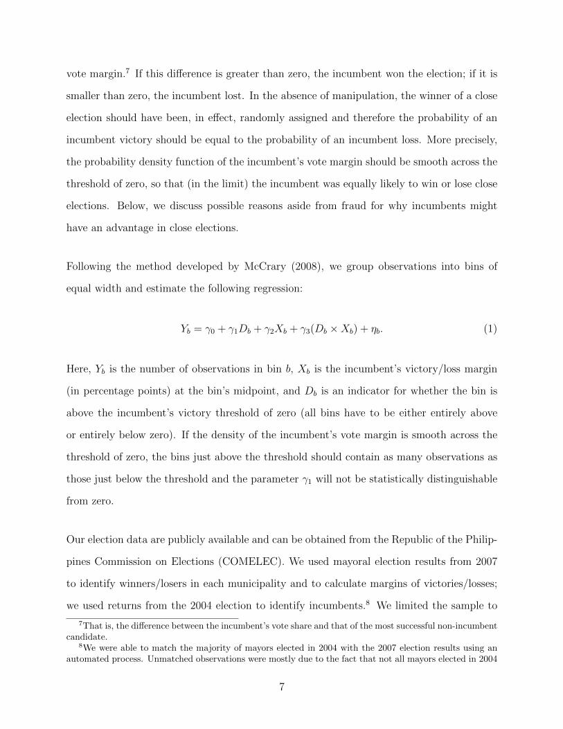
Following the method developed by McCrary (2008), we group observations into bins of
equal width and estimate the following regression:
Yb = γ0 + γ1Db + γ2Xb + γ3(Db ×Xb) + ηb. (1)
Here, Yb is the number of observations in bin b, Xb is the incumbent’s victory/loss margin
(in percentage points) at the bin’s midpoint, and Db is an indicator for whether the bin is
above the incumbent’s victory threshold of zero (all bins have to be either entirely above
or entirely below zero). If the density of the incumbent’s vote margin is smooth across the
threshold of zero, the bins just above the threshold should contain as many observations as
those just below the threshold and the parameter γ1 will not be statistically distinguishable
from zero.
Our election data are publicly available and can be obtained from the Republic of the Philip-
pines Commission on Elections (COMELEC). We used mayoral election results from 2007
to identify winners/losers in each municipality and to calculate margins of victories/losses;
we used returns from the 2004 election to identify incumbents.8 We limited the sample to
7That is, the difference between the incumbent’s vote share and that of the most successful non-incumbentcandidate.
8We were able to match the majority of mayors elected in 2004 with the 2007 election results using anautomated process. Unmatched observations were mostly due to the fact that not all mayors elected in 2004
7

municipalities in which the incumbent mayor’s vote margin was within a 5 percentage-point
bandwidth of the zero threshold and created 15 bins on either side of this threshold. This
resulted in a sample of 153 municipalities. The incumbent won re-election in 81 of these
municipalities and lost in the remaining 72.
Figure 1 plots the probability that a municipality falls into a particular bin against the
margin of victory at the midpoint of the bin. The top panel plots results for the entire
country, the middle panel for the poorer half of municipalities, and the bottom panel for the
richer half.9 Because there are no direct measures of poverty available at the municipal level,
we constructed a poverty proxy by taking the first factor in a factor analysis of housing quality
indicators. This method was proposed by Sahn and Stifel (2003) as a method of measuring
poverty in the absence of data on income and expenditures.10
Figure 1 shows that incumbent mayors in the poorer half of municipalities were more likely
to win elections decided by a margin of between 0 and 1.5 percentage points. In contrast,
there is little evidence that incumbents in the richer half of municipalities were more likely
to win tightly contested elections. Below, we provide evidence that this pattern of electoral
manipulation closely corresponds to the pattern of violence observed after the election.
Table 2 reports McCrary test results (i.e., estimates of equation 1). The constant term of
equation 1 represents the height at which the pdf intercepts the threshold of zero from below,
which is an estimate of how likely incumbents were to lose tightly contested elections. The
ran for re-election or to spelling errors. In the latter case, we matched incumbent mayors manually.9In genral, there is a strong association between poverty and corruption (Olken and Pande, 2012). This
could be because populations in poor areas are less informed about the election process and the participatingcandidates (Ferraz and Finan, 2008; Besley and Burgess, 2002).
10We use all 5 indicators of housing quality recorded by the 2000 Philippine Census: access to electricity,piped water and indoor plumbing, as well as the material of the roof and walls. Table 1 shows the weightswith which the housing characteristics enter the first factor. As expected, values that indicate higher housingquality influence the first factor in the same direction for all variables. If a municipality’s predicted valueof the first factor is below the median, we define it as poor. If the predicted value is above the median, wedefine it as rich.
8

parameter associated with incumbent victories reflects the discontinuous change in the pdf at
the zero threshold. For the entire sample, we estimate a constant of 0.028 and a discontinuous
increase of 0.016, which is statistically significant at the 5 percent level. Thus, incumbents
were approximately 57 percent (0.016/0.028) more likely to win tightly contested elections
than to lose them. This constitutes evidence that incumbents were able to manipulate tightly
contested elections in order to secure victory.
The results in columns (2) and (3) show that manipulation took place primarily in poor
municipalities. When the sample is restricted to the poorer half of municipalities, we obtain a
constant of 0.027 and there is a discontinuous increase of 0.031 in the pdf at the zero threshold
indicating that incumbents were more than twice as likely to win tightly contested elections
than to lose them. In the richer half of municipalities, the discontinuous decrease of 0.009
is small relative to the constant of 0.038 and is not statistically significant at conventional
levels.
The results presented in Table 2 are based on a bandwidth of 5 percentage points and 15
bins on either side of the zero threshold. In general, estimates with smaller bandwidths
should be closer to the true value, since they are more strongly informed by observations
closer to the threshold (McCrary 2008). However, reducing the bandwidth also decreases the
effective sample size and therefore leads to less precise estimates. Table 3 provides evidence
that our estimates are robust to limiting the bandwidth to 3 or 4 percentage points around
the threshold.
An alternative explanation for the results presented thus far is that incumbents had accurate
polling information and could therefore expend precisely enough effort campaigning to secure
a narrow victory (Grimmer et al., 2011).11 Although this explanation is possible, Figure
11The incumbent could have more precise polling information than the challenger, or the incumbent couldhave more resources and therefore be able to “out-campaign” the challenger by precisely the amount necessaryto win the election.
9

1 provides evidence that incumbents were roughly twice as likely as their challengers to
win elections decided by a margin of between 0 and 0.5 percentage points (a margin that
corresponds to 0-65 votes out of an average of 13,000 cast), and one-and-a-half times more
likely to win elections decided by a margin of between 0.5 and 1 percentage points (which
corresponds to 65-130 votes). It is highly unlikely that polling data in the Philippines were
sufficiently accurate to consistently secure such narrow victories simply through the precise
calibration of campaigning effort.
3.2 Did Narrow Incumbent Victories Cause Conflict?
The second step in our analysis is to test whether conflict increased when incumbents won
close elections. Specifically, we estimate the following equation, based on a regression dis-
continuity (RD) design, for a subsample of municipalities within a small bandwidth around
the incumbent’s victory threshold:
Yi = β0 + β1Di + β2Xi + β3(Di ×Xi) + εi. (2)
Here, Yi is the number of conflict casualties that municipality i experienced in the 6 months
after the 2007 elections, Xi is the incumbent’s vote margin, and Di is an indicator for
whether the incumbent won the election. The parameter β1 represents the difference in
casualties between municipalities where the incumbent won a tightly contested election and
municipalities where the incumbent narrowly lost.
The discontinuous jump in the probability of an incumbent victory at the zero threshold
documented in the previous section is a clear violation of the standard RD assumption that
unobserved variables are continuous across the threshold and would bias the estimate of β1
upwards if incumbents were more likely to manipulate narrow elections in municipalities es-
10

pecially prone to violence. We conduct two tests in an effort to explore this possibility. First,
we estimate equation 2 using the number of casualties that occurred in the 6 months prior to
the 2007 election as the outcome. If municipalities above the zero threshold were more vio-
lent for reasons unrelated to election fraud, we would expect them to have experienced more
casualties before the election took place, not just afterwards. Second, we estimate a stan-
dard difference-in-differences regression that explicitly controls for unobserved municipality
characteristics.
The data on casualties come from records of conflict-related incidents collected by the Armed
Forces of the Philippines (AFP) for the years 2002-2009; they include information on insur-
gents, government forces and civilian casualties. These incident-level data have been used to
analyze the impact of aid and the impact of economic conditions on conflict intensity (Crost
et al., 2012), and are similar to SIGACTS - the US incident-level military data, which have
been used to study the insurgency activities in Afghanistan and Iraq (Berman et al., 2011;
Iyengar et al., 2011; Beath et al., 2011). The data also contain information on the date and
the location of the incident and identify the insurgent group involved. During the period
under study (November of 2006 through November 2007), 2745 conflict incidents leading to
1045 casualties were reported by security forces throughout the country. Our focus is on the
number of casualties that occurred in the 153 municipalities in which the incumbent’s vote
margin was within a 5 percentage-point bandwidth of the zero threshold. In these munic-
ipalities, a total of 521 incidents occurred, leading to 315 casualties.12 Information on the
other municipality characteristics included in the estimation were obtained from the 2000
Philippines Census, available from the National Statistics Office of the Philippines.
Table 4 provides descriptive statistics for the variables used in the analysis separately for mu-
12As Crost et al. (2012) noted, it is possible that the AFP troops misreported the number of casualtiesrelated to an incident. This type of misreporting, however, is likely to be limited since the field data wereoriginally collected to be used internally by the AFP for intelligence purposes and for the planning of futureoperations. Moreover, casualties are typically easy to verify which makes misreporting more difficult, evenif individual AFP units had an incentive to do so.
11

nicipalities where incumbents won by a narrow margin and municipalities where incumbents
lost by a narrow margin. The table shows that the number of casualties in the pre-election
period was similar in municipalities where incumbents went on to win or lose. In the post-
election period, municipalities in which incumbents won averaged more casualties, although
the difference is not statistically significant for the entire sample. Overall, the number of
casualties was larger in the pre-election period. Municipalities where incumbents won were
somewhat more populous and had better access to infrastructure, although the only statis-
tically significant difference is for piped water (at the 10 percent level).
Figure 2 plots casualties during the 12 months before and after the 2007 election against the
incumbent’s margin of victory. Scatter dots represent the mean of casualties per month and
are sized to reflect the number of municipalities in each bin.13 The top panel shows that
municipalities experienced substantially more casualties after the incumbent won an election
by a margin of between 0 and 2 percentage points than after losing by a similar margin.
The bottom panel shows that casualties in the 12 months before the election were essentially
unrelated to incumbent victories.
Table 5 reports Poisson estimates of the regression discontinuity (RD) described by equation
2. The coefficient associated with incumbent victories represents the discontinuous increase
in casualties across the incumbent’s victory threshold. The results in columns (1) and (2)
suggest that municipalities experienced between 0.074 and 0.101 additional casualties per
month after a narrow incumbent victory as compared to a narrow loss. These estimates are
large compared to the post-election average of 0.041 casualties per month and are statistically
significant at the 5 percent level. The results in columns (3) and (4) provide no evidence of
a statistically significant relationship between narrow incumbent victories and pre-election
casualties.
13To create the scatter plot, we divided the sample into 10 bins of equal width on either side of the zerothreshold.
12

One potential concern with the results in Table 5 is that the estimated effect of incumbent
victories decreases substantially when we control for observable municipal characteristics in
column (2). This raises the possibility that the results are driven by unobserved differences
between municipalities in which incumbents were able to manipulate elections and municipal-
ities where they were unable to manipulate elections. In an effort to explore this hypothesis,
we estimate a difference-in-differences regression that explicitly controls for systematic dif-
ferences in unobserved characteristics. Specifically, we estimate the following equation based
on observations from the 12 months before and after the 2007 election:
Yit = β0+β1Di+β2Xi+β3(Dit×Xi)+γ1(Di×Postt)+γ2(Xi×Postt)+γ3(Di×Xi×Postt)+εit.
(3)
Here, Yit is the number of conflict casualties that municipality i experienced at time t, Xi
is the incumbent’s vote margin, and Di is an indicator for whether the incumbent won the
election. Postt is an indicator for whether the observation was made in the post-election
period. The parameter β3 represents the difference in pre-election casualties between munic-
ipalities where incumbents narrowly won or lost. The parameter γ1 represents the increase in
casualties following a narrow incumbent victory, while the parameter β1 captures differences
in pre-election violence due to time-invariant unobserved municipal characteristics.
The first two columns of Table 6 present estimates of this difference-in-differences regression.
They suggest that narrow incumbent victories were associated with between 0.099 and 0.123
additional post-election casualties per month. Table 7 shows that these results are robust to
limiting the bandwidth to 3 or 4 percentage points around the threshold.
13
3.3 Did Election Fraud Cause Conflict?
Although the results presented thus far are consistent with the hypothesis that fraud leads to
an increase in casualties, narrow incumbent victories may have led to post-election violence
for reasons unrelated to fraud. For example, the insurgents might have typically preferred the
challenger’s political platform to the incumbent’s and reacted with violence if their candidate
lost. We conduct several robustness tests to explore this possibility.
First, we tested whether the relationship between narrow incumbent victories and casualties
was driven by the political platform of the incumbent by interacting an indicator for whether
the incumbent was affiliated with the governing coalition of President Arroyo with the other
variables in the difference-in-differences regression. The results are presented in columns (3)
and (4) of Table 6.14 Out of the 153 incumbents who make up our sample, 116 were affiliated
with the governing coalition. The results suggest that the insurgent reaction did not depend
upon the incumbent’s political affiliation. Specifically, none of the interactions between
the governing coalition indicator and the variables in the difference-in-differences regression
are statistically significant at conventional levels. In addition, we re-estimated equation 1
redefining Xb to equal the victory/loss margin between the most successful candidate from
the governing coalition and the most successful candidate from the opposition party. Figure
3 plots the probability that a municipality falls into a particular bin against the coalition
candidate’s margin of victory at the bin’s midpoint. There is little evidence of a discontinuous
change in the probability at the zero threshold, suggesting that mayoral candidates from the
governing coalition were as likely to win narrow elections as to lose them. This is confirmed by
the results of a McCrary test presented in Table 8. The estimated coefficient associated with
the coalition candidate winning is close to zero in magnitude and statistically insignificant.
14As discussed in Section 2, the governing coalition consisted of center-right parties, while the oppositionmostly consisted of center-left parties. Only two incumbents in the 2007 mayoral elections were members ofa far left party and neither of them was involved in a tightly contested election.
14

The top panel of Figure 4 plots the number of casualties in the 6 months before and after the
mayoral elections against the coalition candidate’s margin of victory. There is no indication
that a narrow victory for the coalition candidate is associated with an increase in post-
election casualties. Moreover, there is no evidence of a relationship between the coalition
candidate’s margin of victory and the pre-elections levels of violence. To confirm these
results, we estimated modified versions of equations 2 to explore whether political party was
related to violence. The results of this exercise are reported in Table 9. The coefficients
associated with a governing coalition candidate winning are consistently insignificant in the
RD regressions using either pre- or post-election violence as the outcome.
As an additional robustness test, we analyzed the relationship between incumbent victories
and post-election casualties in poor and rich municipalities (measured by the index of in-
frastructure quality described in Section 3.1). Figure 1 provided evidence that fraud was
concentrated in poor municipalities in which the incumbent’s margin of victory was between
0 and 1.5 percentage points. If fraud had a causal effect on violence we would expect post-
election violence to be highest in these municipalities. Figure 5 shows that this was in fact
the case. There is a discontinuous jump in violence across the incumbent’s victory threshold
in poor municipalities but not in rich ones. Moreover, post-election violence in poor mu-
nicipalities was highest for incumbent victories in which the margin was between 0 and 1.5
percentage points. In contrast, incumbent victories by larger margins do not appear to be
associated with post-election violence. The bottom panels of Figure 5 plot the incumbent’s
victory margin against pre-election casualties. There is little evidence of a relationship be-
tween narrow incumbent victories and pre-election casualties in either the poorer half or the
richer half of municipalities.
Table 10 presents the corresponding regression results. The RD estimates in column (1)
suggest that an incumbent victory in a poor municipality was, on average, associated with
0.175 additional casualties per month during the post-election period. In contrast, the RD
15

estimate in column (2) provides little evidence that incumbent victories in poor municipalities
were related to pre-election violence. The difference-in-differences estimate in column (3)
suggests that an incumbent victory led, on average, to an additional 0.151 casualties in poor
municipalities. In rich municipalities there is no statistically significant relationship between
incumbent victories and violence in either the pre- or the post-election period.
These results suggest that electoral fraud had a substantial impact on post-election violence.
To gauge the magnitude of this impact, we focus on the 102 mayoral elections for which the
evidence of fraud was strongest: those that took place in poor municipalities and were decided
by a margin of between 0 and 1.5 percentage points. In the absence of fraud, incumbents and
challengers should have won an equal number of these tightly contested elections, or 51 each.
In actuality, incumbents won 62 and lost 40, suggesting that 11 incumbent victories were
secured through manipulation. The 62 municipalities won by the incumbent experienced 39
more casualties during the 12-month post-election period than the 40 municipalities in which
the challenger won. Thus, an incumbent victory secured through manipulation is associated
with an additional 3.5 casualties (3911
). In comparison, the typical Philippine municipality
experienced 0.5 casualties during the 12 month post-election period.
A similar logic applies even if challengers won some proportion of mayoral elections through
manipulation. For example, if two of the 40 elections won by the challenger were secured
through manipulation, then incumbents would have had to have successfully manipulated
13 elections in order to arrive at a total of 62 incumbent victories; the additional casualties
per fraudulent incumbent victory is again 3.5 (3911
) as long as we assume that electoral fraud
committed by challengers led to the same increase in casualties as incumbent electoral fraud.
16
4 Conclusion
There is a general consensus among practitioners that fraudulent elections can lead to po-
litical and civil unrest in developing countries (World Bank, 2012). It is not clear, however,
whether election fraud and political violence are causally linked or whether this association
simply reflects cultural or institutional factors. The present study contributes to the litera-
ture by examining the effect of election fraud in the 2007 mayoral elections in the Philippines
on post-election violence between government forces and insurgents.
Our results suggest that incumbent mayors were more likely to win tightly contested elections
compared to their challengers, an indication of election fraud (McCrary, 2008). In addition,
we find that municipalities in which incumbent mayors were narrowly elected experienced
between 0.6 and 1.6 additional post-election casualties during the 12 month period after the
election as compared to municipalities in which the challenger won. However, there is no
evidence of an association between narrow incumbent victories and pre-election violence.
These results are consistent with the hypothesis that election fraud is causally linked to civil
conflict. In an effort to rule out competing explanations, we conducted several tests. For
instance, we showed that narrow incumbent wins were associated with post-election violence
only in poor municipalities. In richer municipalities, where there is little evidence of fraud,
there was essentially no relationship between post-election violence and narrow incumbent
victories. In addition, we showed that the increase in post-election violence was unrelated to
the party affiliation of the incumbent, lending further support to the argument that fraud,
as opposed to the incumbents political platform, was the causal mechanism.
To our knowledge, this is the first study to establish a causal link between election fraud
and post-election violence. Although we are unable to pin down the exact mechanism at
work, we report anecdotal evidence that election fraud increases support for insurgents and
17

makes it easier for them to recruit followers. Our results suggest that election monitoring
could help to dampen post-election unrest. In addition, they suggest that future election
monitoring should not focus on presidential and congressional races to the exclusion of local
races if the goal is to reduce post-election violence.
References
Abadie, Alberto and Javier Gardeazabal, “The economic costs of conflict: A case study
of the Basque Country,” American Economic Review, 2003, 93 (1), 113–132.
Akresh, Richard, Leonardo Lucchetti, and Harsha Thirumurthy, “Wars and Child
Health: Evidence from the Eritrean-Ethiopian Conflict,” Journal of Development Eco-
nomics, 2012, 99 (2), 330–340.
Beath, Andrew, Fotini Christia, and Ruben Enikolopov, “Winning Hearts and Minds
through Development Aid: Evidence from a Field Experiment in Afghanistan,” Centre
for Economic and Financial Research at New Economic School Working Paper No 166,
October 2011.
Beber, Bernd and Alexandra Scacco, “What the Numbers Say: A Digit-Based Test for
Election Fraud,” Political Analysis, 2012, 20 (2), 211–234.
Berman, Eli, Michael Callen, Joseph H. Felter, and Jacob N. Shapiro, “Do Working
Men Rebel? Insurgency and Unemployment in Afghanistan, Iraq, and the Philippines,”
Journal of Conflict Resolution, 2011, 55 (4), 496–528.
Besley, Timothy and Robin Burgess, “The political economy of government responsive-
ness: Theory and evidence from India,” Quarterly Journal of Economics, 2002, 117 (4),
1415–1451.
18

Blakeslee, David S., “Politics and Public Goods in Developing Countries: Evidence from
India,” Unpublished Working Paper, 2013.
Callen, Michael and James D. Long, “Institutional Corruption and Election Fraud:
Evidence from a Field Experiment in Afghanistan,” Unpublished Working Paper, 2012.
Crost, Benjamin, Joseph H. Felter, and Patrick B. Johnston, “Aid Under Fire:
Development Projects and Civil Conflict,” Unpublished Working Paper, 2012.
Daxecker, Ursula E., “The Cost of Exposing Cheating: International Election Monitoring,
Fraud, and Post-Election Violence in Africa,” Journal of Peace Research, 2012, 49 (4),
503–516.
Ferraz, Claudio and Frederico Finan, “Exposing corrupt politicians: The effects of
Brazil’s publicly released audits on electoral outcomes,” Quarterly Journal of Economics,
2008, 123 (2), 703–745.
Grimmer, Justin, Eitan Hersh, Brian Feinstein, and Daniel Carpenter, “Are Close
Elections Random?,” Unpublished Working Paper, 2011.
Hegre, Havard, Tanja Ellingsen, Scott Gates, and Nils Petter Gleditsch, “Toward
a Democratic Civil Peace? Democracy, Political Change, and Civil War, 1816-1992,”
American Political Science Review, 2001, 95 (1), 33–48.
Henderson, Errol A. and J. David Singer, “Civil War in the Post-Colonial World,
1946-92,” Journal of Peace Research, 2000, 37 (3), 275–299.
Holden, William N., “Ashes from the Phoenix: State Terrorism and the Party-List Groups
in the Philippines,” Contemporary Politics, 2009, 15 (4), 377–393.
Iyengar, Radha, Jonathan Monten, and Matthew Hanson, “Building Peace: The
Impact of Aid on the Labor Market for Insurgents,” NBER Working Paper 17297, August
2011.
19

Kelley, Judith, “Assessing the Complex Evolution of Norms: The Rise of International
Election Monitoring,” International Organization, 2008, 62 (2), 221–255.
Leon, Gianmarco, “Civil Conflict and Human Capital Accumulation: The Long Term
Effects of Political Violence in Peru,” 2012.
Madlos, Jorge, “Fight systematic fraud being perpetrated by the Arroyo ruling clique in
the May 2007 elections,” Philippine Revolution Web Central, 2007.
Mansour, Hani and Daniel I. Rees, “Armed conflict and Birth Weight: Evidence from
the al-Aqsa Intifada,” Journal of Development Economics, 2012, 1 (99), 190–199.
McCrary, Justin, “Manipulation of the Running Variable in the Regression Discontinuity
Design: A Density Test,” Journal of Econometrics, 2008, 142 (2), 697–714.
Mebane, Walter, “Election Forensics: The Second-digit Benford’s Law Test and Recent
American Presidential Elections,” Election Fraud Conferece, Salt Lake City, Utah, Septem-
ber 29-30. http://www-personal.umich.edu/ wmebane/fraud06.pdf, 2006.
Network, Solidarity Philippines Australia, “Philippines Elections
2007: A Climate of Resignation, Fraud, and Violence,” KASAMA,
http://cpcabrisbane.org/Kasama/2007/V21n2/IOM-InitialFindings.htm, 2007, 21 (2).
Olken, Ben and Rohini Pande, “Corruption in Developing Countries,” Annual Review
of Economics, 2012, 4, 479–505.
Parashar, Kulkarnim, “Electoral Fraud and Strategic Electoral Reform Politics,” Unpub-
lished Working Paper, 2012.
Pastor, Robert A., “The Role of Electoral Administration in Democratic Transitions:
Implications for Policy and Research,” Democratization, 1999, 6 (4), 1–27.
20

Rabasa, Angel, John IV Gordon, Peter Chalk, Audra K. Grant, Scott K. McMa-
hon, Stephanie Pezard, Caroline Reilly, David Ucko, and Rebecca S. Zimmer-
man, “From Insurgency to Stability, Volume II: Insights from Selected Case Studies.,”
Santa Monica, California: Rand Corporation, 2011.
Sahn, David E. and David Stifel, “Exploring Alternative Measures of Welfare in the
Absence of Expenditure Data,” Review of Income and Wealth, 2003, 49 (4), 463–489.
Salas, Santiago, “NDF-EV condemns virtual martial rule in troop deployment to Tacloban
City and military machinations in the election period,” Philippine Revolution Web Central,
2007.
Schedler, Andreas, “Elections without Democracy: The Menu of Manipulation,” Journal
of Democracy, 2002, 13 (2), 36–50.
Schock, Kurt, “A Conjunctural Model of Political Conflict: The Impact of Political Oppor-
tunities on the Relationship between Economic Inequality and Violent Political Conflict,”
Journal of Conflict Resolution, 1966, 40 (1), 98–133.
Tucker, Joshua A., “Enough! Electoral Fraud, Collective Action Problems, and Post-
Communist Colored Revolutions,” Perspectives on Politics, 2007, 5 (3), 535–551.
USAID, Electoral Security Assessment - Philippines, United States Agency for International
Development, Washington, D.C., 2008.
Weidmann, B. Nils and Michael Callen, “Violence, Control and Election Fraud: Evi-
dence from Afghanistan,” 2013.
World Bank, “World Development Report 2011: Conflict, Security, and Development,”
2012.
21

Figures and Tables
22

Figure 1. Did Incumbents Manipulate Close Elections?
0.0
2.0
4.0
6.0
8.1
-.05 -.04 -.03 -.02 -.01 0 .01 .02 .03 .04 .05Margin of victory
Mean Nonparametric fitLinear fit
Entire Sample
0.0
2.0
4.0
6.0
8.1
-.05 -.04 -.03 -.02 -.01 0 .01 .02 .03 .04 .05Margin of victory
Mean Nonparametric fitLinear fit
Poorer 50% of Municipalities
0.0
2.0
4.0
6.0
8.1
-.05 -.04 -.03 -.02 -.01 0 .01 .02 .03 .04 .05Margin of victory
Mean Nonparametric fitLinear fit
Richer 50% of Municipalities
The figure presents the probability density of incumbent mayors’ margin of victory in the 2007 election. Municipalities weregrouped into 20 bins of equal width according to the incumbent’s margin of victory. Each scatter dot represents one bin. Itshorizontal coordinate represents the midpoint of the bin, its vertical coordinate represents the fraction of municipalities forwhich the incumbent’s margin of victory was within the bin. Dashed lines are linear fits, separately estimated on both sidesof the eligibility threshold. Solid lines are nonparametric fits from a local linear regression that uses triangular kernels with abandwidth of 5 percentage points, separately estimated on both sides of the eligibility threshold.
23

Figure 2. Did Incumbent Victories Cause Violence?
-.05
0.0
5.1
.15
Cas
ualti
es/m
onth
-.05 -.04 -.03 -.02 -.01 0 .01 .02 .03 .04 .05Margin of victory
Mean Nonparametric fitLinear fit
Entire SampleCasualties in Post-Election Period
0.0
5.1
.15
Cas
ualti
es/m
onth
-.05 -.04 -.03 -.02 -.01 0 .01 .02 .03 .04 .05Margin of victory
Mean Nonparametric fitLinear fit
Entire SampleCasualties in Pre-Election Period
The figure presents the relationship between the incumbent’s margin of victory and casualties experienced in the 12 monthsbefore and after the 2007 election. Scatter dots represent the mean of casualties per month and are sized to reflect the numberof municipalities in each bin. Dashed lines are linear fits, separately estimated on both sides of the eligibility threshold. Solidlines are nonparametric fits from a local linear regression that uses triangular kernels with a bandwidth of 5 percentage points,separately estimated on both sides of the eligibility threshold.
24

Figure 3. Did the Governing Coalition Manipulate Elections?
0.0
2.0
4.0
6.0
8.1
-.05 -.04 -.03 -.02 -.01 0 .01 .02 .03 .04 .05Margin of victory
Mean Nonparametric fitLinear fit
The figure presents the probability density of coalition candidates’ margin of victory in the 2007 election. Municipalities weregrouped into 20 bins of equal width according to the incumbent’s margin of victory. Each scatter dot represents one bin. Itshorizontal coordinate represents the midpoint of the bin, its vertical coordinate represents the fraction of municipalities forwhich the incumbent’s margin of victory was within the bin. Dashed lines are linear fits, separately estimated on both sidesof the eligibility threshold. Solid lines are nonparametric fits from a local linear regression that uses triangular kernels with abandwidth of 5 percentage points, separately estimated on both sides of the eligibility threshold.
25

Figure 4. Did Victories by Coalition Candidates Cause Violence?
0.1
.2.3
.4C
asua
lties
/mon
th
-.05 -.04 -.03 -.02 -.01 0 .01 .02 .03 .04 .05Margin of victory
Mean Nonparametric fitLinear fit
Casualties in Post-Election Period0
.1.2
.3.4
Cas
ualti
es/m
onth
-.05 -.04 -.03 -.02 -.01 0 .01 .02 .03 .04 .05Margin of victory
Mean Nonparametric fitLinear fit
Casualties in Pre-Election Period
The figure presents the relationship between the incumbent’s margin of victory and casualties experienced in the 12 monthsbefore and after the 2007 election. Scatter dots represent the mean of casualties per month and are sized to reflect the numberof municipalities in each bin. Dashed lines are linear fits, separately estimated on both sides of the eligibility threshold. Solidlines are nonparametric fits from a local linear regression that uses triangular kernels with a bandwidth of 5 percentage points,separately estimated on both sides of the eligibility threshold.
26
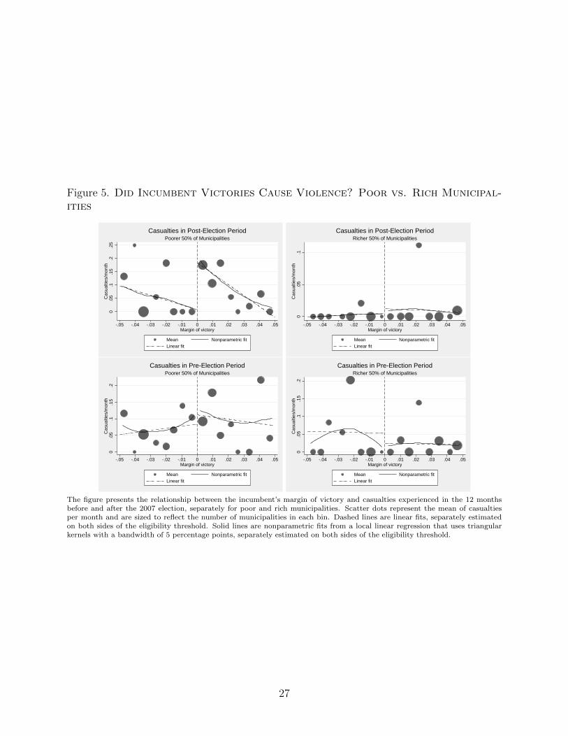
Figure 5. Did Incumbent Victories Cause Violence? Poor vs. Rich Municipal-ities
0.0
5.1
.15
.2.2
5C
asua
lties
/mon
th
-.05 -.04 -.03 -.02 -.01 0 .01 .02 .03 .04 .05Margin of victory
Mean Nonparametric fitLinear fit
Poorer 50% of MunicipalitiesCasualties in Post-Election Period
0.0
5.1
Cas
ualti
es/m
onth
-.05 -.04 -.03 -.02 -.01 0 .01 .02 .03 .04 .05Margin of victory
Mean Nonparametric fitLinear fit
Richer 50% of MunicipalitiesCasualties in Post-Election Period
0.0
5.1
.15
.2C
asua
lties
/mon
th
-.05 -.04 -.03 -.02 -.01 0 .01 .02 .03 .04 .05Margin of victory
Mean Nonparametric fitLinear fit
Poorer 50% of MunicipalitiesCasualties in Pre-Election Period
0.0
5.1
.15
.2C
asua
lties
/mon
th
-.05 -.04 -.03 -.02 -.01 0 .01 .02 .03 .04 .05Margin of victory
Mean Nonparametric fitLinear fit
Richer 50% of MunicipalitiesCasualties in Pre-Election Period
The figure presents the relationship between the incumbent’s margin of victory and casualties experienced in the 12 monthsbefore and after the 2007 election, separately for poor and rich municipalities. Scatter dots represent the mean of casualtiesper month and are sized to reflect the number of municipalities in each bin. Dashed lines are linear fits, separately estimatedon both sides of the eligibility threshold. Solid lines are nonparametric fits from a local linear regression that uses triangularkernels with a bandwidth of 5 percentage points, separately estimated on both sides of the eligibility threshold.
27

Table 1. Estimates of Infrastructure Deprivation: Factor Analysis
Coefficients of Infrastructure Variables in Factors
First Factor Second FactorShare of households with electricity 0.39 -0.53
Share of households with piped water 0.11 0.29
Share of households with indoor plumbing 0.28 -0.05
Share of buildings with walls made of “strong” materials 0.20 0.10
Share of buildings with roofs made of “strong” materials 0.16 0.35
Eigenvalue of factor 2.66 0.21Municipalities 153 153
The table presents coefficients of each variable in the first two factors derived from a factor analysis of the five variables. Data
comes from the 2000 Census of the Philippines. Following the classification of the 2000 Census of the Philippines, “strong”
building materials for walls are defined as: concrete, brick, stone, wood, galvanized iron or aluminum, and asbestos and glass.
“Strong” building materials for roofs are defined as: concrete, galvanized iron or aluminum, and clay tiles and asbestos.
28

Table 2. McCrary Test for Election Manipulation by Incumbent Mayors
OLS EstimatesDependent variable: Fraction of municipalities within bin
Whole Sample Poor Municipalities Rich Municipalities(1) (2) (3)
Incumbent victory 0.016** 0.031*** -0.0087(0.0079) (0.0090) (0.012)
Margin -0.17 -0.26 0.10(0.27) (0.31) (0.45)
Margin× incumbent victory -0.24 -0.76 0.40(0.39) (0.45) (0.61)
Constant 0.028*** 0.027*** 0.038***(0.0056) (0.0064) (0.0094)
Municipalities 153 76 77Observations (bins) 30 30 30
The table reports results of a probability density test for manipulation of the running variable (McCrary, 2008). The running
variable is the incumbent margin of victory. All regressions are weighted by a triangular kernel with a bandwidth of 0.05.
Observations are 30 bins of equal width. The dependent variable is the fraction of municipalities with an incumbent margin of
victory that falls within the bin. ∗, ∗∗ and ∗∗∗ denote statistical significance at the 10%, 5% and 1% levels, respectively.
29

Table 3. McCrary-Test for Election Manipulation by Incumbent Mayors: Robustness toVarying Bandwidths
OLS EstimatesDependent variable:
Fraction of municipalities within bin
Bandwidths: 0.05 0.04 0.03Panel A: All MunicipalitiesIncumbent Victory 0.016** 0.021* 0.023**
(0.0079) (0.011) (0.0094)
Constant 0.028*** 0.025*** 0.022***(0.0056) (0.0076) (0.0066)
# of municipalities 153 123 92Panel B: Poor MunicipalitiesIncumbent Victory 0.031*** 0.038** 0.040***
(0.0090) (0.014) (0.011)
Constant 0.027*** 0.022** 0.024***(0.0064) (0.0095) (0.008)
# of municipalities 76 61 46Panel C: Rich MunicipalitiesEstimate -0.009 -0.006 -0.022
(0.012) (0.014) (0.018)
Constant 0.038*** 0.035*** 0.042***(0.0094) (0.011) (0.015)
# of municipalities 77 62 46
The table reports results of a probability density test for manipulation of the running variable (McCrary, 2008). The running
variable is the incumbent margin of victory. Each regression is weighted by a triangular kernel with the bandwidth shown at
the top of the column. Observations are 30 bins of equal width. The dependent variable is the fraction of municipalities with
an incumbent margin of victory that falls within the bin. ∗, ∗∗ and ∗∗∗ denote statistical significance at the 10%, 5% and 1%
levels, respectively
30

Table 4. Summary Statistics
Incumbent victory Incumbent loss p-value of difference(1) (2) (3)
Casualties in pre-election period (/month) 0.058 0.062 0.88Casualties in post-election period (/month) 0.051 0.030 0.41Population (1000s) 40594 32265 0.29Area (km2) 210 220 0.81Share of households with electricity 0.57 0.55 0.57Share of households with piped water 0.44 0.36 0.09Share of households with indoor plumbing 0.66 0.61 0.18Share of buildings with walls made of “strong” materials 0.64 0.59 0.21Share of buildings with roofs made of “strong” materials 0.69 0.67 0.56
Municipalities 153 153 153
Summary statistics for the sample of municipalities in which incumbents won or lost the 2007 election by a margin of 5percentage points or less. Following the classification of the 2000 Census of the Philippines, “strong” building materials forwalls are defined as: concrete, brick, stone, wood, galvanized iron or aluminum, and asbestos and glass. “Strong” buildingmaterials for roofs are defined as: concrete, galvanized iron or aluminum, and clay tiles and asbestos
31

Table 5. Incumbent Victories and Violence: RD Estimates
Poisson EstimatesDependent variable: Casualties
Post-Election Pre-Election(1) (2) (3) (4)
Incumbent victory 0.101*** 0.074*** 0.024 0.005(0.036) (0.024) (0.051) (0.037)
Margin -1.44*** -0.84 0.10 0.39(0.54) (0.055) (1.40) (0.92)
Margin × incumbent victory -1.46 -1.10 -1.86 -2.32(2.19) (1.40) (2.23) (1.68)
Population (1000s) 1.1×10⁻⁷ 3.5×10−7*(2.0×10−7) (1.9×10⁻⁴)
Area (km2) -0.21 0.40*(0.33) (0.21)
Share of households with electricity -0.015 -0.14***(0.065) (0.051)
Share of households with piped water 0.003 0.069*(0.037) (0.041)
Share of households with indoor plumbing -0.089 -0.063(0.058) (0.051)
Share of buildings with walls made of “strong” materials -0.011 -0.14*(0.038) (0.075)
Share of buildings with roofs made of “strong” materials 0.030 0.099*(0.042) (0.055)
Municipalities 153 153 153 153Observations 1836 1836 1836 1836
The running variable of the RD design is the incumbent margin of victory. All regressions are weighted by a triangular kernel
with a bandwidth of 0.05. The unit of observation is the municipality-month. The sample is restricted to observations within 12
months of the 2007 election (the month of the election is dropped). Reported values are marginal effects. ∗, ∗∗ and ∗∗∗ denote
statistical significance at the 10%, 5% and 1% levels. Standard errors are clustered at the municipality level. Following the
classification of the 2000 Census of the Philippines, “strong” building materials for walls are defined as: concrete, brick, stone,
wood, galvanized iron or aluminum, and asbestos and glass. “Strong” building materials for roofs are defined as: concrete,
galvanized iron or aluminum, and clay tiles and asbestos
32

Table 6. Incumbent Victories and Violence: Difference-in-Differences Estimates
Poisson EstimatesDependent variable: Casualties
(1) (2) (3) (4)Incumbent victory × Post-election 0.123** 0.099** 0.155** 0.147**
(0.055) (0.041) (0.075) (0.067)
Incumbent victory 0.017 0.0036 -0.052 -0.058(0.037) (0.026) (0.043) (0.048)
Margin × Post-election -2.07* -1.45 -1.79* -1.40*(1.26) (0.97) (1.04) (0.82)
Margin 0.074 0.28 0.054 0.33(1.01) (0.67) (0.85) (0.58)
Margin× incumbent victory × Post-election -0.68 0.14 -0.57 0.27(3.15) (2.21) (2.62) (1.96)
Margin× incumbent victory -1.35 -1.67 -1.20 -1.49(1.57) (1.26) (1.34) (1.06)
Post-election period (12 months) -0.091** -0.020 -0.13*** -0.058(0.043) (0.042) (0.048) (0.045)
Gov. coalition× inc. victory× Post-election -0.064 -0.069(0.081) (0.071)
Governing coalition× incumbent victory 0.076* 0.061(0.045) (0.042)
Governing coalition × Post-election 0.069 0.048(0.054) (0.048)
Governing coalition -0.006 0.005(0.081) (0.017)
Controls × time FE No Yes No YesMunicipalities 153 153 153 153Observations 3672 3672 3672 3672
All regressions are weighted by a triangular kernel with a bandwidth of 0.05. The unit of observation is the municipality-month.
The sample is restricted to observations within 12 months of the 2007 election (the month of the election is dropped). Reported
values are marginal effects. ∗, ∗∗ and ∗∗∗ denote statistical significance at the 10%, 5% and 1% levels. Standard errors are
clustered at the municipality level. Control variables are the same as in Table 5
33

Table 7. Estimates from Difference-in-Differences Regressions: Testing the Robustness toVarying Bandwidths
Poisson EstimatesDependent variable: Casualties
Bandwidths: 0.05 0.04 0.03Panel A: All MunicipalitiesIncumbent Victory × Post-election 0.099** 0.099*** 0.160***
(0.041) (0.037) (0.043)
Incumbent Victory 0.004 0.013 0.004(0.026) (0.030) (0.030)
# of municipalities 153 123 92# of observations 3672 2952 2208
All models flexibly control for incumbent margin of victory on both sides of the threshold and are identical to the specification in
column 2 of Table 6. Each regression is weighted by a triangular kernel with the bandwidth shown at the top of the column. The
unit of observation is the municipality-month. The sample is restricted to observations within 12 months of the 2007 election
(the month of the election is dropped). Reported values are marginal effects. ∗, ∗∗ and ∗∗∗ denote statistical significance at
the 10%, 5% and 1% levels. Standard errors are clustered at the municipality level.
34

Table 8. McCrary Test for Election Manipulation by Candidates Affiliated with the Gov-erning Coalition
OLS EstimatesDependent variable: Fraction of municipalities within bin
(1)Coalition victory -0.002
(0.009)
Margin 0.33(0.30)
Margin× Coalition victory -0.045(0.43)
Constant 0.034***(0.006)
Municipalities 198Observations (bins) 30
The table reports results of a probability density test for manipulation of the running variable (McCrary, 2008). The running
variable of the RD design is the coalition candidate’s margin of victory. All regressions are weighted by a triangular kernel with
a bandwidth of 0.05. Observations are 30 bins of equal width. The dependent variable is the fraction of municipalities with
an incumbent margin of victory that falls within the bin. ∗, ∗∗ and ∗∗∗ denote statistical significance at the 10%, 5% and 1%
levels, respectively.
35

Table 9. Coalition Victories and Violence: RD Estimates
Poisson EstimatesDependent variable: Casualties
Post-Election Pre-Election(1) (2) (3) (4)
Coalition victory 0.007 0.003 0.007 -0.006(0.038) (0.028) (0.043) (0.039)
Margin -1.24** -1.02* -1.19 -0.68(0.58) (0.43) (1.04) (1.03)
Margin × coalition victory 2.55** 2.26*** 2.65* 1.99(1.11) (0.73) (1.56) (1.68)
Controls No Yes No YesMunicipalities 198 196 198 196Observations 4752 4704 4752 4704
The running variable of the RD design is the coalition candidate’s margin of victory. All regressions are weighted by a triangular
kernel with a bandwidth of 0.05. The unit of observation is the municipality-month. The sample is restricted to observations
within 12 months of the 2007 election (the month of the election is dropped). Reported values are marginal effects. ∗, ∗∗ and∗∗∗ denote statistical significance at the 10%, 5% and 1% levels. Standard errors are clustered at the municipality level. All
regressions control for the control variables listed in Table 4
36

Table 10. Incumbent Victories and Civil Conflict: Rich vs. Poor Municipalities.
Poisson EstimatesDependent variable: Casualties
Post-Election Pre-Election Full Time Period(RD estimates) (RD estimates) (Diff-in-Diff estimates)
(1) (2) (3)Panel A: All Municipalities (153 municipalities)Effect of Incumbent Victory 0.074** 0.005 0.099**
(0.024) (0.037) (0.041)
Panel B: Rich Municipalities (77 municipalities)Effect of Incumbent Victory -0.032 0.030 0.007
(0.127) (0.047) (0.010)
Panel C: Poor Municipalities (76 municipalities)Effect of Incumbent Victory 0.175*** 0.023 0.151**
(0.058) (0.041) (0.072)
All models flexibly control for incumbent margin of victory on both sides of the threshold. Specifications in columns (1) and
(2) are identical to those reported in columns (2) and (4) of Table 5. The specification in column (3) is identical to that in
columnn (2) of Table 6. All regressions are weighted by a triangular kernel with a bandwidth of 0.05. The unit of observation
is the municipality-month. The sample is restricted to observations within 12 months of the 2007 election (the month of the
election is dropped). Reported values are marginal effects. ∗, ∗∗ and ∗∗∗ denote statistical significance at the 10%, 5% and
1% levels. Standard errors are clustered at the municipality level. All specifications include the same control variables as the
models in Tables 5 and 6.
37