electric machines considering power electronics - ansys · pdf fileelectric machines...
TRANSCRIPT

© 2011 ANSYS, Inc. June 18, 2012 1
Electric Machines Considering Power Electronics
Mark Solveson – Application Engineer
Confidence by Design
Chicago, IL June 14, 2012
© 2011 ANSYS, Inc. June 18, 2012 2
Machine Design Methodology Introduction RMxprt Maxwell Advance Capabilities Core Loss Demagnetization / Magnetization Field-Circuit Co-Simulation Maxwell Circuit Editor Simplorer – Capabilities, Switches, IGBT Characterization
Simplorer Examples Multi-Physics Force Coupling Thermal Coupling
Outline

© 2011 ANSYS, Inc. June 18, 2012 3
Introduction: Machine Design Methodology
© 2011 ANSYS, Inc. June 18, 2012 4
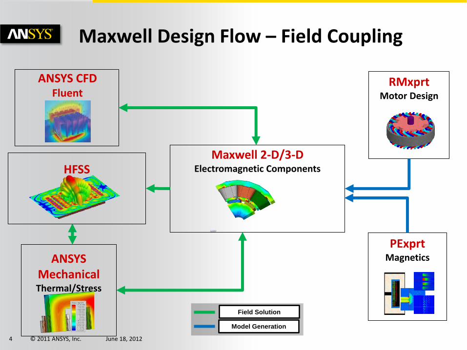
Maxwell 2-D/3-D Electromagnetic Components
Field Solution
Model Generation
HFSS
ANSYS
Mechanical Thermal/Stress
ANSYS CFD Fluent
PExprt Magnetics
RMxprt Motor Design
Maxwell Design Flow – Field Coupling
© 2011 ANSYS, Inc. June 18, 2012 5
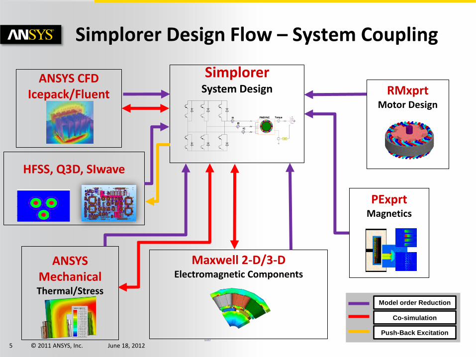
Simplorer System Design
PP := 6
ICA:
A
A
A
GAIN
A
A
A
GAIN
A
JPMSYNCIA
IB
IC
Torque JPMSYNCIA
IB
IC
TorqueD2D
HFSS, Q3D, SIwave
ANSYS CFD Icepack/Fluent
Maxwell 2-D/3-D Electromagnetic Components
ANSYS
Mechanical Thermal/Stress
PExprt Magnetics
RMxprt Motor Design
Simplorer Design Flow – System Coupling
Model order Reduction
Co-simulation
Push-Back Excitation
© 2011 ANSYS, Inc. June 18, 2012 6
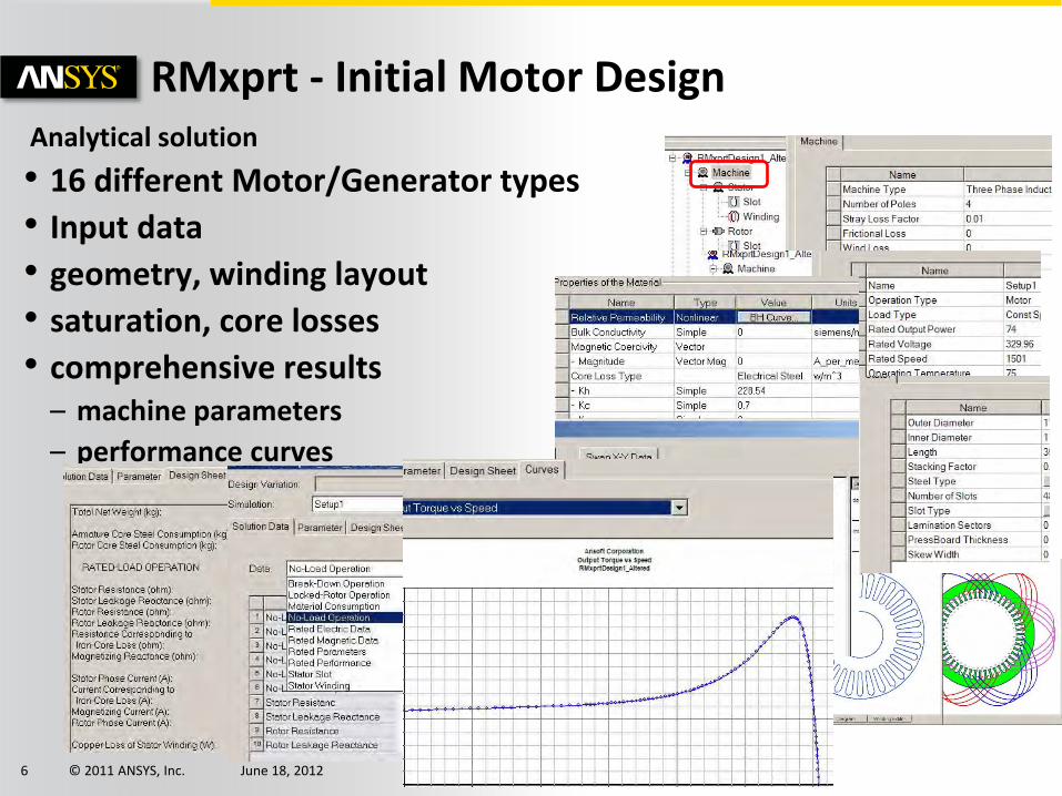
RMxprt - Initial Motor Design Analytical solution
• 16 different Motor/Generator types
• Input data
• geometry, winding layout
• saturation, core losses
• comprehensive results – machine parameters
– performance curves
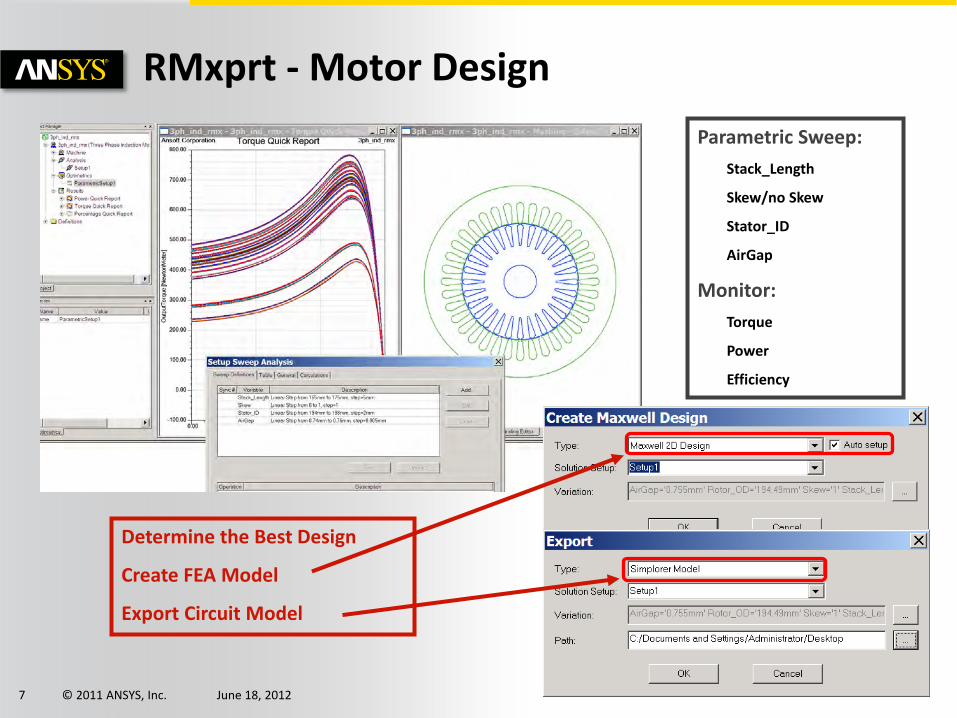
© 2011 ANSYS, Inc. June 18, 2012 7
Parametric Sweep:
Stack_Length
Skew/no Skew
Stator_ID
AirGap
Monitor:
Torque
Power
Efficiency
Determine the Best Design
Create FEA Model
Export Circuit Model
RMxprt - Motor Design
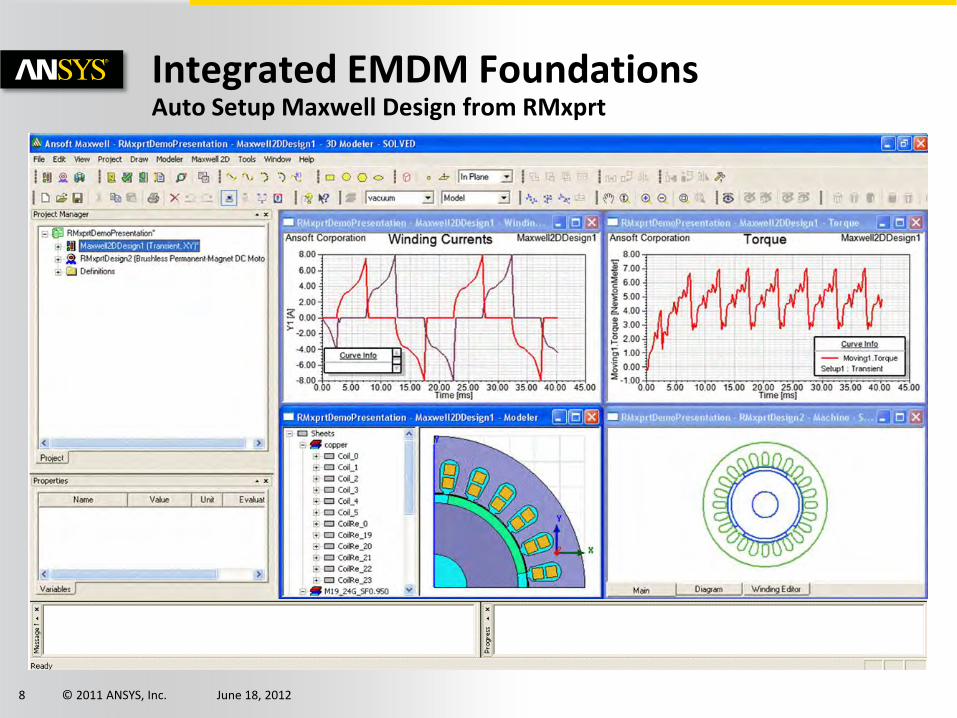
© 2011 ANSYS, Inc. June 18, 2012 8
Integrated EMDM Foundations Auto Setup Maxwell Design from RMxprt

© 2011 ANSYS, Inc. June 18, 2012 9
Maxwell/RMxprt V15 – Axial Flux Machine
• AC or PM Rotor
• Single or Double Side Stator
Sample Inputs
Sample Outputs
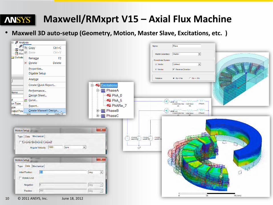
© 2011 ANSYS, Inc. June 18, 2012 10
Maxwell/RMxprt V15 – Axial Flux Machine • Maxwell 3D auto-setup (Geometry, Motion, Master Slave, Excitations, etc. )
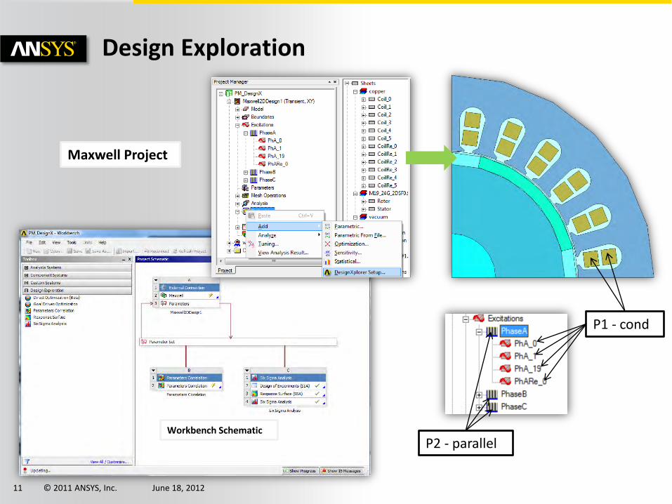
© 2011 ANSYS, Inc. June 18, 2012 11
Design Exploration
P2 - parallel
P1 - cond
Workbench Schematic
Maxwell Project
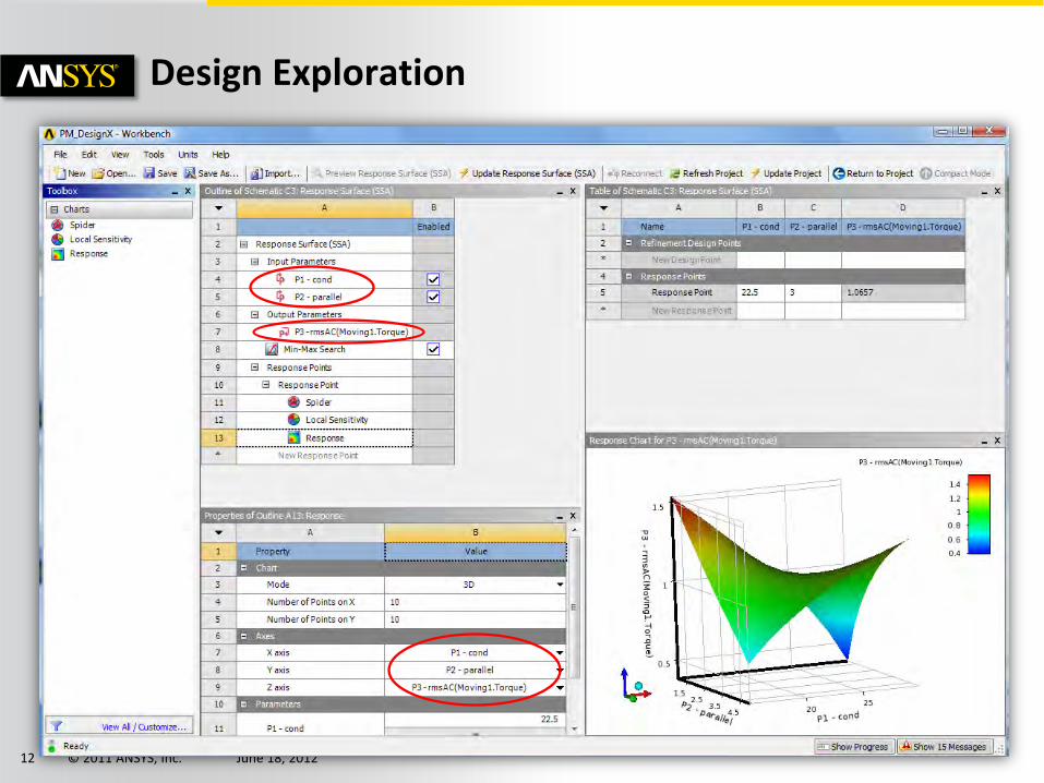
© 2011 ANSYS, Inc. June 18, 2012 12
Design Exploration
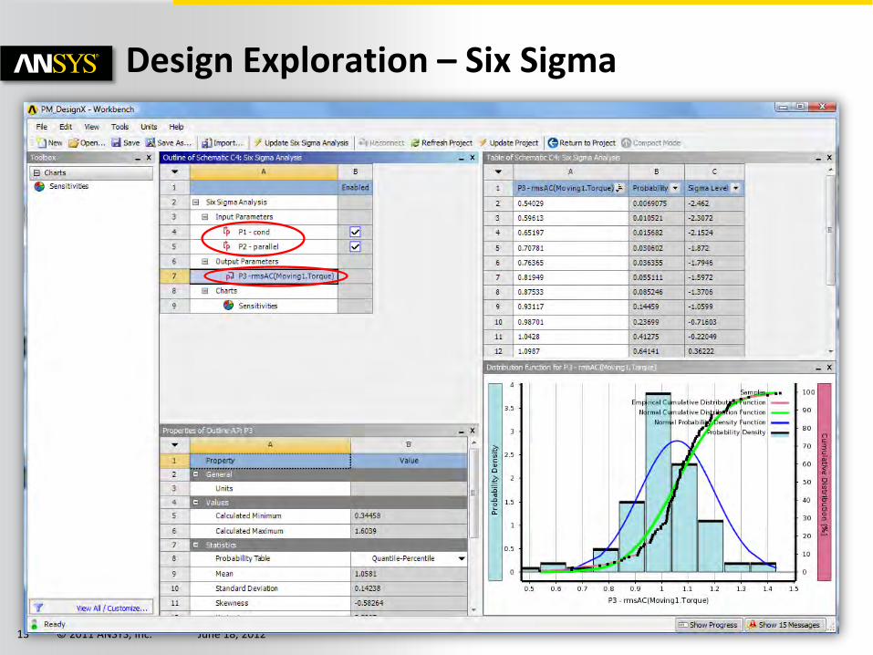
© 2011 ANSYS, Inc. June 18, 2012 13
Design Exploration – Six Sigma
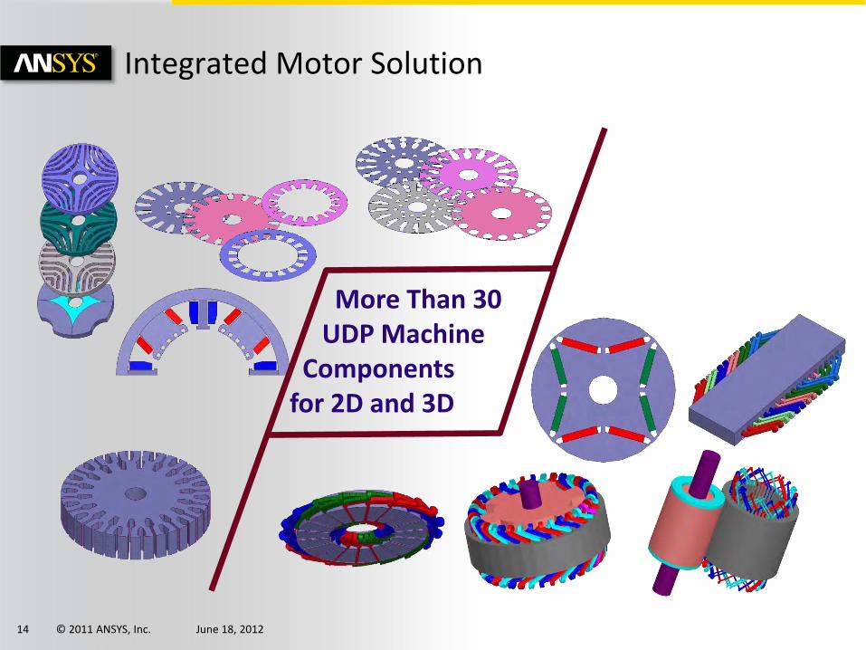
© 2011 ANSYS, Inc. June 18, 2012 14
More Than 30 UDP Machine Components for 2D and 3D
Integrated Motor Solution
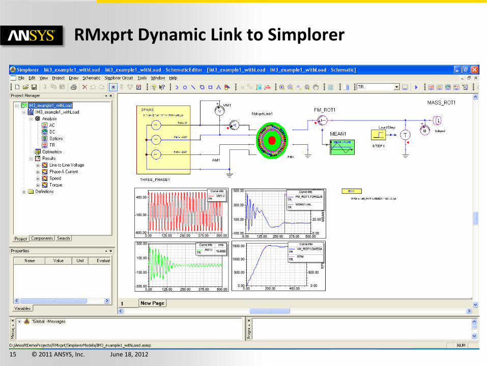
© 2011 ANSYS, Inc. June 18, 2012 15
RMxprt Dynamic Link to Simplorer
© 2011 ANSYS, Inc. June 18, 2012 16
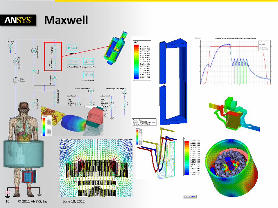
Maxwell
0.00 2.00 4.00 6.00 8.00 10.00 12.00 14.00 16.00 18.00Time [ms]
0.00
0.20
0.40
0.60
0.80
1.00
1.20
1.40
Pos
ition
[mm
]
0.00
0.50
1.00
1.50
2.00
2.50
3.00
3.50
Coi
l Cur
rent
[met
er]
TRW / Ansoft Position & Current Hysteresis Control Close/Open1
Curve Info
Position
Coil Current
Diode Current
© 2011 ANSYS, Inc. June 18, 2012 17
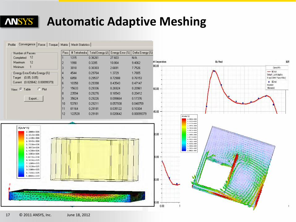
Automatic Adaptive Meshing
© 2011 ANSYS, Inc. June 18, 2012 18
Advanced Capabilities Coreloss Computation
© 2011 ANSYS, Inc. June 18, 2012 21
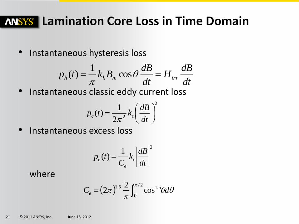
Lamination Core Loss in Time Domain
• Instantaneous hysteresis loss
• Instantaneous classic eddy current loss
• Instantaneous excess loss
where
dt
dBH
dt
dBBktp irrmhh
cos
1)(
2
22
1)(
dt
dBktp cc
dCe 2/
0
5.15.1cos
22
21
)(dt
dBk
Ctp c
e
e
© 2011 ANSYS, Inc. June 18, 2012 22
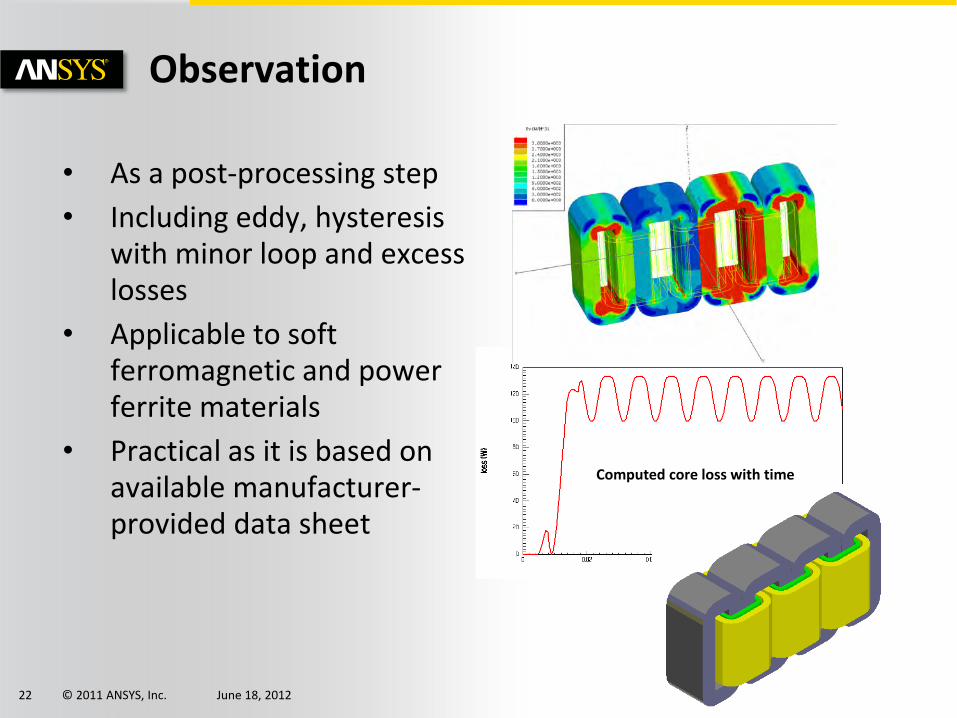
• As a post-processing step
• Including eddy, hysteresis with minor loop and excess losses
• Applicable to soft ferromagnetic and power ferrite materials
• Practical as it is based on available manufacturer-provided data sheet
Computed core loss with time
Observation

© 2011 ANSYS, Inc. June 18, 2012 23
Core Loss Effects on Field Solutions
• Basic concept: the feedback of the core loss is taken into account by introducing an additional component of magnetic field H in core loss regions. This additional component is derived based on the instantaneous core loss in the time domain
© 2011 ANSYS, Inc. June 18, 2012 24
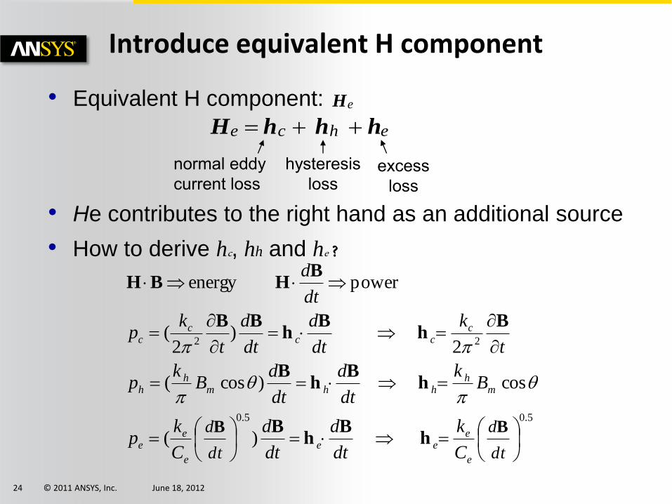
• Equivalent H component:
• He contributes to the right hand as an additional source
Introduce equivalent H component
eH
ehce hhhH
normal eddy current loss
hysteresis loss
excess loss
5.05.0
22
)(
cos )cos(
2 )
2(
power energy
dt
d
dt
d
e
eee
e
ee
mh
hhmh
h
ccc
cc
C
k
dt
d
dt
d
C
kp
Bk
dt
d
dt
dB
kp
t
k
dt
d
dt
d
t
kp
dt
d
BBh
Bh
B
hB
hB
Bh
Bh
BB
BHBH
• How to derive hc, hh and he ?
© 2011 ANSYS, Inc. June 18, 2012 25
Model Validation by Numerical Experiment
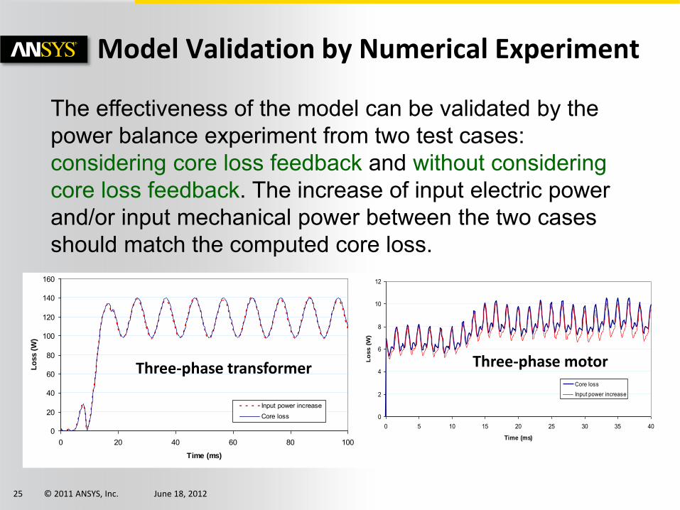
The effectiveness of the model can be validated by the power balance experiment from two test cases: considering core loss feedback and without considering core loss feedback. The increase of input electric power and/or input mechanical power between the two cases should match the computed core loss.
0
20
40
60
80
100
120
140
160
0 20 40 60 80 100
Time (ms)
Lo
ss (
W)
Input power increaseCore loss 0
2
4
6
8
10
12
0 5 10 15 20 25 30 35 40
Time (ms)
Lo
ss (
W)
Core loss
Input power increase
Three-phase transformer Three-phase motor

© 2011 ANSYS, Inc. June 18, 2012 26
Advanced Capabilities Demagnetization Modeling
© 2011 ANSYS, Inc. June 18, 2012 27
Modeling Mechanism
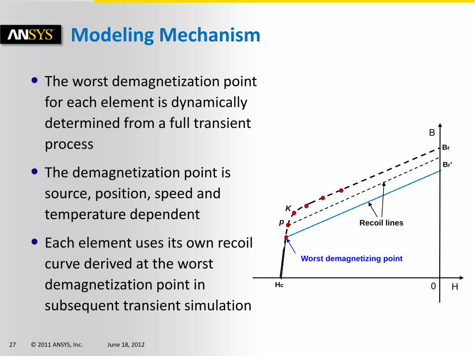
• The worst demagnetization point
for each element is dynamically
determined from a full transient
process
• The demagnetization point is
source, position, speed and
temperature dependent
• Each element uses its own recoil
curve derived at the worst
demagnetization point in
subsequent transient simulation
H Hc
B
0
Br'
Br
K
p Recoil lines
Worst demagnetizing point
© 2011 ANSYS, Inc. June 18, 2012 28
H Hc
B
0
Br'
Br
K
p Recoil line
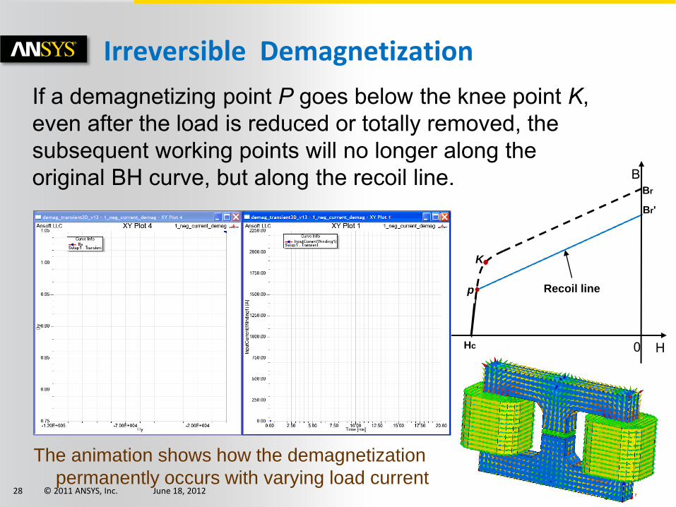
Irreversible Demagnetization
If a demagnetizing point P goes below the knee point K, even after the load is reduced or totally removed, the subsequent working points will no longer along the original BH curve, but along the recoil line.
The animation shows how the demagnetization
permanently occurs with varying load current
© 2011 ANSYS, Inc. June 18, 2012 30
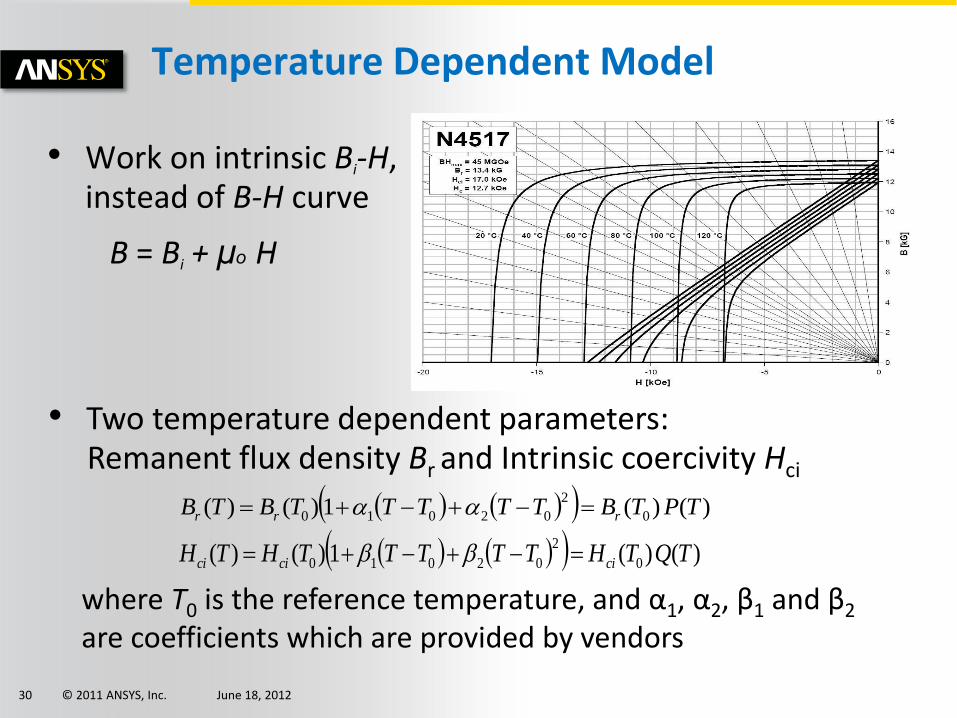
• Two temperature dependent parameters: Remanent flux density Br and Intrinsic coercivity Hci
Temperature Dependent Model
• Work on intrinsic Bi-H, instead of B-H curve
B = Bi + μo H
)()(1)()( 0
2
02010 TPTBTTTTTBTB rrr
)()( 1)()( 0
2
02010 TQTHTTTTTHTH cicici
where T0 is the reference temperature, and α1, α2, β1 and β2 are coefficients which are provided by vendors
© 2011 ANSYS, Inc. June 18, 2012 31
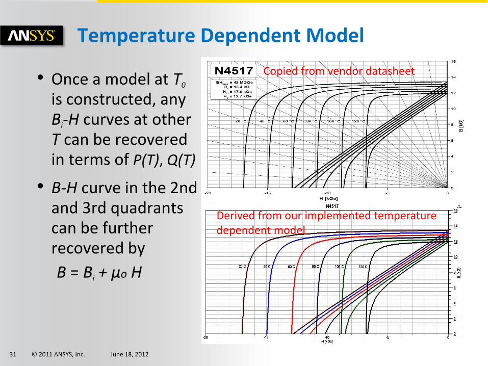
• Once a model at T0
is constructed, any Bi-H curves at other T can be recovered in terms of P(T), Q(T)
• B-H curve in the 2nd and 3rd quadrants can be further recovered by
B = Bi + μo H
Temperature Dependent Model
Copied from vendor datasheet
Derived from our implemented temperature dependent model
© 2011 ANSYS, Inc. June 18, 2012 32
Benchmark Example
• 8-pole, 48-slot, 50 KW, 245 V, 3000 rpm Toyota Prius IPM motor with imbedded NdFeB magnet
• Two steps in 3D transient FEA:
1. Determine the worst operating point element by element during the entire transient process
2. Simulate an actual problem based on the element-based linearized model derived from the step 1
• To further consider the impact of temperature, element-based average loss density over one electrical cycle is used as the thermal load in subsequent thermal analysis
• The computed temperature distribution from thermal solver is further feedback to magnetic transient solver to consider temperature impact on the irreversible demagnetization
© 2011 ANSYS, Inc. June 18, 2012 33
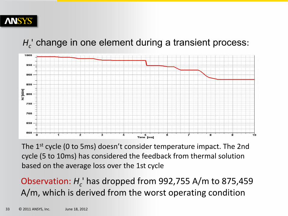
Hc' change in one element during a transient process:
The 1st cycle (0 to 5ms) doesn’t consider temperature impact. The 2nd cycle (5 to 10ms) has considered the feedback from thermal solution based on the average loss over the 1st cycle
Observation: Hc' has dropped from 992,755 A/m to 875,459 A/m, which is derived from the worst operating condition
© 2011 ANSYS, Inc. June 18, 2012 34
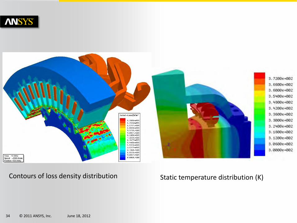
Contours of loss density distribution Static temperature distribution (K)
© 2011 ANSYS, Inc. June 18, 2012 35
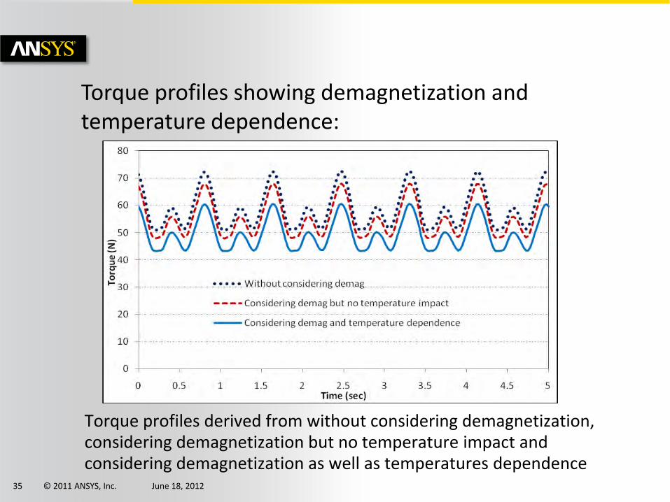
Torque profiles showing demagnetization and temperature dependence:
Torque profiles derived from without considering demagnetization, considering demagnetization but no temperature impact and considering demagnetization as well as temperatures dependence
© 2011 ANSYS, Inc. June 18, 2012 36
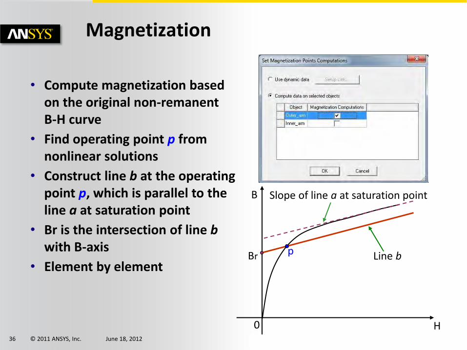
Magnetization
• Compute magnetization based on the original non-remanent B-H curve
• Find operating point p from nonlinear solutions
• Construct line b at the operating point p, which is parallel to the line a at saturation point
• Br is the intersection of line b with B-axis
• Element by element
B
H 0
Br Line b
Slope of line a at saturation point
p
© 2011 ANSYS, Inc. June 18, 2012 37
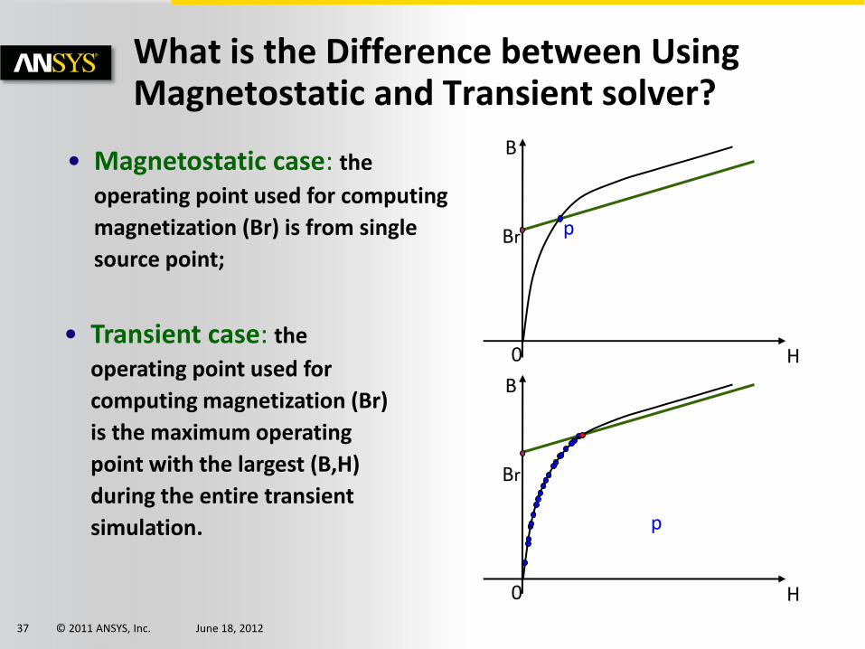
Br
• Magnetostatic case: the
operating point used for computing
magnetization (Br) is from single
source point;
What is the Difference between Using Magnetostatic and Transient solver?
• Transient case: the
operating point used for
computing magnetization (Br)
is the maximum operating
point with the largest (B,H)
during the entire transient
simulation.
H 0
Br p
B
H 0
p
B
© 2011 ANSYS, Inc. June 18, 2012 38
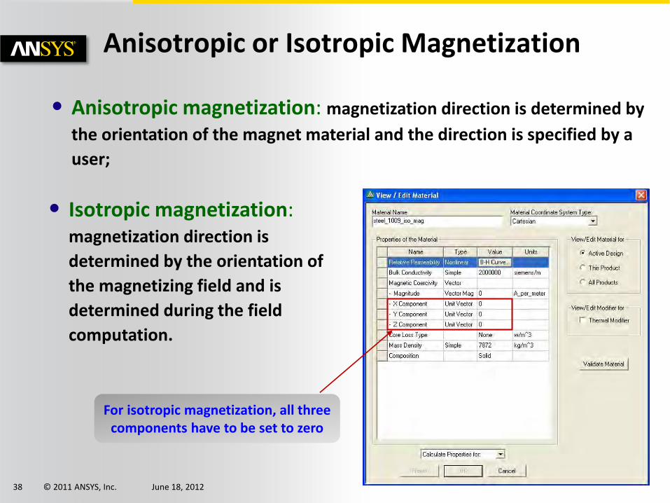
• Anisotropic magnetization: magnetization direction is determined by
the orientation of the magnet material and the direction is specified by a
user;
Anisotropic or Isotropic Magnetization
P(T) input
Q(T) input
• Isotropic magnetization: magnetization direction is
determined by the orientation of
the magnetizing field and is
determined during the field
computation.
For isotropic magnetization, all three
components have to be set to zero
© 2011 ANSYS, Inc. June 18, 2012 39
Field-Circuit Co-simulation
© 2011 ANSYS, Inc. June 18, 2012 40
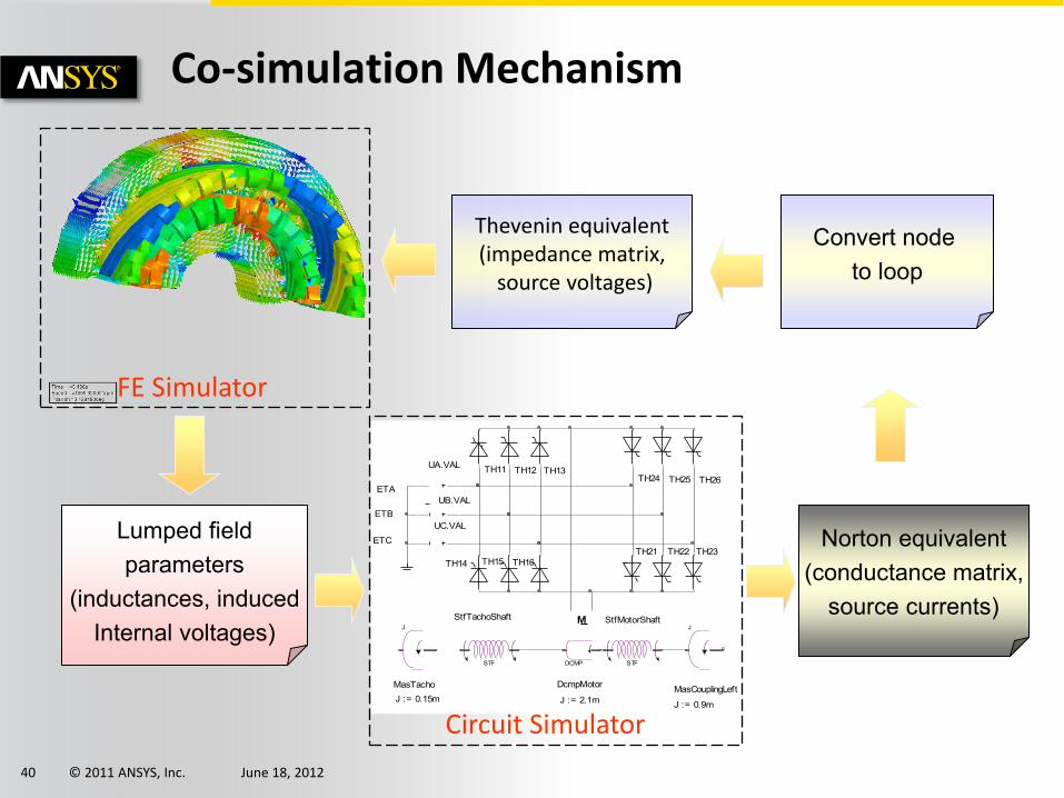
Co-simulation Mechanism
Thevenin equivalent (impedance matrix,
source voltages)
Lumped field parameters
(inductances, induced Internal voltages)
Norton equivalent (conductance matrix,
source currents)
Convert node to loop
FE Simulator
Mww
Rw
Ew J
STF
M
DCMP STF
J
ETA
UA.VAL
ETBUB.VAL
ETCUC.VAL
TH11 TH12 TH13
TH14 TH15 TH16TH21 TH22 TH23
TH24 TH25 TH26
MasTachoJ := 0.15m
StfTachoShaft
DcmpMotor
J := 2.1m
StfMotorShaft
MasCouplingLeft
J := 0.9m
Circuit Simulator
© 2011 ANSYS, Inc. June 18, 2012 41
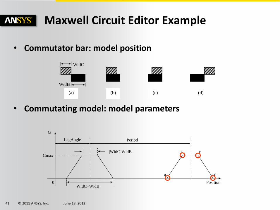
Maxwell Circuit Editor Example
• Commutator bar: model position
• Commutating model: model parameters
(a) (b) (c) (d)
WidB
WidC
Period LagAngle
Position
G
0 WidC+WidB
|WidC-WidB|
a
b c
d
Gmax
© 2011 ANSYS, Inc. June 18, 2012 42
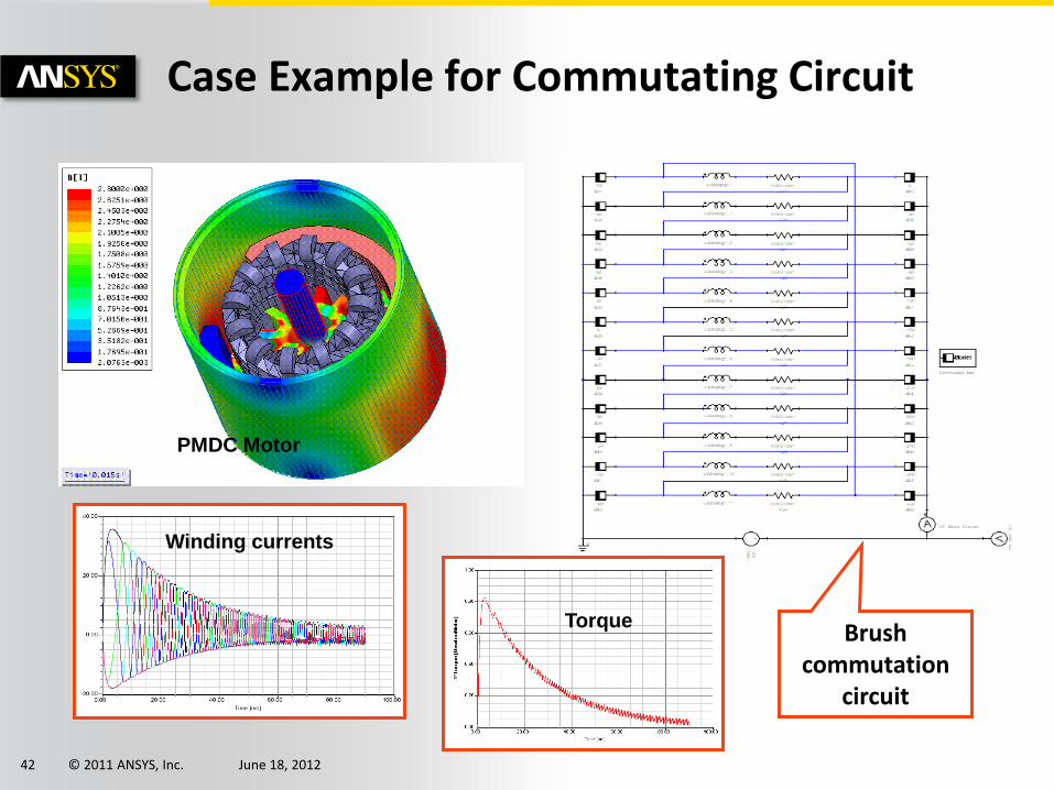
Case Example for Commutating Circuit
Torque
Winding currents
PMDC Motor
Brush commutation
circuit

© 2011 ANSYS, Inc. June 18, 2012 43
Simplorer: Power Electronics

© 2011 ANSYS, Inc. June 18, 2012 44
Simplorer Technology Highlights
© 2011 ANSYS, Inc. June 18, 2012 45
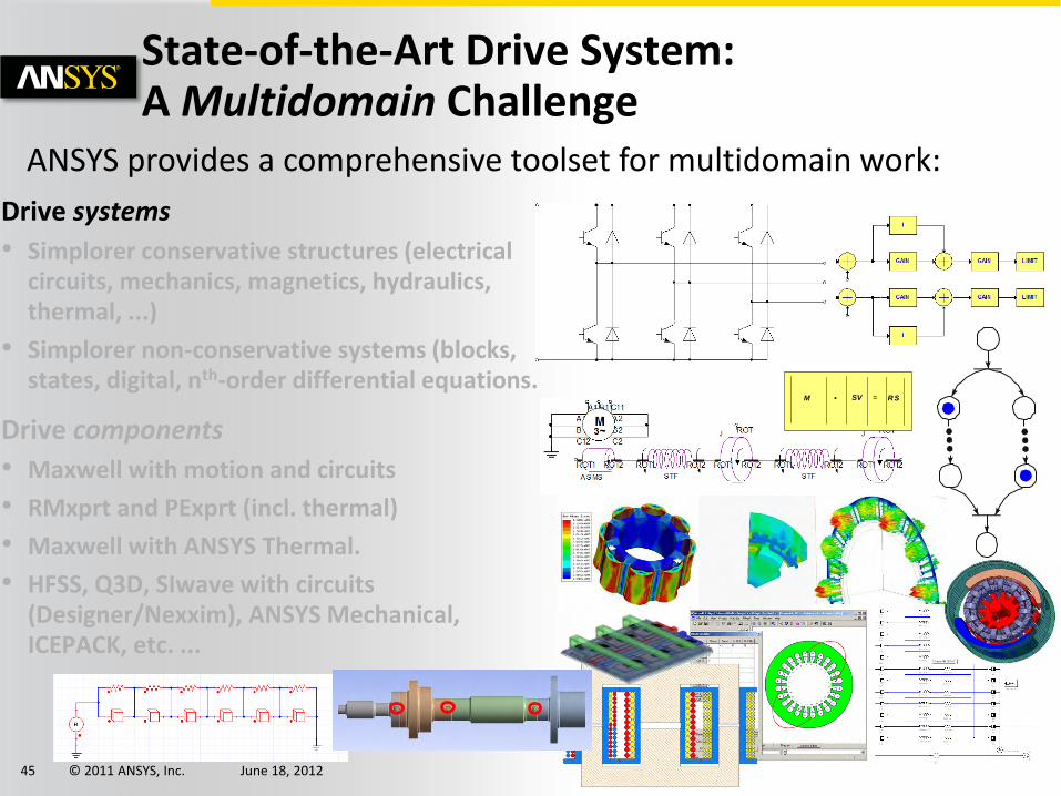
State-of-the-Art Drive System: A Multidomain Challenge
Drive systems
• Simplorer conservative structures (electrical circuits, mechanics, magnetics, hydraulics, thermal, ...)
• Simplorer non-conservative systems (blocks, states, digital, nth-order differential equations.
Drive components
• Maxwell with motion and circuits
• RMxprt and PExprt (incl. thermal)
• Maxwell with ANSYS Thermal.
• HFSS, Q3D, SIwave with circuits (Designer/Nexxim), ANSYS Mechanical, ICEPACK, etc. ...
ANSYS provides a comprehensive toolset for multidomain work:
· = M SV RS

© 2011 ANSYS, Inc. June 18, 2012 46
+
-
B 11A 11 C11
A 12 A 2
B 12 B 2
C12 C2
ROT2ROT1
ASMS
3~M
J
STF
M(t)
GN
D
mSTF
F(t)
GN
D
Magnetics
JA
MMF
Mechanics
L
H Q
Hydraulics, Thermal, ...
Simplorer Simulation Data Bus / Simulator Coupling Technology
State-space Models
statetransition
AUS
SET: TSV1:=0SET: TSV2:=1SET: TSV3:=1SET: TSV4:=0
(R_LAST.I <= I_UGR)
(R_LAST.I >= I_OGR)
EIN
SET: TSV1:=1SET: TSV2:=0SET: TSV3:=0SET: TSV4:=1
Cxy
BuAxx
Electrical circuits
Multi-Domain System Simulator
Analog Simulator
Block Diagram Simulator
State Machine Simulator
Digital/VHDL Simulator
PROCESS (CLK,PST,CLR) BEGIN IF (PST = '0') THEN state <= '1'; ELSIF (CLR = '0') THEN state <= '0'; ENDIF;
JK-Flip flop with Active-low Preset and Clear
CLK
INV
CLK
CLK
J Q
QB
CLR
PST
Flip flop
K
CLK
CLK
INV
0 0 0 0 1 1 1 1 1 1X-Axis
Curve Data
ffjkcpal1.clk:TR
ffjkcpal1.j:TR
ffjkcpal1.k:TR
ffjkcpal1.clr:TR
ffjkcpal1.pst:TR
ffjkcpal1.q:TR
ffjkcpal1.qb:TR
MX1: 0.1000
© 2011 ANSYS, Inc. June 18, 2012 47
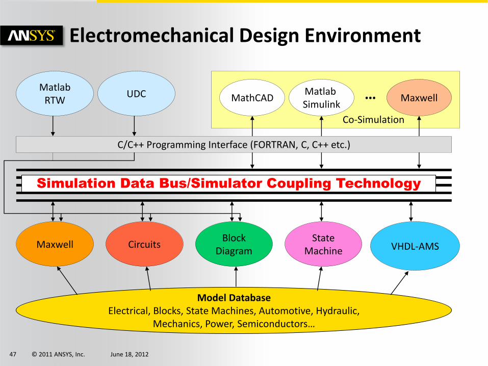
Electromechanical Design Environment
Simulation Data Bus/Simulator Coupling Technology
Model Database Electrical, Blocks, State Machines, Automotive, Hydraulic,
Mechanics, Power, Semiconductors…
Maxwell Circuits Block
Diagram State
Machine VHDL-AMS
Matlab RTW
UDC MathCAD Matlab Simulink
Maxwell
C/C++ Programming Interface (FORTRAN, C, C++ etc.)
…
Co-Simulation
© 2011 ANSYS, Inc. June 18, 2012 48
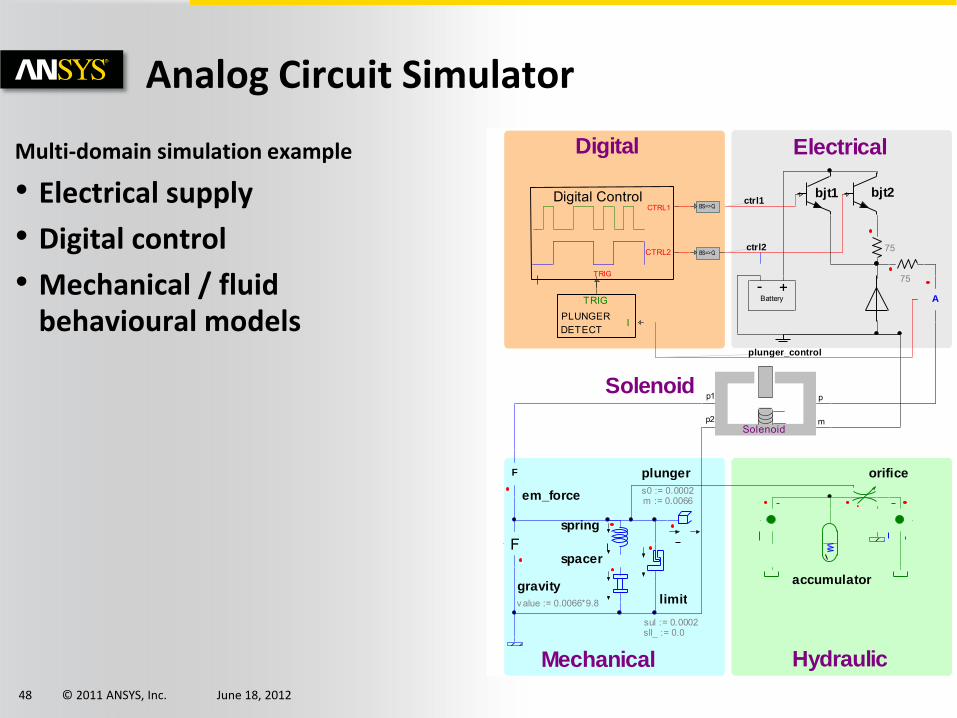
Multi-domain simulation example
• Electrical supply
• Digital control
• Mechanical / fluid behavioural models
plunger
limit
spring
F
F
em_force
Battery- +
bjt1 bjt2
accumulator
Digital Control
TRIG
CTRL2
CTRL1 BS=>Q
BS=>Q
DETECTPLUNGER
I
TRIG
Solenoidmp2
pp1
75
m := 0.0066 s0 := 0.0002
gravity
v alue := 0.0066*9.8
spacer
sul := 0.0002sll_ := 0.0
Digital Electrical
Mechanical Hydraulic
Solenoid
A
orifice
75
ctrl1
ctrl2
plunger_control
Analog Circuit Simulator
© 2011 ANSYS, Inc. June 18, 2012 49
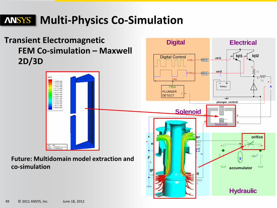
Transient Electromagnetic FEM Co-simulation – Maxwell 2D/3D
Future: Multidomain model extraction and co-simulation
plunger
limit
spring
F
F
em_force
Battery- +
bjt1 bjt2
accumulator
Digital Control
TRIG
CTRL2
CTRL1 BS=>Q
BS=>Q
DETECTPLUNGER
I
TRIG
Solenoidmp2
pp1
75
m := 0.0066 s0 := 0.0002
gravity
v alue := 0.0066*9.8
spacer
sul := 0.0002sll_ := 0.0
Digital Electrical
Mechanical Hydraulic
Solenoid
A
orifice
75
ctrl1
ctrl2
plunger_control
Multi-Physics Co-Simulation

© 2011 ANSYS, Inc. June 18, 2012 50
Semicondutor Modeling In Simplorer
IGBT Device model
• Semiconductor device model on Simplorer
• IGBT Device model : Average / Dynamic
• Capability of IGBTmodel
Thermal management for Inverter
• Thermal model in Simplorer’s semiconductor model.
• Extract thermal network from ANSYS Icepak
• Heat / Power loss coupling with device model
Inverter surge and conduction noise
• Extract parasitic LCR from Q3D Extractor
• Inverter surge and conduction noise in Simplorer

© 2011 ANSYS, Inc. June 18, 2012 51
Semiconductor device model in Simplorer
Ideal switch model
• ON:short, OFF:open
Semiconductor system level
• Modeled as nonlinear resistance in consideration of a static characteristic.
Semiconductor device level
• Dynamic characteristics, therma and physical characteristics are modeled. – BJT / MOSFET /JFET / IGBT / Diode / Thysistors…
SPICE compatible
• spice-3f5 compatible – MOSFET (spice3 Lv.1 - 6, BSIM1 - 4, EKV,JFET)
© 2011 ANSYS, Inc. June 18, 2012 52
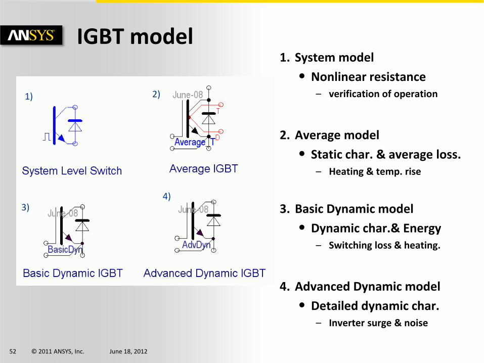
IGBT model 1. System model
• Nonlinear resistance – verification of operation
2. Average model
• Static char. & average loss. – Heating & temp. rise
3. Basic Dynamic model
• Dynamic char.& Energy – Switching loss & heating.
4. Advanced Dynamic model
• Detailed dynamic char. – Inverter surge & noise
1) 2)
3) 4)
© 2011 ANSYS, Inc. June 18, 2012 54
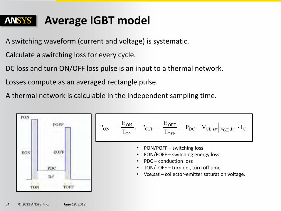
Average IGBT model
A switching waveform (current and voltage) is systematic.
Calculate a switching loss for every cycle.
DC loss and turn ON/OFF loss pulse is an input to a thermal network.
Losses compute as an averaged rectangle pulse.
A thermal network is calculable in the independent sampling time.
• PON/POFF – switching loss • EON/EOFF – switching energy loss • PDC – conduction loss • TON/TOFF – turn on , turn off time • Vce,sat – collector-emitter saturation voltage.
© 2011 ANSYS, Inc. June 18, 2012 55
-231.0n 618.0n0 200.0n 400.0n-50.0
700.0
0
166.7
333.3
500.0
-172.0n 750.0n0 200.0n 400.0n 600.0n-50.0
700.0
0
166.7
333.3
500.0
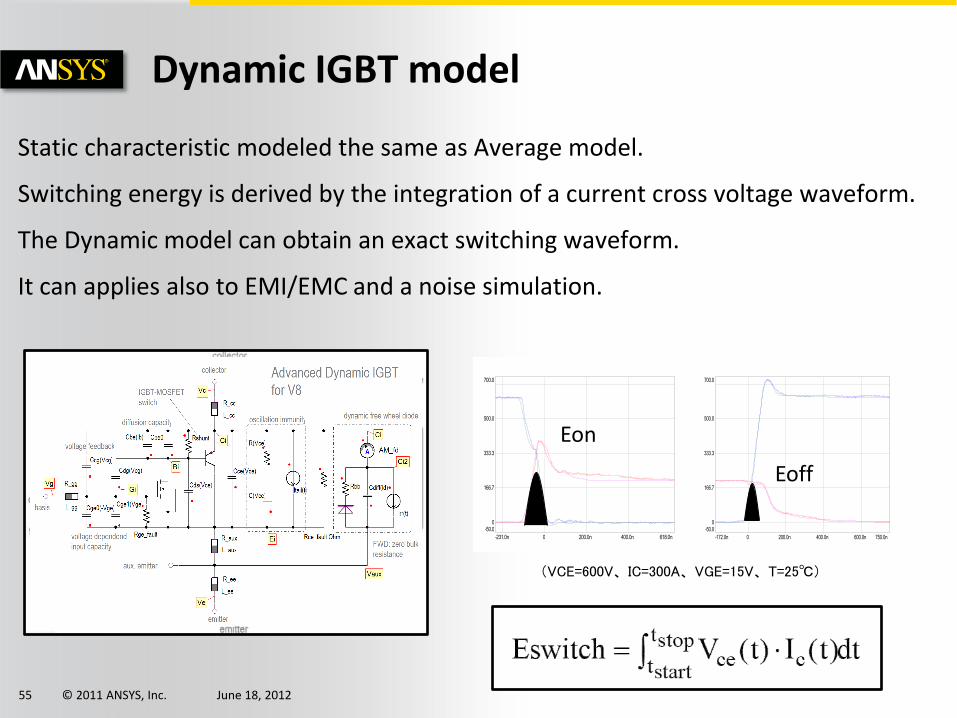
Dynamic IGBT model
Static characteristic modeled the same as Average model.
Switching energy is derived by the integration of a current cross voltage waveform.
The Dynamic model can obtain an exact switching waveform.
It can applies also to EMI/EMC and a noise simulation.
(VCE=600V、IC=300A、VGE=15V、T=25℃)
Eoff
Eon
© 2011 ANSYS, Inc. June 18, 2012 56
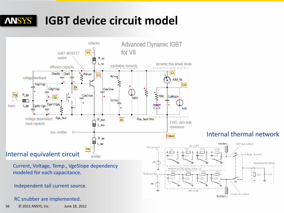
IGBT device circuit model
Internal equivalent circuit
Internal thermal network
Current, Voltage, Temp., VgeSlope dependency modeled for each capacitance. Independent tail current source. RC snubber are implemented.
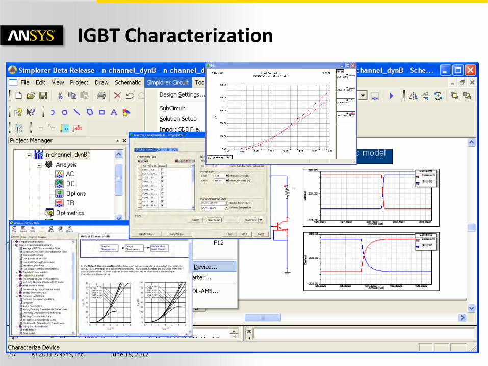
© 2011 ANSYS, Inc. June 18, 2012 57
IGBT Characterization
© 2011 ANSYS, Inc. June 18, 2012 58
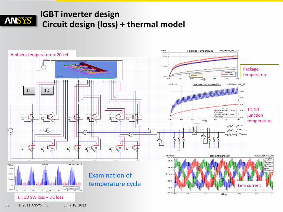
IGBT inverter design Circuit design (loss) + thermal model
Line current
1T, 1D SW loss + DC loss
1T, 1D junction temperature
Package temperature
Examination of temperature cycle
1T 1D
Ambient temperature = 20 cel

© 2011 ANSYS, Inc. June 18, 2012 59
-231.0n 618.0n0 200.0n 400.0n-50.0
700.0
0
166.7
333.3
500.0
Simplorer + Icepak = Detailed modeling of thermal system
Simplorer
ANSYS Icepak Q3D Extractor
Parasitism LCR extraction
Device property and loss consultation
CAD Import
Design of the cooling technique and arrangement
Design of substrate radiating route
The simulation in consideration of change of detailed temperature environment
© 2011 ANSYS, Inc. June 18, 2012 60
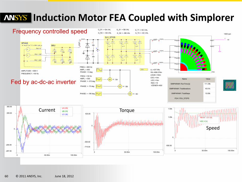
Induction Motor FEA Coupled with Simplorer
FEA
PhaseA1
PhaseA2
PhaseB1
PhaseB2
PhaseC1
PhaseC2
Rotor1
Rotor2
w +
ICA:
1400 rpm
LL:=237.56u
RA:=696.076m
B6U
D1 D3 D5
D2 D4 D6
2L3_GTOS
g_r1
g_r2
g_s1
g_s2
g_t1
g_t2
~
3PHAS
~
~
A * sin (2 * pi * f * t + PHI + phi_u)
PHI = 0°
PHI = -120°
PHI = -240°
LDUM:=100m
CDC:=10m
LDC:=10m
RDC:=10
VZENER:=650
AMPLITUDE := 800 V
FREQUENCY := 60 Hz
-297.50
300.00
-200.00
0
200.00
0 100.00m 50.00m
LA.I [A]
LB.I [A]
LC.I [A]
FREQ := 800 Hz
AMPL := 800
PHASE := 0 deg
AMPL := 500
PHASE := -315 deg
FREQ := 50 Hz
PHASE := -195 deg
PHASE := -75 deg
SA
SB
SC
G_R1 := SA.VAL
G_R2 := -SA.VAL
G_S1 := SB.VAL
G_S2 := -SB.VAL
G_T1 := SC.VAL
G_T2 := -SC.VAL
+ V
Name Value
SIMPARAM1.RunTime [s] 111.29k
SIMPARAM1.TotalIterations 40.51k
SIMPARAM1.TotalSteps 10.00k
FEA1.FEA_STEPS
-500.00
1.50k
0
1.00k
0 100.00m 50.00m
100.00 * LD.I [A]
VDC.V [V]
-715.00
425.00
-500.00
0
0 100.00m 50.00m
Current Torque
Speed
Fed by ac-dc-ac inverter
Frequency controlled speed
© 2011 ANSYS, Inc. June 18, 2012 61
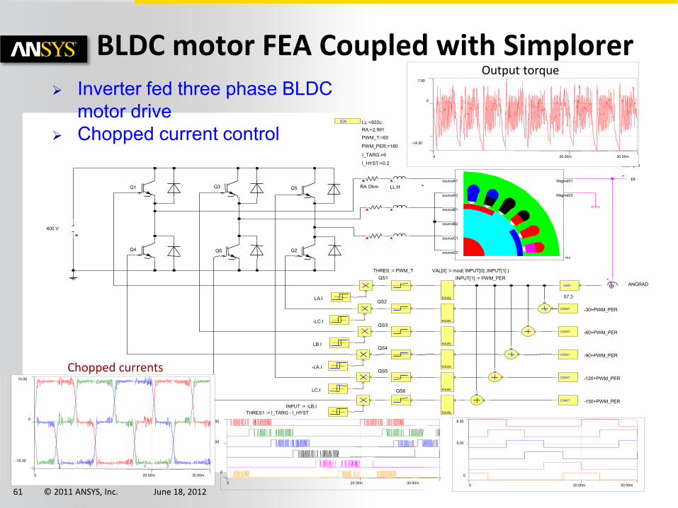
BLDC motor FEA Coupled with Simplorer
FEA
sourceA1
sourceA2
sourceB1
sourceB2
sourceC1
sourceC2
Magnet01
Magnet02
w +
ICA:
+
F GAIN
CONST
CONST
EQUBL
EQUBL
EQUBL
1500 rpm
LL:=922u
RA:=2.991
ANGRAD
57.3
-60+PWM_PER
-30+PWM_PER
QS1
QS2
QS3
VAL[0] := mod( INPUT[0] ,INPUT[1] )
PWM_T:=60
I_TARG:=9
I_HYST:=0.2
Q1
Q2
Q3 Q5
Q4 Q6
400 V
THRES := PWM_T
EQUBL
CONST
QS4
-90+PWM_PER
EQUBL
CONST
QS5
-120+PWM_PER
EQUBL
CONST
QS6
-150+PWM_PER
RA Ohm LL H
PWM_PER:=180
INPUT[1] := PWM_PER
INPUT := -LB.I
LC.I
-LA.I
LB.I
-LC.I
LA.I
THRES1 := I_TARG - I_HYST
0
8.50
5.00
0 20.00m 30.00m
-14.50
7.80
0
0 30.00m 20.00m
-10.30
10.00
0
0 30.00m 20.00m
Output torque
Chopped currents
Inverter fed three phase BLDC motor drive
Chopped current control
0
8.50
5.00
0 30.00m 20.00m
© 2011 ANSYS, Inc. June 18, 2012 62
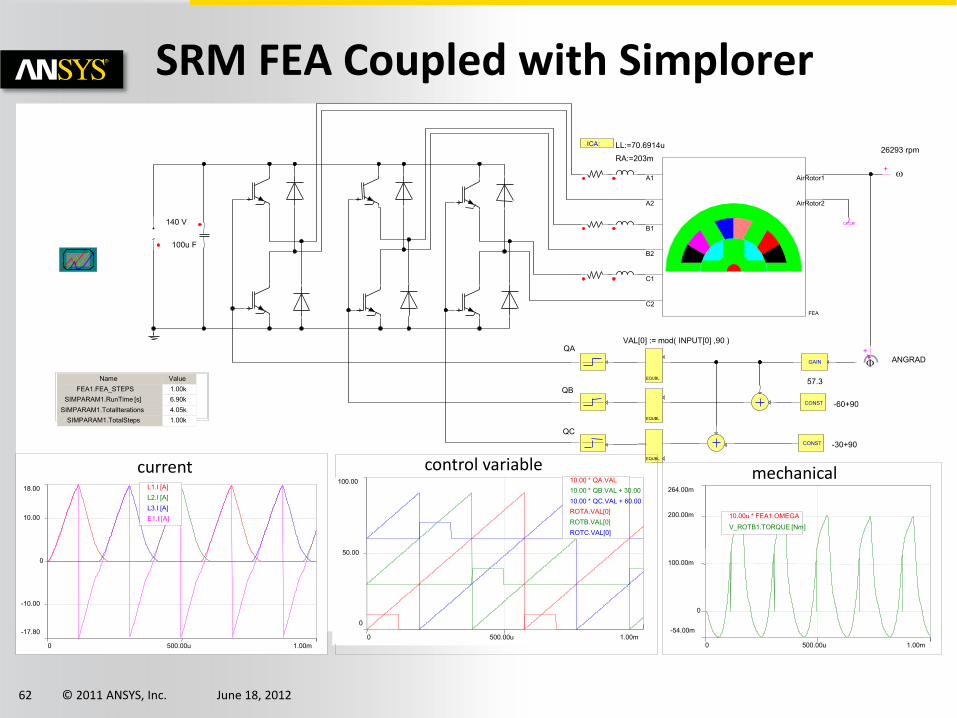
FEA
A1
A2
B1
B2
C1
C2
AirRotor1
AirRotor2
w +
26293 rpm ICA: LL:=70.6914u
RA:=203m
140 V
100u F
+
F ANGRAD GAIN
57.3
CONST -30+90
CONST -60+90
EQUBL
VAL[0] := mod( INPUT[0] ,90 ) QA
QB
QC
EQUBL
EQUBL
Name Value
FEA1.FEA_STEPS 1.00k
SIMPARAM1.RunTime [s] 6.90k
SIMPARAM1.TotalIterations 4.05k
SIMPARAM1.TotalSteps 1.00k
0
100.00
50.00
0 1.00m 500.00u
10.00 * QA.VAL
10.00 * QB.VAL + 30.00
10.00 * QC.VAL + 60.00
ROTA.VAL[0] ROTB.VAL[0] ROTC.VAL[0]
-54.00m
264.00m
0
100.00m
200.00m
0 1.00m 500.00u
10.00u * FEA1.OMEGA
V_ROTB1.TORQUE [Nm]
mechanical
-17.80
18.00
-10.00
0
10.00
0 1.00m 500.00u
L1.I [A] L2.I [A] L3.I [A] E1.I [A]
current control variable
SRM FEA Coupled with Simplorer
© 2011 ANSYS, Inc. June 18, 2012 63
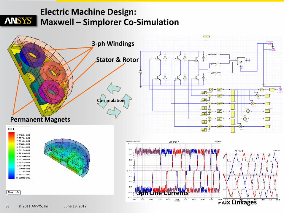
Electric Machine Design: Maxwell – Simplorer Co-Simulation
3-ph Windings
Permanent Magnets
Stator & Rotor
Flux Linkages
3ph Line Currents
Co-simulation

© 2011 ANSYS, Inc. June 18, 2012 64
Multi-physics
© 2011 ANSYS, Inc. June 18, 2012 65
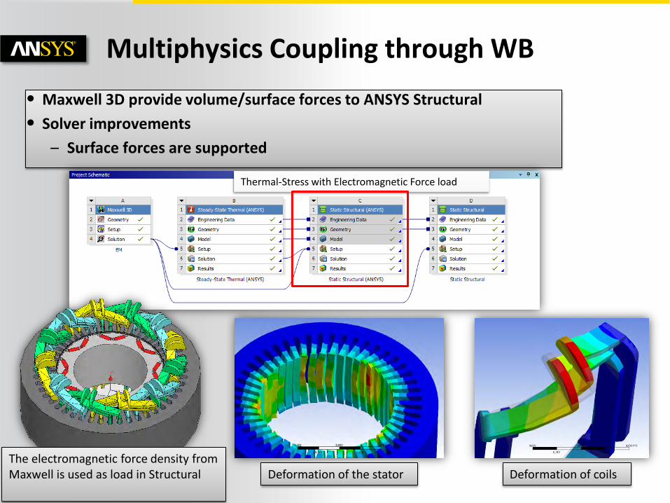
Multiphysics Coupling through WB
• Maxwell 3D provide volume/surface forces to ANSYS Structural
• Solver improvements
– Surface forces are supported
Deformation of the stator Deformation of coils The electromagnetic force density from Maxwell is used as load in Structural
Thermal-Stress with Electromagnetic Force load
© 2011 ANSYS, Inc. June 18, 2012 66
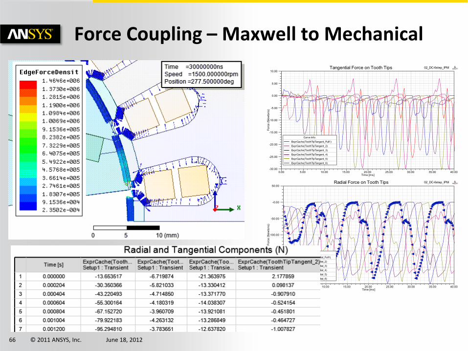
Force Coupling – Maxwell to Mechanical
0.00 5.00 10.00 15.00 20.00 25.00 30.00 35.00 40.00Time [ms]
-250.00
-200.00
-150.00
-100.00
-50.00
-0.00
50.00
Forc
e (N
ewto
ns)
02_DC-6step_IPMRadial Force on Tooth Tips ANSOFT
Curve InfoExprCache(ToothTipRadial_Full1)ExprCache(ToothTipRadial_2)ExprCache(ToothTipRadial_3)ExprCache(ToothTipRadial_4)ExprCache(ToothTipRadial_5)ExprCache(ToothTipRadial_6)
0.00 5.00 10.00 15.00 20.00 25.00 30.00 35.00 40.00Time [ms]
-30.00
-25.00
-20.00
-15.00
-10.00
-5.00
0.00
5.00
10.00
Forc
e (N
ewto
ns)
02_DC-6step_IPMTangential Force on Tooth Tips ANSOFT
Curve InfoExprCache(ToothTipTangent_Full1)ExprCache(ToothTipTangent_2)ExprCache(ToothTipTangent_3)ExprCache(ToothTipTangent_4)ExprCache(ToothTipTangent_5)ExprCache(ToothTipTangent_6)
© 2011 ANSYS, Inc. June 18, 2012 67
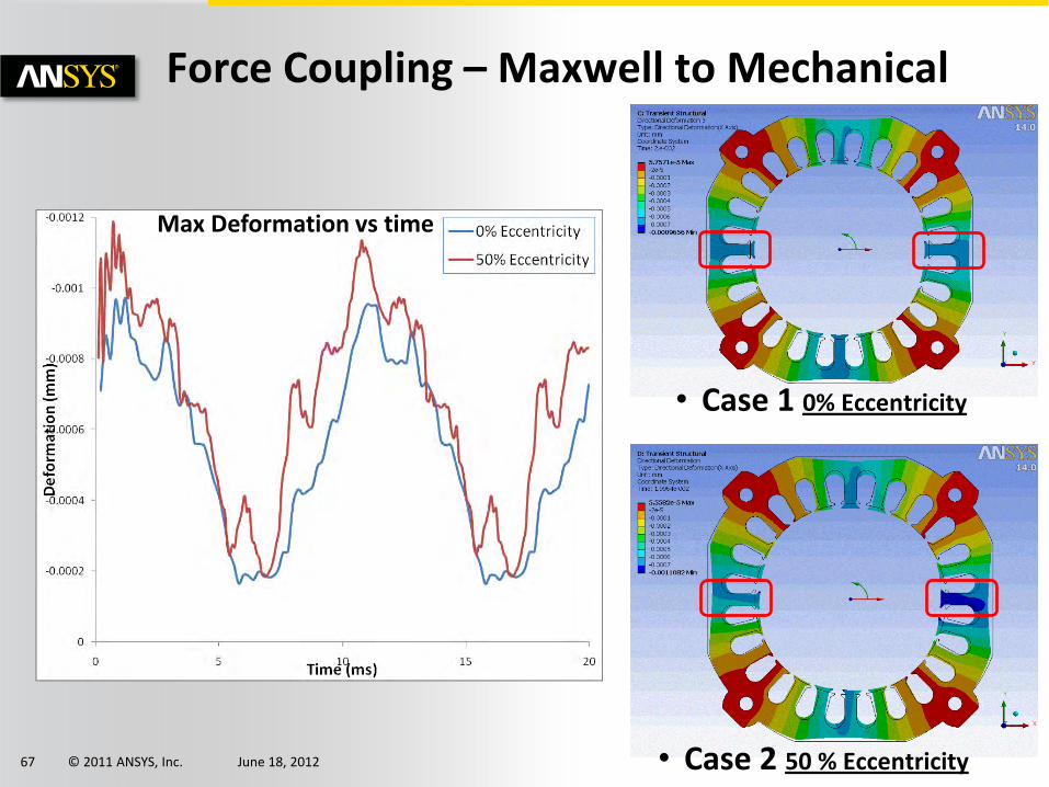
Force Coupling – Maxwell to Mechanical
• Case 1 0% Eccentricity
• Case 2 50 % Eccentricity
Max Deformation vs time
© 2011 ANSYS, Inc. June 18, 2012 68
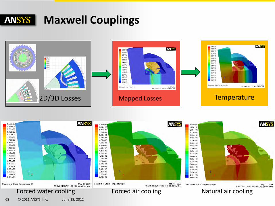
Maxwell Couplings
Forced water cooling Forced air cooling Natural air cooling
Mapped Losses 2D/3D Losses Temperature
© 2011 ANSYS, Inc. June 18, 2012 69
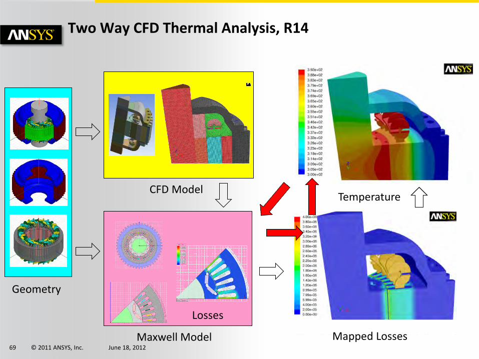
Two Way CFD Thermal Analysis, R14
Geometry
Losses
Maxwell Model
CFD Model
Mapped Losses
Temperature
© 2011 ANSYS, Inc. June 18, 2012 70
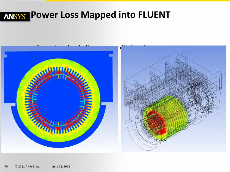
Power Loss in windings are not displayed.
Power Loss Mapped into FLUENT
© 2011 ANSYS, Inc. June 18, 2012 72
Thank you