PROCEEDINGS, 46th Workshop on Geothermal Reservoir Engineering

Stanford University, Stanford, California, February 15-17, 2021

SGP-TR-218

1

Electric Power Generation, Specific Capital Cost, and Specific Power for Advanced Geothermal

Systems (AGS)

Adam E. Malek1, Benjamin M. Adams1, Edoardo Rossi1, Hans O. Schiegg2, and Martin O. Saar* 1

1Geothermal Energy and Geofluids Group, Department of Earth Sciences, ETH-Zürich, Sonneggstrasse 5, 8092 Zürich, Switzerland

2SwissGeoPower Engineering AG, Breiteweg 37, 8707 Uetikon am See, Switzerland

*Corresponding Author: saarm@ethz.ch

Keywords: Geothermal energy, closed-loop, renewable energy, electric power generation, AGS

ABSTRACT

Advanced Geothermal Systems (AGS) generate electric power using a closed-loop system, by circulating a working fluid through a long

wellbore and extracting geothermal heat only through conduction from rock surrounding the wellbore. Quantitative evaluations of electric

power and cost are not available.

In this paper, we simulate an AGS for a wide range of system parameters after modifying the existing genGEO simulator by replacing the

porous reservoir with one or more horizontal lateral wells which are spaced apart to limit thermal interference. Our results include the

computation of the electric power generation, capital cost, specific capital cost (SpCC) (i.e., dollars per Watt), and the specific power (i.e.,

Watts per well meter).

We find that using CO2 as the working fluid rather than water increases the electric power generated from the system. Additionally, for

any vertical well length, there exists an optimal lateral well length, an optimal mass flowrate, and an optimal well diameter which minimize

cost. We also show that ideal well costs and high geothermal gradients significantly decrease the overall cost.

1. INTRODUCTION

Global climate change has driven the emergence of several technologies used to generate power from renewable and sustainable sources

and to curb the use of fossil fuels. Widespread adoption of renewable technologies is limited by the inability of wind and solar to

consistently supply electricity to meet demand (Anvari et al., 2016). A particular advantage of using geothermal resources for electric

power generation is that they are a flexible source of energy, enabling to reliably supply carbon-free electricity when wind and solar are

not able, thereby providing baseload and dispatchable power (Moore and Simmons, 2013).

Advanced Geothermal Systems (AGS) generate electrical power using closed-loop systems, by circulating a working fluid through a long

wellbore and extracting geothermal heat only via conduction from the surrounding rock. Closed-loop geothermal systems are

advantageous because they may be constructed in most geographic locations; long wells are drilled to collect the heat and no specific

subsurface geology is required. In contrast to traditional open-loop geothermal systems, namely hydrothermal and Enhanced (or

Engineered) Geothermal Systems (EGS) (Breede et al., 2013), the fluids circulated within AGS do not come into direct contact with the

subsurface rocks, thus requiring less regulatory approval. Additionally, this eliminates many of the problems which are encountered in

open-loop systems, such as: fluid loss, mineral scaling, fluid-mineral chemical reactions blocking flow paths, and induced seismicity

(Griffiths et al., 2016; Grigoli et al., 2018; Regenspurg et al., 2015).

In this paper, we simulate an AGS using both water and CO2 as the working fluids to determine the electric power generation, capital

cost, specific capital cost (SpCC), and specific power for a wide range of system depths, lateral well lengths and configurations, geothermal

gradients, and wellbore diameters. The specific capital cost (SpCC) is the ratio of capital cost of the geothermal system to the electricity

generation (i.e., dollars per Watt). The specific power is the ratio of electricity generation to well length drilled (i.e., Watts per meter).

These results assist in the evaluation of the feasibility of AGS projects under development throughout the world.

2. METHOD

We simulate the electric power and cost for an Advanced Geothermal System defined in Figure 1.

The model consists of: a surface power plant, a geothermal heat reservoir, a vertical injection well (IW) and a vertical production well

(PW) connected by one or several lateral wells (LW). Either water or CO2 is circulated within these wells.

In such a geothermal system, the circulated fluid (water or CO2) flows through the injection well down to a targeted depth. From the

injection well, the fluid flows through several lateral wells, allowing the fluid to be heated up by conductive heat transfer with the

surrounding rocks. The fluid is then collected from the production wellbore and produced at the surface where it is used to run a turbine

and generate electric power. Electricity is generated either directly in a surface turbine, if CO2 is used, or in an Organic Rankine Cycle

(ORC) system, if water is used as the subsurface working fluid.

Malek et al.

2

First, we define a base-case scenario (Section 2.1). We simulate electric power and calculate costs using genGEO (Adams et al., 2021).

Then, we explain the modifications we made to genGEO to create a conduction-only geothermal system (Section 2.2).

2.1 Base Case Parameters

Figure 1 shows the base case geothermal system, which consists of one vertical IW and one vertical PW, 3.5 km deep. The vertical wells

are connected horizontally by four 5.0 km long (horizontal) lateral wells at the 3.5 km depth. The geometrical configuration of the lateral

wells is trivial and does not affect the electric power or SpCC results, as long as there is sufficient spacing between them to limit thermal

interference (Section 2.1.1).

All results are found from the base case parameters summarized in Table 1, unless explicitly stated otherwise.

Figure 1: Base case system. The results do not depend on the geometrical configuration of the lateral wells, as long as there is

sufficient spacing between them to limit thermal interference (Section 2.1.1). Electricity is generated either directly in a

surface turbine if CO2 is used (left) or in an Organic Rankine Cycle (ORC) system if water is used as the subsurface

working fluid (right).

Malek et al.

3

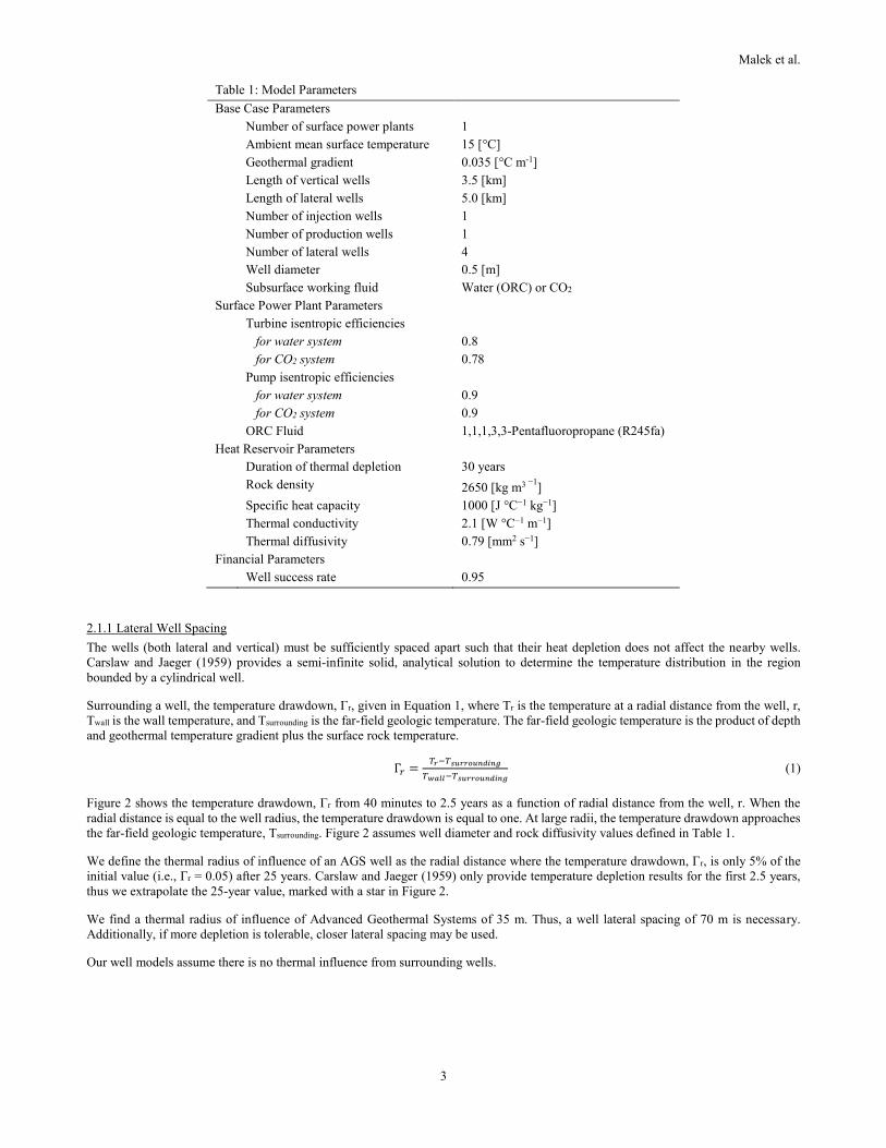
Table 1: Model Parameters

Base Case Parameters

Number of surface power plants 1

Ambient mean surface temperature 15 [°C]

Geothermal gradient 0.035 [°C m-1]

Length of vertical wells 3.5 [km]

Length of lateral wells 5.0 [km]

Number of injection wells 1

Number of production wells 1

Number of lateral wells 4

Well diameter 0.5 [m]

Subsurface working fluid Water (ORC) or CO2

Surface Power Plant Parameters

Turbine isentropic efficiencies

for water system 0.8

for CO2 system 0.78

Pump isentropic efficiencies

for water system 0.9

for CO2 system 0.9

ORC Fluid 1,1,1,3,3-Pentafluoropropane (R245fa)

Heat Reservoir Parameters

Duration of thermal depletion 30 years

Rock density 2650 [kg m3 −1]

Specific heat capacity 1000 [J °C−1 kg−1]

Thermal conductivity 2.1 [W °C−1 m−1]

Thermal diffusivity 0.79 [mm2 s−1]

Financial Parameters

Well success rate 0.95

2.1.1 Lateral Well Spacing

The wells (both lateral and vertical) must be sufficiently spaced apart such that their heat depletion does not affect the nearby wells.

Carslaw and Jaeger (1959) provides a semi-infinite solid, analytical solution to determine the temperature distribution in the region

bounded by a cylindrical well.

Surrounding a well, the temperature drawdown, Γr, given in Equation 1, where Tr is the temperature at a radial distance from the well, r,

Twall is the wall temperature, and Tsurrounding is the far-field geologic temperature. The far-field geologic temperature is the product of depth

and geothermal temperature gradient plus the surface rock temperature.

Γ𝑟 =𝑇𝑟−𝑇𝑠𝑢𝑟𝑟𝑜𝑢𝑛𝑑𝑖𝑛𝑔

𝑇𝑤𝑎𝑙𝑙−𝑇𝑠𝑢𝑟𝑟𝑜𝑢𝑛𝑑𝑖𝑛𝑔 (1)

Figure 2 shows the temperature drawdown, Γr from 40 minutes to 2.5 years as a function of radial distance from the well, r. When the

radial distance is equal to the well radius, the temperature drawdown is equal to one. At large radii, the temperature drawdown approaches

the far-field geologic temperature, Tsurrounding. Figure 2 assumes well diameter and rock diffusivity values defined in Table 1.

We define the thermal radius of influence of an AGS well as the radial distance where the temperature drawdown, Γr, is only 5% of the

initial value (i.e., Γr = 0.05) after 25 years. Carslaw and Jaeger (1959) only provide temperature depletion results for the first 2.5 years,

thus we extrapolate the 25-year value, marked with a star in Figure 2.

We find a thermal radius of influence of Advanced Geothermal Systems of 35 m. Thus, a well lateral spacing of 70 m is necessary.

Additionally, if more depletion is tolerable, closer lateral spacing may be used.

Our well models assume there is no thermal influence from surrounding wells.

Malek et al.

4

Figure 2: Temperature drawdown for different times as a function of radial distance from the well. The temperature drawdown

is the ratio of temperature at the specified radius to the initial temperature. The star indicates the predicted radial distance

from the well which has a 5% temperature drawdown after 25 years. The figure is adapted from Carslaw and Jaeger

(1959) using a well diameter of 0.5 m and a thermal diffusivity of 0.79 mm2 s-1.

2.2 Modifications to genGEO for Electric Power and Cost

The electric power and cost of AGS are modelled with genGEO, a coupled reservoir, power plant, and economic simulator (Adams et al.,

2021). genGEO is an open-source python library which can be extended to many configurations. genGEO was originally developed to

simulate geothermal electricity generation from a porous reservoir, however, we modify it here for conduction-based geothermal.

genGEO is modified for AGS by substituting the porous reservoir with one or more horizontal lateral wells. In genGEO, the vertical wells

already include heat conduction to the surroundings, thus the same module is used for the horizontal laterals. The only modification to the

wells is the mass flowrate, where the mass flowrate in each lateral is equal to the mass flowrate of the injection and production wells

divided by the number of laterals.

We use both CO2 and water as our subsurface working fluids. The electricity generation diagram from these two systems is found in

Figure 1. Electricity generation with water as the geologic fluid requires an indirect Organic Rankine Cycle (ORC). The ORC uses R245fa

as the secondary working fluid. Conversely, electricity is generated with CO2 as the working fluid by directly expanding the CO2 in a

surface turbine.

2.3 Capital Costs and Specific Capital Cost (SpCC)

The capital cost is the total overnight cost in 2019 dollars to construct the geothermal facility, including wells and power plant. The

specific capital cost (SpCC) is the ratio of capital cost to the electricity generation of the power plant considering 30 years of electric

power generation. The SpCC may be converted to an LCOE implementing appropriate financing assumptions (Adams et al., 2021). In the

following, all cost values are provided as 2019 dollars and specified as [$], unless otherwise specified.

The genGEO code is used to calculate the capital cost and SpCC of the geothermal system (Adams et al., 2021). We modify the genGEO

cost code for AGS in three ways: 1) to include the additional cost for the horizontal laterals, 2) to remove wellfield development costs

which are generally included in geothermal developments, and 3) to additionally include ’ideal’ well costs.

Horizontal lateral well cost is given in Equation 2. We assume that the cost of developing each horizontal lateral well, Ih, is the difference

in cost between a vertical well, Iv, with length equivalent to the targeted depth, z, plus half of the lateral well length, LLW, and a vertical

well with length equivalent to the targeted depth, z.

𝐼ℎ(𝐿𝐿𝑊) = 𝐼𝑣(𝑧 + 0.5𝐿𝐿𝑊) − 𝐼𝑣(𝑧) (2)

AGS systems may be developed in nearly any geologic setting, thus we assume exploration costs are zero. Also, a closed-loop system

does not exchange working fluid with the native subsurface fluids, thus we assume permitting costs are also zero. Elimination of these

costs reduces the wellfield costs to only the permitting required for drilling the wells.

Malek et al.

5

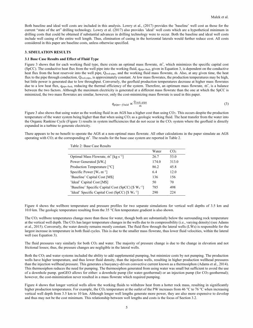
Both baseline and ideal well costs are included in this analysis. Lowry et al., (2017) provides the ’baseline’ well cost as those for the

current “state of the art” drilling technology. Lowry et al. (2017) also provides ’ideal’ well costs which are a hypothetical minimum in

drilling costs that could be obtained if substantial advances in drilling technology were to occur. Both the baseline and ideal well costs

include well casing of the entire well length. Thus, elimination of casing in the horizontal laterals would further reduce cost. All costs

considered in this paper are baseline costs, unless otherwise specified.

3. SIMULATION RESULTS

3.1 Base Case Results and Effect of Fluid Type

Figure 3 shows that for each working fluid type, there exists an optimal mass flowrate, ṁ*, which minimizes the specific capital cost

(SpCC). The conductive heat flux from the well pipe into the working fluid, qpipe-fluid, given in Equation 3, is dependent on the conductive

heat flux from the heat reservoir into the well pipe, Qrock-pipe, and the working fluid mass flowrate, ṁ. Also, at any given time, the heat

flux to the pipe through conduction, Qrock-pipe, is approximately constant. At low mass flowrates, the production temperatures may be high,

but little power is generated due to low throughput. Conversely, the geofluid production temperatures decrease at higher mass flowrates

due to a low heat flux, qpipe-fluid, reducing the thermal efficiency of the system. Therefore, an optimum mass flowrate, ṁ*, is a balance

between the two factors. Although the maximum electricity is generated at a different mass flowrate than the one at which the SpCC is

minimized, the two mass flowrates are similar, however, only the cost-minimizing mass flowrate is used in this paper.

𝑞𝑝𝑖𝑝𝑒−𝑓𝑙𝑢𝑖𝑑 ∝𝑄𝑟𝑜𝑐𝑘−𝑝𝑖𝑝𝑒

�̇� (3)

Figure 3 also shows that using water as the working fluid in an AGS has a higher cost than using CO2. This occurs despite the production

temperature of the water system being higher than that when using CO2 as a geologic working fluid. The heat transfer from the water into

the Organic Rankine Cycle (Figure 1) results in system inefficiencies that do not occur in the CO2 system where the geofluid is directly

expanded in a turbine to generate electricity.

There appears to be no benefit to operate the AGS at a non-optimal mass flowrate. All other calculations in the paper simulate an AGS

operating with CO2 at the corresponding ṁ*. The results for the base case system are reported in Table 2.

Table 2: Base Case Results

Water CO2

Optimal Mass Flowrate, ṁ* [kg s−1] 26.7 53.0

Power Generated [kWe] 174.0 313.0

Production Temperature [°C] 86.2 45.8

Specific Power [We m−1] 6.4 12.0

’Baseline’ Capital Cost [M$] 136 156

’Ideal’ Capital Cost [M$] 50 70

’Baseline’ Specific Capital Cost (SpCC) [$ We−1] 785 498

’Ideal’ Specific Capital Cost (SpCC) [$ We−1] 290 224

Figure 4 shows the wellbore temperature and pressure profiles for two separate simulations for vertical well depths of 3.5 km and

10.0 km. The geologic temperature resulting from the 35 °C/km temperature gradient is also shown.

The CO2 wellbore temperatures change more than those for water, though both are substantially below the surrounding rock temperature

at the vertical well depth. The CO2 has larger temperature changes in the wells due to its compressibility (i.e., varying density) (see Adams

et al., 2015). Conversely, the water density remains mostly constant. The fluid flow through the lateral wells (LWs) is responsible for the

largest increase in temperature in both fluid cycles. This is due to the smaller mass flowrate, thus lower fluid velocities, within the lateral

well (see Equation 3).

The fluid pressures vary similarly for both CO2 and water. The majority of pressure change is due to the change in elevation and not

frictional losses; thus, the pressure changes are negligible in the lateral wells.

Both the CO2 and water systems included the ability to add supplemental pumping, but minimize costs by not pumping. The production

wells have higher temperature, and thus lower fluid density, than the injection wells, resulting in higher production wellhead pressures

than the injection wellhead pressure. This generates a buoyancy-driven convective current known as a thermosiphon (Adams et al., 2014).

This thermosiphon reduces the need for pumping. The thermosiphon generated from using water was small but sufficient to avoid the use

of a downhole pump. genGEO allows for either: a downhole pump (for water-geothermal) or an injection pump (for CO2-geothermal);

however, the cost-minimization never resulted in a mass flowrate which required pumping.

Figure 4 shows that longer vertical wells allow the working fluids to withdraw heat from a hotter rock mass, resulting in significantly

higher production temperatures. For example, the CO2 temperature at the outlet of the PW increases from 46 °C to 76 °C when increasing

vertical well depth from 3.5 km to 10 km. Although longer well lengths generate more power, they are also more expensive to develop

and thus may not be the cost minimum. This relationship between well lengths and costs is the focus of Section 3.2.

Malek et al.

6

Figure 3: Power, Specific Power, Specific Capital Cost (SpCC), Production Temperature for different Mass Flowrates

Figure 4: Temperature and Pressure Profiles of water and CO2 for 3.5 km (left) and 10.0 km (right) vertical well depths. The

working fluids descend down the IW (state 1-2), through four lateral wells (state 2-3), and up the PW (state 3-4). The base

case geothermal gradient of 35 °C/km is included to show the temperature of the surrounding rock at the respective depth.

Malek et al.

7

3.2 Optimal Lateral Well Length and Effect of Ideal Well Costs

The SpCC, electric power, specific electric power, and production temperature as a function of vertical well depth and lateral well length

are shown in Figure 5 for baseline and ideal well costs.

Figure 5: Effect of different combinations of vertical and lateral well lengths on power, specific electric power, specific capital cost

(SpCC) and production temperature. For each vertical well length, an optimal lateral well length, LLW* (dashed line), that

minimizes SpCC is found. The figure includes the effect of baseline (red) and idealized (green) well costs on SpCC.

Figure 5 shows that for every vertical well depth, there exists an optimal lateral well length, LLW*, which minimizes the SpCC (dashed

lines in Figure 5). The length of the lateral well increases the surface area over which heat is conducted into the well from the surrounding

hot rocks. Small lateral well lengths reduce cost, but the amount of electric power generated is not large, resulting in large SpCC values.

Similarly, when the lateral well length is very large, the increase in electric power generated is not enough to cover the costs of increasing

the lateral well length. Therefore, the optimal lateral well length, LLW*, is the lateral well length that minimizes costs.

Similarly, a lateral well length may be found which maximizes the specific electric power for every vertical well length depth. This lateral

length is larger than the length that minimizes cost. This is due to the higher-order growth of the well cost function with increasing depth.

Figure 5 shows that ideal well costs significantly reduce the SpCC. For example, when considering the base case parameters of a 3.5 km

vertical well length and a 5.0 km lateral well length, the SpCC shifts from 498 $ We-1 to 224 $ We

-1 if idealized costs are used. This

highlights the need for significant advancements in drilling technology to reduce SpCC.

All subsequent analyses in this paper will use a lateral well length equal to the LLW*.

3.3 Effect of Number of Lateral Wells (LWs)

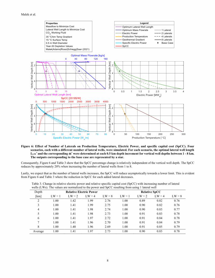
The electric power, specific electric power, specific capital cost (SpCC) and production temperature as a function of vertical well depth

and number of lateral wells are shown in Figure 6.

Figure 6 shows that increasing the number of lateral wells (LWs) does not have a strong impact on changing the working fluid production

temperatures. Increasing the number of LWs increases the total surface area of pipe that is in contact with the surrounding rock, which

increases Qrock-pipe.

Despite the higher conductive heat flux due to increasing the number of laterals, the fluid mass flowrate is increased to minimize cost in

a way where the production fluid temperature is approximately constant. For example, at a vertical well depth of 4.0 km, increasing the

number of LWs from 1 to 8 increases the total horizontal well length by more than three-fold, from 11.5 km to 35.3 km, and increases the

electric power from 260 kWe to 710 kWe the production temperature increases from 48 °C only to 52 °C.

Malek et al.

8

Figure 6: Effect of Number of Laterals on Production Temperature, Electric Power, and specific capital cost (SpCC). Four

scenarios, each with a different number of lateral wells, were simulated. For each scenario, the optimal lateral well length

LLW* and the corresponding ṁ* were determined at each 0.5 km depth increment for vertical well depths between 1 - 8 km.

The outputs corresponding to the base case are represented by a star.

Consequently, Figure 6 and Table 3 show that the SpCC percentage change is relatively independent of the vertical well depth. The SpCC

reduces by approximately 20% when increasing the number of lateral wells from 1 to 8.

Lastly, we expect that as the number of lateral wells increases, the SpCC will reduce asymptotically towards a lower limit. This is evident

from Figure 6 and Table 3 where the reduction in SpCC for each added lateral decreases.

Table 3. Change in relative electric power and relative specific capital cost (SpCC) with increasing number of lateral

wells (LWs). The values are normalized to the power and SpCC resulting from using 1 lateral well

Depth Relative Electric Power Relative SpCC

[km] LW = 1 LW = 2 LW = 4 LW = 8 LW = 1 LW = 2 LW = 4 LW = 8

2 1.00 1.42 1.99 2.76 1.00 0.89 0.82 0.76

3 1.00 1.41 1.99 2.75 1.00 0.90 0.82 0.76

4 1.00 1.41 1.98 2.74 1.00 0.90 0.83 0.77

5 1.00 1.41 1.98 2.73 1.00 0.91 0.83 0.78

6 1.00 1.41 1.97 2.72 1.00 0.91 0.84 0.78

7 1.00 1.41 1.96 2.70 1.00 0.91 0.84 0.79

8 1.00 1.40 1.96 2.69 1.00 0.91 0.85 0.79

Average 1.00 1.41 1.97 2.73 1.00 0.90 0.83 0.78

Malek et al.

9

3.4 Effect of Well Diameter

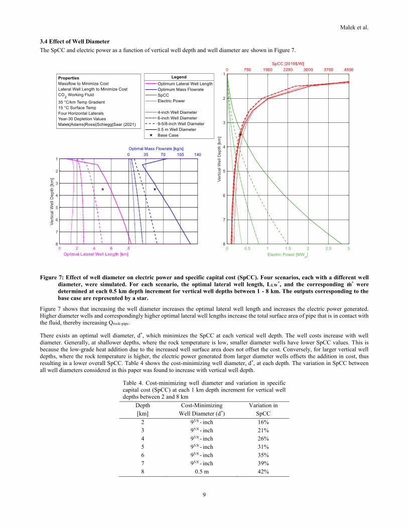
The SpCC and electric power as a function of vertical well depth and well diameter are shown in Figure 7.

Figure 7: Effect of well diameter on electric power and specific capital cost (SpCC). Four scenarios, each with a different well

diameter, were simulated. For each scenario, the optimal lateral well length, LLW*, and the corresponding ṁ* were

determined at each 0.5 km depth increment for vertical well depths between 1 - 8 km. The outputs corresponding to the

base case are represented by a star.

Figure 7 shows that increasing the well diameter increases the optimal lateral well length and increases the electric power generated.

Higher diameter wells and correspondingly higher optimal lateral well lengths increase the total surface area of pipe that is in contact with

the fluid, thereby increasing Qrock-pipe.

There exists an optimal well diameter, d*, which minimizes the SpCC at each vertical well depth. The well costs increase with well

diameter. Generally, at shallower depths, where the rock temperature is low, smaller diameter wells have lower SpCC values. This is

because the low-grade heat addition due to the increased well surface area does not offset the cost. Conversely, for larger vertical well

depths, where the rock temperature is higher, the electric power generated from larger diameter wells offsets the addition in cost, thus

resulting in a lower overall SpCC. Table 4 shows the cost-minimizing well diameter, d*, at each depth. The variation in SpCC between

all well diameters considered in this paper was found to increase with vertical well depth.

Table 4. Cost-minimizing well diameter and variation in specific

capital cost (SpCC) at each 1 km depth increment for vertical well

depths between 2 and 8 km

Depth Cost-Minimizing Variation in

[km] Well Diameter (d*) SpCC

2 95/8 - inch 16%

3 95/8 - inch 21%

4 95/8 - inch 26%

5 95/8 - inch 31%

6 95/8 - inch 35%

7 95/8 - inch 39%

8 0.5 m 42%

Malek et al.

10

3.5 Effect of Geologic Temperature Gradient

The effect of geologic temperature (or geothermal) gradient on electric power and SpCC as a function of depth is shown in Figure 8.

Figure 8: Effect of geologic temperature (or geothermal) gradient on electric power and specific capital cost (SpCC). Four

scenarios, each with a different geothermal gradient, were simulated. For each scenario, the optimal lateral well length,

LLW*, and the corresponding ṁ* were determined at each 0.5 km depth increment for vertical well depths between 1 - 8

km. The outputs corresponding to the base case are represented by a star.

Figure 8 shows that higher geologic temperature gradients increase the electric power and decrease the SpCC, while maintaining a nearly

constant optimal mass flowrate, ṁ*, and optimal lateral well length, LLW*. Higher geothermal gradients yield higher rock temperatures at

depth, increasing Qrock-pipe into the system. For a vertical well depth of 4.0 km, if the geologic temperature gradient is varied from

25 °C/km to 40 °C/km, LLW* and ṁ* vary between 9% and 16%, respectively, while the electricity generated increases by 191% and the

SpCC reduces by 62%. There is an advantage to locating AGS systems in high-temperature regions. Additionally, accurate geologic

temperature gradient measurements are needed for AGS simulations.

The electric power increase with geologic temperature gradient are greatest at larger depth, especially for CO2. The CO2 requires several

kilometers depth change to generate a thermosiphon and drive the turbine. Thus, at very high geologic temperature gradients and shallow

depths, it is likely that a water-based AGS system will generate more electricity than a CO2-based system.

4. DISCUSSION

The majority of cost in an AGS system is due to the well drilling. For example, in the ’baseline’ base case, well drilling and completion

account for 97% of the total capital cost. This reduces to 93% when ’ideal’ well costs are used. Additionally, and as shown in Table 2 for

the case of using CO2 as the working fluid, the specific capital cost (SpCC) decreases from 498 $ We-1 for the ’baseline’ case to

224 $ We-1 in the ’ideal’ well cost assumption. Thus, reductions of well drilling and completion costs have a substantial effect on the

specific capital cost (SpCC) and therefore benefiting the economic viability of geothermal systems in general (Blankenship et al., 2005;

Tester et al., 2006), and more specifically of AGS, as shown in this work. As a consequence, it is crucial to develop novel drilling

technologies aiming at decreasing the overall drilling costs in crystalline rocks. In this regard, ongoing research efforts are investigating

contact-less approaches (Anders et al. 2015; Kant et al., 2017; Rossi et al., 2020a; Schiegg et al., 2015; Timoshkin et al., 2003), as well

as combined/hybrid drilling concepts (Rossi et al., 2020b, 2020c) to provide cost-effective solutions to access deep geo-resources in hard

rocks.

Moreover, variations of system depth have a strong influence on the specific capital cost (SpCC), as shown in Table 5. For instance,

increasing the depth from 3.5 km to 8.0 km, and the other parameters being equal (well diameter of 0.5 m and lateral well length of 5 km),

the ’ideal’ SpCC decreases by more than 75%, i.e., reducing from 224 $ We-1 to 52 $ We

-1. As stated above, construction of deep wells is

challenging, especially in hard rocks. Advances in drilling techniques are required. Also, changes in the well diameter significantly affect

Malek et al.

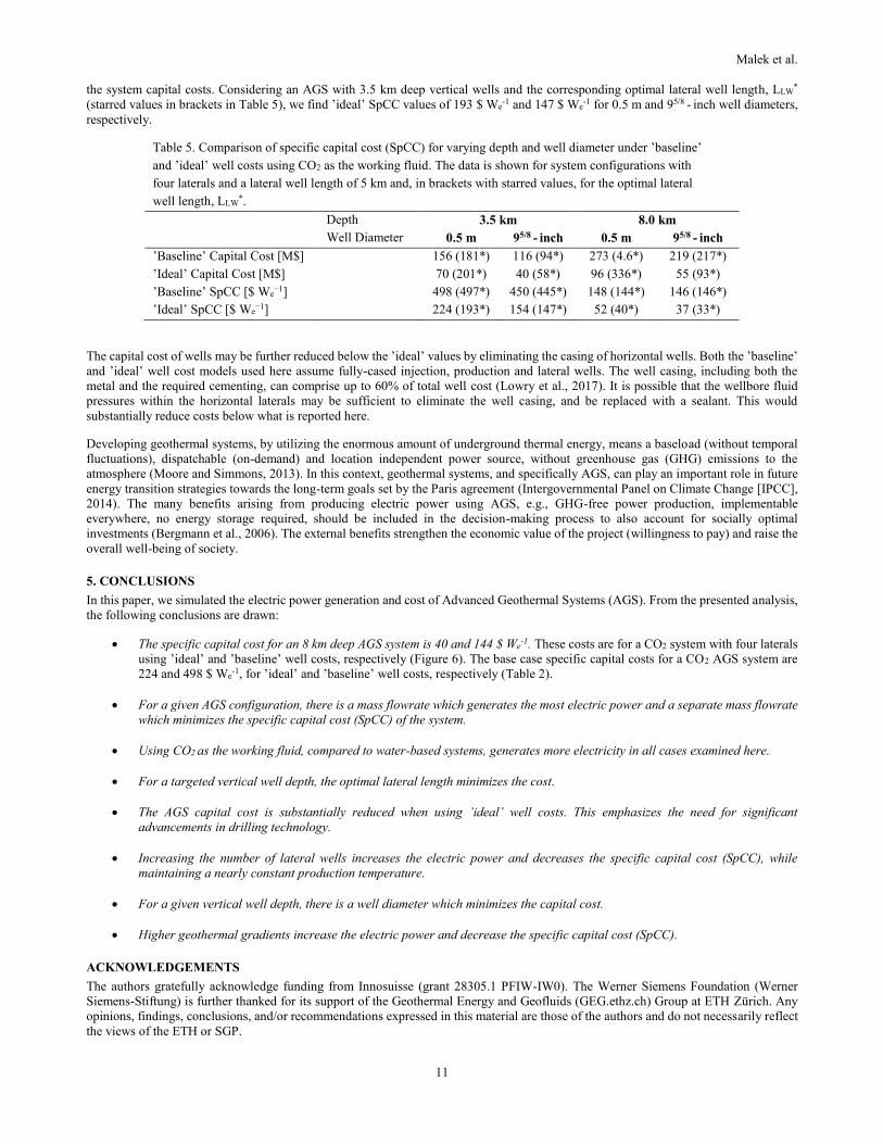
11

the system capital costs. Considering an AGS with 3.5 km deep vertical wells and the corresponding optimal lateral well length, LLW*

(starred values in brackets in Table 5), we find ’ideal’ SpCC values of 193 $ We-1 and 147 $ We

-1 for 0.5 m and 95/8 - inch well diameters,

respectively.

Table 5. Comparison of specific capital cost (SpCC) for varying depth and well diameter under ’baseline’

and ’ideal’ well costs using CO2 as the working fluid. The data is shown for system configurations with

four laterals and a lateral well length of 5 km and, in brackets with starred values, for the optimal lateral

well length, LLW*.

Depth 3.5 km 8.0 km

Well Diameter 0.5 m 95/8 - inch 0.5 m 95/8 - inch

’Baseline’ Capital Cost [M$] 156 (181*) 116 (94*) 273 (4.6*) 219 (217*)

’Ideal’ Capital Cost [M$] 70 (201*) 40 (58*) 96 (336*) 55 (93*)

’Baseline’ SpCC [$ We−1] 498 (497*) 450 (445*) 148 (144*) 146 (146*)

’Ideal’ SpCC [$ We−1] 224 (193*) 154 (147*) 52 (40*) 37 (33*)

The capital cost of wells may be further reduced below the ’ideal’ values by eliminating the casing of horizontal wells. Both the ’baseline’

and ’ideal’ well cost models used here assume fully-cased injection, production and lateral wells. The well casing, including both the

metal and the required cementing, can comprise up to 60% of total well cost (Lowry et al., 2017). It is possible that the wellbore fluid

pressures within the horizontal laterals may be sufficient to eliminate the well casing, and be replaced with a sealant. This would

substantially reduce costs below what is reported here.

Developing geothermal systems, by utilizing the enormous amount of underground thermal energy, means a baseload (without temporal

fluctuations), dispatchable (on-demand) and location independent power source, without greenhouse gas (GHG) emissions to the

atmosphere (Moore and Simmons, 2013). In this context, geothermal systems, and specifically AGS, can play an important role in future

energy transition strategies towards the long-term goals set by the Paris agreement (Intergovernmental Panel on Climate Change [IPCC],

2014). The many benefits arising from producing electric power using AGS, e.g., GHG-free power production, implementable

everywhere, no energy storage required, should be included in the decision-making process to also account for socially optimal

investments (Bergmann et al., 2006). The external benefits strengthen the economic value of the project (willingness to pay) and raise the

overall well-being of society.

5. CONCLUSIONS

In this paper, we simulated the electric power generation and cost of Advanced Geothermal Systems (AGS). From the presented analysis,

the following conclusions are drawn:

The specific capital cost for an 8 km deep AGS system is 40 and 144 $ We-1. These costs are for a CO2 system with four laterals

using ’ideal’ and ’baseline’ well costs, respectively (Figure 6). The base case specific capital costs for a CO2 AGS system are

224 and 498 $ We-1, for ’ideal’ and ’baseline’ well costs, respectively (Table 2).

For a given AGS configuration, there is a mass flowrate which generates the most electric power and a separate mass flowrate

which minimizes the specific capital cost (SpCC) of the system.

Using CO2 as the working fluid, compared to water-based systems, generates more electricity in all cases examined here.

For a targeted vertical well depth, the optimal lateral length minimizes the cost.

The AGS capital cost is substantially reduced when using ’ideal’ well costs. This emphasizes the need for significant

advancements in drilling technology.

Increasing the number of lateral wells increases the electric power and decreases the specific capital cost (SpCC), while

maintaining a nearly constant production temperature.

For a given vertical well depth, there is a well diameter which minimizes the capital cost.

Higher geothermal gradients increase the electric power and decrease the specific capital cost (SpCC).

ACKNOWLEDGEMENTS

The authors gratefully acknowledge funding from Innosuisse (grant 28305.1 PFIW-IW0). The Werner Siemens Foundation (Werner

Siemens-Stiftung) is further thanked for its support of the Geothermal Energy and Geofluids (GEG.ethz.ch) Group at ETH Zürich. Any

opinions, findings, conclusions, and/or recommendations expressed in this material are those of the authors and do not necessarily reflect

the views of the ETH or SGP.

Malek et al.

12

REFERENCES

Adams, B. M., Kuehn, T. H., Bielicki, J. M., Randolph, J. B., & Saar, M. O. (2014). On the importance of the thermosiphon effect in CPG

(CO2 plume geothermal) power systems. Energy, 69, 409 - 418. https://doi.org/10.1016/j.energy.2014.03.032

Adams, B. M., Kuehn, T. H., Bielicki, J. M., Randolph, J. B., & Saar, M. O. (2015). A comparison of electric power output of CO2 Plume

Geothermal (CPG) and brine geothermal systems for varying reservoir conditions. Applied Energy, 140.

https://doi.org/10.1016/j.apenergy.2014.11.043

Adams, B. M., Ogland-Hand, J. D., Bielicki, J. M., Schaedle, P., & Saar, M. O. (submitted). Estimating the geothermal electricity

generation potential of sedimentary basins using genGEO (the generalizable GEOthermal techno-economic simulator). Manuscript

Submitted for Publication. https://doi.org/10.26434/chemrxiv.13514440.v1

Anders, E., Lehmann, F., & Voigt, M. (2015). Electric Impulse Technology-Long Run Drilling in Hard Rocks, In Asme 2015 34th

international conference on ocean, offshore and arctic engineering omae2015, may 31-june 5, st. john’s, newfoundland, canada -

omae2015-41219.

Anvari, M., Lohmann, G., W¨achter, M., Milan, P., Lorenz, E., Heinemann, D., Tabar, M. R. R., & Peinke, J. (2016). Short term

fluctuations of wind and solar power systems. New Journal of Physics, 18 (6). https://doi.org/10.1088/1367-2630/18/6/063027

Bergmann, A., Hanley, N., & Wright, R. (2006). Valuing the attributes of renewable energy investments. Energy Policy, 34 (9).

https://doi.org/10.1016/j.enpol.2004.08.035

Blankenship, D. A., Wise, J. L., Bauer, S. J., Mansure, A. J., Normann, R., Raymond, D., & LaSala, R. (2005). Research Efforts to Reduce

the Cost of Well Development for Geothermal Power Generation, In 40th u.s. symposium on rock mechanics (usrms).

Breede, K., Dzebisashvili, K., Liu, X., & Falcone, G. (2013). A systematic review of enhanced ( or engineered ) geothermal systems: past,

present and future. Geothermal Energy, 1 (4), 1-27. https://doi.org/10.1186/2195-9706-1-4

Carslaw, H., & Jaeger, J. (1959). Conduction of Heat in Solids (2nd Edition). London, Oxford University Press.

Griffiths, L., Heap, M. J., Wang, F., Daval, D., Gilg, H. A., Baud, P., Schmittbuhl, J., & Genter, A. (2016). Geothermal implications for

fracture-filling hydrothermal precipitation. Geothermics, 64, 235-245. https://doi.org/10.1016/j.geothermics.2016.06.006

Grigoli, F., Cesca, S., Rinaldi, A. P., Manconi, A., L´opez-Comino, J. A., Clinton, J. F., Westaway, R., Cauzzi, C., Dahm, T., & Wiemer,

S. (2018). The November 2017 M w 5.5 Pohang earthquake: A possible case of induced seismicity in South Korea. Science, 360

(6392), 1003-1006. https://doi.org/10.1126/science.aat2010

Intergovernmental Panel on Climate Change (IPCC). (2014). Mitigation of Climate Change. Contribution of Working Group III to the

Fifth Assessment Report of the Intergovernmental Panel on Climate Change (tech. rep.).

Kant, M. A., Rossi, E., H¨oser, D., & Rudolf von Rohr, P. (2017). Thermal Spallation Drilling, an Alternative Drilling Technology for

Deep Heat Mining – Performance Analysis, Cost Assessment and Design Aspects, Proceedings, 42nd workshop on geothermal

reservoir engineering, Stanford University, Stanford, California, February 13-15, 2017- sgp-tr-212.

Lowry, T. S., Finger, J. T., Carrigan, C. R., Foris, A., Kennedy, M. B., Corbet, T. F., Doughty, C. A., Pye, S., & Sonnenthal, E. L. (2017).

GeoVision Analysis: Reservoir Maintenance and Development Task Force Report (GeoVision Analysis Supporting Task Force

Report: Reservoir Maintenance and Development) (tech. rep.). Sandia National Laboratories (SNL). Albuquerque, NM, Livermore,

CA (United States). https://doi.org/10.2172/1394062

Moore, J. N., & Simmons, S. F. (2013). More Power from Below. Science, 340 (6135), 93-935. https://doi.org/10.1126/science.1235640

Regenspurg, S., Feldbusch, E., Byrne, J., Deon, F., Driba, D. L., Henninges, J., Kappler, A., Naumann, R., Reinsch, T., & Schubert, C.

(2015). Mineral precipitation during production of geothermal fluid from a Permian Rotliegend reservoir. Geothermics, 54, 122-135.

https://doi.org/10.1016/j.geothermics.2015.01.003

Rossi, E., Adams, B. M., Vogler, D., Rudolf von Rohr, P., Kammermann, B., & Saar, M. O. (2020a). Advanced drilling technologies to

improve the economics of deep georesource utilization, In Proceedings, MIT A+B Applied Energy Symposium 2020, MIT,

Cambridge, USA. https://doi.org/10.3929/ethz-b-000445213

Rossi, E., Jamali, S., Schwarz, D., Saar, M. O., & Rudolf von Rohr, P. (2020b). Field test of a Combined Thermo-Mechanical Drilling

technology. Mode II: Flame-assisted rotary drilling. Journal of Petroleum Science and Engineering, 190 (106880), 1-12.

https://doi.org/10.1016/j.petrol.2019.106880

Rossi, E., Jamali, S., Wittig, V., Saar, M. O., & Rudolf von Rohr, P. (2020c). A combined thermo-mechanical drilling technology for

deep geothermal and hard rock reservoirs. Geothermics, 85C, 1-11. https://doi.org/10.1016/j.geothermics.2019.101771

Schiegg, H. O., Rødland, A., Zhu, G., & Yuen, D. A. (2015). Electro-Pulse-Boring (EPB): Novel Super-Deep Drilling Technology for

Low Cost Electricity. Journal of Earth Science, 26(1), 37-46. https://doi.org/10.1007/s12583-015-0519-x

Tester, J., Anderson, B., Batchelor, A., Blackwell, D., DiPippo, R., Drake, E., Garnish, J., Livesay, B., Moore, M., & Nichols, K. (2006).

The Future of Geothermal Energy (tech. rep. November). Idaho National Laboratory.

Timoshkin, I., Mackersie, J., & MacGregor, S. (2003). Plasma channel microhole drilling technology, In 14th IEEE International Pulsed

Power Conference. https://doi.org/10.1109/PPC.2003.1278062