electric vehicle powertrain architecture and control ... · electric vehicle powertrain...
TRANSCRIPT
EVS24 International Battery Hybrid and Fuel Cell Electric Vehicle Symposium 1
EVS24 Stavanger, Norway, May 13-16, 2009
Electric Vehicle Powertrain Architecture and Control Global Optimization
Noëlle Janiaud1, François-Xavier Vallet1, Marc Petit2, Guillaume Sandou2
1Technocentre RENAULT, 78288 Guyancourt, FRANCE, [email protected] 2SUPELEC, 91192 Gif-sur-Yvette, FRANCE
Abstract
The design of a full electric vehicle (or battery electric vehicle (BEV)) requires the development and
optimization of a complete electric powertrain, including battery, power electronics, electric machine,
sensors and control system.
When designing an electrical platform, from the very beginning of the V-cycle, it is mandatory to rely on
modelling and simulation tools in order to drive the main choices and then to optimize the system. This
paper presents an electric powertrain simulation platform developed with Matlab-Simulink, dedicated to
multiphysic optimization of the system.
As an example, the basic electrical powertrain architecture first considered in this paper includes a battery,
an inverter, a dc-dc buck converter supplying motor inductor and a wound rotor synchronous machine
(WRSM). The purpose is to show how simulation tools can help in comparing different powertrain control
strategies.
The present simulation platform is also useful to study physics architecture. To illustrate this point, another
electrical architecture is also presented, including a dc-dc boost converter between battery and inverter.
This structure must be considered here as an example only in order to show how to optimize control laws
taking into account various criteria, including architecture ones. Simulation results are compared for both
architectures in terms of powertrain performances and range.
Keywords: Electric powertrain, simulation platform, powertrain control strategies, architecture optimization
1 Introduction When designing an electrical platform, from the very beginning of the V-cycle, it is mandatory to rely on modeling and simulation tools in order to drive the main choices and then to optimize the system. The paper is organised as follows. The section 2 presents an electrical powertrain simulation platform developed with Matlab-Simulink. Main
models and equations are described in order to introduce different optimization strategies with criteria on performances and on powertrain losses in section 3. Optimization is performed with a powertrain architecture with three degrees of freedom. As the aim is to expose methodologies and to show typical results, the results presented in this paper are related to typical study cases, and not to an industrial one.
Page 0682
World Electric Vehicle Journal Vol. 3 - ISSN 2032-6653 - © 2009 AVERE

EVS24 International Battery Hybrid and Fuel Cell Electric Vehicle Symposium 2
Section 4 presents an architecture optimization introducing a fourth degree of freedom, specially used when battery is partially discharged. Finally, we draw concluding remarks in section 5.
2 Simulation Platform of an Electric Vehicle Powertrain
2.1 Power system An electric powertrain is a closed-loop system, mainly constituted by battery, converters, motor and control structure (Fig.1).
Figure 1: Simplified representation of a typical electric
powertrain
High-voltage battery has to supply with energy not only traction motor, but also high power loads like air-conditioning or heating as well as the low-voltage network.
2.2 Simulation platform The powertrain simulation platform used for optimization includes the following models (Fig.2) [1] [2]: • A dynamic battery model • Two three-phase AC-DC converter models
supplying WRSM stator: one model for fast transients including switch models and one model for quasi-static transients (first harmonic only) with voltage and current average signals. These models make it possible to simulate fast phenomena over short times (dynamic behaviour of the powertrain) and driving cycles lasting many minutes (e.g. NEDC) as it is explained at the end of this section.
• Two dc-dc converter models supplying WRSM rotor (fast transient / quasi-static transient).
• A WRSM model with consideration of magnetic saturation, using Park (d,q) transformation.
• Sensor models (currents, rotor position …).
Figure 2: Simulation platform of an Electric Powertrain
These models can be split in three categories depending on the frequency scale [3].
The first category implements analytical expressions of losses, range, cost, etc. used in a global approach, for example for the synthesis of control laws. The second category deals with “average” models dedicated to driving cycle simulations (e.g. NEDC) on wider time horizons. Finally, the third category deals with short time switching and fast variation of currents, voltages, torque, etc. For example, it is possible to observe electric resonances on the network and torque oscillations on the drive shaft.
In order to understand powertrain control methods presented in section 3, it is important to detail converters and motor models.
2.3 Electric motor model The three-phase Motor considered in this paper is a Wound Rotor Synchronous Machine (WRSM), represented in Park coordinate (a,b,c) → (d,q).
Indeed, WRSM presents more degrees of freedom than Permanent Magnet Machine, as it will be explained in section 3.1. It is why it has been chosen for the work described in this paper. However, the methodology is quite versatile and can also be applied to any other type of motor (Permanent Magnet, Induction, etc.)
Motor notations and symbols:
qd vv , : Stator voltages (V)
qd ii , : Stator currents (A)
qd ΦΦ , : Stator magnetic fields (Wb)
fv : Rotor voltage (V)
fi : Rotor current (A)
fΦ : Rotor magnetic field (Wb)
Page 0683
World Electric Vehicle Journal Vol. 3 - ISSN 2032-6653 - © 2009 AVERE

EVS24 International Battery Hybrid and Fuel Cell Electric Vehicle Symposium 3
Ω : Motor speed (rad/s)
eC : Motor torque (N.m)
Parameters:
p : Pole-pair number
fs RR , : Stator and rotor resistances (Ω)
fqd LLL ,, : Stator and rotor inductances (H)
fM : Mutual inductance (H)
The electrical equations of stator and rotor are given in [3]. Motor torque equation is as follows:
Torque: ( )qddqe iip
C Φ−Φ= ...2
.3 (1)
Magnetic saturations are taken into account:
ffqd MLLL ,,, depend on stator and rotor
currents through non-linear complex equations.
Each inductance parameter is function of three currents ( )fqd iii ,, . To determine these relations,
we use steady-state maps of magnetic fields
fqd ΦΦΦ ,, depending on ( )fqd iii ,, .
Figure 3 shows magnetic field dΦ according to
( )qd ii , for different constant values of fi :
Figure 3: Stator magnetic field on axe d according to stator current (units = p.u.)
NB : Most figures in this paper are presented with per-unit axes (between 0 and 1).
To include magnetic saturation in Park equations, we proceed as follows:
• a map of ( )fqdq iiiL ,, is obtained by
dividing ( )fqdq iii ,,Φ by qi
• equation ffddd iMiL .. +=Φ is
modified as follows:
fdffddd iiLMiMiL .... ++=Φ (2)
with:
o ( ) ( )d
fqddfqdd i
iiiiiiL
,,,,
Φ=
o ( ) ( )f
fqddfqdf i
iiiiiiM
,,,,
Φ=
o ( )fd
ffdddfqd ii
iMiLiiiLM
.
..,,
−−Φ=
The methodology is the same for rotor field ( )fqdf iii ,,Φ .
In addition to electrical equations, the mechanical part can be modelled by the following equation [4]:
lre CCCdt
dJ −−=
Ω.. (3)
with: J : Motor Inertia (kg.m²)
rC : Resistive torque (N.m)
lC : “Losses” torque (N.m)
A resistive torque lC is added to classical
mechanical equation .. re CCdt
dJ −=
Ω to take
into account some motor losses, such as core losses and mechanical losses. Losses expressions are presented in section 3.3.
To determine lC expression, we solve the
following equation with steady state relations:
TOToutin PPP =− (4)
with:
• ( ) ffqqddin ivivivP ....2
3++= : input
electric power
• Ω= .eout CP : output mechanic power
• MecCoreCoppermotor PPPP ++= : motor losses
(cf. section 3.3).
Page 0684
World Electric Vehicle Journal Vol. 3 - ISSN 2032-6653 - © 2009 AVERE

EVS24 International Battery Hybrid and Fuel Cell Electric Vehicle Symposium 4
2.4 Converters models Three-phase inverter The inverter converts DC-voltage from battery to AC-voltage in order to supply stator of electric motor. This converter is made of six switches. Our model considers simplified IGBT/diode switches (Fig.4).
Figure 4: Three-phase inverter
Switching parameters are series resistors and threshold voltages for both IGBT and diodes.
Concerning inverter control, we use a classical Space Vector PWM: switches closed and open positions are deduced from a reference voltage vector [5].
To simulate complete driving cycles, we use a slow-transient model of inverter (or “first harmonic” model). Inputs are three-phased voltage references, AC current and DC voltage. Outputs are AC voltage and DC current. To take into account converter losses, output DC current is modified according to losses map inside Simulink model.
DC-DC converters
A classical buck converter is used between high-voltage battery and machine rotor. Both fast-transient and slow-transient models are realized in the same way as AC-DC converter.
3 Control Optimization
3.1 Low-level control structure Powertrain architecture, presented in Figure 5, provides three degrees of freedom: two stator
currents qd ii , (hypothesis: 0=++ cba iii ) and
rotor current fi .
Let us briefly describe the powertrain control structure. From the motor torque reference ( )refeC
three currents references ( )reffrefqrefd iii ,, are
defined. Three controllers achieve currents regulation. Finally, controllers outputs are transformed in open / close switching positions for inverter (Space vector PWM is used) and for dc-dc buck converter [6]:
Figure 5: Electric Powertrain Control System
Electric powertrain global optimization is considered at three levels: the first step is the currents reference determination ( )
reffrefqrefd iii ,, , the second step deals with
controllers coefficients and the third step deals with switching control. This paper mainly focuses on the first step: ( )
reffrefqrefd iii ,, triplet
optimization. Many control strategies can be studied, considering one main objective (following torque motor reference ( )refeC ) and three main degrees
of freedom ( )fqd iii ,, . Optimization methods can
thus be applied on variables ( )fqd iii ,, under
torque constraint with vehicle range and performances objectives [7], [8], [9]. Constraints on maximal voltages and currents in battery, converters and machine must also be taken into account. Figure 6 shows an example of simulation results obtained with a losses minimization control strategy (see section 3.3 for more details about this strategy):
Page 0685
World Electric Vehicle Journal Vol. 3 - ISSN 2032-6653 - © 2009 AVERE

EVS24 International Battery Hybrid and Fuel Cell Electric Vehicle Symposium 5
Figure 6: Example of power system simulation with a losses minimization control strategy: machine torque
and speed (typical study case)
Two control strategies with criteria on performances (“torque maximization strategy”) and range (“losses minimization strategy”) are explained and compared in following sections.
3.2 Torque maximization
In a first time, we consider motor inductance parameters as constant. According to torque equation (3), to maximize eC , we set rotor
current at its maximum value : maxff ii = .
Concerning stator current, di and qi are linked by
the relation 22
qd iiI += . The idea is to find
( )qd ii , that maximize eC for any value of I .
Considering constant inductance parameters, we compute eC partial derivatives:
( ) −−+=∂
∂
d
qdqdff
q
e
i
iiLLiM
p
i
C2
...2
.3 (5)
→=∂
∂0
q
e
i
C
( )( )qd
qdffff
d LL
ILLiMiMi
−
−++−=
.4
..8.. 2222
(6)
If qd LL = (round rotor machine),
( ) ( )Iii qd ,0, = corresponds to a maximum of
torque equation. To illustrate these results, we plot eC for
different values of I (Fig.7).
-1 -0.8 -0.6 -0.4 -0.2 0 0.2 0.4 0.6 0.8 10
0.1
0.2
0.3
0.4
0.5
0.6
0.7
0.8
0.9
1
ID
MO
TO
R T
OR
QU
E
Motor torque for different values of I = sqrt(id2+iq2), if = ifmax
Ceref
Figure 7: Motor torque according to stator current for
maximum rotor current (units = p.u.)
Torque maximization control strategy consists in finding the curve for which ( ) ( )maxerefe CC = .
Optimal operating points corresponding to torque maximum values are represented with stars (see Figure 7). Figure 8 shows maximum motor torque versus ( )qd ii , . For a given value of ( )refeC corresponds
a triplet ( )max,, fqd iii maximizing torque.
00.2
0.40.6
0.81
00.2
0.40.6
0.810
0.2
0.4
0.6
0.8
1
ID
MAXIMUM MOTOR TORQUE, if = ifmax
IQ
MA
XIM
UM
MO
TO
R T
OR
QU
E
Figure 8: Maximum motor torque according to stator
current (units = p.u.)
If we take into account magnetic saturation, results are similar, but the method is slightly different: partial derivatives of eC equation cannot be easily
calculated as previously. We use a gradient-based optimization method to find eC maximum value
for each value of I . The relation
maxff ii = remains unchanged.
Page 0686
World Electric Vehicle Journal Vol. 3 - ISSN 2032-6653 - © 2009 AVERE

EVS24 International Battery Hybrid and Fuel Cell Electric Vehicle Symposium 6
Optimization problem: • cost function to minimize:
( )( )qdqdqffopt iiLLiiMp
J .....2
.3−+−= (7)
• variables : qd ii ,
• constraint : 22
qd iiI +=
We use a classical SQP (Successive Quadratic Procedure) to solve this optimization. Results are plotted on Figures 9 and 10.
-1 -0.8 -0.6 -0.4 -0.2 0 0.2 0.4 0.6 0.8 10
0.1
0.2
0.3
0.4
0.5
0.6
0.7
0.8
0.9
1
ID
MO
TO
R T
OR
QU
E
Motor torque for different values of I = sqrt(id2+iq2), if = ifmax
TORQUE MAXIMUM VALUES
- MAGNETIC SATURATION MODEL -
Figure 9: Motor torque according to stator current for
maximum rotor current with a magnetic saturation model (optimal operating points = stars) (units = p.u.)
-0.5
0
0.51
00.2
0.40.6
0.810
0.2
0.4
0.6
0.8
1
ID
MAXIMUM MOTOR TORQUE, if = ifmax
IQ
MA
XIM
UM
MO
TO
R T
OR
QU
E
Figure 10: Maximum motor torque according to stator current with a magnetic saturation model (units = p.u.)
Finally, the Motor Torque Maximization methodology can be summarized in three steps:
Figure 11: Motor torque maximization method
The result is a non analytic algebraic relation giving ( )fqd iii ,, from ( )refeC .
In order to take into account battery output voltage, a constraint on ( )qd vv , is added:
inequality max22 Vvv qd ≤+ must be respected
for all operating points ( )Ω,eC .
3.3 Losses minimization The difficulty of a losses minimization strategy depends on the chosen approach:
• approach 1 : to use a fine and complex model of motor losses (e.g. through losses maps from tests). Advantage is a high correlation between tests and simulation results. Major drawback concerns optimization method complexity: when the cost function to minimize is not an explicit function of optimization variables, simple and fast gradient-based methods can not be applied. More complex methods (such as heuristic algorithms) are required, with longer computation times.
• approach 2 : to use simplified losses model, with explicit expressions of optimization variables. There are two advantages of this approach : first, the use of fast optimization methods is possible; secondly, it allows studying losses variations with motor parameters. Drawback is advantage of first approach (classical compromise between precision and computation times).
Page 0687
World Electric Vehicle Journal Vol. 3 - ISSN 2032-6653 - © 2009 AVERE
EVS24 International Battery Hybrid and Fuel Cell Electric Vehicle Symposium 7
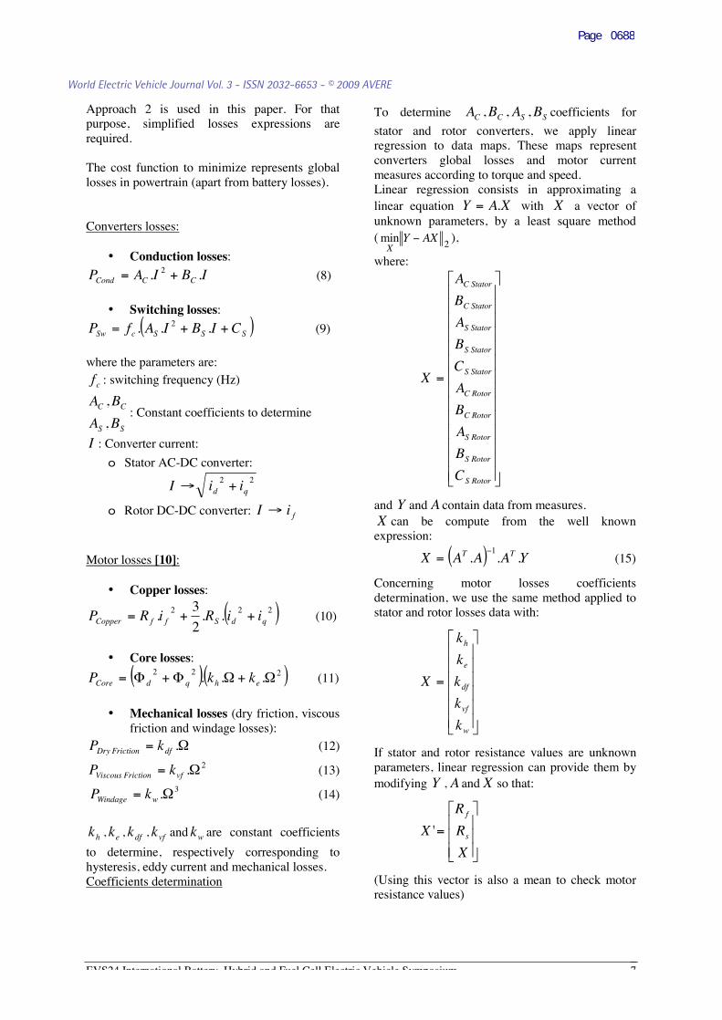
Approach 2 is used in this paper. For that purpose, simplified losses expressions are required. The cost function to minimize represents global losses in powertrain (apart from battery losses). Converters losses:
• Conduction losses:
IBIAP CCCond .. 2 += (8)
• Switching losses:
( )SSScSw CIBIAfP ++= ... 2 (9)
where the parameters are:
cf : switching frequency (Hz)
SS
CC
BA
BA
,
,: Constant coefficients to determine
I : Converter current:
o Stator AC-DC converter: 22
qd iiI +→
o Rotor DC-DC converter: fiI →
Motor losses [10]:
• Copper losses:
( )222 ..2
3. qdSffCopper iiRiRP ++= (10)
• Core losses:
( )( )222 ... Ω+ΩΦ+Φ= ehqdCore kkP (11)
• Mechanical losses (dry friction, viscous
friction and windage losses): Ω= .dfFrictionDry kP (12)
2.Ω= vfFrictionViscous kP (13)
3.Ω= wWindage kP (14)
hk , ek , dfk , vfk and wk are constant coefficients
to determine, respectively corresponding to hysteresis, eddy current and mechanical losses. Coefficients determination
To determine SSCC BABA ,,, coefficients for
stator and rotor converters, we apply linear regression to data maps. These maps represent converters global losses and motor current measures according to torque and speed. Linear regression consists in approximating a linear equation XAY .= with X a vector of unknown parameters, by a least square method (
2min AXYX
− ),
where:
=
RotorS
RotorS
RotorS
RotorC
RotorC
StatorS
StatorS
StatorS
StatorC
StatorC
C
B
A
B
A
C
B
A
B
A
X
and Y and A contain data from measures. X can be compute from the well known
expression:
( ) YAAAX TT ...1−
= (15)
Concerning motor losses coefficients determination, we use the same method applied to stator and rotor losses data with:
=
w
vf
df
e
h
k
k
k
k
k
X
If stator and rotor resistance values are unknown parameters, linear regression can provide them by modifying Y , A and X so that:
=
X
R
R
X s
f
'
(Using this vector is also a mean to check motor resistance values)
Page 0688
World Electric Vehicle Journal Vol. 3 - ISSN 2032-6653 - © 2009 AVERE

EVS24 International Battery Hybrid and Fuel Cell Electric Vehicle Symposium 8
Figures 12 and 13 represent converters and motor losses from tests versus simulation results. Modelling error on converters losses is quasi-inexistent. Concerning motor, in low torque area, there is up to 20% error, certainly due to losses simplified model (e.g. stray losses are neglected).
Figure 12: Motor losses measures vs. simulation results (units = p.u.)
Figure 13: Converters losses measures vs. simulation
results (units = p.u.)
Global losses:
CondRotorSwRotorCondStator
SwStatorMecCoreCopperTOT
PPP
PPPPP
+++
+++= (16)
TOTP is the cost function to minimize.
Optimization variables are fqd iii ,, .
Constraint to respect concerns motor torque (eq.(3)): ( )refee CC = .
For each couple ( )Ω,eC , we find ( )fqd iii ,, that
minimize TOTP , verifying torque expression and
respecting following constraints:
max
max22
max22
ff
qd
qd
Ii
Iii
Vvv
≤
≤+
≤+
(17)
To achieve computation, we use as previously a SQP procedure. To understand the importance of taking into account both losses in motor and converters for optimization (instead of motor losses only for example), we compare global efficiency with two control strategies (Fig.16) [11]:
a. motor losses minimization (Fig.14) b. (motor+converters) losses minimization
(Fig.15)
Figure 14: Powertrain efficiency with a strategy of
motor losses minimization (units = p.u.)
Page 0689
World Electric Vehicle Journal Vol. 3 - ISSN 2032-6653 - © 2009 AVERE
EVS24 International Battery Hybrid and Fuel Cell Electric Vehicle Symposium 9
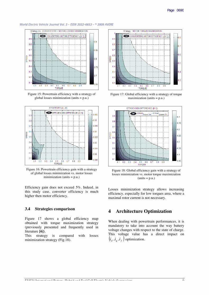
Figure 15: Powertrain efficiency with a strategy of
global losses minimization (units = p.u.)
Figure 16: Powertrain efficiency gain with a strategy
of global losses minimization vs. motor losses minimization (units = p.u.)
Efficiency gain does not exceed 5%. Indeed, in this study case, converter efficiency is much higher then motor efficiency.
3.4 Strategies comparison Figure 17 shows a global efficiency map obtained with torque maximization strategy (previously presented and frequently used in literature [6]). This strategy is compared with losses minimization strategy (Fig.18).
Figure 17: Global efficiency with a strategy of torque maximization (units = p.u.)
Figure 18: Global efficiency gain with a strategy of losses minimization vs. motor torque maximization
(units = p.u.)
Losses minimization strategy allows increasing efficiency, especially for low torques area, where a maximal rotor current is not necessary.
4 Architecture Optimization When dealing with powertrain performances, it is mandatory to take into account the way battery voltage changes with respect to the state of charge. This voltage value has a direct impact on ( )fqd iii ,, optimization.
Page 0690
World Electric Vehicle Journal Vol. 3 - ISSN 2032-6653 - © 2009 AVERE
EVS24 International Battery Hybrid and Fuel Cell Electric Vehicle Symposium 10
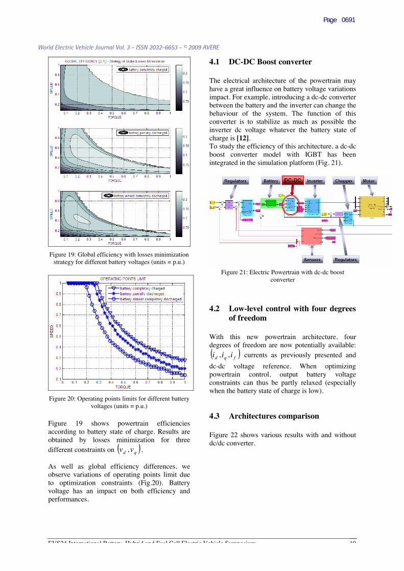
Figure 19: Global efficiency with losses minimization
strategy for different battery voltages (units = p.u.)
Figure 20: Operating points limits for different battery
voltages (units = p.u.)
Figure 19 shows powertrain efficiencies according to battery state of charge. Results are obtained by losses minimization for three different constraints on ( )qd vv , .
As well as global efficiency differences, we observe variations of operating points limit due to optimization constraints (Fig.20). Battery voltage has an impact on both efficiency and performances.
4.1 DC-DC Boost converter The electrical architecture of the powertrain may have a great influence on battery voltage variations impact. For example, introducing a dc-dc converter between the battery and the inverter can change the behaviour of the system. The function of this converter is to stabilize as much as possible the inverter dc voltage whatever the battery state of charge is [12]. To study the efficiency of this architecture, a dc-dc boost converter model with IGBT has been integrated in the simulation platform (Fig. 21).
Figure 21: Electric Powertrain with dc-dc boost converter
4.2 Low-level control with four degrees of freedom
With this new powertrain architecture, four degrees of freedom are now potentially available: ( )fqd iii ,, currents as previously presented and
dc-dc voltage reference. When optimizing powertrain control, output battery voltage constraints can thus be partly relaxed (especially when the battery state of charge is low).
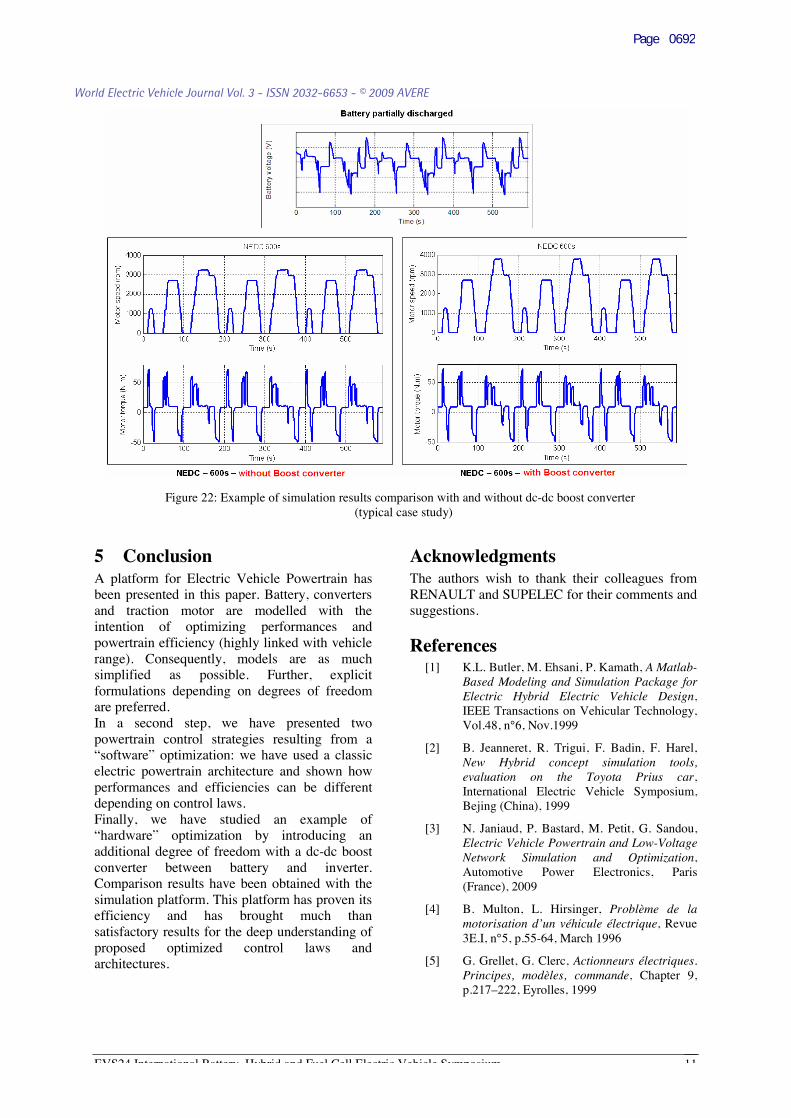
4.3 Architectures comparison Figure 22 shows various results with and without dc/dc converter.
Page 0691
World Electric Vehicle Journal Vol. 3 - ISSN 2032-6653 - © 2009 AVERE
EVS24 International Battery Hybrid and Fuel Cell Electric Vehicle Symposium 11
5 Conclusion A platform for Electric Vehicle Powertrain has been presented in this paper. Battery, converters and traction motor are modelled with the intention of optimizing performances and powertrain efficiency (highly linked with vehicle range). Consequently, models are as much simplified as possible. Further, explicit formulations depending on degrees of freedom are preferred. In a second step, we have presented two powertrain control strategies resulting from a “software” optimization: we have used a classic electric powertrain architecture and shown how performances and efficiencies can be different depending on control laws. Finally, we have studied an example of “hardware” optimization by introducing an additional degree of freedom with a dc-dc boost converter between battery and inverter. Comparison results have been obtained with the simulation platform. This platform has proven its efficiency and has brought much than satisfactory results for the deep understanding of proposed optimized control laws and architectures.
Acknowledgments The authors wish to thank their colleagues from RENAULT and SUPELEC for their comments and suggestions.
References [1] K.L. Butler, M. Ehsani, P. Kamath, A Matlab-
Based Modeling and Simulation Package for Electric Hybrid Electric Vehicle Design, IEEE Transactions on Vehicular Technology, Vol.48, n°6, Nov.1999
[2] B. Jeanneret, R. Trigui, F. Badin, F. Harel, New Hybrid concept simulation tools, evaluation on the Toyota Prius car, International Electric Vehicle Symposium, Bejing (China), 1999
[3] N. Janiaud, P. Bastard, M. Petit, G. Sandou, Electric Vehicle Powertrain and Low-Voltage Network Simulation and Optimization, Automotive Power Electronics, Paris (France), 2009
[4] B. Multon, L. Hirsinger, Problème de la motorisation d’un véhicule électrique, Revue 3E.I, n°5, p.55-64, March 1996
[5] G. Grellet, G. Clerc, Actionneurs électriques. Principes, modèles, commande, Chapter 9, p.217–222, Eyrolles, 1999
Figure 22: Example of simulation results comparison with and without dc-dc boost converter (typical case study)
Page 0692
World Electric Vehicle Journal Vol. 3 - ISSN 2032-6653 - © 2009 AVERE

EVS24 International Battery Hybrid and Fuel Cell Electric Vehicle Symposium 12
[6] R. Trigui, F. Harel, B. Jeanneret, F. Badin, S. Derou, Optimisation globale de la commande d’un moteur synchrone à rotor bobiné. Effets sur la consommation simulée de véhicules électriques et hybrides, Colloque National Génie Electrique Vie et Qualité, Marseille March 21-22, 2000
[7] P. Bastiani, Stratégies de commande minimisant les pertes d’un ensemble convertisseur – machine alternative : Application à la traction électrique, PhD, INSA Lyon, Feb. 23, 2001
[8] J. Regnier, Conception de systèmes hétérogènes en Génie Electrique par optimisation évolutionnaire multicritère, PhD, INP Toulouse, Dec. 18, 2003
[9] A. Haddoun, M. El Hachemi Benbouzid, D. Diallo, R. Abdessemed, J. Ghouili, K. Srairi, A Loss-Minimization DTC Scheme for EV Induction Motors, IEEE Transactions on Vehicular Technology, vol. 56, no.1, Jan. 2007
[10] James L. Kirtley Jr., Analytic Design Evaluation of Induction Machines, Class Notes from MIT (Dpt of Electrical Engineering and Computer Science), Jan. 2006
[11] H. Helali, Méthodologie de pré-dimensionnement de convertisseurs de puissance : Utilisation des techniques d’optimisation multi-objectif et prise en compte de contraintes CEM, PhD thesis, INSA, Lyon (France), 2006
[12] B. Eckardt, A. Hofmann, S. Zeltner, M. Maerz, Automotive Powertrain DC/DC Converter with 25kW/dm3 by using SiC Diodes, CIPS (International Conference on Integrated Power Electronics Systems), Naples (Italy), 2006
Authors
Noëlle Janiaud was born in Paris, France, in 1984. She received the Eng. degree and the Master’s degree in control engineering and signal processing from SUPELEC (Ecole Supérieure d’Electricité), Gif-sur-Yvette, France, in 2007. In 2007, she joined the Advanced Electronics Division of RENAULT in the context of a PhD cooperation with SUPELEC. Her research interests include modeling, simulation and optimization of power systems for electric vehicle.
François-Xavier Vallet is working in RENAULT since 2003. He used to work for the Electronics and Electrical Division before joining the Advanced Electronics Division in 2008 to develop the modeling approach for mechatronic systems designing. He graduated from SUPELEC in 2003.
Marc Petit is a former student of the Ecole Normale Supérieure de Cachan in Paris, France. He received the Ph-D degree from the University of Orsay, France, in 2002. Currently, he is assistant professor in the power systems group of the Department of Power and Energy Systems of SUPELEC.
Guillaume Sandou graduated from the Ecole Supérieure d’Electricité (SUPELEC) in 2002. He obtained his PhD thesis (Modeling, optimization and control of multi energy networks) from the Univerisity Paris Sud XI in 2005. He is currently an assistant professor at the Automatic Control Department of SUPELEC. His research interest deals with the modeling and optimization of complex systems, robust control, mixed integer optimization and metaheuristics.
Page 0693
World Electric Vehicle Journal Vol. 3 - ISSN 2032-6653 - © 2009 AVERE