electron velocity distribtuion functions and thomson
TRANSCRIPT

Electron velocity distribtuion functionsand Thomson scattering
by
Avram L. Milder
Submitted in Partial Fulfillment of theRequirements for the Degree
Doctor of Philosophy
Supervised by Professor Dustin Froula
Department of Physics and AstronomyArts, Sciences and Engineering
School of Arts and Sciences
University of RochesterRochester, New York
2021

ii
Table of Contents
Biographical Sketch iv
Acknowledgments vii
Abstract viii
Contributors and Funding Sources xi
List of Figures xiii
1 Introduction 1
2 Theory 72.1 Kinetic description of a plasma . . . . . . . . . . . . . . . . . . . . . . 72.2 Sources of Maxwellian and non-Maxwellian plasmas . . . . . . . . . . 9
2.2.1 Derivation of Maxwellian distribution function . . . . . . . . . 102.2.2 Inverse bremsstrahlung heating and Langdon effect . . . . . . . 152.2.3 Other non-Maxwellian distribution functions . . . . . . . . . . 20
2.3 Waves in a plasma . . . . . . . . . . . . . . . . . . . . . . . . . . . . . 212.3.1 Waves in the fluid description . . . . . . . . . . . . . . . . . . . 212.3.2 Waves in the kinetic description . . . . . . . . . . . . . . . . . 232.3.3 Effect of non-Maxwellian distribution functions . . . . . . . . . 24
3 Thomson Scattering 263.1 Non-collective Thomson scattering . . . . . . . . . . . . . . . . . . . . 263.2 Collective Thomson scattering . . . . . . . . . . . . . . . . . . . . . . 293.3 Effects of non-Maxwellian distribution functions . . . . . . . . . . . . 32
3.3.1 Changes to the spectral shape . . . . . . . . . . . . . . . . . . . 323.3.2 Changes to the inferred conditions . . . . . . . . . . . . . . . . 34
3.4 Angularly resolved Thomson scattering . . . . . . . . . . . . . . . . . 44
4 Diagnostics 464.1 Laser systems . . . . . . . . . . . . . . . . . . . . . . . . . . . . . . . 46
4.1.1 OMEGA . . . . . . . . . . . . . . . . . . . . . . . . . . . . . 46
iii
4.1.2 Multi-Terrawatt Laser . . . . . . . . . . . . . . . . . . . . . . . 494.2 Gas jet . . . . . . . . . . . . . . . . . . . . . . . . . . . . . . . . . . . 524.3 Thomson-scattering experimental setups . . . . . . . . . . . . . . . . . 54
4.3.1 Imaging Thomson scattering on OMEGA . . . . . . . . . . . . 564.3.2 Time resolved Thomson scattering on OMEGA . . . . . . . . . 584.3.3 Ultrafast time resolved Thomson scattering on MTW . . . . . . 594.3.4 Angularly resolved Thomson scattering on OMEGA . . . . . . 60
5 Results 655.1 Measurements of non-Maxwellian distributions . . . . . . . . . . . . . 66
5.1.1 Evidence of non-Maxwellian distribution functions . . . . . . . 685.1.2 Temporal evolution and evidence of ionization kinetics . . . . . 69
5.2 Measurements of arbitrary distribution functions . . . . . . . . . . . . . 735.2.1 Interpreting ARTS . . . . . . . . . . . . . . . . . . . . . . . . 755.2.2 Measured electron distribution functions . . . . . . . . . . . . . 83
5.3 Absorption . . . . . . . . . . . . . . . . . . . . . . . . . . . . . . . . . 865.3.1 Absorption Measurement . . . . . . . . . . . . . . . . . . . . . 865.3.2 Comparison to Langdon theory . . . . . . . . . . . . . . . . . . 87
5.4 Outstanding questions . . . . . . . . . . . . . . . . . . . . . . . . . . . 89
6 Conclusion 92
A Supplemental Information 95A.1 List of symbols . . . . . . . . . . . . . . . . . . . . . . . . . . . . . . 95A.2 Quartz particle simulation code . . . . . . . . . . . . . . . . . . . . . . 97
B Computation of Angularly resolved Thomson scattering 99B.1 Mathematical Principles . . . . . . . . . . . . . . . . . . . . . . . . . . 99
B.1.1 From Book . . . . . . . . . . . . . . . . . . . . . . . . . . . . 99B.1.2 Change to wavelength-angle . . . . . . . . . . . . . . . . . . . 101B.1.3 Computation of χ and fe0 . . . . . . . . . . . . . . . . . . . . . 103B.1.4 Instrumental Effects . . . . . . . . . . . . . . . . . . . . . . . . 108B.1.5 Matching Data . . . . . . . . . . . . . . . . . . . . . . . . . . 113B.1.6 Post-processing . . . . . . . . . . . . . . . . . . . . . . . . . . 118
B.2 ARTS code . . . . . . . . . . . . . . . . . . . . . . . . . . . . . . . . 119
iv
Biographical Sketch
The author graduated with great distinction from the Commonwealth Honors College
at the University of Massachusetts Amherst, earning a Bachelor of Science in Physics
and Mathematics. He began doctoral studies in the Department of Physics and As-
tronomy at the University of Rochester in 2015. In 2016 he was awarded the Frank J.
Horton Fellowship supporting his research at the Laboratory for Laser Energetics with
Professor Dustin Froula. He received a Master of Arts in Physics in 2017.
Presentations and Publications
The following publications were a result of work conducted during doctoral study:
First-Author Publications
• A. L. Milder, J. Katz, R. Boni, J. P. Palastro, M. Sherlock, W. Rozmus, D. H.Froula. “Statistical analysis of non-Maxwellian electron distribution functionsmeasured with angularly resolved Thomson scattering” Physics of Plasmas APS-DPP invited, In Review (2021)
• A. L. Milder, J. Katz, R. Boni, J. P. Palastro, M. Sherlock, W. Rozmus, D. H.Froula. “Measurements of non-Maxwellian electron distribution functions andtheir effect on laser heating” Physical Review Letters In Review (2021)
• A. L. Milder, H. P. Le, M. Sherlock, P. Franke, J. Katz, S. T. Ivancic, J. L.Shaw, J. P. Palastro, A. M. Hansen, I. A. Begishev, W. Rozmus, D. H. Froula.“Evolution of the Electron Distribution Function in the Presence of InverseBremsstrahlung Heating and Collisional Ionization” Physical Review Letters124:2, 025001 (2020)
• A. L. Milder, S. T. Ivancic, J. P. Palastro, and D. H. Froula. “Impact of non-Maxwellian electron velocity distribution function son inferred plasma parame-ters in collective Thomson scattering” Physics of Plasmas 26, 022711 (2019)

v
Co-Author Publications
• A. M. Hansen, K. L. Nguyen, D. Turnbull, B. Albright, R. K. Follett, R. Huff, J.Katz, D. Mastrosimone, A. L. Milder, L. Yin, J. P. Palastro, and D. H. Froula.“Cross-Beam Energy Transfer Saturation by Ion Heating,” Physical Review Let-ters 126, 75002 (2021)
• David Turnbull, Arnaud Colaıtis, Aaron M. Hansen, Avram L. Milder, John P.Palastro, Joseph Katz, Christophe Dorrer, Brian E. Kruschwitz, David J. Strozzi,Dustin H. Froula. “Impact of the Langdon effect on crossed-beam energy trans-fer” Nature Physics 16:2, 181-185 (2020)
• N. Lemos , P. King , J. L. Shaw, A. L. Milder, K. A. Marsh, A. Pak, B. B.Pollock, C. Goyon , W. Schumaker, A. M. Saunders , D. Papp , R. Polanek, J.E. Ralph, J. Park , R. Tommasini, G. J. Williams, Hui Chen, F. V. Hartemann,S. Q. Wu, S. H. Glenzer , B. M. Hegelich , J. Moody, P. Michel, C. Joshi, andF. Albert. “X-ray sources using a picosecond laser driven plasma accelerator”Physics of Plasmas 26, 083110 (2019)
• P. M. King, N. Lemos, J. L. Shaw, A. L. Milder, K. A. Marsh, A. Pak, B. M.Hegelich, P. Michel, J. Moody, C. Joshi, and F. Albert, “X-Ray Analysis Meth-ods for Sources from Self Modulated Laser Wakefield Acceleration Driven byPicosecond Lasers,” Review of Scientific Instruments 90, 033503 (2019).
• D. Turnbull, S.-W. Bahk, I. A. Begishev, R. Boni, J. Bromage, S. Bucht, A.Davies, P. Franke, D. Haberberger, J. Katz, T. J. Kessler, A. L. Milder, J.P. Palastro, J. L. Shaw, and D. H. Froula, “Flying Focus and Its Applicationto Plasma Based Laser Amplifiers,” Plasma Physics and Controlled Fusion 61,014022 (2019)
• D. Turnbull, P. Franke, J. Katz, J. P. Palastro, I. A. Begishev, R. Boni, J. Bro-mage, A. L. Milder, J. L. Shaw, and D. H. Froula “Ionization Waves of ArbitraryVelocity” Physical Review Letters 120, 225001 (2018)
First Author Conference Presentations
• “Measurements of Electron Distribution Functions in Laser-Produced PlasmasUsing Angularly Resolved Thomson Scattering” Invited talk presented at 62ndAnnual Meeting of the American Physical Society Division of Plasma Physics2020, Virtual
• “Measuring electron distribution functions driven by inverse bremsstrahlungheating with collective Thomson scattering” Invited talk presented at AnomalousAbsorption Conference 2019, Telluride CO

vi
• “Novel techniques and uses of collective Thomson scattering” Invited talk pre-sented at Laser Aided Plasma Diagnostics 2019, Whitefish MT
• “Measurements of arbitrary electron distribution functions using angularly re-solved Thomson scattering” Contributed talk presented at 61st Annual Meetingof the American Physical Society Division of Plasma Physics 2019, Ft. Laud-erdale FL
• “Measurement of the Langdon Effect in laser produced plasma using collectiveThomson scattering” Contributed talk presented at 60st Annual Meeting of theAmerican Physical Society Division of Plasma Physics 2018, Portland OR
• “Measuring Electron Distribution Functions Using Collective Thomson Scatter-ing” Contributed poster presented at LaserNET-US meeting 2018, Lincoln NE
• “Measuring Electron Distribution Functions Using Collective Thomson Scatter-ing” Contributed poster presented at High Temperature Plasma Diagnostics 2018,San Diego CA
• “Concept for measuring electron distribution functions using collective Thomsonscattering” poster presented at 59th Annual Meeting of the American PhysicalSociety Division of Plasma Physics 2017, Milwaukee WI
• “Measuring Non-Maxwellian Distribution Functions Using Expanded ThomsonScattering” poster presented at HED Summer School 2017 San Diego CA

vii
Acknowledgments
I would like to thank my advisor Dustin Froula for his advice, guidance, and interven-
tion when I got stuck down a scientific rabbit hole. I am also grateful for the mentor-
ship and contributions of many other scientists: John Palastro for guidance in math and
theory, Wojciech Rozmus for his physical insights, Mark Sherlock and Hai Le for sup-
porting my work with simulations, Jessica Shaw for teaching me to run an experimental
campaign, Philip Franke for helping me execute experiments on MTW, and Ildar Begi-
shev for managing MTW during my experiments. I would like to thank Owen Mannion
and Steve Ivancic for their numerous discussions about statistical analysis, without your
insight and advice this work would have lacked the rigor it stands on.
I want to thank the entire experimental support team at the Laboratory for Laser En-
ergetics for helping me run experiments, finding shot time for my work, and supporting
my new diagnostic. I would like to especially thank Bob Boni and Dave Nelson for the
design of the angularly resolved Thomson scattering diagnostic, through the numerous
changes in concept and specifications. Most of all Joe Katz for his help with every
project, the countless hours he spent designing, building, and aligning diagnostics for
MTW and OMEGA, and his aid in running them all.
Finally, I would like to thank my friends and family who have supported me during
graduate school. In particular my first year study group; Rhys Taus, Joseph Dulemba,
Colin Fallon, Danika Luntz-Martin, and Alex Debrecht.

viii
Abstract
Statistical mechanics governs the fundamental properties of many body systems and
the corresponding velocity distributions dictates most material properties. In plasmas,
a description through statistical mechanics is challenged by the fact that the move-
ment of one electron effects many others through their Coulomb interactions, leading
to collective motion. Although most of the research in plasma physics assumes equilib-
rium electron distribution functions, or small departures from a Maxwell–Boltzmann
(Maxwellian) distribution, this is not a valid assumption in many situations. Deviations
from a Maxwellian distribution can have significant ramifications on the interpretation
of diagnostic signatures, and more importantly in our ability to understand the basic
nature of plasmas.
Optical collective Thomson scattering provides precise density and temperature
measurements in numerous plasma-physics experiments. A statistically based, quan-
titative analysis of the errors in the measured electron density and temperature is pre-
sented when synthetic data calculated using a non-Maxwellian electron distribution
function is fit assuming a Maxwellian electron distribution [A. L. Milder et al., Phys.
Plasmas 26, 022711 (2019)]. In the specific case of super-Gaussian distributions, such
analysis lead to errors of up to 50% in temperature and 30% in density. Including the
proper family of non-Maxwellian electron distribution functions, as a fitting parame-
ter, in Thomson-scattering analysis removes the model-dependent errors in the inferred
parameters at minimal cost to the statistical uncertainty. This technique was used to

ix
determine the picosecond evolution of non-Maxwellian electron distribution functions
in a laser-produced plasma using utrafast Thomson scattering [A. L. Milder et al., Phys.
Rev. Lett. 124, 025001 (2020)]. During the laser heating, the distribution was mea-
sured to be approximately super-Gaussian due to inverse bremsstrahlung heating. After
the heating laser turned off, collisional ionization caused further modification to the dis-
tribution function while increasing electron density and decreasing temperature. Elec-
tron distribution functions were determined using Vlasov-Fokker-Planck simulations
including atomic kinetics.
A novel technique that encodes the electron motion to the frequency of scattered
light while using collective scattering to improve the scattering efficiency at velocities
where the number of electrons are limited was invented to measure non-Maxwellian
electron distributions [A. L. Milder et al., in review Phys. Rev. Lett. (2021)]. This an-
gularly resolved Thomson-scattering technique is a novel extension of Thomson scat-
tering, enabling the measurement of the electron velocity distribution function over
many orders of magnitude. Electron velocity distribution functions driven by inverse
bremsstrahlung heating were measured to be super-Gaussian in the bulk (v/vth < 3)
and Maxwellian in the tail (v/vth > 3) when the laser heating rate dominated over
the electron-electron thermalization rate. Simulations with the particle code Quartz
showed the shape of the tail was dictated by the uniformity of the laser heating. The
reduction of electrons at slow velocities resulted in a ∼ 40% measured reduction in
inverse bremsstrahlung absorption. A reduced model describing the distribution func-
tion is given and used to perform a Monte Carlo analysis of the uncertainty in the
measurements [A. L. Milder et al., in review Phys. Plasmas (2021)]. The electron
density and temperature were determined to a precision of 12% and 21%, respectively,
on average while all other parameters defining the distribution function were generally
determined to better than 20%. It was found that these uncertainties were primarily

x
due to limited signal to noise and instrumental effects. Distribution function measure-
ments with this level of precision were sufficient to distinguish between Maxwellian
and non-Maxwellian distribution functions.

xi
Contributors and Funding Sources
This work was supervised by a dissertation committee consisting of Professors
Dustin Froula (advistor) of the Department of Physics and Astronomy, John Palas-
tro of the Department of Mechanical Engineering, Eric Blackman of the Department of
Physics and Astronomy, Nick Bigelow of the Department of Physics and Astronomy.
The committee was chaired by Professor Ricardo Betti of the Department of Mechani-
cal Engineering.
Collaboration with Joseph Katz, Robert Boni, Ildar Begishev, Philip Franke, Aaron
Hansen, and Doctors John Palastro, Steven Ivancic, Jessica Shaw, and Dustin Froula of
the Laboratory for Laser Energetics, Doctors Mark Sherlock, and Hai Le of Lawrence
Livermore National Laboratory, and Doctor Wojciech Rozmus of the University of Al-
berta contributed to the work of this thesis.
Portions of this work including figures have been reproduced from A. L. Milder
et al., “Impact of non-Maxwellian electron velocity distribution functions on inferred
plasma parameters in collective Thomson scattering” Physics of Plasmas 26, 022711
(2019) and A. L. Milder et al., “Statistical analysis of non-Maxwellian electron dis-
tribution functions measured with angularly resolved Thomson scattering” Physics of
Plasmas APS-DPP invited, In Review (2021), with the permission of AIP Publishing.
A. L. Milder et al., “Measurements of non-Maxwellian electron distribution functions
and their effect on laser heating” Physical Review Letters In Review (2021) and A.
L. Milder et al., “Evolution of the Electron Distribution Function in the Presence of

xii
Inverse Bremsstrahlung Heating and Collisional Ionization” Physical Review Letters
124:2, 025001 (2020), Copyright ©2011 by American Physical Society. All rights re-
served.
This material is based upon work supported by the Department of Energy National
Nuclear Security Administration under Award Number DE-NA0003856, the Office
of Fusion Energy Sciences under Award Number DE-SC0016253, the University of
Rochester, and the New York State Energy Research and Development Authority. The
work of MS was performed under the auspices of the U.S. Department of Energy by
Lawrence Livermore National Laboratory under Contract DE-AC52-07NA27344.
This report was prepared as an account of work sponsored by an agency of the U.S.
Government. Neither the U.S. Government nor any agency thereof, nor any of their
employees, makes any warranty, express or implied, or assumes any legal liability or
responsibility for the accuracy, completeness, or usefulness of any information, appara-
tus, product, or process disclosed, or represents that its use would not infringe privately
owned rights. Reference herein to any specific commercial product, process, or service
by trade name, trademark, manufacturer, or otherwise does not necessarily constitute
or imply its endorsement, recommendation, or favoring by the U.S. Government or any
agency thereof. The views and opinions of authors expressed herein do not necessarily
state or reflect those of the U.S. Government or any agency thereof.
xiii
List of Figures
3.1 Non-collective Thomson-scattering spectra from plasmas with electrondensity 1013 cm-3 and electron temperatures 200 eV (red) and 400 eV(blue). . . . . . . . . . . . . . . . . . . . . . . . . . . . . . . . . . . . 28
3.2 Collective Thomson-scattering spectra from plasmas with (blue) ne =2×1019 cm-3 and Te = 300 eV and (red) ne = 4×1019 cm-3 and Te =400 eV. Ion-acoustic wave features have been cut off (actual amplitude∼ 150) in order to visualize the electron-plasma wave features. . . . . . 30
3.3 Theoretical spectra for (a) non-collective and (b) collective Thomsonscattering from a Maxwellian plasma (blue) and a non-Maxwellianplasma with super-Gaussian order 5 (red). The circles represent syn-thetic data generated from the theoretical curves. These spectra arefor plasmas with (a) ne = 1× 1013 cm-3 and Te = 400 eV and (b)ne = 4×1019 cm-3 and Te = 400 eV. . . . . . . . . . . . . . . . . . . . 32
3.4 Distribution function (a) and its derivative (b) with respect to x. AMaxwellian is shown in blue, while a super-Gaussian of order 5 isshown in red. A super-Gaussian of order 5 calculated when includingMaxwellian tails (Eq. 2.2.2) is shown in orange. This is likely going tobecome part of the the previous figure as part c/d . . . . . . . . . . . . 33
3.5 Percent error in (a,c) temperature and (b,d) density as a functionof the normalized phase velocity (α) when the fit model assumes aMaxwellian electron distribution function and the true electron distri-bution function is (a,b) super-Gaussian or (c,d) super-Gaussian with aMaxwellian tail (Eq. 2.2.2). The absolute difference between the in-ferred and actual parameter dividend by the actual parameter (percenterror) is calculated for a range of phase velocities. The values for 4 dif-ferent super-Gaussian orders are plotted in different colors with errorbars that represent the standard deviation of 100 fits. . . . . . . . . . . . 36

xiv
3.6 Region where fits to the Stokes and anti-Stokes peaks yield differentplasma conditions as a function of the super-Gaussian order. Errorbars represent the uncertainty due to simulation resolution. Withinthe shaded region, different plasma conditions (namely electron tem-perature) are determined by fitting to synthetic Stokes and anti-Stokesshifted spectra, with a model that assumes a Maxwellian electron dis-tribution function. . . . . . . . . . . . . . . . . . . . . . . . . . . . . . 40
3.7 Images of the fit-metric as a function of temperature and density at m =2,3,4, and 5. The value of the fit metric is shown on a logarithmicscale with the smallest value representing the “best” fit. Each image ofthe fit-metric space is paired with a lineout of the data and the fit thatcorresponds to the minimum in the fit space. The data was generatedwith electron density 1020 electrons/cm3, temperature of 1.2 keV, andm = 4.0 (α = 2.33). . . . . . . . . . . . . . . . . . . . . . . . . . . . . 42
3.8 Synthetic scattered spectrum for electron density 1020 electrons/cm3,temperature of 2 keV, and m = 5.0. A fit to the data using a non-Maxwellian model (red) and a fit using the standard Maxwellian model(yellow) are shown. . . . . . . . . . . . . . . . . . . . . . . . . . . . . 43
4.1 Schematic of the OMEGA laser system. A single oscillator is split into3 legs, amplified, each leg is spilt into 5 and amplified again as the beampropagate from the center of the image to the right. At the end of theroom each of the beams is split into 4 giving the final 60 beams, whichpropagate back down the exterior of the laser bay and are amplified 3more times. The vacuum spacial filters (grey tubes) are supported bya structural scaffold (blue). The pass through the shield wall, and arefrequency triples (color change from red to teal). Each of the beams isdirected into the target chamber on the left (grey sphere surrounded byblues scaffold, a section has been cut away to show the interior). . . . . 47
4.2 (a) Schematic of the Multi-Terrawatt (MTW) laser. An OPCPA front-end is amplified with Nd:glass amplifiers before being recompressed.(b) Picture of the underdense plasma chamber (UDP) where experi-ments are conducted. Shown at atmospheric pressure with multiple ac-cess doors open. Ports on the sides of the chamber allow diagnostics tobe places externally. . . . . . . . . . . . . . . . . . . . . . . . . . . . . 49

xv
4.3 Optical model of the UDP chamber from the modeling software FRED,as built during this work. The vacuum chamber (blue) is surroundedby 5 optical tables (gray). The path of the MTW beam (red) and IRalignment laser (pink) are traced through the chamber along with anyback-scattered IR light (dark red). The path of the 2ω probe (green)and green alignment laser (yellow) are shown. . . . . . . . . . . . . . . 50
4.4 Sketch of a converging/diverging nozzle. In the converging section theflow is subsonic, in the diverging section it is supersonic. Image repro-duced from Hansen et al. [97]. . . . . . . . . . . . . . . . . . . . . . . 53
4.5 General Thomson-scattering setup consisting of a probe, relay andspectrometer. A defined Thomson scattering volume is established withthe intersection of the probe beam and projection of the aperture stopinto the plasma. A wave vector diagram shows how the scattering an-gle, angle between the probe and collection vectors, dictates the probedk-vector. . . . . . . . . . . . . . . . . . . . . . . . . . . . . . . . . . . 54
4.6 (a) Spatially resolved ion-acoustic wave spectrum. (b) Measured elec-tron density (blue points) and electron temperature (red crosses) alongthe path of the probe beam propagating through a nitrogen plasma weremodeled with a Gaussian (blue dashed curve) and sum of sines (reddashed curve) functions respectively. . . . . . . . . . . . . . . . . . . 57
4.7 (a) Temporally resolved electron-plasma wave spectrum and (b) ion-acoustic wave spectrum without background subtraction. . . . . . . . . 58
4.8 (a) A schematic of the experimental setup on MTW is shown with theheater (red) and probe (green) beams incident on the gas jet. The heaterbeam was imaged on a focal-spot diagnostic. Thomson-scattered lightwas collected by an f/3 optic at 80 relative to the probe beam (re-sulting in a 100 scattering angle). (b) Thomson-scattering spectrummeasured from a plasma heated by an intensity of 2.5× 10¹⁴ W/cm2.The heater beam begins at t=0 ps and the probe beam at t=40 ps. . . . . 59
4.9 (a) Experimental setup. The Thomson-scattering probe laser (green)and the view from the temporally or spatially resolved Thomson-scattering instrument (black) are shown. (b) The wave vectors probedby the angularly resolved instrument. (c) A wire-frame model of theangularly resolved Thomson-scattering instrument with ray fans, orig-inating in the collection volume, showing the path of sagittal (green)and tangential (blue) rays.. . . . . . . . . . . . . . . . . . . . . . . . . 61
xvi
4.10 Angularly resolved Thomson-scattering data from six shots. The datawas taken in (a,b,c,f) krypton, (d) hydrogen, and (e) argon. Plasmaconditions for each shot are given in Table 4.1. . . . . . . . . . . . . . . 63
5.1 (a) Thomson-scattering spectrum measured from a plasma heated by anintensity of 2.5× 10¹⁴ W/cm2. The heater beam begins at t=0 ps andthe probe beam at t=40 ps. (b) The measured spectrum at 58 ps (graypoints) plotted with spectrum calculated using Maxwellian (dashedgreen curve) and non-Maxwellian (orange curve) electron distributionfunctions. The best-fit spectra determined Te= 423 eV, ne= 2.03×10¹⁹
cm-3, m= 2 (Maxwellian) and Te= 406 eV, ne= 2.04× 1019 cm-3,m= 3.1 (Non-Maxwellian). . . . . . . . . . . . . . . . . . . . . . . . . 67
5.2 Measured (grey points) Thomson-scattering spectra at (a) 58 ps, (b) 71ps, and (c) 78 ps are shown with the results from K2 simulations with(red curve) and without (dashed blue curve) the atomic physics model,which best represent the data. The results from K2 simulations withoutthe atomic physics model, but adjusted to have the same temperature asthe simulation with atomic physics is shown as the dash-dotted greencurve. . . . . . . . . . . . . . . . . . . . . . . . . . . . . . . . . . . . 69
5.3 The measured (a) temperature and (b) density (black circles) are com-pared to K2 simulation results. The black error bars represent a 95%confidence interval in the given parameter. The results of a K2 simu-lation without atomic kinetics (dashed blue curves) and the results of aK2 simulation with atomic physics (red curve) are shown. . . . . . . . . 70
5.4 (a) Electron distribution functions calculated by K2 when including (redcurve) and not including (blue curve) the atomic physics model at theend of the heater beam (60 ps) compared with a Maxwellian electrondistribution function (dashed green curve). (b) Electron distributionfunctions at 58 ps (red), 71 ps (orange) and 78 ps (green) calculatedby K2 including the atomic physics model. . . . . . . . . . . . . . . . . 72
5.5 Schematic of the experimental configuration. Five UV beams (purple)heat the gas (yellow) from a supersonic Mach-3 gas jet (gray). A greenbeam represents the probe beam used for Thomson scattering. . . . . . 74

xvii
5.6 (a) Measured and (b) calculated spectra from a krypton plasma usedto determine the measured electron distribution shown in Fig. 5.9. (c)The measured (black curve) and calculated (red curve) spectra at fourscattering angles (51, 70, 88, and 107) have been arbitrarily spacedalong the y-axis. . . . . . . . . . . . . . . . . . . . . . . . . . . . . . . 78
5.7 (a) Temporally resolved electron plasma wave spectrum without back-ground subtraction. (b) Spectrum integrated over the entire duration ofthe probe beam (black curve) is compared with calculated spectra us-ing plasma conditions from the beginning (dashed orange curve) andend of the probe duration (dashed red curve). A calculated spectrumaccounting for the temporal gradient in plasma conditions is shown inblue. (Swap (b) for an IAW spectrum and move (b) to arts section?) . . 79
5.8 Marginal probability distributions of each parameter in the reducedmodel (Eq. 5.4) determined from Monte Carlo analysis. . . . . . . . . . 81
5.9 Electron distributions on (a) logarithmic and (b) linear scale determinedwhile the laser beams were heating the krypton plasma. The measureddistribution (black points) is well reproduced in the bulk by a super-Gaussian function (orange curve) consistent with Matte et al. (Eq.2.37, m=3.9). A formalism describing the Maxwellian tail from Fourkalet al.[32] (purple curve), a Maxwellian distribution (blue curve), re-sults from particle simulation (green curve), and the super-Gaussian +Maxwellian result from the Monte Carlo analysis (red) are shown. The90% confidence interval on the measured distribution function (grayregion) is shown. . . . . . . . . . . . . . . . . . . . . . . . . . . . . . 84
5.10 Scaling of the super-Gaussian order with relative strength of inversebremsstrahlung heating to electron-electron collisions (α) and super-Gaussian width (x1). The values for each of the six shots are plottedwith error-bars showing one standard deviation. The dashed lines arethe expected scaling relations from Fokker-Planck simulations. . . . . . 85
5.11 The measured (red circles) and calculated (blue circles) absorption (Eq.5.8), normalized to the absorption calculated assuming a Maxwellianelectron distribution function, is plotted as a function of the ratio ofthe inverse bremsstrahlung heating rate to the electron-electron colli-sion rate determined from the measured plasma conditions at the centerof the plasma. Error-bars represent one standard deviation propagatedfrom uncertainties in the measured plasma conditions. (remove part a) . 88

xviii
5.12 Measured electron distribution functions (black points) on a (a,c) linearand (b,d) logarithmic scale for (a,b) Shot 95830 and (c,d) Shot 95831.The super-Gaussian plus Maxwellian model (red curve), with param-eters from the Monte Carlo analysis (Table 5.1), was compared to thedata. A 90% confidence interval (gray) was computed from the super-Gaussian plus Maxwellian model. A Maxwellian distribution function(blue curve) is shown for reference. (a,b) Shot 95830 was the least con-strained fit, highest error bars and (c,d) Shot 95831 was the closest toMaxwellian. . . . . . . . . . . . . . . . . . . . . . . . . . . . . . . . . 90
5.13 The Measured (red circles) and calculated (blue circles) absorption nor-malized to the absorption calculated assuming a Maxwellian electrondistribution function, is plotted as a function of the ratio of the inversebremsstrahlung heating rate to the electron-electron collision rate deter-mined from the measured plasma conditions at the center of the plasma.The measured absorption is compared to the predicted scaling (bluecurve) and an ad hoc scaling (dashed black curve) . . . . . . . . . . . . 91

1
Chapter 1
Introduction
Plasma is the most abundant state of matter in the universe being the main state of
matter in stars and interstellar space. While examples of terrestrial plasmas are rare,
lightning and aurora being two notable cases [1], they can still have an impact on our
daily life through the solar wind [2–4] or industrial applications [5–7]. Furthermore
there are numerous future technologies that rely on plasma, from extreme ultra-violet
lasers to compact particle accelerators to fusion energy.
One of the main approaches to achieving laboratory fusion is laser driven inertial
confinement fusion where lasers are use to directly or indirectly implode a capsule
of fusion fuel. As the plasma ablates the solid density capsule, x-ray converter, or
experimental hardware, a region of underdense (transparent to laser light) plasma is
established. In this region, the laser can interact with the plasma or other laser beams,
facilitated by the plasma [8, 9]. While necessary to deposit energy into the ablator,
many of these laser plasma interactions degrade implosion performance. If harnessed
laser plasma interactions can be used to alter implosion symmetry or tackle completely
unrelated problems [10–12].
Whether the goal is improving fusion yield, making high-power lasers, or studying
fundamental physics, an understanding of the plasma conditions, coupling, and evolu-

2
tion is paramount. Taking a step further back, even when lasers are not an important
component, simply a way to create or diagnose a plasma, it is important to understand
how the laser effects the plasma and the measurement. For most applications the inter-
action of lasers and plasmas is approximated by treating the plasma as a fluid. This has
lead to numerous advances in the history of plasma physics. As our numerical tools,
modelling capabilities, and measurement techniques improve, we are seeing more and
more places where approximating a plasma as a fluid breaks down. Break downs often
occur when a plasma is highly collisional [13] or where waves are non-linear [14]. The
fluid approximation is built on the assumption that the plasma is locally in thermal equi-
librium and therefor the distribution in velocities of electrons and ions can described
using Maxwell-Boltzmann statistics [15]. In some cases, as we will show, this assump-
tion cannot be made and leads to a misunderstanding of the plasma even where the fluid
approximation is traditionally though to hold. In these cases non-Maxwellian electron
and ion distribution functions must be considered.
The electron and ion distribution functions dictate the properties and evolution of
a plasma. Many of these properties, including energy transport and laser coupling,
are primarily determined by the electron velocity distribution function. The electron
velocity distribution function is often assumed to be Maxwellian [16–19] or close to
Maxwellian [20, 21], however the existence of non-Maxwellian electron distribution
functions have significant ramifications on the behavior of a plasma, and the interpre-
tation of diagnostic signatures. Consequences of non-Maxwellian electron distribution
functions on laser absorption and laser-plasma instabilities were predicted as far back
as the 1980s [22–26], but are often neglected in models and simulations due to a lack
of experimental verification and the computation expense of including a kinetic solver.
Uncertainties in the distribution function have implications across many areas of plasma

3
physics including magnetic and inertial confinement fusion, astrophysics, and space
sciences.
In 1980, it was predicted that laser heating preferentially transfers energy to the
slower electrons driving their velocity distribution to have a flat-top, or super-Gaussian
shape [22]. It was shown that this reduction in slow electrons reduces the inverse
bremsstrahlung heating rate and in subsequent years nearly all hydrodynamic models
that include laser propagation have introduced a factor to adjust the laser absorption due
to this effect [27, 28]. Challenges in measuring absorption and the electron distribu-
tion function [29–31] have made it difficult to verify these theories, although extensive
computational work has been done over the last forty years [23, 24, 32–35].
These computational studies have explored the evolution of the distribution function
resulting from inverse bremsstrahlung heating, including the consideration of the rela-
tively small electron-ion collision rate of the fast electrons [36], thermal transport [24],
and electron-electron collisions [32], which all tend to produce high-velocity electrons
(tails) and a non-Maxwellian bulk of electrons. Despite the various considerations of
these studies, and their physical interpretations, the modeling overwhelmingly supports
the conclusion that inverse bremsstrahlung heating produces an electron distribution
that is super-Gaussian in the bulk and Maxwellian in the tails.
In laser-produced plasmas, inverse bremsstrahlung heating is only one of the pro-
cesses that can alter the electron distirbution function. Thermal transport [37, 38],
laser-plasma instabilities [39], and atomic kinetic processes [40] all provide compet-
ing mechanisms that shape the electron distribution function. A recent computational
study has shown the impact of atomic kinetics on inverse bremsstrahlung heating and
nonlocal thermal transport, through modifications of the electron distribution function
[40]. In a separate study, non-Maxwellian electron distribution functions driven by
thermal transport were shown to modify Landau damping of electron plasma waves
4
and enhance their corresponding instabilities [38]. Furthermore, most atomic physics
models used to calculate x-ray emission for plasma characterization are built assum-
ing a Maxwellian electron distribution and deviation from a Maxwellian modifies these
calculations [23].
Although there have been numerous computational studies of kinetic effects in hy-
drodynamics [41], experiments have been challenged to isolate changes to the electron
distribution function. In the 1990s, microwaves were used in low-temperature (∼ 1
eV), low-density (< 1017 cm-3) plasmas to investigate changes to the electron distribu-
tion function introduced by inverse bremsstrahlung heating [30]. Later in the decade,
initial studies in laser plasmas suggested the existence of non-Maxwellian electron dis-
tribution functions using Thomson scattering [31]. More recently, Thomson-scattering
experiments were able to show the effect of nonlocal thermal transport on electron dis-
tribution function [37].
Thomson scattering has been a workhorse diagnostic for temperature and density
measurements in many areas of plasma physics [37, 42–50], but these studies have as-
sumed Maxwellian distribution functions allowing the plasma conditions [16, 29, 31,
42, 45, 51–53] to be extracted from the spectrum scattered off electrons in the bulk
(non-collective) or in the tails (collective) of the electron distribution functions [54]. In
the non-collective regime, the power scattered at a particular frequency is proportional
to the number of electrons with a velocity that Doppler shifts the frequency of the probe
laser to the measured frequency. This provides a direct measurement of the electron dis-
tribution function, but in practice, the small scattering cross section of the electron and
small number of electrons at high velocities limits this technique to measuring elec-
trons in the bulk of the distribution function [29]. In the collective regime, the power
scattered into the collective features is dominated by scattering from electrons prop-
agating at velocities near the phase velocity of the electron plasma waves, which can
5
be significantly faster than the thermal velocity. In theory, a measurement of the com-
plete scattering spectrum in either of these configurations could be used to determine
the electron distribution function without an assumption on its shape, but in practice
signal-to-noise, instrumental response, and dynamic range of instruments have limited
measurements of the distribution function to the bulk [55–61] or a predetermined class
of distribution functions [26, 30, 31, 37, 62–66].
While abandoning the assumption of Maxwell-Boltzmann statistics is neither uni-
versally appropriate or computationally tractable, understanding where the assumption
breaks down and how it impacts the plasma and our understanding of the plasma could
further propel the field, closing gaps between modeling and experiment and opening
new opportunities to apply plasma to unique problems.
This Thesis will explore measurements of the electron distribution function in laser
produced plasma with Thomson scattering. The sensitivity of electron temperature and
density inferred from collective Thomson scattering to non-Maxwellian electron distri-
bution functions, specifically super-Gaussian distribution functions, showed ignorance
of the true distribution function leads to errors of up to 50% in temperature and 30%
in density [62]. Ultrafast Thomson-scattering was used to make the first measurements
of the interplay between inverse bremsstrahlung heating and ionization kinetics on the
electron distribution function [67]. The preferential heating of the slow electrons by
a laser, coupled with the redistribution of electron kinetic energy due to ionization,
resulted in a non-Maxwellian electron distribution functions.
A technique and diagnostic were invented that uses the angular dependence of
Thomson scattering to simultaneously access the non-collective and collective nature of
plasmas. This angularly resolved Thomson scattering allowed the first measurements
of complete electron distributions without any assumptions on their shape or the under-
lying physics that produced them [68]. This first-principles measurement showed that

6
during significant heating by the laser beams, the distributions had a super-Gaussian
shape in the bulk (v < 3vth) with a Maxwellian tail (v > 3vth). The super-Gaussian bulk
is associated directly with inverse bremsstrahlung heating while particle simulations
show the isotropy of the heating plays a role in accurately predicting the high-velocity
tail [69]. A super-Gaussian + Maxwellian model was developed to accurately repre-
sent the measured distributions. Markov-chain Monte Carlo analysis was preformed
using this reduced model to identify a confidence region on the measured electron dis-
tribution functions. A reduction in laser absorption was measured when the electron
distributions were determined to be super-Gaussian, due to the depleted number or
low-velocity electrons.

7
Chapter 2
Theory
This chapter gives the background plasma physics required for understanding the work
of this thesis. The goal of the chapter is to establish the foundational importance of the
electron distribution function in the behavior and evolution of plasmas. In Section 2.1
the distribution function is defined and shown to govern plasma evolution through the
Boltzmann equation. Section 2.2 shows that Maxwellian and non-Maxwellian electron
distribution functions are solutions to the Boltzmann equation. In Section 2.3 the elec-
trostatic waves in a plasma are derived in the fluid and kinetic pictures and shown to
change with distribution function.
2.1 Kinetic description of a plasma
At the most fundamental level a plasma is a collection of charged particles. It can
therefore be described by
Fq(r,v, t) =Nq
∑j=1
δ (r− r j(t))δ (v−v j(t)). (2.1)
8
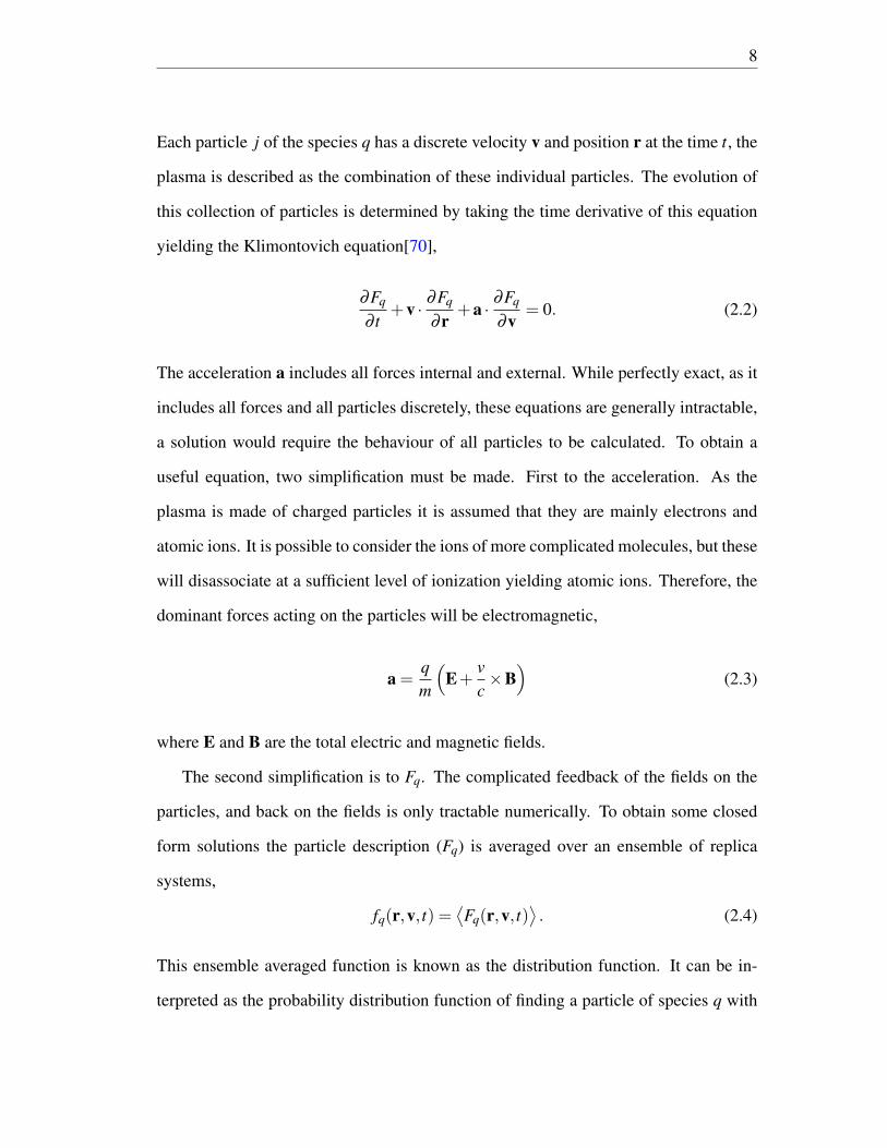
Each particle j of the species q has a discrete velocity v and position r at the time t, the
plasma is described as the combination of these individual particles. The evolution of
this collection of particles is determined by taking the time derivative of this equation
yielding the Klimontovich equation[70],
∂Fq
∂ t+v ·
∂Fq
∂r+a ·
∂Fq
∂v= 0. (2.2)
The acceleration a includes all forces internal and external. While perfectly exact, as it
includes all forces and all particles discretely, these equations are generally intractable,
a solution would require the behaviour of all particles to be calculated. To obtain a
useful equation, two simplification must be made. First to the acceleration. As the
plasma is made of charged particles it is assumed that they are mainly electrons and
atomic ions. It is possible to consider the ions of more complicated molecules, but these
will disassociate at a sufficient level of ionization yielding atomic ions. Therefore, the
dominant forces acting on the particles will be electromagnetic,
a =qm
(E+
vc×B)
(2.3)
where E and B are the total electric and magnetic fields.
The second simplification is to Fq. The complicated feedback of the fields on the
particles, and back on the fields is only tractable numerically. To obtain some closed
form solutions the particle description (Fq) is averaged over an ensemble of replica
systems,
fq(r,v, t) =⟨Fq(r,v, t)
⟩. (2.4)
This ensemble averaged function is known as the distribution function. It can be in-
terpreted as the probability distribution function of finding a particle of species q with

9
position r and velocity v at the time t. This probabilistic approach has the benefit of
providing a continuous, differentiable function. With the additional step of dividing
this distribution function into an average (or slowly varying) and fluctuating (quickly
varying) part,
fq = f0q + f1q, (2.5)
Eq. 2.2 can be written,
∂ f0q
∂ t+v ·∇ f0q +
mq
(E+
vc×B)·∇v f0q =−
mq
⟨(Em +
vc×Bm
)·∇v f1q
⟩. (2.6)
The fields have been split into quickly varying microscopic fields (Em,Bm) and average
(E,B) fields. The left side of Equation 2.6 generally describes collective effects, while
the right is associated with collisional effects. This equation is known as the Boltzmann
equation and is often further simplified by assuming the collisions are negligible. This
collisionless assumption gives an equation known as the Maxwell-Boltzmann or the
Vlasov equation,
∂ f0q
∂ t+v ·∇ f0q +
mq
(E+
vc×B)·∇v f0q = 0. (2.7)
2.2 Sources of Maxwellian and non-Maxwellian plas-
mas
With the distribution function established (Eq. 2.4) and the equation governing its
evolution (Eq. 2.6), the natural question arises, what is the form of fq0. A common

10
assumption is the equilibrium Maxwellian distribution,
fq =
√mq
2πTexp−
mqv2
2T
, (2.8)
as this is the equation for an ideal gas in thermal equilibrium, a very similar system.
This distribution can be derived directly from the micro-canonical ensemble in statis-
tical mechanics[71], but it is informative to derive this distribution function from the
Boltzmann equation. There are multiple approaches to this solution, the one presented
follows the Boltzmann H-theorem[15] but there are also solutions relying on Lenard-
Balescu equation, Fokker-Planck equation, and BBGKY hierarchy.
2.2.1 Derivation of Maxwellian distribution function
The simplest form of the collision operator, the right side of Eq. 2.6, is described by
considering various forms of collisions. The lowest order term is interactions of a single
particle with it’s own microscopic field, but particles do not interact with such a field.
The next term is the electromagnetic interaction of 2 particles, further terms involve
interactions of escalating numbers of particles. Arguing that the interactions involving
the least particles are the most probable, the higher order terms are dropped and only
the 2 particle interactions considered.
Let a particle j with a location r and velocity v j interact with particles i within a
cylindrical shell of radius b and thickness db during the time dt. The probable number
of i particles is,
2π fi(r,vi, t)gi jb db dt (2.9)
where gi j = |vi− v j| is the differential speed of the particles. The integral over the
impact parameter b and velocity vi, gives the total number of interacting particles in the
11
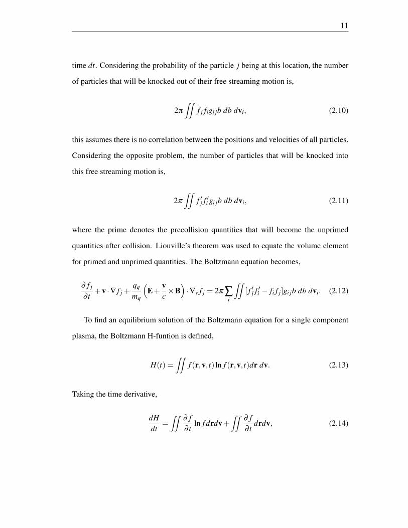
time dt. Considering the probability of the particle j being at this location, the number
of particles that will be knocked out of their free streaming motion is,
2π
∫∫f j figi jb db dvi, (2.10)
this assumes there is no correlation between the positions and velocities of all particles.
Considering the opposite problem, the number of particles that will be knocked into
this free streaming motion is,
2π
∫∫f ′j f ′i gi jb db dvi, (2.11)
where the prime denotes the precollision quantities that will become the unprimed
quantities after collision. Liouville’s theorem was used to equate the volume element
for primed and unprimed quantities. The Boltzmann equation becomes,
∂ f j
∂ t+v ·∇ f j +
mq
(E+
vc×B)·∇v f j = 2π ∑
i
∫∫[ f ′j f ′i − fi f j]gi jb db dvi. (2.12)
To find an equilibrium solution of the Boltzmann equation for a single component
plasma, the Boltzmann H-funtion is defined,
H(t) =∫∫
f (r,v, t) ln f (r,v, t)dr dv. (2.13)
Taking the time derivative,
dHdt
=∫∫
∂ f∂ t
ln f drdv+∫∫
∂ f∂ t
drdv, (2.14)

12
and if the number of particles is conserved then the second term vanishes,
dHdt
=∫∫
∂ f∂ t
ln f drdv. (2.15)
Multiplying the Equation 2.12 by ln f and integrating over r and v,
∫∫∂ f j
∂ tln f jdrdv j +
∫∫ln f jv j ·∇ f jdrdv j +
∫∫ln f j
mq
(E+
vc×B)·∇v f0qdrdv j
= 2π
∫∫∫ln f j[ f ′j f ′i − fi f j]gi jb db dvidv j. (2.16)
Assuming the plasma is uniform in space, at least locally, v ·∇ f → 0. In order for
the number of particles to be finite f (v)→ 0 as v→−∞,∞. Therefore, the second and
third terms vanish,
dHdt
=∫∫
∂ f j
∂ tln f jdrdv j = 2π
∫∫∫ln f j[ f ′j f ′i − fi f j]gi jb db dvidv j. (2.17)
The two particle collisions must be symmetric with respect to time, i.e. for a set of
initial and final velocities the initial velocities are recovered if the collision is reversed,
∫∫∫ln f j[ f ′j f ′i − fi f j]gi jb db dvidv j =
∫∫∫ln f ′j[ f j fi− f ′i f ′j]g
′i jb′ db′ dv′idv′j (2.18)
The definitions of differential speed gi j, impact parameter b, and volume element are
also time symmetric
gi j = g′i j b = b′ dvidv j = dv′idv′j (2.19)

13
Since these forms are equivalent, they also equal half their sum
dHdt
=12
∫∫∫(ln f j− ln f ′j)[ f
′j f ′i − fi f j]gi jb db dvidv j (2.20)
The same arguments apply to the collision being particle symmetric, it does not matter
which particle is called j.
dHdt
=14
∫∫∫(ln f j + ln fi− ln f ′j− ln fi)[ f ′j f ′i − fi f j]gi jb db dvidv j (2.21)
Rearranging the logarithm,
dHdt
=2π
4
∫∫∫(ln
f j fi
f ′j f ′i)[ f ′j f ′i − fi f j]gi jb db dvidv j. (2.22)
The integrand is analogous to −(x− y) lnx/y, which is ≤ 0. So,
dHdt≤ 0 (2.23)
The goal is to obtain a steady state solution, implying for t→ ∞ dH/dt = 0, or ln f ′j +
ln f ′i = ln f j + ln fi. Therefore, ln f must be a summational invariant of the symmetric
two particle collision. For elastic collisions, these invariants are mass (m), momentum
(mv), and kinetic energy (mv2/2).
ln f = αm+β · (mv)− γmv2
2= αm+
m2
β ·βγ− mγ
2(v− β
γ)2 (2.24)
and
f (r,v) = cexp[−mγ
2(v− β
γ)2]
(2.25)
14
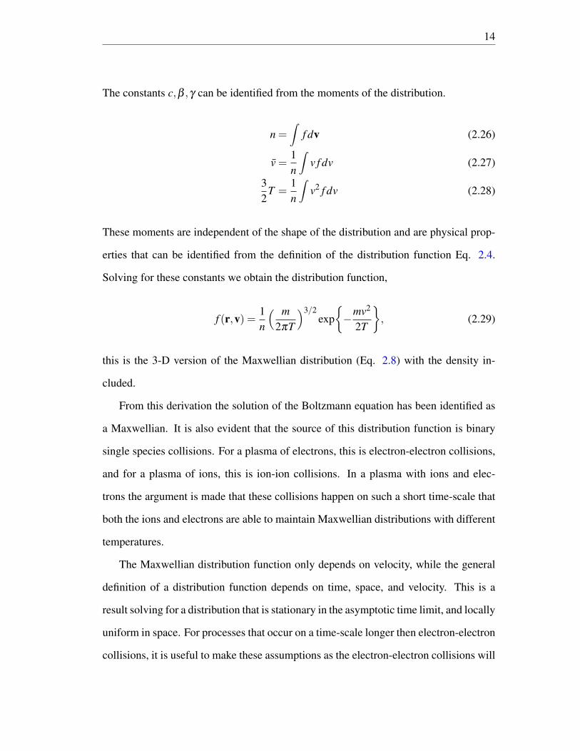
The constants c,β ,γ can be identified from the moments of the distribution.
n =∫
f dv (2.26)
v =1n
∫v f dv (2.27)
32
T =1n
∫v2 f dv (2.28)
These moments are independent of the shape of the distribution and are physical prop-
erties that can be identified from the definition of the distribution function Eq. 2.4.
Solving for these constants we obtain the distribution function,
f (r,v) =1n
( m2πT
)3/2exp−mv2
2T
, (2.29)
this is the 3-D version of the Maxwellian distribution (Eq. 2.8) with the density in-
cluded.
From this derivation the solution of the Boltzmann equation has been identified as
a Maxwellian. It is also evident that the source of this distribution function is binary
single species collisions. For a plasma of electrons, this is electron-electron collisions,
and for a plasma of ions, this is ion-ion collisions. In a plasma with ions and elec-
trons the argument is made that these collisions happen on such a short time-scale that
both the ions and electrons are able to maintain Maxwellian distributions with different
temperatures.
The Maxwellian distribution function only depends on velocity, while the general
definition of a distribution function depends on time, space, and velocity. This is a
result solving for a distribution that is stationary in the asymptotic time limit, and locally
uniform in space. For processes that occur on a time-scale longer then electron-electron
collisions, it is useful to make these assumptions as the electron-electron collisions will

15
establish a new equilibrium. However, in a case where there is a spatial, or temporal
variation of significance these assumptions break down the distribtuion function must
be rederived.
This derivation required 8 assumptions, approximations, and simplifications.
(1) Forces are electromagnetic
(2) Particles can be represented by an ensemble average
(3) The distribution function can be separated into a slow and fast component
(4) The collision are limited to two particles
(5) There is only one type of particle
(6) Collisions are perfectly elastic
(7) The distribution function is uniform in space
(8) There are no external fields
It is possible to solve this problem relaxing some of these assumptions, but it is not
surprising that these do not always hold true. Most of these assumptions can be sum-
marized as saying there are no sources or sinks of energy. One of the simplest ways to
violate these assumptions is if there are collisions other than binary single species col-
lisions. This reintroduces additional terms on the right side of the Boltzmann equation
and depending on their form allows new and unique solutions to this equation.
2.2.2 Inverse bremsstrahlung heating and Langdon effect
For the purposes of this thesis, non-Maxwellian distributions arising from inverse
bremsstrahlung heating will be examined, but some other potential sources will

16
be described in the next section. The distribution function resulting from inverse
bremsstrahlung heating is referred to as the Langdon distribution or the DLM (Dum-
Langdon-Matte) distribution.
Inverse bremsstrahlung is the main heating mechanism in under-dense laser pro-
duced plasmas and an important mechanism across a wide range of plasma physics.
Inverse bremsstrahlung occurs when an electron oscillating in the electric field of the
laser collides with an ion, it retains some of the momentum gained from the laser field,
thereby transferring energy from the field to the electron.
This argument was first proposed in a 1980 paper by Langdon[22], and the follow-
ing derivation follows the argument in the paper. With the presence of a laser field the
Maxwellian electron distribution oscillates relative to the ions and if the relative veloc-
ity is V then the electrons will experience a drag force ∝ V−2, this will have a greater
effect on electrons with small V/vth, where vth =√
Te/me is the electron thermal ve-
locity. Electrons with faster velocities will feel a smaller drag and while some gain
energy other loose energy. The resulting velocity dependence of the electrons can be
found by solving the Boltzmann equation (Eq. 2.6) including electron-ion collisions in
an oscillating electric field.
Assuming the electron density and electric field are uniform in space the Boltzmann
equation is,∂ f∂ t
+e
meE ·∇v f = A∇v ·
[v2 ¯I−vv
v3 ·∇v f
]+Cee( f ). (2.30)
The particle charge has been identified as the electron charge (q = e), the mass is the
electron mass (me) and the spatial gradient was dropped under the uniform assumption.
The collision term has been broken in two, with the second term being the electron-
electron collision operator as derived in the previous section, and the first term is a form
of the Fokker-Plank operator known as the Lorentz collision operator[72] describing the
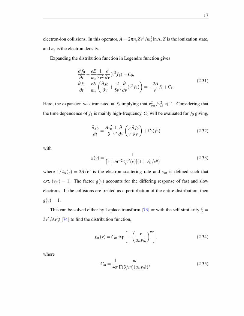
17
electron-ion collisions. In this operator, A = 2πneZe4/m2e lnΛ, Z is the ionization state,
and ne is the electron density.
Expanding the distribution function in Legendre function gives
∂ f0
∂ t− eE
me
13v2
∂
∂v(v2 f1) =C0,
∂ f1
∂ t− eE
me
(∂ f0
∂v+
25v3
∂
∂v(v3 f2)
)=−2A
v3 f1 +C1.
(2.31)
Here, the expansion was truncated at f2 implying that v2osc/v2
th 1. Considering that
the time dependence of f1 is mainly high-frequency, C0 will be evaluated for f0 giving,
∂ f0
∂ t=
Av20
31v2
∂
∂v
(gv
∂ f0
∂v
)+C0( f0) (2.32)
with
g(v) =1
[1+ω−2τ−2ei (v)](1+ v6
ω/v6)(2.33)
where 1/τei(v) = 2A/v3 is the electron scattering rate and vω is defined such that
ωτei(vω) = 1. The factor g(v) accounts for the differing response of fast and slow
electrons. If the collisions are treated as a perturbation of the entire distribution, then
g(v) = 1.
This can be solved either by Laplace transform [73] or with the self similarity ξ =
3v5/Av20t [74] to find the distribution function,
fm (v) =Cm exp[−(
vamvth
)m], (2.34)
where
Cm =1
4π
mΓ(3/m)(amvth)3 (2.35)

18
and
am =Γ(3/m)
Γ(5/m)(2.36)
The result is a super-Gaussian shape, with super-Gaussian order m. Langdon[22]
showed that a maximum order of 5 is obtained if inverse bremsstrahlung collisions are
completely dominant. The normalization constant also allows this distribution function
to maintain the physical meaning of the first three moments, preserving the definitions
of density, flow, and temperature. This shape is consistent with the physical interpre-
tation of the slow electrons being heated to velocities near the thermal velocity, as this
results in the flattening and widening of the peak of the distribution.
Fokker-Planck simulations, performed by Matte et al., showed that the degree
to which the distribution is flattened depends on the relative strength of inverse
bremsstrahlung heating and thermalization due to electron-electron collisions, which
was parameterized as α = Zv2osc/v2
th[23]. vosc = eE0/meω is the velocity of electrons
oscillating in the laser field. This enabled the development of a heuristic scaling law
relating the Langdon parameter (α) to the super-gaussian order,
m(α) = 2+3
1+1.66/α0.724 . (2.37)
Other Fokker-Planck simulations showed an increased range of validity for this
model. While this derivation assumed v2osc/v2
th 1, the result is valid even when
v2osc/v2
th ≈ 1[74]. Another important finding was that inverse bremsstrahlung heating
only induces a small anisotropy. The anisotropic component of the pressure tensor is
only 145v2
osc/v2th [75].
While only inverse bremsstrahlung heating will be discussed here, this distribution
19
function can also arise as a result of ion turbulence, as shown by C. T. Dum[34]. Hence
the alternate name Dum-Langdon-Matte distribution.
While there is consensus on the shape and underlying physics of a super-Gaussian
distribution function, questions remain about the high-energy electrons. Some of the
physics considered has been the relatively small electron-ion collision rate of the fast
electrons [36], thermal transport[24], parametric instabilities[23], and electron-electron
collisions[32]. All of these proposed mechanisms result in a Maxwellian tail, but often
with a different temperature then the bulk distribution. The various formalisms also
differ in where the distribution transitions from super-Gaussian to Maxwellian and the
shape of the transition region.
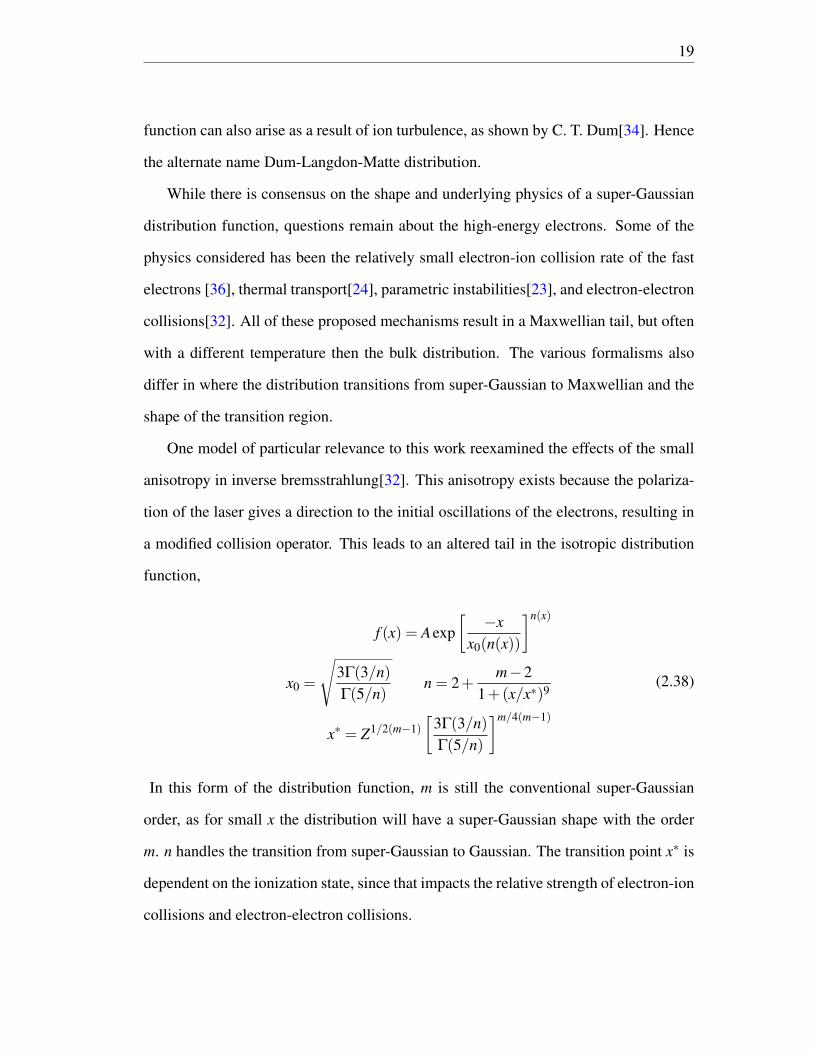
One model of particular relevance to this work reexamined the effects of the small
anisotropy in inverse bremsstrahlung[32]. This anisotropy exists because the polariza-
tion of the laser gives a direction to the initial oscillations of the electrons, resulting in
a modified collision operator. This leads to an altered tail in the isotropic distribution
function,
f (x) = Aexp[−x
x0(n(x))
]n(x)
x0 =
√3Γ(3/n)Γ(5/n)
n = 2+m−2
1+(x/x∗)9
x∗ = Z1/2(m−1)[
3Γ(3/n)Γ(5/n)
]m/4(m−1)
(2.38)
In this form of the distribution function, m is still the conventional super-Gaussian
order, as for small x the distribution will have a super-Gaussian shape with the order
m. n handles the transition from super-Gaussian to Gaussian. The transition point x∗ is
dependent on the ionization state, since that impacts the relative strength of electron-ion
collisions and electron-electron collisions.
20
2.2.3 Other non-Maxwellian distribution functions
There are many other non-Maxwellian distribution functions know to exist in plasmas.
Most of them are unstable and will decay back to a Maxwellian but there is potential
for some to be sustained as long as there is a significant source or sink of energy.
Possibly the most commonly used and observed type of non-Maxwellian distribu-
tions are the bi-Maxwellian distributions. These can take the form of a Maxwellian
with different temperatures in two spatial dimensions, a common result in the presence
of a magnetic field[76, 77]. Or there can be two distinct population present with dif-
ferent apparent temperatures due to heating non-uniformity[78]. Similarly there many
other distributions including bump-on-tail (from a beam in a plasma)[79, 80] and two
stream[81, 82] that can be described as a sum of Maxwellians. While these are some-
times thought of as Maxwellian or modified Maxwellians, they can alter the damping
and resonance of plasma waves.
Other more exotic distributions, such delta-function-like distribution resulting from
field ionization[63, 83] or the complicated spectra of non-linear waves[84, 85], tend to
be treated more kinetically. This ensures the consequences of the distribution function
are treated self-consistently but is computationally expensive and is often limited to
problems with a short time-scale.
As diagnostic techniques become better, non-Maxwellian effects are becoming
more apparent and a better candidate for explaining the complex interaction occurring
in plasma experiments. Consequently, there has been an increased interest in fast ions
(magnetically confined plasmas), non-Maxwellian distribution in the solar wind, and
hot ions escaping the fuel in inertial confinement fusion.
21
2.3 Waves in a plasma
The most common approach to describing plasmas and their behavior is through the
various waves that can propagate through them. By solving wave equations it is possi-
ble to understand how energy will be absorbed, reflected, carried or transformed. The
waves in a plasma can be found using the moments of the Vlasov equation (Eq. 2.7) or
by directly interrogating the Vlasov equation.
2.3.1 Waves in the fluid description
The fluid description of a plasma uses a set of equations that are analogous to the
equations for incompressible fluids. Integrating the Vlasov equation with respect to
velocity gives the continuity equation, which describes the conservation of particles,
∂nq
∂ t+∇(nqvq) = 0. (2.39)
Taking the first moment of the Vlasov equation with respect to velocity yields the
force equation, which describes the momentum conservation in the plasma,
∂
∂ t(nqvq)+∇(nqvv) =
qm
(E+
vq
c×B)
nq. (2.40)
As is seen with the first two equations, each moment equation depends on the next,
known as the closure problem. One way to close this system, is by truncating the series
with,
∇(nqvv) =1
mq∇Pq +nqvqvq, (2.41)
reducing the tensor vv to pressure and the average velocity vq. The pressure can be
22
described by one of the common thermodynamic relations. Such as the adiabatic ap-
proximation where, ∇Pq = 3Tq∇nq.
These equations can be solved for plane wave solutions where only the electrons
move by considering small perturbations of the density, velocity, and electric field,
n = n0 +n1e−iωt+ikx,
v = v1e−iωt+ikx,
E = E1e−iωt+ikx.
(2.42)
Substituting into the moment equations and Gauss’ law, ∇E = 4πρ gives,
n1(−iω)+n0v1(ik) = 0,
men0v1(−iω) =−3Ten1(ik)− en0E1,
ikE =−4πen1.
(2.43)
solving for ω , we find the classic Bohm-Gross dispersion relation for electron-plasma
or Langmuir waves,
ω2 = ω
2pe +3k2v2
th (2.44)
where ω2pe =
4πe2neme
is the electron plasma frequency.
The same procedure can be followed considering the motion of the electrons and
ions. The continuity and momentum equations will become,
ni1(iω) = ni0vi1(ik) ne1(iω) = ne0ve1(ik) (2.45)
mini0vi1(−iω) =−γiTini1(ik)− eZni0E1 0 =−γeTene1(ik)− ene0E1. (2.46)
Here, me has been taken to zero since it is much smaller than mi. The densities have

23
also been related as ne = Zni, where Z is the ionization state. γe,i are the electron and
ion degrees of freedom, also known as the adiabatic index or polytrope index. The
momentum equations can be rearranged to give
ω
kni0
ni1vi1 =
ω2
k2 =γiTi + γeZTe
mi(2.47)
where the the density ratio is found from the continuity equation. This is the dispersion
relation for ion-acoustic waves. These are sound-like waves that are propagated by
electrostatic interactions instead of the collisional interaction of sound waves. This
electrostatic interaction means waves exist even for negligible ion temperature.
2.3.2 Waves in the kinetic description
In the fluid description, the Fourier treatment of waves was applied to the momentum
equations. It is possible to directly apply this to treatment to the Vlasov equation and
Poisson’s equation. The Fourier transformed equations are,
−ω f + ikvz f + iqs
mslΦ
∂ f0
∂vz= 0 (2.48)
and
k2Φ =−4πqs
∞∫−∞
f d3v (2.49)
where the tilde denotes the transformed variable. The first equation can be solved for f
and substituted into the second equation to yeild the genral dispersion relation,
Ds(k,ω) = 1−ω2
ps
k2
∞∫−∞
∂Fs0/∂vz
(vz−ω/k)dvz. (2.50)

24
Here, Fs0 is the distribution projected onto the z direction. Since there is freedom of
aligning the Cartesian grid, it has been defined so z = k.
Unlike in the fluid case, the kinetic dispersion relation has explicit dependence on
the distribution function. If the distribution function is taken to be Maxwellian and the
damping is weak, then the kinetic dispersion relation reduces to the fluid dispersion
relation,
Ds(k,ω) = 1−ω2
ps
ω2− γsC2s k2 . (2.51)
This illustrates the implicit assumption in the fluid description that the distribution
function is Maxwellian. This assumption arises in the closure of the moment equations.
Since the moment equations were closed with an thermodynamic description of the
pressure thermal equilibrium, and therefore a given relation between temperature and
velocity, is imposed.
2.3.3 Effect of non-Maxwellian distribution functions
From the kinetic dispersion relation (Eq. 2.50), it can be seen that significant changes to
the distribution function will modify the dispersion relation for the waves. This means
both a modified resonance and modified damping. It is possible to write new dispersion
relations for certain waves and certain distribution function. As an example, Afeyan
et al.[25] found the dispersion relation for the ion-acoustic waves where the electrons
have a super-Gaussian distribution function,
ω2
k2 =3Γ2(3/m)
Γ(1/m)Γ(5/m)
γiTi + γeZTe
mi(2.52)
Generally, this is a problem that must be treated numerically.
This information about the waves is contained in the dielectric function or suscep-

25
tibility,
ε = 1+χe +χi
χe,i(k,ω) =
∞∫−∞
dv4πe2ne,i
me,ik2
k · ∂ fe,i∂v
ω−k ·v− iγ,
(2.53)
which has the same dependence on the distribution function.

26
Chapter 3
Thomson Scattering
This chapter gives an overview of Thomson scattering and its application to measuring
plasma conditions and the electron distribution function. The goal of this chapter is
to give a physical and mathematical description of Thomson scattering and introduce
the newly developed angularly resolved Thomson-scattering technique. In Section 3.1
the fundamentals of Thomson scattering are discussed along with discussion of the
non-collective Thomson-scattering regime. Section 3.2 describes the case where the
electron motion is correlated leading to collective Thomson scattering. Section 3.3
shows how non-Maxwellian distribution functions effect the spectra and provides a
detailed discussion of its effect on inferred plasma conditions. Section 3.4 describes
the novel angularly resolved Thomson scattering technique and its advantages.
3.1 Non-collective Thomson scattering
Thomson scattering is the elastic scattering of photons off free electrons. In other words
it is the low energy version of Compton scattering, where the electron recoil is ignored
since the photon energy is much less then the rest mass of the electron (2hω0mec2).
This scattering process results in a Doppler shifted photon and an electron whose mo-

27
mentum is unchanged by the interaction. For a plasma, where there is an ensemble of
electrons, the scattered photons contain information about the number and velocities of
all the electrons.
Photons are supplied by a probing laser beam. The power scattered to a location R,
within the solid angle dΩ, by a plasma can be written,
Ps(R,ωs)dωsdΩ =P0r2
0A2π
∣∣s× (s× E0)∣∣2(1+2
ω
ω0
)NS(k,ω). (3.1)
Here the first term describes the energy density of the probe beam with the probe
power (P0) and the cross sectional area of the beam (A). The classical electron radius
(r0 = 2.8179× 10⁻¹³ cm) comes from the Poynting vector. The second term is the
scattering efficiency, based on the observation direction (s) and probe polarization di-
rection (E0), since Thomson scattering is a dipole scattering process the emission is
maximal when observing perpendicular to the polarization. The third term is the first
order relativistic correction, which accounts for the “relativistic headlight” and v×B
effects for electrons up to ∼ 5 keV [86]. The final term is the number of electrons in
the scattering volume N and the spectral density function, which describes the electron
density fluctuation spectrum.
S(k,ω) = limγ→0,V→∞
2γ
V
⟨∣∣ne(k,ω− iγ)∣∣2
ne0
⟩. (3.2)
This description of spectral density function shows the relation to density pertur-
bations, but a more useful form can be found. The spectral density function can be
solved in two regimes the non-collective and collective. In the non-collective regime
(1/kλD < 1), the scale length is smaller than the electron Debye length (λD), the clas-
28
sical shielding length. At this scale length the plasma cannot support waves, so the
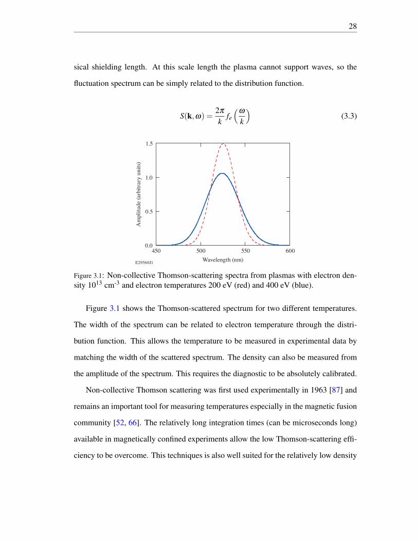
fluctuation spectrum can be simply related to the distribution function.
S(k,ω) =2π
kfe
(ω
k
)(3.3)
Figure 3.1: Non-collective Thomson-scattering spectra from plasmas with electron den-sity 1013 cm-3 and electron temperatures 200 eV (red) and 400 eV (blue).
Figure 3.1 shows the Thomson-scattered spectrum for two different temperatures.
The width of the spectrum can be related to electron temperature through the distri-
bution function. This allows the temperature to be measured in experimental data by
matching the width of the scattered spectrum. The density can also be measured from
the amplitude of the spectrum. This requires the diagnostic to be absolutely calibrated.
Non-collective Thomson scattering was first used experimentally in 1963 [87] and
remains an important tool for measuring temperatures especially in the magnetic fusion
community [52, 66]. The relatively long integration times (can be microseconds long)
available in magnetically confined experiments allow the low Thomson-scattering effi-
ciency to be overcome. This techniques is also well suited for the relatively low density

29
and temperatures (ne ∼ 1013 cm-3, Te ∼ 100 eV), which give larger electron Debye
lengths.
Another important application of non-collective Thomson scattering is x-ray Thom-
son scattering. Here, the extremely shot wavelengths of the x-ray probe keeps experi-
ments in the non-collective regime. This technique can be used experiments where the
plasma is opaque to optical light, allowing applications in warm dense matter and other
high-energy density sciences [56, 57].
3.2 Collective Thomson scattering
In the collective regime, the scattering scale length is larger than the electron Debye
length (1/kλD > 1) and correlated motion of electrons must be considered. Correlated
electron motion, or thermal fluctuations, are heavily damped at the smaller scale length.
The scattering off correlated electrons interferes constructively resulting in peaks in the
spectrum that correspond to thermal fluctuations in the plasma. This transition occurs
around 1 > ZTe/Ti for ion-acoustic waves. Here, the spectral density function can be
written
S(k,ω) =2π
k
∣∣∣∣1− χe
1+χe +χi
∣∣∣∣2 fe0
(ω
k
)+
2πZk
∣∣∣∣ χe
1+χe +χi
∣∣∣∣2 fi0
(ω
k
)(3.4)
where fe0 and fi0 are the one-dimensional (1-D) electron and ion distribution func-
tions, Z is the ionization state, and χe,i are the electron and ion susceptibilities. This
collisionless form factor assumes there is no magnetic field, the measurement is non-
perturbative, and ignores interactions of three or more bodies. The real and imaginary

30
parts of the ion and electron susceptibility are given by[88],
χRe =−Z
k2λ 2Di,e
P
∞∫−∞
∂ fi,e/∂x′
x′− xdx′,
χIm =− Zπ
k2λ 2Di,e
∂ fi,e
∂x′
∣∣∣∣x.
(3.5)
For the electron susceptibility Z = 1. The pole in the real component of the suscepti-
bility gives rise to the peaks mentioned earlier, when the imaginary part is sufficiently
small.
Figure 3.2: Collective Thomson-scattering spectra from plasmas with (blue) ne = 2×1019 cm-3 and Te = 300 eV and (red) ne = 4×1019 cm-3 and Te = 400 eV. Ion-acousticwave features have been cut off (actual amplitude ∼ 150) in order to visualize theelectron-plasma wave features.
Figure 3.2 shows the Thomson-scattered spectrum for two different temperatures
and densities. Two sets of peaks can be seen in the spectrum. The outer peaks are
associated with electron-plasma waves, while the inner peaks are associated with ion-
acoustic waves. For low frequency (ω) the second term in Eq. 3.4 dominates and
the resonance follows the dispersion relation of ion-acoustic waves. The peak sepa-
ration for these inner peaks can be related to√
ZTemi
while their width is dependent on

31
ZTeTi
. With some knowledge about the ionization state and the temperature equilibra-
tion, ion-acoustic Thomson scattering is a useful tool for temperature measurements in
many laboratory experiments. This feature can be orders of magnitude brighter then the
electron-plasma wave feature or non-collective scattering, making ion-acoustic Thom-
son scattering the easiest version to measure.
At high frequency (ω) the first term in Eq. 3.4 dominates and the resonance follows
the dispersion relation for electron-plasma waves. The peak separation of these outer
electron-plasma wave features is primarily based on density. This can be seen with the
Bohm-Gross dispersion relation (Eq. 2.44) where the lowest order term in tempera-
ture is simply ωpe, which is proportional to electron density. The width of these peaks
reflects the damping of the wave, and arises from the imaginary part of the electron sus-
ceptibility, which depends on the slope of the distribution function. The temperature
dictates the width of the distribution and therefore influences the slope at a particu-
lar kλD. This width can be physically interpreted as Landau damping of the thermal
fluctuation.
Early work using the electron-plasma wave feature mainly focused on the peak
separation as a way to measure electron density [19]. More recently experiments mea-
suring the entire collective spectrum have matched the spectral shape in order to derive
electron temperature and density [86]. When possible the electron and ion features have
been measured simultaneously allowing measurements to be made of electron density,
electron temperature, ion temperature, and ionization with a single technique. This
generally requires separate diagnostics to measure the electron and ion features due to
their signal strengths and the required spectral resolution.

32
3.3 Effects of non-Maxwellian distribution functions
Revisiting the spectral density function (Eq. 3.4), the dependence of the spectrum on
plasma conditions can be seen to originate from the dependence on the electron and
ion distribution functions. The standard interpretations of peak separations and widths
ascribe physical intuition to parts of the spectrum, but rely on the standard dispersion
relations. As seen in Sec. 2.3 these dispersion relations inherently assume the distribu-
tion function is Maxwellian.
Thomson scattering is sensitive to more then just the bulk properties, it can mea-
sure the distributions themselves. Here, the focus will be on the electron distribution
function and how it can be measured by focusing on the high-frequency spectrum.
3.3.1 Changes to the spectral shape
Figure 3.3: Theoretical spectra for (a) non-collective and (b) collective Thomson scat-tering from a Maxwellian plasma (blue) and a non-Maxwellian plasma with super-Gaussian order 5 (red). The circles represent synthetic data generated from the theoret-ical curves. These spectra are for plasmas with (a) ne = 1×1013 cm-3 and Te = 400 eVand (b) ne = 4×1019 cm-3 and Te = 400 eV.
Figure 3.3 shows how the non-collective and collective spectra change in response
to the distribution function. These specific changes are a consequence of the type of
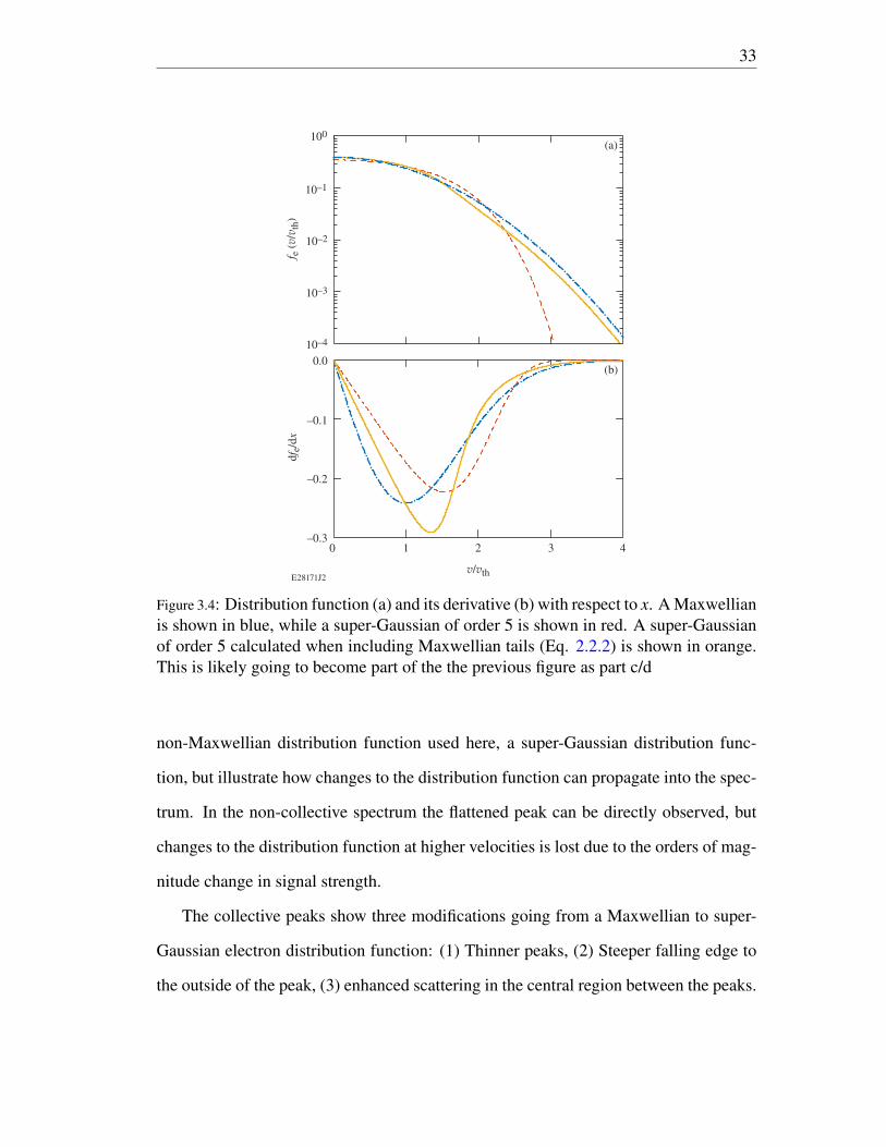
33
Figure 3.4: Distribution function (a) and its derivative (b) with respect to x. A Maxwellianis shown in blue, while a super-Gaussian of order 5 is shown in red. A super-Gaussianof order 5 calculated when including Maxwellian tails (Eq. 2.2.2) is shown in orange.This is likely going to become part of the the previous figure as part c/d
non-Maxwellian distribution function used here, a super-Gaussian distribution func-
tion, but illustrate how changes to the distribution function can propagate into the spec-
trum. In the non-collective spectrum the flattened peak can be directly observed, but
changes to the distribution function at higher velocities is lost due to the orders of mag-
nitude change in signal strength.
The collective peaks show three modifications going from a Maxwellian to super-
Gaussian electron distribution function: (1) Thinner peaks, (2) Steeper falling edge to
the outside of the peak, (3) enhanced scattering in the central region between the peaks.

34
The super-Gaussian electron distribution function has a steeper slope above 2vth, which
leads to less Landau damping and results in the thinner peaks and a steeper falling edge.
The increased central region is due to the increased number of electrons in the region
of 1−2vth.
While both regimes are sensitive to the electron distribution function, experimental
limitations hamper their practicality for measuring the distribution function. The small
electron scattering cross section restricts non-collective Thomson scattering to measur-
ing the bulk of the distribution function where the scattering exceeds thermal back-
ground. Laser heating, filamentation and other laser-plasma instabilities, caused by an
intense probe beam, typically constrain measurements to a couple orders of magnitude.
Collective Thomson scattering has an improved signal-to-noise but is less sensitive the
the distribution function away from the peaks of the spectrum. These regions away
from the peaks also tend to be noisy as the signal is low. These restriction have lim-
ited previous distribution function measurements to the bulk of the distribution function
[55].
3.3.2 Changes to the inferred conditions
Previous Thomson-scattering experiments [37, 42–50] were limited in their ability to
measure the complete electron-plasma wave feature with high signal to noise. As a re-
sult the features of a non-Maxwellian distribution function may have gone unnoticed or
ignored. As will be shown in this section, the assumption that the distribution function
is Maxwellian can lead to significant errors in the inferred plasma conditions. These
errors can be mitigated by including the true distribution function in the accessible fit
space.
To determine the error in inferred plasma conditions synthetic Thomson scattering
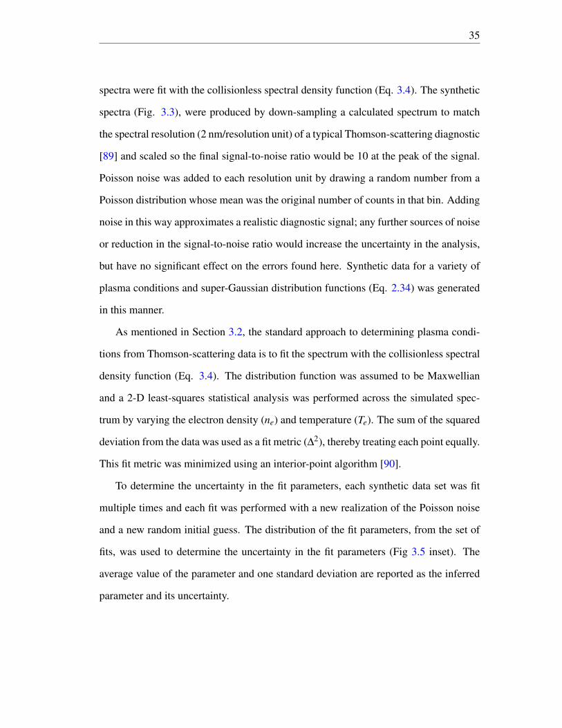
35
spectra were fit with the collisionless spectral density function (Eq. 3.4). The synthetic
spectra (Fig. 3.3), were produced by down-sampling a calculated spectrum to match
the spectral resolution (2 nm/resolution unit) of a typical Thomson-scattering diagnostic
[89] and scaled so the final signal-to-noise ratio would be 10 at the peak of the signal.
Poisson noise was added to each resolution unit by drawing a random number from a
Poisson distribution whose mean was the original number of counts in that bin. Adding
noise in this way approximates a realistic diagnostic signal; any further sources of noise
or reduction in the signal-to-noise ratio would increase the uncertainty in the analysis,
but have no significant effect on the errors found here. Synthetic data for a variety of
plasma conditions and super-Gaussian distribution functions (Eq. 2.34) was generated
in this manner.
As mentioned in Section 3.2, the standard approach to determining plasma condi-
tions from Thomson-scattering data is to fit the spectrum with the collisionless spectral
density function (Eq. 3.4). The distribution function was assumed to be Maxwellian
and a 2-D least-squares statistical analysis was performed across the simulated spec-
trum by varying the electron density (ne) and temperature (Te). The sum of the squared
deviation from the data was used as a fit metric (∆2), thereby treating each point equally.
This fit metric was minimized using an interior-point algorithm [90].
To determine the uncertainty in the fit parameters, each synthetic data set was fit
multiple times and each fit was performed with a new realization of the Poisson noise
and a new random initial guess. The distribution of the fit parameters, from the set of
fits, was used to determine the uncertainty in the fit parameters (Fig 3.5 inset). The
average value of the parameter and one standard deviation are reported as the inferred
parameter and its uncertainty.

36
Errors in super-Gaussian plasmas
Figure 3.5: Percent error in (a,c) temperature and (b,d) density as a function of the nor-malized phase velocity (α) when the fit model assumes a Maxwellian electron distribu-tion function and the true electron distribution function is (a,b) super-Gaussian or (c,d)super-Gaussian with a Maxwellian tail (Eq. 2.2.2). The absolute difference betweenthe inferred and actual parameter dividend by the actual parameter (percent error) iscalculated for a range of phase velocities. The values for 4 different super-Gaussian or-ders are plotted in different colors with error bars that represent the standard deviationof 100 fits.
Figure 3.5 (a,b) shows that the inferred temperature and density can differ from the
actual values by 50% and 30%, respectively. As expected, there is no error when fitting
Maxwellian data with Maxwellian theory, but this provides a benchmark for the analy-

37
sis and quantifies the general uncertainties in the fitting process. For non-Maxwellian
plasmas (m > 2), the percent error in temperature increases as a function of the super-
Gaussian order and normalized phase velocity (α = vφ/vth). The statistical uncertainty
in the inferred parameters [error bars in Fig. 3.5 (a,b)] remains small. This reflects
the strength of the fits and shows that the error is due to changes in the distribution
functions not variability in fitting. The same trend of increasing error as a function of
super-Gaussian order is calculated for density. However, the error decreases or stays
relatively constant as a function of the scattering parameter.
The errors in the electron temperatures result from differences in the Maxwellian
and non-Maxwellian electron distribution functions (Fig. 3.4) at velocities around the
phase velocities of the electron-plasma waves. Over the range of phase velocities stud-
ied (α ' 2→ 4), the super-Gaussian distributions have fewer electrons and a smaller
slope than the Maxwellian electron distribution functions. This consequently reduces
the Landau damping of the probed fluctuations, resulting in narrower peaks in the syn-
thetic Thomson-scattering spectra. To compensate for the narrower peaks, the spectra
calculated with the Maxwellian electron distribution functions (fits) have a reduced
temperature (i.e. smaller Landau damping) than was used to generate the synthetic
spectrum. The reduced electron temperature requires an increased electron density
to maintain the resonant (peak) location of the electron-plasma wave features. These
trade-offs are illustrated in the Bohm-Gross dispersion relation, ω2 = ω2pe +3k2v2
th.
As the phase velocities move farther into the tail of the electron distribution func-
tion, Landau damping decreases faster in the non-Maxwellian than in the Maxwellian
calculations. This results in increased error as a function of phase velocity and super-
Gaussian order, eventually leveling off as the damping rate in all cases approaches zero.
The downward trend in density error with increasing phase velocity is also due to this
apparent temperature. As the electron temperature decreases, a smaller change in elec-

38
tron density is required to maintain the resonant (peak) location of the electron-plasma
wave features.
These errors of 50% in temperature and 30% in density are for extreme changes
to the electron distribution function, but even for small changes in the shape of the
distribution function, the errors in temperature and density are larger than the statistical
uncertainty of ∼ 5% that is typically reported [54, 91] and can be a limiting factor in
determining plasma conditions.
Errors in super-Gaussian with Maxwellian tail plasmas
As discussed in Section 2.2.2, both Fourkal et al. [32] and Brunner et al. [24] have
proposed that the distribution function is super-Gaussian only at small velocities and
trends toward Maxwellian at large velocities. To understand the impact of the tails on
inferred plasma conditions Fig. 3.5 (c,d) repeats the analysis shown in Fig. 3.5 (a,b),
but includes the modified non-Maxwellian electron distribution functions. The errors
are reduced in this case, but when the phase velocities are small, errors of up to 30% in
temperature and 13% in density are found. The trend in error with super-Gaussian order
is preserved, but the trend with phase velocity is reversed. Density errors still show the
trend of increased error with super-Gaussian order, but the error rapidly decreases with
increasing phase velocity until α ' 2, where the error effectively drops to zero.
The trends in error are again due to deviations of the true distribution functions
from a Maxwellian electron distribution function. For the calculations presented in
Fig. 3.5 (c,d), the effective ionization state (Z) was taken to be 1. This results in a
small range for x∗ ' 1.57→ 1.60 when m = 3→ 5. The reduction in errors calcu-
lated when including Maxwellian tails (Eq. 2.2.2) is a result of a convergence between
the Maxwellian and non-Maxwellian electron distribution functions around the phase
velocity of the electron-plasma wave. In the case where the distribution function has

39
Maxwellian tails, decreasing super-Gaussian order or increasing phase velocities re-
sults in less local deviation from a Maxwellian electron distribution function, at the
phase velocity of the probed fluctuations. Therefore, the resonant frequency and width
of the electron-plasma wave features are closer to the expected quantities, reducing the
inferred errors. This trend sheds light on what might happen for arbitrary electron dis-
tribution functions: the greater the deviation from Maxwellian, especially in slope, the
greater the possibility for error in inferred plasma conditions.
Figure 3.5 illustrates a limited range of phase velocities. For smaller phase veloc-
ities, the distribution function has such a strong effect on the scattered spectra that
it is not possible to reproduce key features of the Thomson-scattered spectra with
a Maxwellian model. For larger phase velocities, the chosen spectral resolution (2
nm/resolution element) is on the order of the width of the peak.
The two cases presented, Fig. 3.5 (a,b) and (c,d), represent the limiting cases for the
effects of adding Maxwellian tails to the super-Gaussian electron distribution functions.
As the ionization state is increased, the errors will transition from those presented in
Fig. 3.5 (c,d) to those presented in Fig. 3.5 (a,b). However, it is worth noting that this
is the result only for this formulation of super-Gaussian electron distribution functions
with Maxwellian tails, and previous work [30, 35] has shown good agreement with a
purely super-Gaussian distribution function.
Utilization of the complete high-frequency spectrum
It is common to infer plasma parameters from a single electron-plasma feature [54].
In laser-produced plasmas there can be significant light scattered by other means at
frequencies near one of the electron-plasma wave resonances [92], reducing the signal-
to-noise ratio of the feature. However, in conditions where both electron-plasma wave
features can be measured, the Thomson-scattered spectrum provides more information

40
Figure 3.6: Region where fits to the Stokes and anti-Stokes peaks yield different plasmaconditions as a function of the super-Gaussian order. Error bars represent the uncer-tainty due to simulation resolution. Within the shaded region, different plasma condi-tions (namely electron temperature) are determined by fitting to synthetic Stokes andanti-Stokes shifted spectra, with a model that assumes a Maxwellian electron distribu-tion function.
about the shape of the distribution function. Figure 3.6 shows the conditions at which
fits, that assume a Maxwellian electron distribution function, to the Stokes and anti-
Stokes electron-plasma wave features yield different plasma conditions (red shaded
region). The Stokes and anti-Stokes shifted electron-plasma wave features were fit in-
dependently, and determined to yield the same plasma conditions when the temperature
was in agreement to one standard deviation of 100 fits. Here, temperature was used be-
cause inferred density was found to be nearly the same between the two fits. Below
the points, the two fits yield different temperatures. This indicates missing physics
from the fit model; it is therefore possible to identify the distribution function as non-
Maxwellian, but without further analysis it is not possible to identify the shape of the

41
distribution function. Above the points, both fits yield the same plasma conditions but
with the errors discussed in the previous sections.
The behavior in Fig. 3.6 is due to the competition between super-Gaussian order
and the impact of the spectral resolution on the inferred temperature. For large super-
Gaussian order the two peaks give the same temperature once the damping becomes
so small that the width of the peaks are not resolved by the instrument. This leads
to a decrease in the boundary, α , with super-Gaussian order, as increasing the super-
Gaussian order decreases the damping on the wave (Fig. 3.4). When the super-Gaussian
order is small, it becomes impossible to see the difference in the damping between
the two peaks because the change in the damping, along with the resulting inferred
temperature, falls below the precision of the measurement due to the imposed limited
spectral resolution. Because this curve is highly dependent on spectral resolution, only
the overall trend is meaningful.
Figure 3.7 shows that a global minimum in the fit metric can be found by changing
the super-Gaussian order in the analysis. There is a well-defined minimum in the fit
metric when data generated with m = 4 is fit with m = 2 [Fig. 3.7 (a, e)]. However,
the fit metric gets smaller as the super-Gaussian order goes to the correct value (third
column). This improvement is due to the shape of the spectrum not just the width
and peak location, which can be seen in the top images [Fig. 3.7 (a, b, c, d)]. As
the super-Gaussian order goes to the correct solution (m = 4), the slope on the small
wavelength side of the peak steepens to match the data and the flatter region on the
longer wavelength side rises to match the data. Additionally, the images on the bottom
show the location of the minimum shifting toward the true values.
Figure 3.7 provides insight into the error bars in Fig 3.5. Multiple local minima can
be seen for each super-Gaussian order in Fig. 3.7. While none of the local minima in
Fig. 3.7 are low enough for the gradient decent minimizer to stop, this is not the case at

42
Figure 3.7: Images of the fit-metric as a function of temperature and density at m= 2,3,4,and 5. The value of the fit metric is shown on a logarithmic scale with the smallestvalue representing the “best” fit. Each image of the fit-metric space is paired with alineout of the data and the fit that corresponds to the minimum in the fit space. The datawas generated with electron density 1020 electrons/cm3, temperature of 1.2 keV, andm = 4.0 (α = 2.33).
other scattering parameters. The multiple minima increase the uncertainty of the fit and
correspondingly increase the error-bars. This effect occurs when the spectral feature
becomes smaller than 3 resolution elements.
Allowing the distribution function, via super-Gaussian order, to change as a parame-
ter in the fitting routine can eliminate model-dependent errors with minimally increased
statistical uncertainty. Generally, when the super-Gaussian order of the distribution
function is allowed to change, errors fall below 10%. There is a corresponding increase
in the uncertainties due to the added fit parameter, and uncertainties go from a few per-
cent to ∼ 10%. This is also the case for the distribution functions with Maxwellian
tails, and it does not matter if one or both electron-plasma wave features are used.
Figure 3.8 shows that including the true distribution function in the available fit
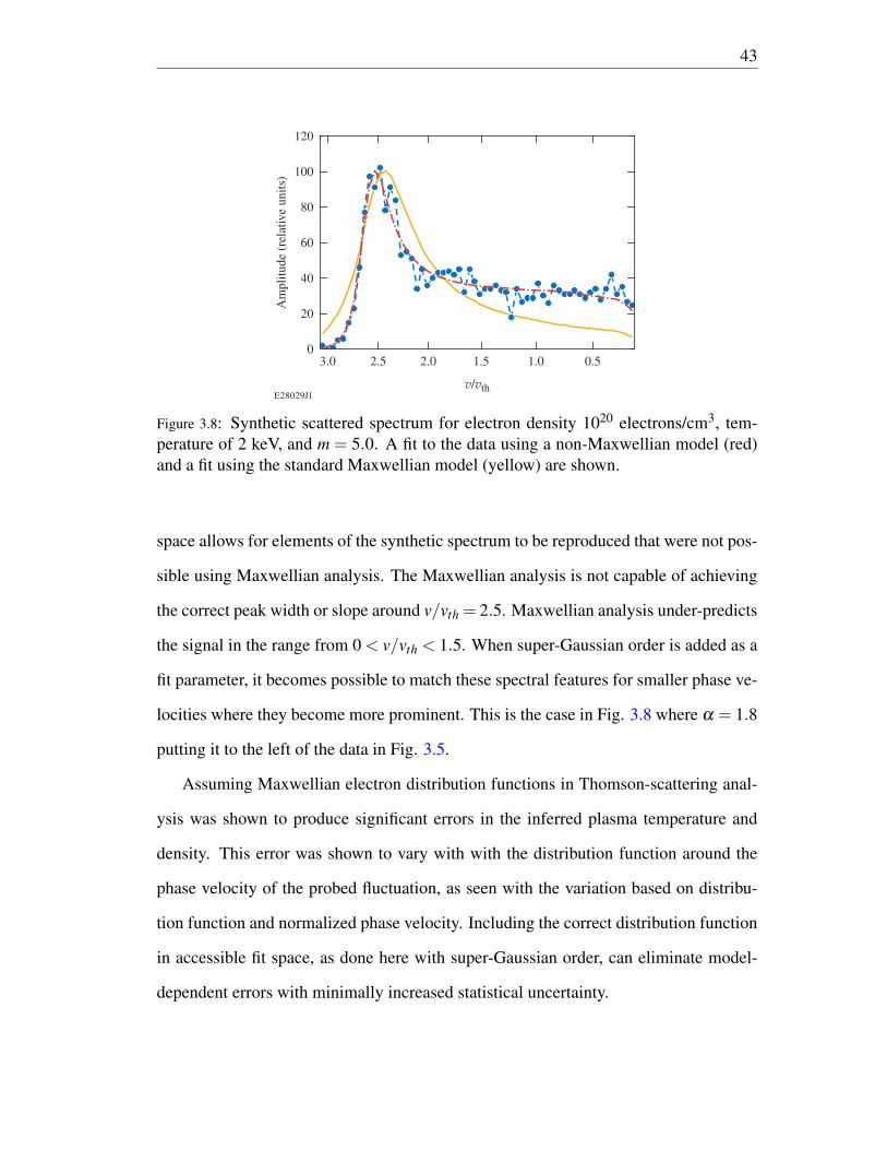
43
Figure 3.8: Synthetic scattered spectrum for electron density 1020 electrons/cm3, tem-perature of 2 keV, and m = 5.0. A fit to the data using a non-Maxwellian model (red)and a fit using the standard Maxwellian model (yellow) are shown.
space allows for elements of the synthetic spectrum to be reproduced that were not pos-
sible using Maxwellian analysis. The Maxwellian analysis is not capable of achieving
the correct peak width or slope around v/vth = 2.5. Maxwellian analysis under-predicts
the signal in the range from 0 < v/vth < 1.5. When super-Gaussian order is added as a
fit parameter, it becomes possible to match these spectral features for smaller phase ve-
locities where they become more prominent. This is the case in Fig. 3.8 where α = 1.8
putting it to the left of the data in Fig. 3.5.
Assuming Maxwellian electron distribution functions in Thomson-scattering anal-
ysis was shown to produce significant errors in the inferred plasma temperature and
density. This error was shown to vary with with the distribution function around the
phase velocity of the probed fluctuation, as seen with the variation based on distribu-
tion function and normalized phase velocity. Including the correct distribution function
in accessible fit space, as done here with super-Gaussian order, can eliminate model-
dependent errors with minimally increased statistical uncertainty.
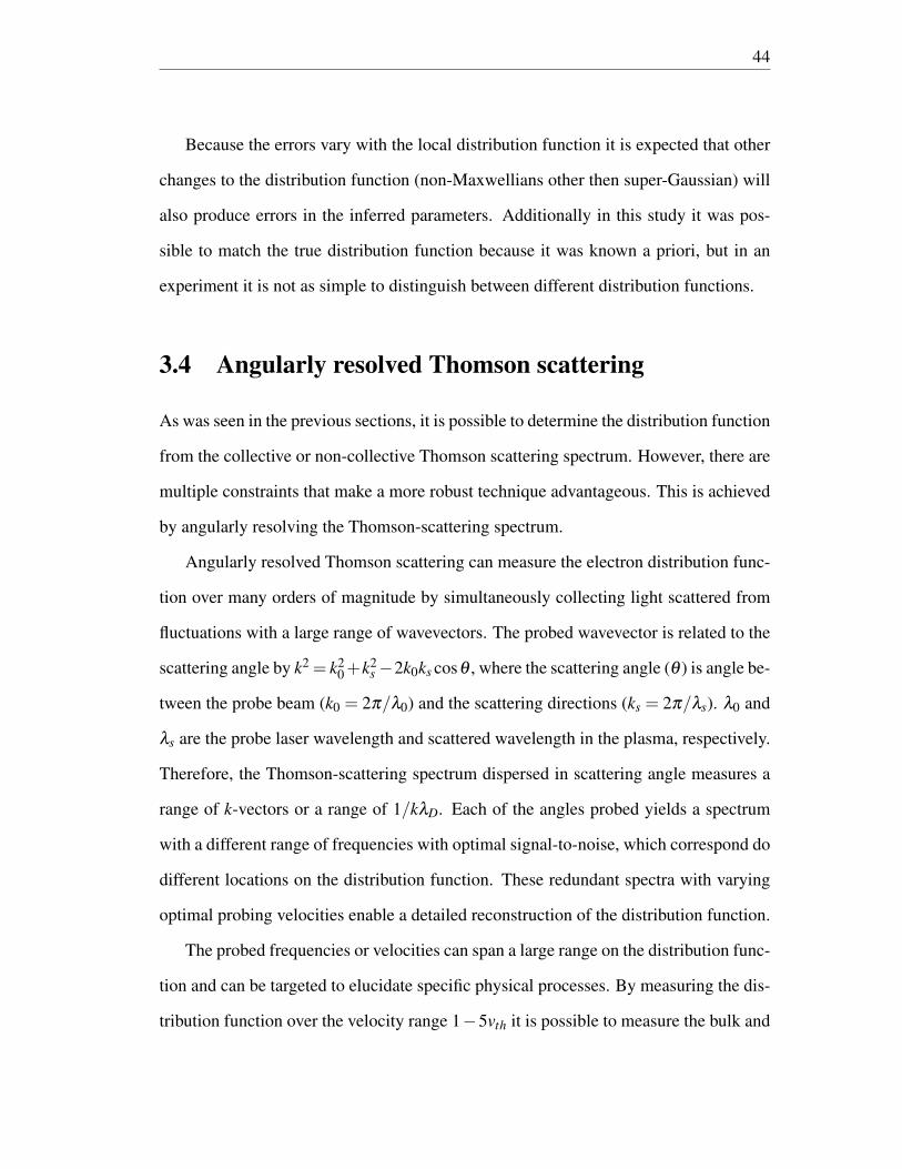
44
Because the errors vary with the local distribution function it is expected that other
changes to the distribution function (non-Maxwellians other then super-Gaussian) will
also produce errors in the inferred parameters. Additionally in this study it was pos-
sible to match the true distribution function because it was known a priori, but in an
experiment it is not as simple to distinguish between different distribution functions.
3.4 Angularly resolved Thomson scattering
As was seen in the previous sections, it is possible to determine the distribution function
from the collective or non-collective Thomson scattering spectrum. However, there are
multiple constraints that make a more robust technique advantageous. This is achieved
by angularly resolving the Thomson-scattering spectrum.
Angularly resolved Thomson scattering can measure the electron distribution func-
tion over many orders of magnitude by simultaneously collecting light scattered from
fluctuations with a large range of wavevectors. The probed wavevector is related to the
scattering angle by k2 = k20+k2
s−2k0ks cosθ , where the scattering angle (θ ) is angle be-
tween the probe beam (k0 = 2π/λ0) and the scattering directions (ks = 2π/λs). λ0 and
λs are the probe laser wavelength and scattered wavelength in the plasma, respectively.
Therefore, the Thomson-scattering spectrum dispersed in scattering angle measures a
range of k-vectors or a range of 1/kλD. Each of the angles probed yields a spectrum
with a different range of frequencies with optimal signal-to-noise, which correspond do
different locations on the distribution function. These redundant spectra with varying
optimal probing velocities enable a detailed reconstruction of the distribution function.
The probed frequencies or velocities can span a large range on the distribution func-
tion and can be targeted to elucidate specific physical processes. By measuring the dis-
tribution function over the velocity range 1−5vth it is possible to measure the bulk and

45
tail of the distribution function. This removes the need to assume a shape for the bulk
or tail as was required in the previous sections analysis.

46
Chapter 4
Diagnostics
This chapter discusses the laser systems, targets, and diagnostics used for measuring
Thomson scattering. The general structure of a Thomson-scattering experiment is intro-
duced with descriptions of various Thomson-scattering diagnostics. Section 4.1 gives
a brief overview of the OMEGA and MTW laser systems where this work was con-
ducted. The gas jet target is discussed in Section 4.2. In Section 4.3 various forms
of Thomson scattering are discussed with escalating complexity. Details are given for
imaging, time-resolved, and the new angularly resolved Thomson-scattering systems.
4.1 Laser systems
Experiments were performed at the Laboratory for Laser Energetics on two laser sys-
tems, the Multi-Terawatt (MTW) laser [93] and the OMEGA Laser System[94].
4.1.1 OMEGA
The OMEGA Laser System has been operational since 1995 and consists of 60 beams,
split into three legs of 20 (Fig. 4.1). Two fiber lasers are used to generate the laser
pulses, allowing the pulses to be temporally shaped. The beams go through a process

47
Figure 4.1: Schematic of the OMEGA laser system. A single oscillator is split into 3 legs,amplified, each leg is spilt into 5 and amplified again as the beam propagate from thecenter of the image to the right. At the end of the room each of the beams is split into 4giving the final 60 beams, which propagate back down the exterior of the laser bay andare amplified 3 more times. The vacuum spacial filters (grey tubes) are supported by astructural scaffold (blue). The pass through the shield wall, and are frequency triples(color change from red to teal). Each of the beams is directed into the target chamberon the left (grey sphere surrounded by blues scaffold, a section has been cut away toshow the interior).

48
of being amplified and split, first into 3, then 5, then 4 to achieve the 60 beams. A
different fiber source can be used for one leg allowing up to 20 beams to have a different
pulse shape. The beams are amplified by a series of neodymium doped glass rod and
disc amplifiers pumped by flash lamps. The beams are capable of achieving a max
energy of 500 J in 1 ns, but the power and delay of individual beams can be adjusted
independently.
A shield wall (Fig. 4.1) separates the target area and laser bay. Prior to passing
through the shield wall the beams are frequency tripled from the lasing wavelength of
the nd:glass amplifiers, 1053 nm, to 351 nm. Each beam is directed into the target
chamber by a set of two mirrors. Prior to entering the target chamber the beams are
smoothed by polarization rotation (DPRs) and distributed phase plates (DPPs) and fo-
cused by a lens to the center of the target chamber (TCC). The phase variations added
by the DPP break the beam into hundreds of small speckles, removing any large scale
spatial non-uniformity from the amplifiers. The DPRs double the number of speckles
by adding a small angle between the two polarization components. These combine with
the spectral smoothing (SSD) supplied prior to amplification to smooth the beam pro-
files. SSD adds a time dependent wavelength shift to the beams causing the speckles to
move from chromatic aberration as the wavelength shifts.
The beams enter the chamber in a hexagonal-pentagonal patter similar to a soccer
ball. Beams are placed symmetrically with each beam having another directly opposed.
To prevent the beams from counter propagating up opposing beam lines and damaging
optics, the energy per beam is limited to 200 J for under-dense plasma experiments.
Beam 25 can be redirected through one of the pentagon centered ports, P9 and
frequency doubled or quadrupled, instead of the standard tripling. This beam was used
as the Thomson-scattering probe.
Diagnostics on OMEGA are permanently attached to a port or inserted with one of
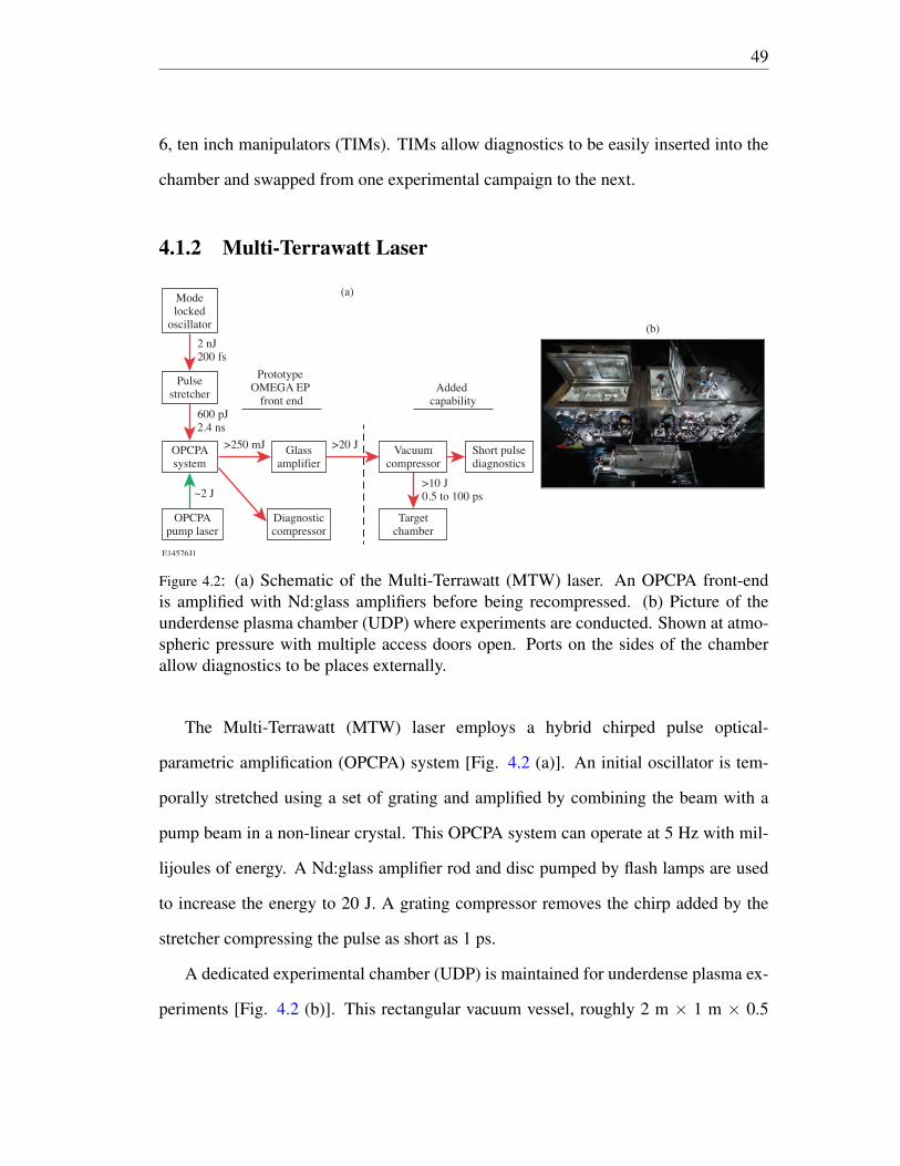
49
6, ten inch manipulators (TIMs). TIMs allow diagnostics to be easily inserted into the
chamber and swapped from one experimental campaign to the next.
4.1.2 Multi-Terrawatt Laser
Figure 4.2: (a) Schematic of the Multi-Terrawatt (MTW) laser. An OPCPA front-endis amplified with Nd:glass amplifiers before being recompressed. (b) Picture of theunderdense plasma chamber (UDP) where experiments are conducted. Shown at atmo-spheric pressure with multiple access doors open. Ports on the sides of the chamberallow diagnostics to be places externally.
The Multi-Terrawatt (MTW) laser employs a hybrid chirped pulse optical-
parametric amplification (OPCPA) system [Fig. 4.2 (a)]. An initial oscillator is tem-
porally stretched using a set of grating and amplified by combining the beam with a
pump beam in a non-linear crystal. This OPCPA system can operate at 5 Hz with mil-
lijoules of energy. A Nd:glass amplifier rod and disc pumped by flash lamps are used
to increase the energy to 20 J. A grating compressor removes the chirp added by the
stretcher compressing the pulse as short as 1 ps.
A dedicated experimental chamber (UDP) is maintained for underdense plasma ex-
periments [Fig. 4.2 (b)]. This rectangular vacuum vessel, roughly 2 m × 1 m × 0.5
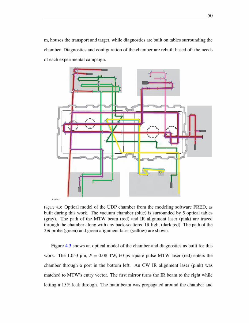
50
m, houses the transport and target, while diagnostics are built on tables surrounding the
chamber. Diagnostics and configuration of the chamber are rebuilt based off the needs
of each experimental campaign.
Figure 4.3: Optical model of the UDP chamber from the modeling software FRED, asbuilt during this work. The vacuum chamber (blue) is surrounded by 5 optical tables(gray). The path of the MTW beam (red) and IR alignment laser (pink) are tracedthrough the chamber along with any back-scattered IR light (dark red). The path of the2ω probe (green) and green alignment laser (yellow) are shown.
Figure 4.3 shows an optical model of the chamber and diagnostics as built for this
work. The 1.053 µm, P = 0.08 TW, 60 ps square pulse MTW laser (red) enters the
chamber through a port in the bottom left. An CW IR alignment laser (pink) was
matched to MTW’s entry vector. The first mirror turns the IR beam to the right while
letting a 15% leak through. The main beam was propagated around the chamber and

51
focused to the interaction volume slightly to the left of the center of the chamber. The
main beam was focused∼1.4 mm before the interaction volume using an f/9 geometry.
The beam was relayed out to the table on the top left where the focal spot was reimaged.
This focal spot diagnostic was used to measure the diameter of the approximately Gaus-
sian focal spot, 200 µm (r = 100 µm) [Full width at half maximum (FWHM)], which
provided a spatially (A = πr2) averaged intensity of I = P/A = 2.5× 10¹⁴ W/cm2 at
the interaction volume in vacuum. A pellicle along the final focusing vector reflected a
small amount of light to the pointing and centering diagnostics, table on the right, aid-
ing in alignment. The pellicle also reflected any light backscattered from the interaction
volume (dark red) up to an energy meter and IR spectrometer.
The initial 15% leak of the main beam was reflected by a second leaky mirror. The
leak through this second leaky mirror was used to diagnose the pointing and center-
ing of MTW’s path into the chamber. The reflected light was frequency doubled with a
KDP crystal to produce a 2ω probe with the same 60 ps square pulse as the MTW beam
and a linear chirp (0.05 nm/ps). The 2ω probe was split in two; one part being used for
interferometry (light green) and the other for Thomson scattering (dark green). The por-
tion split for the Thomson scattering probe was transported with a k-mirror periscope;
a series of three mirrors that rotated the polarization [95]. Both green beams utilized
trombone delay stages, a set of mirror mounted on a movable platform to increase or
decrease the path length, this allowed all beams to be precisely timed relative to each
other. During the experiment the probe was delayed 40 ps from the heater beam, re-
sulting in a 20 ps temporal overlap of the beams. A pick-off of the Thomson-scattering
beam was taken to measure the converted energy. The Thomson-scattering probe beam
was focused at f/20 to the interaction volume at 43 to the main beam. The probe’s
focal spot was imaged onto a camera, on the bottom right table, to ensure the probe
was properly aligned. A green alignment laser (not shown) could be injected onto the

52
same path as the Thomson-scattering probe, while a second green alignment laser (yel-
low) could be injected from the bottom right onto the path of the Thomson-scattering
collection.
The Thomson-scattered light (teal), from a 60 µm × 60 µm × 40 µm volume, was
collected by an f/3 optic at 80 relative to the probe beam (resulting in a 100 scattering
angle). The light passed through a 532 nm dielectric notch filter with a spectral width
of 28 nm to reject the portion of the spectrum associated with ion acoustic waves, or
other scattering of the probe beam. The collimated light was imaged to the 75 µm input
aperture of an ultrafast streaked spectrometer system [96] by an f/4 achromat.
4.2 Gas jet
The target for experiments on both the OMEGA and MTW laser systems was the gas
plume of a supersonic gas jet [97]. A gas jet provides a uniform density of neutral gas
over a few millimeters with a sharp drop-off at the edge. This is useful for basic plasma
and laser-plasma experiments where a uniform density is desirable, and superior to
other techniques, such as gas bags and tubes which have a solid density film that must
be ablated first. This gas-jet system also utilizes a electromagnetically controlled fast
opening valve, suited for many gases, in order to supply gas at high pressure without
discharging large volumes of gas.
An analytic model of the gas jet’s density profile was derived based off a compress-
ible ideal ges in a supersonic converging/diverging geometry[97]. Figure 4.4 shows this
geometry. Gas released from the reservoir accelerates toward the throat of the nozzle,
where the flow velocity equals the speed of sound at the throat. After leaving the throat
the gas undergoes isentropic adiabatic expansion leading to the supersonic velocities.
Exiting the nozzle the gas is traveling supersonicly with a Mach number (M) related to

53
Figure 4.4: Sketch of a converging/diverging nozzle. In the converging section the flowis subsonic, in the diverging section it is supersonic. Image reproduced from Hansen etal. [97].
the nozzle exist area (A) and the throat area (A∗),
AA∗
=1M
[2+(γ−1)M2
γ +1
] γ+12(γ−1)
. (4.1)
The gas travels supersonicaly out of the nozzle, but only expands at the speed of
sound (cs) transverse to the flow. This maintains a cone of gas with steep edges. The
uniform density within the cone at a distance L from the nozzle is given by,
ρ(L)∼= ρ01(
1+ γ−12 M2
) 1γ−1
(Dexit
Dexit +2 LM
)2
. (4.2)
For this work, nozzles with an exit diameter of 1 mm were used on MTW with the
interaction volume 1 mm above the nozzle. On OMEGA, a 2mm exit diameter was
used with the interaction volume (TCC) 2 mm above the nozzle. These nozzles had a
Mach number of 3 for monoatomic gases (Ar and Kr) and 2.6 for diatomic gases (H2
and N2).

54
Figure 4.5: General Thomson-scattering setup consisting of a probe, relay and spectrom-eter. A defined Thomson scattering volume is established with the intersection of theprobe beam and projection of the aperture stop into the plasma. A wave vector dia-gram shows how the scattering angle, angle between the probe and collection vectors,dictates the probed k-vector.
4.3 Thomson-scattering experimental setups
A typical Thomson-scattering system consists of three components: probe beam, scat-
tered light relay, and spectrally resolved detector. Figure 4.5 shows a general Thomson-
scattering setup with these components. The probe provides a source of photons to be
scattered, the relay collects scattered light and images it to a spectrometer, which dis-
perses the light in wavelength space, so the spectrum discussed in Chapter 3 can be
observed and recorded.
The power scattered (Eq. 3.1) provides an insight into one of the main difficulties in
Thomson scattering. Plugging in some characteristic numbers for a laser plasma (L =
100µm,∫
dΩ = 10−2 sr, ne = 1018−20 cm-3) the power ratio Ps/P0 is roughly 10−12−
55
10−10. With the input power being limited to ∼ 1011 W, to prevent fillamentation, a
sensitive diagnostic is required. Additionally, it is advantageous to remove all other
sources of light that might degrade the signal-to-noise ratio (SNR).
A probe beam with a wavelength unique to other beams in the experiment is often
used to isolate the Thomson scattering spectrum. While it is possible for the heating
beam to act as the probe beam, often referred to as self-Thomson-scattering, in multi-
beam experiments the scattering from overlapping beams can make data difficult to
interpret. A common choice is to use a low harmonic of the heater beams. A sepa-
rate probe beams provides more control over the timing, positioning, and power of the
probe. Independent control of the probe beam’s power can be used to prevent filla-
mentation. Increasing the probe power to get a stronger Thomson-scattering signal is
not always an option as high power can lead to pondermotive fillamentation, which can
break up or divert the beam.
An aperture stop is a useful addition to the relay system. While not strictly re-
quired, it limits the collection volume, allowing the collection volume to be matched
to the probe’s size. This prevents collecting background light from a larger volume
than Thomson-scattering light. The aperture stop also allows the measured volume to
be smaller then the whole plasma. Gradients in plasma conditions as a function of
time or space can blur the Thomson-scattering features and a small scattering volume
helps limit these issues. The relay system as a whole must be achromatic over the
wavelength range of interest. This often requires special achromatic lenses or reflective
transport for collective electron plasma wave measurements, which can span hundreds
of nanometers [89].
Some other considerations in the design and analysis of Thomson scattering, are
the instrumental response and finite aperture effects [98]. Instrumental response is the
combination of geometric and diffractive performance of the optical system. For a
56
spectrometer system, the spectral response can be measured by collecting light from a
line emitter such as a mercury lamp. This provides known spectral lines with negligi-
ble spectral width, therefore the measured spectral width will reflect the instrumental
response. For systems that collect with small f-numbers, or have probes focused with
small f-numbers, there is a significant range of angles that are collected. The scattering
angle, the angle between the probes direction and the scattering direction, can vary as
a function of location on the collection optic. This means the measured spectrum is
integrated over some range of scattering angles. Finite aperture effects are important to
consider if large collection optic are used to collect more light.
The spectrometer was coupled to a camera to record data. Since the camera is ca-
pable of measuring along two independent axes, there is an opportunity to gain more
information about the plasma by utilizing this second dimension, the first being fre-
quency. The following sections will examine various versions where the second axis is
space, time, or scattering angle.
4.3.1 Imaging Thomson scattering on OMEGA
An image of the plasma is presented to the aperture stop and the input of the spec-
trometer, if the image is maintained in the non-dispersed direction with an imaging
spectrometer, then the resulting data measures the Thomson scattering as a function of
wavelength and one spacial dimension. The spatially-resolved Thomson-scattering di-
agnostic on OMEGA [95] simultaneously resolved both the high-frequency (electron-
plasma wave) and low-frequency (ion-acoustic wave) features. This system has two
sections, a TIM based collection system, and a fixed optical table with the spectrome-
ters and cameras. The all reflective collection system gathers an f/10 cone of scattered
light using an off-axis section of a Schwarzschild objective, and relays the light from
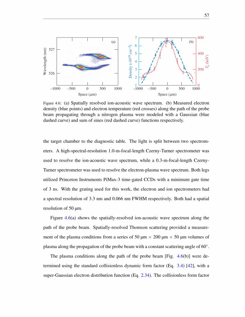
57
Figure 4.6: (a) Spatially resolved ion-acoustic wave spectrum. (b) Measured electrondensity (blue points) and electron temperature (red crosses) along the path of the probebeam propagating through a nitrogen plasma were modeled with a Gaussian (bluedashed curve) and sum of sines (red dashed curve) functions respectively.
the target chamber to the diagnostic table. The light is split between two spectrom-
eters. A high-spectral-resolution 1.0-m-focal-length Czerny-Turner spectrometer was
used to resolve the ion-acoustic wave spectrum, while a 0.3-m-focal-length Czerny-
Turner spectrometer was used to resolve the electron-plasma wave spectrum. Both legs
utilized Princeton Instruments PiMax-3 time-gated CCDs with a minimum gate time
of 3 ns. With the grating used for this work, the electron and ion spectrometers had
a spectral resolution of 3.3 nm and 0.066 nm FWHM respectively. Both had a spatial
resolution of 50 µm.
Figure 4.6(a) shows the spatially-resolved ion-acoustic wave spectrum along the
path of the probe beam. Spatially-resolved Thomson scattering provided a measure-
ment of the plasma conditions from a series of 50 µm × 200 µm × 50 µm volumes of
plasma along the propagation of the probe beam with a constant scattering angle of 60.
The plasma conditions along the path of the probe beam [Fig. 4.6(b)] were de-
termined using the standard collisionless dynamic form factor (Eq. 3.4) [42], with a
super-Gaussian electron distribution function (Eq. 2.34). The collisionless form factor

58
was simultaneously matched to the ion-acoustic wave and electron-plasma wave spec-
tra to obtain the plasma conditions. To first order, the electron temperature and density
were determined from the electron plasma wave features, while the ionization state was
determined from the ion-acoustic wave feature.
4.3.2 Time resolved Thomson scattering on OMEGA
The OMEGA Thomson scattering system can be coupled to a Rochester optical streak
system (ROSS) to measure the Thomson-scattered light as a function of time [89].
A streak camera takes a line image presented to the entrance slit, and images it to a
photocathode, converting the light to electrons. The electrons are accelerated down the
streak tube and a time varying voltage is applied to a set of deflection plates, causing
electrons arriving at different times to land in different positions on a phosphor screen.
The light emitted by the phosphor screen is recorded by a CCD.
Figure 4.7: (a) Temporally resolved electron-plasma wave spectrum and (b) ion-acousticwave spectrum without background subtraction.
The temporally resolved Thomson-scattering diagnostic on OMEGA simultane-
ously resolved both the high-frequency [electron-plasma wave, Fig. 4.7 (a)] and low-
frequency [ion-acoustic wave, Fig. 4.7 (b)] features from a 100 µm × 50 µm × 50 µm

59
volume of plasma at TCC. The temporally resolved system operates at the same scat-
tering angle as the spatially resolved system (θ = 60) [89].
4.3.3 Ultrafast time resolved Thomson scattering on MTW
Ultrafast streak cameras are capable of picosecond temporal resolutions, however spec-
trometers limit this resolution. Light dispersed by a grating is reflected or transmitted
at an angle with respect to the input beam, resulting in a different optical path length
for light from the top and bottom of the grating. This pulse front tilt (PFT) can degrade
the temporal resolution of a streaked spectrometer depending on the required spectral
resolution. In order to measure Thomson scattering with picosecond resolution, the
pulse front tilt must be optimized with the required spectral resolution.
Figure 4.8: (a) A schematic of the experimental setup on MTW is shown with the heater(red) and probe (green) beams incident on the gas jet. The heater beam was imaged ona focal-spot diagnostic. Thomson-scattered light was collected by an f/3 optic at 80
relative to the probe beam (resulting in a 100 scattering angle). (b) Thomson-scatteringspectrum measured from a plasma heated by an intensity of 2.5× 10¹⁴ W/cm2. Theheater beam begins at t=0 ps and the probe beam at t=40 ps.
A f/3 pulse-front-tilt compensated spectrometer was coupled to an ultrafast optical
streak camera (ROSS P820) [Fig. 4.8 (a)]. The spectrometer used an echelon to trade
unrealized resolving power for improved temporal resolution [96]. The echelon was

60
created by stacking a series thin mirror segments with an offset between their faces.
This staircase-like reflective optic separated the beam into pieces with varying delay,
counteracting the pulse-front tilt induced by the grating. Using an echelon, degraded
the spectral resolution to match the resolution the streak camera, as set by the electron
optics. The temporal response function was measured with a fully compressed pulse
from the Multi-Terawatt laser system to be 2.2 ps FWHM [17]. The spectral instrument
response (1.27 nm FWHM) and the spectral dispersion were measured using the emis-
sion lines of a mercury lamp. The spectral instrument response was dominated by the
diameter of the entrance aperture of the spectrometer.
Figure 4.8 (b) shows a Thomson-scattering spectrum measured from an argon
plasma. The angle between the Thomson-scattering probe beam and the collection
optics (80) was chosen to maximize the ability to determine the shape of the electron
distribution function. The electron plasma wave spectral features were clearly resolved
along with the light scattered between the features, which results from the relatively
large Landau damping (kλD ∼ 0.6). The spectra throughout have been summed over
two resolution units in wavelength and time.
4.3.4 Angularly resolved Thomson scattering on OMEGA
A diagnostic was invented to measure the angularly resolved Thomson-scattering spec-
trum discussed in Section 3.4. Figure 4.9 shows the angularly resolved Thomson-
scattering instrument, which collected light from a small collection volume and ulti-
mately imaged it with wavelength dispersed along one axis and scattering angle along
the other. The large primary mirror was located ∼100 mm from the plasma and col-
lected light over 108 in scattering angle, the angle between the probe vector and col-
lection vector. In the tangential plane, referred to as the spectral direction, light was

61
Figure 4.9: (a) Experimental setup. The Thomson-scattering probe laser (green) and theview from the temporally or spatially resolved Thomson-scattering instrument (black)are shown. (b) The wave vectors probed by the angularly resolved instrument. (c) Awire-frame model of the angularly resolved Thomson-scattering instrument with rayfans, originating in the collection volume, showing the path of sagittal (green) andtangential (blue) rays..
integrated over 11.5. In this direction the angular information was not preserved and
therefore did not contribute to the diagnostics 1 angular resolution. Two wires were
placed over the primary mirror to aid in calibration of the angular axis, resulting in
small dips in the spectra near 40 and 110 (not shown in Fig. 4.9).
The primary rectangular section of a spherical mirror that was approximately
200 mm × 50 mm (primary mirror) reflected the collected light back onto an aspheric
secondary mirror in an off-axis Schwarzchild configuration, collimating the collected
light. The aspheric secondary mirror corrected spherical aberration due to the extreme
working angle of the secondary mirror. The light was imaged through a field stop at
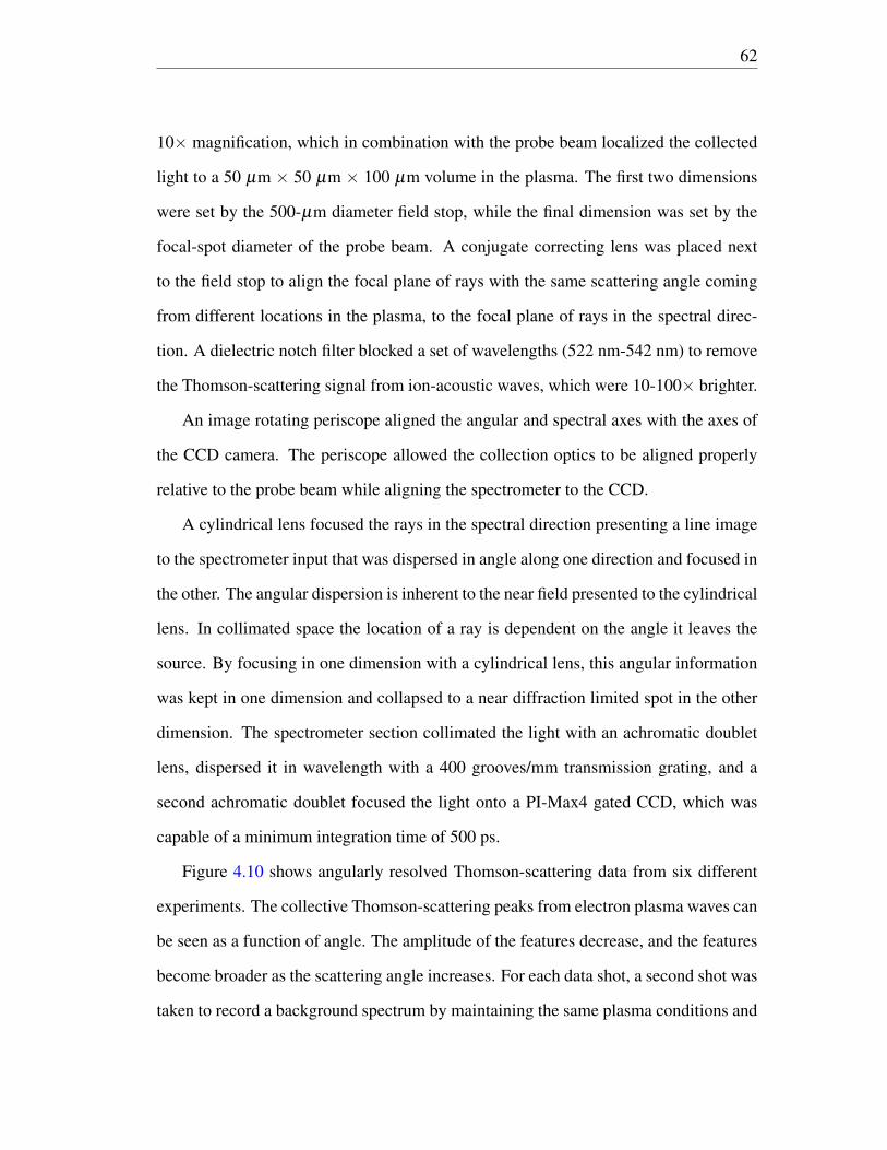
62
10× magnification, which in combination with the probe beam localized the collected
light to a 50 µm × 50 µm × 100 µm volume in the plasma. The first two dimensions
were set by the 500-µm diameter field stop, while the final dimension was set by the
focal-spot diameter of the probe beam. A conjugate correcting lens was placed next
to the field stop to align the focal plane of rays with the same scattering angle coming
from different locations in the plasma, to the focal plane of rays in the spectral direc-
tion. A dielectric notch filter blocked a set of wavelengths (522 nm-542 nm) to remove
the Thomson-scattering signal from ion-acoustic waves, which were 10-100× brighter.
An image rotating periscope aligned the angular and spectral axes with the axes of
the CCD camera. The periscope allowed the collection optics to be aligned properly
relative to the probe beam while aligning the spectrometer to the CCD.
A cylindrical lens focused the rays in the spectral direction presenting a line image
to the spectrometer input that was dispersed in angle along one direction and focused in
the other. The angular dispersion is inherent to the near field presented to the cylindrical
lens. In collimated space the location of a ray is dependent on the angle it leaves the
source. By focusing in one dimension with a cylindrical lens, this angular information
was kept in one dimension and collapsed to a near diffraction limited spot in the other
dimension. The spectrometer section collimated the light with an achromatic doublet
lens, dispersed it in wavelength with a 400 grooves/mm transmission grating, and a
second achromatic doublet focused the light onto a PI-Max4 gated CCD, which was
capable of a minimum integration time of 500 ps.
Figure 4.10 shows angularly resolved Thomson-scattering data from six different
experiments. The collective Thomson-scattering peaks from electron plasma waves can
be seen as a function of angle. The amplitude of the features decrease, and the features
become broader as the scattering angle increases. For each data shot, a second shot was
taken to record a background spectrum by maintaining the same plasma conditions and

63
Figure 4.10: Angularly resolved Thomson-scattering data from six shots. The data wastaken in (a,b,c,f) krypton, (d) hydrogen, and (e) argon. Plasma conditions for each shotare given in Table 4.1.
turning off the probe beam. The background spectrum has been subtracted from the
results presented in Fig. 4.10.
The gas type, heater beam intensity, measured density, and electron temperature
for each shot are shown in Table 4.1. The density was fairly consistent across the
shots, showing a shot-to-shot rms variation of 13%. Shot 95831 was the only shot
with the delayed probe configuration (probing after the heating lasers were turned off),
providing more time for the plasma to expand and cool. The variation in electron
temperatures was due to differences in laser intensities and heating efficiencies.
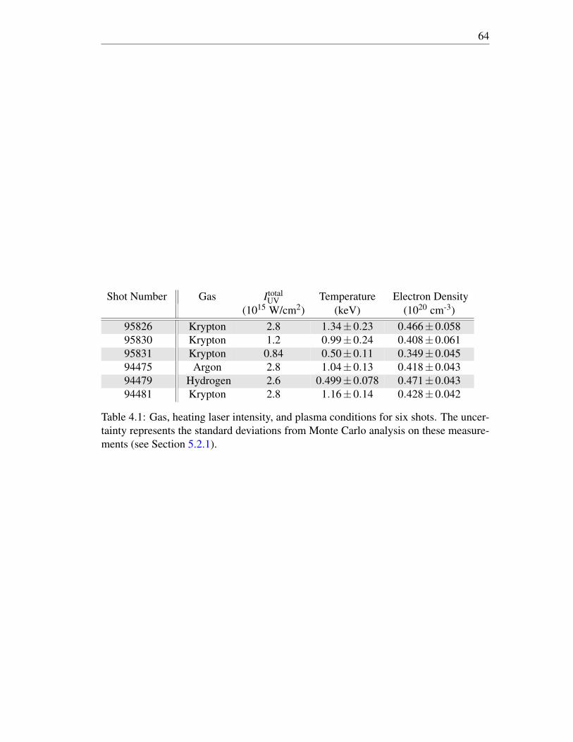
64
Shot Number Gas ItotalUV Temperature Electron Density
(1015 W/cm2) (keV) (1020 cm-3)95826 Krypton 2.8 1.34±0.23 0.466±0.05895830 Krypton 1.2 0.99±0.24 0.408±0.06195831 Krypton 0.84 0.50±0.11 0.349±0.04594475 Argon 2.8 1.04±0.13 0.418±0.04394479 Hydrogen 2.6 0.499±0.078 0.471±0.04394481 Krypton 2.8 1.16±0.14 0.428±0.042
Table 4.1: Gas, heating laser intensity, and plasma conditions for six shots. The uncer-tainty represents the standard deviations from Monte Carlo analysis on these measure-ments (see Section 5.2.1).

65
Chapter 5
Results
This Chapter shows the results of experiments measuring the electron distribution func-
tion and its effect on laser absorption. Electron velocity distribution functions have been
measured over many orders of magnitude for the fist time. Over the course of this work,
experimental and analysis techniques progressed from the ability to infer the distribu-
tion function in single-angle Thomson scattering, to matching Thomson scattering with
simulated distribution functions, to direct measurements of distribution functions using
angularly resolved Thomson scattering. Each improvement provided increasing detail
about the distribution function and the processes occurring within the plasma. Sec-
tion 5.1 discusses the single-angle Thomson scattering results, both the ability to infer
super-Gaussian order (Sec. 5.1.1) and measurements of ionization kinetics by match-
ing data with simulations (Sec. 5.1.2). Section 5.2 discusses the distribution functions
measured with angularly resolved Thomson scattering. A detailed description of the al-
gorithm and thought process behind analysing this new kind of data is given in Section
5.2.1, while Section 5.2.2 focused on the physical interpretation of the measurements
and comparisons to established theory. Section 5.3 reports measurements of reduced
absorption in super-Gaussian plasmas, a result on the non-Maxwellian shape. A few
outstanding questions are discussed in Section 5.4.

66
5.1 Measurements of non-Maxwellian distributions
Section 3.3 showed the sensitivity of collective Thomson-scattering spectrum to a
super-Gaussian distribution function. While some complications to this were noted,
single-angle collective Thomson scattering can still be a powerful tool in measuring
the super-Gaussian order. Proving out the concept, and the existence of super-Gaussian
distribution function was required before investing in the more complicated angularly
resolved measurements.
Here, we present the first measurements of the interplay between inverse
bremsstrahlung heating and ionization kinetics on the electron distribution function.
An ultrafast Thomson-scattering system was used to collect the electron plasma wave
spectrum, which enabled the picosecond evolution of the non-Maxwellian electron dis-
tribution function to be measured in a laser-produced plasma. The preferential heating
of the slow electrons by a laser beam with an intensity of 2.5× 10¹⁴ W/cm2, cou-
pled with the redistribution of electron kinetic energy due to ionization, resulted in a
non-Maxwellian electron distribution function. The shape of the electron distribution
function, 60 ps into the plasma formation, was measured to be approximately a super-
Gaussian of order 3.4. After the laser turned off, the electron density continued to
increase by 15% over the next 40 ps (∼ 25 electron-ion collision times) due to colli-
sional ionization. Over this time, the electron temperature decreased from 400 eV to
300 eV, which is consistent with the energy required for collisional ionization to in-
crease the density. To determine the electron distribution functions consistent with the
measured Thomson-scattered spectra in this rapidly evolving plasma, Vlasov-Fokker-
Planck simulations that included laser heating, thermal transport and ionization were
required. Laser heating was found to have the largest effect on the shape of the dis-

67
Figure 5.1: (a) Thomson-scattering spectrum measured from a plasma heated by an inten-sity of 2.5×10¹⁴ W/cm2. The heater beam begins at t=0 ps and the probe beam at t=40ps. (b) The measured spectrum at 58 ps (gray points) plotted with spectrum calculatedusing Maxwellian (dashed green curve) and non-Maxwellian (orange curve) electrondistribution functions. The best-fit spectra determined Te= 423 eV, ne= 2.03× 10¹⁹
cm-3, m= 2 (Maxwellian) and Te= 406 eV, ne= 2.04× 1019 cm-3, m= 3.1 (Non-Maxwellian).
tribution function, while atomic kinetics provided a smaller effect, it was required to
match the evolution of plasma conditions.
Thomson-scattering experiments were performed using the Multi-Terawatt laser
[93] at the Laboratory for Laser Energetics (Sec. 4.1.2) in the UDP chamber. The
MTW laser provided a spatially averaged intensity of 2.5×10¹⁴ W/cm2. A supersonic
Mach 3 gas jet [97] with an exit diameter of 1 mm was pressurized with argon (Ar)
to 50 psi to achieve a neutral gas density of 2.4× 1018 cm-3 at 1 mm above the noz-
zle. The Thomson-scattering probe beam, with a spatially averaged intensity of ∼ 1014
W/cm2, arrived at the interaction volume 40 ps after the heater beam, resulting in a 20
ps temporal overlap of the beams. Thomson scattering was measured with the ultrafast
time-resolved Thomson-scattering system (Sec. 4.3.3).

68
5.1.1 Evidence of non-Maxwellian distribution functions
Figure 5.1 shows a time resolved Thomson-scattering spectrum measured from an ar-
gon plasma. The spectrum [Fig. 5.1(b)] just prior to turning off the heater beam (∼ 58
ps) shows the effect of inverse bremsstrahlung heating through the modification of the
electron distribution function and the need to include non-Maxwellian electron distribu-
tion functions to accurately reproduce the measured spectra. When limiting the spectral
fit to Maxwellian electron distribution functions, the spectrum fails to reproduce three
regions of the measurements: (1) the calculations underestimate the light scattered into
the central region of the spectrum (∼500 nm to ∼550 nm), (2) the widths of the scat-
tering features are too broad, and (3) the slope on the outermost edges of the scattering
peaks are too shallow.
When calculating the spectra in Fig. 5.1, a super-Gaussian electron distribution
function was assumed, fm =Cm exp[−(v/vm)m] (see Eq. 2.34). A super-Gaussian elec-
tron distribution function significantly improves the fit in all three regions and reduces
the χ2 per degree of freedom from 3.75 to 1.33. This large improvement in χ2 per
degree of freedom is a result of the model doing a better job matching the center of the
variation, instead of the edge, removing any systematic trends from the residuals.
The calculated spectra were determined through a 3-dimensional (m, Te, ne) χ2 =
∑λ
[P(λ )−Ps(λ )]2
1.15Ps(λ )minimization of the measured spectrum [Ps(λ )] and the calculated power
(Eq. 3.1). The electron susceptibility (Eq. 3.5) was determined numerically and the
calculated scattered power was adjusted to account for the finite aperture effects in the
data [98] and the spectral response of the instrument (Sec. 4.3).
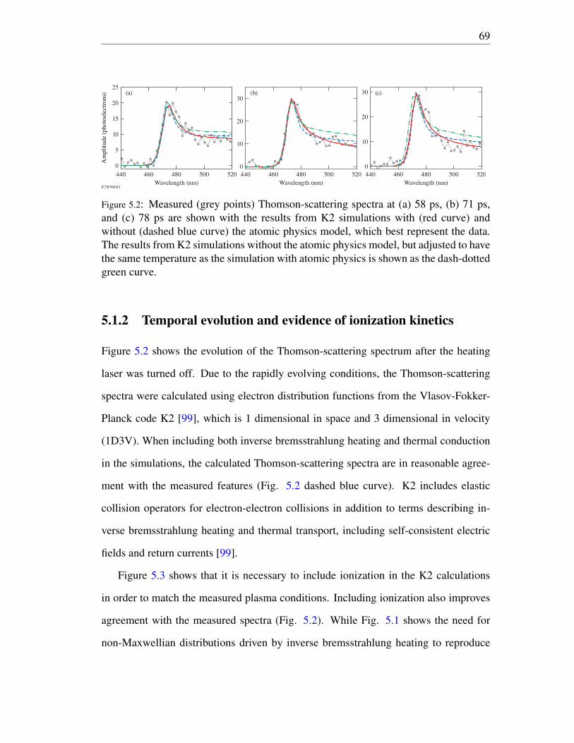
69
Figure 5.2: Measured (grey points) Thomson-scattering spectra at (a) 58 ps, (b) 71 ps,and (c) 78 ps are shown with the results from K2 simulations with (red curve) andwithout (dashed blue curve) the atomic physics model, which best represent the data.The results from K2 simulations without the atomic physics model, but adjusted to havethe same temperature as the simulation with atomic physics is shown as the dash-dottedgreen curve.
5.1.2 Temporal evolution and evidence of ionization kinetics
Figure 5.2 shows the evolution of the Thomson-scattering spectrum after the heating
laser was turned off. Due to the rapidly evolving conditions, the Thomson-scattering
spectra were calculated using electron distribution functions from the Vlasov-Fokker-
Planck code K2 [99], which is 1 dimensional in space and 3 dimensional in velocity
(1D3V). When including both inverse bremsstrahlung heating and thermal conduction
in the simulations, the calculated Thomson-scattering spectra are in reasonable agree-
ment with the measured features (Fig. 5.2 dashed blue curve). K2 includes elastic
collision operators for electron-electron collisions in addition to terms describing in-
verse bremsstrahlung heating and thermal transport, including self-consistent electric
fields and return currents [99].
Figure 5.3 shows that it is necessary to include ionization in the K2 calculations
in order to match the measured plasma conditions. Including ionization also improves
agreement with the measured spectra (Fig. 5.2). While Fig. 5.1 shows the need for
non-Maxwellian distributions driven by inverse bremsstrahlung heating to reproduce

70
Figure 5.3: The measured (a) temperature and (b) density (black circles) are compared toK2 simulation results. The black error bars represent a 95% confidence interval in thegiven parameter. The results of a K2 simulation without atomic kinetics (dashed bluecurves) and the results of a K2 simulation with atomic physics (red curve) are shown.
the spectra, the electron density and temperature reveal the need to include an atomic
physics model. Without ionization, it is not possible to match the density, which rises
by ∼ 15% after the heating beam is turned off. During this time, the collisional ioniza-
tion continues resulting in the rising density (Fig. 5.3). This process uses the kinetic
energy of the free electrons to ionize the plasma further, thereby lowering the tempera-
ture. Without ionization, the simulations lack this energy loss mechanism and therefore
overestimated the temperature by ∼ 15% to 20%. In simulations without ionization,
it is possible to alter the initial plasma conditions to achieve better agreement with the
temperature (Fig. 5.2), but this results in distribution functions that generate spectra
with poor agreement with the measured Thomson-scattering spectra. By coupling K2
with an atomic kinetics model, not only was it possible to account for the temperature
and density evolution, the electron distribution functions were modified bringing the
calculated Thomson-scattering spectra into better agreement with the measurements.
The improved agreement can be seen (Fig. 5.2) in the slightly wider peak and lower
central region of the model with ionization. Resulting in an improved minimum χ2,

71
which was 10% to 15% smaller than the model without atomic kinetics for each case.
The improved spectral match in conjunction with the ability to reproduce the tempera-
ture and density evolution necessitate the inclusion of the atomic physic model.
In laser-produced plasmas, inverse bremsstrahlung heating [22, 23, 32], thermal
transport [37, 38], laser-plasma instabilities [39], and atomic kinetic processes [40] all
provide competing mechanisms that govern the shape of the electron distribution func-
tion. To determine the impact of ionization on the electron distribution function, an
atomic physics model was coupled to K2. An inelastic collsional operator, sometimes
called a Boltzmann operator, was used to model the changes to the distribution due to
all atomic processes. The time evolution of the atomic states were determined through
a set of coupled rate equations. The collisional rates that enter the rate matrix were ob-
tained from direct integration of the actual distribution. The atomic data (energy levels
and cross sections) was constructed based on a screened hydrogenic model using the
code Cretin [100]. While the model used for these simulations includes different types
of collisional and radiative processes (both bound-bound and bound-free), collisional
ionization was identified as the main atomic process affecting the distribution function
[40]. The simulations were performed using the experimental laser conditions. Simu-
lations performed without the atomic physics model used a preionized plasma with an
electron density of 2.2×1019 cm-3 (corresponding to an average ionization state of 9.1)
and an electron temperature of 10 eV. When using the atomic physics model, ioniza-
tion was self-consistently included and the simulations were initialized with a neutral
density of 2.4×1018 cm-3.
Figure 5.4(a) shows the relative contributions of inverse bremsstrahlung heating,
thermal transport, and atomic physics on the electron distribution function. The main
deviation from Maxwellian was due to inverse bremsstrahlung heating and results in
a reduction of slow electrons and an increase in electrons with a velocity of ∼ 1.5vth.

72
E28591J2
0.06
0.04
0.02f e
v/vth
10 2 3
v/vth
10 2 3
(a) (b)
0.00
Figure 5.4: (a) Electron distribution functions calculated by K2 when including (redcurve) and not including (blue curve) the atomic physics model at the end of the heaterbeam (60 ps) compared with a Maxwellian electron distribution function (dashed greencurve). (b) Electron distribution functions at 58 ps (red), 71 ps (orange) and 78 ps(green) calculated by K2 including the atomic physics model.
Heat transport compounds with the effect of inverse bremsstrahlung heating by further
increasing the number of bulk electrons. The electrons in the tail of the electron distri-
bution function carry heat away from the Thomson-scattering volume while the slower
electrons, that maintain charge neutrality, reinforce the bulk of the electron distribution
function. Ionization suppresses the super-Gaussian shape by preferentially removing
electrons from around 2−3vth and supplying electrons with little to no velocity.
Figure 5.4(b) shows how the distribution function evolves. The electron distribution
at 58 ps, while the heater beam is on, was driven to a non-Maxwellian shape. It rapidly
(< 10 ps) evolves to a new super-Gaussian distribution, but is still non-Maxwellian.
Once this new electron distribution has been realized, the evolution slows and only
small changes to the distribution continue through the end of the measurement (100
ps).
In summary, ultrafast Thomson-scattering measurements of the electron-plasma
wave spectrum were used to determine the effects of laser heating and ionization on
73
the electron distribution function. While the argon plasma was being heated, super-
Gaussian electron distribution functions were measured. After the heater beam was
turned off, the electron density continued to rise and the electron temperature dropped
as the free electrons continued to ionize the argon plasma.
Non-Maxwellian electron distribution functions from Vlasov-Fokker-Planck simu-
lations that included both laser heating and ionization were required to reproduce the
measured Thomson-scattering spectra, temperature evolution, and density evolution
simultaneously. Thereby demonstrating the interplay between the effects of inverse
bremsstrahlung and atomic kinetics on the shape of the electron distribution function,
and the level of complexity needed to model the distribution function in simple experi-
ments.
5.2 Measurements of arbitrary distribution functions
Angulary resolved Thomson scattering provides a method to measure the electron dis-
tribution function without assuming a functional form, such as super-Gaussian, or mod-
eling the experiment with kinetic simulations. This allows the measured distribution
function to capture all the relevant physics without needing to specify what that rel-
evant physics is a priori. This technique combines the collective and non-collective
regimes in order to directly measure the electron velocity distribution function over
many orders of magnitude (see Section 3.4).
Here, we present the first measurements of complete electron distributions with-
out any assumptions on their shape or the underlying physics that produced them.
At these conditions the inverse bremsstrahlung heating dominated over thermaliza-
tion by electron-electron collisions. To enable single-shot temporally and spatially
resolved measurements of the electron distribution function over several orders of

74
Figure 5.5: Schematic of the experimental configuration. Five UV beams (purple) heatthe gas (yellow) from a supersonic Mach-3 gas jet (gray). A green beam represents theprobe beam used for Thomson scattering.
magnitude, an optical diagnostic was invented that uses the angular dependence of
scattering to simultaneously access the non-collective and collective nature of plas-
mas. This first-principles measurement showed that during significant heating by the
laser beams, the distributions had a super-Gaussian shape in the bulk (v < 3vth) with
a Maxwellian tail (v > 3vth). The super-Gaussian bulk is associated directly with
the inverse bremsstrahlung heating and is well reproduced by the previous computa-
tional work[23]. The departure from super-Gaussian at high velocities was predicted
by Fourkal et al.[32], but these measurements show this deviation at a higher veloc-
ity. Particle simulations show improved agreement and demonstrate the importance of
isotropic heating in accurately predicting the high-velocity tail.
Angularly resolved Thomson scattering experiments that measured non-
Maxwellian electron distribution functions resulting from laser heating were conducted
on the OMEGA Laser System[94] at the Laboratory for Laser Energetics. Figure 5.5
shows the experimental configuration where five ultraviolet (351-nm UV) laser beams
75
were used to ionize and heat a gas. The uniform density neutral gas plume of argon,
krypton, or hydrogen was produced using a supersonic Mach-3 gas jet[97] with an exit
diameter of 2 mm. To improve the uniformity of heating, each of the five UV heat-
ing beams used a distributed phase plate, polarization smoothing, and smoothing by
spectral dispersion. This ultimately provided Gaussian focal spots, 2 mm above the
center of the gas jet, with a 1/e2 diameter of 400 µm. The heating beams had a 500-ps
pulse duration, full-width at half-maximum (FWHM), and 50 J to 200 J per beam. This
resulted in a total overlapped UV intensity of ItotalUV = 0.62−2.8×10¹⁵ W/cm2.
A 10-J green (526.5 nm) probe beam was focused to the same location as the heating
beams. This probe beam had a shorter 200-ps FWHM duration and was delayed 300 ps
or 600 ps from the rise of the heating beams. This allowed Thomson-scattering mea-
surements at the end of the heating (300 to 500 ps) or shortly after the heating beams
turned off (600 to 800 ps). The probe beam used a distributed phase plate to produce
a flattop focal spot with a 100-µm FWHM diameter (I2ω = 6.5× 10¹⁴ W/cm2). Un-
like the heating beams, the probe did not employ smoothing by spectral dispersion or
polarization smoothing. Instead, the linear polarization was rotated with a waveplate
to maximize the Thomson-scattering efficiency and make it uniform as a function of
angle.
5.2.1 Interpreting ARTS
Algorithm for determining the electron distribution
Figure 4.10 shows the measured angularly resolved Thomson-scattering spectrum
where the ensemble electron motion was encoded on the frequency of the scattered
light. To decode the complete electron distribution function (Fig. 5.9), the total power
76
scattered was calculated across the range of scattering angles,
Ps(λs,θ) =C(2λ0/λ
3s −1/λ
2s)
neS(x), (5.1)
and compared to the measured spectrum. Here, C is a scale factor. The dynamic form
factor (Eq. 3.4) in this regime can be approximated by [42],
S(x)'∣∣∣∣ 11+χRe[x]+ iχIm[x]
∣∣∣∣2 fe[x] (5.2)
where x = ω/kvth is the normalized phase velocity. The frequency of the probed fluc-
tuation is ω = 2πc(
1λs− 1
λ0
). This normalization removes temperature from the dis-
tribution function and it allows representing all Maxwellian distributions regardless of
temperature with a single function. The ion dependence in the dynamic form factor
was removed because the measurements were made only for ω/k & vth where the ion
contribution is negligible.
By assuming the distribution function is isotropic over the range in scattering di-
rections probed, a single projection of the distribution function onto each of the probed
vectors was used. To maintain the highest level of generality, the one-dimensional elec-
tron distribution function projected along the probed fluctuations was defined as a set of
points, fe[x], where the square brackets are used to denote the discrete domain, which
consisted of 64 points. To increase the resolution of the spectral calculation, exponen-
tial interpolation of the electron distribution function between the points was used.
The electron velocity distribution function, measured in the spectra, and plasma
conditions (Table 4.1) were determined simultaneously using an iterative gradient de-
scent algorithm. A numerical distribution function ( fe[x]) was used to forward calculate
a fluctuation spectrum (Eq. 5.2). This spectrum was used to calculate the synthetic
77
power scattered (Eq. 5.1), which was compared to the experimentally measured spec-
trum using,
χ2 = ∑
λs
115
∑θ=40
[Pm(λs,θ)−Ps(λs,θ)]2
σ2 . (5.3)
where σ is the variation of the data, which was ∼ 5% of the signal for all shots, found
by examining the variation in the spectrum at large wavelengths. The region with scat-
tering angles < 40 was excluded because accurate calculation required orders of mag-
nitude higher velocity space resolution. Above a scattering angle of 110 the spectra
generally lacked sufficient signal and were dominated by noise.
A minimization of χ2 over 69 free parameters defining the distribution function (64
points), plasma conditions (ne and Te), and scale parameters (3 parameters) was per-
formed on each shot. The most computationally expensive step was computing the sus-
ceptibility (Eq. 3.5). The real part of the susceptibility was solved using the method of
rational integration [101]. Furthermore, to prevent numerical discontinuities in the sus-
ceptibility from the discrete distribution function, exponential interpolation was used to
produce a continuous distribution function. Convergence was improved by performing
a set of sequential fits with increasing number of distribution function points. Gradi-
ent descent minimizers often struggle to converge for high dimensional problems if the
starting point is too far away from the true values. Fewer points provided significantly
better convergence and starting points for the subsequent minimizations closer to the
optimal values. The discrete domain, equally spaced points spanning [0,7vth], was re-
defined for each minimization requiring the distribution function to be remapped onto
a new set of xs, since the spacing changes each time. This helped overcome local min-
ima by preventing initialization in a local minima. It was found that ∼ 9 distribution
points per thermal velocity (64 points spanning 0− 7vth) was optimal for balancing
computation time and resolving the distribution function.

78
Figure 5.6: (a) Measured and (b) calculated spectra from a krypton plasma used to de-termine the measured electron distribution shown in Fig. 5.9. (c) The measured (blackcurve) and calculated (red curve) spectra at four scattering angles (51, 70, 88, and107) have been arbitrarily spaced along the y-axis.
For each measurement, the background spectrum was measured by repeating the
experiment without the probe beam. The measured spectrum shown [Fig. 5.6 (a)] was
obtained by subtracting the background data from the raw Thomson-scattering spec-
trum. Figure 5.6 (b) shows the final spectrum calculated using the measured distribu-
tion function for shot 94481. Comparing to the experimental spectrum [Fig. 5.6 (a)],
the calculated spectrum qualitatively reproduces the measured spectrum in angle and
wavelength across the entire spectral range [Fig. 5.6 (c)]. Some small discrepancies
are seen at small scattering angle due to numerical artifacts and at high scattering angle
where there is a small clip in the data. The spectrum was corrected for the spectral
transmission of the system. A measurement of the transmission as a function of wave-
length for the entire system was made using a calibrated tungsten lamp placed at the
collection volume.
In order to match the measured spectrum, the effects of temporal gradients, finite
angles, and instrument response were included in the calculation. The instrument re-

79
sponse function was included by convolving the scattered power with a 2-dimensional
Gaussian with a spectral width of 1 nm and angular width of 1, matching the measured
instrument response function. The curvature of the primary mirror and finite solid an-
gle of the probe beam result in a small change in the scattering angle as a function of
height on the mirror. This was included in calculation by treating each angle at the
CCD as a weighted sum of the true constituent scattering angles determined from an
optical model of the instrument.
Figure 5.7: (a) Temporally resolved electron plasma wave spectrum without backgroundsubtraction. (b) Spectrum integrated over the entire duration of the probe beam (blackcurve) is compared with calculated spectra using plasma conditions from the beginning(dashed orange curve) and end of the probe duration (dashed red curve). A calculatedspectrum accounting for the temporal gradient in plasma conditions is shown in blue.(Swap (b) for an IAW spectrum and move (b) to arts section?)
To account for the evolution of the plasma conditions, a range of plasma conditions
were determined from the time-resolved spectrum. Figure 5.7 shows the evolution of
the electron-plasma wave features and the effective broadening of the feature when
time integrated over the duration of the probe. Simulated spectra that match the data at
either the beginning or end of the probe [Fig. 5.7(b)] have the wrong peak wavelength
and smaller width when compared to the measured spectrum integrated over the entire
probe (black curve). By calculating the spectrum integrated over the range of plasma
conditions the peak location and width were matched, while ensuring the spectrum

80
responds appropriately as the scattering angle was changed. The calculated angularly-
resolved spectrum was integrated over this range of plasma conditions.
Reduced model error analysis
A 90% confidence interval was determined for the measured electron distribution func-
tion using the reduced model (Eq. 5.4). This confidence interval is shown as a gray
region in Figure 5.9. Many of the same difficulties faced in calculating the numerical
electron distribution function complicated the uncertainty analysis, preventing direct
calculation of the uncertainties on the numerical distribution function. The high di-
mensionality led to saddle points that prevented the use of Hessian based uncertainty
calculations. More complicated methods such a Monte Carlo or grid analysis were too
computationally expensive.
In order to analyse the quality of the measured distribution functions, a reduced
model comprised of super-Gaussian and Maxwellian functions was introduced,
fe(x) = A1 exp[−(
xx1
)m]+ exp[A2]exp
[−(
xx2
)2]. (5.4)
This model reproduced the distribution function both in the bulk and tail (Fig. 5.9), but
tends to preform worse near the peak (v < 0.5vth). The excellent agreement of the re-
duced model provided an alternative by defining the plasma conditions and distribution
function in 7 parameters, (electron temperature, electron density, and the 5 parameters
of the reduced model). In this lower dimensional space, it was computationally tractable
to perform uncertainty analysis using Markov-chain Monte Carlo. Two additional pa-
rameters were added to determine the sensitivity to calibration of the wavelength axis.
The calibration uncertainty was included to achieve a confidence region on the dis-

81
Figure 5.8: Marginal probability distributions of each parameter in the reduced model(Eq. 5.4) determined from Monte Carlo analysis.
tribution function, which accounts for statistical (model) and instrumental sources of
error.
Figure 5.8 shows the 2-parameter joint and single parameter marginal distributions
from the Monte Carlo analysis. Numerous covariances can be seen between parameters
as the contours are rotated ellipsoids. For two uncorrelated parameters, the contours of
equal probability are circles, while two perfectly correlated parameters would result in
elliptical contours with the semi-major axis aligned to y = x. The width parameter of
the super-Gaussian (x1) is inversely correlated with temperature, density, and ampli-
tude. These are all related to maintaining the normalization of the distribution function.
The positive correlation of the super-Gaussian order (m) and temperature is related to
maintaining the width of the peak in the Thomson-scattering spectrum.
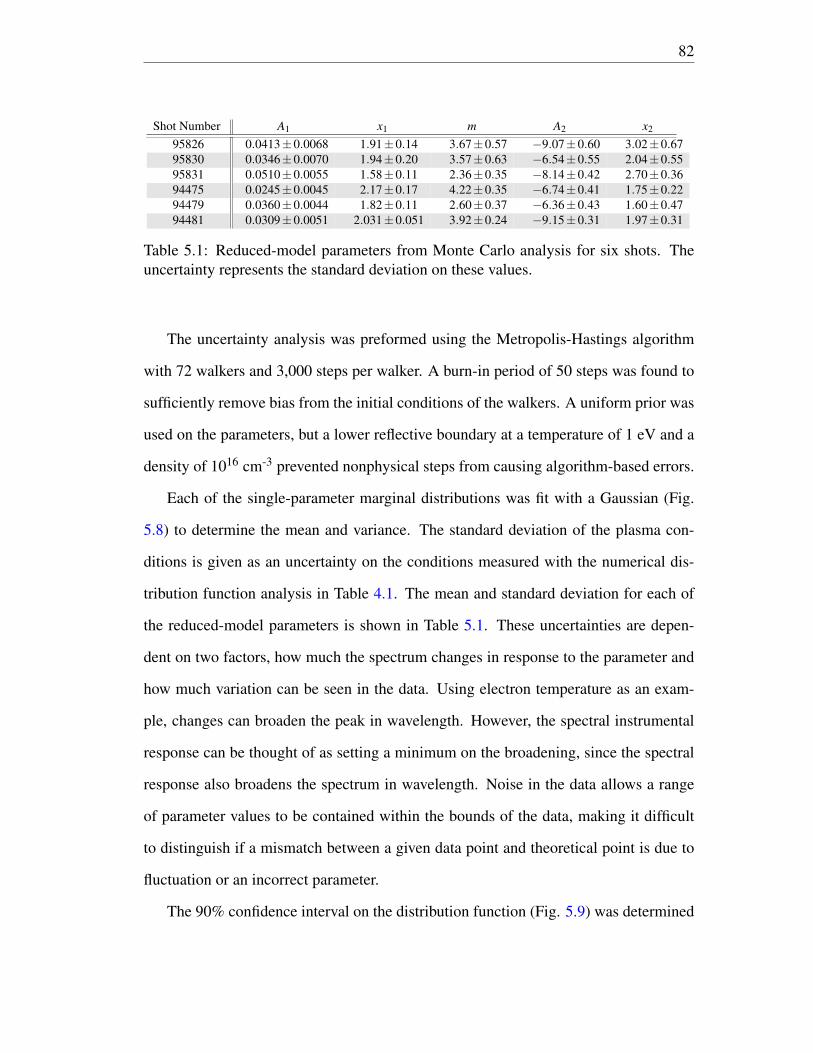
82
Shot Number A1 x1 m A2 x2
95826 0.0413±0.0068 1.91±0.14 3.67±0.57 −9.07±0.60 3.02±0.6795830 0.0346±0.0070 1.94±0.20 3.57±0.63 −6.54±0.55 2.04±0.5595831 0.0510±0.0055 1.58±0.11 2.36±0.35 −8.14±0.42 2.70±0.3694475 0.0245±0.0045 2.17±0.17 4.22±0.35 −6.74±0.41 1.75±0.2294479 0.0360±0.0044 1.82±0.11 2.60±0.37 −6.36±0.43 1.60±0.4794481 0.0309±0.0051 2.031±0.051 3.92±0.24 −9.15±0.31 1.97±0.31
Table 5.1: Reduced-model parameters from Monte Carlo analysis for six shots. Theuncertainty represents the standard deviation on these values.
The uncertainty analysis was preformed using the Metropolis-Hastings algorithm
with 72 walkers and 3,000 steps per walker. A burn-in period of 50 steps was found to
sufficiently remove bias from the initial conditions of the walkers. A uniform prior was
used on the parameters, but a lower reflective boundary at a temperature of 1 eV and a
density of 1016 cm-3 prevented nonphysical steps from causing algorithm-based errors.
Each of the single-parameter marginal distributions was fit with a Gaussian (Fig.
5.8) to determine the mean and variance. The standard deviation of the plasma con-
ditions is given as an uncertainty on the conditions measured with the numerical dis-
tribution function analysis in Table 4.1. The mean and standard deviation for each of
the reduced-model parameters is shown in Table 5.1. These uncertainties are depen-
dent on two factors, how much the spectrum changes in response to the parameter and
how much variation can be seen in the data. Using electron temperature as an exam-
ple, changes can broaden the peak in wavelength. However, the spectral instrumental
response can be thought of as setting a minimum on the broadening, since the spectral
response also broadens the spectrum in wavelength. Noise in the data allows a range
of parameter values to be contained within the bounds of the data, making it difficult
to distinguish if a mismatch between a given data point and theoretical point is due to
fluctuation or an incorrect parameter.
The 90% confidence interval on the distribution function (Fig. 5.9) was determined
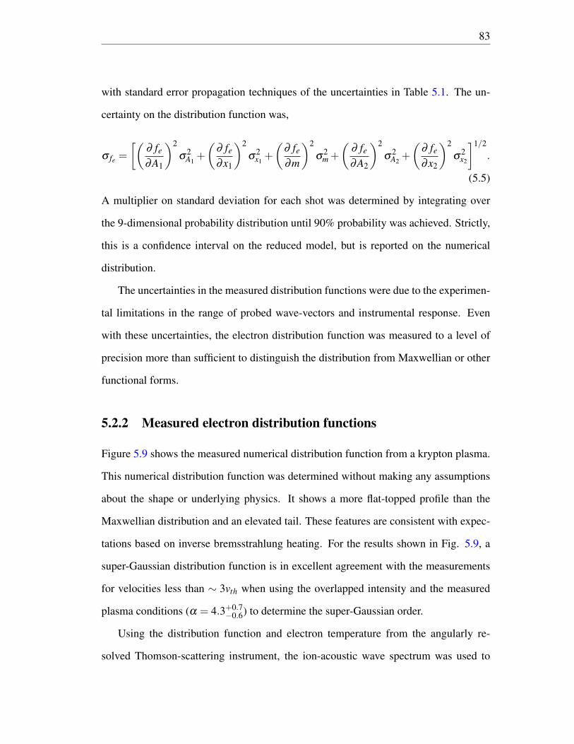
83
with standard error propagation techniques of the uncertainties in Table 5.1. The un-
certainty on the distribution function was,
σ fe =
[(∂ fe
∂A1
)2
σ2A1+
(∂ fe
∂x1
)2
σ2x1+
(∂ fe
∂m
)2
σ2m +
(∂ fe
∂A2
)2
σ2A2+
(∂ fe
∂x2
)2
σ2x2
]1/2
.
(5.5)
A multiplier on standard deviation for each shot was determined by integrating over
the 9-dimensional probability distribution until 90% probability was achieved. Strictly,
this is a confidence interval on the reduced model, but is reported on the numerical
distribution.
The uncertainties in the measured distribution functions were due to the experimen-
tal limitations in the range of probed wave-vectors and instrumental response. Even
with these uncertainties, the electron distribution function was measured to a level of
precision more than sufficient to distinguish the distribution from Maxwellian or other
functional forms.
5.2.2 Measured electron distribution functions
Figure 5.9 shows the measured numerical distribution function from a krypton plasma.
This numerical distribution function was determined without making any assumptions
about the shape or underlying physics. It shows a more flat-topped profile than the
Maxwellian distribution and an elevated tail. These features are consistent with expec-
tations based on inverse bremsstrahlung heating. For the results shown in Fig. 5.9, a
super-Gaussian distribution function is in excellent agreement with the measurements
for velocities less than ∼ 3vth when using the overlapped intensity and the measured
plasma conditions (α = 4.3+0.7−0.6) to determine the super-Gaussian order.
Using the distribution function and electron temperature from the angularly re-
solved Thomson-scattering instrument, the ion-acoustic wave spectrum was used to

84
Figure 5.9: Electron distributions on (a) logarithmic and (b) linear scale determined whilethe laser beams were heating the krypton plasma. The measured distribution (blackpoints) is well reproduced in the bulk by a super-Gaussian function (orange curve) con-sistent with Matte et al. (Eq. 2.37, m=3.9). A formalism describing the Maxwellian tailfrom Fourkal et al.[32] (purple curve), a Maxwellian distribution (blue curve), resultsfrom particle simulation (green curve), and the super-Gaussian + Maxwellian resultfrom the Monte Carlo analysis (red) are shown. The 90% confidence interval on themeasured distribution function (gray region) is shown.
determine the average ionization state. Combining the average ionization state, elec-
tron temperature, and total laser intensity the ratio of inverse bremsstralung heating rate
to electron-electron collision rate (α) was determined for each experiment (Fig.5.10).
Figure 5.10 shows the scaling of the super-Gaussian order (m) with the Langdon
parameter (α) and super-Gaussian width (x1). When using the super-Gaussian plus
Maxwellian model, good agreement is found with the heuristic scaling from Matte et
al.[23] for m (Eq. 2.37). The order of the electron distribution function increases from
a Maxwellian (m = 2) towards a highly super-Gaussian shape (m = 5) as the inverse
bremsstrahlung heating of the slow electrons dominates over the thermalization. The
ratio of inverse bremsstrahlung heating to electron-electron collision rate was varied
by changing the heater beam intensity (ItotalUV = 0.62− 2.8× 10¹⁵ W/cm2) and the gas
species (hydrogen, nitrogen, argon, and krypton), which resulted in a range of temper-
85
Figure 5.10: Scaling of the super-Gaussian order with relative strength of inversebremsstrahlung heating to electron-electron collisions (α) and super-Gaussian width(x1). The values for each of the six shots are plotted with error-bars showing one stan-dard deviation. The dashed lines are the expected scaling relations from Fokker-Plancksimulations.
atures (Te = 0.5−1.3 keV, Table 4.1) and ionization states (Z = 1−25). The electron
density was maintained throughout these shots (ne ≈ 4×1019 cm-3). A notable outlier
is shot 95831, which was measured after the heating beams were turned off, giving
the plasma time to cool and the distribution time to Maxwellianize. The scaling of x1
with m was found to agree with the data, as was expected to maintain the definition of
temperature as the average kinetic energy.
Figure 5.9 shows that the measured electron distribution transitions from a super-
Gaussian to a Maxwellian shape at ∼ 3vth, whereas the theory from Fourkal et al.[32]
predicts an earlier transition around∼ 2.5vth and more electrons in the tail. This depar-
ture of Fourkal from a super-Gaussian distribution was calculated considering a single
plane-wave electromagnetic source, where electrons oscillating in the laser field collide
with electrons in the tail, modifying the distribution function at high energies. By intro-

86
ducing five overlapped beams, consistent with the experimental configuration, particle
simulations using the code Quartz (see Appendix A.2) show the number of electrons in
the tail exceeds the super-Gaussian for velocities in the range 3.5vth . v . 4.5vth, qual-
itatively consistent with the enhancement above super-Gaussian observed in the data.
These results suggest that the increased uniformity due to multiple overlapped beams
reduced the energy transferred to the high-velocity electrons.
5.3 Absorption
The most widely accepted and utilized component of the Langdon effect, is it’s pre-
dicted reduction in absorption. The diminished number of slow electrons, the electrons
primarily responsible for heating, reduces the heating rate. With the ability to measure
the distribution function, simultaneous measurements of the absorption enabled this
effect to be shown definitively.
Experiments were preformed on the OMEGA laser system[94] with a nearly identi-
cal platform to the arbitrary electron distribution function measurements. This time,
eleven ultraviolet (UV, 351 nm) laser beams were focused to the center of the gas
jet. Achieving a uniform overlapped intensity ranging from ItotalUV = 0.35− 2.8× 10¹⁵
W/cm2. The oscillatory velocity was calculated from the total intensity, v2osc[cm2/s2]=
739(ItotalUV [W/cm2]/9+ I2ω [W/cm2]/4).
5.3.1 Absorption Measurement
To determine the absorption of the probe beam, two high-dynamic range scientific CCD
cameras were installed to measure the incident and transmitted energy [102]. The sys-
tem was capable of measuring 0.1% absorption. On all of the shots reported here, very

87
little beam spray outside of the original cone of the probe beam was observed and the
transmitted beam was contained well within the measurement region.
To determine the effects of non-Maxwellian electron distribution functions on laser
absorption, the incident and transmitted power of the probe beam were measured and
compared with the absorption calculated assuming a Maxwellian electron distribution
function. Spatially-resolved Thomson scattering (Section 4.3.1) was used to determine
the plasma conditions along the beam path, which were required to compute the ex-
pected absorption for a plasma with a Maxwellian electron distribution function per
unit length (dL)[103],
dAMax = 1− exp
[−(
ωpe
ω0
)2νei
vgdL
](5.6)
Integrating over the length of the plasma yielded the expected absorption for a
Maxwellian plasma.
The ratio of the total counts measured by the CCD, in the illuminated region of inter-
est (ROIout), on the transmitted side, to the total counts on the input side CCD (ROIin),
(∑ROIout/∑ROIin) provided the transmission of the probe beam. Calibration of the
transmission was measured when no plasma was present (∑ROIcal,out/∑ROIcal,in), and
was determined to be stable over 12 hours with a 0.1% RMS variation. The absorption
of the probe was calculated from this transmission measurement.
A = 1− ∑ROIout
∑ROIin× ∑ROIcal,in
∑ROIcal,out. (5.7)
5.3.2 Comparison to Langdon theory
Figure 5.11 shows that the measured laser absorption was significantly less than the
absorption calculated assuming a plasma with a Maxwellian electron distribution. The

88
Figure 5.11: The measured (red circles) and calculated (blue circles) absorption (Eq. 5.8),normalized to the absorption calculated assuming a Maxwellian electron distributionfunction, is plotted as a function of the ratio of the inverse bremsstrahlung heating rateto the electron-electron collision rate determined from the measured plasma conditionsat the center of the plasma. Error-bars represent one standard deviation propagatedfrom uncertainties in the measured plasma conditions. (remove part a)
absorption rapidly drops to∼ 60% of the Maxwellian expectation as the relative heating
rate increases (large Zv2osc/v2
th). When the inverse bremsstrahlung heating rate domi-
nates over the electron-electron collision rate, the reduction in absorption is in reason-
able agreement with the original predictions[22],
dASG(ne,Te) =
[1− 0.553
1+(0.27v2
th/Zv2osc)0.75
]×dAMax(ne,Te). (5.8)
where dAMax is the differential absorption calculated assuming a Maxwellian plasma
and using the plasma conditions determined along the path of the probe beam using
spatially-resolved Thomson scattering. The calculated absorption shown in Fig. 5.11
was computed by integrating Eq. 5.8 over the path of the probe beam.
89
5.4 Outstanding questions
The ability to measure the electron distribution function opens up many avenues for
future work and further exploration. However, there are 4 questions that remain unan-
swered in this work. What is the source of the Maxwellian tails in the electron distri-
bution function? Are the deviations in the distribution function at low velocity real?
How much further can we extend the range of velocities over which the distribution
function can be measured? Why is the measured absorption systematically high, more
consistent with Z+1?
The Maxwellian tails in the distribution function were shown experimentally to
exist, but not conform to current theories. Simulations indicated that the level of the
tail could be altered based off the anisotropy of the heating. However, this does not
prove that the tails are due to anisotropic heating or why a tail can be seen in the
Maxwellian data [Fig. 5.12 (d)]. It is possible more could be learned by recovering the
distribution function out to higher velocities. There is data at smaller scattering angles
than was used in this analysis due to numerical issues. At smaller scattering angles the
resonance shrinks rapidly requiring increasing numerical resolution.
Some of the measured distribution function show an anomalously steep slope for
the first 3-4 points in the distribution function [Fig. 5.12 (a,c)]. The working theory
is that the current algorithm does not accurately capture the behaviour of the distribu-
tion at these velocities. This information is present in the Thomson-scattering spectrum
close to the ion-acoustic wave feature, which was blocked out of the data with a dielec-
tric filter. However, this information also exists at larger scattering angles where the
spectrum is less collective. Unfortunately the SNR in this region was insufficient, but
this could be improved in future experiments.
The absorption was consistently higher than predicted by Langdon theory (Fig.

90
Figure 5.12: Measured electron distribution functions (black points) on a (a,c) linear and(b,d) logarithmic scale for (a,b) Shot 95830 and (c,d) Shot 95831. The super-Gaussianplus Maxwellian model (red curve), with parameters from the Monte Carlo analysis(Table 5.1), was compared to the data. A 90% confidence interval (gray) was computedfrom the super-Gaussian plus Maxwellian model. A Maxwellian distribution function(blue curve) is shown for reference. (a,b) Shot 95830 was the least constrained fit,highest error bars and (c,d) Shot 95831 was the closest to Maxwellian.
5.13). This was especially stark in hydrogen where the measured absorption doubled
the Maxwellian expectations. If the nominal ionization state is used to calculate AMax
and Z +1 is used to calculate A, the agreement is improved for all the absorption data.
While this might point to an issue with the way Maxwellian absorption is calculated
there could also be other physics impacting the hydrogen data or an experimental is-
sue. These measurements, especially in hydrogen, should be corroborated before any
conclusions are drawn.

91
Figure 5.13: The Measured (red circles) and calculated (blue circles) absorption normal-ized to the absorption calculated assuming a Maxwellian electron distribution function,is plotted as a function of the ratio of the inverse bremsstrahlung heating rate to theelectron-electron collision rate determined from the measured plasma conditions at thecenter of the plasma. The measured absorption is compared to the predicted scaling(blue curve) and an ad hoc scaling (dashed black curve)
92
Chapter 6
Conclusion
This work covers Thomson-scattering measurements with temporal, spatial, and angu-
lar resolution. These provided unprecedented levels of detail in laser-produced plasmas,
measuring electron temperature, electron density, ionization state, and electron distri-
bution function as a function of time or space.
Assuming Maxwellian electron distribution functions in Thomson-scattering analy-
sis was shown to produce significant errors in the inferred plasma temperature and den-
sity [62]. Including the correct distribution function in accessible fit space, as done here
with super-Gaussian order, can eliminate model-dependent errors with minimally in-
creased statistical uncertainty. Including a super-Gaussian distribution function specifi-
cally can account for extra signal in the region between the electron plasma wave peaks.
While not considered here, other distribution functions can correct other common prob-
lems in collective Thomson-scattering analysis such as peak signal asymmetry [37],
relativistic effects [88], and apparent shift in fundamental frequency required to fit both
peaks simultaneously.
In ultrafast Thomson-scattering measurements, the electron plasma wave spectrum
was used to determine the effects of laser heating and ionization on the electron dis-
tribution function [67]. While the argon plasma was being heated, super-Gaussian

93
electron distribution functions were measured. After the heater beam was turned off,
the electron density continued to rise and the electron temperature dropped as the free
electrons continued to ionize the argon plasma. The non-Maxwellian electron distribu-
tion functions from Vlasov-Fokker-Planck simulations that included both laser heating
and ionization were required to reproduce the measured Thomson-scattering spectra,
temperature evolution, and density evolution simultaneously. Thereby demonstrating
the interplay between the effects of inverse bremsstrahlung and atomic kinetics on the
shape of the electron distribution function. These results reinforce the importance of
using non-Maxwellian electron distribution functions in determining plasma conditions
from Thomson-scattering measurements.
Angularly resolved Thomson scattering provided precise measurements of the dis-
tribution function over many orders of magnitude [69]. The distribution function was
measured without a priori knowledge of its shape, and the technique will allow a range
of applications to be studied beyond inverse bremsstrahlung heating. The measured
distribution functions were determined to be significantly different from Maxwellian.
These differences exist in the bulk, where the distribution function is super-Gaussian,
and in the tail, where the distribution function is Maxwellian but with a different am-
plitude and width.
In inertial confinement fusion plasmas, it has long been assumed that these non-
Maxwellian electron distribution functions lead to a reduction in laser heating and
in this work this reduction was measured. Furthermore, it was predicted that non-
Maxwellian distributions change the plasma wave damping, which results in a redis-
tribution of the thermal energy in the fluctuation spectrum. This affects the atomic
transition rates used to describe x-ray spectra [23] and plasma instabilities that grow
from thermal noise, which could have a significant impact on predictive capabilities [8,
25, 38, 47].

94
In laser-plasma studies, the agreement between a super-Gaussian + Maxwellian re-
duced model and these measurements of the distribution function, in shape and scaling,
provides confidence in using this closed form solution in hydrodynamic simulations as
a more tractable option compared to Fokker-Planck simulations when the details of the
electron distribution function are important [68]. For example, when using inline mod-
els to calculate the growth rates of cross-beam energy transfer[26] or stimulated Ra-
man scattering[8, 25, 38, 47] in simulations of inertial confinement fusion experiments
on the National Ignition Facility. More generally, the underlying electron distribution
functions dictate the thermal transport in plasmas and deviation from Maxwellian will
modify the transport coefficients used in hydrodynamic models of laboratory and astro-
physical plasmas[3].
The uncertainties in the measured distribution functions were due to the experimen-
tal limitations in the range of probed wave-vectors and instrumental response. Even
with these uncertainties, the electron distribution function was measured to a level of
precision more than sufficient to distinguish the distribution from Maxwellian or other
functional forms. Understanding the uncertainties in this distribution function analy-
sis is important in determining problems where angularly resolved Thomson scattering
can be applied. This is a tool with significant potential to elucidate the detailed physics
occurring in plasmas, but an understanding of the uncertainties is required to know if
the measured distribution function is distinguishable from other potential solutions.

95
Appendix A
Supplemental Information
A.1 List of symbols
A Absorption
AMax Absorption calculated assuming a Maxwellian elec-
tron distribution function
c Speed of light in vacuum
e Charge on an electron
fe Electron distribution function
I Intensity
k Wavevector of the probed Thomson-scattering fluc-
tuation
ks−k0
k0 Wavevector of the Thomson-scattering probe
ks Wavevector of the collected Thomson-scattered
light
m Super-Gaussian order
me Electron mass

96
mi Ion mass
ne Electron number density
ni Ion number density
P0 Thomson-scattering probe power
Pm Measured Thomson-scattering power
Ps Calculated Thomson-scattering power
r0 Classical electron radius
ROI Region of interest
S(k,ω) Spectral density function
SNR Signal to noise ratio
Te Electron temperature
Ti Ion temperature
vg Group velocity
vosc Electron oscilitory velocity
vth Electron thermal velocity√
Te/me
x Normalized phase velocity
Z Charge state
α Langdon parameter Zv2osc/v2
th
λ Wavelength of the probed Thomson-scattering fluc-
tuation
(1λ0− 1
λs
)−1
λ0 Wavelength of the Thomson-scattering probe
λD Electron Debye length ωpe/vth
λs Wavelength of the collected Thomson-scattered
light
χ2 Chi squared fit metric ∑[Pm−Ps]
2
σ2

97
χe,i Electron and ion susceptibilities
ω Frequency of the probed Thomson-scattering fluctu-
ation
ωs−ω0
ω0 Frequency of the Thomson-scattering probe
ωpe Plasma frequency√
4πe2neme
ωs Frequency of the collected Thomson-scattered light
Ω Solid angle
A.2 Quartz particle simulation code
The Quartz particle simulation code integrates the electron equations of motion in mul-
tiple, speckled lasers using a fourth-order relativistic Runge-Kutta scheme, giving ex-
cellent energy conservation properties. The electromagnetic fields arising from the
overlapping lasers are specified analytically to remove simulation grid effects. The elec-
trostatic response field of the plasma (Es) to the laser ponderomotive force is provided
by a simple phenomenological model derived from complementary two-dimensional
(2D) Vlasov-Fokker-Planck (VFP) calculations [99, 104] of field generation in laser
speckles. In Quartz, the vector potential generated by Nb overlapping laser beams,
each expressed in a Cartesian coordinate system xb = xb (x,θb,ϕb) in which the zb-axis
is aligned along the beam k-vector (kb), generated with Gaussian speckle statistics and
4N2 modes per beam, is given by [105]: AL (x, t) = ∑Nbb
Ab2N ∑
N−1j,l=−N exp
iΩ j,l,b (xb)
,
where Ω j,l,b (xb) =−πjxb+lyb
NL⊥−2 j2+l2
N2zbLz+φ j,l,b , Ab = abAb exp [i(kb.xb−ωt +ψb)],
ω the laser frequency, L⊥ is the mean transverse intensity correlation radius, Lz the
mean speckle length, Ab the mean magnitude of the vector potential of the beam, ab
a unit vector specifying the polarization direction of the beam, φ j,l,b are variables ran-
domly generated with value 0 or π , and ψb is a random phase of the beam chosen

98
between 0 and 2π , and N = 9. The field at an arbitrary point x in the laboratory coordi-
nate system was found by expressing the xb in terms of x using the polar and azimuthal
angles of the beams, θb and ϕb. Note that each beam is generated with its own inde-
pendent speckle statistics, and we also include smoothing by spectral dispersion. By
solving the equations of motion dp/dt =−e(E+v×B) and v = dx/dt for each elec-
tron, where p is the momentum, E = Es−∂AL/∂ t is the electric field and B = ∇×AL
is the magnetic field, the evolution of the electron distribution function was studied.
The above laser parameters were chosen to match the experimental configuration, with
a total of Nb = 6 beams (5 heaters and one probe). A Monte-Carlo method was used to
include both electron-electron and electron-ion Coulomb collisions in the small-angle
approximation [106]. A relatively sophisticated computational model of this sort was
necessary because particle motion in multiple speckled beams becomes chaotic under
the experimental conditions considered here.
99
Appendix B
Computation of Angularly resolved Thomson
scattering
B.1 Mathematical Principles
B.1.1 From Book
To derive the equations used to calculate spectra for arbitrary distributions over a range
of angle we will start from the equations for power scattered and spectral density given
in Plasma scattering of electromagnetic radiation by D. H. Froula et al.
Ps(R,ωs)
dωs=
Pir20L
2πdΩ
(1+
2ω
ωi
)∣∣s× (s× Ei0)∣∣2 neS(k,ω) (B.1)
Here dΩ and dω are the solid angle about the scattering angle θ and the frequency
range about the scattering frequency ωs. Pi is the input power or power of the probe
beam, r0 is the classical electron radius, L is the length of the scattering volume in the
direction of the probe’s propogation, ωi is the probe’s frequency. s is the observation
direction (direction of R) Ei0 is the polarization direction of the probe beam . ne is the
electron density.
100
S(k,ω) =2π
k
∣∣∣1− χe
ε
∣∣∣2 fe0
(ω
k
)+
2πZk
∣∣∣χe
ε
∣∣∣2 fi0
(ω
k
)(B.2)
Here k = |k|= |ki−ki|, Z is the average ionization state, fe0 and fi0 are the one di-
mensional electron and ion distribution functions found by projecting the 3-dimensional
distributions onto k. χe is the electron susceptibility and ε is the dielectric function.
Now we can make our first assumption
(1) scattered light will be measured for∣∣ω
k
∣∣& vth
With this assumption the second term in S(k,ω) goes to 0 since fi0 goes to zero
well before the vth in most cases especially laser produced plasmas, as the laser heat
the electrons.
S(k,ω) =2π
k
∣∣∣1− χe
ε
∣∣∣2 fe0
(ω
k
)(B.3)
Where
χe(k,ω) =
∞∫−∞
dv4πe2ne
mek2
k · ∂ fe∂v
ω−k ·v− iγ(B.4)
and
ε = 1+χe +χi (B.5)
Then we will again use our first assumption to simplify
ε = 1+χe (B.6)

101
So we are left with
S(k,ω) =2π
k
∣∣∣∣ 11+χe
∣∣∣∣2 fe0
(ω
k
)(B.7)
B.1.2 Change to wavelength-angle
Our base equation B.1 is written in frequency-k space but for comparison to experiment
it is useful to rewrite in wavelength-angle space.
Ps(λs,θ)
dωs=
Ps(R,ωs)
dωs
ω2s
2πc=
Pir20L
4π2cω
2s
(1+
2ω
ωi
)∣∣s× (s× Ei0)∣∣2 neS(x,θ)dΩ (B.8)
Here we have left the R dependence unaltered. We will return to this as the method
used depends on the diagnostic. θ (scattering angle) is defined as the angle between
the probe ki and observation ks. We have also introduced the new normalized velocity,
x≡ vvth
= ω
kvth.
In order to write S(x,θ) we have to make our second assumption
(2) the electron distribution is isotropic
The first thing we do with this assumption is give a definition for fe0
fe0(k,ω) =
2π∫0
∞∫0
fe
(ω
k
)vrdvrdvθ (B.9)
We have used the freedom in defining cylindrical coordinates to set z = k making
the projection onto the probed fluctuation simpler. We could write out the components
102
of the velocity in cylindrical but because of assumption (2) fe is only dependent on the
magnitude of the velocity.
For super-Gaussian distributions the resulting distribution will be of the form
fe0(v) =Cm
vthexp[−(|v|
amvth
)m]= fe0(x)/vth (B.10)
The vector dependence of the electron susceptibility (χe) can be dealt with in a
similar way. Again using cylindrical coordinates with z = k
χe(k,ω) =
∞∫−∞
2π∫0
∞∫0
vrdvrdvθ dvz4πe2ne
mek2
k · ∂ fe∂v
ω−k ·v− iγ(B.11)
evaluating the dot products
χe(k,ω) =
∞∫−∞
2π∫0
∞∫0
vrdvrdvθ dvz4πe2ne
mek2
k ∂ fe∂vz
ω− kvz− iγ(B.12)
pulling everything outside the integrals
χe(k,ω) =4πe2ne
mek2
∞∫−∞
dvz
k ∂
∂vz
2π∫0
∞∫0
vrdvrdvθ fe
ω− kvz− iγ(B.13)
noting the definition of fe0
χe(k,ω) =4πe2ne
mek2
∞∫−∞
dvzk ∂
∂vzfe0(k,ω)
ω− kvz− iγ(B.14)
Now substituting v = xvth and omitting the directional notation since we are down
to one dimension.
103
χe(x) =4πe2ne
mek2
∞∫−∞
vthdxk/vth
∂
∂x fe0(x)/vth
ω− kxvth− iγ(B.15)
canceling k in the integral gives
χe(x) =4πe2ne
mek2v2th
∞∫−∞
dx∂
∂x fe0(x)ω
kvth− x− iγ
(B.16)
The factor of kvth that multiplies iγ has be omitted since this integral is evaluated in
the limit γ → 0. We can make one more simplification
χe(x) =1
k2λ 2D
∞∫−∞
dx∂
∂x fe0(x)ω
kvth− x− iγ
(B.17)
B.1.3 Computation of χ and fe0
Equations B.8, B.17, and B.10 are sufficient to calculate the Thomson-scattering spec-
trum. However, in practice when the spectrum will be calculated millions of times as
part of a fit to data, it is advantageous to use forms and simplifications which are most
efficient, as far as computation time, while preserving accuracy.
First in order to maintain the highest possible level of generality the one dimensional
distribution is defined as a set of points.
fdisc : x1,x2, . . .xn→ R>0 (B.18)
i.e. fdisc is a mapping from a discrete domain onto the co-domain of the positive reals.
104
We will use the notational shorthand of fdisc[xi], where the square brackets are used to
denote the discrete domain.
While incredibly general the efficiency and accuracy of this form are based on the
number of points used. To maintain the level of accuracy used in other computations
of the Thomson-scattering spectrum ∼ 10,000 points would be required. For efficient
computation of the spectrum, most critically due to the number of free parameters (see
Sec. B.1.5), it is desirable to use < 100 points. To regain some accuracy with the lower
number of points we made another assumption,
(3) The distribution in locally exponential.
This means if you look at a small portion of the distribution it will be well modeled
by an exponential curve. We expect this assumption to be rather safe as many physical
effects attempt to smooth out the distribution (collisions and damping) and most func-
tional forms are built on exponentials (Gaussian, super-Gaussian, sum of Gaussian).
This allows a far more accurate approximation of interstitial points using interpolation
in logarithmic space.
fe0(x) =
fdisc[x] x ∈ x1,x2, . . .xn
exp[ln fdisc[xa]+ (ln fdisc[xb]− ln fdisc[xa])
x−xaxb−xa
]x /∈ x1,x2, . . .xn
(B.19)
Integrals are generally expensive calculations and the pole in the χe integral (Eq.
B.17) makes it especially tricky. The standard technique to get around this integral
is use of the Z function whose values can be found in Fried and Conte [107]. This
requires the distribution function to be Maxwellian, a more general approach is to use
105
the method described by Palastro et al. [88] to create a lookup table for any given
function. Since we wanted to change the distribution arbitrarily, lookup tables were too
limiting. So we used a faster way to evaluate Eq. B.17 on the fly.
We preformed this in a method from Chapman and Williams [101]. To begin we
will use the Sokhotsky-Plemelj theorem to address the pole.
limε→0
b∫a
f (x)x± iε
dx =∓iπ f (0)+P
b∫a
f (x)x
dx (B.20)
Applying this to Eq. B.17
χei =π
k2λ 2D
∂ fe0
∂x
∣∣∣∣ω
kvth
χer =−1
k2λ 2D
P
∞∫−∞
∂ fe0/∂xx− ω
kvth
dx
(B.21)
Here P denotes the principle value and the subscripts r and i denote the real and
imaginary components respectively. The imaginary part can be easily computed nu-
merically leaving the principal value.
First we consider a simpler problem
y =s1∫
s0
fg
ds (B.22)
Here, we assumed that f and g are piece-wise linear and we know their values at s0
and s1 are known. This allows us to define local linear approximations
106
fs = f0 +ud f
gs = g0 +udg(B.23)
where
d f = f1− f0
dg = g1−g0
u≡ s− s0
s1− s0
(B.24)
We take Eq. B.22, plug in Eq. B.23, and change variables to u
yds
=
1∫0
f0 +ud fg0 +udg
du (B.25)
defining
f =12( f1 + f0) = f0 +
12
d f (B.26)
likewise, for g, Eq. B.25 becomes
=
1∫0
f − 12d f +ud f
g− 12dg+udg
du =
1∫0
f +(u− 1
2
)d f
g+(u− 1
2
)dg
du (B.27)
This integral can be solved in two regimes |dg| g and |dg| 6 g. The second case
can be solved by Mathematica [108]
107
=d f dg− ( f dg− gd f )(ln[−dg+2g]− ln[dg+2g])
dg2 , (B.28)
which can be rearranged to
=d fdg
+[ f dg− gd f ]ln(
g+dg/2g−dg/2
)dg2 . (B.29)
If |dg| g we can Taylor expand Eq. B.27 about dg = 0 out to second order in dg
1g+(u− 1
2
)dg
=1g−(u− 1
2
)dg
g2 +
(u− 1
2
)2dg2
g3 (B.30)
so Eq. B.27 becomes
1∫0
dufg+
(u− 1
2
)d f
g−(u− 1
2
)f dg
g2 −(u− 1
2
)2d f dg
g2 +
(u− 1
2
)2f dg2
g3 +
(u− 1
2
)3d f dg2
g3
(B.31)
Each of these integrals is simple and can be solved trivially with the substitution v =
u−1/2. With this substitution we see the v and v3 terms are odd so they will be zero.
Solving the remaining three terms
=fg− d f dg
12g2 +f dg2
12g3 =fg+
f dg2−d f dgg12g3 =
fg+[ f dg− gd f ]
dg12g3 . (B.32)

108
Putting everything together, the final result is
χer =− 1k2λ 2
Dχrr (B.33)
χrr = ∑χratdz (B.34)
χrat =
fg +[ f dg− gd f ] dg
12g3 |dg|< g10,000
d fdg +[ f dg− gd f ]
ln( ¯g+dg/2
g−dg/2
)dg2 |dg|> g
10,000
(B.35)
B.1.4 Instrumental Effects
Through eqs. B.7, B.8 and B.10 it is possible to calculate the “true” scattering spec-
trum, as would be seen by a perfect detector. Physical measurement systems, consisting
of collection, transport, spectrometers, and CCDs, have finite integration times, diffrac-
tion, aberrations, finite solid angle, and other physical limitations. The net effects of
these physical limitation was considered in order to obtain precise and accurate model-
ing of the measurement.
To accomplish this, we modified Eq. B.8 as
Ps(λs,θ)
dωs= R(λ )∗S(θ)∗
[A(
2λ0
λ 3s− 1
λ 2s
)neW (θ ′,θ)
1Nα
∑α
S(λs,θ′,α)
]dΩ (B.36)
here R(λ ) and S(θ) are instrument response functions to wavelength and angle respec-
tively (Sec. B.1.4) and ∗ denotes a linear convolution. W (θ ′,θ) is a weighting function
109
that converts from scattering angles to measured angles accounting for the finite aper-
ture effect and the polarization efficiency (see Sec. B.1.4). Finally, Nα is the number
of plasma conditions the spectrum is calculated for, so in combination with the sum-
mation, this gives and average spectrum over the range of plasma conditions integrated
due to finite integration time of the detector.
Transmission
Optical elements and their coatings have wavelength dependent transmission. Similarly
the quantum efficiency of photocathodes used in intensifiers are wavelength dependent.
This change to the sensitivity of the instrument as a function of wavelength was dom-
inated by the grating and photocathode for the angularly resolved Thomson-scattering
instrument.
To calculate the transmission T (λ ) the spectrum from a well understood tungsten
lamp was collected (sm(λ )). So T (λ ) = sm(λ )/sk(λ ) where sk(λ ) is the known spec-
trum of the lamp. This transmission was used in Sec. B.1.5 to achieve the correct
amplitudes.
Gradients
If the detector used for an experiment has an integration time larger than the evolution
time of the plasma, it can be important to account for this in calculations. Changing
plasma conditions (especially density) can move the peaks in wavelength as a function
of time, resulting in a measured spectrum with broader peaks of a different shape than
those calculated for a single set of plasma conditions. In our case, the integration
time was ∼200 ps and the characteristic evolution time was ∼1 ps (based on electron-
electron and electron-ion collision times).
The natural solution is to mimic this integration by calculating the spectra for the

110
progression of plasma conditions and then integrating over them. However, we are
again faced with an issue of the number of spectra that must be calculated. The more
spectra we use, the more accurate the result, but the scaling of computation time and
memory requirements associated with this third dimension of calculation (wavelength
and angle being the first two dimensions) is not favorable. It was found heuristically that
seven spectra provided the appropriate compromise between efficiency and accuracy.
Although this number is dependent on the plasma parameters in question and their
range.
To this end, we modify the spectral density function with an added parameter α ,
which represents the plasma conditions in the calculations.
S(λs,θ ,α) =2π
k(λs,θ ,α)vth(α)
∣∣∣∣ 11+χe(x)
∣∣∣∣2 fe0(x) (B.37)
Here, we have been explicit about the dependencies, writing χ and fe0 as a function of
x which combines all three varibles, and showing k is dependent on all three variables
but not through x, in fact recall x = ω/kvth.
IRFs
The measured spectrum is subject to blurring in the wavelength and angle directions
due to optical effects such as diffraction, finite source size, and aberrations. These
are treated by convolving the calculated spectrum with Gaussian instrument response
function in the wavelength and angular directions.
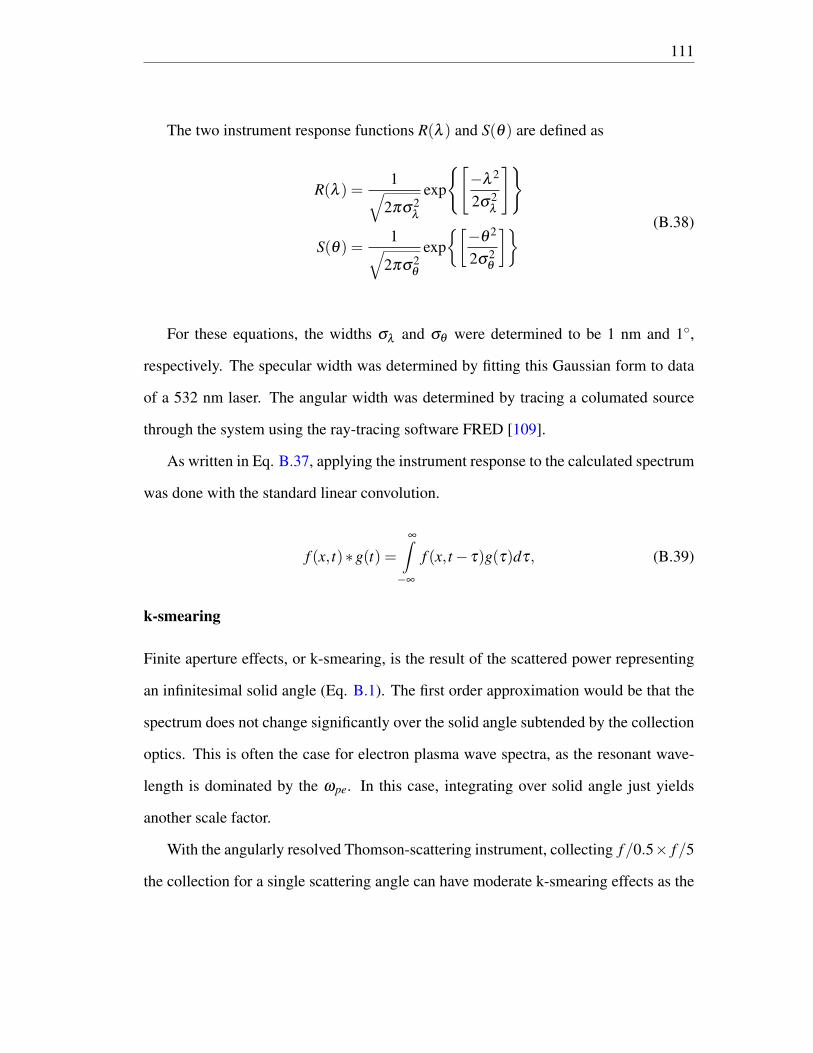
111
The two instrument response functions R(λ ) and S(θ) are defined as
R(λ ) =1√
2πσ2λ
exp
[−λ 2
2σ2λ
]
S(θ) =1√
2πσ2θ
exp[−θ 2
2σ2θ
] (B.38)
For these equations, the widths σλ and σθ were determined to be 1 nm and 1,
respectively. The specular width was determined by fitting this Gaussian form to data
of a 532 nm laser. The angular width was determined by tracing a columated source
through the system using the ray-tracing software FRED [109].
As written in Eq. B.37, applying the instrument response to the calculated spectrum
was done with the standard linear convolution.
f (x, t)∗g(t) =∞∫−∞
f (x, t− τ)g(τ)dτ, (B.39)
k-smearing
Finite aperture effects, or k-smearing, is the result of the scattered power representing
an infinitesimal solid angle (Eq. B.1). The first order approximation would be that the
spectrum does not change significantly over the solid angle subtended by the collection
optics. This is often the case for electron plasma wave spectra, as the resonant wave-
length is dominated by the ωpe. In this case, integrating over solid angle just yields
another scale factor.
With the angularly resolved Thomson-scattering instrument, collecting f/0.5× f/5
the collection for a single scattering angle can have moderate k-smearing effects as the

112
solid angle, especially in the forward and reverse directions, can be significant. To
account for this we follow the method of Follett et al. [98].
We start with a mapping from the optical modeling software FRED. In FRED a
1000 by 200 array of rays are launched from TCC covering a range of θ = 10 →
140 and φ = 201.6 → 264.6 relative to the propagation direction of the probe (z).
The mapping from FRED gives the (x,y)-coordinates there the ray intersects the final
detector. Since FRED uses the accurate size of the optical elements, it accounts for
obstructions and only rays which make it to the final image plane are included.
All the locations of rays on the final image plane are histogramed into 1024 bins
between -6.5 and 6.5 in x. This identifies the rays which hit each of the 1024 columns of
the 1024 by 1024 13 mm square CCD detector. From this histogram identifiers which
match a ray to a bin are kept.
For each of the bins, the list of (θ ,φ)s for all rays in said bin, are converted to Carte-
sian coordinates ksi = (cosφ sinθ ,sinφ sinθ ,cosθ). These vectors are then rotated so
the probe direction is aligned with the OMEGA P9→ P4 axis (p).
ks f = R ·ksi = ksi cosρ + sinρ(u×ksi)+(1− cosρ)(u ·ksi)u (B.40)
here ksi and ksi are the initial and final scattering vectors, R is the rotation matrix
which rotates ksi by ρ about u. As for any rotation of vector a into b we rotate by
the angle between the vectors ρ = cos−1 a.b|a||b| about their mutually perpendicular vector
u = a×b. In our case a = z and b = p.
A 15× 15 grid of vectors are generated about the z axis. Those vectors outside a
radius of 1/2 are thrown out and the grid is resized to match the f-number of the probe

113
beam (6.7) and renormalized so the vectors are unit vectors. The same rotation method
is then used to align these probe vectors around p.
The separation angle (ρ) for each ray in the bin and each vector in the probe beam
is calculated. These separation angles are histogramed and the normalized relative
weights are interpolated onto an array of scattering angles from 19 to 139 with steps
of half a degree. The result is relative weights of the contribution for each angle from
19 to 139 to the given bin, which represents a single column of pixel.
The entire process is repeated for each of the 1024 bins yielding a 1024× 241
matrix W (θ ,θ ′). This matrix maps single scattering angles used to calculate spectra to
the unique combination of scattering angles seen by each column of CCD pixels.
B.1.5 Matching Data
With Eq. B.36 we can calculate spectra which can be matched to data. This process is
broken into three sections, amplitude matching, axes definitions, and regression analy-
sis.
Amplitude Matching
In order to model the amplitude of the Thomson scattered signal, assuming all other
parameter are correct, the data must only include signal from Thomson scattering and
the parameter A (Eq. B.36) must be defined.
Background Subtraction Light collected in the angularly resolved Thomson instru-
ment can come from many sources and require multiple mitigation strategies. Since our
model only calculates light from Thomson scattering, any other sources of light must
be removed. Some of these sources are blocked by physical barriers, such as light not

114
originating from near TCC, or by time constraints, such as emission from the recapture
of electrons.
The main sources of background light within the wavelength, temporal, and spacial
constraints are bremsstrahlung emission and Thomson scattering from other beams. To
remove these sources from angularly resolved Thomson data, a second shot at nearly
the same plasma conditions is taken. If the plasma conditions were identical between a
data and background shot we could subtract one from the other to obtain the Thomson-
scattering signal. Variability in the laser and the neutral gas density can lead to variation
in the backgrounds shape as well as amplitude.
To account for some of this change in amplitude and shape we define the data
Data = (FG−FGdark)− [a1(y−a2)2 +a3(y−a4)+a5](BG−BGdark)
ai = argmina
∑y
[FG(1000,y)]− [a1(y−a2)
2 +a3(y−a4)+a5](BG(1000,y)]2(B.41)
here FG and BG are the foreground and background shots, or the shots with and without
the Thomson-scattering probe beam. The subscript dark denotes an image taken just
prior to the shot with no exposure of the CCD, this measures the dark current on the
CCD. The quadratic multiplying the background attempts to match the amplitude and
shape, as a function of angle, using the 1000th spectral pixel as a reference. This
location is chosen since there is no Thomson-scattering data at that large a wavelength
(∼ 653 nm). This does not take care of all the shot to shot shape changes, especially
those caused by 3ω Thomson scattering, but it improves agreement.
The background data is also smoothed using a five by five kernel to prevent am-
plifying statistical fluctuations. This smoothing is done before the matching and sub-

115
traction. The signal is governed by Poisson statistics so without background smoothing
these fluctuations would be amplified.
Amplitude Scale Factors The amplitude factor A (Eq. B.36) contains the remaining
constants which inform the efficiency of scattering and the power input by the probe.
A = Pir20Lc∣∣s× (s× Ei0
)∣∣2 (B.42)
Instead of using this equation which introduces uncertainties from Pi and L we in-
stead choose to define
A(λ )≡
A1
maxλ∈[540nm,631nm]
Data(λ ,θ)
maxλ∈[540nm,631nm]
Ps(λ ,θ)λ ≤ 510nm
0 510nm < λ < 540nm
A2
maxλ∈[540nm,631nm]
Data(λ ,θ)
maxλ∈[540nm,631nm]
Ps(λ ,θ)λ ≥ 540nm
(B.43)
This definition gives some added flexibility. The zero region models the spectral
filter used to block the ion-acoustic wave Thomson scattering, while using two ampli-
tudes (A1,A2) can account for peak asymmetries that are not currently well understood.
The normalization to the red peak of each scattering angle removes remaining angular
dependence of the amplitude and keeps the scale factors (A1,A2) near 1. Here we have
made an assumption that the dipole efficiency term∣∣s× (s× Ei0
)∣∣2 does not vary over
a single scattering angle. This assumption is based on the use of polarization rotation
to minimize the variation. It is possible to relax this assumption and include it in the
calculation of W (θ ,θ ′) if the polarization of the probe is measured.

116
Axes
Ensuring the axes of the computation match those of the data is always necessary. The
wavelength axis, shown in plots as the x-axis, is calibrated each shot day using a mer-
cury lamp. Three of mercury’s spectral lines are bright enough and withing the wave-
length range to be measured. A linear scaling is assumed to find the conversion from
pixel to wavelength.
While calculating the spectrum (Eq. B.37) an order of magnitude extra wavelength
points are used. 10250 linearly spaced wavelength points are used instead of the 1024
pixels to ensure accurate computations. The experimentally measure spectrum in a sin-
gle pixel is integrated over the wavelength range collected by that pixel, conversely the
calculated spectrum at a wavelength point is only the value at the associated associated
wavelength. This difference can result in spectra calculated with too few points missing
contributions of small feature and being shifted slightly if a pixel is identified by one of
it’s edges as opposed to it center of mass. The solution employed is to use an order of
magnitude more points and report the signal for a pixel as the sum over 10.
Ps(λi,θ) =10i
∑j=10i−9
Ps(λ j,θ) (B.44)
The Angular axis follows from the method in Sec.B.1.4.The weighting matrix is
used to calculate the center of mass angle for each pixel, θcm =W (θ ,θ ′)θlinear. Where
θlinear is the vector of 241 linearly spaced angles used to calculate the spectra. This
method for computing the angular axis captures the non-linearity where angles in the
forward and backward direction or more compact.
The colorized plots showing power scattered as a function of angle and wavelength
are displayed with two y-axes. This first axis is the center of mass scattering angle. The

117
second y-axis is a rough approximation of the normalized phase velocity being probed.
This is calculated as
vvth
=ω
kvth≈√
ne
Te
11486k0 sin θ
2
(B.45)
This equation is a very rough approximation as it is found using ω ≈ ωpe and ks ≈
k0. Using the first assumption directly and the second assumption in the law of cosines
ω
kvth≈
ωpe/vth√2k2
0(1− cosθ)(B.46)
This equation simplifies to the previous one by using the trig identity 1− cosθ =
2sin2θ/2 and the equation for Debye length from the plasma formulary.
Regression
Regression analysis is the statistical process of identifying the most likely relation be-
tween variables. In this case amplitude, wavelength and angle. Since we have built a
detailed relation between these variables (Eq. B.36,B.37,B.43), we look for the most
likely values of each free parameter.
We use the approach of least squares, where a functional form is used to relate
the free parameters too the data. In this approach the most probable set of parameters
are those which minimize the sum of the squared residuals (∑i[Di−Mi]
2). Here the
residuals are defined as the difference between the data (D) and the model (M). We call
the sum of residuals

118
χ2 =
66
∑i=8
90
∑k=30
[D(i,k)−M(i,k)]2 +200
∑i=94
90
∑k=30
[D(i,k)−M(i,k)]2 (B.47)
where
M(i,k) =5i
∑j=5i−4
10l
∑l=10k−9
Ps(λ j,θl)
D(i,k) =5i
∑j=5i−4
10l
∑l=10k−9
Data(λ j,θl)
(B.48)
here we have summed the data and theory over one resolution unit, 5 pixels in wave-
length and 10 pixels in angle, and only used a sub-domain for the calculation. This
sub-domain is 448 nm to 509 nm, 539 nm to 652 nm, and 58 to 115. The wavelength
restrictions eliminate areas with no signal (large wavelength and filter location) and ar-
eas with 3ω signal (small wavelengths). While the angle restrictions eliminate an area
at large angle with poor signal and a region at small angle that is poorly modeled.
The free parameters whose likelihood we seek to maximize are: A1,A2,ne,Te, and
fdisc[x]. Since these parameters are not linearly separable, the problem is one of non-
linear least squares. Non-linear least squares problem do not necessarily have a closed
form solution so we employ a gradient descent algorithm to find parameters that min-
imize χ2. We used the constrained minimization algorithm fmincon from MATLAB
[90].
B.1.6 Post-processing
During minimization the normalization of the distribution function is not maintained.
This is because the shape and amplitude of the distribution function is allowed to vary
simultaneously with the density and temperature. This is advantageous algorithmicly
because a small step in ne or Te correlates to a much larger multidimensional step in
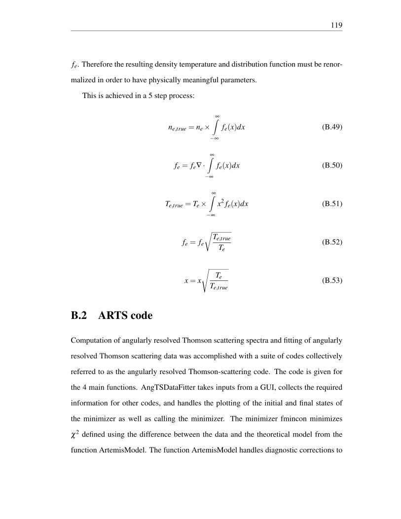
119
fe. Therefore the resulting density temperature and distribution function must be renor-
malized in order to have physically meaningful parameters.
This is achieved in a 5 step process:
ne,true = ne×∞∫−∞
fe(x)dx (B.49)
fe = fe∇ ·∞∫−∞
fe(x)dx (B.50)
Te,true = Te×∞∫−∞
x2 fe(x)dx (B.51)
fe = fe
√Te,true
Te(B.52)
x = x
√Te
Te,true(B.53)
B.2 ARTS code
Computation of angularly resolved Thomson scattering spectra and fitting of angularly
resolved Thomson scattering data was accomplished with a suite of codes collectively
referred to as the angularly resolved Thomson-scattering code. The code is given for
the 4 main functions. AngTSDataFitter takes inputs from a GUI, collects the required
information for other codes, and handles the plotting of the initial and final states of
the minimizer as well as calling the minimizer. The minimizer fmincon minimizes
χ2 defined using the difference between the data and the theoretical model from the
function ArtemisModel. The function ArtemisModel handles diagnostic corrections to
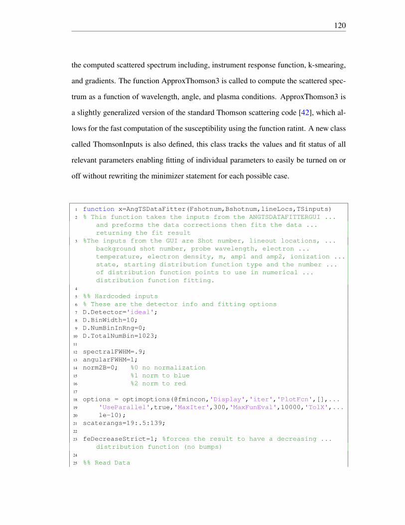
120
the computed scattered spectrum including, instrument response function, k-smearing,
and gradients. The function ApproxThomson3 is called to compute the scattered spec-
trum as a function of wavelength, angle, and plasma conditions. ApproxThomson3 is
a slightly generalized version of the standard Thomson scattering code [42], which al-
lows for the fast computation of the susceptibility using the function ratint. A new class
called ThomsonInputs is also defined, this class tracks the values and fit status of all
relevant parameters enabling fitting of individual parameters to easily be turned on or
off without rewriting the minimizer statement for each possible case.
1 function x=AngTSDataFitter(Fshotnum,Bshotnum,lineLocs,TSinputs)2 % This function takes the inputs from the ANGTSDATAFITTERGUI ...
and preforms the data corrections then fits the data ...returning the fit result
3 %The inputs from the GUI are Shot number, lineout locations, ...background shot number, probe wavelength, electron ...temperature, electron density, m, amp1 and amp2, ionization ...state, starting distribution function type and the number ...of distribution function points to use in numerical ...distribution function fitting.
4
5 %% Hardcoded inputs6 % These are the detector info and fitting options7 D.Detector='ideal';8 D.BinWidth=10;9 D.NumBinInRng=0;
10 D.TotalNumBin=1023;11
12 spectralFWHM=.9;13 angularFWHM=1;14 norm2B=0; %0 no normalization15 %1 norm to blue16 %2 norm to red17
18 options = optimoptions(@fmincon,'Display','iter','PlotFcn',[],...19 'UseParallel',true,'MaxIter',300,'MaxFunEval',10000,'TolX',...20 1e−10);21 scaterangs=19:.5:139;22
23 feDecreaseStrict=1; %forces the result to have a decreasing ...distribution function (no bumps)
24
25 %% Read Data

121
26 FG = hdfread(['ATS−s' num2str(Fshotnum) '.hdf'], 'Streak array');27 BG = hdfread(['ATS−s' num2str(Bshotnum) '.hdf'], 'Streak array');28
29 load ('MyColormaps TS','TS mycmap');30 FG=squeeze(FG(1,:,:)−FG(2,:,:));31 BG=squeeze(BG(1,:,:)−BG(2,:,:));32 FG=double(FG);33 BG=conv2(double(BG),1/25*ones(5),'same');34
35 %Fit a line of the background times a polynomial to a line of ...the data
36 xx=1:1024;37 fun=@(x) sum((FG(1000,:) −((x(1)*(xx−x(4)).ˆ2 + x(2)*(xx−x(4)) ...
+ x(3)).*BG(1000,:))).ˆ2);38 corrfactor=fmincon(fun,[.1 .1 1.15 300],[],[]);39 newBG=(corrfactor(1)*(xx−corrfactor(4)).ˆ2 + ...
corrfactor(2)*(xx−corrfactor(4)) + corrfactor(3)).*BG;40 data=FG−newBG;41
42 load('angsFRED.mat','angsFRED')43 xax=angsFRED;44
45 if Fshotnum<9500046 yax=(0:1023)*.214116+449.5272;47 else48 yax=(0:1023)*.2129+439.8;49 end50
51 %% Correct Thruput52
53 load('spectral sensitivity.mat','speccal');54 if Fshotnum<9500055 data=data./speccal;56 else57 specax=(0:1023)*.214116+449.5272;58 speccalshift=interp1(specax,speccal,yax,'linear',speccal(1));59 data=data./speccalshift;60 end61
62 if norm2B==163 %normalize to blue peak64 data=data./max(data);65 D.PhysParams=Inf,max(max(double(FG−BG)));66 elseif norm2B==267 %normalize to red peak68 data=data./max(data(470:900,:));69 D.PhysParams=Inf,max(max(double(FG−BG)));70 else71 D.PhysParams=Inf,0;72 end73

122
74 ttl=['Artemis data: Shot ' num2str(Fshotnum)];75 ColorPlots(yax, xax, rot90(data), 'Title', ttl, 'Kaxis', ...
[TSinputs.ne.Value*1E20,TSinputs.Te.Value, 526.5], 'Name', ...'Data')
76 curlims=caxis;77 caxis([0 curlims(2)])78 line([yax(1) yax(end)],[xax(end−lineLocs)' xax(end−lineLocs)'])79
80 %% f/5 angular smearing81
82 load('angleWghtsFredfine.mat','weightMatrix')83
84 %%85
86 xie=linspace(0,7,TSinputs.fe.Length);87 [¬,¬,lamAxis,¬]=lamParse([min(yax) ...
max(yax)],TSinputs.lam.Value,10250);88
89 %% Setup x090 if isempty(TSinputs.fe.Value)91 TSinputs=TSinputs.initFe(xie);92 end93 [TSinputs,x0,lb,ub]=genX(TSinputs);94
95 %% Plot starting point96
97 Thryinit=ArtemisModel(TSinputs,xie,scaterangs,x0,weightMatrix,...98 spectralFWHM,angularFWHM,lamAxis,xax,D,norm2B);99 if ¬norm2B
100 Thryinit=Thryinit./max(Thryinit(470:900,:));101 Thryinit=Thryinit.*max(data(470:900,:));102 Thryinit=TSinputs.amp1.Value*Thryinit;103 end104 chisq = sum(sum((data([40:330 ...
470:900],90:1015)−Thryinit([40:330 470:900],90:1015)).ˆ2));105 Thryinit(330:470,:)=0;106
107 ColorPlots(yax,xax,rot90(Thryinit),'Kaxis',...108 [TSinputs.ne.Value*1E20,TSinputs.Te.Value,526.5],'Title', ...
'Starting point','Name','Initial Spectrum');109 ColorPlots(yax,xax,rot90(data−Thryinit),'Title',...110 ['Initial difference: \chiˆ2 =' ...
num2str(chisq)],'Name','Initial Difference');111 load('diffcmap.mat','diffcmap');112 colormap(diffcmap);113
114 if norm2B115 caxis([−1 1]);116 else117 caxis([−8000 8000]);118 end

123
119 %% Perform fit120 tic121 if ¬isempty(x0)122 if feDecreaseStrict && TSinputs.fe.Active123 A=zeros(length(x0));124 inds=sub2ind(size(A), ...
TSinputs.fe.Location−TSinputs.fe.Length+1: ...TSinputs.fe.Location−1, ...TSinputs.fe.Location−TSinputs.fe.Length+1: ...TSinputs.fe.Location−1);
125 A(inds)=−1;126 A(inds+length(x0))=1;127 b=zeros(length(x0),1);128 else129 A=[];130 b=[];131 end132 n=10;133 dataResunit=arrayfun(@(i) ...
sum(data(:,i:i+n−1),2),1:n:1024−n+1,'UniformOutput',0);134 dataResunit=cell2mat(dataResunit);135 n=5;136 dataResunit=arrayfun(@(i) ...
sum(dataResunit(i:i+n−1,:),1),1:n:1024−n+1, ...'UniformOutput',0);
137 dataResunit=cell2mat(dataResunit');138
139 [x,¬,¬,¬,¬,grad,hess]=fmincon(@(x)chiSqArtemis(x, ...TSinputs, xie, scaterangs, weightMatrix, spectralFWHM, ...angularFWHM, lamAxis, xax, D, ...dataResunit,norm2B),x0,A,b,[],[],lb,ub,[],options);
140 else141 x=chisq142 for i=1:length(lineLocs)143 figure('Name',['Lineout ' num2str(i)])144 plot(yax,sum(data(:,lineLocs(i):lineLocs(i)+25),2))145 hold on146 plot(yax,sum(Thryinit(:,lineLocs(i):lineLocs(i)+25),2))147 title(['Lineout at pixel ' num2str(lineLocs(i)) ': ' ...148 num2str(xax(end−lineLocs(i))) '\circ'])149
150 end151
152 figure('Units','normalized','position',[.1 .1 .25 ....6],'Name',['Lineouts'])
153 hold on154 for i=1:length(lineLocs)155 plot(yax,50000*i+sum(data(:,lineLocs(i): ...
lineLocs(i)+25),2))156 plot(yax,50000*i+sum(Thryinit(:,lineLocs(i): ...
lineLocs(i)+25),2))

124
157 end158 xlabel('Wavelength (nm)')159 xlim([450 650])160 set(gca,'YColor','none','fontsize',16,'fontweight','bold')161 title(['Lineouts ' num2str(xax(end−lineLocs)) '\circ'])162
163 return164 end165 toc166
167 function csq=chiSqArtemis(x, TSinputs, xie, sas, wghts, ...spectralFWHM, angularFWHM, lamAxis, xax, D, data, norm2B)
168 Thry=ArtemisModel(TSinputs, xie, sas, x, wghts, ...spectralFWHM, angularFWHM, lamAxis, xax, D, norm2B);
169
170 n2=10;171 Thry=arrayfun(@(i) ...
sum(Thry(:,i:i+n2−1),2),1:n2:1024−n2+1, ...'UniformOutput',0);
172 Thry=cell2mat(Thry);173 n2=5;174 Thry=arrayfun(@(i) ...
sum(Thry(i:i+n2−1,:),1),1:n2:1024−n2+1, ...'UniformOutput',0);
175 Thry=cell2mat(Thry');176 if ¬norm2B177 [amp1,amp2]=genRest(TSinputs,x);178 Thry=Thry./max(Thry(94:180,:));179 Thry=Thry.*max(data(94:180,:));180 Thry(1:90,:)=amp1*Thry(1:90,:);181 Thry(90:end,:)=amp2*Thry(90:end,:);182 end183
184 uncert=(0.01*(data([8:66 94:200],30:end−12)./500)).ˆ2;185 uncert(uncert<200)=200;186 csq = sum(sum(((data([8:66 ...
94:200],30:end−12)./500−Thry([8:66 ...94:200],30:end−12)./500).ˆ2)./uncert));
187 end188
189 %% Plot Result190 Thryfin=ArtemisModel(TSinputs,xie,scaterangs,...191 x,weightMatrix,spectralFWHM,angularFWHM,lamAxis,xax,D,norm2B);192 n2=10;193 ThryfinRes=arrayfun(@(i) ...
sum(Thryfin(:,i:i+n2−1),2),1:n2:1024−n2+1, 'UniformOutput',0);194 ThryfinRes=cell2mat(ThryfinRes);195 xaxRes=arrayfun(@(i) mean(xax(i:i+n2−1)),1:n2:1024−n2+1, ...
'UniformOutput',0);196 xaxRes=cell2mat(xaxRes);197 n2=5;

125
198 ThryfinRes=arrayfun(@(i) ...sum(ThryfinRes(i:i+n2−1,:),1),1:n2:1024−n2+1, ...'UniformOutput',0);
199 ThryfinRes=cell2mat(ThryfinRes');200 yaxRes=arrayfun(@(i) mean(yax(i:i+n2−1)),1:n2:1024−n2+1, ...
'UniformOutput',0);201 yaxRes=cell2mat(yaxRes);202
203 if ¬norm2B204 [amp1,amp2]=genRest(TSinputs,x);205 ThryfinRes=ThryfinRes./max(ThryfinRes(94:180,:));206 ThryfinRes=ThryfinRes.*max(dataResunit(94:180,:));207 ThryfinRes(1:90,:)=amp1*ThryfinRes(1:90,:);208 ThryfinRes(90:end,:)=amp2*ThryfinRes(90:end,:);209 end210 ThryfinRes(66:94,:)=0;211 chisqfin = sum(sum((dataResunit([8:66 ...
94:200],30:end−12)−ThryfinRes([8:66 94:200],30:end−12)).ˆ2));212
213 if ¬norm2B214 [amp1,amp2]=genRest(TSinputs,x);215 Thryfin=Thryfin./max(Thryfin(470:900,:));216 Thryfin=Thryfin.*max(data(470:900,:));217 Thryfin(1:450,:)=amp1*Thryfin(1:450,:);218 Thryfin(450:end,:)=amp2*Thryfin(450:end,:);219 end220 Thryfin(330:470,:)=0;221 chisqfin = sum(sum((data([40:330 ...
470:900],90:1015)−Thryfin([40:330 470:900],90:1015)).ˆ2));222
223 [Tefin,nefin,¬,¬]=genTS(TSinputs,x);224 ColorPlots(yaxRes,xaxRes,rot90(ThryfinRes),'Kaxis', ...
[nefin*1E20,Tefin,526.5],'Title','Final ...Spectrum','Name','Final Spectrum');
225 ColorPlots(yax,xax,rot90(data−Thryfin),'Title', ['Final ...difference: \chiˆ2 =' num2str(chisqfin)],'Name','Final ...Difference');
226 load('diffcmap.mat','diffcmap');227 colormap(diffcmap);228 if norm2B229 caxis([−1 1]);230 else231 caxis([−8000 8000]);232 end233
234 for i=1:length(lineLocs)235 figure('Name',['Lineout ' num2str(i)])236 plot(yaxRes,sum(dataResunit(:,lineLocs(i)/10: ...
lineLocs(i)/10+1),2))237 hold on

126
238 plot(yaxRes,sum(ThryfinRes(:,lineLocs(i)/10: ...lineLocs(i)/10+1),2))
239 title(['Lineout at pixel ' num2str(lineLocs(i)) ': ' ...240 num2str(xax(end−lineLocs(i))) '\circ'])241 end242
243 figure('Units','normalized','position',[.1 .1 .25 ....6],'Name',['Lineouts'])
244 hold on245
246 for i=1:length(lineLocs)247 plot(yaxRes,100000*i+sum(dataResunit(:,lineLocs(i)/10: ...
lineLocs(i)/10+1),2))248 plot(yaxRes,100000*i+sum(ThryfinRes(:,lineLocs(i)/10: ...
lineLocs(i)/10+1),2))249 end250 xlabel('Wavelength (nm)')251 xlim([450 650])252 set(gca,'YColor','none','fontsize',16,'fontweight','bold')253 title(['Lineouts ' num2str(xax(end−lineLocs)) '\circ'])254
255 x=setTo(TSinputs,x);256 x.fitprops.grad=grad;257 x.fitprops.hess=hess;258 end
1 function modl=ArtemisModel(TSins, xie, sas, x, wghts, ...spectralFWHM, angularFWHM, lamAxis, xax, D, norm2B)
2
3 if TSins.m.Active && ¬TSins.fe.Active4 [Te,ne,lam,fecur]=genTS(TSins,x,xie);5 else6 [Te,ne,lam,fecur]=genTS(TSins,x);7 end8 [Te,ne]=genGradients(TSins,Te,ne,7);9 fecur=exp(fecur);
10
11 xiecur=[−flip(xie) xie(2:end)];12 fecur=[flip(fecur) fecur(2:end)];13 Thry=ApproxThomson3(Te,ne*1E20,lamAxis([1 ...
end]),lam,sas,fecur,xiecur);14
15 Thry=mean(Thry,1);16 Thry=squeeze(Thry);17 Thry=permute(Thry,[2 1]);18
19 [amp1,amp2,blur]=genRest(TSins,x);20
21 modl=wghts*Thry;
127
22
23 [modl,lamAx]=S2Signal(modl,lamAxis,D); %rebins the ...spectrum into pixels, similar to rebinning the ...resolution units in AngTSDataFitter
24
25 modl=addIRF2D(spectralFWHM+blur,angularFWHM,lamAx,xax,modl);26 modl=rot90(modl,3);27
28 %normalize to blue peak29 if norm2B30 modl=modl./max(modl(470:900,:));31 modl=amp1*modl;32 end33
34 if ¬isempty(TSins.specCurvature)&&TSins.specCurvature.Active35 invfunc= @(xy) [xy(:,1), xy(:,2)− ...
(TSins.specCurvature.Value/(512ˆ2))* (xy(:,1)−512).ˆ2];36 modl=imwarp(modl, geometricTransform2d(invfunc), ...
'OutputView', imref2d(size(modl)));37 end38
39 end
1 function [Thry]=addIRF2D(width1,width2,ax1,ax2,data)2 % ADDIRF adds a gaussian instrument response function to the ...
data with a3 % FWHM given the the input parameter width4 %ax1 is the xaxis or the axis corresponding to a row lineout5 %ax2 is the yaxis or the axis corresponding to a column lineout6
7 stddev1=width1/2.3548;8 origin1=(max(ax1)+min(ax1))/2; %Conceptual origin so the ...
convolution donsn't shift the signal9
10 inst func1 = (1/(stddev1*sqrt(2*pi)))* ...exp(−(ax1−origin1).ˆ2/(2*(stddev1)ˆ2));
11
12 stddev2=width2/2.3548;13 origin2=(max(ax2)+min(ax2))/2; %Conceptual origin so the ...
convolution donsn't shift the signal14
15 inst func2 = (1/(stddev2*sqrt(2*pi)))* ...exp(−(ax2−origin2).ˆ2/(2*(stddev2)ˆ2));
16
17 Thry=conv2(inst func2,inst func1,data,'same');18 Thry=repmat(sum(data,2)./sum(Thry,2),1,size(data,2)).*Thry;19 end

128
1 function [formfactor] = ApproxThomson3(Te, ne, lamrang, lam, ...sa, DF, x)
2 % APPROXTHOMSON3 calculates the Thomson spectrum using ...ratint and is capable of taking a vector for sa,Te,ne. ...All are expected as row vectors and are reshaped as needed
3
4 %hard coded inputs5 Va=0;6 interpAlg='spline';7
8 % basic quantities9 C=2.99792458e10;
10 Me=510.9896/Cˆ2; % electron mass KeV/Cˆ211 re=2.8179e−13; % classical electron radius cm12 Esq = Me*Cˆ2*re; % sq of the electron charge KeV−cm13 constants = sqrt(4*pi*Esq/Me); % sqrt(4*pi*eˆ2/Me)14 sarad=sa*2*pi/360;15 sarad=reshape(sarad,1,1,[]);% scattering angle in radians16 npts=10250;17
18 %%19 [omgL,omgs,¬,¬]=lamParse(lamrang,lam,npts);20 % calculating k and omega vectors21 omgpe=constants*sqrt(ne)'; % plasma frequency Rad/s22 omg = omgs − omgL;23 ks=sqrt (omgs.ˆ2−omgpe.ˆ2)/C;24 kL=sqrt (omgLˆ2−omgpe.ˆ2)/C; % laser wavenumber in Rad/cm25 k=sqrt(ks.ˆ2+kL.ˆ2−2*ks.*kL.*cos(sarad));26 kdotv = k*Va;27 omgdop=omg − kdotv;28
29 % plasma parameters30 vTe=sqrt(Te/Me)'; % electron thermal velocity31 klde=(vTe./omgpe).*k ;32
33 % electron susceptibility34 % calculating normilized phase velcoity (xi's) for electrons35 xie=omgdop./(k.*vTe) ;36
37 fe vphi=exp(interp1(x,log(DF),xie,interpAlg,−Inf));38 fe vphi(isnan(fe vphi))=0;39
40 df=diff(fe vphi,1,2)./diff(xie,1,2);41 df(:,end+1,:)=zeros(length(ne),1,length(sa));42
43 chiEI = pi./(klde.ˆ2).*sqrt(−1).*df;44
45 h=0.01;46 minmax=8.2;47 h1=1000;
129
48 xi1=linspace(−minmax−sqrt(2.)/h1,minmax+sqrt(2.)/h1,h1);49 xi2=(−minmax:h:minmax);50 ratdf=gradient(exp(interp1(x,log(DF),xi1,interpAlg,−Inf)), ...
xi1);51 ratdf(isnan(ratdf))=0;52
53 for iw=1:length(xi2)54 chiERratprim(iw)=real(ratint(ratdf,xi1−xi2(iw),xi1));55 end56
57 chiERrat=interp1(xi2,chiERratprim,xie,'spline');58
59 chiERrat=− 1./(klde.ˆ2).*chiERrat;60
61 chiE=chiERrat+chiEI;62 epsilon=1+(chiE);63
64 ele comp=double(fe vphi)./vTe;65 SKW ele omg = ...
2*pi*1./klde.*(ele comp)./((abs(epsilon)).ˆ2) .*vTe./omgpe;66
67 PsOmg = (SKW ele omg).*(1+2*omgdop/omgL)*reˆ2.*ne';68 lams=2*pi*C./omgs;69 PsLam = PsOmg*2*pi*C./lams.ˆ2 ;70 %PsLam = bsxfun(@rdivide,PsOmg *2*pi*C,lams.ˆ2) ;71
72 formfactor = PsLam;73
74 end
1 function out=ratint(f,g,z)2
3 % Integrate f/g dz taking each to be piecwise linear. This is4 % more accurate when f/g has a near−pole in an interval5 % f,g and z are 1D complex arrays.6 %7 % Based on newlip routine by Ed Williams.8
9 zdif = z(2:end)−z(1:end−1);10
11 out = sum(ratcen(f,g).*zdif);12
13 end14
15 function out=ratcen(f,g)16
17 % Return "rationally centered" f/g18 % such that int s(1)ˆs(0) ds f(s)/g(s) = ...
sum(ratcen(f,g)*s(dif)) when
130
19 % f and g are linear functions of s.20 % This allows accurate integration through near poles of f/g21 %22 % Based on newlip routine by Ed Williams.23
24 fdif = f(2:end)−f(1:end−1);25 gdif = g(2:end)−g(1:end−1);26 fav = 0.5*(f(2:end)+f(1:end−1));27 gav = 0.5*(g(2:end)+g(1:end−1));28
29 out = 0.*fdif;30
31 iflat = abs(gdif) < 1.e−4*abs(gav);32
33 tmp = (fav.*gdif − gav.*fdif);34 rf = fav./gav + tmp.*gdif./(12.*gav.ˆ3);35
36 rfn = fdif./gdif + tmp.*log((gav+0.5*gdif)./ ...(gav−0.5*gdif))./gdif.ˆ2;
37
38 out(iflat) = rf(iflat);39 out(¬iflat) = rfn(¬iflat);40
41 end
1 classdef ThomsonInputs2 properties3 amp14 amp25 lam6 Te7 Z8 ne9 m
10 fe11 blur12 specCurvature13 fitprops14 end15 methods16 function obj = ThomsonInputs(varargin)17 %creates the ThomsonInputs object. standard inputs ...
have 4 properties. "Active" is 1 if the ...variable it being fit or 0 otherwise. "Value" ...is the initial value. "Location" is the index ...where the variable can be found in the ...minimized array x. "Bound" are the set of ...default lower and upper bounds for the minimizer.
18

131
19 obj.amp1.Location=0;20 obj.amp1.Bounds=[0; 10];21
22 obj.amp2.Location=0;23 obj.amp2.Bounds=[0; 10];24
25 obj.lam.Location=0;26 obj.lam.Bounds=[525; 528];27
28 obj.Te.Location=0;29 obj.Te.Bounds=[0.01; 3];30
31 obj.Z.Location=0;32 obj.Z.Bounds=[1; 25];33
34 obj.ne.Location=0;35 obj.ne.Bounds=[.01; 2];36
37 obj.m.Location=0;38 obj.m.Bounds=[2; 5];39
40 obj.fe.Value=[];41 obj.fe.Location=0;42
43 %fit props is given a dummy Active properties to ...help the genX and setTo and sameActiveState methods
44 obj.fitprops.Active=0;45
46 switch nargin47 case 048
49 obj.amp1.Active=0;50 obj.amp1.Value=[];51
52 obj.amp2.Active=0;53 obj.amp2.Value=[];54
55 obj.lam.Active=0;56 obj.lam.Value=[];57
58 obj.Te.Active=0;59 obj.Te.Value=[];60
61 obj.Z.Active=0;62 obj.Z.Value=[];63
64 obj.ne.Active=0;65 obj.ne.Value=[];66
67 obj.m.Active=0;68 obj.m.Value=[];

132
69
70 obj.fe.Active=0;71 obj.fe.Length=64;72 obj.fe.Type='DLM';73 obj.fe.Bounds=repmat([−100;−.5],1, ...
obj.fe.Length);74
75 case 876 obj.amp1.Active=0;77 obj.amp1.Value=varargin5;78
79 obj.amp2.Active=0;80 obj.amp2.Value=varargin6;81
82 obj.lam.Active=0;83 obj.lam.Value=varargin1;84
85 obj.Te.Active=0;86 obj.Te.Value=varargin3;87
88 obj.Z.Active=0;89 obj.Z.Value=varargin7;90
91 obj.ne.Active=0;92 obj.ne.Value=varargin2;93
94 obj.m.Active=0;95 obj.m.Value=varargin4;96
97 obj.fe.Active=0;98 obj.fe.Length=64;99 obj.fe.Type=varargin8;
100 obj.fe.Bounds=repmat([−100;−.5],1, ...obj.fe.Length);
101
102 case 17103 %The expected order is toglam, boxlam, ...
togne, boxne, togTe, boxTe, togm, boxm, ...togamp1, boxamp1, togamp2, boxamp2, ...togZ, boxZ, togfe, boxfe, boxfetype
104 obj.amp1.Active=varargin9.Value;105 obj.amp1.Value=str2double( ...
varargin10.String);106
107 obj.amp2.Active=varargin11.Value;108 obj.amp2.Value=str2double( ...
varargin12.String);109
110 obj.lam.Active=varargin1.Value;111 obj.lam.Value=str2double( varargin2.String);112

133
113 obj.Te.Active=varargin5.Value;114 obj.Te.Value=str2double( varargin6.String);115
116 obj.Z.Active=varargin13.Value;117 obj.Z.Value=str2double( varargin14.String);118
119 obj.ne.Active=varargin3.Value;120 obj.ne.Value=str2double( varargin4.String);121
122 obj.m.Active=varargin7.Value;123 obj.m.Value=str2double( varargin8.String);124
125 obj.fe.Active=varargin15.Value;126 obj.fe.Length=str2double( ...
varargin16.String);127 obj.fe.Type=varargin17.String;128 obj.fe.Bounds=repmat([−100;−.5],1, ...
obj.fe.Length);129 end130
131 end132
133 %these 2 methods are functions to add the blur and ...curvature properties which are special use ...properties and therefore non−standard
134 function obj = addBlur(obj,blurActive,blurValue)135 obj.blur.Active=blurActive;136 obj.blur.Value=blurValue;137 obj.blur.Location=0;138 obj.blur.Bounds=[0; 10];139 end140
141 function obj = addCurvature(obj,curvActive,curvValue)142 obj.specCurvature.Active=curvActive;143 obj.specCurvature.Value=curvValue;144 obj.specCurvature.Location=0;145 obj.specCurvature.Bounds=[.1; 10];146 end147
148 function obj = ...addGradients(obj,TeActive,TeValue,neActive,neValue)
149 %add gradient percentage values to ne and Te150 if TeActive151 obj.Te.gradient=TeValue;152 end153 if neActive154 obj.ne.gradient=neValue;155 end156 end157
158 function [obj,x,lb,ub] = genX(obj)

134
159 %This method returns the minimizer array x and ...assigns all the location values to the location ...property
160 props=properties(obj);161 x=[];162 lb=[];163 ub=[];164 for i=1:length(props)165 if obj.(propsi).Active166 x=[x obj.(propsi).Value];167 lb=[lb obj.(propsi).Bounds(1,:)];168 ub=[ub obj.(propsi).Bounds(2,:)];169 obj.(propsi).Location=length(x);170 end171 end172 end173
174 function obj = initFe(obj,xie)175 %populate the Value field of fe from the other fields176 if strcmp(obj.fe.Type,'DLM')177 obj.fe.Value=log(NumDistFunc(obj.fe.Type, ...
obj.m.Value,xie,...178 obj.fe.Type)');179 elseif strcmp(obj.fe.Type,'Fourkal')180 obj.fe.Value=log(NumDistFunc(obj.fe.Type, ...
obj.m.Value,...181 obj.Z.Value,xie,obj.fe.Type)');182 end183 obj.fe.Value(obj.fe.Value≤−100)=−99;184 end185
186 function [Te,ne,lam,fecur] = genTS(obj,x,varargin)187 %This method returns the inputs for ...
approxThomson3, i.e. Te ne188 %lam and fecur189 if obj.Te.Active190 Te=x(obj.Te.Location);191 else192 Te=obj.Te.Value;193 end194 if obj.ne.Active195 ne=x(obj.ne.Location);196 else197 ne=obj.ne.Value;198 end199 if obj.lam.Active200 lam=x(obj.lam.Location);201 else202 lam=obj.lam.Value;203 end204 if obj.fe.Active

135
205 fecur=x(obj.fe.Location−obj.fe.Length+1: ...obj.fe.Location);
206 elseif ¬isempty(varargin) && obj.m.Active207 obj.m.Value=x(obj.m.Location);208 obj=obj.initFe(varargin1);209 fecur=obj.fe.Value;210 else211 fecur=obj.fe.Value;212 end213 end214
215 function [Te,ne] = genGradients(obj,Te,ne,varargin)216 %converts the Te and ne values into vectors ...
distributed within the relevant ranges217 if ¬isempty(varargin)218 arlen=varargin1;219 else220 arlen=10;221 end222
223 if isfield(obj.Te,'gradient') && ...isfield(obj.ne,'gradient')
224 Te=linspace((1−obj.Te.gradient/200)*Te, ...(1+obj.Te.gradient/200)*Te,arlen);
225 ne=linspace((1−obj.ne.gradient/200)*ne, ...(1+obj.ne.gradient/200)*ne,arlen);
226 elseif isfield(obj.Te,'gradient')227 Te=linspace((1−obj.Te.gradient/200)*Te, ...
(1+obj.Te.gradient/200)*Te,arlen);228 ne=repmat(ne,1,arlen);229 elseif isfield(obj.ne,'gradient')230 ne=linspace((1−obj.ne.gradient/200)*ne, ...
(1+obj.ne.gradient/200)*ne,arlen);231 Te=repmat(Te,1,arlen);232 end233 end234 function [amp1,amp2,blur] = genRest(obj,x)235 %This method returns the rest of the parameters ...
required for the remainder of the fitter, i.e ...amp1 amp2 blur. Future properties can be added here
236 if obj.amp1.Active237 amp1=x(obj.amp1.Location);238 else239 amp1=obj.amp1.Value;240 end241 if obj.amp2.Active242 amp2=x(obj.amp2.Location);243 elseif obj.amp1.Active244 amp2=x(obj.amp1.Location);245 else246 amp2=obj.amp2.Value;

136
247 end248 if obj.blur.Active249 blur=x(obj.blur.Location);250 else251 blur=obj.blur.Value;252 end253 end254
255 function obj = setTo(obj,x)256 %This method returns the object with all active ...
fit parameters reset to the values given257 props=properties(obj);258
259 for i=1:length(props)260 if obj.(propsi).Active261 obj.(propsi).Value=x(obj.( ...
propsi).Location);262 end263 end264 if obj.fe.Active265 obj.fe.Value=x(obj.fe.Location− ...
obj.fe.Length+1:obj.fe.Location);266 end267 end268
269 function obj = genErrors(obj)270 %This method adds Error fields to each of the ...
active fit parameters271 props=properties(obj);272 if isfield(obj.fitprops,'hess')273 errormat=real(diag(sqrt(inv(obj.fitprops.hess))));274 for i=1:length(props)275 if obj.(propsi).Active276 obj.(propsi).Error=errormat( ...
obj.(propsi).Location);277 end278 end279 if obj.fe.Active280 obj.fe.Error=errormat(obj.fe.Location− ...
obj.fe.Length+1:obj.fe.Location)';281 end282 else283 disp('Errors can not be calculated. No Hessian ...
present');284 end285 end286
287 function tf = sameActiveState(obj1,obj2)288 %compares the states of each properties in the two ...
instances of the ThomsonInputs object as well ...as a the length of the distribution function. ...
137
Return a true−false value saying if they have ...the same states
289 props=properties(obj1);290 c=0;291 for i=1:length(props)292 if ¬isempty(obj1.(propsi)) && ¬...
isempty(obj2.(propsi)) && ...obj1.(propsi).Active==obj2.(propsi).Active
293 c=c+1;294 end295 end296 if c==length(props)297 if obj1.fe.Active298 if obj1.fe.Length==obj2.fe.Length299 tf=true;300 else301 tf=false;302 end303 else304 tf=true;305 end306 else307 tf=false;308 end309 end310
311 end312 end

138
Bibliography
[1] Donald A. Gurnett and Amitava Bhattacharjee. Introduction to Plasma Physics.Cambridge: Cambridge University Press, 2017.
[2] M. J. Owens, M. Lockwood, and P. Riley. “Global solar wind variations overthe last four centuries”. In: Scientific Reports 7.January (2017), pp. 1–11.
[3] S. S.A. Silva et al. “Nonlocal heat flux effects on temperature evolution of thesolar atmosphere”. In: Astronomy and Astrophysics 615 (2018), pp. 1–11.
[4] J. C. Kasper et al. “Alfvenic velocity spikes and rotational flows in the near-Sunsolar wind”. In: Nature 576.7786 (2019), pp. 228–231.
[5] Klaus-Dieter Weltmann et al. “The future for plasma science and technology”.In: Plasma Processes and Polymers 16.1 (Jan. 2019), p. 1800118.
[6] Thomas C. Montie, Kimberly Kelly-Wintenberg, and J. Reece Roth. “Anoverview of research using the one atmosphere uniform glow discharge plasma(OAUGDP) for sterilization of surfaces and materials”. In: IEEE Transactionson Plasma Science 28.1 (2000), pp. 41–50.
[7] A. P. Napartovich. “Overview of atmospheric pressure discharges producingnonthermal plasma”. In: Plasmas and Polymers 6.1-2 (2001), pp. 1–14.
[8] D. J. Strozzi et al. “Interplay of Laser-Plasma Interactions and Inertial FusionHydrodynamics”. In: Physical Review Letters 118.2 (Jan. 2017), p. 025002.
[9] D. A. Callahan et al. “Optimization of the NIF ignition point design hohlraum”.In: Journal of Physics: Conference Series 112.Part 2 (2008).
[10] R. K. Kirkwood et al. “A plasma amplifier to combine multiple beams at NIF”.In: Physics of Plasmas 25.5 (2018).
[11] T Tajima and John M. Dawson. “Laser Electron Accelerator”. In: Physical Re-view Letters 43.4 (July 1979), pp. 267–270.
[12] R. M.G.M. Trines et al. “Simulations of efficient Raman amplification into themultipetawatt regime”. In: Nature Physics 7.1 (2011), pp. 87–92.
[13] C. Bellei et al. “Species separation and kinetic effects in collisional plasmashocks”. In: Physics of Plasmas 21.5 (2014).

139
[14] Steven R. Spangler. “Kinetic effects on Alfven wave nonlinearity. II. The mod-ified nonlinear wave equation”. In: Physics of Fluids B 2.2 (1990), pp. 407–418.
[15] D. A. McQuarrie. Statistical Mechanics. United Kingdom: Harper & Row,1975.
[16] T. E. Tierney IV et al. “Modelling of collective Thomson scattering from col-lisional plasmas”. In: Journal of Physics A: Mathematical and General 36.22SPEC.ISS. (2003), pp. 5981–5989.
[17] A. S. Davies et al. “Picosecond Thermodynamics in Underdense Plasmas Mea-sured with Thomson Scattering”. In: Physical Review Letters 122.15 (2019),p. 155001.
[18] G. F. Swadling et al. “Measurement of Kinetic-Scale Current FilamentationDynamics and Associated Magnetic Fields in Interpenetrating Plasmas”. In:Physical Review Letters 124.21 (2020), p. 215001.
[19] O. L. Landen and R. J. Winfield. “Laser scattering from dense cesium plasmas”.In: Phys. Rev. Lett. 54.15 (1985), pp. 1660–1663.
[20] J. R. Albritton et al. “Nonlocal electron heat transport by not quite maxwell-boltzmann distributions”. In: Physical Review Letters 57.15 (1986), pp. 1887–1890.
[21] P. Helander et al. “Electron kinetics in a cooling plasma”. In: Physics of Plas-mas 11.12 (2004), pp. 5704–5709.
[22] A. Bruce Langdon. “Nonlinear inverse bremsstrahlung and heated-electron dis-tributions”. In: Phys. Rev. Lett. 44.9 (1980), pp. 575–579.
[23] J. P. Matte et al. “Non-Maxwellian electron distributions and continuum X-rayemission in inverse Bremsstrahlung heated plasmas”. In: Plasma Phys. Control.Fusion 30.12 (1988), pp. 1665–1689.
[24] S. Brunner and E. Valeo. “Simulations of electron transport in laser hot spots”.In: Physics of Plasmas 9.3 (2002), p. 923.
[25] B. B. Afeyan, A. E. Chou, and W. L. Kruer. “Effects of Non-Maxwellian Elec-tron Velocity Distributions on Parametric Instabilities”. In: Ucrl-Lr 105821.97(1998), p. 2.
[26] David Turnbull et al. “Impact of the Langdon effect on crossed-beam energytransfer”. In: Nature Physics 16.2 (2020), pp. 181–185.
[27] I. V. Igumenshchev et al. “The effect of resonance absorption in OMEGAdirect-drive designs and experiments”. In: Physics of Plasmas 14.9 (2007).
[28] M. D. Rosen et al. “The role of a detailed configuration accounting (DCA)atomic physics package in explaining the energy balance in ignition-scalehohlraums”. In: High Energy Density Physics 7.3 (2011), pp. 180–190.
140
[29] W.E.R. Davies and S.A. Ramsden. “Scattering of light from the electrons in aplasma”. In: Physics Letters 8.3 (Feb. 1964), pp. 179–180.
[30] J. M. Liu et al. “Measurements of inverse bremsstrahlung absorption and non-maxwellian electron velocity distributions”. In: Phys. Rev. Lett. 72.17 (1994),pp. 2717–2720.
[31] S H Glenzer et al. “Thomson scattering from high-Z laser-produced plasmas”.In: Phys. Rev. Lett. 82 (1999), pp. 97–100.
[32] E. Fourkal et al. “Electron distribution function in laser heated plasmas”. In:Phys. Plasmas 8.2 (2001), pp. 550–556.
[33] Patrick Mora and Herve Yahi. “Thermal heat-flux reduction in laser-producedplasmas”. In: Physical Review A 26.4 (1982), pp. 2259–2261.
[34] C. T. Dum. “Anomalous heating by ion sound turbulence”. In: Physics of Fluids21.6 (1978), pp. 945–955.
[35] Jian Zheng, C. X. Yu, and Z. J. Zheng. “Effects of non-Maxwellian (super-Gaussian) electron velocity distribution on the spectrum of Thomson scatter-ing”. In: Physics of Plasmas 4.7 (1997), pp. 2736–2740.
[36] Max Krook and Tai Tsun Wu. “Formation of maxwellian tails”. In: PhysicalReview Letters 36.19 (1976), pp. 1107–1109.
[37] R J Henchen et al. “Observation of Nonlocal Heat Flux Using Thomson Scat-tering”. In: Physical Review Letters 121.12 (2018), p. 125001.
[38] W. Rozmus et al. “Resonance between heat-carrying electrons and Langmuirwaves in inertial confinement fusion plasmas”. In: Physics of Plasmas 23.1(2016).
[39] L. Yin et al. “Saturation of backward stimulated scattering of a laser beam inthe kinetic regime”. In: Physical Review Letters 99.26 (2007), pp. 1–4.
[40] Hai P. Le, Mark Sherlock, and Howard A. Scott. “Influence of atomic kineticson inverse bremsstrahlung heating and nonlocal thermal transport”. In: PhysicalReview E 100.1 (July 2019), p. 013202.
[41] Hans G. Rinderknecht et al. “Kinetic physics in ICF: Present understanding andfuture directions”. In: Plasma Physics and Controlled Fusion 60.6 (2018).
[42] D. H. Froula et al. Plasma Scattering of Electromagnetic Radiation: Theoryand Measurement Techniques. 2nd. Amsterdam: Academic Press, 2011.
[43] D. Turnbull et al. “Refractive Index Seen by a Probe Beam Interacting with aLaser-Plasma System”. In: Phys. Rev. Lett. 118.1 (2017), pp. 1–5.
[44] C. Rousseaux et al. “Transient development of backward stimulated Ramanand Brillouin scattering on a picosecond time scale measured by subpicosecondthomson diagnostic”. In: Phys. Rev. Lett. 97.1 (2006), pp. 1–4.

141
[45] D. S. Montgomery et al. “Characterization of plasma and laser conditions forsingle hot spot experiments”. In: Laser Part. Beams 17.3 (1999), pp. 349–359.
[46] S. Depierreux et al. “Langmuir Decay Instability Cascade in Laser-Plasma Ex-periments”. In: Phys. Rev. Lett. 89.4 (2002), pp. 22–25.
[47] J. L. Kline et al. “Observation of a transition from fluid to kinetic nonlinearitiesfor langmuir waves driven by stimulated raman backscatter”. In: Phys. Rev.Lett. 94.17 (2005), pp. 4–7.
[48] D. R. Gray and J. D. Kilkenny. “The measurement of ion acoustic turbulenceand reduced thermal conductivity caused by a large temperature gradient in alaser heated plasma”. In: Plasma Phys. 22.2 (1980), pp. 81–110.
[49] S. H. Glenzer et al. “Thomson scattering from laser plasmas”. In: Physics ofPlasmas 6.5 (May 1999), pp. 2117–2128.
[50] D. H. Froula et al. “Thomson-scattering measurements of high electron tem-perature hohlraum plasmas for laser-plasma interaction studies”. In: Physics ofPlasmas 13.5 (May 2006), p. 052704.
[51] D. R. Farley et al. “Radiative jet experiments of astrophysical interest usingintense lasers”. In: Physical Review Letters 83.10 (1999), pp. 1982–1985.
[52] S. V. Lebedev et al. “The formation of reverse shocks in magnetized high energydensity supersonic plasma flows”. In: Physics of Plasmas 21.5 (2014).
[53] G. F. Swadling et al. “Interpenetration and deflection phenomena in collisionsbetween supersonic, magnetized, tungsten plasma flows diagnosed using highresolution optical Thomson scattering”. In: Physics of Plasmas 22.7 (2015).
[54] J. S. Ross et al. “Thomson-scattering measurements in the collective and non-collective regimes in laser produced plasmas (invited)”. In: Review of ScientificInstruments 81.10 (Oct. 2010), p. 10D523.
[55] N. J. Peacock et al. “Measurement of the electron temperature by Thomsonscattering in Tokamak T3”. In: Nature 224.5218 (1969), pp. 488–490.
[56] J. C. Valenzuela et al. “Measurement of temperature and density using non-collective X-ray Thomson scattering in pulsed power produced warm denseplasmas”. In: Scientific Reports 8.1 (2018), pp. 1–8.
[57] S. Frydrych et al. “Demonstration of X-ray Thomson scattering as diagnosticsfor miscibility in warm dense matter”. In: Nature Communications 11.1 (2020).
[58] G. Gregori et al. “Electronic structure measurements of dense plasmas”. In:Physics of Plasmas 11.5 PART 2 (2004), pp. 2754–2762.
[59] S.E. Segre and L. Pieroni. “Measurement of non-maxwellian electron distribu-tion functions in hot plasma and the importance for Thomson scattering diag-nostics”. In: Physics Letters A 51.1 (Jan. 1975), pp. 25–26.

142
[60] T. Hori et al. “Measurement of non-Maxwellian electron energy distributionsin an inductively coupled plasma”. In: Applied Physics Letters 69.24 (1996),pp. 3683–3685.
[61] A. C.A.P. Van Lammeren et al. “Non-Maxwellian electron velocity distribu-tions observed with Thomson scattering in the TORTUR tokamak”. In: NuclearFusion 32.4 (1992), pp. 655–665.
[62] A. L. Milder et al. “Impact of non-Maxwellian electron velocity distributionfunctions on inferred plasma parameters in collective Thomson scattering”. In:Physics of Plasmas 26.2 (Feb. 2019), p. 022711.
[63] Chaojie Zhang et al. “Ultrafast optical field-ionized gases-A laboratory plat-form for studying kinetic plasma instabilities”. In: Science Advances 5.9 (2019).
[64] M. Salewski et al. “On velocity space interrogation regions of fast-ion collectiveThomson scattering at ITER”. In: Nuclear Fusion 51.8 (2011).
[65] H. Bindslev et al. “Fast-ion velocity distributions in jet measured by collectivethomson scattering”. In: Physical Review Letters 83.16 (1999), pp. 3206–3209.
[66] K. V. Beausang et al. “Detecting non-Maxwellian electron velocity distribu-tions at JET by high resolution Thomson scattering”. In: Review of ScientificInstruments 82.3 (2011).
[67] A. L. Milder et al. “Evolution of the Electron Distribution Function in the Pres-ence of Inverse Bremsstrahlung Heating and Collisional Ionization”. In: Physi-cal Review Letters 124.2 (2020), pp. 1–5.
[68] A. L. Milder et al. “Statistical analysis of non-Maxwellian electron distribu-tion functions measured with angularly resolved Thomson scattering”. In: Phys.Plasmas (2021), (In Review).
[69] A. L. Milder et al. “Measurements of non-Maxwellian electron distributionfunctions and their effect on laser heating”. In: Phys. Rev. Lett. (2021), (In Re-view).
[70] Yu L. Klimontovich. The Statistical Theory of Non-Equilibrium Processes in aPlasma. 1967.
[71] Ricardo Lopez-Ruiz and Xavier Calbet. “Derivation of the Maxwellian distri-bution from the microcanonical ensemble”. In: American Journal of Physics75.8 (2007), pp. 752–753.
[72] P. J. Catto and Thomas Speziale. “Strong field inverse bremsstrahlung via aLorentz model”. In: Physics of Fluids 20.1 (1977), pp. 167–168.
[73] R Z Sagdeev and A A Galeev. Nonlinear Plasma Theory [by] R.Z. Sagdeevand A.A. Galeev: Rev. and Edited by T.M. O’Neil [and] D.L. Book. Frontiers inphysics. W.A. Benjamin, 1969.
143
[74] Roger D. Jones and K. Lee. “Kinetic theory, transport, and hydrodynamics ofa high-Z plasma in the presence of an intense laser field”. In: Physics of Fluids25.12 (1982), pp. 2307–2323.
[75] Patrick Mora and R. Pellat. “Ponderomotive effects and magnetic field gen-eration in radiation plasma interaction”. In: Physics of Fluids 22.12 (1979),pp. 2408–2417.
[76] Dmitry Moseev and Mirko Salewski. “Bi-Maxwellian, slowing-down, and ringvelocity distributions of fast ions in magnetized plasmas”. In: Physics of Plas-mas 26.2 (2019).
[77] H. G. Demars and R. W. Schunk. “Solar wind proton velocity distributions:Comparison of the bi-Maxwellian based 16-moment expansion with observa-tions”. In: Planetary and Space Science 38.9 (1990), pp. 1091–1103.
[78] M. A.Mansour Elsabbagh et al. “Observations of bi-Maxwellian and singleMaxwellian electron energy distribution functions in a capacitively coupledradio-frequency plasmas by laser Thomson scattering”. In: Applied Physics Let-ters 78.21 (2001), pp. 3187–3189.
[79] Susmita Sarkar, Samit Paul, and Raicharan Denra. “Bump-on-tail instability inspace plasmas”. In: Physics of Plasmas 22.10 (2015).
[80] Alexander J. Klimas and Richard J. Fitzenreiter. “On the persistence of unsta-ble bump-on-tail electron velocity distributions in the Earth’s foreshock”. In:Journal of Geophysical Research 93.A9 (1988), p. 9628.
[81] L. E. Thode and R. N. Sudan. “Two-Stream Instability Heating of Plasmas byRelativistic Electron Beams”. In: Physical Review Letters 30.16 (Apr. 1973),pp. 732–735.
[82] A. V. Arzhannikov et al. “Dynamics and Spectral Composition of SubterahertzEmission from Plasma Column Due to Two-Stream Instability of Strong Rela-tivistic Electron Beam”. In: IEEE Transactions on Terahertz Science and Tech-nology 6.2 (2016), pp. 245–252.
[83] C. K. Huang et al. “Initializing anisotropic electron velocity distribution func-tions in optical-field ionized plasmas”. In: Plasma Physics and Controlled Fu-sion 62.2 (2020).
[84] S. Rozhkov. “Nonanalyticity in the electron distribution function and nonlinearpropagation of electromagnetic waves in semiconductors”. In: Soviet physics,JETP 71.6 (1990), pp. 1135–1140.
[85] D. Vainchtein et al. “Evolution of Electron Distribution Driven by NonlinearResonances With Intense Field-Aligned Chorus Waves”. In: Journal of Geo-physical Research: Space Physics 123.10 (2018), pp. 8149–8169.
[86] J. S. Ross et al. “Observation of relativistic effects in collective Thomson scat-tering”. In: Phys. Rev. Lett. 104.10 (2010), pp. 1–4.
144
[87] E. Funfer, B. Kronast, and H. J. Kunze. “Experimental results on light scatter-ing by a θ -pinch plasma using a ruby laser”. In: Physics Letters A 5.2 (1963),pp. 125–127.
[88] J. P. Palastro et al. “Fully relativistic form factor for Thomson scattering”. In:Phys. Rev. E 81.3 (2010), p. 036411.
[89] J. Katz et al. “A reflective optical transport system for ultraviolet Thomsonscattering from electron plasma waves on OMEGA”. In: Review of ScientificInstruments 83.10 (2012).
[90] MATLAB. fmincon.
[91] S C Snyder et al. “Electron-temperature and electron-density profiles in an at-mospheric pressure argon plasma jet”. In: Phys. Rev. E 50.1 (1994), p. 519.
[92] G. F. Swadling et al. “Design calculations for a xenon plasma x-ray shield toprotect the NIF optical Thomson scattering diagnostic”. In: Rev. Sci. Instrum.87.11 (2016), p. 11D603.
[93] Vincent Bagnoud et al. “5 Hz, ¿250 mJ optical parametric chirped-pulse ampli-fier at 1053 nm”. In: Optics Letters 30.14 (July 2005), p. 1843.
[94] T. R. Boehly et al. “The upgrade to the OMEGA laser system”. In: Review ofScientific Instruments 66.1 (Jan. 1995), pp. 508–510.
[95] J. Katz et al. “A reflective image-rotating periscope for spatially resolvedThomson-scattering experiments on OMEGA”. In: Journal of Instrumentation8.12 (2013).
[96] J. Katz et al. “A pulse-front-tilt-compensated streaked optical spectrometer withhigh throughput and picosecond time resolution”. In: Review of Scientific In-struments 87.11 (2016).
[97] A. M. Hansen et al. “Supersonic gas-jet characterization with interferometryand Thomson scattering on the OMEGA Laser System”. In: Review of ScientificInstruments 89.10 (2018).
[98] R. K. Follett et al. “Plasma characterization using ultraviolet Thomson scat-tering from ion-acoustic and electron plasma waves (invited)”. In: Review ofScientific Instruments 87.11 (2016).
[99] M. Sherlock, J. P. Brodrick, and C. P. Ridgers. “A comparison of non-local elec-tron transport models for laser-plasmas relevant to inertial confinement fusion”.In: Physics of Plasmas 24.8 (2017).
[100] H. A. Scott and S. B. Hansen. “Advances in NLTE modeling for integratedsimulations”. In: High Energy Density Physics 6.1 (2010), pp. 39–47.
[101] T. Chapmann. private communication. 2019.
[102] J. Katz et al. “A transmitted-beam diagnostic for the wavelength-tunable UVdrive beam on OMEGA”. In: Review of Scientific Instruments 92.3 (2021).
145
[103] William L. Kruer. The Physics Of Laser Plasma Interaction. 1st. CRC Press,2003.
[104] A. R. Bell et al. “Fast electron transport in laser-produced plasmas and theKALOS code for solution of the Vlasov-Fokker-Planck equation”. In: PlasmaPhysics and Controlled Fusion 48.3 (2006).
[105] J. Garnier and L. Videau. “Statistical analysis of the sizes and velocities of laserhot spots of smoothed beams”. In: Physics of Plasmas 8.11 (2001), pp. 4914–4924.
[106] Tomonor Takizuka and Hirotada Abe. “A binary collision model for plasmasimulation with a particle code”. In: Journal of Computational Physics 25.3(1977), pp. 205–219.
[107] Burton D Fried and S. D. Conte. “The Plasma Dispersion Function”. In: Else-vier (1961).
[108] Inc. Wolfram Research. Mathematica, Version 12.2. Champaign, IL, 2020.
[109] Fred Optical Engineering Software.