eleg 867 - compressive sensing and sparse signal
TRANSCRIPT
ELEG 867 - Compressive Sensing and SparseSignal Representations
Gonzalo R. ArceDepart. of Electrical and Computer Engineering
University of Delaware
Fall 2011
Compressive Sensing G. Arce Fall, 2011 1 / 65
Outline
Applications in CS
Single Pixel Camera
Compressive Spectral Imaging
Random Convolution Imaging
Random Demodulator
Compressive Sensing G. Arce Fall, 2011 2 / 65
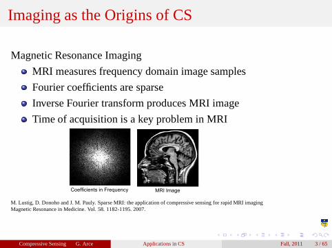
Imaging as the Origins of CS
Magnetic Resonance Imaging
MRI measures frequency domain image samples
Fourier coefficients are sparse
Inverse Fourier transform produces MRI image
Time of acquisition is a key problem in MRI
Coefficients in Frequency MRI Image
M. Lustig, D. Donoho and J. M. Pauly. Sparse MRI: the application of compressive sensing for rapid MRI imagingMagnetic Resonance in Medicine. Vol. 58. 1182-1195. 2007.
Compressive Sensing G. Arce Applications in CS Fall, 2011 3 / 65
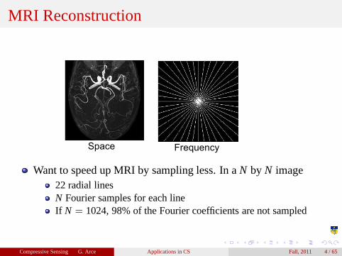
MRI Reconstruction
Space Frequency
Want to speed up MRI by sampling less. In aN by N image22 radial linesN Fourier samples for each lineIf N = 1024, 98% of the Fourier coefficients are not sampled
Compressive Sensing G. Arce Applications in CS Fall, 2011 4 / 65
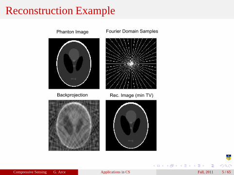
Reconstruction Example
Fourier Domain SamplesPhanton Image
Backprojection Rec. Image (min TV)
Compressive Sensing G. Arce Applications in CS Fall, 2011 5 / 65
MRI Reconstruction: Formulation Problem
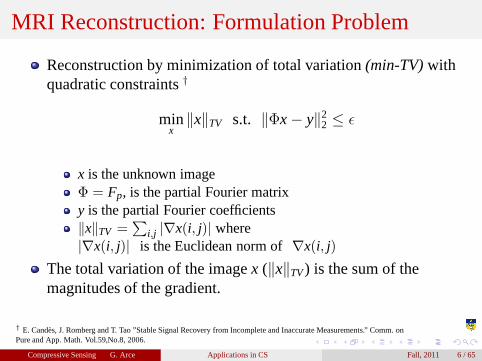
Reconstruction by minimization of total variation(min-TV) withquadratic constraints†
minx
‖x‖TV s.t. ‖Φx − y‖22 ≤ ǫ
x is the unknown imageΦ = Fp, is the partial Fourier matrixy is the partial Fourier coefficients‖x‖TV =
∑
i,j |∇x(i, j)| where|∇x(i, j)| is the Euclidean norm of∇x(i, j)
The total variation of the imagex (‖x‖TV ) is the sum of themagnitudes of the gradient.
† E. Candes, J. Romberg and T. Tao ”Stable Signal Recovery from Incomplete and Inaccurate Measurements.” Comm. onPure and App. Math. Vol.59,No.8, 2006.
Compressive Sensing G. Arce Applications in CS Fall, 2011 6 / 65
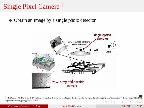
Single Pixel Camera†
Obtain an image by a single photo detector.
† M. Duarte, M. Davenport, D. Takhar, J. Laska, T. Sun, K. Kelly, and R. Baraniuk. ”Single-Pixel Imaging via Compressive Sampling.” IEEESignal Processing Magazine. 2008.
Compressive Sensing G. Arce Single Pixel Camera Fall, 2011 7 / 65
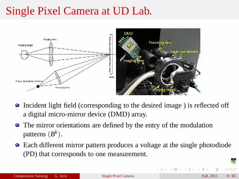
Single Pixel Camera at UD Lab.
Incident light field (corresponding to the desired image ) isreflected offa digital micro-mirror device (DMD) array.
The mirror orientations are defined by the entry of the modulationpatterns(Bk).
Each different mirror pattern produces a voltage at the single photodiode(PD) that corresponds to one measurement.
Compressive Sensing G. Arce Single Pixel Camera Fall, 2011 8 / 65
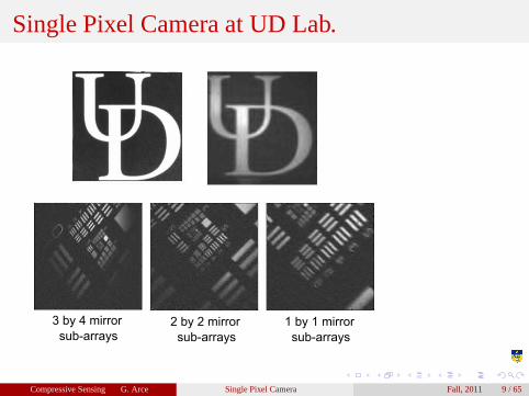
Single Pixel Camera at UD Lab.
3 by 4 mirror
sub-arrays2 by 2 mirror
sub-arrays
1 by 1 mirror
sub-arrays
Compressive Sensing G. Arce Single Pixel Camera Fall, 2011 9 / 65
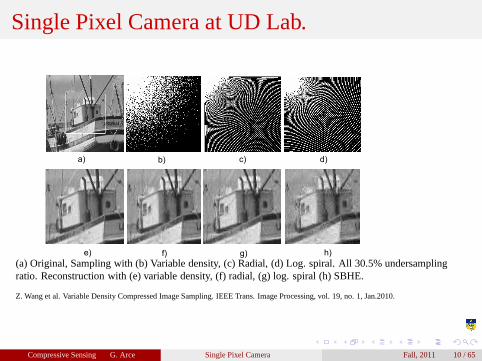
Single Pixel Camera at UD Lab.
a) b) c) d)
e) f) g) h)
(a) Original, Sampling with (b) Variable density, (c) Radial, (d) Log. spiral. All 30.5% undersamplingratio. Reconstruction with (e) variable density, (f) radial, (g) log. spiral (h) SBHE.
Z. Wang et al. Variable Density Compressed Image Sampling. IEEE Trans. Image Processing, vol. 19, no. 1, Jan.2010.
Compressive Sensing G. Arce Single Pixel Camera Fall, 2011 10 / 65
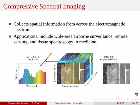
Compressive Spectral Imaging
Collects spatial information from across the electromagneticspectrum.
Applications, include wide-area airborne surveillance, remotesensing, and tissue spectroscopy in medicine.
Compressive Sensing G. Arce Compressive Spectral Imaging Fall, 2011 11 / 65
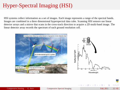
Hyper-Spectral Imaging (HSI)
HSI systems collect information as a set of images. Each image represents a range of the spectral bands.Images are combined in a three dimensional hyperspectral data cube. Scanning HSI sensors use lineardetector arrays and a mirror that scans in the cross-track direction to acquire a 2D multi-band image. Thelinear detector array records the spectrum of each ground resolution cell.
Re
flecte
d lig
ht
Wavelenght
Compressive Sensing G. Arce Compressive Spectral Imaging Fall, 2011 12 / 65
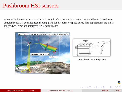
Pushbroom HSI sensors
A 2D array detector is used so that the spectral information of the entire swath width can be collectedsimultaneously. It does not need moving parts for air-borneor space-borne HSI applications and it haslonger dwell time and improved SNR performance.
Datacube of the HSI system
Compressive Sensing G. Arce Compressive Spectral Imaging Fall, 2011 13 / 65
Compressive Spectral Imaging
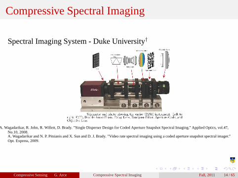
Spectral Imaging System - Duke University†
† A. Wagadarikar, R. John, R. Willett, D. Brady. ”Single Disperser Design for Coded Aperture Snapshot Spectral Imaging.”Applied Optics, vol.47,No.10, 2008.A. Wagadarikar and N. P. Pitsianis and X. Sun and D. J. Brady. ”Video rate spectral imaging using a coded aperture snapshotspectral imager.”Opt. Express, 2009.
Compressive Sensing G. Arce Compressive Spectral Imaging Fall, 2011 14 / 65
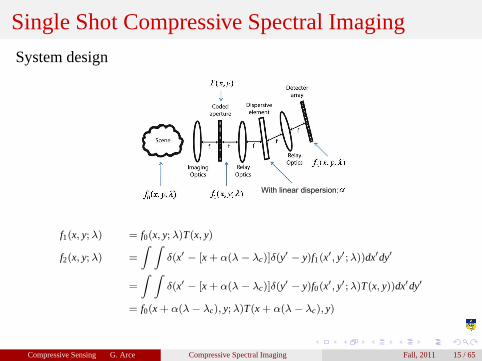
Single Shot Compressive Spectral Imaging
System design
With linear dispersion:
f1(x, y; λ) = f0(x, y; λ)T(x, y)
f2(x, y; λ) =
∫ ∫
δ(x′ − [x + α(λ − λc)]δ(y′ − y)f1(x′, y′;λ))dx′dy′
=
∫ ∫
δ(x′ − [x + α(λ − λc)]δ(y′ − y)f0(x′, y′;λ)T(x, y))dx′dy′
= f0(x + α(λ− λc), y; λ)T(x + α(λ − λc), y)
Compressive Sensing G. Arce Compressive Spectral Imaging Fall, 2011 15 / 65
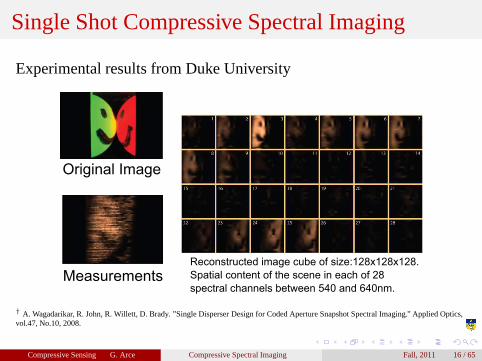
Single Shot Compressive Spectral Imaging
Experimental results from Duke University
Original Image
MeasurementsReconstructed image cube of size:128x128x128.
Spatial content of the scene in each of 28
spectral channels between 540 and 640nm.
† A. Wagadarikar, R. John, R. Willett, D. Brady. ”Single Disperser Design for Coded Aperture Snapshot Spectral Imaging.”Applied Optics,vol.47, No.10, 2008.
Compressive Sensing G. Arce Compressive Spectral Imaging Fall, 2011 16 / 65
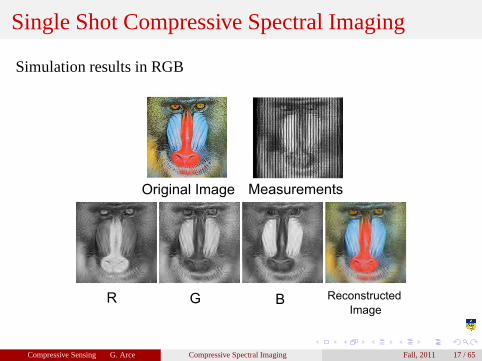
Single Shot Compressive Spectral Imaging
Simulation results in RGB
Original Image Measurements
R G B Reconstructed
Image
Compressive Sensing G. Arce Compressive Spectral Imaging Fall, 2011 17 / 65
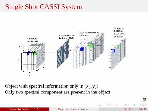
Single Shot CASSI System
Object with spectral information only in(xo, yo)Only two spectral component are present in the object
Compressive Sensing G. Arce Compressive Spectral Imaging Fall, 2011 18 / 65
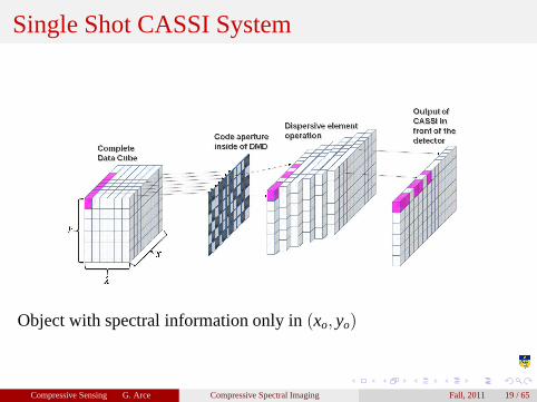
Single Shot CASSI System
Object with spectral information only in(xo, yo)
Compressive Sensing G. Arce Compressive Spectral Imaging Fall, 2011 19 / 65
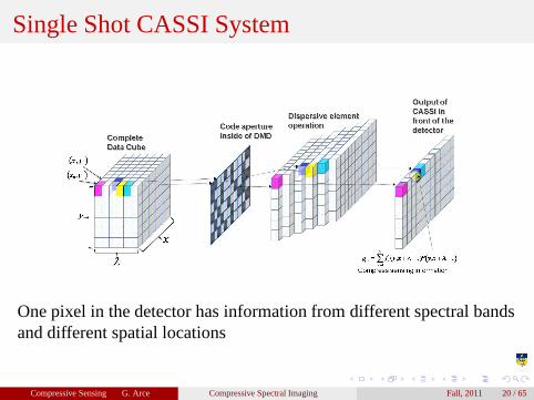
Single Shot CASSI System
One pixel in the detector has information from different spectral bandsand different spatial locations
Compressive Sensing G. Arce Compressive Spectral Imaging Fall, 2011 20 / 65
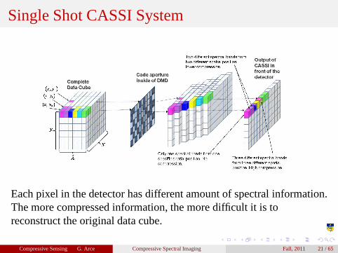
Single Shot CASSI System
Each pixel in the detector has different amount of spectral information.The more compressed information, the more difficult it is toreconstruct the original data cube.
Compressive Sensing G. Arce Compressive Spectral Imaging Fall, 2011 21 / 65
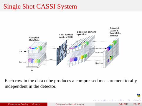
Single Shot CASSI System
Each row in the data cube produces a compressed measurement totallyindependent in the detector.
Compressive Sensing G. Arce Compressive Spectral Imaging Fall, 2011 22 / 65
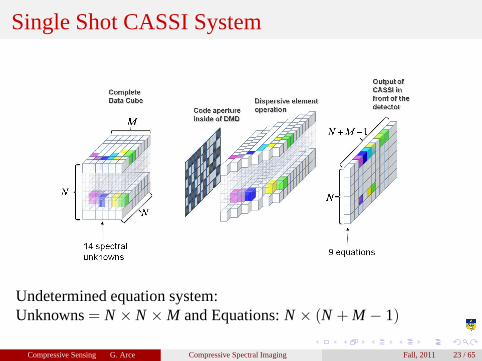
Single Shot CASSI System
Undetermined equation system:Unknowns= N × N × M and Equations:N × (N + M − 1)
Compressive Sensing G. Arce Compressive Spectral Imaging Fall, 2011 23 / 65
Single Shot CASSI System
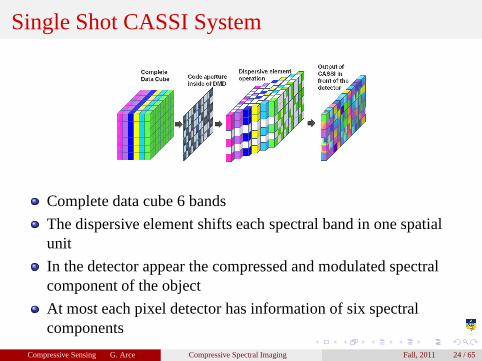
Complete data cube 6 bands
The dispersive element shifts each spectral band in one spatialunit
In the detector appear the compressed and modulated spectralcomponent of the object
At most each pixel detector has information of six spectralcomponents
Compressive Sensing G. Arce Compressive Spectral Imaging Fall, 2011 24 / 65

Single Shot CASSI System
We used theℓ1 − ℓs reconstruction algorithm†.
† S. J. Kim, K. Koh, M. Lustig, S. Boyd and D. Gorinevsky. ”An interior-point method for large scale L1 regularized least squares.” IEEEJournal of Selected Topics in Signal Processing, vol.1, pp.606-617, 2007.
Compressive Sensing G. Arce Compressive Spectral Imaging Fall, 2011 25 / 65
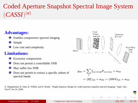
Coded Aperture Snapshot Spectral Image System(CASSI)(a)
Advantages:Enables compressive spectral imaging
Simple
Low cost and complexity
Limitations:Excessive compression
Does not permit a controllable SNR
May suffer low SNR
Does not permit to extract a specific subset ofspectral bands
gmn =∑
k
f(m+k)nkP(m+k)n + wnm
= (Hf )nm + wnm = (HWθ)nm + wnm
A. Wagadarikar, R. John, R. Willett, and D. Brady. ”Single disperser design for coded aperture snapshot spectral imaging.” Appl. Opt.,Vol.47, No.10, 2008.
Compressive Sensing G. Arce Compressive Spectral Imaging Fall, 2011 26 / 65
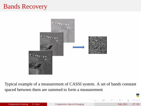
Bands Recovery
Typical example of a measurement of CASSI system. A set of bands constantspaced between them are summed to form a measurement
Compressive Sensing G. Arce Compressive Spectral Imaging Fall, 2011 27 / 65
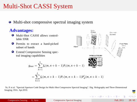
Multi-Shot CASSI System
Multi-shot compressive spectral imaging system
Advantages:Multi-Shot CASSI allows control-lable SNR
Permits to extract a hand-pickedsubset of bands
Extend Compressive Sensing spec-tral imaging capabilities
gmni =L
∑
k=1
fk(m, n + k − 1)Pi(m, n + k − 1)
=L
∑
k=1
fk(m, n + k − 1)Pr(m, n + k − 1)Pig(m, n + k − 1)
Ye, P. et al. ”Spectral Aperture Code Design for Multi-Shot Compressive Spectral Imaging”. Dig. Holography and Three-DimensionalImaging, OSA. Apr.2010.
Compressive Sensing G. Arce Compressive Spectral Imaging Fall, 2011 28 / 65
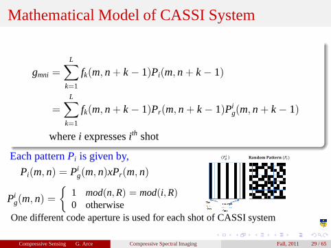
Mathematical Model of CASSI System
gmni =
L∑
k=1
fk(m, n + k − 1)Pi(m, n + k − 1)
=
L∑
k=1
fk(m, n + k − 1)Pr(m, n + k − 1)Pig(m, n + k − 1)
wherei expressesith shot
Each patternPi is given by,
Pi(m, n) = Pig(m, n)xPr(m, n)
Pig(m, n) =
1 mod(n,R) = mod(i,R)0 otherwise
One different code aperture is used for each shot of CASSI system
Compressive Sensing G. Arce Compressive Spectral Imaging Fall, 2011 29 / 65
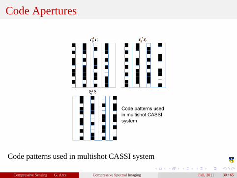
Code Apertures
Code patterns used
in multishot CASSI
system
Code patterns used in multishot CASSI system
Compressive Sensing G. Arce Compressive Spectral Imaging Fall, 2011 30 / 65
Cube Information and Subsets of Spectral Bands
Subset 1
M=bands
Subset 2
M=bands
Subset 3
M=bands... Subset R
M bands
Spatial
axis, N
pixels
Spatial
axis, N
pixels
Spectral axis,
L bands
Complete
Spectral
Data Cube
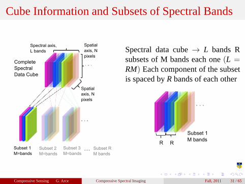
Spectral data cube→ L bands Rsubsets of M bands each one(L =RM) Each component of the subsetis spaced byR bands of each other
R R
Subset 1
M bands
Compressive Sensing G. Arce Compressive Spectral Imaging Fall, 2011 31 / 65
Cube Information and Subsets of Spectral Bands
Subset 1
M=bands
Subset 3
M=bandsSubset 2
M=bands... Subset R
M=bands
Spatial
axis, N
pixels
Spatial
axis, N
pixels
Spectral axis,
L bands
Complete
Spectral
Data Cube
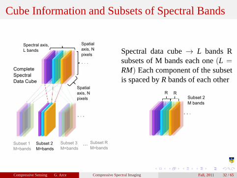
Spectral data cube→ L bands Rsubsets of M bands each one(L =RM) Each component of the subsetis spaced byR bands of each other
R R
Subset 2
M bands
Compressive Sensing G. Arce Compressive Spectral Imaging Fall, 2011 32 / 65
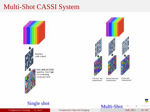
Multi-Shot CASSI System
Single shot
First shot and
measurement
Second shot and
measurement
R shot and
measurement
Multi-ShotCompressive Sensing G. Arce Compressive Spectral Imaging Fall, 2011 33 / 65
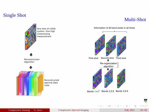
Single Shot
Reconstruction
Algorithm
One shot of CASSI
system. One high
compressing
measurement.
Reconstructed
spectral data
cube.
Multi-Shot
Re-organization
algorithm
Bands 1,4,7 Bands 2,5,8 Bands 3,6,9
First shot Second shot Third shot
Information of all band exists in all shots
Compressive Sensing G. Arce Compressive Spectral Imaging Fall, 2011 34 / 65
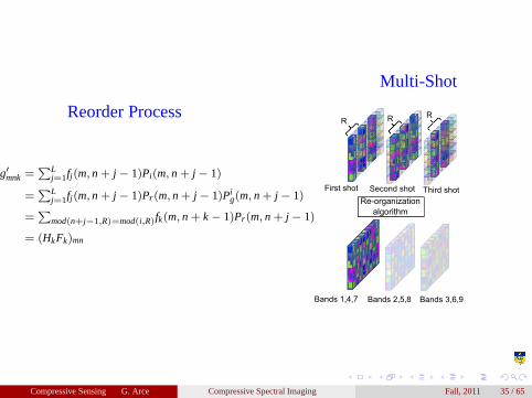
Reorder Process
g′mnk =∑L
j=1fj(m, n + j − 1)Pi(m, n + j − 1)
=∑L
j=1fj(m, n + j − 1)Pr(m, n + j − 1)Pig(m, n + j − 1)
=∑
mod(n+j−1,R)=mod(i,R)fk(m, n + k − 1)Pr(m, n + j − 1)
= (HkFk)mn
Multi-Shot
Re-organization
algorithm
First shot Second shot Third shot
Bands 1,4,7 Bands 2,5,8 Bands 3,6,9
R R R
Compressive Sensing G. Arce Compressive Spectral Imaging Fall, 2011 35 / 65
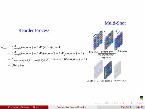
Reorder Process
g′mnk =∑L
j=1fj(m, n + j − 1)Pi(m, n + j − 1)
=∑L
j=1fj(m, n + j − 1)Pr(m, n + j − 1)Pig(m, n + j − 1)
=∑
mod(n+j−1,R)=mod(i,R)fk(m, n + k − 1)Pr(m, n + j − 1)
= (HkFk)mn
Multi-Shot
Re-organization
algorithm
First shot Second shot Third shot
Bands 1,4,7 Bands 2,5,8 Bands 3,6,9
RR
R
Compressive Sensing G. Arce Compressive Spectral Imaging Fall, 2011 36 / 65
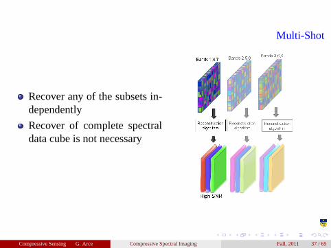
Recover any of the subsets in-dependently
Recover of complete spectraldata cube is not necessary
Multi-Shot
Compressive Sensing G. Arce Compressive Spectral Imaging Fall, 2011 37 / 65
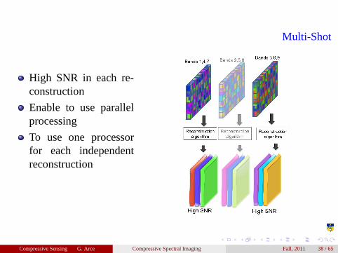
High SNR in each re-construction
Enable to use parallelprocessing
To use one processorfor each independentreconstruction
Multi-Shot
Compressive Sensing G. Arce Compressive Spectral Imaging Fall, 2011 38 / 65
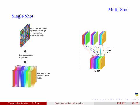
Single Shot
Reconstruction
Algorithm
One shot of CASSI
system. One high
compressing
measurement.
Reconstructed
spectral data
cube.
Multi-Shot
Compressive Sensing G. Arce Compressive Spectral Imaging Fall, 2011 39 / 65
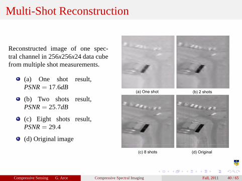
Multi-Shot Reconstruction
Reconstructed image of one spec-tral channel in 256x256x24 data cubefrom multiple shot measurements.
(a) One shot result,PSNRPSNR = 17.6dB
(b) Two shots result,PSNRPSNR = 25.7dB
(c) Eight shots result,PSNRPSNR = 29.4
(d) Original image
(a) One shot (b) 2 shots
(c) 8 shots (d) Original
Compressive Sensing G. Arce Compressive Spectral Imaging Fall, 2011 40 / 65
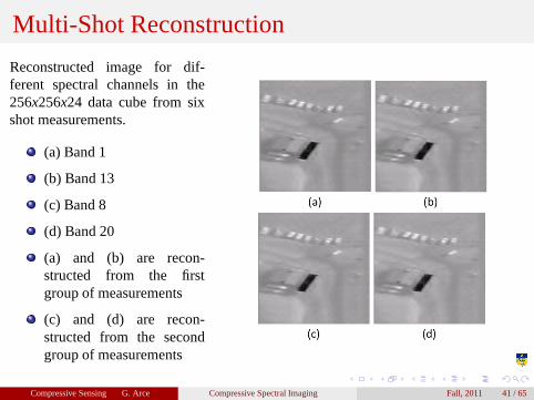
Multi-Shot Reconstruction
Reconstructed image for dif-ferent spectral channels in the256x256x24 data cube from sixshot measurements.
(a) Band 1
(b) Band 13
(c) Band 8
(d) Band 20
(a) and (b) are recon-structed from the firstgroup of measurements
(c) and (d) are recon-structed from the secondgroup of measurements
Compressive Sensing G. Arce Compressive Spectral Imaging Fall, 2011 41 / 65
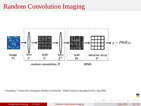
Random Convolution Imaging
J. Romberg. ”Compressive Sensing by Random Convolution.” SIAM Journal on Imaging Science, July,2008.
Compressive Sensing G. Arce Random Convolution Imaging Fall, 2011 42 / 65
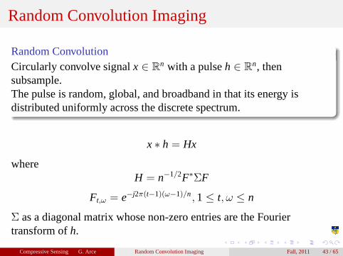
Random Convolution Imaging
Random ConvolutionCircularly convolve signalx ∈ R
n with a pulseh ∈ Rn, then
subsample.The pulse is random, global, and broadband in that its energyisdistributed uniformly across the discrete spectrum.
x ∗ h = Hx
whereH = n−1/2F∗ΣF
Ft,ω = e−j2π(t−1)(ω−1)/n , 1 ≤ t, ω ≤ n
Σ as a diagonal matrix whose non-zero entries are the Fouriertransform ofh.
Compressive Sensing G. Arce Random Convolution Imaging Fall, 2011 43 / 65
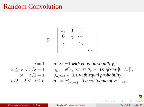
Random Convolution
Σ =
σ1 0 · · ·0 σ2 · · ·...
. . .σn
ω = 1 : σ1 ∼ ±1 with equal probability,2 ≤ ω < n/2+ 1 : σω = ejθω , where θω ∼ Uniform([0, 2π]),
ω = n/2+ 1 : σn/2+1 ∼ ±1 with equal probability,n/2+ 2 ≤ ω ≤ n : σω = σ∗
n−ω+2, the conjugate of σn−ω+2.
Compressive Sensing G. Arce Random Convolution Imaging Fall, 2011 44 / 65
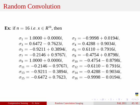
Random Convolution
Ex: if n = 16 i.e. x ∈ R16, then
σ1 = 1.0000+ 0.0000i, σ2 = −0.9998+ 0.0194i,σ3 = 0.6472− 0.7623i, σ4 = 0.4288+ 0.9034i,σ5 = −0.9211+ 0.3894i, σ6 = 0.6110+ 0.7916i,σ7 = −0.2146+ 0.9767i, σ8 = −0.4754+ 0.8798i,σ9 = 1.0000+ 0.0000i, σ10 = −0.4754− 0.8798i,σ11 = −0.2146− 0.9767i, σ12 = −0.6110− 0.7916i,σ13 = −0.9211− 0.3894i, σ14 = −0.4288− 0.9034i,σ15 = −0.6472+ 0.7623, σ16 = −0.9998− 0.0194i,
Compressive Sensing G. Arce Random Convolution Imaging Fall, 2011 45 / 65
Random Convolution
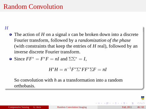
HThe action ofH on a signalx can be broken down into a discreteFourier transform, followed by arandomization of the phase(with constraints that keep the entries ofH real), followed by aninverse discrete Fourier transform.
SinceFF∗ = F∗F = nI andΣΣ∗ = I,
H∗H = n−1F∗Σ∗FF∗ΣF = nI
So convolution withh as a transformation into a randomorthobasis.
Compressive Sensing G. Arce Random Convolution Imaging Fall, 2011 46 / 65

Sampling at Random Locations
Simply observe entries ofHx at a small number of randomly chosenlocations.Thus the measurement matrix can be written as
Φ = RΩH
whereRΩ is the restriction operator to the setΩ (m random locationsubset).
Compressive Sensing G. Arce Random Convolution Imaging Fall, 2011 47 / 65
Randomly Pre-Modulated Summation
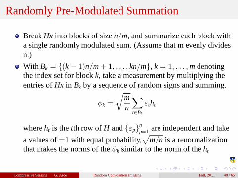
BreakHx into blocks of sizen/m, and summarize each block witha single randomly modulated sum. (Assume that m evenly dividesn.)
With Bk = (k − 1)n/m + 1, . . . , kn/m, k = 1, . . . ,m denotingthe index set for blockk, take a measurement by multiplying theentries ofHx in Bk by a sequence of random signs and summing.
φk =
√
mn
∑
t∈Bk
εtht
whereht is thetth row of H andεpnp=1 are independent and take
a values of±1 with equal probability,√
m/n is a renormalizationthat makes the norms of theφk similar to the norm of theht
Compressive Sensing G. Arce Random Convolution Imaging Fall, 2011 48 / 65
Randomly Pre-Modulated Summation
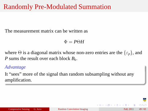
The measurement matrix can be written as
Φ = PΘH
whereΘ is a diagonal matrix whose non-zero entries are theεp, andP sums the result over each blockBk.
Advantage
It “sees” more of the signal than random subsampling withoutanyamplification.
Compressive Sensing G. Arce Random Convolution Imaging Fall, 2011 49 / 65
Randomly Pre-Modulated Summation
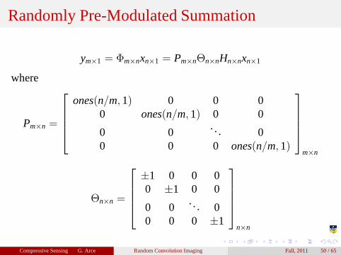
ym×1 = Φm×nxn×1 = Pm×nΘn×nHn×nxn×1
where
Pm×n =
ones(n/m, 1) 0 0 00 ones(n/m, 1) 0 0
0 0... 0
0 0 0 ones(n/m, 1)
m×n
Θn×n =
±1 0 0 00 ±1 0 0
0 0... 0
0 0 0 ±1
n×n
Compressive Sensing G. Arce Random Convolution Imaging Fall, 2011 50 / 65
Randomly Pre-Modulated Summation
Why the summation must be randomly?
Imagine if we were to leave out theεt and simply sumHx over eachBk. This would be equivalent to puttingHx through a boxcar filter thensubsampling uniformly.
Compressive Sensing G. Arce Random Convolution Imaging Fall, 2011 51 / 65
Main Result
The application ofH will not change the magnitude of the Fouriertransform, so signals which are concentrated in frequency willremain concentrated and signals which are spread out will stayspread out.
The randomness ofΣ will make it highly probable that a signalwhich is concentrated in time will not remain so afterH isapplied.
Compressive Sensing G. Arce Random Convolution Imaging Fall, 2011 52 / 65
Main Result
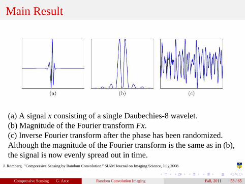
(a) A signalx consisting of a single Daubechies-8 wavelet.(b) Magnitude of the Fourier transformFx.(c) Inverse Fourier transform after the phase has been randomized.Although the magnitude of the Fourier transform is the same as in (b),the signal is now evenly spread out in time.
J. Romberg. ”Compressive Sensing by Random Convolution.” SIAM Journal on Imaging Science, July,2008.
Compressive Sensing G. Arce Random Convolution Imaging Fall, 2011 53 / 65
Application: Fourier Optics
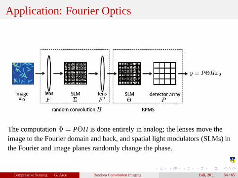
The computationΦ = PΘH is done entirely in analog; the lenses move theimage to the Fourier domain and back, and spatial light modulators (SLMs) inthe Fourier and image planes randomly change the phase.
Compressive Sensing G. Arce Random Convolution Imaging Fall, 2011 54 / 65
Fourier Optics
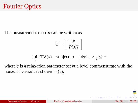
The measurement matrix can be written as
Φ =
[
PPΘH
]
minx
TV(x) subject to ‖Φx − y‖2 ≤ ε
whereε is a relaxation parameter set at a level commensurate with thenoise. The result is shown in (c).
Compressive Sensing G. Arce Random Convolution Imaging Fall, 2011 55 / 65
Fourier Optics
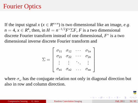
If the input signalx (x ∈ Rn×n) is two dimensional like an image,e.g.n = 4, x ∈ R4, then, inH = n−1/2F∗ΣF, F is a two dimensionaldiscrete Fourier transform instead of one dimensional,F∗ is a twodimensional inverse discrete Fourier transform and
Σ =
σ11 σ12 · · · σ1n
σ21 σ22 · · · σ2n...
.... . .
...σn1 σn2 . . . σnn
whereσω has the conjugate relation not only in diagonal direction butalso in row and column direction.
Compressive Sensing G. Arce Random Convolution Imaging Fall, 2011 56 / 65
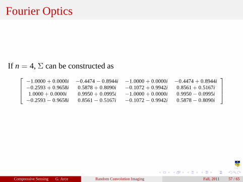
Fourier Optics
If n = 4,Σ can be constructed as
−1.0000+ 0.0000i −0.4474− 0.8944i −1.0000+ 0.0000i −0.4474+ 0.8944i−0.2593+ 0.9658i 0.5878+ 0.8090i −0.1072+ 0.9942i 0.8561+ 0.5167i1.0000+ 0.0000i 0.9950+ 0.0995i −1.0000+ 0.0000i 0.9950− 0.0995i−0.2593− 0.9658i 0.8561− 0.5167i −0.1072− 0.9942i 0.5878− 0.8090i
Compressive Sensing G. Arce Random Convolution Imaging Fall, 2011 57 / 65
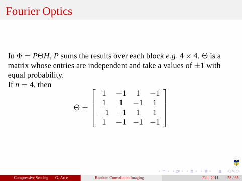
Fourier Optics
In Φ = PΘH, P sums the results over each blocke.g. 4× 4. Θ is amatrix whose entries are independent and take a values of±1 withequal probability.If n = 4, then
Θ =
1 −1 1 −11 1 −1 1−1 −1 1 11 −1 −1 −1
Compressive Sensing G. Arce Random Convolution Imaging Fall, 2011 58 / 65
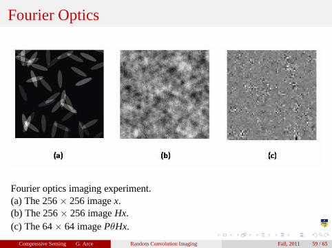
Fourier Optics
Fourier optics imaging experiment.(a) The 256× 256 imagex.(b) The 256× 256 imageHx.(c) The 64× 64 imagePθHx.
Compressive Sensing G. Arce Random Convolution Imaging Fall, 2011 59 / 65

(a) The 256× 256 image we wish to acquire.(b) High-resolution image pixellated by averaging over 4× 4 blocks.(c) The image restored from the pixellated version in (b), plus a set ofincoherent measurements. The incoherent measurements allow us toeffectively super-resolve the image in (b).
Compressive Sensing G. Arce Random Convolution Imaging Fall, 2011 60 / 65
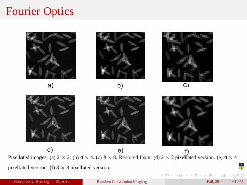
Fourier Optics
C)b)a)
d) e) f)Pixellated images: (a) 2× 2. (b) 4× 4. (c) 8× 8. Restored from: (d) 2× 2 pixellated version. (e) 4× 4
pixellated version. (f) 8× 8 pixellated version.
Compressive Sensing G. Arce Random Convolution Imaging Fall, 2011 61 / 65
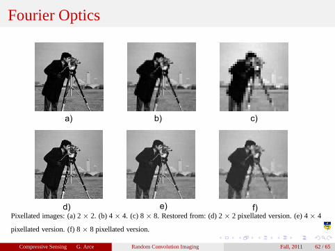
Fourier Optics
c)
d) e) f)
b)a)
Pixellated images: (a) 2× 2. (b) 4× 4. (c) 8× 8. Restored from: (d) 2× 2 pixellated version. (e) 4× 4
pixellated version. (f) 8× 8 pixellated version.
Compressive Sensing G. Arce Random Convolution Imaging Fall, 2011 62 / 65
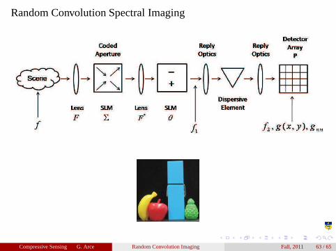
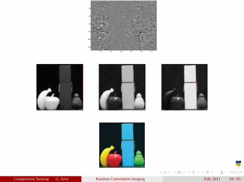
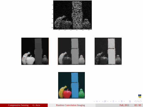
Random Convolution Spectral Imaging
Compressive Sensing G. Arce Random Convolution Imaging Fall, 2011 63 / 65
20 40 60 80 100 120
20
40
60
80
100
120
Compressive Sensing G. Arce Random Convolution Imaging Fall, 2011 64 / 65
20 40 60 80 100 120
20
40
60
80
100
120
Compressive Sensing G. Arce Random Convolution Imaging Fall, 2011 65 / 65