ELEMENTARY KNOT THEORY

MARC LACKENBY

1. Introduction . . . . . . . . . . . . . . . . . . . . . . . . . . . . . . . . . . . . . . . . . . . . . . . . . . . . . . . . . . . . . . . . . . . . . . . . 1

2. The equivalence problem . . . . . . . . . . . . . . . . . . . . . . . . . . . . . . . . . . . . . . . . . . . . . . . . . . . . . . . . . . . . 1

3. The recognition problem . . . . . . . . . . . . . . . . . . . . . . . . . . . . . . . . . . . . . . . . . . . . . . . . . . . . . . . . . . . . 8

4. Reidemeister moves . . . . . . . . . . . . . . . . . . . . . . . . . . . . . . . . . . . . . . . . . . . . . . . . . . . . . . . . . . . . . . . . 15

5. Crossing number . . . . . . . . . . . . . . . . . . . . . . . . . . . . . . . . . . . . . . . . . . . . . . . . . . . . . . . . . . . . . . . . . . .18

6. Crossing changes and unknotting number . . . . . . . . . . . . . . . . . . . . . . . . . . . . . . . . . . . . . . . . . . 22

7. Special classes of knots and links . . . . . . . . . . . . . . . . . . . . . . . . . . . . . . . . . . . . . . . . . . . . . . . . . . .25

8. Epilogue . . . . . . . . . . . . . . . . . . . . . . . . . . . . . . . . . . . . . . . . . . . . . . . . . . . . . . . . . . . . . . . . . . . . . . . . . . .29

1. Introduction

In the past 50 years, knot theory has become an extremely well-developed subject. But there

remain several notoriously intractable problems about knots and links, many of which are surprisingly

easy to state. The focus of this article is this ‘elementary’ aspect to knot theory. Our aim is to

highlight what we still do not understand, as well as to provide a brief survey of what is known.

The problems that we will concentrate on are the non-technical ones, although of course, their

eventual solution is likely to be sophisticated. In fact, one of the attractions of knot theory is its

extensive interactions with many different branches of mathematics: 3-manifold topology, hyperbolic

geometry, Teichmuller theory, gauge theory, mathematical physics, geometric group theory, graph

theory and many other fields.

This survey and problem list is by no means exhaustive. For example, we largely neglect the

theory of braids, because there is an excellent survey by Birman and Brendle [5] on this topic. We

have also avoided 4-dimensional questions, such as the slice-ribbon conjecture (Problem 1.33 in [41]).

Although these do have a significant influence on elementary knot theory, via unknotting number

for example, this field is so extensive that it would best be dealt with in a separate article.

In fact, this article comes with a number of health warnings. It is frequently vague, often

deliberately so, and many standard terms that we use are not defined here. It is certainly far from

complete, and we apologise to anyone whose work has been omitted. And it is not meant to be

a historical account of the many developments in the subject. Instead, it is primarily a list of

fundamental and elementary problems, together with enough of a survey of the field to put these

problems into context.

2. The equivalence problem

The equivalence problem for knots and links asks the most fundamental question in the field:

can we decide whether two knots or links are equivalent? Questions of this sort arise naturally in

just about any branch of mathematics. In topology, there are many well-known negative results.

1

A central result of Markov [63] states that there is no algorithm to determine whether two closed

n-manifolds are homeomorphic, when n ≥ 4. But in dimension 3, the situation is more tractable.

In particular, the equivalence problem for knots and links is soluble. In fact, there are now five

known ways to solve this problem, which we describe briefly below. Four of these techniques focus

on the exterior S3 − int(N(K)) of the link K. Now, one loses a small amount information when

passing to the link exterior, because it is possible for distinct links to have homeomorphic exteriors.

(This is not the case for knots, by the famous theorem of Gordon and Luecke [23]). So, one should

also keep track of a complete set of meridians for the link, in other words, a collection of simple

closed curves on ∂N(K), one on each component of ∂N(K), each of which bounds a meridian disc

in N(K). Then, for two links K and K ′, there is a homeomorphism between their exteriors that

preserves these meridians if and only if K and K ′ are equivalent.

2.1. Hierarchies and normal surfaces

Haken [25], Hemion [30] and Matveev [64] were the first to solve the equivalence problem for

links. Their solution is lengthy and difficult. A full account of their argument was given only fairly

recently by Matveev [64].

Haken used incompressible surfaces arranged into sequences called hierarchies. Recall that a

surface S properly embedded in a 3-manifold M is incompressible if, for any embedded disc D in

M with D ∩ S = ∂D, there is a disc D′ in S with ∂D′ = ∂D. Given such a surface, it is natural

to cut M along S, creating the compact manifold cl(M −N(S)). It turns out that one can always

find another properly embedded incompressible surface in this new manifold, and thereby iterate

this procedure. A hierarchy is a sequence of manifolds and surfaces

M = M1S1−→M2

S2−→ . . .Sn−1−→ Mn

where each Si is a compact orientable incompressible surface properly embedded in Mi with no

2-sphere components, where Mi+1 is obtained from Mi by cutting along Si and where the final

manifold Mn is a collection of 3-balls. Haken proved that the exterior of a non-split link always

admits a hierarchy. He was able to solve the equivalence problem for links via the use of hierarchies

with certain nice properties. An example of a hierarchy for a knot exterior is given in Figure 1.

Associated with a hierarchy, there is a 2-complex embedded in the manifold M . To build this,

one extends each surface Si in turn, by attaching a collar to ∂Si in N(S1 ∪ . . . ∪ Si−1), so that the

boundary of the new surface runs over the earlier surfaces and ∂M . The union of these extended

surfaces and ∂M is the 2-complex. The 0-cells are the points where three surfaces intersect. The 1-

skeleton is the set of points which lie on at least two surfaces. Since the complement of this extended

hierarchy and the boundary of the manifold is a collection of open balls, we actually obtain a cell

structure for M in this way. It is a trivial but important observation that this is a representation of

M that depends only on the topology of the hierarchy. Haken’s solution to the equivalence problem

establishes that, as long as one chooses the hierarchy correctly, there is a way of building this cell

structure, starting only from an arbitrary triangulation of M .

2

(i) The knot 5 (ii) The first surface in the hierarchy

(iii) The exterior of this surface (iv) The second surface in the hierarchy

1

Figure 1: A hierarchy for a knot exterior

Suppose that we are given diagrams for two (non-split) links K and K ′. The first step in the

algorithm is to construct triangulations T and T ′ for their exteriors M and M ′. We know that M

and M ′ admit hierarchies with the required properties. Moreover, if M and M ′ are homeomorphic

(by a homeomorphism preserving the given meridians), then this homeomorphism takes one such

hierarchy for M to a hierarchy for M ′. So, let us focus initially on the hierarchy for M . The next

stage in the procedure is to place the first surface S of the hierarchy into normal form. By definition,

this means that it intersects each tetrahedron of T in a collection of triangles and squares, as shown

in Figure 2.

Triangle Square

Figure 2: Normal surface

Now, any incompressible, boundary-incompressible surface S (with no components that are

2-spheres or boundary-parallel discs) in a compact orientable irreducible boundary-irreducible 3-

manifold M with a given triangulation T may be ambient isotoped into normal form. It can then be

encoded by a finite amount of data. The normal surface S determines a collection of 7t integers, where

t is the number of tetrahedra in T . These integers simply record the number of triangles and squares

of S in each tetrahedron. The list of these integers is denoted [S] and is called the associated normal

surface vector. Normal surface vectors satisfy a number of constraints. Firstly, each co-ordinate is,

of course, a non-negative integer. Secondly, they satisfy various linear equations called the matching

conditions which guarantee that, along each face of T with a tetrahedron on each side, the triangles

3

and squares of S in the two adjacent tetrahedra patch together correctly. Finally, there are the

quadrilateral constraints which require S to have at most one type of square in each tetrahedron. This

is because two different square types cannot co-exist in the same tetrahedron without intersecting.

Haken showed that there is a one-one correspondence between properly embedded normal surfaces

(up to a suitable notion of ‘normal’ isotopy) and vectors satisfying these conditions. Given this

strong connection, it is natural to use tools from linear algebra when studying normal surfaces. In

particular, one can speak of a normal surface S as being the sum of two normal surfaces S1 and S2 if

[S] = [S1] + [S2]. A normal surface S is called fundamental if it cannot be expressed as a sum of two

other non-empty normal surfaces. Haken showed that there is a finite list of fundamental normal

surfaces, and these are all algorithmically constructible. A key part of Haken’s argument is to show

that some surfaces can be realised as fundamental normal surfaces with respect to any triangulation

of the manifold. Thus, if we could find a hierarchy where each surface had this property, then we

could construct the hierarchy starting with any triangulation T of M . In fact, Haken did not prove

that there is a hierarchy with this property, but he did show that there is a hierarchy where each

surface can be realised as a sum of boundedly many fundamental normal surfaces. This is sufficient

to make the argument work.

Thus, Haken’s algorithm essentially proceeds by starting with the triangulations T and T ′ of

the two link exteriors. Then, one constructs all possible hierarchies for each manifold, with the

property that each surface in the hierarchy is a bounded sum of fundamental surfaces. From each

such hierarchy, one forms the associated cell structure for M . If two such cell structures, one from

each of T and T ′, are combinatorially equivalent, then the links are the same. If none of these cell

structures are equivalent, then the links are distinct.

There were two cases that Haken could not handle using these methods. When M fibres over

the circle with fibre S, then cutting M along S results in a copy of S× I. In S× I, there is no good

choice of surface to cut along. In particular, it is not clear how to find a surface that is guaranteed to

be fundamental or at least a bounded sum of fundamental surfaces. The resolution of the equivalence

problem for these manifolds was not completed until work of Hemion [30], where he gave a solution

to the conjugacy problem in the mapping class group of S. A similar problem arises when cutting

along S yields a twisted I-bundle (in which case, S is known as a semi-fibre). This case was fully

dealt with by Matveev [64].

In fact, there is a now an alternative way of sidestepping this issue, by establishing that there is

always a hierarchy for a non-split link exterior which is always constructible. This relies on the result

of Culler and Shalen [13], which says that if M is a compact orientable hyperbolic 3-manifold with

boundary a non-empty collection of tori, then M contains either a closed, non-separating, essential

properly embedded surface or a separating, connected, essential, properly embedded surface with

non-empty boundary. When M is the exterior of a hyperbolic link in the 3-sphere, this surface can

be chosen to be neither a fibre nor a semi-fibre (see Section 7 in [9]). By work of Mijatovic [68],

there is such a surface that can be realised as a bounded sum of fundamental surfaces.

Of course, this summary is a dramatic over-simplification. The details of the argument are

very complicated. A full exposition, which lasts several hundred pages, can be found in the excellent

book by Matveev [64].

4

2.2. Geometric structures

One of the most striking advances in low-dimensional topology was Thurston’s introduction of

hyperbolic geometry, via his Geometrisation Conjecture [96]. This was proved by Perelman in 2003

[78, 79, 80], but Thurston himself proved his conjecture in the case of knot and link complements,

and this can be used to provide another method of solving the equivalence problem. An approximate

statement of the Geometrisation Conjecture is that every compact orientable 3-manifold admits a

‘canonical decomposition’ into ‘geometric pieces’.

The canonical decomposition takes place in two steps. (We focus for simplicity on the case

where the boundary of the 3-manifold is empty or a collection of tori.) Firstly, one decomposes the

3-manifold into its prime connected summands. Secondly, one cuts the manifold along its JSJ tori.

Both processes can be achieved algorithmically using normal surface theory [34]. (See [72] and [64]

for more details of JSJ theory, which was first developed by Jaco, Shalen [33] and Johannson [36].)

Once this decomposition has taken place, the resulting pieces either are Seifert fibred or admit

finite-volume hyperbolic structures. The generic situation is the hyperbolic case, and it is this that

we will focus on. An algorithm to find a finite-volume hyperbolic structure on a 3-manifold, provided

one exists, was given by Manning [61], based on work of Casson. By combining [61] with work of

Weeks [99], it possible to compute the Epstein-Penner decomposition of the manifold [18]. This is

a striking construction: it is a decomposition of a non-compact finite-volume hyperbolic 3-manifold

into ideal polyhedra. The crucial thing about it is that it is canonical: it depends only on the topology

of the manifold, not on any arbitrary choices. Thus, two finite-volume non-compact hyperbolic 3-

manifolds are homeomorphic if and only if their Epstein-Penner decompositions are combinatorially

equivalent. Moreover, one can determine whether there is a homeomorphism between the manifolds,

taking one given collection of disjoint simple closed curves in the boundary to another. This therefore

gives a solution to the equivalence problem for knots and links.

This is more than just a theoretical algorithm. The computer programs Knotscape [31], Snappea

[98] and Snap [10] all attempt to compute the Epstein-Penner decomposition of a hyperbolic 3-

manifold. Unlike the Casson-Manning algorithm, they are not guaranteed to do so. But if Snap

or Knotscape finds what it claims is the Epstein-Penner decomposition, then this is indeed the

correct decomposition, and as a result, these programs are a practical method of reliably determining

whether two links are equivalent.

2.3. Relatively hyperbolic groups

One can also use some of the machinery of geometric group theory to solve the equivalence

problem, at least for hyperbolic knots.

The fundamental group of a closed hyperbolic 3-manifold is Gromov-hyperbolic. Mostow rigid-

ity states that two such manifolds are isometric if and only if their fundamental groups are isomor-

phic. Moreover, Sela provided an algorithm to decide whether two torsion-free Gromov-hyperbolic

groups are isomorphic [88]. Now, the complement of a knot is, of course, not closed. But when

this complement has a hyperbolic structure, its fundamental group is a relatively hyperbolic group,

relative to the fundamental group of the toral boundary. Mostow rigidity applies in this case also.

5

Sela’s result was extended to this class of relatively hyperbolic groups by Dahmani and Groves [14].

So, at least in the case of hyperbolic knots, one can solve the equivalence problem this way. This

does not immediately lead to a solution for hyperbolic links, because links are not determined by

their complements. But presumably, the algorithm of Dahmani and Groves could be adapted to

take account of a set of meridians in the boundary tori. This method also only works in the hyper-

bolic case, and so to turn this into a fully-fledged solution to the equivalence problem for all links,

presumably one would first need to find the ‘canonical decomposition into geometric pieces’ that

was discussed in the previous subsection. Nevertheless, this is a genuinely different solution to the

equivalence problem. But its algorithmic complexity seems to be hard to estimate.

2.4. Reidemeister moves

There is an alternative way of interpreting the equivalence problem in terms of Reidemeister

moves. Recall that a Reidemeister move is a local modification to a link diagram as shown in Figure

3. Reidemeister proved [82] that any two diagrams of a link differ by a sequence of Reidemeister

moves. The algorithmic significance of this is that if two diagrams represent the same link, then one

may always prove this, given enough time and computing power. This is because one can apply all

possible Reidemeister moves to the first diagram, and thereby obtain a collection of diagrams of the

first link. One can then apply all possible Reidemeister moves to each of these, and so on. It is a

consequence of Reidemeister’s theorem that if the two initial diagrams represent the same link, then

this process is guaranteed to produce a sequence of Reidemeister moves taking one diagram to the

other.

Figure 3: Reidemeister moves

Of course, this does not provide a solution to the equivalence problem, because if two diagrams

represent distinct link types, then the above process does not terminate. But if one knew in advance

how many Reidemeister moves were required to take one diagram to other, then one could stop

the process when one had tried all possible sequences of Reidemeister moves of this length and if a

sequence of Reidemeister moves taking one diagram to the other had not been found, then one could

declare that the links are distinct. More specifically, a computable upper bound on the number

of Reidemeister moves required to relate two diagrams of the same link provides a solution to the

equivalence problem. In fact, it is not hard to show that the converse is also true: if there is a

solution to the equivalence problem, then, given natural numbers n1 and n2, one can compute an

upper bound on the number of Reidemeister moves required to relate two diagrams of a link with n1

and n2 crossings. One enumerates all link diagrams with these numbers of crossings, and then one

sorts them into their various link types, using the hypothesised algorithm to solve the equivalence

problem. Then, for all diagrams of the same link type, one starts applying Reidemeister moves

to these diagrams. By Reidemeister’s theorem, eventually a sequence of such moves will be found

relating any two diagrams of the same link. Hence, one can compute an upper bound on the number

of moves that are required.

6

Recently, Coward and the author [9] have provided an explicit, computable upper bound on

Reidemeister moves, thereby giving a new and conceptually simple solution to the equivalence prob-

lem. Unfortunately, it is a huge bound, and so the resulting algorithm is very inefficient. We will

provide more details in Section 4, which is devoted to Reidemeister moves.

2.5. Pachner moves

It is well known that two triangulated manifolds are PL-homeomorphic if and only if they differ

by a sequence of Pachner moves [77]. These are modifications that change the triangulation in a

very simple way. In the case of closed 3-manifolds, the moves are shown in Figure 4. For 3-manifolds

with boundary, there are some extra moves which change the triangulation on the boundary.

Figure 4: Pachner moves

Therefore, just as argued in the previous subsection, if two triangulated manifolds are PL-

homeomorphic, then one will always be able to prove this eventually. Moreover, if one has a com-

putable upper bound on the number of Pachner moves required to pass between two triangulations,

then one can solve the PL-homeomorphism problem. In the case of knot exteriors, such a com-

putable upper bound was found by Mijatovic [68]. Unfortunately, his bound is massive: a tower of

exponentials, exponentially high. So, again, this does not lead to a practical algorithm.

Mijatovic’s method built on work of Haken. As explained in Section 2.1, Haken used a hierarchy

for a link exterior M to build a ‘canonical’ cell structure for M . This had the property that one can

algorithmically build this cellulation starting from any triangulation of M . By carefully modifying

the initial triangulation to one derived from this cellulation, Mijatovic was able to produce an

upper bound on the number of Pachner moves required. The method is not easy, and in particular,

he needed to go beyond what Haken achieved, because he also needed the Rubinstein-Thompson

machinery for 3-sphere recognition [95, 67].

2.6. Solving the equivalence problem efficiently

None of these approaches to the equivalence problem is known to be efficient. Indeed, any

efficient solution seems to be out of reach at present. This leads to our first unsolved problem.

Problem 1. What is the complexity class of the equivalence problem for knots and links?

It is quite striking that, of the five above approaches to the equivalence problem, only the final

two give an a priori estimate for its running time. However, the disadvantage of the approaches

using Reidemeister moves or Pachner moves is that they are almost inevitably lengthy.

7

One the main difficulties in Haken’s approach to the equivalence problem is that, in order to

apply normal surface theory, one needs to build a triangulation Ti for each 3-manifold Mi in the

hierarchy. However, the surface Si may be exponentially complicated in Ti, in the sense of having

exponentially many triangles and squares, as a function of the number of tetrahedra in Ti. So, it

seems inevitable that the next triangulation Ti+1 should be exponentially more complicated than

that of Ti. So, the number of tetrahedra in Tn is massive. As a function of the crossing number of

a given diagram of the link, it is a tower of exponentials. The height of this tower is n, the length

of the hierarchy, and unfortunately, due to the technical requirements of Haken’s hierarchies, n can

be quite large too.

On the other hand, the approach to the equivalence using geometric structures is of unknown

complexity. However, it appears to be computationally efficient in practice, even if one cannot yet

prove this. So, there remains some hope that a provably efficient solution to the equivalence problem

may be found in the future.

One might ask for a polynomial-time algorithm in Problem 1. But this seems rather unlikely,

and there certainly seems no prospect of a proof in sight. Even an NP algorithm seems beyond reach

at the moment. (For a very brief explanation of NP and other complexity classes, see Section 3.1.)

Alternatively, one might try to find lower bounds on the complexity of the problem, conditional upon

well-known conjectures in theoretical computer science. For example, is the equivalence problem NP-

hard? In other words, is it at least as hard as any other NP problem? In particular, if there was a

polynomial-time solution to the equivalence problem for knots and links, would this imply that P

= NP? This seems plausible. Indeed, a seemingly simpler algorithm in 3-manifold theory is known

to be NP-complete, by work of Agol, Hass and Thurston [3]. This is the problem of determining

whether a given knot in a given 3-manifold bounds a compact orientable embedded surface of a

given genus.

3. The recognition problem

An algorithmic problem that is closely related to the equivalence problem is the recognition

problem for a fixed link type. Here, one fixes a link type K, and one asks whether a given diagram

represents this link type. Fairly obviously, a solution to the equivalence problem implies a solution

to the recognition problem for each link type. However, by fixing the link type, we simplify the

problem, and so there may be some hope of coming up with a more efficient solution. The case of

the unknot is particularly intriguing. The following remains unknown.

Problem 2. Is there a polynomial-time algorithm to recognise the unknot?

Currently, the unknot recognition problem is known to lie in the following complexity classes:

NP, co-NP and E. We briefly remind the reader of the definitions of these and various other classes.

3.1. Some basic complexity classes

The class P is possibly simplest to describe. It consists of those problems that be solved in

time nk, where n is the size of the input and k is a fixed constant. Similarly, a problem is in the

8

class E if it can be solved in time kn, where n is the size of the input and k is a fixed constant.

Somewhat confusingly, this is not the same as the class EXP of exponential-time algorithms, since,

by definition, these can solved in time knc

for constants k and c.

A problem is in NP if it admits a polynomial-time certificate. This is an extra piece of infor-

mation that is not provided by the algorithm, rather it is given by some external source. The point

is that if the answer to the problem is ‘yes’, then the certificate proves that it is ‘yes’, and this can

be verified in polynomial time. There are many examples of NP problems; one is the problem of

deciding whether a given positive integer is composite. In this case, a very simple certificate is two

integers (greater than 1) whose product is the given integer. It can be verified in polynomial time (as

a function of the number of digits of the input) that these two integers do indeed multiply together

to produce the given number. One might legitimately wonder why NP problems are solvable at all,

given that they require information from an external source. But the point is that this information

must have polynomially bounded size, because a computer has time enough only to check this many

bits of information. So, a deterministic algorithm proceeds by checking all possible certificates of at

most this size. Thus, problems in NP are also in EXP.

A computational problem is in co-NP if its negation is in NP. Thus, for example, the problem

of deciding whether a positive integer is composite is in co-NP, because there is an NP algorithm

to determine whether a positive integer is prime. This is not at all obvious however. It was first

proved by Pratt [81], using the Lucas primality test.

There is also the well-known class of NP-complete problems. A problem is NP-complete if it is

in NP and any other NP problem may be (efficiently) reduced to it. In particular, if an NP-complete

problem has a polynomial-time solution, then this would imply that P = NP. It is widely believed

that P 6= NP, and so NP-complete problems are, in some conditional sense, provably hard. However,

it is very unlikely that any problem that is both in NP and co-NP is NP-complete, because this

would imply that NP = co-NP, which also is viewed as rather unlikely.

3.2. Haken’s unknot recognition algorithm

The first person to provide an unknot recognition algorithm was Haken [24]. A knot K is the

unknot if and only if its exterior M has compressible boundary. Haken showed how one may use

normal surface theory to determine this. As in Section 2.1, one builds a triangulation of M using the

given diagram of K. Haken showed that if M contains an essential properly embedded disc, then

it contains one that is a fundamental normal surface. He also showed that all fundamental normal

surfaces may be algorithmically constructed. Thus, his unknot recognition algorithm proceeds by

constructing all possible fundamental normal surfaces, and determining whether any of these is an

essential disc.

3.3. The NP algorithm of Hass, Lagarias and Pippenger

Hass, Lagarias and Pippenger [27] provided an NP algorithm, by building on Haken’s work.

Instead of using fundamental surfaces, they used vertex surfaces. By definition, a normal surface S

is a vertex surface if it is connected and whenever n[S] = [S1] + [S2] for a positive integer n and

9

normal surfaces S1 and S2, then each of [S1] and [S2] is a multiple of [S]. The reason for the vertex

terminology is that the set of all normal surface vectors can be viewed as integer points within a

larger subset of R7t, where t is the number of tetrahedra of the 3-manifold M . This subset is the

set of vectors satisfying the matching equations and quadrilateral constraints, but where the vectors

are required only to be non-negative real numbers. It is not hard to see that this subset is a union

of convex polytopes, each of which is the cone on a compact polytope, where the cone point is

the origin. Vertex surfaces are precisely those connected normal surfaces that are a multiple of a

vertex of one of these compact polytopes. Hass, Lagarias and Pippenger showed that if M contains

an essential properly embedded disc, then it has one that is a vertex normal surface. Moreover,

for each such vertex surface that is an essential disc, one can certify that it is an essential disc in

polynomial time. Thus, unknot recognition lies in NP. It is also not hard to prove that the number

of vertex surfaces is at most 27t, because each one is obtained as the unique solution (up to scaling)

of the matching equations plus some extra constraints that force certain co-ordinates to be zero.

So, if one checks each such vertex surface in turn, one can determine whether the given knot is the

unknot in at most kn steps where n is the crossing number of the diagram and k is a fixed constant.

This implies that unknot recognition lies in E.

3.4. The co-NP algorithm of Kuperberg

Kuperberg has recently proved that unknot recognition is in co-NP, assuming the Generalised

Riemann Hypothesis [48]. Here, one wants an efficient way of certifying that a non-trivial knot

K is indeed knotted. Kuperberg achieves this by establishing the existence of a representation

from π1(S3 −K) to some finite group with non-abelian image. The unknot clearly admits no such

representation, because the fundamental group of its complement is Z. Thus, this does establish

that the knot is non-trivial.

The existence of such a representation is not at all clear. Moreover, Kuperberg requires a

representation with small enough image, so that the representation can be verified as a homomor-

phism with non-abelian image in polynomial time. The starting point is the major theorem of

Kronheimer and Mrowka [45] that establishes that, for a non-trivial knot K, there is a homomor-

phism π1(S3−K)→ SU(2) with non-abelian image. This is established using a highly sophisticated

argument that uses taut foliations, contact structures, symplectic fillings, and the instanton equa-

tions. (In the case where the knot K is hyperbolic, one can instead use the associated representation

π1(S3 −K)→ PSL(2,C) in Kuperberg’s argument.)

Once one has a linear representation of Γ = π1(S3−K), there is a standard method of obtaining

finite representations, that goes back to the result of Malce’ev [60] which states that finitely generated

linear groups are residually finite. One considers a finite generating set for Γ, and for each generator,

one considers the entries of the corresponding matrix (in SU(2)). The ring R generated by these

entries is a finitely generated subring of C. Thus, the image of Γ lies in SL(2, R). Such a ring R

contains many finite index ideals I. The desired finite quotients are obtained by mapping SL(2, R)

onto SL(2, R/I) for some such I. The Generalised Riemann Hypothesis is used to prove the existence

of an ideal I with small index, and hence one obtains a finite quotient of Γ with small size. The

actual tools that are used here are results of Korain [43], Lagarias-Odlyzko [57] and Weinberger [100]

10

which imply that, for any integer polynomial, one may reduce its coefficients modulo some small

prime and obtain a polynomial with a root, assuming the Generalised Riemann Hypothesis.

3.5. The co-NP algorithm of Agol

Agol has another certificate for establishing that a non-trivial knot is knotted [1]. This has the

advantage that it is unconditional on any conjectures, and it also provides more information about

the knot, by determining its genus. Recall that the genus of a knot K is the minimal genus of a

Seifert surface for K. It is a fundamental quantity, but for the purposes of this algorithm, all that

one needs is that the genus is zero if and only if the knot is trivial.

It is a consequence of Haken’s work that the genus of a knot is algorithmically computable,

because a minimal genus Seifert surface can be arranged to be a fundamental normal surface. How-

ever, Thurston and Gabai found another method for determining the genus of knots, by using the

theory of taut foliations [97, 21]. In fact, this method naturally measures not the genus of a compact

surface S but its Thurston complexity χ−(S). By definition, when S is connected, then χ−(S) =

max{−χ(S), 0}. When S is disconnected with components S1, . . . , Sn, then χ−(S) =∑n

i=1 χ−(Si).

Thus, when S is orientable, χ−(S) is roughly the negative of the Euler characteristic of the surface,

but one first discards disc and sphere components. So, for knots, a Seifert surface has minimal

possible χ− if and only if it has minimal genus. But for links, this need not be the case, because the

link may have disconnected Seifert surfaces as well as connected ones.

The theory of Thurston and Gabai is concerned with foliations on a 3-manifold, where the leaves

of the foliation have codimension one and where there is a consistent transverse orientation on these

leaves. Such a foliation is taut if there is a simple closed curve in the 3-manifold that is transverse to

the foliation and that intersects every leaf. This may seem a slightly strange definition, but it turns

out that the existence of such a curve rules out various trivial examples of foliations, and in fact

the following was proved by Thurston [97]: If S is a compact leaf of a taut foliation on a compact

orientable 3-manifold M , then S has minimal χ− in its homology class in H2(M,∂S). Hence, if

one starts with a Seifert surface S for an oriented link L, and one can find a taut foliation on the

exterior of L in which S is a compact leaf, then S has minimal χ− among all Seifert surfaces for

L. Gabai [21] introduced a method for constructing these foliations and in fact proved the converse

statement: If S is a Seifert surface for an oriented non-split link L with minimal χ−, then there is

some taut foliation on the exterior of L in which S is a leaf.

One can view this taut foliation as a way of certifying the genus of a knot. However, it is not

a certificate in the strict algorithmic sense, because in principle, an infinite amount of information

is required to specify the foliation. But the key features of Gabai’s foliations are encoded by a

finite amount of information as follows. Gabai utilised hierarchies to construct his foliations, and it

was first observed by Scharlemann [85] that many of the useful topological consequences of Gabai’s

theory can be extracted solely from the hierarchy, without referring to the foliation. The hierarchies

of Gabai and Scharlemann naturally occur in the setting of 3-manifolds with the following extra

structure.

11

A sutured manifold is a compact oriented 3-manifold M with its boundary decomposed into

two subsurfaces R− and R+. A transverse orientation is imposed on these subsurfaces, so that R+

points out of M and R− points into it. These surfaces intersect along a collection of simple closed

curves γ, called sutures. It is usual to denote a sutured manifold by (M,γ), but the surfaces R+ and

R− are also an essential part of the structure. A sutured manifold (M,γ) is taut if M is irreducible,

R+ and R− are incompressible and they minimise χ− in their homology classes in H2(M,γ).

When a sutured manifold (M,γ) is decomposed along a properly embedded, transversely ori-

ented surface S that intersects γ transversely, the resulting 3-manifold M ′ inherits a sutured manifold

structure. This decomposition is taut if M and M ′ are both taut as sutured manifolds and S has

minimal χ− in its homology class in H2(M,∂S). A sequence of such decompositions terminating in

a collection of 3-balls is a sutured manifold hierarchy. A key feature of sutured manifold theory is:

If a sequence of sutured manifold decompositions ends in a collection of taut sutured 3-balls, then

(provided some simple conditions hold) every decomposition in this sequence is taut.

This sequence of decompositions can therefore be viewed as a certificate for knot genus. How-

ever, it is not at all clear that one can produce such a certificate that can be verified in polynomial

time. The principal difficulty is the one explained in Section 2.6 in reference to Haken’s use of

hierarchies. It seems, at first sight, that one needs to keep track of a triangulation of each manifold

in this hierarchy, and the complexity of these triangulations seems to grow rapidly as one proceeds

along the hierarchy. Agol’s alternative approach is to make the entire sutured manifold hierarchy

normal (in some suitable sense) with the respect to the initial triangulation of M . The idea is

that the sutured manifold hierarchy is closely related to a taut foliation and so normalising such a

hierarchy is somewhat analogous to normalising a taut foliation. Techniques exist for placing taut

foliations in ‘normal’ form, due to Brittenham [8] and Gabai [22], and versions of these are used

by Agol. Unfortunately, full details of this proof have not yet been written down. An alternative

approach may be to use the techniques of the author in [49], where sutured manifold hierarchies

were normalised in some weak sense.

3.6. Khovanov homology

In the mid 1980s, knot theory underwent a dramatic revolution, with the introduction of the

Jones polynomial [37], and then Witten’s interpretation of this using Chern-Simons theory [101].

Right from the outset of this work, it was asked: Does the Jones polynomial detect the unknot? In

other words, must a non-trivial knot necessarily have non-trivial Jones polynomial? This question

remains unanswered. Indeed, it may be viewed as a central open problem in knot theory, but it is

not ‘elementary’ and so does not make it onto our problem list.

It was shown recently by Kronheimer and Mrowka [47] that a more refined invariant, Khovanov

homology, does detect the unknot. This followed from a slightly indirect relationship between

Khovanov homology and 4-dimensional gauge-theoretic invariants.

It seems unlikely that this result will lead to an efficient way of recognising the unknot. This

is because determining Khovanov homology is a computationally intensive process. In fact, the less

refined Jones polynomial is, in one sense, provably hard to calculate. For example, it was shown by

12

Jaeger, Vertigana and Welsh [35] that computation of the Jones polynomial of a link is ‘] P-hard’.

(This is somewhat similar to being NP-complete.)

3.7. Heegaard Floer homology

Another major advance in knot theory has been the introduction of Heegaard Floer homology by

Oszvath and Szabo [74]. This was based on earlier instanton invariants, as pioneered by Donaldson

[16] in dimension 4, and then Floer [19] in dimension 3, and monopole invariants, as developed

by Seiberg and Witten [102] in dimension 4 and then Kronheimer and Mrowka [46] in dimension

3. It was clear from the outset that these gauge-theoretic invariants are particularly powerful, but

they were undoubtedly hard to calculate. One of the most attractive features of Heegaard Floer

homology is that, right from its inception, it has been possible to calculate it in many important

examples. Indeed, there are now algorithms to calculate the various different versions of Heegaard

Floer homology, due to Sarkar and Wang [83] and Manolescu, Ozsvath and Sarkar [62]. One of the

earliest results about Heegaard Floer homology was that it detects the unknot [75]. So, coupled with

the fact that it is computable, this provides another unknot recognition algorithm. Again, however,

it seems unlikely that this algorithm is in any way efficient.

3.8. Rectangular diagrams and arc presentations

In 2003, Dynnikov introduced a new and striking solution to the unknot recognition problem

[17]. This used rectangular diagrams and arc presentations. A rectangular diagram (also called grid

diagram) is a planar link diagram that consists of vertical and horizontal arcs, no two of which are

colinear, and with the key property that whenever a horizontal and a vertical arc cross, it is the

vertical arc that is the over-arc at the resulting crossing. The number of vertical arcs is equal to the

number of horizontal arcs; this is known as the arc index of the rectangular diagram.

Figure 5: A rectangular diagram

Rectangular diagrams were studied in detail by Cromwell [12]. He introduced a set of moves

which change a rectangular diagram, without changing the link type, much like Reidemeister moves.

He showed that any two rectangular diagrams for a link differ by a sequence of such moves. (See

Figure 6.) Two of these types of moves (cyclic permutations and exchange moves) leave the arc index

unchanged. The other type of move is a stabilisation/destabilisation which increases/decreases the

arc index by one.

13

stabilisation

cyclic permutation

exchange moves

destabilisation

stabilisation

destabilisation

stabilisation

destabilisation

stabilisation

destabilisation

Figure 6: Modifications to a rectangular diagram

Dynnikov proved that any rectangular diagram of the unknot can be reduced to the trivial

diagram using these moves, but crucially, no stabilisations are required. This leads to the following

unknot recognition algorithm. Start with the given diagram, and using an isotopy of the plane,

make it rectangular. Then keep applying all possible cyclic permutations, exchange moves and

destabilisations. Only finitely many moves are possible at each stage. The key point is that the

number of rectangular diagrams with bounded arc index is finite. So, eventually, one can explore

the entire set of rectangular diagrams that are reachable from the initial one by sequences of these

moves. The given knot is the unknot if and only if the trivial diagram is in this collection.

This does not immediately lead to an efficient solution. This is because the number of rect-

angular diagrams with a given arc index is a super-exponential function, and so the search space

might be quite large. But it is a beautiful and striking result that is perhaps the closest in spirit to

elementary knot theory among all the known unknot recognition algorithms. It also has the follow-

ing consequence, as noted by Dynnikov himself: If a diagram of the unknot has n crossings, then

there is a sequence of Reidemeister moves taking it to the trivial diagram, where each diagram in

this sequence has crossing number at most 2(n+ 1)2. This is simply because a rectangular diagram

with arc index m, say, has crossing number at most (m− 1)2/2.

Dynnikov’s proof builds on previous work of Cromwell [12], Birman, Menasco [7] and Bennequin

[4]. Cromwell observed a correspondence between rectangular diagrams and arc presentations, which

are defined as follows. One fixes a round unknot in the 3-sphere, which is a reference circle, known

as the binding circle. The complement of the binding circle is an open solid torus, which is foliated

by open discs called pages. A link is in an arc presentation if it intersects the binding circle in

finitely many points called vertices, and it intersects each page in either the empty set or a single

open arc joining distinct vertices. Cromwell proved that there is a one-one correspondence between

arc presentations and rectangular diagrams up to cyclic permutation.

14

Thus, Dynnikov’s proof mainly concentrates on arc presentations. Given an arc presentation of

the unknot, its spanning disc can be arranged so that its intersection with the pages induces a singular

foliation on the spanning disc. The singularities occur when the disc slices through the binding circle,

and also at Morse-type singularities in the complement of the binding circle. Dynnikov’s measure

of complexity for the disc is the number of singularities of this foliation. Using an argument that

relies on the fact that the disc has positive Euler characteristic, Dynnikov showed that this singular

foliation must have, at some point, a certain configuration. He then showed that this implies the

existence of some exchange moves, cyclic permutations and possibly a destabilisation, after which

the arc index has been reduced or the number of singularities of the disc has been reduced. Thus,

this process is guaranteed to terminate. In particular, it is possible to simplify the disc without

using stabilisations. Once the disc is as simple as possible, so too is the rectangular diagram.

This style of argument was very much based on earlier work of Cromwell, Birman, Menasco and

Bennequin. For example, Birman and Menasco studied representations of the unknot as a closed

braid, and proved that it may be reduced to the trivial braid (of braid index one) by a sequence of

moves, also known as exchange moves and destabilisations. Thus, the braid index does not increase

during this sequence of moves. However, this does not immediately lead to an unknot recognition

algorithm, because in the case of braids, there are infinitely many possible exchange moves that can

be applied at each stage, and the number of braids with a given braid index is infinite. Nevertheless,

Birman and Hirsch [6] did use braids to produce an unknot recognition algorithm, by combining

these singular foliation techniques with Hass and Lagarias’s work on normal surfaces [26].

4. Reidemeister moves

Reidemeister proved that any two diagrams of a link differ by a sequence of Reidemeister moves

[82]. This result has many applications. For example, it is often used to show that an invariant

of link diagrams actually leads to an invariant of knots and links, by showing that the invariant is

unchanged under each Reidemeister move. It also leads to many natural and interesting questions,

including the following.

Problem 3. Find good upper and lower bounds on the number of Reidemeister moves required to

relate two diagrams of a knot or link.

In addition to being natural and attractive, this question has algorithmic implications. As

explained in Section 2.4, there exists a computable upper bound on Reidemeister moves if and only

if there exists a solution to the equivalence problem. Moreover, if one just considers diagrams of a

fixed link type, then the existence of a computable upper bound on Reidemeister moves is equivalent

to the existence of a solution to the recognition problem for that link type. Obviously, one would

like upper bounds that are as small as possible, because this leads to more efficient algorithms.

We now give a summary of what is known here. The gap between the known upper and lower

bounds are quite startling.

15

4.1. Lower bounds

There is, of course, a linear lower bound on the number of Reidemeister moves required to relate

two diagrams of a link. More precisely, if two diagrams have n1 and n2 crossings, then the number

of moves relating them is at least |n1 − n2|/2, simply because each Reidemeister move changes the

crossing number by at most 2.

Hass and Nowik [28] proved that, in general, at least quadratically many moves may be needed.

For each link type, they produced a sequence of diagrams Dn, where the crossing number of Dn

grows linearly with n, but where the minimal number of Reidemeister moves relating Dn to D0 is a

quadratic function of n. They did this by finding an invariant of knot diagrams that does not lead

to a knot invariant, but that changes in a controlled way when a Reidemeister move is performed.

Hence, a ‘large’ difference in the invariants of two diagrams implies that they necessarily differ by a

long sequence of Reidemeister moves.

4.2. Upper bounds for general knots and links

In contrast to these lower bounds, the known upper bounds on Reidemeister moves are vast.

The best known bound in general is due to Coward and the author [9]: If two diagrams of a link

have n and n′ crossings respectively, then these diagrams differ by a sequence of at most

22···2

(n+n′) }height c(n+n′)

Reidemeister moves, where c = 101000000. This is huge, but it was the first known upper bound that

is primitive recursive.

The proof relied on Mijatovic’s upper bound on Pachner moves between triangulations of a

link exterior, as described in Section 2.5, which in turn built on Haken’s work. Mijatovic’s upper

bound was a tower of exponentials, much like the formula above. However, it is not at all clear

how one can go from a bound on Pachner moves to a bound on Reidemeister moves. The idea is

to use the sequence of Pachner moves to build an explicit homeomorphism from the 3-sphere to

itself taking the link arising from the first diagram to the link arising from the second diagram.

This homeomorphism is isotopic to the identity (via the ‘Alexander trick’), and so one obtains a

one-parameter family of links interpolating between the two given ones. Projecting these links gives

a one-parameter family of diagrams. The control that we have over the homeomorphism of the 3-

sphere can be used to control the complexity of these link projections, and so one obtains an upper

bound on the crossing number of all the intermediate diagrams. This in turn can be used to bound

the number of Reidemeister moves (as explained in more detail in Section 4.5).

4.3. Upper bounds for the unknot

A recent theorem of the author [54] provides a polynomial upper bound on Reidemeister moves

for the unknot: If a diagram of the unknot has n crossings, then there is a sequence of at most

(251n)11 Reidemeister moves taking it to the trivial diagram.

Previously, the best known upper bound was an exponential function of n. This was due to

16

Hass and Lagarias [26]. Their method of proof relied heavily on Haken’s solution of the recognition

problem for the unknot. One is given a diagram of the unknot with n crossings, and from this one

builds a triangulation of the unknot’s exterior. It is not hard to arrange that each tetrahedron of

this triangulation is straight in R3 (apart from the tetrahedron enclosing the point at infinity) and

that the number of tetrahedra is bounded above by a linear function of n. Now a spanning disc for

the unknot can be placed in normal form, and can in fact be realised as a vertex surface. Crucially,

there is an upper bound on the number of triangles and squares in a vertex normal surface, which

is an exponential function of the number of tetrahedra in the triangulation. One then simply slides

the unknot along this disc. Each time one slides across a triangle or square, this induces a controlled

number of Reidemeister moves in the projection to the plane of the diagram.

So, it is the exponential upper bound on the size of the normal spanning disc that leads to the

Hass-Lagarias upper bound on the number of Reidemeister moves. It is possible to prove that the

exponential upper bound on the size of the spanning disc cannot be improved upon. Hass, Snoeyink

and Thurston [29] found a sequence of unknot diagrams Dn, where the crossing number is a linear

function of n, but where any piecewise-linear spanning disc for the unknot must consist of at least

exponentially many triangles.

To prove that there is a polynomial upper bound on Reidemeister moves, the author had to

use both normal surfaces and arc presentations. As in Dynnikov’s work (which is described in

Section 3.8), one starts with an arc presentation of the unknot, and the aim is to apply exchange

moves, cyclic permutations and destabilisations to reduce it to the trivial arc presentation. Dynnikov

examined a spanning disc and its induced singular foliation, and showed that there is always a move

that can be performed which results in a reduction in the number of singularities in the foliation or

a reduction in the arc index. Using normal surface theory, it is not hard to show that initially, the

disc can be arranged to have at most exponentially many singularities. So, although this gives an

upper bound on the number of moves, this bound is exponential. To obtain an improved estimate,

one needs to go deeper into normal surface theory. It is possible to speak of two bits of normal

surface as being normally parallel. The aim is to find many parallel pieces of the disc which can be

moved all at the same time. In this way, one obtains, using a controlled number of exchange moves

cyclic permutations and destabilisations, a substantial decrease in the complexity of the disc. This

decrease is large enough that only polynomially many moves are required before the disc has been

completely simplified, which implies that the arc presentation has become trivial.

4.4. An upper bound for each link type

The polynomial upper bound on Reidemeister moves described above has recently been gener-

alised by the author, as follows [56]. For each link type K, there is a polynomial pK such that any

two diagrams of K with crossing number n and n′ differ by a sequence of at most pK(n) + pK(n′)

Reidemeister moves. As a consequence, for each link type K, the K-recognition problem is in NP.

The certificate is simply a sequence of Reidemeister moves taking the given diagram of K to some

fixed diagram.

The proof uses and extends the techniques that were developed in the case of the unknot. In

particular, both normal surfaces and arc presentations play a central role. In the case of the unknot,

17

the spanning disc was simplified at each stage of the procedure. For a general knot K, one uses

instead an entire hierarchy for the exterior of K. The spanning disc for the unknot could be simplified

until its singular foliation contained just two singularities. This is not possible for the surfaces in a

hierarchy. Instead, the goal is to simplify these surfaces until their number of singularities is bounded

by a polynomial function of the initial arc index. Once this has been achieved, one considers a regular

neighbourhood of this hierarchy together with a regular neighbourhood of the knot. This is a ball B,

and the complexity of B is, in some suitable sense, controlled. The ball inherits a handle structure

by thickening the cell structure of the hierarchy, and K lies inside this handle structure in a way that

depends only on the topology of the hierarchy. The proof proceeds by isotoping K through B until

it lies within a single 0-handle and projects to some fixed diagram for K. Since B has controlled

complexity, so too does the projection of K throughout this isotopy. Thus, one obtains a bound on

the crossing number of the intermediate diagrams, and with a bit more work, a polynomial bound

on the number of Reidemeister moves used in this process.

4.5. Bounds on the crossing number of intermediate diagrams

In addition to bounding the number of Reidemeister moves required to pass between two link

diagrams, one can also seek to bound the complexity of the diagrams in this sequence.

Problem 4. Given two diagrams of a link, find a sequence of Reidemeister moves relating them

where all diagrams in the sequence have small crossing number.

This is, of course, related to Problem 3. Firstly, an upper bound on the number of moves

immediately gives an upper bound on the intermediate crossing numbers. This is because each

Reidemeister move changes the crossing number by at most 2. Secondly, if one has an upper bound on

the crossing number of each intermediate diagram, then one obtains an upper bound on the number

of moves. This is because there are at most (24)n+1 connected diagrams with crossing number at

most n (see Theorem 6.5 in [9] for example). Moreover, in a shortest sequence of Reidemeister moves

joining two diagrams, one never visits the same diagram twice. So, if each diagram in the sequence

has crossing number at most n, say, then the length of the sequence is at most (24)n+1.

However, one can sometimes establish a much better bound than this. As explained in Section

3.8, Dynnikov found, in the case of the unknot, a quadratic upper bound on the crossing number of

intermediate diagrams.

5. Crossing number

The crossing number c(K) of a knot or link K is defined to be the minimal number of crossings

in any diagram for K.

5.1. Computing the crossing number

Crossing number is algorithmically computable. Indeed, this fact is closely related to the

solubility of the equivalence problem for links. For example, the problem of determining whether a

18

knot’s crossing number is zero is clearly equivalent to determining whether it is the unknot. One

can use a solution to the equivalence problem to determine a knot’s crossing number in the following

naive way. Starting with a knot diagram having n crossings, enumerate all diagrams with less than n

crossings, and for each, determine whether it is the same knot as the original one. The one with the

smallest number of crossings clearly realises the knot’s crossing number. This approach is obviously

not very efficient but it seems unlikely that there is any quicker way of determining a link’s crossing

number in general. In fact, this method has been successfully used in practice to compile knot tables,

by Hoste, Thistlethwaite and Weeks for example [32].

5.2. Determining the crossing number for certain link classes

Although there seems little hope of anything more than using a brute-force search to determine

the crossing number of an arbitrary link, one can often determine the crossing number more efficiently

in various interesting cases. For example, the crossing numbers of alternating links are completely

understood, by work of Kauffman [40], Murasugi [69] and Thistlethwaite [93]. Their work, and a

broader analysis of alternating links, is discussed in Section 7.1.

Torus links form another interesting collection, although they are of course more restricted.

Murasugi [70] proved that the crossing number of the (p, q) torus link is pq −max{p, q}.

5.3. The number of knot types

Although crossing number is computable for any given knot, its behaviour is not well understood

for infinite collections of knots. In particular, the following problem remains unresolved.

Problem 5. If N(c) is the number of knot types with crossing number c, determine the asymptotic

behaviour of N(c) as c tends to infinity.

There is a more-or-less obvious exponential upper bound to N(c). As explained in Section 4.5,

the number of connected diagrams with crossing number c is at most 24c+1, and so N(c) ≤ 24c+1.

One can also obtain an exponential lower bound on N(c), by considering alternating knots. As

described in the previous subsection, the crossing numbers of alternating knots are completely un-

derstood: a ‘reduced’ alternating diagram has minimal crossing number. (For an explanation of this

terminology, see Section 7.1.) Moreover, the resolution of the Tait Flyping conjecture by Menasco

and Thistlethwaite [66] implies that one can determine exactly when two alternating diagrams rep-

resent the same knot type. So, enumerating the number of alternating knot types with crossing

number c is nearly the same as enumerating the number of alternating diagrams. Very accurate

asymptotics were established by Sundberg and Thistlethwaite [91] who showed that, if Nalt(c) is the

number of prime alternating link types with crossing number c, then

limc→∞

(Nalt(c))1/c =

101 +√

21001

40.

Using similar methods, Thistlethwaite [94] was also able to show that alternating links are

increasingly scarce among all link types, as the crossing number tends to infinity. In particular,

Nalt(c)/N(c)→ 0 as c→∞. But more precise asymptotics for N(c) seem a long way from resolution.

19

5.4. The crossing number of composite knots

One of the most basic operations in knot theory is connected sum. Here, one starts with two

oriented knots K1 and K2 in the 3-sphere. For each knot, one finds a 3-ball that intersects the knot

in a properly embedded unknotted arc. One removes the interior of this ball. The result is, for each

knot, a knotted arc in the complementary 3-ball. If one glues these two balls together, the result

is the 3-sphere. One performs this gluing so that the two arcs join together to form a knot, and so

that the orientations on the arcs patch together correctly. The resulting knot is the connected sum

of K1 and K2, denoted K1]K2.

K1 K2 K1 K2#

Figure 7: Connected sum

As is evident from Figure 7, one can create a diagram D for K1]K2 starting from diagrams of

K1 and K2. If we use diagrams of K1 and K2 with minimal crossing number, we obtain a diagram

D with crossing number c(D) equal to c(K1) + c(K2). Hence, c(K1]K2) ≤ c(K1) + c(K2). It seems

‘obvious’ that this should be an equality, but actually, it is far from clear, and this is in fact one of

the most notorious unsolved problems in elementary knot theory.

Problem 6. Must c(K1]K2) = c(K1) + c(K2)?

This has been verified for certain knot classes, for example when K1 and K2 are both alternating

[40, 69, 93] or when K1 and K2 are both torus knots [15]. The only general result in this direction

is due to the author [51]: For oriented knots K1 and K2,

c(K1) + c(K2)

152≤ c(K1]K2) ≤ c(K1) + c(K2).

We will give an overview of the proof, because it uses some unexpected methods which may be

applicable to other problems in elementary knot theory.

There is a simple operation on knots and links that is closely related to connected sum. This is

disjoint union. Here one starts with two links L1 and L2, each lying in the 3-sphere. One encloses

each link in the interior of a ball, and then one identifies the boundaries of these balls, thereby

forming a new link in the 3-sphere, which is denoted L1 t L2.

Now, crossing number does behave well with respect to disjoint union. It is easy to prove that

c(L1 t L2) = c(L1) + c(L2). Again we have the upper bound c(L1 t L2) ≤ c(L1) + c(L2), because

one can start with diagrams for L1 and L2 and use these to create a diagram for L1 tL2. To prove

the inequality in the other direction, one must start with a diagram of L1 t L2 (which we may

take to have minimal crossing number) and use this to create diagrams for L1 and L2. But this

20

is straightforward: to form the diagram for L1, say, one simply throws away the parts of the link

projection that come from L2. Thus, one obtains diagrams for L1 and L2, with the property that

the sum of the number of crossings in these diagrams is at most the crossing number of the original

diagram of L1 t L2. Thus, c(L1) + c(L2) ≤ c(L1 t L2).

One can immediately see from this the main difficulty in proving that c(K1)+c(K2) ≤ c(K1]K2).

If one starts with a diagram D for K1]K2 with minimal crossing number, then there is no obvious

way of forming diagrams for K1 and K2 from this. Although one might view a part of the curve

K1]K2 as coming from K1, say, this part is only an arc and so one needs to add in something extra to

form a closed curve representing K1. This may dramatically increase the number of crossings. This

is evident when one considers the 2-sphere that is used to form the connected sum. If one performs

an isotopy on K1]K2 so that it projects to give the diagram D, the 2-sphere may be extremely

distorted in 3-space. It is precisely an arc on this sphere that needs to be inserted to form a copy

of K1. The proof of the lower bound on c(K1]K2) proceeds by controlling the complexity of this

2-sphere. In fact, one cuts K1]K2 at its two points of intersection with the sphere, and then one

adds two arcs, one on either side of this sphere, to form a copy of K1 t K2. By controlling the

sphere, one can control the number of new crossings this introduces. One thereby finds a diagram

for K1 tK2 with crossing number at most 152 c(D), which proves the theorem.

The way that the 2-sphere is controlled is via normal surface theory. One starts with a diagram

D for K1]K2 with minimal crossing number. From this one can build a triangulation of the exterior

M of K1]K2 in a reasonably natural way. The restriction of the 2-sphere to M is a properly

embedded annulus A. Since A is essential, it can be isotoped into normal form. Hence, A intersects

each tetrahedron in a collection of triangles and squares, as shown in Figure 2. Within a tetrahedron,

there are four types of triangle and three types of square. Between adjacent triangles or squares of

the same type, there lies a product region. The union of these product regions forms an I-bundle

B which is embedded in the exterior of A. This is known as the parallelity bundle for the exterior

of A. The ∂I-bundle is the horizontal boundary of B, denoted ∂hB. Note that ∂hB lies in the

two copies of A in the exterior of A. The key part of the argument establishes that one can find

properly embedded arcs in these two copies of A, each joining the two boundary components of

the annulus, and which avoid ∂hB. The significance of this is that these arcs then can be made to

intersect each tetrahedron of the triangulation in a restricted way. To see this, note that in each

tetrahedron, all but at most 6 pieces in the exterior of a normal surface lie in B. Since these arcs

intersect each tetrahedron in a controlled way, one can bound from above the crossing number of

their diagrammatic projection. Thus, we obtain a diagram for K1]K2, and with some work, one can

show that it has at most 152 c(D) crossings.

5.5. The crossing number of satellite knots

A natural generalisation of connected sum is the satellite knot construction. A knot K is said

to be a satellite of a non-trivial knot L if K lies in a regular neighbourhood N(L) of L, but it

does not lie within a 3-ball inside N(L) and is not a core curve of N(L). The knot L is called the

companion.

21

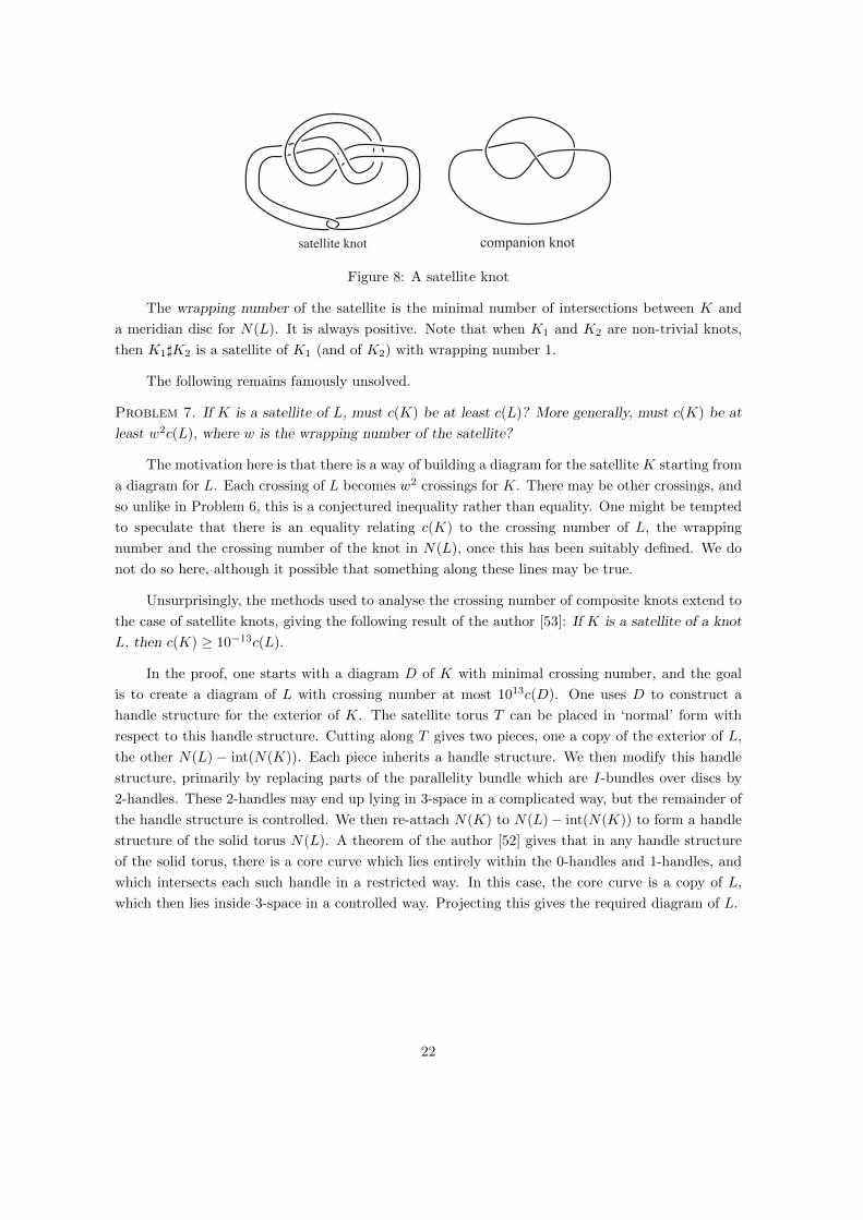
satellite knot companion knot

Figure 8: A satellite knot

The wrapping number of the satellite is the minimal number of intersections between K and

a meridian disc for N(L). It is always positive. Note that when K1 and K2 are non-trivial knots,

then K1]K2 is a satellite of K1 (and of K2) with wrapping number 1.

The following remains famously unsolved.

Problem 7. If K is a satellite of L, must c(K) be at least c(L)? More generally, must c(K) be at

least w2c(L), where w is the wrapping number of the satellite?

The motivation here is that there is a way of building a diagram for the satellite K starting from

a diagram for L. Each crossing of L becomes w2 crossings for K. There may be other crossings, and

so unlike in Problem 6, this is a conjectured inequality rather than equality. One might be tempted

to speculate that there is an equality relating c(K) to the crossing number of L, the wrapping

number and the crossing number of the knot in N(L), once this has been suitably defined. We do

not do so here, although it possible that something along these lines may be true.

Unsurprisingly, the methods used to analyse the crossing number of composite knots extend to

the case of satellite knots, giving the following result of the author [53]: If K is a satellite of a knot

L, then c(K) ≥ 10−13c(L).

In the proof, one starts with a diagram D of K with minimal crossing number, and the goal

is to create a diagram of L with crossing number at most 1013c(D). One uses D to construct a

handle structure for the exterior of K. The satellite torus T can be placed in ‘normal’ form with

respect to this handle structure. Cutting along T gives two pieces, one a copy of the exterior of L,

the other N(L) − int(N(K)). Each piece inherits a handle structure. We then modify this handle

structure, primarily by replacing parts of the parallelity bundle which are I-bundles over discs by

2-handles. These 2-handles may end up lying in 3-space in a complicated way, but the remainder of

the handle structure is controlled. We then re-attach N(K) to N(L)− int(N(K)) to form a handle

structure of the solid torus N(L). A theorem of the author [52] gives that in any handle structure

of the solid torus, there is a core curve which lies entirely within the 0-handles and 1-handles, and

which intersects each such handle in a restricted way. In this case, the core curve is a copy of L,

which then lies inside 3-space in a controlled way. Projecting this gives the required diagram of L.

22

6. Crossing changes and unknotting number

An elementary operation that one can perform on a knot is to change a crossing in one of its

diagrams, as in Figure 9. This is strikingly difficult to analyse, and it leads to some of the most

challenging questions in the subject. An excellent survey of this topic can also be found in [87].

6.1. Computing unknotting number

The unknotting number u(K) of a knot K is the minimal number of crossing changes that

one can make to some diagram that turns it into the unknot. The difficulty of course is that one

quantifies over all possible diagrams, and so although any diagram for K easily gives an upper bound

on u(K), it is rarely clear that this is the best possible. In fact, unknotting number is probably best

understood in a manner that avoids diagrams: it is the minimal number of times that a knot must

pass though itself in a one-parameter family of curves that starts with K and ends with the unknot.

Problem 8. Is the unknotting number of a knot algorithmically computable? Is there even an

algorithm to decide whether a given knot has unknotting number one?

The first of these questions seems a long way out reach at present. It is more than just a

theoretical question: there exist many explicit knots with unknown unknotting number (see [41]

for example). As a result, many intriguing and clever methods have been developed that provide

lower bounds on unknotting number [38, 39, 42, 58, 71, 73, 76, 90, 92]. These utilise a wide variety

of techniques, including the Alexander module [71], the linking form on the double branched cover

[58, 90], 4-dimensional gauge theory [92] and more recently, Heegaard Floer homology [73, 76]. A

major piece of research in this area was the solution by Kronheimer and Mrowka [44] of Milnor’s

conjecture: the unknotting number of the (p, q) torus knot is (p− 1)(q − 1)/2.

However, with each new lower bound on unknotting number, there remain knots with un-

knotting number that cannot be determined. This will continue to be the case until Problem 8 is

resolved.

A useful way of understanding and approaching this problem is via the use of crossing circles.

Given some crossing in a diagram of a knot K, the associated crossing circle is a simple closed curve

in the complement of K that encircles the crossing, as shown in Figure 9. There are two crossing

circles associated with each crossing (that are obtained from one another by rotating the diagram

through 90 degrees). One usually focuses on the crossing circle that has zero linking number with

K. This bounds a disc which intersects K in two points of opposite sign.

K K K Kcrossingcircle

Figure 9: A crossing change

23

Crossing circles are useful for several reasons. Firstly, the crossing change is achieved by ±1

surgery along the crossing circle, and so one can draw on the well-developed theory of Dehn surgery.

Secondly, it also permits crossings in different diagrams to be compared: the crossings are equivalent

if their associated crossing circles are ambient isotopic in the complement of K. Clearly, changing

equivalent crossings results in equivalent knots, and so this is a helpful concept. Some interesting

problems can be phrased in terms of crossing circles.

Although it seems unlikely that we will have an algorithm to determine unknotting number

in the near future, the question of whether unknotting number one knots can be detected is a

tantalising one. Here, the situation seems considerably more promising. To answer this question,

it would suffice to produce a finite list of potential crossing circles with the property that if K has

unknotting number 1, then changing the crossing at one of these crossing circles would unknot the

knot. For one could then check each of these crossing changes systematically to determine whether

they did unknot the knot. (This would use one of the known solutions to the unknot recognition

problem.) Thus, the following arises naturally.

Problem 9. If a knot has unknotting number one, are there only finitely many crossing circles, up

to ambient isotopy, that can be used to unknot the knot?

Much of what is known about knots with unknotting number one comes from sutured manifold

theory. (See Section 3.5 for a very brief summary of some of this theory.) It is possible to show that

if a knot K has unknotting number 1, then its exterior admits a taut sutured manifold hierarchy,

where the penultimate manifold in this decomposition is a solid torus neighbourhood of the crossing

circle plus possibly some 3-balls. In particular, this crossing circle is disjoint from some minimal

genus Seifert surface S for K. In fact, by pushing this argument further, Scharlemann and Thompson

[86] were able to show that this crossing circle can be isotoped to lie in S. This suggests a route

to determining whether a knot has unknotting number 1: find all minimal genus Seifert surfaces

for K, and then search on each such surface for all possible crossing circles which unknot the knot.

The first of these steps is possible, using normal surface theory, as long as K is not a satellite knot.

However, there are infinitely many isotopy classes of curves on a surface with positive genus, and it

is hard to see how to reduce this to a finite list of crossing circles on which to focus.

6.2. The unlinking and splitting numbers of a link

There is a natural analogue of unknotting number for links. The unlinking number u(L) of a

link L is the minimal number of crossing changes required to turn it into the unlink. Many of the

techniques that can be used to analyse unknotting number apply equally well to unlinking number.

But they also often work in the following more general setting. The splitting number s(L) of a link

L is the minimal number of crossing changes required to turn it into a split link.

Unlike the case of unknotting number one, links with splitting number one or unlinking number

one are known to be detectable, under fairly mild hypotheses. It is a recent theorem of the author

[55] that there is an algorithm to determine whether a hyperbolic link of at least 3 components has

splitting number one.

24

This is proved as follows. Suppose that C is a crossing circle, such that changing this crossing

turns a link L into a split link. Just as in Section 6.1, there is a sutured manifold hierarchy for the

exterior of L where the penultimate manifold is a solid torus neighbourhood of C, plus some balls.

The key part of the proof is to place this hierarchy into ‘normal’ form with respect to some initial

triangulation of the exterior of L as in [49]. Thus, one obtains a finite computable list of possibilities

for C. In particular, the version of Problem 9 in this setting is answered affirmatively. Moreover,

each of these crossing changes can be analysed to determine whether they result in the unlink. So,

under the above hypotheses, there is also an algorithm to determine whether the link has unlinking

number one.

6.3. Additivity of unknotting number

One can also ask how unknotting number behaves with respect to simple knot-theoretic oper-

ations. For example, the following is very far from resolution.

Problem 10. Does u(K1]K2) = u(K1) + u(K2) always hold? Less ambitiously, what about the

inequality u(K1]K2) ≥ max{u(K1), u(K2)}?

Scharlemann [84] proved that composite knots have unknotting number at least 2. But we

cannot rule out the following bizarre possibility: two knots might each have unknotting number 100

but their connected sum has unknotting number 2!

6.4. Cosmetic crossing changes

A crossing circle is nugatory if it bounds a disc in the complement of the knot. Clearly changing

a nugatory crossing does not alter the knot. Is this the only way?

Problem 11. Suppose that a crossing change to a knot K does not alter its knot type. Let C be

the associated crossing circle with zero linking number. Must C be nugatory?

This is known when the knot K is the unknot, by work of Scharlemann and Thompson [86],

which relied on Gabai’s sutured manifold theory [21]. However, the general case seems to remain

just out of reach.

7. Special classes of knots

Knots are usually specified by means of a diagram. Typically, this diagram reveals little imme-

diate information about the knot. For example, a superficially complicated diagram may actually

represent the unknot. However, there are certain types of diagram which force a knot to have much

more structure. It is these that we discuss in this section.

7.1. Alternating knots

A diagram for a link is alternating if, as one travels along each component of the link, one

meets ‘over’ and ‘under’ crossings alternately. A link is alternating if it has an alternating diagram.

25

Figure 10: A non-alternating diagram (highlighted are successive ‘over’ crossings)

Some alternating diagrams can be immediately simplified as follows. We say that a diagram

is reducible if, at some crossing, two of the incident regions are actually the same region of the

diagram. When a diagram is reducible, there is an obvious modification that can be made to it,

which reduces the crossing number by 1. When the original diagram is alternating, so too is the new

diagram. So, when dealing with alternating links, there is no loss of generality in assuming that its

alternating diagram is not reducible. It is then known as reduced.

A great deal of information about a link is evident from an alternating diagram. Possibly

the most striking illustration of this is the following result of Kauffman [40], Murasugi [69], and

Thistlethwaite [93]: If D is a reduced alternating diagram of a link L, then c(D) = c(L).

This was proved by means of the Jones polynomial. This link invariant is defined in terms

of some diagram. It is therefore unsurprising that the ‘complexity’ of the polynomial should be

bounded above by the ‘complexity’ of some diagram. In fact, the width of the polynomial, which

is the difference in degree between the highest order term and lowest order term, is always at most

the crossing number of any diagram. But, Kauffman, Murasugi and Thistlethwaite proved that this

inequality is an equality for a reduced alternating diagram D. This implies the above result, because

the width of the Jones polynomial is then the crossing number of D, and the link cannot have a

diagram with fewer crossings, because this would force the width of the polynomial to be at most

this number.

A consequence of this theorem is that there is a very rapid and simple algorithm to decide

whether an alternating diagram represents the unknot: an alternating diagram of the unknot either

has no crossings or is reducible. In fact, this was already known, due to earlier techniques of

Menasco [65], which relied on a very precise analysis of surfaces in the exterior of an alternating

link. This works particularly well when the surface has non-negative Euler characteristic. So, by

examining spheres in the complement of the link, one can also detect whether an alternating link

is split. Menasco showed that an alternating link is split if and only if its alternating diagram is

disconnected. Similarly, an alternating knot is prime if and only if a reduced alternating diagram

is prime. Here, a connected diagram is prime if and only if any simple closed in the plane which

intersects the link projection transversely in two points away from the crossings divides the plane

into two components, one of which contains no crossings.

In Menasco’s proof, he constructs, using the diagram, a special position for the link in R3. The

diagram is viewed as lying in the horizontal plane R2 × {0}. The link mostly lies in this plane,

except near each crossing, where two sub-arcs of the link take detours above and below the plane

of the diagram. More precisely, one places a small 3-ball at each crossing with centre lying in the

26

plane of the diagram, and the two arcs involved in the crossing follow the boundary of this ball.

(See Figure 11.) Let R3+ denote the set of points lying above the union of the plane and the balls,

and define R3− similarly. Menasco showed that a closed incompressible surface in the link exterior

may be arranged so that it intersects each of these balls in a collection of parallel ‘saddles’, and

intersects R3+ and R3

− in a collection of discs. The boundary of these discs in R3+ is a collection of

simple closed curves, which can be viewed as lying within the diagram. A careful analysis of these

curves (particularly, an innermost one in the plane), together with the condition that the diagram

is connected and alternating, implies that the surface S has a meridional compression disc. This is

a disc D in R3 such that D∩S = ∂S and D∩K is a single point in the interior of D. The existence

of such a disc is impossible for a splitting sphere, for example, and this can be used to establish

Menasco’s theorem about split alternating links.

Figure 11: Balls near crossings

A significantly deeper version of this analysis was used to prove the following theorem of

Menasco and Thistlethwaite [66]: any two reduced alternating diagrams of a link differ by a sequence

of flypes (as shown in Figure 12.) This was Tait’s flyping conjecture. The proof of this is very

complex, and so we can only give a very brief overview. Each alternating diagram determines two

checkerboard surfaces. In Menasco and Thistlethwaite’s proof, they examine the surfaces arising

from one diagram and how they interact with other diagram. A careful analysis, together with a

surprising intervention of the Jones polynomial at one point, establishes the existence of a flype

which, in some sense, simplifies these surfaces, and so the theorem is proved by induction.

RR

Figure 12: Flype

Although alternating links are now very well-understood, there are some invariants and prop-

erties of these links that are worthy of further analysis. Some of these are given in the following

problem.

Problem 12. Can one detect (or possibly just estimate) the following invariants of a knot, given

an alternating diagram: its bridge number; its tunnel number; its unknotting number?

One may also ask for estimates for more sophisticated invariants. Indeed, in [50], the author

has given a way of reading off the hyperbolic volume of an alternating link’s complement, up to a

27

bounded multiplicative error. While such problems are interesting, they falls outside the remit of

this survey, which is focused on much more elementary questions.

7.2. Positive knots and positive braids

Given the manifest success in understanding the topological properties of alternating knots,

it is natural to consider other possible classes of knot diagrams. A reasonable way of assessing

whether it is a good class of diagrams is whether it satisfies the minimal requirement that a diagram

specifies the unknot if and only if it ‘obviously’ does so. Another class of diagrams which satisfy

this requirement is positive diagrams.

Positivity is defined for diagrams of oriented links. Positive and negative crossings are shown

in Figure 13. A diagram is said to be positive if all its crossings are positive.

Positive Negative

Figure 13: Positive and negative crossings

Cromwell [11] showed that a reduced positive diagram never represents the unknot. In fact,

one can read off the genus of a positive knot from its positive diagram. This result was significantly

generalised by Kronheimer and Mrowka [44], who showed that the smooth 4-ball genus of a positive

knot can be read off from its positive diagram. Indeed, it is equal to the knot’s genus.

However, positive knots are not totally well-behaved. For example, Stoimenow [89] found a

positive knot which has no positive diagram with minimal crossing number. So, it seems unlikely

that one can read off the crossing number of a positive knot in the way that one can for alternating

knots. Nevertheless, they form an interesting class that is worthy of further investigation. In

particular, it would be instructive to determine other topological and/or elementary invariants of

positive knots. For example, is there a simple relationship between two positive diagrams of the

same knot?

One can also consider, more specifically, closed positive braids. These appear to have even nicer

properties than general positive knots. For example, they are fibred. They may be more amenable

to analysis.

7.3. Other interesting classes of diagram

There are several other related classes of diagrams. Homogeneous diagrams form a common

generalisation of positive diagrams and alternating diagrams. Cromwell [11] in fact established his

formula for knot genus not just for positive knots but homogeneous ones.

Adequate diagrams form another interesting class. These are defined by considering ‘resolutions’

28

for each crossing, which remove the crossing. Each crossing may be removed in one of two ways,

a ‘plus’ or a ‘minus’ resolution. If one resolves every crossing, the result is a collection of planar

curves. At each crossing, the two new arcs may belong to the same simple curve or two distinct

ones. A diagram is plus-adequate if, when all the crossings are resolved in a ‘plus’ way, each resulting

simple closed curve runs through the remnants of each crossing at most once. Minus-adequacy is

defined similarly using the ‘minus’ resolution at each crossing. A diagram is adequate if it is both

plus-adequate and minus-adequate. Adequate knots have well-behaved Jones polynomial. Lickorish

and Thistlethwaite [59] using this to prove that if a knot has a reduced adequate diagram with at

least one crossing, then it is not the unknot. But adequacy has more topological applications, as

shown in the recent monograph of Futer, Kalfagianni and Purcell [20]. Adequate links surely merit

further investigation.

8. Epilogue

The theory of 3-manifolds has seen remarkable progress over the past few years, with the

solution of many key conjectures, for example, the Poincare conjecture [78, 79, 80] and the Virtually

Haken Conjecture [2], to name just two. One might be led to the conclusion that the related field of

knot theory might be devoid of interesting unsolved problems. The purpose of the present article is

to emphasise that this is not the case. There remain many fundamental and interesting challenges

ahead.

References

1. I. Agol, Knot genus is NP, http://www.math.uic.edu/ ∼ agol/research.html

2. I. Agol, The virtual Haken conjecture. (with an appendix by I. Agol, D. Groves and J. Manning)

arXiv:1204.2810

3. I. Agol, J. Hass, W. Thurston, The computational complexity of knot genus and spanning area,

Trans. Amer. Math. Soc. 358 (2006) 3821–3850.

4. D. Bennequin, Entrelacements et equations de Pfaff, Asterisque 107–108 (1983) 87–161.

5. J. Birman, T. Brendle, Braids: a survey. Handbook of knot theory, 19–103, Elsevier B. V., Ams-

terdam, 2005.

6. J. Birman, M. Hirsch, A new algorithm for recognizing the unknot, Geometry and Topology 2 (1998)

178–220.

7. J. Birman, W. Menasco, Studying links via closed braids V: Closed braid representatives of the

unlink, Trans. Amer. Math. Soc. 329 (1992) 585–606.

8. M. Brittenham, Essential laminations and Haken normal form. Pacific J. Math. 168 (1995), no. 2,

217–234.

9. A. Coward, M. Lackenby, An upper bound on Reidemeister moves, arXiv:1104.1882, Amer. J.

Math. (accepted).

10. D. Coulson, O. Goodman, C. Hodgson, W. Neumann, Snap, Available at

http://www.ms.unimelb.edu.au/∼snap/

11. P. Cromwell, Homogeneous links. J. London Math. Soc. (2) 39 (1989), no. 3, 535–552.

12. P. Cromwell, Embedding knots and links in an open book I: basic properties, Topology and its

Applications 64 (1995) 37–58.

29

13. M. Culler, P. Shalen, Bounded, separating, incompressible surfaces in knot manifolds, Invent.

Math. 75 (1984) 537–545.

14. F. Dahmani, D. Groves, The isomorphism problem for toral relatively hyperbolic groups, Publ.

Math. Inst. Hautes Etudes Sci. No. 107 (2008), 211–290.

15. Y. Diao, The additivity of crossing numbers, Journal of knot theory and its Ramifications 13 (2004)

857–866.

16. S. Donaldson, An Application of Gauge Theory to Four Dimensional Topology, J. Differential Geom.

18 (183) 279–315.

17. I. Dynnikov, Arc-presentations of links: monotonic simplification, Fund. Math. 190 (2006), 29–76.

18. D. Epstein, R. Penner, Euclidean decompositions of noncompact hyperbolic manifolds, J. Differential

Geom. 27 (1988) 67–80.

19. A. Floer, An instanton-invariant for 3-manifolds, Comm. Math. Phys. 118 (2) 215–240.

20. D. Futer, E. Kalfagianni, J. Purcell, Guts of surfaces and the colored Jones polynomial, Lecture

Notes in Mathematics, 2069. Springer, Heidelberg, 2013

21. D. Gabai, Foliations and the topology of 3-manifolds. J. Differential Geom. 18 (1983), no. 3, 445–503.

22. D. Gabai, Essential laminations and Kneser normal form. J. Differential Geom. 53 (1999), no. 3,

517–574.

23. C. Gordon, J. Luecke, Knots are determined by their complements. J. Amer. Math. Soc. 2 (1989),

no. 2, 371–415.

24. W. Haken, Theorie der Normalflachen. Acta Math. 105 (1961) 245–375.

25. W. Haken, Some results on surfaces in 3-manifolds. Studies in Modern Topology pp. 39–98 Math.

Assoc. Amer. (1968)

26. J. Hass, J. Lagarias, The number of Reidemeister moves needed for unknotting. J. Amer. Math.

Soc. 14 (2001), no. 2, 399–428

27. J. Hass, J. Lagarias, N. Pippenger, The computational complexity of knot and link problems. J.

ACM 46 (1999), no. 2, 185–211.

28. J. Hass, T. Nowik, Unknot diagrams requiring a quadratic number of Reidemeister moves to untangle.

Discrete Comput. Geom. 44 (2010), no. 1, 91–95.

29. J. Hass, J. Snoeyink, W. Thurston, The size of spanning disks for polygonal curves. Discrete

Comput. Geom. 29 (2003) 1–17.

30. G. Hemion, On the classification of homeomorphisms of 2-manifolds and the classification of 3-

manifolds. Acta Math. 142 (1979), no. 1-2, 123–155.

31. J. Hoste, M. Thistlethwaite, Knotscape, http://www.math.utk.edu/∼morwen/knotscape.html

32. J. Hoste, M. Thistlethwaite, J. Weeks, The first 1,701,936 knots. Math. Intelligencer 20 (1998),

no. 4, 3348.

33. W. Jaco, P. Shalen, Seifert fibered spaces in 3-manifolds. Mem. Amer. Math. Soc. 21 (1979), no.

220.

34. W. Jaco, J. Tollefson, Algorithms for the complete decomposition of a closed 3-manifold, Illinois

J. Math. 39 (1995), no. 3, 358–406.

35. F. Jaeger, D. Vertigana, D. Welsh, On the computational complexity of the Jones and Tutte

polynomials, Math. Proc. Cambridge Phil. Soc. 108 (1990) 35–53.

36. K. Johannson, Homotopy equivalences of 3-manifolds with boundaries. Lecture Notes in Mathemat-

ics, 761. Springer, Berlin, 1979.

30

37. V. Jones, A polynomial invariant for knots via von Neumann algebras. Bull. Amer. Math. Soc.

(N.S.) 12 (1985), no. 1, 103–111.

38. T. Kawamura, The unknotting numbers of 10139 and 10152 are 4. Osaka J. Math. 35 (1998), no. 3,

539–546.

39. T. Kanenobu, H. Murakami, Two-bridge knots with unknotting number one. Proc. Amer. Math.

Soc. 98 (1986) 499–502.

40. L. Kauffman, State models and the Jones polynomial. Topology 26 (1987) 395–407.

41. R. Kirby, Problems in low dimensional manifold theory. Algebraic and geometric topology (Proc.

Sympos. Pure Math., Stanford Univ., Stanford, Calif., 1976), Part 2, pp. 273-312, Proc. Sympos.

Pure Math., XXXII, Amer. Math. Soc., Providence, R.I., 1978.

42. T. Kobayashi, Minimal genus Seifert surface for unknotting number 1 knots. Kobe J. Math. 6 (1989)

53–62.

43. P. Koiran, Hilberts Nullstellensatz is in the polynomial hierarchy, J. Complexity 12 (1996), no. 4,

273286, DIMACS TR 96-27, Special issue for FOCM 1997.

44. P. Kronheimer, T. Mrowka, Gauge theory for embedded surfaces. I. Topology 32 (1993), no. 4,

773–826.

45. P. Kronheimer, T. Mrowka, Dehn surgery, the fundamental group and SU(2), Math. Res. Lett.

11 (2004) 741–754.

46. P. Kronheimer, T. Mrowka, Monopoles and three-manifolds. New Mathematical Monographs, 10.

Cambridge University Press, Cambridge, 2007.

47. P. Kronheimer, T. Mrowka, Khovanov homology is an unknot-detector, Publ. Math. Inst. Hautes

Etudes Sci. 113 (2011) 97–208.

48. G. Kuperberg, Knottedness is in NP, modulo GRH, arXiv:1112.0845.

49. M. Lackenby, Exceptional surgery curves in triangulated 3-manifolds, Pacific J. Math. 210 (2003),

101–163.

50. M. Lackenby, The volume of hyperbolic alternating link complements, Proc. London Math. Soc. 88

(2004) 204–224.

51. M. Lackenby, The crossing number of composite knots, J. Topology 2 (2009) 747-768.

52. M. Lackenby, Core curves of triangulated solid tori, arXiv:1106.2934, Trans. Amer. Math. Soc.

(accepted)

53. M. Lackenby, The crossing number of satellite knots, arXiv:1106.3095, Alg. Geom. Top. (accepted)

54. M. Lackenby, A polynomial upper bound on Reidemeister moves, arXiv:1302.0180

55. M. Lackenby, Links with splitting number one, In preparation.

56. M. Lackenby, A polynomial upper bound on Reidemeister moves for each link type, In preparation.

57. J. Lagarias, A. Odlyzko, Effective versions of the Chebotarev density theorem, Algebraic number

elds: L-functions and Galois properties (Proc. Sympos., Univ. Durham, 1975), Academic Press, 1977,

pp. 409–464.

58. W. B. R. Lickorish, The unknotting number of a classical knot. Contemp. Math. 44 (1985) 117–121.

59. W. B. R. Lickorish, M. Thistlethwaite, Some links with nontrivial polynomials and their crossing-

numbers, Comment. Math. Helv. 63 (1988), no. 4, 527–539.

60. A. Mal’cev, On isomorphic matrix representations of infinite groups, Mat. Sb. 8 (50) (1940), 405–422.

61. J. Manning, Algorithmic detection and description of hyperbolic structures on closed 3-manifolds with

solvable word problem, Geom. Topol. 6 (2002), 1–25.

31

62. C. Manolescu, P. Ozsvath, S. Sarkar, A combinatorial description of knot Floer homology. Ann.

of Math. (2) 169 (2009), no. 2, 633–660.

63. A. Markov, The unsolvability of the homeomorphy problem, Dokl. Akad. Nauk SSSR, 121 (1958)

218–220.

64. S. Matveev, Algorithmic topology and classification of 3-manifold, Algorithms and Computation in

Mathematics, 9. Springer, Berlin, 2007.

65. W. Menasco, Closed incompressible surfaces in alternating knot and link complements. Topology 23

(1984) 37–44.

66. W. Menasco, M. Thistlethwaite, The classification of alternating links. Ann. of Math. (2) 138

(1993) 113–171.

67. A. Mijatovic, Simplifying triangulations of S3. Pacific J. Math. 208 (2003), no. 2, 291–324.

68. A. Mijatovic, Simplical structures of knot complements, Math. Res. Lett. 12 (2005) 843–856.

69. K. Murasugi, Jones polynomials and classical conjectures in knot theory. Topology 26 (1987), no. 2,

187194.

70. K. Murasugi, On the braid index of alternating links. Trans. Amer. Math. Soc. 326 (1991) 237–260.

71. Y. Nakanishi, A note on unknotting number. Math. Sem. Notes Kobe Univ. 9 (1981) 99–108.

72. W. Neumann, G. Swarup, Canonical decompositions of 3-manifolds. Geom. Topol. 1 (1997), 21–40.

73. B. Owens, Unknotting information from Heegaard Floer homology. Adv. Math. 217 (2008), no. 5,

2353–2376.

74. P. Ozsvath and Z. Szabo, Holomorphic disks and topological invariants for closed three-manifolds.

Ann. of Math. (2) 159 (2004), no. 3, 1027–1158.

75. P. Ozsvath and Z. Szabo, Holomorphic disks and genus bounds, Geom. Topol. 8 (2004) 311–334.

76. P. Ozsvath and Z. Szabo, Knots with unknotting number one and Heegaard Floer homology, Topol-

ogy 44 (2005), no. 4, 705–745.

77. U. Pachner P.L. homeomorphic manifolds are equivalent by elementary shellings, European Journal

of Combinatorics 12 (1991) 129–145.

78. G. Perelman, The entropy formula for the Ricci flow and its geometric applications, Preprint,

arxiv:math.DG/0211159

79. G. Perelman, Ricci flow with surgery on three-manifolds, Preprint, arxiv:math.DG/0303109

80. G. Perelman, Finite extinction time for the solutions to the Ricci flow on certain three-manifolds,

Preprint, arxiv:math.DG/0307245

81. V. Pratt. Every prime has a succinct certificate. SIAM Journal on Computing, vol.4, pp.214–220.

1975.

82. K. Reidemeister, Knotten und Gruppen, Abh. Math. Sem. Univ. Hamburg 5 (1927), 7–23.

83. S. Sarkar, J. Wang, An algorithm for computing some Heegaard Floer homologies. Ann. of Math.

(2) 171 (2010), no. 2, 1213–1236.

84. M. Scharlemann, Unknotting number one knots are prime. Invent. Math. 82 (1985), no. 1, 37–55.

85. M. Scharlemann, Sutured manifolds and generalized Thurston norms. J. Differential Geom. 29

(1989), no. 3, 557–614.

86. M. Scharlemann, A. Thompson, Link genus and the Conway moves. Comment. Math. Helv. 64

(1989), no. 4, 527–535

87. M. Scharlemann, Crossing changes. Knot theory and its applications. Chaos Solitons Fractals 9

(1998) 693–704.

32

88. Z. Sela, The isomorphism problem for hyperbolic groups. I. Ann. of Math. (2) 141 (1995) 217–283.

89. A. Stoimenow, On the crossing number of positive knots and braids and braid index criteria of Jones

and Morton-Williams-Franks, Trans. Amer. Math. Soc. 354 (2002), 3927–3954.

90. A. Stoimenow, Polynomial values, the linking form and unknotting numbers. Math. Res. Lett. 11

(2004), no. 5-6, 755–769.

91. C. Sundberg, M. Thistlethwaite, The rate of growth of the number of prime alternating links and

tangles, Pacific J. Math. 182 (1998) 329–358.

92. T. Tanaka, Unknotting numbers of quasipositive knots, Topology Appl. 88 (1998), no. 3, 239–246.

93. M. Thistlethwaite, A spanning tree expansion of the Jones polynomial. Topology 26 (1987) 297–309.

94. M. Thistlethwaite, On the structure and scarcity of alternating links and tangles. J. Knot Theory

Ramications 7 (1998) 981–1004.

95. A. Thompson, Thin position and the recognition problem for S3. Math. Res. Lett. 1 (1994), no. 5,

613–630.

96. W. Thurston, Three-dimensional manifolds, Kleinian groups and hyperbolic geometry. Bull. Amer.

Math. Soc. (N.S.) 6 (1982), no. 3, 357–381.

97. W. Thurston, A norm for the homology of 3-manifolds. Mem. Amer. Math. Soc. 59 (1986), no.

339, i–vi and 99–130.

98. J. Weeks, Snappea, http://www.geometrygames.org/SnapPea/

99. J. Weeks, Convex hulls and isometries of cusped hyperbolic 3-manifolds. Topology Appl. 52 (1993),

no. 2, 127–149.

100. P. Weinberger, Finding the number of factors of a polynomial, J. Algorithms 5 (1984) 180–186.

101. E. Witten, Quantum Field Theory and the Jones Polynomial, Commun. Math. Phys. 121 (1989)

351–399.

102. E. Witten, Monopoles and four-manifolds, Math. Res. Lett. 1 (6) 769–796.

Mathematical Institute, University of Oxford,

Radcliffe Observatory Quarter, Woodstock Road, Oxford OX2 6GG, United Kingdom.

33