Towards Helicopter Simulation with an Index-1Differential-Algebraic Equations System

Efficient Time Integration Methods

Elena Kremser

August 7, 2017

Master’s thesis in Mathematics (M.Sc.)

University of CologneMathematical Institute

First reviewer: Prof. Dr. Angela KunothSecond reviewer: Dr. rer. nat. Margrit KlitzTechnical advisor: Melven Rohrig-Zollner

Abstract

Comprehensive helicopter simulation has been an important subject of research ever since the rise

of the first helicopters. Numerous modeling approaches and software frameworks emerged, each

with its individual advantages and drawbacks. However, a comprehensive approach that yields

an efficient and effective simulation adaptable for research is still missing. Comprehensive here

means that all relevant aspects are taken into account, e. g. vortex dynamics, rotor behavior, vi-

brations, etc. The German Aerospace Center (DLR) is working on a new solution using general

state-space models for submodels of the helicopter which are coupled to a comprehensive model.

This coupling yields an index-1 differential algebraic equation (DAE) system.

In this thesis, we analyze existing numerical algorithms for the solution of index-1 DAE systems

and define a new familiy of methods that suits the challenges of helicopter simulation best. The

challenges here consist in the interaction of large systems that are complex and individual in their

behavior on their own. We focus our analysis on half-explicit Runge-Kutta (HERK) methods.

Their explicit approach delivers the efficiency we seek. However, these methods are not able to

handle stiff systems like the highly vibratory helicopter well. Stiff ordinary differential equation

(ODE) problems can be solved by explicit exponential Runge-Kutta (EERK) methods. In order

to apply them to index-1 DAE systems, we derive the new half-explicit exponential Runge-Kutta

(HEERK) methods.

We test our HEERK methods in comparison to HERK methods on a mechanical model of the

main rotor. The results show that HEERK methods need substantially fewer time steps than HERK

methods for the same approximation quality. We also see that a good choice of submodels, where

the stiff variables are solely placed in the state function, boosts this effect. So, HEERK methods

constitute an essential step towards an effective real-time simulation in comprehensive rotorcraft

simulation.

Acknowledgments

I thank Prof. Dr. Angela Kunoth, University of Cologne, and Dr. Achim Basermann, department

leader of the High Performance Computing division of the German Aerospace Center (DLR) in

Cologne, for their cooperation which made this Master’s thesis possible in the first place.

A thank you also goes to my second reviewer Dr. Margrit Klitz (DLR) for her continuous support

and improvement suggestions.

I also want to thank my technical advisor Melven Rohrig-Zollner (DLR). His visions and ideas

and our constant dialogue substantially contributed to the direction and the contents of my thesis.

A special thanks goes to my fiance Jan Kohlwey who supports and encourages me no matter what.

Contents

Introduction 1

1. Approach 5

1.1. Derivation of coupled index-1 DAE system . . . . . . . . . . . . . . . . . . . . 5

1.2. Mechanical helicopter model . . . . . . . . . . . . . . . . . . . . . . . . . . . . 7

2. Numerical methods for index-1 DAEs 13

2.1. Explicit Runge-Kutta (ERK) methods . . . . . . . . . . . . . . . . . . . . . . . 14

2.1.1. Consistency . . . . . . . . . . . . . . . . . . . . . . . . . . . . . . . . . 17

2.1.2. Stability . . . . . . . . . . . . . . . . . . . . . . . . . . . . . . . . . . . 17

2.2. Half-Explicit Runge-Kutta (HERK) methods . . . . . . . . . . . . . . . . . . . 20

2.2.1. First order consistency . . . . . . . . . . . . . . . . . . . . . . . . . . . 22

2.2.2. Second order consistency . . . . . . . . . . . . . . . . . . . . . . . . . . 24

2.2.3. Note on stability . . . . . . . . . . . . . . . . . . . . . . . . . . . . . . 28

2.3. Explicit Exponential Runge-Kutta (EERK) methods . . . . . . . . . . . . . . . . 28

2.3.1. Consistency . . . . . . . . . . . . . . . . . . . . . . . . . . . . . . . . . 33

2.3.2. Stability . . . . . . . . . . . . . . . . . . . . . . . . . . . . . . . . . . . 34

2.3.3. First order . . . . . . . . . . . . . . . . . . . . . . . . . . . . . . . . . . 36

2.3.4. Second order . . . . . . . . . . . . . . . . . . . . . . . . . . . . . . . . 53

2.3.5. Combined Stability Plots . . . . . . . . . . . . . . . . . . . . . . . . . . 57

2.4. Half-Explicit Exponential Runge-Kutta (HEERK) methods . . . . . . . . . . . . 62

2.4.1. First order consistency . . . . . . . . . . . . . . . . . . . . . . . . . . . 62

2.4.2. Second order consistency . . . . . . . . . . . . . . . . . . . . . . . . . . 64

3. Numerical results 68

3.1. Time width choice for exponential Euler . . . . . . . . . . . . . . . . . . . . . . 68

3.2. Comparison of exponential Euler method and ordinary Euler method . . . . . . . 71

3.3. Comparison of EERK2 and EERK4 for special cases . . . . . . . . . . . . . . . 73

3.4. Comparison of HEERK4 and HERK4 . . . . . . . . . . . . . . . . . . . . . . . 74

4. Conclusion and recommendations for further work 81

List of abbreviations 83

Notation directory 84

i

Appendix 89

A. Basic definitions and theorems 89

A.1. Analysis . . . . . . . . . . . . . . . . . . . . . . . . . . . . . . . . . . . . . . . 89

A.2. Linear Algebra . . . . . . . . . . . . . . . . . . . . . . . . . . . . . . . . . . . 91

A.3. Numerical mathematics . . . . . . . . . . . . . . . . . . . . . . . . . . . . . . . 91

B. Minimal working example of a coupled index-1 system 93

C. The Helicopter model 94

C.1. Original model . . . . . . . . . . . . . . . . . . . . . . . . . . . . . . . . . . . 95

C.2. Advanced model in monolithic form . . . . . . . . . . . . . . . . . . . . . . . . 96

C.3. Advanced model in DAE form . . . . . . . . . . . . . . . . . . . . . . . . . . . 99

D. Matlab Code remarks 106

Bibliography 109

Statutory declaration (Eigenstandigkeitserklarung) 115

ii

Introduction

Today’s helicopters are invaluable in emergency medical assistance, search and rescue, military

missions and tourism. The first helicopters, as we know them today, emerged in the early 20th

century [AHMEC]. Compared to other aircraft, helicopters are of special interest because of their

flight attributes: little space for take-off and landing, a vertical climb flight, flight is possible in

all directions (forward, backward and lateral) and helicopters can even hover which makes their

possible applications so manifold.

However, negative examples in history also show that it is important to study helicopters accu-

rately. Helicopters like the SIKORSKY UH-60 or the SIKORSKY S76 showed unexpected unsta-

ble flight behavior after construction which had to be experimentally corrected resulting in high

expenses [Bi09]. Furthermore, there are still numerous fatal accidents with helicopters due to un-

foreseen behavior of the helicopter in turbulent situations [HSAT16].

Due to these failures, the advantages of a sophisticated simulation tool for helicopters cannot be

stressed enough: it provides a better understanding of the forces acting on the components of

the helicopter in any flight situation and helps preventing accidents. Additionally, the simulation

driven design of helicopters and their components renders the development of new models much

less expensive.

Helicopter simulation codes have existed since the invention of computers. In the 1970’s, the

first generation of codes (C81, REXOR and others) emerged. They exhibited several limitations.

Mostly, particular types of helicopters or only particular parts were simulated. Hence, the analysis

was not comprehensive. The realization of these limitations then triggered a second generation of

codes in the early 1980’s (2GCHAS, RCAS, CAMRAD II amongst others). The new codes were

characterized by a higher modifiability through separation of structural and aerodynamic models

and a building-block structure [Jo13].

In spite of the variety of available codes, there is no solution that suits the requirements for re-

search of the German Aerospace Center (DLR) well. Either the software is too expensive and not

adaptable (CAMRAD II) or not sophisticated enough (HOST). Thus, the DLR works at designing

its own solution for research. Hence, the project VAST – Versatile Aeromechanics Simulation Tool

– was introduced as a cooperation of the Institute of Flight Systems (FT) at DLR Brunswick and

the High Performance Computing department (HPC) of DLR Cologne. The aim of the project is

an independent simulation code that is easily adaptable to related problems, that performs better

than existing codes and that accurately predicts a helicopter’s behavior – even in real time. In order

to fulfill this challenging goal, the VAST software framework is built on two main pillars:

1. Modularity: the individual components of the entire model shall be easily interchangeable.

Thus, changes concerning one part of the simulation can be implemented without changing

1

the others. This way, new designs of helicopters can be integrated smoothly in the framework

improving their development while lowering the costs.

2. Complexity: the complex interdependencies of the individual components shall be consid-

ered as elaborately as possible. The modeling error when mapping the reality to physical

equations can never be entirely eliminated. However, through the choice of more accurate

numerical methods, the approximation of the arising systems can be improved.

Helicopters consist of several systems with different behavior that interact with each other. This

is one of the main challenges that we have to take into account for their simulation. Additionally

to extensive overview books like ‘Helicopter Theory’ [Jo12], ‘Bramwell’s Helicopter Dynam-

ics’ [Br01], ‘Helicopter Flight Dynamics’ [Pa07] and ‘Basic Helicopter Aerodynamics’ [SN11],

there are numerous papers that investigate specific aspects of helicopters. To start with, the elastic

blades of the rotor are among the most interesting parts of the helicopter. They are essential for the

flight behavior and already form a quite sophisticated system themselves; see [BKMS17]. Most

importantly, the helicopter has to be able to fly stable. Thus, the analysis of rotorcraft stability is an

important topic [BN01, BW10, Fr86, Pe94]. Instabilities occur due to the interference of vortices

with the rotor blades. These vortices are modeled by a Partial Differential Equation (PDE) system.

Additionally, we need to take into account the fuselage of the helicopter. Even if, at first glance,

these parts show very different behavior, they are not independent from each other. For instance,

the vortices that are generated by the spinning of the blades introduce a downward force on the

fuselage. Such interactions always have to be considered when modeling the system ‘helicopter’

as a whole [BK93].

As mathematicians, we tend to favor a symbolic system of equations which describes the system

in its entirety. On the computing side, this would mean a monolithic model of aerodynamic and

structural dynamic interactions by a set of partial differential equations that are simultaneously

treated by a single solver. However, as pointed out in [Wa05] this approach lays our aim of modu-

larity to waste: if we implement minor changes or improvements in the aerodynamic or structural

solver this would require a complete update of the computer program. Furthermore, the derivation

of these equations is not straightforward [Wa05]. Last but not least, our modular approach allows

us to reuse already existing codes in the DLR. Therefore, we model the whole system as a col-

lection of individual systems with coupling terms that establish the reciprocal physical influences

and obtain an explicitly loosely coupled system; see [GSJJ13] for different coupling methods. The

system we will work with has the general formx(t) = f (t,x(t),y(t))y(t) = g(t,x(t),y(t))

, (?)

where x : R+ → Rn, y : R+ → Rm, f : R+×Rn×Rm → Rn, g : R+×Rn×Rm → Rm, t ∈ R+and m,n ∈ N. The system (?) is called general form of a state-space model. We assume that the

2

gradient ∂g∂y(t,x(t),y(t)) is regular around the solution which makes the present system an index-1

differential-algebraic equation (DAE) system (cf. [HW96]).

This thesis focuses on the mathematical derivation of a suitable numerical method for the solution

of a system (?). The full specification of the actual equations is ongoing work in the DLR and goes

beyond the scope of this thesis. However, we want to provide a preliminary assessment of existing

and new algorithms for the simulation of general state-space models.

The main contributions of the author are the following:

• We conduct a detailed linear stability analysis of the first order explicit exponential Runge-

Kutta (EERK) method. Although similar linear approaches have been considered in [CM02,

MZ13, OP16, Zh17b], they do not provide a precise analysis of the stability function, which

we do. Experimentally, we provide upper bounds for the time step size when applying the

exponential Euler to an ODE with linear stiff and linear nonstiff terms. Additionally, we

emphasize the advantages of the exponential Euler in comparison to the ordinary Euler for

this setting.

• We create stability plots of EERK methods of orders 1–4 which are similar to the well-

known stability plots for ordinary explicit Runge-Kutta (ERK) methods of orders 1–4. To

the best of our knowledge, these plots are not present in the literature so far.

• We give a straight forward, comprehensible consistency analysis of half-explicit Runge-

Kutta (HERK) methods of first and second order. Comparable results can be found in Arnold

et al. [ASW93].

• Using the findings from our comprehensible consistency analysis of HERK methods, we

newly define half-explicit exponential Runge-Kutta (HEERK) methods. These methods are

very valuable in our setting, where we deal with a linear stiff part and a nonlinear nonstiff

part in our ODE system. To the best of our knowledge, these methods have not been used

before. For the first and second order HEERK methods we conduct a consistency analysis

based on the comprehensible analysis of HERK methods for first and second orders.

• Last but not least, we highlight the advantages of HEERK methods in comparison to HERK

methods by using a simplified stiff rotor model which exhibits a similar behavior to what

we expect from a full helicopter system. Here, we use the mechanical model of Sanches et

al. [SMBA11] as a starting point.

The remainder of this thesis is organized as follows: Section 1 contains a short introduction to

helicopter simulation. We present our approach for the helicopter model and a test model that we

will use for our numerical tests. In Section 2, we analyze suitable time integration approaches for

our system. Here, we start with standard Runge-Kutta methods for the solution of ODEs (Sub-

section 2.1). Then we analyze so-called half-explicit Runge-Kutta methods for the solution of

3

index-1 DAEs (Subsection 2.2). Subsequently, we introduce exponential Runge-Kutta methods

(Subsection 2.3) which work with a more advanced formulation of our system. In Subsection 2.4,

we define half-explicit exponential Runge-Kutta methods in analogy to the common half-explicit

Runge-Kutta methods of Subsection 2.2. Finally, in Section 3, we compare the described methods

with respect to stability, consistency and run time. Some tests are executed on small problems,

whereas the main result is obtained through a simulation with the simplified rotorcraft model from

Section 1.2. We conclude this thesis with a summary and the numerous possibilities for further

research.

4

1. Approach

1.1. Derivation of coupled index-1 DAE system

In contrast to analyzing specific interesting parts of a helicopter, we are interested in the heli-

copter’s behavior as a whole. Here, we need to account for the complexity of the individual parts

of the helicopter in order to obtain a comprehensive approach. Hence, we treat various subsystems

individually. For each physical subsystem i, we consider a model

xi(t) = fi(t,xi(t),ui(t))

yi(t) = gi(t,xi(t),ui(t)), (1.1.1)

where t ∈ R+ denotes the time variable, xi ∈ Rni , ni ∈ N denotes the state vector of system i,

yi ∈ Rmi , mi ∈ N denotes the output vector and ui ∈ Rqi , qi ∈ N denotes the input vector which

consists of combinations of outputs of other subsystems. The functions fi : R+×Rni ×Rqi → Rni

and gi : R+×Rni×Rqi → Rmi describe the behavior of model i. We only want to consider ordinary

differential equations (ODEs). For models that contain partial differential equations (PDEs), we

apply a discretization on the differential operators to obtain ODEs as well.

A combined model of all parts has the formx(t) = f (t,x(t),y(t))y(t) = g(t,x(t),y(t))

, (?)

where x : R+→ Rn, y : R+→ Rm, f : R+×Rn×Rm→ Rn, g : R+×Rn×Rm→ Rm, n = ∑i

ni and

m = ∑i

mi. Here, x denotes the global state vector, y denotes the global output vector and f and g

arise when constructing the model by combining all fi and gi of (1.1.1), respectively. We will call

the first part of this system the dynamic part and the second part will be called the algebraic part.

With the definition

g(t,x(t),y(t)) := g(t,x(t),y(t))−y(t), (1.1.2)

we can also write system (?) as x(t) = f (t,x(t),y(t))

0 = g(t,x(t),y(t)). (??)

This form is often discussed in the literature, where it is either called semi-explicit DAE system

(e. g. [BT99]) or index-1 DAE system (e. g. [ASW93, HLR89]). We will use the latter term.

Since our system reflects physical behavior, it is reasonable to assume that the implicit function

theorem (see Theorem A.1.1) is applicable to g(t,x(t),y(t)) = 0. This implies that the coupling

5

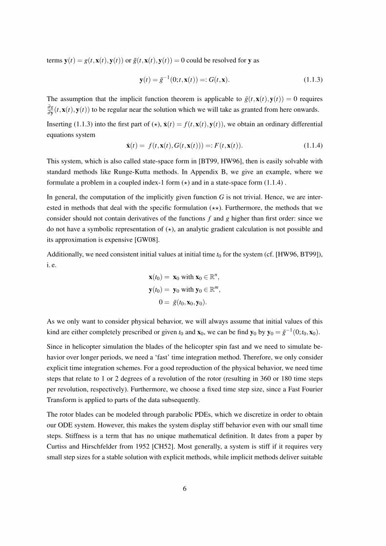
terms y(t) = g(t,x(t),y(t)) or g(t,x(t),y(t)) = 0 could be resolved for y as

y(t) = g−1(0; t,x(t)) =: G(t,x). (1.1.3)

The assumption that the implicit function theorem is applicable to g(t,x(t),y(t)) = 0 requires∂g∂y(t,x(t),y(t)) to be regular near the solution which we will take as granted from here onwards.

Inserting (1.1.3) into the first part of (?), x(t) = f (t,x(t),y(t)), we obtain an ordinary differential

equations system

x(t) = f (t,x(t),G(t,x(t))) =: F(t,x(t)). (1.1.4)

This system, which is also called state-space form in [BT99, HW96], then is easily solvable with

standard methods like Runge-Kutta methods. In Appendix B, we give an example, where we

formulate a problem in a coupled index-1 form (?) and in a state-space form (1.1.4) .

In general, the computation of the implicitly given function G is not trivial. Hence, we are inter-

ested in methods that deal with the specific formulation (??). Furthermore, the methods that we

consider should not contain derivatives of the functions f and g higher than first order: since we

do not have a symbolic representation of (?), an analytic gradient calculation is not possible and

its approximation is expensive [GW08].

Additionally, we need consistent initial values at initial time t0 for the system (cf. [HW96, BT99]),

i. e.

x(t0) = x0 with x0 ∈ Rn,

y(t0) = y0 with y0 ∈ Rm,

0 = g(t0,x0,y0).

As we only want to consider physical behavior, we will always assume that initial values of this

kind are either completely prescribed or given t0 and x0, we can be find y0 by y0 = g−1(0; t0,x0).

Since in helicopter simulation the blades of the helicopter spin fast and we need to simulate be-

havior over longer periods, we need a ‘fast’ time integration method. Therefore, we only consider

explicit time integration schemes. For a good reproduction of the physical behavior, we need time

steps that relate to 1 or 2 degrees of a revolution of the rotor (resulting in 360 or 180 time steps

per revolution, respectively). Furthermore, we choose a fixed time step size, since a Fast Fourier

Transform is applied to parts of the data subsequently.

The rotor blades can be modeled through parabolic PDEs, which we discretize in order to obtain

our ODE system. However, this makes the system display stiff behavior even with our small time

steps. Stiffness is a term that has no unique mathematical definition. It dates from a paper by

Curtiss and Hirschfelder from 1952 [CH52]. Most generally, a system is stiff if it requires very

small step sizes for a stable solution with explicit methods, while implicit methods deliver suitable

6

results with a much higher step size (cf. [Sp96] (Definition 2.1)). Several definitions of stiffness

can be found in [La91].

Certainly, we will encounter problems when using explicit methods on a stiff system (cf. [La73]).

In order to deal with the stiffness for our solver, we assume that it is possible to split every

fi(t,xi(t),ui(t)) into a linear stiff part Si ∈ Rni×ni and a nonlinear nonstiff part fi(t,xi(t),ui(t)).

Combining all subsystems we obtain

x(t) = Sx+ f (t,x(t),y(t)), (1.1.5)

where S ∈ Rn×n denotes a constant matrix with the matrices Si on its diagonal, and

f : R×Rn×Rm→ Rn denotes a possibly nonlinear function that contains the nonstiff part of

f , i. e. it has a sufficiently small Lipschitz constant [HO10]. The assumption that S contains the

stiff part can either be given by the model or we can linearize f in a neighborhood of the solution.

In total, we obtain a system x(t) = Sx+ f (t,x(t),y(t))y(t) = g(t,x(t),y(t))

. (???)

1.2. Mechanical helicopter model

So far, we have obtained an impression of the challenges of helicopter simulation and we have

presented our strategy for modeling such a system. In the following, we construct a model that

represents a simplified part of the helicopter. For our model, we build on the work of Sanches et

al. [SMBA11] who model a simplified rotor fixed to a fuselage (see Figure 1.2.1). The fuselage is

considered to be a rigid body connected to a rotor hub with 4 blades which are represented by a

concentrated mass located at a distance b from the point B [SMBA11].

Figure 1.2.1: Simplified rotor fixed to a fuselage (adapted sketch from [SMBA11] (Figure 1))

7

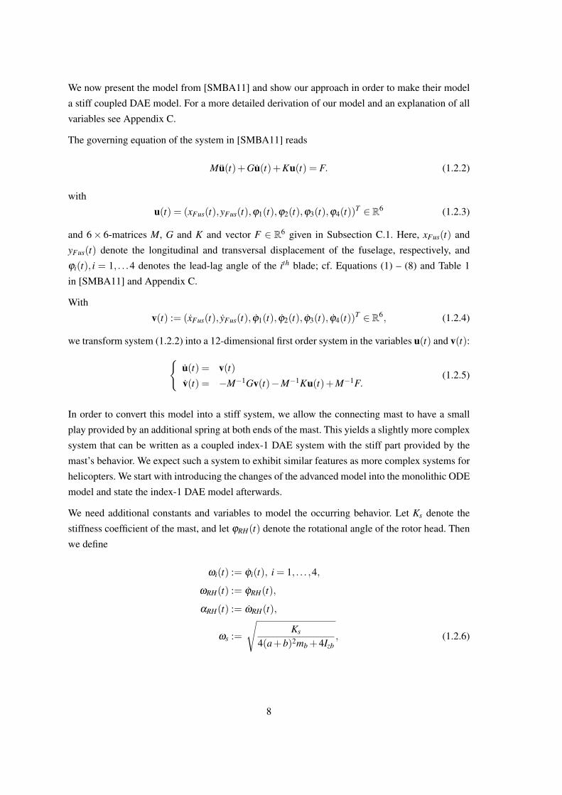
We now present the model from [SMBA11] and show our approach in order to make their model

a stiff coupled DAE model. For a more detailed derivation of our model and an explanation of all

variables see Appendix C.

The governing equation of the system in [SMBA11] reads

Mu(t)+Gu(t)+Ku(t) = F. (1.2.2)

with

u(t) = (xFus(t),yFus(t),ϕ1(t),ϕ2(t),ϕ3(t),ϕ4(t))T ∈ R6 (1.2.3)

and 6× 6-matrices M, G and K and vector F ∈ R6 given in Subsection C.1. Here, xFus(t) and

yFus(t) denote the longitudinal and transversal displacement of the fuselage, respectively, and

ϕi(t), i = 1, . . .4 denotes the lead-lag angle of the ith blade; cf. Equations (1) – (8) and Table 1

in [SMBA11] and Appendix C.

With

v(t) := (xFus(t), yFus(t), ϕ1(t), ϕ2(t), ϕ3(t), ϕ4(t))T ∈ R6, (1.2.4)

we transform system (1.2.2) into a 12-dimensional first order system in the variables u(t) and v(t):u(t) = v(t)v(t) = −M−1Gv(t)−M−1Ku(t)+M−1F.

(1.2.5)

In order to convert this model into a stiff system, we allow the connecting mast to have a small

play provided by an additional spring at both ends of the mast. This yields a slightly more complex

system that can be written as a coupled index-1 DAE system with the stiff part provided by the

mast’s behavior. We expect such a system to exhibit similar features as more complex systems for

helicopters. We start with introducing the changes of the advanced model into the monolithic ODE

model and state the index-1 DAE model afterwards.

We need additional constants and variables to model the occurring behavior. Let Ks denote the

stiffness coefficient of the mast, and let ϕRH(t) denote the rotational angle of the rotor head. Then

we define

ωi(t) := ϕi(t), i = 1, . . . ,4,

ωRH(t) := ϕRH(t),

αRH(t) := ωRH(t),

ωs :=

√Ks

4(a+b)2mb +4Izb, (1.2.6)

8

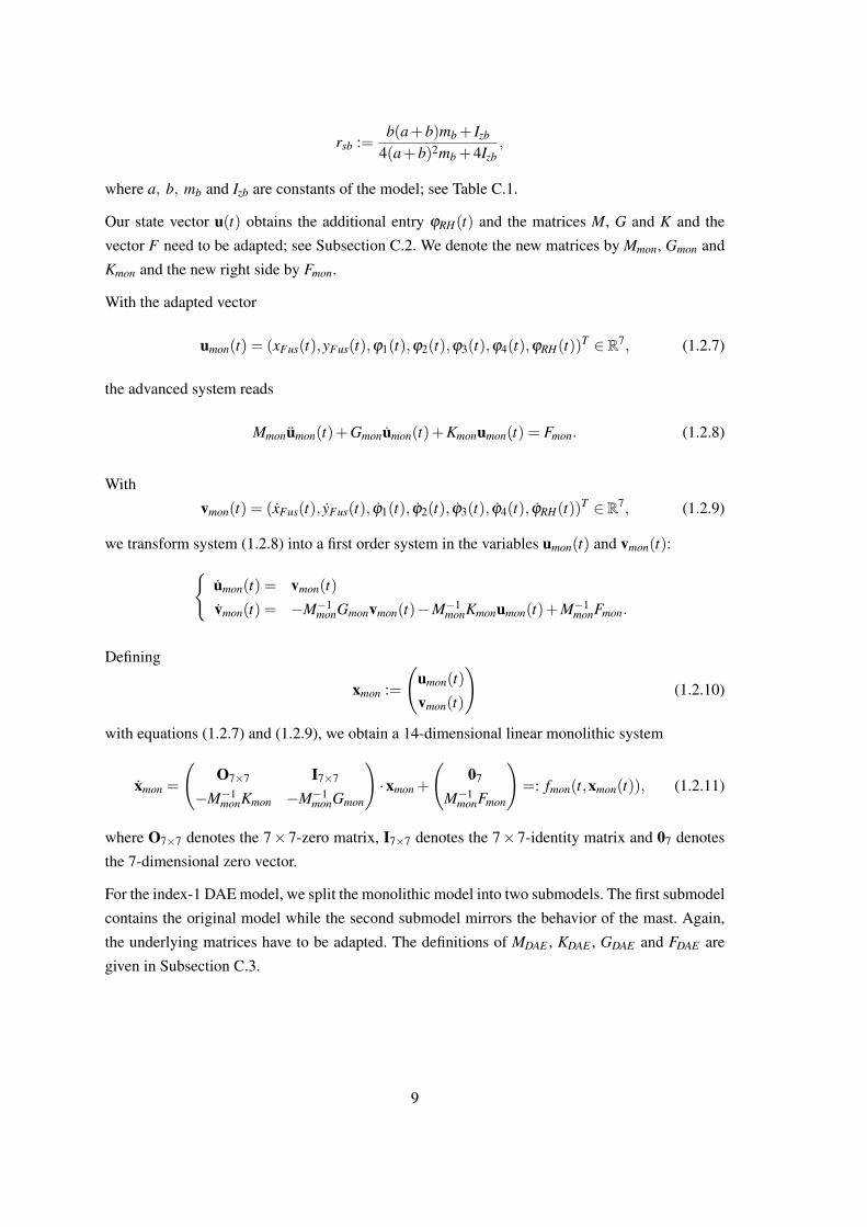
rsb :=b(a+b)mb + Izb

4(a+b)2mb +4Izb,

where a, b, mb and Izb are constants of the model; see Table C.1.

Our state vector u(t) obtains the additional entry ϕRH(t) and the matrices M, G and K and the

vector F need to be adapted; see Subsection C.2. We denote the new matrices by Mmon, Gmon and

Kmon and the new right side by Fmon.

With the adapted vector

umon(t) = (xFus(t),yFus(t),ϕ1(t),ϕ2(t),ϕ3(t),ϕ4(t),ϕRH(t))T ∈ R7, (1.2.7)

the advanced system reads

Mmonumon(t)+Gmonumon(t)+Kmonumon(t) = Fmon. (1.2.8)

With

vmon(t) = (xFus(t), yFus(t), ϕ1(t), ϕ2(t), ϕ3(t), ϕ4(t), ϕRH(t))T ∈ R7, (1.2.9)

we transform system (1.2.8) into a first order system in the variables umon(t) and vmon(t):umon(t) = vmon(t)

vmon(t) = −M−1monGmonvmon(t)−M−1

monKmonumon(t)+M−1monFmon.

Defining

xmon :=

(umon(t)

vmon(t)

)(1.2.10)

with equations (1.2.7) and (1.2.9), we obtain a 14-dimensional linear monolithic system

xmon =

(O7×7 I7×7

−M−1monKmon −M−1

monGmon

)·xmon +

(07

M−1monFmon

)=: fmon(t,xmon(t)), (1.2.11)

where O7×7 denotes the 7×7-zero matrix, I7×7 denotes the 7×7-identity matrix and 07 denotes

the 7-dimensional zero vector.

For the index-1 DAE model, we split the monolithic model into two submodels. The first submodel

contains the original model while the second submodel mirrors the behavior of the mast. Again,

the underlying matrices have to be adapted. The definitions of MDAE , KDAE , GDAE and FDAE are

given in Subsection C.3.

9

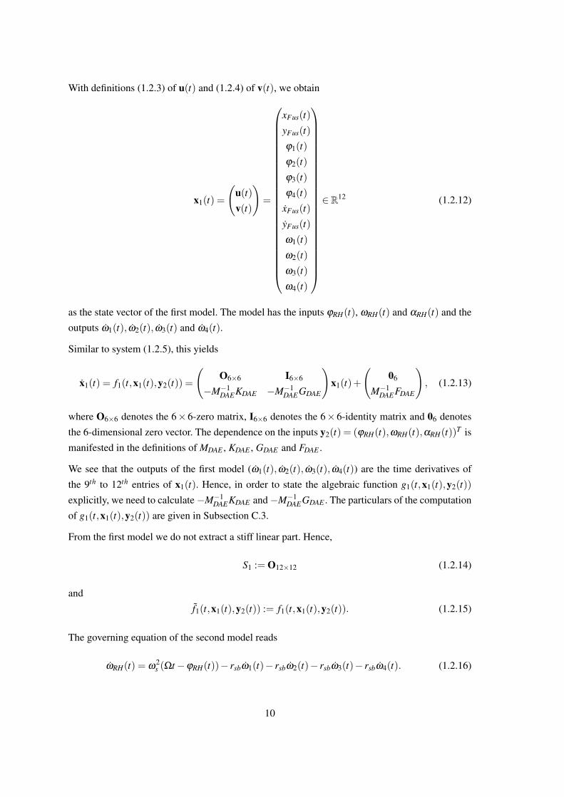
With definitions (1.2.3) of u(t) and (1.2.4) of v(t), we obtain

x1(t) =

(u(t)v(t)

)=

xFus(t)

yFus(t)

ϕ1(t)

ϕ2(t)

ϕ3(t)

ϕ4(t)

xFus(t)

yFus(t)

ω1(t)

ω2(t)

ω3(t)

ω4(t)

∈ R12 (1.2.12)

as the state vector of the first model. The model has the inputs ϕRH(t), ωRH(t) and αRH(t) and the

outputs ω1(t), ω2(t), ω3(t) and ω4(t).

Similar to system (1.2.5), this yields

x1(t) = f1(t,x1(t),y2(t)) =

(O6×6 I6×6

−M−1DAEKDAE −M−1

DAEGDAE

)x1(t)+

(06

M−1DAEFDAE

), (1.2.13)

where O6×6 denotes the 6×6-zero matrix, I6×6 denotes the 6×6-identity matrix and 06 denotes

the 6-dimensional zero vector. The dependence on the inputs y2(t) = (ϕRH(t),ωRH(t),αRH(t))T is

manifested in the definitions of MDAE , KDAE , GDAE and FDAE .

We see that the outputs of the first model (ω1(t), ω2(t), ω3(t), ω4(t)) are the time derivatives of

the 9th to 12th entries of x1(t). Hence, in order to state the algebraic function g1(t,x1(t),y2(t))

explicitly, we need to calculate−M−1DAEKDAE and−M−1

DAEGDAE . The particulars of the computation

of g1(t,x1(t),y2(t)) are given in Subsection C.3.

From the first model we do not extract a stiff linear part. Hence,

S1 := O12×12 (1.2.14)

and

f1(t,x1(t),y2(t)) := f1(t,x1(t),y2(t)). (1.2.15)

The governing equation of the second model reads

ωRH(t) = ω2s (Ωt−ϕRH(t))− rsbω1(t)− rsbω2(t)− rsbω3(t)− rsbω4(t). (1.2.16)

10

Here, we have the inputs ω1(t), ω2(t), ω3(t), ω4(t) and the outputs ϕRH(t), ωRH(t) and αRH(t).

With the local state vector

x2(t) :=

(ϕRH(t)

ωRH(t)

)∈ R2, (1.2.17)

equation (1.2.16) becomes

x2(t) =

(0 1

−ω2s 0

)x2(t)+

(0

ω2s Ωt− rsbω1(t)− rsbω2(t)− rsbω3(t)− rsbω4(t)

).

Since ω2s (defined in (1.2.6)) is the variable which is mainly responsible for the stiffness of the

system, we want it to be solely part of the first linear summand of the differential equations system.

So far, it also appears in the second line of the above equation. Hence, we redefine our variables.

Let

x(1)2 := ϕRH(t) := ϕRH(t)−Ωt,

x(2)2 := ωRH(t) := ˙ϕRH(t) = ϕRH(t)−Ω,(1.2.18)

which yields

x2(t) =

(0 1

−ω2s 0

)x2(t)+

(0

−rsbω1(t)− rsbω2(t)− rsbω3(t)− rsbω4(t)

).

Accordingly, we define

S2 :=

(0 1

−ω2s 0

)(1.2.19)

and

f2(t,x2(t),y1(t)) :=

(0

−rsbω1(t)− rsbω2(t)− rsbω3(t)− rsbω4(t)

). (1.2.20)

In this formulation, the variable ωs is not part of the nonlinear part f2(t,x2(t),y1(t)).

The local output vector and hence the local output function g2(t,x2(t),y1(t)) is given by

y2(t) =

ϕRH(t)

ωRH(t)

αRH(t)

=

x(1)2 (t)+Ωt

x(2)2 (t)+Ω

x(2)2 (t)

=: g2(t,x2(t),y1(t)). (1.2.21)

We can now collect the global model. Using the definitions of x1(t) and x2(t) in equations (1.2.12)

11

and (1.2.18), we obtain the global state vector

x(t) =

(x1(t)

x2(t)

)=

xFus(t)

yFus(t)

ϕ1(t)

ϕ2(t)

ϕ3(t)

ϕ4(t)

xFus(t)

yFus(t)

ω1(t)

ω2(t)

ω3(t)

ω4(t)

ϕRH(t)

ωRH(t)

. (1.2.22)

With the definitions of y1(t) and y2(t), our global output vector reads

y(t) =

(y1(t)

y2(t)

)=

ω1(t)

ω2(t)

ω3(t)

ω4(t)

ϕRH(t)

ωRH(t)

αRH(t)

. (1.2.23)

The global functions fDAE(t,x(t),y(t)) and gDAE(t,x(t),y(t)) arise from equations (1.2.14),

(1.2.15), (1.2.19), (1.2.20), (C.3.5) and (1.2.21):

fDAE(t,x(t),y(t)) := Sx(t)+ fDAE(t,x(t),y(t)) (1.2.24)

=

(S1 O12×2

O2×12 S2

)x(t)+

(f1(t,x(t),y(t))f2(t,x(t),y(t))

),

gDAE(t,x(t),y(t)) :=

(g1(t,x(t),y(t))g2(t,x(t),y(t))

). (1.2.25)

Now we have the advanced stiff model in monolithic and in DAE representation. In the DAE rep-

resentation, we extracted a stiff linear part and obtained a system of the form (???). In Section 3.4,

we use this model to evaluate the algorithm defined in Section 2.4.

12

2. Numerical methods for index-1 DAEs

In Section 1.1, we explained the approach that we take towards helicopter simulation: we model

the governing equations as a coupled index-1 DAE system. In this section, we examine numerical

methods that can be applied to our system.

There are two popular approaches for the numerical solution of index-1 differential alge-

braic equations: ε-embedding methods [BT99, HW96] and half-explicit Runge-Kutta meth-

ods [BT99, ASW93, HLR89], also called state space form methods [BT99, HW96].

In order to apply ε-embedding methods, we need to consider the singularly perturbed problem

(SPP) x(t) = f (t,x(t),y(t))

ε y(t) = g(t,x(t),y(t)), (SPP)

where 0 < ε 1 ([BT99] (p. 5)). For ε = 0, we obtain system (??). Despite ε , we have a system

of ODEs which can be solved by slightly adapted standard methods; see [HW96] (pp. 374/5).

However for small ε , the arising system is stiff which makes it necessary to use implicit solution

schemes; see [BT99] (Section 2.2.2). Alternatively, implicit-explicit methods [Bo07] could be

applied. When using fully implicit methods, we need to solve a generally nonlinear system of

equations in every stage. This results in a significantly higher run time of the algorithms, which is

not suitable for our needs.

Instead, half-explicit Runge-Kutta methods do not exhibit these limitations since they are explicit

methods. Thus, we want to analyze them in more detail.

We start this section with introducing general Runge-Kutta methods in Subsection 2.1, where we

briefly state well-known consistency and stability results. Subsequently, we present the deriva-

tion of half-explicit Runge-Kutta methods in Subsection 2.2. Here, we conduct a comprehensible

consistency analysis of first and second order methods. In order to deal with the earlier described

stiffness of our system, we introduce explicit exponential Runge-Kutta methods in Subsection 2.3

and transfer the findings for half-explicit Runge-Kutta methods on these exponential integrators in

order to obtain half-explicit exponential Runge-Kutta methods in Subsection 2.4. An overview of

these topics is given in Table 2.1.

13

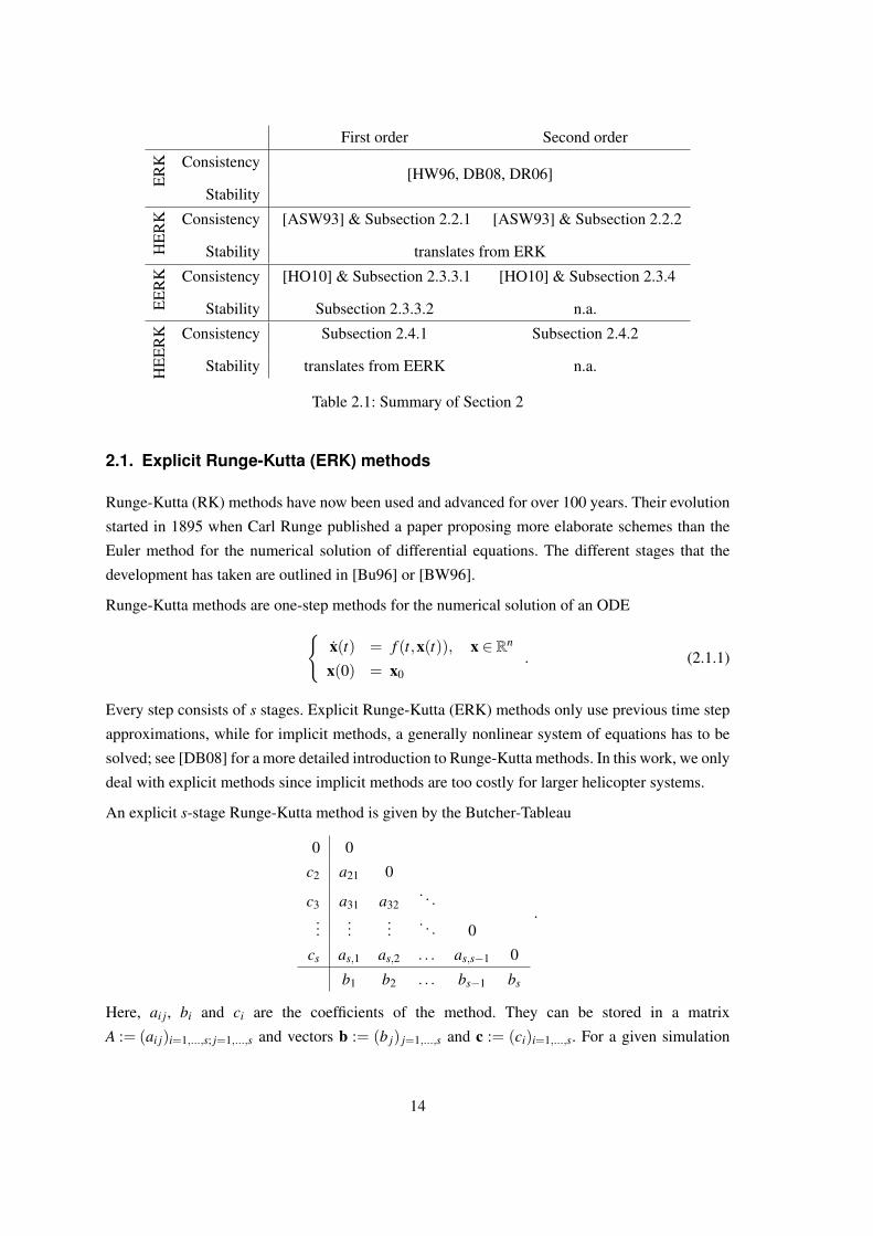
First order Second orderE

RK Consistency

[HW96, DB08, DR06]Stability

HE

RK Consistency [ASW93] & Subsection 2.2.1 [ASW93] & Subsection 2.2.2

Stability translates from ERK

EE

RK Consistency [HO10] & Subsection 2.3.3.1 [HO10] & Subsection 2.3.4

Stability Subsection 2.3.3.2 n.a.

HE

ER

K Consistency Subsection 2.4.1 Subsection 2.4.2

Stability translates from EERK n.a.

Table 2.1: Summary of Section 2

2.1. Explicit Runge-Kutta (ERK) methods

Runge-Kutta (RK) methods have now been used and advanced for over 100 years. Their evolution

started in 1895 when Carl Runge published a paper proposing more elaborate schemes than the

Euler method for the numerical solution of differential equations. The different stages that the

development has taken are outlined in [Bu96] or [BW96].

Runge-Kutta methods are one-step methods for the numerical solution of an ODEx(t) = f (t,x(t)), x ∈ Rn

x(0) = x0. (2.1.1)

Every step consists of s stages. Explicit Runge-Kutta (ERK) methods only use previous time step

approximations, while for implicit methods, a generally nonlinear system of equations has to be

solved; see [DB08] for a more detailed introduction to Runge-Kutta methods. In this work, we only

deal with explicit methods since implicit methods are too costly for larger helicopter systems.

An explicit s-stage Runge-Kutta method is given by the Butcher-Tableau

0 0

c2 a21 0

c3 a31 a32. . .

......

.... . . 0

cs as,1 as,2 . . . as,s−1 0

b1 b2 . . . bs−1 bs

.

Here, ai j, bi and ci are the coefficients of the method. They can be stored in a matrix

A := (ai j)i=1,...,s; j=1,...,s and vectors b := (b j) j=1,...,s and c := (ci)i=1,...,s. For a given simulation

14

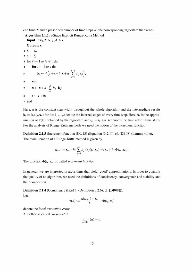
end time T and a prescribed number of time steps N, the corresponding algorithm then reads

Algorithm 2.1.2: s-Stage Explicit Runge-Kutta MethodInput : x0,T,N, f ,A,b,c.

Output: x1 x← x0

2 h← TN

3 for `← 1 to N +1 do4 for i← 1 to s do

5 ki← f(

t + ci ·h,x+h ·i−1∑j=1

ai jk j

);

6 end

7 x← x+h ·s∑j=1

b j ·k j;

8 t← t +h;

9 end

Here, h is the constant step width throughout the whole algorithm and the intermediate results

ki := ki(tn,xn) for i = 1, . . . ,s denote the internal stages of every time step. Here, xn is the approx-

imation of x(tn) obtained by the algorithm and tn := t0 +n ·h denotes the time after n time steps.

For the analysis of Runge-Kutta methods we need the notion of the increment function.

Definition 2.1.3 (Increment function ([Ku13] (Equation (3.2.1)), cf. [DB08] (Lemma 4.4))).The main iteration of a Runge-Kutta method is given by

xn+1 = xn +h ·s

∑j=1

b j ·k j(tn,xn) =: xn +h ·Φ(tn,xn).

The function Φ(tn,xn) is called increment function.

In general, we are interested in algorithms that yield ‘good’ approximations. In order to quantify

the quality of an algorithm, we need the definitions of consistency, convergence and stability and

their connection.

Definition 2.1.4 (Consistency ([Ku13] (Definition 3.2.6), cf. [DB08])).Let

τ(h) :=x(tn+1)−xn

h−Φ(tn,xn)

denote the local truncation error.

A method is called consistent if

limh→0

τ(h) = 0.

15

A method is called consistent of order k if

τ(h) = O(hk) for h→ 0.

In contrary to the local truncation error for consistency, we need to analyze the global truncation

error for convergence.

Definition 2.1.5 (Convergence ([Ku13])).Let xh(t) denote the approximation of x(t) obtained by a one-step method. The method is called

convergent if the global truncation error

ε(t,h) := xh(t)−x(t)

converges to 0 for h→ 0.

In order to proof a consistency order k of Runge-Kutta methods, we can compare the Taylor

expansion to kth order of x′(t) with the Taylor expansion to kth order of the increment function

Φ(t,x). If their difference is of kth order, then the method has consistency order k. However, this

result is purely asymptotic. It does not say how small h needs to be for specific problems in order

for the methods to converge of order k. To this end, we additionally need the notion of stability.

In order to analyze the stability of one-step methods applied to an ODE of the form (2.1.1), we

consider a one-dimensional Dahlquist test equation

x(t) = λx(t) =: f (t,x(t)), (2.1.6)

where t ∈ R+, λ ∈ C, x : R→ R. We can bring our underlying method in the form

xn+1 = φ(hλ )xn (2.1.7)

with a stability function φ . Then the method is stable in the region

z ∈ C : |φ(z)| ≤ 1 ,

hence, for those h ∈ R+ such that |φ(hλ )| ≤ 1 (cf. [HW96] (Chapter IV.2) or

[DR06] (Section 11.9.3)).

This is a linear stability analysis and certainly has shortcomings. However, nonlinear stability

theory is much more sophisticated (cf. [La91], Chapter 7), which makes the nonlinear stability

results rare. Futhermore, the findings for the linear analysis have proven to be quite good estimates

even for nonlinear systems [HR07].

In total, we obtain convergence, if a method is consistent and stable.

16

Lemma 2.1.8 (adapted from [La91] (Chapter 7) and [Ku13]).If a method is consistent of order k and stable, then it is convergent of order k or short

Consistency + Stability ⇔ Convergence.

Remark 2.1.9 ([Ku13] (Theorem 3.3.5), [DR06] (Theorem 11.25)).For the stability of explicit one-step methods it is sufficient to show a Lipschitz condition of the

increment function in x, i. e. it exists M ∈ R, such that

||Φ(t,x)−Φ(t, x)|| ≤M||x− x||, x, x ∈ Rn.

2.1.1. Consistency

The derivation of consistency conditions for various orders of Runge-Kutta methods has been “an

interesting challenge” [Bu96] since their formulation. Consistency conditions for Runge-Kutta

methods of orders one to four can be found in [DB08]. We will not deal with this subject for

ordinary Runge-Kutta methods in this thesis.

2.1.2. Stability

The analysis of stability in this subsection is based on [Fr08] (Chapter 10, pp. 58–59). See

also [Bu96, DB08]. Starting from an autonomous one-dimensional ODE of the form

x(t) = f (x(t)), x ∈ R,

an s-stage Runge-Kutta method is given by the iteration

ki = f(

xn +hs

∑j=1

ai jk j

), i = 1, . . . ,s (2.1.10a)

xn+1 = xn +hs

∑i=1

biki, (2.1.10b)

where the coefficients ai j and bi can be stored in a matrix A := (ai j)i=1,...,s; j=1,...,s and a vector

b := (bi)i=1,...,s. In order to determine the stability region of the method, we consider the Dahlquist

test equation (2.1.6), which we insert into (2.1.10a) to obtain

ki = λ

(xn +h

s

∑j=1

ai jk j

).

17

With k = (k1, . . . ,ks)T and e = (1, . . . ,1)T ∈ Rs, this transforms to

k = λ (xne+hAk)

⇔ k = (I−hλA)−1λxne. (2.1.11)

In order to obtain an equation of the form (2.1.7) we insert (2.1.11) into (2.1.10b):

xn+1 = xn +hbT k

= xn +hbT (I−hλA)−1λxne

=[1+hλbT (I−hλA)−1e

]xn.

Hence, using z := hλ , the stability function reads

φ(z) = 1+ zbT (I− zA)−1e. (2.1.12)

Lemma 2.1.13 (cf. [Fr08] (Chapter 10, pp. 58–59)).For an n-dimensional problem, the derivation of the stability function can be reduced to finding

the stability function for n one-dimensional problems.

Proof.

We consider the problem

x(t) = Lx(t) =: f (x(t)), x ∈ Rn, L ∈ Rn×n. (2.1.14)

Case 1: Let L be diagonalizable.

Let U ∈ Rn×n contain all eigenvectors of L and let Λ ∈ Rn×n have the eigenvalues λi, i = 1, . . . ,n

of L on its diagonal, such that U−1LU = Λ. Define

xn := U−1xn (2.1.15a)

ki := U−1ki, i = 1, . . .s (2.1.15b)

and insert (2.1.15a) and (2.1.15b) into (2.1.10). For (2.1.10a), we obtain

ki = L(

xn +hs

∑j=1

ai jk j

)⇔U ki = LU xn +h

s

∑j=1

ai jLU k j

⇔ ki = U−1LU xn +hs

∑j=1

ai jU−1LU k j

18

⇔ ki = Λxn +hs

∑j=1

ai jΛk j.

Similarly, for (2.1.10b), we get

xn+1 = xn +hs

∑i=1

biki

⇔U xn+1 = U xn +hs

∑i=1

biU ki

⇔ xn+1 = xn +hs

∑i=1

biki.

We obtain n independent problems, since for any ` = 1, . . . ,n, the `th entries of ki and xn+1 only

depend on the `th entries of xn and all k j, j = 1, . . . ,s, namely

k(`)i = λ`x

(`)n +h

s

∑j=1

ai jλ`k(`)j

x(`)n+1 = x(`)n +hs

∑i=1

bik(`)i .

Case 2: Let L be non-diagonalizable.

For non-diagonalizable L the situation is more complex. We can bring L in Jordan normal

form (see Lemma A.2.2). Then, certain results can be shown. A detailed analysis is given in

[Sp98] (Chapters 4–6).

If we now insert the Butcher-Tableau for classical Runge-Kutta methods into the stability func-

tion (2.1.12), we obtain the following results.

Corollary 2.1.16 (cf. [HW96] (Theorem 2.2)).The stability function of an s-stage explicit Runge-Kutta method of consistency order k, with k≤ s,

is given by

φ(z) =k

∑i=0

zi

i!.

Corollary 2.1.17 (cf. [HW96] (Theorem 2.2)).The stability functions φ1(z) to φ4(z) of the explicit Runge-Kutta methods of orders 1–4 are given

by

φ1(z) = 1+ z, (2.1.18a)

φ2(z) = 1+ z+12

z2, (2.1.18b)

19

φ3(z) = 1+ z+12

z2 +16

z3, (2.1.18c)

φ4(z) = 1+ z+12

z2 +16

z3 +1

24z4. (2.1.18d)

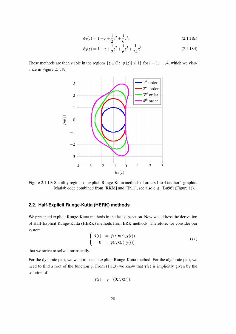
These methods are then stable in the regions z ∈ C : |φi(z)| ≤ 1 for i = 1, . . . ,4, which we visu-

alize in Figure 2.1.19.

−4 −3 −2 −1 0 1 2 3

−3

−2

−1

0

1

2

3

Re(z)

Im(z)

1st order2nd order3rd order4th order

Figure 2.1.19: Stability regions of explicit Runge-Kutta methods of orders 1 to 4 (author’s graphic,Matlab code combined from [RKM] and [Tr11], see also e. g. [Bu96] (Figure 1)).

2.2. Half-Explicit Runge-Kutta (HERK) methods

We presented explicit Runge-Kutta methods in the last subsection. Now we address the derivation

of Half-Explicit Runge-Kutta (HERK) methods from ERK methods. Therefore, we consider our

system x(t) = f (t,x(t),y(t))

0 = g(t,x(t),y(t))(??)

that we strive to solve, intrinsically.

For the dynamic part, we want to use an explicit Runge-Kutta method. For the algebraic part, we

need to find a root of the function g. From (1.1.3) we know that y(t) is implicitly given by the

solution of

y(t) = g−1(0; t,x(t)).

20

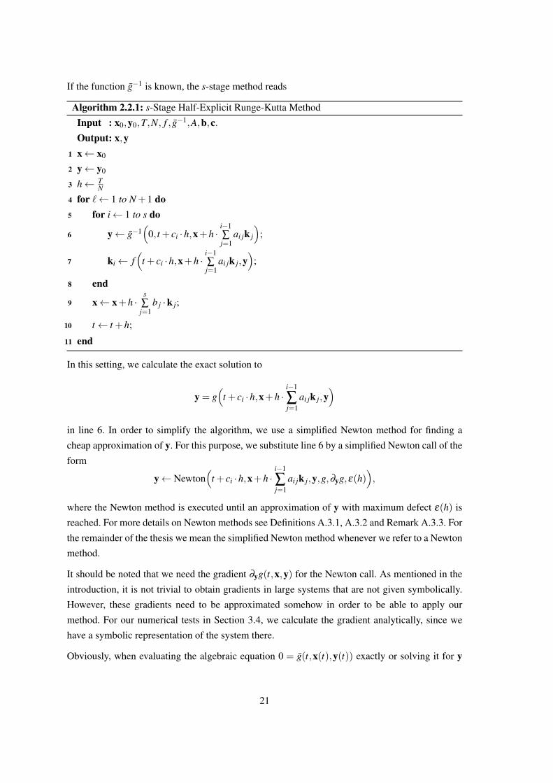
If the function g−1 is known, the s-stage method reads

Algorithm 2.2.1: s-Stage Half-Explicit Runge-Kutta Method

Input : x0,y0,T,N, f , g−1,A,b,c.Output: x,y

1 x← x0

2 y← y0

3 h← TN

4 for `← 1 to N +1 do5 for i← 1 to s do

6 y← g−1(

0, t + ci ·h,x+h ·i−1∑j=1

ai jk j

);

7 ki← f(

t + ci ·h,x+h ·i−1∑j=1

ai jk j,y)

;

8 end

9 x← x+h ·s∑j=1

b j ·k j;

10 t← t +h;

11 end

In this setting, we calculate the exact solution to

y = g(

t + ci ·h,x+h ·i−1

∑j=1

ai jk j,y)

in line 6. In order to simplify the algorithm, we use a simplified Newton method for finding a

cheap approximation of y. For this purpose, we substitute line 6 by a simplified Newton call of the

form

y← Newton(

t + ci ·h,x+h ·i−1

∑j=1

ai jk j,y,g,∂yg,ε(h)),

where the Newton method is executed until an approximation of y with maximum defect ε(h) is

reached. For more details on Newton methods see Definitions A.3.1, A.3.2 and Remark A.3.3. For

the remainder of the thesis we mean the simplified Newton method whenever we refer to a Newton

method.

It should be noted that we need the gradient ∂yg(t,x,y) for the Newton call. As mentioned in the

introduction, it is not trivial to obtain gradients in large systems that are not given symbolically.

However, these gradients need to be approximated somehow in order to be able to apply our

method. For our numerical tests in Section 3.4, we calculate the gradient analytically, since we

have a symbolic representation of the system there.

Obviously, when evaluating the algebraic equation 0 = g(t,x(t),y(t)) exactly or solving it for y

21

as in (1.1.4), we do not need to investigate the convergence orders of the underlying methods,

since they are equivalent to the convergence orders of these methods for ODEs. However, for

approximations of y(t) = g(t,x(t),y(t)) e. g. by a Newton method, we need to know how many

Newton steps we need in every iteration or to which accuracy we need to apply the Newton method

in order to sustain the convergence order of the underlying Runge-Kutta method. The number of

needed Newton steps is analyzed in [ASW93]. Instead here, we focus on the accuracy to which our

output vector y needs to be computed by the Newton method. We investigate this question using

the example of the first and second order half-explicit Runge-Kutta methods which are given

in Algorithms 2.2.2 and 2.2.9. The respective findings of [ASW93] are given in Remarks 2.2.6

and 2.2.16.

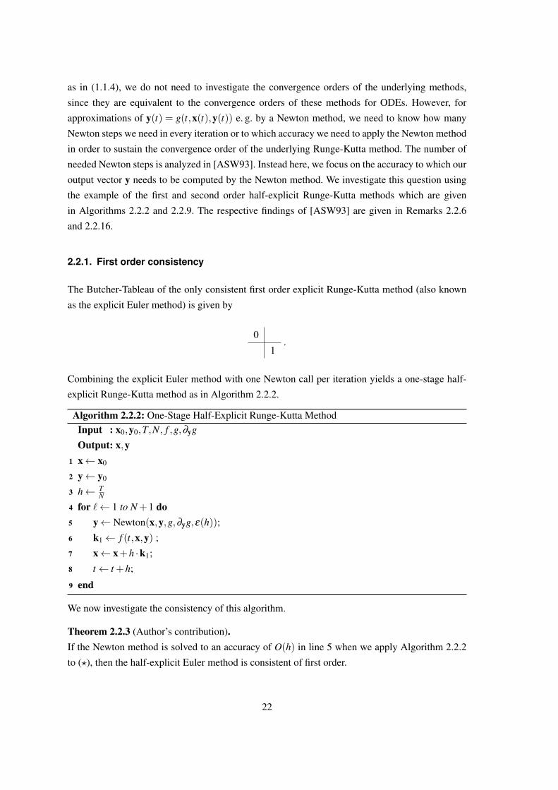
2.2.1. First order consistency

The Butcher-Tableau of the only consistent first order explicit Runge-Kutta method (also known

as the explicit Euler method) is given by

0

1.

Combining the explicit Euler method with one Newton call per iteration yields a one-stage half-

explicit Runge-Kutta method as in Algorithm 2.2.2.

Algorithm 2.2.2: One-Stage Half-Explicit Runge-Kutta MethodInput : x0,y0,T,N, f ,g,∂yg

Output: x,y1 x← x0

2 y← y0

3 h← TN

4 for `← 1 to N +1 do5 y← Newton(x,y,g,∂yg,ε(h));

6 k1← f (t,x,y) ;

7 x← x+h ·k1;

8 t← t +h;

9 end

We now investigate the consistency of this algorithm.

Theorem 2.2.3 (Author’s contribution).If the Newton method is solved to an accuracy of O(h) in line 5 when we apply Algorithm 2.2.2

to (?), then the half-explicit Euler method is consistent of first order.

22

Proof.

We consider the system x(t) = f (t,x(t),y(t))y(t) = g(t,x(t),y(t))

. (?)

Locally, we have a unique solution

y(t) = g−1(0; t,x(t))

as in (1.1.3).

However, we commit an error when applying the Newton method. Hence, we only get an inex-

act version g−1 instead of g−1 for y and subsequently a defective y, which has an error 4y in

comparison to the correct y, i. e.

y := g−1(0; t,x) = g−1(0; t,x)+4y = y+4y.

In order to observe the consistency error, we need to compare the Taylor expansion of the differ-

ence operator with the Taylor expansion of the increment function Φ(t,x,y). First, we calculate

the Taylor expansion of the difference operator up to first order

x′(t) =x(t +h)−x(t)

h= x′(t)+O(h)

= f (t,x,y)+O(h).

Hence,

x′(t) = f (t,x,y)+O(h). (2.2.4)

The increment function Φ(t,x,y) reads

Φ(t,x,y) = k1(t,x, y) = f (t,x,y+4y).

The corresponding Taylor expansion of the increment function Φ(t,x,y) under the assumption that

4y is at least of order O(h) reads:

Φ(t,x,y) = f (t,x,y)+4y ∂ f∂y (t,x,y)+O

((4y)2).

So we obtain

Φ(t,x,y) = f (t,x,y)+O(h). (2.2.5)

23

The comparison of (2.2.4) and (2.2.5) yields the desired result. If 4y = O(h), then the method is

consistent of first order.

The respective result of Arnold et al. ([ASW93]) reads

Remark 2.2.6 ([ASW93] (Example 2.a) ).For a first order half-explicit Runge-Kutta method, at least one simplified Newton step is required

to achieve the desired accuracy.

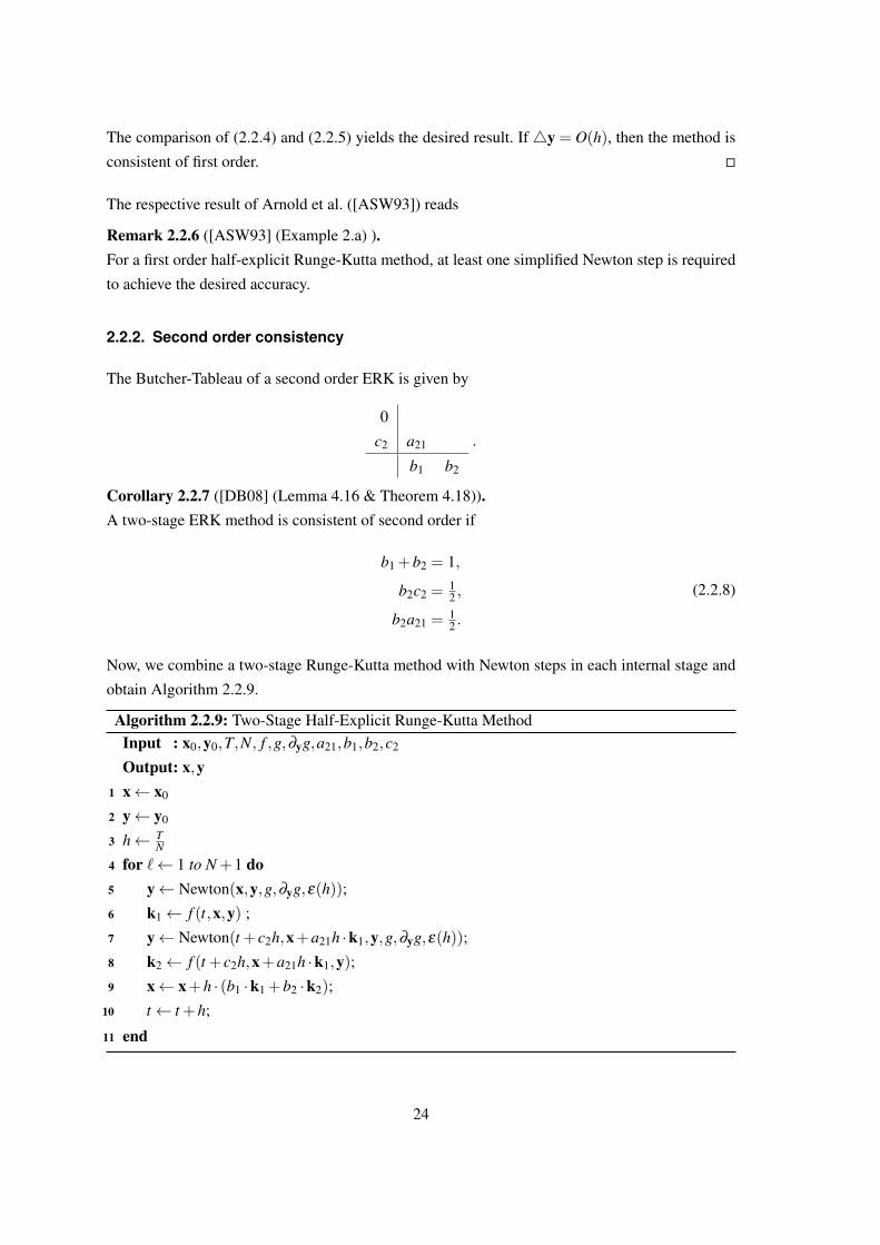
2.2.2. Second order consistency

The Butcher-Tableau of a second order ERK is given by

0

c2 a21

b1 b2

.

Corollary 2.2.7 ([DB08] (Lemma 4.16 & Theorem 4.18)).A two-stage ERK method is consistent of second order if

b1 +b2 = 1,

b2c2 =12 ,

b2a21 =12 .

(2.2.8)

Now, we combine a two-stage Runge-Kutta method with Newton steps in each internal stage and

obtain Algorithm 2.2.9.

Algorithm 2.2.9: Two-Stage Half-Explicit Runge-Kutta MethodInput : x0,y0,T,N, f ,g,∂yg,a21,b1,b2,c2

Output: x,y1 x← x0

2 y← y0

3 h← TN

4 for `← 1 to N +1 do5 y← Newton(x,y,g,∂yg,ε(h));

6 k1← f (t,x,y) ;

7 y← Newton(t + c2h,x+a21h ·k1,y,g,∂yg,ε(h));

8 k2← f (t + c2h,x+a21h ·k1,y);9 x← x+h · (b1 ·k1 +b2 ·k2);

10 t← t +h;

11 end

24

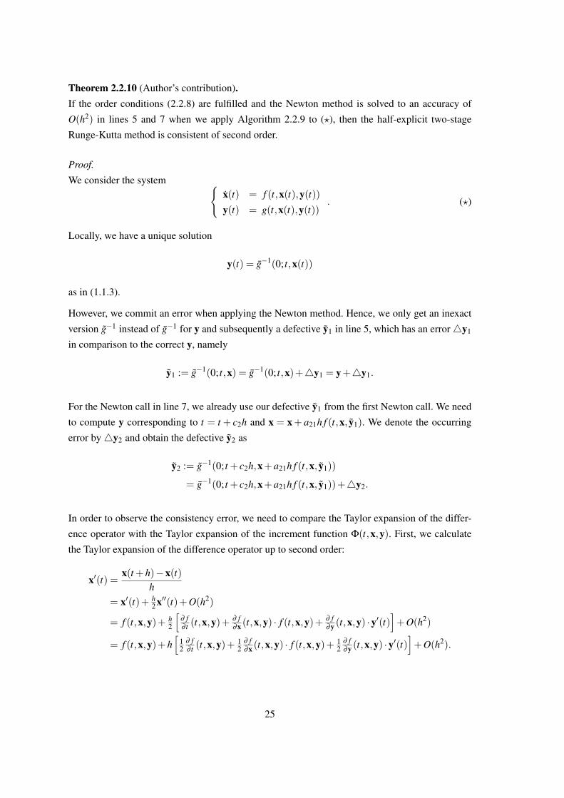
Theorem 2.2.10 (Author’s contribution).If the order conditions (2.2.8) are fulfilled and the Newton method is solved to an accuracy of

O(h2) in lines 5 and 7 when we apply Algorithm 2.2.9 to (?), then the half-explicit two-stage

Runge-Kutta method is consistent of second order.

Proof.

We consider the system x(t) = f (t,x(t),y(t))y(t) = g(t,x(t),y(t))

. (?)

Locally, we have a unique solution

y(t) = g−1(0; t,x(t))

as in (1.1.3).

However, we commit an error when applying the Newton method. Hence, we only get an inexact

version g−1 instead of g−1 for y and subsequently a defective y1 in line 5, which has an error4y1

in comparison to the correct y, namely

y1 := g−1(0; t,x) = g−1(0; t,x)+4y1 = y+4y1.

For the Newton call in line 7, we already use our defective y1 from the first Newton call. We need

to compute y corresponding to t = t + c2h and x = x+ a21h f (t,x, y1). We denote the occurring

error by4y2 and obtain the defective y2 as

y2 := g−1(0; t + c2h,x+a21h f (t,x, y1))

= g−1(0; t + c2h,x+a21h f (t,x, y1))+4y2.

In order to observe the consistency error, we need to compare the Taylor expansion of the differ-

ence operator with the Taylor expansion of the increment function Φ(t,x,y). First, we calculate

the Taylor expansion of the difference operator up to second order:

x′(t) =x(t +h)−x(t)

h= x′(t)+ h

2 x′′(t)+O(h2)

= f (t,x,y)+ h2

[∂ f∂ t (t,x,y)+

∂ f∂x (t,x,y) · f (t,x,y)+ ∂ f

∂y (t,x,y) ·y′(t)]+O(h2)

= f (t,x,y)+h[

12

∂ f∂ t (t,x,y)+

12

∂ f∂x (t,x,y) · f (t,x,y)+ 1

2∂ f∂y (t,x,y) ·y

′(t)]+O(h2).

25

So we have

x′(t) = f (t,x,y)+h[

12

∂ f∂ t (t,x,y)+

12

∂ f∂x (t,x,y) · f (t,x,y)+ 1

2∂ f∂y (t,x,y) ·y

′(t)]+O(h2) (2.2.11)

Here, we can further calculate y′(t) from (1.1.3) and obtain

y′(t) = ∂ g−1

∂ t (0; t,x)+ ∂ g−1

∂x (0; t,x) ·x′(t) = ∂ g−1

∂ t (0; t,x)+ ∂ g−1

∂x (0; t,x) · f (t,x,y). (2.2.12)

The increment function Φ(t,x,y) reads

Φ(t,x,y) = b1k1(t,x, y1)+b2k2(t,x, y2)

= b1 f (t,x, y1)+b2 f(t + c2h,x+a21h f (t,x, y1), g−1(0; t + c2h,x+a21h f (t,x, y1))

)= b1 f (t,x, y1)

+b2 f(t + c2h,x+a21h f (t,x, y1), g−1(0; t + c2h,x+a21h f (t,x, y1))+4y2

)= b1 f (t,x,y+4y1)+b2 f

(t + c2h,x+a21h f (t,x,y+4y1),

g−1(0; t + c2h,x+a21h f (t,x,y+4y1))+4y2).

In order to simplify the notation in the Taylor expansion of the increment function Φ(t,x,y), we

bring some calculations forward. Under the assumption that 4y1 and 4y2 are at least of order

O(h), we have

h · f (t,x,y+4y1) = h[ f (t,x,y)+ ∂ f∂y (t,x,y)4y1 +O(4y2

1)]

= h f (t,x,y)+h ·O(h) ∂ f∂y (t,x,y)+h ·O(h2)

= h f (t,x,y)+O(h2)

⇒ h · f (t,x,y+4y1) = h f (t,x,y)+O(h2) (2.2.13)

and

g−1(0; t + c2h,x+a21h f (t,x,y+4y1)) = g−1(0; t,x)+ c2h ∂ g−1

∂ t (0; t,x)

+ ∂ g−1

∂x (0; t,x) ·a21h f (t,x,y+4y1)+O(h2)

= y+ c2h ∂ g−1

∂ t (0; t,x)

+a21h ∂ g−1

∂x (0; t,x) f (t,x,y+4y1)+O(h2)

(2.2.13)= y+ c2h ∂ g−1

∂ t (0; t,x)

+a21h ∂ g−1

∂x (0; t,x) f (t,x,y)+O(h2),

26

which yields

g−1(0; t + c2h,x+a21h f (t,x,y+4y1))=

a21h ∂ g−1

∂x (0; t,x) f (t,x,y)+4y2−y +c2h ∂ g−1

∂ t (0; t,x)+4y2 +O(h2).(2.2.14)

The corresponding Taylor expansion of the increment function Φ(t,x,y) under the assumptions

that4y1 and4y2 are at least of order O(h) and the conditions (2.2.8) are fulfilled reads

Φ(t,x,y) = b1

(f (t,x,y)+ ∂ f

∂y (t,x,y)4y1

)+b2

[f (t,x,y)+ c2h ∂ f

∂ t (t,x,y)+a21h ∂ f∂x (t,x,y) f (t,x,y+4y1)

+ ∂ f∂y (t,x,y)

(g−1(0; t + c2h,x+a21h f (t,x,y+4y1))+4y2−y

)]+O(h2)

(2.2.14)= (b1 +b2) f (t,x,y)+b2c2h ∂ f

∂ t (t,x,y)+b2a21h ∂ f∂x (t,x,y) f (t,x,y+4y1)

+b2∂ f∂y (t,x,y)

(c2h ∂ g−1

∂ t (0; t,x)+ ∂ g−1

∂x (0; t,x) ·a21h f (t,x,y)+4y2

)+b1

∂ f∂y (t,x,y)4y1 +O(h2)

(2.2.13)= (b1 +b2) f (t,x,y)+b2c2h ∂ f

∂ t (t,x,y)+b2a21h ∂ f∂x (t,x,y) f (t,x,y)

+b2∂ f∂y (t,x,y)

(c2h ∂ g−1

∂ t (0; t,x)+a21h ∂ g−1

∂x (0; t,x) f (t,x,y)+4y2

)+b1

∂ f∂y (t,x,y)4y1 +O(h2)

(2.2.8)= f (t,x,y)+h

[12

∂ f∂ t (t,x,y)+

12

∂ f∂x (t,x,y) f (t,x,y)

+12

∂ f∂y (t,x,y)

(∂ g−1

∂ t (0; t,x)+ ∂ g−1

∂x (0; t,x) f (t,x,y))]

+ ∂ f∂y (t,x,y) · (b14y1 +b24y2)+O(h2)

(2.2.12)= f (t,x,y)+h

[12

∂ f∂ t (t,x,y)+

12

∂ f∂x (t,x,y) f (t,x,y)+ 1

2∂ f∂y (t,x,y)y

′(t)]

+ ∂ f∂y (t,x,y) · (b14y1 +b24y2)+O(h2).

So, we have

Φ(t,x,y) = f (t,x,y)+h[

12

∂ f∂ t (t,x,y)+

12

∂ f∂x (t,x,y) f (t,x,y)+ 1

2∂ f∂y (t,x,y)y

′(t)]

+ ∂ f∂y (t,x,y) · (b14y1 +b24y2)+O(h2).

(2.2.15)

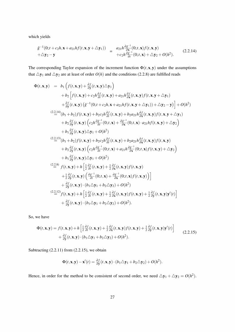
Subtracting (2.2.11) from (2.2.15), we obtain

Φ(t,x,y)−x′(t) = ∂ f∂y (t,x,y) · (b14y1 +b24y2)+O(h2).

Hence, in order for the method to be consistent of second order, we need 4y1 +4y2 = O(h2).

27

Now, if we solve both Newton methods to second order accuracy, we obtain 4y1 = O(h2) and

4y2 = O(h2) which yields4y1 +4y2 = O(h2).

The respective result by [ASW93] reads

Remark 2.2.16 ([ASW93] (Example 2.b) ).For a second order half-explicit Runge-Kutta methods, at least one Newton step is required after

the computation of k1 (line 7 in Algorithm 2.2.9) and also at least one Newton step is needed after

the computation of the new x (which is equivalent to the Newton call in line 5 of Algorithm 2.2.9).

2.2.3. Note on stability

When applying half-explicit methods, we solve the algebraic part of (?) in every iteration up to

the accuracy that is equal to the convergence order that the method shall achieve. However, this

means that only the error in the state variable x is propagated by the iteration of the method. Thus,

we only need to analyze the stability properties of the explicit methods, which then translate to the

respective half-explicit methods. For a more detailed analysis see [HLR89] (Theorem 3.1).

2.3. Explicit Exponential Runge-Kutta (EERK) methods

In Subsection 1.1, we stated that the dynamic part of our DAE system (?) can be split into a linear

stiff part and a nonlinear nonstiff part (cf. equation (1.1.5)). Additionally to fully implicit methods,

Implicit-Explicit (IMEX) methods (also called linearly implicit methods) and exponential integra-

tors are known for their ability to deal with this setting. IMEX methods are helpful whenever an

ODE consists of a stiff part which needs to be integrated implicitly and a nonstiff part for which

an explicit procedure is preferable (for more information on IMEX methods consult among others

[ARW93, CFN01, Bo07, Ko08, BR09, BFR16, ZSB16]). For the application of exponential inte-

grators the ODE needs to contain a linear part and a nonlinear part. Explicit methods require the

nonlinear part to not display stiff behavior, whereas the linear part may be stiff. Since we have a

linear stiff part in our setting, we want to focus on explicit exponential integrators on the basis of

the work of Hochbruck and Ostermann [HO05a, HO05b, HO10].

General exponential methods have been studied since the middle of the 20th century, whereas

exponential Runge-Kutta methods evolved in the 1970’s; see [HO10] (Section 6) for more de-

tailed historical remarks. Originally, these methods were not considered to be efficient, since the

exponential of a matrix has to be calculated. With the evolution of more efficient techniques for

computing a matrix exponential, the exponential integrators have been revisited [Zh17b] and are a

subject of recent research for applications e. g. in biochemistry [Zh17a] and ecology [OP16].

28

In this subsection, we first derive Explicit Exponential Runge-Kutta (EERK) methods. We give

an overview of consistency in Subsection 2.3.1 and supply approaches to compute the numerical

stability of these methods in Subsection 2.3.2. For first and second order methods, we investigate

the consistency and for the first order methods we additionally examine stability properties in more

detail (Subsections 2.3.3 and 2.3.4). Finally, we supply stability region plots for EERK methods

of first to fourth order in Subsection 2.3.5.

We consider the ODE x(t) = Sx(t)+ f (t,x(t))

x(t0) = x0(2.3.1)

similar to (1.1.5).

For an analytic solution of this problem, we would start with the linear homogeneous problem

x(t) = Sx(t),

the solution of which is given by

x(t) = eSt ·C, C := C(t) ∈ Rn.

Here, the matrix exponential eSt is defined as in Lemma A.2.3. The variation of the constant then

provides a solution for the inhomogeneous problem. Inserting x(t) = eSt ·C(t) into (2.3.1), we

obtainSeSt ·C(t)+ eSt ·C′(t) = SeSt ·C(t)+ f (t,x(t))

⇔ eSt ·C′(t) = f (t,x(t))⇔ C′(t) = e−St · f (t,x(t)).

Since x(t0) = eSt0 ·C(t0)!= x0, C(t) additionally has to fulfill the initial condition

C(t0) = e−St0x0.

In integral form, we can express C(t) as

C(t) =t∫

t0

e−Sτ · f (τ,x(τ))dτ + e−St0x0.

Altogether, we obtain

x(t) = eSt ·

t∫t0

e−Sτ · f (τ,x(τ))dτ + e−St0x0

=

t∫t0

eS(t−τ) · f (τ,x(τ))dτ + eS(t−t0)x0.

29

for the analytical solution x(t).

Choosing t0 = tn, x0 = xn = x(tn) and t = tn +h =: tn+1 (then t− t0 = tn +h− tn = h), we obtain

x(tn +h) =tn+h∫tn

eS(tn+h−τ) · f (τ,x(τ))dτ + eShxn.

Substituting τ(τ) = τ− tn and considering

• dτ

dτ= 1⇔ dτ = dτ ,

• τ = τ + tn,

• τ(tn) = 0 and τ(tn +h) = h for the integration limits,

we obtain the solution at time tn+1 := tn +h based on the prior solution xn = x(tn) as

x(tn +h) =h∫

0

eS(h−τ) · f (τ + tn,x(τ + tn))dτ + eShxn.

When approximating the integral by quadrature rules, we obtain

x(tn +h) = xn+1 = ehSxn +hs

∑i=1

bi(hS) f (tn + cih,x(tn + cih)) (2.3.2)

with weights

bi(hS) =1∫

0

eh(1−θ)S`i(θ)dθ ∈ Rn×n,

where

`i(θ) =s

∏m=1m,i

θ − cm

ci− cm, i = 1, . . . ,s

are the Lagrange interpolation polynomials. Since the unknown function x appears in (2.3.2), we

further need to approximate x(tn + cih) using the relation (2.3.2) once again with tn + cih instead

of tn +h resulting in

x(tn + cih)≈ ecihSxn +hs

∑j=1

ai j(hS)Fn j =: Xni,

where the Fn j are approximations of f (tn + c jh,x(tn + c jh)). Hence

Fn j = f (tn + c jh,Xn j).

30

Altogether, this yields the general form of the exponential Runge-Kutta methods

xn+1 = χ(hS)xn +hs

∑i=1

bi(hS)Fni, (2.3.3a)

Xni = χi(hS)xn +hs

∑j=1

ai j(hS)Fn j, (2.3.3b)

Fn j = f (tn + c jh,Xn j), (2.3.3c)

where

s

∑i=1

bi(z) =χ(z)−1

zs

∑j=1

ai j(z) =χi(z)−1

z, i = 1, . . . ,s

(2.3.4)

and the coefficients χ and χi are given by

χ(z) = ez,

χi(z) = eciz, i = 1, . . . ,s.(2.3.5)

The respective Butcher-Tableau to this explicit exponential method is

c1 0 χ1(hS)

c2 a21(hS) χ2(hS)...

.... . .

. . ....

cs as,1(hS) . . . as,s−1(hS) χs(hS)

b1(hS) . . . bs−1(hS) bs(hS) χ(hS)

.

Here c1, . . . ,cs denote the nodes in time (as for usual RK methods). The matrices χi(hS) are in-

troduced to accommodate for the linear stiff part. They all become the identity matrix for S = 0;

see equations (2.3.5). A further difference to ordinary Runge-Kutta methods are the coefficients

ai j(hS) and b j(hS). These are n×n-matrices and not scalar anymore. Furthermore, these matrices

depend on the stiff matrix S and on the step size h. However, for a fixed time step size, they only

need to be computed at the beginning of the execution of an algorithm.

For S→ 0, the coefficient matrices ai j(hS) and b j(hS) converge to a diagonal matrix with identical

values on the diagonal. The resulting method is equivalent to an ordinary Runge-Kutta method

with coefficients bi equal to one diagonal entry of b j(0) and ai j equal to one diagonal entry of

ai j(0). This resulting method is called the underlying Runge-Kutta method (cf. [HO10] (p. 220)).

31

Additionally for explicit methods,

χ1(z) = 1 and ai j(z) = 0,1≤ i≤ j ≤ s

have to hold.

When solving the conditions (2.3.4) for the coefficients χ(hS) and χi(hS) as

χ(hS) = 1+s

∑i=1

bi(hS) ·hS

χi(hS) = 1+s

∑j=1

ai j(hS) ·hS, i = 1, . . . ,s

and inserting them into (2.3.3a)

xn+1 = χ(hS)xn +hs

∑i=1

bi(hS)Fni

=(

1+s

∑i=1

bi(hS) ·hS)

xn +hs

∑i=1

bi(hS)Fni

= xn +hs

∑i=1

bi(hS)(Fni +Sxn)

and (2.3.3b)

Xni = χi(hS)xn +hs

∑j=1

ai j(hS)Fn j

=(

1+s

∑j=1

ai j(hS) ·hS)

xn +hs

∑j=1

ai j(hS)Fn j

= xn +hs

∑j=1

ai j(hS)(Fni +Sxn),

we obtain a simpler formulation

xn+1 = xn +hs

∑i=1

bi(hS)(Fni +Sxn), (2.3.6a)

Xni = xn +hs

∑j=1

ai j(hS)(Fn j +Sxn), (2.3.6b)

Fni = f (tn + cih,Xni), (2.3.6c)

which can again be displayed in a more familiar looking Butcher-Tableau without the χ-functions:

32

c1 0

c2 a21(hS)...

.... . .

. . .

cs as,1(hS) . . . as,s−1(hS)

b1(hS) . . . bs−1(hS) bs(hS)

.

We will use this Butcher-Tableau for our algorithms in the following. If we insert (2.3.6b)

into (2.3.6c), the iteration in (2.3.6) changes to

xn+1 = xn +hs

∑i=1

bi(hS)(Fni +Sxn), (2.3.7a)

Fni = f(

xn +hs

∑j=1

ai j(hS)(Fn j +Sxn)). (2.3.7b)

Remark 2.3.8.Since our matrix S is obtained by combining several submodels, it has block diagonal form. This

lowers the effort for the computation of ehS and eh(1−θ)S. This is an additional reason why expo-

nential integrators are interesting for system (???).

It should be noted that the coefficients of the methods depend on the step width h. For variable

step widths, the computation effort for the coefficients grows. However, for a fixed step width – as

we have in mind – we only need to calculate the coefficients once at the beginning of the method.

2.3.1. Consistency

In order to simplify the statement of the order conditions, we need the following definitions; see

(2.10), (2.17) and (2.37) in [HO10]:

ϕk(hS) :=1∫

0

eh(1−θ)S θ k−1

(k−1)!dθ , k ≥ 1, (2.3.9a)

ϕk,`(hS) := ϕk(c`hS), (2.3.9b)

ψk(hS) := ϕk(hS)−m

∑i=1

bi(hS)ck−1

i(k−1)!

, (2.3.9c)

ψk,`(hS) := ϕk,`(hS)ck`−

`−1

∑j=1

a` j(hS)ck−1

j

(k−1)!. (2.3.9d)

For reasons of notational simplicity, we will occasionally drop the argument hS of the above func-

tions.

As mentioned before, exponential integrators have been used for some time. A rigorous analysis

33

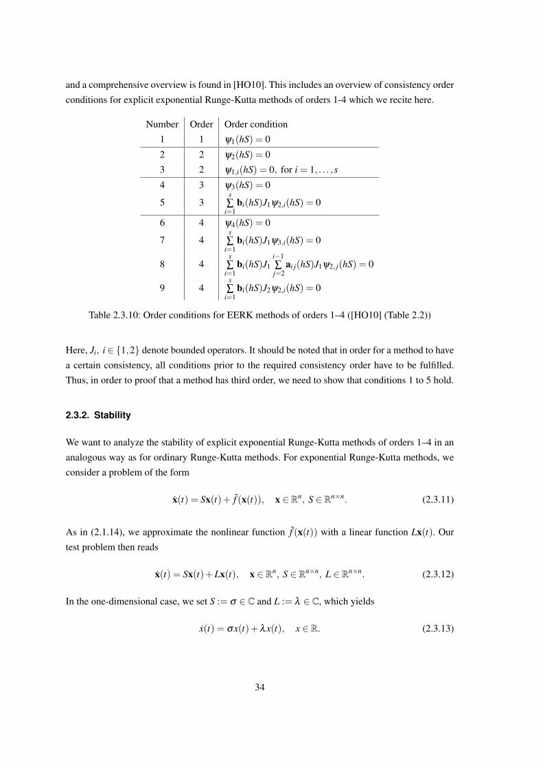
and a comprehensive overview is found in [HO10]. This includes an overview of consistency order

conditions for explicit exponential Runge-Kutta methods of orders 1-4 which we recite here.

Number Order Order condition

1 1 ψ1(hS) = 0

2 2 ψ2(hS) = 0

3 2 ψ1,i(hS) = 0, for i = 1, . . . ,s

4 3 ψ3(hS) = 0

5 3s∑

i=1bi(hS)J1ψ2,i(hS) = 0

6 4 ψ4(hS) = 0

7 4s∑

i=1bi(hS)J1ψ3,i(hS) = 0

8 4s∑

i=1bi(hS)J1

i−1∑j=2

ai j(hS)J1ψ2, j(hS) = 0

9 4s∑

i=1bi(hS)J2ψ2,i(hS) = 0

Table 2.3.10: Order conditions for EERK methods of orders 1–4 ([HO10] (Table 2.2))

Here, Ji, i ∈ 1,2 denote bounded operators. It should be noted that in order for a method to have

a certain consistency, all conditions prior to the required consistency order have to be fulfilled.

Thus, in order to proof that a method has third order, we need to show that conditions 1 to 5 hold.

2.3.2. Stability

We want to analyze the stability of explicit exponential Runge-Kutta methods of orders 1–4 in an

analogous way as for ordinary Runge-Kutta methods. For exponential Runge-Kutta methods, we

consider a problem of the form

x(t) = Sx(t)+ f (x(t)), x ∈ Rn, S ∈ Rn×n. (2.3.11)

As in (2.1.14), we approximate the nonlinear function f (x(t)) with a linear function Lx(t). Our

test problem then reads

x(t) = Sx(t)+Lx(t), x ∈ Rn, S ∈ Rn×n, L ∈ Rn×n. (2.3.12)

In the one-dimensional case, we set S := σ ∈ C and L := λ ∈ C, which yields

x(t) = σx(t)+λx(t), x ∈ R. (2.3.13)

34

In Section 2.1.2, we saw that the stability region is two-dimensional for the test equation (2.1.6).

So here, the stability region will be four-dimensional in the general case. This problem can be

handled by fixing or restraining certain parts of σ and λ as we will see.

Analyses with the same approach yet with other focuses are carried out in e. g. [BKV98, FD99,

CM02, MZ09, MZ13, OP16, Zh17b]. We shortly summarize their findings and distinct our aim.

In [BKV98], the stability of different exponential integration methods like the Adams-Moulton

and Adams-Bashforth schemes (not exponential RK methods) is analyzed. In order to deal with

the above mentioned problem, Beylkin et. al [BKV98] consider σ to be fixed and real (negative). In

contrast, Fornberg and Driscoll [FD99] analyze the stability of implicit-explicit Adams-Moulton

and Adams-Bashforth schemes for purely imaginary values of σ and λ . Cox and Matthews

[CM02] then build on these works and consider σ and λ to take real (negative) values for Adams-

Moulton and Adams-Bashforth schemes but also for a second order exponential Runge-Kutta

method. A real negative σ is also the subject of investigation of Owolabi and Patidar [OP16]

(fourth order EERK) and Zhu [Zh17b] (second order EERK). In our case, we expect σ to be purely

imaginary (with high modulus). As we will see later on, this setting is comparably critical to a real

negative σ but not yet analyzed. Maset and Zennaro [MZ09, MZ13] analyze the conditional and

unconditional stability properties of exponential Runge-Kutta methods. Their approach is very

close to our approach. However, they focus on the asymptotic behavior of the stability function.

From their results one cannot directly see how to choose a step size h for a certain setting.

We now start our analysis of the linear one-dimensional stability function. As in Section 2.1.2, we

insert the test equation (2.3.13) into the iteration (2.3.7b) and obtain

Fni = λ

(xn +h

s

∑j=1

ai j(hσ)(Fn j +σxn)). (2.3.14)

Let F := (Fn1, . . . , Fns)T ∈ Rs, A(hσ) := (ai j(hσ))i=1,...,s; j=1,...,s ∈ Rs×s, e := (1, . . . ,1)T ∈ Rs and

b(hσ) := (b1(hσ), . . . ,bs(hσ))T ∈ Rs. Then,

F = λxne+hλA(hσ)F+hλA(hσ)σxne

⇔ (I−hλA(hσ))F = (λ I +hλσA(hσ))xne

⇔ F = λ (I−hλA(hσ))−1(I +hσA(hσ))exn.

35

Inserting this into (2.3.7a), we obtain

xn+1 = xn +hm

∑i=1

bi(hσ)(Fni +σxn)

= xn +hb(hσ)T F+hb(hσ)T eσxn

= xn +hb(hσ)Tλ (I−hλA(hσ))−1(I +hσA(hσ))exn +hσb(hσ)T exn

=[I +hλb(hσ)T (I−hλA(hσ))−1(I +hσA(hσ))e+hσb(hσ)T e

]xn.

Hence,

φ(hσ ,hλ ) = I +hλb(hσ)T (I−hλA(hσ))−1(I +hσA(hσ))e+hσb(hσ)T e

or with w := hσ and z := hλ , we write

φ(w,z) = I + zb(w)T (I− zA(w))−1(I +wA(w))e+wb(w)T e. (2.3.15)

Before continuing the stability analysis, we would like to obtain a similar result to Lemma 2.1.13

for our n-dimensional test problem (2.3.12). Unfortunately, this is not as straight forward as in

the ordinary RK case. A similar result can only be shown, if S and L commute, which does not

generally occur in real applications. However, as Hundsdorfer states, the step size predictions

obtained by the study of the scalar test equation are surprisingly accurate in practical applications

which makes their in depth study valuable anyway [HR07]. Therefore, we now content ourselves

with the scalar stability analysis in this thesis.

2.3.3. First order

The only one-stage explicit exponential Runge-Kutta method is called the exponential Euler

method (cf. [HO10] (Example 2.12)). Its Butcher-Tableau is given by:

0

ϕ1(hS).

36

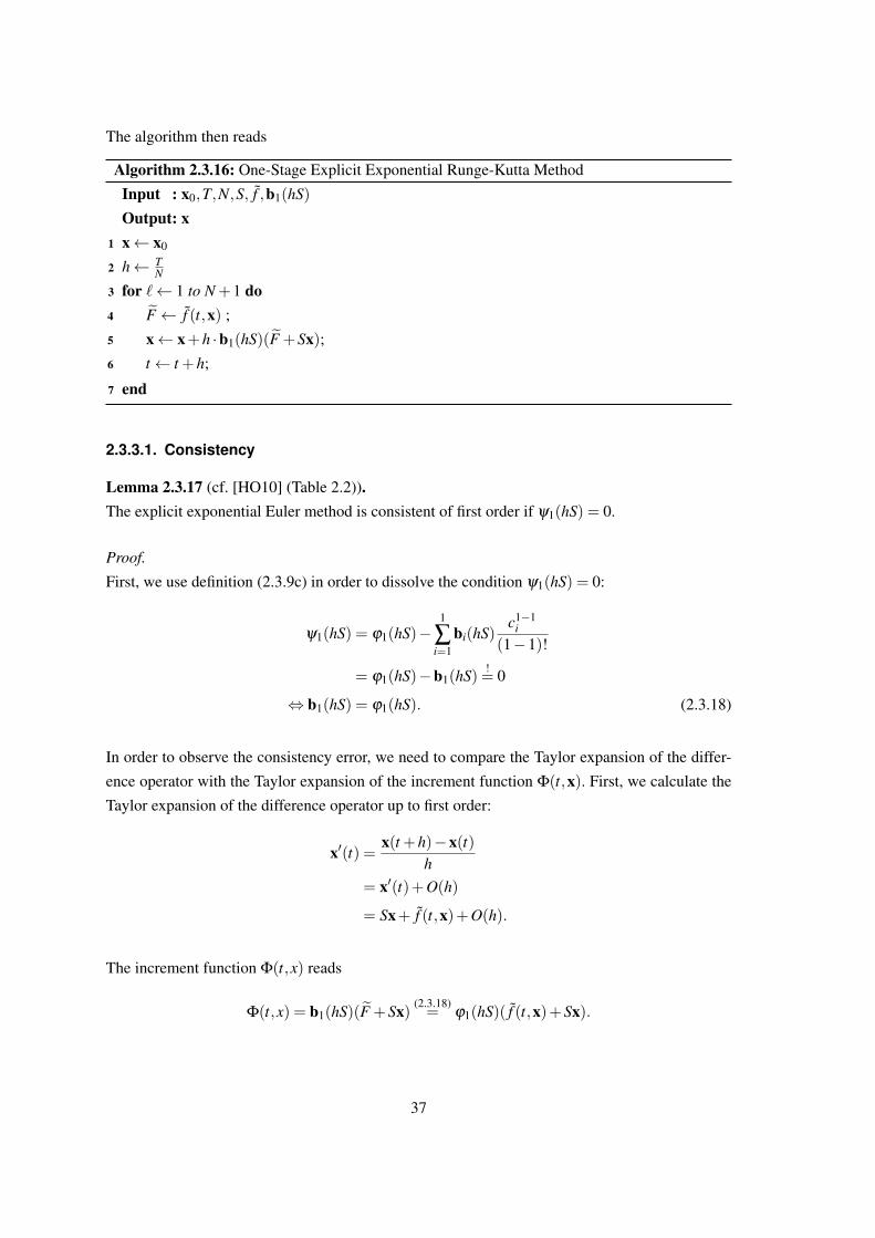
The algorithm then reads

Algorithm 2.3.16: One-Stage Explicit Exponential Runge-Kutta Method

Input : x0,T,N,S, f ,b1(hS)

Output: x1 x← x0

2 h← TN

3 for `← 1 to N +1 do4 F ← f (t,x) ;

5 x← x+h ·b1(hS)(F +Sx);6 t← t +h;

7 end

2.3.3.1. Consistency

Lemma 2.3.17 (cf. [HO10] (Table 2.2)).The explicit exponential Euler method is consistent of first order if ψ1(hS) = 0.

Proof.

First, we use definition (2.3.9c) in order to dissolve the condition ψ1(hS) = 0:

ψ1(hS) = ϕ1(hS)−1

∑i=1

bi(hS)c1−1

i(1−1)!

= ϕ1(hS)−b1(hS) != 0

⇔ b1(hS) = ϕ1(hS). (2.3.18)

In order to observe the consistency error, we need to compare the Taylor expansion of the differ-

ence operator with the Taylor expansion of the increment function Φ(t,x). First, we calculate the

Taylor expansion of the difference operator up to first order:

x′(t) =x(t +h)−x(t)

h= x′(t)+O(h)

= Sx+ f (t,x)+O(h).

The increment function Φ(t,x) reads

Φ(t,x) = b1(hS)(F +Sx) (2.3.18)= ϕ1(hS)( f (t,x)+Sx).

37

We know that the exponential function in ϕ1(hS) (see definition (2.3.9a)) has a power series rep-

resentation (see Lemma A.1.6) as

ϕ1(hS) =1∫

0

eh(1−θ)Sdθ =

1∫0

∞

∑k=0

(h(1−θ)S)k

k!dθ .

By Theorem A.1.7 and Remark A.1.8, we can interchange summation and integration in the fol-

lowing Taylor expansion of the increment function Φ(t,x):

Φ(t,x) = ϕ1(hS)( f (t,x)+Sx)

=

1∫0

∞

∑k=0

(h(1−θ)S)k

k!dθ · ( f (t,x)+Sx)

=

1∫0

I +h ·∞

∑k=1

hk−1((1−θ)S)k

k!dθ · ( f (t,x)+Sx)

=

1∫0

Idθ +O(h)

( f (t,x)+Sx)

= f (t,x)+Sx+O(h).

Since Φ(t,x)−x′(t) = O(h), the method is convergent of first order.

2.3.3.2. Stability

For the analysis of stability, we use the one-dimensional test equation in (2.3.13) and the definitions

w := hσ and z := hλ .

Using definition (2.3.9a), we can then explicitly calculate ϕ1(hσ):

ϕ1(hσ) = ϕ1(w) =1∫

0

e(1−θ)wdθ =

[− 1

we(1−θ)w

]1

0=− 1

w+

1w

ew.

Inserted in (2.3.15), we obtain the stability function

φ(w,z) = 1+ zb(w)+wb(w))

= 1+(z+w)b(w)

= 1+(z+w)ϕ1(w)

38

= 1+(z+w)(− 1

w+

1w

ew)

= 1+z+w

w(−1+ ew) .

So, for the explicit exponential Euler method, the stability function reads

φ(w,z) = 1+z+w

w(−1+ ew) . (2.3.19)

Theorem 2.3.20 (Author’s contribution).The stability region of the explicit exponential Euler method is given by

w,z ∈ C : |φ(w,z)| ≤ 1 ,

with

|φ(w,z)|2 = e2wre +(1−2ewre cos(wim)+ e2wre)

w2re +w2

im(z2

re + z2im)

+2wre(−ewre cos(wim)+ e2wre)+wimewre sin(wim)

w2re +w2

imzre

+2wim(−ewre cos(wim)+ e2wre)−wreewre sin(wim)

w2re +w2

imzim.

(2.3.21)

Proof.

Let

σ := σre + iσim,

λ := `re + i`im,

w := wre + iwim := hσre + ihσim,

z := zre + izim := h`re + ih`im.

Additionally, let w , 0 ∈ C. We now calculate |φ(w,z)|. For the modulus of a complex statement,

we need to know its imaginary and its real part, which we determine first by inserting the defini-

tions of z and w into (2.3.19) and sorting the summands:

φ(w,z) = 1+z+w

w(−1+ ew)

= 1+zre +wre + i(zim +wim)

wre + iwim(−1+ ewre(cos(wim)+ isin(wim)))

= 1+

(zre +wre + i(zim +wim)

)· (wre− iwim)

w2re +w2

im(−1+ ewre(cos(wim)+ isin(wim)))

39

= 1+(zre +wre)wre +(zim +wim)wim + i(−(zre +wre)wim +(zim +wim)wre)

w2re +w2

im

· (−1+ ewre(cos(wim)+ isin(wim)))

=

[1− (zre +wre)wre +(zim +wim)wim

w2re +w2

im(1− ewre cos(wim))

−−(zre +wre)wim +(zim +wim)wre

w2re +w2

imewre sin(wim)

]+ i[(zre +wre)wre +(zim +wim)wim

w2re +w2

imewre sin(wim)

−−(zre +wre)wim +(zim +wim)wre

w2re +w2

im(1− ewre cos(wim))

].

In order to simplify the notation, let

a :=(zre +wre)wre +(zim +wim)wim

w2re +w2

im=

zrewre + zimwim

w2re +w2

im+1 =

wre

w2re +w2

imzre +

wim

w2re +w2

imzim +1

and

b :=−(zre +wre)wim +(zim +wim)wre

w2re +w2

im=−zrewim + zimwre

w2re +w2

im=−wim

w2re +w2

imzre +

wre

w2re +w2

imzim.

Then,

φ(w,z) = [1−a(1− ewre cos(wim))−bewre sin(wim)]

+ i [aewre sin(wim)−b(1− ewre cos(wim))] .(2.3.22)

If we take the modulus of (2.3.22), we have:

|φ(w,z)|=√

[1−a(1− ewre cos(wim))−bewre sin(wim)]2 +[aewre sin(wim)−b(1− ewre cos(wim))]

2.

We want to know for which h > 0 and which w, z we have |φ(w,z)| ≤ 1. Hence, we only need to

consider the term under the root, since for x ∈ R+, we know that√

x≤ 1 if and only if x≤ 1:

|φ(w,z)|2 = 1+a2(1− ewre cos(wim))2 +b2e2wre sin2(wim)

−2(a(1− ewre cos(wim))+bewre sin(wim))+2ab(1− ewre cos(wim))ewre sin(wim)

+a2e2wre sin2(wim)−2abewre sin(wim)(1− ewre cos(wim))+b2(1− ewre cos(wim))2

= 1+a2(1− ewre cos(wim))2 +b2e2wre sin2(wim)

−2(a(1− ewre cos(wim))+bewre sin(wim))

+a2e2wre sin2(wim)+b2(1− ewre cos(wim))2

40

= 1+a2(1−2ewre cos(wim)+ e2wre cos2(wim))+b2e2wre sin2(wim)

−2(a(1− ewre cos(wim))+bewre sin(wim))

+a2e2wre sin2(wim)+b2(1−2ewre cos(wim)+ e2wre cos2(wim))

= 1+a2(1−2ewre cos(wim)+ e2wre)−2(a(1− ewre cos(wim))+bewre sin(wim))

+b2(1−2ewre cos(wim)+ e2wre)

= 1+(a2 +b2)(1−2ewre cos(wim)+ e2wre)−2(a(1− ewre cos(wim))+bewre sin(wim)) .

Now,

a2 +b2 =

(zrewre + zimwim

w2re +w2

im+1)2

+

(−zrewim + zimwre

w2re +w2

im

)2

=z2

rew2re +2zrewrezimwim + z2

imw2im

(w2re +w2

im)2 +2

zrewre + zimwim

w2re +w2

im+1

+z2

rew2im +−2zrewimzimwre + z2

imw2re

(w2re +w2

im)2

=1

w2re +w2

im(z2

re + z2im)+2

wre

w2re +w2

imzre +2

wim

w2re +w2

imzim +1.

In order to obtain circle equations (see Lemma 2.3.27 and Theorem 2.3.29), we need to sort the

summands by terms in z2re, z2

im, zre and zim. We have:

|φ(w,z)|2 = 1+(a2 +b2)(1−2ewre cos(wim)+ e2wre)−2(a(1− ewre cos(wim))+bewre sin(wim))

= 1+(

1w2

re +w2im(z2

re + z2im)+2

wre

w2re +w2

imzre +2

wim

w2re +w2

imzim +1

)· (1−2ewre cos(wim)+ e2wre)

−2(( wre

w2re +w2

imzre +

wim

w2re +w2

imzim +1

)(1− ewre cos(wim))

+( −wim

w2re +w2

imzre +

wre

w2re +w2

imzim

)ewre sin(wim)

)= 1+(1−2ewre cos(wim)+ e2wre)−2(1− ewre cos(wim))

+(1−2ewre cos(wim)+ e2wre)

w2re +w2

im(z2

re + z2im)

+2wre(1−2ewre cos(wim)+ e2wre)−2wre(1− ewre cos(wim))+2wimewre sin(wim)

w2re +w2

imzre

+2wim(1−2ewre cos(wim)+ e2wre)−2wim(1− ewre cos(wim))−2wreewre sin(wim)

w2re +w2

imzim

41

= e2wre +(1−2ewre cos(wim)+ e2wre)

w2re +w2

im(z2

re + z2im)

+2wre(−ewre cos(wim)+ e2wre)+wimewre sin(wim)

w2re +w2

imzre

+2wim(−ewre cos(wim)+ e2wre)−wreewre sin(wim)

w2re +w2

imzim.

So,

|φ(w,z)|2 = e2wre +(1−2ewre cos(wim)+ e2wre)

w2re +w2

im(z2

re + z2im)

+2wre(−ewre cos(wim)+ e2wre)+wimewre sin(wim)

w2re +w2

imzre

+2wim(−ewre cos(wim)+ e2wre)−wreewre sin(wim)

w2re +w2

imzim.

Before starting the analysis of the function given in (2.3.21) with respect to wre and wim, we start

with a peculiar case (a purely imaginary σ , where wim = σh is a multiple of 2π) that we can leave

out of our considerations subsequently:

Lemma 2.3.23 (Author’s contribution).Let h ∈ R+ be the step size. For wre = 0 and wim = 2kπ,k ∈ N, we have φ(w,z) = 1 for all z ∈ C.

Proof.

Consider equation (2.3.21). For wre = 0 and wim = 2kπ , we have ewre = 1,e2wre = 1,cos(wim) = 1

and sin(wim) = 0. Hence

|φ(w,z)|2 = 1+(1−2 ·1 ·1+1)

02 +(2kπ)2 (z2re + z2

im)+20 · (−1 ·1+1)+2kπ ·1 ·0

02 +(2kπ)2 zre

+22kπ · (−1 ·1+1)−0 ·1 ·0

02 +(2kπ)2 zim

= 1.

Now, we analyze the case when wim , 2kπ,k ∈N. We want to show that the stability regions given

by z ∈ C : |φ(w,z)| ≤ 1 , where |φ(w,z)| is given in (2.3.21), are circles. Therefore, we first need

to state the formulation of a circle in the complex plane.

42

Lemma 2.3.24. (cf. [Ru08])

Let α,z ∈ C and β ,γ ∈ R. A circle in the complex plane is given by

α z+ αz = β zz+ γ, (2.3.25)

where α

βdenotes the center and 1

βdenotes the radius. Additionally,

αα−1 = βγ (2.3.26)

has to be fulfilled.

Proof.

In general, a circle is given by

|z−o|= r,

where o ∈ C denotes the center of the circle and r ∈ R its radius. Squaring the equation, we obtain

(z−o)(z− o) = r2.

With β := 1r and α := βo, this equation transforms to(

z− α

β

)(z− α

β

)=

1β 2

·β⇔(

z− α

β

)(β z− α) =

1β

⇔ β zz−α z− αz+αα

β− 1

β= 0

With γ := αα−1β

(condition in (2.3.26)), we obtain the equation (2.3.25).

Lemma 2.3.27 (Author’s contribution).Let z = zre + izim and α = αre + iαim. Then equation (2.3.25) is equivalent to

0 =−2αrezre−2αimzim +β (z2re + z2

im)+ γ. (2.3.28)

Proof.

0 = α z+ αz−β zz− γ

= (αre + iαim)(zre− izim)+(αre− iαim)(zre + izim)−β (z2re + z2

im)− γ

= 2αrezre +2αimzim−β (z2re + z2

im)− γ.

43

With these circle equations we obtain the following theorem

Theorem 2.3.29 (Author’s contribution).Let w , 2kπi, k ∈N. The stability regions of the explicit exponential Euler method are circles. For

given w the circles have their center at(−wre(−ewre cos(wim)+e2wre )+wimewre sin(wim)

1−2ewre cos(wim)+e2wre ,−wim(−ewre cos(wim)+e2wre )−wreewre sin(wim)1−2ewre cos(wim)+e2wre

)∈ C

and their radius is|w|√

1−2ewre cos(wim)+ e2wre.

Proof.

Consider equation (2.3.21):

|φ(w,z)|2 = e2wre +(1−2ewre cos(wim)+ e2wre)

w2re +w2

im(z2

re + z2im)

+2wre(−ewre cos(wim)+ e2wre)+2wimewre sin(wim)

w2re +w2

imzre

+2wim(−ewre cos(wim)+ e2wre)−2wreewre sin(wim)

w2re +w2

imzim.

We are interested in the circle for |φ(w,z)|2 = 1. Hence, putting |φ(w,z)|2 = 1 and bringing every-

thing on one side we obtain:

0 = e2wre−1+(1−2ewre cos(wim)+ e2wre)

w2re +w2

im(z2

re + z2im)

+2wre(−ewre cos(wim)+ e2wre)+2wimewre sin(wim)

w2re +w2

imzre

+2wim(−ewre cos(wim)+ e2wre)−2wreewre sin(wim)

w2re +w2

imzim.

Comparing this to the circle equation

0 = β (z2re + z2

im)−2αrezre−2αimzim + γ

from Lemma 2.3.27, we could think of

β =(1−2ewre cos(wim)+ e2wre)

w2re +w2

im

γ = e2wre−1

44

αre = −wre(−ewre cos(wim)+ e2wre)+wimewre sin(wim)

w2re +w2

im

αim = − wim(−ewre cos(wim)+ e2wre)−wreewre sin(wim)

w2re +w2

im.

We need α ¯α − β γ = 1 (see (2.3.26)) in order for this to be the real coefficients of the circle. At

the moment, we have:

α ¯α = α2re + α

2im

=

(−wre(−ewre cos(wim)+ e2wre)+wimewre sin(wim)

w2re +w2

im

)2

+

(−wim(−ewre cos(wim)+ e2wre)−wreewre sin(wim)

w2re +w2

im

)2

=1

(w2re +w2

im)2

(w2

re(−ewre cos(wim)+ e2wre)2 +2wre(−ewre cos(wim)+ e2wre)wimewre sin(wim)

+w2ime2wre sin2(wim)+w2

im(−ewre cos(wim)+ e2wre)2

−2wim(−ewre cos(wim)+ e2wre)wreewre sin(wim)+w2ree2wre sin2(wim)

)=

1(w2

re +w2im)

2

(w2

re(e2wre cos2(wim)−2ewre cos(wim)e2wre + e4wre + e2wre sin2(wim)

)+w2

im(e2wre cos2(wim)−2ewre cos(wim)e2wre + e4wre + e2wre sin2(wim)

))=

e2wre cos2(wim)−2ewre cos(wim)e2wre + e4wre + e2wre sin2(wim)

w2re +w2

im

=e2wre−2ewre cos(wim)e2wre + e4wre

w2re +w2

im

= e2wre1−2ewre cos(wim)+ e2wre

w2re +w2

im

and

β γ =1−2ewre cos(wim)+ e2wre

w2re +w2

im· (e2wre−1).

Hence,

α ¯α− β γ =1−2ewre cos(wim)+ e2wre

w2re +w2

im.

The function η(wre,wim) := 1 − 2ewre cos(wim) + e2wre is greater than or equal to 0 for all

wre,wim ∈ R. It has its minima at (wre,wim) = (0,2kπ), k ∈ N where η(0,2kπ) = 0. However,

45

these values for wre and wim are excluded by our requirements. Hence, η(wre,wim) > 0 for all

(wre,wim) , (0,2kπ), k ∈N. In order to meet requirement (2.3.26), we divide our coefficients α, β

and γ by

η :=

√1−2ewre cos(wim)+ e2wre

w2re +w2

im> 0

and obtain new equations for α,β and γ as α = α

η,β = β

ηand γ = γ

η.

Let

β =1−2ewre cos(wim)+ e2wre

w2re +w2

im·

√w2

re +w2im√

1−2ewre cos(wim)+ e2wre

=

√1−2ewre cos(wim)+ e2wre

w2re +w2

im,

γ = (e2wre−1) ·

√w2

re +w2im√

1−2ewre cos(wim)+ e2wre,

αre = −wre(−ewre cos(wim)+ e2wre)+wimewre sin(wim)

w2re +w2

im·

√w2

re +w2im√

1−2ewre cos(wim)+ e2wre

= − wre(−ewre cos(wim)+ e2wre)+wimewre sin(wim)√w2

re +w2im

√1−2ewre cos(wim)+ e2wre

,

αim = − wim(−ewre cos(wim)+ e2wre)−wreewre sin(wim)

w2re +w2

im·

√w2

re +w2im√

1−2ewre cos(wim)+ e2wre

= − wim(−ewre cos(wim)+ e2wre)−wreewre sin(wim)√w2

re +w2im

√1−2ewre cos(wim)+ e2wre

.

Then,

αα−βγ = 1.

Note that η =

√β . Hence, β = β√

β=

√β = η . So, the center of the circle is located at

α

β= α

η· 1

β= α

η· 1

η= α

η2 which is

α

η2 =

[−(wre(−ewre cos(wim)+ e2wre)+wimewre sin(wim))

w2re +w2

im

−i

(wim(−ewre cos(wim)+ e2wre)−wreewre sin(wim)

)w2

re +w2im

]· w2

re +w2im

1−2ewre cos(wim)+ e2wre

46

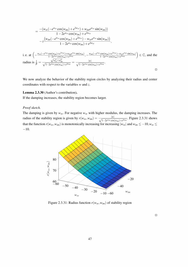
=−(wre(−ewre cos(wim)+ e2wre)+wimewre sin(wim))

1−2ewre cos(wim)+ e2wre

− i

(wim(−ewre cos(wim)+ e2wre)−wreewre sin(wim)

)1−2ewre cos(wim)+ e2wre

,

i. e. at(−wre(−ewre cos(wim)+e2wre )+wimewre sin(wim)

1−2ewre cos(wim)+e2wre ,−wim(−ewre cos(wim)+e2wre )−wreewre sin(wim)1−2ewre cos(wim)+e2wre

)∈ C, and the

radius is 1β=

√w2

re+w2im√

1−2ewre cos(wim)+e2wre= |w|√

1−2ewre cos(wim)+e2wre.

We now analyze the behavior of the stability region circles by analyzing their radius and center

coordinates with respect to the variables w and z.

Lemma 2.3.30 (Author’s contribution).If the damping increases, the stability region becomes larger.

Proof sketch.

The damping is given by wre. For negative wre with higher modulus, the damping increases. The

radius of the stability region is given by r(wre,wim) =|w|√

1−2ewre cos(wim)+e2wre. Figure 2.3.31 shows

that the function r(wre,wim) is monotonically increasing for increasing |wre| and wim ≤−10,wre ≤−10.

−60 −50 −40 −30 −20 −10−60

−40

−2060

70

80

wre

wim

r(w

re,w

im)

Figure 2.3.31: Radius function r(wre,wim) of stability region

47

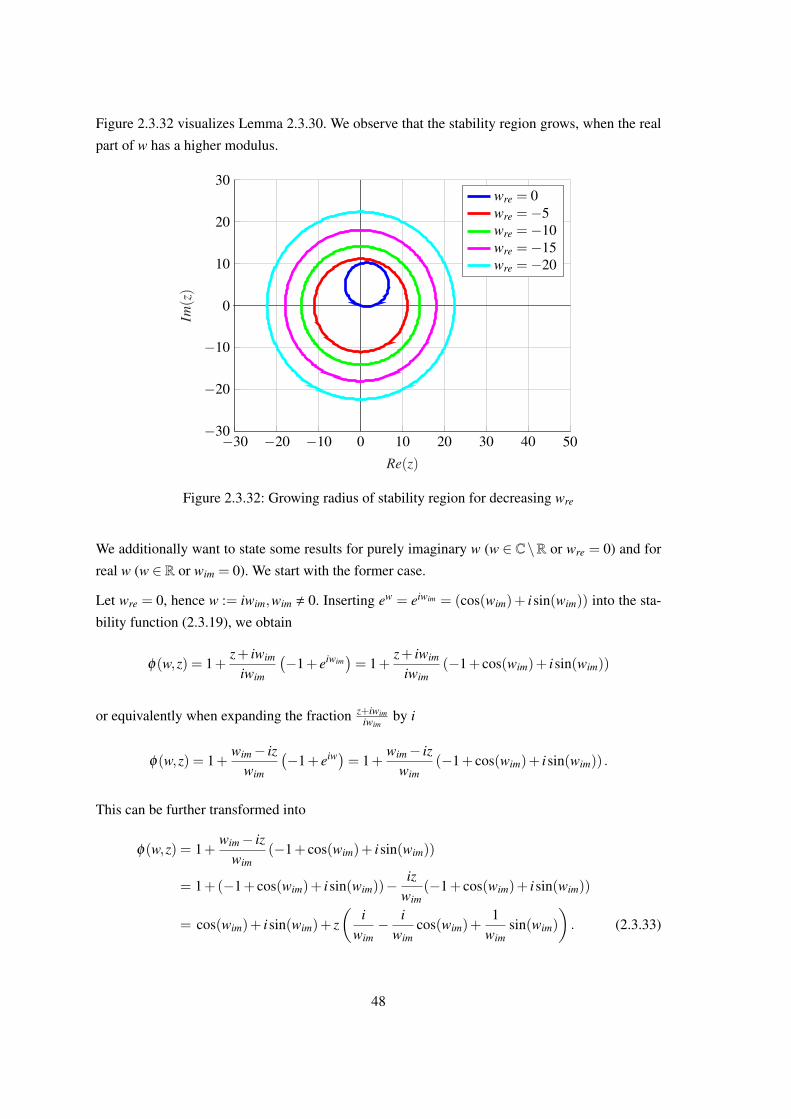
Figure 2.3.32 visualizes Lemma 2.3.30. We observe that the stability region grows, when the real

part of w has a higher modulus.

−30 −20 −10 0 10 20 30 40 50−30

−20

−10

0

10

20

30

Re(z)

Im(z)

wre = 0wre =−5wre =−10wre =−15wre =−20

Figure 2.3.32: Growing radius of stability region for decreasing wre

We additionally want to state some results for purely imaginary w (w ∈ C\R or wre = 0) and for

real w (w ∈ R or wim = 0). We start with the former case.

Let wre = 0, hence w := iwim,wim , 0. Inserting ew = eiwim = (cos(wim)+ isin(wim)) into the sta-

bility function (2.3.19), we obtain

φ(w,z) = 1+z+ iwim

iwim

(−1+ eiwim

)= 1+

z+ iwim

iwim(−1+ cos(wim)+ isin(wim))

or equivalently when expanding the fraction z+iwimiwim

by i

φ(w,z) = 1+wim− iz

wim

(−1+ eiw)= 1+

wim− izwim

(−1+ cos(wim)+ isin(wim)) .

This can be further transformed into

φ(w,z) = 1+wim− iz

wim(−1+ cos(wim)+ isin(wim))

= 1+(−1+ cos(wim)+ isin(wim))−iz

wim(−1+ cos(wim)+ isin(wim))

= cos(wim)+ isin(wim)+ z(

iwim− i

wimcos(wim)+

1wim

sin(wim)

). (2.3.33)

48

As a first result we want to consider the limit case w→ 0.

Theorem 2.3.34 (cf. [HO10]).Let wre = 0. Then, lim

wim→0φ(w,z) = 1+ z.

Proof.

Consider the form (2.3.33):

φ(w,z) = cos(wim)+ isin(wim)+ z(

iwim− i

wimcos(wim)+

1wim

sin(wim)

)= cos(wim)+ isin(wim)+ z

(i1− cos(wim)

wim+

sin(wim)

wim

).

For wim → 0, also w→ 0. We know that cos(wim)wim→0−→ 1 and sin(wim)

wim→0−→ 0. The appearing

terms 1−cos(wim)wim

and sin(wim)wim

need to be analyzed. We use L’Hospital’s rule (see Theorem A.1.2)

and differentiate numerator and denominator of our fraction respectively:

• Since limwim→0

sin(wim)1 = 0, we obtain lim

wim→0

1−cos(w)w = 0 and

• since limwim→0

cos(wim)1 = 1, we have lim

wim→0

sin(wim)wim

= 1.

In total,

limw→0

φ(w,z) = 1+0+ z(0+1) = 1+ z.

Remark 2.3.35.For wim → 0, we obtain the stability function φ(z) = 1+ z, which is the stability function of the

ordinary explicit Euler method.

Lemma 2.3.36 (Author’s contribution).For wre = 0, the stability circles have their center at

(−wim

2 cot(wim2 ),−wim

2

)∈ C and their radius is

1β= |wim|√

2(1−cos(wim)).

Proof.

Using Theorem 2.3.29, setting wre = 0 and applying sin(wim)1−cos(wim)

= cot(wim

2

), we obtain the desired

result.

Lemma 2.3.37 (Author’s contribution).For wim→ 2kπ, k ∈ Z\0, the radius goes to infinity.

Proof.

The radius of the circle is given by |wim|√2(1−cos(wim))

. For wim → 2kπ, k ∈ Z, the denominator√2(1− cos(wim)) goes to zero, while |wim| stays bounded. Hence, the radius goes to infinity.

49

Lemma 2.3.38 (Author’s contribution).For an interval [2kπ,2(k+1)π], k ∈ Z\−1,0 the radius is smallest for wim = (2k+1)π, k ∈ Z.

For the interval [−2π,2π], the radius is smallest at wim = 0.

Proof.

The radius of the circle is given by |wim|√2(1−cos(wim))

. For wim = (2k + 1)π, k ∈ Z, we have

cos(wim) = cos((2k+1)π) =−1 which makes the denominator√

2(1− cos(wim)) equal to 2.

This is the highest value it can achieve. Hence, the radius is smallest at wim = (2k+1)π, k ∈ Z.

However for the interval [−2π,2π], the smallest radius is achieved at wim = 0, where it is equal to

1 which is smaller than π

2 which is the radius at wim =±π .

Lemma 2.3.39 (Author’s contribution).For wim → −∞, the center of the circle moves upwards. For wim → ∞, the center of the circle

moves downwards.

Proof.

The vertical coordinate of the circle is given by −wim2 . Hence, for wim → −∞ this goes to plus

infinity and for wim→ ∞, it goes to minus infinity.

Lemma 2.3.40 (Author’s contribution).For positive (negative) wim, the horizontal coordinate of the circle moves from minus infinity (plus

infinity) to plus infinity (minus infinity) for every interval [2kπ,2(k+1)π], k ∈ Z\−1,0.

Proof.

The horizontal coordinate of the circle center is given by the function h(wim) :=−wim2 cot(wim

2 ). It

has roots at wim = (2k+1)π, k ∈ Z and poles at wim = 2kπ, k ∈ Z\0, where for positive wim

limwim↑2kπ

h(wim) = ∞ and

limwim↓2kπ

h(wim) = −∞.

Furthermore,

limwim→0

h(wim) =−1.

A plot of h(wim) is given in Figure 2.3.41.

50

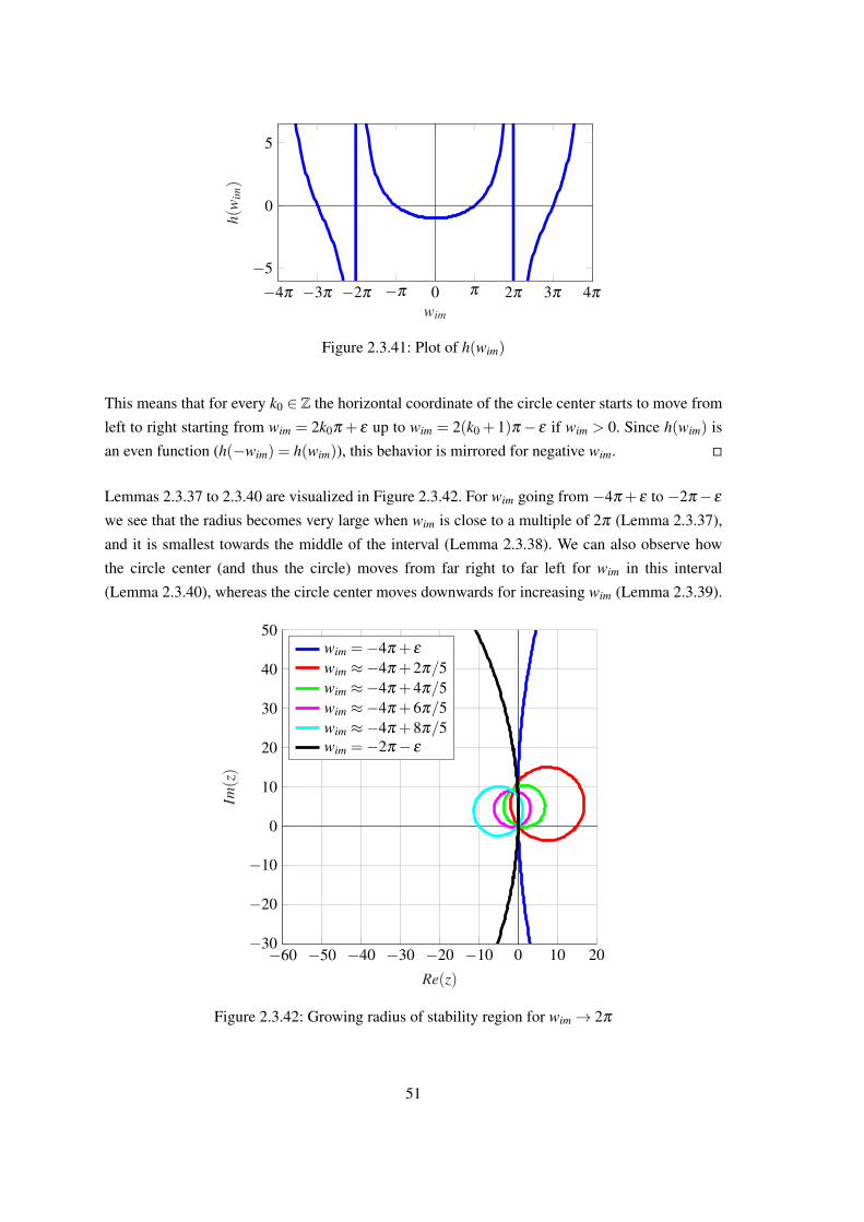
−4π −3π −2π −π 0 π 2π 3π 4π

−5

0

5

wim

h(w

im)

Figure 2.3.41: Plot of h(wim)

This means that for every k0 ∈ Z the horizontal coordinate of the circle center starts to move from

left to right starting from wim = 2k0π + ε up to wim = 2(k0 +1)π− ε if wim > 0. Since h(wim) is

an even function (h(−wim) = h(wim)), this behavior is mirrored for negative wim.

Lemmas 2.3.37 to 2.3.40 are visualized in Figure 2.3.42. For wim going from −4π +ε to −2π−ε

we see that the radius becomes very large when wim is close to a multiple of 2π (Lemma 2.3.37),

and it is smallest towards the middle of the interval (Lemma 2.3.38). We can also observe how

the circle center (and thus the circle) moves from far right to far left for wim in this interval

(Lemma 2.3.40), whereas the circle center moves downwards for increasing wim (Lemma 2.3.39).

−60 −50 −40 −30 −20 −10 0 10 20−30

−20

−10

0

10

20

30

40

50

Re(z)

Im(z)

wim =−4π + ε

wim ≈−4π +2π/5wim ≈−4π +4π/5wim ≈−4π +6π/5wim ≈−4π +8π/5wim =−2π− ε

Figure 2.3.42: Growing radius of stability region for wim→ 2π

51

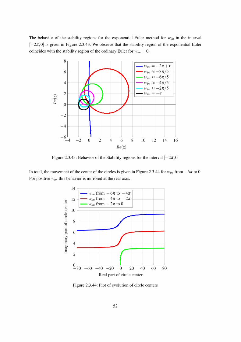
The behavior of the stability regions for the exponential Euler method for wim in the interval

[−2π,0] is given in Figure 2.3.43. We observe that the stability region of the exponential Euler

coincides with the stability region of the ordinary Euler for wim = 0.

−4 −2 0 2 4 6 8 10 12 14 16−6

−4

−2

0

2

4

6

8

Re(z)

Im(z)

wim =−2π + ε

wim ≈−8π/5wim ≈−6π/5wim ≈−4π/5wim ≈−2π/5wim =−ε

Figure 2.3.43: Behavior of the Stability regions for the interval [−2π,0]

In total, the movement of the center of the circles is given in Figure 2.3.44 for wim from −6π to 0.

For positive wim this behavior is mirrored at the real axis.

−80 −60 −40 −20 0 20 40 60 800

2

4

6

8

10

12

14

Real part of circle center

Imag

inar

ypa

rtof

circ

lece

nter

wim from −6π to −4π

wim from −4π to −2π

wim from −2π to 0

Figure 2.3.44: Plot of evolution of circle centers

52

Now we briefly consider the case that w is a real number. Hence, we consider w := wre ∈ R and

wim = 0.

Lemma 2.3.45.For wim = 0, the stability circles have their center at

(wreewre

1−ewre ,0)∈ C and their radius is |wre|

1−ewre .

Proof.

Using Theorem 2.3.29, setting wim = 0 and using cos(wim) = cos(0) = 1, sin(wim) = sin(0) = 0,

we obtain for the real coordinate

wre(ewre− e2wre)

1−2ewre + e2wre=

wreewre(1− ewre)

(1− ewre)2 =wreewre

1− ewre,

whereas we obtain 0 for the imaginary coordinate. The radius is given by 1β= |wre|

1−ewre .

In this subsection, we saw that the stability regions of the exponential Euler method are circles.

Their radius and center can be determined with respect to w. We determined that the stability

circles completely move to the right side of the imaginary axis when wim < 0 is close to −2kπ +

ε, k ∈ N. Furthermore, the stability regions grow if w contains a negative real part.

2.3.4. Second order

Two-stage EERK methods are given by the Butcher-Tableau

0

c2 a21

b1 b2

,

and the according algorithm reads

Algorithm 2.3.46: Two-Stage Explicit Exponential Runge-Kutta Method

Input : x0,T,N,S, f ,a21(hS),b1(hS),b2(hS)

Output: x1 x← x0

2 h← TN

3 for `← 1 to N +1 do4 F1← f (t,x) ;

5 F2← f(t + c2h,x+ha21(hS) · (F1 +Sx)

);

6 x← x+h · [b1(hS)(F1 +Sx)+b2(hS)(F2 +Sx)];7 t← t +h;

8 end

53

2.3.4.1. Consistency

Lemma 2.3.47 (cf. [HO10] (Table 2.2, Numbers 1–3)).The two-stage explicit exponential method is consistent of second order if

1. ψ1(hS) = 0,

2. ψ2(hS) = 0,

3. ψ1,i(hS) = 0.

Proof.

Using the definitions in (2.3.9), we obtain the conditions as

1.

ψ1(hS) = ϕ1(hS)−2

∑i=1

bi(hS)c1−1

i(1−1)!

= ϕ1(hS)−b1(hS)−b2(hS)

⇔ b1(hS)+b2(hS) = ϕ1(hS). (2.3.48)

2.

ψ2(hS) = ϕ2(hS)−2

∑i=1

bi(hS)c2−1

i(2−1)!

= ϕ2(hS)−b1(hS) · c1−b2(hS) · c2

c1=0= ϕ2(hS)−b2(hS) · c2

⇔ b2(hS) =1c2

ϕ2(hS). (2.3.49)

3. Since a21(hS) is the only non-zero coefficient of type ai, j(hS), we only need to consider

ψ1,2(hS):

ψ1,2(hS) = ϕ1,2(hS)c12−

2−1

∑j=1

a2, j(hS)c1−1

j

(1−1)!

= ϕ1(c2hS)c2−a21(hS)

a21(hS) = c2ϕ1(c2hS). (2.3.50)

In order to observe the consistency error, we need to compare the Taylor expansion of the differ-

ence operator with the Taylor expansion of the increment function Φ(t,x). First, we calculate the

54

Taylor expansion of the difference operator up to second order:

x′(t) =x(t +h)−x(t)

h= x′(t)+ h

2 x′′(t)+O(h2)

= f (t,x)+ h2

[∂ f∂ t (t,x)+

∂ f∂x (t,x) · f (t,x)

]+O(h2)

= Sx+ f (t,x)+h[

12

∂ f∂ t (t,x)+

12

(S+ ∂ f

∂x (t,x))·(Sx+ f (t,x)

)]+O(h2).

The increment function Φ(t,x) reads:

Φ(t,x) = b1(hS)(F1 +Sx)+b2(hS)(F2 +Sx)(2.3.48)=

(2.3.49)

(ϕ1(hS)− 1

c2ϕ2(hS)

)( f (t,x)+Sx)

+ 1c2

ϕ2(hS)( f(t + c2h,x+ha21(hS) · (F1 +Sx)

)+Sx)

(2.3.50)=

(ϕ1(hS)− 1

c2ϕ2(hS)

)( f (t,x)+Sx)

+ 1c2

ϕ2(hS)( f(t + c2h,x+hc2ϕ1(c2hS) · ( f (t,x)+Sx)

)+Sx)

with

F1 = f (t,x),

F2 = f(t + c2h,x+ha21(hS) · (F1 +Sx)

)= f(t + c2h,x+ha21(hS) · ( f (t,x)+Sx)

).

In order to simplify the notation, we start by calculating second order approximations of the coef-

ficients ϕ1(hS), ϕ2(hS) and ϕ1(c2hS):

ϕ1(hS) =

1∫0

eh(1−θ)Sdθ =

1∫0

I +h(1−θ)S+O(h2)dθ

Lemma A.1.7=

[θ I +h

(θ − 1

2 θ2)S]1

0 +O(h2) = I + 12 hS+O(h2)

ϕ2(hS) =

1∫0

eh(1−θ)S ·θdθ =

1∫0

(I +h(1−θ)S+O(h2)) ·θdθ

Lemma A.1.7=

[12 Iθ

2 +h(1

2 θ2− 1

3 θ3)S]1

0 +O(h2) = 12 I + 1

6 hS+O(h2)

ϕ1(c2hS) =

1∫0

ec2h(1−θ)Sdθ =

1∫0

I + c2h(1−θ)S+O(h2)dθ

Lemma A.1.7=

[θ I + c2h

(θ − 1

2 θ2)S]1

0 +O(h2) = I + 12 c2hS+O(h2).

55

Subsequently, the coefficient ϕ1(hS)− 1c2

ϕ2(hS) in Φ(t,x) simplifies to

ϕ1(hS)− 1c2

ϕ2(hS) = I + 12 hS+O(h2)− 1

c2

(12 I + 1

6 hS+O(h2))

=(

1− 12c2

)I +(

12 −

16c2

)hS+O(h2).

Also, we have

h ·ϕ1(c2hS) = Ih+O(h2).

The Taylor expansion of the increment function Φ(t,x) then reads

Φ(t,x) =[(

1− 12c2

)I +(

12 −

16c2

)hS]( f (t,x)+Sx)

+ 1c2

(12 I + 1

6 hS)[

f (t,x)+ c2h ∂ f∂ t +

∂ f∂x (t,x) ·hc2ϕ1(c2hS) · ( f (t,x)+Sx)+Sx

]+O(h2)

=[(

1− 12c2

)I + 1

2c2I]( f (t,x)+Sx)+

[(12 −

16c2

)hS+ 1

6c2hS]( f (t,x)+Sx)

+ 12c2

I[c2h ∂ f

∂ t +hc2∂ f∂x (t,x) · ( f (t,x)+Sx)

]+O(h2)

= f (t,x)+Sx+ 12 hS( f (t,x)+Sx)+ 1

2 I[h ∂ f

∂ t +h ∂ f∂x (t,x) · ( f (t,x)+Sx)

]+O(h2)

= f (t,x)+Sx+h[

12

∂ f∂ t +

12

(S+ ∂ f

∂x (t,x))· ( f (t,x)+Sx)

]+O(h2).

Since Φ(t,x)−x′(t) = O(h2), the method is convergent of second order.

Abiding by the conditions 1.–3. of Lemma 2.3.47, we obtain a family of second order EERK

methods (see [HO10] (Example 2.18)) which is given by the Butcher-Tableau

0

c2 c2ϕ1,2

ϕ1− 1c2

ϕ21c2

ϕ2

.

Corollary 2.3.51 (cf. [HO10] (Example 2.6)).The easiest choice is c2 = 1 which leads to the explicit exponential trapezoidal rule given by the

Butcher-Tableau

0

1 ϕ1

ϕ1−ϕ2 ϕ2

.

56

2.3.5. Combined Stability Plots

We already know the explicit exponential Runge-Kutta methods of orders 1 and 2. In this subsec-

tion we want to compare the stability regions of exponential Runge-Kutta methods of order 1–4

to the stability plot of ordinary Runge-Kutta methods in Figure 2.1.19. For a comparison, we still

need to mention the EERK methods of orders 3 and 4. We provide the respective Butcher-Tableaus

without further analysis here. Consistency results and derivations can be found in [HO05a, HO10].

There are various families of third order methods. An overview is given in [HO05a] (Section 5.2).

We use the ETD3RK method ([HO05a], (Equation (5.13))) with the Butcher-Tableau

012

12 ϕ1,2(hS)

1 −ϕ1,3(hS) 2ϕ1,3(hS)

4ϕ3(hS)−2ϕ2(hS)+ϕ1(hS) −8ϕ3(hS)+4ϕ2(hS) 4ϕ3(hS)−ϕ2(hS)

.

There are also numerous fourth-order methods. We use the following five-stage fourth order

method [HO10] (p.229):

012

12 ϕ1,2

12

12 ϕ1,3−ϕ2,3 ϕ2,3

1 ϕ1,4−2ϕ2,4 ϕ2,4 ϕ2,412

12 ϕ1,5−2a5,2−a5,4 a5,2 a5,2

14 ϕ2,5−a5,2

ϕ1−3ϕ2 +4ϕ3 0 0 −ϕ2 +4ϕ3 4ϕ2−8ϕ3

with

a5,2 :=12

ϕ2,5−ϕ3,4 +14

ϕ2,4−12

ϕ3,5.

We start with the stability regions where w is equal to zero in Figure 2.3.52. The stability regions of

the exponential Runge-Kutta methods are exactly the stability regions of the ordinary Runge-Kutta

methods (see Figure 2.1.19) in this case.

57

−4 −3 −2 −1 0 1 2−3

−2

−1

0

1

2

3

Re(z)

Im(z)

Figure 2.3.52: Plot of stability regions of 1st (blue), 2nd (red), 3rd (green) and 4th (pink) orderexponential methods for w = 0 (author’s plot)

2.3.5.1. Varying imaginary part of w

With varying wim the appearance of the stability regions changes. For wim = −6, we are already

quite close to−2π , which is a singularity for the exponential Euler as we saw in Subsection 2.3.3.2.

It also seems to be a critical value for the other methods as we can see in Figure 2.3.53d. For a

purely imaginary w close to 2π (Figure 2.3.53d), we need very small step sizes for the methods

of orders 1, 3 and 4. Especially, if we expect our system to have complex conjugate eigenvalues

with high modulus, we can only count on the second order method whose stability region covers

the same parts of the positive and the negative imaginary axis.

We also notice a part of the imaginary axis (circa from 1 to 2.5), where the methods of third and

fourth order are unstable but both the methods of first and second order are stable in Figure 2.3.53b.

Additionally, we see that the stability regions of the third and fourth order methods split into sev-

eral disjoint regions with growing modulus of wim. In Section 3.3 we look into these peculiarities.

58

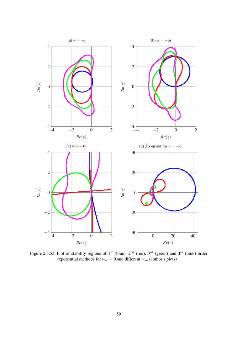
(a) w =−i

−4 −2 0 2−4

−2

0

2

4

Re(z)

Im(z)

(b) w =−3i

−4 −2 0 2−4

−2

0

2

4

Re(z)

Im(z)

(c) w =−6i

−4 −2 0 2−4

−2

0

2

4

Re(z)

Im(z)

(d) Zoom out for w =−6i

0 20 40−40

−20

0

20

40

Re(z)

Im(z)

Figure 2.3.53: Plot of stability regions of 1st (blue), 2nd (red), 3rd (green) and 4th (pink) orderexponential methods for wre = 0 and different wim (author’s plots)

59

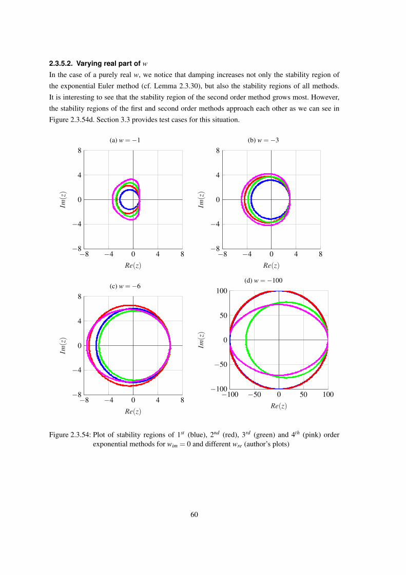
2.3.5.2. Varying real part of w

In the case of a purely real w, we notice that damping increases not only the stability region of

the exponential Euler method (cf. Lemma 2.3.30), but also the stability regions of all methods.

It is interesting to see that the stability region of the second order method grows most. However,

the stability regions of the first and second order methods approach each other as we can see in

Figure 2.3.54d. Section 3.3 provides test cases for this situation.

(a) w =−1

−8 −4 0 4 8−8

−4

0

4

8

Re(z)

Im(z)

(b) w =−3

−8 −4 0 4 8−8

−4

0

4

8

Re(z)

Im(z)

(c) w =−6

−8 −4 0 4 8−8

−4

0

4

8

Re(z)

Im(z)

(d) w =−100

−100 −50 0 50 100−100

−50

0

50

100

Re(z)

Im(z)

Figure 2.3.54: Plot of stability regions of 1st (blue), 2nd (red), 3rd (green) and 4th (pink) orderexponential methods for wim = 0 and different wre (author’s plots)

60

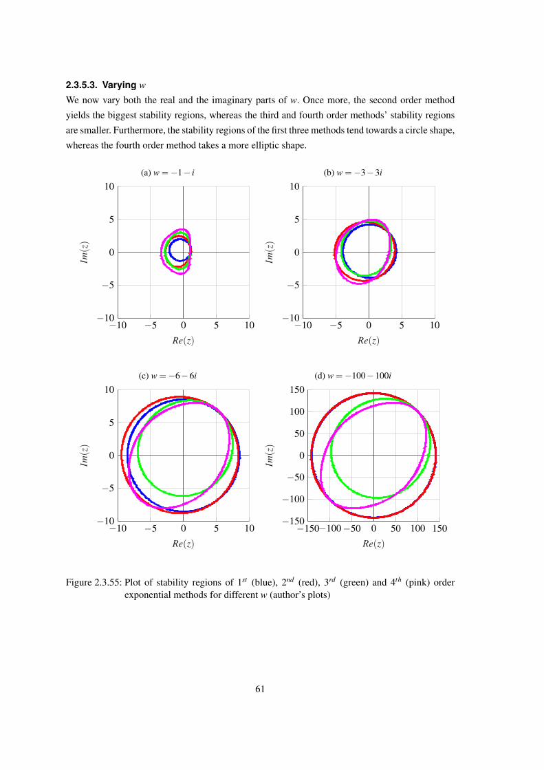
2.3.5.3. Varying w

We now vary both the real and the imaginary parts of w. Once more, the second order method

yields the biggest stability regions, whereas the third and fourth order methods’ stability regions

are smaller. Furthermore, the stability regions of the first three methods tend towards a circle shape,

whereas the fourth order method takes a more elliptic shape.

(a) w =−1− i

−10 −5 0 5 10−10

−5

0

5

10

Re(z)

Im(z)

(b) w =−3−3i

−10 −5 0 5 10−10

−5

0

5

10

Re(z)

Im(z)

(c) w =−6−6i

−10 −5 0 5 10−10

−5

0

5

10

Re(z)

Im(z)

(d) w =−100−100i

−150−100−50 0 50 100 150−150

−100

−50

0

50

100

150

Re(z)

Im(z)

Figure 2.3.55: Plot of stability regions of 1st (blue), 2nd (red), 3rd (green) and 4th (pink) orderexponential methods for different w (author’s plots)

61

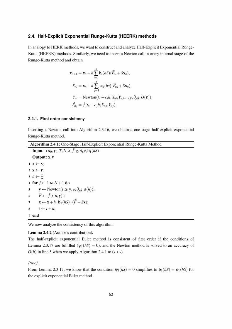
2.4. Half-Explicit Exponential Runge-Kutta (HEERK) methods

In analogy to HERK methods, we want to construct and analyze Half-Explicit Exponential Runge-

Kutta (HEERK) methods. Similarly, we need to insert a Newton call in every internal stage of the

Runge-Kutta method and obtain

xn+1 = xn +hs

∑i=1

bi(hS)(Fni +Sxn),

Xni = xn +hs

∑j=1

ai j(hs)(Fn j +Sxn),

Yni = Newton(tn + cih,Xni,Yn,i−1,g,∂yg,O(ε)),

Fn j = f (tn + c jh,Xn j,Yn j).

2.4.1. First order consistency

Inserting a Newton call into Algorithm 2.3.16, we obtain a one-stage half-explicit exponential

Runge-Kutta method.

Algorithm 2.4.1: One-Stage Half-Explicit Exponential Runge-Kutta Method

Input : x0,y0,T,N,S, f ,g,∂yg,b1(hS)

Output: x,y1 x← x0

2 y← y0

3 h← TN

4 for j← 1 to N +1 do5 y← Newton(t,x,y,g,∂yg,ε(h));

6 F ← f (t,x,y) ;

7 x← x+h ·b1(hS) · (F +Sx);8 t← t +h;

9 end

We now analyze the consistency of this algorithm.

Lemma 2.4.2 (Author’s contribution).The half-explicit exponential Euler method is consistent of first order if the conditions of

Lemma 2.3.17 are fulfilled (ψ1(hS) = 0), and the Newton method is solved to an accuracy of

O(h) in line 5 when we apply Algorithm 2.4.1 to (???).

Proof.

From Lemma 2.3.17, we know that the condition ψ1(hS) = 0 simplifies to b1(hS) = ϕ1(hS) for

the explicit exponential Euler method.

62

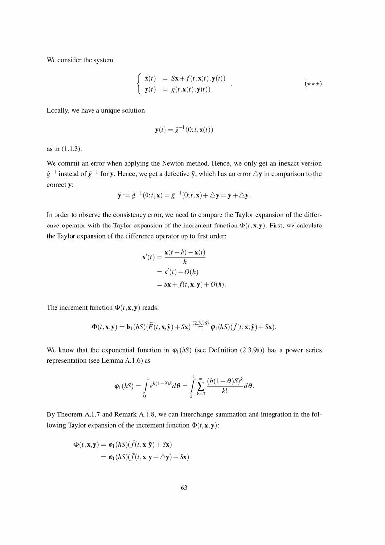
We consider the system x(t) = Sx+ f (t,x(t),y(t))y(t) = g(t,x(t),y(t))

. (???)

Locally, we have a unique solution

y(t) = g−1(0; t,x(t))

as in (1.1.3).

We commit an error when applying the Newton method. Hence, we only get an inexact version

g−1 instead of g−1 for y. Hence, we get a defective y, which has an error4y in comparison to the

correct y:

y := g−1(0; t,x) = g−1(0; t,x)+4y = y+4y.

In order to observe the consistency error, we need to compare the Taylor expansion of the differ-

ence operator with the Taylor expansion of the increment function Φ(t,x,y). First, we calculate

the Taylor expansion of the difference operator up to first order:

x′(t) =x(t +h)−x(t)

h= x′(t)+O(h)

= Sx+ f (t,x,y)+O(h).

The increment function Φ(t,x,y) reads:

Φ(t,x,y) = b1(hS)(F(t,x, y)+Sx) (2.3.18)= ϕ1(hS)( f (t,x, y)+Sx).

We know that the exponential function in ϕ1(hS) (see Definition (2.3.9a)) has a power series

representation (see Lemma A.1.6) as

ϕ1(hS) =1∫

0

eh(1−θ)Sdθ =

1∫0

∞

∑k=0

(h(1−θ)S)k

k!dθ .

By Theorem A.1.7 and Remark A.1.8, we can interchange summation and integration in the fol-

lowing Taylor expansion of the increment function Φ(t,x,y):

Φ(t,x,y) = ϕ1(hS)( f (t,x, y)+Sx)

= ϕ1(hS)( f (t,x,y+4y)+Sx)

63

=

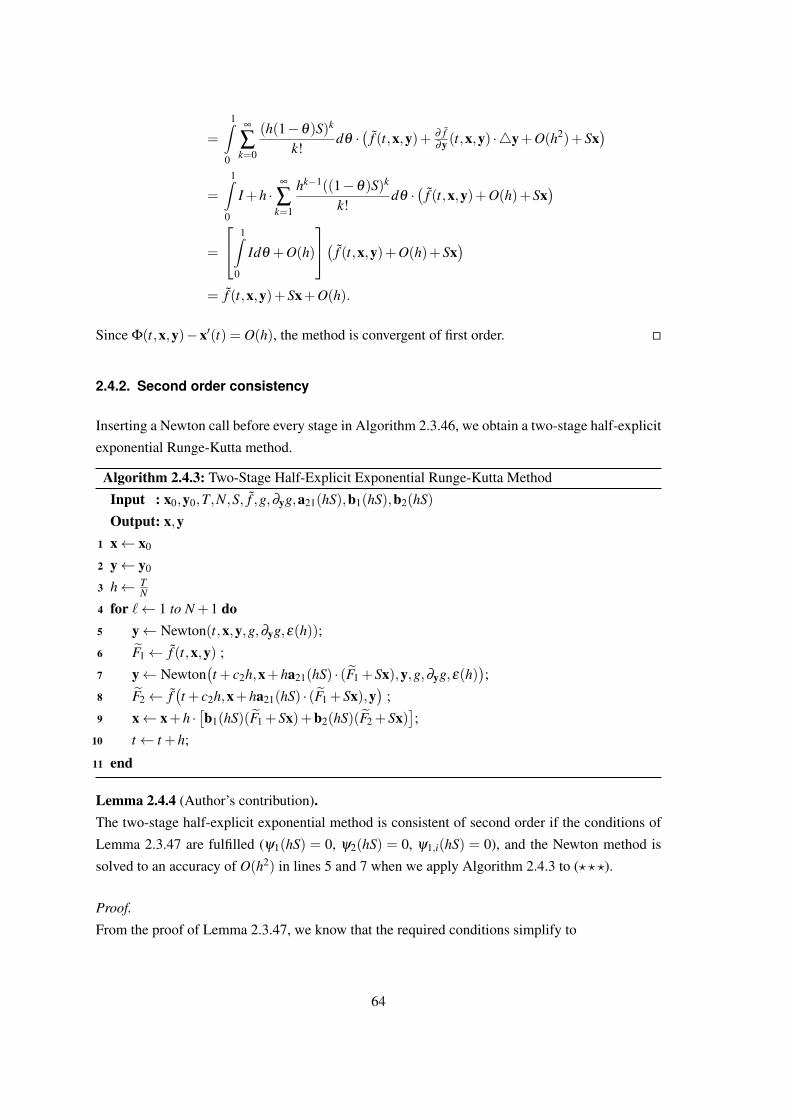
1∫0

∞

∑k=0

(h(1−θ)S)k

k!dθ ·

(f (t,x,y)+ ∂ f

∂y (t,x,y) ·4y+O(h2)+Sx)

=

1∫0

I +h ·∞

∑k=1

hk−1((1−θ)S)k

k!dθ ·

(f (t,x,y)+O(h)+Sx

)

=

1∫0

Idθ +O(h)

( f (t,x,y)+O(h)+Sx)

= f (t,x,y)+Sx+O(h).

Since Φ(t,x,y)−x′(t) = O(h), the method is convergent of first order.

2.4.2. Second order consistency

Inserting a Newton call before every stage in Algorithm 2.3.46, we obtain a two-stage half-explicit

exponential Runge-Kutta method.

Algorithm 2.4.3: Two-Stage Half-Explicit Exponential Runge-Kutta Method

Input : x0,y0,T,N,S, f ,g,∂yg,a21(hS),b1(hS),b2(hS)

Output: x,y1 x← x0

2 y← y0

3 h← TN

4 for `← 1 to N +1 do5 y← Newton(t,x,y,g,∂yg,ε(h));

6 F1← f (t,x,y) ;

7 y← Newton(t + c2h,x+ha21(hS) · (F1 +Sx),y,g,∂yg,ε(h)

);

8 F2← f(t + c2h,x+ha21(hS) · (F1 +Sx),y

);

9 x← x+h ·[b1(hS)(F1 +Sx)+b2(hS)(F2 +Sx)

];

10 t← t +h;

11 end

Lemma 2.4.4 (Author’s contribution).The two-stage half-explicit exponential method is consistent of second order if the conditions of

Lemma 2.3.47 are fulfilled (ψ1(hS) = 0, ψ2(hS) = 0, ψ1,i(hS) = 0), and the Newton method is

solved to an accuracy of O(h2) in lines 5 and 7 when we apply Algorithm 2.4.3 to (???).

Proof.

From the proof of Lemma 2.3.47, we know that the required conditions simplify to

64

1. b1(hS)+b2(hS) = ϕ1(hS),

2. b2(hS) = 1c2

ϕ2(hS),

3. a21(hS) = c2ϕ1(c2hS)

for an explicit exponential two-stage method.

We consider the system x(t) = Sx+ f (t,x(t),y(t))y(t) = g(t,x(t),y(t))

. (???)

Locally, we have a unique solution

y(t) = g−1(0; t,x(t))

as in (1.1.3).

However, we commit an error when applying the Newton method. Hence, we only get an inexact

version g−1 instead of g−1 for y. In line 5, we obtain a defective y1, which has an error 4y1 in

comparison to the correct y:

y1 := g−1(0; t,x) = g−1(0; t,x)+4y1 = y+4y1.

For the Newton call in line 7, we already use our defective y1 from the first Newton call. We need

to compute y corresponding to t = t+c2h and x = x+ha21(hS) f (t,x, y1). We denote the occurring

error by4y2 and obtain the defective y2 as:

y2 := g−1(0; t + c2h,x+ha21(hS) f (t,x, y1))

= g−1(0; t + c2h,x+ha21(hS) f (t,x, y1))+4y2.

In order to observe the consistency error, we need to compare the Taylor expansion of the differ-

ence operator with the Taylor expansion of the increment function Φ(t,x,y).

Using (2.2.12), we calculate the Taylor expansion of the difference operator up to second order:

x′(t) =x(t +h)−x(t)

h= x′(t)+ h

2 x′′(t)+O(h2)

= f (t,x,y)+ h2

[∂ f∂ t (t,x,y)+

∂ f∂x (t,x,y) · f (t,x,y)+ ∂ f

∂y (t,x,y) ·y′(t)]+O(h2)

= f (t,x,y)+h[

12

∂ f∂ t (t,x,y)+

12

∂ f∂x (t,x,y) · f (t,x,y)+ 1

2∂ f∂y (t,x,y) ·y

′(t)]+O(h2)

65

= Sx+ f (t,x,y)

+h[

12

∂ f∂ t (t,x,y)+

12

(S+ ∂ f

∂x (t,x,y))·(Sx+ f (t,x,y)

)+ 1

2∂ f∂y (t,x,y) ·y

′(t)]+O(h2).

The increment function Φ(t,x,y) reads:

Φ(t,x,y) = b1(hS)(F1 +S ·x)+b2(hS)(F2 +Sx)(2.3.48)=

(2.3.49)

(ϕ1(hS)− 1

c2ϕ2(hS)

)(f (t,x, y1)+Sx

)+ 1

c2ϕ2(hS)

(f(t + c2h,x+ha21(hS) · (F1 +Sx), y2

)+Sx

)(2.3.50)=

(ϕ1(hS)− 1

c2ϕ2(hS)

)( f (t,x, y1)+Sx)

+ 1c2

ϕ2(hS)(

f(t + c2h,x+hc2ϕ1(c2hS) · ( f (t,x, y1)+Sx), y2

)+Sx

)with

F1 = f (t,x, y1),

F2 = f(t + c2h,x+ha21(hS) · (F1 +Sx), y2

)= f

(t + c2h,x+ha21(hS) · ( f (t,x, y1)+Sx), y2

).

As in the proof of Lemma 2.3.47, second order approximations of the needed coefficients are given

by

ϕ1(hS) = I + 12 hS+O(h2),

ϕ2(hS) = 12 I + 1

6 hS+O(h2),

ϕ1(c2hS) = I + 12 c2hS+O(h2),

ϕ1(hS)− 1c2

ϕ2(hS) =(

1− 12c2

)I +(

12 −

16c2

)hS+O(h2),

h ·ϕ1(c2hS) = Ih+O(h2). (2.4.5)

Furthermore,

h · f (t,x, y1) = h ·(

f (t,x,y)+ ∂ f∂y (t,x,y) ·4y1 +O((4y1)

2))= h · f (t,x,y)+O(h2). (2.4.6)

In order to keep the calculations neat, we calculate

y2−y = g−1(0; t + c2h,x+a21h f (t,x, y1))+4y2−y(2.4.6)= g−1(0; t,x)+ c2h · ∂ g−1

∂ t (0; t,x)+ ∂ g−1

∂x (0; t,x) ·a21h f (t,x,y)+O(h2)+4y2−y

66

Cond. 3.= c2h · ∂ g−1

∂ t (0; t,x)+ ∂ g−1

∂x (0; t,x) · c2hϕ1(c2hS) f (t,x,y)+O(h2)+4y2

(2.4.5)=

(2.2.12)c2hy′(t)+4y2 +O(h2). (2.4.7)

The Taylor expansion of the increment function Φ(t,x,y) then reads

Φ(t,x,y) =[(

1− 12c2

)I +(

12 −

16c2

)hS]( f (t,x, y1)+Sx)+ 1

c2

(12 I + 1

6 hS)[

f (t,x,y)

+c2h ∂ f∂ t (t,x,y)+

∂ f∂x (t,x,y) · (hc2ϕ1(c2hS) · ( f (t,x, y1)+Sx))

+ ∂ f∂y (t,x,y) · (y2−y)+Sx

]+O(h2)

(2.4.7)=

(2.4.6)

[(1− 1

2c2

)I +(

12 −

16c2

)hS](

f (t,x,y)+ ∂ f∂y (t,x,y)4y1 +Sx

)+ 1

c2

(12 I + 1

6 hS)[

f (t,x,y)+ c2h ∂ f∂ t (t,xx,y)+ ∂ f

∂x (t,x,y) · (c2Ih · ( f (t,x,y)+Sx))

+ ∂ f∂y (t,x,y)(c2hy′(t)+4y2)+Sx

]+O(h2)

= f (t,x,y)+Sx+(

1− 12c2

)∂ f∂y (t,x,y)4y1 +

(12 −

16c2

)hS · ( f (t,x,y)+Sx)

+ 12c2

[c2h ∂ f

∂ t (t,x,y)+∂ f∂x (t,x,y)(c2Ih · ( f (t,x,y)+Sx))

+ ∂ f∂y (t,x,y) · (c2hy′(t)+4y2)

]+ 1

6c2hS · ( f (t,x,y)+Sx)+O(h2)

= f (t,x,y)+Sx+ 12 hS · ( f (t,x,y)+Sx)

+ 12 h ∂ f

∂ t (t,x,y)+12 h · ∂ f

∂x (t,x,y) · ( f (t,x,y)+Sx)+ 12 h ∂ f

∂y (t,x,y) ·y′(t)

+(

1− 12c2

)∂ f∂y (t,x,y)4y1 +

12c2

∂ f∂y (t,x,y) ·4y2 +O(h2)

= f (t,x,y)+Sx+ 12 h ∂ f

∂ t (t,x,y)

+ 12 h ·(

∂ f∂x (t,x,y)+S

)· ( f (t,x,y)+Sx)+ 1

2 h ∂ f∂y (t,x,y) ·y

′(t)

+(

1− 12c2

)∂ f∂y (t,x,y)4y1 +

12c2

∂ f∂y (t,x,y)4y2 +O(h2).

Now if 4y1 = O(h2) and 4y2 = O(h2), we obtain Φ(t,x,y)− x′(t) = O(h2) which makes the

method convergent of second order.

67

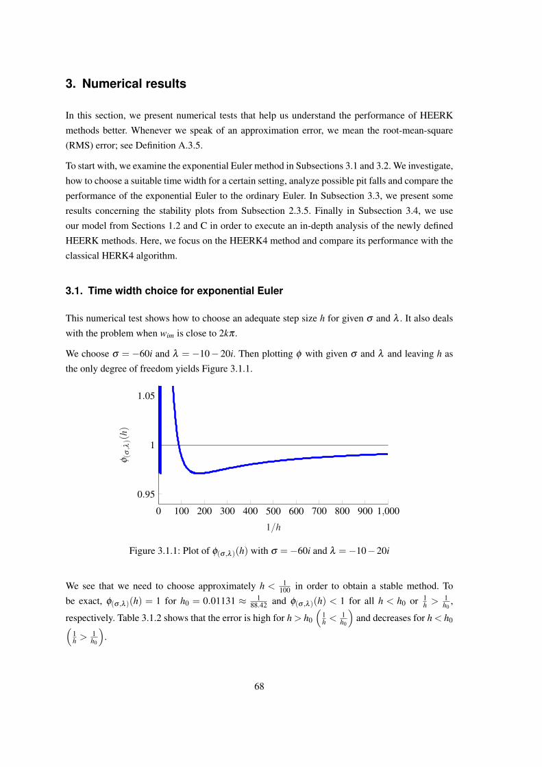
3. Numerical results

In this section, we present numerical tests that help us understand the performance of HEERK

methods better. Whenever we speak of an approximation error, we mean the root-mean-square

(RMS) error; see Definition A.3.5.

To start with, we examine the exponential Euler method in Subsections 3.1 and 3.2. We investigate,

how to choose a suitable time width for a certain setting, analyze possible pit falls and compare the

performance of the exponential Euler to the ordinary Euler. In Subsection 3.3, we present some

results concerning the stability plots from Subsection 2.3.5. Finally in Subsection 3.4, we use

our model from Sections 1.2 and C in order to execute an in-depth analysis of the newly defined

HEERK methods. Here, we focus on the HEERK4 method and compare its performance with the

classical HERK4 algorithm.

3.1. Time width choice for exponential Euler

This numerical test shows how to choose an adequate step size h for given σ and λ . It also deals

with the problem when wim is close to 2kπ .

We choose σ = −60i and λ = −10− 20i. Then plotting φ with given σ and λ and leaving h as

the only degree of freedom yields Figure 3.1.1.

0 100 200 300 400 500 600 700 800 900 1,000

0.95

1

1.05

1/h

φ(σ

,λ)(

h)

Figure 3.1.1: Plot of φ(σ ,λ )(h) with σ =−60i and λ =−10−20i

We see that we need to choose approximately h < 1100 in order to obtain a stable method. To

be exact, φ(σ ,λ )(h) = 1 for h0 = 0.01131 ≈ 188.42 and φ(σ ,λ )(h) < 1 for all h < h0 or 1

h > 1h0

,

respectively. Table 3.1.2 shows that the error is high for h > h0

(1h < 1

h0

)and decreases for h < h0(

1h > 1

h0

).

68

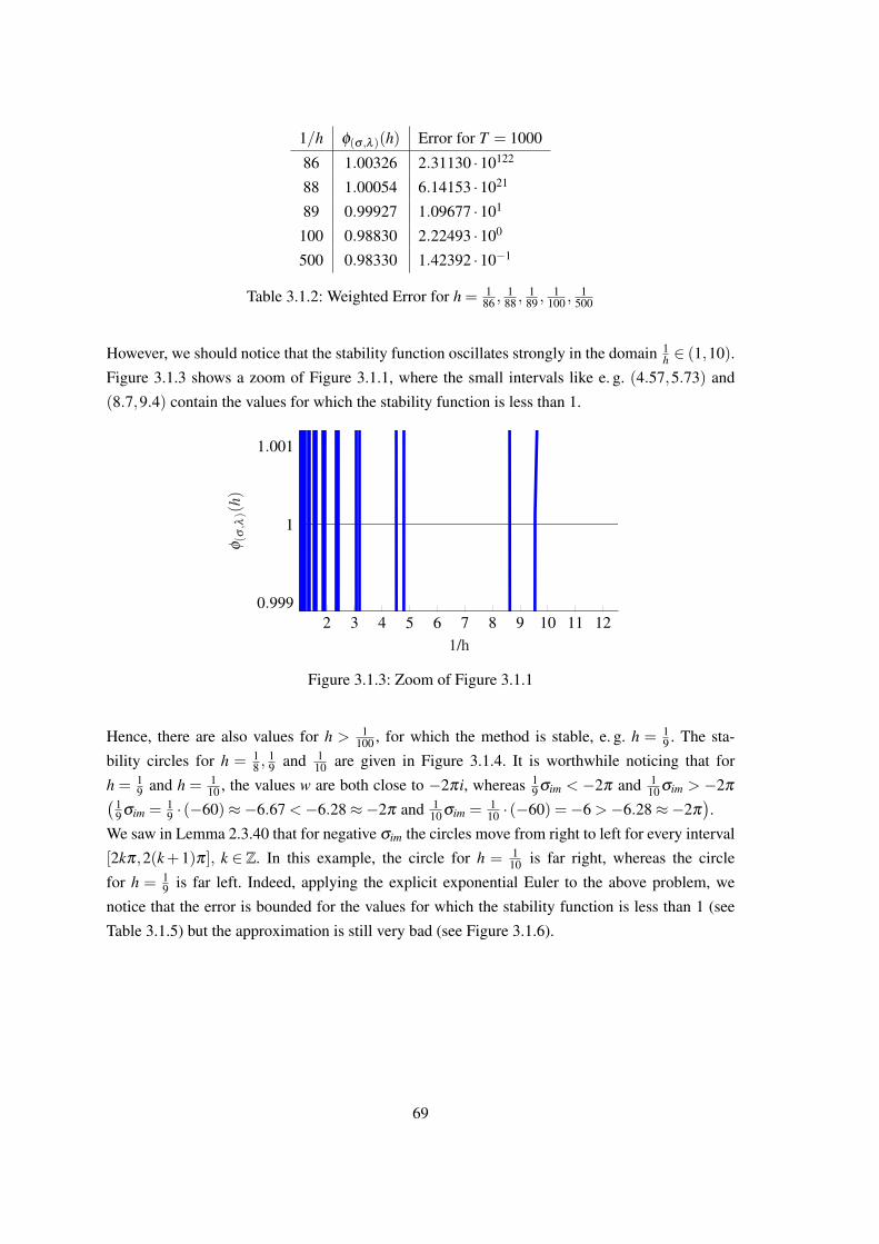
1/h φ(σ ,λ )(h) Error for T = 1000

86 1.00326 2.31130 ·10122

88 1.00054 6.14153 ·1021

89 0.99927 1.09677 ·101

100 0.98830 2.22493 ·100

500 0.98330 1.42392 ·10−1

Table 3.1.2: Weighted Error for h = 186 ,

188 ,

189 ,

1100 ,

1500

However, we should notice that the stability function oscillates strongly in the domain 1h ∈ (1,10).

Figure 3.1.3 shows a zoom of Figure 3.1.1, where the small intervals like e. g. (4.57,5.73) and

(8.7,9.4) contain the values for which the stability function is less than 1.

2 3 4 5 6 7 8 9 10 11 120.999

1

1.001

1/h

φ(σ

,λ)(

h)

Figure 3.1.3: Zoom of Figure 3.1.1

Hence, there are also values for h > 1100 , for which the method is stable, e. g. h = 1

9 . The sta-

bility circles for h = 18 ,

19 and 1

10 are given in Figure 3.1.4. It is worthwhile noticing that for

h = 19 and h = 1

10 , the values w are both close to −2πi, whereas 19 σim < −2π and 1

10 σim > −2π(19 σim = 1

9 · (−60)≈−6.67 <−6.28≈−2π and 110 σim = 1

10 · (−60) =−6 >−6.28≈−2π).

We saw in Lemma 2.3.40 that for negative σim the circles move from right to left for every interval

[2kπ,2(k+1)π], k ∈ Z. In this example, the circle for h = 110 is far right, whereas the circle

for h = 19 is far left. Indeed, applying the explicit exponential Euler to the above problem, we

notice that the error is bounded for the values for which the stability function is less than 1 (see

Table 3.1.5) but the approximation is still very bad (see Figure 3.1.6).

69

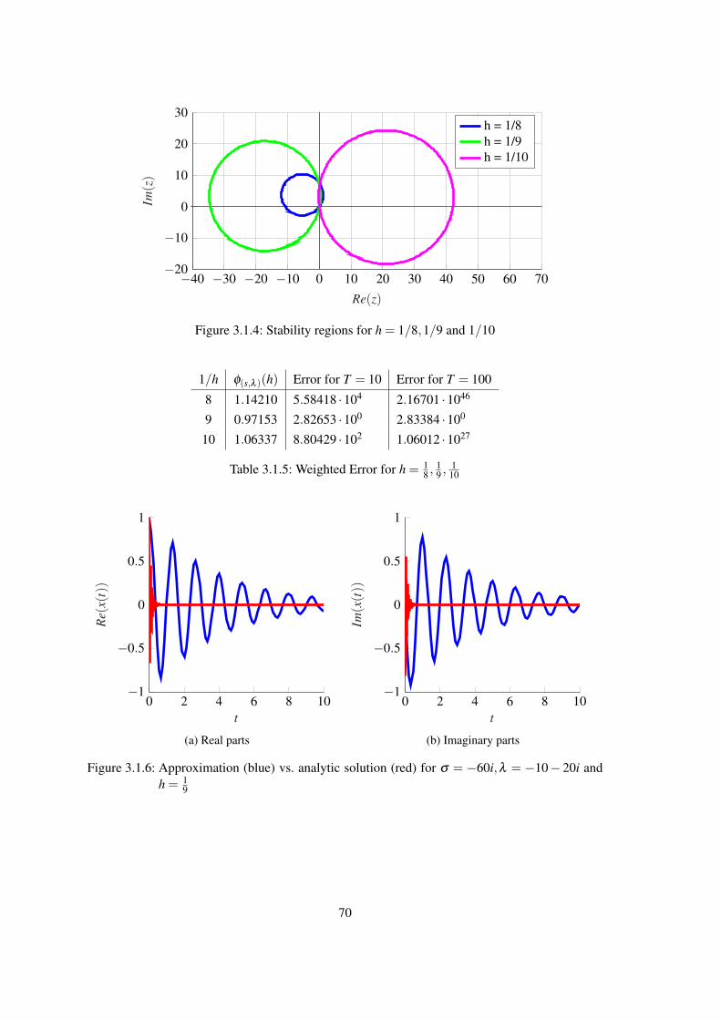
−40 −30 −20 −10 0 10 20 30 40 50 60 70−20

−10

0

10

20

30

Re(z)

Im(z)

h = 1/8h = 1/9h = 1/10

Figure 3.1.4: Stability regions for h = 1/8,1/9 and 1/10

1/h φ(s,λ )(h) Error for T = 10 Error for T = 100

8 1.14210 5.58418 ·104 2.16701 ·1046

9 0.97153 2.82653 ·100 2.83384 ·100

10 1.06337 8.80429 ·102 1.06012 ·1027

Table 3.1.5: Weighted Error for h = 18 ,

19 ,

110

0 2 4 6 8 10−1

−0.5

0

0.5

1

t

Re(

x(t))

(a) Real parts

0 2 4 6 8 10−1

−0.5

0

0.5

1

t

Im(x(t))

(b) Imaginary parts

Figure 3.1.6: Approximation (blue) vs. analytic solution (red) for σ = −60i,λ = −10− 20i andh = 1

9

70

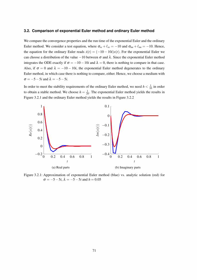
3.2. Comparison of exponential Euler method and ordinary Euler method

We compare the convergence properties and the run time of the exponential Euler and the ordinary

Euler method. We consider a test equation, where σre + `re = −10 and σim + `im = −10. Hence,

the equation for the ordinary Euler reads x(t) = (−10− 10i)x(t). For the exponential Euler we

can choose a distribution of the value −10 between σ and λ . Since the exponential Euler method

integrates the ODE exactly if σ =−10−10i and λ = 0, there is nothing to compare in that case.

Also, if σ = 0 and λ = −10− 10i, the exponential Euler method degenerates to the ordinary

Euler method, in which case there is nothing to compare, either. Hence, we choose a medium with

σ =−5−5i and λ =−5−5i.

In order to meet the stability requirements of the ordinary Euler method, we need h < 110 in order

to obtain a stable method. We choose h = 120 . The exponential Euler method yields the results in

Figure 3.2.1 and the ordinary Euler method yields the results in Figure 3.2.2

0 0.2 0.4 0.6 0.8 1−0.2

0

0.2

0.4

0.6

0.8

1

t

Re(

x(t))

(a) Real parts

0 0.2 0.4 0.6 0.8 1−0.4

−0.3

−0.2

−0.1

0

0.1

t

Im(x(t))

(b) Imaginary parts

Figure 3.2.1: Approximation of exponential Euler method (blue) vs. analytic solution (red) forσ =−5−5i, λ =−5−5i and h = 0.05

71

0 0.2 0.4 0.6 0.8 1−0.2

0

0.2

0.4

0.6

0.8

1

t

Re(

x(t))

(a) Real parts

0 0.2 0.4 0.6 0.8 1−0.4

−0.3

−0.2

−0.1

0

0.1

t

Im(x(t))

(b) Imaginary parts

Figure 3.2.2: Approximation of ordinary Euler method (blue) vs. analytic solution (red) forσ =−5−5i, λ =−5−5i and h = 0.05

We observe that the exponential Euler method (RMS error 1.5 ·10−1) yields more accurate results

than the ordinary Euler (RMS error 3.6 · 10−1)for the same step width, when at least some linear

parts of the right side are stored in σ .

As we can see in Figure 3.2.3, both methods have convergence order 1. However, the error of the

exponential Euler approximation is less than the Error of the ordinary Euler method.

10−6 10−5 10−4 10−3 10−2 10−110−10

10−7

10−4

10−1

O(h)O(h2)O(h3)O(h4)

Step width

RM

Ser

ror

Figure 3.2.3: Comparison of the convergence orders of the exponential Euler method (blue) andthe ordinary Euler method (red) for σ =−5−5i, λ =−5−5i

Figure 3.2.4 shows the run time comparison. Naturally, we need to input more effort into the

exponential Euler method since it yields more accurate results than the ordinary Euler method

whereas both have the same convergence order 1. We observe that there exists a difference between

exponential Euler and ordinary Euler for a small amount of time steps but it diminishes for a

72

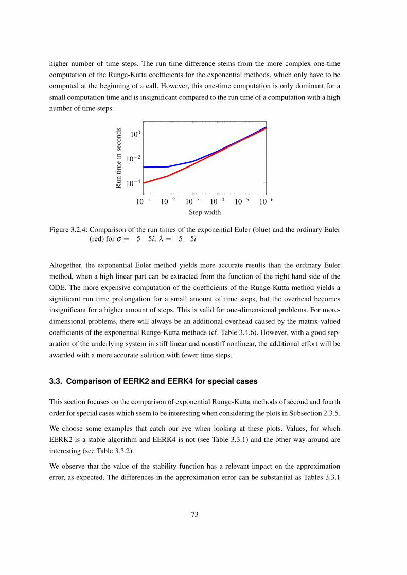
higher number of time steps. The run time difference stems from the more complex one-time

computation of the Runge-Kutta coefficients for the exponential methods, which only have to be

computed at the beginning of a call. However, this one-time computation is only dominant for a

small computation time and is insignificant compared to the run time of a computation with a high

number of time steps.

10−610−510−410−310−210−1

10−4

10−2

100

Step width

Run

time

inse

cond

s

Figure 3.2.4: Comparison of the run times of the exponential Euler (blue) and the ordinary Euler(red) for σ =−5−5i, λ =−5−5i

Altogether, the exponential Euler method yields more accurate results than the ordinary Euler

method, when a high linear part can be extracted from the function of the right hand side of the

ODE. The more expensive computation of the coefficients of the Runge-Kutta method yields a

significant run time prolongation for a small amount of time steps, but the overhead becomes

insignificant for a higher amount of steps. This is valid for one-dimensional problems. For more-

dimensional problems, there will always be an additional overhead caused by the matrix-valued

coefficients of the exponential Runge-Kutta methods (cf. Table 3.4.6). However, with a good sep-

aration of the underlying system in stiff linear and nonstiff nonlinear, the additional effort will be

awarded with a more accurate solution with fewer time steps.

3.3. Comparison of EERK2 and EERK4 for special cases

This section focuses on the comparison of exponential Runge-Kutta methods of second and fourth

order for special cases which seem to be interesting when considering the plots in Subsection 2.3.5.

We choose some examples that catch our eye when looking at these plots. Values, for which

EERK2 is a stable algorithm and EERK4 is not (see Table 3.3.1) and the other way around are

interesting (see Table 3.3.2).

We observe that the value of the stability function has a relevant impact on the approximation

error, as expected. The differences in the approximation error can be substantial as Tables 3.3.1

73

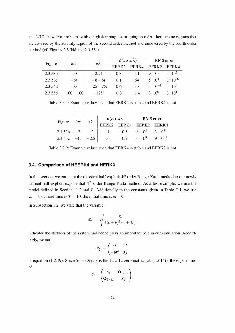
and 3.3.2 show. For problems with a high damping factor going into hσ , there are no regions that

are covered by the stability region of the second order method and uncovered by the fourth order

method (cf. Figures 2.3.54d and 2.3.55d).

Figure hσ hλφ(hσ ,hλ ) RMS error

EERK2 EERK4 EERK2 EERK4

2.3.53b −3i 2.2i 0.3 1.1 9 ·101 4 ·102

2.3.53c −6i −8−8i 0.1 64 5 ·104 2 ·1016

2.3.54d −100 −25−75i 0.6 1.3 5 ·10−1 1 ·101

2.3.55d −100−100i −125i 0.8 1.4 3 ·100 3 ·104

Table 3.3.1: Example values such that EERK2 is stable and EERK4 is not

Figure hσ hλφ(hσ ,hλ ) RMS error

EERK2 EERK4 EERK2 EERK4

2.3.53b −3i −2 1.1 0.5 6 ·105 3 ·103

2.3.53c −6i −2.5 1.0 0.9 6 ·100 9 ·10−1

Table 3.3.2: Example values such that EERK4 is stable and EERK2 is not

3.4. Comparison of HEERK4 and HERK4

In this section, we compare the classical half-explicit 4th order Runge-Kutta method to our newly

defined half-explicit exponential 4th order Runge-Kutta method. As a test example, we use the

model defined in Sections 1.2 and C. Additionally to the constants given in Table C.1, we use

Ω = 7, our end time is T = 10, the initial time is t0 = 0.

In Subsection 1.2, we state that the variable

ωs :=

√Ks

4(a+b)2mb +4Izb

indicates the stiffness of the system and hence plays an important role in our simulation. Accord-

ingly, we set

S2 :=

(0 1

−ω2s 0

)in equation (1.2.19). Since S1 = O12×12 is the 12× 12-zero matrix (cf. (1.2.14)), the eigenvalues

of

S :=

(S1 O12×2

O2×12 S2

),

74

are 0,±ωsi. The higher ωs is the stiffer the system gets. For our simulation, we will try different

values of Ks in order to influence the value of ωs.

We obtain a reference solution by solving the monolithic system (given in Section C.2) with an

explicit 4th order Runge-Kutta method with small time steps (h = 10−5). For our analysis of the

convergence error, we focus on the variables φi(t), i = 1, . . . ,4 as they exhibit the most interesting

behavior. φ1(t) indicates the local angle of the first blade. If we start with a small displacement

(0.01 rad) for one blade – say the first – leaving the other blades at rest, then the first blade will

vibrate when rotating around the mast. Since the mast has also some play, this vibration will set

the other blades in a vibrating motion as well. The frequency of the vibrations and the transmission

rate depend on the particular degree of stiffness of the mast. Figure 3.4.1 shows the motion of the

four blades for t ∈ [0,10] and ωs ∈ 3.91,12.35,39.06 (Ks ∈ 30,000;300,000;3,000,000).

0 2 4 6 8 10

−0.01

0

0.01

t

Lag

angl

e[r

ad]

(a) ωs = 3.91

0 2 4 6 8 10

−0.01

0

0.01

t

Lag

angl

e[r

ad]

(b) ωs = 12.35

0 2 4 6 8 10

−0.01

0

0.01

t

Lag

angl

e[r

ad]

(c) ωs = 39.06

Figure 3.4.1: Motion of the four blades (blade 1: blue, blade 2: red, blade 3: green, blade 4: pink)of the model for different values of ωs (author’s plot)

We see that the initial displacement of the first blade is 0.01rad, whereas the other three start

75

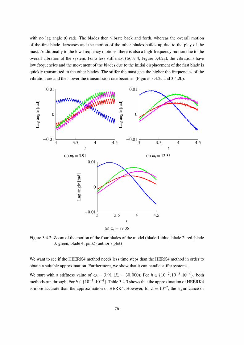
with no lag angle (0 rad). The blades then vibrate back and forth, whereas the overall motion

of the first blade decreases and the motion of the other blades builds up due to the play of the

mast. Additionally to the low-frequency motions, there is also a high-frequency motion due to the

overall vibration of the system. For a less stiff mast (ωs ≈ 4, Figure 3.4.2a), the vibrations have

low frequencies and the movement of the blades due to the initial displacement of the first blade is

quickly transmitted to the other blades. The stiffer the mast gets the higher the frequencies of the

vibration are and the slower the transmission rate becomes (Figures 3.4.2c and 3.4.2b).

3 3.5 4 4.5−0.01

0

0.01

t

Lag

angl

e[r

ad]

(a) ωs = 3.91

3 3.5 4 4.5−0.01

0

0.01

t

Lag

angl

e[r

ad]

(b) ωs = 12.35

3 3.5 4 4.5−0.01

0

0.01

t

Lag

angl

e[r

ad]

(c) ωs = 39.06

Figure 3.4.2: Zoom of the motion of the four blades of the model (blade 1: blue, blade 2: red, blade3: green, blade 4: pink) (author’s plot)

We want to see if the HEERK4 method needs less time steps than the HERK4 method in order to

obtain a suitable approximation. Furthermore, we show that it can handle stiffer systems.

We start with a stiffness value of ωs = 3.91 (Ks = 30,000). For h ∈ 10−2,10−3,10−4, both

methods run through. For h∈ 10−3,10−4, Table 3.4.3 shows that the approximation of HEERK4

is more accurate than the approximation of HERK4. However, for h = 10−2, the significance of

76

the approximation error is low since the approximation of HERK4 starts off with accounting for

the high frequency vibrations in the beginning and finally ends up smoothing them out, whereas

the approximation of HEERK4 accounts for the vibrations but obtains an offset with advancing

time (see Figure 3.4.4). Both approximations yield a similar RMS error while approximating the

solution in very different ways.

h HERK4 HEERK4

10−2 1.5 ·10−1 1.2 ·10−1

10−3 1.4 ·10−4 7.3 ·10−6

10−4 1.4 ·10−8 7.2 ·10−10

Table 3.4.3: RMS error for ωs = 3.91

0 0.2 0.4 0.60.006

0.008

0.01

t

ϕ1(

t)

(a) t ∈ [0,0.6]

8.2 8.4 8.6 8.80

0.002

0.004

t

ϕ1(

t)

(b) t ∈ [8.2,8.8]

Figure 3.4.4: Plot of reference solution (blue), approximation HERK4 (red) and approximationHEERK4 (green) for ϕ1(t) (author’s plot)

The simulation also shows the convergence orders of HERK4 and HEERK4. As expected, both

are fourth order methods (cf. Table 3.4.3 and Figure 3.4.5).

10−5 10−4 10−3 10−210−11

10−6

10−1O(h)

O(h2)O(h3)O(h4)

Step width

RM

SE

rror

HERK4HEERK4

Figure 3.4.5: Visualization of convergence rates of HERK4 and HEERK4

77

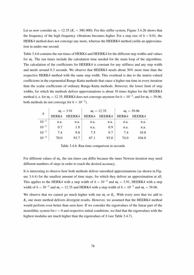
Let us now consider ωs = 12.35 (Ks = 300,000). For this stiffer system, Figure 3.4.2b shows that

the frequency of the high frequency vibrations becomes higher. For a step size of h = 0.01, the

HERK4 method does not converge any more, whereas the HEERK4 method yields an approxima-

tion in under one second.

Table 3.4.6 contains the run times of HERK4 and HEERK4 for the different step widths and values

for ωs. The run times include the calculation time needed for the main loop of the algorithms.

The calculation of the coefficients for HEERK4 is constant for any stiffness and any step width

and needs around 0.3 seconds. We observe that HEERK4 needs about 30% more time than the

respective HERK4 method with the same step width. This overhead is due to the matrix-valued

coefficients in the exponential Runge-Kutta methods that cause a higher run time in every iteration

than the scalar coefficients of ordinary Runge-Kutta methods. However, the lower limit of step

widths, for which the methods deliver approximations is about 10 times higher for the HEERK4

method (i. e. for ωs = 12.35, HERK4 does not converge anymore for h= 10−2, and for ωs = 39.06,

both methods do not converge for h = 10−2).

hωs = 3.91 ωs = 12.35 ωs = 39.06

HERK4 HEERK4 HERK4 HEERK4 HERK4 HEERK4

10−1 n.a. n.a. n.a. n.a. n.a. n.a.

10−2 0.7 1.0 n.a. 0.9 n.a. n.a.

10−3 7.4 9.8 7.5 9.7 7.4 10.8

10−4 70.0 93.7 67.1 93.0 74.0 104.0

Table 3.4.6: Run time comparison in seconds

For different values of ωs, the run times can differ because the inner Newton iteration may need

different numbers of steps in order to reach the desired accuracy.

It is interesting to observe how both methods deliver smoothed approximations (as shown in Fig-

ure 3.4.4) for the smallest amount of time steps, for which they deliver an approximation at all.

This applies to the HERK4 with a step width of h = 10−2 and ωs = 3.91, HEERK4 with a step

width of h = 10−2 and ωs = 12.35 and HERK4 with a step width of h = 10−3 and ωs = 39.06.

We observe that we cannot go much higher with our ωs or Ks. With every zero that we add to

Ks one more method delivers divergent results. However, we assumed that the HEERK4 method

would perform even better than seen here. If we consider the eigenvalues of the linear part of the

monolithic system for t = 0 and respective initial conditions, we find that the eigenvalues with the

highest modulus are much higher than the eigenvalues of S (see Table 3.4.7).

78

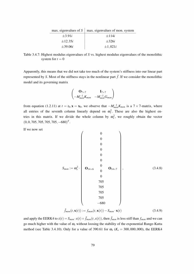
max. eigenvalues of S max. eigenvalues of mon. system

±3.91i ±114i

±12.35i ±326i

±39.06i ±1,021i

Table 3.4.7: Highest modulus eigenvalues of S vs. highest modulus eigenvalues of the monolithicsystem for t = 0

Apparently, this means that we did not take too much of the system’s stiffness into our linear part

represented by S. Most of the stiffness stays in the nonlinear part f . If we consider the monolithic

model and its governing matrix (O7×7 I7×7

−M−1monKmon −M−1

monGmon

)

from equation (1.2.11) at t = t0,x = x0, we observe that −M−1monKmon is a 7× 7-matrix, where

all entries of the seventh column linearly depend on ω2s . These are also the highest en-

tries in this matrix. If we divide the whole column by ω2s , we roughly obtain the vector

(0,0,705,705,705,705,−680)T .

If we now set

Smon := ω2s ·

O14×6

0

O14×7

0

0

0

0

0

0

0

0

705

705

705

705

−680

, (3.4.8)

fmon(t,x(t)) := fmon(t,x(t))−Smon ·x(t) (3.4.9)

and apply the EERK4 to x(t)= Smon ·x(t)+ fmon(t,x(t)), then fmon is less stiff than fmon and we can

go much higher with the value of ωs without loosing the stability of the exponential Runge-Kutta

method (see Table 3.4.10). Only for a value of 390.61 for ωs (Ks = 300,000,000), the EERK4

79

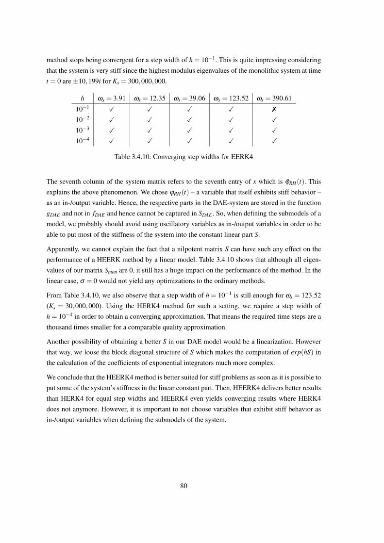
method stops being convergent for a step width of h = 10−1. This is quite impressing considering

that the system is very stiff since the highest modulus eigenvalues of the monolithic system at time

t = 0 are ±10,199i for Ks = 300,000,000.

h ωs = 3.91 ωs = 12.35 ωs = 39.06 ωs = 123.52 ωs = 390.61

10−1 X X X X 7

10−2 X X X X X

10−3 X X X X X

10−4 X X X X X

Table 3.4.10: Converging step widths for EERK4

The seventh column of the system matrix refers to the seventh entry of x which is ϕRH(t). This

explains the above phenomenon. We chose ϕRH(t) – a variable that itself exhibits stiff behavior –

as an in-/output variable. Hence, the respective parts in the DAE-system are stored in the function

gDAE and not in fDAE and hence cannot be captured in SDAE . So, when defining the submodels of a

model, we probably should avoid using oscillatory variables as in-/output variables in order to be

able to put most of the stiffness of the system into the constant linear part S.

Apparently, we cannot explain the fact that a nilpotent matrix S can have such any effect on the

performance of a HEERK method by a linear model. Table 3.4.10 shows that although all eigen-

values of our matrix Smon are 0, it still has a huge impact on the performance of the method. In the

linear case, σ = 0 would not yield any optimizations to the ordinary methods.

From Table 3.4.10, we also observe that a step width of h = 10−1 is still enough for ωs = 123.52

(Ks = 30,000,000). Using the HERK4 method for such a setting, we require a step width of

h = 10−4 in order to obtain a converging approximation. That means the required time steps are a

thousand times smaller for a comparable quality approximation.

Another possibility of obtaining a better S in our DAE model would be a linearization. However

that way, we loose the block diagonal structure of S which makes the computation of exp(hS) in

the calculation of the coefficients of exponential integrators much more complex.

We conclude that the HEERK4 method is better suited for stiff problems as soon as it is possible to

put some of the system’s stiffness in the linear constant part. Then, HEERK4 delivers better results

than HERK4 for equal step widths and HEERK4 even yields converging results where HERK4

does not anymore. However, it is important to not choose variables that exhibit stiff behavior as

in-/output variables when defining the submodels of the system.

80

4. Conclusion and recommendations for further work

With the definition of half-explicit exponential Runge-Kutta (HEERK) methods, we did a first step

towards a more efficient helicopter simulation. We started this thesis with an overview of already

existing numerical approaches and software. After a discussion of the drawbacks of the current

state of the art, we presented our approach: a general coupled state-space model or mathematically

speaking: an index-1 differential algebraic equations (DAEs) system.

Since we were looking for a method that would simulate the helicopter’s behavior over longer peri-

ods in an acceptable simulation time, we focused on explicit methods. A family of existing explicit

methods for index-1 DAEs are half-explicit Runge-Kutta (HERK) methods that are derived from

explicit Runge-Kutta (ERK) methods for ODEs paired with a Newton method. These methods are

well suited for solving index-1 DAEs. However, they cannot handle the stiff helicopter system. For

such stiff ODE systems, there exist explicit exponential Runge-Kutta (EERK) methods. For these

methods, a formulation of the ODE is necessary where the stiffness of the ODE is separately given

in form of a linear part. In order to make exponential integrators applicable to index-1 systems, we

needed to define half-explicit exponential Runge-Kutta (HEERK) methods analogously to HERK

methods.

With this aim, we investigated consistency and stability properties of ERK and their translation

to HERK methods. Stability and consistency results for ERK methods are well known. While the

stability results translate to HERK methods, the consistency results need to be shown seperately.

Although, there are proofs of consistency in the literature (e. g. [ASW93, HW96]), we chose to

conduct a straight forward and more comprehensible proof for methods of orders one and two

which we could then translate more easily to HEERK methods.

In an analogous way, we analyzed EERK methods focusing on consistency and stability. Here,

consistency results were available in the literature [HO10]. However, we could not find a linear

stability analysis of EERK methods. For the first order explicit exponential method (exponential

Euler method) we considered the stability function and its behavior. For methods of higher orders,

we plotted the stability regions in analogy to the well-known stability plots of ordinary Runge-

Kutta methods. Since the stability functions additionally depend on the linear stiff part of the

state function, we obtained interesting plots, where the stability regions deformed and moved with

respect to different inputs.

Combining our findings for HERK methods and EERK methods, we developped HEERK meth-

ods. To the best of our knowledge, they have not been used in the literature before. For the methods

of first and second order we used our comprehensible proofs to show consistency.

Our numerical testing showed the strengths of HEERK methods compared to HERK methods.

We used a mechanical model, the stiffness of which we could adapt according to our needs. We

81

saw that HEERK methods need far less time steps than HERK methods in order to achieve a

comparable approximation quality on stiff systems. However, we need to be careful when defining

the submodels. We chose the rotational angle of the rotor head as an in-/output variable in our

example. However, this variable exhibits stiff behavior itself. As a result, our HEERK method

already becomes instable with comparably small step sizes and hence is not that much better than

the ordinary integrators. Though if we place the oscillatory variables solely in the state function

and if we are able to seperate them into the linear part, then we can dramatically enhance the

approximation quality of HEERK methods which makes them a very efficient tool for solving stiff

index-1 DAE systems.

This thesis already contains a lot of promising results. However, there are still many aspects that

could be analyzed for an even better framework.

Concerning stability aspects of exponential methods, we covered the behavior of the stability

regions of methods up to order 4 for various settings of linear problems. We also thoroughly in-

vestigated the analytical stability function of the exponential Euler method (first order exponential

Runge-Kutta method). An in-depth analysis of the analytical functions describing the stability

regions of higher order methods is just as interesting but has not yet been conducted.

For the consistency of HERK and HEERK methods, we have shown that the Newton methods

need to be executed to the accuracy that we want the underlying Runge-Kutta method to have.

In [ARW93], Arnold et al. give a stronger statement for HERK methods. They indicate specific

numbers of Newton steps that are necessary for the underlying Runge-Kutta method to be conver-

gent of its ordinary order. It would be interesting to apply their results to half-explicit exponential

Runge-Kutta methods. This would further enhance their run time.

Future research will show how our HEERK methods will perform on more complex helicopter

models. Our mechanical model showed that the submodels need to be chosen cautiously. The in-

/output variables should not exhibit any oscillatory behavior and the linear part should contain

most of the stiffness of the system. In our experiment we learned that this does not have to mean

that the matrix S needs to have high modulus eigenvalues. It will be enlightening to analyze the

criteria which S has to fulfil for HEERK methods to work well.

Altogether, half-explicit exponential methods bring us considerably closer to a more efficient and

effective simulation of large stiff systems in a general coupled state-space representation. Their

elaborate application in comprehensive helicopter simulation has the ability to prevent accidents

and support the simulation driven design of helicopters in the future.

82

List of abbreviations

cf. confer . . . . . . . . . . . . . . . . . . . . . . . . . . . . . . . . . . . . . . . . . . . . . . . . . . . . . . . . . . . . . . . . . . 3

DAE Differential-Algebraic Equation . . . . . . . . . . . . . . . . . . . . . . . . . . . . . . . . . . . . . . . . . . . 3

DLR German Aerospace Center . . . . . . . . . . . . . . . . . . . . . . . . . . . . . . . . . . . . . . . . . . . . . . . . 1

EERK Explicit Exponential Runge-Kutta . . . . . . . . . . . . . . . . . . . . . . . . . . . . . . . . . . . . . . . . 29

e. g. Exempli gratia (for example) . . . . . . . . . . . . . . . . . . . . . . . . . . . . . . . . . . . . . . . . . . . . . . 5

ERK Explicit Runge-Kutta . . . . . . . . . . . . . . . . . . . . . . . . . . . . . . . . . . . . . . . . . . . . . . . . . . . . 14

FT Institute of Flight Systems . . . . . . . . . . . . . . . . . . . . . . . . . . . . . . . . . . . . . . . . . . . . . . . . 1

HEERK Half-Explicit Exponential Runge-Kutta . . . . . . . . . . . . . . . . . . . . . . . . . . . . . . . . . . . 62

HERK Half-Explicit Runge-Kutta . . . . . . . . . . . . . . . . . . . . . . . . . . . . . . . . . . . . . . . . . . . . . . . 20

HPC High Performance Computing . . . . . . . . . . . . . . . . . . . . . . . . . . . . . . . . . . . . . . . . . . . . . 1

i. e. Id est (that is to say) . . . . . . . . . . . . . . . . . . . . . . . . . . . . . . . . . . . . . . . . . . . . . . . . . . . . . . 7

IMEX Implicit-Explicit . . . . . . . . . . . . . . . . . . . . . . . . . . . . . . . . . . . . . . . . . . . . . . . . . . . . . . . . 28

ODE Ordinary Differential Equation . . . . . . . . . . . . . . . . . . . . . . . . . . . . . . . . . . . . . . . . . . . . 5

p. page . . . . . . . . . . . . . . . . . . . . . . . . . . . . . . . . . . . . . . . . . . . . . . . . . . . . . . . . . . . . . . . . . . . 13

PDE Partial Differential Equation. . . . . . . . . . . . . . . . . . . . . . . . . . . . . . . . . . . . . . . . . . . . . . .2

pp. pages . . . . . . . . . . . . . . . . . . . . . . . . . . . . . . . . . . . . . . . . . . . . . . . . . . . . . . . . . . . . . . . . . . 13

RK Runge-Kutta . . . . . . . . . . . . . . . . . . . . . . . . . . . . . . . . . . . . . . . . . . . . . . . . . . . . . . . . . . . 14

SPP Singularly Perturbed Problem . . . . . . . . . . . . . . . . . . . . . . . . . . . . . . . . . . . . . . . . . . . . 13

VAST Versatile Aeromechanics Simulation Tool . . . . . . . . . . . . . . . . . . . . . . . . . . . . . . . . . . 1

83

Notation directory

Section 1

Notation Description Def. ont ∈ R+ Real time variable . . . . . . . . . . . . . . . . . . . . . . . . . . . . . . . . . . page 5

ni ∈ N Degrees of freedom of the state vector of subsystem i . . page 5

mi ∈ N Degrees of freedom of the output vector of subsystem i . page 5

qi ∈ N Degrees of freedom of the input vector of subsystem i . . page 5

xi(t) ∈ Rni Local vector of state variables of subsystem i . . . . . . . . . . page 5

xi(t) ∈ Rni Also x′i(t), time derivative of xi(t) . . . . . . . . . . . . . . . . . . . . page 5

yi(t) ∈ Rmi Local vector of output variables of subsystem i . . . . . . . . page 5

ui(t) ∈ Rqi Local vector of input variables of subsystem i . . . . . . . . . page 5

fi :R+×Rni×Rqi →Rni State function of subsystem i . . . . . . . . . . . . . . . . . . . . . . . . . page 5

gi :R+×Rni×Rqi→Rmi Output function of subsystem i . . . . . . . . . . . . . . . . . . . . . . . page 5

n = ∑i

ni Degrees of freedom of the global state vector . . . . . . . . . . page 5

m = ∑i

mi Degrees of freedom of the global output vector . . . . . . . . page 5

x(t) ∈ Rn Vector of global state variables . . . . . . . . . . . . . . . . . . . . . . . page 5

y(t) ∈ Rm Vector of global output variables . . . . . . . . . . . . . . . . . . . . . page 5

f : R+×Rn×Rm→ Rn Global state function . . . . . . . . . . . . . . . . . . . . . . . . . . . . . . . . page 5

g : R+×Rn×Rm→ Rm Global output function . . . . . . . . . . . . . . . . . . . . . . . . . . . . . . page 5

g : R+×Rn×Rm→ Rm Modified output function . . . . . . . . . . . . . . . . . . . . . . . . . . . . . page 5

g−1 : 0×R+×Rn Implicit function to g(t,x(t),y(t)) = 0 . . . . . . . . . . . . . . . . page 6∂g∂y(t,x(t),y(t)) Also ∂yg(t,x(t),y(t)), partial derivative of g with respect

to y . . . . . . . . . . . . . . . . . . . . . . . . . . . . . . . . . . . . . . . . . . . . . . . .

page 6

t0 ∈ R+ Initial time . . . . . . . . . . . . . . . . . . . . . . . . . . . . . . . . . . . . . . . . . page 6

x0 ∈ Rn Initial vector for the state variables . . . . . . . . . . . . . . . . . . . page 6

y0 ∈ Rm Initial vector for the output variables . . . . . . . . . . . . . . . . . . page 6

Si ∈ Rni×ni Constant matrix containing the stiff part of fi . . . . . . . . . . page 7

fi :R+×Rni×Rqi →Rni In general nonlinear function containing the nonstiff part

of fi . . . . . . . . . . . . . . . . . . . . . . . . . . . . . . . . . . . . . . . . . . . . . . .

page 7

S ∈ Rn×n Constant block diagonal matrix containing the stiff part

of f . . . . . . . . . . . . . . . . . . . . . . . . . . . . . . . . . . . . . . . . . . . . . . .

page 7

f : R+×Rn×Rm→ Rn In general nonlinear function containing the nonstiff part

of f . . . . . . . . . . . . . . . . . . . . . . . . . . . . . . . . . . . . . . . . . . . . . . . .

page 7

M ∈ R6×6 Mass matrix of the rotor model in [SMBA11] . . . . . . . . . . page 8

u : R+→ R6 Vector of variables of the rotor model in [SMBA11] . . . . page 8

G ∈ R6×6 Damping matrix of the rotor model in [SMBA11] . . . . . . page 8

84

K ∈ R6×6 Stiffness matrix of the rotor model in [SMBA11] . . . . . . page 8

F ∈ R6 External force vector of the rotor model in [SMBA11] . . page 8

xFus : R+→ R Longitudinal displacement of the fuselage in meters . . . . page 8

yFus : R+→ R Transversal displacement of the fuselage in meters . . . . . page 8

ϕi : R+→ R Lead-lag angle of ith blade in rad . . . . . . . . . . . . . . . . . . . . . page 8

v : R+→ R6 Vector of derivatives of variables of the rotor model in

[SMBA11] . . . . . . . . . . . . . . . . . . . . . . . . . . . . . . . . . . . . . . . . .

page 8

M−1 ∈ R6×6 Inverse of the matrix M . . . . . . . . . . . . . . . . . . . . . . . . . . . . . page 8

Ks ∈ R Stiffness coefficient of the mast . . . . . . . . . . . . . . . . . . . . . . page 8

ϕRH : R+→ R Rotational angle of the rotor head in rad . . . . . . . . . . . . . . . page 8

ωi : R+→ R Time derivative of ϕi(t) . . . . . . . . . . . . . . . . . . . . . . . . . . . . . page 8

ωRH : R+→ R Rotor head’s resonance frequency in Hz (time derivative

of ϕRH(t)) . . . . . . . . . . . . . . . . . . . . . . . . . . . . . . . . . . . . . . . . .

page 8

αRH : R+→ R Time derivative of ωRH(t) . . . . . . . . . . . . . . . . . . . . . . . . . . . page 8

a ∈ R Rotor eccentricity in meters . . . . . . . . . . . . . . . . . . . . . . . . . . page 8

b ∈ R Blade length in meters . . . . . . . . . . . . . . . . . . . . . . . . . . . . . . page 8

mb ∈ R Mass of a blade in kilogramm . . . . . . . . . . . . . . . . . . . . . . . . page 8

Izb ∈ R Lag rotational inertia of a blade around its center of grav-

ity in kg m2 . . . . . . . . . . . . . . . . . . . . . . . . . . . . . . . . . . . . . . . .

page 8

ωs ∈ R Variable in the advanced monolithic rotor model . . . . . . . page 8

rsb ∈ R Variable in the advanced monolithic rotor model . . . . . . . page 9

Mmon ∈ R7×7 Mass matrix of the advanced monolithic rotor model . . . page 9

Gmon ∈ R7×7 Damping matrix of the advanced monolithic rotor model page 9

Kmon ∈ R7×7 Stiffness matrix of the advanced monolithic rotor model page 9

Fmon ∈ R7 External force vector of the advanced monolithic rotor

model . . . . . . . . . . . . . . . . . . . . . . . . . . . . . . . . . . . . . . . . . . . . .

page 9

umon : R+→ R7 Vector of variables of the advanced monolithic rotor

model . . . . . . . . . . . . . . . . . . . . . . . . . . . . . . . . . . . . . . . . . . . . .

page 9

vmon(t) Vector of derivatives of variables of the advanced mono-

lithic rotor model . . . . . . . . . . . . . . . . . . . . . . . . . . . . . . . . . . .

page 9

xmon(t) State vector of variables of the advanced monolithic rotor

model . . . . . . . . . . . . . . . . . . . . . . . . . . . . . . . . . . . . . . . . . . . . .

page 9

On×n n×n-zero matrix . . . . . . . . . . . . . . . . . . . . . . . . . . . . . . . . . . . page 9

In×n n×n-identity matrix . . . . . . . . . . . . . . . . . . . . . . . . . . . . . . . . page 9

0n n-dimensional zero vector . . . . . . . . . . . . . . . . . . . . . . . . . . . page 9

MDAE ∈ R6×6 Mass matrix of the advanced rotor model in DAE formu-

lation . . . . . . . . . . . . . . . . . . . . . . . . . . . . . . . . . . . . . . . . . . . . . .

page 9

85

GDAE ∈ R6×6 Damping matrix of the advanced rotor model in DAE for-

mulation . . . . . . . . . . . . . . . . . . . . . . . . . . . . . . . . . . . . . . . . . . .

page 9

KDAE ∈ R6×6 Stiffness matrix of the advanced rotor model in DAE for-

mulation . . . . . . . . . . . . . . . . . . . . . . . . . . . . . . . . . . . . . . . . . . .

page 9

FDAE ∈ R6 External force vector of the advanced rotor model in DAE

formulation . . . . . . . . . . . . . . . . . . . . . . . . . . . . . . . . . . . . . . . .

page 9

Section 2

Notation Description Def. onε ∈ R Small value greater than zero page 13

s Number of stages of a method . . . . . . . . . . . . . . . . . . . . . . . page 14

A = (ai j) Coefficient matrix in Butcher-Tableau for Runge-Kutta

methods . . . . . . . . . . . . . . . . . . . . . . . . . . . . . . . . . . . . . . . . . . .

page 14

b = (bi) Coefficient vector in Butcher-Tableau for Runge-Kutta

methods . . . . . . . . . . . . . . . . . . . . . . . . . . . . . . . . . . . . . . . . . . .

page 14

c = (c j) Coefficient vector in Butcher-Tableau for Runge-Kutta

methods . . . . . . . . . . . . . . . . . . . . . . . . . . . . . . . . . . . . . . . . . . .

page 14

T End time of a numerical simulation . . . . . . . . . . . . . . . . . . . page 15

N Total number of steps between 0 and T . . . . . . . . . . . . . . . page 15

h Constant step width for numerical algorithm . . . . . . . . . . . page 15

ki or ki Internal stages of Runge-Kutta methods . . . . . . . . . . . . . . . page 15

tn Time after n time steps (tn := t0 +n ·h) . . . . . . . . . . . . . . . . page 15

xn Approximation of x(tn) supplied by the algorithm . . . . . . page 15

Φ(t,x(t)) Increment function of Runge-Kutta methods . . . . . . . . . . . page 15

τ(h) Local truncation error . . . . . . . . . . . . . . . . . . . . . . . . . . . . . . . page 15

O(·) Landau symbol / Big O notation . . . . . . . . . . . . . . . . . . . . . . page 15

xh(t) Numerical approximation of x(t) . . . . . . . . . . . . . . . . . . . . . page 16

ε(t,h) Global truncation error . . . . . . . . . . . . . . . . . . . . . . . . . . . . . . page 16

λ ∈ C Parameter in the Dahlquist test equation . . . . . . . . . . . . . . . page 16

z Variable for hλ . . . . . . . . . . . . . . . . . . . . . . . . . . . . . . . . . . . . . page 16

φ(z) Stability function of explicit Runge-Kutta methods . . . . . page 16

k ∈ Rs Vector containing all internal stages ki . . . . . . . . . . . . . . . . page 18

e ∈ Rs One vector in Rs . . . . . . . . . . . . . . . . . . . . . . . . . . . . . . . . . . . . page 18

L ∈ Rn×n Constant matrix in n-dimensional Dahlquist test equation page 18

U ∈ Rn×n Matrix containing the eigenvectors of L . . . . . . . . . . . . . . . . page 18

λi ∈ C ith eigenvalue of L . . . . . . . . . . . . . . . . . . . . . . . . . . . . . . . . . . page 18

Λ ∈ Rn×n Matrix containing the eigenvalues λi of L on its diagonal page 18

86

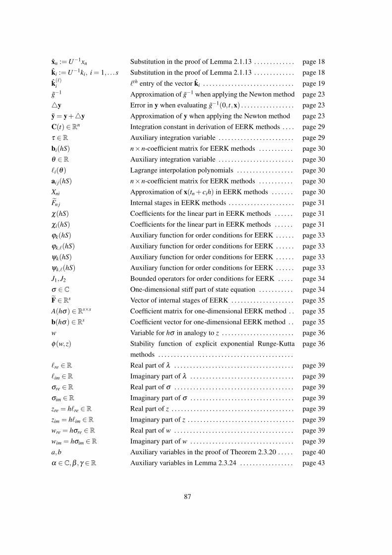
xn :=U−1xn Substitution in the proof of Lemma 2.1.13 . . . . . . . . . . . . . page 18

ki :=U−1ki, i = 1, . . .s Substitution in the proof of Lemma 2.1.13 . . . . . . . . . . . . . page 18

k(`)i `th entry of the vector ki . . . . . . . . . . . . . . . . . . . . . . . . . . . . . page 19

g−1 Approximation of g−1 when applying the Newton method page 23

4y Error in y when evaluating g−1(0, t,x) . . . . . . . . . . . . . . . . . page 23

y = y+4y Approximation of y when applying the Newton method page 23

C(t) ∈ Rn Integration constant in derivation of EERK methods . . . . page 29

τ ∈ R Auxiliary integration variable . . . . . . . . . . . . . . . . . . . . . . . . page 29

bi(hS) n×n-coefficient matrix for EERK methods . . . . . . . . . . . page 30

θ ∈ R Auxiliary integration variable . . . . . . . . . . . . . . . . . . . . . . . . page 30

`i(θ) Lagrange interpolation polynomials . . . . . . . . . . . . . . . . . . page 30

ai j(hS) n×n-coefficient matrix for EERK methods . . . . . . . . . . . page 30

Xni Approximation of x(tn + cih) in EERK methods . . . . . . . page 30

Fn j Internal stages in EERK methods . . . . . . . . . . . . . . . . . . . . . page 31

χ(hS) Coefficients for the linear part in EERK methods . . . . . . page 31

χi(hS) Coefficients for the linear part in EERK methods . . . . . . page 31

ϕk(hS) Auxiliary function for order conditions for EERK . . . . . . page 33

ϕk,`(hS) Auxiliary function for order conditions for EERK . . . . . . page 33

ψk(hS) Auxiliary function for order conditions for EERK . . . . . . page 33

ψk,`(hS) Auxiliary function for order conditions for EERK . . . . . . page 33

J1,J2 Bounded operators for order conditions for EERK . . . . . page 34

σ ∈ C One-dimensional stiff part of state equation . . . . . . . . . . . page 34

F ∈ Rs Vector of internal stages of EERK . . . . . . . . . . . . . . . . . . . . page 35

A(hσ) ∈ Rs×s Coefficient matrix for one-dimensional EERK method . . page 35

b(hσ) ∈ Rs Coefficient vector for one-dimensional EERK method . . page 35

w Variable for hσ in analogy to z . . . . . . . . . . . . . . . . . . . . . . . page 36

φ(w,z) Stability function of explicit exponential Runge-Kutta

methods . . . . . . . . . . . . . . . . . . . . . . . . . . . . . . . . . . . . . . . . . . .

page 36

`re ∈ R Real part of λ . . . . . . . . . . . . . . . . . . . . . . . . . . . . . . . . . . . . . . page 39

`im ∈ R Imaginary part of λ . . . . . . . . . . . . . . . . . . . . . . . . . . . . . . . . . page 39

σre ∈ R Real part of σ . . . . . . . . . . . . . . . . . . . . . . . . . . . . . . . . . . . . . . page 39

σim ∈ R Imaginary part of σ . . . . . . . . . . . . . . . . . . . . . . . . . . . . . . . . . page 39

zre = h`re ∈ R Real part of z . . . . . . . . . . . . . . . . . . . . . . . . . . . . . . . . . . . . . . . page 39

zim = h`im ∈ R Imaginary part of z . . . . . . . . . . . . . . . . . . . . . . . . . . . . . . . . . . page 39

wre = hσre ∈ R Real part of w . . . . . . . . . . . . . . . . . . . . . . . . . . . . . . . . . . . . . . page 39

wim = hσim ∈ R Imaginary part of w . . . . . . . . . . . . . . . . . . . . . . . . . . . . . . . . . page 39

a,b Auxiliary variables in the proof of Theorem 2.3.20 . . . . . page 40

α ∈ C,β ,γ ∈ R Auxiliary variables in Lemma 2.3.24 . . . . . . . . . . . . . . . . . page 43

87

o ∈ C Circle center of a circle in C . . . . . . . . . . . . . . . . . . . . . . . . . page 43

r ∈ R Radius of a circle . . . . . . . . . . . . . . . . . . . . . . . . . . . . . . . . . . . page 43

α ∈ C, β , γ ∈ R Auxiliary variables in the proof of Theorem 2.3.29 . . . . . page 44

η(wre,wim) Auxiliary function in the proof of Theorem 2.3.29 . . . . . . page 45

η Auxiliary variable in the proof of Theorem 2.3.29 . . . . . . page 45

r(wre,wim) Auxiliary function in the proof of Lemma 2.3.30 . . . . . . . page 47

h(wim) Auxiliary function in the proof of Lemma 2.3.40 . . . . . . . page 50

Section 3

Notation Description Def. onφ(σ ,λ )(h) Stability function for fixed σ and λ . . . . . . . . . . . . . . . . . . . page 68

88

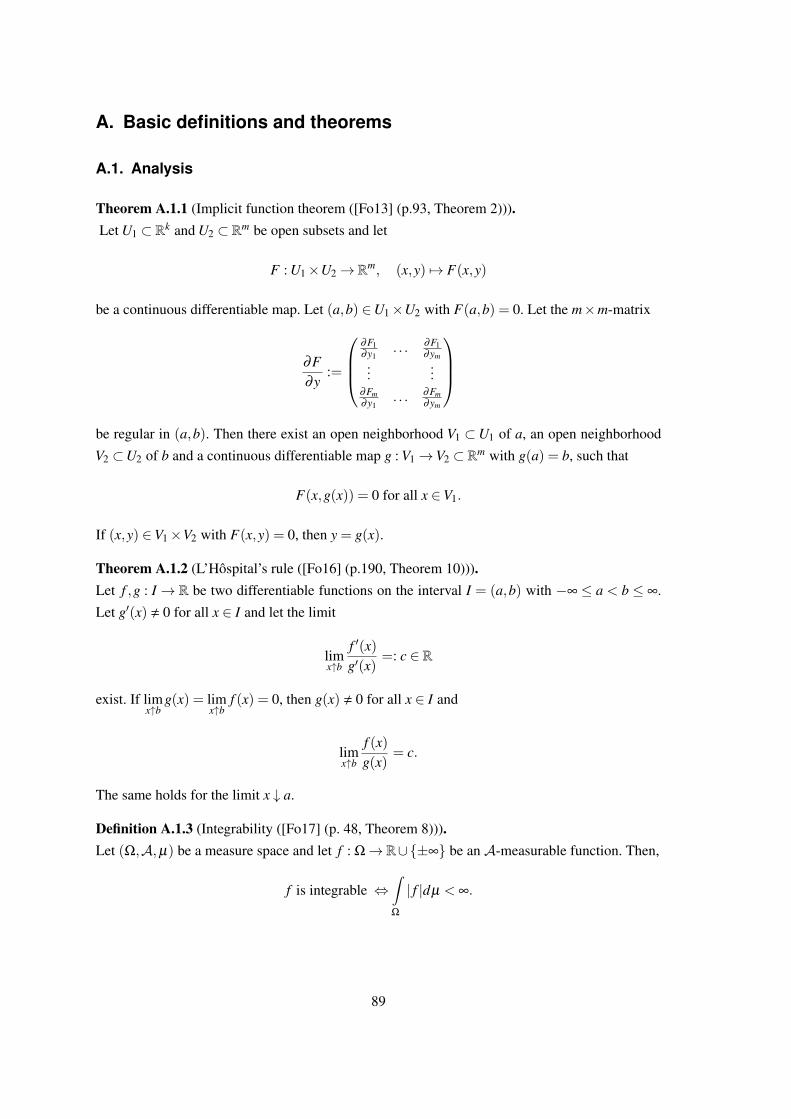
A. Basic definitions and theorems

A.1. Analysis

Theorem A.1.1 (Implicit function theorem ([Fo13] (p.93, Theorem 2))).Let U1 ⊂ Rk and U2 ⊂ Rm be open subsets and let

F : U1×U2→ Rm, (x,y) 7→ F(x,y)

be a continuous differentiable map. Let (a,b) ∈U1×U2 with F(a,b) = 0. Let the m×m-matrix

∂F∂y

:=

∂F1∂y1

. . . ∂F1∂ym

......

∂Fm∂y1

. . . ∂Fm∂ym

be regular in (a,b). Then there exist an open neighborhood V1 ⊂U1 of a, an open neighborhood

V2 ⊂U2 of b and a continuous differentiable map g : V1→V2 ⊂ Rm with g(a) = b, such that

F(x,g(x)) = 0 for all x ∈V1.

If (x,y) ∈V1×V2 with F(x,y) = 0, then y = g(x).

Theorem A.1.2 (L’Hospital’s rule ([Fo16] (p.190, Theorem 10))).Let f ,g : I→ R be two differentiable functions on the interval I = (a,b) with −∞ ≤ a < b ≤ ∞.

Let g′(x) , 0 for all x ∈ I and let the limit

limx↑b

f ′(x)g′(x)

=: c ∈ R

exist. If limx↑b

g(x) = limx↑b

f (x) = 0, then g(x) , 0 for all x ∈ I and

limx↑b

f (x)g(x)

= c.

The same holds for the limit x ↓ a.

Definition A.1.3 (Integrability ([Fo17] (p. 48, Theorem 8))).Let (Ω,A,µ) be a measure space and let f : Ω→ R∪±∞ be an A-measurable function. Then,

f is integrable ⇔∫Ω

| f |dµ < ∞.

89

Definition A.1.4 (Uniform convergence ([Fo13] (p.24))).Let X be a set, let Y be a metric space and let

fk : X → Y,k ∈ N, and f : X → Y

be maps. The series ( fk)k∈N converges uniformly towards f , if for every ε > 0, there exists an

N ∈ N such that

‖ fk(x), f (x)‖< ε for all x ∈ X and all k ≥ N.

Definition A.1.5 (Absolute convergence ([Fo16] (p.74))).A series

∞

∑k=0

ak is called absolutely convergent, if the series of the moduli∞

∑k=0|ak| converges.

Lemma A.1.6. ([Fo16] (p. 83, Theorem 1))

The power series exp(x) :=∞

∑k=0

xk

k! converges absolutely towards exp(x) for every x ∈ R.

Theorem A.1.7 (Interchange of summation and integration ([Re08] (p. 85, Theorem 8))).Let fk : [a,b]→ K be functions such that the limit

F(x) :=∞

∑k=0

fk(x) for all x ∈ [a,b]

exists. If all fk are integrable and if the sequence

n∑

k=0fk(x)

converges uniformly towards F(x),

thenb∫

a

F(x)dx =b∫

a

∞

∑k=0

fk(x)dx =∞

∑k=0

b∫a

fk(x)dx for all x ∈ [a,b].

Remark A.1.8.Let M ∈Rn×n,n∈N and fk := (Mθ)k

k! ,k ∈N. Since the exponential power series∞

∑k=0

fk is absolutely

convergent towards the exponential function (Lemma A.1.6), it is particularly locally uniformly

convergent in Ω := [0,1]. Furthermore the partial sums sn :=n∑

k=0fk are locally integrable in Ω.

Since all requirements of Theorem A.1.7 are met, we obtain

1∫0

eMθ dθ =

1∫0

∞

∑k=0

(Mθ)k

k!dθ =

∞

∑k=0

1∫0

(Mθ)k

k!dθ .

90

A.2. Linear Algebra

Definition A.2.1 (Jordan matrix ([Fi03] (p. 264, 4.6.5))).A matrix

Jk :=

0 1 0

. . .. . .

. . . 1

0 0

∈ Rk×k

is called Jordan matrix.

Lemma A.2.2 (Jordan normal form ([Fi03] (p.268))).Let A ∈ Rn×n such that the characteristic polynomial decomposes in linear factors

PA =±(λ −λ1)r1 · · · · · (λ −λk)

rk .

Then there exists a basis B of Rn×n, such that

MB(A) =

λ1Er1 + J1 0

. . .

0 λkErk + Jk

,

where Ji, i = 1, . . . ,k denotes a Jordan matrix.

Lemma A.2.3 (Matrix exponential ([Fi03] (pp. 272/3, Exercise 5))).Let A ∈ Rn×n.

exp(A) := limm→∞

m

∑k=0

1k!

Ak.

A.3. Numerical mathematics

Definition A.3.1 (Newton method ([DR06] (Theorem 5.22))).Let f : R→ R be twice continuously differentiable in a neighborhood U := (a,b) of a root x∗ of f

( f (x∗) = 0, f ′(x∗) , 0). Then, the classical Newton iteration is given by

xk+1 = xk−f (xk)

f ′(xk), k = 0,1,2, . . . .

Definition A.3.2 (Simplified Newton method ([DR06] (Section 5.6.2))).The simplified Newton iteration is given by

xk+1 = xk−f (xk)

f ′(x0), k = 0,1,2, . . . .

91

Remark A.3.3.Particularly for systems, the evaluation of the Jacobian matrix f ′(xk) in every iteration is expensive.

Hence for these systems, the simplified Newton method is preferred.

Definition A.3.4 (Classical 4th order Runge-Kutta method ([DR06] (Algorithm 11.28))).The classical 4th order Runge-Kutta method is given by the Butcher-Tableau

012

12

12 0 1

2

1 0 0 116

13

13

16

.

Definition A.3.5 (RMS error [GSJJ13]).Let N be the number of time steps executed by a numerical algorithm for the solution of ODEs.

Let x ∈ RN+1 denote the approximation vector and let x : R+→ R denote the analytical solution.

The root-mean-square (RMS) error is defined as

ε(x) :=

√√√√√√√N+1∑

k=0[xk− x(tk)]2

N+1∑

k=0[x(tk)]2

.

92

B. Minimal working example of a coupled index-1 system

This example shows how submodels can be chosen in a coupled dynamic system. Both the mono-

lithic and the coupled index-1 DAE system are provided. Let us consider two water containers (see

Figure B.1) which are interconnected by two pipes. The containers have water levels x1,x2 and an

amount y1 – which is a percentage α of x1 – continuously flows from container 1 to container 2,

whereas a pump pumps an amount y2 of water – which is a percentage β of the inflow y1 – back

to container 1.

Figure B.1: Example of two interconnected water containers (sketch by Melven Rohrig-Zollner)

Certainly this system is easily written as an ordinary differential equation:x1 = (βα−α)x1

x2 = (α−βα)x1. (B.2)

Prescribing initial conditions x1(0) = x01, x2(0) = x0

2, we can also easily compute the analytic

solution of system (B.2): x1(t) = x0

1e(βα−α)t

x2(t) = −x01e(βα−α)t + x0

1 + x02

. (B.3)

However for our purposes, we can also formulate it as an index-1 differential algebraic equation,

where each water container forms a submodel with a state, an input and an output:x1 = y2−αx1

x2 = y1−βy1

y1 = αx1(= u2)

y2 = βy1(= u1)

. (B.4)

93

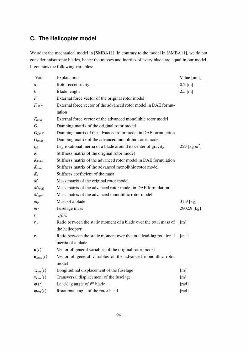
C. The Helicopter model

We adapt the mechanical model in [SMBA11]. In contrary to the model in [SMBA11], we do not

consider anisotropic blades, hence the masses and inertias of every blade are equal in our model.

It contains the following variables:

Var. Explanation Value [unit]

a Rotor eccentricity 0.2 [m]

b Blade length 2.5 [m]

F External force vector of the original rotor model

FDAE External force vector of the advanced rotor model in DAE formu-

lation

Fmon External force vector of the advanced monolithic rotor model

G Damping matrix of the original rotor model

GDAE Damping matrix of the advanced rotor model in DAE formulation

Gmon Damping matrix of the advanced monolithic rotor model

Izb Lag rotational inertia of a blade around its center of gravity 259 [kg m2]

K Stiffness matrix of the original rotor model

KDAE Stiffness matrix of the advanced rotor model in DAE formulation

Kmon Stiffness matrix of the advanced monolithic rotor model

Ks Stiffness coefficient of the mast

M Mass matrix of the original rotor model

MDAE Mass matrix of the advanced rotor model in DAE formulation

Mmon Mass matrix of the advanced monolithic rotor model

mb Mass of a blade 31.9 [kg]

m f Fuselage mass 2902.9 [kg]

ra√

arb

rm Ratio between the static moment of a blade over the total mass of

the helicopter

[m]

rb Ratio between the static moment over the total lead-lag rotational

inertia of a blade

[m−1]

u(t) Vector of general variables of the original rotor model

umon(t) Vector of general variables of the advanced monolithic rotor

model

xFus(t) Longitudinal displacement of the fuselage [m]

yFus(t) Transversal displacement of the fuselage [m]

ϕi(t) Lead-lag angle of ith blade [rad]

ϕRH(t) Rotational angle of the rotor head [rad]

94

ωb Lag resonance frequency of the a blade at Ω = 0 1.5 [Hz]

ωRH(t) Rotor head’s resonance frequency [Hz]

ωx Fuselage’s resonance frequency in x direction 3 [Hz]

ωy Fuselage’s resonance frequency in y direction 3 [Hz]

Ω Rotor speed [Hz]

Table C.1: Variables for the rotor model given in [SMBA11], Section 1.1 and Table 1

This section contains three parts. We first state the original model from [SMBA11] in Subsec-

tion C.1. In Subsection C.2, we present the advanced model in a monolithic form and subsequently

we deal with the advanced model in a DAE formulation in Subsection C.3.

C.1. Original model

The matrices of the original model are

M =

1 0 −rm sin(Ωt) −rm cos(Ωt) rm sin(Ωt) rm cos(Ωt)

0 1 rm cos(Ωt) −rm sin(Ωt) −rm cos(Ωt) rm sin(Ωt)

−rb sin(Ωt) rb cos(Ωt) 1 0 0 0

−rb cos(Ωt) −rb sin(Ωt) 0 1 0 0

rb sin(Ωt) −rb cos(Ωt) 0 0 1 0

rb cos(Ωt) rb sin(Ωt) 0 0 0 1

,

G =

0 0 −2rmΩcos(Ωt) 2rmΩsin(Ωt) 2rmΩcos(Ωt) −2rmΩsin(Ωt)

0 0 −2rmΩsin(Ωt) −2rmΩcos(Ωt) 2rmΩsin(Ωt) 2rmΩcos(Ωt)

0 0 0 0 0 0 0

0 0 0 0 0 0 0

0 0 0 0 0 0 0

0 0 0 0 0 0 0

0 0 0 0 0 0 0

,

K =

ω2x 0 Ω2rm sin(Ωt) Ω2rm cos(Ωt) −Ω2rm sin(Ωt) −Ω2rm cos(Ωt)

0 ω2y −Ω2rm cos(Ωt) Ω2rm sin(Ωt) Ω2rm cos(Ωt) −Ω2rm sin(Ωt)

0 0 Ω2arb +ω2b 0 0 0

0 0 0 Ω2arb +ω2b 0 0

0 0 0 0 Ω2arb +ω2b 0

0 0 0 0 0 Ω2arb +ω2b

95

and

F =

0

0

0

0

0

0

.

The model with

u(t) = (xFus(t),yFus(t),ϕ1(t),ϕ2(t),ϕ3(t),ϕ4(t))T

reads

Mu(t)+Gu(t)+Ku(t) = F. (C.1.1)

With

v(t) := (xFus(t), yFus(t), ϕ1(t), ϕ2(t), ϕ3(t), ϕ4(t))T ,

we transform system (C.1.1) into a first order system in the variables u(t) and v(t)u(t) = v(t)v(t) = −M−1Gv(t)−M−1Ku(t)+M−1F.

C.2. Advanced model in monolithic form

In the advanced model, we have additional springs at both ends of the mast that connects the fuse-

lage with the rotor. We need additional constants and variables to model the occurring behavior.

Let

• Ks denote the stiffness coefficient of the mast

• ϕRH(t) denote the rotational angle of the rotor head.

Then we define

ωi(t) := ϕi(t), i = 1, . . . ,4,

ωRH(t) := ϕRH(t),

αRH(t) := ωRH(t),

ωs :=

√Ks

4(a+b)2mb +4Izb, (C.2.1)

rsb :=b(a+b)mb + Izb

4(a+b)2mb +4Izb. (C.2.2)

96

The model matrices become

Mmon =

1 0 −rm sin(ϕRH(t)) −rm cos(ϕRH(t)) rm sin(ϕRH(t))

0 1 rm cos(ϕRH(t)) −rm sin(ϕRH(t)) −rm cos(ϕRH(t))

−rb sin(ϕRH(t)) rb cos(ϕRH(t)) 1 0 0

−rb cos(ϕRH(t)) −rb sin(ϕRH(t)) 0 1 0

rb sin(ϕRH(t)) −rb cos(ϕRH(t)) 0 0 1

rb cos(ϕRH(t)) rb sin(ϕRH(t)) 0 0 0

0 0 rsb rsb rsb

rm cos(ϕRH(t)) −rm((ϕ1(t)−ϕ3(t))cos(ϕRH(t))−sin(ϕRH(t))(ϕ2(t)−ϕ4(t)))

rm sin(ϕRH(t)) −rm((ϕ2(t)−ϕ4(t))cos(ϕRH(t))+sin(ϕRH(t))(ϕ1(t)−ϕ3(t)))

0 r2a+1

0 r2a+1

0 r2a+1

1 r2a+1

rsb 1

,

(C.2.3)

Gmon =

0 0 0 0 0 0 0

0 0 0 0 0 0 0

0 0 0 0 0 0 0

0 0 0 0 0 0 0

0 0 0 0 0 0 0

0 0 0 0 0 0 0

0 0 0 0 0 0 0

, (C.2.4)

and

Kmon =

ω2x 0 0 0 0 0 0

0 ω2y 0 0 0 0 0

0 0 r2aω2

RH(t)+ω2b 0 0 0 0

0 0 0 r2aω2

RH(t)+ω2b 0 0 0

0 0 0 0 r2aω2

RH(t)+ω2b 0 0

0 0 0 0 0 r2aω2

RH(t)+ω2b 0

0 0 0 0 0 0 ω2s

. (C.2.5)

With ϕ2,4 = ϕ2(t)−ϕ4(t), ϕ3,1 = ϕ3(t)−ϕ1(t), ϕRH := ϕRH(t) ωRH := ωRH(t) and ωi := ωi(t),

97

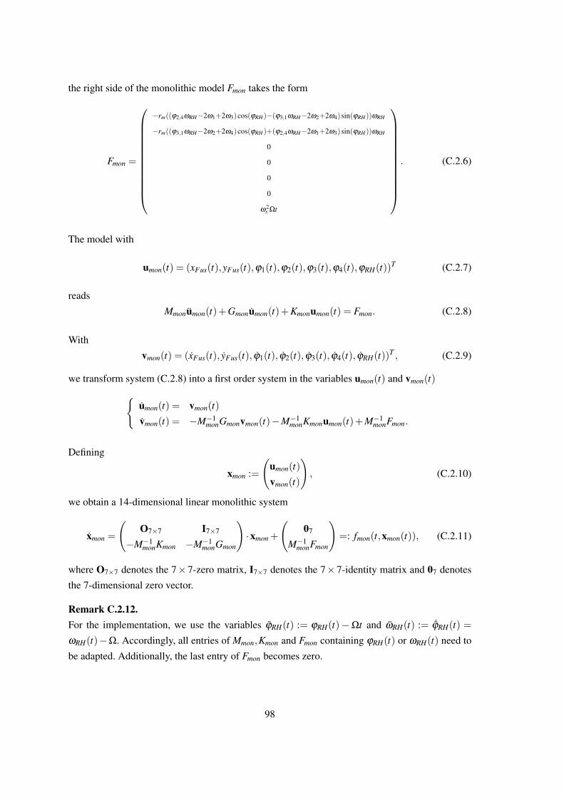
the right side of the monolithic model Fmon takes the form

Fmon =

−rm((ϕ2,4ωRH−2ω1+2ω3)cos(ϕRH)−(ϕ3,1ωRH−2ω2+2ω4)sin(ϕRH))ωRH

−rm((ϕ3,1ωRH−2ω2+2ω4)cos(ϕRH)+(ϕ2,4ωRH−2ω1+2ω3)sin(ϕRH))ωRH

0

0

0

0

ω2s Ωt

. (C.2.6)

The model with

umon(t) = (xFus(t),yFus(t),ϕ1(t),ϕ2(t),ϕ3(t),ϕ4(t),ϕRH(t))T (C.2.7)

reads

Mmonumon(t)+Gmonumon(t)+Kmonumon(t) = Fmon. (C.2.8)

With

vmon(t) = (xFus(t), yFus(t), ϕ1(t), ϕ2(t), ϕ3(t), ϕ4(t), ϕRH(t))T , (C.2.9)

we transform system (C.2.8) into a first order system in the variables umon(t) and vmon(t)umon(t) = vmon(t)

vmon(t) = −M−1monGmonvmon(t)−M−1

monKmonumon(t)+M−1monFmon.

Defining

xmon :=

(umon(t)

vmon(t)

), (C.2.10)

we obtain a 14-dimensional linear monolithic system

xmon =

(O7×7 I7×7

−M−1monKmon −M−1

monGmon

)·xmon +

(07

M−1monFmon

)=: fmon(t,xmon(t)), (C.2.11)

where O7×7 denotes the 7×7-zero matrix, I7×7 denotes the 7×7-identity matrix and 07 denotes

the 7-dimensional zero vector.

Remark C.2.12.For the implementation, we use the variables ϕRH(t) := ϕRH(t)−Ωt and ωRH(t) := ˙ϕRH(t) =

ωRH(t)−Ω. Accordingly, all entries of Mmon,Kmon and Fmon containing ϕRH(t) or ωRH(t) need to

be adapted. Additionally, the last entry of Fmon becomes zero.

98

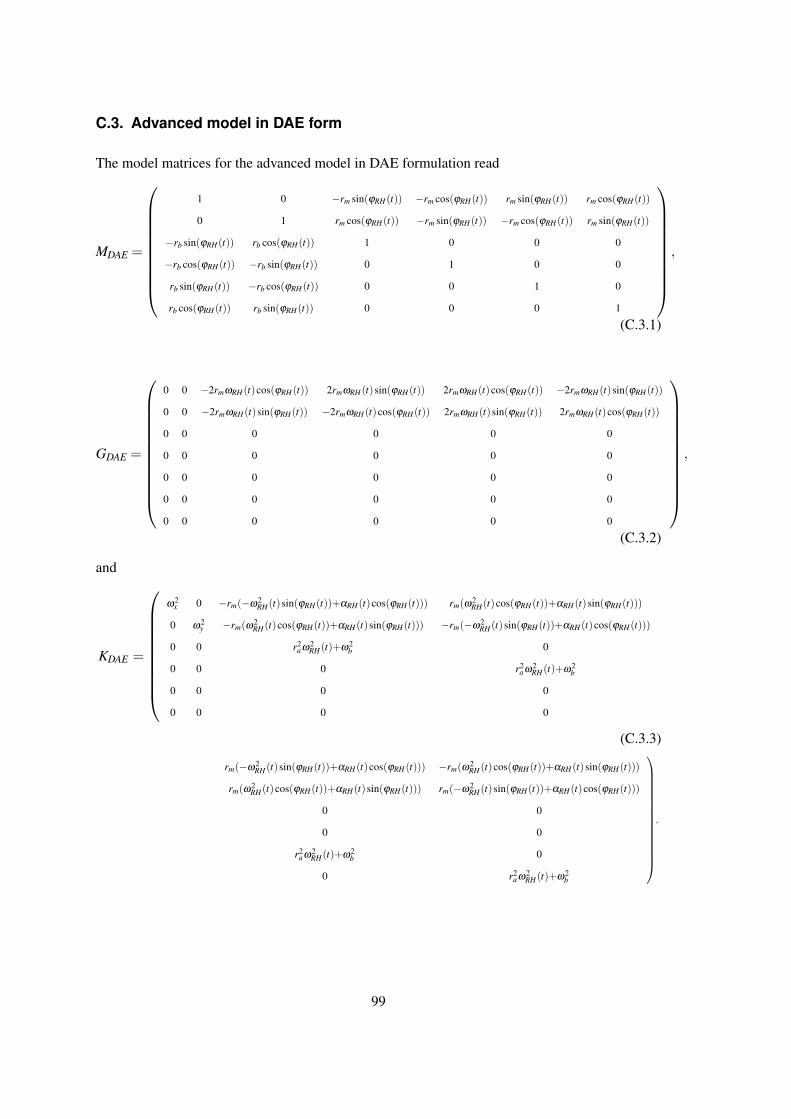
C.3. Advanced model in DAE form

The model matrices for the advanced model in DAE formulation read

MDAE =

1 0 −rm sin(ϕRH(t)) −rm cos(ϕRH(t)) rm sin(ϕRH(t)) rm cos(ϕRH(t))

0 1 rm cos(ϕRH(t)) −rm sin(ϕRH(t)) −rm cos(ϕRH(t)) rm sin(ϕRH(t))

−rb sin(ϕRH(t)) rb cos(ϕRH(t)) 1 0 0 0

−rb cos(ϕRH(t)) −rb sin(ϕRH(t)) 0 1 0 0

rb sin(ϕRH(t)) −rb cos(ϕRH(t)) 0 0 1 0

rb cos(ϕRH(t)) rb sin(ϕRH(t)) 0 0 0 1

,

(C.3.1)

GDAE =

0 0 −2rmωRH(t)cos(ϕRH(t)) 2rmωRH(t)sin(ϕRH(t)) 2rmωRH(t)cos(ϕRH(t)) −2rmωRH(t)sin(ϕRH(t))

0 0 −2rmωRH(t)sin(ϕRH(t)) −2rmωRH(t)cos(ϕRH(t)) 2rmωRH(t)sin(ϕRH(t)) 2rmωRH(t)cos(ϕRH(t))

0 0 0 0 0 0

0 0 0 0 0 0

0 0 0 0 0 0

0 0 0 0 0 0

0 0 0 0 0 0

,

(C.3.2)

and

KDAE =

ω2x 0 −rm(−ω2

RH(t)sin(ϕRH(t))+αRH(t)cos(ϕRH(t))) rm(ω2RH(t)cos(ϕRH(t))+αRH(t)sin(ϕRH(t)))

0 ω2y −rm(ω

2RH(t)cos(ϕRH(t))+αRH(t)sin(ϕRH(t))) −rm(−ω2

RH(t)sin(ϕRH(t))+αRH(t)cos(ϕRH(t)))

0 0 r2aω2

RH(t)+ω2b 0

0 0 0 r2aω2

RH(t)+ω2b

0 0 0 0

0 0 0 0

(C.3.3)

rm(−ω2RH(t)sin(ϕRH(t))+αRH(t)cos(ϕRH(t))) −rm(ω

2RH(t)cos(ϕRH(t))+αRH(t)sin(ϕRH(t)))

rm(ω2RH(t)cos(ϕRH(t))+αRH(t)sin(ϕRH(t))) rm(−ω2

RH(t)sin(ϕRH(t))+αRH(t)cos(ϕRH(t)))

0 0

0 0

r2aω2

RH(t)+ω2b 0

0 r2aω2

RH(t)+ω2b

.

99

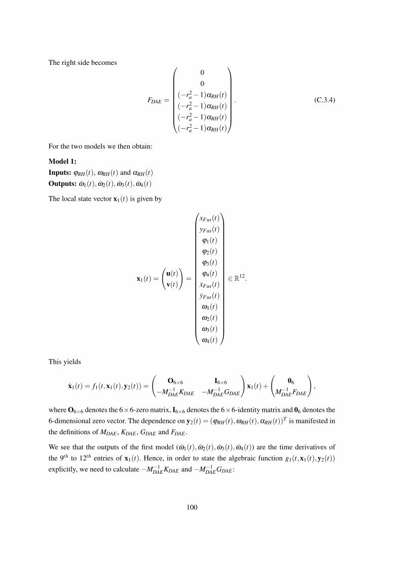
The right side becomes

FDAE =

0

0

(−r2a−1)αRH(t)

(−r2a−1)αRH(t)

(−r2a−1)αRH(t)

(−r2a−1)αRH(t)

. (C.3.4)

For the two models we then obtain:

Model 1:Inputs: ϕRH(t), ωRH(t) and αRH(t)

Outputs: ω1(t), ω2(t), ω3(t), ω4(t)

The local state vector x1(t) is given by

x1(t) =

(u(t)v(t)

)=

xFus(t)

yFus(t)

ϕ1(t)

ϕ2(t)

ϕ3(t)

ϕ4(t)

xFus(t)

yFus(t)

ω1(t)

ω2(t)

ω3(t)

ω4(t)

∈ R12.

This yields

x1(t) = f1(t,x1(t),y2(t)) =

(O6×6 I6×6

−M−1DAEKDAE −M−1

DAEGDAE

)x1(t)+

(06

M−1DAEFDAE

),

where O6×6 denotes the 6×6-zero matrix, I6×6 denotes the 6×6-identity matrix and 06 denotes the

6-dimensional zero vector. The dependence on y2(t) = (ϕRH(t),ωRH(t),αRH(t))T is manifested in

the definitions of MDAE , KDAE , GDAE and FDAE .

We see that the outputs of the first model (ω1(t), ω2(t), ω3(t), ω4(t)) are the time derivatives of

the 9th to 12th entries of x1(t). Hence, in order to state the algebraic function g1(t,x1(t),y2(t))

explicitly, we need to calculate −M−1DAEKDAE and −M−1

DAEGDAE :

100

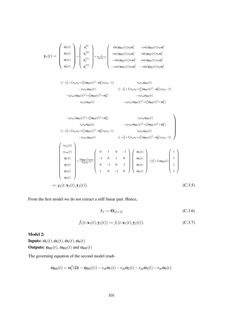
y1(t) =

ω1(t)

ω2(t)

ω3(t)

ω4(t)

=

x(9)1

x(10)1

x(11)1

x(12)1

= 1

2rbrm−1

sin(ϕRH(t))rbω2x −cos(ϕRH(t))rbω2

y

cos(ϕRH(t))rbω2x sin(ϕRH(t))rbω2

y

−sin(ϕRH(t))rbω2x cos(ϕRH(t))rbω2

y

−cos(ϕRH(t))rbω2x −sin(ϕRH(t))rbω2

y

((−r2a+1)rmrb+r2

a)ωRH(t)2−ω2b (rbrm−1) rbrmαRH(t)

−rbrmαRH(t) ((−r2a+1)rmrb+r2

a)ωRH(t)2−ω2b (rbrm−1)

−rbrm(ωRH(t)2+r2aωRH(t)2+ω2

b ) −rbrmαRH(t)

rbrmαRH(t) −rbrm(ωRH(t)2+r2aωRH(t)2+ω2

b )

−rbrm(ωRH(t)2+r2aωRH(t)2+ω2

b ) −rbrmαRH(t)

rbrmαRH(t) −rbrm(ωRH(t)2+r2aωRH(t)2+ω2

b )

((−r2a+1)rmrb+r2

a)ωRH(t)2−ω2b (rbrm−1) rbrmαRH(t)

−rbrmαRH(t) ((−r2a+1)rmrb+r2

a)ωRH(t)2−ω2b (rbrm−1)

·

xFus(t)

yFus(t)

ϕ1(t)

ϕ2(t)

ϕ3(t)

ϕ4(t)

+

2ωRH (t)rbrm2rbrm−1

0 1 0 −1

−1 0 1 0

0 −1 0 1

1 0 −1 0

·

ω1(t)

ω2(t)

ω3(t)

ω4(t)

−(r2

a+1)αRH(t)

1

1

1

1

=: g1(t,x1(t),y2(t)). (C.3.5)

From the first model we do not extract a stiff linear part. Hence,

S1 := O12×12 (C.3.6)

f1(t,x1(t),y2(t)) := f1(t,x1(t),y2(t)). (C.3.7)

Model 2:Inputs: ω1(t), ω2(t), ω3(t), ω4(t)

Outputs: ϕRH(t), ωRH(t) and αRH(t)

The governing equation of the second model reads

ωRH(t) = ω2s (Ωt−ϕRH(t))− rsbω1(t)− rsbω2(t)− rsbω3(t)− rsbω4(t).

101

With the local state vector

x2(t) :=

(ϕRH(t)

ωRH(t)

)∈ R2,

this yields

x2(t) =

(0 1

−ω2s 0

)x2(t)+

(0

ω2s Ωt− rsbω1(t)− rsbω2(t)− rsbω3(t)− rsbω4(t)

).

Since ω2s is the variable which is responsible for the stiffness of the system, we want it to be solely

part of the first linear summand of the differential equations system. Hence we define

x(1)2 := ϕRH(t) := ϕRH(t)−Ωt,

x(2)2 := ωRH(t) := ˙ϕRH(t) = ϕRH(t)−Ω,

which yields

x2(t) =

(0 1

−ω2s 0

)x2(t)+

(0

−rsbω1(t)− rsbω2(t)− rsbω3(t)− rsbω4(t)

).

Accordingly, we define

S2 :=

(0 1

−ω2s 0

)(C.3.8)

and

f2(t,x2(t),y1(t)) :=

(0

−rsbω1(t)− rsbω2(t)− rsbω3(t)− rsbω4(t)

). (C.3.9)

The local output vector and hence the local output function g2(t,x2(t),y1(t)) is given by

y2(t) =

ϕRH(t)

ωRH(t)

αRH(t)

=

x(1)2 (t)+Ωt

x(2)2 (t)+Ω

x(2)2 (t)

=

x(1)2 (t)+Ωt

x(2)2 (t)+Ω

−ω2s x(1)2 (t)− rsbω1(t)− rsbω2(t)− rsbω3(t)− rsbω4(t)

=: g2(t,x2(t),y1(t)).

102

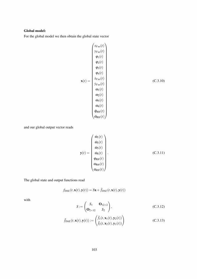
Global model:For the global model we then obtain the global state vector

x(t) =

xFus(t)

yFus(t)

ϕ1(t)

ϕ2(t)

ϕ3(t)

ϕ4(t)

xFus(t)

yFus(t)

ω1(t)

ω2(t)

ω3(t)

ω4(t)

ϕRH(t)

ωRH(t)

(C.3.10)

and our global output vector reads

y(t) =

ω1(t)

ω2(t)

ω3(t)

ω4(t)

ϕRH(t)

ωRH(t)

αRH(t)

. (C.3.11)

The global state and output functions read

fDAE(t,x(t),y(t)) = Sx+ fDAE(t,x(t),y(t))

with

S :=

(S1 O12×2

O2×12 S2

), (C.3.12)

fDAE(t,x(t),y(t)) :=

(f1(t,x1(t),y2(t))

f2(t,x2(t),y1(t))

)(C.3.13)

103

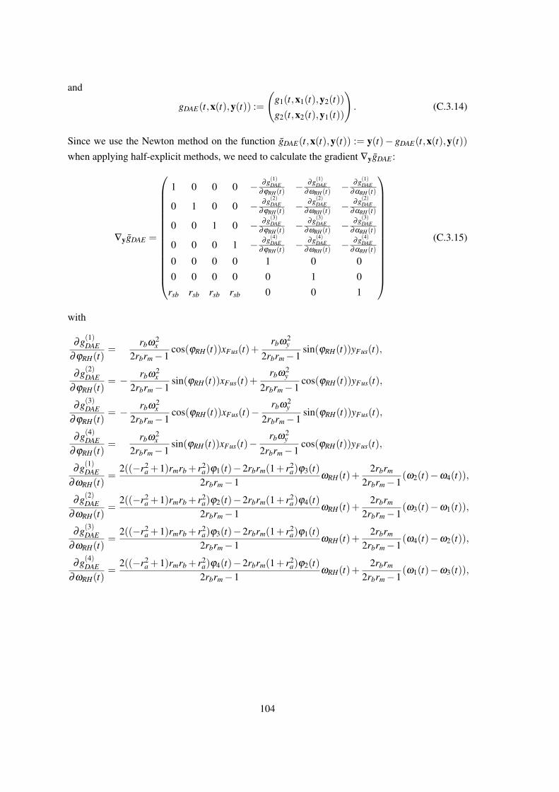
and

gDAE(t,x(t),y(t)) :=

(g1(t,x1(t),y2(t))

g2(t,x2(t),y1(t))

). (C.3.14)

Since we use the Newton method on the function gDAE(t,x(t),y(t)) := y(t)− gDAE(t,x(t),y(t))when applying half-explicit methods, we need to calculate the gradient ∇ygDAE :

∇ygDAE =

1 0 0 0 − ∂g(1)DAE∂ϕRH(t)

− ∂g(1)DAE∂ωRH(t)

− ∂g(1)DAE∂αRH(t)

0 1 0 0 − ∂g(2)DAE∂ϕRH(t)

− ∂g(2)DAE∂ωRH(t)

− ∂g(2)DAE∂αRH(t)

0 0 1 0 − ∂g(3)DAE∂ϕRH(t)

− ∂g(3)DAE∂ωRH(t)

− ∂g(3)DAE∂αRH(t)

0 0 0 1 − ∂g(4)DAE∂ϕRH(t)

− ∂g(4)DAE∂ωRH(t)

− ∂g(4)DAE∂αRH(t)

0 0 0 0 1 0 0

0 0 0 0 0 1 0

rsb rsb rsb rsb 0 0 1

(C.3.15)

with

∂g(1)DAE∂ϕRH(t)

=rbω2

x

2rbrm−1cos(ϕRH(t))xFus(t)+

rbω2y

2rbrm−1sin(ϕRH(t))yFus(t),

∂g(2)DAE∂ϕRH(t)

= − rbω2x

2rbrm−1sin(ϕRH(t))xFus(t)+

rbω2y

2rbrm−1cos(ϕRH(t))yFus(t),

∂g(3)DAE∂ϕRH(t)

= − rbω2x

2rbrm−1cos(ϕRH(t))xFus(t)−

rbω2y

2rbrm−1sin(ϕRH(t))yFus(t),

∂g(4)DAE∂ϕRH(t)

=rbω2

x

2rbrm−1sin(ϕRH(t))xFus(t)−

rbω2y

2rbrm−1cos(ϕRH(t))yFus(t),

∂g(1)DAE∂ωRH(t)

=2((−r2

a +1)rmrb + r2a)ϕ1(t)−2rbrm(1+ r2

a)ϕ3(t)2rbrm−1

ωRH(t)+2rbrm

2rbrm−1(ω2(t)−ω4(t)),

∂g(2)DAE∂ωRH(t)

=2((−r2

a +1)rmrb + r2a)ϕ2(t)−2rbrm(1+ r2

a)ϕ4(t)2rbrm−1

ωRH(t)+2rbrm

2rbrm−1(ω3(t)−ω1(t)),

∂g(3)DAE∂ωRH(t)

=2((−r2

a +1)rmrb + r2a)ϕ3(t)−2rbrm(1+ r2

a)ϕ1(t)2rbrm−1

ωRH(t)+2rbrm

2rbrm−1(ω4(t)−ω2(t)),

∂g(4)DAE∂ωRH(t)

=2((−r2

a +1)rmrb + r2a)ϕ4(t)−2rbrm(1+ r2

a)ϕ2(t)2rbrm−1

ωRH(t)+2rbrm

2rbrm−1(ω1(t)−ω3(t)),

104

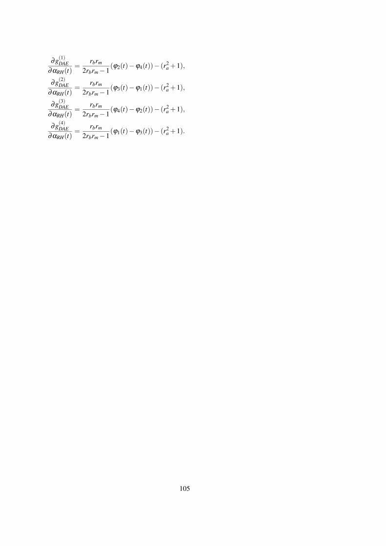
∂g(1)DAE∂αRH(t)

=rbrm

2rbrm−1(ϕ2(t)−ϕ4(t))− (r2

a +1),

∂g(2)DAE∂αRH(t)

=rbrm

2rbrm−1(ϕ3(t)−ϕ1(t))− (r2

a +1),

∂g(3)DAE∂αRH(t)

=rbrm

2rbrm−1(ϕ4(t)−ϕ2(t))− (r2

a +1),

∂g(4)DAE∂αRH(t)

=rbrm

2rbrm−1(ϕ1(t)−ϕ3(t))− (r2

a +1).

105

D. Matlab Code remarks

In order to simplify the Matlab code for the stability plots in Subsection 2.3.5, we derive the

general form of a stability function of explicit s-stage exponential Runge-Kutta methods. We con-

sider one-dimensional problems for the plots. Since we only consider explicit methods up to or-

der 4 (5 stages), we can simply insert the explicit equations for the Fni (as in (2.3.14)) directly

(ai j := ai j(hσ) ∈ R):

Fn1 = λ︸︷︷︸=:ξ1

xn,

Fn2 = λ (xn +ha21(Fn1 +σxn))

= λ (xn +ha21(ξ1xn +σxn))

= λ +λha21(ξ1 +σ)︸ ︷︷ ︸=:ξ2

xn,

Fn3 = λ (xn +h[a31(Fn1 +σxn)+a32(Fn2 +σxn))])

= λ (xn +h[a31(ξ1xn +σxn)+a32(ξ2xn +σxn)])

= λ +λha31(ξ1 +σ)+λha32(ξ2 +σ)︸ ︷︷ ︸=:ξ3

xn,

Fn4 = λ (xn +h[a41(Fn1 +σxn)+a42(Fn2 +σxn)+a43(Fn3 +σxn)])

= λ (xn +h[a41(ξ1xn +σxn)+a42(ξ2xn +σxn)+a43(ξ3xn +σxn)])

= λ +λha41(ξ1 +σ)+λha42(ξ2 +σ)+λha43(ξ3 +σ)︸ ︷︷ ︸=:ξ4

xn,

Fn5 = λ (xn +h[a51(Fn1 +σxn)+a52(Fn2 +σxn)+a53(Fn3 +σxn)+a54(Fn4 +σxn)])

= λ (xn +h[a51(ξ1xn +σxn)+a52(ξ2xn +σxn)+a53(ξ3xn +σxn)

+a54(ξ4xn +σxn)])

= λ +λha51(ξ1 +σ)+λha52(ξ2 +σ)+λha53(ξ3 +σ)+λha54(ξ4 +σ)︸ ︷︷ ︸=:ξ5

xn.

In general, for explicit methods, we can compute ξi as

ξi = λ +i−1

∑j=1

λhai j(ξ j +σ). (D.1)

So, short with the above definitions:

Fni = ξixn. (D.2)

106

Hence, inserting (D.2) into (2.3.7a), we obtain

xn+1 = xn +hs

∑i=1

bi(hσ)(Fni +σxn)

= xn +hs

∑i=1

bi(hσ)(ξixn +σxn)

=

[1+h

s

∑i=1

bi(hσ)(ξi +σ)

]xn.

So, the stability function for an explicit s-stage exponential Runge-Kutta method reads

φ = 1+hs

∑i=1

bi(hσ)(ξi +σ). (D.3)

107

References

[AHMEC] American Helicopter Museum & Education Center, History of he-

licopters, available from http://americanhelicopter.museum/

exhibits-and-resources/history-helicopters (29.03.2017).

[ARW93] Ascher, U. M., Ruuth, S. J., Wetton, B. T. R., Implicit-explicit methods for time-

dependent PDE’s, University of British Columbia, Department of Computer Sci-

ence, 1993.

[ASW93] Arnold, M., Strehmel, K., Weiner, R., Half-explicit Runge-Kutta methods for semi-

explicit differential-algebraic equations of index 1, Numerische Mathematik, Vol-

ume 64, Issue 1, pp. 409–431, 1993.

[BFR16] Boscarino, S., Filbet, F., Russo, G., High order semi-implicit schemes for time de-

pendent partial differential equations, Journal of Scientific Computing, Volume 68,

Issue 3, pp. 1–27, 2016.

[Bi09] Bittner, W., Flugmechanik der Hubschrauber: Technologie, das flugdynamische

System Hubschrauber, Flugstabilitaten, Steuerbarkeit, Springer Science & Business

Media, 2009.

[BK93] Bauchau, O. A., Kang, N. K., A multibody formulation for helicopter structural dy-

namic analysis, Journal of the American Helicopter Society, Volume 38, Issue 2,

pp. 3–14, 1993.

[BKV98] Beylkin, G., Keiser, J. M., Vozovoi, L., A new class of time discretization schemes

for the solution of nonlinear PDEs, Journal of Computational Physics, Volume 147,

Issue 2, pp. 362–387, 1998.

[BKMS17] Bab, S., Khadem, S. E., Mahdiabadi, M. K., Shahgholi, M., Vibration mitigation of

a rotating beam under external periodic force using a nonlinear energy sink (NES),

Journal of Vibration and Control, Volume 23, Issue 6, pp. 1001–1025, 2017.

[BN01] Bachau, O. A., Nikishkov, Y. G., An implicit Floquet analysis for rotorcraft stability

evaluation, Journal of the American Helicopter Society, Volume 46, Issue 3, pp

200–209, 2001.

[Bo07] Boscarino, S., Error analysis of IMEX Runge-Kutta methods derived from

differential-algebraic systems, SIAM Journal on Numerical Analysis, Volume 45,

Issue 4, pp. 1600–1621, 2007.

[Br01] Bramwell, A. R. S., Done, G., Balmford, D., Bramwell’s Helicopter Dynamics,

Butterworth-Heinemann, 2nd edition, 2001.

109

[BR09] Boscarino, S., Russo, G., On a class of uniformily accurate IMEX Runge-Kutta

schemes and applications to hyperbolic systems with relaxation, SIAM Journal on

Scientific Computing, Volume 31, Issue 3, pp. 1926–1945, 2009.

[BT99] Bendtsen, C., Thomsen, P. G., Numerical solution of differential algebraic equa-

tions, IMM, Department of Mathematical Modeling, Technical University of Den-

mark, 1999.

[Bu96] Butcher, J. C., A history of Runge-Kutta methods, Applied Numerical Mathematics,

Volume 20, Issue 3, pp. 247–260, 1996.

[BW96] Butcher, J. C., Wanner, G., Runge-Kutta methods: some historical notes, Applied

Numerical Mathematics, Volume 22, Issues 1–3, pp. 113–151, 1996.

[BW10] Bachau, O. A., Wang, J., Efficient and robust approaches for rotorcraft stability

analysis, Journal of the American Helicopter Society, Volume 55, Issue 3, pp.

32006-1–32006-9, 2010.

[CFN01] Calvo, M. P., De Frutos, J., Novo, J., Linearly implicit Runge-Kutta methods for

advection-reaction-diffusion equations, Applied Numerical Mathematics, Volume

37, Issue 4, pp. 535–549, 2001.

[CH52] Curtiss, C. F., Hirschfelder, J. O., Integration of stiff equations, Proceedings of the

National Academy of Sciences, Volume 38, Issue 3, pp. 235–243, 1952.

[CM02] Cox, S. M., Matthews, P. C., Exponential time differencing for stiff systems, Journal

of Computational Physics, Volume 176, Issue 2, pp. 430–455, 2002.

[DB08] Deuflhard, P., Bornemann, F., Numerische Mathematik 2 - Gewohnliche Differen-

tialgleichungen, 3. Auflage, De Gruyter, 2008.

[DR06] Dahmen, W., Reusken, A., Numerik fur Ingenieure und Naturwissenschaftler,

Springer-Verlag, 2006.

[FD99] Fornberg, B., Driscoll, T. A., A fast spectral algorithm for nonlinear wave equations

with linear dispersion, Journal of Computational Physics, Volume 155, Issue 2, pp.

456–467, 1999.

[Fi03] Fischer, G., Lineare Algebra, Friedr. Vieweg & Sohn Verlag, 14. Auflage, 2003.

[Fo13] Forster, O., Analysis 2, Springer, 10. Auflage, 2013.

[Fo16] Forster, O., Analysis 1, Springer, 12. Auflage, 2016.

[Fo17] Forster, O., Analysis 3, Springer, 8. Auflage, 2017.

[Fr86] Friedmann, P. P., Numerical methods for determining the stability and response of

periodic systems with applications to helicopter rotor dynamics and aeroelasticity,

110

Computers and Mathematics with Applications, Volume 12, Issue 1, pp. 131–148,

1986.

[Fr08] Frank, J., Numerical modelling of dynamical systems, Centrum Wiskunde & In-

formatica (CWI), Lecture notes, Chapter 10 (Stability), available from http:

//www.staff.science.uu.nl/˜frank011/Classes/numwisk/ (23.11.2016),

2008.

[GSJJ13] Gasmi, A., Sprague, M., Jonkman, J., Jones, W., Numerical stability and accu-

racy of temporally coupled multi-physics modules in wind turbine CAE tools,

51st AIAA Aerospace Sciences Meeting including the New Horizons Forum and

Aerospace Exposition, 2013.

[GW08] Griewank, A., Walther, A., Evaluating derivatives: principles and techniques of al-

gorithmic differentiation, Society for Industrial and Applied Mathematics, 2nd edi-

tion, 2008.

[HLR89] Hairer, E., Lubich, C., Roche, M., The numerical solution of differential-algebraic

systems by Runge-Kutta methods, Springer-Verlag, 1989.

[HO05a] Hochbruck, M., Ostermann, A., Explicit exponential Runge-Kutta methods for

semilinear parabolic problems, SIAM Journal on Numerical Analysis, Volume 43,

Issue 3, pp. 1069–1090, 2005.

[HO05b] Hochbruck, M., Ostermann, A., Exponential Runge-Kutta methods for parabolic

problems, Applied Numerical Mathematics, Volume 53, Issues 2-4, pp. 323–339,

2005.

[HO10] Hochbruck, M., Ostermann, A., Exponential integrators, Acta Numerica, Volume

19, pp. 209–286, 2010.

[HR07] Hundsdorfer, W., Ruuth, S. J., IMEX extensions of linear multistep methods

with general monotonicity and boundedness properties, Journal of Computational

Physics, Volume 225, Issue 2, pp. 2016–2042, 2007.

[HSAT16] Helicopter Safety Analysis Team of IHSTI-CIS, Helicopter accidents: statistics,

trends and causes, Presentation slides for IHST Regional Partners Panel, Louisville,

Kentucky, USA, 2016.

[HW96] Hairer, E., Wanner, G., Solving ordinary differential equations II. Stiff and

differential-algebraic problems, Springer-Verlag, second revised edition, 1996.

[Jo12] Johnson, W., Helicopter theory, Courier Corporation, 2012.

[Jo13] Johnson, W., A history of rotorcraft comprehensive analyses, NASA Ames Re-

search Center, 2013.

111

[Ko08] Koto, T., Stability of IMEX Runge-Kutta methods for delay differential equations,

Journal of Computational and Applied Mathematics, Volume 211, Issue 2, pp. 201–

212, 2008.

[Ku13] Kunoth, A., Numerik II - Wissenschaftliches Rechnen I, Vorlesungsskript, Univer-

sitat zu Koln, Wintersemester 2013/14.

[La73] Lambert, J. D., Computational methods in ordinary differential equations, John Wi-

ley & Sons, 1973.

[La91] Lambert, J. D., Numerical methods for ordinary differential systems: the initial

value problem, John Wiley & Sons, 1991.

[MZ09] Maset, S., Zennaro, M., Unconditional stability of explicit exponential Runge-Kutta

methods for semilinear ordinary differential equations, Mathematics of Computa-

tion, Volume 78, Issue 266, pp. 957–967, 2009.

[MZ13] Maset, S., Zennaro, M., Stability properties of explicit exponential Runge-Kutta

methods, IMA Journal of Numerical Analysis, Volume 33, Issue 1, pp. 111–135,

2013.

[OP16] Owolabi, K. M., Patidar, K. C., Numerical simulations of multicomponent ecologi-

cal models with adaptive methods, Theoretical Biology & Medical Modelling, Vol-

ume 13, Issue 1, doi: 10.1186/s12976-016-0027-4, 2016.

[Pa07] Padfield, G. D., Helicopter flight dynamics, Blackwell Publishing, 2007.

[Pe94] Peters, D. A., Fast Floquet Theory and Trim for Multi-Bladed Rotorcraft, Journal

of the American Helicopter Society, Volume 39, Issue 4, pp. 82–89, 1994.

[Re08] Reinhardt, H.-J., Arbeitsmaterialien Analysis I + II, Lecture notes, University

Siegen, 2007&2008.

[RKM] No author, Runge-Kutta Methods, available from http://web.mit.

edu/course/16/16.90/OldFiles/BackUp/www/pdfs/Chapter10.pdf

(16.02.2017), no date.

[Ru08] Rump, W., Lecture HM III for aer, autip, verf, wewi, (folien Jan13) avail-

able from http://www.mathematik.uni-stuttgart.de/studium/infomat/

HM-Rump-WS0708/Folien/ (16.02.2017), winter term 2007/8.

[SN11] Seddon, J. M., Newman, S., Basic helicopter aerodynamics, John Wiley & Sons,

Volume 40, 2011.

[SMBA11] Sanches L., Michon G., Berlioz A., Alazard D., Instability zones for isotropic and

anisotropic multibladed rotor configurations, Mechanism and Machine Theory, Vol-

ume 46, Issue 8, pp. 1054–1065, 2011.

112

[Sp96] Spijker, M. N., Stiffness in numerical initial-value problems, Journal of Computa-

tional and Applied Mathematics, Volume 72, Issue 2, pp. 393–406, 1996.

[Sp98] Spijker, M. N., Numerical stability - stability estimates and resolvent sonditions

in the numerical solution of initial value problems, Lecture Notes, University of

Leider, 1998.

[Tr11] Trefethen, N., Stability regions of ODE formulas, File Exchange, Math-

Works, available from https://de.mathworks.com/matlabcentral/

fileexchange/23972-chebfun/content/chebfun/examples/ode/html/

Regions.html (16.02.2017), 2011.

[Wa05] Wagner, S., Flow-structure interactions on helicopter rotors in forward flight,

GAMM-Mitteilungen, Volume 28, Issue 1, pp. 7–36, 2005.

[ZSB16] Zhang, H., Sandu, A., Blaise, S., High order implicit-explicit general linear methods

with optimized stability regions, SIAM Journal on Scientific Computing, Volume

38, Issue 3, pp. A1430–A1453, 2016.

[Zh17a] Zhang, R. et al., Steady-state-preserving simulation of genetic regula-

tory systems, Computational and Mathematical Methods in Medicine,

doi:10.1155/2017/2729683, 2017.

[Zh17b] Zhu, L., Efficient and stable exponential Runge-Kutta methods for parabolic equa-

tions, Advances in Applied Mathematics and Mechanics, Volume 9, Issue 1, pp.

157–172, 2017.

113

Eigenstandigkeitserklarung

Hiermit versichere ich an Eides statt, dass ich die vorliegende Arbeit selbststandig und ohne die

Benutzung anderer als der angegebenen Hilfsmittel angefertig habe. Alle Stellen der Arbeit, die

wortlich oder sinngemaß aus veroffentlichten und nicht veroffentlichten Schriften entnommen

wurden, sind als solche kenntlich gemacht. Die Arbeit ist in gleicher oder ahnlicher Form oder

auszugsweise im Rahmen einer anderen Prufung noch nicht vorgelegt worden. Ich versichere, dass

die eingereichte elektronische Fassung der eingereichten Druckfassung vollstandig entspricht.

. . . . . . . . . . . . . . . . . . . . . . . . . . . . . . . . . . . . . . . . . . . . . . . . . . .

Datum Unterschrift