eliciting willingness to pay without bias using follow-up ...gattonweb.uky.edu/faculty/blomquist/ere...
TRANSCRIPT
Environ Resource Econ (2009) 43:473–502DOI 10.1007/s10640-008-9242-8
Eliciting Willingness to Pay without Bias using Follow-upCertainty Statements: Comparisons betweenProbably/Definitely and a 10-point Certainty Scale
Glenn C. Blomquist · Karen Blumenschein ·Magnus Johannesson
Received: 10 March 2008 / Accepted: 3 October 2008 / Published online: 26 October 2008© Springer Science+Business Media B.V. 2008
Abstract Correction for hypothetical bias using follow up certainty questions often takesone of two forms: (1) two options, “definitely sure” and “probably sure”, or (2) a 10-pointscale with 10 very certain. While both have been successful in eliminating hypothetical biasfrom estimates of WTP by calibrating based on the certainty of yes responses, little is knownabout the relationship between the two. The purpose of this paper is to compare the twousing data from three field experiments in a private good, dichotomous choice format. Wecompare four types of yes responses that differ in the criterion used to determine if thereis sufficient certainty for a hypothetical yes response to be considered a true yes response.We make several comparisons, but focus on determining which values on the 10-point scalegive the same estimates of WTP as “definitely sure” hypothetical yeses and real yeses (actualpurchases). Values that produce equivalence are near 10 on the certainty scale.
Prepared for the 6th iHEA World Congress held July 8–11, 2007 in Copenhagen, Denmark and theConference “Validating Values of Safety and Travel Time” held August 16–17, 2007 at Örebro University inÖrebro, Sweden. For comments we thank conference participants, participants in a seminar at the BalticInternational Centre for Policy Studies in Riga, Latvia, as well as John Horowitz, John Whitehead, and twoanonymous referees. Work on this paper was done while Glenn Blomquist was a Visiting Fulbright Scholarat the Stockholm School of Economics in Riga. He gratefully acknowledges this support. Brandon Kofordprovided exemplary research assistance.
G. C. Blomquist (B)Department of Economics and Martin School of Public Policy and Administration, University of Kentucky,Gatton Business and Economics Building 335,Lexington, KY 40506-0034, USAe-mail: [email protected]
K. BlumenscheinCollege of Pharmacy and Martin School of Public Policy and Administration, University of Kentucky,Lexington, KY 40536-0082, USAe-mail: [email protected]
M. JohannessonDepartment of Economics, Stockholm School of Economics, Box 6501, SE-113 83, Stockholm, Swedene-mail: [email protected]
123
474 G. C. Blomquist et al.
Keywords Certainty statements · Contingent valuation · Field experiments · Hypotheticalbias · Willingness to pay
JEL Classification C93 · D61 · I10
1 Introduction
Valuation of non-market goods is essential to making efficient individual and public deci-sions. Undervaluation leads to missed opportunities for worthwhile investment or consump-tion. Overvaluation leads to investment or consumption which costs too much in terms ofother valuable options. Behavior in implicit markets for non-market goods can yield usefulinformation such as compensating wage or housing price differences. Stated preferencesin constructed markets can yield useful information also in the form of contingent values.Contingent valuation is useful for health, safety, and environmental goods for which markets,implicit or explicit, do not exist. While a great deal of progress has been made with variousvaluation approaches and collectively they offer much to decision makers, each valuationapproach has limitations. One limitation of contingent valuation, perhaps the most impor-tant, is that hypothetical responses tend to overestimate real responses. Meta-analyses by Listand Gallet (2001), Little and Berrens (2004) and reviews by Harrison (2006) and Harrisonand Rutström (2008) suggest that contingent valuation tends to produce hypothetical bias inthe form of overestimation of actual (real) value.
Eliciting willingness to pay (WTP) values with confidence and without bias requiresmitigation of potential hypothetical bias.1 Mitigation efforts include ex ante countermea-sures taken before elicitation, ex post countermeasures taken after elicitation, and in mediasres countermeasures taken during elicitation. Ex ante mitigation includes state of the artsurvey design that incorporates reminders of closely-related goods, especially substitutes,and reminders of the individual or household budget constraint, see Loomis et al. (1996)and Whitehead and Cherry (2007). Ex ante cheap talk explicitly informs respondents that insimilar hypothetical situations people tend to say yes more than they would in real situationsand exhorts respondents to state what they would actually do. Cummings and Taylor (1999)find that cheap talk works well for their four environmental goods, but Little and Berrens(2004) meta analysis showed mixed success for cheap talk.
Ex post mitigation primarily has taken the form of determining how certain respondentsare that they would actually do what they say they would do. All respondents are asked acontingent valuation question. After they state what they would do, they are asked a followup question to determine how certain they are. Only respondents who are sufficiently certainthat yes they would actually pay are counted as giving a yes response. This calibration tendsto remove any hypothetical bias in the initial elicitation. One way to determine if individualsare sufficiently sure is to follow up and ask if they are “probably sure” or “definitely sure.”Based on comparisons between hypothetical and real purchases decisions Blumenscheinet al. (1998, 2001, 2008) find that willingness to pay can be elicited without bias if only yesresponses by individuals who are “definitely sure” are considered true yes responses. Anotherway to determine if individuals are sufficiently sure is to follow up and ask respondents to
1 Evidence that hypothetical bias is a problem in contingent valuation does not imply that all estimates ofWTP are biased upwards. Farmer and Lipscomb (2008), for example, illustrate how estimates can be biaseddownwards by conservative responses. Their analysis depends on identifying different types of respondentswho have different incentives. To get unbiased estimates using follow up certainty statements what matters isidentifying respondents who will actually pay out of the group that says that they will pay.
123
Eliciting Willingness to Pay without Bias using Follow-up Certainty Statements 475
indicate how certain they are using a 10-point scale where ten is very certain. Champ et al.(1997) and Champ and Bishop (2001) find that average WTP can be estimated without biasif only yes responses with a certainty value greater than a critical value are considered trueyes responses.
Calibration using either type of follow up certainty questions is based on the idea that theindividual has a value for the good and compares the value to the price. For prices below thevalue, the lower is the price the more certain the individual is about paying. For prices abovethe value, the higher is the price the more certain the individual is about not paying. For pricesclose to the value, the individual is less certain the closer is the price to the value. This ideacan be expanded to allow for the individual to have a range or distribution of values for thegood, see for example, Ready et al. (1995). When the price falls below or at the lower end ofthe distribution of values, the individual is likely to be definitely sure or very certain aboutpaying. When the price falls above or at the upper end of the distribution, the individual islikely to be definitely sure or very certain about not paying. When the price falls in between,the respondent is less certain about the decision with certainty of payment varying inverselywith price.2
In medias res mitigation incorporates the degree of certainty into elicitation. The “don’tknow” option recommended by the NOAA panel (Arrow et al. 1993) can be interpreted asincorporating certainty into elicitation. Wang (1997) uses don’t know responses to estimatea value distribution function. Johannesson et al. (1993) and Ready et al. (1995) incorporateseveral levels of certainty with polychotomous choice contingent valuation. Multiple-boundeddiscrete choice (MBDC) incorporates the uncertainty extensively by integrating certainty intoa payment card. For example, Vossler et al. (2003) present to the individual a two-dimensionalmatrix with several dollar amounts (prices or bids) and several levels of certainty at each price.The five levels of certainty are definitely no, probably no, not sure, probably yes, and defini-tely yes. It is polychotomous choice at various prices in the format of a payment card. Theyuse multiple bounded logit to estimate separate willingness to pay (WTP) distributions foreach level of certainty. WTP for the definitely yes is lower than WTP which includes theprobably yes which, in turn, is lower than the WTP which includes the not sure. They findthe best match between hypothetical and real behavior when counting probably yes as thethreshold level of certainty.3
Evans et al. (2003) draw on cognitive research that indicates that verbal probabilitystatements convey subjective probabilities. They use a payment card that has dollar amountsand the five qualitative categories and assign probabilities of yes to each category. Estimatesfrom their base case (definitely no 0, 0.15, 0.50, 0.75, and 1 definitely yes) are comparedto estimates from a Definitely Yes Model (0, 0, 0, 0, 1) and estimates from models basedon other assignments of probabilities. Berrens et al. (2002) use a 0–10 scale to elicit howlikely the individual would be to pay the stated amount and treat the response as a subjectiveprobability; the scale value divided by 10 is the probability. They compare estimates based on
2 The idea that individuals who are uncertain will be conservative has been applied to explaining part ofthe difference between willingness to pay and willingness to accept regarding risks to health and safety. SeeDubourg et al. (1994).3 Vossler and McKee (2006) compare elicitation formats including dichotomous choice with follow upcertainty statements and MBDC payment cards for hypothetical bias. Their study is related but different fromthe current study. One difference is that they allow “probably” yes responses to count as true yes responsessometimes instead of only “definitely.” A more fundamental difference is that in the induced-value experiments,values are assigned to subjects as part of the experimental design. The current study allows for preferenceuncertainty and estimates individuals’ values for the goods.
123

476 G. C. Blomquist et al.
incorporating the 0–10 into the value elicitation question directly and using it as a follow-upquestion to dichotomous choice.4
Regardless of whether the elicited certainty is interpreted as a subjective probability or not,individuals who are more certain of their stated responses have a better match between statedintentions in contingent valuation and real behavior. In addition, and perhaps not surprisingly,individuals who are more certain of their stated responses give more internally valid responses.For example, Blumenschein et al. (2008) compare logit regressions of hypothetical purchasedecisions for a diabetes management program for two subsamples: (1) when the definitelysure yes responses are excluded and only the probably sure yes responses and no responses areincluded and (2) when the probably sure yes responses are excluded and only the definitelysure and no responses are included. The second subsample with the definitely sure yesresponses is explained better in that the Chi-squared value, percentage of correct predictions,and McFadden’s R-squared are all much higher than for the subsample with the probably sureyes responses included. In addition, the coefficient on price is negative and highly significantin the subsample with the definitely sure responses while the coefficient on price is notstatistically significant at conventional levels in the subsample with the probably sure yesresponses.
Another example of more internally valid responses is the Watson and Ryan (2007) studyof willingness to pay for air ambulance services in which values are elicited using double-bounded dichotomous choice. Respondent certainty is determined by a follow up certaintyscale.5 Their analysis focuses on anomalies in terms of internal validity. A key finding is thatindividuals who are very certain exhibit few anomalies such as starting point bias comparedto individuals who are less certain.
Ex post mitigation of hypothetical bias using follow up certainty questions has produ-ced promising results in which stated hypothetical intentions match real behavior. Twooft-used ways in which follow up certainty questions have been asked are: (1) using twooptions, definitely sure and probably sure, and (2) using a 10-point scale with 10 very cer-tain. While both have been successful in eliminating hypothetical bias from estimates ofWTP, little is known about the relationship between the two.6 The purpose of this paperis to compare these two ways of asking follow-up certainty questions. The data are fromthree field experiments, the first offered a diabetes management program, the second offe-red an asthma management program, and the third offered a lipid management program.In each experiment the good was offered hypothetically in contingent valuation and forreal, i.e., actual purchases. By (split sample) design in the diabetes and asthma experi-ments, individuals were offered the good either hypothetically or for real purchase. In thelipid experiment, approximately half of the individuals were offered the good hypotheti-cally in contingent valuation and then for real purchase and the other half was only offeredthe good for real purchase. We make several comparisons, but the focus is on determiningwhich values on the 10-point scale give the same estimates of WTP as definitely sure. We
4 Li and Mattsson (1995) ask a follow up question using a 0–100% certain scale and interpret it as a probability.5 Watson and Ryan (2007) ask a follow-up certainty question using a 1–5 scale where 5 is very certain. Asmentioned above, the 0–100 scale has also been used to elicit the probability of paying.6 Svensson (2000) notes that rating scales have been used for many years in many contexts. Her results fromnonparametric tests for consistency for a verbal descriptor scale, a graphic rating scale, and a visual analogscale can be interpreted as relevant to our comparison. She finds that the verbal descriptor scale similar toprobably sure/definitely sure is best and slightly better than the graphic rating scale similar to the 10-pointcertainty scale. Both are superior to the visual analog scale. However, the matches between her scales andthe two certainty scales compared in this paper are loose enough and the subject matter is different enough tomake closer comparisons worthwhile.
123
Eliciting Willingness to Pay without Bias using Follow-up Certainty Statements 477
also determine which values on the 10-point scale give the same estimates of WTP as thereal purchases. We find that the values that produce equivalence are always near 10 on thecertainty scale.
2 Types of Hypothetical Yes Responses in Contingent Valuation—What is True?
We make comparisons for four types of yes responses in contingent valuation. We choosefour types that have generated interest in eliciting WTP without bias. They differ in how theydetermine the subset of hypothetical yes responses that are presumably true yes responses.
2.1 Definitely Sure
The first type is based on the follow up certainty question that offers two options: “definitelysure” and “probably sure.” In contingent valuation if the respondent answers yes and isdefinitely sure, then the response is considered a true yes. If the respondent answers yes andprobably sure or answers no, then the response is considered a true no. It is possible thatcertainty matters for no responses, but in two previous experiments and the lipid experimentreported in this paper a respondent who says no and then actually makes a purchase whenoffered the real choice has not been observed.7
2.2 Comparison to a Critical Value Based on Our Estimated Statistical Bias Function
The second type is based on calibration using a statistical bias function. Johannesson et al.(1999) estimate a statistical bias function based on experiments for two goods. Individualswere first offered the good hypothetically and then the same individuals were offered the goodsfor real. This sequence allows for within sample comparisons, i.e., for the same individuals.For all individuals who said yes in the contingent market, the probability of a hypothetical yesmatching a real yes was estimated using the individual’s self-assessed certainty as measuredon a ten point scale and a variable representing the price of the good. The probability that ahypothetical yes was followed by a real yes was estimated. It was found that the probabilityincreased with certainty and with the proportion of yes responses (representing lower price.)The statistical bias function was then used to calibrate hypothetical yes responses. If the statedcertainty value was greater than the critical value based on the calibration function, then thehypothetical yes was counted as a true yes. If the stated certainty value was less than the criticalvalue, then the hypothetical yes was considered a true no. Without calibration hypotheticalbias was found, but after calibration there was no statistically significant difference betweenhypothetical and real responses.
7 Johannesson et al. (1999) report results from two experiments in which subjects were first offered a goodhypothetically in contingent valuation and then offered it for real purchase. Fifty-nine subjects from oneexperiment and 114 from the other experiment said no in contingent valuation. None of those subjects made areal purchase when it was offered. In the lipid management field experiment that will be described below, 39subjects said no in contingent valuation and then were offered the real opportunity to purchase. None madethe real purchase when offered. In total, none of the 212 hypothetical no responses were followed by a realpurchase. In our experiments a hypothetical no, regardless of certainty, means a real no. This result is broadlyconsistent with Loomis and Ekstrand (1998) who find that calibration of only yes responses for certaintyproduces better fit of WTP logit regressions than recoding both yes and no responses. (Berrens et al. 2002,p. 158) also find a “yes means maybe and no means no” pattern.
123

478 G. C. Blomquist et al.
In this paper we update the statistical bias function from Johannesson et al. (1999) byadding the 19 observations available from the lipid management program field experimentreported in this paper to the 99 observations from the chocolates and sunglasses experimentsused in Johannesson et al. (1999) and reestimating the statistical bias function. Using thesame parsimonious specification for the sample of 118 respondents who stated yes in thecontingent valuation part of the experiment, we estimated the following probit regression:
real yes/no = −4.635 + 0.530 certainty scale value + 1.869 proportion yes(0.818) (0.091) (0.617)
(1)
where standard errors are shown in parentheses and the constant and both coefficients arestatistically significant at the 1% level.8 The Chi-squared value equals 78.76 and is statisticallysignificant at the 1% level. The McFadden’s R-squared is 0.5211.
This updated statistical bias function is used to determine if a hypothetical yes is a true yesby comparing the calculated value for an individual to the critical value for the price that theindividual faced. For example, for the diabetes management program, the critical value foran individual who was offered the program at a price of $80 (which had a proportion yes of0.17), the critical value on the certainty scale is 8.15. A respondent who gave a certainty scalevalue of 10 would be considered to have given a true yes. If that respondent had been lesscertain and given a value of 5, then the answer would be considered a no. For all respondentswho say yes in contingent valuation, the statistical bias function is used to determine if theyes should be considered a true yes.
2.3 Comparison to a Critical Value Based on Representative Studies: Eight or Greater
The third type of yes is based on a follow-up certainty question that offers a 10-point certaintyscale. If the respondent answers yes and indicates a certainty value that is high enough on the10-point scale, then the response is considered a true yes. The crucial decision concerns thecritical value. With the statistical bias function, the second type of yes, the critical certaintyvalue was determined by within sample comparisons between hypothetical yes responsesand real decisions. For this third type of yes, the critical value is determined by the value thatproduces a good match between hypothetical and real decisions in studies by others. Fieldexperiments for environmental goods by Champ et al. (1997) and Champ and Bishop (2001)find a good match between hypothetical and real donations for respondents who report thatthey are certain with value of at least 8 on the 10-point scale. Not all studies find exactlythis result, but we believe it characterizes the studies that use the 10-point scale.9 For now, arespondent who answers yes in contingent valuation and gives a value of 8 or greater will beconsidered to have given a true yes response. While we believe a value of at least 8 representsthe spirit of using the 10-point scale for calibration, a critical value other than eight can beused. In fact, in Sect. 8 below we make comparisons for all values on the 10-point scale.
8 The field experiment for the lipid management program was the only one of the three experiments that weconsider in this paper that had respondents who sequentially were offered the good hypothetically and then forreal. Therefore only the additional observations from the lipid experiment allow for within sample comparison.
We tried several specifications for the statistical bias function, but we kept the same specification as in ourearlier study for ease of comparison and because no other specifications were obviously better than the simplespecification based on standard criteria.9 For example, Poe et al. (2002) find the best match between hypothetical and real for certainty scale valuesgreater than or equal to 7 or 8 depending on the criteria.
123
Eliciting Willingness to Pay without Bias using Follow-up Certainty Statements 479
2.4 All Yeses
In contrast to the first three types of yes responses which are subsamples of hypothetical yesresponses, the last type of yes response includes all hypothetical yes responses. This type ofyes response is influenced by the quality of the contingent valuation study. It is influencedby ex ante mitigation measures such as reminders of related goods and the personal budgetconstraint and elicitation format. However, unlike the first three types of yes, it is not calibratedin an attempt to identify true yes responses.10
Before comparing results using these four types of hypothetical yes responses, we firstdescribe briefly the three field experiments.
3 Three Field Experiments and Certainty of the Hypothetical Responses
We conducted three separate field experiments with three different goods. In each experimenta good was offered for hypothetical purchase and for real purchase. In the first two experi-ments, subjects were offered the good either hypothetically or for real, i.e., a split-sampledesign. In the third experiment, approximately half of the subjects were offered the goodhypothetically and then for real, i.e., within-sample design, and the other half were offeredthe good for real only. Face-to-face interviews were used, and the subjects were asked to valuea non-trivial, private good that was not available on the market. The good was described indetail and the description was read aloud by the interviewer while the subject followed alongon a written description. The elicitation format was dichotomous choice with two options,“yes” and “no”. The dichotomous choice contingent valuation question was followed by aquestion in which the subjects were asked to state how certain they were of their answers.This question appeared on the page following the willingness to pay question and was wordedas follows:11
If you answered YES, are you “probably sure” or “definitely sure” that you would buythe diabetes management service here and now at a price of $40? Please circle youranswer below.
(A similar question was asked for subjects who answered no.) This definitely sure/probablysure question was followed by a question that asked subjects to state how certain they wereon a 10-point visual analog scale. This question was worded as follows:
If you answered YES, mark with an “x” on the line below how sure you are that youwould buy the diabetes management service here and now at a price of $40.
10 Other types of hypothetical yes responses could be defined with more data. In elicitation Evans et al.(2003) include “not sure” and Ready et al. (1995) include “maybe yes” as less certain than “probably yes”and “maybe no” as being less certain of no than “probably no”. Follow up questions could be made using thesame categories. Ready et al. (2001) find that responses from dichotomous choice and payment card formatsfor valuing changes in health converge for respondents who are certain. If incorporating certainty in the valueelicitation and asking certainty in a follow up question have the same effect, then based on our previousstudies we would expect that “definitely yes” is a true yes and all others are true no responses, see for exampleBlumenschein et al. (2008). Because we included only definitely sure and probably sure in follow up questionswe leave tests for other types of yeses for future work.11 The price of $40 is shown as an example. Each subject was offered the good at only one price as is thepractice in dichotomous choice contingent valuation. The price was varied across individuals so as to be ableto estimate demand curves for the goods.
123
480 G. C. Blomquist et al.
______________________________________________________________0 1 2 3 4 5 6 7 8 9 10Very unsure Very sure
A similar question was asked for subjects who answered no. Both the definitelysure/probably sure and 10-point follow up certainty questions were asked of the same subjects.Because certainty was elicited in these two ways, we are able to compare the four differenttypes of hypothetical yes responses. We can compare the three types of calibrated, “true”responses and compare them to all hypothetical (uncalibrated) yes responses.12
Three pharmacist-provided health management programs were offered in the field experi-ments. Diabetics were offered a diabetes management program through their local pharmacyin one experiment. Asthmatics were offered an asthma management program in a second,separate experiment. Individuals with heart and blood pressure problems were offered alipid management program in a third, separate experiment. In each experiment, subjectswere recruited from prescription patient lists at the participating pharmacies and the diseasemanagement programs were offered through a number of pharmacies in Kentucky.
All three studies used focus groups in development of the survey instrument and experi-mental protocol and all three were approved by the University of Kentucky Medical Insti-tutional Review Board. Subjects were paid $25 for participating in the diabetes and asthmaexperiments and $20 for the lipid experiment. For the diabetes experiment, we use a sampleof 181 subjects with 91 offered the program hypothetically and 90 for real at prices of $15,$40, and $80. They were interviewed during the period May 1 to July 23, 2003. For theasthma experiment, we use the entire sample of 172 subjects who were offered the pro-gram at prices of $15, $40, and $80 during the period October 1–November 19, 1999. Forthe lipid experiment, we use the entire sample of 114 who were offered the program atprices of $15 and $60 and were interviewed during the period November 5–December 21,2000.13
Before making comparisons among the various types of yes responses, it is worth reportinghow certain the subjects are about their responses. We focus only on the hypothetical yesresponses because, as described above, a subject who responded with a hypothetical no andthen made a real purchase has not been observed in the three experiments.
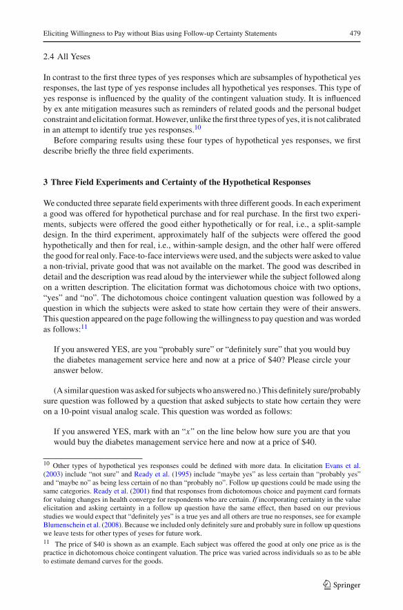
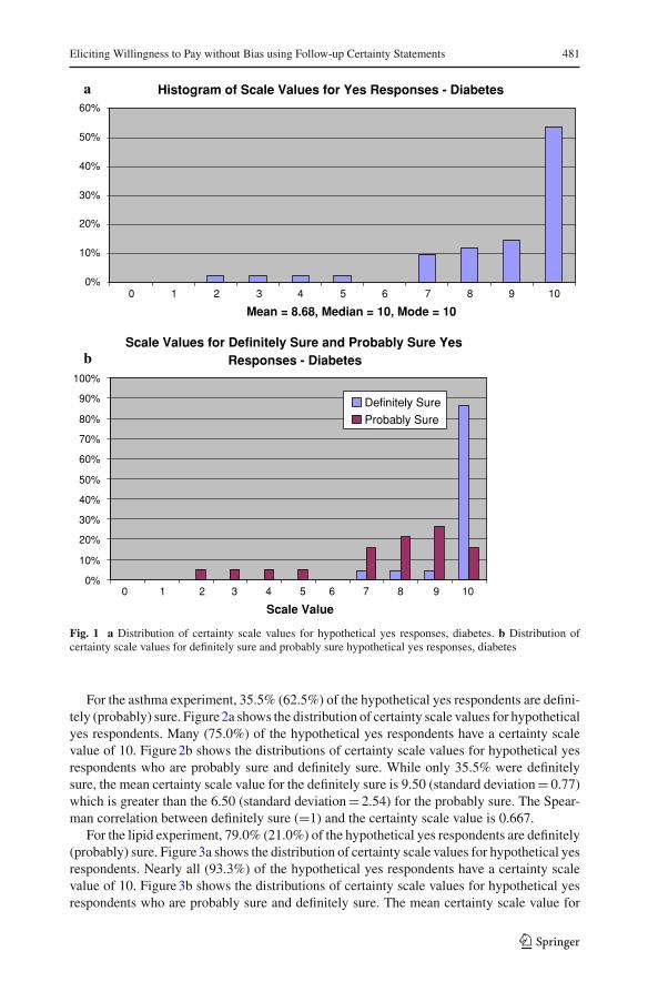
For the diabetes experiment, 53.7% (46.3%) of the hypothetical yes respondents are defini-tely (probably) sure. Figure 1a shows the distribution of certainty scale values for hypotheticalyes respondents. More than half (53.7%) of the hypothetical yes respondents have a certaintyscale value of 10. Figure 1b shows the distributions of certainty scale values for hypotheticalyes respondents who are probably sure and definitely sure. As expected, definitely sure yesresponses have certainty scale values closer to 10 than the probably sure. The mean certaintyscale value for definitely sure is 9.73 (standard deviation = 0.77) while the mean for theprobably sure is only 7.47 (standard deviation = 2.37). The Spearman correlation betweendefinitely sure (=1) and the certainty scale value is 0.683.
12 Champ et al. (1997) and Champ and Bishop (2001) use a 1–10 scale. We have been using a 0–10 scalebecause it is easy to mark the midpoint of 5. Solving the equation y = −(10/9) + (10/9)x for when y = 8yields that the value of 8 on the 0–10 scale is comparable to 8.2 on the 1–10 scale. For comparison of thiscalibration to others, we think the difference seems inconsequential.13 In this study we use 181 of the 267 subjects used in Blumenschein et al. (2008) which contains a fulldescription of the diabetes experiment. In this study we do not include the 86 subjects who were read a cheaptalk script in contingent valuation and included in the earlier study. Additional information about the asthmaexperiment is reported in Blumenschein et al. (2001). Additional information about the lipid experiment canbe found in the Blumenschein and Johannesson (2001) report that is available upon request.
123
Eliciting Willingness to Pay without Bias using Follow-up Certainty Statements 481
Histogram of Scale Values for Yes Responses - Diabetes
0%
10%
20%
30%
40%
50%
60%
0 1 2 3 4 5 6 7 8 9 10
Mean = 8.68, Median = 10, Mode = 10
Scale Values for Definitely Sure and Probably Sure Yes Responses - Diabetes
0%
10%
20%
30%
40%
50%
60%
70%
80%
90%
100%
Scale Value
Definitely Sure
Probably Sure
0 1 2 3 4 5 6 7 8 9 10
a
b
Fig. 1 a Distribution of certainty scale values for hypothetical yes responses, diabetes. b Distribution ofcertainty scale values for definitely sure and probably sure hypothetical yes responses, diabetes
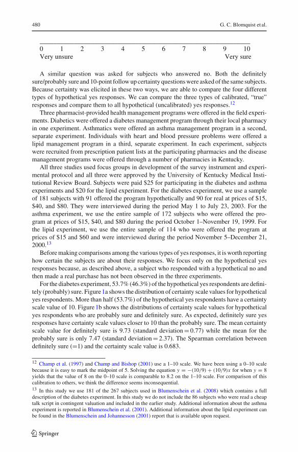
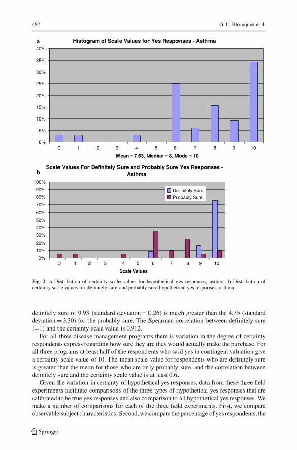
For the asthma experiment, 35.5% (62.5%) of the hypothetical yes respondents are defini-tely (probably) sure. Figure 2a shows the distribution of certainty scale values for hypotheticalyes respondents. Many (75.0%) of the hypothetical yes respondents have a certainty scalevalue of 10. Figure 2b shows the distributions of certainty scale values for hypothetical yesrespondents who are probably sure and definitely sure. While only 35.5% were definitelysure, the mean certainty scale value for the definitely sure is 9.50 (standard deviation = 0.77)which is greater than the 6.50 (standard deviation = 2.54) for the probably sure. The Spear-man correlation between definitely sure (=1) and the certainty scale value is 0.667.
For the lipid experiment, 79.0% (21.0%) of the hypothetical yes respondents are definitely(probably) sure. Figure 3a shows the distribution of certainty scale values for hypothetical yesrespondents. Nearly all (93.3%) of the hypothetical yes respondents have a certainty scalevalue of 10. Figure 3b shows the distributions of certainty scale values for hypothetical yesrespondents who are probably sure and definitely sure. The mean certainty scale value for
123
482 G. C. Blomquist et al.
Histogram of Scale Values for Yes Responses - Asthma
0%
5%
10%
15%
20%
25%
30%
35%
40%
0
Mean = 7.63, Median = 8, Mode = 10
Scale Values For Definitely Sure and Probably Sure Yes Responses - Asthma
0%
10%
20%
30%
40%
50%
60%
70%
80%
90%
100%
Scale Values
Definitely Sure
Probably Sure
1 2 3 4 5 6 7 8 9 10
0 1 2 3 4 5 6 7 8 9 10
a
b
Fig. 2 a Distribution of certainty scale values for hypothetical yes responses, asthma. b Distribution ofcertainty scale values for definitely sure and probably sure hypothetical yes responses, asthma
definitely sure of 9.93 (standard deviation = 0.26) is much greater than the 4.75 (standarddeviation = 3.30) for the probably sure. The Spearman correlation between definitely sure(=1) and the certainty scale value is 0.912.
For all three disease management programs there is variation in the degree of certaintyrespondents express regarding how sure they are they would actually make the purchase. Forall three programs at least half of the respondents who said yes in contingent valuation givea certainty scale value of 10. The mean scale value for respondents who are definitely sureis greater than the mean for those who are only probably sure, and the correlation betweendefinitely sure and the certainty scale value is at least 0.6.
Given the variation in certainty of hypothetical yes responses, data from these three fieldexperiments facilitate comparisons of the three types of hypothetical yes responses that arecalibrated to be true yes responses and also comparison to all hypothetical yes responses. Wemake a number of comparisons for each of the three field experiments. First, we compareobservable subject characteristics. Second, we compare the percentage of yes respondents, the
123

Eliciting Willingness to Pay without Bias using Follow-up Certainty Statements 483
Histogram of Scale Values for Yes Responses - Lipid
0%
10%
20%
30%
40%
50%
60%
70%
80%
90%
100%
0
Mean = 8.84, Median = 10, Mode = 10
Scale Values For Definitely Sure and Probably Sure Yes Responses - Lipid
0%
10%
20%
30%
40%
50%
60%
70%
80%
90%
100%
Scale Values
Definitely Sure
Probably Sure
1 2 3 4 5 6 7 8 9 10
0 1 2 3 4 5 6 7 8 9 10
a
b
Fig. 3 a Distribution of certainty scale values for hypothetical yes responses, lipid. b Distribution of certaintyscale values for definitely sure and probably sure hypothetical yes responses, lipid
performance of the dummy variable Hypothetical in logit regressions of all yes responses,and the mean WTP. Third, we report our estimate of the value on the 10-point scale thatproduces the same calibrated mean WTP as definitely sure, and we report our estimate ofthe value on the 10-point scale that produces the same calibrated mean WTP as mean WTPfrom real purchases.
4 Differences in Observable Characteristics of Subjects
Champ and Bishop (2001) find that when hypothetical and real donations to generatingelectricity using wind power are compared, a cutoff value of 8 on the 10-point scale yieldeda mean WTP that was indistinguishable from the mean of real payments. They report that,
123
484 G. C. Blomquist et al.
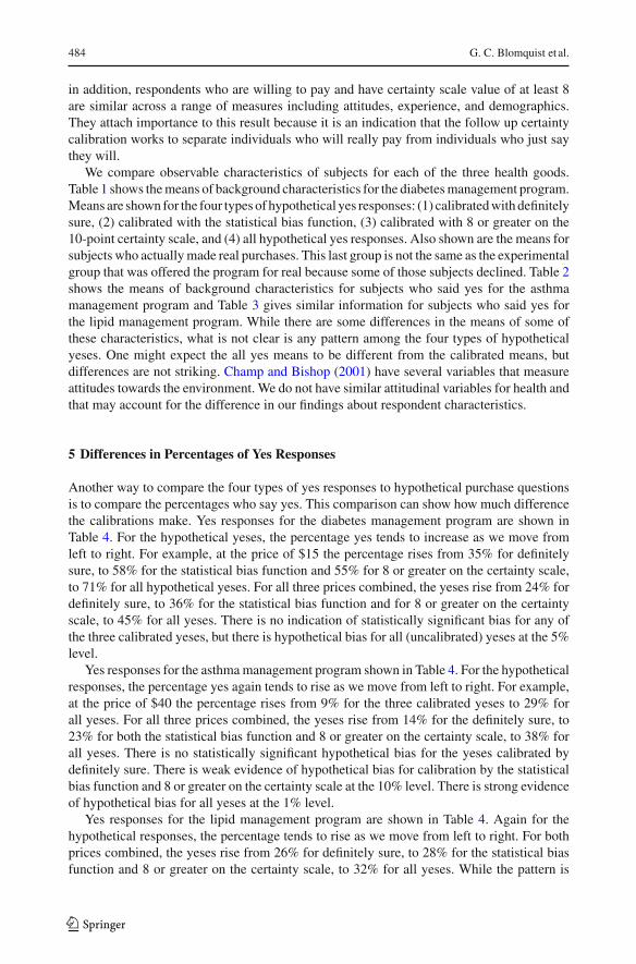
in addition, respondents who are willing to pay and have certainty scale value of at least 8are similar across a range of measures including attitudes, experience, and demographics.They attach importance to this result because it is an indication that the follow up certaintycalibration works to separate individuals who will really pay from individuals who just saythey will.
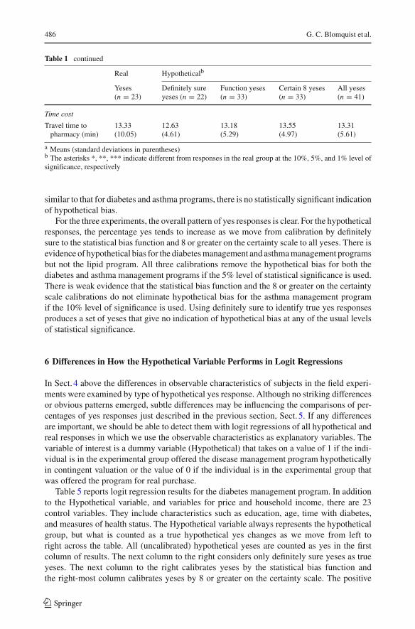
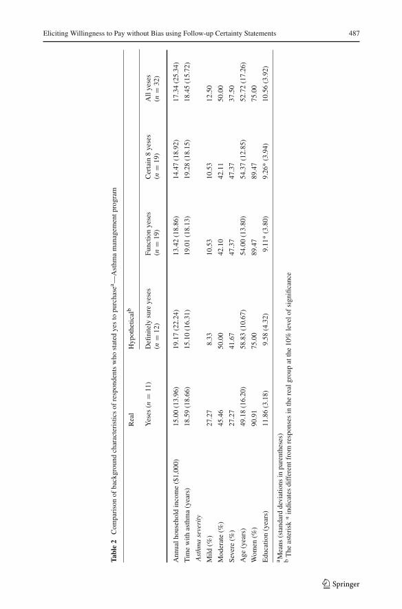
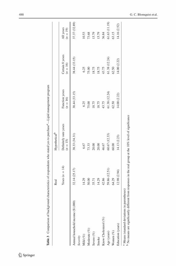
We compare observable characteristics of subjects for each of the three health goods.Table 1 shows the means of background characteristics for the diabetes management program.Means are shown for the four types of hypothetical yes responses: (1) calibrated with definitelysure, (2) calibrated with the statistical bias function, (3) calibrated with 8 or greater on the10-point certainty scale, and (4) all hypothetical yes responses. Also shown are the means forsubjects who actually made real purchases. This last group is not the same as the experimentalgroup that was offered the program for real because some of those subjects declined. Table 2shows the means of background characteristics for subjects who said yes for the asthmamanagement program and Table 3 gives similar information for subjects who said yes forthe lipid management program. While there are some differences in the means of some ofthese characteristics, what is not clear is any pattern among the four types of hypotheticalyeses. One might expect the all yes means to be different from the calibrated means, butdifferences are not striking. Champ and Bishop (2001) have several variables that measureattitudes towards the environment. We do not have similar attitudinal variables for health andthat may account for the difference in our findings about respondent characteristics.
5 Differences in Percentages of Yes Responses
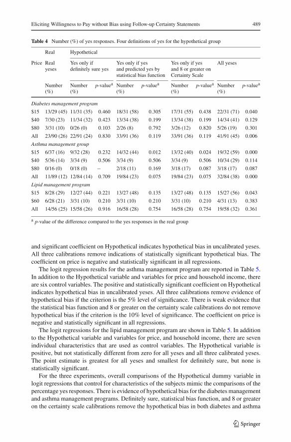
Another way to compare the four types of yes responses to hypothetical purchase questionsis to compare the percentages who say yes. This comparison can show how much differencethe calibrations make. Yes responses for the diabetes management program are shown inTable 4. For the hypothetical yeses, the percentage yes tends to increase as we move fromleft to right. For example, at the price of $15 the percentage rises from 35% for definitelysure, to 58% for the statistical bias function and 55% for 8 or greater on the certainty scale,to 71% for all hypothetical yeses. For all three prices combined, the yeses rise from 24% fordefinitely sure, to 36% for the statistical bias function and for 8 or greater on the certaintyscale, to 45% for all yeses. There is no indication of statistically significant bias for any ofthe three calibrated yeses, but there is hypothetical bias for all (uncalibrated) yeses at the 5%level.
Yes responses for the asthma management program shown in Table 4. For the hypotheticalresponses, the percentage yes again tends to rise as we move from left to right. For example,at the price of $40 the percentage rises from 9% for the three calibrated yeses to 29% forall yeses. For all three prices combined, the yeses rise from 14% for the definitely sure, to23% for both the statistical bias function and 8 or greater on the certainty scale, to 38% forall yeses. There is no statistically significant hypothetical bias for the yeses calibrated bydefinitely sure. There is weak evidence of hypothetical bias for calibration by the statisticalbias function and 8 or greater on the certainty scale at the 10% level. There is strong evidenceof hypothetical bias for all yeses at the 1% level.
Yes responses for the lipid management program are shown in Table 4. Again for thehypothetical responses, the percentage tends to rise as we move from left to right. For bothprices combined, the yeses rise from 26% for definitely sure, to 28% for the statistical biasfunction and 8 or greater on the certainty scale, to 32% for all yeses. While the pattern is
123

Eliciting Willingness to Pay without Bias using Follow-up Certainty Statements 485
Table 1 Comparison of background characteristics of respondents who stated yes to purchasea-Diabetesmanagement program
Real Hypotheticalb
Yeses(n = 23)
Definitely sureyeses (n = 22)
Function yeses(n = 33)
Certain 8 yeses(n = 33)
All yeses(n = 41)
Income and wealth
Annual householdincome ($1,000)
32.62(23.67)
40.12(25.68)
39.06(26.13)
38.75(26.36)
35.94(26.19)
Household size 2.04(1.22)
2.55(1.22)
2.63*(1.32)
2.67*(1.29)
2.61*(1.26)
Owns residence (%) 86.96 95.45 90.91 90.91 90.24
Health and health behavior
Previous participationin disease
17.39 9.10 9.10 12.12 9.77
management (%)
Member of diabetessupport group (%)
8.70 4.55 6.10 6.06 4.88
Time with diabetes(years)
7.87(7.09)
7.25(6.40)
7.54(6.39)
7.70(6.27)
7.63(5.81)
Diabetes severity
Mild (%) 21.74 18.18 18.18 15.15 19.51
Moderate (%) 69.56 63.63 66.67 66.67 63.41
Severe (%) 8.70 18.18 15.15 18.18 17.07
Cardiovasculardisease (%)
86.70 86.36 81.82 84.85 85.37
Renal disease (%) 8.70 4.55 3.03 3.03 2.44
Vision problems (%) 30.43 22.73 27.27 30.30 29.27
Neuropathies (%) 60.87 68.18 57.58 57.58 58.54
Complications ofdiabetes in family(%)
43.48 63.64 60.61 60.61 60.98
Smoking (%) 30.43 13.64 12.12* 15.15 14.63
Body mass index 36.63(8.35)
31.54**(7.83)
31.66**(7.05)
31.91**(7.08)
32.45**(6.97)
Know theirhemoglobin A1Clevel (%)
30.43 22.73 21.21 24.24 21.95
General health
Excellent (%) 4.35 0 0 0 0
Very good (%) 4.35 18.18 15.15 15.15 12.20
Good (%) 21.74 36.36 36.36 36.36 39.02
Fair (%) 39.13 40.91 45.45 45.45 41.46
Poor (%) 30.43 4.55** 3.03*** 3.03*** 7.32**
Socioeconomics
Age (years) 57.87(10.91)
60.32(12.70)
60.12(13.15)
60.72(11.88)
59.39(12.63)
Women (%) 65.22 63.64 69.70 69.70 70.73
Education (years) 10.70(4.26)
12.25(2.75)
12.26(2.92)
12.09(2.77)
12.26*(2.77)
Ethnic backgroundwhite (%)
86.96 90.91 93.94 93.94 90.24
123
486 G. C. Blomquist et al.
Table 1 continued
Real Hypotheticalb
Yeses(n = 23)
Definitely sureyeses (n = 22)
Function yeses(n = 33)
Certain 8 yeses(n = 33)
All yeses(n = 41)
Time cost
Travel time topharmacy (min)
13.33(10.05)
12.63(4.61)
13.18(5.29)
13.55(4.97)
13.31(5.61)
a Means (standard deviations in parentheses)b The asterisks *, **, *** indicate different from responses in the real group at the 10%, 5%, and 1% level ofsignificance, respectively
similar to that for diabetes and asthma programs, there is no statistically significant indicationof hypothetical bias.
For the three experiments, the overall pattern of yes responses is clear. For the hypotheticalresponses, the percentage yes tends to increase as we move from calibration by definitelysure to the statistical bias function and 8 or greater on the certainty scale to all yeses. There isevidence of hypothetical bias for the diabetes management and asthma management programsbut not the lipid program. All three calibrations remove the hypothetical bias for both thediabetes and asthma management programs if the 5% level of statistical significance is used.There is weak evidence that the statistical bias function and the 8 or greater on the certaintyscale calibrations do not eliminate hypothetical bias for the asthma management programif the 10% level of significance is used. Using definitely sure to identify true yes responsesproduces a set of yeses that give no indication of hypothetical bias at any of the usual levelsof statistical significance.
6 Differences in How the Hypothetical Variable Performs in Logit Regressions
In Sect. 4 above the differences in observable characteristics of subjects in the field experi-ments were examined by type of hypothetical yes response. Although no striking differencesor obvious patterns emerged, subtle differences may be influencing the comparisons of per-centages of yes responses just described in the previous section, Sect. 5. If any differencesare important, we should be able to detect them with logit regressions of all hypothetical andreal responses in which we use the observable characteristics as explanatory variables. Thevariable of interest is a dummy variable (Hypothetical) that takes on a value of 1 if the indi-vidual is in the experimental group offered the disease management program hypotheticallyin contingent valuation or the value of 0 if the individual is in the experimental group thatwas offered the program for real purchase.
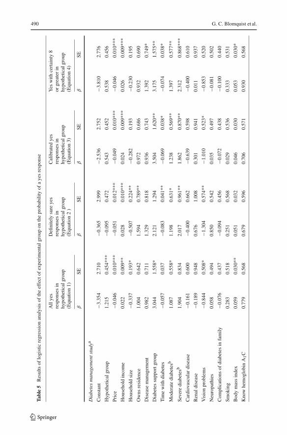
Table 5 reports logit regression results for the diabetes management program. In additionto the Hypothetical variable, and variables for price and household income, there are 23control variables. They include characteristics such as education, age, time with diabetes,and measures of health status. The Hypothetical variable always represents the hypotheticalgroup, but what is counted as a true hypothetical yes changes as we move from left toright across the table. All (uncalibrated) hypothetical yeses are counted as yes in the firstcolumn of results. The next column to the right considers only definitely sure yeses as trueyeses. The next column to the right calibrates yeses by the statistical bias function andthe right-most column calibrates yeses by 8 or greater on the certainty scale. The positive
123
Eliciting Willingness to Pay without Bias using Follow-up Certainty Statements 487
Tabl
e2
Com
pari
son
ofba
ckgr
ound
char
acte
rist
ics
ofre
spon
dent
sw
host
ated
yes
topu
rcha
sea —
Ast
hma
man
agem
entp
rogr
am
Rea
lH
ypot
hetic
alb
Yes
es(n
=11
)D
efini
tely
sure
yese
sFu
nctio
nye
ses
Cer
tain
8ye
ses
All
yese
s(n
=12
)(n
=19
)(n
=19
)(n
=32
)
Ann
ualh
ouse
hold
inco
me
($1,
000)
15.0
0(1
3.96
)19
.17
(22.
24)
13.4
2(1
8.86
)14
.47
(18.
92)
17.3
4(2
5.34
)
Tim
ew
ithas
thm
a(y
ears
)18
.59
(18.
66)
15.1
0(1
6.31
)19
.01
(18.
13)
19.2
8(1
8.15
)18
.45
(15.
72)
Ast
hma
seve
rity
Mild
(%)
27.2
78.
3310
.53
10.5
312
.50
Mod
erat
e(%
)45
.46
50.0
042
.10
42.1
150
.00
Seve
re(%
)27
.27
41.6
747
.37
47.3
737
.50
Age
(yea
rs)
49.1
8(1
6.20
)58
.83
(10.
67)
54.0
0(1
3.80
)54
.37
(12.
85)
52.7
2(1
7.26
)
Wom
en(%
)90
.91
75.0
089
.47
89.4
775
.00
Edu
catio
n(y
ears
)11
.86
(3.1
8)9.
58(4
.32)
9.11
*(3
.80)
9.26
*(3
.94)
10.5
6(3
.92)
a Mea
ns(s
tand
ard
devi
atio
nsin
pare
nthe
ses)
bT
heas
teri
sk*
indi
cate
sdi
ffer
entf
rom
resp
onse
sin
the
real
grou
pat
the
10%
leve
lof
sign
ifica
nce
123
488 G. C. Blomquist et al.
Tabl
e3
Com
pari
son
ofba
ckgr
ound
char
acte
rist
ics
ofre
spon
dent
sw
host
ated
yes
topu
rcha
sea —
Lip
idm
anag
emen
tpro
gram
Rea
lH
ypot
hetic
alb
Yes
es(n
=14
)D
efini
tely
sure
yese
sFu
nctio
nye
ses
Cer
tain
8ye
ses
All
yese
s(n
=15
)(n
=16
)(n
=16
)(n
=19
)
Ann
ualh
ouse
hold
inco
me
($1,
000)
32.1
4(2
5.17
)38
.33
(34.
31)
38.4
4(3
3.15
)38
.44
(33.
15)
37.3
7(3
2.89
)
Seve
rity
Mild
(%)
14.2
96.
676.
256.
2510
.53
Mod
erat
e(%
)50
.00
73.3
375
.00
75.0
073
.68
Seve
re(%
)35
.71
20.0
018
.75
18.7
515
.79
Smok
e14
.29
20.0
018
.75
18.7
515
.79
Kno
wC
hole
ster
ol(%
)42
.86
46.6
743
.75
43.7
536
.84
Age
(yea
rs)
59.8
6(1
2.51
)60
.67
(12.
33)
61.3
8(1
2.24
)61
.38
(12.
24)
61.6
3(1
1.19
)
Wom
en(%
)64
.29
60.0
062
.50
62.5
063
.15
Edu
catio
n(y
ears
)12
.98
(2.9
4)14
.13
(2.2
3)14
.00
(2.2
2)14
.00
(2.2
2)14
.16
(2.5
2)
aM
eans
(sta
ndar
dde
viat
ions
inpa
rent
hese
s)b
No
mea
nsar
esi
gnifi
cant
lydi
ffer
entf
rom
resp
onse
sin
the
real
grou
pat
the
10%
leve
lof
sign
ifica
nce
123
Eliciting Willingness to Pay without Bias using Follow-up Certainty Statements 489
Table 4 Number (%) of yes responses. Four definitions of yes for the hypothetical group
Real Hypothetical
Price Real Yes only if Yes only if yes Yes only if yes All yesesyeses definitely sure yes and predicted yes by and 8 or greater on
statistical bias function Certainty Scale
Number Number p-valuea Number p-valuea Number p-valuea Number p-valuea
(%) (%) (%) (%) (%)
Diabetes management program
$15 13/29 (45) 11/31 (35) 0.460 18/31 (58) 0.305 17/31 (55) 0.438 22/31 (71) 0.040
$40 7/30 (23) 11/34 (32) 0.423 13/34 (38) 0.199 13/34 (38) 0.199 14/34 (41) 0.129
$80 3/31 (10) 0/26 (0) 0.103 2/26 (8) 0.792 3/26 (12) 0.820 5/26 (19) 0.301
All 23/90 (26) 22/91 (24) 0.830 33/91 (36) 0.119 33/91 (36) 0.119 41/91 (45) 0.006
Asthma management group
$15 6/37 (16) 9/32 (28) 0.232 14/32 (44) 0.012 13/32 (40) 0.024 19/32 (59) 0.000
$40 5/36 (14) 3/34 (9) 0.506 3/34 (9) 0.506 3/34 (9) 0.506 10/34 (29) 0.114
$80 0/16 (0) 0/18 (0) − 2/18 (11) 0.169 3/18 (17) 0.087 3/18 (17) 0.087
All 11/89 (12) 12/84 (14) 0.709 19/84 (23) 0.075 19/84 (23) 0.075 32/84 (38) 0.000
Lipid management program
$15 8/28 (29) 12/27 (44) 0.221 13/27 (48) 0.135 13/27 (48) 0.135 15/27 (56) 0.043
$60 6/28 (21) 3/31 (10) 0.210 3/31 (10) 0.210 3/31 (10) 0.210 4/31 (13) 0.383
All 14/56 (25) 15/58 (26) 0.916 16/58 (28) 0.754 16/58 (28) 0.754 19/58 (32) 0.361
a p-value of the difference compared to the yes responses in the real group
and significant coefficient on Hypothetical indicates hypothetical bias in uncalibrated yeses.All three calibrations remove indications of statistically significant hypothetical bias. Thecoefficient on price is negative and statistically significant in all regressions.
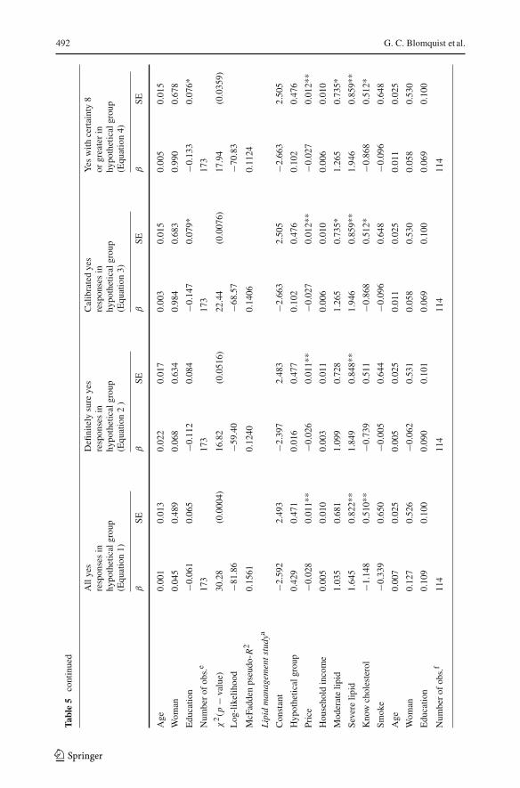
The logit regression results for the asthma management program are reported in Table 5.In addition to the Hypothetical variable and variables for price and household income, thereare six control variables. The positive and statistically significant coefficient on Hypotheticalindicates hypothetical bias in uncalibrated yeses. All three calibrations remove evidence ofhypothetical bias if the criterion is the 5% level of significance. There is weak evidence thatthe statistical bias function and 8 or greater on the certainty scale calibrations do not removehypothetical bias if the criterion is the 10% level of significance. The coefficient on price isnegative and statistically significant in all regressions.
The logit regressions for the lipid management program are shown in Table 5. In additionto the Hypothetical variable and variables for price, and household income, there are sevenindividual characteristics that are used as control variables. The Hypothetical variable ispositive, but not statistically different from zero for all yeses and all three calibrated yeses.The point estimate is greatest for all yeses and smallest for definitely sure, but none isstatistically significant.
For the three experiments, overall comparisons of the Hypothetical dummy variable inlogit regressions that control for characteristics of the subjects mimic the comparisons of thepercentage yes responses. There is evidence of hypothetical bias for the diabetes managementand asthma management programs. Definitely sure, statistical bias function, and 8 or greateron the certainty scale calibrations remove the hypothetical bias in both diabetes and asthma
123
490 G. C. Blomquist et al.
Tabl
e5
Res
ults
oflo
gist
icre
gres
sion
anal
ysis
ofth
eef
fect
ofex
peri
men
talg
roup
onth
epr
obab
ility
ofa
yes
resp
onse
All
yes
Defi
nite
lysu
reye
sC
alib
rate
dye
sY
esw
ithce
rtai
nty
8re
spon
ses
inre
spon
ses
inre
spon
ses
inor
grea
ter
inhy
poth
etic
algr
oup
hypo
thet
ical
grou
phy
poth
etic
algr
oup
hypo
thet
ical
grou
p(E
quat
ion
1)(E
quat
ion
2)
(Equ
atio
n3)
(Equ
atio
n4)
βSE
βSE
βSE
βSE
Dia
bete
sm
anag
emen
tstu
dya
Con
stan
t−3
.354
2.71
0−0
.365
2.99
9−2
.536
2.75
2−3
.810
2.77
6
Hyp
othe
tical
grou
p1.
215
0.45
4***
−0.0
950.
472
0.54
30.
452
0.53
80.
456
Pric
e−0
.046
0.01
0***
−0.0
510.
012*
**−0
.049
0.01
0***
−0.0
460.
010*
**
Hou
seho
ldin
com
e0.
022
0.00
9**
0.02
80.
010*
**0.
024
0.00
9***
0.02
60.
009*
**
Hou
seho
ldsi
ze−0
.337
0.19
3*−0
.507
0.22
4**
−0.2
820.
193
−0.2
300.
195
Ow
nsre
side
nce
1.00
40.
642
1.59
40.
789*
*0.
972
0.68
60.
932
0.69
0
Dis
ease
man
agem
ent
0.98
20.
711
1.32
90.
818
0.93
60.
743
1.39
20.
749*
Dia
bete
ssu
ppor
tgro
up3.
044
1.55
8*2.
121
1.29
43.
504
1.62
0**
3.17
51.
575*
*
Tim
ew
ithdi
abet
es−0
.057
0.03
7−0
.083
0.04
1**
−0.0
690.
038*
−0.0
740.
038*
Mod
erat
edi
abet
esb
1.08
70.
558*
1.19
80.
631*
1.23
80.
569*
*1.
397
0.57
7**
Seve
redi
abet
esb
1.90
40.
834
2.01
70.
961*
*1.
862
0.87
0**
2.31
20.
868*
**
Car
diov
ascu
lar
dise
ase
−0.1
610.
600
−0.4
000.
662
−0.6
390.
598
−0.4
000.
610
Ren
aldi
seas
e−0
.189
0.94
80.
676
1.00
80.
301
0.94
10.
011
0.93
7
Vis
ion
prob
lem
s−0
.844
0.50
8*−1
.304
0.57
4**
−1.0
100.
523*
−0.8
530.
520
Neu
ropa
thie
s0.
058
0.49
40.
850
0.54
20.
035
0.49
7−0
.081
0.50
2
Com
plic
atio
nsof
diab
etes
infa
mily
−0.0
760.
437
−0.0
940.
456
−0.0
720.
438
−0.1
000.
440
Smok
ing
0.28
30.
518
0.25
10.
568
0.02
90.
536
0.33
30.
531
Bod
ym
ass
inde
x0.
059
0.03
0**
0.05
10.
032
0.04
60.
030
0.05
30.
030*
Kno
whe
mog
lobi
nA
1C
0.77
90.
568
0.67
90.
596
0.70
60.
571
0.93
00.
568
123

Eliciting Willingness to Pay without Bias using Follow-up Certainty Statements 491
Tabl
e5
cont
inue
d
All
yes
Defi
nite
lysu
reye
sC
alib
rate
dye
sY
esw
ithce
rtai
nty
8re
spon
ses
inre
spon
ses
inre
spon
ses
inor
grea
ter
inhy
poth
etic
algr
oup
hypo
thet
ical
grou
phy
poth
etic
algr
oup
hypo
thet
ical
grou
p(E
quat
ion
1)(E
quat
ion
2)
(Equ
atio
n3)
(Equ
atio
n4)
βSE
βSE
βSE
βSE
Goo
dhe
alth
c1.
909
0.78
0**
1.25
00.
774
1.47
30.
755*
1.51
70.
768*
Fair
heal
thc
1.36
60.
791*
0.61
90.
765
1.15
30.
767
1.13
00.
780
Poor
heal
thc
1.66
70.
970*
0.61
01.
022
1.00
40.
971
0.86
70.
982
Age
0.01
10.
022
0.00
40.
023
0.01
70.
022
0.02
80.
022
Wom
an0.
210
0.44
8−0
.020
0.47
80.
200
0.44
80.
259
0.44
8
Edu
catio
n−0
.621
0.08
3−0
.152
0.09
7−0
.095
0.08
7−0
.121
0.08
8
Eth
nic:
whi
te−0
.944
0.72
3−1
.232
0.78
1−0
.319
0.74
9−0
.449
0.74
8
Tra
velt
ime
0.18
10.
027
−0.0
150.
030
0.00
90.
028
0.02
00.
028
Num
ber
ofob
s.d
181
181
181
181
χ2(p
−va
lue)
72.7
2(<
0.00
01)
59.8
3(0
.000
2)65
.55
(<0.
0001
)66
.23
(<0.
0001
)
Log
-lik
elih
ood
−81.
223
−71.
59−7
9.19
23−7
8.85
McF
adde
nps
eudo
-R2
0.30
920.
2947
0.29
270.
2958
Ast
hma
man
agem
ents
tudy
a
Con
stan
t−0
.616
1.29
2−0
.792
1.67
8−0
.425
1.56
4−0
.905
1.53
7
Hyp
othe
tical
grou
p1.
590
0.42
5***
0.00
90.
499
0.76
30.
454*
0.75
30.
447*
Pric
e−0
.032
0.01
0***
−0.0
450.
016*
**−0
.035
0.01
2***
−0.0
260.
011*
*
Hou
seho
ldin
com
e0.
007
0.00
90.
012
0.01
20.
006
0.01
10.
007
0.01
0
Tim
ew
ithas
thm
a−0
.003
0.01
2−0
.012
0.01
5−0
.002
0.01
3−0
.002
0.01
3
Mod
erat
eas
thm
a0.
327
0.56
10.
525
0.69
00.
164
0.63
20.
098
0.62
5
Seve
reas
thm
a0.
283
0.61
20.
273
0.74
20.
227
0.67
30.
226
0.66
6
123
492 G. C. Blomquist et al.
Tabl
e5
cont
inue
d
All
yes
Defi
nite
lysu
reye
sC
alib
rate
dye
sY
esw
ithce
rtai
nty
8re
spon
ses
inre
spon
ses
inre
spon
ses
inor
grea
ter
inhy
poth
etic
algr
oup
hypo
thet
ical
grou
phy
poth
etic
algr
oup
hypo
thet
ical
grou
p(E
quat
ion
1)(E
quat
ion
2)
(Equ
atio
n3)
(Equ
atio
n4)
βSE
βSE
βSE
βSE
Age
0.00
10.
013
0.02
20.
017
0.00
30.
015
0.00
50.
015
Wom
an0.
045
0.48
90.
068
0.63
40.
984
0.68
30.
990
0.67
8
Edu
catio
n−0
.061
0.06
5−0
.112
0.08
4−0
.147
0.07
9*−0
.133
0.07
6*
Num
ber
ofob
s.e
173
173
173
173
χ2(p
−va
lue)
30.2
8(0
.000
4)16
.82
(0.0
516)
22.4
4(0
.007
6)17
.94
(0.0
359)
Log
-lik
elih
ood
−81.
86−5
9.40
−68.
57−7
0.83
McF
adde
nps
eudo
-R2
0.15
610.
1240
0.14
060.
1124
Lip
idm
anag
emen
tstu
dya
Con
stan
t−2
.592
2.49
3−2
.397
2.48
3−2
.663
2.50
5−2
.663
2.50
5
Hyp
othe
tical
grou
p0.
429
0.47
10.
016
0.47
70.
102
0.47
60.
102
0.47
6
Pric
e−0
.028
0.01
1**
−0.0
260.
011*
*−0
.027
0.01
2**
−0.0
270.
012*
*
Hou
seho
ldin
com
e0.
005
0.01
00.
003
0.01
10.
006
0.01
00.
006
0.01
0
Mod
erat
elip
id1.
035
0.68
11.
099
0.72
81.
265
0.73
5*1.
265
0.73
5*
Seve
relip
id1.
645
0.82
2**
1.84
90.
848*
*1.
946
0.85
9**
1.94
60.
859*
*
Kno
wch
oles
tero
l−1
.148
0.51
0**
−0.7
390.
511
−0.8
680.
512*
−0.8
680.
512*
Smok
e−0
.339
0.65
0−0
.005
0.64
4−0
.096
0.64
8−0
.096
0.64
8
Age
0.00
70.
025
0.00
50.
025
0.01
10.
025
0.01
10.
025
Wom
an0.
127
0.52
6−0
.062
0.53
10.
058
0.53
00.
058
0.53
0
Edu
catio
n0.
109
0.10
00.
090
0.10
10.
069
0.10
00.
069
0.10
0
Num
ber
ofob
s.f
114
114
114
114
123

Eliciting Willingness to Pay without Bias using Follow-up Certainty Statements 493
Tabl
e5
cont
inue
d
All
yes
Defi
nite
lysu
reye
sC
alib
rate
dye
sY
esw
ithce
rtai
nty
8re
spon
ses
inre
spon
ses
inre
spon
ses
inor
grea
ter
inhy
poth
etic
algr
oup
hypo
thet
ical
grou
phy
poth
etic
algr
oup
hypo
thet
ical
grou
p(E
quat
ion
1)(E
quat
ion
2)
(Equ
atio
n3)
(Equ
atio
n4)
βSE
βSE
βSE
βSE
χ2(p
−va
lue)
21.4
9(0
.017
9)15
.29
(0.1
217)
17.4
0(0
.065
9)17
.40
(0.0
659)
Log
-lik
elih
ood
−57.
846
−57.
003
−57.
001
−57.
001
McF
adde
nps
eudo
-R2
0.15
670.
1183
0.13
240.
1324
aSt
atis
tical
sign
ifica
nce
isin
dica
ted
by**
*at
the
1%le
vel,
**at
the
5%le
vel,
and
*at
the
10%
leve
lb
Bas
elin
eca
tego
ry:m
ilddi
abet
esc
Bas
elin
eca
tego
ry:e
xcel
lent
orve
rygo
odge
nera
lhea
lthd
The
num
ber
ofsu
bjec
tsof
fere
dth
edi
abet
esm
anag
emen
tpro
gram
for
real
is90
eT
henu
mbe
rof
subj
ects
offe
red
the
asth
ma
man
agem
entp
rogr
amfo
rre
alis
89f
The
num
ber
ofsu
bjec
tsof
fere
dth
elip
idm
anag
emen
tpro
gram
for
real
is56
123

494 G. C. Blomquist et al.
management programs if the 5% level of statistical significance is used. There is weakevidence that the statistical bias function and the 8 or greater on the certainty scale calibrationsdo not eliminate hypothetical bias for the asthma management program if the 10% level ofsignificance is used. Using definitely sure to identify true yes responses produces a set ofyeses that give no indication of hypothetical bias at any of the usual levels of statisticalsignificance.
7 Differences in Estimates of Average Willingness to Pay
Given the interest in using estimates of WTP in benefit-cost analysis, comparison of estimatesof average WTP is the crux of the matter. We compare mean WTP for all hypothetical yesesand each of the three calibrated hypothetical yes responses. We also compare the estimates tothe mean WTP of real purchases to check for hypothetical bias. We make these comparisonsfor each of the three disease management programs using both nonparametric and parametricmethods.
For the nonparametric estimates of WTP we use a method developed by Kriström (1990)in which the area under the demand curve (price and fraction of buyers) is an estimate ofthe mean. For each experiment, we assume that the maximum WTP equals the highest price(either $60 or $80) used in the experiment and that the proportion of subjects with zeroWTP equals the proportion of responses at the lowest price ($15) used in the experiment.For the parametric estimates of WTP, we use a method developed by Johansson (1995) thatrestricts the value to be positive which is appropriate for these private disease managementprograms that do not have to be consumed. The estimation of mean willingness to pay isbased on estimating the area below the demand curve using the formula: −(1/β)ln(1+ eα),where β is the price coefficient in the logistic regression equation and α is the constant in thelogistic regression equation with the effect of all other covariates evaluated at their means andadded to the constant. The results, while not identical, are similar for the nonparametric andparametric methods, and so our discussion will focus on the parametric estimates of meanWTP.
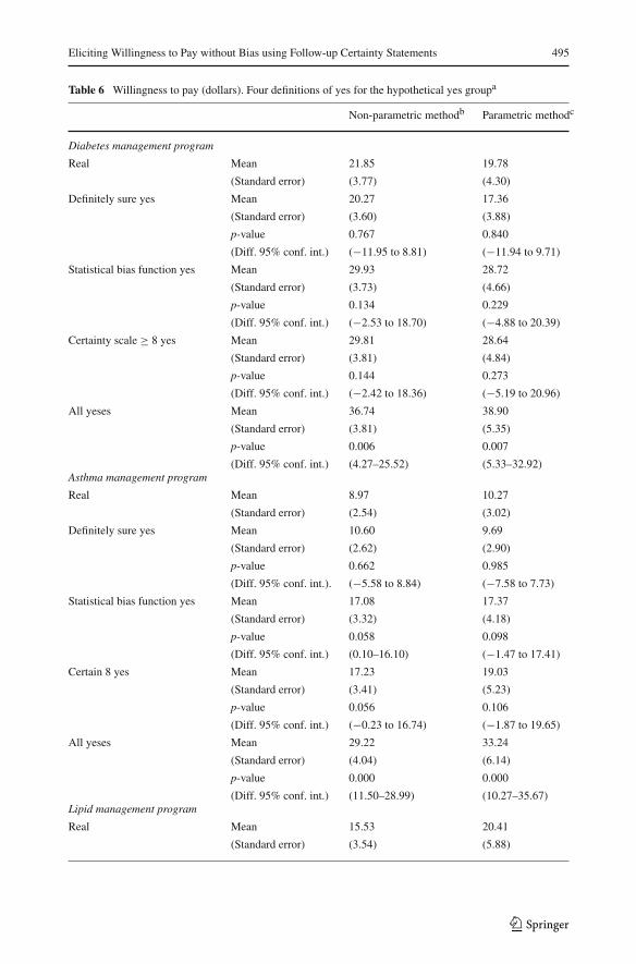
Estimates of mean WTP for the diabetes management program for the different types ofyes responses are reported in Table 6. As we read down the column for the different typesof yeses, the mean WTP tends to increase. For the parametric estimates, the mean increasesfrom $17.36 for the definitely sure yeses, to $28.72 and $28.64 for the yeses calibrated by thestatistical bias function and 8 or greater on the certainty scale, to $38.90 for all hypothetical(uncalibrated) yeses. There is no evidence of hypothetical bias for the calibrated yeses, butthere is evidence at the 5% level for all hypothetical yeses.
Estimates of mean WTP for the asthma management program for the different types ofyeses are shown in Table 6. Again as we read down the column for the different types ofyeses, the mean WTP increases. For the parametric estimates, the mean increases from $9.69for the definitely sure, to $17.37 for the statistical bias function, to $19.03 for the 8 or greateron the certainty scale, to $33.24 for all yeses. There is no evidence of hypothetical bias forthe definitely sure yeses. There is evidence of hypothetical bias at the 10% level for yesescalibrated by the statistical bias function and it is close to the 10% level for 8 or greater.There is evidence at the 5% level for all yeses.
For the lipid management program estimates of mean WTP for the different types of yesesare reported in Table 6. As with the other two goods, as we read down the column for thedifferent types of yeses, the estimate of mean WTP tends to increase. For the parametric esti-mates, the mean WTP increases from $21.76 for definitely sure, to $22.65 for the calibration
123
Eliciting Willingness to Pay without Bias using Follow-up Certainty Statements 495
Table 6 Willingness to pay (dollars). Four definitions of yes for the hypothetical yes groupa
Non-parametric methodb Parametric methodc
Diabetes management program
Real Mean 21.85 19.78
(Standard error) (3.77) (4.30)
Definitely sure yes Mean 20.27 17.36
(Standard error) (3.60) (3.88)
p-value 0.767 0.840
(Diff. 95% conf. int.) (−11.95 to 8.81) (−11.94 to 9.71)
Statistical bias function yes Mean 29.93 28.72
(Standard error) (3.73) (4.66)
p-value 0.134 0.229
(Diff. 95% conf. int.) (−2.53 to 18.70) (−4.88 to 20.39)
Certainty scale ≥ 8 yes Mean 29.81 28.64
(Standard error) (3.81) (4.84)
p-value 0.144 0.273
(Diff. 95% conf. int.) (−2.42 to 18.36) (−5.19 to 20.96)
All yeses Mean 36.74 38.90
(Standard error) (3.81) (5.35)
p-value 0.006 0.007
(Diff. 95% conf. int.) (4.27–25.52) (5.33–32.92)Asthma management program
Real Mean 8.97 10.27
(Standard error) (2.54) (3.02)
Definitely sure yes Mean 10.60 9.69
(Standard error) (2.62) (2.90)
p-value 0.662 0.985
(Diff. 95% conf. int.). (−5.58 to 8.84) (−7.58 to 7.73)
Statistical bias function yes Mean 17.08 17.37
(Standard error) (3.32) (4.18)
p-value 0.058 0.098
(Diff. 95% conf. int.) (0.10–16.10) (−1.47 to 17.41)
Certain 8 yes Mean 17.23 19.03
(Standard error) (3.41) (5.23)
p-value 0.056 0.106
(Diff. 95% conf. int.) (−0.23 to 16.74) (−1.87 to 19.65)
All yeses Mean 29.22 33.24
(Standard error) (4.04) (6.14)
p-value 0.000 0.000
(Diff. 95% conf. int.) (11.50–28.99) (10.27–35.67)Lipid management program
Real Mean 15.53 20.41
(Standard error) (3.54) (5.88)
123
496 G. C. Blomquist et al.
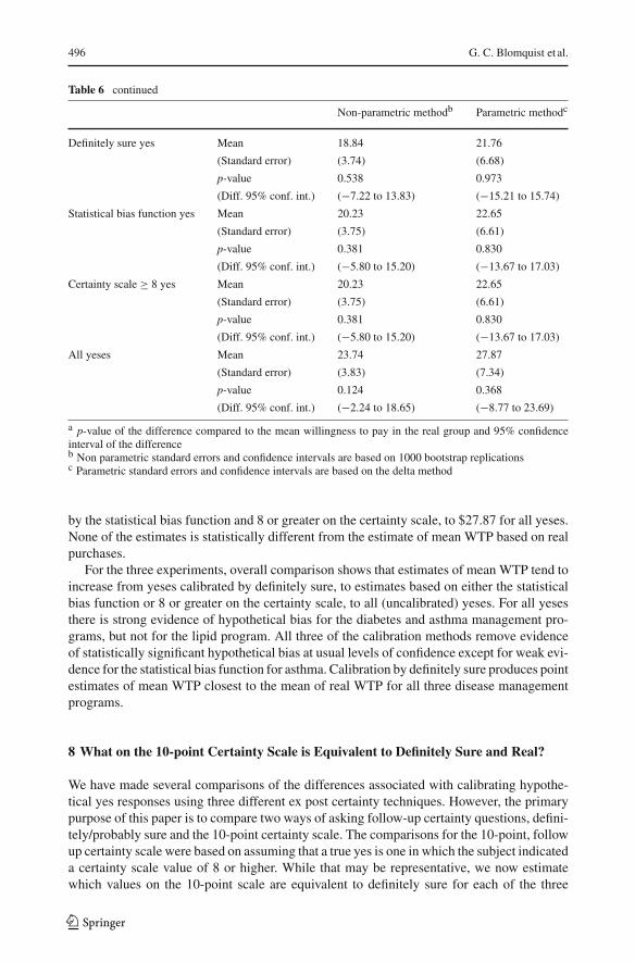
Table 6 continued
Non-parametric methodb Parametric methodc
Definitely sure yes Mean 18.84 21.76
(Standard error) (3.74) (6.68)
p-value 0.538 0.973
(Diff. 95% conf. int.) (−7.22 to 13.83) (−15.21 to 15.74)
Statistical bias function yes Mean 20.23 22.65
(Standard error) (3.75) (6.61)
p-value 0.381 0.830
(Diff. 95% conf. int.) (−5.80 to 15.20) (−13.67 to 17.03)
Certainty scale ≥ 8 yes Mean 20.23 22.65
(Standard error) (3.75) (6.61)
p-value 0.381 0.830
(Diff. 95% conf. int.) (−5.80 to 15.20) (−13.67 to 17.03)
All yeses Mean 23.74 27.87
(Standard error) (3.83) (7.34)
p-value 0.124 0.368
(Diff. 95% conf. int.) (−2.24 to 18.65) (−8.77 to 23.69)
a p-value of the difference compared to the mean willingness to pay in the real group and 95% confidenceinterval of the differenceb Non parametric standard errors and confidence intervals are based on 1000 bootstrap replicationsc Parametric standard errors and confidence intervals are based on the delta method
by the statistical bias function and 8 or greater on the certainty scale, to $27.87 for all yeses.None of the estimates is statistically different from the estimate of mean WTP based on realpurchases.
For the three experiments, overall comparison shows that estimates of mean WTP tend toincrease from yeses calibrated by definitely sure, to estimates based on either the statisticalbias function or 8 or greater on the certainty scale, to all (uncalibrated) yeses. For all yesesthere is strong evidence of hypothetical bias for the diabetes and asthma management pro-grams, but not for the lipid program. All three of the calibration methods remove evidenceof statistically significant hypothetical bias at usual levels of confidence except for weak evi-dence for the statistical bias function for asthma. Calibration by definitely sure produces pointestimates of mean WTP closest to the mean of real WTP for all three disease managementprograms.
8 What on the 10-point Certainty Scale is Equivalent to Definitely Sure and Real?
We have made several comparisons of the differences associated with calibrating hypothe-tical yes responses using three different ex post certainty techniques. However, the primarypurpose of this paper is to compare two ways of asking follow-up certainty questions, defini-tely/probably sure and the 10-point certainty scale. The comparisons for the 10-point, followup certainty scale were based on assuming that a true yes is one in which the subject indicateda certainty scale value of 8 or higher. While that may be representative, we now estimatewhich values on the 10-point scale are equivalent to definitely sure for each of the three
123
Eliciting Willingness to Pay without Bias using Follow-up Certainty Statements 497
disease management programs. By equivalent, we mean what value on the 10-point scaleproduces an estimate of mean WTP that equals the mean WTP using definitely sure yeses.We also determine which values on the 10-point scale give the same estimates of WTP asthe real purchases.
Allowing all values on the 10-point certainty scale is the same as considering all yesesto be true yeses, i.e., no calibration. Allowing only yes responses for subjects who indicate8 or greater on the certainty scale, for example, decreases the number of calibrated trueyeses by the number of subjects with certainty less than 8 and reduces the estimate of meanWTP accordingly. The estimate of the mean WTP cannot increase as the critical scale valueincreases and will typically decrease. The estimate of the mean WTP will be lowest for acritical certainty scale value of 10. A figure that shows a plot of mean WTP on the verticalaxis and critical certainty scale value that is used for calibration on the horizontal axis willshow a downward-sloping curve from left to right. Because the estimates of mean WTP aresimilar for nonparametric and parametric estimations we will discuss just the parametricestimates.
Figure 4a shows the downward-sloping curve for the diabetes management program. Whenall yeses are counted as true yeses, the estimate of the mean WTP is $38.90. The point atcertainty scale value 2.00, the minimum value reported, and $38.90 is for all (uncalibrated)hypothetical yeses. When only yeses with certainty greater than the value required by thestatistical bias function are considered true yeses, the estimate of the mean WTP is $28.72.The estimate of mean WTP for definitely sure calibration is $17.36, and the value on the10-point certainty scale that produces the same estimate of mean WTP is 9.93. The estimateof mean WTP for real purchases is $19.78, and the value on the 10-point scale that producesthe same estimate of mean WTP is 9.53.
The downward-sloping line in Fig. 4b shows the relationship between mean WTP andcertainty scale value for the asthma management program. When all yeses are counted astrue yeses, the estimate of mean WTP is $33.24. When only yeses with certainty value greaterthan the value required by the statistical bias function are considered true yeses, the estimateof the mean WTP is $17.37. The estimate of mean WTP for definitely sure calibration is$9.69, and the value on the 10-point certainty scale that produces the closest estimate ofmean WTP is 10. The estimate of mean WTP for real purchases is $10.27, and the value onthe 10-point scale that produces the closest estimate of mean WTP is 10.
The downward-sloping line in Fig. 4c depicts the relationship between mean WTP andcertainty scale value for the lipid management program. When all yeses are counted as trueyeses, the estimate of mean WTP is $27.87. When only yeses with certainty value greaterthan the value required by the statistical bias function are considered true yeses, the estimateof the mean WTP is $22.65. The estimate of mean WTP for definitely sure calibration is$21.76, and the value on the 10-point certainty scale that produces the same estimate ofmean WTP is 9.00. The estimate of mean WTP for real purchases is $20.41, and the valueon the 10-point scale that produces the closest estimate of mean WTP is 10.
9 Discussion and Conclusions
In striving to elicit willingness to pay without bias researchers use a variety of measures tomitigate hypothetical bias including ex ante, in medias res, and ex post efforts. This paperfocuses on two ex post measures, follow up certainty statements. One asks respondentsto indicate whether they are “definitely sure” of their decision in contingent valuation or“probably sure.” The other asks respondents to indicate their certainty on a 10-point scale.
123
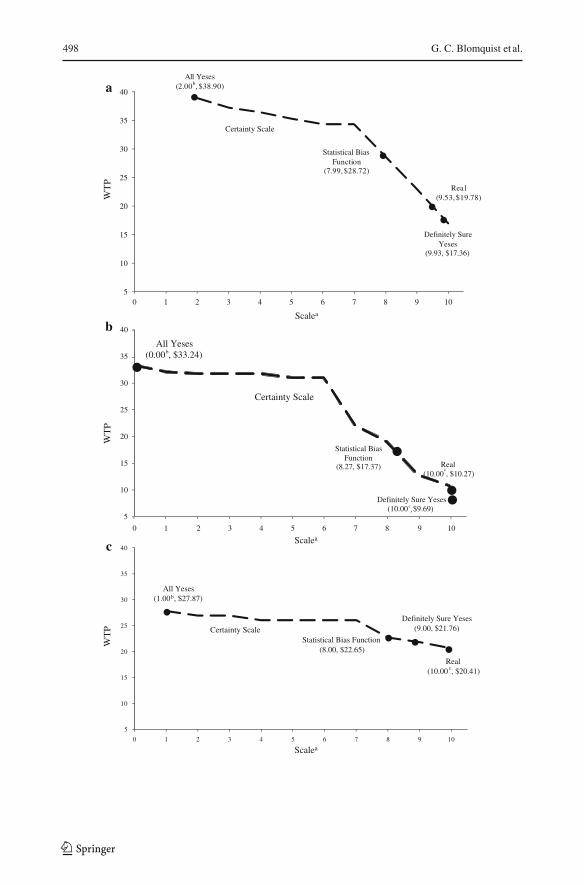
498 G. C. Blomquist et al.
Scalea
Scalea
Scalea
123
Eliciting Willingness to Pay without Bias using Follow-up Certainty Statements 499
Fig. 4� a Scale value producing WTP equal to definitely sure WTP. Diabetes. Mean WTP declines as thecritical certainty scale value increases toward 10a.Superscript ‘a’ indicates the mean WTP based on certainty scale values of 7, 8, 9, and 10 are $34.32, $28.64,$22.99, and $16.96, respectively; Superscript ‘b’ indicates the minimum certainty scale value reported by asubject was 2.b Scale value producing WTP equal to definitely sure WTP. Asthma. Mean WTP declines as the criticalcertainty scale value increases toward 10a.Superscript ‘a’ indicates the mean WTP based on certainty scale values of 7, 8, 9, and 10 are $22.04, $19.03,$12.86, and $10.75, respectively; Superscript ‘b’ indicates the minimum certainty scale value reported bya subject was 0; Superscript ‘c’ indicates the even a certainty scale value of 10 yields a point estimate ofwillingness to pay greater than this point estimate.c Scale value producing WTP equal to definitely sure WTP. Lipid. Mean WTP declines as the critical certaintyscale value increases toward 10a.Superscript ‘a’ indicates The mean WTP based on certainty scale values of 7, 8, 9, and 10 are $26.11, $22.65,$21.76, and $20.59, respectively; Superscript ‘b’ indicates the The minimum certainty scale value reportedby a subject was 1; Superscript ‘c’ indicates even a certainty scale value of 10 yields a point estimate ofwillingness to pay greater than $20.41
Both types of follow up certainty statements have produced calibration of hypothetical yesesthat match well with real purchases of environmental and health related goods.
We make comparisons using data from three separate field experiments in a private good,dichotomous choice setting. One was for a diabetes management program, a second wasfor an asthma management program, and a third was for a lipid management program. Ineach experiment the program was offered hypothetically in contingent valuation and for realpurchase. The diabetes and asthma experiments allow for split sample comparisons becauseindividuals were offered the good either hypothetically or for real. We compare four types ofhypothetical yes responses. They are yeses calibrated by definitely sure, an updated statisticalbias function, 8 or greater on the 10-point certainty scale, and lastly all (uncalibrated) yeses.We compared these hypothetical responses to real purchases also. We compared the means ofobservable characteristics of the respondents for the four types of yeses. While there are somedifferences in the means of some of these characteristics, it is not clear if there is any pattern.
We compared the percentage of yes responses in contingent valuation. The percentage ofyeses tends to increase as we move from calibration by definitely sure to the statistical biasfunction and 8 or greater on the certainty scale, to all yeses. Comparisons to the real purchasedecisions showed that all three calibrations remove indications of hypothetical bias at the5% level for diabetes and asthma, the two programs for which bias was indicated. Usingdefinitely sure to identify true yes responses produces a set of yeses that give no indicationof hypothetical bias at any of the usual levels of statistical significance. To account for anyinfluential differences in observable characteristics of subjects we compared the performanceof a dummy variable for being a hypothetical yes in contingent valuation in logit regressionsof all (hypothetical and real, yes and no) responses. We found that overall comparisons ofthe Hypothetical dummy variable in logit regressions that control for characteristics of thesubjects mimic the comparisons of the percentage yes responses. Our interpretation is that anydifferences in the observable characteristics do not have much effect on differences betweenhypothetical and real responses for the three disease management programs.
We compared the estimates of mean WTP based on the three calibrations and all yesesand also based on real purchases. For the three experiments, estimates of mean WTP tend toincrease from yeses calibrated by definitely sure, to estimates based on either the statisticalbias function or 8 or greater on the certainty scale, to all hypothetical (uncalibrated) yeses. Forall yeses there is strong evidence of hypothetical bias for the diabetes and asthma managementprograms. All three of the calibration methods remove evidence of statistically significant
123
500 G. C. Blomquist et al.
hypothetical bias at usual levels of confidence for diabetes and asthma programs except forweak evidence for the statistical bias function for asthma. For all three disease managementprograms, calibration by definitely sure produces point estimates of mean WTP closest tothe mean of real WTP.
Finally, we estimated the values on the 10-point certainty scale that will produce the sameestimate of mean WTP as calibration by “definitely sure” and the same estimate of meanWTP as real purchases. For the three disease management programs the certainty scale valuesthat produce the same estimates of mean WTP as calibration by definitely sure are 9.9 fordiabetes, 10 for asthma, and 9.0 for lipid. The certainty scale values that produce the sameor closest estimates of mean WTP as real purchases are 9.5 for diabetes, 10 for asthma, and10 for lipid. All of these values are close to 10.
Eliciting willingness to pay without bias means that the ratio of sample estimates ofhypothetical values divided by real values equals one. Little and Berrens (2004) conduct ameta-analysis of ratios from 41 studies that, on average, have hypothetical values that areapproximately triple the real values. Factors considered relevant to explaining hypotheticalbias include laboratory setting or not, private or public good, elicitation method, and hypothe-tical bias mitigation measures such as cheap talk and certainty corrections. Their analysis (andthat of Murphy et al. 2005) find little evidence that hypothetical bias differs between privateand public goods. However, they also find that a referendum format for public goods reduceshypothetical bias consistent with Carson and Groves (2007) contention that a consequential,coercive dichotomous choice referendum can be incentive compatible. Their meta-analysisshows that correction for certainty reduces hypothetical bias.
Whether calibration by the simple definitely sure follow up question would perform as welland be equivalent to values near 10 on the certainty scale for environmental goods or othergoods that might be provided publicly remains an open question. Recent work by Flachaireand Hollard (2007) based on “coherent arbitrariness” suggests that uncertain respondentswill tend to say yes for environmental goods such as preventing another oil spill like theone by Exxon Valdez and that estimates of WTP are likely to be upper bounds unless asecond dichotomous choice question is asked. Whether more reliable estimates are obtainedby asking a follow up valuation question or a follow up certainty question is another openquestion. Håkansson (2008) develops a classic and interval open-ended elicitation (CIOE)format that permits respondents who know their value to report a single value and respondentswho are less certain to report an interval of values. How the mean and lower and upper boundestimates from this format compare to estimates based on dichotomous choice with certaintyfollow up statements is worth exploring. For now, we do have some idea how identifyingtrue hypothetical yes responses by definitely sure/probably sure follow up certainty questionscompares to calibration using a 10-point certainty scale for private goods when values areelicited using dichotomous choice.
References
Arrow K, Solow R, Leamer E, Portney P, Radner R, Schuman H (1993) Report of the NOAA panel oncontingent valuation. Fed Regist 58:4602–4614
Berrens RP, Jenkins-Smith H, Bohara AK, Silva CL (2002) Further investigation of voluntary contributioncontingent valuation: fair share, time of contribution, and respondent uncertainty. J Environ Econ Manag44(1):144–168
Blumenschein K, Johannesson M (2001) Patient willingness to pay for lipid management services providedby pharmacists: an application of the contingent valuation method. University of Kentucky, College ofPharmacy, Unpublished Report
123
Eliciting Willingness to Pay without Bias using Follow-up Certainty Statements 501
Blumenschein K, Johannesson M, Blomquist GC, Liljas B, O’Conor RM (1998) Experimental results onexpressed certainty and hypothetical bias in contingent valuation. South Econ J 65(1):169–177
Blumenschein K, Johannesson M, Yokoyama KK, Freeman PR (2001) Hypothetical versus real willingnessto pay in the health care sector: results from a field experiment. J Health Econ 20(3):441–457
Blumenschein K, Blomquist GC, Johannesson M, Horn N, Freeman P (2008) Eliciting willingness to paywithout bias: evidence from a field experiment. Econ J 118(525):114–137
Carson RT, Groves T (2007) Incentive and informational properties of preference questions. Environ ResourEcon 37(1):181–210
Champ PA, Bishop RC (2001) Donation payment mechanisms and contingent valuation: an empirical studyof hypothetical bias. Environ Resour Econ 19(4):383–402
Champ PA, Bishop RC, Brown TC, McCollum DW (1997) Using donation mechanisms to value nonusebenefits from public goods. J Environ Econ Manag 33(2):151–162
Cummings RG, Taylor LO (1999) Unbiased value estimates for environmental goods: a cheap talk design forthe contingent valuation method. Am Econ Rev 89(3):649–665
Dubourg WR, Jones-Lee MW, Loomes G (1994) Imprecise preferences and the WTP-WTA disparity. J RiskUncertain 9:115–133
Evans MF, Flores NE, Boyle KJ (2003) Multiple-bounded uncertainty choice data as probabilistic intentions.Land Econ 79:549–560
Farmer MC, Lipscomb CA (2008) Conservative dichotomous choice responses in the active policy setting:DC rejections below WTP. Environ Resour Econ 39:223–246
Flachaire E, Hollard G (2007) Starting point bias and respondent uncertainty in dichotomous choice contingentvaluation surveys. Resour Energy Econ 29(3):183–194
Håkansson C (2008) A new valuation question: analysis and insights from interval open-ended data in contin-gent valuation. Environ Resour Econ 39:175–188
Harrison GW (2006) Experimental evidence on alternative environmental valuation methods. Environ ResourEcon 34(1):125–162
Harrison GW, Rutström E (2008) Experimental evidence on the existence of hypothetical bias in value elicita-tion methods. In Plott C, Smith VL (eds) Handbook of experimental economics results. Elsevier Science,New York
Johannesson M, Johansson P-O, Kriström B, Gerdtham U-G (1993) Willingness to pay for antihypertensivetherapy: further results. J Health Econ 12(1):95–108
Johannesson M, Blomquist GC, Blumenschein K, Johansson P-O, Liljas B, O’Conor RM (1999) Calibratinghypothetical willingness to pay responses. J Risk Uncertain 18(1):21–32
Johansson P-O (1995) Evaluating health risks: an economic approach. Cambridge University Press, Cam-bridge
Kriström B (1990) A non-parametric approach to the estimation of welfare measures in discrete responsevaluation studies. Land Econ 66(2):135–139
Li C-Z, Mattsson L (1995) Discrete choice under preference uncertainty: an improved structural model forcontingent valuation. J Environ Econ Manag 28:256–269
List JA, Gallet CA (2001) What experimental protocol influence disparities between actual and hypotheticalstated values. Environ Resour Econ 20(3):241–254
Little J, Berrens R (2004) Explaining disparities between actual and hypothetical stated values: further inves-tigation using meta-analysis. Econ Bull 3(6):1–13
Loomis J, Ekstrand E (1998) Alternative approaches for incorporating respondent uncertainty when estimatingwillingness to pay: the case of the Mexican spotted owl. Ecol Econ 27(1):29–41
Loomis J, Brown T, Lucero B, Peterson G (1996) Improving validity of experiments of contingent valuationmethods: results of efforts to reduce the disparity of hypothetical and actual willingness to pay. LandEcon 72(4):450–461
Murphy JJ, Allen PG, Stevens TH, Weatherhead D (2005) Meta-analysis of hypothetical bias in stated prefe-rence valuation. Environ Resour Econ 30(3):313–325
Poe GL, Clark JE, Rondeau D, Schulze WD (2002) Provision point mechanisms and field validity tests ofcontingent valuation. Environ Resour Econ 23(1):105–131
Ready RC, Whitehead JC, Blomquist GC (1995) Contingent valuation when respondents are ambivalent.J Environ Econ Manag 29(2):181–196
Ready RC, Navrud S, Dubourg WR (2001) How do respondents with uncertain willingness to pay answercontingent valuation questions. Land Econ 77(3):315–326
Svensson E (2000) Comparison of the quality of assessments using continuous and discrete ordinal ratingscales. Biometr J 42(4):417–434
Vossler CA, Ethier RG, Poe GL, Welsh MP (2003) Payment certainty in discrete choice contingent valuationresponses: results from a field validity test. South Econ J 69(4):886–902
123

502 G. C. Blomquist et al.
Vossler CA, McKee M (2006) Induced-value tests of contingent valuation elicitation mechanisms. EnvironResour Econ 35:137–168
Wang H (1997) Treatment of don’t-know responses in contingent valuation surveys: a random valuation model.J Environ Econ Manag 32(2):219–232
Watson V, Ryan M (2007) Exploring preference anomalies in double-bounded contingent valuation. J HealthEcon 26(3):463–482
Whitehead JC, Cherry T (2007) Willingness to pay for a green energy program: a comparison of ex-ante andex-post hypothetical bias mitigation approaches. Resour Energy Econ 29(4):247–326
123