elimination algorithms for data flow analysisropas.snu.ac.kr/lib/dock/rypa1986.pdf ·...

Elimination Algorithms for Data Flow Analysis

BARBARA G. RYDER and MARVIN C. PAULL

Department of Computer Science, Hill Center for the Mathematical Sciences, Busch Campus, Rutgers University, New Brunswick, New Jersey 08903

A unified model of a family of data flow algorithms, called elimination methods, is presented. The algorithms, which gather information about the definition and use of data in a program or a set of programs, are characterized by the manner in which they solve the systems of equations that describe data flow problems of interest. The unified model provides implementation-independent descriptions of the algorithms to facilitate comparisons among them and illustrate the sources of improvement in worst case complexity bounds. This tutorial provides a study in algorithm design, as well as a new view of these algorithms and their interrelationships.

Categories and Subject Descriptors: D.3.4 [Programming Languages]: Processors- optimization; F.2 [Analysis of Algorithms and Problem Complexity]: Nonnumerical Algorithms and Problems

General Terms: Algorithms, Languages

Additional Key Words and Phrases: data flow analysis, elimination algorithms

INTRODUCTION

Compile-time analysis of programs was originally developed to allow the optimization of compiler-generated code. Compile- time analysis of programs includes control flow analysk, which traces the patterns of possible execution paths in a program, and data flow analysis, which traces the possible definitions and uses of data in the program. The information gathered is used to optimize the program by transforming it to a semantically equivalent one that executes faster and/or uses less space.

Optimization of compiled code probably remains the most important use of data flow information. The powerful constructs in modern programming languages necessitate data flow analysis for efficient trans- lation. For example, in a language with late bindings, data flow information allows the replacement of an execution-time check by

a compile-time check; if the type of a variable is constrained to be consistent with its use, data flow information can be used to ascertain the type of the variable. Data flow information is also used in many noncom- piling applications. When source-to-source transformation systems convert a high- level description of an algorithm into another that is optimized for execution, data flow information is used to ensure that the transformations preserve meaning.

Software tools in interactive programming environments make data flow information available to programmers. The ability to see all the definitions or uses of a variable facilitates design, debugging, maintenance, and documentation of code. Interprocedural data flow analysis, which traces data definition and usage across procedure boundaries, is especially suited to this application [Banning 1979; Barth 1978; Burke 1984; Cooper and Kennedy

Permission to copy without fee all or part of this material is granted provided that the copies are not made or distributed for direct commercial advantage, the ACM copyright notice and the title of the publication and its date appear, and notice is given that copying is by permission of the Association for Computing Machinery. To copy otherwise, or to republish, requires a fee and/or specific permission. 0 1987 ACM 0360-0300/86/0900-0277 $01.50

ACM Computing Surveys, Vol. 18, No. 3, September 1986

278 l B. G. Ryder and M. C. Paul1

CONTENTS

INTRODUCTION 1. EQUATIONS MODEL

OF DATA FLOW ANALYSIS 2. ALLEN-COCKE INTERVAL ANALYSIS

2.1 Finding Intervals 2.2 Algorithm Statement 2.3 Linear Performance of Allen-Cocke

Interval Analysis 3. HECHT-ULLMAN T,-T, ANALYSIS

3.1 Parse Generation 3.2 T,-T, Transformations and Elimination 3.3 Propagation 3.4 Algorithm Statement 3.5 Comparison with Allen-Cocke

Interval Analysis 4. TARJAN INTERVAL ANALYSIS

4.1 Reduction Order and Finding Intervals 4.2 T3 Transformations and Elimination 4.3 Propagation 4.4 Algorithm Statement 4.5 Comparison with the Allen-Cocke

and Hecht-Ullman Algorithms 5. GRAHAM-WEGMAN ANALYSIS

5.1 S-Sets and S,, Sf, S, Transformations 5.2 Propagation 5.3 Algorithm Statement 5.4 Comparisons with the Allen-Cocke,

Hecht-Ullman, and Tarjan Algorithms 6. Summary ACKNOWLEDGMENTS REFERENCES

19841. Interprocedural analysis uncovers possible side effects of a procedure call and can help to maintain intricate, inade- quately documented code [Ryder 1974, 1985; Ryder and Carroll 19861.

In complex software, a small change in the program is expected to have localized effect and therefore produce a small change in the data flow information. An incremental update algorithm for data flow analysis only modifies the original data flow solution to reflect changes in a problem and is usually more efficient than a complete reanalysis. Clearly, incremental updating has application to programming environments [Cooper and Kennedy 1984; Zadeck 19841. The modeling work presented in this tutorial was part of the development of incremental update algorithms for data

flow analysis [Ryder 1982a; Ryder and Paul1 19831.

Today, there are two families of global data flow algorithms in use: the elimination methods and the iterative methods. The elimination methods include an original algorithm, Allen-Cocke interval analysis, and three improvements on it: Hecht- Ullman Z’,-Z’, analysis, Graham-Wegman analysis, and Tarjan interval analysis. Our models of elimination methods describe how each algorithm solves the data flow equations that define useful data flow problems. The iterative methods, called workset, round robin, and node listing, solve the data flow equations by initializ- ing them to a safe value and then iterating to a fixed-point solution. These methods, which we do not treat here, originated with G. Kildall’s algorithm [Hecht 1977; Kildall 19731.

In the literature, all of these algorithms are described in terms of a specific implementation, and it is difficult to see their similarities and differences. Our aim is to present the elimination algorithms in an implementation-independent manner that highlights the main ideas of each. To accomplish this we define the data flow problem by a system of equations and describe how each technique solves these equations [Cocke 19701. This reveals the similarities and differences of the algorithms, as well as where and why the complexity savings occur in each, which is not clear from their implementation descriptions. In addition, the models show the algorithms to be general solution procedures applicable to certain systems of equations.

In the remainder of this section we intro- duce data flow analysis, giving examples to illustrate the definitions and concepts. In the program fragment in Figure 1 the question is, “Can execution reach statement L withy never having been assigned a value?” To answer, we insert statement K (see Fig- ure 2), assuming that neither a nor b can have the value 9999, and use our analysis to determine whether it is possible for y to have the value 9999 at statement L. If so, then in the original fragment, the value of y may be undefined at statement L. To


Elimination Algorithms for Data Flow Analysis 9 279

if x> 2 then y := a else if z > 3 * w then y := b

L: q:=2*y /* can y be undefined here? */

Figure 1. Program fragment.

K: y := 9999 if x > z then y := a

else if .a > 3 * w then y := b L: q:=2*y /* can y = 9999 here? */

Figure 2. Transformed program fragment.

analyze the program fragment of Figure 2, we transform it into the graphical representation of Figure 3. The directed graph em- bodies possible execution paths through the statements in the program.

Data flow analysis is usually performed on some intermediate form of a program. We can start with either a control flow graph, which is a directed graph that describes the possible execution paths in a procedure [Hecht 19771, or a parse tree representation of a procedure [Farrow et al. 1975; Kennedy and Zucconi 19771; we use the former in Figure 3. To build the control flow graph of a program, we partition its statements into basic blocks, maximal single-entry sequences that are exited only at their end [Backus et al. 19571. Each basic block is represented by a node in the control flow graph. There is an edge (i, j) in the control flow graph if, during execution, control can transfer from basic block i to basic block j.’ If (i, j) is an edge, then we call j an immediate successor of i and i an immediate predecessor of j. Although each basic block has only one entry, it can have more than one immediate predecessor.

Data flow analysis can also be performed on a call graph, a directed graph that describes the possible calling relations between procedures in a software system [Allen 1974; Ryder 19791. Each procedure in the system is represented by a node in the call graph, and each directed edge represents a possible procedure invocation. In

1 We make the underlying assumption of all static analysis, that all paths in the program are executable, since it is an undecidable problem to identify those that are not.

1 y := 9999 (i)

1 2 r>z-------+3 y:=a(ii)*

1 4 z>3+w+5 y:=b(iii)

6 q:=2*y

Figure 3. Control flow paths for Figure 2.

interprocedural analysis, we trace data flow through the use of reference parameters and global variables [Banning 1979; Barth 1978; Burke 1984; Cooper and Kennedy 1984; Schwartz and Sharir 1979; Sharir 19771.

The term flow graph covers both control flow and call graphs. Throughout this tutorial n is the number of nodes in the flow graph and e is the number of edges. A flow graph has a unique source node (source), which has no predecessors, and one or more exit nodes, each of which has no successors. Each node in the flow graph is associated with a function that describes how the code at the node affects data in the program. Data flow analysis algorithms gather this local information and from it infer the global data flow. The global information then can be specialized to provide data flow information for any node in the flow graph.

By using Figures 2 and 3, we want to calculate the set of possible values for y at statement L (i.e., node 6). This is tanta- mount to considering the set of definitions or value-setting statements for y that can



be propagated along paths containing no subsequent redefinitions of y, called the set of reaching definitions of y. For example, definition (i) of y at statement K (node 1) can be propagated to statement L (node 6) along (1 2 4 6) but not along (1 2 3 6) because definition (ii) at node 3 blocks (i).

The problem of reaching definitions can be expressed concisely using equations. Let pj be the set of all definitions of y in the program if y is not defined at node j, and the empty set otherwise. Let dj be the set of definitions of y created at node j if there are definitions of y at j, and the empty set otherwise. Then Xi, the set of definitions of y that reach node i, can be expressed for our example by the equations in Figure 4. The intersection of pj and Xj either eliminates all definitions that reach node j if y is defined at j, or keeps them all if y is not defined at j.

data flow algorithm for REACH-must solve

More formally, X, is the set of all definitions of variables reaching node m; if a

these equations. The equation for X,,,,,

definition of variable y at node n reaches node m, then y may have the value assigned

reflects the assumption that no variable

to it at node n when execution reaches the

definitions reach the entry to the source

code at node m. A definition-clear path for variable y from node n to m is a path along which there is no value-setting statement

node. We have

for y; therefore the definition of y at node n reaches node m if there is a definition- clear path for y from n to m. Finding

x, = 0,

the definitions reaching a node is referred

m = source,

to as the reaching definitions problem (REACH).

Equations (1) completely describe REACH on an arbitrary flow graph; any

x, = er,

X, = plnXlUd1,

X, = X, = pznXzud2,

Xa = p,nX,ud,,

X, = (fin&ud,)u(p,nX,U&)

u(pan&Udd.

Figure 4. Equations for Figure 3.

(3) pj is the set of all variable definitions that may be preserved through node j (i.e., the set of definitions of variables not redefined at j);

(4) dj is the set of locally exposed definitions at node j, that is, the set of last definitions of each variable -defined at node j [Hecht 19771.

The solution of REACH can be used to optimize the code generated for each basic block in the flow graph. For example, if all the definitions of a variable reaching node m are the same constant value, then we know the variable has that value at m until it is redefined; we can instantiate this constant value in the appropriate places.

common subexpressions elimination). Consider

& = ~jES,l%n,j n Zj U b,,j) U cm

for 15 m 5 n,

where

The four classical data flow problems- reaching definitions, live uses of variables, available expressions, and very busy expressions-all can be formulated as in eq. (2), which is a generalized of eq. (1) [Hecht 19771. The data flow solutions of these classical problems are sufficient for most compiler optimizations (e.g., dead code elimination, constant propagation,

(2)

m # source,

where

(1) pred(m) is the set of all immediate predecessors of m;

(2) Xj is the set of all variable definitions reaching the entry to node j;

(1) 2, is the data flow solution either on entry to or on exit from node m;

(2) 0 is intersection or union; (3) a,,j, b,,j, and c,,, are constants derived

from local data flow information (pos- sibly null);

(4) S, G (i 1 1 5 i I n).

Each variable in the system of equations (Z,)&1 is identified with a unique flow


Elimination Algorithms for Data Flow Analysis l 281

graph node; its value is the data flow solution on entry to (or exit from) the node. Given this one-to-one relationship between nodes and variables, we use these terms interchangeably; interpretation will be clear from the context. The coefficients and constants in the equations are defined using the local data flow characteristics associated with each node, analogous to their definition in eq. (1). From a flow graph annotated with this information at each node, we can obtain a system of equations describing an associated data flow problem.

Data flow problems are called forward or backward, according to the direction of information flow in the flow graph [Kennedy 1971, 19791. In REACH, variable definitions are propagated along paths in the flow graph that represent possible execution paths in the program; this is a forward data flow problem. For such problems the set S, in eq. (2) is the set of immediate predecessors of node m (i.e., predlm}). We limit our attention to forward data flow problems, although some of the methods developed are applicable to backward data flow problems as well [Allen and Cocke 19771.

If X,,, is a solution to a forward data flow problem on entry to node m, then there is a Y, that is the solution for the same problem on exit from node m. In particular, if

Xn = fljEpred{m) h,j n Xj U bm,j), (3)

then

Ym = ~jEpredlml(&?m,j n yi) U GTI, (4)

where

(1) B is intersection or union; (2) o,,j and b,,j are constants associated

with data flow through node j; (3) g,,j and cm are constants associated

with data flow through node m; (4) pred(m) is the set of immediate prede-

cessors of node m.

The choice of which system to solve depends in part on the data flow problem being solved and the use for that data flow information; different equation forms seem natural for different problems. For a forward problem, Y,,, consists of elements of

x, = 0,

X2 = X3 = X4 = X6 = (i),

X6 = (i ii iii).

Figure 5. Solution to Figure 4.

X, that are not affected by the code at node m plus any relevant side effects of the code at node m; there is a linear function f such that Y, = f(X,). Our model can handle data flow solutions on entry to or exit from a node equally well. In subsequent discussions, we use the form most conven- ient for the algorithm modeled.

In data flow problems the initial equations for certain variables, called boundary uariables, are particularly simple. X8,,,, is the boundary variable of a forward data flow problem; (Xj), for j an exit node of the flow graph, are the boundary variables of a backward data flow problem. The initial equation for a boundary variable depends on the specific data flow problem and the equation form being used; a correct initial equation is essential for obtaining a correct data flow solution. For example, for REACH, as illustrated in Figure 4, the initial equation for X,,,, is

X Bo”lVX = 0,

using eq. (3). Using eq. (4), the equation is

Y Eo”me = d source,

where d,,,, is the set of all value-setting statements in the source node that assign a value to a variable that may be its value on exit from the source node.

The solution of the equations in Figure 4 tells which definitions of y reach each node.’ We can obtain this solution by successive substitutions in the equations taken in order. We substitute 0 for X1, solve for X,, and use that solution to obtain X3 and X4. By using those solutions we can obtain X, and X6 and thus fully solve the system, obtaining the solution shown in Figure 5. Since the added definition of y (i) reaches statement L (i.e., node 6), we know that y may be undefined at L dur-

’ In this example we are only concerned with definitions of the variable y.



K: y := 9999 M: if x > z then (x := x - y; goto M]

else if z > 3 * w then y := b L: q := 2*Y /* can y = 9999 here? */

Figure 6. Program variant of Figure 2.

ing the execution of the original program fragment in Figure 1.

Unfortunately, the solution procedure is not always so straightforward. The program fragment in Figure 6 is a variant of the one in Figure 2; we have introduced a loop in the if statement labeled M. The flow graph for the program fragment is shown in Figure 7, and the corresponding REACH equations are shown in Figure 8.

If we try to solve these equations using successive substitutions, we find that X2 is a function of both Xi and X3, and so we cannot obtain its value merely by substituting for the term in X1. Moreover, if we try to obtain a value for X3 first, we see that we need the value of X, in order to obtain a value for X3! Therefore the successive substitution procedure alone is not sufficient to solve the equations. Never- theless, by examining the flow graph in Figure 7, we can obtain the solution shown in Figure 9.

In Section 1 we present general techniques for solving data flow equations, even when loops are present in the flow graph. A straightforward Gaussian-elimination- like method yields a solution with O(n3) complexity. Each of the algorithms presented is a refinement of this method. Allen-Cocke interval analysis defines a natural order on the equations that leads to a highly structured coefficient matrix. Ordered substitutions are used to reduce the solution of the entire system to the solution of a smaller system. This process is repeated, yielding successively smaller systems of similarly structured equations and producing an 0 (n’) solution [Allen and Cocke 19771. Algorithms that improve on interval analysis detect common substitution sequences in the equations and utilize them to reduce the work to 0 (n log n). The Hecht-Ullman Z’i-Z’, algorithm substitutes for individual terms in the equations in a nondeterministic manner but retains a rec-


1 y := 9999 (i)

2 1,

X>Z.-k3 x:=x-y1

1 1 ;z32;:,-*5 y:=b(iill

Figure 7. Flow graph of Figure 6.

x, = 0,

x2 = (P~nx,ud,)u(P3nXud3),

X, = X, = pnnXzUdz,

X5 = p4n-&u&,

X, = (p4nX,ud,)u(p,nX,ud,).

Figure 6. Equations for Figure 7.

Xl = 0,

X2 = X3 = X4 = X5 = (i),

X6 = (i ii).

Figure 9. Solution for Figure 8.

ord of them in a 2-3 tree, calculating common substitution sequences only once [Ullman 19731. The Tarjan algorithm uses a constrained substitution order in which a reduced equation for a variable is obtained by substituting for all dependent variables, that is, those on the right-hand side of the equation, at once [Tarjan 1974, 1981a]. A path-compressed tree is used to remember the substitution sequences so as to eliminate duplicate calculations. The Graham- Wegman algorithm uses a different constrained substitution order for individual terms in the equations [Graham and Wegman 19761, taking advantage of common substitution sequences in the equa-

Elimination Algorithms for Data Flow Analysis 283

tions by delaying the substitutions for terms involving such sequences until the calculations corresponding to such sequences have been performed.

We describe the Gaussian-elimination- like solution procedure and the concept of reducibility. We present models for each of the algorithms and discuss their key ideas. The linear performance of Allen-Cocke interval analysis on a large class of flow

graphs is shown. We compare and contrast the Hecht-Ullman, Tarjan, and Graham- Wegman methods with the Allen-Cocke approach and with each other. One example is worked by all four algorithms to highlight their characteristics. We then summarize the results of our modeling efforts.

1. EQUATIONS MODEL OF DATA FLOW ANALYSIS

We now show in detail the procedure used to obtain the solutions to the REACH problems in Figures 4 and 8 and use these techniques to motivate a formal solution procedure for data flow equations, with and without loops, which is illustrated in an additional example. We consider the struc- tural properties of the dependency graph of the equations and show how they affect the efficiency of the solution procedure. We make use of the reducibility property of flow graphs and show that it provides an order-of-magnitude improvement for the four algorithms modeled.

In Figure 4, given a variable whose solution is known (e.g., X1), we simply substitute the solution for all occurrences of that variable in the system. Repetition of this substitution procedure solves the system of equations, as shown in Figure 10. In Figures 6-8 we see that a loop in the program being analyzed interferes with this procedure by introducing a self-reference in an equation. When we substitute the solution for X1 into the equation for X2, we obtain

x2 = (pl n x1 u 4) u b3 n x3 u d3)

= ((0 fl 0) U (4) U (p3 f-7 X3 U d3)

= (p3 n X3 U d3) U (i).

Now we attempt to eliminate X3 from the equation by substituting the right-hand side of its equation for the X3 term. Since

x3 = pz n x2 u &,

we obtain

X2 = (p3 n X3 u d3) u (4

= (13~ n ((p2 n X2) u d2) u d3) u (4

= (pa f-7 p2 n x2) u (p3 n d2)

U cl3 U (i)

= ((i ii) n (i ii} n X2)

U ((i ii) n 0) U 0 U (i)

= ((i ii) n X2) U (i).

We have introduced a self-dependence in the equation for X2. Examining the flow graph in Figure 7, we see that the X2 term corresponds to definitions reaching node 2 and subsequently traversing the path (2 3 2). The only definition that can do this is definition (i); therefore

X2 = (i).

Rather than resolve each self-reference in this manner, we develop rules for dealing with a self-referential equation by replacing it with another equation in such a way that a solution to the system containing the new equation is also a solution to the original system. This replacement is referred to as “loop breaking.”

In the remainder of this section we present our “equations” model of elimination algorithms more formally. Consider those data flow problems that can be defined by a system of equations Q = (Q,,J L, where Q,,, is an equation of the form of eq. (2) and is solved by a Gaussian-elimination-like method [Isaacson and Keller 19661. Each equation Q,,, in the system is associated with a node m in the flow graph. We assume that the set of possible solution values, each an n-tuple (2, o-e 2,) that satisfies the system Q, admits a partial ordering (s).~

In Gaussian elimination variables are successively eliminated from a system of

3 All the classical data flow problems have this property.


284 ’ B. G. Ryder and M. C. Paul1

x, = 0,

X2 = d, = {i),

X, = X, = (pznXz)udz

= ((i ii iii} fl (i)) U0

= (i),

X5 = b4nX4)ud4

= (Ii ii iii) fl {i)) U0

= lil,

X6 = ~P3nx3~u~Plnx,~u~P5nx5~ud3ud,ud6

= (0rl(i))U((i ii iii)fl(i))

U (ran {i)) U (ii) U0U (iii)

= {i ii iii].

Figure 10. Solution procedure for the equations of Figure 4.

equations by repeated substitution of the right-hand side of an equation for a term in that variable. We define an analogous substitution process. A substitution transformation of a system of equations Q, s(Q, m, j) for 1 5 m, j I n, is the result of substituting the right-hand side of Q,,, for a term in 2, on the right of equation Qj, m # j, and simplifying the resultant right- hand side of Qj. Then s( Q, m, j) differs from Q by having at most a different Qj equation; all other equations are the same. It is clear that a solution of s( Q, m, j) is also a solution to Q, and vice versa.

To handle possible self-references introduced by the substitution transformations, we use a loop-breaking rule. An equation Q,,, has a loop-breaking rule if there is another equation for 2, called q,,, such that

(i) 2, does not appear on the right-hand side of q,,,;

(ii) every solution of qm is also a solution of Qm;

(iii) for every solution S of Q,,, there is a solution s of qm such that s I S [Paul1 19861.

A set of equations Q is said to have a loop- breaking rule if for each equation in Q initially there is a loop-breaking rule, and for any equation in any set that can result from Q by a sequence of substitution transfor-


mations of Q there is also a loop-breaking rule. A loop-breaking transformation of Q, b(Q, m), for 1 5 m 5 n is the result of replacing Q,,, by qm.

The Gaussian-elimination-like solution procedure for the system of equations consists of applying a sequence of the substitution and loop-breaking transformations; the procedure is shown in Figure 11. The complexity of this algorithm is O(n3), assuming (as usually holds) that each application of b is O(1) and of s is O(n).4 It can be shown that if a sequence of these transformations is applied to a system of equations Q producing the system R and {S, ] 1 I m I n) is a solution to R, then it is also a solution to Q. Further, if (L, ] 1 5 m 5 n] is a solution to Q, then there is a solution of R, (K,,, 1 1 5 m 5 n) such that K,,, I L, for 1 5 m 5 n. If Q has a loop-breaking rule, then the procedure in Figure 11 terminates and produces the unique minimal solution (in terms of the partial ordering) [ Paul1 19871.

For the classical data flow problems, the implementation of this method can involve

‘These assumptions hold even for a multigraph for data flow problems defined by equations of the form of eq. (2). With the operators of union and intersection, multiple terms in one variable can always be combined to yield one term. After a substitution transformation is completed, there will be not more than n distinct terms on any right-hand side of an equation.

Elimination Algorithms for Data Flow Anulysis l 285

/* elimination */ for i = 1 to n - 1 do

begin

Q t b(Q, i) for j = i + 1 to n do Q+- s(Q, i, j)

end /* back substitution */ for i = n to 2 do

begin for j = i - 1 to 1 do Q c s(Q, i, j)

end

Figure 11. Gaussian-elimination-like solution procedure.

bit vector or set operations. The partial ordering on the n-tuples is one of componentwise set inclusion for a set implementation and componentwise comparison for a bit vector implementation. The loop- breaking rules for these problems are very simple.5 In eq. (2), if fl is U as in REACH, then we have

Qm: 2 = a n 2 u p, (5)

where a is a constant and B can contain terms in variables other than 2 as well as constants. The corresponding loop- breaking rule substitutes equation qm for Q,,,:

qm: z = p. (6)

In this case we say the loop-breaking rule is to drop the self-referential term (i.e., a n 2). In eq. (2), if 0 is n, then we have

Qm: 2 = (a n 2 u C) n p, (7)

where a and c are constants and fi can contain terms in variables other than 2 as well as constants. The corresponding loop-breaking rule substitutes equation qm for Qm:

qm: 2 = c n p. (8)

To validate a loop-breaking rule for an equation, we must satisfy the conditions (i)-(iii) given above. Clearly, 2 does not appear on the right-hand side of q,,, in eq. (6) (i.e., (i) is satisfied). Then the solution of the loop-breaking rule qm must be

6 In general, loop-breaking rules are determined by the operators in the equations [Paul1 19871.

1 81: X1=0,

1 2

0

Qz: X2 = (~lnX~ud,)U(wnXaUd,),

3 Qa:Xa=pznX,udp.

Flow graph

Figure 12. REACH example with loop.

shown to satisfy the original equation Qm. Letting 2 = p in eq. (5), we have

p =? (a n p) U p,

which is clearly true (i.e., (ii) is satisfied). Finally, for every solution S of Qm there must be a solution s of qm such that s 5 S. Here, if S is a solution to Qm, then

S=(anS)uP*BGS.

Therefore 2 = p 5 S for S any solution of Qm (i.e., (iii) is satisfied). By replacing eq. (5) by eq. (6) we are selecting the minimal solution for 2 from the set of possible solutions satisfying Qm.

We use an example of REACH to illustrate these ideas. In Figure 12, we apply a loop-breaking rule; the variable whose equation becomes self-referential corresponds to node 2, which is an entry node of a loop in the flow graph. The substitution transformation s(Q, 3, 2) introduces an X2 term in the right-hand side of Qz,

Qz: Xz = (PI n X, u dd

u b3 f-7 b n x2 u d2) u d3),


286 . B. G. Ryder and M. C. Paul1

which is eliminated by a loop-breaking transformation b(s(Q, 3, 2), 2),

qz: X2 = (PI n XI u 4)

u (~3 n dd u &.

Let R = (Qi, q2, Q3). Now two substitution transformations solve the system R, 4R, 1, 21,

X2 = (~1 n 0 u 4) u (~3 n 4) u da,

X2 = 4 u (~3 n 4) u da,

and s(R’, 2,3), where R’ is R with the result of s(R, 1, 2) replacing q2,

X3 = ~2 n (4 u (~3 n d2) u d3) u d2,

x3 = (p2 n dl) u (p2 f-7 p3 n dd

u (PZ n &) u &,

yielding after simplification,

x, = 0,

X2 = dt u (~3 n d2) u d3,

X3 = (~2 n 4) u (~2 n d3) u d2.

Thus the loop-breaking transformations guarantee the effectiveness of the procedure in Figure 11 on flow graphs with loops.

Thus far we have described the data flow problems as defined by the flow graph of the corresponding program. However, we can use the solution technique presented here on any system of equations that has a loop-breaking rule. Given a set of equations of the form of eq. (2), we can define a dependency graph, a directed graph corresponding to the interdependencies of variables given by the equations in that system. Each node represents a variable; each directed edge (m, n) represents the dependence of X,, on X,,, (i.e., the occur- rence of X,,, on the right-hand side of the equation for X,,). For forward data flow problems, the dependency graph is the flow graph of the problem.

We describe the elimination algorithms as solution procedures for systems of equations and their corresponding dependency graphs, comparing and contrasting the data flow algorithms by examining how they solve these systems. The equations can be solved by a method patterned after


straightforward Gaussian elimination with order O(n3) complexity. In fact, the elimination methods described here all have better worst case bounds because they take advantage of a special coefficient structure, first utilized by Allen-Cocke interval analysis, that results from the sparseness of the system of equations and the reducibility of the dependency graph. A standard assumption in data flow analysis of control flow graphs that correspond to real programs is that e = O(n) [Hecht 1977; Hopcroft and Ullman 1972; Tarjan 1974; Ullman 19731.

A reducible directed graph is one with no multiple-entry loops [Hecht 1977a].6 In a system with a reducible dependency graph, the variables of the system are naturally partitioned into groups that can affect each other only in a highly constrained manner. In practice, irreducible control flow graphs are rare; therefore data flow methods that require reducible systems are almost always sufficient [Hecht 1977; Knuth 19711. The Hecht-Ullman and Tarjan interval analysis algorithms are restricted to systems of equations with reducible dependency graphs. The Graham-Wegman algorithm can handle irreducible systems (see Sec- tion 5.3). Allen-Cocke interval analysis can be adjusted to handle irreducibilities as well [Schwartz and Sharir 19791. We should bear in mind that an irreducible system can always be solved straight- forwardly, if inefficiently, by the Gaussian- elimination-like method in Figure 11.

2. ALLEN-COCKE INTERVAL ANALYSIS

Interval analysis was orginally developed in the elimination algorithm in Allen [1971]. The key step is to use the reducibility of the dependency graph to convert the solution of a system of n equations to the solution of a smaller system of r equations by partitioning the equation variables into r subgroups called intervals, single- entry regions corresponding approximately to loops in the dependency graph.’ The partitioning algorithm that finds the inter-

6 A subgraph is defined to be single entry if all incident edges are incident on a single vertex. Single exit is defined similarly. ‘For forward data flow problems, the dependency graph will be the flow graph.


INT := null; I := null; H := [s];

while (H # null) do

/” list of intervals */ /* each interval */

/* header list initialized to source node */

Destructively select h from H; I := (h]; /* form Zh */ while (There is a node m not s, whose immediate predecessors are all

in I but m is not yet in I) do Add m to I;

endwhile; Add I to INT; while (There is node n not in H and not in INT, with at least one

predecessor in I) do Add n to H;

endwhile ; endwhile ;

Figure 13. Interval-finding algorithm.

vals is explained in Section 2.1. If h is the entry node of an interval, we call it the interval head node of interval Ih. The order in which nodes are added to an interval, called an interval order, preserves the partial order of the dependency graph. By forming a linear order of all the nodes in the graph that embeds the interval orders on every interval and writing the equations in this order, we obtain a highly structured coefficient matrix, amenable to simplification by a sequence of substitution transformations. This structure ensures that the equation for each variable in an interval can be parameterized in terms of the interval head variable (i.e., the variable corresponding to the interval head node). We call the result of this parameterization a reduced equation.

In this section we present our model of the Allen-Cocke algorithm. First we infor- mally discuss the algorithm that finds the intervals and demonstrate their use in solving the system of equations. We then state the interval analysis algorithm formally, and we show that the Allen-Cocke algorithm in practice has linear worst case complexity on a reducible flow graph with maximal loop nesting level bounded by a constant.

2.1 Finding intervals

The partitioning algorithm finds single- entry regions in the dependency graph. This algorithm is presented in Figure 13

and may be paraphrased as follows [Allen and Cocke 19771. We initialize a set S to contain the unique source node of the dependency graph. Then we look for any nodes whose immediate predecessors are all in S. We add any such nodes into S and continue. Eventually, either every node will be in S or we will have exhausted all the nodes that could be added to S and have remaining a set of nodes H that have been examined but have predecessors both in S and not in S. At this point all nodes cur- rently in S constitute an interval, headed by the first node added to S. Arbitrarily we choose a node from H, reinitialize S to contain only that node, and continue as before. The process terminates when every node in the graph has been added to some interval.

Clearly an interval order as defined by Figure 13 is not unique; that is, different representations of the same graph will result in different interval orders. The order also preserves the ancestor-first relations on the graph. Characteristics of intervals guaranteed by the algorithm are [Allen and Cocke 19771:

(i) The set of interval head nodes on a flow graph is unique.’

(ii) The head node of an interval dominates internal interval nodes.

(iii) An interval is single entry.

‘This follows from the fact that a flow graph has a unique source node.



(iv) Any back edge in an interval has the interval head node as its target [Hecht 19771.

(v) The interval order on an interval is consistent with the partial ordering imposed by the predecessor relations of the flow graph.

2.2 Algorithm Statement

The algorithmic reduction of the solution of a system of n equations to a smaller system of r equations, where r is the number of intervals in the dependency graph of the equations, consists of two phases: elimination and propagation. During elimination we perform successive substitution and loop-breaking transformations on the systems of equations; this phase gathers and summarizes the local data flow side effects. During propagation we perform back-substitutions of solutions for terms in equations; this phase propagates global data flow side effects to the local regions where they apply. The model of the algorithm is given at the end of this section.

The elimination phase consists of iterating three steps: finding intervals in the dependency graph associated with the system of equations, reducing the equations to form a new system of reduced interval head variable equations, and forming the dependency graph of the reduced system. Within each interval in the system, a sequence of substitution transformations reduces all the equations to linear functions of the interval head variable. A derived system of equations is formed that consists of the r reduced interval head variable equations and depends only on interval head variables from the former system. This derived system is partitioned in turn into intervals: each with an interval order, and the coeffuxent matrix structure of the origin& problem is preserved in its equations.’ When the original flow graph is reducible, the three-step process can be continued, yielding a sequence of systems of equations and a final system of one equation.

’ The arguments establishing the coefficient matrix structure utilize only the properties of intervals and an interval order.

The propagation phase consists of iterating two steps: establishing variable cor- respondences and substituting interval head variable solutions into reduced equations, thus obtaining solutions for internal interval variables. To begin, we solve a system of one equation. The final variable is associated with the corresponding interval head variable in the preceding system as they share the same solution. Focusing on the preceding system, the interval head solution is substituted into the reduced equations for variables in its interval. Then, each of these newly solved variables is associated with its corresponding interval head variable in the system preceding the one just solved. The solutions for all variables in this system are similarly obtained. This variable correspondence/substitution process is iterated through the derived systems of equations established in the elimination phase in reverse order until all solutions are obtained.

The sequence of dependency graphs (G’)ki corresponding to the sequence of systems of equations is called the derived sequence of graphs, and G’+’ is called the derived graph of G’. Whenever we use G i, we are referring to a graph in the derived sequence of graphs in Allen-Cocke interval analysis. When we say that y in G’+’ represents I,, in G’, we are referring to the fact that all variables in Ih are represented by variable X, in G i+l, the corresponding node of which in G’+’ is y. The definition of represents is extendible over finite subsequences of the derived sequence. Therefore, if

ml E &a, ii G’, . . . , mk E &+, c G i+k-l,

we say that mk represents ml in Gi+k-‘. During elimination, when we remove all

dependence in the system of equations on variables in Ih, we replace those dependences by a dependence on Xh. The graphical interpretation of this action is that h in G2 represents I,, in G ‘. In Figure 14, node 2 in G2 represents I2 in G ‘. This signifies that internal interval variables in I2 on G1 (i.e., (3)) do not appear in the derived system corresponding to G2. Of course, since we partition the nodes of both G ’ and G 2 into intervals, node 2 belongs to



G’ G2 G3

Zl = Ill, Zl = (1 2 41 z = Ill

12 = I2 3t,

14 = (41

Figure 14. Derived sequence.

two different intervals on the two graphs: node 2 is in I2 on G * and in I1 on G ‘. That is, there are two different systems of equations depicted in these graphs; X2 is in a different partition element in each system. A REACH problem fully solved using Allen-Cocke interval analysis is presented in Figure 22, Section 3.5.

2.2.1 Model of the Allen-Cocke Algorithm

Elimination Phase

(9

(ii)

(iii)

Define the forward data flow equations on the original flow graph, G1. Let 12 = 1. Find the intervals in Gk using the Allen-Cocke interval finding algorithm in Figure 13. Number the variables in each interval according to an interval order. Apply substitution transformations within each interval to obtain the system of reduced equations. Use the relevant loop- breaking transformation on any self-dependences introduced in the process. Use substitution transformations to render all interval head variable equations independent of noninterval head variables. Create the dependency graph G k+l the nodes of which are the interval head variables from Gk and the edges of which are defined by the dependences in the reduced system of equations

(i.e., insert an edge (m, n) if the data flow equation for X, contains a dependence on X,,,).

(iv) If there is more than one node in G k+l, then increment k by 1 and return to step (ii).

Propagation Phase

(v) Solve the final equation. (vi) Each interval Ih in Gk corresponds to

a node w in Gk+l. For each interval head node h in Gk set Xh equal to the solution at the node corresponding to I,, in Gk+l, X,. Then substitute this value of Xh into the reduced equations in Ih to solve for all variables, thus solving the system of equations associated with G k.

(vii) If k = 1, stop. Otherwise, decrement k by 1 and return to step (vi).

2.3 Linear Performance of Allen-Cocke Interval Analysis

In this section we show that in Allen-Cocke interval analysis, the amount of work both in finding the intervals and in solving the equations exhibits a linear worst case complexity bound on reducible flow graphs under common conditions. Our result is a practical limit on the performance of the Allen-Cocke algorithm on reasonable flow graphs encountered in practice; it does not hold for general graphs.

The worst case performance of the Allen- Cocke algorithm can be O(n2) even if e is only O(n). This bound is achieved on the worst case reducible flow graph, which is pictured in Figure 15. This graph of n nodes has approximately 2n edges and a loop nested at a depth of approximately 2n/3 [Ullman 19731. However, reasonable programs do not contain highly nested loops.

Empirical surveys of high-level programming languages confirm that in actual practice, loop-nesting depths of greater than six are rare. Two FORTRAN surveys in the 1970s reported that typical nesting of do statements was very shallow [Knuth 1971; Robinson and Torsun 19761. Knuth, reporting on programs from Stanford University and the Lockheed Corpora- tion, stated that 91 percent of the do



Figure 15. Pathological flow graph for Allen-Cocke interval analysis.

statements had fewer than four levels. Robinson, surveying two program popula- tions from students and systems programmers at Brunel University in England, noted that a majority of the do statements had fewer than four levels: 76-84 percent (student/systems) of the do statements had fewer than seven. The assumption of a six- level limit of loop nesting in PL/I programs was supported by Allen [private communi- cation, 19791.

Thus in reasonable programs it is valid to assume a maximum loop-nesting depth that is a constant k, k << n, that is independent of the number of nodes in the control flow graph. Under that assumption for a reducible control flow graph, Theorem 1 shows that the equation solution work of the Allen-Cocke algorithm has O(n) complexity using the standard assumption that e is O(n). Furthermore, a work-set form of the interval-finding algorithm is O(n) on a flow graph when e is O(n) [Hecht 19771; by restricting the loop nesting depth to a constant k, we restrict the possible length of the derived sequence, resulting in an O(n) bound on interval finding over the entire algorithm.” These results corroborate the common observation that the O(n2) worst case complexity bound is not observed in practice.

lo It seems straightforward to extend Theorem 1 to show that Allen-Cocke interval analysis has a worst case complexity hound of O(nf(n)) if the loop nesting depth is bounded above by f(n).

Theorem 1 also holds on call graphs that satisfy its hypotheses for data flow problems defined by equations of the form of eq. (2). Although call graphs are multi- graphs, we can combine multiple terms in one variable into one term, because of the form of our equation. Therefore they become nonmultigraphs at a cost of no more than O(e).

Theorem 1

Given a reducible flow graph G in which e is O(n), suppose that the maximum loop nesting depth is less than or equal to a constant k. Assume that Allen-Co&e interval analysis is applied to solve a forward data flow analysis problem on G. Then the worst case complexity of the equation solution work of the Allen-Co& algorithm on that flow graph is O(n), where n is the number of nodes in G.

PROOF. From our model of Allen-Cocke interval analysis we see that the terms in the system of equations can be partitioned into two disjoint sets: a set S1 of elements that are substituted for once during elimination and a set S2 of those elements for which substitution takes place more than once. The work of elimination can be calculated by considering the sum of the elimination work for terms in Si and Sp.

The elimination work for terms in Si is 0( ] S1 ] ) 5 O(n), by our assumption that e is O(n). The terms in S2 occur in interval



head equations in G = G1. If a term involving Xj E Sz occurs in the equation of Xi in G1, then in step (iii) of the Allen- Cocke algorithm a linear function of X,, will be substituted for the variable Xi, where j E Ih in G. Likewise, in G2 a linear function of X, will be substituted for the variable X,, in the equation of Xi, where h E 1q in G2. Because G ’ is reducible, this process continues for finitely many steps until the edge representing (j, i) in G1 no longer exists on some G”.

Assume that each interval in the flow graph corresponds to a loop. Each step in the derived sequence accomplishes the collapse of the innermost loop of a nested loop. Since the maximum nesting level is k, all loops will be collapsed in Gk+l. Under our assumption, the source node will also be in a loop; therefore Gk+l will be the trivial graph of a singleton node.”

Alternatively, there may be intervals not corresponding to loops in the flow graph; call these “null loops.” By the properties of the interval-finding algorithm of Figure 13 we can show that if there are no loops in the graph Gj, then there can be no null loops in Gj except for the entire graph Gj itself. If there are null loops on G’ and loops are nested no deeper than k, then Gk+l is acyclic, although it may contain more than one node. Therefore the derived sequence is at most k + 2 long, with either Gk” or G k+2 being the trivial graph of a singleton node.

Thus an edge (j, i) in G1 can be represented on at most k + 1 graphs in the derived sequence, and the elimination cost for terms in S2 is bounded above by c 1 S2 1 (k + 1) for c a constant. Since the total number of terms is the number of edges in the original flow graph, both 1 S1 1 and 1 S2 1 are no greater than O(n). There- fore the elimination work is bounded by O(n).

The propagation work is bounded by the number of nodes in the entire derived sequence since we are merely substituting into reduced equations each a function of

I1 We “violate” the definition of source node here to allow its inclusion in a loop.

one variable. Since the number of nodes in successive graphs in the derived sequence decreases, the number of nodes in any G’ is bounded by O(n). Therefore the total number of nodes is bounded by bn(k + 1) + 1 for b a constant and (k + 2) the length of the derived sequence, and so O(n) also bounds the work of the propagation phase.

Thus the worst case complexity of the equation solving by Allen-Cocke interval analysis is bounded by O(n). Q.E.D.

In the proof of the theorem we assume that 1 S:! 1 on G1 dominates the number of substitutions on each G’, i > 1. This is true because any term requiring substitution on G’, i > 1, corresponds to a term on G ‘. In some models of interval analysis the derived graph can become a multigraph. Since the parallel edges correspond to distinct edges in the original graph, this does not affect the complexity arguments in the proof.

3. HECHT-ULLMAN T,-Tz ANALYSIS

In the next three sections we present models of three closely related data flow algorithms, all improvements on the Allen- Cocke algorithm. On flow graphs in which the number of edges e is O(n) these algorithms achieve a worst case bound of O(nlogn)12 rather than the O(n2) bound of the Allen-Cocke algorithm. The performance is improved by the delay of certain calculations and the discovery and utiliza- tion of common substitution factors in the equations. We compare them with the Allen-Cocke algorithm on forward data flow problems.

In this section we present our model of Hecht-Ullman Tl-T2 analysis. The group- ing of variables is less constrained than in the Allen-Cocke algorithm and is performed using a “nearest neighbor” heuris- tic. The delay in the calculation of common coefficient/constant factors in the reduced equations yields savings in elimination. These shared factors necessitate the use of

I2 The Tajan algorithm can achieve an almost linear worst case bound of O(n C&Z)) but its practical implementation explained in Section 4 achieves a 0 (n log n) bound [Tarjan 1981a].



a data structure to remember them; a height-balanced 2-3 tree is used [Aho et al. 19761. The Hecht-Ullman method consists of three phases analogous to those of Allen- Cocke interval analysis: parse generation, elimination, and propagation. We contrast the two for each of these phases. The Hecht-Ullman algorithm can only be applied to programs with reducible flow graphs [Hecht 19771, but as we noted above, this is not really a limitation in practice.

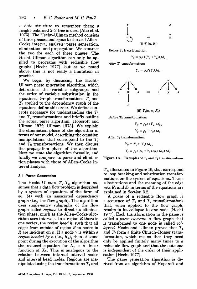
We begin by discussing the Hecht- Ullman parse generation algorithm, which determines the variable subgroups and the order of variable substitution in the equations. Graph transformations TI and T2 applied to the dependency graph of the equations define this order. We define concepts necessary for understanding the TI and T2 transformations and briefly outline the actual parse algorithm [Hopcroft and Ullman 1972; Ullman 19731. We explain the elimination phase of the algorithm in terms of our model, describing the equation manipulations that correspond to the TI and Tz transformations. We then discuss the propagation phase of the algorithm. Next we state the algorithm formally, and finally we compare its parse and elimination phases with those of Allen-Cocke interval analysis.

3.1 Parse Generation

The Hecht-Ullman TI-T, algorithm assumes that a data flow problem is described by a system of equations of the form of eq. (4) with an associated dependency graph (i.e., the flow graph). The algorithm uses single-entry subgraphs of the flow graph called regions to direct its elimination phase, much as the Allen-Cocke algorithm uses intervals. In a region R there is one vertex, the region head h, such that all edges from outside of region R to nodes in R are incident on h. If a node y is within a region headed by h (i.e., Rh), then at some point during the execution of the algorithm the reduced equation for X, is a linear function of Xh. This is analogous to the relation between internal interval nodes and interval head nodes. Regions are ma- nipulated using the transformations TI and

Before T, transformation:

After Tl transformation:

1 Y

(ii) Th, w, &)

Before Tz transformation:

Yw = pton Yuu&,

Yy = pyn Ywud,.

After T2 transformation:

Y, = Pwn Yuud,,

Y, = prnpmn Y,Up,nd,ud,.

Figure 16. Examples of Tl and T2 transformations.

T2, illustrated in Figure 16, that correspond to loop breaking and substitution transformations on the system of equations. These substitutions and the meaning of the edge sets E1 and E2 in terms of the equations are explained in Section 3.2.

A parse of a reducible flow graph is a sequence of TI and T2 transformations that, when applied to the flow graph, results in its collapse to one node [Hecht 19771. Each transformation in the parse is called a parse element. A flow graph that is transformed to one node is called collapsed. Hecht and Ullman proved that TI and Tz form a finite Church-Rosser transformation, which means that they need only be applied finitely many times to a reducible flow graph and that the outcome is independent of the order of their application [Hecht 19771.

The parse generation algorithm is derived from an algorithm of Hopcroft and



Ullman [Hopcroft and Ullman 1972; Ullman 19731. The algorithm examines a flow graph that is represented by a set of nodes and the lists of in-edges and out- edges associated with each node. The order of the edges on these lists influences the parse generated. An explicit search and test are made for each T2 transformation; Tl transformations result from these tests whenever a self-loop is detected. The same node may appear in more than one Tl transformation in a parse, although an edge can appear in only one parse element.

In parse generation a sweep through all nodes and edges in the flow graph initially finds T2 candidates and any self-loops. Figure 17 illustrates a suhgraph in which node v is a T2 candidate because it has a unique parent. For each T, candidate v, its immediate neighbors are checked for Tz candidacy. First each immediate descendant of v is checked to see whether it becomes a Tz candidate after T&z, v, *), and if necessary Z’,(y, *) is performed. Then z the immediate parent of v is checked to see if it becomes a Tz candidate after T&, v, *) and if necessary Tl(z, *) is performed; for example, this can occur if (v, z) prevented z from being a Tz candidate previously, as in Figure 17. The parse of a flow graph is nonunique; the order of the transformations obviously depends on the flow graph representation. The outline of the parse generation algorithm is given in Figure 18.

In practice, when edge lists are manipu- lated, the parse generation algorithm of Figure 18 always merges the smaller region into the larger one by counting the number of nodes represented by each node in the partially collapsed flow graph [Ullman 19731. This strategy ensures a worst case bound for flow graphs with the usual assumption for flow graphs that e is O(n) [Hopcroft and Ullman 1972; Ullman 19731.

3.2 T,-T2 Transformations and Elimination

The calculations of the elimination phase are directed by the parse of the flow graph. A region in equation terms is a subgroup of variables all of which have reduced equations that are linear functions of the region head variable. Our descriptions of the Tl

Y

Figure 17. TS transformation candidate.

and T2 transformations in Section 3.1 are graphical. In this section we explain the sequence of equation manipulations to which they correspond. Each Tl or T2 transformation triggers a coefficient/constant calculation that further reduces at least one of the equations in the system. Examples of these calculations are given in the REACH equations in Figure 16.

A T2 transformation can be applied when a node has a unique predecessor, that is, when the equation of the corresponding variable is a function of one variable. The T2 transformation Tz(u, w, E2) in Figure 16(ii) merges R,, the region represented by node w in the partially collapsed flow graph, into its unique predecessor region R,, represented by node u. Here Ez is the set of edges in the original flow graph represented by (u, w) in the partially collapsed flow graph. In the elimination phase this Tz parse element corresponds to selecting two subgroups of variables (R, R,), each with a region head variable (Y, Y,), and merging them into one subgroup (R,). After the merge there is one region head variable Y, representing all the members of the newly merged subgroup; therefore the reduced equation of each variable in the new subgroup is a linear function of Y,.

Each edge in the set of edges E2 corresponds to a term in the original equation for Y,. These terms are represented in the partially reduced equation for Y, by the term in Y,. When the parse element Tz(u, w, E2) is performed, we do a sequence of substitution transformations such that the right-hand side of the reduced equation for Y,, a linear function of Yu, is substituted into the equations of any variables cur- rently dependent on Y,. These include all variables in R, represented by w in the partially collapsed flow graph, as well as all variables corresponding to immediate



L := null; /* L is a list of Tz candidates */ for i := 1 do n do

if in-edges(i) contains (i, i) then Generate T,(i, *); if in-edges(i) contains only one edge then Add i to L;

endfor; while L # null do

Destructively select v from L; Find unique predecessor of v, z; Generate T2(z, v, *); Determine if z can be added to L, perhaps after a T, transformation

of z; for each immediate descendant of v, y do

Determine if y can be added to L, perhaps after a T, transformation of y;

endf or ; Add out-edges(v) to out-edges(z);

endwhile ;

Figure 18. Parse generation algorithm.

descendants of w; in Figure 16(ii), the latter category includes Yy . Updated reduced equations are obtained for all nodes in R, and for these immediate descendant nodes; thus all dependence on Y, in the current system is eliminated.

A T1 transformation is applied to remove a self-loop, or in equation terms, a variable from the right-hand side of its own equation. The Z’i transformation Z’i(u, Ei) in Figure 16(i) removes a self-loop from node u. E, is the set of edges in the original flow graph, represented by (u, u) in the partially collapsed flow graph. Each edge in El corresponds to a term in the original equation for Y,; each was a back edge to u in the original flow graph. When the T1(u, El) parse element is encountered, the heads of these edges are nodes already in region R,. When they were merged by previous Tz transformations into R,, the associated variable substitutions may have resulted in the introduction of Y, on the right-hand side of the partially reduced equation for Y,. The self-loop in Figure 16(i) represents this dependence. In the elimination phase, when a Tl parse element is encountered, we apply the appropriate loop-breaking rule (see Section 1) to eliminate any dependence of Y, on itself.

The basic elimination step of the Hecht- Ullman T,-T2 algorithm, associated with the T2 transformation, is the complete

removal of a particular variable in the partially reduced system of equations (e.g., performing T2(u, w, Ez) removes Y, from the system). In practice the algorithm ac- tually performs the calculation associated with T2(u, w, Ez) only for variables with nodes in region R, after the T2 graph transformation is performed; all other calculations are delayed. That is, if the equation for Y, contains a term Y, and z 4 R, after Tz(u, w, E2) is performed, then replacement of Y, by a linear function of Y, (i.e., s(Q, w, z)) is delayed until z and w are in the same region. At that time, occurrences of Y, are replaced by the right-hand side of the then current reduced equation for Y,. Eventually z and w must be in the same region, as all nodes are finally in the region of the entire graph, R,,,,.

For example, in Figure 19 the graph has two possible parses.13 In both, when T2(3, 4, ((3, 4))) is performed, node 5 is in neither R3 nor R4. The existence of edge (4, 5) implies that there is a Y4 term in the equation of Ys. The replacement of that Y4 term is delayed until nodes 4 and 5 are in the same region; this occurs after parse element TAl, 5, ((2, 5)(3,5)(4, 5))) is performed. Then the current reduced equation for Y4 as a linear function of Y1 is substituted into the equation for Ys.

I3 It has a unique interval order (1,2,3,4, 5).



Parse A Parse B

T*(3,4, H3,4)1) T-2(1,2, I(19 2)l)

T2(1, 2, Hl, 2))) T2(3,4, {(3,4)1)

TI(3, ((4, 3N TI(3, N4,3N

T,U, 3, I& 3)(2,3)1) Tz(l, 3, W,3)(2,3)l)

T*U, 5, I@, 5)(3,5)(4,5)l) TZU, 5, w&5)(3,5)(4, 5)l)

T,(l, 1(5, l)l) Tl(l, 1(5, Ul)

Figure lg. Delayed substitutions example.

Graph

Figure 20.

Parse

1. T,(5,6, l(5,W

2. T,(5,7, l(5,7)l)

3. T2(4,5, 1(4,5)l)

4. T&3,% (@,g)l)

5. Tz@, 10, W3, WI)

6. T2(4,6, l(4,W)

7. T1(4, ((6,4)l)

6. Td3,4, l(3,4)l)

9. TI(3, H793)l)

10. T2(2,3, w, 3)))

11. TIC4 w, al)

12. Tz(L 2, 0 2)l)

13. TlU, IOO, w

Common factors example.

The delay in performing out-of-region and 21 illustrate these. Figure 20 shows variable substitutions enables the Hecht- the Ullman worst case flow graph for Ullman algorithm to avoid recalculating Allen-Cocke interval analysis for n = 10 common coefficient factors in some reduced (see Figure 15), with a possible parse equations. These factors occur because [Ullman 19731. Figure 21 shows the common substitution sequences exist in Hecht-Ullman algorithm applied to a the system: The example in Figures 20 REACH problem formulated on that



Initially:

Yl = pin Y,oud,,

Yz = pzn Y,upzn Ysu&r

Ya = PZ~ Ysupsn YTu&,

Y, = p,n Y3up,n Ysud,. Let di ,... i, = pi,n.. . npiti,nd,Upi,n.. . npiJd;k,U.. . ud,.

After parse element 7. Y4 E &, Y3 E I&, Y2 E RP, Yl E RI: YI, Y2, Y3 same as initially,

Y~=p4nY3upln(psn(p5nY~ud5)uds)ud,.

After loop breaking,

Y, = pdn Ysud,czs

= an Y,ub.

After parse element 9. YI E RI, Yz E Rz, Ys, Yd E RB: Y,, Y2 same as initially,

Y3=p3nY2up3n(p,n(~5n(anY,Ub)UdS)Ud7)Ud3.


Y3 = p3n Y2ud315495,

= cn Y,ud.

Y, same as after parse element 7.

After parse element 11. YI E RI, Y2, Y3, Yd E Rt:

YI same as initially,

Y2=p2nY~upzn(p&(psn(anknY2Ud)Ub)Uds)U~)Ud2.

After loop breaking and simplification,

Yz = fin Y,udzssr~~5Udms,s5

= en Y,uf.

Y3 same as after parse element 9.

Y,=an(cnYzud)ub.

After parse element 13. YI, Yz, Y3, Y4 E RI: Y~=pln(p~on(p8n(an(cn(enY~uf)Ud)Ub)Uds)Udlo)Udl.


Yl =pln(p,on(psn(ancnfuandub)ud8)Ud,o)Udl

= ~~~~~~~~~~~~~~~~~~~~~~~~~~~~~

Yz same as after parse element 11.

Y3 = cn(enY,uf)ud,

Y, = an(cn(enYIuf)ud)ub.

Figure 21. Hecht-Ullman algorithm on REACH problem for Figure 20.



flow graph, using equations of the form of eq. (4).14 The algebraically simplified, partially reduced equations for Yi, Yz, Y3, and Y4 are displayed at various times during the elimination.

After parse element 7. is performed, the reduced equations for (Yi]il=o5 are linear functions of Y4. The equation for Y1 is the same as it was initially because the substitution for the YiO term has been delayed. Likewise, the equations for Y2 and Y3 are the same as initially, with the substitution for the Ys and Y7 terms delayed. After parse element 9. is performed, Y3, Y4 E R3. The Y7 term in the equation for Y3 is replaced by the right-hand side of the reduced equation for Y4 as a linear function of Y3, and a loop-breaking rule is applied. After parse element 11. is performed, Y2, Y3, and Y4 E Rz. The delayed substitution for the Ys term in the equation for Yz is performed using, as a subcalculation, the right-hand side of the reduced equation for Y4 as a linear function of

Y2: Y4=an(cnY,ud)ub. (9)

After parse element 13. is performed, all variables are contained in RI. The delayed substitution for the Y1o term in the equation for Y1 is performed using, as a subcalculation, the right-hand side of eq. (9). Therefore the equations for Y1 and Y2 share a common interregional substitution factor, the right-hand side of eq. (9), introduced by the variable substitutions for the YiO and Ys terms, respectively.

The control flow paths,

(234892) (12348101) (2345734892) (12345648101) (234564892) (123457348101)

(1234892348101)

which are substitution sequences in the system as well, all share subpath (2 3 4), which is an interregional path containing three region heads that are back edge targets. The variable substitutions along that

“Because node 1 has a predecessor, node 10, it does not satisfy our definition of the source node. Never- theless, we can analyze this flow graph by considering Y, a boundary variable with an equation of the form given in Section 1 plus a term for Y,,.

subpath resulting in eq. (9) are only calculated once by the Hecht-Ullman algorithm. The longer the common interregional substitution paths, which are shared by two or more factors in the system of equations, the larger is the savings.

Efficient use of these delayed common calculations requires an appropriate data structure. The Hecht-Ullman method builds a 2-3 height-balanced calculation forest to keep track of the common factors [Aho et al. 1976; Ryder 1982b; Ullman 19731. At the end of the elimination phase, one tree contains all the reduced equations in factored form.

For a flow graph for which e is O(n), the savings provide a solution with complexity O(nlogn) rather than O(n2) as for the Al- len-Cocke algorithm. In Section 3.5 the Allen-Cocke algorithm is applied to the flow graph in Figure 20, and comparison shows the calculations saved by the Hecht- Ullman algorithm. We also solve this example using Tarjan interval analysis in Section 4.5 and Graham-Wegman analysis in Section 5.4.

3.3 Propagation

The propagation phase of the Hecht- Ullman algorithm involves only the back substitution of the value of the source node variable. By substitution of this solution in each reduced equation, the solution for every other variable is obtained.


In the first phase of the Hecht-Ullman algorithm a parse generation method forms a parse of the flow graph, establishing an order for the elimination phase substitutions. At the end of this phase, all equations are reduced to linear functions of the source node variable. Then the propagation phase finds the solution for the source node variable and uses the reduced equations to solve for all other variables in the system.

3.4.1 Model of Hecht-Ullman T,-T2 Analysis Algorithm

Parse Generation

(i) Find a T1-Tz parse of the flow graph (see Figure 18) to establish a substi-



tution order for the terms in the system.

Elimination Phase

(ii) In parse order for each parse element, do

(iii) (a) If the parse element is TAi, j, Ez), then perform any delayed substitution transformations necessary to transform the equation for Yj into

Yj = a n Yi U b, (10)

where a and b are constants. Change any dependence on Yj in equations for variables with corresponding nodes in Ri U Rj into a dependence on Yi by a sequence of substitution transformations that substitute the right-hand side of eq. (10) for each Yj term. Delay this substitution for nodes outside Ri U Rj.

(b) If the parse element is Ti(i, El), then perform any delayed substitution transformations for Yj

where (j, i) E El. Apply the relevant loop-breaking rule (see Sec- tion 1) to eliminate Yi from the right-hand side of the current reduced equation for Yi.

Propagation Phase

(iv) Determine the solution of Y,,,,,. Sub-

3.5

stitute the value of YWW, into each reduced equation to obtain a solution.

Comparison with Allen-Cocke Interval Analysis

The complexity distinction between the Allen-Cocke and Hecht-Ullman algorithms arises because the latter finds common factors in the reduced equations that elude the former. Figure 22 illustrates the common factors for which multiple calculations are saved by the Hecht-Ullman computation; it shows Allen-Cocke interval analysis applied to the example of Fig-

ure 20, highlighting the equations for Yi, Yz, Y3, and Y4 in the sequence of systems.15 We use the same names for the constants wherever possible in Figures 21 and 22 for ease of comparison. In calculating the reduced equations of interval head nodes in G1, the Y,, term in the equation for Y1 is replaced by a linear function of Y4, defined by the right-hand side of the ‘reduced equation of YiO since 10 E 1,. Similarly, the Ys and Y7 terms in the equations for Yz and Y3 are replaced by linear functions of Y4. Substitution for the Ys term in the equation of Y4 triggers application of a loop-breaking rule, resulting in the Y4 equation in G2 shown in Figure 22. In obtaining reduced equations in G2, the Y4 terms in the equations for Yi , Yz, and Y3 are each replaced by a linear function of Y3 derived from the reduced equation for Y4 as a linear function of Y3. A loop-breaking rule is applied to the equation of Y3 to obtain the reduced equation of Y3 as a linear function of Y2. In the reduced equation derivation in G3, the two Y3 terms in the equations for Yi and Y2 are each replaced by a linear function of Y2. By using a loop-breaking rule, we obtain the reduced equation of Y2 as a linear fimc- tion of Y1. Finally, in G4 the Y2 term in the equation of Y1 is replaced by a linear function of Y1. After loop-breaking and simplification we will have calculated the source node reduced equation.

The substitutions represented by the right-hand side of eq. (9) in Section 3.2, performed in the derivation of reduced equations, are duplicate work, indicating the possibility of savings due to common factors. Essentially, the Hecht-Ullman method perceives the I4 C 13 C I2 reduction and calculates the substitutions associated with it only once. The more interinterval paths that occur in the flow graph, the more common substitution sequences there may be. For example, in a heavily nested loop structure with many back edges to outer loops, there may be many common factors.

I5 For ease of comparison, we assume that equations of the form of eq. (4) are used by the Allen-Cocke algorithm, rather than equations of the form of eq. (3).


1

1 2

1 3

1 4

il

I

Letdi ,... ir=pi,n...np,,nd,Upi,n...np,,nd,,u.-.udi,.

Equations in G 5

Yl = pin YdJdl,

Yz =pznY,UpznYsUdz,

Ya = p3nyzup3n y7ud3,

Y, = p,n Y3up,n Y,ud,.

Equations in G’:

Yl =pln(plon(psnY,Uds)Udlo)Udl,

Y2 =p2nYlupzn(psn(p&Y,Uds)Uds)Ud2,

Y3 = pan Y,up,n(pn(p5n Y,uds)ud7)ud3,

Y, = p,n Y3up,n(p6n(p5n Y,u&)u&)Ud,.


Y, = p,n Y,u&,

= anY3ub.

Equations in G3:

YI =pln(plon(p8n(anY,ub)Uds)Udlo)Udl,

Y2 =p,nY,up2n(p&(psn(anY3Ub)Ud8)udg)Ud2,

Y3=p3nY2up3n(prn(p5n(anY3ub)Ud5)Ud7)Ud3.


Ys = pzn Yzudm,os

= cn Y2Ud.

Equations in G’:

YI =pln(plon(psn(on(cnY,ud)ub)Uds)Udto)Udl,

Y? =pznYIup2n(psn(psn(on(cnY,Ud)Ub)Uds)Ud9)Udz.


Y2 = pzn Yl~d298,375~d298,65

= en Y,Uf.

Equations in G5:

YI =pln(plon(psn(on(cn(enY,uf)ud)Ub)Ud,)Ud,,)Ud,.


YI = pln(plon(psn(ancnfuandub)Uds)Udlo)Udl

Figure 22. Allen-Cocke algorithm on REACH problem for Figure 20.


4. TARJAN INTERVAL ANALYSIS

In this section we present our model of Tarjan interval analysis, which we contrast with Allen-Cocke interval analysis and Hecht-Ullman Tl-T2 analysis. The node order for variable substitutions in Tarjan interval analysis is similar to that of the Allen-Cocke algorithm; however, the definition of a Tarjan interval as a single-entry, strongly connected subgraph [Reingold et al. 19771 of the dependency graph of the original system of equations is more restric- tive than the definition of an Allen-Cocke interval and more closely models the loop structure of the underlying flow graph [Tarjan 19741. The key elements of the Tarjan algorithm are the order of variable substitution and the judicious delay of certain substitutions until a time when common factors can be detected, calculated once, and used.

Tarjan interval analysis consists of three phases: interval finding, elimination, and propagation. For clarity we explain these as distinct, although the first two can be intermingled. Interval finding defines a node order, reduction order, closely connected to the depth-first spanning tree construction. Variable elimination occurs in each interval according to the reduction order. Some substitutions are delayed, as in the Hecht-Ullman algorithm, enabling the Tarjan algorithm to take advantage of common substitution sequences in the equations. The propagation phase performs back-substitutions of known solutions into reduced equations of variables dependent on them. Tarjan interval analysis is applied to programs with reducible flow graphs; once again, this is not a restriction in practice.

We first present the node order used by Tarjan interval analysis to order the variable substitutions during elimination. We then consider the elimination phase, defin- ing the T3 graph transformation and its corresponding equation manipulations. Several examples illustrate how the Tarjan algorithm achieves the same delayed calculation savings as the Hecht-Ullman algorithm. We next discuss the propagation phase of the algorithm. The Tarjan interval

analysis algorithm is stated formally, and finally the three algorithms modeled so far are compared.

4.1 Reduction Order and Finding Intervals

Tarjan interval analysis assumes a data flow problem described by a system of equations of the form of eq. (3) with an associated dependency graph. Like the Allen- Cocke algorithm, the Tarjan algorithm uses subgraphs of the dependency graph called intervals to direct its elimination phase. An interval here is a single-entry, strongly connected subgraph, differing from an Allen-Cocke interval, which need not even contain a cycle; the Tarjan interval more closely reflects the loop structure of the flow graph. The term “interval” in this section refers to Tarjan intervals unless otherwise indicated. I,, represents the interval headed by h. If n E I,,, then the reduced equation calculated for X,, is a linear function of Xh. By definition the source node is the interval head node of the outermost interval, which need not be strongly connected.

In calculating intervals, Tarjan interval analysis defines a linear order on the nodes called a reduction order. Reduction order determines the order in which reduced equations are calculated in an interval as well as the relative order among the intervals themselves. The determination of a reduction order for a reducible flow graph is fairly straightforward using a depth-first spanning tree (DFST) [Schwartz and Sharir 1978; Tarjan 1972,1974].

We first form a DFST on the flow graph G, rooted at the source node of G, and number the nodes by a preorder traversal. We obtain the set of all back edges in G; back edge targets become interval head nodes. For each back edge target x in reverse preorder, we then repeat the following procedure. We calculate the set reachunder(x), where a node n is a member of this set if there is a simple path from n to x for which the final edge is a back edge [Schwartz and Sharir 19781. Reachunder U (x) is the interval I,. All the nodes in 1, are removed from G and represented by node x in a newly derived flow graph. We

ACM Computing Surveys, Vol. 16, NO. 3, September 1986


set HIGHPT(y) = x for all nodes y in reachunder and continue to form reachunder sets using the newly derived graph. If the original flow graph is reducible, the graph transformation process results in a final graph consisting of one interval, Isource. This final interval contains all nodes that are not within any strongly connected subgraph of the flow graph, and some nodes representing intervals not nested within any other intervals.

After all the intervals are calculated, we number the nodes according to an ancestor- first, rightmost-first traversal of the DFST, calling this numbering SNUMBER. If (y, u) is a tree or cross edge, then SNUMBER(y) < SNUMBER(u). We associate the tuple

WIGHPT(y), SNUMBER(y)) = (YI,Y~),

with every node y, sorting the tuples so that x precedes y in reduction order if and only if xi > y1 or x1 = y1 and x2 < y2.16 From the derivation we see that each DFST has a unique associated reduction order.

Nodes within the same interval occur as contiguous subsequences in the reduction order, since all HIGHPT values within an interval are its interval head node. There- fore, if reduced equations in the system are calculated in reduction order, all the equations in one interval are reduced before any equations in the next interval. Reduction order is an ancestor-first order on each interval; this is similar to Allen-Cocke interval order. When the equation for X,,, n E I,,, is reduced to a linear function of X,,, this ancestor-first property ensures that every term on the right-hand side of the equation for X,, already has a reduced equation that is a linear function of Xh.

The selection criterion on HIGHPT ensures that the equations for variables in inner, nested intervals are reduced before the equations for variables in outer, syn- tactically surrounding intervals, another property shared with Allen-Cocke interval analysis. Nestings of intervals can be traced

I6 An exception is that the source node always is last in reduction order. The sort is performed by an O(n) radix sort [Knuth 1968, Tajan 19741.

Figure 23. Example of SNUMBER values.

by following reverse sequences of HIGHPT values corresponding to interval head nodes. For example, if 3c E Ih c 14, then (HIGHPT(x) = h, HIGHPT(h) = q}. The HIGHPT function yields loop-nesting information for the program represented by the flow graph, since Tarjan intervals directly correspond to loops.

We can show that SNUMBER values for nodes within the same interval guarantee that if there is a path from y to v of tree and/or cross edges in the DFST, then y > u in reduction order, substantiating our claim that reduction order within an interval is an ancestor-first order. If only tree edges appear on the path, finite induc- tion on the definition of SNUMBER yields this result. Figure 23 illustrates the case in which tree and cross edges are in- volved, here u, y E I,,, and there is a path of tree edges from y to x represented by a solid line and one cross edge from x to v represented by a dotted line. By finite in- duction on the definition of SNUMBER, we have SNUMBER( y) < SNUMBER(x). Also, SNUMBER is defined as a rightmost-first order on the DFST, and so SNUMBER(x) < SNUMBER(u). There- fore SNUMBER( y) < SNUMBER(u).

These reduction-order and interval-finding calculations can be accomplished in time bounded by O(ea(e, n)), where cr(e, n) is related to the inverse of Ackermann’s function and cr(e, n) I 3 virtually always [Schwartz and Sharir 1978; Tarjan 1981a]. For a flow graph where e is O(n) this reduces to O(na(n)). Schwartz and Sharir [1978] give a SETL procedure for optimiz- ing of the reduction-order calculation. A simpler O(n log n) algorithm for computing the Tarjan intervals of a flow graph is also available, using path compressed trees



Node HIGHPT(node) SNUMBER(node) Intervals

1 0 1 4 = (1, {2,3,4, (9, 10, 121, (596981, 71,111 2 0 2 Zz = (2, 394, 19, 10,12l, 1596,819 71 3 2 3 4 2 8 5 2 9 1s = kX6,8l 6 5 10 7 2 12 8 5 11 9 2 4 19 = 19, 10, 12)

10 9 5 11 0 7 12 9 6

Reduction order: (10, 12, 6, 8, 3, 9, 4, 5, 7, 2, 11, 1)

Figure 24. Example of Tajan interval-finding algorithm.

rather than the balanced, path compressed trees needed to achieve the almost linear bound [Tarjan 19791. It is the implementation suggested by Tarjan [1981a] for practical use.

Figure 24 shows a reduction-order calculation. In the flow graph, the DFST edges are solid lines, the back edges are dashed lines, and the cross edge appears as a dotted line. The table lists the HIGHPT and SNUMBER values for the nodes, the set of intervals on the flow graph with their nodes listed in interval order, and the reduction order for this DFST. The appearance of {9, 10, 12) in Iz indicates that when I9 is collapsed to node 9, that node is an internal interval node in 12.

4.2 T3 Transformations and Elimination

We now discuss how the reduction order defined here directs variable substitution during elimination, as do the interval order in the Allen-Cocke algorithm and the parse in the Hecht-Ullman algorithm. The basic elimination step of Tarjan interval analysis is the application of a T3 transformation, which corresponds to the calculation of the reduced equation of a variable as a linear function of its interval head variable.

A T3 transformation is the composite of a Tl and a T2 transformation; that is, T3 = T2 . Tl (see Section 3.2). Figure 25 illustrates the transformation T3(u, w, El, I&). Edge (u, w) in the partially collapsed flow



u. u

A3 A V W V Y

1

Y

Figure 25. T&J, w, El, I&) = T&, UJ, &J . TI(w, EJ.

graph represents a set of original flow graph edges E2. Likewise, edge (w, w) represents a set of original flow graph edges El. The graphical interpretation of the T~(u, w, El, E2) transformation is the merger of node w into I, (represented in the partially collapsed flow graph by u).

The equation manipulations corresponding to the T3 transformation in Figure 25 first apply a loop-breaking rule to eliminate any self-dependency in the equation for X, and then apply a sequence of substitution transformations to eliminate the variable X,,, from the current system of partially reduced equations. The former occurs only when w itself is an interval head node; the latter is accomplished by substitution of the right-hand side of the reduced equation for X,,

X, = a fl X, U b,

where a and b are constants, for any occur- rence of X, in the system of equations.

Figure 26 presents the Tarjan algorithm elimination phase. The variables have T3 transformations applied to them in reduction order within each interval. Nested intervals are processed in reduction order, from innermost to outermost. The final Ti(source, E1) transformation in Figure 26 handles those flow graphs for which the source node is the outermost loop head.17

The actual calculations in Tarjan interval analysis are performed somewhat dif- ferently than in our interpretation. When Ta(u, w, El, E2) is performed, the substitution of a linear function of X, for an X, term is accomplished only in the equations of those variables that precede X, in the

I7 These graphs violate our definition of source node, but they can be accommodated.

reduction order. For other dependencies on X, the variable substitution is delayed, much as in the Hecht-Ullman algorithm. The delayed substitution takes place when the reduced equation for the variable dependent on X, is calculated.

For example, if there is a back edge (w, u) in the flow graph such that w E I,!G **- G I”, then (w, u) will be in the E1 set of the T3 transformation of u. The substitution for the X, term in the equation for X, will not occur when a T3 transformation is applied to w; it will be delayed until the reduced equation for X, is calculated. The actual substitution will occur in step (iiia) of the Tarjan algorithm in Section 4.4. At the time the delayed substitution is performed, the current reduced equation for X, is a linear function of X,. It is possible that other delayed substitutions involve the same interinterval control flow paths on the flow graph from v to u or subpaths of these. These common subpaths correspond to the common interregional paths referred to in Section 3.2.

4.3 Propagation

The propagation phase of Tarjan interval analysis is fairly straightforward and similar to that of the Allen-Cocke algorithm. The initial conditions of the data flow problem expressed in the original equation for X source enable us to solve the reduced equation for X,,,,,. This solution is substituted into the reduced equations of all variables dependent on X,,,,,. Some of these variables are interval head variables. Solutions for variables in an interval are obtained by substituting the interval head variable solution into the reduced equations of variables in that interval. This process continues until all solutions are obtained.


Tarjan interval analysis consists of the same three phases as Allen-Cocke interval analysis: interval finding, elimination, and propagation. Interval finding requires the establishment of a reduction order on the flow graph using a DFST (see Section 4.1). The elimination phase performs



/* H is queue of interval head nodes, ordered in reduction order */ while H # null do

Destructively select first element from H, h; for a reduction order pass through all nodes n in Ih do

Apply T3(h, n, El, G): endfor;

endwhile ; Apply T, (source, E,) if necessary;

Figure 26. Reduction order variable substitution.

coefficient/constant substitutions in the equations in reduction order, within intervals that themselves are ordered in reduction order. At the end of elimination, the reduced equation for each variable X,, is a linear function of an interval head vari- ableXh,wherenEIP,C . . . CI,,,G&for k L 0. The propagation phase obtains the solution for the source variable and performs back substitutions in the reduced equations.

(c) By a sequence of substitution transformations, substitute the right-hand side of eq. (11) for an X,, term wherever necessary, changing any dependence on X,, to a dependence on X,,, for the equations of nodes that precede n in reduction order. Delay all other substitutions for X,.

4.4.1 Model of Tarjan Interval Analysis Algorithm

Interval Finding

Propagation Phase

(iv) Determine the solution of X,,,,,. (Note: If X,,,,, is in a loop, apply a loop-breaking rule to the reduced equation for X,,,,,.) Let S = (X,,,,).

Iterate until all solutions are obtained: (i) Using a DFST construction, find a (v) reduction order and the intervals of the flow graph (see Section 4.1).

Elimination Phase

(ii) In reduction order, for each interval 1, and each n E I,, perform T&n, n, EI, Ed:

(iii) (a) For each edge (z, n) E El apply a substitution transformation, replacing the X, term in the equation for X,, by the right-hand side of the reduced equation for X,. Apply the relevant loop-breaking rule (see Section 1).

(b) For each edge (w, n) E E2 apply a substitution transformation replacing the X, term in the equation for X, by the right-hand side of the reduced equation for X,. The reduced equation for X,,

X,=anX,ub (11)

is obtained for constants a and b.

For each unsolved variable X, for which the reduced equation is a linear function of Xk E S, substitute the value of the solution of Xk into that equation, obtaining the value of X,,. Add x, to s.

4.5 Comparison with the Allen-Cocke and Hecht-Ullman Algorithms

In this section we compare the definitions of intervals used in the Allen-Cocke and Tarjan algorithms, using an interval dependency tree or id-tree to illustrate the source of common substitution factors used by the Tarjan and Hecht-Ullman algorithms. We then show the solution of the REACH example of Figure 20 by the Tar- jan algorithm and comment on the data structures used by the Tarjan and the Hecht-Ullman algorithms to remember common factors.

Figure 27 illustrates some differences between Tarjan and Allen-Cocke intervals,



Tarjan intervals:

4 = (6, 71,

13 = 13, 41,

42 = (2, 13, 411,

4 = 11, 12, (3, 411, (6, 71, 51.

Reduction order: (7,4,3,6,2,5, 1)

Allen-Cocke intervals:

G’ G2 G3 G’

11 = Ill Z, = {l, 61 Zl = (1,2,5) Zl = (1) 12 = 64 12 = 12,31 16 = 151 Is = I51 13 = 13941 1s = IS,71

Figure 27. Comparison of Tajan and Allen-Cocke intervals.

defined on the same flow graph. Again DFST edges are solid lines, back edges are dashed lines, and cross edges are dotted lines. Since Tarjan intervals correspond to the loop structure of the flow graph, nested loops in Figure 27 appear as explicit nested intervals. For example, loop 3 is nested within loop 2, which is nested within loop 1, and HIGHPT(3) = 2, HIGHPT(2) = 1. The same information is found by the Allen-Cocke algorithm, but it must be determined by examination of the derived sequence, and so it is less explicit.

In both algorithms the set of interval head nodes of a reducible flow graph is unique, depending only on the underlying flow graph, not on its representation. We showed this for Allen-Cocke intervals in

Section 2.1; for Tarjan intervals it follows since

(1) a flow graph is reducible if and only if it has a unique decomposition into a set of back edges plus a directed acyclic graph (DAG) [Hecht 19771, and

(2) the set of back edges of a reducible flow graph is the set of backward arcs of any DFST on that flow graph [Hecht 19771.

Both an interval order and a reduction order of nodes impose an ancestor-first order within an interval; each is nonunique. An interval order partially depends on the order of the edges in the representation of the flow graph. A reduction order depends on the DFST constructed starting at the source node, which is similarly dependent on the graph representation.

To further illustrate the common substitution sequences found by the Tarjan algorithm, we define an interval dependency tree or id-tree to be a directed tree rooted in the source node, with nodes that are the nodes of the flow graph and edges that reflect the interval structure of the flow graph. A directed edge (h, y) in the id-tree signifies that h is an interval head node in the flow graph and y E Ih. Clearly, the id- tree for a reducible flow graph is unique because the set of interval head nodes of the flow graph is unique. All internal nodes in the tree are interval head nodes.

Each node y in the id-tree has associated with it the reduced equation for X, as a linear function of Xh for h the parent of y in the id-tree. A path (pl . - - pk) in the id- tree represents a set of interinterval paths in the dependency graph. It follows from the association of a reduced equation with each node in the id-tree that such paths represent variable substitution sequences in the system of equations for the data flow problem. If we traverse the reverse id-tree path (pk - -. pl), successively substituting the right-hand side of the reduced equation for X,,, for the X,,, term in the equation for Xpi for i = k, k - 1, . . . , 3, we obtain an equation for X,, as a linear function of X,,. If subpaths are common to two or more equation calculations, Tarjan interval analysis will accrue savings over the



1

0 2

15 3

15 4

A 5 2 7

1 1 1 6 3 8

1 4

Figure 28. Flow graph and its id-tree.

straightforward Allen-Cocke approach by identifying these common factors and using delayed substitutions to take advantage of them.

Our first example of common substitution factors involves two transfers out of a nested loop as shown in Figure 28. Edges (4, 5) and (4, 7) appear in the T3 transformations that add nodes 5 and 7 respectively to interval I1. The interinterval path (1 2 3) in the id-tree is shared by both reduced equation calculations, as X4 appears in the equation for X5 and XT. Again, the substitution path in the flow graph is represented by the identical path (12 3) in the id-tree. In the Tarjan algorithm, the reduced equation for X, as a linear function of X1 is calculated once and used in a delayed substitution in both the X5 and XT equations. In Allen-Cocke interval analysis the X4 term in the equations for X5 and X7 would be transformed in turn into a term in X3, X2, and X1 by explicit successive substitutions in each equation separately.

In our second example we assume there are back edges in the flow graph that share variable substitution subpaths. Figure 29 shows Ullman’s worst case graph for Allen- Cocke interval analysis for the case of n = 10 (see Figure 20) and its id-tree [Ullman 19731. The data flow effect of back edge (9, 2) is calculated when TJl, 2, ((9, 2)}, ((1, 2))) is performed. A corresponding substitution path in the flow graph is (2 3 4 8 9 2). Likewise, the data flow effect of

1

l\ 2 10

llhA 3 89

l\ 4 7

11 5 6

Figure 29. Graph from Figure 20 and its interval dependency tree.

(10, 1) is calculated when Tl( 1, ((10, 1))) is performed; the corresponding substitution pathintheflowgraphis(12348101).‘8 These two calculations share interinterval subpath (2 3 4) in the id-tree. By coinci- dence, (2 3 4) in the id-tree represents the same path (2 3 4) in the flow graph. Thus, if the coefficient/constant substitutions that obtain X, as a linear function of X2 are performed once, they can be used in two different variable substitutions: for the X, term in the reduced equation for X2 and for the Xi0 term in the reduced equation for X1. Figure 30 shows the simpli- tied reduced equations calculated at each step of the Tarjan algorithm. After T3(2, 8, ((4, 8))) the shared computation of X, as a linear function of X2 is calculated. In Section 4.5 we applied the Allen-Cocke algorithm to this example; comparison will show the duplicate variable substitutions avoided.

Both the Tarjan and Hecht-Ullman algorithms use an auxiliary data structure, a tree, to store the common-factors information. The Tarjan path-compressed tree, with nodes that store the partially reduced equations of the corresponding variables, is easier to understand and implement than the height-balanced 2-3 tree of the Hecht-

la Recall from Fig. 26 that this final TI transformation must be applied when the source node is in a loop in the flow graph.



Reduction order (5, 6,4, ‘7, 3, 8, 9, 2, 10, 1). After 2’3(3,4, ((6,4)), ((3,4)1):

Intervals: X, =panX3udsUds5,.

h = IL 12, (3, 14, 5, 61, 71, 6, 91, 1% After 7’3(3, 7,) ((5, 711):

Zz = (2, (3, (4, 5, 61, 71, 6, 91, X, = p,anXaud,sud,m,

13 = (3, (4, 5, 61, 71, x7 = pr,,~nX~udmudm.

1, = (4, 5, 6). After T3(2, 3, ((7, 3)), ((2, 3))):

Initially: x, =pznX*Ud2Ud,5,3Ud?s,~.

X, = plonXloudlo, After 7’3(2, S,, ((4,S))):

x2 =p,nx,u~~nxd~d~uds, x, = paznX2ud32ud3?6,Udss,,

X3 = p2nX2UpYnX,UdzUd7, xs = p,32nXzud,32Ud,3~5Ud,a~.

X, = p,nXsUp,nXsUdsUda, After T&9,, ((8, 91):

x5 = p,nx,ud,, x9 =ps,32nX*Uds,32Uda,37~Ud~,6s.

Xg = X, = p,nXsUda, After 7’3(1, 2, ((9, 2)), ((1, 2))): x8 = p,nX,ud,, X, =p,nX,ud,udss,32udss,~~~Ud~s,~~.

X9 = Xxi, = psnX8Uds. After !I’&, lo,, ((8, 10))):

Let di ,... ir = pi,n.. . npic,nd;*U

pi,n.. . nptc2ndi,,U.. . Udi,,

pi ,... ih = pi,n . . . npih.

x8 = p,3zlnX,Ud,32,Ud,3t6Ud,~~Ud,~~~~,

xl0 = p8,321 nX1Uds,321Uds,37aUds,~~Ud~,3~9.

After Ti(1, ((10, I))):

After 7’a(4,5,, ((4, 5))), no change in equations. Xl = d,osraz1ud,084375ud108465ud1o8,329.

After T,(4, 6, ,((4,6)1):

X6 =p5,nX,ud5,.

Figure 30. Tarjan interval analysis on REACH problem for Figure 20.

Ullman algorithm, which encodes the factored reduced equations as edge labels in the tree.

5. GRAHAM-WEGMAN ANALYSIS

The Graham-Wegman algorithm is very similar to the Hecht-Ullman and Tarjan techniques. The groupings of the variables used by the Graham-Wegman algorithm are called S-sets. The elimination process is described using graph transformations similar to those of the Hecht-Ullman algorithm. The Graham-Wegman algorithm substitutes for each term in the system individually as in the Hecht-Ullman algorithm rather than substituting for the

entire right-hand side of an equation at once as in the Allen-Cocke algorithm. The specified substitution order for terms in the equations results in common substitution sequences only being performed once. This algorithm makes explicit the delay in substitutions utilized in the Tarjan and Hecht-Ullman algorithms. A transformed version of the original flow graph is used to remember substitution sequences.

We start by discussing the S-sets and the node order that governs substitution in the equations, and we describe the graph transformations (&, &,, &), their graphical interpretations, and the corresponding equation manipulations. We present the formal algorithm and compare it with the



other three. An example is given to illustrate the Graham-Wegman algorithm in Figure 20.

5.1 S-Sets and S,, S2, SB Transformations

The Graham-Wegman algorithm assumes that a data flow problem is defined by a system of equations of the form of eq. (3) and defines a node numbering num on the dependency graph of the system of equations using a depth-first spanning tree (i.e., DFST). The order guarantees that for any edge (x, y), num(x) > num( y) if it is a back arc in the flow graph; otherwise, num(x) < num(y). In deriving this node order, the algorithm partitions the variables into non- disjoint sets called S-sets. Back arc target nodes are S-set entry nodes. The S-set headed by node h is defined by starting at h and following, in their reverse direction, paths in the flow graph that end in a back arc to h. S-sets are analogous to Tarjan intervals; they are strongly connected regions of the flow graph. However, not all nodes in an S-set are collapsed into the S-set entry node as they are in Tarjan interval analysis; nodes in the S-set that still have corresponding terms in the system of equations after the S-set is processed remain in the derived flow graph. Thus the Graham-Wegman algorithm makes explicit the delayed substitutions in the system of equations.

Substitutions for terms in the equations occur as follows. S-sets are considered in reverse num order of their entry nodes, ensuring that inner loops are processed before outer loops. Within an S-set, variables are processed in num order, and so when a variable is processed, it always has a unique parent variable in the S-set.

When a variable X,, is processed, a loop- breaking rule is applied to the equation for X,,, and a sequence of substitution transformations is applied to the equations of its descendants in the S-set. Descendants that are not in the same S-set as X,, represent delayed substitutions. Therefore, unlike Tarjan intervals, S-sets are not collapsed to one variable after being processed, since there still may be dependencies on variables in the S-set in the system of equations.

Only when all dependence on a variable is removed from the system of equations is that variable also removed. The final reduced equation of a variable is a linear function of the entry variable of the outermost S-set containing that variable (see Section 5.4).

The substitutions of the Graham- Wegman algorithm are described in terms of (Si, Sz, &J, the three graph transformations described below. As in the Hecht-Ullman algorithm, each transformation has a corresponding sequence of equation manipulations. Transformations Si and Sz are applied to the flow graph until a final flow graph is obtained, whereas transformation SB is a technical device necessary to collapse the outermost S-set of the flow graph if the source node does not lie on a cycle. When the original flow graph is reducible, 5’3 results in a final graph of one node [Wegman 19811. All three transformations can only be applied to a node with a unique parent. They are illustrated in Figure 31.

Si and Sz are closely related to Tl and T2, respectively, of the Hecht-Ullman algorithm. S1 and Tl are approximately equivalent; Tl does not require a unique parent node for its application. A set of k Sz transformations are the equivalent of a Tz transformation on a node with k descendants in the same S-set. SJu, v, w, (v, w)) does not eliminate X, from the system of equations (see Figure 31); however, the sequence &(u, v, w, (v, w)), &(u, v, x, (v, x)), &(u, v, y, (v, y)) will accomplish this when applied to S-set (u, v, w, x, y). Thus only when the node in the Sz transformation has a unique descendant will that variable be eliminated from the system of equations by the Sz transformation. Ss is a degenerate Sp transformation, which eliminates a node without descendants, that is, a variable that does not appear in a right-hand side of any equation in the system.

The similarities between (&, &, SJ and (Tl, T2) carry over to their interpretation as equation manipulations. The S1 transformation is a loop-breaking rule as was the Tl transformation (see Section 3.2). &(u, v, (v, v)) removes the self-dependence



U U

U

1 d V 3

(4

W x Y W x Y

W

U

(4 (4

Figure31. Graham-Wegman &, Sz, S3 transformations: (a) &(u, v, (v, v)). (b) &(u, v, w, (v, w)). (c) Wu, v, z, (u, ~1). (d) S,, (u, v, (u, u)).

on X, from the equation for X,; that is,

X,=anX,ubnX,uc

becomes

obtain their corresponding solutions, and iterate this process until solutions for all variables are obtained.

X, = a n X, u C. 5.3 Algorithm Statement

The &(u, u, w, (IJ, w)) transformation is a substitution transformation that corresponds to substitution of the right-hand side of the equation for X, into the equation of X,; that is, if

then

X, = a n X, U C,

x, = enX,ud

becomes

X,=enanX,uencud,

Graham-Wegman analysis consists of three phases: S-set finding, elimination, and propagation. Forming S-sets and establishing a num node order require the use of a DFST (see Section 5.1). The elimination phase performs coefficient/constant substitutions in the equations of variables in num order within S-sets considered in reverse num order of their entry variables. The propagation phase obtains a solution for the source variable and performs the back substitutions in the reduced equations.

removing dependence on X, from the equation for X,. If XV appears only in the X, equation (i.e., u has only one descendant node w), then this transformation removes X, from the system of equations.

5.2 Propagation

The propagation phase of this algorithm resembles that of Tarjan interval analysis. We obtain a solution for the final S-set entry variable, substitute this solution into all reduced equations dependent upon it,

The Graham-Wegman algorithm can be transformed to handle irreducible dependency graphs also. The irreducibility is discernible during S-set construction [Wegman 19811. If we encounter a node x such that num(x) c num(h) while we are performing a reverse traversal of all paths ending in a back arc to h, then we know we have a multiple entry loop by the properties of num, and therefore an irreducible dependency graph [Hecht 19771. This situa- tion can be handled by generalizing the definition of S-set to allow multiple



‘\ JW * L JW V V

(4

z

(4

U W

r x Y

u W

\J V

U W

=a

(4

Figure 32. Graham-Wegmen G&, G&, GS, transformations. (a) GS,(P, v, (v, v)), P = (y w). (b) GSAP, v, v, (v, v)). P = lu, ~1. GSAP, v, 2, (v, d), p = b, 4. (4 GE&P, v, (u, VI), p = b, 4.

entry regions and the transformations (Si, Sp, SgJ to (GS,, G&, G&j, which handle nodes with multiple parents.

To form the generalized S-sets, we use the constructive definition of S-sets given in Section 5.1. During a reverse traversal of all paths ending in a back arc to h, if a node x such that num(x) < num(h) is encountered, x is simply not added into the S-set being constructed. If the node imme- diately preceding x on the reverse traversal is z, then during elimination, when node z is processed, it will have two parent nodes, one within the S-set and one not. We must use the generalized transformations shown in Figure 32, to accommodate the possibility of multiple parents for S-set nodes. The meaning of transformations (GSi, GS2, G&j in terms of the corresponding equation manipulations is similar to that of (Si, Sz, SSJ (see Section 5.1).

Application of G&(P, U, (u, u)) is a loop- breaking rule for the equation for X,. Thus, using the nodes in Figure 32,

X,=anX,UbnX,ucnX,ud

becomes

X, = b n X, u c n X, u d.

GSAP, u, r, (v, r)) is a substitution transformation that corresponds to the substitution of the right-hand side of the equation

for X,, which is a linear function of the (X,), p E P, for the X, term in the equation of X,. That is, if

X, = a n X, u b n X, u C,

then

X,=eflX,ud

becomes

X, = (e n a n X,) u (e n b n X,)

u (e n C) u d.

If, as in Figure 32(c), X, appears only in the X, equation, then this transformation removes X, from the system of equations. GSs follows similarly from S3.

Thus the Graham-Wegman algorithm can easily be adapted to handle irreducible dependency graphs. Since the irreducibility is discovered during the first phase of the algorithm, there is no question as to which set of transformations is appropriate.

5.3.1 Model of Graham-Wegman Analysis

S-Set Finding

(i) Using a DFST construction, identify back arcs of the dependency graph of the system of equations. Form S-sets. Establish the num node order on the DFST (see Section 5.1).



Elimination Phase

(ii) Process S-sets in reverse num order of their entry nodes. Within an S-set process each node n in num order.

(a) If necessary, perform &(n, (n, n)). Apply a loop-breaking rule to the equation for X,.

(b) For each descendant z of n in the S-set perform the substitution transformation Sz(m, n, 2, (n, 2)). Substitute the right-hand side of the reduced equation for X,, for the X, term in the equation for X,. (If X, appears in only one place in the system, this eliminates X, .)

(iii) If necessary, use SB transformations to reduce the final graph to one node.

Propagation Phase

(iv) Determine the solution of X,,,,. (Note: If X,,,,, is in a loop, apply a loop-breaking rule to the reduced equation for X,,,,,.) Let S = (X,,,,). Iterate until all solutions are obtained: (VI For each unsolved variable X,, with a reduced equation that is a linear function of X, E S, substitute the value of the solution of Xk into that equation, obtaining the value of X,,. Add X,, to s.

5.4 Comparisons with the Allen-Cocke, Hecht-Ullman, and Tarjan Algorithms

The Graham-Wegman algorithm is closely related to Tarjan interval analysis. Com- mon substitution sequences in the system of equations are recognized and used to avoid duplicate calculations. The substitution sequences are shown explicitly in the Graham-Wegman algorithm through the node listing, rather than as a node order as in the Tarjan algorithm. The delayed substitutions are represented explicitly in the flow graph by not collapsing S-sets to one node. Substitutions are remembered in a transformed version of the original flow graph rather than the 2-3 tree of the Hecht-Ullman algorithm or the path-

compressed tree of the Tarjan algorithm. The Graham-Wegman algorithm is the only one that handles irreducible flow graphs gracefully by accommodating such graphs rather than transforming them to eliminate the irreducibility or not handling them at all.

In Figure 33 the Graham-Wegman algorithm is applied to the example of Figure 20, as were the other algorithms. We show the four S-sets corresponding to the flow graph and their S1 and Sz transformations.ig In Figure 34 we define a REACH problem on this flow graph with equations of the form of eq. (3), which facilitates comparison with Figure 30. The solid lines are edges within the S-sets; the dashed lines are flow graph edges not within the S-set. We give the equation transformations corresponding to the S1 and Sz transformations on the S-sets. Because of the ordering of the substitutions, calculations along the interregional substitution path (2 3 4) are only performed once and then used in the equations of X8, X9, and Xi,.

The Tarjan and Graham-Wegman variable substitution orders are similar; in the equation transformations in Figures 30 and 34 the order is the same. The Tarjan algorithm elimination is described in terms of a linear node order (reduction order), delayed calculations, and a path-compressed tree for keeping track of delayed substitutions. In the Graham-Wegman algorithm the node listing is longer, with multiple appearances of variables representing substitutions for individual terms in that variable; the equation calculations are kept in the transformed version of the original flow graph. The Graham-Wegman algorithm makes explicit the delayed calculations of the Tarjan algorithm. In Figure 34 the Graham-Wegman node listing is

15, 6, 4, 5, 7, 3, 4, 8, 9, 2, 10, 11,

whereas the reduction order is

6, 6, 4, 7, 3, 8, 9, 2, 10, 11.

I9 No SS transformation is needed here because the source node is the entry node of the outermost cycle in the flow graph.


312 l

\

\

L

8 \

\ L

7

\ \

L 8

B. G. Ryder and M. C. Paul1

\ \

L 8

\

‘L 7

(a)

\ \

L 8

(b)

c 4

1

\ \

L 5 8

\ \

L

\

‘L 8

c 3

1 4

\ \

L 8

\ \

L 10

1 c

c 2

1 8

\ \

L 10

(4

Figure 33. S-sets obtained in the example of Figure 20. (a) First S-set. (b) Second S-set. (c) Third S-set. (d) Fourth S-set.

6. SUMMARY worst case complexity improvement. The original algorithm, Allen-Cocke interval

Our use of systems of equations to model analysis, establishes a natural partition of elimination algorithms enables us to com- the variables and a variable order on each pare them and contrast their sources of of a sequence of systems that, when used

ACM Computing Surveya, Vol. 18, No. 3, September 1986

Initially:

Xl = pm r-l -%I u 40,

Xz = plnX~upsnxsud,uds,

X, = pznXzup7nXrUd2UdT,

x, = p3nXauPsnXsud3u&,

X5 = p,nX,ud,,

X6 = X, = pbnXsud5,

Xs = p,nX,u&,

X9 = Xl0 = psnX,,ud.+

Let di,...i, = pi, fl . . npib,

Elimination Algorithms for Data Flow Analysis l

S-set = 12, 3,4,8,9).

After S,(3, (3, 3)):

Xa = p2nX2ud,3,3Ud,arsUd2.

After &(2, 3, 4, (3, 4)), eliminating X,:

X, = p32nX2Ud32ud3,5rUdos,.

After &(2,4, 8, (4, 8)), eliminating X,:

X9 = P432nX2Ud432Ud4375Ud455.

After &(2, 8, 9, (8, 9)):

XS = Psr32nXzUdsr32udsr37~Ud0,~~.

After &(2,9, 2, (9, 2)), eliminating X9: -. __. fld;,Upi,fl . . . flpib,flUik,U.. . UU;,,

pi,..+ = pi,ll.. . llpi*.

S-set = (4, 5, 6).

X, = plnx,UP98132nX2Udl

Uds sr32udssrmu&srsa.

After &(4, 5, 6, (5, 6)):

X9 =p5,nX4Ud5,.

S-set = (1, 2, 8, 10).

After Sr(2, (2, 2)):

X2 = PInX,ud,udss,32udss,3,6ud~~,~~.

313

After &(4, 6, 4, (6, 4)), eliminating X,:

X4 =p3nX3UpssrnX~UdsarUda.

S-set = (3, 4, 5, 7).

After S,(4, (4, 4)):

X, =p3nX3UdG5,Uds.

After SJl, 2,8, (2, 8)), eliminating X,:

Xs = p43*,nX1Ud,32saUdra7aUdlGBUd,~~,.

After S2(3, 4, 5, (4, 5)):

X5 =p43nX3Ud466Ud43.

After &(3, 5, 7, (5, 7)), eliminating X5:

XT =pwnXsudwudm

After S,(3,7,3, (7, 3)), eliminating X7:

After S,(l, 8, 10, (8, lo)), eliminating Xs:

Xo = par32lnX,udsr32sUdsr375Uds,o3Ud3,32,.

After &(l, 10, 1, (10, l)), eliminating XI,:

XI = ~~~~~~~~~~~~~~~~~~~~

Ud,o*,315Ud,o8,65Ud,o*,32,.

After S,(l, (1, 1)):

XI = ~~~~~~~~~~~~~~~~~~~~~~~~~~~~~~~~~~~

X3 = pznX*Up76,3nX3Ud?s,3Ud?516Ud2.

Figure 34. Graham-Wegman algorithm on REACH problem from Figure 20.

to order the equations, results in a highly a nondeterministic substitution order for structured coefficient matrix facilitating terms in the equations; the substitutions the equation-reduction process. The other are recorded in a height-balanced 2-3 tree algorithms, Hecht-Ullman T,-T2 analysis, to take advantage of possible common fac- Tarjan interval analysis, and Graham- tors in subsequent calculations. Tarjan in- Wegman analysis, avoid repeated calcula- terval analysis establishes a linear variable tions of common substitution sequences in order and eliminates variables from the the equations by delaying certain compu- system of equations in that order, delaying tations. Hecht-Ullman T,-T2 analysis uses some calculations; a path-compressed tree



is used to remember sequences of reduced equations for these delayed calculations. Graham-Wegman analysis establishes an order for substitution for each term in the system that avoids duplication of common substitution sequence calculations. It uses a transformed version of the original flow graph to remember previous substitutions.

The best elimination algorithm in terms of worst case complexity is the Tarjan almost-linear interval analysis algorithm, which balances the path-compressed tree in a preprocessing operation. This algorithm is the best for doing a sequence of unions and finds but is not used for data flow analysis in practice [Tarjan 19791. Tarjan suggests the use of path-compressed trees for ease of calculation; they ensure a bound of O(nlogn) [Tarjan 19811.

The four algorithms vary in their worst case complexity bounds for reducible flow graphs as shown:”

Allen-Cocke: O(N) Hecht-Ullman: 0 (n log n) Tarjan: O(ncu(n)) Graham-Wegman: O(n log n)

Here N is the total number of nodes in the derived sequence of graphs and is bounded by n2. Recall from Theorem 1 that this O(N) bound is 0 (n) for many reasonable programs. The (Y function is related to the inverse of Ackermann’s function; a(n) I 3 for all practical purposes (see Section 4.1).

All of these algorithms represent a savings on reducible flow graphs over a straightforward Gaussian-elimination-like algorithm, which is a O(n3) method. Both the Tarjan and Graham-Wegman algorithms identify an irreducible system of equations using an O(nlogn) algorithm for a flow graph. The Allen-Cocke and Graham-Wegman algorithms are applicable in this eventuality although their performance cannot be guaranteed to be better than the Gaussian-elimination-like technique. All the algorithms can be used on a reducible flow graph.

” Recall that for a flow graph, e is O(n).

The use of a uniform model for these algorithms, reveals their similarities and differences. All are applicable to general systems of equations with coefficient structures similar to those described here. The reducibility of the dependency graph is necessary to partition the problem into smaller, more easily solved problems. We are interested in discerning related struc- tural properties of systems of equations that may aid in their solution; it is hoped that the models described here will suggest an approach for improving algorithms in other problem domains.

ACKNOWLEDGMENTS

We wish to thank the referees who aided us greatly in organizing this presentation; their support and en- couragement are appreciated. We also owe thanks to Tom Marlowe for his help in improving our writing.

REFERENCES

AHO, A. V., HOPCROFT, J. E., AND ULLMAN, J. D. 1976. The Design and Analysis of Computer Algorithms. Addison-Wesley, Reading, Mass.

ALLEN, F. E. 1971. A basis for program optimization. In Proceediws of the 1971 IFIP Cowress. IEEE, North Holland Publ., Amsterdam, pp. 385-390.

ALLEN, F. E. 1974. Interprocedural data flow analysis. In Proceedings of I974 ZFZP Congress. IEEE, North Holland Publ., Amsterdam, pp. 398-402.

ALLEN, F. E., AND COCKE, J. 1977. A program data flow analysis procedure. Commun. ACM 19, 3 (Mar.), 137-147.

BACKUS, J. W., BEEMER, R. J., BEST, S., GOLDBERG, R., .HAIB~, L. M., .HER~ICK, H. L., NELSON, R. A., SAYRE, D., SHERIDAN, P. B., STERN, H., ZILLER, I., HUGHES, R. A., AND NUTT, R. 1957. The FORTRAN automatic coding system. In Proceedinps of the Western Joint Computer Conference (Los Angeles, Calif.), pp. 188-198. Also in Programming Systems and Languages, S. Rosen, Ed. McGraw-Hill, New York, 1967, pp. 29-47.

BANNING, J. 1979. An efficient way to find the side effects of procedure calls and the aliases of variables. In Conference Record of the 6th Annual ACM Symposium on Principles of Programming Languages (San Antonio, Tex., Jan. 29-31). ACM, New York, pp. 29-41.

BARTH, J. M. 1978. A practical interprocedural data flow analysis algorithm. Commun. ACM 21, 9 (Sept.), 724-736.

BURKE, M. 1984. An interval analysis approach toward interprocedural data flow analysis.



Computer Science Tech. Rep. RC 10640, IBM Thomas J. Watson Research Center, Yorktown Heights, New York, July.

KNUTH, D. E. 1971. An empirical study of FOR- TRAN programs. Softw. Pratt. Exper. 1,105-133.

PAULL, M. C. 1987. Introduction to Algorithm Design Principles. Wiley-Interscience, New York, in press.

COCKE, J. 1970. Global common subexpression elimination. In Proceedines of ACM SIGPLAN Svm- posium on Compiler -Co&u&ion (July). AeM, New York, pp. 20-24.

COOPER, K., AND KENNEDY, K. 1984. Efficient computation of flow insensitive interprocedural summary information. In Proceed& of SIGPLAN ‘84 Symposium on Compiler Con&u&ion (Mon- treal,. Qbebec, Canada,-June 17-22). SZGbL,AN Not. 19, No. 6. ACM, New York, pp. 247-258.

FARROW, R., KENNEDY, K., AND ZUCCONI, L. 1975. Graph grammars and global program data flow analysis. In Proceedings of the 17th Annual IEEE Symposium on the Foundations of Computer Sci- ence (Nov.). IEEE, New York, pp. 42-56.

FONG, A. C., AND ULLMAN, J. D. 1977. Finding the depth of a flow graph. Comput. Syst. Sci. 15,300- 309.

GRAHAM, S., AND WEGMAN, M. 1976. Fast and usually linear algorithm for global flow analysis. J. ACM 23, 1 (Jan.), 172-202.

HECHT, M. S. 1977. Flow Analysis of Computer Pro- grams. Elsevier North-Holland, Amsterdam.

HECHT, M. S., AND ULLMAN, J. D. 1977. A simple algorithm for global data flow analysis problems. SIAM J. Comput. 4,4 (Dec.), 519-532.

HOPCROFT, J. E., AND ULLMAN, J. D. 1972. An n log n algorithm for reduction of flow graphs. In Proceedings of the 6th Annual Princeton Confer- ence on Information Sciences and Systems (Princeton, N.J., Mar.), M. E. Van Valkenberg and M. Edelberg, Eds. Dept of Electrical Engi- neering, Princeton Univ., Princeton, N.J., pp. 119-122.

ISAACSON, E., AND KELLER, H. B. 1966. Analysis of Numerical Methods. Wiley, New York.

KENNEDY, K. 1971. A global flow analysis algorithm. Znt. J. Comput. Math. Sect. A 3, (Dec.), 5-15.

KENNEDY, K. 1979. A survey of data flow analysis techniques. In Prozram Flow Analysis: Theory and Applications, s. Muchnick an-d N. Jones Eds., Prentice-Hall, Englewood Cliffs, N.J., pp. 5-54.

KENNEDY, K., AND ZUCCONI, L. 1977. Application of a graph grammar for program control flow analysis. In Conference Record of the 4th Symposium on Principles of Programming Languages (Los Angeles, Calif., Jan. 17-19). ACM, New York, pp. 72-85.

KILDALL, G. 1973. A unified approach to global program optimization. In Conference Record of the ACM Symposium on the Principles of Pro- gramming Lunguuges (Jan.). ACM, New York, pp. 194-206.

KNUTH, D. E. 1968. The Art of Computer Program- ming, Vol. I: Fundamental Algorithms. Addison Wesley, Reading, Mass.

REINGOLD, E. M., NIEVERGELT, J., AND DEO, N. 1977. Combinatorial Algorithms: Theory and Practice. Prentice-Hall, Englewood Cliffs, N.J.

ROBINSON, S. K., AND TORSUN, I. S. 1976. An em- nirical analvsis of FORTRAN nromams. Commk iJ. 19, 1, 5&62.

- -

RYDER, B. G. 1974. The PFORT verifier. Softw. Pratt. Exper. 4,359-377.

RYDER, B. G. 1979. Constructing the call graph of a program. IEEE Trans. Softw. Eng. SE-$3 (May), 216-225.

RYDER, B. G. 1982a. Incremental data flow analysis. In Conference Record of the 10th Annual ACM Symposium on Principles of Programming Lan- guuges (Austin, Tex., Jan. 24-26). ACM, New York, pp. 167-176.

RYDER, B. G. 198213. Incremental Data Flow Analy- sis Based on a Unified Model of Elimination Algorithms. Ph.D. dissertation, Dept. of Com- puter Science, Rutgers Univ., New Brunswick, N.J.

RYDER, B. G. 1985. Incremental algorithms for software systems. Tech. Rep. DCS-TR-158, Dept. of Computer Science, Rutgers Univ., New Bruns- wick, N.J., July.

RYDER, B. G., AND CARROLL, M. D. 1986. An incremental algorithm for software analysis. In Pro- ceedings of the ACM SIGSOFTISIGPLAN Soft- ware Engineering Symposium on Practical Soft- ware Development Environments (Palo Alto, Calif., Dec. 9-11). SZGPLAN Not. 22, 1 (ACM), 171-179.

RYDER, B. G., AND PAULL, M. C. 1983. Incremental data flow analysis algorithms. Tech. Rep. DCS- TR-131. Dept. of Computer Science. Rutgers Univ., New Brunswick, N.J. Being re;iewebfor publication.

SCHWARTZ, J. T., AND SHARIR, M. 1978. Tarjan’s fast interval finding algorithm. SETL Newsletter No. 204, Mar. 3,1978, Courant Institute of Math- ematical Sciences, New York Univ., New York.

SCHWARTZ, J. T., AND SHARIR, M. 1979. A design for optimizations of the bitvectoring class. Tech. Rep. 17, Dept. of Computer Science, Courant Institute of Mathematical Sciences, New York Univ., New York, Sept.

SHARIR, M. 1977. On interprocedural flow analysis. SETL Newsletters No. 187, Apr. 1977. No. 187a. May 1977, Courant Instit&d of Maihematicai Sciences, New York Univ., New York.

TARJAN, R. E. 1972. Depth-first search and linear graph algorithms. SIAM J. Comput. 1, 2, 146- 159.

TARJAN, R. E. 1974. Testing flow graph reducibility. J. Comput. Syst. Sci. 9,355-365.



TARJAN, R. E. 1979. Applications of path compres- WEGMAN, M. 1981. General and efficient methods sion on balanced trees. J. ACM 26, 4, 690-715. for global code improvement. Ph.D. thesis, Dept.

TARJAN, R. E. 1981a. Fast algorithms for solving of Computer Science, Univ. of California at

path problems. J. ACM 28,3 (July), 594-614. Berkeley.

TARJAN, R. E. 1981b. A unified approach to path ZADECK, F. K. 1984. Incremental data flow analysis

problems. J. ACM 28,3 (July), 577-593. in a structured program editor. In Proceedings of the SIGPLAN 1984 Symposium on Compiler Con-

ULLMAN, J. D. 1973. Fast algorithms for the elimi- struction (Montreal, Quebec, Canada, June 17- nation of common subexpressions. Acta Inform. 22). SZGPLAN Not. 19, No. 6. ACM, New York, 2, 3, 191-213. pp. 132-143.

Received January 1984; revised November 1984; August 1985; July 1986; final revwul I accepted December 1986.


elimination algorithms for data flow analysisropas.snu.ac.kr/lib/dock/rypa1986.pdf ·...

Documents