emerging trends and challenges in electric power - iit mandi
TRANSCRIPT

Emerging Trends and Challenges in Electric Power Systems
Dr. Bharat Singh Rajpurohit

Objective
• Introduction to Indian power systems and emerging trends
• Case Studies

Evolution of Power Systems
Late 1870s Commercial use of electricity
1882
First Electric power system ( Gen., cable, fuse,
load) by Thomas Edison at Pearl Street Station in
NY.
- DC system, 59 customers, 1.5 km in radius
- 110 V load, underground cable, incandescent
Lamps
1884
1886
1889
Motors were developed by Frank Sprague
Limitation of DC become apparent
- High losses and voltage drop.
- Transformation of voltage required.
Transformers and AC distribution (150 lamps)
developed by William Stanley of Westinghouse
First ac transmission system in USA between
Willamette Falls and Portland, Oregon.
- 1- phase, 4000 V, over 21 km

Evolution of Power Systems (Contd.)
1888 N. Tesla developed poly-phase systems and
had patents of gen., motors, transformers, trans.
Lines.
Westinghouse bought it.
1890s Controversy on whether industry should
standardize AC or DC. Edison advocated DC
and Westinghouse AC.
- Voltage increase, simpler & cheaper gen. and
motors
1893 First 3-phase line, 2300 V, 12 km in California.
ac was chosen at Niagara Falls ( 30 km)

1922
1923
1935
1953
1965
1966
1969
19902
000s
Early Voltage (Highest)
165 kV
220 kV
287 kV
330 kV
500 kV
735 kV
765 kV
1100 kV
1200 kV
Standards are 115, 138, 161, 230 kV – HV
345, 400, 500 kV - EHV
765, 1100 1200 kV - UHV
Earlier Frequencies were
25, 50, 60, 125 and 133 Hz; USA - 60 Hz and some
countries - 50 Hz

1950s
1954
HVDC Transmission System
Mercury arc valve
First HVDC transmission between Sweden and
Got land island by cable
Limitations of HVAC Transmission
1. Reactive Power Loss
2. Stability
3. Current Carrying Capacity
4. Ferranti Effect
5. No smooth control of power flow

Interconnected
transmission
and
transformation
400kv
220kv
132kv
(GT)(GS)(GT)11KV
(GS)
Sub transmission system
66kv
(GT)
Small generating unit
Primary distribution
33kv,25kv,11kv
Secondary distribution
400v
THE LINE
THE LINE
Structure of Power System

ALL INDIA
INSTALLED CAPACITY
NORTH :- 53.9 GW
EAST :- 26.3 GW
SOUTH :- 52.7 GW
WEST :- 64.4 GW
NORTH-EAST :- 2.4 GW
TOTAL :- 200 GW
REGIONAL GRIDS
Total 3,287,263 sq. km area More than 1 Billion people
SOUTHERN
REGION
WESTERN
REGION
EASTERN
REGION
NORTHERN
REGION NORTH-EASTERN REGION
REGIONAL GRIDS Area : 1010,000 SQ KMS
Population : 369 Million Peak Demand : 37 GW
Max energy Consumption: 873 MU
Area : 951470 SQ KMS Population : 273 Million Peak Demand : 37 GW
Max energy consumption : 832 MU
Area : 636280 SQ KMS Population : 252 Million Peak Demand : 30 GW
Max energy consumption : 726 MU
Area : 433680 SQ KMS Population : 271 Million Peak Demand : 14 GW
Max energy consumption: 294 MU
Area : 255,090 SQ KMS Population : 44 Million Peak Demand : 1.7GW
Max energy consumption : 33 MU
Total 3,287,263 sq. km area
More than 1.2 Billion people As on 31st March 2012

Inter-regional links – At present
CHANDRAPUR
U.SILERU
NAGJHARI
SR
KOLHAPUR
PONDA
BELGAUM
MW1000
GAZUWAKA
RAIPUR
VINDHYACHAL
GORAKHPUR
WR
GWALIOR
UJJAIN
MALANPUR
AGRA
KOTA
AURAIYA
NR
BIRPARA
ER
MALDA
PURI
BALIMELA
KORBA
ROURKELA
TALCHER
DEHRI
SAHU
BALIAMUZAFFARPUR
PATNA
BARH
NERBONGAIGAON
SALAKATI
1000MW
500MW
BUDHIPADAR
SASARAM
Inter-regional capacity : 14,600MW


Peculiarities of Regional Grids in India
SOUTHERN
REGION
WESTERN
REGION
EASTERN
REGION
NORTHERN
REGION NORTH-
EASTERN
REGION
REGIONAL GRIDS
Deficit Region
Snow fed – run-of –the –river hydro
Highly weather sensitive load
Adverse weather conditions: Fog & Dust
Storm
Very low load
High hydro potential
Evacuation problems
Industrial load and agricultural load
Low load
High coal reserves
Pit head base load plants
High load (40% agricultural load)
Monsoon dependent hydro

Orissa – 30,000 MW
A. P. – 24,000 MW
T. N. – 10,000 MW
Chattisgarh – 58,000 MW
NER – 4000 MW
Concentrated Generation Pockets •Massive investment by
private sector
•IPPs
•Merchant Plants
•New challenges
•New actors in the arena
•Connectivity and Access
to grid
•Control Area Jurisdiction
•Access to Market
•Breach of PPAs
•Transfer Capability
•Ultra – Mega Power Projects
•4000 MW Capacity
•Super – Critical
Technology
•Upcoming Nuclear Stations
•1000 MW Sets

7/3/2013 NLDC - POSOCO 13
NEW Grid
South Grid
South
West
North
East
Northeast
Five Regional Grids
Five Frequencies
October 1991
East and Northeast
synchronized
March 2003
West synchronized
With East & Northeast
August 2006
North synchronized With Central Grid
Central Grid
Five Regional Grids
Two Frequencies
MERGING OF MARKETS
Renewables: 24 GW
Installed Capacity: 201 GW
SR Synch By 2013-14
Inter – Regional
Capacity:
25 GW
Evolution of the Grid

7/3/2013 NLDC - POSOCO 14 NLDC 14
ROURKELA
RAIPURHIRMA
TALCHER
JAIPUR
NER
ER
WR
NR
SR
B'SHARIF
ALLAHABAD
SIPAT
GAZUWAKA
JEYPORECHANDRAPUR
SINGRAULI
VINDHYA-
2000M
W
2000MW
2500MW
1000MW
500MW
LUCKNOW
DIHANG
CHICKEN NECK
TEESTA
TIPAIMUKH
BADARPUR
MISA
DAMWE
KATHAL-GURI
LEGEND
765 KV LINES
400 KV LINES
HVDC B/B
HVDC BIPOLE
EXISTING/ X PLAN NATIONAL
ZERDA
HISSAR
BONGAIGAON
DEVELOPMENT OF NATIONAL GRID
KOLHAPUR
NARENDRA
KAIGA
PONDA
IX PLAN
MARIANI
NORTH
KAHALGAON
RANGANADI
SEONI
CHEGAON
BHANDARA
DEHGAM
KARAD
LONIKAND
VAPI
GANDHAR/
TALA
BANGLA
BALLABGARH A'PUR(DELHI RING)
BANGALORE
KOZHIKODE
COCHIN
KAYAMKULAM
TRIVANDRUM
PUGALUR
KAYATHAR
KARAIKUDI
CUDDALORE
SOUTH CHENNAI
KRISHNAPATNAM
CHITTOOR
VIJAYAWADA
SINGARPET
PIPAVAV
LIMBDI
KISHENPUR
DULHASTI
WAGOORA
MOGA
URI
BHUTAN
RAMAGUNDAM
SATLUJRAVI
JULLANDHAR
DESH
VARANASI/UNNAO
M'BAD
PURNEA
KORBA
NAGDA
SILIGURI/BIRPARA
LAK
SH
AD
WE
EP
TEHRI
MEERUT
BHIWADI
BINA
SATNA
MALANPURSHIROHI
KAWAS
AMRAVATI
AKOLA
AGRA
SIRSI
CHAL
JETPURAMRELI
BOISARTARAPUR
PADGHE
DHABOL
KOYNA
BARH
G'PUR
HOSURMYSORE
KUDANKULAM
M'PUR
KARANPURA
MAITHON
JAMSHEDPUR
PARLI
WARDA
BEARILLY
SALEM GRID
XI PLAN
765 KV LINES IN X PLAN. TO BE CHARGED AT 400KV INITIALLY
TO BE CHARGED AT 765 KV UNDER NATIONAL GRID
765 KV RING MAIN SYSTEM
THE POWER
‘HIGHWAY’
CHEAP HYDRO POWER FROM THE
NORTH-EAST AND PIT HEAD
THERMAL POWER FROM THE EAST
ENTERS THE RING AND EXITS TO
POWER STARVED REGIONS
Hydro

Transmission System through Narrow Area
• Requirement of Power Flow between NER & ER/WR/NR: 50 GW
• Required Transmission Capacity : 57.5 GW (15% redundancy)
• Existing & planned Capacity : 9.5 GW
• Additional Trans. Capacity to be planned : 48 GW
Options : 1. +800kV HVDC : 8nos.
2. +800kV HVDC : 5nos.; 765kV EHVAC : 6nos.
3. +800kV HVDC : 4nos.; 1200kV UHVAC : 2nos.
• Selection of Next Level Transmission Voltage i.e. 1200kV UHVAC in view of :
– Loading lines upto Thermal Capacity(10000 MW) compared to SIL(6000 MW)
– Saving Right of Way
Eastern Region/ Western Region/ Southern Region
North-eastern Region
50 GW

POWERGRID - NRLDC 16
‘N-E-W’ Grid
SOUTH Grid
SOUTHERN
REGION
WESTERNRE
GION
EASTERN
REGION
NORTHERN
REGION
NORTH-
EASTERN
REGION
1
2
The ‘Electrical’ Regions

Indian Power System - Present
• Transmission Grid Comprises:
–765kV/400kV Lines - 77,500 ckt. km
–220/132kV Lines - 114,600 ckt. km
–HVDC bipoles - 3 nos.
–HVDC back-to-back - 7 nos.
–FSC – 18 nos.; TCSC – 6 nos.
• NER, ER, NR & WR operating as single grid of
90,000MW
• Inter-regional capacity : 14,600 MW

Pushing Technological Frontiers
400 kV
1977 1990 2000 2011 2012/13
765kV AC
±800 kV HVDC 1200kV UHVAC
±500 kV HVDC

Line Parameters
• Line parameters of 1200kV/765kV/400kV Transmission System
1200 kV 765kV 400kV
Nominal Voltage (kV) 1150 765 400
Highest voltage(kV) 1200 800 420
Resistance (pu/km) 4.338 x10⁻⁷ 1.951x10⁻⁶ 1.862x10⁻⁵
Reactance (pu/km) 1.772 x10⁻⁵ 4.475x10⁻⁵ 2.075x10⁻⁴
Susceptance (pu/km) 6.447 x10⁻² 2.4x10⁻² 5.55x10⁻³
Surge Impedance
Loading (MW)
6030 2315 515
Base kV :1200kV/765kV/400kV; Base MVA :100 MVA

Adoption of Generating unit size
500MW
200/ 210MW
Less than 200MW
1970’s 1980’s 1990’s 2000’s
660/800/ 1000MW

Likely power transfer requirement between various regions by 2022 & beyond
North-eastern Region
Northern Region 27 GW
15 GW 15 GW
10,000MW
18 GW
23 GW
IC = 145 GW Despatch = 110 GW Demand = 140 GW
Deficit = 30 GW
Western Region
IC = 135 GW Despatch = 100 GW Demand = 130 GW
Deficit = 30 GW
Southern Region
Eastern Region
IC = 106 GW Despatch = 80 GW Demand = 40 GW Surplus = 40 GW
IC = 135 GW Despatch = 100 GW Demand = 130 GW
Deficit = 30,GW
IC = 80 GW Despatch = 60 GW Demand = 10 GW Surplus = 50 GW
20 GW
ALL INDIA IC = 600 GW
Demand = 450 GW

New Transmission Technologies
• High Voltage Overhead Transmission
– Voltage up to 1200 kV
– High EM radiation and noise
– High corona loss
– More ROW clearance
• Gas Insulated Cables/Transmission lines
• HVDC-Light
• Flexible AC Transmission Systems (FACTS)


Gas insulated Transmission Lines
• Benefits of GITL – Low resistive losses (reduced by factor 4)
– Low capacitive losses and less charging current
– No external electromagnetic fields
– No correction of phase angle is necessary even for long distance transmission
– No cooling needed
– No danger of fire
– Short repair time
– No aging
– Lower total life cycle costs.
– http://www.energy.siemens.com/hq/en/power-transmission/gas-insulated-transmission-lines.htm#content=Description
HVDC-Light
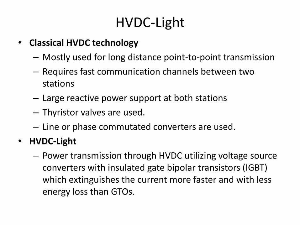
• Classical HVDC technology
– Mostly used for long distance point-to-point transmission
– Requires fast communication channels between two stations
– Large reactive power support at both stations
– Thyristor valves are used.
– Line or phase commutated converters are used.
• HVDC-Light
– Power transmission through HVDC utilizing voltage source converters with insulated gate bipolar transistors (IGBT) which extinguishes the current more faster and with less energy loss than GTOs.

HVDC-Light
– It is economical even in low power range.
– Real and reactive power is controlled independently in two HVDC light converters.
– Controls AC voltage rapidly.
– There is possibility to connect passive loads.
– No contribution to short circuit current.
– No need to have fast communication between two converter stations.
– Operates in all four quadrants.
– PWM scheme is used.
– Opportunity to transmit any amount of current of power over long distance via cables.

HVDC-Light
– Low complexity-thanks to fewer components
– Small and compact
– Useful in windmills
– Offers asynchronous operation.
• First HVDC-Light pilot transmission for 3 MW, 10kV in March, 1997 (Sweden)
• First commercial project 50 MW, 70 kV, 72 km, in 1999.
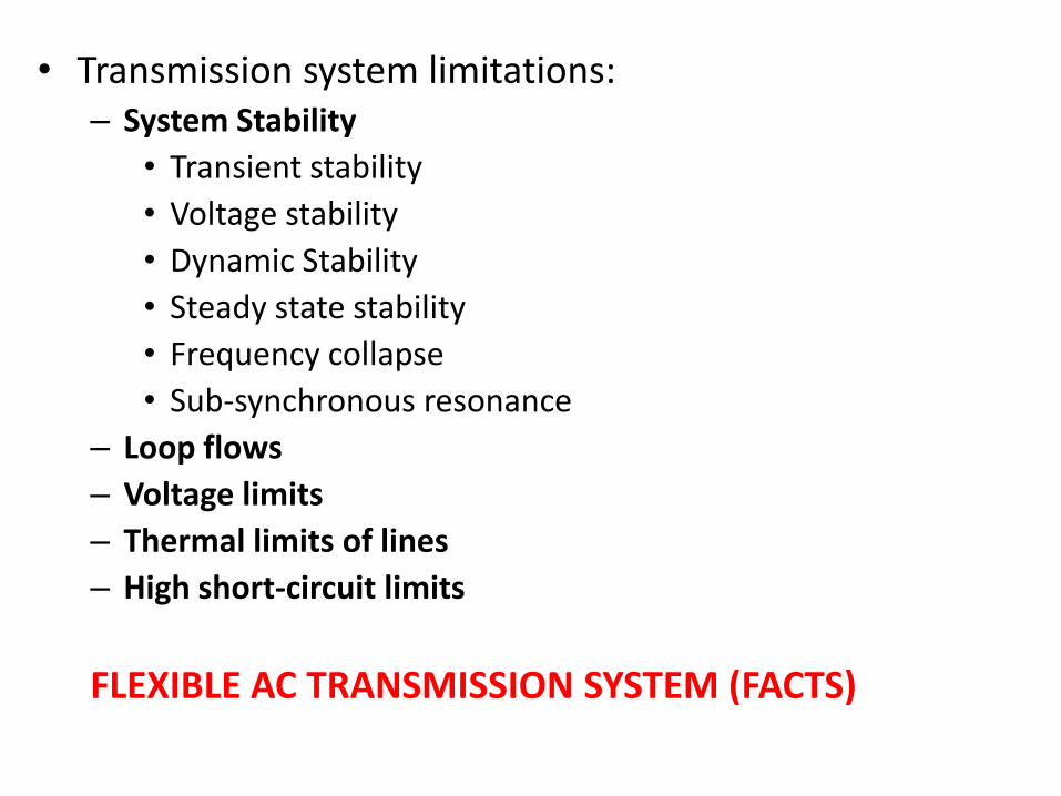
• Transmission system limitations: – System Stability
• Transient stability
• Voltage stability
• Dynamic Stability
• Steady state stability
• Frequency collapse
• Sub-synchronous resonance
– Loop flows
– Voltage limits
– Thermal limits of lines
– High short-circuit limits
FLEXIBLE AC TRANSMISSION SYSTEM (FACTS)

Flexible AC Transmission Systems (FACTS) are the name given to the application of power electronics devices
to control the power flows and other quantities in power systems.

• Benefits of FACTS Technology – To increase the power transfer capability of transmission
networks and – To provide direct control of power flow over designated
transmission routes.
• However it offers following opportunities – Control of power flow as ordered so that it follows on the
prescribed transmission corridors. – The use of control of the power flow may be to follow a
contract, meet the utilities’ own needs, ensure optimum power flow, ride through emergency conditions, or a combination thereof.
– Increase the loading capability of lines to their thermal capabilities, including short-term and seasonal.
– Increase the system security through raising the transient stability limit, limiting short-circuit currents and overloads, managing cascading blackouts and damping electromechanical oscillations of power systems and machines.
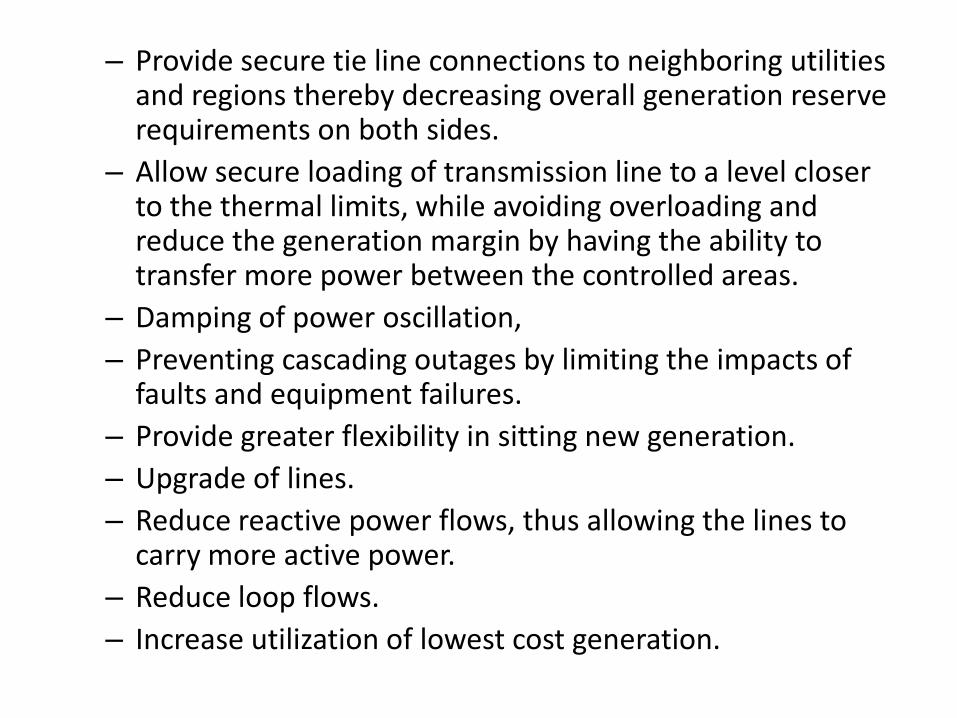
– Provide secure tie line connections to neighboring utilities and regions thereby decreasing overall generation reserve requirements on both sides.
– Allow secure loading of transmission line to a level closer to the thermal limits, while avoiding overloading and reduce the generation margin by having the ability to transfer more power between the controlled areas.
– Damping of power oscillation,
– Preventing cascading outages by limiting the impacts of faults and equipment failures.
– Provide greater flexibility in sitting new generation.
– Upgrade of lines.
– Reduce reactive power flows, thus allowing the lines to carry more active power.
– Reduce loop flows.
– Increase utilization of lowest cost generation.

• Whether HVDC or FACTS ?
– Both are complementary technologies.
– The role of HVDC is to interconnect ac systems where a reliable ac interconnection would be too expensive. • Independent frequency and control
• Lower line cost
• Power control, voltage control and stability control possible.
– The large market potential for FACTS is within AC system on a value added basis where • The existing steady-state phase angle between bus nodes is
reasonable.
• The cost of FACTS solution is lower than the HVDC cost and
• The required FACTS controller capacity is lesser than the transmission rating.
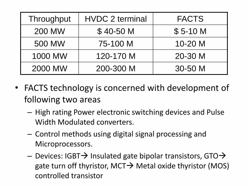
• FACTS technology is concerned with development of following two areas
– High rating Power electronic switching devices and Pulse Width Modulated converters.
– Control methods using digital signal processing and Microprocessors.
– Devices: IGBT Insulated gate bipolar transistors, GTO gate turn off thyristor, MCT Metal oxide thyristor (MOS) controlled transistor
Throughput HVDC 2 terminal FACTS
200 MW $ 40-50 M $ 5-10 M
500 MW 75-100 M 10-20 M
1000 MW 120-170 M 20-30 M
2000 MW 200-300 M 30-50 M
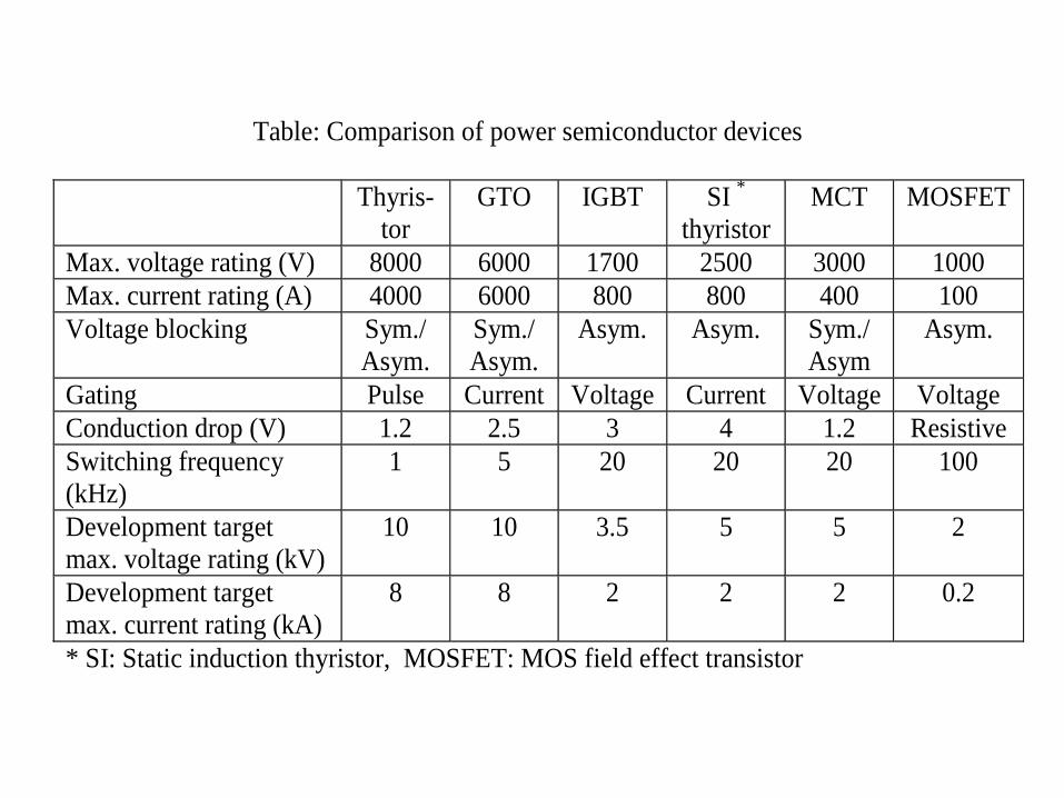
Table: Comparison of power semiconductor devices
Thyris-
tor
GTO IGBT SI *
thyristor
MCT MOSFET
Max. voltage rating (V) 8000 6000 1700 2500 3000 1000
Max. current rating (A) 4000 6000 800 800 400 100
Voltage blocking Sym./
Asym.
Sym./
Asym.
Asym. Asym. Sym./
Asym
Asym.
Gating Pulse Current Voltage Current Voltage Voltage
Conduction drop (V) 1.2 2.5 3 4 1.2 Resistive
Switching frequency
(kHz)
1 5 20 20 20 100
Development target
max. voltage rating (kV)
10 10 3.5 5 5 2
Development target
max. current rating (kA)
8 8 2 2 2 0.2
* SI: Static induction thyristor, MOSFET: MOS field effect transistor

• Developments in Generation side
– Powerformer Energy System
– Distributed Generations
• Wind Power
• Fuel Cells
• Biomass etc.
– Combined Cycle Power Plants

Powerformer Energy System

PowerformerTM Benefits
• Higher performance (availability, overload)
• Environmental improvement
• Lower weight
• Less total space requirement
• Lower cost for Civil Works
• Less maintenance
• Reduced losses
• Lower investment
• Lower LCC

E (
kV
/mm
)
3kV/mm
6-9kV/mm
E-field
non-uniform
E-field
uniform
Bar Cable
Electrical Field Distribution

Stator winding
Conductor (1), Inner semi-conducting layer (2),
Insulation (3) and an outer semi-conducting layer (4).
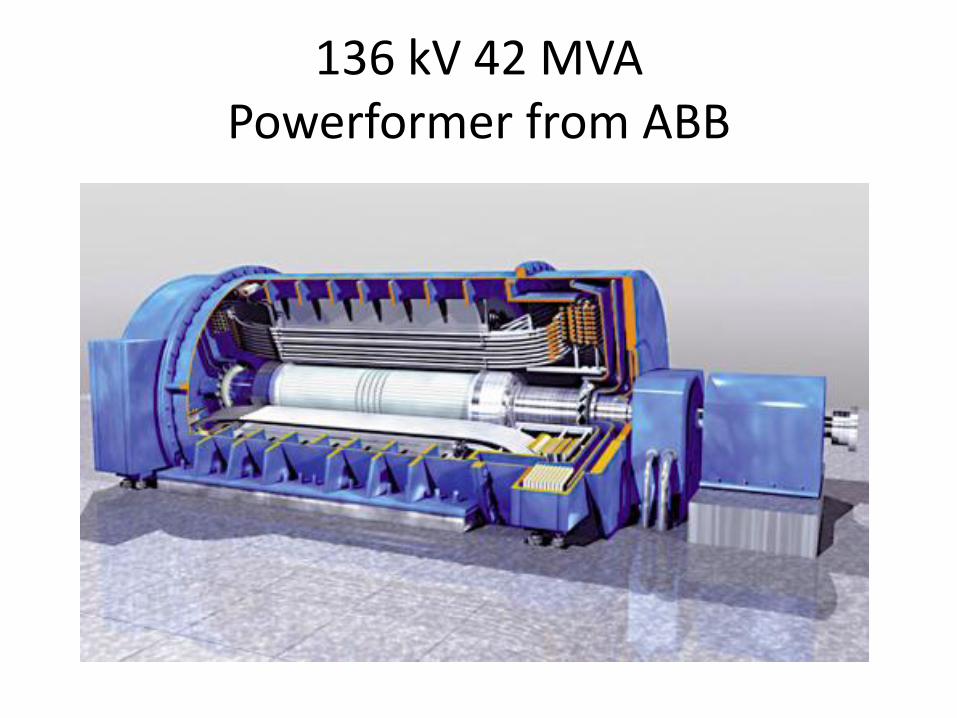
136 kV 42 MVA Powerformer from ABB

DG includes the application of small generations in the range of 15 to 10,000 kW, scattered throughout a power system
DG includes all use of small electric power generators whether located on the utility system at the site of a utility customer, or at an isolated site not connected to the power grid.
By contrast, dispersed generation (capacity ranges from 10 to 250 kW), a subset of distributed generation, refers to generation that is located at customer facilities or off the utility system.
Distributed Generation/Dispersed Generation

DG includes traditional -- diesel, combustion turbine, combined cycle turbine, low-head hydro, or other rotating machinery and renewable -- wind, solar, or low-head hydro generation.
The plant efficiency of most existing large central generation units is in the range of 28 to 35%, converting between 28 to 35% of the energy in their fuel into useful electric power.
By contrast, efficiencies of 40 to 55% are attributed to small fuel cells and to various hi-tech gas turbine and combined cycle units suitable for DG application.
Part of this comparison is unfair. Modern DG utilize prefect hi-tech materials and incorporating advanced designs that minimize wear and required maintenance and include extensive computerized control that reduces operating labor.

DG “Wins” Not Because It is Efficient, But Because It Avoids T&D Costs
Proximity is often more important than efficiency
Why use DG units, if they are not most efficient or the lowest cost? The reason is that they are closer to the customer. They only have
to be more economical than the central station generation and its associated T&D system. A T&D system represents a significant cost in initial capital and continuing O&M.
By avoiding T&D costs and those reliability problems, DG can provide better service at lower cost, at least in some cases. For example, in situations where an existing distribution system is near capacity, so that it must be reinforced in order to serve new or additional electrical demand, the capital cost/kW for T&D expansion alone can exceed that for DG units.

Renewable Energy Scenario in India

NLDC 45
Renewable Installed Capacity

Growth pattern of RE addition in different five year plans
(Source-MNRE)

Opportunities/Challenges
• Transmision of power
• Renewable Energy/Distributed Generation
• DC Distribution System
• Smart grid

Operational Changes in Power Systems

RTU RTU RTU
SUB LDC SUB LDC SUB LDC
SLDC SLDC SLDC
ERLDC WRLDC NRLDC SRLDC NERLDC
NLDC Modernisation of Load Despatch Centres
Implementation of Grid Code Manning of Load Despatch Centres with trained personnel Adoption of Availability Based Tariff (ABT)
Grid Management Initiatives
Future Prospective- Intelligent Grid -Smart Power Delivery System
Wide area monitoring system
Adaptive islanding schemes
Self healing capability
Voltage Security Assessment, Dynamic Security
Assessment

Availability Based Tariff Mechanism
In India

BULK POWER TRANSACTION Example: NR, Rajasthan, BBMB
W.R N.R
NER
SR
CENTRAL SECTOR GENERATORS
STATE SYSTEMS
STATE SECTOR GENERATORS

Capacity Ch. + Energy Ch. UI
A + B C
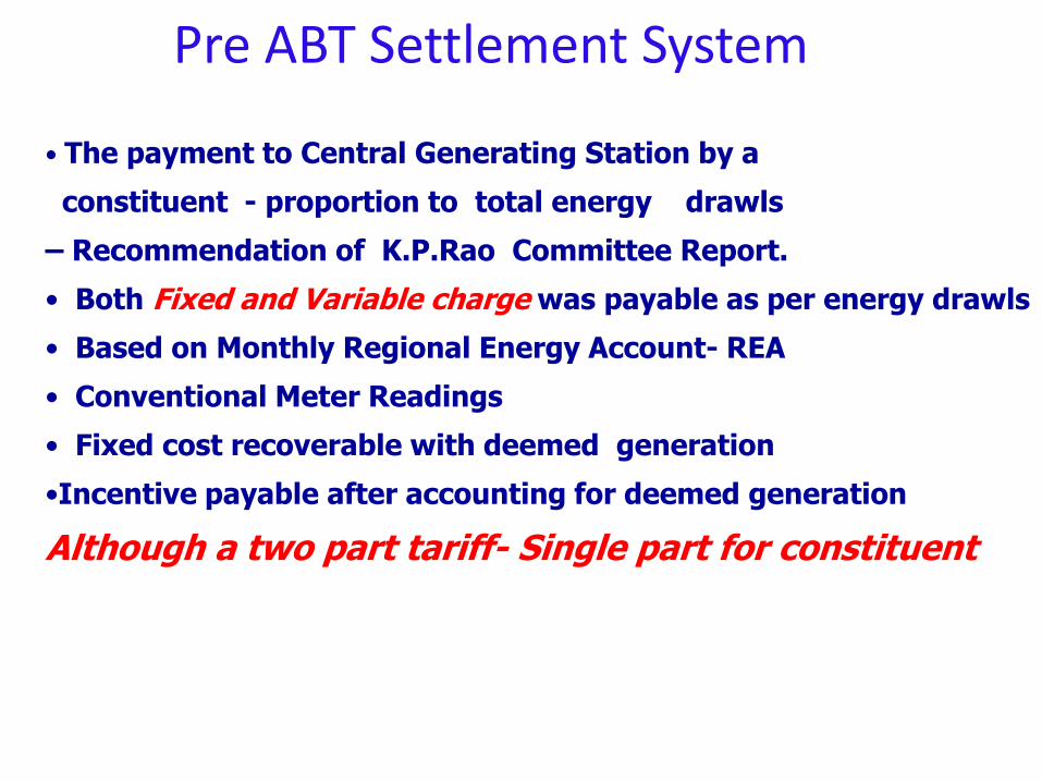
Pre ABT Settlement System
• The payment to Central Generating Station by a
constituent - proportion to total energy drawls
– Recommendation of K.P.Rao Committee Report.
• Both Fixed and Variable charge was payable as per energy drawls
• Based on Monthly Regional Energy Account- REA
• Conventional Meter Readings
• Fixed cost recoverable with deemed generation
•Incentive payable after accounting for deemed generation
Although a two part tariff- Single part for constituent

54
Components of Availability Tariff (a) Capacity Charge: for payment of fixed cost
-Proportionate to entitlements (not actual drawls)
-is a function of ex-bus MW capability of the power plant for the day declared in advance, paid by beneficiaries @ their respective % share in the plant
(b) Energy Charge: for payment of variable cost
-Payable for schedules (not as per actual drawls)
= MWh for the day as per ex-bus drawl schedule for the beneficiary finalized in advance x Energy charge rate for the Plant
(c) Unscheduled Interchange : Payable for deviations from schedules
= Σ [( Actual energy interchange in a 15- minutes time block scheduled interchange for the time block) x UI rate for the time block ]
Total Payment for the day = (a) + (b) (c)

55
BACKGROUND (situation upto early 2002)
Deplorable state of regional grid operation
• Uncontrolled frequency fluctuations, from below 48.0 Hz to above 52.0 Hz.
• Voltages beyond permissible limits
• Frequent grid disturbances
• Lack of optimization in generation
(merit – order compromised)
• Unchecked deviations from schedules
• Perpetual operational and commercial disputes between utilities

56
MAIN REASONS :
• Shortage and poor availability of generating capacity → extensive (but inadequate) load curtailment, particularly during peak load hours.
• Reluctance to back down generation during off-peak hours, due to faulty bulk power tariff structure (single-part, constant paise / kWh)
• Inadequate reactive compensation at load end
• Blocked governors
• Gaps in understanding of the subject, and a lack of consensus on how to tackle the problem.

57
• Federal democracy : Tussle between Central Government organisations and State Government-owned vertically integrated utilities
• Lack of load dispatch and communication facilities to apply conventional load-frequency control, tie-line bias, control area concepts, etc.
A structured study in 1993-94 by M/s. ECC of USA, sponsored by World Bank/Asian Development Bank
→ AVAILABILITY TARIFF Implementation started in 2002

Inherent Disadvantage
• No incentives for generators /utilities to respond to dispatch orders for issues like frequency control
– No Incentive for helping the grid
– No disincentive for hurting the grid
• No signal to generators to match availability with system needs
• Did not promote Grid Discipline
• No signal for trading of power.
Overall economy was lost.

Ultimate Effect
• Grid Indiscipline- • Low Frequency during peak
• High Frequency during off peak
• Control Instructions • Subjective decisions
• Not based on overall economy
• Perpetual Operational & Commercial Dispute amongst Utilities/Central Generators
• Poor Supply quality to consumers/industries • Damage to equipments
• Shifting of Industries/Investments

Unscheduled Interchange Regulations 2009 (and subsequent
amendments)

Unscheduled Interchange
• ‘Unscheduled Interchange’ in a time-block for a generating station or a seller means its total actual generation minus its total scheduled generation, and,
• for a beneficiary or buyer means its total actual drawal minus its total scheduled drawal.

Unscheduled Interchange

Advantages due to implementation of ABT

64
Frequency Profile of SR
FREQUENCY COMPARISION FOR 26-JUNE 02 & 03
47.5
48.0
48.5
49.0
49.5
50.0
50.5
51.0
51.5
00
01
02
03
04
05
06
07
08
09
10
11
12
13
14
15
16
17
18
19
20
21
22
23
HOUR ---->
FR
EQ
UE
NC
Y IN
HZ
---
->
2003
2002

65
Frequency Profile of ER
FREQUENCY CURVE
6th June02
6th June03
47.00
48.00
49.00
50.00
51.00
52.00
53.00
00 01 02 03 04 05 06 07 08 09 10 11 12 13 14 15 16 17 18 19 20 21 22 23 Time (Hrs.)
Frq
e (
Hz.
)

• Power System Restructuring (Privatization or Deregulation) – But not only Privatization
• Deregulation is also known as
– Competitive power market – Re-regulated market – Open Power Market – Vertically unbundled power system – Open access

Transmission
Business
Distribution
Business
Generation
Business
Vertical separation
Horizontal separation or Vertical cut
Horizontal separation or Vertical cut

• Why Restructuring of Electric Supply Industries? – Better experience of other restructured market
such as communication, banking, oil and gas, airlines, etc.
– Competition among energy suppliers and wide choice for electric customers.
• Why was the electric utility industry regulated? – Regulation originally reduced risk, as it was
perceived by both business and government.
– Several important benefits: • It legitimized the electric utility business.

• Forces behind the Restructuring are – High tariffs and over staffing
– Global economic crisis
– Regulatory failure
– Political and ideological changes
– Managerial inefficiency
– Lack of public resources for the future development
– Technological advancement
– Rise of environmentalism
– Pressure of Financial institutions
– Rise in public awareness
– Some more …….

• Reasons why deregulation is appealing
No longer necessary The primary reason for regulation,
to foster the development of ESI
infrastructure, had been achieved.
Electricity Price may drop Expected to drop due to innovation
and competition.
Customer focus will improve Expected to result in wider
customer choice and more attention
to improve service
Encourage innovation Rewards to risk takers and
encourage new technology and
business approaches,
Augments privatization In the countries where Govt. wishes
to sell state -owned utilities,
deregulation may provide potential
buyers and new producers.

• What will be the transformation ?
– Vertically integrated => vertically unbundled
– Regulated cost-based ==> Unregulated price-based
– Monopoly ==> Competition
– service ==> commodity
– consumer ==> customer
– privilege ==> choice
– Engineers Lawyer/Manager

• What will be the Potential Problems ? – Congestion and Market power – Obligation to serve – Some suppliers at disadvantages – Price volatility – Non-performance obligation – Loss operating flexibility – Pricing of energy and transmission services – ATC calculations – Ancillary services Management
• Reserves • Black start capability • Voltage and frequency control • System security and stability • Transmission reserves
– Market Settlements and disputes

Milestones of Restructuring
- 1982 Chile
- 1990 UK
- 1992 Argentina, Sweden & Norway
- 1993 Bolivia & Colombia
- 1994 Australia
- 1996 New Zeeland
- 1997 Panama, El Salvador, Guatemala, Nicaragua, Costa Rica and Honduras
- 1998 California, USA and several others.
- 2000 Several EU and American States

• Markets are defined by the commodity traded
– Energy
– Transmission system
– Ancillary services
• Markets defined by the time-frame of trade
– Day-ahead
– Hour-ahead
– Real-time
• Based on auction - single-sided or double sided
• Based on type of bids --> block or linear bid
• Based on generation settlement - uniform price (MCP) or pay-as-bid

Market Clearing Price
Gen. Price
($)
MW
Gen-1 2.5 20
Gen-2 2.0 10
Gen-3 2.4 15
Gen-4 2.3 45
Gen-5 2.2 30
Gen-2
Gen-5
Gen-4
Gen-3
Gen-1
Demand = 80 MW
O MW
1O MW
40 MW
85 MW
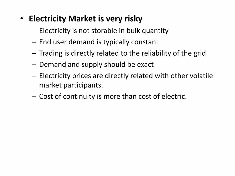
• Electricity Market is very risky
– Electricity is not storable in bulk quantity
– End user demand is typically constant
– Trading is directly related to the reliability of the grid
– Demand and supply should be exact
– Electricity prices are directly related with other volatile market participants.
– Cost of continuity is more than cost of electric.

Intelligent Grid - WAMS
Leader not a follower

• What is Smart Grid?
• Is the present grid not smart?
• Why Smart Grid?
• Smart or Intelligent ???

What is Smart Grid?
• The electric industry is poised to make the transformation from a centralized, producer‐ controlled network to one that is less centralized and more consumer‐interactive.
• The move to a smarter grid promises to change the industry’s entire business model and its relationship with all stakeholders.
• A smarter grid makes this transformation possible by bringing the philosophies, concepts and technologies that enabled the internet to the utility and the electric grid.

• What is Smart Grid?
• Is the present grid not smart?
• Why Smart Grid?
• Smart or Intelligent ???
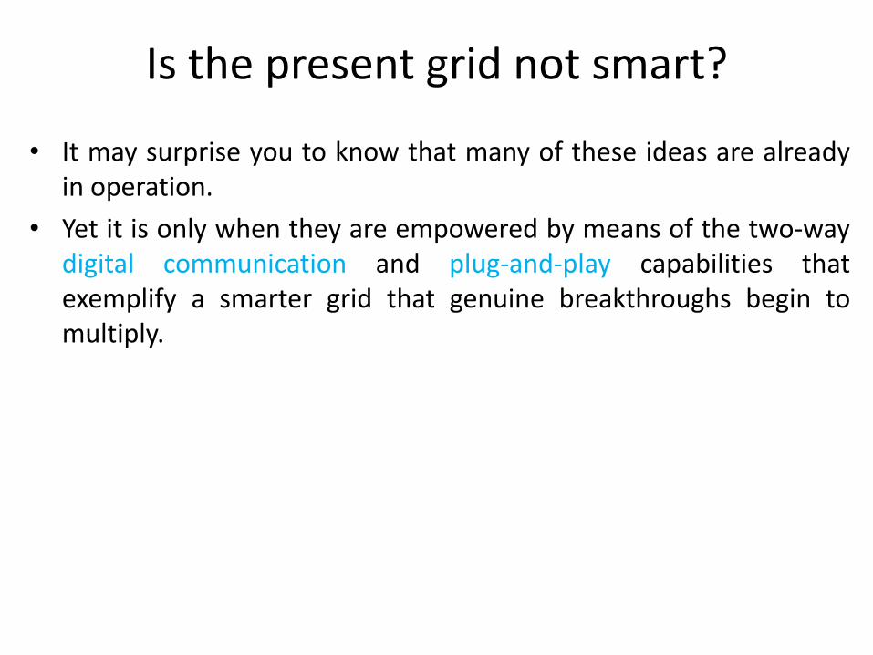
Is the present grid not smart?
• It may surprise you to know that many of these ideas are already in operation.
• Yet it is only when they are empowered by means of the two‐way digital communication and plug‐and‐play capabilities that exemplify a smarter grid that genuine breakthroughs begin to multiply.

Merging Two Technologies
Electrical
Infrastructure
Information Infrastructure
The integration of two infrastructures… securely…
Source: EPRI® Intelligrid at http://intelligrid.epri.com

What a Smart Grid would look like?
Two-way integrated communication, adaptive, responsive, wider control
• What is Smart Grid?
• Is the present grid not smart?
• Why Smart Grid?
• Smart or Intelligent ???

Some of the Recent Concerns • Limited expansion of transmission network as compared
to the generation addition. – Most of the generation, T&D systems have become old.
• Efficiency: Increased transmission and distribution losses.
• Lack of dynamic data for health monitoring and control.
• Reliability & Security: Increased concern towards vulnerability and resilience of the system under natural and man made disasters.
• Growing environmental concerns including the global warming.
• Poor power quality, limited customer focus and their participation in energy Management.
• Meeting the ever increasing electricity demand.
• Affordability:

Present and Future Power System
Present Power System - Heavily Relying on Fossil Fuels - Generation follows load - Limited ICT use
Future Power System - More use of RES, clean coal,
nuclear power - Load follows Generation - More ICT & Smart meter use

Today’s Electricity …
Power park
Hydrogen Storage
Industrial DG
Tomorrow’s Choices …
Combined Heat and Power
Fuel Cell e -
e -
Wind Farms
Rooftop Photovoltaics
Remote Loads
Load as a resource
SMES
Smart Substation
Fuel Cell

What a Smart Grid would look like? Green, Environment friendly
Source: European Technology Platform SmartGrids
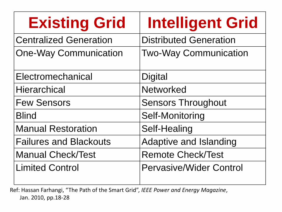
Existing Grid Intelligent Grid Centralized Generation Distributed Generation
One-Way Communication Two-Way Communication
Electromechanical Digital
Hierarchical Networked
Few Sensors Sensors Throughout
Blind Self-Monitoring
Manual Restoration Self-Healing
Failures and Blackouts Adaptive and Islanding
Manual Check/Test Remote Check/Test
Limited Control Pervasive/Wider Control
Ref: Hassan Farhangi, “The Path of the Smart Grid”, IEEE Power and Energy Magazine, Jan. 2010, pp.18-28

Central Station
The overall power system is traditionally viewed in terms of 7 layers; each performing its function from central station generation supplying power out to customers.
Wind Energy
Solar Energy
Fuel Cells
Combustion Engines
MicroTurbines
Interconnecting Distributed Power Systems
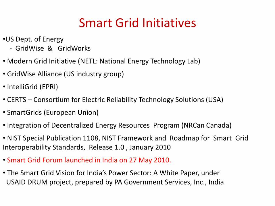
Smart Grid Initiatives
•US Dept. of Energy - GridWise & GridWorks
• Modern Grid Initiative (NETL: National Energy Technology Lab)
• GridWise Alliance (US industry group)
• IntelliGrid (EPRI)
• CERTS – Consortium for Electric Reliability Technology Solutions (USA)
• SmartGrids (European Union)
• Integration of Decentralized Energy Resources Program (NRCan Canada)
• NIST Special Publication 1108, NIST Framework and Roadmap for Smart Grid Interoperability Standards, Release 1.0 , January 2010
• Smart Grid Forum launched in India on 27 May 2010.
• The Smart Grid Vision for India’s Power Sector: A White Paper, under USAID DRUM project, prepared by PA Government Services, Inc., India

Smart Grid: Challenges and Opportunities
• The concept of a smart grid has its origins in the development
of advanced metering infrastructure for
better demand-side management;
greater energy efficiency; and
improved supply reliability.
• Other developments have expanded the scope of smart grids:
renewable energy generation (wind and solar, among others);
maximizing the utilisation of generating assets; and
increased customer choice.
• New technologies will continue to expand the scope:
electric vehicles;
energy storage (batteries); and
smart appliances.

Challenges of the New Energy Economy
The Smart-Grid
Automating the Grid
Return on Asset (ROA)
Dynamic Pricing
Dealing with Evolutionary Change
Greater 30% Renewable, Distributed
• Photovoltaic, Solar/Thermal, Wind, Biofuels
• Climate Modelling & Prediction
• Distribution becomes Transmission
Electric Vehicles
Transmission Capacity and Location

Micro Grid (DC or AC ?)
• Micro-grids are independently controlled (small) electric
networks, powered by local units (distributed generation).

Why continue to use AC appliances?
• Lighting
• LEDs, 10 to 100 times more efficient as compared to
tungsten bulb, use only DC power
• CFL is neutral to AC or DC power
• Motor: a small DC motor can be 2.5 tomes more energy
efficient as compared to a AC motor
• Historically brush replacement needed – but not anymore
• A fan is primarily a motor – a dc fan also allows better speed control
• A refrigerator is essentially a motor
• An air-conditioner is primarily a motor
• A washing-machine / grinder is a motor
• Electronics: all electronics (mobiles/TV/Computers) use low voltage DC
• Need a ac/dc power adaptor to charge
• World switched to AC primarily for transmission of power
• Any ac / dc conversion or vice-versa implies 7 to 15% losses

DC Micro-grid System.

Hybrid AC/DC Microgrid

AC vs. DC Micro Grid
Some of the issues with Edison’s dc system:
Voltage-transformation complexities
Incompatibility with induction (AC) motors
Power electronics help to overcome difficulties
Also introduces other benefits – DC micro-grids
DC micro-grids
Help eliminate long AC transmission and distribution paths
Most modern loads are DC – modernized conventional loads too!
No need for frequency and phase control – stability issues?

AC vs. DC Micro Grid
Cabling in DC distribution
Greater current carrying capacity with DC system over AC
Therefore smaller and cheaper distribution cables for a
given power
Interconnection into HVDC schemes
Lower reacatance as large transformers & filters AC can be
removed at offshore platform
Less components provides higher availability and less
maintenance
DC transformer less, & filter less generation can provide
efficiency improvements

Challenges to DC systems
Technology
Lack of DC on-load circuit breakers.
– Converteam’s Foldback Technology provides a solution
Can we generate in DC effectively?
Standards
Real need for open standards if ideas such as Multi-
terminal HVDC schemes, i.e. Supergrid, are to be realised
– Best achieved at pre-competitive stage
Supply chain partnering
To be ready and on time
Fantastic opportunities for innovation
Great challenges for Universities and R&D teams

VOLTAGE STABILITY ASSESSMENT OF
GRID CONNECTED OFFSHORE WIND
FARMS


Comparison of Bulk Power Transmission
HVAC LCC based HVDC VSC based HVDC
Maximum voltage Level 150 kV installed 245 kV claimed
Nor Ned: ±450 kV ± 150 kV installed ± 300 kV claimed
Substation volume Smallest size Biggest size Medium size
Cable installation Complex Simple Simple
Substation Installation Cost Low High Highest
Compensation needed Yes Yes No
Active power control No Yes Yes
Reactive power control No No Yes
Grid interconnections Synchronous Any Any
Black start capability Yes No Yes
Installation cost of cables High Low Low

Offshore wind farms are connected to the grid through a
long offshore/onshore cable having substantial capacitive
impedance .
Voltage stability and reactive power management are the
concern.
The fluctuations in mechanical input and gusts of wind will
result in output-power spikes at the generator terminals.
This causes poor voltage regulation and may lead to voltage
collapse .
A generalized dynamic voltage collapse index (GDVCI)
suitable for long radial long transmission network has been
proposed.
GDVCI represents the distance to voltage collapse in terms
of loading margin to maximum loading .

*r
Ir
Vr
S
and BBAA
cosh lDA sinh lZB C
CZ
l sinhC
B
rVA
B
rV
sV
rS
2
Let,
where, A, B, C and D are generalized circuit constant and can be
given as,
where,
z , y = Series & shunt impedance per unit length, respectively,
l = Length of line
Z (=zl), Y (=yl )= Total series & shunt impedance, respectively
ZC = sqrt (z/y) = characteristic impedance
= sqrt (zy) = propagation constant
Generalized Dynamic Voltage Collapse Index
Distributed Line
ABCD Parameters
sV 0rV
Bus-1 Bus-2
rS

coscos
2
B
VA
B
rV
sV
rP
r
sin
2
sinB
rVA
B
rV
sV
rQ
B
sV
rQ
rP
B
rVA
B
rVA
rQ
rP
2
sincos
2
22
4222
022
2
sin
cos2
2
2
24
rQ
rP
B
sV
rQ
rP
B
A
rV
B
A
rV
The active power (Pr) and reactive power (Qr) at
receiving end (Bus-2) i.e. at the PCC can be written as
Squaring and adding equations , we get
GENERALIZED DYNAMIC VOLTAGE COLLAPSE
INDEX
Distributed Line
ABCD Parameters
sV 0rV
Bus-1 Bus-2
rS

a
acbb
Vr2
422
B
sV
rQ
rP
B
Ab
rQ
rPc
B
Aa
2
sincos2
22,2
2
042
acb
022
2
2
4
22
sin
cos2
rQ
rP
B
A
B
sV
rQ
rP
B
A
Solution of equation will exist only if,
i.e.
Generalized Dynamic Voltage Collapse Index
Distributed Line
ABCD Parameters
sV 0rV
Bus-1 Bus-2
rS

22
22 2 22 cos sin 4 0
2
VA AsGDVCI P GDVCI Q GDVCI P Q
r r r rB B B
2 4
22sin cos cos sin 0
2 24
V Vs s
GDVCI P Q GDVCI P Qr r r rA B A B
1
1111
2
42
a
cabb
GDVCI
22
4
1
2
1
1
4
sincos
2cossin
BA
Vc
rQ
rP
BA
Vb
rQ
rPa
s
s
At maximum loadability point (Pr + j Qr) is replaced
by GDVCI * (Pr + j Qr)
Generalized Dynamic Voltage Collapse Index
Distributed Line
ABCD Parameters
sV 0rV
Bus-1 Bus-2
rS

The GDVCI is expressed in terms of active and reactive power
at Bus-2, voltage at Bus-1 and ABCD parameters of transmission
Line/cable
The index, GDVCI, when multiplied with a complex power at
Bus-2 will give the maximum power that can be delivered at
Bus-2 for given Bus-1 voltage.
GDVCI represents the additional power (maximum loading –
existing loading) that may be increased /decreased at Bus-2 before
reaching collapse point .
If GDVCI approaches to unity, it infers that transmission line
is at its maximum loading and on the proximity to voltage collapse.
For voltage stability, GDVCI must be higher than 1.
GENERALIZED DYNAMIC VOLTAGE COLLAPSE
INDEX

Simulation Results
MVA
loading at
Bus-2
Voltage
at bus-2
(p.u.)
GDVCI
at
Bus-2
Loading margin to reach
maximum loading point
MVA*(GDVCI-1)
L-index
at
Bus-2
48.84 1.0121 6.3418 260.8959 0.0429
62.04 1.0008 4.9925 247.6959 0.0538
75.24 0.9891 4.1166 234.4959 0.0657
88.44 0.9771 3.5022 221.2959 0.0784
101.64 0.9646 3.0474 208.0959 0.0920
114.84 0.9517 2.6971 194.8959 0.1066
128.04 0.9384 2.4191 181.6959 0.1221
141.24 0.9244 2.193 168.4959 0.1388
154.44 0.9099 2.0055 155.2959 0.1568
167.64 0.8948 1.8476 142.0959 0.1763
180.84 0.8788 1.7128 128.8959 0.1975
194.04 0.862 1.5962 115.6959 0.2208
207.24 0.8441 1.4946 102.4959 0.2466
220.44 0.8249 1.4051 89.2959 0.2755
233.64 0.8042 1.3257 76.0959 0.3083
246.84 0.7815 1.2548 62.8959 0.3462
260.04 0.7562 1.1911 49.6959 0.3912
273.24 0.7271 1.1336 36.4959 0.4469
286.44 0.6917 1.0813 23.2959 0.5207
299.64 0.6435 1.0337 10.0959 0.6347
312.84 No Sol. 0.9901 -3.1041 0.9141
Distributed Line
ABCD Parameters
sV 0rV
Bus-1 Bus-2
rS

GDVCI Index with OLTC operation
2
2222
2
42
a
cabb
GDVCIo
22
44
2
22
2
2
4
sincos
2cossin
oo
s
oooo
oo
s
oooo
BA
Enc
rQ
rP
BA
Enb
rQ
rPa

Effects of OLTC Operation
0 50 100 150 200 250 300 3500
0.5
1
Active Power (MW)
Vo
ltag
e (p
.u.)
n = 0.9, 0.95, 1.0, 1.05, 1.10
n = 1.0
0 50 100 150 200 250 300 3500
1
2
3
Active Power (MW)
GD
VC
I O
n = 0.9, 0.95, 1.0, 1.05, 1.10
n =1.0
(a) P-V curves
(b) Voltage Collapse Index
There is increase in the maximum power transfer limit and GDVCI0 with increase
in tap setting (n)

Case Studies: Offshore Wind Farms
0 2 4 6 8 10 12 14 16 18 200.4
0.5
0.6
0.7
0.8
0.9
1
1.1
time (s)
Torq
ue (p
.u.)
Change in input torque for offshore wind farms

4 6 8 10 12 14 16 18 20-200
0
200
P (
MW
) &
Q (
MV
Ar)
4 6 8 10 12 14 16 18 200
100
200
Vo
ltag
e (
kV
)
4 6 8 10 12 14 16 18 200
5
10
time (s)
GD
VC
I
P
Q
4 6 8 10 12 14 16 18 20
0
100
200
P (
MW
) &
Q (
MV
Ar)
4 6 8 10 12 14 16 18 200
100
200
Volt
age (
kV
)
4 6 8 10 12 14 16 18 200
5
10
time (s)
GD
VC
I
P
Q
Two transmission lines (50 km each) of different
parameters connected in cascading
Transmission line length of 100 km
DYNAMIC RESPONSE OF THE 171 MW
OFFSHORE WIND FARM

4 6 8 10 12 14 16 18 200
1
2
3
4
5
6
7
time (s)
GD
VC
I
80 km
100 km
120 km
Three different transmission
line length (80,100,120 km) on GDVCI
5 5.1 5.2 5.3 5.4 5.5 5.6 5.7 5.8 5.9 6-200
0
200
P (
MW
) &
Q (
MV
ar)
5 5.1 5.2 5.3 5.4 5.5 5.6 5.7 5.8 5.9 60
100
200
Volt
age (
kV
)
5 5.1 5.2 5.3 5.4 5.5 5.6 5.7 5.8 5.9 6
0
5
10
time (s)
GD
VC
I
P
Q
Dynamic Response of the 171 MW
Offshore Wind Farm
Three-phase gird short circuit fault
4 6 8 10 12 14 16 18 20
0
10
20
30
40
P (
MW
) &
Q (
MV
Ar)
4 6 8 10 12 14 16 18 200
10
20
Volt
age (
kV
)
4 6 8 10 12 14 16 18 200
2
4
6
time (s)
GD
VC
I
P
Q
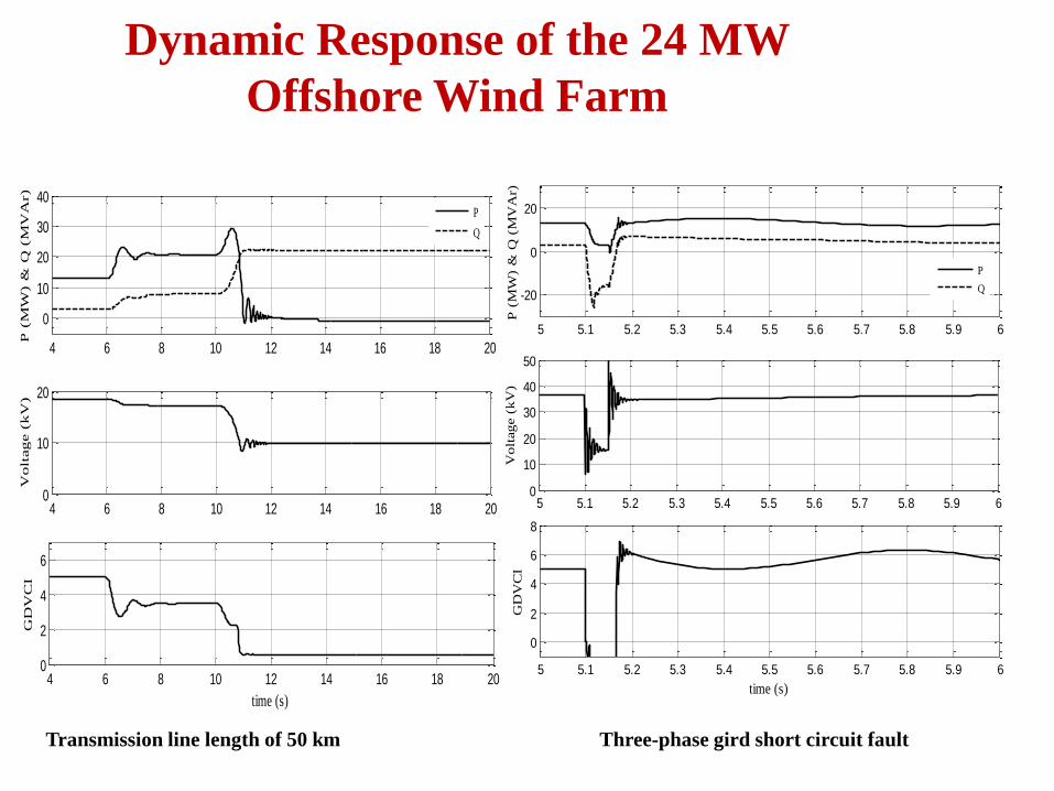
Transmission line length of 50 km
5 5.1 5.2 5.3 5.4 5.5 5.6 5.7 5.8 5.9 6
-20
0
20
P (
MW
) &
Q (
MV
Ar)
5 5.1 5.2 5.3 5.4 5.5 5.6 5.7 5.8 5.9 60
10
20
30
40
50
Volt
age (
kV
)
5 5.1 5.2 5.3 5.4 5.5 5.6 5.7 5.8 5.9 6
0
2
4
6
8
time (s)
GD
VC
I
P
Q
Three-phase gird short circuit fault
Dynamic Response of the 24 MW
Offshore Wind Farm

Conclusions
Formulation of the GDVCI is very general and can be
easily extended to incorporate power system elements in
between two buses of radial system.
Implementation of GDVCI does not involve iterations and
hence gives instantaneous values.
GDVCI performs better than L-index.
The dynamic performance of GDVCI for a fault condition
on offshore wind farms shows effective performance in
estimating voltage collapse (i.e. loading margins) and can
be used as a protective measure as voltage collapse
indicator.

Thank You and Questions