1

Employment Risk and Performance

Susan Godlonton

1

Version: 19th

October, 2012

JOB MARKET PAPER

Abstract

This paper examines the relationship between employment risk and performance. To induce exogenous

variation in employment risk, I randomize outside options for job seekers undergoing a real recruitment

process. I do this by assigning job seekers a 0, 1, 5, 50, 75 or 100 percent chance of real alternative

employment of the same duration and wage as the jobs for which they are applying.

I find that performance is highest and effort is lowest among those assigned the lowest employment

risk (a guaranteed alternative job), and performance is lowest and effort highest among those facing the

highest employment risk (those without any job guarantee). Moreover, I find a non-linear relationship

between employment risk and performance. My findings are consistent with a framework in which

performance is increasing in effort and inverse u-shaped in stress tying together insights from economics

and psychology. The results are not driven by gift-exchange, stereotype threat or the nutritional efficiency

wage hypothesis.

The performance improvements have significant welfare implications. In this study, job seekers

assigned a high probability of an outside option were twice as likely to be hired in the standard job

recruitment process compared to those assigned a low probability of receiving an outside option. More

broadly, these results suggest that stress-induced performance reductions are a potential mechanism

through which exposure to high employment risk can sustain poverty and unemployment.

1 Department of Economics and Ford School of Public Policy, University of Michigan, 112 Lorch Hall, 611 Tappan St. Ann

Arbor MI, 48109-1220, USA. Email: susgod@umich.edu. This project was supported with research grants from the Rackham

Graduate School and the African Studies Center at the University of Michigan. I gratefully acknowledge use of the services and

facilities of the Population Studies Center at the University of Michigan, funded by NICHD Center Grant R24 HD041028. I

acknowledge Ernest Mlenga and his recruitment team for their willingness to provide their recruitment data as well as enabling

the integration of this research into their recruitment process. I also acknowledge Kelvin Balakasi for his field and research

assistance in Malawi and Soo Ji Ha for her research assistance in Michigan. I thank Sarah Burgard, David Lam, Jeff Smith,

Rebecca Thornton, Emily Beam, Jessica Goldberg, and Caroline Theoharides for valuable comments as well as seminar

participants at the Michigan State University Africanist Graduate Student Conference 2011, North East Universities

Development Consortium 2011, University of Cape Town, Center for Study of African Economies Conference 2012, Midwest

International Economic Development Conference 2012, Informal Development Seminar and Economic Development and

Transition Seminar at the University of Michigan.

2

1. Introduction

Currently the world faces a “job crisis” with 200 million people worldwide unemployed and looking for

work (ILO, 2012). The individual and social consequences of unemployment are well-documented in

many disciplines. In economics, some of the effects of unemployment include reductions in future

employment probabilities and wages (Stevens, 1997; Chan and Stevens, 2001; Ruhm, 1991 and 1994;

Topel, 1990), reduced access to credit (Sullivan, 2008); higher crime (Raphael and Winter-Ebmar, 2001;

Edmark, 2005), and increased marital dissolution (Jensen and Smith, 1990).2 Other disciplines such as

public health and psychology document associations of unemployment with poorer mental and physical

health, stress and suicide.3

In economics, the literature studying the consequences of unemployment has focused either on

the effects of a bad employment realization; or on risk mitigation mechanisms.4,5

However, the impact of

employment risk is not well-studied.6 This is true for a number of reasons. First, measuring exposure to

risk is difficult. For example, research examining the relationship between risk and savings, use proxies

for uncertainty either using variability in household income (e.g. Caroll, 1994), or variability in

expenditures (e.g. Dynan, 1993), or in more recent work using the probability of a job loss (e.g. Lusardi,

1998). I examine employment risk, so an appropriate proxy might by the probability of a job gain rather

than a job loss. However, none of these proxies are a direct measure of risk. A second concern, even if

one can directly measure employment risk, it is usually endogenous with key economic outcomes of

interest. For example, in the case of performance, individuals of higher ability are likely to face lower

employment risk yet also perform better on average. Third, while laboratory experiments enable scope for

inducing exogenous variation they are limited in providing insights into real world behaviors. Fourth,

measuring performance particularly in contexts outside of laboratory experiments is difficult due to self-

report biases and lack of good quality firm level data.

2 The recent World Development Report (2013) provides an extensive review of the key impacts of unemployment. 3 Unemployment has been found to be correlated with physical health (Brenner, 1971 and 1979; Jin, Shah and Svoboda, 1995);

alcohol consumption (Brenner, 1975); mental health (Dooley, et al. 1994 and 2000; Murphy and Athanasou, 1999); suicide

(Lundin and Hemmingsson, 2009). 4 Often this empirical work use an exogenous shock that results in job loss such as plant closures and retrenchments to examine

both short term and long term consequences on future employment, and earnings (Stevens, 1997; Chan and Stevens, 2001; Ruhm

(1991, 1994); Topel, 1990; Schoeni and Dardia, 1996; Gregg and Tominey, 2005; Couch, 2001). 5 A second strand of relevant literature examines risk coping mechanisms and their impacts in the labor market. This literature

has examined the role of unions (Magruder, 2012), unemployment insurance (Gruber, 1997 and Green and Riddell, 1993) and

informal networks (Burns, et al. 2010, Beaman and Magruder, 2012) and how individuals use these support structures to mitigate

risk of unemployment. 6 As discussed in-depth in Fafchamps (2010), shocks and risk are often used interchangeably despite being distinct. He highlights

the lack of research on the impact of any type of risk in the empirical development literature noting that the literature has instead

focused on the effects of shocks ignoring the anticipatory nature of the shocks. This is in contrast to older theoretical work that

has explicitly addressed this and shows that risk aversion should lead to underinvestment and underproduction (Sandmo, 1971).

3

In this paper, I overcome these challenges by explicitly varying employment risk using a field

experiment to examine the impact of employment risk on performance. I randomize job-seekers’ outside

options during a real recruitment process working in collaboration with a real recruiter offering short-term

jobs. I randomly assign 268 job-seekers a probabilistic chance (0, 1, 5, 50, 75 or 100 percent chance) of

an alternative job. This reduces the downside risk of performing poorly during the recruitment process.

For those receiving a guaranteed outside option employment risk is zero. To examine the relationship

between employment risk and job-seeker performance and employment, I utilize both objective and

subjective performance assessments from administrative data. To measure effort I use indicators from

both administrative and self-reported data sources.

I find that sufficiently improving a job-seekers’ outside option leads to improved performance

while effort declines. Job-seekers assigned a guaranteed outside option performed 0.3 to 0.45 standard

deviations better than those that received no outside option on recruiter administered tests testing

knowledge taught in training. Moreover, I observe that the relationship between risk and performance is

highly non-linear. These findings are confirmed using performance measures of training engagement. I

find higher average quality engagement in training by those assigned high outside options compared to

those assigned no outside option. For effort indicators I find the reverse, that is, I find job-seekers

assigned the highest outside options engage in the lowest effort, while those assigned the lowest outside

options engage in the highest effort. In terms of punctuality job-seekers’ assigned a guaranteed outside

option were 9.3 percentage points more likely to ever arrive late during the training conducted during

recruitment compared to those assigned no outside option, however the difference is not statistically

significant. I do find large, robust and statistically significant differences in self-reported effort.

Individuals assigned a guaranteed outside option spend 25 minutes less per day studying training

materials compared to job-trainees assigned no outside option. They substitute this time by increasing

time spent watching television or listening to the radio.

In sum, I find that performance is highest and effort is lowest among those assigned the lowest

employment risk, and performance is lowest and effort highest among those facing the highest

employment risk. These results are robust to a number of different robustness specification checks

including using multiple observations per person, as well as to a host of robustness checks to address

concerns arising from differential survey non-response such as weighted regressions and Lee bounds.

While this is the first study to my knowledge that has examined this question in labor markets,

my results are consistent with laboratory experiment findings conducted by Ariely et al. (2009).7 They

7 Psychologists have extensively studied conditions under which increased pressure to perform has resulted in choking under

pressure. Seminal work is presented in Baumeister, 1984 and Baumeister and Showers, 1986. More recently, Beilock (2010)

4

conducted laboratory experiments among 76 participants in rural India and offered either a high, medium,

or low incentive for meeting a performance target on six different games testing concentration, creativity

or motor skills. These performance incentives are in some sense the inverse of the variation in my

experiment: while I decrease risk, high power incentives increase it. They consistently find that

performance in the group assigned the high incentive (400 Indian Rs, equivalent to a month’s salary) was

always lowest. With the exception of one task, performance in the low incentive group (4 Indian Rs per

game) and the medium incentive group (40 Rs per game) were not statistically significant.

My findings, then, are consistent with Ariely et al.’s in the sense that performance is negatively

correlated with risk and effort is positively correlated with risk. My contributions go beyond affirming

this finding, however. I extend the experiment from the risk associated with wage incentives to study

employment risk, a distinct though clearly related construct with potentially larger welfare consequences.

I also extend the literature from the lab to the field. The variation in risk in laboratory studies is artificial

and over windfall income, but in my setting, the variation is over risk in securing real, meaningful

employment equivalent to that subjects have chosen to apply for through a competitive and arduous

process. To my knowledge, no evidence in real-world settings has illustrated the link between risk,

performance, and effort, and as noted by Kamenica (2012), whether the previous findings will extend was

previously unknown. Moreover, I document that the relationship between risk and performance in this

context is highly non-linear.

Additionally, I collect a rich series of baseline and outcome data in order to incorporate an

important strand of the psychology literature, which studies the mechanisms through which risk and

uncertainty affect behavior. Many previous studies in economics have only identified the reduced-form

relationship between uncertainty or risk and performance, though Angelucci et al. (2012) measures

cortisol in a laboratory study of how stress affects entrepreneurship. The data I collect allow me to rule

out alternative mechanisms. There are a number of behavioral theories that are consistent with the key

result that individuals facing a lower incentive to perform (better outside options) exhibit higher

performance. I attempt to shed light on the underlying mechanism for the observed results. I explore

stress, gift-exchange, nutritional wage and stereotype threat as potential mechanisms.

The stress mechanism draws on economic and psychological insights, whereby reducing risk

reduces the incentive to perform but also reduces the stress experienced during the job-seeking process.

By improving a job-seekers’ outside option, the incentive to exert effort during recruitment is reduced.

Therefore, as outside options increase, effort in the recruitment process should decline, and therefore so

too should performance. I refer to this as the incentive effect. However, at the same time, by improving a

provides a comprehensive review of this literature covering performance in sporting events, academic environments and

professional settings.

5

job-seekers’ outside option the job-search process should be less stressful, motivated by the fact that the

psychology and public health literature finds that uncertain employment prospects are stressful (Feather,

1990; de Witte 1999, 2005; Burgard et al., 2009). This reduction in stress likely has performance

implications as Yerkes-Dodson (1908) show that performance has an inverse U-shaped correlation with

arousal (stress). Therefore, as stress decreases due to improved outside options, performance could

increase or decrease. I refer to this as the stress effect. The resulting predictions suggest that as risk

declines so too should effort, but it is ambiguous whether performance would increase or decrease.

Research on the implications of stress on performance is under-studied within economics. The research

that does exist focuses on how stress affects performance in professional activities, sports performance

and academic settings.8 ,9,10

In fact in Kamenica’s recent (2012) review article he states that “Overall, to

date there is no compelling empirical evidence that choking plays an important role in any real-world

labor market.” My results fill this gap.

There are a number of other behavioral theories that are consistent with the key result that

individuals facing a lower incentive to perform (better outside options) exhibit higher performance. Gift

exchange is one possibility. However, I find that individuals exert less effort in studying for the tests

during recruitment suggesting that gift-exchange hypothesis is not the mechanism driving the observed

performance results. Second, the nutritional-wage hypothesis might be a possibility. However, I do not

observe differences in food expenditures by treatment group during the training as such it is unlikely this

is the driving mechanism. Third, stereotype threat might be the driving mechanism. However, I find that

job-trainees’ perceptions about their own likelihood of being hired by the recruiter do not significantly

differ across treatment groups suggesting that stereotype threat is an unlikely mechanism. While my

results are consistent with a stress response I cannot rule out that there is some other psychological

consideration that operates in a similar way to stress, moreover I cannot identify the mechanism through

which stress might act to impair performance.

8 In the public health and industrial psychology literatures, stress has been shown to be correlated with performance among

nurses, medical doctors, policemen and teachers (Jamal, 1984; Motowidlo, 1986; Sullivan and Bhagat, 1992; Band and Manuele,

1987). 9 The literature on sports performance presents relatively mixed results. Primarily this literature has looked at the probability of

scoring penalty kicks in professional soccer. Dohmen (2008) finds that when the importance of scoring is greatest, individuals

tend to score. Apesteguia and Palacios-Huerta (2010) find that players who shoot second in a penalty shoot-out lose 60.5 percent

of the time. They argue that this is driven by increased pressure to perform, and identification is achieved because the order of the

shoot-out is determined randomly from a coin flip. However, Kocher et al (2011) fail to replicate these findings using an

extended dataset. Paserman (2010) examines performance in tennis and sets up a structural model. He finds that individuals

would be substantially more likely to win if they could score when it mattered most. 10 The literature examining high-stakes testing also finds mixed evidence. Ors et al. (forthcoming), find that women perform

worse on a high-stakes entrance exam for an elite University relative to men despite higher performance on other low-stakes

exams in France. In the education literature more broadly, testing anxiety has been widely observed and studied. Evidence shows

that test anxiety can both increase and decrease performance (Sarason and Mandler, 1952; Tryon ,1980 provide extensive

reviews).

6

In my study, the finding that performance is highest among individuals with guaranteed outside

options has important policy implications. First, the performance results have important welfare

implications. In this study, differences in employment rates by treatment status show that individuals’

assigned a 75- or 100- percent chance of an alternative job were twice as likely to be employed by the

recruiter compared to those in the other treatment groups. I also examine heterogeneous employment

impacts by mental health status and ability. I find no differential effects by mental health status but do

find suggestive evidence that the reduction in employment risk derived from the employment guarantees

offer the greatest impact for individuals in the middle of the ability distribution.

Perhaps the broader implications of these results are that individuals with greater income support

through employment guarantees, cash transfer programs, family support or employment income are likely

to perform better. This may have positive feedback effects. Poor initial unemployment probabilities can

induce stress induced performance reductions resulting in poverty persistence across individuals,

communities or countries. Lastly, the results presented yield insights into the types of people that are

more likely hired with different recruitment strategies. For example, individuals exposed to higher

employment risk have a greater chance of employment in process that place greater emphasis on effort

than on performance in their hiring process.

There are some limitations to my findings. First, this study was conducted using short term job

opportunities; the effects of longer term job security cannot be assessed in this context. Second, the

experiment was among a sample of relatively well-educated men in the capital city of Malawi. This paper

cannot speak to how other groups might respond. Third, it would have been optimal to have biomarker

indicators to measure stress (e.g. cortisol) but due to logistical and budgetary limitations this was not

feasible. Fourth, while I do examine heterogeneity of the performance and employment results and find

that risk matters most for those in the middle of the ability distribution, and limited difference by mental

health status I am limited by power to draw robust conclusions.

The remainder of the paper proceeds as follows. Section 2 provides some contextual information

about labor markets and recruitment in Malawi and presents the experimental design. Section 3 outlines

the different data sources used. Section 4 presents the estimation strategy and Section 5 presents and

discusses the results. Section 6 concludes.

2. Experimental Design

To examine the relationship between employment risk and job trainee performance, I vary

individuals’ outside options during a recruitment process. In the absence of this intervention the

distribution of job-seekers’ outside options is correlated with their own ability, prior work experience, and

social networks. I offer job-trainees a randomly assigned probability of an alternative job with the same

7

wage and duration as the job for which they have applied. I work in collaboration with a real recruiter and

embed the experimental component into an already existing recruitment process. In this section I provide

some background to the experimental setting; outline the details and timeline of the recruitment process;

and provide details of the intervention.

2.1 Setting

Developing country urban labor markets are characterized by high unemployment and

underemployment; as well as high job instability (WDR, 2013). In many respects these labor markets are

similar to low-income labor markets in developed economies. High rates of in-migration to urban areas in

developing countries suggest these problems are likely to increase. Malawi, where this study is

conducted, is no exception. It is the fourth-fastest urbanizing country in Africa (HDR, 2009). Data from

the nationally representative Integrated Household Survey shows that only 39.8 percent of urban

Malawian men aged 18- 49, report ever being employed for a wage, salary or commission in the last 12

months. When examining activity in the last 7 days, 29.6 percent report either engaging in household

agricultural activities; running or helping to run household small businesses; engaging in “ganyu” or day

labor; or being employed for a wage, salary or commission. Information on job turnover or the prevalence

of short term contracting is not well measured. However, sectors that are characterized by high turnover,

fixed term contracts and seasonality are the most common among urban residents. For example, 7.9

percent report working in construction; and 46.8 percent in community, social and personnel services

(IHS2010/11).11

There is widespread poverty in urban areas and poverty is not isolated to the least educated. Even

relatively well-educated individuals face financial struggles driven by poor labor market conditions,

limited social security systems, and significant pressures on their income.

The sample in this paper is restricted to men aged 18 and older who had completed secondary

schooling due to the recruiter’s eligibility restrictions. Approximately 39 percent of urban men aged 18 to

49 have completed secondary schooling in Malawi. However, they too face high rates of unemployment,

only 52.5 percent had worked in the past year (IHS, 2010/11).12

Due to their relative higher social status,

these men also face considerable financial responsibility not only from their immediate family but often

from extended family members. On average these men report sending 10 percent of their wage income to

other households (IHS2010/11).

11 The community, social and personnel services sector also includes teachers which have been excluded in calculating the

fraction working in this sector as teaching although low-paying it is a stable profession in this context. 12 When examining responses regarding activities in the past 7 days, 1 percent report working in household agricultural activities;

6.2 percent had run or were assisting to run small household businesses; 1.95 percent were engaged in ganyu/day labor and 21.7

percent had been employed for a wage, salary or commission.

8

2.2 Recruitment Process and Timeline

The sample of respondents is drawn from a recruitment process hiring interviewers for a health

survey. 13

Contract work on survey projects for government or international organizations, research

projects, or NGOs is quite common in the capital city. Data collected by Chinkumba et al. (2012) which

samples approximately 1200 men aged 18 to 40 in the Malawi capital finds that one in ten individuals had

ever worked as an interviewer, and one in four of those who had completed secondary schooling. This

data set also provides some descriptive data on hiring practices.14

A total of 38 percent report competing

for a job, 23 percent report having taken a test for a job, 51.5 percent report undergoing an interview and

33 percent report attending training for their most recent job.15

The jobs offered by the recruiter are relatively high paying, offering approximately three times

the average wage for men who have completed secondary school.16

However, the wages offered by this

recruiter are comparable to those offered by other employers hiring for this type of work.17

The recruitment process timeline is presented in Figure 1. There are three phases of the

recruitment process: pre-screening; training and screening; and final selection. The experimental

component was conducted during the training and screening phase.

Recruitment Process: Pre-screening

To advertise positions, advertisements are placed in multiple public places.18

The placement was

determined and conducted by the recruiter and followed their standard protocol. The public

advertisements notified the public about the job, including eligibility requirements and the application

procedure. Only men, aged 18 or older, who had completed secondary schooling were eligible to apply.

To apply, individuals were required to take a screening assessment test and submit a copy of their

resume.19

The written assessment included numeracy and literacy modules and a brief background

module. A total of 554 applicants wrote this written assessment test. Based on the numeracy and literacy

13 The recruiter conducts independent consulting within Malawi and has for several years implemented various randomized

controlled trials and other data collection efforts in Malawi for Universities and other international NGOs. 14 Unfortunately the Integrated Household survey which would provide nationally representative data asks only a single question

related to job search. Individuals who had not worked in the past 7 days are asked whether or not they looked for work in the past

four weeks. Moreover, firm level data on hiring practices is not available. 15 These numbers come from authors own tabulations from unpublished data collected by Chinkhumba, Godlonton and Thornton

(2012). 16 The mandated monthly minimum wage at this time for urban individuals was only $24 per month. However, more relevant

wage information regarding comparable wages can be assessed using the Integrated Household Survey (2010/11). The average

wage among men, in urban areas, with completed secondary schooling aged 18 to 49 is approximately $4.75, the median is

somewhat lower at $2.02. 17 Wages at institutions hiring interviewers regularly (such as Innovations for Poverty Action, National Statistics Office and

others) ranged from $15 to $32 per day for urban interviewers. Wages offered in this case are on the low end for this type of work

at $15 MKW. 18 These include: public libraries, educational institutions, public notice boards, and along streets. 19 Individuals were encouraged to bring a copy of their resume. Most (95 percent) did bring a resume. Those who did not bring a

resume were not prevented from writing the pre-screening assessment test.

9

scores from that test, the recruiter selected the top 278 applicants to advance to the job training phase of

the recruitment process.20

Recruitment Process: Training

The 278 job-seekers that advanced to job training attended a pre-training information session.

During this session job trainees were provided logistical information related to the training process and

provided materials required for training. They were also informed about the opportunity to participate in

this research study. A total of 268 applicants of the applicant pool opted to participate (95 percent). This

constitutes the main sample. Consenting participants were asked to self-administer a baseline

questionnaire after which they were issued their probabilistic job guarantee. Details related to the nature

and assignment of the probabilistic job guarantees are discussed in Section 2.3.

All 278 job-trainees were invited to attend three days of full-time training and further screening.

They were paid a wage equivalent to one-half of the daily wage of the employment opportunity. During

training, applicants were monitored for their punctuality and engagement in the classroom environment in

which they were taught the materials relevant to the health survey for which they were being trained.

Individuals were also tested based on materials taught. Summary statistics and details related to these

administrative data are discussed in Section 3.

Also, for the purposes of this study, on each day of training, respondents were asked to self-

administer a survey questionnaire. The recruitment team did not know who chose to participate in the

research, what alternative job probabilities were assigned, nor if participants completed the daily

questionnaires. Moreover the recruiter did not get access to their survey questionnaires. This was

carefully explained to the respondents and monitored to ensure confidentiality regarding participation in

the research study.

At the end of the final day of training the alternative job draws were conducted and participants

learned their alternative job employment realization. The recruiting team was not present at the time of

the probabilistic job draws, and they were not at any point informed who received an outside job offer.

Recruitment Process: Selection by Recruiter

Two days after completing the training, the successful applicants for the recruiter were contacted.

20 The 278 individuals selected were screened based on a clear cut-off using the numeracy and literacy test administered. The

distributions of these scores are presented in Figures 2a, 2b and 2c. Given this selection criteria, the sample of interest is a non-

representative sample of applicants. However, it is representative of the individuals who were selected for training by the

recruiter and therefore captures the population of interest relevant for the research question.

10

2.3 Intervention: Probabilistic Outside Employment Options

During the information session prior to the commencement of the job training, job trainees were

randomly assigned some probability of employment via a job guarantee for an alternative job. There were

six different probabilistic guarantees – 0, 1, 5, 50, 75, and 100 percent chance of an alternative job.21

Thus, the intervention experimentally altered individuals’ outside options.

The alternative jobs were constructed to mimic as closely as possible the jobs offered by the

recruiter. The alternative jobs were for equal duration and pay as the job being offered by the recruiter.

They were real jobs, requiring real effort and paying real wages. While the recruiter is hiring for

interviewer positions the alternative jobs were other research jobs. In both cases, individuals were

working for research projects for the same University albeit on different projects and performing different

types of research tasks. The alternative jobs included data entry, translation, transcription and archival

research.22

Treatment status was single-blind. Job trainees learned their status in the following manner. Each

job trainee was given an envelope with their employment ID written on it. Inside the sealed envelope was

an employment contract stating which probabilistic job guarantee they had received. Job trainees assigned

a 0-percent chance of an alternative job also received an envelope.23

Randomization was conducted at an

individual level and stratified on quintiles of baseline ability and an indicator variable of whether or not

they had ever worked for the recruiter. 24

Baseline ability was determined using participants’ scores from

the numeracy and literacy components of the pre-training assessment test. The distribution of the

probabilities was pre-assigned to successful job applicants invited to the information session (278 men).

Ten individuals opted not to participate in the research project or in the recruitment process. These

participants made their decision before knowing which treatment group they had been assigned to. In the

final sample of the 268 male participants, the distribution of the probabilistic job guarantees is similar to

the intended assignment (Table 1, Panel A).

Prior to learning their own treatment assignment, trainees were informed about the distribution of

the alternative job probabilities within the group. The distribution of treatment allocated approximately 20

percent to the 0, 1, 5 and 50 percent chance groups and approximately10 percent of the sample to the 75

21 In a pilot version of this experiment, there also existed a 25 percent chance of a job guarantee. However, given the results of

the pilot, the sample size required to detect reasonable effect sizes was too large given the financial constraints of this project.

While I would have liked to have included a 99 percent chance of a job guarantee to test differences in small changes in risk at

different points in the distribution (specifically 0 to 1 percent and 99 to 100 percent) due to budgetary limitations, it was not

possible to implement. I hope to explore this in future work. 22

If individuals were selected by the recruiter and also received an alternative job they were required to take the recruiter’s job

and not the alternative job. 23 Individuals could choose to reveal their contract to anyone within or outside of the group but they were not required nor

encouraged to do so. 24 “Ever worked with the recruiter” is broadly defined. That is, even individuals who had attended a prior job training session

held by the recruiter but had never successfully been employed are included in this category.

11

and 100-percent chance groups.25

Respondents were informed about the distribution of the probabilities to

ensure that all participants had the same beliefs about the distribution. Had respondents not been told the

underlying distribution, then individuals would have variable information about the distribution which

would be endogenous to the truthfulness and size of their social network among other job trainees.

Job trainees were also informed that their treatment assignment would not be revealed by the

research team to the recruiter or anyone else. To ensure individuals were clearly informed about how the

probabilities worked and how the draws would be conducted they were discussed in detail and

demonstrations were conducted to illustrate the process. The draws were conducted in the following way,

if a job applicant received a probabilistic job guarantee of 75 percent then on the final day of training after

training was concluded they faced a bag of 100 bottle tops. In the bag there were 75 red bottle tops and 25

green bottle tops. If the individual drew a red bottle top they would receive an alternative job; if they

selected a green bottle top they would not. Similarly, for the other treatment groups.

It was consistently emphasized that their probability of an alternative job would have no direct

bearing on their probability of being hired by the recruiter. In fact, no one in the recruitment team knew

the distribution or the assignment of the probabilities to job trainees.

An important concern is whether individuals actually understood the probabilistic nature of the

alternative job offers.26

After the treatment was explained, but before individuals learned their own

probability, participants’ perceptions related to their understanding of these probabilities were elicited

through surveys. Participants were asked for each treatment arm what they expected the realization of

alternative jobs to be. For example: “If 60 participants received the 50-percent job guarantee, how many

of them are likely to receive an alternative job.” The modal response by respondents was fairly accurate.

For the 5 and 50 percent treatment groups the modal response translated into 5 and 50 percent

respectively. For the 1 percent group the modal response was 1.6 percent.27

For the 75 percent treatment

group the modal response translated into an 83 percent chance, which is a slight overestimate.28

Given

this, it seems reasonable that participants understood the assigned outside options.29

25 While equal proportions across groups was desirable this was not feasible due to budgetary limitations. 26 Although the sample is relatively well educated, mathematical literacy particularly related to probability is not universal. For

example, one of the numeracy questions during the selection screening test asks: “To pass an exam which comprises a part A, B

and C, a person needs to pass not less than 40 percent in A, not less than 30 percent in B and not less than 30 percent in C. If A,

B, and C have 50, 30 and 20 marks respectively, what is the minimum mark to pass the exam?” Only 45 percent of the sample of

job trainees got this question correct. 27 Given the phrasing of the question for the 1 percent chance treatment group, it was impossible for individuals to select an

integer that would map into 1 percent of the distribution getting alternative jobs. The mode is 1 person is selected which maps to

the 1.6 percent, but the second most frequent response recorded was 0. 28 These priors are not differential across treatment status. 29 Open ended questions on the survey asked respondents to explain how they understood the job probabilities. The responses in

general suggest they understood how this worked. For example: “The probability criteria are dependent on the chance and not

merit of a person in terms of experience and qualification.”; “Those that have 75% chance have higher chances as compared to

those that have 1% chance.” “It's a good idea after all if you are guaranteed a 100% probability you don’t have to worry about the

12

3. Data

I use two sources of data in this paper. Primarily, I use administrative data collected by the

recruiter. I supplement this with survey data I collected for this project using self-administered

questionnaires by respondents that were completed in private. Once respondents had completed their

survey questionnaires they were asked to put them in a sealed box at the training venue in a private

location.

3.1 Baseline Data

Pre-screening assessment test (administrative data): From the recruiter I have data from the

screening assessment test that was conducted to select the job trainees. Recall this test consists of

numeracy; literacy; and background information modules. 30

The average numeracy score was 52.5

percent, and the average literacy score was 70.3 percent among the 554 job applicants. For the sample of

short-listed candidates, the sample frame for this paper, the average numeracy score was 63 percent, and

the literacy score was 80 percent. The ability score that will be referred to throughout the remainder of the

paper is a composite measure of the individuals’ numeracy and literacy score. The distribution of the

numeracy, literacy and composite ability scores are presented in Figures 2a, 2b and 2c.

Baseline questionnaire (survey data): To supplement this administrative data I conducted a

baseline questionnaire. The survey instrument was administered during the information session to

consenting participants before the commencement of training. It includes questions about previous work

experience, employment perceptions and attitudes, physical and mental health indicators, time use, and a

work and health retrospective calendar history.

3.2 Training and Post-Training Data

I use administrative data collected during the training as well as the hiring decisions made by the

recruiter to construct the key outcome variables of interest used in the analysis. I supplement this with

daily follow-up survey questionnaires that were also conducted during the training.

Participation in training: Table 1 Panel B presents the participation rates of the 268 consenting

participants. Most of the selected job trainees opted to participate in the training – 94 percent attended

training every day. There is no large statistically significant difference in training participation across

treatment groups.

other job. Since not all the people can get the main job it is another nice way of selection.” “Those who have 100%, 75%, 50%

have a high chance of getting an alternative jobs whilst those who have a 5% and 1% have a low chance.” 30 During the pilot a similar standardized test of literacy and numeracy was used but the literacy component was slightly too easy,

and this was adjusted for the population in this implementation. A large proportion of the numeracy module used comes from the

South African National Income and Dynamics Survey wave 1 survey. Additional questions come from previous recruitment tests

used by the recruiter as well as other survey implementers in the country such as the Malawi National Statistics Office. The

literacy module comprises questions taken from the South African Cape Area Panel Study Wave 1 survey and is supplemented

with additional more difficult literacy questions.

13

Punctuality records: Recruitment staff recorded daily attendance including job trainee arrival

times. Participants were required to sign-in when they arrived to determine which classroom they had

been assigned to that day. When participants signed-in, their time was recorded. I use the sign-in times to

measure punctuality as an effort indicator.

Room assignment: Participants were randomly assigned to one of three training rooms on day 1.

On day 2 they were randomly assigned one of the other two rooms, and on the third day they were

assigned to the training room they had not yet attended.31

Test scores: On each training day, a test is administered to job trainees by the recruiter. These test

comprehension of the materials taught during the training sessions and are used in hiring decisions. These

are the most important observable performance indicator used by the recruiter in making employment

decisions. Refer to Appendix A for a detailed discussion on the determinants of hiring decisions.

Contribution records: Recruitment staff also recorded the verbal contributions made by job-

trainees. These records enable me to construct a performance indicator of engagement. In the education

literature, similar measures of engagement have been used. Typically, this literature uses teacher

evaluations of student engagement (Dee and West, 2011; Friedricks et al. 2004 reviews the education

literature pertaining to student engagement). I also construct a subjective assessment of the quality of the

contribution made. The quality scale is graded as Good, Neutral or Bad. In some cases, multiple members

of the recruitment team were documenting these contributions. To eliminate double counting, I count a

contribution only once assuming that it came within 5 minutes of a second contribution. In instances

where a contribution is recorded twice I use the lowest quality assessment if the rankings differ. The

double counting allows me to assess the correlation in subjective assessments made. In 61.5 percent of the

cases the two separate records were recorded as the same quality.32

Employment records: I obtain the employment records for the consenting job trainees.

Daily survey questionnaires: I supplement these administrative data sources with daily self-

administered follow-up questionnaires. While respondents were completing these surveys all recruitment

staff left the training venue. Research staff were available to address any questions. Participants were

asked to drop their completed questionnaires in a sealed dropbox available at the venue. The daily

questionnaire asked about time use and mental and physical health as well as employment attitudes and

beliefs.

31 This ensures that all participants were in a different room on each training day. Although the same materials were taught

simultaneously across training rooms, the recruiter felt it was necessary for the participants to be exposed to all the different

trainers. All 3 training rooms were at the same venue. Participants were free to sit as they desired within the room they were

assigned, their seating choice was recorded by the recruitment team. These records are used in later analysis. 32 Additionally, in 26.5 cases, one record reports the contribution as good while the other rates it as neutral. In 9.64 percent of

cases, one record reports the contribution as neutral and the other rates it as bad. Finally, in only two cases where the quality

assessment differs one report assess it as good and the other as bad.

14

Table 1 Panel B presents survey data completion rates. There is some evidence of differential

non-response with the follow-up questionnaires by treatment status.33

Only 83 percent of the participants

who received no chance of an alternative job completed the follow-up survey questionnaire every day

compared to 96 percent among those who were assigned a 100 percent chance of an alternative job. This

difference of 13 percentage points is significant at the five percent level.34

I primarily use the follow-up

data to examine the impact of the outside options on self-reported effort as well as to shed light on the

potential mechanism driving the performance results. To address the differential non-response in the

survey data I conduct a number of specification checks that are discussed in Section 4 and the results are

presented in Section 5.3.

3.3 Sample

The sample used in the analysis in this paper comprises the 268 consenting job trainees. All job

trainees are men, aged 18 and older who have completed secondary schooling and actively sought work

due to the eligibility requirements of the recruiter. Table 2 presents other summary statistics about the

sample. On average, respondents are 25 years old, and 18 percent are married. Approximately 17.6

percent of the sample had at least one child.35

Respondents are relatively well educated for Malawi, with

an average of 13 years of education, a direct consequence of the hiring requirement that individuals have

completed at least secondary schooling (12 years).36

Respondents report earnings of approximately $220

over the last 3 months.

Most of the men, 86.9 percent, report having worked previously. Although most men (86.1

percent) had worked at some point during the past 6 months they had only worked on average 2.7 months

of the preceding 6 months.37

Individuals who had previously worked were asked a series of questions

about their three most recent jobs. For their most recent job, 58 percent report competing for it, 26.8

percent report having had to write a test as part of the hiring process, almost 70 percent were required to

33 Completing the daily questionnaires was not a condition of receiving the alternative job. 34 Differential completion rates are largest on day 1 and decline across time. By day 3 there is no differential attrition across

treatment status for the follow-up survey completion. One possibility is that any resentment towards the research project due to

being assigned a low probability of an alternative job declined over time. This is consistent with the happiness literature that

shows that shocks to happiness are mitigated across time (Kimball, 2006) . 35 Although the fraction married and the fraction with at least one child are similar, these groups do represent different job-

seekers – 19.6 percent of those who are married report having no children; while 16 percent of those with no children report not

being married. 36 Although this is relatively high for Malawi in general, it is not atypical for a representative sample of men in urban Malawi.

From another survey (Chinkumba, et al. 2012) that randomly selected men, the average years of schooling was 11. 37 The sample used here is similar to the nationally representative integrated household survey sample in terms of key work

related characteristics – for instance respondents in the IHS10/11 worked on average 5.6 months of the year which is similar to

the 2.7 months (over the last 6 months) worked by respondents in the sample in this paper.

15

attend an interview, and slightly more than half had required some job-training prior to employment.38

In

sum, the process is not atypical to the general hiring processes in this context.

4. Estimation Strategy

In this section, I discuss the key outcome variables of interest followed by the main estimating

equation. I discuss the validity of the random assignment in the sample. Lastly, I briefly discuss key

alternative specifications implemented as robustness checks.

Key outcomes

To measure performance, I rely on administrative records only. I use test scores from the training

assessment tests as well as engagement in training. I use both quantity and quality measures of

engagement in training: any contributions; cumulative number of contributions; total number of good

contributions; total number of neutral contributions; and total number of bad contributions. I construct a

performance index measure as a summary index of these performance indicators. The index is constructed

as the average of the normalized values of each of these measures (Kling, Liebman and Katz, 2007).

To measure effort, I use both administrative data and survey data. From the administrative data, I

use the rich arrival data and construct measures of punctuality: ever late; always late; and minutes early or

late. Using the survey data, I use time use diaries to measure the number of hours spent studying training

materials and the amount on leisure activities (watching television, listening to radio). Similar to the

performance index, I also construct an effort index as a summary measure of effort. This is constructed by

taking the average of the normalized values of the minutes arrived late and time use variables.

Lastly, I examine employment outcomes using data from the recruiter regarding which

respondents were hired by the recruiter.

Main empirical specification

The experimental design of the study permits a relatively straightforward analysis. To estimate

the differential performance, effort and employment by treatment group, I estimate the following

regression:

(1)

where: Yi indicates job trainee i’s average performance or effort. The average for each indicator is

constructed using data from three observations per individual. In the case, of missing data, the average is

constructed from the observations available. The indicators T0, T1, T5, T50, T75 and T100 are binary

variables equal to 1 if the individual received a 0, 1, 5, 50, 75 or 100-percent chance of an alternative job

respectively and a 0 otherwise. Rather than assuming a linear relationship, I specifically allow a flexible

38 Averages across the 3 most recent jobs are similar (results not shown).

16

non-linear relationship between the probabilistic job guarantees and the outcome variables of interest.

This allows me to examine the reduced form relationship between employment risk and performance.

Lastly, Xi is a vector of covariates including stratification cell fixed effects, ability score, previous

experience with employer, age, and other background characteristics. To facilitate easier interpretation of

the coefficients, I demean all control variables, so coefficients are interpretable as group means at the

mean of all controls in the regression. Unlike many program evaluation randomized controlled trials there

is no clear control group in my sample. Although individuals offered no outside option are akin to what

individuals would face in the absence of this experiment, it is not a clean control group as they are

allocated a poor draw for the purposes of the research.

My main comparison of interest is between those assigned no outside option (T0), and the certain

employment guarantee (T100) that removes all risk from the job application process. While employment

risk is decreasing in the magnitude of the outside option, uncertainty of the alternative jobs is highest

among those in the 50-percent group. I do however, present the average performance, effort and

employment results for all treatment groups yielding insights to the relationship of these outcomes across

the distribution of the outside options assigned.

Given the random assignment of individuals to the different treatment groups, the identification

assumption that assignment to treatment group is orthogonal to the error term should hold. One test of this

assumption is to compare observable characteristics across the different treatment arms. Table 2 shows

that the different treatment arms appear to be balanced when examining multiple baseline characteristics.

In most cases, I cannot reject the null hypothesis that all the treatments jointly exhibit the same means.

Similarly for most pair-wise comparisons I cannot reject that the groups exhibit the same means. As

assignment was predetermined, no strategic behavior was possible to change treatment status. Controls

will be included in the results that follow, but the results are robust to whether or not controls are

included.

Alternative specifications

I conduct a host of robustness checks. First, for binary performance or effort indicators I use

probit specifications. Second, I create a panel dataset using multiple observations per individual and

conduct similar analysis as that presented in equation (1). However, when using multiple observations per

person, it is important to adjust the standard errors appropriately given correlation in outcomes by

individual, training room, and day of training. I discuss this in more detail in Section 5.3. Third, for any

remaining concerns regarding imbalance of treatment assignment, I present the analysis with and without

controls, as well as construct a measure of the extent to which omitted variable bias would have to differ

in unobservables relative to observables to explain away the observed differences in performance and

effort by treatment group (Altonji, 2005; Bellows and Miguel, 2008). Fourth, I address missing data in the

17

administrative records and differential non-response in survey data records. I use three strategies to

address both of these concerns. The first approach I take is to follow Fitzgerald, Gottschalk and Moffitt

(1998) and present weighted results. Second, I present conservative bounded results where I implement

min-max bounds (Horowitz and Manski, 1998). Third, I restrict the sample to the 0 and 100-percent

treatment groups and estimate Lee (2009) bounds on the average treatment effect of the 100 percent group

relative to the 0-percent treatment group. I discuss the implications of each of these robustness checks for

the performance and effort indicators in Section 5.3.

5. Results

This section presents the results. First, I show the performance results using administrative data

including training test scores and measures of engagement in training. Second, I present and discuss the

effort results using indicators both from administrative data (e.g. punctuality) and self-reported data (e.g.

time spent studying training materials). Third, I present a broad set of robustness checks for the

performance and effort results. Fourth, I discuss potential mechanisms that may be driving the

performance and effort results. Fifth, I present the welfare implications of employment risk by examining

differences in employment by treatment group. Lastly, I discuss heterogeneity of the performance and

employment results by baseline mental health status and ability.

5.1 Performance Indicators

I use two key indicators of performance in the analysis: performance on administered tests and

engagement of the job trainees in the training. To measure engagement in training, I examine differences

across treatment groups in the quantity and quality of verbal contributions.

Administrative Training Tests

The most important assessment tool used by the recruiter for hiring decisions is the performance

of the job trainees on the written tests administered during the job training. The correlation between

performance on these tests and the probability of being hired by the recruiter is 0.60. The R-squared of a

univariate regression of employment on the standardized average test score is 0.357, and the coefficient in

this case is 0.225 (standard error is 0.0311). Therefore, for every additional standard deviation, the

individual is 31 percentage points more likely to be hired. The determinants of hiring are presented in

Appendix Table 1 and discussed in detail in Appendix A.

Figure 3 and Table 3 present the main test results using the average performance on the

standardized test scores as the dependent variable. I find that job trainees assigned no outside option

18

performed significantly worse than those assigned a 100 percent outside option. The magnitude of the

difference ranges from 0.438 to 0.451 standard deviations depending on the set of controls used and is

consistently significant at the 10 percent level. The magnitude of these effect sizes is quite large. Perhaps

the best way of contextualizing the effects is comparing them to education interventions in developing

countries that aim to impact test scores. Kremer and Holla (2008) review education randomized

controlled trials conducted in developing countries. Test score effect sizes from the 26 papers reviewed

range between 0 and 0.46 standard deviations, with the exception of a technology assisted education

intervention in Nicaragua that found large effects of 1.5 standard deviations (Heyneman, 1981). The

median effect size from this review was 0.16 standard deviations. The observed test impacts in my setting

are large.

There is also suggestive evidence in support of an increasing trend of performance as a function

of employment risk. One exception to this trend is the relatively poor performance by those assigned the

75-percent chance of an alternative job. There is considerable variation in the performance of this group

which is further explored when examining heterogeneity of the impacts in Section 5.6. Moreover, the

results show that there is considerable non-linearities in the performance-risk relationship. Typically we

only observe a small window of the distribution which may be quite limited in drawing general

conclusions.

Verbal Contributions

Next, I examine differential performance across treatment groups for verbal contributions made

during the training sessions monitored by the recruitment team. In the education literature, measures of

student engagement have been used in assessing student performance. For example, student engagement

is often assessed either through pupil self-reports or through teacher evaluations (Dee and West, 2011).39

Appendix A discusses the importance engagement in employment decisions and highlights the

importance of good quality engagement during training as a key predictor of employment in the current

context.

39 Classroom behavior in schools has also been shown to be important for labor market success (Segal, 2008, 2012, and

forthcoming). I do have a similar measure of behavior to that used in this literature. However, in my setting, training classroom

behavior was not an important predictor for determining employment outcomes (See Appendix A). Recruitment staff recorded

disruptions by participants during the training sessions. Disruptions include answering phone calls, exiting and re-entering the

room, making jokes and chatting to other trainees, among other things. Almost half of the participants (47.1 percent) were

recorded as being disruptive at some point during the training, the total average number of disruptions made was 2.11 conditional

on making any disruption. In 47 percent of the cases the disruptive behavior relates to making noise, chatting with friends,

banging on desks etc; in 42 percent of the cases the disruptive behavior refers to unnecessary moving around the room, or

entering and exiting the training room; and in 11 percent of cases refers to participants answering the cellphone during training.

Using this data, I construct measures of whether the job-trainee was ever disruptive, the number of times he was disruptive and

the number of each type of disruption. I do not observe statistically significant differences across treatment groups (See Appendix

Table 2).

19

I construct both a quantity and quality measure of student engagement. More than half the

participants (67 percent) made a contribution at least once during the course of training. Individuals who

engaged contributed 2.3 times on average. Approximately 46 percent of the contributions made were

classified as good, 39 percent as neutral and 15 percent as bad.

The regression results that control for covariates and stratification cell fixed effects are presented

in Table 4. The performance indicators used here aggregate performance across the three training days.

Column 1 shows that job-trainees receiving the 100-percent chance of the alternative job were 11.2

percentage points more likely to make any type of verbal contribution. Probit results are broadly

consistent (Appendix Table 3). While these differences are quantitatively large they are not statistically

significant. The total number of contributions is an alternative measure of the quantity of engagement.

Table 4 column 2 shows that job-seekers’ assigned a guaranteed outside option make 0.704 contributions

more than those assigned no outside option.

A key dimension of engagement in determining employment decisions is the subjective quality

assessment. Appendix A shows that making a good quality contribution impacts the probability of being

hired. Job trainees assigned a 100-percent job probability are more likely to make good and neutral

contributions relative to the other treatment groups. Similar to the test performance results, participants

receiving the 100-percent job probability make 0.410 additional good contributions relative to those in the

0-percent job probability treatment group. This difference is statistically significant at the 10 percent

level. In fact, individuals in the 0-percent group are the least likely compared to all groups to make a good

contribution (only 0.528 contributions on average). This is consistent with the test performance results,

which showed that individuals in the 0-percent group performed the worst on average, and those in the

100-percent treatment group performed the best (Table 4, Column 3). Similarly, job trainees assigned to

the 100-percent treatment group are the most likely to make neutral contributions but the difference is not

statistically significant (p=0.127).

Performance index

To address the issue of multiple inferences, I create a performance index. This index is the mean

of the normalized value of the average test score; and all the engagement measures (Kling, Liebman and

Katz, 2007). Table 4 Column 6 presents these results. Individuals assigned no outside option perform

0.369 standard deviations worse than those assigned the guaranteed outside option. The difference is

statistically significant at the 5 percent significance level. It is also interesting to look beyond the mean

and consider the performance index distribution. The distribution of this index for the no outside option

(T0) and the employment guarantee (T100) are presented in Figure 5. This figure shows that the

20

performance distribution for those guaranteed outside employment is shifted quite significantly to the

right. The p-value associated with a Kolmogorov distribution test of equality is 0.043.

In sum, I find that performance is highest among those assigned guaranteed outside options, and

lowest among those with the poorest outside options. Differences are large in magnitude and often

statistically significant. This suggests that at least in this context, a potential stress effect exists and is

large and of the opposite sign as the incentive effect, resulting in overall lower performance among those

with the greatest incentive to perform. Next, I turn to examine effort indicators to assess whether these

results are driven by changes in effort.

5.2 Effort Indicators

In this section I examine effort indicators. To measure effort I use administrative data to measure

punctuality, and self-report data to observe time use on study time on materials and leisure activities. I

also combine these data to construct an effort index as a summary measure of effort.

Punctuality

One potentially important indicator of effort is job trainee punctuality. On average, job trainees

arrived 21 minutes prior to the beginning of the training start time. Approximately 16 percent arrived late

on the first day, 11 percent on the second and only 5 percent on the final day (results not shown).

Evidently, job trainees realized that their punctuality was being recorded and altered their behavior over

time.40

To measure punctuality I use three measures: ever late, always late, and average minutes early/late

across the three training days. Table 5 shows that individuals assigned to the 100 percent treatment groups

are 9.3 percentage points more likely to ever arrive late and 6.3 percentage points more likely to be

always late compared to those assigned no outside option. These are large in magnitude but are not

statistically significant (p=0.34; p=0.271). Probit results are broadly consistent (Appendix Table 2).

Table 5 Column 3 presents average minutes arrived early or late. I do not observe statistically

significant differences in arrival times. To explore this further I use Kolmogorov-Smirnov distribution

tests of equality. I cannot reject at any reasonable level of significance that the distribution of arrival times

on each day comparing any two treatment groups are different (Appendix Table 4).

40 An alternative explanation is that individuals learned across time how long it would take them to get to the venue as most

relied on public transportation that can be very unreliable.

21

Time use

A second dimension of effort is self-reported effort. As part of the daily follow-up questionnaires

individuals were administered a time use module. I focus on two key categories: time spent studying

training material; and leisure time spent listening to the radio/watching television. I construct the average

hours spent on each of these activities across the three training days.

Table 5 column 4 presents the mean number of hours spent studying the training materials for each

treatment group. Those with the guarantee of employment report spending the least amount of time

studying the training materials, as much as 25 minutes less than those who received no chance of

alternative employment.41

Moreover, Table 5 Column 5 indicates that individuals in the 100-percent

chance treatment group are watching 53 minutes more television or listening to the radio. These results

suggest individuals are substituting time spent studying for the training for leisure time.

Effort index

Similar to the performance index, I create an effort index. This index is the mean of the

normalized value of the average minutes arrived early or late; number of hours spent studying the training

materials and number of hours spent watching television and listening to the radio (Kling, Liebman and

Katz, 2007). The results are presented in Table 5 Column 6. I find that those assigned no outside option

exhibit 0.587 standard deviations less effort compared to those assigned a guaranteed outside option. The

distribution of this index for the no outside option (T0) and the employment guarantee (T100) are

presented in Figure 6. This figure shows that the effort distribution for those guaranteed outside

employment is shifted to the left. The p-value associated with a Kolmogorov distribution test of equality

is 0.005.

In sum, I find that individuals assigned high outside options exert lower levels of effort whereas

those assigned poor outside option exhibit higher effort. Therefore, the poorer performance among those

with poor outside options is not driven by lower effort. These results taken together are interesting and in

the Section 5.4 I outline potential mechanisms that may be driving these results.

5.3 Robustness

There are a number of specification checks that can be conducted. First, I discuss the robustness

of the results to using multiple outcomes per individual. Second, I discuss additional checks related to

covariate imbalance across treatment status. Third, I attempt to address missing data and differential

attrition.

41 (1.179 – 0.750)*60

22

Multiple outcomes per individual

For all performance and effort indicators presented I have multiple observations for each job-

trainee. I can use the multiple observations for each job trainee and create a panel data set. In this case I

estimate:

(2)

where: indicates job trainee i’s performance as measured by the recruiter at time t, and

captures fixed effects for the day or test on which the performance indicator is measured. Taking this

approach however, has implications for the standard errors. Clustering the standard errors by job trainee

when multiple outcomes for each job trainee are used accounts for correlation in outcomes within

individual. However, this does not suffice because there are other systematic correlations that should be

accounted for. These include correlation in outcomes at the day-room level, and correlation in outcomes

at the day or test level. In the first case, there could be correlation in outcomes at the day level that is not

specific to the training room. For example, if all individuals learn across time about the types of

performance indicators monitored, then there will be correlation within outcomes at the day level that is

not related to the specific room to which they are assigned. In the second case, correlation in outcomes at

the day-room level could arise due to external disturbances that affect the whole room. Individuals were

assigned to different training rooms. Although all rooms were in relatively close proximity, disturbances

in one room are not necessarily experienced by all rooms. Therefore there is likely to be correlation in

outcomes at the day-room level. To address these concerns I use two-way clustering to adjust for both

individual and day-room correlations simultaneously (Cameron, Gelbach, and Miller, 2008). This

accounts for individual and day-room level correlations. Day or test correlations are subsumed in the day-

room adjustment. I discuss the results of adopting this approach for the performance and effort indicators

below.

Performance indicators: Appendix Table 5 presents these results. I use the standard specification

that includes stratification cell fixed effects and covariates as well as test fixed effects. For the

administrative tests I use the standardized score on each test as a separate outcome; thus, there are three

observations per individual. I find smaller but still large differences between the 0-percent and 100-

percent treatment groups of 0.3 standard deviations (Appendix Table 5 Column 1). This difference is

statistically significant at the 10 percent level and is consistent with the prior results.42

42 The coefficients estimated in this case are somewhat smaller compared to the estimates where the average across all three

training tests is used as the outcome measures. This is driven by the fact that the estimated effects are different across tests. For

test 1, the observed effect is small and insignificant, while the estimated differences are large (approximately 0.4 standard

deviations) for test 2 and test 3.

23

For engagement indicators, I also find somewhat smaller differences than that observed using the

aggregate indicators (Appendix Table 5 Columns 2 – 6). However, again these results are consistent with

the aggregate findings presented earlier.

Effort indicators: Similarly, Appendix Table 6 presents panel data results using the set of effort

indicators. For punctuality, I use whether or not the respondent is late and the minutes arrived early or

late. I find smaller effect sizes but qualitatively similar results as before. The difference between those

assigned no outside option and a guarantee (T100) remain statistically insignificant (Appendix Table 6

Columns 1 and 2).

Reported effort results are also qualitatively similar to the aggregate results. Respondents

assigned the guaranteed outside option reduce study time by 26.5 minutes and increase time spent

watching television and listening to the radio by 51.6 minutes (Appendix Table 6 Columns 3 and 4).

Covariate imbalance specification checks

Another specification check relates to potential violations of the identification assumption that

treatment assignment is uncorrelated with the error term. Although treatment was randomly assigned and

covariates appear to be balanced at baseline, given the relatively small sample there may still be persistent

concerns regarding omitted variable bias in unobservables. Adding covariates does not influence the

results substantively further suggesting that imbalance is not a serious concern (Appendix Tables 7 and

8). However, as an additional specification check, I construct a ratio that assesses the extent of omitted

variable bias that would be required to explain away the results (Altonji et al., 2005; Bellows and Miguel,

2008). The ratio measures the extent to which selection on unobservables would need to exceed selection

on observables to explain away the coefficient. Therefore, a larger ratio implies that the relative omitted

variable bias from unobservables relative to observables is greater, and therefore estimated effects are less

likely to be explained away. Appendix Table 9 presents the ratios for each of the performance and effort

indicators for which significant difference between those assigned no outside option and a guaranteed

outside option exist.

Performance indicators: For the case of this key performance results, the ratio is 68 which is

considerably high. This ratio means that the selection on unobservables would have to be 68 times greater

than selection based on observables controlled for. For engagement indicators, the ratios are somewhat

lower around 1.5 to 1.8.

Effort indicators: Similarly, the effort indicators suggest that selection on unobservable would

have to be much larger than the selection based on observables ranging between 7 and 9.7.

24

Differential non-response in survey data and missing administrative data

For the administrative data there are missing values for some of the performance indicators. For

example, there is a subset of test scores that are missing (5.2 percent). This data is missing for a number

of reasons: missing test scripts, illegible or incorrect employment IDs on submitted tests; and partial

training attendance resulting in some individuals not writing all tests.43

Given that the participation rates

in training are not differential across treatment groups, we would not expect there to be significant

implications of the missing data on the results. Also as noted in Section 3.1 and presented in Table 1

Panel B, there is differential attrition with respect to survey data completion rates. Differential attrition by

treatment group may bias the observed results where survey data was used. Conducting robustness checks

in this case is particularly important.

I use the same strategies to address concerns arising from both missing administrative data and

differential non-response survey data. First, I present weighted results (Fitzgerald, Gottschalk and Moffitt,

1998). I predict the probability of attrition. Using these predicted probabilities I construct propensity score

weights for each individual. I then rerun the regressions using the computed weights. Second, I present

conservative bounded results where I implement min-max bounds (Horowitz and Manski, 1998). First, I

impute the maximum test score for all treatment groups except for the 100-percent treatment group where

I impute the minimum test score. In a second regression, I impute the minimum test score for all treatment

groups except the 100-percent treatment group where I impute the maximum test score. Lastly, I restrict

the sample to the 0 and 100-percent treatment groups and estimate Lee (2009) bounds on the average

treatment effect of the 100 percent group relative to the 0-percent treatment group. I discuss the

implications of each of these robustness checks for the performance and effort indicators.

Performance indicators: Appendix Table 10 presents these results. Columns 1, 4, 7 and 10

present the weighted regressions. Columns 2, 5, 8 and 11 present a conservative minimum bound, and

Columns 3, 6, 9 and 12 present a conservative maximum bound. Appendix Table 8 Panel A presents the

Lee bounds. For all performance indicators both test results and engagement in training the weighted

results are very similar to the main results.

Using the conservative min-max bounds, the differential performance on tests between

individuals receiving a 0 and those receiving a 100-percent chance of an alternative job is no longer

statistically significant. However, the differential effect remains positive albeit considerably smaller

(Appendix Table 10, Col 2).

The Lee bounds for the average test performance results are presented in Table 11. In this case I

restrict the analysis to only the 0 and 100-percent treatment groups and estimate a lower bound of the

43 Recall participation rates were not 100 percent across all training days (Table 1).

25

performance improvement of the T100 group (compared to the T0 group) at 0.346 standard deviations (p-

value=0.154); and the upper bound is 0.492 (p-value=0.054).

For engagement in training indicators, using the conservative bounding approach does not affect

the direction of the coefficients although the magnitude of the differences is muted, and for the number of

good contributions, the difference between T0 and T100 is no longer statistically significant at the 10

percent level (p=0.249). The Lee bounds for the key engagement variable, the number of good

contributions, comparing those with the guaranteed outside options to those assigned no outside option

are 0.413 (p-value=0.192) and 0.5092 (p-value=0.099).

Effort indicators: Appendix Table 12 presents the robustness checks for the effort indicators.

Columns 1, 4, and 7 present the weighted regressions. Columns 2, 5, and 8 present a conservative

minimum bound, and Columns 3, 6, and 9 present a conservative maximum bound. Lee Bounds are

presented in Appendix Table 11 Panel B. In all cases, including the time use indicators the results

discussed are robust. Even using the most conservative bounds for the time use results, the difference

between the amount of time spent between T0 and T100 remains quantitatively large and statistically

significant at the 5 percent significance level. Those assigned the job guarantee (T100) spend 19 minutes

less studying the training materials, and 41 minutes less watching television/listening to the radio. The

Lee bounds are particularly important in the case of the time use data. The Lee bounds show that those

assigned a guaranteed outside option study the training materials less, and watch more television. The

upper and lower bounds are statistically significant and consistently show large differences between those

assigned the job guarantee (T100) and those assigned no additional probability of outside employment

(T0).

In sum, the results are generally robust to a number of alternative specifications. I consistently

find that performance is highest among those with guaranteed outside options, and lowest among those

assigned no outside option. However, effort is highest among those assigned no outside option, and

lowest among those with the guaranteed outside options.

5.4 Potential Mechanisms

The results presented examine the reduced form impact of employment risk on performance and

effort during the recruitment process. I also observe a non-linear relationship between performance and

risk. In this section, I try to unpack the mechanism driving these results.

Essentially the outside options change the incentive to perform. In this case, performance is

rewarded if individuals are able to perform sufficiently well such that they get hired. Another way to think

about it is that the outside options are akin to unemployment insurance, or any other similar type of

intervention that offers income support when an individual fails to secure employment. Standard

26

economic theory would predict that by reducing the incentive to perform (by offering the outside options)

should lead to decreased effort. We typically assume in economics that performance is monotonically

increasing in effort, so reducing the incentive to perform should also reduce performance. Prendergast

(1999) reviews the literature which largely finds that incentives have the intended effect on the

incentivized outcome particularly in the case of simple tasks. This review touches on some cases where

incentives fail to lead to the intended outcome, and Kamenica (2012) reviews the newer literature

focusing on the empirical evidence in which we observe incentives having anomalous effects. A number

of behavioral theories have been put forth to explain anomalous incentive effects. In this section I discuss

behavioral theories relevant to my findings, and try to rule out some of the competing explanations that

might be driving my results.

5.4.1 Incentives and stress: potential for choking under pressure

Combining insights from economics and psychology there are multiple channels through which

reducing employment risk might affect performance during the recruitment. First, by offering individuals

improved outside options the incentive of performing well during the recruitment process is reduced.

Second, by improving job-seekers’ outside options the recruitment process is likely to be less stressful.

Incentive effect

Intuitively an improvement in an individuals’ outside option reduces the marginal benefit of any

particular employment opportunity. Therefore, the optimal level of effort should decline as outside

options improve assuming that the cost of effort is not zero. If performance is increasing in effort, this

implies that as outside options improve performance will decline.

In the recruitment setting I study, assume that p is the probability of being hired in the current

recruitment process, and w is the wage associated with this job. The probability of being hired is likely a

positive and monotonically increasing function of performance (at least in this setting); therefore

predictions for performance and employment should be the same. Also, 1-p is the probability of not being

successful in the recruitment process. Also, b is the expected value of the individuals’ outside option (i.e.

their probability of outside employment multiplied by the expected wage of outside employment). Also,

assume that effort is costly. Therefore an individual selects effort level e* to maximize:

( ) ( )

subject to:

( ) ( ) ( )

( ) ( ) ( )

27

We typically implicitly assume that performance is increasing in effort as presented above.

Therefore, a reduction in effort leads to a reduction in performance (and therefore the probability of being

hired).

Stress effect

A second key channel through which employment risk may affect performance is through its

impact on stress. Extensive literatures in both psychology and public health show that unemployment is

stressful, as is perceived job insecurity (Feather, 1990; de Witte 1999, 2005; Burgard et al., 2009).

Therefore, given the existing evidence that job uncertainty is stressful, it is reasonable to assume that

stress is a decreasing function of an individuals’ outside options, i.e. s= s(b), and . Therefore,

reducing the risk of unemployment should reduce stress.

The Yerkes-Dodson law (1908) maps the relationship between stress and performance, and

performance has been shown to be inverse u-shaped in stress. As stress increases performance improves

up to a bliss point beyond which performance declines as stress continues to increase (Figure 1a).

Assuming this to be true, then performance is a function not only of effort but also of stress, i.e. p = f(e,s).

Also, given the inverse u-shaped relationship between performance and stress we cannot sign

Therefore, it could be that .

Therefore, as outside options improve (b increases), stress should decline (s) and it is ambiguous

as to how this would impact performance. Therefore, the stress effect induced by reduced risk may be

positive or negative.

Resulting predictions combining incentive and stress effects

Given that these effects occur simultaneously, the predicted relationship between risk and

performance is ambiguous. On the one hand there exists an incentive effect when outside options increase

so too should effort and performance. However, as outside options improve, stress is reduced and this

could result in a performance improvement or decline. This results in ambiguous predictions for the net

effect of employment risk on performance depending on the relative size of the incentive and stress effect.

Thus, there are three possibilities when employment risk declines:

Performance and effort decline:

If the stress effect leads to a performance decline, then effort and performance should decline.

Alternatively, if the stress effect leads to a performance improvement but this is smaller in

magnitude compared to the incentive effect, then effort and performance will both decline.

28

No change to performance, but effort declines:

If the stress effect leads to a performance improvement and exactly equals the incentive effect,

then we will observe no net effect of employment risk on performance.

Improved performance, but effort declines:

If the stress effect leads to a performance improvement that exceeds the magnitude of the

incentive effect then we will observe effort declining and performance improving when outside

options are improved.

In sum, for performance indicators it is ambiguous whether performance will increase, decrease, or be

constant as outside options vary. Second, effort indicators unambiguously decline as outside options

improve. The results I find are consistent with this framework as I find performance improving and effort

declining.

Ideally, to determine whether the stress effect really is the driver of the observed performance

effects biomarker data collection (e.g. cortisol) would have been optimal. Unfortunately due to budgetary

and logistical restrictions this was not possible. However, in a pilot that I conducted in a similar setting

heart rate readings prior to the announcement of the job probabilities and then at the end of the training

around the same time of day were taken. Individuals assigned a guaranteed outside option experienced a

6.4 point greater decline in their heart rate (se=3.25) compared to those assigned a 1 percent outside

option (in the pilot the “no outside option” did not exist). This provides further support in favor of a

reduction in stress driven by the assigned job guarantee.

While biomarker data collection would yield insight into the presence of a biological stress response

it would not address outstanding questions regarding how the stress acts to inhibit performance.

Psychologists extensively study the precise mechanisms driving sub-optimal performance. Many factors

have been identified in psychological research that all contribute to sub-optimal performance including:

the mere presence of an audience, public speaking, public announcements about performance (Baumeister

and Showers 1986; and Beilock, 2010). The psychological literature moves beyond identifying factors

that affect performance in this way and examine precise mechanisms related to how working memory is

affected that leads to the sub-optimal performance. In my setting, it could be that job-seekers assigned the

low outside option overthink their performance whereby paying too much attention actually becomes

counterproductive (Beilock et al, 2002). Another possibility is that individuals assigned no outside option

reflect on the saliency of their likely continued unemployment which results in an increase in distracting

thoughts related to worrying preventing them to focus attention on the important information (Hayes,

Hirsh and Matthews, 2008). In this study, I cannot determine the precise mechanism through which the

stress may operate to impair performance.

29

There are a number of alternative behavioral theories that might explain the performance results.

Some possibilities include: Gift exchange; Stereotype-threat; Nutritional efficiency-wage hypothesis; and

alternative psychological considerations. I discuss each of these in turn.

5.4.1 Gift exchange

One potential explanation might be some model of reciprocity. The gift exchange hypothesis

presented in seminal work by Akerlof (1982) and built upon in the work by Akerlof and Yellen (1988 and

1990) relies on the key assumption that there exists a positive relationship between wages and worker

effort. This relationship explains higher than market clearing prices where workers reciprocate higher

wages with more effort. There exists substantive lab experimental evidence in support of the gift

exchange model. Fehr, Kirchsteiger and Riedl (1993) provide some of the first evidence, and Fehr and

Gaechter (2000) provide a survey of the reciprocity literature more generally. Recently, Gneezy and List

(2006) tested the gift exchange model in the field and find only short term evidence of the gift exchange

model. They find that offering workers higher wages led to increased effort exerted only in the first

couple of hours, after which positive reciprocity was not observed.

In my setting job trainees may feel rewarded when allocated a high outside option and may exert

more effort to reciprocate and in turn perform better. In sum, although a gift exchange hypothesis yields

similar performance predictions for gift exchange to be the key driving mechanism effort indicators

should also increase as outside options increase and I find the opposite results for effort indicators.

5.4.3 Efficiency wage hypothesis

Another framework that would also yield similar predictions for the performance results is the

efficiency wage hypothesis. This hypothesis has been extensively researched (Liebenstien, 1957 and

1958; Stiglitz, 1976; Deolalikar, 1988). Improved nutritional intake improves both physical and mental

well-being which translates into increased productivity.

In the current setting, individuals that were guaranteed an alternative job may have been able to

borrow against this guarantee and improve their nutritional intake. The results in this paper may be

attributable to better nutrition over this short period. While a comprehensive caloric intake daily roster

was not administered, I do collect information on daily expenditures on food. This includes expenses on

food consumed at home, and away from home. Table 8 Columns 2 and 3 present these results. I find that

food expenditures are relatively consistent across the treatment groups. I do not observe statistically

significant differences between expenditures between the 0-percent and 100-percent treatment groups.

30

When accounting for the differential survey non-response (Appendix Tables 11 and 13) using weighted

and conservative bounds I still cannot reject that the 0-percent and 100-percent treatment groups spent

differential amounts on food either on groceries or by eating out.

Given these findings, it is unlikely that the key driver for the results observed is driven by

nutritional intake changes.

5.4.4 Stereotype threat

Another potential explanation has its origins in psychology. Steele (1997) defines stereotype

threat as: “the event of a negative stereotype about a group to which one belongs becoming self-relevant,

usually as a plausible interpretation for something one is doing, for an experience one is having, or for a

situation one is in, that has relevance to one's self-definition.” A substantive literature exists addressing

stereotype threat and test performance (Spencer et al., 1997, Maas and Cadinu, 2003; Inzlicht and Ben

Zeev, 2000; Steele and Aronson, 1995).

In my setting, job trainees may perceive their outside option as a signal of their ability. Although

assignment does not reveal information regarding an individuals’ ability or performance relative to the

other participants, job trainees may still believe that assignment is correlated with their ability.44

In this

case, performance of individuals could be driven by self-fulfilling perceptions of their own ability. This

hypothesis predicts that individuals assigned low outside options are likely to perform worse, consistent

with my findings.

To test whether this is the mechanism driving the performance results I examine the extent to

which job trainees’ updated their beliefs about getting the recruiter’s job by treatment status. Respondents

were asked “What percentage chance do you think you have of getting one of the available positions for

the RECRUITER’S PROJECT?” with the following options: No chance of getting a job; Less than 25

percent; Between 25 and 50 percent; 50 percent; Between 50 and 75 percent; Between 75 and 99 percent;

and Certain about employment with recruiter. To create a measure of the likelihood of employment I

assign the mid-point to categories that are brackets and creating a continuous variable. Using this variable

I do not observe statistically significant differences among most groups, except for the 75-percent

treatment group who do report significantly better perceptions about their chances of getting a recruiter’s

job (Table 8, Column 5) compared to all other groups.

44 From open-ended questions on the survey it is evident that respondents understood that the assignment of the outside options

was not correlated with ability. For example, “The probability criteria are dependent on the chance and not merit of a person in

terms of experience and qualification.”; or “It is about chances.”; or “Simply it’s about luck”.

31

One can also examine how the distribution of perceptions among the different treatment groups

compares across time. Using Kolmogorov-Smirnov distribution tests of equality I find that the

distribution of perceptions using this measure are not different when comparing those assigned no outside

option and those assigned a guaranteed outside option. In fact, with the exception of the distribution of the

50-percent probability group all of the pairwise distribution comparisons between the various treatment

groups are not statistically significant. Given the large number of pairwise comparisons it is perhaps ill-

advised to over-interpret this result. These results are presented in Appendix Table 14.

These results do not however, suggest that individuals were not updating their beliefs as they

underwent the recruitment process, just that individuals did not update their beliefs differentially by

treatment status.

However, again the starkest key performance result is observed between individuals in the 0-

percent treatment group and those in the 100-percent treatment group and this does not seem to be driven

by stereotype threat because there are not large differences in these two groups’ perceptions of their

chance of being recruited.

In sum, it seems that the most plausible mechanism driving the performance and effort results is a

framework in which the varied outside options reduce effort, and simultaneously reduce stress enabling a

higher return to effort.

5.5 Welfare Implications: Employment

It is important to assess the welfare implications of the observed performance response to

employment risk. To do this, I examine employment outcomes.45

As discussed in Appendix A, while the

performance indicators do a relatively good job of predicting performance there is still a large

unobservable component determining employment outcomes. Therefore, while one might expect an

employment response it depends on the role of the large unobserved component.46

45 There are a number of on-the-job performance measures that can be constructed, ie. performance on the job when successfully

hired and working for the recruiter. On-the-job performance was not measured during the alternative jobs however the long term

impacts of being assigned an alternative job on future employment and wages are presented in Godlonton (2012). Recall that job

trainees were hired as interviewers for a health survey. Therefore to measure on-the-job performance one can use survey data

from the health survey. For example, one can measure the number of skip rules incorrectly followed; and the number of

inconsistencies by interviewer. For these indicators there is little difference by treatment group. Also, one could construct the

number of interviews conducted per day by interviewer; or the amount of time spent interviewing during the day. However, these

indicators are not a clean measure of performance because supervisors shift interviewers to optimize fieldwork. For example,

good interviewers may be given hard to find respondents and so the amount of time worked and the number of interviews

conducted per day are not good indicators of performance. Rather, a summary measure of performance that may be more

informative is whether the recruiter offers an individual a renewed short term employment contract. The recruiter had three

waves of contract renewals. In general, the likelihood individuals in the 75 and 100 percent groups are hired in each subsequent

round is about twice the employment rates of the other groups. Differences are often not statistically significant due to limited

power. 46 One potential behavioral response in this setting is that job-trainees assigned poor outside options reduced their participation in

training, opting to rather increase external job search effort. Recall that individuals were paid for participation during the training,

and the wage rates paid for training are relatively competitive in this environment. While there is some evidence supporting lower

32

Figure 7 depicts the share of job trainees hired by the recruiter by treatment group. About 25

percent of trainees in the 75 and 100 percent chance of an alternative job groups were offered

employment by the recruiter.47

Thirteen percent of individuals who received no chance of an alternative

job were hired by the recruiter. Those individuals that received a 50-percent chance of an alternative job

were the least likely of all treatment groups to be hired by the recruiter – only 11 percent of these

participants were hired by the recruiter, making them half as likely to be hired relative to those who knew

they had high chances of alternative employment.48

Table 7 Panel A presents the OLS results for employment as depicted in Figure 7. Table 7 Panel

B presents the probit results. The marginal effects reported are the partial derivatives evaluated at the

mean of the covariates. Given the performance indicator results it seems reasonable to use the 100-percent

treatment group as the omitted category. The results are similar in the full sample as compared to a

restricted sample that consists only of trainees who attended training every day. Individuals in the 0, 5,

and 50 percent chance of alternative work treatment groups are less likely to be employed by the recruiter

by between 9 to11 percentage points. These impacts are statistically significant and are large in magnitude

as they translate into a 50 percent lower chance they will be hired compared to those in the 100-percent

treatment group.

Two other interesting results are worth noting. First, individuals assigned to the 75-percent

treatment group are no less likely than those in the 100-percent group to be hired by the recruiter. Recall,

that on average that this group did not perform well on the written tests but there is considerable

heterogeneity in their performance both by mental health status and ability (See Section 6.6). Second,

there is suggestive evidence that the individuals in the 1-percent treatment group are more likely to be

recruited than the 0-percent treatment group. Although there is insufficient power in the current sample to

determine this it is interesting to note that a small change potentially has large impacts.

Potential confounders for employment results

One concern with the employment results is potential strategic behavior by the recruiter in their

hiring decision in response to the treatment assignment. However, the recruitment team had no knowledge

of the specific alternative job probability assigned to each participant. The only way in which the

attendance of individuals in the 0-percent treatment group relative to the 100-percent treatment group, the difference is neither

large (4 percentage points) nor statistically significant (although p-value is 0.147). Job search among those who attended training

would have been difficult. Participants spent approximately 8 hours in training per day, and report another 1.6 hours in transit,

6.8 hours sleeping (on average). Moreover, the job training period was conducted over a relatively short time frame, and delaying

job search by 3 days would not be seen to be costly. 47 Note that only one participant who was offered a position by the recruiter opted not to take the job, as such the offer of a job

and the record of who got hired are approximately the same.

33

recruitment staff would know of a trainees’ alternative job probability would be if that participant directly

informed a recruiter. Even if this did occur, although anecdotally there are no reports of this occurring,

one would expect that it would bias the results in favor of having higher employment rates for those

assigned lower alternative job probabilities. Given that I observe lower employment rates in this group, if

such strategic behavior had been present my results are a downward biased estimate.

Another concern is that assuming that the recruiter did learn a trainee’s alternative job probability

they may have (incorrectly) inferred that a high probability of an alternative job implied something about

the ability of the trainee. The recruiter has worked in implementing randomized controlled trials for a

number of years within Malawi and understands the concept of random assignment. Moreover, the

recruiter handed over the ability scores precisely for the random assignment of treatments to be stratified

across baseline. As such, strategic behavior from the recruiter’s perspective regarding their hiring

decisions based on the random assignment is unlikely whether or not the trainees tried to lobby in any

particular way.

Next, I turn to examining the heterogeneity of the performance and employment results.

5.6 Heterogeneity of Performance and Employment Differences

Research in psychology finds that individuals differ in their response to stress (Hobfoll, 2004).

Therefore, examining heterogeneity in the effect of uncertainty on performance and employment is

motivated by the previous literature and may have important policy considerations or distributional

implications.

Heterogeneity may arise for a number of reasons. Job-seekers likely face different cost of effort

functions for example, the cost of effort may be dependent on ability, resulting in differential effort

responses to reductions in risk. Also, there is likely to be heterogeneity of the stress effect induced by the

reduction in employment risk. This arises for two different reasons. First, there is variation in baseline

stress, and previous literature shows that the response to stress is non-linear. For example, compare

individuals at and on the Yerkes-Dodson curve illustrated in Figure 1a. A reduction in stress of

amount s results in differential changes in performance for these individuals. Second, even among

individuals with the same baseline stress level, extensive research shows that individuals differ in their

ability to cope with stress (Ditzen et al., 2008; Fiocco, Joober and Lupien, 2007). Therefore, the same

change in employment risk may yield differential stress reductions across individuals. For example,

consider two different individuals at in Figure 1b, for one individual the employment guarantee may

reduce stress by s for a second individual it may reduce stress by resulting in different implications for

performance.

34

Clearly, there are multiple sources of potential heterogeneity. While I cannot in this setting

measure the extent to which there is heterogeneity in the stress and the incentive effects separately, I can

show how the reduced form relationship between employment risk and performance and employment

differs for different types of job-seekers. I focus on how performance and employment differ by baseline

mental health status and ability. It is important to highlight that my power to detect differences is limited

and results should be interpreted with caution. To maximize power I first adopt a simple approach to

explore heterogeneity by categorizing individuals as exhibiting high/low mental health and, separately,

high/low baseline ability. I then plot the average performance and employment by treatment group for

these groups. Then I present regression results from the following regression:

(3)

where: all treatment dummy indicators are interacted with a job-seeker attribute (Het). In one set of

results, the Het variable is a measure of baseline mental health; I present specifications using a binary

measure of good mental health as well as a standardized continuous mental health score. Similarly, in the

second set of results, Het measures baseline ability either using an indicator of high ability, or using a

standardized measure of baseline ability. This approach assumes that any risk-performance differences

are linear in ability or mental health. To explore whether this is a problematic assumption I present fan

regressions of the difference between individuals assigned a guaranteed outside option and no outside

option across the mental health and baseline ability distribution. The assumption seems reasonable for the

mental health results, but not for the ability results. To allow a more flexible relationship for the risk-

performance relationship to vary across ability, I split the sample into three ability groups – low ability,

medium ability and high ability and present the treatment group averages for each group.

Mental health

I examine variation by baseline mental health status as there is extensive research showing that

long term and short term stressors have different impacts and interact in important ways. Individuals with

better mental health are more able to cope when faced with employment uncertainty and in my case may

incur a smaller benefit from the stress reduction of the employment guarantee. However, given that

mental health and stress are highly correlated, individuals with better mental health may exhibit lower

baseline stress levels and therefore may benefit more from the stress reduction due to the concavity of the

Yerkes-Dodson curve. Therefore, it is ambiguous how effects may differ across groups.

To measure mental health status I use the SF-36 instrument that maps into eight health indicators.

Four pertain to mental health and can be used to construct a composite mental health summary measure;

and four pertain to physical health (Ware and Sherborne, 1992; Ware, Kosinski, and Keller, 1994 and

35

1995). This instrument has been widely used worldwide and validated in other African countries (Wagner

et al., 1999; Wyss et al. 1999). Because the mental health composite measure has been shown to perform

as well or better than the individual mental health indices in predicting mental health problems (Ware et

al, 1995), I use the composite index. The mental health index takes on values from zero to 100 where a

higher number represents better mental health. In the sample, I observe a range of 39 to 81. I also

construct a binary indicator of exhibiting good mental health status which is equal to one if the individual

scores above the mean mental health score in the sample.

Figure 8 presents a bar graph of the average performance by mental health type (good or poor)

and treatment group. First, on average individuals exhibiting poorer mental health perform worse on

average than those with better mental health regardless of their assigned outside option.49

Second, among

those who exhibit good mental health, performance increases as the probability of the outside option.

However, for those with poorer mental health status the relationship between performance and risk is non-

monotonic.

Table 6 presents regression results controlling for covariates and shows that the gap between the

performance of individuals with better mental health (compared to those with poorer mental health) is

weakly larger when assigned a higher outside option. To illustrate this, consider the following test:

. The p-value associated with this test is 0.099. However, this result is not robust to

using a binary indicator of “good” mental health (p=0.377).

Figure 9 presents the fan regression of the difference between the performance among those

assigned a guaranteed outside option and those assigned no outside option, across the mental health

distribution. This graph is trimmed to achieve common support on either end of the mental health

distribution among the two treatment conditions. However, this graph merely serves to illustrate that there

does not seem to be significant differences in the performance differential when eliminating risk across

the mental health distribution. Therefore, the imposed linearity in Table 6 seems appropriate.

While test performance was noted to be the most important predictor of employment, it is useful

to examine heterogeneity in employment outcomes by mental health status. Figure 10 presents the

average employment rate by mental health type and treatment group. Across most of the treatment

conditions, the differences in the fraction employed by mental health status are mostly small and

statistically insignificant. Only in the case of the group assigned the 75 percent chance of outside

employment do we observe marginally significant (although quantatively large) differences. In sum,

although there appear to be large differences in test scores by mental health status, these do not translate

into differential employment outcomes in this sample. It is beyond the scope of the current experiment to

49 This relationship is not driven by correlation between ability and mental health. Although Figure 8 does not control for any

covariates, Table 6 does and this relationship persists even controlling for ability.

36

determine how individuals with lower mental health are able to compensate for their poor test

performance and achieve equal probability of employment by the recruiter, but this is an important

avenue for future research.

Baseline Ability

Next, I turn to examining heterogeneity by baseline ability. Given that I stratified treatment

assignment by ability and prior work experience with this recruiter these are two obvious dimensions to

explore heterogeneity of the performance and employment impacts. My power to detect differences by

familiarity with this specific recruiter is limited, since only 10 percent of the sample (26 individuals) had

prior work experience with the recruiter.

Figure 11 presents the test results by ability type and treatment group graphically. 50

I find that

among low ability types, reducing the risk of unemployment generally increases performance. The

extremely poor performance by those assigned a 75 percent chance of an alternative job is hard to explain

and may simply be an artifact of the data. The relationship between risk and performance is non-linear

among the high ability types.

Table 6 presents the average performance by treatment group from the regressions controlling for

other covariates and the results support the interpretation of the graphs. As with the mental health results,

these specifications assume a linear relationship across the ability distribution. Unlike the mental health

case, the fan regression (Figure 12) plotting the difference in performance for those assigned the

guarantee versus no outside option across the ability distribution shows that this linear assumption is not

consistent with the data. This figure suggests that a quadratic format might be more appropriate as the

largest differences are incurred by the job-seekers in the middle of the ability distribution. I therefore split

the sample into three groups – low ability, medium and high ability – and present the performance and

employment differences for these three types.

Figure 13 present the average performance by ability type using these three categories. I find the

increasing trend in performance for the high and low ability types (with the exception of the 75 percent

treatment group for the low ability types). I also find that the relationship is non-linear for those in the

middle of the ability distribution.

Figure 14 presents the average employment using this three ability type classification. Here we

observe large differences in employment across the different treatment groups. High ability types are the

most likely to be hired, and their employment rates are least affected by the varied employment risk. The

50

However, for the purposes of examining stress or choking under pressure, this selection test is not a good measure

of ability as it too was a high stakes test and individuals prone to choking under pressure may have performed sub-

optimally on this test.

37

risk appears to affect individuals in the middle of the distribution most dramatically: this group benefits

the most from the eliminated employment risk (the guaranteed outside option). While reduced risk also

benefits low ability types, those differences are marginal.

These results suggest that individuals at either end of the distribution are the least affected by

changing employment risk in terms of employment losses, but individuals in the middle of the ability

distribution are the most susceptible to such risk.

7. Conclusion

I find that job seeker performance during recruitment is highest and effort is lowest among those

assigned the poorest outside employment options, while the converse is true for those facing guaranteed

outside options. Job trainees both perform better on tests of materials taught during training, and are more

actively engaged in the recruitment process. However, these improvements are not driven by changes in

effort, and are not linear in the probability of outside employment.

These findings are consistent with prior laboratory evidence (Ariely et al. 2009) that observed

lower performance under high stake incentives. However, I observe this relationship in a real environment

where the risk I study is real. The variation in risk in laboratory studies is artificial and over windfall

income, but in my setting, the variation is over risk in securing real, meaningful employment equivalent

to that subjects have chosen to apply for through a competitive and arduous process. To my knowledge,

no evidence in real-world settings has illustrated the link between risk, performance, and effort, and I

have provided the first evidence that previous findings do extend beyond the laboratory into real-world

labor markets, something noted as an open question as recently as Kamenica (2012). There are many

possible extensions to this research now that I have moved it to a real-world setting. My results examine

performance during recruitment; how performance may be affected on-the-job is an important and

interesting avenue for further research. Also, my results are obtained in a context in which cognitive

performance is important. Whether such results will be observed in manual rural labor markets is also

interesting in theory as it pertains to the mechanism through which uncertainty affect performance and

because of its policy relevance to the large fraction of adults in developing countries who do manual

labor.

My paper also contributes to conceptual questions about the relationship between risk and

performance. My results suggest considerable non-linearities in the relationship between performance

and risk, which deserves further attention. Because realized outcomes are binary, studies conducted using

secondary data typically do not observe the full distribution of uncertainty between an event occurring

with probability zero and it occurring for certain. My results suggest conclusions about the relationship

between risk and performance are sensitive to the range of risk observed. Moreover, the observed

38

relationship between risk and performance also has implications for how to model behavior under

uncertainty. Typically, when we consider risk in theoretical models it is modeled a parameter of the utility

function. My results do not reject that model, but do imply that we should also consider risk in

production functions.

While the reduced-form effect of risk on performance is interesting in its own right and has real-

world welfare implications, I also explore the mechanisms that might be driving the key results that I

observe. Using rich baseline and outcome data, I combine economic and psychological insights to explore

potential mechanisms through which risk and uncertainty affect behavior. My findings suggest that the

relationship between risk and performance is likely driven by a stress response. However, unlike

laboratory evidence that directly measures stress using biomarkers such as cortisol (for example,

Angelucci, et al. 2012) I was not able to measure hormonal stress in this manner. That said, my results do

not seem to be driven by models of reciprocity, self-fulfilling expectations, or the nutritional-wage

hypothesis. I cannot rule out that some other psychological consideration that operates similar to stress is

driving the result. Moreover, I cannot determine the precise psychological mechanism through which

stress operates, i.e. whether it is distraction, or over-thinking. Future research that more precisely

measures stress would be a natural extension of this work.

Finally, while my paper is most closely tied to the laboratory experiments about the effect of risk

and stress on performance, my study also speaks to the growing literature about the effect of high-stakes

testing. In my study, performance under high stakes (low probability of an outside job) is worse than

performance under low stakes (high probability or guarantee of an outside job). There is a growing body

of literature demonstrating heterogeneous responses to high stakes settings. For example, Ors et al

(forthcoming) show large gender disparities in low stakes testing where females outperform males;

however the same females perform sub-optimally and on average worse than the males on a high stakes

testing entrance exam to an elite University. I have limited power to detect differences by ability and

mental health status, but these results suggest that performance differences differ by mental health status

but these differences do not translate into differential employment outcomes. However, there are

differences by ability and these are important for employment outcomes, in particular individuals in the

middle of the distribution are the most affected by the reduction in risk. Understanding which types of

individuals are most susceptible to risk-related performance declines could have substantive policy

implications for job training or recruiting processes and deserves further attention in future research.

39

8. References

Akerlof, G.A. (1982): “Labor Contracts as Partial Gift Exchange”, The Quarterly Journal of Economics,

Vo. 97, No. 4, pp. 543 – 569.

Akerlof, G.A. and Yellen, J. (1988): “Fairness and Unemployment”, American Economic

Review, Papers and Proceedings, Vol. 83, pp. 44 – 49.

Akerlof, G.A. and Yellen, J. (1990): “The Fair Wage-Effort Hypothesis and Unemployment”, Quarterly

Journal of Economics, Vol. 105, pp. 255 – 283.

Altonji, Joseph G., Todd E. Elder and Christopher R. Taber. (2005): “Selection on Observed and

Unobserved Variables: Assessing the Effectiveness of Catholic Schools.” Journal of Political

Economy 113 (1): 151 – 184

Angelucci, M., Breman, A., Cordova, K and Ordonez, L. (2012): “Mental Overload and

Entrepeneurship”, University of Michigan working paper

Ariely, D., U. Gneezy, G. Loewenstein and N. Mazar (2009). “Large Stakes and Big Mistakes,”

The Review of Economic Studies, 76, 451-469.

Apesteguia, J. and Palacios-Huerta,I. (2010) “Psychological Pressure in Competitive Environment:

Evidence from a Randomized Natural Experiment”, American Economic Review, Vol. 100(5) pp.

2548 – 2564.

Band, S.R. and Manuele C.A. (1987), Stress and Police Officer Performance: An Examination of

Effective Coping Behavior, Police Studies Vol. 10(3) pp. 122 – 131.

Baumeister, Roy F. “Choking under Pressure: Self-consciousness and Paradoxical Effects of

Incentives on Skillful Performance.” Journal of Personality and Social Psychology, 46(3), March

1984, 610-620.

Baumeister, Roy F., and Carolin J. Showers. (1986), “A review of paradoxical performance effects:

Choking under pressure in sports and mental tests,” European Journal of Social Psychology,

XVI (October-December), 361-383.

Beaman, L. and Magruder, J. (forthcoming), “Who gets the job referral? Evidence from a social networks

experiment,” American Economic Review.

Beilock, S. L., Carr, T. H., MacMahon, C., & Starkes, J. L. (2002): “When paying attention becomes

counterproductive: Impact of divided versus skill-focused attention on novice and experienced

performance of sensorimotor skills. Journal of Experimental Psychology: Applied, 8, 6–16

Beilock, S. (2010) “Choke: What the secrets of the brain reveal about getting it right when you have to,”

New York: Free Press.

Bellows, J. and Miguel, E. (2009) “War and Local Collective Action in Sierra Leone,” Journal of

Public Economics, Vol. 93(11-12) pp. 1144 – 1157.

40

Brenner, Harvey. 1971. "Economic Changes and Heart Disease Mortality." American Journal of

Public Health 65: 606–11.

--------. 1975. "Trends in Alcohol Consumption and Associated Illnesses: Some Effects of

Economic Changes." American Journal of Public Health 65: 1279–92.

--------. 1979. "Mortality and the National Economy." The Lancet 26: 568–573.

Burgard, S., Brand, J.E. and House, J.S. (2009): “Perceived job insecurity and worker health in the United

States”, Social Science and Medicine Vol. 69 pp. 777 – 785.

Burns, J., Godlonton, S. and Keswell, M. (2010) “Social Networks, Employment and Worker

Discouragement: Evidence from South Africa”, Labour Economics, 17, pp. 336 – 344.

Cameron, C.A., Gelbach, J.B. and Miller, D.L. (2008) “Bootstrap-based improvements for inference with

clustered errors. Review of Economics and Statistics, 90(3):414- 427.

Carroll, C. D. (1994): “How Does Future Income Affect Current Consumption?” Quarterly Journal of

Economics, Vol. 109 pp. 111–148.

Chan, S. and Stevens, A.H. (2001): “Job loss and employment patterns of older workers”, Journal of

Labor Economics, Vol. 19 (2) pp. 484 – 521.

Chinkhumba, Jobiba, Susan Godlonton, and Rebecca Thornton. "Demand for Medical Male

Circumcision." Working Paper, University of Michigan. 2012.

Couch, K.A. ( 2001): “Earnings Losses and Hours Reductions of Displaced Workers in Germany.”

Industrial and Labor Relations Review, 54(3): 559-572.

Dee, T. and West, W.R. (2011): “The non-cognitive returns to class size.” Educational Evaluation and

Policy Analysis, 30(1), pp. 23 – 46.

Deolalikar, A.B. (1988): “Nutrition and Labor Productivity in Agriculture: Estimates for Rural South

India”, Review of Economics and Statistics, Vol. 70(3).

de Witte, H. (1999): “Job insercurity and psychological well-being. Review of the literature and

exploration of some unresolved issues”, European Journal of Work and Organizational

Psychology, Vol. 8(2), pp. 155 – 177.

de Witte, H. (2005): “Job insecurity: Review of the International Literautre on definitions, prevalence,

antecedents and consequences”, SA Jounral of Industrial Psychology Vol. 31(4) pp. 1 -6.

Ditzen, B., Hoppman, C. and Klumb, P. (2008): “Positive couple interactions and daily cortisol: on the

stress-protecting role of intimacy”, Clinical Psychology and Psychotherapy, Vol. October 70(8)

pp. 883 – 889.

Dohmen, Thomas J. “Do Professionals Choke Under Pressure?” Journal of Economic Behavior

and Organization, 2006, doi:10.1016/j.jebo.2005.12.004.

Dooley, David, Ralph Catalano, and Georjeanna Wilson. 1994. "Depression and Unemployment:

41

Panel Findings from the Epidemiologic Catchment Area Study." American Journal of

Community Psychology 61 (3): 745–65.

Dooley, David, JoAnn Prause, and Kathleen Ham-Rowbottom. 2000. "Inadequate Employment

and High Depressive Symptoms: Panel analyses." International Journal of Psychology

35: 294–294.

Dynan, K.E. (1993): “How Prudent Are Consumers?” Journal of Political Economy, Vol. 101, pp. 1104–

1113.

Edmark, K. (2005): "Unemployment and Crime: Is There a Connection?", The Scandinavian Journal of

Economics, Vol. 107, No. 2 pp. 353 - 373.

Fafchamps, M. (2010): “Vulnerability, Risk Management and Agricultural Development,” African

Journal of Agricultural Economics, Vol. 5(1).

Feather, N.T. (1990): “The Psychological Impact of Unemployment”, Springer series in social

psychology. New York, NY, US: Springer-Verlag Publishing.

Fehr, E. and Gaechter, S. (2000): “Fairness and Retaliation: The Economics of Reciprocity”, Journal of

Economic Perspectives, Vol. 14, pp. 159 – 181.

Fehr, E., Kirchsteiger, G. and Riedl, A. (1993): “Does Fairness Prevent Market Clearing? An

Experimental Investigation”, Quarterly Journal of Economics, Vol. 108, pp. 437 – 460.

Fiocco, A. J., R. Joober, Lupien, S.J., et al. (2007). "Education Modulates Cortisol Reactivity to the Trier

Social Stress Test in Middle-Aged Adults." Psychoneuroendocrinology 32(8-10): 1158-63.

Fitzgerald, J. and Gottschalk, P. and Moffitt, R. (1998): "An Analysis of Sample Attrition in Panel Data:

The Michigan Panel Study of Income Dynamics," Journal of Human Resources, University of

Wisconsin Press, vol. 33(2), pp. 251-299.

Gneezy and List (2006): “Putting Behavioral Economics to Work: Testing for Gift Exchange in Labor

Markets using Field Experiments”, Econometrica, Vol. 74 No.5 pp. 1365 – 1384.

Godlonton, S. (2012): “Returns to Work Experience: Evidence from Malawi,” University of Michigan

Working Paper.

Green, D.A. and Riddell, W.G. (1993) “The Economic Effects of Unemployment Insurance in Canada:

An Empirical Analysis of UI Disentitlement”, Journal of Labor Economics, Vol. 11, No. 1,

Part 2: U.S. and Canadian Income Maintenance Programs (Jan., 1993), pp. S96-S147

Gregg, P. and Tominey, E. (2005) “The wage scar from male youth unemployment,” Labour Economics

Vol.12(4), August, pp. 487–509.

Gruber, J. (1997): “The Consumption Smoothing Benefits of Unemployment Insurance,” American

Economic Review, Vol. 87(1) pp. 192 – 205.

Heyneman, S.P. et al. (1981): “Improving Elementary Mathematics Education in Nicaragua: An

42

Experimental Study of the Impact of Textbooks and Radio on Achievement,” Journal of

Education Psychology, Vol. 73, No. 4, pp. 556-567.

Hayes, S., Hirsch, C. and Matthews, A. (2008): “Restriction of Working Memory Capacity during

Worry,” Journal of Abnormal Psychology, Vol. 117(3): 712-7.

Hobfoll, S. E. ( 1998). Stress, culture, and community. New York: Plenum.

Horowitz, J. L., and Manski, C. F. (1998), “Censoring of Outcomes and Regressors Due to Survey

Nonresponse: Identification and Estimation Using Weights and Imputations,” Journal of

Econometrics, 84, 37-58.

Human Development Report. (2009): “Overcoming barriers: Human mobility and development,”

Published for United Nations Development Programme.

ILO. (2012): “Global Employment Trends 2012: Preventing a deeper job crisis”, ILO: Geneva

Integrated Household Survey (IHS). (2010/11): “Third Integrated Household Survey Data conducted by

Malawi National Statistics Office in collaboration with the World Bank.

Inzlicht, M. and Ben-Zeev,T. (2000): “A threatening intellectual environment: Why Females are

susceptible to experiencing problem-solving deficits in the presence of males”, Psychological

Science, Vol. 11, No. 5, pp. 365 – 371.

Jamal,M. (1984) “Job stress and job performance controversy: An empirical assessment”, Organizational

Behavior and Human Performance, Volume 33, Issue 1, February 1984, Pages 1-21, ISSN

0030-5073, 10.1016/0030-5073(84)90009-6.

Jensen, P. and Smith, N. (1990) “Unemployment and Marital Dissolution,” Journal of Population

Economics, Vol. 3, No. 3. pp. 215 – 229.

Jin, R.L. and Shah, C.P. and Svoboda, T.J. (1995) “The impact of unemployment on health: a review of

the evidence,” CMAJ Vol. 135(11).

Kamenica, E.(2012) “Behavioral Economics and Psychology of Incentives”, Annual Review of

Economics Vol. 4, pp. 427-52.

Kimball, M. and Willis, R. (2006): “Utility and Happiness”, University of Michigan working paper.

Kling, J.R., Liebman, J.B. and Katz, L.F. (2007) “Experimental Analysis of Neighborhood Effects”,

Econometrica, Vol. 75(1) pp. 83 – 119.

Kremer, M. and Holla, A. (2008): “Improving Education in the Developing World: What Have We

Learned from Randomized Evaluations?” in Kenneth J. Arrow and Timoothy F. Bresnahan, eds.,

Annual Review of Economics, Volume One.

Lee, D. (2009):“Training, Wages, and Sample Selection: Estimating Sharp Bounds on Treatment

Effects”, Review of Economic Studies, 2009, 76(3), 1071-1102.

Leibenstein, H. (1957): “The Theory of Underemployment in Backward Economies.” Journal of

43

Political Economy, vol. 65.

Leibenstein, H. (1958): “Underemployment in Backward Economies: Some Additional Notes.”

Journal of Political Economy, vol. 66.

Linn, M.W., Sandifer, R. and Stein, S. (1985) “Effects of unemployment on mental and physical health,”

Am J Public Health. 1985 May; 75(5): pp. 502–506.

Lundin, Andreas, and Tomas Hemmingsson. 2009. "Unemployment and Suicide." The Lancet

374: 270–1.

Lusardi, A. (1998): “On the Importance of Precautionary Saving,” American Economic Review, Vol. 88

pp. 448–453

Maas, A. and Cadinu, M. (2003): “Stereotype threat: When minority members underperform”, European

Review of Social Psychology, Vol. 14. Pp. 243- 275.

Magruder, J. (2012): “High Unemployment Yet Few Small Firms: The Role of Centralized Bargaining in

South Africa”, American Economic Journal: Applied Economics, vol 4(3) pp 138‐66.

Manning, Alan and Saidi, Farzad. “Understanding the Gender Pay Gap. What's Competition Got

to Do with It?” CEP Discussion Paper, 2008.

Motowidlo, Stephan J.; Packard, John S.; Manning, Michael R. “Occupational stress: Its causes and

consequences for job performance,” Journal of Applied Psychology, Vol 71(4), Nov 1986, pp.

618-629. doi: 10.1037/0021-9010.71.4.618

Murphy G.C., and Athanasou J.A. 1999. "The Effect of Unemployment on Mental Health." Journal of

Occupational and Organizational Psychology 72: 83–99.

Örs, E., F. Palomino, and E. Peyrache (forthcoming). “Performance Gender‐Gap: Does Competition

Matter?”, Journal of Labor Economics.

Paserman, D. (2010) “Gender Differences in Performance in Competitive Environments: Evidence from

Professional Tennis Players.” Discussion Paper, Boston University.

Raphael, S. and Winter-Ebmer, R. (2001): “Identifying the Effect of Unemployment on Crime”, Journal

of Law and Economics, Vol. 44. No. 1 pp. 259 – 283.

Ruhm, C.J. (1991b): “Are workers permanently scarred by job displacements”, American Economic

Review, Vol. 81 pp. 319 – 324.

Ruhm, C.J. (1994): “Advance Notice, Job Search, and Postdisplacement Earnings”, Journal of Labor

Economics, 12(1), January 1994, 1-28.

Ruhm, C.J. (2000): “Are Recessions Good For Your Health?”, Quarterly Journal of Economics, 115( 2),

May 2000, 617-650.

Sandmo, A. (1971): “On the Theory of the Competitive Firm Under Price Uncertainty. American

Economic Review, Vol. 61(1): pp. 65 - 73.

44

Sarason, G. and Mandler, S.B. (1952): “A study of anxiety and learning,” Journal of Abnormal and

Social Psychology, Vol. 47, pp.166-73.

Segal, C. (2008): “Classroom Behavior,” Journal of Human Resources, 43(4), 2008, pp. 783-814.

Segal, C. (2012): “Working When No One is Watching: Motivation, Test Scores, and Economic

Success”, University of Zurich working paper.

Segal, C. (forthcoming): “Misbehavior, Education, and Labor Market Outcomes”, The Journal of the

European Economic Association.

Spencer, S., Steele, C.M, Quinn, D. (1999): “Under Stereotype threat and women’s math

performance”, Journal of Experimental Social Psychology, Vol. 35 pp. 4-28.

Steele, C.M. (1997): “A threat in the air: How stereotypes shape intellectual identity and performance,”

American Psychologist, Vol. 6, pp. 613 – 629.

Steele, C.M. and Aronson, J. (1995): “Stereotype threat and the intellectual test performance of African

Americans. Journal of Personality and Social Psychology, Vol. 29 pp. 797-811.

Stevens, A.H. (1997): “Persistent effects of job displacement: The importance of multiple job losses”,

Journal of Labor Economics, Vol. 15 pp. 165 – 188.

Stiglitz, J.E. (1976). “The efficiency wage hypothesis, surplus labour and the distribution of labour

in LDCs.” Oxford Economic Papers, vol. 28.

Sullivan, J.X. (2008): “Borrowing during Unemployment: Unsecured Debt as a safety net”, Journal of

Human Resources, Vol. 43 (2) pp. 383 – 412.

Sullivan, S.E. and Bhagat, R.S. (1992): “Organizational Stress, Job Satisfaction and Job Performance:

Where do we go from here?”, Journal of Management Vol. 18(2) pp. 353 – 374.

Topel, R. (1990): “Specific Captial and Unemployment: Measuring the Costs and Consequences of Job

loss”, Carnegie-Rochester Conference series on Public Policy, Vol 22, pp. 181 – 214.

Tryon, G.S. (1980): “The Measurement and Treatment of Test Anxiety,” Review of Educational

Research, Vol. 50(2) pp. 343 – 372.

Wagner, A.K. (1999): “A Kiswahili version of the SF-36 Health Survey for use in Tanzania: translation

and tests of scaling assumptions”, Quality of Life Research Vol. 8 (1-2) pp. 101- 110.

Ware JE, Kosinski M, Keller SD. SF-12®: How to Score the SF-12® Physical and Mental Health

Summary Scales. Second Edition. Boston, MA: The Health Institute.

Ware JE, Kosinski M, Keller SK. SF-36® Physical and Mental Health Summary Scales: A User's

Manual. Boston, MA: The Health Institute, 1994.

Ware JE, Sherbourne CD. The MOS 36-Item Short-Form Health Survey (SF-36®): I. conceptual

framework and item selection. Med Care 1992; 30(6):473-83.

World Development Report: Jobs (2013). World Bank.

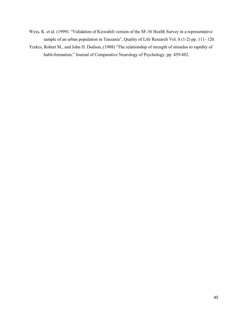
45

Wyss, K. et al. (1999): “Validation of Kiswahili version of the SF-36 Health Survey in a representative

sample of an urban population in Tanzania”, Quality of Life Research Vol. 8 (1-2) pp. 111- 120.

Yerkes, Robert M., and John D. Dodson, (1908) “The relationship of strength of stimulus to rapidity of

habit-formation,” Journal of Comparative Neurology of Psychology, pp. 459-482.

46

Figure 1a and b: Yerkes-Dodson (1908): Relationship between Stress and Performance

Figure 2: Timeline of recruitment and research activities

Notes: Items in blue indicate research activities conducted for the purposes of this study. Items in black indicate

standard recruitment activities performed by the recruiter.

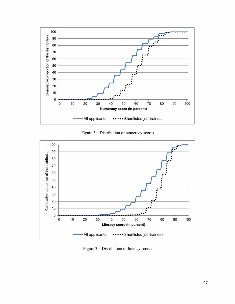
47

Figure 3a: Distribution of numeracy scores

Figure 3b: Distribution of literacy scores

0

10

20

30

40

50

60

70

80

90

100

0 10 20 30 40 50 60 70 80 90 100

Cu

mu

lative

pro

po

rtio

n o

f th

e d

istr

ibu

tio

n

Numeracy score (in percent)

All applicants Shortlisted job-trainees

0

10

20

30

40

50

60

70

80

90

100

0 10 20 30 40 50 60 70 80 90 100

Cum

ula

tive

pro

po

rtio

n o

f th

e d

istr

ibu

tio

n

Literacy score (in percent)

All applicants Shortlisted job-trainees

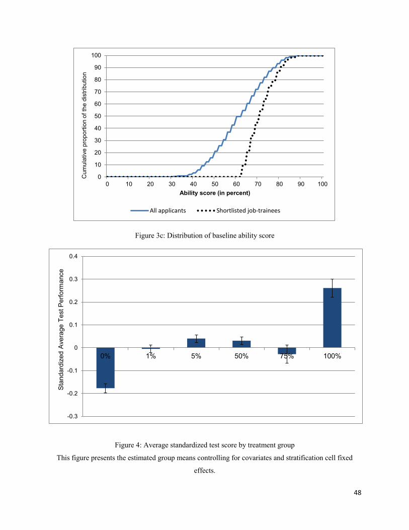
48

Figure 3c: Distribution of baseline ability score

Figure 4: Average standardized test score by treatment group

This figure presents the estimated group means controlling for covariates and stratification cell fixed

effects.

0

10

20

30

40

50

60

70

80

90

100

0 10 20 30 40 50 60 70 80 90 100

Cu

mu

lative

pro

po

rtio

n o

f th

e d

istr

ibu

tio

n

Ability score (in percent)

All applicants Shortlisted job-trainees

-0.3

-0.2

-0.1

0

0.1

0.2

0.3

0.4

0% 1% 5% 50% 75% 100%

Sta

ndard

ized A

vera

ge T

est P

erf

orm

ance

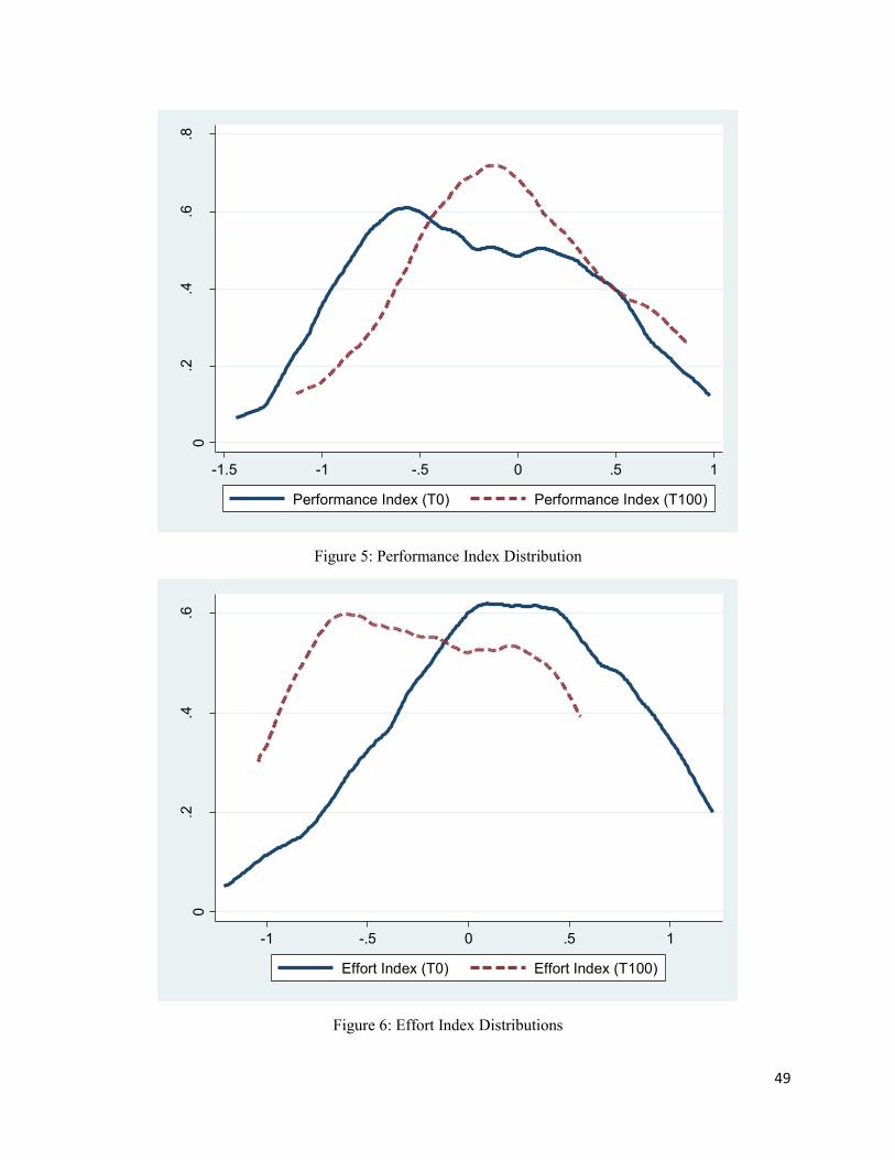
49

Figure 5: Performance Index Distribution

Figure 6: Effort Index Distributions

0.2

.4.6

.8

Den

sity

-1.5 -1 -.5 0 .5 1

Performance Index (T0) Performance Index (T100)

0.2

.4.6

Den

sity

-1 -.5 0 .5 1

Effort Index (T0) Effort Index (T100)

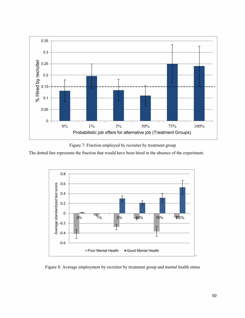
50

Figure 7: Fraction employed by recruiter by treatment group

The dotted line represents the fraction that would have been hired in the absence of the experiment.

-

Figure 8: Average employment by recruiter by treatment group and mental health status

0

0.05

0.1

0.15

0.2

0.25

0.3

0.35

0% 1% 5% 50% 75% 100%

% H

ired

by r

ecru

ite

r

Probabilistic job offers for alternative job (Treatment Groups)

-0.6

-0.4

-0.2

0

0.2

0.4

0.6

0.8

0% 1% 5% 50% 75% 100%

Ave

rag

e s

tan

da

rdiz

ed

te

st sco

re

Poor Mental Health Good Mental Health

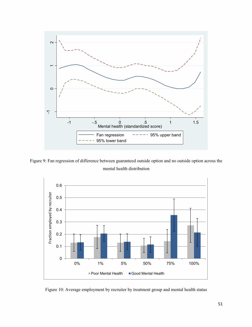
51

Figure 9: Fan regression of difference between guaranteed outside option and no outside option across the

mental health distribution

Figure 10: Average employment by recruiter by treatment group and mental health status

-10

12

-1 -.5 0 .5 1 1.5Mental health (standardized score)

Fan regression 95% upper band

95% lower band

0

0.1

0.2

0.3

0.4

0.5

0.6

0% 1% 5% 50% 75% 100%

Frac

tio

n e

mp

loye

d b

y re

cru

iter

Poor Mental Health Good Mental Health

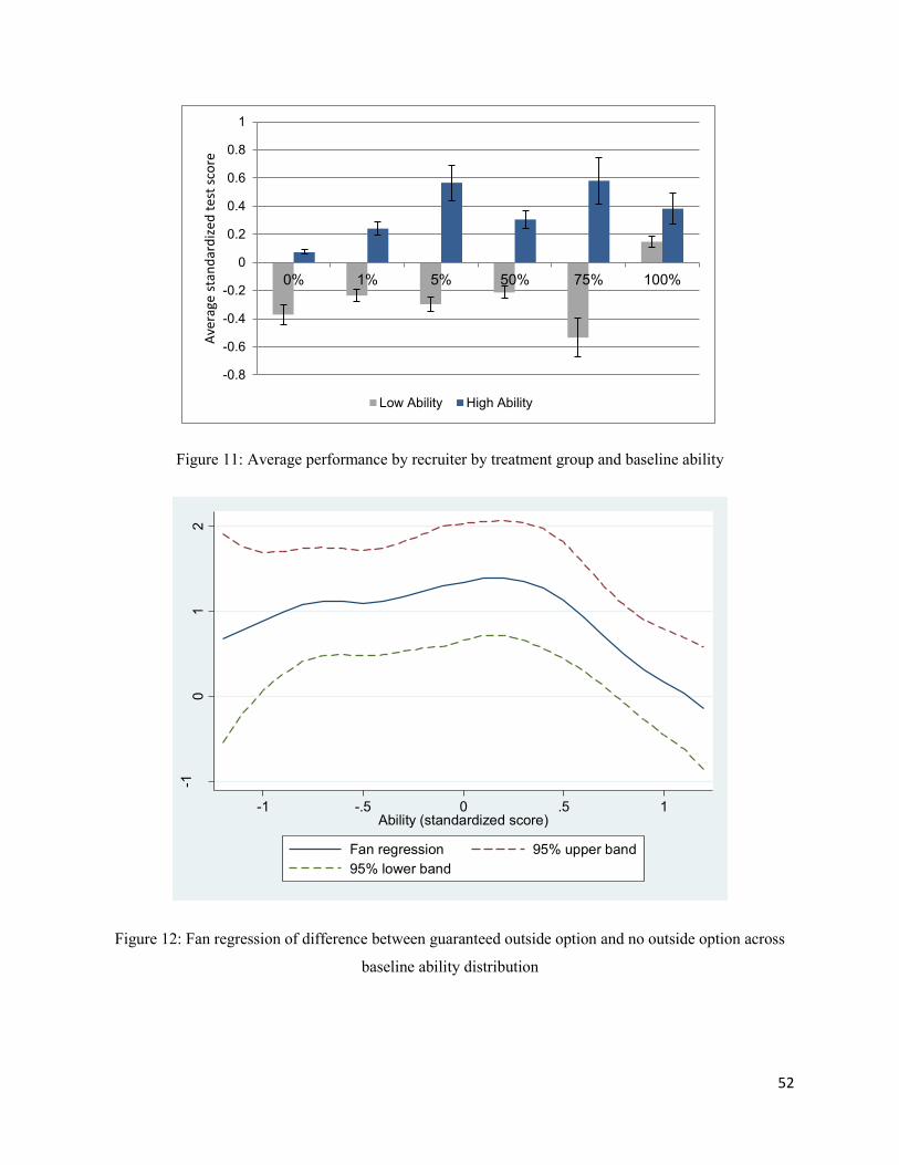
52

Figure 11: Average performance by recruiter by treatment group and baseline ability

Figure 12: Fan regression of difference between guaranteed outside option and no outside option across

baseline ability distribution

-0.8

-0.6

-0.4

-0.2

0

0.2

0.4

0.6

0.8

1

0% 1% 5% 50% 75% 100%

Ave

rage

sta

nd

ard

ized

tes

t sc

ore

Low Ability High Ability

-10

12

-1 -.5 0 .5 1Ability (standardized score)

Fan regression 95% upper band

95% lower band

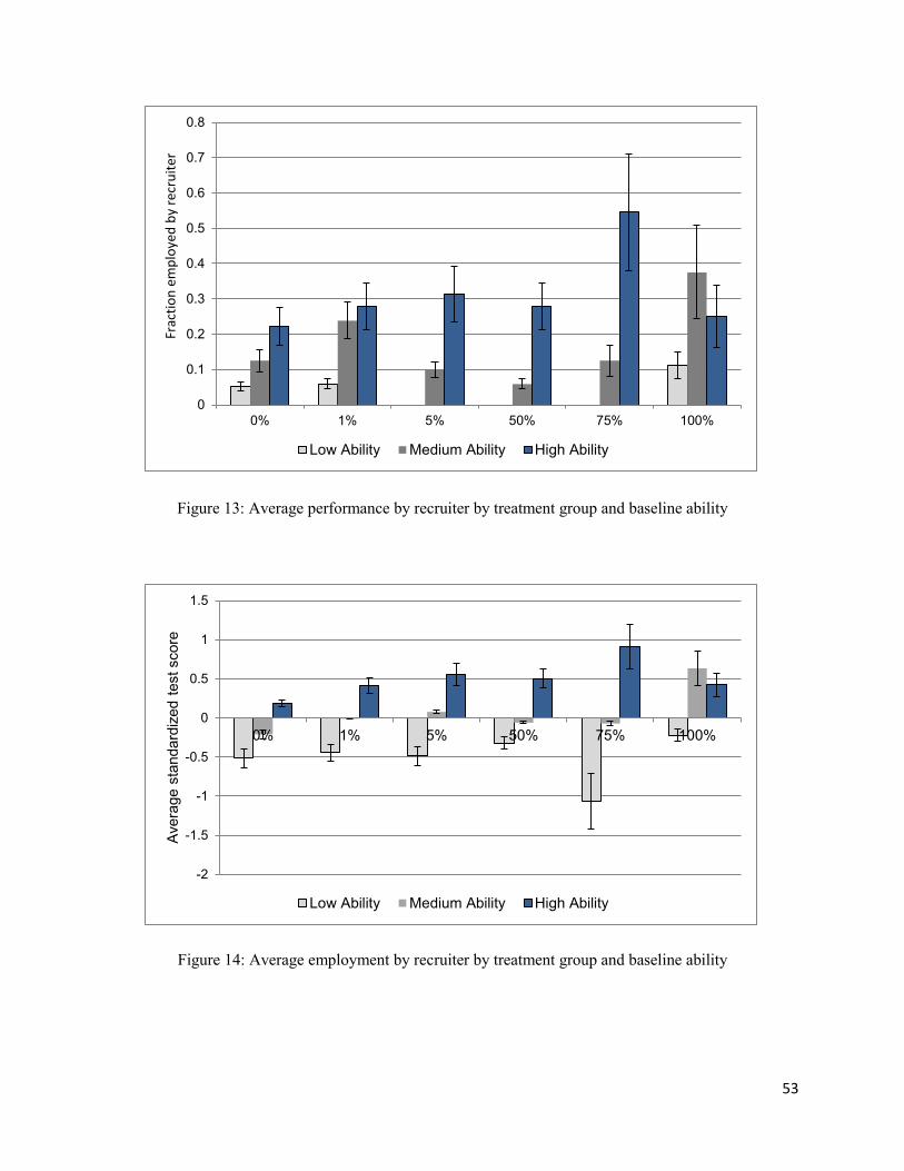
53

Figure 13: Average performance by recruiter by treatment group and baseline ability

Figure 14: Average employment by recruiter by treatment group and baseline ability

0

0.1

0.2

0.3

0.4

0.5

0.6

0.7

0.8

0% 1% 5% 50% 75% 100%

Frac

tio

n e

mp

loye

d b

y re

cru

iter

Low Ability Medium Ability High Ability

-2

-1.5

-1

-0.5

0

0.5

1

1.5

0% 1% 5% 50% 75% 100%

Avera

ge s

tandard

ized t

est score

Low Ability Medium Ability High Ability

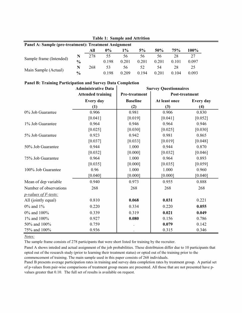
Panel A: Sample (pre-treatment): Treatment Assignment

All 0% 1% 5% 50% 75% 100%

N 278 55 56 56 56 28 27

% 0.198 0.201 0.201 0.201 0.101 0.097

N 268 53 56 52 54 28 25

% 0.198 0.209 0.194 0.201 0.104 0.093

Panel B: Training Participation and Survey Data Completion

0% Job Guarantee

1% Job Guarantee

5% Job Guarantee

50% Job Guarantee

75% Job Guarantee

100% Job Guarantee

Mean of dep variable

Number of observations

p-values of F-tests:

All (jointly equal)

0% and 1%

0% and 100%

1% and 100%

50% and 100%

75% and 100%

Notes:

The sample frame consists of 278 participants that were short listed for training by the recruiter.

0.055

0.049

0.865

[0.048]

0.870

[0.046]

0.221

0.893

[0.059]

0.960

0.786

Pre-treatment

0.079

268

0.031

0.220

1.000

Post-treatment

0.830

[0.052]

0.142

(4)

0.888

268

[0.040]

0.940

268

0.810

0.220

0.339

Table 1: Sample and Attrition

Sample frame (Intended)

Main Sample (Actual)

Survey Questionnaires

[0.030]

Baseline

(2)

0.981

[0.019]

0.946

[0.030]

At least once

(3)

0.906

[0.041]

0.964

Administrative Data

[0.025]

Every day

(1)

0.906

0.946

Every day

0.942

[0.033]

1.000

[0.000]

268

0.068

0.334

0.981

[0.019]

0.944

[0.032]

0.964

[0.035]

1.000

[0.000]

0.955

[0.000]

0.973

1.000

[0.000]

[0.040]

Panel A shows inteded and actual assignment of the job probabilities. These distribtuion differ due to 10 participants that

opted out of the research study (prior to learning their treatment status) or opted out of the training prior to the

commencement of training. The main sample used in this paper consists of 268 individuals.

Panel B presents average participation rates in training and survey data completion rates by treatment group. A partial set

of p-values from pair-wise comparisons of treatment group means are presented. All those that are not presented have p-

values greater that 0.10. The full set of results is available on request.

0.936 .

0.319

0.080

.

0.315 0.346

0.021

0.1560.927

0.759

Attended training

0.964

[0.025]

0.923

[0.037]

0.944

[0.032]

0.964

[0.035]

0.96

[0.041]

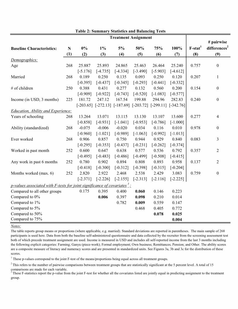
Baseline Characteristics: N 0% 1% 5% 50% 75% 100% F-stat1

# pairwise

differences2

(1) (2) (3) (4) (5) (6) (7) (8) (9)

Demographics:

Age 268 25.887 25.893 24.865 25.463 26.464 25.240 0.757 0

[-5.176] [-4.735] [-4.334] [-3.490] [-5.903] [-4.612]

Married 268 0.189 0.250 0.135 0.093 0.250 0.120 0.207 1

[-0.395] [-0.437] [-0.345] [-0.293] [-0.441] [-0.332]

# of children 250 0.388 0.431 0.277 0.132 0.560 0.200 0.154 0

[-0.909] [-0.922] [-0.743] [-0.520] [-1.083] [-0.577]

Income (in USD, 3 months) 225 181.72 247.12 167.54 199.88 294.96 282.83 0.240 0

[-203.65] [-272.13] [-187.69] [-203.72] [-299.11] [-342.76]

Education, Ability and Experience:

Years of schooling 268 13.264 13.071 13.115 13.130 13.107 13.600 0.277 4

[-0.858] [-0.931] [-1.041] [-0.953] [-0.786] [-1.000]

Ability (standardized) 268 -0.075 -0.006 -0.020 0.034 0.116 0.010 0.978 0

[-0.960] [-1.021] [-0.989] [-1.063] [-0.992] [-1.013]

Ever worked 268 0.906 0.857 0.750 0.944 0.929 0.840 0.083 3

[-0.295] [-0.353] [-0.437] [-0.231] [-0.262] [-0.374]

Worked in past month 252 0.600 0.647 0.638 0.577 0.536 0.792 0.357 2

[-0.495] [-0.483] [-0.486] [-0.499] [-0.508] [-0.415]

Any work in past 6 months 252 0.780 0.902 0.894 0.808 0.893 0.958 0.137 2

[-0.418] [-0.300] [-0.312] [-0.398] [-0.315] [-0.204]

Months worked (max. 6) 252 2.820 2.922 2.468 2.538 2.429 3.083 0.759 0

[-2.371] [-2.226] [-2.155] [-2.313] [-2.116] [-2.225]

p-values associated with F-tests for joint significance of covariates3

:

Compared to all other groups 0.175 0.395 0.400 0.060 0.146 0.223

Compared to 0% 0.006 0.397 0.098 0.210 0.014

Compared to 1% 0.782 0.009 0.559 0.147

Compared to 5% 0.468 0.405 0.772

Compared to 50% 0.078 0.025

Compared to 75% 0.004

Notes:

1 These p-values correspond to the joint F-test of the means/proportions being equal across all treatment groups.

Table 2: Summary Statistics and Balancing Tests

The table reports group means or proportions (where applicable, e.g. married). Standard deviations are reported in parentheses. The main sample of 268

participants is used here. Data from both the baseline self-administered questionnaire and data collected by the recruiter from the screening assessment test

both of which precede treatment assignment are used. Income is measured in USD and includes all self-reported income from the last 3 months including

the following explicit categories: Farming; Ganyu (piece-work); Formal employment; Own business; Remittances; Pension; and Other. The ability scores

are a composite measure of literacy and numeracy scores and are presented in standardized units. See Figures 3a, 3b and 3c for the distribution of these

scores.

2 This refers to the number of pairwise comparisons between treatment groups that are statistically significant at the 5 percent level. A total of 15

comparisons are made for each variable.3

These F-statistics report the p-value from the joint F-test for whether all the covariates listed are jointly equal in predicting assignment to the treatment

group.

Treatment Assignment

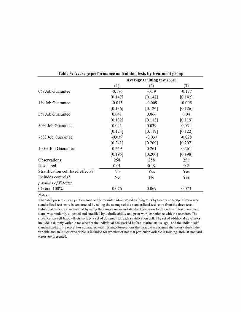
(1) (2) (3)

0% Job Guarantee -0.176 -0.19 -0.177

[0.147] [0.142] [0.142]

1% Job Guarantee -0.015 -0.009 -0.005

[0.136] [0.126] [0.126]

5% Job Guarantee 0.041 0.066 0.04

[0.132] [0.113] [0.119]

50% Job Guarantee 0.041 0.039 0.031

[0.124] [0.119] [0.122]

75% Job Guarantee -0.039 -0.037 -0.028

[0.241] [0.209] [0.207]

0.259 0.261 0.261

[0.195] [0.200] [0.198]

Observations 258 258 258

R-squared 0.01 0.19 0.2

Stratification cell fixed effects? No Yes Yes

Includes controls? No No Yes

p-values of F-tests:

0% and 100% 0.076 0.069 0.073

Notes:

100% Job Guarantee

Average training test score

Table 3: Average performance on training tests by treatment group

This table presents mean performance on the recruiter adminstered training tests by treatment group. The average

standardized test score is constructed by taking the average of the standardized test score from the three tests.

Individual tests are standardized by using the sample mean and standard deviation for the relevant test. Treatment

status was randomly allocated and stratified by quintile ability and prior work experience with the recruiter. The

stratification cell fixed effects include a set of dummies for each stratification cell. The set of additional covariates

include: a dummy variable for whether the individual has worked before, marital status, age, and the individuals'

standardized ability score. For covariates with missing observations the variable is assigned the mean value of the

variable and an indicator variable is included for whether or not that particular variable is missing. Robust standard

errors are presented.

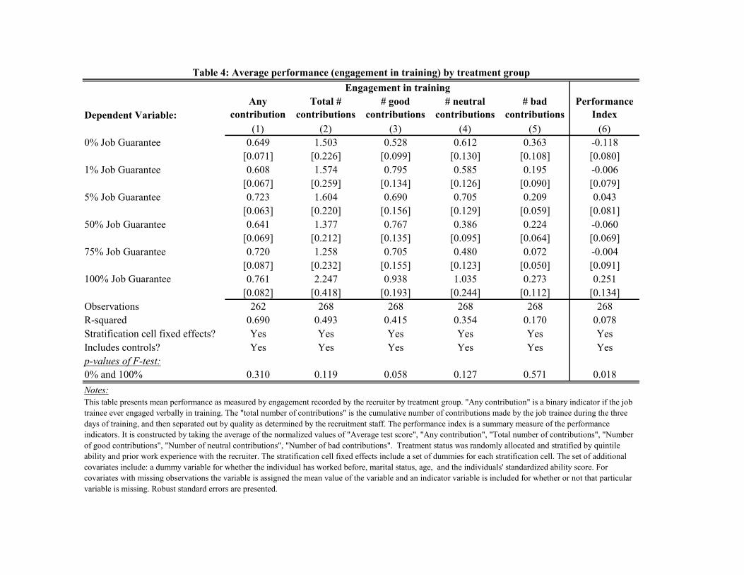
Dependent Variable:

Any

contribution

Total #

contributions

# good

contributions

# neutral

contributions

# bad

contributions

Performance

Index

(1) (2) (3) (4) (5) (6)

0% Job Guarantee 0.649 1.503 0.528 0.612 0.363 -0.118

[0.071] [0.226] [0.099] [0.130] [0.108] [0.080]

1% Job Guarantee 0.608 1.574 0.795 0.585 0.195 -0.006

[0.067] [0.259] [0.134] [0.126] [0.090] [0.079]

5% Job Guarantee 0.723 1.604 0.690 0.705 0.209 0.043

[0.063] [0.220] [0.156] [0.129] [0.059] [0.081]

50% Job Guarantee 0.641 1.377 0.767 0.386 0.224 -0.060

[0.069] [0.212] [0.135] [0.095] [0.064] [0.069]

75% Job Guarantee 0.720 1.258 0.705 0.480 0.072 -0.004

[0.087] [0.232] [0.155] [0.123] [0.050] [0.091]

0.761 2.247 0.938 1.035 0.273 0.251

[0.082] [0.418] [0.193] [0.244] [0.112] [0.134]

Observations 262 268 268 268 268 268

R-squared 0.690 0.493 0.415 0.354 0.170 0.078

Stratification cell fixed effects? Yes Yes Yes Yes Yes Yes

Includes controls? Yes Yes Yes Yes Yes Yes

p-values of F-test:

0% and 100% 0.310 0.119 0.058 0.127 0.571 0.018

Notes:

100% Job Guarantee

Engagement in training

This table presents mean performance as measured by engagement recorded by the recruiter by treatment group. "Any contribution" is a binary indicator if the job

trainee ever engaged verbally in training. The "total number of contributions" is the cumulative number of contributions made by the job trainee during the three

days of training, and then separated out by quality as determined by the recruitment staff. The performance index is a summary measure of the performance

indicators. It is constructed by taking the average of the normalized values of "Average test score", "Any contribution", "Total number of contributions", "Number

of good contributions", "Number of neutral contributions", "Number of bad contributions". Treatment status was randomly allocated and stratified by quintile

ability and prior work experience with the recruiter. The stratification cell fixed effects include a set of dummies for each stratification cell. The set of additional

covariates include: a dummy variable for whether the individual has worked before, marital status, age, and the individuals' standardized ability score. For

covariates with missing observations the variable is assigned the mean value of the variable and an indicator variable is included for whether or not that particular

variable is missing. Robust standard errors are presented.

Table 4: Average performance (engagement in training) by treatment group

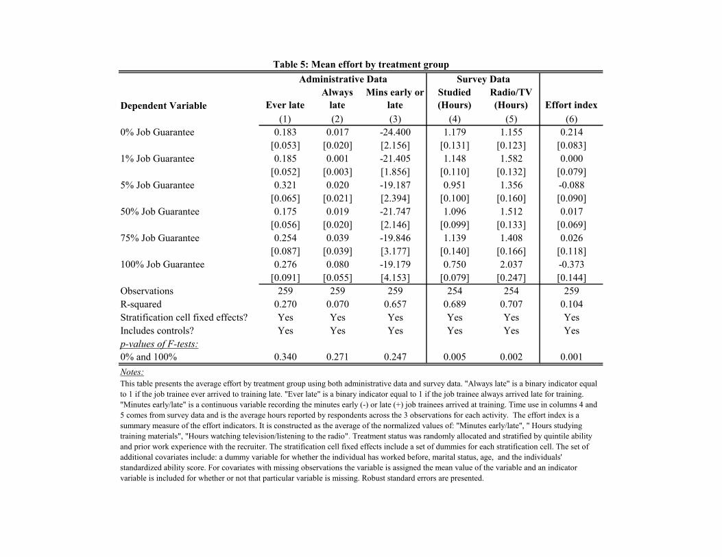
Dependent Variable Ever late

Always

late

Mins early or

late

Studied

(Hours)

Radio/TV

(Hours) Effort index

(1) (2) (3) (4) (5) (6)

0% Job Guarantee 0.183 0.017 -24.400 1.179 1.155 0.214

[0.053] [0.020] [2.156] [0.131] [0.123] [0.083]

1% Job Guarantee 0.185 0.001 -21.405 1.148 1.582 0.000

[0.052] [0.003] [1.856] [0.110] [0.132] [0.079]

5% Job Guarantee 0.321 0.020 -19.187 0.951 1.356 -0.088

[0.065] [0.021] [2.394] [0.100] [0.160] [0.090]

50% Job Guarantee 0.175 0.019 -21.747 1.096 1.512 0.017

[0.056] [0.020] [2.146] [0.099] [0.133] [0.069]

75% Job Guarantee 0.254 0.039 -19.846 1.139 1.408 0.026

[0.087] [0.039] [3.177] [0.140] [0.166] [0.118]

100% Job Guarantee 0.276 0.080 -19.179 0.750 2.037 -0.373

[0.091] [0.055] [4.153] [0.079] [0.247] [0.144]

Observations 259 259 259 254 254 259

R-squared 0.270 0.070 0.657 0.689 0.707 0.104

Stratification cell fixed effects? Yes Yes Yes Yes Yes Yes

Includes controls? Yes Yes Yes Yes Yes Yes

p-values of F-tests:

0% and 100% 0.340 0.271 0.247 0.005 0.002 0.001

Notes:

Administrative Data Survey Data

Table 5: Mean effort by treatment group

This table presents the average effort by treatment group using both administrative data and survey data. "Always late" is a binary indicator equal

to 1 if the job trainee ever arrived to training late. "Ever late" is a binary indicator equal to 1 if the job trainee always arrived late for training.

"Minutes early/late" is a continuous variable recording the minutes early (-) or late (+) job trainees arrived at training. Time use in columns 4 and

5 comes from survey data and is the average hours reported by respondents across the 3 observations for each activity. The effort index is a

summary measure of the effort indicators. It is constructed as the average of the normalized values of: "Minutes early/late", " Hours studying

training materials", "Hours watching television/listening to the radio". Treatment status was randomly allocated and stratified by quintile ability

and prior work experience with the recruiter. The stratification cell fixed effects include a set of dummies for each stratification cell. The set of

additional covariates include: a dummy variable for whether the individual has worked before, marital status, age, and the individuals'

standardized ability score. For covariates with missing observations the variable is assigned the mean value of the variable and an indicator

variable is included for whether or not that particular variable is missing. Robust standard errors are presented.

Average

Food

Expenditures (in

MKW)

Eat out

Expenditures (in

MKW)

(1) (2) (3)

0% Job Guarantee 349.479 124.151 73.058

[77.118] [16.339] [3.557]

1% Job Guarantee 425.084 165.495 73.538

[98.487] [15.067] [2.996]

5% Job Guarantee 372.697 154.952 76.109

[92.836] [21.179] [3.170]

50% Job Guarantee 439.111 147.49 72.706

[97.689] [20.097] [2.343]

75% Job Guarantee 335.364 183.878 83.596

[74.342] [27.507] [3.376]

100% Job Guarantee 328.482 123.887 77.596

[79.742] [23.159] [3.553]

Observations 256 256 256

R-squared 0.36 0.6 0.94

p-values of F-tests:

0% and 100% 0.797 0.543 0.363

Notes:This table presents the treatment group means for each outcome.

Attendance is a binary variable equal to 1 if the respondent ever attended training (i.e. attended at

least one of the training days).

"Perceived chance of employment with recruiter" is constructed using the following question: “What

percentage chance do you think you have of getting one of the available positions for the

RECRUITER’S PROJECT?” with the following options: No chance of getting a job; Less than 25

percent; Between 25 and 50 percent; 50 percent; Between 50 and 75 percent; Between 75 and 99

percent; and Certain about employment with recruiter. To create a measure of the likelihood of

employment I assign the mid-point to categories that are brackets and creating a continuous variable.

Food Expenditures (in MKW) is the average amount spent on food reported by the respondent

across the 3 training days. "Eat out expenditures (in MKW)" is similar except measures food

expenditures for food consumed away from the home.

Perceived chance

of employment

with recruiter

Treatment status was randomly allocated and stratified by quintile ability and prior work experience

with the recruiter. The stratification cell fixed effects include a set of dummies for each stratification

cell. The set of additional covariates include: a dummy variable for whether the individual has

worked before, marital status, age, and the individuals' standardized ability score. For covariates

with missing observations the variable is assigned the mean value of the variable and an indicator

variable is included for whether or not that particular variable is missing. Robust standard errors are

presented.

Table 6: Alternative Explanations?

Panel A: OLS Regressions

(1) (2) (3) (4) (5) (6)

0% Job Guarantee 0.132 0.126 0.133 0.137 0.129 0.136

[0.047] [0.045] [0.046] [0.049] [0.047] [0.047]

1% Job Guarantee 0.196 0.195 0.197 0.2 0.198 0.197

[0.054] [0.051] [0.051] [0.055] [0.052] [0.052]

5% Job Guarantee 0.135 0.139 0.136 0.137 0.143 0.141

[0.048] [0.043] [0.044] [0.049] [0.043] [0.045]

50% Job Guarantee 0.111 0.114 0.108 0.118 0.117 0.11

[0.043] [0.043] [0.044] [0.046] [0.046] [0.047]

75% Job Guarantee 0.250 0.241 0.238 0.259 0.256 0.251

[0.083] [0.074] [0.071] [0.085] [0.075] [0.073]

0.240 0.250 0.256 0.240 0.25 0.255

[0.086] [0.091] [0.089] [0.086] [0.091] [0.089]Stratification cell fixed

effects? No Yes Yes No Yes Yes

Includes controls? No No Yes No No Yes

Observations 268 268 268 260 260 260

R-squared 0.18 0.28 0.29 0.18 0.29 0.3

p-values of F-tests:

0% and 100% 0.274 0.224 0.221 0.314 0.241 0.238

Panel B: Probit Regressions

(1) (2) (3) (4) (5) (6)

0% Job Guarantee -0.088 -0.095* -0.090* -0.085 -0.094* -0.090*

[0.065] [0.054] [0.051] [0.068] [0.056] [0.054]

1% Job Guarantee -0.034 -0.048 -0.051 -0.032 -0.048 -0.052

[0.075] [0.064] [0.060] [0.077] [0.067] [0.062]

5% Job Guarantee -0.085 -0.093* -0.093* -0.085 -0.094* -0.093*

[0.065] [0.052] [0.049] [0.068] [0.055] [0.052]

50% Job Guarantee -0.106* -0.104** -0.109** -0.103 -0.104* -0.109**

[0.061] [0.051] [0.046] [0.064] [0.053] [0.049]

75% Job Guarantee 0.008 -0.024 -0.031 0.015 -0.014 -0.022

[0.094] [0.073] [0.067] [0.099] [0.080] [0.073]Stratification cell fixed

effects? No Yes Yes No Yes Yes

Includes controls? No No Yes No No Yes

Observations 268 268 268 260 260 260

Notes:

Table 7: Employment (With Recruiter) by treatment group

Full sample Attend all training days

100% Job Guarantee

Full sample Attend all training days

Treatment status was randomly allocated and stratified by quintile ability and prior work experience with the recruiter.

The stratification cell fixed effects include a set of dummies for each stratification cell. The set of additional covariates

include: a dummy variable for whether the individual has worked before, marital status, age, and the individuals'

standardized ability score. For covariates with missing observations the variable is assigned the mean value of the

variable and an indicator variable is included for whether or not that particular variable is missing. Robust standard

errors are presented. *** indicates significance at the 1% level, ** indicates significance at the 5% level, * indicates

significance at the 10% level

Columns 1 through 3 present results for the full sample, while Columns 4 through 6 exclude those that did not attend all

training days.

Panel B presents the impact on employment of the 0-, 1-, 5-, 50-, 75- job probabilities treatment compared to the 100

percent treatment group where employment risk is 0.

Panel A presents employment rates (with recruiter) by treatment group.

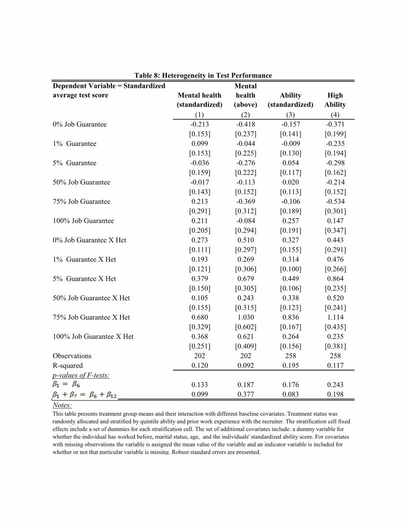
Dependent Variable = Standardized

average test score Mental health

(standardized)

Mental

health

(above)

Ability

(standardized)

High

Ability

(1) (2) (3) (4)

0% Job Guarantee -0.213 -0.418 -0.157 -0.371

[0.153] [0.237] [0.141] [0.199]

1% Guarantee 0.099 -0.044 -0.009 -0.235

[0.153] [0.225] [0.130] [0.194]

5% Guarantee -0.036 -0.276 0.054 -0.298

[0.159] [0.222] [0.117] [0.162]

50% Job Guarantee -0.017 -0.113 0.020 -0.214

[0.143] [0.152] [0.113] [0.152]

75% Job Guarantee 0.213 -0.369 -0.106 -0.534

[0.291] [0.312] [0.189] [0.301]

0.211 -0.084 0.257 0.147

[0.205] [0.294] [0.191] [0.347]

0% Job Guarantee X Het 0.273 0.510 0.327 0.443

[0.111] [0.297] [0.155] [0.291]

1% Guarantee X Het 0.193 0.269 0.314 0.476

[0.121] [0.306] [0.100] [0.266]

5% Guarantee X Het 0.379 0.679 0.449 0.864

[0.150] [0.305] [0.106] [0.235]

50% Job Guarantee X Het 0.105 0.243 0.338 0.520

[0.155] [0.315] [0.123] [0.241]

75% Job Guarantee X Het 0.680 1.030 0.836 1.114

[0.329] [0.602] [0.167] [0.435]

0.368 0.621 0.264 0.235

[0.251] [0.409] [0.156] [0.381]

Observations 202 202 258 258

R-squared 0.120 0.092 0.195 0.117

p-values of F-tests:

0.133 0.187 0.176 0.243

. 0.099 0.377 0.083 0.198

Notes:

100% Job Guarantee

100% Job Guarantee X Het

This table presents treatment group means and their interaction with different baseline covariates. Treatment status was

randomly allocated and stratified by quintile ability and prior work experience with the recruiter. The stratification cell fixed

effects include a set of dummies for each stratification cell. The set of additional covariates include: a dummy variable for

whether the individual has worked before, marital status, age, and the individuals' standardized ability score. For covariates

with missing observations the variable is assigned the mean value of the variable and an indicator variable is included for

whether or not that particular variable is missing. Robust standard errors are presented.

Table 8: Heterogeneity in Test Performance

1

Appendix A: Determinants of hiring decision using administrative data

In making hiring decisions the recruiter took a number of factors into account. As discussed

above the recruiter conducted multiple tests to ensure that trainee participants paid attention and to ensure

an objective measure of assessment was available to them. No participants were hired that had a

standardized test score (using the composite test measure) less than 0.05. All participants that had a

standardized test score greater than 1.3 were hired. As such although performing well on the test is a key

factor in the hiring decision, 72 percent of the group that were hired had test scores in a region where that

was not a sufficient determining factor. That is, performing well on the test was a necessary condition to

get hired. It was not however a sufficient condition for those participants with a standardized test score

between 0.05 and 1.3.

Appendix Table 2 presents the determinants of the hiring decision making process of the

recruiter. This shows that the standardized test score is an important determinant of whether the person

gets hired - a 1 standard deviation increase in the composite test score results in 9.7 percentage point

increase in the likelihood that the individual is hired. Other key indicators that were measured by the

recruiter include the punctuality, contributions and disruptions. Given Appendix Figure 1, it suggests that

any alternative measures of evaluating performance should be interacted with the test score.

Punctuality appears to have little impact on the hiring decision. Interestingly for those individuals

that do come late, this seems to increase their chances of employment if they have higher standardized

tests scores (although the magnitude is small – for every additional minute late they are 0.3 percentage

points more likely to be hired if they have a standardized test score of 1) (Column 2 of Appendix Table

2). Appendix Table 2 also shows that for those performing well (in terms of their standardized test score),

making “good” and “neutral” contributions during the training sessions increased the probability that they

were hired. In such a large hiring process being noticed in a good way mattered for those participants that

performed well but not exceptionally well. Lastly, Column 4 of Appendix Table 2 also includes measures

for disruptions made by participants during the training. This appears not to have any significant impact

on the hiring decision making process as the magnitude of the coefficients are small and statistically

insignificant.

Evidently, the most significant factor taken into account by the recruiter in its hiring decisions

was the performance of participants on the written tests. However, there is evidence that other

performance indicators were also taken into account – in particular whether or not the applicant made a

“good” contribution to the discussion

2

Appendix Table 1: Scatter plot employed by recruiter and training test score

0.2

.4.6

.81

Em

plo

yed

by R

ecru

ite

r

-3 -2 -1 0 1 2Standardized Average Training Test Score

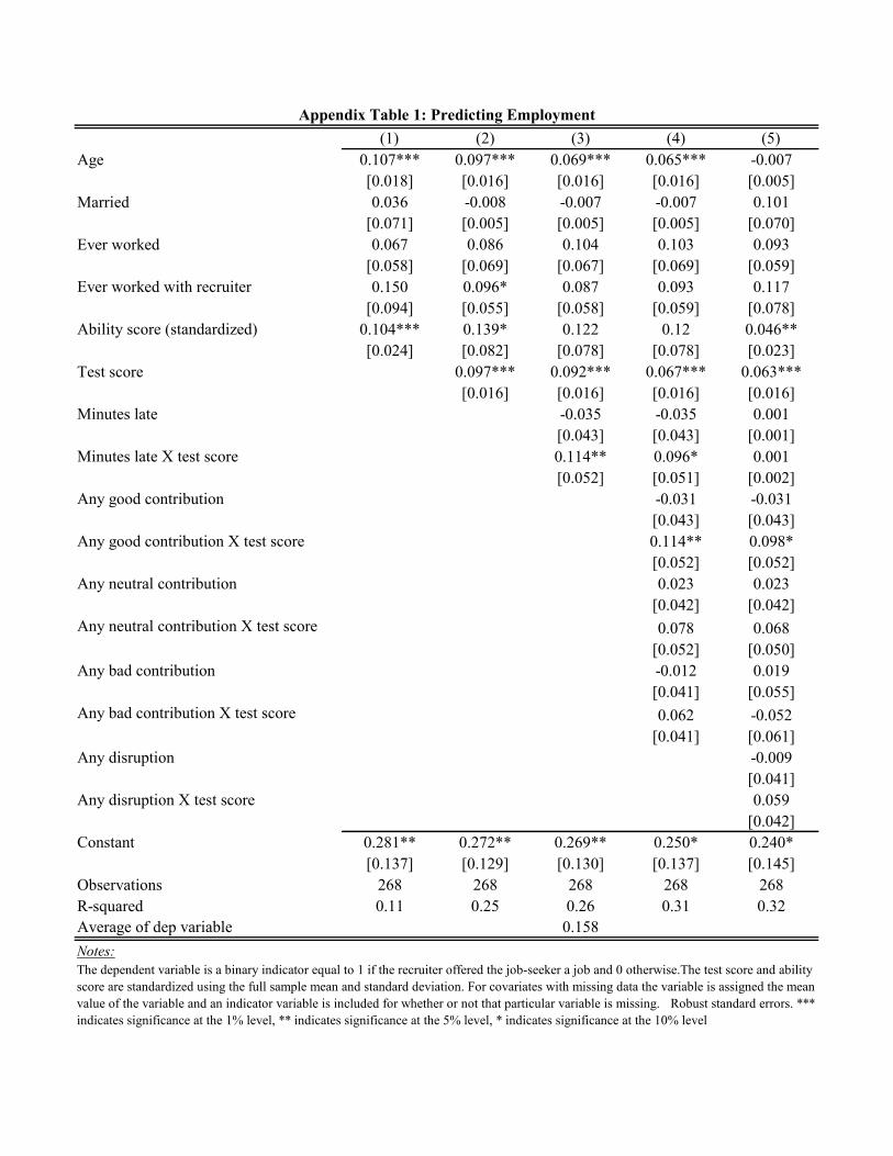
(1) (2) (3) (4) (5)

Age 0.107*** 0.097*** 0.069*** 0.065*** -0.007

[0.018] [0.016] [0.016] [0.016] [0.005]

Married 0.036 -0.008 -0.007 -0.007 0.101

[0.071] [0.005] [0.005] [0.005] [0.070]

Ever worked 0.067 0.086 0.104 0.103 0.093

[0.058] [0.069] [0.067] [0.069] [0.059]

Ever worked with recruiter 0.150 0.096* 0.087 0.093 0.117

[0.094] [0.055] [0.058] [0.059] [0.078]

Ability score (standardized) 0.104*** 0.139* 0.122 0.12 0.046**

[0.024] [0.082] [0.078] [0.078] [0.023]

Test score 0.097*** 0.092*** 0.067*** 0.063***

[0.016] [0.016] [0.016] [0.016]

Minutes late -0.035 -0.035 0.001

[0.043] [0.043] [0.001]

Minutes late X test score 0.114** 0.096* 0.001

[0.052] [0.051] [0.002]

Any good contribution -0.031 -0.031

[0.043] [0.043]

Any good contribution X test score 0.114** 0.098*

[0.052] [0.052]

Any neutral contribution 0.023 0.023

[0.042] [0.042]

Any neutral contribution X test score 0.078 0.068

[0.052] [0.050]

Any bad contribution -0.012 0.019

[0.041] [0.055]

Any bad contribution X test score 0.062 -0.052

[0.041] [0.061]

Any disruption -0.009

[0.041]

Any disruption X test score 0.059

[0.042]

Constant 0.281** 0.272** 0.269** 0.250* 0.240*

[0.137] [0.129] [0.130] [0.137] [0.145]

Observations 268 268 268 268 268

R-squared 0.11 0.25 0.26 0.31 0.32

Average of dep variable

Notes:

Appendix Table 1: Predicting Employment

The dependent variable is a binary indicator equal to 1 if the recruiter offered the job-seeker a job and 0 otherwise.The test score and ability

score are standardized using the full sample mean and standard deviation. For covariates with missing data the variable is assigned the mean

value of the variable and an indicator variable is included for whether or not that particular variable is missing. Robust standard errors. ***

indicates significance at the 1% level, ** indicates significance at the 5% level, * indicates significance at the 10% level

0.158

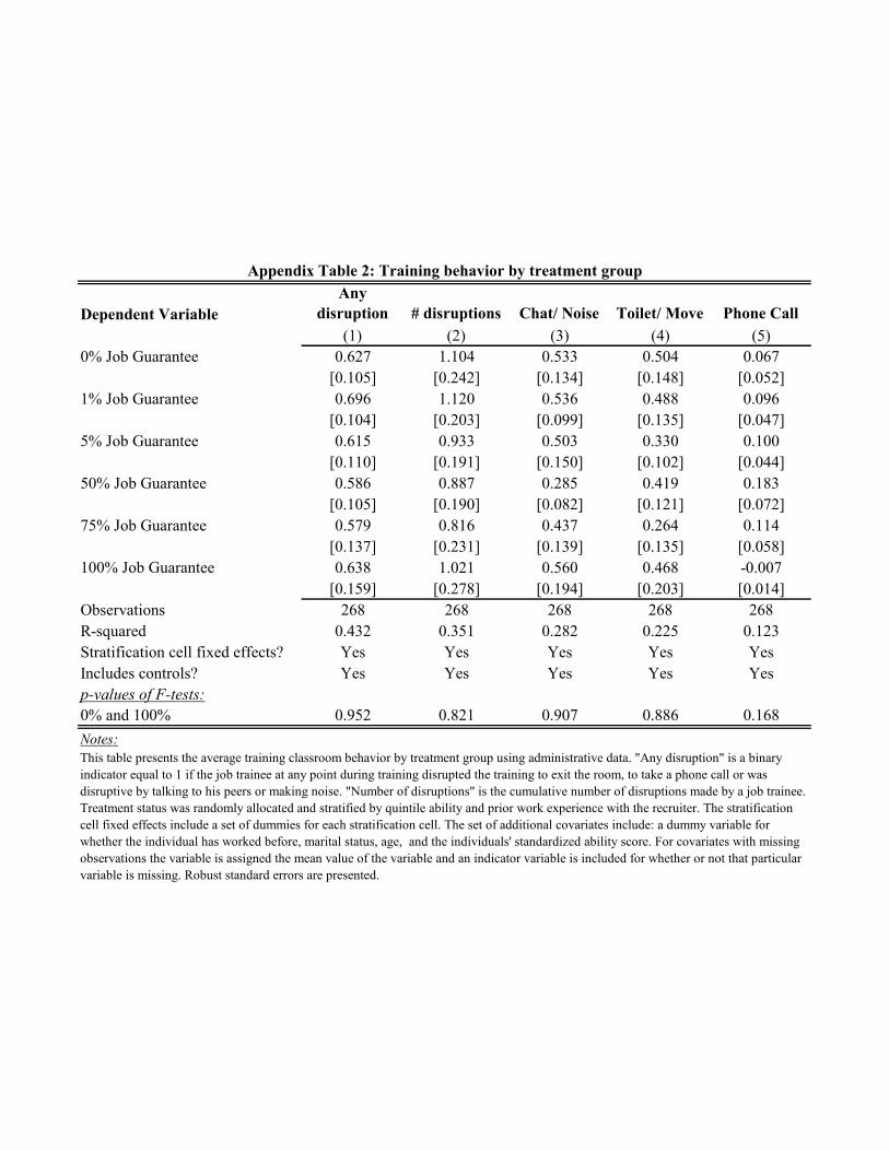
Dependent Variable

Any

disruption # disruptions Chat/ Noise Toilet/ Move Phone Call

(1) (2) (3) (4) (5)

0% Job Guarantee 0.627 1.104 0.533 0.504 0.067

[0.105] [0.242] [0.134] [0.148] [0.052]

1% Job Guarantee 0.696 1.120 0.536 0.488 0.096

[0.104] [0.203] [0.099] [0.135] [0.047]

5% Job Guarantee 0.615 0.933 0.503 0.330 0.100

[0.110] [0.191] [0.150] [0.102] [0.044]

50% Job Guarantee 0.586 0.887 0.285 0.419 0.183

[0.105] [0.190] [0.082] [0.121] [0.072]

75% Job Guarantee 0.579 0.816 0.437 0.264 0.114

[0.137] [0.231] [0.139] [0.135] [0.058]

100% Job Guarantee 0.638 1.021 0.560 0.468 -0.007

[0.159] [0.278] [0.194] [0.203] [0.014]

Observations 268 268 268 268 268

R-squared 0.432 0.351 0.282 0.225 0.123

Stratification cell fixed effects? Yes Yes Yes Yes Yes

Includes controls? Yes Yes Yes Yes Yes

p-values of F-tests:

0% and 100% 0.952 0.821 0.907 0.886 0.168

Notes:

This table presents the average training classroom behavior by treatment group using administrative data. "Any disruption" is a binary

indicator equal to 1 if the job trainee at any point during training disrupted the training to exit the room, to take a phone call or was

disruptive by talking to his peers or making noise. "Number of disruptions" is the cumulative number of disruptions made by a job trainee.

Treatment status was randomly allocated and stratified by quintile ability and prior work experience with the recruiter. The stratification

cell fixed effects include a set of dummies for each stratification cell. The set of additional covariates include: a dummy variable for

whether the individual has worked before, marital status, age, and the individuals' standardized ability score. For covariates with missing

observations the variable is assigned the mean value of the variable and an indicator variable is included for whether or not that particular

variable is missing. Robust standard errors are presented.

Appendix Table 2: Training behavior by treatment group

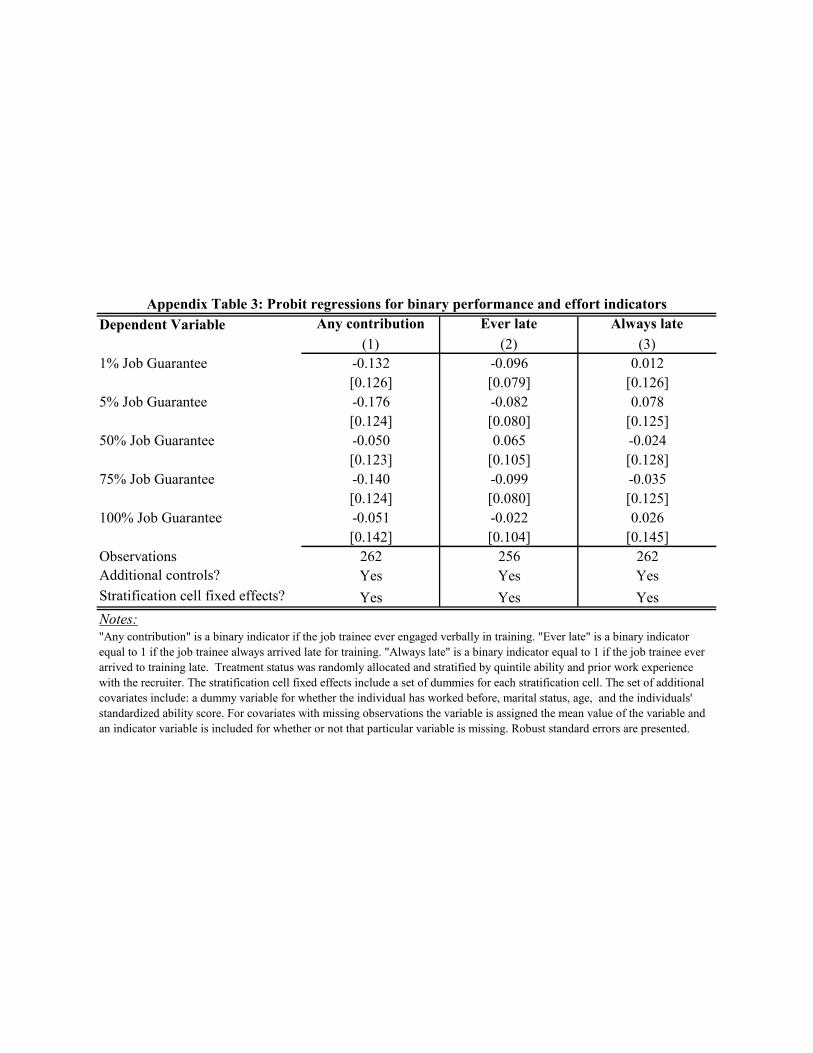
Dependent Variable Any contribution Ever late Always late

(1) (2) (3)

1% Job Guarantee -0.132 -0.096 0.012

[0.126] [0.079] [0.126]

5% Job Guarantee -0.176 -0.082 0.078

[0.124] [0.080] [0.125]

50% Job Guarantee -0.050 0.065 -0.024

[0.123] [0.105] [0.128]

75% Job Guarantee -0.140 -0.099 -0.035

[0.124] [0.080] [0.125]

100% Job Guarantee -0.051 -0.022 0.026

[0.142] [0.104] [0.145]

Observations 262 256 262

Additional controls? Yes Yes Yes

Stratification cell fixed effects? Yes Yes Yes

Notes:

Appendix Table 3: Probit regressions for binary performance and effort indicators

"Any contribution" is a binary indicator if the job trainee ever engaged verbally in training. "Ever late" is a binary indicator

equal to 1 if the job trainee always arrived late for training. "Always late" is a binary indicator equal to 1 if the job trainee ever

arrived to training late. Treatment status was randomly allocated and stratified by quintile ability and prior work experience

with the recruiter. The stratification cell fixed effects include a set of dummies for each stratification cell. The set of additional

covariates include: a dummy variable for whether the individual has worked before, marital status, age, and the individuals'

standardized ability score. For covariates with missing observations the variable is assigned the mean value of the variable and

an indicator variable is included for whether or not that particular variable is missing. Robust standard errors are presented.

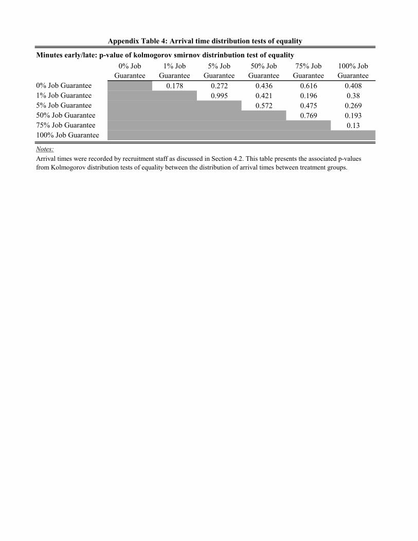
Minutes early/late: p-value of kolmogorov smirnov distrinbution test of equality

0% Job

Guarantee

1% Job

Guarantee

5% Job

Guarantee

50% Job

Guarantee

75% Job

Guarantee

100% Job

Guarantee

0% Job Guarantee 0.178 0.272 0.436 0.616 0.408

1% Job Guarantee 0.995 0.421 0.196 0.38

5% Job Guarantee 0.572 0.475 0.269

50% Job Guarantee 0.769 0.193

75% Job Guarantee 0.13

100% Job Guarantee

Notes:

Appendix Table 4: Arrival time distribution tests of equality

Arrival times were recorded by recruitment staff as discussed in Section 4.2. This table presents the associated p-values

from Kolmogorov distribution tests of equality between the distribution of arrival times between treatment groups.

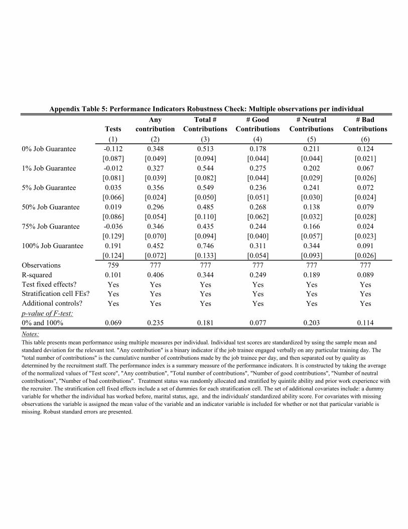
Tests

Any

contribution

Total #

Contributions

# Good

Contributions

# Neutral

Contributions

# Bad

Contributions

(1) (2) (3) (4) (5) (6)

0% Job Guarantee -0.112 0.348 0.513 0.178 0.211 0.124

[0.087] [0.049] [0.094] [0.044] [0.044] [0.021]

1% Job Guarantee -0.012 0.327 0.544 0.275 0.202 0.067

[0.081] [0.039] [0.082] [0.044] [0.029] [0.026]

5% Job Guarantee 0.035 0.356 0.549 0.236 0.241 0.072

[0.066] [0.024] [0.050] [0.051] [0.030] [0.024]

50% Job Guarantee 0.019 0.296 0.485 0.268 0.138 0.079

[0.086] [0.054] [0.110] [0.062] [0.032] [0.028]

75% Job Guarantee -0.036 0.346 0.435 0.244 0.166 0.024

[0.129] [0.070] [0.094] [0.040] [0.057] [0.023]

0.191 0.452 0.746 0.311 0.344 0.091

[0.124] [0.072] [0.133] [0.054] [0.093] [0.026]

Observations 759 777 777 777 777 777

R-squared 0.101 0.406 0.344 0.249 0.189 0.089

Test fixed effects? Yes Yes Yes Yes Yes Yes

Stratification cell FEs? Yes Yes Yes Yes Yes Yes

Additional controls? Yes Yes Yes Yes Yes Yes

p-value of F-test:

0% and 100% 0.069 0.235 0.181 0.077 0.203 0.114

Notes:

100% Job Guarantee

Appendix Table 5: Performance Indicators Robustness Check: Multiple observations per individual

This table presents mean performance using multiple measures per individual. Individual test scores are standardized by using the sample mean and

standard deviation for the relevant test. "Any contribution" is a binary indicator if the job trainee engaged verbally on any particular training day. The

"total number of contributions" is the cumulative number of contributions made by the job trainee per day, and then separated out by quality as

determined by the recruitment staff. The performance index is a summary measure of the performance indicators. It is constructed by taking the average

of the normalized values of "Test score", "Any contribution", "Total number of contributions", "Number of good contributions", "Number of neutral

contributions", "Number of bad contributions". Treatment status was randomly allocated and stratified by quintile ability and prior work experience with

the recruiter. The stratification cell fixed effects include a set of dummies for each stratification cell. The set of additional covariates include: a dummy

variable for whether the individual has worked before, marital status, age, and the individuals' standardized ability score. For covariates with missing

observations the variable is assigned the mean value of the variable and an indicator variable is included for whether or not that particular variable is

missing. Robust standard errors are presented.

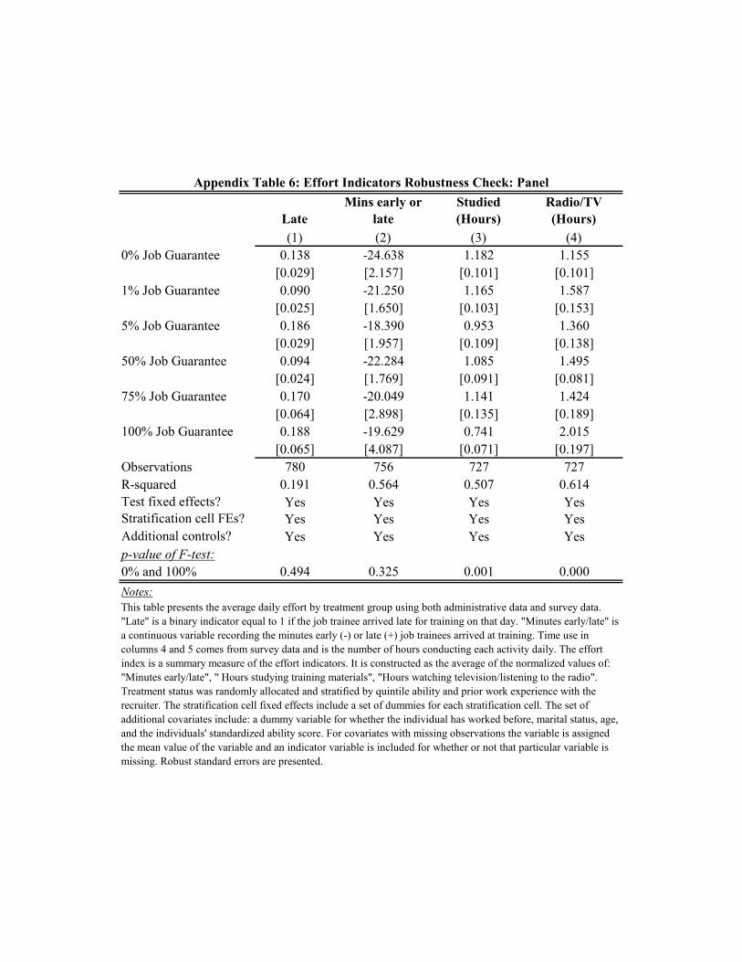
Late

Mins early or

late

Studied

(Hours)

Radio/TV

(Hours)

(1) (2) (3) (4)

0% Job Guarantee 0.138 -24.638 1.182 1.155

[0.029] [2.157] [0.101] [0.101]

1% Job Guarantee 0.090 -21.250 1.165 1.587

[0.025] [1.650] [0.103] [0.153]

5% Job Guarantee 0.186 -18.390 0.953 1.360

[0.029] [1.957] [0.109] [0.138]

50% Job Guarantee 0.094 -22.284 1.085 1.495

[0.024] [1.769] [0.091] [0.081]

75% Job Guarantee 0.170 -20.049 1.141 1.424

[0.064] [2.898] [0.135] [0.189]

0.188 -19.629 0.741 2.015

[0.065] [4.087] [0.071] [0.197]

Observations 780 756 727 727

R-squared 0.191 0.564 0.507 0.614

Test fixed effects? Yes Yes Yes Yes

Stratification cell FEs? Yes Yes Yes Yes

Additional controls? Yes Yes Yes Yes

p-value of F-test:

0% and 100% 0.494 0.325 0.001 0.000

Notes:

Appendix Table 6: Effort Indicators Robustness Check: Panel

100% Job Guarantee

This table presents the average daily effort by treatment group using both administrative data and survey data.

"Late" is a binary indicator equal to 1 if the job trainee arrived late for training on that day. "Minutes early/late" is

a continuous variable recording the minutes early (-) or late (+) job trainees arrived at training. Time use in

columns 4 and 5 comes from survey data and is the number of hours conducting each activity daily. The effort

index is a summary measure of the effort indicators. It is constructed as the average of the normalized values of:

"Minutes early/late", " Hours studying training materials", "Hours watching television/listening to the radio".

Treatment status was randomly allocated and stratified by quintile ability and prior work experience with the

recruiter. The stratification cell fixed effects include a set of dummies for each stratification cell. The set of

additional covariates include: a dummy variable for whether the individual has worked before, marital status, age,

and the individuals' standardized ability score. For covariates with missing observations the variable is assigned

the mean value of the variable and an indicator variable is included for whether or not that particular variable is

missing. Robust standard errors are presented.

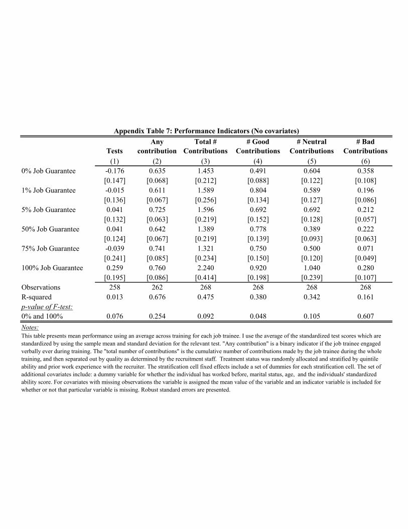
Tests

Any

contribution

Total #

Contributions

# Good

Contributions

# Neutral

Contributions

# Bad

Contributions

(1) (2) (3) (4) (5) (6)

0% Job Guarantee -0.176 0.635 1.453 0.491 0.604 0.358

[0.147] [0.068] [0.212] [0.088] [0.122] [0.108]

1% Job Guarantee -0.015 0.611 1.589 0.804 0.589 0.196

[0.136] [0.067] [0.256] [0.134] [0.127] [0.086]

5% Job Guarantee 0.041 0.725 1.596 0.692 0.692 0.212

[0.132] [0.063] [0.219] [0.152] [0.128] [0.057]

50% Job Guarantee 0.041 0.642 1.389 0.778 0.389 0.222

[0.124] [0.067] [0.219] [0.139] [0.093] [0.063]

75% Job Guarantee -0.039 0.741 1.321 0.750 0.500 0.071

[0.241] [0.085] [0.234] [0.150] [0.120] [0.049]

0.259 0.760 2.240 0.920 1.040 0.280

[0.195] [0.086] [0.414] [0.198] [0.239] [0.107]

Observations 258 262 268 268 268 268

R-squared 0.013 0.676 0.475 0.380 0.342 0.161

p-value of F-test:

0% and 100% 0.076 0.254 0.092 0.048 0.105 0.607

Notes:

Appendix Table 7: Performance Indicators (No covariates)

100% Job Guarantee

This table presents mean performance using an average across training for each job trainee. I use the average of the standardized test scores which are

standardized by using the sample mean and standard deviation for the relevant test. "Any contribution" is a binary indicator if the job trainee engaged

verbally ever during training. The "total number of contributions" is the cumulative number of contributions made by the job trainee during the whole

training, and then separated out by quality as determined by the recruitment staff. Treatment status was randomly allocated and stratified by quintile

ability and prior work experience with the recruiter. The stratification cell fixed effects include a set of dummies for each stratification cell. The set of

additional covariates include: a dummy variable for whether the individual has worked before, marital status, age, and the individuals' standardized

ability score. For covariates with missing observations the variable is assigned the mean value of the variable and an indicator variable is included for

whether or not that particular variable is missing. Robust standard errors are presented.

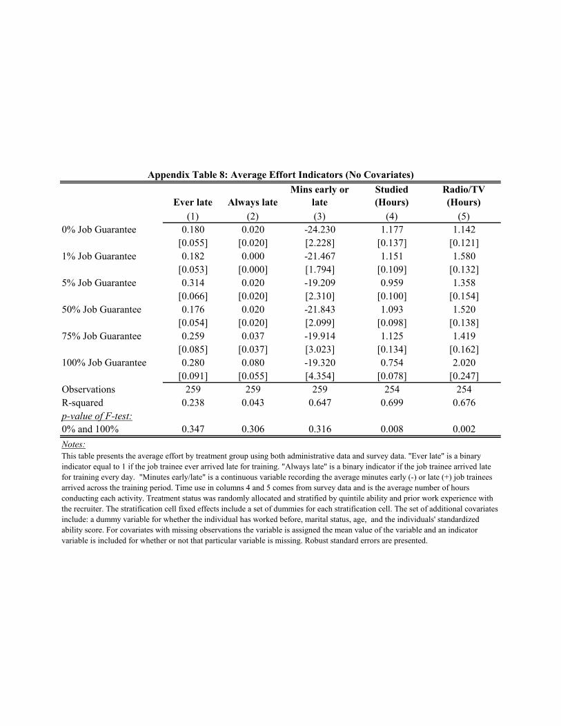
Ever late Always late

Mins early or

late

Studied

(Hours)

Radio/TV

(Hours)

(1) (2) (3) (4) (5)

0% Job Guarantee 0.180 0.020 -24.230 1.177 1.142

[0.055] [0.020] [2.228] [0.137] [0.121]

1% Job Guarantee 0.182 0.000 -21.467 1.151 1.580

[0.053] [0.000] [1.794] [0.109] [0.132]

5% Job Guarantee 0.314 0.020 -19.209 0.959 1.358

[0.066] [0.020] [2.310] [0.100] [0.154]

50% Job Guarantee 0.176 0.020 -21.843 1.093 1.520

[0.054] [0.020] [2.099] [0.098] [0.138]

75% Job Guarantee 0.259 0.037 -19.914 1.125 1.419

[0.085] [0.037] [3.023] [0.134] [0.162]

0.280 0.080 -19.320 0.754 2.020

[0.091] [0.055] [4.354] [0.078] [0.247]

Observations 259 259 259 254 254

R-squared 0.238 0.043 0.647 0.699 0.676

p-value of F-test:

0% and 100% 0.347 0.306 0.316 0.008 0.002

Notes:

Appendix Table 8: Average Effort Indicators (No Covariates)

100% Job Guarantee

This table presents the average effort by treatment group using both administrative data and survey data. "Ever late" is a binary

indicator equal to 1 if the job trainee ever arrived late for training. "Always late" is a binary indicator if the job trainee arrived late

for training every day. "Minutes early/late" is a continuous variable recording the average minutes early (-) or late (+) job trainees

arrived across the training period. Time use in columns 4 and 5 comes from survey data and is the average number of hours

conducting each activity. Treatment status was randomly allocated and stratified by quintile ability and prior work experience with

the recruiter. The stratification cell fixed effects include a set of dummies for each stratification cell. The set of additional covariates

include: a dummy variable for whether the individual has worked before, marital status, age, and the individuals' standardized

ability score. For covariates with missing observations the variable is assigned the mean value of the variable and an indicator

variable is included for whether or not that particular variable is missing. Robust standard errors are presented.

Ratio

(1)

Performance indicators:

Tests 67.994

Engagement:

* # of contributions -1.504

* # good contributions -1.672

* # neutral contributions -1.796

Effort indicators:

Time use:

* Hours studied training materials 7.003

* Hours watching tv/listening to radio 9.668

Notes:

Appendix Table 9: Omitted variable bias ratio

Following Altonji et al. (2005) and Bellows and Miguel (2008), I construct

a ratio that assesses the extent of omitted variable bias that would be

required to explain away the results. This table presents the ratios for each

of the performance and effort indicators for the estimated difference

between those assigned no outside option and a guaranteed outside option.

The ratio measures the extent to which selection on unobservables would

need to exceed selection on observables to explain away the coefficient.

Therefore, a larger ratio implies that the relative omitted variable bias from

unobservables relative to observables is greater, and therefore estimated

effects are less likely to be explained away.

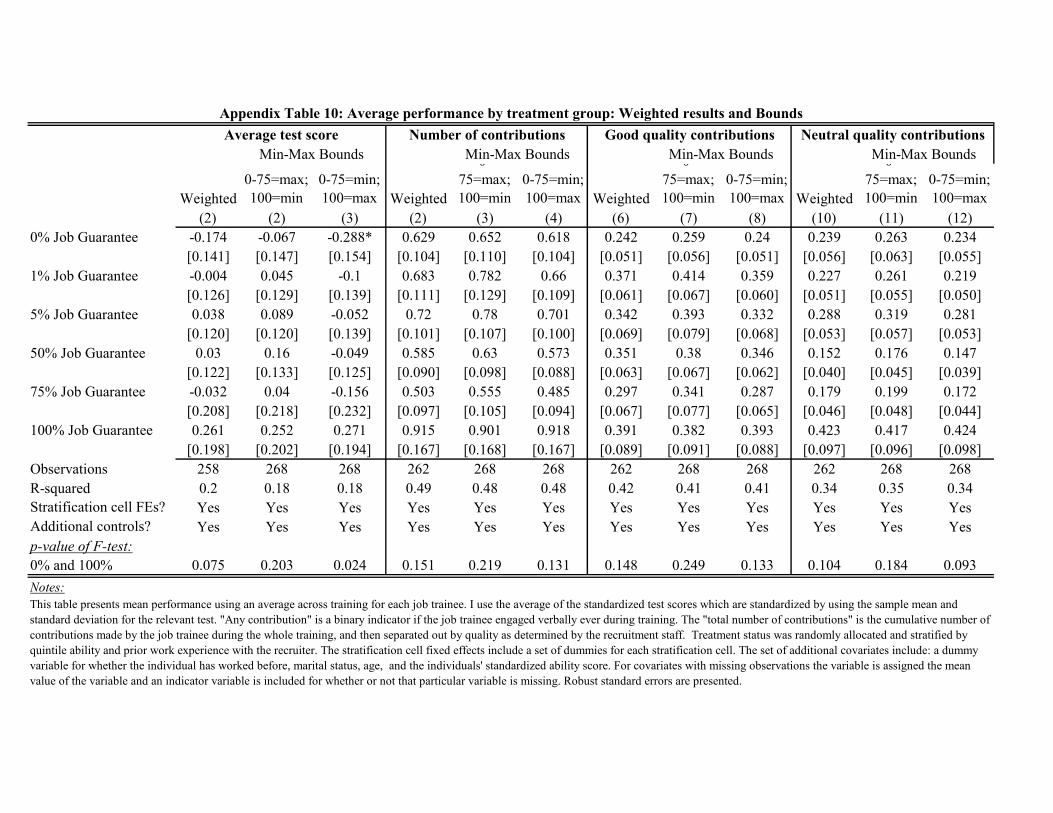
Weighted

0-75=max;

100=min

0-75=min;

100=max Weighted

0-

75=max;

100=min

0-75=min;

100=max Weighted

0-

75=max;

100=min

0-75=min;

100=max Weighted

0-

75=max;

100=min

0-75=min;

100=max

(2) (2) (3) (2) (3) (4) (6) (7) (8) (10) (11) (12)

0% Job Guarantee -0.174 -0.067 -0.288* 0.629 0.652 0.618 0.242 0.259 0.24 0.239 0.263 0.234

[0.141] [0.147] [0.154] [0.104] [0.110] [0.104] [0.051] [0.056] [0.051] [0.056] [0.063] [0.055]

1% Job Guarantee -0.004 0.045 -0.1 0.683 0.782 0.66 0.371 0.414 0.359 0.227 0.261 0.219

[0.126] [0.129] [0.139] [0.111] [0.129] [0.109] [0.061] [0.067] [0.060] [0.051] [0.055] [0.050]

5% Job Guarantee 0.038 0.089 -0.052 0.72 0.78 0.701 0.342 0.393 0.332 0.288 0.319 0.281

[0.120] [0.120] [0.139] [0.101] [0.107] [0.100] [0.069] [0.079] [0.068] [0.053] [0.057] [0.053]

50% Job Guarantee 0.03 0.16 -0.049 0.585 0.63 0.573 0.351 0.38 0.346 0.152 0.176 0.147

[0.122] [0.133] [0.125] [0.090] [0.098] [0.088] [0.063] [0.067] [0.062] [0.040] [0.045] [0.039]

75% Job Guarantee -0.032 0.04 -0.156 0.503 0.555 0.485 0.297 0.341 0.287 0.179 0.199 0.172

[0.208] [0.218] [0.232] [0.097] [0.105] [0.094] [0.067] [0.077] [0.065] [0.046] [0.048] [0.044]

0.261 0.252 0.271 0.915 0.901 0.918 0.391 0.382 0.393 0.423 0.417 0.424

[0.198] [0.202] [0.194] [0.167] [0.168] [0.167] [0.089] [0.091] [0.088] [0.097] [0.096] [0.098]

Observations 258 268 268 262 268 268 262 268 268 262 268 268

R-squared 0.2 0.18 0.18 0.49 0.48 0.48 0.42 0.41 0.41 0.34 0.35 0.34

Stratification cell FEs? Yes Yes Yes Yes Yes Yes Yes Yes Yes Yes Yes Yes

Additional controls? Yes Yes Yes Yes Yes Yes Yes Yes Yes Yes Yes Yes

p-value of F-test:

0% and 100% 0.075 0.203 0.024 0.151 0.219 0.131 0.148 0.249 0.133 0.104 0.184 0.093

Notes:

100% Job Guarantee

This table presents mean performance using an average across training for each job trainee. I use the average of the standardized test scores which are standardized by using the sample mean and

standard deviation for the relevant test. "Any contribution" is a binary indicator if the job trainee engaged verbally ever during training. The "total number of contributions" is the cumulative number of

contributions made by the job trainee during the whole training, and then separated out by quality as determined by the recruitment staff. Treatment status was randomly allocated and stratified by

quintile ability and prior work experience with the recruiter. The stratification cell fixed effects include a set of dummies for each stratification cell. The set of additional covariates include: a dummy

variable for whether the individual has worked before, marital status, age, and the individuals' standardized ability score. For covariates with missing observations the variable is assigned the mean

value of the variable and an indicator variable is included for whether or not that particular variable is missing. Robust standard errors are presented.

Min-Max Bounds Min-Max Bounds Min-Max Bounds Min-Max Bounds

Appendix Table 10: Average performance by treatment group: Weighted results and Bounds

Average test score Number of contributions Good quality contributions Neutral quality contributions

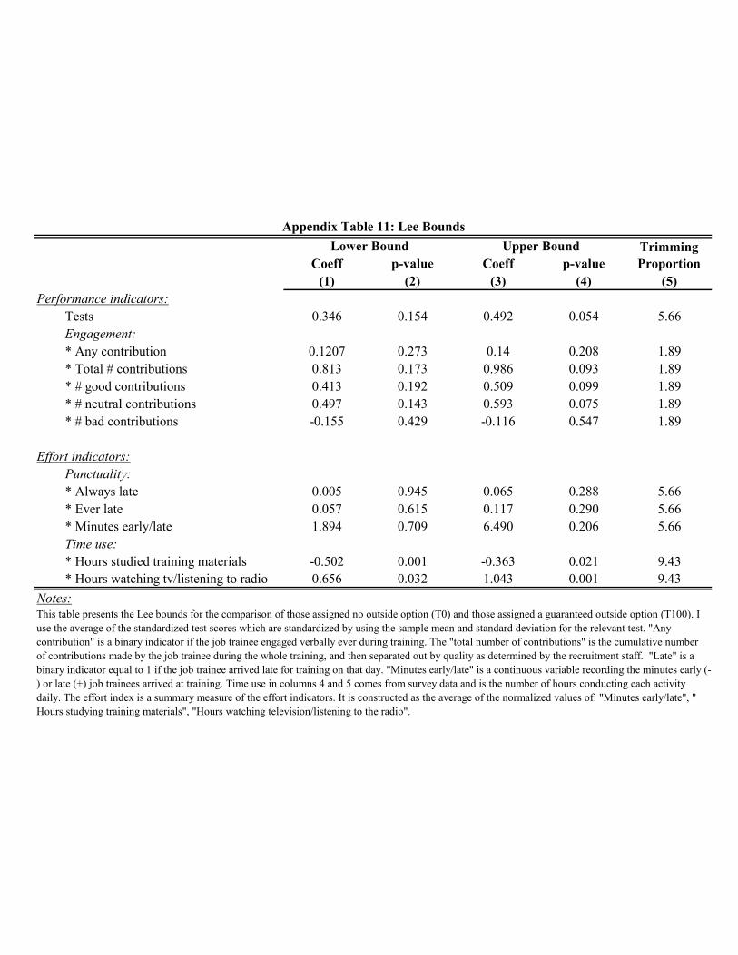
Coeff p-value Coeff p-value

(1) (2) (3) (4) (5)

Performance indicators:

Tests 0.346 0.154 0.492 0.054 5.66

Engagement:

* Any contribution 0.1207 0.273 0.14 0.208 1.89

* Total # contributions 0.813 0.173 0.986 0.093 1.89

* # good contributions 0.413 0.192 0.509 0.099 1.89

* # neutral contributions 0.497 0.143 0.593 0.075 1.89

* # bad contributions -0.155 0.429 -0.116 0.547 1.89

Effort indicators:

Punctuality:

* Always late 0.005 0.945 0.065 0.288 5.66

* Ever late 0.057 0.615 0.117 0.290 5.66

* Minutes early/late 1.894 0.709 6.490 0.206 5.66

Time use:

* Hours studied training materials -0.502 0.001 -0.363 0.021 9.43

* Hours watching tv/listening to radio 0.656 0.032 1.043 0.001 9.43

Notes:

Lower Bound Upper Bound Trimming

Proportion

Appendix Table 11: Lee Bounds

This table presents the Lee bounds for the comparison of those assigned no outside option (T0) and those assigned a guaranteed outside option (T100). I

use the average of the standardized test scores which are standardized by using the sample mean and standard deviation for the relevant test. "Any

contribution" is a binary indicator if the job trainee engaged verbally ever during training. The "total number of contributions" is the cumulative number

of contributions made by the job trainee during the whole training, and then separated out by quality as determined by the recruitment staff. "Late" is a

binary indicator equal to 1 if the job trainee arrived late for training on that day. "Minutes early/late" is a continuous variable recording the minutes early (-

) or late (+) job trainees arrived at training. Time use in columns 4 and 5 comes from survey data and is the number of hours conducting each activity

daily. The effort index is a summary measure of the effort indicators. It is constructed as the average of the normalized values of: "Minutes early/late", "

Hours studying training materials", "Hours watching television/listening to the radio".

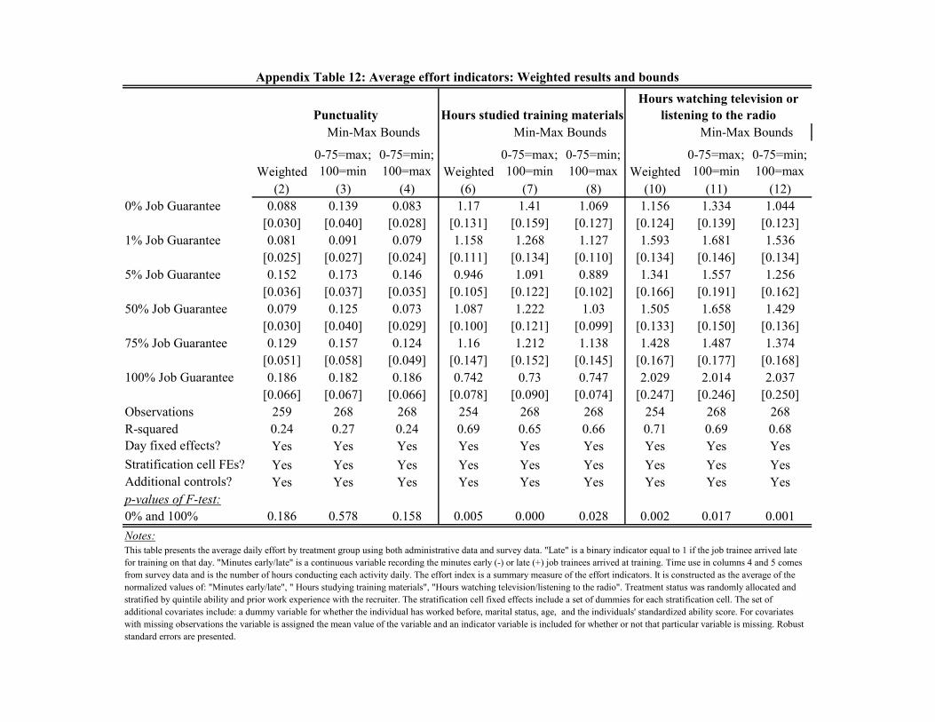
Weighted

0-75=max;

100=min

0-75=min;

100=max Weighted

0-75=max;

100=min

0-75=min;

100=max Weighted

0-75=max;

100=min

0-75=min;

100=max

(2) (3) (4) (6) (7) (8) (10) (11) (12)

0% Job Guarantee 0.088 0.139 0.083 1.17 1.41 1.069 1.156 1.334 1.044

[0.030] [0.040] [0.028] [0.131] [0.159] [0.127] [0.124] [0.139] [0.123]

1% Job Guarantee 0.081 0.091 0.079 1.158 1.268 1.127 1.593 1.681 1.536

[0.025] [0.027] [0.024] [0.111] [0.134] [0.110] [0.134] [0.146] [0.134]

5% Job Guarantee 0.152 0.173 0.146 0.946 1.091 0.889 1.341 1.557 1.256

[0.036] [0.037] [0.035] [0.105] [0.122] [0.102] [0.166] [0.191] [0.162]

50% Job Guarantee 0.079 0.125 0.073 1.087 1.222 1.03 1.505 1.658 1.429

[0.030] [0.040] [0.029] [0.100] [0.121] [0.099] [0.133] [0.150] [0.136]

75% Job Guarantee 0.129 0.157 0.124 1.16 1.212 1.138 1.428 1.487 1.374

[0.051] [0.058] [0.049] [0.147] [0.152] [0.145] [0.167] [0.177] [0.168]

0.186 0.182 0.186 0.742 0.73 0.747 2.029 2.014 2.037

[0.066] [0.067] [0.066] [0.078] [0.090] [0.074] [0.247] [0.246] [0.250]

Observations 259 268 268 254 268 268 254 268 268

R-squared 0.24 0.27 0.24 0.69 0.65 0.66 0.71 0.69 0.68

Day fixed effects? Yes Yes Yes Yes Yes Yes Yes Yes Yes

Stratification cell FEs? Yes Yes Yes Yes Yes Yes Yes Yes Yes

Additional controls? Yes Yes Yes Yes Yes Yes Yes Yes Yes

p-values of F-test:

0% and 100% 0.186 0.578 0.158 0.005 0.000 0.028 0.002 0.017 0.001

Notes:

100% Job Guarantee

This table presents the average daily effort by treatment group using both administrative data and survey data. "Late" is a binary indicator equal to 1 if the job trainee arrived late

for training on that day. "Minutes early/late" is a continuous variable recording the minutes early (-) or late (+) job trainees arrived at training. Time use in columns 4 and 5 comes

from survey data and is the number of hours conducting each activity daily. The effort index is a summary measure of the effort indicators. It is constructed as the average of the

normalized values of: "Minutes early/late", " Hours studying training materials", "Hours watching television/listening to the radio". Treatment status was randomly allocated and

stratified by quintile ability and prior work experience with the recruiter. The stratification cell fixed effects include a set of dummies for each stratification cell. The set of

additional covariates include: a dummy variable for whether the individual has worked before, marital status, age, and the individuals' standardized ability score. For covariates

with missing observations the variable is assigned the mean value of the variable and an indicator variable is included for whether or not that particular variable is missing. Robust

standard errors are presented.

Appendix Table 12: Average effort indicators: Weighted results and bounds

Punctuality

Min-Max Bounds Min-Max Bounds

Hours studied training materials

Min-Max Bounds

Hours watching television or

listening to the radio

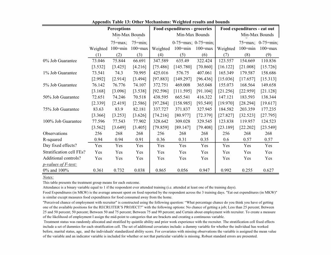
Weighted

0-

75=max;

100=min

0-

75=min;

100=max Weighted

0-75=max;

100=min

0-75=min;

100=max Weighted

0-

75=max;

100=min

0-75=min;

100=max

(1) (2) (3) (4) (5) (6) (7) (8) (9)

0% Job Guarantee 73.046 75.844 66.691 347.589 635.49 322.424 123.557 154.669 110.836

[3.532] [3.425] [4.216] [75.486] [145.780] [70.860] [16.122] [21.008] [15.726]

1% Job Guarantee 73.541 74.3 70.995 425.016 576.75 407.061 165.349 179.587 158.686

[2.992] [2.914] [3.494] [97.883] [149.297] [96.436] [15.036] [17.657] [15.313]

5% Job Guarantee 76.142 76.776 74.107 372.751 469.008 365.048 155.073 168.564 149.658

[3.168] [3.096] [3.538] [92.596] [111.595] [91.104] [21.256] [22.959] [21.128]

50% Job Guarantee 72.651 74.246 70.518 438.595 665.541 416.322 147.121 183.593 138.344

[2.339] [2.419] [2.586] [97.284] [158.985] [93.549] [19.970] [28.294] [19.617]

75% Job Guarantee 83.63 83.9 82.181 337.727 371.837 327.945 184.582 203.359 177.235

[3.366] [3.253] [3.626] [74.216] [80.977] [72.379] [27.827] [32.523] [27.795]

77.596 77.543 77.902 328.642 309.028 329.545 123.838 119.957 124.523

[3.562] [3.649] [3.405] [79.859] [89.147] [79.408] [23.189] [22.202] [23.549]

Observations 256 268 268 256 268 268 256 268 268

R-squared 0.94 0.94 0.91 0.36 0.31 0.35 0.6 0.57 0.57

Day fixed effects? Yes Yes Yes Yes Yes Yes Yes Yes Yes

Stratification cell FEs? Yes Yes Yes Yes Yes Yes Yes Yes Yes

Additional controls? Yes Yes Yes Yes Yes Yes Yes Yes Yes

p-values of F-test:

0% and 100% 0.361 0.732 0.038 0.865 0.056 0.947 0.992 0.255 0.627

Notes:

Appendix Table 13: Other Mechanisms: Weighted results and bounds

Food Expenditures (in MKW) is the average amount spent on food reported by the respondent across the 3 training days. "Eat out expenditures (in MKW)"

is similar except measures food expenditures for food consumed away from the home.

"Perceived chance of employment with recruiter" is constructed using the following question: “What percentage chance do you think you have of getting

one of the available positions for the RECRUITER’S PROJECT?” with the following options: No chance of getting a job; Less than 25 percent; Between

25 and 50 percent; 50 percent; Between 50 and 75 percent; Between 75 and 99 percent; and Certain about employment with recruiter. To create a measure

of the likelihood of employment I assign the mid-point to categories that are brackets and creating a continuous variable.

Treatment status was randomly allocated and stratified by quintile ability and prior work experience with the recruiter. The stratification cell fixed effects

include a set of dummies for each stratification cell. The set of additional covariates include: a dummy variable for whether the individual has worked

before, marital status, age, and the individuals' standardized ability score. For covariates with missing observations the variable is assigned the mean value

of the variable and an indicator variable is included for whether or not that particular variable is missing. Robust standard errors are presented.

100% Job Guarantee

Food expenditures - eat outPerceptions Food expenditures - groceries

Min-Max Bounds Min-Max Bounds Min-Max Bounds

This table presents the treatment group means for each outcome.

Attendance is a binary variable equal to 1 if the respondent ever attended training (i.e. attended at least one of the training days).

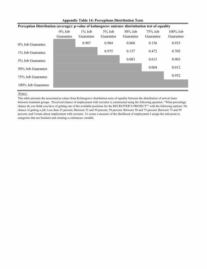
Perception Distribution (average): p-value of kolmogorov smirnov distrinbution test of equality

0% Job

Guarantee

1% Job

Guarantee

5% Job

Guarantee

50% Job

Guarantee

75% Job

Guarantee

100% Job

Guarantee

0% Job Guarantee 0.987 0.984 0.068 0.156 0.933

1% Job Guarantee 0.975 0.157 0.472 0.705

5% Job Guarantee 0.083 0.615 0.903

50% Job Guarantee 0.004 0.012

75% Job Guarantee 0.952

100% Job Guarantee

Notes:

Appendix Table 14: Perceptions Distribution Tests

This table presents the associated p-values from Kolmogorov distribution tests of equality between the distribution of arrival times

between treatment groups. Perceived chance of employment with recruiter is constructed using the following question: “What percentage

chance do you think you have of getting one of the available positions for the RECRUITER’S PROJECT?” with the following options: No

chance of getting a job; Less than 25 percent; Between 25 and 50 percent; 50 percent; Between 50 and 75 percent; Between 75 and 99

percent; and Certain about employment with recruiter. To create a measure of the likelihood of employment I assign the mid-point to

categories that are brackets and creating a continuous variable.