en route sector capacity model final report

Lincoln Laboratory MASSACHUSETTS INSTITUTE OF TECHNOLOGY

LEXINGTON, MASSACHUSETTS

Project Report ATC-426

En Route Sector Capacity Model Final Report

J.D. Welch

15 August 2015

Prepared under Air Force Contract No. FA8721-05-C-0002 and FA8702-15-D-0001 and sponsored by the Federal Aviation Administration under Interagency Agreement DTFAWA-11-X-80007.

This document is available to the public through the National Technical Information Service,

Springfield, Virginia 22161.

This document is disseminated under the sponsorship of the Department of Transportation, Federal Aviation Administration, in the interest of information exchange. The United States Government assumes no liability for its contents or use thereof. This material is based upon work supported under Air Force Contract No. FA8721-05-C-0002 and FA8702-15-D-0001. Any opinions, findings, conclusions or recommendations expressed in this material are those of the author(s) and do not necessarily reflect the views of the U.S. Air Force.

© (2015) MASSACHUSETTS INSTITUTE OF TECHNOLOGY

MIT PROPRIETARY, subject to FAR 52.227-11 – Patent Rights – Ownership by the Contractor (May 2014).

Delivered to the U.S. Government with Unlimited Rights, as defined in DFARS Part 252.227-7013 or 7014 (Feb 2014). Notwithstanding any copyright notice, U.S. Government rights in this work are defined by DFARS 252.227-7013 or DFARS 252.227-7014 as detailed above. Use of this work other than as specifically authorized by the U.S. Government may violate any copyrights that exist in this work.

17. Key Words 18. Distribution Statement

19. Security Classif. (of this report) 20. Security Classif. (of this page) 21. No. of Pages 22. Price

TECHNICAL REPORT STANDARD TITLE PAGE

1. Report No. 2. Government Accession No. 3. Recipient's Catalog No.

4. Title and Subtitle 5. Report Date

6. Performing Organization Code

7. Author(s) 8. Performing Organization Report No.

9. Performing Organization Name and Address 10. Work Unit No. (TRAIS)

11. Contract or Grant No.

12. Sponsoring Agency Name and Address 13. Type of Report and Period Covered

14. Sponsoring Agency Code

15. Supplementary Notes

16. Abstract

Unclassified Unclassified 78

FORM DOT F 1700.7 (8-72) Reproduction of completed page authorized

Jerry D. Welch

MIT Lincoln Laboratory244 Wood StreetLexington, MA 02420-9108

This report is based on studies performed at Lincoln Laboratory, a federally funded research and development center operated by Massachusetts Institute of Technology, under Air Force Contract FA8721-05-C-0002 and FA8702-15-D-0001.

This document is available to the public through the National Technical Information Service, Springfield, VA 22161.

ATC-426

En Route Sector Capacity Model Final Report

Department of TransportationFederal Aviation Administration800 Independence Ave., S.W. Washington, DC 20591

Project Report

ATC-426

TBD

Accurate predictions of en route sector capacity are vital when analyzing the benefits of proposed new air traffic management decision-support tools or new airspace designs. Controller workload is the main determinant of sector capacity. This report describes a new workload-based capacity model that improves upon the Federal Aviation Administration’s current Monitor Alert capacity model. Analysts often use Monitor Alert sector capacities in evaluating the benefits of decision-support aids or airspace designs. However, Monitor Alert, which was designed to warn controllers of possible sector overload, sets sector capacity limits based solely on handoff workload and fixed procedural constraints. It ignores the effects of conflict workload and recurring workload (from activities such as monitoring, vectoring, spacing, and metering). Each workload type varies differently as traffic counts and airspace designs are changed. When used for benefits analysis, Monitor Alert’s concentration on a single workload type can lead to erroneous conclusions.

The new model considers all three workload types. We determine the relative contribution of the three workload types by fitting the model to the upper frontiers that appear in peak daily sector traffic counts from today’s system. When we fit the Monitor Alert model to these same peak traffic counts, it can only explain the observed frontiers by hypothesizing large handoff workload. Large handoff workload would imply that decision-support aids should focus on handoff tasks. The new model fits the traffic data with less error, and shows that recurring tasks create significantly more workload in all sectors than do handoff tasks. The new model also shows that conflict workload dominates in very small sectors. These findings suggest that it is more beneficial to develop decision-support aids for recurring tasks and conflict tasks than for handoff tasks.

FA8721-05-C-0002 & FA8702-15-D-0001

This page intentionally left blank.

iii

ABSTRACT

Accurate predictions of en route sector capacity are vital when analyzing the benefits of proposed new air traffic management decision-support tools or new airspace designs. Controller workload is the main determinant of sector capacity. This report describes a new workload-based capacity model that improves upon the Federal Aviation Administration’s current Monitor Alert capacity model. Analysts often use Monitor Alert sector capacities in evaluating the benefits of decision-support aids or airspace designs. However, Monitor Alert, which was designed to warn controllers of possible sector overload, sets sector capacity limits based solely on handoff workload and fixed procedural constraints. It ignores the effects of conflict workload and recurring workload (from activities such as monitoring, vectoring, spacing, and metering). Each workload type varies differently as traffic counts and airspace designs are changed. When used for benefits analysis, Monitor Alert’s concentration on a single workload type can lead to erroneous conclusions.

The new model considers all three workload types. We determine the relative contribution of the three workload types by fitting the model to the upper frontiers that appear in peak daily sector traffic counts from today’s system. When we fit the Monitor Alert model to these same peak traffic counts, it can only explain the observed frontiers by hypothesizing large handoff workload. Large handoff workload would imply that decision-support aids should focus on handoff tasks. The new model fits the traffic data with less error, and shows that recurring tasks create significantly more workload in all sectors than do handoff tasks. The new model also shows that conflict workload dominates in very small sectors. These findings suggest that it is more beneficial to develop decision-support aids for recurring tasks and conflict tasks than for handoff tasks.

v

EXECUTIVE SUMMARY

This is a final report on the development of a workload-based capacity model for en route air traffic control sectors. Controller workload is the main determinant of sector capacity. Accurate predictions of airspace capacity are essential for the safe and efficient operation of the National Airspace System (NAS). Sector capacity models are important operational aids for estimating the capacity of existing sectors, of sectors proposed for modification, and of sectors with airspace blocked by weather or flight restrictions. Sector capacity models are also vital research tools in airspace design studies and air traffic management benefits simulations. This new model improves upon the Federal Aviation Administration’s current Monitor Alert capacity model, which is used both to predict operational sector overloads and to support system design and benefits studies.

Any sector capacity model requires one or more sector attributes to distinguish between the peak traffic handling capabilities of individual sectors. The Monitor Alert model uses mean sector transit time (the average time required for aircraft to fly through the sector) as the sole attribute for determining capacity. This implies that the model bases its individual capacity estimates on handoff-related workload. The reasoning goes as follows: as transit time increases, the handoff rate decreases, and the controller team has time to handle more aircraft. The Monitor Alert Parameter (MAP) operational rules allow manual capacity adjustments for individual sectors and set an upper capacity limit for all sectors, thereby acknowledging that other important workload factors also influence individual sector capacity. However, the model’s reliance on manual adjustments limits its utility in applications that require automatic capacity updates.

Like Monitor Alert, the new model also uses sector transit time to estimate handoff workload. However, it adds two other sector attributes that allow it to estimate capacity with greater accuracy. The new operational attributes are the sector airspace volume, which helps to estimate conflict workload, and the fraction of sector aircraft with significant altitude changes, which is used for estimating recurring workload. Conflict workload occurs when the controller team perceives a potential loss of separation. Recurring workload results from periodic activities such as surveillance monitoring, vectoring, metering, and spacing.

Knowledge of the sector airspace volume allows the model to calculate traffic density, which is needed for estimating the mean conflict rate. The sector volume attribute also helps estimate the benefits of combining and redesigning sectors or the disruption caused by partial airspace blockages.

Controllers consistently identify altitude changes as a major source of workload. The full model accounts for the sector altitude change fraction and confirms its importance. The model accuracy improves significantly when we introduce a relationship to increase recurring workload proportionally to altitude change fraction.

vi

Analysts often use Monitor Alert to estimate sector capacity in evaluating decision-support tools or airspace designs. When used for this purpose, its concentration on a single workload type, ignoring the effects of conflict and recurring workload, can lead to erroneous conclusions. Each workload type varies differently when traffic counts change and when controllers redesign airspace. The new attributes in the full model improve the ability to compare the relative workload contributions of distinct task types when analyzing the benefits of proposed air traffic decision-support tools and initiatives.

The Monitor Alert model has a practical operational advantage in that it requires only a single sector attribute to estimate capacity. We have examined another single-attribute model that uses the sector altitude change fraction to estimate recurring workload. The sector altitude change fraction is more stable than the sector transit time, and could be more practical for operational use. A recurring workload model based solely on the daily sector aircraft change fraction achieves nearly the same system-wide accuracy as the Monitor Alert model.

In addition to sector-specific attributes, capacity models also require system-wide numerical parameters. The Monitor Alert model and the full model both include parameters to quantify their estimates of the system-wide average time that controllers spend servicing a handoff. The full model adds similar parameters for average conflict service time and recurring service time. The full model also includes a parameter that defines the proportionality between altitude change fraction and recurring workload. We determine the numerical values of these parameters by regressing against operational traffic data.

A major challenge in developing the new model has been locating and processing operational data for the regression. The data must allow us to examine the correlation between the three sector attributes and actual peak daily sector traffic counts. We use the Federal Aviation Administration’s Sector Design and Analysis Tool database for this purpose. It includes information for determining historical peak daily sector traffic counts as well as mean sector transit times and sector volumes at the times of those peak counts. It also reports the daily fraction of aircraft with significant altitude changes for each sector.

When plotting peak daily sector counts versus each of the three sector attributes, distinct upper traffic frontiers are evident. We fit the model to the traffic frontiers by considering only those combinations of NAS-wide parameter values for which at least 95 percent of the sectors have model capacities exceeding their peak counts. We then search for the parameter combination in that 95-percentile subset that gives the least mean error between the calculated sector capacities and the corresponding daily sector traffic counts.

The full model includes more unknown parameters than required to fit the data. If the unknown parameters take on continuous values, the excess degrees of freedom result in an infinite number of solutions with identical mean error. To find a unique optimum, we quantize and scale the unknowns to integer search values. We then search for the discrete solution with least mean error. The analytic model and the simple mean-error objective function make it practical to search exhaustively through millions of

vii

parameter combinations. These searches return thousands of local solutions, many of which have mean errors close to that of the optimum.

We find that solutions with mean errors close to the optimum also return discrete parameter sets that are close to the optimum. Consequently, they predict nearly identical system-wide average workload and individual sector capacities. Because no near-optimum solutions produce conflicting estimates, the optimum solution can be used with confidence when analyzing the benefits of proposed air traffic decision-support tools.

We fitted four versions of the model to the peak daily sector traffic count data. The improvement in mean capacity error of the full model relative to an optimized version of the Monitor Alert model is about 15 percent. The full model estimates less conservative capacities than the Monitor Alert model for most individual sectors. It also provides significantly better visual fits to the traffic frontiers. However, its main value is its ability to guide air traffic managers by distinguishing between distinct workload sources. The full model provides important information on the relative importance of the three workload types. It tells us that, on a system-wide basis, recurring workload dominates at all traffic levels. Recurring workload dominates in sectors of average size and eventually becomes the sole workload component as sector volume increases. In very small sectors, conflict workload dominates, and handoff workload consistently lies well below recurring workload. Because the Monitor Alert model can only explain observed capacity frontiers by hypothesizing large handoff workload, it suggests misleadingly large potential capacity gains from automating handoffs.

The full model indicates that recurring tasks are the best candidates for decision-support aids. The system-wide dominance of recurring workload indicates a large potential for capacity improvement by aiding activities such as surveillance monitoring, vectoring, spacing, and metering. Furthermore, the relative freedom of recurring tasks from intricacies of inter-sector coordination could simplify the operational implementation of those decision-support aids.

The full model also suggests that it would be beneficial to focus on decision support for conflict resolution tasks in small sectors. Small sectors provide an organized means to deploy additional controllers to handle traffic in dense airspace. The model contributes to our understanding of NAS airspace conflicts by allowing us to directly infer mean sector conflict rates from peak traffic data. It shows that conflict workload dominates all other workload components in small sectors operating near capacity.

ix

ACKNOWLEDGMENTS

This report is the result of research and development sponsored by the Federal Aviation Administration Office of Systems Analysis and Modeling. The author appreciates the assistance provided by Joseph Post, who has supported the development of new en route sector capacity models for analyzing the benefits of Next Generation program initiatives in the National Airspace System.

This work has benefitted from discussions with and/or contributions by: John Andrews, James Bonn, Steve Bradford, John Cho, Richard DeLaura, Daniel Delahaye, George Donahue, James Evans, R. John Hansman, James Kurdzo, Michael Matthews, Brian Martin, Joseph Post, Eric Shank, Gregg Shoults, Banavar Shridhar, Kapil Sheth, Ngaire Underhill, Mark Weber, and Shannon Zelinski.

xi

TABLE OF CONTENTS

Page

Abstract iiiExecutive Summary vAcknowledgments ixList of Illustrations xvList of Tables xvii

1. BACKGROUND 1

1.1 Goal 11.2 Workload Models 11.3 Summary of Model Nomenclature 21.4 The Ambiguity Problem 2

2. OBSERVED SECTOR PERFORMANCE 5

2.1 Fitting Model Parameters to Observed Traffic 52.2 Recorded Traffic Counts 52.3 Peak Count Variance 72.4 Best-Case Sense of Model Capacity 82.5 Influence of MAP Operational Constraints on Observed Performance 8

3. THE FULL WORKLOAD MODEL 9

3.1 Model Overview 93.2 Handoff Workload 93.3 Conflict Workload 93.4 Recurring Workload 113.5 Human Workload Intensity Limit 113.6 Model Equations 12

4. FITTING MODEL PARAMETERS TO THE TRAFFIC DATA 13

4.1 Regression Objective Function and Percentile Constraint 134.2 Data Outliers 144.3 The Search Process 14

TABLE OF CONTENTS (Continued)

Page

xii

5. PERFORMANCE OF THE FULL MODEL 17

5.1 Fitted Parameter Values 175.2 Comparison of Full Model Capacities and Peak Counts 185.3 Growth of Workload Intensity Components with Traffic 215.4 Error Distribution of the Full Model 235.5 Performance Comparison with Other Model Versions 24

6. BENEFITS ANALYSIS 27

6.1 The Benefits Analysis Problem 27

7. GENERAL CONCLUSIONS 29

7.1 Summary of Results 297.2 Conclusions Regarding Automation Benefits 297.3 Conclusions Regarding Workload and Tube-Shaped Sectors 30

APPENDIX A MODEL TERMINOLOGY 31

APPENDIX B FULL MODEL EQUATIONS 33

APPENDIX C MODEL PERFORMANCE COMPARISONS 37

APPENDIX D ANALYSIS OF PARAMETER AMBIGUITY 45

APPENDIX E MULTI-SECTOR AIRSPACE WORKLOAD CAPACITY 51

TABLE OF CONTENTS (Continued)

Page

xiii

APPENDIX F DURATION OF PEAK COUNTS 53

Glossary 57References 59

xv

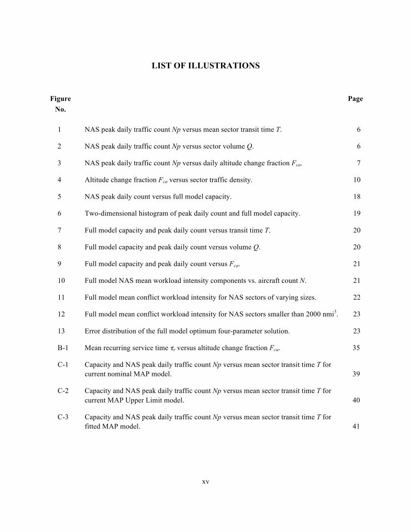
LIST OF ILLUSTRATIONS

Figure Page No.

1 NAS peak daily traffic count Np versus mean sector transit time T. 6

2 NAS peak daily traffic count Np versus sector volume Q. 6

3 NAS peak daily traffic count Np versus daily altitude change fraction Fca. 7

4 Altitude change fraction Fca versus sector traffic density. 10

5 NAS peak daily count versus full model capacity. 18

6 Two-dimensional histogram of peak daily count and full model capacity. 19

7 Full model capacity and peak daily count versus transit time T. 20

8 Full model capacity and peak daily count versus volume Q. 20

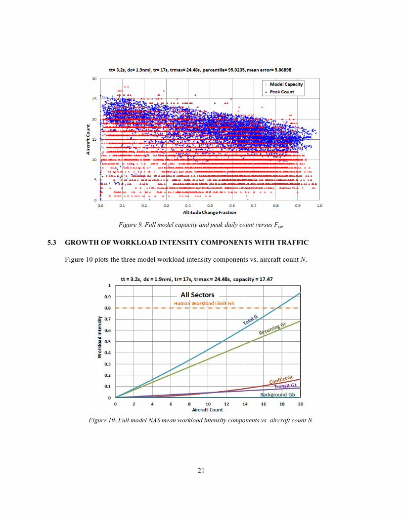
9 Full model capacity and peak daily count versus Fca. 21

10 Full model NAS mean workload intensity components vs. aircraft count N. 21

11 Full model mean conflict workload intensity for NAS sectors of varying sizes. 22

12 Full model mean conflict workload intensity for NAS sectors smaller than 2000 nmi3. 23

13 Error distribution of the full model optimum four-parameter solution. 23

B-1 Mean recurring service time τr versus altitude change fraction Fca. 35

C-1 Capacity and NAS peak daily traffic count Np versus mean sector transit time T for current nominal MAP model. 39

C-2 Capacity and NAS peak daily traffic count Np versus mean sector transit time T for current MAP Upper Limit model. 40

C-3 Capacity and NAS peak daily traffic count Np versus mean sector transit time T for fitted MAP model. 41

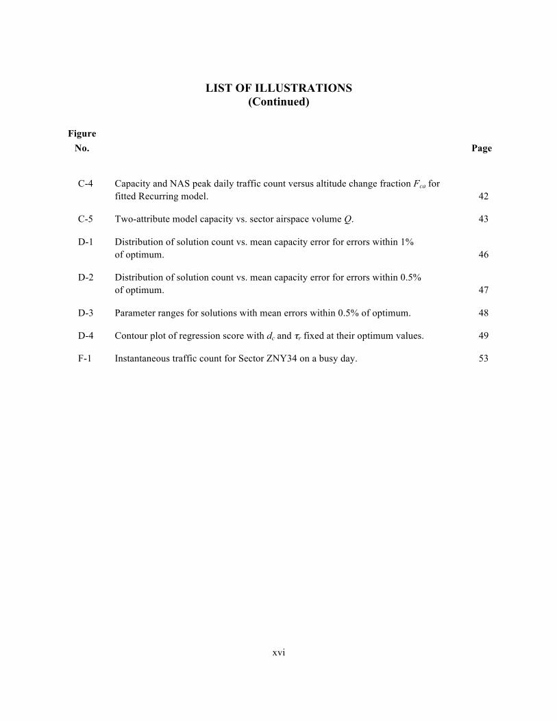
LIST OF ILLUSTRATIONS (Continued)

Figure No. Page

xvi

C-4 Capacity and NAS peak daily traffic count versus altitude change fraction Fca for fitted Recurring model. 42

C-5 Two-attribute model capacity vs. sector airspace volume Q. 43

D-1 Distribution of solution count vs. mean capacity error for errors within 1% of optimum. 46

D-2 Distribution of solution count vs. mean capacity error for errors within 0.5% of optimum. 47

D-3 Parameter ranges for solutions with mean errors within 0.5% of optimum. 48

D-4 Contour plot of regression score with dc and τr fixed at their optimum values. 49

F-1 Instantaneous traffic count for Sector ZNY34 on a busy day. 53

xvii

LIST OF TABLES

Table Page No.

1 Model Attributes, Parameters, and Mean Error 25

C-1 MAP Baseline Capacity Values 38

D-1 Parameters of Optimum Solution and Closest Local Solution 47

F-1 Numerical Details for Final Busy Period in Sector ZNY34 on 1 July 2007 55

1

1. BACKGROUND

1.1 GOAL

This is a final report on the development of a new analytical workload-based capacity model for en route air traffic control sectors. Simple and accurate means for predicting sector airspace capacity are essential for the design and efficient operation of the National Airspace System (NAS) [1].

Sector capacity models are important tools for estimating the operational capacity of existing sectors [2], of sectors proposed for modification, and of sectors with airspace blocked by weather or flight restrictions [3, 4]. Sector capacity models are also essential elements of many air traffic management simulations and airspace design studies [5, 6]. Controller workload is the principal determinant of sector capacity [7]. Consequently, capacity models based on workload can be particularly useful in predicting the benefits of air traffic management initiatives for decreasing specific types of controller workload.

The analytical, workload-based sector capacity model described in this report is a generalization of the model underlying the operational Monitor Alert system that the Federal Aviation Administration (FAA) uses to warn air traffic managers of possible sector overloads [8]. Monitor Alert sets sector capacity limits based on handoff workload and fixed procedural constraints. The resulting sector capacity estimates ignore the effects of conflict workload (from collision avoidance activities) and recurring workload (from activities such as monitoring, vectoring, spacing, and metering). Conflict and recurring workload change differently than handoff workload as traffic counts and airspace designs are changed. The Monitor Alert Parameter (MAP) model therefore cannot serve as a reliable source of relative workload information in such benefit predictions [9].

The main goal of this work has been to examine the ability of a more complete capacity model to quantify benefit predictions by accurately distinguishing between different workload types.

1.2 WORKLOAD MODELS

Workload-based capacity models use a simple queuing principle based on workload intensity, which is the fraction of the available sector controller time dedicated to each task type. The intensity of each workload component is the product of the mean task rate and the mean time required for the sector controller team to service that type of task. We define the capacity of the sector as the highest instantaneous sector traffic count at which the total workload intensity can be safely handled by the controller team.

The MAP model is limited in its ability to guide benefits studies because it accounts for only one workload type (handoff workload) and because it considers only a single measurable sector workload attribute (the mean sector transit time). The MAP model is based on the observation that handoff workload is proportional to the number of aircraft in the sector N and is inversely proportional to the

2

mean transit time T of the aircraft. Although a model based solely on handoff workload tends to over-estimate capacity in both small and large sectors, the addition of a fixed capacity limit for large sectors (together with an allowance for operational capacity adjustments) allows the MAP model to serve sectors of all sizes.

The new model extends the accuracy and utility of the handoff capacity estimates by accounting for two additional workload types. These are conflict workload and recurring workload. Conflict workload increases as N2 and decreases with sector volume Q. This allows the new model to be used in operational situations with dynamic airspace volume changes. Recurring workload increases linearly with N and is independent of transit time T. Recurring workload grows in situations that call for increased flight monitoring or flight vectoring. One important operational situation that involves both volume changes and recurring workload growth is the presence of hazardous weather.

In addition to the two new workload types, the new model adds two new sector workload attributes to the transit time attribute used in the MAP model. One new attribute is the sector airspace volume Q, which provides information about the traffic density of the sector. The other new attribute is the fraction of sector aircraft with significant altitude changes Fca. The altitude change fraction provides important information about airspace complexity. These three sector workload attributes are key model independent variables. We can measure and predict them in operational settings and we can relate them analytically to the intensity of the three variable workload types.

1.3 SUMMARY OF MODEL NOMENCLATURE

The distinctions between sector workload types, individual sector workload complexity attributes, and system-wide unknown model parameters are summarized in Appendix A.

1.4 THE AMBIGUITY PROBLEM

A potential problem arises in the use of the new model for benefits analysis. All models include system-wide unknown parameters to be determined by regression. These numerical values are determined by searching for the combination of parameters that best fits the model predictions to operational observations of sector peak traffic counts. At least one unknown parameter is required for each workload type. The MAP model’s unknown parameter is the mean service time for each entry/exit handoff pair. The new model requires two more unknown parameters to help quantify conflict workload and recurring workload. These are, respectively, the mean loss of separation while servicing a conflict and the mean service time for each recurring workload event.

The new model expresses sector capacity as a quadratic function of the sector traffic count N. This means that three parameters suffice to determine capacity. However, we have found that we can improve the accuracy of the sector capacity estimate by increasing recurring workload proportionally to the fraction of sector aircraft with significant altitude changes. This introduces an excess degree of freedom that can lead to multiple solutions with identical accuracy.

3

When analyzing benefits, it is important that such multiple regression solutions do not compromise the model’s ability to unambiguously distinguish between different workload types. An important goal of this effort has been to maximize the accuracy of the fit between the model and the data while developing a robust regression process that returns a unique set of model parameters that reliably distinguish between workload intensity components.

5

2. OBSERVED SECTOR PERFORMANCE

2.1 FITTING MODEL PARAMETERS TO OBSERVED TRAFFIC

We determine model parameters by fitting model capacity predictions to recorded peak sector traffic counts in the National Airspace System. The NAS database also includes numbers for the workload complexity attributes T, Q, and Fca of each sector.

We gathered this data for 9170 sector-days in 2007, the busiest year on record for the NAS. We identified the ten highest-traffic days for all twenty continental en route centers and recorded the peak traffic count for each sector in each center on each center’s top ten traffic days. We extracted the traffic data from the FAA Sector Design and Analysis Tool (SDAT) database [10]. This database includes information for determining peak daily sector traffic counts, as well as mean sector transit times and sector volumes at the times of those peak counts. It also includes a field that directly provides the daily fraction of aircraft with altitude changes exceeding 2000 ft. for each sector.

The SDAT database also includes 248 traffic counts from large Terminal Radar Approach Control (TRACON) and oceanic sectors where extra controller staffing, airspeed constraints, and special airspace designs increase capacity beyond normal en route sector levels. We use the model to identify and remove these high sector counts from the regression process (see Section 4.2, below). All plots of peak daily sector counts in this report have been condensed to include only the 8922 remaining counts from actual en route sectors.

We did not associate meteorological conditions with the high-traffic days because it is unlikely that a significant number of those days were adversely affected by hazardous weather.

2.2 RECORDED TRAFFIC COUNTS

Figures 1 through 3 are scatter plots of recorded NAS peak daily traffic counts Np versus the measureable sector workload complexity attributes T, Q, and Fca, respectively. All three figures exhibit upper traffic count frontiers that define the capacity of the NAS en route sectors.

Figure 1 shows that the capacity frontier increases with transit time T. Handoff workload occurs only when aircraft enter and exit a sector. When the mean transit time increases, the sector controller team can accommodate more aircraft with the same amount of effort. Air traffic managers use this principle to increase capacity by elongating sectors in the direction of busy routes or by using S-turns or holding stacks. The frontier does not increase linearly with transit time because other workload types act to constrain the capacity growth.

6

Figure 1. NAS peak daily traffic count Np versus mean sector transit time T.

Figure 2. NAS peak daily traffic count Np versus sector volume Q.

7

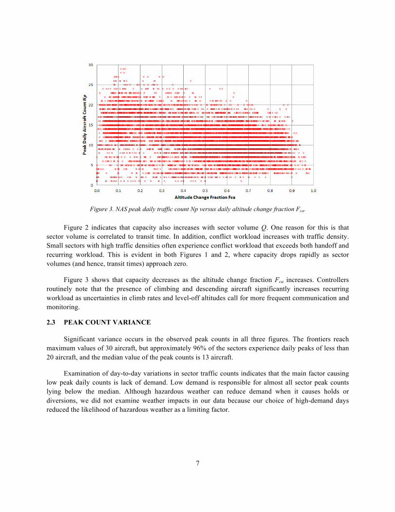
Figure 3. NAS peak daily traffic count Np versus daily altitude change fraction Fca.

Figure 2 indicates that capacity also increases with sector volume Q. One reason for this is that sector volume is correlated to transit time. In addition, conflict workload increases with traffic density. Small sectors with high traffic densities often experience conflict workload that exceeds both handoff and recurring workload. This is evident in both Figures 1 and 2, where capacity drops rapidly as sector volumes (and hence, transit times) approach zero.

Figure 3 shows that capacity decreases as the altitude change fraction Fca increases. Controllers routinely note that the presence of climbing and descending aircraft significantly increases recurring workload as uncertainties in climb rates and level-off altitudes call for more frequent communication and monitoring.

2.3 PEAK COUNT VARIANCE

Significant variance occurs in the observed peak counts in all three figures. The frontiers reach maximum values of 30 aircraft, but approximately 96% of the sectors experience daily peaks of less than 20 aircraft, and the median value of the peak counts is 13 aircraft.

Examination of day-to-day variations in sector traffic counts indicates that the main factor causing low peak daily counts is lack of demand. Low demand is responsible for almost all sector peak counts lying below the median. Although hazardous weather can reduce demand when it causes holds or diversions, we did not examine weather impacts in our data because our choice of high-demand days reduced the likelihood of hazardous weather as a limiting factor.

8

Any one of the model complexity attributes can cause low sector counts that may appear anomalous when analyzing the other complexity attributes. For example, small sector volumes or large fractions of ascending or descending flights can cause low traffic counts in sectors that might otherwise be expected to have high traffic because of their relatively long transit times.

Additional complexity attributes exist that can also increase workload and produce low peak counts. Numerous such attributes have been identified, but many are subtle and difficult to quantify [11–14]. The new model focuses on three easily measured complexity attributes that have quantifiable operational influences on workload.

2.4 BEST-CASE SENSE OF MODEL CAPACITY

Only about ten percent of the NAS sector-days in these plots contribute to the capacity frontiers. Consequentially, many of the individual model sector capacities determined from the frontiers must be considered as best-case or ideal capacities in that those sectors never operationally experience such high traffic counts.

Furthermore, peak counts are typically transient events that persist for at most a few minutes. Examination of count durations for all sectors in the New York Air Route Traffic Control Center on 1 July 2007 indicated that few peak daily counts exceeding 13 aircraft persisted for more than 2 minutes, and that higher peak counts tended to persist for shorter times (see Appendix F).

This means that the model capacity of any individual sector is the peak traffic count that could be expected in a sector of that size, transit time, and altitude change fraction only when manned by an experienced controller team under favorable conditions with short-term bursts of high traffic demand [15].

2.5 INFLUENCE OF MAP OPERATIONAL CONSTRAINTS ON OBSERVED PERFORMANCE

When air traffic managers use the MAP rule and its fixed upper limit to manage operational traffic, the MAP rule necessarily influences the NAS traffic count frontiers for many sectors. This means that the utility of these peak daily traffic observations as a capacity measure may be compromised by the MAP bound. However, three operational factors reduce the influence of this constraint. First, the MAP rule allows traffic managers considerable flexibility to adjust for local conditions. Secondly, larger sectors inherently tend to experience low traffic demand relative to capacity. Finally, because the MAP rule does not account for traffic density, it systematically over-estimates capacity in the smallest sectors, and thus does not actually constrain peak sector counts in sectors with short transit times.

9

3. THE FULL WORKLOAD MODEL

3.1 MODEL OVERVIEW

The model provides an analytical relationship between individual sector workload complexity attributes and the sector capacity. The model aggregates sector workload into three general task types: handoff (also designated as transit or coordination tasks), conflict, and recurring. The model quantifies these three workload components using the concept of workload intensity, which is the fraction of the sector controller time that is occupied with a given task type. Each of the three workload intensity components grows as a function of the instantaneous sector traffic count N. Each workload component is proportional to the product of the mean time required to service that type of task and the mean task rate. The proportionality factors are determined by fitting the model to sector peak traffic observations

The capacity of a sector is the instantaneous traffic count that causes the sum of its three workload intensity components to equal a defined maximum safe human workload intensity limit Gh. The solution of the resulting quadratic equation for N defines the model sector capacity Nm, which can be thought of as the maximum instantaneous aircraft count that an experienced controller team could safely handle in that sector.

3.2 HANDOFF WORKLOAD

Handoff or transit workload intensity Gt increases proportionally to the instantaneous sector traffic count N, and is inversely proportional to the mean transit time T of the traffic through the sector. Mean transit time naturally tends to increase with sector size, making handoff workload less significant in larger sectors, or in sector designs that are elongated in the major flow direction.

3.3 CONFLICT WORKLOAD

Conflict workload intensity Gc increases as the square of the traffic count. Conflict workload grows with traffic density and thus becomes more significant in small sectors, which are designed expressly to provide an organized means for allowing additional controllers to share the responsibility for traffic in dense airspace.

Conflict workload intensity is proportional to the product of two unknowns. The first is the mean of the closing speeds of the aircraft pairs in the sector that could pass each other with less than a defined safe miss distance. The second unknown is the conflict resolution service time per flight. The product of the two has the physical dimension of distance; its operational significance is the mean separation lost while resolving each conflict. This separation loss is the unknown conflict workload parameter that we directly determine by fitting the model to the observed traffic frontiers.

10

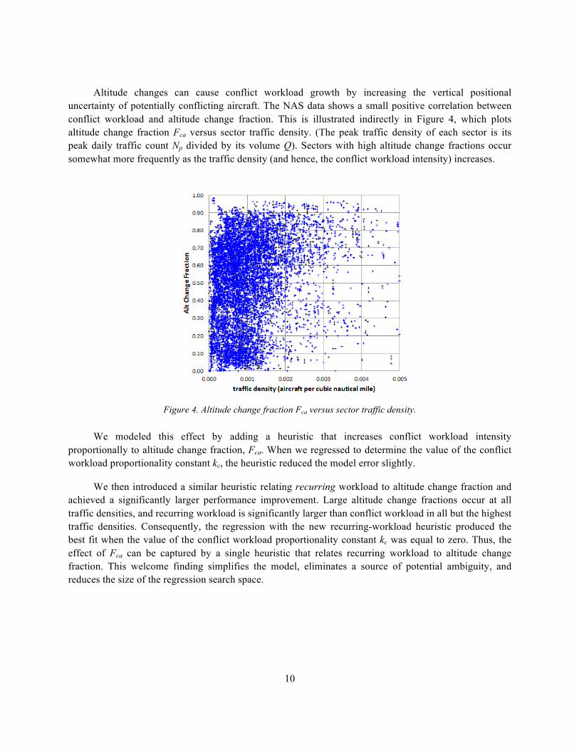
Altitude changes can cause conflict workload growth by increasing the vertical positional uncertainty of potentially conflicting aircraft. The NAS data shows a small positive correlation between conflict workload and altitude change fraction. This is illustrated indirectly in Figure 4, which plots altitude change fraction Fca versus sector traffic density. (The peak traffic density of each sector is its peak daily traffic count Np divided by its volume Q). Sectors with high altitude change fractions occur somewhat more frequently as the traffic density (and hence, the conflict workload intensity) increases.

Figure 4. Altitude change fraction Fca versus sector traffic density.

We modeled this effect by adding a heuristic that increases conflict workload intensity proportionally to altitude change fraction, Fca. When we regressed to determine the value of the conflict workload proportionality constant kc, the heuristic reduced the model error slightly.

We then introduced a similar heuristic relating recurring workload to altitude change fraction and achieved a significantly larger performance improvement. Large altitude change fractions occur at all traffic densities, and recurring workload is significantly larger than conflict workload in all but the highest traffic densities. Consequently, the regression with the new recurring-workload heuristic produced the best fit when the value of the conflict workload proportionality constant kc was equal to zero. Thus, the effect of Fca can be captured by a single heuristic that relates recurring workload to altitude change fraction. This welcome finding simplifies the model, eliminates a source of potential ambiguity, and reduces the size of the regression search space.

11

3.4 RECURRING WORKLOAD

Recurring workload and handoff workload both increase linearly with traffic count. However, unlike handoff workload, recurring workload is independent of transit time. Recurring workload differs from both handoff and conflict workload, in that it does not decrease as sectors grow larger. Recurring workload dominates and ultimately limits the peak traffic count of very large sectors. A complete capacity model must account for recurring workload. Otherwise, there would be no limit on the growth of capacity in sectors with long transit times and large volumes1.

As noted above, altitude changes cause significant recurring workload growth. The final model includes a heuristic that increases recurring workload intensity linearly with Fca. We determine the recurring workload proportionality constant kr by regression. The result indicates that, on average, recurring workload increases by 44% when all aircraft in a sector change altitude by more than 2000 ft.

3.5 HUMAN WORKLOAD INTENSITY LIMIT

The model also includes two constant workload intensity components. The first is background workload intensity Gb, which results from housekeeping tasks occurring at a constant average rate, independently of traffic count N. The second is the maximum safe human workload intensity limit Gh. The arithmetic difference between Gb and Gh is equal to the constant term c in the expression for the solution of the capacity quadratic equation.

The quadratic constant c cannot be determined uniquely by regression. For any value of c, a parameter combination exists that defines the least mean-error solution. If we change c and repeat the regression, the other parameters scale linearly to accommodate the change in c and return the identical mean error.

Thus, we must find values for the two constant workload intensities by means other than regression analysis of peak sector traffic counts. D.K. Schmidt reported direct observations of the workload limit for controllers handling simulated traffic [16]. The maximum workload limit Gh occurred when the controller team devoted approximately 80 percent of its available time to the control tasks. We use Gh = 0.8 in all model regressions.

Schmidt’s controller workload observations did not specify background workload intensity Gb. Background workload was likely included as part of the maximum human workload limit. Zero background workload is a reasonable hypothesis for a sector capacity model. As noted in Section 2.4 and Appendix F, sectors rarely experience peak demand for more than a few minutes. Therefore, housekeeping tasks can be deferred until the sector no longer operates near capacity. We set background

1 The MAP rule accounts for the absence of a recurring workload component by arbitrarily limiting the capacity of all sectors to 21 aircraft.

12

workload intensity Gb = 0 (or c = –0.8) in all model regressions. This is an important simplification because it eliminates a source of ambiguity and further reduces the size of the regression search space.

3.6 MODEL EQUATIONS

We define the capacity of a sector as the instantaneous traffic count that causes the sum of its four workload intensity components to reach a defined maximum safe human workload intensity limit. Appendix B summarizes the resulting set of equations for the full analytic model.

13

4. FITTING MODEL PARAMETERS TO THE TRAFFIC DATA

4.1 REGRESSION OBJECTIVE FUNCTION AND PERCENTILE CONSTRAINT

We complete the model by finding the combination of unknown numerical model parameters that gives the best fit between the model capacities for the NAS sectors and the observed peak-count data frontiers for those sectors. We use mean error as the regression score (objective function) in this regression process. The best fit is the set of parameter values that minimizes the mean error between the model capacity and the observed peak traffic count for each sector-day.

The fit is subject to a further constraint that 95 percent of the model capacities must exceed their corresponding peak counts. A fixed high percentile constraint serves three essential functions in the capacity regression process.

• It forces the model to conform to the peak count frontier, and counters the tendency of the many low peak counts to bias the capacity downwards. This is important because approximately half of all peak daily sector counts are well below their inherent sector capacities because of lack of demand.

• It makes it possible to use mean error as the objective function in the regression. Minimizing mean error without a percentile constraint would result in zero mean error, with the model defining the median of the count distribution rather than the capacity frontier. Mean error is precisely defined, involves no arbitrary cost factors, and is trivial to compute.

• It defines and guarantees the existence of a minimum mean error with no percentile bias. Mean error tends to decrease as the percentile drops. Solutions with percentiles less than 95 can have mean errors as small as zero. However, the solutions with the least mean error among those with percentiles greater than or equal to the chosen percentile are optimum. (Note that a high percentile constraint does not guarantee a unique optimum if the search parameters take on continuous values.)

Although the mean error definition involves no arbitrary cost factors, the high percentile constraint is essentially arbitrary. It is conventional practice to use a 95-percentile constraint because it closely approximates the two-sigma value of a normal distribution and produces a good visual fit to a data frontier2.

2 For comparison, the nominal version of the current operational MAP rule results in an 88-percentile fit to the NAS data set. The upper limit version of the MAP rule, which increases all capacities by 3 aircraft, gives a 97-percentile fit.

14

We examined regression results using 93-percentile and 97-percentile constraints. Changing the specified percentile changes the solution parameters, and increasing the specified percentile increases the mean error. However, conclusions regarding model performance and relative workload intensity magnitudes did not change when we changed the percentile constraint.

4.2 DATA OUTLIERS

As noted in Section 2.1, the FAA’s Sector Design and Analysis Tool traffic data includes a few sector-days with unusually high peak traffic counts. Consequently, the error distribution has significant negative outliers. Their high peak counts indicate that these sectors are not operating as ordinary en route sectors. To prevent them from biasing the mean error and percentile calculations, we condense the data by removing each sector-day whose peak traffic count exceeds its full model capacity by more than four aircraft. When examining the performance of the MAP model or the reduced versions of the model, we compare each model’s capacity predictions against the same condensed data set used to fit the full model.

At the other end of the error distribution, many sectors have very low peak counts, presumably for lack of demand. Because we have insufficient information about these sectors to identify the true causes of the low counts, we include all low-count sectors in our regressions and in our calculations of mean error and percentile. This avoids an arbitrary bias in these calculations.

4.3 THE SEARCH PROCESS

The new model has more unknown search parameters than required to fit the data. Excess degrees of freedom produce an infinite number of regression solutions with identical fitness scores if the search parameters take on continuous values. The standard means for avoiding this is to discretize the unknowns. We accomplish this by quantizing and scaling the unknowns so that the search parameters take on integer values that can serve as indices in for-loops. The search then returns a large number of unique3 solutions that fit the data with low mean error. The solution with the least mean error is closest to the true optimum.

The parameter quantization resolution determines the number of local optima and the size of the search space. The quantization can be adjusted to trade solution accuracy against search time in exhaustive searches. The simple analytic model combines with the 95-percentile constraint and the mean-error objective function to make it practical to discretize the parameters with sufficient resolution to allow exhaustive searches through millions of parameter combinations.

The full model includes four unknowns. When we assign forty integer search values to each unknown, we produce 2,560,000 combinations. This large search space combines with the thousands of

3Each combination of discretized parameters is unique. The computations of capacity and mean error return irrational numbers because sector capacity involves the square root of a non-integer real number. The unlimited resolution of irrational numbers guarantees that each mean error is unique.

15

sector-days in the traffic database to produce numerous solutions that satisfy the percentile constraint with mean errors close to that of the optimum. The search returned thirty-eight additional solutions with mean errors within one percent of the minimum error of 5.86898 aircraft4. We examined these solutions to assure that they do not provide conflicting results. T lie zation heir parameters mostly within a few quantisteps of the optimum and dividual , they all predict nearly identical system-wide workload averages and insector capacities .

, although there is no selection ambiguity because no higher percentile We thus conclude thatsolution with lower mean error than the optimum exists within the search space, any of the near-optimum solutions could relative be used with confidence when analyzing the benefits of proposed air traffic

for reducing individual workload typesdecision-support initiatives .

4 The percentile of the optimum solution is 95.0235.

17

5. PERFORMANCE OF THE FULL MODEL

5.1 FITTED PARAMETER VALUES

The new model employs three variable workload types and three sector complexity attributes to find four unknown parameters that best fit the model sector capacities to the peak sector counts in the NAS database. The fitting process returns the following numerical values:

τt = 3.2 seconds, dc = 1.9 nautical miles, tr = 17 seconds, and kr = 0.44. (1)

Each of these parameter values has a unique operational significance.

• The 3.2-second service time τt is the average time per aircraft spent by the controller team handling each pair of inter-sector handoffs as flights transit each sector. The mean transit time of the NAS sectors is Tm = 872 seconds, and the mean model capacity is Nm = 17 aircraft. When the average NAS sector operates at capacity, its controller team devotes a fraction Nm τt /Tm = 0.062 of that transit time to handoffs. Handoffs are not a major source of workload in the average sector; and, by definition, transit workload becomes less signicant as sector transit times increase. Section 5.3 examines the impact of sector volume and aircraft count on transit workload in smaller sectors.

• The 1.9-nautical mile NAS conflict parameter dc is the mean loss of separation that occurs while each conflict is serviced. This separation loss is 27% of the nominal 7-nautical mile horizontal miss distance threshold that defines the conflict resolution airspace volume in the full model. The model contributes to our understanding of NAS airspace conflicts by allowing us to directly infer mean sector conflict rates from peak traffic data.

• The regression returns a 17-second NAS mean recurring service time tr per aircraft. This value is based on an arbitrary assumption in the model of a nominal NAS mean recurring service period of P = 600 seconds. Taken together, these numbers tell us that the controller team in a NAS sector with no ascending or descending aircraft devotes tr/P = 0.028 of its available time per aircraft to recurring tasks. The controllers in a sector handling 17 aircraft at cruise altitude devote 0.482 of their time to recurring tasks. This is approximately eight times larger than the time devoted to handoff tasks in the NAS average sector operating at capacity. Recurring workload becomes even more significant relative to handoff workload in larger sectors as capacity increases and handoff workload decreases.

• The parameter kr is the proportionality constant in the heuristic function that relates recurring workload intensity to sector altitude rate fraction Fca. It tells us that, relative to a sector with constant altitude aircraft (Fca = 0), recurring workload increases by 44% when all aircraft in the sector change altitude by more than 2000 ft. (Fca = 1). An alternative metric defining the effect

18

of kr is the maximum effective value of tr that results when Fca = 1. We refer to this as trmax. It has a value of 24.48 seconds, and further increases the dominance of recurring workload.

5.2 COMPARISON OF FULL MODEL CAPACITIES AND PEAK COUNTS

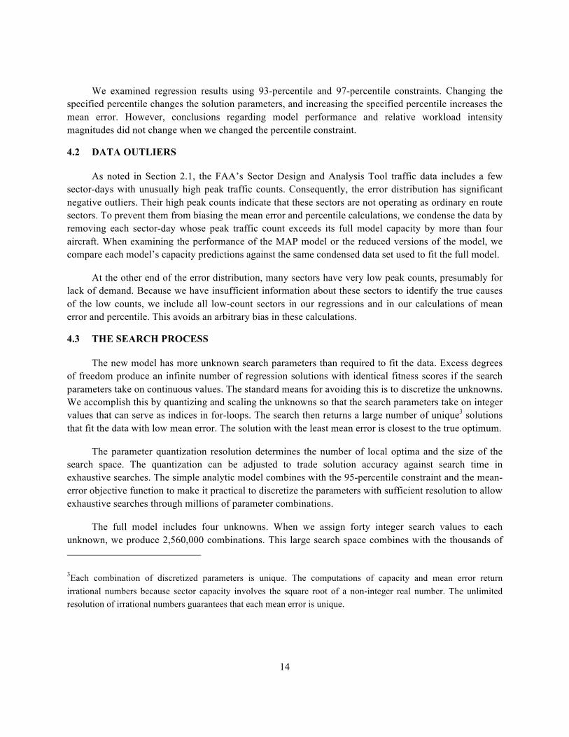
Figure 5 shows the NAS peak daily count as a function of the full four-parameter model capacity. The frontier relationship is approximately linear except for a gap in sectors with model capacities between seven and nine aircraft. The largest recorded NAS sector count of 28 aircraft occurred on two sector-days, and the corresponding model capacities were 24.45 and 24.93. The peak model capacity of 25.91 aircraft also occurred on two sector-days, and the corresponding peak counts were 2 and 7 aircraft.

Figure 5. NAS peak daily count versus full model capacity.

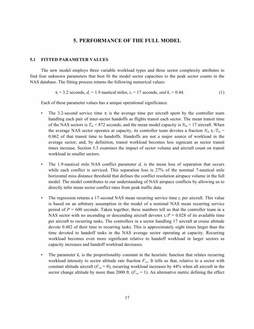
Figure 6 is a two-dimensional histogram of the data shown in Figure 5 with all model capacities rounded to the nearest integer. It shows the number of instances of each combination of recorded peak count and capacity. The fit is extended and linear with nearly uniform counts along the frontier. The most common combination is a model capacity of 15 aircraft and a peak count of 10. This combination occurred on 122 sector-days.

19

Figure 6. Two-dimensional histogram of peak daily count and full model capacity.

Figure 7 plots model capacity and peak daily count versus transit time T for the full four-parameter model. This figure shows a significant variance in model capacity caused by sector-to-sector differences in sector volume and altitude change fraction. The variance is largest for sectors with transit times near 1200 seconds (20 minutes). A few sector-days with very short transit times, moderate peak aircraft counts, large airspace volumes, and no aircraft with altitude changes (Fca = 0) stand out with distinct capacity profiles in this plot. These systematic results all derive from two large oceanic sectors, ZMA30 and ZMA31 in the Miami Center. Aircraft pass through these sectors with relatively short transit times. Most of the other sectors with transit times less than 600 seconds have larger fractions of aircraft with altitude changes, a fact that results in a separate grouping with lower model capacities. Similar altitude change dichotomies create a slightly bifurcated distribution of model capacities for sectors with transit times exceeding 1200 seconds.

Figures 8 and 9 are similar plots versus, respectively, sector volume Q and altitude change fraction Fca. These figures also show significant variance in model capacity. The variance in Figure 8 is caused by sector-to-sector differences in altitude change fraction and transit time. Figure 8 shows a pronounced, systematic reduction in model variance as sector volume approaches zero and conflict workload increasingly dominates transit and recurring workload. Figure 9 shows a reduction in model capacity that fits the reduction in observed peak traffic count as altitude change fraction increases. The variance in Figure 9 is caused by sector-to-sector differences in transit time and sector volume. The magnitude of the variance is relatively insensitive to altitude change fraction.

20

Figure 7. Full model capacity and peak daily count versus transit time T.

Figure 8. Full model capacity and peak daily count versus volume Q.

21

Figure 9. Full model capacity and peak daily count versus Fca.

5.3 GROWTH OF WORKLOAD INTENSITY COMPONENTS WITH TRAFFIC

Figure 10 plots the three model workload intensity components vs. aircraft count N.

Figure 10. Full model NAS mean workload intensity components vs. aircraft count N.

22

The figure also shows the background workload intensity, which is zero. The workload intensities are averaged over all NAS sectors. The model capacity of the average NAS sector (17.47 aircraft) is the traffic level at which the total workload intensity G reaches the Gh = 0.8 human workload limit. Conflict workload is less than transit workload when traffic is light. However conflict workload grows quadratically and exceeds transit workload when the traffic count reaches 11 aircraft. Recurring workload dominates at all traffic counts; it is still roughly five times larger than either conflict or transit workload at capacity.

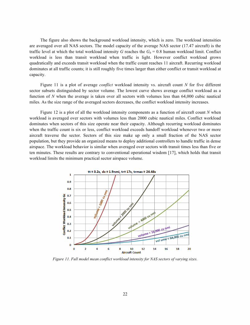
Figure 11 is a plot of average conflict workload intensity vs. aircraft count N for five different sector subsets distinguished by sector volume. The lowest curve shows average conflict workload as a function of N when the average is taken over all sectors with volumes less than 64,000 cubic nautical miles. As the size range of the averaged sectors decreases, the conflict workload intensity increases.

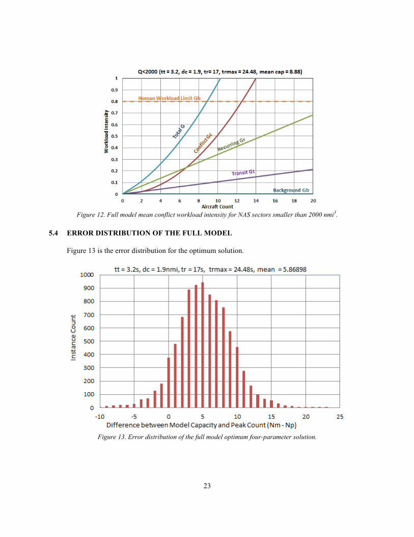
Figure 12 is a plot of all the workload intensity components as a function of aircraft count N when workload is averaged over sectors with volumes less than 2000 cubic nautical miles. Conflict workload dominates when sectors of this size operate near their capacity. Although recurring workload dominates when the traffic count is six or less, conflict workload exceeds handoff workload whenever two or more aircraft traverse the sector. Sectors of this size make up only a small fraction of the NAS sector population, but they provide an organized means to deploy additional controllers to handle traffic in dense airspace. The workload behavior is similar when averaged over sectors with transit times less than five or ten minutes. These results are contrary to conventional operational wisdom [17], which holds that transit workload limits the minimum practical sector airspace volume.

Figure 11. Full model mean conflict workload intensity for NAS sectors of varying sizes.

23

Figure 12. Full model mean conflict workload intensity for NAS sectors smaller than 2000 nmi3.

5.4 ERROR DISTRIBUTION OF THE FULL MODEL

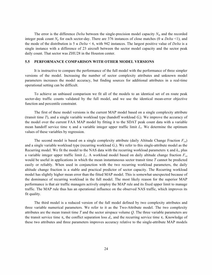
Figure 13 is the error distribution for the optimum solution.

Figure 13. Error distribution of the full model optimum four-parameter solution.

24

The error is the difference Delta between the single-precision model capacity Nm and the recorded integer peak count Np for each sector-day. There are 376 instances of close matches (0 ≤ Delta <1), and the mode of the distribution is 5 ≤ Delta < 6, with 942 instances. The largest positive value of Delta is a single instance with a difference of 23 aircraft between the sector model capacity and the sector peak daily count. That sector was ZHU28 in the Houston center.

5.5 PERFORMANCE COMPARISON WITH OTHER MODEL VERSIONS

It is instructive to compare the performance of the full model with the performance of three simpler versions of the model. Increasing the number of sector complexity attributes and unknown model parameters increases the model accuracy, but finding sources for additional attributes in a real-time operational setting can be difficult.

To achieve an unbiased comparison we fit all of the models to an identical set of en route peak sector-day traffic counts validated by the full model, and we use the identical mean-error objective function and percentile constraint.

The first of these model versions is the current MAP model based on a single complexity attribute (transit time T), and a single variable workload type (handoff workload Gt). We improve the accuracy of the model over the current FAA MAP model by fitting it to the SDAT peak count data with a variable mean handoff service time τt and a variable integer upper traffic limit Lt. We determine the optimum values of these variables by regression.

The second model is based on a single complexity attribute (daily Altitude Change Fraction Fca) and a single variable workload type (recurring workload Gr). We refer to this single-attribute model as the Recurring model. We fit the model to the NAS data with the recurring workload parameters τt and kr, plus a variable integer upper traffic limit Lr. A workload model based on daily altitude change fraction Fca would be useful in applications in which the mean instantaneous sector transit time T cannot be predicted easily or reliably. When used in conjunction with the two recurring workload parameters, the daily altitude change fraction is a stable and practical predictor of sector capacity. The Recurring workload model has slightly higher mean error than the fitted MAP model. This is somewhat unexpected because of the dominance of recurring workload in the full model. The most likely reason for the superior MAP performance is that air traffic managers actively employ the MAP rule and its fixed upper limit to manage traffic. The MAP rule thus has an operational influence on the observed NAS traffic, which improves its fit quality.

The third model is a reduced version of the full model defined by two complexity attributes and three variable numerical parameters. We refer to it as the Two-Attribute model. The two complexity attributes are the mean transit time T and the sector airspace volume Q. The three variable parameters are the transit service time τt, the conflict separation loss dc, and the recurring service time τr. Knowledge of these two attributes and three parameters improves accuracy relative to the single-attribute MAP models

25

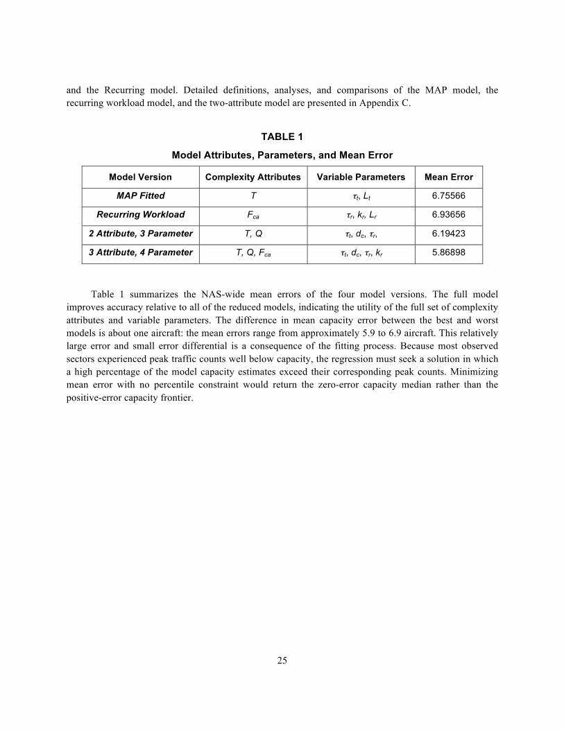
and the Recurring model. Detailed definitions, analyses, and comparisons of the MAP model, the recurring workload model, and the two-attribute model are presented in Appendix C.

TABLE 1

Model Attributes, Parameters, and Mean Error

Model Version Complexity Attributes Variable Parameters Mean Error

MAP Fitted T τt, Lt 6.75566

Recurring Workload Fca τr, kr, Lr 6.93656

2 Attribute, 3 Parameter T, Q τt, dc, τr, 6.19423

3 Attribute, 4 Parameter T, Q, Fca τt, dc, τr, kr 5.86898

Table 1 summarizes the NAS-wide mean errors of the four model versions. The full model improves accuracy relative to all of the reduced models, indicating the utility of the full set of complexity attributes and variable parameters. The difference in mean capacity error between the best and worst models is about one aircraft: the mean errors range from approximately 5.9 to 6.9 aircraft. This relatively large error and small error differential is a consequence of the fitting process. Because most observed sectors experienced peak traffic counts well below capacity, the regression must seek a solution in which a high percentage of the model capacity estimates exceed their corresponding peak counts. Minimizing mean error with no percentile constraint would return the zero-error capacity median rather than the positive-error capacity frontier.

27

6. BENEFITS ANALYSIS

6.1 THE BENEFITS ANALYSIS PROBLEM

A major focus of this research was to examine the use of the model for guidance in benefits studies that analyze programs to reduce controller workload of various types. This guidance could be ambiguous if the regression returned multiple solutions that fit the NAS traffic with nearly the same mean error but with significantly different parameter combinations.

Multiple solutions are unavoidable. The density of local solutions depends on the regression parameter quantization. Our particular quantization choices returned eight solutions with mean errors within one-half percent of the optimum and thirty-eight solutions within one percent. Appendix D analyzes these local solutions in detail.

All thirty-eight solutions in the large set predict a NAS mean capacity nearly identical to that of the optimum. They all agree that NAS mean conflict workload and handoff workload are consistently small relative to recurring workload. The two solutions whose mean transit service time parameters are farthest apart disagree significantly on capacities of individual sectors with short transit times. However, their predictions have no operational relevance because they both have mean errors nearly one percent larger than the optimum, and more than thirty 95-percentile solutions with smaller mean errors lie between them and the optimum.

The eight solutions within one-half percent agree with the optimum solution on the relative importance of NAS-wide handoff and conflict workload. All eight agree on most individual sector capacities to within one aircraft count. The key finding is that the two solutions closest to the optimum agree with the optimum on all key metrics.

29

7. GENERAL CONCLUSIONS

7.1 SUMMARY OF RESULTS

The full model has a mechanism relating sector workload to flight altitude changes. Although this mechanism decreases NAS-wide mean capacity errors, it introduces excess degrees of freedom that allow multiple regression solutions. When analyzing benefits, multiple solutions can compromise the model’s ability to distinguish between different workload types. An important goal of this work has been to identify a unique regression solution with a set of optimum model parameters that accurately fits observed traffic peaks and reliably distinguishes between the three key workload intensity components.

We have accomplished this goal by means of

a. an integer optimization process with quantized variables to – avoid an infinite number of solutions and – allow exhaustive searches;

b. a mean-error objective function with no arbitrary cost factors; and

c. a 95-percentile constraint to – automatically fit NAS peak traffic frontiers and – avoid mean-error calculation bias.

These regression techniques return a unique 95-percentile minimum-error solution along with a few distinct near-optimum local solutions that are almost identical in all important capacity metrics. The regression also returns numerous 95-percentile solutions with higher mean errors. Solutions with higher errors create larger disagreements, but they do not cause ambiguity. The key finding is a total absence of close solutions that fit the NAS traffic with near-optimum mean error, but with parameter differences that cause disagreement in significant capacity metrics.

Compared to the current MAP model, the full model provides more accurate sector capacity predictions and also individual workload intensity estimates that are inherently unavailable from a model based on a single workload type. We conclude that the full workload model can be used with confidence to guide NAS-wide benefits studies.

7.2 CONCLUSIONS REGARDING AUTOMATION BENEFITS

The full model provides important insight into the relative importance of the three workload types. The regression results show that, on a NAS-wide basis, mean recurring workload dominates at all traffic levels. At the individual sector level, recurring workload dominates sectors of average size and eventually becomes the sole workload component as sector volume increases. Recurring workload is also significant

30

in very small sectors. Although conflict workload dominates when small sectors operate near capacity, recurring workload dominates at all lower traffic levels. Handoff workload typically accounts for less than 10% of total workload in most sectors operating at capacity.

The Monitor Alert model ignores recurring and conflict workload and implies that handoff workload limits capacity in all sectors. The Monitor Alert model has no alternative explanation for observed peak sector counts other than an over-estimated handoff service time. As a consequence, it misleadingly suggests large potential capacity gains from automating handoffs.

The full model indicates that recurring tasks are the best candidates for decision-support automation. The system-wide dominance of recurring workload suggests a large potential for improving capacity by partially automating recurring tasks. Furthermore, the stability of the altitude change fraction as a sector attribute and the relative freedom of recurring tasks from inter-sector coordination would reduce their operational complexity.

Recurring workload intensity Gr does not decrease as the sector grows in volume. As a result, recurring workload becomes more dominant and ultimately limits the peak traffic count of large sectors. The dominance of recurring workload may explain why progress in automating handoffs has been slow. Little would be gained by automating handoffs in good weather because inter-sector coordination is relatively straightforward, particularly in the majority of sectors whose capacities exceed demand by safe margins. In hazardous weather, handoffs become more difficult to automate.

7.3 CONCLUSIONS REGARDING WORKLOAD AND TUBE-SHAPED SECTORS

The full model allows us to estimate the capacity of long tubular sectors between airport pairs. Tubular sectors have often been proposed for organizing and managing aircraft flow [18, 19]. In the limit, when the sector length and volume are very large, handoff workload and conflict workload become negligible and only recurring workload remains.

The maximum capacity of a tube-shape sector occurs when the aircraft count grows such that the product of recurring workload intensity per aircraft and aircraft count reaches the human workload intensity limit. The full model indicates that the current NAS mean recurring workload intensity per aircraft is 0.0283 (when all sector aircraft are cruising at constant altitude). Our standard estimate for the safe human workload intensity limit is eighty percent of the available time of the controller team. Thus the maximum capacity of a long tubular sector with constant-altitude flights, manual control, and current NAS procedures is 0.8 / 0.0283 = 28.2 aircraft. This is more than 50% larger than the current nominal MAP capacity limit of 18 aircraft. Automation aids to help monitor flights in the sector could reduce the recurring workload and further increase the capacity of such a sector.

31

APPENDIX A MODEL TERMINOLOGY

This appendix details the distinctions between sector workload types, sector workload complexity attributes and unknown model parameters.

WORKLOAD TYPES

The three traffic-dependent sector workload intensity types are

a. transit (or handoff) workload intensity Gt,

b. conflict workload intensity Gc, and

c. recurring workload intensity Gr.

Any workload model must also account for two constant, traffic-independent workload intensities. These are

d. background workload intensity Gb and

e. the human workload intensity limit Gh.

The human workload limit is the maximum workload intensity that the controller team finds it safe to handle. The arithmetic difference between the two constant workload intensity components is equal to the constant term c in the customary quadratic equation for capacity. We note in Section 3.5 that the constant c cannot be uniquely determined by fitting the model to observed sector traffic. Therefore, the two constant workload intensities must be estimated by observations of controller performance. As noted in Section 3.5, controllers handling simulated traffic tend to reach the maximum human workload limit Gh when devoting approximately 80 percent of their available time to the control tasks. We thus use Gh = 0.8 in all model regressions.

Zero background workload is the most reasonable hypothesis for any sector capacity model. Even the busiest sectors experience low demand most of the time (see Appendix F). Therefore, housekeeping tasks that cannot be delegated can be deferred until the sector is no longer operating near capacity. We therefore set background workload intensity Gb = 0 in all model regressions.

MEASUREABLE SECTOR WORKLOAD COMPLEXITY ATTRIBUTES

Many sector workload complexity attributes have been identified [20]. It is difficult to obtain operational data to quantify most of these attributes. We limit the full model to three measureable

32

attributes for which operational data is available. These attributes also have well-defined analytical relationships to workload intensity. These are:

a. the mean transit time T for the aircraft in the sector at the time of the peak count,

b. the sector airspace volume Q at the time of the peak count, and

c. the daily fraction Fca of sector aircraft with altitude changes greater than 2000 ft. (we call this the “altitude change fraction”).

UNKNOWN MODEL PARAMETERS

The analytical relationships in the model introduce unknown model parameters that must be quantified by fitting to operational data. Additional numerical parameters can produce a more accurate fit, but at the cost of additional potential ambiguity. A total of five unknown parameters have been examined in the full model. These are:

a. the mean transit service time τt,

b. the mean conflict separation loss dc, which is the product of the mean conflict service time and the mean conflict closing speed,

c. the mean recurring service time τr,

d. a proportionality constant kr, relating growth in recurring workload to Fca, and

e. a proportionality constant kc, relating growth in conflict workload to Fca.

The first four of these parameters are determined by regression. As noted in Section 3.3, the fifth parameter (proportionality constant kc) has been found to consistently regress to zero in NAS-wide regressions. We thus routinely speed up these regressions by omitting kc. However, it is advisable to retain kc when regressing against other traffic data.

33

APPENDIX B FULL MODEL EQUATIONS

As noted in Appendix A, sector workload can be aggregated into four general task types: handoff (or transit), conflict, recurring, and background. We quantify these four aggregated workload components using the concept of workload intensity, which is the fraction of the sector controller time that is occupied with a given task type.

Transit workload is associated with sector handoffs. Transit workload intensity Gt increases proportionally to the instantaneous sector traffic count N, and is inversely proportional to the mean transit time T of the traffic through the sector. Mean transit time tends to increase with sector size, making handoff workload less significant in large sectors.

Conflict workload occurs when the controller team perceives a potential loss of separation. Conflict workload intensity Gc increases as the square of the traffic count. Conflict workload grows with traffic density, which is the ratio of sector traffic count N to sector volume Q. Conflict workload thus becomes more significant in small sectors, which are designed expressly to provide an organized means for allowing additional controllers to share traffic in dense airspace. Altitude changes can also cause conflict workload growth by increasing the vertical positional uncertainty of potentially conflicting aircraft. We capture this effect by introducing a heuristic that increases conflict workload intensity proportionally to Fca. We determine the proportionality constant by regression.

Recurring workload results from periodic activities such as surveillance monitoring, vectoring, metering, and spacing. Recurring workload intensity Gr increases linearly with traffic count. However, unlike handoff workload, recurring workload is independent of transit time. Thus, recurring workload continues to grow as sectors increase in volume and it dominates large sectors that operate near capacity. Altitude changes cause additional recurring workload for the controller team. Accordingly, we introduce a heuristic similar to that used for conflict workload to increase recurring workload intensity proportionally to Fca.

We include a background workload intensity component Gb to quantify tasks that occur at a constant rate, independent of traffic count.

We define the capacity of a sector as the instantaneous traffic count Nm that causes the sum of its four workload intensity components to reach a defined maximum safe human workload intensity limit Gh.

Thus, the workload intensity equation that determines Nm is:

Gb + Gt + Gc + Gr = Gh. (B-1) The solution of the resulting quadratic equation for N defines the model sector capacity Nm.

34

The arithmetic difference between Gb and Gh is equal to the constant term customarily identified as “c” in the expression for the solution of a quadratic equation. As noted in Section 3.5, observations of controllers handling simulated traffic show that the maximum human workload limit Gh occurs when the controller team is devoting approximately 80 percent of its available time to the control tasks, and zero background workload is the most reasonable hypothesis for a sector capacity model. We therefore use Gh = 0.8, Gb = 0, and thus the quadratic constant c = –0.8 in all model regressions.

Each of the three variable workload intensity components is the product of the mean time required to service that type of task and the mean task rate.

We noted above in Section 2.5 that the handoff (transit) workload intensity is:

Gt = N(τt /T). (B-2) The mean handoff service time τt is one of the unknown model parameters that we determine by

fitting to observed traffic.

We have shown [21] that the conflict workload intensity is:

Gc = N(N+1)B/Q, (B-3) where

B = 2τcV12MhMv(1 + 0.2kcFca). (B-4) The factors Mh and Mv are the horizontal and vertical miss distances (nominally 7 miles and 1000

ft., respectively) that constitute a separation violation. The term V12 is the mean of the pair-wise closing speeds of the aircraft in the sector that could pass closer than the defined miss distances, and τc is the conflict resolution task service time per flight. Both of these terms are unknown. Operationally, their product τcV12 is the mean separation lost while resolving each conflict. We refer to the product τcV12 as dc, and we determine its value by fitting to observed traffic.

The final factor in parentheses in Eq. B-4 is a heuristic function that increases conflict workload intensity proportionally to Fca. The proportionality constant kc is one of the unknown parameters in the model that we determine by fitting to observed traffic. We multiply kc by a factor of 5 to provide discrete integer values in the search process. The factor 0.2 reverses the integer scaling.

The recurring workload intensity is:

Gr = NR, (B-5) where R is the recurring workload intensity per aircraft

R = (τr/Pr)(1 + 0.04krFca). (B-6) Here τr is the recurring task controller service time per flight. The quotient τr/Pr is another of the

unknown model parameters that we determine by regression. We arbitrarily set the mean task recurrence period Pr to 600 seconds and determine the value of τr when searching for a fit to the observed traffic

35

data. The factor in the final parentheses in R is a heuristic analogous to the one we use for conflict workload. Recurring service time τr increases linearly with Fca. A scaling factor of 25 allows us to step through integer values of kr in the search process.

Figure B-1 illustrates the resulting relationship between mean recurring service time τr and altitude change fraction Fca for the optimum solution situation in which τr = 17 seconds and kr = 0.44 (that is, the integer search value of kr is 11). When Fca = 0, the mean recurring service time per aircraft is 17 seconds. When Fca = 1, the mean recurring service time increases to 17(1 + 0.44) seconds = 24.48 seconds.

Figure B-1. Mean recurring service time τr versus altitude change fraction Fca.

Solving the quadratic equation (A-1) and supplying the physical constants gives us the following familiar quadratic solution for sector capacity:

𝑁𝑚 =−𝑏 + 𝑏! − 4𝑎𝑐

2𝑎 (B-7)

where

𝑎 = 𝐵/𝑄, (B-8)

𝑏 = !!!+ 𝑅 + 𝑎, (B-9)

and

𝑐 = 𝐺! − 𝐺!. (B-10)

τ rmin = 17 s τ rmax =24.48 s

37

APPENDIX C MODEL PERFORMANCE COMPARISONS

This appendix examines the performance of several versions of the model, ordered by increasing numbers of complexity attributes and unknown model parameters. More attributes and parameters result in higher model accuracy, but at the expense of increased model complexity. It is instructive to compare these results with the performance of the full model.

The first model that we examine is the current MAP model based on a single complexity attribute (transit time T) and a single variable workload type (handoff workload Gt). We begin by reviewing two versions of the MAP model using current operational parameter values. We then perform a regression to determine the values of those parameters that best fit our NAS database.

The second model is a Recurring workload model based on a single complexity attribute (altitude change fraction Fca) and a single variable workload type (recurring workload Gr). The third is a version of the full model defined by two complexity attributes and three variable numerical parameters. The two complexity attributes are the mean transit time T and the sector airspace volume Q. The three variable parameters are the transit service time τt, the conflict separation loss dc, and the recurring service time τr.

We base all of these models on the full model workload equations as presented in Appendix B. All the models use the same values for background workload intensity (Gb = 0) and human workload limit (Gh = 0.8). All mean error calculations are based on the identical set of condensed NAS en route sector data defined by the full model. All regressions use mean error as the objective function and all are subject to the same 95-percentile constraint.

MONITOR ALERT PARAMETER RULE

The MAP rule is a piecewise linear version of the sector capacity model defined by a single complexity attribute, the sector transit time T. The rule specifies an approximately linear increase in sector capacity with transit time followed by a constant sector traffic limit. It can be reduced to two numerical parameters: the slope of the linear segment and the constant traffic limit L. The slope of the linear segment is related to the mean transit service time τt.

We noted in Section 3.2 that the handoff (transit) workload intensity is:

Gt = N(τt /T), (C-1) Where the mean handoff service time τt is determined by fitting to observed traffic.

The workload intensity equation that determines the capacity Nm is thus:

38

Gb + N(τt /T) = Gh,, (C-2)

where the maximum safe human workload intensity limit Gh is unknown, as is the traffic-independent workload intensity, Gb. When we set Gb = 0 and Gh = 0.8, the solution of the resulting equation for Nm defines the model sector capacity:

Nm(τt /T)= 0.8 (C-3)

Given observed operational ratios of Nm/T, we can solve for τt :

τt = 0.8T/Νm (C-4) The current FAA operational MAP rule http://www.faa.gov/air_traffic/publications/atpubs/fac/

1708.html is based on sector traffic observations that define the allowed ratio of Nm to T.

The MAP rule specifies baseline capacity values as shown in Table C-1. These baseline values may be adjusted by counts of +/–3 aircraft.

Table C-1

MAP Baseline Capacity Values

Average Sector Flight Time MAP Value

3 min. 5

4 min. 7

5 min. 8

6 min. 10

7 min. 12

8 min. 13

9 min. 15

10 min. 17

11 min. 18

12 min. or more 18

This table employs integer increments for minutes of transit time and for aircraft counts. It thus does not define a unique capacity/transit-time ratio. We linearize the table and use its most conservative

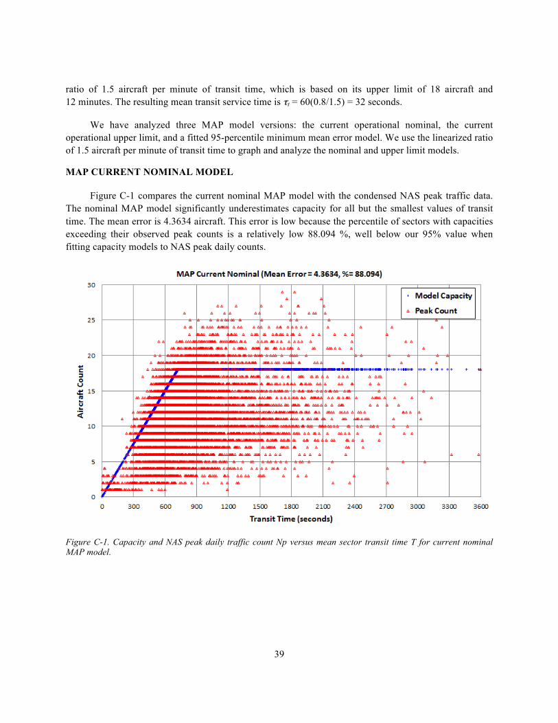
39

ratio of 1.5 aircraft per minute of transit time, which is based on its upper limit of 18 aircraft and 12 minutes. The resulting mean transit service time is τt = 60(0.8/1.5) = 32 seconds.

We have analyzed three MAP model versions: the current operational nominal, the current operational upper limit, and a fitted 95-percentile minimum mean error model. We use the linearized ratio of 1.5 aircraft per minute of transit time to graph and analyze the nominal and upper limit models.

MAP CURRENT NOMINAL MODEL

Figure C-1 compares the current nominal MAP model with the condensed NAS peak traffic data. The nominal MAP model significantly underestimates capacity for all but the smallest values of transit time. The mean error is 4.3634 aircraft. This error is low because the percentile of sectors with capacities exceeding their observed peak counts is a relatively low 88.094 %, well below our 95% value when fitting capacity models to NAS peak daily counts.

Figure C-1. Capacity and NAS peak daily traffic count Np versus mean sector transit time T for current nominal MAP model.

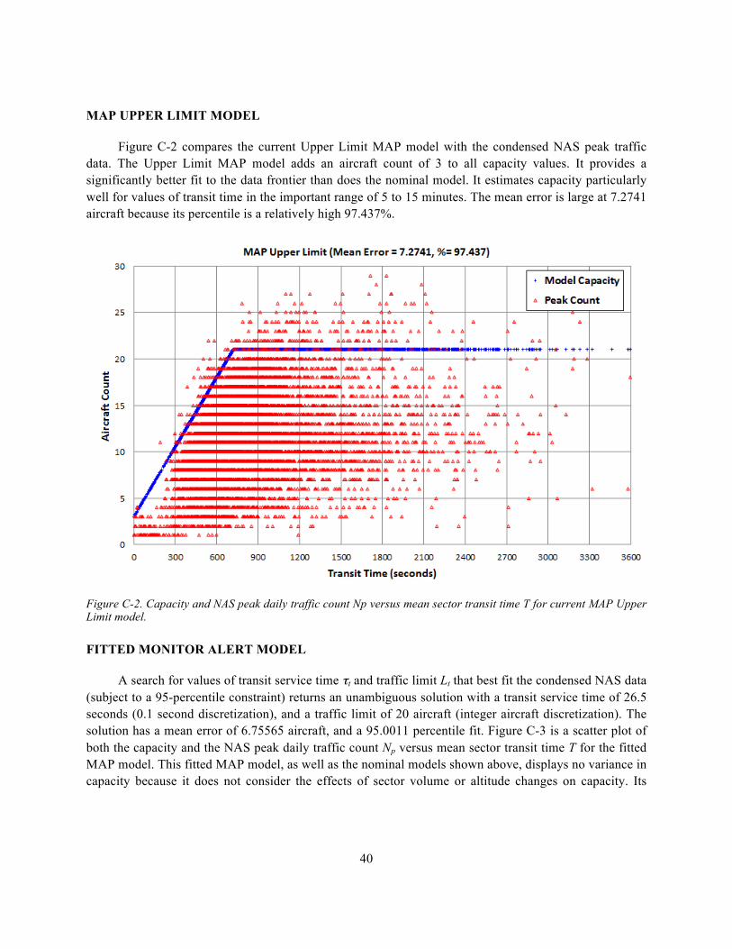
40

MAP UPPER LIMIT MODEL

Figure C-2 compares the current Upper Limit MAP model with the condensed NAS peak traffic data. The Upper Limit MAP model adds an aircraft count of 3 to all capacity values. It provides a significantly better fit to the data frontier than does the nominal model. It estimates capacity particularly well for values of transit time in the important range of 5 to 15 minutes. The mean error is large at 7.2741 aircraft because its percentile is a relatively high 97.437%.

Figure C-2. Capacity and NAS peak daily traffic count Np versus mean sector transit time T for current MAP Upper Limit model.

FITTED MONITOR ALERT MODEL

A search for values of transit service time τt and traffic limit Lt that best fit the condensed NAS data (subject to a 95-percentile constraint) returns an unambiguous solution with a transit service time of 26.5 seconds (0.1 second discretization), and a traffic limit of 20 aircraft (integer aircraft discretization). The solution has a mean error of 6.75565 aircraft, and a 95.0011 percentile fit. Figure C-3 is a scatter plot of both the capacity and the NAS peak daily traffic count Np versus mean sector transit time T for the fitted MAP model. This fitted MAP model, as well as the nominal models shown above, displays no variance in capacity because it does not consider the effects of sector volume or altitude changes on capacity. Its

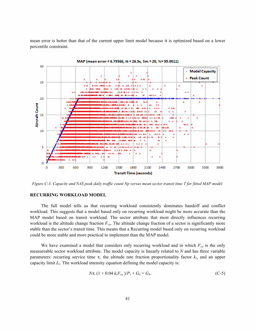
41

mean error is better than that of the current upper limit model because it is optimized based on a lower percentile constraint.

Figure C-3. Capacity and NAS peak daily traffic count Np versus mean sector transit time T for fitted MAP model.

RECURRING WORKLOAD MODEL

The full model tells us that recurring workload consistently dominates handoff and conflict workload. This suggests that a model based only on recurring workload might be more accurate than the MAP model based on transit workload. The sector attribute that most directly influences recurring workload is the altitude change fraction Fca. The altitude change fraction of a sector is significantly more stable than the sector’s transit time. This means that a Recurring model based only on recurring workload could be more stable and more practical to implement than the MAP model.

We have examined a model that considers only recurring workload and in which Fca is the only measureable sector workload attribute. The model capacity is linearly related to N and has three variable parameters: recurring service time τr, the altitude rate fraction proportionality factor kr, and an upper capacity limit Lr. The workload intensity equation defining the model capacity is:

Nτr (1 + 0.04 krFca )/Pr + Gb = Gh. (C-5)

42

A search for values of recurring service time τr, traffic limit Lr, and kr that best fit the condensed NAS data (subject to a 95-percentile constraint) returns an unambiguous solution with a recurring service time of 14 seconds (1 second discretization), a traffic limit of 21 aircraft (integer aircraft discretization), and an altitude rate fraction proportionality factor of 11 (0.25 discretization). The solution has a mean error of 6.75565 aircraft, and a 95.0011 percentile fit.

Figure C-4 is a plot of the result vs. Fca. Like the MAP model, it does not reveal capacity variations resulting from the other measureable sector workload attributes. The two models have coincidentally identical percentile fits.

Figure C-4. Capacity and NAS peak daily traffic count versus altitude change fraction Fca for fitted Recurring model.

The recurring workload model has slightly higher mean error than the fitted MAP model. This is an unexpected result in view of the dominant nature of recurring workload revealed by the full model results. The likely reason for the superior MAP performance is that air traffic managers use the MAP rule to limit the operational traffic that determines the model fit. The MAP rule thus constrains the observed NAS traffic to behave in ways that reduce the rule’s traffic prediction error. We noted in Section 2.5 that this constraining impact is reduced by three operational factors: manual adjustments to account for local

43

conditions, low traffic demand in large sectors, and overestimated capacity in small sectors. However, a residual degree of operational constraint is to be expected.

TWO ATTRIBUTE MODEL

A third version of the model is defined by two complexity attributes and three variable numerical parameters. The two complexity attributes are the mean transit time T and the sector airspace volume Q. The three variable parameters are the transit service time τt, the conflict separation loss dc, and the recurring service time τr. The fitted values of the variable parameters are respectively, 4.8 seconds, 2.3 nautical miles, and 18 seconds. The performance difference between the fitted MAP model and the two-attribute model is significant. The two-attribute model reduces the mean error by approximately one-half aircraft count and noticeably improves the visual fit for all sector volumes.

Figure C-5. Two-attribute model capacity vs. sector airspace volume Q.

Figure C-5 is a scatter plot of the two-attribute model capacity and the NAS peak daily traffic count Np versus sector volume Q. The absence of heuristics linking Fca with conflict and recurring workload creates a smaller capacity variance in this plot than in the corresponding plot for the full model. Any residual variance is caused solely by T.

45

APPENDIX D ANALYSIS OF PARAMETER AMBIGUITY

Benefits studies of programs to reduce controller workload require unambiguous capacity information. A fixed-percentile integer search always returns a unique optimum. However, finely quantized parameters can generate hundreds of local solutions with mean errors within a few percent of the optimum. The regression process should not return any solution with mean capacity error nearly identical to that of the optimum solution but with significantly different parameters.

Our quantization choices returned 8 solutions whose mean errors were within one-half percent of the optimum. The number of solutions accumulates rapidly with the mean error tolerance. The regression returned 38 solutions with errors within one percent and 117 solutions with errors within two percent.

Figure D-1 is a plot of the cumulative solution count versus mean error for solutions with errors within one percent of the minimum. The first solution is the optimum (mean error of 5.86898 aircraft). All solutions within the one-percent range of this figure predict NAS mean capacities that are nearly identical to those of the optimum. Most of these one-percent solutions also indicate that NAS mean conflict workload and handoff workload are consistently small relative to recurring workload5.

5 The two solutions in this set whose transit service time parameters tt are farthest apart disagree significantly on several metrics. Whereas the optimum solution has a handoff service time of 3.2 seconds, the two maximum-distance solutions have mean handoff service times tt of 1.6 and 5.8 seconds. They agree that recurring workload is consistently dominant, but they disagree on the relative importance of NAS-wide handoff and conflict workload. They also disagree by differences as large as five aircraft on the capacities of individual sectors with short transit times. The 5.8-second solution further disagrees with the optimum solution by indicating that NAS-mean handoff workload exceeds conflict workload for all values of demand.

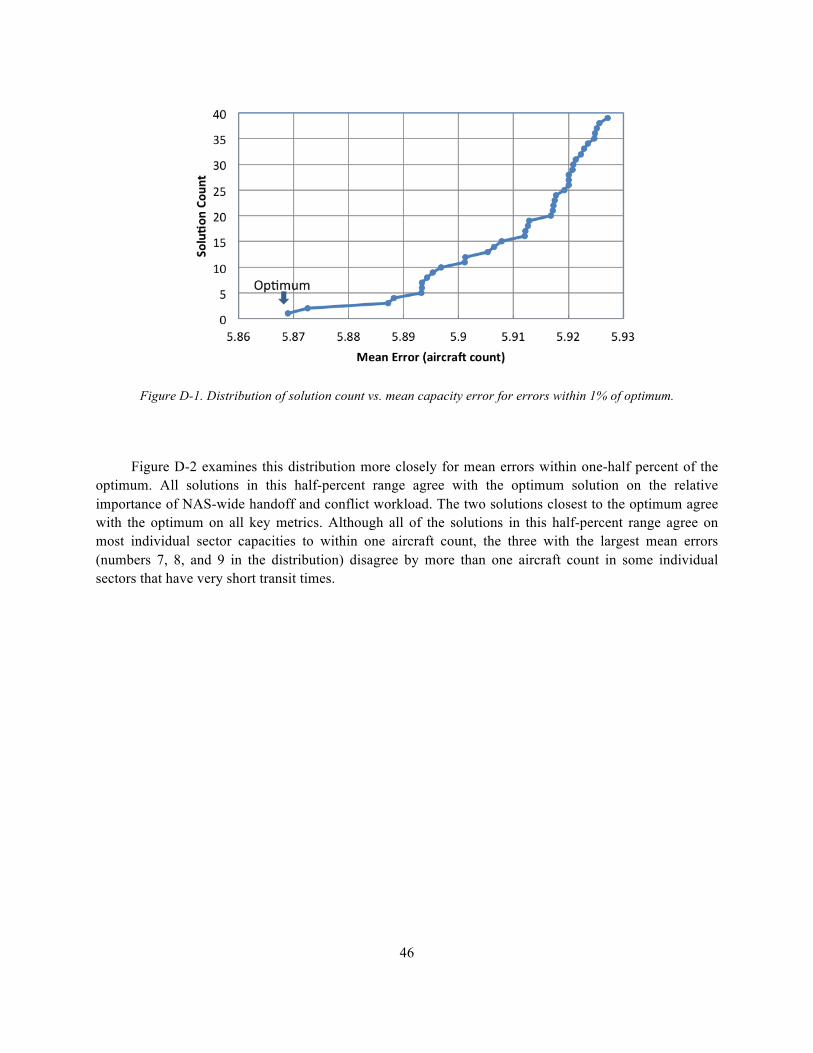
46

Figure D-1. Distribution of solution count vs. mean capacity error for errors within 1% of optimum.

Figure D-2 examines this distribution more closely for mean errors within one-half percent of the optimum. All solutions in this half-percent range agree with the optimum solution on the relative importance of NAS-wide handoff and conflict workload. The two solutions closest to the optimum agree with the optimum on all key metrics. Although all of the solutions in this half-percent range agree on most individual sector capacities to within one aircraft count, the three with the largest mean errors (numbers 7, 8, and 9 in the distribution) disagree by more than one aircraft count in some individual sectors that have very short transit times.

47

Figure D-2. Distribution of solution count vs. mean capacity error for errors within 0.5% of optimum.

Table D-1 summarizes the capacity parameters and errors for the optimum solution and the local solution closest to the optimum in mean error. The closest local solution has capacity parameters that differ only slightly from the optimum. Its transit service time is larger by 12.5%. This is offset by its 10% smaller value of kr. The result is close agreement on all capacity performance metrics.

TABLE D-1

Parameters of Optimum Solution and Closest Local Solution

τ t dc τ r kr Mean Error Percentile

Optimum 3.2 1.9 17 .44 5.86898 0.950235

Closest Local 3.6 1.9 17 .40 5.87256 0.950112

Disagreements between solutions with higher errors are of little operational concern when the local solution with the lowest error has no parameter differences large enough to cause disagreement on significant capacity metrics.

Figure D-3 compares the overall search space with the parameter sub-spaces spanned by 95-percentile solutions with mean error within 0.5% of optimum. In the exhaustive regression, we step each

Optimum

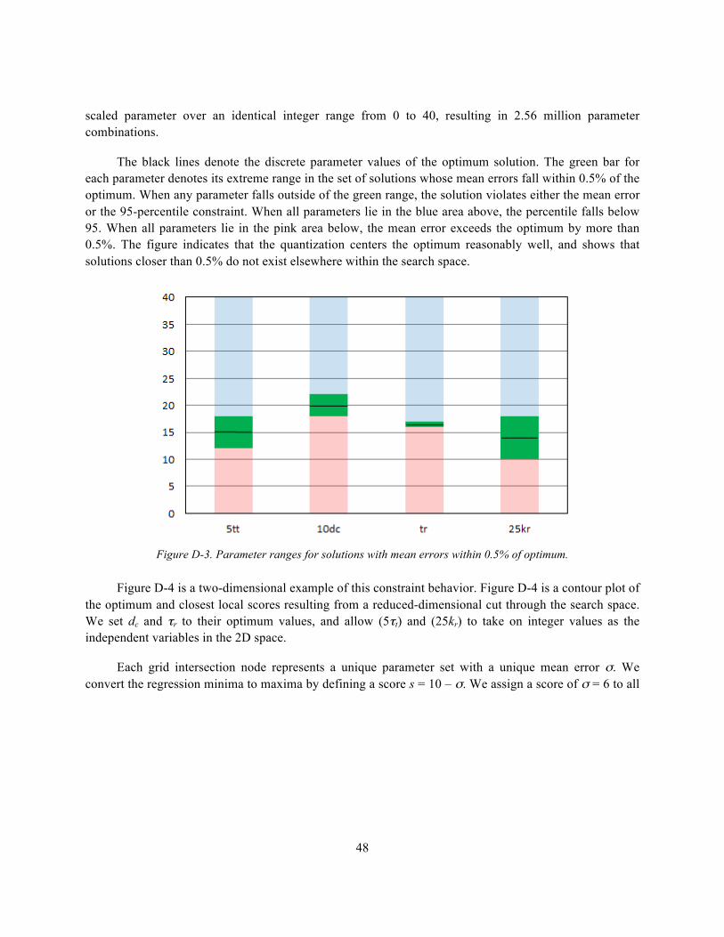
48

scaled parameter over an identical integer range from 0 to 40, resulting in 2.56 million parameter combinations.

The black lines denote the discrete parameter values of the optimum solution. The green bar for each parameter denotes its extreme range in the set of solutions whose mean errors fall within 0.5% of the optimum. When any parameter falls outside of the green range, the solution violates either the mean error or the 95-percentile constraint. When all parameters lie in the blue area above, the percentile falls below 95. When all parameters lie in the pink area below, the mean error exceeds the optimum by more than 0.5%. The figure indicates that the quantization centers the optimum reasonably well, and shows that solutions closer than 0.5% do not exist elsewhere within the search space.

Figure D-3. Parameter ranges for solutions with mean errors within 0.5% of optimum.

Figure D-4 is a two-dimensional example of this constraint behavior. Figure D-4 is a contour plot of the optimum and closest local scores resulting from a reduced-dimensional cut through the search space. We set dc and τr to their optimum values, and allow (5τt) and (25kr) to take on integer values as the independent variables in the 2D space.

Each grid intersection node represents a unique parameter set with a unique mean error σ. We convert the regression minima to maxima by defining a score s = 10 – σ. We assign a score of σ = 6 to all

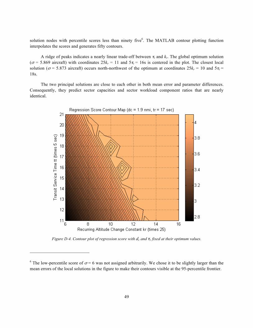
49

solution nodes with percentile scores less than ninety five6. The MATLAB contour plotting function interpolates the scores and generates fifty contours.

A ridge of peaks indicates a nearly linear trade-off between τt and kr. The global optimum solution (σ = 5.869 aircraft) with coordinates 25kr = 11 and 5τt = 16s is centered in the plot. The closest local solution (σ = 5.873 aircraft) occurs north-northwest of the optimum at coordinates 25kr = 10 and 5τt = 18s.

The two principal solutions are close to each other in both mean error and parameter differences. Consequently, they predict sector capacities and sector workload component ratios that are nearly identical.

Figure D-4. Contour plot of regression score with dc and τr fixed at their optimum values.

6 The low-percentile score of σ = 6 was not assigned arbitrarily. We chose it to be slightly larger than the mean errors of the local solutions in the figure to make their contours visible at the 95-percentile frontier.

50

The other local peaks along the ridge have larger mean errors (lower scores). Mean error grows in the west-southwest direction as τt and kr become smaller. The nodes in the east-northeast direction all fall below the 95-percentile constraint. Even though many of them have mean errors lower than the optimum, they are not valid regression solutions.

51

APPENDIX E MULTI-SECTOR AIRSPACE WORKLOAD CAPACITY

The workload capacity model expresses capacity in terms of the peak instantaneous aircraft count of a single sector. However, air traffic managers also need to estimate capacity for larger airspace volumes encompassing multiple sectors. The capacity of large airspace volumes focuses on route networks and is expressed in terms of throughput or flow rate, typically using units of aircraft per hour.

In principle, a workload-based capacity model can estimate the peak safe instantaneous throughput of a sector as well as its peak safe traffic count. Safe instantaneous throughput is equal to safe peak traffic count Nm divided by the mean transit time T of the counted traffic.

However, this throughput definition only applies when input and output flow are equal. In many operational situations the relationship between traffic flow and traffic count is more complex. Throughput and traffic count do not always peak at the same time. When controllers use holding stacks to increase transit time, they generally reduce a sector’s outflow rate and increase its instantaneous traffic count. This may either increase or decrease its inflow rate.

Another fundamental complication arises because flow is a vector concept. Additional information is required to define flow direction for each sector. Directional information is embodied in the sector route structure. Since flow is continuous along each route, large-area route capacity is ultimately limited by the sector along the route with the most severely constrained flow. The flow capacity through a large airspace boundary is the sum of the flow rates of all the routes through the airspace boundary.

The FAA’s current scalar Monitor Alert workload capacity model is used only for warning controllers of potential sector overloads. Its exclusive focus on handoff workload makes it incapable of useful flow rate predictions. Recall that the Monitor Alert capacity Nm is proportional to transit time T. If the Monitor Alert flow capacity is equal to Nm divided by transit time T, then the Monitor Alert model implies that all sectors have the same fixed flow capacity.

Because the full model capacity considers more than handoff workload, the Np/T throughput definition allows it to distinguish high-throughput from low-throughput sectors. With additional information on sector route structures and sector shape, the full model could also estimate the flow capacity of individual routes by partitioning the routes and their individual transit times and altitude rate fractions. Operational route information and airspace geometries are available for all sectors. The use of such information for estimating the effect of airspace blockages on flow capacity is an important area of research, but beyond the scope of this study.

53

APPENDIX F DURATION OF PEAK COUNTS

Peak counts typically persist for at most a few minutes. An example of peak count timing is shown in Figure F-1, which plots instantaneous sector traffic count versus time for New York sector ZNY34 on 1 July 20077. ZNY34 is one of the busier sectors in the New York Air Route Traffic Control Center. Its MAP capacity, indicated by the green line in the figure, is fifteen aircraft. Based on its observed peak traffic and its attributes, the full model estimates its capacity as eighteen aircraft.

Figure F-1. Instantaneous traffic count for Sector ZNY34 on a busy day.

7 This scatter plot is formatted with no markers, and consists of straight lines connecting successive points in the two-dimensional count, time space. The time resolution of the sector handoff data is one second. Most points represent a count change of plus or minus one (resulting from a single aircraft entering or exiting the sector in a one-second period). However, points occasionally indicate changes of more than one aircraft when two or more flights cross the sector boundary in the same second.

0

2

4

6

8

10

12

14

16

18

20

05:00:00 09:00:00 13:00:00 17:00:00 21:00:00 01:00:00 05:00:00

Traf

fic C

ount

UTC Time

Instantaneous Traffic Count For Sector ZNY34 on 7/1/2007 Traffic Count

54

The figure shows that ZNY34 experienced four busy periods during the day with counts matching or exceeding its FAA MAP value. The third busy period twice logged a count of sixteen aircraft. The cumulative time of those counts was 1.9 minutes. The last busy period experienced a peak of eighteen aircraft, the highest of the day.

Table F-1 details the numerical time and traffic count data at the time of the last busy period. The sixteen-aircraft peak occurred at UTC time 01:22:10 (local time 21:22:10 EDT).

55

Table F-1

Numerical Details for Final Busy Period in Sector ZNY34 on 1 July 2007

Time Count

01:19:58 14

01:19:58 15

01:20:04 14

01:20:16 15

01:20:46 14

01:20:52 15

01:21:04 16

01:21:40 17

01:22:10 18

01:22:46 17

01:22:46 16

01:23:04 15

01:23:22 14

01:23:52 15

01:24:04 14

01:24:34 15

01:24:40 14

01:25:04 13

01:25:16 14

01:25:40 13

01:26:10 14

01:26:28 15

01:26:40 14

56

The count first reached the MAP value of fifteen at 01:19:58 and dropped below fifteen for the last time about 7 minutes later. The count rose and remained above fifteen aircraft for 1 minute and 42 seconds (yellow area). The count remained at the day’s peak count of eighteen aircraft for 36 seconds.

These are typical durations for high peak daily counts. Examination of count durations for all thirty sectors in ZNY on 1 July 2007 data indicated that no peak daily count exceeding thirteen aircraft persisted for more than 2.2 minutes, and that higher peak counts tended to persist for shorter times.

57

GLOSSARY

FAA Federal Aviation Administration

MAP Monitor Alert Parameter

NAS National Airspace System

SDAT Sector Design and Analysis Tool

TRACON Terminal Radar Approach Control

ZHU Houston Center

ZMA Miami Center

ZNY New York Center

59

REFERENCES

1. G. Donahue, “A simplified air transportation system capacity model,” Journal of ATC, April–June 1999.

2. J. Welch, J. Andrews, B. Martin, and B. Sridhar, “Workload model for estimating en route sector capacity,” 7th USA/Europe ATM R&D Seminar, Barcelona, Spain, 2007.

3. J.Y.N. Cho, J.D. Welch, and N.K. Underhill, “Analytical workload model for estimating en route sector capacity in convective weather,” 9th USA/Europe ATM R&D Seminar, Berlin, Germany, 2011.

4. J.D. Welch, J.Y.N. Cho, N.K. Underhill, and R.A. DeLaura, “Sector workload model for benefits analysis and convective weather capacity prediction,” 10th USA/Europe Air Traffic Management R&D Seminar, Chicago, IL, 2013.

5. M. Bennett, D. Knorr, and J. Rakas, “Economic benefits of an increase in en route sector capacity from controller-pilot data link communications,” Transportation Research Record, vol. 1888, 2004.

6. J. Post, M. Wells, J. Bonn, and P. Ramsey, “Financial incentives for NextGen avionics, ADS-B case study,” 9th USA/Europe ATM R&D Seminar, Berlin, Germany, 2011.

7. J.D. Welch and J.W. Andrews, “Macroscopic capacity model with individual sector closing speed estimates,” 9th AIAA Aviation, Technology, Integration, and Operations Conf., Hilton Head, SC, September 2009.

8. Federal Aviation Administration, “Monitor Alert Parameter,” Air Traffic Organization Policy Order JO7210.3W, US DOT 2010. http://www.faa.gov/air_traffic/publications/atpubs/fac/1708.html.

9. J.D. Welch, J.W. Andrews, B.D. Martin, and E.M. Shank, “Applications of a macroscopic model for en route sector capacity,” AIAA Guidance, Navigation, and Control Conf., Honolulu, HI, August 2008.

10. K. Geisinger and B. MacLennan, “Sector Design Analysis Tool (SDAT) workload model design document,” Operations Research Service, AOR-200, Federal Aviation Administration, 1994.

11. B. Sridhar, K.S. Seth, and S. Grabbe, “Airspace complexity and its application in air traffic management,” 2nd USA/Europe ATM R&D Seminar, Orlando, FL, December 1998.

12. G.B. Chatterji and B. Sridhar, “Measures for air traffic controller workload prediction,” 1st AIAA Aircraft Technology Integration and Operations Forum, Los Angeles, CA, 2001.

60

13. A. Majumdar, W. Ochieng, and J. Polak, “Estimation of European airspace capacity from a model of controller workload,” J. Navigation, vol. 55, pp. 381–403, 2002.

14. P. Kopardekar, A. Schwartz, S. Magyarits, and J. Rhodes, “Airspace complexity measurement: an air traffic control simulation analysis,” 7th USA/Europe Air Traffic Management R&D Seminar, Barcelona, Spain, July 2007.

15. J. Welch, J. Andrews, and J. Post, “Validation of en route capacity model with peak counts from the US National Airspace System,” EN-012, 2nd ENRI International Workshop on ATM/CNS, Tokyo, Japan, 2010.

16. D.K. Schmidt, “A queuing analysis of the air traffic controller’s work load,” IEEE Trans. Systems, Man, Cybernetics, vol. SMC-8, pp. 492–498, June 1978.

17. A.D. Mundra, “A description of air traffic control in the current terminal airspace environment,” MITRE/CASD, McLean,Va, MTR−88W00167, 1989.

18. A. Yousefi, G.L. Donohue, and L. Sherry, “High-volume tube-shape sectors (HTS): a network of high capacity ribbons connecting congested city pairs,” 23rd Digital Avionics Systems Conference, Oct. 2004.

19. P. Kotecha and I. Hwang, “Optimization based tube network design for the next generation air transportation System,” AIAA GNC Conference, Chicago, August 2009.

20. D. Delahaye and S. Puechmorel, “Air traffic complexity: towards intrinsic metrics,” 3rd USA/Europe ATM R&D Seminar, Napoli, Italy, June 2000.

21. J. Andrews and J. Welch, “Workload implications of free flight concepts,” 1st USA/Europe ATM R&D Seminar, Saclay, France, 1997.

en route sector capacity model final report

Documents