Endogeneous Household Interaction1

Daniela Del Boca2 Christopher Flinn3

August 2010JEL Classification: C79,D19,J22

Keywords: Household Time Allocation; Grim Trigger Strategy; HouseholdProduction; Endogenous Mixing Distribution

1This research was partially supported by the National Science Foundation and by the C.V.StarrCenter for Applied Economics at NYU. Luca Flabbi provided excellent research assistance at theearly stages of this project. For helpful comments and discussions, we are grateful to two anonymousreferees, Pierre-Andre Chiappori, Olivier Donni, Douglas Gale, Ahu Gemici, Arthur Lewbel, DavidPearce, Yoram Weiss, workshop participants at Torino, Duke, Carnegie-Mellon, Penn, Tel Aviv,the 2007 SITE “Household Economics and the Macroeconomy” segment, the June 2008 Conferenceon Household Economics in Nice, the June 2008 IFS Conference “Modeling Household Behaviour,”and the February 2009 Milton Friedman Institute Conference “New Economics of the Family.” Weare solely responsible for all errors, omissions, and interpretations.

2Department of Economics, University of Torino and Collegio Carlo Alberto3Department of Economics, New York University, and Collegio Carlo Alberto

Abstract

Most econometric models of intrahousehold behavior assume that household decision-making is efficient, i.e., utility realizations lie on the Pareto frontier. In this paper weinvestigate this claim by adding a number of participation constraints to the householdallocation problem. Short-run constraints ensure that each spouse obtains a utility levelat least equal to what they would realize under (inefficient) Nash equilibrium. Long-runconstraints ensure that each spouse obtains a utility level at least equal to what they wouldrealize by cheating on the efficient allocation and receiving Nash equilibrium payoffs in allsuccessive periods. Given household characteristics and the (common) discount factor ofthe spouses, not all households may be able to attain payoffs on the Pareto frontier. Weestimate these models using a Method of Simulated Moments estimator and data from onewave of the Panel Study of Income Dynamics. We find that both short- and long-run con-straints are binding for sizable proportions of households in the sample. We conclude thatit is important to carefully model the constraint sets household members face when mod-eling household allocation decisions, and to allow for the possibility that efficient outcomesmay not be implementable for some households.

1 Introduction

Despite there being a vast theoretical and empirical literature on household decision-makingprocesses, there remains a lack of consensus regarding the best way to model householdbehavior. In Becker’s early approach to analyzing household behavior, the social welfarefunction approach of Bergson-Samuelson was used to define a single objective of the house-hold that represented an aggregated version of individual utilities or that was viewed asrepresenting the preferences of a benevolent dictator directing the household. This “uni-tary” version of household preferences proved satisfactory in a large number of theoreticalanalyses, but yielded empirical implications broadly inconsistent with consumption andtime allocation decisions observed in household-level data. For this reason, this specifica-tion of household objectives has largely been abandoned as a framework for conductingempirical analyses of household behavior.

Over the past several decades, there has been a movement to view the family as acollection of agents with their own clearly-demarcated preferences who are united throughthe sharing of public goods, emotional ties, and production technologies. Household mem-bers are often viewed as behaving strategically with respect to one another given theirrather complicated and interconnected resource constraints. Analysis of these situationshas focused on describing and analyzing cooperative equilibrium outcomes. Though mod-els using the cooperative approach (e.g., Manser and Brown (1980), McElroy and Horney(1981), Chiappori (1988)) differ in many respects, they share the common characteristic offocusing on outcomes that are Pareto-efficient (the primary distinction between them beingthe method for selecting a point on the Pareto frontier). The main alternative approach,which uses noncooperative Nash equilibrium as the solution concept (e.g. Leuthold (1968),Bourgignon (1984), Del Boca and Flinn (1995), Chen and Woolley (2001)), leads to out-comes that are generally Pareto-dominated. The analytic attractiveness of noncooperativeequilibrium models lies in the fact that equilibria are often unique, an especially distinctadvantage when formulating an econometric model and conducting empirical analysis.

In this paper we develop and estimate a model of household time allocation which allowsfor both efficient and inefficient intrahousehold behavior. Gains from marriage are takento arise from the presence of a publicly-consumed good that is produced in the householdwith time inputs from the spouses and goods purchased in the market. In the presenceof a public good, efficient outcomes, which by definition lie on the Pareto frontier, mustweakly dominate the value of the noncooperative equilibrium for each spouse. So whywould some households fail to determine allocations in an efficient manner? We focus onimplementation issues in this paper. We consider the case in which household interactionsare repeated over an indefinitely long horizon, and determine whether cooperative behaviorcan be supported using Folk Theorem-inspired arguments. In this view, a key determinantof whether or not Pareto-efficient outcomes can be implemented is the forward-lookingnessof the spouses.

There have been few empirical studies to date that have attempted to actually estimate

1

a collective model of household labor supply (some notable exceptions include Kapteyn andKooreman (1992), Browning et al. (1994), Fortin and Lacroix (1997), and Blundell et al.(2005)). Two of the more important reasons for the paucity of empirical studies are thestringent data requirements for estimation of such a model and lack of agreement regardingthe “refinement” to utilize when selecting a unique equilibrium when a multiplicity exist (asis the case in virtually all cooperative models). Some researchers have advocated using theassumption of Pareto efficiency in nonunitary models as an identification device (see, e.g.,Bourguignon and Chiappori (1992) and Flinn (2000)).1 We view household time allocationdecisions as either being associated with a particular utility outcome on the Pareto frontier,or to be associated with the noncooperative (static Nash) equilibrium point. In realitythere are a continuum of points that dominate the noncooperative equilibrium point andthat do not lie on the Pareto frontier, however developing an estimable model that allowssuch outcomes to enter the choice set of the household seems beyond our means. Ourpaper expands the equilibrium choice set to two focal points, but it still represents a veryrestrictive view of the world.

Even under an assumption of efficiency, there is wide latitude in modeling the mech-anism by which a specific efficient outcome is implemented, as is evidenced by the livelydebate between advocates of the use of Nash bargaining or other axiomatic systems (e.g.,McElroy and Horney (1981,1990), McElroy (1990)) and those advocating a more datadriven approach (e.g., Chiappori (1988)). The use of an axiomatic system such as Nashbargaining requires that one first specify a “disagreement outcome” with respect to whicheach party’s surplus can be explicitly defined. It has long been appreciated that the bar-gaining outcome can depend critically on the specification of this threat point.2 Most often(in the household economics literature) the threat point has been assumed to represent thevalue to each agent of living independently from the other. Lundberg and Pollak (1993)provide an illuminating discussion of the consequences of alternative specifications of thethreat point on the analysis of household decision-making. In particular, instead of assum-ing the value of the divorce state as the disagreement point for each partner, they considerthis point to be determined by the value of the marriage to each given some default modeof behavior, which they call “separate spheres.” In this state, each party takes decisionsand generally acts in a manner in accordance with “customary” gender roles. Lundbergand Pollak state that households will choose to behave in this customary way when the

1An argument sometimes given for this assumption relies on the Folk Theorem. As household membersinteract frequently and can observe many of each other’s constraint sets and actions, for reasonable valuesof a discount factor efficient behavior should be attainable. The most general behavioral specificationestimated here allows us to examine this claim empirically, and we find that efficient allocations cannot besustained for a small percentage of households.

2Lugo-Gil (2003) demonstrates this point nicely. In her case, spouses decide on consumption allocationsin a cooperative manner after the outside option is optimally chosen. All “intact” households chose athreat point either of divorce or noncooperative behavior. The choice of threat point has an impact onintrahousehold allocations. In her case, all household allocations are determined efficiently (using a Nashbargaining framework), whereas in ours, some allocations are determined in an inefficient manner.

2

“transactions costs” they face are too high.The approach taken in this paper is something of a synthesis of the standard bargain-

ing and “sharing rule” approaches to modeling household behavior. We introduce outsideoptions that household members must recognize and meet, if possible, when choosing ef-ficient allocations. These side conditions on the household’s optimization problem areinterpretable more as participation constraints than “threat points,” and these options donot serve as a basis for conducting bargaining in the axiomatic Nash sense. Practicallyspeaking, we view the household allocation decisions as emanating from maximization ofthe sum of the utilities of the two spouses where the Pareto weight associated with theutility of spouse 1 is α. Adding side constraints to the household optimization problemrestricts the set of α-generated time allocations that are implementable, and, dependingon the nature of the constraints, may make it impossible to implement any efficient so-lution. Mazzocco (2007) follows a somewhat similar strategy in his dynamic contractingformulation of the household’s intertemporal allocation problem. In his set up, though,participation constraints may or may not result in reallocations of the cooperative surplusover time. All households are assumed to behave efficiently at all points in time, however.

We build four distinct models of household behavior that are taken to the householdtime allocation data. They are not strictly nested for the most part, but do have a reason-ably natural ordering in terms of complexity. The models are described and developed ina general manner in the following section. They are, in general order of complexity:

1. (Static) Nash equilibrium, in which case equilibrium is defined as the intersection ofthe spouses’ reaction functions.

2. Pareto-weight formulation, in which case household allocations are the solutions tothe maximization of the Pareto-weighted sum of spousal utilities.

3. Constrained Pareto-weight specification, in which case household allocations are so-lutions to the maximization of the Pareto-weighted sum of spousal utilities subjectto the constraint that each spouse receive at least the utility they would receive inNash equilibrium.

4. Endogenous Interaction model, in which case household allocations are solutions tothe maximization of the Pareto-weighted sum of spousal utilities subject to the con-straint that each spouse receive at least the utility they would receive by deviatingfrom the efficient allocation, if any such outcome is possible. If no such outcome ispossible, the household allocations are determined under the (static) Nash equilib-rium.

We view the contribution of the paper as bringing short- and long-run implementationissues into the estimation of models of household behavior. While basic versions of thefirst and second models described above, those of inefficient Nash equilibrium and the

3

“collective” model, have been estimated on numerous occasions, estimation of the collectivemodel subject to the constraint that no spouse’s welfare level be less than what they canobtain under the Nash equilibrium has not been performed.3 We demonstrate empiricallythat adding such a constraint has significant effects on the point estimates of the modeland, consequently, on the welfare inferences that can be drawn.

The addition of the incentive compatibility constraint in our final model specificationis noteworthy in that it allows spouses the choice of their mode of interaction. Somehouseholds, given their state variables, will choose to behave in an inefficient manner,while others will behave in a “constrained” efficient manner. This carries the importantimplication that small changes in state variables, such as in wages or nonlabor income,may potentially have large changes on actions if these small changes prompt a change inbehavioral regime.

While we have added two sets of constraints to the household optimization problem,it is obviously the case that other types of constraints could be added instead of, or inaddition to, the two we have included. For example, it is common to specify the value ofeach spouse in the divorce state as the disagreement point when using a Nash bargainingframework to analyze household decisions. Clearly, this constraint could be added to thoseconsidered here when determining the set of implementable values of the Pareto weight α.These types of generalizations are left to future research, and are probably best consideredin a truly dynamic model of the household that allows for divorce outcomes.

The plan of the paper is as follows. In Section 2 we lay out the theoretical structureof the model. Section 3 presents the specific functional form assumptions that underliethe empirical analysis. Section 4 contains a discussion of estimation issues and developsthe nonparametric and parametric estimators used in the empirical analysis. We provide adescription of the data, present model estimates, and conduct a small comparative staticsexercise in Section 5. Section 6 concludes.

3Mazzocco (2007) is a valuable contribution to the literature that also considers implementation issuesexplicitly. The focus of his analysis is on determining whether intertemporal household allocations areconsistent with ex ante efficient allocations, or whether welfare weights have to be continually adjustedto meet short-run participation issues that arise when household members cannot credibly make life-longcommitments to a given ex ante efficient allocation. He finds evidence supporting the lack of commitmenthypothesis.There are a number of differences between his approach and the one taken here, the most salient of which

are the following. First, the dynamic setting he considers is not nearly as stylized as the one employed here.Second, participation constraints change over the life cycle, though they are modeled as exogenous randomprocesses, whereas in our case the outside option is explicitly modeled. Third, in his model all householdsbehave efficiently in every period, that is, the outside option is never chosen. In our case, the outside optionof inefficient behavior is chosen in some states of the world.Another valuable paper that examines commitment issues in a household setting using a dynamic con-

tracting approach is Ligon (2002). As in Mazzocco (2007), all final household allocation decisions areconstrained efficient, which is not the case in our EI specification.

4

2 The Household’s Decision Problem

In the first part of this section we describe the objectives and constraints facing the spouses.We then turn to a consideration of the manner in which a household equilibrium allocationis determined under our four different modeling assumptions.

2.1 The General Environment

While the empirical application will require us to make a number of functional form as-sumptions, the model of household behavior we develop is applicable quite generally. Weassume egoistic preferences, with the current period payoff function of spouse i given bythe function

ui(a1, a2),

where ai is a vector of actions available to spouse i. These actions may consist of purchasesof inputs for a household production technology, the supply of time to that technology, orpurchases of market goods, the consumption of which directly impacts the satisfaction ofone or both spouses. All of the actions considered in the paper are continuous, and choiceswill be a continuous function of the state variables facing the household. To be able toinvert decision rules to recover primitive parameters, we will require the existence of a 1-1mapping between a subset of (unobserved) state variables and the (observed) decisions.This will require us to rule out corner solutions.

We assume the presence of intrahousehold externalities, which for us means that thewell-being of a spouse or their (household) productivity is directly affected by the actionsof the other spouse. Given the presence of a household externality, assumed throughout,there exists a welfare-improving set of feasible actions that differ from the (static) Nashequilibrium actions.

2.2 The Behavioral Regimes

2.2.1 Nash Equilibrium

We make the following assumptions.

Assumption 1 There exists a unique Nash equilibrium in actions

(aN1 aN2 )(u1, u2, CS)

where U is a family of period-payoff functions and CS denotes the choice set.

Assumption 1 rules out, most importantly, various types of nonconvexities in the choicesets of the household members, such as the existence of fixed time or money costs associatedwith supplying time to the labor market or in household production. The Nash equilibriumis derived as follows. Let a∗i (ai0 , ui, CSi) denote the best response functions of spouse

5

i given that spouse i0 chooses actions ai0 when they have choice set CSi and objectivefunction ui. Then the Nash equilibrium actions are given by (aN1 aN2 )(u1, u2, CS), whereaN1 = a∗1(a

N2 , u1, CS1) and aN2 = a∗2(a

N1 , u2, CS2), and CS = CS1 ∪ CS2.

2.2.2 Pareto Optimal Decisions

We write the Benthamite social welfare function for the household as

Wα(a1, a2) = αu1(a1, a2) + (1− α)u2(a1, a2).

Maximizing the value of Wα(a1, a2) with respect to the actions of the two spouses givenCS traces out the Pareto frontier. In particular,

(aP1 aP2 )(α, u1, u2, CS) = arg max(a1,a2)∈CS

Wα(a1, a2).

Assumption 2 The Pareto optimal actions (aP1 aP2 )(α, u1, u2, CS) are unique.

The Pareto frontier is defined by the set of points

PF (u1, u2, CS) ≡u1(aP1 (α, u1, u2, CS), aP2 (α, u1, u2, CS)), u2(aP1 (α, u1, u2, CS), aP2 (α, u1, u2, CS)),

α ∈ [0, 1]

It follows that u1 is nondecreasing in α and u2 is nonincreasing in α along PF. Assumingdifferentiability along the Pareto frontier with respect to α,

du2du1

¯u2,u1∈PF

< 0.

Our analysis is based on the existence of externalities within the household. It followsthat the pair of Nash equilibrium utility levels, V N

1 , V N2 , defined by

V Ni = ui(a

N1 , a

N2 ), i = 1, 2,

is not a point on the Pareto frontier.

2.2.3 Constrained Pareto Outcomes

Pareto efficient outcomes have the desirable feature that one spouse’s utility cannot beimproved without decreasing the other’s, but may or may not meet certain reasonable“fairness” criteria. We singled out Nash equilibrium play as a natural focal point for thebehavior of spouses since it involves no coordination or policing of actions due to the fact

6

that strategies are best responses. This gives the Nash equilibrium a type of stability notpossessed by efficient outcomes.

At a minimum, then, it seems reasonable to restrict attention to efficient outcomes thatyield each spouse at least the level of welfare they can attain under the Nash equilibriumactions. We think of this as a “short-run” participation constraint, where short-run refersto the fact that it ensures that each party is at least as well-off under the efficient allocationas they would be under Nash equilibrium in the current period. The following propositionfollows directly from the relatively weak assumptions made to this point. To reduce nota-tional clutter, we drop the explicit conditioning on the utility functions ui and the choiceset CS.

Proposition 1 There exists a nonempty interval IC(V N1 , V N

2 ) ≡ [α(V N1 ), α(V

N2 )] ⊂ (0, 1),

with α(V N1 ) < α(V N

2 ), such that

u1(aP1 (α), a

P2 (α)) ≥ V N

1

u2(aP1 (α), a

P2 (α)) ≥ V N

2

if and only if α ∈ IC(V N1 , V N

2 ).

Proof. The points on the Pareto frontier are monotone and continuous functions of α.By Assumption 2, the Nash equilibrium payoffs are dominated by a set of points on thePareto frontier. Define the unique value α(V N

1 ) by

u1(aP1 (α(V

N1 ), a

P2 (α(V

N1 ))) = V N

1 ,

and, similarly, define α(V N2 ) by

u2(aP1 (α(V

N2 )), a

P2 (α(V

N2 ))) = V N

2 .

Define the set of all α values that yield an efficient payoff at least as large as V N1 for spouse

1 asIC1 (V

N1 ),

the minimum element of which is α(V N1 ). Define the set of all values of α that yield an

efficient payoff at least as large as V N2 to spouse 2 as

IC2 (VN2 ),

the maximum element of which is α(V N2 ). Then

IC(V N1 , V N

2 ) = IC1 (VN1 ) ∩ IC2 (V N

2 )

= [α(V N1 ), α(V

N2 )]

6= ∅

7

Given problems associated with the identification of the welfare weight α, which arediscussed in detail below, we will typically assume that there exists one value of α, commonto all marriages, which could be culturally determined. The constrained Pareto optimalallocation is determined by first determining whether α ∈ IC(V N

1 , V N2 ). If so, each spouse’s

utility level using the Pareto weight of α exceeds their static Nash equilibrium utility level,and the constraint is not binding. Instead, if α < α(V N

1 ), the Pareto efficient solutionyields less utility to spouse 1 than the Nash equilibrium solution. To get this spouse toparticipate in the Pareto efficient solution, it is necessary to provide them with at least asmuch utility as they would obtain in the static Nash equilibrium, which means adjustingthe Pareto weight up to the value α(V N

1 ). Conversely, if α > α(V N2 ), then the Pareto weight

has to be adjusted downward to α(V N2 ) to provide the incentive for the second spouse to

participate in the household efficient allocation. The formal statement of the actions inthis environment is as follows. If α ∈ IC , then

(aC1 aC2 )(α) = (aP1 aP2 )(α), α ∈ IC , (1)

since the “participation constraint” is not binding. If α < α(V N1 ), so that spouse 1 would

have a higher payoff in Nash equilibrium, the α must be “adjusted” up so that he has thesame welfare in either regime. In this case,

(aC1 aC2 )(α) = (aP1 aP2 )(α(V

N1 )), α < α(V N

1 ). (2)

Conversely, if spouse 2 suffers utility-wise in the efficient allocation associated with α, theα must be adjusted downward, and we have

(aC1 aC2 )(α) = (aP1 aP2 )(α(V

N2 )), α > α(V N

2 ). (3)

Note that under this behavioral rule, there is still, in general, a continuum of possiblesolutions, associated with all values of α belonging to IC .

2.2.4 Endogenous Interaction

The time allocations in the Pareto optimal and constrained Pareto optimal cases may ormay not satisfy another set of constraints, one that involves implementation. The essentialissue is that utility levels that lie along the Pareto frontier are not associated with timeallocation choices by either spouse that are “best responses” (in the static sense) to thechoices of their partner. As we know, only the static Nash equilibrium has that property,and is associated with utility outcomes that are dominated by those associated with theconstrained Pareto optimal choices we have just discussed.

Why might spouses cheat on an efficient agreement that improves the welfare of bothwith respect to the Nash equilibrium outcome? The temptation to cheat in this case mayarise from purely self-interested behavior, as it does when we study the incentives of firms

8

engaged in collusive behavior to deviate from their assigned production quotas (e.g., Greenand Porter, 1984). In that case, the welfare of firms is linked through a common market foroutputs or inputs, though firms’ objectives are typically taken to be solely the maximizationof their own monetary profits. In the case of households, the objectives of spouses maybe considerably more complex than those of firms, and may include altruism, for example.However, the existence of caring preferences, in and of itself, does not make implementationof an efficient allocation a foregone conclusion. Indeed, spouses may care so much abouteach other that an efficient solution may involve each behaving in what would appear tobe a more self-interested manner to an observer. In this case, “cheating” on the efficientoutcome may imply a spouse spends more of their resources on goods of direct value onlyto the other spouse. In the household context cheating may be prevalent, but due to thepresence of household production technologies and interconnected preferences, it is difficultto detect without strong assumptions on preferences or technologies.

As is well-known from Folk theorem results, in order to implement equilibrium outcomesthat are not best responses in a static sense, it is necessary to provide an intertemporalcontext to household choices. Accordingly we define the welfare of each spouse to be

Ji =∞Xt=1

βt−1ui(a1(t), a2(t)),

where β is a discount factor taking values in the unit interval, and aj(t) are the actionschosen by spouse j in period t. For reasons related to data availability and computationalfeasibility, we restrict our attention to the case in which the stage game played by thespouses has the same structure in every period. That is, preferences and technology para-meters are fixed over time, as well as wage offers and nonlabor income levels.

We assume that the couple utilize a grim trigger strategy, with the punishment phasebeing perpetual Nash equilibrium play.4 We assume that the allocation is determined by

aEi (t) =

½aCi (α) if ai0(t

0) = aCi0 (α), t0 = 1, ..., t− 1

aNi if ai0(t0) 6= aCi0 (α) for any t

0 = 1, ..., t− 1 (4)

in the equilibrium. In this case, a divergence by either spouse from their prescribed actionaCi (α) leads to the play of Nash equilibrium in all subsequent periods. aCi (α) denotes theprescribed efficient allocation, which is determined using the Pareto weight α.

To determine whether there exists an implementable cooperative equilibrium in thehousehold, we must check whether there is sufficient patience among the spouses to sustainthe efficient outcome given the size of the penalty they face for deviation. Each spouse’sobjective is to maximize the present discounted value of their sequence of payoffs given the

4We are aware that there are more ‘efficient’ punishment strategies available to the household members,but the incorporation of these punishments into the econometric model is a difficult task. The importantpoint for the analysis is that given our modeling set up, a measurable subset of the state vector space willresult in a lack of implementability of efficient outcomes, the main point of our analysis.

9

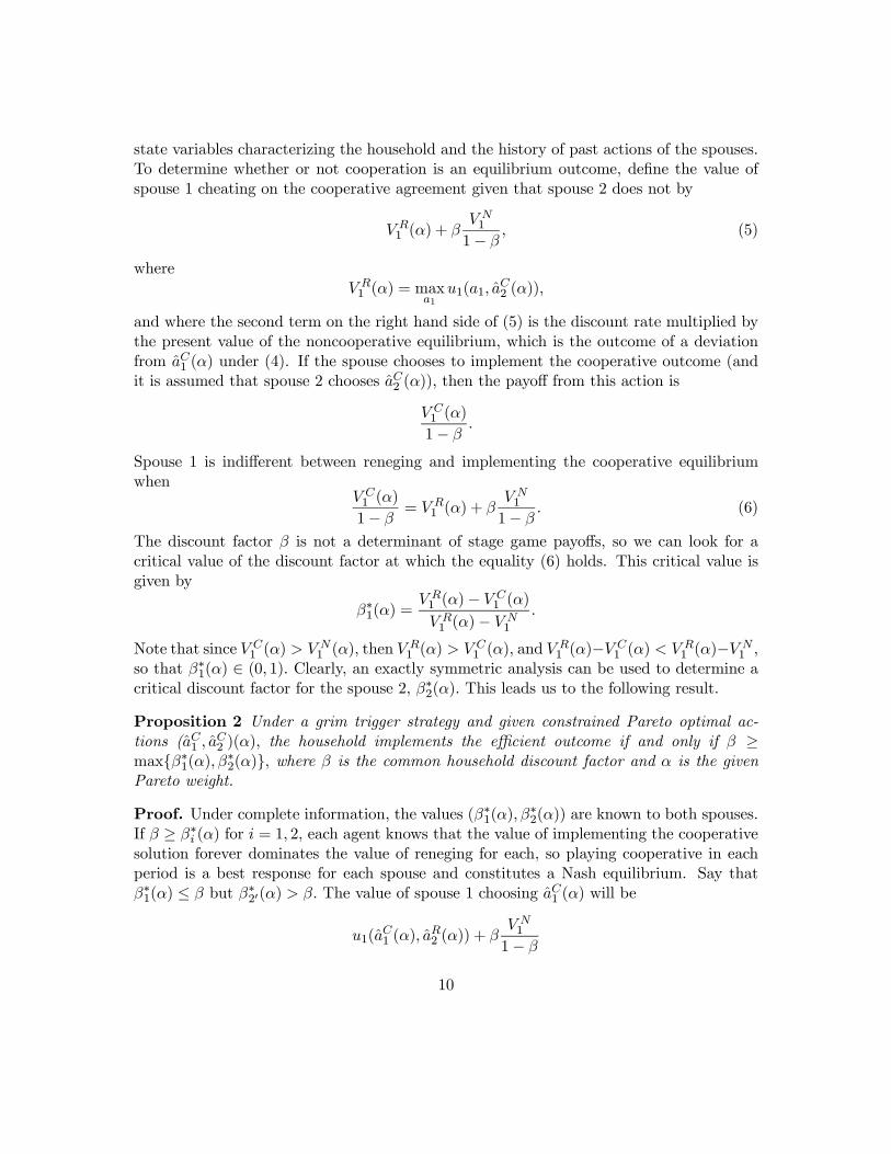
state variables characterizing the household and the history of past actions of the spouses.To determine whether or not cooperation is an equilibrium outcome, define the value ofspouse 1 cheating on the cooperative agreement given that spouse 2 does not by

V R1 (α) + β

V N1

1− β, (5)

whereV R1 (α) = maxa1

u1(a1, aC2 (α)),

and where the second term on the right hand side of (5) is the discount rate multiplied bythe present value of the noncooperative equilibrium, which is the outcome of a deviationfrom aC1 (α) under (4). If the spouse chooses to implement the cooperative outcome (andit is assumed that spouse 2 chooses aC2 (α)), then the payoff from this action is

V C1 (α)

1− β.

Spouse 1 is indifferent between reneging and implementing the cooperative equilibriumwhen

V C1 (α)

1− β= V R

1 (α) + βV N1

1− β. (6)

The discount factor β is not a determinant of stage game payoffs, so we can look for acritical value of the discount factor at which the equality (6) holds. This critical value isgiven by

β∗1(α) =V R1 (α)− V C

1 (α)

V R1 (α)− V N

1

.

Note that since V C1 (α) > V N

1 (α), then VR1 (α) > V C

1 (α), and VR1 (α)−V C

1 (α) < V R1 (α)−V N

1 ,so that β∗1(α) ∈ (0, 1). Clearly, an exactly symmetric analysis can be used to determine acritical discount factor for the spouse 2, β∗2(α). This leads us to the following result.

Proposition 2 Under a grim trigger strategy and given constrained Pareto optimal ac-tions (aC1 , a

C2 )(α), the household implements the efficient outcome if and only if β ≥

maxβ∗1(α), β∗2(α), where β is the common household discount factor and α is the givenPareto weight.

Proof. Under complete information, the values (β∗1(α), β∗2(α)) are known to both spouses.

If β ≥ β∗i (α) for i = 1, 2, each agent knows that the value of implementing the cooperativesolution forever dominates the value of reneging for each, so playing cooperative in eachperiod is a best response for each spouse and constitutes a Nash equilibrium. Say thatβ∗1(α) ≤ β but β∗20(α) > β. The value of spouse 1 choosing aC1 (α) will be

u1(aC1 (α), a

R2 (α)) + β

V N1

1− β

10

under the grim trigger strategy, since aR2 (α) 6= aC2 (α) triggers the punishment phase. Giventhe reneging action aR2 (α), a

C1 (α) will not maximize this payoff, and spouse 1 will best

respond a∗1(aR2 (α)), say, to which spouse 2, will best respond, with the actions converging

to those of the (unique) Nash equilibrium (aN1 , aN2 ). Thus both spouses will play the Nash

equilibrium at every point in time. For the same reason, when β < β∗1(α) and β < β∗2(α),the sequence of best responses to the reneging behavior of the other spouse leads to theNash equilibrium being played in each period.

We now turn to the consideration of the determination of the actions (aE1 (α), aE2 (α)) in

the Endogenous Interactions case. After determining the efficient allocation of the house-hold under CPO given an initial notional value of α, we can determine if this solution isimplementable. For simplicity, let αCPO denote the ex post value of α that satisfies theparticipation constraint for a household (given the choice set CS) under the CPO speci-fication. If β ≥ β∗1(αCPO) and β ≥ β∗2(αCPO), then the CPO outcome is implementable,and the actions in the Endogenous Interactions case are the same as are specified underCPO.

In general, the ex post Pareto weight associated with the CPO regime is not imple-mentable under the EI regime. This is clearly the case when αCPO is determined in sucha way that the participation constraint is binding for one of the spouses, which is alwaysthe case whenever αCPO 6= α0. In this case, there will be no long run welfare gains for thespouse with the binding participation constraint, and his or her best response will be tocheat on the efficient outcome. In such a case, to induce that spouse not to deviate fromthe efficient outcome, the Pareto weight associated with that spouse must be increased. Ifthere is an implementable efficient outcome, for a given value of β, it will be the one forwhich the “long run” participation (i.e., no cheating) constraint is exactly satisfied. For agiven value of β, there may be no value of the Pareto weight that simultaneously satisfiesthe “no cheating” constraint for both spouses, and in this case, no efficient allocation isattainable. The formal definition of implementability is the following:

Definition 3 A household has an implementable outcome on the Pareto frontier if thereexists an α ∈ (0, 1) such that β ≥ maxβ∗1(α), β∗2(α).

Figure 1 contains the graph of the β∗i , i = 1, 2, for a given set of state variables thatfully characterize spousal preferences, household technology, and choice sets. We note thatβ∗1 is a decreasing function of α, since increasing (static) gains associated with the efficientallocation (as α increases) require lower levels of patience to sustain implementation onthe part of spouse 1. Obviously, β∗2 is increasing in α for the opposite reason. We see thatfor this set of state variables, the household has an implementable efficient outcome if thecommon discount factor of the spouses exceeds β∗∗. If the discount factor is less than that,no outcome on the Pareto frontier can be implemented, even though there are a continuumof allocations with static payoffs that strictly exceed the static Nash equilibrium payoffs.

In Figure 1 we have also indicated the manner in which the ex post Pareto weightis determined when an implementable allocation exists. Since the value of the discount

11

factor, β, exceeds β∗∗, an implementable solution exists. Starting from the ex post αassociated with the static Nash equilibrium participation constraint, αCPO, we see that atthis value β∗1(αCPO) > β and β∗2(αCPO) < β, so that at this low level of α spouse 1 wouldcheat on the efficient allocation, while spouse 2 would not, meaning that in equilibriumthe αCPO−generated allocation could not be implemented. In this case, α is increaseduntil it reaches the value αEI , which is that value at which the no-cheating participationconstraint is met for spouse 1.

In summary, we think of the determination of the EI allocations as consisting of thefollowing steps.

1. Determine the functions β∗j (α).

2. If β < β∗∗, then the household is not able to implement efficient allocations. ThenaEj = aNj , j = 1, 2.

3. If β ≥ β∗∗, the household is able to implement an efficient time allocation. Let α0denote the notational Pareto weight. Then

(aE1 , aE2 ) =

⎧⎨⎩(aE1 (α0), a

E2 (α0)) if β∗1(α0) ≤ β and β∗2(α0) ≤ β

(aE1 ((β∗1)−1(β)), aE2 ((β

∗1)−1(β))) if β∗1(α0) > β

(aE1 ((β∗2)−1(β)), aE2 ((β

∗2)−1(β))) if β∗2(α0) > β

,

where (β∗j )−1 is the inverse of β∗j .

2.3 Summary

We summarize the results of this section with the aid of Figure 2. For any given household,there exists a unique (static) household Nash equilibrium of actions aN1 , aN2 and payoffsV N1 , V N

2 , with the pair of payoffs given by the intersection of the two lines in Figure2. Varying the Pareto weight α over (0, 1) in the weighted household utility functionspecification (PO) traces out the Pareto frontier. When we impose the side constraint thatthe Pareto weight must be chosen so that each spouse obtains at least their payoff V N

i ,this defines a lower bound α(V N ) at which the participation constraint is just binding forspouse 1 and an upper bound α(V N) at which the participation constraint is just bindingfor spouse 2. If the notional value of the Pareto weight, α0, falls in this interval, then thatvalue is used to define the efficient outcome, which will be the same as in the unconstrainedcase. If the value of α0 is less than α(V N), then the efficient outcome is determined usingthe Pareto weight α(V N ). If, instead, α0 > α(V N), then the efficient outcome is determinedusing the Pareto weight α(V N ).

The “dynamic” participation constraint imposes a tighter set of restrictions on the αchoice problem than does the “static” participation constraint, except in the extreme caseof β = 1. For any β < 1, there either exists a nonempty interval [α(V N , β), α(V N , β)] ⊂[α(V N), α(V N)] = [α(V N , β = 1), α(V N , β = 1)], or the set of implementable α is empty,

12

and inefficient behavior results. Put another way, for any given household, there exists acritical value β∗∗, with any β < β∗∗ inducing the household to behave inefficiently. Whenthere does exist a nonempty set of α that satisfy the dynamic participation constraint,the ultimate household allocation is determined in the same manner as it was when weimposed the static participation constraint.

3 Functional Form Assumptions

In order to estimate the model with the data available to us, a number of functional formassumptions are required. Our strategy in this first section is to present the assumptionsmade regarding the form of spousal preferences and the household production technology,and then to demonstrate that the resulting household behavior is consistent with Assump-tions 1 and 2.

We assume that each spouse possesses a utility function defined over the consumptionof a good produced in the household with time inputs of the household members and agood (or goods) purchased in the market, which we denote by τ1, τ2, and M, respectively.The household production technology is given by

K = τ δ11 τδ22 M

1−δ1−δ2 ,

where M is total household income, τ i is the time supplied by spouse i in householdproduction, and δ1 ≥ 0, δ2 ≥ 0, and δ1+δ2 ≤ 1. Thus the household production technologyexhibits constant returns to scale.

Individuals supply time in a competitive market to generate earnings. The wage rateof spouse i is wi, and the time they spend in market activities is hi. The nonlabor incomeof the household is denoted by Y, and is the sum of the nonlabor incomes of the spouses,Y1 + Y2, plus any nonattributable nonlabor income that accrues to the household, Y . Thesources of nonlabor income will play no role in our analysis. Total income of the householdis then M = w1h1 +w2h2 + Y.

Each spouse has Cobb-Douglas preferences over a private good, leisure, and the house-hold public good, so that

ui = λi ln(li) + (1− λi) lnK, i = 1, 2,

where li is the leisure consumed by spouse i, and λi ∈ [0, 1], i = 1, 2, is the Cobb-Douglaspreference parameter. Each spouse has a time endowment of T, so that

T = hi + τ i + li, i = 1, 2,

defines the time constraint. Spouse i controls his or her time allocations regarding hi andτ i (which determine li, of course).

13

By substituting the household production technology into the utility functions of eachspouse, we get a payoff function

u1(l1, τ1, τ2,M) = λ1 ln l1 + δ11 ln τ1 + δ12 ln τ2 + δ13 lnM

u2(l2, τ1, τ2,M) = λ2 ln l2 + δ21 ln τ1 + δ22 ln τ2 + δ23 lnM,

where δ3 = 1 − δ2 − δ1 and δij ≡ (1 − λi)δj , and where λi + δi1 + δi2 + δi3 = 1, i = 1, 2.The reaction function of spouse 1, for example, is

(h∗1 τ∗1)(h2 τ2) = arg max

h1≥0,τ1λ1 ln(T−h1−τ1)+δ11 ln τ1+δ12 ln τ2+δ13 ln(w1h1+w2h2+Y ),

and it is straightforward to establish that this best response is uniquely determined forall (h2 τ2) and for any values of the preference and production parameters satisfying theconstraints imposed above. There exists a unique best response for the second spouse,(h∗2 τ

∗2)(h1 τ1) by symmetry. Since h

∗i is a nonincreasing function of hi0 and is independent

of τ i0 , and since τ∗i is independent of both hi0 and τ i0 , there exists a unique Nash equilibrium

(hN1 τN1 ) = (h∗1 τ∗1)(h

N2 τN2 )

(hN2 τN2 ) = (h∗2 τ∗2)(h

N1 τN1 ).

Thus these functional form assumptions satisfy Assumption 1.When considering the Pareto weight allocations, we can write the household objective

function as

Wα(l1, l2, τ1, τ2,M) = αu1(l1, τ1, τ2,M) + (1− α)u2(l2, τ1, τ2,M)

= λ1(α) ln l1 + λ2(α) ln l2 + φ1(α) ln τ1 + φ2(α) ln τ2 + φ3(α) lnM,

where λ1(α) ≡ αλ1, λ2(α) ≡ (1 − α)λ2, φj(α) ≡ ω(α)δj , j = 1, 2, 3, and ω(α) ≡ (α(1 −λ1) + (1 − α)(1 − λ2). Since the objective function is concave in its arguments and theconstraint set is convex, there exists a unique solution to the household’s optimizationproblem, which, for a given value of α, is given by

(hP1 τP1 hP2 τP2 ) = arg maxh1≥0,h2≥0.

τ1,τ2

nλ1(α) ln(T − h1 − τ1) + λ2(α) ln(T − h2 − τ2)

+φ1(α) ln τ1 + φ2(α) ln τ2 + φ3(α) ln(w1h1 + w2h2 + Y )o. (7)

Thus these functional forms are consistent with Assumption 2.

We conclude this brief section with a comment on the specific functional form as-sumptions adopted for the empirical analysis. While the assumptions on preferences andproduction technology do imply a number of strong restrictions on household behavior, wewill allow for very general forms of between- and within-household heterogeneity that will

14

enable us to capture most or all of the variation in the data. In fact, under the most gen-eral specification, we show that the distribution of parameters is just-identified given thePSID available to us. The point being made is that the restrictiveness of functional formassumptions can only be judged in conjunction with the type of restrictions imposed on thepopulation distribution of parameters. That said, other functional form assumptions thatsatisfied Assumptions 1 and 2 could have been used as a basis for the empirical work, andthe implications drawn regarding the behavioral choices of households and marital sortingpatterns could well have been different using a different set of “basis functions.”

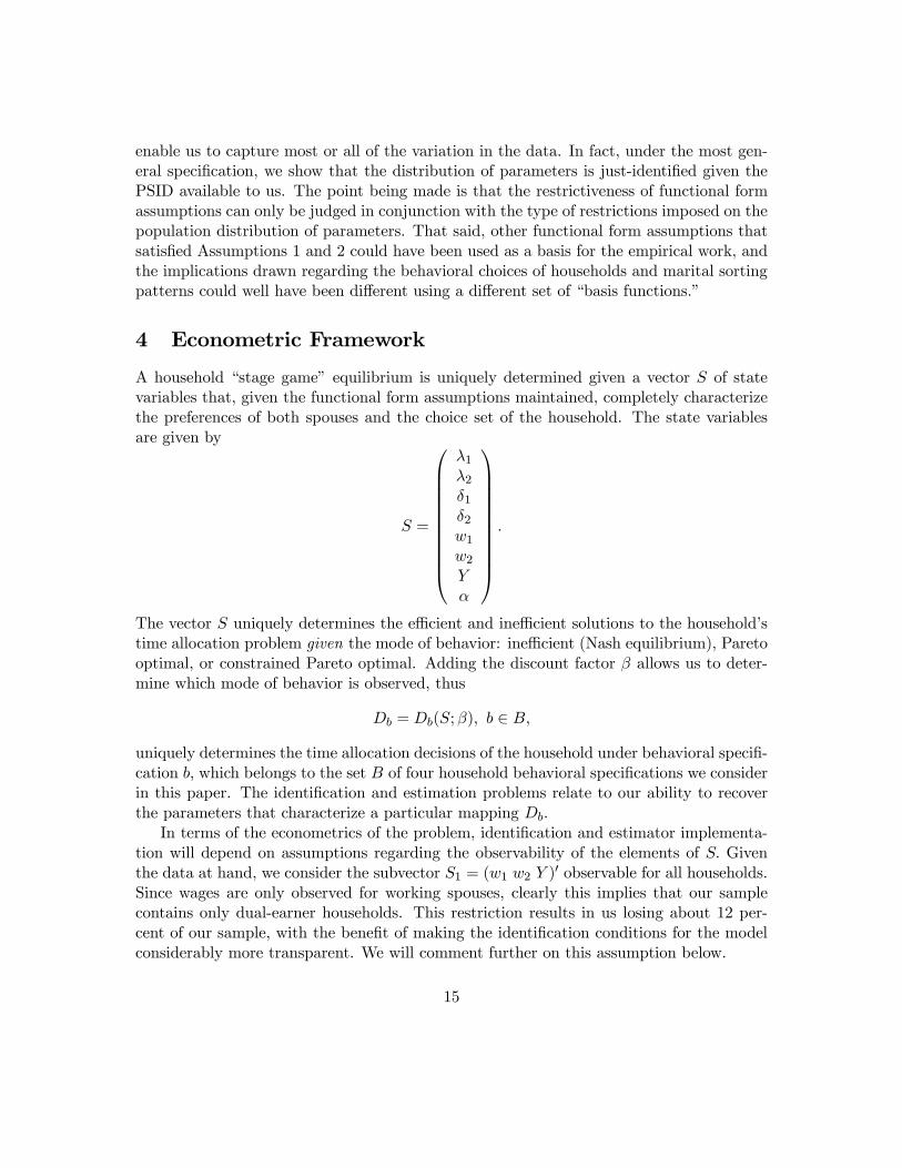
4 Econometric Framework

A household “stage game” equilibrium is uniquely determined given a vector S of statevariables that, given the functional form assumptions maintained, completely characterizethe preferences of both spouses and the choice set of the household. The state variablesare given by

S =

⎛⎜⎜⎜⎜⎜⎜⎜⎜⎜⎜⎝

λ1λ2δ1δ2w1w2Yα

⎞⎟⎟⎟⎟⎟⎟⎟⎟⎟⎟⎠.

The vector S uniquely determines the efficient and inefficient solutions to the household’stime allocation problem given the mode of behavior: inefficient (Nash equilibrium), Paretooptimal, or constrained Pareto optimal. Adding the discount factor β allows us to deter-mine which mode of behavior is observed, thus

Db = Db(S;β), b ∈ B,

uniquely determines the time allocation decisions of the household under behavioral specifi-cation b, which belongs to the set B of four household behavioral specifications we considerin this paper. The identification and estimation problems relate to our ability to recoverthe parameters that characterize a particular mapping Db.

In terms of the econometrics of the problem, identification and estimator implementa-tion will depend on assumptions regarding the observability of the elements of S. Giventhe data at hand, we consider the subvector S1 = (w1 w2 Y )0 observable for all households.Since wages are only observed for working spouses, clearly this implies that our samplecontains only dual-earner households. This restriction results in us losing about 12 per-cent of our sample, with the benefit of making the identification conditions for the modelconsiderably more transparent. We will comment further on this assumption below.

15

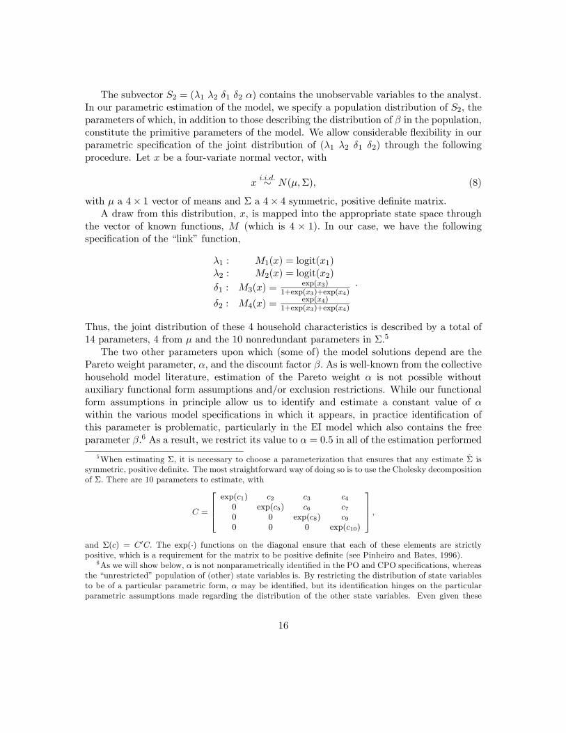
The subvector S2 = (λ1 λ2 δ1 δ2 α) contains the unobservable variables to the analyst.In our parametric estimation of the model, we specify a population distribution of S2, theparameters of which, in addition to those describing the distribution of β in the population,constitute the primitive parameters of the model. We allow considerable flexibility in ourparametric specification of the joint distribution of (λ1 λ2 δ1 δ2) through the followingprocedure. Let x be a four-variate normal vector, with

xi.i.d.∼ N(μ,Σ), (8)

with μ a 4× 1 vector of means and Σ a 4× 4 symmetric, positive definite matrix.A draw from this distribution, x, is mapped into the appropriate state space through

the vector of known functions, M (which is 4 × 1). In our case, we have the followingspecification of the “link” function,

λ1 : M1(x) = logit(x1)λ2 : M2(x) = logit(x2)δ1 : M3(x) =

exp(x3)1+exp(x3)+exp(x4)

δ2 : M4(x) =exp(x4)

1+exp(x3)+exp(x4)

.

Thus, the joint distribution of these 4 household characteristics is described by a total of14 parameters, 4 from μ and the 10 nonredundant parameters in Σ.5

The two other parameters upon which (some of) the model solutions depend are thePareto weight parameter, α, and the discount factor β. As is well-known from the collectivehousehold model literature, estimation of the Pareto weight α is not possible withoutauxiliary functional form assumptions and/or exclusion restrictions. While our functionalform assumptions in principle allow us to identify and estimate a constant value of αwithin the various model specifications in which it appears, in practice identification ofthis parameter is problematic, particularly in the EI model which also contains the freeparameter β.6 As a result, we restrict its value to α = 0.5 in all of the estimation performed

5When estimating Σ, it is necessary to choose a parameterization that ensures that any estimate Σ issymmetric, positive definite. The most straightforward way of doing so is to use the Cholesky decompositionof Σ. There are 10 parameters to estimate, with

C =

⎡⎢⎢⎣exp(c1) c2 c3 c40 exp(c5) c6 c70 0 exp(c8) c90 0 0 exp(c10)

⎤⎥⎥⎦ ,and Σ(c) = C0C. The exp(·) functions on the diagonal ensure that each of these elements are strictlypositive, which is a requirement for the matrix to be positive definite (see Pinheiro and Bates, 1996).

6As we will show below, α is not nonparametrically identified in the PO and CPO specifications, whereasthe “unrestricted” population of (other) state variables is. By restricting the distribution of state variablesto be of a particular parametric form, α may be identified, but its identification hinges on the particularparametric assumptions made regarding the distribution of the other state variables. Even given these

16

below. This is not as a severe of a restriction as it appears, since in the Constrained ParetoOptimal and Endogenous Interaction models the side constraints that the efficient solutionis required to satisfy produce, in general, a nondegenerate distribution of “ex post” valuesof α, . even if the “notational” value of α (α0) is equal to 0.5 for all households. As we willsee in the results reported below, most households end up using a value of α not equal tothe notional value of 0.5 in the CPO and EI specifications.

It is possible to allow for variability of β in the population, though for a variety ofreasons we have decided against this. Perhaps the key ingredient for forming a “cooper-ative” marriage is that both spouses be sufficiently forward-looking. Though we believethat allowing heterogeneous β within and across households should be an important goalin extending existing models of marriage market equilibrium, we sidestep sorting (on β)issues here by assuming a common value in the population. This restriction also allows usto draw some sharp conclusions when we compare the fits of the CPO and the EI modelsto the data.

4.1 Simulation-Based Estimation

Let the parameter vector of the model be given by Ω = (μ0 vec(Σ)0 ω)0, where vec(Σ) is acolumn vector containing all of the nonredundant parameters in Σ, ω is empty in the NEspecification, contains α in the PO and CPO specifications, or contains (α, β) in the EIspecification, so that Ω is a 16× 1 vector in the most “heterogeneous” model we consider.We have access to a sample of married households taken from the Panel Study of IncomeDynamics (PSID) from the 2005 wave, which we consider to a random sample from thepopulation of married households in the U.S. within a given age range. In terms of theobservable information available to us, we see the decision variables for household i,

Ai = (h1,i τ1,i h2,i τ2,i),

and we see the state variablesS1,i = (w1,i w2,i Yi).

Define the union of these two vectors, which is the vector of all of the observable variablesof the analysis, by Qi = (Ai S1,i), so that the N × 7 data matrix is

Q =

⎡⎢⎢⎢⎣Q1Q2...

QN

⎤⎥⎥⎥⎦ .restrictions, we often found that estimates of α tended to the boundary of the parameter space, whichmeant, in the case of CPO, that all outcomes where determined by the participation constraints. In sucha case, the ex ante value of α was locally not identified. These experiences led us to the prudent choice offixing the ex ante value at a point that might be consistent with social norms.

17

We choose m characteristics of the empirical distribution of Q upon which to base ourestimator. Denote the values of these characteristics by the m× 1 vector Z.

Simulation proceeds as follows. For each of the N households in the analysis, we drawNR values of x, and also β when it is included in a model specification and allowed to beheterogeneous. For simplicity, we will consider the set of simulation draws as generating(λ1 λ2 δ1 δ2 β), even when β is treated as fixed in the population. Let a given simulationdraw of these state variables be given by θi,j , i = 1, ..., N ; j = 1, ...,NR. The draws θi,jare functions of the parameter vector Ω, which we emphasize by writing θi,j(Ω). Given avalue of Ω, for each household i we solve for household decisions under behavioral modeb, (ab1,i,j , a

b2,i,j)(S1,i, θi,j) = Db(S1,i, θi,j), j = 1, ..., NR, where abs,i,j is the market labor

supply and time in household production of spouse s in household i given draws θi,j underbehavioral regime b. The time allocations associated with the simulation are stacked in anew matrix

Qb(Ω) =

⎡⎢⎢⎢⎢⎢⎢⎢⎢⎢⎢⎢⎢⎢⎢⎢⎢⎢⎢⎣

Ab1,1(Ω) S1,1...

...Ab1,NR(Ω) S1,1Ab2,1(Ω) S1,2...

...Ab2,NR(Ω) S1,2...

...AN,1(Ω) S1,N

......

AN,NR(Ω) S1,N

⎤⎥⎥⎥⎥⎥⎥⎥⎥⎥⎥⎥⎥⎥⎥⎥⎥⎥⎥⎦

,

where Abi,j(Ω) = (ab1,i,j ab2,i,j). The analogous value of Zb(Ω) is computed from the (N ×

NR) × 7 matrix Qb(Ω). Given a positive-definite, conformable weighting matrix W, theestimator of Ω is given by

Ωb = argminΩ(Z − Zb(Ω))

0W (Z − Zb(Ω)).

The weighting matrix W is computed by resampling the original data Q a total of5000 times, and for each resampling we compute the value of Z, which we denote Zk forreplication k. We then form

Z =

⎡⎢⎢⎢⎣Z1Z2...

Z5000

⎤⎥⎥⎥⎦ .W is the covariance matrix of Z. Since a major focus of our empirical investigation is acomparison of the behavioral models in B in terms of their ability to fit the sample momentsZ, it is advantageous to utilize a weighting matrix W that is not model dependent.

18

4.2 Identification

As is true of many (or most) simulation-based estimators, especially those used to estimaterelatively complex behavioral models, providing exact conditions for identification is notfeasible. Nevertheless, it may be useful to understand what features of the data gener-ating process are being used to obtain point estimates of the parameters in our ‘flexible’parametric model of the household. With this goal in mind, we proceed through a fairlycareful consideration of nonparametric identification of the first three behavioral specifi-cations. We will then discuss the reasons that the Endogenous Interaction model is notnonparametrically identified, which is the primary reason for our interest in the estimationof a flexible parametric specification of the distribution of primitive parameters.

The identification arguments we present in this section condition on observed wages,and do not allow for measurement error in any of the variables included in Qi, whichcontains the conditioning variables S1,i = (w1,i w2,1 Yi), as well as the four time allocationmeasures Ai = (h1,i τ1,i h2,i τ2,i). We begin by considering the nonparametric identificationcase. We assume that there exists a joint distribution of FS(s), with the vector S =(w1 w2 Y λ1 λ2 δ1 δ2 α β)0 in the most general model. An individual household in thePSID subsample is considered to be an i.i.d. draw from the distribution FS . No parametricassumptions on FS are made, at this point.

4.2.1 All Households Behave Inefficiently (Static Nash equilibrium)

In the case of Nash equilibrium, it is straightforward to show that the model is nonpara-metrically identified in the sense that we can define a nonparametric, maximum likelihoodestimator (NPMLE) of FS in the following (constructive) manner.

Proposition 4 The distribution FS is nonparametrically identified from Q when the be-havioral rule is static Nash equilibrium and there are no corner solutions.

Proof. The Nash equilibrium is the unique fixed point of the reaction functions of spouse 1and spouse 2 given the time allocations of the other spouse. Given that both spouses work,we observe the vector (w1,j w2,j , Yj) for all households, so that the marginal distributionFS1 is nonparametrically identified by construction. Given the observation Qj , we caninvert the reaction functions for household j to yield the two equation linear system

δ1,j =B1,j(1−B2,j)

1−B1, jB2,j

δ2,j =B2,j(1−B1,j)

1−B1, jB2,j,

where Bi,j = wi,jτ i,j/(Mj + wi,jτ i,j), with Mj = w1,jh1,j + w2,jh2,j + Yj . Given constantreturns to scale in household production, δ3,j = 1 − δ1,j − δ2,j , and we can invert the

19

remaining two equations in the system of reaction functions to obtain

λi,j =δ3,jwi,j(T − hi,j − τ i,j)

Mj + δ3,jwi,j(T − hi,j − τ i,j), i = 1, 2.

Since these values of (δ1,j , δ2,j , α1,j , α2,j) are uniquely determined by (h1,j , τ1,j , h2,j , τ2,j , w1,j , w2,j , Yj),we “observe” the complete vector of values Sj = (w1,j w2,j Yj λ1,j λ2,j δ1,j δ2,j), and thenonparametric maximum likelihood estimator of FS is the empirical distribution of SjNj=1.

Note that the restriction of no corner solutions is essential in our ability to nonpara-metrically identify the model. Say that, for example, h1,j = 0. Even if the offered wage w1,jwere available, an unlikely event, there would exist a set of values of λ1,j consistent with theobserved choices and the observed state variables, with no way to assess the likelihood ofany value in the set relative to that of any other. In the presence of any kind of truncationor censoring, nonparametric point identification of the complete distribution is typicallyimpossible, since some functional form assumptions are required to assign likelihoods oversets of values of parameters consistent with observed outcomes.

4.2.2 All Households Behave Efficiently

Proposition 5 The distribution FS is nonparametrically identified from Q when the be-havioral rule is Pareto efficiency, there are no corner solutions, data points are consistentwith the model, and α is known.

Proof. Household time allocation is determined by solving the system of four first orderconditions associated with (7). We find that

δ1j =B1j(1−B2,j)

1−B1jB2,j

δ2j =B2j(1−B1,j)

1−B1jB2,j,

the same as in the Nash equilibrium case. Conditional on these values of δ1j and δ2j (⇒δ3j = 1− δ1j − δ2j under the CRS assumption) and a value of α, we find

λ1j =1

αR1j

λ2j =1

1− αR2j

where

R1j ≡C1j(1− C2j)

1−C1jC2j

R2j =C2j(1− C1j)

1−C1jC2j.

20

and

C1j =δ3jw1j(T − h1j − τ1j)

δ3jw1j(T − h1j − τ1j) +Mj

C2j =δ3jw1j(T − h2j − τ2j)

δ3jw2j(T − h2j − τ2j) +Mj.

The values of C1j and C2j lie in the unit interval for all j, which implies that λ1j andλ2j are always positive. However, for given values of α and all other state variables andchoice variables, either or both λ1j and λ2j may not belong to the open unit interval. Inthis case, the data for household j are not consistent with the model and are not used inthe estimation of FS , which is the empirical distribution of Sjj∈κ , where κ is the set ofhousehold indices for which λ1j and λ2j both belong to the open unit interval.

We found that the implied values of λ1j and λ2j belonged to the unit interval for all ofthe sample cases. In the proposition, in constructing the NPMLE for FS we specified thatonly implied values of the preference parameters that satisfied our theoretical restrictionswould be utilized. One could argue that the satisfaction of theoretical restrictions shouldbe treated as a necessary condition for defining the estimator, instead. In this particularapplication, we did not have to explicitly confront this problem.

4.2.3 Constrained Efficient Case

The constrained efficient case imposes a side constraint on the efficient solution, one whichinsures that each spouse attains a utility value at least as large as what could be obtainedin the inefficient, Nash equilibrium case. This makes the mapping from the observed timeallocations and observed state variables into the unobserved state variables more complex.However, we are able to establish the following result

Proposition 6 The distribution FS is nonparametrically identified from Q when the be-havioral rule is Constrained Pareto efficiency, there are no corner solutions, data pointsare consistent with the model, and α is known.

Proof. As we showed in the proof of the nonparametric identification of the Pareto weightcase, inverting the system of first order conditions for household j yields solutions for δ1jand δ2j which are not functions of α, while

λ1j =R1jα

λ2j =R2j1− α

,

where Rij is a positive-valued function of the data, i = 1, 2. A feasible value of α forhousehold j must satisfy the conditions

UPij (α) ≥ UN

ij , i = 1, 2,

21

where UPij (α) is individual i

0s utility at the efficient solution when the Pareto weight is αand UN

ij is that individual’s utility in the inefficient equilibrium. This condition can bewritten

Dij(α) = λi(ln lPij − ln lNij ) + (1− λi)(lnK

PWj − lnKN

j ) ≥ 0, i = 1, 2.

Now, conditional on δ1j and δ2j , which are not a function of α, and R1j and R2j , any givenvalue of α implies values of λ1j and λ2j , with

∂λ1j∂α

= −R1jα2

< 0

∂λ2j∂α

=R2j

(1− α)2> 0.

Partially differentiating Dij with respect to α, we have

∂(UPij (α)− UN

ij )

∂α=

∂λij∂α

(ln lPij − ln lNij )−λij

lNij∂lNij∂λ1j

∂λ1j∂α

+∂lNij∂λ2j

∂λ2j∂α

− ∂λij∂α

(lnKPj − lnKN

j )−1− λij

KNj

∂KN

j

∂λ1j

∂λ1j∂α

+∂KN

j

∂λ2j

∂λ2j∂α

, i = 1, 2.

Note that∂UP

ij (α)

∂α

¯¯R1j ,R2j ,Bi1,B2j

= 0,

since the first order conditions for the Pareto weight problem are characterized in termsof these values, not the preference and production parameters and α individually. This isthe reason that only partial derivatives involving the Nash equilibrium values of householdchoices are present. For any values of (λ1, λ2, δ1, δ2, w1, w2, Y ), lPij ≤ lNij , i = 1, 2, andKPj ≥ KN

j . Consider individual 1, for example. In this case,

∂lN1j∂λ1j

≥ 0

∂lNij∂λ2j

≤ 0,

while

∂KNj

∂λ1j≤ 0

∂KNj

∂λ2j≤ 0,

22

which implies that∂D1j(α)

∂α≥ 0.

A similar argument yields∂D2j(α)

∂α≤ 0.

Finally, it must be the case that if one individual is indifferent at the efficientsolution, the other individual must be strictly better off. Thus D1j = 0 ⇒ D2j > 0 andD2j = 0⇒ D1j > 0. Then D1j and D2j intersect at a value of α, α say, where D1j(α) > 0and D2j(α) > 0. The set of all feasible values of α is connected, and is given by

αFj = [αj , αj ],

where αj is defined by D1j(αj) = 0 and αj is defined by D2j(αj) = 0. The values of allprimitive parameters, given the known, notional Pareto weight value α0, are determinedfrom the ex post value of α, defined as

α =

⎧⎨⎩αj if α0 < αjα0 if α0 ∈ αF

αj if α0 > αj

.

The “data” for household j are given by the observed state variables wij , w2j , and Yj , andthe primitive parameters λ1j(α) = R1j/α, λ2j(α) = R2j/(1 − α), δ1j , and δ2j . Under ourrandom sampling assumption, the empirical c.d.f. of these variables is the nonparametricmaximum likelihood estimator of FS.

4.2.4 Endogenous Interaction Case

We cannot show that FS is nonparametrically identified in the EI case; in fact, it is straight-forward to provide counterexamples to show that it is not. We can continue to assumethat the technology parameters are uniquely determined without reference to the behav-ioral regime or value of α used in efficient cases. The fundamental identification problemsthen concern the discount factor β and the preference parameters, λ1 and λ2.

Since we could not identify the notional value of α0 nonparametrically, it comes as nosurprise that the same is true of β. We know that if β = 0, no efficient allocations can besupported, and the resulting time allocations are all generated in NE. Conversely, as β →1, all households make efficient time allocation decisions, and the preference parametersimplied by the data are those generated under CPO. Both sets of values of the preferenceparameters are one-to-one mappings from the data, so we have two separate estimators ofFS.

Unfortunately, the lack of identification result continues to hold even after fixing β atsome predetermined value β0. Having a notional value of α, α0, and a fixed value of β, β0,

23

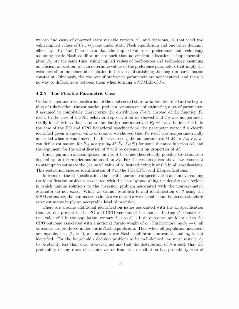
we can find cases of observed state variable vectors, S1, and decisions, A, that yield twovalid implied values of (λ1, λ2), one under static Nash equilibrium and one other dynamicefficiency. By “valid” we mean that the implied values of preferences and technologyassuming static Nash equilibrium are such that no efficient allocation is implementablegiven β0. At the same time, using implied values of preferences and technology assumingan efficient allocation, we can determine values of the preference parameters that imply theexistence of an implementable solution in the sense of satisfying the long-run participationconstraint. Obviously, the two sets of preference parameters are not identical, and there isno way to differentiate between them when forming a NPMLE of FS.

4.2.5 The Flexible Parametric Case

Under the parametric specification of the unobserved state variables described at the begin-ning of this Section, the estimation problem becomes one of estimating a set of parametersθ assumed to completely characterize the distribution FS(θ), instead of the function FSitself. In the case of the NE behavioral specification we showed that FS was nonparamet-rically identified, so that a (nonredundantly) parameterized FS will also be identified. Inthe case of the PO and CPO behavioral specifications, the parameter vector θ is clearlyidentified given a known value of α since we showed that FS itself was nonparametricallyidentified when α was known. In this case, using the nonparametric MLE for FS , FS , wecan define estimators for θM = argminθM(FS , FS(θ)) for some distance function M, andthe argument for the identification of θ will be dependent on properties of M.

Under parametric assumptions on FS , it becomes theoretically possible to estimate αdepending on the restrictions imposed on FS . For the reasons given above, we chose notto attempt to estimate the (ex ante) value of α, instead fixing it at 0.5 in all specifcations.This restriction ensures identification of θ in the PO, CPO, and EI specifications.

In terms of the EI specification, the flexible parametric specification aids in overcomingthe identification problems associated with this case by smoothing the density over regionsin which unique solutions to the inversion problem associated with the nonparametricestimator do not exist. While we cannot establish formal identification of θ using theMSM estimator, the parameter estimates we obtain are reasonable and bootstrap standarderror estimates imply an acceptable level of precision.

There are a some additional identification issues associated with the EI specificationthat are not present in the PO and CPO versions of the model. Letting β0 denote thetrue value of β in the population, we saw that as β → 1, all outcomes are identical to theCPO outcome associated with a notional Pareto weight of α0. Furthermore, as β0 → 0, alloutcomes are produced under static Nash equilibrium. Then when all population membersare myopic, i.e., β0 = 0, all outcomes are Nash equilibrium outcomes, and α0 is notidentified. For the household’s decision problem to be well-defined, we must restrict β0to be strictly less than one. However, assume that the distribution of S is such that theprobability of any draw of a state vector from this distribution has probability zero of

24

resulting in a static Nash equilibrium outcome for any value of β ∈ (1− ε, 1), where ε is asmall positive constant. Then if 1− ε < β0 < 1, all observed outcomes will be associatedwith the CPO solution, α0 will be identified, but β0 will not be point-identified. Thus, wehave two extreme cases of local nonidentification in the EI specification. When β0 is 0, orabitrarily close to zero, α0 is not identified. When β0 is arbitrarily close to 1, β0 is notpoint identified, but α0 is identified. When β0 assumes “intermediate” values, so that themeasure of noncooperative households in the population is not equal to 0 or 1, then bothare, in principle at least, identified under parametric restrictions on FS . In the estimates ofthe EI specification reported below, we find that the estimate of β is one which produces aproper mixture distribution, i.e., the estimates imply that a measurable set of householdsare in the cooperative and noncooperative regimes.

5 Empirical Results

We begin this section by presenting the sample selection criteria used in creating thefinal sample from the PSID with which we work. This is followed by a discussion of theestimates of the distributions of primitive parameters in the “nonparametric” analysis forthe three identified models: Nash equilibrium, Pareto efficiency, and Constrained Paretoefficiency. We then move on to our focus of interest, which are the estimates from theflexible parametric analysis.

5.1 Sample Selection Criteria and Descriptive Statistics

We use sample information from the 2005 wave of the PSID. All models are essentiallystatic, and therefore we only utilize cross-sectional information from this wave of the survey.We only considered households in which the head was married, with the spouse present inthe household. In this wave, the PSID obtained the standard information regarding usualhours of work over the previous year for both spouses, and this information correspondsto h1 and h2 in the model. Every few years, the PSID also includes a question regardingthe usual hours devoted to housework by each spouse, and this information is included inthe 2005 wave. The responses to these items are interpreted as τ1 and τ2 in the model.These time allocation questions are regarded as referring to the same time period. We usetotal hours worked from the previous year and labor earnings for each spouse to infer awage rate, wi for spouse i. In addition, information is available on the nonlabor income ofthe spouses over the previous year, and we divide this amount by 52 to obtain a weeklynonlabor income level, Y.

We only utilize information from households in which both spouses are between the agesof 30 and 49, inclusive. In addition to this age requirement, we excluded all householdswith any child less than 7 years of age, since the household production function is likelyto be far different when small children are present. We also excluded couples with whatwe considered to be excessively high time allocations to housework and the labor market,

25

namely, those with over 100 hours combined in these two activities. We selected this amountsince we set T = 112, which we arrived at by assuming 16 hours to allocate to leisure,housework, and the labor market for each of the seven days in a week. We also excludedhouseholds reporting a nonlabor income level of more than $1000 a week, on the groundsthat such people were likely to be generating a significant amount of self-employmentincome, making the labor supply information they supplied difficult to interpret. Notmany households were lost to this exclusion criterion.

By far the most significant sample selection criterion we imposed was the one requiringboth spouses to work. If a spouse does not work, then clearly we have no wage informationfor that spouse, making the nonparametric analysis we discuss above and report on belowimpossible to implement. Within the flexible parametric estimator we implement, it wouldbe possible to allow for corner solutions in labor supply if we are willing to impose aparametric assumption regarding the wage offer process.7 While this allows for more modelgenerality, in principle, it comes at the expense of having to take a position on the partiallyunobservable wage process. We chose to follow the route of ruling out corner solutions,allowing us to condition all of our analysis on observed wages. Because we restricted ourattention to households without small children, imposing the condition that both spousessupply time to the market resulted in a reduction of 12 percent in our (otherwise) finalsample. We were left with 823 valid cases, which were those satisfying the conditions statedabove and with no missing data on any of the state and decision variables included in theanalysis.

A description of the decisions and state variables is contained in Table 1. As hasbeen often remarked upon in other analyses of household behavior that include time inhousework, the average time spent in the both housework and labor supply to the marketis very similar for husbands and wives. On average, husbands spend approximately 7 hoursmore per week in the labor market than their (working) wives, but devote 7 hours less tohousework. Under our assumption that each spouse has 112 ‘disposable’ hours of time toallocate each week, on average each spouse spends slightly more than one-half of their timeconsuming leisure. We also note that the wives’ distributions of hours in the market andhousework are much more disperse than the corresponding distributions of husbands. Interms of market work, this is undoubtedly due to the fact that married women are muchmore likely to be employed in part-time work than their husbands (see, e.g., Mabli (2007)).The limited amount of variation in the distribution of husbands’ housework is mainly dueto the floor effect - most observations are clustered in the neighborhood of zero.

In terms of the observed state variables of the analysis, the mean wage of husbands isapproximately 39 percent greater than the mean wage of wives, and exhibits considerablymore dispersion, some of it due to the presence of a few wage outliers among the husbands(the maximum wage of wives is $80.50, while the maximum wage of husbands is $144.93).

7This was precisely what was done in an earlier version of this paper, when we only considered laborsupply in a model without a household production component.

26

Average weekly nonlabor income of the household is $118.15, and this distribution is quitedisperse, even though the sample is restricted to households receiving no more than $1000of nonlabor income per week. No nonlabor income is reported by 27 percent of samplehouseholds.

Table 2 contains the zero-order correlation matrix of the variables reported in Table 1.There is no correlation between the labor supply and housework of husbands, while thereis a reasonably strong negative correlation (-0.189) between them for wives. There is astrong positive correlation (0.321) between the times spent in housework by husbands andwives. The wage of a husband and the labor supply of his wife have a negative correlationof -0.132, while wives with high wages tend to spend less time in housework. There areno particularly noteworthy correlations between household nonlabor income and othervariables in the analysis, with the possible exception of the husband’s wage (0.115). Thecorrelation between the wages of the spouses (0.294) indicates positive assortative matingin the marriage market.

5.2 Nonparametric Estimation of the Distribution of State Variables

Under the Nash equilibrium, Pareto efficient, and constrained Pareto efficient modelingassumptions, we were able to obtain estimates of the distributions of S in our sample.In all cases other than static Nash equilibrium, we established that the Pareto weightparameter α was not identified. Accordingly, in all of these models, we simply assumethat the ‘notional’ Pareto weight is 0.5. Of course, the Nash equilibrium solution is not afunction of the parameter α.

In Section 4.2.2, we noted that the mapping from the time allocation decisions andthe observed state variables, the wages of the spouses and household nonlabor income, didnot necessarily produce values of the preference parameters λ1 and λ2 contained in (0, 1).Nevertheless, all of our 823 sample cases generated values of λ1 and λ2 in the unit interval,so that all cases are used to generate ‘data’ on preferences and household productionparameters that are used to form the nonparametric estimator of FS.

Table 3 contains estimates of the means and standard deviations of the marginal dis-tributions of preference and production parameters of the model under the three estimablebehavioral specifications. As discussed above, under our functional form assumptions onpreferences and household production, the implied value of the production parameters δ1jand δ2j for household j are the same functions of the decisions of household j, Dj , and theobserved state variables for household j, S1j , for each of the three behavioral models forwhich we obtain nonparametric estimates of FS . This explains the fact that the estimatedmeans and standard deviations of the production parameters are identical across the threebehavioral specifications. We note that wives have a higher average productivity in house-hold production than husbands, with the mean for wives being about 41 percent larger.There is also slightly more dispersion in the wives’ productivity parameter.

Large differences are observed across the three specifications in terms of the distribution

27

of the preference parameters. Given that the Nash equilibrium outcomes are inefficient, it isnot surprising to find that the means of the preference parameters under Nash equilibriumare considerably less than they are under constrained or unconstrained Pareto efficiency. Inall three behavioral cases, the average weight placed on the private good, leisure, is smallerfor wives than their husbands. In the unconstrained Pareto weight case, the average weightplaced on leisure by husbands is 0.580, in comparison with an average leisure weight of 0.430for wives. There are similar levels of dispersion in the distributions of preference parametersfor husbands and wives across the three behavioral specifications.

Comparing estimates across columns two and three, it is interesting to note that theconstraint that the payoffs under the efficient solution are at least as large as the payoffsunder Nash equilibrium for both spouses is binding for a number of sample cases given thenotional value of α = 0.5. This is evidenced by the differences in the preference parameterdistributions. Imposing this particular constraint narrows the difference in the mean ofspousal preference parameters, while reducing dispersion as well.

Recall that all three estimates of FS, are equally “valid,” and no statistical criterioncan be used to distinguish between the behavioral specifications given that they are allbased on (different) one-to-one mappings from the data and observed state space to theunobserved state space. In the next section, when we make flexible parametric assumptionsregarding the distributions of the parameters, we will be able to compare the performanceof the various behavioral models, including the Endogenous Interaction specification.

5.3 Parametric Estimation of the Distribution of State Variables

Before looking at the estimates produced by the parametric estimator under the four be-havioral specifications, it may be worthwhile to consider why we expect them to differto some degree from the nonparametric estimators of FS discussed in the preceding sub-section. First, we have assumed that the distribution of the state variables (subvector)S2 = (λ1 λ2 δ1 δ2) is independent of the state variables S1 = (w1 w2 Y ). This is a strongassumption, but without specifying some form of parametric dependence between S2 andS1, it would not be possible to relax it. There are reasons to doubt the validity of theindependence assumption. For example, a spouse i with a low value of leisure might haveworked and invested more in the past, so that wi and Y may be negatively related to λi.To fully account for such dependencies, we would require a life cycle household model withcapital accumulation, which is beyond the scope of the current paper.

Second, while our parametric specification of the distribution of S2 is reasonably flex-ible, it does impose restrictions on the data. These restrictions are what allow us to saysomething about the relative abilities of the four different behavioral specifications to fitthe data. Nevertheless, different parametric specifications of the distribution of S2 couldlead to different inferences concerning which behavioral framework is most consistent withthe data features chosen for the MSM estimator.

In implementing any moments-based estimator, the analyst faces the problem of choos-

28

ing which moments to utilize in defining the estimator. We have used a set of 23 momentsthroughout, and never made any change to this set in the course of the estimation process.The list of moments appears in Table A.1, and is reasonably standard. It includes themeans and standard deviations of all of the endogenous variables, as well as some cross-products terms involving the endogenous variables, and some involving the observed statevariables of the household, wages and nonlabor income. The last few moments listed inthe table pick up some distributional features of the labor market hours distributions notcaptured solely by the first two moments of the distribution.

Table 4 contains the MSM estimates of the four behavioral specifications. The estimatespresented were computed as follows. We obtained point estimates of the 14 parametersused to characterize the distribution of S2 for each of the four specifications. We thentook a large number of draws (one million) from the estimated distribution of S2, andcomputed the means and standard deviations of each of the components of the vector S2.In the EI specification, we also estimated the discount factor β, which was constrained tobe homogeneous in the population. For the CPO and EI specifications, we also computedthe (ex post) Pareto weight at which the efficient outcome was implemented for each drawin the simulation process. The means and standard deviations of the ex post α distributionare presented for the CPO and EI specifications..The last row in the table reports the valueof the distance metric for the model; obviously, a lower value indicates that the model isable to better fit the selected moments at the optimally-chosen parameter estimates.

The Nash equilibrium specification produces estimates of the mean values of the prefer-ence parameters, λ1 and λ2, roughly in accord with those produced by the nonparametricestimator, though the mean value of the preference weight on leisure of the wife is almostequal to that of the husband. While the mean value of λ1 is similar for the two estimators,the estimated dispersion in λ1 is about 50 percent greater when the parametric estimatoris used. The estimated mean of λ2 is significantly higher in the parametric case, as is theestimated dispersion in this parameter. The estimated distributions of production func-tion parameters are quite a bit different under the flexible parametric estimator and thenonparametric one. We still find that, on average, wives are more productive in houseworkthan their husbands, but the difference in the means is now a bit larger than was the caseusing the nonparametric estimator (0.068 versus 0.046). The parametric estimator pro-duces a lower amount of dispersion in δ1 and δ2 than does the nonparametric estimator.Our sense is that a substantial amount of these differences are due to the restriction thatthe state variables in S2 are independently distributed with respect to S1 that is imposedusing the parametric estimator and that is not imposed under the nonparametric estimator,rather than arising from the parametric restrictions on the distribution of S2, per se.8

The first two moments of S2 estimated under the assumption of Pareto efficiency are

8We performed some experimentation with making the mean vector of the 4 variate normal that generatesthe primitive parameters a linear function of the 3 observed state variables w1, w2, and Y.We concludedthat it was too difficult to precisely estimate this conditional mean specification, and so stayed with thespecification that assumes independence between S1 and S2.

29

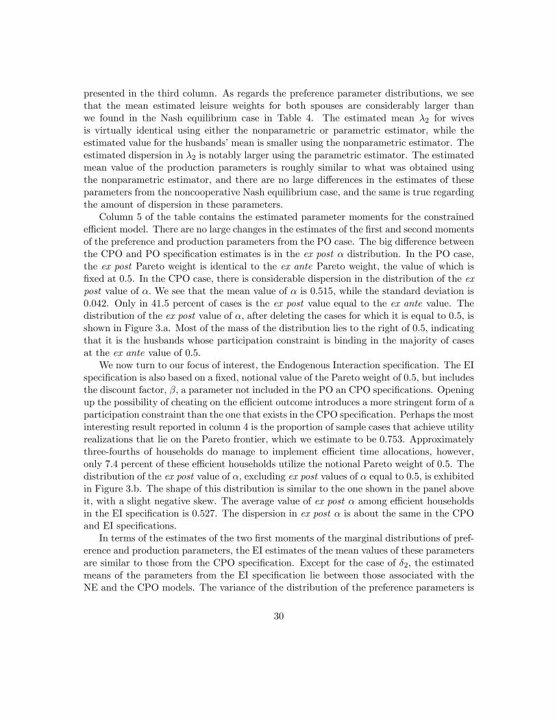
presented in the third column. As regards the preference parameter distributions, we seethat the mean estimated leisure weights for both spouses are considerably larger thanwe found in the Nash equilibrium case in Table 4. The estimated mean λ2 for wivesis virtually identical using either the nonparametric or parametric estimator, while theestimated value for the husbands’ mean is smaller using the nonparametric estimator. Theestimated dispersion in λ2 is notably larger using the parametric estimator. The estimatedmean value of the production parameters is roughly similar to what was obtained usingthe nonparametric estimator, and there are no large differences in the estimates of theseparameters from the noncooperative Nash equilibrium case, and the same is true regardingthe amount of dispersion in these parameters.

Column 5 of the table contains the estimated parameter moments for the constrainedefficient model. There are no large changes in the estimates of the first and second momentsof the preference and production parameters from the PO case. The big difference betweenthe CPO and PO specification estimates is in the ex post α distribution. In the PO case,the ex post Pareto weight is identical to the ex ante Pareto weight, the value of which isfixed at 0.5. In the CPO case, there is considerable dispersion in the distribution of the expost value of α. We see that the mean value of α is 0.515, while the standard deviation is0.042. Only in 41.5 percent of cases is the ex post value equal to the ex ante value. Thedistribution of the ex post value of α, after deleting the cases for which it is equal to 0.5, isshown in Figure 3.a. Most of the mass of the distribution lies to the right of 0.5, indicatingthat it is the husbands whose participation constraint is binding in the majority of casesat the ex ante value of 0.5.

We now turn to our focus of interest, the Endogenous Interaction specification. The EIspecification is also based on a fixed, notional value of the Pareto weight of 0.5, but includesthe discount factor, β, a parameter not included in the PO an CPO specifications. Openingup the possibility of cheating on the efficient outcome introduces a more stringent form of aparticipation constraint than the one that exists in the CPO specification. Perhaps the mostinteresting result reported in column 4 is the proportion of sample cases that achieve utilityrealizations that lie on the Pareto frontier, which we estimate to be 0.753. Approximatelythree-fourths of households do manage to implement efficient time allocations, however,only 7.4 percent of these efficient households utilize the notional Pareto weight of 0.5. Thedistribution of the ex post value of α, excluding ex post values of α equal to 0.5, is exhibitedin Figure 3.b. The shape of this distribution is similar to the one shown in the panel aboveit, with a slight negative skew. The average value of ex post α among efficient householdsin the EI specification is 0.527. The dispersion in ex post α is about the same in the CPOand EI specifications.

In terms of the estimates of the two first moments of the marginal distributions of pref-erence and production parameters, the EI estimates of the mean values of these parametersare similar to those from the CPO specification. Except for the case of δ2, the estimatedmeans of the parameters from the EI specification lie between those associated with theNE and the CPO models. The variance of the distribution of the preference parameters is

30

less than under any of the other specifications estimated. This may be attributable to thefact that a lower level of heterogeneity in the primitive parameters is capable of generatingthe same amount of variability in household allocations given the additional variabilityproduced by the two sets of decision rules (efficient and inefficient).

To induce any households to behave inefficiently, a relatively low value of β is required,and our point estimate is 0.524, which we interpret as referring to a yearly period, since thedata refer to a representative week in 2004, and we think of participation decisions beingmade on a yearly basis. While the estimate of β is ‘low,’ it is not very much out of linewith respect to other estimates of the subjective rate of discount found in the experimentaland microeconomics literature (see, for example, Hausman (1979) and Thaler (1981)). Thecompilation of estimates of time preference performed by Frederick et al. (Table 1, 2002)is striking for the huge range of values of the subjective discount rate that have beenfound using both experimental and empirical methods. To our knowledge, this is the firstapplication to attempt to use a formal model with a grim trigger strategy to estimatea discount factor, so there are no other studies with which we can directly compare ourestimate.9 ,10

We now compare the model fits across the four specifications. The first three specifica-tions contain the same number of free parameters, which are 14. The EI specification alsoincludes the parameter β. Thus the fits of the first three models are very much directlycomparable, since the parameter space is identical. We see that, under the restriction thatthe notional value of α = 0.5, the fit of the PO specification is the worst, followed by theNE specification, and then CPO. The EI specification produces a marked increase in theability of the model to fit the data features we have selected. Recall that the EI specifica-tion nests the NE and CPO models as special cases. As β → 0, no efficient solutions couldbe supported, so all households would behave in an innefficient manner, with allocationsgiven by the Nash equilibrium values. As β → 1, all households will behave efficiently, withthe only constraint on the allocations being that they satisfy the participation constraint,which imposes the restriction on α associated with the CPO specification. Moving β from avalue of 1 (implicit in the CPO specification) to 0.524 results in a reduction in the distancemetric of 14 percent. Moving β from a value of 0 (implicit in the NE specification) to0.524 results in a reduction of almost 20 percent. The estimate of β we obtained suggeststhat the “cheating” problem is an important one in determining observed household timeallocations.

In order to conduct a more proper “horse race” between the models, we need to compare

9Porter (1983) and Lee and Porter (1983) estimate a switching regressions model motivated by thetrigger price strategy model of Green and Porter (1984). In that model of collusive behavior with imperfectsignals regarding other agents’ actions, a noncooperative punishment period is enterred whenever publicsignals indicate a high probability of cheating. The punishment period is determined endogenously, and atits termination another collusive regime is begun. The econometric framework used in the two empiricalpapers cited does not allow one to back out an estimate of the discount factor of firms.10 In addition, as one referee has noted, the discount factor may incorporate the “death” rate of marriages,

in the simple case where we consider this to be exogenous and constant.

31

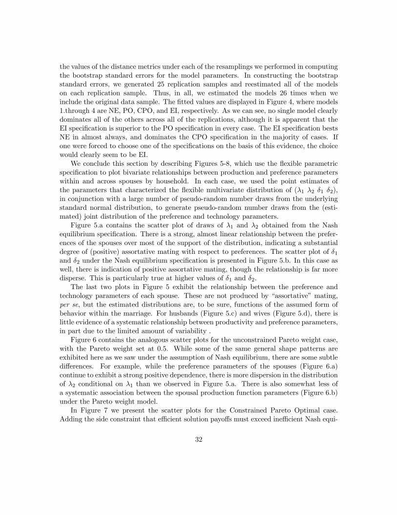
the values of the distance metrics under each of the resamplings we performed in computingthe bootstrap standard errors for the model parameters. In constructing the bootstrapstandard errors, we generated 25 replication samples and reestimated all of the modelson each replication sample. Thus, in all, we estimated the models 26 times when weinclude the original data sample. The fitted values are displayed in Figure 4, where models1.through 4 are NE, PO, CPO, and EI, respectively. As we can see, no single model clearlydominates all of the others across all of the replications, although it is apparent that theEI specification is superior to the PO specification in every case. The EI specification bestsNE in almost always, and dominates the CPO specification in the majority of cases. Ifone were forced to choose one of the specifications on the basis of this evidence, the choicewould clearly seem to be EI.

We conclude this section by describing Figures 5-8, which use the flexible parametricspecification to plot bivariate relationships between production and preference parameterswithin and across spouses by household. In each case, we used the point estimates ofthe parameters that characterized the flexible multivariate distribution of (λ1 λ2 δ1 δ2),in conjunction with a large number of pseudo-random number draws from the underlyingstandard normal distribution, to generate pseudo-random number draws from the (esti-mated) joint distribution of the preference and technology parameters.

Figure 5.a contains the scatter plot of draws of λ1 and λ2 obtained from the Nashequilibrium specification. There is a strong, almost linear relationship between the prefer-ences of the spouses over most of the support of the distribution, indicating a substantialdegree of (positive) assortative mating with respect to preferences. The scatter plot of δ1and δ2 under the Nash equilibrium specification is presented in Figure 5.b. In this case aswell, there is indication of positive assortative mating, though the relationship is far moredisperse. This is particularly true at higher values of δ1 and δ2.

The last two plots in Figure 5 exhibit the relationship between the preference andtechnology parameters of each spouse. These are not produced by “assortative” mating,per se, but the estimated distributions are, to be sure, functions of the assumed form ofbehavior within the marriage. For husbands (Figure 5.c) and wives (Figure 5.d), there islittle evidence of a systematic relationship between productivity and preference parameters,in part due to the limited amount of variability .

Figure 6 contains the analogous scatter plots for the unconstrained Pareto weight case,with the Pareto weight set at 0.5. While some of the same general shape patterns areexhibited here as we saw under the assumption of Nash equilibrium, there are some subtledifferences. For example, while the preference parameters of the spouses (Figure 6.a)continue to exhibit a strong positive dependence, there is more dispersion in the distributionof λ2 conditional on λ1 than we observed in Figure 5.a. There is also somewhat less ofa systematic association between the spousal production function parameters (Figure 6.b)under the Pareto weight model.

In Figure 7 we present the scatter plots for the Constrained Pareto Optimal case.Adding the side constraint that efficient solution payoffs must exceed inefficient Nash equi-

32

librium payoffs has a negligible impact on the relationships between the parameters thatwe have already observed for the previous two cases. The strong positive relationship be-tween preference parameters of the spouses is similar to what was observed in the NE case(Figure 7.a), while the relationship between productivity parameters (Figure 7.b) is some-what intermediate to the two cases already discussed. Once again, there is some indicationof a negative relationship between the husband’s productivity and preference parameters(Figure 7.c).

Our preferred specification, that of Endogenous Interaction, yields implied associationsbetween parameters somewhat intermediate to the others we have examined to this point.The association between preference parameters is positive and approximately linear, aswas true in the other cases. The support of the distribution is smaller than was the casepreviously. There is fairly clear positive dependence between the productivity parametersof the spouses (Figure 8.b). Once again, we see that there is a negative relationship betweenλ1 and δ1 in the population (Figure 8.c) and no indication of a relationship between λ2and δ2 (Figure 8.d).

5.4 Welfare Implications of the Analysis

Our estimates of the distributions of the unobserved state variables, used in conjunctionwith the observed state variables in the data, allow us to examine the implied joint distrib-ution of spousal welfare within our sample. We follow the methodology used in computingthe scatter plots described above to compute the intrahousehold welfare levels. For house-hold j in the sample, defined in terms of (w1j w2j Yj), we draw 1000 values of the unobservedstate variable from the estimated distribution under behavioral regime k. Given the entirestate variable vector, we compute time allocations under behavioral rule k, and then theutility level of each spouse. We then plot the utility levels (u1, u2) for each state variablevector under the four behavioral regimes. The results are shown in Figure 9.

In all four behavioral regimes, there is a very strong relationship between the attainedutility levels of the spouses. This is not totally unexpected given the specifications ofthe utility and household production functions, which posit that all consumption in thehousehold, aside from leisure, is public. Nonetheless, the specification in and of itself doesnot specify the preference weights associated with the public good, which, in principle,could have been small.

Within each figure we see that a strong majority of the points lie above the 45-degreeline, indicating that wives have a somewhat higher payoff on average under our cardinalutility representation. If husbands and wives were perfectly symmetric, in the sense thatλ1 = λ2, δ1 = δ2, and w1 = w2, then all utility outcomes in each figure should lie onthe 45-degree line. In Figures 8.b through 8.d, where the outcomes involve the Paretoweight parameter α, even under perfect symmetry of preferences, productivity, and wages,values of α different than 0.5 will produce outcomes off of the 45-degree line. Since thenotional Pareto weight is always set to 0.5, utility realizations are produced by asymmetry

33

in spousal characteristics, both observed and unobserved.The plot of utility payoffs for the Endogenous Interaction case (Figure 9.d) is somewhat

interesting, in that the utility values are somewhat more highly related than in the other“cooperative” cases (Figures 9.b and 9.c). We attribute this to the presence of a “tighter”participation constraint for both partners, which limits the ability of either spouse toextract an inordinate share of the surplus. The correlation between welfare outcomes ishighest in the Nash equilibrium case and lowest in the unconstrained Pareto environment.

5.5 Comparative Statics Exercise

We conclude the empirical analysis with another look at the importance of the discountfactor in determining household outcomes. As we have emphasized at several points, theNE and CPO specifications are special cases of EI. When β is approximately equal to 0,all outcomes are determined in noncooperative Nash equilibrium, and the solutions areidentical to those associated with NE. When β is arbitrarily close to 1, all outcomes areassociated with CPO, meaning all households behave in an efficient manner. Our estimateof β, taken together with our estimates of the distribution of primitive parameters, impliedthat about one-fourth of households behaved inefficiently.

In this exercise, we utilize the estimate of the distribution of the primitive parametersunder the EI specification to examine the impact of changing β on household decisions and(current period) utility. To do this, we generated data under the model estimates for 99values of β, beginning with 0.01 and ending with 0.99. For each simulation, we computedthe mean values of household time allocations and current period utility levels for each ofthe spouses. The results are presented in Figure 10.

Figure 10.a plots the average hours in the market by spouse over the range of β. Wenotice that the curves are flat until β increases to approximately 0.42; this is due to thefact that all households are in the noncooperative regime and time allocations in thisregime are independent of β. As β increases beyond 0.42, the proportion of householdsable to implement efficient allocations is steadily increasing; beyond a β value of 0.52,all (simulated) households are able to behave efficiently. As a result, we see the largestchange in market labor supply over the range 0.42 to 0.52, where average hours of workin the market goes up by over one-third for husbands and wives. For β > 0.52, when allhouseholds are behaving efficiently, changes in β merely change the constraint set facingthe household members. The average effect of these changes is more beneficial for wivesthan for husbands, as we can see from Figure 10.c, which plots average (period) utility. Asβ increases over the “cooperative” range, the labor supply of wives is falling while that ofhusbands is increasing. In terms of time spent in housework (Figure 10.b), the time spentin housework by wives is increasing over this range, until it flattens out when β reaches0.8. The housework of males is constant when β reaches the value 0.55 (approximately).

These results indicate the importance of the discount factor in household labor supplydecisions. Even though we found that all households were able to reach the Pareto frontier

34

for reasonably low values of β, β continues to have an impact on time allocation decisionsand welfare outcomes even when all households behave cooperatively through its effect onthe participation constraints of the spouses.

6 Conclusion

In this paper we have examined a general household time allocation model in a variety ofbehavioral frameworks, including one, that of Endogenous Interaction, that nests efficientand inefficient behavioral choices within it. We have worked within a very specific specifi-cation of preferences and household production technology when carrying out the empiricalapplication, but we have considered very general forms of household heterogeneity. Thepoint of this portion of the analysis, which is always probably worth making, is that strongfunctional form assumptions and restrictions on the distributions of state variables in thepopulation are always required to identify the parameters characterizing any particularbehavioral model. Testing between behavioral models cannot be done without resort toa number of nontestable identifying restrictions. We showed that a model that assumedCobb-Douglas preferences with a CRS Cobb-Douglas household good production functionwhich, along with spousal wages and household nonlabor income, were distributed accord-ing to an unspecified distribution F in the population could be consistently estimated withthe data available in the PSID for any of three behavioral specifications, NE, PO, or CPO.Most importantly, there was no case that could be made for preferring one behavioral spec-ification to another, since all were simply different representations of a saturated statisticalmodel, in which there was a one-to-one mapping between data points and parameters.

The main theoretical contribution of the paper was the development of the model ofEndogenous Interaction, which had households endogenously sorting into inefficient andefficient time allocation regimes. This model cannot be used to formulate a nonparametricestimator of F, and so can only be estimated using classes of estimators that rely onsome parametric assumptions. We worked with a reasonably flexible parametric model ofthe distribution of the unobserved state variables, always conditioning on the set of statevariables that were observable for each household (i.e., wages and nonlabor income). Wefound that the homogeneous discount factor was low (β = 0.524), which in combinationwith our estimates of the distribution of the state variables in the population, implied thatone-fourth of households behaved inefficiently.

We believe that there is a methodological contribution in our approach to creating “en-dogenous” mixing distributions. An obvious way to proceed when considering behavioralheterogeneity in the population is simply to allow some proportion of households to behaveaccording to rule A and the rest according to rule B, where this probability is consideredto be a primitive of the model. In our case, the mixing probability is not a primitiveparameter, but is determined by the distribution of the state variables in the population,the ex ante value of α, and the value of the discount factor. Changes in the distribution

35

of state variables, α, or β, in general.When constraints are imposed on the Pareto weight formulation of the household time

allocation problem, a constant population value of the “notional” Pareto weight must beadjusted to satisfy the time constraints. This produces what we might term model-induced“structural” heterogeneity in the ex post Pareto weights associated with the efficient out-comes in the population. We find that the Pareto models with side constraints producesignificant amounts of heterogeneity in the ex post Pareto weight distributions. Under theConstrained Pareto specification, virtually all households implemented efficient outcomesat Pareto weights not equal to the ex ante value; in the EI specification, only 7 percentof cooperative households implemented a solution with a Pareto weight of 0.5, the ex antevalue. On the basis of these results, we conclude that it is extremely import to considerthe ex post heterogeneity induced by behavioral constraints which produce substantial het-erogeneity in implied Pareto weights even when the notional Pareto weight is constant inthe population. This finding is consistent with that of Mazzocco’s (2007) analysis, whichsupports the dynamic adjustment of Pareto weights to satisfy evolving participation con-straints.

In this paper we have only considered the impact of adding two particular side con-straints to the efficient allocation problem. In terms of the Constrained Pareto specifica-tion, we added the constraint that each spouse receive at least what they would in Nashequilibrium. A number of bargaining-based models of household behavior assume that theoutside option for each spouse is the value of being single. On a conceptual level, addingfurther constraints to the efficient allocation problem is straightforward, and, as we haveseen, adding such constraints allows for a better correspondence between household timeallocations observed in the data and those generated by the model. Extending such frame-works to a realistic dynamic setting which allowed for the possibility of inefficient householdallocations would also considerably increase the appeal of the Pareto-weight approach tothe analysis of household behavior

36

References

[1] Aaberge, R., U. Colombino, and S. Strom (1999). “An Empirical Analysis of JointHousehold Decisions, with Taxes and Quantity Constraints.” Journal of AppliedEconometrics 14: 403-422.

[2] Becker, G. (1981). A Treatise on the Family. Cambridge: Harvard University Press.

[3] Blundell R. W. P. A Chiappori, T. Magnac, and C. Meghir (2007) “Collective LabourSupply: Heterogeneity and Non-Participation.” Review of Economic Studies 74: 417-445.

[4] Bourguignon, F. (1984) “Individual or Strategic Rationality: The Case of FamilyLabor Supply.” (in French) Revue Economique 35: 147-162.

[5] Bourguignon, F. and P.A. Chiappori (1992) “Collective Models of Household Behavior:An Introduction.” European Economic Review 36: 355-364.

[6] Brown, M. and C. Flinn. (2007) “Investment in Child Quality over Marital States.”Mimeo, UW-Madison and NYU.

[7] Brien, M., L. Lillard, and S. Stern (2006) “Cohabitation, Marriage, and Divorce in aModel of Match Quality.” International Economic Review 47: 451-494.

[8] Chen, Z. and F. Woolley (2001) “A Cournot-Nash Model of Family Decision-Making.”Economic Journal 111: 722-748.

[9] Chiappori P.A. (1988). “Rational Household Labor Supply” Econometrica 56: 63-89.

[10] Del Boca, D. and C. Flinn (1995). “Rationalizing Child Support Orders.” AmericanEconomic Review 85: 1241-1262.

[11] Flinn, C. (2000) “Modes of Interaction Between Divorced Parents.” International Eco-nomic Review 41: 545-578.

[12] Fortin, B. and G. Lacroix (1997) ”A Test of Neoclassical Model and Collective Modelsof Household Labour Supply.” Economic Journal 107: 933-955.

[13] Frederick,S.,G.Loewenstein,and T. O’Donoghue.(2002) “Time Discounting and TimePreference:A Critical Review“ 41:545-578.

[14] Green, E. and R. Porter. (1984) “Noncooperative Collusion under Imperfect PriceInformation.” Econometrica 52: 87-100.

[15] Hausman,J. (1979) “Individual Discount Rates and the Purchase and Utilization ofEnergy-Using Durables“Bell Journal of Economics 10:33-54.

37

[16] Kapteyn, A. and P. Kooreman (1990). “On the Empirical Implementation of SomeGame-Theoretic Models of Household Labor Supply.” Journal of Human Resources25: 584-598.

[17] Lee, L.-F., and R. Porter (1984) “Switching-Regression Models with Imperfect SampleSeparation Information - With an Application to Cartel Stability.” Econometrica 52:391-418.

[18] Leuthold, J. H. (1968) “An Empirical Study of Female Income Transfers and the WorkDecision of the Poor.” Journal of Human Resources 3: 312-323.

[19] Ligon, E. (2002) “Dynamic Bargaining in Households (with an Application toBangladesh)”. CUDARE Working Paper 972, UC-Berkeley Department of Agricul-tural and Resource Economics.

[20] Lugo-Gil, J. (2003). “Intrahousehold Bargaining and Welfare in Intact Families.”Mimeo, NYU.

[21] Lundberg, S. and R. Pollak (1993). “Separate Spheres Bargaining and the MarriageMarket.” Journal of Political Economy 101: 988-1010.

[22] Mabli, J. (2007) “Life Cycle Inequality and Labor Supply: A Household Search Ap-proach over Wages and Hours.” Mimeo, NYU.

[23] Manser, M. and M. Brown (1980). “Marriage and Household Decision Making: ABargaining Analysis.” International Economic Review 21: 31-44.

[24] Mazzocco, M. (2007) “Household Intertemporal Behaviour: A Collective Characteri-zation and a Test of Commitment.” Review of Economic Studies 74: 857-895.

[25] McElroy M. and M. Horney (1981). “Nash-Bargained Household Decisions: Towardsa Generalization of the Theory of Demand.” International Economic Review 22: 333-349.

[26] McElroy, M. and M. Horney (1990). “Nash-Bargained Household Decisions: Reply.”International Economic Review 31: 237-242.

[27] Pinheiro, J. and D. Bates (1996). “Unconstrained Parameterizations for Variance-Covariance Matrices." Statistics and Computing 6: 289-296.

[28] Porter, R. (1983) “A Study of Cartel Stability: The Joint Executive Committee, 1880-1886.” Bell Journal of Economics 14: 301-314.

[29] Thaler,R.(1981) “Some Empirical Evidence on Dynamic Inconsistency“EconomicsLetters 8:201-207.

38

Table 1PSID 2005 Sample

Means and (Standard Deviations)

N = 823

Variable Husband Wife

h 45.706 38.588(8.546) (10.512)

τ 7.787 14.920(6.418) (9.428)

w 22.009 15.823(13.626) (9.327)

Y 118.151(182.526)

39

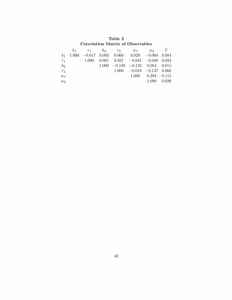
Table 2Correlation Matrix of Observables

h1 τ1 h2 τ2 w1 w2 Yh1 1.000 −0.017 0.093 0.060 0.029 −0.004 0.084τ1 1.000 0.081 0.321 −0.031 −0.026 0.024h2 1.000 −0.189 −0.132 0.084 0.011τ2 1.000 −0.018 −0.137 0.066w1 1.000 0.294 0.115w2 1.000 0.026

40

Table 3Moments of Primitive Parameters

Fixed Effects Distributions

Parameter Behavioral SpecificationNE PO CPO

μ(λ1) 0.369 0.580 0.531σ(λ1) 0.095 0.166 0.106

μ(λ2) 0.302 0.430 0.456σ(λ2) 0.102 0.158 0.120

μ(δ1) 0.075 0.075 0.075σ(δ1) 0.057 0.057 0.057

μ(δ2) 0.106 0.106 0.106σ(δ2) 0.066 0.066 0.066

α 0.500 0.500

41

Table 4Estimates of Primitive Parameter Moments

Flexible Parametric Specificationwith Bootstrap Standard Errors

NE PO CPO EHIEstimate S.E. Estimate S. E. Estimate S. E. Estimate S.E.

μ(λ1) 0.349 0.016 0.469 0.012 0.483 0.005 0.449 0.006σ(λ1) 0.142 0.010 0.152 0.033 0.140 0.006 0.102 0.017

μ(λ2) 0.342 0.022 0.419 0.023 0.450 0.005 0.419 0.006σ(λ2) 0.245 0.022 0.233 0.022 0.227 0.009 0.150 0.024

μ(δ1) 0.053 0.015 0.064 0.004 0.065 0.004 0.060 0.003σ(δ1) 0.038 0.010 0.033 0.011 0.034 0.006 0.037 0.008

μ(δ2) 0.121 0.003 0.113 0.004 0.109 0.002 0.116 0.005σ(δ2) 0.039 0.003 0.029 0.008 0.026 0.016 0.047 0.015

μ(α) - - - - 0.515 0.527σ(α) - - - - 0.042 0.039

P (α = 0.5|C) - - 0.415 0.074

P (C) 0 1 1 0.753

β - - - - - - 0.524 0.004

Distance Measure 4682.370 4926.074 4389.950 3768.480

42

Table A.1

Moments Used in the MSM Estimator

Sample Characteristic Sample ValueAverage h1 45.706Average h2 38.588Average τ1 7.787Average τ2 14.920St. Dev. h1 8.546St. Dev. h2 10.512

Average (h1 × h2) 1772.074Average (h1 × Y ) 5530.755Average (h2 × Y ) 4580.739Average (h1 × w1) 1009.293Average (h2 × w2) 618.773Average (τ1 × Y ) 947.620Average (τ2 × Y ) 1876.535St. Dev. τ1 6.418St. Dev. τ2 9.423

Average (h1 × w2) 722.880Average (h2 × w1) 830.367Average (h1 ≥ 40) 0.955Average (h2 ≥ 40) 0.694

Average (25 ≤ h1 < 40) 0.0346Average (25 ≤ h2 < 40) 0.210

43

Figure 1 Critical Values

*1 ( ) *

2 ( )

**

0 1

1

CPOE I

Figure 2 Pareto Frontier and Admissible Solutions

1NV

2NV

( )NV

( )NV

( , )NV

( , )NV

2u

1u