energy-efficient transmission range optimization model for

echT PressScienceComputers, Materials & ContinuaDOI:10.32604/cmc.2021.015426

Article

Energy-Ef�cient Transmission Range Optimization Model forWSN-Based Internet of Things

Md. Jalil Piran1, Sandeep Verma2, Varun G. Menon3 and Doug Young Suh4,*

1Department of Computer Science and Engineering, Sejong University, Seoul, Korea2Department of Electronics and Communication Engineering, D.B.R.A. National Institute of Technology, Jalandhar, India

3SCMS School of Engineering and Technology, Ernakulam, India4Department of Electronics Engineer, Kyung Hee University, Yongin, Korea

*Corresponding Author: Doug Young Suh. Email: [email protected]: 02 November 2020; Accepted: 10 December 2020

Abstract: With the explosive advancements in wireless communications anddigital electronics, some tiny devices, sensors, became a part of our daily life innumerous �elds. Wireless sensor networks (WSNs) is composed of tiny sensordevices. WSNs have emerged as a key technology enabling the realizationof the Internet of Things (IoT). In particular, the sensor-based revolutionof WSN-based IoT has led to considerable technological growth in nearlyall circles of our life such as smart cities, smart homes, smart healthcare,security applications, environmental monitoring, etc. However, the limitationsof energy, communication range, and computational resources are bottlenecksto the widespread applications of this technology. In order to tackle theseissues, in this paper, we propose an Energy-ef�cient Transmission Range Opti-mized Model for IoT (ETROMI), which can optimize the transmission rangeof the sensor nodes to curb the hot-spot problem occurring in multi-hopcommunication. In particular, we maximize the transmission range by employ-ing linear programming to alleviate the sensor nodes’ energy consumptionand considerably enhance the network longevity compared to that achievableusing state-of-the-art algorithms. Through extensive simulation results, wedemonstrate the superiority of the proposed model. ETROMI is expectedto be extensively used for various smart city, smart home, and smart health-care applications in which the transmission range of the sensor nodes is akey concern.

Keywords: Internet of Things; wireless sensor networks; routing; transmissionrange optimization; energy-ef�ciency; hot-spot problem; linear programming

1 Introduction

1.1 Background and Problem StatementData-driven wireless sensor networks (WSNs) are widely applied to enhance the Internet

of Things (IoT) in terms of the data throughput, energy ef�ciency, and self-management [1].WSN-based IoTs are composed of wireless sensor nodes, which realize data collection and

This work is licensed under a Creative Commons Attribution 4.0 International License,which permits unrestricted use, distribution, and reproduction in any medium, providedthe original work is properly cited.

http://dx.doi.org/10.32604/cmc.2021.015426

2990 CMC, 2021, vol.67, no.3

communication [2,3]. In this framework, the sensor nodes are deployed in the physical environmentto sense the phenomena and report their readings in a distributed manner to the sinks [4].However, the sensor nodes exhibit certain limitations in terms of energy, computation resources,and communication range [5,6].

When a WSN-based IoT is deployed over a large application area, the nodes perform mul-tihop communication due to the limited transmission range, and direct data transmission cannotbe realized. Furthermore, it has been reported that a larger number of relay nodes on the pathof data delivery to the sink corresponds to a higher probability of these nodes closer to the sinksuffering from hot-spot problem [7]. In such a scenario, the number of intermediate nodes shouldbe reduced to decrease the emergence of a no-connection zone for distantly located nodes.

Moreover, the battery of the sensor nodes may not be able to be changed or recharged. There-fore, it is necessary to ensure ef�cient power consumption in a WSN-based IoT [8]. Furthermore,transmitting one kilobyte of data corresponds to the processing of three million instructions [9].Therefore, data transmission in the WSNs should be minimized with regard to the distancebetween any two entities among sensor nodes, cluster heads (CHs), or sinks [10].

One solution is to maximize the transmission range between nodes. The key concept oftransmission range maximization is that if a sensor initiates a data packet transmission to a sinklocated 1000 m away, the least number of relay sensors should be selected to forward the packet.The communication range of sensor nodes depends on their transmission power and the volumeof the packet to be transmitted. Transmission over long distances requires a higher energy [11,12].Therefore, it is necessary to determine the maximum possible distance (transmission range) towhich the sensor nodes can transmit the data packets.

Many researchers have attempted to reduce the energy consumption by avoiding the hot-spot problem [13]. In particular, Verma et al. [14] proposed the multiple sink-based geneticalgorithm-based optimized clustering (MS-GAOC) approach, in which four data collection sinkswere incorporated outside the network. However, the cost of using four sinks may be prohibitivein various applications.

Moreover, researchers generally apply the corona-based model to avoid hot-spot problems.A survey of the various corona-based approaches has been presented in an existing study [15].Nevertheless, even corona-based methods are not suf�ciently reliable in mitigating the hot-spotproblem. In fact, the literature review indicates that the concept of transmission range adjustmentfor the sensor nodes, to realize direct data transfer to the sink or transfer with the least possiblenumber of intermediate nodes, has not been extensively investigated.

1.2 MotivationThe review pertaining to the mitigation of hot-spot problems indicated that the optimization-

based approach can provide a balanced solution to speci�c problems. Therefore, in this work, weused linear programming (LP) to compute the maximum data transmission range [16,17]. In par-ticular, LP exhibits remarkable exploration and exploitation capabilities, enabling fast convergenceto the optimal solution. Moreover, LP is highly computationally ef�cient [16].

CMC, 2021, vol.67, no.3 2991

1.3 Our ContributionsIn the context of the aforementioned problems, the key contributions of this work are

as follow:

a) We propose an energy-ef�cient transmission range optimized model for IoT (ETROMI) tooptimize the transmission range of the sensor nodes to reduce the hot-spot problem inWSN-based IoT.

b) The mathematical model and formulation using LP is presented.c) The simplex method is used to solve the de�ned problem.d) The proposed model’s performance of the proposed model is analyzed in terms of various

aspects, and the optimal solution is identi�ed.

1.4 Paper OrganizationThe remaining paper is structured as follows. Section 2 presents the background of trans-

mission range adjustment algorithms and describes the existing work pertaining to the hot-spotproblem in WSNs. Section 3 describes the system model and explains the LP formulation.Section 4 describes the performance evaluation of ETROMI, which is used to compute themaximized distance corresponding to the transmission range of a node. The concluding remarks,along with the limitations and scope for future work, are presented in Section 5.

2 Related Work

In this section, we discuss the existing work focused on addressing the hot-spot problemthrough various state-of-the-art techniques and on realizing the transmission range adjustment ofa sensor node.

2.1 Approaches to Solve the Hot-Spot ProblemIn applications involving an extremely large network area, the sensor nodes inevitably perform

multi-hop communication [18]. In this process, a hot-spot is created at the nodes located nearest tothe sink. Several researchers have addressed this concern through various topology-based methods.Moreover, the many-to-one approach (many sensor nodes corresponding to one sink) has beenwidely implemented through corona-based structures [13]. Many researchers use the term “energy-hole,” which is equivalent in meaning to a hot-spot.

Elkamel et al. [19] proposed an unequal clustering method to overcome the hot-spot prob-lem by placing the small and large clusters nearer to and farther from the sink, respectively.However, the proposed technique failed to eliminate the hot-spot problem, and the network’senergy consumption was high. Verma et al. [7,14] implemented multiple data sinks in a givennetwork to mitigate the hot-spot problem. In their former and latter studies, the authors usedthe conventional approach and the genetic algorithm, respectively. However, the network incurreda higher �nancial cost owing to the use of multiple data sinks. The authors in [20] proposed avirtual-force-based energy-hole mitigation strategy to ensure sensor nodes’ uniform distribution.Moreover, the network was composed of various annuli, and virtual gravity was used to optimizethe sensor node positions in each annulus. However, due to the multi-hop communication, thenumber of overheads in each annulus was extremely high, which increased the energy consumptionin the network. Sharmin et al. [21] proposed a strategy in which the network was partitionedinto several wedges, and residual energy was considered to combine the various wedges. The head

2992 CMC, 2021, vol.67, no.3

node was selected based on the distance between the innermost corona and node. However, theinef�cient selection of the head node led to the mediocre performance of this strategy.

In addition to the static network scenario, certain researchers introduced sink mobility tocurb the hot-spot problem. Sahoo et al. [22] proposed a particle-swarm-optimization-based energy-ef�cient clustering and sink mobility (PSO-ECSM) technique, in which the sink mobility wasused to alleviate the hot-spot problem. However, the mobility scenario was not ef�ciently uti-lized, and the slow convergence of the PSO degraded the performance of the proposed scheme.Furthermore, Kaur et al. [23] introduced dual sink mobility outside the network to targetunattended applications. Although the authors implemented the PSO-based sink mobility, the useof the dual sink introduced overheads in the network, which increased the energy consumption.In addition, the data delivery was required to be synchronized when using the two sinks in thenetwork. Certain other researchers also employed the sink mobility scenario to alleviate the hot-spot problem. However, it was observed that the use of sink mobility limited the applicability ofthe approaches in various real-time scenarios.

2.2 Transmission Range Adjustment AlgorithmsIn addition to the network topological changes associated with the introduction of the corona-

based model, the characteristics of sensor nodes have been examined. The focus of the presentstudy is to optimize the transmission range. Although certain researchers have attempted to adjustthe transmission range to alleviate the hot-spot problem, the proposed approaches suffer from theinherent problems, which limit their relevance.

In an existing strategy [24] pertaining to the transmission range adjustment, the network wasdivided into various concentric sets termed as coronas. Every corona was assigned a transmissionrange level. Furthermore, the authors presented an ant colony optimization (ACO)-based trans-mission range adjustment strategy [24] to prolong the network lifetime. Liu [25] considered theenergy consumption balancing (ECB) and energy consumption minimization (ECM) techniquesto avoid the occurrence of energy holes. The authors exploited the short-trip moving schemefor the ACO, which helped in decreasing the complexity and in the amelioration of convergencespeed. Furthermore, the authors considered a reference transmission distance to implement theECB and ECM techniques. Xin et al. [26] were the �rst to attempt to solve the many-to-one datatransmission problem, particularly in strip-based WSNs. The authors adjusted the transmissionrange based on the computation of the accurate distance. The objective was to prolong thenetwork lifetime. However, the proposed algorithm was applicable only for strip-based WSNs, forexample, railway track, bridge, and tunnel systems.

In summary, only a few studies have been focused on addressing the hot-spot problem throughtransmission range adjustment, and this approach exhibits considerable scope for improvement.Furthermore, the use of LP for energy-hole mitigation in the transmission range adjustmentcontext is yet to be explored. Therefore, we implement these aspects in our proposed strategy.

3 System Model

In this section, we describe the network assumptions and the system model.

3.1 Network AssumptionsThe following network assumptions are considered to implement ETROMI.

CMC, 2021, vol.67, no.3 2993

a) The WSN is composed of one sink and several sensor nodes that collect data and transferthem to the sink.

b) Each sensor has a unique ID.c) There is no dispute for medium access, and thus, proportional fair channel access is

available to all the sensors.d) The minimum cost forwarding approach is employed as the multi-hop-routing protocol.e) The sensor nodes are homogeneous, i.e., all the nodes have the same con�guration in terms

of energy, computational resources, transmission range, etc.f) The entire network is static, including the CHs and the sink.g) The entire network has ideal conditions in terms of security, physical medium factors,

re�ection, refraction, splitting of signals, and presence of other obstacles.

3.2 Fundamental Principle of ETROMIAssume a WSN with N sensor nodes, in which one of the sensor nodes initiates a data packet

with the intent to transmit it to the sink (�nal receiver base station). In the conventional clusteringmethod, a CH collects the data from the sensors node in the corresponding cluster and forwardsthe data toward the sink via the other CHs. However, this approach is not ef�cient because theCHs suffer from battery limitations, even more than the other data collecting elements, but mustbe involved in all transmissions.

In contrast, the lifetime of the WSNs depends on the remaining energy of the members, i.e.,the sensor nodes. Therefore, the number of forwarding nodes must be minimized. In this study,we assume that instead of always selecting the CHs to receive and forward the data packets, thesensors select the farthest sensor node in their transmission range. In other words, the sensornodes increase their transmission power to transmit a data packet over a longer distance. In thiscon�guration, the number of nodes that are involved in a transmission are minimized, which canconsiderably improve the energy ef�ciency. In Fig. 1, the red dotted line represents the routingprocedure in a clustering-based method.

In this approach, the nodes send their packets to their corresponding CH, which then for-wards the packet to the next CH and so on. Finally, the closest CH delivers the packet to thesink. In contrast, in the approach represented by the green dashed line, the node that initiatesthe packet sends the packet to the farthest node, and the receiver node follows the same principleand send the packet to the farthest node in its transmission range. Consequently, the number ofnodes involved in the transmission procedure is less than that in the clustering-based method.

Consider a network involving 100 sensor nodes. Sensor 1 initiates a data packet and wantsto send it to node 100. As mentioned earlier, in the WSNs, the topology is multi-hop. In otherwords, node 1 sends its packet to its neighbor, which receives the packet and forwards it to theneighboring nodes, excluding the node that the packet was received from. This process continuesuntil node 100 receives the packet. The problem then is to determine the number of nodes in thetransmission process that receive and forward the packet. This number of the relay nodes shouldbe minimized to abate the energy consumption and, in turn, prolongs the network lifetime.

One solution is to increase the transmission range of the nodes involved in the transmissionprocess from the source to the destination. In this case, a node selects a neighboring node,which is far from it, but in its range, i.e., on the edge of its transmission range, and thenumber of intermediate nodes is decreased. To this end, we consider the energy consumptionaccounted to transmission and reception of data packets and also the magnitude of data packets.

2994 CMC, 2021, vol.67, no.3

The total required energy can be expressed as

Eij =Etx×Pi× dij +N×Erx

+

N−1∑i=1

Di. (1)

Figure 1: Routing procedure in WSNs

The list of main symbols used in this paper are listed in Tab. 1.

Table 1: List of symbols

Symbol De�nition

Di The distance between node i to the sinkEI The initial powerEij Total energy consumption of a linkErx The receiving powerEtx Transmission powerPi Packet volumedij The distance between node i and jN The number of nodes

CMC, 2021, vol.67, no.3 2995

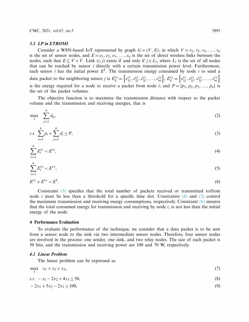
3.3 LP in ETROMIConsider a WSN-based IoT represented by graph G = (V , E), in which V = v1, v2, v3, . . . , vn

is the set of sensor nodes, and E = e1, e2, e3, . . . , en is the set of direct wireless links between thenodes, such that E ⊆V×V . Link (i, j) exists if and only if j ∈Li, where Li is the set of all nodesthat can be reached by sensor i directly with a certain transmission power level. Furthermore,each sensor i has the initial power EI . The transmission energy consumed by node i to send a

data packet to the neighboring sensor j is Etxij =

{etx

1j , etx2j , etx

3j , . . . , etxnj

}; Erx

ij =

{erx

1j , erx2j , erx

3j , . . . , erxnj

}is the energy required for a node to receive a packet from node i; and P= {p1, p2, p3, . . . , pn} isthe set of the packet volumes.

The objective function is to maximize the transmission distance with respect to the packetvolume and the transmission and receiving energies, that is

maxx

n∑j=1

dij, (2)

s.t.n∑

i=1

pi+

n∑j=1

dj ≤P, (3)

n∑i=1

Etxi < Etx, (4)

n∑i=1

Erxi < Erx, (5)

Etx+Erx < EI . (6)

Constraint (3) speci�es that the total number of packets received or transmitted to/fromnode i must be less than a threshold for a speci�c time slot. Constraints (4) and (5) controlthe maximum transmission and receiving energy consumptions, respectively. Constraint (6) ensuresthat the total consumed energy for transmission and receiving by node i, is not less than the initialenergy of the node.

4 Performance Evaluation

To evaluate the performance of the technique, we consider that a data packet is to be sentfrom a sensor node to the sink via two intermediate sensor nodes. Therefore, four sensor nodesare involved in the process: one sender, one sink, and two relay nodes. The size of each packet is50 bits, and the transmission and receiving power are 100 and 70 W, respectively.

4.1 Linear ProblemThe linear problem can be expressed as

maxx

x1+ x2+ x3, (7)

s.t. − x1− 2x2+ 4x3 ≤ 50, (8)

− 2x1+ 5x2− 2x3 ≤ 100, (9)

2996 CMC, 2021, vol.67, no.3

4x1− 2x2− x3 ≤ 70, (10)

x1, x2, x3 ≥ 0. (11)

By adding slack variables to constraints, the primal problem in standard format is representedas follows:

maxx

x1+ x2+ x3+ 0x4+ 0x5+ 0x6, (12)

s.t. − x1− 2x2+ 4x3+ x4 = 50, (13)

− 2x1+ 5x2− 2x3+ x5 = 100, (14)

4x1− 2x2− x3+ x6 = 70, (15)

x1, x2, x3, x4, x5, x6 ≥ 0. (16)

4.2 Simplex MethodWe use the simplex method to solve the problem. The simplex method is used to solve LP

models by using slack variables, tableaus, and pivot variables to determine the optimal solu-tion of an optimization problem [27]. To solve the optimization problem, the following stepsare performed:

a) Obtain the standard form,b) Introduce slack variables,c) Create the tableau,d) Identify the pivot variables,e) Create a new tableau,f) Check for optimality,g) Identify the optimal values.

The procedure starts with an initialization phase, followed by several iterations to determinethe optimal solution.

The initialization step for our optimization problem is presented in Tab. 2. After the �rst step,x6 is the leaving variable, x1 is the entering variable, and 4 is the pivot element.

Subsequently, we apply the �rst iteration, as indicated in Tab. 3. Upon completing thisiteration, the leaving variable is x5, the entering variable is x2, and the pivot element is 4.

Table 2: Stating section

Maximize 1 1 1 0 0 0 RHS Θ

x1 x2 x3 x4 x5 x6

0x4 −1 −2 4 1 0 0 50 –0x5 −2 5 −2 0 1 0 100 –0x6 4 −2 −1 0 0 1 70 70/4Cj −Zj 1 1 1 0 0 0 0

We continue by applying the second iteration as indicated in Tab. 4, which results in a leavingvariable x4, an entering variable x3, and a pivot element, 35/16.

CMC, 2021, vol.67, no.3 2997

Table 3: Iteration I

0x4 0 −5/2 15/4 1 0 1/4 270/4 –0x5 0 4 −5/2 0 1 1/2 135 135/41x1 1 −1/2 −1/4 0 0 1/4 70/4Cj −Zj 0 3/2 5/4 0 0 −1/4 70/4

Table 4: Iteration II

0x4 0 0 35/16 1 5/8 9/16 1215/8 486/71x2 0 1 −5/8 0 1/4 1/8 135/4 –1x1 1 0 −9/16 0 1/8 5/16 275/8 –Cj −Zj 0 0 35/16 0 −3/8 −7/16 545/8

We proceed to the third iteration, in which all Cj−Zj values are zero or negative; therefore,the simplex method is terminated at this step, as indicated in Tab. 5. The optimal solution for thede�ned problem is presented in Tab. 6.

Table 5: Iteration III

1x3 0 0 1 16/35 2/7 9/35 486/71x2 0 1 0 2/7 3/7 2/7 540/71x1 1 0 0 9/35 2/7 16/35 514/7Cj −Zj 0 0 0 −1 −1 −1 220

Table 6: The optimal solution

Z 220

x1 514/7x2 540/7x3 486/7

4.3 DualityThe duality refers to a speci�c relationship between an LP problem and another problem,

both of which involve the same original data, albeit located differently [28]. The former andlatter problems are referred to as the primal and dual problems, respectively. The feasible regions,optimal solutions, and optimal values of these problems must be strongly correlated. The dualityand optimality conditions obtained from these aspects are a basis for the LP theory. Once eitherof the primal or dual problems is solved, both the problems can be solved owing to duality. Toconvert the primal problem to a dual problem, the following steps are performed:

a) If the primal problem corresponds to “Maximize,” the dual problem correspondsto “Minimize.”

b) The number of variables in the dual problem is equal to the number of constraints in theprimal problem.

c) The number of constraints in the dual problem, is equal to the number of variables in theprimal problem.

2998 CMC, 2021, vol.67, no.3

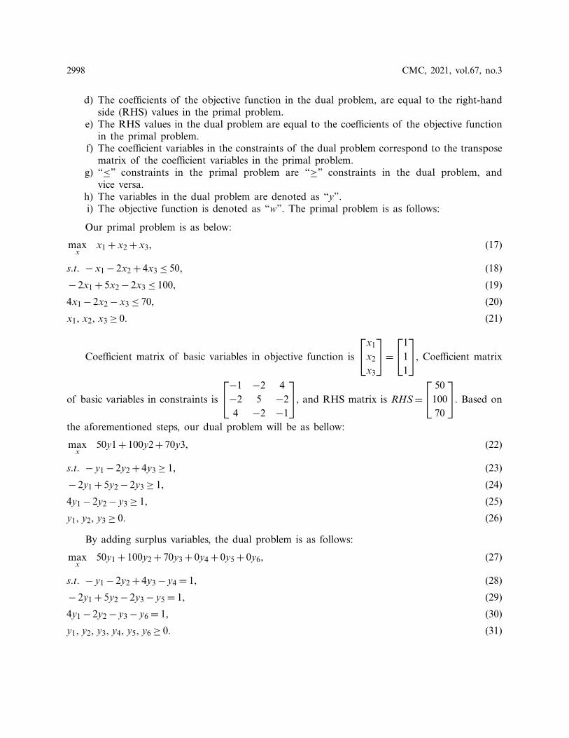
d) The coef�cients of the objective function in the dual problem, are equal to the right-handside (RHS) values in the primal problem.

e) The RHS values in the dual problem are equal to the coef�cients of the objective functionin the primal problem.

f) The coef�cient variables in the constraints of the dual problem correspond to the transposematrix of the coef�cient variables in the primal problem.

g) “≤” constraints in the primal problem are “≥” constraints in the dual problem, andvice versa.

h) The variables in the dual problem are denoted as “y”.i) The objective function is denoted as “w”. The primal problem is as follows:

Our primal problem is as below:

maxx

x1+ x2+ x3, (17)

s.t. − x1− 2x2+ 4x3 ≤ 50, (18)

− 2x1+ 5x2− 2x3 ≤ 100, (19)

4x1− 2x2− x3 ≤ 70, (20)

x1, x2, x3 ≥ 0. (21)

Coef�cient matrix of basic variables in objective function is

x1

x2

x3

=1

11

, Coef�cient matrix

of basic variables in constraints is

−1 −2 4−2 5 −24 −2 −1

, and RHS matrix is RHS=

5010070

. Based on

the aforementioned steps, our dual problem will be as bellow:

maxx

50y1+ 100y2+ 70y3, (22)

s.t. − y1− 2y2+ 4y3 ≥ 1, (23)

− 2y1+ 5y2− 2y3 ≥ 1, (24)

4y1− 2y2− y3 ≥ 1, (25)

y1, y2, y3 ≥ 0. (26)

By adding surplus variables, the dual problem is as follows:

maxx

50y1+ 100y2+ 70y3+ 0y4+ 0y5+ 0y6, (27)

s.t. − y1− 2y2+ 4y3− y4 = 1, (28)

− 2y1+ 5y2− 2y3− y5 = 1, (29)

4y1− 2y2− y3− y6 = 1, (30)

y1, y2, y3, y4, y5, y6 ≥ 0. (31)

CMC, 2021, vol.67, no.3 2999

As indicated in the dual problem, no identity matrix exists for the coef�cients of the variablesin the constraints; therefore, arti�cial variables must be introduced. In this case, the dual problemin the standard format is:

maxx

50y1+ 100y2+ 70y3+ 0y4+ 0y5+ 0y6−Ma1−Ma2−Ma3, (32)

s.t. − y1− 2y2+ 4y3− y4+ a1 = 1, (33)

− 2y1+ 5y2− 2y3− y5+ a2 = 1, (34)

4y1− 2y2− y3− y6+ a3 = 1, (35)

y1, y2, y3, y4, y5, y6 ≥ 0. (36)

By adding arti�cial variables, an identity matrix can be generated, and the simplex methodcan be implemented.

As indicated in Tab. 7, after completing the initialization section, the leaving variable is a3, theentering variable is x1, and the pivot element is 4. Subsequently, we implement the �rst iteration,as indicated in Tab. 8. Upon completing iteration I, the leaving variable is a2, the entering variableis x2, and our pivot element is 4. We then proceed to the second iteration, as indicated in Tab. 9.After the second iteration, the leaving variable is a1, the entering variable is x3, and the pivotelement is 35/16. We attempt to determine the optimal solution by using the two-phase simplexmethod. All the arti�cial variables are removed, and the problem can be solved through the othervariables. We then apply the third iteration in two phases, as indicated in Tabs. 10 and 11.

Table 7: Starting section

Min 50 100 70 0 0 0 −M −M −M RHS Θ

y1 y2 y3 y4 y5 y6 a1 a2 a3

−Ma1 −1 −2 4 −1 0 0 1 0 0 1 –−Ma2 −2 5 −2 0 −1 0 0 1 0 1 –−Ma3 4 −2 −1 0 0 −1 0 0 1 1 1/4Cj −Wj −1 −1 −1 1 1 1 0 0 0 3


−Ma1 0 −9/4 15/4 -1 0 −1/4 1 0 1/4 5/4 –−Ma2 0 4 −9/4 0 −1 −1/2 0 1 1/2 3/2 3/850y1 1 −1/2 −1/4 0 0 −1/4 0 0 1/4 1/4 –Cj −Wj 0 −3/2 −5/4 1 1 3

4 0 0 1/4 11/4


−Ma1 0 0 35/16 −1 −5/8 −9/16 1 5/8 9/16 35/16 1100y2 0 1 −5/8 0 −1/4 −1/8 0 1

4 1/8 3/8 –50y1 1 0 −9/16 0 −1/8 −5/16 0 1/8 5/16 7/16 –Cj −Wj 0 0 −35/16 1 5/8 9/16 0 3/8 7/16 35/16

3000 CMC, 2021, vol.67, no.3

Table 10: Phase I, Iteration III

70y3 0 0 1 −16/35 −2/7 −9/35 16/35 2/7 9/35 1100y2 0 1 0 −2/7 −3/7 −2/7 2/7 3/7 2/7 150y1 1 0 0 −9/35 −2/7 −16/35 9/35 2/7 16/35 1Cj −Wj 0 0 0 0 0 0 1 1 1 0

Table 11: Phase II, Iteration III

70y3 0 0 1 −16/35 −2/7 −9/35 1100y2 0 1 0 −2/7 −3/7 −2/7 11y1 1 0 0 −9/35 −2/7 −16/35 1Cj −Wj 0 0 0 514/7 540/7 486/7 220

Finally, it is observed that the primal solution, presented in Tab. 12, is equal to the dualsolution, presented in Tab. 13, that is Z∗ =W∗.

Table 12: Primal optimal Solution

Z 220

x1 514/7x2 540/7x3 486/7

Table 13: Dual optimal solution

W 220

y1 1y2 1y3 1

4.4 Sensitivity AnalysisSensitivity analysis is aimed at examining the in�uence of changes in the variables, such as

the RHS, coef�cients of the objective function, and constraints, on the solution. We start withTab. 14 and make the some changes as explained in the next subsection.

4.4.1 Change in the Objective Function Coef�cient for Non-Basic VariablesIn the last iteration, no non-basic variables of the objective function exist. Therefore, if one

of the coef�cients is changed, the optimal solution is not in�uenced.

CMC, 2021, vol.67, no.3 3001

Table 14: Simplex optimum tableau

Maximize 1 1 1 0 0 0 RHS

x1 x2 x3 x4 x5 x6

1x3 0 0 1 16/35 2/7 9/35 486/71x2 0 1 0 2/7 3/7 2/7 540/71x1 1 0 0 9/35 2/7 16/35 514/7Cj −Zj 0 0 0 −1 −1 −1 220

4.4.2 Change in the RHS Value

Suppose the intention is to change the �rst RHS to b1; then we have

5010070

. To calculate

new RHS;

RHS=B−1 b=

16/35 2/7 9/35

2/7 3/7 2/7

9/35 2/7 16/35

b1

100

70

16b1+ 163035

2b1+ 4407

9b1+ 212035

, (37)

∴

16b1+ 163035

≥ 0⇒ b1 ≥−815

8

2b1+ 4407

≥ 0⇒ b1 ≥−80

9b1+ 212035

≥ 0⇒ b1 ≥−−725

8

. (38)

Because, b1≥−815/8. We suppose a b1 value beyond the speci�ed range; as an example −110.

RHS=B−1 b=

16/35 2/7 9/35

2/7 3/7 2/7

9/35 2/7 16/35

−110

100

70

=

2787

2207

2267

. (39)

Now, we continue the tableau with new RHS values;

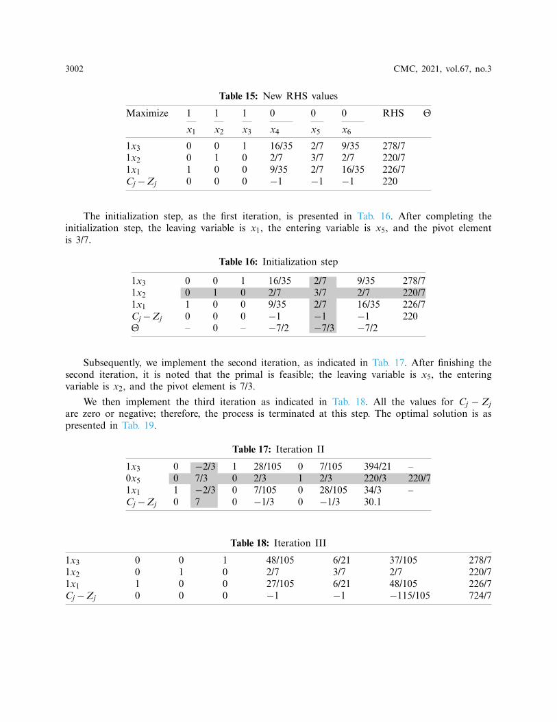
As indicated in Tab. 15, the primal solution is not feasible; therefore, we attempt to �nd theoptimal solution through the dual problem.

3002 CMC, 2021, vol.67, no.3

Table 15: New RHS values


x1 x2 x3 x4 x5 x6

1x3 0 0 1 16/35 2/7 9/35 278/71x2 0 1 0 2/7 3/7 2/7 220/71x1 1 0 0 9/35 2/7 16/35 226/7Cj −Zj 0 0 0 −1 −1 −1 220

The initialization step, as the �rst iteration, is presented in Tab. 16. After completing theinitialization step, the leaving variable is x1, the entering variable is x5, and the pivot elementis 3/7.

Table 16: Initialization step

1x3 0 0 1 16/35 2/7 9/35 278/71x2 0 1 0 2/7 3/7 2/7 220/71x1 1 0 0 9/35 2/7 16/35 226/7Cj −Zj 0 0 0 −1 −1 −1 220Θ – 0 – −7/2 −7/3 −7/2

Subsequently, we implement the second iteration, as indicated in Tab. 17. After �nishing thesecond iteration, it is noted that the primal is feasible; the leaving variable is x5, the enteringvariable is x2, and the pivot element is 7/3.

We then implement the third iteration as indicated in Tab. 18. All the values for Cj − Zjare zero or negative; therefore, the process is terminated at this step. The optimal solution is aspresented in Tab. 19.


1x3 0 −2/3 1 28/105 0 7/105 394/21 –0x5 0 7/3 0 2/3 1 2/3 220/3 220/71x1 1 −2/3 0 7/105 0 28/105 34/3 –Cj −Zj 0 7 0 −1/3 0 −1/3 30.1


1x3 0 0 1 48/105 6/21 37/105 278/71x2 0 1 0 2/7 3/7 2/7 220/71x1 1 0 0 27/105 6/21 48/105 226/7Cj −Zj 0 0 0 −1 −1 −115/105 724/7

CMC, 2021, vol.67, no.3 3003

Table 19: Optimal solution

Z 724/7

x1 226/7x2 220/7x3 278/7

4.4.3 Change in the Objective Function Coef�cient for the Basic VariableWe consider the case in which the coef�cient of x1 changes. Suppose the coef�cient of x1 is c1.

Any change in the coef�cient of the basic variables of the objective function affects the valueof Cj −Zj.

For x4⇒Cj−Zj= 0−[(

1 ∗1635

)+

(1 ∗

27

)+

(c1 ∗

935

)]⇒−9c1

35−

2635

. (40)


1×27

)+

(1×

37

)+

(c1×

27

)]⇒−2c1

7−

57

. (41)


1×9

35

)+

(1×

27

)+

(c1×

1635

)]⇒−16c1

35−

1935

. (42)

If Cj−Zj ≤ 0 then the present solution remains optimal solution;

−9c1

35−

2635≤ 0⇒ c1 ≤

−269

, (43)

−2c1

7−

57≤ 0⇒ c1 ≤

−52

, (44)

−16c1

35−

1935≤ 0⇒ c1 ≤

−1916

, (45)

In this case, the range of c1 is greater than −26/9. Thus, we assign c1 beyond this range, forexample c1 =−4, and implement the �rst iteration, as indicated in Tab. 20.


Maximize −4 1 1 0 0 0 RHS Θ

x1 x2 x3 x4 x5 x6

1x3 0 0 1 16/35 2/7 9/35 486/7 2701x2 0 1 0 2/7 3/7 2/7 540/7 270−4x1 1 0 0 9/35 2/7 16/35 514/7 1285/8Cj −Zj 0 0 0 2/7 3/7 9/7 −1030/7

Upon completing the �rst iteration, the leaving variable is x3, the entering variable is x6, andthe pivot element is 9/35.

3004 CMC, 2021, vol.67, no.3

The second iteration is presented in Tab. 21. All the values for Cj −Zj are zero or negative;therefore, the process is terminated at this step. We conclude that the optimal solution is asfollows: x1 =−50, x2 = 0, x3 = 270 and z= 470.


1x3 0 0 35/9 16/9 10/9 1 2701x2 0 1 −10/9 −2/9 1/9 0 0−4x1 1 0 −16/9 −7/9 −2/9 0 −50Cj −Zj 0 0 −80/9 −42/9 −19/9 −1 470

4.4.4 Change in the Constraint Coef�cient Corresponding to Non-basic VariablesIn the last iteration, no non-basic variable of the objective function exists. Therefore, if one

of the coef�cients is changed, the optimal solution is not in�uenced.

4.4.5 Addition of a New Variable

Consider a new variable x7 with coef�cient c7 = 12 and P7 =

122

, then;

P7 =B−1P7⇒

16/35 2/7 9/35

2/7 3/7 2/7

9/35 2/7 16/35

1

2

2

=

638105

127

6135

. (46)



x1 x2 x3 x4 x5 x6

1x3 0 0 1 16/35 2/7 9/35 486/71x2 0 1 0 2/7 3/7 2/7 540/71x1 1 0 0 9/35 2/7 16/35 514/7Cj −Zj 0 0 0 −1 −1 −1 220

In this case, we perform three iterations as indicated in Tabs. 22–24.

Upon completing the �rst iteration, the leaving variable is x3, the entering variable is x7, andthe pivot element is 212/35.

The third iteration is presented in Tab. 12, in which all the values for Cj − Zj are zero ornegative and; therefore, the program is terminated at this step, and the optimal solution is asindicated in Tab. 25.

CMC, 2021, vol.67, no.3 3005


Maximize 1 1 1 0 0 0 12 RHS Θ

x1 x2 x3 x4 x5 x6 x7

1x3 0 0 1 16/35 2/7 9/35 212/35 486/7 104/91x2 0 1 0 2/7 3/7 2/7 12/7 540/7 451x1 1 0 0 9/35 2/7 16/35 61/35 514/7 2570/61Cj −Zj 0 0 0 −1 −1 −1 137/105


Maximize 1 1 1 0 0 0 12 RHS Θ

x1 x2 x3 x4 x5 x6 x7

12x7 0 0 3/18 8/9 15/9 27/18 1 104/181x2 1 0 37/127 68/319 65/319 67/319 0 36/181x1 0 1 −18/63 −78/63 −153/63 −144/63 0 235/18Cj −Zj 0 0 −1 −87/9 −160/9 −143/9 0 115

Table 25: Optimal solution

Z 115

x1 235/18x2 36/18x7 104/18

4.4.6 Addition of a New ConstraintTo examine the in�uence of the addition of a new constraint to the problem, we consider

x3 ≤ 40:

As indicated in Tab. 26, the optimal solution is as follows: x1 = 514/7, x2 = 540/7, x3 = 486/7,and Z= 20.

Table 26: Additional constraint

Maximize 1 1 1 0 0 0 0 RHS

x1 x2 x3 x4 x5 x6 x7

1x3 0 0 1 16/35 2/7 9/35 0 486/71x2 0 1 0 2/7 3/7 2/7 0 540/71x1 1 0 0 9/35 2/7 16/35 0 514/70x7 0 0 1 0 0 0 1 40Cj −Zj 0 0 0 −1 −1 −1 0 220

3006 CMC, 2021, vol.67, no.3

5 Conclusion and Future Direction

The transmission range of a sensor node de�nes whether the communication mode is single-hop or multi-hop. In this paper, we proposed the use of ETROMI, which can determine themaximum distance to which a sensor node can transmit data with the least possible number ofrelay nodes. We presented an LP-based analytical model to determine the transmission range ofthe sensor node. Moreover, we explained the mathematical model associated with the ETROMIto reduce the energy consumption of WSN-based IoT. A key concern about the ETROMI is thatit considers the ideal conditions involving no obstacles between the sensor nodes and the sink.Therefore, the model performance is speci�c to the circumstances. Furthermore, the network isassumed to be homogeneous, whereas homogeneity does not exist in an actual network due tothe different factors associated with network deployment. In future work, we aim to extend ourwork to address the aforementioned scenarios.

Funding Statement: This research was supported by Korea Electric Power Corporation (GrantNumber: R18XA02).

Con�icts of Interest: The authors declare that they have no con�icts of interest to report regardingthe present study.

References[1] S. Kumar and V. K. Chaurasiya, “A strategy for elimination of data redundancy in Internet of Things

(IoT) based wireless sensor network (WSN),” IEEE Systems Journal, vol. 13, pp. 1650–1657, 2018.[2] P. Swarna, P. Maddikunta, M. Parimala, S. Koppu, T. Gadekallu et al., “An effective feature engi-

neering for DNN using hybrid PCA-GWO for intrusion detection in IoMT architecture,” ComputerCommunications, vol. 160, pp. 139–149, 2020.

[3] R. Vinayakumar, M. Alazab, S. Srinivasan, Q. Pham, S. Padannayil et al., “A visualized botnet detec-tion system based deep learning for the Internet of Things networks of smart cities,” IEEE Transactionson Industry Applications, vol. 56, no. 4, pp. 4436–4456, 2020.

[4] M. Piran, Y. Cho, J. Yun and D. Y. Suh, “Cognitive radio-based vehicular ad hoc and sensor networks(CR-VASNET),” International Journal of Distributed Sensor Networks, vol. 2014, pp. 1–11, 2014.

[5] T. M. Behera, S. K. Mohapatra, U. C. Samal and M. S. Khan, “Hybrid heterogeneous routing schemefor improved network performance in WSNs for animal tracking,” Internet of Things, vol. 6, pp. 1–9, 2019.

[6] T. M. Behera, S. K. Mohapatra, U. C. Samal, M. S. Khan, M. Daneshmand et al., “Residual energy-based cluster-head selection in WSNs for IoT application,” IEEE Internet of Things Journal, vol. 6,pp. 5132–5139, 2019.

[7] S. Verma, N. Sood and A. K. Sharma, “A novelistic approach for energy ef�cient routing usingsingle and multiple data sinks in heterogeneous wireless sensor network,” Peer-to-Peer Networking andApplications, vol. 12, pp. 1110–1136, 2019.

[8] Y. Liu, C. Yang, L. Jiang, S. Xie and Y. Zhang, “Intelligent edge computing for IoT-based energymanagement in smart cities,” IEEE Network, vol. 33, pp. 111–117, 2019.

[9] D. K. Gupta, “A review on wireless sensor networks,” Network and Complex Systems, vol. 3, no. 1,pp. 18–23, 2013.

[10] L. Krishnasamy, R. K. Dhanaraj, G. D. Ganesh, G. Reddy, M. K. Aboudaif et al., “A heuristic angularclustering framework for secured statistical data aggregation in sensor networks,” Sensors, vol. 20,pp. 1–15, 2020.

[11] S. Bhattacharya, P. Maddikunta, S. Somayaji, K. Lakshmanna, R. Kaluri et al., “Load balancing ofenergy cloud using wind driven and �re�y algorithms in internet of everything,” Journal of Parallel andDistributed Computing, vol. 142, pp. 16–26, 2020.

CMC, 2021, vol.67, no.3 3007

[12] C. Iwendi, P. K. Maddikunta, T. R. Gadekallu, K. Lakshmanna, A. K. Bashir et al., “A metaheuristicoptimization approach for energy ef�ciency in the IoT networks,” Software: Practice and Experience,vol. 22, no. 6, pp. 1–14, 2020.

[13] H. Asharioun, H. Asadollahi, T. C. Wan and N. Gharaei, “A survey on analytical modeling andmitigation techniques for the energy hole problem in corona-based wireless sensor network,” WirelessPersonal Communications, vol. 81, pp. 161–187, 2015.

[14] S. Verma, N. Sood and A. K. Sharma, “Genetic algorithm-based optimized cluster head selectionfor single and multiple data sinks in heterogeneous wireless sensor network,” Applied Soft Computing,vol. 85, pp. 1–21, 2019.

[15] A. U. Rahman, A. Alharby, H. Hasbullah and K. Almuzaini, “Corona based deployment strategiesin wireless sensor network: A survey,” Journal of Network and Computer Applications, vol. 64, pp. 176–193, 2016.

[16] D. Bertsimas and J. N. Tsitsiklis, Introduction to Linear Optimization, vol. 6. Belmont, MA: AthenaScienti�c, 1997.

[17] V. Tabus, D. Moltchanov, Y. Koucheryavy, I. Tabus and J. Astola, “Energy ef�cient wireless sen-sor networks using linear-programming optimization of the communication schedule,” Journal ofCommunications and Networks, vol. 17, pp. 184–197, 2015.

[18] V. Sandeep, N. Sood and A. K. Sharma, “QoS provisioning-based routing protocols using multipledata sink in IoT-based WSN,” Modern Physics Letters, vol. 34, pp. 1–36, 2019.

[19] R. Elkamel, A. Messouadi and A. Cherif , “Extending the lifetime of wireless sensor networksthrough mitigating the hot spot problem,” Journal of Parallel and Distributed Computing, vol. 133,pp. 159–169, 2019.

[20] C. Sha, C. Ren, R. Malekian, M. Wu, H. Huang et al., “A type of virtual force-based energy-holemitigation strategy for sensor networks,” IEEE Sensors Journal, vol. 20, pp. 1105–1119, 2019.

[21] N. Sharmin, A. Karmaker, W. Lambert, M. Alam and M. Shawkat, “Minimizing the energy holeproblem in wireless sensor networks: A wedge merging approach,” Sensors, vol. 20, pp. 1–25, 2020.

[22] B. Sahoo, T. Amgoth and H. Pandey, “Particle swarm optimization based energy ef�cient clus-tering and sink mobility in heterogeneous wireless sensor network,” Ad Hoc Networks, vol. 106,pp. 1–21, 2020.

[23] S. Kaur and V. Grewal, “A novel approach for particle swarm optimization-based clustering with dualsink mobility in wireless sensor network,” International Journal of Communication Systems, vol. 33,no. 16, pp. 1–23, 2020.

[24] M. Liu and C. Song, “Ant-based transmission range assignment scheme for energy hole problem inwireless sensor networks,” International Journal of Distributed Sensor Networks, vol. 8, pp. 1–12, 2012.

[25] X. Liu, “A novel transmission range adjustment strategy for energy hole avoiding in wireless sensornetworks,” Journal of Network and Computer Applications, vol. 67, pp. 43–52, 2016.

[26] H. Xin and X. Liu, “Energy-balanced transmission with accurate distances for strip-based wirelesssensor networks,” IEEE Access, vol. 5, pp. 16193–16204, 2017.

[27] V. Zhadan, “Two-phase simplex method for linear semide�nite optimization,” Optimization Letters,vol. 13, pp. 1969–1984, 2019.

[28] S. Nasseri and D. Darvishi, “Duality results on grey linear programming problems,” The Journal of GreySystem, vol. 30, pp. 127–142, 2018.

energy-efficient transmission range optimization model for

Documents