Energy Resources and Potential GNPROBERT H. RASCH.E and JOHN A. TATOM

dramatic change in supply conditions forenergy resources since 1973 had a substantial effecton the productive capabilities of the U.S. economy.Higher prices of energy resources, relative to theprices of labor and capital resources, resulted in a lossof economic capacity and higher output prices. It hasbeen estimated that four to five percentage points ofboth the higher price level and reduction in nationaloutput in 1974 were due to the increased scarcity ofenergy resources entailed by the quadrnpling ofOPEC petroleum prices.’

The loss of national output because of energy mar-ket developments was a permanent loss. The energyprice revision reduced the effective supply of re-sources available. Thus, the rate of output achievableby fully utilizing the nation’s resources, the “potential”output of the economy, was lowered.

Conventional methods of measuring the economy’spotential have focused primarily upon the availabilityand productivity of labor resources. More recentlysuch efforts have also attempted to account for theavailability and productivity of capital resources. Es-timates of potential output which consider the rela-tionship of only capital and labor resources to nationaloutput are not well suited to the task of accountingfor the effects of changes in the availability or cost ofenergy resources. Nevertheless, the Council of Eco-nomic Advisers (CEA) has recently pointed to evi-dence which indicates that a permanent drop in theproductivity of U.S. capital and labor resources mayhave occurred after 1973. The CEA suggests that thisdrop is due to the higher cost of energy resources.2

A direct route to estimating potential output, whichaccounts for the supplies of labor, capital, and energyresources under conditions of full utilization, is pos-sible. Such an approach shows that a preoccupationwith the supply of energy resources in measuring po-tential output is not important prior to 1973. Only

1See Robert II. Rasche and John A. Tatom, “The Effects ofthe New Energy Regime on Economic Capacity, Production,and Prices,” this Review (May 1977), pp. 2-12.

2See Council of Economic Advisers, Economic Report of thePresident, 1977, pp. 55-56.

small year-to-year changes in the relative scarcity ofenergy occurred before 1973. The effect of suchchanges was minor and capable of being captured bythe trend growth of productivity of labor and capital.However, such a direct approach also demonstratesthe fundamental importance of accounting for energyin measuring potential output after 1973. Whenenergy is included in the production relationship link-ing resources to output, the effect of the increasedscarcity of energy is seen to be of the magnitude ofour earlier estimates which were based upon eco-nomic theory and more indirect evidence.

Aside from clarifying the recent performance of theU.S. economy relative to its potential, estimates ofpotential output which account for energy resourceshave important implications for economic and socialprospects. Potential output measures which do notinclude the loss due to the change in the world energymarket overstate the gains in output achievable byfull utilization of resources. Consequently, such meas-ures, in addition to endorsing impossible short-termgrowth possibilities, foster an inflationary bias in ef-forts to achieve an unattainable potential output. Also,unrealistically high estimates of potential output im-ply corresponding overestimates of the tax revenuesassociated with full resource utilization. Thus, federalbudget planning tends to have a greater bias towarddeficits.

THE DEVELOPMENT OF MEASURESOF POTENTIAL GNP

The Original CEA EstimatesThe notion of potential GNP, the output rate pro-

duced when the economy fully utilizes its resources,was first developed by the Council of Economic Ad-visers in 1962.~ The original estimates of potentialGNP were based on three simple statistical approaches

3See Council of Economic Advisers, Economic Report of thePresident, 1962, pp. 49-56, and Arthur M. Okun, “PotentialCNP: Its Measurement and Significance,” American Statisti-cal Association, 1962 Proceedings of the Economic StatisticsSection, pp. 98-104, also reprinted in his The Political Econ-omy of Prosperity, (Washington, D.C.: Brookings Institution,1970).

Page 10

FEDERAL RESERVE BANK OF St LOUIS JUNE 1977

developed by Okun that related the unemploymentrate to actual real GNP. The estimates assumed thatfull utilization of resources occurs when the unemploy-ment rate for the civilian labor force is four percent,that is, the economy operated at its potential in mid-1955. The original estimates assumed that potentialoutput grew at an annual trend rate of about 4.5 per-cent from 1947 to 1953, and at about a 3.5 percentrate from 1953 to 1962.~

The original estimates achieved widespread recog-nition. The simple device of relating departures ofthe unemployment rate from four percent to the“gap” between actual and potential output facilitatedthe popular discussion of both economic goals, suchas full employment and growth, and fiscal policy.With regard to the latter, the notion of a high-em-ployment Federal budget was developed and usedto indicate the state of the budget deficit or surplusunder high-employment economic conditions as wellas the magnitude of fiscal efforts required to move theeconomy to a four percent unemployment rate.

Since these original estimates, the CEA has recog-nized that various forces, particularly demographic

4See Okun, “Potential CNP,” pp. 101-02.

factors, can change the trend rate of growth of re-sources and, hence, potential output. Consequently,the CEA has from time to time adjusted the trend rateof growth used to update their data series for potentialoutput. From 1952 through 1962, the CEA uses the 3.5percent trend rate of growth derived by Okun. Thistrend rate was raised to 3.75 percent for the periodfrom 1962 through 1968 and further increased to fourpercent from 1969 through 1975. Because of a slow-down in the rate of growth of the labor force, the CEAreduced the trend rate of growth of potential GNPafter 1975 to 3.75 percent. This series is referred tobelow as the “old” CEA estimate and is shown inChart I along with actual GNP.5

Okun indicated in his original work that his analysisskipped over important links between changes in theunemployment rate and output, and in an oftenquoted passage he concluded:

Still, I shall feel much more satisfied with the esti-mation of potential output when our data and ouranalysis have advanced to the point where the esti-

5For a full description of the old estimate see the note inU.S. Department of Commerce, Bureau of Economic Analysis,Business Conditions Digest (September 1976), p. 95 and thediscussion in issues of the CEA Economic Report since 1962.

Cl,’,,

“Old CEA” Potential ONP and Actual Output

1952 1953 *954 1955 1956 *957 1958 1959 7960 1961 7962 7963 7964 7965 1966 7961 7968 1969 7970 7917 7972 1973 1914 7975 1916of,., dot. pt.t1,d: 976 S oor~,, U& D,po,lo,,’ of Corn,,,,,. o,d Coo,dl of foo,,,,,o Ad,i,e,s

Page 11

FEDERAL RESERVE BANK OF ST LOUIS JUNE 1977

mation can proceed step-by-step and where the cap-ital factor can be taken explicitly into account,6

Since 1962 several studies have attempted to improveupon the original work. The major efforts attemptedto account for capital resources and for the interactionbetween actual output and prospective potential out-put. The major development has been to use an ap-proach based upon an aggregate production function.7

However, until recently no serious problems have beendetected with the old CEA estimates.8

The “New” CEA Potential Output Series

More recently, studies of potential output have in-dicated some major departures from old estimates.In addition to the slowdown in the long-term growthof the labor force pointed out by the CEA in the fall1976 revision of the growth trend, a study by DataResources, Inc., suggests a further slowdown since1973 because of a substantial decline in the growth ofthe capital stock.° More importantly, the CEA itselfhas pointed out an apparent slowdown in productivitygrowth since 1966. Clark has developed a new poten-tial output series for the CEA which is based, to anextent, on production function estimates rather thansimple trends.1° These new estimates imply a growthrate of potential output of about 3.5 percent in the

8Okun, “Potential GNP,” p. 104.

~A few of the major studies are Edwin Kuh, “Measurementof Potential Output,” American Economic Review (Septem-ber 1966), pp. 758-76; Lester C, Thurow and L. D. Taylor,“The Interaction Between the Actual and the Potential Ratesof Growth,” The Review of Economics and Statistics (No-vember 1966), pp. 351-60; Stanley W, Black and R. RobertRussell, “An Altemative Estimate of Potential GNP,” TheReview of Economics and Statistics (February 1969), pp.70-76; and Benjamin M. Friedman and Michael L. Wachter,“Unemployment Okun’s Law, Labor Force, and Productiv-ity,” The Review of Economics and Statistics (May 1974),pp. 167-76.

8For example, see the discussion by George M. vonFurstenberg,“Comments on Estimating Potential Output for the U.S.Economy in a Model Framework,” Achieving the Goals of theEmployment Act of 1946— Thirtieth Anniversary Review,U.S. Congress, Joint Economic Committee, 94th Cong. 2ndsess., December 3, 1976, pp. 26-28, He points out that moreelaborate “supply-oriented models” are valuable for improv-ing understanding, but estimates from them are not “demon-strably more reliable” than the old official estimates. He alsonotes that the usefulness of the old CEA potential outputestimates “would be unaffected by anyone showing, for in-stance, that potential is consistently one percent larger orsmaller than officially estimated” (p. 28).

°SeeRoger Brinner, “Potential Growth to 1980,” Otto Ecksteinet. al., Economic Issues and Parameters of the Next 4 Years,(Lexington, Massachusetts: Data Resources, Inc., EconomicStudy Series, 1977), pp. 9-17.

10See the CEA, Economic Report, 1977, pp. 45-57 and PeterK. Clark, “A New Estimate of Potential GNP,” Council ofEconomic Advisers, unpublished memorandum, January 27,1977.

late 1960s and early 1970s. These new estimatesare in agreement with projections made in 1972 byWilliam Nordhaus.11

In two respects the new CEA series on poten-tial output represents a major departure from themethods used to compute the old series. First, poten-tial output now is viewed more as high-employmentoutput rather than being linked to a four percent un-employment rate. The new CEA estimates are basedon explicit considerations of participation rates and dif-ferential high-employment unemployment experiencesof different age-sex groups. The high-employmentbenchmark of a four percent civilian labor force un-employment rate in mid-1955 is preserved, but thenew series is based on explicit estimates of the revi-sion in the high-employment benchmark over timedue primarily to changes in the composition of thelabor force. The second major departure is an at-tempt to account more explicitly for capital resourcesin the estimation of productivity and potential output.However, the new estimates of the CEA do not takeinto account a further one-time reduction in produc-tivity and potential output which their analysis indi-cates occurred in 1974 and which they suggest may bea permanent change due to the energy price shock.12

A comparison of the new and old series is presentedin Chart II for the period 1952-1976. Until 1967, thetwo CEA potential output series are very similar. Thenew CEA estimates show potential output to be aboutone percent lower from 1952 to 1967, but growing atroughly the same rate. After 1967 the new estimatesfall short of the old series by a growing amount. By1976 the new estimate of $1363.6 billion is only 95.9percent of the old estimate of $1421.2 billion.13 Thebulk of the $57.8 billion reduction is attributed to aslowdown in the growth of labor productivity and anincrease in the full-employment unemployment rate,

As noted above, the CEA has suggested that pro-ductivity fell further in 1974, so that by 1976, poten-tial output may be $30 billion lower than their ownnew estimates. These new estimates, like those ofData Resources, Inc., mentioned above, assume a

t1See William D. Nordhaus, “The Recent Productivity Slow-down,” Brookings Papers on Economic Activity (3:1972),pp. 493~545.

12While the Economic Report discusses the new estimates,neither the old nor new series have been published in themonthly publication of the Bureau of Economic Analysis,Business Conditions Digest, since October 1976.

13See CEA, Economic Report, 1977, p. 55. All potential outputmeasures are in constant (1972) dollars throughout thisarticle.

Page 12

FEDERAL RESERVE BANK OF ST. LOUIS JUNE 1977

Ch,,t U

Ratio of “New CEA” to “Old CEA” Potential GNPP erce~I Percent

— Ito

1111I~1IIIIIII~ITN

1111 IITII~T TTI~ITTTTTTTTTTTTTTTTTTTTTTTT

1952 1953 1954 195$ 195$ 1957 1958 1959 1960 1961 1962 1963 1964 1965 1966 1967 196$ 1969 1970 1971 1972 1913 9914 197$ 19766,’, pF,R,5 976 5,’,,’-. C,,,,i F t,,,,,,i, 66,1,,,,

T

Cobb-Douglas production function with only laborand capital resources and assume output elasticitiesof one-third for capital and two-thirds for labor.Thus, neither estimate is able to capture fully changesin productivity of labor and capital resources due toreductions in potential energy usage associated witha higher relative price of energy resources.

The production-function approach to the estimationof potential output taken in this article accountsexplicitly for energy resources. The potential outputmeasures draw heavily upon the recent work involvedin the new CEA measures of potential output, specifi-cally by using their estimates of the potential laborforce and the full-employment unemployment rate.

One recent study, that of Eckstein and Heien (E-H),has attempted to account for energy effects on poten-tial output through the aggregate production func-tion.14 The E-H results indicate, however, that inrecent years potential output is much higher than theold CEA estimates. While the methodology used in

‘4Albert J. Eckstein and Dale M. Heien, “Estimating PotentialOutput for the U.S. Economy in a Model Framework,”Achieving the Coals of the Employment Act of 1946—Thirtieth Anniversary Review, U.S. Congress, Joint Ecu,nomic Committee, 94th Cong., 2nd sess., December 3, 1976,pp. 1-25.

the E-H study is similar to that used here, the conclu-sions are markedly different. These differences resultfrom serious data problems and a specification error intheir demand for energy. Since their study has sucha similar methodology and reaches such different re-sults, a full critique is contained in Appendix 1.15

ACCOUNTING FOR ENERGY IN AN

AGGREGATE PRODUCTION FUNCTION

The first step in a production-function approach tomeasuring potential output is the estimation of an

15Another study which includes energy price developments inan estimate of potential output is that by Jacques B.Artus, “Measures of Potential Output in Manufacturingfor Eight Industrial Countries, 1955-78,” International Mon-etary Fund Staff Papers (March, 1977), pp. 1-35. LikeClark’s study he finds an energy price impact using adummy variable approach instead of explicitly incorporat-ing the energy price. Since his study includes sevencountries he is forced by data limitations to impose severalarbitrary constraints which raise serious questions about themeaningfulness of his coefficient estimates. Relaxing the con-straint that the effect is the same acrpss countries, his esti-mate of the energy price impact is that U.S. potentialmanufacturing output fell 2.7 percent in 1974 which isbelow both Clark’s estimate of 4.2 percent for the privatebusiness sector and our earlier estimate of five percent whichis confirmed below. Ignoring the other constraint problems,it may be noted that his estimate is not significantly differentfrom ours given its relatively large standard error.

98

New C EAI N

97

N99

98

97

96

0

Page 13

FEDERAL RESERVE SANK OF ST LOUIS JUNE 1977

aggregate production function. The approach takenhere follows the usual practice with one major ex-ception: energy resources are considered as an inte-gral part of the production function. This is in con-trast to the usual practice of estimating the functionalrelationship between output and only labor andcapital resources. The latter approach implicitly as-sumes that changes in the stock and flow of energyresources are captured by movements in the capitalstock and need not be explicitly taken into account.

The measure of output for which a production func-tion is estimated is the output of the private businesssector. Real GNP includes, in addition to the out-put of the private business sector, gross output orig-inating in the rest of the world, the output of thegeneral government sector, output imputed to owner-occupied dwellings, and output of households andnonprofit institutions. For estimating potential realGNP these components of actual GNP are simplyadded to potential real output of the private businesssector.

Actual real output in the private business sectordepends upon the employment of capital and laborservices as well as energy resources. The productionfunction may be written as

(1) ‘1 A ers L” K0

E7

where Y is output, L is labor measured in manhours,K is the effective flow of capital services, E is theflow of energy resources, and t is time. The otherterms in equation (1) are estimated statistically. TheA term is essentially a scaling factor, r is the trendrate of growth of output due to technological change,and a, f3, -y are the output elasticities of the respec-tive inputs. The estimated production function was re-stricted by requinng that the sum of the exponentsa, 3, y equal unity. The basic implications of such a“Cobb-Douglas” production function are constant re-turns to scale and partial elasticities of substitution ofunity.16

The output and manhours data for the private busi-ness sector are those prepared by the Bureau ofLabor Statistics of the U.S. Department of Labor. Theeffective services of capital are found by multiplying

t6Constant returns to scale means that equal proportionatechanges in each of the resources employed causes a propor-tionate change in output. This is a common assumption em-ployed in estimating production functions, especially at sucha highly aggregated level. Unit partial elasticities of substitu-tion have also been employed in earlier studies, although al-ternative production function specifications exist which relaxthis constraint.

the Federal Reserve Board index of capacity utiliza-tion times the capital stock in place at the beginningof each period.17 The annual capital stock measure isthe constant dollar (1972) net stock of fixed non-residential equipment and structures.18 A comparabledata series on energy use in the private business sec-tor could not be found. However, the rate of energyuse in the private business sector is presumably thatdemanded and the demand for energy is determinedcompletely by the production function and the rela-tive price of energy.

If firms in the private business sector maximizeeconomic profits, they employ energy at a rate wherethe value of the additional product obtained fromemploying more energy equals its price. The demandfor energy from equation (1) is

(2) E y Y“B

1

where P~is the price of energy and ~ is the priceof output of the private business sector.’° Equation(2) can be used for the energy input in the productionfunction so equation (1) may be found by estimating

(3) Y = (A’ e” L” K0

P~15-7

where A’ is another scaling factor and P is the rela-tive price of energy ~ /P8). The relative price ofenergy is measured by the ratio of the wholesale priceindex for fuel, related products, and power to theimplicit price deflator for the output of the privatebusiness sector.

The credibility of the assumed Cobb-Douglas pro-duction function is, of course, purely an empiricalmatter that can be subjected to statistical testing. Theassumption implies relatively high price and outputelasticities of demand for energy and unit partialelasticities of substitution between energy and capital

171n a previous paper, “The Effects of the New Energy Re-gime,~we discussed the possible biases of the FRB capacityutilization index in recent years as a result of changes in therelative price of energy, when it is viewed as a measure ofutilization of economic capacity. In the present context, weneed a measure of utilized capital. When this index isviewed as such a measure, there is no reason to believe thatthe change in the relative price of energy has introduced asystematic measurement bias.

t8See John C. Musgrave, “Fixed Nonresidential Business andResidential Capital in the United States, 1925-75,” Survey ofCurrent Business (April 1976), pp. 46-52.

10The marginal product of energy from equation (1) is ‘y Y/E,so the profit-maximizing employment of energy occurs whereP

1. = (y Y/E) ~

Page 14

FEDERAL RESERVE BANK OF ST. LOUIS

or labor.20 There is, however, some evidence thatthese properties apply to the U.S. economy. An outputelasticity of demand for energy of unity in the longrun for at least the United States, Japan, and WesternEurope is supported by a number of studies.2’ Usingcross-sectional data and the trans-log production func-tion, Griffin and Gregory have demonstrated that fornine industrial nations the production function -haspartial elasticities of substitution of energy for capitaland labor that are constant and unity.22 Most impor-tantly for the purpose at hand, the assumption of aCobb-Douglas production function cannot be rejectedwith the data examined.

Recent studies of productivity suggest that in esti-mating an aggregate production function it is impor-tant to account for qualitative changes in manhoursand for productivity differences in capital due to theincreasing importance of mandated pollution-abate-ment capital expenditures.23 Attempts to control forskill differences by including variables for the com-position of the labor force by age were unsuccessfulexcept for the 16- 19 age group; a negative effect ofthe share of the latter group on productivity was notstatistically significant when the estimation was ad-justed for autoregression. Clark’s gross capital stockdata are adjusted for pollution-abatement capital. Useof his series produced results essentially identical tothose found using the gross nonresidential stock ofbusiness capital (constant 1972 dollars). Thus, noattempt is made to adjust the net nonresidential stockof business capital for pollution-abatement capital.24

The production function (3) estimated with annualdata for the period 1949-75 is given in logarithmicform in Table I. The equation was estimated with theconstant-returns-to-scale restriction imposed by taking

Table I

An Aggregate Ptoduction Function with Energy(Annual Data 1949 75)

In 1 17124 + 7371 tnt + , 629 In K(11711 fl201) (428)

1363 In P + 0185tC 5 661 (9.671

R5

96 OW 145S.E 0093 63

Vhs upaeuls e aet-staV

the ratio of output to capital and manhours to capital.The hypothesized negative effect of the relative priceof energy is statistically significant.

The estimates of the output elasticities of the pro-duction function, based on the equation in Table I,are presented in the Table II. The output elasticity ofthe energy resource is 12 percent which is consistentwith the Griffin and Gregory estimate of the costshare of energy and energy price elasticity of demandfor capital.25 The latter estimates have been used toshow that capacity in manufacturing fell five percentin 1974 due to the 45.3 percent rise in the nominalprice of energy from the end of 1973 to the end of1974. The estimate also supports the assumption thatthe manufacturing result is representative of the effectof the energy price change on the private businesssector.2°The estimated standard error of the estimateof y is 2.12 percent.27

The estimate of the output elasticity of labor inTable I is very close to the usual estimate of labor’sshare of income as well as being approximately equalto labor’s average share of cost in the private busi-ness sector over the period of estimation. The aver-age share of labor in the private business sectorover the sample period is 66.37 percent. A test forthe differences between the estimated output elastic-ity and the sample period average labor share yieldeda t-value of 0.2914. Thus, the hypothesis that the esti-mated output elasticity of manhours is equal to labor’sshare cannot be rejected.

Since the relative price of energy changed dramati-cally in 1974 and 1975, the production function in

25See Griffin and Gregory, “An Intercountry Translog Model,”pp. 849-52.

26See Rasche and Tatom, “The New Energy Regime,” p. 5 andpp. 10-12.

27Formulas for computing the variance of the restricted par-amaters (a, ~, y) may be found in Jan Kmenta, Elementsof Econometrics, (New York: The Macmillan Company,1971), p. 444.

Page 15

JUNE 1977

20The potential biases introduced by assuming a Cobb-Douglasproduction function and some indications of their absenceare discussed in Appendix II.2iSee, for example, Joseph A. Yager and Eleanor 13. Steinberg,“Trends in the International Oil Market,” Higher Oil Pricesand the World Economy: The Adjustment Problem, ed.Edward R. Fried and Charles L. Schultze (Washington,D.C.; Brookings Institution, 1975), pp. 246-47, and the ref-erences cited in their footnote 45.

22See James M. Griffin and Paul R. Gregory, “An IntercountryTranslog Model of Energy Substitution Responses,” TheAmerican Economic Review (December 1976), pp. 845-57.

23See, for example, Clark, “A New Measure of PotentialOutput.”

24No doubt pollution-abatement capital investment will be-come an increasingly important factor for such studies in thefuture, Thus, the problems of measuring such investmentwill also become more pressing. The unimportance of theadjustment now is due only to its small size to date. Forexample, in Clark’s estimates the pollution-abatement capi-tal stock is only about two percent of the gross fixed non-residential capital stock by 1975.

FEDERAL RESERVE BANK OF ST. LOUIS JUNE 1977

tobte It

ttntates of Output ElasticiresAccounting for Energy

Snipte perseds 1949 7 1949 7

( I $4 9% 58 e%I ,Ió%j f493 a

Capret ED) 231% 294°(514%!120% 11.7%(212%) (808%)

Ttnetreinjfl 16% 12%

t~ 6%) (021%)

V in~~,a e 8 darlerro

Table I was reestimated over the period ending in1973 to assess the impact of the large price change onthe estimates. The estimates of the output elasticitiesfor the earlier period are also given in Table II. Theestimates are practically the same as those for thelonger period, especially for energy.28 Thus, it doesnot appear that the importance of energy resourcesin the production function estimate is due to thedramatic energy developments which have occurredsince 1973.

The importance of accounting for energy and itsrelative price in estimating production relationships isillustrated by the equations in Table III. A standardCobb-Douglas production function omitting energy isestimated for the two periods 1949-73 and 1949-75.The first equation, for the period prior to the largerise in the relative price of energy, performs about thesame as the equation in Table I which includes energyin the production function. When 1974 and 1975are included to estimate the second equation, how-ever, the simple production function performs muchworse. The standard error of the second equation ismore than 50 percent larger than that for the earlierperiod and almost 50 percent larger than that given inTable J.2° The omission of energy from productionfunction studies prior to 1974 would appear to be a

28The estimated standard error of a is 6.93 percent, so a 95percent confidence interval for the restricted estimate oflabor’s share contains the sample average share of 66.2 per-cent for 1949-73.

29For the sake of comparison it may he noted that the stand-ard error of the equation in Table I over the shorter period,1949-73, is .82 percent, about the same as for the firstequation in Table III, Also, before the Cochrane-Orcuttadjustment, the coefficients of the Table III equations arenot as stable. For example, the manhours coefficient dropssignificantly from 82 percent for the 1949-73 period to 47Rercent for the 1949-75 period. Such a significant changedoes not occur in the production function estimates whichinclude energy, nor was there a noticeable change in thelabor share data for 1974-75 in private business sector data.

Table Ill

The Cobb Dougkzs Production Fun ttonWithout Energy

(Anna Dote)

(LII 19497 bY 10143 696SIut+~ 0 Zlnj($15) (1248) (5431

01 I t1 96)

V 9$ OW, 1$SE 0085 P S~

(3.2)149

7$.tnY 1~G2 7043 tnt, 29 ZIp(974) (9.02) (373)

0148(4S3)

P 9i OW 1*2$ 415 p 84

np U

minor pioblem, if indeed it is a problem at all.’°Afterthe dramatic change in energy prices, explicit con-sideration of energy resources and the relative priceof energy resources is required to obtain stable esti-mates of U.S. production relationships.”

AN ESTIMATE OF POTENTIAL OUTPUT

The production function estimates can be used toestimate potential output in the U.S. economy whensupplemented with assumptions concerning the full-employment availability of resources. The stock ofcapital available during a period is essentially thesame regardless of whether the economy operates atits potential. The utilization rate of capital, however,varies with economic conditions. Consequently, esti-mations of potential output for the private businesssector and the economy as a whole requires some es-timate of the utilization rate that would prevail atpotential output. Quarterly estimates of the FederalReserve Board index of capacity utilization in manu-facturing since 1948 indicate that the 87.7 percentutilization rate of capital achieved in late 1973 hasbeen exceeded in only two prior peak periods, dur-ing the Korean War and the Vietnam War, when it

was about 90 percent. During mid-1955, a bench-mark year for original studies of potential output,

30The unimportance of accounting for energy in some earlierestimates of the production function is due to its high corre-lation with time trends and capital. For example, from 1948through 1970 a trend decline of the relative price of energyof 1.33 percent per year accounts for over 95 percent of itsvariation with a standard error of two percent.

“When the energy price is excluded from the productionfunction, a Chow test or, the additional observations,1974-75, indicates structural change at a one percent sig-nificance level. At this significance level, equality of thecoefficients of the production function including the energyprice cannot be rejected when these observations are added.

Page 18

FEDERAL RESERVE BANK OF ST. LOUIS JUNE 1977

the index was 87.5 percent. 32 This latter rate is usedhere as the assumed full-employment capital utiliza-tion rate.

The flow of manhours at the potential output ratedepends upon both the size of the “potential laborforce” and the supply of hours per worker at potentialoutput. Clark’s recent study provides annual estimatesof the potential civilian labor force. The estimates arebased upon the population and labor force participa-tion rate of each of eight age-sex groups adjusted forcyclical effects. Clark has also estimated a full-em-ployment unemployment rate annually since 1948which is equivalent to a four percent unemploymentrate in 1955. These estimates are based upon therelationship between the unemployment rate for eachof the eight age-sex groups and: 1) the unemploy-ment rate of adult males (age 25-54) and 2) therelative size of the potential group in the potentiallabor force,” An annual series for potential civilianemployment is obtained by adjusting the potentiallabor force for the full-employment unemploymentrate. Potential employment in the private businesssector in each period is the difference between poten-tial civilian employment and actual employment out-side the private busine2.s sector, principally in

government.

Hours per worker in the private business sector atpotential output is estimated in a fairly standardmanner,’4 Hours per worker varies cyclically as wellas secularly. flours per worker at potential output,adjusted for Clark’s full-employment unemploymentrate, is estimated using the postwar relationship inTable IV, which treats hours per worker as a functionof the unemployment rate and a time trend. Potentialmanhours is the product of the estimated potentialhours per worker and potential employment in theprivate business sector.

The relative price of energy at potential output isassumed to be the actual relative price. Until 1974 it

is conceivable that moving from a smaller output topotential output in any period would have raised thisrelative price. However, since any change of this typewould have probably been quite small given the smallvariance in this relative price in the postwar periodthrough mid-1973, and since the coefficient of the

32See Richard D. Raddock and Lawrence II. Forest, “NewEstimates of Capacity Utilization: Manufacturing arid Mate-rials,” Federal Reserve Bulletin (November 1976), pp.892-905.

“See Clark, “A New Measure of Potential CNP,” pp. 14-22.34

For example, see Black and Russell, “An Alternative Estimateof Potential CNP,” pp. 70-76.

Toblo IV

Hours per Worker in the Private Business Sector

Annual Data ~In HPW .8125 0030 U 0040t

(169.271 (30.00) (40.00)

HPW ho~r~per worke.U uncmployrnent roleI “rn,

i .97 D.W .55SE. .0062

V:l

relative price is not large, it is unhkely that the as-sumption has any noticeable impact on the estimatesof potential output.

The production function and the assumptions aboveprovide an estimate of potential output in the privatebusiness sector.” Potential real GNP is found byadding the actual component of output outside theprivate business sector. The annual estimates of poten-tial real GNP from 1952 to 1976 are shown in Chart IIIalong with the old CEA series.’6 Unlike both the newand old estimates of the Council of Economic Ad-visers, the series is not smoothed. The average annualrate of growth of the series from 1952 to 1975 is 3.4percent. This is slightly lower than the 3.6 percentaverage rate of growth in the new CEA series or the3.7 percent in the old series for the same period.

The estimate of potential output is virtually identi-cal to the old CEA estimates in their benchmark year1955 as well as in 1969-70. Chart IV shows the ratio ofthe estimated potential GNP to the old CEA measureof potential output. Except for the early and mid-1950s and 1969-70, the old CEA estimates show theeconomy with greater potential than the estimateshere. The chart indicates that the old CEA measuregrows more rapidly in the late 1950s and early 1960s,but that this is compensated for by a lower estimateof potential output growth in the late 1960s.” Chart

~~The exponential of the estimate of the logarithm of potentialoutput is a biased estimate of potential output. An exactcorrection fur this bias is derived in Dan Bradu and YairMundlak, “Estimation in Lognormal Lij,ear Models,” Amer-ican Statistical Association Journal (March 1970), pp. 198-211. The bias correction factor was computed for the esti-mates of potential output presented here. In no case was thecorrection more than .1 billion dollars.

86The equations necessary to construct quarterly potentialoutput employing the same methodology are presented inAppendix III.

3’Black and Ru.sseli, “An Alternative Estimate of Potential

GNP,” p. 74, also found that the Council overstated thetrend growth in the late fifties. The fairly constant percent-age from 1963-65 in Chart IV is also in agreement withBlack and Russell’s claim that the Council estimate ofgrowth was about right in this period.

Page 17

FEDERAL RESERVE SANK OF ST. LOUIS . JUNE 1077

RaIl’ ScaleIrilli,,, at Dollar’‘.5 — — —

2,0

C60

9 ill

Estimates of Potential GNP9,11, Sc,l,

Trillion’ nO Doll, ra‘.5

ii iii:

~,

I

~I

ii:,

±, ..

Sir. :.•~i::i~~:i~~

I ii ±

~ii, ~-~~~d,cIior-Fonclion~Dared P

I

I

Gloria INP :

17

~

7

~ -

.7

2949 2950 1951 2952 2953 1954 19S5 19S6 2957 19S8 2959 2960 1961 2962 1963 2964 1965 2966 1967 960 2969 2970 1971 1973 2973 1974 1975 2976

7,,,.,l,,,,1116i,oi. ,11119

’,,i,,I9

..I#I.9

I,,,F,h#.,g,k9

.,,,rli,,,,9

1P6

1,9

i1,IGN9 S’’,n. 79911111 III ‘*6611k,,,

Lat~,l6,1, pI,’l’d: 1976

IV also indicates that, according to our estimates, afour percent trend rate of growth is slightly too highfor the period 1969-71 and about right for 1971-73.

2.2

2.l

1.0

After 1973, the ratio plummets as the old trend-based estimates of potential output are unaffected byenergy developments.

I,.

76

Ratio of Estimated Potential GNP to “Old CEA” Potential GNP

2952 2953 1954 1955 2956 1957 2958 1959 1960 296! 1962 1963 2964 1965 2966 1967 1968 2969 1970 1971 2972 1973 1974 2975 1976dole pI,9,d~ 1976 9911990:

Page 18

FEDERAL RESERVE BANK OF ST. LOUIS JUNE 1977

As indicated in Chart II, the new CEA measures ofpotential output are about 99 percent of the oldmeasures until 1967. Thus, the new CEA series showspotential output to be smaller than the estimates herefrom 1952-59 and from 1968-73. The new officialCEA estimates do not account for energy price de-velopments so they are higher than the productionfunction estimates for 1974-75. However, when theadditional productivity shift discussed by the CEA istaken into account, their new estimate of potentialoutput for 1974 and 1975 is not niuch different fromthose presented in Chart III.

A primary difference, besides excluding energy con-siderations, between the new CEA potential outputseries and that presented in Chart III is a produc-tivity slowdown in 1967. The new CEA series incjudessuch a slowdown and it is estimated that the trendrate of growth falls 25 percent after 1966. The timingof this shift appears to be arbitrary and its size ap-pears to be quite large given the reasons cited.’8

Nonetheless, such a shift is statistically significantwhen a variable intended to capture such an effectis added to the equation in Table I. Moreover, thesize of the reduction in the trend rate of growthagrees with the estimates of the CEA. The estimatedequation is presented in Table V. It may be notedthat the equation implies a significant output elas-ticity of energy of 9.8 percent and an output elasticityof manhours of 66.8 percent. Given the size of thestandard errors of the coefficients, it does not appearthat the inclusion of the productivity shift parameter,T2, significantly affects the results indicated in TablesI and II. The only major differences between theequation in Table V and the equation in Table I arethe differences in the trend rate and the slight im-provement in the standard error.

For comparison purposes, a potential output serieswas estimated as before using the production functionin Table V. The comparison is essentially the same asthat discussed above without the shift term T2. Theratio of the estimated potential output, with andwithout the slowdown in productivity growth, to newCEA potential output is shown in Chart V. The new

‘8The principal source cited by Clark, “A New Estimate ofPotential GNP,” for the productivity slowdown is the studyby J. R. Norsworthy and L. J. Fulco, “Productivity andCosts in the Private Economy, 1973,” Monthly Labor Re-view (June 1974), pp. 3-9. The reason given by Norsworthyand Fulco is a slowdown in the shift of labor from the agri-culture sector. The slowdown in the shift appears to’ becontradicted by more recent evidence. See Robert Reinhold,“Decrease in Farm Population Accelerates: Figures Show a14 percent Decline from 1970-75,” New York Times’,April 15, 1977, p. A14.

Table V

An Aggregate Production Function with Energy andA Shift on the Trend Rate of Growth After 1966

(Annual Data 1949 75)

liii 15616+ 74051n1, .2595lnK .lOB3InPfc’93) (1155} (4.41) ( 421)

0202 t 0047 12(9.03) ( 2.28)

12 ço. 1949 66~l, 2 . .9; 2967 1968,. .. 1975

.97 0.W — 1 54SE 0089 P 41

& sos% zaA% ~ 98%

(SE 663%) (SE 663%) (SE. 232%)

value paren 0~ r tote en yb e othe yo er deated

CEA estimates are lower than our estimates of poten-tial output before 1959 and in 1968-73. Like the oldCEA estimates, the new CEA estimates indicate ahigher rate of growth of potential output until themid-1960s and a lower rate of growth of potentialfrom 1965-69. The new CEA rate of growth of poten-tial output from 1969-73 is in agreement with theenergy based estimate. Finally, like the old CEAestimates, the new CEA estimates show a higher rateof growth of potential output in 1974-75.

THE IMPLICATIONS OF NEW

ESTIMATES OF POTENTIAL OUTPUT

Regardless of the historical pattern of the alterna-tive estimates of potential output, the new CEA esti-mates and those presented here have similar implica-tions for the recent and near term performance of theeconomy. Table VJ shows the potential output meas-ures for 1973-76 from the old series, the new series,and those estimated using the equation in Table I andshown in Chart III.” Both of the new estimates showthat the economy was much closer to potential outputin 1973 than the old CEA series indicates. Moreimportantly, both new series show a substantiallyslower growth of potential output in recent years,compared to the old series and, thus, a substantiallysmaller gap between actual and potential output in1976.

Our estimate of potential output also supports theCEA’s recent suggestion that energy price develop-

‘°Theconclusions from Table VI would be unaffected by usingthe production function in Table V since the potential meas-ures for 1973-76 are essentially the same on either basis.

Page 19

FEDERAL RESERVE BANK OF ST. LOUIS JUNE 1977

Ch,,, V

Potentiol GNP* to “New CEA” Potential GNP

6011,1,. 7,1,1,11 of E,o,,,,k Ad,i,,n

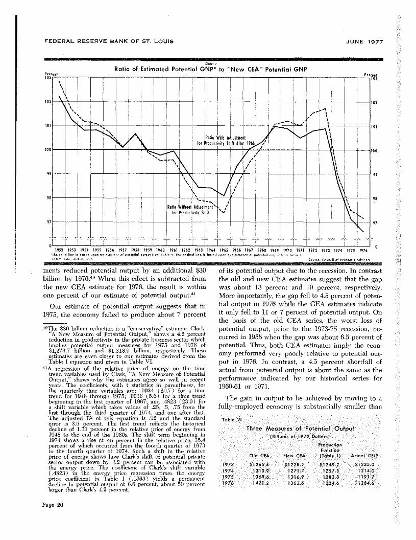
ments reduced potential output by an additional $30billion by 1976.~°When this effect is subtracted fromthe new CEA estimate for 1976, the result is withinone percent of our estimate of potential output.41

Our estimate of potential output suggests that in1975, the economy failed to produce about 7 percent

40The $30 billion reduction is a “conservative” estimate. Clark,“A New Measure of Potential Output,” shows a 4.2 percentreduction in productivity in the private business sector whichimplies potential output measures for 1975 and 1976 of$1,273.7 billion and $1,318.9 billion, respectively. Theseestimates are even closer to our estimates derived from theTable I equation and given in Table VI.

‘hA regressiosi of the relative price of energy on the timetrend variables used by Clark, “A New Measure of PotentialOutput,” shows why the estimates agree so well in recentyears. The coefficients, with t statistics in parentheses, forthe quarterly time variables are: .0034 (20.7) for a timetrend for 1948 through 1975; .0036 (5.6) for a time trendbeginning in the first quarter of 1967; and .4823 (23.0) fora sbift variable which takes values of .25, .5, .75 from thefirst through the third quarter of 1974, and one after that.The adjusted R

2of this equation is .92 and the standard

error is 3.5 percent. The first trend reflects the historicaldecline of 1.33 percent in the relative price of energy from1948 to the end of the 1960s. The shift term beginning in1974 shows a rise of 48 percent in the relative price, 35.4percent of which occurred from the fourth quarter of 1973to the fourth quarter of 1974. Such a shift in the relativeprice of energy shows how Clark’s shift of potential privatesector output down by 4.2 percent can be associated withthe energy price. The coefficient of Clark’s shift variable(.4823) in the energy price regression times the energyprice coefficient in Table I (.1363) yields a permanentdecline in potential output of 6.6 percent, about 50 perccntlarger than Clark’s 4.2 percent.

of its potential output due to the recession. In contrastthe old and new CEA estimates suggest that the gapwas about 13 percent and 10 percent, respectively.More importantly, the gap fell to 4.5 percent of poten-tial output in 1976 while the CEA estimates indicateit only fell to 11 or 7 percent of potential output. Onthe basis of the old CEA series, the worst loss ofpotential output, prior to the 1973-75 recession, oc-curred in 1958 when the gap was about 6.5 percent ofpotential. Thus, both CEA estimates imply the econ-omy performed very poorly relative to potential out-put in 1976. In contrast, a 4.5 percent shortfall ofactual from potential output is about the same as theperformance indicated by our historical series for1960-61 or 1971,

The gain in output to be achieved by moving to afully-employed economy is substantially smaller than

Icibic VI

Three Measures of Potential Output(Billions of 972 DoIlciru I

ProductionFunction

Oid GA Now CE.’ (loble I) Actcal GNP

‘973 $12654 51228.7 S1249 2 52225.3

2974 13159 12/1.7 225/.8 121-40

2975 13686 1316.9 12838 2191.7

19/6 2421 2 1363.6 12246 22646

Ratio of Estimoted

1952 2953 1954 2955 2956 2957 1958 2959 1960 1961 1961 1963 2964 2965 2966 1967 2968 1969 1970 1971‘Tb, o,Iid li,,i, b,,ed ‘9,, cc ,,fie,o1, ‘I pe’,,’i’l’,lp,l II,,, 9,61, V Th, do,h,d Ii,,, b,’od ,p,,,’’ ‘‘‘I,,,” of p’looli,I ‘‘‘99’ I,,, 7,61,1.*1001 dot, plo1’,th 1976

2971 2973 1974 975 2976

Page 20

FEDERAL RESERVE BANK OF ST. LOUIS

either the old or the new CEA measures indicate.Attempts to expand demand and production to suchunattainable levels in the near term would cerise-(1uently accelerate inflation. The period of time overwhich output may grow at a given rate faster thanthe growth rate of potential output is correspond-ingly smaller. The rate of growth of potential out-put will constrain actual output growth much earlierthan the old measure suggests. Also, at the outputrate achieved at full employment, Federal tax re-ceipts arid budget surpluses will be smaller than thehigher measures of potential indicate. Thus, a goalof a balanced budget at full employment will requiremore effort than either of the CEA estimates indicate.

CONCLUSIONS

Since 1962 estimates of potential output have be-come popular and important sources of informationfor policy formulation, The early estImates, and untilrecently the official estimates, focused upon laborresources only. New estimates by the CEA have at-tempted, to some extent, to account explicitly for theimportance of capital resources and a p1’oductionfunction. The CEA has also suggested that e:cergydevelopments are an important factor affecting theproductivity of fully-employed resources.

Using a production function which accounts ex-plicitly for capital and energy resources, an alterna-tive measure of potential output has been developed.The production function support the argu—

JUNE 1977

ment that the new energy regime imposed in 1974permanently reduced potential output by about fourpercent. The production function estimates show thatfailure to account for energy prior to 1973 is notcritical, but that serious inconsistencies arise whcn thesample period is extended to include recent years.

Until 1973 the historical series for potential outputdeveloped here tends to conform more to the oldCEA series than the new series, After 1973, however,the new CEA estimates adjusted for the magnitude oftheir suggested decline in productivity are very closeto our estimates. Thus, while our estimates cast somedoubt on the historical accuracy of the new CEAestimates, they support the CEA’s suggestion thatenergy price developments after 1973 reduced poten-tial output.

The implications of the new CEA estimates andthose presented here are of great significance for thefull-employment and growth prospects of the econ-omy. Attempts to achieve an unattainable potentialoutput rate through stimulative policy will not onlyfail, but will acid to inflationary pressures. Also, thereis little prospect for an extended period of growth atrates higher than the rate of growth of potential out-put (about 3.5 percent per year). The gap betweenpotential and actual output will tend to close withintwo years, even with the moderate growth of actualoutput achieved in 1976. Finally, at full employment,existing tax and spending policies will result in amuch larger budget deficit than higher measures ofpotential output indicate.

APPENIMX I

An Analysis of the Eckstein-Heien Model for

Determining Potential Output1

In a recent study for the Joint Economic Committee,Eckstein and Heien (E-H) have estimated an annual

1Albert J. Eckstein and Dale M. Heien, “Estimating PotentialOutput for the U.S. Economy in a Model Framework,”Achieving the Goals of the Employment Act of 1946 — Thir-tieth Anniversary Review, U.S. Congress, Joint EconomicCounmittee, 94th Cong., 2nd sess., December 3, 1976,pp. 1-25.

model which they use to construct an alternative to theofficial CEA potential output series. Since their analy-

sis purports to introduce the impact of energy price

changes on potential output, and since the conclusions oftheir analysis are remarkably different from those re-

ported here, this appendix attempts to analyze the rea-sons for the different conclusions.

Page 21

FEDERAL RESERVE BANK OF ST. LOUIS JUNE 1977

The first difference involves the choice of data series,E-H choose to study the private nonfarm sector of theeconomy. This differs from the private business sector asdefined in the text, in that the E-H measure excludes thefarm sector of the economy, and includes the imputedoutput to owner-occupied housing and output originatingin households and non-profit institutions, They also chooseto use raw materials as the third factor of production intheir estimated production function, in contrast to theenergy input concept employed above, In practice thisdifference should not be too important, since 88 percentof the weight in their Laspeyres index of raw materialscomes from the crude oil, tefined petroleum products,natural gas and coal components of their index. Thewholesale price index of energy used above measuresjust these components plus electrical power, so the cor-relation of the two input measures should be very high.

E-H estimate a three factor Cobb-Douglas productionfunction on annual data from 1950-74. The estimatedoutput elasticities in their function can be compared withthose implied by the production function which is re-ported above. All three estimated elasticities are essen-tially identical in both studies. In addition, the estimatedcoefficient on the time variable is almost exactly thesame in both equations. The differences in the conclu-sions of the two studies, therefore, cannot be attributedto differences in the underlying production function, thecentral relationship in both analyses.

E-H present a 12 equation model, while the analysisabove explicitly involves only one equation. For the pur-

poses of constructing potential output, the elaboration intheir 12 equations is somewhat misleading. They use theassumption that four percent unemployment is the ap-propriate rate of labor force utilization at which to con-struct potential output. With this assumption, their modelcan be characterized by three distinct blocks: 1) anemployment block consisting of the labor force participa-tion equations and the various identities defining em-ployment, labor force and unemployment, 2) a wage-price block consisting of the equations for the wage ratein the private nonfann economy and the price of outputin the private nonfarm economy, and 3) an output blockconsisting of the production function, a derived demandequation for raw materials, and an equation for the aver-age hours per worker.

Under the assumed “full-employment” conditions, theemployment block is completely independent of the restof the model. The size of the male labor force is ex-pressed solely as a function of exogenous variables, so itis also an exogenous variable for purposes of the model.The female labor force is a function of exogenous vari-ables, other variables within the employment block of themodel, and lagged variables from other blocks of themodel. The various identities in this block relate vari-ables defined within the block to exogenous variables.Therefore, it is possible to solve this subset of theirequation system for the total private nonfarm employ-ment as a function of only exogenous variables. Privatenonfarm employment can affect variables in both thewage-price block and the output block.

The wage-price block is affected by two exogenous

variables, the price of raw materials and the full-employ-ment unemployment rate. It is also affected by the em-ployment block and the output block, since these partsof the model detennine employment and output whichaffect unit labor costs. Unit labor costs are specified asan important influence in the determination of privatenonfarnn wages.

The output block is affected by the exogenous capitalstock and exogenous capacity utilization rate. It is af-fected by the employment block through employmentin the private nonfann sector which enters into theaggregate production function. Furthermore, the onlylink between the wage-price block and the output blockis through the relationship for the average number ofhours per worker, which depends on the real %vage rate,This relationship is not particularly strong, since theelasticity of the average number of hours per worker withrespect to the real wage rate is only .2, but it explainswhy E-H obtain a positive relationship between rawmaterials prices and potential output.

In the Eli model, an increase in raw materials pricedirectly affects the price of output in the nonfann sector.A higher price level in turn causes higher wages, but theincrease is less than proportional, so the real wage ratefalls in response to the increase in raw materials prices.Real wages have a negative impact on the average num-ber of hours per worker, so hours per worker rise in re-sponse to the increase in raw materials prices. But totalprivate sector employment in the model is exogenous atpotential output as discussed above, so total manhoursrise in response to the increase in raw materials prices.The net effect is an elasticity of real output with respectto raw materials prices in the E-H model of .02. The smallmagnitude of this elasticity illustrates the weakness ofthe interrelationship of the price-wage equations of themodel with the output equation through the averagehours equation.

If E-H had assumed, as do the authors of other studiesof potential output, a fixed number of hours per personat full employment, then the link between the wage-price block and output block in their model would bebroken. Their potential output model would then consistonly of two equations; the production function and thedemand for raw materials equation, supplemented byexogenous assumptions on the magnitude of manhourssupplied at potential output. Under these circumstancestheft analysis would imply that there is no effect ofchanges in raw materials prices on potential output. Inpractice, their analysis effectively implies such a conclu-sion since the price elasticity reported above is so closeto zero.

The two equation model which is so closely approxi-mated by the E-H model is exactly the two equationmodel which is implicit in the analysis presented above.The aggregate production function, with the relativeprice of energy as one of the right hand side variables,is derived by substituting the demand equation forenergy under the assumption that the real price of energy

Page 22

FEDERAL RESERVE BANK OF ST. LOUIS JUNE 1977

inputs is exogenous. Recall that the estimates of theproduction function parameters are essentially the samefor the two studies. Therefore, the difference in the re-sults obtained must be attributable to differences in theexplicit or implicit demand functions for energy inputs.

The problem with the E-H model is that the demandfunctions for both labor and raw material inputs aremisspecified. Such demand functions normally would beexpected to be consistent with the first-order conditionsfor cost minimization and/or profit maximization, In thecase of the Cobb-Douglas production function, this im-plies that the input demand functions must be log-linear.Yet both the demand function for raw materials and thedemand function for labor services in the E-H study arespecified as linear functions. This probably accounts forthe insignificance of the estimated coefficient of therelative price term in the raw material demand equationwhich E-H report in the text, but not in the equations ofthe model.

The approach used in this study implicitly assumesthat both the output elasticity and the price elasticity ofthe demand for energy are one, and that the functionalform of this equation is log-linear. If this were not thecase, then the output elasticities derived from the pro-duction function parameter estimates should be biased.Three pieces of evidence suggest that this is not the case.First, the estimated output elasticity of labor servicesconform quite closely to the share of labor in total incomeas it should under the constant-returns-to-scale restric-tion. Second, the estimated output elasticity of energyinputs conforms almost exactly with the estimates fromcross-section time series data of several countries, includ-ing the United States obtained by Criffin and Cregory.Third, as mentioned above, the estimated output elas-ticity of energy (as well as of other resources) obtainedin this study are almost identical to those obtained byE-H even though they used a measure of the quantity ofraw materials input in estimating the production func-tion directly.

APPENDIX II

Equation (2) constrains both the output and priceelasticities of energy demand to unity. Consider the

regressors, (In L-ln K), so all of the estimated regressioncoefficients K Ys) would be biased.

unconstrained hypothesis for the energy demand curve: .If the price elasticity of energy demand, 52,~ is notIn E +

3u In Y — 5,ln (~C~~R)+

If this is substituted in the Cobb-Douglas productionfunction:

In Y = a + a In L + fin K + yIn E + u.

where a + $ + y 1. the result us:

unity, then the estimated regression coefficients (is’s) arenot biased, but the output elasticities which we havederived from the regression coefficients are biased. Ourestimates~ofthe output elasticities for labor and energyare a~~2/(1 — ~s) and y*~a/(1 — pa), respectively.The unbiased estimates of these output elasticities are

lInY_InKI$u+PrllnL~Iu1KI

+f3ln(P

1,/P

13)+$

4lnK+ ‘suY

ç=y*[ land&=oo[ 1l+~—l)(1—5~) l+yO(

62)

a + ~where (3, ( ) (3, = K ‘~ )

1 — y - 1 —5u v

Consequently, if 52 < 1, our estimate of the output elas-ticity of energy is biased downward and our estimateof the output elasticity of labor is biased upward. Theconsistency of our estimates of the output elasticities

— a —1 + += ‘~2 (3 = ( $ ~‘

1 — a y I — S~y

with estimates from other sources and the consistency ofthe output elasticity with the labor share data, suggeststhat biases from these sources are not substantial. Evenif the output elasticities were biased because the price

Therefore, if the output elasticity of energy demand, elasticity of energy demand was less than unity, theSi, were not unity, the specification which has been esti- biases would not affect our potential output computa-mated would have an omitted variable, In K, whichwould be correlated with at least one of the included

tions, since these are based on the unbiased estimatedregression coefficients (frs).

Page 23

A quarterly series for potential CNP can be constructedusing the same method and data when some additional as-sumptions are made concerning the data. The principaldata problems involve quarterly estimates of the capitalstock and potential employment or manhours.

Quarterly data on the stock of capital are found byprorating the annual year-end changes in the net stock offixed nonresidential equipment and structures over quar-ters using quarterly rates of investment in nonresidentialfixed investment as the weights. Clark’s annual data onthe potential labor force are assumed to be for thesecond quarter of each year and a linear interpolation isused for other quarters. To find potential manhours, aquarterly estimate of hours per worker is obtained suchas that contained in Table IV. The quarterly potentialhours per worker is found by using Clark’s full-employ-ment unemployment rate for the respective years in theequation(1) In HPW.8120 — .0033 U -- .0010

(346.6) (—7.08) (—50.75)~297 D.W.’=.31

which is estimated for the period from the second quar-ter of 1948 through 1975.

The quarterly production function comparable to theannual estimate in Table I, (fl/1948-IV/1975) is

(2) In Y=1.5974 + .7192 in L + .2808 In K(14,20) (20.85) (8.14)

—.1164 In P + .0045(—5.64) (15.00)

~2,,,98 i).W.= 1.90

S.E.= .008 = .80

The estimated coefficients are essentially the same as forthe equation in Table I. The estimated output elasticitiesand trend growth term are (standard errors inparentheses)

= 64A% (3.08%), ~ = 25.2% (3.08%),

= 10,4% (1.85%), i = .4% (.03%).

APPENDIX III

S.E,= .0062