enhancing transportation equity analysis for long...
TRANSCRIPT

Enhancing Transportation Equity Analysis for Long-Range Planning and Decision Making
By
Tierra Suzan Bills
A dissertation submitted in partial satisfaction of the
Requirements for the degree of
Doctor of Philosophy
In
Engineering - Civil and Environmental Engineering
in the
Graduate Division
of the
University of California, Berkeley
Committee in Charge:
Professor Joan Walker, Chair
Professor Samer Madanat
Professor Paul Waddell
Professor Elizabeth Deakin
Fall 2013


1
Abstract
Enhancing Transportation Equity Analysis for Long-Range Planning and Decision Making
By
Tierra Suzan Bills
Doctor of Philosophy in Engineering - Civil and Environmental Engineering
University of California, Berkeley
Professor Joan Walker, Chair
Metropolitan Planning Organizations (MPOs) regularly perform equity analyses for their long-
range transportation plans, as this is required by Environmental Justice regulations. These
regional-level plans may propose hundreds of transportation infrastructure and policy changes
(e.g. highway and transit extensions, fare changes, pricing schemes, etc.) as well as land-use
policy changes. The challenge is to assess the distribution of impacts from all the proposed
changes across different population segments. In addition, these agencies are to confirm that
disadvantaged groups will share equitably in the benefits and not be overly adversely affected.
While there are a number of approaches used for regional transportation equity analyses in
practice, approaches using large scale travel models are emerging as a common existing practice.
However, the existing methods used generally fail to paint a clear picture of what groups benefit
or do not benefit from the transportation improvements. In particular, there are four critical
shortcomings of the existing transportation equity analysis practice. First, there is no clear
framework outlining the key components of a transportation equity analysis at the regional-level.
Second, the existing zonal-level group segmentation used for identifying target and comparison
groups are problematic and can lead to significant biases. Third, the use of average equity
indicators can be misleading, as averages tend to mask important information about the
underlying distributions. Finally, there is no clear guidance on implementing scenario ranking
based on the equity objectives.
In addressing the first shortcoming of existing equity analysis practices, we present a guiding
framework for transportation equity analysis that organizes the components of equity analysis in
terms of transportation priorities, the model, and the equity indicators. The first component
emphasizes the need to identify the priority transportation improvement(s) relevant for
communities, as this guides the transportation benefits (or costs) to be evaluated. The second
component is the model to be used for facilitating scenario analysis and measuring the expected
transportation and land-use changes. The third component refers to the selection of equity
indicators (ideally selected based on the transportation priorities identified), and the evaluation of
these indicators. This three-part framework is also useful for outlining the research needs for
transportation equity analysis. Among other key research needs, the literature indicates that the
development of meaningful distributional comparison methods for transportation planning and
decision-making and the use of more comprehensive measures of transportation benefit (for use
as equity indicators) are critical.

2
The primary contributions of this dissertation relate to the third component; we develop an
advanced approach for evaluating transportation equity outcomes (as represented by the equity
indicator(s)). Our proposed analytical approach to transportation equity analysis addresses the
existing shortcomings with respect to zonal-level group segmentation and average measures of
transportation equity indicators. In addition, our approach emphasizes the importance of scenario
ranking using explicit equity criteria. Our approach leverages the disaggregate functionality of
activity-based travel demand models and applies individual-level data analysis to advance the
existing equity analysis practices.
There are four steps in our proposed equity analysis process. The first step is to select the equity
indicators to be evaluated and segment the population into a target group and comparison
group(s). In this case we advocate for an individual -unit of segmentation and therefore
individual-level equity indicators. This minimizes the biases associated with aggregate group
segmentation and average equity indicators. The second step is to calculate the indicators from
the model data output, which involves determining the exact measures (formulas) for the selected
equity indicators. Here we advocate for measures that are comprehensive and sensitive to both
transportation system changes and land-use factors, such as the logsum accessibility and
consumer surplus measure. The third step in the process is to generate and evaluate distributions
of the individual-level equity indicators. In particular, we advocate for the use of what we refer
to as the “Individual Difference Density” comparison, which compares distributions of
individual-level changes for the population segments across the planning scenarios. This
comparison allows for the “winners” and “losers” resulting from the transportation and land-use
plans to be identified. The fourth and final step in the process is to identify equity criteria
(associated with the chosen equity standard (objective)) and rank the planning scenarios based on
the degree to which they meet the equity criteria.
We present two conceptual demonstrations of the advantages of distributional comparisons,
relative to average measures. The first case uses a synthetic data set and simple binary mode
choice model to show and the second case uses an empirical data set (the 2000 Bay Area Travel
Survey) and more sophisticated mode choice model. These demonstrations show that
distributional comparisons are capable of revealing a much richer picture of how different
population segments are affected by transportation plans, in comparison with average measures.
Further, distributional comparison provides a framework for evaluating what population’s
characteristics and conditions lead to certain distribution transportation outcomes.
Our proposed process for regional transportation equity analysis is subsequently applied in a case
study for the San Francisco Bay Area. We evaluate joint transportation and land-use scenarios
modeled using the Metropolitan Transportation Commission’s state-of-the-art activity-based
travel demand model. We demonstrate the power of individual-level data analysis in a real-world
setting. We calculate individual-level measures of commute travel time and logsum-based
accessibility/consumer surplus using the model output and compare the scenario changes across
income segments. We generate empirical distributions of these indicators and compare the
changes associated with the planning scenarios for low and high income commuters. Further, we
apply criteria for a set of equity standards (which represent alternative equity objectives) and
rank the planning scenarios. There are four key takeaways from this case study. First is that our
results show a significant difference in equity outcomes when using the individual-level

3
population segmentation approach, compared to using the zonal segmentation approach done in
practice. In fact we find opposite results. For average commute travel time, the Metropolitan
Transportation Commission’s zonal segmentation approach indicates that low income commuters
are worse off than all other commuters, while the individual segmentation approach (in our case)
indicates that low income commuters are significantly better off than high income commuters.
While the underlying causes for these results warrant further investigation, we hypothesize that
this difference is due to the fact that the zone-based approach only captures 40% of the target
(low income) group. The individual-level segmentation approach is able to capture 100% of the
target group. Second is regarding the equity indicators evaluated. The commute travel time
indicator results indicate that low income commuters are better off than high income commuters,
while the accessibility/consumer surplus results indicate that low income commuters are worse
off than high income commuters. The underlying causes for these results warrant further
investigation, but we hypothesize that this difference in results to due to the fact that the logsum
accessibility/consumer surplus measure by design is able to capture transportation and land-use
related factors, while the travel time measure only captures one dimension of transportation user
factors. Focusing on travel time may be misleading because it does not fully capture the true
benefits of the transportation scenarios. Third is regarding the use of distributional comparisons,
relative to average measures. We find that distributional comparisons are much more informative
than average measures. The distributional measures are capable of providing a much richer
picture of individuals-level transportation impacts, in terms of who gains and who loses due the
transportation planning scenarios. Using the accessibility/ consumer surplus measure, the
Individual Difference Densities show that as many as 33.3% of low income commuters
experience losses, compared to 13.4% for high income commuters. Finally, we make the case
that the use of equity standards for scenario ranking plays an important role in the equity analysis
process. Our results show that different equity standards result in different rankings for the
transportation planning scenarios. This points to the need for agencies (and communities) to
make conscious decisions on what equity standard(s) should be used and apply this/these in the
scenario ranking process.
This dissertation work includes the first known full-scale application of a regional activity-based
travel model for transportation equity analysis that involves distributional comparisons of
individual-level equity indicators and scenario ranking based on equity criteria. We find that
while the existing practice is to use average measures to represent how difference are affected by
transportation plans, distributional comparison are able to provide for a richer evaluation of
individual-level transportation impacts. Distributional comparisons provide a framework for
quantifying the “winners” and “losers” of transportation plans, while average measures and be
misleading and uninformative. We make significant progress with regard to evaluating equity
indicators (part three of the guiding framework). However, our proposed process is flexible and
can be extended to include a number of additional advances, including more environmental and
long-term land-use related equity indicators (e.g. emissions exposure, gentrification and
displacement risk, employment participation, etc.) and additional population segments (e.g. age,
ethnicity, household type, auto-ownership class, etc.). Among other important research
directions, our analytical framework for regional transportation equity analysis can be applied to
investigating why certain groups are more likely to be “losers” and what factors of transportation
planning scenarios to modify in order to arrive at a more equitable transportation and land-use
plan.

i
To my mother for her love, support and encouragement,
and to my aunties for their inspiration and examples.

ii
Table of Contents
Table of Contents .......................................................................................................................... ii
List of Figures ................................................................................................................................ v
List of Tables ................................................................................................................................. vi
Acknowledgements ..................................................................................................................... vii
Chapter 1 . Introduction
1.1 Introduction ........................................................................................................................... 1
1.2 Research Scope ..................................................................................................................... 2
1.3 Objectives .............................................................................................................................. 3
1.4 Contributions ......................................................................................................................... 3
1.5 Dissertation Outline............................................................................................................... 5
. Transportation Equity Analysis: Background, Literature, and Existing Chapter 2
Practices
2.1 Introduction ........................................................................................................................... 6
2.2 Background ........................................................................................................................... 6
2.2.1 Origins of Equity in Transportation Planning................................................................. 6
2.2.2 Defining Transportation Equity ...................................................................................... 7
2.2.3 Transportation Equity Analysis and Environmental Justice Regulations ....................... 8
2.2.4 The Significance of Equity Analysis in Transportation Planning ................................... 9
2.3 A Guiding framework for Transportation equity Analysis .................................................... 9
2.3.1 Component 1: Priorities ................................................................................................ 10
2.3.2 Component 2: Model .....................................................................................................11
2.3.3 Component 3: Indicators .............................................................................................. 12
2.3.4 Feedback: Linking Equity Indicators and Transportation Priorities ............................. 13
2.3.5 Summary and Critique of Literature and Existing Equity Analysis Practice ............... 13
2.4 The Existing Practice for Regional Transportation Equity Analysis ................................... 14
2.4.1 “Non-modeling” Approach to Regional Transportation Equity Analysis .................... 14
2.4.2 “Modeling” Approach to Regional Transportation Equity Analysis ............................ 15
2.5 Critiquing the Existing Equity Analysis Process ................................................................ 18
2.6 Conclusion ........................................................................................................................... 19
iii
. Methodology: An Analytical Framework for Transportation Equity Analysis of Chapter 3
Long-Range Transportation Plans
3.1 Introduction ......................................................................................................................... 21
3.2 Activity-Based Travel Demand Modeling for Transportation Equity Analysis ................. 21
3.2.1 Modeling Process ......................................................................................................... 22
3.2.2 Model Estimation ......................................................................................................... 22
3.2.3 Scenario Forecasting ..................................................................................................... 26
3.2.4 Data Processing ............................................................................................................ 27
3.3 Proposed Equity Analysis Process ...................................................................................... 28
3.3.1 Overview of Proposed Equity Analysis Process........................................................... 28
3.3.2 Step 1: Define Population Segments and Identify Equity Indicators ........................... 29
3.3.3 Step 2: Indicator Calculations ....................................................................................... 35
3.3.4 Step 3: Generate and Analyze Distributions of Indicators ........................................... 39
3.3.5 Step 4: Equity Criteria and Scenario Ranking .............................................................. 44
3.4 Issues of Implementation .................................................................................................... 46
3.4.1 Size and Complexity of Activity-Based Travel Demand Models................................. 46
3.4.2 Micro-simulation and Individual Level Comparisons .................................................. 46
3.4.3 Logsum Accessibility and Consumer Surplus Measure ............................................... 47
3.5 Conclusion ........................................................................................................................... 48
. Distributions and Transportation Equity Analysis: Conceptual Evaluations Chapter 4
4.1 Introduction ......................................................................................................................... 49
4.2 Distributional Comparisons Using a Hypothetical Setting ................................................. 50
4.2.1 Data Synthesis .............................................................................................................. 50
4.2.2 Equity Indicator: Logsum Measure .............................................................................. 52
4.2.3 Scenario ........................................................................................................................ 53
4.2.4 Results .......................................................................................................................... 53
4.3 Distributional Comparisons Using a (More) Realistic Setting............................................ 55
4.3.1 Data: 2000 Bay Area Travel Survey ............................................................................. 55
4.3.2 Mode Choice Model ..................................................................................................... 55
4.3.3 Setting and Planning Scenarios .................................................................................... 55
4.3.4 Results .......................................................................................................................... 56
4.4 Conclusion ........................................................................................................................... 59

iv
. San Francisco Bay Area Case Study: Real-World Evaluation of Proposed Chapter 5
Transportation Equity Analysis Proces
5.1 Introduction ......................................................................................................................... 60
5.2 Bay Area Transportation and MTC’s Regional Activity-Based Travel Demand Model ..... 60
5.2.1 MTC Model Design ...................................................................................................... 61
5.2.2 Transportation and Affordability in the Bay area ......................................................... 63
5.2.3 Case Study Context and Data Set ................................................................................. 64
5.3 Model Data Description ...................................................................................................... 67
5.3.1 Summary of Population and Travel Characteristics ..................................................... 68
5.4 Methodology and Results: Proposed Equity Analysis Process ........................................... 69
5.4.1 Step 1: Population Segmentation and Indicators .......................................................... 69
5.4.2 Step 2: Indicator Calculations ....................................................................................... 72
5.4.3 Step 3: Distributional Comparisons .............................................................................. 75
5.4.4 Step 4: Equity Criteria and Scenario Ranking .............................................................. 89
5.5 Extensions and Considerations ........................................................................................... 92
5.5.1 Model Data Validation .................................................................................................. 92
5.5.2 Population Segmentation and Additional Equity Indicators ......................................... 93
5.5.3 Statistical Comparison of Distributions ........................................................................ 94
5.6 Conclusion ........................................................................................................................... 95
. Conclusions Chapter 6
6.1. Introduction ........................................................................................................................ 97
6.2. Revisiting the Guiding Framework for Transportation Equity Analysis............................ 97
6.3. Summary of Findings ......................................................................................................... 98
6.4. Research Directions.......................................................................................................... 101
6.5. Conclusion ........................................................................................................................ 102
References .................................................................................................................................. 104
Appendix A: Conceptual Evaluation Data Descriptions and Model Choice Model
Estimation Results ..................................................................................................................... 113
Appendix B: Bay Area Case Study Data Description ............................................................. 115
Appendix C: MTC Communities of Concern Descriptive Statistics .................................... 127
v
List of Figures
2.1 Equity Analysis Framework .................................................................................................... 10
2.2 MTC Equity Analysis of 2035 RTP Example: ........................................................................ 17 2.3 MTC Equity Analysis of 2035 RTP Calculations Example (MTC, 2009) .............................. 17 2.4 MTC Equity Analysis of 2040 RTP/SCS Example: Commute Time (Minute), ..................... 18
3.1 Full Modeling and Analysis Process Supporting Transportation Equity Analysis ................ 22
3.2 Generic Activity-Based Travel Model Schematic................................................................... 23
3.3 (A-C). Hypothetical Commute Travel Time Distributions ..................................................... 41
3.4 Hypothetical Aggregate Density Comparison ........................................................................ 43 3.5 Hypothetical Individual Difference Density Comparison ...................................................... 44
4.1 Hypothetical City Setting for Generating Synthetic Population. ............................................ 51
4.2 Individual Difference Density Comparison for a Hypothetical Setting .................................. 54 4.3 Mode Shares for Low Income and High Income Workers ..................................................... 56
4.4 Individual Difference Comparison for Scenario 1 (20% Travel Cost Reduction) .................. 57 4.5 Individual Difference Comparison for Scenario 2 (20% Travel Time Reduction) ................. 58
5.1 Model Schematic for MTC’s Activity-Based Travel Demand Model .................................... 62
5.2 Average Transportation and Housing Costs at a Percent of Average Household .................... 64
5.3 MTC Equity Analysis of 2040 RTP/SCS Example: ............................................................... 77 5.4 (A-D) Aggregate Commute Travel Time Densities (Low Income) ........................................ 80
5.5 (A-D) Aggregate Commute Travel Time Densities (High Income)........................................ 81 5.6 (A-D) Individual difference Density Comparisons (Commute Travel Time) ......................... 84 5.7 (A-D) Individual difference Density Comparisons (Access./Cons. Surp.) ............................ 87
5.8 Real World vs. Model Data Work Tour Mode-Shares ............................................................ 93
6.1 Equity Analysis Framework and Dissertation Emphasis ........................................................ 98
A.1 Distributions of Travel Times for Low income and High Income Workers…………..……113
A.2 Distributions of Travel Costs for Low income and High Income Workers…...……………113
B.1 A and B. (A) Household Income Shares and (B) Person-Type Distributions. ......................117 B.2 Low Income Community (Earning $30k or less) Residential Locations ..............................118
B.3 High Income Community (Earning $100k or more) Residential Locations .........................119 B.4 A-D. Household Member Characteristics ............................................................................ 120 B.5 A-D. Tour and Stop Frequency. ............................................................................................ 123 B.6 A and B Individual Tour Frequencies .................................................................................. 124 B.7 Mode Shares for Mandatory and Non-Mandatory Tours ..................................................... 125
B.8 Household Auto Ownership ................................................................................................. 126
C.1 MTC Communities of Concern Statistics…………….………………...………………….127

vi
List of Tables
3.1 Summary of Proposed Process for Regional Transportation Equity Analysis ........................ 28
3.2 Existing vs. Proposed Equity Analysis Process ...................................................................... 29 3.3 Population Data ....................................................................................................................... 30 3.4 Travel Behavior Data .............................................................................................................. 30 3.5 Travel Network Data ............................................................................................................... 30 3.6 Spatial Data ............................................................................................................................. 31
3.7 Example Population Segmentation Variables for Equity Dimensions .................................... 31
3.8 Common Equity indicators used for Regional Transportation Equity Analysis ..................... 33
3.9 Types of Accessibility Measures ............................................................................................. 36 3.10 Descriptions of Equity Standards.......................................................................................... 45
4.1 Synthetic Data Parameters ...................................................................................................... 51
4.2 Average Change in Logsum Consumer Surplus Measure ....................................................... 53 4.3 Share of Workers Who Experienced a Reduction in Consumer Surplus ................................ 54
4.4 Average Change in Consumer Surplus due to Scenario 1 ....................................................... 56 4.5 Average Change in Consumer Surplus due to Scenario 2 ....................................................... 57
5.1 Summary of Transportation and Land-use Scenarios ............................................................. 65
5.2 Household Income Class Definitions...................................................................................... 67
5.3 MTC Communities of Concern Selection Criteria ................................................................. 72 5.4 Average Travel Time Results .................................................................................................. 78
5.5 Travel Time Group Results (Low Income) ............................................................................. 79 5.6 Travel Time Group Results (High Income) ............................................................................ 82 5.7 Share of Commuters who Experience an Increase in Commute Travel Time ........................ 83
5.8 Average Difference in Logsum Accessibility/ Consumer Surplus ......................................... 85 5.9 Share of Households Who Experience a Decrease in Accessibility ....................................... 86
5.10 Average Daily loss in Consumer Surplus for “losers” ......................................................... 86 5.11 Equality Standard Results ..................................................................................................... 90
5.12 Proportionality Results for the Transit Priority Scenario ...................................................... 90 5.13 Proportionality Results for the Jobs-Housing Scenario ........................................................ 90 5.14 Proportionality Results for the Environmental Scenario ...................................................... 91 5.15 Proportionality Results for the Connected Scenario ............................................................. 91 5.16 Rawls-Utilitarian Results ...................................................................................................... 91
A.1 Mode Choice Model Estimation Results……………………..…………………………….114

vii
Acknowledgements
There are a number of people that I want to thank for enriching my experience while at UC
Berkeley. First I want to thank my advisor Professor Joan Walker. It has truly been an honor and
privilege to work with and learn from her. I thank her for her patience with me, continuous
support, guidance, and inspiration. At times when the stress of graduate work seemed too great,
Joan helped to renew my focus and excitement about research. I could not have asked for a better
advisor and researcher after which to model myself. Next, I would like to thank my other
dissertation committee members. I thank Professor Paul Waddell for his guidance, insight, and
inspiration; Professor Samer Madanat for his guidance and enthusiasm; and Professor Betty
Deakin for her advice, continuous support, and encouragement throughout my tenure at
Berkeley. I also want to thank David Ory at the Metropolitan Transportation Commission for his
help in shaping and reviewing my dissertation, and his advice; and Elizabeth Sall of the San
Francisco County Transportation Authority for her advice on my dissertation work. Next, I want
to thank Professor Aaron Golub at Arizona State University for his encouragement and for
reviewing my qualifying exam prospectus. Next, I want to thank Professor Susan Shaheen and
Professor Karen Frick for their support and encouragement during my time at Berkeley. Also, I
want to thank Professor Adib Kanafani for his insight, support, and encouragement. To Celeste,
Vikash, Eleni and other friends from the fourth floor of McLaughlin Hall, thank you all for your
continuous help and encouragement, starting from my very first semester in the TE program. I
would not have had it without you all. To Andre, Vij, and DJ, thank you all for your advice and
friendship. To my cohort members Sowmya, Aditya, Vanvisa, Julia, and others, thank all for your
help and advice during those rough first semesters in the TE program. To the girls (you know
who you are), thank you for your love and support during my time at Berkeley. Thank you for
being the sisters that I never had. Next, I want thank my undergraduate advisor Professor Charles
Wright for inspiring me to pursue transportation research and continue on to graduate school.
Last and certainly not least, I want to thank my wonderful family. Ma, thank you for your never-
ending love and support. Thank you for inspiring me. To Gayle, Carol, Lin, Gra-Ma, Bonnie,
Dale, Mrika, April, Melanna, Olanda, Terri, Destiny, Gary, Ngozi, Sol, Big Keith, Little Keith,
Terrance, Destiny, Joshua, and so many more family members (past and present), thank you. I
am because you are.
1
Chapter 1 . Introduction
This dissertation aims to advance the methods for transportation equity analysis of regional level
long range transportation plans. This is the process of analyzing social equity outcomes resulting
from multiple large scale transportation improvements. The methods presented herein leverage
the power of activity-based travel demand modeling, which represents the best practice in travel
demand modeling. In particular, we propose a process for regional equity analysis that makes use
of individual and household level data generated from these models, and among other things,
emphasizes the use of distributional comparisons to reveal individual-level equity outcomes.
1.1 Introduction
Addressing inequities across all areas of society is critical for thoughtful public policy. The
global financial crisis of 2008 drove the subject of inequity into the forefront of public discourse,
as income inequity was arguably a key trigger of this financial meltdown (Vandemoortele, 2009).
In the United States, where income inequity is drastically pronounced relative to the world’s
other developed nations and rising (Tomaskovic-Devey and Lin, 2013), evidence of inequities
can be found in numerous areas of society.
Equity concerns are particularly relevant in the transportation realm. Current conditions of
inequitable transportation accessibility levels among society have resulted from transportation
planning processes which place unfair weight on the preferences of the more advantaged
members of society. We are left with the reality that disadvantaged members of society have
experienced less-than-fair shares of transportation benefits and disproportionately high shares of
transportation externalities. These are long recognized concerns and have led to federal
Environmental Justice legislation and directives (1994 Executive Order 12898, and Title VI of
the Civil Rights Act of 1964) calling for government agencies (e.g. the US Department of
Agriculture (USDA), the US Environmental Protection Agency (EPA), US Department of
Transportation (DOT), State DOTs, and Metropolitan Transportation Organizations (MPOs)) to
investigate the expected outcomes of proposed infrastructure and policy changes, and confirm
that low income and minority (disadvantaged) groups will share equitably in the project benefits
and not be overly adversely affected.
The critical issues addressed in this dissertation lie with the approaches taken to analyze equity
outcomes of transportation infrastructure and policy improvements. In spite of the regulations
mandating equity analysis for long range transportation plans for many years now, the
approaches generally fail to paint a comprehensive picture the various transportation experiences
that result from transportation plans. In many cases the measures themselves are insensitive to
the heterogeneity of transportation experiences across different groups.
The remainder of this chapter is organized as follows: In Section 1.2, we give the dissertation
research scope. We then give the dissertation objectives, contributions, and chapter outline in
Sections 1.3, 1.4, and 1.5, respectively.

2
1.2 Research Scope
This research focuses on enhancing the methodology for transportation equity analysis of
regional-level transportation plans. These plans may include hundreds of transportation and land-
use investments, including large scale highway and transit improvements, fare changes and
tolling/pricing schemes (e.g. bridge tolling, variable tolling lanes, cordon pricing), land
development incentives, growth boundaries, etc. Because of this scale and great number of
projects, it is necessary to use large scale transportation models in order to evaluate the overall
impact of a transportation plan on travel in the region. As will be discussed throughout this
dissertation, activity-based travel demand models are particularly useful for equity analysis of
regional transportation, because of their use of micro-simulation and ability to generate
population and travel-related data at disaggregate (individual and household) levels. Activity-
based travel models represent the best practices in travel demand modeling and have great
potential for disaggregate level transportation equity analysis. That is, the disaggregate
population and travel-related data from these models enable us to explore the use of
distributional comparison tools and reveal the “winners” and “losers” resulting from
transportation plans.
The Use of Travel Demand Models for Regional Equity Analysis The equity analysis process proposed in this dissertation falls under what we define as a
modeling approach to regional equity analysis (as will be discussed in Section 2.4), where large
scale travel models are applied to measuring the impact of transportation plans on regional
travel. The literature indicates that equity analyses using large scale regional travel models are
becoming more prevalent (Johnston, et al., 2001; Rodier et al., 2009; Castiglione et al., 2006;
MTC, 2001; MTC, 2013). Further, more and more MPOs are adopting activity-based travel
models for evaluation their Regional Transportation Plans (RTPs) (Bowman, 2009). The concern
is that methods used for regional transportation equity analyses are lagging behind. The
advantages of using disaggregate data from activity-based models for equity analysis are well
cited in the literature (e.g. Walker, 2005); although to date, there are no examples of an
application that uses disaggregate level indicators for regional equity analysis. Further, only one
other example is found in the literature where disaggregate population segmentation is applied
for regional transportation equity analysis (Castiglione et al, 2007).

3
1.3 Objectives
The objective of this dissertation is to develop a quantitative methodological approach for
regional transportation equity analysis that leverages the power of activity-based travel demand
modeling. Our proposed equity analysis method, compared to prior methods used, will extend
the capacity to analyze transportation equity impacts by taking advantage of the individual and
household level data from an activity-based model. Our method further emphasizes and the
usefulness of distributional comparison methods (among other tools) in understanding
transportation equity outcomes.
This objective is carried out in the following two steps:
Develop an enhanced analytical framework for transportation equity analysis
Execute an application of this proposed analysis process via a real world case study
With this improved framework, we endeavor to provide guidance for regional level
transportation equity analysis, as well as provide a richer understanding of the equity impacts of
regional transportation plans.
1.4 Contributions
This dissertation work makes three primary contributions. These contributions relate to multiple
bodies of literature, including policy analysis, transportation planning, and travel demand
modeling.
Developing an Enhanced Methodology for Transportation Equity Analysis of Regional Transportation Plans Our first contribution is in developing an analytical process for regional-level transportation
equity analysis. Our process leverages the disaggregate functionality of activity-based travel
demand models and distributional comparisons to gain a fuller and more accurate understanding
of individual-level equity outcomes across population segments. Our methods emphasize the
significance of distributional comparison methods, relative to the existing practice of using
average measure. Our methods also emphasize the need to adopt an equity standard and rank
planning scenarios based on the defined equity standard. This serves to link the outcome of the
equity analysis to the equity goals outlined by the agency, stakeholders, and/or practitioners.
Demonstrating Equity Analysis Using a Real World Activity-Based Modeling System and Transportation and Land-Use Scenarios The second contribution is that we demonstrate our proposed equity analysis process in a full
scale, real world case study using the San Francisco Bay Area Metropolitan Transportation
Commission’s activity-based travel model and recently developed transportation and land-use
scenarios. We detail the considerations and challenges with applying this advanced equity
analysis process in practice, and we provide some solutions to these challenges. There are four
key findings from this case study:

4
While a zonal segmentation approach for distinguishing the target and non-target groups
is used in most regional transportation equity analyses, this approach only allows for 40%
of the target (low income) group to be captured in the Metropolitan Transportation
Commission’s case. In comparison, the individual-level segmentation approach allows
for 100% of the target group to be captured. This difference in approach results in
opposite findings in our case, relative to comparable results from the San Metropolitan
Transportation Commission’s 2013 regional transportation equity analysis. Using the
commute travel time indicator, we find that low income commuters experience
significantly higher gains than high income commuters, while the Metropolitan
Transportation Commission finds that low income commuters experience lower gains
than all other commuters.
The accessibility/consumer surplus indicator produced opposite results than the travel
time indicator in our case. That is, the accessibility/consumer surplus results show that
low income commuters are worst off and most likely to experience losses than high
income commuters, while the travel time results show that low income commuters are
better off and most likely to experience gains than high income commuters. We attribute
this difference in results to the fact that the accessibility/consumer surplus indicator is
capable of capturing both transportation level-of-service and land-use factors, while
travel time only captures level-of-service.
Distributional comparisons (in comparison with the existing practice of using average
measures) are more informative and capable of providing a much richer picture of how
individuals-level transportation impacts, in terms of who gains and who loses due the
transportation planning scenarios.
While not common in practice, the use of equity standards for ranking transportation
planning scenarios is an important step in transportation equity analysis and powerful
approach to linking equity objectives for regional transportation and the results of the
equity analysis. In our demonstrations we find that application of different equity
standards results in different scenario rankings. This points to the need for agencies (and
communities) to make conscious decisions on what equity standard should be used and
apply this standard in the scenario ranking process.
Documenting an Application of Disaggregate Data Analysis using Data from Activity-Based Travel Models Since the early development and application of activity-based models for regional transportation
planning (in practice), the disaggregate-level data enabled through micro-simulation has been
touted as one of the key advantages of activity-based modeling. Yet no studies have
demonstrated individual-level measures for regional transportation planning applications. To the
author’s knowledge, this dissertation work documents the first such application using a full scale
activity-based travel model to generate and evaluate individual and household-level
transportation measures.

5
1.5 Dissertation Outline
The remainder of this dissertation is organized as follows. In Chapter 2, we provide discussions
on the background, literature, and existing practice for regional transportation equity analysis.
Chapter 3 presents a new analytical framework for equity analysis of regional transportation
plans. First, we provide an overview of activity-based travel modeling, and then we discuss the
proposed equity analysis process. Chapter 4 works through two examples to demonstrate the
usefulness of distributional comparisons for transportation equity analysis. To do this, we employ
a combination of synthetic and real-world travel datasets and some simplistic travel demand
models to calculate individual (logsum) consumer surplus measures. In Chapter 5, we present a
full scale case study of the proposed equity analysis process. In this case study for the San
Francisco Bay Area, we use a full scale activity-based travel modeling system to evaluate a set of
transportation and land-use scenarios. The travel demand model and planning scenarios were all
developed by the Metropolitan Transportation Commission (the Metropolitan Planning
Organization for the nine-county San Francisco Bay area). In the final chapter we summarize the
findings and contributions of this dissertation and give a discussion of future research needs.

6
. Transportation Equity Analysis: Background, Chapter 2
Literature, and Existing Practices
2.1 Introduction
In this chapter, we provide the background information for transportation equity analysis. The
existing challenges with understanding transportation equity analysis (of transportation
infrastructure and policy changes) stem from the inconsistencies in the literature. We aim to
organize of the literature starting with a discussion of the definitions, dimensions, and
interpretations of transportation equity. We then provide a guiding framework for transportation
equity analysis that relates three important components of transportation equity analysis: equity
priorities, modeling system, and equity indicators. In addition, these three equity analysis
components serve as a useful framework for reviewing and critiquing the academic literature
supporting transportation equity analysis. We finish with a discussion of the existing practices for
equity analysis of regional transportation plans. These discussions set the foundations for how
transportation equity is defined for this dissertation work, and the existing shortcomings of
current regional transportation equity analysis practices that we address in subsequent chapters.
This chapter is organized as follows. In Section 2.2 we provide some background discussions for
transportation equity analysis, including the origins of equity concepts in transportation planning,
definitions of transportation equity, the significance of equity in transportation planning, and
federal requirements for transportation equity analysis. In Section 2.3 we present a guiding
framework for transportation equity. In Section 2.4 we discuss and critique the existing practice
for transportation equity analysis, and in Section 2.5 we provide the chapter conclusions.
2.2 Background
2.2.1 Origins of Equity in Transportation Planning
Equity finds its roots in the philosophical and political concept of justice. Justice, is an important
and fundamental moral concept, and refers to conformity with the principles of righteousness and
fairness. The related concept of social justice refers to the application of these principles of
justice to the functions of society, with emphasis on fairness among social classes. These
principles are viewed as desired qualities of ethical and social decision making, and they
characterize the desired qualities of the political system. Further, regarding the relationship
between citizens and government, justice is commonly discussed in terms of distributive justice
(concerning the fairness of outcomes), and procedural justice (concerning the fairness of
processes), with the former being more emphasized in the literature and discourse (Konow,
2003).
From an economic perspective, the principle of equity is paired with economic efficiency, which
represent the fundamental criteria by which the performance of the economy is evaluated (as is
the objective in Welfare Economics) (Just et al., 2004). Much of the study on how to define and
measure an equitable distribution of goods and services across various markets falls under the

7
umbrella of Welfare Economics. However, the emphasis here has primarily been on the income
distribution of society, and whether income groups accrue their fair share of total national wealth
(i.e. gross domestic product).
The evaluation of equity outcomes in noneconomic domains has increasingly a central topic in
the evaluations of public programs and investments (Konow, 2003). Transportation policies are
an example of where policy makers and practitioners seek to apply principles of equity. As will
be discussed below, Environmental Justice regulations require equity analysis for all government
funded investments (including infrastructure and policies). Our concern is with the distribution
of transportation costs and benefits that result from such transportation-related investments.
These cost and benefits include a mix of economic, environmental, and transportation system
related factors. While federal transportation regulations attempt to outline equity principles for
transportation programs, the challenge of measuring and evaluating transportation equity
outcomes remains.
2.2.2 Defining Transportation Equity
A number of definitions for transportation equity can be found in the literature. To date, there
seems to be no consensus among academics on how transportation equity should be defined
(Levinson, 2010). In effort to bring organization to these definitions and provide a clearer
understanding of what is meant by transportation equity in this dissertation, we have structured
the definitions in terms of a general equity concept, equity dimensions, and equity standards.
Concept: Transportation Equity generally refers to the fair or just distribution of
transportation costs and benefits, among current (and future) members of society.
(Note that there are a number of distributions that may be considered fair, and
these will be referred to as equity standards, as discussed below.) Transportation
costs include the actual costs of building, operating, and maintaining the
transportation infrastructure, as well as transportation user costs and
environmental costs that result from the transportation operations and use. These
environmental costs may include the direct emissions from auto use, traffic
congestion, and noise pollution, etc. Transportation benefits range from
improvements in accessibility, mobility, and economic vitality on the general
scale, to reductions in travel time and travel user costs. Improved consumer
surplus is also an indication of transportation benefit.
Dimensions: Transportation equity can be defined along two primary dimensions: Horizontal
and Vertical equity (Musgrave and Musgrave, 1989; Litman, 2002). Horizontal
equity, which may include spatial and generational equity, refers to the
distribution of impacts (costs and benefits) across groups that are considered to be
equal in ability and need. Vertical equity refers to the distribution of transportation
impacts on sub-populations that differ in ability and needs, such as different social
and income classes, and disabled or special needs groups. In some cases spatial
and generational equity are seen as separate dimensions, but for simplification
purposes we group them with the Horizontal equity dimension.

8
Standards1: We refer to competing principles of equity as equity standards. A number of
different standards have been discussed in the academic literature. These
standards represent alternative ideas of what distribution (regarding rights,
opportunities, resources, wealth, primary goods, welfare, utility, etc.) is accepted
as fair or most desired.
2.2.3 Transportation Equity Analysis and Environmental Justice Regulations
Transportation Equity Analysis (sometimes referred to as Environmental Justice Assessment)
refers to the process of evaluating the distribution of outcomes resulting from transportation
plans (Lui, 2010). Beyond the evaluation of the transportation costs and benefits to various
population segments, the objective is to confirm that some desired equity standard (fair
distribution of transportation costs and benefits) is met. It is mandated that all federally-funded
transportation agencies perform equity analyses in evaluating proposed infrastructure and policy
changes. This mandate was established as a result of the 1994 Executive Order 12898, “Federal
Actions to Address Environmental Justice in Minority Populations and Low-Income
Populations,” as well as Title VI of the Civil Rights Act of 1964. The Executive Order directs
Federal agencies to make Environmental Justice a part of their mission by identifying and
addressing the impacts of all programs, policies, and activities, on minority and low-income
populations. Additionally, Title VI states that “No person in the United States shall, on the
grounds of race, color, or national origin, be excluded from participation in, be denied the
benefits of, or be subjected to discrimination under any program or activity receiving Federal
financial assistance.”
The three basic goals of Environmental Justice are as follows:
1. To avoid, minimize, or mitigate disproportionately high and adverse human health and
environmental effects, including social and economic effects, on minority populations
and low-income populations.
2. To ensure the full and fair participation of all potentially affected communities in the
transportation decision-making process.
3. To prevent the denial of, reduction in, or significant delay in the receipt of benefits by
minority and low-income populations
Although our focus is on Environment Justice requirements for transportation planning, it is
important to recognize that Environmental Justice regulations apply to all other Federal agencies,
such as the Environmental Protection Agency (EPA) and the US Department of Agriculture
(USDA). A full review of Environmental Justice analysis in other such areas is provided by Lui
(2010).
1A subset of these equity standards, seen frequently in the literature, has been compiled and is shown
Table 3.10 (in Chapter 2 of this dissertation).

9
2.2.4 The Significance of Equity Analysis in Transportation Planning
The U.S. Department of Transportation requires equity analysis for all projects that it helps to
fund, and for this reason transportation equity analysis is a federal requirement for MPOs.
However, there are broader reasons that equity analysis is critical for evaluating transportation
plans. The transportation system, largely funded by public dollars, plays a significant role in
supporting quality of life and social welfare. The infrastructure that facilitates the movement of
people and goods is also influential in shaping land-use patterns, livability of communities, and
economic interactions. In addition to mobility and accessibility improvements, transportation
investments can improve safety, health, and environmental conditions. There are also negative
externalities associated with transportation investments, including emissions exposure and noise.
However, the reality is that all of society will not experience the same level of transportation
impacts. Some will gain from transportation investments (winners) and some will be made worse
off (losers). Individuals will be affected differently by transportation changes, given the variance
in population and transportation conditions (income level, residential and work locations,
accessibility to alternative travel modes, etc.). Further, we know that historically, negative
transportation externalities have been born disproportionately by disadvantaged segments of
society (Ward, 2005; Schweitzer and Stephenson, 2007). For these reasons, it is inappropriate to
ignore that transportation plans will result in a distribution of impacts across members of society.
Planning organizations have a responsibility to fully evaluate and disclose the expected impacts
of transportation plans, for all segments of society.
2.3 A Guiding framework for Transportation equity Analysis: Literature Review and Research Needs
Here, we organize the literature and research needs within a general guiding equity analysis
framework. While federal Environmental Justice regulations require equity analysis for regional
transportation plans, little methodological guidance is provided. This has resulted in a wide range
of equity analysis methods (varying by scale, approaches, etc.). There has been some effort
around establishing goals for the distribution of transportation benefits (Martens, et al. 2012), but
no efforts have been found on providing clear outline on the process for conducting equity
analysis. With this framework, we seek to address two needs. The first is to define the important
components of equity analysis, which will guide this dissertation work going forward. The
second aim is to summarize the literature with respect to these components. This guiding
framework is illustrated in Figure 2.1 and the research areas are discussed below.

10
Figure 2.1 Equity Analysis Framework
2.3.1 Component 1: Priorities
The first component and research area (“Priorities”) is regarding the types of transportation
objectives that are most important to communities. Given the full range of possible transportation
benefits to society, which are most important for which communities? In many cases,
accessibility to employment is viewed as a primary transportation objective for low income and
minority groups of interest. Other priority objectives may be accessibility to health care
resources or grocery stores, shorter travel times, reduced traffic congestion and delay, improved
walkability, etc. A clear understanding of the transportation priorities, based on the needs of
communities is critical for selecting appropriate equity indicators (as will be discussed in Section
2.3.4).
There are two general approaches that practitioners can use to go about identifying the
transportation priorities for different communities, one qualitative and one quantitative. In the
qualitative approach, surveys, interviews, focus groups, etc., can be conducted to engage the
different communities and directly record what they view as transportation needs and priorities.
In the quantitative approach, travel behavior data can be analyzed to glean the travel limitations
and constraints for disadvantaged communities, relative to the majority population. The two
methods are complementary and participation requirements mandate that community members
be engaged and not simply treated as objects of study. In other words, qualitative methods for
involving communities are expected to shape and inform quantitative analysis. The
transportation needs and priorities of different communities would be based on their own
assessments, and not that of transportation practitioners. This dissertation focuses on advancing
quantitative methods for equity analysis but recognizes that in a real world application this would
have to be coupled with participatory processes whose findings would shape the priorities,
indicators, and model runs done.
There are a number of related studies which have sought to understand the differences in travel
behavior for different communities. A large number of studies have assessed the gender
differences in travel behavior (White, 1986; Mauch and Taylor, 1997; Pucher and Renne, 2003;
Nobis and Lenz, 2005; Zhou et al., 2005; Rogalsky, 2010). Some studies have also emphasized

11
the travel constraints of women, relative to their male counterparts (Astrop et al., 1996). These
studies have generally found that the travel behavior of women is heavily influenced by
household-serving responsibilities (grocery shopping, other non-work trips, etc.) and child
chauffeuring necessities, resulting is a greater number of trips with shorter trip lengths, and more
trip chaining. Other studies have assessed the travel behavior characteristics of the elderly and
disabled (Pucher and Renne, 2003; Alsnih and Hensher, 2003; Rashidi and Mohammadian,
2009). The elderly and disabled are found to have lower modality rates and greater dependence
on transit. This literature is one example of where the transportation needs have been assessed
for the purpose of recommending transportation improvements. Some studies have also focused
on travel behavior differences across various ethnicities and income classes (Mauch and Taylor,
1997; Giuliano, 2003; Tal and Handy, 2005; Srinivasan and Rogers, 2005; Agrawal et al., 2011),
with some further emphasizing the travel behavior differences by immigration status (Srinivasan
and Rogers, 2005). While there doesn’t seem to be a strong causal link between ethnicity and
travel behavior (Mauch and Taylor, 1997), there is a higher instance of residential clustering
among ethnic minorities as well as recent immigrants, resulting in high trip densities (the
majority of trips are made within a smaller radius of home). Lower income residents are also
more likely to be transit dependent, although the majority of trips are still made by automobile
(Astrop et al., 1996; Pucher and Renne, 2003; Alsnih and Hensher, 2003). In addition, the travel
behavior of lower income residents is generally characterized by fewer trips, with shorter trip
lengths, although it is unclear whether this is an indicator of transportation disadvantage (i.e. low
levels of accessibility), or simply a characteristic of low income traveler behavior. This body of
literature on the travel behavior of different communities is rather large; however, few studies
were found that have linked these travel behavior evaluations to transportation needs and how
these may vary across communities.
2.3.2 Component 2: Model
This component and research area (“Model”) focuses on the modeling tool to be used for
scenario analysis. The used of large scale travel demand models of regional level transportation
equity analysis is becoming more widespread, although this modeling tool can vary based on the
scale of the transportation investments being evaluated. This scenario analysis tool may refer to a
process or tool used to calculate the expected transportation, economic, land-use, and/or
environmental related changes due to transportation investments. Here, the task is to identify
which model (or process) is most suitable, and whether this model is accurate and
comprehensive with respect to the expected changes.
Using regional level analysis as an example, the literature indicates that more and more regional
planning authorities are applying travel demand models for transportation equity analyses, yet
few efforts have been done to assess whether output from these models effectively represents the
heterogeneity of travel behavior observed in the real world. These differences are critical for
equity analysis. This is, for example, because a model that is insensitive to the differences in
travel behavior between different income groups is likely unable to accurately model the
differences in equity outcomes between high and low income travelers. In practice, the statistical
significance of socio-demographic variables (in travel models) and the use of model calibration
processes (confirming that model forecasts to match some empirical control totals) is seen as
sufficient for assessing model sensitivity. However, for activity-based travel models, which are
able to generate person-level data, validation at the across population segments is not common.
12
One such study (Bills et al., 2012) compared distributions of travel time generated from a real
world activity-based model and the travel diary data used to estimate the travel model. In this
case, the tests of distributional equality fail, although the comparisons of the general shape of the
distributions and central tendencies indicate that the relative difference between the low and
high-income travelers is maintained. As this is only one example of such a study, there is a need
from more evaluations this kind.
It is important to note the influence of the travel diary data that is used to estimate activity-based
models. These models are estimated and calibrated on a sample of data (on individuals and their
travel patterns), and quality of this data has implications for the sensitivity of the model to the
differences between groups. That is, the model’s sensitivity is undoubtedly tied to how well the
sample data reflects the true characteristics of these groups of interest. In other words, the model
estimates are only as good as the travel diary survey data. This is certainly a research area that is
critical for making progress is the area of activity-based travel modeling for transportation equity
analysis.
2.3.3 Component 3: Indicators
The third component and research area focuses on the equity indicators used to measure equity
impacts (transportation-related costs and benefits). These indicators are quantitative
representations of the transportation priorities (described under component 1). For example, if
we determine that the transportation priority is to improve employment accessibility, then we
should use the change in employment accessibility (due to the transportation plan) as an equity
indicator. This third component in the framework deals with what equity indicators to use, as
well as how to compare the equity indicator measurements across communities or population
segments. The existing practice for regional level transportation equity analysis is to calculate
average measures of the indicators for the difference population segments and evaluate the
percentage change across these segments and across scenarios. The use of averages tends to
mask important information about the change in the distribution of transportation experiences (as
measured by the equity indicators). In particular, changes in the shape of a distribution may have
equity implications that can’t be fully captured using a mean measurement (Franklin, 2005). In
this dissertation, we emphasize the important of distributional comparisons of these indicators,
for different communities. However, few examples of distributional comparisons in equity
analysis are found in practice.
In one example, Franklin (2005) used Relative Distribution methods to do transportation equity
analysis. A Relative Distribution is a non–parametric and scale–invariant comparison between
two distributions (Handcock and Morris, 1999; Handcock and Aldrich, 2002; Franklin, 2005).
Accompanying statistical summary measures (polarization measures) provide a way to
decompose and interpret the differences between the distributions. Franklin (2005) clearly
demonstrates that more can be understood about equity outcomes (i.e. the progressivity and
regressivity of a policy) using distributional comparison measures, as opposed to comparing
mean values. However, Relative Distribution methods are very mathematically complex and
difficult for practitioners as well as academics to understand. Thus, there is a need to research
distributional comparison methods which are more readily usable in practice. Beyond the
Franklin example, no studies were found to have emphasized alternative methods for measuring
the changes in distributions, and apply these methods to equity analysis. Given that the purpose

13
of transportation equity analysis is to access the distribution of transportation costs and benefits,
it is understandable that the application of such methods (i.e. Relative Distribution methods)
would provide for a richer understanding of equity outcomes. In this dissertation, we take the
first steps toward developing distributional comparison methods for use in practice.
2.3.4 Feedback: Linking Equity Indicators and Transportation Priorities
An important criterion for identifying equity indicators, as represented by the black dashed
curve, is whether the chosen equity indicators are truly representative of the transportation
priorities for the groups of interests. As an example, accessibility is a widely used indicator of
transportation equity, but there is little in the literature that describes the direct link between
access and the desired societal benefits; economic opportunity or the probability of employment.
This question of whether job accessibility in linked to employment outcomes has been tackled in
the number of studies (O'Regan and Quigley, 1998; Cervero and Appleyard, 1999; Aguilera,
2002; Ory and Mokhtarian, 2005; Gurmu et al., 2006), but there doesn’t seem to be a consensus
on whether a measurable causal link exists, nor the direction of this relationship. Some studies
have found no evidence of a relationship between accessibility and employment (Cervero and
Appleyard 1999), while others (Gurmu et al., 2006) have found that accessibility to jobs and
child care resources are significant indicators of the probability of employment. This same
question can be asked of other commonly used equity indicators (accessibility to health care,
consumer surplus, travel time savings, etc.). There is some evidence in the literature on the
positive relationship between increased healthcare accessibility and the uptake of healthcare
services, among minority groups (Guendelman et al., 2000). This certainly represents a step in
the right direction, in terms the potential to identify equity indicators most relevant and
meaningful, and linked to the transportation priorities of different communities. However, there
is a need for more research efforts to develop the larger understanding of how different
transportation priorities link to societal benefits, and apply this understanding to the selecting
transportation equity indicators.
2.3.5 Summary and Critique of Literature and Existing Equity Analysis Practice
In summary, the equity analysis framework illustrated in Figure 2.1 serves as a useful and
standard guide for identifying the key components of transportation equity analysis, as well as
overviewing the current state of equity analysis practices and identifying the research needs.
These research needs are as follows:
There is a large body of literature focusing on the differences in travel behavior across
ethnicities, income levels, genders, etc., but has yet to be applied is the equity analysis
realm for identifying transportation needs and constraints, and thereby prioritizing
transportation improvements, for various population segments.

14
The use of activity-based travel models for equity analysis is becoming more common,
but there is a need to fully assess how well these models represent the differences in
travel-related outcomes for different groups of interest at the disaggregate level. This is
important for confirming the suitability of these models transportation equity analysis.
Further, given that the use of activity-based travel models in practice is relatively new,
there is a need to outline clear steps for effectively applying such models for equity
analysis.
The use of average measures of equity indicators is problematic, as they mask important
information underlying distributions (and changes in these distributions). Distributional
comparisons can provide for a richer understanding of equity outcomes at the individual
and household levels, but there is a need to develop more practical distributional
comparison methods.
The equity measures and indicators used are weakly linked to transportation costs and
benefits. For example, travel time is a commonly equity indicator used in practice, but
only captures one dimension of total transportation benefits. A more comprehensive
measure of would capture multi-dimensions, including costs, quality, satisfaction, etc.
There is a great need to identify more meaningful and comprehensive equity indicators
capable of representing true transportation benefits.
2.4 The Existing Practice for Regional Transportation Equity Analysis
The development and assessment of Regional Transportation Plans (RTP) are regular practices
for MPOs, usually taking place every three to five years. This periodic practice involves an
assessment of long-term transportation needs and proposals for transportation (and land-use)
improvements to address these needs. Among other foci, this process involves assessments of
equity impacts. Planning agencies (i.e. Metropolitan Planning Organizations (MPOs)) have
applied a range of methods for transportation equity analyses of Regional Transportation Plans.
The literature points to two primary analysis approaches. The first approach, which we refer to as
a “Modeling” approach, analyzes equity impacts using regional travel demand models, and
second approach, which we refer to as a “Non-modeling” approach does not apply travel demand
models to evaluate equity outcomes.
2.4.1 “Non-modeling” Approach to Regional Transportation Equity Analysis
The non-modeling approach, which tends to be most common among planning organizations
(Amakutzi et al., 2012), is characterized by the use of spatial analysis tools to map the residential
locations of low income and minority communities in relation to the location of the proposed
transportation project(s). This is done to discern the level of benefits to these communities based
on spatial proximity. In some cases, these analyses include determining whether the communities
are being overly exposed to transportation externalities (air or noise pollution, traffic congestion,
etc.) (e.g. MTC, 2001; Rodier et al., 2009).

15
2.4.2 “Modeling” Approach to Regional Transportation Equity Analysis
In the modeling approach to equity analyses, transportation and land-use scenarios are modeled
using a regional travel demand model. The general approach is to measure the expected impacts
of transportation and land use improvements on the travel behavior of defined population
segments, calculate some indicators of the costs and/or benefits to these segments (due to the
transportation and land-use improvements), and then compare these costs and/or benefits across
the segments in order to judge whether the distributions of costs and/or benefits is equitable.
Existing Equity Analysis Practice As further description of this modeling approach to regional transportation equity analysis, we
summarize the process in three steps below. Following, we give brief descriptions for population
segmentation and equity indicators, and then two examples of transportation equity analyses
done using travel demand models, as this approach is the focus of this dissertation.
Overview
This general equity analysis process (using travel demand models) is summarized in the
following three steps:
1. Select equity indicators (such as travel times, transit mode share, accessibility to
jobs, etc.) and segment the population into two categories: target group(s) and
comparison group(s).
2. Calculate indicators for the population segments (the target and non-target
groups).
3. Compare the changes in these measured values across the groups, and across
scenarios (simulating changes after some transportation policy or project has been
implemented).
Population Segmentation
This refers to the defining of target and comparison groups, and involves the use one or more
variables of segmentation (e.g. income, ethnicity, gender, etc.) and a unit of segmentation (e.g.
individuals, households, census blocks, travel analysis zones, etc.). Most commonly, the target
group is defined in terms of “communities of concern”. These are zones or census blocks that are
identified based on high concentrations of low income and minority residents. In this case, the
variables of segmentation are commonly income and ethnicity, and units of segmentation are
zones or census tracts (MTC, 2009; MTC, 2013b).
Equity Indicators
These are measures of the costs or benefits resulting from the transportation plan. There is a
range of indicators used in equity analysis of regional transportation plans. These will be outlined
in more detail in Section 5.4.1, but the most common are work travel time, accessibility to jobs,
emissions exposure, and project investments by population segment (MTC, 2009; SANDAG,
2011; MTC 2013).
16
Equity Analysis Examples
To illustrate the comparison process common for equity analyses done using travel demand
models, two examples are taken from equity analyses done by the Metropolitan Transportation
Commission (MTC), for their 2035 and 2040 Regional Transportation Plans. We use MTC’s
analyses as example for two primary reasons. The first is that they are one of the more
experienced MPOs with regard to applying travel demand models for transportation equity
analysis. Second is that MTC’s methodology represents to best practices in equity analysis of
regional transportation plans, given that they are currently the only MPO known to have applied
an activity-based travel model2 for regional transportation equity analysis.
MTC 2035 Equity Analysis (2009)
In this analysis, four scenarios are modeled to represent transportation and land-use
improvements and the (expected) resulting travel-related changes. These scenarios include a
“No-Project” scenario, the “Project” scenario (the agency’s “preferred” scenario), and two
additional alternative scenarios. These are modeled using a 4-step Travel Demand Model3. For
this analysis, the variables of segmentation were income and ethnicity, and the units of
segmentation were travel analysis zones. The zones were selected as communities of concern
based on the presence of high concentrations of low income or minority residents. The zones
with high concentrations of low income and minority populations are defined as communities of
concern, and a comparison is made between these communities of concern (target group) and
the remainder of the region (comparison group).
MTC evaluated a number of indicators, including work and non-work accessibility, vehicle
emissions exposure, and transportation/housing affordability4. The results for the work
accessibility measure (the weighted average of total low income employment opportunities,
within 30 minutes by transit) for the target group (communities of concern) and comparison
group (the remainder of zones in the Bay Area.) are shown Figure 2.2 and Figure 2.3. The
comparison was done by calculating the average change in the indicators (for each population
segment, and for the “Project”, “Pricing”, and “Land Use” scenarios relative to the “No-Project”
scenario). Focusing on the right-most column in Figure 2.3, they found that Communities of
Concern would accrue a similar level of accessibility benefits as would the Remainder of the
Region, although on average the Remainder of the Regional would experience slightly higher
gains in accessibility compared to the Communities of Concern.
MTC 2040 Equity Analysis (2013)
In MTC’s more recent equity analysis (MTC, 2013a), five scenarios are modeled, including a
No-Project scenario, Project (preferred) scenario, and three additional alternative scenarios.
These scenarios were modeled using their recently developed activity-based travel demand
model. In this case, the target (and comparison) groups are defined using zones as the units of
segmentation (as in the previous example), but using more variables of segmentation than
previously. In addition to ethnicity and income, these variables of segmentation include English
2It is important to note the MTC also applied a disaggregate land-use model (UrbanSim) in developing the
transportation and land-use scenario. For more details, see Waddell (2002) and Waddell (2013). 3For a description of MTC’s 4-step travel demand model, see Purvis (1997).
4For more details on the measurement of these indicators, see MTC (2013a).

17
proficiency, auto ownership, senior citizen status, disability status, number of parents in the
home, and rent burden. Zones with high concentrations for at least four of these variables are
classified as Communities of Concern. The indicators evaluated in this analysis were commute
and non-commute travel time (for all modes), transportation/housing affordability, displacement
risk, and vehicle miles traveled (VMT) and emissions density (exposure to vehicle emissions).
Figure 2.2 MTC Equity Analysis of 2035 RTP Example:
(Cumulative) Job Accessibility within 30 Minutes by Transit (MTC, 2009).
Figure 2.3 MTC Equity Analysis of 2035 RTP Calculations Example (MTC, 2009)

18
The comparison is done using the same methods from the previous example, where the average
change in the indicators are calculated and compared across population segments and across
scenarios. It is also important to note that this analysis included some mapping of Communities
of Concern vs. the planned investments, which is characteristic of the qualitative approach to
regional equity analysis. Figure 2.4 gives the results for the commute travel time indicator. From
this analysis, MTC concluded that although Communities of Concern experienced a slightly
smaller reduction in travel time, overall they fair comparably to the Remainder of the Region.
This is because the reductions in travel cost to Communities of Concern (due to some shifting to
less expensive travel modes) likely offset the negative travel time outcomes.
Figure 2.4 MTC Equity Analysis of 2040 RTP/SCS Example: Commute Time (Minute),
based on individual modes taken (MTC, 2013a)
Overall, we emphasize key takeaways. The first is that the type of travel model used to forecast
the MTC scenarios and applied for equity analysis was upgraded from a 4-step model to an
activity-based model in recent years, as is the new direction in regional travel modeling
practices. The second point is that the methodology (i.e. using zones as the unit of analysis and
using average measures of equity indicators) for these regional equity analyses have remained
relatively the same, even though activity-based models enable new and significant advantages in
these areas.
2.5 Critiquing the Existing Equity Analysis Process
Here we elaborate on the shortcomings of the existing practice for regional transportation equity
analysis. Recall from earlier that the first step in the existing practice is to identify transportation
equity indicators and define the population segments, the second step is to calculate the
indicators for the population segments, and the third step is to compare these indicators across
the population segments. There are three critical issues with the existing practice emphasized
here. These are regarding the unit of analysis by which the population is segmented, the
indicators used in the group comparison, and the method of comparison.
Regarding the unit of population segmentation, MPOs commonly classify the target group into
what are called “communities of concern” or Environmental Justice communities (MTC, 2009;
SANDAG, 2011; MTC 2013a). While the variables of segmentation vary some, these are
generally selected to capture high concentrations low income and minority households. Further,
the units of segmentation used are aggregate spatially-based units, such as travel analysis zones
(TAZs) or census tracts. In this case, the communities of concern represent the target group,
while all other zones in the regional represent the comparison group. The issue here is with the

19
use of zones as the unit of analysis, as this will likely lead to a degree of aggregation bias in
evaluating the impacts on population segments. Take the case that we are interested in vertical
equity and we want to compare impacts on low income travelers, relative to high income
travelers. Using a zone-based unit of segmentation is clearly problematic, as there would likely
be some share of other income groups living in the same zones. In this case, it is impossible to
isolate the impacts for the difference groups5. Activity-based travel models are capable of
measuring disaggregate impacts, which would alleviate issues with aggregation bias.
The second step in the existing process in to calculate equity indicators for the different
population segments, for the different planning scenarios. While our focus is not on discussing
which equity indicators are best, it is important to note a key challenge with common equity
indicators used in practice. This is regarding the extent to which the equity indicators represent
transportation-related benefits (or costs). For example, while travel time indicators are attractive
and intuitive mobility-based measures, they only capture a portion of transportation benefits. On
the other hand, accessibility measures are more comprehensive and capable of capturing land-use
related impacts, in addition to mobility impacts. As will be discussed in Chapter 3, the logsum
accessibility and consumer surplus measure is particularly desirable for its sensitivity to
individual costs and preferences.
The third and final step in the existing practice is to compare the indicators measured for the
population segments, across the different planning scenarios. As seen earlier, the common
approach is to calculate an average value of the equity indicator and compare the percentage
change across the population segments, from the base-case scenario to another project scenario.
The concern is that the use of average measures is problematic, because averages tend to mask
the individual level outcomes. For example, the average may indicate that overall, all groups are
better off as a result of the scenario, when in reality only 80% of individuals benefit and 20% are
made to be worse off.
2.6 Conclusion
In this chapter we have discussed the background, literature, and existing practice for
transportation equity analysis. Transportation equity analysis is a process undertaken to
determine how different groups will be affected by transportation plans, with an emphasis in
verifying that disadvantaged groups are not overly adversely affected. Although this analysis can
be done using a range of modeling and non-modeling approaches, the modeling approaches for
equity analysis becoming more prevalent. Overall, there are three key components to
transportation equity analysis, including transportation priorities, modeling tool, and equity
indicators. Our review of the literature and the existing practice for transportation equity analysis
points to a number of research needs and shortcomings. Regarding research needs, there are three
primary takeaways. First, the literature indicates the need to further verify that travel models
sufficiently represent the behavioral differences in travel behavior, observed in the real world.
Second is that there is a need to develop more useful distributional comparison methods for
5There are certainly some cases where spatial units of analysis are more appropriate: such as in the case of
“horizontal equity” analyses.

20
evaluating individual level equity outcomes. Third is that considerations for long-term
transportation and land-use impacts have largely been left out of transportation equity analyses.
Regarding the existing practice, the key shortcomings are related to the using of zones as units of
populations segments, weaknesses in how well the equity indicators represent transportation
benefits (or costs), and the use of average measure for equity indicators. The proposed equity
analysis process presented in Chapter 3 aims to address these shortcomings.

21
. Methodology: An Analytical Framework for Chapter 3
Transportation Equity Analysis of Long-Range
Transportation Plans
3.1 Introduction
Here we present an analytical framework for regional transportation equity analysis that
advances the existing equity analysis practice, and address the shortcomings discussed in
Chapter 2. This analysis framework draws on the power of activity-based travel demand models,
which represents the state-of-the-art in modeling and forecasting. We use these models to
measure the expected changes in travel behavior to result from transportation and land-use plans.
Among other things, this proposed process leverages the disaggregate functionality of activity-
based travel models, and the usefulness of distributional comparison for transportation equity
analysis.
The remainder of this chapter is organized as follows: Section 3.2 give an overview of the
activity-based modeling process, including model estimation, scenario forecasting, and data
analysis. In Section 3.3, we discuss each step in the proposed equity analysis process, including
some considerations for implementing such a process in practice. In Section 3.4, we discuss
some issues with implementing the proposed equity analysis process in practice. Finally, we give
concluding statements in Section 3.5.
3.2 Activity-Based Travel Demand Modeling for Transportation Equity Analysis
Travel demand models serve as the primary transportation planning tools for measuring and
forecasting changes in travel behavior that result from large scale transportation investments.
These models measure the effects of transportation system and land-use changes, as well as
travel and residential costs, and demographic changes on travel behavior (mode, destination,
time-of-day, and other travel choices). In this case, the model to be estimated in an activity-based
travel demand model. Activity-based travel models, described in this section, represent the best
practices in travel demand modeling and have tremendous potential for transportation equity
analysis. The disaggregate population and travel-related data from these models enable us to
explore the use of distributional comparison tools for transportation equity analysis, which are
capable of revealing the “winners” and “losers” resulting from transportation plans. In this way,
we can provide a clearer and more accurate understanding of equity outcomes across groups.

22
3.2.1 Modeling Process
From start to finish, the full modeling and analysis process used in transportation equity analysis
includes development and estimation of the travel demand models, forecasting of the
transportation and land-use scenarios, and then processing of the data. These three phases are
illustrated in the Figure 3.1. The primary contribution of this dissertation is with the Data
Processing phase, and will be detailed in Section 3.3. However, it is important to review the
Model Estimation and Scenario Forecasting phases from an equity analysis perspective. For
these two initial phases, the emphasis with respect to equity analysis is on capturing the
heterogeneity across population segments, such that the (expected) behavioral responses to
transportation and land-use changes can be modeled. These are critical for accurately measuring
the differences between population segments, and therefore equity outcomes across population
segments.
3.2.2 Model Estimation
This description of the Model Estimation phase includes the following: a general overview of
activity-based modeling systems, description of each model component, and a brief introduction
to utility theory and discrete choice modeling.
Model Description
Activity-based travel models were developed on the basic principle that one’s travel is derived
from their desire to participate in various activities (Bhat and Koppelman, 1999). Therefore,
individuals’ make their daily travel decisions based on their (individual and household)
established daily activities. This approach further aims to model travel from a more behaviorally
realistic (choice-based) perspective. It therefore breaks travel actions into a set of travel-related
choice dimensions and models each type of travel behavior using (logit) discrete choice models.
These travel choice dimensions generally include work location, auto ownership, (daily) activity
pattern, time-of-day, stop location, and mode choice dimensions. Figure 3.2 shows a schematic
for a typical activity-based travel demand model. These model components are linked together in
a “nested-like” structure, using feedback variables6.
6These “feedback” variables are logsums, which can be generated from any (logit) choice dimension in the activity-
based modeling system. The significance of these logsums is further discussed in Section 3.3.3.
Scenario Forecasting
Model Estimation
Data Processing
Figure 3.1 Full Modeling and Analysis Process Supporting Transportation Equity Analysis

23
The activity-based model components fall into three general groupings; land-use, demand, and
assignment. In addition, the modeling system includes a population synthesizer. Given the
discrete choice framework of the activity-based modeling system, it is necessary to enumerate a
sample of individual agents, with as full set of population characteristics.
Model Components
Each demand-related component of the activity-based travel demand model represents a different
travel choice dimension. Although the land-use and route/network related components are key
travel related dimensions, the emphasis here is on the demand-related components of the model.
This is because these capture the majority of the travel behaviors that are important for
generating transportation equity indicators. We emphasize the use of land-use indicators a key
topic in further research direction. Following are descriptions for Population Synthesis, as well
as the demand-related travel model components.
Residential Location
Work Location
Auto Ownership
Stop Location
Time-of-day
Activity Pattern
Mode Choice
Assignment
Demand-Related
Route/ Network- Related
Land-use-Related
Feedback Conditionality
Figure 3.2 Generic Activity-Based Travel Model Schematic

24
Population Synthesis: The purpose of the population synthesizer is to generate a sample of
individual agents that is representative of the real-world population. This population sample is
typically generated for the base year or forecast year scenario. Each individual record generated
has a set of characteristics (identification number, age, gender, etc.) and is assigned to a
household with a set of characteristics (size, number of workers, income, number of vehicles,
etc.). Further, (in the absence of a residential location choice model) each household is assigned
to a residential location in the region (travel analysis zone (TAZ)). Associated with each TAZ is
the location’s size, population, employment, and other land-use related information.
Work Location Choice Model: The work location choice model seeks to answer the question of
“Where in geographic space will a particular individual work?” Among other things, this choice
will be a function of the “size” (e.g. amount of employment by sector), and impedance or level-
or-service (LOS) associated with traveling to an alternative location. The alternatives for this
choice are all possible locations in geographic space, which are partitioned into TAZs7. The
model specification is multinomial logit. Further, location choice model alternations (the choice
set) can be partitioned by person type (e.g. workers, college, high school, and elementary school
students.)
Auto Ownership Choice Model: This model predicts the household level choice of “How many
automobiles to own?” The alternatives represent the range of number of automobiles (e.g. 0 to
4+ automobiles). This choice is a function of various household level characteristics and the
model is specified as a multinomial logit model.
Full-Day Activity Pattern Model(s): These models predict each individual’s tour patterns. This
information includes the tour purpose class (Mandatory8, non-mandatory
9, and home), tour
frequency (including for sub-tours), trip-chain pattern (whether there will be stops on the out-
bound and/or in-bound legs of the tour), and stop frequency. It is also possible to model joint tour
patterns among house members10
. These models are commonly specified as binary and
multinomial logit models.
Time-of-Day Choice Models: These models predict to departure and arrival times for each leg of
each tour, and for each tour purpose class. The choice set here is comprised of different
combinations of departure and arrival times. These models are specified as multinomial logit.
7
As a computational simplification, the location choice-set is a selected subset of the full set of alternatives. For a
more detailed review of the aggregation theory that supports the sampling of alternatives, see Ben-Akiva and
Lerman (1985). 8 Mandatory tour purposes include work, college, high school, and elementary school.
9 Non-Mandatory tour purposes include shopping, maintenance, dining, dining, visiting, recreational, and other.
10 See and Bradley and Vovsha (2005) for description of household interactions activity pattern modeling.

25
Stop Location Choice Model: This model predicts the location of stops made along each leg of
each tour (given the number of stops predicted by the stop frequency model). The choice set for
this model is sampled from possible locations in geographic space. The location of a particular
stop will be a function of various tour pattern characteristics, the “size” of the location, and the
impedance or cost11
associated with reaching that destination. This model specification is
multinomial logit.
Tour and Trip Model Choice Models: Travel mode is modeled at the tour and trip levels. The tour
mode choice model predicts the primary mode of travel for each tour, and the trip mode choice
model predicts the model of travel for each trip made along the tour (mode for travel between
each stop made along the tour). The choice set for the trip mode choice model represents all
possible modes of travel, while the choice set for the tour mode choice is typically a set of
aggregated categories of these (trip-level) travel modes; representing the primary mode of travel.
For example, the tour level transit mode may be associated with bus, train, and ferry modes at the
trip level. These models are specified as nested logit. It is important to note that these models are
commonly used to generate the LOS variables used precedent choice models, representing the
level of impedance associated with traveling to a particular destination, by all travel modes.
Utility Theory and Discrete Choice Models
Each of the demand-related choice dimensions modeled in the activity-based travel demand
model is formulated as a logit discrete choice model. The objective of the choice modeling
process is to understand the behavioral process that leads to a particular choice being made. Here
we do not engage in a full introduction to utility theory and discrete choice model estimation, but
it is important to highlight how the different data types (person, transportation, and land-use
data) enter into the choice model formulation, and therefore the transportation demand modeling
framework. This is because the sensitivity of the equity indicators generated from the models,
will be a function of the data types that enter the choice models specifications.
The principle of utility maximization guides the mathematical form of the discrete choice model.
The general concept is that decision making agents (individual, household, firms, etc.) select the
alternative that provides the highest utility, among all alternatives available in the choice set. A
choice model consists of utility functions; one for each alternative in the choice set (e.g. travel
modes, work destination, etc.). The expression for each utility function includes parameterized
observable variables, which are characteristics of the decision maker and attributes of the
alternative. The parameter(s) associated with each of the variables, which are known to the
decision maker and unknown to the researcher, are estimated12
from a data sample (representing
choices made by the decision makers when presented with a choice situation). These parameters
represent the “tastes” or value that the decision maker associates with the factors. Because there
are always factors which influence the choice of alternative, but are unknown to the researcher,
there is an independent and identically distributed (iid) error term 𝜀 associated with each utility
11
The “cost” of reaching a particular location is typically represented using the highway distance between the origin
and the particular location (Castiglione et al., 2006). 12
In this case, the parameters are estimated using Maximum Likelihood Estimation (MLE), although there are
difference estimation protocols possible.

26
function. This unobservable component of the utility is considered random and follows some
density 𝑓(𝜀).
Mathematically, the utility 𝑈𝑖𝑛 of alternative i, for individual n, is expressed as:
𝑈𝑛𝑖 = ℎ(𝒙, 𝜀) = 𝑉𝑛𝑖 + 𝜀𝑛𝑖 = 𝒙𝒏𝒊𝜷𝒊 + 𝜀𝑛𝑖 (3.1)
where, h denotes the generic functional form, 𝑉𝑛𝑖 is the systematic utility for decision maker n
and alterative 𝑖, 𝒙𝒏𝒊 is a row vector of observed attributes of alterative 𝑖 and characteristics of
the decision maker n, 𝜷𝒊 is the column vector of parameters associated with the attributes and
characteristics, and 𝜀𝑛𝑖 is the random unobserved portion of the utility function. Assumptions on
the distribution of the error term guide the mathematical form of the probability equation (3.2).
In this case, the error terms are assumed to follow an Extreme Value distribution, which gives
rise to the logit probability equation (3.2). The probability that the decision maker chooses a
particular alternative is the probability that the unobservable factors, given the observable
factors, result of the alternative being selected. The formula for the logit probability equity is as
follows:
𝑃𝑛𝑖(𝑖|𝒙, 𝐶𝑛) = 𝑒𝑥𝑝 (𝒙𝒏𝒊𝜷𝒊)
∑ 𝑒𝑥𝑝 (𝒙𝒏𝒋𝜷𝒋)𝑗∈𝐶𝑛⁄ (3.2)
where, 𝑃𝑛𝑖(𝑖|𝒙, 𝐶𝑛) denotes the probability of alternative 𝑖, conditional on the attributes and
characteristics 𝒙, and choice set 𝐶𝑛 presented to the decision maker 𝑛, and 𝑗 denotes any
alternative in the choice set.
The types of data that enter the utility specification of a discrete choice model will vary
according to the choice dimension that is being modeled. For example, the specification for
mode choice model utilities will include attributes of the travel modes in the choice set (e.g.
travel time and travel cost for each travel mode) and characteristics of the decision maker
(income, gender, age, etc.), while destination choice model utilities would include attributes of
the destination (e.g. employment by industry sector, number of households, LOS, etc.).
3.2.3 Scenario Forecasting
Once the models of individual travel behavior of are estimated, they are used to forecast the
changes in travel behavior that will result from changes in the attributes of the alternatives. These
scenarios are new instances of the travel model, where the input data13
have been altered to
reflect the implementation of various transportation and land-use changes. That is, these
scenarios represent the influence on the transportation system and land-use patterns of various
transportation projects (e.g. highway expansion, transit extension, etc.), transportation policies
(e.g. fare changes, pricing schemes, etc.), and land-use policies (e.g. transit oriented development
13
The key types of input data to the travel model include level-of-service data (travel times, costs, and distances,
etc.) for each link in the transportation network and land-use data (zone level population, employment, etc.)

27
incentives, growth boundaries, etc.). These changes are specified as adjustments to the
transportation system parameters. For example, in the case of a new transit project where a rail
transit alternative is made available in areas that previously did not have access to transit; this
would be reflected in the mode choice model availabilities, indicating to decision makers that a
new transit alternative is now available for particular links in the network. In addition, the
attributes of the new alternative, would be added to the various model input files.
Once the scenarios have been specified for evaluation, the modeling system is run to generate the
model outputs14
. Running the model primarily involves the assignment of travel-related choices
(for each choice dimension) to the individual decision-making agents of the model. These
choices reflect the individual behavior expected to occur in response to the scenario
specifications. Activity-based models use Monte-Carlo simulation to generate choice realizations
for each individual agent and for each choice dimension. That is, a realization is randomly drawn
from a probability distribution (estimated from the choice model), for each individual. For
example, say that an individual’s mode choice probability is 0.15 for the first of two mode
alternatives (and 1- 0.15 for the second alternative); if the random number drawn is less than or
equal to 0.15, then the first alternative is assigned to that individual. From a system perspective
(given that all the choice models together comprise the travel demand modeling system), we can
view the choice simulations for all model components together as one draw from a complex joint
distribution, which results in a sequence of random draws (relative to some initial “seed” value).
In this case, there is one draw per iteration of the modeling system. Ultimately, this Monte-Carlo
simulation process results in the assignment of travel-related choices to each individual in the
population, which together are representative of the choice probabilities at the aggregate level.
Each run of the model results in new data files being generated. These data include work
destination choices, daily travel pattern data for individuals and households, times-of-day for
tours and trips, tour and trip more choices, other variables related to the travel choice
dimensions. The organization of these data files are further described in Section 3.3.2. Once
these new data are generated for each scenario run, equity indicators can be calculated for each
population segment and for each scenario, for the purpose of equity analysis.
3.2.4 Data Processing
The primary contribution of this dissertation is with regard to the Data Processing phase of
transportation equity analysis. This phase involves developing equity indicators from the
activity-based travel model, and comparing and evaluating these indicators across population
segments. In the following sections, we present our proposed equity analysis process, which
whish address the shortcomings with existing equity analysis practice, discuss in Chapter 2. We
also discuss some issues of implementation and outline some solutions for these issues.
14
The model output is generated in the form of transportation link volumes, number of tours taken at the individual
(and sometimes household) level, number of stops on each tour, tour and trip purposes, tour and trip modes, etc.
These are generated as new tour and trip files, origin-destination matrices, etc.

28
3.3 Proposed Equity Analysis Process
This proposed equity analysis process seeks to address the shortcomings of the existing practice,
by leveraging the power of activity-based travel models. Among other steps, this process
involves generating and comparing distributions of equity indicators, in order to reveal the
individual level equity outcomes of transportation plans. This is to reveal a clearer and fuller
picture of equity outcomes across segments of society. Further, we advocate for the adoption of
scenario ranking criteria which reflect the transportation equity goals for the region.
3.3.1 Overview of Proposed Equity Analysis Process
In developing a method of applying activity-based travel models for regional equity analysis, it is
necessary to determine the step-by-step process, starting with the model output, through the data
processing phase, and culminating in a ranking of the scenarios being evaluated. Note that this
process assumes that transportation and land use scenarios have previously been generated using
the activity-based model. Therefore, this proposed equity analysis process refers to the post
processing of the travel model data. The steps of the proposed analysis process are summarized
in Table 3.1. We also give a general comparison of the existing vs. the proposed equity analysis
process is presented in the Table 3.2 The third column in this table describes the improvements
that the proposed equity analysis process makes, relative to the existing equity analysis practice.
Table 3.1 Summary of Proposed Process for Regional Transportation Equity Analysis
Process Description
Step 1. Who and What: Identify the equity indicator(s) and determine how to segment the population (How are the target and comparison groups identified?).
Step 2. Calculations: Determine how to calculate the indicator(s) from the travel model data, for each unit (individual, household, etc.)
Step 3. Distributional Comparison: Generate distributions of the indicator(s), and evaluate to determine what the distributions indicate about the impacts on the target and comparison groups.
Step 4. Rank via Equity Criteria: Select the equity criteria by which the scenarios should be ranked, and rank the scenarios based on this criteria.

29
Table 3.2 Existing vs. Proposed Equity Analysis Process
Existing Practice
Proposed Process
Improvements
1. Segment population and identify indicators
1. Segment population and identify indicators
The population is segmented using individuals and households as the units of analysis, rather than zones.
2. Calculate indicators
2. Calculate indicators
The logsum accessibility and consumer surplus measure is emphasized as a more comprehensive measure of user benefits.
3. Compare changes in indicators across groups
3. Compare changes in indicators across groups
Distributional comparison measures are used, rather than average measures.
4. Rank scenarios using equity criteria
This is emphasized as an important final step, in order to select a scenario that best meets the transportation equity goals for the region.
3.3.2 Step 1: Define Population Segments and Identify Equity Indicators
This first step in our proposed equity analysis process deals with the initial questions of “who?”
and “what?” That is, this step involves segmentation the population into target and non-target
groups, and identifying the equity indicators to evaluate. Our contribution here is not in
recommending the best variables of segmentation or equity indicators, but we give important
considerations for approaching population segmentation and identification of equity indicators.
We begin with presenting the data variable types typically available from activity-based travel
models, as this is relevant to the population segmentation and indicators possible for analysis.
Following, we give considerations for determining the population segments and equity
indicators. The choice of variable of segmentation is closely tied to the agencies adopted equity
dimensions, while the selection of equity indicators requires some initial thought on the types of
costs and/or benefits to result from the transportation plan, and potential confounding factors
associated with the indicators of these costs and/or benefits.

30
Data Available from Activity-Based Travel Demand Models
The input and output data from an activity-based travel model sets the foundation for data
available for transportation equity analysis. These data guide the populations to be segmented
and well as the indicators to be evaluated. In understanding the data available from activity-
based travel models, we categorize the data into population, travel behavior, travel network, and
spatial data. The population data, travel behavior, and travel network data are generated from the
activity-based modeling system. In particular, the population data are generated from the
population synthesizer, the travel behavior data are simulated from the travel model, and the
travel network data are generated from a combination of travel model output and input data. In
addition, the forth data type, which serves as input into the modeling system, is the spatial data.
From these data, there are numerous ways of segmenting the population and a range of possible
equity indicators.
Table 3.3 Population Data
Population Data Element Features Individual Ethnicity, age, gender, employment status, employment
sector
Household Size, income, residential location, # workers, # children, # vehicles
Table 3.4 Travel Behavior Data
Travel Data Element Features Stop Location, Purpose
Trip Mode, time-of-day, travel time, cost, distance
Tour Tour class (home-based mandatory, home-based non mandatory work-based, etc.), stop frequency, primary mode, Primary origin and destination
Full-Day Pattern Tour frequency
Table 3.5 Travel Network Data
Travel Network Element Features Travel Time Skims In-vehicle time, wait times, access times
Travel Cost Skims Vehicle operating cost, tolls, parking costs, transit fare
Travel Distance Skims Auto network distance, transit network distance, walk and bike distance
Network-link Volumes Vehicle-Miles-Traveled

31
Table 3.6 Spatial Data
Spatial Data Element Features Zone
Location, # households, Employment, by sector, amenities (shopping, hospitals, banks, etc.)
Neighborhood City
County Region
Population Segmentation
Here we discuss population segmentation for defining the target and comparison groups. The
population segmentation involves the use of one of more variables of segmentation, a unit of
segmentation, and a definition or threshold(s) for distinguishing the target and non-target
(comparison) groups. Most commonly, variables of segmentation include income and ethnicity,
and zones or census block as the units of segmentation. The target and comparison group
thresholds vary significantly, as it depends on how transportation disadvantage is defined.
Variable of Segmentation
The dimension of equity adopted for a particular evaluation will guide the selection of the
variable(s) of segmentation. Equity is commonly defined along two dimensions; “vertical” and
“horizontal” equity. Vertical equity refers to the distribution of transportation impacts on sub-
populations that differ in ability and needs, such as different social and income classes, and
disabled or special needs groups; while horizontal equity refers to the distribution of impacts
across groups which are considered to be equal in ability and need. Table 3.7 gives some
examples of variables associated with vertical and horizontal equity dimensions. Note that it is
also possible to segment by a combination of vertical and horizontal equity variables, as is done
by MTC for their selection of communities of concern.
Table 3.7 Example Population Segmentation Variables for Equity Dimensions
Vertical Equity Horizontal Equity Segment By: Income Location
Gender Travel Mode Age Time-of-Day
Unit of Segmentation
The unit of segmentation refers to “what” we are segmenting. The most common for large scale
equity analyses are zones (i.e. travel analysis zones) and census blocks. However, the use of
zones (and other spatial units) can be problematic and lead to biased indicator measurements. For
example, say that we are interested in vertical equity impacts across income class. Even if a
particular zone has a very high share of households or individual of a particular income class,
there will certainly be some households of other income classes located in that same zone.
Therefore, such an analysis would lead to some degree of aggregation bias, as there would be no
way to fully isolate and evaluate the impacts within income classes.

32
For this reason, disaggregate (individual and household level) units of segmentation are most
desirable. It is possible to generate most population, travel behavior, travel network data at the
individual level, although some measures (which do not vary significantly across individuals)
may be more appropriately generated at higher aggregation levels, such as households. We
particularly caution against the use of zonal units, when considering vertical equity. In the case
of MTC’s equity analyses (MTC, 2009; MTC, 2013a), as much as 50% of the target group reside
outside of the target zones (communities of concern).In comparison, the use of disaggregate units
of segmentation available from an activity-based modeling system would allow for 100% of the
target group to be captured and evaluated, alleviating issues with aggregation bias.
Definition of Target and Comparison Groups
Once the variable(s) and unit of segmentation have been identified, it is necessary to determine
thresholds for the target and comparison groups. These thresholds define exactly what portion of
the population units (i.e. individual, households, or zones) falls in and outside of the target and
comparison groups. For example, say that our variable and units of segmentation are income and
individuals, respectively. Regarding income, it is common to select low income individuals as
the target group, with the comparison group being any other income group or all other income
groups in the population. The threshold for defining the low income group can take a number of
forms. For example, the low income group can be defined using the first quartile of the income
distribution or some other general poverty class definition, such as the federal poverty threshold
(established by the U.S. Department of Human and Health Services). Ideally, the thresholds for
defining the target and comparison groups will be a function of how transportation disadvantage
is defined15
.
Equity Indicators
Equity indicators are measures of the costs or benefits associated with implementing a
transportation plan. We have established that the data types available from the activity-based
travel modeling system can be used to generate a wide range of equity indicators, at all levels of
data aggregation: from the individual level to neighborhood and higher levels. A list of equity
indicators used in practice is given in Table 3.8. This list is compiled from regional equity
analysis (done using travel demand models) from across the US. By far the most common
indicators used are work travel time and accessibility to jobs.
Considerations of Selecting Equity Indicators
The primary consideration for identifying equity indicators is regarding the extent to which the
indicators represent costs or benefits of the transportation plan. It is important that the change in
these indicators (due to the transportation plan) reflect whether travel conditions are actually
being made better or worse. One approach to determining whether the indicators reflect
transportation benefits (or costs) is to consider the conceptual definition of a transportation
benefit. Another approach to determining whether an indicator represents true transportation
benefits (or costs) is to check and control for factors that may confound the relationship between
the indicator and the expected benefit. Further discussions and examples of these two approaches
are given below.
15
For more discussion of transport disadvantage, see Currie (2011).

33
Table 3.8 Common Equity indicators used for Regional Transportation Equity Analysis16
Indicator Type Details
Accessibility (by auto and transit modes) To jobs
To Schools
To Shopping
To Medical Services
To Parks
Travel Time For All purposes
For Mandatory Purposes (including work, and school Purposes)
For Shopping Purposes
For Other purposes
To the Central Business District
Travel Distance To Work
Mode Share For Transit Modes
For Walk and Bike Modes
Project Investments By Population Segment
Environmental Quality Exposure to Vehicle Emissions
Noise
Congested Vehicle Miles Traveled (VMT) During Peak Hours
Displacement Due to Highway Projects
Considerations for “True’ Transportation Benefits
An example regarding the definition of a transportation benefit is rooted in the debate of mobility
vs. accessibility (objectives and performance measures) in transportation planning. Are mobility-
centric indicators such as travel time truly an adequate measure of user benefit (or cost), or are
accessibility-centric indicators more appropriate? For many years, transportation planning goals
and system performance evaluations have been dominated by a mobility-centric perspective.
That is, the goals and criteria for evaluating the performance of transportation systems, has been
centered on how fast we can move vehicles through the transportation network, or reducing
travel delay. However, over there past 30 years the literature indicates a gradual paradigm shift
from mobility-centric transportation planning, to accessibility-centric planning. This is,
transportation researchers and practitioners are now arguing that transportation planning goals
(and system and social performance measures) should be centered on increasing the ease is
reaching opportunities that are scattered across geographic space, as opposed to simply
increasing the ease of traveling (mobility) (Cervero, 1996; Cervero and Appleyard, 1999; Handy,
2002).
16
This list of equity indicators is compiled from recent equity analyses of Regional Transportation Plans in
California (MTC, 2013a; SCAG, 2011; SACOG, 2012; and SANDAG, 2011). A more comprehensive summary of
equity indicators is given by Rodier and Spiller (2012).

34
Another example regarding the definition of a transportation benefit is with the use of transit
mode share as an equity indicator. As we indicate in the Table 3.8, transit mode share is
commonly used as an equity indicator in regional analysis, although it is not clear that an
increase in transit mode share can be understood as a benefit to all population segments. It is true
that increasing the use of public transportation has long been an objective for transportation
investments; therefore, transit mode share serves as an important performance measure for
justifying transit investment. However for equity analysis, if transit mode share for low income
travelers increases relative to high income travelers (for example), can this be considered a true
benefit? We argue that changes in transit model can have ambiguous interpretations. While
increases in transit mode share could mean that improvements in transit service, accessibility,
and quality are drawing more users, these increases could also be interpreted user being forced to
use a less expensive or low-accessibility travel mode (relative to auto) because of rising
automobile costs (i.e. gas, insurance, parking and toll/pricing costs). Because of this uncertainty
as to whether an increase in transit mode share can be understood as a benefit or a cost, the use
of this as an equity indicators can be problematic.
Consideration for Confounding Factors
Regarding confounding factors, it is important to consider possible preferences, constraints, and
travel characteristics that may be correlated with the expected transportation costs/benefits. In
further describing possible issues with confounding factors, we give examples using consumer
surplus, and travel time indicators to describe preference, constraint, and travel behavior related
confounding factors.
The question of how individuals value a given benefit (or cost), or willingness-to-pay, is
particularly relevant for selecting equity indicators (of transportation costs/benefits). Another
way of wording this question is whether the utility gains (or losses) due to the change in a given
equity indicator varies significantly across population segments or individuals. Indicators of
consumer surplus serve as good examples for describing such preference related confounding
factors is. A fuller discussion of considerations for applying consumer surplus measures is given
in Section 3.4. Here we simply want to describe how heterogeneous willingness-to-pay across
population segments can be very problematic is equity analysis. The fact the higher income
corresponds to a higher willingness-to-pay for goods and services, is well known in the literature
(Kickhofer et al., 2011). Further, given that consumer surplus is theoretically the difference
between ones willingness-to-pay and the price of a given commodity, this implies that a higher
willingness-to-pay (and higher income level) is associated with higher gains in consumer
surplus. From an equity analysis perspective where the focus may be on comparing outcomes
across income categories, this means that high income groups are inherently more likely to
experience higher gains (or higher loses) in consumer surplus relative to low income groups,
which is highly problematic.
Regarding confounding factors related to travel behavior, the travel time indicator serves as a
useful example. Travel-time measures (or travel delay) are commonly used as indicators of
transportation user benefit. However, increases in average travel time can also be associated with
differences in travel frequency or system usage across income groups. Given that higher income
groups exhibit higher rates of travel (Astrop et al., 1996; Pucher and Renne, 2003), there is likely
a bias associated travel time comparisons across income groups. For this reason, it is important

35
to control for trip/travel frequency when comparing travel times across income groups. This is
similar to the problem of averaging impacts without controlling for the size of the comparison
group. Without controlling for travel frequency, an evaluation of travel time/costs for high
income travelers vs. low income travelers may falsely conclude that high income travelers are
more likely to gain (or lose) in terms of travel time benefits.
3.3.3 Step 2: Indicator Calculations
For the second step in the analysis process, the task is to calculate the equity indicators using
data from the activity-based travel model. This involves determining how to measure the equity
indicators (selecting and computing the formula for the measure(s)), and assigning the computed
values to the individual records. Here we describe the calculation processes using travel time and
accessibility indicators. The immediate outputs of these calculation processes are tables (for each
indicator) that contain the computed values of the measure, along with the value of the
segmentation variable (e.g. annual income). These tables are ultimately used to generate
distributions for comparison across the population segments.
Measures of Equity Indicators
Here we emphasize the need to determine how to measure the pre-identified equity indicators.
This key initial step in calculating the equity indicators is to identify the formulas to be
calculated, as there will likely be a number of approaches to calculating each indicator. In the
following sections, we summarize the various types of travel time and accessibility measures.
Travel Time Measure
There are a number of travel time measures possible from activity-based travel model data. At a
very basic level, travel time is the estimated time of travel between two locations, which is a
function of distance and speed. Further, distance and travel speed vary by mode of transportation.
For example, rail transit generally runs at slower speeds and at longer distances (along a fixed
network) compared to automobiles. In addition, time-of-day (the time that the trip is taken)
affects travel time, given that congestion levels tend to be significantly higher during peak travel
periods, relative to off-peak times. Travel times can be further categorized by travel activity type.
That is, travel time can be represented at the trip, tour, and daily-travel pattern levels17
.
Therefore, travel time measures can vary along three general dimensions: travel mode, time-of-
day, and travel activity type.
17
Using these basic activity-based travel types, the tour is the primary unit of travel, which is the summation of all
trips from primary origin to primary destination. For example, a home-based work tour would include the
residential location as the primary origin, and the work location as the primary destination. This tour may also
include a number of trips (or stops). For example the out-bound leg of the tour may include a stop to drop off
children at daycare before continuing on to work. In this case, the out-bound leg of the tour is made up of two
trips (or one stop). A daily-travel pattern would be comprised by aggregating an individual’s tours taken
throughout the day.

36
Accessibility Measure
Accessibility is generally defined as the “ease with which any land-use activity can be reached
from a location, using a particular transport system” (Dalvi and Martin, 1976). Conceptually,
accessibility is considered to be an important indicator of social welfare. A number of studies
have shown that greater accessibility is associated with improved economic opportunity and
social welfare (Kain, 1968; Wachs and Kumagai, 1973; O'Regan and Quigley, 1998). There are a
number of accessibility measures found in the transportation literature, including infrastructure-
based, location-based, person-based, and utility-based accessibility measures. Examples of these
are given in Table 3.9.
Table 3.9 Types of Accessibility Measures
Group Type Description
Infrastructure-based
Infrastructure These measures use transportation level-of-service characteristics (i.e. traffic congestion levels, operating speed, average travel time, etc.) to access the infrastructure’s level of accessibility. (Thill and Horowitz, 1997; Geurs and Wee, 2004).
Location-based Gravity Location-based measures generally analyze the accessibility from a particular location to spatially distributed activities, given a transportation mode. (Handy and Neimeier, 1997). The gravity-based accessibility measure, first introduced by Hansen (1959), is derived by weighting the opportunities in an area by a measure of attraction, and discounting each opportunity by a measure of impedance.
Location-based Contour These measures sum the number of activities (e.g. jobs) that can be reached in a given time period (e.g. 30 minutes) and using a specific travel mode (Handy and Neineier, 1997; Cervero, 2005).
Person-based Time-Space Person-based measures analyze individuals’ level of access to activities, given their temporal and spatial constraints. These measures, are based on Hägerstrand’s (1970) proposed time-space prism (Kwan, 1998; Geurs and Wee, 2004)
Utility-based Logsum These measures calculate individuals’ level of access
as the maximum utility derived from a set of transportation alternatives. (Ben-Akiva and Lerman, 1985; Geurs and Wee, 2004; Dong et al., 2006)

37
The logsum measure has a number of desirable qualities relative to other accessibility measures.
In addition to being flexible across various travel purposes and capable of sensitivity to time and
space factors, the logsum measure is sensitive to individual-level costs and preferences. Given
our emphasis on individual level measures for equity analysis, this measure is particularly useful.
We discuss the logsum measure in the following sections.
The Logsum Measure
The “logsum” measures the expected maximum utility or welfare derived from a choice
situation. This utility-based measure takes the mathematical formulation of the denominator of
the logit discrete choice probability. The basic expression for the logsum is as follows:
𝐿𝑜𝑔𝑠𝑢𝑚𝑛 = 𝐸[𝑚𝑎𝑥𝑗 (𝑉𝑛𝑗 + 𝜀𝑛𝑗)] = [𝑙𝑛(∑ 𝑒𝑥𝑝 (𝑉𝑛𝑗)𝑗 ) + 𝐶] (3.3)
where 𝐿𝑜𝑔𝑠𝑢𝑚𝑛 is the expected maximum utility for individual 𝑛, 𝑗 is the subscript for all
possible alternatives, 𝑉𝑛𝑗 is the systematic utility expression, 𝜀𝑛𝑗 is the random error term, and C
is the constant18
. While the logsum can be a useful measure of transportation accessibility, it is
also mathematically equivalent to a measure of consumer surplus (Train, 2003). These two
interpretations of the logsum measure (accessibility and consumer surplus) are discussed further
in the following sections.
Logsum Accessibility Measure
The logsum (generated from a travel-related logit choice model) is interpreted as a measure of
accessibility because it measures the expected “worth” of a set of travel alternatives (Ben-Akiva
and Lerman, 1985). The logsum accessibility measure can be calculated from a number of
different choice models of travel choice dimensions, including destination, mode, joint
destination-model, and full activity-based choice models.
Usually, the logsum accessibility measure is calculated from a nested destination-mode choice
model. In this case, the logsum would measure the ease of reaching all possible activities,
relative to the origin location. The systematic utility for each destination alternative takes the
following form:
𝑉𝑛𝑖𝑗 = 𝑚𝑐𝐿𝑜𝑔𝑠𝑢𝑚𝑛𝑖𝑗𝛽𝑚𝑐𝐿𝑜𝑔𝑠𝑢𝑚 + 𝑙𝑛 (𝑠𝑖𝑧𝑒𝑗)𝛽𝑠𝑖𝑧𝑒 (3.4)
where, Vnij denotes the systematic utility for individual n and from origin i to destination
alterative j, 𝛽𝑚𝑐𝐿𝑜𝑔𝑠𝑢𝑚 is the parameter associated with the mode choice logsum mcLogsumnij,
and 𝛽𝑠𝑖𝑧𝑒 is the parameter associated the log-size variable ln (𝑠𝑖𝑧𝑒𝑗). As shown in Equation 3.4, a
logsum accessibility measure generated from a destination choice model measures two important
factors: travel impedance and the “size” of opportunities. Note that Equation 3.4 represents the
simple case where the log-size term does not vary across individuals. However, this can be
extended to vary for different person-types (e.g. employees in different work sectors, grade
school students and university students), as well as for different activity types (e.g. employment,
18
The unknown constant C represents that the absolute level of utility cannot be measured (Train, 2003).

38
shopping, and recreation). For travel impedance, that standard is to use a mode choice logsum
(Ben-Akiva, 1973) to represent the hardship of traveling to a particular destination by all mode
of travel (in the mode choice set). This can be simplifies to measure impedance by a particular
travel mode, using a level-of-service variable (e.g. travel time, cost, and distance). The generic
mode choice logsum expression is as follows:
𝑚𝑐𝐿𝑜𝑔𝑠𝑢𝑚𝑛𝑖𝑗 = 𝑙𝑛(∑ 𝑒𝑥𝑝 (𝑉𝑛𝑖𝑗𝑘))𝑘 (3.5)
where, 𝑚𝑐𝐿𝑜𝑔𝑠𝑢𝑚𝑛𝑖𝑗 is the mode choice logsum impedance for individual n, from origin i to
destination j, k denotes the travel mode, and 𝑉𝑛𝑖𝑗𝑘 is the systematic utility in the mode choice
model. The interpretation in this case would be the ease of reaching the opportunities in location
j using all travel modes, from an origin location i. The “size” measure associated with each
possible destination represents the attractiveness of the destinations based on the area allocated
to a given activity type or amount of activities available in the zones. These activities are
typically distinguished by activity type (e.g. employment, school, shopping, and recreational
activities). The general expression for the size function is as follows:
𝑠𝑖𝑧𝑒𝑗 = #𝑜𝑝𝑝𝑜𝑟𝑡𝑢𝑛𝑖𝑡𝑖𝑒𝑠𝑗 (3.6)
where, 𝑠𝑖𝑧𝑒𝑗 is the size variable for destination j and individual n, and #𝑜𝑝𝑝𝑜𝑟𝑡𝑢𝑛𝑖𝑡𝑖𝑒𝑠𝑗 is the
number of opportunities of the particular activity type available in location j. In the case that we
are measuring accessibility to total employment, the size term for each destination would be the
log of the number of employment opportunities available is that particular destination location.
This functional form of the log follows from theory on aggregation of the alternatives in the
location19
.
Not only can the logsum accessibility measure be simplified in terms of the size and impedance
terms, but the measure can be extended to more complex choice dimensions. Notably, there are
cases of logsum accessibility generated from joint mode-destination models (Handy and
Niemeier, 1997), and full activity-based models (Dong et al., 2006), where the measures are
sensitive to activity pattern behaviors such as scheduling, trip-chaining, and time-of-day travel
choices.
Logsum Consumer Surplus
Consumer surplus is a welfare economics concept that generally refers to the total value (in
monetary terms) that individuals place on goods and services (Just et al., 2004). For any
particular group, the consumer surplus can be understood as the summation of the difference in
individuals' willingness to pay, relative to the market prices for goods.
The logsum measures the Compensating Variation (CV), which is a Hicksian (compensated
demand) measure of consumer surplus, as opposed to a Marshillian or uncompensated demand
measure. We do not present a full introduction to CV here, but this measure of consumer surplus
is interpreted as the maximum amount of money given to (or taken from) a particular consumer,
19
For more on the theory of aggregating alternatives, see Ben-Akiva and Lerman (1985).

39
in order for them to maintain their existing level of utility before a commodity price change (a
function of the old utility level and the new) (Just et al., 2004).
The expression for this logsum consumer surplus measure is as follows:
𝐶𝑆𝑛 = (1
𝛼𝑛)[𝑙𝑛(∑ 𝑒𝑥𝑝 (𝑉𝑛𝑗)𝑗 ) + 𝐶] (3.7)
where the difference here relative to equation (3.3) is that the expression is divided by the
marginal utility of income 𝛼𝑛, which converts the measure to monetary units.
Calculate and Assign Measures to Individual Records
This last step involves computing the measures of the indicators and assigning them to the
appropriate individual or household level records. In the case of the travel time measure, it is
clear that variables from multiple model output files need to be managed and assigned to
individual records. This process is described below. Estimated travel times for all possible origin-destination pairs (in the planning region) are made
available in the travel time skim files. The locations of the origin and destination locations (for a
given individual tour) reflect a number of factors: travel purpose, the travel tour type and
patterns, destination choice, etc. This means, for example, that a primary origin and destination
pair for an individual’s work tour, will be related to outcomes from the work destination choice
model, activity pattern models, and mode choice (as the distance may vary for transit vs.
highway networks, for example). Further, time-of-day for travel will be a reflection of the time-
of-day choice model. Therefore, the assignment of travel times requires model output from these
travel model components. In the case of a work tour travel time, it is necessary to assign the
appropriate travel time to each worker’s origin-destination pair(s), based on time-of-day, and
travel model taken.
3.3.4 Step 3: Generate and Analyze Distributions of Indicators
The primary task in this third step is to compare the disaggregate indicators across the population
segments and for each scenario relative to the “No-Project” scenario conditions. We have
established that taking averages of the indicators will likely mask important information about
the distribution of travel impacts due to transportation plans, resulting in misleading equity
analysis results. Alternatively, we emphasize the use of distributional comparisons, where
distributions20
of the selected indicator(s) are generated and analyzed for the different population
segments. In this section, we discuss categories of distributional change and how these changes
are interpreted. We follow up with descriptions of two types of distributional comparisons: one
of the aggregate densities and one of individual differences.
20
Here, a distribution or density refers to a graph that maps the frequency of values of an indicator, for all individuals
or agents in the population.

40
With distributional comparisons, there are two basic questions: 1) In what ways are the
distributions different across planning scenarios, and 2) how do these changes compare across
the population segments? As a first step, it is important to understand how to interpret the
differences or changes in two distributions. In most cases, there will be graphical differences in
the distribution, which can provide meaningful information beyond parametric measures. In
addition there are methods of quantifying the changes in the distributions, ranging from simple
quantile comparisons, to more sophisticated methods. We discuss two types of distributional
comparisons in particular. The first comparison is of the aggregate density of the equity indicator
measured for the No-Project scenario and the indicator measured for alternative scenario
conditions. The Figure 3.4 shows a hypothetical example of this type of comparison, referred to
as the “Aggregate Density” comparison. The second type of comparison is of the individual or
household level differences in the indicator. For this comparison, we calculate the differences in
the given indicator across planning scenarios and generate distributions of these values for the
different population segments. We refer to this comparison as the “Individual Difference
Density” comparison. This is shown in Figure 3.5.
Comparing Distributions
Graphical Differences: Understanding the Basics
An initial step in comparing distributions is to characterize graphical differences. The differences
between any two distributions can generally be characterized in terms of shifts in location
(central tendency) and shifts in shape (Handcock and Morris, 1999).
The locational shift (illustrated in Figure 3.3A) can be understood as the horizontal movement of
a distribution. Consider a case where we are evaluating the changes in travel time for a group of
travelers, after a new transit link is built. We have recorded the travel times from before (sample
A) and after (sample B) the new transit link is constructed21
. If the relationship between the
values of A and B is purely a locational shift, then the B values are simply the A values plus a
constant, C. In this case, a purely locational shift in the travel time distribution means that all
travelers experience the same amount of change in travel time.
The shape shift of a distribution (illustrated in Figure 3.3B) refers to changes in higher
distributional moments, such at variance, skew, etc. The variance captures the spread of the
distribution. Using our commute travel time example from above, an increase in the variance of
the distribution would indicate some degree of disparity in travel time impacts. That is, some
travelers experience a positive change (longer travel times), while other travelers experience a
negative change (shorter travel times). It is also possible that some travelers experience no
change in travel time while others experience positive and negative changes, or that travelers
experience different rates of change (some small and some large changes in travel time). A
decrease in the variance, on the other hand, would indicate that travelers’ experiences (travel
times) are growing more similar. The skewness captures the asymmetry of a distribution. A right-
21
Note that sample A and sample B need not only represent the indicator (e.g. travel time) measured under two
different circumstances. These may, for example, be of an indicator measured for two groups (e.g. income groups,
age groups, neighborhoods, etc.).

41
skewed distribution (a long tail extending to the right and the bulk of the values to the left of the
mean) indicates there is a higher probability of travelers experiencing shorter travel times, while
a left-skewed distribution has the opposite interpretation.
In reality, transportation policy actions will most likely result in a combination of locational and
shape shifts. There may be shorter travel times experienced overall (locational shift), while some
travelers are not affected and some experience much longer travel times (shape shift).
Figure 3.3 (A-C). Hypothetical Commute Travel Time Distributions
Quantifying Differences
The next step beyond graphical comparisons of distributions is to quantify the differences. That
is, we want to understand the magnitude of the differences between distributions. Our interest
here is not simply in parametric comparisons (of the central tendency and variance) of the
distributions, but of the distributional differences overall. With this special focus, there are few
tools to quantify differences in distributions, as common statistical tests for distributions (e.g.
Mann-Whitney U test, Wilcoxon Signed-Ranks test, etc.) are unable to explain overall
differences in distributions. Some tests are able to judge equality of two distributions e.g.
Kolmogorov–Smirnov test, Pearson Chi-Square test), but are still unable to quantify overall
differences in the distributions. A simple approach involves using data binning to group to data
42
and then comparing across these groups. A more sophisticated approach is known as the Relative
Distribution Method and is one of few statistical approaches to quantifying distributional
differences (Liao, 2002).
Data Binning and Comparisons
The data binning approach involves reducing the data into groups, and comparing the group
frequencies. In this way, the distributional differences in specific data ranges of can be evaluated.
This can be useful particularly in cases where graphical comparisons fall short of showing the
direction of overall change or differences in the distributions. As an example, consider the case
that we want to compare distributions of travel time for two different groups of travelers; a
reference distribution and comparison distribution. The aim is to measure how the travel time
distributions are different. We first define the bins as some fixed interval of data for the reference
distribution. These can be quantiles, some classes of equal width, or other meaningful classes
defined based on the type of data (Larose, 2005). In this case, we define the bins as quartiles,
which divide the data for each distribution into four equal parts. In this hypothetical case, say
that the range of travel times for the first quartile of the reference distribution is 0 to 10 minutes
in travel time. Next we calculate and compare the share of data points (travel times) that fall into
the 0 to 10 minute range for the two distributions. This is also done for the remaining travel time
bins. In this way, we can measure precisely how the bin frequencies differ across the
distributions.
Relative Distributions Methods
Relative distribution methods were developed for use in the social sciences, where differences
among groups or changes over time are commonly the focus of study. Traditionally, parametric
measures of distributions (i.e. means) are used at the basis for comparing data samples. However
in many cases, there are questions that are only fully addressed through understanding the
underlying properties of the distributions which cannot be captured by these summary measures.
Relative distribution methods (i.e. the relative density and polarization measures) provide for a
full comparative distributional analysis. These methods compare two distributions based on the
changes in the location and shape of the distribution. A more through discussion of the
calculation process for relative distribution tools can be found in Handcock and Morris (1998).
The relative density itself serves as a graphical component that simplifies exploratory data
analysis and display, and provides a basis for calculating more robust distributional comparison
metrics of change: polarization measures. These polarization measures decompose the relative
density in terms of the degree that the comparison distribution shifts in location and the degree
that the shape changes, relative to the reference distribution. These polarization measures are
useful for equity analysis given the ability to capture the changes in the upper and lower tails and
indicate the regressive or progressive tendencies of the relative distribution (Franklin, 2005).
While relative distribution tools can be powerful measures of overall distributional differences,
there is a need for tools that are capable of evaluating changes at the individual level. Relative
distribution methods operate at the aggregate distribution level, where changes at the individual
level go undetected. Further regarding application for equity analysis, relative distributions can
be difficult to interpret for practitioners and decision-makers. Therefore, there is a need for
distributional measures that are both able to evaluate disaggregate level changes and more
accessibility to transportation practitioners and decision-makers.

43
Two Types of Distributional Comparisons
Figure 3.4 gives a hypothetical example of the “Aggregate Density” comparison using travel
time. This shows a case where there is an overall reduction in travel times, as indicated by the
left-ward locational shift of the green “After” distribution, relative to the black “Before”
distribution. However, the right tail of the green distribution indicates that some travelers
experience an increase travel times. While the Aggregate Density comparison can provide
practitioners with a general sense of how a scenario is impacting travelers, further processing can
be done to better quantify the change in conditions for target and comparison groups. For
example, the data binning approach described above can be useful for more precise measurement
of distributional differences.
The “Individual Difference Density” comparison evaluates the individual level changes across
the population. With this type of comparison, it is possible to identify the portion of the segment
likely to experience positive or negative changes: “winners” and “losers”. Figure 3.5 gives a
hypothetical example of the Individual Difference Density comparison, using the individual level
changes in travel time for a target group vs. comparison group. Values to the right of the origin
(0) represent increases in travel time (losers), while values to the left of the origin represent
decreases in travel time (winners). In this hypothetical case, a significant share of the target
group experiences a losses in travel time, while very few in the comparison group experience
losses. This type of finding is not possible using the Aggregate Density comparison. The
graphical Individual Difference Density comparison provides a meaningful picture of how
population segments will be affected. This distributional comparison also lends itself nicely to
cases where the impacts of several groups need to be compared. Further, there are a number of
summary measures that can be generated from this type of comparison, including the share of
winners, share of losers, total gains, total losses, and relative losses/gains.
Travel Time
Before
After
0
Figure 3.4 Hypothetical Aggregate Density Comparison

44
3.3.5 Step 4: Equity Criteria and Scenario Ranking
With transportation equity analysis, the question is not so much whether or not a plan results in
equitable outcomes, but the degree to which a plan results in equitable outcomes (Levinson,
2010). This principle lends itself to a ranking strategy, rather than an absolute determination of
whether a plan is equitable or not. We address this as a final step in the analysis process and rank
the alternative scenarios based on a defined equity standard. The tasks are to first identify some
equity standard(s) or criteria by which to rank the scenarios. It is then necessary to determine the
degree to which these criteria are satisfied using the comparison results from Step 3. In the
literature, we find a number of proposed equity standards. These are various proposals for what
should be considered “fair' with regard to the distribution of benefits. A sample of these is
presented in the Table 3.10. Ultimately, the selection of equity criteria is at the discretion of the
practitioner and agency, based on consultation with community members and stakeholders, as
well as federal regulations.
Significance of Adopting Equity Standard
The explicit use of equity criteria is critical in transportation equity analysis. In practice, our
review of existing equity analysis practices suggests that some type of rubric is used to judge the
acceptability of planning scenarios, from an equity perspective. However, it is unclear whether
MPOs actually adopt a particular equity standard and apply it.
Equity Criteria in Practice
While equity standards are primarily discussed from a theoretical perceptive in the literature, it is
important to consider how to express these standards and operationalize the criteria for ranking
scenarios. One example has been found literature of these equity criteria being operationalized
for evaluating planning scenarios (LeGrand, 1991). Although MPOs are mandated to adopt
Environmental Justice (EJ) regulations, these seem to serve primarily as general guidance over
the planning process and not as specific criteria for ranking planning scenarios. We present
examples of operationalizing equity criteria in the case study presented in Chapter 5 of this
dissertation.
-10 5 0
Comparison Group
Target Group
Change in Travel Time
Figure 3.5 Hypothetical Individual Difference Density Comparison

45
Table 3.10 Descriptions of Equity Standards
Equity Standard Description
Basic Needs A compromise between egalitarian and market–based equity; first the basic needs to each group are satisfied, then the remainder of the benefits are distributed according to market-based equity (Khristy, 1996; Duthie et al., 2007).
Equality/ Egalitarian Providing an equal level of benefits among all groups of interest. Note that given the different levels of need and value that individuals place on these benefits, equality of benefits may be achieved without the actual amount of benefits being equal (Miller, 1979; Forkenbrock, 2001; Rosenbloom, 2009).
Market-based “You get what you pay for”: an allocation in proportion to the price paid for the use of facilities. This is typically evaluated by comparing the amount a group pays in taxes and fees with the level of benefits receive (Forkenbrock, 2001; Levinson, 2009).
Maximum Average Net Benefit
Maximizing the average benefit, using a certain amount as a constraint, to ensure that certain groups of interest (the most neglected groups) receive a certain minimum amount of benefit (Frohlich and Oppenheimer 1992, Khristy 1996).
Pareto A change in benefits that results in at least one individual or group benefiting, without making anyone else worse off (Juran, 1950; Just, et al 2004).
Proportionality Distributing benefits is proportion to the share that a group represents of the total population (Young, 1995; Forkenbrook and Sheeley 2004, Martens, et al 2010).
Restorative Justice A distribution of benefits that calls for the “equalizing” of existing differences between groups of interest; that is remediating the existing disproportionality of transportation benefits (Martens, et al 2010).
Utilitarianism Providing a distribution that produces the greatest utility or level of satisfaction, for the greatest number of people (Hensher, 1977).
Rawls-Utilitarianism Providing the greatest level of benefits to those who are the most disadvantaged (Rawls, 1972).

46
3.4 Issues of Implementation
In our investigation of how to apply activity-based models for regional level transportation
equity analysis, we expose a number of challenges. There are concerning three important topics:
1) the size and complexity of activity-based travel demand models, 2) the generation of the
“Individual Difference Density” described in Sections 3.3.4, and 3) the use of the logsum
accessibility/consumer surplus as an equity indicator. First, the size and complexity of activity-
based models presents the challenge of defining the scope of equity analysis, particularly
regarding to the selection of equity indicators. Second, the activity-based model’s use of micro-
simulation limits the ability to generate “winners” and “losers”. Third, the use of a utility-based
measure, given the previously documented issues with heterogeneous willingness-to-pay in
welfare analysis, calls for the use of a simplified consumer surplus measure used in this proposed
equity analysis process. Because of these challenges, we make a number of constraints to the
model data when calculating equity indicators and performing the distributional comparisons.
These constraints will vary based on the particular questions that need to be answered.
3.4.1 Size and Complexity of Activity-Based Travel Demand Models
Because of the size and complexity of activity-based travel models, it is important to make
efforts toward defining the scope of the evaluation. This is for the following general reasons:
The population synthesis generates a sample of decision-makers that is fully
representative of the real world population, including a wide range of socio-demographic
factors. This implies that there are numerous dimensions by which to evaluate indicators
(numerous ways of population segmentation).
The model is designed to be behaviorally realistic, which implies a high level of
complexity given linkages (conditionality) between the different travel choice
dimensions.
The output from the activity pattern models are an example of the vast potential for travel
indicators from activity-based models. The question of how to calculate travel time, for
example, can be very complex. It is possible to calculate, trip level, tour level, and daily
travel time measures, for various travel modes, travel purposes, and times-of-day. It is
also possible to calculate direct primary origin-destination travel times or tour level travel
times accounting for all stops along the tour, among other things. So the question of how
to calculate travel time or any other indicator is nontrivial to say the least.
3.4.2 Micro-simulation and Individual Level Comparisons
The activity-based travel model uses a Monte Carlo micro-simulation protocol to assign choices
to the decision-making agents, for each choice dimension in the modeling system. This means
that although the choice share for any particular travel choice dimension will reflect the
probability distribution at the aggregate level, for each model run, a different outcome is likely to
be drawn and assigned to a particular decision-maker. Because of this, we cannot assume that a

47
particular decision maker maintains the same residential location, work location, mode choice, or
any other travel-related choice across scenario runs.
This challenge with micro simulation does not impact the aggregate densities, but has
implications for the generation of the “Individual Difference Density” and the calculation of
winners and losers. For this disaggregate level of comparison where the distribution of
differences (in a given indicator) across decision makers is generated, is it necessary that the
values of the indicators across the scenarios be comparable. For example, if we aim to measure
the losses or gains in accessibility (a location-related measure) due to a transportation investment
for a given household, then it is necessary that the household’s location remains the same for the
comparison scenarios. Using similar logic, the constraints used in calculating individual level
changes in other indicators (such as travel time) will vary.
3.4.3 Logsum Accessibility and Consumer Surplus Measure
There are two relevant challenges with applying the logsum measure in our proposed equity
analysis process. The first challenge is regarding the need to compare utility-based measures
across individuals. The second challenge is regarding the use of a constant marginal utility of
income in calculating the compensating variation (CV) derived from a choice model (the logsum
measure).
The logsum is the expected maximum utility derived from a choice situation. In economic terms,
an individual’s utility represents their level of satisfaction or pleasure received from their
consumption of goods and services. Therefore, it is not meaningful to compare one individual’s
level of utility to another individual’s, as these values are of different (individual specific) scales.
That is, one individual may derive a much higher level of utility for consuming a particular good,
relative to her neighbor. This has implications for the generation of aggregate densities of any
utility based indicator, as this would assume that the utility values are of a consistent and
comparable scale. This however, does not impact the generation of individual difference
densities, as the values that are distributed are only compared for individuals. For example, an
individual’s utility in scenario 2 is compared to the value of that individual’s utility in scenario 1,
and the distribution of this difference value is evaluated across decision makers.
The second issue is regarding the use of a constant vs. heterogeneous marginal utility of income
in the calculation of consumer surplus. In equation (3.4), the logsum is converted into monetary
units using the marginal utility of income (𝛼𝑛). In theory, it is possible and more realistic that this
marginal utility of income be individual specific and vary according to income level, as denoted
by the subscript n. However this would introduce a significant challenge with respect to
comparing welfare changes across income categories (as is frequently done in transportation
policy analyses). The issue is that high income individuals are known to have a higher
willingness’ to pay for travel-related factors (e.g. value of time). Therefore, an analysis of
welfare variations across income groups would assign greater weight to impacts on higher
income individuals, relative to low income individuals. This outcome is particularly disturbing
from an equity analysis perspective, given the explicit objective of providing fair distribution of
outcomes for all groups.

48
This issue is not new to transportation policy analysis, as these objections to welfare-based
analyses of user benefits are well cited in the literature on Cost-Benefit Analysis (Frank, 2000;
Martens, 2009). However, few if any satisfying solutions have been proposed and tested. The
most common method of overcoming this issue is the use of a constant marginal utility of
income (for all individuals), effectively constraining the willingness-to-pay of all income groups
to be the same. Although unrealistic, this “quick fix” allows for some level of useful welfare
change comparison across income categories.
3.5 Conclusion
In this chapter we have presented a review of the activity-based modeling process and outlined
the steps for applying such a modeling system for regional transportation equity analysis. This
proposed equity analysis process takes advantage of disaggregate level output from the activity-
based travel model and emphasizes the use of distributional comparisons to evaluate equity
outcomes are the individual level. This includes the calculation of the shares of winners and
losers that result from the transportation and land-use scenarios being evaluated.
The steps in the proposed equity analysis process include 1) Identifying the equity indicator(s)
and determining how to segment the population into groups, 2) determining how to calculate to
indicator(s) from the model output, 3) comparing the indicator(s) across population segments and
across scenarios using distributional comparisons tools, and 4) selecting equity criteria and
ranking the scenarios based on this criteria. We have provided a discussion of each of these steps.
Finally, we have exposed a number of challenges with operationalizing the proposed equity
analysis process, and presented some solutions to these challenges. These challenges involve
making individual level comparisons, given the activity-based model’s micro-simulation
framework, comparing utility-based measure across individual, and calculating a measure of
consumer surplus, given the questions around using constant vs. heterogeneous marginal utility
of income.

49
. Distributions and Transportation Equity Chapter 4
Analysis: Conceptual Evaluations
4.1 Introduction
The proposed process for regional transportation equity analysis presented in Chapter 3
emphasizes the use of distributional comparisons for evaluating individual level equity impacts,
among other improvements. The micro-simulation framework of activity-based travel models
makes the calculation of individual level equity indicators possible, from which a number of
distributions can be generated and evaluated. In this chapter, we give conceptual evaluations of
our proposed equity analysis process and highlight the explanatory power of distributions. Here
we are particularly concerned with Step 3 in the proposed analysis process, which calls for the
generation and evaluation of distributions of individual level equity indicators. Operating in
controlled settings, we aim to provide clear demonstrations of how distributions are derived. This
addresses the question of what individual level factors lead to various distributional outcomes.
Second, we seek to explore the relationships between the population characteristics of a sample
in conjunction with transportation changes, and the distribution of outcomes resulting from these
transportation changes. In this way, we provide a foundation for interpreting various
distributional changes possible in the real world setting, which is the subject of Chapter 5 of this
dissertation. These objectives are carried out in two steps. In addressing the first objective, we
evaluate distributions derived from a hypothetical transportation planning context and scenarios
using a simplistic model of travel behavior and a synthesized dataset. We address the second
objective using a real world dataset and realistic model of travel behavior to generate and
evaluate empirical distributions.
The remainder of this chapter is organized as follows. In Section 4.2 we discuss distributions
derived in a hypothetical setting. This involves the use of a synthesized sample of individuals
and assumed mode choice parameters to generate individual level measures of consumer surplus.
As a next step we generate distributions of consumer surplus from a mode choice model
estimated using a real world travel dataset (the 2000 Bay Area Travel Survey). This is described
in Section 4.3. We give concluding remarks in Section 4.4.

50
4.2 Distributional Comparisons Using a Hypothetical Setting
The idea of using a large scale travel model and a fully representative population to generate
distributions equity indicators for equity analysis can be off-putting. There are numerous
population and environmental (transportation and land-use) factors that together shape the
transportation experiences of individuals. In a real world setting, for example, one’s income
level, age, gender, ethnicity, residential location, work location, and access to various travel
modes all play key roles in determining how one is affected by the transportation system. In such
a complex system where numerous population, land-use, and transportation factors are at play,
the influence of these factors on distributional outcomes can be difficult to disentangle. For this
reason, our analysis approach is to start by reducing much of this complexity to a simplified case.
We synthesize a population sample with a basic set of socio-demographic characteristics and
limited options for residential location. Our variable of segmentation is income and we compare
the impacts on low income individuals to high income individuals. We apply a simple
(hypothetical) transportation scenario and calculate the change in (logsum) consumer surplus for
each individual. The consumer surplus measures are calculated from a basic model of travel
behavior: a binary mode choice model. We then generate and evaluate distributions of individual
changes in consumer surplus. In the following sections we discuss the development of the
synthetic data set, consumer surplus calculations, transportation scenarios, and the comparison
results.
4.2.1 Data Synthesis
Synthetic Data Setting and Sample Generation
Ultimately, the variation in traveler characteristics and experiences is what allows us to generate
distributions. Therefore the objective here is to develop a sample with some basic level of
heterogeneity. We do this by varying the characteristics along three dimensions: population, land-
use, and transportation. Each individual is assigned one population variable (income level), land-
use variable (residential location), and four transportation variables (travel mode, travel time,
transit wait time, and travel cost).
There are two simplified income categories (low income and high income), three residential
location options (neighborhoods 1-3), and two travel mode alternatives (auto and bus) which
make up the dataset. In this hypothetical setting, all individuals travel to work in the Central
Business District (CBD) during the morning peak commute period (there is no variation in travel
time-of-day). For the three residential locations, one is characterized as an urban neighborhood
that is located closest to the CBD, one is a suburban neighborhood located farthest from the
CBD, and one is a neighborhood with mixed urban and suburban characteristics that is located
medium distances from the CBD. Each neighborhood varies with respect to population size,
share of income groups, availability of travel modes, and mean distance to the CBD. The total
sample size is 1500. This hypothetical city setting is illustrated in Figure 4.1, and the population
parameters for each neighborhood are given in Table 4.1.

51
The income levels and travel characteristics (travel time, transit wait time, and travel cost) are
drawn from different log-normal distributions. For the travel time calculations, we first draw log-
normally distributed travel distances. This is to simulate residences that are scattered across
geographic space for each zone. A mean travel distance is selected for each neighborhood, from
which the neighborhood’s travel distance distribution is generated. The travel times are
calculated from the assigned travel distances for each individual, using fixed travel speeds: 60
miles/hour for auto and 35 mile/hour for transit. These speeds represent the average highway
travel speed and bus network speed. The transit wait times follow a truncated log-normal
distribution, with a minimum wait time of 1 minute and a maximum wait time of 25 minutes.
Similarly, the auto travel costs are calculated from the travel distances using a fixed unit auto
operation cost of $0.30 per mile. The transit fares follow a truncated log-normal distribution,
with a minimum fair of $0.50 and a maximum fair of $4.00.
Figure 4.1 Hypothetical City Setting for Generating Synthetic Population.
Table 4.1 Synthetic Data Parameters
Neighborhood Population
Size % Low Income
% High Income
Mean Travel
Distances (Miles)
Modes Available
1 City Dwellers 650 80% 20% 10 Transit
2 Suburbanites: 350 20% 80% 15 Auto*, Transit
3 Mixed Income Neighbors:
500 40% 60% 12 Auto,
Transit
*Only high income individuals have access to auto in neighborhood 2.
CBD
1. City Dwellers
2 Suburbanites
3. Mixed Income
Neighbors

52
Mode Choice Simulation
Here we describe the process taken to simulate mode choices for each individual in the sample.
Using a discrete choice framework, we develop binary mode choice utilities using the synthetic
data variables (travel times, cost, and income) to determine the choice that generates the greatest
level of utility for each individual. In this case, the mode choice model is not only important for
assigning the mode choices, but also for calculating the change in the mode choice logsum which
results from implementing the planning scenario.
Our process for developing the model and assigning mode choices is similar to those
documented in Williams and Ortúzar (1982) and Raveau et al,. (2010). There are two rules used
in identifying the mode choice parameters. The first is that the resulting value of time be within a
range of reasonable values of time. The rule of thumb for values of time in the San Francisco
Bay Area is that on average, ones value of time is equal to 25-50% of their wage rate (Purvis,
1997). Given the average wage of $16.5 in our synthetic sample, this indicates an approximate
range of $4 to $8. The second rule used is that the wait time parameter be 2-3 times the travel
time parameter, as a number of studies have found that travelers tend to be much more sensitive
to out-of-vehicle travel times, relative to in-vehicle travel time (Iseki et al., 2006).
Once initial values for the parameters are selected, we assign a mode choice to each travel record
(based on the mode that generates the greatest level of utility) and verify that the model is
estimable by recovering the parameters. That is, we estimate the parameters using the synthetic
sample to determine if the original parameters can be recovered. Note that these parameters have
a generic specification. The software used for estimation is Biogeme (Bierlaire, 2003). This
iterative process in done in the following steps:
1. Select ideal parameters based on rules of thumb
a. Is the value-of-time reasonable?
b. Is the ratio of in-vehicle to out-of-vehicle time parameters reasonable?
2. Generate mode choices
a. If the utility of auto is greater than the utility of bus, choose auto; otherwise
choose bus.
3. Estimate parameters
a. If estimates are not within one standard error of the original parameter, adjust
parameters and repeat process (starting at step 2).
4.2.2 Equity Indicator: Logsum Measure
We use the logsum accessibility/consumer surplus measure as the equity indicator, which has
been previously described in Section 3.3.3. Other possible indicators could be calculated based
on travel time or cost, given that they are available in the simulated dataset. However, in the
absence of a full travel modeling system to generate travel skims, it is necessary to calculate the
expectation of travel time or cost changes; neither of which give realistic or meaningful
representations of transportation benefits. In this case, the logsum measure, which is the expected
maximum benefit derived from the individuals’ mode choices, it is a comprehensive measure that
captures all changes in utility due to the policy change.

53
4.2.3 Scenario
Our objective for developing this hypothetical policy is to demonstrate positive impacts overall,
but negative impacts for a small population segment. In this way, we intend to give a clear
example of how average measures of indicators can be grossly misleading. These (contrived)
policy changes are developed to reflect a relocation of transit services (in an efficient manner),
where some bus services from Neighborhoods 2 and 3 are moved to Neighborhood 1. The policy
changes result in an average 10% reduction in all travel times and 15% reduction in transit wait
times overall. For Neighborhood 1, bus riders experience a 50% reduction travel time. Further,
because the bus frequencies for Neighborhoods 2 and 3 are drastically reduced, results in a 100%
increase in transit fare, a 100% increase in wait time, and 50% increase in transit travel time. In
this way, we directly introduce vertical inequity (given that low income residents in
Neighborhood 2 only have access to bus) and horizontal inequity (spatial differences in travel
times and costs), resulting in winners and losers. Note that this scenario is not intended to be
realistic, but to demonstrate the distributional changes resulting from a (controlled)
transportation investment scenario.
4.2.4 Results
Here we discuss the results of the hypothetical transportation investment scenario introduced
above. As a first step, we calculate the average change in the logsum measure, due to the
scenario. These values are given in Table 4.2. In this case we find that although both groups
experience positive gains, high income commuters experience relatively higher gains.
Table 4.2 Average Change in Logsum Consumer Surplus Measure
Average Change in Logsum Consumer Surplus Low Income High Income
Change per person $0.80 $0.92
Next, we generate the Individual Difference Densities for high and low income commuters, using
the process described in Section 3.3.4. We calculate the change in the logsum measure due the
scenario and convert the values to consumer surplus, in units of dollars ($). This comparison is
shown in Figure 4.2.

54
Figure 4.2 Individual Difference Density Comparison for a Hypothetical Setting
The results show that most commuters experience an increase in consumer surplus (winners).
Further, the relative positions of the curves for low income and high income commuters indicate
that many low income commuters are more likely to experience higher gains, relative to high
income commuters. However, it is also the case that low income commuters are more likely to
experience loses in consumer surplus (losers). This distributional comparison is not only useful
for visual comparison and identifying winners and losers across population segments, but it can
also be used to calculate the shares of winners and losers for each population segment. As shown
in Table 4.3, we find that approximately 21% of low income commuters experience a reduction
in consumer surplus, relative to less than 2% for high income commuters. We can further
calculate the amount of loss experienced for each group. The low income commuters experience
a loss of approximately $14.00 per person, relative to $0.45 for high income commuters, which
represents a considerable disparity in transportation impacts.
Table 4.3 Share of Workers Who Experienced a Reduction in Consumer Surplus (Losers) and
Magnitudes of Loss
Experienced a Reduction in Logsum
Consumer Surplus
Low Income High Income
Share of Segment 20.9% 1.6%
Loss per person ($) -$14.31 -$0.45
0
0.1
0.2
0.3
0.4
0.5
0.6
0.7
-30.00 -25.00 -20.00 -15.00 -10.00 -5.00 0.00 5.00 10.00 15.00
Fre
qu
en
cy (
%)
Change in Logsum Measure ($)
Change in Logsum Measure
Low Income
High Income

55
4.3 Distributional Comparisons Using a (More) Realistic Setting
In the previous example we employed a simplistic travel model of travel behavior and an
unrealistic planning scenario to demonstrate the advantages of distributional comparisons. Now
we turn our attention to generating these distributions from a more realistic travel model,
estimated from empirical data, and using less orchestrated scenarios. The emphasis here is on
highlighting the distributional changes resulting in a real world context (the San Francisco Bay
Area) and possible transportation changes (reductions in travel time and cost). To do this, we
estimate a nested logit mode choice model, using the 2000 Bay Area Travel Survey.
4.3.1 Data: 2000 Bay Area Travel Survey
The 2000 Bay Area Travel Survey (BATS) was used for model estimation. This is a regional-
scale household travel survey collected by MTC to support modeling and evaluation of travel
across the Bay Area. For this survey, travel diary data for over 14,000 households was collected.
This includes household population data (location, income, size, # workers, # children, #
vehicles, etc.) and personal travel records over a two-day period (travel destinations, time-of-day,
purpose, travel mode, etc.). For our purposes, we use the work tour data and some household
characteristics to estimate our mode choice model. Note that the raw BATS travel records are in
the form of person-trips. However, we make use of the San Francisco Metropolitan County
Authority’s (SFCTA) version of the data, in which the trips are processed into tours (linked trips
from primary origin to primary destination) and corresponding level-of-service skims (travel
times and costs) are attached. A total of 26701 work tours from across the Bay Area are used for
model estimation. Of these tours, 12% are made by low income commuters (earning less than
$30,000 annually) and 30% are made by high income commuters (earning more than $100,000
annually).
4.3.2 Mode Choice Model
We specify and estimate a tour-level mode choice model for home-based work tours. For the
purpose of employing a more realistic representation of travel behavior and adding travel
complexity, the model is developed to resemble the structure of MTC’s mode choice model. The
model structure is nested logit with three nests. The first nest includes Drive Alone, Shared Ride
2, and Shared Ride 3 mode alternatives; the second nest includes Drive-Transit and Walk-Transit
mode alternatives; and the third nest includes Walk and Bike mode alternatives. This nested logit
specification allows for a more realistic correlation structure between the choice alternatives,
relative to multinomial logit. The estimation results are given in Appendix A.
4.3.3 Setting and Planning Scenarios
The setting for this evaluation is the nine-county San Francisco Bay region. The region is
spatially divided into travel analysis zones. Based on MTC’s zonal system, there are a total of
1454 zones representing the region. The residential and employment locations of commuters are
scattered across the region, in contrast to the previous example where all commuters lived in
three neighborhoods and all traveled to the same employment destination. There are a number of
travel modes available. There include three auto modes, which are distinguished by occupancy

56
level: single occupancy (Drive-Alone), double occupancy (Shared-Ride 2), and three or more
occupants (Shared-Ride 3). The transit modes are distinguished by access mode: drive-to-transit
or walk-to-transit. Walk and bike modes are also included in the mode choice set. As with
MTC’s model and other mode choice models used in practice, the choice set varies across
individuals. For example some individuals may not have access to the Drive-Alone or Walk
alternatives due to a disability, or if they simply do not own a vehicle. Similarly, some
individuals may not have access the Bike mode if they do not own a bike, or if there is poor bike
infrastructure between their residential and work locations. Further, travel takes place at various
times-of-day, based on individual needs. Regarding mode share, there are significant differences
across income groups. The low income group is much more likely to take Transit and Walk/Bike
modes, relative to the high income group. This is shown in Figure 4.3.
Figure 4.3 Mode Shares for Low Income and High Income Workers
4.3.4 Results
Here we present the results from two planning scenarios. For the first scenario, there is a 20%
reduction in travel costs. As with the previous example, we start by calculating the average
change in the logsum measure, and then follow with the Individual Difference Density
comparison. The average changes in the losgum measure for low and high income commuters
are given in Table 4.4. In this case, we find that the average effects for income groups are
similar: a small but positive change. Higher income commuters experience a (slightly) greater
positive impact.
Table 4.4 Average Change in Consumer Surplus due to Scenario 1 (20% Travel Cost Reduction)
Average Change in Consumer Surplus Low Income High Income
Change per person $0.14 $0.15
75.2%
16.3%
7.2%
84.4%
12.6% 2.9%
79.0%
14.2% 6.8%
Auto Transit WalkBike
Low Income
High Income

57
The findings with the distributional comparison are consistent with the finding from the average
measures. In Figure 4.4, we see that relative positions of the curves for low income and high
income commuters indicate that high income commuters are likely to experience higher gains,
relative to low income commuters.
Figure 4.4 Individual Difference Comparison for Scenario 1 (20% Travel Cost Reduction)
For the second scenario, there is a 20% reduction in travel times for all commuters. The results
from the average change in the logsum measure for low and high income commuters are given in
Table 4.5, and the Individual Difference Density comparison results are given in Figure 4.5. As
with the first scenario, we find positive average changes in the logsum measures for both low
and high income commuters. However in this case, low income commuters experience a higher
average benefit relative to high income commuters. Further, the magnitudes of the average
changes are (approximately) two times greater than those resulting from the first scenario.
Table 4.5 Average Change in Consumer Surplus due to Scenario 2 (20% Travel Time Reduction)
Average Change in Logsum Consumer Surplus Low Income High Income
Change per person $0.30 $0.25
Regarding the Individual Difference Density comparison, this scenario produces more interesting
results. In Figure 4.5, we see that this scenario results in a multi-modal distribution with two
peaks. In the first and taller peak (ranging approximately from $0.10 to $0.30), the curve for high
income commuters is positioned above the curve for low income commuters, indicating that the
higher income commuters are more likely to experience gains ranging from $0.10 to $0.30. For
the second peak area (ranging approximately from $0.30 to $0.50), the low income curve is
positioned to the right of the high income curve, indicating that lower income commuters are
more likely to experience higher gains. A relevant question here is why the travel cost changes
0%
10%
20%
30%
40%
50%
0 0.1 0.2 0.3 0.4 0.5 0.6 0.7
Fre
qu
en
cy (
%)
Change in Logsum ($)
Change in Logsum Measure due to 20% Travel Cost Reduction
Low Income
High Income

58
result in a uni-modal distribution (with one peak), while the travel time changes result is a multi-
modal distribution (with two peaks). In contrast to the travel cost reductions imposed in the first
scenario, all travel modes contribute to the logsum (utility) gains due to the travel time
reductions. Only auto and transit modes contribute to the logsum gains that are due to travel cost
reductions, as walk and bike mode have no travel costs (in our mode choice model specification).
In the case of the travel time reductions in Scenario 2, we find that the first and taller peak
(shown in Figure 4.5) corresponds to the commuters who derive a significant portion of their
utility gains from auto or transit modes, while the second and shorter peak corresponds to those
commuters who derive a significant portion of their gains from walk or bike modes. Given the
positions of the low income and high income curves, we find that high income commuters derive
much more of their utility gains from auto and transit modes, while low income commuters gain
significant levels of utility from auto and transit modes, and walk and bike modes. These
findings are supported by the mode shares for low and high income commuters; while the
majority of work tours (for both groups) are made by auto modes, low income commuters are
much more likely to travel by walk and bike mode (relative to high income commuters).
Figure 4.5 Individual Difference Comparison for Scenario 2 (20% Travel Time Reduction)
0%
10%
20%
30%
40%
50%
0 0.1 0.2 0.3 0.4 0.5 0.6 0.7
Fre
qu
en
cy (
%)
Change in Logsum ($)
Change in Logsum Measure due to 20% Travel Time Reduction
Low Income
High Income
59
4.4 Conclusion
In this chapter, we have demonstrated distributional comparisons of (hypothetical) transportation
impacts, using disaggregate (synthetic and empirical) travel data. The synthetic data are
generated from a hypothetical setting, while the empirical data is taken from the 2000 Bay Area
Travel Survey dataset. Using these data and simplistic models of travel behavior (mode choice
models), we have shown the advantages of distributional comparisons, relative to comparisons
using average calculations. In particular, we emphasize the relationships between characteristics
of the populations segments and the distributional outcomes due to the (hypothetical) scenarios.
The hypothetical evaluation results (Section 4.2) points to two data variables that strongly
influence the distributional disparities between population segments. There are travel mode
availability and residential location. The disparity with regard to winners and losers could not be
achieved simply by varying travel network variables: travel times and costs (e.g. a 10% increase
or reduction in travel costs). This produces locational distribution shifts only, meaning that all
individuals experience very similar effects. However, disparities are pronounced in the presence
of travel mode constraints by residential location. The implication here is that the presence of
residential clustering by income class (or other segmentation dimensions) in a region may be
associated with higher disparities in transportation investment outcomes.
The empirical evaluation results (Section 4.3) show a clear relationship between the travel
behavior characteristics of low income and high income workers, and the resulting scenario
outcomes. In particular, the shapes of the Individual Difference Densities are reflective of the
mode shares for the low and high income groups. While high income commuters derive much
more of their utility gains from auto and transit modes, low income commuters gain significant
levels of utility from auto and transit modes, and walk and bike modes. In this case, the policy
implication is that bicycle and pedestrian investments may provide significant improvements, in
terms equitable transportation benefits in the region.
Overall, we find the distributional comparisons are capable of providing a fuller picture of
individual travel experiences due to transportation investments. Further, they provide a means of
reverse-engineering the scenario impacts and determining specifically what factors lead to
various transportation (equity) outcomes. This level of analysis is otherwise limited using
average measures.

60
. San Francisco Bay Area Case Study: Real-Chapter 5
World Evaluation of Proposed Transportation Equity
Analysis Process
5.1 Introduction
Thus far, we have presented an advanced methodology for regional transportation equity analysis
using activity-based travel demand models (in Chapter 3), and demonstrated the usefulness of
distributional comparisons in hypothetical settings (Chapter 4). Here we apply our proposed
equity analysis process in a full-scale evaluation of real-world regional transportation planning
scenarios. For this case study, we use the Metropolitan Transportation Commission's (MTC)
regional activity-based travel model and perform an equity analysis of their recently developed
transportation and land-use planning scenarios. The primary objective for this chapter, beyond
the application of a full-scale activity-based travel model for regional transportation equity
analysis, is to detail the advantages and challenges with such an application. We compare the
results of this case study to the results of MTC’s 2013 equity analysis of their regional
transportation plans, in which they evaluate the same set of planning scenarios as evaluated here.
This latest MTC equity analysis is one of very few cases where a full-scale activity-based travel
model has been applied for equity analysis of regional transportation plans. Through this
comparative perspective, we aim to demonstrate the advantages of our proposed equity analysis
process, relative to the existing practices for regional transportation equity analysis.
The remainder of the chapter is organized as follows: Section 5.2 gives a brief overview of
MTC's activity-based modeling system and describes the transportation and land-use scenarios
being evaluated. Section 5.3 provides a description of the case study data. Section 5.4 gives the
evaluation results for each step in the proposed equity analysis process. Section 5.5 presents
some important methodological extensions relevant to this case study, and Section 5.6 gives the
concluding remarks.
5.2 Bay Area Transportation and MTC’s Regional Activity-Based Travel Demand Model
In this section, we give a description of transportation in the San Francisco Bay Area and how it
is modeled. MTC uses an activity-based travel model to forecast the transportation and land-use
planning scenarios evaluated in this case study: MTC’s Travel Model One (MTC, 2013b). We
have given a general discussion of activity-based models in Section 3.2. Here we first emphasize
important features that are specific to MTC’s activity-based modeling system. This is for the
purpose of understanding the structure of the model data evaluated herein. For example, the
presence of household interaction for travel choices for MTC’s model affects the household data
output from the model. This is to say that in some cases, the type and organization of the data are
simply a construct of the model and may vary for other activity-based modeling systems.

61
Second, we briefly discuss the Bay Area’s transportation system and how it influences
transportation affordability for different population segments in the regions. This sets a
foundation for understanding existing equity related issues in the Bay Area. Third and finally, we
discuss some of the basic population, travel, and land-use characteristic for different population
segments.
5.2.1 MTC Model Design
Development for Travel Model One started in 2005 as a joint initiative between MTC and
Parsons Brinckerhoff, Inc. The model is estimated and calibrated using a combination of Bay
Area Travel Survey (BATS) data for the year 2000, census data, and local transit operator data.
The design of the model is intended to realistically represent travel behavior, and it is based on a
number of analytical approaches, including multinomial and nested logit models, activity
duration models, and entropy-maximization models. The travel model components are grouped
into five model component categories; population synthesizer, long-term decisions, daily
decisions, tour-level decisions, and trip-level decisions. These groupings, which are for demand-
related choice components, are illustrated in the Figure 5.1.
A prominent feature of MTC’s model relates to the third grouping of model components: daily
decisions. These components model the individual and household daily travel activities, which
include the daily activity pattern, tour frequency, scheduling, party size and participation (for
joint-tours), and location choice (for all but individual mandatory tours). The daily activity
pattern (DAP) model predicts the tour type (mandatory, non-mandatory, or home (no-tour)) for
each member in a household. The choice of activity pattern represents a household level choice
for single or multiple (possible) individual participants. The tour frequency, scheduling, party
and participation (for joint tours), and location choices are predicted (where applicable) for the
mandatory and non-mandatory tour types. In particular we want to highlight that these daily
pattern-type components for the MTC model capture the influence of household interactions on
travel choices. For example, the daily activity pattern model predicts the probability of different
combinations of household members’ choice of travel pattern. That is, the choice set for this
model is the enumeration of all possible combinations of household members and activity pattern
types. Further, a joint tour model is included to predict the household level choice of engaging on
a joint tour.
While the overall model structure is typical of other existing activity-based models, the
household interactions in travel decision-making are not necessarily standard for activity-based
travel models. In this case, the design of MTC’s model results of joint-tour output files, which
contain information on the tours in which multiple household members have decided to
participate. These are included for this case study evaluation.

62
Figure 5.1 Model Schematic for MTC’s Activity-Based Travel Demand Model
(“Travel Model One”) (Ory, 2012)

63
5.2.2 Transportation and Affordability in the Bay area
The San Francisco Bay Area has a population of some 7.1 million residents in an area
encompassing nine counties and over 100 cities. The metropolitan region has three primary
central business districts, with San Francisco to the west of the Bay, Oakland to the east, and San
Jose to the south. The CBDs are connected to each other and to residential and suburban
locations via a complex multimodal transportation network. The transportation network includes
an extensive highway system, numerous bus services, eight toll bridges, heavy rail, light rail,
commuter rail, and ferries.
The Bay Area’s vast transit network helps to provide for significantly lower household
transportation expenditures for the region, as compared to other major metropolitan areas (Haas
et al., 2006; CNT, 2009; Urban Land Institute, 2012). However, the Bay Area is also among the
most expensive of U.S. metropolitan areas regarding housing expenditures. Haas et al. (2006), a
study by the Center for Neighborhood Technology, calculated household transportation and
housing expenditures as a share of the median household income for 28 major US metropolitan
regions. They found that for the San Francisco Bay Area, 15% of the median household income
is spent on transportation, while 30% is spent on housing. This is shown in Figure 5.2.
In CNT (2009), a joint study with MTC, they further investigate what this means for low income
households earning less than $35,000 annually. According to this study, the conventional rule
that housing and transportation expenditures should consume no more that 48% of a household’s
total income implies that the Bay Area’s low income households are in a particularly vulnerable
and constrained condition. The high housing costs in the Bay Area in conjunction with the rule of
48% suggests that only 4% of Bay Area housing would be affordable to low income households
(CNT, 2009), which are approximately 30% of the region’s population. These residential choices
are mostly concentrated in eastern San Francisco and some parts of Oakland. This places
significant constraints on where low income households are able to reside, as compare to options
for higher income households. These higher transportation and housing costs have direct and
significant impacts on household budgets, limiting opportunities for (among other activities)
saving and creating wealth (CNT, 2009). Further, the constraints on residential location choices
directly influence the quality of services and amenities to low income households, as well as
accessibility to desired activities and destinations.
The Bay Area’s low income residents live under particularly constrained housing conditions.
These high housing costs in the Bay Area not only limit where low income residents can afford
to live, but limits their opportunities and ability to create wealth. Further, these constraints in
residential location likely have implications on their level of access to transportation modes and
clustering patterns in the region. As we discuss in Chapter 4, residential clustering patterns can
have great impacts of how these residents are affected by transportation plans. Again, this
implies that low income residents are particularly vulnerable with regards to transportation and
land-use changes. It is supports the need to place some emphasis on low income residents
(among other groups) and evaluate equity effects of on low income groups due to transportation
plans.

64
Figure 5.2 Average Transportation and Housing Costs at a Percent of Average Household
Income, for 28 US Metropolitan Regions (Haas et al., 2006)
5.2.3 Case Study Context and Data Set
Now that we have given some context on equity related issues in the San Francisco Bay Area, we
move on to describing each of the transportation and land-use scenarios evaluated in this case
study. We also give a data description of the basic population (exogenous) and travel
(endogenous) characteristics exhibited in the data. These scenario and data descriptions will
serve to support the discussion of the case study results, as the equity impacts on population
segments will be a reflection of the basic population and travel characteristics of these segments,
as well as the expected transportation and land-use changes.
Transportation and Land-use Planning Scenarios
MTC developed five planning scenarios for their 2013 Regional Transportation Plan evaluation;
one being a “No-Project” scenario and the remaining being four “Project” scenarios that are
composed of different transportation investments and land-use policy alternatives (MTC, 2013,
Waddell, 2013). The investments included in all scenarios are fiscally constrained, meaning that
the investments are feasible from a financial perspective. The travel model data associated with
0%
5%
10%
15%
20%
25%
30%
35%
Mia
mi,
FL
Lo
s A
nge
les,
CA
New
Yo
rk, N
Y
San
Die
go, C
A
Ho
no
lulu
, H
I
San
Fra
nci
sco
, C
A
Sea
tte,
WA
An
cho
rage
, A
K
Bo
sto
n, M
A
Ch
icag
o, IL
Ph
iladel
ph
ia, P
A
Po
rtla
nd, O
R
Atl
anta
, G
A
Bal
tim
ore
, M
D
Den
ver
, C
O
Ph
oen
ix, A
Z
Tam
pa,
FL
Cle
vel
and, O
H
Dal
las,
TX
Ho
ust
on
, T
X
Milw
aukee
, W
I
Was
hin
gto
n, D
C
Cin
cin
nat
i, O
H
Det
roit
, M
I
Min
nea
po
lis, M
N
Pit
tsb
urg
h, P
A
Kan
sas
Cit
y, M
O-K
S
St.
Lo
uis
, M
O
Aver
age
of
28 M
etro
s
Perc
en
t o
f A
vera
ge H
ou
seh
old
In
co
me (
%)
Average Housing Expenditure Average Transportation Expenditure

65
each scenario includes the full regional-scale forecasts for travel behavior changes that are likely
to arise due to the combinations of projects and policies specified in the scenarios. In this case
study, we evaluate equity outcomes from each of the four “Project” scenarios, relative to the
“No-Project” scenario.
Each planning scenario can be summarized in terms of transportation investments (i.e.
infrastructure changes), transportation policy investments (e.g. fare changes and congestion
pricing schemes), and land-use policy investments (e.g. urban growth boundaries and transit-
oriented development). These scenarios have been specified for a 30-year planning horizon (from
2010 to 2040). The total population in the Bay Area in 2010 was 7.15 million, and this is
expected to grow to 9.30 million residents by 204022
. Table 5.1 provides summaries of the five
scenarios23
, using these categories.
Table 5.1 Summary of Transportation and Land-use Scenarios
Transportation Investments
Transportation Policies
Land-use Policies
No-Project Existing Existing Existing
Jobs-Housing Majority Maintained investments and upgrades
No Policy Changes
PDA24-Concentrated Growth, and PDA Subsidies
Transit Priority Jobs-Housing project list with fewer HOV lanes, and VMT tax
Higher Peak Bridge Tolls
TPP25-Concentrated Growth, and Urban Core Subsidies
Environmental Justice Additional service for all major transit operators
Higher Peak Bridge Tolls and VMT tax
PDA-Concentrated Growth, PDA and Urban Core Subsidies
Connected Same as Jobs-Housing
Higher Peak Bridge Tolls
PDA-Concentrated Growth, PDA Subsidies
No-Project (Base Case) Scenario: This scenario represents the expected changes, based on the
2010 existing transportation system and project list26
, and existing land-use patterns and policies.
This can be interpreted as the “business as usual” scenario; there are no new transportation
investments (beyond what was fully approved as of May 1, 2011) no new fees, subsidies, or,
land-use incentives, and growth/ relocation patterns follow the historic rates and trends.
22
This growth total is consistent for all scenarios except the Connected scenario. 23
For more detail on these planning scenarios, see MTC (2013b). 24
Priority Developments Area (PDA) 25
Transit Priority Project (TPP) Areas 26
For a full list of the projects represented in the scenarios, see MTC (2013b)

66
Jobs-Housing Connection (Jobs-Housing) Scenario: Regarding transportation investments, this
scenario dedicates close to 90% of future revenues to operating and maintaining the (2010)
existing road and transit system. This scenario includes major capital investments, such as a San
Jose BART extension, Caltrain electrification projects, and Bus Rapid Transit lines plan for some
of the region's urban core areas. These improvements correspond to a 27% increase in daily
transit capacity from existing conditions across the region, due to transit expansion and
frequency improvements. This scenario also includes some highway improvements what will
result in a 3% increase in highway capacity. Regarding landuse policy, the Jobs-Housing scenario
tests a development pattern that concentrates housing and job growth in areas identified as
Priority Development Areas (PDAs), which were identified by local jurisdictions. With this
development strategy, 80% of new housing and 66% of new employment will be concentrated in
PDAs.
Transit Priority Focus (Transit Priority) Scenario: For this scenario, the transportation
investments are similar to those outlined for the “Jobs-Housing” scenario, but have a greater
emphasis on strengthening travel and connectivity in the urban core areas of the region. Here,
investment are scaled back from highway enhancements and invested for additional BART and
AC Transit services in the urban core. Transportation policies for this scenario include an
increase of the San Francisco-Oakland Bay Bridge toll to $8 during peak hours. Regarding land-
use policies, this scenario tests the potential for more efficient land uses areas called Transit
Priority Project (TPP) areas (as defined by Senate Bill 375 (PRC Section 21155)). These TPPs
would be developed at higher densities than existing conditions to support high quality transit.
There is also a Regional Development Fee based on development in areas that generate high
levels of vehicle miles traveled.
Environment, Equity, and Jobs (Environment Justice) Scenario: This scenario reflects a joint
proposal developed by a group of transportation equity advocates in the Bay Area: Public
Advocates, Urban Habitat, and TransForm (MTC, 2013a). The transportation investments for
this scenario generally support increased transit service to historically disadvantaged
communities and a reduced roadway network. Regarding transportation policies, this scenario
tests a Vehicle Miles Traveled (VMT) tax, as well as an increase of the San Francisco-Oakland
Bay Bridge toll to $8 during peak hours. Regarding land use policies, this scenario seeks to
maximize affordable housing in “opportunity rich” urban and suburban areas through incentives
and housing subsidies in these areas.
Enhanced Network of Communities (Connected) Scenario: For this scenario, the transportation
investment strategy is consistent with that of the Jobs-Housing Scenario. Regarding
transportation policies, this scenario tests an increase of the San Francisco-Oakland Bay Bridge
toll to $8 during peak hours. Regarding land-use policies, this scenario seeks to provide
sufficient housing for all Bay Area residents, with no in-commuters from other regions. This
scenario also allows for more dispersed residential and employment growth patterns than in the
Jobs-Housing Scenario, although development is still primarily focused in PDAs.

67
5.3 Model Data Description
Here we briefly describe the data used in this case study evaluation. A more thorough discussion
is provided in Appendix B. Note that although the travel characteristics will vary due to the
(transportation and land-use) changes specified for each scenario, our aim here is simply to
provide a general picture of the data trends. As this general picture does not vary significantly
across the scenarios, we describe only the “No-Project” scenario data here.
There are two data types available from activity-based travel demand models. The first data type
is referred to as population data, and includes exogenous data from economic and population
forecasts of individual and household level characteristics. These are relatively the same across
all scenarios27
. The second data type is simply referred to as travel behavior data, and includes
the endogenous data that is predicted from the travel model. These include destination choices,
auto ownership, tour and stop frequency, tour type, and mode choice, among other variables. We
also include a description of residential choices. Given that we evaluate the equity outcomes
from groups segmented by income class (for this case study), we particularly emphasize the
differences in these population and travel behavior data variables across income classes. The
income class definitions are given in Table 5.2. Note that these income classes (roughly)
represent income quartiles, and we adopt these income class definitions in order to be consistent
with how income is specified for the MTC travel model.
It is important to note that the travel patterns and trends described here are artifacts of the model
specification. While the synthetic population and travel behavior features are designed to
represent what is observed for actual commuters in the San Francisco Bay Area, it is not our
objective to validate how well the model data represents empirical data, specifically across
income groups. Nevertheless, we acknowledge that this is an important research direction. Our
point here is to give a description of the model output evaluated, and support subsequent
discussions of the case study results.
Table 5.2 Household Income Class Definitions
Income Class Annual Household Income Range (in year 2000 dollars)
Share of 2040 Population
Low Income 0 - $30,000 28.6% Medium Income $30,000 – 60,000 24.5% Medium-High Income $60,000 - $100,000 23.5% High Income $100,000 and greater 23.4%
27
Only the Connected scenario has a different population forecast.

68
5.3.1 Summary of Population and Travel Characteristics
Population Data
The population related data used for this case study are contained in the person and household
output files. The relevant person file contents include age, gender, and employment status
characteristics. There is a household identification number associated with each person record in
the person file, which links an individual to a household. The relevant household file contents
include income level, household location, household size (e.g. total household members, #
workers, # minors, and # seniors), and number of automobiles. Each household’s residential
location is represented as a travel analysis zone (TAZ) in the region. There is a total of 1454
travel analysis in MTC’s zonal system.
The population data (see Appendix B) shows that the lower income individuals are characterized
as mostly retirees, non-workers, part-time workers, or university students, while higher income
individuals are most likely to be full-time workers than any other person type. Low income
household tend to live closer to transit rich areas, relative to high income households. Further,
low income households are characterized as smaller households with zeros or few workers, few
minors, and are more likely to have seniors, relative to all other income classes. On the other
hand, high income households are characterized as larger households, with one or more workers,
more minors and fewer seniors, relative to all other households.
Travel Data
The relevant travel behavior related data used in this case study includes the individual and joint
tour files, and the travel time skim files. The individual tours comprise approximately 98% of all
tours taken, and the file contents include the tour category (mandatory, non-mandatory, or at-
work), tour purpose (eat out, escort, school, university, shopping, social, work, etc.), primary
origin and destination, origin and destination time-of-day, and number of stops. Note that the
mandatory tour type includes work, university, high school, and grade school travel purposes.
The joint tours, are non-mandatory tours with multiple household participants. This tour file
contains a similar list of variables as the individual tour file. The travel time skim files contain
the estimates of travel time between each origin-destination zone pair (1454 x 1454 pairs), for
each mode28
, and each time-of-day29
. Also, the transit time are broken down into types (e.g. wait
times, in-vehicle time, transfer times, etc.).
We characterize the travel behavior across income classes in terms of tour frequency (for
households and individuals), stop frequency (the number of stops made on a given tour), mode
share for mandatory and non-mandatory tours, and household auto ownership. There are a total
28
There are a total of 17 available travel modes in the dataset. These include Drive Alone (toll), Drive Alone (no
toll), Shared-Ride 2 (toll), Shared-Ride 2 (no toll), Shared-Ride 3 (no toll), Walk, Bike, Walk-Transit (Local Bus),
Walk-Transit (Light Rail/Ferry), Walk-Transit (Express Bus), Walk-Transit (BART), Walk-Transit (Commuter
Rail), Drive-Transit (Local Bus), Drive-Transit (Light Rail/Ferry), Drive-Transit (Express Bus), Drive-Transit
(BART), and Drive-Transit (Commuter Rail). 29
There are five time-of-day categories; early morning, morning peak, mid-day, afternoon peak, and evening.

69
of 5,585,018 individual and joint tours contained in the tour files. This represents a 50% sample
of all Bay Area tours on a daily basis. Of these, 43% are mandatory tours.
The travel data (see Appendix B) shows that lower income commuters tend to take fewer tours
(for mandatory and non-mandatory tour types), relative to high income commuters. Further,
lower income households are more likely to own zero or one automobile, and they have a higher
tendency toward transit, walk, and bike modes. Higher income households have relatively higher
trips frequencies, although the majority of higher income households stay within one to two
mandatory and non-mandatory tours daily. In contrast, higher income households are much more
likely to travel by auto models, relative to lower income households. Regarding residential
location choices, there are high concentrations of low income households primarily in the inner
north, east and south bay areas. These areas tend to have higher transit network densities,
although there are certainly some low income households residing in less transit accessible areas.
Higher income households are more concentrated in the outer south and east bay areas.
5.4 Methodology and Results: Proposed Equity Analysis Process
In the following sections, we present the proposed equity analysis process as it has been applied
for this San Francisco Bay Area case. As described in Chapter 3, our proposed process includes
four steps. The first step is to identify the equity indicator(s) and determine how to segment the
population. The second step is to calculate the indicator(s) from the travel model output. The
third step is to generate the distributions from the disaggregate indicators (calculated in step 2)
and determining the winners and losers that result from the transportation scenarios. The fourth
and final step is to select the equity criteria and apply these criteria to rank the scenarios.
We provide detailed descriptions for each step in our analysis process. In addition, we discuss the
evaluation results and limitations where applicable. Further, we take a comparative perspective
and discuss our results of each step in relation to the results from the Metropolitan Transportation
Commission’s Equity Analysis of their 2040 Regional Transportation Plan30
. This MTC equity
analysis represents the current state of best practices for regional transportation equity analysis.
With this comparison we aim to make the case that the proposed equity analysis process of this
dissertation improves significantly on the existing best practices.
5.4.1 Step 1: Population Segmentation and Indicators
Here we describe the population segmentation approach and indicators used for this case study
evaluation. Population segmentation involves the use of one or more variables of segmentation, a
unit of segmentation, and a definition or threshold(s) to distinguish the target and non-target
groups. For the selection of equity indicators, it is important to consider of whether the indicator
truly represents a transportation user benefit (or cost), as well whether there are factors that may
confound the expected benefit (or cost) to result from the transportation plan. Note that a more
thorough discussion of the considerations for selecting a segmentation approach and indicators is
provided in Section 3.3.2.
30
For more detail on the MTC’s recent equity analysis, see MTC (2013a).

70
Population Segmentation
Our focus for this case study evaluation is on the vertical equity dimension, and we use income
as the variable of segmentation. We focus on vertical equity primarily because this is a
dimension of equity emphasized in the Environmental Justice regulations, and adopted
commonly for regional transportation equity analyses. We select income as the variable of
segmentation for two reasons. The first is that income is one of two primary variables for
characterizing transportation disadvantage groups for Environmental Justice issues; with the
other variable being ethnicity. The second reason is related to the MTC travel model
specification; ethnicity is not included as a socio-demographic variable in the population
synthesis for the MTC model, therefore this leaves us to adopt the income variable for
segmentation.
We use individual and household level units of analysis in the case study evaluation. In
comparison to other more aggregate units such as zones and census blocks, these disaggregate
units provide for a more accurate analysis. We give a more thorough discussion in Section 3.3.2;
but here disaggregate data analysis is a key advantage of using activity-based travel demand
models or the traditional four-step travel models.
We define the low income class as the target group and the high income class as the comparison
group. We define low income commuters as the target group to be consistent with how protected
groups are defined by Environmental Justice regulations. The high income commuters are
selected as the comparison group because they are the least financially constrained; by virtue of
their higher income levels, they are afforded more advantages regarding travel. In this way, we
are comparing the extreme groups in the population: the lowest and highest income groups. This
deviates from MTC’s segmentation approach, given that we do not define the comparison group
as all other income groups (except low income individuals). While is it certainly important to
consider the impacts on middle income groups, our emphasis in this case study demonstration is
on presenting the results for the most and least financially constrained income groups. Although
not presented in this dissertation, we have done all calculations for the middle income groups and
their impacts will range between those of the low income and high income two groups. We use
MTC’s income class definitions31
(shown in Table 5.2) in order to be consistent with how income
variables are specified for the MTC model. However, it is certainly possible to select any
number of other classifications (e.g. quintiles, deciles, etc.).
Indicators
The indicators evaluated for this case study are commute tour travel time (for the outbound leg of
the tour), and logsum accessibility/consumer surplus, which is generated from the work
destination and mode choice models. While work purpose is the standard travel purpose
evaluated in regional transportation equity analyses, other travel purposes can and should be
evaluated. Here we aim to evaluate and compare the performance of these two indicators, travel
time (mobility) and logsum measure (accessibility), for regional transportation equity analysis.
One reason for using these measures in the case study is that they are two of the most common
indicators used in regional transportation equity analyses (as shown in Table 3.8). Travel time is
31
Note that MTC’s income class definitions approximate income quartiles.

71
arguably the most common equity indicator used. Regarding accessibility, there are a number of
approaches to measuring accessibility. The accessibility measure used most common is the
cumulative opportunity measure (the number of opportunities that can be reaching within a
certain travel time). The logsum accessibility measure is selected because of its sensitivity to
individual preferences, which makes it suitable as an individual level transportation measure of
user benefit. Further the discrete choice framework of activity-based travel demand models
makes the calculation of the logsum measure quite convenient. As a final point, the equation of
these two indicators will provide some additional insight into the debate on mobility vs.
accessibility based measures in transportation planning.
Comparison with MTC Equity Analysis
Regarding equity indicators (specifically those generated using the travel model), MTC evaluates
average commute travel time, average non-commute travel time, transportation/housing
affordability, and emissions exposure. It is important to note that in a previous MTC equity
analysis (MTC, 2009), they evaluated an average cumulative transit accessibility measure for
low income jobs as an equity indicator. These equity indicators measure the number of low
income jobs that can be reached within 30 minutes by transit. In comparison to our proposed
equity analysis process, travel time indicators are used in both studies, while the remaining
equity indicators differ (between MTC’s study and the current case study).
MTC’s equity analysis uses the zonal segmentation approach and defines disadvantaged groups
as communities of concern. These communities of concern are geographic units (travel analysis
zones) that are defined along multiple dimensions, including minority status, income, English
proficiency, auto ownership, senior citizen status, disability status, number of parents in the
home, and rent burden. These criteria are given in Table 5.3, along with the concentration
thresholds. A zone is classified as a community of concern if four or more of these criteria are
met. MTC also provides a version of their results for each dimension separately. Overall, we
emphasize that MTC’s method of segmentation differs from the approach taken in this case
study. MTC uses a multi-criteria definition for the disadvantaged group, while we define the
disadvantaged group along one dimension; income. In addition, MTC’s unit of analysis
(communities of concern) is tied to geographic zones, while we use individuals and households
as the units of analysis. MTC also provides a version of their results for each dimension
separately. Overall, we emphasize that MTC’s method of segmentation differs from the approach
taken in this case study. MTC uses a multi-criteria definition for the disadvantaged group, while
we define the disadvantaged group along one dimension; income. In addition, MTC’s unit of
analysis (communities of concern) is tied to geographic zones, while we use individuals and
households as the units of analysis.
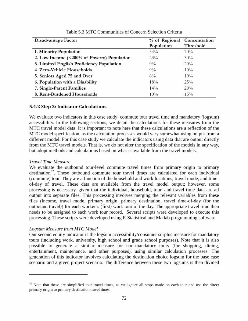
72
Table 5.3 MTC Communities of Concern Selection Criteria
Disadvantage Factor % of Regional Population
Concentration Threshold
1. Minority Population 54% 70%
2. Low Income (<200% of Poverty) Population 23% 30%
3. Limited English Proficiency Population 9% 20%
4. Zero-Vehicle Households 9% 10%
5. Seniors Aged 75 and Over 6% 10%
6. Population with a Disability 18% 25%
7. Single-Parent Families 14% 20%
8. Rent-Burdened Households 10% 15%
5.4.2 Step 2: Indicator Calculations
We evaluate two indicators in this case study: commute tour travel time and mandatory (logsum)
accessibility. In the following sections, we detail the calculations for these measures from the
MTC travel model data. It is important to note here that these calculations are a reflection of the
MTC model specification, as the calculation processes would vary somewhat using output from a
different model. For this case study we calculate the indicators using data that are output directly
from the MTC travel models. That is, we do not alter the specification of the models in any way,
but adopt methods and calculations based on what is available from the travel models.
Travel Time Measure
We evaluate the outbound tour-level commute travel times from primary origin to primary
destination32
. These outbound commute tour travel times are calculated for each individual
(commute) tour. They are a function of the household and work locations, travel mode, and time-
of-day of travel. These data are available from the travel model output; however, some
processing is necessary, given that the individual, household, tour, and travel time data are all
output into separate files. This processing involves merging the relevant variables from these
files (income, travel mode, primary origin, primary destination, travel time-of-day (for the
outbound travel)) for each worker’s (first) work tour of the day. The appropriate travel time then
needs to be assigned to each work tour record. Several scripts were developed to execute this
processing. These scripts were developed using R Statistical and Matlab programming software.
Logsum Measure from MTC Model
Our second equity indicator is the logsum accessibility/consumer surplus measure for mandatory
tours (including work, university, high school and grade school purposes). Note that it is also
possible to generate a similar measure for non-mandatory tours (for shopping, dining,
entertainment, maintenance, and other purposes), using similar calculation processes. The
generation of this indicator involves calculating the destination choice logsum for the base case
scenario and a given project scenario. The difference between these two logsums is then divided
32
Note that these are simplified tour travel times, as we ignore all stops made on each tour and use the direct
primary origin to primary destination travel times.

73
by the marginal utility of income, α, which converts the logsum (originally in utils) to dollar ($)
units.
The formula for this is as follows:
𝐶𝑆𝑖𝑎𝑒𝑝 = (1
𝛼)[𝑙𝑛(∑ 𝑒𝑥𝑝 (𝑉𝑖𝑗𝑎𝑒𝑝
1 )𝑗 ) − 𝑙𝑛(∑ 𝑒𝑥𝑝 (𝑉𝑖𝑗𝑎𝑒𝑝0 )𝑗 )] (5.1)
𝛼 = 𝛽𝑚𝑐𝐿𝑜𝑔𝑠𝑢𝑚𝛽𝑂𝑃𝑐𝑜𝑠𝑡∗ (5.2)
𝑉𝑖𝑗𝑎𝑒𝑝 = 𝑚𝑐𝐿𝑜𝑔𝑠𝑢𝑚𝑖𝑗𝑎𝑒𝛽𝑚𝑐𝐿𝑜𝑔𝑠𝑢𝑚 + 𝑙𝑛(𝑠𝑖𝑧𝑒𝑗𝑒𝑝)𝛽𝑠𝑖𝑧𝑒 (5.3)
𝑚𝑐𝐿𝑜𝑔𝑠𝑢𝑚𝑖𝑗𝑎𝑒 = 𝑙𝑛 (∑ 𝑒𝑥𝑝 (𝑉𝑖𝑗𝑘𝑎𝑒))𝑘 (5.4)
𝑉𝑖𝑗𝑘𝑎𝑒 = 𝛼𝑘𝑎 + 𝒕𝒊𝒎𝒆𝒊𝒋𝒌𝜷𝒕𝒊𝒎𝒆 + 𝒄𝒐𝒔𝒕𝒊𝒋𝒌𝜷𝒄𝒐𝒔𝒕,𝒆 + 𝒍𝒂𝒏𝒅𝒖𝒔𝒆𝒊𝒋𝒌𝜷𝒍𝒂𝒏𝒅𝒖𝒔𝒆 (5.5)
𝑠𝑖𝑧𝑒𝑗𝑒𝑝 =
{
𝒆𝒎𝒑𝒋𝜷𝒆𝒎𝒑,𝒆, 𝑖𝑓 𝑝 = 𝑤𝑜𝑟𝑘𝑒𝑟
𝑢𝑛𝑖𝑣𝑒𝑟𝑠𝑖𝑡𝑖𝑒𝑠𝑗𝛽𝑢𝑛𝑖𝑣𝑒𝑟𝑠𝑖𝑡𝑖𝑒𝑠, 𝑖𝑓 𝑝 = 𝑢𝑛𝑖𝑣𝑒𝑟𝑠𝑖𝑡𝑦 𝑠𝑡𝑢𝑑𝑒𝑛𝑡
ℎ𝑖𝑔ℎ𝑆𝑐ℎ𝑜𝑜𝑙𝑠𝑗𝛽ℎ𝑖𝑔ℎ𝑆𝑐ℎ𝑜𝑜𝑙𝑠, 𝑖𝑓 𝑝 = ℎ𝑖𝑔ℎ𝑠𝑐ℎ𝑜𝑜𝑙 𝑠𝑡𝑢𝑑𝑒𝑛𝑡
𝑔𝑟𝑎𝑑𝑒𝑆𝑐ℎ𝑜𝑜𝑙𝑠𝑗𝛽𝑔𝑟𝑎𝑑𝑒𝑆𝑐ℎ𝑜𝑜𝑙𝑠, 𝑖𝑓 𝑝 = 𝑔𝑟𝑎𝑑𝑒 𝑠𝑐ℎ𝑜𝑜𝑙 𝑠𝑡𝑢𝑑𝑒𝑛𝑡}
(5.6)
, where i is the subscript for the origin (home) zone; j is for the destination zone; 𝑎 is for auto
ownership class; e is for income class; p is for person-type; k is for each mode; superscript 1 is
for the project scenario; and 0 is for the No-Project scenario.
For equation (5.1), 𝐶𝑆𝑖𝑎𝑒𝑝 is the consumer surplus for zone i, auto-ownership class 𝑎, income
class e, and person-type p; 𝛼 is the marginal utility of income; the superscripts 0 and 1 refer to
the No-Project scenario and a project scenario, respectively; 𝑉𝑖𝑗𝑎𝑒𝑝 is the systematic utility
(regarding the base case or project scenarios) for travel between origin i and destination
alternative j. Note that equation (5.1) shows the total calculations performed. Although the MTC
model directly generates the logsum accessibility values (which vary by residential location,
income class, and auto-ownership class) from the destination choice model, the consumer surplus
calculation is completed manually. That is, once the logsum values are calculated by the MTC
model, a series of further calculations are done manually. Each household is assigned an
accessibility value for each scenario. Then, the difference in each household’s project scenario
logsum value is calculated relative to their base case (No-Project) scenario value. This difference
value (for each household) is then divided by the (constant) marginal utility of income, as shown
in equation (5.1).
Typically, the marginal utility is simply the negative of the cost parameter. However, given that
the destination choice utilities do not directly include travel cost, we use the cost parameter from
the mode choice model. The mode choice cost parameter enters the destination choice utilities
indirectly, via the mode choice logsum. That is, the travel costs enter directly into the mode

74
choice model, and the logsums from the mode choice model enter into the destination choice
model utilities33
. Because of this nested-like model structure, it is necessary to modify the scale
of mode choice cost parameter (or marginal utility of income) to the scale of the destination
choice utilities. The expression for the (re-scaled) marginal utility of income is given in equation
(5.2) (Kalmanje and Kockelman, 2004), where, 𝛼 is the marginal utility of income, 𝛽𝑚𝑐𝐿𝑜𝑔𝑠𝑢𝑚 is
the mode choice logsum coefficient (parameter associated with the mode choice logsum), and
𝛽𝑂𝑃𝑐𝑜𝑠𝑡∗ is the parameter associated with travel operation costs from the mode choice model. The
superscript * indicates that this cost parameter is fixed and does not vary by income class, as
does the cost parameter of the mode choice model. This formulation can be easily understood if
we consider that 𝛽𝑂𝑃𝑐𝑜𝑠𝑡∗ is actually multiplied by the mode choice scale parameter 𝜇𝑚𝑐 and
𝛽𝑚𝑐𝐿𝑜𝑔𝑠𝑢𝑚 is actually the ratio of the destination choice scale parameter to the mode choice scale
parameter, 𝜇𝑑𝑐 𝜇𝑚𝑐⁄ . Therefore mathematically, equation (5.2) gives us the re-scaled mode
choice cost parameter: 𝜇𝑑𝑐𝛽𝑂𝑃𝑐𝑜𝑠𝑡∗ = 𝜇𝑚𝑐𝛽𝑂𝑃𝑐𝑜𝑠𝑡
∗ ∗ 𝜇𝑑𝑐 𝜇𝑚𝑐⁄ . For a fuller discussion of scale
parameters of discrete choice models, see Train (2003).
It is important to note that the marginal utility of income may in reality vary according to the
income levels of the decision makers (Abouchar, 1982; Jara-Díaz and Videla, 1988). However,
the use of heterogeneous marginal utilities of income (the inclusion of income effects) would
lead to the issues outlined in Section 3.4.3. That is, the use of heterogeneous marginal utilities of
income would result in greater (positive or negative) weight to the impacts on high income
travelers. The use of a constant value for the marginal utility of income has been validated and is
common, particularly in the case of welfare changes in discrete choice situations (Williams,
1976; Rosen and Small, 1981). Therefore, we apply a constant marginal utility of income for
this case study evaluation. Although this measure (using a constant marginal utility of income) is
inconsistent with the theoretical consumer surplus measure (using heterogeneous marginal
utilities), this approach allows for useful consumer surplus comparisons across income groups.
The systematic destination choice utility takes the formulation given in equation (5.3), where
𝑉𝑖𝑗𝑎𝑒𝑝 is the systematic utility for origin i and destination alternative j, auto-ownership class 𝑎,
income class e, and person-type p; 𝛽𝑚𝑐𝐿𝑜𝑔𝑠𝑢𝑚 is the parameter associated with the mode choice
logsum, 𝑚𝑐𝐿𝑜𝑔𝑠𝑢𝑚𝑖𝑗𝑎𝑒, and 𝛽𝑠𝑖𝑧𝑒 is the parameter associated with the log-size
term, ln(sizejep). As indicated in equation (5.1), the systematic destination choice utilities are
calculated for the No-Project (Vijaep0 ) and Project scenarios (Vijaep
1 ).
The mode choice logsum takes the general formulation given in equation (5.4), where
𝑚𝑐𝐿𝑜𝑔𝑠𝑢𝑚𝑖𝑗𝑎𝑒 is the mode choice logsum value for origin i and destination alternative j, auto-
ownership class 𝑎, and income class e, and 𝑉𝑖𝑗𝑘𝑎𝑒 is the systematic utility for mode alternative k.
There are five (simplified) mode alternatives included in the mode choice logsum; single
occupancy vehicle (SOV), high occupancy vehicle (HOV), walk-transit (WT), drive-transit (DT),
and non-motorized.
33
Note that the mode choice logsum is included in the destination choice utilities as a measure of level-of-service.

75
The systematic utilities for the simplified mode choice alternatives take the form given in
equation (5.5), where, 𝑉𝑖𝑗𝑘𝑎𝑒 again is the systematic utility from origin i to destination alternative
j, for mode alternative k, auto-ownership class 𝑎, and income class e; α𝑘𝑎 is the alterative
specific constant; 𝜷𝒕𝒊𝒎𝒆 is the vector of parameters associated with travel times 𝒕𝒊𝒎𝒆𝒊𝒋𝒌, 𝜷𝒄𝒐𝒔𝒕 is
the vector of parameters associated with travel costs 𝒄𝒐𝒔𝒕𝒊𝒋𝒌, and 𝜷𝒍𝒂𝒏𝒅𝒖𝒔𝒆 is the vector of
parameters associated with land-use variables 𝒍𝒂𝒏𝒅𝒖𝒔𝒆𝒊𝒋𝒌. The travel time variables include in-
vehicle and/or walk access for all modes, and access, auxiliary, egress, and wait times for transit
modes. Travel costs variables include operating cost for all motorized modes, and toll and
parking costs for single and high occupancy vehicle modes. There are no costs included for the
non-motorized mode. Finally, the land use variables include area density34
and topology
measures for non-motorized and transit modes. These land-use variables are not included for
single and high occupancy vehicle modes.
Finally, the formulation for the mandatory size term 𝑠𝑖𝑧𝑒𝑗𝑒𝑝 is given in equation (5.6). Here,
𝑠𝑖𝑧𝑒𝑗𝑒𝑝 is the linear combination of mandatory activities for destination zone j, income class e,
and person-type p. The variable 𝜷𝒆𝒎𝒑,𝒆,𝒑 represents the vector of parameters associated with
employment types, 𝒆𝒎𝒑𝒋; 𝛽𝑢𝑛𝑖𝑣𝑒𝑟𝑠𝑖𝑡𝑖𝑒𝑠,𝑝 is the parameter associated with the number of
universities, 𝑢𝑛𝑖𝑣𝑒𝑟𝑠𝑖𝑡𝑖𝑒𝑠𝑗; 𝛽ℎ𝑖𝑔ℎ𝑆𝑐ℎ𝑜𝑜𝑙𝑠,𝑝 is the parameter associated with the number of high
schools, ℎ𝑖𝑔ℎ𝑆𝑐ℎ𝑜𝑜𝑙𝑠𝑗; and 𝛽𝑔𝑟𝑎𝑑𝑒𝑆𝑐ℎ𝑜𝑜𝑙𝑠,𝑗,𝑝 is the parameter associated with the number of
grade schools, 𝑔𝑟𝑎𝑑𝑒𝑆𝑐ℎ𝑜𝑜𝑙𝑠𝑗. The employment types (sectors) include trade and retail,
financial and professional services, health, educational and recreational services, agricultural and
natural resources, and manufacturing and transportation. The person types include workers, and
university, high school, and grade school students. Additionally, the size term (for workers only)
varies by income.
5.4.3 Step 3: Distributional Comparisons
Here we present the distributional comparison results for the two equity measures: commute tour
travel time and logsum accessibility/ consumer surplus. The emphasis here is on showing the
level of information gained from distributional comparisons, beyond the comparison of average
measures. We first present some results from MTC’s average commute travel time measure.
These results are taken directly from MTC’s equity analysis report for their 2040 Regional
Transportation Plan. We then present similar calculations for average commute travel time, but
using our own processing scripts. The key difference here is with the group segmentation
approach (their zonal vs. our individual-level segmentation). We then compare our results for the
average measures to our distributional measures of commute travel time change. Next, we
present the results for our accessibility/ consumer measure. MTC does not evaluate the logsum
accessibility/consumer surplus measure in their analysis, so we are unable to make a comparison
using this indicator. However, we calculate measures of average change in
accessibility/consumer surplus and compare these results to the distributional comparison results
for the accessibility/consumer surplus measure. The two types of distributional comparisons used
here are the Aggregate Density comparison and the Individual Difference Density comparison.
34
The area density is a measure of population and employment density. For more on this see (MTC, 2013a).

76
Constraints and Implications
The activity-based travel models’ use of micro-simulation for forecasting travel behavior makes
it necessary to make constraints on the calculation of the equity indicators. In the micro-
simulation process, realizations of the outcomes for each choice dimension are drawn randomly
from a distribution for each model run. This means we cannot assume that fundamental
individual and household level characteristics such as work locations or residential location, are
consistent across model runs. For these reasons, we make some constraints on the calculations of
commute tour travel time and mandatory logsum accessibility/ consumer surplus. These
constraints apply specifically to the Individual Difference Density comparisons and not the
Aggregate Density comparisons. The types of constraints vary based on the equity indicator.
Before proceeding with the distributional evaluation results, it is important to revisit the
constraints made on calculating the two indicators and discuss the implications of these
constraints.
Travel Time Indicator: Regarding commute tour travel time, the household residential location,
work location, travel mode, and travel time-of-day are constrained to be the same across model
runs. This means that for the different scenarios, only the travel time skim (a function of level-
of-service) varies. The implication here is that the choices of residential location, work location,
travel time-of-day, and travel mode are not influenced as a result of transportation and land-use
changes. However, in reality an individual may certainly (for example) decide to take rail transit
to work (instead of auto), leave for work at an earlier time, or even (over time) change work
locations due a new congestion pricing policy. Regarding the impact of these constraints on
evaluation results, it is likely that the share “losers” calculated, as well as their magnitude of loss
is over estimated.
Logsum Indicator: Regarding the accessibility/consumer surplus measure, the household
location is constrained to be the same across scenario runs. This means that the transportation
and land-use changes for each scenario have no impact on residential location choice. This may
introduce a bias, as in reality, households may choose to relocate due to transportation and/or
land-use changes. Therefore, it is likely that the share of “losers” (as well as “winners”), and the
magnitudes of losses and gains are over or underestimated. The direction of this bias is not
immediately clear and will require further investigation.

77
Results for Commute Travel Time Measure
MTC Equity Analysis Results (Averages)
MTC results for commute travel time are shown in Figure 5.3. Note that MTC generally uses
multiple segmentation variables (listed in Table 5.3) to segment the population. However, the
results shown in Figure 5.3 are segmented along single variables as opposed to the full multi-
criteria definitions. These results show that on average low income communities35
(for the Project
scenario relative to the No-Project scenario) will experience a 3% reduction in mandatory travel
time, while all other (higher) income communities will on average experience a 6% reduction in
mandatory travel time. That is, low income groups benefit only half as much from the Project
scenario relative to all other income groups. Note that the Project scenario emphasized here
refers to the “Job-Housing” scenario. Further, MTC focuses on this scenario because it is
ultimately selected as the preferred scenario for their Regional Transportation Plan.
Figure 5.3 MTC Equity Analysis of 2040 RTP/SCS Example:
Commute Time (Minute), based on individual modes taken (MTC, 2013).
Note that 40% of the low income population is represented in the “Low-Income Pop. > 30%”
community type (see Appendix C).
35
Here, low income communities are defined as zones where 30% or more of households earn less than $50,000 per
year (MTC, 2013a).

78
SF Bay Area Case Study Equity Analysis Results (Averages)
Table 5.4 shows the results for average commute travel time, for low income and high income
individuals, for all scenarios. Note that the key differences relative to the MTC results (above) is
that these are averaged across individuals instead of zones, and the low income group here is
defined as any individual living in a household earning less than $30,000 annually, as opposed to
$50,000 annually. Overall, the evaluation of the percentage change in commute travel times
indicates that on average, low income and high income commuters will experience a reduction in
travel time, relative to the No-Project scenario. Further, the savings benefits accrued to low
income commuters is greater than the benefits to high income commuters for all scenarios. The
exception is with the “Connected” scenario results for High income commuters. In this case, they
experience an increase in travel time (on average).
Table 5.4 Average Travel Time Results
Scenarios Average Commute
Travel Time
%Change in Commute Travel
Time
All
Individuals Low
Income High
Income Low
Income High
Income
No-Project 28.4 28.3 28.6 -- --
Transit Priority 26.3 24.1 28.0 -14.7% -2.1%
Environmental Justice 26.9 24.8 28.5 -12.2% -0.5%
Connected 27.1 24.2 29.3 -14.4% 2.5%
Jobs-Housing 27.0 25.2 28.1 -11.0% -1.8%
SF Bay Area Case Study Equity Analysis Results (Distributional Comparisons)
Aggregate Density Comparison
Here we present graphical and quantitative comparisons of the Aggregate Densities, for low
income (Figure 5.4) and high income commuters (Figure 5.5). The graphs in each figure are
frequency plots, where the frequency of travel times has been plotted for one-minute bins. (Note
that these graphs are similar to histograms, but the points are connected in a continuous fashion
instead of vertical bars.) For the graphical comparisons, we are interested in the position of the
scenario (dashed) curves, relative to the No-Project (solid) curve. This gives an overall indication
of whether travel times are increasing or decreasing. For the quantitative comparisons, we group
the travel times into bins and calculate the shares of tours that fall into each bin. The bins36
,
which are marked on the figures using vertical dashed lines, are quartiles that have been slightly
adjusted to correspond with more meaningful travel time ranges.
Figure 5.4 (A) through (D) show the graphical Aggregate Density comparisons for commute
travel time for low income commuters. The dotted curves representing the distributions of
36
Data binning refers to the categorization of data into a manageable intervals which are convenient for analysis
(Larose, 2005).

79
commute travel time under the different scenarios generally fall just above the solid (No-Project
scenario) curve. This indicates an overall reduction in travel times. However, there is very little
visual difference in the aggregate densities.
We do observe some noticeable differences when we compare travel time bins for low income
commuters. For each travel time group, we calculate the share of observations associated with
each bin. These are presented in the Table 5.5. Again, we do not observe much change when
comparing across the Project scenarios, but relative to the No-Project scenario, we observe a
more noticeable reduction in the frequencies of tours longer than 40 minutes. Of the four Project
scenarios, the Transit Priority scenario resents in the greatest reduction in times over 40 minutes,
with 15.7% for the Transit Priority scenario vs. 20.8% for the No-Project scenario.
Overall we find a positive trend for low income commuters: commute travel times are being
reduced as a result of the scenarios. The quantitative comparisons (using travel time bins)
provide useful information about the types of tours that are affected in the different scenarios. We
see that at the aggregate level, the distributions shift away from longer travel times (40+ minutes)
and toward shorter travel times (ranging from 0 to 40 minutes), particularly in the case of the
Transit Priority scenario.
Table 5.5 Travel Time Group Results (Low Income)
Bins Low Income Travel Time Groupings
No-Project Transit Priority Env. Justice Connected Jobs-Housing
0-10 Minutes 25.5% 27.6% 27.2% 28.1% 27.7%
10-20 Minutes 28.0% 30.1% 28.8% 29.3% 29.0%
20-40 Minutes 25.6% 26.6% 26.6% 26.5% 26.5%
40+ Minutes 20.8% 15.7% 17.4% 16.1% 16.8%

80
Figure 5.4 (A-D) Aggregate Commute Travel Time Densities (Low Income). Environmental Justice Scenario (A),
Transit Priority Scenario (B), Connected Scenario (C), Jobs-Housing Scenario (D).
0
0.01
0.02
0.03
0.04
0.05
0 10 20 30 40 50 60 70 80 90 100
Fre
qu
en
cy
Travel Time (Minutes)
Environmental Jusrice
No Build Env. Justice
0
0.01
0.02
0.03
0.04
0.05
0 10 20 30 40 50 60 70 80 90 100
Fre
qu
en
cy
Travel Time (Minutes)
Transit Priority
No Build Transit Priority
0
0.01
0.02
0.03
0.04
0.05
0 10 20 30 40 50 60 70 80 90 100
Fre
qu
en
cy
Travel Time (Minutes)
Connected
No Build Connected
0
0.01
0.02
0.03
0.04
0.05
0 10 20 30 40 50 60 70 80 90 100
Fre
qu
en
cy
Travel Time (Minutes)
Jobs-Housing
No Project Preferred
(A) (B)
(C) (D)

81
Figure 5.5 (A-D) Aggregate Commute Travel Time Densities (High Income). Environmental Justice Scenario (A),
Transit Priority Scenario (B), Connected Scenario (C), Jobs-Housing Scenario (D).
0
0.01
0.02
0.03
0.04
0.05
0 10 20 30 40 50 60 70 80 90 100
Fre
qu
en
cy
Travel Time (Minutes)
Environmental Justice
No Project Env. Justice
0
0.01
0.02
0.03
0.04
0.05
0 10 20 30 40 50 60 70 80 90 100
Fre
qu
en
cy
Travel Time (Minutes)
Transit Priority
No Build Transit Priority
0
0.01
0.02
0.03
0.04
0.05
0 10 20 30 40 50 60 70 80 90 100
Fre
qu
en
cy
Travel Time (Minutes)
Connected
No Project Connected
0.0%
1.0%
2.0%
3.0%
4.0%
5.0%
0 10 20 30 40 50 60 70 80 90 100
Fre
qu
en
cy (
%)
Travel Time (Minutes)
Jobs-Housing
No Build Preferred
(A) (B)
(C) (D)

82
Figure 5.5. (A) through (D) show the Aggregate Density comparisons of the commute travel time
distributions for high income commuters. When compared to the distributions for low income
travel times, we see that the travel time distributions of high income commuters have greater
spreads (variance), indicating that high income commuters generally experience longer travel
times. This is consistent with the reality that higher income commuters tend to live farther from
employment districts, therefore experience longer traveler times (White, 1986).
As we saw for the scenario comparisons for low income commuters, the (slight) left-ward shift
of the dashed curve indicates a general reduction in travel times for high income commuters.
However, there is very little visual change in any of these distributions relative to the No-Project
scenario.
The travel time frequency bins for high income commuters are presented in Table 5.6. As we saw
for low income commuters, the travel time bins show more significant differences for the 40+
travel time group, although only slightly so. Particularly, we observe slight reductions in the
shares for very long travel times for the Transit Priority, Environmental Justice, and Jobs-
Housing scenarios, and a slight increase in the share of very longer travel times for the
Connected scenario. In comparison with the results for low income commuters, we observe
much less of a reduction in travel times of 40+ minutes, for all scenarios. It seems that high
income commuters are much less affected by the transportation and land use changes of the
different scenarios.
Table 5.6 Travel Time Group Results (High Income)
Individual Difference Density Comparison
Figure 5.6 (A) through (D) show the results for the commute travel times individual difference
density comparison for the four Project scenarios. In this case, any data point to the right of the
origin (zero on the x-axis) represents a positive change or increase in commute travel time, while
a data point to the left of the origin represents a negative change or reduction in commute travel
time. On other words, the share of the distribution to the right of the origin represents the
“losers” 37
and the share of the distribution to the left represents the “winners”. For the Transit
Priority, Environmental Justice, and Connected scenarios, we observe that the black curve,
representing low income commuters, falls primarily to the left of the gray curve. This indicates
that low income commuters are more likely to experience reductions in travel time, relative to
37
Note that we consider individuals who experience no change in travel time as “losers.”
High Income Travel Time Groupings
No-Project Transit Priority Env. Justice Connected Jobs-Housing
0-10 Minutes 16.0% 16.5% 16.5% 16.0% 16.5%
10-20 Minutes 30.1% 30.6% 30.2% 30.0% 30.9%
20-40 Minutes 32.3% 32.4% 32.0% 31.2% 31.9%
>40 Minutes 21.6% 20.5% 21.4% 22.8% 20.7%

83
the high income commuters. However, the visual comparison is less clear for the Jobs-Housing
scenario.
We can evaluate more clearly the impacts on the income classes by calculating the share of
individuals who experience increases in travel times (“losers”). These are presented in Table 5.7.
For low income commuters, we see that they are least likely to experience an increase in
commute travel time for the Environmental Justice scenario, with 17.55% losers for
Environmental Justice vs. 19.18%, 25.86%, and 23.23% for the Transit Priority, Connected, and
Jobs-Housing scenarios, respectively. For High income commuters, they are more likely to
experience an increase in commute travel time for the Connected scenario, relative to all other
scenarios, with 30.48% for the Connected scenario vs. 25.53%, 25.53%, and 25.47% for the
Transit Priority, Connected, and Jobs-Housing scenarios, respectively. When we compare across
the income classes, we see that the high income commuter are more likely than low income
commuters to experience increases in travel time, for all scenarios.
Table 5.7 Share of Commuters who Experience an Increase in Commute Travel Time
Experienced an Increase in Travel Time (Losers)
Low Income High Income
Transit Priority 19.18% 25.53%
Environmental Justice
17.55% 23.53%
Connected 25.86% 30.48%
Jobs-Housing 23.23% 25.47%
Summary of Travel Time Results
The distributional comparisons reveal additional useful information about the travel time related
impacts on the two income classes, beyond what is indicated by the average measures used in the
MTC equity analysis. The Aggregate Density frequency bin comparisons show that there are
more distinct decreases in longer travel time frequencies for all scenarios, for both income
classes. This is with the exception of the Connected scenario for high income commuters, where
there is a slight increase in the share of longer trips. When we compare the impacts for low
income commuters relative to high income commuters, we observe that they are more affected
by the scenario changes, relative to high income commuters. The Individual Difference density
comparisons reveal that the share of low income commuters experiencing an increase in travel
time is at least 17.55% for all cases, as compared to 23.5% for high income commuters. It is
important to note that this level of insight is not possible using average measures, as is typical of
equity analyses done in practice. For example, MTC’s results indicate that on average all
commuters gain in travel time savings. Overall, our evaluation of commute travel time
distributions show that the low income commuters are left slightly better off after the two
scenarios, based on the calculated shares of “losers”. This is opposite of MTC’s findings, where
higher income commuters are better off, relative to the low income commuters.

84
Figure 5.6 (A-D) Individual difference Density Comparisons (Commute Travel Time) Transit Priority Scenario (A),
Environmental Justice Scenario (B) Connected Scenario (C), Jobs-Housing Scenario (D).
0
0.1
0.2
0.3
0.4
0.5
0.6
0.7
-8 -6 -4 -2 0 2
Fre
qu
en
cy
Change in Travel Time (Minutes)
Transit Priority Scenario
Low Income
High Income
0
0.1
0.2
0.3
0.4
0.5
0.6
0.7
-8 -6 -4 -2 0 2
Fre
qu
en
cy
Change in Travel Time (Minutes)
Environmental Justice
Low Income
High Income
0
0.1
0.2
0.3
0.4
0.5
0.6
0.7
-8 -6 -4 -2 0 2
Fre
qu
en
cy
Change in Travel Time (Minutes)
Connected
Low Income
High Income
0
0.1
0.2
0.3
0.4
0.5
0.6
0.7
-8 -6 -4 -2 0 2
Fre
qu
en
cy
Change in Travel Time (Minutes)
Jobs-Housing Scenario
Low Income
High Income
(A) (B)
(C) (D)

85
Results for Logsum Accessibility/Consumer Surplus Measure
SF Bay Area Case Study Equity Analysis Results (Averages)
Table 5.8 presents the average difference in accessibility experienced daily and annually for low
income and high income households. Recall from Section 3.3.3 that consumer surplus refers to
the total value that individuals place on goods and services (Just et al., 2004). The calculation of
the logsum consumer surplus measure calls for the use of heterogeneous marginal utilities of
income, representing that individuals with different income levels have different willingness-to-
pay for goods and services. Because the use of heterogeneous marginal utilities of income results
in inconsistent scales when comparing consumer surplus measures across income groups, we use
an average marginal utility of income for all individuals. If these were true measures of
consumer surplus (using heterogeneous marginal utility of income), we would observe that the
gains for higher income commuters would be greater that the gains for lower income commuters.
These values (in Table 5.8) (which are calculated at the household level) are calculated by
measuring the difference in logsum accessibility due to each scenario relative to the No-Project
scenario. The groups are segmented income classes and the differences are averaged within each
income class. These evaluation results demonstrate the outcomes likely to result using the
existing practice of applying average measures. The results show that on average, households
will benefit in the case of all scenarios, although high income households benefit more so than
low income households. Further, there are higher gains in accessibility due to the Jobs-Housing
scenario, relative to all other scenarios. We also include ratios of high income to low income
consumer surplus in Table 5.8. These show that on average, the high income commuter benefits
are almost two times as much as the benefits to low income commuters. Further, these ratios
show that the scenarios all result in very similar relative impacts.
Table 5.8 Average Difference in Logsum Accessibility/ Consumer Surplus (in unit of dollars)
Scenarios Average (Daily) Change in
Consumer Surplus ($) Average (Annual) Change in Consumer Surplus ($)
High/Low Inc. Ratio
Low Income High Income
Low Income
High Income
No-Project -- -- -- -- --
Transit Priority $0.98 $1.61 $254.80 $418.60 1.64
Environmental Justice
$0.83 $1.44 $215.80 $374.40 1.73
Connected $1.11 $1.93 $288.60 $501.80 1.74
Jobs-Housing $1.26 $2.19 $327.60 $569.40 1.74

86
SF Bay Area Case Study Equity Analysis Results (Distributional Comparisons)
Figure 5.7 (A) through (D) show the Individual Difference Density comparisons of accessibility,
for the four Project scenarios. Any data point to the right of the origin represents an increase or
positive change in accessibility, and point to left of the origin represents decrease or negative
change in accessibility. Given that an increase in the accessibility value is the desired result, the
share of the distribution to the right of the origin represents the “Winners”, while the share of the
distribution to the left of the origin represents the “losers”. For all scenarios, we see that the
curve for low income commuters falls to the left of the curve for high income commuters,
indicating that low income households are much more likely to experience reductions in
accessibility, relative to high income households. Further, the Transit Priority scenario
distribution is bi-modal for low income commuters. The visual interpretation is that there are
high frequencies of households experiencing small positive changes and small negative changes
in accessibly. From the calculated shares of “losers” presented in Table 5.9, we see again that for
all scenarios, low income households are most likely to experience a decrease in accessibility. In
the most extreme case (the Transit Priority scenario), as many as 33.3% of low income
commuters experience a loss in accessibility/ consumer surplus, compared to 13.4% for high
income commuters. Here, we also calculate the average amount of loss in consumer surplus (in
dollars) to be experienced by low income and high income losers (shown in Table 5.10). These
are the average daily amounts of loss for households that experience a loss in consumer surplus
(losers), for each income class and scenario. We see that regarding order of magnitude, low
income households lose more in consumer surplus, for all scenarios, on a daily basis.
Table 5.9 Share of Households Who Experience a Decrease in Accessibility
Experienced a Decrease in Accessibility (Losers)
Transit Priority Jobs-Housing Environmental
Justice Connected
Low Income 33.3% 19.3% 25.1% 16.7%
High Income 13.4% 6.0% 10.1% 7.7%
Table 5.10 Average Daily loss in Consumer Surplus for “losers”
(Daily) Amount of Loss ($)
Transit Priority Jobs-Housing
Environmental Justice
Connected
Low Income -$1.76 -$3.54 -$2.04 -$4.14
High Income -$1.38 -$3.34 -$1.50 -$3.02
Overall, the Individual Difference Density comparisons for the Accessibility/consumer surplus
indicator reveal that as much as 33% of low income households will experience decreases in
accessibility relative to 13.4% of high income households. Further, we observe the trend that the
lowest income commuters are most likely to experience reductions in accessibility. A more
thorough investigation of the travel-related conditions for low income and high groups is
necessary to better understand the reasons for these results.

87
Figure 5.7 (A-D) Individual difference Density Comparisons (Logsum Accessibility/Consumer Surplus) Transit Priority Scenario (A),
Environmental Justice Scenario (B) Connected Scenario (C), Jobs-Housing Scenario (D).
0
0.05
0.1
0.15
0.2
-10 -5 0 5 10
Fre
qu
en
cy
Change in Consumer Surplus ($)
Transit Priority
Low Income
High Income
0
0.05
0.1
0.15
0.2
-10 -5 0 5 10
Fre
qu
en
cy
Change in Consumer Surplus ($)
Env. Justice
Low Income
High Income
0
0.05
0.1
0.15
0.2
-10 -5 0 5 10
Fre
qu
en
cy
Change Consumer Surplus ($)
Jobs-Housing
Low Income
High Income
0
0.05
0.1
0.15
0.2
-10 -5 0 5 10
Fre
qu
en
cy
Change in Consumer Surplus ($)
Connected
Low Income
High Income
(A) (B)
(C) (D)

88
Discussion of Comparison Results
These results provide important insights in three key areas. These are regarding the choice of unit
of segmentation, the use of distributional measures compared to average measures, and the
choice of equity indicator(s).
Our results provide strong support the use of individuals in population segmentation. This allows
for greater accuracy in measuring the equity impacts of on the population segments. This is
evidenced in the comparison of our average commute travel time results and MTC’s results. Our
average commute travel time measures show that for all Project scenarios the disadvantaged
group (low income commuters) will on average experience a greater reduction in travel times
than the comparison group (high income commuters). MTC’s commute travel time results show
the opposite, where the disadvantaged group (communities with at least 30% or more low
income households) experience much smaller reductions in travel time than the comparison
group (communities with less than 30% low income households). As highlighted throughout this
chapter, the key methodological differences relevant here are with MTC’s use of zones as units
of analysis instead of individuals, as well as the definitions for disadvantaged and comparison
groups. In our case, we define the disadvantaged group as low income individuals (individuals
living in households earning $30,000 or less annually), while the comparison group is high
income individuals (individuals living in households earning $100,000 or more annually). MTC
defines the disadvantaged group as zones with 30% or more of households earning $50,000 or
less, while the comparison group includes zones with less that 30% of households earning
$50,000 or less. Although further investigation is needed to measure the bias associated with
zone-based population segmentation, we attribute this difference in results to the fact that MTC’s
Communities of Concern only captures a portion of the intended target (low income) group. In
fact, only about 40-55% of the target group is captured using the zone-based Communities on
Concern (MTC, 2009, MTC, 2013a), whereas 100% of the target group can be capture using the
individual-based approach. These results provide clear support for more disaggregate data
representation in travel demand modeling and transportation equity analysis.
These results further show support for distributional measures over average measures.
Particularly in the case of the Individual Difference density comparisons, we are able to evaluate
correlations between socio-demographics (as well as other data dimensions) and transportation
impacts on individuals. That is, this comparison reveals who the “winners” and “losers” are for
the difference population segments. For both the travel time and accessibility/consumer surplus
indicators we find clear relationships between income level and losing (or winning) as a result of
the scenario. For the travel time indicators, the Individual Difference Density comparisons show
that higher income groups are more likely to be losers, while this comparison for the
accessibility/ consumer surplus indicator shows that low income households are more likely to
be losers.
Finally, these results support the use of the logsum accessibility/ consumer surplus measure in
transportation equity analysis. By design, this accessibility/ consumer surplus measure is more
comprehensive than the travel time measure. In addition to travel times, the accessibility/
consumer surplus measure captures changes in travel costs and mandatory opportunities. The
results show a difference in outcome between the travel time and accessibility/ consumer surplus

89
indicators. The results for the travel time indicator show that low income commuters benefit
more than high income commuters, both in terms of overall reductions in travel time and a
smaller share of low income losers. In contrast, the accessibility/ consumer surplus results show
that high income commuters benefit more than low income commuters. We attribute this
difference to the fact that the travel time measure only captures a portion of the impacts of
transportation plans, while the logsum accessibility/ consumer surplus measure is better are
capturing more of the impacts, both transportation and land-use related.
5.4.4 Step 4: Equity Criteria and Scenario Ranking
Here we present the results of applying three different equity standards for ranking the four
Project scenarios. It is necessary to translate these theoretical concepts into numerical criteria in
order to apply the standards in ranking the scenarios. Of the equity standards presented in Table
3.10, these three are selected for demonstration because they are the most straight-forward in
identifying the numerical ranking criteria, given the data available in this case study. We evaluate
these criteria using the logsum accessibility/consumer surplus indicator. It is important to note
that our contribution here is not with defining the best criteria for ranking scenarios, but to
demonstrate the relevance of adopting some equity criteria, by which to rank the scenarios.
The three equity standards applied here are as follows:
Equality Providing an equal level of benefits among all groups of interest. Note that
given the different levels of need and value that individuals place on these
benefits, equality of benefits may be achieved without the actual amount
of benefits being equal (Miller, 1979; Forkenbrock, 2001; Rosenbloom,
2009).
Proportionality Distributing benefits in proportion to the share that a group represents of
the total population (Young, 1995; Forkenbrook and Sheeley 2004,
Martens, et al 2011).
Rawls-Utilitarian Providing a distribution that produces the greatest utility or level of
satisfaction, for the most disadvantaged group (Rawls, 1972).
Equality
In order to implement the Equality standard for ranking scenarios, we adopt a simple criterion.
Based on the weighted average daily benefit accrued to each income class, the Equality standard
dictates that we rank the scenario with the smallest difference between the two income classes.
The results are presented in Table 5.11. By this criterion we select the Transit Priority scenario as
the top scenario. It is interesting to note that both the Jobs-Housing and Connected scenarios
result in greater benefits for that the priorities scenario both income groups. This shows that the
Equality criteria does not account for level of benefits for the income groups, but only the
difference in these benefits across income groups.

90
Table 5.11 Equality Standard Results
Average Daily Benefits per Household ($)
Transit Priority Jobs-Housing
Environmental Justice
Connected
Low Income $3.80 $3.95 $2.91 $4.11
High Income $3.93 $4.88 $3.37 $4.43
High ($) – Low ($) $0.13 $0.92 $0.46 $0.32
Proportionality
The Proportionality standard dictates that the equitable scenario is the one in which the share of
benefits received is proportional to the share that a group represents in the full population. Table
5.12 through Table 5.15 show the shares of each income group in the population, compared their
shares in aggregate consumer surplus. The tables also include the absolute difference in the
population and benefit shares for each income group. This standard dictates that the scenario
with the smallest difference between the shares is ranked as most equitable. Note that we present
a separate scenario ranking for the two income classes. This is because the difference in the
population and benefit shares differs between the income groups (for each scenario); however,
the Proportionality criteria do not point to how the overall benefit (for both income groups)
should be calculated. In this case, we rank the Connected scenario as most equitable for low
income traveler and Transit Priority scenario as most equity able for high income commuters.
Similar to the Equality criteria example above, this support the need for a multi-criteria equity
standard for ranking the planning scenarios. It is also interesting the note that the sign of the
difference (between the population benefit shares) is not relevant for ranking the scenarios using
the Proportionality criteria. This is in contrast to some other equity standards (e.g. the
Restorative Justice equity standard), where a greater share in benefits for the low income group
would be considered more equitable.
Table 5.12 Proportionality Results for the Transit Priority Scenario
Table 5.13 Proportionality Results for the Jobs-Housing Scenario
Share in Population Share of Benefits
|Population % - Benefits%|
Low Income 28.60% 23.70% 4.90%
High Income 23.40% 25.95% 2.55%
Share in Population Share of Benefits
|Population % - Benefits%|
Low Income 28.60% 23.24% 5.36%
High Income 23.40% 27.21% 3.81%

91
Table 5.14 Proportionality Results for the Environmental Scenario
Table 5.15 Proportionality Results for the Connected Scenario
Rawls-Utilitarian
The Rawls-Utilitarian standard defines the more equitable scenario as the one in which the
greatest level of utility or benefit is accrued to the most disadvantage group. Here we define the
low income group as the most disadvantaged group. Based on these criteria we select the top
scenario as the one in which the low income group accrues the highest level of benefit, which is
the Connected scenario. Interestingly, the high income group also accrues the highest level of
benefits from the Connected scenario, although this is not considered in this equity criteria.
These results are shown in Table 5.16.
Table 5.16 Rawls-Utilitarian Results
Summary of Scenario Ranking Results
In summary, this ranking process requires that a numerical protocol (equity criteria) be
developed and applied for the equity standard that is adopted. This is because the standards
found in the literature are theoretical concepts and few if any have been applied in practice. For
example, in applying the Equality standard, it is first necessary to define the benefit(s) to be
evaluated, and then define the protocol for judging equality of these benefits across the
population segments. Overall we find that scenario ranking vary based on the definition. For the
Equality standards, the Transit Priority scenario was ranked as most equitable; for the
Share in Population Share of Benefits
|Population % - Benefits%|
Low Income 28.60% 23.79% 4.81%
High Income 23.40% 27.02% 3.62%
Share in Population Share of Benefits
|Population % - Benefits%|
Low Income 28.60% 24.54% 4.06%
High Income 23.40% 26.64% 3.24%
Total Annual Benefits
Transit Priority Jobs-Housing
Environmental Justice
Connected
Low Income $3.80 $3.95 $2.91 $4.11
High Income $3.93 $4.88 $3.37 $4.43

92
Proportionality standard the Connected and Transit Priority Scenario are ranked as most
equitable, for low and high income commuters respectively; and based on the Rawls-Utilitarian
standard, the Connected scenario was ranked as most equitable. Therefore it is critical that an
equity standard be explicitly adopted and applied for the scenario analysis. It is also clear that
some standards may call for some multi-criteria that accounts for the varying impacts across
population segments. For example, the Proportionality standard lends itself to a separate ranking
for the low income and high income segments. In this case, it is important to take the next step
toward defining criteria that weights these impacts and produces a single scenario ranking.
5.5 Extensions and Considerations
The Proposed Equity Analysis Process is a flexible methodology and can be adapted to include a
number of additional important extensions. These include the options for using a multi-criteria
definition of population segmentation and additional equity indicators. Further, there are
additions that may significantly improve the evaluation results. These are model data validation
for population segments and statistical comparison of the equity outcome distributions. Here we
discuss the usefulness of these extensions and considerations, and give examples where relevant.
5.5.1 Model Data Validation
The degree to which equity analysis results will reflect real world transportation impacts is
closely tied the travel model input data and how well this data represents real world population
characteristics and travel behavior data. In Section 5.3.2 (and Appendix B), we describe in some
detail the basic population characteristics and travel behaviors from MTC’s activity-based travel
model, although we do not take the additional step of verifying that the data are representative of
real world conditions. Further, it is important to verify that the model data are representative of
differences across population segments. Although data validation is standard practice in the
initial development of this large scale travel models, this is not necessarily done across all
segmentation variables of interest relevant for equity analyses. Therefore, data validation across
population segments is an important initial step for ensuring that equity analyses reflect realistic
impacts for the defined population segments.
There are a number of data validation approaches. This could involve a simple comparison to
verify that the model data matches the real world data, within some defined margins of error. An
example comparing mode-share for work tours is illustrated in Figure 5.8. Bay Area Travel
Survey Data for the year 2000 is used to represent the real world data, and MTC’s Base Case
2000 data is used to represent the model data. Here we see that the general relative order of
usage is preserved. The largest mode share is the auto mode, while the smallest is for walk/bike
modes. However, there are some small differences between the model data and the real world
data. For the transit and walk/bike mode shares, the model data shows slightly higher shares.
The logical question here is whether these differences are statistically significant. In this case,
this can be addressed this using simple t-tests. In other cases where we need to test the equality
of two distributions (e.g. the distribution of travel distances), a non-parametric test of
distributions that is appropriate for empirical distributions would need to be employed.

93
Figure 5.8 Real World vs. Model Data Work Tour Mode-Shares
It is also important to mention the significance of model calibration in verifying the
representativeness of the travel model data, as the data validation is only part of the task of
ensuring model data representativeness. Model calibration is common for mathematical models
of complex outcomes where unknown parameters are to be estimated. This involves adjusting the
model parameters such that the model predictions match observed data. The challenge here is
regarding whether the model’s sensitivity to individual preferences and overall travel behavior is
preserved through the calibration process. For example, the addition of an alternative specific
constant for low income transit riders in a mode choice model may certainly improve the
accuracy of the mode share predicted by the model in the calibration year (providing a closer
match to the observed mode share). However, this does not necessarily indicate an improvement
in the model’s sensitivity to mode choice preferences in the population, nor does it ensure the
models ability to forecast mode share over time. For this reasoning, the influence of model
calibration on data representativeness is a critical question for future work or applying travel
demand models for equity analysis.
5.5.2 Population Segmentation and Additional Equity Indicators
In the results presented in this chapter, we use a single variable for population segmentation:
income. However, the extension using additional variables is trivial. As is done in MTC’s latest
equity analysis, it is certainly possible to adopt multiple variables of population segmentation
within our proposed equity analysis framework. For example, our description of the population
data indicates a relationship between household size and income level. In this case it is desirable
to segment groups using both income and household size. Regarding definitions of segmentation,
the literature on transportation disadvantage points to a number of important variables. These
include income level, auto ownership, and education level, walk accessibility (to activities), age,
75.2%
16.3%
7.2%
74.4%
17.6%
8.0%
84.4%
12.6% 2.9%
83.0%
13.8% 3.2%
79.0%
14.2% 6.8%
Auto Transit WalkBike
Low Income
High Income
Real World Data
Model Data

94
and political engagement (Currie et al., 2010). In some cases, the availability of segmentation
variables can be constrained by variables available from the travel model. Otherwise, there is
nothing restricting the application of multiply segmentation variables using the Proposed Equity
Analysis Framework.
The importance of using multiple indicators is demonstrated from the current Bay Area case
study, as a project may be equitable along one dimension and inequitable along another. Our
proposed analysis process can be extended to evaluate any number of equity indicators. Further
(as with population segmentation), the variables available for calculating equity indicators are
constrained by the model can output available, particularly with the use of individuals as the unit
of segmentation. However, activity-based travel models are able to generate a range of
population, travel behavior, travel network, and spatial data from which numerous equity
indicators can be calculated.
5.5.3 Statistical Comparison of Distributions
Once the distributions of the equity indicators have been generated, an important next step is to
test that the distributional differences are statistically significant. There are actually two
dimensions of change relevant here. The first dimension is regarding the changes across
scenarios; are the changes associated with each project scenario, relative to the No-Project
scenario, significant? The second dimension is regarding the changes across population
segments; are the changes experienced by the different population segments significant? In both
cases, we want to verify that the distributional differences we observe are not due to model error.
The first dimension falls under a much larger discussion about error and uncertainly in travel
models. This is especially important in the context of activity-based travel models where
simulation error is present. Because of the micro-simulation used, the results will vary
stochastically. That is, each time the random number generator produces a seed value for the
Monte Carlo simulation, the choice assignments for all travel choice dimensions will change.
Although the error can be significantly reduced by increasing the sample size (Castiglione et al.,
2003; Walker, 2006), there will always be some error present. In addition, there are other
possible sources of error, including input data, model structure, and parameter estimation. A
fuller discussion of error and uncertainty of travel model outcomes from a policy perspective can
be found in (Walker et al., 2005). Although there are approaches to measuring uncertainty from
travel demand models, this extends beyond the scope of the current research. In our case, we
assume that the level of uncertainly is such that meaningful results are still generated from the
travel model.
The second dimension focuses on testing whether distributional differences across population
segments are statistically significant. Typically, there are a number of statistical hypothesis tests
appropriate for testing the significance of scenario analysis results. Tests such as the
Kolmogorov-Simirnov two sample tests and the Karl Pearson Chi-Squared goodness-of-fit test
would generally be appropriate for testing the difference between two of more empirical
distributions. However, the presence of simulation error in results from activity-based travel
demand models presents some challenges regarding the application of these frequentist statistical
tests. It is unclear whether currently available tests (such as the Kolmogorov-Simirnov and Karl

95
Pearson Chi Squared test) are able to account for simulation error. This challenge falls under the
broader subject of statistical tests for simulation data, and is an important area of future work for
testing the differences between distributions that are generated from activity-based travel demand
model data.
5.6 Conclusion
We have presented a real world application of the proposed equity analysis process discussed in
Chapter 3. We use the activity-based travel modeling system and transportation and land-use
scenarios developed by the Metropolitan Transportation Commission (the Metropolitan Planning
Organization for the nine-county San Francisco Bay area). In this case study we evaluate the
equity impacts of four “Project” scenarios for low and high income commuters, using commute
travel time and mandatory logsum accessibility/consumer surplus as equity indicators.
There are four primary takeaways from this chapter. First is regarding the unit of population
segmentation. The case study results show a significant difference in equity outcome when using
individual-level population segmentation, compared to using the zonal segmentation approach.
In fact we find opposite results. We hypothesize that this difference is due to the fact that the
zone-based approach only captures a portion of the target (40% in MTC’s case), while the
individual-level segmentation approach is able to capture 100% of the target group. Second is
regarding the equity indicators evaluated. The commute travel time measure results suggests that
low income commuters are better off than high income commuters, while the mandatory logsum
accessibility/ consumer surplus measure results suggest that low income commuters are worse
off than high income commuters. The logsum measure results further show that low income
households are most likely to be “losers” relative to high income households. Although further
investigation is warranted to understand the reasons for these results, we hypothesize that this
difference in results is due to the fact that the logsum accessibility/consumer surplus measure by
design is able to capture transportation and land-use related factors. In comparison, the travel
time measure only captures one dimension of transportation user affects. In spite of the concerns
discussed in Section 3.4.3, the logsum measure has a number of desirable qualities for equity
analysis. This measure is a more comprehensive measure of transportation user benefits. Third is
regarding the use of distributional comparisons for transportation equity analysis. Our results
show that they can provide a richer picture of how groups are affected by transportation plans.
The Individual Difference Densities can be used to identify the winners and losers resulting from
the scenarios. It is also important to note the consistency of our results in the presence of strict
restrictions on the calculations for the Individual Difference Densities. Both our average
commute travel time measure and Individual Difference Densities for commute travel time
indicate that low income commuters are better off, relative to high income commuters. This
result holds even though mode, location, and time-of-day choices are held constant for the
Individual Difference Densities calculation. No constraints are made on calculating the average
measures. The average and distributional measures for accessibility/ consumer surplus results are
also consistent. Finally, we make the case that scenario ranking, using an adopted equity
standard, plays an important role in the analysis process. The results support our
recommendation that transportation practitioners should explicitly adopt and apply equity criteria
in determining the extent to which transportation scenarios are equitable.

96
In summary, the individual-level segmentation approach is preferred to the zonal approach, and
results on the relative transportation effects of low income and high income commuters vary
based on the equity indicator used. Further, distributional comparisons provide a much richer
picture of how population segments are affected by transportation plans relative to average
measure. Finally, the use of equity criteria for ranking transportation scenarios is an important
and powerful step in transportation equity analysis.

97
. Conclusions Chapter 6
6.1. Introduction
Although the transportation system plays an integral role in quality of life for all members of
society, all transportation benefits (or costs) are not created equal. That is, transportation changes
will indeed result in a distribution of transportation experiences that is a reflection of the
heterogeneity among us. In spite of this, existing practices for regional transportation equity
analysis fail to effectively evaluate the distribution of transportation outcomes across different
segments of society, because they largely ignore these differences in transportation experiences
at the individual level.
This dissertation endeavors to advance the practices for regional transportation equity analysis
and overcome the existing shortcomings. We have presented an analytical framework for
regional transportation equity analysis that leverages to power of activity-based travel demand
models and distributional analysis (among other tools) to identify the “winners” and “losers”
resulting from transportation plans. We started by developing a guiding framework, which
outlines the important components of transportation equity analysis. We then presented our
proposed process for equity analysis of regional transportation plans, emphasizing individual
level population segmentation, distributional comparisons of the individual level equity
indicators, and scenario ranking using equity standards. We gave two demonstrations usefulness
of distributional comparisons, using hypothetical and real world settings. We concluded with a
full scale, real world application of our proposed equity analysis approach, using the
Metropolitan Transportation Commission’s regional activity-based travel model and
transportation and land-use scenarios for the San Francisco Bay Area. In this final chapter, we
summarize the overall takeaways from this dissertation and discuss next steps and research
directions.
The remainder of this chapter is organized as follows: in Section 6.2 we revisit the guiding
framework for equity analysis that was introduced in Chapter 3 and discuss the efforts of this
dissertation relative to this three-part framework. In Section 6.3 we summarize the major
findings from each of the preceding chapters in this dissertation. In Section 6.4 we discuss
important next steps and research directions, and in Section 6.5 we give concluding remarks.
6.2. Revisiting the Guiding Framework for Transportation Equity Analysis
The framework presented in Chapter 2 outlined three key components of transportation equity
analysis: priorities, model, and indicators. The framework is illustrated in Figure 6.1. The first
component emphasizes the importance of identifying community priorities. This involves
accessing what the needs are for different communities. Although the Environmental Justice
literature suggests certain areas of investigation, such as air quality, travel times, and vehicle-
miles-travels (Forkenbrock and Weisbrod, 2001; Sanchez etal., 2007; Burt et al., 2010), priorities
will likely vary for different groups. The second component of the analysis is the model used to

98
measure the expected changes due to the transportation plan. The challenge here is with selecting
a modeling tool that is appropriate for measuring the desired transportation (and/or land-use)
changes. In this case, it is necessary that the model be capable of representing real world travel-
related behaviors at the individual level. The third component deals with the selection and
evaluation of equity indicators. These are the measures of transportation benefits (or costs) to be
evaluated. The challenge here is in selecting indicators that reflect communities’ transportation
priorities, as indicated by the black dashed curve. Further, the approach taken for comparing
these indicators across population segments is critical. As is emphasized through this
dissertation, the use of aggregate level comparisons (average equity indicators) can result in
misleading equity outcomes. Finally, the gray dashed curve emphasizes the iterative nature of
equity analysis. That is, the results from evaluating the indicators may point to important changes
in the model structure. For example as will be discussed later in this chapter, our analyses point
to the inclusion of more long-term travel and land-use related equity indicators as an important
next step, which has implications for the population synthesis and individual and household
evolution over the planning horizon.
Figure 6.1 Equity Analysis Framework and Dissertation Emphasis
As indicated by the shaded region of the equity analysis framework in Figure 6.1, the methods
presented in this dissertation primarily address the second and third components of the
framework. Regarding the model, this dissertation makes a clear case for applying disaggregate
data from activity-based models for regional transportation equity analysis. Regarding indicators,
we demonstrated the power of distributional analysis, which provides a means of identifying the
winners and losers resulting from transportation plans.
6.3. Summary of Findings
In Chapter 2, after presenting the guiding framework for transportation equity analysis (Figure
6.1), we reviewed the literature supporting the components of this framework and described the
existing practice for regional transportation equity analysis. Here we first review the broader
research needs from the literature regarding our guiding equity analysis framework. We then
review the more specific research needs regarding the public practice on regional scale
transportation equity analysis using travel demand models. We address some of these needs in
this dissertation.

99
Regarding broader research needs relating to our guiding framework for transportation equity
analysis, first is on validating the use of activity-based travel demand models for transportation
equity analysis. There is only one case found in the literature where the ability of these models
to represent the differences across population segments has been investigated (Bills et al., 2012).
For this dissertation work, we accepted that these models are sufficient and provide for
meaningful comparisons a cross population segments. However, this is an important research
area, given that the representation of longer term population behavior (e.g. individual and
household change or growth over time), and land-use behavior (e.g. gentrification and
displacement) have yet to be accomplished together in practice. Second is regarding
distributional comparison methods for transportation equity analysis. There is a need to develop
more distributional comparison tools capable of evaluating individual level equity. There is one
known approach to evaluating overall differences in distributions: Relative Distribution methods.
However, these methods operate at the aggregate distribution level, as opposed to the individual
level. Further, relative distribution methods are very mathematically complex and difficult for
practitioners as well as academics to interpret. Thus, there is a need to develop distributional
comparison methods that are more readily usable in practice. The third takeaway is regarding the
consideration of long-term transportation and land-use related behaviors. Some effects of
transportation changes in land-use impacts such as segregation, gentrification, and displacement
are well investigated in the literature (Kennedy and Leonard, 2001; Sanchez et al., 2003;
Sanchez, 2004; Kahn, 2007); however, such impacts have yet to be full captured for in equity
analysis of long-range transportation plans.
Regarding more specific research needs relating to the existing practice for equity analysis of
regional transportation plans, three critical shortcomings were found. First, the use of zones as
units of segmentation can be problematic and result in aggregation bias. Second, the equity
measures and indicators used in practice are weakly linked to transportation costs and benefits.
For example, travel time is a very common equity indicator used in practice. However, it only
captures one dimension of the benefits (or costs) associated with possible transportation and
land-use investments (e.g. accessibility, user costs, and environmental factors). Finally, the use of
average measures of equity indicators can be misleading and uninformative.
In Chapter 3 we proposed a process for regional transportation equity analysis that addresses the
existing shortcomings relating to equity analysis. We discuss considerations and improvements
to transportation equity analysis concerning population segmentation, equity indicators,
distributional comparisons, and scenario ranking. The segmentation of the population into target
and comparison groups involves the selection of one or more variables of segmentation, a unit of
segmentation, and definitions of segmentation. The choice of variable of segmentation is closely
tied to the equity dimension(s) adopted by the planning agency. For example, income is
associated with vertical equity, while location is associated with horizontal equity. It is desirable
for the unit of segmentation to be as disaggregate as possible, in order to overcome issues with
aggregate bias. Given the capabilities of activity-based travel models, we recommend individuals
or households as the unit of segmentation. The threshold for defining the target and comparison
groups (e.g. defining the target group for low income households as those earning less than $30k
annually), are ideally selected based on established definitions of transportation disadvantage.
Regarding the selection of equity indicators, any number of equity indicators can be generated

100
from the travel model output. However, consideration for how well the indicator(s) represents
transportation impacts (costs or benefits) is critical. It is important to verify that the indicator(s)
represents benefits (or costs) to individuals, and are not simply transportation system
performance measures. Further, it is important to identify potential confounding factors
associated with the indicators of these costs and/or benefits. For example, travel time measures
can be confounded by travel frequency. Therefore if the travel frequency of different population
segments are not controlled for when comparing travel time measures across population
segments, this could result in biased measurements. Regarding distributional comparisons, we
emphasize the importance of evaluating the individual-level changes in the equity analyses. A
comparison of aggregate densities can provide useful information on the overall differences in
distributions due to a planning scenario (e.g. a shift toward smaller or larger values). However,
comparisons of Individual Difference Densities are able to reveal the share of the population
segments expected to gain (winners) or be made worse off (losers) by a planning scenario. As a
final step in the analysis process, we emphasize the importance of ranking the planning scenarios
using explicit equity criteria. This is a step that is largely overlooked in practice.
In Chapter 4 we demonstrate the advantages of distributional comparisons, relative to average
measures. We employ hypothetical transportation scenarios and develop two mode choice
models, using synthetic and empirical travel data. The synthetic data are generated from a
hypothetical setting, while the empirical data is taken from the 2000 Bay Area Travel Survey
dataset. In these controlled settings, we explore the relationships between the characteristics and
travel behavior of the population segments and the distributional outcomes due to the
(hypothetical) scenarios. Overall, we find the distributional comparisons are capable of providing
a fuller picture of individual travel experiences due to transportation investments. Not only do
the Individual Difference Density comparisons reveal how individuals are affected by the
scenarios (in terms of which individuals benefit and which individuals do not benefit), but they
provide a means of reverse-engineering the scenario impacts and determining specifically what
factors led to various transportation (equity) outcomes. This level of analysis is otherwise limited
using average comparison measures.
The San Francisco Bay Area case study presented in Chapter 5 provided a number of key
insights with respect to applying our proposed equity analysis process and the MTC activity-
based travel model for regional transportation equity analysis. In this case study, we evaluate the
equity impacts of four transportation and land-use scenarios for low income commuters, relative
to high income commuters. We use commute travel time and mandatory logsum
accessibility/consumer surplus as equity indicators, we segment the population at the individual
level, and we calculate individual level measures of the indicators. We use two types of
distributional comparisons to evaluate equity impacts on low and high income commuters: the
Aggregate Density comparison and the Individual Difference Density comparison. The
Aggregate Density comparison is done using the commute travel time measure, while the
Individual Difference Density comparison is done for both the commute travel time and logsum
accessibility/ consumer surplus measures. The Aggregate Density comparison is not done using
the logsum measure because they would treat the individual utility-based values as if they were
on an equal scale, and this is inappropriate. Our travel time results from the Aggregate Density
comparison show that for all Project scenarios, low income commuters will overall experience a
greater reduction in travel times than the comparison group (high income commuters). Further,

101
the Individual Difference Density comparison shows that the share of low income commuters
who do experience an increase in travel time (losers) is smaller than for high income commuters.
The logsum accessibility/ consumer surplus results show the opposite; lower income households
are more likely to experience losses due to the planning scenarios. We hypothesize that this
difference between the travel time and accessibility/ consumer surplus results is due to the fact
that the travel time measure only captures a portion of the impacts of transportation plans’
impacts, while the logsum accessibility/ consumer surplus measure by design captures more of
the impacts (both transportation and land-use related). When we look at travel time only, the low
income group is better off, in comparison to the high income group. However, when we add
impacts due to the change in employment (and other mandatory) opportunities, the low income
group is worse off. Regarding scenario ranking, we develop ranking criteria using three different
(theoretical) equity standards: Equality, Proportionality, and Rawls-Utilitarianism. Application of
these equity standards result in all different rankings for the planning scenarios. This
demonstrates the importance of adopting equity criteria (which represent the equity goals for the
transportation plan) and applying these criteria in determining the most equitable planning
scenario. A transportation plan can be considered equitable based one standard, but inequitable
based on another.
6.4. Research Directions
While this dissertation takes a number of important steps toward advancing transportation equity
analysis, process in the follows areas is critical for further understanding the potential of using
activity-based travel demand models for equity analysis, and uncovering the full range of equity
outcomes possible from transportation-related improvements. We use our guiding equity analysis
framework to outline these research directions.
Priorities
In our analysis, we assume that the transportation priorities are reductions in commute travel
time and increases in mandatory accessibility. However, there is a need to investigate (though
qualitative and quantitative approaches) the transportation needs of various population segments.
There is a large body of literature around travel behavior differences by ethnicity, income level,
gender, etc., but this has yet to be applied in the equity analysis realm to identify transportation
needs and constraints. This is also related to the question of what equity standard(s) to adopt. In
this dissertation we establish that the selection of an equity standard is key; however, we do not
provide a process for selecting the equity standard that is most desirable. There is considerable
effort in this area, although to date, no consensus has been reached. Further, there is need to
identify more robust equity criteria for scenario ranking based on the adopted equity standard(s).
In our analysis, we demonstrate the scenario ranking using simplistic criteria, based on a single
indicator. In the case of multiple indicators, it would be important to incorporate these indicators
in the form a multi-criteria for scenario ranking.
Model
There are a number of research directions concerning the model to be used for scenario
modeling. The first is regarding uncertainty in the model. There are a number of sources for error
and uncertainty in large scale travel models, which will influence the model results. In our
analysis we assumed that this influence was insignificant; however, there is a critical need to

102
explore the magnitude of this influence. Second is regarding changes to the model structure to
account for longer-term behaviors. This includes individual and household changes over time.
The basic idea is that over time, individuals grow and evolve in terms their age, income level,
preferences, etc., while households change and evolve in similar ways (e.g. household structure),
and the model should be adapted to account for these effects. Third and also relating to long-term
travel behavior is the need to model land-use related changes, such as gentrification and
displacement, as mentioned earlier. Fourth is regarding how traveler purpose and activities are
represented in the model. Currently, travel purposes are not modeled from a behavioral
perspective: they are simply assigned to individual (and joint) travel records. In cases where we
are interested in understanding the influence of transportation investments of health related
activities, it would be useful to be able to forecast the change in these activities as a function of
the transportation changes, and additionally how these vary by population segment.
Indicators
In this dissertation, we discuss important considerations for selecting equity indicators, as well as
how to compare them across groups. However, we do not address the question of what equity
indicators are best, and under what conditions. This is a fundamental question for transportation
equity analysis that has yet to be addressed. Further, we have only scratched the surface with
developing useful distributional comparison methods and meaningful summary measures based
on these distributions. First, there are the issues of tracking individuals represented in the travel
models across scenarios. Currently, new realizations for transportation-related choices are drawn
each time the model is run, which makes it impossible to compare individuals and households
across scenarios. In our case, we place a number of constraints on the calculations of equity
indicators (for individuals and households) in order to make comparisons across scenarios, but
further exploration regarding how to accurately monitor individual agents across different
scenario runs is critical for distributional evaluation using the Individual Difference Density
comparison approach. The second research need with respect to evaluating indicators is for more
exploration into what population, travel behavior, and land-use related factors are associated with
being a “winner” or “loser”. In our analysis, we gave some hypotheses for our results, but a
much more in-depth analysis is an important next step. Specifically, it is important to investigate
the underlying causes for our results (why is it that our average travel time results were opposite
of MTC’s results, and why is it that our travel time and accessibility/ consumer surplus measures
produced opposite results?). Further, it is important to understand how the losers can be
compensated for their losses. Finally, an important next step is to apply our proposed equity
analysis process to a range of transportation and land-use improvements in order to determine the
types of improvements that are more equitable, and what factors can be adjusted in order to
provide a more equitable outcome overall.
6.5. Conclusion
We have developed and demonstrated an approach to regional transportation equity analysis that
addresses shortcomings of the existing practice and ultimately brings us closer to measuring and
understanding the full of range equity outcomes associated with transportation plans. Other
primary contributions are in providing a guiding framework for the important components of
transportation equity analysis, making the case for disaggregate level population segmentation,

103
evaluating the usefulness of an accessibility measure relative to a travel time (mobility) measure,
demonstrating the usefulness of distributional comparison methods in equity analysis, and
demonstrating the significance of equity criteria for scenario ranking. We have laid out a
framework for using activity-based travel demand models to evaluate individual-level equity
impacts and reveal the “winners” and “losers” resulting from transportation plans. In addition,
this work serves to link equity analysis methods from the academic literature to equity analysis
in practice. While we have made significant process, there are a number of key next steps and
research directions. Among other improvements, these include the need to explore best practices
for adopting equity standards and developing scenario ranking criteria based on these standards,
the need to determine the influence of model-related uncertainty on equity analysis results, the
need to explore how travel models can be adapted to represent longer-term travel and land-use
related behavior, the need to evaluate the most desirable equity indicators for representing the
costs and benefits of transportation plans, and finally the need to apply our proposed methods to
a range of transportation-related improvements in order to explore which types of improvements
are most (and least) equitable.

104
References
Abouchar, A. (1982). Marshall, Consumer Surplus, and the Marginal Utility of Money. Eastern
Economic Journal, 8(1), 79-82.
Aguilera, M. B. (2002). The impact of social capital on labor force participation: Evidence from
the 2000 Social Capital Benchmark Survey. Social Science Quarterly, 83(3), 853-874.
Agrawal, A. W., E. A. Blumenberg, S. Abel, G. Pierce, and C. N. Darrah (2011). Getting Around
When You’re Just Getting By: The Travel Behavior and Transportation Behavior Expenditures
of Low-Income Adults. MTI Report 10-02. Mineta Transportation Institute, College of Business,
San José State University, San José, CA
Akiva, M. E. B., & Lerman, S. R. (1985). Discrete choice analysis: theory and application to
predict travel demand (Vol. 9). The MIT press.
Alsnih, R., & Hensher, D. A. (2003). The mobility and accessibility expectations of seniors in an
aging population. Transportation Research Part A: Policy and Practice, 37(10), 903-916.
Amekudzi, A. A., Smith, M. K., Brodie, S. R., Fischer, J. M., & Ross, C. L. (2012). Impact of
Environmental Justice on Transportation. Transportation Research Record: Journal of the
Transportation Research Board, 2320(1), 1-9.
Astrop, A., Palmer, C., Maunder, D., & DM, B. (1996, October). The urban travel behaviour and
constraints of low income households and females in Pune, India. In National Conference on
Women's Travel Issues, Baltimore, Maryland.
Ben-Akiva, M.E. (1973). Structure of passenger travel demand models. Ph.D. Thesis,
Massachusetts Institute ofTechnology, USA.
Bierlaire, M. (2003). BIOGEME: a free package for the estimation of discrete choice models.
Bhat, C. R., & Koppelman, F. S. (1999). Activity-based modeling of travel demand. In Handbook
of transportation Science (pp. 35-61). Springer US.
Bills, T. S., Sall, E. A., & Walker, J. L. (2012). Activity-Based Travel Models and Transportation
Equity Analysis. Transportation Research Record: Journal of the Transportation Research
Board, 2320(1), 18-27.
Bradley, M., & Vovsha, P. (2005). A model for joint choice of daily activity pattern types of
household members. Transportation, 32(5), 545-571.
Burt, M., Sowell, G., Crawford, J., & Carlson, T. (2010). Synthesis of Congestion Pricing-
Related Environmental Impact Analyses–Final Report (No. FHWA-HOP-11-008).

105
Castiglione, J., Freedman, J., & Bradley, M. (2003). Systematic investigation of variability due to
random simulation error in an activity-based microsimulation forecasting model. Transportation
Research Record: Journal of the Transportation Research Board, 1831(1), 76-88.
Castiglione, J., Hiatt, R., Chang, T., & Charlton, B. (2006). Application of Travel Demand
Microsimulation Model for Equity Analysis. Transportation Research Record: Journal of the
Transportation Research Board, 1977(1), 35-42.
Center for Neighborhood Technology (2009). Bay Area Housing and Transportation
Affordability: A Closer Look. (CNT, 2009).
Cervero, R. (1996). Paradigm shift: from automobility to accessibility planning(No. Working
Paper 677).
Cervero, R. (2005). Accessible cities and regions: a framework for sustainable transport and
urbanism in the 21st century.
Cervero, R., Rood, T., & Appleyard, B. (1999). Tracking accessibility: employment and housing
opportunities in the San Francisco Bay Area.Environment and Planning A, 31(7), 1259-1278.
Currie, G. (Ed.). (2011). New Perspectives and Methods in Transport and Social Exclusion
Research. Emerald Group Publishing.
Dalvi and Martin (1976). M.Q. Dalvi and K.M. Martin , The measurement of accessibility: Some
preliminary results. Transportation 5 .
Dong, X., Ben-Akiva, M. E., Bowman, J. L., & Walker, J. L. (2006). Moving from trip-based to
activity-based measures of accessibility. Transportation Research Part A: policy and
practice, 40(2), 163-180.
Duthie, J., K. Cervenka, and S. T. Waller (2007). Environmental Justice Analysis: Challenges for
Metropolitan Transportation Planning. In Transportation Research Record: Journal of the
Transportation Research Board, No. 2013, Transportation Research Board of the National
Academies, Washington, D. C., pp. 8-12.
Executive Order 12898: Federal Actions to Address Environmental Justice in Minority
Populations and Low-Income Populations. (1994). Federal Register, Vol. 59, No. 32, February
16,
Forkenbrock, David J., and Glen Weisbrob (2001), Guidebook for Assessing the Social and
Economic Effects of Transportation Projects, NCHRP Report # 456, National Academy Press,
Washington, D.C.
Forkenbrock, D. J., & Sheeley, J. (2004). Effective methods for environmental justice
assessment. Publication NCHRP Report 532. Washington, DC: Transportation Research Board.

106
Franklin, J. P. (2005, January). Non-parametric distributional analysis of a transportation policy:
The case of Stockholm’s congestion pricing trial. In The Transportation Research Board 84th
Annual Meeting, Washington, DC (Vol. 1, pp. 365-412).
Frohlich, N., & Oppenheimer, J. A. (1992). Choosing justice. Berkeley: University of California
Press.
Geurs, K. T. and Wee, B. Van (2004), Accessibility evaluation of land-use and transport
strategies: review and research directions, Journal of Transport Geography, 12, pp. 127–140.
Giuliano, G. (2003). Travel, location and race/ethnicity. Transportation Research Part A: Policy
and Practice, 37(4), 351-372.
Guendelman, S., & Wagner, T. H. (2000). Health services utilization among Latinos and white
non-Latinos: results from a national survey. Journal of health care for the poor and
underserved, 11(2), 179-194.
Gurmu, K. R. Ihlanfeldt, and W. J. Smith (2006), Does Space Matter to the Employment of
TANF Recipients? Evidence from a Dynamic Discrete Choice Model with Unobserved Effects,
Journal of Urban Economics, (2006).
Haas, P. M., Makarewicz, C., Benedict, A., Sanchez, T. W., & Dawkins, C. J. (2006). Housing &
Transportation Cost Trade-Offs and Burdens of Working Households in 28 Metros. Center for
Neighborhood Technology, 2.
Hägerstrand, T. (1970). What about people in regional science? Papers of the Regional Science
Association, 24, 1–12.
Handcock, Mark S. and Eric Aldrich (2002), Applying Relative Distribution Methods in R,
Working Paper No. 27, Center for Statistics and the Social Sciences, University of Washington.
Handcock, Mark S. and Martina Morris (1999), Statistics for Social Science and Public Policy,
Springer-Verlad, Inc., New York
Handy, S. L. (2002). Accessibility-vs. mobility-enhancing strategies for addressing automobile
dependence in the US.
Handy, S. L., & Niemeier, D. A. (1997). Measuring accessibility: an exploration of issues and
alternatives. Environment and planning A, 29(7), 1175-1194.
Hansen, W. G. (1959). How accessibility shapes land use. Journal of the American Institute of
Planners, 25(2), 73-76.
Hensher, D. A., ed. Urban Transport Economics. Cambridge University Press, Cambridge,
England, 1977.

107
Iseki, Hiroyuki, D. Taylor, Brian, and Miller, Mark. (2006). The Effects of Out-of-Vehicle Time
on Travel Behavior: Implications for Transit Transfers (Deliverable #1). California Department
of Transportation Division of Research and Innovation.
< http://www.its.ucla.edu/research/EPIC/Appendix%20A.pdf>
Rodier, C. J., Abraham, J. E., & Tonkin, G. J. (2001). Applying an Integrated Model to the
Evaluation of Travel Demand Management Policies in the Sacramento Region. Mineta
Transportation Institute, San José State University.
Jara‐Díaz, S. R., & Farah, M. (1988). Valuation of users’ benefits in transport systems. Transport
Reviews, 8(3), 197-218.
Juran, J.M. (1950) "Pareto. Lorenz, Cournot Bernoulli, Juran and Others," Industrial Quality
Control, p. 25.
Just, Richard, Darrell L. Hueth, and Andrew Schmitz (2004), The Welfare of Economics of
Public Policy, Edward Elgar Publishing, Northampton, MA.
Kahn, M. E. (2007). Gentrification Trends in New Transit‐Oriented Communities: Evidence
from 14 Cities That Expanded and Built Rail Transit Systems. Real Estate Economics, 35(2),
155-182.
Kain, J. F. (1968). Housing segregation, negro employment, and metropolitan
decentralization. The Quarterly Journal of Economics, 82(2), 175-197.
Kalmanje, S., & Kockelman, K. M. (2004). Credit-based congestion pricing: Travel, land value,
and welfare impacts. Transportation Research Record: Journal of the Transportation Research
Board, 1864(1), 45-53.
Kennedy, M. & Leonard, P. (2001) Dealing with neighborhood change: a primer on gentrification
and policy choices. Working Paper (Washington, DC: The Brookings Institute).
Khisty, C. J. (1996). Operationalizing Concepts of Equity for Public Project Investments. In
Transportation Research Record 1559, TRB, National Research Council, Washington, D.C., pp.
94-99.
Kickhöfer, B., Grether, D., & Nagel, K. (2011). Income-contingent user preferences in policy
evaluation: application and discussion based on multi-agent transport
simulations. Transportation, 38(6), 849-870.
Konow, J. (2003). Which is the fairest one of all? A positive analysis of justice theories. Journal
of economic literature, 41(4), 1188-1239.
Kwan, M. P. (1998). “Space-Time and Integral Measures of Individual Accessibility: A
Comparative Analysis Using a Point-based Framework.” Geographical Analysis 30 (July), 191-
216.

108
Larose, D. T. (2005). Discovering knowledge in data: an introduction to data mining. Wiley.
com.
Le Grand, J. (1991). Equity and choice: an essay in economics and applied philosophy.
Routledge.
Levinson, David (2010) Equity Effects of Road Pricing: A Review. Transport Reviews 30(1) 33-
57.
Litman, T. (2002). Evaluating Transportation Equity Todd Litman. Editorial board, 8(2), 50-65.
Liao, T. F. (2011). Statistical group comparison (Vol. 896). Wiley. com.
Liu, F. (2010). Environmental justice analysis: Theories, methods, and practice. CRC Press.
Nobis, C., & Lenz, B. (2005). Gender Differences in Travel Patterns. Research on Women’s
Issues in Transportation, 114.
Martens, K. (2009). Equity Concerns and Cost-Benefit Analysis: Opening the Black Box.
In Transportation Research Board 88th Annual Meeting (No. 09-0586).
Martens, K., Golub, A., & Robinson, G. (2012). A justice-theoretic approach to the distribution
of transportation benefits: Implications for transportation planning practice in the United
States. Transportation research part A: policy and practice, 46(4), 684-695.
Martens, K., A. Golub, and G. Robinson (2010). "A justice-theoretic approach to the distribution
of transportation benefits - Working Paper 10-001"
Mauch, M., & Taylor, B. D. (1997). Gender, race, and travel behavior: Analysis of household-
serving travel and commuting in San Francisco bay area.Transportation Research Record:
Journal of the Transportation Research Board, 1607(1), 147-153.
Metropolitan Transportation Commission (2001), The 2001 Regional Transportation Plan Equity
Analysis and Environmental Justice Report. (MTC, 2001).
Metropolitan transportation Commission (2009), Transportation 2035 Plan for the San Francisco
Bay Area Equity Analysis Report. (MTC, 2009).
Metropolitan Transportation Commission (2013), Draft Equity Analysis Report. MTC, 2013a
Retrieved from:
http://onebayarea.org/pdf/Draft_Plan_Bay_Area/Draft_Equity_Analysis_Report.pdf (MTC,
2013a)

109
Metropolitan Transportation Commission (2013), Plan Bay Area: Regional Transportation Plan
and Sustainable Communities Strategy for the San Francisco Bay Area 2013–2040. (MTC,
2013b)
Miller, D. (1979). Social justice. Oxford University Press.
Musgrave, R., & Musgrave, P. P.(1989) Public Finance in Theory And Practice.International
Edition McGraw-hill Book Company.
O'Regan, K. M., & Quigley, J. M. (1998). Where youth live: economic effects of urban space on
employment prospects. Urban Studies, 35(7), 1187-1205.
Ory, David (2012). Model Schematic. Retrieved from
http://mtcgis.mtc.ca.gov/foswiki/Main/ModelSchematic
Ory, D. T., & Mokhtarian, P. L. (2005). Don’t Work, Work at Home, or Commute? Discrete
Choice Models of the Decision for San Francisco Bay Area Residents.
Pucher, J., & Renne, J. L. (2003). Socioeconomics of urban travel: evidence from the 2001
NHTS. Transportation Quarterly, 57(3), 49-77.
Purvis, C. (1997). Travel Demand Models for the San Francisco Bay Area (BAYCAST-
90). Technical Summary. Metropolitan Transportation Commission, Oakland, CA.
Raveau, S., Álvarez-Daziano, R., Yáñez, M. F., Bolduc, D., & de Dios Ortúzar, J. (2010).
Sequential and Simultaneous Estimation of Hybrid Discrete Choice Models. Transportation
Research Record: Journal of the Transportation Research Board, 2156(1), 131-139
Rawls, John. (1972). A Theory of Justice. Clarendon Press, Oxford.
Rodier, Caroline J., Abraham, John E., Dix, Brenda N., & Hunt, John Douglas Dr.(2009). Equity
Analysis of Land Use and Transport Plans Using an Integrated Spatial Model. UC Davis:
Institute of Transportation Studies. Retrieved from: http://escholarship.org/uc/item/7vd6g46
National Research Council, Washington, D.C., pp. 35-42.
Rodier, C., & Spiller, M. (2012). Model-Based Transportation Performance: A Comparative
Framework and Literature Synthesis (No. CA-MTI-12-2805).
Rogalsky, J. (2010). Bartering for basics: Using ethnography and travel diaries to understand
transportation constraints and social networks among working-poor women. Urban
Geography, 31(8), 1018-1038.
Rosen, H. S., & Small, K. A. (1981). Applied welfare economics with discrete choice models.

110
Rosenbloom, S. (2009), “The Equity Implications of Financing the Nation’s Surface
Transportation System,” TR News, Transportation Research Board, Vol. 261 (March-April),
pages 3-9.
Sanchez, T. W., Stolz, R., & Ma, J. S. (2003). Moving to equity: Addressing inequitable effects
of transportation policies on minorities.
Sanchez, T. W., Stolz, R., & Ma, J. S. (2004). Inequitable effects of transportation policies on
minorities. Transportation Research Record: Journal of the Transportation Research
Board, 1885(1), 104-110.
Sanchez, T. W., & Wolf, J. F. (2007, January). Environmental justice and transportation equity: A
review of metropolitan planning organizations. Racial Equity in Transportation: Establishing
Priorities for Research and Policy.
Sacramento Area Council of Governments (SACOG) (2012). 2035 Metropolitan Transportation
Plan/Sustainable Communities Strategy (MTP/SCS), Chapter 8: Equity and Choice.
http://www.sacog.org/2035/files/Final-Draft-MTP/8-%20Equity%20&%20Choice%20Final.pdf
San Diego Association of Governments (SANDAG) (2011). 2050 Regional Transportation Plan.
<http://www.sandag.org/uploads/2050RTP/F2050rtp_all.pdf>
Schweitzer, L., & Stephenson, M. (2007). Right answers, wrong questions: Environmental
justice as urban research. Urban Studies, 44(2), 319-337.
Southern California Association of governments (SCAG) (2011). 2012-2035 Draft Regional
Transportation Plan/Sustainable Communities Strategy (RTP/SCS) Environmental Justice
Appendix.
<http://rtpscs.scag.ca.gov/Documents/2012/draft/SR/2012dRTP_EnvironmentalJustice.pdf>
Srinivasan, S., & Rogers, P. (2005). Travel behavior of low-income residents: Studying two
contrasting locations in the city of Chennai, India. Journal of Transport Geography, 13(3), 265-
274.
Tal, G., & Handy, S. L. (2005). The travel behavior of immigrants and race/ethnicity groups: an
analysis of the 2001 national household transportation survey.
Tomaskovic-Devey, D., & Lin, K. H. (2011). Income dynamics, economic rents, and the
financialization of the US economy. American Sociological Review,76(4), 538-559.
Transportation and Environmental Justice Case Studies: MPO Environmental Justice Report
Mid-Ohio Regional Planning Commission. Report FHWA-EP-01-010. FHWA, U.S. Department
of Transportation, 2000.
Theil, H. (1967). Economics and Information Theory. Chicago: Rand McNally and Company.

111
Thill, J.C., Horowitz, J.L. (1997), Travel time constraints on destination-choice sets. Geographic
Analysis 29, pp. 108–123
Train, K. (2009). Discrete choice methods with simulation. Cambridge university press.
Urban Land Institute (2012). Bay Area Burden.
Vandemoortele, M. (2009). Within-Country Inequality, Global Imbalances and Financial
Instability. Desk Study for Netherlands Ministry of Foreign Affairs, Overseas Development
Institute, London.
Waddell, P. (2002). UrbanSim: Modeling urban development for land use, transportation, and
environmental planning. Journal of the American Planning Association, 68(3), 297-314.
Waddell, P. (2013). Draft Technical Documentation: San Francisco Bay Area UrbanSim
Application.
Wachs, M., & Kumagai, T. G. (1973). Physical accessibility as a social indicator. Socio-
Economic Planning Sciences, 7(5), 437-456.
Walker, J. L. (2005). Making household microsimulation of travel and activities accessible to
planners. Transportation Research Record: Journal of the Transportation Research
Board, 1931(1), 38-48.
W.E. Walker, P. Harremoës, J. Rotmans, J.P. van der Sluijs, M.B.A. van Asselt, P. Janssen, and
M.P. Krayer von Krauss (2003); Defining Uncertainty: A Conceptual Basis for Uncertainty
Management in Model-Based Decision Support, Integrated Assessment, Vol. 4, No. 1, 2003, pp.
5-17.
Ward, B. G. (2005). Case studies in environmental justice and public transit title VI
reporting (No. NCTR 576-12/BD 549-10). National Center for Transit Research, Center for
Urban Transportation Research, University of South Florida.
White MJ (1986) Sex differences in urban commuting patterns. The American Economic Review
76(2): 368–332.
Willig, R. D. (1976). Consumer's surplus without apology. The American Economic
Review, 66(4), 589-597.
Williams, H. C. W. L., & Ortúzar, J. D. D. (1982). Behavioural theories of dispersion and the
mis-specification of travel demand models. Transportation Research Part B:
Methodological, 16(3), 167-219.
Young, H. P. (1995). Equity: in theory and practice. Princeton University Press.

112
Zhou, Y., Outwater, M. L., & Proussaloglou, K. (2005). Market research on gender-based
attitudinal preferences and travel behavior. In Conference Proceedings 35: Research on Women’s
Issues in Transportation, Report of a Conference (Vol. 2, pp. 171-179).

113
Appendix A : Conceptual Evaluation Data Descriptions
and Model Choice Model Estimation Results
Figure A. 1 Distributions of Travel Times for Low Income and High Income Workers
Figure A. 2 Distributions of Travel Costs for Low Income and High Income Workers
0
0.05
0.1
0.15
0.2
0 10 20 30 40 50 60 70 80 90
Fre
qu
en
cy
Travel Time (Minutes)
Travel Time
Low Income (<30k)
High Income (>100k)
0
0.05
0.1
0.15
0.2
0.25
0.3
0 2 4 6 8 10
Fre
qu
en
cy
Travel Cost ($)
Travel Cost
Low Income (<30k)
High Income (>100k)

114
Table A. 1 Mode Choice Model Estimation Results
Parameter Name Estimate
Alternative Specific Constants
Auto Modes
Shared-Ride 2 -1.7090
Shared-Ride 3 -2.5825
Active Modes
Walk -0.2205
Bike -1.6223
Transit Modes
Walk-Transit 0.2987*
Drive-Transit -1.0560
In-Vehicle Travel Times
Auto and Transit -0.0245
Bike -0.0785*
Walk -0.0551
Transit Wait Times
Initial Wait -0.0365
Transfer -0.0349
Costs
Travel Cost -0.2494
Parking Cost -0.0416
Income Categories
Active Modes
Low Income 0.7076
Low-Medium Income 0.4533
Medium-High Income 0.5112
Transit Modes
Low Income 0.2331
Low-Medium Income 0.1314
Medium-High Income 0.0003*
Tour Stops (Greater than 1)
Active Modes -0.8113
Transit Modes -0.2292
Nest Coefficients
Active Modes 1.2633
Transit Modes 1.4365
*Not significant at the 5% confidence level

115
Appendix B : Bay Area Case Study Data Description
Here we present a data description of the basic population (exogenous) and travel (endogenous)
characteristics exhibited in the data used for the Bay Area case study in Chapter 5. As this
general picture does not vary significantly across the MTC planning scenarios, we describe only
the “No-Project” scenario data here. This data description serves to support the discussion of
the case study results, as the equity impacts on population segments will be a reflection of the
basic population and travel characteristics of these segments, as well as the expected
transportation and land-use changes.
Population Data
There are a total of 4,357,430 individuals, living in 1,640,662 households in the data sample,
which represents a 50% sample of all households in the region. The low income class represents
the largest share of households, although only slightly so, with low income households
representing 28.6% of the population and medium income, medium-high income, and high
income classes representing 24.5%, 23.5%, and 23.4%, respectively. These income shares are
illustrated in Figure B.1A.
In the person file, individuals are classified into person types. These person-types are as follows:
Child – too young for school
Student – non-driving age
Student – driving age
University Student
Non-Worker
Part-time Worker
Full-time Worker
Retired
The distributions of person-types by income class are shown in Figure B.1B. There are some
interesting differences in the distribution of person-types across income classes. Overall, the
highest share of individuals is full-time workers, for all income classes except the low income
class. For the low income class, the highest person-type share is retirees (23.0%), with the next
highest person-type shares being non-workers (18.54%) and full-time workers (17.9%). In
contrast, 34.2% of medium income individuals, 43.6% of medium-high income individuals, and
48.6% of high income individuals are full-time workers. Relative to the higher income classes,
low income individuals are most likely to be university students, non-workers, part-time
workers, and retirees.
Each household’s residential choice is represented as a travel analysis zone in the region. There
is a total of 1454 travel analysis in MTC’s zonal system. To give an idea of residential choices
for low income and high income households, we map the share of low income and high income
households for all zones in the Bay Area. These maps for low and high income communities are
shown in Figure B.2 and Figure B.3, respectively. These maps show high concentrations of low
income households primarily in the inner north, east and south bay areas which tend to have

116
higher transit network densities, although there are certainly some low income households
residing in less transit accessible areas. Higher income households are more concentrated in the
outer south and east bay areas.
The size of households can generally be described in terms of the total number of household
members, the number of workers, minors (children ages 0 to 17), and seniors (ages 65 and older).
The total number of household members in the dataset ranges from one to 25 members, although
this range is truncated at 6 household members in Figure B.4A for simplification purposes38
.
Regarding household sizes across income classes, lower income levels are associated with
smaller households, while higher income levels are associated with larger households. For low
income households, 77.4% are 1 and 2 person households, while 60.8% of medium income
household, 48.1% of medium-high income households, and 39.2% of the high income
households are 1 and 2 person households. Regarding the number of household workers, low
income households are also more likely to have zero or 1 workers in the household, with 89.6%39
of low income households and 66.6%40
of medium income households having 0 or 1 workers.
This is in contrast to the higher income classes, which are much more likely to have 1 or more
workers in the household. Regarding the number of household minors, the large majority of
households have no minors. Low income households are most likely to have zeros minors
(76.6%), which high income households are least likely to have zeros minors (61.2%). Similarly,
the large majority of households have zeros seniors; however, low income households are least
likely to have zeros seniors while high income households are most likely to have zeros seniors.
That is, the share of households with zero seniors ranges from 54.6% for low income households,
to 76.7% for high income households.
Overall, it seems that the lower income individuals are characterized as mostly retirees, non-
workers, part-time workers, or university students, while higher income individuals are most
likely to be full-time workers than any other person type. Low income household tend to live
closer to transit rich areas, relative to high income households. Further, low income households
are characterized as smaller households with zeros or few workers, few minors, and are more
likely to have seniors, relative to all other income classes. On the other hand, high income
households are characterized as larger households, with one or more workers, more minors and
fewer seniors, relative to all other households.
38
Only 2.6% of household have more than 6 members. 39
That is, 49.4% of low income households are 0 worker households and 40.2% and 1 worker households. 40
That is, 17.2% of medium income households are 0 worker households and 49.4% and 1 worker households.

117
Figure B.1 A and B. (A) Household Income Shares and (B) Person-Type Distributions.
28.6%
24.5% 23.5%
23.4%
Low Income Med Income
Med-High Income High Income
Income Share
0%
10%
20%
30%
40%
50%
60%
Child - tooyoung for
school
Student -Non-driving
age
Student-Driving age
UniversityStudent
Non-Worker Part TimeWorker
Full TimeWorker
RetiredSh
are
of I
nd
ivid
uals
(%
)
Person Types
Person Types
Low Income Med Income Med-High Income High Income
(A)
(B)

118
Figure B.2 Low Income Community (Earning $30k or less) Residential Locations

119
Figure B.3 High Income Community (Earning $100k or more) Residential Locations

120
Figure B.4 A-D. Household Member Characteristics. (A) Total Members; (B) Number of Workers; (C) Number of Minors; (D)
Number of Seniors.
0%
20%
40%
60%
80%
1 2 3 4 5 6
Sh
are
of H
ou
seh
old
s (%
)
Number of Household Members
Household Size
Low Income Med Income
Med-High Income High Income
0%
20%
40%
60%
80%
0 1 2 3 4
Sh
are
of H
ou
seh
old
s (%
)
Number of Household Workers
Household Workers
Low Income Med Income
Med-High Income High Income
0%
20%
40%
60%
80%
0 1 2 3 4
Sh
are
of H
ou
seh
old
s (%
)
Number of Household Minors
Household Minors
Low Income Med Income
Med-High Income High Income
0%
20%
40%
60%
80%
0 1 2
Sh
are
of H
ou
seh
old
s (%
)
Number of Household Seniors
Household Seniors
Low Income Med Income
Med-High Income High Income
(A) (B)
(C) (D)

121
Travel Behavior Data
Regarding household tour frequency (as illustrated in Figure B.5A), it is clear that the low
income households are much more likely to take one mandatory tour daily, while high income
households are more likely to take two or more mandatory tours daily. That is 80.9% of low
income households only take one tour daily, compared to 62.6% of medium income households,
48.9% of medium-high income households, and 39.9% of high income households. The non-
mandatory tour frequencies are illustrated in Figure B.5B. Similarly, low income households are
more likely to take one non-mandatory tour, although less so compared to that case of mandatory
tours. That is, 67.3% of low income households, 56.5% of medium income households, 52.9% of
medium-high income households, and 48.1% of high income households take one non-
mandatory tour.
The number of individual tours range from one to two tours per day for mandatory tours, and
from one to 541
non-mandatory tours per day. As shown in Figure B.6A, there is very little
difference in mandatory tours across income classes. For all income classes, approximately 94%
of individuals take one mandatory tour per day. Although, there is a slight trend suggesting that
lower income individuals are more likely to take two mandatory tours a day; with 5.8% of low
income individuals taking two mandatory tours per day, compared to 5.6%, 5.5%, and 5.7% for
medium income, medium-high income, and high income individuals, respectively. Regarding
non-mandatory tours, while the tendency overall is towards one or two tours, lower income
individuals are relatively more likely to take one tour daily, while higher income individuals are
relatively more likely to take 2 or more tours daily.
Regarding stop frequency for mandatory tours (as shown is Figure B.5C), there doesn’t seem to
be any interesting differences across income classes. Generally, there are few stops taken, with
approximately 63% of all tours having zero stops, and 22% of tours having one stop, for all
income classes. For non-mandatory tour stops (shown in Figure B.5D), there seems to be a slight
trend. That is, for low income households, 36.3% of non-mandatory tours involve one or more
stops, compared to 34.6% for medium income households, 33.3% for medium-high income
households, and 32.1% for high income households.
Figure B.7 shows the tour mode shares for mandatory and non-mandatory tours. Note that for the
purpose of simplicity, the travel modes have been grouped into auto, transit, and “walkBike”
modes, where auto includes single and shared occupancy auto modes, transit includes all walk-
transit and drive-transit modes, and walkBike includes walk and bike modes. We observe some
interesting differences across tours types as well as income classes. For mandatory tours, lower
income groups are more likely to travel by and transit and walkBike modes, while higher income
groups are more likely to travel by automobile. That is, 17.5% and 13.8% of low income tours
are made by transit and walkBike modes, respectively. This is compared to 14.2% and 6.8% of
high income tours made by transit and walkBike modes, respectively. We observe a similar trend
for non-mandatory tour mode shares. However, the transit mode shares are much smaller for
41
The Figure B.6B is truncated at four tours per day, for simplicity purposes. Less that 0.5% of individuals will make
more than four non-mandatory tours per day.

122
non-mandatory mode, relative to mandatory tours, while walkBike mode share are slightly
higher.
Regarding household automobile ownership, the number of automobiles among household range
from zero to four-plus automobiles. There are some observable differences in household auto
ownership, by income class. As shown in Figure B.8, low income households are significantly
more likely to own zero or one automobiles, relative to other income classes. Further, the higher
income households are more likely to own two or more automobiles, relative to low income
households.
Overall, we characterize the travel behavior of the lower income class by fewer tours (for
mandatory and non-mandatory tour types). Further, lower income households are more likely to
own zero or one automobiles, and have a higher tendency toward transit, walk, and bike modes.
Higher income households have relatively higher trips frequencies, although the majority of
higher income households stay within one to two mandatory and non-mandatory tours daily. In
contrast, higher income households are much more likely to travel by auto models, relative to
lower income households.

123
Figure B.5 A-D. Tour and Stop Frequency. (A) Mandatory Tour Frequency; (B) Non-Mandatory Tour Frequency; (C) Mandatory Tour
Stop Frequency; (D) Non-Mandatory Tour Stop Frequency
0%
20%
40%
60%
80%
1 2 3 4 5
Sh
are
of H
ou
seh
old
s (%
)
Number of Mandatory Tours
Household Mandatory Tour Frequency
Low Income Med Income
Med-High Income High Income
0%
20%
40%
60%
80%
1 2 3 4 5
Sh
are
of H
ou
seh
old
s (%
)
Number of Non-Mandatory Tours
Household Non-Mandatory Tour Frequency
Low Income Med Income
Med-High Income High Income
0%
20%
40%
60%
80%
0 1 2 3 4
Sh
are
of T
ou
rs (
%)
Number of Mandatory Tour Stops
Household Mandatory Tour Stop Frequency
Low Income Med Income
Med-High Income High Income
0%
20%
40%
60%
80%
0 1 2 3 4S
hare
of T
ou
rs (
%)
Number of Non-Mandatory Tour Stops
Household Non-Mandatory Tour Stop Frequency
Low Income Med Income
Med-High Income High Income
(A) (B)
(C) (D)

124
Figure B.6 A and B Individual Tour Frequencies for Mandatory (A) and Non-Mandatory (B)
Tours
0.0%
20.0%
40.0%
60.0%
80.0%
100.0%
1 2
Sh
are
of I
nd
ivid
uals
(%
)
Number of Mandatory Tours
Individual Mandatory Tour Frequency
Low Income Med Income Med-High Income High Income
0.0%
20.0%
40.0%
60.0%
80.0%
100.0%
1 2 3 4
Sh
are
of I
nd
ivid
uals
(%
)
Number of Mandatory Tours
Individual Non-Mandatory Tour Frequency
Low Income Med Income Med-High Income High Income
(A)
(B)
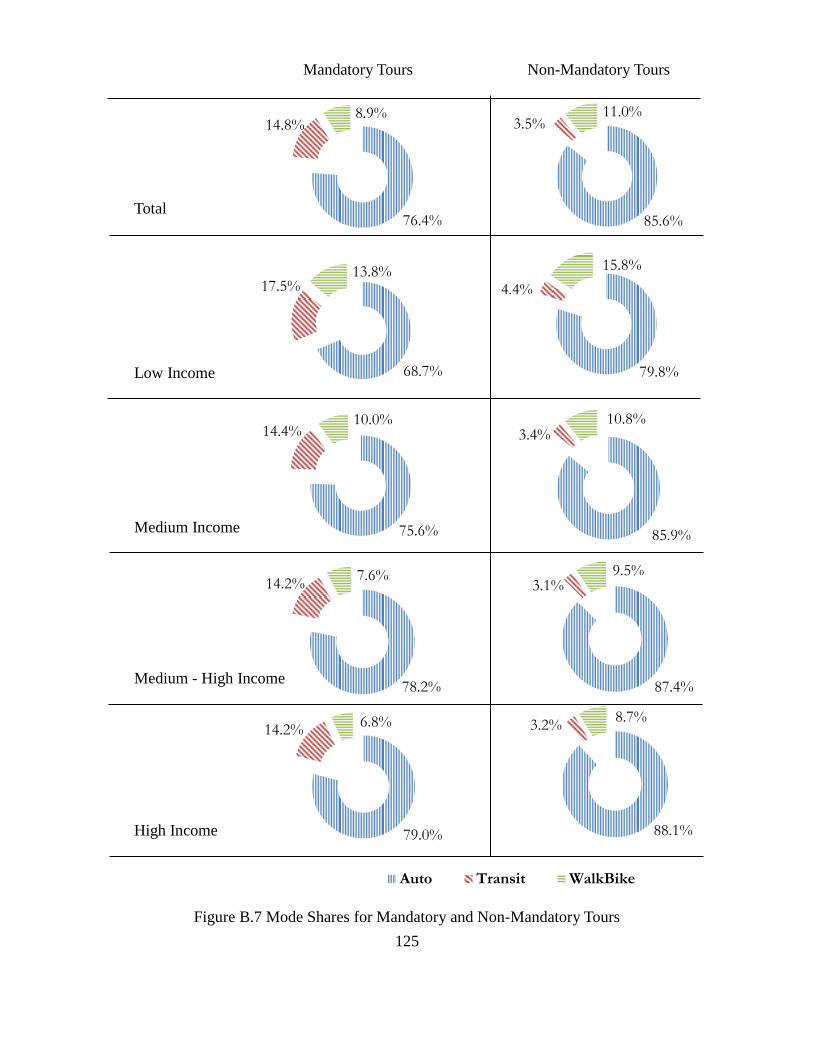
125
Figure B.7 Mode Shares for Mandatory and Non-Mandatory Tours
76.4%
14.8% 8.9%
85.6%
3.5% 11.0%
68.7%
17.5% 13.8%
79.8%
4.4%
15.8%
75.6%
14.4% 10.0%
85.9%
3.4% 10.8%
78.2%
14.2% 7.6%
87.4%
3.1% 9.5%
79.0%
14.2% 6.8%
88.1%
3.2% 8.7%
79.0%
14.2% 6.8%
Auto Transit WalkBike
Total
Low Income
Medium Income
Medium - High Income
High Income
Mandatory Tours
Non-Mandatory Tours

126
Figure B.8 Household Auto Ownership
0%
10%
20%
30%
40%
50%
60%
0 Autos 1 Auto 2 Autos 3 Autos 4 AutosSh
are
of H
ou
seh
old
s (%
)
Number of Household Automobiles
Household Auto Ownership
Low Income Med Income
Med-High Income High Income

127
Appendix C : MTC Communities of Concern Descriptive
Statistics
Figure C. 1 MTC Communities of Concern Statistics (MTC, 2013a)