ensemble data assimilation and particle filters for nwp · dan crisan h.r. künsch amos lawless s....
TRANSCRIPT

Heinz-Werner Bitzer, Annika Schomburg, Silke May, Marc Pondrom, Kristin Raykova, Thomas Rösch, Michael Bender, Christian Welzbacher, Lilo Bach, Lisa Neef, Zoi Paschalidi, Walter Acevedo, Axel Hutt, Daniel Egerer, Gerhard Paul, Ana Fernandez, Stefan Declair
Ensemble Data Assimilation and
Particle Filters for NWP
ECMWF September 2018
Roland PotthastNWP @ DWD &
University of Reading
With the help ofmany people, in particular:
Anne Walter,Andreas RhodinHarald Anlauf, Christina Köpken,Robin Faulwetter,Olaf Stiller,Alexander Cress,Martin Lange,Stefanie Hollborn,E. Bauernschubert, Christoph Schraff,Hendrik Reich, Klaus Stephan Ulrich Blahak
Partners include:P.-J van LeeuwenSebastian ReichDan CrisanH.R. KünschAmos LawlessS. DanceNancy Nichols
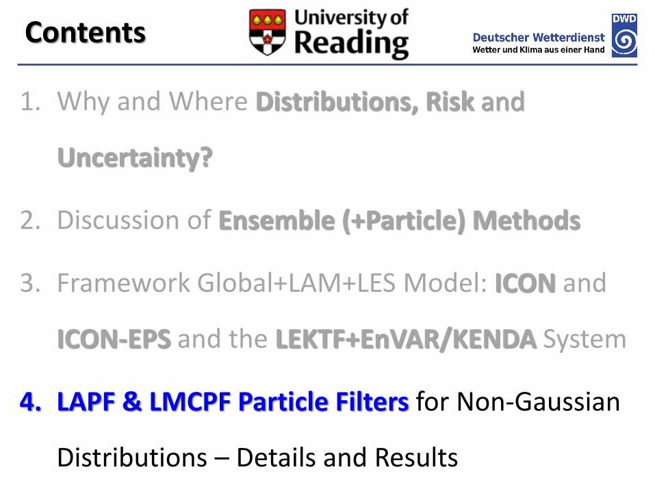
1. Why and Where Distributions, Risk and
Uncertainty?
2. Discussion of Ensemble (+Particle) Methods
3. Framework Global+LAM+LES Model: ICON and
ICON-EPS and the LEKTF+EnVAR/KENDA System
4. LAPF & LMCPF Particle Filters for Non-Gaussian
Distributions – Details and Results
Contents

Extreme Weather Events aretriggered by deep convection andthreaten lifes, infrastructure andeconomy!
Lightning, Gusts, Hail and strong precipitation or tornados impactthe life of individuals ans thesociety.
Thunderstorms with the following properties:s Level
Strong Gusts (Bft. 7) Moderate
Storm Force Gusts (Bft. 8-10) Strong
Heavy Rainfall (10-25mm/h) Strong
Storm Force Gusts, Heavy Rainfall Strong
Storm Force Gusts, Heavy Rainfall, Hail Strong
Hurricane Force Gusts (Bft. 11-12) Severe
Storm Force Gusts, Very Heavy Rain(25-50mm/h) Severe
Storm Force Gusts, Very Heavy Rain, Hail Severe
Hurricane Force Gusts, Very Heavy Rain, Hail Severe
National Task: Warn and Protect
Why Distributions , Risk, Uncertainty?
NOW, 5min, 30min, … 1h, 2h, 6h, 24h, 72h, …

Why Distributions , Risk, Uncertainty?

Bildquelle: https://de.wikipedia.org/wiki/%C3%9Cbertragungsnetzbetreiber
Bildquelle: http://www.amprion.net/pressemitteilung-76
Renawable Energy Forecasting
Why Distributions , Risk, Uncertainty?
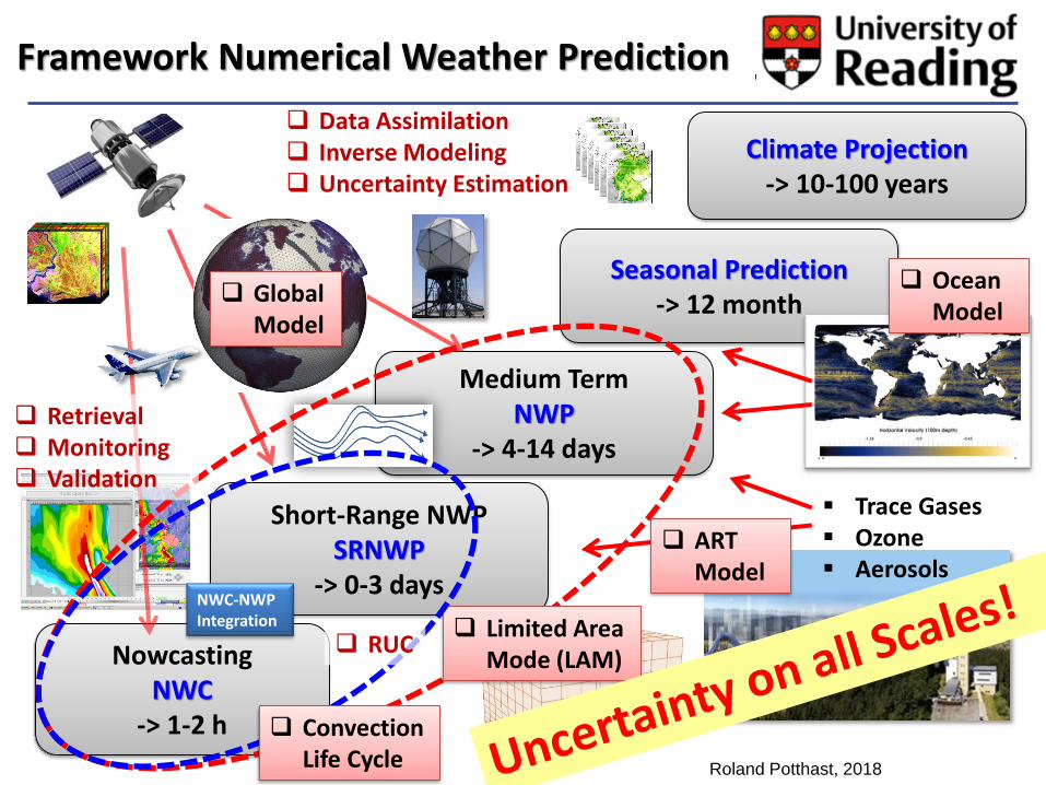
Medium TermNWP
-> 4-14 days
NowcastingNWC
-> 1-2 h
Framework Numerical Weather Prediction
Short-Range NWP SRNWP
-> 0-3 days
Seasonal Prediction-> 12 month
Climate Projection-> 10-100 years
▪ Trace Gases▪ Ozone▪ Aerosols
OceanModel
Retrieval Monitoring Validation
Data Assimilation Inverse Modeling Uncertainty Estimation
ARTModel
Limited Area Mode (LAM)
GlobalModel
Roland Potthast, 2018
ConvectionLife Cycle
RUC
NWC-NWPIntegration

40 Countries
Cosmo User Seminar + Training Course + Symposium

1. Why and Where Distributions, Risk and
Uncertainty?
2. Discussion of Ensemble (+Particle) Methods
3. Framework Global+LAM+LES Model: ICON and
ICON-EPS and the LEKTF+EnVAR/KENDA System
4. LAPF & LMCPF Particle Filters for Non-Gaussian
Distributions – Details and Results
Contents
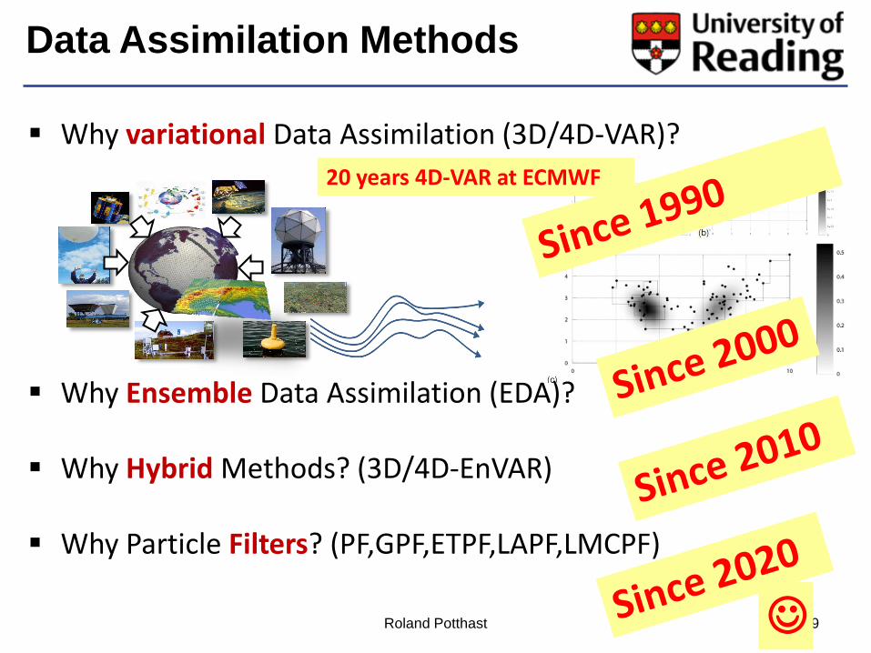
▪ Why variational Data Assimilation (3D/4D-VAR)?
▪ Why Ensemble Data Assimilation (EDA)?
▪ Why Hybrid Methods? (3D/4D-EnVAR)
▪ Why Particle Filters? (PF,GPF,ETPF,LAPF,LMCPF)
Roland Potthast 9
Data Assimilation Methods
☺
20 years 4D-VAR at ECMWF
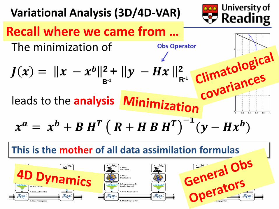
The minimization of
leads to the analysis
Variational Analysis (3D/4D-VAR)
𝑱 𝒙 = 𝒙 − 𝒙𝒃 2 + 𝒚 − 𝑯𝒙 2
B-1 R-1
𝒙𝒂 = 𝒙𝒃 +𝑩𝑯𝑻 𝑹+𝑯 𝑩𝑯𝑻 −𝟏(𝒚 − 𝑯𝒙𝒃)
This is the mother of all data assimilation formulas
Obs Operator
Recall where we came from …

Maximum Likelyhood Estimator =Minimization of Functional = 3/4DVar
Stochastic View Minimization
𝑝 𝑥 = 𝑒−1
2𝑥−𝑥𝑏
𝑇𝐵−1(𝑥−𝑥𝑏) Gaussian Prior
𝑝 𝑦|𝑥 = 𝑒−1
2𝑦−𝐻𝑥 𝑇𝑅−1(𝑦−𝐻𝑥) Gaussian Data Error
Gaussian Posterior
𝑝 𝑥|𝑦 = 𝑐 𝑒−12 𝑥−𝑥𝑏
𝑇𝐵−1 𝑥−𝑥𝑏 + 𝑦−𝐻𝑥 𝑇𝑅−1(𝑦−𝐻𝑥)
Pro
bab
ility
Prior Observation Error
Posterior
Pro
bab
ility
Prior Observation Error
Posterior
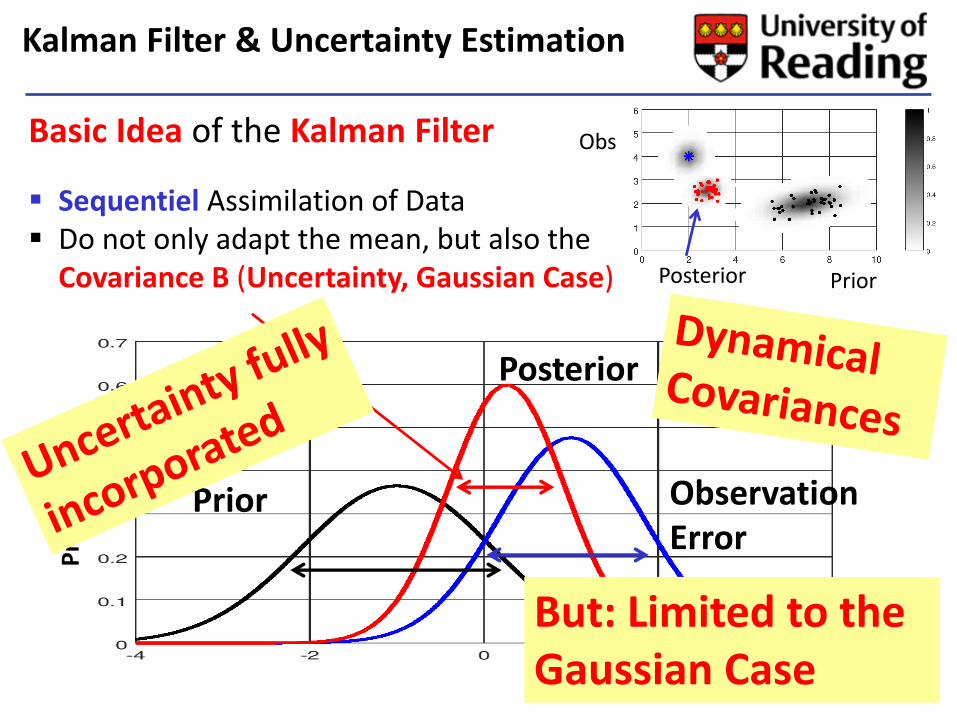
Kalman Filter & Uncertainty Estimation
Basic Idea of the Kalman Filter
▪ Sequentiel Assimilation of Data▪ Do not only adapt the mean, but also the
Covariance B (Uncertainty, Gaussian Case) Prior
Obs
Posterior
But: Limited to the Gaussian Case

▪ Kalman Filter needs B update => expensive!
▪ Estimate B based on an ensemble of forecasted states (stochastic estimator).
EDA: Ensemble Kalman Filter (EnKF)
Needs Localization
B will be flow-dependent and variable, depending on the model dynamics and on the observations
Localized: LETKF

1. Why and Where Distributions, Risk and
Uncertainty?
2. Discussion of Ensemble (+Particle) Methods
3. Framework Global+LAM+LES Model: ICON and
ICON-EPS and the LEKTF+EnVAR/KENDA System
4. LAPF & LMCPF Particle Filters for Non-Gaussian
Distributions – Details and Results
Contents
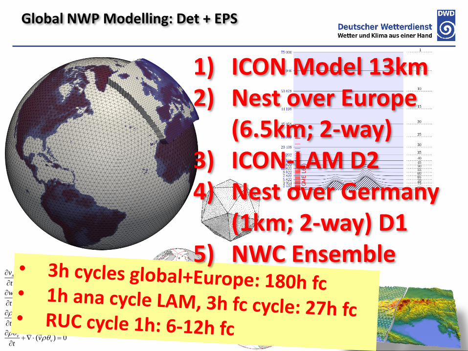
Global NWP Modelling: Det + EPS
0)(
0)(
vv
vpdh
vpdn
tn
vt
vt
gz
cz
wwwv
t
w
nc
z
vw
n
Kvf
t
v
1) ICON Model 13km 2) Nest over Europe
(6.5km; 2-way) 3) ICON-LAM D2 4) Nest over Germany
(1km; 2-way) D1 5) NWC Ensemble

Full Observation System
Radiosonde
Meteor.
Observatorium
Lindenberg
Wind-Profiler
1. Doppler-LIDAR (Wind)
2. DIAL (Humidity)
3. Raman LIDAR (Temp+Hum)
4. MWR (Temp+Hum)
5. GPS STD (Hum)
6. Cloud Radar
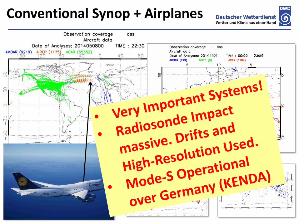
Conventional Synop + Airplanes
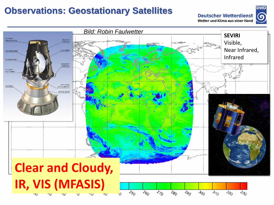
Observations: Geostationary Satellites
SEVIRI Visible, Near Infrared, Infrared
Bild: Robin Faulwetter
Clear and Cloudy, IR, VIS (MFASIS)
Radianzen von polar umlaufenden Satelliten
GBFE, Roland Potthast – 07/2015
Bild: Robin Faulwetter
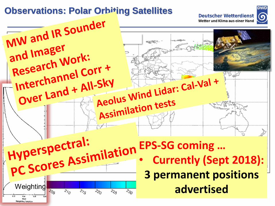
Observations: Polar Orbiting Satellites
EPS-SG coming …• Currently (Sept 2018):3 permanent positions
advertised
20
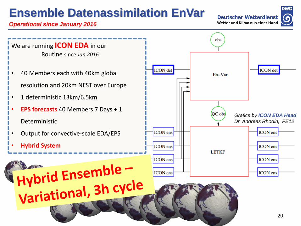
Ensemble Datenassimilation EnVar
We are running ICON EDA in our
Routine since Jan 2016
• 40 Members each with 40km global
resolution and 20km NEST over Europe
• 1 deterministic 13km/6.5km
• EPS forecasts 40 Members 7 Days + 1
Deterministic
• Output for convective-scale EDA/EPS
• Hybrid System
Grafics by ICON EDA Head
Dr. Andreas Rhodin, FE12
Operational since January 2016
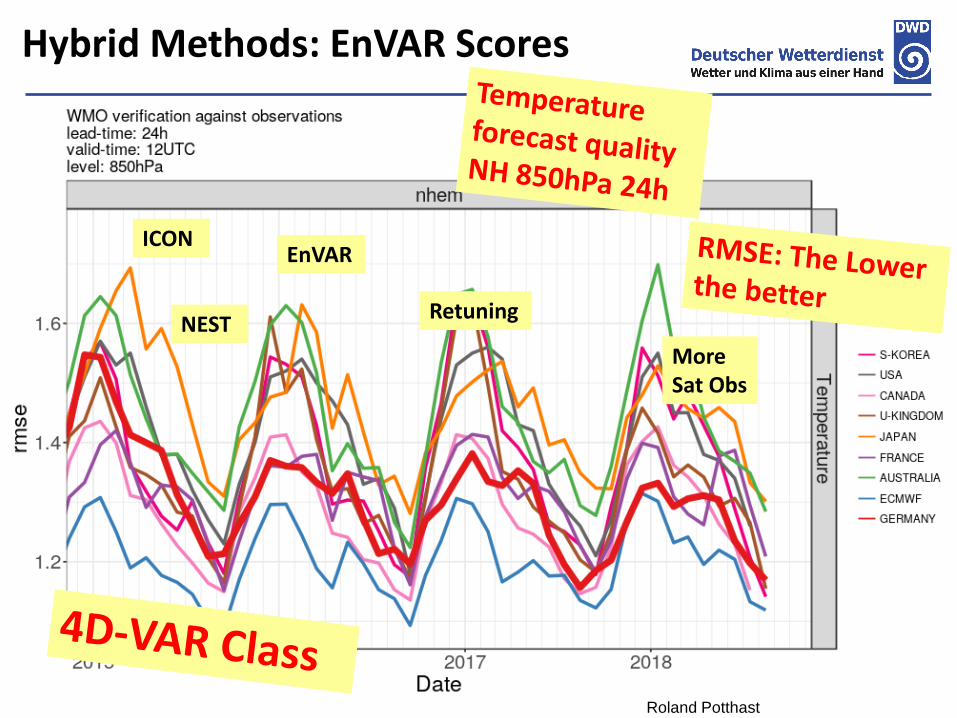
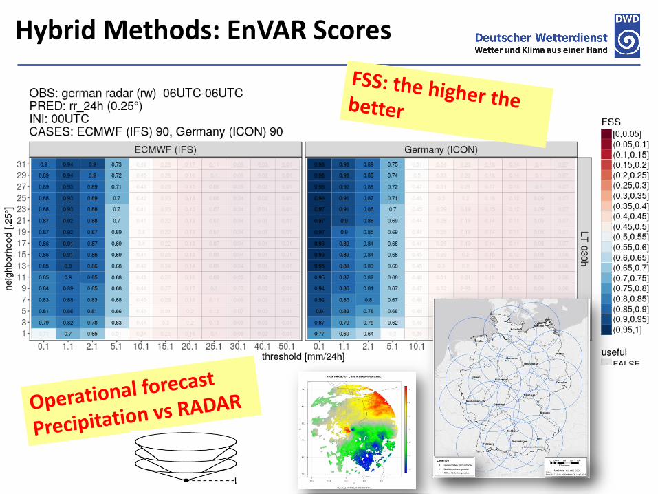
Hybrid Methods: EnVAR Scores
Roland Potthast
ICONEnVAR
More Sat Obs
NESTRetuning

Roland Potthast
Hybrid Methods: EnVAR Scores
ICONEnVAR
More Sat Obs
NESTRetuning
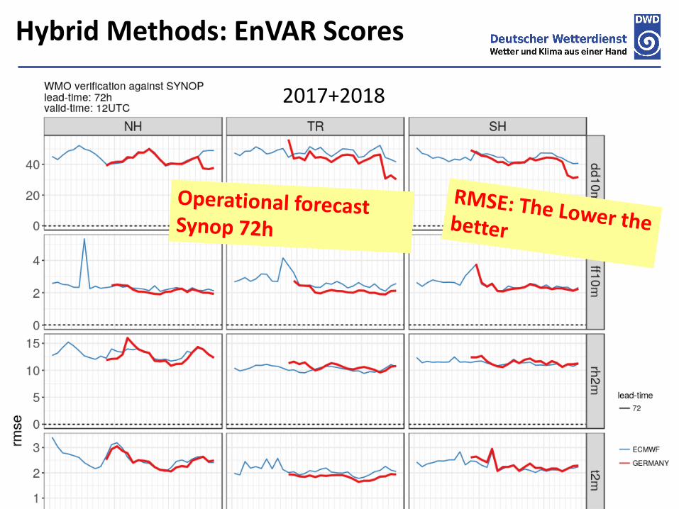
Hybrid Methods: EnVAR Scores
2017+2018
Hybrid Methods: EnVAR Scores
1. Why and Where Distributions, Risk and
Uncertainty?
2. Discussion of Ensemble (+Particle) Methods
3. Framework Global+LAM+LES Model: ICON and
ICON-EPS and the LEKTF+EnVAR/KENDA System
4. LAPF & LMCPF Particle Filters for Non-Gaussian
Distributions – Details and Results
Contents

PRIOR
DATA
Posterior
Analysis
Ensemble
BAYES Data Assimilation

Bayesian Filtering via PF
April 2018
LETKF
Classical PF
DATA
Prior
Posterior
DATA
Prior
Posterior
LAPF
DATA
Prior
Posterior

Prior
Bayesian Filtering via PF
LETKF
Classical PF LAPF
LAPF = Transform, Localization, Adaptivity with global modulated Resampling

• Bayes formula to calculate new analysis distribution
𝑝𝑘𝑎 𝑥 := 𝑝 𝑥 𝑦𝑘 = 𝑐 𝑝 𝑦𝑘 𝑥 𝑝𝑘
𝑏 𝑥 , 𝑥 ∈ ℝ𝑛
𝑐 is a normalization factor: 𝑋 𝑝𝑘𝑎 𝑥 𝑑𝑥 = 1
• To carry out the analysis step at time 𝑡𝑘aposteriori weights 𝑝𝑘
𝑎 are calculated
𝑝𝑘,𝑙(𝑎)
= 𝑐 𝑒−12 𝑦−𝐻𝑥 𝑙 𝑇
𝑅−1(𝑦−𝐻𝑥 𝑙 )
𝑐 is chosen such that σ𝑙=1𝐿 𝑝𝑘,𝑙
(𝑎)= 𝐿
First Step: The Classical Particle Filter
Classical PF Approach

Second Step: Classical Resampling
• Accumulated weights 𝑤𝑎𝑐 are defined:𝑤𝑎𝑐0 = 0
𝑤𝑎𝑐𝑖 = 𝑤𝑎𝑐𝑖−1 + 𝑝𝑖𝑎, 𝑖 = 1, … , 𝐿
where 𝐿 denotes the ensemble size
• Drawing 𝑟𝑗~𝑈 0,1 , 𝑗 = 1,… , 𝐿, set 𝑅𝑗 = 𝑗 − 1 + 𝑟𝑗 anddefine transform matrix W for the particles by:
𝑊𝑖,𝑗 = ൝1 𝑖𝑓 𝑅𝑗 ∈ 𝑤𝑎𝑐𝑖−1 , 𝑤𝑎𝑐𝑖 ,
0 𝑜𝑡ℎ𝑒𝑟𝑤𝑖𝑠𝑒,
𝑖, 𝑗 = 1,… , 𝐿 with 𝑊 ∈ ℝ𝐿𝑥𝐿, (𝑠, 𝑡] denotes the interval ofvalues 𝑠 < 𝜂 ≤ 𝑡. Resampling
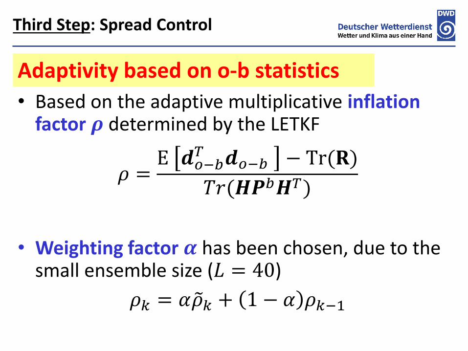
Third Step: Spread Control
• Based on the adaptive multiplicative inflationfactor 𝝆 determined by the LETKF
𝜌 =Ε 𝒅𝑜−𝑏
𝑇 𝒅𝑜−𝑏 − Tr(𝐑)
𝑇𝑟(𝑯𝑷𝑏𝑯𝑇)
• Weighting factor 𝜶 has been chosen, due to the small ensemble size (𝐿 = 40)
𝜌𝑘 = 𝛼 𝜌𝑘 + 1 − 𝛼 𝜌𝑘−1
Adaptivity based on o-b statistics

• Pertubation factor 𝜎 is used to add spread to thesystem
𝜎 =
𝑐0, 𝜌 < 𝜌(0)
𝑐0 + 𝑐1 − 𝑐0 ∗𝜌 − 𝜌(0)
𝜌(1) − 𝜌(0), 𝜌(0) ≤ 𝜌 ≤ 𝜌(1)
𝑐1, 𝜌 > 𝜌(1)
where 𝑐0 = 0.02, 𝑐1 = 0.2,
𝜌(0) = 1.0 and 𝜌(1) = 1.4, with𝜎 = 𝑐1if 𝜌 ≥ 𝜌(1) and
𝜎 = 𝑐0 if 𝜌 ≤ 𝜌(0)
Third Step: Spread Control

• Weights W are modified byapplying the pertubation factor 𝝈
𝑊 = 𝑊 + 𝑅𝑛𝑑 ∗ 𝜎
with 𝑅𝑛𝑑 normally distributed random numbers
Fourth Step: Gaussian Resampling
An example for a W-Matrix after applying 𝜎determined with the LAPF for 60°N/90°O ~500 hPa, 26.05.2016 0 UTC is shown. 10 particles are chosen
DATA
Prior
Posterior

Effective Ensemble Size Distributions
100 hPa 500 hPa 1000 hPa
May 20
May 25
May 31
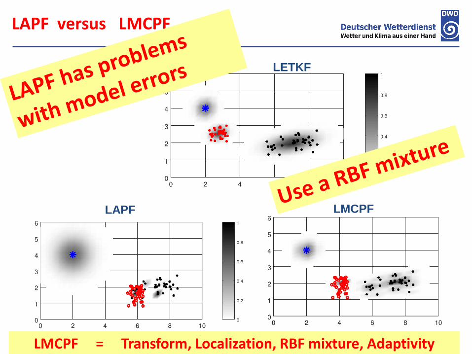
LMCPFLAPF
LETKF
LAPF versus LMCPF
LMCPF = Transform, Localization, RBF mixture, Adaptivity
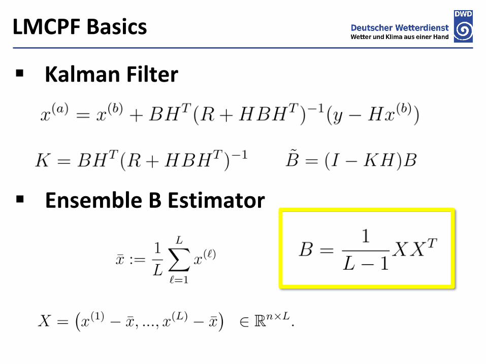
LMCPF Basics
▪ Kalman Filter
▪ Ensemble B Estimator
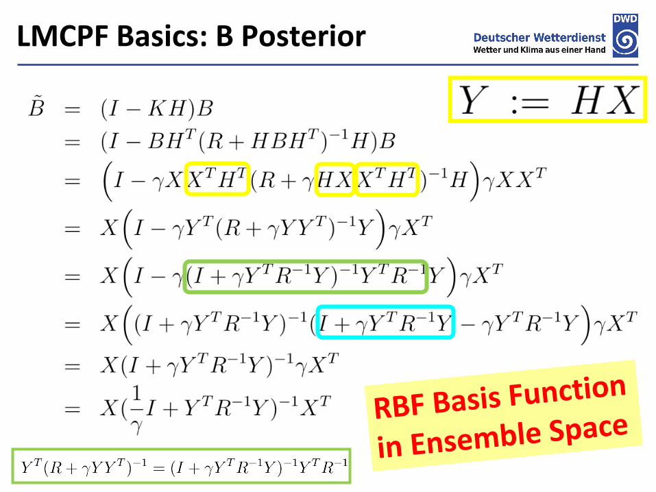
LMCPF Basics: B Posterior
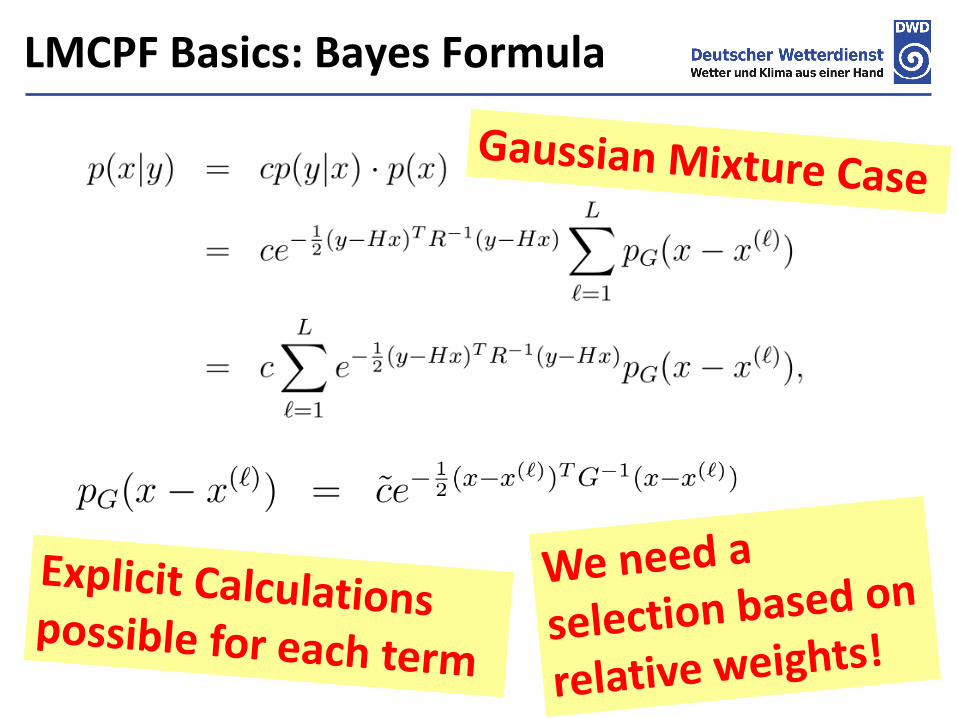
LMCPF Basics: Bayes Formula

LMCPF Basics: Relative Weights
LMCPFLAPF
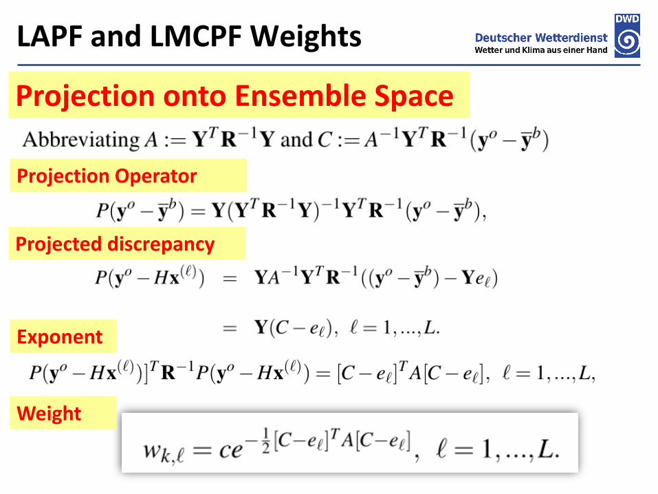
LAPF and LMCPF Weights
Projection onto Ensemble Space
Projection Operator
Projected discrepancy
Exponent
Weight
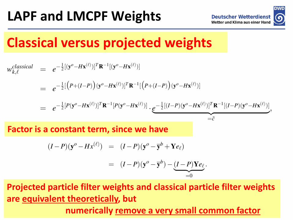
LAPF and LMCPF Weights
Classical versus projected weights
Factor is a constant term, since we have
Projected particle filter weights and classical particle filter weightsare equivalent theoretically, but
numerically remove a very small common factor
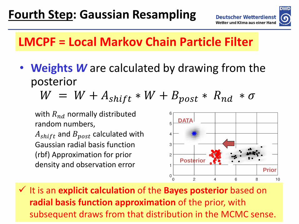
• Weights W are calculated by drawing from theposterior𝑊 = 𝑊 + 𝐴𝑠ℎ𝑖𝑓𝑡 ∗ 𝑊 + 𝐵𝑝𝑜𝑠𝑡 ∗ 𝑅𝑛𝑑 ∗ 𝜎
with 𝑅𝑛𝑑 normally distributed random numbers,𝐴𝑠ℎ𝑖𝑓𝑡 and 𝐵𝑝𝑜𝑠𝑡 calculated with
Gaussian radial basis function (rbf) Approximation for prior density and observation error
DATA
Prior
Posterior
✓ It is an explicit calculation of the Bayes posterior based on radial basis function approximation of the prior, with subsequent draws from that distribution in the MCMC sense.
Fourth Step: Gaussian Resampling
LMCPF = Local Markov Chain Particle Filter
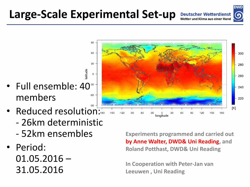
Large-Scale Experimental Set-up
• Full ensemble: 40 members
• Reduced resolution: - 26km deterministic- 52km ensembles
• Period: 01.05.2016 –31.05.2016
Experiments programmed and carried out by Anne Walter, DWD& Uni Reading, and Roland Potthast, DWD& Uni Reading
In Cooperation with Peter-Jan van Leeuwen , Uni Reading
RMSE
LETKFLAPF
RMSE
p-l
evel
[h
Pa]
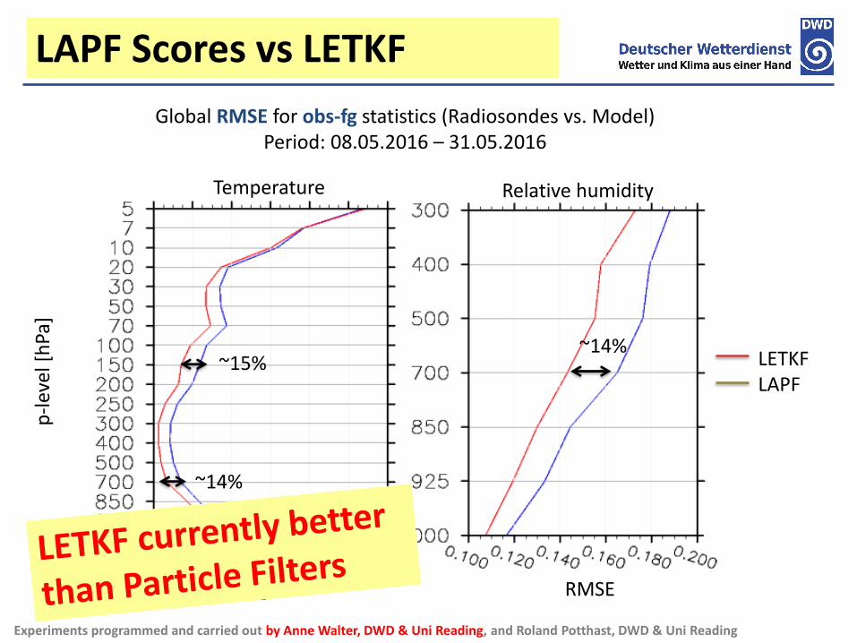
Global RMSE for obs-fg statistics (Radiosondes vs. Model)Period: 08.05.2016 – 31.05.2016
Relative humidityTemperature
~14%~15%
~14%
LAPF Scores vs LETKF
Experiments programmed and carried out by Anne Walter, DWD & Uni Reading, and Roland Potthast, DWD & Uni Reading
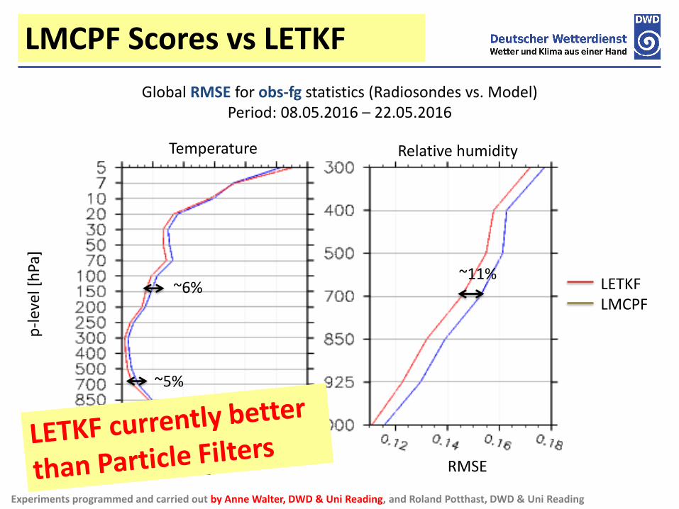
RMSE
LETKFLMCPF
RMSE
p-l
evel
[h
Pa]
Global RMSE for obs-fg statistics (Radiosondes vs. Model)Period: 08.05.2016 – 22.05.2016
Relative humidityTemperature
~11%~6%
~5%
LMCPF Scores vs LETKF
Experiments programmed and carried out by Anne Walter, DWD & Uni Reading, and Roland Potthast, DWD & Uni Reading

RMSE
LAPFLMCPF
RMSE
p-l
evel
[h
Pa]
Global RMSE for obs-fg statistics (Radiosondes vs. Model)Period: 08.05.2016 – 22.05.2016
Relative humidityTemperature
~7%
~7%
LMCPF Scores vs LAPF
Experiments programmed and carried out by Anne Walter, DWD & Uni Reading, and Roland Potthast, DWD & Uni Reading
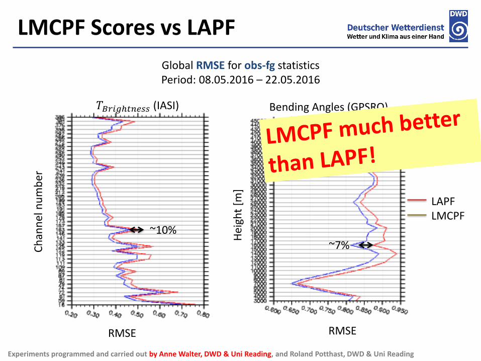
RMSE
LAPFLMCPF
RMSE
Ch
ann
el n
um
ber
Global RMSE for obs-fg statisticsPeriod: 08.05.2016 – 22.05.2016
Bending Angles (GPSRO)𝑇𝐵𝑟𝑖𝑔ℎ𝑡𝑛𝑒𝑠𝑠 (IASI)
~7%
~10%H
eigh
t [m
]
LMCPF Scores vs LAPF
Experiments programmed and carried out by Anne Walter, DWD & Uni Reading, and Roland Potthast, DWD & Uni Reading

New LAMCPF Scores vs LETKF
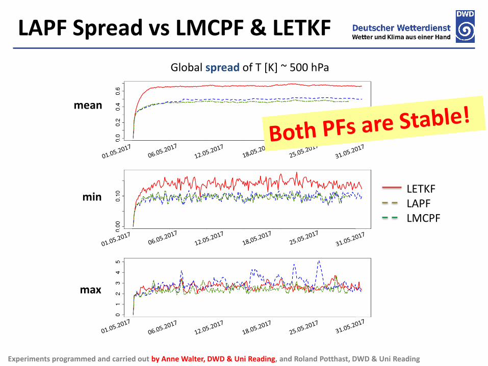
mean
min
max
LETKFLAPFLMCPF
Global spread of T [K] ~ 500 hPa
LAPF Spread vs LMCPF & LETKF
Experiments programmed and carried out by Anne Walter, DWD & Uni Reading, and Roland Potthast, DWD & Uni Reading


LETKFLMCPF
LMCPF Scores vs LETKF
Experiments programmed and carried out by Anne Walter, DWD & Uni Reading, and Roland Potthast, DWD & Uni Reading

LMCPF Scores vs LETKF
LETKFLMCPF
Experiments programmed and carried out by Anne Walter, DWD & Uni Reading, and Roland Potthast, DWD & Uni Reading

• LAPF and LMCPF are implemented in an operational NWP system:
• Both Particle Filters are able to provide reasonable atmospheric analysis in a large-scale (high-dimensional) environment and are running stably over a period of one month
• The LMCPF outperforms the LAPF but not yet the LETKF, but both Particle Filters are not far behind the operational LETKF
Summary LAPF and LMCPFLMCPFLAPF
Globally + mesoscale, convective scale
Both Particle Filters are showing promising results; further tuning and development is in progress.

Many Thanks!