ensemble verification ii
TRANSCRIPT

Ensemble Verification II
Martin Leutbecher
Training Course 2017
1 Proper scores
2 Continuous scalar variables
3 Comparison of ensemble with single forecasts
4 Observation uncertainty
5 Climatological distribution
6 Statistical significance
7 Further topics
M. Leutbecher Ensemble Verification II Training Course 2017 1
Proper scores
• A score for a probabilistic forecast is a summary measure that evaluates theprobability distribution. This condenses all the information into a single numberand can be potentially misleading.
• Let us assume that we predict the distribution pfc(x) while the verification isdistributed according to a distribution py (x). Not all scores indicate maximumskill for pfc = py .
• A score (or scoring rule) is (strictly) proper if the score reaches its optimal value if(and only if) the predicted distribution is equal to the distribution of theverification.
• If a forecaster is judged by a score that is not proper, (s)he is encouraged to issueforecasts that differ from what her/his true belief of the best forecast is! In such asituation, one says that the forecast is hedged or that the forecaster plays thescore.
• Examples of proper scores are: Brier Score, continuous (and discrete) rankedprobability score, logarithmic score
• see Gneiting and Raftery (2007) for more details
M. Leutbecher Ensemble Verification II Training Course 2017 2

Example of a score that is not proper
• consider the linear score: LinS = |p − o|• dichotomous event e: e occured (o = 1), e did not occur (o = 0)
• assume the event occurs with the true probability of 0.4
• If the prediction is 0.4, the expected linear score is
E(LinS) = 0.4|0.4− 1|+ (1− 0.4) |0.4− 0| = 0.48
• If the prediction is instead 0, the expected linear score is
E(LinS) = 0.4|0− 1|+ (1− 0.4)|0− 0| = 0.40
Note, that it is easy to prove that the Brier score is strictly proper (e.g. Wilks 2011)
M. Leutbecher Ensemble Verification II Training Course 2017 3
An example with two proper scoreSimple idealised example
We compare Alice’s and Bob’s forecasts for Y ∼ N (0, 1),
FAlice = N (0, 1) FBob = N (4, 1)
Based on 10, 000 forecast experiments,
Forecaster CRPS LogS
Alice 0.56 1.42Bob 3.53 9.36
M. Leutbecher Ensemble Verification II Training Course 2017 4

A conditional sample for evaluating Alice and BobSimple toy example
Based on the 10 largest observations,
Forecaster CRPS LogS
Alice 2.70 6.29Bob 0.46 1.21
●●●●●●●●●●●●●●●●
●●●●
●●●●●●●
●
●
●
●
●
●
●●●●●●●●●●
●●●●●
●
●
●
●
●
●
●●●●●●●●●●●●●●●●●●●●●●●●●●●●●●●●●●●●●●●●●●●●●●●●●●●●●●●●●●●●●●●●●●●
−4 −2 0 2 4 6 8
0.0
0.1
0.2
0.3
0.4
0.5
x
Den
sity
AliceBob
M. Leutbecher Ensemble Verification II Training Course 2017 5
The forecaster’s dilemma
More generally, for non-constant weight functions w , any scoring rule
S∗(F , y) = w(y)S(F , y)
is improper even if S is a proper scoring rule (Gneiting and Ranjan, 2011). Here, y andF denote the verifying observation and the predicted distribution, respectively.
Forecaster’s dilemmaForecast evaluation only based on a subset of extreme observations corresponds toimproper verification methods and is bound to discredit skillful forecasters.
Acknowledgement: Forecaster’s dilemma and Alice and Bob’s forecast based on slides provided by
Sebastian Lerch (Heidelberg Institute for Theoretical Studies), see also
http://arxiv.org/pdf/1512.09244
M. Leutbecher Ensemble Verification II Training Course 2017 6

Scores for probabilistic/ensemble forecasts of continuousscalar variables
some (but not all) useful measures
• RMSE and other scores used for single forecasts applied to ensemble mean
• rank histograms (reliability again)
• continuous ranked probability score (reliability and resolution)
• logarithmic score (for Gaussian) (reliability and resolution)
• reliability of the ensemble spread (domain-integrated and local)
M. Leutbecher Ensemble Verification II Training Course 2017 7
Continuous ranked probability scoreCRPS = Mean squared error of the cumulative distribution Pfc
cdf of observation Py (x) = P(y ≤ x) = H(x − y) = 1{y ≤ x}cdf of forecast Pfc(x) = P(xfc ≤ x)
Here, H and 1 denote the Heaviside step function and the indicator function,respectively.
CRPS =
∫ +∞
−∞(Pfc(x)− Py (x))2 dx =
∫ +∞
−∞BSx dx
−2 −1 0 1 2 3 4 5
0.0
0.2
0.4
0.6
0.8
1.0
x
P
(P_fc − P_obs)^2P_fcP_obs
−2 −1 0 1 2 3 4 5
0.0
0.2
0.4
0.6
0.8
1.0
x
P
(P_fc − P_obs)^2P_fcP_obs
−2 −1 0 1 2 3 4 5
0.0
0.2
0.4
0.6
0.8
1.0
x
P
(P_fc − P_obs)^2P_fcP_obs
equal to mean absolute error for a single forecastM. Leutbecher Ensemble Verification II Training Course 2017 8
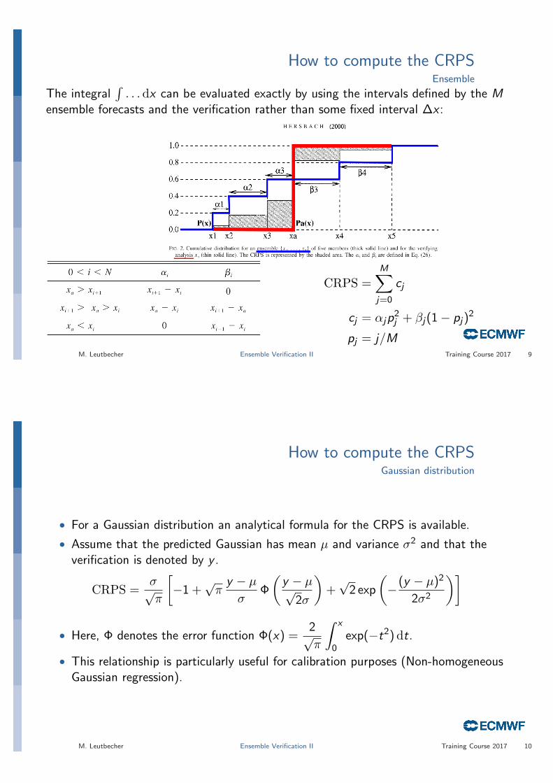
How to compute the CRPSEnsemble
The integral∫. . . dx can be evaluated exactly by using the intervals defined by the M
ensemble forecasts and the verification rather than some fixed interval ∆x :
CRPS =M∑j=0
cj
cj = αjp2j + βj(1− pj)
2
pj = j/MM. Leutbecher Ensemble Verification II Training Course 2017 9
How to compute the CRPSGaussian distribution
• For a Gaussian distribution an analytical formula for the CRPS is available.
• Assume that the predicted Gaussian has mean µ and variance σ2 and that theverification is denoted by y .
CRPS =σ√π
[−1 +
√πy − µσ
Φ
(y − µ√
2σ
)+√
2 exp
(−(y − µ)2
2σ2
)]
• Here, Φ denotes the error function Φ(x) =2√π
∫ x
0exp(−t2)dt.
• This relationship is particularly useful for calibration purposes (Non-homogeneousGaussian regression).
M. Leutbecher Ensemble Verification II Training Course 2017 10

CRPSDecomposition
• The CRPS can be decomposed into a reliability component and a resolutioncomponent.
• The CRPS is additive: The CRPS for the union of two samples is the weighted(arithmetic) average of the CRPS of the two samples with the weightsproportional to the respective sample sizes.
• The components of the CRPS are not additive. The components can becomputed from the sample averages of the αj and βj distances.
• This is similar to the decomposition of the Brier score. However, the reliability(resolution) component of the CRPS is not the integral of the reliability(resolution) component of the Brier scores.
• The reliability component of the CRPS is related to the rank histogram but notidentical.
• see Hersbach (2000) for details
M. Leutbecher Ensemble Verification II Training Course 2017 11
CRPS with threshold-weighting
Can be used for instance to focus on the tails of the climatological distribution, e.g.strong wind, intense rainfall.
The threshold-weighted CRPS weights the integrand (= Brier score for threshold z)
twCRPS(F , y) =
∫ ∞−∞
(F (z)− 1{y ≤ z})2w(z)dz
w(z) is a weight function on the real line. The score twCRPS is proper and avoids theproblem with looking only at a sample of extreme outcomes (Alice and Bob’s example).
Gneiting, T. and Ranjan, R. (2011)
Comparing density forecasts using threshold- and quantile-weighted scoring rules. J. Bus. Econ. Stat.,
29, 411–422. (adapted from a slide by Sebastian Lerch)
M. Leutbecher Ensemble Verification II Training Course 2017 12

Ranked Probability Score (RPS)• The CRPS
∫BSx dx has a discrete analog, the (discrete) ranked probability score:
RPS =L∑
k=1
BSxk =L∑
k=1
(Pfc(k)− Py (k))2
• The thresholds xk that separate the L categories can be chosen in various ways• equidistant (RPS → CRPS as ∆x → 0)• climatologically equally likely, e.g. tercile boundaries
M. Leutbecher Ensemble Verification II Training Course 2017 13
Logarithmic scoreIgnorance score
• For a forecast consisting of a probability density pfc(x), define
LS = − log(pfc(y))
where y denotes the observation (or analysis).
• This score is proper and local.
• ensemble forecasts −→ probability density
• A simple yet useful exercise is to use the Gaussian density given by the ensemblemean µ and the ensemble variance σ2. Then, the logarithmic score is given by
LS =(µ− y)2
2σ2+ 1
2 log(2πσ2)
• Thus, it consists of the squared error of the ensemble mean normalized by theensemble variance and a logarithmic term that penalizes large variance. The firstterm is a measure of the reliability and the second term is a measure of thesharpness of the forecast.
M. Leutbecher Ensemble Verification II Training Course 2017 14

Daily EPS stdev (shaded) and ens. mean (cont.)500 hPa geopotential (m2 s−2) at 72 h lead; init. time 6 December 2010
H
L
L
70°N70°N
70°N
60°N
60°N
60°N
60°N
60°N
50°N
50°N
50°N
50°N
50°N
50°N
50°N
40°N
40°N
40°N
40°N
40°N
40°N
30°N
30°N
30°N
30°N
30°N
60°E40°E20°E20°W40°W60°W
20°E20°W
0 75 150 225 300 375 450 525 600 675 750 825EM
M. Leutbecher Ensemble Verification II Training Course 2017 15
Spread-reliabilitymethodology
consider (local) pairs of ensemble variance and squared error of the ensemble mean —stratified by the ensemble variance
M. Leutbecher Ensemble Verification II Training Course 2017 16

Spread-reliability: An example500 hPa height — 20◦–90◦N
24 h 48 h
4 6 8 10 12 14 16 18RMS spread (m)
4
6
8
10
12
14
16
18
RM
S e
rror
(m
)
.
as 36R1
as 36R4
4 8 12 16 20 24 28 32 36RMS spread (m)
4
8
12
16
20
24
28
32
36
RM
S e
rror
(m
)
.
as 36R1
as 36R4
• 40 cases
• T639, 50 member
• Jan 2010 config. (“as 36r1”)
• Nov 2010 config. (“as 36r4”):revised initial perturbations andrevised tendency pertns.
M. Leutbecher Ensemble Verification II Training Course 2017 17
Verification of ensembles and single forecasts
• When monitoring an operational forecasting system that consists of single(unperturbed) forecasts and an ensemble, it is useful to compare changes in theperformance of the ensemble with changes seen for the single forecast(s).
• But what scores should be compared when looking at a single forecast versus anensemble?
• Many scores for ensembles are meaningful when computed for single forecasts
• equivalences• CRPS — MAE• BS — BS single fc (using probabilities 0 and 1)
• Obviously, probabilistic skill of a “naked” (= raw) single forecast is inferior to theprobabilistic skill of a dressed single forecast. The dressing kernel can beestimated from past error statistics.
M. Leutbecher Ensemble Verification II Training Course 2017 18

Dressed control forecast: v 850 hPa, 35◦–65◦N, DJF09EPS raw prob. for CRPS; Gaussian for LS
N(CF, σ2err(CF)) σerr estimated from reforecasts
CRPS
0 2 4 6 8 10 12 14fc-step (d)
0
1
2
3
4
5
CR
PS
2008120100-2009022800 (90)ContinuousRankedProbabilityScore, ContinuousRankedProbabilityScoreCFWithErrClim
v850hPa, Northern Mid-latitudes
TMP161ec7
LS
0 2 4 6 8 10 12 14fc-step (d)
0
1
Con
tinuo
usIg
nora
nceS
core
Gau
ssia
n
2008120100-2009022800 (90)ContinuousIgnoranceScoreGaussian, ContinuousIgnoranceScoreCFWithGaussianErrClim
v850hPa, Northern Mid-latitudes
TMP161ec7
M. Leutbecher Ensemble Verification II Training Course 2017 19
Dressed ens. mean forecast: v 850 hPa, 35◦–65◦N, DJF09EPS raw prob. for CRPS; Gaussian for LS
N(EM, σ2err(EM)) σerr estimated from reforecasts
CRPS
0 2 4 6 8 10 12 14fc-step (d)
0
1
2
3
CR
PS
2008120100-2009022800 (90)ContinuousRankedProbabilityScore, ContinuousRankedProbabilityScoreEMWithErrClim
v850hPa, Northern Mid-latitudes
TMP161ec7
LS
0 2 4 6 8 10 12 14fc-step (d)
-0.2
0
0.2
0.4
0.6
0.8
1
1.2
1.4
Con
tinuo
usIg
nora
nceS
core
Gau
ssia
n
2008120100-2009022800 (90)ContinuousIgnoranceScoreGaussian, ContinuousIgnoranceScoreEMWithGaussianErrClim
v850hPa, Northern Mid-latitudes
TMP161ec7
• EM more accurate than CF ⇒ this permits a sharper Gaussian distribution.
• The Logarithmic score discriminates better the value of flow-dependent variations in ensemblevariance than the CRPS.
M. Leutbecher Ensemble Verification II Training Course 2017 20

Uncertainty of the verifying observationsor, more generally, the verifying data
• In real applications the true state xt of the atmosphere is not know exactly. Theobservation y has an error
y = xt + ε
• Assume an ensemble is perfectly reliable, i.e. ensemble members xe ∼ ρe and thetrue state xt ∼ ρt are realisations of the same distribution ρe = ρt .
• Then, the observation y is a realisation of the distribution given by theconvolution of the true distribution and the error distribution
ρy = ρt ∗ ρε
• Thus, a verification with respect to y will indicate a lack of reliability.
M. Leutbecher Ensemble Verification II Training Course 2017 21
Verification in the presence of observation uncertainties
ρε ρt = ρe , ρy = ρE
• solution: postprocess ensemble members prior to verification
• verify ensemble members to which noise has been added:xE = xe + ε with ε ∼ ρε
• Then ρE = ρy
M. Leutbecher Ensemble Verification II Training Course 2017 22

The climatological distributiontemperature in 850 hPa
15 March (based on ERA-Interim 1989–2008)
-12
-8-8
-8
-4-4
-4
-4
0
0
0
0
4
4
4
4
8
8
8
8
120
1
2
3
4
5
6
7
8
contours: mean — shading: stdevM. Leutbecher Ensemble Verification II Training Course 2017 23
Ficticious skill due to a poor climatological distribution
• If one uses the same climatological distribution for a domain with differentclimatological characteristics (mean, stdev, . . . ), the skill with respect to thatdistribution is not real skill. It reflects the poor quality of the climatologicaldistribution.
• Same applies if seasonal variations of the climatological distribution are notrepresented.
• This criticism applies for instance if the climatological distribution is derived fromthe verification sample itself by aggregating different start times and differentlocations.
• It can also be misleading to compare skill scores from different prediction centreswhen the skill scores have been computed against own analyses.
• If the same climatological distribution (say ERA-Interim) is used as reference, thisclimatological distribution has the lowest skill when verified against the analysisthat deviates most from the analyses used for computing the climatologicaldistribution.
M. Leutbecher Ensemble Verification II Training Course 2017 24

Comparing model versions/ numerical experiments
0
100
200
300
400
500
CR
PS
0 5 10 15 20 25 30fc-step (d)
2013120100-2014112600 (46)
ContinuousRankedProbabilityScore
z500hPa, Northern Extra-tropics
IP only
SPPT
• 46 cases (1 year, every 8days)
• Could difference in scorebe a result of chance?
• How large does adifference have to be tobe trusted?
• case-to-case variability of predictabilityimplies distribution of score for givenlead time is fairly wide
• ⇒ not easy to get enough cases todistinguish score distributions of twonumerical experiments
M. Leutbecher Ensemble Verification II Training Course 2017 25
95% confidence intervalsPaired sample of cases: t test applied to score differences
-18
-12
-6
0
6
CR
PS
0 5 10 15 20 25 30fc-step (d)
2013120100-2014112600 (46)
ContinuousRankedProbabilityScore [sign p=0.0500]
z500hPa, Northern Extra-tropics
IP only
SPPT
• 46 cases (1 year, every 8days)
• Variability of scoredifferences is muchsmaller!
• ⇒ Paired sample of cases(start dates)
• For each forecast leadtime, consider sample ofscore differences
• Temporal auto-correlation taken into account using AR(1) model when estimatingvariance of mean difference
M. Leutbecher Ensemble Verification II Training Course 2017 26

More verification topics
• sensitivity to ensemble size and estimation of verification statistics in the limitM →∞
• skill on different spatial scales
• multivariate aspects
• decision making and verification
M. Leutbecher Ensemble Verification II Training Course 2017 27
Probabilities can help with making decisions
• Open air restaurant scenario:• to open additional tables costs £20 and provides £100 extra income
(if T > 24◦ C)• On a particular day, the forecast is P(T > 24◦ C) = 0.30• What should the restaurant do?
• Compute the profit/loss (£) over 100 days (assuming reliable probabilities):
profit on warm days(T > 24◦ C) = 30× (100− 20) = +2400
profit on cool days(T ≤ 24◦ C ) = 70× (0− 20) = −1400
total profit = +1000
• It is profitable to open additional tables if the probability of a warm day exceeds0.20 .
• The ratio of cost to loss (or cost to extra profit) determines at what probabilityvalue it is beneficial to take action. For low (high) cost/loss, action should betaken already (only) if the event is predicted with a low (high) probability.
M. Leutbecher Ensemble Verification II Training Course 2017 28

Decision making — cost loss model
expense when using climatological prob. Ec = min(C , oL)
expense when using a perfect forecast Ep = oC
expense when using the forecast Ef = aC + bC + cL
value V =saving from using forecast
saving from using perfect fc.=
Ec − Ef
Ec − Ep=
=min(α, o)− F (1− o)α + Ho(1− α)− o
min(α, o)− oαwhere
α = C/L; H =a
a + c; F =
b
b + d; o = a + c
M. Leutbecher Ensemble Verification II Training Course 2017 29
(Potential) economic value
• maximum value reached at α = C/L = o• maximum value for all C/L is maxV = H − F• when a (reliable) probabilistic forecast predicts an event with probability p, all
users with C/L < p should act.• one speaks of potential economic value if calibrated probabilities are used to make
decisionM. Leutbecher Ensemble Verification II Training Course 2017 30

Potential economic valueand ensemble size
M. Leutbecher Ensemble Verification II Training Course 2017 31
Decision making — weather roulette
Hagedorn and Smith (2009)
M. Leutbecher Ensemble Verification II Training Course 2017 32

Decision making — weather roulette
M. Leutbecher Ensemble Verification II Training Course 2017 33
Decision making — weather roulette3-day forecasts
M. Leutbecher Ensemble Verification II Training Course 2017 34
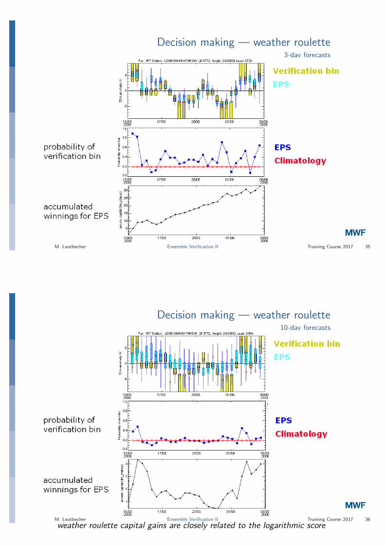
Decision making — weather roulette3-day forecasts
M. Leutbecher Ensemble Verification II Training Course 2017 35
Decision making — weather roulette10-day forecasts
weather roulette capital gains are closely related to the logarithmic scoreM. Leutbecher Ensemble Verification II Training Course 2017 36

References
Candille, G. and O. Talagrand, 2005: Evaluation of probabilistic prediction systems for a scalar variable. Q. J. R. Meteorol. Soc., 131, 2131–2150.
Ferro, C. A. T., D. S. Richardson, and A. P. Weigel, 2008: On the effect of ensemble size on the discrete and continuous ranked probability scores.Meteorol. Appl., 15, 19–24.
Gneiting, T. and A. E. Raftery, 2007: Strictly proper scoring rules, prediction and estimation. Journal of the American Statistical Association, 102,359–378.
Hagedorn, R. and L. A. Smith, 2009: Communicating the value of probabilistic forecasts with weather roulette. Meteorol. Appl., 16, 143–155.
Hamill, T. M., 2001: Interpretation of rank histograms for verifying ensemble forecasts. Mon. Wea. Rev., 129, 550–560.
Hamill, T. M. and J. Juras, 2006: Measuring forecast skill: Is it real skill or is it the varying climatology? Q. J. R. Meteorol. Soc., 132, 2905–2923.
Hersbach, H., 2000: Decomposition of the continous ranked probability score for ensemble prediction systems. Weather and Forecasting, 15,559–570.
Jung, T. and M. Leutbecher, 2008: Scale-dependent verification of ensemble forecasts. Q. J. R. Meteorol. Soc., 134, 973–984.
Leutbecher, M., 2009: Diagnosis of ensemble forecasting systems. In Seminar on Diagnosis of Forecasting and Data Assimilation Systems,ECMWF, Reading, UK, 235–266.
Murphy, A. and R. L. Winkler, 1987: A general framework for forecast verification. Mon. Wea. Rev., 115, 1330–1338.
Richardson, D. S., 2000: Skill and relative economic value of the ECMWF ensemble prediction system. Q. J. R. Meteorol. Soc., 126, 649–667.
Roulston, M. S. and L. A. Smith, 2002: Evaluating probabilistic forecasts using information theory. Mon. Wea. Rev., 130, 1653–1660.
Saetra, Ø., H. Hersbach, J.-R. Bidlot, and D. S. Richardson, 2004: Effects of observation errors on the statistics for ensemble spread and reliability.Mon. Wea. Rev., 132, 1487–1501.
Weigel, A. P., 2011: Ensemble verification. In Forecast Verification: A Practitioner’s Guide in Atmospheric Science, Jolliffe, I. T. and Stephenson,D. B., editors. Wiley, 2nd edition.
Wilks, D. S., 2011: Statistical Methods in the Atmospheric Sciences. Academic Press, 3rd edition.
M. Leutbecher Ensemble Verification II Training Course 2017 37