ensemble verification system (evs) manual · the ensemble verification service ... 7.2 streamflow...
TRANSCRIPT
Ensemble Verification Service (EVS)
Version 5.7
User’s Manual
Dr. James D. Brown
Hydrologic Solutions Limited, Southampton, UK.
HSL

2
Preface
The Ensemble Verification Service (EVS) is a Java-based software tool originally
developed by the U.S. National Weather Service’s Office of Hydrologic Development
(OHD) and, subsequently, by Hydrologic Solutions Limited (HSL), Southampton, UK.
The software is currently developed and marketed by HSL as the Ensemble
Verification System. The EVS is designed to verify ensemble forecasts of hydrologic
and hydrometeorological variables, such as temperature, precipitation, streamflow
and river stage. The software is intended to be flexible, modular, and open to
accommodate enhancements and additions, not only by its developers, but also by
its users. The EVS is “open source” software and is released under the GNU Lesser
General Public License (LGPL), Version 3.0. We welcome your participation in the
continuing development of the EVS toward a versatile and standardized tool for
ensemble verification.
Contact: [email protected]
Acknowledgments
Parts of this work were funded by NOAA’s Advanced Hydrologic Prediction Service
(AHPS) and by the Climate Prediction Program for the Americas (CPPA).

3
Disclaimer
This software and related documentation was originally developed by the National
Weather Service (NWS) and, subsequently, by Hydrologic Solutions Limited (HSL),
hereafter referred to as “The Developers”. Pursuant to title 17, section 105 of the
United States Code this software is not subject to copyright protection and may be
used, copied, modified, and distributed without fee or cost. Parties who develop
software incorporating predominantly NWS developed software must include notice,
as required by Title 17, Section 403 of the United States Code. The Developers
provide no warranty, expressed or implied, as to the correctness of the furnished
software or its suitability for any purpose. The Developers assume no responsibility,
whatsoever, for its use by other parties, about its quality, reliability, or any other
characteristic. The Developers may change this software to meet their own needs or
discontinue its use without prior notice. The Developers cannot assist users without
prior agreement and are not obligated to fix reported problems. The EVS is released
under the GNU Lesser General Public License (LGPL) Version 3.0. A copy of the
LGPL is provided with this distribution.

4
Contents
1. INTRODUCTION ............................................................................................................. 6
2. INSTALLATION INSTRUCTIONS AND START-UP ...................................................... 9
2.1 Contents of the full distribution ........................................................................................ 9
2.2 Requirements ................................................................................................................... 9
2.3 Unpacking and running the EVS .................................................................................... 10
2.4 Troubleshooting the installation ..................................................................................... 11
2.5 Altering memory settings ............................................................................................... 12
2.6 Source code and documentation ................................................................................... 12
2.7 Computer resource considerations ................................................................................ 13
3. OVERVIEW OF FUNCTIONALITY ............................................................................... 15
3.1 Summary of functionality in the EVS Version 5.7 .......................................................... 15
3.2 Planned functionality ...................................................................................................... 17
4. GETTING STARTED ..................................................................................................... 18
4.1 Structure of the GUI ....................................................................................................... 18
4.2 Stage 1: Verification ....................................................................................................... 19
4.3 Stage 2: Aggregation ..................................................................................................... 23
4.4 Stage 3: Output .............................................................................................................. 24
4.5 Data formats supported by the EVS .............................................................................. 25
4.6 Command line options ................................................................................................... 30
4.7 Changing the format of the XML outputs from the EVS ................................................ 30
4.8 Creating custom plots of the EVS outputs in R ............................................................. 31
5. A DETAILED GUIDE TO THE OPTIONS IN EACH WINDOW OF THE GUI ............... 32
5.1 Administrative functions in the main window ................................................................. 32
5.2 The first window in the Verification stage ...................................................................... 32
5.3 The second window in the Verification stage ................................................................ 46
5.4 The Aggregation window ............................................................................................... 55
5.5 The Output window ........................................................................................................ 58
6. THE VERIFICATION METRICS AVAILABLE IN THE EVS ......................................... 63
6.1 Classes of verification metric and attributes of forecast quality ..................................... 63
6.2 Metrics developed for the EVS with an emphasis on operational forecasting .............. 67
7. EXAMPLE APPLICATIONS OF THE EVS ................................................................... 72
7.1 Precipitation forecasts from the NWS Ensemble Pre-Processor (EPP) ........................ 72
7.2 Streamflow forecasts from the NWS Ensemble Streamflow Prediction system ............ 77

5
8. THE APPLICATION PROGRAMMERS INTERFACE (API) ......................................... 83
8.1 Overview ........................................................................................................................ 83
8.2 Procedure for adding a new metric to the EVS ............................................................. 85
APPENDIX A1 VERIFICATION STATISTICS COMPUTED IN THE EVS ...................... 87
APPENDIX A2 XML OUTPUT FORMATS ..................................................................... 104
APPENDIX A3 DATA SERVICES .................................................................................. 120
A3.1 Flood Early Warning System Data Service (FEWS-DS) ............................................. 120
APPENDIX A4 REFERENCES ...................................................................................... 126

6
1. INTRODUCTION
Ensemble forecasting is widely used in meteorology and, increasingly, in hydrology
to quantify and propagate modeling uncertainty (Stensrud et al., 1999; Brown and
Heuvelink, 2007; Park and Xu, 2009). Uncertainties in model predictions originate
from the inputs, structure and parameters of a model, among other things (Brown
and Heuvelink, 2005; Gupta et al., 2005). In practice, ensemble forecasts cannot
account for all of these uncertainties, and some uncertainties are difficult to quantify
accurately (NRC, 2006). Thus, ensemble forecasts are subject to errors. These
errors are manifest as differences between the forecast probabilities and the
corresponding observed probabilities over a large sample of forecasts and verifying
observations (subject to sampling and observational uncertainty; Jolliffe and
Stephenson, 2003; Hashino et al., 2006; Wilks, 2006). Unlike single-valued forecasts,
ensemble forecasts cannot be verified with deterministic measures, such as the
mean error or the root mean square error (RMSE). Rather, each ensemble member,
and thus each error, is associated with only a partial probability of occurrence. Many
of the techniques used to verify ensemble forecasts were pioneered in meteorology
(Wilks, 2006). For example, the Brier Score (BS; Brier, 1950) was developed to verify
probability forecasts of discrete weather events, such as tornados. The BS measures
the average squared difference between the forecast probability of an event and its
observed probability (which is 1 if the event occurred and 0 otherwise). With the
growth of probabilistic forecasting, ensemble verification is increasingly used in other
disciplines, such as hydrology (Bradley et al., 2004), oceanography (Park and Xu,
2009), ecology (Araújo and New, 2007) and volcanology (Bonadonna et al., 2005).
The basic attributes of ensemble forecast quality are broadly applicable, since they
are concerned with probability distributions or measures on probability distributions.
However, the specific approach to verification will depend on the forecast variables
and their temporal and spatial scales, as well as the intended applications and users
of the forecasts (e.g. research versus operational forecasting). In order to support
ensemble verification for a wide range of applications in hydrology and beyond,
flexible and user-friendly software is required. This is illustrated with an example from
the National Weather Service (NWS). The River Forecast Centers (RFCs) of the
NWS produce ensemble forecasts of temperature, precipitation and streamflow at a
variety of lead times (Schaake et al., 2007; Demargne et al., 2007; Demargne et al.,
2009, Wu et al., 2010). In one experimental operation, ensemble traces of
precipitation and temperature are generated from single-valued forecasts using an

7
Ensemble Pre-Processor (EPP; Schaake et al., 2007, Wu et al., 2010). These traces
are input into the Ensemble Streamflow Prediction (ESP) subsystem of the NWS
River Forecast System (NWSRFS; NWS, 2005), from which ensemble traces of
streamflow are output. There is a need to verify these forecasts and to identify the
factors responsible for model error and skill in different situations. Verification is
required at multiple temporal and spatial scales, ranging from minutes and kilometers
(e.g. for flash flood guidance) to years and entire regions (e.g. for water resource
planning and national verification). Furthermore, there is a need to support both
operational forecasting within the RFCs and hydrologic research and development
within the NWS. In order to meet these needs, work on ensemble verification is
separated into two themes (see Demargne et al., 2009 for further details); 1)
verification and bias-correction of real-time ensemble forecasts, which should directly
improve decisions that rely on forecast probabilities (“real-time verification”; see
Brown and Seo, 2010a); and 2) verification of archived operational forecasts and
hindcasts, which should indirectly improve decision making via enhanced techniques
for generating ensemble forecasts (“diagnostic verification”).
The Ensemble Verification Service (EVS) is a flexible, user-friendly, software tool that
is designed to verify ensemble forecasts of continuous numeric variables, such as
temperature, precipitation and streamflow (Brown et al., 2010b). The EVS can be
applied to forecasts from any number of geographic locations (points or areas) and
issued with any frequency and lead time. It can also aggregate forecasts in time,
such as daily precipitation totals based on hourly forecasts, and can aggregate
verification statistics across several discrete locations. However, it does not support
the verification of uncertain spatial fields, such as gridded atmospheric pressure, or
uncertain spatial objects, such as storm cells.
A verification study with the EVS is separated into three stages (Brown et al., 2010b),
namely: 1) Verification; 2) Aggregation; and 3) Output. In the Verification stage, one
or more Verification Units (VUs) are defined. Each VU comprises a set of forecasts
and verifying observations for one environmental variable at one geographic location.
The ensemble forecasts and observations are provided in an XML or ASCII format.
The Verification stage also requires one or more verification metrics to be selected.
The forecasts and observations are then paired by forecast lead time and the
verification metrics computed. The results are written to the Output dialog, where the
metrics can be plotted in an internal viewer or written to file in a variety of graphical

8
formats or in XML. The Aggregation stage allows for the averaging of verification
statistics across multiple VUs.
The verification metrics in the EVS comprise both deterministic metrics, which verify
the ensemble average (mean, median or mode), and probabilistic metrics, which
verify the forecast probabilities. The probabilistic metrics comprise distribution-
oriented metrics, which verify the joint probability distribution of the forecasts and
observations (or its factors), and statistical measures, which summarize the forecast
quality in a score. Their combination allow for specific attributes of forecast quality,
such as reliability and discrimination, to be examined in varying levels of detail. This
is important, as the EVS is intended for a wide range of applications and users,
including both scientific researchers and operational forecasters in the National
Weather Service (NWS) and beyond. In addition to implementing standard measures
of forecast quality, the EVS provides a platform for testing new verification metrics.
The EVS is currently being used by operational forecasters at several of the NWS
RFCs. It is also used routinely to support scientific research and development within
the NWS (e.g. Demargne et al., 2007; Wu et al., 2010; Brown et al., 2010b). In future,
the EVS will be expanded to allow for the verification of both single-valued and
probabilistic forecasts issued by the RFCs. Such verification is needed to identify the
nature and sources of forecasting error, document forecast performance as a
function of changing practices, and to support targeted improvements in forecast
models and field data collection. These topics are being pursued by the NWS in
collaboration with Environment Canada, the European Center for Medium Range
Weather Forecasting (ECMWF), the Verification Testbed of the Hydrologic Ensemble
Prediction Experiment (HEPEX), and with several universities. It is hoped that the
introduction of verification standards, supported by a common verification tool, will
allow for inter-comparisons of forecasting models and methods in different regions
and over extended periods of time, contributing to the better use of uncertain weather
and water forecasts, as outlined in NRC (2006).
The EVS is free to use, distribute, and modify, but is provided without technical
support.

9
2. INSTALLATION INSTRUCTIONS AND START-UP
2.1 Contents of the full distribution
The full distribution comprises (** are required to run the EVS):
Item Description
EVS.jar** The main executable and associated libraries
EVS_MANUAL.pdf This manual
EVS_RELEASE_NOTES.pdf The release notes, including changes and bug-fixes
EVS_TEST_DATA.zip An example dataset for running the EVS (see README.TXT)
/reporting Contains a template to report bugs or suggested enhancements
EVS_SOURCE.zip A folder containing the Java source-code for the EVS
/javadoc A folder containing “Javadoc” source code documentation
/nonsrc/rscripts/ A series of scripts for generating custom verification plots in R
/nonsrc/statsexplained/ Html guides to particular metrics available in the EVS.
EVS.bat Example Windows batch file and command to use more RAM
EVS.ico An icon to use when associating EVS project files with the EVS
2.2 Requirements
No formal installation of the EVS is required. However, in order to run the EVS you
will need:
1. The JavaTM Runtime Environment (JRE) version 8.0 (1.8) or higher. You can
check your current version of Java by opening a command prompt and
typing java –version. If the command is not recognized, you do not have a
version of the JRE installed. If the installed version is older than 1.8, you
should update the JRE. The JRE is free software and may be downloaded
from the Sun website:
http://java.sun.com/javase/downloads/index.jsp
2. The EVS executable, EVS.jar, and associated resources in EVS_5.7.zip;

10
3. Microsoft Windows (98/2000/NT/XP/Vista/7) or Linux Operating System
(OS). In addition, you will need:
A minimum of 256MB of Random-Access Memory (RAM) and ~50MB of
hard-disk space free (not including the associated datasets).
For many applications of the EVS, involving verification of large datasets
more RAM and disk space will be required. A minimum of 1GB of RAM
and 2GB of disk space is recommended (see Section 2.7).
2.3 Unpacking and running the EVS
Once you have obtained the EVS software, unpack the zipped archive to any folder
on your computer (e.g. C:/EVS/EVS_5.7/) using, for example, WinZipTM on
Windows or the unzip command in Linux/Unix:
unzip EVS_5.7.zip
There are two possible ways of running the EVS, namely: 1) by executing the
Graphical User Interface (GUI); and 2) by executing the EVS from the command line
with a pre-defined project file.
Executing the EVS with the GUI:
Once you have unpacked the software, you may run the EVS by double-clicking on
“EVS.jar” in Windows or by opening a command prompt, navigating to the root folder,
and typing a java command that references the EVS jar file, such as:
java –jar EVS.jar.
The GUI can be opened with a specified EVS project file by typing:
java –jar EVS.jar –gui project_1.evs
where project_1.evs is an EVS project file (the file need not be located in the root
folder, but should be referenced by its full path otherwise). Project files can be
associated with the EVS application in Windows and other OS. In Windows, this is

11
achieved by updating the registry to associate .evs project files with a batch file that
contains the following command:
java –jar EVS.jar –gui %1
where %1 is substituted for an EVS project file on execution (e.g. on double-clicking
an EVS project file) and EVS.jar is the full path to the EVS executable. An EVS
icon is provided in the root folder of the EVS distribution, namely EVS.ico.
Executing the EVS without the GUI:
In order to execute the EVS without the GUI, you must have one or more pre-defined
EVS projects available. The EVS projects are specified in XML (see Appendix A2)
and may be created with or without the GUI. For example, a base project may be
created with the GUI and then altered manually or with a script outside of the GUI
(e.g. changing the input and output data sources). One or more EVS projects may be
invoked from a command prompt by typing a java command with the paths to the
project(s) listed afterwards, for example:
java –jar EVS.jar project_1.evs
where project_1.evs is an EVS project file. By default, the graphical and
numerical results are written to the output directories specified in the projects.
2.4 Troubleshooting the installation
List of typical problems and actions:
“Nothing happens when executing EVS.jar”
Ensure that the Java Runtime Environment (JRE) is installed on your machine and is
in your PATH. The JRE should be version 8.0 (1.8) or higher. To check that a
suitable version of the JRE is installed and in your PATH, open a command prompt
and type:
java -version

12
If the command is not recognized, the JRE is not installed and in your PATH. If the
version is below 8.0 (1.8), update the JRE (see above).
If this does not help, check the root folder of your installation for a log file named
evs.log. Send the error message to the authors for advice on how to proceed
“An error message is thrown when executing EVS.jar”
If an error message is thrown by the JRE (i.e. a java error appears in the message),
the error may be caused by the local installation of Java.
2.5 Altering memory settings
By default, the amount of RAM memory available to the EVS is restricted by the Java
Virtual Machine. In order to perform ensemble verification with large datasets, it may
be necessary to change this default and increase the amount of memory available.
This is achieved by executing the EVS on the command line, whether invoking the
GUI or running a project without the GUI. To execute the GUI with altered memory
settings, navigate to the installation folder of the EVS, and type:
java –Xmx1000m –jar EVS.jar
where 1000 is the maximum amount of memory (in megabytes) allocated to the EVS
in this example. The maximum memory allocation should be significantly lower than
the total amount of RAM available on your machine, as other programs, including the
OS, will require memory to run. For example, on a 32-bit Windows OS with 4000
megabtyes of memory, around 1200 megabytes of memory will typically be available
for the EVS. The EVS will only start with an increased memory setting if the Java
Virtual Machine can actually allocate the desired amount of memory.
2.6 Source code and documentation
The Java source code for the EVS can be found in the src.zip archive in the root
folder of your installation. The Application Programming Interface (API) is described

13
in the html documentation, which accompanies the software (in the /javadoc
folder).
2.7 Computer resource considerations
The time required to execute an EVS project, as well as the amount of RAM and
hard-disk space required, will depend on a wide range of factors, including:
The number of forecast locations;
The number of paired forecasts and observations for each location, which itself
depends on the forecast frequency, the forecast horizon or number of “lead
times”, the number of ensemble members etc;
The verification metrics required and the number of thresholds at which they are
computed;
Whether the forecasts and observations are already paired (quicker) or need to
be paired and written to an associated paired file (slower);
When performing conditional verification (i.e. with a subset of the overall pairs),
whether those pairs should also be written to file (slower, and the default) or not
written (quicker);
When writing the pairs, whether they are written in a compressed (gzip) format
(considerably less space) or in uncompressed ASCII format (easier to check);
When aggregating verification results across several locations, whether the
verification metrics should be computed by averaging the values of the
verification metrics at the individual locations (quicker, and the default) or by
pooling the pairs and then computing the metrics for the pooled pairs (much
slower);
The requirements for computing confidence intervals via bootstrap resampling,
including the number and types of metrics for which confidence intervals are
required and the number of samples requested. When several processors/cores
are directly available to the EVS, the bootstrap samples will be distributed across
the available processors/cores (the bootstrap algorithm is multi-threaded); and
Whether the EVS is executed from the command line or via the GUI (in terms of
RAM consumed). When executing from the command line, each VU and AU is
executed sequentially and the numerical and/or graphical outputs are written
sequentially. When executing from the GUI, all of the verification results (not the

14
verification pairs, unless pooling pairs with aggregation) are stored in memory,
until a decision is made about what outputs to generate.
The computer resources available, including the amount of RAM allocated. If the
EVS application becomes progressively slower while reading forecasts, this may
originate from “housekeeping” activities; that is, an attempt to free memory within
the constraints imposed. In that case, increase the memory available on startup
(see Section 2.5).
All floating point numbers stored and manipulated by the EVS are double-precision
(64-bit) numbers. Thus, a single observed or forecast (ensemble member) value will
consume 8 bytes of RAM. The EVS requires more RAM than implied by the data, as
some duplication of data is necessary, and the EVS itself has an overhead of ~15
megabytes. In the absence of sufficient memory to complete a calculation, an
OutOfMemoryError will be thrown. To save disk space, the default maximum
precision for writing floating point numbers (the forecasts and observations) to the
EVS paired file is five decimal places, with fewer decimal places written as required.
The maximum precision may be controlled via the GUI (see Section 4) or directly via
the <paired_write_precision> tag within the EVS project file (see Appendix
A2, but note that calculations are always performed in double-precision).

15
3. OVERVIEW OF FUNCTIONALITY
3.1 Summary of functionality in the EVS Version 5.7
A complete list of the enhancements, changes in default behavior, and bug fixes
between successive versions of the EVS can be found in the release notes that
accompany this distribution (EVS_RELEASE_NOTES.pdf).
The functionality currently supported by the EVS includes:
Pairing of observed and ensemble forecast values, which may be provided in a
variety of file formats, to perform verification for a given forecast point or area.
The observed and forecast values may be in different time systems or at different
temporal scales, the times and scales being defined by the user;
Computation of multiple verification metrics for arbitrary numeric forecast
variables (e.g. precipitation, temperature, streamflow, river stage) at a single
forecast point or area. The verification metrics are computed for each of the
forecast lead times available. The available metrics include:
For verification of the ensemble average forecast (mean, median, mode):
the correlation coefficient;
the mean error,
the root mean square error;
the mean absolute error; and
the relative mean error (the mean error as a fraction of the mean
observation).
For verification of the ensemble-derived forecast probabilities:
the Brier Score, including its calibration-refinement factors (“reliability”,
“resolution” and “uncertainty”) and likelihood-base-rate factors (“Type-
II conditional bias”, “discrimination” and “sharpness”);
the Brier Skill Score and its calibration-refinement and likelihood-base-
rate factors;
the Continuous Ranked Probability Score and its calibration-
refinement factors;
the Continuous Ranked Probability Skill Score and its calibration-
refinement factors;

16
the Relative Operating Characteristic, including the fitting of a smooth
curve (bivariate normal model);
the Relative Operating Characteristic Score, including the integration
of a fitted curve (bivariate normal model);
the reliability diagram;
the rank histogram; and
several newly-developed metrics (see Section 6.2).
Conditional verification. Two forms of conditional verification are supported by the
EVS, namely 1) the identification of logical “pre-conditions” to sub-select pairs;
and 2) verification with respect to thresholds (for metrics that verify discrete
events, such as flooding, these thresholds are necessary, as they define the
events). The pre-conditions include: 1) a restricted set of dates (e.g. months,
days, weeks, hours of the day, or some combination of these); 2) a restricted set
of observed or forecast values (e.g. ensemble mean exceeding some threshold,
maximum observed values within a 90 day window, forecast probability of
exceeding some threshold greater than 0.95, observed values of another variable
not exceeding some threshold). When verifying the remaining pairs against
particular thresholds, the thresholds may be defined with respect to the
climatological probability distribution (of a specific sample of observed or forecast
values), such as the 95th percentile flow, or in real values, such as flood stage;
Aggregation of verification results across a group of forecast locations, either by
averaging the (possibly weighted) verification metrics from the individual locations
or by pooling the pairs and computing the verification metrics for the pooled pairs.
When aggregating in space, the individual locations must have common
properties (e.g. common variables, units and scales); and
Generation of graphical and numerical products, which may be written to file in
various formats (e.g. png, jpeg, svg files) or plotted within EVS. In addition,
several R scripts are provided in the /nonsrc/rscripts folder for importing
and plotting data in the R statistical environment (R Development Core Team,
2008).
The ability to compute verification results for each of m bootstrap re-samples of
the (possibly conditional) verification pairs and to generate associated measures
of sampling uncertainty, such as one or more confidence intervals (of which one

17
can be displayed for each metric). The bootstrap resampling procedure can
account for space-time dependence in the verification pairs across multiple lead
times and locations and the computational load is distributed across the available
processing cores.
3.2 Planned functionality
The additional functionalities planned for future versions of the EVS includes, in no
particular order:
The addition of options for combining several metrics into one plot and for
increasing the flexibility of plotting more generally;
Functionality for verifying joint distributions; that is, the statistical dependencies in
space and time, as well as the marginal distributions (e.g. to verify the reliability of
the correlations associated with forecast values across several lead times);
The ability to compute forecast skill for several reference forecasts at once, such
as climatology, persistence or raw model output (e.g. before data assimilation or
manual adjustment). Currently, only one reference forecast may be defined for
each combination of forecast point and skill score;
The development of a batch language to support the generation of verification
products without running the GUI. For example, it should be possible to create a
template point and apply this to a wider group of forecast points, changing only
the observed and forecast data sources via a batch processor;
The ability to separate errors in hydrologic forecasts into phase (timing) and
amplitude errors; and
The ability to verify additional types of forecasts, such as probability forecasts.

18
4. GETTING STARTED
As indicated above, there are two possible ways to use the EVS, namely: 1) with the
Graphical User Interface (GUI); and 2) from the command line with a pre-defined
project. The GUI provides a structured interface for defining an ensemble verification
study and is considered in some detail below. Once familiar with the software, or
when conducting verification at a large number of forecast points, execution via the
command line, with a pre-defined project, may be preferred.
4.1 Structure of the GUI
A verification study with the EVS is separated into three stages:
1. Verification: identification of one or more Verification Units (VUs), pairing of
forecasts and observations, and computation of verification metrics. Each VU
comprises a set of forecasts and verifying observations for one environmental
variable at one geographic location, together with a list of verification metrics to
be computed;
2. Aggregation: identification of one or more Aggregation Units (AUs). Each
aggregation unit comprises two or more VUs and is used to measure the
average performance across these VUs. This is an optional stage;
3. Output: production of graphical and numerical outputs of the verification
statistics for one or more previously defined VUs and AUs.
These stages are separated into “tabbed panes” in the GUI, which also contains a
taskbar for administrative operations, such as creating, opening, and saving projects
(Fig. 1). Initially, a verification study may involve linearly navigating through these
tabbed panes until one or more VUs and AUs have been defined, the verification
statistics generated, and the results written to file. However, once a VU has been
defined and saved, the point of entry into the software may vary. For example, an
existing project may be modified, a new AU identified from a set of pre-existing VUs,
or new graphical outputs generated. Project files, which are written in an XML format
(see Section 4.4 for the file data formats), can be created or edited manually and
then executed from a command prompt (e.g. Microsoft DOS, Cygwin, Linux) rather

19
than from the GUI, thereby allowing simple batch processing of VUs and AUs
through shell scripting.
Each tabbed pane within the GUI comprises one or more panels, which correspond
to intermediate steps within the verification stage, such as the specification of data
sources (one panel in Stage 1) and the selection of verification statistics to compute
(another panel in Stage 1). At each stage, “basic options”, such as the identification
of observed and forecast data, are separated from more “advanced options”, such as
the selection of specific months over which to verify the forecasts. The latter are
accessible via pop-up dialogs.
4.2 Stage 1: Verification
The first stage of a verification study in the EVS involves the identification of a VU,
followed by the selection and computation of verification metrics (Fig. 1). The basic
attributes of a VU are:
a unique identifier, which is built from a ‘location identifier’, an ‘environmental
variable identifier’ and, optionally, an ‘additional identifier’, which can be used to
distinguish between forecasts from several modeling systems, among other
things;
the paths to the observed and forecast data, which may be absolute or relative
to the folder in which the EVS.jar is located;
the formats in which the forecasts and observations are stored (Section 4.5)
the time systems in which the forecasts and observations are stored (e.g.
UTC);
the temporal and spatial ‘support’ of the forecasts and observations (i.e. space-
time scale) and their associated measurement units;
the period for which verification statistics should be computed;
the forecast lead times for which verification statistics should be computed; and
the folder where verification outputs should be written, which may be an
absolute path or relative to the folder in which the EVS.jar is located.

20
Fig. 1: The opening panel in the “Verification” stage
In addition to the basic attributes of a VU, several refinements are possible. For
example, the verification period may be refined to include only winter months or
specific days of the week. Similarly, the analysis may be restricted to a subset of the
observed and forecast values, such as temperature forecasts whose ensemble mean
is below freezing. Collectively, these “pre-conditions” lead to some of the pairs being
ignored when computing the verification results. Another common requirement is to
verify the forecasts at aggregated temporal scales. For example, six-hourly
precipitation totals may be aggregated to daily totals before conducting verification.
Temporal aggregation is achieved by applying an aggregation function (e.g. the sum)
to each ensemble trace within the period of aggregation, and then collating the traces
into an aggregated ensemble forecast. This ensures that any statistical
dependencies between forecast lead times are preserved in the aggregated traces.
Temporal disaggregation is not supported by the EVS.
21
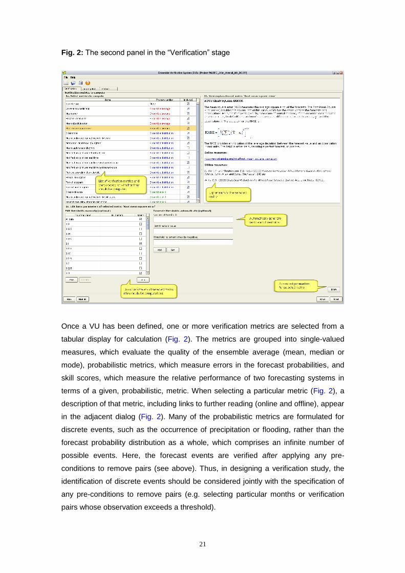
Fig. 2: The second panel in the “Verification” stage
Once a VU has been defined, one or more verification metrics are selected from a
tabular display for calculation (Fig. 2). The metrics are grouped into single-valued
measures, which evaluate the quality of the ensemble average (mean, median or
mode), probabilistic metrics, which measure errors in the forecast probabilities, and
skill scores, which measure the relative performance of two forecasting systems in
terms of a given, probabilistic, metric. When selecting a particular metric (Fig. 2), a
description of that metric, including links to further reading (online and offline), appear
in the adjacent dialog (Fig. 2). Many of the probabilistic metrics are formulated for
discrete events, such as the occurrence of precipitation or flooding, rather than the
forecast probability distribution as a whole, which comprises an infinite number of
possible events. Here, the forecast events are verified after applying any pre-
conditions to remove pairs (see above). Thus, in designing a verification study, the
identification of discrete events should be considered jointly with the specification of
any pre-conditions to remove pairs (e.g. selecting particular months or verification
pairs whose observation exceeds a threshold).

22
The metrics may be computed for several discrete events (conditions), for which the
event thresholds and associated logical conditions must be defined (e.g. <, >). The
event thresholds may be given in real units, such as flow in m3 s-1, or in climatological
probabilities. Real units are useful when an event threshold is physically meaningful,
such as the exceedence of a flood threshold. Climatological probabilities are useful
when the aim is to verify the forecasts at relative thresholds (e.g. “large” flows) or
when the verification results will be averaged across several locations with different
observed or forecast climatologies. However, the climatological probabilities are
computed from a limited sample of observations or forecasts and are, therefore,
subject to sampling uncertainty. For convenience, the option to verify against
thresholds is also provided for the deterministic metrics and for those probabilistic
metrics that do not require discrete events. While these metrics depend continuously
on the data, they may be computed for subsets of the overall dataset (selected by
thresholds) in order to evaluate the ensemble forecast quality in a conditional sense.
The thresholds may be input manually or generated semi-automatically using a
combination of: 1) the number of thresholds; 2) the first threshold; and 3) a constant
increment between thresholds, which may be positive (increasing from the first
threshold) or negative (decreasing). Optionally, the thresholds identified for one
metric can be applied to all other metrics for the selected VU (the “Do all” button in
Fig. 2). The thresholds may be identified as “main” thresholds or “auxiliary”
thresholds. Currently, this distinction affects plotting only; the verification results for
“main” thresholds are plotted within the EVS and the results for both “main” and
“auxiliary” thresholds are written to file, allowing more complex plots to be generated
outside of the EVS (e.g. plots of verification scores as a “continuous” function of
threshold value).
Depending on the chosen verification metric, other parameters may be modified (see
Section 5.3 also). For example, the reliability of the forecast probabilities may be
computed by grouping the forecast probabilities into smaller bins (with finer
resolution, but fewer samples per bin) or larger bins (coarser resolution, but more
samples per bin).
On executing a VU for the first time, the forecasts and observations are paired
together by forecast valid time and lead time. Verification is conducted separately for
each forecast lead time, as forecasting errors depend strongly on lead time. The
paired data are then written to file (Section 4.5), both to enable quality control and to
improve the speed of execution when modifying and re-running VUs. Since all of the
23
outputs from the EVS are based on the paired data, they should be checked to
ensure that the forecasts and observations were read and interpreted correctly (e.g.
that the time systems were correctly specified).
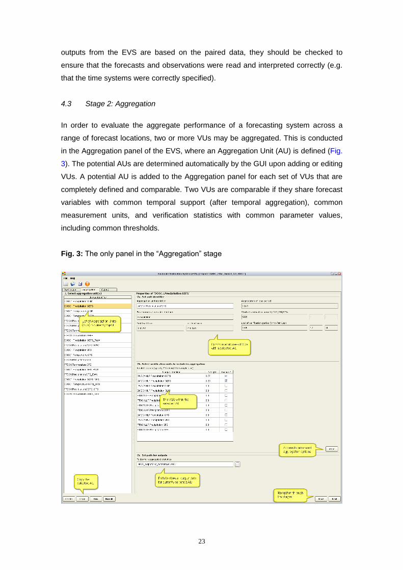
4.3 Stage 2: Aggregation
In order to evaluate the aggregate performance of a forecasting system across a
range of forecast locations, two or more VUs may be aggregated. This is conducted
in the Aggregation panel of the EVS, where an Aggregation Unit (AU) is defined (Fig.
3). The potential AUs are determined automatically by the GUI upon adding or editing
VUs. A potential AU is added to the Aggregation panel for each set of VUs that are
completely defined and comparable. Two VUs are comparable if they share forecast
variables with common temporal support (after temporal aggregation), common
measurement units, and verification statistics with common parameter values,
including common thresholds.
Fig. 3: The only panel in the “Aggregation” stage

24
By default, the verification results for an AU comprise a weighted average of the
verification results from the component VUs. Optionally (under the advanced options
accessed via the “More” button in Fig. 3), the verification metrics may be derived by
pooled the pairs from several locations, rather than averaging the verification results
(this is rarely feasible for large datasets). Once a potential AU has been determined
in the GUI, four attributes are user-defined (Fig. 3): 1) a unique identifier for the AU;
2) the component VUs, which are selected from a list of candidates; 3) the weight
associated with each VU in the aggregation (which is ignored when pooling pairs);
and 4) the output folder for the aggregated statistics. On executing an AU, the
verification metrics from the component VUs are collated and their weighted
averages determined. For verification metrics that comprise binned statistics (e.g. the
reliability diagram; see below), the sample means are computed for each bin in turn.
For verification statistics that are conditional upon one or more event thresholds, the
statistics are averaged across the same thresholds at each location. In order to have
a meaningful spatial aggregation, the threshold must have a consistent physical
interpretation in space and time, such as the exceedence of a local flood threshold
rather than a fixed river stage. The weights assigned to each VU must be within [0,1]
and the sum of all weights must be equal to 1. By default, equal weights are assigned
to each VU, but unequal weights may be input manually or the character ‘S’ specified
to weigh by the relative sample size at the first forecast lead time (maintaining
constant weights across lead times).
4.4 Stage 3: Output
The Output panel of the EVS stores the verification results for each of the VUs and
AUs in the current project. The results are organized by the unique identifier of the
VU or AU, the name of the verification metric, and by forecast lead time (Fig. 4). The
VUs and AUs available for plotting are shown in the top left table and are colored
blue and red, respectively (Fig. 4). On selecting a particular VU or AU, a list of
metrics with available results appears in the right-hand table. On selecting a
particular metric, the bottom left table displays a list of lead times (in hours) for which
the metric results are available. The basic options for plotting and writing metrics are
shown in the bottom-right dialog. Options are provided on the tables for rapidly
selecting particular combinations of metric and lead time. The options are provided in
context menus, which are displayed by right-clicking on one of the tables. For
example, by right-clicking on the table of metrics (top right in Fig. 4), an option
appears for selecting all metrics and lead times. The metrics can be plotted in an

25
internal graphing tool, which includes basic functionality for animating metrics across
a sequence of lead times, or written to file in a variety of graphical formats (Section
4.4). Also, the underlying statistics can be written to file in an XML format and viewed
in a text editor or web browser.
Fig. 4: The only panel in the “Output” stage
4.5 Data formats supported by the EVS
The data formats supported by the EVS are summarized in Table 1. Further details
can be found in Appendix A2. They are separated into: 1) input data, comprising the
ensemble forecasts and verifying observations for each VU; 2) paired data,
comprising the paired forecasts and observations for a specific VU; 3) output data,
comprising the verification statistics for a particular VU or AU in a graphical or
numerical format; and 4) a project file, containing the parameter values of one or
more VUs and AUs.

26
As indicated above, a VU is defined for each forecast variable and location. The input
data for a single VU comprises the ensemble predictions and observations. In both
cases, the inputs may be provided in a single file, a collection of files, by prescribing
a directory that contains one or more files, or by connecting to a data service whose
outputs are generated in a supported file format (see Appendix A3).
Table 1: main file formats supported by the EVS
Data store Format Extension Description
Project data XML evs VUs and AUs and their parameters
Paired data XML xml Paired forecasts and observations
Input data
ASCII fcst Ensemble forecasts in ASCII
ASCII obs Observations in ASCII
XML xml Ensemble forecasts in PI-XML
XML xml Observations in PI-XML
XML fi/bin Ensemble forecasts in binary Fast Infoset XML
XML fi/bin Observations in binary Fast Infoset XML
TAR/GZIP tar.gz or tgz Tarred and Gzipped ASCII or PI-XML forecasts
NetCDF nc Ensemble forecasts in NetCDF [experimental]
NetCDF nc Observations in NetCDF [experimental]
Graphical output
JPEG jpg Plots of verification metrics in raster format
PNG png Plots of verification metrics in raster format
SVG svg Plots of verification metrics in vector format
Numerical output XML xml Numerical output of verification metrics
The forecasts and observations can be provided in XML or ASCII formats and the
ASCII and PI-XML forecast files can be provided separately or inside a tarred and
gzipped archive. Reading of NetCDF time-series files is supported experimentally, for
which some information can be found here:
https://publicwiki.deltares.nl/display/NETCDF/Time+series
Various internal formats are used by the NWS for storing and exchanging ensemble
forecasts and observations. These can also be read by the EVS, but are not
described here. The ASCII format for storing the ensemble forecasts comprises one
forecast per line (Fig. 5 shows sixteen forecasts). Each forecast requires the forecast

27
valid date and time, the forecast lead time, and the forecast ensemble members in
trace-order (this is important to preserve any temporal statistical dependencies when
aggregating forecasts in time). The default format for dates and times is MM/dd/yyyy
HH, but other formats can be defined manually (see Section 5.2). The forecast lead
times are always given in hours. Adjacent entries are separated by whitespace or a
comma. The ASCII format for storing the single-valued observations also comprises
one instance per line, and includes the date and time of the observation, together
with the observed value (Fig. 6). Again, adjacent entries can be separated by
whitespace or a comma. The XML format for storing the observed and forecast data
(as opposed to paired data: see below) follows the Published-Interface (PI-) XML
format used in the Flood Early Warning System (FEWS). The XML format is
described in detail here:
http://public.deltares.nl/display/FEWSDOC/The+Delft-Fews+Published+interface+(PI)
Several NWS formats are also supported by the EVS, including the “NWS Card
format” and the “NWS CS binary” format. The NWS Card format is described here:
http://www.nws.noaa.gov/ohd/hrl/nwsrfs/users_manual/part7/_pdf/72datacard.pdf
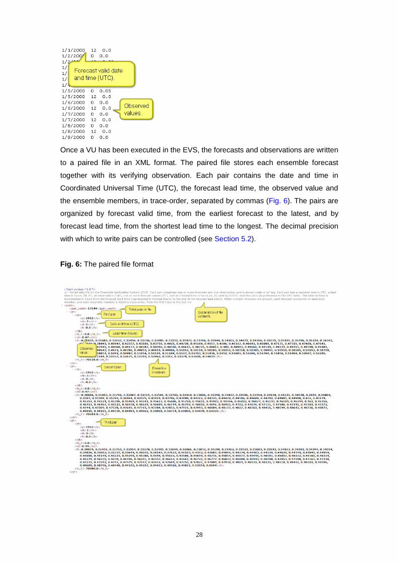
Fig. 5: The ASCII format for ensemble forecasts (upper) and observations (lower)
28
Once a VU has been executed in the EVS, the forecasts and observations are written
to a paired file in an XML format. The paired file stores each ensemble forecast
together with its verifying observation. Each pair contains the date and time in
Coordinated Universal Time (UTC), the forecast lead time, the observed value and
the ensemble members, in trace-order, separated by commas (Fig. 6). The pairs are
organized by forecast valid time, from the earliest forecast to the latest, and by
forecast lead time, from the shortest lead time to the longest. The decimal precision
with which to write pairs can be controlled (see Section 5.2).
Fig. 6: The paired file format

29
The output files from the EVS comprise the verification statistics for a specific VU or
AU in one of several graphical formats, and corresponding numerical results in an
XML format (see Appendix A2). The supported graphical formats include two raster
formats: the Portable Network Graphic (PNG) format (a lossless format) and the Joint
Photographic Experts Group (JPEG) format (a lossy format). The Scalable Vector
Graphics (SVG) format is also supported by the EVS, as this allows for verification
plots to be rescaled without loss of quality. Scripts are also available to import and
plot the numerical results in R (R Development Core Team, 2008), where many more
output formats and plotting options are available. Example scripts are provided in the
nonsrc\rscripts folder of the installation.
Finally, the parameters of each VU and AU are saved in a project file in an XML
format. The project files are ordinarily written by the EVS, but may be produced or
edited outside of the EVS (e.g. with a script, to enable batch processing). The XML is
organized by VU and AU, with entries for each input required in the GUI (Fig. 7).
Fig. 7: The project file format

30
4.6 Command line options
Alongside the Java command line options (e.g. for allocating memory), the EVS
provides several command line options for running an existing project file, together
with utilities for converting between input data formats, which are summarized in
Table 2.
Table 2: command line options in the EVS
Option Example Description
-p -p in.xml out.asc Converts a paired file, in.xml, to ASCII, out.asc
-aggOnly -aggOnly Executes the aggregation units only
-g -g Suppress the writing of graphics
-n -n Suppress the writing of numerics
-gui -gui Project_1.evs Open Project_1.evs in the EVS GUI.
-fcardtoasc -fcardtoasc in.fsct out.fcst Convert an NWS Card forecast file, in.fsct, to ASCII, out.fcst
-ocard2asc -ocardtoasc in.obs out.obs Convert an NWS Card observed file, in.obs, to ASCII, out.obs
-bin2asc -obintoasc in.CS out.fcst Convert an NWS CS binary forecast file, in.CS, to ASCII, out.fcst
-xslt -xslt input.xml style.xml output Convert input.xml to output (e.g. text) using the XSLT stylesheet, style.xml
4.7 Changing the format of the XML outputs from the EVS
The EVS outputs are strongly layered, and comprise results by forecast lead time
and threshold, as well as for score decompositions and other secondary elements
(e.g. the sharpness plot in a reliability diagram). In order to read the EVS outputs into
a secondary application, it may be necessary to change the data format. The
Extensible Stylesheet Language Transformation (XSLT) applies a transform to an
XML document, allowing the data to be filtered, manipulated or transformed into
another format, such as ASCII CSV or html. The transform is specified in a
stylesheet. A description can be found here:
http://en.wikipedia.org/wiki/XSLT

31
The ability to manipulate or transform the XML outputs from the EVS into another
format is implemented on the command line as follows:
java –jar EVS.jar –xslt input.xml style.xml output
where:
xslt is the command to perform the transform;
input.xml is the input xml file containing the EVS xml output data;
style.xml is the XSLT style sheet in which the transform is specified; and
output is the output location, such as a text file [an empty argument will print to
standard out].
As indicated above, the transform is specified in the XSLT stylesheet, style.xml. This
can be modified to extract any information required from the EVS output files and
then re-directed to any output stream as necessary. An example of an XSLT
transformation is provided in Appendix A2.
4.8 Creating custom plots of the EVS outputs in R
The numerical outputs from the EVS can be read into the R environment for
statistical computing (www.R-project.org). A utilities script is provided in the
/nonsrc/rscripts folder at the root of the installation. There are three methods
for reading the different EVS outputs, namely readEVSScores, which reads the
deterministic measures (e.g. mean error of the ensemble mean) and probabilistic
verification scores (e.g. Brier score), readEVSDiagrams, which reads the
verification diagrams (e.g. reliability diagram) and readEVSBoxPlots, which reads
the EVS box plots. In addition to the utilities script, example scripts are provided in
/nonsrc/rscripts/example_scripts for plotting specific (sets of) EVS metrics
in R, including the plotting of sampling uncertainties (via confidence intervals).

32
5. A DETAILED GUIDE TO THE OPTIONS IN EACH WINDOW OF THE GUI
This section provides a guide to the options available in each window of the GUI.
5.1 Administrative functions in the main window
The opening window of the GUI, together with the Taskbar, is shown in Fig. 1. The
opening window displays the Verification Units loaded into the software. The Taskbar
is visible throughout the operation of the GUI and is used for administrative tasks,
such as creating, opening, closing and saving a project. The Taskbar options are
explained in Table 3. Shortcuts are provided on the Taskbar for some common
operations, but all operations are otherwise accessible through the dropdown lists.
Table 3: Menu items
Menu Function Use
File
New project… Creates a new project
Open project… Opens a project file (*.evs)
Close project Closes a project
Save project Updates or creates a project file (*.evs)
Save project as… Updates or creates a named project file (*.evs)
Exit Exits EVS
Help
Messages on/off Displays/hides tool tips
Console Shows the details of errors thrown
About Credits
All work within the EVS can be saved to a project file with the .evs extension. A new
project is created with the New project… option under the File dialog. An existing
project is saved using the Save or Save As… options. These options are also
available on the Taskbar. Project files are stored in an XML format and may be
opened in a web browser or text editor. An example is given in Fig. 7.
5.2 The first window in the Verification stage
The first stage of an ensemble verification study requires one or more Verification
Units (VUs) to be defined (Fig. 1). In this context, a VU comprises a time-series of a
single variable at one location. The spatial scale or support of the variable is not
identified in the EVS, but is assumed to be consistent for the observed and forecast

33
data. For example, observations from a rain gauge should not, in general, be
compared with precipitation forecasts averaged over a large grid cell. The actual
spatial support may be arbitrarily small or large, but should be equivalent for the
forecasts and observations. A VU is uniquely identified by a location ID, a variable ID
and, optionally, an additional ID. These IDs must be entered in the first window, and
are then displayed in the table and identifiers panel. A new VU may be added to the
current project by clicking “Add” in the bottom left corner of the window (Fig. 1). This
adds a VU with some default values for the identifiers. On entering multiple VUs, the
basic properties of the selected VU (i.e. the item highlighted in the table) will be
shown in the panels on the right. Existing units may be deleted or copied by selecting
an existing unit in the table and clicking “Delete” or “Copy”, respectively. On copying
a unit, all of the properties of the unit are copied except the identifiers, which must be
unique. This provides a convenient way to specify multiple units with the same
verification properties (multiple segments to be verified for the same variable with the
same temporal parameters).
The VU is defined by four different dialogs: identifiers (2a), input data (2b), time
parameters (2c), and output data (2d).
2a. Set unit identifiers:
Location identifier: an identifier denoting the location of the forecast point;
Environmental variable identifier: an identifier denoting the environmental
variable to be verified; and
Additional identifier: arbitrary additional ID. For example, this may be used to
distinguish between forecasts from different models for a common variable and
location.
The names of the location and environmental variable are unrestricted (aside from a
blank name or a name containing the character ‘.’, which is used to separate the
identifiers). Several default names for environmental variables are provided by right-
clicking on the variable identifier box (Fig. 1).
2b. Identify input data sources:
- Forecast data source: path to the folder, files, or data service that contains the
ensemble predictions (for connections to data services, see Appendix A3).

34
When the ensemble forecasts are distributed across multiple files, selecting
only those files that contain relevant forecasts will confer some efficiency, as all
files must be processed before being checked against verification conditions
(e.g. if the files are separated by date, and a limited set of dates is
subsequently defined);
- Observed data source: path to the folder, files, or data service that contains the
verifying observations (for connections to data services, see Appendix A3);
- Forecast data type: the data format for the forecasts;
- Observed data type: the data format for the observations; and
- Forecast time zone: the time zone for the forecasts. The time zone is required
for pairing (on the basis of date and time);
- Observed time zone: as above, for the observations.
The paths to the observed and forecast data may be absolute or relative to the
location of the EVS.jar. For example, a relative path beginning ../ would denote the
folder one level above the EVS.jar. Absolute paths may be entered manually or by
clicking on the adjacent button, which opens a file dialog. Relative paths must be
entered manually.
When conducting verification for the first time, the observations and forecasts are
paired. These pairs are used to compute the differences between the observed and
forecast values (i.e. the forecast ‘errors’) at concurrent times, i.e. the valid times. For
subsequent work with the same VU, no pairing is necessary unless some of the input
parameters that affect the pairs have changed (at which point, the pairs are deleted).
The paired data are stored in an XML format, which may be opened in a web
browser or text editor. Each forecast-observation pair is stored with a date in UTC
(year, month, day, and hour of day), the forecast lead time in hours, the observed
value, and the corresponding forecast ensemble members. A detailed explanation is
also provided in the paired file header. An example of a paired file is given in Fig. 6.
The EVS generates two paired files, for which writing is optional, namely the “raw”
pairs and the “conditional” pairs.
The raw pairs comprise the paired forecasts and observations after any required
change of support but before any changes in measurement units, temporal
aggregation (of the pairs), or any other conditioning. The raw pairs are written to a file
ending with _pairs_raw.xml. The values should match those contained in the
original observed and forecast files (after any change of support). The conditional
35
pairs comprise the paired forecasts and observations from which the verification
metrics will be computed. The conditional pairs are written to a file ending with
_pairs_cond.xml. By default, both the raw and conditional pairs are written to file.
The paired files may be written in uncompressed ASCII or gzipped ASCII format.
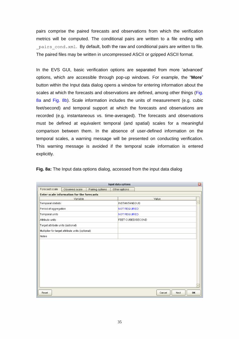
In the EVS GUI, basic verification options are separated from more ‘advanced’
options, which are accessible through pop-up windows. For example, the “More”
button within the Input data dialog opens a window for entering information about the
scales at which the forecasts and observations are defined, among other things (Fig.
8a and Fig. 8b). Scale information includes the units of measurement (e.g. cubic
feet/second) and temporal support at which the forecasts and observations are
recorded (e.g. instantaneous vs. time-averaged). The forecasts and observations
must be defined at equivalent temporal (and spatial) scales for a meaningful
comparison between them. In the absence of user-defined information on the
temporal scales, a warning message will be presented on conducting verification.
This warning message is avoided if the temporal scale information is entered
explicitly.
Fig. 8a: The Input data options dialog, accessed from the input data dialog

36
Fig. 8b: Pairing options, accessed from the Input data options dialog
Fig. 8c: Other options, accessed from the Input data options dialog
37
In most cases, changes of scale should be conducted before using the EVS, but
some options are provided internally. In particular, the measurement or “attribute”
units of the forecasts or observations may be changed with some restrictions:
- Changes in attribute units are achieved by either: 1) specifying a named
change from the current “Attribute units” to the “Target attribute
units” (Fig. 8a); or 2) specifying a factor by which to multiply the current
“Attribute units”, in order to arrive at the “Target attribute units”,
namely the “Multiplier for target attribute units”. Named
changes of units (without manually defining a multiplier) are currently limited to:
DEGREES (CELCIUS) <--> DEGREES (FAHRENHEIT);
MILLIMETRE <--> INCH
METRE <--> FEET
METRE CUBED/SECOND <--> FEET CUBED/SECOND
In addition to changes in attribute units, there is some flexibility for verifying forecasts
and observations with different temporal support when the verification is desired at
an aggregated level of support (see the discussion below on temporal aggregation,
and Fig. 9c). This is only possible under the following conditions:
1. The temporal support is INSTANTANEOUS, and the desired temporal
aggregation involves a supported function (e.g. mean) over a period that is
exactly divisible by the frequency of the data; and
2. The temporal support is the TOTAL over a specified period and the desired
level of aggregation is a total over a longer period that is an exact multiple of
the shorter period and the frequency of the data (e.g. verifying at a daily
timestep when the observations are six-hourly totals, available every six hours).
Further control on the pairing of forecasts and observations is provided in the “Pairing
options” tab of the Input data options dialog (Fig. 8b). The options comprise:
Skip output for ensemble members that match the no-data value: omit
ensemble members from the paired file that are missing (default is TRUE);
Output raw pairs in aggregated resolution (when aggregating pairs): in order to
circumvent the large amount of RAM memory required for locations where the

38
forecasts are much more resolved (e.g. hourly) than the temporal resolution
required for verification (e.g. daily), this option allows for the paired data to be
computed and stored in their aggregate (e.g. daily) resolution only. In this case,
the forecast files are processed and aggregated individually (this is only
beneficial when storing the data across multiple files), avoiding the need to
read and store all forecasts at their native resolution. When using this option,
any attempt to recompute verification results at a higher resolution than the
resolution available in the aggregated pairs will result in the pairs being deleted
and re-computed (possibly resulting in an out-of-memory error, unless sufficient
memory is allocated to the reading of the observed and forecast data at their
native resolution). By default the pairs are stored in their native resolution
(FALSE);
Number of decimal places for writing pairs: the number of decimal places for
writing pairs (default is 5);
Start time for aggregation of observations [hours, UTC]: if the observations
comprise a finer scale or support than the forecasts, they must be aggregated
prior to pairing. This parameter controls the start time in UTC at which to begin
aggregating the observations (no default).
Start time for aggregation of forecasts [hours, UTC]: if the forecasts comprise a
finer scale or support than the observations, they must be aggregated prior to
pairing. This parameter controls the start time in UTC at which to begin
aggregating the forecasts (no default).
First lead time for aggregation of forecasts [hours]: if the forecasts comprise a
finer scale or support than the forecasts, they must be aggregated prior to
pairing. This parameter controls the first lead time at which to begin
aggregating the forecasts (no default).
Use only pairs that also appear in verification unit: when comparing forecasts
from two different systems, restrict the calculation of verification metrics to only
those pairs that appear in the selected VU. This amounts to jointly pairing with
another VU (no default).
The “Other options” tab of the Input data options dialog (Fig. 8c) contains further
options for interpreting the input data, namely:
Global no-data value: the global identifier for ‘null’ or missing values (i.e. values
ignored throughout a verification study including metric calculation. The global

39
no-data value is used to discriminate between valid and missing data internally
and in the EVS outputs (e.g. verification pairs). For those input data sources
that explicitly define the missing value, the global no data value replaces the
original missing values. For those input data sources that do not explicitly
define the missing value, any values that match the global no data value are
interpreted as missing. By default, the no data value is -999.0 and only numeric
missing values are accepted. Input data sources with a missing value are
replaced with the global no data value, which cannot be NaN;
Use all observations (not just paired) to determine climate thresholds: when
conducting verification for thresholds whose values represent climatological
probabilities, those climatological probabilities may be determined from the
paired observations (FALSE) or all observations in the specified observed data
source (TRUE). The default is FALSE, i.e. to use the paired observations only;
Apply date conditions when determining climate thresholds: when conducting
verification for thresholds whose values represent climatological probabilities,
those probabilities (and corresponding real values) may be determined prior to
applying any pre-conditions on the dates (FALSE) or afterwards (TRUE). Such
preconditions may include the elimination of particular calendar months (see
2c. Set time parameters, below);
Apply value conditions when determining climate thresholds: when conducting
verification for thresholds whose values represent climatological probabilities,
those probabilities (and corresponding real values) may be determined prior to
applying any pre-conditions on the values (FALSE) or afterwards (TRUE). Such
preconditions may include the elimination of values that exceed a particular
threshold (see 2c. Set time parameters, below);
Date format used in ASCII forecast/observed data files: the date formats used
for observations and forecasts in ASCII format (ignored for other file types).
The dates are formed from the case-sensitive elements, yyyy (year), MM
(calendar month), dd (day of month), HH (hour of day in the 24-hour clock), mm
(minute of hour) and ss (second of minute) using appropriate, single-character,
separators or whitespace (e.g. MM/dd/yyyy HH) or no separators (e.g.
yyyyMMddHH). The default date format is MM/dd/yyyy HH;
Forecast/observed data location ID: when reading XML and NetCDF files that
contain specific location identifiers, the required location identifier may be
defined explicitly or resolved to the VU location identifier (i.e. left blank, the
default); and

40
Forecast/observed data variable ID: when reading XML and NetCDF files that
contain specific variable identifiers, the required variable identifier may be
defined explicitly or resolved to the VU environmental variable identifier (i.e. left
blank, the default).
Forecast data ensemble ID: for those data sources that use an ensemble ID to
discriminate between time-series (e.g. XML), the ensemble ID may be defined
here. This is only required when the input data source contains more than one
time-series with a given location ID and variable ID.
Forecast data filter: when reading forecast files from a folder that contains
multiple file types (e.g. including subdirectories), specify a string pattern (e.g.
.xml) to read only those files that match the pattern (no filter by default).
Forecast archive filter: when reading forecast files from an archive that contains
multiple file types (e.g. .tar.gz), specify a string pattern (e.g. .xml) to read only
those files that match the pattern (no filter by default).
Threshold for inadmissible data (in attribute units of verification); Logical
condition associated with threshold for inadmissible data; and Value assigned
to inadmissible data (in attribute units of verification): specify a constraint on
admissible values of the forecasts and observations. The constraint is defined
with a threshold and associated logical condition. When the constraint is met,
the inadmissible values are replaced with the specified value. When a change
in measurement units is requested, the detection limit is defined in the target
measurement units of the forecasts and observations (i.e. in the units of the
conditional paired data).
Ignore time zone in forecast/observed data source (use EVS entry instead):
when reading data formats that contain a time zone, ignore this time zone and
use the explicit entry in the EVS instead (see 2b. Set input data sources). This
is necessary when applying a false time zone to the forecasts and/or
observations (e.g. to support pairing without interpolation/rescaling).
Eliminate ensemble member whose index matches the forecast valid year: use
this option to remove an ensemble member whose index (historical year)
matches the forecast valid year. This may be necessary when verifying
climatological ensemble forecasts, such as forecasts produced through
Ensemble Streamflow Prediction (ESP). When producing retrospective ESP
forecasts, one ensemble member corresponds to the verifying observation.
Clearly, this must be removed prior to verification.

41
2c. Set time parameters for outputs:
Start of verification period: the start date for verification purposes. This may
occur before or after the period for which data are available. Missing periods
will be ignored. The verification period is defined in UTC hours from 00 UTC on
the input start date. The start date may be entered manually or via a calendar
utility accessed through the adjacent button. In sub-selecting forecasts, the
start of the verification period refers to the forecast valid date, not the forecast
issue date;
End of verification period: as above, but defines the last date to consider. The
end date is also defined as 00 UTC on the specified date (i.e. add one day if
the input date should be included in the verification window). In sub-selecting
forecasts, the end of the verification period refers to the forecast valid date, not
the forecast issue date;
First lead time: the first forecast lead time (in given units) for which verification
results will be computed;
Last lead time: the last forecast lead time (in given units) for which verification
results will be computed. Must be greater than the first lead time; and
Aggregation period: the time period over which to aggregate the verification
pairs. Aggregation removes short-range variability (“noise”) by averaging over a
period that matters for decision making purposes. For example, the verification
pairs may be aggregated into ninety-day averages (assuming that the forecast
time horizon is at least ninety days). When the temporal support of the
forecasts and observations is different, verification may still be possible at an
aggregated temporal support (see above). The aggregation period is applied to
the verification pairs after any change of temporal support (of the forecast and
observations) necessary to conduct pairing. For the same reason, changing the
aggregation period will not delete existing pairs.
The dialog for conditioning on date and variable value is shown in Fig. 9a and Fig.
9b, respectively. The conditions on dates or variable values entered in the verification
window apply to all verification metrics computed for that VU. Alongside these pre-
conditions, the individual metrics may be computed with respect to one or more
threshold values, such as flows exceeding flood stage (see below). When designing
a verification study, the pre-conditions used to sub-select pairs should be compatible
with any discrete events that might be verified later. For example, it would not make
sense to assess the quality of Probability of Precipitation (PoP) forecasts (using a
42
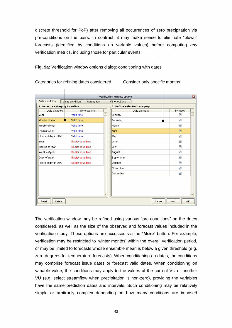
discrete threshold for PoP) after removing all occurrences of zero precipitation via
pre-conditions on the pairs. In contrast, it may make sense to eliminate “blown”
forecasts (identified by conditions on variable values) before computing any
verification metrics, including those for particular events.
Fig. 9a: Verification window options dialog: conditioning with dates
Categories for refining dates considered Consider only specific months
The verification window may be refined using various “pre-conditions” on the dates
considered, as well as the size of the observed and forecast values included in the
verification study. These options are accessed via the “More” button. For example,
verification may be restricted to ‘winter months’ within the overall verification period,
or may be limited to forecasts whose ensemble mean is below a given threshold (e.g.
zero degrees for temperature forecasts). When conditioning on dates, the conditions
may comprise forecast issue dates or forecast valid dates. When conditioning on
variable value, the conditions may apply to the values of the current VU or another
VU (e.g. select streamflow when precipitation is non-zero), providing the variables
have the same prediction dates and intervals. Such conditioning may be relatively
simple or arbitrarily complex depending on how many conditions are imposed

43
simultaneously. However, there is a trade-off between the specificity of a verification
study, which is increased by conditioning, and the number of samples available to
compute the verification statistics, which is reduced by conditioning (i.e. sampling
uncertainty is increased).
Fig. 9b: Verification window options dialog: conditioning with variable value
Variables available for conditioning Forecast ensemble mean > 0
Additional options for temporal aggregation are provided in the “Aggregation” section
of the Verification window options dialog (Fig. 9c). These include:
Temporal aggregation function: this allows for a temporal aggregation function
to be defined. By default, aggregations requested in the main verification
window involve a mean average over the specified period. This may be
changed to a total (i.e. accumulation), minimum or maximum value, among
others;
Aggregation start hour UTC: the time of day in hours UTC [0,23] at which
temporal aggregation begins. By default, aggregation begins at the first

44
available verification pair (i.e. the start of the time-series of forecasts and
observations that cover a given forecast ensemble trace);
Aggregation start lead hour: the forecast lead time in hours at which to begin
temporal aggregation. By default, aggregation begins at the first available
forecast lead time;
Type of aggregation; Rolling aggregation frequency; and Units of aggregation
frequency: by default, temporal aggregation is conducted without overlapping
periods (BACK-TO-BACK). Optionally, however, a ROLLING aggregation may
be performed with a given frequency and associated temporal units. For
example, parameter values of ROLLING, 1 and DAY would conduct a rolling
aggregation with the specified aggregation period (defined in 2c. Set time
parameters) at an interval of 1 day between aggregations.
Fig. 9c: Verification window options dialog: aggregation options
The “Other options” section of the Verification window options dialog (Fig. 9d)
comprises the following options:
Minimum sample fraction: this allows for the specification of a minimum sample
size per forecast lead time for computing verification results. The sample size
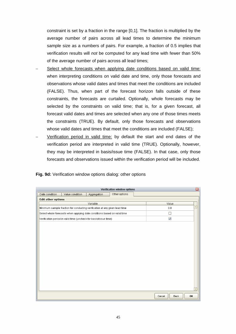
45
constraint is set by a fraction in the range [0,1]. The fraction is multiplied by the
average number of pairs across all lead times to determine the minimum
sample size as a numbers of pairs. For example, a fraction of 0.5 implies that
verification results will not be computed for any lead time with fewer than 50%
of the average number of pairs across all lead times;
Select whole forecasts when applying date conditions based on valid time:
when interpreting conditions on valid date and time, only those forecasts and
observations whose valid dates and times that meet the conditions are included
(FALSE). Thus, when part of the forecast horizon falls outside of these
constraints, the forecasts are curtailed. Optionally, whole forecasts may be
selected by the constraints on valid time; that is, for a given forecast, all
forecast valid dates and times are selected when any one of those times meets
the constraints (TRUE). By default, only those forecasts and observations
whose valid dates and times that meet the conditions are included (FALSE);
Verification period in valid time: by default the start and end dates of the
verification period are interpreted in valid time (TRUE). Optionally, however,
they may be interpreted in basis/issue time (FALSE). In that case, only those
forecasts and observations issued within the verification period will be included.
Fig. 9d: Verification window options dialog: other options

46
2d. Set path for outputs:
Folder for output statistics: path to the folder for writing the paired files and the
verification output data generated by the system, if written output is requested
(see below).
A “More” button, which opens an advanced options dialog with options to:
Write conditional pairs: write the conditional pairs (TRUE, by default).
Write unconditional pairs: write the unconditional pairs (TRUE, by default).
Write pairs in compressed (gzip) format: gzip all written pairs (FALSE, by
default).
5.3 The second window in the Verification stage
The second window in the Verification stage is shown in Fig. 2 and is accessed by
clicking “Next” from the first window (Fig. 1). The second window shows the
verification metrics available for the VU selected in the first window.
The EVS includes single-valued measures, which can be used to verify the ensemble
average forecast (mean, median or mode), and statistics that measure the quality of
the forecast probabilities. While single-valued measures cannot verify the forecast
probabilities, they are useful for evaluating the “best estimate” from the ensemble
forecast. Currently, the single-valued measures available in the EVS include the
mean error, the RMSE, the mean absolute error, the relative mean error, and the
coefficient of correlation between the ensemble average forecast and observed
values. Table 4 lists the metrics available in the EVS, which contain varying levels of
detail about forecast quality. Some of the ensemble verification metrics verify discrete
events, such as the (non-)exceedence of a particular threshold (e.g. flood stage),
whereas other metrics evaluate the forecasting errors across all possible thresholds.
Further information about the metrics available in the EVS can be found in Section 6
and Appendix A1. Examples of their interpretation can be found in Section 7.
Table 4: summary of the verification metrics available in the EVS
Metric name Quality attribute tested Discrete events? Detail
Sample size None N/A N/A
Correlation coefficient Ensemble average (deterministic) No Lowest

47
Mean error Ensemble average (deterministic) No Lowest
Relative mean error Ensemble average (deterministic) No Lowest
Mean absolute error Ensemble average (deterministic) No Lowest
RMSE Ensemble average (deterministic) No Lowest
Brier Score Lumped error score Yes Low
Brier Skill Score Lumped error score vs. reference Yes Low
Mean CRPS Lumped error score No Low
Mean CRPSS Lumped error score vs. reference No Low
ROC score Lumped discrimination score Yes Low
Mean error of prob. diag. Reliability (unconditional bias) No Low
Mean capture rate diag. Probability of real-valued error No High
Rank histogram Reliability (conditional bias) No High
Spread-bias diagram Reliability (conditional bias) No High
Reliability diagram Reliability (conditional bias) Yes High
ROC diagram Discrimination Yes High
Modified box plots Error visualization No Highest
On selecting a given metric in the table, information about that metric is provided in
the top right dialog, and the parameters of the metric are displayed for
entering/editing in the bottom-left panel. A metric is included, and its parameter
values are enabled for editing, by checking the box adjacent to the metric in the top
left table. The parameters of each metric are listed in Table 5. After modifying the
verification statistics and their parameters, the new information is saved to the
current unit by clicking “Save”.
Table 5: Parameters for each verification metric
Metric Parameter (and type) Meaning
Mean Error
Thresholds (basic)
Produces the metric for each subset of data specified by the threshold. The thresholds may be defined in real units or in probabilities. By default, they refer to non-exceedence probabilities from the observed climatology.
Use unconditional pairs for this metric (advanced)
Any pre-conditions based on dates or variable values used to subset the pairs will be ignored for this metric. Instead, the metric will be computed for each prescribed threshold using the unconditional pairs.

48
Method for computing ensemble average (advanced)
Select the desired average of the ensemble member values to verify. Options include the ensemble mean, median and mode. By default, the ensemble mean is used.
Threshold type (advanced)
Numerical thresholds may comprise non-exceedence probabilities or real values (in the units of the verification pairs, such as cubic feet per second). Probability thresholds are used to derive real values from a corresponding climatological distribution. For example, a threshold value of 0.2 would select pairs using the real value corresponding to probability 0.2 in the climatological probability distribution. The precise form of the conditioning implied by the threshold will depend on the metric (e.g. the threshold defines a discrete event for discrete metrics) and the logical condition associated with the threshold. When using climatological probabilities, the climatological distribution may be derived from the historical (paired) observations or forecasts. When deriving a climatological distribution from the ensemble forecasts, a function is required to generate a single forecast value from the collection of ensemble members (“Function to compute forecast threshold”; see below). In summary, there are four options for the threshold type: 1) Observed climatological probabilities; 2) Forecast climatological probabilities; 3) Observed values; and 4) Forecast values. The default threshold type comprises observed climatological probabilities.
Function to compute forecast threshold (advanced)
When computing verification metrics for a particular threshold, the threshold may comprise observed or forecast values (or probabilities). When the threshold refers to forecast values or probabilities, a function is required to derive a single-valued forecast from the collection of ensemble members. There is no default.
Logical condition for threshold (advanced)
Changes the logical condition for any thresholds used to subset data. For example, if the logical condition is “greater than”, only those forecast -observation pairs whose values are greater than the threshold (observed or forecast values, depending on the threshold type) will be used.
Lower bound on thresholds (real value) (advanced)
Specify a lower bound on the thresholds for which verification metrics will be computed in units of the paired data (after applying any change of units).
Upper bound on thresholds (real value) (advanced)
Specify an upper bound on the thresholds for which verification metrics will be computed in units of the paired data (after applying any change of units).
Root Mean Square Error
Same as Mean Error Same as Mean Error
Relative mean error Same as Mean Error Same as Mean Error

49
Mean Absolute Error
Same as Mean Error Same as Mean Error
Correlation Coefficient
Same as Mean Error Same as Mean Error
Brier score
Same as Mean Error Same as Mean Error, without “Method for computing ensemble average”.
Select score decomposition (advanced)
The Brier Score may be decomposed into the calibration-refinement (CR) and/or the likelihood-base-rate (LBR) factors. In terms of the CR, the overall score comprises reliability - resolution + uncertainty. In terms of the LBR, it comprises Type-II conditional bias – discrimination + sharpness.
Brier Skill Score
Same as Brier Score Same as Brier Score.
Reference forecast for skill (advanced)
Allows a reference forecast to be selected for use in the skill calculation. The reference forecast must be loaded into the EVS as another VU. By default, the reference forecast is sample climatology.
Mean Continuous Ranked Probability Score
Same as Brier Score. Same as Brier Score.
Select score decomposition (advanced)
Allows for the calibration-refinement decomposition of the overall score into contributions due to (lack of) reliability, resolution and uncertainty (climatological variability). The overall score comprises reliability - resolution + uncertainty.
Mean Continuous Ranked Probability Skill Score
Same as Mean Continuous Ranked Probability Score
Same as Mean Continuous Ranked Probability Score.
Reference forecast for skill (advanced)
Same as parameter for Brier Skill Score.
Mean Error of Probability diagram
Same as Mean Error Same as Mean Error, without “Method for computing ensemble average”.
Number of points in diagram (advanced)
Sets the number of equally-spaced probability values (from 0-1) for which the metric will be computed and plotted.
Mean Capture Rate Diagram
Same as Mean Error of Probability diagram
Same as Mean Error of Probability diagram.
Modified box plot pooled by lead time
Use unconditional pairs for this metric (advanced)
Same as parameter for Mean Error.
Number of points in diagram (advanced)
Sets the number of equally-spaced probability values (from 0-1) at which the boxes will be computed and plotted. The middle thresholds form the boxes and outer thresholds form the whiskers.

50
Modified box plot per lead time by observed value
Same as Modified Box Plot Pooled By Lead Time
Same as Modified Box Plot Pooled By Lead Time.
Modified box plot per lead time by forecast value
Same as Modified Box Plot Pooled By Lead Time
Same as Modified Box Plot Pooled By Lead Time.
Method for computing ensemble average (advanced)
Same as parameter for Mean Error.
Relative Operating Characteristic
Same as Mean Error of Probability diagram
Same as Mean Error of Probability diagram.
Fit a smooth function to empirical ROC (advanced)
If this parameter is true (checked; not the default option), the binormal approximation will be used to model the bivariate distribution of the Probability of Detection (PoD) and Probability of False Detection (PoFD). The empirical pairs of PoD and PoFD are provided alongside the binormal model fit. If this parameter is false, only the empirical pairs of PoD and PoFD will be provided.
Relative Operating Characteristic Score
Same as Mean Error of Probability diagram
Same as Mean Error of Probability diagram.
Reference forecast for skill (advanced)
Same as parameter for Brier Skill Score.
Fit a smooth function to empirical ROC (advanced)
Same as parameter for Relative Operating Characteristic.
Method for computing AUC (advanced)
Sets the method for computing the Area Under the Curve (AUC). By default, the trapezoid rule is used to integrate the Relative Operating Characteristic curve based on the specified number of points. Optionally, the score may be computed using the algorithm from Mason and Graham (2000).
Reliability Diagram
Same as Mean Error of Probability diagram
Same as Mean Error of Probability diagram.
Use a constant sample count in each bin (advanced)
If this parameter is false (unchecked; the default option), the forecasts probability bins for which the reliability values are computed will take a fixed width in the range 0-1 depending on the number of points requested for the diagram (below). If this parameter is true (checked), the forecast probability bins for which the reliability values are computed will vary in width such that each bin captures the same number of forecasts.

51
Number of points in diagram (advanced)
Sets the number of probability bins (from 0-1) for which the metric will be computed and plotted. These bins may capture an equal sample count (see above) or may be equally spaced.
Rank histogram
Same as Mean Error of Probability diagram
Same as Mean Error of Probability diagram.
Use relative frequencies (uncheck for abs. sample counts) (advanced)
If this parameter is true (checked, the default), the rank histogram will show the fraction of observations that fall between each ensemble member, otherwise it will show the absolute number of observations.
Use cumulative frequencies (advanced)
If this parameter is false (unchecked, the default), the rank histogram will show the fraction or count of observations that fall between each ensemble member, otherwise it will show the cumulative fraction or count of observations that fall below each ensemble member.
Spread-Bias Diagram
Same as Mean Error of Probability diagram
Same as Mean Error of Probability diagram.
Center windows around forecast median (advanced).
If this parameter is false (unchecked; the default option), the probability of an observation falling within a forecast bin is determined for bins separated by probabilities within the forecast distribution. For example, if the parameter for the ‘Number of points in the diagram’ (see below) is 10, probabilities will be determined for bins representing deciles of the forecast. If this parameter is true (checked), probabilities of the observation falling within a forecast bin will be determined for symmetric forecast bins defined with respect to the forecast median.
Number of points in diagram (advanced).
Defines the number of forecast bins for which the probability of an observation falling within that bin is determined.
Most of the ensemble verification metrics compare the observed and forecast values
at specific thresholds. In some cases, these thresholds define a subset of data from
which the metric is calculated. Most of the metrics can be computed from all data, as
well as subsets of data defined by the thresholds. Other metrics verify only discrete
events within the continuous forecast distributions. For example, the reliability
diagram, relative operating characteristic and the Brier score, require one or more
thresholds to be defined, and cannot be computed from all data. For these metrics,
the thresholds represent cutoff values from which discrete events are computed. By
default, the thresholds refer to non-exceedence probabilities within the climatological
probability distribution and must, therefore, cover an interval of [0,1]. For example, a
threshold of 0.2 would refer to all pairs whose values (observed or forecast,
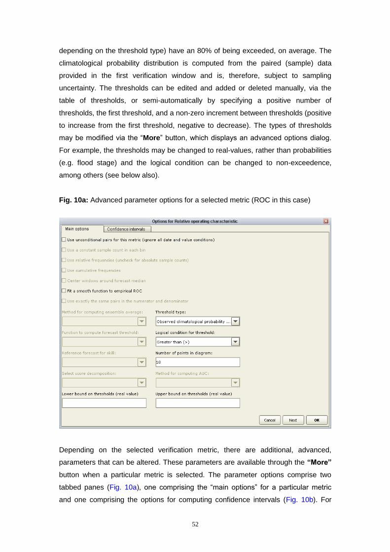
52
depending on the threshold type) have an 80% of being exceeded, on average. The
climatological probability distribution is computed from the paired (sample) data
provided in the first verification window and is, therefore, subject to sampling
uncertainty. The thresholds can be edited and added or deleted manually, via the
table of thresholds, or semi-automatically by specifying a positive number of
thresholds, the first threshold, and a non-zero increment between thresholds (positive
to increase from the first threshold, negative to decrease). The types of thresholds
may be modified via the “More” button, which displays an advanced options dialog.
For example, the thresholds may be changed to real-values, rather than probabilities
(e.g. flood stage) and the logical condition can be changed to non-exceedence,
among others (see below also).
Fig. 10a: Advanced parameter options for a selected metric (ROC in this case)
Depending on the selected verification metric, there are additional, advanced,
parameters that can be altered. These parameters are available through the “More”
button when a particular metric is selected. The parameter options comprise two
tabbed panes (Fig. 10a), one comprising the “main options” for a particular metric
and one comprising the options for computing confidence intervals (Fig. 10b). For

53
example, when computing ensemble metrics using thresholds, the thresholds may be
treated as non-exceedence (<, <=) or exceedence (>, >=) thresholds, which may be
useful for exploring low- versus high-flow conditions, respectively (Fig. 10a). The
parameter options for each metric are summarized in Table 3. A ‘basic’ parameter is
accessed through the main window in EVS, while an ‘advanced’ parameter is
accessed through the “More” button (as in Fig. 10a).
Fig. 10b: Confidence intervals for a selected metric (correlation in this case)
Confidence intervals can be computed for any of the verification metrics within the
EVS, except for the box plots. In future, knowledge of the sampling distributions of
particular verification metrics may be incorporated into the EVS. Currently, however,
confidence intervals are derived numerically using a common algorithm for all
metrics, namely the stationary block bootstrap (Fig. 10b). The parameters for deriving
the confidence intervals are:
Technique: select “none” (default) to omit confidence intervals from the
verification results and “Stationary block bootstrap” to use the stationary block
bootstrap (Politis and Romano, 1994);

54
Sample size: The number of bootstrap samples to use in computing the
confidence intervals. Each sample represents one bootstrap configuration of
the verification pairs and associated metric calculation. Using more samples
implies a better estimate of the confidence interval, but (potentially much)
greater computational time. Also, bootstrapping is a resampling procedure and
thus inherently constrained by the available verification pairs (sample
size/diversity). In general, somewhere between 1000 and 10000 bootstrap
samples may be appropriate (which implies between 1000 and 10000
computations of the chosen metric at all required thresholds);
Minimum sample size: the minimum number of samples required in order to
compute confidence intervals. If fewer than the required number of samples are
found, the intervals will be omitted. The sample size constraint applies to a
specific metric and (un)conditional sample. For example, when computing the
unconditional mean error (mean error for “All data”) at a particular forecast lead
time, the minimum sample size should exceed the total number of verification
pairs available (after applying any pre-conditions). When computing the
reliability diagram for a particular forecast lead time and threshold, the
confidence intervals will be computed for each forecast probability bin in which
the minimum sample size was exceeded. Thus, depending on the minimum
sample size and metric, confidence intervals may be displayed for none, some,
or all of the metric results at a given forecast lead time. Also, depending on the
bootstrap samples generated, the actual number of samples that meet the
minimum requirements (and hence the presence and appearance of the
confidence intervals) will vary each time the bootstrapping is repeated. In
general, a minimum sample size of 50 is reasonable;
Average block size: the stationary block bootstrap attempts to account for
temporal statistical dependence by randomly sampling contiguous ‘blocks’ of
verification pairs that may be assumed statistically independent given the
average block length. The blocks are sampled from a geometric probability
distribution, which is completely defined by its mean (the average block length).
The central time index of each block is sampled from a discrete uniform
distribution whereby each time in the paired sample is equally probable. A
single bootstrap sample comprises a resampled paired dataset with an equal
number of pairs to the original dataset. When computing confidence intervals
for several VUs, the component VUs may be assumed statistically dependent
or statistically independent (see Section 5.4);
Units for block size: the time units for the average block size; and

55
Interval specification: confidence intervals are computed from the bootstrap
sample of metric values. One or more intervals may be defined by their lower
and upper limits (e.g. [0.05,0.95]). Optionally, one interval can be selected for
display in the graphical outputs by denoting that interval a “main” interval. All
intervals are written to the numerical outputs (XML).
Confidence intervals are added and deleted using the “Add” and “Delete” buttons,
respectively, while the “Do all” button applies the list of intervals to all metrics
associated with the current VU (or removes them when the list is empty).
All of the information necessary to verify the ensemble forecasts is now available,
and verification may be performed. Clicking “Run” will execute only those VUs that
are selected in the first window of the Verification stage (Fig. 1). Clicking “Run all”
will execute all VUs in the current project. A progress dialog is then displayed. The
progress dialog provides options to cancel processing, to minimize (iconify) the GUI,
and to show further details of any errors thrown during processing. Processing may
take several minutes or longer (i.e. hours or even days), depending on the size of the
project. If not already available, the paired files are created (see above) and the
selected metrics are then computed for each unit. No products are displayed or
written at this stage; instead the numerical results are stored in memory, in
preparation for generating these products in the Output window (see Section 5.5).
5.4 The Aggregation window
Alongside verification of ensemble forecasts from a single point or area, it is possible
to aggregate verification statistics across multiple locations (e.g. for precipitation
across multiple river basins). This is achieved in the Aggregation window (Fig. 3). By
default, a potential Aggregation Unit (AU) is added for each set of VUs that are fully
defined and comparable for the purposes of aggregation. If no AUs are displayed,
there are no fully defined VUs that are comparable. Additional AUs may be derived
by copying one of the default AUs using the “Copy” button (Fig. 3). In this way, AUs
can be derived for each possible combinations of the component VUs. A VU is fully
defined for the purposes of aggregation if the following parameters are set:
The unique identifiers for each VU;
The verification period, comprising the start and end dates;
The time systems in which the forecasts and observations are recorded;

56
A valid output folder for each VU; and
One or more verification metrics.
Two or more VUs are comparable if the following parameters are equal:
The first and last lead times;
The aggregated resolution of the verification pairs, including the aggregation
period and function;
The support of the forecasts (after applying any required change of support);
The support of the observations (after applying any required change of
support); and
The verification metrics and their associated parameter values.
If one or more of these parameters is undefined, the VUs are deemed provisionally
comparable, but the aggregation may fail at run time.
The properties of an AU may be viewed or edited by selecting an AU in the table.
Each AU is given a default identifier, which may be altered by the user. Multiple AUs
may be defined in one project to generate aggregate statistics from various groups of
VUs with common verification parameters (see below). On selecting a particular AU,
a list of candidate VUs appears under “Verification units to include in aggregation”
and the common properties of those VUs appear under “Common parameter values”.
Two or more VUs must be selected to perform aggregation. Editing of the VUs upon
which one or more AUs is based will result in a warning message and the option to
either remove the edited VU from each of the AUs to which it belongs or to cancel the
edits. The output folder in which the aggregated statistics will be written appears
under “2c. Set path for outputs”. Clicking “Run” will execute only those AUs that are
selected in the Aggregation window. Clicking “Run all” will execute all AUs.
Aggregation is achieved by either: 1) averaging the verification results from the input
metrics or: 2) by pooling the verification pairs. Averaging of the outputs is preferred
over pooling of the input pairs for reasons of computational efficiency (especially
when pooling across many VUs), but pooling of pairs is preferred when the
verification metrics are not a simple (linear) function of the data (e.g. the correlation
coefficient and most other metrics in the EVS). Pooling of pairs is required when
computing confidence intervals for an AU (in general, this is extremely time-
consuming). Averaging comprises a weighted sum of the input metrics from the

57
individual VUs, with user-defined weights that sum to 1.0. For verification metrics that
comprise binned statistics (e.g. the reliability diagram; see below), the sample means
are computed for each bin in turn. For verification statistics that are conditional upon
one or more event thresholds, the statistics are averaged across the same thresholds
at each location. The weights assigned to each VU must be within [0,1] and the sum
of all weights must be equal to 1. By default, equal weights are assigned to each VU,
but unequal weights may be input manually or a value of ‘S’ defined to weigh by the
relative sample size at the first forecast lead time (maintaining constant weights
across lead times).
Fig. 11: advanced aggregation options dialog
The default approach to spatial aggregation adopted in the EVS is somewhat
pragmatic. In general, computing the average of a set of metrics (outputs) will not
produce the same results as computing the metric from the pooled inputs, i.e. the
pooled pairs. The option to pool pairs, rather than average metrics, is available in the
advanced options dialog, which is accessed by the “More” button in the aggregation
window (Fig. 3). The advanced options are shown in Fig. 11 and comprise:

58
Pool pairs: if selected (default is not selected), the verification metrics will be
computed from the pooled pairs, otherwise they will be computed from the
pooled verification results (i.e. a weighted averaged). When pooling pairs, the
weights associated with the VUs in the main aggregation window (Fig. 3) will be
ignored;
Compute confidence intervals: by default, confidence intervals are not
computed for any AUs. When selected, confidence intervals will be computed,
providing they are also chosen for the component VUs (and are consistent
across the VUs); and
Verification units are statistically dependent in space: when computing
confidence intervals, the stationary block bootstrap can account for spatial
dependence between the component VUs by fixing (in absolute time) the
sampled block of pairs across the component VUs, i.e. by sampling within the
same window for the component VUs. Otherwise (by default), no spatial
dependence is assumed, and the bootstrap samples are derived separately for
each VU.
5.5 The Output window
The Output window of the EVS allows for plotting of the verification results from one
or more VUs or AUs. The units available for plotting are shown in the top left table,
with VUs colored blue and AUs colored red (see Fig. 4). On selecting a particular unit
under “1a. Select unit(s) with results”, a list of metrics with available results appears
in the right-hand table, “1b. Choose products for selected unit”. On selecting a
particular metric, the bottom left table, “1c. Choose lead times for selected product”,
displays a list of lead times (in hours) for which the metric results are available.
When verifying or aggregating the paired data, the sample from which verification
metrics are computed is generated by pooling pairs from equivalent lead times.
Products may be generated for some or all of these lead times, and will vary with the
metric selected. For example, in selecting ten lead times for the modified box plot, it
is possible to produce one graphic with ten boxes showing the (pooled) errors across
those ten lead times. In contrast, for the reliability diagram, one graphic is produced
for each lead time, with reliability curves for all thresholds specified in each graphic.
The units, products, and lead times and are selected by checking the adjacent boxes
in the last column of each table. In addition, when the product and lead time tables

59
are populated, right clicking on these tables will provide additional options for
selecting multiple products and lead times. The additional options comprise:
Right-click on table “1a. Select unit(s) with results”:
Select all products for all units: selects all verification metrics at all forecast lead
times across all units. This is the “select all” option; and
Clear selection: this is the “select none” option.
Right-click on table “1b. Choose products for selected unit”:
Select all times and products: selects all verification metrics and associated
forecast lead times for the unit selected in the units table (above);
Select all times for the highlighted products across all units: selects the
highlighted products and associated forecast lead times across all units in the
units table (if they exist for other units);
Select all times for the highlighted products: selects the highlighted products
and associated forecast lead times for the unit selected in the units table
(multiple rows may be highlighted); and
Clear selection: clears the selection for the current unit.
Right-click on the table “1c. Choose lead times for selected product”:
Select all times: selects all forecast lead times for the verification metric
selected in the products table (above). If multiple verification metrics are
selected in the products table, the lead times will be displayed and selected for
the metric that was chosen first, i.e. for the metric at the anchor selection index;
Select highlighted times: selects the highlighted forecast lead times; and
Clear selection: clears the selection of forecast lead times.
Products are generated with default options by clicking “Run”. The default options
are to write the numerical results in an XML format and the corresponding graphics in
png format to the predefined output folder. The file naming convention is
unit_identifiers.metric_name.lead_time for plots that comprise a single
lead time and unit_identifiers.metric_name for the plots that comprise
multiple lead times and for the numerical results.

60
As indicated above, the default output options are defined for each project, and
comprise writing of numerical results to an XML file and writing of graphical results to
a PNG file. These options are displayed in the bottom right dialog of the main Output
window (Fig. 4). Fig. 12a and Fig. 12b show the writing and display options in more
detail.
Fig. 12a: product writing options
Fig. 12b: product display options

61
The image parameters and formats for writing image files may be modified, and
include the PNG and JPEG raster formats and the SVG vector format (which writes
much larger files, but maintains line quality with re-scaling). The graphical result may
be plotted, edited (re-titled etc.) and saved using an internal viewer, and the
numerical results can be shown within the default web-browser. When plotting results
for multiple graphics in the internal viewer, a warning is given when more than five
graphics will be plotted. A tabbed pane is used to collect plots together for metrics
that have one plot for each lead time (Fig. 13). For rapid viewing, these plots may be
animated by pressing the “Animate” button.
Fig. 13: plot collection for a metric with one plot for each lead time
Current lead time (hours) Animate lead times
When writing numerical outputs for metrics that are based on one or more thresholds
of the observations, such as the Brier Score, Relative Operating Characteristic and
Reliability diagram, information about these thresholds is written to an XML file with
the _metadata.xml extension. Specifically, the probability thresholds are written
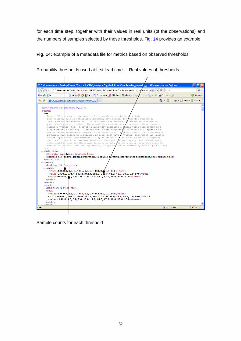
62
for each time step, together with their values in real units (of the observations) and
the numbers of samples selected by those thresholds. Fig. 14 provides an example.
Fig. 14: example of a metadata file for metrics based on observed thresholds
Probability thresholds used at first lead time Real values of thresholds
Sample counts for each threshold
63
6. THE VERIFICATION METRICS AVAILABLE IN THE EVS
6.1 Classes of verification metric and attributes of forecast quality
Detailed reviews of ensemble forecast quality can be found in Wilks (2006) and
Jolliffe and Stephenson (2003). This section focuses on the verification metrics
available in the EVS and the attributes of forecast quality to which they refer. In this
context, “attribute” refers to a specific dimension of quality, such as the unbiasedness
or “reliability” of the forecast probabilities. Important attributes of forecast quality are
obtained by examining the joint probability distribution function (pdf) of the forecasts,
Y, and observations, X, XYf ( x, y ) . The joint distribution can be factored into
X|Y Yf ( x | y ) f ( y ) , which is known as the “calibration-refinement” factorization or
Y|X Xf ( y | x ) f ( x ) , which is known as the “likelihood-base rate” factorization (Murphy
and Winkler, 1987). Differences between Xf ( x ) and Yf ( y ) describe the
unconditional biases in the forecast probabilities. The conditional pdf, X|Yf ( x | y ) ,
describes the conditional reliability of the forecast probabilities when compared to
Yf ( y ) and “resolution” when only its sensitivity to Yf ( y ) is considered. For a given
level of reliability, forecasts that contain less uncertainty, i.e. “sharp forecasts”, may
be preferred over “unsharp” ones, as they contribute less uncertainty to decision
making (Gneiting et al., 2007). By way of illustration, a flood forecasting system is
“reliable”, or conditionally unbiased in its forecast probabilities, if flooding is observed
twenty percent of the time when it is forecast with probability 0.2 (repeated for all
forecast probabilities). A flood forecasting system has “resolution” if small changes in
the forecast probabilities are associated with different observed outcomes, whether
or not the forecast probabilities are reliable. In contrast, Y|Xf ( y | x ) measures the
ability of the forecasts to “discriminate” between different observed outcomes. An
ensemble forecasting system is discriminatory with respect to an event if it
consistently forecasts the event’s (observed) occurrence with a probability higher
than chance (i.e. climatology) and consistently forecasts its (observed) non-
occurrence with a probability lower than chance.
In general, the utility of a forecasting system will depend on several attributes of
forecast quality (Jolliffe and Stephenson, 2003). However, for a particular application
of the forecasts, some attributes of forecast quality may be more important than
others. For example, when issuing flood warnings, it is particularly important that

64
observed flood flows and non-flood flows are discriminated between, because flood
warnings are only effective if they are consistently correct and do not “cry wolf”.
For any given attribute of forecast quality, there are several possible metrics or
measures of quality. For example, summary statistics for reliability and resolution can
be obtained from quadratic error statistics, such as the BS (Brier, 1950), which
contains a summed contribution from these two components (Murphy, 1996). When
more details are required, specific events may be defined, such as flooding or the
occurrence of precipitation, and forecast quality determined over specific ranges of
forecast probability (as in the reliability diagram; Hsu and Murphy, 1986). Only those
metrics thought to convey significantly different aspects of forecast quality are
included in the EVS, which includes metrics that convey specific attributes of quality
at various levels of detail (see Table 4). The flexibility to consider different attributes
of forecast quality at various levels of detail is important, as the EVS is intended for a
wide range of applications and users.
The EVS includes single-valued error statistics, which can be used to verify the
ensemble average forecast, and statistics that measure the quality of the forecast
probabilities. While single-valued metrics cannot verify the forecast probabilities, they
are useful for comparing deterministic forecasts with the “best estimate” from the
ensemble forecast (such as the ensemble mean), particularly if the ensemble
forecasts were derived from single-valued forecasts (e.g. via Model Output Statistics;
Gneiting et al., 2005). However, caution should be exercised when using single-
valued measures to verify the ensemble mean forecast, because the ensemble
spread adds potential skill to the ensemble forecast and is not verified by a single-
valued measure. Currently, the single-valued measures available in the EVS include
the mean error, the mean absolute error, the RMSE, and the coefficient of correlation
between the ensemble average forecast and the observed outcome (Table 4). Table
4 lists the verification metrics that are currently available in the EVS, which contain
varying levels of detail about the forecasting errors. The verification scores, such as
the BS and the Continuous Ranked Probability Score (CRPS) are integral measures
of forecast quality and are less sensitive to sampling uncertainty. Sampling
uncertainty is an important concern when verifying forecast probabilities (Jolliffe and
Stephenson, 2003; Wilks, 2006), particularly for extreme events (Bradley et al.,
2003). Also, the BS and CRPS may be decomposed into summed contributions from
(lack of) reliability and resolution (Murphy 1996, Hersbach 2000).

65
As indicated above, reliability and discrimination are two key attributes of ensemble
forecast quality. Both unconditional and conditional biases contribute to a lack of
reliability in the forecast probabilities. If the forecasting system is conditionally
unbiased, it is also unconditionally unbiased, but the reverse may not hold. The
conditional biases are often considered alongside the forecast spread or “sharpness”,
because sharp forecasts are more informative, but not necessarily more reliable
(Gneiting et al., 2007). For example, a forecast that issues the climatological
probability of an event is unconditionally unbiased, because the average observed
and forecast probabilities are, by definition, the same. However, it is conditionally
biased, because hydrologic events are conditional upon several factors, such as
precipitation amount and antecedent soil conditions. The conditional bias
corresponds to the difference between a forecast issued from a perfectly reliable
forecasting system (the diagonal line in the reliability diagram; Hsu and Murphy,
1986) and the climatological probability of occurrence (a horizontal line in the
reliability diagram). Several metrics are available in the EVS for assessing the
unconditional and conditional biases that contribute to unreliable forecast
probabilities. In order of increasing detail, these include; 1) the reliability component
of the mean CRPS (CRPS ; Matheson and Winkler, 1976; Hersbach, 2000); 2) a plot
of the unconditional biases in the forecast probabilities (the mean error of probability
diagram, MEPD); 3) a plot of the conditional biases in the forecast probabilities (the
spread-bias diagram, SBD), which that is similar to the cumulative rank histogram
(Anderson, 1996; Hamill, 1997; Talagrand, 1997); and 4) the reliability diagram,
which plots the conditional biases in the forecast probabilities of a discrete event,
such as flooding, and includes a plot of sharpness (Hsu and Murphy, 1986).
The reliability component of the CRPS measures the average reliability of the
ensemble forecasts across all possible events (Hersbach, 2000). Specifically, it
shows whether the observed outcome falls below the jth of m ranked ensemble
members, {zj-1≤ zj; j=2,…,m} , in proportion to j/m, on average. The MEPD shows the
frequency with which an observed outcome falls below a probability threshold in the
unconditional or “climatological” forecast distribution (Section 6.2). The SBD is
closely related to the reliability component of the CRPS . It shows the frequency with
which an observed outcome falls below a probability threshold in the (conditional)
forecast distribution (see Section 6.2). The MEPD, the SBD, and the reliability
diagram all measure bias in probability and have a common graphical interpretation.
In each case, a deviation from the diagonal line represents to a lack of calibration in

66
the forecast probabilities, whether unconditional (the MEPD) or conditional upon the
forecast ensemble (the SBD) or specific forecast events (the reliability diagram). The
reliability diagram plots the conditional probability that an event is observed to occur,
given the forecast, against its forecast probability of occurrence (Hsu and Murphy,
1986; Bröcker and Smith, 2007a). It is useful to distinguish between the unconditional
and conditional biases in the forecast probabilities, because the unconditional biases
are more easily removed (e.g. through post-processing; Hashino et al., 2006), and
may originate from different sources.
One measure of resolution and two measures of discrimination are currently
available in the EVS, namely: 1) the resolution component of the CRPS (Hersbach,
2000); 2) the Relative Operating Characteristic (ROC) score (Mason and Graham,
2002; Fawcett, 2006); and; 3) the ROC curve (Green and Swets, 1966; Mason and
Graham, 2002). The resolution component of the CRPS measures the average
ability of the forecasts to distinguish between different observed outcomes, whether
or not they were forecast reliably (Hersbach, 2000). The forecasting system has
positive resolution if it performs better than the climatological probability forecast. The
ROC score and ROC curve measure the ability of the forecasts to discriminate
between observed events and non-events, such as flooding versus no flooding. In
this context, there is a trade-off between the correct prediction of occurrences and
the correct prediction of non-occurrences, or the probability level at which actions are
triggered. For example, if a flood warning is triggered by only a small probability of
flooding, there is a smaller chance that a flood event will evade detection, but there is
a concomitantly higher chance that a non-event will be forecast incorrectly (i.e. of
“crying wolf”; other factors being equal). Thus, the ROC curve plots the probability of
detection against the probability of false detection for a range of forecast probability
levels (Green and Swets, 1966). The ROC score measures the average gain over
climatology for all probability levels (based on the integral of the ROC curve).
In addition to measures of reliability and discrimination, there are several composite
measures of forecasting error provided in the EVS. In order of increasing information
content, these include: 1) the BS; 2) the CRPS ; 3) the Mean Capture Rate Diagram
(MCRD); and 4) box plots of errors in the forecast ensemble members. The BS and
the CRPS quantify the mean square error of the forecast probabilities for a single
threshold and for all thresholds, respectively. In contrast, the MCRD and box plots
show the forecasting errors in linear units (see Section 6.2). The quadratic form of

67
the BS and the CRPS allows for their decomposition into reliability, resolution, and
uncertainty (Murphy, 1996). However, this also complicates their use in operational
forecasting, where low-probability, high-impact, events are crucial, but the square
errors of probability in the forecasts are necessarily small (see Section 6.2 also). In
order to support comparisons between forecasting systems and across hydroclimatic
regimes, the Brier Skill Score (BSS) and the Continuous Ranked Probability Skill
Score (CRPSS) are also provided in the EVS. In both cases, the reference forecast is
user-defined, and is introduced by defining an additional VU in the EVS.
6.2 Metrics developed for the EVS with an emphasis on operational forecasting
In addition to the standard metrics for reliability, resolution and discrimination, the
EVS provides a platform for testing new metrics. Currently, these include the mean
error of probability diagram (MEPD), which measures the unconditional biases in the
forecast probabilities, the spread-bias diagram (SBD), which is similar to the
(cumulative) rank histogram and tests the forecasts for conditional reliability
(Anderson, 1996; Hamill, 1997; Talagrand, 1997), the Mean Capture Rate Diagram
(MCRD), which is based on the Probability Score of Wilson et al. (1999), and
modified box plots of the ensemble forecast errors versus observed amount. An
important aim in developing these metrics was to provide operational forecasters with
more application-oriented measures of ensemble forecast quality.
The MEPD measures the reliability of an ensemble forecasting system in an
unconditional sense. Let zij denote the jth of m ensemble members from the ith of n
ensemble forecasts and let xio denote the observed outcome associated with the ith
ensemble forecast. The forecast climatology has an empirical distribution function,
nmF̂ ( v ) , which is computed from the n ensemble forecasts as
{ }
1i i
n m
nm m m iji 1 j 1
ˆ ˆ ˆ1 1F (v ) F ( v ) where F ( v ) z v ,n m
(1)
and {}1 is a step function that assumes value 1 if the condition is met and 0
otherwise. Let H [a,b|a,b [0,1]] denote an interval of fixed width on the
support of nmF̂ ( v ) . The MEPD counts the fraction of observations that fall within the
interval, H, namely

68
{ }.
1n o
nm ii 1
ˆ1MEPD( H ) F ( x ) Hn (2)
An ensemble forecasting system is unconditionally reliable or marginally calibrated
over the interval, H, if it captures observations in proportion to the width of that
interval
{ }
1n o
nm ii 1n,m
ˆ1lim F ( x ) H b a.n
(3)
The MEPD shows MEPD( H ) against the width of H for each of k windows that
span the unit interval. In practice, the k windows may cover any subintervals of the
unit interval. The MEPD is similar to the quantile-quantile (Q-Q) plot (Wilks, 2006)
and the probability-probability (P-P) plot (Shorack and Wellner, 1986; Gneiting et al.,
2007). The Q-Q plot compares the order statistics of two samples, or the order
statistics of one sample against the values of a theoretical distribution at
corresponding quantiles (Wilks, 2006). The P-P plot compares the quantiles
corresponding to these order statistics. Indeed, the MEPD is equivalent to a P-P plot
of the climatological distributions of X and Y when evaluated for the n intervals,
j j j
jH [0,b ] |b , j 1,...,n .
n 1 As indicated above, the MEPD assumes
asymptotic convergence of MEPD( H ) as n→∞. In practice, this may be evaluated
by comparing the MEPD( H ) for g subsamples of the n available data.
For continuous random variables, such as temperature and streamflow, the SBD
provides a simple measure of conditional reliability. It involves counting the fraction of
observations, SBD( I ) , that fall within an interval of fixed width on the support of the
ith forecast, I [c,d |c,d [0,1]]
{ }.
1i
n o
m ii 1
ˆ1SBD( I ) F ( x ) In
(4)
An ensemble forecasting system is reliable over the interval, I, if it captures
observations in proportion to the width of that interval
{ }
1i
n o
m ii 1n,m
ˆ1lim F ( x ) I d c.n
(5)

69
By defining k windows on the unit interval, j j j j jI [ c ,d ] |c ,d [0,1]; j 1,...,k ,
the reliability can be determined for the entire range of forecast probabilities. In
practice, the k windows may cover any subintervals of the unit interval. Certain
windows may be preferred for some applications or for sampling reasons. For
example, if the forecasts are uncertain in the tails, windows centered on the forecast
median may be preferred. The SBD shows the observed frequency, SBD( I ) ,
against the expected frequency, d-c. Any deviation from the diagonal line represents
a lack of reliability in the forecast probabilities. More specifically, the ensemble
forecasts are unreliable if the observed frequency, SBD( I ) , deviates from the
expected frequency by more than the sampling uncertainty of SBD( I ) . If the k
windows each cover a probability interval of 1/k, the expected frequency has a
uniform probability distribution, and the actual reliability can be tested for its
goodness-of-fit to a uniform distribution (e.g. using the one-sided Cramer von Mises
test; Anderson, 1962; Elmore, 2005; Bröcker, 2008).
For continuous random variables, the expected SBD( I ) is equal to the width of the
interval, I, and is, therefore, strictly increasing as the width increases (see above).
However, for mixed random variables, such as precipitation and wind-speed, the
discrete portion of the probability distribution comprises an infinite number of intervals
of different width. Although the window definition could be adapted for this case (see
Hamill and Colucci, 1997 for a similar discussion), the reliability diagram may be
preferred for mixed random variables.
While the SBD is analogous to the cumulative rank histogram, it explicitly defines the
width of the interval, I, into which observations fall. When these windows are based
on non-exceedence probabilities and are uniform in width (as well as non-
overlapping and exhaustive), the SBD is also analogous to the Probability Integral
Transform (PIT) (Casella and Berger, 1990), although the latter involves fitting a
parametric cdf to the ensemble forecast distribution prior to evaluating the PIT
(Gneiting et al., 2005). In that case, the SBD, the cumulative rank histogram and the
PIT can also be summarized with the reliability component of the CRPS (Hersbach,
2000), which tests whether an observation falls below a threshold with a frequency
proportional to the cumulative probability of that threshold (averaged across all
thresholds).

70
Integral measures of forecasting error are widely used in ensemble verification and
include the BS and CRPS. As indicated above, the BS and CRPS may be
decomposed into a reliability component, a resolution component, and an uncertainty
component (Hersbach, 2000). In addition, they have the important property of being
“strictly proper” (Bröcker and Smith, 2007b; Gneiting et al., 2007). A scoring rule is
“proper” if it is maximized for a forecaster’s true belief and is “strictly proper” if its
maximum is unique (Gneiting et al., 2007). While linear scores are improper,
quadratic scores, such as the BS and CRPS, are strictly proper. Nevertheless, if the
user has a strong risk aversion towards extreme events, quadratic scores may not be
desirable. The Probability Score (PS) of Wilson et al. (1999) is not strictly proper but
has some appeal in operational forecasting (see also, Mason, 2008). The PS
integrates the forecast probability distribution, Yf ( y ) , over a symmetric window of
width, w, around the observed outcome, xo, and is defined as o
YPS( f ,x ,w)
o
o
x 0.5wo
Y Yx 0.5w
PS( f ,x ,w) f ( y )dy. (6)
As with the CRPS , the o
YPS( f ,x ,w) is averaged over n pairs of forecasts and
verifying observations to form the PS( w)
i
n o
Y ii 1
1PS( w) PS( f ,x ,w).n
(7)
On average, the probability that a forecast value (or ensemble member) will fall within
w of the observed value is PS( w). The expected PS of a perfect forecasting system
is 1, because any given window around xo will fully capture Yf ( y ) . The PS( w) may
be separated into an unconditional bias term, UPS ( w) , and a conditional bias term,
CPS ( w) , where U CPS( w) PS ( w) PS ( w) . The UPS ( w)stems from a lack of
reliability in the forecast climatology, Yf , relative to the observed climatology,
Xf ,
and is given by the absolute difference in the PS( w) for the forecasts Yf and
Xf ,
i.e. i i
n no o
U Y i X ii 1 i 1
1 1PS ( w) PS( f ,x ,w) PS( f ,x ,w) .n n
The conditional bias
may be deduced from C UPS ( w) PS( w) PS ( w) .

71
When basing decisions on the PS( w) , w may be interpreted as a “significant
operating error”. For example, when forecasting dam inflows, a high probability of
realizing an error greater than w (i.e. 1- PS( w)), on average, may have some
practical implications for regulating dam outflows. In other cases, there may be no
single w on which to base decisions. The Mean Capture Rate Diagram (MCRD) plots
1- PS( w) for all possible w. The integral of the MCRD for the perfect forecasting
system is 0, since E[1-PS]=0 for all real values of w. While the PS is not strictly
proper, there is an analytical relationship between the integral of the MCRD, denoted
IPS, where
o
o
x 0.5w
Yx 0.5w
IPS f ( y )dy dw , and the strictly proper CRPS
YIPS CRPS 2E[ X F ( y )] E[ X ]. (8)
Thus, the integral of the MCRD is directly related to the CRPS . However, of greater
practical significance, the IPS is more sensitive to errors in the tails of the forecast
probability distribution than the CRPS .

72
7. EXAMPLE APPLICATIONS OF THE EVS
7.1 Precipitation forecasts from the NWS Ensemble Pre-Processor (EPP)
Six-hourly mean areal precipitation (MAP) totals were hindcast for a 17 year period
between 1 January 1979 and 31 December 1996 for the North Fork of the American
River above the North Fork Dam (USGS stream gauge station 11427000, NWS
forecast point NFDC1), near Sacramento, California. The hindcasts were produced
with the NWS Ensemble Pre-Processor (EPP; Schaake et al., 2007) for two MAP
areas that contribute to streamflow at NFDC1. The EPP uses a form of Model Output
Statistics (MOS) to generate ensemble forecasts of precipitation from single-valued
forecasts. The technique is based on a linear regression of the single-valued
forecasts and observations in normal probability space. Ensemble traces are then
sampled from the conditional probability distribution of the observations, given the
single-valued precipitation forecast (Schaake et al., 2007). When sampling from the
conditional probability distribution at different lead times, the temporal correlations
are reconstructed approximately using the Schaake Shuffle technique (Clark et al.,
2003). In the current application, the single-valued forecasts were obtained from the
frozen version of the Global Forecast System (GFS; frozen circa 1998) of the
National Centers for Environmental Prediction (NCEP) and comprise the ensemble
mean of the GFS forecasts (Toth et al., 1997; Hamill et al., 2006; Schaake et al.
2007; Wei et al., 2008). The GFS-EPP precipitation ensembles comprise a
continuous record of six-hourly forecasts, with lead times ranging from 6 to 336 hours
in six-hourly increments. Each GFS-EPP forecast contains 40 ensemble members,
and each member represents an equally likely prediction of the total precipitation
within the six-hour period. Using the EVS, the forecasts were aggregated from six-
hourly totals to daily totals, and the verification statistics were averaged across the
two MAP areas.
Fig. 15 shows the reliability of the GFS-EPP forecasts for daily precipitation totals
exceeding 0.0 (i.e. probability of precipitation, PoP), 5.0, 12.5, and 25 mm at lead
times of 1, 2, 4, 6, 10 and 14 days. The sampling uncertainties were too large to
evaluate forecast reliability at thresholds exceeding 25 mm. As indicated in Fig. 15,
the forecast probabilities are reliable for PoP and low precipitation amounts (e.g. >5.0
mm), particularly at lead times of 4 and 6 days, and are reasonably reliable for other
precipitation amounts. At moderate (>12.5 mm) and high (>25 mm) precipitation
thresholds, there is a tendency for the forecast probabilities to fall below the

73
observed relative frequencies. This is associated with a low-bias in the ensemble
mean forecast for large precipitation amounts (see the upper-right plot in Fig. 17,
together with Fig. 18). Also, as the event thresholds and lead times increase, the
number of forecasts issued with high probability, i.e. the “sharpness”, declines
rapidly.
Fig. 15: Reliability diagrams for the EPP precipitation forecasts
ROC measures the ability of an ensemble forecasting system to discriminate
predefined events, such as the occurrence versus non-occurrence of precipitation,
and is insensitive to reliability. The ROC curves in Fig. 16 show the Probability of
Detection (POD) versus the Probability of False Detection (POFD) for varying
probability levels of the GFS-EPP forecasts. Here, an event is defined for daily

74
precipitation totals exceeding 0.0, 5.0, 12.5 or 25 mm at lead times of 1, 2, 4, 6, 10 or
14 days. The POD and POFD are plotted for twelve, equally spaced, probability
thresholds. The diagonal line in each plot represents the climatological probability
forecast or “zero skill” line. At short lead times, the ensemble forecasts are much
more skillful than the climatological probability forecast across all precipitation
amounts. Notably, while the ROC area declines consistently with forecast lead time,
it increases slightly with precipitation threshold at lead times of 1 and 2 days. This is
contrary to the expectation that forecast skill declines with increasing precipitation
amount. However, NFDC1 lies on the upslope of the Sierra Nevada mountain range,
where significant precipitation events are often enhanced by orographic lifting and
are, therefore, relatively predictable at short lead times.
Fig. 16: Empirical ROC curves for the EPP precipitation forecasts
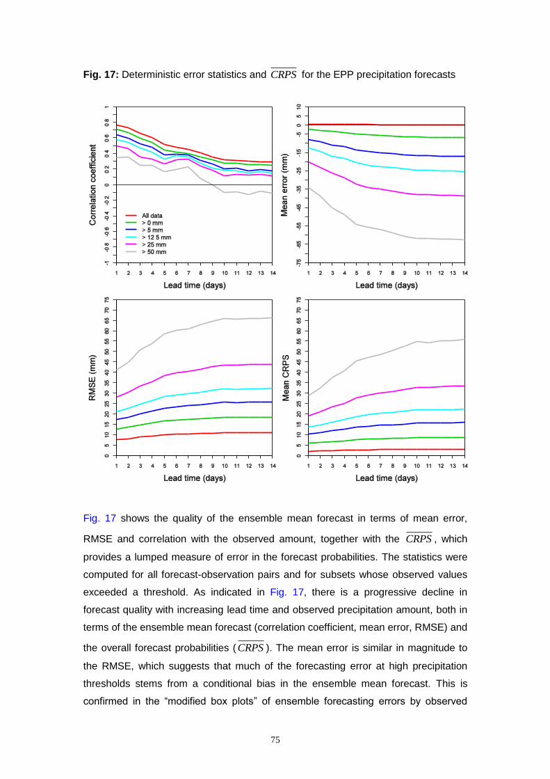
75
Fig. 17: Deterministic error statistics and CRPS for the EPP precipitation forecasts
Fig. 17 shows the quality of the ensemble mean forecast in terms of mean error,
RMSE and correlation with the observed amount, together with the CRPS , which
provides a lumped measure of error in the forecast probabilities. The statistics were
computed for all forecast-observation pairs and for subsets whose observed values
exceeded a threshold. As indicated in Fig. 17, there is a progressive decline in
forecast quality with increasing lead time and observed precipitation amount, both in
terms of the ensemble mean forecast (correlation coefficient, mean error, RMSE) and
the overall forecast probabilities (CRPS ). The mean error is similar in magnitude to
the RMSE, which suggests that much of the forecasting error at high precipitation
thresholds stems from a conditional bias in the ensemble mean forecast. This is
confirmed in the “modified box plots” of ensemble forecasting errors by observed

76
precipitation amount, which are shown in Fig. 18 for lead day 1. Here, the forecasting
errors (ensemble member – observed value) are plotted with box-and-whisker
diagrams, where the whiskers are drawn at quantiles of the forecast error distribution
(deciles in this case) and the middle quantiles are shaded (the middle six deciles in
this case). The-box-and-whisker diagrams are then arranged by observed value in
ascending order. The conditional bias in the ensemble mean forecast is readily
apparent in Fig. 18, and shows over-forecasting of low precipitation amounts and
under-forecasting of high amounts.
Fig. 18: Box plots for the EPP precipitation forecasts on lead day 1

77
7.2 Streamflow forecasts from the NWS Ensemble Streamflow Prediction system
Mean daily inflows were hindcast for a 17 year period between 1 January 1979 and
31 December 1996 at the North Fork Dam, California (NFDC1). The hindcasts were
produced with the NWS Hydrologic Ensemble Hindcaster, which implements part of
the NWSRFS in an ensemble framework, known as the Ensemble Streamflow
Prediction (ESP) system (Demargne et al., 2007). The NWSRFS was forced with
temperature and precipitation ensembles from the GFS-EPP (as described in Section
7.1). The streamflow hindcasts should only be considered illustrative of the EVS and
not representative of the operational streamflow forecasts for NFDC1, which are
forced with short-range QPF rather than the frozen GFS. These QPFs originate from
the NWS Hydrometeorological Prediction Center and may be modified by the RFC
forecasters to reflect the real-time streamflow conditions (a form of manual data-
assimilation, known as run-time MODs). In general, the modified QPFs are much
more skillful than the ensemble means of the frozen GFS. The hindcasts were
aggregated from a six-hourly timestep to daily averages for comparison with the
observed flows, which were only available as daily averages. The observed flows are
based on stage observations, which were converted to flows using measured stage-
discharge relations (Kennedy, 1983).
Fig. 19 shows the reliability of the forecasts at selected lead times. The results are
shown for flow thresholds corresponding to climatological non-exceedence
probabilities of 0.5 (10 m3 s-1), 0.75 (32 m3 s-1), 0.95 (85 m3 s-1) and 0.99 (210 m3 s-1).
As indicated in Fig. 19, the forecast probabilities are reliable across a wide range of
flow exceedence thresholds and lead times. However, they are slightly overconfident
at moderately high flows, as evidenced by the higher forecast probabilities than
observed relative frequencies. The forecasts are also consistently less reliable but
sharper on lead day 1. This is understandable because the current version of the
ESP system ignores uncertainties in the hydrologic model, including those in its initial
conditions, structure and parameter values (Seo et al. 2006). Noise in the sharpness
and reliability curves for streamflows that were forecast to exceed 210 m3 s-1 with
high probability (0.8-1.0) reflects the small sample size and correspondingly high
sampling uncertainty for such forecast events. Fig. 20 shows the spread-bias plots
for the ESP flow forecasts. These plots show the reliability of the forecast
probabilities for all forecast-observation pairs and for subsets of pairs whose
observed values exceed a probability threshold in the observed climatological
distribution. As indicated in Fig. 20, the forecasts are reasonably reliable across all

78
flow exceedence thresholds and lead times, but tend to underpredict the observed
streamflows at the highest flow threshold. Fig. 21 shows the mean error of the
ensemble mean forecast, the correlation of the ensemble mean flow with the
observed flow, the ROC score, and the mean error of probability diagram (MEPD).
While the forecasts are marginally well-calibrated (see the MEPD in Fig. 21), there is
a loss of conditional reliability at the highest flow threshold across all forecast lead
times (Fig. 19). This conditional bias originates from the conditional bias in the
ensemble mean flow (Fig. 21). Overall, the conditional biases in the ESP streamflow
forecasts (Fig. 21) are consistent with the conditional biases in the GFS-EPP
precipitation forecasts (Fig. 17), which comprise over-forecasting of low precipitation
amounts and under-forecasting of high amounts (Fig. 18).
Fig. 19: Reliability diagrams for the ESP forecasts

79
Fig. 20: Spread-bias diagrams for the ESP forecasts

80
Fig. 21: Deterministic error statistics, ROC score and MEPD for the ESP forecasts
Fig. 22 shows the ROC curves for mean daily flows that correspond to climatological
non-exceedence probabilities of 0.5, 0.75, 0.95 and 0.99. In comparison to the
precipitation hindcasts, there is more consistent decline in discrimination with
increasing forecast lead time and event threshold. Also, the flow forecasts are
substantially more skillful than the climatological probability forecast for all forecast
lead times and event thresholds. The MCRDs in Fig. 23 show a rapid increase in the
mean error of any given ensemble member over lead times of 1 and 2 days and a
much slower decline in forecast quality over lead times of 4 to 14 days.

81
Fig. 22: Empirical ROC curves for the ESP flow forecasts
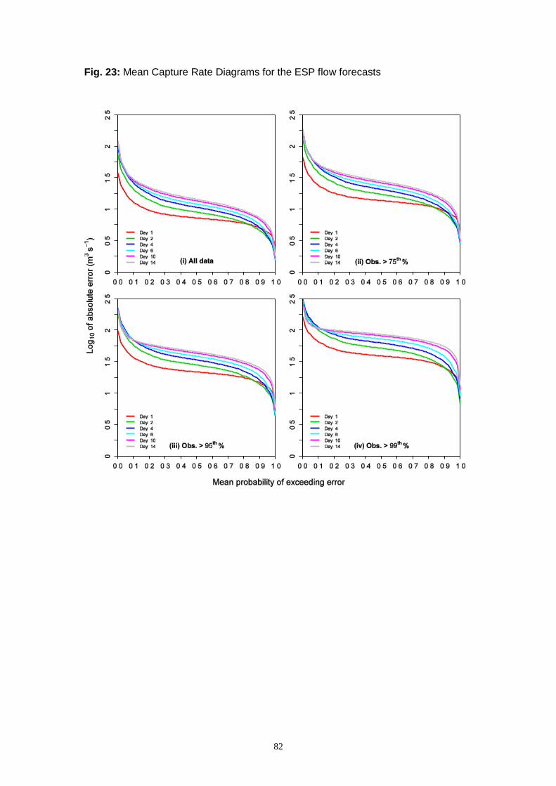
82
Fig. 23: Mean Capture Rate Diagrams for the ESP flow forecasts

83
8. THE APPLICATION PROGRAMMERS INTERFACE (API)
8.1 Overview
This section provides a brief overview of the API for the EVS and the procedure for
adding a new verification metric. Detailed documentation of the code is provided in
the hyperlinked html documentation that accompanies the software distribution.
Developers may contact the authors for additional information about the source code.
The EVS is written in Java, which is a modern, object-oriented, programming
language (Flanagan, 2005). The Java platform comprises the language itself, a
library of classes, and a Virtual Machine (VM), which runs on a specific operating
system (OS). The VM allows for the “platform-independence” of Java applications. A
popular class library and one set of VMs are implemented by Oracle as the Java
Runtime Environment (JRE). The EVS requires version 1.8 or higher of the JRE. This
is freely available to download from the Java website:
http://www.java.com/en/download/index.jsp
In object-oriented programming, the source code is separated into classes, each of
which provides the blueprint for a particular object. For example, a class that
computes the BS for a verification dataset, a, at an event threshold, b, provides the
template for a BrierScore object with specific values of a and b. A class also
contains methods, which determine the behavior of an object. For example, the
BrierScore class contains the method getThreshold, which returns the event
threshold associated with a particular BrierScore object. Similarities among objects
are exploited by linking classes together. This leads to a family tree in which children
inherit and extend the functionality of their parents. For example, the BrierScore
class inherits the functionalities of the EnsembleMetric, ScoreMetric, and
ThresholdMetric classes, among others. Groups of classes with related
functionalities are stored in packages. For example, the BrierScore class is stored
in the metrics package. The EVS comprises ~50,000 lines of code, which are
separated into in 308 classes and stored in a hierarchy of 26 packages. Fig. 24
shows the main package hierarchy in the EVS. The API is fully documented in
hyperlinked HTML, and the code itself is extensively commented (~35,000 lines).

Fig. 24: A UML description of the main packages in the EVS

8.2 Procedure for adding a new metric to the EVS
Due to its modular design, the procedure for adding a new metric to the EVS is tightly
structured and requires little code development (beyond that required for the metric
calculation). Indeed, much of the code required to implement a new metric in the
EVS is dictated by, or already implemented in, a more general class of metric. This is
illustrated by adding the logarithmic scoring rule or ‘Ignorance Score’ to the EVS. The
Ignorance Score measures the quality of a probabilistic forecasting system with a
numeric score (Good, 1952). A new metric, IgnoranceScore, is created in the
package /evs/metric/metrics. The metric extends the ScoreMetric and
implements EnsembleMetric, ThresholdMetric, DecomposableScore,
CategoricalMetric, and BootstrapableMetric. In inheriting these classes,
several methods must be implemented (for which templates can be found in similar
classes, such as the BrierScore). For example, in inheriting from ScoreMetric,
the following methods must be implemented:
getID, returns a unique identifier for the metric;
getResultID, returns an identifier from the list of identifiers in the
MetricResult class that indicates the data type of the result;
hasRealUnits, returns true if the metric is defined in units of the observed
and forecast variables (e.g. error in mm/day), false otherwise;
deepCopy, returns an independent copy of the metric object. Changes to the
parameter values of the copied object are not reflected in the original object;
and
compute, computes the metric for each forecast lead time and stores the
result.
In order to display the Ignorance Score in the EVS, a default plot must also be
created. By adding a class to the evs/products/plots/defaults package (e.g.
IgnoranceScorePlot) and associating the plot with the IgnoranceScore class,
the Ignorance Score will be plotted in the EVS. The IgnoranceScorePlot
extends the class DefaultXYPlotByLeadTime to plot the Ignorance Score by

86
forecast lead time. A single method, getDefaultChart, is then implemented to
return an IgnoranceScorePlot with the correct y-axis dimension for the Ignorance
Score (0-1), and any other information specific to the plotting of this score (e.g. axis
and chart titles) [approximately five lines of code]. The plots themselves are created
with the JFreeChart library (see www.jfree.org/jfreechart/). Once the
IgnoranceScorePlot is associated with the results from an IgnoranceScore,
the new metric can be displayed in the Output dialog of the EVS (Section 5.5).
Descriptive information about the Ignorance Score can also be displayed in the GUI.
This is achieved by setting the descriptionURL parameter of the
IgnoranceScore class (which was inherited from the Metric class via
EnsembleMetric) to the URL of a stable resource with descriptive information. For
example, it may point to an html file in the statsexplained package, which contains
descriptive information for the other metrics in the EVS.

87
APPENDIX A1 VERIFICATION STATISTICS COMPUTED IN THE EVS
Table 4 provides a list of the verification metrics supported by the EVS. Below is a
short description of each metric, which is also available in the GUI.
Mean error
The mean error (ME) measures the average difference between a set of forecasts
and corresponding observations. Here, it measures the average difference between
the center of the ensemble forecast (the mean average, by default) and observation.
The ME of the ensemble average forecast, Y , given the observation, x, is
n
i ii 1
1ME Y xn
. (A1)
The ME provides a measure of first-order bias in the forecasts, and may be positive,
zero, or negative. A positive mean error denotes overforecasting and a negative
mean error denotes underforecasting. A mean error of zero (in the ensemble mean
forecast) denotes an absence of bias.
Relative mean error
The relative mean error (RME), or relative bias, measures the mean difference
between a set of forecasts and corresponding observations, divided by the mean of
the observations. Here, it measures the relative mean difference between the center
of the ensemble forecast (the mean average value, by default) and the observations.
Given n pairs of forecasts and observations, the RME of the center of the ensemble
forecast, Y , given the observation, x, is
n
i ii 1
n
ii 1
Y xRME
x
. (A2)
The RME provides a measure of relative, first-order, bias in the forecasts, and may
be positive, zero, or negative. A positive RME denotes overforecasting and a
negative RME denotes underforecasting (assuming that the chosen measure of

88
central tendency should match the observed value, on average). A RME of zero
denotes the absence of relative bias in the center of the ensemble forecast.
Mean absolute error
The mean absolute error (MAE) measures the mean absolute difference between a
set of forecasts and corresponding observations. Here, it measures the mean
absolute difference between the center of the ensemble forecast (the mean average,
by default) and the observation.
The MAE of the ensemble mean forecast, Y , given the observation, x, is given by
n
i ii 1
1MAE Y xn
. (A3)
The MAE provides a measure of error spread in the center of the forecast
distribution. It is similar to the Root Mean Square Error (RMSE), except the RMSE
employs square deviations, such that large errors contribution proportionally more to
the overall score. The MAE generalizes to the Continuous Ranked Probability Score
(CRPS) for ensemble or probability forecasts.
Root mean square error
The mean square error (MSE) measures the average square error of the forecasts.
The Root Mean Square Error (RMSE) provides the square root of this value, which
has the same units as the forecasts and observations. Here, the forecast
corresponds to the ensemble average value (the mean, by default) and an 'error'
represents the difference between the ensemble average, Y , and the observation, x.
The equation for the RMSE is
0.5
2n
i ii 1
1RMSE Y xn
. (A4)
The RMSE provides an indication of the ‘average deviation’ between the forecast
value and an observation in real units. The RMSE is either zero, denoting a perfect
forecast, or positive.

89
Correlation coefficient
The correlation coefficient measures the strength of linear association between two
variables. Here, it measures the linear relationship between n pairs of ensemble
average forecasts and corresponding observations. A correlation coefficient of 1.0
denotes a perfect linear relationship between the forecasts and observations. A
correlation coefficient of -1.0 denotes a perfect inverse linear relationship (i.e. the
observed values increase when the forecasts values decline and vice versa). The
ensemble average forecast may be perfectly correlated with the observations and still
contain biases, because the correlation coefficient is normalized by the overall mean
of each variable. A correlation coefficient of 0.0 denotes the absence of any linear
association between the forecasts and observations. However, a low correlation
coefficient may occur in the presence of a strong non-linear relationship, because the
correlation coefficient measures linear association only.
EVS computes the Pearson product-moment correlation coefficient, r, which is given
by
Cov(x,Y)r
Std(x) Std(Y)
, (A5)
where Cov(x,Y) is the sample covariance between the ensemble average forecasts
and their corresponding observations. The sample standard deviations of the
forecasts and observations are denoted Std(Y) and Std(x) , respectively. The
sample covariance between the n pairs of forecasts and observations is
n
i x i Yi 1
1Cov(x,Y) (x )(Y )
n 1
, (A6)
where Y
and x are the overall sample means of the (ensemble average) forecasts
and observations, respectively.
Brier Score
The Brier Score (BS) measures the average square error of a probability forecast. It
is analogous to the mean square error of a deterministic forecast, but the forecasts,
and hence error units, are given in probabilities. The Brier Score measures the error
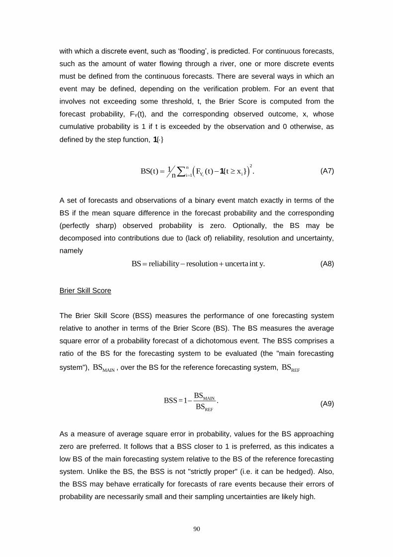
90
with which a discrete event, such as ‘flooding’, is predicted. For continuous forecasts,
such as the amount of water flowing through a river, one or more discrete events
must be defined from the continuous forecasts. There are several ways in which an
event may be defined, depending on the verification problem. For an event that
involves not exceeding some threshold, t, the Brier Score is computed from the
forecast probability, FY(t), and the corresponding observed outcome, x, whose
cumulative probability is 1 if t is exceeded by the observation and 0 otherwise, as
defined by the step function, {}1
i
2n
Y ii 1
1BS(t) F (t) {t x } .n
1 (A7)
A set of forecasts and observations of a binary event match exactly in terms of the
BS if the mean square difference in the forecast probability and the corresponding
(perfectly sharp) observed probability is zero. Optionally, the BS may be
decomposed into contributions due to (lack of) reliability, resolution and uncertainty,
namely
BS reliability resolution uncerta int y. (A8)
Brier Skill Score
The Brier Skill Score (BSS) measures the performance of one forecasting system
relative to another in terms of the Brier Score (BS). The BS measures the average
square error of a probability forecast of a dichotomous event. The BSS comprises a
ratio of the BS for the forecasting system to be evaluated (the "main forecasting
system"), MAINBS , over the BS for the reference forecasting system, REFBS
MAIN
REF
BSBSS = 1 .
BS (A9)
As a measure of average square error in probability, values for the BS approaching
zero are preferred. It follows that a BSS closer to 1 is preferred, as this indicates a
low BS of the main forecasting system relative to the BS of the reference forecasting
system. Unlike the BS, the BSS is not "strictly proper" (i.e. it can be hedged). Also,
the BSS may behave erratically for forecasts of rare events because their errors of
probability are necessarily small and their sampling uncertainties are likely high.
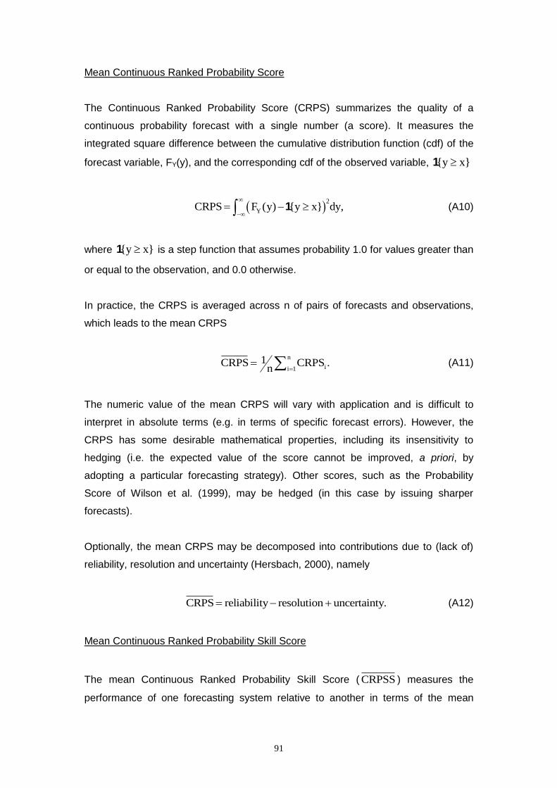
91
Mean Continuous Ranked Probability Score
The Continuous Ranked Probability Score (CRPS) summarizes the quality of a
continuous probability forecast with a single number (a score). It measures the
integrated square difference between the cumulative distribution function (cdf) of the
forecast variable, FY(y), and the corresponding cdf of the observed variable, {y x}1
2
YCRPS F (y) {y x} dy,
1 (A10)
where {y x}1 is a step function that assumes probability 1.0 for values greater than
or equal to the observation, and 0.0 otherwise.
In practice, the CRPS is averaged across n of pairs of forecasts and observations,
which leads to the mean CRPS
n
ii 1
1CRPS CRPS .n
(A11)
The numeric value of the mean CRPS will vary with application and is difficult to
interpret in absolute terms (e.g. in terms of specific forecast errors). However, the
CRPS has some desirable mathematical properties, including its insensitivity to
hedging (i.e. the expected value of the score cannot be improved, a priori, by
adopting a particular forecasting strategy). Other scores, such as the Probability
Score of Wilson et al. (1999), may be hedged (in this case by issuing sharper
forecasts).
Optionally, the mean CRPS may be decomposed into contributions due to (lack of)
reliability, resolution and uncertainty (Hersbach, 2000), namely
CRPS reliability resolution uncertainty. (A12)
Mean Continuous Ranked Probability Skill Score
The mean Continuous Ranked Probability Skill Score ( CRPSS ) measures the
performance of one forecasting system relative to another in terms of the mean
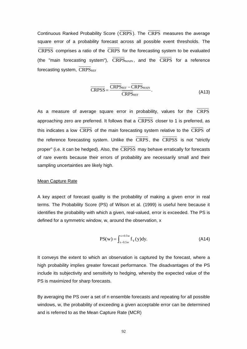
92
Continuous Ranked Probability Score ( CRPS ). The CRPS measures the average
square error of a probability forecast across all possible event thresholds. The
CRPSS comprises a ratio of the CRPS for the forecasting system to be evaluated
(the "main forecasting system"), MAINCRPS , and the CRPS for a reference
forecasting system, REFCRPS
REF MAIN
REF
CRPS CRPSCRPSS .
CRPS
(A13)
As a measure of average square error in probability, values for the CRPS
approaching zero are preferred. It follows that a CRPSS closer to 1 is preferred, as
this indicates a low CRPS of the main forecasting system relative to the CRPS of
the reference forecasting system. Unlike the CRPS , the CRPSS is not "strictly
proper" (i.e. it can be hedged). Also, the CRPSS may behave erratically for forecasts
of rare events because their errors of probability are necessarily small and their
sampling uncertainties are likely high.
Mean Capture Rate
A key aspect of forecast quality is the probability of making a given error in real
terms. The Probability Score (PS) of Wilson et al. (1999) is useful here because it
identifies the probability with which a given, real-valued, error is exceeded. The PS is
defined for a symmetric window, w, around the observation, x
x 0.5w
Yx 0.5w
PS(w) f (y)dy.
(A14)
It conveys the extent to which an observation is captured by the forecast, where a
high probability implies greater forecast performance. The disadvantages of the PS
include its subjectivity and sensitivity to hedging, whereby the expected value of the
PS is maximized for sharp forecasts.
By averaging the PS over a set of n ensemble forecasts and repeating for all possible
windows, w, the probability of exceeding a given acceptable error can be determined
and is referred to as the Mean Capture Rate (MCR)

93
n
i 1
1MCR(w) 1 PS(w) wn
R (A15)
It should be noted that sensitivity to hedging does not apply to the MCR, as it is not a
score. The resulting curve may be separated into errors of over-prediction and under-
prediction by computing the MCR for ensemble members that exceed the
observation and fall below the observation, respectively.
Modified box plots
Box plots (or box-and-whisker diagrams) provide a discrete representation of a
continuous empirical probability distribution (Tukey, 1977).
Building on this idea, an empirical probability distribution function (pdf) may be
summarized with an arbitrary set of percentile bins of which an arbitrary proportion
may be shaded (e.g. the middle 60%), to convey the outer and inner probability
densities, respectively. The modified box plots show the forecasting errors (ensemble
member – observed value) by forecast lead time. Forecasts with common lead times
are pooled before computing the errors and displaying them as a box.
Modified box plots by observed value
Constructs a modified box plot where the errors are plotted against observed value
for one forecast lead time. When there are multiple forecasts that have a common
observed amount, the errors are pooled across those forecasts.
Modified box plots by forecast value
Constructs a modified box plot where the errors are plotted against forecast value for
one forecast lead time. The forecast values are determined by applying a specified
function (e.g. mean) to the ensemble members. When there are multiple forecasts
that have a common forecast value, the errors are pooled across those forecasts.
94
Reliability diagram
The reliability diagram measures the accuracy with which a discrete event is forecast
by an ensemble or probabilistic forecasting system. The discrete event may be
defined in several ways. For example, flooding is a discrete event that involves the
exceedence of a flow threshold. According to the reliability diagram, an event should
be observed to occur with the same relative frequency as its forecast probability of
occurrence over a large number of such forecast-observation pairs. For example,
over a large number of cases where flooding is forecast to occur with a probability of
0.95, it should be observed to occur roughly 95% of the time. However, the
calculation of the observed relative frequency is subject to sampling uncertainty. For
example, there may be few cases in the historic record where flooding is forecast to
occur with probability 0.95. In practice, the forecasts are binned into discrete
probability intervals and the observed relative frequencies are plotted against the
average forecast probability within each bin. The sampling uncertainty will decline as
the width of the bin increases, but the precision of the diagram will also decline.
The Reliability diagram plots the average forecast probability within each bin on the
x-axis. For a forecast event defined by the non-exceedence of some threshold, t, the
average probability of the forecasts that fall in the kth forecast bin, Bk is given by
i
k
Y
i Ik
1F (t),
| I |
(A16)
where kI denotes the set of all indices, k kI {i : i B } , whose forecasts (and
associated paired observations) fall in the kth bin and k| I | denotes the number of
elements in that set. The y-axis shows the corresponding fraction of observations
that fall in the kth bin
k
i
i Ik
1{t x },
| I |
1 (A17)
where i{t x }1 is a step function that assumes value 1 if the ith observation, xi,
exceeds the threshold, t, and 0 otherwise. If the forecast is perfectly reliable, the
observed fraction within each bin will equal the average of the associated forecast

95
probabilities, forming a diagonal line on the reliability diagram. Deviation from the
diagonal line represents bias in the forecast probabilities, notwithstanding sampling
uncertainty. The reliability diagram may be computed for several discrete events.
Each event is represented by a separate reliability curve.
Collectively, the number of forecasts that fall within each of the k bins, k| I | , denotes
the 'sharpness' of the forecasts and is displayed as a histogram. Ideally, the forecast
probabilities will be sharp, i.e. issued with little uncertainty, but also reliable.
Relative Operating Characteristic
The Relative Operating Characteristic (ROC; also known as the Receiver Operating
Characteristic) measures the quality of a forecast for the occurrence of a discrete
event, such as rainfall or flooding. For a probability forecast, the ROC curve
measures the quality of a binary prediction or “decision” based on the forecast
probability. A binary prediction is generated from the forecast by defining a probability
threshold above which the discrete event is considered to occur. For example, a
decision maker might issue a flood warning when the forecast probability of a flood
exceeds 0.9. The ROC curve plots the forecast quality for several probability
thresholds. Each threshold corresponds to a different level of risk aversion. For
example, given a decision on whether to issue a flood warning, a probability
threshold of 0.7 corresponds to a higher level of risk aversion (i.e. a lower threshold
for warning) than a probability of 0.9. As the threshold declines, the probability of
correctly detecting an event (the Probability of Detection or POD) will increase, but
the probably of “crying wolf” (the probability of False Detection or POFD) will also
increase. The ROC curve plots the trade-off between POD and POFD on two axes:
Y-axis: the POD or probability with which an event is correctly forecast to occur.
The POD is estimated from n sample data as the total number of correct
forecasts divided by the total number of occurrences. For an event defined by
the exceedance of a real-valued threshold, t, which is forecast to occur when
the forecast probability exceeds a probability threshold, pt, the POD is given by
i
n
Y t ii=1t n
ii=1
{1- F (t) > p | x > t}POD(t,p ) = ,
{x > t}
1
1 (A18)

96
where {}1 is a step function that assumes the value 1 if the condition, {·}, is
met and 0 otherwise.
X-axis: the POFD or probability with which an event is incorrectly forecast to not
occur (i.e. the event occurs, but the forecast was for non-occurrence). The
POFD is estimated from n sample data as the total number of incorrect
forecasts divided by the total number of non-occurrences
i
n
Y t ii=1t n
ii=1
{1- F (t) > p | x t}POFD(t,p ) = .
{x t}
1
1 (A19)
These values are computed for probability thresholds that exhaust the unit interval,
which is normally defined by a number of plotting points, q, that separate the unit
interval, [0,1], into q thresholds at equal intervals. Additionally, the curve is forced to
intersect (0,0), and (1,1).
For an ensemble forecasting system to perform well in terms of ROC, the POD must
be high relative to the POFD. An ensemble forecasting system that produces
forecasts in line with climatological expectation will have as many "successful"
predictions as the climatological probability of the event implies. A skillful forecasting
system will always produce a ROC curve that lies above the diagonal line.
Practical applications of the ROC in the medical, atmospheric, and other sciences
frequently fit a smooth curve to the empirical POD and POFD data. A common
approach is to fit a binormal model, which assumes that the POD and POFD are
normally distributed, each with given mean and variance (standard deviation).
Experience has shown that the binormal model typically provides a good fit to the
empirical POD and POFD, even when they are "significantly" non-normal (i.e. the
binormal approximation is robust). The binormal model is given by
1
POD POFD
POD
POFD
POD
POD = (a b (POFD)), where
a = , and
b = .
(A20)

97
Here, is the cumulative distribution function of the standard normal distribution,
POD and POFD are, respectively, the means of the POD and POFD, and POD and
POFD are their corresponding standard deviations.
There are several approaches to estimating the parameters of the binormal model, a
and b (or the means and standard deviations from which they are derived; for
example, see Cai and Moskowitz, 2004). The simplest and most direct approach
stems from the observation that
1 1(POD) = a b (POFD). (A21)
Hence, the parameters, a and b, are the intercept and slope, respectively, of a linear
(regression) relationship between the POD and POFD following their transformation
to the probit scale. The EVS estimates these parameters through ordinary least
squares regression. While the resulting model fit is mathematically correct, the
standard errors of the model (or confidence intervals for the associated ROC Score)
cannot be computed in this way, and are not reported by the EVS. Since the
parameters of the binormal model are estimated from the empirical POD and POFD,
the model fit will depend on the number of probability thresholds used to compute the
ROC curve. The number of thresholds cannot (usefully) exceed the number of
ensemble members, m, (or m+1 thresholds) from which the POD and POFD are
derived, as the ensemble forecast only contains information at these thresholds
(members). However, the binormal curve is plotted for a large number of points in
between these thresholds, in order to convey the smoothness of the fitted model.
The ROC Score is derived from the Area Under the Curve (AUC), and is an analytical
function of the binormal model parameters
2
aAUC = .
1 b
(A22)
Upon request, the binormal approximation to the ROC Score is also provided by the
EVS. Since the model fit depends on the number of thresholds used to compute the
ROC curve, the number of thresholds must be defined when computing the binormal
approximation to the ROC Score. For an exact comparison between the binormal

98
ROC curve and the binormal ROC Score (or AUC), the same number of thresholds,
q, must be used for each metric.
Relative Operating Characteristic Score
The Relative Operating Characteristic (also known as the Receiver Operating
Characteristic) measures the quality of a forecast for the occurrence of a discrete
event, such as rainfall or flooding. It does not consider the quality of forecasts that
predict no occurrence of the event defined (e.g. no rainfall or no flooding).
The ROC Score is based on the area underneath the ROC curve or AUC, which is
normalized by the AUC of a reference forecast, refAUC (Mason and Graham, 2002).
The AUC of the climatological probability forecast is 0.5, which corresponds to the
diagonal line in the ROC plot. Thus, the ROC Score for the climatological probability
forecast is
ref
ref
AUC- AUC AUC-0.5ROC Score = = = 2 AUC-1.
1.0 - AUC 1.0 -0.5 (A23)
As discussed under the Relative Operating Characteristic, practical applications of
ROC analysis in the medical, atmospheric, and other sciences frequently fit a smooth
curve to the paired values of the Probability of Detection (POD) and Probability of
False Detection (POFD) derived from the sample data. A common approach is to fit a
binormal model, which assumes that the POD and POFD are normally distributed,
each with given mean and variance (standard deviation). Experience has shown that
the binormal model typically provides a good fit to the empirical POD and POFD,
even when the sample data are "significantly" non-normal (i.e. the binormal
approximation is robust). The binormal approximation to the AUC (and hence the
ROC Score) is given by
2
aAUC = .
1 b
(A24)
Here, a and b are the parameters of the binormal model, and is the cumulative
distribution function of the standard normal distribution. The parameters a and b are,
respectively, the intercept and slope of the (assumed) linear relationship between the

99
POD and POFD following their transformation to the probit scale (see the discussion
under the Relative Operating Characteristic). Unlike the empirical AUC (Mason and
Graham, 2002), which bypasses the calculation of the ROC curve, the binormal
approximation to the AUC (and ROC Score) is based on the q pairs of (POD, POFD)
data from which the empirical ROC curve is computed (where q is the number of
probability thresholds). Thus, for an exact comparison between the binormal ROC
curve and the binormal ROC Score, the same number of thresholds, q, must be used
for each metric. However, the binormal ROC Score will be closest to the empirical
ROC Score when the ROC curve is constructed from m+1 probability thresholds,
where m is the (fixed) number of ensemble members in each forecast. Put differently,
the empirical AUC, described by Mason and Graham (2002), approximates the area
under the ROC curve when constructed with as many probability thresholds as the
(fixed) number of ensemble members in each forecast.
By default, the algorithm described in Mason and Graham (2002) is used to compute
the empirical AUC. Optionally, the AUC may be derived from the empirical ROC
curve, which is constructed for a specified number of points. In that case, the
empirical ROC curve is integrated using the trapezoid rule. In most cases, the
algorithm described by Mason and Graham (2002) generates larger values of the
empirical AUC (skill) than integrating the empirical ROC curve.
Spread-bias diagram
For continuous random variables, such as temperature and streamflow, the SBD
provides a simple measure of conditional reliability. It involves counting the fraction of
observations, SBD(I) , that fall within a probability interval of fixed width on the
support of the ith forecast, I = [c,d | c,d [0,1]]
i
n o
m ii=1
1SBD(I) = {F (x ) I}.n
ˆ1 (A25)
An ensemble forecasting system is reliable over the interval, I, if it captures
observations in proportion to the width of that interval
i
n o
m ii=1n,m
1lim {F (x ) I} = d -c.n
ˆ1 (A26)

100
By defining k windows on the unit interval, j j j j jI = [c ,d ] | c ,d [0,1]; j =1,...,k , the
reliability can be determined for the entire range of forecast probabilities. In practice,
the k windows may cover any subintervals of the unit interval. Certain windows may
be preferred for some applications or for sampling reasons. For example, if the
forecasts are uncertain in the tails, windows centered on the forecast median may be
preferred. The SBD shows the observed frequency, SBD(I) , against the expected
frequency, d-c. Any deviation from the diagonal line represents a lack of reliability in
the forecast probabilities. More specifically, the ensemble forecasts are unreliable if
the observed frequency, SBD(I) , deviates from the expected frequency by more
than the sampling uncertainty of SBD(I) . If the k windows each cover a probability
interval of 1/k, the expected frequency has a uniform probability distribution, and the
actual reliability can be tested for its goodness-of-fit to a uniform distribution (e.g.
using the one-sided Cramer von Mises test; Anderson, 1962; Elmore, 2005; Bröcker,
2008).
For continuous random variables, the expected SBD(I) is equal to the width of the
interval, I, and is, therefore, strictly increasing as the width increases (see above).
However, for mixed random variables, such as precipitation and wind-speed, the
discrete portion of the probability distribution comprises an infinite number of intervals
of different width. Although the window definition could be adapted for this case (see
Hamill and Colucci, 1997 for a similar discussion), the reliability diagram may be
preferred for mixed random variables.
While the SBD is analogous to the cumulative rank histogram, it explicitly defines the
width of the interval, I, into which observations fall. When these windows are based
on non-exceedence probabilities and are uniform in width (as well as non-
overlapping and exhaustive), the SBD is also analogous to the Probability Integral
Transform (PIT) (Casella and Berger, 1990), although the latter involves fitting a
parametric cdf to the ensemble forecast distribution prior to evaluating the PIT
(Gneiting et al., 2005). In that case, the SBD, the cumulative rank histogram and the
PIT can also be summarized with the reliability component of the CRPS (Hersbach,
2000), which tests whether an observation falls below a threshold with a frequency
proportional to the cumulative probability of that threshold (averaged across all
thresholds).

101
Rank histogram
The rank histogram measures the reliability of an ensemble forecasting system. It is
similar to the spread-bias diagram and involves counting the fraction of observations
that fall between any two ranked ensemble members in the forecast distribution (the
spread-bias diagram uses an explicit probability interval derived from the members).
For an ensemble forecast that comprises m ensemble members ranked in ascending
order, there are m+1 “gaps”, {g1,…,gm+1}, between any two ranked ensemble
members (i.e. m-1 internal gaps, and one at each bound) into which the observation
could fall. The rank histogram measures the fraction of observations, h, that fall within
each gap
n
i j ijj=1
1h {x g }.n
1 (A27)
where hi is the fraction in the ith bin, xj is the jth observed value, gij is the ith gap
associated with the jth forecast, and {}1 is a step function that assumes value 1 if
the condition is met and 0 otherwise.
If the forecasting system is reliable in terms of the rank histogram, the probability that
an observation falls between any two ranked ensemble members is approximately
uniform. Indeed, the actual reliability can be tested for goodness-of-fit of the sample
fractions to a uniform probability distribution (e.g. using the one-sided Cramer von
Mises test; Anderson, 1962; Elmore, 2005; Broecker, 2008).
Notwithstanding any sampling and observational uncertainties (see below), a lack of
uniformity in the rank histogram is indicative of an unreliable forecasting system.
Greater than expected probabilities in the tails of the rank histogram (i.e. in low and
high bins) can lead to a "U" shape, which is indicative of a lack of spread in the
ensemble. Greater than expected probabilities in the center of the rank histogram
(i.e. in central bins) can lead to an inverted "U" shape, which is indicative of too much
spread in the ensemble. Other systematic features, such as a gradient, or a
combination of features, may be indicative of biases in the mean and possibly higher
moments of the ensemble.
While a perfectly reliable ensemble (in the context of the rank histogram) will
ordinarily produce a rank histogram that is approximately uniform (given any

102
sampling uncertainty), systematic non-uniformities are possible when the
observations are uncertain, even if they are unbiased in the mean. The precise
effects of observational uncertainty will depend upon the shapes of the two
probability distributions (forecast and observed), but observational uncertainties
typically exaggerate the probability of falling in the tails of the forecast distribution,
falsely indicating a lack of spread in the ensemble or a "U-shaped" rank histogram
(Hamill, 2001).
When computing the rank histogram, ties are handled by randomly assigning one of
the tied ranks (i.e. assigning the observation randomly to one of the tied bins). In
particular, this avoids the appearance of bias for mixed variables, such as
precipitation; an artifact that stems from consistently assigning the observation to the
lower (or higher) of the tied bins when the bins are, in fact, indistinguishable.
Mean error of probability diagram
The mean error of probability diagram (MEPD) measures the reliability of an
ensemble forecasting system in an unconditional sense. Let zij denote the jth of m
ensemble members from the ith of n ensemble forecasts and let xio denote the
observed outcome associated with the ith ensemble forecast. The forecast
climatology has an empirical distribution function, nmF (v)ˆ , which is computed from
the n ensemble forecasts as
i i
n m
nm m m iji=1 j=1
1 1F (v) = F (v) where F (v) = 1{z v},n m
ˆ ˆ ˆ (A28)
and {}1 is a step function that assumes value 1 if the condition is met and 0
otherwise. Let H = [a,b | a,b [0,1]] denote an interval of fixed width on the support
of nmF (v)ˆ . The MEPD counts the fraction of observations that fall within the interval,
H, namely
n o
nm ii=1
1MEPD(H) = 1{F (x ) H}.n
ˆ (A29)

103
An ensemble forecasting system is unconditionally reliable or marginally calibrated
over the interval, H, if it captures observations in proportion to the width of that
interval
n o
nm ii=1n,m
1lim 1{F (x ) H} = b -a.n
ˆ (A30)
The MEPD shows MEPD(H) against the width of H for each of k windows that span
the unit interval. In practice, the k windows may cover any subintervals of the unit
interval. The MEPD is similar to the quantile-quantile (Q-Q) plot (Wilks, 2006) and the
probability-probability (P-P) plot (Shorack and Wellner, 1986; Gneiting et al., 2007).
The Q-Q plot compares the order statistics of two samples, or the order statistics of
one sample against the values of a theoretical distribution at corresponding quantiles
(Wilks, 2006). The P-P plot compares the quantiles corresponding to these order
statistics. Indeed, the MEPD is equivalent to a P-P plot of the climatological
distributions of X and Y when evaluated for the n intervals,
j j j
jH = [0,b ] | b = , j =1,..., n .
n +1 As indicated above, the MEPD assumes
asymptotic convergence of MEPD(H) as n→∞. In practice, this may be evaluated by
comparing the MEPD(H) for g subsamples of the n available data.
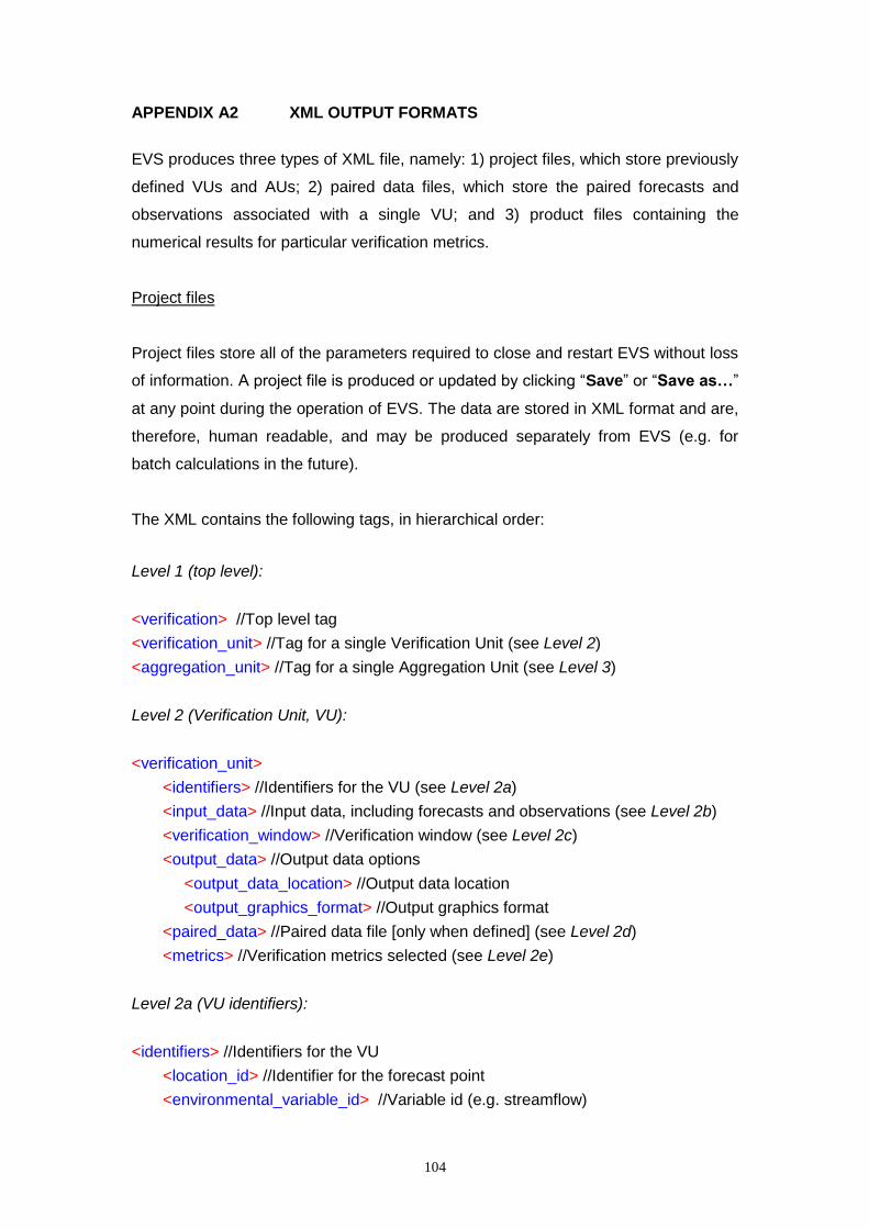
104
APPENDIX A2 XML OUTPUT FORMATS
EVS produces three types of XML file, namely: 1) project files, which store previously
defined VUs and AUs; 2) paired data files, which store the paired forecasts and
observations associated with a single VU; and 3) product files containing the
numerical results for particular verification metrics.
Project files
Project files store all of the parameters required to close and restart EVS without loss
of information. A project file is produced or updated by clicking “Save” or “Save as…”
at any point during the operation of EVS. The data are stored in XML format and are,
therefore, human readable, and may be produced separately from EVS (e.g. for
batch calculations in the future).
The XML contains the following tags, in hierarchical order:
Level 1 (top level):
<verification> //Top level tag
<verification_unit> //Tag for a single Verification Unit (see Level 2)
<aggregation_unit> //Tag for a single Aggregation Unit (see Level 3)
Level 2 (Verification Unit, VU):
<verification_unit>
<identifiers> //Identifiers for the VU (see Level 2a)
<input_data> //Input data, including forecasts and observations (see Level 2b)
<verification_window> //Verification window (see Level 2c)
<output_data> //Output data options
<output_data_location> //Output data location
<output_graphics_format> //Output graphics format
<paired_data> //Paired data file [only when defined] (see Level 2d)
<metrics> //Verification metrics selected (see Level 2e)
Level 2a (VU identifiers):
<identifiers> //Identifiers for the VU
<location_id> //Identifier for the forecast point
<environmental_variable_id> //Variable id (e.g. streamflow)

105
<additional_id> // Additional id (e.g. forecast_model_1) [only when defined]
Level 2b (VU input data sources):
<input_data> //Identifiers for the VU
<forecast_data_source> //Forecast data
<data> //Path to first file/folder (e.g. first file in a file array or a folder)
<data> //Path to second file in a file array [when defined]
<data> //Etc.
…
<observed_data_source> //Path to observed data file
<forecast_filter> //String for filtering files within a folder [when defined]
<forecast_archive filter> //String for filtering files within an archive [when defined]
<forecast_data_type> //File type for forecast data file
<observed_data_type> //File type for observed data file
<forecast_data_location_id> //Location name in forecast file [when defined]
<observed_data_location_id> //Location name in observed file [when defined]
<forecast_data_variable_id> //Variable name in forecast file [when defined]
<observed_data_variable_id> //Variable name in observed file [when defined]
<forecast_data_ensemble_id> //Ensemble identifier in forecast file [when defined]
<forecast_time_system> //Name of forecast time system
<observed_time_system> //Observed time system
<ignore_timezone_in_forecast_source> //Ignore time zone in file [when defined]
<ignore_timezone_in_observed_source> //Ignore time zone in file [when defined]
<ignore_valid_year_member> //Ignore ensemble index of valid year [when defined]
<forecast_support> //Scale of forecasts
<statistic> //E.g. “instantaneous”
<period> //E.g. “1” [only when defined: blank when statistic = instantaneous]
<period_units> //E.g. “DAY” [when defined: as above]
<existing_attribute_units> //E.g. “feet cubed/second”
<target_attribute_units> //E.g. “meter cubed/second”
<attribute_units_function> //Multiplier to arrive at stated attribute units [1.0]
<notes> //Additional textual info. [when defined]
<observed_support> //Scale of observations [see forecast_support]
<use_all_observations_for_climatology> //Use unpaired observations for climatology
<apply_date_cond_to_climatology> //Apply date conditions to climatology
<apply_value_cond_to_climatology> //Apply value conditions to climatology
<forecast_date_format> //Date format for ASCII forecasts (e.g. MM/dd/yyyy HH)
<observed_date_format> //Date format for ASCII observations
<global_null_value> //Global no-data value

106
Level 2c (verification window for a given VU):
<verification_window> //Window parameters
<start_date> //Start date (in UTC)
<year> //Start year
<month> //Start month of year
<day> //Start day of month
<end_date> //End date, see start date
<window_in_valid_time> //Time system of verification window
<first_lead_period> //Minimum lead time considered
<last_lead_period> //Maximum lead time considered
<forecast_lead_units> //Units for the maximum lead time
<aggregation_lead_period> //Temporal aggregation window [when defined]
<aggregation_lead_units> //Aggregation window units [when defined]
<aggregation_lead_frequency> //Frequency of rolling aggregation [when defined]
<aggregation_lead_frequency_units> //Units of rolling aggregation [when defined]
<aggregation_function> //Function used to aggregate pairs [when defined]
<sample_size_constraint> //Constraint on minimum sample size per lead time
<date_conditions> //Date conditions (see Level 2c_1) [when defined]
<value_conditions> //Value conditions (see Level 2c_2) [when defined]
Level 2c_1 (date conditions on the verification window) [when defined]:
<date_conditions> //Date conditions
<valid_time> //Date conditions based on forecast valid time
<exclude_years> //Integer years to exclude from the overall range
<exclude_months> //Integer months to exclude from the overall range
<exclude_weeks> //Integer weeks to exclude from the overall range
<exclude_days_of_week> //Integer days to exclude from the overall range
<exclude_hours_of_day_UTC> //Integer [0,23] to exclude UTC hours of day
<whole_forecasts> //Use date conditions to select complete forecasts only
<issue_time> //Date conditions based on forecast issue time [see valid_time]
…
Level 2c_2 (value conditions on the verification window) [only when defined]:
<value_conditions> //Value conditions.
<condition> //First of n possible conditions
<unit_id> //Identifier of the VU on which the condition is built
<forecast_type> //True for forecasts, false for observed values
<statistic> //Name of statistic, e.g. mean
<statistic_constant> //Constant associated with statistic [when defined]

107
<consecutive_period> //Window size [when defined]
<consecutive_period_units> //Window time units [when defined]
<consecutive_period_statistic> //Window statistic [when defined]
<logical_conditions> //Set of n possible logical arguments
<function> //First logical argument
<name> //Unary function name, e.g. isLessThan (<)
<value> //Unary function threshold, e.g. 0.5 means “< 0.5”
…
Level 2d (paired data for a given VU) [only when defined]:
<paired_data> //Start of paired data specification
<paired_data_location> //Path to paired data
<eliminate_duplicates> //Is true to eliminate pairs with the same valid/lead times
<write_conditional_pairs> //Is true to write the conditional pairs
<write_unconditional_pairs> //Is true to write the unconditional pairs
<write_gzip_pairs> //Is true to write pairs in a compressed gzip format
<paired_write_precision> //Integer number of decimal places for writing pairs > 0
<strip_nulls_from_paired_file> //Is true to not write null member values
<raw_pairs_in_aggregated_res> //Store only aggregated pairs to save space
<detection_limit> //Detection limit (see Level 2d_1) [when defined]
Level 2d_1 (detection limit):
<detection_limit > //Set of n possible metrics to compute
<limit> //The detection limit
<bound> //The boundary to assign when falling outside the detection limit
<type> //The logical test for the limit (isGreater, isLess, isGreaterEqual, isLessEqual)
Level 2e (verification metrics for a given VU):
<metrics> //Set of n possible metrics to compute
<metric> //First of n metrics
<name> //Name of metric
Storage of parameters follows: varies by metric
…
Level 3 (Aggregation Unit, AU) [only when defined]:
<aggregation_unit> //Aggregation Unit
<name> //The name of the AU
<unit_id> //First of n possible VU identifiers associated with the aggregation unit
…

108
<weights> //Weights to assign to each of the n units identified above [sum to 1]
<output_data > //See equivalent tag under VU
<pool_pairs> //Is true to pool pairs from the VUs rather than average metrics
<statistically_dependent> //Is true to sample VUs assuming perfect dependence
<bootstrap> //Is true to compute bootstrap intervals for the AU if defined for the VUs
An example of an EVS project file is given below:
<?xml version="1.0" standalone="yes"?><verification>
<verification_unit>
<identifiers>
<location_id>Kampen</location_id>
<environmental_variable_id>waterlevel</environmental_variable_id>
<additional_id>COSMO-LEPS</additional_id>
</identifiers>
<input_data>
<forecast_data_location>
<data>D:/some_data/forecasts/</data>
</forecast_data_location>
<observed_data_location>
<data> D:/some_data/observed.obs</data>
</observed_data_location>
<forecast_filter>xml</forecast_filter>
<forecast_archive_filter>xml</forecast_archive_filter>
<forecast_data_type>NetCDF</forecast_data_type>
<observed_data_type>ASCII</observed_data_type>
<forecast_data_location_id>A</forecast_data_location_id>
<observed_data_location_id>A</observed_data_location_id>
<forecast_data_variable_id>B</forecast_data_variable_id>
<forecast_data_ensemble_id>C</forecast_data_ensemble_id>
<observed_data_variable_id>B</observed_data_variable_id>
<forecast_time_system>Coordinated Universal Time (UTC)</forecast_time_system>
<observed_time_system>Central Standard Time (CST)</observed_time_system>
<ignore_timezone_in_forecast_source>true</ignore_timezone_in_forecast_source>
<ignore_timezone_in_observed_source>true</ignore_timezone_in_observed_source>
<ignore_valid_year_member>true</ignore_valid_year_member>
<forecast_support>
<statistic>INSTANTANEOUS</statistic>
<existing_attribute_units>METER</existing_attribute_units>
<notes></notes>
</forecast_support>
<observed_support>
<statistic>INSTANTANEOUS</statistic>
<existing_attribute_units>METER</existing_attribute_units>
<notes></notes>
</observed_support>
<use_all_observations_for_climatology>true</use_all_observations_for_climatology>
<apply_date_cond_to_climatology>true</apply_date_cond_to_climatology>
<apply_value_cond_to_climatology>true</apply_value_cond_to_climatology>
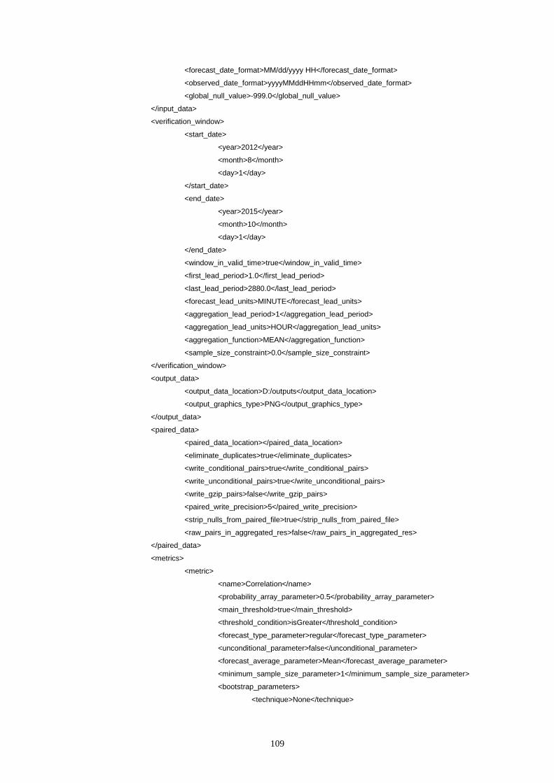
109
<forecast_date_format>MM/dd/yyyy HH</forecast_date_format>
<observed_date_format>yyyyMMddHHmm</observed_date_format>
<global_null_value>-999.0</global_null_value>
</input_data>
<verification_window>
<start_date>
<year>2012</year>
<month>8</month>
<day>1</day>
</start_date>
<end_date>
<year>2015</year>
<month>10</month>
<day>1</day>
</end_date>
<window_in_valid_time>true</window_in_valid_time>
<first_lead_period>1.0</first_lead_period>
<last_lead_period>2880.0</last_lead_period>
<forecast_lead_units>MINUTE</forecast_lead_units>
<aggregation_lead_period>1</aggregation_lead_period>
<aggregation_lead_units>HOUR</aggregation_lead_units>
<aggregation_function>MEAN</aggregation_function>
<sample_size_constraint>0.0</sample_size_constraint>
</verification_window>
<output_data>
<output_data_location>D:/outputs</output_data_location>
<output_graphics_type>PNG</output_graphics_type>
</output_data>
<paired_data>
<paired_data_location></paired_data_location>
<eliminate_duplicates>true</eliminate_duplicates>
<write_conditional_pairs>true</write_conditional_pairs>
<write_unconditional_pairs>true</write_unconditional_pairs>
<write_gzip_pairs>false</write_gzip_pairs>
<paired_write_precision>5</paired_write_precision>
<strip_nulls_from_paired_file>true</strip_nulls_from_paired_file>
<raw_pairs_in_aggregated_res>false</raw_pairs_in_aggregated_res>
</paired_data>
<metrics>
<metric>
<name>Correlation</name>
<probability_array_parameter>0.5</probability_array_parameter>
<main_threshold>true</main_threshold>
<threshold_condition>isGreater</threshold_condition>
<forecast_type_parameter>regular</forecast_type_parameter>
<unconditional_parameter>false</unconditional_parameter>
<forecast_average_parameter>Mean</forecast_average_parameter>
<minimum_sample_size_parameter>1</minimum_sample_size_parameter>
<bootstrap_parameters>
<technique>None</technique>

110
</bootstrap_parameters>
</metric>
<metric>
<name>MeanAbsoluteError</name>
<probability_array_parameter>0.5</probability_array_parameter>
<main_threshold>true</main_threshold>
<threshold_condition>isGreater</threshold_condition>
<forecast_type_parameter>regular</forecast_type_parameter>
<unconditional_parameter>false</unconditional_parameter>
<forecast_average_parameter>Mean</forecast_average_parameter>
<minimum_sample_size_parameter>1</minimum_sample_size_parameter>
<bootstrap_parameters>
<technique>None</technique>
</bootstrap_parameters>
</metric>
<metric>
<name>RankHistogram</name>
<probability_array_parameter>0.5</probability_array_parameter>
<main_threshold>true</main_threshold>
<threshold_condition>isGreater</threshold_condition>
<rank_hist_sample_parameter>true</rank_hist_sample_parameter>
<rank_hist_cum_parameter>false</rank_hist_cum_parameter>
<forecast_type_parameter>regular</forecast_type_parameter>
<unconditional_parameter>false</unconditional_parameter>
<minimum_sample_size_parameter>1</minimum_sample_size_parameter>
<bootstrap_parameters>
<technique>None</technique>
</bootstrap_parameters>
</metric>
<metric>
<name>RelativeMeanError</name>
<probability_array_parameter>0.5</probability_array_parameter>
<main_threshold>true</main_threshold>
<threshold_condition>isGreater</threshold_condition>
<forecast_type_parameter>regular</forecast_type_parameter>
<unconditional_parameter>false</unconditional_parameter>
<forecast_average_parameter>Mean</forecast_average_parameter>
<minimum_sample_size_parameter>1</minimum_sample_size_parameter>
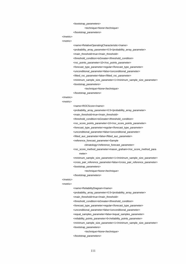
111
<bootstrap_parameters>
<technique>None</technique>
</bootstrap_parameters>
</metric>
<metric>
<name>RelativeOperatingCharacteristic</name>
<probability_array_parameter>0.5</probability_array_parameter>
<main_threshold>true</main_threshold>
<threshold_condition>isGreater</threshold_condition>
<roc_points_parameter>10</roc_points_parameter>
<forecast_type_parameter>regular</forecast_type_parameter>
<unconditional_parameter>false</unconditional_parameter>
<fitted_roc_parameter>false</fitted_roc_parameter>
<minimum_sample_size_parameter>1</minimum_sample_size_parameter>
<bootstrap_parameters>
<technique>None</technique>
</bootstrap_parameters>
</metric>
<metric>
<name>ROCScore</name>
<probability_array_parameter>0.5</probability_array_parameter>
<main_threshold>true</main_threshold>
<threshold_condition>isGreater</threshold_condition>
<roc_score_points_parameter>10</roc_score_points_parameter>
<forecast_type_parameter>regular</forecast_type_parameter>
<unconditional_parameter>false</unconditional_parameter>
<fitted_auc_parameter>false</fitted_auc_parameter>
<reference_forecast_parameter>Sample
climatology</reference_forecast_parameter>
<roc_score_method_parameter>mason_graham</roc_score_method_para
meter>
<minimum_sample_size_parameter>1</minimum_sample_size_parameter>
<cross_pair_reference_parameter>false</cross_pair_reference_parameter>
<bootstrap_parameters>
<technique>None</technique>
</bootstrap_parameters>
</metric>
<metric>
<name>ReliabilityDiagram</name>
<probability_array_parameter>0.5</probability_array_parameter>
<main_threshold>true</main_threshold>
<threshold_condition>isGreater</threshold_condition>
<forecast_type_parameter>regular</forecast_type_parameter>
<unconditional_parameter>false</unconditional_parameter>
<equal_samples_parameter>false</equal_samples_parameter>
<reliability_points_parameter>5</reliability_points_parameter>
<minimum_sample_size_parameter>1</minimum_sample_size_parameter>
<bootstrap_parameters>
<technique>None</technique>
</bootstrap_parameters>

112
</metric>
<metric>
<name>RootMeanSquareError</name>
<probability_array_parameter>0.5</probability_array_parameter>
<main_threshold>true</main_threshold>
<threshold_condition>isGreater</threshold_condition>
<forecast_type_parameter>regular</forecast_type_parameter>
<unconditional_parameter>false</unconditional_parameter>
<forecast_average_parameter>Mean</forecast_average_parameter>
<minimum_sample_size_parameter>1</minimum_sample_size_parameter>
<bootstrap_parameters>
<technique>None</technique>
</bootstrap_parameters>
</metric>
<metric>
<name>SampleSize</name>
<probability_array_parameter>-Infinity</probability_array_parameter>
<main_threshold>true</main_threshold>
<threshold_condition>isGreater</threshold_condition>
<forecast_type_parameter>regular</forecast_type_parameter>
<unconditional_parameter>false</unconditional_parameter>
</metric>
</metrics>
</verification_unit>
</verification>
Advanced options only available in the EVS project file:
Occasionally, in testing experimental or advanced options, these options are only
accessible via the EVS project file. The current experimental options are summarized
below with an XML code block provided for context. These options should be used
with care.
Tag: <minimum_sample_size_parameter>
Function: Sets a minimum sample size constraint on computing a given metric.
If the constraint is not met, the metric will not be computed. The
precise meaning of that constraint varies between metrics. For
example, when computing dichotomous metrics (i.e. metrics computed
with respect to discrete events), such as the Brier Score or reliability
diagram, the minimum sample size refers to the smaller of the number
of occurrences and non-occurrences of the event. For continuous
metrics, such as the mean error or the CRPS, it simply comprises the
number of samples from which the metric was computed.

113
Context:
<metric>
<name>BrierScore</name>
<probability_array_parameter>0.0,0.025 </probability_array_parameter>
<main_threshold>true, false</main_threshold>
<threshold_condition>isGreater</threshold_condition>
<decompose_parameter>CR_LBR</decompose_parameter>
<forecast_type_parameter>regular</forecast_type_parameter>
<unconditional_parameter>false</unconditional_parameter>
<minimum_sample_size_parameter>30</minimum_sample_size_parameter>
<bootstrap_parameters>
<technique>None</technique>
</bootstrap_parameters>
</metric>
Tag: <thinning>
Function: Verification results are sensitive to the paired forecasts and
observations available. Forecasts and observations from consecutive
lead times and from adjacent locations are typically related to each
other or “statistically dependent”. If the verification pairs contain
shared information, the effective sample size is smaller than the
nominal sample size. Particularly when the nominal sample size is
small (e.g. extreme events), the verification results may be over-
sensitive to a small number of observed events that are shared across
multiple forecast issue times. In order to explore these sensitivities, the
verification pairs may be thinned using a prescribed start index and
interval. Only those forecasts issued at the start index and every
subsequent nth index will be retained for verification.
Context:
<verification_window>
<start_date>
<year>1985</year>
<month>0</month>
<day>1</day>
</start_date>
<end_date>
<year>2008</year>
<month>11</month>
<day>31</day>
</end_date>
<window_in_valid_time>false</window_in_valid_time>
<first_lead_period>24.0</first_lead_period>
<last_lead_period>360.0</last_lead_period>
<forecast_lead_units>HOUR</forecast_lead_units>

114
<aggregation_lead_period>1</aggregation_lead_period>
<aggregation_lead_units>DAY</aggregation_lead_units>
<aggregation_function>MEAN</aggregation_function>
<sample_size_constraint>0.1</sample_size_constraint>
<thinning>
<start_index>0</start_index>
<frequency>3</frequency>
</thinning>
</verification_window>
Tag: <metric>
Function: The Ensemble Quantile-Quantile Diagram is used to measure the
unbiasedness of the (average) climatology of the ensemble members.
The metric forms an average of the order statistics of the individual
ensemble members and compares them to the corresponding order
statistics of the observations.
Context:
<metrics>
<metric>
<name>EnsembleQQDiagram</name>
<forecast_type_parameter>regular</forecast_type_parameter>
<unconditional_parameter>false</unconditional_parameter>
<bootstrap_parameters>
<technique>None</technique>
</bootstrap_parameters>
</metric>
<metrics>
Paired data files
A paired data file stores the pairs of forecasts and observations for a single VU in
XML format. The file name corresponds to the VU identifier with a _pairs.xml
extension.
Each pair comprises one or more forecasts and one observation, and is stored under
a <pr> tag. Each pair has a readable date in Coordinated Universal Time (UTC or
GMT), a lead time in hours (<ld_h>), an observation (<ob>), one or more forecast
values (<fc>), and an internal time in hours (<in_h>) used by EVS to read the pairs
(in preference to the UTC date). The internal time is incremented in hours from the
forecast start time (represented in internal hours) to the end of the forecast time
horizon. When multiple forecasts are present, each forecast represents an ensemble

115
member, and each ensemble member is listed in trace-order, from the first trace to
the last. An example of the first few lines of a pair within a paired file is given below:
<pairs> //Denotes start of paired data
<pair_count>448<pair_count> //Total number of pairs on file <pr> //First pair
<dt> //Date tag
<y>2005</y> //Year
<m>11</m> //Month
<d>31</d> //Day
<h>18</h> //Hour
</dt> //End of date tag
<ld_h>6.0</ld_h> //Lead time in hours
<ob>150.625</ob> //Observed value <fc> //Forecast values: in this case 49 ensemble members
157.31567,157.31598,157.31627,157.3342,157.3148,
157.31598,157.31509,157.31509,157.31572,157.31567,
157.31538,157.31598,157.31598,157.3148,157.31627,
157.31393,157.31567,157.31598,157.31595,
157.31627,157.32852,157.31569,157.3148,157.34517,
157.34586,157.34148,157.31664,157.31538,
157.31509,157.31644,157.31509,157.31567,
157.31639,157.31598,157.31598,157.31627,
157.31598,157.31567,157.3161,157.31538,157.34439,
157.3148,157.31627,157.3148,157.31598,157.31598,
157.31657,157.3156,157.31567
</fc>
<in_h>315570</in_h> //Internal hour incremented from start time
</pr> //End of first pair tag
…
…
</pairs> //Denotes end of paired data
Product files
Product files include the numerical and graphical results associated with verification
metrics.
Numerical results are written in XML format. One file is written for each metric. The
file name comprises the unique identifier of the VU or AU, together with the metric
name (e.g. CBNK1.Q.Mean_error.xml). Some metrics, such as reliability
diagrams, have results for specific thresholds (e.g. probability thresholds). In that
case, the results are stored by lead time and then by threshold value. The actual data
associated with a result always appears within a 'values' tag. A metric result that
comprises a single value will appear as a single value in this tag. A metric result that

116
comprises a 1D matrix will appear as a row of values separated by commas in the
input order. A metric result that comprises a 2D matrix will appear as a sequence of
rows, each with a <values> tag, which are written in the input order. For example, a
diagram metric with an x and y axis will comprise two rows of data (i.e. two rows
within two separate <values> tags). The default input order would be data for the x
axis followed by data for the y axis. Data that refer to cumulative probabilities are, by
default, always defined in increasing size of probability. If available, sample counts
are given in the last <values> tag. Sample counts are also printed out in a separate
XML file for each metric. This information is written to a file with the VU identifier,
metric name and a _metadata.xml extension.
An example of the first few lines of a numerical result file for one metric, namely the
‘mean error, is given below:
<results> //Denotes the start of the results data
<meta_data> //Tag for metadata on the results //The next tag indicates whether the results are ordered by one or more thresholds of the observed variable as well as by forecast lead time <thresholds_type>true</thresholds_type>
<original_file_id>CBNK1.Q.mean_error.xml</original_f
ile_id > //Original file name
</meta_data> //End of metadata
<result> //First of n possible results
<lead_hour>6</lead_hour> //Result applies to lead hour 6 <threshold_data>
<threshold>
//Threshold value > 5.0 <threshold_value>GT 5.0</threshold_value>
<data> //Start of data <values>0.0</values> //Mean error
</data> //End of data
</threshold>
…
</threshold_data> //End of data
</result> //End of first result
…
… </results> //Denotes the end of the results data
For verification measures that comprise multiple factors alongside the overall scores,
these factors are written as comma delimited values in a <values> tag. The order of
the factors is described in Table A2a.
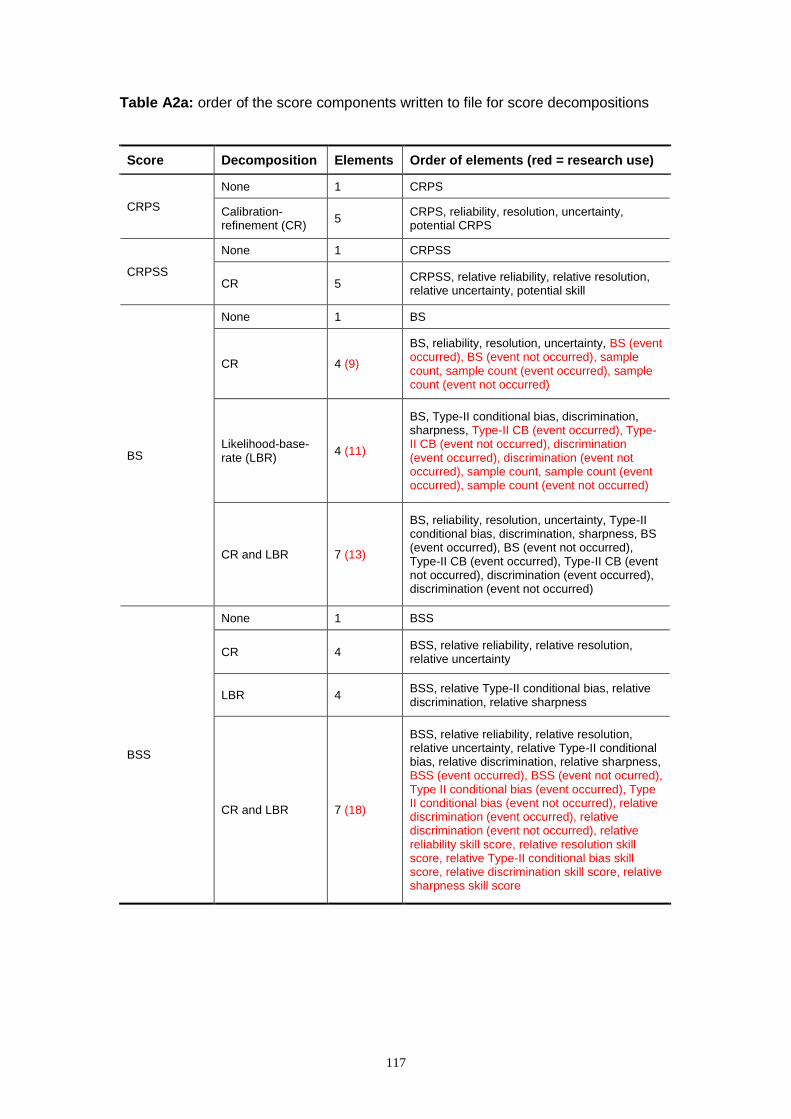
117
Table A2a: order of the score components written to file for score decompositions
Score Decomposition Elements Order of elements (red = research use)
CRPS
None 1 CRPS
Calibration-refinement (CR)
5 CRPS, reliability, resolution, uncertainty, potential CRPS
CRPSS
None 1 CRPSS
CR 5 CRPSS, relative reliability, relative resolution, relative uncertainty, potential skill
BS
None 1 BS
CR 4 (9)
BS, reliability, resolution, uncertainty, BS (event occurred), BS (event not occurred), sample count, sample count (event occurred), sample count (event not occurred)
Likelihood-base-rate (LBR)
4 (11)
BS, Type-II conditional bias, discrimination, sharpness, Type-II CB (event occurred), Type-II CB (event not occurred), discrimination (event occurred), discrimination (event not occurred), sample count, sample count (event occurred), sample count (event not occurred)
CR and LBR 7 (13)
BS, reliability, resolution, uncertainty, Type-II conditional bias, discrimination, sharpness, BS (event occurred), BS (event not occurred), Type-II CB (event occurred), Type-II CB (event not occurred), discrimination (event occurred), discrimination (event not occurred)
BSS
None 1 BSS
CR 4 BSS, relative reliability, relative resolution, relative uncertainty
LBR 4 BSS, relative Type-II conditional bias, relative discrimination, relative sharpness
CR and LBR 7 (18)
BSS, relative reliability, relative resolution, relative uncertainty, relative Type-II conditional bias, relative discrimination, relative sharpness, BSS (event occurred), BSS (event not ocurred), Type II conditional bias (event occurred), Type II conditional bias (event not occurred), relative discrimination (event occurred), relative discrimination (event not occurred), relative reliability skill score, relative resolution skill score, relative Type-II conditional bias skill score, relative discrimination skill score, relative sharpness skill score
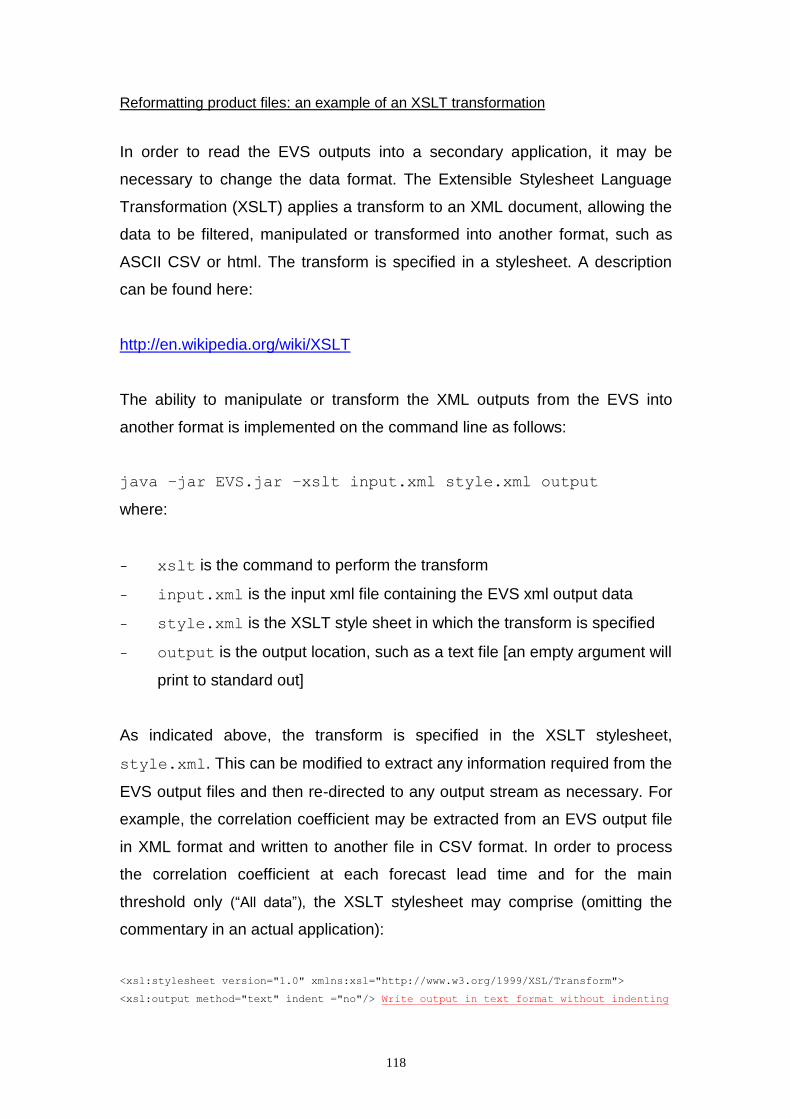
118
Reformatting product files: an example of an XSLT transformation
In order to read the EVS outputs into a secondary application, it may be
necessary to change the data format. The Extensible Stylesheet Language
Transformation (XSLT) applies a transform to an XML document, allowing the
data to be filtered, manipulated or transformed into another format, such as
ASCII CSV or html. The transform is specified in a stylesheet. A description
can be found here:
http://en.wikipedia.org/wiki/XSLT
The ability to manipulate or transform the XML outputs from the EVS into
another format is implemented on the command line as follows:
java –jar EVS.jar –xslt input.xml style.xml output
where:
xslt is the command to perform the transform
input.xml is the input xml file containing the EVS xml output data
style.xml is the XSLT style sheet in which the transform is specified
output is the output location, such as a text file [an empty argument will
print to standard out]
As indicated above, the transform is specified in the XSLT stylesheet,
style.xml. This can be modified to extract any information required from the
EVS output files and then re-directed to any output stream as necessary. For
example, the correlation coefficient may be extracted from an EVS output file
in XML format and written to another file in CSV format. In order to process
the correlation coefficient at each forecast lead time and for the main
threshold only (“All data”), the XSLT stylesheet may comprise (omitting the
commentary in an actual application):
<xsl:stylesheet version="1.0" xmlns:xsl="http://www.w3.org/1999/XSL/Transform">
<xsl:output method="text" indent ="no"/> Write output in text format without indenting

119
<xsl:template match="/">
<xsl:text>Lead time, correlation
</xsl:text> Titles and line separator
<xsl:for-each select="results/result"> Iterate through all result blocks
Print lead hour <xsl:value-of select="lead_hour"/>, <xsl:for-each
select="threshold_data/threshold"> Iterate through each threshold
<xsl:if test="threshold_value = 'All data'"> If = All data:
<xsl:value-of select="data/values"/> select values
<xsl:text>
</xsl:text> Add new line
</xsl:if>
</xsl:for-each>
</xsl:for-each>
</xsl:template>
</xsl:stylesheet>
Subject to defining appropriate XSLT stylesheets, the EVS outputs are easily
reformatted for secondary applications, such as displaying verification results on a
website.

120
APPENDIX A3 DATA SERVICES
A3.1 Flood Early Warning System Data Service (FEWS-DS)
In addition to reading forecasts and observations from the local file system, the EVS
will read these datasets from the Flood Early Warning System (FEWS) Data Service
(FEWS-DS). The FEWS-DS implements the Representational State Transfer (REST)
model with HTTP access. Currently, it provides time-series data in Published
Interface (PI) XML format. By default the PI-XML datasets are compressed (gzipped)
for transfer between the FEWS-DS and the EVS. A particular dataset is resolved
within the FEWS-DS by a Uniform Resource Locator (URL) or “endpoint”, which is
constructed by the EVS. The URL includes fixed elements, whose default values are
provided in an EVS configuration file (see below). It also includes dynamic elements,
whose values are defined for each verification scenario. Among other things, the
dynamic elements of the URL include the location and variable identifiers for which
verification is required. By default, the FEWS-DS is configured as a local service
(running on the localhost). No instructions are provided here on installing or running
the FEWS-DS (contact Deltares USA, Inc, for further instructions). Rather, it is
assumed that the FEWS-DS, and any associated archive services, are installed and
running.
As indicated above, a unique dataset is resolved within the FEWS-DS by a URL. The
elements of this URL are provided in an EVS (XML) configuration file, together with
schema definition file (XSD):
/parameterfiles/data_services.xml
/parameterfiles/data_services.xsd
In practice, the data_services.xml will not be edited routinely. However, it may be
edited, initially, when configuring the EVS to operate with a local data service. The
data_services.xml may be edited directly within the EVS.jar executable. The files
within a Java Archive (JAR) can be read (and updated/replaced) using a generic
archive utility, such as 7-Zip (on Windows) or PeaZip (on Windows/Linux).
The data_services.xml is separated into two layers, namely:
<service_constants>
<query_variables>

121
The <service_constants> identify the URL of the data server and the initial point of
entry. By default, the FEWS-DS is configured to run locally (i.e. on the localhost):
http://localhost:6080/FewsPiServiceRest/fewspiservice/v1/timeseries
Each component of this URL is mapped to an <element> of <service_constants>.
New elements may be added, as required.
The <query_variables> include the elements of the URL that resolve to a unique
dataset within the FEWS-DS. Again, each component is mapped to a separate
<element>. However, unlike the <service_constants>, most of the <query_variables>
are dynamic variables. In other words, they do not have any default values and are
user-defined for each Verification Unit (VU) within an EVS project. When a default
value is available, it is included in the <default> entry of that <element>. In general,
each <name> corresponds, exactly, to a named parameter within the FEWS-DS.
However, while the FEWS-DS comprises a single “filterID” to identify a given data
type, the data_services.xml contains a separate “filterId” for each data type:
<element>
<name>forecast_filterId</name>
<default>simulated</default>
</element>
<element>
<name>observed_filterId</name>
<default>observed</default>
</element>
When requesting observed data from the FEWS-DS, the “filterId” is populated with
the “Observed data source” from the EVS. In keeping with the observed_filterId in the
data_services.xml, this has a default value of “observed”. Indeed, when selecting
FEWS-DS as the “Observed data source” within the EVS (2b. Set input data sources
> Observed data source), the input field is populated with this default value, as
shown below.
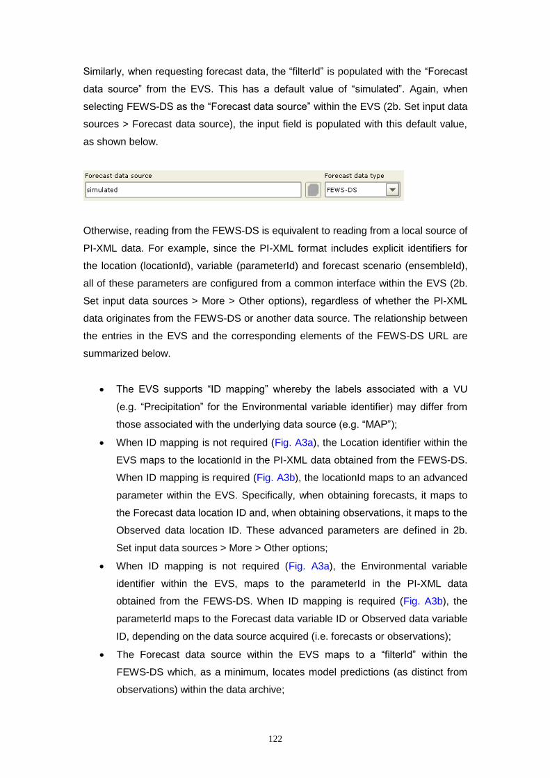
122
Similarly, when requesting forecast data, the “filterId” is populated with the “Forecast
data source” from the EVS. This has a default value of “simulated”. Again, when
selecting FEWS-DS as the “Forecast data source” within the EVS (2b. Set input data
sources > Forecast data source), the input field is populated with this default value,
as shown below.
Otherwise, reading from the FEWS-DS is equivalent to reading from a local source of
PI-XML data. For example, since the PI-XML format includes explicit identifiers for
the location (locationId), variable (parameterId) and forecast scenario (ensembleId),
all of these parameters are configured from a common interface within the EVS (2b.
Set input data sources > More > Other options), regardless of whether the PI-XML
data originates from the FEWS-DS or another data source. The relationship between
the entries in the EVS and the corresponding elements of the FEWS-DS URL are
summarized below.
The EVS supports “ID mapping” whereby the labels associated with a VU
(e.g. “Precipitation” for the Environmental variable identifier) may differ from
those associated with the underlying data source (e.g. “MAP”);
When ID mapping is not required (Fig. A3a), the Location identifier within the
EVS maps to the locationId in the PI-XML data obtained from the FEWS-DS.
When ID mapping is required (Fig. A3b), the locationId maps to an advanced
parameter within the EVS. Specifically, when obtaining forecasts, it maps to
the Forecast data location ID and, when obtaining observations, it maps to the
Observed data location ID. These advanced parameters are defined in 2b.
Set input data sources > More > Other options;
When ID mapping is not required (Fig. A3a), the Environmental variable
identifier within the EVS, maps to the parameterId in the PI-XML data
obtained from the FEWS-DS. When ID mapping is required (Fig. A3b), the
parameterId maps to the Forecast data variable ID or Observed data variable
ID, depending on the data source acquired (i.e. forecasts or observations);
The Forecast data source within the EVS maps to a “filterId” within the
FEWS-DS which, as a minimum, locates model predictions (as distinct from
observations) within the data archive;

123
The Observed data source within the EVS maps to a “filterId” within the
FEWS-DS which, as a minimum, locates “observations” (as distinct from
model predictions) within the data archive; and
The Start of verification period and End of verification period within the EVS
correspond to the start and end dates, respectively, for which time-series data
are acquired from the FEWS-DS. When reading forecasts from the FEWS-
DS, the EVS requests the data in one-year sub-periods, in order to monitor
the progress of a long-running task (this is not currently configurable).
Fig. A3a: Fields within the EVS GUI that map to elements of the URL that retrieves
time-series datasets from the FEWS-DS (when not using ID mapping)
1
2
3
4
5
6
7
8
1 = locationId (PI-XML, no ID mapping)
2 = parameterId (PI-XML, no ID mapping)
3 = filter ID (locates predictions in FEWS-DS)
4 = filter ID (locates observations in FEWS-DS)
5 = forecast data type (FEWS-DS)
6 = observed data type (FEWS-DS)
7 = start of verification period
8 = end of verification period

124
When these elements are appended to a URL that identifies the root of the data
service (see above), they provide a sufficient, albeit minimal, interface to the FEWS-
DS for a single VU. Clearly, they do not use all of the information available within the
EVS to constrain a selection from the FEWS-DS, such as the “date conditions” and
“value conditions” associated with a VU. However, these constraints may be
introduced in future, and remain applicable once the data has been returned from the
FEWS-DS.
Fig. A3b: Fields within the EVS GUI that map to elements of the URL that retrieves
time-series datasets from the FEWS-DS when using ID mapping
Currently, the EVS does not cache any of the datasets obtained from the FEWS-DS
for re-use. In other words, if the connection fails, any partially retrieved datasets will
be lost. Similarly, if a dataset is fully retrieved, but verification pairs cannot be
constructed (e.g. because the timing information is incorrect), the input data will not
1a
2a
1b 2b
1a = locationId (PI-XML, forecasts)
1b = locationId (PI-XML, observations)
2a = parameterId (PI-XML, forecasts; e.g. SQIN)
2b = parameterId (PI-XML, observations; e.g. QME)
3 = ensembleId (PI-XML, forecasts)
3

125
be cached locally. Once the verification pairs have been created, the pairs
themselves are written to file (upon request). For these reasons, when retrieving a
large dataset from the FEWS-DS, the pairing process should be tested, first, with a
subset of the overall dataset (e.g. a shorter period of record). In future, the EVS may
include a mechanism for caching or writing (partially or fully recovered) datasets from
the FEWS-DS.
126
APPENDIX A4 REFERENCES
Anderson, J. L., 1996: A method for producing and evaluating probabilistic forecasts
from ensemble model integrations. Journal of Climate, 9, 1518-1530.
Anderson, T.W., 1962: On the Distribution of the Two-Sample Cramer-von Mises
Criterion. The Annals of Mathematical Statistics, 33 (3), 1148–1159.
Araújo M.B and New, M., 2007: Ensemble forecasting of species distributions.
Trends in Ecology and Evolution, 22, 42–47.
Bonadonna, C., Connor, C.B., Houghton, B.F., Connor, L., Byrne, M., Laing, A., and
Hincks, T., 2005: Probabilistic modeling of tephra dispersion: hazard
assessment of a multi-phase eruption at Tarawera, New Zealand. Journal of
Geophysical Research, 110(B3, B03203).
Bradley, A.A., Hashino, T. and Schwartz, S.S., 2003: Distributions-oriented
verification of probability forecasts for small data samples. Weather and
Forecasting, 18, 903-917.
Bradley, A. A., Schwartz, S. S. and Hashino, T., 2004: Distributions-Oriented
Verification of Ensemble Streamflow Predictions. Journal of
Hydrometeorology, 5(3), 532-545.
Brier, G. W., 1950: Verification of forecasts expressed in terms of probability. Monthly
Weather Review, 78, 1-3.
Bröcker, J. and Smith, L.A., 2007a: Increasing the reliability of reliability diagrams.
Weather and forecasting, 22(3), 651-661.
Bröcker, J. and Smith, L.A., 2007b: Scoring Probabilistic Forecasts: On the
Importance of Being Proper. Weather and Forecasting, 22(2), 382-388.
Bröcker, J., 2008: On reliability analysis of multi-categorical forecasts. Nonlinear
Processes in Geophysics, 15(4), 661–673.
Brown, J.D. and Heuvelink, G., 2005: Assessing uncertainty propagation through
physically based models of soil water flow and solute transport. In Anderson,
M. (ed.) The Encyclopedia of Hydrological Sciences, Chichester: John Wiley
and Sons, 1181–1195.
Brown, J.D. and Heuvelink, G., 2007: The Data Uncertainty Engine (DUE): a
software tool for assessing and simulating uncertain environmental variables.
Computers and Geosciences, 33(2), 172-190.
Brown, J.D. and Seo. D-J., 2010a: A non-parametric post-processor for bias
correcting ensemble forecasts of hydrometeorological and hydrologic
variables. Journal of Hydrometeorology, 11(3), 642-665.

127
Brown, J.D., Demargne, J., Seo, D-J and Liu, Y. 2010b: The Ensemble Verification
System (EVS): a software tool for verifying ensemble forecasts of
hydrometeorological and hydrologic variables at discrete locations.
Environmental Modelling and Software, 25(7), 854-872.
Cai, T. and Moskowitz, C.S., 2004: Semi-parametric estimation of the binormal ROC
curve for continuous diagnostic tests. Biostatistics, 5(4), 573-586.
Casella, G. and Berger, R. L., 1990: Statistical Inference. Duxbury Press, 650 pp.
Demargne, J., Wu, L., Seo, D-J, and Schaake, J. 2007: Experimental
hydrometeorological and hydrologic ensemble forecasts and their verification
in the U.S. National Weather Service. Quantification and Reduction of
Predictive Uncertainty for Sustainable Water Resources Management
(Proceedings of Symposium HS2004 at IUGG2007, Perugia, July 2007).
IAHS Publication, 313, 177-187.
Demargne, J., Mullusky, M., Werner, K., Adams, T. Lindsey, S. Schwein, N. Marosi,
W. and Welles, E. 2009: Application of Forecast Verification Science to
Operational River Forecasting in the U.S. National Weather Service. Bulletin
of the American Meteorological Society, 90(6), 779-784.
Demargne, J., Brown, J.D., Liu, Y., Seo, D-J, Wu, L., Toth, Z. and Zhu, Y. 2010:
Diagnostic verification of hydrometeorological and hydrologic ensembles.
Atmospheric Science Letters, 11(2), 114-122.
Elmore, K. L., 2005: Alternatives to the Chi-Square Test for Evaluating Rank
Histograms from Ensemble Forecasts. Weather and Forecasting, 20, 789–
795.
Fawcett, T. 2006: An introduction to ROC analysis. Pattern Recognition Letters, 27,
861-874.
Flanagan, D., 2005. Java in a Nutshell, 5th ed. North Sebastopol, CA: O’Reilly and
Associates, 1252pp.
Gneiting, T.A., Raftery, E., Westveld III, A. H., and Goldman, T., 2005: Calibrated
probabilistic forecasting using ensemble Model Output Statistics and
minimum CRPS estimation. Monthly Weather Review, 133, 1098–1118.
Gneiting, T., F. Balabdaoui, and Raftery, A. E., 2007: Probabilistic forecasts,
calibration and sharpness. Journal of the Royal Statistical Society Series B:
Statistical Methodology, 69(2), 243 – 268.
Good, I.J., 1952: Rational decisions, Journal of the Royal Statistical Society, 14, 107-
114.
Green, D.M. and Swets, J.M., 1966: Signal detection theory and psychophysics. New
York: John Wiley and Sons Inc., 455pp.

128
Gupta, H.V., Beven, K.J. and Wagener, T., 2005: Model calibration and uncertainty
estimation. In Anderson, M. (ed.) The Encyclopedia of Hydrological Sciences,
John Wiley & Sons, Chichester, 2015-2032.
Hamill, T.M., 1997: Reliability diagrams for multicategory probabilistic forecasts.
Weather and Forecasting, 12, 736-741.
Hamill, T.M., 2001: Interpretation of rank histograms for verifying ensemble forecasts.
Monthly Weather Review, 129, 550-560.
Hamill, T.M., and Colucci, S.J. 1997: Verification of Eta–RSM Short-Range Ensemble
Forecasts. Monthly Weather Review, 125, 1312–1327.
Hamill, T.M., J. S. Whittaker, and S. L. Mullen, 2006: Reforecasts: an important data
set for improving weather predictions. Bulletin of the American Meteorological
Society, 87(1), 33-46.
Hashino, T., Bradley, A.A. and Schwartz, S.S., 2006: Evaluation of bias-correction
methods for ensemble streamflow volume forecasts. Hydrology and Earth
System Sciences Discussions, 3, 561-594.
Hersbach, H., 2000: Decomposition of the continuous ranked probability score for
ensemble prediction systems. Weather and Forecasting, 15, 559-570.
Hsu, W.-R. and Murphy, A.H., 1986: The attributes diagram: A geometrical
framework for assessing the quality of probability forecasts. International
Journal of Forecasting, 2, 285-293.
Jolliffe, I.T. and Stephenson, D.B. (eds), 2003: Forecast Verification: A Practitioner’s
Guide in Atmospheric Science. Chichester: John Wiley and Sons, 240pp.
Kennedy, E.J., 1983: Techniques of Water-Resources Investigations of the United
States Geological Survey, Book 3. Chapter A13: Computation of Continuous
Records of Streamflow, US Government Printing Office, 52pp. [Available at
http://pubs.usgs.gov/twri/twri3-a13/pdf/TWRI_3-A13.pdf, accessed 10/05/11].
Mason, S.J. and Graham N.E., 2002: Areas beneath the relative operating
characteristics (ROC) and relative operating levels (ROL) curves: Statistical
significance and interpretation, Quarterly Journal of the Royal Meteorological
Society, 30, 291-303.
Mason, S.J., 2008: Understanding forecast verification statistics. Meteorological
Applications, 15, 31-40.
Matheson, J. E., and Winkler, R.L., 1976: Scoring rules for continuous probability
distributions. Management Science, 22, 1087–1095.
Murphy, A. H. and Winkler, R.L., 1987: A general framework for forecast verification.
Monthly Weather Review, 115, 1330-1338.
129
Murphy, A.H., 1996: General decompositions of MSE-based skill scores: Measures
of some basic aspects of forecast quality. Monthly Weather Review, 124,
2353-2369.
National Research Council of the National Academies (NRC), 2006: Completing the
Forecast: Characterizing and Communicating Uncertainty for Better Decisions
Using Weather and Climate Forecasts [Available at: http://www.nap.edu/,
accessed 10/05/11].
National Weather Service (NWS), 2005: National Weather Service River Forecast
System (NWSRFS) User Manual Documentation. National Weather Service
documentation, Silver Spring, Maryland, USA [Available at:
http://www.nws.noaa.gov/oh/hrl/nwsrfs/users_manual/htm/xrfsdocpdf.php,
accessed 10/05/11].
Park, S.K. and Xu, L., 2009: Data Assimilation for Atmospheric, Oceanic and
Hydrologic Applications. Springer-Verlag, 495pp.
Politis, D.N. and Romano, J.P., 1994: The stationary bootstrap. Journal of the
American Statistical Association, 89, 1303–1313.
R Development Core Team, 2008: R: A language and environment for statistical
computing, reference index version 2.7.2. R Foundation for Statistical
Computing, Vienna, Austria. ISBN 3-900051-07-0, [Available at: http://www.R-
project.org, accessed 10/05/11].
Schaake, J., Demargne, J., Hartman, R., Mullusky, M., Welles, E. Wu, L., Herr, H.,
Fan, X. and Seo, D.J., 2007: Precipitation and temperature ensemble
forecasts from single-value forecasts. Hydrology and Earth Systems
Sciences, 4, 655-717.
Seo, D.-J., Herr, H.D. and Schaake, J.C., 2006: A statistical post-processor for
accounting of hydrologic uncertainty in short-range ensemble streamflow
prediction. Hydrology and Earth System Sciences, 3, 1987-2035.
Shorack, G.R., and Wellner, J.A. 1986: Empirical Processes with Applications to
Statistics. John Wiley and Sons Inc., 976 pp.
Stensrud, D.J., Brooks, H.E., Du, J., Tracton, M.S. and Rogers, E. 1999: Using
Ensembles for Short-Range Forecasting. Monthly Weather Review, 127,
433–446.
Talagrand, O., 1997: Assimilation of observations, an introduction. Journal of the
Meteorological Society of Japan, 75, 191–209.
Toth, Z., E. Kalnay, S. M. Tracton, R. Wobus and J. Irwin, 1997: A synoptic
evaluation of the NCEP ensemble. Weather and Forecasting, 12, 140-153.

130
Tukey, J.W. (1977) Exploratory Data Analysis. Addison-Wesley, Reading, MA.
688pp.
Wei, M. and Toth, Z., Wobus, R. and Zhu, Y., 2008: Initial perturbations based on the
ensemble transform (ET) technique in the NCEP global operational forecast
system. Tellus, 60A, 62–79.
Wilks, D.S., 2006: Statistical Methods in the Atmospheric Sciences, 2nd ed. Academic
Press, 627pp.
Wilson, L.J., Burrows, W.R. and Lanzinger, A., 1999: A strategy for verification of
weather element forecasts from an ensemble prediction system. Monthly
Weather Review, 127, 956-970.
Wu, L., Seo, D-J, Demargne, J. and Brown, J.D., Cong, S. and Schaake, J. 2010:
Applying mixed-type meta-Gaussian models to precipitation ensemble
generation from single-valued forecasts. Manuscript submitted to Journal of
Hydrology.